FLUID STRUCTURE INTERACTIONS

UNSTEADY FLOW

IN PIPE NETWORKS

PREAMBLE

Unsteady flow in pipe networks can be caused by a number of

factors. A turbomachine with blades can send pressure waves

down a pipe. If the period of these waves matches a natural

period of the pipe wave speed resonance develops. A piston

pump can send similar waves down a pipe. Waves on the surface

of a water reservoir can also excite resonance of inlet

pipes. One way to avoid resonance is to change the wave speed

of the pipes in the network. For liquids, one can do this by

adding a gas such as air. This can be bled into the network

at critical locations or it can be held in a flexible tube

which runs inside the pipes. One could also use a flexible

pipe to change the wave speed. Sudden valve or turbomachine

changes can send waves up and down pipes. These can cause the

pipes to explode or implode. In some cases interaction

between pipes and devices is such that oscillations develop

automatically. Examples include oscillations set up by leaky

valves and those set up by slow turbomachine controllers. To

lessen the severity of transients in a hydraulic network, one

can use gas accumulators. Hydro plants use surge pipes.

Another way to lessen the severity of transients is use of

relief valves. These are spring loaded valves which open when

the pressure reaches a preset level. This can be high or low.

For high pressure liquids, they create a pathway back to a

sump. For low pressure liquids, they allow a gas such as air

to enter the pipe. Bypass valves and check valves can be used

to isolate turbomachines when they fail.

There are three procedures that can be used to study unsteady

flow in pipe networks. The most complex of these is the

Method of Characteristics. This finds directions in space and

time along which the partial differential equations of mass

and momentum reduce to an ordinary differential equation in

time. Computational Fluid Dynamics codes have been developed

based on this method that can handle extremely complex pipe

networks. A second procedure is known as Graphical

Waterhammer. It is a graphical form of a procedure known as

Algebraic Waterhammer. It makes extensive use of PU plots. A

third procedure is known as the Impedance Method. This makes

use of Laplace Transforms. It employs something called the

Impedance Transfer Function. It resembles closely a method

used to study Electrical Transmission Lines.

These notes start with a physical description of how pressure

waves propagate along a pipe. This is followed by a

derivation of the basic wave equations. Then, wave speeds for

waves in flexible tubes and mixtures are given. Next, an

outline of Algebraic/Graphical Waterhammer is given. Finally,

the Method of Characteristics is presented.

WAVE PROPAGATION IN PIPES

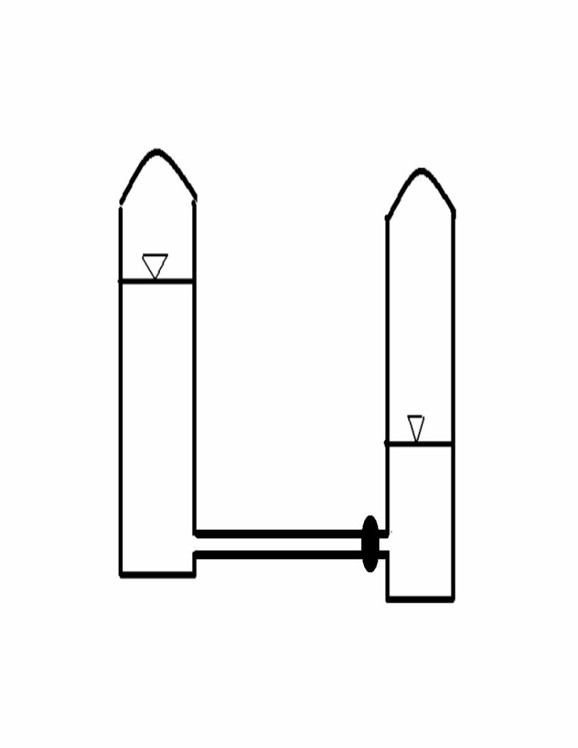
Consider flow in a rigid pipe with a valve at its downstream

end and a reservoir at its upstream end. Assume that there

are no friction losses. This implies that the pressure and

flow speed are the same everywhere along the pipe.

Imagine now that the valve is suddenly closed. This causes a

high pressure or surge wave to propagate up the pipe. As it

does so, it brings the fluid to rest. The fluid immediately

next to the valve is stopped first. The valve is like a wall.

Fluid enters an infinitesimal layer next to this wall and

pressurizes it and stops. This layer becomes like a wall for

an infinitesimal layer just upstream. Fluid then enters that

layer and pressurizes it and stops. As the surge wave

propagates up the pipe, it causes an infinite number of these

pressurizations. When it reaches the reservoir, all of the

inflow has been stopped, and pressure is high everywhere

along the pipe. The pipe resembles a compressed spring.

When the surge wave reaches the reservoir, it creates a

pressure imbalance. The layer of fluid just inside the pipe

has high pressure fluid downstream of it and reservoir

pressure upstream. Fluid exits the layer on its upstream side

and depressurizes it. The pressure drops back to the

reservoir level. A backflow wave is created. The speed of the

backflow is exactly the same as the speed of the original

inflow. The pressure that was generated by taking the

original inflow away is exactly what is available to generate

the backflow. The backflow wave propagates down the pipe

restoring pressure everywhere to its original level.

When the backflow wave reaches the valve, it creates a flow

imbalance. This causes a low pressure or suction wave to

propagate up the pipe. As it does so, it brings the fluid to

rest. Again, the valve is like a wall. Because of backflow,

fluid exits an infinitesimal layer next to this wall and

depressurizes it and stops. The pressure drops below the

reservoir level by exactly the amount it was above the

reservoir level in the surge wave.

When the suction wave reaches the reservoir, all of the

backflow has been stopped, and pressure is low everywhere

along the pipe. The pipe resembles a stretched spring. At the

reservoir, the suction wave creates a pressure imbalance. An

inflow wave is created. The speed of the inflow is exactly

the same as the speed of the backflow. The inflow wave

travels down the pipe restoring pressure to its original

level. Conditions in the pipe become what they were just

before the valve was closed.

During one cycle of vibration, there are 4 transits of the

pipe by pressure waves. This means that the natural period of

the pipe is 4 times the length of the pipe divided by the

wave speed. Without friction, the vibration cycle repeats

over and over. With friction, it gradually dies away.

BASIC WAVE EQUATIONS

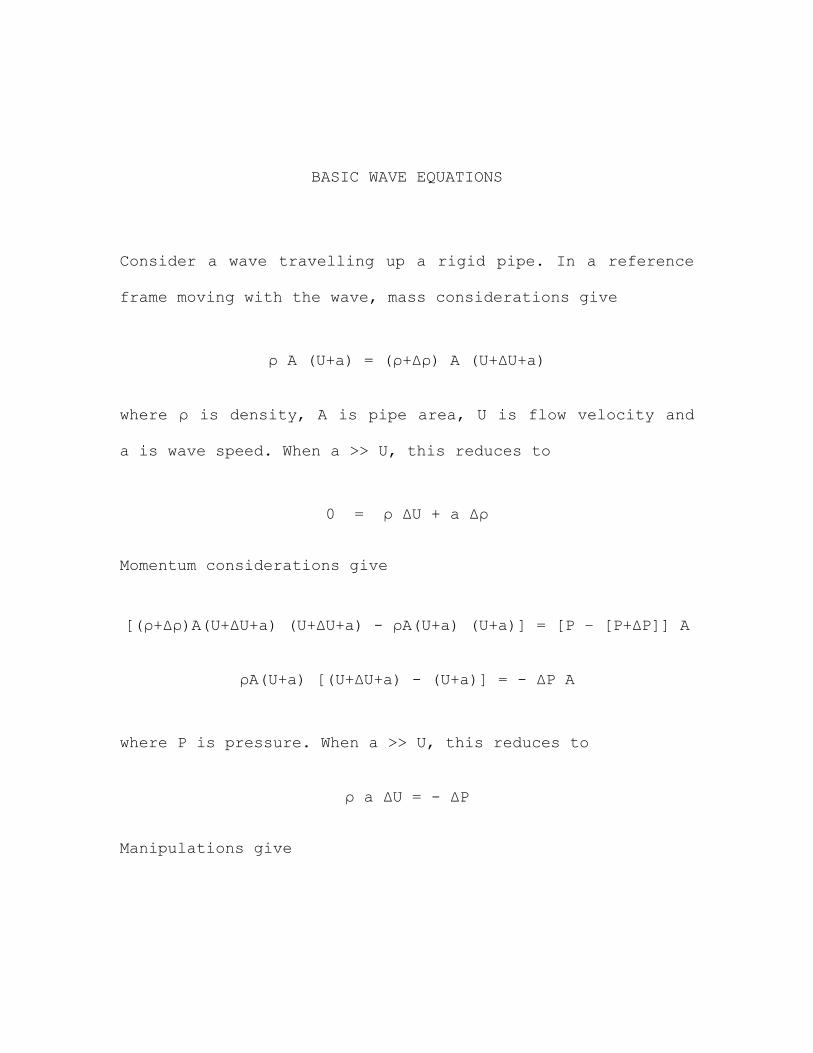
Consider a wave travelling up a rigid pipe. In a reference

frame moving with the wave, mass considerations give

ρ A (U+a) = (ρ+Δρ) A (U+ΔU+a)

where ρ is density, A is pipe area, U is flow velocity and

a is wave speed. When a >> U, this reduces to

0 = ρ ΔU + a Δρ

Momentum considerations give

[(ρ+Δρ)A(U+ΔU+a) (U+ΔU+a) - ρA(U+a) (U+a)] = [P – [P+ΔP]] A

ρA(U+a) [(U+ΔU+a) - (U+a)] = - ΔP A

where P is pressure. When a >> U, this reduces to

ρ a ΔU = - ΔP

Manipulations give

a = [ΔP/Δρ]

For a gas such as air moving down a pipe, one can assume

ideal gas behavior for which:

P/ρ = R T

R is the ideal gas constant and T is the absolute

temperature of the gas. For a wave propagating through a

gas, one can assume processes are isentropic: in other

words, adiabatic and frictionless. The wave moves so fast

through the gas that there is no time for heat transfer or

friction. The isentropic equation of state is:

P = K ρk

where K is another constant and k is the ratio of specific

heats. Differentiation of this equation gives

ΔP/Δρ = K k ρk-1

= K k ρk / ρ

= k/ρ K ρk = k P/ρ

The ideal gas law into this gives

ΔP/Δρ = k R T

So wave speed for a gas becomes

a = k R T]

For a liquid, fluid mechanics shows that

ΔP = - K ΔV/V

where K is the bulk modulus of the liquid. It is a measure

of its compressibility. For a bit of fluid mass

ΔM = Δ [ρ V] = V Δρ + ρ ΔV = 0

This implies that

ΔP = K Δρ/ρ ΔP/Δρ = K/ρ

So wave speed for a liquid becomes

a = [K/ρ]

The bulk modulus of a gas follows from

a = k R T] = [K/ρ]

K/ρ = k R T K = k ρ R T

K = k P

WAVES IN FLEXIBLE TUBES

Conservation of Mass for a flexible tube is

ρ A (U+a) = (ρ+Δρ) (A+ΔA) (U+ΔU+a)

Manipulation of this equation gives when U<<a

ρA ΔU + (U+a)A Δρ + ρ(U+a) ΔA = 0

ΔU/a + Δρ/ρ + ΔA/A = 0

Conservation of Momentum for a flexible tube is

[ρA(U+a)] [(U+ΔU+a)-(U+a)] =

PA + [P+ΔP] ΔA – [P+ΔP][A+ΔA]

Manipulation of this equation gives when U<<a

ρA(U+a) ΔU + A ΔP = 0

ρa ΔU + ΔP = 0

More manipulation gives

ΔU = - ΔP/[ρa] ΔU/a = -ΔP/[ρa2]

Experiments show that

ΔP = K Δρ/ρ Δρ/ρ = ΔP/K

For a thin wall tube, the hoop stress follows from

[2e] σ = ΔP D σ = ΔP D/[2e]

where e is the wall thickness and D is the tube diameter.

The hoop strain is

ε = [πΔD]/[πD] = ΔD/D

Substitution into the stress strain connection gives

σ = E ε ΔP D/[2e] = E ΔD/D

where E is the Elastic Modulus of the wall material.

Geometry gives

A = π D2/4 ΔA = π 2D/4 ΔD

ΔA/A = 2 ΔD/D = ΔP D/[Ee]

With this Conservation of Mass becomes

- ΔP/[ρa2] + ΔP/K + ΔP D/[Ee] = 0

Manipulation of Conservation of Mass gives

a = [K/ρ]

K = K / [ 1 + [DK]/[Ee] ]

WAVES IN MIXTURES

For a mixture the wave speed is:

aM = [KM/ρM]

For a two component mixture the density follows from:

MM = MA + MB ρMVM = ρAVA + ρBVB

ρM = [ ρAVA + ρBVB ] / VM

Experiments show that

ΔP = - KM [ΔVM/VM]

Manipulation gives the bulk modulus

KM = - ΔP / [ΔVM/VM]

VM = VA + VB ΔVM = ΔVA + ΔVB

For each component in the mixture:

ΔP = - KA [ΔVA/VA] ΔVA = - [VA/KA] ΔP

ΔP = - KB [ΔVB/VB] ΔVB = - [VB/KB] ΔP

The mixture bulk modulus becomes:

KM = [ VA + VB ] / [ VA/KA + VB/KB ]

The mixture analysis is also valid for mixtures of small

solid particles and a fluid, such as a dusty gas.

ALGEBRAIC/GRAPHICAL WATERHAMMER

Waterhammer analysis allows one to connect unknown pressure

and flow velocity at one end of a pipe to known pressure and

velocity at the other end of the pipe one transit time back

in time. The derivation of the waterhammer equations starts

with the conservation of momentum and mass equations for

unsteady flow in a pipe. These are:

ρ U/t + ρU U/x + P/x - ρg Sinα + f/D ρU|U|/2 = 0

P/t + U P/x + ρa2 U/x = 0

where P is pressure and U is velocity. For the case where

gravity and friction are insignificant and the mean flow

speed is approximately zero, these reduce to:

ρ U/t + P/x = 0

P/t + ρa2 U/x = 0

Manipulation gives the wave equations:

2P/t2 = a2 2P/x2

2U/t2 = a2 2U/x2

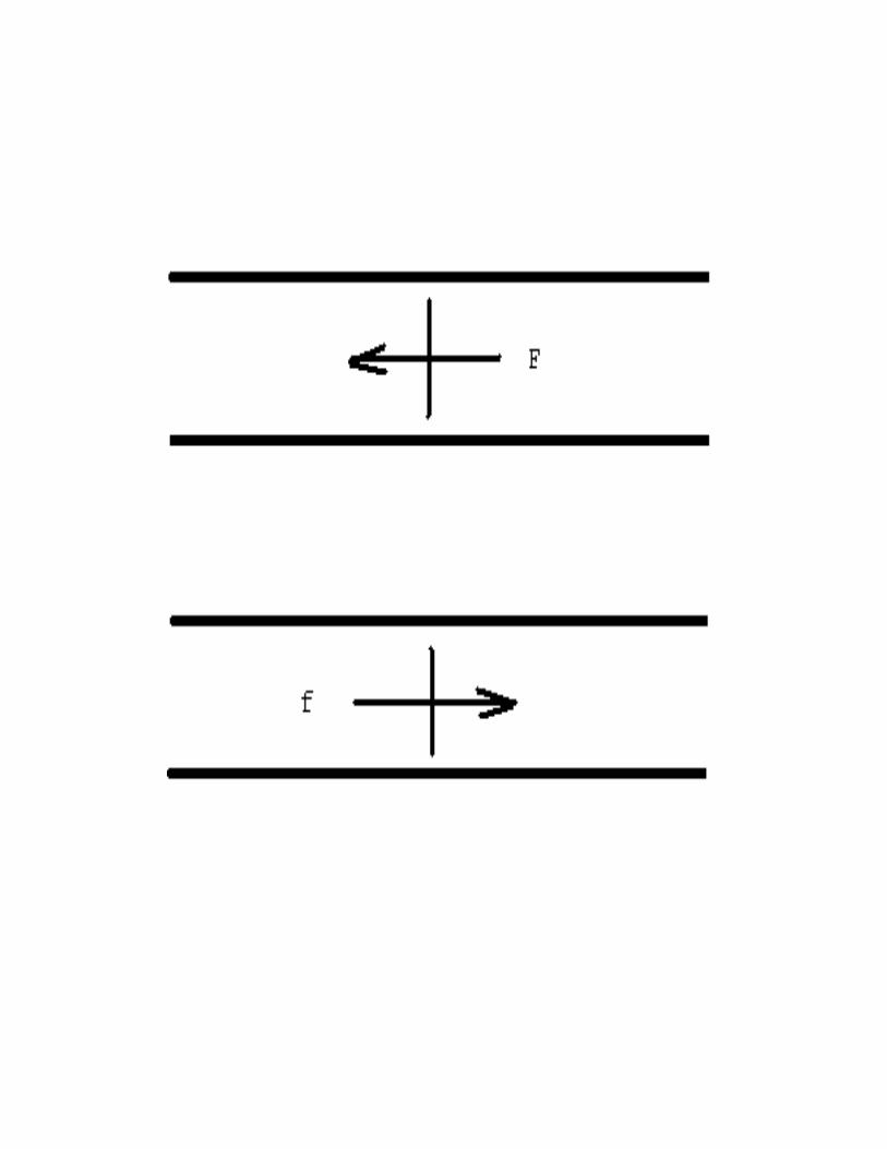
The general solution consists of two waves: one wave which

travels up the pipe known as the F wave and the other which

travels down the pipe known as the f wave.

In terms of these waves, pressure and velocity are:

P – Po = f(N) + F(M)

U - Uo = [f(N) - F(M)] / [ρa]

where N and M are wave fixed frames given by:

N = x – a t M = x + a t

For a given point N on the f wave, the N equation shows that

x must increase as time increases, which means the wave must

be moving down the pipe. For a given point M on the F wave,

the M equation shows that x must decrease as time increases,

which means the wave must be moving up the pipe. Substitution

of the general solution into mass or momentum or the wave

equations shows that they are valid solutions.

Multiplying U by ρa and subtracting it from P gives:

[P–Po] – ρa[U-Uo] = 2F(M)

Let the F wave travel from the downstream end of the pipe to

the upstream end. For a point on the wave, the value of F

would be the same. This implies

ΔP = + ρa ΔU

Multiplying U by ρa and adding it to P gives:

[P–Po] + ρa[U-Uo] = 2f(N)

Let the f wave travel from the upstream end of the pipe to

the downstream end. For a point on the wave, the value of f

would be the same. This implies

ΔP = - ρa ΔU

The ΔP vs ΔU equations allow us to connect unknown conditions

at one end of a pipe at some point in time to known

conditions at the other end back in time. They are known as

the algebraic/graphical waterhammer equations.

DERIVATION OF WAVE EQUATIONS

Conservation of Momentum and Mass are:

ρ U/t + P/x = 0

P/t + ρa2 U/x = 0

Differentiation of Momentum with respect to t gives

ρ 2U/t2 + (P/x)/t = 0

Differentiation of Mass with respect to x gives

(P/t)/x + ρa2 2U/x2 = 0

Subtraction of Mass from Momentum gives

ρ 2U/t2 = ρa2 2U/x2

2U/t2 = a2 2U/x2

Similar manipulations of Momentum and Mass give

ρa2 (U/t)/x + a2 2P/x2 = 0

2P/t2 + ρa2 (U/x)/t = 0

2P/t2 = a2 2P/x2

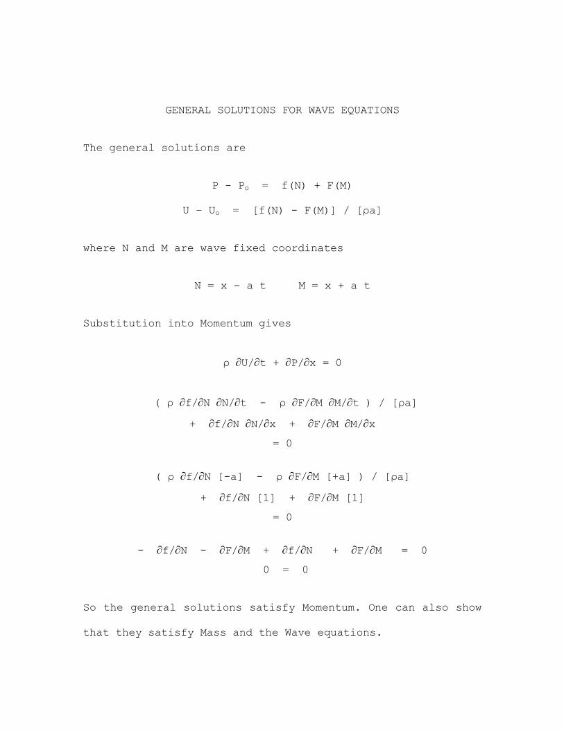
GENERAL SOLUTIONS FOR WAVE EQUATIONS

The general solutions are

P - Po = f(N) + F(M)

U – Uo = [f(N) - F(M)] / [ρa]

where N and M are wave fixed coordinates

N = x – a t M = x + a t

Substitution into Momentum gives

ρ U/t + P/x = 0

( ρ f/N N/t - ρ F/M M/t ) / [ρa]

+ f/N N/x + F/M M/x

= 0

( ρ f/N [-a] - ρ F/M [+a] ) / [ρa]

+ f/N [1] + F/M [1]

= 0

- f/N - F/M + f/N + F/M = 0

0 = 0

So the general solutions satisfy Momentum. One can also show

that they satisfy Mass and the Wave equations.

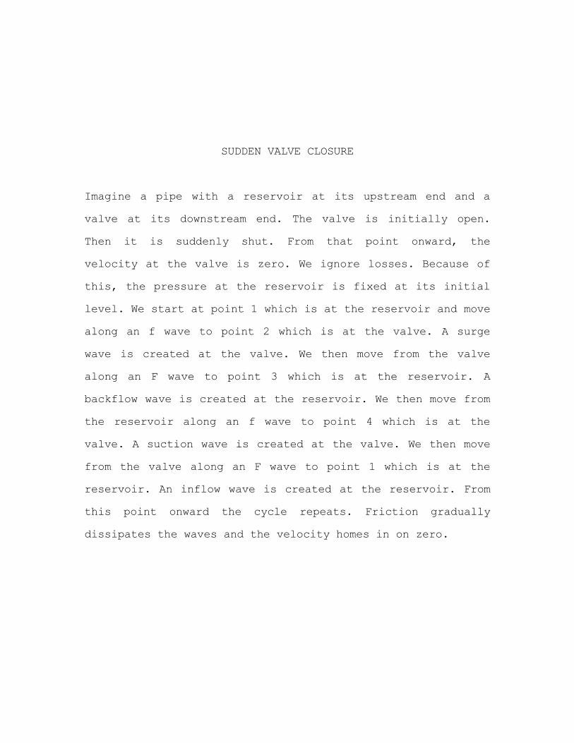
SUDDEN VALVE CLOSURE

Imagine a pipe with a reservoir at its upstream end and a

valve at its downstream end. The valve is initially open.

Then it is suddenly shut. From that point onward, the

velocity at the valve is zero. We ignore losses. Because of

this, the pressure at the reservoir is fixed at its initial

level. We start at point 1 which is at the reservoir and move

along an f wave to point 2 which is at the valve. A surge

wave is created at the valve. We then move from the valve

along an F wave to point 3 which is at the reservoir. A

backflow wave is created at the reservoir. We then move from

the reservoir along an f wave to point 4 which is at the

valve. A suction wave is created at the valve. We then move

from the valve along an F wave to point 1 which is at the

reservoir. An inflow wave is created at the reservoir. From

this point onward the cycle repeats. Friction gradually

dissipates the waves and the velocity homes in on zero.

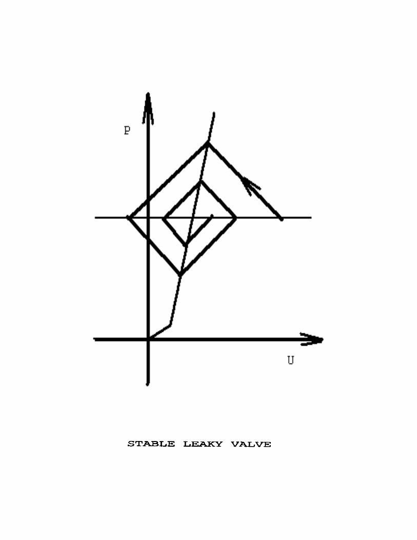
LEAKY VALVES

A stable leaky valve is basically one that has a P versus U

characteristic which resembles that of a wide open valve.

This has a parabolic shape with positive slope throughout.

An unstable leaky valve has a characteristic that has a

positive slope at low pressure but negative slope at high

pressure. Basically, the valve tries to shut itself at high

pressure. The flow rate just upstream of a valve is pipe

flow speed times pipe area. The flow rate within the valve

is valve flow speed times valve area. In a stable leaky

valve, the areas are both constant. The valve flow speed

increases with pipe pressure so the pipe flow speed also

increases. In an unstable leaky valve, the flow speed

within the valve also increases with pipe pressure but the

valve area drops because of suction within the valve. The

suction is generated by high speed flow through the small

passageway within the valve. It pulls on flexible elements

within the valve and attempts to shut it. Graphical

waterhammer plots for stable and unstable leaky valves are

given below. As can be seen, they both resemble the sudden

valve closure plot, but the stable one is decaying while

the unstable one is growing. In the unstable case, greater

suction is needed each time a backflow wave comes up to the

valve because the flow requirements of the valve keep

getting bigger. In the stable case, less suction is needed

because the flow requirements keep getting smaller.

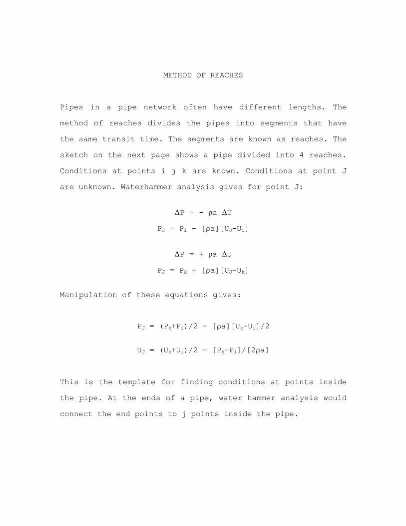
METHOD OF REACHES

Pipes in a pipe network often have different lengths. The

method of reaches divides the pipes into segments that have

the same transit time. The segments are known as reaches. The

sketch on the next page shows a pipe divided into 4 reaches.

Conditions at points i j k are known. Conditions at point J

are unknown. Waterhammer analysis gives for point J:

ΔP = - ρa ΔU

PJ = Pi - [ρa][UJ-Ui]

ΔP = + ρa ΔU

PJ = Pk + [ρa][UJ-Uk]

Manipulation of these equations gives:

PJ = (Pk+Pi)/2 - [ρa][Uk-Ui]/2

UJ = (Uk+Ui)/2 - [Pk-Pi]/[2ρa]

This is the template for finding conditions at points inside

the pipe. At the ends of a pipe, water hammer analysis would

connect the end points to j points inside the pipe.

TREATMENT OF PIPE JUNCTIONS

Pipes in a pipe network are connected at junctions. The

sketch on the next page shows a junction which connects 3

pipes. Lower case letters indicate known conditions. Upper

case letters indicate unknown conditions. A junction is often

small. This allows us to assume that the junction pressure is

common to all pipes. It also allows us to assume that the net

flow into or out of the junction is zero. Conservation of

Mass considerations give:

ρ AN UN + ρ AH UH + ρ AW UW = 0

Waterhammer analysis gives:

PN - Pm = + [ρaN] [UN-Um]

PH - Pg = + [ρaH] [UH-Ug]

PW - Pv = + [ρaW] [UW-Uv]

Manipulation gives

UN = Um + [PN-Pm]/[ρaN]

UH = Ug + [PH-Pg]/[ρaH]

UW = Uv + [PW-Pv]/[ρaW]

In these equations PN = PH = PW = PJ. Substitution into

Conservation of Mass gives:

ρ AN [ Um + [PJ-Pm]/[ρaN] ]

+ ρ AH [ Ug + [PJ-Pg]/[ρaH] ]

+ ρ AW [ Uv + [PJ-Pv]/[ρaW] ] = 0

Manipulation gives the junction pressure:

PJ = [X – Y] / Z

where

X = [ AN/aN Pm + AH/aH Pg + AW/aW Pv ]

Y = ρ [ ANUm + AHUg + AWUv ]

Z = [ AN/aN + AH/aH + AW/aW ]

The velocities at the junction are:

UN = Um + [PJ-Pm]/[ρaN]

UH = Ug + [PJ-Pg]/[ρaH]

UW = Uv + [PJ-Pv]/[ρaW]

ACCUMULATOTS

Accumulators are used to dampen transients in pipe networks.

They generally consist of a neck or constriction containing

liquid which is connected directly to the pipe network. A

pocket of gas is at the other end of the neck. The gas is

usually contained inside a flexible bladder.

There are two ways to model an accumulator. The first is the

Helmholtz Resonator mass spring model where the slug of

liquid in the neck bounces on the gas spring. This gives the

natural frequency of the accumulator and one tries to match

that to the natural period of the network. The second model

is a transient model where the equation of motion of the slug

of liquid in the neck and the equations for the gas pocket

are solved step by step in time and this is coupled a water

hammer analysis transient model.

The Helmholtz Resonator model starts with the equation of

motion of a mass on a spring:

m d2ΔZ/dt

2 + k ΔZ = f

where m is the mass of liquid in the neck and k is the spring

due to gas compressibility.

The natural frequency and period of the accumulator are

ω = √ [k/m] T = 2π/ω

The mass m of the slug of liquid in the neck is

m = ρ A L

where ρ is the density of the liquid in the neck, A is the

area of the neck and L is the length of the neck.

Conservation of Mass for the gas pocket gives

Δ [ σ V ] = V Δσ + σ ΔV = 0

Thermodynamics gives

ΔP/Δσ = a2 a = √[nRT]

Geometry gives

ΔV = - A ΔZ

Substitution into mass gives

V ΔP/a2 – σ A ΔZ = 0

ΔP = [σ A a2 / V] ΔZ

The force on the slug of liquid is

ΔF = ΔP A = [σ A2 a

2 / V] ΔZ = k ΔZ

This gives the spring constant k

k = [σ A2 a

2 / V]

Substitution into the frequency equation gives

ω = √ [ [σ A2 a

2 / V] / [ρ A L] ]

= √ [ [σ A a2] / [ρ V L] ]

For the transient model the equation governing the motion of

the slug of liquid in the neck is:

m dU/dt = [ PJ – PG ] A – fL/D ρ U|U|/2 A

where PJ is the junction pressure and PG is the gas pressure.

The volume of gas is governed by

dV/dt = - U A

The pressure of the gas is

PG = N σn = N (M/V)

n

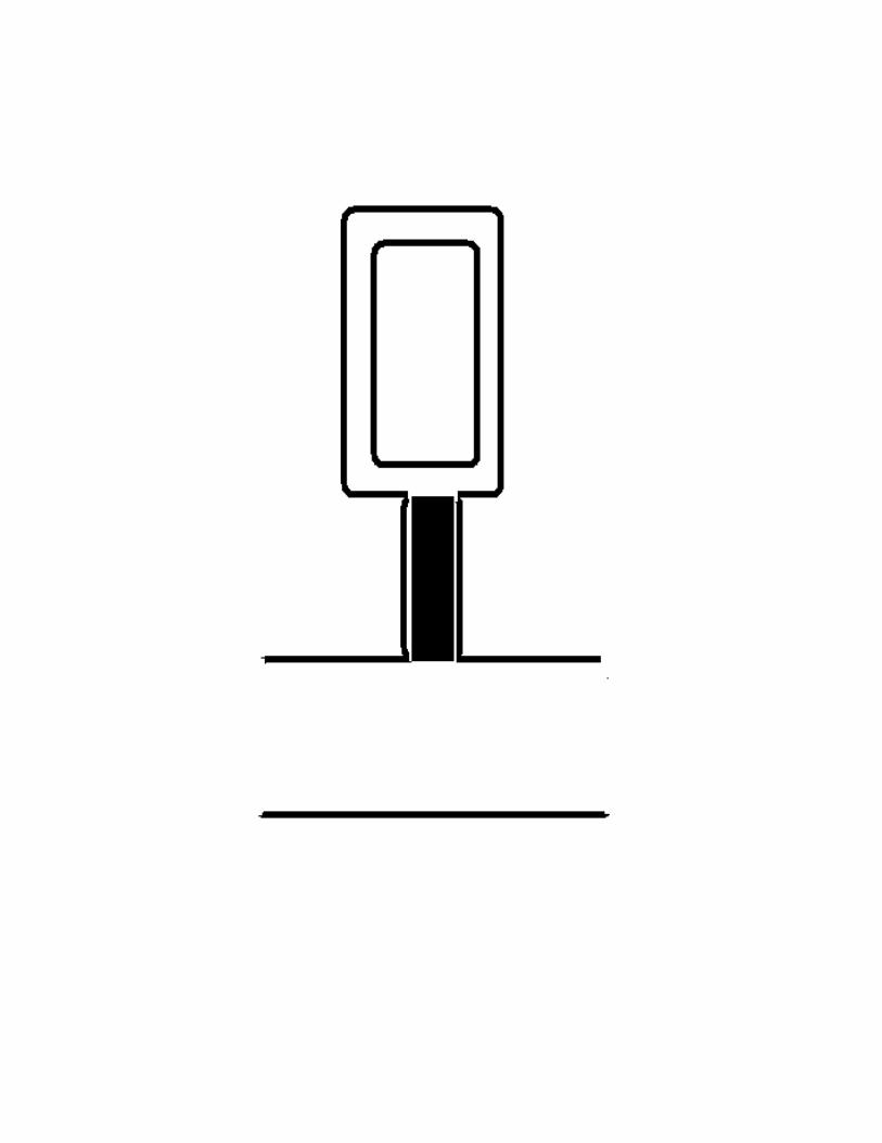
TREATMENT OF VALVES

A sketch of a valve is shown on the next page. The governing

equation for the flow through it is:

PN – PX = K U|U|

For constant pipe properties

U = UN = UX P = PN - PX

P = K U|U|

Water hammer analysis gives

PN – Pm = - ρa (UN – Um)

PX – Py = + ρa (UX – Uy)

Substitution into the valve equation gives

[Pm - ρa (U – Um)] – [Py + ρa (U – Uy)] = K U|U|

This gives U at each time step. Back substitution gives the

pressure upstream and downstream of the valve.

METHOD OF CHARACTERISTICS

The method of characteristics is a way to determine the

pressure and velocity variations in a pipe network when

valves are adjusted or turbomachines undergo load changes.

The equations governing flow in a typical pipe are:

ρ U/t + ρU U/x + P/x - ρg Sinα + f/D ρU|U|/2 = 0

P/t + U P/x + ρa2 U/x = 0

where P is pressure, U is velocity, t is time, x is distance

along the pipe, ρ is the fluid density, g is gravity, α is

the pipe slope, f is the pipe friction factor, D is the pipe

diameter and a is the wave speed. The wave speed is:

a2 = K/ρ K = K / [1 + DK/Ee]

where K is the bulk modulus of the fluid, E is the Youngs

Modulus of the pipe wall and e is its thickness.

The governing equations can be combined as follows:

ρ U/t + ρ U U/x + P/x + ρ C

+ λ (P/t + U P/x + ρa2 U/x) = 0

where

C = f/D U|U|/2 - g Sinα

Manipulation gives

ρ (U/t + [U+λa2] U/x)

+ λ (P/t + [1/λ+U] P/x) + ρC = 0

According to Calculus

dP/dt = P/t + dx/dt P/x

dU/dt = U/t + dx/dt U/x

Inspection of the last three equations suggests:

dx/dt = U + λa2 = 1/λ + U

In this case, the PDE becomes the ODE:

ρ dU/dt + λ dP/dt + ρ C = 0

The dx/dt equation gives

λa2 = 1/λ or λ

2 = 1/a

2 or λ = ± 1/a

So there are 2 values of λ. They give

ρ dU/dt + 1/a dP/dt + ρ C = 0 dx/dt = U + a

ρ dU/dt - 1/a dP/dt + ρ C = 0 dx/dt = U - a

The dx/dt equations define directions in space and time along

which the PDE becomes an ODE. Using finite differences, each

ODE and dx/dt equation can be written as:

ρ ΔU/Δt + 1/a ΔP/Δt + ρ C = 0 Δx/Δt = U + a

ρ ΔU/Δt - 1/a ΔP/Δt + ρ C = 0 Δx/Δt = U - a

Manipulation gives

ρa ΔU + ΔP + Δt ρa C = 0

ρa ΔU - ΔP + Δt ρa C = 0

When the wave speed a is much greater than the flow speed U

and when Δx is the length of the pipe L and Δt is the pipe

transit time T, these equations are basically the water

hammer equations but with friction added.

For pipes divided into reaches, one gets

UP - UL + (PP-PL)/[ρa] + CL(tP-tL) = 0 xP-xL = (UL+a)(tP-tL)

UP - UR - (PP-PR)/[ρa] + CR(tP-tR) = 0 xP-xR = (UR-a)(tP-tR)

Manipulation gives

UP = (UL+UR)/2 + (PL-PR)/[2ρa] - Δt(CL+CR)/2

PP = (PL+PR)/2 + [ρa](UL-UR)/2 - Δt[ρa](CL-CR)/2

Linear interpolation gives U and P at points L and R in terms

of known U and P at grid points A and B and C:

UL = UA + (xL-xA)/(xB-xA) (UB-UA)

UR = UC + (xR-xC)/(xB-xC) (UB-UC)

PL = PA + (xL-xA)/(xB-xA) (PB-PA)

PR = PC + (xR-xC)/(xB-xC) (PB-PC)

At each end of the pipe, a boundary condition relates the PP

and UP there. A finite difference equation also relates the

PP and UP there. So, one can solve for the PP and UP there.

% UNSTEADY FLOW IN A PIPE

% METHOD OF CHARACTERISTICS

% RESERVOIR / PIPE / VALVE

% PRESSURE = POLD / PNEW

% VELOCITY = UOLD / UNEW

% HEAD = RESERVOIR HEAD

% PIPE = HEAD PRESSURE

% SLOPE = VALVE SLOPE

% OD = PIPE DIAMETER

% OL = PIPE LENGTH

% CF = FRICTION FACTOR

% SOUND = SOUND SPEED

% GRAVITY = GRAVITY

% DENSITY = DENSITY

% NIT = NUMBER OF TIME STEPS

% MIT = NUMBER OF PIPE NODES

% DELT = STEP IN TIME

% DATA

DELT=0.001;

CF=0.5;

CMAX=+10.0;

CMIN=0.0;

OD=0.15;OL=100.0;

SOUND=1000.0;

GRAVITY=10.0;

DENSITY=1000.0;

SLOPE=-100000.0;

HEAD=20.0;SPEED=0.1;

NIT=5000;MIT=100;KIT=1;

PIPE=HEAD*DENSITY*GRAVITY;

%

ONE=PIPE;

TWO=0.0;

ZERO=0.0;

BIT=MIT/2;

GIT=MIT-1;

DELX=OL/(MIT-1);

FLD=CF*OL/OD;

PMAX=CMAX*PIPE;

PMIN=CMIN*PIPE;

WAY=SPEED*SPEED/2.0;

LOSS=FLD*WAY/GRAVITY;

G=LOSS*DENSITY*GRAVITY;

DELP=G/GIT;

for IM=1:MIT

POLD(IM)=ONE;

UOLD(IM)=SPEED;

X(IM)=TWO;

ONE=ONE-DELP;

TWO=TWO+DELX;

end

PV=POLD(MIT);

UV=UOLD(MIT);

% START LOOP ON TIME

TIME=0.0;

for IT=1:NIT

TIME=TIME+DELT;

T(IT)=TIME;

% POINTS INSIDE PIPE

for IM=2:MIT-1

XA=X(IM-1);

XB=X(IM);

XC=X(IM+1);

PA=POLD(IM-1);

PB=POLD(IM);

PC=POLD(IM+1);

UA=UOLD(IM-1);

UB=UOLD(IM);

UC=UOLD(IM+1);

XL=XB-(UB+SOUND)*DELT;

XR=XB-(UB-SOUND)*DELT;

UL=UA+(XL-XA)/(XB-XA)*(UB-UA);

PL=PA+(XL-XA)/(XB-XA)*(PB-PA);

UR=UC+(XR-XC)/(XB-XC)*(UB-UC);

PR=PC+(XR-XC)/(XB-XC)*(PB-PC);

UNEW(IM)=0.5*(UL+UR+(PL-PR)/DENSITY/SOUND ...

-DELT*(CF/2.0/OD*(UL*abs(UL)+UR*abs(UR))));

PNEW(IM)=0.5*(PL+PR+(UL-UR)*DENSITY*SOUND-DENSITY ...

*SOUND*CF/2.0/OD*DELT*(UL*abs(UL)-UR*abs(UR)));

end

% DOWNSTREAM END OF PIPE

if(KIT==1) UNEW(MIT)=ZERO;end;

if(KIT==2) UNEW(MIT)=UV ...

+(POLD(MIT)-PV)/SLOPE;end;

if(UNEW(MIT)<=ZERO) ...

UNEW(MIT)=ZERO;end;

XA=X(MIT-1);

XB=X(MIT);

PA=POLD(MIT-1);

PB=POLD(MIT);

UA=UOLD(MIT-1);

UB=UOLD(MIT);

XL=XB-(UB+SOUND)*DELT;

UL=UA+(XL-XA)/(XB-XA)*(UB-UA);

PL=PA+(XL-XA)/(XB-XA)*(PB-PA);

PNEW(MIT)=PL-(UNEW(MIT)-UL)*DENSITY*SOUND ...

-DELT*DENSITY*SOUND*(CF/2.0/OD*UL*abs(UL));

if(PNEW(MIT)<=PMIN) PNEW(MIT)=PMIN;end;

if(PNEW(MIT)>=PMAX) PNEW(MIT)=PMAX;end;

if(PNEW(MIT)==PMAX | PNEW(MIT)==PMIN) ...

UNEW(MIT)=UL-(PNEW(MIT)-PL)/DENSITY/SOUND ...

-DELT*(CF/2.0/OD*UL*abs(UL));end;

% UPSTREAM END OF PIPE

XB=X(1);

XC=X(2);

PB=POLD(1);

PC=POLD(2);

UB=UOLD(1);

UC=UOLD(2);

XR=XB-(UB-SOUND)*DELT;

UR=UC+(XR-XC)/(XB-XC)*(UB-UC);

PR=PC+(XR-XC)/(XB-XC)*(PB-PC);

PNEW(1)=PIPE;

UNEW(1)=UR+(PNEW(1)-PR)/DENSITY/SOUND ...

-DELT*(CF/2.0/OD*UR*abs(UR));

% STORING P AND U

for IM=1:MIT

POLD(IM)=PNEW(IM);

UOLD(IM)=UNEW(IM);

if (IM==BIT) PIT(IT)=PNEW(IM); ...

HIT(IT)=PIT(IT)/DENSITY/GRAVITY; ...

BAR(IT)=HIT(IT)/10.0; ...

UIT(IT)=UNEW(IM);end;

end

% END OF TIME LOOP

end

%

plot(T,UIT)

plot(UIT,HIT)

plot(UIT,BAR)

plot(UIT,PIT)

plot(T,PIT)

plot(T,BAR)

xlabel('TIME')

ylabel('BAR')

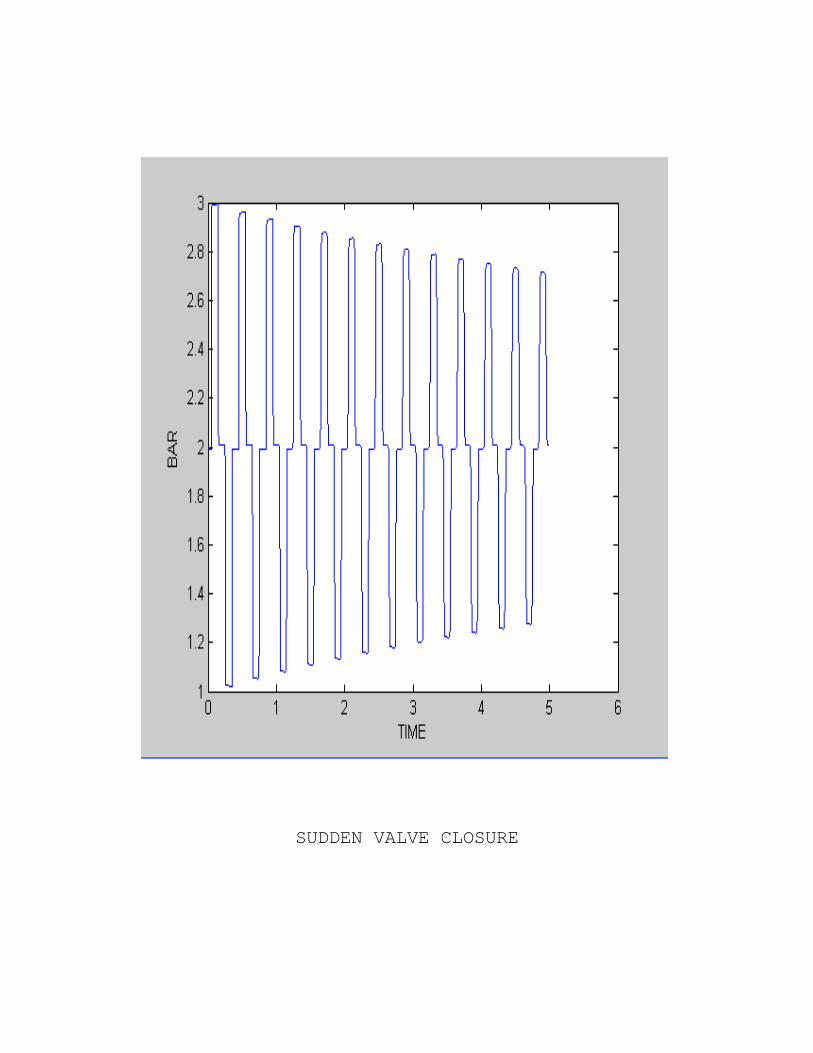
SUDDEN VALVE CLOSURE

STABLE LEAKY VALVE

UNSTABLE LEAKY VALVE

REACHES WITH FRICTION

Pipes in a pipe network often have different lengths. The

method of reaches divides the pipes into segments that have

the same transit time. The segments are known as reaches. The

sketch on the next page shows a pipe divided into 4 reaches.

Conditions at points i j k are known. Conditions at point J

are unknown. Waterhammer analysis gives for point J:

[ρa] dU/dt + dP/dt + [ρa]C = 0

PJ - Pi = - [ρa][UJ-Ui] - Δt [ρa]Ci

[ρa] dU/dt - dP/dt + [ρa]C = 0

PJ - Pk = + [ρa][UJ-Uk] + Δt [ρa]Ck

Manipulation of these equations gives:

PJ = (Pk+Pi)/2 - [ρa][Uk-Ui]/2 + Δt [ρa][Ck-Ci]/2

UJ = (Uk+Ui)/2 - [Pk-Pi]/[2ρa] - Δt [Ck+Ci]/2

This is the template for finding conditions at points inside

the pipe. At the ends of a pipe, water hammer analysis would

connect the end points to j points inside the pipe.

JUNCTIONS WITH FRICTION

Pipes in a pipe network are connected at junctions. The

sketch on the next page shows a junction which connects 3

pipes. Lower case letters indicate known conditions. Upper

case letters indicate unknown conditions. A junction is often

small. This allows us to assume that the junction pressure is

common to all pipes. It also allows us to assume that the net

flow into or out of the junction is zero. Conservation of

Mass considerations give:

+ ρ AN UN + ρ AH UH + ρ AW UW = 0

Waterhammer analysis gives:

PN - Pm = + [ρaN][UN-Um] + Δt [ρa]Cm

PH - Pg = + [ρaH][UH-Ug] + Δt [ρa]Cg

PW - Pv = + [ρaW][UW-Uv] + Δt [ρa]Cv

Manipulation gives

UN = Um + [PN-Pm]/[ρaN] - Δt Cm

UH = Ug + [PH-Pg]/[ρaH] - Δt Cg

UW = Uv + [PW-Pv]/[ρaW] - Δt Cv

In these equations PN = PH = PW = PJ. Substitution into

Conservation of Mass gives:

+ ρ AN [ Um + [PJ-Pm]/[ρaN] - Δt Cm]

+ ρ AH [ Ug + [PJ-Pg]/[ρaH] - Δt Cg]

+ ρ AW [ Uv + [PJ-Pv]/[ρaW] - Δt Cv] = 0

Manipulation gives the junction pressure:

PJ = [X – Y] / Z

X = [ + AN/aN Pm + AH/aH Pg + AW/aW Pv ]

Y = ρ [ + AN[Um-ΔtCm] + AH[Ug-ΔtCg] + AW[Uv-ΔtCv] ]

Z = [ + AN/aN + AH/aH + AW/aW ]

The velocities at the junction are:

UN = Um + [PJ-Pm]/[ρaN] - Δt Cm

UH = Ug + [PJ-Pg]/[ρaH] - Δt Cg

UW = Uv + [PJ-Pv]/[ρaW] - Δt Cv

THREE PHASE VALVE STROKING

Three phase valve stroking is a process where a valve is

opened or closed very fast in such a way that pressures are

kept within preset limits and no waves are left at the end.

It is described below for a complete closure case.

In phase I the valve is moved in such a way that the

pressure at the valve rises linearly in time from PLOW to

PHIGH in 2T pipe transit times. At the end of phase I the

pressure variation along the pipe is linear and the

velocity everywhere because of a combination of pressure

surges and back flows has been reduced by P/[a] where P

is PHIGH minus PLOW. In phase II the valve is moved in such a

way that the pressure variation along the pipe stays

constant and the velocity drops by 2P/[a] everywhere every

2T transit times. The pressure variation remains constant

because pressure surges generated by valve motion are

cancelled by suction waves at the valve caused by back

flows. The constant pressure variation causes a constant

deceleration of the fluid in the pipe. Phase III takes 2T

pipe transit times to complete. During this time the

velocity everywhere drops P/[a] and pressure falls

linearly at the valve from PHIGH to PLOW. The valve is moved

in such a way that suction waves at the valve caused by

back flows are allowed to bring the pressure down again to

PLOW. Because phases I and III reduce the velocity by a

total of 2P/[a] phase II must take (U-2P/[a])/(2P/[a])

2T seconds to complete. One can calculate what the valve

area should be at each instant in time during stroking. A

fast acting feedback control system can then be used to

move the valve in the desired manner.

Phase I sets up conditions in the pipe for phase II.

Similarly, phase II sets up conditions in the pipe for

phase III. In phase II, the pressure surge rate is twice

that of phases I and III. In a set period of time, one

pressure surge maintains a backflow that would have

otherwise been stopped by a suction wave. The other

pressure surge balances a pressure release. There are no

suction waves in phase II and all backflows are maintained.

Every point in the pipe has a velocity reduction due to a

surge wave and one due to a backflow. In phase III, the

pressure surge rate is cut in half. This allows suction

waves to form at the valve. These propagate up the pipe and

eliminate backflows. Conditions in the pipe are controlled

by these waves and by waves already there from phase II.

During the first half of phase III, conditions in the pipe

are still under the influence of phase II. Velocity falls

faster at the reservoir than at the valve because of this.

Half way through phase III, there is a linear pressure

variation and a linear velocity variation along the pipe.

During the second half of phase III, a wave travels down

the pipe which brings the pressure back to PLOW everywhere

and the velocity to zero everywhere.