Unseasonal Seasonals? - University of Pennsylvaniafdiebold/NoHesitations/Wright2013.pdfpeak of...
62
65 JONATHAN H. WRIGHT Johns Hopkins University Unseasonal Seasonals? ABSTRACT In any seasonal adjustment filter, some cyclical variation will be misattributed to seasonal factors and vice versa. The issue has long been well understood but it has resurfaced as a problem of special concern because the timing of the sharp downturn during the Great Recession appears to have distorted seasonals. In this paper, I find that initially this effect pushed reported seasonally adjusted nonfarm payrolls up in the first half of the year and down in the second half of the year, by slightly more than 100,000 in both cases. But the effect declined in later years and is quite small at the time of writing. Going beyond the special case of the Great Recession, I argue for using filters that constrain the seasonal factors to be more stable than the default filters used by U.S. statistical agencies, and also for using filters that are based on estimation of a state-space model. Finally, I report some evidence of predictability in revisions to seasonal factors. M ost macroeconomic data contain substantial regular variations associated with the time of year stemming from weather changes, vacations, or other sources. Overlooking the regular nature of this varia- tion would obscure longer-term trends and business cycle variation. Conse- quently, statistical agencies generally report seasonally adjusted (SA) data, aiming to purge the effect of this regular variation. Seasonal adjustment is extraordinarily consequential. Figure 1 plots the levels of SA and NSA (not-seasonally-adjusted) nonfarm payrolls, as reported by the Bureau of Labor Statistics (BLS). The regular within-year variation in employment is comparable in magnitude to the effects of the 1990–1991 and 2001 recessions. In monthly change, the average absolute difference between the SA and NSA number is 660,000, which dwarfs the normal month-over-month variation in the SA data. All this implies that we should think very carefully about how seasonal adjustment is done. Conceptually, one may define seasonal adjustment as the purging of any variations in economic data that are predictable using the calendar alone. This includes not only effects associated with the time of year but factors
Transcript of Unseasonal Seasonals? - University of Pennsylvaniafdiebold/NoHesitations/Wright2013.pdfpeak of...
65
Jonathan h. WrightJohns Hopkins University
Unseasonal Seasonals?
ABSTRACT In any seasonal adjustment filter, some cyclical variation will be misattributed to seasonal factors and vice versa. The issue has long been well understood but it has resurfaced as a problem of special concern because the timing of the sharp downturn during the Great Recession appears to have distorted seasonals. In this paper, I find that initially this effect pushed reported seasonally adjusted nonfarm payrolls up in the first half of the year and down in the second half of the year, by slightly more than 100,000 in both cases. But the effect declined in later years and is quite small at the time of writing. Going beyond the special case of the Great Recession, I argue for using filters that constrain the seasonal factors to be more stable than the default filters used by U.S. statistical agencies, and also for using filters that are based on estimation of a state-space model. Finally, I report some evidence of predictability in revisions to seasonal factors.
Most macroeconomic data contain substantial regular variations associated with the time of year stemming from weather changes,
vacations, or other sources. Overlooking the regular nature of this varia-tion would obscure longer-term trends and business cycle variation. Conse-quently, statistical agencies generally report seasonally adjusted (SA) data, aiming to purge the effect of this regular variation.
Seasonal adjustment is extraordinarily consequential. Figure 1 plots the levels of SA and NSA (not-seasonally-adjusted) nonfarm payrolls, as reported by the Bureau of Labor Statistics (BLS). The regular within-year variation in employment is comparable in magnitude to the effects of the 1990–1991 and 2001 recessions. In monthly change, the average absolute difference between the SA and NSA number is 660,000, which dwarfs the normal month-over-month variation in the SA data. All this implies that we should think very carefully about how seasonal adjustment is done.
Conceptually, one may define seasonal adjustment as the purging of any variations in economic data that are predictable using the calendar alone. This includes not only effects associated with the time of year but factors

66 Brookings Papers on Economic Activity, Fall 2013
such as the timing of Easter or the number of business days in a month. It does not include variations in economic data owing to deviations in weather from the norms for a given time of year.
What makes estimation of seasonal effects difficult is that they can change over time. For example, the rise of air conditioning changed the peak of electricity demand from the winter to the summer (this is, for exam-ple, documented in Energy Efficient Strategies 2005). Demographic trends affect the number of school- and college-age people seeking employment primarily during the summer. Climate change may also affect seasonal pat-terns. If seasonal effects were constant over time, econometricians could eventually learn the “true” seasonal patterns. But given that seasonal effects do vary over time, the seasonal factor is an unobserved component that can be estimated but never perfectly identified.
Two broad approaches are generally used to undertake seasonal adjust-ment. One approach tracks the seasonal component in a time series by a moving average of the series during the same period in different years.
Employment (millions)
110
Jan 1995 Jan 2000
Seasonally adjustedNon-seasonally adjusted
Jan 2005 Jan 2010
115
120
125
130
135
Note: Level of nonfarm payrolls employment as reported by the BLS.Source: Author’s calculations.
Figure 1. nonfarm Payrolls Employment: Seasonally adjusted and Unadjusted, 1990–2013

Jonathan h. Wright 67
This is the idea behind the Bureau of the Census X-12 ARIMA seasonal adjustment methodology.1 Henceforth in this paper, I will refer to this as the X-12 filter. This methodology involves first fitting a time series model to forecast and backcast the series, and then applying the moving average approach to the resulting extended series. If the data are not extended far enough, then asymmetric weights are used at the start and end of the sample. The different treatment of the start and end of the sample is important, both because the latest data are most important for the purposes of economic analysis and because the seasonal filter must inherently be one-sided at these points. The algorithm is described in some detail in the appendix to this paper and in greater detail by David Findley and others (1998) and by Dominique Ladiray and Benoît Quenneville (1989). U.S. and Canadian statistical agencies generally use the X-12 filter, and this will be my main focus in this paper.2 An alternative is to write down a model decomposing a series into components (such as trend, seasonal, and irregular) and to estimate this through the Kalman filter. The TRAMO-SEATS program developed at the Bank of Spain (Gómez and Maravall, 1996) is an example of a model-based methodology.
Unfortunately, in academic economic and econometric research, issues of seasonal adjustment are typically given short shrift.3 A great deal of work has been done on the question of how to do seasonal adjustment, but these papers get limited outside attention and are seldom published in leading journals. Most academics treat seasonal adjustment as a very mundane job, rumored to be undertaken by hobbits living in holes in the ground. I believe that this is a terrible mistake, though it is one in which the statistical agencies share at least a little of the blame. Statistical agencies emphasize SA data (and in some cases do not even publish NSA data), and while they generally document their seasonal adjustment process thoroughly, they do not always do so in a way that facilitates replication or encourages entry into this research area. Yet seasonality is both substantively important and
1. ARIMA stands for AutoRegressive Integrated Moving Average.2. As of the time of writing, the Census Bureau is developing an X-13 ARIMA program,
which is intended to allow users to choose between model-based and nonparametric seasonal adjustment, but this is not yet used by statistical agencies.
3. There are important papers studying seasonal fluctuations and arguing that they are useful sources of identifying information in macroeconomic models, including Ghysels (1988), Barsky and Miron (1989), Hansen and Sargent (1993), Sims (1993), and Saijo (2013). Barsky and Miron (1989) also study stylized facts over the seasonal cycle and find that they are quite similar to the stylized facts over the business cycle. However, these papers do not focus on how to parse data into seasonal and nonseasonal components.

68 Brookings Papers on Economic Activity, Fall 2013
difficult. It essentially involves issues such as bandwidth choice, or choos-ing between parametric and nonparametric approaches, that are all quite standard in modern econometrics. In short, seasonal adjustment could and should be better integrated into mainstream econometrics.
This paper therefore revisits the question of seasonal adjustment, including the difficulty of disentangling seasonality from cyclical factors. It focuses on seasonal adjustment of the BLS current employment statistics (CES) survey (the “establishment” survey), which includes total nonfarm payrolls, since this is the most widely followed monthly economic indicator. Section I discusses the impact of the Great Recession on seasonality as an important illustration of the problem. In this section, I also provide confi-dence intervals for seasonal factors. I find that these are quite wide—a direct implication of the intrinsic difficulty in separating business cycle and sea-sonal fluctuations. In section II, I discuss the choice of an “optimal” filter. I argue for using filters that constrain the seasonal factors to vary less over time than the filters used by U.S. statistical agencies. My main criterion for optimality is forecasting. Decomposing a time series into different com-ponents may be helpful for prediction, if those components have different dynamics. Section III establishes some results from revisions to estimated seasonal factors. Section IV concludes, offering suggestions for the practice of seasonal adjustment.
I. Seasonals and the Great Recession
I.A. Distortions from the Timing of the Recession’s Acute Phase
There has been a great deal of commentary among Wall Street analysts and in the press suggesting that the Great Recession may have distorted seasonals. The basic intuition is that the worst of the downturn came from November 2008 to March 2009. Standard seasonal filters will treat this as an indication that the “winter effect” became more negative,4 even though the downturn owed to a collapse in financial intermediation that had nothing to do with seasonality. The result is that SA data in subsequent years may have been biased upward in the winter and downward at other times. This possibility has led many to question how seasonal adjustment is undertaken, and it serves as the motivating example for this paper.
4. The X-12 seasonal filters include an automatic treatment for outliers, discussed in the appendix. But these are only outliers affecting a single month, so they do not resolve the concern that the recessions distorted seasonals.

Jonathan h. Wright 69
Seasonal adjustment in the BLS CES and Current Population Survey (CPS) is quite involved. In the CES, it is done at the three-digit NAICS5 level (or more disaggregated for some series) using the X-12 seasonal adjustment process, and these series are then aggregated to constructed SA total nonfarm payrolls.6 In the CPS, eight disaggregates are each season-ally adjusted, and they are then used to compute the SA unemployment rate. I approximately replicate the full CES seasonal adjustment process, taking each of the 152 NSA disaggregated employment series, which are combined to form total nonfarm payrolls as an input, seasonally adjusting each of them, and then aggregating them.7 Likewise, I approximately rep-licate the CPS seasonal adjustment process, taking eight CPS disaggregate series, seasonally adjusting them separately, and computing the resultant unemployment rate.8
I am aware of two pieces of detailed existing work on the Great Reces-sion and CES seasonal factors. Steven Wieting (2012a) runs the X-12 pro-gram on aggregate NSA employment data,9 replacing the actual data with a fictitious path that has a constant pace of decline from September 2008 to March 2009. He finds that this materially changed the contours of SA employment growth in 2010 and 2011, although in both years other factors just happened to give growth a bounce in the early spring that faded later on. Jurgen Kropf and Nicole Hudson (2012) redo the seasonal adjustment for the entire establishment survey using an alternative methodology to control for the impact of the recession.
In contrast to Wieting, they find that the Great Recession had no material impact on seasonals. Their methodology is to allow for “ramps,” that is, additional level shifts that occur linearly over a period of time. Their start- and
5. NAICS stands for the North American Industry Classification System, the industrial code system used for the past decade by BLS.
6. In this paper, I take the practice of statistical agencies in seasonally adjusting disaggre-gates as given, but note that Geweke (1978) argued for instead applying seasonal adjustment directly to the aggregate data.
7. The mean absolute deviation between my implementation of seasonal adjustment and the published BLS number for total nonfarm payroll employment is 10,000. At least some part of this is completely unavoidable because the BLS only publishes rounded unadjusted data, whereas their seasonal adjustment uses the unrounded numbers. Also, seasonal adjustment for data from November 2012 and earlier were computed by the BLS using disaggregate data as observed at the time of the January 2013 employment report release, which I do not have and the last two months of which have subsequently been revised.
8. The mean absolute deviation between my implementation of seasonal adjustment and the published BLS number for the unemployment rate is 0.02 percent.
9. Applying the X-12 program to aggregate NSA data does not produce aggregate SA data as reported by the BLS.

70 Brookings Papers on Economic Activity, Fall 2013
end-dates vary by series, but averaging across series they are October 2007 (start) and May 2010 (end; this is nearly a year after the NBER trough). These dates are not focused on the few months during the Great Recession in which employment was hemorrhaging. In my view, Kropf and Hudson’s methodology does not address the concern that job losses concentrated from November 2008 to March 2009 have distorted estimates of seasonal factors. They do not report employment data during 2008–09 using their alternative seasonal adjustment, but I strongly suspect that it would exhibit the same unusual concentration of job losses during the winter months as in the published SA series.
My approach to assessing the possibility that the Great Recession dis-torted seasonals is similar in spirit to that of Wieting (2012a), but I conduct the seasonal adjustment at the disaggregate level to get closer to what BLS is actually doing. For each month t from July 2008 to May 2009, I multi-ply each of the disaggregated CES employment numbers by a constant qt. The 11 constants qt are picked so as to ensure that seasonally adjusted aggregate nonfarm payrolls decline linearly from July 2008 to June 2009. More precisely, they are selected numerically to minimize the variance of month-over-month changes in aggregate seasonally adjusted payrolls from June 2008 to June 2009. Any unusual seasonal variation over this period is thus wiped out in these fictitious data.
Figure 2 plots SA monthly payroll changes during 2008–09 in both the real and the fictitious data; in the latter, SA employment declines at a steady pace of about 550,000 jobs per month. Here, and throughout this section, the seasonal adjustment is applied to the whole sample at the end of the sample period; this is not a real-time seasonal adjustment exercise.
Next, figure 3 plots the difference between the monthly level of actual seasonally adjusted total nonfarm payroll employment and the correspond-ing series based on the alternative, fictitious path for employment during the Great Recession. Consequently, figure 3 can be interpreted as showing the distortion to the monthly level of employment induced by the Great Recession, under the assumption that the unusual seasonal variation in 2008–09 did not in fact owe to changing seasonals.
In figure 3, the distortion to seasonal factors induced by the Great Recession pushes down the level of seasonally adjusted employment in the second half of the year and drives it up in the first half of the year. The effect repeats itself each year, generally getting smaller over time. The effect is largest in the second half of 2009 and the first half of 2010, where the level of employment is off by more than 100,000. As time goes by, the effect diminishes. At the end of the sample, it is small, but still not negligible.

Jonathan h. Wright 71
Reality
Fictitious path
–300
Employment (1,000s)
–400
–500
–600
–700
–800
Oct 2008July 2008 Jan 2009 Apr 2009
Note: Monthly changes in total SA nonfarm payroll employment from July 2008 to June 2009 both as reported by the BLS and using the alternative fictitious data (see text) that I use for the purpose of calculating post-recession seasonal factors.
Source: Author’s calculations.
Figure 2. Monthly Changes in Seasonally adjusted nonfarm Payroll Employment, July 2008–June 2009
Figure 3 shows the estimated effects of the Great Recession on the sub-sequent monthly level of seasonally adjusted employment. When one con-siders the monthly change in seasonally adjusted employment, it follows that each year from about November to April the apparently distorted seasonals biased the employment changes upward, whereas from May to October they had the reverse effect. In each year from 2010 to 2013, there has been a tendency for strong economic growth in the early spring being followed by a summer of discontent, as discussed in Wieting (2012b). Figure 3 shows that a part of this pattern is due to distortions in seasonal factors, but the seasonal distortions story can only explain a part of the phenomenon in 2010–2012, and it explains very little of it in 2013.10
10. The X-12 program incorporates a diagnostic check for whether a seasonal adjustment procedure is excessively unstable, based on sliding spans (Findley and others 1990). This procedure flags instability for 25 out of the 152 series (in the sense that the maximum abso-lute percentage difference in the estimated seasonal factor across spans exceeds 3 percent for these series).

72 Brookings Papers on Economic Activity, Fall 2013
An adjustment for the Great Recession effect along the lines that I envision could not have been implemented during the winter of 2008–09. However, it could have been implemented after the summer of 2009. The apparent consequences of the seasonal distortions from the Great Recession lasted for a few years, and so such an adjustment implemented in late 2009 or 2010 would still have been applicable to real-time analysis of incoming data during the post-recession period. Indeed, as discussed further below, the Federal Reserve Board implemented an adjustment for the effects of the Great Recession in the 2010 annual revision of industrial production data (published June 25, 2010).
I also consider the CPS reports, which include the unemployment rate. I multiply each of the four CPS unemployment numbers for each month from July 2008 to May 2009 by a month-specific adjustment parameter, so as to ensure that the total seasonally adjusted unemployment level climbs
Employment (1,000s)
150
100
50
0
–50
–100
–150
Jan 2010 Jan 2011 Jan 2012 Jan 2013
Note: For each month from July 2009 to April 2013, this figure shows the difference between the level of seasonally adjusted nonfarm payrolls using the actual current vintage of data and the level using the alternative fictitious data (described in the text), in which seasonally adjusted employment declined linearly from June 2008 to June 2009. The vertical dotted grid lines denote year turns, so that the bars immediately to the right represent January data.
Source: Author’s calculations.
Figure 3. Estimated Effect of recession-induced Seasonal Distortion on Monthly Payroll Levels, July 2009–april 2013
Jonathan h. Wright 73
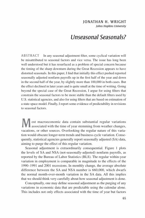
linearly from June 2008 to June 2009. I likewise adjust each of the four CPS employment numbers to ensure that the employment level falls linearly. Figure 4 plots the resulting difference between the actual unemployment rate and the corresponding series based on the alternative fictitious path. The pattern is roughly the mirror image of figure 3: the Great Recession drives down the unemployment rate in the first half of each year and drives it up in the second half. The effect diminishes over time. The estimated dis-tortion is, at most, about 0.08 percent. This seems less consequential than the distortion in the CES, but it is still not negligible (for scaling purposes, note that the standard deviation of monthly changes in the unemployment rate since 1984:01 is 0.16 percent).
In the remainder of this paper I focus on the seasonal adjustment of the CES survey. But the impact of the Great Recession on seasonals might well apply to other macroeconomic data as well. Lewis Alexander and
Unemployment rate (percent)
0.08
0.06
0.04
0.02
–0.02
–0.04
–0.06
–0.08
0
Jan 2010 Jan 2011 Jan 2012 Jan 2013
Note: For each month from July 2009 to April 2013, this figure shows the difference between the seasonally adjusted unemployment rate using the actual current vintage of data and using the alternative fictitious data, described in the text, in which seasonally adjusted unemployment climbed linearly from June 2008 to June 2009. The vertical dotted grid lines denote year turns, so that the bars immediately to the right represent January data.
Source: Author’s calculations.
Figure 4. Estimated Effect of recession-induced Seasonal Distortion on Monthly Unemployment rate, July 2009–april 2013

74 Brookings Papers on Economic Activity, Fall 2013
Jeffrey Greenberg (2012) argue that it affects initial jobless claims. Ellen Zentner, Aichi Amemiya, and Jeffrey Greenberg (2012) argue that it affects the Chicago PMI and the ISM index. And the Federal Reserve Board has made an intervention in its seasonal adjustment procedures for industrial production.
Finally, it is worth noting that the Great Recession did not just affect SA data after the recession was over, it also affected the SA data from before the recession, notably 2005–07. This effect is much less important, though, because the monthly contours of data from about seven years ago are of little relevance for policy today.
I.B. Another Way to Measure the Distortions
There are of course other possible ways of measuring distortions in sea-sonal adjustment arising from the Great Recession. One approach, pro-posed by Thomas Evans and Richard Tiller (2013) in the context of the CPS, is to treat all the data for 2008 and 2009 as missing. The X-12 program would then fill in these data with forecasts based on earlier data. A level shift dummy can be included for January 2010. In common with the approach that I propose, but unlike that of Kropf and Hudson (2012), this method forces the seasonal adjustment filter to operate without any knowledge of the tim-ing of the acute phase of the Great Recession.
I apply this Evans and Tiller approach to the 152 CES disaggregates. Figure 5 plots the resulting difference between the monthly level of actual seasonally adjusted total nonfarm payroll employment and the correspond-ing series based on this alternative seasonal adjustment from January 2010 on. The difference is qualitatively similar to what I found earlier, shown in figure 3: The distortion to seasonal factors induced by the Great Recession pushes down the level of seasonally adjusted employment in the second half of the year and drives it up in the first half of the year. The magnitude of the effect is about 100,000 in 2010 and gets smaller over time.
I.C. Might Seasonal Patterns Have Recently Changed?
The distortions discussed in the last two subsections are a case of cyclical variation being mistakenly attributed to seasonal effects. But the converse is also possible. A striking example of a series where seasonal patterns are changing and the filters are slow to catch up is employment by couriers and messengers (Wieting, 2012a). Figure 6 plots monthly changes in sea-sonally adjusted employment in this industry. Notwithstanding the fact that the series has been seasonally adjusted, there is a clear spike upward each December, which is reversed in the New Year. This appears to owe to the

Jonathan h. Wright 75
fact that people do more of their Christmas shopping online than in the past, and it creates a surge in employment by companies such as UPS and FedEx. This is a changing seasonal pattern that the filter is mistaking for a cyclical effect, though it may not be very important in the aggregate, because there is an offsetting secular shift toward less Christmas shopping at bricks-and-mortar retailers.
It could be that the Great Recession and its aftermath genuinely changed seasonal patterns, and that filters mistakenly attribute some of this to cyclical effects. Wieting (2012b) and Hyatt and Spletzer (2013) argue that job turn-over has declined sharply in the last few years. That means less hiring during the early summer months, when employers normally expand their payrolls, and less firing in January and February. Of course, it is a bit unclear whether one would want to treat this as a change in seasonal patterns or just
Employment (1,000s)
100
50
0
–50
–100
Jan 2010 Jan 2011 Jan 2012 Jan 2013
Note: For each month from January 2010 to April 2013, this figure shows the difference between the level of seasonally adjusted nonfarm payrolls using the actual current vintage of data and the level using the alternative seasonal adjustment in which data from 2008 and 2009 are treated as missing (with a level shift in 2010:01), following Evans and Tiller (2013). The vertical dotted grid lines denote year turns, so that the bars immediately to the right represent January data.
Source: Author’s calculations.
Figure 5. Estimated Effect of recession-induced Seasonal Distortion on Monthly Payroll Levels: alternative Methodology, January 2010–april 2013

76 Brookings Papers on Economic Activity, Fall 2013
as unusual cyclical behavior for a few years. If it lasts long enough, though, it should be viewed as a change in seasonal patterns. Since seasonal factors take some time to adjust to this change, seasonally adjusted data would then be biased downward in the summer months and upward in the winter months. This is a separate but seasonal-related story that could also explain part of the tendency for employment data to be strong in the early spring and weak later in the year.11
I.D. Impulse Responses
The broad concern, of which the effect of the Great Recession on sea-sonals is an important special case, is that the seasonal filter may incor-rectly attribute cyclical patterns or month-to-month “noise” to changing seasonality, or vice versa. To see how the former can happen generically, I
11. Indeed, well before the Great Recession, Canova and Ghysels (1994) found evidence that seasonal patterns can to some extent be affected by the business cycle.
Employment (1,000s)
20
10
0
–10
–20
Jan 2009 Jan 2010 Jan 2011 Jan 2012 Jan 2013
Note: The vertical dotted grid lines denote year turns, so that the bars immediately to the right represent January data.
Source: Author’s calculations.
Figure 6. Seasonally adjusted Monthly Change in Employment of Couriers and Messengers, 2009–13
Jonathan h. Wright 77
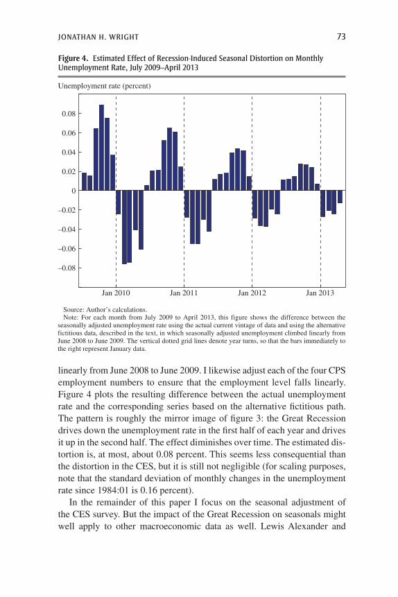
perform an experiment of adding 1 percent to each NSA employment dis-aggregate in January–March 2007 and then trace out the dynamic effects of this on SA aggregate employment data.
The results of this exercise are shown in figure 7. The shock drives SA employment up in January–March 2007 by about 0.8 percent, because the impact on the seasonal factors attenuates the shock. In the following January, the result is to push SA data down by about 0.15 percent and to drive SA data up a little in the rest of the year. The effects are smaller the next year, smaller again the following year, and have more or less worked through the system after 3 years, although the shock still has some effects on sporadic months after that. Figure 7 also shows the effect of the shock on SA employ-ment in earlier years—the echo effect is two-sided. This exercise only illus-trates the impulse response of a very particular shock: A one-percent shock that lasts for 3 months. To figure out the precise effects of other shocks, such as a shock that lasts for 6 months, the impulse response would have to be computed separately. The seasonal adjustment process is complicated and
Employment (percent)
0.8
0.6
0.4
0.2
0
Jan 2003 Jan 2005 Jan 2007 Jan 2009 Jan 2011
Note: This figure plots the effect on SA aggregate employment resulting from a hypothetical 1 percent increase in NSA disaggregate employment in January–March 2007. The vertical dotted grid lines denote year turns, so that the bars immediately to the right represent January data.
Source: Author’s calculations.
Figure 7. Estimated Effect of Shock to Employment, 2003–13

78 Brookings Papers on Economic Activity, Fall 2013
nonlinear; authors including Allan Young (1968) and Eric Ghysels, Clive Granger, and Pierre Siklos (1996) discuss the extent to which it may be approximated by a linear process.
I.E. Discussion
Amid signs of economic recovery at the start of 2010, 2011, and 2012, the Federal Reserve began each year by moving toward an “exit strategy” from unconventional monetary policy, hoping on each occasion that the recovery had gained enough momentum to be self-sustaining. In each case, when the apparent rebound faltered, the Federal Reserve restarted uncon-ventional policy. The problems with disentangling cyclical and seasonal patterns are of course well known to Federal Reserve staff. However, it is possible that some of the stop-start nature of asset purchase policy over this period reflects misleading estimates of seasonal factors, especially since the Federal Open Market Committee (FOMC) is remarkably sensitive to small changes in the payrolls number.
It is likewise possible that financial markets were to some extent fooled by problems with seasonal adjustments, as conjectured by Wieting (2012c). His argument is that in the aftermath of the Great Recession, the Citigroup economic surprise index was positive in the winter and negative the rest of the year. This index is a weighted average of differences between actual and expected data (from surveys). To test this, I compute the correlation between the surprise component of the monthly change in nonfarm payrolls and the distortion in these data from my estimates discussed above. I find that the correlation is positive, meaning that better-than-expected SA data tended to be overstated, although the correlation is not statistically significant.
The case of the Great Recession highlights the broader difficulty in separating cyclical and seasonal effects. This broad problem has been noted in earlier business cycles as well, including the recessions of 1957–58 and 1973–75 (Gilbert 2012; Ghysels 1987; Sargent 1978).
In the case of the Great Recession one may want to interfere in the normal econometric seasonal filter in some way so as to prevent the timing of the most acute part of the downturn from doing much to affect seasonal factors. In its seasonal adjustment of industrial production data, the Federal Reserve Board has decided to pre-adjust the NSA data for much of 2009 in order to eliminate the Great Recession effect before applying the normal seasonal filter. The BLS has not conducted such an adjustment. It seems clear that the Great Recession has distorted seasonals in the CES—the pace of job losses from November 2008 to March 2009 surely owed very little to shifting seasonal patterns. Still, it is understandable that a statistical agency
Jonathan h. Wright 79
might not want to make such consequential judgmental interventions in the construction of data. The data produced by the BLS are extremely influential in election campaigns, so making seasonal adjustments with a methodology that limits manual intervention may be important to insulate the agency from unfounded claims of political bias. But the situation is dif-ferent for sophisticated end-users of the data, such as the Federal Reserve Board. These users should—and perhaps for internal purposes they already do—construct alternative seasonal factors in employment data that in some way override the effect of the timing of the worst part of the Great Recession.
In the end a reasonable compromise would be for statistical agencies to provide both SA and NSA data, with the seasonal adjustment conducted by a filter that involves only limited manual intervention, allowing the end-user to apply the appropriate filter. Producing only NSA data and leaving the seasonal adjustment up to end-users would mean that there would be no single usable baseline measure of month-to-month fluctuations in employ-ment, unemployment, or other such variables. At the same time, I agree with Agustín Maravall (1995) that producing only SA data would be much worse, since users would then be unable to undertake their own decomposition of data into seasonal and nonseasonal components. Yet amazingly, the Bureau of Economic Analysis stopped releasing NSA GDP data some years ago as a cost-cutting measure. It is hard to imagine that the savings were material. While it seems likely that the drop in output in 2008Q4 and 2009Q1 has meaningfully affected national income and product account seasonal factors, data availability precludes a complete analysis of this possibility.
More generally, it is very unfortunate that for the most basic measure of economic activity in the largest economy in the world, researchers are effectively prevented from evaluating any difficulties associated with sea-sonal adjustment.
I.F. Providing Confidence Intervals for Seasonal Factors
Given the nature of the decomposition of data into seasonal and nonseasonal components, it seems important to provide confidence intervals for seasonal factors. Jerry Hausman and Mark Watson (1985) argued for the importance of providing such confidence intervals, but more than 25 years later their plea has largely fallen on deaf ears.12 Methods for seasonal adjustment such
12. There are exceptions. Tiller and Natale (2005) use a structural model, along the lines that I consider later in this paper, to get an estimate with standard error for the seasonal com-ponent of the unemployment rate. Scott, Sverchkov, and Pfeffermann (2005) also consider estimating the variance of the X-11 seasonal adjustment filter.
80 Brookings Papers on Economic Activity, Fall 2013
as the X-12 lack any direct means for constructing confidence intervals. However, an advantage of the model-based approach to seasonal adjustment is that confidence intervals are provided as a by-product of the Kalman filter.
As an illustrative exercise for forming confidence intervals for seasonal factors, I take one of the basic structural models of Andrew Harvey (1989). In this model, a time series yt can be decomposed as:
y s vt t t t= τ + + ,
where tt, st, and vt denote the stochastic trend, stochastic seasonal, and irregular components, respectively, which follow the specifications:
s s
v
t t t t
t t t
t t jj
s
t
t t
∑
τ = τ + β + ε
β = β + ε
= − + ε
= ε
− −
−
−=
−
,
1 1 1
1 2
1
1
3
4
where {e1t, e2t, e3t, e4t} are zero mean shocks that are each identically dis-tributed over time, and that are independent of each other both over time and cross-sectionally and S is the number of periods in a year. The model is simple, but it mirrors the X-12 model in seeking to decompose the series into trend, seasonal, and irregular components.
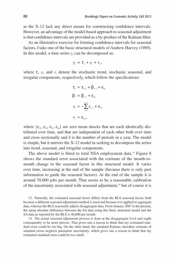
The above model is fitted to total NSA employment data.13 Figure 8 shows the standard error associated with the estimate of the month-to-month change in the seasonal factor in this structural model. It varies over time, increasing at the end of the sample (because there is only past information to guide the seasonal factors). At the end of the sample it is around 70,000 jobs per month. That seems to be a reasonable calibration of the uncertainty associated with seasonal adjustment,14 but of course it is
13. Naturally, the estimated seasonal factor differs from the BLS seasonal factor, both because a different seasonal adjustment method is used and because it is applied to aggregate data, whereas the BLS seasonally adjusts disaggregate data. From January 2007 to the present, the mean absolute difference between the SA data using this basic structural model and the SA data as reported by the BLS is 46,000 per month.
14. The actual seasonal adjustment process is done at the disaggregate level and ought consequently to be more precise. That gives one a reason to think that my estimated stan-dard error could be too big. On the other hand, the standard Kalman smoother estimate of standard errors neglects parameter uncertainty, which gives one a reason to think that my estimated standard error could be too small.

Jonathan h. Wright 81
dependent on the specific model used. Including a cyclical component in the structural model does reduce the standard error on the seasonal compo-nent, but only slightly.
It should be stressed that this calibration ignores any sampling error in the payrolls number. The BLS estimates the sampling standard error in the monthly level of employment to be about 56,000. Combining sampling error with uncertainty about the seasonal decomposition implies enormous uncertainty in SA monthly payrolls changes.15 Given this, it is remark-able that the FOMC reacts to very modest payrolls surprises. It is likewise noteworthy—but perhaps a consequence of the FOMC’s sensitivity—that financial market asset prices are so responsive to such noisy data.
15. Moreover, even if one treats the weights in the seasonal adjustment filter as known, the sampling error will still impart uncertainty to the estimation of the seasonal factors (Hausman and Watson 1985).
Employment (1,000s)
80
70
60
50
40
10
20
30
Jan 2008 Jan 2010 Jan 2012
Note: This figure plots the standard error of the seasonal component estimate in month-over-month changes in payroll employment when the basic seasonal structural model is applied to aggregate payroll employment. The standard error is computed via the Kalman smoother, treating parameters as fixed.
Source: Author’s calculations.
Figure 8. Standard Error of Seasonal Component in Monthly Payroll Changes, January 2007–april 2013

82 Brookings Papers on Economic Activity, Fall 2013
II. Optimal Seasonal Adjustment
This section departs from the specific issue of the impact of the Great Recession on seasonals and instead considers the broader question of what is the “optimal” choice from among the many seasonal filters that are available.
II.A. Attention to Bandwidth Choice
A critical part of the X-12 process involves estimating the seasonal factors by taking weighted moving averages of data in the same period of different years. This is done by taking a symmetric n-term moving average of m-term averages, which is referred to as an n × m seasonal filter. For example, for n = m = 3, the weights are 1/3 on the year in question, 2/9 on the years before and after, and 1/9 on the two years before and after.16 The filter can be a 3 × 1, 3 × 3, 3 × 5, 3 × 9, 3 × 15, or stable filter. The stable filter averages the data in the same period of all available years. The default settings of the X-12, as described in the appendix, involve using a 3 × 3, 3 × 5, or 3 × 9 seasonal filter, depending on a criterion discussed in the appendix. Figure 9 plots the weights for the different filters. The choice of filter is effectively the bandwidth choice in a nonparametric statistical problem, and the choice of bandwidth involves a bias-variance trade-off. If seasonal patterns fluc-tuate a great deal, then a small choice of bandwidth will be appropriate to reduce the problem of changing seasonals being incorrectly attributed to cyclical variation (bias). The example of changing seasonality coming from the sudden expansion in online retailing in figure 6 is an illustration of where a low bandwidth is suitable. On the other hand, if seasonal patterns do not flap around much, a higher choice of bandwidth will reduce the problem of cyclical patterns being incorrectly attributed to seasonals (variance). The problem of the Great Recession distorting seasonals illustrates a situation where a high bandwidth is suitable.
Out of the 152 CES seasonal series that I seasonally adjust in section 2 with the default X-12 settings, 118 end up using the 3 × 5 filter, 31 use the 3 × 3 filter, and 3 use the 3 × 9 filter.17 The 3 × 3 and 3 × 5 filters that are effectively used in CES seasonal adjustment have a very small bandwidth. The 3 × 3 filter only weights the current year and the previous and sub-sequent two years. The 3 × 5 filter puts 87 percent of the weight on these five years. This small bandwidth means that a special factor in one year can have a large effect on seasonals. The flip side is that the distortion will wash
16. Note that an n × m filter and an m × n filter are the same thing.17. This is the filter used on the D step of the algorithm as described in the appendix.

Jonathan h. Wright 83
out after 2 or 3 years. This bandwidth also means that genuine changes in seasonal patterns will be picked up fairly quickly.
In the X-12 filter the data are extended with forecasts and backcasts from a seasonal ARIMA model. If they are not extended far enough, then an asymmetric filter is used at the beginning and end of the sample instead (more details are given in the appendix). Importantly, this means that at the end of the sample the seasonal adjustment may be even more heavily
Weight
3 � 1 3 � 3
0.3
0.2
0.1
Weight
0.3
0.2
0.1
–5 0 5 –5 0Years before/after Years before/after
Years before/after Years before/after
5
Weight
3 � 5 3 � 9
0.3
0.2
0.1
Weight
0.3
0.2
0.1
–5 0 5
Weight
3 � 15
0.3
0.2
0.1
–5 0Years before/after
5
–5 0 5
Note: This figure plots the weights on the same period each year used by alternative seasonal MA filters in the X-12. The stable filter is not reported, but gives equal weight to all years over the sample on which the seasonal filter is run.
Source: Author’s calculations.
Figure 9. alternative Seasonal Ma Filters

84 Brookings Papers on Economic Activity, Fall 2013
influenced by a small number of observations than would be the case in the middle of the sample.
It is also important to note that the BLS implements seasonal adjustment using about 10 years of data. So even the stable filter does not assume that seasonal factors never change, just that the changes within the last 10 years are negligible.
II.B. Criteria for Optimality
A number of criteria are possible for making the optimal choice of band-width within the X-12 filter, or indeed for deciding between the X-12 and other methods of seasonal adjustment. One might pick the seasonal filter to maximize the accuracy of parameter estimates in a rational expectations model or to control the size or maximize the power of tests of such a model (Hansen and Sargent 1993; Sims 1993; Saijo 2013). The predictability of seasonal patterns makes them potentially very useful for inference in ratio-nal expectations models.
Alternatively, one might pick the filter to minimize the mean square error of the estimate of the seasonal component. This is easiest to conceptualize if one has an explicit model. Of course, given a correctly specified model, the model itself should give the best estimate of the seasonal component.18 But all models are mis-specified, and so other methods may then do better. Treating the data as approximated by a model, one could then ask what X-12 filter gives the minimum mean square error. Raoul Depoutot and Christophe Planas (1998) consider approximating a time series yt with the model:
L L y L L at t( )( )( )( )− − = + θ + θ1 1 1 1 ,121 12
12
where at is independent and identically distributed (iid) noise—a so-called “airline” model (Box and Jenkins 1986), which implies a decomposition of the series into trend, seasonal, and irregular components (Hillmer and Tiao, 1982). Depoutot and Planas (1998) provide a look-up table telling us which X-12 filter from among the 3 × 3, 3 × 5, 3 × 9, and 3 × 15 alternatives gives the minimum mean square error of the seasonal component, for a given choice of the parameters q1 and q12. Out of the 152 CES seasonal series that I seasonally adjust, based on this criterion, the 3 × 3 would be
18. Burridge and Wallis (1984) show that an unobserved component model with particular parameter values can come close to the X-11 filter that was in use at that time. But the X-11 is still suboptimal for any other time-series models.

Jonathan h. Wright 85
optimal for 20 series, the 3 × 5 for 16 series, the 3 × 9 for 18 series, and the 3 × 15 for 98 series. These filters are generally higher bandwidth than in the default X-12 program, implying that seasonal factors should be con-strained to vary less over time. Depoutot and Planas (1998) and Richard Tiller, Daniel Chow, and Stuart Scott (2007) use this same methodology to determine the optimal X-12 filter for a range of series, and likewise find that higher bandwidth filters are optimal for many series.
However, the main objective for seasonal adjustment under consideration in this paper is to obtain data for a forecasting model. Decomposing a time series into different components may be helpful for prediction, if those components have different dynamics. Thus, if one’s objective is to forecast NSA data at the h-month horizon, one might want to split the data into SA data and the seasonal factor. One could fit a forecasting model to the SA data and forecast the seasonal factor by the last available value for that month in the sample period. Using SA data in this way, one can ask what seasonal filter gives the most accurate forecasts. This is my proposed optimality criterion.
The forecasting objective may be somewhat narrow, but it is easy to quantify any gains from seasonal adjustment, and of course these fore-casts are inputs to a forward-looking Taylor rule. In the same spirit, Eric Ghysels, Denise Osborn, and Paulo Rodrigues (2006) do a Monte Carlo simulation comparing the ability of different models to forecast artificially simulated NSA data. William Bell and Ekaterina Sotiris (2010) consider fore casting as an objective for seasonal adjustment, and indeed, Julius Shishkin (1957, p. 222) made this case more than half a century ago:
A principal purpose of studying economic indicators is to determine the stage of the business cycle at which the economy stands. Such knowledge helps in forecasting subsequent cyclical movements and provides a factual basis for taking steps to moderate the amplitude and scope of the business cycle. . . . In using indicators, however, analysts are perennially troubled by the difficulty of separating cyclical from other types of fluctuations, particularly seasonal fluctuations.
It is also true that the seasonal adjustment process itself directly implies a forecast for the future time series. However, in practice, forecasters almost invariably simply download data and fit time series models directly to these data. Taking this practice as given, I aim to see what seasonal filter it is best to have applied, addressing the question in a standard pseudo-out-of-sample forecasting exercise.
Before continuing to the forecasting exercise, note that the X-12 seasonal filter considers only a few specific possible choices of weights. Considering how statisticians and econometricians tackle other nonparametric problems,
86 Brookings Papers on Economic Activity, Fall 2013
it would seem more natural to select some kernel function and then pick the bandwidth from a continuum of possible values according to some criterion.19 Nevertheless, in this paper I restrict attention to filter choices available within the X-12 program.
II.C. Univariate Forecasting
Let yt (j) denote the value of total nonfarm payroll employment at time t, summing each of the CES disaggregates using the jth seasonal adjustment filter. I treat this as stationary in log first differences (following, for example, Stock and Watson 2002) and consider the AR model for the log first differ-ences of this series:
y j y j ut i t i ti
p
∑( )( ) ( )( )∆ = α + α ∆ +−=
(1) log log ,01
where ut is an iid error term. I estimate equation 1 in a recursive out-of-sample forecasting scheme with data from 1990:01 up to month t (which ranges from 2000:01 to 2012:04), using seasonal adjustment applied to the sample from 1990:01 to month t and with the lag order p selected by the Bayesian information criterion.20 I then construct the implied forecast of SA employment growth over the next h months, log [yT+h(j)] - log [yT(j)], and call this gT,T+h(j). I convert this into a forecast of NSA employment growth as
g j y y
y j y jT T h T h l T
T h l T
)){ }
((
) )) ))
( (( ((
) )( (+ −− −+ + −
+ −
(2) ˆ log 0 log 0
log log ,,
where l = 12ceil(h/12) and ceil(.) denotes the argument rounded up to the next integer. This latter forecast is then compared to the actual realized value of NSA employment growth over the subsequent h months. If h = 12, equation 2 reduces to gT,T+12(j) as above.
The seasonal filters that I consider in this exercise are all the alterna-tives in the X-12 program: 3 × 1, 3 × 3, 3 × 5, 3 × 9, 3 × 15, stable, and the default. Recall from subsection II.A that the default settings, which are
19. Also, the weights in the X-12 seasonal filter are always nonnegative. In other non-parametric problems, researchers often use higher-order kernels that can be negative in the tails. It may be somewhat counterintuitive, but this turns out to reduce bias (Bartlett 1963; Silverman 1986) and might in principle be helpful in the context of seasonal adjustment. Nevertheless, to my knowledge the possibility has never been explored.
20. The 152 disaggregates that go into total nonfarm payrolls are all reported only as far back as 1990:01.

Jonathan h. Wright 87
described in the appendix, amount in the context of the CES to using 3 × 5 for most series and 3 × 3 for nearly all of the others.21 In addition, I consider three other alternatives, as follows.
First alternative: Simply using NSA data.Second alternative: Using NSA data but augmenting equation 1 with
seasonal dummies. This is the optimal way of doing seasonal adjustment if the seasonal effects are constant over time and simply amount to level shifts depending on the current month.
Third alternative: Doing seasonal adjustment using, instead, the basic structural model, described in subsection I.F, estimated recursively through the Kalman filter.
For forecasts made as of time t, the seasonal adjustment is implemented only using data up to time t and the parameters are estimated using only these data. However, this is still not a genuine real-time forecasting exer-cise, as I do not have real-time data on NSA employment disaggregates. Although the seasonal adjustment is done recursively, the current vintage of NSA employment data is used (both for disaggregates and for the aggre-gate data).
Table 1 reports the root mean square prediction error (RMSPE) for each seasonal filter at forecast horizons of h = 1, 6, and 12 months. Table 1 also reports tests of the hypothesis of equal root forecast accuracy comparing (i) forecasts using NSA data and all other forecasts and (ii) forecasts using the X-12 default seasonal filter and all other forecasts. The test of equal forecast accuracy uses the approach of Diebold and Mariano (1995).
Forecasting is consistently much more accurate using SA data. This seems intuitive. For example, strong growth in retail sales in October might suggest that the economy has momentum; the same data in December would not. This is just one of a number of contexts in time series where decomposing data into components with different dynamics helps with forecasting. As another example, breaking out inflation measures into core inflation and food and energy inflation helps in predicting total inflation, because food and energy inflation is much less persistent (Faust and Wright 2013). In the volatility forecasting literature, Torben Andersen, Tim Bollerslev, and Francis Diebold (2007) find that separating volatility into smooth compo-nents and jumps gives better predictions, because the two parts of volatility have different persistence patterns.
21. The implementation of the X-12 is in all respects carried out exactly as by the BLS, except for the choice of seasonal filter (such as whether the model is additive or multiplicative).

88 Brookings Papers on Economic Activity, Fall 2013
Table 1. out-of-Sample Forecasting of Payroll Employment in a Univariate autoregression Using Different Seasonal Filters
1 month 6 months 12 months
RMSPEsNSAa 0.24 1.29 2.42X-12 default 0.14 0.77 1.733 × 1 0.14 0.78 1.743 × 3 0.14 0.77 1.733 × 5 0.14 0.76 1.713 × 9 0.13 0.74 1.703 × 15 0.14 0.74 1.69Stable 0.15 0.72 1.66NSA+Duma 0.15 0.78 1.82Model 0.14 0.72 1.68
Diebold-Mariano p-valuesb
NSA v. X-12 default 0.00 0.00 0.00NSA v. 3 × 1 0.00 0.00 0.00NSA v. 3 × 3 0.00 0.00 0.00NSA v. 3 × 5 0.00 0.00 0.00NSA v. 3 × 9 0.00 0.00 0.00NSA v. 3 × 15 0.00 0.00 0.00NSA v. stable 0.00 0.00 0.00NSA v. NSA+Dum 0.00 0.00 0.00NSA v. model 0.00 0.00 0.00X-12 default v. 3 × 1 0.05 0.01 0.11X-12 default v. 3 × 3 0.72 0.09 0.49X-12 default v. 3 × 5 0.02 0.00 0.03X-12 default v. 3 × 9 0.02 0.00 0.03X-12 default v. 3 × 15 0.80 0.01 0.12X-12 default v. stable 0.15 0.03 0.01X-12 default v. model 0.84 0.01 0.203 × 1 v. stable 0.50 0.01 0.01
Note: This table reports the out-of-sample root mean square prediction error (RMSPE) of 100 times log aggregate employment change over horizons h = 1, 6, 12 months from estimation of a univariate autoregression using each of the possible approaches to seasonal adjustment (at the disaggregate level). For each horizon, the smallest RMSPE is shown in bold. The model is the trend+seasonal+noise basic structural model, as described in the text, and the remaining seasonal filters are variants of the X-12.
a. NSA means no seasonal adjustment; NSA+Dum means no seasonal adjustment but includes seasonal dummies.
b. The p-values included are from Diebold-Mariano tests of equal predictive accuracy.

Jonathan h. Wright 89
The performance of the forecasts using seasonally adjusted data is gen-erally comparable, but the forecasts are somewhat more accurate using nonstandard seasonal filters that force the seasonal effects to be relatively stable rather than using the X-12 default filter. These are the 3 × 9, 3 × 15, and stable filters.22
In some cases, the improvement is statistically significant. The fore-casts augmented with dummy variables do not perform very well. But the model-based forecasts are at or close to the top of the ranking of forecast performance. A useful comparison is between the 3 × 1 and stable filter, since these are the filters with the most and least flexible seasonals. The stable filter provides significantly more accurate forecasts than the 3 × 1 filter at the h = 6 and h = 12 horizons, though the two are similar at the h = 1 horizon.
Two main conclusions can be drawn from this forecast exercise. First and foremost, it is important to seasonally adjust. Second, using relatively high bandwidth filters or the simple model-based filter is generally the best approach to seasonal adjustment. This is a very simple model that omits many of the bells and whistles that are present in the X-12. It is quite possible, though by no means guaranteed, that richer models will provide SA data that are better for forecasting purposes. I leave this possibility for future investigations.
The best forecasts are apparently obtained using either a simple state-space model or using versions of the X-12 filter with relatively stable seasonals. These two findings are not in conflict. The estimated state-space models (using the full sample) are different for each of the 152 disaggregates, but they generally imply seasonal filters that spread weight across many years. This is further support for the argument that if one is using the X-12, the seasonals should not be allowed to be quite as variable as in the current default settings.
I also investigated using the univariate AR model to do recursive out-of-sample forecasting for each of the 152 employment disaggregates separately. Table 2 reports the number of series for which each choice of seasonal filter
22. In this exercise, the seasonal adjustment is applied to the same sample as is being used in each step of the recursive forecasting exercise. For example, when forecasting using data from 1990:01 up to 2009:12, the seasonal filters are applied to the 20 years of data from 1990:01 up to 2009:12. When one attempts to apply the 3 × 15 seasonal filter to a sample ending in 2006:12 or earlier, the X-12 program does not have enough data for the 3 × 15 filter and simply uses the stable filter instead. However, in longer samples, the 3 × 15 and stable filters are different. This is why the entries in table 1 for the 3 × 15 and stable alternatives are not the same.

90 Brookings Papers on Economic Activity, Fall 2013
minimizes out-of-sample mean-square prediction errors. At each horizon, for more than half of the series, forecast accuracy is optimized by using the basic structural model or a higher bandwidth X-12 filter (3 × 9, 3 × 15, or stable).23
II.D. Forecasting with a Factor Model
Next I turn to multivariate forecasting, using sectoral detail in employment disaggregates to forecast total employment. With a set of 152 employment disaggregates, a multivariate model that does not impose some additional structure will be overparameterized. I let {fit( j )}m
i=1 denote the first m static principal components of the monthly log first differences of 152 employment disaggregates, using the jth seasonal adjustment filter. I then consider the factor-augmented autoregression (FAAR) (Stock and Watson 2002):
y j y j y j f jt h t i t ii
p
i iti
m
t∑ ∑[ ] [ ] [ ]( ) ( ) ( ) ( )− = β + β ∆ + γ + ε+ + −= =
(3) log log log .0 11 1
I consider recursive out-of-sample forecasting of log [yt+h ( j)] - log [yt ( j)] using the FAAR, with the data starting in 1990:01, the first forecast being made in 2000:01 and the final forecast being made in 2012:04. The forecasts
23. Viewing forecasting as the objective leaves open the possibility that we might also want to control for other things in addition to seasonality—notably year-to-year weather fluctuations—which are not part of seasonal effects, as discussed in the introduction. In prac-tice, an econometric model that takes account of recent weather in macroeconomic forecasting is likely to be unwieldy and overparameterized. However, for some series, such as construction employment, it might be useful to construct a series that is both seasonally adjusted and weather adjusted. The latter would involve taking the residuals from a regression of season-ally adjusted data on deviation of weather indicators from norms for that time of year.
Table 2. number of Series for Which Each Filter gives Best out-of-Sample Forecasts
Filter 1 month 6 months 12 months
X-12 default 9 6 73 × 1 12 40 433 × 3 14 17 163 × 5 11 8 53 × 9 20 20 103 × 15 15 5 13Stable 28 23 23Model 43 33 35
Note: At each horizon, this table reports the number of CES series for which the smallest out-of-sample mean square prediction is given by each possible seasonal filter. There are 152 CES disaggregates.

Jonathan h. Wright 91
are then converted into implied forecasts of NSA employment growth using equation 2 and are compared with realized employment growth.
Comparisons of RMSPEs and tests of hypotheses of equal forecast accu-racy are shown in table 3. The results are broadly similar to those in the uni-variate case. The best forecasts are obtained using the 3 × 9 filter or stable implementations of the X-12 or basic structural model. Using the 3 × 9 filter rather than the X-12 default gives an improvement in forecast accuracy that is significant at the 10 percent level at the h = 1 and h = 6 horizons. Other-wise, the gains in forecast accuracy from using the 3 × 9, stable, or model-based filtering, rather than the X-12 default, are not statistically significant.
Table 3. out-of-Sample Forecasting of Payroll Employment in a Faar Using Different Seasonal Filters
1 month 6 months 12 months
RMSPEsNSA 0.23 1.27 2.05X-12 default 0.13 0.74 1.723 × 1 0.13 0.75 1.753 × 3 0.13 0.74 1.733 × 5 0.13 0.73 1.723 × 9 0.12 0.72 1.713 × 15 0.13 0.73 1.77Stable 0.13 0.73 1.69NSA+Dum 0.14 0.83 1.75Model 0.13 0.71 1.69
Diebold-Mariano p-valuesNSA v. X-12 default 0.00 0.00 0.00NSA v. 3 × 1 0.00 0.00 0.00NSA v. 3 × 3 0.00 0.00 0.00NSA v. 3 × 5 0.00 0.00 0.00NSA v. 3 × 9 0.00 0.00 0.00NSA v. 3 × 15 0.00 0.00 0.00NSA v. stable 0.00 0.00 0.00NSA v. NSA+Dum 0.00 0.00 0.00NSA v. model 0.00 0.00 0.00X-12 default v. 3 × 1 0.03 0.03 0.05X-12 default v. 3 × 3 0.73 0.08 0.06X-12 default v. 3 × 5 0.04 0.19 0.43X-12 default v. 3 × 9 0.06 0.09 0.45X-12 default v. 3 × 15 0.47 0.82 0.25X-12 default v. stable 0.92 0.74 0.66X-12 default v. model 0.97 0.17 0.483 × 1 v. stable 0.48 0.46 0.47
Note: See footnotes to table 1 for clarifying details.
92 Brookings Papers on Economic Activity, Fall 2013
II.E. Forecasting Other Series
In subsections II.C and II.D I found that for forecasting nonfarm pay-rolls, the best predictions are obtained using either a simple state-space model or versions of the X-12 filter with relatively stable seasonals. One might wonder whether this is unique to nonfarm payrolls or is a broader feature of macroeconomic data.
To gather more evidence to answer this, I take the aggregate NSA values of six other monthly time series from 1960:01 to 2013:06 and apply the different seasonal filters to each of these aggregates. The series are the industrial production index (total and manufacturing), the CPI and PPI indexes, housing starts, and housing permits. To be clear, seasonal filtering is in practice undertaken at the disaggregate level—and that is not what I am doing here. But I am applying each seasonal filter in exactly the same way, allowing at least an apples-to-apples comparison. For each filtered series, I consider the AR model for the log first differences of this series as in equation 1 in a recursive out-of-sample forecasting scheme with data from 1960:01 up to month T (which ranges from 1970:01 to 2013:04), using seasonal adjustment applied to the sample from 1960:01 to month T. I then construct the implied forecast of SA growth over the next 12 months and assess this as a forecast of NSA growth.
The results are shown in table 4. The general conclusions from this exer-cise are similar to those from tables 1–3. Seasonal adjustment is important; simply using dummies does not work. Within the seasonal filters that I consider, the differences are not overwhelming, but the best forecasts are obtained using the 3 × 9 or stable X-12 filter, except in the case of housing starts, where the model-based adjustment fares best. This is all broadly consistent with what I found for nonfarm payrolls in tables 1–3. Moreover, it applies over a very long forecast evaluation period and therefore miti-gates any concern that the earlier findings were dominated by the Great Recession.
II.F. Recent Employment Data with a Higher-Bandwidth Filter
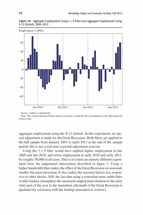
In the foregoing, I have found some support for the idea of altering the X-12 filter by using a higher bandwidth and so preventing the seasonal factors from varying so erratically. This then begs the question of what payrolls data would have looked like if the CES had indeed used a higher bandwidth filter. To address this question, I re-did the X-12 seasonal adjust-ment using the 3 × 9 filter instead of the X-12 default. Figure 10 plots the difference between aggregate employment using the 3 × 9 filter and

Jonathan h. Wright 93
Table 4. 12-Month-ahead out-of-Sample Forecasting of Macroeconomic aggregates in a Univariate autoregression Using Different Seasonal Filters
IPTa IPMa CPIb PPIb STARTc PERMc
RMSPEsNSAd 5.48 6.29 2.24 3.80 24.89 26.84X-12 default 4.95 5.61 2.13 3.90 24.84 26.263 × 1 5.05 5.75 2.22 3.99 25.22 26.203 × 3 5.00 5.63 2.19 3.95 24.66 26.123 × 5 4.93 5.55 2.16 3.95 24.84 26.183 × 9 4.87 5.54 2.12 3.75 24.85 26.103 × 15 4.87 5.54 2.13 3.75 24.82 26.13Stable 4.99 5.76 2.13 3.68 24.83 25.99NSA+Dum 5.23 5.91 2.22 3.72 25.51 27.34Model 4.89 5.59 2.14 3.82 24.42 32.51
Diebold-Mariano p-valuese
NSA v. X-12 default 0.00 0.00 0.04 0.09 0.81 0.21NSA v. 3 × 1 0.00 0.00 0.65 0.03 0.23 0.18NSA v. 3 × 3 0.00 0.00 0.34 0.04 0.27 0.12NSA v. 3 × 5 0.00 0.00 0.15 0.03 0.81 0.16NSA v. 3 × 9 0.00 0.00 0.02 0.86 0.86 0.12NSA v. 3 × 15 0.00 0.00 0.02 0.81 0.77 0.15NSA v. stable 0.00 0.00 0.01 0.09 0.79 0.07NSA v. NSA+Dum 0.00 0.00 0.21 0.01 0.07 0.42NSA v. model 0.00 0.00 0.02 0.27 0.13 0.37X-12 default v. 3 × 1 0.02 0.01 0.00 0.01 0.00 0.63X-12 default v. 3 × 3 0.04 0.27 0.00 0.02 0.00 0.04X-12 default v. 3 × 5 0.08 0.20 0.02 0.04 0.96 0.06X-12 default v. 3 × 9 0.06 0.19 0.25 0.01 0.52 0.10X-12 default v. 3 × 15 0.12 0.24 0.79 0.08 0.65 0.19X-12 default v. stable 0.56 0.06 0.87 0.02 0.85 0.04X-12 default v. model 0.24 0.65 0.79 0.24 0.13 0.333 × 1 v. stable 0.49 0.94 0.04 0.01 0.00 0.20
Note: This table reports the out-of-sample root mean square prediction error (RMSPE) of 100 times the log change of 6 different macroeconomic series over 12-month horizons from estimation of a univariate autoregression using each of the possible approaches to seasonal adjustment (at the aggregate level). For each series, the smallest RMSPE is shown in bold. The model is the trend+seasonal+noise basic structural model, as described in the text, and the remaining seasonal filters are variants of the X-12.
a. Industrial production index, total (IPT), and industrial production index, manufacturing (IPM).b. Consumer price index (CPI) and producer price index (PPI).c. Housing starts (START) and housing permits (PERM).d. NSA means no seasonal adjustment, NSA+Dum means no seasonal adjustment but includes seasonal
dummies.e. The p-values included are from Diebold-Mariano tests of equal predictive accuracy.
94 Brookings Papers on Economic Activity, Fall 2013
aggregate employment using the X-12 default. In this experiment, no spe-cial adjustment is made for the Great Recession. Both filters are applied to the full sample from January 2003 to April 2013 at the end of the sample period; this is not a real-time seasonal adjustment exercise.
Using the 3 × 9 filter would have implied higher employment in late 2009 and late 2010, and lower employment in early 2010 and early 2011, by roughly 50,000 in all cases. This is of course an entirely different experi-ment from the judgmental intervention described in figure 3. Using a higher bandwidth filter makes the effect of the Great Recession on seasonals smaller but more persistent. It also makes the seasonal factors less respon-sive to other shocks. Still, the fact that using a somewhat more stable filter would weaken (strengthen) the measured employment situation in the early (late) part of the year in the immediate aftermath of the Great Recession is qualitatively consistent with the findings presented in section I.
Employment (1,000s)
60
40
20
0
–20
–40
–60
Jan 2010 Jan 2011 Jan 2012 Jan 2013
Note: The vertical dotted grid lines denote year turns, so that the bars immediately to the right represent January data.
Source: Author’s calculations.
Figure 10. aggregate Employment Using 3 × 9 Filter Less aggregate Employment Using X-12 Default, 2009–2013
Jonathan h. Wright 95
II.G. Outlier-Robust Filters
Most causes of time variation in seasonal effects seem to consist of insti-tutional, technological, or environmental factors that are unlikely to change suddenly. I conjecture that while NSA changes are “fat-tailed,” the changes to underlying seasonal factors are not. If that is right, then an optimal filter will be nonlinear in the sense of attributing a smaller share of huge shifts (like the aftermath of the Lehman collapse) to seasonals than would be the case for normal-sized fluctuations. It is essentially this idea that moti-vates the manual intervention in the seasonal adjustment process around the Great Recession discussed in section I, but this same idea could to some extent be made an automatic part of seasonal filtering.
As discussed in the appendix, the X-12 does automatically detect out liers in a single month and restricts their impact on seasonal factors. But it is possible to go further in the direction of making seasonal filters outlier-robust. William Cleveland, Douglas Dunn, and Irma Terpenning (1978) and Robert Cleveland and others (1990) discuss using seasonal moving medians instead of seasonal moving averages to downweight extreme observations. The idea might best be explored in the context of a state-space model, one in which either the shocks to nonseasonal components could be specified to have fatter tails than the shocks to seasonal compo-nents or else the distributions of the shocks to the different components could be estimated. As long as the nonseasonal components have fatter tails, extreme events will tend to have proportionately less impact on the seasonal factors. I do not explore the idea further in this paper, but note that it could perhaps mitigate—but certainly not eliminate—the difficulty of separating seasonal and nonseasonal components.
III. Revisions to Seasonal Factors
Nearly all macroeconomic data are revised as more complete information becomes available. For example, in the CES the initial data are based on a survey, whereas later on as tax records become available they become an obvious source of revision. But seasonal adjustment is another impor-tant source of data revisions. Dennis Fixler, Bruce Grimm, and Anne Lee (2003) show that revisions to the seasonal factors in the National Income and Product Accounts (NIPA) can be large.24 The X-12 program contains
24. They wrote this paper before BEA stopped publishing NSA data.

96 Brookings Papers on Economic Activity, Fall 2013
diagnostics on revisions to seasonal factors. Nonetheless, revisions to sea-sonal factors often go unnoticed.
An obstacle to doing empirical work on revisions to seasonal factors is that only very limited real-time data are readily available on NSA series. For example, the flagship real-time data set of the Federal Reserve Bank of Philadelphia keeps only SA data. However, the BLS has recorded the month-over-month changes in total nonfarm payrolls, both SA and NSA, as first reported, going back to 1979 on its website.
Over the period since 1979, the standard deviations of revisions (from first-release to current-vintage) to NSA and SA month-over-month changes in total nonfarm payrolls are 93,000 and 111,000, respectively. Defining the seasonal adjustment factor as the NSA month-over-month change less the SA counterpart, the standard deviation of revisions to the seasonal adjustment factor is 81,000.
Revisions to seasonal factors are quite large and come from at least three sources. First, revisions to NSA data should naturally change the estimated seasonal factors.25 Second, early releases of SA data involve a forecast-ing step to extend the data forward, plus an asymmetric filter where the extension is not long enough, whereas later vintages use only actual data. Third, the window over which seasonal factors are estimated changes over time. For example, CES data first released in 2013 use a window starting in January 2003 for computing seasonal factors. When these are revised in 2014, the window used for computing seasonal factors will instead start in January 2004.
The use of forecast extensions, which began in 1980, reduces the mag-nitude of revisions (Findley and others 1998). We should expect that the smaller the bandwidth used in the X-12 filter is, the larger the revisions to seasonal factors should be.
III.A. Predictability of Revisions
It is a desirable property of any data that revisions should not be fore-castable ex ante—otherwise, the statistical agency could have done a better job and users of the data can in principle benefit from making systematic corrections to the initially released data. As argued by Gregory Mankiw and David Runkle (1986) and Mankiw, Runkle, and Matthew Shapiro (1984),
25. The correlation between revisions to the seasonal factor and revisions to NSA data is fairly low at 0.19, indicating that revisions to seasonal factors are not only the mechanical consequence of revisions to NSA data.

Jonathan h. Wright 97
if the revision process consists only of incorporating additional information (“news”), then revisions should not be forecastable.
Define st as the seasonal factor for the month-over-month change in total nonfarm payrolls for month t as first released, and sF
t as the seasonal factor for that same month, but as observed in May 2013. To assess the predict-ability of revisions to seasonal factors, I consider the regression:
s s s stF
t t t t( )− = α + β − + ε−(4) ,12
which is a regression for forecasting revisions to seasonal adjustment factors. If a = b = 0, then the revisions to the seasonal adjustment factor are unpredictable.
Table 5 shows the estimates of this regression for different sample peri-ods. For every sample period, the estimate of b is significantly negative, and the point estimate is around -0.25. This means that if the seasonal for a particular month is revised upward from the same time in the previous year, around 25 percent of this increase will be “given back” in subsequent revisions.
In the past, the BLS used to set the seasonal factors in advance and then update them twice a year.26 Beginning in 2004, the BLS adopted concur-rent seasonal adjustment. This means that the BLS now updates seasonal factors with the revisions of the data one and two months after the data are released, and then again with the annual revision each year, until they are frozen after five years. But as can be seen in table 5, the significance of b continues even in the short sample since concurrent seasonal adjustment
26. Other agencies still have practices of this sort, including the Federal Reserve Board in its generation of industrial production data.
Table 5. Estimates of Equation 4
Sample period a b
1979:01–2013:02 -2.54(3.46)
-0.24***(0.05)
1979:01–1994:12 -0.40(2.52)
-0.33***(0.09)
1995:01–2013:02 -4.29(5.98)
-0.19***(0.06)
2004:01–2013:02 -10.63(10.61)
-0.21***(0.09)
Note: Newey-West standard errors, with a lag truncation parameter of 18, are in parentheses.*** denotes significance at the 1 percent level.

98 Brookings Papers on Economic Activity, Fall 2013
was adopted.27 This predictability of revisions seems to be a troubling prop-erty of seasonal filters.
Moreover, it is possible that the regression estimates provide forecasters with a rule of thumb to anticipate revisions to seasonal factors. To inves-tigate how usable this rule of thumb would be, I run a recursive forecast-ing exercise, estimating equation 4 for each month from January 2003 to December 2011, in each case using data from at least six years earlier. The motivation for this is that because the BLS re-estimates seasonal fac-tors five times and then freezes them, the final seasonal adjustment factors should effectively be observed with about a 6-year lag. This approximates a regression that a researcher could have used in real time. I then use the estimated coefficients to forecast the revision to the seasonal factors for that month. In table 6, I report the root mean square prediction error of the resulting forecasts of st
F - st, along with the root mean square prediction error of the forecast that the revision to the seasonal factors will be zero. Estimation of equation 4 reduces the root mean square prediction error by about 5 percent. However, using the test of Diebold and Mariano (1995), this improvement is not statistically significant at conventional significance levels.28 Thus while the estimate of b in equation 4 is significantly negative, the jury is still out on whether it is negative enough and stable enough to give forecasters a usable way of anticipating revisions to seasonal factors.
There is another way that revisions to published seasonal factors are likely to have some predictability, noted in Dean Croushore (2011). The current
27. The BLS switched from X-11 to X-11 ARIMA in January 1980 and to X-12 ARIMA in January 2003. The last subsample post-dates both of these changes.
28. This is a nested forecast comparison, in the sense that one model is a restricted version of the other. I follow the recommendation of Clark and McCracken (2013) in con-structing the test statistic using a rectangular window with lag truncation parameter equal to the forecast horizon, and the small-sample adjustment of Harvey, Leybourne, and Newbold (1997), and then I compare the test statistic to standard normal critical values.
Table 6. root Mean Square Prediction Error of Forecasts of revision to Seasonal Factors
Using recursive estimation of equation 4 67.3Predicting no revision 71.1
Diebold-Mariano test 1.07
Note: This table reports the root mean square prediction error of forecasts of s Ft - st in equation 4 from
January 2003 to December 2011. The first row uses recursive estimation of equation 4, as discussed in the test. The second row just takes the forecast as being equal to zero. The final row is a test of the hypothesis of equality of forecast accuracy, using the statistic proposed by Diebold and Mariano (1995).

Jonathan h. Wright 99
practice of the BLS is to publish revised seasonal factors only if the NSA data for that month are also being revised. For example, the CES data for each January are first published in early February and are then revised in early March and April, with the seasonal factors being recomputed at each of these dates. But the seasonal factors are then frozen until the benchmark annual revision comes out with the employment report for the following January. A researcher running the seasonal filters just before the annual revision would surely be able to anticipate most of the revision to seasonal factors, although I cannot demonstrate this conclusively as there is no source of real-time data on the 152 NSA employment disaggregates. It may seem odd for the BLS to revise SA data without changing NSA data for that same month. Still, it also seems much more logical to revise all the SA data every time a new observation comes in, rather than artificially constraining the process to update seasonal factors for only the previous three months. (The BLS clearly recomputes the seasonal factors every month. It just chooses not to publish revisions going back more than three months, other than in the annual benchmark revision.)
The current practice of the BLS is especially problematic when one thinks of the second revision of month-over-month payroll changes. As an example, early each July, the public receives the second revision of April data, which use seasonal filters that incorporate all the data through June. But the month-over-month payroll change is the difference between this and the March data, which use seasonal filters incorporating only the data through May. Thus the second revision of month-over-month payroll changes is effectively an apples-and-oranges comparison. This practice may be making second revisions to payrolls data unnecessarily noisy. To investigate this possibility, I consider the regression
f i r rt t t t t= β + β + β + β + ε(5) ,0 1 2 1 3 2
where ft is the current vintage SA month-over-month total payrolls change for month t, it is the SA payrolls change for that same month as initially released, and r1t and r2t are the first two revisions. If each vintage of the data represents the conditional expectation of the final number, then we should have b1 = b2 = b3 = 1 (Patton and Timmermann [2012] use exactly this reasoning in a different context). I run the regression over the period June 2003–October 2012: June 2003 is the date that concurrent seasonal adjustment began and October 2012 is the last month for which data have undergone a revision beyond the second monthly update. The results are shown in table 7. In this regression, b1 is significantly above one, implying

100 Brookings Papers on Economic Activity, Fall 2013
that unusually high/low initial data tend to be revised up/down further. This is also found by Aruoba (2008), and it might owe to the CES birth/death model being too pessimistic at times when employment is expanding rapidly and vice versa.
Turning to the coefficients on the revisions, b2 is not significantly differ-ent from 1, while b3 is estimated to be below 0.5 and significantly different from 1. That indicates that the second revision is in some way adding noise. I conjecture that the staggered timing of the computing of seasonals may be part of the story.
The issue could readily be resolved by updating the published season-ally adjusted data every month. I do not know why BLS does not do this. Perhaps the agency worries that changing the SA data even for the months when NSA data are not being revised might confuse users. If so, I think their concern has the matter backwards. The users who are paying attention to revisions are more likely to be confused by the full set of seasonals not being updated each month. Or perhaps the BLS’s practice is based on saving publishing costs. If so, this too is hard to justify, since today data can be and often are simply posted online, rather than being published in hard copy; the marginal cost of posting the available data online is zero.
IV. Conclusions and Recommendations
In any seasonal adjustment filter some cyclical variation will be mis-attributed to seasonal factors and vice versa. The problem is inherent in any decomposition of time series into unobserved components. It has resurfaced recently, because the timing of the sharp downturn during the Great Reces-sion appears to have distorted seasonals. In this paper, I find that at first, this effect pushed reported SA nonfarm payrolls up in the first half of the year and down in the second half of the year, by a bit more than 100,000 in both cases. But the effect declined in later years and is quite small at the time
Table 7. Estimates of Equation 5
Coefficient Estimate Standard Error
b0 -13.12 10.59b1 1.17 0.02b2 1.00 0.14b3 0.49 0.13
Note: Newey-West standard errors, with a lag truncation parameter of 18, are in parentheses. The sample period is June 2003–October 2012, as explained in the text.
Jonathan h. Wright 101
of writing. Statistical agencies may not wish to incorporate adjustments to prevent the extreme pace of job losses from November 2008 to March 2009 from having much effect on seasonals, but end-users should do so.
Apart from the issue of the impact of the Great Recession on seasonal factors, my main recommendation from this research is that seasonal adjust-ment should be based on filters with a higher bandwidth—in which seasonal factors vary less over time—than is the practice in the current X-12 pro-gram, or else should be based on estimation of a suitable state-space model. Model-based adjustment will generally make the seasonal factors more stable. It is also more transparent, and it produces confidence intervals for seasonal factors (as discussed in subsection I.F) as a by-product. Within the family of filters that are based on taking weighted moving averages of data in the same period of different years, it would be better to pick the bandwidth from a continuum of possible values according to some criterion, rather than constraining the researcher to the six particular bandwidth choices that are available within the X-12 program.
Statistical agencies at present estimate seasonal factors over fairly short rolling windows. For example, the BLS uses the latest 10 years of data. If seasonal adjustment uses a small bandwidth, then the length of the sample for computing seasonal factors is not very consequential—it is a redundant way of making sure that seasonal factors forget the past quickly. But if a larger bandwidth is used, then the sample span is more important, and 10 years seems likely to be too short. It may be preferable to drop data from before 2003, because the CES made a major change in its industrial classification system in that year. But even with this constraint, in the future the sample for seasonal adjustment could start in 2003 and have a span longer than 10 years.
The three other changes to the practice of seasonal adjustment that I would propose are (i) for statistical agencies to always provide unadjusted data, (ii) for these agencies to publish a full history of revised seasonal factors with every data release (not just at the time of annual benchmark revisions), and (iii) to make the seasonal adjustment process entirely replicable by outside researchers. In the case of the CES, replication is not presently possible for three reasons: (i) because the BLS publishes only rounded disaggregate data, (ii) because real-time data on NSA disaggregates are not available, and (iii) because some of the disaggregates that go into computing total nonfarm payrolls are not published until the first revision, even though the BLS clearly has these data at the time of the initial release.
The issues with seasonal adjustment that I have discussed in this paper are entirely standard in mainstream modern econometrics. These issues include bandwidth choice, the benefits of forecasting by use of disaggregates

102 Brookings Papers on Economic Activity, Fall 2013
when their dynamics are different, and the trade-off between model-based and nonparametric estimation. Seasonal adjustment is a crucial and mas-sively underappreciated task. Going forward, I hope that it can be better integrated into econometrics, can make more use of the insights that have been developed in closely related problems, and can be studied more thor-oughly by econometricians and empirical macroeconomists.
a P P E n D i X
Description of the X-12 ARIMA Algorithm
This appendix describes the X-12 adjustment process using the default settings, as it applies to monthly data. Let yt be the monthly time series that is to be seasonally adjusted. The idea of the X-12 algorithm is to estimate a decomposition of the series into trend, seasonal, and irregular components. The decomposition could be multiplicative or additive, at the user’s discre-tion. Multiplicative means that the series is the product of trend, seasonal, and irregular components; additive means that it is their sum. There are two further options in X-12: log-additive and pseudo-additive, but I omit these. Before beginning, the raw data may be adjusted for special effects (in the context of the CES, this include strikes or the buildup in federal employment around the decennial census). The algorithm then involves the following iterations: First on iteration A, the time series is specified to be of a seasonal ARIMA form, such that:
L L L L y x L Ld D
t t t( )( ) ( )( ) ( ) ( ) ( )ϕ Φ − − − β′ = θ Θ ε1 1 ,12 12 12
where xt are user-chosen regressors; L denotes the lag operator; j(L), F(L12), q(L), and Q(L12) are polynomials of orders p, P, q, and Q respectively; d and D are integer difference operators; and et is an iid error term. Regres-sors for Easter, Labor Day, and Thanksgiving are built in. For the CES, a regressor for the number of weeks since the last survey (always 4 or 5) for each month except March is also included. March is excluded because the number of weeks since last survey will be 4 (except for once every seven leap years). Regressors that capture outliers, level shifts, or “ramps” (as employed by Kropf and Hudson [2012]) may also be included. The model is then estimated by maximum likelihood and used to generate fore-casts of future values of yt and backcasts. In this step, yt may be replaced by a nonlinear transformation, such as the log. If b denotes the estimator of b, then the data are replaced by yt - b ′xt.

Jonathan h. Wright 103
The next iteration, iteration B, involves the following steps:(1) An initial estimate of the trend is computed as
T y y y yt t t t t…= + + +( )− − + +
1
24
1
12
1
12
1
24.1
6 5 5 6
(2) An initial detrended series is computed as y (1)t = yt / Tt
(1) for a mul-tiplicative decomposition or yt
(1) = yt - Tt (1) for an additive decomposition.
(3) Compute an initial preliminary seasonal factor from the 3 × 3 sea-sonal filter:
� � � � �S y y y y ytp
t t t t t= + + + +( ) ( ) ( ) ( ) ( ) ( )− − + +
1
9
2
9
3
9
2
9
1
9.1,
241
121 1
121
241
(4) Compute an initial seasonal factor as:
…S
S
S S S St
tP
tP
tP
tP
tP
=+ + +
( )( )
( ) ( ) ( ) ( )− − + +
124
112
112
124
11,
61,
51,
51,
61,
for a multiplicative decomposition, or
…S S S S S St tP
tP
tP
tP
tP{ }= − + + +( ) ( ) ( ) ( ) ( ) ( )
− − + +
1
24
1
12
1
12
1
241 1,
61,
51,
51,
61,
for an additive decomposition. This ensures that the seasonal factors approx-imately average to one over the course of the year.
(5) Compute the initial seasonally adjusted data as ytSA(1) = yt / St
(1) for a multiplicative decomposition of yt
SA(1) = yt - St(1) for an additive decomposition.
(6) Compute a new estimate of the trend from the Henderson filter:
T h yt j t jSA
j H
H
∑=( ) ( )+
=−
,2 1
where
h
H j H j
H j H j
H H H Hj
{ }{ }{ }{ }{ }{ }{ }
( ) ( )( ) ( )
{ } ( ) ( ) ( )=
+ − + −+ − + − −
+ + − + − + −
315 1 2
3 3 2 16 11
8 2 2 1 4 2 9 4 2 25,
2 2 2 2
2 2 2 2
2 2 2
and H is chosen from 4 or 6 (giving a 9 or 13-term filter) based on the ratio of the absolute value of the irregular component to the absolute value of

104 Brookings Papers on Economic Activity, Fall 2013
the trend (the I/C ratio), as decomposed above. If this ratio is smaller than 1, then set H = 4, otherwise H = 6.
(7) A new detrended series is computed as yt(2) = yt / Tt
(2) for a multiplica-tive decomposition or y (2)
t = yt -Tt(2) for an additive decomposition.
(8) Compute a preliminary seasonal factor from the 3 × 5 seasonal filter:
� � � � �
� �
S y y y y y
y y
tP
t t t t t
t t
= + + + +
+ +
( ) ( ) ( ) ( ) ( ) ( )
( ) ( )
− − − +
+ +
1
15
2
15
3
15
3
15
3
152
15
1
15.
2,36
224
212
2 212
2
242
362
(9) Compute a final seasonal factor, St(2) as in step 5, and then the finally
seasonally adjusted data, ytSA(2), as in step 4.
(10) Compute a final estimate of the trend as
T h yt j t jSA
j H
H
∑=( ) ( )+
=−
,3 2
where hj is determined as in step 6.(11) Compute the irregular component, It
(3), of the series as ytSA(2) / Tt
(3) or yt
SA(2) - Tt(3) for multiplicative and additive decompositions, respectively.
(12) Next I turn to the “trading day” adjustment that the user may apply in some circumstances.
Let Djt be the number of days of day-of-the week j in month t (j is indexed from 1 to 7). Let Nt denote the number of days in month t and N denote the average number of days per month.
For the multiplicative decomposition, estimate the equation
NI N D D et t j jt tj
t∑ ( )− = β − +( )
=
37
1
6
by OLS, letting b j denote the estimate of bj. Then divide the irregular component by
ND Dj jt t
jj
j∑ ∑( )β − + β
= =
1 ˆ ˆ .71
6
1
7
For the additive decomposition, instead estimate the equation
I N N D D et t j jt tj
t3
0 71
6( )
== −( ) + −( ) +∑β β
again by OLS and subtract D Dj jt tj∑ ( )β −
=
ˆ7
1
6
from the irregular component.

Jonathan h. Wright 105
(13) Compute a 60-month rolling standard deviation of the irregular component, st
(1). Recompute this 60-month rolling standard deviation of the irregular component dropping any observations for which It
(3) > 2.5 st(1).
Call this rolling standard deviation st(2). Define the weighting function
wI
tt
t
= −σ
( )
( )min max 0, 2.5
ˆ,1 .
3
2
If wt < 1, replace It(3) with the average value for that month over the
60-month window, weighting the month in the current year by wt and the same month in other years by 1(wt = 1). The data are then replaced with the sum/product of the trend, seasonal, and irregular components, as currently computed, in the additive/multiplicative decompositions, respectively.
The next iteration, the C iteration, involves repeating steps 1–13 again. However, on the C iteration, in step 6, H = 4 if the I/C ratio is below 1, H = 6 if the I/C ratio is between 1 and 3.5, and otherwise H = 11.
On the final iteration, the D iteration, the series are run through steps 1–9 one last time. However, on the D iteration, step 6 is modified as in the C iteration. Also, the filter chosen in step 8 will be the 3 × 3, 3 × 5, or 3 × 9 filter, depending on the value of the I/S ratio, which is the ratio of the absolute value of the irregular component to the absolute value of the seasonal component. If this ratio is below 2.5, the 3 × 3 filter is used. If it is between 3.5 and 5.5, the 3 × 5 filter is used. If it is above 6.5, the 3 × 9 filter is used. If it does not fall into any of these three regions, then the last year of data is deleted and the procedure is re-run. This algorithm is iter-ated until one of the three filters is selected or five years’ data have been dropped, whichever comes sooner. If in the end no filter has been selected, the 3 × 5 filter is employed. Instead of the default setting described here, the seasonal moving average filter in the X-12 process can be fixed at the 3 × 1, 3 × 5, or 3 × 9, or 3 × 15 or stable alternatives, as considered in sec-tion II of the paper.
In the A iteration, the user decides how far to extend the series forward and backward. Depending on this choice, there may not be enough data for the seasonal filters in steps 3 and 8 of the B, C, and D iterations to be applied at the start and end of the sample. In this case, the filters are replaced with asymmetric filters, which are provided on page 45 of Domi-nique Ladiray and Benoît Quenneville (1989). For example, the asymmet-ric 3 × 3 filter with no future data available puts weights of 11/27 on the current and previous year and a weight of 5/27 on the second previous year. The estimates of the trend in steps 1 and 6 likewise need to be adjusted, as

106 Brookings Papers on Economic Activity, Fall 2013
also discussed in Ladiray and Quenneville’s book. The CES implementa-tion of the X-12 ARIMA seasonal adjustment process does no backcasting and allows forecasts to extend the series by only 24 months. Thus asym-metric filters will apply at the start and end of the sample.
The final seasonally adjusted data consist of the original data divided by/less the seasonal factor in the multiplicative/additive model, respectively.
ACKNOWLEDGMENTS I am grateful to Bob Barbera, Jon Faust, Eric Ghysels, Jurgen Kropf, Kurt Lewis, Elmar Mertens, James Stock, Richard Tiller, Mark Watson, Tiemen Woutersen, and the editors for very helpful comments and suggestions. All errors are my sole responsibility. I also wish to acknowl-edge that I am a consultant at the Federal Reserve Bank of Philadelphia.

Jonathan h. Wright 107
References
Alexander, Lewis, and Jeffrey Greenberg. 2012. “Echo of Financial Crisis Heard in Recent Jobless Claims Drop.” Special Comment dated February 23, published by Nomura Securities International. https://www.bea.gov/about/pdf/Echo%20in %20financial%20crisis.pdf.
Andersen, Torben G., Tim Bollerslev, and Francis X. Diebold. 2007. “Roughing It Up: Disentangling Continuous and Jump Components in Measuring, Modeling and Forecasting Asset Return Volatility,” Review of Economics and Statistics 89, no. 4: 701–20.
Aruoba, S. Boragan. 2008. “Data Revisions Are Not Well-Behaved.” Journal of Money, Credit and Banking 40, nos. 2, 3: 319–40.
Barsky, Robert B., and Jeffrey A. Miron. 1989. “The Seasonal Cycle and the Business Cycle.” Journal of Political Economy 97: 503–34.
Bartlett, Maurice S. 1963. “Statistical Estimation of Density Functions.” Sankhya 25: 245–54.
Bell, William R., and Ekaterina Sotiris. 2010. “Seasonal Adjustment to Facilitate Forecasting: Empirical Results.” Research Staff Paper. Washington, D.C.: U.S. Bureau of the Census.
Box, George E. P., Gwilym M. Jenkins, and Gregory C. Reinsel. 1986. Time Series Analysis: Forecasting and Control, 4th edition. San Francisco: Holden-Day.
Burridge, Peter, and Kenneth F. Wallis. 1984. “Unobserved Component Models for Seasonal Adjustment Filters.” Journal of Business and Economic Statistics 2, no. 4: 350–59.
Canova, Fabio, and Eric Ghysels. 1994. “Changes in Seasonal Patterns: Are They Cyclical?” Journal of Economic Dynamics and Control 18, no. 6: 1143–71.
Clark, Todd E., and Michael W. McCracken. 2013. “Advances in Forecast Evaluation.” In Handbook of Economic Forecasting, vol. 2, ed. by Graham Elliott and Allan Timmermann. Elsevier.
Cleveland, Robert B., William S. Cleveland, Jean E. McRae, and Irma Terpenning. 1990. “STL: A Seasonal-Trend Decomposition Procedure Based on LOESS.” Journal of Official Statistics 6: 3–73.
Cleveland, William S., Douglas M. Dunn, and Irma J. Terpenning. 1978. “SABL: A Resistant Seasonal Adjustment Procedure with Graphical Methods for Inter-pretation and Diagnostics.” In Seasonal Analysis of Economic Time Series, ed. by Arnold Zellner. Cambridge, Mass.: National Bureau of Economic Research.
Croushore, Dean. 2011. “Frontiers of Real-Time Data Analysis.” Journal of Economic Literature 49, no. 1: 72–100.
Depoutot, Raoul, and Christophe Planas. 1998. “Comparing Seasonal Adjustment Extraction Filters with Application to a Model-Based Selection of X-11 Linear Filters.” Working Paper. Eurostat.
Diebold, Francis X., and Roberto S. Mariano. 1995. “Comparing Predictive Accuracy.” Journal of Business and Economic Statistics 13, no. 3: 253–63.

108 Brookings Papers on Economic Activity, Fall 2013
Energy Efficient Strategies. 2005. “Electrical Peak Load Analysis: Victoria 1999–2003” (http://www.energyrating.gov.au/wp-content/uploads/Energy_Rating_Documents/Library/General/End_Use_Metering/2005-ac-peakloadexecsumm.pdf).
Evans, Thomas D., and Richard T. Tiller. 2013. “Seasonal Adjustment of CPS Labor Force Series during the Latest Recession.” Unpublished Working Paper. Washington, D.C.: Bureau of Labor Statistics.
Faust, Jon, and Jonathan H. Wright. 2013. “Forecasting Inflation.” In Handbook of Economic Forecasting, Vol. 2, ed. by Graham Elliott and Allan Timmermann. Elsevier.
Findley, David F., Brian C. Monsell, William R. Bell, Mark C. Otto, and Bor-Chung Chen. 1998. “New Capabilities and Methods of the X-12-ARIMA Seasonal-Adjustment Program.” Journal of Business and Economic Statistics 16: 127–52.
Findley, David F., Brian C. Monsell, Holly B. Shulman, and Marian G. Pugh. 1990. “Sliding-Spans Diagnostics for Seasonal and Related Adjustments.” Journal of the American Statistical Association 85, no. 410: 345–55.
Fixler, Dennis, Bruce T. Grimm, and Anne E. Lee. 2003. “The Effects of Revisions to Seasonal Factors on Revisions to Seasonally Adjusted Estimates: The Case of Exports and Imports.” Survey of Current Business 83: 43–80.
Geweke, John. 1978. “The Temporal and Sectoral Aggregation of Seasonally Adjusted Time Series.” In Seasonal Analysis of Economic Time Series, ed. by Arnold Zellner. Cambridge, Mass.: National Bureau of Economic Research.
Ghysels, Eric. 1987. “Seasonal Extraction in the Presence of Feedback.” Journal of Business and Economic Statistics 5, no. 2: 191–94.
———. 1988. “A Study toward a Dynamic Theory of Seasonality for Economic Time Series.” Journal of the American Statistical Association 83, no. 401: 168–72.
———, Clive W. J. Granger, and Pierre L. Siklos. 1996. “Is Seasonal Adjustment a Linear or Nonlinear Data-Filtering Process?” Journal of Business and Eco-nomic Statistics 14, no. 3: 374–86.
Ghysels, Eric, Denise R. Osborn, and Paulo M.M. Rodrigues. 2006. “Forecasting Seasonal Time Series.” In Handbook of Economic Forecasting, vol. 1, ed. by Graham Elliott, Clive W. J. Granger, and Allan Timmermann. Elsevier.
Gilbert, Charles. 2012. “Recessions and the Seasonal Adjustment of Industrial Pro-duction.” Powerpoint presented to the Bureau of Economic Analysis, May 11, 2012. Available at the Federal Reserve Board website. http://www.federal reserve.gov/releases/g17/about.htm.
Gómez, Victor, and Agustín Maravall. 1996. “Programs TRAMO and SEATS. Instructions for the User.” Working Paper no. 9628, Servicio de Estudios, Bank of Spain.
Hansen, Lars P., and Thomas J. Sargent. 1993. “Seasonality and Approximation Errors in Rational Expectations Models.” Journal of Econometrics 55, nos. 1–2: 21–55.
Harvey, Andrew C. 1989. Forecasting, Structural Time Series Models, and the Kalman Filter. Cambridge: Cambridge University Press.

Jonathan h. Wright 109
Harvey, David I., Stephen J. Leybourne, and Paul Newbold. 1997. “Testing the Equality of Prediction Mean Squared Errors.” International Journal of Fore-casting 13, no. 2: 281–91.
Hausman, Jerry A., and Mark W. Watson. 1985. “Errors in Variables and Seasonal Adjustment Procedures.” Journal of the American Statistical Association 80: 541–52.
Hillmer, Steven C., and George C. Tiao. 1982. “An ARIMA-Model-Based Approach to Seasonal Adjustment.” Journal of the American Statistical Association 77, no. 377: 63–70.
Hyatt, Henry R., and James R. Spletzer. 2013. “The Recent Decline in Employment Dynamics.” Working Paper. Washington, D.C.: Center for Economic Studies, U.S. Bureau of the Census.
Kropf, Jurgen, and Nicole Hudson. 2012. “Current Employment Statistics Seasonal Adjustment and the 2007–2009 Recession.” Monthly Labor Review 10: 42–53.
Ladiray, Dominique, and Benoît Quenneville. 1989. Seasonal Adjustment with the X-11 Method. Springer.
Mankiw, N. Gregory, and David E. Runkle. 1986. “News or Noise: An Analysis of GNP Revisions.” Survey of Current Business 66, no. 5: 20–25.
Mankiw, N. Gregory, David E. Runkle, and Matthew D. Shapiro. 1984. “Are Preliminary Announcements of the Money Stock Rational Forecasts?” Journal of Monetary Economics 14: 15–27.
Maravall, Agustín. 1995. “Unobserved Components in Economic Time Series.” In The Handbook of Applied Econometrics, ed. by Hashem Pesaran and Michael Wickens. Basil Blackwell.
Patton, Andrew J., and Allan Timmermann. 2012. “Forecast Rationality Tests Based on Multi-Horizon Bounds.” Journal of Business and Economic Statistics 30, no. 1: 1–17.
Saijo, Hikaru. 2013. “Estimating DSGE Models Using Seasonally Adjusted and Unadjusted Data.” Journal of Econometrics 173, no. 1: 22–35.
Sargent, Thomas J. 1978. “Comments on ‘Seasonal Adjustment and Multiple Time Series Analysis,’ by Kenneth F. Wallis.” In Seasonal Analysis of Economic Time Series, ed. by Arnold Zellner. Cambridge, Mass.: National Bureau of Economic Research.
Scott, Stuart, Michail Sverchkov, and Danny Pfeffermann. 2005. “Variance Mea-sures for X-11 Seasonal Adjustment: A Summing Up of Empirical Work.” Working Paper. Washington, D.C.: Office of Survey Methods Research, Bureau of Labor Statistics.
Shishkin, Julius. 1957. “Electronic Computers and Business Indicators.” Journal of Business 30: 219–67.
Silverman, Bernard W. 1986. Density Estimation for Statistics and Data Analysis. Chapman Hall Monographs on Statistics and Applied Probability.
Sims, Christopher A. 1993. “Rational Expectations Modeling with Seasonally Adjusted Data.” Journal of Econometrics 55, nos. 1–2: 9–19.
110 Brookings Papers on Economic Activity, Fall 2013
Stock, James H., and Mark W. Watson. 2002. “Forecasting Using Principal Com-ponents from a Large Number of Predictors.” Journal of the American Statistical Association 97: 1167–79.
Tiller, Richard T., Daniel Chow, and Stuart Scott. 2007. “Empirical Evaluation of X-11 and Model-Based Seasonal Adjustment Method.” Working Paper. Wash-ington, D.C.: Bureau of Labor Statistics.
Tiller, Richard, and Marisa Di Natale. 2005. “Model-Based Seasonally Adjusted Estimates and Sampling Error.” Monthly Labor Review 9: 27–37.
Wieting, Steven C. 2012a. “Broken Seasonal Factors or Changing Seasonal Patterns?” Evening Comments (blog), February 2, Citigroup Global Markets (online).
———. 2012b. “Charts of the Week Feature: That Recession Time of Year Again?” U.S. Macro Focus (blog), July 10, Citi Research (online).
———. 2012c. “3rd Annual Mid-Year U.S. Growth Scare. What’s Really Changed?” Morning Comments (blog), July 30, Citi Research (online).
Young, Allan H. 1968. “Linear Approximations to the Census and BLS Seasonal Adjustment Methods.” Journal of the American Statistical Association 68: 445–71.
Zentner, Ellen, Aichi Amemiya, and Jeffrey Greenberg. 2012. “Stronger Data Ahead: Explanation and Implication.” Nomura Global Weekly Economic Monitor, 28 October.
111
Comments and Discussion
COMMENT BYJAMES H. STOCK1 The organizers deserve our thanks for bravely put-ting a paper on seasonal adjustment on the Brookings Panel. Although sea-sonal adjustment is a classic topic in time series econometrics, recently it has been a bit of a research backwater. It is high time for the topic to get some publicity. The hook for Jonathan Wright’s paper is the extent to which seasonal adjustment choices shade our understanding of job losses during the Great Recession and job gains during the recovery. But the paper goes beyond this important albeit narrow question and shows that there are methodologically interesting problems to tackle in seasonal adjustment, that those problems matter, and that methodological work in this area can improve seasonal adjustment in practice. I hope the paper stimulates time series econometricians and statisticians to return to the methodological issues of seasonal adjustment.
One of Wright’s broader conclusions is that the conventional X-12 filter allows for too much time variation in the unobserved true seasonal factors. If so, then the filter used to estimate the seasonal factors is shorter than optimal, in the sense that the mean squared error of the estimated seasonal factors is larger than necessary because of an overemphasis on reducing bias at the expense of increasing variance. Using a filter that is too short results in seasonal factors that are overly sensitive to data in the period at hand, ascribing non-seasonal fluctuations to seasonal ones. The under-lying question is how much time variation there actually is in the seasonal factors. Most of my discussion focuses on this question and in turn on the optimal filter for estimating those seasonal factors.
1. I thank John Coglianese for research assistance in preparing these comments.

112 Brookings Papers on Economic Activity, Fall 2013
Before turning to those comments, however, let me stress that from a practical perspective the details of seasonal adjustment do matter, espe-cially for those who closely follow economic developments in real time as we do at the Council of Economic Advisers. You can see the importance of seasonal adjustment mechanisms in Wright’s figure 10, which shows that using the X-12 default and X-12 3×9 filters yields seasonally adjusted monthly changes in total employment that differ in a number of months by more than 40,000 jobs and in one month by more than 70,000 jobs. While the standard deviation of the difference between the two season-ally adjusted series is substantially less than the standard deviation of either of the series alone, the gaps are large enough that they would make a difference to real-time interpretations of economic performance in a given month.
Also from a practical perspective, I would like to underscore another of Wright’s findings, which is that the uncertainty associated with estimating monthly seasonal factors is very large. The monthly jobs data are fore-cast by professional economists and are reported on very closely. When Wright estimates the seasonal factors using a state-space model, the Kalman smoother standard error is approximately 50,000 jobs per month. This is less than the standard deviation of first-to-current vintage revisions in the seasonal factors, which he estimates to be 81,000 over the post-1979 sample. These standard deviations are only for the seasonal factors and thus do not account for revisions to the raw data. In fact, Wright finds that the post-1979 standard deviation of the first-to-current vintage revisions to monthly total seasonally adjusted job changes is 110,000.
These standard deviations are very large and have at least two impli-cations. First, they should be kept in mind when the media reports, for example, that jobs numbers exceeded survey expectations by 25,000 or fell short by 11,000. Second, they underscore that it makes sense, from a statistical perspective, to look at changes over the past 3 months—or even over the past 12 months. Changes over the past 12 months are particularly reliable both because the sampling variability is reduced and because the seasonal factors net out to zero for 12-month changes, except for time vari-ation in the seasonal factors. Perhaps the press could report these expecta-tion gaps in standard deviation units, for example, so that jobs would be reported as falling short of expectations (using my example above) not by 11,000 but by one-eighth of a standard deviation. Although this suggestion is tongue-in-cheek, the underlying point is a serious one: those who follow these statistics closely should be fully aware of the very large uncertainty from sampling and estimating seasonal factors that is associated with these
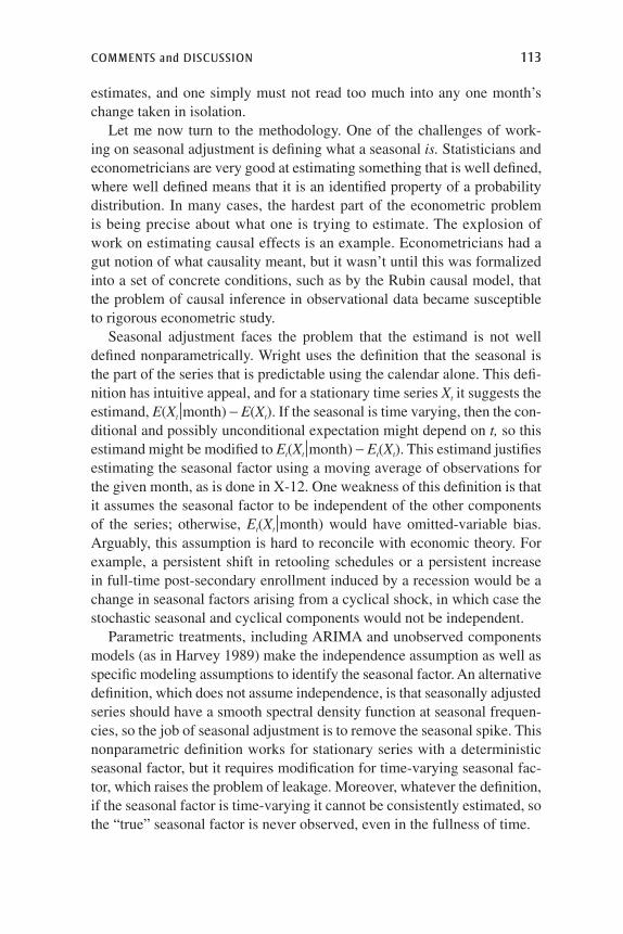
comments and discussion 113
estimates, and one simply must not read too much into any one month’s change taken in isolation.
Let me now turn to the methodology. One of the challenges of work-ing on seasonal adjustment is defining what a seasonal is. Statisticians and econometricians are very good at estimating something that is well defined, where well defined means that it is an identified property of a probability distribution. In many cases, the hardest part of the econometric problem is being precise about what one is trying to estimate. The explosion of work on estimating causal effects is an example. Econometricians had a gut notion of what causality meant, but it wasn’t until this was formalized into a set of concrete conditions, such as by the Rubin causal model, that the problem of causal inference in observational data became susceptible to rigorous econometric study.
Seasonal adjustment faces the problem that the estimand is not well defined nonparametrically. Wright uses the definition that the seasonal is the part of the series that is predictable using the calendar alone. This defi-nition has intuitive appeal, and for a stationary time series Xt it suggests the estimand, E(Xtmonth) - E(Xt). If the seasonal is time varying, then the con-ditional and possibly unconditional expectation might depend on t, so this estimand might be modified to Et(Xtmonth) - Et(Xt). This estimand justifies estimating the seasonal factor using a moving average of observations for the given month, as is done in X-12. One weakness of this definition is that it assumes the seasonal factor to be independent of the other components of the series; otherwise, Et(Xtmonth) would have omitted-variable bias. Arguably, this assumption is hard to reconcile with economic theory. For example, a persistent shift in retooling schedules or a persistent increase in full-time post-secondary enrollment induced by a recession would be a change in seasonal factors arising from a cyclical shock, in which case the stochastic seasonal and cyclical components would not be independent.
Parametric treatments, including ARIMA and unobserved components models (as in Harvey 1989) make the independence assumption as well as specific modeling assumptions to identify the seasonal factor. An alternative definition, which does not assume independence, is that seasonally adjusted series should have a smooth spectral density function at seasonal frequen-cies, so the job of seasonal adjustment is to remove the seasonal spike. This nonparametric definition works for stationary series with a deterministic seasonal factor, but it requires modification for time-varying seasonal fac-tor, which raises the problem of leakage. Moreover, whatever the definition, if the seasonal factor is time-varying it cannot be consistently estimated, so the “true” seasonal factor is never observed, even in the fullness of time.
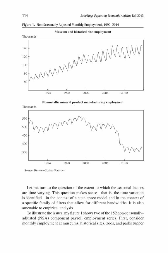
114 Brookings Papers on Economic Activity, Fall 2013
Let me turn to the question of the extent to which the seasonal factors are time-varying. This question makes sense—that is, the time-variation is identified—in the context of a state-space model and in the context of a specific family of filters that allow for different bandwidths. It is also amenable to empirical analysis.
To illustrate the issues, my figure 1 shows two of the 152 non-seasonally- adjusted (NSA) component payroll employment series. First, consider monthly employment at museums, historical sites, zoos, and parks (upper
Figure 1. non-seasonally-Adjusted monthly employment, 1990–2014
60
80
100
120
140
1994 1998 2002 2006 2010
Thousands
Museum and historical site employment
Source: Bureau of Labor Statistics.
350
400
450
500
550
1994 1998 2002 2006 2010
Thousands
Nonmetallic mineral product manufacturing employment

comments and discussion 115
2. The apparent shift in these seasonals might be related to the reporting changes, not to structural economic changes. If so, then a structural-break approach might be a more appropriate modeling strategy than the slowly evolving seasonal approach used below.
panel). Not surprisingly, more people go to parks and zoos during summer vacation than in January, and this employment series is highly seasonal. More to the point, the seasonal patterns clearly have been varying, and the seasonal employment changes are larger now than they were 20 years ago. This doesn’t seem to be just an artifact of viewing seasonal factors in job numbers as opposed to logarithms, because the pattern appears to have shifted rather abruptly in the mid-2000s.2 In contrast, monthly employment in nonmetallic mineral product manufacturing (lower panel) shows little evidence of time-varying seasonal factors, at least by visual inspection.
These two series raise the question of how one might best measure the time variation in the seasonal factors and use this to inform the filter. Wright presents one clever way, by casting this question in terms of forecast-ing NSA changes in employment. His exercise is easiest to understand at the 12-month horizon: if the seasonal factors were constant, the 12-month change in SA employment would be the same as the 12-month change in NSA employment. If seasonal factors were time-varying, then the change in NSA employment would equal the change in the seasonal factors plus the change in SA employment. If the seasonal factors followed a random walk, then the change in the seasonal factors would be unforecastable, so seasonal adjustment filters could be compared by comparing the ability of the resulting SA series to forecast 12-month NSA changes. This provides a way to compare filters and in particular to estimate the bandwidth on a series-by-series basis.
As a method of determining which filter to use, this method has the vir-tue of being nonparametric, but it might not be particularly efficient either as an estimator or as a test for time-varying seasonal factors. Because the purpose of seasonal adjustment is generally not for forecasting NSA data but rather to provide as precise an estimate (for example, lowest mean squared error) of the seasonally adjusted series as possible, the task of connecting Wright’s forecast approach to the original seasonal adjustment problem needs to be done. In particular, the best filter for solving Wright’s problem may or may not be the best filter to solve the original seasonal adjustment problem.
A second approach would be to estimate state-space models of the type used here by maximum likelihood. This approach has the advantage of

116 Brookings Papers on Economic Activity, Fall 2013
estimating the parameters for the model-optimum filter, which is given by the Kalman smoother with the true parameters. Although I have not seen the details worked out, my suspicion is that this estimator would be subject to the econometric problems associated with the estimation of the variance of a random walk intercept, which is the so-called pileup problem at zero. This problem is the state-space counterpart of the unit root pileup problem that is familiar in estimating a moving average with a unit or near-unit root. If so, the maximum likelihood estimator of the state-space model parameters might not produce well-behaved Kalman smoother estimates.
These considerations suggest looking for a different way to tackle this question of quantifying the time variation in the seasonal factors, one that both is efficient and has well understood properties for inference without the pileup problem. One way to do this is to invert a test for parameter con-stancy, in particular, the test for constant seasonal factors developed by Fabio Canova and Bruce Hansen (1995). They test the null hypothesis that the sea-sonal factors are nonrandom against the alternative that the seasonal factors (that is, the coefficients on seasonal dummies) follow a random walk. This test is a member of the broader family of tests for persistent time-varying parameters. Canova and Hansen’s model is the unobserved components model, yt = µ + f ′t gt + et, where gt = gt-1 + ut, where ut is serially uncorre-lated with mean zero and variance t2I11, where I11 is the 11-dimensional identity matrix (12 monthly indicators minus one for identifying the mean) and where et is mean zero and stationary but possibly serially corre-lated.3 Their heteroskedasticity- and autocorrelation-robust test statistic, L, tests the null hypothesis that t2 = 0 against the alternative that t2 > 0.
My table 1 summarizes the results of applying this Canova-Hansen test to the 152 NSA series that aggregate up to total employment. Fully 48 per-cent of the series reject the null of constant seasonal factors at the 5 percent significance level. For employment in leisure and hospitality, all the series reject; for employment in finance, only 30 percent of the series reject.
The next step is to move from test results to estimation of the extent to which there is seasonal variation. An advantage of working within the framework of tests for random walk components is that this can be done by inverting the test statistic. The technology to do this exists for a pure random walk component, that is, a random walk component at frequency zero, and I believe that this should be possible for a random
3. Canova and Hansen (1995) include the possibility of additional regressors; however, the implementation here has no additional regressors.

comments and discussion 117
walk at the seasonal frequency. Specifically, under the null, the Canova and Hanson (1995) test statistic has a Cramer-von Mises–type distribution with 11 degrees of freedom. The results of Stock and Watson (1998) for a random walk at frequency zero suggest that, under a local alternative in which the innovation variance is proportional to l/T, where T is the sample size and l is a constant, the L-statistic will have a noncentral version of the Cramer-von-Mises–type distribution. As a result, for a given series the L-statistic can be inverted to provide a median-unbiased estimator of the local variance parameter l, and can also be used to compute asymptotic confidence intervals.
With multiple series, as we have here, it is reasonable to imagine that each series has its own noncentrality parameter. Thus the empirical distri-bution of L-statistics based on the 152 series would be a mixture of non-central Cramer-von-Mises–type distributions, where the mixing is over the local parameter l. As an initial step, figure 2 shows the empirical distribu-tion of asymptotic p-values of the 152 series (a monotonic transformation of the L-statistic) and, in lighter lines, simulated versions of the theoretical asymptotic distribution of the p-values for different local parameters l. The asymptotic distributions given by the lighter lines are for single fixed values of l, that is, without any mixing. Surprisingly, this chart suggests that the local asymptotic distribution for l = 0.03 provides a good fit, at least for the approximately 70 percent of series with p-values less than 0.2. For larger p-values, the l = 0.03 local asymptotic distribution fits less well, which suggests that perhaps mixing in smaller values of l is appropriate.
Table 1. Results of canova-Hansen (1995) test for time-Varying seasonal FactorsApplied to 152 employment series, monthly, January 1990–August 2013
Employment categoryPercent rejections at
5 percent significance level
All 48Leisure and hospitality 100Government 83Trade 61Manufacturing 60Professional and business services 58Construction 38Education and health 35Finance 30
Notes: The null hypothesis is constant seasonal factors, and the alternative is that the seasonal factors (the coefficients on seasonal dummies) follow a random walk. The Canova-Hansen (1995) test was implemented with no regressors and with a Newey-West variance matrix, with a bandwidth of 12.

118 Brookings Papers on Economic Activity, Fall 2013
As a matter of calibration, the value of l = 0.03 corresponds to the standard deviation of the drift in the seasonal factors, over the course of 10 years, being approximately one-fourth the monthly standard deviation of the non-seasonal component. This strikes me as a relatively small amount of drift.
These preliminary results suggest that inverting tests could provide a useful way to quantify the time variation of the series. One could imagine, for example, an empirical Bayes approach in which a prior based on the estimated mixing distribution alluded to above was used in conjunction with information on a specific series to provide an estimate of l. Additional calculations would be needed to translate the series-specific estimate of l into the optimal seasonal bandwidth.
Source: Author’s calculations. See the notes to table 1.Notes: Function is computed using the 152 disaggregated monthly changes in seasonally adjusted
employment (dark line). Light lines are the asymptotic distribution under the local alternative that τ² is proportional to λ/T, where λ is a constant and T is the sample size, for the indicated values of λ. The dashed line is the 45° line.
Rejection rate
0.2
0.4
0.6
0.8
0.2 0.4 0.6 0.8Quantile
λ = 0.01
λ = 0.02
λ = 0.05
λ = 0.03
λ = 0.04λ = 0.05
Figure 2. empirical cumulative distribution Function of p-Values of the canova-Hansen (1995) test statistic

comments and discussion 119
The results here, while preliminary, point in the same direction as Wright’s, which is that the time variation in the seasonal factors might not be that large, at least on average across these series. If so, then using larger bandwidths than the X-12 ARIMA bandwidth would be justified. Of course, this conjecture needs to be studied in further research: the indi-cations in this direction presented here and using Wright’s forecasting approach are preliminary. I would encourage the academic community to start bringing to bear the many developments in time series econometrics to this important but neglected topic.
ReFeRences FoR tHe stock comment
Canova, Fabio, and Bruce E. Hansen. 1995. “Are Seasonal Patterns Constant over Time? A Test for Seasonal Stability.” Journal of Business & Economic Statistics 13, no. 3: 237–52.
Harvey, Andrew C. 1989. Forecasting, Structural Time Series Models and the Kalman Filter. Cambridge: Cambridge University Press.
Stock, James H., and Mark W. Watson. 1998. “Median Unbiased Estimation of Coefficient Variance in a Time-Varying Parameter Model.” Journal of the Amer-ican Statistical Association 93, no. 441: 349–58.
COMMENT BYRICHARD B. TILLER and THOMAS J. NARDONE The occurrence of the most severe recession of the post-World War II era has made seasonal adjust-ment a hot topic, as evidenced by this session of the Brookings Panel on Economic Activity. Historically, most major innovations in seasonal adjustment were introduced by government agencies, such as the U.S. Bureau of the Census (Shiskin 1957; and Findley and others 1998), Sta-tistics Canada (Dagum 1980), and the Bank of Spain (Gómez and Maravall 1996). Government agencies continue to be the major source of seasonal adjustment (SA) research. In contrast, the mainstream community of aca-demic economists and econometricians has neglected this field of study. This is a critical oversight, in the view of Jonathan Wright, whose paper we hope will generate further interest and discussion by independent research-ers and provide feedback to statistical agencies on how their methods and practices might be improved.
The paper deals with two principal issues concerning SA practice by government agencies, using as an example the Bureau of Labor Statistics (BLS) employment and unemployment estimates. The first issue concerns bias, principally in the post-recession Current Employment Statistics

120 Brookings Papers on Economic Activity, Fall 2013
(CES) SA estimates. Such a bias, if it exists, may have misled data users, especially policymakers such as those at the Federal Reserve. If it exists, it also raises the issue of how appropriate it would be for a statistical agency to make a judgmental intervention and whether an intervention could be undertaken quickly enough to make much difference.
The second major issue concerns the more general question of how to improve bandwidth selection of the seasonal filter selected by X-11. This highly technical issue has important methodological implications, which go beyond the bias issue and affect how BLS might improve the way it handles SA in general.
tHe Question oF BiAs Turning to the first issue, the paper concludes that a trend-cycle bias in the seasonal factors has caused SA CES employ-ment during the post-recession years to show strong growth in the early spring and weaker growth later in the year. A similar but much weaker bias is claimed to exist in the SA unemployment rate.
The author’s use of the term bias is unfortunate, since this can easily be confused with the statistical concept of systematic errors in the estima-tors of the “true” values. While the paper does briefly acknowledge a key caveat—the identification problem well known in the SA literature (Bell and Hillmer 1984)—it is worth repeating here with more emphasis. Since seasonal adjustment involves the estimation of unobserved components, there is no such thing as “true values” in this context. All that is observed are estimates, and different methods produce different estimates. How a data user chooses among the alternatives depends on that user’s specific purpose for analyzing the data.
Like seasonality, aberrations due to the Great Recession are not observ-able, and there are many different ways of estimating them depending on the user’s objectives. In the seasonal adjustment software used by BLS there are standard methods for doing this. Footnote 4 of the paper refers to the treatment of outliers in the original X-11 software but does not mention the more powerful tools that have been available since the development of X-12 in the 1990s. For this reason it is worthwhile to briefly review the standard approach.
The standard approach used by BLS for its national employment and unemployment series is X-12, an enhanced version of X-11. Designed to fit local cubic polynomials, the standard X-11 Henderson trend filters (Dagum 1980) used in X-12 can closely approximate business cycle behav-ior involving accelerations, decelerations, and turning points. These filters cannot handle economic shocks resulting in large discontinuous level shifts in the data. The REGARIMA section of this software provides power-

comments and discussion 121
ful model-based tools for identifying and correcting for a wide variety of distortions (Findley and others 1998). Large level shifts in the data can be easily identified in an automated way by the outlier option of REGARIMA provided they do not occur too close to the end of the series.
The BLS studies cited by the author—Jurgen Kropf and Nicole Hudson (2012) for CES and Thomas Evans and Richard Tiller (2013) for the Cur-rent Population Survey unemployment rate—did not find evidence that aberrations in the data caused serious distortions in the X-11 trend cycle estimates. When it comes to bias, the author’s focus is on the CES SA employment estimates. The standard X-12 methodology for removing the effects of aberrations due to the Great Recession is not examined in the paper. Such an investigation would have been useful in providing guidance to BLS, but apparently it was irrelevant to the author’s objective in pro-ducing bias estimates. Rather, the author’s concern is with behavior in the estimates over a short period of time beginning in July 2008, two months before the bankruptcy of Lehman Brothers, and ending in July 2009.
The author’s contention is that the very steep drop in employment levels caused distortions in the CES SA estimates following the recession, and these distortions were confusing for specific uses of the data. This seems hard to objectify, hence the emphasis on a judgmental intervention that replaces, at the detailed industry level, 11 months of data with a fictitious linear decline. (The author also uses another method for discounting the recession data by treating them as missing, as was done by Evans and Tiller for the unemployment series).
By dampening some of the early year increases and late year declines, this intervention presumably would have made the data easier to interpret. Still, even after bias correction, interpreting monthly change in the esti-mates requires caution, because there is uncertainty due to measurement error in the not-seasonally-adjusted (NSA) estimates and there is uncer-tainty in the seasonal decomposition, which is especially high toward the end of the series. Unfortunately, users of the data often ignore the measures of reliability produced by BLS. The author rightly expresses concern with the way policymakers and financial markets react “to very modest payrolls surprises.”
The judgmental intervention used in the paper is retrospective. What could have been done in real time is not so clear. The author recognizes that during the second half of 2009 and the first half of 2010, when the bias effect was largest and most likely to cause confusion among data users, intervention may not have been feasible. Afterward the bias effect is diminished and more easily masked by the ever-present noise from
122 Brookings Papers on Economic Activity, Fall 2013
unavoidable estimation error. What is clear from the official estimates is that a doubling of the unemployment rate in about a year and the loss of 8.7 million jobs within two years identifies the recession as the worst one in the post–World War II period and that the current recovery remains far from complete. Nothing suggested by the author alters that assessment of the recent business cycle.
BAndwidtH selection in tHe FilteR The paper’s second major issue concerns the way in which X-11 selects the bandwidth or length of the sea-sonal filter. Drawing on research by Raoul Depoutot and Christophe Planas (1998), Wright finds in the analysis of his own ARIMA fits to the CES series that X-11 selects shorter filters than may be desired in comparison to an ARIMA model-based approach to seasonal adjustment. If filter selection is done in a more optimal way by using the model-based method, either as a guide or substitute for X-11, longer filters would be selected that produce more stable estimates of SA factors. These findings are consistent with many other studies, including a BLS study referenced in the paper (Tiller, Chow, and Scott 2007). However, while longer sea-sonal filters are more robust to trend-cycle aberrations, they do not reduce the author’s bias estimates by much. The author does present evidence of other benefits, such as better user forecasts and smaller initial revisions (but a longer revision period). Moreover, with the direct use of a model-based approach, there is the additional benefit of having standard errors for the estimated components of the seasonal adjustment.
conceRning tHe RecommendAtions The paper makes a number of rec-ommendations regarding methodology and policy. The seasonal filter bandwidth should be selected in a more optimal way, Wright argues, and this will lead to longer filters. For this to work in practice, the author points out that the data span should not be arbitrarily restricted to 10 years, as is the current practice in the CES program.
However, there are practical limitations, since filters requiring more than 10 years of data are not feasible with short series and may not be desirable for longer series with major structural breaks.
The question of how to deal with recessionary distortions to the sepa-ration of seasonality from the trend-cycle is a difficult one, and there is a long-standing history of concern over it, as evident in Julius Shiskin’s comment on it in 1957, which the author quotes. The author recognizes that a judgmental intervention is not necessarily an appropriate recommenda-tion. For statistical agencies technical issues are easier to deal with, while judgmental interventions raise the issue of transparency, especially if they are attempted in real time. The author rightly questions whether it is

comments and discussion 123
appropriate for a statistical agency to make such subjective adjustments during a period when there is so much uncertainty about the future course of the economy. For statistical agencies, the author recommends that the NSA data be made available so that sophisticated users can apply their own filters and make their own risky bets about the future. The official SA estimates, based on automated methods with limited interventions, provide in the author’s words “a usable baseline measure” for more gen-eral uses of the data and a comparison for researchers who do their own seasonal adjustments.
We strongly agree with the author that independent researchers should have the NSA data needed to explore alternatives to the official estimates. In fact, it has been a long-standing policy by BLS to make these data avail-able. Unfortunately, independent researchers have seldom shown interest in seasonal adjustment methodology. We applaud the author’s admonishment of his colleagues to become more involved. Such an involvement would be beneficial to BLS as well, especially if it could lead to the development of more transparent methods for adjusting for trend-cycle aberrations to improve the interpretability of the data.
Finally, the author recommends that BLS produce and publish the full set of revised seasonal factors every month and make the SA process repli-cable by outside researchers. It may not be feasible for the BLS to publish the full history of revisions, but BLS can explore other ways of making this information available. Also, BLS is willing to work with researchers to make sure they have what they need to replicate official estimates.
In conclusion, no SA estimate is the “correct” one for all conceiv-able uses of the data. As a government statistical agency, BLS emphasizes objectivity and transparency and is conservative in the use of judgments that affect estimates. BLS agrees that users with specific needs may have to apply their own filters or models to produce alternative estimates.
We have benefited from the author’s review and constructive recom-mendations. We applaud his call for more involvement of econometricians in seasonal adjustment. We believe BLS SA estimates provide timely, accu-rate, and relevant information even during significant events. Users of eco-nomic data should always consider reliability of estimates; informed users make better decisions.
ReFeRences FoR tHe tilleR And nARdone comment
Bell, William R., and Steven C. Hillmer. 1984. “Issues Involved with the Seasonal Adjustment of Economic Time Series,” Journal of Business & Economic Sta-tistics 2: 291–320.
124 Brookings Papers on Economic Activity, Fall 2013
Dagum, E. B. 1980. The X-11-ARIMA Seasonal Adjustment Method, Number 12–564E. Ottawa: Statistics Canada.
Depoutot, Raoul, and Christophe Planas. 1998. “Comparing Seasonal Adjustment Extraction Filters with Application to a Model-Based Selection of X-11 Linear Filters.” Working Paper, Eurostat.
Evans, Thomas D., and Richard T. Tiller. 2013. “Seasonal Adjustment of CPS Labor Force Series during the Latest Recession.” Unpublished Working Paper. Washington, D.C.: Bureau of Labor Statistics.
Findley, David F., Brian C. Monsell, William R. Bell, Mark C. Otto, and Bor-Chung Chen. 1998. “New Capabilities and Methods of the X-12-ARIMA Seasonal-Adjustment Program.” Journal of Business and Economic Statistics 16, no. 2: 127–52.
Gómez, Victor, and Agustín Maravall. 1996. “Programs TRAMO and SEATS. Instructions for the User.” Working Paper no. 9628. Madrid: Servicio de Estu-dios, Bank of Spain.
Kropf, Jurgen, and Nicole Hudson. 2012. “Current Employment Statistics Seasonal Adjustment and the 2007–2009 Recession.” Monthly Labor Review 10: 42–53.
Shiskin, Julius. 1957. “Electronic Computers and Business Indicators.” Journal of Business 30: 219–67.
Tiller, Richard T., Daniel Chow, and Stuart Scott. 2007. “Empirical Evaluation of X-11 and Model-Based Seasonal Adjustment Method.” Working Paper. Wash-ington, D.C.: Bureau of Labor Statistics.
GENERAL DISCUSSION Edward Glaeser pointed out that problems with seasonality adjustments are a major concern among those analyzing the housing market. He noted that some economists have suggested basing adjustments on previous boom and bust cycles rather than on temporally proximate years. His suggestion was that the Bureau of Labor Statistics (BLS) produce multiple seasonally adjusted numbers in order to indicate the degree of uncertainty regarding the adjustments.
David Wilcox reported that the Federal Reserve was well aware of the possible distortions of seasonal factors related to the recent recession. In fact, it had decided to change its methods for seasonally adjusting the industrial production data that it publishes, precisely in order to insulate them as much as possible from these distortions.
Justin Wolfers found Wright’s results very compelling, particularly regarding the X-12 seasonal adjustment used by the BLS. Until this paper he had not realized that this method places most of the weight on the previous two years and the following two years, so that when making seasonal adjustments in real time using the X-12 filter only three years of data are considered and whatever may have happened before that tight

comments and discussion 125
frame is thrown out. Wright’s alternative approaches, using wider time spans, surpassed the BLS approach every time, as Wolfers understood the paper. In short, the BLS should begin using these alternative methods as soon as possible.
Steven Braun agreed with Wolfers that the limitation of considering only three years’ worth of data in the X-12 filter made alternative season-ality adjustments attractive. He also pointed out that the choice of optimal bandwidth would depend on whether one wanted to emphasize the middle or the end of the data series.
David Romer thought that the BLS was actually cognizant of the sea-sonality adjustment problems and of the strong case for using a wider bandwidth, especially since the agency’s internal studies also seem to be pointing in that direction. He also wondered whether there was something about the BLS’s review process that caused it to use a bandwidth that was too short. Meanwhile, he urged the agency to make two other changes: to make its non-rounded numbers publicly available and to make the real-time data easily available.
Richard Tiller responded by briefly describing the BLS’s methods and general approach. First, the agency is largely in agreement with Wright on the bandwidth issue. In fact, researchers at the BLS also use longer seasonal filters than the X-12, as identified by model-based methods, in their research. The use of longer filters, however, did not reduce estimates of “bias” by much in either the author’s results or in the BLS’s research. Second, subjective intervention, when not supported by diagnostic test results, can be risky for a statistical agency to do. He added that the BLS acknowledges that different economists may have more effective sea-sonal filters appropriate to their subject matter, and that is why the agency always releases unadjusted data as well.
Thomas Nardone responded to Romer’s other suggestions. He noted that the BLS was planning to make previous vintages of the CES data avail-able. He added that the seasonality adjustments are reviewed annually at BLS. As a federal statistical agency, BLS has an obligation to be transpar-ent about its methodology and any changes made to it. For that reason, BLS tends to be cautious by nature, and the seasonal adjustments in 2009 were consistent with this conservative approach.
David Romer spoke up a second time to add that in his view, the BLS’s emphasis in revising its seasonality adjustments should not be on cor-recting the data from the Great Recession, because ad hoc adjustments to data tend to raise very politically sensitive questions. At the same time, he felt the BLS may want to look closely at its own review process since its

126 Brookings Papers on Economic Activity, Fall 2013
current seasonal adjustment methods do not appear to follow the thrust of what both external studies and its own internal studies are finding.
Jonathan Wright agreed with the discussants that the establishment sur-vey was noisy and he agreed that the seasonality adjustment was only one part of the noise. He emphasized the usefulness of real-time projections and noted that his proposed seasonality adjustment could not have been undertaken in 2008 or 2009 to understand ongoing data. However, had it been implemented in late 2009, after the recession was over, it could have been used to better understand incoming data from then up to the end of 2012.