Unscented Kalman Filters for Multiple Target Tracking With Symmetric Measurement Equations

370 IEEE TRANSACTIONS ON AUTOMATIC CONTROL, VOL. 54, NO. 2, FEBRUARY 2009

Unscented Kalman Filters for MultipleTarget Tracking With Symmetric

Measurement Equations

William F. Leven, Member, IEEE, andAaron D. Lanterman, Member, IEEE

Abstract—The symmetric measurement equation approach to multipletarget tracking is revisited using the unscented Kalman filter. The perfor-mance of this filter is compared to the original symmetric measurementequation implementation using an extended Kalman filter. Counterintu-itive results are presented and explained for two sets of symmetric mea-surement equations. We find that the performance of the SME approach isdependent on the interaction of the SME equations and filter used. Further-more, an SME/unscented Kalman filter pairing is shown to have improvedperformance versus previous approaches while possessing simpler imple-mentation and equivalent computational complexity.

Index Terms—Extended Kalman filter, nonlinear filtering.

I. INTRODUCTION

In the early 1990’s, Kamen and Sastry presented a novel approachto multiple target tracking based on symmetric measurement equations(SME) [1], [2]. The underlying idea was to create a “pseudomeasure-ment” vector � consisting of symmetric functions of the original data�. For example, consider a simple case of tracking three targets in onedimension. Two possible sets of SME are the sum of products and sumof powers1 as

��

��

��

��

(1)

��

��

��

� ��

��

� ��

� (2)

Notice that the original �� may be rearranged without affecting �. Itcan be shown that the �� may be recovered uniquely (up to a permu-tation) from �, so there is no fundamental loss of information. Thisapproach turns the data association problem into an analytic nonlin-earity. In this way, one difficult problem is traded for another difficult,but quite different, problem.

The first studies of the SME approach used extended Kalman filters(EKF) to handle the nonlinearities [1]–[5]. In practice, this turned out to

Manuscript received June 27, 2006; revised February 15, 2008 and June 25,2008. Current version published February 11, 2009. This work was supportedby the School of Electrical and Computer Engineering, Georgia Institute ofTechnology and the Demetrius T. Paris Junior Professorship. Recommendedby Associate Editor L. Glielmo.

W. F. Leven was with the School of Electrical and Computer Engineering,Georgia Institute of Technology, Atlanta, GA 30332 USA and is currently withTexas Instruments, Inc., Dallas, TX 75243-0592 USA (e-mail: [email protected]).

A. D. Lanterman is with the School of Electrical and Computer Engineering,Georgia Institute of Technology, Atlanta, GA 30332-0250 USA (e-mail:[email protected]).

Color versions of one or more of the figures in this technical note are availableonline at http://ieeexplore.ieee.org.

Digital Object Identifier 10.1109/TAC.2008.2008327

1In practice, we subtract some constants to ensure the pseudomeasurementsare zero mean, as shown in (43). We suppress those constants here to avoidcluttering the exposition.

have some difficulties as the EKF often exhibits instability, particularlywhen targets cross, and can be extremely sensitive to initial state anderror covariance values as well as the chosen process noise covariance[6]. The trouble lies not in the underlying SME idea, but in the fragilityof the EKF. The EKF seems well-suited to handle gentle nonlinearities,but not the sort that arise in the SME approach.

One problem inherent in pairing Kalman filters and the SME ap-proach is that the nonlinear SME transformations produce measure-ments that cannot be perfectly modeled as signal plus additive Gaussiannoise, which potentially reduces the performance of Kalman filters.One must find an additive Gaussian noise approximation to the truemeasurement probability density. The unscented Kalman filter (UKF),introduced by Julier and Uhlmann [7]–[9], conveniently finds this ap-proximation as part of its basic structure, whereas the EKF requiresa pre-computed analytical approximation. The UKF compares favor-ably to the EKF in two other aspects as well. The UKF, like the EKF,forces the posterior density to be Gaussian, but the posterior mean andcovariance are accurate to a third-order Taylor series expansion com-pared to first-order accuracy for the EKF [8]. Finally, the UKF has thesame order of computational complexity as the EKF [10]. With thesecredentials, the UKF was expected to consistently outperform the EKF.

This technical note revisits the SME approach, replacing the ex-tended Kalman filter with the unscented Kalman filter. The UKFexperiment produced two unexpected results. First, the UKF using thesum-of-products form of the SME cannot handle the unobservabilitycondition that arises when targets cross. Second, we show that thesum-of-powers form, when paired with the UKF, outperforms thesum-of-products form paired with the EKF. This contrasts withKamen’s early studies where the sum-of-products form outperformedthe sum-of-powers form with the EKF; hence, all later work by himand his colleagues focused on the sum-of-products form.

II. SME-BASED TRACKING SYSTEM

The general nonlinear tracking system equations are given by thefollowing, with the subscript indicating the time index:

�� (3)

�� (4)

where �� is the state at time �, �� is the measurement at time �, ��is the process noise, �� is the observation noise, �� is the state updateequation, and �� is the observation equation. For this technical note, wehave made several assumptions. First, we have assumed that the state ismaintained in Cartesian coordinates, and we have used a linear constantvelocity model. With these assumptions, our state vector consists ofelements for position and velocity, and we stack entries for multipletargets, i.e.

�� (5)

for � targets. We have also assumed that the state and measurement up-date equations are time invariant. This allows us to replace the generalstate transition function �� with the matrices � and �, and replace�� with ��.

Implementing the SME approach via Kalman filters also requiresus to make some assumptions about the observation noise. The actualreceived measurement, ��, is modeled as the truth, ��, plus an additiveGaussian noise, ��, so that

�� (6)

For compactness, we have suppressed the time index � in (6). We willtypically use the subscript � on bold-faced vector variables to represent

0018-9286/$25.00 © 2009 IEEE

IEEE TRANSACTIONS ON AUTOMATIC CONTROL, VOL. 54, NO. 2, FEBRUARY 2009 371

time and the subscript � on italics symbols to indicate individual vectorelements. The subfunctions �� of the observation function ��

� in the UKF operate directly on the measurements,but the EKF assumes that the observation function is only applied tothe truth, which yields

�� (7)

�� (8)

where � is a zero-mean noise term whose distribution depends on�� . Although � is not Gaussian because the SME func-tions are nonlinear, we generate a Gaussian approximation2 � to usethe EKF. The state update and observation equations can then be mod-ified to

�� (9)

�� (10)

where � is white Gaussian observation noise3 � � �� .

III. THE UNSCENTED KALMAN FILTER

A. The Unscented Transform

The UKF relies upon a mathematical technique known as the un-scented transform [7], [9]. The unscented transform captures the meanand variance of any random variable using a set of “sigma points,”whose weighted sample mean and sample variance match the statisticsof the original random variable. Julier and Uhlmann show that findingthese sigma points is a straightforward process using the square root4

of the random variable’s covariance matrix [8].For example, let � be an �-dimensional random variable with mean

� and covariance matrix ��. Let � be the set of sigma points for therandom variable �. Julier and Uhlmann show that the �� sigmapoints should be chosen as

�� (11)

�� (12)

where � are the �� columns of � �� , ��

��

�� , and � � �� is a com-posite scaling parameter [7]. � controls the spread of the sigma pointsaround the mean, and we have chosen � � from the recommendedrange �� [10]. The authors of [7] recommend choosing� such that � � � � �, unless this leads to � � �,5 in which casechoose � � �. Since � � � is the minimum value of � consideredin this technical note, we set � � �. This choice of � and � leads to� � � for our simulations.

Suppose we are interested in the random variable � � ��. Theestimated statistics of � can be found by generating a new set of sigmapoints, � , where

�� (13)

2See Appendix A for more information on this approximation. Note that (8)is a linearization of (7).

3In SME-based tracking,� is additive and white, but not Gaussian. However,we generally approximate it as Gaussian.

4While any square root is acceptable, the Cholesky decomposition is gener-ally chosen for its numerical stability.

5Choosing � � � may lead to non-positive semidefinite estimates of theposterior covariance matrix.

The estimated statistics of � are then related to the sample mean andvariance of � :

��

��

��

�� (14)

��

�

��

��

�� (15)

where

�� (16)

�� (17)

��

�� (18)

� is a parameter that can be used to incorporate knowledge about thedistribution of �. � � � is the optimal choice for the Gaussian distri-butions of � used in this technical note, and these estimated statisticsare accurate up to a third-order Taylor series expansion [10].

B. Building a Kalman Filter

Here we present a brief overview of the UKF; see [7] and [10] fora detailed derivation. Building the unscented transform into a filter re-quires augmenting the state variable to include noise terms. Specifi-cally, we now define our state at time instant � as ��

� ,where � is the original (desired) state information, � is the processnoise, and � is the observation noise. The covariance, �� , is

��

��

� (19)

The unscented transform is then applied to the augmented state,�� , andaugmented covariance, �� , to generate a set of sigma points, � .To find the predicted state, the state transition function, ��, is appliedto the sigma points � , generating a new set of sigma points �� .The predicted6 state, ��, and the predicted covariance, ��

� �,

are the weighted sample statistics of �� given by

��

��

��

�� (20)

��

�

��

��

��

��

��

�� (21)

Now suppose the observation function, ��, generates a third set ofsigma points, �� , to represent the predicted obser-vation, ��, and the predicted observation covariance, �� ,which are the weighted sample statistics of �� given by

��

��

��

�� (22)

��

��

��

��

��

��

�� (23)

6The superscript indicates a value after applying the state transition func-tion, but before including the current observation.


The predicted cross correlation, �� , is the sample cross corre-lation of �� and ��

��

��

��

��

��

��

��

(24)We now have the familiar setup of a Kalman filter. The Kalman gainis � � ��

� � , and the filter estimates of the state andcovariance are

��

��

�� (25)

��

�� (26)

IV. THE UNSCENTED KALMAN FILTER AND SME TRACKING

A. A Limitation of the Sum of Products SME With the UnscentedKalman Filter

This section uses a simple example to illustrate the problems withusing the sum-of-products SME with the UKF. Suppose we aretracking two targets in one-dimensional space. Define the state to be� � ��

� , where �� and �� are the positions of targetsone and two, and �� and �� are the observation noise terms. We havenot included the velocity terms of a constant velocity model, whichsimplifies analysis without changing the conclusion.

Following the unscented transform, we need 9 sigma points. Theposition7 sigma points are

��

�� (27)

where

��

�� (28)

Applying the state transition function �� to �� , the predicted sigmapoints are

��

��

��

��

��

�� (29)

The sum-of-products observation function is

� � ��

��

��

�� (30)

Applying the observation function when the targets are estimated tocross paths, i.e. �� , the predicted sigma points become

��

��

��

��

��

��

��

��

��

��

��

�

(31)

7The four observation noise sigma points will be accounted for later.

When the targets behave independently,8 the cross-correlation terms of�� shrink towards zero as the filter locks on to the targets’behavior. In equation form,

��

� �� (32)

Recall (28), where we defined �� such that

��

��

��

��

��

�� (33)

Comparing (32) and (33), �� and �� tend towards zero when ourassumption that the targets move independently is met. Before con-tinuing, let us consider the observation noise sigma points. We havealready assumed that the �� are uncorrelated, so �� is diagonal. Toaugment the sigma points, we generate a set of sigma points for theobservation noise covariance:

��

� � �� (34)

The sigma points, after including the observation noise covariance andapplying the observation function �, are

��

��

��

��

��

��

��

��

��

� (35)

The covariance matrix is calculated using (23). Using the sigma pointsin (35), setting � �

�� , and computing �� according to (23)

leads to (36), shown at the bottom of the page, where � � ��

�� and � � �

�� . Since � is the difference of the predicted

observation and the actual observation, it can be decomposed into twoparts: the prediction error and the observation noise such that � � �� . In the extreme case that � � � � �, �� becomes asingular matrix with the second column being the first scaled by ��.This means that the previously two-dimensional space has degeneratedinto a one-dimensional space—all the sigma points lie along a singleline as seen in the top, right portion of Fig. 1. For the matrix inversionto be ill-conditioned, it is sufficient for the � to be small instead ofexactly zero. The effective reduction in dimensionality means��

�� willhave elements with extremely large values. The Kalman gain, � ��

�� , will then multiply the observed data by enormous values and

produce inaccurate target tracks. Since the prediction error �� islikely to be small if the tracker is performing well and since �� is zeromean, it is likely that the � will frequently be small and this problemwill occur. It does not always occur; sometimes the noise operates suchthat the points in the upper right portion of Fig. 1 are moved off theline. Note that these results are independent of the choice of the UKFscaling parameters �, �, �, and , since the loss of dimensionality doesnot depend upon their values. The UKF only guarantees that �� will

8Targets moving independently, by definition, have no correlation in their be-havior. The filter models this by estimating a state covariance matrix with smalloff-diagonal terms.

��

� � ��

� � ��

� � � � ��

� � ��

� (36)


Fig. 1. Illustration of the sigma point transformation for the sum-of-productsand sum-of-powers SMEs.

be positive semidefinite, and in this situation, �� will have zero ornear-zero eigenvalues.

B. When the Unscented Kalman Filter Works

This section follows a similar derivation as Section IV-A for thesum-of-powers SME implementation and illustrates how the problemsof the previous section are avoided by the sum of powers. Now the ob-servation function is

��

��

��

�� (37)

In the case of targets crossing and �� , applying (23) leadsto (38), shown at the bottom of the page. In contrast to Section IV-A,the columns of �� are clearly linearly independent, so �� remainsfull rank with a well-defined inverse. The lower right portion of Fig. 1shows the graphical perspective. Again, all the sigma points fall ontothe same curve, but this curve is quadratic, maintaining two dimensionsrather than collapsing to one as happened with the sum of products.

C. Comparison to the EKF

A natural question to ask is whether the extended Kalman filter ex-periences the same problem in the same situation. The trouble with theUKF/sum-of-products combination lies in the matrix inversion of ��in the Kalman gain calculation. The Kalman gain in the EKF also re-quires the inversion of �� , but �� is calculated differently. For theEKF,

��

��

� � ��

�

�� (39)

where �� is the Jacobian matrix of the SME observation function,�� is the predicted state covariance, and �� is the obser-vation noise covariance matrix. Assuming the same state vector as weused for the UKF and that the tracker estimates the targets are crossing��

�

� �,

��

��

� ��

�

� (40)

Also assuming that the filter estimates that the targets move indepen-dently,

��

� � ��

� �� (41)

With these assumptions,

��

��

� � ��

�

��

��

��

� (42)

This covariance matrix is similar to the covariance matrix in (36), andit is also singular since the second row is the first row scaled by �

�

� .At this point it would seem that the EKF might exhibit the same prob-lems as the UKF when paired with the sum-of-products SME. How-ever, the addition of �� generally keeps the inversion of ��

well-conditioned. The need to artificially increase the covariance fornumerical stability of the UKF has been addressed in [11], [12]. Thisis, however, simply modifying the UKF with ad-hoc techniques, whichdefeats the purpose of using it in the first place.

V. EXAMPLE

A. Simulation Setup

The simulation9 consisted of three targets moving in one dimension.Each target moved independently with nearly constant velocity anda known process noise variance. Initial positions and velocities werechosen so that the targets were likely to cross paths. The observationdata were generated by adding Gaussian noise with zero mean and aknown variance.

To ease discussion, pairing a filter with an SME will be referredto by a pair of abbreviations, e.g. UKF-Products for the unscentedKalman filter paired with the sum of products. We have also includedtwo non-SME data association techniques for reference: the globalnearest neighbor (GNN) approach and a KF with known associations.The GNN algorithm represents a straightforward solution to the mul-tiple target tracking problem. Since the simulation scenario does notinclude false alarms and missed detections, each observation is used toupdate exactly one track. The GNN algorithm associates observationswith tracks such that the sum of the distances from the observations tothe predicted positions is minimized [14]. This approach may also bethought of as a 2-D assignment algorithm. Separate standard Kalmanfilters are run for each track. The KF with known associations runs astandard Kalman filter for each track. It represents the optimal solutionsince the data association is perfect, and the state and observationmodels meet the optimality requirements for the Kalman filter.

B. Results

In Table I, the term “associated” in associated mean squared errorindicates that the error is only included in the average when the filtermaintains the correct target association. The set estimation MSE is cal-culated by finding the track-estimate/track-truth association with the

9Software developed by Wan and van der Merwe provided the basis for thesesimulations [13].

��

��

��

��

��

��

(38)


TABLE ISIMULATION RESULTS

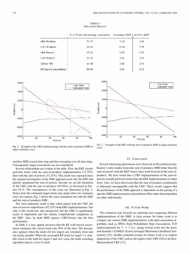
Fig. 2. Example of the UKF malfunctioning with the sum-of-products SME astarget estimates cross.

smallest MSE at each time step and then averaging over all time steps.Consequently, target associations are not considered.

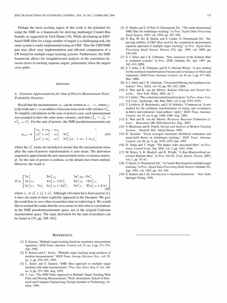
Several relationships are evident in the table. First, the EKF clearlyperforms better with the sum-of-products implementation (73.75%)than with the sum of powers (37.25%). This result was expected sincethe original investigators of the SME approach used only the EKF andquickly abandoned the sum of powers. Second, we see the limitationof the UKF with the sum of products (40.50%), as discussed in Sec-tion IV-A. The consequences of this issue are illustrated in Fig. 2.Notice how the estimated target tracks may jump when two estimatescross. In contrast, Fig. 3 shows the same simulation run with the EKFand the sum-of-products SME.

The most important result is that, when paired with the UKF, thesum-of-powers outperforms (82.25%) both EKF implementations. Notonly is this result new and unexpected, but the UKF is significantlyeasier to implement and has similar computational complexity asthe EKF. Also, by both MSE metrics, UKF-Powers has the bestperformance.

In Table I, it may appear incorrect that the KF with known associ-ations maintains the correct track only 98% of the time. The discrep-ancy appears when the tracks for two targets are extremely close andrun nearly parallel. When the associated KF track for target 1 is actu-ally closer to the truth for target 2 and vice versa, the track-switchingalgorithm detects a loss of track.

Fig. 3. Example of the EKF with the sum-of-products SME as target estimatescross.

VI. CONCLUSION

Several interesting phenomena were observed in this technical note.Kamen’s early studies found the sum-of-products SME better than thesum of powers with the EKF; hence, later work focused on the sum-of-products. We have found that a UKF implementation of the sum-of-powers actually performs better than the EKF implementation of eitherform. Also, we have discovered that the sum-of-products nonlinearityis inherently incompatible with the UKF. These results suggest thatthe performance of the SME approach is dependent on the pairing of aspecific SME implementation and nonlinear filter rather than dependenton either individually.

VII. FUTURE WORK

This technical note focused on exploring and comparing differentimplementations of the SME. A clear avenue for future work is tocompare our various SME implementations with other association al-gorithms such as JPDA (Joint Probabilistic Data Association), N-Dmultiassignment for � � � (i.e., going several scans into the past),and Kastella’s EAMLE (Event-Averaged Maximum-Likelihood Esti-mation) [15]. Another potential avenue for future work is to exploreadaptations of the UKF, such as the higher-order UKF [16] or the Rao-Blackwellised UKF [17].


Perhaps the most exciting aspect of this work is the potential forusing the SME as a framework for deriving multitarget Cramér-Raobounds, as suggested by Fred Daum [18]. While developing an EKF-based SME filter for a large number of targets is a challenging task, thesame system is easily implemented using an UKF. Thus the UKF/SMEpair may allow easy implementation and efficient computation of aCR bound for multiple target tracking systems. Furthermore, the SMEframework allows for straightforward analysis of the correlation be-tween errors in tracking separate targets, particularly when the targetscross paths.

APPENDIX

A. Gaussian Approximations for Sum of Powers Measurement NoiseProbability Densities

Recall that the measurements�� can be written as �� where ��is the truth and�� is an additive Gaussian noise term with variance �� .To simplify calculations in the sum-of-powers case, each measurementwas assumed to have the same noise variance, such that ��

�

� ��

� � ��

� . For the sum of powers, the SME pseudomeasurements are

��

��

��

� ��

� ��

� � ��

�

� ��

� ��

� � ��

(43)

where the �� terms are included to ensure that the measurement noiseafter the sum-of-powers transformation is zero mean. The derivationrequired to approximate the new measurement noise covariance matrix,�, for the sum of powers is tedious, so the details have been omitted.However, the result is

� �

��

(44)where ��

��

��

�� . Although (44) must have been used in [1],

it does not seem to have explicitly appeared in the literature. We givethe result here to save other researchers time in rederiving it. We wouldlike to remind the reader that the cross terms in (44) refer to correlationsin the SME pseudomeasurement space, not in the original Cartesianmeasurement space. The same derivation for the sum-of-products canbe found in [19, pp. 298–301].

REFERENCES

[1] E. Kamen, “Multiple target tracking based on symmetric measurementequations,” IEEE Trans. Automat. Control, vol. 37, no. 4, pp. 371–374,Apr. 1992.

[2] E. Kamen and C. Sastry, “Multiple target tracking using products ofposition measurements,” IEEE Trans. Aerosp. Electron. Syst., vol. 29,no. 2, pp. 476–493, 1993.

[3] C. Sastry and E. Kamen, “SME filter approach to multiple targettracking with radar measurements,” Proc. Inst. Elect. Eng. F, vol. 140,no. 4, pp. 251–260, Aug. 1993.

[4] Y. Lee, “The SME Filter Approach to Multiple Target Tracking WithFalse and Missing Measurements,” Ph.D. dissertation, School of Elec-trical and Computer Engineering, Georgia Institute of Technology, At-lanta, 1994.

[5] D. Muder and S. O’Neil, O. Drummond, Ed., “The multi-dimensionalSME filter for multitarget tracking,” in Proc. Signal Data ProcessingSmall Targets, 1993, vol. 1954, pp. 587–599.

[6] Ö. Bas, M. Ho, B. Shafai, and S. Linder, O. Drummond, Ed., “Im-proving stability of EKF filter used by the symmetrical measurementequation approach to multiple target tracking,” in Proc. Signal DataProcessing Small Targets, Denver, CO, Apr. 1999, vol. 3809, pp.230–240.

[7] S. J. Julier and J. K. Uhlmann, “New extension of the Kalman filterto nonlinear systems,” in Proc. SPIE, Orlando, FL, Apr. 1997, pp.182–193, SPIE.

[8] S. J. Julier, J. K. Uhlmann, and H. F. Durrant-Whyte, “A new methodfor the nonlinear transformation of means and covariances in filters andestimators,” IEEE Trans. Automat. Control, vol. 45, no. 3, pp. 477–482,Mar. 2000.

[9] S. J. Julier and J. K. Uhlmann, “Unscented filtering and nonlinear esti-mation,” Proc. IEEE, vol. 92, pp. 401–422, 2004.

[10] E. Wan and R. van der Merwe, Kalman Filtering and Neural Net-works. New York: Wiley, 2001, ch. 7.

[11] S. J. Julier, “The scaled unscented transformation,” in Proc. Amer. Con-trol Conf., Anchorage, AK, May 2002, vol. 6, pp. 4555–4559.

[12] T. Lefebvre, H. Bruyninckx, and J. D. Schuller, “Comment on ‘A newmethod for the nonlinear transformation of means and covariancesin filters and estimators’ [and authors’ reply],” IEEE Trans. Automat.Control, vol. 47, no. 8, pp. 1406–1409, Aug. 2002.

[13] E. Wan and R. van der Merwe, Recursive Bayesian Estimation Li-brary. Beaverton, OR: OGI School Sci. Eng., 2003.

[14] S. Blackman and R. Popoli, Design and Analysis of Modern TrackingSystems. Norwell, MA: Artech House, 1999.

[15] K. Kastella, “Event averaged maximum likelihood estimation andmean-field theory in multitarget tracking,” IEEE Trans. Automat.Control, vol. 40, no. 6, pp. 1070–1074, Jun. 1995.

[16] D. Tenne and T. Singh, “The higher order unscented filter,” in Proc.Amer. Control Conf., Jun. 2003, vol. 3, pp. 2441–2446.

[17] M. Briers, S. R. Maskell, and R. Wright, “A Rao-Blackwellised un-scented Kalman filter,” in Proc. 6th Int. Conf. Inform. Fusion, 2003,vol. 1, pp. 55–61.

[18] F. Daum, O. Drummond, Ed., “A Cramér-Rao bound for multiple targettracking,” in Proc. Signal Data Processing Small Targets, Orlando, FL,Apr. 1991, vol. 1481, pp. 341–344.

[19] E. Kamen and J. Su, Introduction to Optimal Estimation. New York:Springer-Verlag, 1999.

Unscented Kalman Filters for Multiple Target Tracking With Symmetric Measurement Equations

Documents

Transcript of Unscented Kalman Filters for Multiple Target Tracking With Symmetric Measurement Equations