AN ANALYSIS OF THE GLOBAL WARMING IMPACT OF HUMBOLDT STATE

UNIVERSITY’S REFRIGERANT INVENTORY

By

Alex Eckert-Ross

A Master’s Project Presented to

The Faculty of Humboldt State University

In Partial Fulfillment of the Requirements for the Degree

Master of Science in Environmental Systems: Energy, Technology and Policy

Committee Membership

Dr. Arne Jacobson, Committee Chair

Dr. Charles Chamberlin, Committee Member

Dr. Margarita Otero-Diaz, Committee Member

Dr. Margaret Lang, Graduate Coordinator

May 2021

ii

ABSTRACT

AN ANALYSIS OF THE GLOBAL WARMING IMPACT OF HUMBOLDT STATE

UNIVERSITY’S REFRIGERANT INVENTORY

Alex Eckert-Ross

With global warming potentials (GWP) in the thousands to tens of thousands of

metric tons of carbon dioxide equivalent (MTCO2e) and the possibility for substantial

emissions associated with leaks of refrigerants used in heating, ventilation, air

conditioning, and refrigeration (HVACR) equipment, it is important for Humboldt State

University (HSU) to document and report greenhouse gas emissions (GHG) associated

with refrigerant leaks.

This study has collected data on HSU’s HVACR inventory, emphasizing the

refrigerant types used, the charges of the equipment (i.e., the amounts of refrigerant in the

systems), and the types of equipment. The data were aggregated into a model and paired

with typical annual leak rate values for the respective equipment types. The

corresponding amount of refrigerant lost through annual leaks was used to estimate a

range of GHG emissions.

The HSU campus likely emits between 57 and 429 MTCO2e annually through

refrigerant leaks. This amounts to 1% to 5% of the total 2019 campus GHG emissions.

Additionally, it is likely that refrigerated condensing units that use the refrigerant R-404a

are the most significant contributor to these emissions.

iii

As HSU progresses towards its carbon neutrality goals and as the global

community takes measures to eliminate some of the refrigerants used at HSU, it is

increasingly important for the university to take action to better understand and eliminate

the use of high-GWP refrigerants. Given the commercial availability of lower-GWP

refrigerants, it is HSU’s responsibility to determine how to reduce this portion of its

environmental impact.

iv

ACKNOWLEDGEMENTS

I have been very fortunate in my life to have so many wonderful, caring, and

supportive people around me. My experience at HSU and throughout this project has

been a testament to that. I would first like to thank my mom, dad, brother, grandma, and

grandpa. You have all been an unparalleled support system in my life, and without you, I

would not be here. To my partner, Jackie, thank you for motivating and supporting me

endlessly throughout this process. The friends that I have made in Humboldt are too

many to name, but you have all made this experience worth having. Carisse, Grishma,

and Chih-Wei, you three have been especially supportive. I could not have asked for a

better cohort. Thank you to my teachers; you are some of the best that I have had, and to

my committee, for guiding me through this impossible process. Finally, thank you to Dan

Bouchard, Mike Dotson, Morgan King, and the rest of the Housing and Dining Services

and Facilities Management teams. I have asked a lot of you all, and you have taken time

out of your busy schedules to accommodate me completely. This project would not be

possible without your help.

v

TABLE OF CONTENTS

ABSTRACT ........................................................................................................................ ii

ACKNOWLEDGEMENTS ............................................................................................... iv

LIST OF TABLES ............................................................................................................ vii

LIST OF FIGURES .............................................................................................................x

LIST OF APPENDICIES ................................................................................................. xii

LIST OF ACRONYMS ................................................................................................... xiii

INTRODUCTION ...............................................................................................................1

LITERATURE REVIEW ....................................................................................................4

What is a Refrigerant? ..................................................................................................... 4

What is the Problem with Them? .................................................................................. 10

Ozone Depletion .........................................................................................................10

Global Warming .........................................................................................................12

What is Being Done About Them? ............................................................................... 18

International Action ....................................................................................................18

National Action...........................................................................................................21

University Action .......................................................................................................26

What are Their Alternatives? ........................................................................................ 32

Natural Refrigerants ...................................................................................................37

Fluorinated Refrigerants .............................................................................................51

MATERIALS AND METHODS .......................................................................................56

Inventory ....................................................................................................................... 56

vi

Model ............................................................................................................................ 59

Projections ..................................................................................................................... 67

Uncertainty .................................................................................................................... 72

HSU INVENTORY ...........................................................................................................78

Refrigerants Used on Campus ....................................................................................... 78

Application Descriptions ............................................................................................... 87

Domestic Refrigerators ...............................................................................................89

Stand-Alone Hermetically Sealed ..............................................................................90

Refrigerated Condensing Units ..................................................................................91

Small to Medium Unitary HVAC ...............................................................................92

AC Chillers .................................................................................................................93

RESULTS ..........................................................................................................................95

Current Emissions ......................................................................................................... 95

Projected Emissions .................................................................................................... 107

Alternatives ................................................................................................................. 110

DISCUSSION ..................................................................................................................115

Is This Range of Emissions Reasonable? .................................................................... 115

HSU’s Refrigerant Outlook ......................................................................................... 122

CONCLUSION AND RECOMMENDATIONS ............................................................129

REFERENCES ................................................................................................................133

APPENDICES .................................................................................................................147

vii

LIST OF TABLES

Table 1. Desirable refrigerant criteria. Adapted from (McLinden & Didion, 1987). ......... 7

Table 2. Summary of the evolution of refrigerant groups from oldest to newest with the

refrigerant types that characterize the generations and their descriptions. Adapted from

(Calm, 2008). ...................................................................................................................... 9

Table 3. Comparison of various pollutant's GWPs. Adapted from (Refrigeration, Air

Conditioning and Heat Pumps Technical Options Committee, 2019). ............................. 15

Table 4. Breakdown of Scope One and Scope Two emissions at Humboldt State

University for the 2019 fiscal year. Data were collected over a period of twelve months

starting July 1st, 2018. Adapted from (Humboldt State University, 2020). ...................... 29

Table 5. Refrigerant safety classifications. Example refrigerants or refrigerant types, if

more widely applicable, are included for each safety class. The first letter of each

classification represents the toxicity of the refrigerant and the number indicates the level

of flammability. The inclusion of a second letter, “L”, in the lower flammability row

indicates a maximum burning velocity lower than 10 cm/s. Adapted from (Comstock &

Eltalouny, 2020). ............................................................................................................... 34

Table 6. Descriptions highlighting GWP, ODP, safety category, atmospheric lifetime, and

suitable applications for popular low-GWP natural and fluorinated refrigerants. Adapted

from (Refrigeration, Air Conditioning and Heat Pumps Technical Options Committee,

2019; EPA, 2020a; Nair & Yu, 2020;). ............................................................................ 36

Table 7. Design challenges to the adaptation of natural refrigerants when compared to

HFCs. Adapted from (Lilya, 2019). .................................................................................. 44

Table 8. Typical equipment characteristics and refrigerant leak rates from literature (each

row includes data from the listed source). ........................................................................ 61

Table 9. Chosen replacements for HSU’s current refrigerant inventory by equipment

category. This table is meant to show which refrigerants were used in the projected

emissions analysis. The three “replacing” refrigerants that are shown for each existing

refrigerant make up the high, moderate, and low scenarios/pathways. The placement of

each “replacing” refrigerant is based on the literature informing Figure 1 and the Natural

Refrigerants sub-section.................................................................................................... 69

Table 10. Refrigerants used at Humboldt State University and their corresponding

impacts. Adapted from (Refrigeration, Air Conditioning and Heat Pumps Technical

Options Committee, 2019). ............................................................................................... 80

viii

Table 11. Quantities of installed refrigerants at Humboldt State University and their

corresponding operators. Values are given in pounds. Percent totals are given to show

each refrigerant’s relative abundance on campus. ............................................................ 83

Table 12. Quantities of installed equipment types at Humboldt State University and their

respective operators. Values are given in number of units. .............................................. 88

Table 13. Comparison of HSU's reported emissions for the 2019 year using 100-year and

20-year time horizon GWP values. Emissions sources are organized into groups (e.g.,

commuting) and sub-groups (e.g., student commuting) based on origin. They are also

classified by their scope. Data for HSU’s 2019 emissions inventory were retrieved from

(Humboldt State University, 2020). The 100-year and 20-year GWP values were

retrieved from (Intergovernmental Panel on Climate Change, 2014). Emissions values are

given metric tons of CO2 equivalent per year (MTCO2e/yr). ........................................... 98

Table 14. Relative contributions of refrigerant fugitive emissions by equipment type and

operator at Humboldt State University. Emissions estimates are divided to show the

respective impact of each equipment type. These equipment type categories are further

divided to show H&DS’ and Facilities Management’s contribution to the impact of each

equipment type. The high, average, and low emissions estimates are given in metric tons

of CO2 equivalent per year (MTCO2e/yr). The respective contributions are given as a

percentage of the total emissions for the campus and of the impact of the individual

equipment type. Values may not add up to totals due to rounding. ................................ 100

Table 15. Relative contributions of refrigerant fugitive emissions by refrigerant type and

operator at Humboldt State University. Emissions estimates are divided to show the

respective impact of each refrigerant type. These refrigerant type categories are further

divided to show H&DS’ and Facilities Management’s contribution to the impact of each

refrigerant type. The high, average, and low emissions estimates are given in metric tons

of carbon dioxide equivalent per year (MTCO2e/yr). The respective contributions are

given as a percentage of the total emissions for the campus under the average emissions

estimate. Values may not add up to totals due to rounding. ........................................... 102

Table 16. Relative contributions of refrigerant fugitive emissions by refrigerant within

each equipment type and operator at Humboldt State University. Emissions estimates are

divided to show the respective impact of each refrigerant type used in each equipment

type. These emissions categories are further divided to show H&DS’ and Facilities

Management’s contribution to the impact of each category. The high, average, and low

emissions estimates are given in metric tons of CO2 equivalent per year (MTCO2e/yr).

The respective contributions are given as a percentage of the total emissions for the

campus under the average emissions estimate. Values may not add up to totals due to

rounding. ......................................................................................................................... 105

ix

Table 17. Comparison of the emissions estimates for the HSU campus using different

GWP reference data. The estimates made in this project are based on the 100-year GWP

values given by the Refrigeration, Air Conditioning and Heat Pumps Technical Options

Committee (2019), but there are other reasonable references on which they could be

based. This table looks at the difference that using one reference over another makes.

Emissions estimates are given in metric tons of carbon dioxide equivalent per year

(MTCO2e/yr). .................................................................................................................. 111

Table 18. Summary of reviewed universities’ climate action plans. The total emissions

column represents the emissions from the Scope One and Scope Two emissions

categories. Data for emissions are given MTCO2e. The contribution of refrigerants to the

total emissions for each campus is given as a percentage. ............................................. 116

Table C.1. Master list of all the refrigerants referenced in this study. Adapted from

(Refrigeration, Air Conditioning and Heat Pumps Technical Options Committee, 2019).

......................................................................................................................................... 154

x

LIST OF FIGURES

Figure 1. Flowchart showing the progression through time of the most popular

fluorinated refrigerant replacement options. Three generations of refrigerants, including

those used in retrofit and new equipment replacements, are shown. Retrieved from

(Kedzierski et al., 2015; Refrigeration, Air Conditioning and Heat Pumps Technical

Options Committee, 2019; Hughes, 2018; Pardo & Mondot, 2018; Bobbo et al., 2019;

Makhnatch, 2019). ............................................................................................................ 53

Figure 2. Comparison of the installed masses of each refrigerant currently used at

Humboldt State University. Data are shown for systems managed by Facilities

Management and Housing and Dining Services. .............................................................. 84

Figure 3. Map of the Humboldt State University campus highlighting the buildings which

house HVACR equipment. These buildings are categorized into six groups based on the

amount of refrigerant installed within each building and whether they are operated by

Facilities Management or Housing and Dining Services. Not pictured in this figure are

the HSU marine lab, cell tower, and KHSU transmitter site. ........................................... 86

Figure 4. Example of a domestic refrigerator. Retrieved from (Best Buy, 2021). ........... 89

Figure 5. Example of a stand-alone hermetically sealed commercial refrigerator.

Retrieved from (Amazon, 2020). ...................................................................................... 90

Figure 6. Example of a refrigerated condensing unit display case. Retrieved from

(Alibaba, 2021). ................................................................................................................ 91

Figure 7. Example of a medium sized packaged HVAC unit. Retrieved from (Trane,

2020). ................................................................................................................................ 93

Figure 8. Example of a packaged AC Chiller. Retrieved from (Carrier, 2021). ............... 94

Figure 9. Estimated annual emissions associated with fugitive refrigerant leaks at

Humboldt State University. Data are shown for systems managed by Facilities

Management and Housing and Dining Services. Emissions estimates are given in metric

tons of carbon dioxide equivalent per year (MTCO2e/yr). Amount of released refrigerant

is calculated based on the charges of each reported/surveyed heating, ventilation, air

conditioning, and refrigeration unit and reported average annual leak rates for each unit

type in the literature. These annual values for the high, average, and low ends of the leak

rate spectrum were then converted to annual emissions using the global warming

potentials of each refrigerant. There is a 20% uncertainty assigned to each charge datum,

and error bars are included to show a 95% confidence interval. The reported emissions

xi

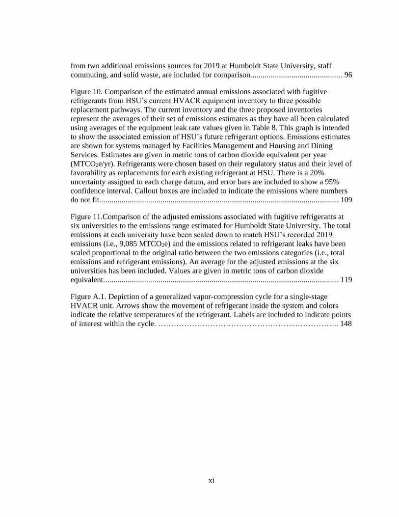
from two additional emissions sources for 2019 at Humboldt State University, staff

commuting, and solid waste, are included for comparison. .............................................. 96

Figure 10. Comparison of the estimated annual emissions associated with fugitive

refrigerants from HSU’s current HVACR equipment inventory to three possible

replacement pathways. The current inventory and the three proposed inventories

represent the averages of their set of emissions estimates as they have all been calculated

using averages of the equipment leak rate values given in Table 8. This graph is intended

to show the associated emission of HSU’s future refrigerant options. Emissions estimates

are shown for systems managed by Facilities Management and Housing and Dining

Services. Estimates are given in metric tons of carbon dioxide equivalent per year

(MTCO2e/yr). Refrigerants were chosen based on their regulatory status and their level of

favorability as replacements for each existing refrigerant at HSU. There is a 20%

uncertainty assigned to each charge datum, and error bars are included to show a 95%

confidence interval. Callout boxes are included to indicate the emissions where numbers

do not fit. ......................................................................................................................... 109

Figure 11.Comparison of the adjusted emissions associated with fugitive refrigerants at

six universities to the emissions range estimated for Humboldt State University. The total

emissions at each university have been scaled down to match HSU’s recorded 2019

emissions (i.e., 9,085 MTCO2e) and the emissions related to refrigerant leaks have been

scaled proportional to the original ratio between the two emissions categories (i.e., total

emissions and refrigerant emissions). An average for the adjusted emissions at the six

universities has been included. Values are given in metric tons of carbon dioxide

equivalent. ....................................................................................................................... 119

Figure A.1. Depiction of a generalized vapor-compression cycle for a single-stage

HVACR unit. Arrows show the movement of refrigerant inside the system and colors

indicate the relative temperatures of the refrigerant. Labels are included to indicate points

of interest within the cycle. ……………………………………………..…………….. 148

xii

LIST OF APPENDICIES

Appendix A. Explanation of Refrigeration Cycles ......................................................... 147

Appendix B. Expansion on Global Warming Molecules................................................ 150

Appendix C. Refrigerant Descriptions ............................................................................ 153

xiii

LIST OF ACRONYMS

AC – Air conditioning

AIM – American Innovation and Manufacturing

CARB – California Air Resources Board

CFC – Chlorofluorocarbons

COP – Coefficient of performance

EIA – Environmental Investigation Agency

EoL – End of life

EPA – Environmental Protection Agency

EU – European Union

GHG – Greenhouse gas

GWP – Global warming potentials

H&DS – Housing and Dining Services

HC – Hydrocarbons

HCFC – Hydrochlorofluorocarbons

HFC – Hydrofluorocarbons

HFO – Hydrofluoroolefins

HSU – Humboldt State University

HVACR – Heating, ventilation, air conditioning, and refrigeration

IPCC – Intergovernmental Panel on Climate Change

IR – Infrared radiation

xiv

MTCO2e – Metric tons of carbon dioxide equivalent

NASA – National Aeronautics and Space Administration

ODP – Ozone depletion potential

SNAP – Significant New Alternatives Policy

UNEP – United Nations Environment Programme

US – United States

UV – Ultraviolet

1

INTRODUCTION

Humboldt State University (HSU), in its mission to reduce its greenhouse gas

emissions and have a net-zero carbon footprint by 2050 (HSU Office of Sustainability,

2016), has so far considered the emissions from the greenhouse gas (GHG) refrigerants in

its inventories to be insignificant (Morgan King, personal communication, 2019).

Refrigerants are substances that are used in a variety of important applications, from

refrigerant systems to propellants to air conditioning. However, they have the potential to

contribute serious harm to our environment and accelerate the rate of global warming

when they are released into the atmosphere. With annual refrigerant leaks as high as 35%

of the total capacity for medium to large commercial refrigeration systems

(Intergovernmental Panel on Climate Change [IPCC], 2006), and global warming

potentials (GWP) in the thousands of metric tons of carbon dioxide equivalent

(MTCO2e), the heating, ventilation, air conditioning, and refrigeration (HVACR) systems

at HSU could be a significant contributor to the campus’ annual emissions.

This project intends to identify the scale of the contribution that leaked refrigerants

make to HSU’s greenhouse gas inventory. It is also meant to inform HSU of approaching

requirements, assist in compiling a complete refrigerant and refrigeration system

inventory, and provide recommendations for the next steps. To narrow this project’s

scope, its focus is on refrigerants and their associated trends, restrictions, and emissions

from leaks and other releases to the atmosphere. Large portions are informed by a

2

literature review, but the Humboldt-specific information comes from data collected from

HSU Facilities Management and HSU’s Housing and Dining Services (H&DS).

A literature review was conducted on the trends in commercial refrigerant use

globally with a concentration on fugitive leaks. Research was conducted on the

refrigerants currently used on-campus and the new generation of low-impact refrigerants.

Information was collected on 101 refrigeration and air conditioning systems across 29

buildings at HSU. The current and potential future refrigerants in these units have been

compared by GWP, ozone depletion potential (ODP), associated hazards, and system

energy efficiency. Published estimates are used to determine a range of possible leak

rates for the systems found on campus in cases where data on recharge rates for campus

systems are missing. Case studies have been reviewed to inform estimates on price,

efficiencies, and success of replacing existing refrigerants with lower ODP and GWP

ones.

The focus of this project is on refrigerants. As a result, the energy use of the systems,

carbon emissions embedded within the refrigerants and systems (mostly resulting from

their manufacturing and transportation), and the energy efficiencies of different

configurations may be mentioned. However, these factors do not affect the primary

analysis, which focuses on the climate change impact of fugitive emissions of refrigerants

used on campus. The outcome of this analysis informs whether or not fugitive emissions

from refrigerant leaks contribute a significant amount to the campus’ larger emissions

inventory.

3

HSU needs a full accounting of the refrigerants it uses on campus, their

environmental impacts, and the regulations restricting their use so the University can

adequately assess the situation and take measures to minimize their environmental

impact. There is an opportunity to better understand the distribution and use of

refrigerants, and the associated emissions, so that HSU can more effectively reduce its

carbon footprint, meet its own goals and obligations, and maintain economic feasibility.

Additionally, there is a broader incentive for HSU to support the movement, driven by

the Montreal Protocol, to eliminate and reduce the use of these environmentally

damaging substances. Whether it be adopting low-GWP and ODP alternatives or

developing a tighter set of procedures around refrigerants and their tracking, committing

to the “greenest” alternative would further support the dedication to environmentalism

and sustainability that is already so prominent at this university.

4

LITERATURE REVIEW

Context is undoubtedly as important in identifying and addressing a potential

problem with the fugitive emissions of refrigerants at Humboldt State University as the

actual findings and recommendations are. Information that provides context allows one to

determine not just whether there is a problem but where the problem lies, why it is a

problem, how serious or common the problem is, and what may be done about it. This

chapter provides information about what refrigerants are, their associated problems, the

work that is being done to address those problems, and available alternatives that can be

considered.

What is a Refrigerant?

Refrigerants are substances with specific thermodynamic characteristics that make

them effective tools to assist in certain applications. Of the properties associated with

refrigerants, it may be their ability to change phase at low temperatures and their

compressibility that are most useful. Both properties are needed for many of the

applications that they are used in. The phase changes of refrigerants (usually gas to liquid

and vice versa) add heat to and remove heat from refrigeration and air conditioning

systems, and the pressurization of those refrigerants with vapor compressors adds

additional heat energy. The low temperature phase changes of pressurized refrigerant also

provide the propellant in hairspray, inhalers, and other aerosols.

5

Refrigerants are used in applications found in residential, commercial, industrial,

medical, and automotive settings (Refrigeration, Air Conditioning and Heat Pumps

Technical Options Committee, 2019). The equipment that uses refrigerants can contain

amounts of refrigerants (i.e., charges1) that range from a few ounces to thousands of

pounds (California Air Resources Board [CARB], 2016). This study focuses on heating,

ventilation, air conditioning, and refrigeration, so the refrigerant’s use as a means to

allow for the transfer of heat, rather than the expulsion of some substance, is what will be

referred to from now on. Specifically, it is their use as working fluids within vapor-

compression refrigeration cycles to take in heat at a low temperature and low pressure

and dump heat at a high temperature and high pressure that is relevant here.

Refrigerants, and the vapor-compression cycles they are used in, are important

because they incorporate energy from their surroundings, thus using less electrical

energy, for instance, to achieve the same outcome (Hundy, 2016). This means that a unit

of energy input (as electricity) produces more than one unit of energy output (as heat

flow) for something like an electric heat pump. By contrast, a natural gas water heater

might only theoretically be able to approach a 1:1 energy balance (or 100% efficiency)

and realistically would achieve a lower efficiency depending on energy losses in its

system (Afework et al., 2020). In vapor-compression systems, the ratio of energy output

to energy input can be multiple times greater than 100%. This is referred to as the

system’s coefficient of performance (COP) (Hundy, 2016). Only through the use of

1 Charge is the mass of refrigerant used to operate a certain system, like the quantity of gas in the tank of a

car.

6

refrigerants can external thermal reservoirs (e.g., water bodies or air) be utilized in such a

way.

The refrigerant’s ability to draw in and release heat through changes in phase

(evaporation and condensation, respectively) transfers energy through the systems they

work in without requiring more input electricity or fuel (Hundy, 2016). The vapor-

compression process can service either direction. Heat can be removed from a desired

area like in a refrigerator or air-conditioner (AC), or it can be brought to a desired area

with a heat pump, and the effectiveness of this cycle is dependent on the properties of the

specific refrigerant used within (Hundy, 2016). More information on vapor-compression

cycles along with a diagram illustrating the movement of refrigerant through one of these

generalized cycles can be found in Appendix A. Explanation of Refrigeration Cycles.

Different refrigerants are better suited for some applications than others. Table 1

outlines the general criteria that determine the appropriateness of a refrigerant for certain

applications and guide the development of new refrigerant types. Toxicity, for instance, is

a more serious problem for in-home HVACR equipment than it is for a roof-top unit

because of the respective proximities to humans and the differences in the ventilation at

each location. Thus, these different scenarios would require different refrigerants to meet

the safety requirements of each application.

7

Table 1. Desirable refrigerant criteria. Adapted from (McLinden & Didion, 1987).

• Chemical

o Stable and inert

• Health, Safety, and Environment

o Nontoxic

o Nonflammable

o Does not degrade the atmosphere (i.e., global warming and ozone

depletion)

• Thermal (Thermodynamic and Transport)

o Critical point and boiling point temperatures appropriate for the

application

o Low vapor heat capacity

o Low viscosity

o High thermal conductivity

• Miscellaneous

o Satisfactory oil solubility

o High dielectric constant vapor

o Low freezing point

o Reasonable containment materials

o Easy leak detection

o Low cost

It should be noted that there is no perfect refrigerant and that while many refrigerants

exhibit some positive characteristics from this table, they all also display the downsides

of one or more (and in some cases many) of these traits as well. Thus, the refrigerants

that are deemed desirable may have serious drawbacks associated with their use, but the

priorities of the user, industry, or society are such that these traits may be overlooked or

worked around to benefit from certain advantageous traits that they might have. Propane,

for example, is a refrigerant that is rapidly growing in popularity and use, despite its high

8

flammability and moderate toxicity, because its environmental impacts are so minimal

(Refrigeration, Air Conditioning and Heat Pumps Technical Options Committee, 2019).

As defined by Calm (2008), there have been four generations of refrigerant evolution

and rejection, each characterized by refrigerant groups with distinct properties. These

generations have advanced as responses to changing concerns or priorities with

refrigerant safety (Calm, 2008). The refrigerant types that characterized these generations

and their summarized descriptions can be found in Table 2. The three most recent

generations and refrigerants that are associated with them are the most relevant in this

study, as they represent the near past, the currently used, and the foreseeable future in

both the refrigerant industry and HSU (Calm, 2008).

9

Table 2. Summary of the evolution of refrigerant groups from oldest to newest with the refrigerant types that characterize the

generations and their descriptions. Adapted from (Calm, 2008).

Generations of

Refrigerants Associated Refrigerant Types Descriptions

Generation One • Natural Refrigerants

• “Whatever worked.” Used due to abundance and availability.

• Include solvents and other volatile fluids like propane,

ammonia, carbon dioxide, and even water.

• Discarded initially due to high toxicity and flammability.

Generation Two • Chlorofluorocarbons (CFC),

Hydrochlorofluorocarbons

(HCFC) & Halons

• A safer and more durable alternative to the former generation.

• Popularized because of their effectiveness in a wide variety of

applications.

• Include saturated organic compounds made up of hydrogen,

chlorine, fluorine, and carbon.

• Banned due to concerns over ozone depletion.

Generation Three • Hydrofluorocarbons (HFC)

& Blends

• The less environmentally harmful replacement for the previous

generation.

• Popularized due to similarities in thermodynamic properties

and absence of harmful side-effects.

• Currently being phased-down due to global warming concerns.

Generation Four • Hydrofluoroolefins (HFO),

Hydrocarbons (HC) &

Natural Refrigerants

• The least environmentally hazardous group.

• Many of the natural refrigerants from Generation One and a

group of unsaturated organic compounds are used here.

• Development is ongoing and commercial uptake is still in its

early stages.

10

What is the Problem with Them?

Many refrigerants are made up of chemicals that interact with Earth’s atmosphere in

ways that may negatively impact its “health.” There may also be additional dangers

associated with their use, like their flammability, toxicity, and potential for asphyxiation

and explosion when leaked or maintained incorrectly (Environmental Protection Agency

[EPA], 2016), but the notoriety associated with refrigerants comes from the effects that

they have on the environment. There are two main ways that refrigerants negatively

affect the environment: stratospheric ozone layer depletion and global warming (EPA,

2020d). In each instance, they pose such a threat that global cooperation to fix damages

caused by refrigerants was deemed necessary. The decade- to century-long lifespans of

some of these gases and the significant impacts that they have on Earth’s atmosphere

make them great threats to the condition of Earth’s environment and the well-being of its

inhabitants (Leahy, 2017).

Ozone Depletion

Though largely a problem of the past now, ozone depletion was a very serious

problem caused by refrigerants in our atmosphere that required global organization to fix.

Ozone (O3) is a gas that occurs naturally in the upper part of our atmosphere (the

stratosphere) and unnaturally in the lower part of our atmosphere (the troposphere) (EPA,

2020g). The stratospheric ozone layer, unlike the tropospheric layer, is beneficial to

humans and life on Earth because it absorbs a wide range of the harmful ultraviolet (UV)

11

radiation traveling to the Earth’s surface from the sun (National Aeronautics and Space

Administration [NASA], 1999).

Because some refrigerants (especially CFCs, halons, and HCFCs less so) have a

molecular structure that makes them less likely to react in our atmosphere, they can

remain stable for many years until they reach our stratosphere (EPA, 2018). Once they

reach these upper atmospheric layers, the incoming UV radiation is strong enough to

break apart the carbon-chlorine bonds in the gas (EPA, 2018). The chlorine, now free,

reacts with the O3 molecules that make up the ozone layer.2 Ozone molecules naturally

break up in the process of converting UV energy to heat, but there is a balance between

their destruction and later reformation (NASA, 1999). A single atom of chlorine can react

with and destroy over 100,000 molecules of ozone before it is removed (EPA, 2018), so

higher concentrations of it create large imbalances in this natural cycle. The scale of

ozone depletion inherent and specific to each refrigerant is referred to as its ozone

depletion potential (ODP), and gases that directly deplete the ozone are referred to as

ozone-depleting substances (ODS). However, due to their warming effects, all high-GWP

refrigerants (as defined in the “Global Warming” section) indirectly contribute to ozone

depletion (Hurwitz et al., 2015).3

By the 1970s, measured concentrations of atmospheric ozone had begun to decrease

annually, and by the 1990s, total global ozone levels had decreased by five percent

2 This reaction, along with the following reactions, produces oxygen molecules, which do not absorb UV

radiation and leaves the chlorine to continue to react. 3 Stratospheric warming caused by high-GWP refrigerants accelerates the chemical reactions that destroy

the ozone layer (Hurwitz et al., 2015).

12

(National Oceanic and Atmospheric Administration, 2010). This eventually gave way to

the Antarctic “ozone hole,”4 a name that describes an area of the largest and most

extreme depletion5 (reaching 11.5 million square miles at its maximum in 2000) over the

South Pole that gained global attention in the 1980s (Leahy, 2017). Scientists began to

suggest that chlorine monoxide and bromine monoxide from CFCs and halons were the

sources of the depletion (United Nations Environment Programme [UNEP], 2018). By

1987 global recognition over the harms caused by refrigerants gave way to international

action (Handwerk, 2010). A depleted ozone layer, even one not as extreme as in the

“ozone hole,” allows for increased UV radiation to reach the Earth. This would have

significant consequences resulting in higher incidences of skin cancers, eye cataracts,

more-compromised immune systems, negative effects on watersheds, agricultural lands,

and forests, among others (Leahy, 2017).

Global Warming

Unlike ozone depletion, global warming is a problem of the past, present, and future,

and all commercial refrigerants (not just chlorinated ones) directly contribute to this. The

term global warming refers, generally, to the long-term increase in Earth’s average

temperatures as a byproduct of greenhouse gas emissions and land-use changes like

deforestation (NASA, 2021). It is a topic that gains more and more attention every year

as its effects are increasingly recognizable, widespread, and intense. The most well-

4 This is not an actual hole, rather a substantial drop in concentrations below historical levels (Handwerk,

2010). 5 This is due to the Antarctic’s higher latitude, particular weather patterns, and extreme cold temperatures

(Wuebbles, 2020)

13

known contributor to this problem, carbon dioxide, has the impact that it does because

there are vast amounts of it being emitted all the time and because it lasts in our

atmosphere for centuries (Buis, 2019).6 However, there is a group of other gases, called

short-lived climate pollutants, that, because of their incredible warming potentials and

projected increase in use, are approaching a level of threat that is likely to match carbon

dioxide’s (Institute for Governance and Sustainable Development, 2013). Of this group,

methane, the main component in natural gas, currently has the greatest impact on global

emissions (EPA, 2020b).7 Many refrigerants have an extremely large potential for global

warming impact, and, collectively, they represent a significant contributor to global

climate change.

Simply put, the greenhouse gas effect describes the accumulation of molecules in the

atmosphere that absorb outgoing infrared (IR) radiation and trap their heat energy close

to Earth. The ability of a unit of mass (e.g., kg, ton, etc.) of emitted gas to absorb

escaping energy over time, relative to carbon dioxide (the baseline for this metric), is

referred to as the gas’ global warming potential (IPCC, 2018). This is the unit of

measurement used to compare the relative warming impact of GHGs with different

atmospheric lifetimes and is dependent on molecular structure and composition. A

commonly used refrigerant, R-22, for instance, absorbs much more energy than carbon

dioxide, but it lasts in the atmosphere a significantly shorter amount of time. R-22’s GWP

6 The length of time that an increment of a given substance remains in the atmosphere after being leaked or

released and before being removed through some chemical or physical process is referred to as that

substance’s atmospheric lifetime (Armoo & Fagbenle, 2020). 7 Black carbon contributes more to global warming (Institute for Governance and Sustainable

Development, 2013), though since it is a solid particle and not a gas, it is not included here.

14

is the net effect of its absorption compared to carbon dioxide over a set period of time

(EPA, 2017). On a 100-year time period basis, the GWP of R-22 is 1,780 (Refrigeration,

Air Conditioning and Heat Pumps Technical Options Committee, 2019). See Appendix

B. Expansion on Global Warming Molecules. for more information on the properties of

refrigerants that make them highly potent GHGs.

Common time horizons used to compare these impacts include 20-years, 100-years,

and 500-years. The time horizon used is a somewhat controversial topic because each

gas’ associated impact is changed based on the length of its atmospheric lifetime.

Currently, the 100-year interval is the standard, though some believe these GHGs should

be measured by their 20-year impact to prioritize emissions reductions for gases with

shorter lifetimes, as this could help reduce the short-term effects of warming more rapidly

(Climate Analytics, 2017).

Many modern commercial refrigerants are considered to be high-GWP substances

because they are 1508 to tens of thousands of times more potent of a GHG than an equal

mass of carbon dioxide (CARB, 2021). The global warming impacts and other

descriptions of the refrigerants referenced in this study can be found in Appendix C.

Refrigerant Descriptions. One of the highest GWP refrigerants, R-12, has a 100-year

GWP of 10,300 (Refrigeration, Air Conditioning and Heat Pumps Technical Options

Committee, 2019). To put this into perspective, the emissions that would result from

dumping ten pounds of R-12 into the atmosphere are equivalent to 103,000 pounds of

8 A GWP of 150 is the cutoff to be considered high-GWP (CARB, 2021).

15

carbon dioxide emissions which is roughly equal to driving an average passenger vehicle

116,000 miles, burning 51,500 pounds of coal, or consuming 5,200 gallons of gasoline

(EPA, 2020c). Of course, not all refrigerants have this effect, and many are one or more

order of magnitude less impactful than R-12. Still, many refrigerants that remain in use

today have GWP values thousands of time greater than carbon dioxide. This includes R-

12, of which HSU has more than 28 pounds installed right now, with more in reserve.

Table 3. Comparison of various pollutant's GWPs. Adapted from (Refrigeration, Air

Conditioning and Heat Pumps Technical Options Committee, 2019).

Pollutant Global Warming Potential

(100-year time horizon)

Propane (R-290) <1

Carbon Dioxide (CO2) 1

Methane (CH4) 30

R-134a 1,360

R-22 1,780

R-404a 4,200

R-12 10,300

16

While the potential for impact associated with many of these chemicals is alarming,

they are typically not the leading contributor to the emissions that are associated with

HVACR equipment. Because of the fossil-fuel-based sources that supply most of the

world’s energy, it is the electricity consumption of refrigerators, air conditioners, and

similar equipment that represent the most emissive of their impacts under normal

circumstances (Coulomb, 2010). Still, leaked refrigerants represent an opportunity for

considerable emissions reductions on top of the reductions that can occur in relation to

their energy use.

17

What is Being Done About Them?

We know that refrigerants are problematic. Their effects can be intense, globally

encompassing, and long-lasting. The unchecked use of these substances in the middle to

late 20th century has already caused damages that are expected to take over a century to

heal. With the demand for air-conditioning and refrigeration projected to soar as global

temperatures rise, populations grow, and wealth in developing countries increases, the

role that refrigerants play in the “health” of our atmosphere will become significantly

larger if left unrestrained. So, what are we doing about it?

Fortunately, there has been a recognition and movement against the effects that

refrigerants have on our ozone layer and a similar movement, occurring within this past

decade, that focuses on the warming impact of these substances, as well. However, the

high-GWP HFCs that lead the refrigerant market are currently the fastest-growing source

of GHG emissions globally (Xu et al., 2013). To appropriately respond to this growing

threat, all refrigerant users from national governments and state agencies to private

organizations and community mechanics must acknowledge the harm that refrigerants

cause and gradually work towards their safer alternatives.

International Action

Globally, much has been accomplished to phase out harmful refrigerants and repair

the damage they have caused. The Montreal Protocol on Substances that Deplete the

Ozone Layer, which targeted the depleted ozone and the substances that depleted it, is the

biggest and most successful instance of this movement (Handwerk, 2010). Though, in its

18

success, the treaty left a space that was soon filled with other harmful substances.

Recently, however, additional rounds of negotiation of the Montreal Protocol have

moved to amend this treaty and address the powerful GHGs still in use (UNEP, 2021).

The Montreal Protocol. The Montreal Protocol on Substances that Deplete the Ozone

Layer is an international treaty that was established in 1987 to protect the stratospheric

ozone layer from harmful ozone-depleting CFCs, HCFCs, and halons (UNEP, 2021). It

focuses on eliminating the consumption and production of nearly 100 ozone-depleting

chemicals through binding commitments to a time-dependent phase-down schedule and a

Multilateral Fund (Leahy, 2017). All countries share the responsibility to eliminate their

ODSs equally, though the phase-down schedules are different for “developed” and

“developing” countries. The Multilateral Fund was established to assist countries in their

transition to non-ODS use. Its clear articulation of the problem and its goals, inclusive

negotiation and decision making, and encouragement of cooperation (Rae & Gabriel,

2012) make it an effective model for successfully addressing a global environmental

issue.

The Montreal Protocol is widely recognized as the most successful environmental

treaty in history (Molina & Zaelke, 2017). It has achieved a 98% reduction in the global

abundance of ODSs below 1990 levels, where its absence would have resulted in a

tenfold increase, and it has had a profound impact on the health of the environment and

of life on Earth (UNEP, 2021). It has prevented an estimated 45 million cataracts, 280

million skin cancer cases, and 1.5 million skin cancer deaths in the United States alone

(EPA, 2015). It has also resulted in the prevention of a three-fold increase in the potential

19

intensity of severe weather like hurricanes and cyclones (Polvani et al., 2016). It has even

prevented roughly 1°C of average global temperature increase and up to 4°C of warming

in the arctic (Goyal et al., 2019). The stratospheric ozone layer is expected to recover to

its 1980 levels globally by the middle of the century, with a full recovery by the end of

the century (Eyring et al., 2010). Its success, however, meant that high-GWP refrigerants

would fill in as transitional alternatives in lieu of environmentally safer options.

The Kigali Amendment. The Kigali Amendment is an addition to the Montreal

Protocol that targets these ODS replacements. This amendment entered into effect on

January 1st, 2019, with 104 countries ratifying it so far (United Nations, 2020). The

Kigali Amendment works just like the Montreal Protocol with clear phase-down targets

that follow set time-tables, offset schedules for developed, developing, and especially hot

countries with no reasonable alternative, and a fund to help countries that are in need

meet their targets (Refrigeration, Air Conditioning and Heat Pumps Technical Options

Committee, 2019). It outlines the 85% phase-down of HFCs by 2036 for “developed”

countries and by 2047 for “developing” countries (JMS Consulting & INFORUM, 2018).

Like the original protocol, this amendment is expected to have significant impacts on the

refrigerant industry and the global environment at large.

Estimates of the Kigali Amendment’s impact vary, but it is generally agreed upon

that it will prevent up to another 0.5°C temperature rise because it will mitigate the

substantial increase in global HFC consumption expected to occur by 2050 (Xu et al.,

2013). HFCs account for less than 1% of the total GHG emissions today, but if their use

were left unrestrained, an increase in use, at a rate of 10 – 15% per year (Zaelke et al.,

20

2018), could potentially push them to account for as much as 45% of total projected

carbon dioxide emissions in carbon dioxide stabilization scenarios by 2050 (Velders et

al., 2009). The reduction of HFC emissions plays a significant role in the phase-down of

short-lived climate pollutants (SLCPs), which is the larger class of potent GHGs that

HFCs are included in. The Kigali Amendment is expected to provide a crucial

contribution to the ability of the global community to restrict average global temperature

rise to below 2°C (Doniger, 2016).

National Action

Though many countries have taken bold initiatives, especially now that so many have

ratified the Kigali Amendment, there are a handful of refrigerant-producing countries that

are spearheading the way towards widespread use of low-GWP refrigerants. The

European Union has so far been the biggest name in the movement towards reducing

HFC and ODS emissions and incentivizing next-generation refrigerants, though many

other countries, including the US, have begun to follow in their footsteps.

European Union. The European Union (EU) has been a global leader in HFC

reductions since 2014 with its F-gas Regulations. These regulations, which are an update

to earlier F-gas restrictions set in 2006, outline an HFC reduction goal and phase-down

schedule similar to the one outlined by the Kigali Amendment but with an earlier and

more aggressive start to its phase-down (European Partnership for Energy and the

Environment, 2018). This early uptake has put the EU in a good position for compliance

with the Kigali Amendment. For example, by the time “developed” countries reach the

50% reduction milestone to their 85% goal, the EU will only be one year away from its

21

final goal of 79% reduction below the same 2013 baseline used by the Kigali Amendment

(Environmental Investigation Agency [EIA], 2015). This leading approach to natural

refrigerants is not new, either. There was a proposed measure, passed by the European

Committee in 2005 but later rejected by the European Parliament, which would have

fully abolished fluorinated gases (International Energy Agency, 2016). The longer-lived

embrace of natural refrigerants is evident when you look at global uptake rates for these

replacement refrigerants, as they have become standard options in many end-uses for the

EU.

United States. Even with the significant impacts of the Kigali Amendment, the

United States (US) has not yet ratified the amendment and, in doing so, has sent mixed

messages to the US industry and other countries which saw the US as a leader in the

original treaty. Additionally, hesitation on the matter forces a more aggressive phase-

down strategy and increases the risk that US industry will lag behind the other nations

that have ratified and have already developed working alternatives. Executives urging the

ratification of the amendment, citing environmental, economic, and political benefits

(JMS Consulting & INFORUM, 2018), sent a letter to the president in May of 2018, but

were, at the time, met with more inaction.

With the recent induction of a new president and a Democratic Party led Senate

and House of Representatives, there may be a greater inclination towards progressing

environmentally-focused legislation. Already, a bill has been passed in December of

2020 to bring the US into compliance with the Kigali Amendment (EIA, 2021). The

American Innovation and Manufacturing (AIM) Act, which was included in the 2020

22

coronavirus relief package, outlines the schedule that dictates the phase-down of HFC

refrigerants, returns power to the US EPA to prohibit the use of individual refrigerants,

and increases the EPA’s authority over the management of refrigerants and leaks (EIA,

2021). This does not mean that the US has ratified the Kigali Amendment, a still

important step towards international cooperation and accountability, but it does show

progress is being made.

This is by no means the first step made within the US to restrict the use of HFCs.

Before 2021, the most significant action towards environmentally friendly refrigerants in

the US occurred in 2015 when the EPA issued two new rulings (20 and 21) to its

Significant New Alternatives Policy (SNAP) program. This program was established in

1993 to evaluate and regulate the use of ozone-depleting substance replacements (EPA,

2018). Each new chemical proposed as a replacement underwent an assessment that

focused on environmental and safety impacts like ODP, GWP, flammability, and toxicity

(Natural Resources Defense Council, 2019). All alternatives were determined to be either

acceptable or unacceptable for certain uses and were published on a comprehensive list.

These new regulations were meant to shape the direction of future HFC refrigerants used

in the US while continuing to provide a safe and smooth transition away from the ODS’

being phased out.

In 2017, however, the EPA’s authority over these alternatives was limited by a

federal court’s decision. The newest rulings were reversed on the basis that the EPA

could not “require manufacturers to replace HFCs with a substitute substance” (EPA,

2018). In other words, EPA had authority over ODS replacements but did not have the

23

power to require an additional substitution if the switch to HFCs had already taken place,

even if the replacement was deemed environmentally unacceptable. The SNAP rules

were projected to prevent about 68 million metric tons of carbon dioxide equivalent

emissions from HFCs in 2025 (Natural Resources Defense Council, 2019). Though the

rulings were vacated, the EPA has maintained its list of evaluated substances, and many

states have used these rulings as guidelines while introducing their own refrigerant

regulations.

Additionally, the Clean Air Act has established regulation that focuses on the

general emissions of refrigerants and prevents against the mishandling and excessive loss

of refrigerants. Section 608 is a group of federal legislation within the Clean Air Act that

was enacted in 1993 to limit the amount of refrigerant released to the atmosphere and

includes laws on the safe and responsible handling of refrigerants and the equipment that

utilize them (Cornell Law School, 2020). These laws include certification requirements

for technicians and service-people, guidelines for refrigerant leak tests, leak repairs and

leak recordkeeping, and reporting requirements, among others. However, Section 608

does not specify the phase-down of any refrigerant group and is only applicable to some

equipment and refrigerants.

The most notable state-lead action towards an environmentally-friendly

refrigerant transition has come from a group of 24 states that make up the U.S Climate

Alliance. California, Washington, Vermont, New York, and others have joined together,

with a cumulative 55% of the US population and 60% of US GDP, to greatly reduce the

use of short-lived climate pollutants (Natural Resources Defense Council, 2019). Their

24

formation, in June of 2017, is a direct response to the Trump administration’s withdrawal

from the Paris Climate Accord (Johnson, 2020). Their objective is to avoid a fragmented,

state-by-state movement which would be burdensome for refrigerant manufacturers,

distributors, and the refrigeration industry at large, who would have to cater to each

state’s specific laws (Doniger & Theodoridi, 2020). They coordinate the reduction efforts

of these individual states to make the refrigerant transition consistent and easier for

manufacturers and, they hope, other regulatory bodies. Of the 24 states that are members

of this group, 16 have legislation in place to curb emissions from HFCs by prohibiting

HFC-containing products (Doniger & Theodoridi, 2020).

California set the standard for HFC reductions in the US early, with its Senate Bill

1383, which requires the reduction of HFC emissions 40% below 2013 levels (CARB,

2018). With the California Cooling Act (Senate Bill 1013) and regulation approved by

CARB, California was able to set restrictions on HFC use, based on the partially vacated

SNAP Rules 20 and 21, to meet this goal (CARB, 2018). These senate bills set

prohibitions on certain refrigerants for new and retrofitted equipment and require record-

keeping, leak repair, and new certification requirements.

Under CARB’s newest proposal, refrigerants may not have GWP values above

150 for new stationary refrigeration systems with charges greater than 50 lbs. starting on

January 1st of 2022 (CARB, 2019). New stationary air conditioners and new chillers also

may not use refrigerants with GWP values above 750 starting on January 1st of 2023 and

2024, respectively (CARB, 2019). Virgin refrigerants with GWPs at or above 1500 are

banned from sale, distribution, or import in California (Westbrook, 2018). And a handful

25

of commonly used high-GWP refrigerants (e.g., R-404a and R-407c) are prohibited

starting at varying times depending on the equipment type. California also utilizes its

Refrigerant Management Program and F-gas Reduction Incentive Program (Natural

Resources Defense Council, 2019).

University Action

HSU is pursuing a “bold and transformational commitment to sustainability” so that

it may have a positive impact on the global environment and climate and a lasting

influence on its students. It is taking a stand against emissions by developing a Campus

Climate Action Plan (HSU Office of Sustainability, 2016). This action plan outlines long-

term and short-term goals to meet its mission of sustainable campus operation and social

justice- and environmental sustainability-based education. Among other things, the

Climate Action Plan (HSU Office of Sustainability, 2016) includes a statement on HSU’s

commitment to sustainability, a description of the historical, current, and projected

emissions at HSU and the sources that contribute to them, and an outline of 50 strategies,

and their associated project descriptions, that HSU plans to pursue to curb these

emissions.

To effectively reduce its emissions, the campus must, and has been, taking inventory

of the greenhouse gases that it is responsible for. The emissions attributed to the campus

can be broken up into three categories, referred to as Scope One, Scope Two, and Scope

Three. Scope One covers all direct emissions on the campus and includes mobile and

stationary combustion (e.g., the campus’ vehicle fleet and natural gas for space heating

and water heating in buildings) and fugitive emissions from refrigerants. Scope Two are

26

the indirect emissions not produced at HSU, but ones for which HSU is responsible, such

as emissions associated with purchased electricity. Scope Three emissions are associated

with a variety of additional activities which are associated with HSU, ranging from

vehicle emissions from students, staff, and faulty that commute to campus to emissions

associated with management of waste produced on campus. Though HSU considers all

three categories and is working to address each, it focuses on the first two more so, in

accordance with other California State University GHG reduction programs (HSU Office

of Sustainability, 2016). Scope Three emissions will, thus, not be included in further

mentions of the campus’ reported emissions.

HSU has pledged to achieve three emissions reduction goals on its path to becoming

a more sustainable campus.9 The first goal is that of a reduction in its emissions to the

campus’ 1990 levels by 2020. HSU appears to have met this goal based on data from

2019 and expected emissions for 2020. The estimation of the 2020 emissions is not yet

completed. However, 2019 emissions, as shown in Table 4, amounted to 9,085 MTCO2e

(Humboldt State University, 2020). This is already well below the goal of 12,000

MTCO2e.10 The second goal requires a reduction of emissions to 80% below HSU’s 1990

levels by 2040. This leaves 20 years to eliminate roughly 6,584 MTCO2e. And the third

goal is achieving carbon neutrality by 2050. Significant changes in operations are

9 These goals may change after an update to the CSU sustainability policy that is expected to be released in

2021. This update will likely change the ultimate goal of carbon neutrality to 2045 instead of 2050 (Morgan

King, personal communication, 2020). 10 This number is not known with 100% certainty because complete records were not kept on HSU’s

emissions in 1990 (Morgan King, personal communication, 2020). The graph referenced in HSU’s CAP

has its 1990 emissions at just over 12,000 MTCO2e, though it is rounded down here to be conservative.

27

required to achieve these last two goals. Fortunately, HSU has already made progress and

has plans for its future.

Table 4. Breakdown of Scope One and Scope Two emissions at Humboldt State

University for the 2019 fiscal year. Data were collected over a period of twelve

months starting July 1st, 2018. Adapted from (Humboldt State University, 2020).

Category Subcategory Annual Emissions

(MTCO2e/yr)

Scope One Stationary Combustion 5,500

Scope One Mobile Combustion 220

Scope One Process Emissions 0

Scope One Fugitive Emissions 0

Cumulative 5,720

Scope Two Purchased Electricity 3,365

Scope Two Purchased Heating 0

Scope Two Purchased Cooling 0

Scope Two Purchased Steam 0

Cumulative 3,365

Total Emissions 9,085

28

However, the sources of emissions that HSU considers are not all-inclusive.

Fugitive emissions from refrigerant leaks or losses are omitted because they are believed

to contribute insignificantly to the campus’ emissions inventory. Since HSU does not

have a complete inventory of the equipment and refrigerants they use or a complete

record of their leak and recharge rates, refrigerants have the potential to contribute to the

campus’ emissions considerably more than expected.

Currently, there are detailed refrigerant management compliance plans in place at

HSU. The two versions made available by Facilities Management outline the

organization’s response to Section 608 of the Clean Air Act and amendments to that

section that have arisen in recent years (Humboldt State University, 2007; Sine & Busby,

2018). The compliance plans at Facilities Management describe the context to the Section

608 legislation, including a discussion of what refrigerants are, refrigerant nomenclature,

various refrigerant characteristics (e.g., boiling point and specific heat capacity), and

environmental, health, and safety hazards associated with refrigerants. These plans also

describe the requirements and procedures established by the legislation that are relevant

to Facilities Management, including contractor requirements, refrigerant inventory

processes, leak testing requirements, and the disposal of refrigerant, among others.

Finally, they designate which job titles are responsible for the tasks that are required to

remain in compliance. For example, two of the Division Refrigerant Supervisor’s

responsibilities are implementing the Refrigerant Compliance Plan and maintaining the

records of refrigerant inventories, usage, and disposal.

29

These compliance plans are very detailed and appear to be exhaustive in the

regulations that are relevant to the refrigerant management at HSU at the time that they

were written.11 Though, neither Facilities Management nor H&DS are in full compliance

with the requirements outlined by these plans, they are in compliance with the regulations

as they are described in Section 608. The compliance plans do not specify this, but the

Section 608 laws apply only to equipment that contain, at their full charge, 50 or more

pounds of ozone-depleting refrigerant. So, for the areas where either Facilities

Management or H&DS do not meet the listed requirements, they are not required to do so

by law because they have no units meeting those characteristics.

Currently, Facilities Management performs routine leak tests on its equipment

every year and keeps a record of the names, locations, and characteristics of the

equipment it operates, including the full charges of each unit (Mike Dotson, personal

communication, 2020). However, it does not keep records of the leaks that are

experienced by its equipment nor does it have a log of its service history describing the

type of work performed or the amount of refrigerant that was added or removed from

each unit (Travis Fleming, personal communication, 2021). Housing and Dining Services

now has an inventory of its equipment, as a result of this study. Still, it does not keep

records of leaks or of its equipment service history, nor does it perform regular leak

checks at this time (Dan Bouchard, personal communication). However, both Facilities

11 The most recent of these refrigerant compliance plans is an update to the requirements of Section 608

that was written in 2018.

30

Management and H&DS have expressed their plans to incorporate these tasks into their

refrigerant management procedures.

31

What are Their Alternatives?

This study is being written during the early stages of what appears to be a

substantial shift in the types of refrigerants used worldwide. In response to the growing

recognition of the global warming impacts associated with the currently used transitional

refrigerants (HCFCs and HFCs) and the international support for the Kigali Amendment,

which provides a plan to significantly reduce their use, researchers, policymakers, and

industry leaders have set their sights on the next generation of refrigerants. Though many

refrigerants in this new generation have been known about for decades (e.g., carbon

dioxide and propane are among the first refrigerants ever used) and some have been used

commercially for years (e.g., ammonia in industrial settings), their latest surge as

replacements for harmful HCFCs and HFCs comes with some significant hurdles.

Higher toxicity, flammability, and upfront installation costs, the changing

regulatory environment, and the ongoing research, development, and market maturity are

among the reasons that these technologies require careful consideration before they can

be adopted (Calm, 2008). However, these refrigerants’ often negligible or reduced

environmental impact, their potential for significant savings in energy consumption, and

their status as the only group of refrigerants not targeted by international regulation make

them attractive, and in fact, necessary options to consider.

These alternatives can be grouped into two general categories, “natural

refrigerants” and fluorinated refrigerants. Natural refrigerants, which include carbon

dioxide, hydrocarbons, and ammonia, have negligible GWPs and ODPs but, in many

32

cases, have safety or technological drawbacks that must be addressed before more

widespread implementation is possible (GlobalFACT, 2018). Fluorinated refrigerants,

which include HFOs, low-GWP HFCs, and HFC/HFO blends, are a mixed group of

reduced GWP refrigerants that do not have the safety hazards of the natural refrigerants.

However, they also either do not have GWPs values below the high-GWP threshold (i.e.,

GWP values below 150) and thus are not considered as long-term solutions or they are

not developed enough for efficient use in HAVCR applications (Calm, 2008). There is a

need to better understand the strengths and weaknesses of the individual refrigerants and

these groups because, as the Refrigeration, Air Conditioning and Heat Pumps Technical

Options Committee (2019) has shown, there are no more “silver bullet” solutions that

check as many “ideal refrigerant” boxes as was the case for chemicals like R-22.

It is relevant to describe early on how these refrigerants are categorized with

respect to safety. The associated toxicity and flammability of this generation of

refrigerants are such that they demand greater attention than their predecessors when

considering their fit for an application. Table 5 shows the standard guidelines for

classifying a refrigerant by its risk potential.

33

Table 5. Refrigerant safety classifications. Example refrigerants or refrigerant types, if

more widely applicable, are included for each safety class. The first letter of each

classification represents the toxicity of the refrigerant and the number indicates

the level of flammability. The inclusion of a second letter, “L”, in the lower

flammability row indicates a maximum burning velocity lower than 10 cm/s.

Adapted from (Comstock & Eltalouny, 2020).

Lower Toxicity Higher Toxicity

A3 (Hydrocarbons) B3 (No refrigerants) Higher Flammability

A2 (Rarely used) B2 (Rarely used) Lower Flammability

A2L (Low-GWP, HFC

replacements) B2L (Ammonia) Lower Flammability (L)

A1 (HFCs) B1 (Rarely used) No Flame Propagation

As can be seen, there are greater toxicity and flammability hazards associated

with some of the low-GWP and hydrocarbon refrigerants of this next generation than

there are with the HFCs of the current generation. HFCs are generally classified as A1

substances with low flammability and toxicity. Their replacements, however, occupy

classifications with greater associated hazards, like A2L, A3, and B2L. Flammability,

especially, is a major concern. In fact, the amount of high flammability refrigerants, like

hydrocarbons, that can be used in an individual unit are restricted in many areas,

including the US (Garry, 2019). Toxicity is a less common concern, generally limited to

the use of ammonia, but it is no less dangerous. The differences in safety between these

refrigerant types have considerable implications for their adoption in their respective

uses.

34

Though this next generation of refrigerants is still being developed and tested,

there are a growing number of low- and moderate-GWP refrigerants commercially

available and currently used worldwide that have proved to be the most likely options for

future growth. These refrigerants are typically effective replacements for a narrower

range of applications than their predecessors. This is largely due to the regulations that

presently restrict their acceptable charge ranges, but other limiting factors include lower

efficiencies at high ambient temperatures and additional complexities associated with

some systems (Refrigeration, Air Conditioning and Heat Pumps Technical Options

Committee, 2019). Table 6 summarizes the most promising available options as

described by the literature and the applications in which they most efficiently operate.

Further descriptions can be found in the sections following.

35

Table 6. Descriptions highlighting GWP, ODP, safety category, atmospheric lifetime, and suitable applications for popular

low-GWP natural and fluorinated refrigerants. Adapted from (Refrigeration, Air Conditioning and Heat Pumps

Technical Options Committee, 2019; EPA, 2020a; Nair & Yu, 2020;).

Refrigerant 100

-yea

r

GW

P

20-y

ear

GW

P

ODP Safety Class Atmospheric

Lifetime Applications

Propane

(R-290) <1 <1 0 A3 12.5 days

Domestic Refrigerators, Stand-alone

hermetically sealed, Refrigerated

condensing units, Small to medium

HVAC, AC chillers

Carbon Dioxide

(R-744) 1 1 0 A1 Undefined12

Refrigerated condensing units, AC

chillers

Isobutane

(R-600a) <1 <1 0 A3 6.0 days

Domestic Refrigerators, Stand-alone

hermetically sealed

Ammonia

(R-717) 0 0 0 B2L ≤1 day

Industrial refrigeration, AC chillers,

Centralized refrigeration

R-32 704 2530 0 A2L 1971 days AC chillers

R-1234yf <1 1 <1 A2L 10.5 days Small to medium HVAC

12 As EPA (2020a) has stated, the atmospheric lifetime of CO2 cannot be represented by a single value. The gas is not destroyed over time through

chemical or physical properties like the other substances described here. Rather, it is transferred to other reservoirs like the ocean or in plant matter

and over time (sometimes thousands of years) is deposited in various ways (e.g., ocean sediments, soil, rocks).

36

Natural Refrigerants

Though lower-GWP refrigerants and blends may satisfy short-term needs in this

transitional period, it must be emphasized that the success of a transition to low-GWP

refrigerants is highly dependent on the widespread adoption of natural refrigerants in a

broad range of applications. Hydrocarbons, the popular choice for use in nearly all low-

charge HVACR equipment categories, have already begun to dominate these markets in

most industrialized countries (Zeiger et al., 2014). Carbon dioxide has also already been a

part of many successful transitions to low-GWP refrigerants in countries across the

world, especially for medium to large-sized equipment.

Natural refrigerants are not drop-in replacements for HFCs, however, and in many

cases, substantial design changes are required for their use in existing equipment. As a

result, developers must take innovative approaches to modify or redesign existing

systems in cases where full replacement is not economically feasible or where other

barriers to replacement exist. Transcritical, cascade, secondary loop, and booster systems

are a few of the technologies that have been employed globally to aid in achieving more

ideal systems with respect to safety, efficiency, cost, and other key factors (Refrigeration,

Air Conditioning and Heat Pumps Technical Options Committee, 2019).

Popular Options. Carbon Dioxide (R-744) has low flammability, toxicity, and

refrigerant cost; it also has zero ODP and a negligible GWP. It has advantageous heat

transfer properties, like high thermal conductivity, specific heat capacity, latent heat, and

lower dynamic viscosity (Bellos & Tzivanidis, 2019). It also has a high volumetric

cooling capacity, meaning that because of its high density, it has a greater ability to

37

remove heat per unit of volume (Shecco, 2018). This means that less refrigerant is needed

to provide the same amount of cooling as a refrigerant with a lower volumetric cooling

capacity. It also means that the refrigeration system can be smaller.

However, the high pressures needed in carbon dioxide systems prohibit the use of

traditional single-stage compression circuits and prevent retrofits of existing equipment.

Cascade and transcritical systems have shown good performances in small, medium, and

large applications, especially at low and medium ambient temperatures, though they do

require specialized training to operate and maintain (Emani & Mandal, 2018). Currently,

the complicated nature of these system designs is seen by some as a barrier

(Refrigeration, Air Conditioning and Heat Pumps Technical Options Committee, 2019).

Carbon dioxide systems do require specialized valves, piping, and compressors

because of their high operating pressures. However, Hillphoenix (2019) has shown that,

though upfront equipment costs are higher for transcritical CO2 booster systems,

additional costs, including initial and annual refrigerant costs, refrigeration and electrical

installation costs, and annual operational costs are lower across their entire study area. In

this same study, it is shown that for smaller systems, this equipment cost is a relatively

higher portion of the overall system cost (though still in line with the HFC system

equipment costs) and, thus, may be more of a barrier.

Still, carbon dioxide has experienced a surge in use in recent years because of its

lower refrigerant cost and higher energy efficiencies compared to HFC systems

(Hillphoenix, 2019). Between 2018 and 2020, the US experienced a 76% growth rate in

38

the number of transcritical CO2 systems used by various end-users13, including

supermarket/commercial, industrial/manufacturing, and datacenters (Shecco, 2020).

Further, the use of transcritical CO2 systems has grown around the world, with Europe

having installed 29,000 units by 2020 and countries like Australia, New Zealand, and

South Africa experiencing growth rates of 375%, 150%, and 100%, respectively, since

2018 (Shecco, 2020).

Propane (R-290) has been more successful in a wider range of commercial

applications than any other natural refrigerant and is also the refrigerant that exhibits the

most similar performance to R-2214 and the other refrigerants it is expected to replace

(Zeiger et al., 2014). Choudhari and Sapali’s (2018) literature review showed that for

window air conditioning, split air conditioning, and heat pumps, propane exhibited higher

energy efficiencies but lower cooling capacity when compared to R-22 under the same

conditions. They have also shown that propane exhibits physical and thermodynamic

traits that are similar to R-22, with some parameters being advantageous compared to

those for R-22, like higher latent heat of evaporation, lower liquid density, lower

viscosity, higher thermal conductivity, and higher specific heat. When comparing the two

refrigerants in a typical vapor-compression cycle, Choudhari and Sapali (2018) found that

R-290 had lower pressure ratios, compressor discharge temperatures, volumetric

13 This growth rate was developed from a survey collected from 29 end-users. 14 Refrigerants are commonly compared to R-22, not only because it was the standard refrigerant used in a

large array of applications for decades but also because of the high efficiency, safety, and affordability

associated with it which contributed to its popularity.

39

refrigerating capacities, and mass flow rates than R-22 under the same conditions.

Coefficients of performance, however, were also lower for propane.

Out of all of the natural refrigerants, propane seems to have the most promising

future. It has, so far, had more recognition in studies, reports, and press than any other

hydrocarbon and most other low-GWP options. It has also been shown to be more

versatile and efficient in a wider-range of applications than any other low-GWP

alternative, including AC chillers, split and window AC, and small to medium domestic

and commercial refrigeration. Refrigeration, Air Conditioning and Heat Pumps Technical

Options Committee (2019) has suggested that it has the highest growth in expected

production. It has been a commercially available and, in some cases, the standard option

for manufacturers in a number of countries, including India and China, for almost a

decade, and in Europe and Australia for several years (Refrigeration, Air Conditioning

and Heat Pumps Technical Options Committee, 2019). Its use in the US is also growing.

Isobutane (R-600a) is a low toxicity, high flammability, and inexpensive option

that is already in use on the HSU campus at the Schatz Energy Research Center and

throughout the on-campus residence halls. Its high density reduces the charge mass

required to service systems by 45% and 60% when compared to R-134a and R-12,

respectively (Johnson, 2019). The low operating pressures required in isobutane systems

reduce the noise of the unit and the chance of failures and extend the life of the

compressor (Johnson, 2019). However, its high flammability rating is still a major

concern. In small applications, isobutane can be used in traditional hermetically sealed

40

direct expansion circuits but added safety precautions to address this flammability are

needed.

Isobutane has also been shown to be the dominant option for new domestic

refrigeration applications (Refrigeration, Air Conditioning and Heat Pumps Technical

Options Committee, 2019). Globally, more than one billion domestic refrigerators use it

currently, and its use was expected to grow to 75% of all new domestic refrigerators and

freezers by 2020 (Refrigeration, Air Conditioning and Heat Pumps Technical Options

Committee, 2019). It already occupies 95% of new domestic refrigeration in Europe,

China, Brazil, and Argentina (Johnson, 2019). Isobutane is especially efficient in

medium-, high-, and very high-temperature applications (Johnson, 2019). United States

industry has plans to phase out all other refrigerants from use in domestic appliances by

2024 (Refrigeration, Air Conditioning and Heat Pumps Technical Options Committee,

2019). Isobutane is also being considered for other low-charge applications, but domestic

refrigeration is the only category where it has been as successful to date.

Ammonia has been a proven and widely used refrigerant in AC chiller and

industrial systems for decades. It is said to be one of the most energy and cost-efficient

refrigerants available (ICF International, 2011). Its “superior thermodynamic qualities”

allow systems using ammonia to have lower charges and smaller pipes and heat transfer

areas while providing up to a 15 to 20 percent more efficient service when compared to

HCFCs (Kessler, 2016). Though ammonia refrigeration systems come with a high

upfront cost, ammonia itself is a naturally occurring and relatively inexpensive substance,

41

and its high energy efficiency make operational costs low enough that these systems are

cost-competitive (ASHRAE, 2017).

While ammonia is well-established and dominant in a few certain equipment

categories, it is also largely confined to them. Its high toxicity is a major barrier to its

growth in other HVACR applications. It is well suited for medium to large secondary

loop and cascade systems where, to reduce risk, its use is removed from populated areas,

like roof-tops or central mechanical rooms (ASHRAE, 2017). Kessler (2016) has shown

that ammonia is extremely dangerous, resulting in severe burns, respiratory problems,

frostbite when in liquid form, and death in high concentrations. Kessler (2016) describes

incidents where systems have failed and ammonia has leaked, and the resulting property

damage cost between $100,000 and $1,000,000. An additional barrier to its

implementation can be found in the lack of technicians trained specifically in its use

(ASHRAE, 2017).

Current State. As mentioned before, the natural refrigerant category has had great

success to date. Globally, up to 65% of all new commercial refrigeration is installed with

low-GWP refrigerants, and uptake has also been substantial for domestic refrigeration

(Zaelke et al., 2018). By 2017, the members of Refrigerants, Naturally!, an initiative of

international refrigerant-using companies, including Coca-Cola, PepsiCo, Red Bull, and

others that are working to eliminate their use of harmful refrigerants, had collectively

installed 7.25 million natural refrigerant units across the world (Gkizelis, 2018). In the

US alone, some of these companies have begun implementing propane, isobutane, and

carbon dioxide in thousands of their vending machines, bottle coolers, and ice-cream

42

freezers (UNEP, 2019). Major supermarket chains like ALDI, Target, and Whole Foods

have converted hundreds of their large, centralized rack systems to transcritical CO2

systems and CO2 cascade or secondary loop systems (EIA, 2021). Many supermarkets are

even abandoning the standard centralized system designs for individual stand-alone

systems, with one US grocery store, H-E-B, being fully supported by self-contained

propane units since 2013 (McLaughlin, 2019).15

As Lilya (2019) has shown, and as is increasingly evident elsewhere (see above),

the acceptance of natural refrigerants as feasible alternatives to HFCs is undeniable. Still,

the US has not seen the substantial growth in the use of these products that Europe and

other early adopters have. In fact, in a recent EIA study where US supermarkets were

ranked on their actions to reduce HFC emissions, all but one chain (ALDI) scored below

50%, with most scoring below 20% (EIA, 2021). This is likely due to the lack, at least

until recently, of widespread incentives and regulations promoting these refrigerants and

disincentivizing HFCs in the US Such incentives and regulations have been in place in

the EU since its first adoption of “F-Gas” legislation in 2006 (European Partnership for

Energy and the Environment, 2018).

The reluctance to switch to natural refrigerants, despite their proven advantages,

is a complicated issue with many elements to consider. Table 7 presents information

about common concerns that users have expressed in the designing of their systems.

15 This is an interesting case study where no leaks were found for six years. It has been labeled as a great

success, though they had not achieved as much energy savings as they had hoped.

43

While these barriers are quickly becoming less prominent, as Lilya (2019) has shown,

they should still be considerations in any development plan.

Table 7. Design challenges to the adaptation of natural refrigerants when compared to

HFCs. Adapted from (Lilya, 2019).

• Higher than expected initial investments

• Lack of availability of equipment parts and/or service technicians

• Safety (pressures, toxicity, and flammability)

• Lack of availability of refrigerants

• Unfamiliarity with installation and design requirements

• Compatibility with traditional control systems

• Delays in construction due to the permitting of unfamiliar systems and

additional scrutiny of code inspectors

44

Cost. Cost is an important factor in the decision to convert to natural refrigerant

systems, though the information surrounding the topic is vague and highly variable. It is

difficult to address the concerns of high upfront investments and new-system transitional

costs for the variety of equipment types found at HSU because, as Booten and others

(2020) state, data on costs, prices, trading patterns, and production are largely

unavailable. This information is often business-sensitive or proprietary, is subject to a

dynamic market right now, and is dependent on the specific design requirements of the

installation (Booten et al., 2020).

This study has had considerable difficulty finding research that compares HFC

refrigerants to natural refrigerants in similar applications where initial and/or ongoing

costs are considered. It is possible that this is due to the variability that can be found in

the costs for these systems. The location of the system, including the regulations which

govern the area and the area’s accessibility (especially important with a city as isolated as

Arcata), its design and situational requirements, the manufacturer contacted, among other

irregularities, can completely change the economics of a decision. Additionally, the

changing landscape of the past few years is such that studies that have compared the

economics of these systems for one region or over many regions now likely do not reflect

current prices or technology.

There has been a fair amount of research comparing the economics of transitions to

natural refrigerants in supermarket settings. However, the systems used in supermarkets

tend to be large, centralized, distributed, or multiple loop systems, and HSU does not

utilize these types of systems. While it is still difficult to find a consensus between these

45

projects because of the considerable variations in each study’s parameters, supermarket

refrigeration systems are useful to review to draw attention to patterns that seem to be

common in the investments of these systems.

Though not necessarily the case, as Nelson and others (2015) have asserted, natural

refrigerant systems tend to have a moderate to significant price premium on their

equipment compared to HFC-based systems (Hillphoenix, 2019; Lilya, 2019). These high

equipment costs are largely a result of expensive safety measures that are required to

reduce the risk of the hazards associated with this category of refrigerants but can also be

attributed to the high pressures that CO2 systems require (Refrigeration, Air Conditioning

and Heat Pumps Technical Options Committee, 2019). Smith (2019) states that the higher

upfront equipment investment is a result of not having reached the “tipping point” for

these technologies and, thus, not developing the economies of scale necessary to reduce

their costs. Still, the Refrigeration, Air Conditioning and Heat Pumps Technical Options

Committee (2019) expects that with increased production capacity and financial

incentives, the cost barrier associated with some of these technologies will shortly be

overcome.

Generally speaking, these refrigerants and their accompanying equipment are already

at parity with their HFC equivalents16 in terms of energy efficiencies and installation

costs (Lilya, 2019). Reports of the energy consumption of these refrigerants when

compared to comparable HFC systems differ and are very situationally dependent. For

16 For the larger supermarket application types, these refrigerants are most often compared to R-404a and

R-448a.

46

CO2 systems, users have experienced between a 13% decrease in energy consumption

and an 18% increase in consumption compared to HFC alternatives (Elbel et al., 2016;

Skacanova & Gkizelis, 2018; Lilya, 2019). However, fewer studies have found that CO2

systems are less energy consumptive than HFCs, as the requirements needed to keep CO2

systems at operating pressures generally increase their consumption. Alternatively, for

hydrocarbons, this study has not found any reports of their operation being more energy

consumptive than HFCs. Users of hydrocarbon refrigeration systems have reported

energy consumption ranges between 10% and 37% less than their HFC alternatives (Elbel

et al., 2016; Peters, 2017; Gaurav & Kuma, 2018; Skacanova & Gkizelis, 2018; Shecco,

2019).

Installation costs can range from 20% more expensive to 22% less expensive than a

comparable HFC system (Hillphoenix, 2019; Lilya, 2019). These larger supermarket

applications tend to use more expensive and complicated CO2 systems. However, the

much smaller diameter copper piping required for the higher pressures found in CO2

refrigeration, the generally cheaper electrical costs, and much cheaper refrigerant costs

reduce the cost of their installation considerably (Hillphoenix, 2019).

The operational costs of these natural refrigerant systems are often lower than their

comparable HFC alternatives. Annual operating and refrigerant costs for these larger

systems can range between 8% and 30% less than with HFCs (Airconstruct, 2019;

Hillphoenix, 2019). This is due to the price difference between synthetic refrigerants and

“natural” refrigerants (Hillphoenix, 2019), the necessary refrigerant charges for both

47

system types (Shecco, 2018), and the changes in maintenance requirements associated

with their use (Zgliczynski, 2018).17

When comparing these findings to the many fewer studies on the system types that

are more relevant to HSU, the general patterns and inconsistencies in reported successes

or drawbacks remain. Elbel and others (2016) have shown that for light commercial

refrigeration applications, the system costs of CO2 and propane systems are “not too

different” when compared to the costs of a similar R-134a unit. They go on to say that the

slightly higher costs of the CO2 systems (inferring that the propane systems are either at

parity or cheaper than the R-134a units) are expected to drop in the future. Additionally,

they have found that for a small-scale glass door merchandiser system, the energy

consumption is three percent higher for the transcritical CO2 unit and nine percent lower

for the propane unit when compared to R-134a.

The reasons that users are investing in these natural refrigerants in the short term have

as much to do with intangible benefits as they do with tangible ones, it seems. Significant

reductions in environmental impacts (mainly due to direct emissions) and reduced risks

and troubles related to approaching and uncertain phase-out regulations are often cited as

being influential on a prospective user’s decision to transition. As the US Vice President

of the ALDI grocery chain (one of few grocery chains leading the transition to low-GWP

alternatives) has discussed, the 20 to 30% increase in upfront costs of these systems is a

17 Namely, there is a considerable reduction in labor costs that comes from being able to vent some of these

refrigerants to the atmosphere when repairing or retiring a system. There are still special precautions that

one must take to work with natural refrigerants, as they can be deadly, but in well-vented areas, they do not

have the same recapture requirements as HFCs.

48

worthwhile expense because, ultimately, a net gain is expected, especially when

considering avoided refrigerant phase-outs and increasing HFC refrigerant costs (Garry &

Williams, 2018).

It should be reemphasized that there is a great deal of variation from one project or

installation to another. There are many factors that influence the life-cycle costs of

natural refrigerant systems. Even in the results of the literature that was reviewed for this

study, there are surprising inconsistencies between and within studies. For instance, DC

Engineering’s (2020) study showed the exact opposite of my findings above. That is,

when compared to an HFC baseline system, the equipment and installation costs were

lowest for the transcritical CO2 unit option, while the energy consumption was higher.18

Finally, even after expanding its study location to observe the differences that

geographical region has on price, DC Engineering (2020) indicates that the largest

disparity in price estimates was between two manufacturers in the same region. As such,

a comprehensive techno-economic analysis is needed to fully understand the effects that

situational “quirks” might have on system costs.

Additionally, the specialized equipment that natural refrigerants require to address

their safety concerns or higher operating pressures prevent them from being used as

“drop-in” replacements or options in retrofits (Emerson, 2011). This means that the use

of these refrigerants must come with an entirely new refrigeration system. So, regardless

of the differences in costs between natural refrigerant systems and HFC systems, the cost

18 The DC Engineering study differs somewhat from other studies referenced as it is the only one that has

reported both cheaper equipment/installation costs and lower energy efficiencies. One, or the other, of these

claims, is common, just not both.

49

of transitioning to a lower-GWP refrigerant that is better suited as a drop-in will be far

less initially because much less will need to be changed. An entity hoping to reduce the

impact of their used but still working equipment while also putting off this initial

investment may be better suited to low-GWP fluorinated refrigerants. For systems that

are reaching the ends of their lives and are in need of replacement, however, natural

refrigerants are competitive options.19

Safety. Refrigerants with A3, A2, and A2L ratings have been restricted to charges of

no more than 150 grams (roughly a third of a pound) since 2017 (Garry, 2019), and to no

more than 57 grams previously (Garry, 2018). This greatly limited their use to a few low-

charge applications. For reference, charges for domestic refrigerators can range from 28

grams to 185 grams (Sanders, 2017). However, for the units described in the analysis

presented here, 150 grams is less than half of the lowest charge reported. Just recently, in

2019, however, the International Electrochemical Commission raised the charge limit on

these refrigerants to 500 g for A3 refrigerants and 1,200 g for A2 and A2L refrigerants

(just over one and two and a half pounds, respectively) (Garry, 2019). This and future

rulings of this nature expand the possible options for these refrigerants and thus pave the

way for their more widespread uptake.

19 They are not so competitive, however, that they warrant completely replacing existing infrastructure

before it is retired.

50

Fluorinated Refrigerants

Hydrofluoroolefins and their mixtures with HFCs dominate the market for lower-

GWP fluorinated refrigerants. HFOs are chemicals designed to have desirable refrigerant

traits like low-GWPs, flammability, and toxicity, but they lack the efficiencies of other

modern refrigerant types. The use of HFOs is largely in conjunction with these other

high-GWP refrigerants to optimize for the beneficial qualities respective to each type. In

other words, they are mixed to achieve the “best of both worlds.” In many cases, a high-

GWP refrigerant is mixed with one or more low-GWP refrigerant(s) to maintain the

performance, thermodynamic characteristics, and safety of the former while lowering its

impact to levels near the latter’s.

This group has more potential for drop-in replacements or retrofits than natural

refrigerants, but they are currently not seen as a long-term solution. There is much less

required to change in a given HFC-based system when considering a transition to an

HFO/HFC blend because of their similarities in performance and safety standards.

However, even most low-GWP fluorinated refrigerants have GWPs much higher than

what is expected to be required of refrigerants moving forward (i.e., values no greater

than 150). Though some of these refrigerants, like R-1234yf, have GWP values of one,

many others have GWP values in the thousands. For example, R-448a, a suitable

replacement for R-22 and other HFC refrigerants, has a GWP of 1400, nearly as high as

some of the refrigerants it replaces. Still, they may play an important role in bridging the

gap from the worst of an older generation to a still-developing next generation.

51

Popular Options. Figure 1 shows a general outline of fluorinated refrigerant

replacement decisions from the high-GWP refrigerants used at HSU to their lower-GWP

alternatives. The placement and specific refrigerants used in each decision are based on

literature and are supported by multiple sources. This figure does not include all of the

high-GWP replacements for R-12 or R-22, only the ones already used at HSU, nor does it

include all of the lower-GWP replacements for these refrigerants. Only the lower-GWP

options that had appeared most prolifically in or with the greatest approval from the

literature are included. Finally, because this section is focused on fluorinated refrigerants,

natural refrigerants are not included in Figure 1.

52

Figure 1. Flowchart showing the progression through time of the most popular

fluorinated refrigerant replacement options. Three generations of refrigerants,

including those used in retrofit and new equipment replacements, are shown.

Retrieved from (Kedzierski et al., 2015; Refrigeration, Air Conditioning and Heat

Pumps Technical Options Committee, 2019; Hughes, 2018; Pardo & Mondot,

2018; Bobbo et al., 2019; Makhnatch, 2019).

Rep

lacemen

ts

Retro

fit N

ew

R-450a,

R-513a,

R-1234ze,

R-1234yf

R-449a,

R-448a,

R-452a,

R-454c

R-32,

R-452b,

R-454b

R-12 R-22

R-407c

R-410a/b R-404a R-134a

R-409a R-401a/b

First to

be b

anned

L

ow

er-GW

P

53

This figure shows that the older generation of HFC refrigerants has typically been

replaced with a distinct set of refrigerants and that those refrigerants have their own

specific replacement options. The retrofitted refrigerants shown do not have their own

replacement options because they were themselves a short-term replacement solution and

are likely to have been used to further the lifespans of existing equipment. Thus,

replacement options have not been developed for these refrigerants as extensively as they

have for the “new equipment” refrigerants (i.e., R-134a, R-404a, or R-410a).

Additionally, a full equipment replacement should be considered for existing “retrofit

replacements” rather than another retrofit. For the remaining stock, these refrigerants can

be considered for either drop-in/retrofit replacements or as options for total equipment

replacements.

It seems that most high-GWP HFO/HFC blends are at parity with the HFCs that

they replace with respect to operational performances and energy efficiencies (Patenaude,

2018). Unlike with natural refrigerants, many of these refrigerant blends have been

designed to match the characteristics of the refrigerants that they are set to replace. For

example, R-448a was designed specifically for the replacement of R-404a. Consequently,

comparing any two refrigerants can be relatively easy, but a comparison of HFOs as a

group of refrigerants to HFCs or natural refrigerants can be difficult. This means that the

characteristic of each HVACR application and each system projected to be replaced must

be carefully considered. Still, some believe that HVACR operators planning to convert a

large number of their systems to safer and more environmentally friendlier alternatives

54

will find that HFO blends are the quicker, easier, and less expensive option (Patenaude,

2018).

Still, while they might meet short-term demands, HFOs are not long-term

solutions to the global refrigerant problems described above. There are a few HFOs and

HFO blends that have low-GWPs, like R-454c and R-1234yf, but there are nearly as

many popular options that are on par or greater in their GWP values than some of the

HFC refrigerants we use now. Additionally, they come with their own environmental

hazards. The breakdown of some HFOs can result in a compound called Trifluoroacetic

acid that is harmful when inhaled and can cause severe skin burns (Garry, 2021).

Trifluoroacetic acid is deposited as acid rain and because of its durability and mobility it

can accumulate in bodies of water (Garry, 2021). It may be that HFOs can be used to

greatly reduce the direct emissions of a user’s refrigeration inventory, but it is reasonable

to expect them to be the next refrigerant group targeted for phase-down after HFCs

because of their impact.

55

MATERIALS AND METHODS

This chapter presents this project’s inventory process, the model used to calculate

the potential impact of refrigerants on campus, the alternative inventories explored, and

the uncertainties involved.

Inventory

The refrigerant and refrigeration-system inventory is an aggregate of information and

data recorded by HSU’s Facilities Management and retrieved in-person through facility

tours given by HSU’s Housing and Dining Services. It includes descriptions of the 101

HVACR systems operating in 25 buildings on the HSU campus. This inventory is limited

to commercial systems and, as is discussed below, does not include personal

refrigerators, dormitory refrigerators, or vending machines. This equipment inventory is

the base for the GHG emissions analysis that follows.

The Facilities Management Building Service Engineer, Mike Dotson, was generous

enough to have provided this study with all of Facilities Management’s files on

refrigerants used and kept on campus, including their own equipment inventory. These

records were made possible largely because of the existence of Facilities Management’s

record-keeping database, AiM.20 Housing, & Dining Services, the entity which maintains

20 AiM is a software package developed by AssetWorks LLC. to meet the unique needs of facilities

management entities. It is a multi-faceted product that can include organizational assistance for operations

and maintenance, capital planning and project management, space management, real estate and property

management, and energy management (AssetWorks LLC., 2020)

56

and operates the other portion of HSU’s refrigeration systems, had until recently operated

without AiM. As a result, it does not have data records available that are as

comprehensive for its equipment or refrigerants. Fortunately, Dan Bouchard, the H&DS

Maintenance Lead, and Ron Lyons, one of H&DS’ facilities maintenance mechanics,

were both kind enough to host extensive tours through the Jolly Giant Commons, the

University Center, the College Creek Community Center, and the three on-campus dining

halls, so that information could be collected on the equipment that operates there.

For the in-person data collection, this study focused on recording details like

location, type of equipment, type and charge of refrigerants, equipment identifiers like

the manufacturer and serial numbers, and lubricant used in an effort to mirror the

contents of the spreadsheet already filled out by Facilities Management. Some of this

information was easier to find than others. Electrical parameters such as voltages, phase,

and frequency, for instance, were clearly labeled on most of the equipment surveyed. The

type of refrigerant used by each system was also either included on the system’s

nameplate or written to the side in marker. The amount of refrigerant charge, however,

was absent from most of the split condensing systems because of their constructed-on-site

nature and the variability in the lengths of pipework between each system.

Since their charge is dependent on the specific refrigeration system configuration, it

was not included on the manufacturer’s equipment nameplate where other unit-specific

information could be found. There are several direct ways to determine the charge of a

system when records are not available. These methods include using gauges to determine

relevant operating temperatures and compare them to the temperatures intended for the

57

system, measuring the lengths and diameters of relevant piping, and removing all of the

refrigerant in the system and weighing it (Temple, 2004; Trakref, 2019). However,

because of time restrictions and the inability to access installed pipework or remove

refrigerant from the system while they were needed for use, none of these direct methods

could be used.

Instead, Dan Bouchard and Ron Lyons estimated the refrigerant charge of the units

that were without a known charge. These estimates were based on Mr. Bouchard’s and/or

Mr. Lyons’ experience and knowledge surrounding the equipment and assumptions that

they had made on the size of the components within each unit. Namely, they were

looking at the size of the receiver, which is a storage tank designed to hold excess liquid

refrigerant not in circulation and is typically sized proportional to the volume of

refrigerant housed within a system (Marchese, 2014). For this study, however, the size of

each receiver was visually determined rather than measured, and the corresponding

charge was influenced by judgment more than calculation. Thus, there was not a single

formula that was applied to each unit. Instead, a set of information and assumptions

specific to the individual equipment informed these estimates. Still, the effectiveness of

using the receiver size as a quick-estimation technique in the way that this study had is

supported by both Mr. Bouchard and Mr. Dotson. 21

21 There is evidence that basing charge estimates on receiver size is a method used, or at least taught by the

HVACR industry. It is accepted that receivers are generally sized to hold the system’s expected charge at,

or no more than, 80% of their capacity (Marchese, 2014; Orr, 2018). Thus, it can be inferred that a system’s

charge is likely to be near 80% of the refrigerant capacity of its receiver. This is supported by a Honeywell

(2018) technical bulletin named “Refrigerant Charge Calculation.” However, the bulletin also states that

rarely is it the case that these receivers are filled to this 80% limit and, in fact, a 30% fill is more common.

58

The estimation methods used here were not as accurate as would be possible given

perfect conditions, but they were based some-what on supported techniques. The cited

inaccuracies of receiver-based estimations and the assumptions made by Mr. Bouchard

and/or Mr. Lyons about those receivers are sources of uncertainty in this study. It may be

that these estimates represent the lower boundary of what the actual charges are, since

they are influenced by just one part of the system, the receiver, and do not take into

consideration the other areas, like the long stretches of pipework that make up the rest of

the system, that may dictate the volume of refrigerant within. The level of uncertainty is

reduced in part by the expertise of the operators who are making these estimates and by

their familiarity with the systems in question, but it does not eliminate them. An

explanation of how these uncertainties factor into the understanding of the results

presented in this study is included below.

Model

The two equipment inventories (i.e., Facilities Management’s AiM inventory and

the results from the Housing and Dining Services tour) were combined, and their systems

categorized so that they could be organized into a model and analyzed by their impact.

The various systems were split into six classifications based on their general equipment

types: (i) Residential Appliance, (ii) Stand-Alone Hermetically Sealed, (iii) Refrigerated

Condensing Unit, (iv) Small to Medium Unitary HVAC, and (v) AC Chiller. This was

This is supported through personal communications with professionals on an HVAC discussion forum, who

added that while this 80% estimation is appropriate for sizing a system, it is not accurate for determining

the charge within an already operating system because of the tendency to oversize receivers.

59

done so the charge estimates could be compared to averages and assigned leak rate ranges

gathered from the literature. The ODP and GWP of the refrigerant in each system/unit are

used to determine the installed and annually leaked quantity of refrigerant in metric tons

of carbon dioxide equivalent and metric tons of ODP.

For some portions of this refrigerant inventory, information regarding refrigerant

leaks, annual recharge quantities, purchase history, and disposal is unavailable. Since

existing data at HSU are limited, published data have been consulted to fill in current

information gaps. The typical HVACR equipment characteristics, and specifically the

usable lifetime of the equipment and leak rate values at various stages of the equipment’s

life, shown in Table 8 have been used to estimate HSU’s likely refrigerant loss rate. It is

assumed that the systems at HSU fall into or are near the same ranges of annual

refrigerant loss shown here.

60

Table 8. Typical equipment characteristics and refrigerant leak rates from literature (each row includes data from the listed

source).

Commercial Appliance

Type Source22

Average

Charge

Range

(lbs.)

Usable

Lifetime

(years)

Installation

Loss Rate

(% of

capacity)

Operational

Leak Rate

(% of

capacity/yr)

Charge at

EoL (% of

capacity)23

Recovery

Efficiency

(% of

remaining)

Disposal

Loss Rate

(% of

original)

Domestic Refrigerator [a]24 0.1-1 12-20 0.2-1% 0.1-0.5% 0-80% 0-70% 24-100%

Domestic Refrigerator [c] 0.2 15 0.6% 0.3% - - 35%

Domestic Refrigerator [e]25 0.34 - - 1% 85% - 77%

Domestic Refrigerator [f] 0.33 14 - 0.5% 91% 31% 63%

Stand Alone

Hermetically Sealed [a] 0.4-13 10-15 0.5-3% 1-15% 0-80% 0-70% 24-80%

Stand Alone

Hermetically Sealed [c] 1 10 1% 1.5% - - 40%

22 [a] (Ashford et al., 2006), [b] (Seidler et al., 2009), [c] (ICF International, 2011), [d] (UNEP Ozone Secretariat, 2015), [e] (CARB, 2016), [f] (ICF

International, 2016). 23 An end-of-life charge of 100% is possible for two reasons: there is assumed to be no operational leaks (only with hermetically sealed units), or

maintenance is possible, and the equipment has been recharged before its end-of-life (all other units). 24 This and the remaining IPCC, 2006 citations in this table have reported leak rates for a wider range of users than the other sources here. In doing so,

they have grouped values from “developed” and “developing” countries together. Consequently, the higher end is more accurate for “developing”

countries. 25 This source presents data from the US Environmental Protection Agency’s Vintaging Model version 4.4. The original publishing of this data cannot

be found.

61

Commercial Appliance

Type Source22

Average

Charge

Range

(lbs.)

Usable

Lifetime

(years)

Installation

Loss Rate

(% of

capacity)

Operational

Leak Rate

(% of

capacity/yr)

Charge at

EoL (% of

capacity)23

Recovery

Efficiency

(% of

remaining)

Disposal

Loss Rate

(% of

original)

Stand Alone

Hermetically Sealed [d] 0.2-1 - - <1% - - -

Stand Alone

Hermetically Sealed [e] 7 - - 0% 100% - 100%

Stand Alone

Hermetically Sealed [f] 0.88 10 - 1% 90% 25% 68%

Refrigerated

Condensing Unit [a]

110-

4,409 7-15 0.5-3% 10-35% 50-100% 0-70% 15-100%

Refrigerated

Condensing Unit [b] 50-200 - - 14% - - -

Refrigerated

Condensing Unit [c] 11 14 2% 10% - - 15%

Refrigerated

Condensing Unit [d] 2-22 - 5-20% - - -

Refrigerated

Condensing Unit [e] 0-200 - 15% 86-100% - 20-34%

Refrigerated

Condensing Unit [f] 22 20 2% 12-25% 90% 70-85%

13.5-

27%

Small to Medium

Unitary HVAC [a] 1.1-220 10-20 0.2-1% 1-10% 0-80% 0-80% 16-80%

Small to Medium

Unitary HVAC [b] 50-200 - - 11% - - -

62

Commercial Appliance

Type Source22

Average

Charge

Range

(lbs.)

Usable

Lifetime

(years)

Installation

Loss Rate

(% of

capacity)

Operational

Leak Rate

(% of

capacity/yr)

Charge at

EoL (% of

capacity)23

Recovery

Efficiency

(% of

remaining)

Disposal

Loss Rate

(% of

original)

Small to Medium

Unitary HVAC [c] 6.6-397 15-18 0.5-1% 3-6% - -

20%-

30%

Small to Medium

Unitary HVAC [e] 0-50 - - 10 80% - 56%

Small to Medium

Unitary HVAC [f] 11-28.6 15-25 - 8% 80% 50-70% 24-40%

AC Chiller [a] 22-4409 15-30 0.2-1% 2-15% 80-100% 0-95% 4-100%

AC Chiller [b] 200-

2,000 - - 1% - - -

AC Chiller [c] 397 18 0.5% 3% - - 20%

AC Chiller [e] 200-

2,000 - - 6.9% 93% - 20%

AC Chiller [f] 1,102 23 0.5% 2% 95% 85% 14%

63

Among other descriptive features, Table 8 also gives typical leak rate values for

these general types of commercial appliances using refrigerants on the HSU campus.

There are three stages in the life-cycle of HVACR equipment where refrigerants leak.

These losses occur when: 1) initially charging new equipment, 2) through normal use and

servicing, and 3) through the process of retiring the equipment (also referred to as the

equipment’s end-of-life or EoL) (IPCC, 2006). The scale of loss in each of these phases

is dependent on several variables, including system charge, size, type, age, the frequency

of maintenance, any governing regulations, and the manner of disposal.

The leak rate ranges reported here were developed through various studies using

large volumes of surveyed units. For example, California Air Resources Board (part of

the California Environmental Protection Agency) (2016) averaged leak rates from just

under 400,000 condensing unit refrigerators alone. Study areas range from the state of

California to various countries around the world. This table is limited, however, in that

the youngest dataset it uses was collected in 2014, more than six years ago. This may

affect the accuracy of these values.

High, average, and low leak estimates are used to give a more realistic range of

HSU’s leak rate potential and, thus, its GHG emission values. The three levels of loss

(high, average, and low) are obtained from the values presented in Table 8. The highest

and lowest leak rate values at each phase of loss (i.e., installation, operation, and

disposal) for each equipment type constitute the high and low leak rate scenarios,

respectively. For example, the high leak rate scenario for AC Chillers is 1% loss at

installation, 15% annual loss through operation, and 100% loss during disposal. The

64

average leak rate scenario is a calculated average of all of the leak rate values for each

equipment category. For example, AC Chillers have an average of 0.6% loss at

installation, a 7.3% loss through operation and a 50.6% loss during disposal.

The annual operational leak rates were combined with the installation and EoL

leak rates, distributed throughout the equipment’s documented average lifetime,26 to give

the estimated average annual loss as a percent of the total system charge. Each system’s

charge was then factored in to give its annual refrigerant loss rate as a mass per year.

Finally, the GWP of the refrigerant used in each system was factored in to give the

annual carbon dioxide equivalent impact for each unit. This was repeated for each level

of leak estimate and resulted in a three-value range of possible emissions. In other words,

the impact calculated for the campus is a function of the GWP values of the refrigerants

used, the amount of each refrigerant used, and the leak rates of the equipment types on

campus.

The most recent values for GWP and ODP from the 2018 report of the

Refrigeration, Air Conditioning and Heat Pumps Technical Options Committee (2019)

were used to compare the refrigerants used on campus. Over generations of scientific

assessment, several sets of values for ODP and GWP have been developed by the World

Meteorological Organization and the Intergovernmental Panel on Climate Change

(IPCC). These values differ for a number of reasons, including different sources used,

updates in research and scientific understanding, and the range of uncertainty associated

26 This method maintains each units’ average total emissions without knowing their individual ages or

actual total lifetimes. However, it will inflate annual emissions in years when few units are retired and

deflate emissions when many are retired.

65

with each value (UNEP, 2016). The set of values used in this report, however, reflects the

most complete (including HFC blends) of the recent scientific assessments. The

Refrigeration, Air Conditioning and Heat Pumps Technical Options Committee (2019)

pulls its data from the World Meteorological Organization (2018), the IPCC (2014), the

World Meteorological Organization (2011), and the IPCC (2007).

The California Air Resources Board uses a different set of values than were

chosen for use here, and it is important to understand the implications of this choice.

CARB currently uses IPCC (2007), the fourth IPCC Assessment Report, in its studies and

regulation. Since CARB is the agency in charge of all of California’s air pollution

control, these are also the values, then, that the California State University system, and

thus, HSU, must use. So, it would be reasonable to use this report as the main reference

in this study. However, the fourth IPCC Assessment Report is the second most recent,

and even the most recent is somewhat dated as it was published more than six years ago

(2014). This study has prioritized the use of data that reflects the most up-to-date

scientific knowledge over using the somewhat outdated values used by CARB. The

multiple reports that are considered as potential options for use are compared by their

percent difference in values and in results.

This study also reports its results using the 100-year time horizon, though a

section that shows the impact of using the 20-year horizon is also included. These 100-

year values are far more often what will be found in reports concerning refrigerant

pollution, and they are what CARB references, so complying with regulations will mean

using these values. However, the difference between the two time-horizons is in the

66

priorities of those using them. Here, and perhaps in other global settings, it may be wise

not to set sights so far off.

The 100-year horizon prioritizes the distant future and how the effects of

something are felt over that time period. But now, in 2021, with the extreme impacts of

climate change already felt all over the world, it seems irresponsible to disregard the high

impact that a substance can have on the climate in the shorter-term. Most of the

refrigerants in this report have atmospheric lifetimes shorter than 20 years. HSU has

pledged carbon neutrality by 2050 (30 years from now) (HSU Office of Sustainability,

2016). And it is far more important to focus on curbing the fuel to climate change by the

middle of this century rather than at the end, as it may be too late by then. Still, it is

important to use what will be most useful by the affected parties at HSU. Nonetheless,

the near-term outlook is important, and the results using a 20-year time horizon value set

show the seriousness of the issue.

Projections

Multiple emissions scenarios are considered based on economic, technological,

and practical feasibility. These scenarios give a sense of what the impact would look like

if the refrigerants used on campus today were replaced with alternatives. Three pathways

of commercially available replacement options for HSU’s current inventory are outlined

below to do this. The replacement pathways will be compared based on their respective

GHG emissions and the nature of the replacement (i.e., drop-in refrigerants vs. full

equipment replacements). This is an informed look at what the next steps for HSU’s

67

HVACR systems could be and a chance to consider how upcoming action might affect

future campus GHG emissions.

The replacements that were selected for this analysis are currently accepted as the

most suitable alternatives for each refrigerant that they are replacing, based on recent

literature. These replacements were chosen based on assumptions made about the

refrigeration requirements rather than the equipment types alone. For some equipment

types, there is a greater variety of proposed replacements because there is such a large

variety of current refrigerants which are distinctly suited for one application over another.

Though there are many refrigerants that are available and are discussed as appropriate

options in the literature for a given application, the ones chosen for this analysis were

those that were discussed most often and were found to have received more positive

assessment than others. Table 9 below specifies the refrigerants that were chosen as

replacements for the current inventory, outlines the high, moderate, and low, replacement

pathways explored, and presents the associated GWP impacts of those refrigerants.

68

Table 9. Chosen replacements for HSU’s current refrigerant inventory by equipment

category. This table is meant to show which refrigerants were used in the

projected emissions analysis. The three “replacing” refrigerants that are shown for

each existing refrigerant make up the high, moderate, and low

scenarios/pathways. The placement of each “replacing” refrigerant is based on the

literature informing Figure 1 and the Natural Refrigerants sub-section.

Equipment Type Existing

Refrigerant

Existing

Refrigerant

100-year

GWP

Replacing

Refrigerant

Replacing

Refrigerant

100-year

GWP

Stand Alone Hermetically Sealed R-22 1,780 R-448a/R-449a 1400

Stand Alone Hermetically Sealed R-22 1,780 R-454c 150

Stand Alone Hermetically Sealed R-22 1,780 R-290 1

Stand Alone Hermetically Sealed R-134a 1,360 R-513a 600

Stand Alone Hermetically Sealed R-134a 1,360 R-450a 570

Stand Alone Hermetically Sealed R-134a 1,360 R-290 1

Stand Alone Hermetically Sealed R-404a 4,200 R-448a/R-449a 1400

Stand Alone Hermetically Sealed R-404a 4,200 R-454c 150

Stand Alone Hermetically Sealed R-404a 4,200 R-290 1

Stand Alone Hermetically Sealed R-410a 2,100 R-32 704

Stand Alone Hermetically Sealed R-410a 2,100 R-454b 490

Stand Alone Hermetically Sealed R-410a 2,100 R-290 1

Refrigerated Condensing Unit R-12 10,300 R-134a 1360

Refrigerated Condensing Unit R-12 10,300 R-513a 600

Refrigerated Condensing Unit R-12 10,300 R-290/R-744 1

Refrigerated Condensing Unit R-22 1,780 R-448a/R-449a 1400

Refrigerated Condensing Unit R-22 1,780 R-454c 150

Refrigerated Condensing Unit R-22 1,780 R-290/R-744 1

Refrigerated Condensing Unit R-134a 1,360 R-513a 600

Refrigerated Condensing Unit R-134a 1,360 R-450a 570

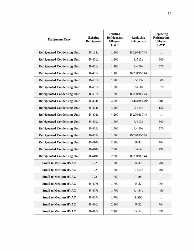
69

Equipment Type Existing

Refrigerant

Existing

Refrigerant

100-year

GWP

Replacing

Refrigerant

Replacing

Refrigerant

100-year

GWP

Refrigerated Condensing Unit R-134a 1,360 R-290/R-744 1

Refrigerated Condensing Unit R-401a 1,100 R-513a 600

Refrigerated Condensing Unit R-401a 1,100 R-450a 570

Refrigerated Condensing Unit R-401a 1,100 R-290/R-744 1

Refrigerated Condensing Unit R-401b 1,200 R-513a 600

Refrigerated Condensing Unit R-401b 1,200 R-450a 570

Refrigerated Condensing Unit R-401b 1,200 R-290/R-744 1

Refrigerated Condensing Unit R-404a 4,200 R-448a/R-449a 1400

Refrigerated Condensing Unit R-404a 4,200 R-454c 150

Refrigerated Condensing Unit R-404a 4,200 R-290/R-744 1

Refrigerated Condensing Unit R-409a 1,500 R-513a 600

Refrigerated Condensing Unit R-409a 1,500 R-450a 570

Refrigerated Condensing Unit R-409a 1,500 R-290/R-744 1

Refrigerated Condensing Unit R-410b 2,200 R-32 704

Refrigerated Condensing Unit R-410b 2,200 R-454b 490

Refrigerated Condensing Unit R-410b 2,200 R-290/R-744 1

Small to Medium HVAC R-22 1,780 R-32 704

Small to Medium HVAC R-22 1,780 R-454b 490

Small to Medium HVAC R-22 1,780 R-290 1

Small to Medium HVAC R-407c 1,700 R-32 704

Small to Medium HVAC R-407c 1,700 R-454b 490

Small to Medium HVAC R-407c 1,700 R-290 1

Small to Medium HVAC R-410a 2,100 R-32 704

Small to Medium HVAC R-410a 2,100 R-454b 490

70

Equipment Type Existing

Refrigerant

Existing

Refrigerant

100-year

GWP

Replacing

Refrigerant

Replacing

Refrigerant

100-year

GWP

Small to Medium HVAC R-410a 2,100 R-290 1

AC Chiller R-22 1,780 R-32 704

AC Chiller R-22 1,780 R-454b 490

AC Chiller R-22 1,780 R-717 0

AC Chiller R-407c 1,700 R-32 704

AC Chiller R-407c 1,700 R-454b 490

AC Chiller R-407c 1,700 R-717 0

71

These refrigerants are categorized into high, moderate, and low replacement

categories based on their GWP values. The explored pathways are limited here to three

GWP value ranges. The high scenario GWP values include values from 600 to 1,400. The

moderate scenario is a range of refrigerants with GWP values from 150 to 600. The low

scenario is limited to GWP values of 1. The relevance of these limits comes mostly from

the exclusion of R-452a, an HFO refrigerant blend shown in Figure 1 to be a suitable

option to replace R-22 and some of its HFC alternatives. However, because its 100-year

GWP, 2100, is higher than most of the refrigerants it would be replacing, this study has

chosen to exclude it from consideration in its replacement pathways.

Uncertainty

It is important to recognize the uncertainty in any analysis performed within a

project. The data collected for the HSU refrigerant inventory represents an initial point of

error/uncertainty. There is a level of uncertainty associated with every charge value

reported. The Facilities Management data are assumed to be well-known. However, given

the nature of the estimates made about the equipment charges collected with H&DS and

because information on the collection of Facilities Management’s charges was

unavailable due to COVID-19 restrictions, this study assumes a plus/minus 20%

uncertainty for each charge entry.27 The estimated charges described above that are not

27 It was the intention of this study to corroborate this with an explanation from Facilities Management

about their charge measurements, but this information was inaccessible due to COVID-19 related

difficulties. This error value should be updated, however, with a more accurate value of uncertainty related

to charge measurements.

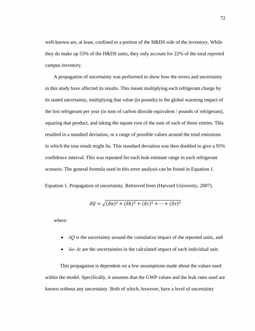
72

well-known are, at least, confined to a portion of the H&DS side of the inventory. While

they do make up 53% of the H&DS units, they only account for 22% of the total reported

campus inventory.

A propagation of uncertainty was performed to show how the errors and uncertainty

in this study have affected its results. This meant multiplying each refrigerant charge by

its stated uncertainty, multiplying that value (in pounds) to the global warming impact of

the lost refrigerant per year (in tons of carbon dioxide equivalent / pounds of refrigerant),

squaring that product, and taking the square root of the sum of each of those entries. This

resulted in a standard deviation, or a range of possible values around the total emissions

in which the true result might lie. This standard deviation was then doubled to give a 95%

confidence interval. This was repeated for each leak estimate range in each refrigerant

scenario. The general formula used in this error analysis can be found in Equation 1.

Equation 1. Propagation of uncertainty. Retrieved from (Harvard University, 2007).

𝛿𝑄 = √(𝛿𝑎)2 + (𝛿𝑏)2 + (𝛿𝑐)2 +⋯+ (𝛿𝑧)2

where:

• δQ is the uncertainty around the cumulative impact of the reported units, and

• δa- δz are the uncertainties in the calculated impact of each individual unit.

This propagation is dependent on a few assumptions made about the values used

within the model. Specifically, it assumes that the GWP values and the leak rates used are

known without any uncertainty. Both of which, however, have a level of uncertainty

73

associated with them.28 It also assumes that there is no correlation between the

measurements of refrigerant charge for each system and that the impact of each system is

a function of the leaked refrigerant alone.

Some assumptions were made about the natural refrigerants chosen to constitute

the low scenario replacements, as shown in Table 9. This refrigerant selection, and, in

general, the inclusion of natural refrigerants as options for approaching use within about

the next five years assumes that they will have developed and proliferated throughout the

US by then. HSU may be a school that is willing to try new things, but it is unlikely it is

in a position to be the first school to try a new, potentially dangerous refrigerant. This is a

reasonable assumption to make, especially with the new pro-low-GWP refrigerant laws

that have passed this year, in 2021, alone. The natural refrigerants used with reported

GWP values that are “less than one” (but not zero) have been given GWP values of one

in this analysis to reduce difficulties in calculations.

Ozone depletion is an aspect of refrigerant use that is important but, ultimately, it

is outside of the project’s scope. The notoriety of refrigerants may, indeed, be more a

consequence of the effects they have had and continue to have on Earth’s atmospheric

ozone layer than their global warming impacts. Additionally, some of the worst offenders

of this ozone depletion, especially R-12, are still used on the HSU campus. However,

28 The uncertainty associated with GWP values for a refrigerant is defined by their atmospheric lifetimes, as

stated in IPCC (2014). Their lifetime ranges can be grouped into centuries, decades, or years, with the

shortest periods having the most uncertainty. Refrigerants with century-long lifetimes can be assumed to

have an uncertainty range of 30%, decade-long lifetimes of 35%, and short-lived gases of 50%. This means

that for a refrigerant with a stated life of 500 years, the actual life may be anywhere between 350 and 650

years. This is consistent with World Meteorological Organization (2014), which states that GWPs for the

100-year time-horizon have uncertainties of roughly ±35% with higher uncertainties attributed to shorter-

lived gases, and IPCC (1996), which states that typical uncertainties for GWPs are on the order of 35%.

74

metric tons of ozone depletion potential emitted is a metric that is not easily comparable

on a small scale. Ozone depletion seems to be exclusively reported on the national or

global scales. This study has been unable to find any universities, businesses, or other

similarly sized organizations that report their ozone depletion, nor has it found any that

specify the refrigerants lost each year so that their associated ozone depletion could be

calculated. Consequently, the current analysis is focused on global warming impacts.

This study does not include or pursue the emissions from dorm refrigerators,

dorm minifridges, office minifridges, and vending machines. The number of refrigerators

and minifridges in the on-campus residence halls, some 210 refrigerators, and 653

minifridges, may indicate that they could, collectively, have a substantial emissions

profile. Interestingly enough, though, they all operate using isobutane, a hydrocarbon

refrigerant with a negligible GWP (Dan Bouchard, personal communication, 2020). So,

when this low-GWP is coupled with each unit’s small charge29 and low operational leak

rates, the result is a negligible global warming impact.30 The descriptions and counts of

refrigerants and equipment are still included for reference and context. However, they

will not be included in any emissions analysis here.

Previously collected information regarding office minifridges and vending

machines, were unavailable at the time of this study and may be non-existent. There were

29 Assumed to be 0.3 lbs. for refrigerators and 0.15 lbs. for minifridges. 30 Assuming a charge of 0.15 lbs. and a set of loss rate values reflecting the Domestic Refrigerator

equipment category, as described in Table 8, the most that a given mini-fridge would lose in a year is 0.01

lbs. of refrigerant. When converted to tons and when the GWP of isobutane is factored in, the resulting

emissions in MTCO2e are 0.00. Even when all of the hundreds of housing mini-fridges and refrigerators are

totaled, their cumulative associated emissions are still only 0.01 MTCO2e.

75

also no clear rules allowing or disallowing faculty and staff from owning personal

minifridges in their own offices or other workspaces. It was the intention of this study to

collect data through an inventory exercise of a subset of offices and then extrapolate from

this effort to cover the whole campus to provide an estimate that could be used to

examine their contribution. With the restrictions and lack of accessibility brought on by

the COVID-19 pandemic, however, it was not possible to collect this information. When

Andrea Alstone, the Energy Planner/Analyst at HSU Facilities Management was

questioned about the contribution of these minifridges and vending machines she

mentioned that she thought they would probably play a minimal role when compared to

the rest of the campus’ inventory. It is likely that this is the case, especially because

minifridges are shown above as being responsible for small amounts of emissions per

year.

Finally, it was the intention of this study to compare known refrigerant recharge

data to published data to gauge the campus’ general positioning within the range of leak

rates developed here, but that comparison was not possible as of the writing of this report.

In early communications with Mike Dotson, he had mentioned the existence of logs kept

by Facilities Management that detail the exchanges of refrigerants into and out of

equipment that they manage. These logs could have been used to identify patterns of

recharge frequency and quantity over some number of years at HSU. Priority would have

been placed on the ranges of recharge rates within the individual equipment types, as that

would most align with the leak rates from the literature described above. Trends in

equipment age and size would also have been a focus. Unfortunately, this was

76

unachievable due to the COVID-19 pandemic and the restrictions and busyness which it

brought to HSU Facilities Management and the world.

Knowing the frequency of leaks and the average percentage of refrigerant lost for

a given equipment type annually would certainly improve the accuracy of the emissions

analysis. As will be shown below, the emissions calculated are so heavily influenced by

the rates of refrigerant loss, that the information based on recorded data would likely

eliminate the need to estimate annual emissions, at least for the current inventory. Still,

my results are based on leak rate values that have been measured for similar systems in a

wide variety of settings, providing a reasonable estimate of what can be expected for

typical systems of the respective types. The values should be updated, however, with data

collected at HSU when that becomes possible again.

77

HSU INVENTORY

In order to know whether high-GWP refrigerant use at HSU is a problem, one

must first look at the individual pieces, the impact of the refrigerants themselves, the

regulations governing them, the equipment using them, and the entities that manage

them. These pieces provide clues as to what, if anything, is problematic, whether

something should or can be done about it, and what should be done. Understanding the

refrigerants and the technology using them can highlight possible hazards or areas with

higher-than-normal impact. Knowing where and how much of each refrigerant is used

also allows for a better understanding of the courses of action that can be taken when

considering their possible replacement. Questions like, “who is in a position to address

these problems and how big of a fix will it be?” are as important as identifying the

problem itself. The following section is intended to cover some of these details.

Refrigerants Used on Campus

Table 10 lists the eleven different types of refrigerants currently used on campus

with their respective refrigerant category, GWP, ODP, and atmospheric lifetime.

Refrigerants are grouped into six categories: CFCs, HCFCs, HFCs, HCFC blends, HFC

blends and HCs. Most of the refrigerants used are zeotropic blends, which are mixtures of

two or more refrigerants designed to match certain properties of the refrigerants used

before them while also complying with regulations (UNEP Compliance Assistance

Programme, 2016). All but one of these refrigerants have high-GWPs, with the highest at

78

10,300 and the lowest at 1,100. Only half deplete the ozone directly with ODPs between

0.02 and 0.73. However, because of their warming effects, they all indirectly deplete the

ozone layer (Hurwitz et al., 2015).

79

Table 10. Refrigerants used at Humboldt State University and their corresponding

impacts. Adapted from (Refrigeration, Air Conditioning and Heat Pumps

Technical Options Committee, 2019).

Refrigerant Type 100-year

GWP

20-year

GWP ODP

Atmospheric

Lifetime

R-12 CFC 10,300 10,800 0.73 102 years.

R-22 HCFC 1,780 5,310 0.034 12 years.

R-134a HFC 1,360 3,810 0 14 years.

R-401a HCFC

Blend 1,100 3,500 0.02 -

R-401b HCFC

Blend 1,200 3,800 0.03 -

R-404a HFC Blend 4,200 6,600 0 -

R-407c HFC Blend 1,700 4,100 0 -

R-409a HFC Blend 1,500 4,400 0.03 -

R-410a HFC Blend 2,100 4,400 0 -

R-410b HFC Blend 2,200 4,600 0 -

R-600a HC <1 <1 0 6 days

All of the refrigerants used, with the exception of R-600a, are either banned or are

at some point in the process of being phased down. R-12, and now, R-22 and the

refrigerants that contain it (i.e., R-401a, R-401b, and R-409a) have all been banned for

production and import (in “developed” countries) since 1996 and 2020, respectively, as a

80

result of the Montreal Protocol (EPA, 2020e; EPA, 2020f). R-22, R-401a, R-401b, and R-

409a have also all been banned in new equipment since 2010 (EPA, 2020f).31

The use of these “banned” refrigerants is still legal. However, the equipment

affected will have to be serviced with recycled and reclaimed refrigerant rather than new

refrigerant, as no new refrigerant can be produced nor imported (EPA, 2020f). The

extension of any existing unit’s cooling capacity qualifies that unit as “new equipment”,

and thus, disqualifies it from using even reclaimed supplies of any of these banned

refrigerants (EPA, 2020e). Otherwise, existing equipment can still be operated like

normal until refrigerant reserves run out.

The rest of the refrigerants used here are not regulated nationally or globally, as

the Kigali amendment does not target individual refrigerants. Even the new AIM act

leaves out specific refrigerant restrictions, and although their bans had been scheduled in

earlier federal legislation, those rules have been vacated. Still, in California, all of these

remaining refrigerants have been prohibited for use in new equipment as of or before

January 1st of 2021 (CARB, 2018). Additionally, R-404a has been banned from all

retrofitted equipment since 2019 (CARB, 2018). Currently, only R-134a, R-407c, R-

410a, and R-410b are available for retrofitted equipment from the list. However, all but

R-134a have GWP values that are as high or higher than the refrigerant they are most

likely to replace, R-22.

31 The extension of any existing unit’s cooling capacity qualifies that unit as “new equipment”, and thus,

disqualifies it from using any of these banned refrigerants. under these rules.

81

The distribution of refrigerants across the campus and their estimated cumulative

installed totals in pounds is tabulated in Table 11 and illustrated in Figure 2. R-22, R-

407c, R-404a, and R-410a are the refrigerants with the most installed capacity on campus

at 483, 260, 141, and 142 lbs. respectively, accounting for 89% of the total installed

mass. Three refrigerants alone (R-22, R-407c, and R-404a) are estimated to account of

78% of the total Nearly all of this capacity is operated by Facilities Management with the

exception of R-404a, which is used predominantly by H&DS. Moreover, 72% of the total

mass of refrigerants used on campus are under the supervision of Facilities Management.

In total, there are about 1,260 lbs. of refrigerant used at HSU.

82

Table 11. Quantities of installed refrigerants at Humboldt State University and their

corresponding operators. Values are given in pounds. Percent totals are given to

show each refrigerant’s relative abundance on campus.

32 The installed amount of R-600a is included for reference. However, because the domestic refrigerator

equipment category is excluded from the following emissions analysis, the refrigerant type which it

exclusively uses is also excluded from the total quantities given here.

Refrigerant Facilities

Management

Housing &

Dining

Services

Total Percent of

Total

R-12 28 - 28 2%

R-22 451 32 483 40%

R-134a 14 2 16 1%

R-401a 8 8 16 1%

R-401b - 2 2 0%

R-404a 60 181 241 20%

R-407c 210 50 260 22%

R-409a - 15 15 1%

R-410a 140 3 143 12%

R-410b - 2 2

0%

R-600a32 - 54 54 -

Totals

(excluding R-

600a)

911 295 1,206

83

Figure 2. Comparison of the installed masses of each refrigerant currently used at Humboldt State University. Data are shown

for systems managed by Facilities Management and Housing and Dining Services.

84

Figure 3 shows the distribution between the two organizations spatially by

highlighting the 25 buildings on the HSU campus which contain the refrigerants and

HVACR equipment included in this project33. These buildings include four dining areas:

the Jolly Giant Commons, the College Creek Marketplace, the Depot, and Windows

Café; six non-classroom buildings: the HSU Library, the greenhouse, the fish hatchery,

Student and Business Services, Facilities Management, and the Toddler Center; and

sixteen classroom buildings: Seimens Hall, Theater Arts, Founders Hall, Van Metre Hall,

Art A, Gist Hall, Jenkins Hall, Science A, Science B, Science C, Science D, Wildlife and

Fisheries, Harry Griffith Hall, Natural Resources, Forestry, and Behavioral and Social

Sciences.

33 Though it is true that only 25 buildings are included in this inventory, one building is divided so that both

Facilities Management and H&DS operate out of it. This division is shown in Figure 3 at points “b” – The

Depot / Windows Café – and “e” – University Center.

85

Figure 3. Map of the Humboldt State University campus highlighting the buildings which

house HVACR equipment. These buildings are categorized into six groups based

on the amount of refrigerant installed within each building and whether they are

operated by Facilities Management or Housing and Dining Services. See

alternative text for a listing of the buildings within each group. Not pictured in

this figure are the HSU marine lab, cell tower, and KHSU transmitter site.

Building Key

a. Jolly Giant

Commons

b. The Depot /

Windows Cafe

c. Founders Hall

d. Siemens Hall

e. University Center

f. Theatre Arts

g. Van Matre Hall

h. Library

i. Art A

j. Science A

k. Gist Hall

l. Jenkins Hall

m. Science C

n. Science B

o. Wildlife &

Fisheries

p. Student & Business

Services

q. Science D

r. Science E

s. Fish Hatchery

t. Harry Griffith Hall

u. College Creek

Marketplace

v. Natural Resources

w. Forestry

x. Behavioral &

Social Sciences

y. Facilities

Management Plant

Operations

z. Toddler Annex

Color Key

Facilities Management

<10 lbs.

10 - 25 lbs.

25 - 50 lbs.

50 - 100 lbs.

Housing and Dining

Services

50 - 100 lbs.

>100 lbs.

86

Application Descriptions

There are five general categories of refrigeration and air conditioning applications

on campus: domestic refrigeration, stand-alone hermetically sealed systems, refrigerated

condensing units, small to medium unitary HVAC, and AC chillers. Each category

satisfies HSU’s many needs in different ways, and they also contribute differently to the

impact that HSU has on the environment. Table 12 shows a count of each equipment type

by operator. Below are brief descriptions for these equipment categories. The category

descriptions help inform where HSU’s equipment fits in each category, what can and

cannot be easily changed and when, what is contributing more or less to GWP, and what

can be done about it. These descriptions also provide much of the equipment-specific

information used in the analysis of this study.

87

Table 12. Quantities of installed equipment types at Humboldt State University and their

respective operators. Values are given in number of units.

Application Facilities

Management

Housing &

Dining Services Total

Domestic

Refrigeration34

(excluded from

analysis

- 863 863

Stand-Alone

Hermetically Sealed 7 5 12

Refrigerated

Condensing Units 14 28 42

Small to Medium

Unitary HVAC 40 2 42

AC Chillers 5 - 5

Total (excluding

Domestic

Refrigeration)

66 38 10135

34 The number of installed domestic refrigerators is included for reference. However, because the domestic

refrigerator equipment category is excluded from the following emissions analysis, it is also excluded it

from the total quantities given here. 35 This includes three units not represented in the following emissions analysis here. One heat pump that

was included in the Facilities Management inventory, but not filled out, and two split condensing units that

were inaccessible on the H&DS equipment tours.

88

Domestic Refrigerators

The domestic refrigerator category describes most non-commercial or industrial

refrigeration. They include residential refrigerators, minifridges, coolers, and freezers.

Figure 4 shows an example of a basic refrigerator. These are standard units that can be

found at homes, offices, and dorm rooms. These individual units are self-contained,

factory built, and hermetically sealed (meaning airtight). This equipment type has the

lowest refrigerant charge (commonly under 1 lb.) of any equipment category mentioned

here because of its smaller cooling duty and minimal pipework. Because its compressor is

sealed, there are few operational leakages associated with these systems. The main source

of emissions for this equipment type is at the end of its life due to equipment failure or

inappropriate disposal methods, including not following end-of-life (EoL) recovery

procedures (UNEP Ozone Secretariat, 2015). Common refrigerants include R-134a and

R-600a. Lifespans around 15 years can be expected.

Figure 4. Example of a domestic refrigerator. Retrieved from (Best Buy, 2021).

89

Stand-Alone Hermetically Sealed

The stand-alone hermetically sealed equipment category describes small commercial

refrigeration systems, similar to domestic refrigerators that are commonly used in retail

food operations. Figure 5 shows an example of a common stand-alone hermetically

sealed unit. Like domestic refrigerators, these units are also individual, self-contained,

factory built, and hermetically sealed. They include food display cases, growth chambers,

stand-alone refrigerators/freezers, and ice makers. Their charges can be much higher than

domestic refrigerators36, but when compared to other equipment they are still relatively

low. Like with any hermetically sealed equipment, operational emissions are almost

negligible, but end-of-life (EoL) emissions can be very high. Popular refrigerants used in

this category include R-12, R-22, R-404a, and, most recently, hydrocarbons. A typical

lifetime of about ten years can be expected (ICF International, 2011).

Figure 5. Example of a stand-alone hermetically sealed commercial refrigerator.

Retrieved from (Amazon, 2020).

36 Based on the data from (Ashford et al., 2006), the charge range for a stand-alone hermetically sealed unit

is 0.4-13 pounds. The upper limit of this category is 13 times greater than the upper unit for domestic

refrigerators from the same study (i.e., one pound).

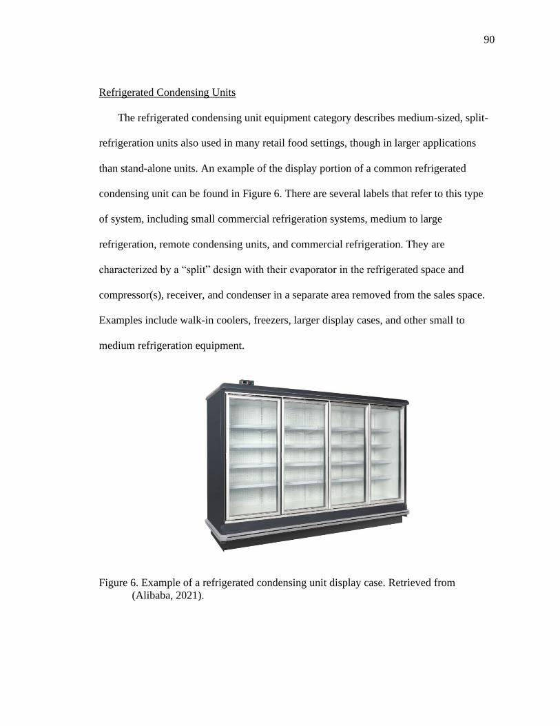
90

Refrigerated Condensing Units

The refrigerated condensing unit equipment category describes medium-sized, split-

refrigeration units also used in many retail food settings, though in larger applications

than stand-alone units. An example of the display portion of a common refrigerated

condensing unit can be found in Figure 6. There are several labels that refer to this type

of system, including small commercial refrigeration systems, medium to large

refrigeration, remote condensing units, and commercial refrigeration. They are

characterized by a “split” design with their evaporator in the refrigerated space and

compressor(s), receiver, and condenser in a separate area removed from the sales space.

Examples include walk-in coolers, freezers, larger display cases, and other small to

medium refrigeration equipment.

Figure 6. Example of a refrigerated condensing unit display case. Retrieved from

(Alibaba, 2021).

91

The UNEP Ozone Secretariat (2015) puts the typical charge range between 2 and 22

lbs. while CARB (2016) puts it at 50 to 200 lbs. The considerable higher charge for this

category is due to the much longer lengths of refrigerant pipework needed to connect the

two remote elements of the system. The opportunity for leakage is much higher in these

systems due to the longer lengths of pipework necessary for their site-specific

construction and the ability for operators to perform maintenance. Because access to the

refrigerant held in these systems is not restricted, there is a much better outlook for

refrigerant recovery associated with them. Since condensing units can be recharged with

refrigerant, it is possible that they have a full charge at the end of their life, but a charge

anywhere between 50% to 100% can be expected. This full charge, however, allows for

the opportunity that all the refrigerant is released during disposal (Ashford et al., 2006).

This equipment category has a possible average lifespan of about 20 years. Popular

refrigerants used include R-12, R-22, R-134a, R-404a, and a variety of other zeotropic

blends.

Small to Medium Unitary HVAC

The small to medium unitary HVAC category describes the lower end of the

commercial comfort heating and cooling covered here. Because of its lower cooling

capacity, this category includes equipment used in residential applications or ones that

are very similar. Examples include self-contained AC units, ducted and non-ducted split

AC systems, and packaged roof-top units. Figure 7 shows an example of one of these

packaged HVAC units. A range of refrigerant charge between 0 and 200 lbs. is common

for these systems (IPCC, 2006), though ICF International (2011) reported a range as high

92

as 400 lbs. This range combines both small and medium HVAC systems which are

sometimes split in reports but are more often grouped. Because of their shorter piping,

annual operational leak rates for this equipment type are relatively low and recovery

efficiencies at EoL are relatively high. Popular refrigerants used in this category include

R-12, R-22, R-134a, R-407c, R-410a, and now, hydrocarbons. Typical lifetimes are

between 15 and 25 years (ICF International, 2016).

Figure 7. Example of a medium sized packaged HVAC unit. Retrieved from (Trane,

2020).

AC Chillers

The AC chiller category generally represents the higher end of commercial comfort

cooling and heating at HSU. The word “generally” is used because at HSU, heat pumps,

which are essentially chillers operating in reverse, fit more neatly in the small to medium

HVAC equipment category because of their smaller applications, heating capacity, and

charge. However, because it is the same type of system, it is subject to the same

93

conditions as the higher capacity chillers. Examples include package chillers and air

source heat pumps. Figure 8 gives an example of a packaged chiller.

Figure 8. Example of a packaged AC Chiller. Retrieved from (Carrier, 2021).

The chiller equipment category has the highest charge range of any category used at

HSU. The typical charge range commonly falls within 200 to 2,000 lbs. (ICF

International, 2011; CARB, 2016; ICF International, 2016), though Ashford and others

(2006) define it more broadly as being between 22 and 4,409 lbs. Annual operational leak

rates for chillers are in line with those reported for the smaller HVAC category. Disposal

leak rates are also comparable to smaller HVAC equipment, though they have the

potential to be much higher and lower. One can expect a lifetime of about 20 years for

these units. Popular refrigerants include R-12, R-22, R-134a, R-407c, R-410a, and

ammonia.

94

RESULTS

The following chapter presents the estimated emissions associated with HSU’s

current refrigerant inventory and a few of the available pathways that the University it

could pursue moving forward to reduce these emissions. The contributions of the

refrigerant types, the equipment types, and the set of values used to compare the impacts

of each refrigerant are also discussed.

Current Emissions

Figure 9 shows the range of estimated annual emissions at HSU for the current

inventory along with benchmarks for reference. The high, average, and low leak rate

possibilities used to develop this range cover a wide array of possible situations. This is

shown by the variation in emissions for each scenario. The current inventory is expected

to emit between 429 ±15 MTCO2e and 57 ±2 MTCO2e annually, with an average37 of

224 ±8 MTCO2e annually. That correlates to 295 lbs., 36 lbs., and 154 lbs. of annual

refrigerant loss, respectively, over the range of different refrigerant types at HSU. This

range of greenhouse gas emissions is on the order of the emissions associated with the

staff commuting and solid waste disposal categories at HSU, which in 2019 amounted to

about 408 and 183 MTCO2e, respectively (Humboldt State University, 2020).

Information is needed from Facilities Management to compare their known recharge rates

to these estimates of loss.

37 Based on calculated average leak rates from the literature

95

Figure 9. Estimated annual emissions associated with fugitive refrigerant leaks at

Humboldt State University. Data are shown for systems managed by Facilities

Management and Housing and Dining Services. Emissions estimates are given in

metric tons of carbon dioxide equivalent per year (MTCO2e/yr). Amount of

released refrigerant is calculated based on the charges of each reported/surveyed

heating, ventilation, air conditioning, and refrigeration unit and reported average

annual leak rates for each unit type in the literature. These annual values for the

high, average, and low ends of the leak rate spectrum were then converted to

annual emissions using the global warming potentials of each refrigerant. There is

a 20% uncertainty assigned to each charge datum, and error bars are included to

show a 95% confidence interval. The reported emissions from two additional

emissions sources for 2019 at Humboldt State University, staff commuting, and

solid waste, are included for comparison.

96

Figure 9 also shows what these emissions ranges look like when they are categorized

by the campus entity that manages them. Facilities Management’s systems account for an

estimated 57%, 57%, and 53% of the emissions in the high, average, and low emissions

scenarios, respectively. As a reference, if we look back at Table 11 and Table 12, we find

that Facilities Management operates 66% of the total units on campus and those units

contain 72% of the total mass of the refrigerants on campus.

Table 13 details HSU’s 2019 emissions inventory and is broken down by emissions

source categories and subcategories. The emissions from this inventory total 9,085

MTCO2e.38 Emissions from fugitive refrigerants could contribute between 1% and 5% to

this inventory, depending on the equipment’s leak rates.

38 This only includes emissions from Scope 1 and 2 sources. Although Scope 3 is acknowledged as a group

of emissions associated with campus, it is not included in the total emissions reported in the campus’

inventory.

97

Table 13. Comparison of HSU's reported emissions for the 2019 year using 100-year and

20-year time horizon GWP values. Emissions sources are organized into groups

(e.g., commuting) and sub-groups (e.g., student commuting) based on origin.

They are also classified by their scope. Data for HSU’s 2019 emissions inventory

were retrieved from (Humboldt State University, 2020). The 100-year and 20-year

GWP values were retrieved from (Intergovernmental Panel on Climate Change,

2014). Emissions values are given metric tons of CO2 equivalent per year

(MTCO2e/yr).

Scope Source39 Totals

100-Year

Totals

20-Year

One Direct Transportation: University Fleet: B20 Fleet 13 13

One Direct Transportation: University Fleet: Diesel Fleet 36 36

One Direct Transportation: University Fleet: Gas Fleet 170 170

One On-Campus Stationary: LPG (Propane) 20 20

One On-Campus Stationary: Natural Gas 5,317 5,347

One Cogeneration: Natural Gas 164 165

Two Electricity, Steam, and Chilled Water: Electricity 3,365 3,377

Three Commuting: Faculty Commuting: Automobile 221 221

Three Commuting: Faculty Commuting: Bike 0 0

Three Commuting: Faculty Commuting: Carpool 26 26

Three Commuting: Faculty Commuting: Public Bus 11 11

Three Commuting: Faculty Commuting: Walk 0 0

Three Commuting: Staff Commuting: Automobile 349 351

Three Commuting: Staff Commuting: Bike 0 0

Three Commuting: Staff Commuting: Carpool 41 41

Three Commuting: Staff Commuting: Public Bus 18 18

Three Commuting: Staff Commuting: Walk 0 0

Three Commuting: Student Commuting: Automobile 1,268 1,271

Three Commuting: Student Commuting: Bike 0 0

Three Commuting: Student Commuting: Carpool 131 132

Three Commuting: Student Commuting: Public Bus 226 226

Three Commuting: Student Commuting: Walk 0 0

Three Directly Financed Outsourced Travel: Air: Faculty / Staff 1,102 1,102

Three Electricity, Steam, and Chilled Water: T&D Losses 169 170

Three Solid Waste: Landfilled Waste: CH4 Recovery and Flaring 183 549

39 Emissions sources attributed to H&DS are not included as they are recognized as auxiliary to the campus.

98

Compared to this inventory, emissions from fugitive refrigerant leaks, under the

average leak scenario, are greater than 71% of the individual emissions source

subcategories for Scope One and Scope Two emissions. In fact, fugitive refrigerants have

the potential to contribute more on average to HSU’s emissions inventory than all but two

emissions subcategories: 1) On-Campus Stationary Sources (Natural Gas); 2) Electricity,

Steam, and Chilled Water (Electricity). When emissions associated with the Scope One,

Two, and Three categories are considered, the percent of emissions subcategories that the

average refrigerant emissions scenario is greater than increases to 76%.

The current refrigerant fugitive emissions impact of the campus can be broken down

further by looking at the equipment and refrigerants used. Further analysis looks at the

impact of each refrigerant used within their equipment. This can help determine what the

campus’ “problems areas” are so that HSU can tackle the pieces of its inventory that will

have the largest impact on its emissions profile.

Table 14 shows the relative impact of each equipment type on campus. Each

category has a separate listing for the respective operators. These subcategories are

analyzed to show their relative contribution to each equipment category and to the total

emissions. It should be noted that Facilities Management is responsible for the greater

percentage of emissions in every category except refrigerated condensing units, which it

splits roughly 40/60 with H&DS. Recalling the number of units owned by each party

given in Table 12, there is a similar pattern where Facilities Management is responsible

for a greater percentage of the total equipment in each category except refrigerated

condensing units.

99

Table 14. Relative contributions of refrigerant fugitive emissions by equipment type and operator at Humboldt State

University. Emissions estimates are divided to show the respective impact of each equipment type. These equipment

type categories are further divided to show H&DS’ and Facilities Management’s contribution to the impact of each

equipment type. The high, average, and low emissions estimates are given in metric tons of CO2 equivalent per year

(MTCO2e/yr). The respective contributions are given as a percentage of the total emissions for the campus and of the

impact of the individual equipment type. Values may not add up to totals due to rounding.

Equipment Operator High

(MTCO2e/yr)

% of

Total

Ave.

(MTCO2e/yr)

% of

Total

Low

(MTCO2e/yr)

% of

Total

% of

Equip

Stand-Alone Hermetically

Sealed

Housing &

Dining Services 2 <1% 1 <1% <1 1% 23%

Stand-Alone Hermetically

Sealed

Facilities

Management 5 1% 3 1% 1 2% 77%

Total 7 2% 4 2% 1 3% -

Refrigerated Condensing

Units

Housing &

Dining Services 175 41% 91 41% 25 45% 57%

Refrigerated Condensing

Units

Facilities

Management 130 30% 68 30% 19 33% 43%

Total 305 71% 159 71% 44 78% -

Small to Medium Unitary

HVAC

Housing &

Dining Services 7 2% 4 2% 1 1% 10%

Small to Medium Unitary

HVAC

Facilities

Management 61 14% 33 15% 7 13% 90%

Total 67 16% 36 16% 8 15% -

AC Chillers Housing &

Dining Services - - - - - - -

AC Chillers Facilities

Management 50 12% 25 11% 3 5% 100%

Total 50 12% 25 11% 3 5% -

100

The refrigerated condensing unit category is overwhelmingly the largest

contributor to the campus’ emissions. It contributes roughly 305, 159, and 44 MTCO2e/yr

in the high, average, and low scenarios, respectfully. This works out to be between 71%

and 78% of all direct refrigerant emissions across all scenarios. The Small to Medium

Unitary HVAC category is the second most emissive at between 15% and 16% of total

emissions. AC Chillers are the third most emissive with between 5% and 12%. And Stand

Alone Hermetically Sealed is the least emissive equipment type with about 2% of total

direct emissions.

Table 15 shows the contribution of each refrigerant type to the campus’ inventory.

Unlike equipment type, this comparison is more dependent on the operator. For Facilities

Management, the greatest impact is shared by R-22 and R-12, though R-404a, R-407c,

and R-410a all have reasonably high contributions as well. For H&DS, the greatest

contribution is by far R-404a, with 157, 82, and 23 MTCO2e annually in the high,

average, and low scenarios, respectively. R-404a contributes 86% of the GWP-weighted

emissions associated with the refrigeration systems managed by H&DS. In each case, the

impact of R-404a is a full magnitude higher than any other refrigerant used by H&DS.

Further, R-404a contributes a cumulative 48% to the total emissions associated with

fugitive refrigerants across the campus.

101

Table 15. Relative contributions of refrigerant fugitive emissions by refrigerant type and operator at Humboldt State

University. Emissions estimates are divided to show the respective impact of each refrigerant type. These refrigerant

type categories are further divided to show H&DS’ and Facilities Management’s contribution to the impact of each

refrigerant type. The high, average, and low emissions estimates are given in metric tons of carbon dioxide equivalent

per year (MTCO2e/yr). The respective contributions are given as a percentage of the total emissions for the campus

under the average emissions estimate. Values may not add up to totals due to rounding.

Operator Refrigerant High

(MTCO2e/yr)

Ave.

(MTCO2e/yr)

Low

(MTCO2e/yr)

Ave. % of

Total

Facilities

Management R-12 61 32 9 14%

Facilities

Management R-22 75 39 9 18%

Facilities

Management R-134a 4 2 1 1%

Facilities

Management R-401a 2 1 <1 0%

Facilities

Management R-401b - - - 0%

Facilities

Management R-404a 46 24 7 11%

Facilities

Management R-407c 36 18 2 8%

Facilities

Management R-409a - - - 0%

Facilities

Management R-410a 23 12 3 5%

Facilities

Management R-410b - - - 0%

Totals 246 128 30 57%

102

Operator Refrigerant High

(MTCO2e/yr)

Ave.

(MTCO2e/yr)

Low

(MTCO2e/yr)

Ave. % of

Total

Housing and Dining

Services R-12 - - - 0%

Housing and Dining

Services R-22 12 6 2 3%

Housing and Dining

Services R-134a <1 <1 <1 0%

Housing and Dining

Services R-401a 2 1 <1 0%

Housing and Dining

Services R-401b <1 <1 <1 0%

Housing and Dining

Services R-404a 157 82 23 37%

Housing and Dining

Services R-407c 7 4 1 2%

Housing and Dining

Services R-409a 5 3 1 1%

Housing and Dining

Services R-410a <1 <1 <1 0%

Housing and Dining

Services R-410b 1 <1 <1 0%

Totals 183 96 26 43%

103

Table 16 shows the relationship between the refrigerants used on campus and the

equipment categories in which they are used. This table adds evidence to the previous

two by showing that most of the emissions on campus are coming from the Refrigerated

Condensing Unit category and from the five refrigerants described above. However, it

also narrows the problem area even further, showing that the greatest contributions are

coming from the refrigerants with the greatest impact potentials that are used in the

equipment types with the highest leak rates. R-12, with a GWP of 10,300, and R-404a,

with a GWP of 4,200 (the two highest GWP values on campus), are almost exclusively

used by the refrigerated condensing unit category, which has the highest annual

equipment leak rate, at 35% of the total unit charge. However, it is the use of R-404a in

refrigerated condensing units that makes the greatest contribution to these emissions with

a cumulative 47% of all emissions being attributable to the combination of the two. The

impact that is shown in this table still follows the same patterns of relative contributions

that the previous two tables have shown.

104

Table 16. Relative contributions of refrigerant fugitive emissions by refrigerant within each equipment type and operator at

Humboldt State University. Emissions estimates are divided to show the respective impact of each refrigerant type used

in each equipment type. These emissions categories are further divided to show H&DS’ and Facilities Management’s

contribution to the impact of each category. The high, average, and low emissions estimates are given in metric tons of

CO2 equivalent per year (MTCO2e/yr). The respective contributions are given as a percentage of the total emissions for

the campus under the average emissions estimate. Values may not add up to totals due to rounding.

Operator Equipment Refrigerant High

(MTCO2e/yr)

Average

(MTCO2e/yr)

Low

(MTCO2e/yr)

Ave. %

of Total

Facilities Management Stand Alone Hermetically Sealed R-22 5 3 1 1%

Facilities Management Stand Alone Hermetically Sealed R-134a - - - 0%

Facilities Management Stand Alone Hermetically Sealed R-404a - - - 0%

Facilities Management Stand Alone Hermetically Sealed R-410a - - - 0%

Facilities Management Refrigerated Condensing Units R-12 61 32 9 14%

Facilities Management Refrigerated Condensing Units R-22 18 9 3 4%

Facilities Management Refrigerated Condensing Units R-134a 4 2 1 1%

Facilities Management Refrigerated Condensing Units R-401a 2 1 <1 0%

Facilities Management Refrigerated Condensing Units R-401b - - - 0%

Facilities Management Refrigerated Condensing Units R-404a 46 24 7 11%

Facilities Management Refrigerated Condensing Units R-409a - - - 0%

Facilities Management Refrigerated Condensing Units R-410b - - - 0%

Facilities Management Small to Medium Unitary HVAC R-22 38 21 5 9%

Facilities Management Small to Medium Unitary HVAC R-407c - - - 0%

Facilities Management Small to Medium Unitary HVAC R-410a 23 12 3 6%

Facilities Management AC Chillers R-22 14 7 1 3%

Facilities Management AC Chillers R-407c 36 18 2 8%

105

Operator Equipment Refrigerant High

(MTCO2e/yr)

Average

(MTCO2e/yr)

Low

(MTCO2e/yr)

Ave. %

of Total

Housing and Dining

Services Stand Alone Hermetically Sealed R-22 - - - 0%

Housing and Dining

Services Stand Alone Hermetically Sealed R-134a <1 <1 <1 0%

Housing and Dining

Services Stand Alone Hermetically Sealed R-404a 1 1 <1 0%

Housing and Dining

Services Stand Alone Hermetically Sealed R-410a <1 <1 <1 0%

Housing and Dining

Services Refrigerated Condensing Units R-12 - - - 0%

Housing and Dining

Services Refrigerated Condensing Units R-22 12 6 2 3%

Housing and Dining

Services Refrigerated Condensing Units R-134a - - - 0%

Housing and Dining

Services Refrigerated Condensing Units R-401a 2 1 <1 0%

Housing and Dining

Services Refrigerated Condensing Units R-401b <1 <1 <1 0%

Housing and Dining

Services Refrigerated Condensing Units R-404a 155 81 22 36%

Housing and Dining

Services Refrigerated Condensing Units R-409a 5 3 1 1%

Housing and Dining

Services Refrigerated Condensing Units R-410b 1 <1 <1 0%

Housing and Dining

Services Small to Medium Unitary HVAC R-22 - - - 0%

Housing and Dining

Services Small to Medium Unitary HVAC R-407c 7 4 1 2%

Housing and Dining

Services Small to Medium Unitary HVAC R-410a - - - 0%

Housing and Dining

Services AC Chillers R-22 - - - 0%

Housing and Dining

Services AC Chillers R-407c - - - 0%

106

The magnitude of these fugitive emissions cannot be attributed solely to the

refrigerant used or the equipment type, but rather the combination of the two together. It

is more of an unfortunate coincidence rather than a mistake that the most emissive

refrigerants are paired with the equipment with the greatest leak rates. For the

applications that this equipment serves, especially with bigger units and greater cooling

demands, these high-GWP refrigerants were the thermodynamically most appropriate and

most efficient fits. The lower temperature demands of the commercial refrigeration

equipment categories require refrigerants with specific characteristics like extremely low

boiling points to meet those needs. It seems to be the case that those more extreme

characteristics go hand in hand with more extreme GWP values. It also just so happens

that those applications are the ones with the longer lengths of pipework and more

potential for leaks.

Projected Emissions

Figure 10 compares the emissions from HSU’s current inventory to three possible

emissions pathways, which are outlined as potential next steps here. These pathways

signify the possible responses to current and approaching refrigerant regulations. Since

all of HSU’s current refrigerants (excluding R-600a) are banned for use to some degree,

this study has outlined alternatives for each refrigerant used and categorized them by

GWP. These pathways are described in Table 9 above. They represent the high,

moderate, and low emissions choices that the campus could make when deciding to

replace its existing stock. These scenario groups are meant to show a comparison

107

between the emissions from business-as-usual and, alternatively, the early adoption of

current or upcoming refrigerant bans.

108

Figure 10. Comparison of the estimated annual emissions associated with fugitive refrigerants from HSU’s current HVACR

equipment inventory to three possible replacement pathways. The current inventory and the three proposed inventories

represent the averages of their set of emissions estimates as they have all been calculated using averages of the

equipment leak rate values given in Table 8. This graph is intended to show the associated emission of HSU’s future

refrigerant options. Emissions estimates are shown for systems managed by Facilities Management and Housing and

Dining Services. Estimates are given in metric tons of carbon dioxide equivalent per year (MTCO2e/yr). Refrigerants

were chosen based on their regulatory status and their level of favorability as replacements for each existing refrigerant

at HSU. There is a 20% uncertainty assigned to each charge datum, and error bars are included to show a 95%

confidence interval. Callout boxes are included to indicate the emissions where numbers do not fit.

109

Though the benefits of a complete replacement like the one shown here are likely

to be drawn out over time as units are incrementally replaced, the potential emissions

reductions are substantial. The result of an instantaneous replacement of HSU’s existing

refrigerant stock with even the most environmentally harmful of their more favorable

alternatives is a decrease in emissions associated with refrigerant use by 64%. Further, an

88% reduction can be achieved through the moderate emissions pathway. All of HSU’s

fugitive emissions from refrigerants can be eliminated when the low emissions pathway

is pursued. Even without the use of natural refrigerants, HSU can reduce its refrigerant

emissions to a point where they might reasonably be considered negligible.

Alternatives

The GWP values and time-horizon used have a substantial effect on the outcome of

these emissions calculations. As mentioned above, this report uses the 100-year GWP

values from the Refrigeration, Air Conditioning, and Heat Pumps (2019) assessment

report to be consistent with the most recent available science regarding GWP values.

However, the California Air Board Resource uses the IPCC (2007) fourth assessment

report, and many argue for the use of the 20-year time-horizon when discussing short-

lived pollutants. Table 17 shows the impact that these choices have on the results

reported here.

110

Table 17. Comparison of the emissions estimates for the HSU campus using different

GWP reference data. The estimates made in this project are based on the 100-year

GWP values given by the Refrigeration, Air Conditioning and Heat Pumps

Technical Options Committee (2019), but there are other reasonable references on

which they could be based. This table looks at the difference that using one

reference over another makes. Emissions estimates are given in metric tons of

carbon dioxide equivalent per year (MTCO2e/yr).

High Estimate

(MTCO2e/yr)

Ave. Estimate

(MTCO2e/yr)

Low Estimate

(MTCO2e/yr)

100-Year GWP Values

(Refrigeration, Air

Conditioning and Heat

Pumps Technical

Options Committee,

2019)

429 224 57

100-Year GWP Values

(IPCC, 2007) 424 224 56

Percent Change -1% 0% -2%

20-Year GWP Values

(Refrigeration, Air

Conditioning and Heat

Pumps Technical

Options Committee,

2019)

831 433 106

Percent Change 94% 93% 86%

111

There is very little difference between the results using the Refrigeration, Air

Conditioning and Heat Pumps Technical Options Committee (2019) GWP values and the

ones using IPCC (2007) values, with less than a two percent difference between the two.

Further, there is very little difference between the GWP values themselves in these

reports, or with older reports, for that matter. When considering the high-GWP

refrigerants discussed in this project (found in Table 10). GWP values for the respective

refrigerants change by one to nine percent from IPCC (2007) to the Refrigeration, Air

Conditioning and Heat Pumps Technical Options Committee (2019). Most of the GWPs

have decreased from the fourth assessment report (IPCC, 2007) to the one used here

(Refrigeration, Air Conditioning and Heat Pumps Technical Options Committee, 2019).

There is a smaller difference, between one and five percent, from the most recent

IPCC (2014) assessment report to the Refrigeration, Air Conditioning and Heat Pumps

Technical Options Committee (2019) report. There is a larger difference between the

GWP values reported in the second IPCC assessment report (IPCC, 1996) and the more

recent reports. For example, the differences range from four to twenty-nine percent

between the second assessment report and the Refrigeration, Air Conditioning and Heat

Pumps Technical Options Committee (2019).

The time horizon used, unlike the GWP reference values, has a very large influence

on the emissions reported. The emissions estimates for refrigerant leaks at HSU almost

double when the time-horizon used is switched from 100-years to 20-years. There is

between an 86% and 94% difference between the two sets of results. While there is

uncertainty regarding where HSU falls in the range between the low, average, and high

112

emissions cases, once 20-year GWP values are considered the emissions are sufficiently

high to indicate a need for action in any case.

To compare the emissions from refrigerant leaks with GWP values of a shorter time-

horizon to the campus’ emissions, the latter must be converted first. Table 13 above

shows what HSU’s overall 2019 emissions inventory would look like if it were calculated

with GWP values under a 20-year time horizon. This recalculation only increased the

total emissions by 3%. However, refrigerant emissions, as we have seen in Table 17,

nearly double across all estimates.

The switch to a 20-year time horizon does not result in large changes in HSU’s

overall emissions because most of HSU’s emissions are in the form of carbon dioxide

from natural gas and electricity use. The GWP value for carbon dioxide is not dependent

on the time frame considered, as it is the baseline for the metric and always has a GWP of

one. Considerable emissions from methane, the only short-lived gas recognized in HSU’s

inventory, can be found for four emission sources. Those four sources can be seen as

experiencing the largest increases in their total emissions when a 20-year time horizon is

considered. This is because methane’s GWP increases from 28 to 84 when considering a

20-year time horizon (Intergovernmental Panel on Climate Change, 2014).

Like methane, there is a considerable increase in the GWP values of many individual

refrigerants. Thus, the contribution of emissions from refrigerant leakage increases.

Because few other emissions in the inventory increase, the relative contribution of

refrigerant emissions also increases. Under a 20-year time-horizon, estimated refrigerant

fugitive emissions remain greater than 71% of HSU’s emissions source subcategories.

113

However, estimated refrigerant emissions account for nearly twice the relative impact

they had under the 100-year time horizon. They are estimated to contribute between 1%

and 9% of the total emissions from the campus under the 20-year time horizon.

114

DISCUSSION

The following chapter presents a comparison of the emissions estimates presented

in this study to other schools who have noted fugitive emissions in their own inventories.

The outlook of HSU’s refrigerant inventory and the applications and/or equipment that

may be suitable for low GWP replacements are also discussed.

Is This Range of Emissions Reasonable?

As noted previously the results presented here are based on leak rate values that were

collected from the literature rather than through measurements at HSU. This raises the

question of whether the range of estimated emissions is consistent with expectations for

other universities. As a point of comparison, six universities’ GHG emissions inventories

and/or climate action plans have been reviewed focusing on cases where refrigerant

fugitive emissions are covered, to see how they line up with what is presented here. The

universities reviewed are California State Polytechnic University Pomona, California

State University Los Angeles, North Carolina State University, University of California

Berkeley, University of North Carolina Wilmington, and University of Virginia. The

information in these reports concerning refrigerants is summarized in Table 18. There are

some common trends that are of relevance to this project.

115

Table 18. Summary of reviewed universities’ climate action plans. The total emissions column represents the emissions from

the Scope One and Scope Two emissions categories. Data for emissions are given MTCO2e. The contribution of

refrigerants to the total emissions for each campus is given as a percentage.

University Source Total Emissions

(MTCO2e)

Scope One

Emissions

(MTCO2e)

Emissions

Associated with

Refrigerants

(MTCO2e)

Percent

Contribution to

Total Emissions

California State

Polytechnic

University Pomona

(California State

Polytechnic

University,

Pomona, 2019)

36,002 11,971 729 2%

California State

University Los

Angeles

(California State

University, Los

Angeles, 2019)

18,098 3,382 185 1%

North Carolina

State University

(North Carolina

State University,

2021)

173,236 105,346 2,484 1%

University of

California Berkeley

(UC Berkeley,

2021) 147,004 144,684 779 1%

University of North

Carolina

Wilmington

(Ponder et al.,

2014) 39,828 10,423 1,466 4%

University of

Virginia (Pettit, 2019) 227,390 94,136 1,699 1%

116

The most important of these trends is that refrigerants at each university account for

between less than 1% and 4% of the total emissions. For the reports that clearly

described/differentiated their emissions categories (i.e., Scopes One, Two, & Three),

refrigerants accounted for 1% to 14% of their Scope One emissions, though only one

university, the University of North Carolina Wilmington, reported a value above 6%.

The range of emissions from fugitive leaks reported here makes up between 1% and

5% of HSU’s 2019 emissions. This is between 1% and 8% of the Scope One category,

which is the category that accounts for the largest share of HSU’s GHG emissions. The

HSU values are therefore within a range that is consistent with values reported by other

universities.

The range of reported emissions from other universities can be made easier to

compare to the values given here by scaling their emissions associated with refrigerant

leaks to a level that is proportional to the ratio between HSU’s total emissions and their

total emissions. For example, North Carolina State University’s emissions for 2017

totaled 173,236 MTCO2e and their emissions associated with fugitive refrigerants totaled

2,484 MTCO2e. If their total emissions were scaled to be equal to HSU’s 2019 emissions

(i.e., 9,085 MTCO2e) and the ratio between their total emissions and the emissions

associated with refrigerants was kept, their adjusted refrigerant emissions would be 130

MTCO2e.

The adjusted fugitive refrigerant emissions for the universities described here ranged

between 68 and 334 MTCO2e. The range of emissions estimated for HSU is between 57

and 429 MTCO2e, with an average of 224 MTCO2e. Figure 11 shows this comparison

117

more fully by presenting each university’s adjusted emissions alongside the three

emissions estimates for HSU’s inventory. An average for the six reviewed universities,

143 MTCO2e, is included in this figure, as well. The low and average estimates for

HSU’s emissions match the values reported by other universities, while the high-end

value for HSU falls somewhat outside values reported elsewhere.

118

Figure 11.Comparison of the adjusted emissions associated with fugitive refrigerants at six universities to the emissions range

estimated for Humboldt State University. The total emissions at each university have been scaled down to match

HSU’s recorded 2019 emissions (i.e., 9,085 MTCO2e) and the emissions related to refrigerant leaks have been scaled

proportional to the original ratio between the two emissions categories (i.e., total emissions and refrigerant

emissions). An average for the adjusted emissions at the six universities has been included. Values are given in metric

tons of carbon dioxide equivalent.

119

The maintenance personnel in charge of these systems were convinced in their

conversations that the leakage of refrigerants at HSU was minimal and practically non-

existent. The error in this study from their perspective would likely be that the leak rates

associated with each equipment type were too high. However, they were unable to

provide any real evidence that this was the case. In fact, during my survey of the H&DS

equipment, one stand-alone hermetically sealed refrigerator was out of service because it

experienced a leak and all of the refrigerant inside had escaped.

It may be that HSU’s actual emissions associated with refrigerant loss are somewhat

closer to the lower end of the range of emissions reported here. It is no surprise that if

there were 295 lbs. of refrigerant being lost annually,40 it would be a noticeable problem

not just because of the emissions but also for the loss of the regular function of the

equipment, the cost of new refrigerant, and the reductions in energy efficiency. This type

of annual refrigerant loss would likely be known to the staff governing it, and those

interviewed for this study were convinced that leaks are uncommon and do not amount to

high refrigerant losses each year.

The leak rates used in this report to analyze the HVACR equipment at HSU are

based on literature values, and it is possible that HSU has leak rates that are lower or

higher than the ones used here. Discussions with Dan Bouchard indicate that he believes

that the actual leak rates at HSU are lower than the values reported in the literature. He

states that H&DS has years where there are no leaks across their entire inventory and that

40 The amount of loss needed by the HSU campus to result in the high end of the emissions reported here.

120

it would take a “complete rupture” of their largest system to produce the amount of

refrigerant loss to make up even the lowest boundary of the emissions range (Dan

Bouchard, personal communication, 2020).

The emissions range reported above for the current inventory incorporates the one-

time losses that occur at the installation and the disposal of the equipment in a way that

they appear proportionally in the annual values. Thus, they could seem greater than

expected to anyone keeping track of refrigerant lost through operation alone. Also, since

the refrigerant losses reported here and their corresponding emissions are annual

averages, it is likely that there is a good deal of variation from one year to the next

around these values.

The true leak rate values for the HVACR equipment at HSU will remain uncertain,

unfortunately, until there is ongoing and comprehensive record-keeping completed by

both Facilities Management and H&DS. Fortunately, there are already upcoming changes

that will aid in this management, like the movement to electronic record-keeping and

annual inventory leak searches by H&DS (Dan Bouchard, personal communication,

2020). Additionally, there are operational and EoL procedures already used at HSU

which address the problems with refrigerant management that might lead to the higher

limits of these ranges. This project should, in any case, show what is possible for the

current situation at HSU and how important good refrigerant management is.

121

HSU’s Refrigerant Outlook

Knowing now that this is a reasonable estimate for the range of refrigerant-related

emissions at HSU, there are a number of “next-steps” available to the school to address

them. The first of which should be a period of data collection and re-analysis. The

comparison above to other universities normalizes the range of emissions presented here;

however, there are positions within that range that would demand more or less attention

(i.e., if subsequent study confirms that HSU’s fugitive refrigerant emissions fall near the

lower end of the estimated annual emissions, this may indicate that there is not a

significant problem with refrigerant leaks and that little is in need of change or vice

versa).

The second next step is a consideration of the potential to replace HSU’s “worst

offenders,” or the R-12, R-22 and, R-404a refrigerants. Replacing these refrigerants

and/or the associated equipment should take priority over the others because of their

considerable contribution to HSU’s negative environmental impacts, though with the

current status of almost all of the refrigerants used on campus, there needs to be an

inventory-wide effort made towards upcoming replacements.

The importance of record-keeping cannot be understated here. Currently, there are no

available refrigerant fugitive emissions records kept by either H&DS or Facilities

Management. They are not, after all, mandated by CARB or the EPA to keep them.

Current refrigerant laws specify that all equipment containing 50 or more pounds of

refrigerant at full charge must have regular leak inspections, and invoices must be kept

122

when any refrigerant is added to a unit (EPA, 2021). However, all but one unit at HSU is

under 50 pounds when charged. Both the Facilities Management and H&DS teams have

already expressed their intention to begin keeping records and have acknowledged its

importance, as well.

Until then, with no ongoing tracking of these chemicals, it seems unlikely that either

party would be fully aware of the true scale of refrigerant loss. Small ongoing problems

may go unnoticed for longer periods of time, and it may be that these otherwise

unnoticeable leaks add up over the entire inventory through time. Without records it is

not possible to document leak rates for refrigeration systems on campus. Record-keeping

is also the only way to get a more accurate picture of HSU’s emissions from fugitive

leaks.

Next, there are a number of factors that should be considered with respect to carrying

out the replacement of R-12, R-22 and, R-404a, some of the most used refrigerants on

campus. These three refrigerants are collectively used in 70% of the current equipment

inventory. In other words, transitioning away from the worst substances currently used at

HSU would mean replacing or retrofitting, in some way, 71 of the 101 units operating on

campus now. This includes 31 Refrigerated Condensing Units, 29 Small to Medium

Unitary HVAC units, 9 Stand Alone Hermetically Sealed units, and 2 AC Chillers.

The business-as-usual option replaces the refrigerants in these units with HFCs like

R-134a and R-407c in retrofits where possible and with HFO blends like R-448, R-449a,

R-32 through retrofit or replacement. These replacements would likely occur when R-12,

R-22, and R-404a eventually become unavailable, or too expensive, and supplies are

123

exhausted. While all of these replacements still constitute a moderate to high-GWP

pathway, they are also allowed by current and upcoming legislation and, in some cases,

have lower environmental impacts than the ones that they are replacing.

This business-as-usual approach includes easy and relatively inexpensive refrigerant

switches with noticeable reductions in associated emissions. The properties of the

replacement refrigerants may be similar enough in nature to the existing ones to allow

their operators to retain a sense of familiarity with the refrigerant itself and the

equipment’s servicing demands. It is a safe and reasonable option, especially if the actual

leak rates are determined to be lower than the values from literature used in this analysis.

But what of the rapidly developing next generation of natural refrigerants? Is it wise

to commit such a large portion of the HVACR equipment inventory to refrigerants that

are still considered to be moderate to high-GWP now when there is the potential for a

better-suited option right around the corner? It seems that the current development of this

next generation is better suited for some equipment types than others. In order to

eliminate the most problematic areas of HSUs refrigerant inventory in the short-term, as

they are required, there can and should be a mixed approach. For instance, the moderate-

GWP business-as-usual option may work well for the Refrigerated Condensing Units and

AC Chiller replacements, while the low-GWP option is better suited for the Stand-Alone

Hermetically Sealed units and Small to Medium HVAC equipment. The appropriateness

of each option is dependent on safety, cost/ease of replacement, and the availability of a

suitable low-GWP replacement.

124

Dan Bouchard has mentioned that he would like to stay away from natural

refrigerants as much as possible to avoid their flammability and toxicity dangers. This is

a completely reasonable perspective that prioritizes the immediate safety of the people

servicing the equipment, the students benefiting from the equipment, and the buildings

that house the equipment above what may be fairly modest global warming

environmental impacts associated with fugitive refrigerant emissions from the equipment.

While wanting to avoid the use of natural refrigerants for these reasons is a clear and

good sentiment, there are options like using hermetically sealed equipment, outdoor

staging locations, and better venting/air circulation that reduce the risks associated with

them. The low charge limits and heightened safety measures required for equipment

using high flammability and toxicity refrigerants can lower this risk even further.

Natural refrigerant systems may not cost much more than HFC systems for long, but

a completely new system will always cost more in the short term than a retrofit or

component replacement involving a switch to a similar but less impactful HFC. This is

especially true for the built-on-site units, which require replacement of more equipment.

It is less true, for instance, with factory packaged equipment like the hermetically sealed

units. Studies have found that there was a short return on investment for some natural

refrigerant technologies (Hillphoenix, 2019), that some system types were more energy-

efficient than their HFC counterparts (Elbel et al., 2016; ICF International, 2011; Peters,

2017; Choudhari & Sapali, 2018; Gaurav & Kuma, 2018; Skacanova & Gkizelis, 2018;

Shecco, 2019), and that there was a net benefit, through reductions in environmental

impact, avoided risks regarding regulation uncertainty, and increasing HFC refrigerant

125

costs (Garry & Williams, 2018) such that even when their energy consumption was

greater, they were a worthwhile investment. But, currently, transitioning entirely to

natural refrigerants may not be the most cost-effective investment to make for reducing

emissions at this time compared to other options (such as measures to reduce natural gas

use on campus).

In many ways the natural refrigerants and other low-GWP options discussed above

are commercially ready worldwide and in the US While there are some barriers that must

be overcome to use them, many are not as concerning as they seem, and even more are

expected to be overcome shortly. Still, while natural refrigerants have proven to be

commercially ready for some system categories, their success has not translated to every

equipment type. The smaller and larger ends of the HVACR equipment world have

experienced enough technical development to where refrigerants like isobutane and

ammonia are standard and favorable options for use. Middle-ground equipment like split

condensing units and some medium to large HVAC units do not necessarily have a clear

or favorable natural refrigerant alternative available. Carbon dioxide is a promising

option for both, but this and other suggested options require more from a system design

in terms of complexity, understanding, and cost (at the moment) than an HFC-based

system would.

Despite considerable effort, only one university was found, California State

Polytechnic University, Pomona, that mentioned transitioning to lower-GWP refrigerants

as a considered emission-reducing method (California State Polytechnic University,

Pomona, 2019). And it seems that only one university, the University of the West Indies

126

in Jamaica, has made that transition to a portion of its main commercial HVACR

inventory (Lobnig, 2010).41 Nevertheless, an outcome of this project is that the range of

estimated fugitive refrigerant emissions at HSU do not make up a large enough portion of

the greater campus’ emissions to warrant a complete transition to natural refrigerants in

the near term. This may be why few other universities have made the switch themselves.

It may also be the case that universities have prioritized more cost-effective options for

reducing their emissions, like reconsidering the source(s) of their electricity or focusing

on building heating options.

Still, HSU has the opportunity to adopt these technologies where their adoption is

practical. And there are even more opportunities where at first glance, their adoption

seems impractical. It is my suggestion that all stand-alone hermetically sealed equipment

be replaced with units that use R-290. Any outside HVAC equipment should also be

considered for a natural refrigerant replacement, especially those with low to medium

charge. Finally, there are reach-in split condensing unit display cases at each dining

facility that could potentially be removed and replaced with hydrocarbon-based stand-

alone hermetically sealed units.

Retrofits for equipment using R-12, R-22, and R-404a, where possible, should be

considered immediately so that their impact on the university’s emissions can be reduced

while also prolonging their lifetime. All of the complete equipment replacements should

occur at the end of the existing equipment’s lifetimes so as to avoid generating

41 Though, it is unclear if other universities have discreetly transitioned their entire residence hall

refrigerator stock to hydrocarbons, like HSU has.

127

unnecessary waste. The portion of the HSU inventory that is considered to be unsuitable

for natural refrigerant replacement in the short term should be replaced with low to

moderate HFO blends or, if needed, higher-GWP HFCs and HFO blends. We have seen

that even the transition to high-GWP HFO blends is one that would result in considerable

emissions reductions.

128

CONCLUSION AND RECOMMENDATIONS

Fugitive refrigerants are likely to be a greater source of emissions for the HSU

campus than is currently acknowledged by the university. This project has identified that

refrigerants lost through the installation, operation, and disposal of HVACR equipment at

HSU may be responsible for between 57 MTCO2e/yr and 429 MTCO2e/yr with an

average of 224 MTCO2e/yr, depending on the leak rate value used for these systems. This

amounts to between 1% and 5% of the total GHG emissions recorded for the campus in

2019. This project has also found that the portion of the refrigerated condensing unit

equipment category that uses the refrigerant R-404a is likely to be the most significant

contributor to those emissions. These units are responsible for roughly 47% of all

estimated annual emissions from fugitive refrigerants.

This project has identified what are likely to be the problem areas with respect to

refrigerant emissions. It has aggregated the current HVACR and refrigerant inventory on

campus. It has described the individual environmental impact potentials for each

refrigerant and has estimated their cumulative impact at HSU. And it has considered what

general next step options are available to the university and what their benefits and

drawbacks are. Still, of equal importance is what HSU’s response to this information can

and should be. In other words, what is the next course of action for HSU to meet

emissions goals, current regulations, and global trends?

129

There are three things that this study has identified as priority recommendations for

HSU. They are:

• Updating the inventory presented here with more accurate charge data, measured

leak rates, and uncertainty values. Some of the information that is critical for

accurately calculating the emissions associated with refrigerant leaks was

unavailable, for a number of reasons, during the course of this project. With more

attention and time given to the subject, this analysis can be updated and

reconsidered.

• Eliminating the use of the R-12, R-22, and R-404a refrigerants. Nearly all of the

refrigerants used on campus are either currently banned from use or have

approaching bans, but these three contribute a disproportionately large amount to

HSU’s refrigerant fugitive GHG emissions. These refrigerants also contribute to

ozone depletion, and their replacement would have corresponding benefits in this

regard.

• Acknowledge direct refrigerant emissions in future campus emissions reports.

Currently, these emissions are considered to be “de minimis” or insignificant, but

the full picture is still not yet known. There is a potential for fugitive emissions to

contribute as much, or more, to HSU’s emissions inventory as emissions sources

already included as lower-level priorities in published reports. Careful

documentation and reporting of refrigerant fugitive emissions could help generate

a better understanding of the full impact of this GHG emissions source.

130

Given the range of possible emissions for the equipment and refrigerants currently

used on the HSU campus, the number of similarly emissive activities or byproducts at

HSU that have received recognition in HSU’s Climate Action Plan, and the necessity for

greater coordination and organization with respect to campus refrigerant management and

planning for the next generation of refrigerants and equipment, this study recommends

that a more detailed analysis is warranted. For HSU to contribute to the historical success

and current push in eliminating the use of these environmentally destructive substances, it

must fully consider the emissions associated with their use on campus. While these

refrigerants affect the entire campus, their divided management makes a comprehensive

analysis of their use difficult. A lack of records in some areas further complicates this.

However, HSU has the opportunity to play an important role in the future of refrigerants

and their own campus sustainability by staying informed about upcoming trends in their

regulation and use and complying with current phase-out mandates.

If it is discovered upon further analysis of data collected by HSU’s refrigerant

operators that HSU falls in the lower portion of the estimated emissions range reported

here, then it will have benefitted from better understanding a portion of its operation that

is potentially harmful, and it will be in a better position to comply with upcoming

regulation by transitioning to lower-GWP alternatives. It is true that the emissions from

the refrigeration and air conditioning sector are dominated by the impact of their energy

consumption rather than fugitive leaks. However, reducing leaks through updated

management procedures will keep system charges optimized and eliminate wasted

energy. Updating equipment and equipment infrastructure will both increase energy

131

efficiencies and decrease leak potential. Even a partial transition to low-GWP alternatives

would further increase energy efficiency, decrease leaks, and eliminate the damage

associated with the leaks, as well. There are, then, multiple options that can be taken with

refrigerants which will lead to a reduced emissions inventory.

132

REFERENCES

Airconstruct. (2019). Natural Hydrocarbon Refrigerants Case Study. Retrieved February

14, 2021, from Airconstruct IEQ:

http://www.airconstruct.com.au/portfolio_page/natural-hydrocarbon-refrigerants-

case-study/

Alibaba. (2021). Supermarket refrigeration equipment glass door display refrigerator

showcase, commercial cooler. Retrieved January 23, 2021, from Alibaba.com:

https://hnxueying.en.alibaba.com/product/60327415982-

814327512/supermarket_refrigeration_equipment_glass_door_display_refrigerato

r_showcase_commercial_cooler.html

Amazon. (2020). Dukers D55R 40.7 cu. ft. 2-Door Commercial Refrigerator. Retrieved

January 23, 2021, from Amazon: https://www.amazon.com/Dukers-D55R-2-

Door-Commercial-Refrigerator/dp/B0778KD8SF

American Chemical Society. (2021). What are the properties of a greenhouse gas?

Retrieved April 29, 2020, from ACS Chemistry for Life:

https://www.acs.org/content/acs/en/climatescience/greenhousegases/properties.ht

ml

Armoo, L. M., & Fagbenle, R. L. (2020). Climate change in developing nations of the

world. In Applications of Heat, Mass and Fluid Boundary Layers (pp. 437-471).

Woodhead Publishing. doi:10.1016/C2018-0-01750-8

Ashford, P., Baker, J. A., Clodic, D., Devotta, S., Godwin, D., Harnisch, J., . . . Verdonik,

D. P. (2006). Emissions of Fluorinated Substitutes for Ozone Depleting

Substances. Institute for Global Environmental Strategies.

ASHRAE. (2017). Ammonia as a Refrigerant. Atlanta, Georgia: ASHRAE.

AssetWorks LLC. (2020). AiM: The Core of our Real Estate & Facility Management

Solution. Retrieved January 25, 2021, from AssetWORKS:

https://www.goassetworks.com/products/aim

Bellos, E., & Tzivanidis, C. (2019). A comparative study of CO2 refrigeration systems.

Energy Conservation and Management, 1. doi:10.1016/j.ecmx.2018.100002

Bera, P. P., Fransisco, J. S., & Lee, T. J. (2009). Identifying the Molecular Origin of

Global Warming. The Journal of Physical Chemistry A, 113(43), 12694-12699.

doi:10.1021/jp905097g

133

Best Buy. (2021). Insignia™ - 18.1 Cu. Ft. Top-Freezer Refrigerator - White. Retrieved

January 24, 2021, from Best Buy: https://www.bestbuy.com/site/insignia-18-1-cu-

ft-top-freezer-refrigerator-white/5838109.p?skuId=5838109&ref=212&loc=1

Bethel Afework, J. H. (2020). Carnot efficiency. Retrieved January 19, 2021, from

Energy Education: https://energyeducation.ca/encyclopedia/Carnot_efficiency

Bobbo, S., Fedele, L., Curcio, M., Bet, A., Carli, M. D., Emmi, G., . . . Bernardi, A.

(2019). Energetic and Exergetic Analysis of Low Global Warming Potential

Refrigerants as Substitutes for R410A in Ground Source Heat Pumps. Energies,

12(18). doi:10.3390/en12183538

Booten, C., Nicholson, S., Mann, M., & Abdelaziz, O. (2020). Refrigerants: Market

Trends and Supply Chain Assessment. Golden, CO: Clean Energy Manufacturing

Analysis Center.

Buis, A. (2019). The Atmosphere: Getting a Handle on Carbon Dioxide. Retrieved

February 3, 2021, from NASA: Global Climate Change:

https://climate.nasa.gov/news/2915/the-atmosphere-getting-a-handle-on-carbon-

dioxide/#:~:text=Carbon%20dioxide%20is%20a%20different,timescale%20of%2

0many%20human%20lives.

Caleb Nelson, C. R. (2015). Refrigerant Playbook: Natural Refrigerants. Denver: NREL.

California Air Resources Board. (2016). California's High Global Warming Potential

Gases Emissions Inventory: Emissions Inventory Methodology and Technical

Support Document. State of California Air Resources Board Air Quality Planning

and Science Division.

California Air Resources Board. (2018). Hydrofluorocarbon (HFC) Prohibitions in

California. Retrieved March 11, 2020, from CA.Gov:

https://ww2.arb.ca.gov/resources/fact-sheets/hydrofluorocarbon-hfc-prohibitions-

california

California Air Resources Board. (2019). Public Workshop for Stationary Refrigeration

and Air Conditioning. Sacramento, CA. Retrieved from

https://ww2.arb.ca.gov/sites/default/files/2019-12/Website%20Notice.pdf

California Air Resources Board. (2021). High-GWP Refrigerants. Retrieved March 3,

2020, from CA.gov: https://ww2.arb.ca.gov/resources/documents/high-gwp-

refrigerants

California State Polytechnic University, Pomona. (2019). Climate Action Plan. Retrieved

from

134

http://sustainabilitycpp.weebly.com/uploads/8/3/9/3/83931624/cap_update_2019.

pdf

California State University, Los Angeles. (2019). Climate Action Plan: Pushing

Boundaries in a Changing Climate. Retrieved from

https://www.calstatela.edu/sites/default/files/groups/Sustainability/cal_state_la_20

19_climate_action_plan_-_final_online_version.pdf

Calm, J. M. (2008). The next generation of refrigerants - Historical review,

considerations, and outlook. International Journal of Refrigeration, 31, 1123-

1133. doi:10.1016/j.ijrefrig.2008.01.013

Carrier. (2021). AquaForce® Air-Cooled Screw Chiller. Retrieved January 23, 2021,

from Commercial Systems North America:

https://www.carrier.com/commercial/en/us/products/chillers-components/air-

cooled-chillers/30xa/

Choudhari, C. S., & Sapali, S. N. (2018). Testing of Environment Friendly Refrigerant

R290 for Water Cooler Application. International Journal of Engineering, 31(1),

157-163. doi:10.5829/ije.2018.31.01a.21

Climate Analytics. (2017). Why using 20-year Global Warming Potentials (GWPs) for

emission targets is a very bad idea for climate policy. Retrieved from

Climateanalytics.org: https://climateanalytics.org/media/20-

year_gwps_bad_idea_for_climate_policy_16112017.pdf

Comstock, S., & Eltalouny, A. (2020). Update on New Refrigerants Designations and

Safety Classifications. United Nations Environmental Programme, ASHRAE.

Cornell Law School. (2020). 40 CFR § 82.157 - Appliance maintenance and leak repair.

Retrieved May 5, 2021, from Legal Information Institute:

https://www.law.cornell.edu/cfr/text/40/82.157

Coulomb, D. (2010). Global Warming: A key issue for refrigeration and air conditioning.

Retrieved April 16, 2021, from Energy Learning: https://energy-

learning.com/index.php/archive/86-global-warming-a-key-issue-for-refrigeration-

and-air-conditioning

DC Engineering. (2020). A Comprehensive Pricing Review of Alternative Refrigeration

Systems. Meridian, ID.

Dlugokencky, E., Houweling, S., Dirksen, R., Schröder, M., Hurst, D., Forster, P., &

WMO Secretariat. (2016). Observing Water Vapor. Retrieved from World

Meteorological Organization:

https://public.wmo.int/en/resources/bulletin/observing-water-vapour

135

Doniger, D. (2016). Countries Adopt Kigali Amendment to Phase Down HFCs. Retrieved

January 28, 2021, from National Resources Defense Council:

https://www.nrdc.org/experts/david-doniger/countries-adopt-kigali-amendment-

phase-down-hfcs

Doniger, D., & Theodoridi, C. (2020). Colorado and Virginia Shift from Super-Polluting

HFCs. Retrieved August 30, 2020, from National Resources Defense Council:

https://www.nrdc.org/experts/david-doniger/colorado-and-virginia-shift-super-

polluting-hfcs

Elbel, S., Visek, M., & Hrnjak, P. (2016). A fair comparison of CO2 and propane used in

light commercial applications featuring natural refrigerants. International

Refrigeration and Air Conditioning Conference. Retrieved from

http://docs.lib.purdue.edu/iracc/1748

Emani, M. S., & Mandal, B. K. (2018). The Use of Natural Refrigerants in Refrigeration

and Air Conditioning Systems: A Review. IOP Conf. Series: Materials Science

and Engineering. 377, p. 377. IOP Publishing. doi:10.1088/1757-

899X/377/1/012064

Emerson. (2011). Refrigerants for commercial refrigeration applications. Retrieved from

https://www.rsd.net/fx/pdf/suite/Copeland_Refrigerants_White_Paper.pdf

Environmental Investigation Agency. (2015). EU F-Gas Regulation Handbook: Keeping

Ahead of the Curve as Europe Phases Down HFCs. Environmental Investigation

Agency.

Environmental Investigation Agency. (2021). Supermarket Scorecard. Retrieved April 2,

2021, from Climate-Friendly Supermarkets:

https://www.climatefriendlysupermarkets.org/scorecard

Environmental Investigation Agency. (2021). The AIM Act: Your Questions on U.S. HFC

Legislation – Answered. Retrieved February 7, 2021, from EIA: https://eia-

global.org/blog-posts/20210107-aim-act-questions-answered

Environmental Protection Agency. (2015). Updating Ozone Calculations and Emissions

Profiles for Use in the Atmospheric and Health Effects Framework Model.

Washington, D.C.: United States Environmental Protection Agency.

Environmental Protection Agency. (2016). Refrigerant Safety. Retrieved January 19,

2021, from United States Environmental Protection Agency:

https://www.epa.gov/snap/refrigerant-safety

136

Environmental Protection Agency. (2017). Understanding Global Warming Potentials.

Retrieved March 14, 2021, from United States Environmental Protection Agency:

https://www.epa.gov/ghgemissions/understanding-global-warming-potentials

Environmental Protection Agency. (2018). Basic Ozone Layer Science. Retrieved March

14, 2021, from United States Environmental Protection Agency:

https://www.epa.gov/ozone-layer-protection/basic-ozone-layer-science

Environmental Protection Agency. (2018). Protection of Stratospheric Ozone:

Notification of Guidance and a Stakeholder Meeting Concerning the Significant

New Alternatives Policy (SNAP) Program. Retrieved from

https://www.federalregister.gov/documents/2018/04/27/2018-08310/protection-

of-stratospheric-ozone-notification-of-guidance-and-a-stakeholder-meeting-

concerning-the

Environmental Protection Agency. (2020a). Climate Change Indicators: Greenhouse

Gases. Retrieved March 27, 2021, from United States Environmental Protection

Agency: https://www.epa.gov/climate-indicators/greenhouse-gases

Environmental Protection Agency. (2020b). Global Greenhouse Gas Emissions Data.

Retrieved February 20, 2021, from United States Environmental Protection

Agency: https://www.epa.gov/ghgemissions/global-greenhouse-gas-emissions-

data

Environmental Protection Agency. (2020c). Greenhouse Gas Equivalencies Calculator.

Retrieved March 14, 2021, from Energy and the Environment:

https://www.epa.gov/energy/greenhouse-gas-equivalencies-calculator

Environmental Protection Agency. (2020d). Overview of SNAP. Retrieved January 19,

2021, from United States Environmental Protection Agency:

https://www.epa.gov/snap/overview-snap

Environmental Protection Agency. (2020e). Phaseout of Class I Ozone-Depleting

Substances. Retrieved January 24, 2021, from United States Environmental

Protection Agency: https://www.epa.gov/ods-phaseout/phaseout-class-i-ozone-

depleting-

substances#:~:text=The%20ban%20on%20production%20and,effect%20on%20J

anuary%201%2C%201996.

Environmental Protection Agency. (2020f). Phaseout of Class II Ozone-Depleting

Substances. Retrieved January 24, 2021, from United States Environmental

Protection Agency: https://www.epa.gov/ods-phaseout/phaseout-class-ii-ozone-

depleting-substances

137

Environmental Protection Agency. (2020g). Significant New Alternatives Policy (SNAP):

Substitutes in Refrigeration and Air Conditioning. Retrieved February 21, 2021,

from United States Environmental Protection Agency:

https://www.epa.gov/snap/substitutes-refrigeration-and-air-conditioning

Environmental Protection Agency. (2020h). What is Ozone? Retrieved March 14, 2021,

from U.S. Environmental Protection Agency: https://www.epa.gov/ozone-

pollution-and-your-patients-health/what-ozone

Environmental Protection Agency. (2021). Recordkeeping and Reporting Requirements

for Stationary Refrigeration. Retrieved February 20, 2021, from United States

Environmental Protection Agency:

https://www.epa.gov/section608/recordkeeping-and-reporting-requirements-

stationary-refrigeration

European Partnership for Energy and the Environment. (2018). The New F-Gas

Regulation. Brussels, Belgium: EPEE Secretariat.

Eyring, V., Cionni, I., Bodeker, G. E., Charlton-Perez, A. J., Kinnison, D. E., Scinocca, J.

F., . . . Yamashita, Y. (2010). Multi-model assessment of stratospheric ozone

return dates and ozone recovery in CCMVal-2 models. Atmospheric Chemistry

and Physics, 10, 9451-9472. doi:10.5194/acp-10-9451-2010

Garry, M. (2018). Home fridge makers push for higher charge for isobutane. Retrieved

March 22, 2021, from Hydrocarbons21:

https://hydrocarbons21.com/articles/8311/home_fridge_makers_push_for_higher

_charge_for_isobutane

Garry, M. (2019). In Reversal, IEC Approves Increase of Charge Limit for Flammable

Refrigerants to 500 g, Setting Stage for Wider HC Use. Retrieved from Accelerate

24 News: https://accelerate24.news/regions/in-reversal-iec-approves-increase-of-

charge-limit-for-flammable-refrigerants-to-500-g-setting-stage-for-wider-hc-

use/2019/#:~:text=Following%20a%20surprising%20recount%2C%20the,from%

20150%20g%20%E2%80%93%20in%20self%2D

Garry, M. (2021). German Study of HFO and TFA Due in Early 2021. Retrieved May 5,

2021, from Hydrocarbons21:

https://hydrocarbons21.com/articles/9900/german_study_of_hfo_and_tfa_due_in_

early_2021

Garry, M., & Williams, A. (2018). Leader of the Rack. Accelerate: Advancing HVAC&R

Naturally(1), pp. 42-44. Retrieved from

http://publication.shecco.com/upload/file/org/5aa901bee1f6a1521025470I13ni.pd

f

138

Gaurav, & Kuma, R. (2018). Thermo economic analysis of environmental friendly

refrigerant mixtures for replacement of R134a. ARPN Journal of Engineering and

Applied Sciences, 13(4).

Gkizelis, A. (2018). Refrigerants, Naturally! members surpass 7.25 million NatRef units.

Retrieved March 22, 2021, from Hydrocarbons 21:

http://hydrocarbons21.com/articles/8388/refrigerants_naturally_members_surpass

_7_25_million_natref_units

GlobalFACT. (2018). Selecting the Right Refrigerant for Commercial Refrigeration:

Achieving High Performance While Reducing Environmental Impact.

Goyal, R., England, M. H., Gupta, A. S., & Jucker, M. (2019). Reduction in surface

climate change achieved by the 1987 Montreal Protocol. Environmental Research

Letters, 14(12). doi:https://doi.org/10.1088/1748-9326/ab4874

Handwerk, B. (2010). Whatever Happened to the Ozone Hole? Retrieved January 19,

2021, from National Geographic:

https://www.nationalgeographic.com/news/2010/5/100505-science-environment-

ozone-hole-25-years/

Harvard University. (2007). Physical Sciences 2. Retrieved January 29, 2021, from

Instructional Physics Laboratory: http://ipl.physics.harvard.edu/wp-

uploads/2014/01/ps2_fa13_err.pdf

Hillphoenix. (2019). DeCO2ded: Understanding ROI on CO2 Refrigeration Systems.

Retrieved from https://www.hillphoenix.com/wp-

content/uploads/2018/02/Advansor-White-Paper-RS-DeCO2ded-Understanding-

ROI-on-CO2-Systems-Final-.pdf

Honeywell Refrigerants. (2018). Refrigerant Charge Calculation. Morris Plains:

Honeywell International Inc.

HSU Office of Sustainability. (2016). Climate Action Plan. Humboldt State University.

Hughes, M. (2018). Options for Replacing R-404a. Portishead: IOR.

Humboldt State University. (2007). Refrigerant Compliance Plan.

Humboldt State University. (2020). Annual Progress Evaluation for Humboldt State

University, 2020. Retrieved 11 30, 2020, from Second Nature:

https://reporting.secondnature.org/ape/ape-public!1058

139

Hundy, G. F. (2016). Refrigeration, Air Conditioning and Heat Pumps. Retrieved

January 19, 2021, from ProQuest Ebook Central:

https://ebookcentral.proquest.com/lib/humboldt/detail.action?docID=4443183.

Hurwitz, M. M., Fleming, E. L., Newman, P. A., Li, F., Mlawer, E., Cady‐Pereira, K., &

Bailey, R. (2015). Ozone depletion by hydrofluorocarbons. Geophysical Research

Letters, 42(20). doi:https://doi.org/10.1002/2015GL065856

ICF International. (2011). Development of the GHG Refrigeration and Air Conditioning

Model.

ICF International. (2016). Accounting Tool to Support Federal Reporting of

Hydrofluorocarbon Emissions: Supporting Documentation. Washington, DC.

Institute for Governance and Sustainable Development. (2013). Primer on Short-Lived

Climate Pollutants. Institute for Governance and Sustainable Development.

Intergovernmental Panel on Climate Change. (1996). Climate Change 1995: The Science

of Climate Change. Cambridge: Cambridge University Press.

Intergovernmental Panel on Climate Change. (2006). Emissions of Fluorinated

Substitutes for Ozone Depleting Substances. 3(7). Retrieved from

https://www.ipcc-

nggip.iges.or.jp/public/2006gl/pdf/3_Volume3/V3_7_Ch7_ODS_Substitutes.pdf

Intergovernmental Panel on Climate Change. (2007). Climate Change 2007: Synthesis

Report. Contribution of Working Groups I, II and III to the Fourth Assessment

Report of the Intergovernmental Panel on Climate Change. Geneva, Switzerland:

IPCC.

Intergovernmental Panel on Climate Change. (2014). Anthropogenic and Natural

Radiative Forcing. Climate Change 2013 – The Physical Science Basis: Working

Group I Contribution to the Fifth Assessment Report of the Intergovernmental

Panel on Climate Change, 659-740. doi:10.1017/CBO9781107415324.018

Intergovernmental Panel on Climate Change. (2018). Climate Change: The IPCC

Scientific Assessment. World Meteorological Organization/United Nations

Environmental Programme. Cambridge: Cambridge University Press.

International Energy Agency. (2016). Latest trends in Global Refrigerant Regulations.

Retrieved January 12, 2021, from Technology Collaboration Programme:

https://heatpumpingtechnologies.org/news/1/49950/

140

JMS Consulting & INFORUM. (2018). Economic Impacts of U.S. Ratification of the

Kigali Amendment. Arlington: The Air-Conditioning, Heating, and Refrigeration

Institute and Alliance for a Responsible Atmospheric Policy.

Johnson, A. (2019). R-600a Isobutane Refrigerant Fact & Info Sheet. Retrieved March

22, 2021, from RefrigerantHQ: https://refrigeranthq.com/r-600a-isobutane-

refrigerant-fact-info-sheet/

Johnson, A. (2020). Colorado & Virginia Announce HFC Phase Down. Retrieved March

22, 2021, from RefrigerantHQ: https://refrigeranthq.com/colorado-virginia-

announce-hfc-phase-down/

Kedzierski, M., Brown, J. S., & Koo, J. (2015). Performance ranking of refrigerants with

low global warming potential. Science and Technology for the Built Environment,

207-219. doi: 10.1080/10789669.2014.974479

Kessler, W. S. (2016). The Good, the Bad, and the Ugly of Using Anhydrous Ammonia

Refrigerant in the Process Industries. Chilworth Technology Inc.

Leahy, S. (2017). Without the Ozone Treaty You'd Get Sunburned in 5 Minutes. Retrieved

April 4, 2021, from National Geographic:

https://www.nationalgeographic.com/news/2017/09/montreal-protocol-ozone-

treaty-30-climate-change-hcfs-hfcs/#close

Lee, B.-S., & Chiou, C.-B. (2008). The relationship of meteorological and anthropogenic

factors to time series measurements of CFC-11, CFC-12, and CH3CCl3

concentrations in the urban atmosphere. Atmospheric Environment, 42(33), 7706-

7717. doi:10.1016/j.atmosenv.2008.05.042

Lilya, D. (2019). Natural Refrigerant System Selection Comparisons in Commercial

Systems. IIAR Natural Refrigeration Conference & Expo. Phoenix, AZ: North

American Sustainable Refrigeration Council.

Lobnig, S. (2010). Jamaica: realising energy savings from AC while protecting the

climate. Retrieved April 4, 2021, from Hydrocarbons21:

https://hydrocarbons21.com/articles/2568/jamaica_realising_energy_savings_fro

m_ac_while_protecting_the_climate

Makhnatch, P. (2019). New refrigerants for vapour compression refrigeration and heat

pump systems. Stockholm: KTH Royal Institute of Technology.

Marchese, J. (2014). Ice Breaker: The Role of the Liquid Receiver. Retrieved April 26,

2021, from Air Conditioning, Heating, Refrigeration News:

https://www.achrnews.com/articles/128203-the-role-of-the-liquid-receiver

141

McLaughlin, C. (2019). No R290 leaks since 2013 at H-E-B store. Retrieved from

Hydrocarbons21:

http://hydrocarbons21.com/articles/8854/no_r290_leaks_since_2013_at_h_e_b_st

ore

McLinden, M. O., & Didion, D. A. (1987). Quest for alternattives. ASHRAE, 29(12), 32-

42.

Molina, M., & Zaelke, D. (2017). The Montreal Protocol: triumph by treaty. Retrieved

December 1, 2020, from UN Environmental Programme:

https://www.unenvironment.org/news-and-stories/story/montreal-protocol-

triumph-treaty

Nair, A. A., & Yu, F. (2020). Quantification of Atmospheric Ammonia Concentrations:

A Review of Its Measurement and Modeling. Atmosphere, 11(1092), 1-32.

doi:10.3390/atmos11101092

National Aeronautics and Space Administration. (1999). Ozone. Retrieved March 29,

2021, from Earth Observatory:

https://earthobservatory.nasa.gov/features/Ozone/ozone_2.php

National Aeronautics and Space Administration. (2021). Overview: Weather, Global

Warming and Climate Change. Retrieved February 20, 2021, from NASA:

https://climate.nasa.gov/resources/global-warming-vs-climate-change/

National Library of Medicine. (2021). Dichlorodifluoromethane. Retrieved April 16,

2021, from PubChem:

https://pubchem.ncbi.nlm.nih.gov/compound/Dichlorodifluoromethane

National Oceanic and Atmospheric Administration. (2010). How large is the depletion of

the global ozone layer? Retrieved March 1, 2020, from NOAA ESRL:

https://www.esrl.noaa.gov/csl/assessments/ozone/2010/twentyquestions/Q13.pdf

Natural Resources Defense Council. (2019). U.S. States Take the Lead in HFC

Phasedown. 41st Meeting of the Open-Ended Working Group of the Parties to the

Montreal Protocol.

North Carolina State University. (2021). Climate. Retrieved April 1, 2021, from

Sustainability: https://sustainability.ncsu.edu/campus/climate/

Orr, B. (2018). Receiver Basics. Retrieved March 22, 2021, from HVAC School:

https://www.hvacrschool.com/receiver-basics/

142

Pardo, P., & Mondot, M. (2018). Experimental evaluation of R410A, R407C and R134a

alternative refrigerants in residential heat pumps. International Refrigeration and

Air Conditioning Conference. Purdue University.

Patenaude, A. (2018). How to Transition Into the Future With HFO Blend Refrigerants.

Retrieved May 5, 2021, from Emerson Climate Conversations:

https://emersonclimateconversations.com/2018/10/23/how-to-transition-into-the-

future-with-hfo-blend-refrigerants/

Peters, T. (2017). Retail refrigeration: Making the transition to clean cold. Birmingham:

University of Birmingham, Birmingham Energy Institute.

Pettit, A. (2019). UVA 2018 Greenhouse Gas Inventory. Charlottesville: University of

Virginia. Retrieved from

https://sustainability.virginia.edu/sites/sustainability/files/2019-08/Greenhouse-

Gas-Inventory-Report-UVA-CY2018.pdf

Polvani, L. M., Camargo, S. J., & Garcia, R. R. (2016). The Importance of the Montreal

Protocol in Mitigating the Potential Intensity of Tropical Cyclones. Journal of

Climate, 2275-2289. doi:10.1175/JCLI-D-15-0232.1

Ponder, D., Toneys, A., & Hoyle, J. (2014). Greenhouse Gas Inventory. University of

North Carolina Wilmington. Retrieved from

https://uncw.edu/sustainability/documents/uncwghginventory9.13.14.pdf

Rae, I., & Gabriel, A. (2012). Saving the ozone layer: why the Montreal Protocol worked.

Retrieved April 29, 2021, from The Conversation:

https://theconversation.com/saving-the-ozone-layer-why-the-montreal-protocol-

worked-9249

Refrigeration, Air Conditioning and Heat Pumps Technical Options Committee. (2019).

2018 Report of the Refrigeration, Air Conditioning and Heat Pumps Technical

Options Committee. Kenya: United Nations Environmental Programme.

Sanders, A. (2017). FREON(tm) refridgerent Capacity for a Refrigerator. Retrieved

April 4, 2021, from HomeSteady: https://homesteady.com/info-12170824-freon-

capacity-refrigerator.html

Seidler, C., Baythavong, B., Gallagher, G., & Bowers, K. (2009). Initial Statement of

Reasons for Proposed Regulation for High Global Warming Potential

Refrigerants for Stationary Sources. Sacramento: California Environmental

Protection Agency Air Resources Board.

Shecco. (2018). CO2 refrigeration - a future-proof option. Retrieved April 29, 2021,

from R744.com:

143

https://r744.com/knowledge/papersView/co2_refrigeration_a_future_proof_optio

n

Shecco. (2019). Towards energy-efficient refrigeration with natural refrigerants:

Understanding the benefits of hydrocarbons. Shecco. Retrieved February 15,

2021, from

https://issuu.com/shecco/docs/brochure_benefits_of_hydrocarbons_en_2019

Shecco. (2020). World Guide to Transcritical CO2 Refrigeration. Retrieved February 21,

2021, from issuu: https://issuu.com/shecco/docs/r744-guide

Sine, M., & Busby, K. (2018). EPA updates refrigerant management requirements under

Section 608. Humboldt State University.

Skacanova, K. Z., & Gkizelis, A. (2018). Technical report on energy efficiency in HFC-

free supermarket refrigeration. Washington, DC: Shecco, Environmental

Investigation Agency.

Smith, M. (2019). Financial Overview: Natural Refrigerants. North American

Sustainable Refrigeration Council.

Solomon, S., & Wuebbles, D. (1994). Ozone Depletion Potentials, Global Warming

Potentials, and Future Chlorine/Bromine Loading Lead. World Meteorological

Organization. Retrieved from

https://www.esrl.noaa.gov/csl/assessments/ozone/1994/chapters/chapter13.pdf

Temple, K. A. (2004). A Performance Based Method to Determine Refrigerant Charge

Level in Unitary Air Conditioning and Heat Pump Systems. International

Refrigeration and Air Conditioning Conference (pp. 1-8). Purdue University.

Trakref. (2019). Quick Guide: How to Calculate Your Refrigerant Charge. Nashville:

Trakref.

Trane. (2020). Voyager® Rooftop Units. Retrieved January 23, 2021, from Trane

Technologies: https://www.trane.com/commercial/north-america/us/en/products-

systems/packaged-units-and-split-systems/rooftop-units/voyager.html

UC Berkeley. (2021). Greenhouse Gas Inventory. Retrieved April 1, 2021, from

Sustainability & Carbon Solutions: https://sustainability.berkeley.edu/carbon-

neutrality/greenhouse-gas-inventory

UNEP Compliance Assistance Programme. (2016). Fact Sheet No. 16: Refrigerant

Blends. Retrieved from

https://wedocs.unep.org/bitstream/handle/20.500.11822/28348/7785ODPBlends_

EN.pdf?sequence=1&isAllowed=y

144

UNEP Ozone Secretariat. (2015). Fact Sheet 4: Commercial Refrigeration.

United Nations. (2020). Amendment to the Montreal Protocol on Substances that Deplete

the Ozone Layer. Retrieved August 3, 2020, from United Nations Treaty

Collection:

https://treaties.un.org/Pages/ViewDetails.aspx?src=IND&mtdsg_no=XXVII-2-

f&chapter=27&clang=_en

United Nations Environment Programme. (2016). Global Warming Potential (GWP) of

Refrigerants: Why are Particular Values Used.

United Nations Environment Programme. (2018). 20 Questions and Answers. Retrieved

January 19, 2021, from UN Environmental Programme:

https://ozone.unep.org/20-questions-and-answers

United Nations Environment Programme. (2019). Refrigerants, Naturally! Retrieved

December 12, 2020, from Climate Initiatives:

http://climateinitiativesplatform.org/index.php/Refrigerants,_Naturally!

United Nations Environment Programme. (2021). About Montreal Protocol. Retrieved

April 29, 2021, from UN Environmental Programme:

https://www.unenvironment.org/ozonaction/who-we-are/about-montreal-protocol

University Corporation for Atmospheric Research. (2012). Carbon Dioxide Absorbs and

Re-emits Infrared Radiation. Retrieved August 2, 2020, from UCAR Center for

Science Education: https://scied.ucar.edu/carbon-dioxide-absorbs-and-re-emits-

infrared-radiation

University Corporation for Atmospheric Research. (2012). Molecules Vibrate. Retrieved

August 3, 2020, from UCAR Center for Science Education:

https://scied.ucar.edu/molecular-vibration-

modes#:~:text=Molecules%20vibrate.,together%20and%20then%20further%20ap

art.&text=Molecules%20with%203%20or%20more,called%20a%20vibration%20

%22mode%22.

Velders, G. J., Fahey, D. W., Daniel, J. S., McFarland, M., & Andersen, S. O. (2009).

The large contribution of projected HFC emissions to future climate forcing.

PNAS, 106(27), 10949-10954. doi:10.1073/pnas.0902817106

Westbrook, P. (2018). Update on HFC Regulations. Retrieved March 22, 2021, from

ColdZone: https://coldzone.htpg.com/news-and-events/article/update-on-hfc-

regulations/

145

World Meteorological Organization. (2011). Scientific Assessment of Ozone Depletion:

2010. Global Ozone Research and Monitoring Project, Report No. 50. Geneva,

Switzerland: World Meteorological Organization.

World Meteorological Organization. (2014). Scientific Assessment of Ozone Depletion:

2014. Geneva, Switzerland: World Meteorological Organization.

World Meteorological Organization. (2018). Scientific Assessment of Ozone Depletion:

2018. Global Ozone Research and Monitoring Project, Report No. 58, Geneva,

Switzerland.

Wuebbles, D. (2020). Ozone depletion. Retrieved March 22, 2021, from Britannica:

https://www.britannica.com/science/ozone-depletion/Ozone-layer-recovery

Xu, Y., Zaelke, D., Velders, G. J., & Ramanathan, V. (2013). The role of HFCs in

mitigating 21st century climate change. Atmospheric Chemistry and Physics, 13,

6038-6089. doi:10.5194/acp-13-6083-2013

Zaelke, D., Borgford-Parnell, N., & Andersen, S. O. (2018). Primer on HFCs. Institute

for Governance & Sustainable Development.

Zeiger, B., Gschrey, B., & Schwarz, W. (2014). Alternatives to HCFCs/HFCs in

developing countries with a focus on high ambient temperatures. Frankfurt: Oko-

Recherche.

Zgliczynski, M. (2018). Benefits of natural refrigerants in the supermarket industry.

Retrieved February 14, 2021, from Refrigerated and Frozen Foods:

https://www.refrigeratedfrozenfood.com/articles/95703-benefits-of-natural-

refrigerants-in-the-supermarket-industry

146

APPENDICES

Appendix A. Explanation of Refrigeration Cycles

Figure A.1. shows a simplified version of a vapor-compression cycle. This cycle

can be described as follows: the refrigerant enters the evaporator as a low-temperature,

low-pressure liquid. Air or water from a reservoir interacts with the coils containing

refrigerant in the evaporator. The refrigerant, with its low boiling point, changes phase to

a vapor and, in the process, absorbs heat energy from the reservoir. It then enters position

“a” as a high-temperature, low-pressure, vapor. The refrigerant then moves through the

compressor, which adds energy to the refrigerant through pressurization. The refrigerant

leaves the compressor and enters position “b” as a high-temperature, high-pressure,

vapor. As the refrigerant travels through the coils in the condenser it interacts with

another reservoir, which is also often air or water, and is cooled to the point that it

changes phase back to a liquid. Through its phase change, the refrigerant releases its heat

energy. The refrigerant leaves the condenser as a low-temperature, high-pressure liquid at

position “c”. Finally, the expansion valve reduces the pressure on the refrigerant where it

is then able to restart its cycle at position “d” as a low-temperature, low-pressure liquid.

147

This vapor-compression cycle can service either direction. All refrigeration and air

conditioning generally work where the evaporator is in the area where cooling is desired

(e.g., the inside of a house) and the reservoir that interacts with the evaporator is air. The

condenser is in an area where it can interact with air or water that is external to the first

reservoir. In the example of a domestic AC unit, the condenser is typically outside of

house and its heat rejection is directed towards the outside air. For heating systems, the

cycle is opposite. Heat is absorbed by the evaporator at an external reservoir and rejected

to the area where heating is desired.

Figure A.1. Depiction of a generalized vapor-compression cycle for a single-stage

HVACR unit. Arrows show the movement of refrigerant inside the system and

colors indicate the relative temperatures of the refrigerant. Labels are included to

indicate points of interest within the cycle.

148

The equipment surrounding these cycles is much more complex than how it is

described above. In reality, there may be multiple evaporators connected to one system

where cooling is desired in separate areas, like in some commercial refrigeration

applications. There may also be more than one of these vapor-compression cycles liked

together so that two refrigerants are utilized separately, and a greater range of

temperatures can be reached.

The correct sizing of each component in the system is also crucial and is fine-

tuned specifically to the refrigerant(s) in use and the application at hand. The receiver, for

instance, must be sized to hold a systems total charge and be no more than 80% filled

(Orr, 2018). Since the receiver acts as a storage tank for the system and moderates the

amount of refrigerant being used at any given time to meet changing system demands,

under-sizing it could result in pressure-related problems in the system which could cause

damage to other mechanical components or affect normal operation (Marchese, 2014)

149

Appendix B. Expansion on Global Warming Molecules.

The details of how greenhouse gases contribute to global warming are difficult to

conceptualize. Terms like global warming potential (GWP) and atmospheric lifetime are

important, though, to understand in order to get a better appreciation of the lasting and

intense global warming effects of refrigerants. This section is a discussion of what

molecular level characteristics of refrigerants make them highly potent greenhouse gases.

Molecules vibrate. Some molecules have many different, and sometimes complex,

ways in which they can vibrate; carbon dioxide, for instance, has three different modes of

vibration (University Corporation for Atmospheric Research, 2012). Depending on the

structure and modes in which it vibrates, a molecule can interact with passing waves of

electromagnetic radiation (University Corporation for Atmospheric Research, 2012).

Certain gases have molecular structures that allow them to absorb specific ranges of

wavelengths of outgoing infrared (IR) radiation because of these vibrational interactions.

The absorption of this radiation causes the vibration of the molecule to increase.

Because these molecules are energized and vibrating more, there are more collisions

between them, which increases their thermal energy and raises their temperature

(American Chemical Society, 2021). These molecules also eventually release their IR

energy, which can then be released back into space or re-absorbed by other surrounding

molecules (University Corporation for Atmospheric Research, 2012). An increase in

number of these heat-absorbing molecules in the atmosphere leads to more warming.

This is because outgoing radiation is trapped and because of the heat generated by the

150

increase in molecular collisions. This is the general process behind what is known as the

greenhouse gas effect.

The GWP of a gas is dependent on the amount of time that the molecule remains

intact in the atmosphere and the vibrational interactions between the molecule and

outgoing infrared radiation (IR) while it is intact. The amount and strength of this IR

absorption are dependent on the range in which IR waves interact with the molecule

(American Chemical Society, 2021). Molecules that interact with wavelengths not

absorbed by water vapor or carbon dioxide (the two most abundant GHGs in Earth’s

atmosphere (Dlugokencky et al., 2016) tap into radiation that would otherwise be lost to

space and, thus, have the potential to make significant contributions to atmospheric

warming (American Chemical Society, 2021). The length of time that these substances

remain in our atmosphere is dependent on the efficiency of two general processes:

physical removal, through absorptions at Earth’s surface, and chemical removal,

including UV light and hydroxide reactions (Solomon & Wuebbles, 1994). Most

refrigerants have characteristics that make them, in each of these three ways, significantly

more potent of GHGs in the short-term and long-term than carbon dioxide (Bera et al.,

2009).

Specifically, it is the chemical bonds with chlorine (Cl) or fluorine (F) in the

molecular structure of these refrigerants which make them such effective global warming

agents. Bera and others (2009) have shown that molecules with these bonds, and

especially with carbon-fluorine bonds, have vibrational modes that allow them to strongly

absorb IR radiation in the “atmospheric window” of wavelengths not already absorbed by

151

CO2 or H2O. As the number of these bonds within a molecule increases, the range of IR

wavelength absorption narrows to be more situated within the atmospheric window (Bera

et al., 2009). Additionally, these fluorine bonds do not readily react with molecules in the

atmosphere that remove and break up GHGs (i.e., hydroxide (OH-)), so molecules

containing them have much longer lifespans (Bera et al., 2009).

Unfortunately, the some of the refrigerants that are most widely and heavily used

have many of these bonds that make them so effective at absorbing IR radiation and so

resistant to being broken down. For instance, the refrigerant R-12 has a chemical formula

of CCl2F2 (National Library of Medicine, 2021). Each atom of carbon has four bonds,

and they are all either chlorine or fluorine, the two elements which intensify the effects of

a greenhouse gas. Since the breakdown of chlorine is also a contributor to ozone

depletion, as well as global warming, it is exclusive as a chemical constituent to the

chlorofluorocarbons and hydrochlorofluorocarbons of the earlier refrigerant generations.

Fluorine, however, is a component of even the approaching generation of lower-GWP

refrigerants and can be found in hydrofluoroolefins.

152

Appendix C. Refrigerant Descriptions

Descriptions for the refrigerants referenced in this study can be found in Table

C.1. These descriptions include each refrigerant’s name, type, chemical formula or

composition, safety classification, global warming potentials under various time horizons,

ozone depletion potential, and atmospheric lifetime, where they are available.

153

Table C.1. Master list of all the refrigerants referenced in this study. Adapted from (Refrigeration, Air Conditioning and Heat

Pumps Technical Options Committee, 2019).

Name Refrigerant

Type

Chemical Formula/

Composition

Safety

Class

100-year

GWP

20-year

GWP ODP

Atmospheric

Lifetime

R-12 CFC CCl2F2 A1 10,300 10,800 0.73 102 years.

R-22 HCFC CHClF2 A1 1,780 5,310 0.034 12 years.

R-32 HFC CH2F2 A2L 704 2,530 0 5.4 years.

R-134A HFC CH2FCF3 A1 1,360 3,810 0 14 years.

R-290

(Propane) HC CH3CH2CH3 A3 <1 <1 0 12.5 days

R-401A HCFC Blend R-22/152a/124

(53/13/34) A1 1,100 3,500 0.02 -

R-401B HCFC Blend R-22/152a/124

(61/11/28) A1 1,200 3,800 0.03 -

R-404A HFC Blend R-25/143a/134a

(44/52/4) A1 4,200 6,600 0 -

R-407C HFC Blend

R-32/125/134a

(23/25/52)

A1 1,700 4,100 0 -

154

Name Refrigerant

Type

Chemical Formula/

Composition

Safety

Class

100-year

GWP

20-year

GWP ODP

Atmospheric

Lifetime

R-409A HFC Blend R-22/124/142b

(60/25/15) A1 1,500 4,400 0.03 -

R-410A HFC Blend R-32/125

(50/50) A1 2,100 4,400 0 -

R-410b HFC Blend R-32/125

(45/55) A1 2,200 4,600 0 -

R-448a HFO Blend

R-32/125/1234yf/134a

/1234ze(E)

(26/26/20/21/7)

A1 1,400 3,100 0 -

R-449a HFO Blend R-32/125/1234yf/134a

(24.3/24.7/25.3/25.7) A1 1,400 3,100 0 -

R-450a HFO Blend R-1234ze(E)/134a

(58/42) A1 570 1,600 0 -

R-452a HFO Blend R-1234yf/32/125

(30/11/59) A1 2,100 4,000 0 -

R-452b HFO Blend R-32/125/1234yf

(67/7/26) A2L 710 2,100 0 -

155

Name Refrigerant

Type

Chemical Formula/

Composition

Safety

Class

100-year

GWP

20-year

GWP ODP

Atmospheric

Lifetime

R-454b HFO Blend R-32/1234yf

(68.9/31.1) A2L 490 1700 0 -

R-454c HFO Blend R-32/1234yf

(21.5/78.5) A2L 150 540 0 -

R-513a HFO Blend R-1234yf/134a

(56/44) A1 210 710 0 -

R-600a

(Isobutane) HC CH(CH3)2CH3 A3 <1 <1 0 6 days

R-717

(Ammonia) Natural NH3 B2L 0 0 0 <1 day

R-744

(Carbon

Dioxide)

Natural CO2 A1 1 1 0 Undefined42

R-1234ze HFO CF3CH=CHCl A2L <1 4 0 16.4 days

R-1234yf HFO CF3CH=CH2 A2L <1 1 0 10.5 days

42 As Environmental Protection Agency (2020a) has stated, the atmospheric lifetime of CO2 cannot be represented by a single value. The gas is not

destroyed over time through chemical or physical properties like the other substances described here. Rather, it is transferred to other reservoirs like

the ocean or in plant matter and over time (sometimes thousands of years) is deposited in various ways (e.g., ocean sediments, soil, rocks).

156