UNIVERSITY - UiO
41
Life Cycle Wages of Doctors An Empirical Analysis of the Earnings of Norwegian Physicians Knut Fjeldvig Department of Economics, University of Oslo UNIVERSITY OF OSLO HEALTH ECONOMICS RESEARCH PROGRAMME Working paper 2009: 11 HERO
Transcript of UNIVERSITY - UiO

Life Cycle Wages of Doctors An Empirical Analysis of the Earnings of Norwegian Physicians Knut Fjeldvig Department of Economics, University of Oslo
UNIVERSITY OF OSLO HEALTH ECONOMICS RESEARCH PROGRAMME
Working paper 2009: 11
HERO

Life Cycle Wages of Doctors
An Empirical Analysis of the Earnings of Norwegian Physicians
Knut Fjeldvig Department of Economics, University of Oslo
E-mail: [email protected]
November 2009
Health Economics Research Programme at the University of Oslo
HERO 2009 Keywords: Physicians, age-earnings, income, mincer function, gender,
empirical analysis, Norway JEL classification: J44, J31 Acknowledgments: I would like to thank Bernt Bratsberg for valuable discussion and comments. I am grateful to the Ragnar Frisch Centre of Economic Research for providing me with excellent working conditions. This study is part of the research activities under Frisch project 1134, "A Viable Welfare State," which is supported by the Norwegian Research Council. Data supplied by Statistics Norway have been crucial for the completion of this research. Health Economics Research Programme at the University of Oslo
Financial support from The Research Council of Norway is acknowledged. ISSN 1501-9071 , ISSN 1890-1735 , ISBN (print version.) (online) 978-82-7756-212-4

ii
Abstract:
We use individual panel data to estimate age‐earnings profiles for Norwegian physicians. Based
on data covering the 1993‐2006 period we find that the age‐earning profiles of physicians
share many of the attributes of the classical Mincer function. Physician`s earnings rise, but a
decreasing rate, for the first 20 years after medical training; they peak between the ages of 55
and 59; and they decline slightly toward the end of the career. We observe that there will be
complications when using the regular cross‐sectional methods because of cohort and period
effects on income. Using fixed‐effects method therefore provides a more accurate picture of
the profiles. When looking at profiles by gender we find that there are large differences
between the earnings of male and female physicians, some of which can be attributed to
reduced labor supply during child‐rearing years and some to lower investments in specialization
among female doctors. We also discover differences in the profiles of physicians educated in
Norway and abroad and discuss alternative explanations for this pattern.

iii
Table of contents Chapter 1: Institutional setting and past research 1.1 The setting 11.2 The labor market 11.3 Recent income development 31.4 Past research 4 Chapter 2: Data and methodology 2.1 The dataset 52.2 Sample descriptive statistics and restrictions 62.3 Choice of independent variable 72.4 Dependent variable 82.5 Empirical model 9 Chapter 3: Empirical Analysis 3.1 General overview of the age earning profile 103.2 Cohorts effects 133.3 Period effects 153.4 Differences between male and female physicians 193.5 Differences between Norwegian and foreign education 23 Chapter 4: Conclusion 25

1
Chapter 1: Institutional setting and past research
1.1 The setting
The Norwegian health care sector is financed and, for the most part, provided for by the
government. Total health expenditures in 2006 were $4520 per capita, of which 83.6% was
government spending. This is much higher than the OECD average of $2915, of which 71.5% is
government spending. (OECD, 2008).
Norwegian hospitals are mostly owned by the government and were managed by the counties
until 2002. After a reform in 2002 the responsibility was transferred to the central government,
which divided the country into 5 different regions. North, West, Middle Norway, South and
East. South and East merged 1 July 2007 into South‐ East. The regions have divided their areas
of responsibility among the local, county and regional hospitals. The local hospitals handle the
basic operations and medicine while the regional hospitals handle the most advanced and
serious needs. Each citizen is registered to a “designated” physician who takes care of their
primary health needs and refers the patient to the hospitals if needed. This is often provided by
private practices founded by public contracts. The majority of physicians in Norway work in
public hospitals, but it is not uncommon to have a private practice at the same time.
Medical studies in Norway are six years followed by an internship of 18 months of medical
practice. Medical students are also able to practice medicine after 4‐5 years of study under a
student license with the same wage as an intern.
1.2 The labor market
The physician labor market in Norway has been strongly influenced by a shortage of doctors
since 1990. This is the opposite situation to that of the other Nordic countries, like Sweden and
Finland, which have been experiencing a physician surplus. The main reason for this deficit was
that in the early 1980s the governments of the Nordic countries predicted that there would be
an economic recession, which was expected to reduce the demand for health services. This
recession was milder in Norway than in other Nordic countries, resulting in a higher demand for

2
health services than predicted. Because of this Norway is the only country that has experienced
a continuous shortage of physicians since 1980.
In 1981 there were 8500 working physicians in Norway with a supply deficit of 300 vacant jobs.
Both the government and the labor union were concerned that this deficit would turn into a
surplus in next 20 years. The reason for this concern was that the physician’s labor market
differentiates itself from the rest for the academic work force because of the fact that
physicians are educated to be physicians and after such a long education few find the
motivation for re‐education. It is also a very specialized education and it may be difficult to
apply this knowledge to new jobs. Hence it is important to make forecasts of the labor market
for physicians.
A inter departmental committee, named the “Willumsen committee”, published a report called
“Health plan for the 1980s” in 1983 in which they concluded that based on economic growth
that Norway would have 14200 physicians in year 2000. They also predicted that the demand
would approximately be 11 000 physicians, resulting in a surplus of 3200 unemployed
physicians. This resulted in a government intervention that reduced the number of students per
year from 370 in 1980‐82 to 300 in 1984‐87. The government also took action to reduce the
number of Norwegian students studying abroad.
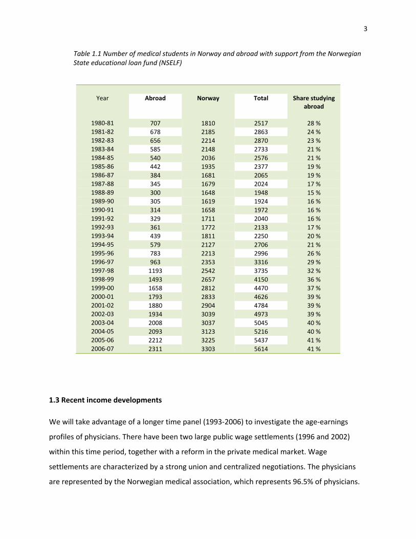
These labor market interventions continued until 1990 when the educational capacity was
increased to 345 students followed by an increase to 415 students in 1993 and 490 students in
1996. During the same period the number of students studying abroad increased rapidly. Table
1.1 shows the number of medical students from 1980‐2006. The reductions in the number of
educated physicians, together with increased demand for labor caused a large shortage of
physicians in the 1990s (Legeforeningen, 2007).
3
Table 1.1 Number of medical students in Norway and abroad with support from the Norwegian State educational loan fund (NSELF)
Year Abroad Norway Total Share studyingabroad
1980‐81 707 1810 2517 28 % 1981‐82 678 2185 2863 24 % 1982‐83 656 2214 2870 23 % 1983‐84 585 2148 2733 21 % 1984‐85 540 2036 2576 21 % 1985‐86 442 1935 2377 19 % 1986‐87 384 1681 2065 19 % 1987‐88 345 1679 2024 17 % 1988‐89 300 1648 1948 15 % 1989‐90 305 1619 1924 16 % 1990‐91 314 1658 1972 16 % 1991‐92 329 1711 2040 16 % 1992‐93 361 1772 2133 17 % 1993‐94 439 1811 2250 20 % 1994‐95 579 2127 2706 21 % 1995‐96 783 2213 2996 26 % 1996‐97 963 2353 3316 29 % 1997‐98 1193 2542 3735 32 % 1998‐99 1493 2657 4150 36 % 1999‐00 1658 2812 4470 37 % 2000‐01 1793 2833 4626 39 % 2001‐02 1880 2904 4784 39 % 2002‐03 1934 3039 4973 39 % 2003‐04 2008 3037 5045 40 % 2004‐05 2093 3123 5216 40 % 2005‐06 2212 3225 5437 41 % 2006‐07 2311 3303 5614 41 %
1.3 Recent income developments
We will take advantage of a longer time panel (1993‐2006) to investigate the age‐earnings
profiles of physicians. There have been two large public wage settlements (1996 and 2002)
within this time period, together with a reform in the private medical market. Wage
settlements are characterized by a strong union and centralized negotiations. The physicians
are represented by the Norwegian medical association, which represents 96.5% of physicians.

4
The tariff revision in 1996 entailed that more public physicians were required to work more
hours, resulting in treatment of additional patients. The physicians could also choose to more
than the required number of hours at a fixed overtime wage. The concept behind this wage
settlement was to motivate the doctors to work more, with a low basic wage and a high
variable wage.
This arrangement came to an end with the last reform in 2002. The new arrangement gave the
hospitals more flexibility when it came to working hours and working arrangements, resulting in
higher basic wages and lower payment for extra hours. This raise in basic wage also included a
compensation for the expansion of the workweek by 2.5 hours. The new structure gave the
physicians a higher minimum wage, and also gave the employer the liberty to distribute the
work hours (Legeforeningen ,2005).
In 1997 the Parliament introduced a national "regular” practitioner scheme (FLO), which took
effect on 1June 2001. The FLO gives all Norwegian inhabitants the right to have a general
practitioner registered as their primary physician. The general practitioners get a split payment:
a fee‐for‐service component paid comprised of a government payment and a patient co‐
payment, and an annual capitation fee of 299 Norwegian kroner per listed patient from the
government. Before the reform the primary doctor was either an employee of a municipality or
of a private practice with a public contract (www.ssb.no, Samfunnsspeilet utg. 5, 2003).
1.4 Past research
There has not been a great deal of research within this field in Norway. The main focus has
been on the labor supply, where two earlier studies examine the effect of the wage settlement
in 1996 on the hospital physician labor supply and work hours; see Sæther (2005) and Baltagi et
al (2005). These two studies reach different conclusions. Sæther (2005) studies male and
female physicians and finds that the work hour elasticity is 0.16. Baltagi et al (2005), who only
study male hospital doctors, find a much higher elasticity (short term 0.34 and long term 0.58).
We do not explore this topic further.

5
A few articles examine the life time earnings of physicians abroad, these have mostly been
about income expectations and motivation for specialization, like Frank A. Sloan (1970). Baker
(1996) studies the differences in earnings between male and female physician and concludes
that young male and female physicians with similar characteristics earn equal amounts of
money, but some differences still exist among older physicians in some specialties.
Jacob Mincer and George J. Borjas have both done extensive research about the theory of
creating age earnings profiles. We will refer to this later in the analysis, especially in chapter 3.
Empirical studies of labor supply among working men and women show that women’s working
hours correlate more strongly with wage than the working hours of men, both in Norway and in
other countries; Dagsvik and Zhiyang (2006) and Blau and Kahn (2006).
Chapter 2: Data and methodology
This study relies on quantitative methods. We specify the regression model and introduce the
datasets in this chapter.
2.1 The dataset
Our empirical focus is the wage and self‐employment income of physicians during the fourteen‐
year period 1993‐2006. By covering this period we can examine the effects of the two major
wage settlements.
To establish this projects database we merged data records from four different sources: "The
health personnel register" (HPR), the NUDB register (the national education database), a
demographic database that contains information about personnel who are registered as
residents in Norway and a database containing annual earnings data for each year between
1993 and 2006.
The health personnel register is a database with all health personnel authorized by the

6
department of health supervision, including personnel that has applied for authorization from
abroad but never immigrated to the country. This database gives us information about who is
authorized, time of authorization, registered specializations and other licenses for practice,
such as student, intern and temporary licenses.
The NUDB register includes all those who are registered as residents in Norway and contains
information about all lower and higher education in Norway. To be able to practice medicine in
Norway you must either have a cand. med. degree from Norway, a cand. med degree from a
country inside the EU or a supplementary course in addition to a foreign cand. med degree if
taken outside the EU. To identify these we use NUS code 763101 (cand med) and 763102
(supplementary course).
By combining these three databases we are able extract the necessary basic information (sex,
birth year, etc) and classify individuals according to:
‐ Norwegian born or immigrant (seasonal worker or a resident)
‐ Educated in Norway or abroad. Individuals registered with a “supplementary course" or who
are registered in the HPR but not in the educational register are considered to have been
educated abroad.
After obtaining this database we merged it with the SSB income data 1993‐2006, obtaining
30146 unique individuals with 380 562 income observations.
2.2 Sample descriptive statistics and restrictions
The purpose of this study is to investigate the age‐earnings profiles of working Norwegian
physicians. We have therefore implemented some restrictions to the sample we are going to
use in the econometric analysis.

7
The sample is restricted to those:
‐ registered with a doctor’s license in the Health Personnel Register
‐ born in Norway
‐ registered annual income higher than 100000 NOK.
‐ within the age range of 28 to 65, where of 65 is the first possible pension age.
Table 2.2 Sample descriptive statistics
females males males
w/Norw ed. males
w/foreign ed. real income 654 680 902 665 911 223 870 767 log real income 13.29 13.61 13.63 13.55 age 40.35 46.60 46.41 47.28 birth year 1959.98 1953.05 1953.18 1952.54 individuals 5676 10784 8389 2395 observations 53315 117395 92561 24834 Note: Sample period is 1993‐2006. Real income is measured in 2006 prices.
By examining table 2.2 we see that there are some differences between characteristics of male
and female physicians in the sample. The average age of male physicians is 6.3 years higher
than for female physicians. This may be a result of the increasing share of women among the
physicians in Norway from 24.9 % in 1993 to 37.5% of the total physicians in 2006
(Legeforeningen, 2008). Female physicians also have a significantly lower mean income than
their male colleagues, a result that merits further investigation. We also observe that, on
average, doctors educated abroad earn slightly less than doctors educated in Norway, an
earnings difference we will examine further in the empirical analysis.

8
2.3 Choice of independent variables
When choosing the independent variable representing time, we considered three alternatives;
age and two different experience variables (after education completed and after authorization).
After conducting some pretests of these variables we found that the post‐education experience
variable was only representative of individuals with education from Norway and not those with
foreign education, something that made it inferior to the other two variables. Age and the
authorization variable produced similar earning profiles, but age showed to be the most
covered and accurate of the two in the dataset. The average age in the sample for finishing a
Cand.med is 28‐29 while the average age for authorization is 30‐31.
We chose to use dummy variables for each age instead of a polynomial structure, because this
gave a more flexible structure and made the analysis more accurate.
2.4 The dependent variable
The dependent variable is the real income variable “Income from work” which is the sum of
“employee income” (wage) and “net self‐employment income”. The latter variable is important
to include because of the many physicians who have net income from a private practice. The
income variable has been converted into to real income, (2006 currency) by using numbers
from Statistics Norway (2008).
The three variables are described at Statistics Norway (2009) as:
“Income from work is the sum of employee income and net income from self‐employment
earned during the calendar year”
“Employee income is the sum of cash wages and salaries, taxable in‐kind earnings and sickness
and maternity benefits received during calendar year.”
“Net self‐employment income is the sum of self employment income in agriculture, forestry and
fishing and self‐employment from other industries received during the calendar year, less deficit.
It also includes sickness benefits by the self employed”

9
2.5 Empirical Model
We will first use a cross‐sectional method to define the general age earning profiles and second
a fixed‐effects method to investigate whether there exists unmeasured individual effects that
influence our general profiles exist.
We will start with a cross‐sectional method estimated by ordinary least squares (OLS). Cross‐
sectional data is a common type of data, which contains observations for distinct individuals at
a given point in time. These variables are normally measurements taken in a certain time frame.
The main difference between cross‐sectional data and time series is that cross‐sectional data
tell us who earns what during a single year, while a time series shows how the income level
changes from year to year. The OLS method is described by the following equation:
(1) 2
1 , (0, )it o it it ity B B x IID σ= + +ε ε ∼
2
( | ) 0, 1,..., , 1,...,
, | ) 0
0
it it
it js it
x i N t T
for j i t sx
otherwise
σ
Ε ε = = =
⎧ = =Ε(ε ε = ⎨
⎩
where is the dependent variable that is described by the independent variableity itx . The error
term contains all effects that are significant for the dependent variable, but are not included
in the model. is the number of individuals and t is the year of the observation.
itε
N
After the first section we will start to analyze the panel data with a fixed effects method. We
use individual fixed effects to control for unobserved heterogeneity in the micro units. When
we use cross‐sectional methods there may exist unmeasured explanatory variables that affect
the behavior of our observations and cause a bias in the estimation. The fixed effect method
uses panel data to control for unmeasured variables that differ across entities but are constant
over time.

10
(2) 2
1 , (0, )it o it i it ity B B x u IIDυ υ σ= + + + ∼
2
( | , ) 0, 1,..., , 1,...,
, | , ) 0
0
it it i
it js it i
x u i N t T
for j i t sx u
otherwise
υ
συ υ
Ε = = =
⎧ = =Ε( = ⎨
⎩
Where is the dependent variable that is described by the independent variableity itx . But now
we introduce a fixed effect term that controls for any correlation that may exist between the
error term and independent variable. The error term
iu
itυ contains all effects that are significant
for the dependent variable, but are not included in the regressors ( itx ) or captured by the
individual fixed effect ( ). is the number of individuals and t is the year of the observation;
(Kennedy, 2003) and (Erik Biørn, 2003 & 2008).
iu N
Chapter 3: Empirical Analysis
3.1 General overview of age earning profiles
In this section we will examine a general age earning profile for physicians practicing in Norway.
We will first estimate the age‐earnings profile using cross‐sectional analyses.
(3) 65 2006
029 1994
log ,it j jit t it itj t
rinc B B D age T Dyear= =
= + + + ε∑ ∑
where is real income of labor, is the constant term (age = 28 and year = 1993), itrinc 0B
jitD age and itDyear are dummy variables for age and observation year. jitD age are set to
unity if doctor attains agei j in year , and are otherwise set to zero. t itDyear are set to unity if
observation year is t , and are otherwise set to zero.

11
Figure 3.1 Predicted age‐earning profiles from cross‐sectional regressions
12.5
1313
.514
30 35 40 45 50 55 60 65 30 35 40 45 50 55 60 65
female male
log
rea
l ear
nin
gs
age
Figure 3.1 shows the estimated career profiles of male and female physicians. The profiles are
upward sloping and concave. The physicians have a high rate of earnings growth early in their
career and a diminishing earnings profile as they get older. The male physicians have a stable
concave growth in earnings, while the female physicians have a non‐smooth shape from the
age of 33 followed by a lower growth in income than their male colleagues. This is not
surprising, when taking into consideration that this is around the age when most women
become mothers.
The types of age‐earning profiles like in figure 3.1 have been explained by different theories of
human capital. Jacob Mincer conducted one of the most extensive analyses of age‐ earning
profiles . He concluded that older workers earn more because they spend less time investing in
human capital and also earn the returns to earlier investments. The growth rate of earnings
slows down over time because workers accumulate less human capital as they age. Building on
the classical human capital framework of Gary Becker (1964), Borjas (1999, page 255‐275)
highlights three important properties of the age earnings profiles:

12
“1. That high educated workers earn more than less educated either because of a correlation
between productivity and education or as a signal of the workers ability
2. Earnings rise over time, but at a decreasing rate. The increase in income over the life cycle
may be a result of a rise in productivity even post school, mainly because of some on‐ the‐job
(OJT) investment/experience.
3. The age earning profiles of the different education groups diverge over time, the profile slope
is steeper the more education, implying the ones that invest much in education also invest the
most after in their career.”
The OJT theory fits well with the career development for doctors who have acquired a high
level of experience, since doctors often have strong incentives to specialize during their career.
To show this effect we set up a standard investment model (Yoram Ben‐Porath (1967)). The
individuals want to invest as long as the marginal revenue is higher than or equal to the
marginal cost. Let us assume that all training, after education and specialization can be
measured as R NOK per unit of investment, and that each unit generates some kind of rent
each year. We assume that the physicians enter the labor market after they finish their
education at the age of 28 and are able to retire at age 65.
With this assumption we can generate a regular equation showing the net present value of
investing one more unit.
The marginal revenue of acquiring one efficiency unit of human capital at age 28 is:
(4) 28 2 3...
1 (1 ) (1 ) (1 )
R R R RMR R
r r r r= + + + + +
+ + + + 37
At age 38:
(5) 38 2 3...
1 (1 ) (1 ) (1 )
R R R RMR R
r r r r= + + + + +
+ + + + 27
where r is the discount rate. From equation (4) and (5) we see that a unit invested at age 28 is
worth more than an investment made at age 38. This is because an investment of human

13
capital acquired early in the career can be rented out for a long period of time while
investments undertaken late in the career can only be rented out for a shorter period.
Assuming that these investments impose a cost equal to MC per unit, the individual will
continue to invest until MC=MR. Because the MR is decreasing as the individual becomes older,
the returns to investments in human capital will decline with age, which implies that the closer
the worker gets to the pension age the less he invests in human capital. This is what makes the
shapes of the age‐earning profiles concave.
Building on the human capital investment theory, Jacob Mincer (1974) introduced the equation
also known as the "Mincer earnings functions" to generate his age earning profiles:
(6) 2log exp expi o i i iw a as b c= + + − + ε i
where is the worker’s wage rate, iw is is the years of schooling, is the years of labor
market experience, and
expi
iε is the classical error term with an expected value equal to zero. The
coefficient reflects returns to schooling. Although not relevant to this study (because
physicians have the same amount of schooling), empirical studies typically place the coefficient
between 0.05 and 0.10, implying that the return to one additional year of schooling lies
between 5% and 10%. The combination of coefficients b and c estimates the return to one
additional year of labor experience, interpreted as measuring the impact of OJT in the
physician’s human capital portfolio as well as any depreciation of human capital.
a
When looking at figure 3.1 is easy to see the resemblance between doctors’ lifecycle wages and
these theories. Because physicians are highly educated and most likely resourceful people we
understand that the rise in income the first 30 years is not unusual. Physicians also receive a
large share of their income from overtime work, something that may explain the peak about 5‐
6 years before reaching the pension age. People are slowing down and focusing less on work.

14
3.2 Cohort effects
One curious pattern in figure 3.1 male profile is that it starts to drop around age 52‐53 (56‐57
for women). Intuitively this stagnation of growth should be later, closer to pension age. This
effect may be caused by cohort differences in earnings.
To check for cohort effects we will use a fixed effect model that introduces the fixed individual
term in the regression. The equation now looks like this:
(7) 65
029
log it j jit i itj
rinc B B D age u υ=
= + + +∑
where is real income of labor, is the constant term (age = 28), itrinc 0B jitD age are dummy
variables for age and is the variable that captures the fixed individual effects. The error termiu
itυ contains all effects that are significant for the dependent variable, but not included in the
model. jitD age are set to unity if doctor attains agei j in year , and are otherwise set to 0. t
Figure 3.2 Predicted age‐earning profiles from fixed effects and cross‐sectional
regressions
12.5
1313
.514
30 35 40 45 50 55 60 65 30 35 40 45 50 55 60 65
female male
fixed effects cross-sectional
log
rea
l ear
nin
gs
age

15
From figu
for both
physician
same age
sectional
Explainin
groups in
income g
then one
error ter
the pred
ure 3.2 we s
groups, but
ns have a str
e. The male
l method, bu
ng this by co
n this analys
growth. In ot
e born in 194
m and the in
icted age ea
ee that indiv
the effect v
ronger growt
physicians h
ut they expe
hort effects
is, have a low
ther words a
45. Such coh
ndependent
rnings profi
vidual fixed
aries slightly
th in income
have almost
erience a mo
means that
wer wage th
a 30‐year‐old
hort effects w
variable of t
le.
effects have
y between m
e, but the sta
the same g
ore natural fa
earlier coho
han the youn
d physician b
would cause
the cross‐se
e a quite larg
male and fem
agnation in g
rowth as pre
all in income
orts, which r
nger cohorts
born in 1965
e a negative c
ectional meth
ge impact on
male physicia
growth appe
edicted by th
e around the
represent th
s would have
5 earns a hig
correlation b
hod, resultin
n the estima
ans. The fem
ears around
he cross‐
e age of 60‐6
e older age
e with the sa
gher real inco
between the
ng in a bias f
tes
male
the
61.
ame
ome
e
for
Table 3.1 and Figure 3..3 Average prredicted valuee of fixed effeect, by birth coohort
00.10.20.30.40.50.60.70.80.91
000
Note: The vthe average
Year M
1935
1940
1945
1950
1955
1960
1965
1970
1975
alue of the indive fixed effect acr
Male F
‐0.10428
‐0.07619
‐0.0695
‐0.0131
0.044329
0.010232
0.023342
0.079937
0.167981
vidual fixed effecross individuals b
Female
‐0.31598
‐0.11627
‐0.09038
‐0.06743
‐0.00208
0.010967
0.027914
0.033449
0.107468
0000000000000000000000
ct is predicted frby birth cohort.
rom the regressiion model in equ
#REF!
00000000000
uation (7). Table
#REF!
0000000000000
e and figure entrries list

16
To evaluate this explanation, we examine whether the fixed error component in equation (7)
relates to the birth year. Table 3.1 and figure 3.3 display the average predicted value of u, in
equation (4), for each birth cohort. We see that there are large differences between the cohorts
at the same age. A male individual who is born in 1940 has an approximately 16% lower real
wage at the same age as one born in 1970. This provides a strong argument for using fixed
effect regression since regular cross sectional methods do not take this into consideration. In
other words, in a cross section of physicians there is a negative correlation between age and
the error term, causing the estimates of age earnings profiles to be biased.
3.3 Period effects
Another effect that may influence the shape of our cross‐sectional profiles is the two large
wage settlements during the sample period that may have a large effect on the real wage. A
35‐year‐old physician’s income in 1994 is bound to have a different life cycle path then the
income of a 35‐year‐old physician in 1997, if there was a large favorable wage increase because
of the settlement in 1996.

17
Table 3.2 Effects of observation years
Male female
Coef. Std. Err P>|t| Coef. Std. Err P>|t|
Dyear1994 ‐0.0208578 0.006991 0.003 ‐0.00869 0.011689 0.457
Dyear1995 ‐0.0137059 0.006978 0.05 ‐0.01213 0.011537 0.293
Dyear1996 ‐0.0450166 0.00698 0 ‐0.00129 0.011452 0.91
Dyear1997 0.0164137 0.006952 0.018 0.056419 0.011283 0
Dyear1998 0.005186 0.006941 0.455 0.028493 0.011163 0.011
Dyear1999 ‐0.0088022 0.006938 0.205 0.023458 0.011037 0.034
Dyear2000 ‐0.0043642 0.006924 0.529 0.012584 0.010925 0.249
Dyear2001 0.014542 0.006904 0.035 0.026876 0.010801 0.013
Dyear2002 0.0096566 0.006902 0.162 0.025367 0.010721 0.018
Dyear2003 0.0476276 0.0069 0 0.071437 0.010602 0
Dyear2004 0.0438213 0.006876 0 0.063011 0.010487 0
Dyear2005 0.0562823 0.006861 0 0.076634 0.010381 0
Dyear2006 0.0439631 0.006872 0 0.076376 0.01032 0
Note: Omitted year is 1993.
Table 3.2 lists the estimated coefficients of the year variables from the cross‐sectional model.
As we see there is an unsteady growth in real income, with negative growth in the first years
1993‐1996, while followed by the settlement, we have a large rise in 1997. After this there is
some negative growth for the male physicians that most likely stabilizes the wage after the
jump. After that there is only positive growth, including a large jump because of the settlement
in 2002. We see some of the numbers are not significant, but since the most important years
are 1997 and 2003 we are still able to discover some effects from the wage settlements.

18
To investigate these effects we split the observation years into three periods:
‐ Before the first settlement 1993‐1996
‐ Between the two settlements 1997‐2002
‐ And after the last settlement 2003‐2006
By interacting these period dummies with the age variables we get the equation:
(8) 65 65 65
029 28 28
log ( 2 * ) ( 3 * ) it j jit j it jit j it jit i itj j j
rinc B B D age p Dage p Dage uγ φ υ= = =
= + + + + +∑ ∑ ∑
where 2itp is a dummy variable set to unity if the observed year is after 1996 and 3itp after
2002. As such, the jγ coefficients measure the effects of the first settlement (relative to the pre
1997 wage) and the jφ coefficient the effects of the second wage settlement.
Figure 3.4 gives us some interesting information on how the different wage settlements have
affected the physicians wage development. Both settlements seem to have significant positive
changes on the age earning profiles of both sexes. After the first settlement the physicians
between age 30‐40 and 50‐60 experienced the largest positive rise in earnings. The second
settlement affected the female physicians at the age of 30‐35 and the male physicians at the
age 40‐50 the most.

19
Figure 3.4 Predicted age‐earnings profiles by pay‐regime
12.5
1313
.514
30 35 40 45 50 55 60 65 30 35 40 45 50 55 60 65
female male
1993-1996 1997-2002 2003-2006
log
rea
l ear
nin
gs
age
3.4 Differences between male and female physicians
As we saw from section 3.1 and figure 3.1 there exist large income differences between male
and female physicians. A cross‐sectional regression controlling for sex, gives us a coefficient of ‐
0.22. So what are the reasons for these differences?
‐ Do male physicians work more than female physicians, or do they get paid more by the hour?
‐ How does having children effect the age earnings profile for female physicians?
‐ Do the sexes invest differently in human capital?
The children effect is the easiest to identify, by controlling for children in the regression. Here
we introduce 6 new dummy variables, one for having a new born child, the second dummy for a
one year old, then a two year old, 3‐6 year old, 7‐12 year old and a 13‐18 year old child1 .
1 These dummies are created from the demographic database, where individuals are connected to their parents. By subtracting the individual’s birth year from the mother’s we can identify how old the mother was when her children were born.

20
(9)
65
0 1 2 3 4 5 629
log 0 1 2 36 712 1318it j jit it it it it it it i itj
rinc B B D age Dc Dc Dc Dc Dc Dc uη η η η η η=
= + + + + + + + + +∑ υ
Figure 3.4 Predicted age‐earning profiles with and without controlling for the effect of having
children.
12.8
1313
.213
.413
.613
.8lo
g r
eal e
arni
ngs
30 35 40 45 50 55 60 65age
Norw. women with one child
Norw. women without children
Note: The age‐earnings profile of the Norw. women with one child is estimated for a female physician who gives birth at age 32, the median age of child birth is 32 years in the sample.
21
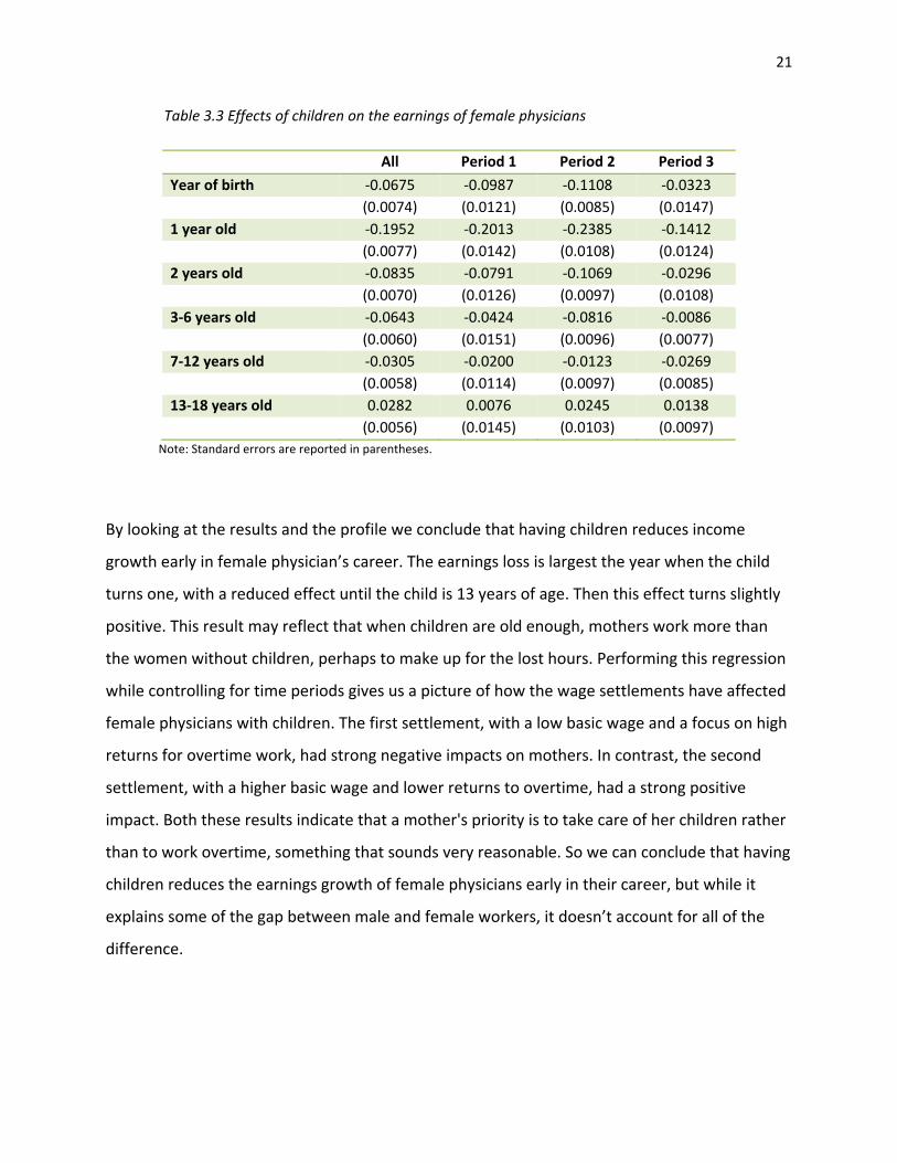
Table 3.3 Effects of children on the earnings of female physicians
All Period 1 Period 2 Period 3
Year of birth ‐0.0675 ‐0.0987 ‐0.1108 ‐0.0323 (0.0074) (0.0121) (0.0085) (0.0147) 1 year old ‐0.1952 ‐0.2013 ‐0.2385 ‐0.1412 (0.0077) (0.0142) (0.0108) (0.0124) 2 years old ‐0.0835 ‐0.0791 ‐0.1069 ‐0.0296 (0.0070) (0.0126) (0.0097) (0.0108) 3‐6 years old ‐0.0643 ‐0.0424 ‐0.0816 ‐0.0086 (0.0060) (0.0151) (0.0096) (0.0077) 7‐12 years old ‐0.0305 ‐0.0200 ‐0.0123 ‐0.0269 (0.0058) (0.0114) (0.0097) (0.0085) 13‐18 years old 0.0282 0.0076 0.0245 0.0138 (0.0056) (0.0145) (0.0103) (0.0097)
Note: Standard errors are reported in parentheses.
By looking at the results and the profile we conclude that having children reduces income
growth early in female physician’s career. The earnings loss is largest the year when the child
turns one, with a reduced effect until the child is 13 years of age. Then this effect turns slightly
positive. This result may reflect that when children are old enough, mothers work more than
the women without children, perhaps to make up for the lost hours. Performing this regression
while controlling for time periods gives us a picture of how the wage settlements have affected
female physicians with children. The first settlement, with a low basic wage and a focus on high
returns for overtime work, had strong negative impacts on mothers. In contrast, the second
settlement, with a higher basic wage and lower returns to overtime, had a strong positive
impact. Both these results indicate that a mother's priority is to take care of her children rather
than to work overtime, something that sounds very reasonable. So we can conclude that having
children reduces the earnings growth of female physicians early in their career, but while it
explains some of the gap between male and female workers, it doesn’t account for all of the
difference.

22
Table 3.4 Share of physicians that are registered as a specialist, by observation year.
Year male Female 1993 0.54 0.29 1994 0.55 0.29 1995 0.59 0.31 1996 0.60 0.33 1997 0.62 0.35 1998 0.64 0.37 1999 0.66 0.39 2000 0.66 0.40 2001 0.66 0.41 2002 0.66 0.41 2003 0.65 0.42 2004 0.65 0.43 2005 0.65 0.44 2006 0.65 0.45
The next topic to address is Gary Becker and Jacob Mincer`s theory of "On‐the‐job‐training".
One of the most obvious ways for a physician to invest in human capital is to specialize. A quick
look at the income data shows that the physicians with a specialization have a considerable
higher average income than those without a specialization. Table 3.4 shows the share of
specialists in each of the income years. As we see there is a larger number of male specialists
than female specialists compared to total amount of physicians. This may lead us to
hypothesize that female physicians undertake fewer "on the job" investments.
As mentioned previously, there may be a connection here between the income gap and hours
worked. Both the children effect and the human capital investment effect may be a signal for
fewer working hours among female physicians. There is also extensive research showing that
female physicians value family life and leisure time higher than their male colleagues (Dagsvik
and Zhiyang, 2006; Blau and Kahn, 2006).
3.5 Difference between Norwegian and foreign education

23
In this section we want to examine the age earning profiles for Norwegian students with and
without a medical degree from Norway. Here we will focus on the male physicians.
Figure 3.5 Predicted age‐earnings profiles by foreign and Norwegian education.
12.8
1313
.213
.413
.613
.8lo
g r
eal e
arni
ngs
30 35 40 45 50 55 60 65age
Norw. men w/Norw. education
Norw. men w/foreign education
We can see from figure 3.5 that there are strong differences in the lifetime earnings between
Norwegian male physicians with a degree from Norway versus those with a degree from
abroad. The physicians have an equal development in the early stages of their careers, probably
because of the strict wage regulation during the intern period and the first years as a doctor,
but beginning approximately at the age of 35 and continuing through their careers the
physicians with Norwegian education have larger growth in income than physicians with foreign
education continuing out their career.
This result prompts many of the same questions as in the study of male and female doctors in
the last section. Are differences because of on‐the‐job investments or a lower wage? Perhaps
studying abroad signals that students with foreign education did not possess the necessary
qualifications or productivity to get into a Norwegian medical education program. It may also

24
be that the medical training programs in Eastern Europe offer lower quality of education,
making it harder for the newly educated physicians to adapt to the Norwegian labor market.
These effects may create a signal of lower productivity to employers making them prefer
students educated in Norway. The third mechanism may be some form of network effect, that
the students with Norwegian education studying at a University hospital develop connections
that give them benefits in their career development. These are hypotheses for the gap in the
profiles, but they are hard to test with the available dataset.
Table 3.6 Share of physicians that are registered as a specialist, by observation year.
Year Norw. education foreign education 1993 0.55 0.51 1994 0.56 0.52 1995 0.60 0.55 1996 0.61 0.57 1997 0.63 0.59 1998 0.65 0.60 1999 0.67 0.61 2000 0.67 0.60 2001 0.68 0.59 2002 0.68 0.58 2003 0.68 0.57 2004 0.68 0.55 2005 0.68 0.55 2006 0.69 0.55
Table 3.6 shows that students with foreign education have a tendency to invest less in human
capital in the form of specialization compared to students with Norwegian education. This
investment gap between the two groups increases over the observation period and may be the
result of an increasing share of students studying abroad. Evaluating the relative merit of the
different mechanisms that could generate the observed differences in earnings profiles of
doctors educated in Norway and abroad may contribute important knowledge about the wage
setting institutions of the physician labor market, and should be a priority for future work.

25
Chapter 4: Conclusion
Our study revealed that the age earning profiles of physicians share many of the attributes
Jacob Mincer discussed in his book “Schooling, experience and earnings”, published in 1974.
Physician earnings rise, but at a decreasing rate, for the first 20 years after medical training and
then even out at approximately age 50. We observe that there will be complications when
using the regular cross‐sectional methods because of the cohort and period effects on earnings,
therefore, using the fixed‐effects method provides a more accurate picture of the profiles.
When looking at profiles in terms of gender we find that there are large differences between
the earnings of male and female physicians, some of which can be attributed to reduced labor
supply during child‐rearing years and some to lower investments in specialization among
female doctors. We also discovered differences in the profiles of physicians educated in Norway
and abroad and discussed the alternative explanations for this pattern.
26
References:
Baker, C. Laurence (1996). Differences in earnings between male and female physicians. New England
Journal of medicine Volume 334:960‐964.
Baltagi, B. H., E. Bratberg and T. H. Holmås (2005). A panel study of physicians’ labor supply: the case of Norway. Health Economics, 14: 1035‐1045.
Becker, Gary (1964). Human Capital. University of Chicago Press.
Biørn, Erik (2003). Økonometriske emner 2.utgave. Unipub forlag.
Biørn, Erik (2008). Økonometriske emner, En videreføring. Unipub forlag
Blau, F.D., and L.W. Kahn (2006). Changes in the Labor Supply Behavior of Married Women: 1980‐2000, IZA DP No. 2180.
Borjas, George J. (1999). Labor Economics. McGraw‐Hill.
Dagsvik, J. and J. Zhiyang (2006). Labour Supply as a Choice among Latent Job Opportunities, Discussion Paper No. 481, Statistics Norway.
Kennedy, Peter (2003). A guide to econometrics. Blackwell.
Legeforeningen (2005), Tidsskrift for den norske legeforeningen Nr 17
(http://www.tidsskriftet.no/?seks_id=1255230)
Legeforeningen (2007). Legemarkedet i Norden 1980‐2000 (http://www.tidsskriftet.no/index.php?seks_id=130304).
Legeforeningen (2008) Historisk legestatistikk 1920‐2008 (http://legeforeningen.no/id/1458).
Lånekassen, Statistikk – stipend og lån. (www.lånekassen.no)
Mincer, Jacob (1974). Schooling, experience and earnings. National Bureau of Economic Research.
OECD (2008). OECD Health Data 2008 ‐ Frequently Requested Data. http://www.oecd.org/document/16/0,3343,en_2649_34631_2085200_1_1_1_37407,00.html
Sloan, Frank A. (1970). Lifetime Earnings and Physicians’ Choice of Specialty. Industrial and labor relations review 24, No. 1:47‐56

27
Sæther, E.M. (2005). Physicians’ Labor Supply: The Wage Impact on Hours and Practice Combinations. Labour , 19(4): 673‐703.
Statistics Norway (2008), Lønn per normalårsverk, 1930‐2008 nominelt og reelt,
http://www.ssb.no/emner/historisk_statistikk/aarbok/ht‐0901‐lonn.html
Statistics Norway (2009), Detaljert variableinformasjon fra inntektsdata,
http://www.ssb.no/mikrodata/datasamling/inntekt/variabler/main/kodelistn

A
Appendix 1
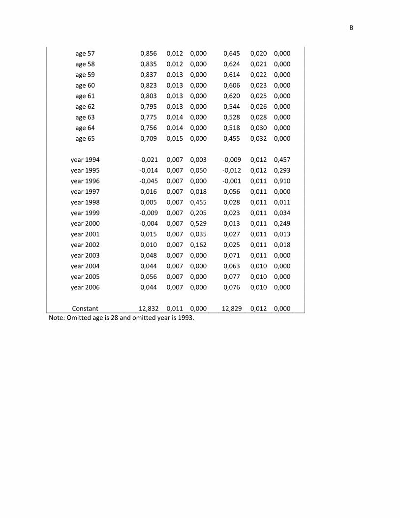
Cross‐sectional regression
male female
Number of obs 117395 53315
Variable Coef. Std. Err. P>|t| Coef. Std. Err. P>|t|
age 29 0,212 0,013 0,000 0,144 0,012 0,000
age 30 0,357 0,013 0,000 0,211 0,012 0,000
age 31 0,429 0,013 0,000 0,265 0,012 0,000
age 32 0,503 0,013 0,000 0,297 0,012 0,000
age 33 0,561 0,013 0,000 0,323 0,013 0,000
age 34 0,605 0,013 0,000 0,335 0,013 0,000
age 35 0,644 0,013 0,000 0,353 0,013 0,000
age 36 0,690 0,013 0,000 0,374 0,013 0,000
age 37 0,726 0,013 0,000 0,406 0,013 0,000
age 38 0,755 0,013 0,000 0,431 0,013 0,000
age 39 0,775 0,012 0,000 0,455 0,013 0,000
age 40 0,797 0,012 0,000 0,467 0,013 0,000
age 41 0,820 0,012 0,000 0,492 0,013 0,000
age 42 0,837 0,012 0,000 0,519 0,014 0,000
age 43 0,846 0,012 0,000 0,543 0,014 0,000
age 44 0,860 0,012 0,000 0,559 0,014 0,000
age 45 0,872 0,012 0,000 0,575 0,014 0,000
age 46 0,882 0,012 0,000 0,598 0,014 0,000
age 47 0,879 0,012 0,000 0,615 0,015 0,000
age 48 0,876 0,012 0,000 0,619 0,015 0,000
age 49 0,886 0,012 0,000 0,626 0,015 0,000
age 50 0,879 0,012 0,000 0,624 0,016 0,000
age 51 0,885 0,012 0,000 0,643 0,016 0,000
age 52 0,881 0,012 0,000 0,646 0,017 0,000
age 53 0,872 0,012 0,000 0,639 0,017 0,000
age 54 0,873 0,012 0,000 0,644 0,018 0,000
age 55 0,871 0,012 0,000 0,646 0,019 0,000
age 56 0,869 0,012 0,000 0,653 0,020 0,000
B
age 57 0,856 0,012 0,000 0,645 0,020 0,000
age 58 0,835 0,012 0,000 0,624 0,021 0,000
age 59 0,837 0,013 0,000 0,614 0,022 0,000
age 60 0,823 0,013 0,000 0,606 0,023 0,000
age 61 0,803 0,013 0,000 0,620 0,025 0,000
age 62 0,795 0,013 0,000 0,544 0,026 0,000
age 63 0,775 0,014 0,000 0,528 0,028 0,000
age 64 0,756 0,014 0,000 0,518 0,030 0,000
age 65 0,709 0,015 0,000 0,455 0,032 0,000
year 1994 ‐0,021 0,007 0,003 ‐0,009 0,012 0,457
year 1995 ‐0,014 0,007 0,050 ‐0,012 0,012 0,293
year 1996 ‐0,045 0,007 0,000 ‐0,001 0,011 0,910
year 1997 0,016 0,007 0,018 0,056 0,011 0,000
year 1998 0,005 0,007 0,455 0,028 0,011 0,011
year 1999 ‐0,009 0,007 0,205 0,023 0,011 0,034
year 2000 ‐0,004 0,007 0,529 0,013 0,011 0,249
year 2001 0,015 0,007 0,035 0,027 0,011 0,013
year 2002 0,010 0,007 0,162 0,025 0,011 0,018
year 2003 0,048 0,007 0,000 0,071 0,011 0,000
year 2004 0,044 0,007 0,000 0,063 0,010 0,000
year 2005 0,056 0,007 0,000 0,077 0,010 0,000
year 2006 0,044 0,007 0,000 0,076 0,010 0,000
Constant 12,832 0,011 0,000 12,829 0,012 0,000 Note: Omitted age is 28 and omitted year is 1993.

C
Appendix 2 Fixed‐effects regressions males Females Number of obs 117395 53315 Variable Coef. Std. Err. P>|t| Coef. Std. Err. P>|t|
age 29 0.260 0.009 0.000 0.176 0.009 0.000 age 30 0.435 0.009 0.000 0.277 0.009 0.000 age 31 0.536 0.009 0.000 0.347 0.009 0.000 age 32 0.622 0.010 0.000 0.388 0.010 0.000 age 33 0.690 0.010 0.000 0.418 0.010 0.000 age 34 0.739 0.010 0.000 0.439 0.010 0.000 age 35 0.783 0.010 0.000 0.465 0.010 0.000 age 36 0.829 0.010 0.000 0.486 0.010 0.000 age 37 0.869 0.010 0.000 0.523 0.010 0.000 age 38 0.896 0.010 0.000 0.550 0.011 0.000 age 39 0.913 0.010 0.000 0.579 0.011 0.000 age 40 0.939 0.010 0.000 0.597 0.011 0.000 age 41 0.965 0.010 0.000 0.629 0.011 0.000 age 42 0.985 0.010 0.000 0.667 0.011 0.000 age 43 1.000 0.010 0.000 0.698 0.012 0.000 age 44 1.019 0.010 0.000 0.725 0.012 0.000 age 45 1.033 0.010 0.000 0.750 0.012 0.000 age 46 1.050 0.010 0.000 0.781 0.012 0.000 age 47 1.053 0.010 0.000 0.807 0.013 0.000 age 48 1.059 0.010 0.000 0.813 0.013 0.000 age 49 1.072 0.010 0.000 0.826 0.014 0.000 age 50 1.071 0.010 0.000 0.833 0.014 0.000 age 51 1.082 0.011 0.000 0.849 0.014 0.000 age 52 1.084 0.011 0.000 0.864 0.015 0.000 age 53 1.084 0.011 0.000 0.869 0.015 0.000 age 54 1.089 0.011 0.000 0.874 0.016 0.000 age 55 1.094 0.011 0.000 0.889 0.017 0.000 age 56 1.097 0.011 0.000 0.897 0.017 0.000 age 57 1.089 0.011 0.000 0.896 0.018 0.000 age 58 1.077 0.011 0.000 0.886 0.019 0.000 age 59 1.085 0.012 0.000 0.876 0.019 0.000 age 60 1.072 0.012 0.000 0.863 0.020 0.000

D
age 61 1.051 0.012 0.000 0.868 0.022 0.000 age 62 1.040 0.012 0.000 0.805 0.023 0.000 age 63 1.016 0.013 0.000 0.781 0.024 0.000 age 64 0.997 0.013 0.000 0.770 0.026 0.000 age 65 0.946 0.014 0.000 0.706 0.029 0.000 Constant 12.668 0.009 0.000 12.730 0.008 0.000

E
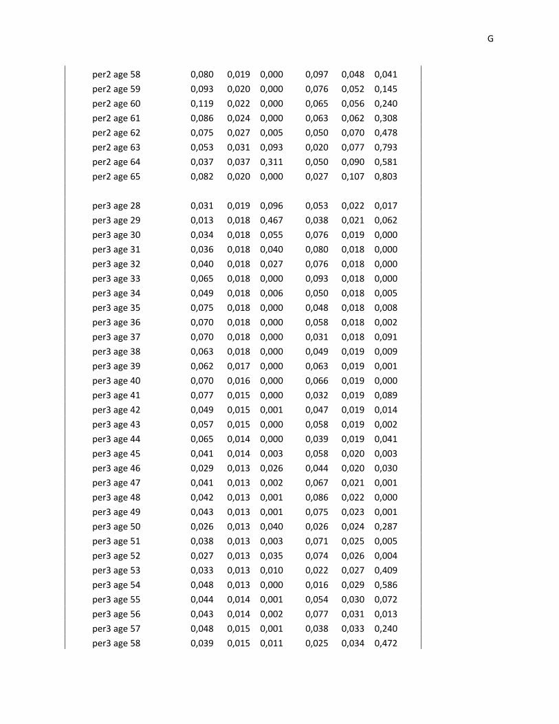
Appendix 3
Fixed‐effects regressions
with periods
males females
Number of obs 117395 53315
Variable Coef. Std. Err. P>|t| Coef. Std. Err. P>|t|
age 29 0,183 0,020 0,000 0,097 0,019 0,000
age 30 0,326 0,020 0,000 0,152 0,020 0,000
age 31 0,402 0,020 0,000 0,209 0,020 0,000
age 32 0,449 0,020 0,000 0,227 0,021 0,000
age 33 0,525 0,020 0,000 0,238 0,021 0,000
age 34 0,554 0,021 0,000 0,237 0,022 0,000
age 35 0,605 0,021 0,000 0,272 0,022 0,000
age 36 0,640 0,021 0,000 0,281 0,023 0,000
age 37 0,676 0,021 0,000 0,293 0,024 0,000
age 38 0,702 0,021 0,000 0,312 0,024 0,000
age 39 0,704 0,021 0,000 0,356 0,025 0,000
age 40 0,721 0,022 0,000 0,330 0,026 0,000
age 41 0,743 0,022 0,000 0,381 0,027 0,000
age 42 0,760 0,022 0,000 0,422 0,028 0,000
age 43 0,768 0,022 0,000 0,444 0,029 0,000
age 44 0,787 0,022 0,000 0,470 0,030 0,000
age 45 0,804 0,023 0,000 0,485 0,031 0,000
age 46 0,801 0,023 0,000 0,527 0,032 0,000
age 47 0,793 0,023 0,000 0,539 0,034 0,000
age 48 0,788 0,023 0,000 0,530 0,035 0,000
age 49 0,779 0,024 0,000 0,515 0,036 0,000
age 50 0,787 0,024 0,000 0,504 0,038 0,000
age 51 0,778 0,024 0,000 0,476 0,039 0,000
age 52 0,772 0,025 0,000 0,522 0,041 0,000
age 53 0,751 0,026 0,000 0,534 0,043 0,000
age 54 0,773 0,026 0,000 0,539 0,045 0,000
age 55 0,775 0,027 0,000 0,542 0,048 0,000
age 56 0,759 0,027 0,000 0,511 0,050 0,000

F
age 57 0,741 0,028 0,000 0,488 0,053 0,000
age 58 0,723 0,028 0,000 0,466 0,056 0,000
age 59 0,692 0,029 0,000 0,457 0,060 0,000
age 60 0,661 0,030 0,000 0,426 0,064 0,000
age 61 0,611 0,032 0,000 0,411 0,070 0,000
age 62 0,611 0,034 0,000 0,380 0,078 0,000
age 63 0,582 0,036 0,000 0,386 0,085 0,000
age 64 0,562 0,040 0,000 0,292 0,098 0,003
age 65 0,104 0,020 0,000 0,307 0,116 0,008
per2 age 28 0,030 0,019 0,124 0,098 0,020 0,000
per2 age 29 0,024 0,019 0,200 0,005 0,019 0,791
per2 age 30 0,057 0,019 0,002 0,038 0,019 0,042
per2 age 31 0,092 0,018 0,000 0,043 0,019 0,024
per2 age 32 0,070 0,018 0,000 0,062 0,019 0,001
per2 age 33 0,087 0,017 0,000 0,068 0,019 0,000
per2 age 34 0,052 0,017 0,002 0,101 0,019 0,000
per2 age 35 0,064 0,016 0,000 0,077 0,019 0,000
per2 age 36 0,044 0,015 0,005 0,076 0,019 0,000
per2 age 37 0,035 0,015 0,017 0,107 0,019 0,000
per2 age 38 0,045 0,014 0,002 0,094 0,019 0,000
per2 age 39 0,046 0,014 0,001 0,055 0,020 0,006
per2 age 40 0,038 0,014 0,005 0,096 0,020 0,000
per2 age 41 0,027 0,013 0,045 0,071 0,021 0,001
per2 age 42 0,023 0,013 0,075 0,045 0,022 0,038
per2 age 43 0,022 0,013 0,091 0,041 0,023 0,072
per2 age 44 0,004 0,013 0,731 0,037 0,024 0,118
per2 age 45 0,021 0,013 0,093 0,031 0,025 0,223
per2 age 46 0,034 0,013 0,007 0,012 0,026 0,656
per2 age 47 0,044 0,013 0,001 0,007 0,027 0,796
per2 age 48 0,060 0,013 0,000 0,006 0,028 0,839
per2 age 49 0,038 0,013 0,003 0,035 0,029 0,233
per2 age 50 0,055 0,013 0,000 0,071 0,031 0,020
per2 age 51 0,062 0,014 0,000 0,091 0,032 0,005
per2 age 52 0,074 0,015 0,000 0,042 0,034 0,215
per2 age 53 0,048 0,015 0,002 0,051 0,036 0,152
per2 age 54 0,041 0,016 0,011 0,045 0,038 0,235
per2 age 55 0,048 0,016 0,003 0,031 0,040 0,441
per2 age 56 0,051 0,017 0,003 0,054 0,042 0,203
per2 age 57 0,047 0,018 0,009 0,088 0,045 0,050
G
per2 age 58 0,080 0,019 0,000 0,097 0,048 0,041
per2 age 59 0,093 0,020 0,000 0,076 0,052 0,145
per2 age 60 0,119 0,022 0,000 0,065 0,056 0,240
per2 age 61 0,086 0,024 0,000 0,063 0,062 0,308
per2 age 62 0,075 0,027 0,005 0,050 0,070 0,478
per2 age 63 0,053 0,031 0,093 0,020 0,077 0,793
per2 age 64 0,037 0,037 0,311 0,050 0,090 0,581
per2 age 65 0,082 0,020 0,000 0,027 0,107 0,803
per3 age 28 0,031 0,019 0,096 0,053 0,022 0,017
per3 age 29 0,013 0,018 0,467 0,038 0,021 0,062
per3 age 30 0,034 0,018 0,055 0,076 0,019 0,000
per3 age 31 0,036 0,018 0,040 0,080 0,018 0,000
per3 age 32 0,040 0,018 0,027 0,076 0,018 0,000
per3 age 33 0,065 0,018 0,000 0,093 0,018 0,000
per3 age 34 0,049 0,018 0,006 0,050 0,018 0,005
per3 age 35 0,075 0,018 0,000 0,048 0,018 0,008
per3 age 36 0,070 0,018 0,000 0,058 0,018 0,002
per3 age 37 0,070 0,018 0,000 0,031 0,018 0,091
per3 age 38 0,063 0,018 0,000 0,049 0,019 0,009
per3 age 39 0,062 0,017 0,000 0,063 0,019 0,001
per3 age 40 0,070 0,016 0,000 0,066 0,019 0,000
per3 age 41 0,077 0,015 0,000 0,032 0,019 0,089
per3 age 42 0,049 0,015 0,001 0,047 0,019 0,014
per3 age 43 0,057 0,015 0,000 0,058 0,019 0,002
per3 age 44 0,065 0,014 0,000 0,039 0,019 0,041
per3 age 45 0,041 0,014 0,003 0,058 0,020 0,003
per3 age 46 0,029 0,013 0,026 0,044 0,020 0,030
per3 age 47 0,041 0,013 0,002 0,067 0,021 0,001
per3 age 48 0,042 0,013 0,001 0,086 0,022 0,000
per3 age 49 0,043 0,013 0,001 0,075 0,023 0,001
per3 age 50 0,026 0,013 0,040 0,026 0,024 0,287
per3 age 51 0,038 0,013 0,003 0,071 0,025 0,005
per3 age 52 0,027 0,013 0,035 0,074 0,026 0,004
per3 age 53 0,033 0,013 0,010 0,022 0,027 0,409
per3 age 54 0,048 0,013 0,000 0,016 0,029 0,586
per3 age 55 0,044 0,014 0,001 0,054 0,030 0,072
per3 age 56 0,043 0,014 0,002 0,077 0,031 0,013
per3 age 57 0,048 0,015 0,001 0,038 0,033 0,240
per3 age 58 0,039 0,015 0,011 0,025 0,034 0,472

H
per3 age 59 0,033 0,016 0,042 0,042 0,036 0,244
per3 age 60 0,047 0,017 0,005 0,077 0,038 0,042
per3 age 61 0,061 0,018 0,001 0,098 0,041 0,017
per3 age 62 0,081 0,019 0,000 0,035 0,044 0,419
per3 age 63 0,099 0,020 0,000 0,082 0,048 0,086
per3 age 64 12,886 0,018 0,000 0,115 0,052 0,026
per3 age 65 0,099 0,013 0,000 0,061 0,057 0,284
Constant 12,886 0,029 0,000 12,900 0,017 0,000

I
Appendix 4 Fixed‐effects regressions, Norwegian vs. foreign education
Norwegian education
Foreign education
Number of obs 92561 24834
Variable Coef. Std. Err. P>|t| Coef.
Std. Err. P>|t|
age 29 0.276 0.010 0.000 0.200 0.020 0.000 age 30 0.452 0.010 0.000 0.368 0.021 0.000 age 31 0.559 0.011 0.000 0.443 0.021 0.000 age 32 0.641 0.011 0.000 0.545 0.022 0.000 age 33 0.714 0.011 0.000 0.590 0.022 0.000 age 34 0.760 0.011 0.000 0.648 0.023 0.000 age 35 0.806 0.011 0.000 0.684 0.024 0.000 age 36 0.854 0.011 0.000 0.718 0.024 0.000 age 37 0.893 0.011 0.000 0.759 0.025 0.000 age 38 0.925 0.011 0.000 0.763 0.025 0.000 age 39 0.943 0.011 0.000 0.773 0.025 0.000 age 40 0.967 0.011 0.000 0.809 0.025 0.000 age 41 0.992 0.011 0.000 0.843 0.025 0.000 age 42 1.012 0.011 0.000 0.863 0.025 0.000 age 43 1.030 0.011 0.000 0.862 0.025 0.000 age 44 1.052 0.011 0.000 0.864 0.025 0.000 age 45 1.065 0.011 0.000 0.886 0.025 0.000 age 46 1.086 0.011 0.000 0.885 0.025 0.000 age 47 1.088 0.011 0.000 0.890 0.025 0.000 age 48 1.096 0.011 0.000 0.888 0.025 0.000 age 49 1.109 0.012 0.000 0.900 0.025 0.000 age 50 1.108 0.012 0.000 0.903 0.025 0.000 age 51 1.118 0.012 0.000 0.916 0.025 0.000 age 52 1.123 0.012 0.000 0.908 0.025 0.000 age 53 1.122 0.012 0.000 0.912 0.025 0.000 age 54 1.128 0.012 0.000 0.914 0.025 0.000 age 55 1.133 0.012 0.000 0.921 0.025 0.000 age 56 1.136 0.012 0.000 0.921 0.026 0.000

J
age 57 1.132 0.013 0.000 0.905 0.026 0.000 age 58 1.119 0.013 0.000 0.895 0.026 0.000 age 59 1.129 0.013 0.000 0.899 0.026 0.000 age 60 1.115 0.013 0.000 0.889 0.027 0.000 age 61 1.090 0.013 0.000 0.880 0.028 0.000 age 62 1.082 0.014 0.000 0.856 0.029 0.000 age 63 1.053 0.014 0.000 0.856 0.030 0.000 age 64 1.033 0.014 0.000 0.843 0.032 0.000 age 65 0.986 0.015 0.000 0.774 0.035 0.000 Constant 12.655 0.010 0.000 12.744 0.021 0.000