Wealth inequality: data and models∗

Marco CagettiUniversity of Virginia

Mariacristina De NardiUniversity of Minnesota and Federal Reserve Bank of Minneapolis

Abstract

In the United States wealth is highly concentrated and very un-equally distributed: the richest 1% hold one third of the total wealth inthe economy. Understanding the determinants of wealth inequality isa challenge for many economic models. We summarize some key factsabout the wealth distribution and what economic models have been ableto explain so far.

∗We gratefully acknowledge financial support from NSF grants (respectively) SES-0318014 and SES-0317872. We are grateful to Marco Bassetto for helpful comments. Theviews expressed herein are those of the authors and not necessarily those of the FederalReserve Bank of Minneapolis, the Federal Reserve System, or the NSF.

1 Introduction

In the United States wealth is highly concentrated and very unequally dis-

tributed: the richest 1% of the households owns one third of the total wealth

in the economy. Understanding the determinants of wealth inequality is a chal-

lenge for many economic models. In this paper, we summarize what is known

about the wealth distribution and what economic models have been able to

explain so far.

The development of various data sets in the past 30 years (in particular

the Survey of Consumer Finances) has allowed economists to quantify more

precisely the degree of wealth concentration in the United States. The picture

that emerged from the different waves of these surveys confirmed the fact that

a large fraction of the total wealth in the economy is concentrated in the hand

of the richest percentiles: the top 1% hold one third, and the richest 5% hold

more than half of total wealth. At the other extreme, a significant fraction of

the population holds little or no wealth at all.

Income is also unequally distributed, and a large body of work has studied

earnings and wage inequality. Income inequality leads to wealth inequality as

well, but income is much less concentrated than wealth, and economic mod-

els have had difficulties in quantitatively generating the observed degree of

wealth concentration from the observed income inequality. The question is

what mechanisms are necessary to generate saving behavior that leads to a

distribution of asset holdings consistent with the actual data.

In this work, we describe the main framework for studying wealth in-

equality, that of general equilibrium models with heterogeneous agents, in

which some elements of a life-cycle structure and of intergenerational links are

present. Some models consider a dynasty as a single, infinitely-lived agent,

1

while others consider more explicitly the life-cycle aspect of the saving deci-

sion. Baseline versions of these models are unable to replicate the observed

wealth concentration. More recently, however, some works have shown that

certain ingredients are necessary, and sometimes enable the model to replicate

the data. Bequests are a key determinants of inequality, and careful mod-

elling of bequests is vital to understand wealth concentration. In addition,

entrepreneurs constitute a large fraction of the very rich, and models that ex-

plicitly consider the entrepreneurial saving decision succeed in dramatically

increasing wealth dispersion. The type of earnings risk faced by the richest is

also a potential explanation worth investigating.

Considerable work must still be done to better understand the quantitative

importance of each factor in determining wealth inequality and to understand

which models are most useful and computationally convenient to study it. The

recent advances in modelling have however already helped in providing a more

precise picture. The challenge now is improve these models even further and

to apply them to the study of several problems for which inequality is a key

determinant. For instance, the effects of several tax policies (in particular the

estate tax) might depend crucially on how wealth is concentrated in the hands

of the richest percentiles of the distribution. In the last section of this paper,

we will highlight some of the areas in which models of inequality could and

should be profitably employed and extended.

2 Data

We first summarize the main facts about the wealth distribution in the United

States, facts provided mainly by the Survey of Consumer Finances. We will

also mention some facts about the historical trends, although in this paper we

2

will not focus on understanding them (an area on which little work has been

done).

2.1 Data sources

The main source of microeconomic data on wealth for the U.S. is the Survey

of Consumer Finances (SCF)1 which, starting from 1983, every three years

collects detailed information about wealth for a cross-section of households.

It also includes a limited panel (between 1983 and 1989), as well as a link

to two previous smaller surveys (1962 Survey of Financial Characteristics of

Consumers and the 1963 Survey of Changes in Family Finances).

The SCF was explicitly designed to measure the balance sheet of house-

holds and the distribution of wealth. It has a large number of detailed questions

about different assets and liabilities, which allows highly disaggregated data

analysis on each component of the total net worth of the household. More

importantly, the SCF oversamples rich households by including, in addition to

a national area probability sample (representing the entire population), a list

sample drawn from tax records (to extract a list of high income households).

Oversampling is especially important given the high degree of wealth concen-

tration (see Davies and Shorrocks [24]) observed in the data. For this reason,

the SCF is able to provide a more accurate measure of wealth inequality and

of total wealth holdings: Curtin et al. [22] and Antoniewicz [5] document that

the total net worth implied by the SCF matches quite well the total wealth

implied by the (aggregate) Flow of Funds Accounts (although not perfectly,

especially when disaggregating the various components).

1The survey is publicly available from the Federal Reserve Board website athttp://www.federalreserve.gov/pubs/oss/oss2/scfindex.html.

3

Unfortunately, the SCF does not follow households over time, unlike the

Panel Study of Income Dynamics (PSID). The PSID2 is a longitudinal study,

which begun in 1968, and follows families and individuals over time. It focuses

on income and demographic variables, but since 1984 it has also included (every

5 years) a supplement with questions on wealth. The PSID includes a national

sample of low-income families, but it does not oversample the rich. As a result,

this data set is unable to describe appropriately the right tail of the wealth

distribution: Curtin et al. [22] show that the PSID tracks the distribution of

total household net worth implied by the SCF only up to the top 2%-3% of

richest household, but misses much of the wealth holdings of the top richest.

Given that the richest 5% hold more than half of the total net worth in the

U.S., this is an important shortcoming.

Another important data source is the Health and Retirement Study (HRS),

which recently absorbed the Study of Assets and Health Dynamics Among the

Oldest Old (AHEAD). This survey focuses on the older households (from before

retirement and on), and provides a large amount of information regarding their

economic and health condition. However, as the PSID, this survey misses the

richest households.

Other data sets also contain some information on wealth and asset hold-

ings (in particular, the U.S. Bureau of Census’s Survey of Income and Program

Participation, or, for the very richest, the data on the richest 400 people iden-

tified by the Forbes magazine). However, because of its careful sample choice,

the SCF remains the main source of information about the distribution of

wealth in the U.S. Due to their demographic and health data, the PSID and

the HRS provide additional information for studying the wealth holdings of

2See http://psidonline.isr.umich.edu/.

4

Percentile Yeargroup 1989 1992 1995 1998 20010-49.9 2.7 3.3 3.6 3.0 2.850-89.9 29.9 29.7 28.6 28.4 27.490-94.9 13.0 12.6 11.9 11.4 12.195-98.9 24.1 24.4 21.3 23.3 25.099-100 30.3 30.2 34.6 33.9 32.7

Table 1: Percent of net worth held by various groups defined in terms ofpercentiles of the wealth distribution (taken from Kennickell [44], p. 9).

most households (except the richest), and above all for certain groups, such as

the low-income families and the old.

2.2 Wealth concentration in the U.S.

The most striking aspect of the wealth distribution in the U.S. is its degree

of concentration. Table 1 shows that the households in the top 1% of the

wealth distribution hold around one third of the total wealth in the economy,

and those in the top 5% hold more than half. At the other extreme, many

households (more than 10%) have little or no assets at all.

The data in Table 1 and 2 refer to total net worth. There are many possible

measures of wealth, the most appropriate one depending on the problem ob-

ject of study. Net worth includes all assets held by the households (real estate,

financial wealth, vehicles) net of all liabilities (mortgages and other debts); it

is thus a comprehensive measure of most marketable wealth. This measure

thus includes the value of most defined contribution plans (such as IRAs), but

excludes the implied values of defined benefit plans and social security. Defined

contribution plans can of course be important sources of income after retire-

5

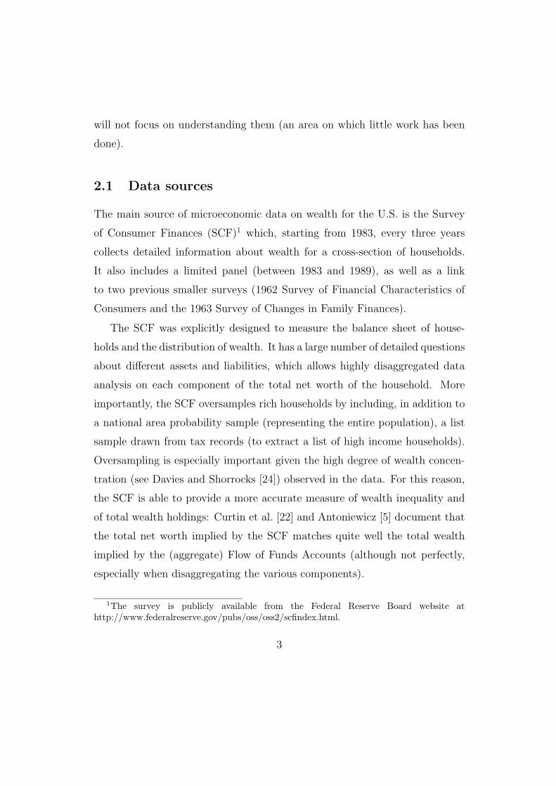
Net Yearworth 1989 1992 1995 1998 2001< $0 7.3 7.2 7.1 8.0 6.9$0-$1,000 8.0 6.3 5.2 5.8 5.4$1,000-$5,000 12.7 14.4 15.0 13.1 12.8$25,000-$100,000 23.2 25.4 26.4 22.9 22.0$100,000-$250,000 20.2 21.6 22.1 22.6 19.2$250,000-$500,000 11.0 9.3 9.3 12.0 13.0$500,000-$1,000,000 5.4 4.6 5.1 6.0 7.8≥ $1,000,000 4.7 3.8 3.6 4.9 7.0

Table 2: Percent distribution of household net worth over wealth groups, 2001dollars(taken from Kennickell [44], p. 9).

ment; but their measure is problematic because their value has to be imputed.

To study other questions it may be useful to look at more restricted measures

of wealth, that for example exclude less liquid assets (such as housing), and

focus on financial wealth instead. Throughout this paper, we focus on net

worth.3

The key facts about the distribution of wealth have been highlighted in

a large number of studies, among others Wolff [72], [71], and Kennickell [44].

Wealth is extremely concentrated, and much more so than earnings and in-

come, as shown by Dıaz-Gimenez et al. [27] and Budria et al. [63]. For instance,

in 1992 the Gini index for labor earnings, income (inclusive of transfers) and

wealth were respectively .63, .57, and .78 (Dıaz-Gimenez et al. [27]), while in

1995 they were .61, .55 and .80 (Budria et al. [63]). These two studies also

3It must be noted that the exact definition of net worth varies across studies. Therefore,the numbers we cite below when referring to other works are not directly comparable, asthey may include different sets of assets. However, the general picture of a highly skeweddistribution and the main trends are unchanged and do not depend on the exact measureof wealth.

6

Top % 1 5 10 20Whole populationpercentage of total net worth held 30 54 67 81Entrepreneurspercentage of households in a given percentile 63 49 39 28percentage of net worth held in a given percentile 68 58 53 47

Table 3: Entrepreneurs and the distribution of wealth. SCF 1989.

report that the correlation between these three variables is positive, but far

from perfect.

There is also significant wealth inequality within various age and demo-

graphic groups. For instance, Venti and Wise [68] and Bernheim at al. [8]

show that wealth is highly dispersed at retirement even for people with similar

lifetime incomes, and argue that this differences cannot be explained only by

events such as family status, health and inheritances, nor by portfolio choice.

Several studies have also highlighted the differences in wealth holdings

across different groups. There is a very large inequality in wealth holdings by

race (see for example Altonji and Doraszelski [2] and Smith [65]). Wolff [72]

documents that, in the 1980s and 1990s, the ratio of average net worth of

blacks and whites was around 17% to 19%, and the ratio of median wealth

varied, depending on the year, across much lower values, in the range of 3%

to 17%. Unfortunately, relatively little work has been done to understand

quantitatively the sources of this persistent difference across race groups. (See

White [69] for a study of how much of current black-white income and wealth

inequality can be explained by initial conditions at Emancipation.)

A large difference in wealth holdings is also between entrepreneurs and non-

entrepreneurs, as shown in Table 3 (taken from Cagetti and De Nardi [16]).

7

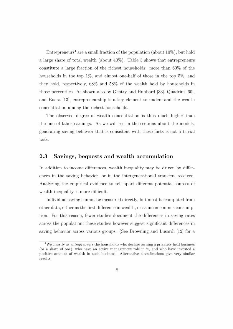
Entrepreneurs4 are a small fraction of the population (about 10%), but hold

a large share of total wealth (about 40%). Table 3 shows that entrepreneurs

constitute a large fraction of the richest households: more than 60% of the

households in the top 1%, and almost one-half of those in the top 5%, and

they hold, respectively, 68% and 58% of the wealth held by households in

those percentiles. As shown also by Gentry and Hubbard [33], Quadrini [60],

and Buera [13], entrepreneurship is a key element to understand the wealth

concentration among the richest households.

The observed degree of wealth concentration is thus much higher than

the one of labor earnings. As we will see in the sections about the models,

generating saving behavior that is consistent with these facts is not a trivial

task.

2.3 Savings, bequests and wealth accumulation

In addition to income differences, wealth inequality may be driven by differ-

ences in the saving behavior, or in the intergenerational transfers received.

Analyzing the empirical evidence to tell apart different potential sources of

wealth inequality is more difficult.

Individual saving cannot be measured directly, but must be computed from

other data, either as the first difference in wealth, or as income minus consump-

tion. For this reason, fewer studies document the differences in saving rates

across the population; these studies however suggest significant differences in

saving behavior across various groups. (See Browning and Lusardi [12] for a

4We classify as entrepreneurs the households who declare owning a privately held business(or a share of one), who have an active management role in it, and who have invested apositive amount of wealth in such business. Alternative classifications give very similarresults.

8

review of the literature.) In particular, Dynan et al. [28] show that higher-

lifetime income households save a larger fraction of their income than lower-

income households. Quadrini [60] documents that entrepreneurs, who tend to

be among the richest households, also exhibit higher saving rates.

Bequests also play an important role in shaping wealth inequality. Kotlikoff

and Summers [45] were the first to argue that life-cycle savings for retirement

account for a small fraction of total capital accumulation, while intergenera-

tional transmission of wealth accounts for the vast majority of capital forma-

tion (with a baseline estimate of around 80% of the total). Further studies have

confirmed the importance of intergenerational transfers; for instance, Gale and

Scholz [32] find that bequests account for about 30% of total wealth accumula-

tion, and various other types of intended inter-vivos transfers for an additional

20%.

It is more difficult to measure the size of intended bequests relative to that

of purely accidental ones, due to uncertainty about the life-span. Hurd [42]

estimates a very low marginal utility from leaving bequests. Altonji and Vil-

lanueva [3] also find relatively small values for the elasticity of bequests to

permanent income, although they do show that this number increases with

life-time resources. Most of the bequests, however, are concentrated among

the top percentiles, a group that these papers ignore. Looking at a sample

of TIAA retirees (whose average wealth is higher than in the other groups),

Laitner and Juster [50] find that about half of the households in their sam-

ple plan to leave estate and that the amount of wealth attributable to estate

building is significant, accounting for half or more of the total for those who

plan to leave bequests. While more empirical research is needed in the area,

it appears that intergenerational altruism and intended bequests are a crucial

element to understand the distribution of wealth, above all for the very rich.

9

2.4 Trends in wealth inequality

It is quite difficult to measure wealth inequality before the second half of the

twentieth century. Some limited data exists (Census surveys in the nineteenth

century and other records of estates), but their the interpretation is still de-

bated. Some argue that inequality has always been high and has changed little

from the end of the eighteenth century to the first decades of the twentieth

(for example, Soltow [66]), while others argue for a sharp increase in inequality

over the period (among others, Lindert [53]). It is however interesting to note

that wealth inequality has always been substantial, and, even according to

Lindert [53], by 1860 the richest 1% held approximately 30% of total wealth,

an amount that remained more or less stable until the 1920’s.

There is evidence that wealth inequality decreased significantly between

the 1920 and the 1970s (Davies and Shorrocks [24], Wolff and Marley [73]).

Wolff [71], for instance, documents that the share of total wealth held by

the top 1% of individuals fell from 38% in 1922 to 19% in 1976. After that,

however, wealth inequality has risen again to levels similar to those observed

in earlier periods.

Wolff [70] argues that while wealth inequality fell during the 1970s, it rose

sharply after 1979, with a dramatic increase over the 1980s, and then levelled

off in the 1990s. For instance, the share of net worth of the richest 1% increased

from 34% in 1983, to 37% in 1989 (see Wolff [72]), while there does not seem

to be a clear trend after 1989 (Kennickell [44]).

Because of the purely cross-sectional nature of the SCF, it is difficult to

characterize the mobility of households across the wealth distribution. Using

PSID data, Hurst et al. [43] analyze the wealth dynamics between 1984 and

1994, for different socio-economic groups and for different types of asset hold-

10

ings, pointing out that most of the mobility occurs in the midrange deciles,

while the top and bottom ones show high persistence. Unfortunately, the

PSID does not allow to study what happens at the top percentile. Using the

same dataset, Quadrini [60] studies the wealth mobility for entrepreneurs and

non-entrepreneurs, showing that entrepreneurs are more upwardly mobile.

3 Models

In the following sections, we will describe the main class of models used to study

wealth concentration. Most of these models are general-equilibrium, quanti-

tative models with heterogeneous agents. We will distinguish these works

into three sub-categories: models with infinitely-lived dynasties, models with

overlapping-generations (OLG), and models that mix both of these features.

The first type of models ignore the life-cycle structure, but consider each

dynasty as a single agent who lives forever. The second type explicitly intro-

duces an age and life-cycle structure, with various degrees of intergenerational

transmission of wealth and abilities. The third type relaxes the infinitely-

lived dynasty assumption of the first type of models, but greatly simplifies the

life-cycle structure.

Almost all the current general equilibrium, quantitative models of wealth

inequality are versions of Bewley models5. These are incomplete-markets mod-

els in which households are ex-ante identical6, in the sense that they face the

same stochastic labor earnings and ability processes, but are ex-post heteroge-

5See Ljungqvist and Sargent [55] for an exposition of the properties of these models andof their numerical solution.

6See Quadrini and Rıos-Rull [62] for a discussion about why we need incomplete marketmodels to study wealth inequality.

11

neous because they receive different realizations of such shocks. These models

are typically solved for stationary equilibria in which, over time, there is a

constant distribution of people over the relevant state variables for the econ-

omy, but people move around in the distribution, and thus face considerable

uncertainty. These models endogenously generate differences in asset holdings

and hence a given amount of wealth concentration, as a result of the house-

hold’s desire to save and the realization of the shocks. An exogenous earnings

process is typically the source of these shocks, and its properties are generally

estimated from the data

3.1 Earlier contributions

Before moving to the analysis of these models, it is worth mentioning some of

the earlier contributions to understanding wealth inequality.

Many models were developed to study life-cycle and savings decisions.

The most important to understand intergenerational linkages is Becker and

Tomes [7]. Becker and Tomes were the first to model explicitly the parental

decision problem, and to characterize the structure of transfers across genera-

tions, in the form of both human capital and bequests. They showed that in

the presence of constraints, parental transfers are first in the form of human

capital, and only after the optimal amount of human capital has been reached

they do take the form of monetary transfers such as bequests. Bequests are

thus a luxury good in this framework.

A few papers also tried to develop quantitative implications. Among the

earlier, partial equilibrium literature, Davies [23] studies the effects of vari-

ous factors, including bequests, on economic inequality in a one-period model

without uncertainty. In his setup one generation of parents cares about their

12

children’s future consumption, and there is regression to the mean between

parents and children’s earnings. As a consequence, the income elasticity of

bequests is high and inherited wealth is a major cause of wealth inequality.

Laitner [48] adopted a partial equilibrium model with two sided altruism

among generations, constraints on net worth being non negative, and random

lifetime earnings. He showed that in this setup intergenerational transfers are

a luxury good and that liquidity constraints are less binding for generations

receiving larger transfers. He also discusses how this economy can generate

realistic capital to output ratios. He does not explore the implications of

his model for wealth inequality and abstracts from lifetime uncertainty and

earnings uncertainty over the life cycle.

4 Infinitely-lived dynasty models

4.1 A general framework

Let us consider the simplest version of a Bewley model with infinitely-lived

agents. There is a continuum of agents. All agents have identical preferences,

and have the following utility function when they first enter the model econ-

omy:

E

{ ∞∑t=1

βtu(ct)

},

where u(ct) is the constant relative-risk aversion flow of utility from consump-

tion. The labor endowment of each household is given by an idiosyncratic

labor productivity shock z that assumes a finite number of possible values and

follows a first order Markov process with transition matrix (Γ(z)). There is

only one asset, a, that people can use to self-insure against earnings risk.

13

A constant returns to scale production technology converts aggregate cap-

ital (K) and aggregate labor (L) into aggregate output (Y ).

During each period each household chooses how much to consume (c) and

save for next period by holding risk free assets (a′). The household’s state

variables are denoted by x = (a, z), where a is asset holdings carried into the

period and z is the labor shock endowment.

The household’s recursive problem can thus be written as

V (x) = max(c,a′)

{u(c) + βE

[V (a′, z′)|x

]}

subject to

c + a′ = (1 + r)a + zw

c ≥ 0, a′ ≥ a

where r is the interest rate net of taxes and depreciation, w is the wage, and

a is a net borrowing limit7. For simplicity, we have not explicitly introduce

taxes and government policies, but of course the setup can easily accomodate

various types of taxes and transfers.

At every point in time this model economy can be described by a probability

distribution of people over assets a and earnings shocks z.

A stationary equilibrium for this economy is a set of consumption and

saving rules, prices, aggregate capital and labor, and invariant distribution of

households over the state variables of the system such that:

1. Given prices, the decision rules solve the household’s recursive problem

7See Bewley [10], Aiyagari [1], Huggett [40] and Ljungqvist and Sargent [55] for moreexhausting descriptions of this framework and its equilibrium.

14

described above.

2. Aggregate capital is equal to total savings of all of the households of the

economy, while aggregate labor is equal to total labor supplied by all of

the households of the economy.

3. Prices, that is the interest rate and the wage rate, gross of taxes, equal

the marginal product of capital, net of depreciation, and the marginal

product of labor.

4. The constant distribution of people is the one induced by the law of

motion of the system, which is determined by the exogenous earnings

shocks and by the endogenous policy functions of the households.

4.2 Results

Quadrini and Rıos-Rull [62] nicely summarize the results obtained from this

type of models until 1997 with the first three lines of Table 4.

% wealth in topGini 1% 5% 20%U.S. data.78 29 53 80Baseline Aiyagari.38 3.2 12.2 41.0High variability Aiyagari.41 4.0 15.6 44.6Quadrini: entrepreneurs.74 24.9 45.8 73.2

Table 4: Dynasty models of wealth inequality.

15

Most of the models in Table 4 display significantly less wealth concentration

than in the data. The reasons why households save in this type of models is to

create a buffer stock of assets to self-insure against earnings fluctuations. Once

such buffer stock is reached, the agents don’t save any more, and the model is

thus not capable to explain why the rich people keep saving at very high rates.

Given that that this is the key reason to save, what matters in generating

wealth dispersion is temporary differences in earnings, not permanent ones.

Line two and three of the table compares two identical economies, other than

the fact that the second one displays much higher earnings variability than

the first one (and thus higher cross-sectional earnings inequality) and show

that second economy does generate a slightly more concentrated distribution

of wealth.

Given the key reason to save in this framework, introducing ex-ante hetero-

geneity such as classes of people with different skills or education levels does

not help in generating more concentration of wealth because it does not change

the nature of uncertainty that people face (see Quadrini and Rıos-Rull [62] for

more details.)

4.3 Extensions of the basic model

The failure of the basic model to explain wealth inequality suggests that one

needs to look at other mechanisms. Two such mechanisms are entrepreneurship

and preference heterogeneity.

The setup presented so far assumes implicitly that the agents are employed

workers, who receive some labor income. Entrepreneurs, however, face a dif-

ferent decision problem, as their income is related to their business. A more

recent contribution by Quadrini [61] introduces entrepreneurial choice in a dy-

16

nastic framework: during each period the households decide whether to be

entrepreneurs or not. Quadrini finds that a calibrated version of his model

can generate a much larger amount of wealth concentration in the hands of

the richest. In his model, three elements are crucial to generate this result.

First, the existence of capital market imperfections induces workers that have

entrepreneurial ideas to accumulate more wealth to reach minimal capital re-

quirements. Second, in the presence of costly financial intermediation, the

interest rate on borrowing is higher than the return from saving, therefore an

entrepreneur whose net worth is negative faces a higher marginal return from

saving and reducing his debt. Third, there is additional risk associated with

being an entrepreneur, hence risk averse individuals will save more. Quadrini

chooses some of the parameters of his model to match moments of the dis-

tribution of wealth and he comes much closer to fitting the upper tail of the

wealth distribution than the previous models, although his model still does

not generate enough asset holdings in the hands of the very richest compared

to the data.

Another mechanism to generate wealth inequality is heterogeneity in pref-

erences. The decision to save depends crucially on the specific parameter values

of the utility function. In particular, a higher degree of patience (summarized

by a higher discount factor β) leads people to save more. In the presence

of precautionary savings, a higher coefficient of risk aversion may also induce

higher savings.

Krusell and Smith [46] generalize the basic framework by adding a stochas-

tic process for the dynasty’s preferences (both discount factor and risk aver-

sion). The discount factor (or the risk aversion) changes on average every

generation and is meant to recover the fact that parents and children in the

same dynasty may have different preferences. Krusell and Smith find that it

17

is possible to find a stochastic process for the dynasties’ discount factor to

match the variance of the cross-sectional distribution of wealth, while uncer-

tainty about risk aversion does not affect the results much (although, as shown

by Cagetti [14], the results are very sensitive to the values for the utility pa-

rameters chosen). However, while capturing the variance, their model fails

to match the extreme degree of concentration of wealth in the hands of the

richest 1%. There is empirical evidence of heterogeneity in preferences, with

potentially large differences across people, in particular in the discount factor

(as show for instance by Lawrance [51] and Cagetti [15]), and this may play an

important role in shaping wealth inequality. Given Krusell and Smith’s results,

however, preference heterogeneity alone does not seem sufficient to replicate

the facts on wealth inequality highlighted in the previous section.

One possibility is to extend the standard functional form for the utility

function. Dıaz, Pijoan-Mas, and Rıos-Rull [26] study the effect of habit for-

mation in preferences and find that introducing habit formation decreases the

concentration of wealth generated by this type of models and is hence not help-

ful in reconciling the models with the key features of wealth concentration.

Yet another possibility is to assume directly that wealth per se enters the

utility function. Carroll [20] concentrates on the fact that in the data house-

holds with higher levels of lifetime income have higher lifetime saving rates

(see Dynan, Skinner and Zeldes [28] and Lillard and Karoly [52]). He shows

that neither standard life-cycle, nor dynastic models can recover the saving

behavior of rich and poor families at the same time. To solve this puzzle he

suggests a “capitalist spirit” model, in which finitely lived consumers have

wealth in the utility function. This can be calibrated to make wealth a luxury

good, thus rendering nonhomothetic preferences.

18

5 Overlapping-generations models

5.1 A benchmark framework

We use Huggett’s [40] formulation as a benchmark OLG. Each period a con-

tinuum of agents are born. They live at most N periods, and face an age-

dependent survival probability st of surviving up to age t, conditional on sur-

viving up to age t − 1. The demographic patterns are stable, so age t agents

make up a constant fraction µt of the population at every point in time.

All agents have identical preferences, and have the following utility function

when they first enter the model economy:

E

{N∑

t=1

βt(Πt

j=1st

)u(ct)

},

where u(ct) is the constant relative-risk aversion flow of utility from consump-

tion, and the expected value is computed with respect to the household’s earn-

ings shocks.

The labor endowment of each household is given by a function e(z, t), which

depends on the agent’s age t, and on an idiosyncratic labor productivity shock

z, that assumes a finite number of possible values and that follows a first order

Markov chain with transition matrix Γ(z).

There are no annuity markets8. People save to insure against earnings risk,

for retirement, and in case they live a long life. People that die prematurely

leave accidental bequests.

There is a constant returns to scale production technology that converts

8This is a very common assumption given how small the annuity market is in practice.Eichenbaum and Peled [29] show that in the presence of moral hazard people will choose toself-insure rather than use annuity markets even if the rate of return on annuities is high.

19

aggregate capital (K) and labor (L) into output (Y ).

During each period each household choose how much to consume (c) and

save for next period by holding risk free assets (a′). The household’s state

variables are denoted by x = (a, z), where a is asset holdings carried into the

period and z is the labor shock endowment.

The household’s recursive problem can be written as:

V (x, t) = max(c,a′)

{u(c) + βst+1E

[v(a′, z′, t + 1)|x

]}

subject to

c + a′ = (1 + r)a + e(z, t)w + T + bt

c ≥ 0, a′ ≥ a and a′ ≥ 0 if t = N

where r is the interest rate net of taxes and depreciation, w is the wage net

of taxes, T are accidental bequests that left by all of the deceased in a period,

which are assumed to be redistributed by the government to all people alive,

and bt are social security payments to the retirees. Modelling explicitly social

security is important because social security redistributes a significant fraction

of income from the young to the old and thus reduces the saving rate and

changes the aggregate capital-output ratio.

At every point in time this model economy can be described by a probability

distribution of people over age t, assets a , and earnings shocks z.

A stationary equilibrium for this economy can be defined analogously to the

one described for the infinitely-lived model, with the additional requirements

that during each period total lump-sum transfers received by the households

alive equal accidental bequests left by the deceased, and the government budget

constraint balances every period.

20

5.2 Results

Huggett [40] calibrates this model economy to key features of the U.S. data

and uses different versions of it to quantify how much wealth inequality can

be generated using a pure life-cycle model with labor earnings shocks and un-

certain life span. The paper succeeds in matching the U.S. Gini coefficient for

wealth, but the concentration is obtained by having too many people holding

little wealth and by not concentrating enough wealth in the upper tail of the

wealth distribution. The key reason of this failure is that in the data the rich

(people with high permanent income) have a very high saving rate, while in

the model households that have accumulated a sufficiently high buffer stock

of assets and retirement saving don’t keep saving until they reach huge levels

of wealth. Huggett finds that relaxing the household’s borrowing constraint

increases the fraction of people bunched at zero or negative wealth, but does

not increase much the asset holdings of the rich, and hence does not help in

generating a distribution of wealth closer to the observed one.

Huggett also studies the amount of wealth inequality generated by his

model at different ages and finds that, starting from age 40, the model under-

predicts the amount of wealth inequality by age. This point is further studied

by recent work by Hendricks [37], that focuses on the performance of the

OLG model on cross-sectional wealth inequality at retirement age. Hendricks

shows that, at retirement age, this version of the OLG model overstates wealth

differences between earnings-rich and earnings-poor, while it understates the

amount of wealth inequality conditional on similar lifetime earnings.

21

5.3 Bequest motives

De Nardi [25] introduces two types of intergenerational links in the OLG model

used by Huggett: voluntary bequests and transmission of human capital. She

models the utility from bequests as providing “warm glow” (as in Andreoni [4]).

In this framework parents and their children are linked by voluntary and ac-

cidental bequests and by the transmission of earnings ability. The households

thus save to self-insure against labor earnings shocks and life-span risk, for

retirement, and possibly to leave bequests to their children.

Compared to Huggett, there is thus an extra term in the value function of

a retired person that faces a positive probability of death:

V (a, t) = maxc,a′

{u(c) + stβEtV (a′, t + 1) + (1 − st)φ(b(a′))

}(1)

where

φ(b) = φ1

(1 +

b

φ2

)1−σ

(2)

The utility from leaving bequests thus depends on two parameters: φ1, which

represents the strength of the bequest motive, and φ2, which measures the

extent to which bequests are a luxury good. These two parameters are respec-

tively calibrated to match Kotlikoff and Summers’s [45] data on the fraction

of capital due to intergenerational transfers, and to match one moment of the

observed distribution of bequests.

Table 5 summarizes her results. The first line of the table refers to the

U.S. data. The second one to a version of Huggett’s model economy in which

there are only accidental bequests, which are redistributed equally to all peo-

ple alive every year. The third line also refers to an economy in which there

are only accidental bequests, but these are received by the children of the de-

22

Transfer Percentage wealth in the top Percentage withwealth Wealth negative orratio Gini 1% 5% 20% 40% 60% zero wealth

U.S. data.60 .78 29 53 80 93 98 5.8–15.0

No intergenerational links, equal bequests to all.67 .67 7 27 69 90 98 17

No intergenerational links, unequal bequests to children.38 .68 7 27 69 91 99 17

One link: parent’s bequest motive.55 .74 14 37 76 95 100 19

Both links: parent’s bequest motive and productivity inheritance.60 .76 18 42 79 95 100 19

Table 5: OLG models of wealth inequality, from De Nardi [25]

ceased upon their parent’s death, and are thus unequally distributed. This

experiment shows that accidental bequests, even if unequally distributed, do

not generate a more unequal distribution. This is because receipt of a bequest

per se does not alter the saving behavior of the richest. This experiment also

highlights the fact that the Auerbach and Kotlikoff’s measure on intergenera-

tional transfers is sensitive to the timing of transfers: if children inherit only

once, when their parent dies (rather than every year as in line three), this

measure generates a fraction of wealth due to intergenerational transfers that

is much lower than the one computed by Huggett. The fourth line allows for

a voluntary bequest motive, and shows that voluntary bequests can explain

the emergence of large estates, which are often accumulated in more than one

generation, and characterize the upper tail of the wealth distribution in the

data. The fifth line allows for both voluntary bequests and transmission of

ability and shows that a human-capital link, through which children partially

23

inherit the productivity of their parents, generates an even more concentrated

wealth distribution. More productive parents accumulate larger estates and

leave larger bequests to their children, who, in turn, are more productive than

average in the workplace.

The presence of a bequest motive also generates lifetime saving profiles

more consistent with the data: saving for precautionary purposes and saving

for retirement are the primary factors for wealth accumulation at the lower tail

of the distribution, while saving to leave bequests significantly affects the shape

of the upper tail. Also, with this parameterization of the voluntary bequest

motive, and consistently with the data, the rich elderly do not decumulate

their assets as fast as predicted by a standard a OLG model.

De Nardi finds that φ2 is a large number, so bequests are a luxury good,

and that the extent to which they are a luxury good is key in generating more

concentration in the hands of the richest and producing a more realistic lifetime

savings profiles (many papers that do not find evidence in favor of a bequest

motive, such as Hurd [42] and Hendricks [37], assume that φ2 = 0.) With this

parameterization, and consistently with the data, the bequest motive to save is

much stronger for the richest households, who, even when very old, keep some

assets to leave to their children. The rich leave more wealth to their offspring,

who, in turn, tend to do the same. This behavior generates some large estates

that are transmitted across generations because of the voluntary bequests,

while being quantitatively consistent with the elasticity of the savings of the

elderly to permanent income that has been estimated from microeconomic data

(Altonji and Villanueva [3]).

It is clear from this table that, although modeling explicitly both of these

mechanisms does help to better explain the the savings of the richest, De

Nardi’s model is not capable of matching the wealth concentration of the rich-

24

est 1% of the people.

5.4 Other extensions

Heer [36] adopts a model in which richer and poorer people have different

tastes for leaving bequests. His characterization of the labor income process

(people can be employed or unemployed) does not generate enough income

inequality compared with the data and his model does not produce large wealth

concentration.

Hendricks [38] studies the effects of allowing for preference heterogeneity

in a life-cycle framework with only accidental bequests. Consistently with

Krusell and Smith [46], he finds that heterogeneity in risk aversion has only

minimal effects on saving and wealth inequality. Moreover, he shows that time

preference heterogeneity only makes a modest contribution in accounting for

high wealth observations if the heterogeneity in discount factor is chosen to

generate realistic patterns of consumption and wealth inequality as cohorts

age.

Hubbard Skinner and Zeldes [39] focus on the effects of social insurance

programs on wealth holdings of poorer people because micro data find a sig-

nificant group in the population with little wealth. They show that in presence

of precautionary savings the asset-based means testing of welfare programs can

imply that a significant fraction of people with lower lifetime earnings do not

accumulate wealth.

Gokhale et al. [34] aim at evaluating how much wealth inequality at re-

tirement age arises from inheritance inequality. To do so, they construct an

overlapping-generations model that allows for random death, random fertility,

assortative mating, heterogeneous human capital, progressive income taxation

25

and social security. All of these elements are exogenous and calibrated to the

data. The families are assumed not to care about their offspring, hence all

bequests are involuntary. To solve the model, they impose that individuals are

infinitely risk averse and that the rate of time preference equals the interest

rate. In their framework inheritances in the presence of social security play

an important role in generating intra-generational wealth inequality at retire-

ment. The intuition is that social security annuitizes completely the savings

of poor and middle-income people but is a very small fraction of the wealth of

richer people, who thus keep assets to insure against life-span risk.

6 Mixtures of life-cycle and dynastic behavior

The third class of models mixes features of both life-cycle models and infinitely-

lived dynasties, simplifying some aspects of either model to make them more

computationally tractable.

Among these works, Laitner [49] assumes that all households save for life-

cycle purposes, but only some of them care about their own descendants.

There are perfect annuity markets, therefore all bequests are voluntary, and

no earning risk over the life cycle, hence no precautionary savings. Laitner’s

model is simple to compute and provides a number of interesting insights.

The concentration in the upper tail of the wealth distribution is matched by

choosing the fraction of households that behave as a dynasty and also depends

on the assumptions on the distribution of wealth within the dynasty, which is

indeterminate in the model.

Nishiyama [58] adopts an OLG model with bequests and intervivos trans-

fers in which households in the same family line behave strategically. As De

Nardi, he concludes that the model with intergenerational transfers better

26

explains, although not fully, the observed wealth distribution.

Castaneda, Dıaz-Gimenez and Rıos–Rull [21] consider a model economy

populated by dynastic households that have some life-cycle flavor: workers

have a constant probability of retiring at each period and once they are retired

they face a constant probability of dying. Each household is perfectly altruistic

toward its household. The paper employs a number of parameters to match

some features of the U.S. data, including measures of wealth inequality.

The key feature of the model that generates huge amount of wealth holdings

in the hands of the richest is the productivity shocks process. This process is

calibrated so that the highest productivity level is more than 100 times higher

than the second highest. There thus is an enormous discrepancy between

the highest productivity level and all of the others. Moreover, if one is at

the highest productivity level, the chance of being 100 times less productive

during the next period is more than 20%. High-ability households thus face

much higher earnings risk, save at very high rates to self-insure against earnings

risk, and thus build huge buffer stocks of assets.

As Quadrini [60], Cagetti and De Nardi [16] take seriously the observation

that entrepreneurs, that is, households that own and manage privately-held

businesses, make up for the largest fraction of rich people in the data. Cagetti

and De Nardi build on Quadrini’s [61] model of wealth inequality by endoge-

nizing the firm size distribution, the interest rate at which firms borrow and

lend, and the amount of borrowing as a function of the entrepreneur’s collat-

eral, and by modeling the life-cycle and the intergenerational linkages. They

adopt Castaneda, Dıaz-Gimenez and Rıos–Rull [21] demographic structure.

Compared to Quadrini, they are able to obtain a much better fit of the

upper tail of the wealth distribution. They do not choose any of the parameter

of their model to generate this result, which should hence be interpreted as a

27

check of the goodness of the model. The key reason why their model succeeds in

generating this large amount of wealth concentration is linked to the fact that,

while entrepreneurs could invest capital at a higher rate of return, the presence

of borrowing constraints and collateral requirements makes the entrepreneur

to save to exploit the high rate of return even when the entrepreneur becomes

“rich”. In their parameterization there is only one level of entrepreneurial

ability, and all of the heterogeneity in firm size and asset holdings is due to the

interaction between the borrowing constraints and the stochastic evolution of

entrepreneurial and working ability, which make firms grow slowly over time.

This key intuition does not depend on the demographic structure assumed, and

would also hold in a dynastic model. Cagetti and De Nardi chose to formulate

it in an economy with more realistic life-cycle features to study the effects of

government policies such as estate taxation.

7 Future directions

In the previous sections, we have discussed if and to what extent the current

economic models have been able to explain the determinants of wealth inequal-

ity in the United States. While the baseline versions of the standard economic

models badly fail to replicate the degree of wealth concentration observed in

the data, some extensions have had a much greater success.

As we learn more about the determinants of wealth concentration, we can

start applying new frameworks to study many economic problems for which

inequality is a key element. In what follows, we will briefly discuss some of

these areas. The discussion, of course, is by no means complete.

28

7.1 Human capital

All quantitative models of wealth inequality that we are aware of take human

capital as exogenous. As documented by Huggett et al. [41], modelling human

capital investment in presence of heterogenous learning abilities and exogenous

shocks is important to reproduce the data on earnings inequality over the life

cycle. This approach could also allow a better measuring of how much earnings

inequality is due to differences in initial conditions, for example in terms of

learning abilities, and how much is due to subsequent shocks over the life

cycle. As we have seen, the implications in terms of saving behavior and

wealth inequality of permanent and transitory differences in earnings ability

are very different, with one having very little effect, while the other having a

potentially much bigger effect on wealth inequality. Modeling human capital

explicitly would also allow a better measurement of the relative importance of

human capital formation relative to bequests in generating wealth inequality, in

the spirit of Becker and Tomes [7], above all when human capital acquisition

is limited by imperfect financial markets (as for instance in the analysis of

Heckman et al. [35]). For these reasons it would be worthwhile to study saving

decisions and wealth inequality in a framework that also considers human

capital accumulation and disentagles the permanent and transitory sources of

inequality as in Huggett et al. [41].

7.2 Portfolio choice

The models we have discussed typically assume only one riskless asset, or at

most two with the addition of entrepreneurial investment. An important issue,

however, is portfolio choice. Households’ portfolio are very heterogeneous,

with differences also by age or income (see for instance Bertaut and Starr-

29

McCluer [9], Poterba and Samwick [59], and Banks et al. [6]).

A few papers have started to study portfolio choice with heterogeneous

agents in a life-cycle setting. For example, Campbell et al. [18] and Campbell

and Viceira [19] have shown that the fraction of risky assets in the portfolio

should decrease with age as people move closer to retirement.

Moreover, a large fraction of total wealth for most households is in the form

of housing, a relatively illiquid, indivisible type of investment with particular

risk and tax characteristics. While standard finance models focused on other

types of risky assets, recent works have explicitly modeled the peculiar char-

acteristics of housing. For instance, Yao and Zhang [74] show that inclusion

of housing dramatically changes the fraction of risky and riskless assets held

in a portfolio, and Flavin and Yamashita [31] examine the life-cycle pattern of

portfolio composition induced by the lumpy housing investment.

In the data, households with different wealth levels hold completely differ-

ent portfolios. In order to understand the aggregate impact of these microeco-

nomic portfolio decisions on aggregate investment and equilibrium prices, it is

vital to consider how wealth is distributed in the population, and in particular,

to understand the saving and portfolio of all households, including the richest

ones, who hold a disproportionate share of total wealth. The models of wealth

inequality presented in this paper may help shed light on these issues.

7.3 Public policy: adequacy of savings

Wealth inequality is also vital to understand policy and redistributional issues.

While wealth inequality is often seen per se as a negative aspect that must

be addressed by redistributional policies, a different question is whether the

observed levels of wealth for most households outside of the richest percentiles

30

are in fact in some way suboptimal and inadequate.

There has been some debate on the adequacy of savings. Some economists

believe that the wealth holding for many (or most) households are too low.

Most of these works are based on some form of myopia or inconsistency in

preferences, as for instance in Lusardi [56] or in the hyperbolic discounting

models such as Laibson et al. [47]. Given this lack of foresight or of com-

mitment, households tend to save less than optimally, and thus government

intervention may improve welfare.

Other works, however, have shown that the currently observed levels of

wealth are consistent with a rational, optimizing life-cycle model of wealth

accumulation. For instance, Engen et al. [30] show that the amount of sav-

ings of most households (except those at the bottom quartile of the wealth

distribution) is similar if not larger than that implied by a standard life-cycle

model of wealth accumulation with social security and retirement benefits,

while Scholz et al. [64] argue that, even for most households in the bottom of

the distribution, the wealth deficit, relative to the optimal target, is generally

small.

The key element of these works is the current level of social security bene-

fits and other transfers after retirement. While the individual decisions may be

optimal given those policies, an entirely different questions is whether the cur-

rent amount of social security is optimal, and whether aggregate welfare may

be improved by different schemes and different saving program incentives such

as IRAs. There is a vast literature on this topic, and the question remains, to

a large extent, unresolved. We will not try to summarize the various positions,

but we point out that careful quantitative models of wealth inequality can help

shed light on the issue.

31

7.4 Public policy: tax reforms

An area of public policy that crucially depend on wealth inequality is taxation,

in particular for those taxes that tend to fall on the richest households, such

as estate and progressive income taxes.

Given the current exemption levels, a very small fraction of people pays

any estate tax (approximately 2% of estates are taxed), and the aggregate

revenue for the tax is a relatively small .3% of GDP. However, the households

that pay the tax are also those who do most of the saving and hold a large

fraction of total wealth. Therefore, their behavior may have a large effect on

the aggregates in the economy.

Reforms of these taxes are now being actively debated. To understand the

impact of such reforms, it is vital to understand how many and in which way

these rich households are affected. Quantitative models that carefully analyze

the determinants of wealth inequality are thus key to study the problem. Using

such models, Meh [57] studies changes in the degree of tax progressivity in

Quadrini’s [61] model, and Cagetti and De Nardi [17] study estate and income

taxation in their setup. Cagetti and De Nardi [17] find that, in such models, tax

reforms act through many different channels, and in addition to considering

the partial equilibrium effects on individual decisions, the aggregate effects

depends also on the general equilibrium effect on rates of return and on the

subsequent changes in other taxes required to balance the budget.

7.5 Macroeconomics and the representative agent

When analyzing the effects of aggregate shocks, macroeconomics typically as-

sumes a representative agent. This allows a considerable simplification, at the

cost of ignoring the effect of heterogeneity in the population. While heterogene-

32

ity may be irrelevant for studying some macroeconomic problems, Browning

et al. [11] have argued that in certain cases the behavior of an economy with

many agents is significantly different from that of a representative agent one.

However, few works so far have been able to address the issue. The difficulty

lies in the fact that with heterogeneity and aggregate shocks, the distribution

of people over state variables may change over time, and, at least in theory,

one needs to keep track of the distribution as an additional state variable. The

Bewley-type of models studied so far consider steady states without aggregate

shocks, in which therefore the distribution is constant. But in the presence of

aggregate shocks this is not true anymore.

Krusell and Smith [46] were the first to solve a model with aggregate pro-

ductivity shocks and heterogeneous agents. They find that in their model

heterogeneity does not matter for aggregate movements, a result partly con-

firmed also by Storesletten et al. [67], who extend their setup to a life-cycle

economy. In this economy, heterogeneity may have consequences for mobility

and individual welfare, but does not affect the aggregate movements due to

the business cycle. It is exactly because of this irrelevance that these authors

are able to solve their models numerically. When the distribution has little

effect on the aggregates, it ceases to be a significant state variable, and one

need only keep track of it its mean, or at most its variance.

While they generate wealth inequality, these models fail to replicate the

extreme degree of wealth concentration and the fraction of wealth held by the

richest percentiles. As argued before, the behavior of this group may be quite

different from that of the median households. Entrepreneurship, for instance,

may imply different responses of investment and savings to aggregate shocks.

Incorporating the insights of the models that study wealth concentration into

a setup with aggregate shocks is therefore an open question. This extension

33

provides a considerable computational challenge. It is necessary to solve the

decision problem for a large number of agents (as in a standard Bewley model),

while at the same time keeping track of the distribution of wealth (a function)

as a state variable. As computational power increases and new algorithms are

developed, more and more of these problems may start to be tackled.

34

References

[1] S. Rao Aiyagari. Uninsured idiosyncratic risk and aggregate saving. Quarterly Journalof Economics, 109(3):659–684, August 1994.

[2] Joseph G. Altonji and Ulrich Doraszelski. The role of permanent income and demo-graphics in black/white differences in wealth. Yale University, Economic Growth CenterDiscussion Papers, 2002.

[3] Joseph G. Altonji and Ernesto Villanueva. The marginal propensity to spend on adultchildren. NBER Working Paper 9811, July 2003.

[4] James Andreoni. Giving with impure altruism: Applications to charity and ricardianequivalence. Journal of Political Economy, 97:1447–1458, 1989.

[5] Rochelle L. Antoniewicz. A comparison of the household sector from the flow of fundsaccounts and the survey of consumer finances. Mimeo, October 2000.

[6] James Banks, Richard Blundell, and James P. Smith. Understanding differences inhousehold financial wealth between the united states and great britain. Journal ofHuman Resources, 38(2):241–279, Spring 2003.

[7] Gary Becker and Nigel Tomes. Human capital and the rise and fall of families. Journalof Labor Economics, 4(3):S1–S39, July 1979.

[8] B. Douglas Bernheim, Jonathan Skinner, and Steven Weinberg. What accounts for thevariation in retirement wealth among U.S. households? American Economic Review,91(4):832–857, September 2001.

[9] Carol Bertaut and Martha Starr-McCluer. Household portfolios in the United States.In Luigi Guiso, Michael Haliassos, and Tullio Jappelli, editors, Household Portfolios,pages 181–217. MIT Press, 2002.

[10] Truman F. Bewley. The permanent income hypothesis: A theoretical formulation.Journal of Economic Theory, 16(2):252–292, December 1977.

[11] Martin Browning, Lars Peter Hansen, and James Heckman. Micro data and gen-eral equilibrium models. In John Taylor and Michael Woodford, editors, Handbook ofMacroeconomics, volume 1A, pages 543–633. Elsevier, 1999.

[12] Martin Browning and Annamaria Lusardi. Household saving: Micro theories and microfacts. Journal of Economic Literature, 24:1797–1855, December 1996.

[13] Francisco Buera. A dynamic model of entrepreneurship with borrowing constraints.Mimeo, 2004.

[14] Marco Cagetti. Interest elasticity in a life-cycle model with precautionary savings.American Economic Review, 91(2):418–421, May 2001.

[15] Marco Cagetti. Wealth accumulation over the life cycle and precautionary savings.Journal of Business and Economic Statistics, 21(3):339–353, July 2003.

35

[16] Marco Cagetti and Mariacristina De Nardi. Entrepreneurship, frictions, and wealth.Federal Reserve Bank of Minneapolis Staff Report 322, September 2003.

[17] Marco Cagetti and Mariacristina De Nardi. Taxation, entrepreneurship and wealth.Federal Reserve Bank of Minneapolis Staff Report 340, July 2004.

[18] John Cambell, Joao Cocco, Francisco Gomez, and Pascal Maenhout. Investing retire-ment wealth: A life cycle model. Mimeo, March 1999.

[19] John Y. Campbell and Luis Viceira. Strategic Asset Allocation. Oxford UniversityPress, New York, NY, 2002.

[20] Christopher D. Carroll. Why do the rich save so much? In Joel B. Slemrod, editor,Does Atlas Shrug? The Economic Consequences of Taxing the Rich, pages 466–484.Harvard University Press, Cambridge, 2000.

[21] Ana Castaneda, Javier Dıaz-Gimenez, and Jose-Victor Rıos-Rull. Accounting for theU.S. earnings and wealth inequality. Journal of Political Economy, 111(4):818–857,August 2003.

[22] Richard T. Curtin, F. Thomas Juster, and James N. Morgan. Survey estimates ofwealth: An assessment of quality. In Lipsey and Tice [54], pages 473–548.

[23] James B. Davies. The relative impact of inheritance and other factors on economicinequality. Quarterly Journal of Economics, 9(3):471–498, 1982.

[24] James B. Davies and Anthony F. Shorrocks. The distribution of wealth. In A.B.Atkinson and F. Bourguignon, editors, Handbook of Income Distribution, pages 605–675. Elsevier, 2000.

[25] Mariacristina De Nardi. Wealth inequality and intergenerational links. Review ofEconomic Studies, 71(3):743–768, July 2004.

[26] Antonia Dıaz, Josep Pijoan-Mas, and Jose-Victor Rıos-Rull. Habit formation: Impli-cations for the wealth distribution. Journal of Monetary Economics, 50(6):1257–1291,August 2002.

[27] Javier Dıaz-Gimenez, Vincenzo Quadrini, and Jose-Victor Rıos-Rull. Dimensions ofinequality: Facts on the U.S. distributions of earnings, income and wealth. FederalReserve Bank of Minneapolis Quarterly Review, 21(2):3–21, Spring 1997.

[28] Karen Dynan, Jonathan Skinner, and Stephen Zeldes. Do the rich save more? Journalof Political Economy, 112(2):397–444, April 2004.

[29] Martin Eichenbaum and Dan Peled. Capital accumulation and annuities in an adverseselection economy. Journal of Political Economy, 95(2):334–354, April 1987.

[30] Eric M. Engen, William G. Gale, and Cori R. Uccello. The adequacy of householdsaving. Brookings Papers on Economic Activity, (2):65–187, 1999.

[31] Marjorie Flavin and Takashi Yamashita. Owner-occupied housing and the compositionof the household portfolio. American Economic Review, 92(1):345–362, 2002.

36

[32] William G. Gale and John Karl Scholz. Intergenerational transfers and the accumula-tion of wealth. Journal of Economic Perspectives, 8(4):145–160, Fall 1994.

[33] William M. Gentry and R. Glenn Hubbard. Entrepreneurship and household savings.NBER working paper 7894, September 2000.

[34] Jagadeesh Gokhale, Laurence J. Kotlikoff, James Sefton, and Martin Weale. Simulat-ing the transmission of wealth inequality via bequests. Journal of Public Economics,79(1):93–128, 2000.

[35] James Heckman, Lance Lochner, and Cristopher Taber. Explaining rising wage in-equality: Explorations with a dynamic general equilibrium model. Review of EconomicDynamics, 1(1):1–58, 1998.

[36] Burkhard Heer. Wealth distribution and optimal inheritance taxation in life-cycleeconomies with intergenerational transfers. Mimeo. University of Cologne, Germany,1999.

[37] Lutz Hendricks. Accounting for patterns of wealth inequality. Mimeo. Iowa StateUniversity, 2004.

[38] Lutz Hendricks. How important is preference heterogeneity for wealth inequality?Mimeo. Iowa State University, 2004.

[39] R. Glenn Hubbard, Jonathan Skinner, and Stephen P. Zeldes. Precautionary savingand social insurance. Journal of Political Economy, 103(2):360–399, 1995.

[40] Mark Huggett. Wealth distribution in life-cycle economies. Journal of Monetary Eco-nomics, 38(3):469–494, December 1996.

[41] Mark Huggett, Gustavo Ventura, and Amir Yaron. Human capital and earnings distri-bution dynamics. Mimeo, 2003.

[42] Michael D. Hurd. Mortality risk and bequests. Econometrica, 57(4):779–813, July 1989.

[43] Erik Hurst, Ming Ching Luoh, and Frank P. Stafford. Wealth dynamics of Americanfamilies, 1984-94. Brookings Papers on Economic Activity, (1):267–337, 1998.

[44] Arthur B. Kennickell. A rolling tide: Changes in the distribution of wealth in the U.S.,1989-2001. Mimeo, September 2003.

[45] Laurence J. Kotlikoff and Lawrence H. Summers. The role of intergenerational transfersin aggregate capital accumulation. Journal of Political Economy, 89(4):706–732, August1981.

[46] Per Krusell and Anthony Smith, Jr. Income and wealth heterogeneity in the macroe-conomy. Journal of Political Economy, 106(5):867–896, October 1998.

[47] David I. Laibson, Andrea Repetto, and Jeremy Tobacman. Self control and retirementsavings. Brookings Papers on Economic Activity, 1(1):91–172, 1998.

[48] John Laitner. Random earnings differences, lifetime liquidity constraints, and altruisticintergenerational transfers. Journal of Economic Theory, 58(2):135–170, 1992.

37

[49] John Laitner. Secular changes in wealth inequality and inheritance. The EconomicJournal, 111(474):691–721, 2001.

[50] John Laitner and Thomas F. Juster. New evidence on altruism, a study of tiaa-crefretirees. The American Economic Review, 86(4):893–908, 1996.

[51] Emily Lawrance. Poverty and the rate of time preference: Evidence from panel data.Journal of Political Economy, 99:54–77, 1991.

[52] Lee A. Lillard and Lynn A. Karoly. Income and wealth accumulation over the life-cycle.Manuscript, RAND Corporation, 1997.

[53] Peter H. Lindert. When did inequality rise in Britain and America? Journal of IncomeDistribution, 9:11–25, 2000.

[54] Robert E. Lipsey and Helen Stone Tice, editors. The Measurement of Saving, Invest-ment and Wealth, volume 52 of Studies in Income and Wealth. University of ChicagoPress, 1989.

[55] Lars Ljungqvist and Thomas J. Sargent. Recursive Macroeconomic Theory. MIT Press,Boston, MA, 2000.

[56] Annamaria Lusardi. Explaining why so many households do not save. Mimeo, January2000.

[57] Cesaire Meh. Entrepreneurship, inequality and taxation. Working Paper, Bank ofCanada, 2003.

[58] Shinichi Nishiyama. Bequests, inter vivos transfers, and wealth distribution. Review ofEconomic Dynamics, 5(4):892–931, October 2002.

[59] James M. Poterba and Andrew A. Samwick. Household portfolio allocation over thelife-cycle. NBER Working Paper 6185, 1997.

[60] Vincenzo Quadrini. The importance of entrepreneurship for wealth concentration andmobility. Review of Income and Wealth, 45(1):1–19, March 1999.

[61] Vincenzo Quadrini. Entrepreneurship, saving, and social mobility. Review of EconomicDynamics, 3(1):1–40, January 2000.

[62] Vincenzo Quadrini and Jose-Victor Rıos-Rull. Models of the distribution of wealth.Federal Reserve Bank of Minneapolis Quarterly Review, 21(2):1–21, Spring 1997.

[63] Santiago Budria Rodriguez, Javier Dıaz-Gimenez, Vincenzo Quadrini, and Jose-VictorRıos-Rull. Updated facts on the U.S. distributions of earnings, income, and wealth.Federal Reserve Bank of Minneapolis Quarterly Review, 26(3):2–35, Summer 2002.

[64] John Karl Scholz, Ananth Seshadri, and Surachai Khitatrakun. Are americans savingoptimally for retirement? NBER working paper 10260, January 2004.

[65] James P. Smith. Racial and ethnic differences in wealth in the health and retirementstudy. Journal of Human Resources, 30:S158–S183, 1995. Supplement.

38

[66] Lee Soltow. Wealth inequality in the United States in 1798 and 1860. Review ofEconomic and Statistics, 66:444–451, 1984.

[67] Kjetil Storesletten, Chris Telmer, and Amir Yaron. Asset pricing with idiosyncraticrisk and overlapping generations. Mimeo, June 1999.

[68] Steven F. Venti and David A. Wise. The cause of wealth dispersion at retirement:Choice or chance? American Economic Review, 88(2):185–191, May 1988.

[69] Kirk White. Initial conditions at emancipation: the long run effect on black-whitewealth and income inequality. Mimeo, September 2003.

[70] Edward N. Wolff. Estimates of wealth inequality in the U.S., 1962-1983. Review ofIncome and Wealth, 33:231–256, 1987.

[71] Edward N. Wolff. Changing inequality of wealth. American Economic Review,82(2):552–558, may 1992.

[72] Edward N. Wolff. Recent trends in the size distribution of household wealth. Journalof Economic Perspectives, 12(3):131–150, Summer 1998.

[73] Edward N. Wolff and Marcia Marley. Long term trends in U.S. wealth inequality:Methodological issues and results. In Lipsey and Tice [54], pages 765–844.

[74] Rui Yao and Harold H. Zhang. Optimal consumption and portfolio choices with riskyhousing and borrowing constraints. Review of Financial Studies, 2004. Forthcoming.

39