UNIVERSITY OF VAASA

FACULTY OF TECHNOLOGY

ELECTRICAL ENGINEERING

Elina Määttä

EARTH FAULT PROTECTION OF COMPENSATED RURAL AREA CABLED

MEDIUM VOLTAGE NETWORKS

Master’s thesis for the degree of Master of Science in Technology submitted for

inspection, Vaasa, 30 April, 2014.

Supervisor Timo Vekara

Instructor Kimmo Kauhaniemi

1

ACKNOWLEDGEMENT

This Master Thesis was carried out at the Faculty of Tecnology at the University of

Vaasa related to the Smart Grids and Energy Markets (SGEM) research program

coordinated by CLEEN Ltd. with funding from the Finnish Funding Agency for

Technology and Innovation, Tekes. This Thesis was a part of the task 2.3: Large Scale

Cabling.

First of all, I want to thank Professor and my instructor Kimmo Kauhaniemi at the

Faculty of Technology at the University of Vaasa for such an interesting topic,

guidance, valuable comments, and advice during this work. I would also like to thank

Timo Vekara, Ari Wahlroos, Lauri Kumpulainen, and Hanna-Mari Pekkala.

Special thanks to my family and friends for supporting me during my studies and this

work.

Vaasa, 30 April, 2014

Elina Määttä

2

TABLE OF CONTENTS

ACKNOWLEDGEMENT 1

SYMBOLS AND ABBREVIATIONS 4

ABSTRACT 8

TIIVISTELMÄ 9

1 INTRODUCTION 10

2 EARTH FAULTS IN MEDIUM VOLTAGE NETWORKS 13

2.1 Earth fault 13

2.2 Single phase earth fault and symmetrical components 13

2.3 Network earthing 15

2.3.1 Earth fault in isolated neutral network 16

2.3.2 Earth fault in compensated neutral network 20

2.4 Admittance theory 24

2.4.1 Background 24

2.4.2 Fundamentals of admittance-based earth fault protection 24

2.5 Other earth fault types 29

2.5.1 Double earth fault 29

2.5.2 Arcing and intermittent faults 29

2.6 Extensive underground cabling and conventional earth fault analysis 31

2.7 Cable characteristics and zero sequence impedance 33

3 COMPENSATION AND PROTECTION METHODS 36

3.1 Network safety 36

3.1.1 Current effects on human body 37

3.1.2 Step and touch voltages 38

3.1.3 Earth fault regulations and standardization and legislation 40

3.2 Compensation methods 41

3.2.1 Centralized compensation 43

3.2.2 Decentralized compensation 44

3.2.3 Practical aspects 45

3.3 Earth fault protection 46

3.3.1 Protection system in MV distribution networks 48

3.3.2 Errors in protection quantity measurements 51

3.4 Directional earth fault protection methods in compensated neutral networks 52

3.4.1 I0cosφ method 53

3.4.2 Phase angle criterion 53

3.4.3 Wattmetric method 54

3.4.4 Admittance-based criterion 55

4 SIMULATION MODELS 60

4.1 Simulation parameters and constant values 61

4.2 Simulation models 62

3

4.2.1 Cabled radial network 62

4.2.2 Mixed radial network with recloser 64

4.2.3 Cabled radial network with recloser 66

4.2.4 Ring-shaped network 68

5 SIMULATION RESULTS 70

5.1 Cabled radial network 71

5.1.1 Full background network 71

5.1.2 Two overhead lines in the background network 73

5.2 Mixed radial network with recloser 76

5.2.1 Full background network 76

5.2.2 One overhead line in the background network 82

5.3 Cabled radial network with recloser 89

5.4 Ring-shaped network 92

5.5 Error analysis 96

6 CONCLUSIONS AND FURTHER STUDIES 99

REFERENCES 105

APPENDICES 113

Appendix 1. Equation derivations 113

Appendix 2. Phase angle criterion settings 114

Appendix 3. Admittance boundary calculations 119

Appendix 4. Matlab® scripts 122

Appendix 5. Results of mixed radial network with recloser 124

Appendix 6. Results of cabled radial network with recloser 128

Appendix 7. Results of ring-shaped network 132

Appendix 8. Results of phase angle error calculations 133

4

SYMBOLS AND ABBREVIATIONS

Symbols

φ

φ0

∆φ

ω

3I0

3I0_fault

3I0_prefault

a0

a1

a2

B

BBg

BBgtot

BcCC

BFd

BFdtot

Bwhole

C

C0

CFd

d

di0

E

Ea

G

GBg

GBgtot

GcCC

Gcc

Phase angle

Relay characteristic angle

Relay tolerance

Angular frequency

Residual current

Residual current during fault

Residual current before fault

Zero sequence network coordinate base of three phasors

Positive sequence network coordinate base of three phasors

Negative sequence network coordinate base of three phasors

Susceptance

Background network susceptance of local compensation coil

Total susceptance of background network

Susceptance of compensation coil at the substation

Protected feeder susceptance of local compensation coil

Total suceptance of protected feeder

Total network susceptance

Total phase-to-earth capacitance

Phase-to-earth capacitance per phase

Capacitance per phase of faulted feeder

Distance between conductors

Distance between cable’s conductor and earthing wire

Phase-to-earth voltage

Phase-to-earth voltage in phase a

Conductance

Background network conductance of local compensation coil

Total conductance of background network

Conductance of compensation coil at the substation

Parallel resistor conductance

5

GFBg

GFd

GFdtot

GFFd

Gwhole

I0

I0*

IC

Ie

Iew

If

Ih

IL

Ir

IR

Ish

XC

K

L

LBG

LFd

rc

Rer

rew

Rf

RFBg

RFFd

RL

rsh

U’A

U’B

U’C

U0

Fault conductance of background network

Protected feeder conductance of local compensation coil

Total conductance of protected feeder

Fault conductance of protected feeder

Total network conductance

Zero sequence current

Complex conjugate of I0

Capacitive earth fault current

Returning residual current via earth

Returning residual current in additional earthing wire

Earth fault current

Current threshold value

Inductive earth fault current

Residual current

Resistive earth fault current

Returning residual current in sheat

Capacitive reactance

Compensation degree

Coil inductance

Total coil inductance of background network

Total coil inductance of faulted feeder

Radius of one conductor

Earthing resistance

Radius of earthing wire

Fault resistance

Fault resistance of background network

Fault resistance of protected feeder

Parallel resistor

Radius of cable

Voltage-to-earth in phase A

Voltage-to-earth in phase B

Voltage-to-earth in phase C

Zero sequence voltage

6

U0_fault

U0_prefault

U0q

U1eq

U1q

U2q

UA

UB

UC

Ue

Uoh

Ur

UST

UTP

Uv

W

Y0

YBg

YBga

YBgb

YBgc

YBgtot

YcCC

YCC

YFd

YFda

YFdb

YFdc

YFdtot

YuBg

YuFd

Ywhole

Z0

Zero sequence voltage during fault

Zero sequence voltage before fault

Phase-to-earth voltage of zero sequence network

Equivalent phase-to-earth voltage

Phase-to-earth voltage of positive sequence network

Phase-to-earth voltage of negative sequence network

Phase-to-phase voltage in phase A

Phase-to-phase voltage in phase B

Phase-to-phase voltage in phase C

Voltage-to-earth

Voltage threshold value

Residual voltage

Step voltage

Touch voltage

Phase-to-earth voltage

Power measured by wattmetric method

Neutral admittance

Background network admittance of local compensation coil

Background network admittance in phase a

Background network admittance in phase b

Background network admittance in phase c

Total admittance of background network

Admittance of compensation coil at the substation

Admittance of compensation coil and parallel resistor

Protected feeder admittance of local compensation coil

Protected feeder admittance in phase a

Protected feeder admittance in phase b

Protected feeder admittance in phase c

Total admittance of ptotected feeder

Asymmetrical part of phase-to-earth background network admittance

Asymmetrical part of phase-to-earth protected feeder admittance

Total network admittance

Impedance of zero sequence network equivalent

7

Z1

Z2

ZT0

ZT1

ZT2

Abbreviations

ABB

ACF

AC

AHXAMK-W

APYAKM

BG

CENELEC

CT

DC

DNO

E/F

HV

IEC

IEEE

IED

IT

LV

MV

OHL

PSCAD

RCC

SFS

UGC

VT

Impedance of positive sequence network equivalent

Impedance of negative sequence network equivalent

Zero sequence network impedance of transformer

Positive sequence network impedance of transformer

Negative sequence network impedance of transformer

Asea Brown Boveri

Active Current Forcing

Alternating Current

A medium voltage power cable

A medium voltage power cable

Background

The European Committee for Electrotechnical Standardization

Current Transformer

Direct Current

Distribution Network Operator

Earth Fault

High Voltage

The International Electrotechnical Commission

The Institute of Electrical and Electronics Engineers

Intelligent Electronic Device

Instrument Transformer

Low Voltage

Medium Voltage

Overhead Line

Power System Computer Aided Design, a simulation software

Residual Current Compensation

The Finnish Standards Association

Underground Cabling

Voltage Transformer

8

UNIVERSITY OF VAASA

Faculty of Technology

Author: Elina Määttä

Topic of the Thesis: Earth Fault Protection of Compensated Rural Area

Cabled Medium Voltage Networks

Supervisor: Professor Timo Vekara

Instructor: Professor Kimmo Kauhaniemi

Degree: Master of Science in Technology

Degree Programme: Electrical and Energy Engineering

Major of Subject: Electrical Engineering

Year of Entering the University: 2009

Year of Completing the Thesis: 2014 Pages: 133

ABSTRACT

Recent storms in Nordic countries have damaged MV distribution networks and caused

major outages. Furthermore, new quality requirements of electricity supply, and cus-

tomers’ demands for more uninterruptable and better quality of supply have led to build

weatherproof and reliable networks by replacing overhead lines by underground cables

in rural areas. However, the rising level of cabling increases earth fault currents and

produces dangerously high touch voltages in surrounding areas. Earth fault current

through human body and related consequences depend on its magnitude and duration. In

worst case even a low current can be fatal to victim.

Because earth fault current consists of increased capacitive component and resistive part

due to considered zero sequence series impedance with longer feeders, protection has to

be implemented in different ways ensuring safety and selectivity during earth faults. Re-

sistive part can not be compensated with Petersen coils, but it can be limited with de-

centralized compensation. Moreover, network structure and earthing method impact on

the magnitude of earth fault current.

Earth fault phenomenon with phase angle and admittance criteria was studied. Typical

MV distribution network models using PSCAD simulation software were created. The

aim was to find out how earth fault protection should be arranged with defined fault

scenarios in different cases and what is the sensitivity that can be reached. The impacts

of phase angle errors on protection were also studied in one situation. The results

showed that admittance criterion is reliable and sensitive in radial networks, and protec-

tion even operates without the parallel resistor in some cases. However, it requires care-

ful setting of certain admittance boundaries. When using phase angle criterion, parallel

resistor should be connected or wider tolerance should be set in some cases. Phase angle

criterion was not affected by errors, which was accounted for parallel resistor connec-

tion. In theory the admittance method was vulnerable to errors, but false operations can

be avoided by placing the boundaries with sufficient margins. Consequently, threshold

settings and accurate calculations of protection quantities should be done carefully.

KEYWORDS: earth fault protection, cable network, compensation, sensitivity

9

VAASAN YLIOPISTO

Teknillinen tiedekunta

Tekijä: Elina Määttä

Diplomityön nimi: Maaseudun kompensoidun keskijännitemaakaapeli-

verkon maasulkusuojaus

Valvoja: Professori Timo Vekara

Ohjaaja: Professori Kimmo Kauhaniemi

Tutkinto: Diplomi-insinööri

Koulutusohjelma: Sähkö- ja energiatekniikka

Suunta: Sähkötekniikka

Opintojen aloitusvuosi: 2009

Diplomityön valmistumisvuosi: 2014 Sivumäärä: 133

TIIVISTELMÄ

Viime aikoina Pohjoismaihin iskeneet myrskyt ja siitä aiheutuneet laajamittaiset kat-

kokset keskijännitejakeluverkossa, uudet sähkön laatuvaatimukset ja asiakkaiden entistä

tiukemmat kriteerit häiriöttömälle ja parempilaatuiselle sähkölle ovat saaneet jakelu-

verkkojen haltijat korvaamaan avojohtoverkkoa maakaapeleilla yhä enemmän myös

maaseudulla. Kaapeloinnin lisääntyminen nostaa maasulkuvirtoja ja aiheuttaa vaaralli-

sen korkeita kosketusjännitteitä. Virran suuruus ja kestoaika vaikuttavat sen aiheutta-

miin vaurioihin ihmiskehossa. Jopa melko pienet virta-arvot voivat aiheuttaa kuoleman.

Koska maasulkuvirta sisältää nyt suuremman kapasitiivisen komponentin ohella resis-

tiivisen osan, joka syntyy huomioidusta nollaverkon sarjaimpedanssista eli nollaimpe-

danssista kasvavilla johtopituuksilla, suojaus tulee toteuttaa eri tavalla. Siten varmiste-

taan edelleen verkon turvallisuus ja selektiivisyys maasuluissa. Resisistiivistä virtakom-

ponenttia ei voi kuitenkaan kompensoida kuristimella, mutta sen suuruutta voidaan ra-

joittaa riittävän alhaiselle tasolle hajautetun kompensoinnin avulla. Verkon rakenne ja

maadoitustapa vaikuttavat myös maasulkuvirran suuruuteen.

Maasulkusuojausta tutkittiin vaihekulma- ja admittanssikriteerien avulla luomalla erilai-

sia keskijännitejakeluverkkomalleja PSCAD-simulointiohjelmassa. Työn tavoitteena oli

selvittää eri vikatilanteiden avulla kuinka maasulkusuojaus tulisi toteuttaa ja kuinka

suureen suojauksen herkkyyteen päästään eri tilanteissa. Myös vaihekulmavirheiden

vaikutusta tutkittiin yhdessä tilanteessa. Tuloksien perusteella admittanssimenetelmä on

luotettava ja herkkä perinteisillä verkkomalleilla, ja se toimii myös joissain tilanteissa

ilman rinnakkaisresistanssia. Tiettyjen admittanssirajojen asettelussa täytyy olla kuiten-

kin huolellinen. Vaihekulmakriteeriä käytettäessä rinnakkaisresistanssin tulee olla kyt-

ketty tai asettaa laajempi toimintakulmasektori. Virheet vaihekulmamittauksessa eivät

vaikuttaneet suojauksen toimintaan vaihekulmakriteerissä. Tämä johtuu rinnankytketys-

tä resistanssista. Teoriassa vaihekulmavirheet voisivat vaikuttaa admittanssimenetel-

mään ja siten myös suojaukseen, mutta virheiden vaikutukset voidaan välttää asettamal-

la rajat riittävillä marginaaleilla. Kaiken kaikkiaan suojausasetteluiden määrittely tulee

tehdä huolellisesti.

AVAINSANAT: maasulkusuojaus, kaapeliverkko, kompensointi, herkkyys

10

1 INTRODUCTION

In the today’s power systems safety, quality issues and continuity of supply have no-

ticeable importance. For customers the continuity of supply is an important issue espe-

cially, considering new power electronic equipment, which is very vulnerable to sudden

blackouts. Also major part of the industrial plants is dependent of steady electricity sup-

ply. Even a short outage can cause problems in their production and result in loss of

profit. The quality of supply has to fulfil the stated requirements, which are also regu-

lated by standards.

Earth faults or related faults originated initially from medium voltage (MV) distribution

networks, where the voltage level is mainly 20 kV or 10 kV (Guldbrand 2009: 3), are

the most common faults in Nordic countries (Nikander & Järventausta 2005). For ex-

ample, weather conditions, human errors or excavation works, which are random fail-

ures, can cause earth faults (Guldbrand 2007: 5). More than 90 % of the disturbances,

which electricity users are experiencing, are caused by faults in MV distribution net-

works (Lakervi & Partanen 2008: 125).

During the past few years there have been some major storms, e.g. Gudrun in Sweden

and Tapani in Finland, causing extensive and long outages for customers, and destroy-

ing and damaging MV distribution networks. (Guldbrand 2009: 1; Jaakkola & Kauha-

niemi 2013.) It was investigated that majority of the customers in rural areas, which

were supplied by overhead lines (OHLs), experienced much more outages than those

with underground cables during Gudrun storm (ER 16:2005). Consequently, the vulner-

ability of MV distribution networks raised great attention towards distribution net-

work’s operators (DNOs) and the question, how the quality of supply should be im-

proved? As a solution, the amount of underground cables was increased, and by year

2011, 12 % of MV distribution networks in Finland were cabled (Suvanto 2013: 18).

For example Elenia, which is one of the largest DNOs in Finland, has planned to in-

crease their underground cabling (UGC) degree up to 70 % of their MV networks dur-

ing the next 15 years (Elenia 2014). On the other hand, increasing the UGC in large ex-

tent is not without consequences. UGC increases earth fault current causing rising touch

11

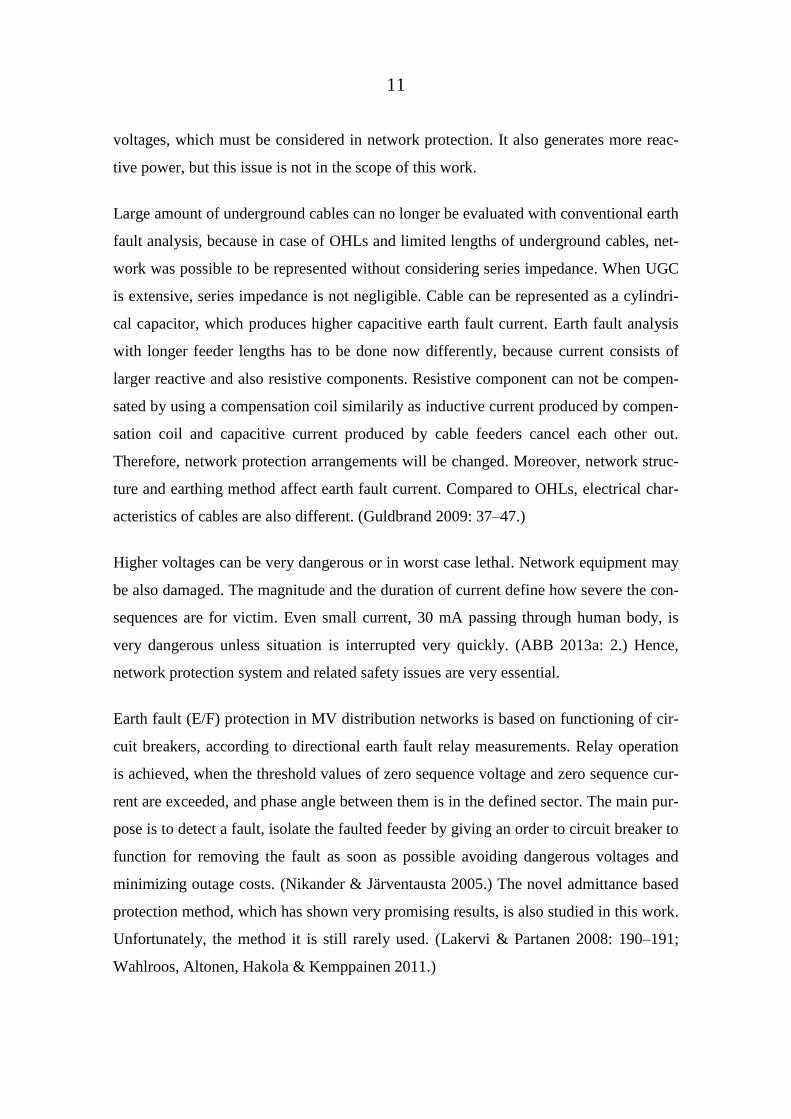
voltages, which must be considered in network protection. It also generates more reac-

tive power, but this issue is not in the scope of this work.

Large amount of underground cables can no longer be evaluated with conventional earth

fault analysis, because in case of OHLs and limited lengths of underground cables, net-

work was possible to be represented without considering series impedance. When UGC

is extensive, series impedance is not negligible. Cable can be represented as a cylindri-

cal capacitor, which produces higher capacitive earth fault current. Earth fault analysis

with longer feeder lengths has to be done now differently, because current consists of

larger reactive and also resistive components. Resistive component can not be compen-

sated by using a compensation coil similarily as inductive current produced by compen-

sation coil and capacitive current produced by cable feeders cancel each other out.

Therefore, network protection arrangements will be changed. Moreover, network struc-

ture and earthing method affect earth fault current. Compared to OHLs, electrical char-

acteristics of cables are also different. (Guldbrand 2009: 37–47.)

Higher voltages can be very dangerous or in worst case lethal. Network equipment may

be also damaged. The magnitude and the duration of current define how severe the con-

sequences are for victim. Even small current, 30 mA passing through human body, is

very dangerous unless situation is interrupted very quickly. (ABB 2013a: 2.) Hence,

network protection system and related safety issues are very essential.

Earth fault (E/F) protection in MV distribution networks is based on functioning of cir-

cuit breakers, according to directional earth fault relay measurements. Relay operation

is achieved, when the threshold values of zero sequence voltage and zero sequence cur-

rent are exceeded, and phase angle between them is in the defined sector. The main pur-

pose is to detect a fault, isolate the faulted feeder by giving an order to circuit breaker to

function for removing the fault as soon as possible avoiding dangerous voltages and

minimizing outage costs. (Nikander & Järventausta 2005.) The novel admittance based

protection method, which has shown very promising results, is also studied in this work.

Unfortunately, the method it is still rarely used. (Lakervi & Partanen 2008: 190–191;

Wahlroos, Altonen, Hakola & Kemppainen 2011.)

12

E/F phenomenon in MV distribution networks with long feeders and related protection

issues has recently raised discussion in Nordic countries, especially in Sweden and in

Finland. Moreover, this phenomenon has not yet been under of many researches, be-

cause traditional MV distribution networks in rural areas comprise still mainly of OHLs

and urban networks with shorter and limited lengths of underground cables. Therefore,

the subject being rather topical at the moment, it was chosen to be studied in this thesis.

The arisen problem of protection issues in mixed and cabled MV networks is under

consideration in this thesis. The main purpose of this work is to find out by simulations:

how the protection should be arranged in different cases using partly decentralized

compensation? What is the maximum protection sensitivity in terms of fault resistance

that can be still reached? Could errors in measurements affect on the functioning of

earth fault protection? The above mentioned questions are studied during this thesis

with the help of computer simulations. Selected network topologies with defined fault

scenarios are simulated and studied with PSCAD network modelling tool.

The structure of this work consists of six chapters. After the introduction part, Chapters

2 and 3 comprise the basic theory of earth faults for creating better understanding for

protection issues. Chapters 4 and 5 concentrate on the empirical part of this work. Chap-

ter 4 introduces the main features of the created network simulation models, and to

Chapter 5 the simulated results are gathered and presented. In the final Chapter 6, the

results and their accuracy are analysed, and based on them, conclucions are made. Pos-

sible further study subjects in related field are also discussed in Chapter 6.

13

2 EARTH FAULTS IN MEDIUM VOLTAGE NETWORKS

2.1 Earth fault

Earth fault is an insulation fault, where a phase line and earth are connected or there is a

connection between phase line and earth via a conductive part. When one of the phases

is connected to earth, earth fault is called a single phase earth fault or in case of two

phases are connected, it is called a two-phased earth fault. Earth faults are mainly sin-

gle-phased, and therefore this study is primarily focusing on single phase earth faults.

Earth faults in underground cabled networks are mostly caused by, e.g. excavation work

or insulation breakdowns. In OHL networks, earth faults are caused by leaning trees or

fallen lines. (ABB 2000: 248; Elovaara & Haarla 2011b: 340,342; Vehmasvaara 2012:

15–16.)

2.2 Single phase earth fault and symmetrical components

When there are no faults in network, system is nearly symmetrical. Phase voltages and

currents have 120° phase shift and the same magnitude compared to each other. Sym-

metry indicates that there is normally neither zero sequence voltage U0, which is sum of

phase-to-earth voltages, nor zero sequence current I0 present in network. When a single

phase earth fault occurs, voltages and currents no longer cancel each other out. Voltages

in two healthy phases rises and voltage of faulted phase reduces. This asymmetry raises

zero sequence voltage or sometimes called as residual voltage Ur or neutral point dis-

placement voltage. In the same way, voltage drop in the faulted phase caused by asym-

metry affects currents. It means that the zero sequence current, which can be also called

as a residual current Ir or 3I0, is no longer zero. (Lakervi & Holmes 1996: 50–56; Pek-

kala 2010:15; Elovaara & Haarla 2011a: 177–181; Elovaara & Haarla 2011b: 14–16;

Siirto, Loukkalahti, Hyvärinen, Heine & Lehtonen 2012.)

14

Zero sequence voltage can be measured in different locations in network. Normally, it is

measured at the substation, but it can be also measured at different points along the

feeder. Therefore, zero sequence voltage measured at the substation may differ from U0

measured at the feeder. This is evident, when UGC increases, and series impedance has

to be considered. This is an important aspect, which DNOs should consider, when plan-

ning the earth fault protection settings of networks in future. (Lakervi & Holmes 1996:

50–56; Pekkala 2010:15; Elovaara & Haarla 2011a: 177–181; Elovaara & Haarla

2011b: 14–16; Siirto, Loukkalahti, Hyvärinen, Heine & Lehtonen 2012.)

Because earth faults are unsymmetrical, network will be analyzed by using symmetrical

components and sequence networks. Symmetrical component analysis, which is a math-

ematical method, is achieved by converting the phasors to sequence coordinates.

Asymmetrical network can be represented now by a combination of three sequence

networks, which are positive, negative and zero sequences, which are illustrated in Fig.

1. Furthermore, it is also possible represent a three-phased network as two-terminal

equivalents, which are introduced in Fig. 2. In Fig 2, Z1, Z2 and Z0 represent the equiva-

lent impendances in positive-, negative and zero sequence networks, U1q, U2q and U0q

are the phase-to-earth voltages in positive-, negative and zero sequence networks, and

U1eq is the voltage source representing the positive sequence voltage calculated from all

three source voltages of the three-phased network. (Guldbrand 2009: 13–15.)

Figure 1. Positive (a1), negative (a2), and zero (a0) sequence network coordinate ba-

ses. (Guldbrand 2009: 13.)

15

Figure 2. Two-terminal equivalents of sequence networks. (Guldbrand 2009: 14.)

In addition to voltage level of the MV distribution network, the earth fault current If is

defined by the length and type of the lines, which are galvanically-connected, and their

phase-to-earth capacitances. Earth fault current increases, when the total length of net-

work increases. (Lakervi & Partanen 2009: 186–187.) In the traditional earth fault anal-

ysis the series impedance is negligible and shunt capacitance is dominant. Because ca-

ble can be represented as a cylindrical capacitor, and in case of longer cable feeders, the

capacitance-to-earth will naturally increase, and series impedance can no longer be ex-

cluded. Compared to OHLs in 20 kV system, which capacitance is ca. 6 nF/km per

phase and earth fault current 0.067 A/km, cables produce earth fault current apprx. from

2.7 A to 4 A/km, and phase-to-earth capacitance is 230–360 nF/km per phase. Also ca-

ble type, geometry, and structure of cables have an effect on earth fault current. (Lak-

ervi & Partanen 2009: 186.)

2.3 Network earthing

Earthing, which has a major effect on earth fault behavior with series impedance and

shunt capacitance of the lines, can be defined as a used combination of the components

connected between earth and neutral point of the transformer. (Guldbrand 2006: 1). Sys-

tem earthing controls the value of unsymmetrical earth fault current, and by that the po-

tential rise in live parts and dangerous voltage levels in system. Earth fault current de-

fines also the zero sequence voltage. (Lakervi & Holmes 1996: 40; Lehtonen & Hakola

1996: 11; Roberts, Altuve & Hou 2001: 2; Guldbrand 2009: 19.)

16

Moreover, earthing protect network equipment from thermal stress, reduce overvoltag-

es, avoid interference in communications systems, guarantee safety for operational per-

sonnel and to general public, and help to detect and remove earth faults as quickly as

possible. (Lakervi & Holmes 1996: 40; Roberts et al. 2001: 2.) In Finland MV distribu-

tion networks are either isolated neutral and compensated neutral systems. Compensated

neutral network will be studied in this thesis, because compensation reduces earth fault

current to 3–10 % of isolated neutral system earth fault current (Roberts et al. 2001: 7).

2.3.1 Earth fault in isolated neutral network

When neutral point of the transformer has no connection to earth, network is called an

isolated neutral or an unearthed neutral system. Isolated neutral system with a single

phase earth fault is illustrated in Fig. 3 and corresponding Thévenin’s equivalent in

Fig. 4.

Figure 3. Single phase earth fault in isolated neutral system. (Lakervi & Partanen

2009: 183.)

17

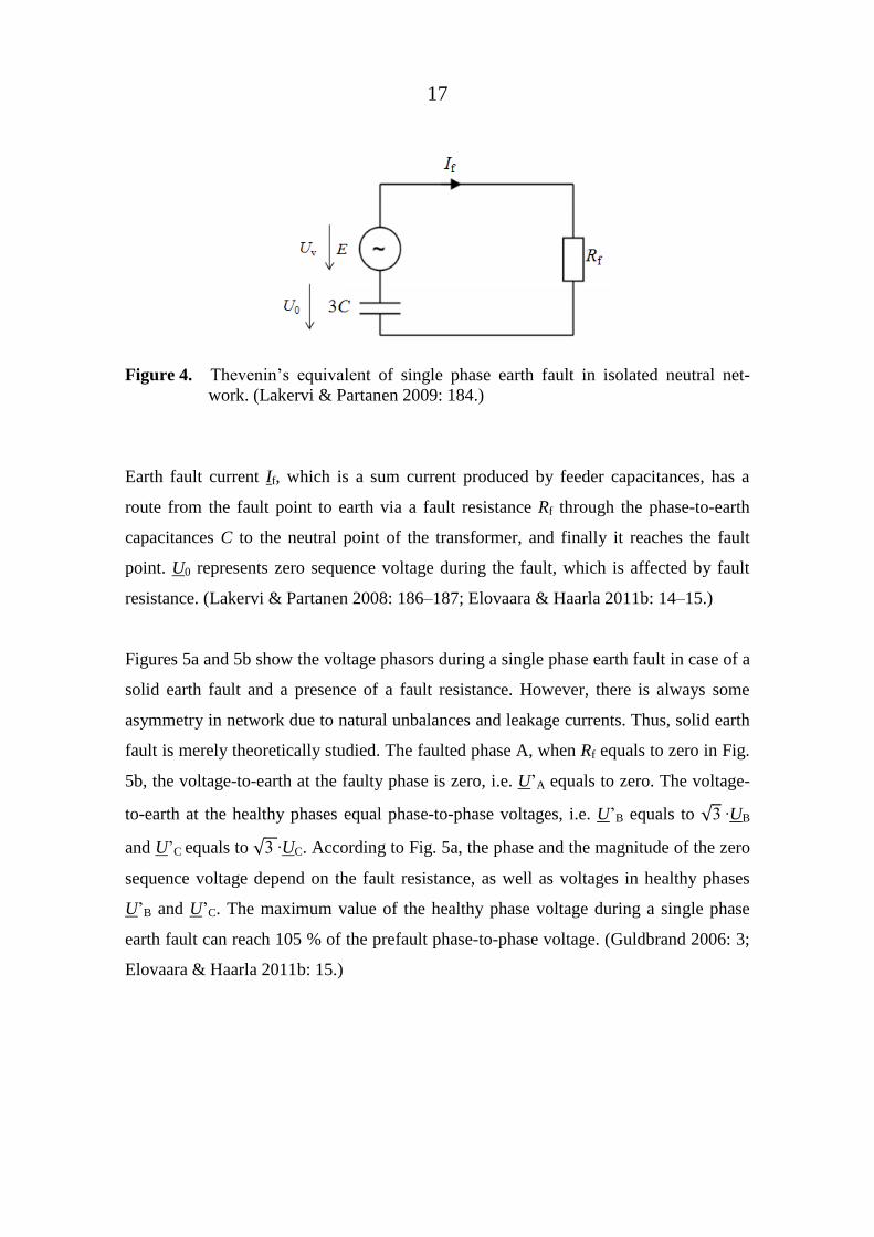
Figure 4. Thevenin’s equivalent of single phase earth fault in isolated neutral net-

work. (Lakervi & Partanen 2009: 184.)

Earth fault current If, which is a sum current produced by feeder capacitances, has a

route from the fault point to earth via a fault resistance Rf through the phase-to-earth

capacitances C to the neutral point of the transformer, and finally it reaches the fault

point. U0 represents zero sequence voltage during the fault, which is affected by fault

resistance. (Lakervi & Partanen 2008: 186–187; Elovaara & Haarla 2011b: 14–15.)

Figures 5a and 5b show the voltage phasors during a single phase earth fault in case of a

solid earth fault and a presence of a fault resistance. However, there is always some

asymmetry in network due to natural unbalances and leakage currents. Thus, solid earth

fault is merely theoretically studied. The faulted phase A, when Rf equals to zero in Fig.

5b, the voltage-to-earth at the faulty phase is zero, i.e. U’A equals to zero. The voltage-

to-earth at the healthy phases equal phase-to-phase voltages, i.e. U’B equals to √ ∙UB

and U’C equals to √ ∙UC. According to Fig. 5a, the phase and the magnitude of the zero

sequence voltage depend on the fault resistance, as well as voltages in healthy phases

U’B and U’C. The maximum value of the healthy phase voltage during a single phase

earth fault can reach 105 % of the prefault phase-to-phase voltage. (Guldbrand 2006: 3;

Elovaara & Haarla 2011b: 15.)

18

a) b)

Figure 5. Phase voltages UA, UB and UC, zero sequence voltage U0 and and healthy

phase voltages U’B and U’C in single phase earth fault in an isolated neutral

network. a) Rf ≠ 0 b) Rf = 0. (Guldbrand 2006: 3; Elovaara & Haarla 2011b:

15.)

Earth fault current can be solved according to Fig. 4, and it can be calculated according

to equations (Guldbrand 2009: 22; Lakervi & Partanen 2009: 184.)

If =

ω

= ω

ω Uv, (2.1)

and

If = IR + jIC = ω )

v

ω ) + j

ω v

ω ) , (2.2)

where

ω is the angular frequency,

C is the total phase-to-earth capacitance of the network,

E is the phase-to-earth voltage,

IC is the capacitive part of the earth fault current,

If is the earth fault current,

IR is the resistive part of the earth fault current,

Rf is the fault resistance, and

Uv is the phase-to-earth voltage.

19

The fault resistance reduces both the earth fault current, which is comprised by both re-

sistive and capacitive components, and the magnitude of zero sequence voltage. Zero

sequence voltage can be defined as follows (Lakervi & Partanen 2009: 184.):

U0 =

ω (-If ) =

-

ω Uv. (2.3)

Earth fault current can be calculated in case of a solid earth fault from equation

(Guldbrand 2009: 21.)

If = jIC = j3ωCUv. (2.4)

It can be seen from Eq. 2.4 that fault current is proportional to the total capacitive con-

nection to earth. Earth fault current has only the capacitive component, and zero se-

quence voltage reaches the prefault phase-to-earth voltage at the faulty phase.

(Guldbrand 2009: 21) In the faulty phase, the current flows towards the fault place be-

ing opposite to the sum current and in the healthy phases the current flows towards the

busbar. Because of the component of fault current flowing in both directions, the effect

of capacitances of faulted feeder has to be ignored, when calculating the residual current

in the beginning of the faulted feeder. The residual current of faulted feeder can be cal-

culated according to equation (Lakervi & Partanen 2009: 191.)

Ir = 3I0 = -

d

If, (2.5)

where

CFd represents the phase-to-earth capacitance of faulted feeder, and

Ir is the residual current of faulted feeder.

Isolated neutral network is inexpensive and easy to construct and earth fault current is

minor due to high impedance. (Guldbrand 2009: 20). However, networks with large to-

tal phase-to-earth capacitance creating high earth fault currents are not advantageous to

20

apply unearthed neutral earthing method. Therefore, compensation has to be used for

extent use of UGC in order to limit earth fault current. (Guldbrand 2009: 24.)

2.3.2 Earth fault in compensated neutral network

In a compensated neutral network or a resonant earthed system, where neutral point of

the network is connected via a Petersen coil or an arc suppression coil to earth, induc-

tive current of the coil is adjusted to compensate almost all the capacitive current during

an earth fault. Petersen coil was invented by Waldemar Petersen in the early 20th

centu-

ry, in purpose of limiting earth fault current near to zero (Wahlroos, Altonen & Fulczyk

2013). (Lakervi & Partanen 2009: 184–185; Wahlroos & Altonen 2011: 3.)

Single phase earth fault in compensated neutral network is represented in Fig. 6. Coil is

tuned to cancel the capacitive current almost entirely. Because IL and IC have opposite

direction, the earth fault current If is reduced considerably, and it is mainly resistive.

Therefore, relays in compensated networks are set to measure the resistive component

of the residual current. (Lakervi & Partanen 2009: 184–185.)

Figure 6. Single phase earth fault in compensated neutral network. (Lakervi & Par-

tanen 2009: 185.)

21

When series impedance is negligible, earth fault current If and zero sequence voltage U0

can be calculated in compensated neutral network according to equations (Lakervi &

Partanen 2009: 185–186.)

If =

ω -

ω ) Uv, (2.7)

and

U0 = -

ω -

ω )

Uv, (2.8)

where

L is the coil inductance, and

RL is the parallel resistor.

Because earth fault protection relays measure in addition to magnitudes also phase an-

gles, calculations describing relay operation quantities in this thesis are represented by

phasors. However, considering the empirical part of this work, also the absolute value

of the zero sequence voltage is needed and it can be calculated as follows (Mörsky

1992: 317; Lakervi & Partanen 2009: 186.):

U0 =

√ )

ω -

ω )

√ . (2.9)

If the system is exactly tuned i.e. compensation degree K equals to 1 (or 100 %), fault

current contains only a resistive component (Guldbrand 2009: 30–31). If the K has a

value more than 1, network is overcompensated and respectively if K has a value less

than 1, network is undercompensated. Compensation degree can be calculated according

to equation (ABB 2000: 254.)

22

K =

, (2.6)

where

IC is capacitive earth fault current,

IL is inductive earth fault current, and

K is the compensation degree.

Coil(s) can be installed either centrally at the neutral point of the main transformer at

substation or locally along the feeders (decentralized compensation). Locally installed

coils have usually fixed value of inductance and smaller rating. In practice, there is also

a parallel resistor RL connected to coil. It helps to increase earth fault current for better

fault detection and selective relay operation. (Hänninen, Lehtola & Antila 1998;

Guldbrand 2009: 33; Lakervi & Partanen 2009: 182–185; Elovaara & Haarla 2011a:

210–211; Wahlroos & Altonen 2011: 3–5.) In this thesis the network is partly decentral-

ly compensated. At the neutral point of the transformer at the substation is one coil

compensating the beginning of the feeders, and the locally installed coils compensate

the rest of the feeders. Fig. 7 shows the single phase equivalent of partly decentrally

compensated network.

Figure 7. Single phase equivalent of partly decentrally compensated network modi-

fied from (Lakervi & Partanen 2009: 185).

23

The absolute value of residual current in partly decentrally compensated networks,

which derivation can be found in Appendix 1, can be defined for the faulted feeder ac-

cording to Fig. 7 as follows:

Ir =

√ ω - d) -

ω ))

√ ) ω -

ω ))

v, (2.10)

where

LBG is the coil inductance located in the BG network,

LFd is the coil inductance located in the faulted feeder, and

L = d

d.

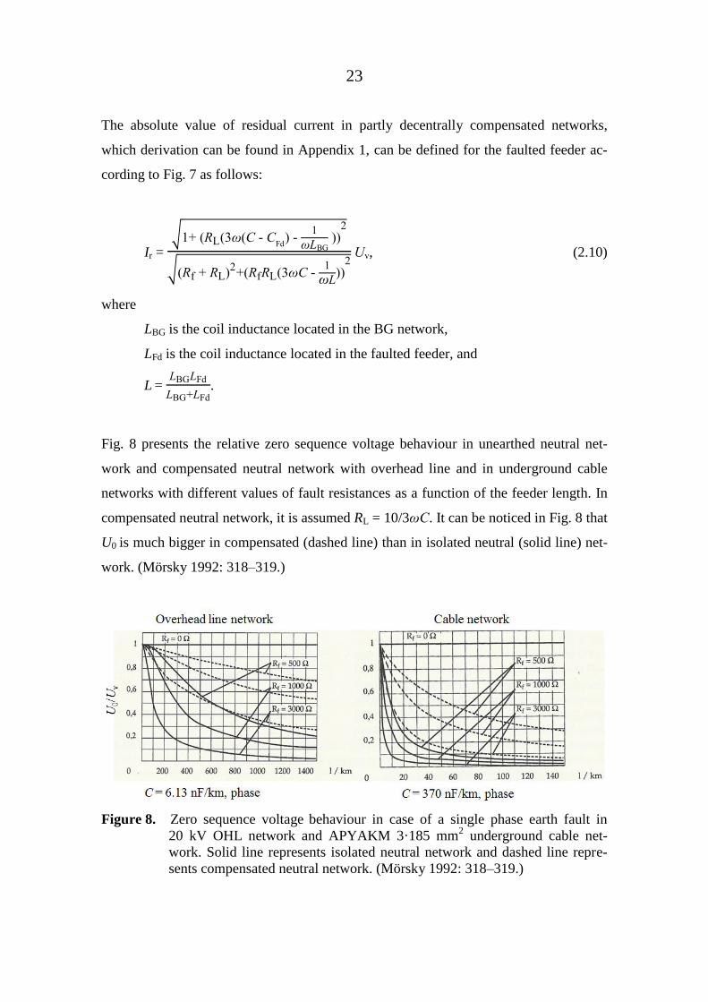
Fig. 8 presents the relative zero sequence voltage behaviour in unearthed neutral net-

work and compensated neutral network with overhead line and in underground cable

networks with different values of fault resistances as a function of the feeder length. In

compensated neutral network, it is assumed RL = 10/3ω . It can be noticed in Fig. 8 that

U0 is much bigger in compensated (dashed line) than in isolated neutral (solid line) net-

work. (Mörsky 1992: 318–319.)

Figure 8. Zero sequence voltage behaviour in case of a single phase earth fault in

20 kV OHL network and APYAKM 3·185 mm2 underground cable net-

work. Solid line represents isolated neutral network and dashed line repre-

sents compensated neutral network. (Mörsky 1992: 318–319.)

24

In compensated neutral networks fault detection is more difficult, and the probability of

double and intermittent faults is increased due to voltage rise (Zamora, Mazon, Eguia,

Valverde & Vicente 2004). Personnel have to be also trained for assimilating new tech-

nology and fault analysis pattern (Loukkalahti 2013).

2.4 Admittance theory

2.4.1 Background

The earth fault analysis can be also made by using admittances between three phases

and earth. This admittance-based theory has been implemented originally into earth-

fault protection in Poland in 1980s among a group of researchers, which was headed by

Józef Lorenc from Poznan University of Technology. Later, the idea by using admit-

tance-based protection has become a requirement for local utilities in Poland. Still, it is

less known among protection engineers in other countries, but it has a great potential in

protection field due to already good and promising results. (Wahlroos 2012; Wahlroos

et al. 2013.) Therefore, the basics from admittance theory according to Wahlroos & Al-

tonen (2011) are introduced in the following section.

2.4.2 Fundamentals of admittance-based earth fault protection

The admittance criterion is based on the fundamental frequency components of 3I0 and

U0. Neutral admittance Y0 can be now determined in symmetrical networks dividing re-

sidual current phasor by zero sequence voltage phasor, according to equation

Y0 = G0 + jB0 =

0 ault

- 0 ault

, (2.11)

where

3I0_fault is the residual current during the fault,

B0 is the neutral susceptance,

G0 is the neutral conductance,

25

U0_fault is the zero sequence voltage during the fault, and

Y0 is the neutral admittance.

The shunt admittance for a single phase line can be defined as follows:

Y0 = G0 + jB0 = G0 + j(ωC0), (2.12)

where G0 is the shunt conductance being usually rather small (10–100 times smaller

than the susceptance value) due to efficient dielectric features of cables. Shunt conduct-

ance illustrates the resistive leakage current flowing via dielectric material, air and insu-

lators, and hence it produces resistive losses of the system. C0 is the phase-to-earth ca-

pacitance per phase.

Modern microprocessor based intelligent electronic devices (IEDs) utilize the calclula-

tion, which was presented in Eq. 2.11. Alternatively, eliminating the effect of network

asymmetry and under specific conditions the effect of fault resistance, admittance can

be calculated by “delta-quantities” as follows:

Y0 =

0 ault -

0 pre ault)

- 0 ault

- 0 pre ault

) =

∆ 0

- ∆ 0

, (2.13)

where

3I0_prefault is the residual current before fault, and

U0_prefault is the zero sequence voltage before fault.

For networks, consisting of underground cables, the admittance calculation according to

Eq. 2.11 can be used. In case of mixed networks, which contain also a large amount of

OHLs in addition to underground cables causing the network becoming very unsymmet-

rical, the use of delta-quantities in admittance calculation is recommended. Fig. 9 shows

a three-phased distribution network including two feeders, protected feeder (Fd), which

is the feeder where the protection relay quantities are studied and the background net-

work (Bg), which represents the rest of the whole galvanically-connected network.

26

Figure 9. Three-phased distribution network model consisting of two feeders:

protected feeder and background network in a single phase earth fault situa-

tion in phase a. (Wahlroos & Altonen 2011: 6.)

Dominant shunt admittances are presented, but series impedance being rather small can

be left out consideration. Neither loads nor phase to phase capacitances are being evalu-

ated. YFd and YBg are the total admittances of the coils located in the protected feeder and

in the BG network. YcCC is the admittance of the compensation coil at the substation.

The total admittance of the network Ywhole, which represents the total network admit-

tance including the whole BG network and feeder admittances, can be defined accord-

ing to equation

Ywhole = YFdtot + YBgtot = Gwhole + jBwhole, (2.14)

where

YBgtot = YBga + YBgb + YBgc = GBgtot + jBBgtot, and

YFdtot = YFda + YFdb + YFdc = GFdtot + jBFdtot,

and

YBga, YBgb, YBgc are background network admittances in phases a,b, and c, and

YFda, YFdb, YFdc are protected feeder admittances in phases a,b, and c.

27

Equation for U0 according to Fig. 9 can be defined as follows:

U0 = -Ea u d

u g

d g

c

d

g

dtot

gtot

g , (2.15)

and for residual current of the protected feeder as follows:

3I0 = U0 (YFdtot + YFd + GFFd) + Ea (YuFd + GFFd), (2.16)

where

YuBg = YBga + a2 YBgb + a

YBgc, a = cos (120°) + jsin(120°), and

YuFd = YFda + a2 YFdb + a

YFdc.

YuBg and YuFd are asymmetrical parts of the total phase-to-earth feeder and BG network

admittances, YBgtot and YFdtot. If the phase-to-earth admittances can be assumed to be

completely symmetrical in the network (YuFd = YuBg = 0), Equations 2.15 and 2.16 will

be shortened. Fault analysis can be calculated either in case of fault is located at the pro-

tected feeder, when GFBg = 1/RFBg = 0 and GFFd = 1/RFFd > 0 or when fault is located at

the BG network, when GFFd = 0 and GFBg > 0.

Admittance calculation is evaluated either fault locating in the protected feeder or in the

BG network. When fault is at the protected feeder, admittance seen by admittance crite-

rion can be calculated according to equation

Y0 = YBgtot + YcCC + YBg = ((GBgtot + GcCC + GBg) + j(BBgtot - (BcCC + BBg)). (2.17)

By replacing BcCC = K·Bwhole, and BBgtot = Bwhole - BFdtot, where K is the compensation

degree, the admittance will be

Y0 = ((GBgtot + GcCC + GBg) + j((Bwhole(1 - K) - BFdtot - BBg)). (2.18)

28

The total admittance, which is positive-signed, is now defined by the admittance meas-

ured from the BG network according to Eq. 2.18, and including the admittances of the

coils in the BG network. The conductance is positive all the time, and the sign of the

susceptance is affected by K. The effect of susceptances of decentralized compensation

coils has to be also considered.

For the fault locating in the BG network, the admittance seen by admittance criterion

can be calculated as follows:

Y0 = - (YFdtot + YFd) = - ((GFdtot + GFd) + j(BFdtot - BFd)). (2.19)

As can be seen from the Eq. 2.19, the admittance method measures total admittance of

the protected feeder, which is negative-signed and contain coil admittances of the pro-

tected feeder. When using central compensation, admittance is negative-signed admit-

tance of the protected feeder. Consequently, the conductance and the susceptance are

always negative-signed. However, it is possible that the conductance of the protected

feeder is rather small to be measured accurately. Errors in U0 and 3I0 measurements

might lead to the false conductance value by turning it into positive-signed. Also, de-

centralized compensation might lead to unpreferred overcompensation situation, where

the measured susceptance is positive. In order to implement E/F protection, and to pre-

vent malfunctions of protection, such situation demands particular attention.

As can be seen from the Equations 2.18 and 2.19 by theoretical point of view, the fault

resistance does not have an effect on admittance calculation. Therefore, settings for ad-

mittance based criterion can be defined by a very simple way.

29

2.5 Other earth fault types

2.5.1 Double earth fault

When two phases are in a conductive connection with earth in network, fault is then

called a double earth fault or a cross country fault. Fault points can be in same locations,

when it is called a phase-to-phase-to-earth fault, or locate very far from each other not

having a short circuit connection. Usually, double earth fault is due to single phase earth

fault. Voltage rise in healthy phases can inflict to function of overvoltage protection.

Especially, in distribution networks double earth fault is problematic. Fault current is

rather substantial: it can reach almost the value of short circuit current. Moreover, it is

problematic to calculate precisely and it flows rather well via different conductive

routes, including water mains or sheaths of communication cables. Poor conductivity of

soil can cause major damages, when fault current flows in sheaths. Thermal stress and

electric breakdowns between sheath and conductor can arise. To prevent double earth

faults, fast and secure functioning of earth fault and overvoltage protections is needed.

(Lakervi & Partanen 2009: 198.)

2.5.2 Arcing and intermittent faults

Arc fault is typically a very short and can be cleared by self-extinction (Guldbrand

2009: 11). The recovery voltage is defined by a voltage at the fault place after it has

been eliminated. In isolated neutral networks the recovery voltage is quite steep. The

rising speed of recovery voltage is high and may cause problems with self-

extinguishing, despite rather small fault current. This is a drawback in isolated neutral

network due to an absence of inductance, compared to the compensated neutral net-

work. Arc re-ignitions are more likely to arise in isolated neutral networks. Phase-to-

earth voltages in the healthy feeders might reach to the magnitude of the phase-to-phase

voltage level and evolve to cross country faults due to overvoltages. (Lehtonen & Hako-

la 1996: 26–28; Roberts et al. 2001: 7–8.)

30

By using Petersen coils, self-extinguishment is more evident and power quality via re-

duced number of reclosings is improved. Recovery voltage’s rising speed will be de-

creased by coils, but the compensation degree has to be more than 75 % enabling the

more improved self-extinguishment. (Hänninen 2001: 26–28.)

Intermittent earth fault is common in compensated neutral systems consisting mainly of

underground cables. This special fault type has arisen in attention particularly recently

due to demand for more uninterruptable power supply (Mäkinen 2001: 1–2). Intermit-

tent fault, or so-called restriking earth fault, is a special fault type, which is caused by a

series of cable insulation breakdowns or deterioration of insulation due to diminished

voltage withstand (Altonen, Mäkinen, Kauhaniemi & Persson 2003). Intermittent earth

fault is introduced in this study only briefly, because the focus is to concentrate only to

permanent single phase earth faults.

Insulation breakdowns can occur due to moisture, water, dirt, chemical reactions, mate-

rial ageing, mechanical stress or insulation layer damages. Because of reduced insula-

tion of faulted place, fault will appear when the phase-to-earth voltage reaches the

breakdown voltage. However, the fault will be cleared mostly by itself, when the fault

current reaches its zero point for the first time. (Altonen et al. 2003.)

Conventional earth fault protection relays are not capable of detecting very irregular

wave shapes of current and voltage, as illustrated in Fig. 10. Relay may not be able to

trip the faulted feeder and situation can lead to unselective operation of protection.

Therefore, network protection in case of intermittent faults is challenging. And a lot of

attention should be paid for detecting and removing them. Especially, because the gen-

eral trend is going towards increased use of UGC and the natural ageing of the existing

cables will increase the probability of intermittent earth faults. However, residual volt-

age, which is presented in Fig. 11 with recovery voltage (sum of the phase-to-earth

voltage and residual voltage), has more stable waveform compared to current. There-

fore, back-up protection of substation based on residual overvoltage may operate, if

feeder protection can not clear the fault. Nonetheless, unnecessary relay operations of

the substation protection and related high outage costs can occur. (Altonen et. al 2003.)

31

Figure 10. Residual voltage and current waveforms in the intermittent earth fault situa-

tion. (Altonen et al. 2003.)

Figure 11. Recovery voltage in the intermittent fault situation. (Altonen et al. 2003.)

2.6 Extensive underground cabling and conventional earth fault analysis

Distribution system has composed merely with OHLs in rural areas and limited lengths

of underground cables in urban networks due to restricted space and high expenses. In

urban networks, feeders are short and can be presented by pi-sections, which are parallel

connected. High voltage (HV) network and series impedances (transformer impedances)

can be considered negligible, ZT1 = ZT2 = ZT0 = 0, whereas the shunt capacitance has a

major effect on earth fault analysis, see Fig. 12. (Guldbrand 2009: 46–47.)

32

Figure 12. Urban network consisting of positive, negative and zero sequence networks.

(Guldbrand 2009: 46.)

According to Guldbrand (2009: 38–39), the conventional earth fault analysis assump-

tions are valid in systems consisting of limited cable lengths. These assumptions for tra-

ditional analysis state the earth fault behaviour is defined by total cable length, hence it

does not define whether network consists a couple of long feeders or several short cable

lines. Secondly, the whole earth fault current can be compensated via Petersen coil,

which is in relation to total cable length. If the capacitive and inductive currents cancel

each other out completely, zero sequence voltage can be defined by the fault resistance

and the coil resistance. Moreover, earth fault behaviour is not affected by fault place. It

gives same earth fault current values and zero sequence voltages in the bus bar fault like

fault e.g at the end of the feeder.

In case of longer cable lines the situation is now different and traditional analysis and

assumptions are not anymore valid according to Guldbrand (2009: 39–40). Analyzing

the effects with longer cable feeders requires different modeling methods to achieve ac-

curate results and avoid false results. The increased lengths of feeders stipulate to use

several pi-section connections (like in this thesis) instead of one section. These pi-

sections are in series; see Fig. 13, compared to parallel line connections in urban net-

work. It is also possible to compensate the non-linear behaviour of the reactive imped-

ance by using correction factors. Because of larger series impedance, it has a bigger in-

fluence on earth fault situation. Now, the series impedance is taken into account, which

33

impacts the earth fault current consisting in addition to capacitive, also a resistive com-

ponent. This is proved in Guldbrand (2009: 41–45). Resistive component has to be kept

within limited set of values because of the safety issues. Fault place influences zero se-

quence voltage in case of long cable lines compared to conventional system assump-

tions. From this, zero sequence voltage measured by the substation, differs now from

the zero sequence voltage measured at the feeder. (Guldbrand 2009: 42–45.)

Figure 13. Rural network consisting of positive, negative, and zero sequence networks,

which are connected in series, when fault occurs. (Guldbrand 2009: 47.)

2.7 Cable characteristics and zero sequence impedance

Compared to OHLs, underground cables have slightly different features in zero se-

quence network parameters and they affect on the zero sequence impedance. Fig. 14

illustrates a simplified model of a three-phased cable and its dimensions. According to

Fig. 14, the diameter of the total cable is represented by 2rsh, the diameter of the one

conductor is represented by 2rc, the distance between the conductors is represented by d.

di0 defines the distance between the cable’s conductor and earthing wire and 2rew is the

diameter of the earthing wire. (Guldbrand 2009: 16–17; 92–93.)

34

Figure 14. Underground cable dimensions and earthing wire in a cross-section view.

(Guldbrand 2009: 93.)

According to conventional earth fault analysis, the series impedance can be ignored.

However, recently arised interest for zero sequence impedance among researchers was

resulted from increased cabling and longer lengths in rural areas. Gunnar Henning from

ABB has developed a schema for analyzing zero sequence impedance, which is present-

ed with more details in Pekkala (2010: 33–34) and Guldbrand (2006: 14). There are still

many uncertainties among researchers concerning the zero sequence impedance.

(Guldbrand 2009: 91–100.)

Many factors are affecting to zero sequence impedance. Zero sequence capacitance, ca-

ble characteristics, which are presented in Fig. 15, ground resistivity, earthing wire and

its distance to earth and earthing resistance, all impact the zero sequence impedance.

Fig. 15 shows the cable characteristics of underground installation. Cable is three-

phased, Uv equals in all phases, the residual current 3I0 flows in conductors, along the

sheat Ish, through the earthing wire Iew and earth Ie. Cable has also a conductive connec-

tion to earth both at the beginning and at the end of the cable via an earthing resistance

Rer. Arised self- and mutual impedances as a result of different current routes in the ca-

ble and between the cable and earthing wire, have an effect on zero sequence imped-

ance. Moreover, these values are affected by cable features and current return routes.

(Guldbrand 2009: 42–44; 91–100.)

35

Figure 15. Cable characteristics for underground installations and related current

flows. (Guldbrand 2009: 92.)

The feeder length has a minor influence to the magnitude of the zero sequence imped-

ance, whereas the change in the argument of the impedance is more evident. Due to

longer cable lengths, fault current consists of reactive and resistive components, which

can be seen in ig. 6. As a result, the traditional earth ault analysis isn’t accurate

anymore.

Figure 16. Magnitude and angle of the zero sequence impedance of cables. Dashed line

represents cable modelling by pi-sections and solid line by capacitance only.

(Guldbrand 2009: 43.)

36

3 COMPENSATION AND PROTECTION METHODS

3.1 Network safety

Guaranteeing safety is the main priority in network protection and after that come relia-

bility and economic issues. The purpose is to ensure safety for customers, operation per-

sonnel and surrounding areas and animals during and after fault situations. Ensuring

safety in network there has to be determined certain limiting values in currents and volt-

ages and fault duration time. (Guldbrand 2009: 7.)

When the primary coil of the distribution transformer is coupled in delta-connection and

without taking care of asymmetry due to earth fault in MV network, the voltages are in

the secondary side e.g. in low voltage (LV)-side at normal state. Therefore, LV custom-

ers will not notice any disturbances or problems and normal usage of network could be

possible during an earth fault. The magnitude of earth fault current can be rather slight,

which may not damage household devices. (Lakervi & Partanen 2009: 189.)

The increase of earth fault current is possible to limit, e.g by adding a new main trans-

former to power station. Because of high costs, it is not reasonable just for limiting earth

fault. It it also possible to limit earth fault current by decreasing earthing resistance, but

due to low soil conductivity it would not be suitable. One possible solution could be to

shorten the clearing times, which would however impacts to the quality of supply by

giving less time for faults to be removed by themselves. (Lakervi & Partanen 2009:

189.) On the other and, current flow duration would be shorter, which could be benefi-

cial by safety point of view (Nikander & Järventausta 2005). Consequently, the best al-

ternative for earth fault current to be in limited values is to use Petersen coils

(Vehmasvaara 2012: 23).

37

3.1.1 Current effects on human body

During human contact with energized part of the network, voltage is formed due to po-

tential difference, and it will produce current. Current flows through certain non-linear

body impedance, which is resistive and slightly differs in everyone due to different fac-

tors, e.g. amount of water and mass of body. Supposing large contact extents and affect-

ed voltage over 1000 V, the body resistance varies between 575 Ω, which consists 5 %

o the population and 050 Ω, which have the majority, 95 % of the population (IEC

2005). (Guldbrand 2009: 7–10.)

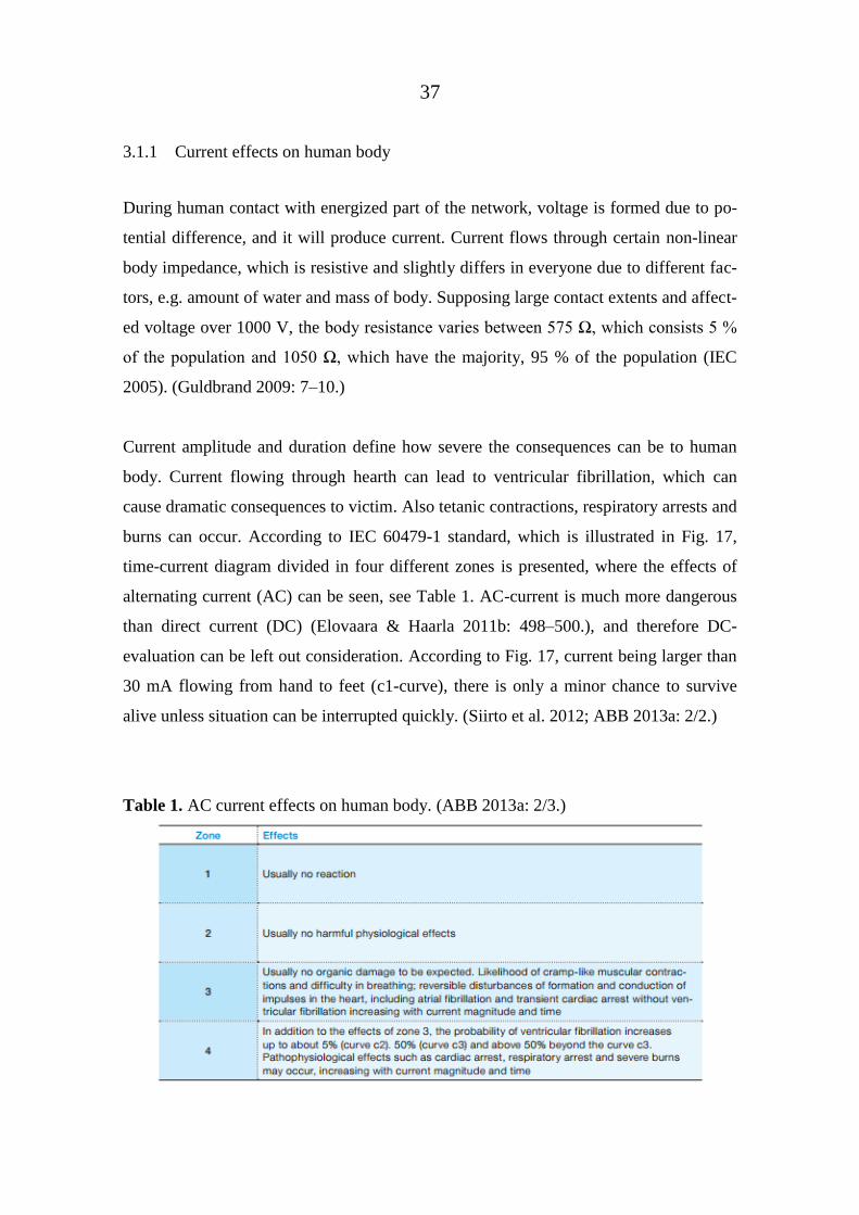
Current amplitude and duration define how severe the consequences can be to human

body. Current flowing through hearth can lead to ventricular fibrillation, which can

cause dramatic consequences to victim. Also tetanic contractions, respiratory arrests and

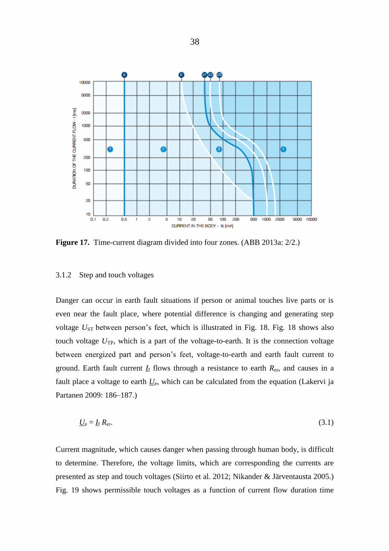
burns can occur. According to IEC 60479-1 standard, which is illustrated in Fig. 17,

time-current diagram divided in four different zones is presented, where the effects of

alternating current (AC) can be seen, see Table 1. AC-current is much more dangerous

than direct current (DC) (Elovaara & Haarla 2011b: 498–500.), and therefore DC-

evaluation can be left out consideration. According to Fig. 17, current being larger than

30 mA flowing from hand to feet (c1-curve), there is only a minor chance to survive

alive unless situation can be interrupted quickly. (Siirto et al. 2012; ABB 2013a: 2/2.)

Table 1. AC current effects on human body. (ABB 2013a: 2/3.)

38

Figure 17. Time-current diagram divided into four zones. (ABB 2013a: 2/2.)

3.1.2 Step and touch voltages

Danger can occur in earth fault situations if person or animal touches live parts or is

even near the fault place, where potential difference is changing and generating step

voltage UST between person’s eet, which is illustrated in Fig. 18. Fig. 18 shows also

touch voltage UTP, which is a part of the voltage-to-earth. It is the connection voltage

between energized part and person’s eet, voltage-to-earth and earth fault current to

ground. Earth fault current If flows through a resistance to earth Rer, and causes in a

fault place a voltage to earth Ue, which can be calculated from the equation (Lakervi ja

Partanen 2009: 186–187.)

Ue = If Rer. (3.1)

Current magnitude, which causes danger when passing through human body, is difficult

to determine. Therefore, the voltage limits, which are corresponding the currents are

presented as step and touch voltages (Siirto et al. 2012; Nikander & Järventausta 2005.)

Fig. 19 shows permissible touch voltages as a function of current flow duration time

39

assuming with 10 % probability of ventricle fibrillation by SFS-6001 standard. It can be

seen that the lower the voltage is, the longer is the time it can be allowed (Siirto et al.

2012). In isolated or compensated neutral networks the common tripping delays vary

between 0.2 s or 0.3 s, and 1.0 s (Nikander & Järventausta 2005). (Lehtonen & Hakola

1996: 55–59; Lakervi & Partanen 2009: 187–188; Elovaara & Haarla 2011b: 428–432.)

Figure 18. Generated different voltages during an earth fault situation. (Lehtonen &

Hakola 1996: 58.)

Figure 19. Permissible touch voltage UTP as a function of current duration time. (SFS

2005: 78.)

40

3.1.3 Earth fault regulations and standardization and legislation

Earth fault legislation is based on regulations and definitions by different authorities

both in globally and national level. Distribution network safety is mainly a concern of

DNOs, which have to ensure safe conditions during normal network usage and also in

fault circumstances, limit access from normal people e.g. power stations and restrict

consequences as small as possible due to faults by following earth fault related safety

regulations. Compared to short circuit legislation, issues dealing with earth fault current

legislation are more specifically controlled by SFS 6001 regulation in Finland and

ELSÄK-FS in Sweden. Earth faults have to be removed either automatically or manual-

ly. However, SFS 6001 standard advises to use automatic system. Higher voltage levels

may create danger for customers and network equipment even in LV-side. (ELSÄK-FS

2008: 1; Pekkala 2010: 48–49.)

In Finland SFS 6001 standard defines limiting touch voltage values as a function of cur-

rent duration flow. According to ELSÄK-FS (2008: 1), there are specific values for

earth voltage in Sweden. (Pekkala 2010: 48–49.) High-impedance earth faults are not so

dangerous in cabled systems compared to OHLs, because cables are out of reach of

normal people. In Sweden, in case of cable systems, detecting fault is enough. If net-

work contains partly or entirely OHLs and ault impedance is either under kΩ or 5 kΩ

in case of covered lines, fault will be detected and removed (ELSÄK-FS 2008: 1). In

Finland, protection is based on electrical safety regulation. Earth faults have to be

cleared up to 500 Ω fault resistances. Faults have to be also cleared during two hours

from the fault detection. If it is possible, even higher fault resistance faults would be

beneficial to detect. (ABB 2000: 258; Guldbrand 2009: 10.)

Due to storms and related power failures and outage costs in distribution network, the

Finnish government has finished its new energy market legislation by Ministry of Em-

ployment and the Economy, which came into effect in the fall 2013. It takes stand more

precisely to the quality of supply. According to the new legislation, distribution net-

works has to be designed, implemented and maintained in case of storms and mass of

snow, in such way that it can not cause supply outages to customers over six hours in

41

urban areas or over 36 hours in other areas. These requirements have to be implemented

stepwise during the next 15 years. 50 % of the delivery reliability requirements have to

be achieved by the end of 2019, 75 % by the end of 2023, and 100 % by the end of

2028. In case of extraordinary extent cabling, DNOs may have time to meet the re-

quirements by end of the year 2036. (Ministry of Employment and the Economy 2013.)

In Sweden the parliament decided to change the power supply regulation by new law

regulation 2005, which improves customers’ rights compensating power outages

(Guldbrand & Samuelsson 2007). Consequently, these new requirements for quality of

supply will definitely set more pressure on DNOs in near future.

3.2 Compensation methods

Petersen coils are an effective way to limit earth fault current. Therefore, it is discussed

with more details and studied via computer simulations in this work. Compensation

with Petersen coils has not yet been widely used in Finland compared to Sweden, where

compensation covers nearly all the MV distribution networks. Compensation with coils

is increasing in Finland and will replace isolated neutral networks in future. (Pekkala

2010: 52.) This method and its redeeming features in MV distribution networks have

gained more awareness among DNOs. Especially with this method, reliability and quali-

ty of supply are guaranteed. It has also noticed that compensation diminish outages, in

case of faults consisting mainly of momentary faults. (Wahlroos & Altonen 2011: 3.)

The residual current compensation (RCC) is a compensation method, which was origi-

nally developed by Swedish Neutral. It eliminates the fundamental frequency fault cur-

rent, and dangerous high voltage levels in compensated networks. It does not trip the

faulted feeder, it cancels fault current out by injecting opposite current to neutral point,

and single-phased earth faults can be removed without disconnections. As a result, the

distribution network during earth fault situations can be used. (Nikander & Järventausta

2005.) However, this residual current compensation is not studied with more details in

this work.

42

Network can be compensated practically in three different ways; centrally, decentrally

or partly decentrally, when it can be also called as a hybrid, like in Wahlroos & Altonen

(2011) or mixed like in Jaakkola & Kauhaniemi (2013). Earlier, centralized compensa-

tion was used due to costs and more easiness, but decentralized and partly decentralized

compensation methods have shown their good potential in compensation field. (Wahl-

roos & Altonen 2011: 3.)

In practice, there is also a resistance RL connected parallel to the coil, which is used to

increase active earth fault current for fault detection and selective relay operation (Hän-

ninen et al. 1998; Wahlroos & Altonen 2011: 4). It is called “Active Current Forcing”

(ACF) scheme by Wahlroos & Altonen (2011: 4). The connection logic of the parallel

resistor can be implemented in three different ways: connected all the time, connected a

short time interval after fault appears, but it is not connected during normal network us-

age or disconnect it a short time interval after fault and connect it again if fault has not

been cleared.

By permanent connection of the parallel resistor, the aim is to limit U0 at the healthy

state in totally cabled networks. However, it might be eliminated totally due to resistor

and hindering coil control. In the second alternative, self-extinguishment of arc is more

likely to happen and before connecting the resistance, U0 might reach large values due

to compensation degree and capacitive unbalance. By disconnecting the resistance after

a short time period, the advantages from previously mentioned two methods are com-

bined: reducing U0 and enabling self-extinguishment of arc. However, parallel resistor

has to withstand higher continuous power. (Mörsky 1992: 336–337; Isomäki 2010: 30;

Wahlroos & Altonen 2011: 4.) There are varying viewpoints of how the parallel resistor

should be connected, and some DNOs are just using the method, which they have no-

ticed to function properly, e.g via practical experience. In this thesis, the differences be-

tween on and off situations of the parallel resistor are studied.

43

3.2.1 Centralized compensation

When compensation coil is connected to neutral point of the main transformer’s second-

ary side, i.e. MV side at the substation, see Fig. 20, or via grounding transformer, the

system is centrally compensated. Main transformers in Finland are basically YNd-

coupled and distribution transformers Dy-coupled. Due to delta-wiring in the MV-side,

there is not a neutral point for coil connection. YNyn-coupled transformers would be

suitable considering costs and unbalanced loadings, but are inconvenient in parallel use

with Yd-coupled transformers. Therefore, neutral point has to be generated via a seper-

ate, Znyn-coupled grounding transformer. (Mörsky 1992: 319–321; Pekkala 2010: 52–

54.)

Figure 20. Centrally compensated network. (Guldbrand & Samuelsson 2007.)

Centralized compensation is beneficial in case of poor earthing and when the value of

earth fault current is larger than 35 A. Costs are a major factor in centralized compensa-

tion. Therefore, in the long run, careful planning of the network is needed. (Lehtonen &

Hakola 1996: 70; Pouttu 2007: 30.) However, based on the results from Pekkala (2010)

using centralized compensation with long cables, the resistive part of the earth fault cur-

rent might be a problem. Therefore, decentralized compensation should be used to re-

duce high resistive part of the earth fault current to allowed levels. (Lehtonen & Hakola

1996: 69–70; Wahlroos & Altonen 2011: 5.)

44

3.2.2 Decentralized compensation

Decentralized or distributed, or sometimes called as local compensation, which is illus-

trated in Fig. 21, is based on placing several fixed coils along the feeders, which are

tuned to compensate almost the total capacitive part of the specific feeder sections. This

is advantageous in feeder disconnection situations deactivating the same amount of

compensation, which is extracted. By doing this, the right compensation degree re-

mains, the balance in the network will be guaranteed, and harmful overcompensation

situations leading to false relay operations can be avoided. (Guldbrand & Samuelsson

2007; Wahlroos & Altonen 2011: 5–6.)

Figure 21. Decentrally compensated network, where Petersen coils are located along

the feeders. (Guldbrand & Samuelsson 2007.)

However, careful placing of the coils is needed. The balance of the network is ensured if

coils would be disconnected for some reason. This kind of situation responds to earth

fault behaviour situation in isolated neutral system. (Guldbrand & Samuelsson 2007;

Wahlroos & Altonen 2011: 5–6.)

In practise, decentralized compensation coils are rated to compensate a fixed value

varying typically between 5 A and 15 A. It is useful method in rural areas and with long

feeder lengths. (Hänninen & Lehtonen 1997.) Coils are connected to distribution trans-

45

formers’ neutral. A lack of neutral point in distribution transformers due to delta-

connection (Dy-coupling), ZNzn0- or Zn(d)yn-coupled transformers have to be used.

These couplings also prevent earth fault current flow to LV-side. The distance of coils

between each other has also to be determined accurately due to the influence of the se-

ries impedance. When the distance between coils is increased, resistive part of the

equivalent impedance and resistive part of the earth fault current increase, i.e. resistive

losses increase, and these depend on size of coils. (Guldbrand 2009: 32–34; Pekkala

2010: 55; Vehmasvaara 2012: 24–25.)

According to uldbrand’s 009) thesis, the most reasonable distance between coils

would be 5 km or 10 km, and same results were achieved by Jaakkola & Kauhaniemi

(2012). If the coil density of 10 km is used, there would be needed a smaller amount of

expensive transformers. On the other hand, if the distance was 10 km, there might be a

problem to maintain the steady compensation degree if part of the system would be dis-

connected. If the coil distance was 20 km, the series impedance would increase the re-

sistive earth fault current. Compensating feeder with only locally installed compensa-

tion coils, the optimal coil distance would be at least 6.7 km. (Guldbrand 2009: 76;

Pekkala 2010: 121.)

3.2.3 Practical aspects

Leakage resistances and resistances of the coil and network cause the resistive part of

the residual current (Hänninen et al. 1998). Typically the resisitive part of the residual

current in MV networks is ca. between 5 % and 8 % of the capacitive residual current

(Hubensteiner 1989). With OHLs, residual current might reach 15 % (Claudelin 1991).

When network consists of only cables, residual current is smaller, 2.3 % (Hubensteiner

1989).

In many European countries, compensation is implemented by overcompensation, like

in Sweden, but it requires different relay settings compared to network configurations in

case of undercompensated networks. Overcompensation is an optimal solution in case

of a part of the network would be disconnected. Distance to resonance point would be

46

increased. In Finland the systems are mainly undercompensated, 95 % or in practice

most DNOs are using ampere values in order to explain compensation degree.

(Guldbrand 2009:30; Pekkala 2010: 20,54; Elovaara & Haarla 2011a: 210–211;

Vehmasvaara 2012: 21.)

It is not reasonable to operate network with full compensation degree; i.e. resonance,

because zero sequence voltage is increased during normal network use. Fundamental

frequency situation with OHLs is achieved with quite long feeder distances. In case of

underground cables, the resonance point is achieved by relative short line lengths, be-

cause of different line features, e.g. zero sequence parameters. According to experiences

in MV distribution networks, tuning value can vary ca. 25 % from full compensation

degree before causing any dramatic disadvantages in protection scheme or unacceptable

fault current levels (Lakervi & Holmes 1996: 43; Guldbrand 2009: 114; Pekkala 2010:

20.)

3.3 Earth fault protection

Earth fault protection system has to be designed and implemented in such a way that it

follows standards, does not cause dangerous voltages to customers and guarantees safe-

ty in every part of the network. What kind of qualifications and definitions systems

must consider in fault situations? Earth fault protection system is based on directional

relays, which are usually located at substations, and functioning of circuit breakers,

which compose overlapping protection zones. Circuit breaker is a part of the primary

circuit, which operates according to instructions of relays via on or off contact termi-

nals. Overlapping protection zones means that every part of the network is covered by at

least two different relay protection zones. (Elovaara & Haarla 2011b: 342–344.)

Relays’ doubling is implemented either with two different main protection or delayed

stage of relay working as a non-selective back-up protection. Usually, neutral overvolt-

age relays are used, and threshold settings should be above the feeder protection setting

value, e.g. 10 %. Neutral overvoltage relays protect a substation busbar from earth

47

faults. To gain the sufficient sensitivity, back-up protection should be set to be inde-

pendent of the feeder protection or to use different equipment for voltage measurement.

(Lehtonen & Hakola 1996: 88–94; Guldbrand 2009: 23–24; Lakervi & Partanen 2009:

190–191; Elovaara & Haarla 2011b: 342–344.)

Networks can be divided into smaller sections by reclosers. Those help to minimize the

number of customers, which experience interruptions, and hence improve the quality of

supply. According to Pekkala (2010: 123), the quality of supply, which can be measured

by certain indexes, may improve 30–40 % with accurate recloser placements. Recloser

can be de ined as “a protective device that combines the sensing, relaying, fault-

interrupting and reclosing unctions in one integrated unit” IEEE 2008: 31). Reclosers

detect faults, remove them and restore supply, and those can be categorized into three

di erent groups, “by their interrupting medium, by their means of control and by their

number o phases” (IEEE 2008: 31). However, planning of reclosers involves extreme

meticulousness, because it influences the network protection issues (Pekkala 2010: 61).

In this study, the protected feeder is studied considering also a recloser at the middle

point of the protected feeder in addition to normal feeder protection at the substation.

Sensitivity is defined by protection relay settings, which means relay operation thresh-

old values. Uoh can be defined as a threshold voltage and Ih a threshold current. In prac-

tise, todays’ relays can measure less than 1 A zero sequence current values and zero se-

quence voltages ca. 3–5 % of the phase-to-earth voltages. Considering errors in current

measurements, the value of 1–2 A is more reasonable for setting in compensated neutral

systems. Due to higher zero sequence voltage in compensated neutral networks (Fig. 8)

Uoh value has to be set also higher. (Pekkala 2010: 82–83.) Calculated threshold values

used in this work are discussed more precisely later. Moreover, these values have to be

more precise in compensated neutral networks than in isolated neutral networks. Be-

cause of this, the implementation of protection in compensated neutral networks is more

challenging. (Mörsky 1992: 332; Lakervi & Partanen 2009: 190–191.)

A good relay protection is selective, which means relay detects only the faulted part and

disconnect it from the network. In compensated neutral networks higher selectivity is

48

needed, because of considerably low earth fault current (Roberts et al. 2001: 2). Discon-

nected part of the network is supposed to be as small as possible to minimize outages:

the smaller the disconnected part the smaller the outage costs. Altogether, the protection

has to be fast, selective and reliable. Reliability consists of security of protection (trip-

ping does not happen if protection zone does not include fault) and dependability, which

means relay operates only when fault is in its own zone. The stabillity of network has to

be ensured in every condition. Good protection system withstands an absence of a one

network component without adjustment changes. (Guldbrand 2009: 23–24; Pekkala

2010: 57–60; Elovaara & Haarla 2011b: 342–344.)

3.3.1 Protection system in MV distribution networks

Relays, which are placed in MV distribution networks for observing fault situations,

have developed enormously and nowadays there are a huge number of different relay

types for certain purposes: from old electromechanical relays to static, digital, and nu-

merical relays. Relays can be also divided in primary (main circuits) and secondary

(connected to secondary side of instrument transformers) relays. It has to take some fac-

tors into account, when choosing relays, e.g. nominal values, adjustment region, opera-

tional accuracy, loading capacity of contact makers, dynamic and thermal resistance,

and operation and resetting values. (Mörsky 1992: 328–334; Lakervi & Partanen 2009:

190.)

Typical relays nowadays, which are used in E/F protection, are numerical microproces-

sor-based, directional and secondary side relays. Different protection functions are

combined to a single relay and self-supervision is implemented via communication sys-

tem to control the system. (Javora, Stefanka, Mähönen, Niemi & Rintamäki 2009.) In

Finland, relays can also include settings both for isolated and compensated neutral net-

works. The new settings due to changes, e.g. coil disconnection, can be then adjusted

automatically. (Mörsky 1992: 328–334; Lakervi & Partanen 2009: 190–194; Elovaara

& Haarla 2011b: 353.)

49

There are many other components, which are needed for protection: instrument trans-

formers (ITs), transducers, auxiliary power sources, alarm- and reporting centers, and

measurement, launching and data transfer connections. Auxiliary power source is nor-

mally a battery, which guarantees the functioning of important network equipment dur-

ing faults, e.g. circuit breakers, and it completes the relay protection system. In order to

have fast and reliable fault situation summary, alarm and reporting centers are needed.

Those gather information concerted from several different places located relays, and

information can be particularly useful for post-analysis. (Mörsky 1992: 15–18.)

The aim of ITs, which are current transformer (CT) and voltage transformer (VT), is to

convert measured value into right scale for relays or measuring equipment. Relays are

then able to process the values in their scaling and to function or not according meas-

ured protection quantities. It makes possible to manage very large measured values from

primary circuits. ITs also seperate measuring circuit from primary circuit, protect meas-

uring circuit from overloadings, and enable measuring equipment or relays to locate a

quite long distance from the measuring point. Protection relay perfomance is highly de-

pending on the ITs per ormance, because relays’ responses are based on the signals

transferred from ITs (IEEE 2008: 32–33). (Mörsky 1992: 16,85; Uski 2001: 6,25; Ja-

vora et al. 2009.)

Other ITs, non-conventional tranducers, are voltage dividers, Rogowski coils, low pow-

er current transducers and optical sensors. Those are, safe, proper-sized, possess linear

characteristics, reliable, and have good energy efficiency, and of course the most im-

portant thing: those produce extremely accurate measurement values (Celko & Prokop

2013.) Rogowski coils, which are current sensors, have the same operating principles

than traditional iron-core CTs. However, Rogowski coils are wound over an air core

(linear due to air core non-saturation) compared to traditional CTs, which are wound

over an iron core. Compared to traditional CTs, Rogowski coils are e.g. very precise in

measuring current, current range can be very broad, and lower power consumption (no

core losses). These coils, which function in all voltage levels, could replace traditional

CTs, but instead of producing a secondary current (in relation to primary), coils gener-

ate voltage (in relation to time derivative of the primary current). Signal processing is

50

needed and receiving devices (microprocessors) design has to be able to process these

signals. (Öhström 2003: 23–24; Kojovic, Beresh, Bishop, Javora, Magruder, McLaren,

Mugalian & Offner 2010.)

Cable type current transformer is a special type of current transformer, which is more

sensitive than normal current transformers. It is possible to measure smaller than 0.5 A

zero sequence current values. Therefore, cable type current transformer is used with ca-

ble feeders. The nominal current of the primary coil have to be chosen by considering

the earth fault current of the network (Lakervi & Partanen 2009: 193). (Mörsky 1992:

125–127.)

Directional earth fault protection is based on measured protection quantities. Relay will

function if the magnitudes of U0 and 3I0 are exceeding the threshold values, and the an-

gle between them is in the defined operating sector. Uoh is typically used for the start

function for E/F protection, which has to be set above the magnitude of healthy state U0

to avoid false starts (Wahlroos & Altonen 2009; Wahlroos et al. 2011). U0 is measured

by the secondary winding of voltage transformer (open delta-connection). Zero se-

quence current is measured by current trans ormer’s sum or by cable type current trans-

former. (Mörsky 1992: 328–334; Lakervi & Partanen 2009: 192.)

According to Fig. 22a in isolated neutral network, the operation sector is

90°–∆φ < φ < 90°+∆φ. Practically, earth fault current in isolated neutral network is ca-

pacitive, i.e current is 90° ahead compared to voltage. The difference between compen-

sated neutral networks is the phase angle between current and voltage. It is ± ∆φ, which

can be also written by 0°–∆φ < φ < 0°+∆φ, see Fig. 22b. According to Fig. 22, U0 is the

zero sequence voltage, 3I0 is the residual current, Ih is the threshold current, ∆φ repre-

sents the tolerance, φ is the phase angle between U0 and 3I0, and φ0 is the relay charac-

teristic angle. (Mörsky 1992: 328–334; Lakervi & Partanen 2009: 191–194.)

51

a) b)

Figure 22. Directional earth fault relay operation criterion (phase-angle criterion) for

isolated neutral network a) and, compensated neutral network b). (Lakervi

and Partanen 2009: 192.)

3.3.2 Errors in protection quantity measurements

The whole measuring chain is composed mainly by VTs, CTs, relays’ own trans ormers

and filters. ITs are not completely ideal. All of these equipments produce some error for

total result. A minor error in one component does not have a notable meaning for result

compared to error, which is produced by all of these components together. Especially it

has to be very careful with measuring CTs, because variations in currents are larger. CT

should be select carefully, because CT specifications, magnitude of fault current, burden

and aim of the protection application on the CT selection (ABB 2013b: 781). (Mörsky

1992: 85–140; Pouttu 2007: 40–52.)

According to IEC 60044 standard for ITs, certain accuracy limits for CTs and VTs are

defined. CTs and VTs, which can be divide into measuring and protection purposes or

both consisting of several cores, have different relevance ratios (declared by numbers).

Core intended for measuring puposes has to be very precise, because traditional E/F

52

protection methods depend highly on the accuracy of CT. (Mörsky 1992: 85–140;

Pouttu 2007: 40–52.)

According to IEC 60044 standard for protection purpose CTs, the accuracy limit gives

the highest fault current magnitude, which is allowed to achieve the desired precision.

Current error is ± 1 % and angle error ± 1° according to accuracy class 5P for MV net-

works in fundamental frequency. Angle error is the phase angle difference between sec-

ondary current and primary current, which is reduced to secondary. Combined maxi-

mum error is ± 5 %. For measuring purposes, current and voltage ratios have to be more

precise. Typically, the ratios for VTs are based on accuracy class 3P. Voltage error is

then ± 3 % and angle error ± 2°. (IEC 60044-1 2003: 76; IEC 60044-2 2003: 75.) A few

degree errors in phase angle measurement might lead to unslective relay operation,

where the phasor is turned into wrong sector. Moreover, E/F protection relays can cause

some error for the results, e.g. ± 1–2°. As a result, it can be concluded that the worst er-

ror situation in phase angle measuring can be apprx. ± 4–5°. (Mörsky 1992: 85–140;

Pouttu 2007: 40–52; ABB 2013b: 357,781.) Therefore, the effect of errors is studied in

this thesis only in this worst case.

3.4 Directional earth fault protection methods in compensated neutral networks

E/F protection can be implemented by using different methods. The traditional methods,

which are universally well-known among protection engineers, are introduced first. The

drawbacks with these are the decreasing sensitivity, when fault resistance increases, and

problems with intermittent earth faults. These methods are I0cosφ, phase angle and

wattmetric methods. (Wahlroos et al. 2011.) After these the novel admittance criterion

is introduced. The first three methods have rather small variations compared to each

other. Phase angle method is chosen to be evaluated with the simulated results in this

thesis. In addition to phase angle criterion, the novel admittance criterion, which has

proven to have a good performance, is studied in this thesis (Wahlroos et al. 2011).

53

3.4.1 I0cosφ method

I0cosφ-method is based on the magnitude of resistive component of zero sequence cur-

rent. When the resistive component of zero sequence current has exceeded the start cur-

rent Ih setting value, and also the amplitude of U0 has exceed Uoh value, the operation is

achieved. (Roberts et al. 2001: 25; Wahlroos et al. 2011.) However, changes in feeder

lengths and fault resistances have an affect on zero sequence current and hence, protec-

tion sensitivity. Therefore, maintaining selectivity can be problematic. (Mörsky 1992:

329.)

3.4.2 Phase angle criterion

Phase angle criterion, which was already introduced in Fig. 22, is based on three re-

quirements. The operation requires both magnitudes of 3I0 and U0 values to exceed their

threshold values. The phase angle between voltage and current has to be also between

certain values. Typically operation sector width can be set to ± 80° (ABB 2013b: 233),

like it is used in this thesis. In compensated neutral networks the relay characteristic an-

gle have to be set to 0° and in isolated neutral network to 90°. (Mörsky 1992: 332–333;

Wahlroos et al. 2011.)

Because the aim of this work was to find out how large fault resistance values can be

detected by earth fault protection, so that the fault is still being detected in different sit-

uations, Rf basis was chosen to equal 5000 Ω. For example, within Elenia, earth faults

can be be detected up to 5000 Ω ault resistances, in some cases even up to 0 kΩ (Pek-

kala 2010: 73). However, high-resistance faults are rare in networks that are consisting

only cable. Therefore the desired sensitivity for detecting faults up to 5000 Ω can be

assumed to be quite adequate. The magnitudes of U0 and 3I0 were first calculated ac-

cording to created PSCAD models by using Eq. 2.9 and 2.10. According to calculated

results, the threshold values Uoh and Ih were set.

Because the network models differ compared to each other, the relay threshold settings

have some variations. Achieving more uniform and definent threshold settings, and also

54

ensuring the zero sequence voltage threshold setting to be above the healthy state zero

sequence voltage, Uoh was set to be either to 7 % or to 4 %. In the same way was done

with Ih value by setting it to 1 A in all cases. Calculated values can be found precisely

solved in Appendix 2. Values are gathered and discussed in case of every network mod-

el situation seperately and presented later on this thesis. Values for the relay characteris-

tic angle and the tolerance were explained earlier in this work.

3.4.3 Wattmetric method

According to IEEE (2008: 2) the relays, which are using wattmetric method for earth

ault protection “respond to the in-phase (real) component current as compared to the

polarizing voltage”. In other words, wattmetric relays measure the real component of

the product of I0 and U0 (the active power), which can be obtained also from equation

(Roberts et al. 2001: 26.)

W = Re (U0 ∙ I0*) = U0∙I0cos(φ), (3.3)

where

W is the active power measured by wattmetric method, and

I0* is the complex conjugate of I0.

The sign of calculated product defines either fault locating at the protected feeder or in

the BG network. Wattmetric method is commonly used in compensated neutral net-

works, but due to low earth fault currents, the use of method is restricted. Wattmetric

method is selective up to a few kilohoms, but usually there are additional devices for

helping the earth fault protection to be selective in case of high-ohmic and intermittent

earth faults. There are varying viewpoints among authors of how sensitive wattmetric

method can be. Some think parallel resistor can not help protection to detect faults se-

lectively over 3 kΩ resistances within the newest digital relays, but others think the

wattmetric method is reliable only up to kΩ. (Roberts et al. 2001: 26; Kulis, Marusic

& Zutobradic 2004.)

55

Threshold values have an effect on sensitivity, and by that the minimum values, which

relays can measure reliably. Wattmeric method can be perceived as easy, safe and relia-

ble in case of low-resistance faults, but inappropriate for high-resistance earth fault de-

tection. Despite the usage of parallel resistor, high-resistance faults due to small zero

sequence current values are not detected reliably. Moreover, in compensated neutral

networks the problem is the low magnitude of zero sequence voltage, and by that the

wattmetric value is even more decreased, because it is the product of resistive compo-

nent of zero sequence current, and zero sequence voltage. (Kulis et al. 2004; Pouttu

2007: 63–65.)

3.4.4 Admittance-based criterion

Admittance-based protection method or Y0-principle is based on calculating the quan-

titent of phasors of 3I0 and U0, which gives the neutral admittance value. The calculated

admittance value is checked in the admittance plane with adequate boundaries if it is

located inside or outside these boundaries. When located outside the boundaries, the re-

lay operates and respectively, when the calculated admittance is located inside the

boundaries, relay does not operate, which can be seen in Fig. 23. There are many varia-

tions of admittance protection characteristics depending on the network and protection

principle (ABB 2013b: 270–279). Fig. 23 shows the box-characteristic, which is valid

both in isolated and in compensated neutral networks enabling good sensitivity (Wahl-

roos 2012). The box-characteristic is also used representing the simulated results in this

thesis, because decentralized compensation is used.

The aim is to cover the -YFdtot (the total neutral admittance of protected feeder) value

with sufficient margins. A guidline for different fault situations, see Fig. 24, either the

fault is located in reverse direction, i.e. located in the BG network or in forward direc-

tion, i.e. at the protected feeder. (Wahlroos et al. 2011; Wahlroos & Altonen 2011: 8–

11.)

56

Figure 23. Admittance criterion with box-shaped characteristic. (Wahlroos & Altonen

2011: 11.)

Figure 24. Measured admittances in reverse and forward fault situations. (ABB 2013b:

267.)

U0 overvoltage condition (E/F start function) has to be always considered with the ad-

mittance method for E/F detection in the same way with traditional E/F protection

methods. Uoh value must be above the healthy state U0 to avoid false starts. The mini-

mum current threshold value, which have to be set also with admittance criterion, is

57

0.5 A (Lorenc, Marszalkiewicz & Andruszkiewicz 1997; Wahlroos & Altonen 2009;

Wahlroos et al. 2011.)

Admittance-based E/F protection with box-characteristic will function properly in case

of coil disconnection and setting changes defining the operation characteristics are not

needed. The admittance criterion enables adjustment calculation being unproblematic,

selectivity is ensured, distributed compensation can be considered, and sensitivity is

easy to set by Uoh. Protection will function even without the parallel resistor of the coil,

but only in specific circumstances (Wahlroos 2012.) Despite of the benefits introduced

by the admittance principle, the amount of relays containing the admittance method is

low. One solution to make the admittance method more highlighted in relaying field,

could be by converting the the Y0-domain into the I0-domain, where settings would be

more familiar for protection engineers, and the application of this method would be

more simple. (Wahlroos et al. 2011.)

The admittance characteristic boundaries used in this thesis can be calculated according

to Fig. 25, where settings for conductance forward, conductance reverse, susceptance

forward and susceptance reverse values are considered. Tilt angles are not applied. The

setting values, which are used in this work for above mentioned four parameters, are

calculated according to ABB (2013: 282–283). Calculated values for each network can

be found in Appendix 3.

All E/F protection methods, which are based on resistive component of fault current,

power or admittance, require good accuracy of current and voltage measurement. Espe-

cially, the accuracy of phase angle measurement is critical. When using admittance cri-

terion, the produced errors have to be taken into account with cable type CT.

58

Figure 25. The box-characteristic of novel admittance criterion. (Wahlroos 2014.)

The conductance boundary, which limits the operating area in the positive direction of

the Re(Y0)-axis, has to be select carefully. When the fault is located in the BG network,

the measured admittance in the protected feeder is negative-signed and represents the

total admittance of the protected feeder. The real part of this admittance i.e. conductance

is rather small, because of the small losses of network. However, the resistive part might

even become positive and the admittance may be located now in the operating area.

Therefore, the conductance boundary of the positive Re(Y0)-direction have to be set tak-

ing into account the measuring errors of CTs and VTs. (Wahlroos & Altonen 2011: 11.)

According to Wahlroos (2014), a default setting value for conductance forward can be

2 A in a primary voltage level, which equals 0.17 mS in the secondary side. With decen-

tralized compensation, fault locating at the protected feeder and fault locating in the BG

network, the imaginary part of measured admittance at the protected feeder, i.e. the sus-

ceptance, may turn into positive in case of overcompensation. Earth fault current of the

feeder is then inductive. Positive imaginary part has to be taken into account by placing

the sufficient boundary line in the direction of the positive Im(Y0)-axis. (Wahlroos &

Altonen 2011: 11.)

59

There are also few variations of admittance principle: delta-quantity method (uses

prefault values), cumulative multi-frequence admittance method (uses fundamental fre-

quency and harmonics and calculates admittance utilizing accumulated phasors) by

Wahlroos, Altonen, Uggla & Wall (2013), and admittance protection principle utilizing

harmonics (the 5th

harmonic component). Only the basic fundamental frequency admit-

tance criterion is analyzed in this thesis. The novel multi-frequency admittance criterion

is also capable of operating selectively during intermittent earth faults. (Wahlroos

2012). However, restriking faults, which are very common in cabled distribution net-

works, are not in scope of this work, because of their large extent.

60

4 SIMULATION MODELS

The simulated network model was created to match a typical Finnish MV distribution

network as closely as possible. Therefore, the protected feeder was comprised of OHL

and cable, which was matched closely to situation in a near future, when UGC increases

gradually. It is likely that cables will be installed by starting first from the beginning of

the feeder, which was taken into account by adding cabling to be started from the be-

ginning of the protected feeder. Also, the BG network was consisted of partly by cables.

In other two situations the protected feeder consisted of only a cable, because it is evi-

dent that all feeders are containing cable at some point. As it was mentioned earlier

about the sectionalizing network into smaller zones, the recloser was placed to the mid-

dle point of the protected feeder to analyze protection operations at this point. A closed

ring-shaped network model was also created to be able to study the earth fault protec-

tion in this special case.

The PSCAD-model, which is used in this thesis, was based partly on the earlier reports

by Kauhaniemi, Lågland, Hietalahti and Jaakkola (2010) relating to WP 2.1 large-scale

cabling in distribution task, and its continuation by Jaakkola & Kauhaniemi (2012). The

basic structure used in radial models was the same as used in earlier studies conducted

by Jaakkola (2012), but in this thesis only a few parameters were varied and studied.

The network model consisted of 110 kV main supply, 110/20 kV main transformer, par-

allel resistor, and a busbar. In the model there was one protected feeder, which was

studied with its varying structure. The BG network consisted of four feeders (two OHLs

and two cables) and their loads. The length of the BG network was also possible to ad-

just. According to partly decentralized compensation scheme, the compensation coil

was connected to system neutral point at the substation with the adjustable parallel re-

sistor, which was adjusted to produce resistive current of 5 A at primary voltage level,

with decentrally installed coils. The load in the BG network was 8 MW and in the pro-

tected feeder, 2 MW or 2 MW per feeder. Loads were connected all the time, and the

resistances of loads were delta-connected. The healthy state U0 was adjusted to be 2 %

of the main voltage, which was created by star-connected resistances referrering to

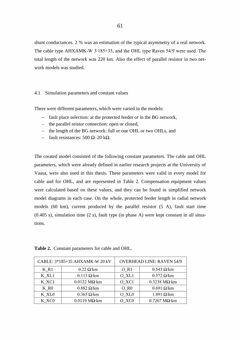
61

shunt conductances. 2 % was an estimation of the typical asymmetry of a real network.

The cable type AHXAMK-W ∙ 85 5, and the OH type Raven 54/9 were used. The

total length of the network was 220 km. Also the effect of parallel resistor in two net-

work models was studied.

4.1 Simulation parameters and constant values

There were different parameters, which were varied in the models:

fault place selection: at the protected feeder or in the BG network,

the parallel reistor connection: open or closed,

the length of the BG network: full or one OHL or two OHLs, and

fault resistances: 500 Ω–20 kΩ.

The created model consisted of the following constant parameters. The cable and OHL

parameters, which were already defined in earlier research projects at the University of

Vaasa, were also used in this thesis. These parameters were valid in every model for

cable and for OHL, and are represented in Table 2. Compensation equipment values

were calculated based on these values, and they can be found in simplified network

model diagrams in each case. On the whole, protected feeder length in radial network

models (60 km), current produced by the parallel resistor (5 A), fault start time

(0.405 s), simulation time (2 s), fault type (in phase A) were kept constant in all situa-

tions.

Table 2. Constant parameters for cable and OHL.

CABLE: 3*185+35 AHXAMK-W 20 kV OVERHEAD LINE: RAVEN 54/9

K_R1 0. Ω/km O_R1 0.54 Ω/km

K_XL1 0. Ω/km O_XL1 0. 7 Ω/km

K_XC1 0.0 MΩ∙km O_XC1 0. 8 MΩ∙km

K_R0 0.88 Ω/km O_R0 0.69 Ω/km

K_XL0 0. 65 Ω/km O_XL0 .89 Ω/km

K_XC0 0.0119 MΩ∙km O_XC0 0.7267 MΩ∙km

62

4.2 Simulation models

There were four different simulated network model types. Cabled radial network (simu-

lated already earlier relating to Jaakkola (2012), mixed and cabled radial networks with

recloser and ring-shaped network. In the next following sections, all network models are

introduced. In each case, the simplified diagrams of the networks are presented. Be-

cause partly decentralized compensation was used, in addition to central coil, there were

also several locally installed coils along the feeders. However, due to graphical reasons

only one local coil for compensating each feeder in the diagrams was drawn. The calcu-

lated relay settings for each case can be found in Appendices 2–3.

4.2.1 Cabled radial network

In this case the already existing simulated results of the radial network model by Jaak-

kola (2012) were used. In this simulation model, which is presented in Fig. 26, the be-

ginning (10 km) of the feeders were centrally compensated. The parallel resistor was

continuously closed, there was not a recloser at the middle point of the protected feeder,

and the rest of the feeders were decentrally compensated in every 10 km. Fault re-

sistances were: 500 Ω, 000 Ω, 000 Ω, 5000 Ω, 0 kΩ, and 20 kΩ. The fault locations

were at the beginning of the feeder (1), at the end of the feeder (5), and in the BG net-

work (9) or (7). Fig. 26 illustrates also the capacitive earth fault currents produced by

the feeders, the resisitive earth fault current IR produced by the parallel resistor, and the

inductive current of the central compensation coil. Moreover, the number of decentrally

installed compensation coils and their inductive currents can be found in Fig. 26.

63

Figure 26. Simplified diagram of cabled radial network model.

Varying compensation degrees and feeder lengths were simulated earlier, but simulation

cases with 0.9 compensation degree and 60 km feeder length at three fault points in case

of full BG network, and BG network consisting of only two OHLs were chosen for fur-

ther analysis. In order to set reliable earth fault protection, it is important to calculate the

desired quantities of zero sequence voltage and residual current with the smallest and

largest network situations. The full BG situation was examined in order to find the

smallest detectionable zero sequence voltage. When BG network consists of only one

OHL, the smallest residual current value can be defined. However, in this case the re-

sults of the BG network comprising two OHLs were utilized. BG network consisting of

two OHLs illustrates now the smallest detectionable zero sequence current at the pro-

tected feeder. Therefore, it has to be remembered that the results from BG network con-

sisting two OHLs are slightly higher than the desired in case of BG network consisting

only one OHL. Based on the results from these simulations, the performance of phase

64

angle and admittance criterion was analysed, and the results can be found in Section 5.1.

The chosen threshold settings of relays, which were used in analysis, can be found in

Tables 3–4.

Table 3. Relay settings in case of phase angle criterion in cabled radial network.

Phase angle criterion settings

Uoh (V) 4 % ≈ 460

Ih (A) 1

± ∆φ (°) ± 80

φ0 (°) 0

Table 4. Relay settings in case of admittance criterion in cabled radial network.

Admittance criterion settings

Conductance forward (mS) 0.09

Conductance reverse (mS) -1.0

Susceptance forward (mS) 0.1

Susceptance reverse (mS) -5.67

Uoh (V) 4 % ≈ 460

Ih (A) 0.5

4.2.2 Mixed radial network with recloser

In this model the main difference compared to the earlier radial network model was the

recloser place at the middle point of the protected feeder. The beginning of the protected

feeder (30 km) was cable. Moreover, the rest of the protected feeder (30 km) was re-

placed by OHL and there was one coil, which compensated this part of the feeder. The

first 10 km of the feeder were centrally compensated and the rest of the cable part was

decentrally compensated in every 5 km. The above mentioned differences compared to

radial network model can be found in Fig. 27. Fig. 27 shows also the capacitive earth

fault currents of each feeder, the inductive currents produced by decentrally installed

65

compensation coils and the number of those in each feeder, the inductive current of the

central coil, and the resistive current produced by the parallel resistor.

Figure 27. Simplified diagram of mixed radial network model with recloser.

In the BG network, there were six coils compensating the cable feeders, because the

length of the feeder was now 40 km, the decentrally compensated part was 30 km, and

the coil density was 5 km. OHL feeders in the BG network were compensated by one

coil in both feeders located at the middle of the feeder. Two different cases were simu-

lated in this model: full BG network and BG network consisting only one OHL. Fault

resistances were: 500 Ω, 000 Ω, 500 Ω, 5000 Ω, 0 kΩ, and 0 kΩ. The fault loca-

tions were at the beginning of the feeder (1), at the middle of the feeder (3) at the end of

the feeder (5), and in the BG network (9) or (6). The results from the analysis of the pro-

tection schemes can be found in Section 5.2. The chosen threshold settings of relays can

be found in Tables 5–6.

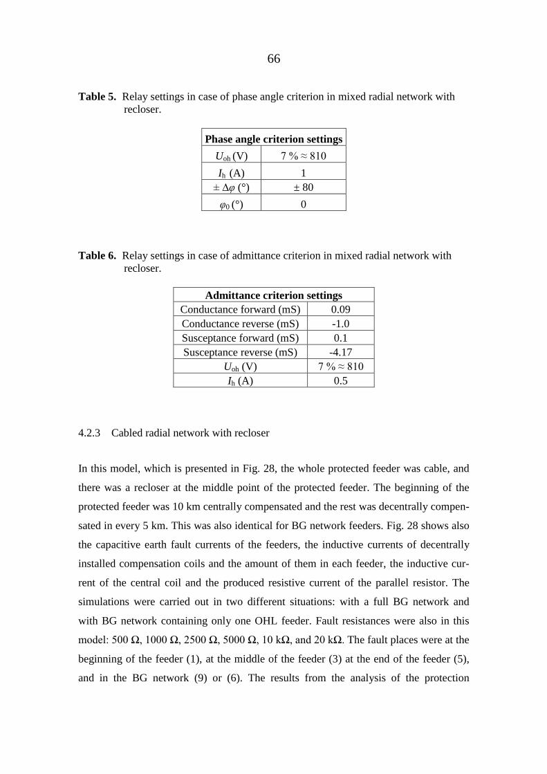
66

Table 5. Relay settings in case of phase angle criterion in mixed radial network with

recloser.

Phase angle criterion settings

Uoh (V) 7 % ≈ 8 0

Ih (A) 1

± ∆φ (°) ± 80

φ0 (°) 0

Table 6. Relay settings in case of admittance criterion in mixed radial network with

recloser.

Admittance criterion settings

Conductance forward (mS) 0.09

Conductance reverse (mS) -1.0

Susceptance forward (mS) 0.1

Susceptance reverse (mS) -4.17

Uoh (V) 7 % ≈ 8 0

Ih (A) 0.5

4.2.3 Cabled radial network with recloser

In this model, which is presented in Fig. 28, the whole protected feeder was cable, and

there was a recloser at the middle point of the protected feeder. The beginning of the

protected feeder was 10 km centrally compensated and the rest was decentrally compen-

sated in every 5 km. This was also identical for BG network feeders. Fig. 28 shows also

the capacitive earth fault currents of the feeders, the inductive currents of decentrally

installed compensation coils and the amount of them in each feeder, the inductive cur-

rent of the central coil and the produced resistive current of the parallel resistor. The

simulations were carried out in two different situations: with a full BG network and

with BG network containing only one OHL feeder. Fault resistances were also in this

model: 500 Ω, 000 Ω, 500 Ω, 5000 Ω, 0 kΩ, and 0 kΩ. The fault places were at the

beginning of the feeder (1), at the middle of the feeder (3) at the end of the feeder (5),

and in the BG network (9) or (6). The results from the analysis of the protection

67

schemes can be found in Section 5.3. The chosen threshold settings of relays, which

were utilized in this model type, can be found in Tables 7–8.

Figure 28. Simplified diagram of cabled radial network model with recloser.

Table 7. Relay settings in case of phase angle criterion in cabled radial network with

recloser.

Phase angle criterion settings

Uoh (V) 7 % ≈ 810

Ih (A) 1

± ∆φ (°) ± 80

φ0 (°) 0

68

Table 8. Relay settings in case of admittance criterion in cabled radial network with

recloser.

Admittance criterion settings

Conductance forward (mS) 0.09

Conductance reverse (mS) -1.0

Susceptance forward (mS) 0.1

Susceptance reverse (mS) -4.73

Uoh (V) 7 % ≈ 8 0

Ih (A) 0.5

4.2.4 Ring-shaped network

In addition to traditional configurations of typical radial MV distribution network mod-

els, the closed ring-shaped model was also created. Because the structure of this kind of

network is rather exceptional compared to traditional radial network models, the aim of

this network model was mainly to study how the protection methods behave during dif-

ferent fault locations with varying fault resistances in this kind of unique network situa-

tion. In this case the threshold settings of relays were unimportant and therefore not

considered more thoroughly.

The total length of the protected ring was 120 km. Fig. 29 shows the ring-shaped net-

work model with the capacitive earth fault currents of the ring and the BG feeders, the

inductive currents of decentrally installed compensation coils and the amount of those

in each feeder and in the protected ring, and the inductive current of the central coil and

the resistive current of the parallel resistor. The model was used to simulate relay quan-

tities both at the beginning of the ring’s other end (lower in the Fig. 29), and at the mid-

dle point of the ring, 60 km from the beginning. The ring was compensated centrally

10 km from the beginning of both ends. The first halves of the both ends were cabled

and they were compensated in every 5 km after the part covered with centralized com-

pensation. The rest (the middle part of the ring) was OHL, and there were two coils for

compensating 30 km. Compensation coils were placed in the middle of the OHL parts.

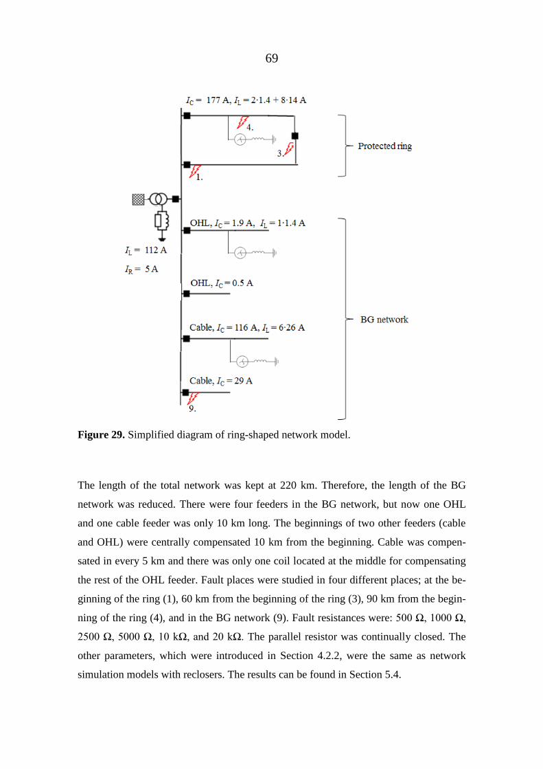
69

Figure 29. Simplified diagram of ring-shaped network model.

The length of the total network was kept at 220 km. Therefore, the length of the BG

network was reduced. There were four feeders in the BG network, but now one OHL

and one cable feeder was only 10 km long. The beginnings of two other feeders (cable

and OHL) were centrally compensated 10 km from the beginning. Cable was compen-

sated in every 5 km and there was only one coil located at the middle for compensating

the rest of the OHL feeder. Fault places were studied in four different places; at the be-

ginning of the ring (1), 60 km from the beginning of the ring (3), 90 km from the begin-

ning of the ring (4), and in the BG network (9). Fault resistances were: 500 Ω, 000 Ω,

500 Ω, 5000 Ω, 0 kΩ, and 0 kΩ. The parallel resistor was continually closed. The

other parameters, which were introduced in Section 4.2.2, were the same as network

simulation models with reclosers. The results can be found in Section 5.4.

70

5 SIMULATION RESULTS

After the simulations, the results were gathered from separate files created by the multi-

run blocks. Next they were brought into Excel for processing and excecuting essential

calculations. Finally, the graphs for the protection schemes, phase angle and admittance

criteria were created with Matlab® calculation program. Two scripts were created,

which can be found in Appendix 4. Following the conventional way to illustrate the

phase angle criterion the graphs were drawn so that the phase angle (φ = 0°) corre-

sponded to the direction of positive y-axis. In case of phase angle criterion, the faults

with varying fault resistances were located in such a way that the larger the fault re-

sistance is, the closer it is to the threshold setting boundary and origin. In the admittance

criterion the effect of fault resistance is in some cases negligible, which was also proved

earlier in the admittance theory-section. However, in practise considering also the Uoh-

condition, the fault resistance may impact on the protection sensitivity.

There were apprx. 500 simulation runs executed in this study. To help this time-

consuming process to simulate all situations, multirun-block was used. Multirun simu-

lates automatically all possible combinations according to user’s de initions, and save

the data into a separate file. Using multirun also the human errors can be minimized.

Two multirun-blocks for measuring magnitudes of 3I0 and U0 and phase angles of both

at the beginning of the protected feeder and at the middle point of the protected feeder

were used.

Results for different fault locations were marked by different colours. In cabled radial

network, there was no fault location at the middle of the feeder. The colour codes were:

blue equaled to begin, green equaled to end, and red equaled to BG network. In mixed

and cabled networks with reclosers: blue equaled to begin, green equaled to middle, cy-

an equaled to end, and red equaled to BG network. In the ring-shaped model: blue

equaled to begin, green equaled to middle (60 km from the beginning), cyan equaled to

end (90 km from the beginning), and red equaled to BG network. In some graphs, the

calculated results have only little variation, which can be observed by seeing only one

or possible two colour marked results in graphs. It was noticed that the calculations for

71

0 kΩ were exactly the same as the results in case of 0 kΩ faults even though they

should not equal. This must be accounted for the asymmetry (2 %), which was created

to network model. After a certain point, in this case when the fault resistance was above

0 kΩ, the value of fault resistance became insignificant. In practise, the maximum fault

resistance value, which the computer was able to simulate, and was used in calculations,

was 0 kΩ.

5.1 Cabled radial network

Two different simulations were carried out with this model. The network was first simu-

lated by full BG network situation; i.e. consisting of all four feeders and then BG net-

work consisting of only two OHLs. The operations of phase angle and admittance crite-

ria were analyzed according to these situations assuming relay location at the beginning

of the feeder. The results from these two network topologies can be found in the follow-

ing sections.

5.1.1 Full background network

In case of a full BG network, the phase angle criterion is illustrated in Fig. 30 and the

admittance criterion in Fig. 31. The simulated results and calculated protection quanti-

ties can be found in Table 9. According to Fig. 30 and Table 9, the faults at the begin-

ning of the feeder and the end of the feeder were detected up to 000 Ω by phase angle

criterion with the setting applied. The sensitivity is limited by the magnitude of the re-

sidual current, because current threshold setting was exceeded after Rf equaled to

000 Ω, compared to magnitudes of U0, which would have allowed the faults with

5000 Ω ault resistances to be detected. The faults in the BG network were located cor-

rectly outside the operating sector. According to Fig. 31, and considering the magni-

tudes of U0 in Table 9 and the set minimum Ih-condition, admittance protection method

detected the faults at the protected feeder up to 3000 Ω and they located correctly out-

side the box, whereas the BG network faults were located inside the box, where relay

operation was restrained.

72

Figure 30. Phase angle criterion in cabled radial network in a full BG network situa-

tion.

Figure 31. Admittance criterion in cabled radial network in a full BG network situa-

tion.

73

Table 9. Results and current and voltage thresholds in cabled radial network in a full

BG network situation.

5.1.2 Two overhead lines in the background network

When there were only two OHLs in the BG network, it was possible to detect all faults

at the protected feeder with phase angle protection method up to 20 kΩ 0 kΩ) accord-

ing to Table 10, and Fig 32. Faults in the BG network were located correctly outside the

operating sector, because the phase angle differences were varied between -9 …-94°.

Because of the size of the whole network was smaller, the magnitudes of U0 were higher

compared to full BG network situation.

Fault place Fault resistance (Ω) U 0 Mag (V) 3I 0 Mag (A) Phase Angle (deg) Y 0 Mag (mS)

1 500 5017.031 2.891 -5.030 0.576

1 1000 2809.722 1.596 -5.866 0.568

1 3000 1010.495 0.549 -13.059 0.543

1 5000 611.089 0.353 -14.584 0.578

1 10000 298.208 0.220 -11.626 0.737

1 20000 298.208 0.220 -11.626 0.737

5 500 4938.656 2.848 -4.956 0.577

5 1000 2775.013 1.582 -5.915 0.570

5 3000 999.437 0.547 -12.721 0.547

5 5000 603.427 0.350 -13.819 0.580

5 10000 292.799 0.217 -10.098 0.740

5 20000 292.799 0.217 -10.098 0.740

9 500 5016.925 19.507 -92.237 3.888

9 1000 2809.663 10.926 -92.253 3.889

9 3000 1010.473 3.911 -92.294 3.870

9 5000 611.075 2.365 -92.999 3.870

9 10000 298.201 1.161 -95.743 3.892

9 20000 298.201 1.161 -95.743 3.892

Radial network Part 10 km

Admittance criterion Phase angle criterion

U oh = 460 V U oh = 460 V

I h = 1 AI h = 0.5 A

Relay settings:

74

Table 10. Results and current and voltage thresholds in cabled radial network with two

OHLs in the BG network.

Figure 32. Phase angle criterion in cabled radial network with two OHLs.

Fault place Fault resistance (Ω) U 0 Mag (V) 3I 0 Mag (A) Phase Angle (deg) Y 0 Mag (mS)

1 500 7524.575 17.134 -77.974 2.277

1 1000 4996.928 11.382 -77.716 2.278

1 3000 1972.967 4.506 -76.696 2.284

1 5000 1201.631 2.757 -75.665 2.294

1 10000 589.484 1.380 -73.080 2.341

1 20000 589.484 1.380 -73.080 2.341

5 500 7463.247 16.992 -77.961 2.277

5 1000 4965.598 11.306 -77.701 2.277

5 3000 1955.501 4.460 -76.661 2.281

5 5000 1187.491 2.719 -75.598 2.289

5 10000 578.396 1.349 -72.882 2.331

5 20000 578.396 1.349 -72.882 2.331

7 500 7524.410 29.215 -92.103 3.883

7 1000 4996.820 19.409 -92.248 3.884

7 3000 1972.925 7.668 -92.726 3.887

7 5000 1201.605 4.669 -93.212 3.886

7 10000 589.472 2.282 -94.668 3.871

7 20000 589.472 2.282 -94.668 3.871

I h = 0.5 A I h = 1 A

Radial network Part 10 km 2 OHL

Admittance criterion Phase angle criterion

U oh = 460 V U oh = 460 V

Relay settings:

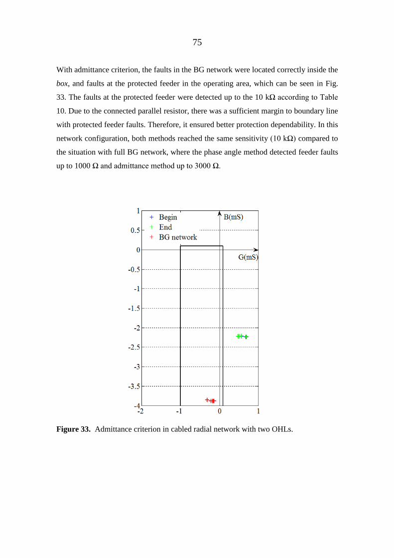
75

With admittance criterion, the faults in the BG network were located correctly inside the

box, and faults at the protected feeder in the operating area, which can be seen in Fig.

33. The faults at the protected feeder were detected up to the 10 kΩ according to Table

10. Due to the connected parallel resistor, there was a sufficient margin to boundary line

with protected feeder faults. Therefore, it ensured better protection dependability. In this

network configuration, both methods reached the same sensitivity 0 kΩ) compared to

the situation with full BG network, where the phase angle method detected feeder faults

up to 1000 Ω and admittance method up to 000 Ω.

Figure 33. Admittance criterion in cabled radial network with two OHLs.

76

5.2 Mixed radial network with recloser

In in this situation, there were simulated eight different cases with phase angle and ad-

mittance criteria the relay locations at the beginning of the feeder and at the middle of

the feeder. The purpose was to study the earth fault protection performance in case of

the smallest and the largest network situations. Therefore, the network was simulated

with full BG, and with only one OHL connected in the BG network. In these cases the

parallel resistor was either connected or disconnected. The results from these situations

can be found in the following sections. The simulation results from each case can be

found in Appendix 5.

5.2.1 Full background network

Phase angle criterion in case of relay located at the beginning of the protected feeder

As can be seen from the Fig. 34, when the parallel resistor was not connected, the faults

at the protected feeder (begin, middle, end) were detected only with fault resistance be-

ing 5000 Ω. In case of 500– 500 Ω feeder faults, the phase angle was smaller than -80°,

and in case of 10 kΩ aults, the magnitudes of U0 were too small to be detected, when

faults were located in the beginning of the feeder. Respectively, the magnitude of the

residual current was too small with the magnitude of U0 faults locating at the middle

and the end of the feeder. It can be concluded that the results are only theoretical, and

the phase angle criterion is incapable of detecting the above mentioned faults. When the

resistance was connected in Fig. 35, faults at the protected feeder were detected up to

5000 Ω. 0 kΩ faults were not detected because of the magnitudes of U0 and 3I0 did not

exceed the threshold settings.

77

Figure 34. Phase angle criterion in a full BG situation at the beginning of the feeder,

when RL was not connected.

Figure 35. Phase angle criterion in a full BG situation at the beginning of the feeder,

when RL was connected.

Admittance criterion in case of relay located at the beginning of the protected feeder

According to Fig. 36, when the parallel resistor was not connected, the BG network

faults were located correctly in the non-operating zone (inside the box). The faults at the

protected feeder were detected up to 5000 Ω according to calculated admittance values

from Appendix 5, and also considering the thresholds. According to Fig. 37, when the

parallel resistor (producing 5 A resistive current) was connected, the faults located at the

protected feeder were detected up to 5000 Ω, as it was without the parallel resistor con-

nection above. There was a sufficient margin in this case to boundary line ensuring the

78

better protection dependability and provides more margin for possible errors in meas-

urements.

Figure 36. Admittance criterion in a full BG situation at the beginning of the feeder,

when RL was not connected.

79

Figure 37. Admittance criterion in a full BG situation at the beginning of the feeder,

when RL was connected.

Phase angle criterion in case of relay located at the middle of the protected feeder

When studied phase angle criterion for a relay located at the middle point of the protect-

ed feeder, only the faults in a forward direction, i.e at the end of the feeder, should be

detetced. In case of RL was not connected, see Fig. 38, the fault at the end of the feeder

with 5000 Ω ault resistance was only detected. In case of 500– 500 Ω aults, the phase

angle condition was not achieved, and with 10 kΩ the magnitude o U0 did not exceed

the Uoh. This kind of result can be assumed to be only theoretically valid, and it is likely

that earth fault protection does not detect the faults in this situation at all. Faults at the

beginning and at the middle of the protected feeder were located correctly with BG net-

work faults in the non-operating zone.

80

Figure 38. Phase angle criterion in a full BG situation at the middle point of the feeder,

when RL was not connected.

After the parallel resistor connection according to Fig. 39, and considering also the Uoh-

condition, the faults located at the end of the protected feeder were detected from 500 Ω

up to 5000 Ω. It can be seen that the network situation seen by the relay refers to isolat-

ed neutral network. This should be considered by setting the relay characteristic angle to

90°, when it responds to isolated neutral network situation or set extended operating

sector. When the fault is located in a reverse direction, the feeder does not seem to pro-

duce current at all, which means that the feeder is almost completely compensated.

Figure 39. Phase angle criterion in a full BG situation at the middle point of the feeder,

when RL was connected.

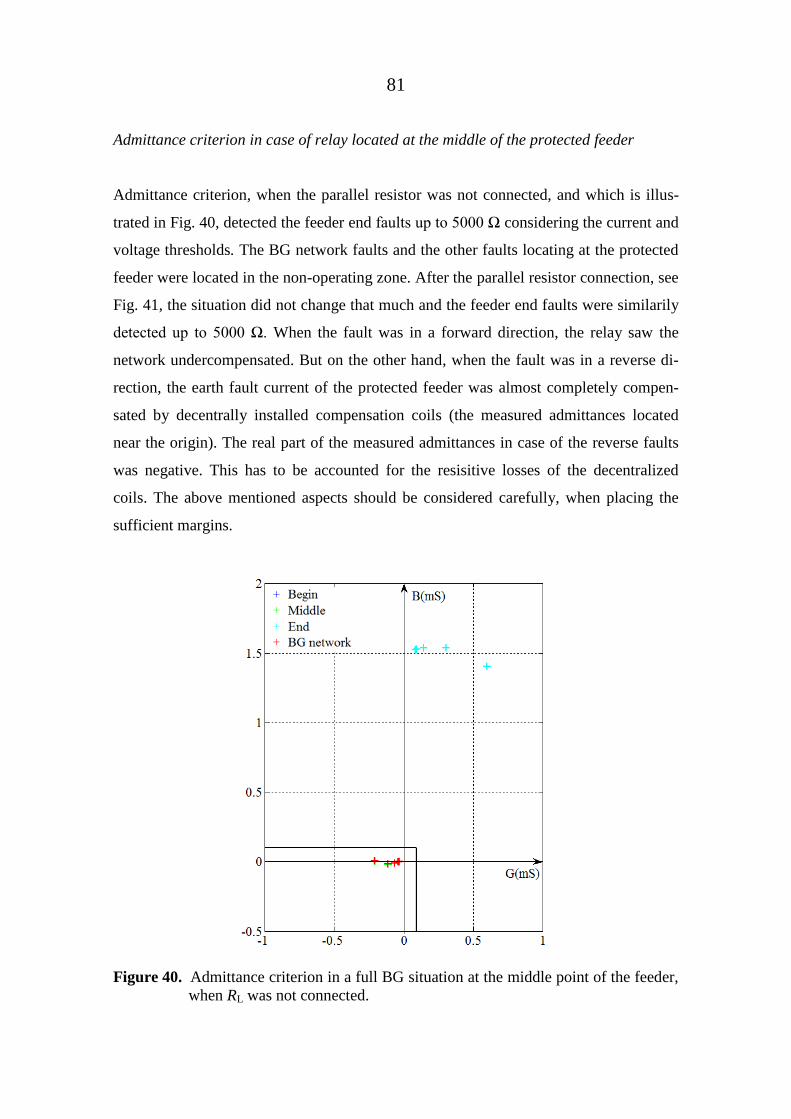
81

Admittance criterion in case of relay located at the middle of the protected feeder

Admittance criterion, when the parallel resistor was not connected, and which is illus-

trated in Fig. 40, detected the feeder end aults up to 5000 Ω considering the current and

voltage thresholds. The BG network faults and the other faults locating at the protected

feeder were located in the non-operating zone. After the parallel resistor connection, see

Fig. 41, the situation did not change that much and the feeder end faults were similarily

detected up to 5000 Ω. When the fault was in a forward direction, the relay saw the

network undercompensated. But on the other hand, when the fault was in a reverse di-

rection, the earth fault current of the protected feeder was almost completely compen-

sated by decentrally installed compensation coils (the measured admittances located

near the origin). The real part of the measured admittances in case of the reverse faults

was negative. This has to be accounted for the resisitive losses of the decentralized

coils. The above mentioned aspects should be considered carefully, when placing the

sufficient margins.

Figure 40. Admittance criterion in a full BG situation at the middle point of the feeder,

when RL was not connected.

82

Figure 41. Admittance criterion in a full BG situation at the middle point of the feeder,

when RL was connected.

5.2.2 One overhead line in the background network

Phase angle criterion in case of relay located at the beginning of the protected feeder

When only one OHL was connected in the BG network without the parallel resistor,

faults at the protected feeder and in the BG network remained undetected. Phase angles

were smaller than -80° according to Fig. 42. After the parallel resistor connection in Fig.

43, the phase angles of the feeder faults were turned into operating sector. Now it was

possible to detect even the highest fault resistance feeder faults. The BG network faults

were not detected due to phase angles of being still smaller than -80°. Because there

was now only one OHL connected in the BG network, the system was seen by the relay

overcompensated due to smaller capacitive strength of the BG network according to

83

Figs. 42–43. It can be also seen in Fig. 43 that the feeder faults are located near the op-

erating sector, because of the phase angles. This might endanger the functioning of the

protection, if errors would arise.

Figure 42. Phase angle criterion in case of only one OHL in the BG network at the be-

ginning of the feeder, when RL was not connected.

Figure 43. Phase angle criterion in case of only one OHL in the BG network at the be-

ginning of the feeder, when RL was connected.

Admittance criterion in case of relay located at the beginning of the protected feeder

As it was noticed earlier in case of phase angle criterion, the capacitance of the BG net-

work was small, and hence the network was seen by the relay overcompensated. The

admittance-based protection method did not detect the feeder faults, because the calcu-

84

lated admittances were located inside the box, which was referring to non-operating

zone according to Fig. 44. When the parallel resistor was connected, see Fig 45, the ad-

mittance-based protection method detected feeder faults up to 10 kΩ and network

faults were located correctly in the non-operating zone. It can be noticed that the resis-

tive losses of the BG network were small, which could cause problems to detect the

feeder faults without the parallel resistor. By connecting the parallel resistor, the resis-

tive current is increased, which facilitate the detection of the feeder faults according to

Fig. 45.

Figure 44. Admittance criterion in case of only one OHL in the BG network at the be-

ginning of the feeder, when RL was not connected.

85

Figure 45. Admittance criterion in case of only one OHL in the BG network at the be-

ginning of the feeder, when RL was connected.

Phase angle criterion in case of relay located at the middle of the protected feeder

Phase angle criterion considered for a relay located at the middle point of the feeder

should be able to detect only the feeder end faults. When the parallel resistor was not

connected, only the feeder end fault was detected, when Rf equaled to 5000 Ω, see Fig.

46. The phase angle was located very near (79.62°) the boundary (80°) and therefore, it

would be very vulnerable to even minor errors turning the phasor in the non-operating

zone. With 500– 500 Ω aults, the limiting factor was the phase angle, and with 10 kΩ

faults the residual current. It can be concluded that the protection is incapable of detect-

ing the fault locating at the end of the protected feeder.

86

Figure 46. Phase angle criterion in case of only one OHL in the BG network at the

middle point of the feeder, when RL was not connected.

When the parallel resistor was connected in Fig. 47, the feeder end faults were detected

up to 5000 Ω considering the threshold voltage to be exceeded. In addition to BG net-

work faults, the other feeder faults (begin and middle) were located also in the non-

operating zone. It seems that the earth fault current of the protected feeder was almost

completetly compensated by its own decentralized compensation coils, when the fault

was in a reverse direction.

87

Figure 47. Phase angle criterion in case of only one OHL in the BG network at the

middle point of the feeder, when RL was connected.

Admittance criterion in case of relay located at the middle of the protected feeder

The admittance method detected the feeder end faults up to the largest fault resistances,

which is illustrated in Fig. 48, even without the parallel resistor connection. Other faults

at the protected feeder (in the first half) and in the BG network were not detected, which

showed protection to be selective. After the parallel resistor connection, which is illus-

trated in Fig. 49, the highest fault resistance faults were detected similarily as in case of

without the parallel resistor connection. However, it can be noticed in Fig. 49 that the

calculated admittances of the BG network faults and other feeder faults moved to the

positive side of the y-axis. Similarily, with some fault resistances in case of feeder and

BG network faults, this kind of behaviour was noticed earlier in Fig. 40 and 41. Usually,

the value of the BG network admittance is very small and negative, and due to natural

unbalances and errors, the susceptance, i.e. the imaginary part, may therefore turn into

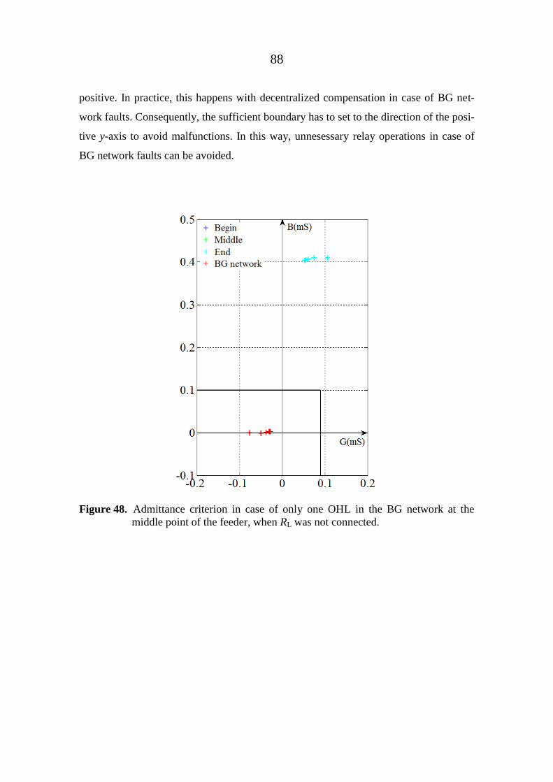
88

positive. In practice, this happens with decentralized compensation in case of BG net-

work faults. Consequently, the sufficient boundary has to set to the direction of the posi-

tive y-axis to avoid malfunctions. In this way, unnesessary relay operations in case of

BG network faults can be avoided.

Figure 48. Admittance criterion in case of only one OHL in the BG network at the

middle point of the feeder, when RL was not connected.

89

Figure 49. Admittance criterion in case of only one OHL in the BG network at the

middle point of the feeder, when RL was connected.

5.3 Cabled radial network with recloser

With the cabled radial network with recloser the same situations than in mixed radial

network with recloser in Chapter 5.2 were simulated. The simulated results from these

situations were created in both protection methods, but it was noticed there were no sig-

nificant differences in each situation compared to mixed radial network model regarding

the sensitivity of the protection schemes. Therefore, most of the results of this model are

not analyzed again. The simulated and calculated results from each case can be found in

Appendix 6. However, when only one OHL feeder was connected in the BG network

and studied at the beginning of the protected feeder without the parallel resistor, the

admittance criterion detected only the highest ault resistance eeder aults 0 kΩ) ac-

cording to Figures 50–51 and Appendix 6.

90

Figure 50. Admittance criterion in cabled network in case of one OHL in the BG net-

work at the beginning of the feeder, when RL was not connected.

Figure 51. Close-up of the admittance criterion in cabled network in case of one OHL

in the BG network at the beginning of the feeder, when RL was not connect-

ed.

91

Moreover, in case of one OHL in the BG network studied at the middle point of the pro-

tected feeder, the admittances of the BG network were measured minus-signed accord-

ing to Fig. 52–53, compared to mixed protected feeder situation, see Fig. 48–49. Earth

fault protection with admittance method was in this case more reliable, and there was no

concern about reaching the positive side of the y-axis and possible maloperations.

Figure 52. Admittance criterion in cabled network in case of one OHL in the BG net-

work at the middle point of the feeder, when RL was not connected.

92

Figure 53. Admittance criterion in cabled network in case of one OHL in the BG net-

work at the middle point of the feeder, when RL was connected.

5.4 Ring-shaped network

Two different cases with phase angle criterion and admittance criterion were simulated

at the beginning and at the middle of the protected ring. The simulation results can be

found in Appendix 7. Even though the network model is rather simple setting reliable

E/F protection is problematic. This is due to real component of the earth fault current

divided into two parts. In practice, real networks are divided into smaller radial zones by

breakers in case of faults emerge or it is used communication connection between re-

lays, which help relays to detect the faulted part. Consequently, the above mentioned

procedures facilitate earth fault protection to function correctly. (ABB 2011: 15–16.)

Because the network topology was in this case rather different compared to traditional

network topologies, the aim was only to study the behaviour of the earth fault quanti-

ties. Instead the settings from the case mixed radial network with recloser were used for

illustrative purposes.

93

Relay located at the beginning of the protected ring

According to Fig. 54, where the phase angle criterion at the beginning of the protected

ring is presented, only the closest forward faults (begin), could be detected. Other faults

(60 km from the beginning equaled to middle, and 90 km from the beginning equaled to

end) further along the ring were not detected. On the contrary, the admittance method

could detect further faults (begin and middle) at the protected ring, including the faults

at the end of the feeder (from 90 km from the beginning) according to Fig. 55. Howev-

er, it was noticed the further the fault, the closer the value was to the conductance for-

ward boundary line. Because the ring was divided in two protection zones, the feeder

fault (end) should be detected at the middle point and thus, the conductance forward

boundary line should be placed in Fig. 55 to cover also the feeder faults (end), so that

they would be located in the non-operating zone. Consequently, it would need careful

placing of the conductance forward boundary line or possibly also tilting the line.

Figure 54. Phase angle criterion in ring-shaped network at the beginning of the pro-

tected ring.

94

Figure 55. Admittance criterion in ring-shaped network at the beginning of the protect-

ed ring.

Relay located at the middle of the protected ring

Phase angle criterion studied at the middle of the protected ring, which is illustrated in

Fig. 56, could detect only the forward faults (end). In case of reverse faults, they were

located correctly in the non-operating area. Similarily, the admittance method, see Fig.

57, was capable to detect only forward faults (end). The admittance method measured

the reverse faults (begin and end) at the protected ring, and they were located into the

non-operating zone. The measured admittances of BG network faults were positive with

respect to both real and imaginary axes, which would be challenging when placing suf-

ficient boundaries to the box-characteristic considering these two directions to avoid

false trippings.

95

Figure 56. Phase angle criterion in ring-shaped network at the middle point of the pro-

tected ring.

Figure 57. Admittance criterion in ring-shaped network at the middle point of the pro-

tected ring.

96

5.5 Error analysis

The effect of errors in measurements on E/F protection was analysed in one situation,

where the BG network was the largest, and the parallel resistor was continuously con-

nected. This case was chosen, because it responded a real network situation. The calcu-

lated phase angle error limits, which can be also found in Appendix 8, were added then

into the same protection graphs with the original results for further analysis.

As it was mentioned earlier about errors in measurements, there are errors in current,

voltage and phase angle measurements. However, the current and voltage errors are

very small, hence only the phase angle measurement errors may have an impact on the

functioning of the protection. Therefore, the error calculations were studied only assum-

ing that the phase angle errors were apprx. ± 5°. In practice, the phase angle error can be

assumed to be in real networks apprx. ± 3° according to Wahlroos (2014). Therefore,

the error calculations presented here can be considered as worst case estimates. The re-

sults including errors are illustrated both with phase angle criterion and admittance cri-

terion, see Fig. 58 and 59, where the original results are marked by crosses and calculat-

ed error limits by dots.

According to Fig. 58, where the calculated -5° phase angle errors in case of faults locat-

ed at the protected feeder, are located more near the operating sector, because the phase

angle is now smaller. On the other hand, when the fault is located in the BG network,

the -5° phase angle errors turn the fault more clearly away from the operating sector,

which is beneficial. Positive phase angle error is respectively beneficial in case of fault

locating at the protected feeder, whereas the BG network fault might get closer to oper-

ating sector. It can be concluded that the calculated errors did not turn the feeder faults

to the non-operating zone even the calculated errors represented the worst case esti-

mates. In this situation it can be seen the reason why parallel resistor should be connect-

ed. The increased resisitive component of the residual current facilitates the protection

to be selective by turning the current phasor more into the operating sector.

97

Figure 58. Error analysis of phase angle criterion.

Fig. 59 shows the admittance criterion in each fault place with varying fault resistances,

where the calculated phase angle error limits (± 5°) are marked. It can be seen that the

feeder faults were not affected substantially. Nonetheless, those faults are still detected

if errors would arise. The negative-signed phase angle error could decrease the reliabil-

ity of the fault detection in case of fault locating at the protected feeder if the conduct-

ance forward boundary would not be carefully set. Moreover, the positive phase angle

error in the BG network faults might turn the calculated admittances falsely to operating

area according to Fig. 59, where the calculated admittances with errors are exceeding

the set conductance forward boundary. It has to be remembered that calculated error

values represent the worst case values, and real errors can be assumed to be a bit small-

er.

98

Figure 59. Error analysis of admittance criterion.

99

6 CONCLUSIONS AND FURTHER STUDIES

The aim of this thesis was to find out how earth fault protection should be arranged with

defined fault scenarios in different MV distribution networks and what is the protection

sensitivity that can be reached. The network model was studied with mixed and cabled

structures using partly decentralized compensation. Moreover, the effects of phase angle

errors in measurements on protection were studied in one case. The simulations were

carried out by using PSCAD network modelling tool.

Earth fault protection was studied by using two different protection methods: traditional

phase angle criterion and novel admittance criterion in four different MV distribution

network simulation models. In cabled radial network with full BG network, i.e. consist-

ing of all four feeders, the admittance method detected feeder faults up to 3000 Ω,

whereas the phase angle criterion reached only up to 000 Ω. When the BG network

was reduced to contain only two OHLs, both methods were able to detect even the

highest fault resistance feeder faults.

In case of mixed and cabled radial network with recloser, the protected feeder was now

studied in addition at the beginning also at the middle point of protected feeder. It was

noticed that most of the results corresponended between these two networks by earth

fault protection sensitivity point of view. And by that, there were no significant differ-

ences either the protected feeder was mixed or totally cabled. According to results

gained from full BG network situation, where earth fault protection was studied at the

beginning of the feeder and the parallel resistor was connected, feeder faults with both

methods were detected up to 5000 Ω. Even without the parallel resistor connection, ad-

mittance criterion achieved the same sensitivity, but it was interesting that phase angle

criterion detected only the feeder faults, when fault resistance was 5000 Ω. With lower

fault resistances the phase angles were not between ± 80°. In the same way behaved the

results achieved from the middle point of the feeder, where the selective protection

method detected now only forward feeder faults. In these simulations faults were locat-

ed at the end of the protected feeder. The results can be assumed to be only theoretical,

100

which would mean that earth fault protection is incapable of detecting these faults in

real situation.

When there was only one OHL in the BG network and the parallel resistor was not con-

nected, both methods were not able to detect feeder faults. But when the protected feed-

er contained only cable, admittance criterion detected only the feeder faults with 0 kΩ

fault resistances. As a result, the protection is not able to detect the faults in real situa-

tion in this case. When studied at the middle of the protected feeder and without the

parallel resistor connection, the fault at the end of the feeder was detected only when the

fault resistance was 5000 Ω by phase angle criterion. This result can be also assumed to

be only theoretical. The admittance method detected all the feeder end faults and simi-

larily, when RL was connected. When the parallel resistor was connected, phase angle

criterion detected aults rom 500 Ω up to 5000 Ω. When the BG network was contain-

ing only one or two OHLs, feeder faults were located near the boundary line of the op-

erating sector in the phase angle criterion. It refers that the BG network became over-

compensated. Therefore, it is recommended the tolerance range is not too narrow to

avoid malfunctions.

Phase angle boundary settings with Uoh was set a little higher (7 %) in case of mixed

and cabled radial networks with recloser than in cabled radial network (4 %) due to cho-

sen compensation degree (0.95). The zero sequence voltage was calculated to be higher

in mixed network with recloser than cabled network with recloser. It was set to equal in

both cases in order to achieve more clear representation of the results. In the same way

was done with Ih setting: 1 A in every situation despite the lower zero sequence current

value of cabled radial network. However, it was noticed if the current threshold was set

in that case e.g. to 0.2 A, the desired sensitivity would have been achieved. But in prac-

tice, this would not be reasonable, because the minimum current threshold value is

0.5 A within admittance criterion. It has to be remembered that such low values have to

be measured by cable type CT, and at some point the smaller the current magnitude is

the bigger is the effect of errors to measurement accuracy. Moreover, because there

were two OHLs in the BG network, it can be assumed that the values would have been

even smaller.

101

Earth fault protection was also studied by creating a protected, closed ring-shaped net-

work model, which was rather special case compared to traditional network topologies.

According to simulations, the results showed the admittance method could work with

forward faults, when it was studied at the beginning of the ring, but the further the fault

was, the closer it was located to conductance forward boundary line. Therefore, the set-

tings should be very accurate to avoid false starts. Because the ring was divided into

two protection zones, the further fault at the protected ring (90 km from the beginning)

should not be detected at the beginning. This could be handled by setting the conduct-

ance forward boundary line accurately to cover the feeder fault into the non-operating

zone. Consequently, it would be needed careful placing of the boundary line. When

studied at the middle point of the ring, admittance method seems to achieve better sensi-

tivity with forward fault than phase angle criterion. However, it cannot be stated that the

created network model would respond exactly to the situation in reality, and there is not

much of field test data or practical experience of this kind of network structure. There-

fore, achieved results from these simulations can not be compared to measured real val-

ues, and further to be reliable. Therefore, the results can be assumed to be only rough

estimates.

Partly decentralized compensation is studied yet fairly little, and experiences from it are

all mainly theoretical inspections. By simulation results of the residual current magni-

tudes gained from the created network models, matched quite well for calculated resid-

ual current magnitudes in each case. It was noticed that according to derived formula for

residual current magnitude, the amount of calculated residual current magnitude was

reduced, when the protected feeder was totally cabled ≈ .5 A) compared to situation,

when it contained OHL and cable ≈ .8 A). When compensation degree was lower

(0.9), the protected feeder was totally cabled and the local coils were installed in every

10 km (first simulated situation), the magnitude of residual current ≈ 0. A) was in this

case much smaller compared to above mentioned situations, where the coil density was

5 km and compensation degree was 0.95. Therefore, the derived formula can be as-

sumed to be valid, because also the simulated results at the protected feeder, which can

be found in Appendices 5 and 6, of the mixed and both cabled situations matched close-

ly to these values despite the small variations due to fault locations.

102

Error analysis was carried out by choosing the typical MV distribution network situa-

tion. According to error analysis of phase angle criterion, there were no significant

changes by fault detection point of view. In this situation, it can be noticed the relevance

of the parallel resistor. Connection of the parallel resistor eliminates the effect of errors

by increasing the resistive component and turning the residual current phasor even more

to the operating sector. It has to be remembered that calculated errors were the worst

case estimates. However, the error analysis of the admittance criterion showed that in

theory some of the BG network faults may be located falsely in the operating sector and

therefore cause maloperations. But, the calculated results of phase angle errors were a

bit larger than in real situations, which would not probably impact on the funtioning of

the protection. It is possible to avoid BG network faults to be located in the operating

zone by setting the conductance forward boundary line with sufficient margin.

It can be concluded that admittance criterion is very promising method detecting earth

faults even some cases without the parallel resistor connection. The box-shaped charac-

teristic was utilized in this thesis and simulations showed that it was valid in these net-

works. Many other admittance characteristics can be chosen, but the decentralized com-

pensation was considered in the box-characteristic, and it is valid if network would be-

have like isolated neutral networks. However, careful defining of the boundary lines

with conductance and susceptance forward values is needed. The minimum current

threshold should be considered. The Uoh-condition has to be also set above the healthy

state zero sequence voltage both with admittance and phase angle criterion to avoid

false starts. According to results achieved from these simulations, the other two bounda-

ries in admittance criterion were meaningless. Therefore, admittance method could have

been also implemented by setting only conductance and susceptance forward bounda-

ries. It was noticed, especially with susceptance forward value, which was utlilized in

this thesis according to chosen source that there was no additional explanation of the

used susceptance forward value. Therefore, it can not be stated that the used value in

this thesis is the right one.

If phase angle criterion is used for earth fault protection, parallel resistor should be con-

nected. In these network models the desired sensitivity (5000 Ω fault resistance faults)

103

with calculated settings applied, was mainly achieved. However, when the compensa-

tion degree was lower in cabled radial network, feeder faults were detected only up to

000 Ω. The limiting actor was the magnitude o the residual current. It can be stated

that the accurate threshold settings, quaranteed reliable earth fault protection in mixed

and cabled radial networks with reclosers. But in order to define more generalized

threshold settings, more simulations are definitely needed. It can be observed that accu-

rate calculations for protection quantities, where are considered errors, are high im-

portant. However, more realiable results are gained, when the parallel resistor is con-

nected; e.g. with phase angle criterion, the 500– 500 Ω ault resistance eeder aults can

be detected.

In this thesis, the basic admittance criterion was used by dividing residual current phas-

or with zero sequence phasor. For further studies it would be interesting to study, how

much better earth fault protection accuracy could be possible to achieve by using the

delta-quantities-calculation, which was actually recommended to use with mixed net-

works. The novel cumulative admittance method would be also interesting to study

thoroughly. It seems to be promising method by calculating the cumulative phasor sum,

which stabilizes earth fault protection relevant phasors considerably. However, further

analysis of these methods would require more complicated calculation schema than

used in this thesis.

Only permanent single phase earth faults were studied in this thesis, because they are

the most common faults in MV distribution networks. But in order to study and under-

stand more intermittent faults in MV distrubution networks, they should be also consid-

ered in further studies. Especially, because it seems the general trend is going towards

increased use of UGC, and the natural ageing of the existing cables will increase the

probability of intermittent earth faults.

In this thesis only measurement blocks relevant to performance of earth fault protection

were studied. It would have been interesting to study the network models also with earth

fault relay model blocks. By that, starting of relay trippings and the operation time anal-

104

ysis of relays, which were not studied in this thesis, would be able to study in each case

at least with traditional protection methods.

Zero sequence impedance of cable due to increased cable lengths is affected by many

factors, but unfortunately there exist still many uncertainties related to it. In future, zero

sequence impedance and related uncertainties should be considered and studied more

thoroughly.

105

REFERENCES

ABB (2000). Teknisiä tietoja ja Taulukoita. (Technical Data and Tables.) In Finnish.

Handbook. 9th

ed. Vaasa: ABB Oy. 626 p. ISBN: 951-99366-0-2.

ABB (2011). Distribution Automation Handbook: MV Feeder earth fault protection.

Vaasa: ABB Oy. [online] [cited February 17, 2014] Available at: <URL:

http://www05.abb.com/global/scot/scot229.nsf/veritydisplay/948f3fb78a335cb6c1

25795f0042ef8b/$file/dahandbook_section_08p06_feeder_ef_protection_757287_

ena.pdf>.

ABB (2013a). Protection against earth faults with residual current devices. Technical

guide. Vittuone, Italy: ABB Sace. 80 p.

ABB (2013b). 615 series Technical Manual. Relion® Protection and Control. Vaasa:

ABB Oy Medium Voltage Products, Vadorara: ABB Limited Distribution Auto-

mation. 825 p.

Altonen, J., Mäkinen, O., Kauhaniemi, K., Persson, K. (2003). Intermittent earth faults -

need to improve the existing feeder earth fault protection schemes? CIRED 17th

International Conference on Electricity Distribution, 3:48, 1–6. Barcelona, Spain.

Celko, M., Prokop V. (2013). Earth fault protection with sensors. CIRED 22nd

Interna-

tional Conference on Electricity Distribution, 1–4. Stockholm, Sweden.

Claudelin, P. (1991). Compensation of the earth fault current in a MV distribution net-

work. Earth fault problems in MV systems. Helsinki: INSKO 157–91. 38 p.

Elenia (2014). Elenia säävarma karttapalvelu. (Elenia weatherproof mapservice) In

Finnish. [online] [cited March 3, 2014] Available at: <URL:

http://www.elenia.fi/sahko/saavarma>.

106

Elovaara, J., Haarla, L. (2011a). Sähköverkot 1. (Power Distribution Networks 1.) In

Finnish. Tallinn Raamatutrükikoda: Gaudeamus Helsinki University Press / Ota-

tieto. 520 p. ISBN: 978-951-672-360-3.

Elovaara, J., Haarla, L. (2011b). Sähköverkot 2. (Power Distribution Networks 2.) In

Finnish. Tallinn Raamatutrükikoda: Gaudeamus Helsinki University Press / Ota-

tieto. 551 p. ISBN: 978-951-672-363-4.

ELSÄK-FS (2008). Elsäkerhetsverkets föreskrifter och allmänna råd om hur elektriska

starkströmsanläggningar ska vara utförda. [online] [cited October 22, 2013]

Available at: <URL: http://www.elsakerhetsverket.se/Global/F%C3%B6reskrifter

/2008-1.pdf>.

ER (2005). Stormen Gudrun - Konsekvenser för nätbolag och samhälle. 134 p. [online]

[cited September 26, 2013] Available at: <URL: http://www.finessi.info/CARA

VAN/materials/Sweden/KBM%20stormen%20gudrun.pdf>.

European Committee for Electrotechnical Standardization (CENELEC) (1999). Power

installations exceeding 1 kVa.c. Harmonization document HD 637 S1. 107 p.

Guldbrand, A. (2007). Reliability engineering methods for distribution systems. Lund

University. Lund. [online] [cited Oct. 13, 2013] Available at: <URL:

http://www.iea.lth.se/ publications/Reports/ LTH-IEA-7218.pdf>.

Guldbrand, A. (2009). Earth faults in extensive cable networks. Licentiate Thesis. In-

dustrial electrical engineering. Lund University. Lund, Sweden. 121 p.

Guldbrand, A., Samuelsson, O. (2007). Central or local compensation of earth fault cur-

rents in non-effectively earthed distribution systems. International Conference on

Power Tech, 1129–1134. Lausanne, Switzerland.

Hubensteiner, H. (1989). Schutztechnik in Elektrischen Netzen. Offenbach/Berlin: VDE-

Verlag. 282 p. ISBN: 978-3-8007-1753-8.

107

Hänninen, S. (2001). Single phase earth faults in high impedance grounded networks.

Doctoral Thesis. Espoo: VTT (Technical Research Centre of Finland). 78 p.

ISBN: 951-38-5960-6.

Hänninen, S., Lehtonen, M. (1997). Characteristics of earth faults in electrical distribu-

tion networks with high impedance earthing. Electric Power Systems Research,

44:3, 155–161.

Hänninen, S., Lehtonen, M., Antila, E. (1998). A method for detection and location of

high resistance earth faults. International Conference on Energy Management and

Power Delivery, 2, 495–500. Singapore.

IEC 60044-1 (2003). Instrument transformers- Part: 1 Current transformers. [online]

[cited January. 11, 2013] Available at: <URL: https://docs.google.com/file/d/

0BzInENb0bXfbNC02NFo1TG1acVE/edit?pli=1>.

IEC 60044-2 (2003). Instrument transformers- Part: 2 Inductive voltage transformers.

[online] [cited January. 11, 2013] Available at: <URL: http://cmapspublic2.

ihmc.us /rid=1L6G619GM-QPFK6Z-1H85/iec60044-2.pdf>.

IEC (2005). Effects of current on human beings and livestock – Part 1: General aspects.

IEC/TS 60479-1. Switzerland. 70 p. ISBN: 2-8318-8096-3.

IEEE (2008). Guide for protective relay applications to distribution lines. IEEE Std

C37.230-2007. The institute of Electrical and Electronics Engineers, Inc: New

York, USA. 88 p. ISBN: 978-0-7381-5712-2.

Isomäki, R. (2010). Sammutetun keskijänniteverkon kompensointilaitteiston lisävastuk-

sen ohjaus. (The control of a shunt resistor in a compensation system in a com-

pensated medium voltage distribution network.) In Finnish. Bachelor Thesis. Vaa-

sa University of Applied Sciences. Vaasa. 79 p.

108

Jaakkola, J. (2012). Earth fault in compensated rural network. WP 2.3.12 Large scale

cabling. University of Vaasa. SGEM PSCAD Model Library. Unpublished. 27 p.

Jaakkola, J., Kauhaniemi, K. (2012). Optimal solutions for earth fault protection and

compensation. SGEM WP2.3. Large scale cabling. University of Vaasa. Un-

published project deliverable. 119 p.

Jaakkola, J., Kauhaniemi, K. (2013). Factors affecting the earth fault current in large-

scale rural medium voltage cable network. CIRED 22nd

International Conference

on Electricity Distribution, 1–4. Stockholm, Sweden.

Javora, R., Stefanka, M., Mähönen, P., Niemi, T., Rintamäki, O. (2009). Protection in

MV networks using electronic instrument transformers. CIRED 20th

International

Conference on Electricity Distribution, 1–4. Prague, Czech Republic.

Kauhaniemi, K., Lågland, H., Hietalahti, A., Jaakkola, J. (2010). Protection of rural

cable networks. SGEM WP 2.1 Large scale cabling in distribution networks. Uni-

versity of Vaasa. Unpublished project deliverable. 143 p.

Kojovic, L., Beresh R., Bishop, M., Javora, R., Magruder, B., McLaren, P., Mugalian,

B., Offner, A. (2010). Practical aspects of Rogowski coil applications to relaying.

IEEE PSRC Special Report. 72 p. [online] [cited November. 2, 2013]

Available at: <URL: http://www.pes-psrc.org/Reports/Practical%20Aspects%20

of%20Rogowski%20Coil%20Applications%20to%20Relaying_Final.pdf>.

Kulis, I.G., Marusic, A., Zutobradic, S. (2004). Insuffiency of wattmetric protection in

resonant grounded networks. IEEE 8th

International Conference on Developments

in Power System Protection, 2, 500; 486-489. Amsterdam, The Netherlands.

Lakervi, E., Holmes, E.J. (1996). Electricity Distribution Network Design. 2nd

ed. Eng-

land: Peter Peregrinus Ltd., The Institution of Electrical Engineers. 325 p. ISBN:

0-86341-309-9.

109

Lakervi, E., Partanen, J. (2009). Sähkönjakelutekniikka. 2nd

ed. (Electricity Distribution

Technology.) In Finnish. Helsinki: Gaudeamus Helsinki University Press / Otatie-

to. 295 p. ISBN: 978-951-672-359-7.

Lehtonen, M., Hakola, T. (1996.) Neutral Earthing and Power System Protection. Vaa-

sa: ABB Transmit. 118 p. ISBN: 952-90-7913-3.

Lorenc, J., Marszalkiewicz, K., Andruszkiewicz, J. (1997). Admittance criteria for earth

fault detection in substation automation systems in Polish distribution power net-

works. CIRED 14th

International Conference and Exhibition on Electricity Distri-

bution, 4:438, 19/1–19/5. Birmingham, United Kingdom.

Loukkalahti, M. (2013). Kompensoidun kaupunkiverkon maasulkukokeiden ja vikatilan-

teiden kokemuksia. (The fault excperiences and earth fault tests of compensated

urban network.) In Finnish. Helsingin Energia. Helen Sähköverkko Oy. Presenta-

tion. Unpublished.

Matlab® Central (2011). Draw a straight line in image, given an angle. Discussion fo-

rum. [online] [cited November 19, 2013]. Available at: <URL: http://www.math

works.com/matlabcentral/answers/17086-draw-a-straight-line-in-image-given-an-

angle>.

Ministry of Employment and the Economy (2013). Sähkö- ja kaasumarkkinoita koske-

vat lait voimaan 1.9.2013. (The laws concerning electricity and gas markets come

to an effect 1.9.2013) [online] [cited October 30, 2013]. Available at: <URL:

http://www.tem.fi/ajankohtaista/tiedotteet/tiedotearkisto/vuosi_2013?113256_m=

111203>.

Mäkinen, O. (2001). Keskijänniteverkon katkeileva maasulku ja relesuojaus. (Intermit-

tent earth fault and relay protection in medium voltage network.) In Finnish. Li-

centiate Thesis. Tampere University of Technology. Tampere. 107 p.

110

Mörsky, J. (1992). Relesuojaustekniikka. 1st ed. (Relay Protection Technology.) In

Finnish. Hämeenlinna: Otatieto. 459 p. ISBN: 951-672-143-5.

Nikander, A., Järventausta, P. (2005). Safety aspects and novel technical solutions for

earth fault management in MV electricity distribution networks. 3rd

IEEE Interna-

tional Conference on Reliability of Transmission and Distribution Networks, 207–

211. London, United Kingdom.

Pekkala, H-M. (2010). Challenges in extensive cabling of the rural area networks and

protection in mixed networks. Master Thesis. Electrical engineering. Tampere

University of Technology. Tampere. 177 p.

Pouttu, J-P. (2007). Maasulun suojausmenetelmien vertailu kompensoidussa keskijänni-

teverkossa. (A comparison of earth fault protection methods in compensated me-

dium voltage networks.) In Finnish. Bachelor Thesis. Vaasa University of Applied

Sciences. Vaasa. 90 p.

Roberts, J., Altuve, H., Hou D. (2001). Review of ground fault protection methods for

grounded, ungrounded, and compensated distribution systems. Schweizer Engi-

neering Laboratories, Inc. Pullman, WA, USA. [online] [cited Septemeber 11,

2013]. Available at: <URL: http://citeseerx.ist.psu.edu/viewdoc/download?doi=10

.1.1.22. 2439&rep= rep1&type=pdf>.

SFS (2005). SFS-6001 + A1. High voltage electrical installations. Helsinki: The Finnish

Standards Association. 118 p.

Siirto, O., Loukkalahti, M., Hyvärinen, M., Heine, P., Lehtonen, M. (2012). Neutral

point treatment and earth fault suppression. IEEE Conference on Electric Power

Quality and Supply Reliability, 1–6. Tartu, Estonia.

Suvanto, P. (2013). Loisteho kuriin sekaverkoissa. (Limiting reactive power in mixed

networks) Power 2/13 ABB Oy. Customer magazine. In Finnish. [online] [cited

November 28, 2013]. Available at: <URL: http://www02.abb.com/global/fiabb/fi

111

abb254.nsf/0/558e60db94e63aecc1257b8200239b19/$file/ABB_0213-PDF-

WWW-HQ.pdf>

Uski, S. (2001). 20 kV virta- ja jännitemuuntajat. (20 kV Current and voltage trans-

formers) In Finnish. Seminar work. Lappeenranta University of Technology. Lap-

peenranta. [online] [cited November 1, 2013] Available at: <URL:

https://noppa.lut.fi/noppa/opintojakso/bl20a1000/materiaali/uski__sanna__20_kv_

virta_ja_jannitemuuntajat__seminaarityo__2001.pdf>

Vehmasvaara, S. (2012). Compensation strategies in cabled rural networks. Master

Thesis. Tampere University of Technology. Electrical Engineering. Tampere.

97 p.

Wahlroos, A. (2012). Admittanssimittaukseen pohjautuva maasulkusuojaus. (Earth fault

protection of admittance-based measuring). In Finnish. ABB Oy Distribution Au-

tomation, Finland. Presentation. Unpublished.

Wahlroos, A. (2014). Error analysis and margins. [e-mail]. Receiver: Elina Määttä.

Sent 18.2.2014, 11.59. (GMT +0200).

Wahlroos, A., Altonen, J. (2009). Performance of novel neutral admittance criterion in

MV-feeder earth-fault protection. CIRED 20th

International Conference and Ex-

hibition on Electricity Distribution, 1–4. Prague, Czech Republic.

Wahlroos, A., Altonen, J. (2011). Compensated networks and admittance based earth-

fault protection. ABB Oy. Distribution Automation, Finland. [online] [cited De-

cember 4 , 2013] Available at: URL:http://www05.abb.com/global/scot/scot 229.

nsf/veritydisplay/509d776e7bdcc425c1257847004468f4/$file/compensared%20ne

works%20and%20admittance%20based%20earth%20fault%20protection_techpu

b_757370_ena.pdf.

112

Wahlroos, A., Altonen, J., Fulczyk, M. (2013). Easy admittance. ABB review: 2. The

corporate technical journal. Zurich, Switzerland: ABB Technology Ltd. 80 p.

[online] [cited January 6, 2014] Available at: <URL: http://www05.abb.

com/global/scot/scot271.nsf/veritydisplay/4571d0d0f0d5c4d5c1257b8f0028d642/

$file/ABB%20Review%202-2013_ 72dpi.pdf>.

Wahlroos, A., Altonen, J., Hakola, T., Kemppainen T. (2011). Practical application and

performance of novel admittance based earth fault protection in compensated MV

networks. CIRED 21st Internationl Conference on Electricity Distribution, 1–4.

Frankfurt, Germany.

Wahlroos, A., Altonen, J., Uggla, U., Wall, D. (2013). Application of novel cumulative

phasor sum measurement for earth fault protection in compensated MV networks.

CIRED 22nd

Internationl Conference on Electricity Distribution, 1–4. Stockholm,

Sweden.

Zamora, I., Mazon, A.J., Eguia, P., Valverde, V., Vicente, R. (2004). Influence of reso-

nant coil tuning in the fault current magnitude. 12th

IEEE Mediterranean Electro-

technical Conference, 3,979–982. Dubrovnik, Croatia.

Öhström, M. (2003). Fast fault detection for power distribution systems. Licentiate The-

sis. KTH Royal Institute of Technology. Stockholm. 104 p.

113

APPENDICES

Appendix 1. Equation derivations

Residual current in compensated network

Y0 =

+ j(3ω(C - CFd)) -

ω )

Ir = Y0U0

Ir = (

+ j(3ω(C - CFd) -

ω )U0

Ir =

ω - d) -

ω

)

Uv

Ir = - ω - d) -

ω

)

ω -

ω )

Uv

Absolute value of residual current in compensated network

Ir = | - ω - d) -

ω

)

ω -

ω )

v| =

√ ω - d) -

ω

))

√ ) ω -

ω )) Uv

114

Appendix 2. Phase angle criterion settings

Cable

XC =

ω cable = 0.0119 MΩ∙km => Ccable =

∙ ∙ 50 ∙ 0.0 9 = 0.267487 μF/km,

and it produces earth fault current:

If = ω cableUv = 2 ∙ ∙ 50 ∙ 0. 67487-6∙ √ ∙ 0000 = .9 009 A/km ≈ .9 A/km.

OHL

XC =

ω OH = 0.7267 MΩ∙km => COHL

∙ ∙ 50 ∙ 0.7 67 = 0.004380 μF/km,

and it produces earth fault current:

If = ω OHLUv = 2 ∙ ∙ 50 ∙ 0.004 80-6∙ √ ∙ 0000 = 0.047668 A/km ≈ 0.048 A/km.

MIXED RADIAL NETWORK WITH RECLOSER

Protected feeder consists of 30 km OHL and 30 km cable

C = lcable ∙ Ccable + lOHL ∙ COHL (Total network)

= 0 km ∙ 0.267487 μF/km + 0 km ∙ 0.004380 μF/km = 29.905426 μF

CFd = lcable ∙ Ccable + lOHL ∙ COHL (Protected feeder)

= 30 km ∙ 0.267487 μF/km + 30 km ∙ 0.004380 μF/km = 8.156025 μF

The value of total L:

L =

0.95 ∙ ∙ ω

L

0.95 ∙ ∙ ∙ ∙ 50 ∙ 9.9054 6-6 = 0.118879 H

115

CBG = lBGcable ∙ Ccable + lBGOHL∙ COHL (The capacitance of the BG network, where is con-

sidered the centralized compensation)

= (110 - 20) km ∙ 0.267487 μF/km + (110 - 30) km ∙ 0.004380 μF/km = 24.424273 μF

The BG network coil:

LBG =

0.95 ∙ ∙ ω

LBG

0.95 ∙ ∙ ( ∙ ∙ 50) ∙ 4.4 4 7

-6 = 0.145557 H

Ir =

√ ω ) -

ω

))

√ ) ω -

ω ))

v

=

√ 09.4 ∙ ∙ ∙ ∙50 ∙ 4.4 4 7 -6) -

∙ ∙ 50 ∙ 0. 45557 ))

√ 09.4 5000) 09.4 ∙ 5000 ∙ ∙ ∙ 50 ∙ 9.9054 6-6-

∙ ∙ 50 ∙ 0. 8879)) ∙ 0000

√

= 1.838277A ≈ .8 A

Rf = 5000 Ω, RL = 09.4 Ω produce 5 A), the ault current:

U0 =

√ )

ω -

ω )

√

U0 =

09.4

√ 09.4 5000) 09.4 ∙ 50000 ∙ ∙ ∙ 50 ∙ 9.9054 6-6-

∙ ∙ 50 ∙ 0. 8879) ∙ 0000

√

U0 = 1494.853768 V => 12.9 % of the phase to earth voltage

116

According to these calculations, relay settings can be chosen:

Ih = 1 A, Uoh = 7 % (808.29 V)

CABLED RADIAL NETWORK WITH RECLOSER

Protected feeder consists of 60 km cable

C = lcable ∙ Ccable + lOHL ∙ COHL

= 40 km ∙ 0.267487 μF/km + 80 km ∙ 0.004380 μF/km = 37.798638 μF

CFd = lcable ∙ Ccable

= 60 km ∙ 0.267487 μF/km = 13.374364 μF

The value of total L:

L =

0.95 ∙ ∙ ω

L =

0.95 ∙ ∙ ∙ ∙ 50 ∙ 7.7986 8 = 0.094054 H

CBG = = (140 - 50) km ∙ 0.267487 μF/km + 80 km ∙ 0.004380 μF/km = 24.424273 μF

(The capacitance of the BG network, where is considered the centralized compensa-

tion)

The BG network coil:

LBG =

0.95 ∙ ∙ ω

LBG

0.95 ∙ ∙ ( ∙ ∙ 50) ∙ 4.4 4 7

-6 = 0.145557 H

Ir =

√ ω ) -

ω

))

√ ) ω -

ω ))

v

117

=

√ 09.4 ∙ ∙ ∙ 50 ∙ 4.4 4 7 -6) -

∙ ∙ 50 ∙ 0. 45557 ))

√ 09.4 5000) 09.4 ∙ 5000 ∙ ∙ ∙ ∙ 50 ∙ 7.7986 8-6

-

∙ ∙ 50 ∙ 0.094054)) ∙ 0000

√

= 1.502439 A ≈ .5 A

Rf = 5000 Ω, RL = 09.4 Ω (produce 5 A), the fault current:

U0 =

√ )

ω -

ω )

√

U0 =

09.4

√ 09.4 5000) 09.4 ∙ 50000 ∙ ∙ ∙ ∙ 50 ∙ 7.7986 8-6-

∙ ∙ 50 ∙ 0.094054) ∙ 0000

√

U0 = 1221.675174 V => 10,6 % of the phase to earth voltage

According to these calculations, relay settings can be chosen:

Ih = 1 A, Uoh = 7 % (808.29 V)

CABLED RADIAL NETWORK

C = 37.798638 μF

CFd = 16.049238 μF

The value of total L:

L =

0.9 ∙ ∙ ω

L =

0.9 ∙ ∙ ∙ ∙ 50 ∙ 7.7986 8 = 0.099279 H

118

CBG = 24.424273 μF (the same as cabled radial network with recloser)

The BG network coil:

LBG =

0.9 ∙ ∙ ω

LBG

0.9 ∙ ∙ ( ∙ ∙ 50) ∙ 4.4 4 7

-6 = 0.153643 H

Ir =

√ ω ) -

ω ))

√ ) ω -

ω ))

v

=

√ 09.4 ∙ ∙ ∙ ∙ 50 ∙ 4.4 4 7 -6) -

∙ ∙ 50 ∙ 0. 5 64 ))

√ 09.4 5000) 09.4∙5000 ∙ ∙ ∙ ∙ 50 ∙ 7.7986 8-6

-

∙ ∙ 50 ∙ 0.099 79)) ∙

0000

√

= 0.278063 A ≈ 0. A

Rf = 5000 Ω, RL = 09.4 Ω produce 5 A), the ault current:

U0 =

√ )

ω -

ω )

√

U0 =

09.4

√ 09.4 5000) 09.4 ∙ 50000 ∙ ∙ ∙ ∙ 50 ∙ 7.7986 8-6-

∙ ∙ 50 ∙ 0.099 79) ∙ 0000

√

U0 = 638.266232 V => 5.53 % of the phase to earth voltage

According to these calculations, relay settings can be chosen:

Ih = 1 A, Uoh = 4 % (461.88 V)

119

Appendix 3. Admittance boundary calculations

According to Appendix 2, cable produces earth fault current per phase 2.911009 A/km

and OHL 0.047668 A/km.

MIXED NETWORK WITH RECLOSER

0 km cable: 0 km ∙ 2.911009 A/km = 87.330928 A

30 km OHL: 30 km ∙ 0.047668 A/km = 1.430068 A

0 km decentrally compensated: 0 km ∙ 2.911009 A/km = 58.220195 A, and the induc-

tive part: 0.95 ∙ (58.667750 A + 1.430068 A) = 56.667750 A

Earth fault current of the protected feeder is:

(30 km cable + 30 km OHL) - the inductive part = (87.330928 + 1.430068) A -

56.667750 A = 32.092610 A

Earth fault current can be converted into admittance:

YFdtot = .09 6 0

0000/√ ≈ j2.779 mS

A parallel resistor produces 5 A current and it can be converted into admittance:

Gcc = 5

0000/√ ≈ 0.4 mS

outside fault: Y0 = -YFdtot = - j2.779 mS

inside fault: Y0 = YBgtot + YCC = (0.433 + jB) mS, B depends on compensation

degree

The admittance boundaries with sufficient margins:

onductance orward = 0.4 mS ∙ 0.2 = 0.086602 ≈ 0.09 mS

Conductance reverse = - .0 mS range apprx. 0.5 ∙ .779 – . ∙ 0.4

= - . 8965…-0.64952)

Susceptance forward = 0.1 mS (from the manual)

120

Susceptance reverse = .5 ∙ -2.779 mS = -4.16895 mS ≈ -4.17 mS (1.5 is the sufficient

safety factor

CABLED NETWORK WITH RECLOSER

50 km cable: 60 km ∙ 2.911009 A/km = 174.660585 A

50 km decentrally compensated: 50 km ∙ 2.911009 A/km = 145.550488 A, and the in-

ductive part: 0.95 ∙ (145.550488 A) = 138.272963 A

An earth fault current of the protected feeder is:

60 km cable – the inductive part = 174.660585 - 138.272963 = 36.387622 A

Earth fault current can be converted into admittance:

YFdtot = 6. 876

0000/√ ≈ j3.151260 mS

A parallel resistor produces 5 A current and it can be converted into admittance:

Gcc = 5

0000/√ ≈ 0.433 mS

outside fault: Y0 = -YFdtot ≈ - j3.151 mS

inside fault: Y0 = YBgtot + YCC = (0.433 + jB) mS, B depends on compensation

degree

The admittance boundaries with sufficient margins:

onductance orward = 0.4 mS ∙ 0. = 0.08660 ≈ 0.09 mS

Conductance reverse = -1.0 mS (range apprx. 0.5 ∙ - . 5 … . ∙ -0.433

= - . 8965…-0.51961)

Susceptance forward = 0.1 mS (from the manual)

Susceptance reverse = .5 ∙ -3.151 mS = -4.726890 mS ≈ -4.73 mS (1.5 is the sufficient

safety factor

121

CABLED RADIAL NETWORK

60 km cable: 60 km ∙ 2.911009 A / km = 174.660585 A

50 km decentrally compensated: 50 km ∙ 2.911009 A / km = 145.550488 A, and the in-

ductive part: 0.9 ∙ 45.550488 A) = 0.9954 9 A

An earth fault current of the protected feeder is:

60 km cable - the inductive part = 174.660585 A - 130.995439 A = 43.6651458 A

Earth fault current can be converted into admittance:

YFdtot = 4 .665 45

0000/√ ≈ j3.781 mS

A parallel resistor produces 5 A current and it can be converted into admittance:

Gcc = 5

0000/√ ≈ 0.433 mS

outside fault: Y0 = -YFdtot ≈ - j3.781 mS

inside fault: Y0 = YBgtot + YCC = (0.433 + jB) mS, B depends on compensation

degree

The admittance boundaries with sufficient margins:

onductance orward = 0.4 mS ∙ 0. = 0.08660 ≈ 0.09 mS

Conductance reverse = -1.0 mS range apprx. 0.5 ∙ - .78 … . ∙ -0.433

= - .89075…-0.51961)

Susceptance forward = 0.1 mS (from the manual)

Susceptance reverse = .5 ∙ -3.781 mS = -5.67225 mS ≈ -5.67 mS (1.5 is the sufficient

safety factor

122

Appendix 4. Matlab® scripts

The calculated results were transferred to Matlab®. Each fault place value consisted of

two columns. In the first column, there were the magnitudes of the zero sequence cur-

rent, and in the second column the scaled phase angles in radians in case of phase angle

criterion. The created script, calculated now the real and imaginary parts, for each fault

place with varying fault resistance (0–20 kΩ). In cabled radial network, there were three

fault places compared to other situations. In the same way, the script calculated the real

and the imaginary parts of the total admittance. Scaling was not necessary with admit-

tance method. The boundaries were selected according to each network model calcula-

tion values from Appendices 2–3. Phase angle criterion script was modified partly by

(Matlab®

central 2011.) The erros analysis was excecuted in the same way, but now the

script consisted in addition the original results, the calculated error limits; i.e. total

amount of the columns was 24.

Phase angle criterion:

I=A(:,1).*cos(A(:,2));

ang=A(:,1).*sin(A(:,2));

plot(I,ang,'b+ ')

hold on;

I=A(:,3).*cos(A(:,4));

ang=A(:,3).*sin(A(:,4));

plot(I,ang,'g+ ')

hold on;

I=A(:,5).*cos(A(:,6));

ang=A(:,5).*sin(A(:,6));

plot(I,ang,'c+ ')

hold on;

I=A(:,7).*cos(A(:,8));

ang=A(:,7).*sin(A(:,8));

plot(I,ang,'r+ ')

hold on;

lineLength = 30;

angle = (10);

x(1) = cosd (10);

y(1) = sind (10);

x(2) = x(1) + lineLength * cosd(angle);

y(2) = y(1) + lineLength * sind(angle);

plot(x, y, 'k');

hold on;

lineLength = 30;

123

angle = (170);

x(1) = cosd (170);

y(1) = sind (170);

x(2) = -x(1)+ lineLength * cosd(angle);

y(2) = y(1) + lineLength * sind(angle);

hold on;

plot(x, y, 'k');

t = 10*pi/180: 0.01 : 170*pi/180;

r = 1;

a = r * cos(t);

b = r * sin(t);

plot(a, b, 'k');

axis equal;

hold on;

grid on;

Admittance criterion: (The example boundary settings are from mixed network)

I1=A(:,1).*cos(A(:,2));

ang1=A(:,1).*sin(A(:,2));

plot(I1,ang1,'b+ ')

hold on;

I2=A(:,3).*cos(A(:,4));

ang2=A(:,3).*sin(A(:,4));

plot(I2,ang2,'g+ ')

hold on;

I3=A(:,5).*cos(A(:,6));

ang3=A(:,5).*sin(A(:,6));

plot(I3,ang3,'c+ ')

hold on;

I3=A(:,7).*cos(A(:,8));

ang3=A(:,7).*sin(A(:,8));

plot(I3,ang3,'r+ ')

hold on;

plot([0.09 0.09],[-4.17 0.1],'k');

plot([-1 -1],[-4.17 0.1],'k');

plot([-1 0.09],[0.1 0.1],'k');

plot([-1 0.09],[-4.17 -4.17],'k');

axis equal;

grid on;

124

Appendix 5. Results of mixed radial network with recloser

BE

GIN

MID

DL

E

Fau

lt p

lace

Fau

lt r

esi

stan

ce (

Ω)

U0 M

ag

(V

)3

I0

Mag

(A

)P

hase

An

gle

(d

eg

)Y

0 M

ag

(m

S)

U0 M

ag

(V

)3

I0

Mag

(A

)P

hase

An

gle

(d

eg

)Y

0 M

ag

(m

S)

15

00

90

06

.41

41

1.4

82

-86

.93

41

.27

59

01

4.8

63

0.3

02

-18

0.0

20

0.0

34

11

00

06

16

1.8

41

7.8

36

-86

.55

71

.27

26

16

7.5

03

0.2

56

-17

5.4

08

0.0

42

12

50

02

81

9.3

54

3.5

68

-84

.63

01

.26

52

82

1.7

34

0.1

90

-16

9.7

59

0.0

67

15

00

01

40

1.9

22

1.7

95

-78

.78

31

.28

11

40

2.8

38

0.1

61

-17

1.2

14

0.1

15

11

00

00

69

9.1

65

1.0

03

-70

.12

71

.43

46

99

.32

40

.14

5-1

81

.97

90

.20

8

12

00

00

69

9.1

65

1.0

03

-70

.12

71

.43

46

99

.32

40

.14

5-1

81

.97

90

.20

8

35

00

89

29

.30

51

1.3

83

-86

.92

51

.27

58

92

4.1

88

0.3

01

-17

9.9

64

0.0

34

31

00

06

10

7.2

45

7.7

65

-86

.54

61

.27

26

10

3.8

66

0.2

55

-17

5.2

72

0.0

42

32

50

02

79

3.0

32

3.5

32

-84

.61

01

.26

52

79

1.8

15

0.1

90

-16

9.5

17

0.0

68

35

00

01

38

7.3

36

1.7

74

-78

.72

21

.27

91

38

7.3

02

0.1

60

-17

0.9

45

0.1

16

31

00

00

69

0.9

20

0.9

91

-69

.97

41

.43

46

91

.51

30

.14

5-1

81

.78

20

.21

0

32

00

00

69

0.9

20

0.9

91

-69

.97

41

.43

46

91

.51

30

.14

5-1

81

.78

20

.21

0

55

00

87

31

.25

31

1.1

28

-86

.90

01

.27

48

72

6.2

59

13

.30

88

6.7

93

1.5

25

51

00

05

93

7.3

45

7.5

46

-86

.51

31

.27

15

93

4.0

67

9.0

76

86

.48

61

.53

0

52

50

02

70

7.9

67

3.4

20

-84

.53

41

.26

32

70

6.7

94

4.1

78

84

.70

01

.54

3

55

00

01

34

3.7

48

1.7

17

-78

.54

41

.27

71

34

3.7

27

2.1

04

78

.76

21

.56

5

51

00

00

66

8.8

47

0.9

62

-69

.68

21

.43

86

69

.43

91

.02

46

6.9

16

1.5

29

52

00

00

66

8.8

47

0.9

62

-69

.68

21

.43

86

69

.43

91

.02

46

6.9

16

1.5

29

95

00

90

06

.24

02

5.1

83

-91

.04

32

.79

69

01

4.6

89

0.3

02

-18

0.0

20

0.0

34

91

00

06

16

1.7

20

17

.25

1-9

1.2

04

2.8

00

61

67

.38

20

.25

6-1

75

.40

80

.04

2

92

50

02

81

9.2

94

7.9

16

-91

.83

12

.80

82

82

1.6

75

0.1

90

-16

9.7

59

0.0

68

95

00

01

40

1.8

90

3.9

40

-93

.38

62

.81

01

40

2.8

06

0.1

61

-17

1.2

14

0.1

15

91

00

00

69

9.1

48

1.9

33

-96

.46

42

.76

56

99

.30

70

.14

5-1

81

.97

90

.20

8

92

00

00

69

9.1

48

1.9

33

-96

.46

42

.76

56

99

.30

70

.14

5-1

81

.97

90

.20

8

Ih

= 0

.5 A

Ih

= 1

A

Mix

ed r

adia

l P

art

10 k

m R

off

Ad

mit

tan

ce c

rit

erio

nP

hase

an

gle

crit

erio

n

Uo

h =

81

0 V

Uo

h =

81

0 V

Rel

ay s

ettings:

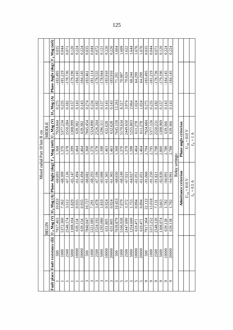
125

BE

GIN

MID

DL

E

Fau

lt p

lace

Fau

lt r

esi

stan

ce (

Ω)

U0 M

ag

(V

)3

I0

Mag

(A

)P

hase

An

gle

(d

eg

)Y

0 M

ag

(m

S)

U0 M

ag

(V

)3

I0

Mag

(A

)P

hase

An

gle

(d

eg

)Y

0 M

ag

(m

S)

15

00

79

17

.46

31

0.8

33

-68

.69

31

.36

87

92

4.8

44

0.2

75

-18

3.4

95

0.0

35

11

00

05

37

2.3

60

7.3

62

-68

.30

91

.37

05

37

7.2

34

0.2

35

-18

1.2

19

0.0

44

12

50

02

54

8.1

74

3.5

12

-67

.13

61

.37

82

55

0.2

84

0.1

82

-17

8.7

36

0.0

71

15

00

01

30

8.1

04

1.8

29

-65

.14

71

.39

91

30

8.9

99

0.1

57

-17

9.1

90

0.1

20

11

00

00

63

9.1

54

0.9

35

-61

.49

41

.46

46

39

.38

20

.14

3-1

84

.14

50

.22

4

12

00

00

63

9.1

54

0.9

35

-61

.49

41

.46

46

39

.38

20

.14

3-1

84

.14

50

.22

4

35

00

78

40

.04

71

0.7

27

-68

.68

21

.36

87

84

5.4

54

0.2

74

-18

3.4

61

0.0

35

31

00

05

32

1.0

85

7.2

91

-68

.29

31

.37

05

32

4.8

90

0.2

34

-18

1.1

14

0.0

44

32

50

02

52

4.1

92

3.4

78

-67

.10

61

.37

82

52

6.2

04

0.1

82

-17

8.5

35

0.0

72

35

00

01

29

5.0

80

1.8

10

-65

.08

81

.39

81

29

6.3

11

0.1

57

-17

8.9

44

0.1

21

31

00

00

63

1.8

05

0.9

24

-61

.36

51

.46

36

32

.62

80

.14

3-1

83

.91

00

.22

6

32

00

00

63

1.8

05

0.9

24

-61

.36

51

.46

36

32

.62

80

.14

3-1

83

.91

00

.22

6

55

00

76

39

.87

91

0.4

53

-68

.65

01

.36

87

64

5.1

59

12

.26

17

1.2

91

1.6

04

51

00

05

16

6.9

28

7.0

79

-68

.24

91

.37

05

17

0.6

34

8.3

17

70

.98

71

.60

9

52

50

02

44

7.6

90

3.3

72

-67

.02

11

.37

82

44

9.6

50

3.9

74

70

.02

41

.62

2

55

00

01

25

4.6

00

1.7

53

-64

.92

71

.39

81

25

5.8

03

2.0

64

68

.24

41

.64

4

51

00

00

61

0.4

71

0.8

94

-61

.05

11

.46

46

11

.27

81

.02

46

4.2

99

1.6

76

52

00

00

61

0.4

71

0.8

94

-61

.05

11

.46

46

11

.27

81

.02

46

4.2

99

1.6

76

95

00

79

17

.30

42

2.1

22

-91

.06

62

.79

47

92

4.6

84

0.2

75

-18

3.4

95

0.0

35

91

00

05

37

2.2

52

15

.01

8-9

1.2

50

2.7

95

53

77

.12

60

.23

5-1

81

.21

90

.04

4

92

50

02

54

8.1

20

7.1

31

-91

.82

12

.79

82

55

0.2

31

0.1

82

-17

8.7

36

0.0

71

95

00

01

30

8.0

74

3.6

63

-92

.83

02

.80

01

30

8.9

69

0.1

57

-17

9.1

90

0.1

20

91

00

00

63

9.1

38

1.7

82

-94

.99

12

.78

86

39

.36

60

.14

3-1

84

.14

50

.22

4

92

00

00

63

9.1

38

1.7

82

-94

.99

12

.78

86

39

.36

60

.14

3-1

84

.14

50

.22

4

Mix

ed r

adia

l P

art

10 k

m R

on

Uo

h =

81

0 V

Ih

= 1

A

Ad

mit

tan

ce c

rit

erio

nP

hase

an

gle

crit

erio

n

Uo

h =

81

0 V

Ih

= 0

.5 A

Rel

ay s

ettings:

126

BE

GIN

MID

DL

E

Fau

lt p

laceF

au

lt r

esi

stan

ce (

Ω)

U0 M

ag

(V

)3

I0

Mag

(A

)P

hase

An

gle

(d

eg

)Y

0 M

ag

(m

S)

U0 M

ag

(V

)3

I0

Mag

(A

)P

hase

An

gle

(d

eg

)Y

0 M

ag

(m

S)

15

00

10

92

9.7

24

26

.14

2-8

9.1

36

2.3

92

10

94

0.1

19

0.3

08

-18

5.7

47

0.0

28

11

00

09

99

9.9

83

23

.91

2-8

9.0

81

2.3

91

10

00

9.4

37

0.3

03

-18

4.1

38

0.0

30

12

50

07

18

3.0

93

17

.16

3-8

8.9

11

2.3

89

71

89

.75

30

.26

6-1

80

.80

90

.03

7

15

00

04

40

9.6

23

10

.52

8-8

8.6

09

2.3

87

44

13

.56

30

.21

7-1

78

.43

60

.04

9

11

00

00

23

12

.16

45

.52

1-8

7.9

42

2.3

88

23

14

.03

50

.17

5-1

79

.58

10

.07

6

12

00

00

23

12

.16

45

.52

1-8

7.9

42

2.3

88

23

14

.03

50

.17

5-1

79

.58

10

.07

6

35

00

10

83

2.8

90

25

.91

1-8

9.1

33

2.3

92

10

84

0.4

47

0.3

06

-18

5.7

87

0.0

28

31

00

09

91

5.6

88

23

.71

0-8

9.0

78

2.3

91

99

22

.66

30

.30

2-1

84

.13

10

.03

0

32

50

07

12

5.0

20

17

.02

4-8

8.9

06

2.3

89

71

30

.16

30

.26

6-1

80

.69

10

.03

7

35

00

04

37

0.6

63

10

.43

3-8

8.6

01

2.3

87

43

73

.96

80

.21

7-1

78

.20

80

.05

0

31

00

00

22

87

.10

75

.46

0-8

7.9

26

2.3

87

22

89

.03

10

.17

5-1

79

.27

50

.07

6

32

00

00

22

87

.10

75

.46

0-8

7.9

26

2.3

87

22

89

.03

10

.17

5-1

79

.27

50

.07

6

55

00

10

57

7.4

49

25

.30

0-8

9.1

23

2.3

92

10

58

4.8

41

4.3

10

82

.63

00

.40

7

51

00

09

66

8.0

67

23

.11

8-8

9.0

66

2.3

91

96

74

.88

03

.95

08

2.3

20

0.4

08

52

50

06

92

6.1

48

16

.54

7-8

8.8

91

2.3

89

69

31

.15

82

.85

28

1.3

57

0.4

11

55

00

04

23

7.9

67

10

.11

5-8

8.5

76

2.3

87

42

41

.18

11

.76

67

9.6

26

0.4

16

51

00

00

22

10

.45

15

.27

6-8

7.8

76

2.3

87

22

12

.32

10

.93

67

5.4

23

0.4

23

52

00

00

22

10

.45

15

.27

6-8

7.8

76

2.3

87

22

12

.32

10

.93

67

5.4

23

0.4

23

65

00

10

92

9.5

01

30

.53

0-9

0.9

29

2.7

93

10

93

9.8

96

0.3

08

-18

5.7

47

0.0

28

61

00

09

99

9.7

77

27

.93

9-9

0.9

74

2.7

94

10

00

9.2

30

0.3

03

-18

4.1

38

0.0

30

62

50

07

18

2.9

43

20

.08

2-9

1.1

15

2.7

96

71

89

.60

20

.26

6-1

80

.80

90

.03

7

65

00

04

40

9.5

29

12

.33

7-9

1.3

66

2.7

98

44

13

.46

90

.21

7-1

78

.43

60

.04

9

61

00

00

23

12

.11

46

.46

7-9

1.9

61

2.7

97

23

13

.98

50

.17

5-1

79

.58

10

.07

6

62

00

00

23

12

.11

46

.46

7-9

1.9

61

2.7

97

23

13

.98

50

.17

5-1

79

.58

10

.07

6

Ih

= 0

.5 A

Ih

= 1

A

Mix

ed r

adia

l P

art

10 k

m 1

OH

L R

off

Ad

mit

tan

ce c

rit

erio

n:

Ph

ase

an

gle

crit

erio

n:

Uo

h =

81

0 V

Uo

h =

81

0 V

Rel

ay s

ettings:

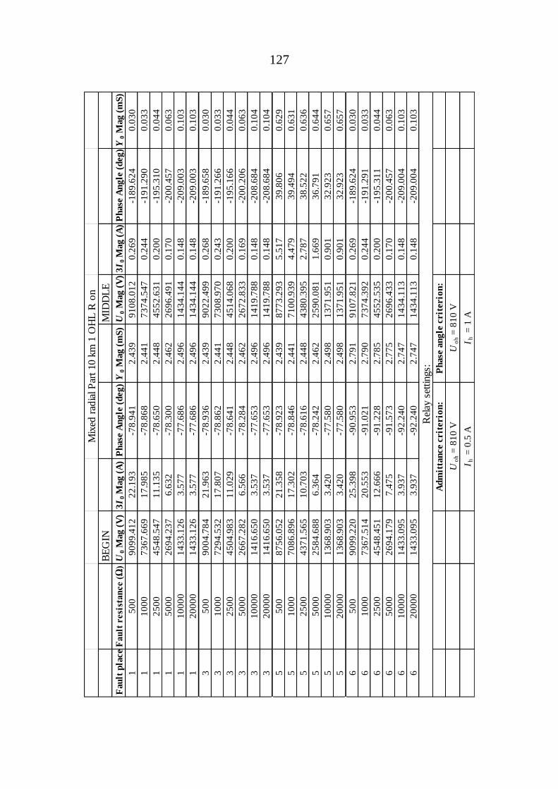
127

BE

GIN

MID

DL

E

Fau

lt p

lace

Fau

lt r

esi

stan

ce (

Ω)

U0 M

ag

(V

)3

I0

Mag

(A

)P

hase

An

gle

(d

eg

)Y

0 M

ag

(m

S)

U0 M

ag

(V

)3

I0

Mag

(A

)P

hase

An

gle

(d

eg

)Y

0 M

ag

(m

S)

15

00

90

99

.41

22

2.1

93

-78

.94

12

.43

99

10

8.0

12

0.2

69

-18

9.6

24

0.0

30

11

00

07

36

7.6

69

17

.98

5-7

8.8

68

2.4

41

73

74

.54

70

.24

4-1

91

.29

00

.03

3

12

50

04

54

8.5

47

11

.13

5-7

8.6

50

2.4

48

45

52

.63

10

.20

0-1

95

.31

00

.04

4

15

00

02

69

4.2

37

6.6

32

-78

.30

02

.46

22

69

6.4

91

0.1

70

-20

0.4

57

0.0

63

11

00

00

14

33

.12

63

.57

7-7

7.6

86

2.4

96

14

34

.14

40

.14

8-2

09

.00

30

.10

3

12

00

00

14

33

.12

63

.57

7-7

7.6

86

2.4

96

14

34

.14

40

.14

8-2

09

.00

30

.10

3

35

00

90

04

.78

42

1.9

63

-78

.93

62

.43

99

02

2.4

99

0.2

68

-18

9.6

58

0.0

30

31

00

07

29

4.5

32

17

.80

7-7

8.8

62

2.4

41

73

08

.97

00

.24

3-1

91

.26

60

.03

3

32

50

04

50

4.9

83

11

.02

9-7

8.6

41

2.4

48

45

14

.06

80

.20

0-1

95

.16

60

.04

4

35

00

02

66

7.2

82

6.5

66

-78

.28

42

.46

22

67

2.8

33

0.1

69

-20

0.2

06

0.0

63

31

00

00

14

16

.65

03

.53

7-7

7.6

53

2.4

96

14

19

.78

80

.14

8-2

08

.68

40

.10

4

32

00

00

14

16

.65

03

.53

7-7

7.6

53

2.4

96

14

19

.78

80

.14

8-2

08

.68

40

.10

4

55

00

87

56

.05

22

1.3

58

-78

.92

32

.43

98

77

3.2

93

5.5

17

39

.80

60

.62

9

51

00

07

08

6.8

96

17

.30

2-7

8.8

46

2.4

41

71

00

.93

94

.47

93

9.4

94

0.6

31

52

50

04

37

1.5

65

10

.70

3-7

8.6

16

2.4

48

43

80

.39

52

.78

73

8.5

22

0.6

36

55

00

02

58

4.6

88

6.3

64

-78

.24

22

.46

22

59

0.0

81

1.6

69

36

.79

10

.64

4

51

00

00

13

68

.90

33

.42

0-7

7.5

80

2.4

98

13

71

.95

10

.90

13

2.9

23

0.6

57

52

00

00

13

68

.90

33

.42

0-7

7.5

80

2.4

98

13

71

.95

10

.90

13

2.9

23

0.6

57

65

00

90

99

.22

02

5.3

98

-90

.95

32

.79

19

10

7.8

21

0.2

69

-18

9.6

24

0.0

30

61

00

07

36

7.5

14

20

.55

3-9

1.0

21

2.7

90

73

74

.39

20

.24

4-1

91

.29

10

.03

3

62

50

04

54

8.4

51

12

.66

6-9

1.2

28

2.7

85

45

52

.53

50

.20

0-1

95

.31

10

.04

4

65

00

02

69

4.1

79

7.4

75

-91

.57

32

.77

52

69

6.4

33

0.1

70

-20

0.4

57

0.0

63

61

00

00

14

33

.09

53

.93

7-9

2.2

40

2.7

47

14

34

.11

30

.14

8-2

09

.00

40

.10

3

62

00

00

14

33

.09

53

.93

7-9

2.2

40

2.7

47

14

34

.11

30

.14

8-2

09

.00

40

.10

3

Ih

= 0

.5 A

Ih

= 1

A

Mix

ed r

adia

l P

art

10 k

m 1

OH

L R

on

Ad

mit

tan

ce c

rit

erio

n:

Ph

ase

an

gle

crit

erio

n:

Uo

h =

81

0 V

Uo

h =

81

0 V

Rel

ay s

ettings:

128

Appendix 6. Results of cabled radial network with recloser

BE

GIN

MID

DL

E

Fau

lt p

lace

Fau

lt r

esi

stan

ce (

Ω)

U0 M

ag

(V

)3

I0

Mag

(A

)P

hase

An

gle

(d

eg

)Y

0 M

ag

(m

S)

U0 M

ag

(V

)3

I0

Mag

(A

)P

hase

An

gle

(d

eg

)Y

0 M

ag

(m

S)

15

00

82

28

.54

51

0.4

83

-86

.84

01

.27

48

24

0.2

12

3.3

30

-95

.20

30

.40

4

11

00

05

23

9.1

58

6.6

54

-86

.34

11

.27

05

24

6.4

53

2.1

49

-96

.58

50

.41

0

12

50

02

26

9.6

85

2.8

65

-83

.03

91

.26

22

27

2.5

04

0.9

73

-10

2.6

13

0.4

28

15

00

01

11

3.7

11

1.4

52

-74

.73

41

.30

31

11

4.6

37

0.5

15

-11

5.7

90

0.4

62

11

00

00

56

7.1

81

0.8

73

-66

.34

01

.54

05

67

.22

80

.28

3-1

38

.33

90

.49

9

12

00

00

56

7.1

81

0.8

73

-66

.34

01

.54

05

67

.22

80

.28

3-1

38

.33

90

.49

9

35

00

81

81

.43

91

0.4

21

-86

.83

11

.27

48

17

6.7

88

3.3

06

-95

.22

80

.40

4

31

00

05

20

7.9

43

6.6

12

-86

.33

31

.27

05

20

5.1

18

2.1

34

-96

.61

00

.41

0

32

50

02

25

4.1

34

2.8

42

-83

.02

31

.26

12

25

3.3

77

0.9

67

-10

2.6

35

0.4

29

35

00

01

10

4.1

18

1.4

36

-74

.64

51

.30

01

10

4.4

25

0.5

12

-11

5.8

34

0.4

64

31

00

00

56

0.9

57

0.8

63

-66

.10

51

.53

95

61

.71

80

.28

2-1

38

.46

60

.50

2

32

00

00

56

0.9

57

0.8

63

-66

.10

51

.53

95

61

.71

80

.28

2-1

38

.46

60

.50

2

55

00

80

68

.28

61

0.2

75

-86

.81

71

.27

48

06

3.7

05

12

.30

78

6.7

28

1.5

26

51

00

05

13

3.2

19

6.5

15

-86

.31

31

.26

95

13

0.4

39

7.8

59

86

.32

21

.53

2

52

50

02

22

5.4

79

2.8

05

-82

.97

11

.26

02

22

4.7

39

3.4

56

83

.17

31

.55

3

55

00

01

09

1.1

35

1.4

19

-74

.55

41

.30

11

09

1.4

46

1.7

30

74

.58

71

.58

5

51

00

00

55

4.5

65

0.8

55

-66

.00

81

.54

15

55

.32

50

.84

86

0.3

59

1.5

27

52

00

00

55

4.5

65

0.8

55

-66

.00

81

.54

15

55

.32

50

.84

86

0.3

59

1.5

27

95

00

82

28

.38

32

6.3

28

-91

.01

33

.20

08

24

0.0

49

3.3

30

-95

.20

30

.40

4

91

00

05

23

9.0

53

16

.78

6-9

1.2

01

3.2

04

52

46

.34

72

.14

9-9

6.5

85

0.4

10

92

50

02

26

9.6

36

7.2

97

-92

.27

73

.21

52

27

2.4

55

0.9

73

-10

2.6

13

0.4

28

95

00

01

11

3.6

85

3.5

75

-95

.01

73

.21

01

11

4.6

11

0.5

15

-11

5.7

90

0.4

62

91

00

00

56

7.1

68

1.7

62

-99

.44

23

.10

65

67

.21

50

.28

3-1

38

.34

00

.49

9

92

00

00

56

7.1

68

1.7

62

-99

.44

23

.10

65

67

.21

50

.28

3-1

38

.34

00

.49

9

Ih

= 0

.5 A

Ih

= 1

A

Cab

led

rad

ial P

art

10 k

m

R o

ff

Ad

mit

tan

ce c

rit

erio

n:

Ph

ase

an

gle

crit

erio

n:

Uo

h =

81

0 V

Uo

h =

81

0 V

Rel

ay s

ettings:

129

BE

GIN

MID

DL

E

Fau

lt p

lace

Fau

lt r

esi

stan

ce (

Ω)

U0 M

ag

(V

)3

I0

Mag

(A

)P

hase

An

gle

(d

eg

)Y

0 M

ag

(m

S)

U0 M

ag

(V

)3

I0

Mag

(A

)P

hase

An

gle

(d

eg

)Y

0 M

ag

(m

S)

15

00

73

79

.14

11

0.0

95

-68

.59

91

.36

87

38

9.5

59

2.9

71

-95

.39

50

.40

2

11

00

04

73

1.0

33

6.4

81

-68

.11

61

.37

04

73

7.5

68

1.9

21

-96

.94

50

.40

6

12

50

02

13

3.5

56

2.9

41

-66

.58

21

.37

92

13

6.2

91

0.8

90

-10

1.7

06

0.4

17

15

00

01

07

5.7

03

1.5

10

-63

.92

81

.40

31

07

6.8

80

0.4

71

-10

9.8

06

0.4

38

11

00

00

52

1.4

42

0.7

75

-59

.23

41

.48

65

21

.79

10

.25

4-1

25

.65

80

.48

6

12

00

00

52

1.4

42

0.7

75

-59

.23

41

.48

65

21

.79

10

.25

4-1

25

.65

80

.48

6

35

00

73

28

.42

41

0.0

25

-68

.58

51

.36

87

33

3.5

11

2.9

50

-95

.42

50

.40

2

31

00

04

69

9.9

13

6.4

37

-68

.09

81

.37

04

70

3.3

17

1.9

09

-96

.97

70

.40

6

32

50

02

11

9.2

78

2.9

20

-66

.54

71

.37

82

12

1.0

30

0.8

86

-10

1.7

45

0.4

18

35

00

01

06

7.4

59

1.4

96

-63

.85

31

.40

11

06

8.5

54

0.4

69

-10

9.8

52

0.4

39

31

00

00

51

6.1

79

0.7

66

-59

.04

61

.48

35

16

.93

90

.25

3-1

25

.71

10

.49

0

32

00

00

51

6.1

79

0.7

66

-59

.04

61

.48

35

16

.93

90

.25

3-1

25

.71

10

.49

0

55

00

72

22

.97

69

.88

0-6

8.5

67

1.3

68

72

27

.99

61

1.6

03

71

.24

51

.60

5

51

00

04

63

3.1

96

6.3

45

-68

.07

41

.36

94

63

6.5

56

7.4

73

70

.88

91

.61

2

52

50

02

09

2.3

48

2.8

82

-66

.50

51

.37

72

09

4.0

82

3.4

15

69

.68

91

.63

1

55

00

01

05

4.3

26

1.4

77

-63

.77

61

.40

11

05

5.4

11

1.7

55

67

.42

31

.66

2

51

00

00

50

9.4

60

0.7

56

-58

.89

41

.48

45

10

.21

50

.87

36

2.5

75

1.7

12

52

00

00

50

9.4

60

0.7

56

-58

.89

41

.48

45

10

.21

50

.87

36

2.5

75

1.7

12

95

00

73

78

.99

12

3.5

94

-91

.03

43

.19

77

38

9.4

09

2.9

71

-95

.39

50

.40

2

91

00

04

73

0.9

36

15

.13

9-9

1.2

36

3.2

00

47

37

.47

21

.92

1-9

6.9

45

0.4

06

92

50

02

13

3.5

11

6.8

40

-91

.88

43

.20

62

13

6.2

46

0.8

90

-10

1.7

07

0.4

17

95

00

01

07

5.6

79

3.4

54

-93

.06

23

.21

11

07

6.8

56

0.4

71

-10

9.8

06

0.4

38

91

00

00

52

1.4

29

1.6

70

-95

.55

53

.20

25

21

.77

80

.25

4-1

25

.65

90

.48

6

92

00

00

52

1.4

29

1.6

70

-95

.55

53

.20

25

21

.77

80

.25

4-1

25

.65

90

.48

6

Ih

= 0

.5 A

Ih

= 1

A

Cab

led

rad

ial P

art

10 k

m

R o

n

Ad

mit

tan

ce c

rit

erio

n:

Ph

ase

an

gle

crit

erio

n:

Uo

h =

81

0 V

Uo

h =

81

0 V

Rel

ay s

ettings:

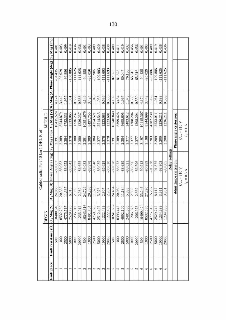
130

BE

GIN

MID

DL

E

Fau

lt p

lace

Fau

lt r

esi

stan

ce (

Ω)

U0 M

ag

(V

)3

I0

Mag

(A

)P

hase

An

gle

(d

eg

)Y

0 M

ag

(m

S)

U0 M

ag

(V

)3

I0

Mag

(A

)P

hase

An

gle

(d

eg

)Y

0 M

ag

(m

S)

15

00

10

40

0.6

40

24

.86

6-8

9.0

87

2.3

91

10

41

5.5

24

4.1

74

-94

.43

50

.40

1

11

00

08

53

2.7

60

20

.38

5-8

8.9

82

2.3

89

85

44

.87

93

.44

2-9

5.0

29

0.4

03

12

50

04

77

5.7

17

11

.38

7-8

8.6

52

2.3

84

47

82

.33

11

.95

5-9

6.8

86

0.4

09

15

00

02

52

9.7

96

6.0

16

-88

.04

22

.37

82

53

3.0

65

1.0

61

-10

0.8

85

0.4

19

11

00

00

12

35

.01

22

.93

9-8

6.6

55

2.3

80

12

36

.23

70

.53

8-1

11

.62

50

.43

6

12

00

00

12

35

.01

22

.93

9-8

6.6

55

2.3

80

12

36

.23

70

.53

8-1

11

.62

50

.43

6

35

00

10

34

3.8

16

24

.72

9-8

9.0

83

2.3

91

10

35

1.0

79

4.1

49

-94

.45

80

.40

1

31

00

08

49

1.7

04

20

.28

6-8

8.9

78

2.3

89

84

97

.75

53

.42

4-9

5.0

50

0.4

03

32

50

04

75

0.9

76

11

.32

6-8

8.6

48

2.3

84

47

54

.52

11

.94

6-9

6.9

05

0.4

09

35

00

02

51

2.4

92

5.9

73

-88

.03

52

.37

72

51

4.5

45

1.0

56

-10

0.9

03

0.4

20

31

00

00

12

22

.43

92

.90

7-8

6.6

28

2.3

78

12

23

.68

10

.53

6-1

11

.69

30

.43

8

32

00

00

12

22

.43

92

.90

7-8

6.6

28

2.3

78

12

23

.68

10

.53

6-1

11

.69

30

.43

8

55

00

10

24

1.6

52

24

.48

4-8

9.0

78

2.3

91

10

24

8.8

49

4.1

89

82

.39

50

.40

9

51

00

08

39

3.4

42

20

.05

0-8

8.9

72

2.3

89

83

99

.42

83

.45

48

1.8

28

0.4

11

52

50

04

69

2.1

00

11

.18

4-8

8.6

39

2.3

84

46

95

.60

51

.96

78

0.0

47

0.4

19

55

00

02

48

1.5

80

5.8

98

-88

.02

12

.37

72

48

3.6

12

1.0

73

76

.16

60

.43

2

51

00

00

12

06

.97

32

.86

9-8

6.5

96

2.3

77

12

08

.20

40

.55

06

5.6

16

0.4

56

52

00

00

12

06

.97

32

.86

9-8

6.5

96

2.3

77

12

08

.20

40

.55

06

5.6

16

0.4

56

65

00

10

40

0.4

24

33

.24

6-9

0.9

12

3.1

97

10

41

5.3

07

4.1

74

-94

.43

50

.40

1

61

00

08

53

2.5

80

27

.29

0-9

0.9

89

3.1

98

85

44

.69

93

.44

2-9

5.0

29

0.4

03

62

50

04

77

5.6

15

15

.29

7-9

1.2

38

3.2

03

47

82

.23

01

.95

5-9

6.8

86

0.4

09

65

00

02

52

9.7

42

8.1

17

-91

.87

53

.20

92

53

3.0

11

1.0

61

-10

0.8

85

0.4

19

61

00

00

12

34

.98

63

.95

1-9

3.8

05

3.2

00

12

36

.21

10

.53

8-1

11

.62

50

.43

6

62

00

00

12

34

.98

63

.95

1-9

3.8

05

3.2

00

12

36

.21

10

.53

8-1

11

.62

50

.43

6

Ih

= 0

.5 A

Ih

= 1

A

Cab

led

rad

ial P

art

10 k

m 1

OH

L R

off

Ad

mit

tan

ce c

rit

erio

n:

Ph

ase

an

gle

crit

erio

n:

Uo

h =

81

0 V

Uo

h =

81

0 V

Rel

ay s

ettings:

131

BE

GIN

MID

DL

E

Fau

lt p

lace

Fau

lt r

esi

stan

ce (

Ω)

U0 M

ag

(V

)3

I0

Mag

(A

)P

hase

An

gle

(d

eg

)Y

0 M

ag

(m

S)

U0 M

ag

(V

)3

I0

Mag

(A

)P

hase

An

gle

(d

eg

)Y

0 M

ag

(m

S)

15

00

87

97

.19

82

1.4

50

-78

.88

92

.43

88

80

9.7

34

3.5

12

-94

.62

70

.39

9

11

00

06

72

6.5

32

16

.41

1-7

8.7

63

2.4

40

67

36

.00

52

.68

5-9

5.4

13

0.3

99

12

50

03

70

9.5

68

9.0

70

-78

.38

22

.44

53

71

4.6

00

1.4

80

-97

.82

90

.39

8

15

00

02

03

6.8

27

5.0

04

-77

.74

22

.45

72

03

9.4

03

0.8

10

-10

2.0

49

0.3

97

11

00

00

10

30

.35

22

.56

9-7

6.5

11

2.4

93

10

31

.44

70

.40

3-1

11

.21

10

.39

1

12

00

00

10

30

.35

22

.56

9-7

6.5

11

2.4

93

10

31

.44

70

.40

3-1

11

.21

10

.39

1

35

00

87

33

.86

82

1.2

95

-78

.88

32

.43

88

75

1.0

90

3.4

90

-94

.65

40

.39

9

31

00

06

68

2.5

40

16

.30

3-7

8.7

56

2.4

40

66

95

.82

92

.67

0-9

5.4

45

0.3

99

32

50

03

68

5.7

60

9.0

10

-78

.36

92

.44

53

69

3.2

83

1.4

73

-97

.87

40

.39

9

35

00

02

02

1.7

74

4.9

66

-77

.71

92

.45

62

02

6.0

89

0.8

06

-10

2.1

22

0.3

98

31

00

00

10

20

.17

82

.54

2-7

6.4

58

2.4

92

10

22

.56

70

.40

1-1

11

.36

50

.39

3

32

00

00

10

20

.17

82

.54

2-7

6.4

58

2.4

92

10

22

.56

70

.40

1-1

11

.36

50

.39

3

55

00

86

30

.68

62

1.0

44

-78

.87

62

.43

88

64

7.7

11

5.4

57

39

.79

50

.63

1

51

00

06

60

0.3

28

16

.10

2-7

8.7

47

2.4

40

66

13

.45

94

.20

13

9.4

52

0.6

35

52

50

03

64

0.8

32

8.9

00

-78

.35

62

.44

53

64

8.2

68

2.3

63

38

.37

70

.64

8

55

00

01

99

7.1

02

4.9

05

-77

.69

62

.45

62

00

1.3

69

1.3

37

36

.43

50

.66

8

51

00

00

10

06

.86

32

.50

9-7

6.4

12

2.4

92

10

09

.22

50

.71

33

1.9

96

0.7

07

52

00

00

10

06

.86

32

.50

9-7

6.4

12

2.4

92

10

09

.22

50

.71

33

1.9

96

0.7

07

65

00

87

97

.01

12

8.1

02

-90

.93

33

.19

48

80

9.5

46

3.5

12

-94

.62

70

.39

9

61

00

06

72

6.3

89

21

.48

4-9

1.0

31

3.1

94

67

35

.86

22

.68

5-9

5.4

13

0.3

99

62

50

03

70

9.4

89

11

.84

1-9

1.3

31

3.1

92

37

14

.52

11

.48

0-9

7.8

29

0.3

98

65

00

02

03

6.7

84

6.4

90

-91

.84

93

.18

62

03

9.3

59

0.8

10

-10

2.0

50

0.3

97

61

00

00

10

30

.33

03

.26

0-9

2.9

21

3.1

64

10

31

.42

50

.40

3-1

11

.21

20

.39

1

62

00

00

10

30

.33

03

.26

0-9

2.9

21

3.1

64

10

31

.42

50

.40

3-1

11

.21

20

.39

1

Ih

= 0

.5 A

Ih

= 1

A

Cab

led

rad

ial P

art

10 k

m 1

OH

L R

on

Ad

mit

tan

ce c

rit

erio

n:

Ph

ase

an

gle

crit

erio

n:

Uo

h =

81

0 V

Uo

h =

81

0 V

Rel

ay s

ettings:

132

Appendix 7. Results of ring-shaped network

BE

GIN

MID

DL

E

Fau

lt p

lace

Fau

lt r

esi

stan

ce (

Ω)

U0 M

ag

(V

)3

I0

Mag

(A

)P

hase

An

gle

(d

eg

)Y

0 M

ag

(m

S)

U0 M

ag

(V

)3

I0

Mag

(A

)P

hase

An

gle

(d

eg

)Y

0 M

ag

(m

S)

15

00

78

31

.12

01

0.5

85

-65

.73

71

.35

27

83

7.5

71

0.3

17

57

.57

30

.04

0

11

00

05

28

2.7

06

7.1

72

-64

.82

71

.35

85

28

6.8

81

0.2

29

54

.92

10

.04

3

12

50

02

48

2.0

47

3.4

32

-62

.11

21

.38

32

48

3.7

29

0.1

29

47

.90

90

.05

2

15

00

01

26

1.3

26

1.8

28

-57

.85

91

.44

91

26

1.8

92

0.0

86

38

.17

60

.06

8

11

00

00

61

2.4

38

1.0

21

-51

.85

71

.66

76

12

.34

10

.06

22

1.9

98

0.1

02

12

00

00

61

2.4

38

1.0

21

-51

.85

71

.66

76

12

.34

10

.06

22

1.9

98

0.1

02

35

00

76

55

.39

01

5.4

13

-82

.40

12

.01

37

62

9.3

50

5.9

48

-11

0.2

80

0.7

80

31

00

05

15

7.8

82

10

.38

0-8

2.1

64

2.0

12

51

40

.47

64

.03

1-1

11

.03

40

.78

4

32

50

02

41

9.9

56

4.8

67

-81

.42

12

.01

12

41

2.0

30

1.9

23

-11

3.4

04

0.7

97

35

00

01

22

7.0

36

2.4

75

-80

.09

72

.01

71

22

3.3

04

0.9

98

-11

7.7

12

0.8

16

31

00

00

59

3.3

20

1.2

22

-77

.46

12

.05

95

91

.93

90

.49

4-1

27

.29

70

.83

5

32

00

00

59

3.3

20

1.2

22

-77

.46

12

.05

95

91

.93

90

.49

4-1

27

.29

70

.83

5

45

00

77

19

.20

62

0.0

61

-85

.50

52

.59

97

72

4.9

43

2.4

84

39

.15

30

.32

2

41

00

05

20

6.8

49

13

.54

1-8

5.5

45

2.6

01

52

10

.75

11

.70

43

8.1

89

0.3

27

42

50

02

44

5.2

54

6.3

73

-85

.68

12

.60

62

44

7.1

23

0.8

41

35

.19

60

.34

4

45

00

01

24

1.0

49

3.2

44

-85

.95

12

.61

41

24

2.0

11

0.4

61

29

.87

00

.37

1

41

00

00

60

1.0

98

1.5

77

-86

.62

52

.62

46

01

.53

00

.25

41

8.2

89

0.4

22

42

00

00

60

1.0

98

1.5

77

-86

.62

52

.62

46

01

.53

00

.25

41

8.2

89

0.4

22

95

00

78

30

.96

12

1.6

10

-90

.50

82

.76

07

83

7.4

12

0.3

17

57

.57

30

.04

0

91

00

05

28

2.5

99

14

.57

7-9

0.6

35

2.7

59

52

86

.77

40

.22

95

4.9

21

0.0

43

92

50

02

48

1.9

94

6.8

45

-91

.03

12

.75

82

48

3.6

77

0.1

29

47

.90

80

.05

2

95

00

01

26

1.2

98

3.4

69

-91

.73

02

.75

11

26

1.8

63

0.0

86

38

.17

60

.06

8

91

00

00

61

2.4

23

1.6

64

-93

.13

52

.71

76

12

.32

60

.06

22

1.9

98

0.1

02

92

00

00

61

2.4

23

1.6

64

-93

.13

52

.71

76

12

.32

60

.06

22

1.9

98

0.1

02

Rin

g-s

hap

ed P

art

10 k

m

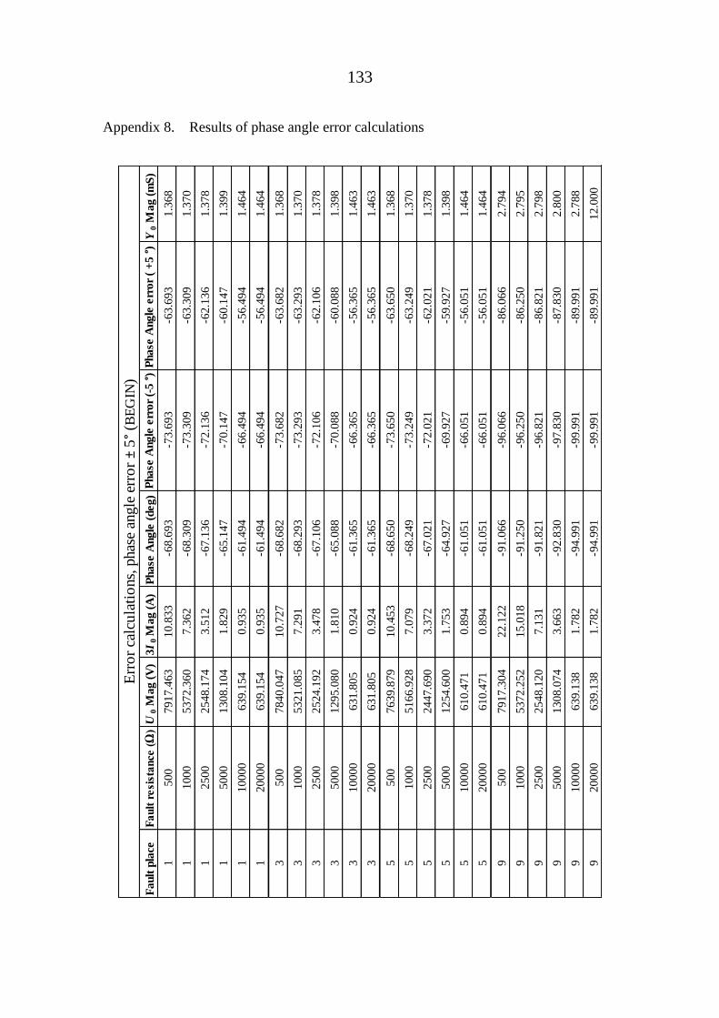
133

Appendix 8. Results of phase angle error calculations

Fault

pla

ceF

ault

resi

stance

(Ω

)U

0 M

ag (

V)

3I

0 M

ag (

A)

Phase

Angle

(deg)

Phase

Angle

err

or

(-5 °

) P

hase

Angle

err

or

( +

5 °

) Y

0 M

ag (

mS

)

1500

7917.4

63

10.8

33

-68.6

93

-73.6

93

-63.6

93

1.3

68

11000

5372.3

60

7.3

62

-68.3

09

-73.3

09

-63.3

09

1.3

70

12500

2548.1

74

3.5

12

-67.1

36

-72.1

36

-62.1

36

1.3

78

15000

1308.1

04

1.8

29

-65.1

47

-70.1

47

-60.1

47

1.3

99

110000

639.1

54

0.9

35

-61.4

94

-66.4

94

-56.4

94

1.4

64

120000

639.1

54

0.9

35

-61.4

94

-66.4

94

-56.4

94

1.4

64

3500

7840.0

47

10.7

27

-68.6

82

-73.6

82

-63.6

82

1.3

68

31000

5321.0

85

7.2

91

-68.2

93

-73.2

93

-63.2

93

1.3

70

32500

2524.1

92

3.4

78

-67.1

06

-72.1

06

-62.1

06

1.3

78

35000

1295.0

80

1.8

10

-65.0

88

-70.0

88

-60.0

88

1.3

98

310000

631.8

05

0.9

24

-61.3

65

-66.3

65

-56.3

65

1.4

63

320000

631.8

05

0.9

24

-61.3

65

-66.3

65

-56.3

65

1.4

63

5500

7639.8

79

10.4

53

-68.6

50

-73.6

50

-63.6

50

1.3

68

51000

5166.9

28

7.0

79

-68.2

49

-73.2

49

-63.2

49

1.3

70

52500

2447.6

90

3.3

72

-67.0

21

-72.0

21

-62.0

21

1.3

78

55000

1254.6

00

1.7

53

-64.9

27

-69.9

27

-59.9

27

1.3

98

510000

610.4

71

0.8

94

-61.0

51

-66.0

51

-56.0

51

1.4

64

520000

610.4

71

0.8

94

-61.0

51

-66.0

51

-56.0

51

1.4

64

9500

7917.3

04

22.1

22

-91.0

66

-96.0

66

-86.0

66

2.7

94

91000

5372.2

52

15.0

18

-91.2

50

-96.2

50

-86.2

50

2.7

95

92500

2548.1

20

7.1

31

-91.8

21

-96.8

21

-86.8

21

2.7

98

95000

1308.0

74

3.6

63

-92.8

30

-97.8

30

-87.8

30

2.8

00

910000

639.1

38

1.7

82

-94.9

91

-99.9

91

-89.9

91

2.7

88

920000

639.1

38

1.7

82

-94.9

91

-99.9

91

-89.9

91

12.0

00

Err

or

calc

ula

tio

ns,

phas

e an

gle

err

or ±

5°

(BE

GIN

)