UNIVERSITY OF THE FREE STATE

MANAGING TRANSITIONS IN SMALLHOLDER COFFEE AGROFORESTRY SYSTEMS OF MOUNT KENYA

Sammy Carsan

A thesis submitted in partial fulfillment for the degree of Doctor of Philosophy

Faculty of Natural and Agricultural Sciences Centre for Sustainable Agriculture, Rural Development

and Extension

May 2012

ii

This thesis is dedicated to my children

Eddie and Talisha

iii

ACKNOWLEDGEMENTS

Perhaps the most rewarding part of my PhD thesis has been connecting with so many

thoughtful people. My sincere thanks to all of them and my apologies to anyone I have

missed. My strongest debt of gratitude goes to Prof. Aldo Stroebel, Dr. Anthony Simons,

Dr. Ramni Jamnadass, Prof. Frans Swanepoel and Prof. Izak Groenewald for their

enthusiasm, advice and encouragement throughout my study at the University of the

Free State (UFS). The UFS, ICRAF (GRP 1) & CAFNET funded this study.

My study committee; Prof. Aldo Stroebel, Dr. Ramni Jamnadass and Prof. Frank Place

are gratefully acknowledged for their insight, guidance and helpful discussions on this

work. My study collaborators, Dr. Fabrice Pinard (CAFNET), Dr. Keith Shepherd (ICRAF,

GRP 4), Andrew Sila, Prof. Fergus Sinclair, Dr. Steve Franzel, Caleb Orwa, Alexious Nzisa,

Moses Munjuga and Agnes Were are thanked for their invaluable inputs at various

stages of this study. Jane Pool (ICRAF/ILRI) and Nicholas Ndhiwa (ICRAF/ILRI) are

thanked for their dedication to guide the research methods executed.

The field work carried out would have been insurmountable were it not for the help

provided by the ICRAF Meru office under the care of Jonathan Muriuki, Sallyannie

Muhoro and Nelly Mutio. Fredrick Maingi, Alex Munyi, Silas Muthuri, Samuel Nabea,

Paul Kithinji, Ambrose, Charlene Maingi, Susan Kimani and Valentine Gitonga provided

excellent field support. To Stepha McMullin for her encouragement and sharing the PhD

experience. Thank you all for being my very loyal friends and reliable colleagues. I’m also

grateful for the support provided by Okello Gard and colleagues at the ICRAF soil

laboratory for their support. Andrew Sila was dedicated to impart me with the rare skills

to use NIR techniques in soil diagnostics and conduct informative statistical data

analysis. Meshack Nyabenge and Jane Wanjara are acknowledged for developing the

study area maps.

iv

Special thanks to the over 30 coffee farmers’ cooperative societies and their 180

members we visited in Meru, Embu and Kirinyaga counties. Indeed these farmers

provided all the answers to my research questions and I sincerely thank them for their

time and willingness to share their knowledge. The Meru Coffee Union, the Embu

District Cooperative office and the Kirinyaga District Cooperative offices are recognized

for supporting this work within their areas of jurisdiction.

Colleagues at the International Office, and the Centre for Sustainable Agriculture Rural

Development and Extension, UFS, are remembered and thanked for their assistance and

friendship during the course of my study in South Africa - Claudine Macaskil, Cecilia

Sejake, Renee Heyns, Mia Kirsten, Arthur Johnson, Refilwe Masiba, Jeanne Niemann,

Dineo Gaofhiwe, Johan van Niekerk, Louise Steyn and Lise Kriel. My appreciation also to

my South African friends at Savanna Lodge, Bloemfontein; Oupa Seobe, Steve Mabalane

and Gabarone Lethogonollo- thank you for your encouragement in Bloemfontein when

the lights sometime seemed to dim on me.

My final thanks go to my wife, Kathuu, for her continuous support and patience while I

took the many hours away from family attention. To my children Eddie and Talisha (my

PhD baby) for their love and understanding.

v

TABLE OF CONTENTS

ACKNOWLEDGEMENTS ...................................................................................................... iii

ABSTRACT ......................................................................................................................... xiii

ACRONYMS ...................................................................................................................... xvii

CHAPTER 1 ...........................................................................................................................1

EVOLUTION OF THE SMALLHOLDER COFFEE SUB SECTOR IN KENYA................................1

ABSTRACT ............................................................................................................................1

INTRODUCTION ....................................................................................................................1

1.1 Coffee production .....................................................................................................3

1.2 Coffee marketing ......................................................................................................5

1.3 Price volatility in the coffee industry ........................................................................8

1.4 Coffee exports.........................................................................................................11

1.5 DISCUSSION ............................................................................................................13

1.6 CONCLUSIONS .........................................................................................................15

CHAPTER 2 .........................................................................................................................18

TRANSITIONS IN SMALLHOLDER COFFEE SYSTEMS: THE ROLE OF AGROFORESTRY AS A LAND-USE OPTION AROUND MOUNT KENYA ..................................................................18

ABSTRACT ..........................................................................................................................18

2.1 Background .............................................................................................................19

2.2 Why agroforestry in coffee systems? .....................................................................21

2.3 Justification of the study.........................................................................................26

2.4 Aims of this study and arrangement of the thesis .................................................28

2.5 Outline of the thesis ...............................................................................................28

CHAPTER 3 .........................................................................................................................33

RESEARCH METHODOLOGY ..............................................................................................33

3.1 Research approach ..................................................................................................33

3.2 Study area ...............................................................................................................35

3.3 Data collection ........................................................................................................39

vi

3.4 Sampling strategy ...................................................................................................39

3.7 Data analysis ...........................................................................................................49

3.8 CONCLUSIONS .........................................................................................................51

3.9 REFERENCES ............................................................................................................52

CHAPTER 4 .........................................................................................................................54

DETERMINING ENTERPRISE DIVERSIFICATION TYPOLOGIES BY SMALLHOLDER COFFEE FARMERS AROUND MOUNT KENYA .................................................................................54

ABSTRACT ..........................................................................................................................54

INTRODUCTION ..................................................................................................................55

4.1 MATERIALS AND METHODS ....................................................................................58

4.1.1 Study area ...............................................................................................................58

4.1.2 Coffee cultivation ....................................................................................................60

4.1.3 Classification of farming systems ............................................................................61

4.1.4 Household survey ....................................................................................................62

4.1.5 Data analysis ............................................................................................................63

4.2 Theoretical model ...................................................................................................64

4.3 RESULTS AND DISCUSSIONS ...................................................................................65

4.3.1 Coffee farm typology...............................................................................................65

4.3.2 Household characteristics .......................................................................................67

4.3.3 Input sizes and types- labour, fertilizer and manure ..............................................70

4.3.4 Smallholder enterprise diversification ....................................................................71

4.3.6 Farmers preferred substitutes to coffee .................................................................74

4.3.7 Factors driving smallholder enterprise choice .......................................................75

4.3.8 General linear regression analysis ..........................................................................77

4.4 DISCUSSION ............................................................................................................83

4.5 CONCLUSIONS .........................................................................................................85

4.6 REFERENCES ............................................................................................................87

vii

CHAPTER 5 .........................................................................................................................91

IMPLICATIONS OF DECREASED COFFEE CULTIVATION ON TREE DIVERSITY IN SMALLHOLDER COFFEE FARMS ........................................................................................91

ABSTRACT ..........................................................................................................................91

INTRODUCTION ..................................................................................................................92

5.1 CONCEPTUAL FRAME ..............................................................................................95

5.2 MATERIALS AND METHODS ....................................................................................98

5.2.1 Study area ...............................................................................................................99

5.2.2 Farm plots sampling frame .................................................................................. 100

5.2.3 Diversity analysis .................................................................................................. 101

5.3 RESULTS ............................................................................................................... 103

5.3.1 Farm characteristics ............................................................................................. 103

5.3.3 Tree (alpha) diversity analysis by coffee farm category ...................................... 106

5.3.4 Tree (beta) diversity analysis by coffee agro-ecological zones ............................ 109

5.3.5 Tree diversity (gamma) for the Mount Kenya coffee ecosystem ........................ 112

5.3.6 Tree species abundance and basal area distribution ........................................... 114

5.3.7 Species richness in the surveyed area ................................................................. 116

5.3.8 Species diversity prediction ................................................................................. 118

5.3.9 Species composition between coffee regions ..................................................... 118

5.4 DISCUSSION ......................................................................................................... 119

5.5 CONCLUSIONS ...................................................................................................... 123

5.6 REFERENCES ......................................................................................................... 125

CHAPTER 6 ...................................................................................................................... 129

IMPLICATIONS OF CHANGES IN COFFEE PRODUCTIVITY ON SOIL FERTILITY MANAGEMENT BY SMALLHOLDER COFFEE FARMERS ................................................. 129

ABSTRACT ....................................................................................................................... 129

INTRODUCTION ............................................................................................................... 130

6.1 CONCEPTUAL FRAME ........................................................................................... 132

6.2 MATERIALS AND METHODS ................................................................................. 138

6.2.1 The study area ...................................................................................................... 138

6.2.2 Farmer sampling strategy .................................................................................... 139

6.2.3 Soil and farm parcel assessments ........................................................................ 141

viii

6.2.4 Near Infrared (NIR) spectroscopy ........................................................................ 142

6.2.5 Sample preparation for NIR spectroscopy ........................................................... 142

6.2.6 Reference samples and calibration instruments ................................................. 145

6.2.7 Spectrometric calibration ..................................................................................... 145

6.2.8 Data analysis ......................................................................................................... 148

6.3 RESULTS ............................................................................................................... 149

6.3.1 Determining soil nutrient indices ........................................................................ 149

6.3.2 Principal components- scores validity ................................................................. 151

6.3.3 Nutrient prevalence in small coffee systems ....................................................... 153

6.3.4 Surveyed households and farm parcel characterization ..................................... 157

6.3.5 Manure application .............................................................................................. 159

6.3.6 Fertilizer inputs .................................................................................................... 160

6.3.7 Factors influencing fertilizer and manure nutrient inputs ................................... 163

6.4 DISCUSSION ......................................................................................................... 164

6.5 CONCLUSIONS ...................................................................................................... 166

6.6 REFERENCES ......................................................................................................... 168

CHAPTER 7 ...................................................................................................................... 172

7.0 CONCLUSIONS ...................................................................................................... 172

ix

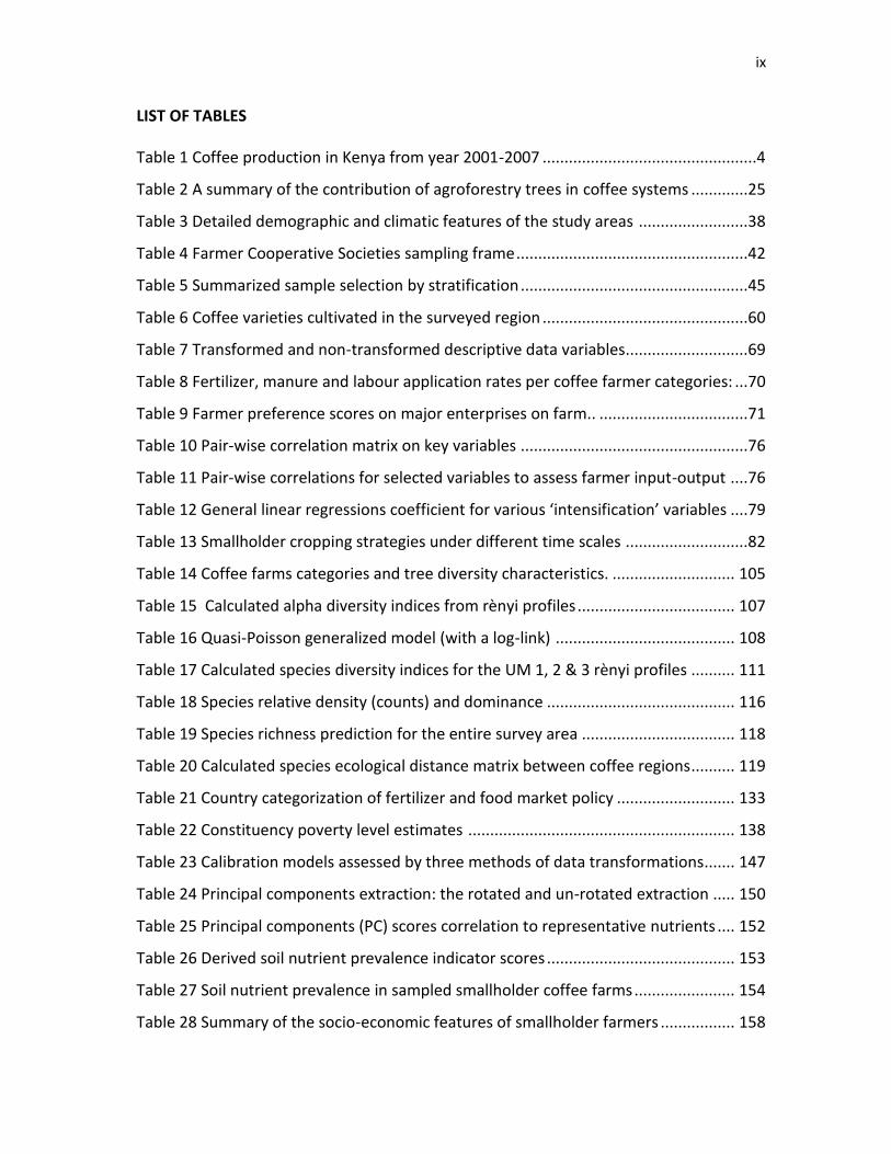
LIST OF TABLES

Table 1 Coffee production in Kenya from year 2001-2007 .................................................4

Table 2 A summary of the contribution of agroforestry trees in coffee systems .............25

Table 3 Detailed demographic and climatic features of the study areas .........................38

Table 4 Farmer Cooperative Societies sampling frame .....................................................42

Table 5 Summarized sample selection by stratification ....................................................45

Table 6 Coffee varieties cultivated in the surveyed region ...............................................60

Table 7 Transformed and non-transformed descriptive data variables ............................69

Table 8 Fertilizer, manure and labour application rates per coffee farmer categories: ...70

Table 9 Farmer preference scores on major enterprises on farm.. ..................................71

Table 10 Pair-wise correlation matrix on key variables ....................................................76

Table 11 Pair-wise correlations for selected variables to assess farmer input-output ....76

Table 12 General linear regressions coefficient for various ‘intensification’ variables ....79

Table 13 Smallholder cropping strategies under different time scales ............................82

Table 14 Coffee farms categories and tree diversity characteristics. ............................ 105

Table 15 Calculated alpha diversity indices from rènyi profiles .................................... 107

Table 16 Quasi-Poisson generalized model (with a log-link) ......................................... 108

Table 17 Calculated species diversity indices for the UM 1, 2 & 3 rènyi profiles .......... 111

Table 18 Species relative density (counts) and dominance ........................................... 116

Table 19 Species richness prediction for the entire survey area ................................... 118

Table 20 Calculated species ecological distance matrix between coffee regions .......... 119

Table 21 Country categorization of fertilizer and food market policy ........................... 133

Table 22 Constituency poverty level estimates ............................................................. 138

Table 23 Calibration models assessed by three methods of data transformations....... 147

Table 24 Principal components extraction: the rotated and un-rotated extraction ..... 150

Table 25 Principal components (PC) scores correlation to representative nutrients .... 152

Table 26 Derived soil nutrient prevalence indicator scores ........................................... 153

Table 27 Soil nutrient prevalence in sampled smallholder coffee farms ....................... 154

Table 28 Summary of the socio-economic features of smallholder farmers ................. 158

x

Table 29 Descriptive variables for three farmer groupings ............................................ 159

Table 30 Farmer priority crops for manure application ................................................. 160

Table 31 Quantity and costs of basal and straight fertilizers used by farmers ............. 162

Table 32 Percentage counts of farmers using basal and straight fertilizers per crop ... 162

Table 33 Correlation between fertilizer and manure application .................................. 163

xi

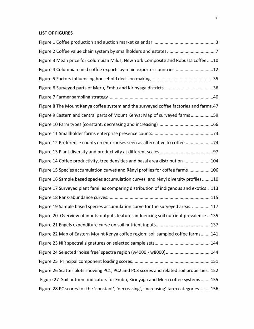
LIST OF FIGURES

Figure 1 Coffee production and auction market calendar ..................................................3

Figure 2 Coffee value chain system by smallholders and estates .......................................7

Figure 3 Mean price for Columbian Milds, New York Composite and Robusta coffee .....10

Figure 4 Columbian mild coffee exports by main exporter countries: ..............................12

Figure 5 Factors influencing household decision making ..................................................35

Figure 6 Surveyed parts of Meru, Embu and Kirinyaga districts .......................................36

Figure 7 Farmer sampling strategy ....................................................................................40

Figure 8 The Mount Kenya coffee system and the surveyed coffee factories and farms. 47

Figure 9 Eastern and central parts of Mount Kenya: Map of surveyed farms ..................59

Figure 10 Farm types (constant, decreasing and increasing) ............................................66

Figure 11 Smallholder farms enterprise presence counts.................................................73

Figure 12 Preference counts on enterprises seen as alternative to coffee ......................74

Figure 13 Plant diversity and productivity at different scales ...........................................97

Figure 14 Coffee productivity, tree densities and basal area distribution ..................... 104

Figure 15 Species accumulation curves and Rènyi profiles for coffee farms ................. 106

Figure 16 Sample based species accumulation curves and rènyi diversity profiles ...... 110

Figure 17 Surveyed plant families comparing distribution of indigenous and exotics . 113

Figure 18 Rank-abundance curves: ................................................................................. 115

Figure 19 Sample based species accumulation curve for the surveyed areas. .............. 117

Figure 20 Overview of inputs-outputs features influencing soil nutrient prevalence .. 135

Figure 21 Engels expenditure curve on soil nutrient inputs ........................................... 137

Figure 22 Map of Eastern Mount Kenya coffee region: soil sampled coffee farms ....... 141

Figure 23 NIR spectral signatures on selected sample sets............................................ 144

Figure 24 Selected ‘noise free’ spectra region (w4000 - w8000) ................................... 144

Figure 25 Principal component loading scores .............................................................. 151

Figure 26 Scatter plots showing PC1, PC2 and PC3 scores and related soil properties . 152

Figure 27 Soil nutrient indicators for Embu, Kirinyaga and Meru coffee systems ....... 155

Figure 28 PC scores for the ‘constant’, ‘decreasing’, ‘increasing’ farm categories ........ 156

xii

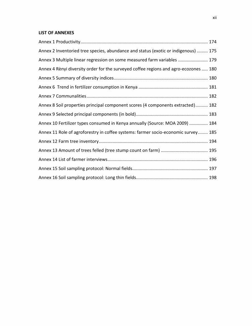
LIST OF ANNEXES

Annex 1 Productivity ....................................................................................................... 174

Annex 2 Inventoried tree species, abundance and status (exotic or indigenous) ......... 175

Annex 3 Multiple linear regression on some measured farm variables ........................ 179

Annex 4 Rènyi diversity order for the surveyed coffee regions and agro-ecozones ..... 180

Annex 5 Summary of diversity indices ............................................................................ 180

Annex 6 Trend in fertilizer consumption in Kenya ........................................................ 181

Annex 7 Communalities .................................................................................................. 182

Annex 8 Soil properties principal component scores (4 components extracted) .......... 182

Annex 9 Selected principal components (in bold) .......................................................... 183

Annex 10 Fertilizer types consumed in Kenya annually (Source: MOA 2009) ............... 184

Annex 11 Role of agroforestry in coffee systems: farmer socio-economic survey ........ 185

Annex 12 Farm tree inventory ........................................................................................ 194

Annex 13 Amount of trees felled (tree stump count on farm) ...................................... 195

Annex 14 List of farmer interviews ................................................................................. 196

Annex 15 Soil sampling protocol: Normal fields............................................................. 197

Annex 16 Soil sampling protocol: Long thin fields.......................................................... 198

xiii

ABSTRACT

Coffee farming has been a major foundation of Kenya’s rural highland economy for the

last four decades or so. Over 600,000 smallholder farmers organized in 579 cooperatives

are engaged in the subsector. Coffee was a major source of income, employment and

food security until the late 1980’s. Though Kenya produces some of the finest world

coffee, the collapse of the International Commodity Agreement (ICA) on coffee and

entry into the world market by major producers like Vietnam marked a near collapse of

Kenya’s coffee. Exports fell by over 50% between the year 2000 and 2010. This was

accompanied by significant loss of productivity (declined to a meagre 200 kg/ha from

600 kg/ha). The situation has contributed to poor living standards in coffee growing

areas. Interestingly, there are no credible alternative investments to merit the allocation

of constrained farm resources to replace coffee growing. In addition, there are concerns

that the current resource base can no longer support enhanced productivity.

This study used several research designs to investigate the performance of smallholder

coffee agroforestry systems around Mount Kenya. More specifically, enterprise

adoption and adaptation practices in the event of increased or decreased coffee

production were researched. The evolution of coffee agroforestry systems was also

evaluated and management of soil fertility determined.

Using coffee yields data obtained from 180 smallholder coffee farmers by stratified

random sampling techniques, coffee farm typologies were identified. These farm

typologies/categories were labeled as increasing, decreasing and constant -

representing their historical trends in coffee production. These farms were then used to

investigate current productivity behavior. Simple descriptive statistics such as means,

range, counts, enterprise scoring, diversity analysis pair wise correlations and

regressions were used to compare farmer enterprise intensification strategies. Results

have showed that farms that are decreasing coffee production, though had smaller land

sizes are not significantly different from those in the coffee increasing category. Further

xiv

results showed similarities in farmer enterprise diversification strategies. Coffee was

nonetheless declining in smaller farms compared to farm sizes where it was increasing.

Results also showed that farms with increasing coffee yields are associated with

productive milk enterprises. These farms appear to afford and benefit from larger

amounts of fertilizer and manure application. Coffee declining farms view banana and

maize as likely alternatives to coffee, perhaps in a strategy to secure household food

security. The study has showed that land size, coffee production (number of bushes,

cherry yields/Ha), livestock units, agroforestry trees, banana, maize value and nutrient

inputs (manure and fertilizer) and labour costs are important factors to assess coffee

farms productivity and distinguish farm types. Results have showed the importance of

creating more awareness among policy makers in order to promote enterprises that are

of interest to farmers.

This research also investigated tree diversity presently maintained by smallholders

showing a shift in coffee cultivation practices. Trees on farm are traditionally

appreciated for product benefits such as timber, fuel wood and food. They are also

important for enhanced farm biodiversity and environmental services such as enhanced

nutrient cycling. This study applied diversity analysis techniques such as species

accumulation curves, rènyi diversity profiles and species rank abundance, to investigate

farm tree diversity. At least 190 species were recorded from 180 coffee farms. For all

the species enumerated, alpha diversity (H0) = 5.25 and H∞ = 0.89. Results showed that

the 10 and 25 most abundant species comprise 75% and 91% of tree individuals present

on farm, respectively. Results suggest that, though there is high abundance of tree

individuals on farms they are of less richness and evenness. Species richness per farm

was calculated at 17 species (15- 19.2, P = 0.95). Grevillea robusta was highly ranked in

terms of relative density and dominance across surveyed farms at proportions of 41-

42%. Tree species basal area distribution showed that fruit trees such as, Persea

americana, Mangifera indica and timber species such as, Cordia africana, Vitex keniensis

and Croton macrostachyus are the most dominant but are of lower relative density.

xv

Species diversity analysis by coffee agro-ecological zones revealed that the upper-

midland (UM) 3 is ranked significantly higher than UM2 and UM1. Results have implied

that farmers with larger quantities of coffee (Coffea arabica L.) also retain more species

diversity than farmers with stagnated production even though this evidence was

inconclusive. Skewed patterns of species heterogeneity and structure among

smallholder coffee plots provide indicators of divergent species cultivation. Tree species

richness distribution between farms is strongly influenced by agro-ecological zones and

presence of coffee cultivation. Only 22.5% of agroforestry tree abundance on farm was

categorized as indigenous. Tree basal area ranking implied that fruit and native timber

species are retained longer on coffee farms.

Finally, this study assessed the implications of recent changes in coffee cultivation on

soil fertility management. It was hypothesized that significant soil nutrient exports have

occurred from coffee systems and that present nutrient prevalence are unknown and

likely to be poorly managed. The purpose of this research was to inform concerns that

with poor soil fertility prevalence, coffee systems face a danger to deteriorate to low

production systems. Near-infrared (NIR) spectroscopy was used to analyse soil

constituent properties for some 189 soil samples collected on 94 farms (within coffee

plots). One third of the samples were used to build calibration models giving correlation

coefficients between measured and partial least square (PLS) predicted soil properties.

Correlations were strong (r > 0.70) except for P, Zn and Na demonstrating the potential

of NIR to accurately predict soil constituents. Principal component analysis (PCA) was

then used to develop soil nutrient indices (principal components scores) to serve as

representative soil nutrient prevalence indicators. PC scores were also used as

dependent variables in regression analysis. Collected data is robust to show that soil

organic C, total N and probably P were most deficient across the coffee sites surveyed.

Farmer nutrient application practices showed wide variability of fertilizer and manure

use. Manure application is less than fertilizer and negatively correlated to farm size.

xvi

Estimation of manure use per household was however challenging due to quantification

and timing aspects of application. Collated evidence showed that farmers with

increasing coffee production were more likely to afford larger fertilizer and manure

application. Overall results point out that smallholders deliberately concentrate nutrient

application on farm enterprises with good market performance. Coffee cultivation has in

the past benefited from fertilizer credit facilities from farmer cooperative movements

and government bilateral programmes. Declined coffee production is therefore

seriously jeopardizing the amount of fertilizer that can be loaned to farmers.

In conclusion, this study has identified a number of factors associated with smallholder

decision making, resource use and enterprise adoption and adaptation behavior within

coffee agroforestry systems of Mount Kenya. Research findings have allowed

recommendations to be made on how best to promote farmer resource use, understand

farmer decision making and enterprise choices that are of interest to farmers. The study

has contributed to knowledge of farmer livelihood strategies when managing coffee

farms in conditions of reduced profitability.

xvii

ACRONYMS

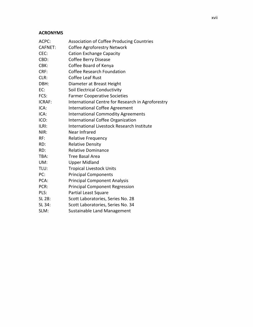
ACPC: Association of Coffee Producing Countries CAFNET: Coffee Agroforestry Network CEC: Cation Exchange Capacity CBD: Coffee Berry Disease CBK: Coffee Board of Kenya CRF: Coffee Research Foundation CLR: Coffee Leaf Rust DBH: Diameter at Breast Height EC: Soil Electrical Conductivity FCS: Farmer Cooperative Societies ICRAF: International Centre for Research in Agroforestry ICA: International Coffee Agreement ICA: International Commodity Agreements ICO: International Coffee Organization ILRI: International Livestock Research Institute NIR: Near Infrared RF: Relative Frequency RD: Relative Density RD: Relative Dominance TBA: Tree Basal Area UM: Upper Midland TLU: Tropical Livestock Units PC: Principal Components PCA: Principal Component Analysis PCR: Principal Component Regression PLS: Partial Least Square SL 28: Scott Laboratories, Series No. 28 SL 34: Scott Laboratories, Series No. 34 SLM: Sustainable Land Management

1

CHAPTER 1 EVOLUTION OF THE SMALLHOLDER COFFEE SUB SECTOR IN KENYA ABSTRACT

Coffee was a major source of farm income, employment and food security in Kenya until

the late 1980’s. The collapse of the International Coffee Agreement (ICA) precipitated an

increase in production costs leaving many farmers exposed to the double tragedy of low

income and low food availability. Coffee productivity by smallholders has therefore

significantly declined or stagnated and even seems unresponsive to recent high prices

offered in the international market. It’s clear that more supportive policies are required

to shift the present situation. Additionally, the impact of climate change, manifested in

prolonged droughts and unpredictable rainfall episodes is likely to affect coffee fruiting

and exacerbate pest and diseases incidence. This background chapter evaluates coffee

production and marketing conditions experienced by thousands of smallholder growers

in Kenya.

INTRODUCTION

Kenya’s coffee systems are strongly associated with coffee growing as the main source

of income since the country’s independence in 1963. Arabica coffee (Coffea arabica)

was successfully brought into Kenya around 1894 from neighboring German East Africa

(now Tanzania) by Roman Catholic missionaries (Waters, 1972). Coffee cultivation was

however reserved exclusively for European settlers. In 1933 coffee growing by African

smallholders was piloted in small areas of Kisii, Embu and Meru under strict supervision

(Barnes, 1979). The Native Grown Coffee Rules of 1934 stipulated coffee growing

regulations. African coffee production was in fact considered experimental. Areas in

which coffee cultivation was permitted were clearly defined by the director of

agriculture. The gazettement of production areas was meant to ensure quality and to

some extent quantity of coffee produce (Akiyama, 1987). Until 1950 planting was

restricted to the altitude range of between 1645 to 1750 m above sea level on the

2

slopes of Mount Kenya (Waters, 1972). Presently, over 90% of Kenya’s highland arabica

are cultivated at altitudes ranging between 1400 m and 1950 m above sea level

(Condliffe et al., 2008).

By 1952 there were about 11,864 farmers cultivating around 3,000 acres of coffee.

Smallholder coffee cultivation accelerated after Kenya’s independence in 1963.

Production increased at a rapid rate of 6% in the early 1960’s as some of the large

estates were given up for sub-divisions to smallholders and un-favourable laws were

lifted (Akiyama, 1987). Nonetheless, coffee cultivation by smallholders was by law

restricted within cooperatives with government as a significant stakeholder so as to

secure foreign exchange earnings and meet obligations entered into under the ICA that

was politically negotiated. Coffee growing became the backbone of Kenya’s rural

highlands economy. Until recently the subsector claimed to support over five million

Kenyans both directly and indirectly as a result of forward and backward linkages.

Coffee remained the nation’s top foreign exchange earner from independence in 1963

until 1989 when it was surpassed by tourism (Karanja, 2002). By 1978, the coffee sector

accounted for 9.5 percent of GDP ($500 million in exports). By 2005, the revenues were

only $75 million - a mere 0.6 percent of GDP (The World Bank, 2005). Coffee is presently

ranked as the fifth foreign currency earner, after remittances from Kenyans abroad, tea,

tourism and horticulture.

Unlike Ethiopia and Uganda, which are Africa's top coffee producers, Kenyan coffee

output is under one percent of global production, but its beans are popular for blends

and buyers have specific volume requirements (Ponte, 2002). On average, Kenya’s

coffee fetches a 10% premium over standard arabica coffees from Central America and

Colombia.

3

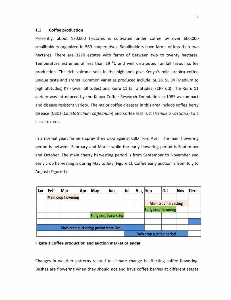
1.1 Coffee production

Presently, about 170,000 hectares is cultivated under coffee by over 600,000

smallholders organized in 569 cooperatives. Smallholders have farms of less than two

hectares. There are 3270 estates with farms of between two to twenty hectares.

Temperature extremes of less than 19 oC and well distributed rainfall favour coffee

production. The rich volcanic soils in the highlands give Kenya’s mild arabica coffee

unique taste and aroma. Common varieties produced include: SL 28, SL 34 (Medium to

high altitudes) K7 (lower altitudes) and Ruiru 11 (all altitudes) (CRF ud). The Ruiru 11

variety was introduced by the Kenya Coffee Research Foundation in 1985 as compact

and disease resistant variety. The major coffee diseases in this area include coffee berry

disease (CBD) (Colletotrichum coffeanum) and coffee leaf rust (Hemileia vastatrix) to a

lesser extent.

In a normal year, farmers spray their crop against CBD from April. The main flowering

period is between February and March while the early flowering period is September

and October. The main cherry harvesting period is from September to November and

early crop harvesting is during May to July (Figure 1). Coffee early auction is from July to

August (Figure 1).

Figure 1 Coffee production and auction market calendar

Changes in weather patterns related to climate change is affecting coffee flowering.

Bushes are flowering when they should not and have coffee berries at different stages

4

of maturity. This means farmers have to hire labor throughout the year to pick little

quantities of coffee. Trees tend to have beans of all ages causing a problem of disease

management, insect management and increased farmer harvesting costs (Reuters

2010). Further, due to the narrow range of temperature for coffee (19-25 oC) slight

increases in temperature affects photosynthesis and in some cases, trees wilt and dry up

especially in the marginal coffee zones. The most immediate solution recommended for

farmers is to conserve whatever rainfall they receive through mulching, digging trenches

to hold water, pruning, forking and planting shade trees (Reuters, 2010).

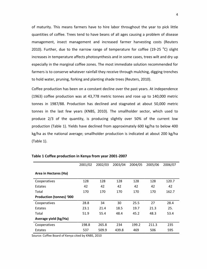
Coffee production has been on a constant decline over the past years. At independence

(1963) coffee production was at 43,778 metric tonnes and rose up to 140,000 metric

tonnes in 1987/88. Production has declined and stagnated at about 50,000 metric

tonnes in the last few years (KNBS, 2010). The smallholder sector, which used to

produce 2/3 of the quantity, is producing slightly over 50% of the current low

production (Table 1). Yields have declined from approximately 600 kg/ha to below 400

kg/ha as the national average; smallholder production is indicated at about 200 kg/ha

(Table 1).

Table 1 Coffee production in Kenya from year 2001-2007

2001/02 2002/03 2003/04 2004/05 2005/06 2006/07

Area in Hectares (Ha)

Cooperatives 128 128 128 128 128 120.7

Estates 42 42 42 42 42 42

Total 170 170 170 170 170 162.7

Production (tonnes) ‘000

Cooperatives 28.8 34 30 25.5 27 28.4

Estates 23.1 21.4 18.5 19.7 21.3 25.

Total 51.9 55.4 48.4 45.2 48.3 53.4

Average yield (kg/Ha)

Cooperatives 198.8 265.8 234 199.2 211.3 235

Estates 537 509.9 439.8 469 506 595

Source: Coffee Board of Kenya cited by KNBS, 2010

5

An estimated 95% of the national production of coffee comes from the central parts of

Kenya. In the area stretching from Nairobi to Muranga, coffee is grown in open sun

plantations mostly with a small number of trees in the boundaries. Smallholder coffee

systems are situated around the central highlands of Mount Kenya, in the Aberdare

area, in the West of Kisii, Nyanza, Bungoma, in the Rift Valley in Nakuru, Trans Nzoia and

in Taita hills, near Mount Kilimanjaro. The main production area between Mount Kenya

and the Aberdare is between 1500 to 1600 m above sea level.

Open sun systems with multiple stems management is preferred as opposed to shaded

coffee system to maximize yields (Kimemia, 1994). Single stem managed, shaded coffee

under Grevillea robusta previously introduced in Kenya is not supported by formal

extension services due to disease incident fears. Farmers nonetheless retain a wide

variety of tree species on coffee farms such as Grevilllea robusta, Vitex keniensis, Cordia

africana, Trichillia emetica, Persea americana and Macadamia tetraphylla. These

species are not grown for shade coffee but rather for their various products and

services.

A coffee crop takes over five years to attain full production. Production is generally

labour intensive and involves appropriate land preparation, fertilizer application, pests

and diseases control, irrigation, primary processing, secondary processing and facilities

maintenance. To produce 400 kg/ha of clean coffee or 2870 kg/ha cherry, it costs about

$531.31/ha ($ 0.181 kg of cherry) (KNBS, 2010).

1.2 Coffee marketing

Kenyan coffee is regarded as one of the best coffees in the World, traded under the

‘Colombian mild’s category. Coffee is mainly traded on the New York and London

futures markets, which exert a strong influence on world coffee prices. Coffee prices are

very volatile varying daily, hourly and even by the second, depending on factors such as

the size of coffee stocks worldwide, weather forecast, insecure political conditions and

6

speculation on the futures markets (ICO, 2010). Almost 99% of Kenyan coffee is

exported and the domestic market only consumes less than 1% of the total coffee

produced.

Coffee marketing is regulated by the Coffee Board of Kenya which also issues licenses

for different categories of stakeholders in the industry including dealers, millers,

roasters, packers, and warehouse license (EPZ, 2005). Coffee estates use licensed

private milling and marketing agents to bring their coffee to the auction, while

smallholder farmers are legally required to process and commercialize their produce

through cooperatives (Mude, 2006). Farmers deliver their cherry to local factories for

primary processing. Cherry for each grower is weighed and recorded. Cherry beans are

sorted and pulped (coffee bean are removed from outer fruit). The beans are spread on

drying beds and later stored in the form of ‘parchment coffee’.

The cooperatives and the estates then send their produce to commercial millers for

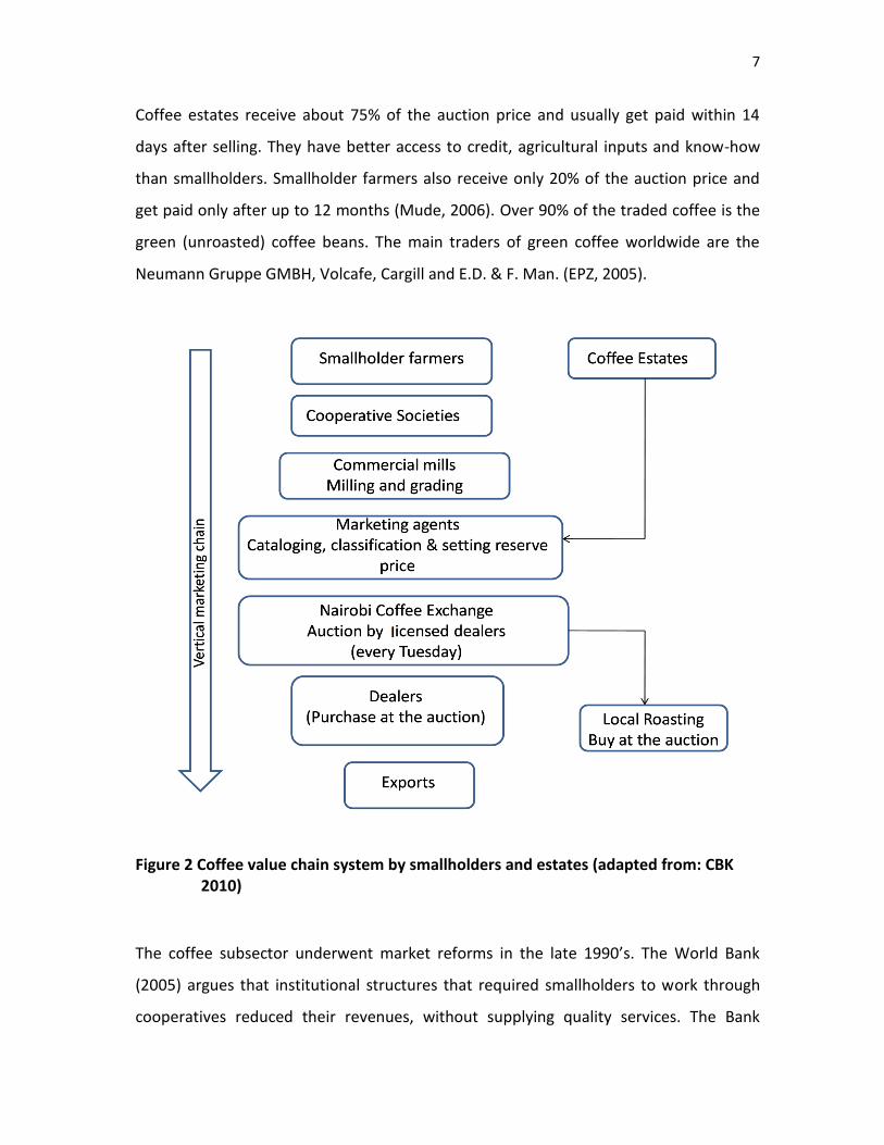
milling and grading (Figure 2). Mills hull and clean parchment coffee to produce green

(unroasted) coffee. The commercial millers then send graded coffee to marketing agents

who prepare, classify the coffee, prepare catalogues and put a reserve price for the

coffee auction through which all Kenyan coffee is sold (EPZ, 2005). The transaction

between buyer and seller at the auction is often carried out on behalf of the cooperative

by an agent hired by the miller. Once the coffee is sold, the miller deducts his share of

the commission and sends the rest to the cooperative.

The larger cooperative management then deducts all of its operating costs including

loan repayments, services and maintenance expenses, and other fees. The deductions

are made from factory kitties as a proportion of each factory’s membership to the total

(i.e. uniform deduction per cooperative member). The remaining funds are then

distributed to factory managers who further deduct the costs of factory level operations

then distribute the remaining money to farmers as their annual payment (Mude, 2006).

7

Coffee estates receive about 75% of the auction price and usually get paid within 14

days after selling. They have better access to credit, agricultural inputs and know-how

than smallholders. Smallholder farmers also receive only 20% of the auction price and

get paid only after up to 12 months (Mude, 2006). Over 90% of the traded coffee is the

green (unroasted) coffee beans. The main traders of green coffee worldwide are the

Neumann Gruppe GMBH, Volcafe, Cargill and E.D. & F. Man. (EPZ, 2005).

Figure 2 Coffee value chain system by smallholders and estates (adapted from: CBK 2010)

The coffee subsector underwent market reforms in the late 1990’s. The World Bank

(2005) argues that institutional structures that required smallholders to work through

cooperatives reduced their revenues, without supplying quality services. The Bank

8

recommended market liberalization to reverse this. They proposed the following steps

in order to create a more open market-place:

a) Farmers require real time market information and the option to sell directly to

consumers.

b) Marketing agents should provide information back to the producers to clarify the

relationship between bean quality, liquor quality and price.

c) The requirement for farmers to discontinue the common coffee auction.

d) Government was required to review all licenses with the goal of abolishing many

of them.

Coffee market liberalization has given smallholders greater control on production but at

the same time enhanced moral hazards. For instance poor and good quality coffee

cherries are often pooled together as quality is not necessarily related to payments.

Further, smallholders are no longer keen to improve quality as there are no incentives

to do so (Karanja and Nyoro, 2002).

1.3 Price volatility in the coffee industry

Coffee is a soft1 commodity and is subject to extreme price volatility (Gilbert and

Brunnette, 1998). The coffee value chain power shifts has significantly been influenced

in two phases; during the International Coffee Agreement (ICA) regime (1962 to 1989)

and secondly in the post ICA regime from 1989 to present. During the ICA era coffee

markets were producer driven, while in the post ICA era, markets became buyer driven

(Ponte, 2002). Producers no longer have much say in the present value chain (ICO,

2005). Previously, the International Coffee Agreement ensured high coffee prices

between 1975 and 1989 but collapsed in 1989 leading to a decline in world coffee prices

(Gilbert, 1996). When the agreements were in force, coffee market was regulated

through a system of export quotas which were triggered when prices fell to significantly

low levels. Gilbert and Brunette (1998) reported that the ICA may have raised producer

1 A soft commodity refers to commodities that are grown rather than mined such as coffee, cocoa, sugar,

corn, wheat, soybean, fruit and others. The commodities are largely traded on the futures market.

9

prices by about 50-60%. Karanja and Nyoro (2002) report that Kenyan farmers benefited

by 30% higher prices under the ICA trade regime.

While coffee growers used to capture about 30% of the value of the final retail price of

coffee in 1975, by 2000, they captured just 10% as downstream players became

increasingly consolidated (Talbot, 1997). In desperation, the coffee producer nations

formed the Association of Coffee Producing Countries (ACPC) in 1993 as a lobby group,

however the lobby has not managed any major impact on the world coffee trade.

During the 1990’s, there were supply increases in the world coffee market, due to

expansion of plantations in Brazil and Vietnam's entry into the market in 1994. As a

result, by 2001, the world price of arabica coffee fell to below 60 cents a pound from

highs of over $2 a pound precipitating a near market collapse (Akiyama et al., 2003; ICO,

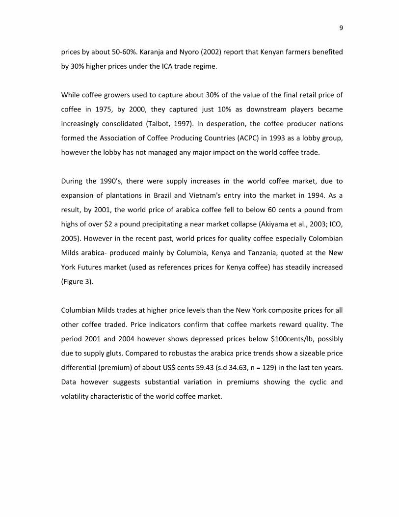
2005). However in the recent past, world prices for quality coffee especially Colombian

Milds arabica- produced mainly by Columbia, Kenya and Tanzania, quoted at the New

York Futures market (used as references prices for Kenya coffee) has steadily increased

(Figure 3).

Columbian Milds trades at higher price levels than the New York composite prices for all

other coffee traded. Price indicators confirm that coffee markets reward quality. The

period 2001 and 2004 however shows depressed prices below $100cents/lb, possibly

due to supply gluts. Compared to robustas the arabica price trends show a sizeable price

differential (premium) of about US$ cents 59.43 (s.d 34.63, n = 129) in the last ten years.

Data however suggests substantial variation in premiums showing the cyclic and

volatility characteristic of the world coffee market.

10

Figure 3 Mean price for Columbian Milds, New York Composite and Robusta coffee from 2000 to 2010 (Source: ICO, 2010)

The present free market environment and liberalization have nonetheless enhanced

price volatility (Karanja, 2002). Higher international coffee prices do not readily translate

to increased productivity. For instance, in Uganda when coffee production declined due

to low market prices in early 2000, efforts to increase production have not been fruitful

despite increased market prices (Baffes, 2006). Market liberalization is also blamed for

exposing smallholders to higher price risks. Liberalization meant a significant reduction

in public expenditure on agriculture which severely constrained the provision of

essential services needed to promote the productivity of smallholder farms. The

expectation that the private sector would take on these roles left behind by government

and its agencies have only been fulfilled to a limited extent (Shepherd and Farolfi, 1999).

11

1.4 Coffee exports

Coffee used to be the most important foreign exchange earner representing 24% of

total African agricultural exports during 1984-1986. This value decreased to only 11.5%,

overtaken by cacao at 13.5%, by 1996-1998 (Ponte, 2002). In the period 1996-1998

coffee exports represented more than 50% of agricultural export earnings in five

countries and more than 20% in nine countries (Ponte, 2002). Globally, coffee

production in terms of exports by 2006 was dominated by Brazil (30%), Vietnam (15%)

and Colombia (12%). Brazil is the largest arabica (Coffea arabica) producer in the world

while Vietnam, is the world’s largest robusta (Coffea canephora) producer (Condliffe et

al., 2008; ICO, 2010).

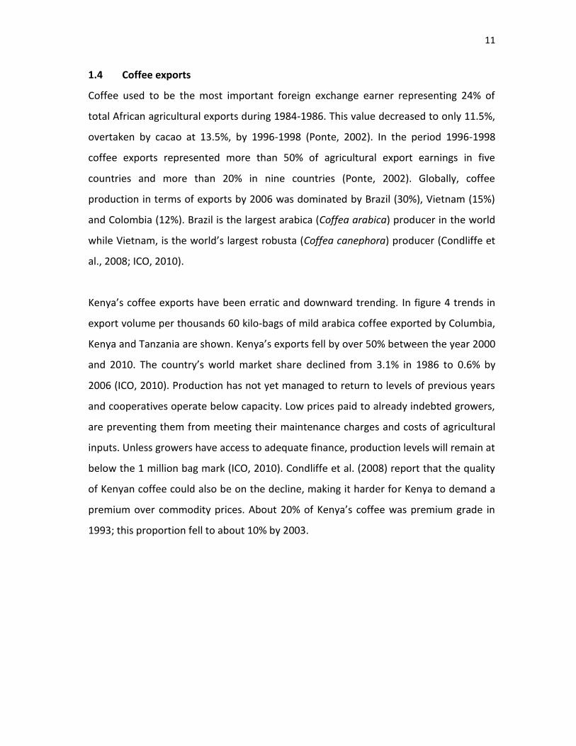
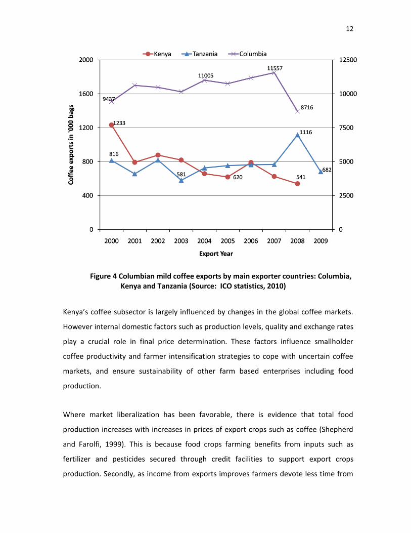
Kenya’s coffee exports have been erratic and downward trending. In figure 4 trends in

export volume per thousands 60 kilo-bags of mild arabica coffee exported by Columbia,

Kenya and Tanzania are shown. Kenya’s exports fell by over 50% between the year 2000

and 2010. The country’s world market share declined from 3.1% in 1986 to 0.6% by

2006 (ICO, 2010). Production has not yet managed to return to levels of previous years

and cooperatives operate below capacity. Low prices paid to already indebted growers,

are preventing them from meeting their maintenance charges and costs of agricultural

inputs. Unless growers have access to adequate finance, production levels will remain at

below the 1 million bag mark (ICO, 2010). Condliffe et al. (2008) report that the quality

of Kenyan coffee could also be on the decline, making it harder for Kenya to demand a

premium over commodity prices. About 20% of Kenya’s coffee was premium grade in

1993; this proportion fell to about 10% by 2003.

12

Figure 4 Columbian mild coffee exports by main exporter countries: Columbia, Kenya and Tanzania (Source: ICO statistics, 2010)

Kenya’s coffee subsector is largely influenced by changes in the global coffee markets.

However internal domestic factors such as production levels, quality and exchange rates

play a crucial role in final price determination. These factors influence smallholder

coffee productivity and farmer intensification strategies to cope with uncertain coffee

markets, and ensure sustainability of other farm based enterprises including food

production.

Where market liberalization has been favorable, there is evidence that total food

production increases with increases in prices of export crops such as coffee (Shepherd

and Farolfi, 1999). This is because food crops farming benefits from inputs such as

fertilizer and pesticides secured through credit facilities to support export crops

production. Secondly, as income from exports improves farmers devote less time from

13

off-farm employment and more time is allocated to food production; and higher

incomes from exports lead to higher investment in food and staple crops production

(Karanja and Nyoro, 2002). Declining market trends are on the other hand proving to

affect yields and family income directly. This is because farmers are not able to manage

their coffee bushes due to lack of adequate income from the crop. Yields can therefore

be regarded to make the difference between satisfactory income and poverty in coffee

farming areas (Kabura-Nyaga, 2007).

A significant feature of the global coffee trade is the high market concentration of

roasters and traders. Four large multinationals export more than half of the coffee

consumed to the 25 main consumer countries. These companies are Jacobs/Kraft

General Foods, Nestle, Proctor and Gamble and Sara Lee/DE. In Germany the big four

control 86% while in The Netherlands, Sara Lee/De controls 70% (Karanja and Nyoro,

2002). According to ICO (2005), in the 90’s coffee producing countries earned an

estimated US$10-12 billion per year, while the value of retail sales in industrialized

countries was about US$ 30 billion. Presently, sales exceed US$70 billion but coffee

producing countries receive a meager US$ 5.5 billion per year (ICO, 2010).

1.5 DISCUSSION

The coffee subsector despite significant marketing challenges has provided livelihood

support to thousands of smallholder farmers. Changes in commodity trade

arrangements from international commodity agreements (ICA) to market liberalization

shifted the coffee value chain power from producers to buyers. This has resulted in

substantial erosion in smallholder profitability. It’s no wonder therefore that even with

price increases in countries like Kenya and Uganda it’s difficult to stimulate more

productivity as farmers remain cautious. Further, gains as a result of price increase do

not translate to significant real incomes to make costs of inputs such as fertilizer and

pesticides more affordable. Farmer cooperatives despite management inefficiencies

have substantially supported access to credit and input facilities to members. These

14

market instruments remain attractive to most smallholders and have contributed to

stabilizing farmer productivity to some extent.

Coffee market liberalization though not fully adopted in the Kenyan coffee subsector

have reduced government’s role in the subsector and given farmers greater autonomy

in coffee marketing (Shepherd and Farolfi, 1999; Karanja and Nyoro, 2002). However

coffee marketing through a central auction still remains in force. Farmer cooperative

societies are however free to elect their preferred coffee millers and marketing agents.

Cooperatives management costs and indebtedness continue to exert enormous

pressure on farmer earnings. All smallholders are legally bound to market their coffee

through cooperatives. Growers whose land falls within a particular coffee society

‘catchment’ are required to register their membership (Mude, 2006). Many

cooperatives however fall short of standards needed in financial and business

management.

It has been difficult to stimulate coffee productivity due to factors such as costs of

inputs and uncertainty in the market prices. Coffee yields have stagnated due to old

coffee bushes. Re-investing in higher yielding coffee bushes could therefore improve

production. Other factors such as poor road networks affect transport costs and foreign

exchange rates affect net earnings by farmers.

Recent efforts to implement certification schemes for smallholder coffee growers have

not really resulted in much added benefits. Preliminary assessment of certification

schemes in Kenya have been showed to carry the risk of a top-down approach and do

not always meet the main needs of farmers (Kirumba, 2011). As such, a more integrated

approach is needed, which takes sustainability and the specific conditions under which

farmers operate as its starting points.

15

Finally, the impact of climate change, manifested in prolonged droughts and extended

rainfall episodes have influenced coffee fruiting. Changes in coffee fruiting have a direct

impact on harvesting costs incurred by farmers. In addition, pest and disease

management in coffee are likely to be negatively influenced (Reuters, 2010).

1.6 CONCLUSIONS

Smallholder coffee production and marketing is driven by a combination of local and

international factors. Coffee prices have been improving in the recent past but farmer

productivity has stagnated suggesting a need to consider more incentives to increase

coffee production and offer farmers better security and stability. On the other hand

getting alternative sources of income has been hard for farmers. In fact it’s not clear if

farmers are presently able to expand coffee production areas due to their small land-

holdings and large family sizes. It appears that increasing farm production and income

can only be through land intensification, but this requires large capital investment which

is limited.

16

1.7 References

Akiyama, T. 1987. Kenyan coffee sector outlook. A framework for policy analysis.

Division Working Paper No. 1987-3. Commodities studies projection division. The

World Bank.

Akiyama, T. Baffes, J. Larson, D. and Varangis, P. 2003. Commodity market reform in

Africa: some recent experience. Economic Systems 27: 83–115.

Baffes, J. 2006. Restructuring Uganda’s Coffee Industry: Why Going Back to the Basics

Matters. World Bank Policy Research Working Paper 4020.

Barnes, C. 1979. An experiment with coffee production by Kenyans, 1933-48. African

Economic History, No. 8: 198-209.

Condliffe, K. Kibuchi, W. Love, C. and Ruparell, R. 2008. Kenya Coffee: A Cluster Analysis.

Harvard Business School Microeconomics of Competitiveness.

CBK (Coffee Board of Kenya) 2010: Area & production 2008/2009.

CRF (Coffee Research Foundation) (Ud) Coffee varieties produced & marketed in Kenya.

EPZ (Export Processing Zones Authority), 2005. Tea and coffee industry in Kenya

http://www.epzakenya.com/UserFiles/File/Beverages.pdf (accessed 5/06/2011).

Gilbert, CL. 1996. International commodity agreements: an obituary notice. World

Development 24:1-19.

Gilbert, CL. and Brunette, C. 1998. Speculation, hedging and volatility in the coffee

market, 1993-1996: department of economics, Queen Mary and Wesfiled

College London.

ICO (International Coffee Organization) 2005. Overview of the coffee market.

International Coffee Council 90rd Session, 18 – 20 May 2005 London, England.

ICO (International Coffee Organization), www.ico.org (accessed November, 2010).

Kabura-Nyaga, EA. 2007. Smallholder cash crop production and its impact on living

standards of rural families in Kenya. Doppler, W. and Bauer, S. (Eds) Farming and

rural systems economics. Vol. 89 Margaraf Publishers, GmbH, Germany.

Karanja, AM. 2002. Liberalization and smallholder agricultural development. A case

study of coffee farms in Kenya. PhD thesis Wageningen, University.

17

Karanja, AM. Nyoro, JK. 2002. Coffee prices and regulation and their impact on

livelihoods of rural community in Kenya. Tegemeo Institute of agricultural policy

and development, Egerton University.

Kimemia, MN. 1994. Influence of tree training and plant density on yields of an

improved cultivar of Coffea Arabica. Experimental Agriculture, 30:89-94.

Kirumba, EG. 2011. Governance and participation of smallholder farmers in coffee

certification programs in Kenya. In: Coffee certification and smallholder

livelihoods in Kenya. A PhD thesis submitted to the department of human

geography, University of Bordeaux III, France.

KNBS (Kenya National Bureau of Statistics), 2010. Principle crops production for sale

2002-2009. Statistical abstract. http://www.knbs.or.ke/agriculture_crops.php

Mude, A. 2006. “Weaknesses in Institutional Organization: Explaining the Dismal

Performance of Kenya’s Coffee Cooperatives” Paper presented at International

Association of Agricultural Economists Conference.

Ponte, S. 2002. Brewing a bitter cup? Deregulation quality and re-organization of coffee

marketing in East Africa. Journal of Agrarian Change, 2: 248-272

Reuters, 2010. Climate change affecting Kenya's coffee output.

http://www.reuters.com/kenya-coffee-climate (accessed 5/02/2011)

Shepherd, AW. Farolfi, S. 1999. Export Crop Liberalization in Africa: A Review. FAO

Agricultural Services Bulletin 135. Rome.

Talbot, JM. 1997. Where does your coffee dollar go? The division of income and surplus

along coffee commodity chain. Studies in Comparative International

Development, 32 (1): 56-91.

The World Bank, 2005. Summary of Kenya Value Chain Analysis. World Bank Group

Africa Region, private sector Unit Note No.8.

Waters, AR. 1972. Change and evolution in the structure of the Kenya coffee industry.

African affairs, Texas A & M University.

http://afraf.oxfordjournals.org/content/71/283/163.full.pdf

18

CHAPTER 2 TRANSITIONS IN SMALLHOLDER COFFEE SYSTEMS: THE ROLE OF AGROFORESTRY AS A LAND-USE OPTION AROUND MOUNT KENYA ABSTRACT

This chapter highlights the role of smallholder agroforestry practices towards

sustainable coffee production systems. Challenges related to family resource availability

and declining living standards in cash crop growing areas are related to decisions at

farm, national, regional and international circles. The adoption of farm enterprises is

largely driven by resource availability and market value for major cash crops such as

coffee. Interestingly, even with significantly reduced coffee profitability, few farming

enterprises have emerged as credible substitutes to replace coffee. Serious concerns on

the sustainability of current resource base within coffee systems due to environmental

degradation have nonetheless been raised. Decisions on the change of farming activities

in these systems will directly affect family income and living standards of many coffee

producers. Strategies to improve smallholder well-being therefore require a better

understanding of the existing resource capacities, their management as well as their

contribution to coffee farming households. This chapter delineates the contribution of

agroforestry often ignored by present agricultural policy, to improve smallholder overall

farm productivity. The research motivation and objectives are outlined and the

structure of the thesis is defined in this chapter.

19

2.1 Background

A multitude of smallholders in high potential parts of Sub-Saharan Africa are engaged in

economic development through subsistence and export commodity production. It is

estimated that 60% of all marketed agricultural outputs in these countries except South

Africa, are by smallholders. In Kenya, coffee systems provide a good example of multiple

cropping systems that support rural household needs of income and food provision.

Reference to coffee systems in this study therefore does not imply coffee production

solely but also other crops produced within the coffee agro-ecological zones.

Coffee farming has nonetheless been the backbone of most rural highland economies in

Kenya for the past three to four decades. Kenya’s coffee and tea farming systems have

been converted from natural forest vegetation (Kindt et al., 2007) thereby directly

experiencing loss of important products and services such as firewood, timber and land

for grazing and subsistence crops cultivation. The impact of converting natural forest to

a coffee agroforestry system is yet to be clear. Nair (1990) has argued that inclusion of

trees in farmland can change a farming system from one of decline to one of

productivity as introduction of trees bring stability to the system.

Due to global natural resource degradation concerns, production of commodity crops

such as coffee (Coffea arabica) and cacao (Theobroma cacao) are claimed to be more

sustainable when practiced under complex agroforests as compared to pure

monoculture plantations (Perfecto et al., 2005; Scroth and Harvey, 2007; Philpott et al.,

2008). This special type of agroforestry is often characterized by forest-like structures

involving a shade tolerant perennial crop such as cacao, coffee or canopy trees such as

rubber (Hevea brasilensis) (Asase and Tetteh, 2010). In fact tree-crop systems have been

showed to have a positive contribution to the environment and biodiversity

preservation (Perfecto et al., 2005). Integration of diverse trees within coffee or cacao

systems is now regarded as a form of intensification as planted trees can also be a

20

source of products and services such as timber, fruits, firewood and enhance soil

nutrient cycling.

More recently, Kenya’s coffee farmers have been challenged by low coffee productivity2

and income shortcomings due to a combination of factors affecting profitability. Low-

input, family-based farming practices use limited resources in terms of technology, cash,

and information in current production practices. This has forced many to become even

more subsistence oriented rather than producing a surplus for the market. In addition

impact of climate change is becoming more apparent as yields fluctuation persists due

to unpredictable drought spells and the amount of rainfall received per season

(Jamnadass et al., 2010). These challenges collectively influence smallholder production

and income streams from traditional cash crops such as coffee, tea and cotton.

In parts of the Mount Kenya coffee systems, smallholders deliberately change their

enterprises compositions on farm as a strategy to deal with some of these challenges

(Carsan, 2007). These changes have involved adoption of agroforestry tree crops, food

crops, horticulture and livestock on farm to balance provision of food and income

needs. This type of farming practice is now commonly referred to as coffee agroforestry

to depict the diversity of practices adapted on farm. Largely, the intensity of smallholder

production is determined by available resource factors such as land, capital and labour

(Chambers and Leach, 1989; Arnold and Dewees, 1998). It is therefore instructive to link

farmer agronomic practices to factor availability. Smaller farm sizes can especially affect

labour availability and overall agricultural production if they fail to fully support

household’s needs - family members tend to seek off-farm employment to supplement

incomes or move out of farming when livelihoods improve significantly (Hazell et al.,

2007).

2 Productivity: is the output of valued product per unit of resource input; common measures of

productivity constitute yield or income per hectare or total production of goods and services per hectare (See Annex 1)

21

Future tree planting or non-planting within coffee system will nonetheless be influenced

by socio-economic factors such as available land, expected market returns, farmers’

beliefs, labour and access to planting material (Lengkeek and Carsan, 2004; Arnold and

Dewees, 1998; Simons and Leakey, 2004). Moreover, the decisions of farmers to adopt

tree planting are based on informal cost-benefit analysis to ensure they earn a

livelihood in their real situations of existence and with limited resources. Often little is

known about farmer perceptions on the value of trees and about the constraints they

face in developing tree resources (Franzel, 2002). For instance, farmers already report

increasing use of ‘inferior’ or mismatched species for fuel wood, timber, fruits and

medicinal purposes (Muriuki, 2011). Ruf (2011) has warned that complex agroforests in

cocoa systems of West Africa are likely to be displaced by less complex systems due to

changes in factor availability especially land.

The purpose of this study was to characterise transitions among smallholder coffee

producers of Mount Kenya, deemed to be at different but comparable trends in coffee

production and related agricultural activities. This study investigated coffee farmers’

enterprise adoption strategies; agroforestry tree diversity maintenance; and coffee

farms land health status- depicted by soil nutrients prevalence under present

management. It was anticipated that the study findings will provide better

understanding of the implication of shifts in smallholder coffee production on future

enterprise choices and sustainable resource use (land management strategies). The

ultimate goal would be to better inform agricultural policies aimed at improving

smallholder coffee productivity, incomes and living standards.

2.2 Why agroforestry in coffee systems?

Agroforestry has been described as the practice of integrating a range of trees with

agricultural crop cultivation and other farm activities. The approach is adopted by

millions of smallholders globally to meet their needs for essential resources such as

food, medicine, timber, fuel, fodder and market commodities, and provides valuable

22

environmental services such as soil fertility replenishment, water catchment protection,

carbon sequestration, biodiversity conservation and landscape restoration (Garrity,

2004). Simons and Leakey (2004) demonstrate that farmers’ interest and willingness to

invest greater household resources in tree growing is indeed accelerated by scarcity of

products from forests relative to the needs of an increasing population and relative to

available substitutes.

Appropriate tree systems are perceived to maintain or improve soil fertility and soil

productivity, to promote soil conservation, reduce soil degradation and achieve

sustainable production (Falconer, 1990; Mucheru et al., 2007). Trees in agricultural

landscapes offer soil protection from erosion and compaction, increased nutrient cycling

and enhanced soil organic matter above and below-ground.

In Latin America, studies have shown that ‘rustic-coffee systems’ protect a greater

diversity of ants, birds, and trees than open sun-coffee systems. Current knowledge

claims that coffee agroforestry practices should be promoted, but not at the expense of

remaining forest patches (Rappole et al., 2003; Perfecto et al., 2005; Philpott et al.,

2008). Displacing natural ecosystems through clearing or replanting with crops and trees

can result in variable levels of domestication of the original landscape and ecosystems

(Asase and Tetteh, 2010). The effect of these conversions is presently not well

understood.

Kenya’s smallholder coffee systems are presently organized along combinations of

annual crops/trees/livestock enterprises. Farmers’ have basically shifted from

subsistence, cereal – based farming systems to mixed – enterprise, market – oriented

systems. Patterns of land use conversion to different crop choices appear to correspond

to prevailing market signals. This study investigated whether tree growing on coffee

farms is considered an investment opportunity in the Mount Kenya coffee farming

systems showing different trends of increased or reduced coffee farming.

23

Participatory tree trials conducted on farms in the eastern parts of Mount Kenya,

showed that farmers were willing to diversify and increase tree species planting on farm

(Lengkeek and Carsan 2004; Lengkeek et al., 2006). However this was dependent on

whether they have enough knowledge and information on how to generate income and

food or even if a potential market would emerge for a given tree based technology

(Lengkeek and Carsan, 2004). Preliminary farm tree inventories on the coffee and cotton

land use systems showed that farmers tend to invest more on tree species such as

eucalyptus and grevillea considered to be fast growing and with fewer marketing

regulations (Carsan, 2007).

Even though tree planting is not always ranked a first priority activity by farmers

compared to food or cash crops or dairy farming activities; trees are revered for

complementary roles in support of seasonal shortfalls of food and income as well as

help reduce risk and lessen impact of droughts and other emergencies (Franzel and

Scherr, 2002; Simons and Leakey, 2004). Trees fill farm niches in place of labour

intensive annual crops when family labour is constrained offering landowners a low-cost

opportunity to develop assets that often have long term benefits (Harrison et al., 2002).

Holding et al. (2006) report increased smallholder timber logging in coffee systems in

parts of Mount Kenya following poor returns on coffee and subsistence crops such as

maize and beans. Farmers frequently sell farm trees to meet household needs such as

paying school fees, buying food and meeting other emergencies such as hospital bills. It

is arguably true that poorer farmers are however under more livelihood pressure to

harvest trees for income (Chambers and Leach, 1989; Muriuki, 2011). Increased farmer

experimentation with trees for different end-uses remains an area of great interest.

Smallholders are therefore known to maintain a large diversity of tree species as part of

their farming strategy and as investment to insure against future changes in market

values or emergencies (Lengkeek et al., 2006; Scherr, 2004). Planting more than one

24

species in sequential or simultaneous patterns tend to respond more to economic goal

of increasing yields. Farmers tend to replace slower growing indigenous species with

species such as grevillea and eucalyptus (See chapter 5). Further, various planting

arrangements are adopted to maximize on available ‘planting holes’ per farm such as:

line or block planting for timber species and mixed cropping with fruits and medicinals;

or hedge and contour planting for fodder species (Simons pers. com). Table 2 provides a

detailed evaluation of farmer tree adoption strategies within smallholder systems in

response to their perceived resource position.

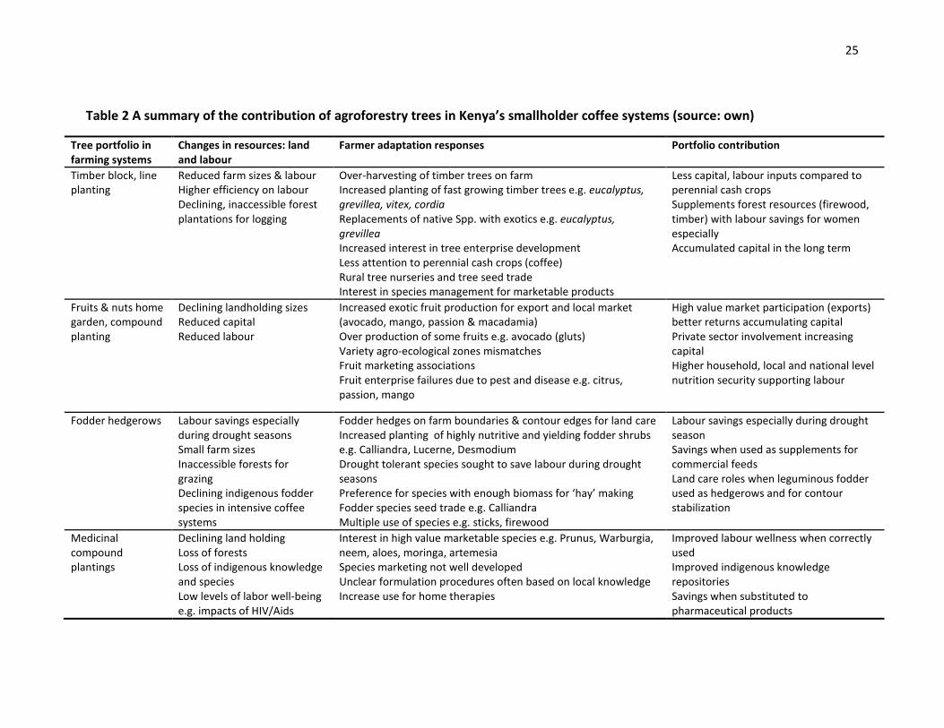
25

Table 2 A summary of the contribution of agroforestry trees in Kenya’s smallholder coffee systems (source: own)

Tree portfolio in farming systems

Changes in resources: land and labour

Farmer adaptation responses Portfolio contribution

Timber block, line planting

Reduced farm sizes & labour Higher efficiency on labour Declining, inaccessible forest plantations for logging

Over-harvesting of timber trees on farm Increased planting of fast growing timber trees e.g. eucalyptus, grevillea, vitex, cordia Replacements of native Spp. with exotics e.g. eucalyptus, grevillea Increased interest in tree enterprise development Less attention to perennial cash crops (coffee) Rural tree nurseries and tree seed trade Interest in species management for marketable products

Less capital, labour inputs compared to perennial cash crops Supplements forest resources (firewood, timber) with labour savings for women especially Accumulated capital in the long term

Fruits & nuts home garden, compound planting

Declining landholding sizes Reduced capital Reduced labour

Increased exotic fruit production for export and local market (avocado, mango, passion & macadamia) Over production of some fruits e.g. avocado (gluts) Variety agro-ecological zones mismatches Fruit marketing associations Fruit enterprise failures due to pest and disease e.g. citrus, passion, mango

High value market participation (exports) better returns accumulating capital Private sector involvement increasing capital Higher household, local and national level nutrition security supporting labour

Fodder hedgerows Labour savings especially during drought seasons Small farm sizes Inaccessible forests for grazing Declining indigenous fodder species in intensive coffee systems

Fodder hedges on farm boundaries & contour edges for land care Increased planting of highly nutritive and yielding fodder shrubs e.g. Calliandra, Lucerne, Desmodium Drought tolerant species sought to save labour during drought seasons Preference for species with enough biomass for ‘hay’ making Fodder species seed trade e.g. Calliandra Multiple use of species e.g. sticks, firewood

Labour savings especially during drought season Savings when used as supplements for commercial feeds Land care roles when leguminous fodder used as hedgerows and for contour stabilization

Medicinal compound plantings

Declining land holding Loss of forests Loss of indigenous knowledge and species Low levels of labor well-being e.g. impacts of HIV/Aids

Interest in high value marketable species e.g. Prunus, Warburgia, neem, aloes, moringa, artemesia Species marketing not well developed Unclear formulation procedures often based on local knowledge Increase use for home therapies

Improved labour wellness when correctly used Improved indigenous knowledge repositories Savings when substituted to pharmaceutical products

26

2.3 Justification of the study

Overall, coffee agroforestry practices are characterized by complexities and competition

for resource use which are the principles that most likely determine the profitability and

sustainability of these systems (Sanchez, 1995). A high human population density in

coffee systems has accelerated land fragmentation to allow space for settlement. There

are concerns on land subdivision and degradation3. More importantly, loss of farm

productivity means that farmers have to seek alternatives that can meet their food and

incomes goals (see Annex 1).

In the Mount Kenya coffee systems, land sizes are presently about a third of the size

they used to be during the 1978 national agricultural survey (Jaetzold and Schmidt,

2007). In Kirinyaga, one of the main coffee producing districts in Kenya, the average

household farm size has decreased from 2.8 ha to 1.09 ha between 1978 and 2004,

respectively. In Nyeri, farm holding size has decreased from 2.7 ha to 0.85 ha in 2004.

While in Embu, available agricultural land per household of 4.44 persons is 0.6 ha per

household. This clearly has serious implications on per capita land productivity with

fertility depleted soils becoming rampant in the Districts (Jaetzold and Schmidt, 2007;

Mucheru et al., 2007).

The present challenge is therefore to prescribe ways to adjust tree and annual cropping

practices to form economical (profitable, diversified for risk) land use patterns for

farmers given the available land and labor. This challenge comes against the backdrop of

uncertain prospects of coffee and other farm enterprises. Productive enterprises in the

eyes of smallholders must result in substantial food and income provisions to be

acceptable. It is held that with reduced resources, smallholders will tend to search for

other income sources such as off farm employment and may put available land into less

labour demanding activities such as tree planting.

3 Land degradation: results of one or more processes that lessen the current and potential capacity of a soil to

produce, quantitatively and or qualitatively, goods or services (FAO, 1989).

27

Productive and profitable annual, perennial and livestock enterprise choices are not a

straight-forward decision. Farmers consider rationally, alternative enterprises to farm

with the available resources such as land, labour and capital (Arnold and Dewees, 1998;

Scherr, 2004; Holding et al., 2006). Coffee farming has previously been a prominent cash

crop investment providing a source of income to thousands of smallholder farm

families. The enterprise catered for school fees payments, food purchases and

supported other farm enterprises such as maize farming and livestock production on

farm. Loss of profitability in the smallholder coffee enterprise have therefore caused the

suffering and disillusionment of farmers. In the Mount Kenya coffee region of Nyeri,

Kirinyaga, Embu and Meru, farmers have recently neglected coffee tending with some

cutting back bushes to allow for food crop production. Recent high food prices are also

expected to stimulate a greater attention towards food crops cultivation. Farmers are

also expected to invest more in dairy animals and keeping of shoats, pigs and rabbits

which require minimum space. The integration of agroforestry trees to complement

subsistence annual cropping has also become more prominent (see chapter 5 for

current data).

Presently, there is limited knowledge available on the productive or economic efficiency

of smallholder coffee agroforestry systems. Biophysical and socio-economic challenges

have not been systematically investigated sometimes resulting in poor

recommendations to address issues of sustainable production in the event of failure of

major enterprises such as coffee. This study contributes to a better understanding of

current position of farmer resources and their livelihood strategies in managing coffee

farms around Mount Kenya. The role of traditional practices such as agroforestry in

circumstance of declined farm productivity is brought to bear. Farmer orientation

towards tree planting or non-planting, in coffee systems is examined. The study traces

the evolution of smallholder coffee growing; present farm enterprise adoption and

adaptation strategies; management of tree diversity on farm and the ‘health’ status of

coffee land in the smallholder coffee areas of Mount Kenya.

28

2.4 Aims of this study and arrangement of the thesis

The main objective of this study was to investigate present farm production strategies

adopted by coffee growers in the eastern parts of Mount Kenya in the light of

constrained land resources and poor market returns in coffee growing. The following

objectives were studied:

1. To investigate the evolution of the smallholder coffee subsector in Kenya and the

improvement of the role of tree growing to livelihood and farming practices

2. To use a pre-determined functional typology of coffee farms to investigate

farmer intensification decisions given their current resource position (e.g land

size) and input and output relationships

3. To measure tree diversity on smallholder farms under ‘increasing’ and/or

‘decreasing’ coffee production trends, and different agro-ecological zones

4. To analyse the prevalence of coffee farms soil nutrient (fertility) under present

coffee and agroforestry intensification practices.

2.5 Outline of the thesis

This work is presented in integrated chapter format, each chapter guided by the stated

objectives. Each chapter follows specific methodologies and provides its own

conclusions.

The introductory Chapter one traces the evolution of the coffee subsector in Kenya and

its present situation as influenced by international and domestic marketing

arrangements. Factors related to farmer cooperatives, productivity, markets and overall

enterprise profitability are discussed.

Chapter two provides an overview of recent transitions experienced in the coffee

subsector while identifying the role of agroforestry in supporting farmer production

decisions to attain better incomes, sustainable production and improved standards of

living.

29

Chapter three includes the research concept and the description of the study area. It

presents recent data on the study area demographics, methods followed in data

collection, processing and analysis. Details of the sampling strategy applied to select

various units of analysis such as farmer households, coffee farms, and coffee societies

are also presented.

Chapter four compares strategies used by three ‘coffee farm typologies’ to cope with

declined coffee productivity and income levels. Farmer enterprise choices, resource

position and analysis of input output relationships are demonstrated. Policy

interventions are further recommended.

Chapter five reports on tree species diversity present on smallholder coffee farms. The

importance and contributions of biodiversity in producing commodity crops such as

coffee is illustrated. The chapter also illustrates farmer preferences on tree species

going by the current tree abundance recorded on farm. Present farm tree populations

are also shown to be dominated by a few exotic species.

Chapter six provides the status of soil fertility management in smallholder coffee farms

with decreasing, constant or increasing coffee cultivation. Soil nutrient indicators are

identified via Near Infra red (NIR) diagnostic tools and discussed. The chapter further

highlights the role and likely implications of shifts in manure and fertilizer applications

practices within coffee systems.

Chapter seven provides the overall conclusions and recommendations of the research.

30

2.6 References

Arnold, JEM. and Dewees, PA. 1998. Trees in managed landscapes: factors in farmer

decision making. In Buck, LE. Lassoie, JP. and Fernandes, BCM. (eds.) Agroforestry in

Sustainable Agricultural Systems. Boca Raron, FL: CRC Press.

Asase, A. and Tetteh, DA. 2010. The role of complex agroforestry systems in the

conservation of forest tree diversity and structure in southeastern Ghana.

Agroforestry Systems, 79: 355–368.

Carsan, S. 2007. Sustainable timber for smallholder cropping systems. A thesis

submitted in partial fulfillment of the requirements of the Masters in Suitable

Agriculture degree of the faculty Natural and Agricultural Science (Centre for

Sustainable Agriculture) University of the Free State, South Africa.

Chambers, R. and Leach, M. 1989. Tree as savings and security for the rural poor. World

Development, 17 (3): 329-42.

Falconer, J. 1990. Agroforestry and household food security. In agroforestry for

sustainable production: economic implications (ed. R.T. prinsley), 215-39. Common

Wealth Science Council, London.

FAO, 1989. Soil Conservation for Small Farmers in the Humid Tropics. Soils Bulletin 60:

FAO, Rome.

Franzel, S. and Scherr, S. 2002. Trees on the farm: assessing the adoption potential of

agroforestry practices in Africa. CABI International, Wallingford, UK.

Garrity, DP. 2004. Agroforestry and the achievement of the Millennium Development

Goals. Agroforestry Systems 61: 5–17.

Harrison, S. Herbohn, J. and Niskanen, A. 2002. Non-industrial, smallholders, small-scale

and family forestry: what’s in a name? Small-scale Forest Economics. Manage Policy

1(1): 1–11.

Hazell, P. Poulton, C. Wiggins, S. and Dorward, A. 2007. The future of small farms for

poverty reduction and growth. International Food Policy Research Institute (IFPRI)

Washington. DC.

31

Holding, C. Carsan, S. and Njuguna, P. 2006. Smallholder timber and firewood marketing

in the coffee and cotton/tobacco zones of eastern Mount Kenya. Wall, S. (ed). Small-

scale forestry and rural development. The intersection of ecosystems, economics

and society. Proceedings of the IUFRO 3.08 conference. Galway-Mayo Institute of

Technology, Galway Ireland, 18-23 June 2006.

Jaetzold, R. and Schmidt, H. 2007 Farm management handbook of Kenya (vol.II), Eastern

Kenya, Ministry of Agriculture, Nairobi.

Jamnadass, R, Dawson, IK, Anegbeh, P, Asaah, E, Atangana, A, Cordeiro, N, Hendricks, H,

Henneh, S, Kadu, CAC, Kattah, C, Misbah, M, Muchugi, A, Munjuga, M, Mwaura, L,

Ndangalasi, HJ, Njau, CS, Nyame, SK, Ofori, D, Peprah, T, Russell, J, Rutatina, F, Sawe,

C, Schmidt, L, Tchoundjeu, Z and Simons, T. 2010. Allanblackia, a new tree crop in

Africa for the global food industry: market development, smallholder cultivation and

biodiversity management. Forest Trees Livelihoods (in press).

Kindt, R. Lillesø, JB. and Van Breugel, P. 2007. Comparisons between original and current

composition of indigenous tree species around Mount Kenya African Journal of

Ecology, 45, 633–644.

Lengkeek, AG and Carsan, S. 2004. The process of participatory tree domestication

project in Meru, Kenya. Development in Practice 14:445-451.

Lengkeek, AG. Muchugi, AM. Agufa, AC. Ahenda, JO. and Dawson, IK. 2006. Comparing

genetic diversity in agroforestry systems with natural forests: A case study of the

important timber tree Vitex fischeri in central Kenya Agroforestry Systems, 67:293-

300.

Mucheru, MM, Mugendi, D, Kung’u J, Mugwe J and Bationo A. 2007. Effects of organic

and mineral fertilizer inputs on maize yield and soil chemical properties in a maize

cropping system in Meru South District, Kenya. Agroforest Systems, 69:189–197.

Muriuki, KJ. 2011 Medicinal trees in smallholder agroforestry systems: assessing some

factors influencing cultivation by farmers East of Mount Kenya. Dissertation for

obtaining a doctorate degree at the University of Natural Resources and Applied Life

Sciences. Department for Forest and Soil Sciences. BOKU University, Vienna, Austria.

32

Nair, PKR. 1990. The Prospects for Agroforestry in the Tropics. World Bank Technical

paper No. 131. World Bank, Washington, DC., USA.

Perfecto, I. Vandermeer, J. Mas, A and Pinto, LS. 2005. Biodiversity, yield and shade

coffee certification. Ecological Economics, 54: 435-446.

Philpott et al. 2008. Biodiversity Loss in Latin American Coffee Landscapes: Review of

the Evidence on Ants, and Birds. Trees Conservation Biology, Volume 22, No. 5.

Rappole, JH. King, DI. and Vega Rivera, JH. 2003. Coffee and conservation. Conservation

Biology, Volume 17, No. 1 334-336 pp.

Ruf, FO. 2011. The myth of complex cocoa agroforests: The case of Ghana. Human Ecol

39:373–388.

Sanchez, PA. 1995. Science in agroforestry. Agroforestry Systems, 12: 2-3.

Scherr, SJ. 2004. Building opportunities for small-farm agroforestry to supply domestic

wood markets in developing countries. Agroforestry Systems, 61: 357–370.

Schroth, G, and Harvey, CA. 2007. Biodiversity conservation in cocoa production

landscapes: an overview. Biodiversity Conservation, 16:2237–2244.

Simons, AJ and Leakey, RRB. 2004. Tree domestication in tropical agroforestry.

Agroforestry Systems, 61: 167–181.

33

CHAPTER 3 RESEARCH METHODOLOGY

This chapter provides insight into how the study was conducted. It highlights the

research design, methods of data collection, sampling and means to drawing key

findings and conclusions.

3.1 Research approach

Smallholder coffee agroforestry systems are characterized as complex. To gain a good

understanding of these systems, broad triangulated data gathering techniques were

used. This study combined qualitative and quantitative research approaches. The two

approaches are complementary, providing different perspectives and answering specific

questions within any one broad area (Scrimshaw, 1990; Stern et al., 2004). This study

investigated how smallholder farm productivity (yields, incomes, crop typologies, tree

diversity, soil fertility and livestock composition) is influenced by socio-economic and

biophysical factors associated with increased or decreased smallholder coffee

cultivation around the Mount Kenya coffee systems.

Smallholders try to achieve their multiple objectives by using resources to which they

have access to. ‘Household resource position’ has therefore been used to refer to

household’s access to and/or possession of human capital (including knowledge, skill,

health and labour availability), natural resources (land, trees and livestock), physical

capital (agricultural implements, household assets), and financial assets (earnings,

credit, savings, remittances) (Sen, 1982; Kragten et al., 2001). To optimally measure

some of these variables it is important to note that household resources can

nonetheless vary greatly within a community or even a village.

Following the “livelihood strategies” theory (Chambers and Leach, 1989; Scherr, 1995;

Ellis, 1998) smallholders are seen as “welfare (utility) maximisers” who base their

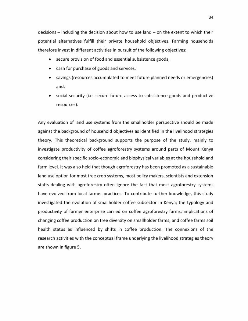
34

decisions – including the decision about how to use land – on the extent to which their

potential alternatives fulfill their private household objectives. Farming households

therefore invest in different activities in pursuit of the following objectives:

secure provision of food and essential subsistence goods,

cash for purchase of goods and services,

savings (resources accumulated to meet future planned needs or emergencies)

and,

social security (i.e. secure future access to subsistence goods and productive

resources).

Any evaluation of land use systems from the smallholder perspective should be made

against the background of household objectives as identified in the livelihood strategies

theory. This theoretical background supports the purpose of the study, mainly to

investigate productivity of coffee agroforestry systems around parts of Mount Kenya

considering their specific socio-economic and biophysical variables at the household and

farm level. It was also held that though agroforestry has been promoted as a sustainable

land use option for most tree crop systems, most policy makers, scientists and extension

staffs dealing with agroforestry often ignore the fact that most agroforestry systems

have evolved from local farmer practices. To contribute further knowledge, this study

investigated the evolution of smallholder coffee subsector in Kenya; the typology and

productivity of farmer enterprise carried on coffee agroforestry farms; implications of

changing coffee production on tree diversity on smallholder farms; and coffee farms soil

health status as influenced by shifts in coffee production. The connexions of the

research activities with the conceptual frame underlying the livelihood strategies theory

are shown in figure 5.

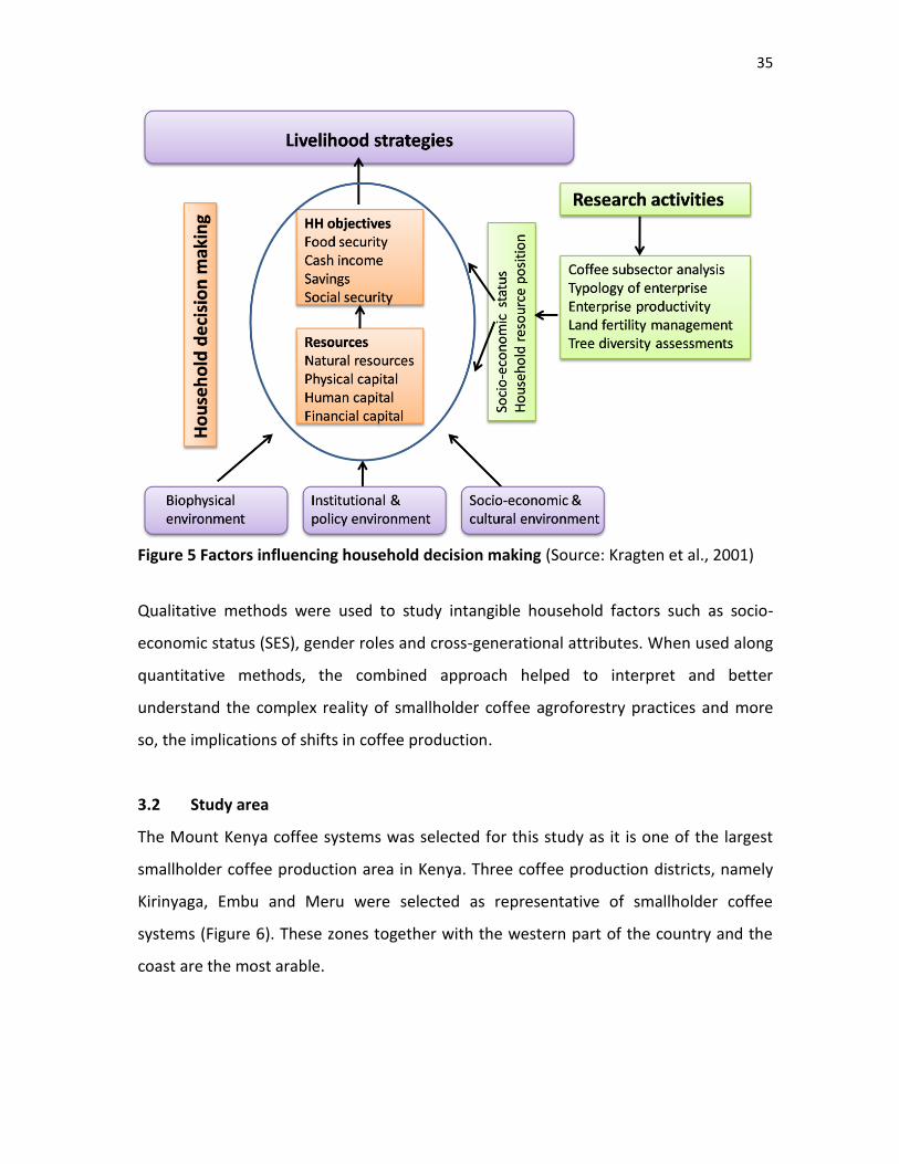
35

Figure 5 Factors influencing household decision making (Source: Kragten et al., 2001)

Qualitative methods were used to study intangible household factors such as socio-

economic status (SES), gender roles and cross-generational attributes. When used along

quantitative methods, the combined approach helped to interpret and better

understand the complex reality of smallholder coffee agroforestry practices and more

so, the implications of shifts in coffee production.

3.2 Study area

The Mount Kenya coffee systems was selected for this study as it is one of the largest

smallholder coffee production area in Kenya. Three coffee production districts, namely

Kirinyaga, Embu and Meru were selected as representative of smallholder coffee

systems (Figure 6). These zones together with the western part of the country and the

coast are the most arable.

36

Figure 6 Surveyed parts of Meru, Embu and Kirinyaga districts

37

Coffee is grown in three agro-ecological zones namely, Upper midland one (UM1),

Upper midland two (UM2) and Upper midland three (UM3). The zones are based on the

FAO (1978) soil and agro-ecological zones (AEZ) classification of Kenya (Jaetzold and

Schimdt, 2007). Each zone is defined based on climatic and edaphic requirements for

recommended crops. Recommendations are meant to improve existing land use

practices in order to increase productivity and limit land degradation (FAO, 1978;

Bationo et al., 2006).

To a large extent, livelihood activities in the Meru, Embu and Kirinyaga coffee areas are

dominated by smallholder farming. A diversity of staple crops such as maize, beans,

banana, sweet potatoes and vegetables such as kales and tomato are cultivated in

mixed cropping patterns. In addition, cropping systems are prominent with agroforestry

tree growing for timber, fuel wood, fodder, and medicinals as windbreaks and boundary

markers. Selected trees such as Cordia africana and Grevillea robusta have been valued

for coffee shade. Livestock production involves intensive poultry keeping, dairying and

limited piggery.

There however seems to be no systematic land use planning. Land is held under private

tenure often with individual title deeds. Family households are densely scattered,

especially in the upper midland coffee zones, in proximity to urban centres. The recent

population census shows high population densities for Embu and Kirinyaga at 409 and

357 persons per square kilometer respectively (GOK, 2010). Meru central has a density

of 194 persons per km2 despite a similar population size with Kirinyaga however in the

main coffee zone densities of up to 400 persons per km2 are reported in the recent

census.

Rainfall is of a bimodal pattern with long rains from March to May and short rains from

October to December (Table 3). This allows two growing seasons. Most of the coffee

growing zones are covered by well-drained extremely deep, dark reddish brown to dark

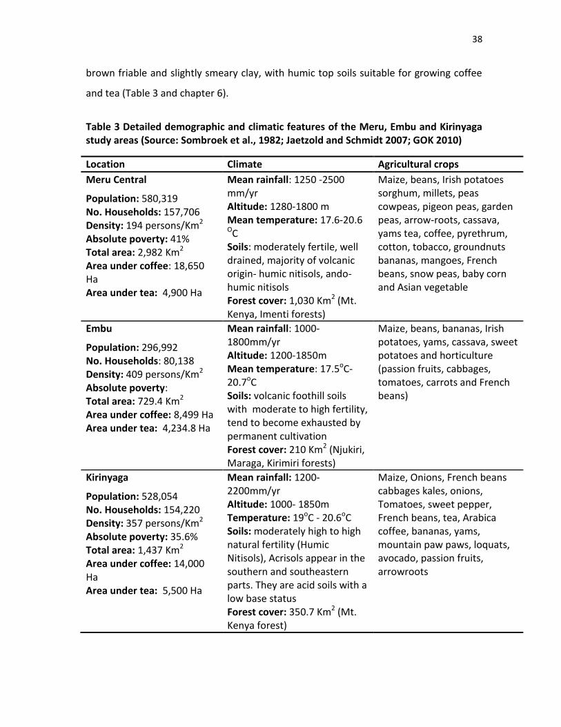
38

brown friable and slightly smeary clay, with humic top soils suitable for growing coffee

and tea (Table 3 and chapter 6).

Table 3 Detailed demographic and climatic features of the Meru, Embu and Kirinyaga study areas (Source: Sombroek et al., 1982; Jaetzold and Schmidt 2007; GOK 2010)

Location Climate Agricultural crops

Meru Central

Population: 580,319 No. Households: 157,706 Density: 194 persons/Km2 Absolute poverty: 41% Total area: 2,982 Km2 Area under coffee: 18,650 Ha Area under tea: 4,900 Ha

Mean rainfall: 1250 -2500 mm/yr Altitude: 1280-1800 m Mean temperature: 17.6-20.6 OC Soils: moderately fertile, well drained, majority of volcanic origin- humic nitisols, ando-humic nitisols Forest cover: 1,030 Km2 (Mt. Kenya, Imenti forests)

Maize, beans, Irish potatoes sorghum, millets, peas cowpeas, pigeon peas, garden peas, arrow-roots, cassava, yams tea, coffee, pyrethrum, cotton, tobacco, groundnuts bananas, mangoes, French beans, snow peas, baby corn and Asian vegetable

Embu

Population: 296,992 No. Households: 80,138 Density: 409 persons/Km2 Absolute poverty: Total area: 729.4 Km2 Area under coffee: 8,499 Ha Area under tea: 4,234.8 Ha

Mean rainfall: 1000-1800mm/yr Altitude: 1200-1850m Mean temperature: 17.5oC- 20.7oC Soils: volcanic foothill soils with moderate to high fertility, tend to become exhausted by permanent cultivation Forest cover: 210 Km2 (Njukiri, Maraga, Kirimiri forests)

Maize, beans, bananas, Irish potatoes, yams, cassava, sweet potatoes and horticulture (passion fruits, cabbages, tomatoes, carrots and French beans)

Kirinyaga

Population: 528,054 No. Households: 154,220 Density: 357 persons/Km2 Absolute poverty: 35.6% Total area: 1,437 Km2

Area under coffee: 14,000 Ha Area under tea: 5,500 Ha

Mean rainfall: 1200-2200mm/yr Altitude: 1000- 1850m Temperature: 19oC - 20.6oC Soils: moderately high to high natural fertility (Humic Nitisols), Acrisols appear in the southern and southeastern parts. They are acid soils with a low base status Forest cover: 350.7 Km2 (Mt. Kenya forest)

Maize, Onions, French beans cabbages kales, onions, Tomatoes, sweet pepper, French beans, tea, Arabica coffee, bananas, yams, mountain paw paws, loquats, avocado, passion fruits, arrowroots

39

3.3 Data collection

This study involved a cross-sectional survey conducted in the main coffee growing parts

in the southern (Kirinyaga), eastern (Embu) and Northern parts (Meru) of Mount Kenya

(Figure 6). Several techniques were used to investigate households and farms within

coffee systems. Focus group discussions were used to identify study target areas and

listing of farmer cooperative societies to use as sampling frame. The technique was also

used to build consensus with the management committee of the local farmer

cooperative societies on the purpose of the research and its contribution. This usually

involved face to face meetings to discuss the study approach and data requirements.

Interviews with individual farmers were used to investigate household socio-economic

status. This involved recording type of agricultural enterprise observed on farm by a

farm walk. All types of livestock kept per household and all tree species on the whole

farm were inventoried. Individual tree diameters at breast height (DBH) were recorded

for all trees above one meter in height. Finally, for the selected sample of ninety farms

soil samples were collected following prescribed procedure according to farm layout

(see chapter 5 and Annex 15 and 16). A questionnaire tool, tree species inventories

sheet and a soil sample collection sheet were used to record their respective data

measurements (see Annex 11, 12). At the farmer cooperative society level, designed

data recording sheets were provided (Annex 14).

3.4 Sampling strategy

The Mount Kenya coffee systems was selected due to its importance in smallholder

coffee production. Farming practices are also comparable between farms but outputs

are variable despite similar ecological settings. The zones are contrasted by their

respective population densities, farm sizes and poverty levels indicated in national

poverty surveys (KNBS, 1998). Stratified sampling was used to obtain the required

sample sets. To capture the complexity of smallholder coffee agroforestry practices,

three adjacent coffee districts were selected to situate this study. Figure 7 shows a

summary of the planned sampling strategy.

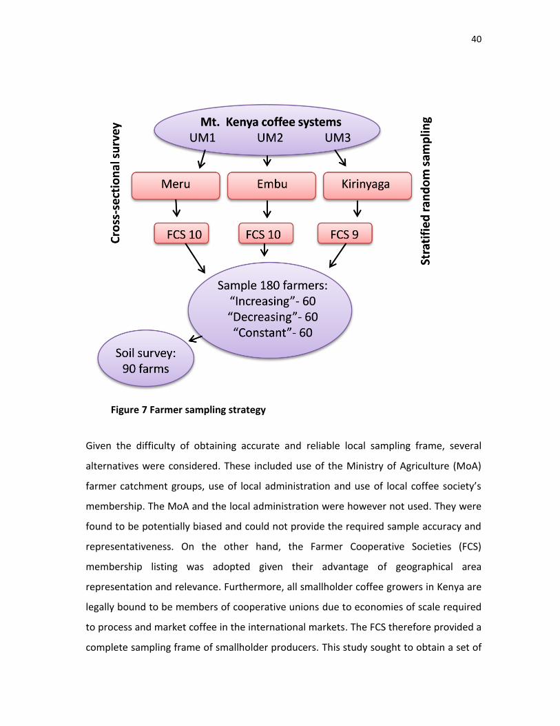
40

Figure 7 Farmer sampling strategy

Given the difficulty of obtaining accurate and reliable local sampling frame, several

alternatives were considered. These included use of the Ministry of Agriculture (MoA)

farmer catchment groups, use of local administration and use of local coffee society’s

membership. The MoA and the local administration were however not used. They were

found to be potentially biased and could not provide the required sample accuracy and

representativeness. On the other hand, the Farmer Cooperative Societies (FCS)

membership listing was adopted given their advantage of geographical area

representation and relevance. Furthermore, all smallholder coffee growers in Kenya are

legally bound to be members of cooperative unions due to economies of scale required

to process and market coffee in the international markets. The FCS therefore provided a

complete sampling frame of smallholder producers. This study sought to obtain a set of

41

smallholder coffee farms and households as units of analysis. The sample of farms was

based on historical coffee yield data from local FCS records. Yields (amount of coffee

cherry in kilogramme) per farmer were obtained for the crop years 2000 to 2008/9.

Three pre-determined farm categories namely increasing, decreasing or constant were

identified to study transitions in coffee farming activities, involving both agroforestry

and livestock keeping. These farm categories were regarded as a functional typology as

they were supposed to reflect the dynamics of local coffee production. The required

sample categories were described as follows:

a) Increasing: These were farmers/farms showing fairly consistent records of

increased coffee yield deliveries to their local FCS in the crop years 2000-2008/9.

b) Decreasing: Farmers/farms showed consistent records of declining coffee yield

deliveries to their local FCS for the crop years 2000-2008/9.

c) Constant: Farmers/farms whose yield production has stagnated for the crop

years 2000-2008/9.

Simple trend analyses were applied on random sample sets in order to discriminate

selected samples into the required categories. This approach was used rather than a

random sample to study more closely the characteristic heterogeneity of present

smallholder coffee farms. In order to successfully implement this sampling strategy

using grass-root coffee FCS, the following steps were undertaken:

a) Visitations: The research team visited the Meru, Embu and Kirinyaga District

Cooperative Office (DCO) for introductory discussions on the planned study

objectives and to make formal requests to allow working collaboration with the

coffee cooperative societies in the district.

b) Study area demarcation: Focused group discussions between the research team

and the district’s coffee cooperative union advisory officers involved use of local

maps to demarcate the main coffee growing zones served by their devolved

farmer societies together with their constituent coffee factories. The coffee

growing zones are mainly comprised of a humid Mid-Upper (MU) and sub humid

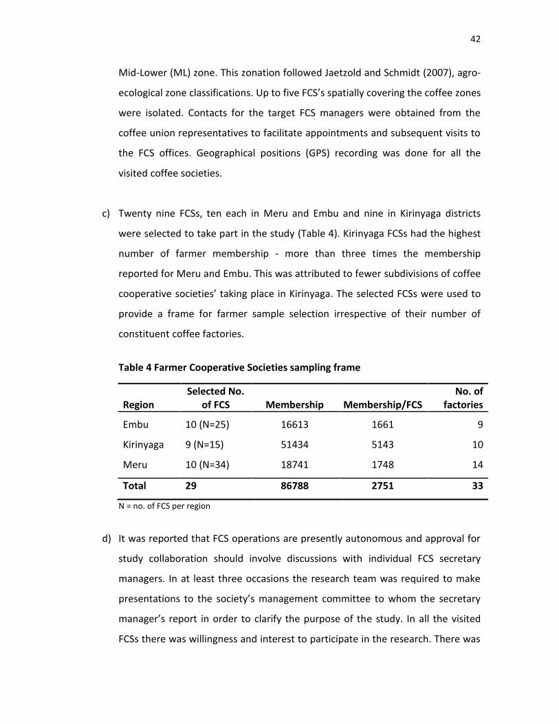
42

Mid-Lower (ML) zone. This zonation followed Jaetzold and Schmidt (2007), agro-

ecological zone classifications. Up to five FCS’s spatially covering the coffee zones

were isolated. Contacts for the target FCS managers were obtained from the

coffee union representatives to facilitate appointments and subsequent visits to

the FCS offices. Geographical positions (GPS) recording was done for all the

visited coffee societies.

c) Twenty nine FCSs, ten each in Meru and Embu and nine in Kirinyaga districts

were selected to take part in the study (Table 4). Kirinyaga FCSs had the highest

number of farmer membership - more than three times the membership

reported for Meru and Embu. This was attributed to fewer subdivisions of coffee

cooperative societies’ taking place in Kirinyaga. The selected FCSs were used to

provide a frame for farmer sample selection irrespective of their number of

constituent coffee factories.

Table 4 Farmer Cooperative Societies sampling frame

Region Selected No.

of FCS Membership Membership/FCS No. of

factories

Embu 10 (N=25) 16613 1661 9

Kirinyaga 9 (N=15) 51434 5143 10

Meru 10 (N=34) 18741 1748 14

Total 29 86788 2751 33

N = no. of FCS per region

d) It was reported that FCS operations are presently autonomous and approval for

study collaboration should involve discussions with individual FCS secretary

managers. In at least three occasions the research team was required to make

presentations to the society’s management committee to whom the secretary

manager’s report in order to clarify the purpose of the study. In all the visited

FCSs there was willingness and interest to participate in the research. There was

43

however a common request to provide feed-back on study findings and

especially the soil analysis reports.

e) FCSs management was requested to provide their membership records on coffee

cherry delivery (in Kilogrammes) from the year 2000 to 2008/9. Sample selection

involved random FCS member’s selection in the categories ‘Increasing’

‘decreasing’ and ‘constant’ covering historical trends in coffee production.

Coffee yields records per farmer were considered on a yearly basis. Coffee

fruiting has a phenological trend of ‘good’ and ‘bad’ years which was born in

mind during sample preparation by assessing overall total production records for

and between societies. This exercise was achieved with relative degree of ease

depending on the state of individual FCS data management. For FCSs that had

computerized their records, sample selection was less tedious. However most

societies still use manual filing systems where hard copy records had to be

manually perused to obtain the required sample records.

f) Data compilation from the various FCSs was mainly done by their secretary

managers who are responsible for the day to day running of the society affairs.

In some instances, the FCS clerical staffs were involved in the compilation. Data

were recorded on prescribed data sheets (Annex 14). Prior discussions with FCS

staff responsible for data compilation was undertaken to explain the search

procedure. In order to ensure bias was adequately managed blind farmer

selection was undertaken through use of FCS membership numbers other than

names of farmers. Practical demonstrations on how to compile the data by

searching records most fitting the required categories was undertaken.

g) Using complete FCS membership records, a sample of five farmers was randomly

drawn for each category - ‘increasing’, ‘decreasing’ and ‘constant’. A total

sample of 15 farmers was assembled per FCS. Before assigning a sample to the

44

prescribed categories simple trend analysis of their cherry delivery records was

undertaken. The exercise involved observation of data records to make a good

judgment on real trends. Most data recorders put very strict measures to fit the

categories prescribed. For instance in one FCS the response returned was that

the categories were not available. In this instance, more guidance discussion was

provided on the steps to draw a sample record. A two week period was allowed

for data assemblage especially where records were stored in hard copy files.

h) Sample selection from societies in the same region was often done concurrently.

This ensured timeliness as several alternative sample sets were always available

for farm visits and eventual data collection. Contacts for data recording

assistants were taken for purposes of follow-ups and backstopping on the data

recording exercise. Meru and Kirinyaga had four FCS, while Embu had three FCSs

with incomplete cherry data for the required time frame. They nonetheless had

at least five years of data considered a useful minimum to observe production

trends for the required farmer category.

i) After ensuring sample sets were ready at the FCS level, there was a ‘researcher

stage’ of sample selection where only two farmers most fitting the study

categories were selected based on simple trend analysis of cherry delivery

records for at least the past five years. A sub-set of six farmers was therefore

selected for interviews per FCS. A total of 180 farmers, 60 each from the three

coffee regions were selected from the 29 FCS. Meru region is larger

geographically with more coffee factories and FCSs. In instances where there

were mistakes of misplaced entries, this was rectified by either returning to the

FCS for extra sample records or by re-aligning category entries. A summary of the

implemented sampling plan is shown in Table 5.

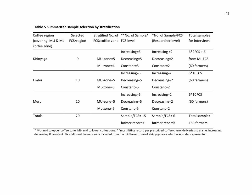
45

Table 5 Summarized sample selection by stratification

Coffee region

(covering: MU & ML

coffee zone)

Selected

FCS/region

Stratified No. of

FCS/coffee zone

**No. of Sample/

FCS level

*No. of Sample/FCS

(Researcher level)

Total samples

for interviews

Kirinyaga

9

MU-zone=5

ML-zone=4

Increasing=5

Decreasing=5

Constant=5

Increasing =2

Decreasing=2

Constant=2

6*9FCS + 6

from ML FCS

(60 farmers)

Embu

10

MU-zone=5

ML-zone=5

Increasing=5

Decreasing=5

Constant=5

Increasing=2

Decreasing=2

Constant=2

6*10FCS

(60 farmers)

Meru

10

MU-zone=5

ML-zone=5

Increasing=5

Decreasing=5

Constant=5

Increasing=2

Decreasing=2

Constant=2

6*10FCS

(60 farmers)

Totals 29 Sample/FCS= 15

farmer records

Sample/FCS= 6

farmer records

Total sample=

180 farmers

* MU- mid to upper coffee zone; ML- mid to lower coffee zone; **most fitting record per prescribed coffee cherry deliveries strata i.e. increasing, decreasing & constant. Six additional farmers were included from the mid lower zone of Kirinyaga area which was under-represented.

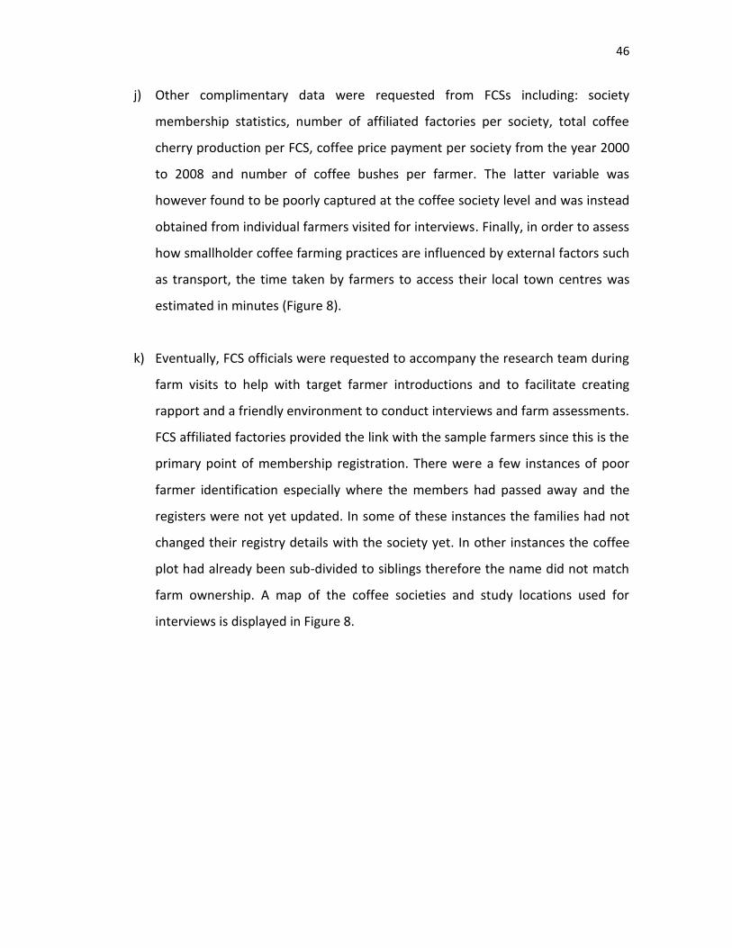
46

j) Other complimentary data were requested from FCSs including: society

membership statistics, number of affiliated factories per society, total coffee

cherry production per FCS, coffee price payment per society from the year 2000

to 2008 and number of coffee bushes per farmer. The latter variable was

however found to be poorly captured at the coffee society level and was instead

obtained from individual farmers visited for interviews. Finally, in order to assess

how smallholder coffee farming practices are influenced by external factors such

as transport, the time taken by farmers to access their local town centres was

estimated in minutes (Figure 8).

k) Eventually, FCS officials were requested to accompany the research team during

farm visits to help with target farmer introductions and to facilitate creating

rapport and a friendly environment to conduct interviews and farm assessments.

FCS affiliated factories provided the link with the sample farmers since this is the

primary point of membership registration. There were a few instances of poor

farmer identification especially where the members had passed away and the

registers were not yet updated. In some of these instances the families had not

changed their registry details with the society yet. In other instances the coffee

plot had already been sub-divided to siblings therefore the name did not match

farm ownership. A map of the coffee societies and study locations used for

interviews is displayed in Figure 8.

47

Figure 8 The Mount Kenya coffee system and the surveyed coffee factories and farms.

48

3.5 Farm surveys

Data collection activities undertaken during the survey of the selected farm-households

covered:

a) Household socio-economic interviews on choices and size of crops cultivated,

kinds and quantities of livestock kept and tree farming and products marketing

activities

b) An entire farm tree inventory and biomass measurements

c) A random soil sample collections on farm plots for basic soil fertility analysis

d) Coffee society’s data on the amount of coffee production for the last 10 years,

prices paid, number of active society membership and gender composition.

Overall, the decision to use the FCS approach as a sampling strategy followed some

assumptions such as:

a) FCS membership are spatially representative of typical coffee smallholders per

selected study strata

b) FCS coffee production records mirror transitions behavior in smallholder coffee

agroforestry systems

c) Farmer records maintained at FCS accurately represent real production efforts

by individual member farmers

d) That if sample selection is based on actual records of farmer coffee produce then

biased sample selection would be minimized

3.6 Drawbacks of using the farmer cooperative membership as a sampling

frame:

a) Several FCSs were found not have adequate data sets necessary to conduct

trend analysis in order to discern the required sample farm categories. Loss of

data was sometimes associated with the concerned FCS management politics. In

at least three instances records were missing after FCSs splits and consequent

change in management. Newer FCSs therefore had data covering only the period

of their existence for instance two FCSs were only four years old therefore

49

providing data for only this time-frame. Most of these societies reported

difficulties in accessing data from their former unions once the splits had

occurred. In another situation, one FCS in Embu had lost most of their data files

in fire incident.

b) The central record keeping system at coffee union level, previously enforced

under law is no longer in practice following the coffee subsector reforms (market

liberalization). Farmer records at the union level (usually at the district), are

therefore severely affected and are no longer up to date. Visited FCSs are

autonomous and see little need to report their operations to their umbrella

union. The individual FCSs deal directly with coffee millers when marketing their

coffee, unlike in the past where the unions marketed coffee on behalf of the

FCSs.

c) A few of the FCSs reported illegal selling of coffee cherry by members to

middlemen hence reduced portions are received at their factories. Though rare,

the practice was attributed to households facing serious income constraints

especially during recent droughts or in instances where farmers have little

produce and wanted to avoid installment payment for input loans. Secondly,

there were incidences of land subdivision but the same farmer account was still

used to sell coffee. These factors tended to influence the coffee cherry data

reflected at the society’s records.

d) Farmer samples for the “increasing” category were in some instances found to

be members of the FCSs management committee, creating some misgiving

regarding the sample. The FCS management committee is often constituted by

‘role model coffee farmers’ with high levels of coffee production.

3.7 Data analysis

Collected data was analyzed following qualitative and quantitative techniques. These

analyses are presented per study chapter/objectives. Each objective had specific but

50

often interlinked analytical requirements. The following types of analysis have been

completed:

a) General linear regressions (Gill, 2000) to show rates of change in coffee

production amongst increasing, decreasing and constant farmer categories

together with an overview on the performance of the smallholder coffee

subsector.

b) Analysis on the typology of enterprise portfolio adopted by farmers at different

level of coffee production. Investigations on production factors such as land size

have been analysed to show kinds and sizes of farmer enterprise selection, and

factors influencing adoption and adaptation. The analysis enabled an evaluation

of likely intensification strategies with coffee and other enterprise such as

banana and maize.

c) Characterization of tree diversity maintained in smallholder coffee agroforestry

systems - this involved showing amounts and diversity of tree adoption amongst

increasing, decreasing and constant coffee farmer categories and within

different coffee agro-ecological zones.

d) Estimate agroforestry tree stocking volumes as related to other economic

activities including annual crop farming, livestock keeping and off-farm

employment activities.

e) Soil nutrient prevalence in smallholder coffee farms of Mount Kenya were

analysed and most limiting nutrient identified. Implications of nutrient inputs via

chemical fertilizers and animal manure were assessed and related to socio-

economic constraints especially land size.

Data entries and management was undertaken using Microsoft Excel 2007. After data

cleaning, coding and standardization, data was subjected to reliability tests visually

using histograms and box and whisker plots to detect influence of extreme values. The

extreme values were checked for source of error. If the values were realistic, they were

retained but otherwise were corrected by replacing them with arithmetic mean.

51

Multivariate analysis involved various descriptive statistics such as means, frequency

counts and percentages (Gill, 2000; Stern et al., 2004).

Details on types of analysis executed are presented under the research methodology

section of each chapter. Multivariate data analysis involved use of several statistical

packages such as PASW statistics 18 (2009), GenStat Release 12.1 (2009); BiodiversityR

based on R statistical software version 2.11.1 (2010); and the unscrambler version 9.2.

Camo Process As (2006).

3.8 CONCLUSIONS

Smallholder coffee agroforestry systems are uniquely complex. Farmer practices are

nested in indigenous knowledge, socio-cultural values, biophysical factors and current

household resource position. To adequately characterize systems productivity,

composite variables measuring these elements have to be gathered. Further, there is

need to exercise flexibility in data collection and collation to involve multiple data

collection instruments and techniques. Finally, selection of an appropriate sampling

frame is critical in rural settings which often have poor formal record keeping practices.

Use of existing farmer organizations such as the coffee cooperative societies

membership was shown to be a useful approach to test different sampling opportunities

as may be required. Clearly, sampling exercises can be challenging, time consuming and

requiring participatory approaches to execute.

52

3.9 REFERENCES

Bationo, A., Hartermink, A., Lungu, O., Naimi, M., Okoth, Pl, Smaling, E. M. A. and

Thiombiano, L. (2006). African Soils: Their productivity and profitability of fertilizer

use. Background paper presented, for the African Fertilizer Summit, 9th – 13th June,

2006, Abuja, Nigeria.

CAMO Inc. 2006. The Unscrambler user manual. CAMO Inc, Corvallis, OR.

Chambers, R, and Leach M. 1989. Trees as savings and security for the rural poor. World

Development 17 (3): 329-342.

Ellis, F. 1998. Household strategies and rural livelihood diversification. Journal of

Development Studies 35 (1): 1-38.

FAO, 1978. Report on the Agro-ecological Zones Project. Vol. 1. Methodology and

results for Africa. World Soil Resources Report 48/1.

GenStat Release 12.1 2009. GenStat Twelfth Edition. GenStat Procedure Library Release

PL20.1 VSN International Ltd. www.genstat.co.uk

GOK (Government of Kenya) 2010. The 2009 Kenya Population and Housing Census.

Volume 1A. Population distribution by administrative units. Kenya National Bureau

of Statistics.

Gill, J. 2000. Generalized Linear Models: A Unified Approach. Sage University Papers

Series on Quantitative Applications in the Social Sciences, Series No. 07-134,

Thousands Oaks, Ca: Sage.

Jaetzold, R and Schmidt, H. 2007 Farm management handbook of Kenya (vol.II), Eastern

Kenya, Ministry of Agriculture, Nairobi.

Kragten, M, Tomich, TP, Vosti S, and Gockowski, J. 2001. Evaluating land use systems

form a socio-economic perspective ASB lecture Notes No. 8.

KNBS, 1998. Incidence and depth of poverty in Kenya. Ministry of National Planning.

PASW statistics 18, 2009. Release 18.0.0 (July 30th, 2009).

Scherr, S. 1995. Economic factors in farmer adoption of agroforestry: patterns observed

in western Kenya. World Development 23 (5): 787-804.

53

Scrimshaw, S. 1990. Combining quantitative and qualitative methods in the study of

intra-household resource allocation. In: Rogers, B and Schlossman, L (Eds). Intra-

household resource allocation issues and methods for development policy and

planning. United Nations University Press. Tokyo. pp 86-88.

Sen, A. 1982. Poverty and Famines: an Essay on Entitlement and Deprivation. Oxford

University Press, New York.

Sombroek, WG, Braun, HMH, van der Pouw, BJA. 1982. Exploratory soil map and agro-

climatic zone Map of Kenya. Exploratory Soil Survey Report No. E1. Kenya Soil

Survey, Ministry of Agriculture, Nairobi.

Stern, RD, Coe R, Allan, EF and Dale, IC. 2004. Good statistical practice for natural

resources research. CABI publishing.

54

CHAPTER 4

DETERMINING ENTERPRISE DIVERSIFICATION TYPOLOGIES BY SMALLHOLDER COFFEE

FARMERS AROUND MOUNT KENYA

ABSTRACT

Improved understanding of the main drivers that influence productivity patterns in

smallholder coffee farming systems can help better target agricultural innovation. The

purpose of this study was to investigate if smallholders with decreasing or increasing

coffee production around Mount Kenya invest in enterprise intensification and

diversification strategies such as with maize, banana, livestock and agroforestry trees.

Using functional typologies of smallholder coffee farms determined a priori, coffee yield

data from 180 farms was used to identify and analyse productivity on farms with

increasing, decreasing and constant coffee production trends. Simple descriptive

statistics such as means, range, counts, enterprise scoring, diversity analysis, pair-wise

correlations and general linear regression analysis were used to compare farm

typologies.

Results show similarities in smallholder farm diversification strategies; coffee production

is nonetheless declining in smaller farm sizes compared to farm sizes where it’s

increasing. Data suggest that on decreasing coffee, farmers with smaller land size

diversify into crops such as banana and maize probably in a strategy to secure

household food security. Results showed that smallholders expanding coffee production

are also associated with productive milk enterprises. Analysis was consistent that, land

size, coffee production (number of bushes, cherry yields/Ha), livestock units, trees,

banana, maize value, nutrient inputs (manure and fertilizer) and labour costs influence

coffee farms productivity and are useful indicators to distinguish farm typologies. In

conclusion, this study highlights the importance of increased awareness by policy

makers on coffee production trends and the need to promote enterprises that are of

interest to farmers.

55

INTRODUCTION

Smallholder farming systems in sub-Saharan Africa are situated in diverse biophysical

and socio-economic environments (Tittonell et al., 2010). Within localities and villages,

households differ in resource endowment, production orientation and objectives,

ethnicity, education, past experience and management skills (Crowley and Carter, 2000)

and in their attitudes towards risks. Rural families therefore tend to develop different

livelihood strategies driven by opportunities and constraints encountered in such

environment (Ruben and Pender, 2004; Stroebel, 2004). Largely, agro-ecology, markets

and local cultures determine different land use patterns and agricultural management

practices across regions. Improved understanding of the main drivers that influence

patterns of households diversity and in turn livelihood strategies and farming objectives

can help better target agricultural innovation (Tittonell et al., 2010). Land users are

known to make decisions about their environment influenced by political and

institutional restrictions at local, regional and international levels (Lambine et al., 2003;

Carmona et al., 2010).

Land use patterns form a farming system that can be described as socially built systems

associated with farm assets and location assets, often situated between social and

biophysical environments. Beets (1990) has described farming systems as a unit

consisting of a human group (households) and the resources it manages in its

environment.

In the region of this study, farming systems correspond to groups of smallholder farms

that share generally similar resource bases, enterprise patterns, livelihood styles and

constraints for which similar development strategies are pertinent (Valbuena et al.,

2008; Van de Steeg et al., 2010; Carmona et al., 2010). Farming systems interface the

relations between farmers and the landscape by integrating biophysical, economic,

social, cultural and political factors that constrain or promote land use and land cover

change (Shepherd and Soule, 1998; Duvernoy, 2000). In the densely populated highland

56

and midland coffee systems of East Africa, variability in the drivers of agricultural

systems have resulted in different land uses that range from strongly market-oriented

smallholder coffee, tea and dairy systems, through semi-commercial cereal/legume-

based systems, to subsistence oriented systems based on crops such as maize and beans

(Place et al., 2003; Tittonell et al., 2005a).

Livelihood strategies to cope with limited access to resources (land, labour, monetary)

have shown that these are not only restricted to alternative methods of farm

management and/or choice of production activities. Off- and non-farm opportunities

can also provide alternative or complementary livelihood options (e.g. Tittonell et al.,

2005a; Barret et al., 2006). Household categorization can therefore help target

agricultural innovations, and more importantly inform farmer decision making processes

with regard to enterprise diversification and considered levels of investments (Stroebel,

2004; Lengkeek and Carsan, 2004). Diversity in farming systems are commonly

evaluated using farm typologies or even land cover characterization approaches

(Duvernoy, 2000). A farm typology has been defined as a tool to simplify the diversity of

farms and farming strategies in a given area, by characterizing different groups of farms

based on a specific criterion. The majority of these typologies take the production

system into account since production decisions have an obvious influence on a farms

economy and its impact on the environment (Duvernoy, 2000; Köbrich et al., 2003;

Keating et al., 2010).

Previous studies have used various criteria and methods to link farming typology to the

extent of soil fertility degradation (Carter 1997; Shepherd and Soule, 1998; Waithaka et

al., 2007). Other farm clustering approaches have used household wealth or resource

endowment indicators, to undertake farm classifications. These constitute examples of

structural household typologies. More appropriately, classification that takes into

account the dynamics of production orientation and livelihood strategies have been

57

shown to improve categorization (Mettrick, 1993). This approach is regarded as

functional typology.

The current study used the functional typology approach to understand the diversity

and productivity of farming strategies used by smallholder coffee growers of Mount

Kenya. It was held that in order to measure implications of changes in coffee production

and better target agroforestry related innovations; a farmer classification strategy

would help avoid making blanket recommendations. This was further expected to

inform enterprise choices amongst coffee farmers assumed to have heterogeneous

farming practices.

It was therefore hypothesized that smallholders with decreasing or stagnated coffee

yield production will invest in more enterprise intensification/diversification options

such as with maize, banana, livestock and trees. Conversely, smallholders with increased

coffee yield production will invest in fewer crop intensification enterprises such as

banana, maize and trees. In order to test these hypotheses, coffee farmers showing

different trends in coffee production over a period of eight years categorized as,

increasing, decreasing or constant (to denote their coffee production trends over the

years) were studied. It was held that smallholders under each category/typology exhibit

different or unique behavior in terms of enterprise adoption to complement coffee

farming.

To characterize productivity on the identified farm typologies, input-output

relationships for key enterprises present on farms were analysed. Enterprises such as

maize, banana, and livestock are farmed together with coffee at different but unclear

intensities. The cropping strategy involves short term/annual cropping, intermediate

cropping and longer term perennial enterprises. This study therefore sought:

(i) To identify factors associated with smallholder household typologies showing

increasing, decreasing or stagnated trends in coffee production

58

(ii) To determine enterprise diversification/intensification strategies used by

smallholder coffee farmers, under conditions of reduced or increased coffee

production

(iii) To investigate use of inputs such as manure, fertilizer and labour under conditions

of smallholder enterprise diversification/intensification.

4.1 MATERIALS AND METHODS

4.1.1 Study area

Livelihoods in the study area (Figure 9) are presently dominated by mixed farming

activities. A diversity of food crops such as maize, beans, banana, sweet potatoes and

vegetables such as kales, tomato and others are intensively produced. Farm cropping

systems are also prominent with agroforestry tree growing valued for timber, fuel

wood, fodder, medicine, windbreaks and as boundary markers (Lengkeek and Carsan,

2004). On the other hand, livestock production involves intensive poultry keeping,

dairying and limited piggery.

Land is held under private tenure often with individual title deeds. Family households

are densely scattered all over, especially in the upper midland coffee zone in proximity

to urban centres. Recent population census has showed high population densities for

Embu and Kirinyaga at 409 and 357 persons per km2 respectively (GOK, 2010). Meru

central has a density of 194 persons per km2 despite a similar population size with

Kirinyaga; however in the main coffee zone, densities of up to 400 persons per km2 were

reported in the latest census (GOK, 2010).

Rainfall is of bimodal pattern, with long rains from March to May and short rains from

October to December. This allows two growing seasons. Most of the coffee growing

zones are covered by well-drained extremely deep, dark reddish brown to dark brown

friable and slightly smeary clay, with humic top soils suitable for growing coffee and tea.

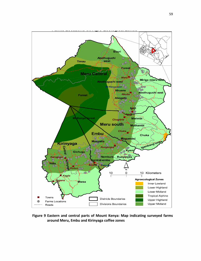
59

Figure 9 Eastern and central parts of Mount Kenya: Map indicating surveyed farms

around Meru, Embu and Kirinyaga coffee zones

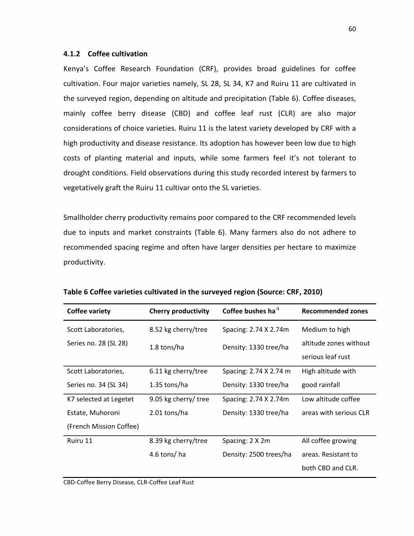
60

4.1.2 Coffee cultivation

Kenya’s Coffee Research Foundation (CRF), provides broad guidelines for coffee

cultivation. Four major varieties namely, SL 28, SL 34, K7 and Ruiru 11 are cultivated in

the surveyed region, depending on altitude and precipitation (Table 6). Coffee diseases,

mainly coffee berry disease (CBD) and coffee leaf rust (CLR) are also major

considerations of choice varieties. Ruiru 11 is the latest variety developed by CRF with a

high productivity and disease resistance. Its adoption has however been low due to high

costs of planting material and inputs, while some farmers feel it’s not tolerant to

drought conditions. Field observations during this study recorded interest by farmers to

vegetatively graft the Ruiru 11 cultivar onto the SL varieties.

Smallholder cherry productivity remains poor compared to the CRF recommended levels

due to inputs and market constraints (Table 6). Many farmers also do not adhere to

recommended spacing regime and often have larger densities per hectare to maximize

productivity.

Table 6 Coffee varieties cultivated in the surveyed region (Source: CRF, 2010)

Coffee variety Cherry productivity Coffee bushes ha-1 Recommended zones

Scott Laboratories,

Series no. 28 (SL 28)

8.52 kg cherry/tree

1.8 tons/ha

Spacing: 2.74 X 2.74m

Density: 1330 tree/ha

Medium to high

altitude zones without

serious leaf rust

Scott Laboratories,

Series no. 34 (SL 34)

6.11 kg cherry/tree

1.35 tons/ha

Spacing: 2.74 X 2.74 m

Density: 1330 tree/ha

High altitude with

good rainfall

K7 selected at Legetet

Estate, Muhoroni

(French Mission Coffee)

9.05 kg cherry/ tree

2.01 tons/ha

Spacing: 2.74 X 2.74m

Density: 1330 tree/ha

Low altitude coffee

areas with serious CLR

Ruiru 11 8.39 kg cherry/tree

4.6 tons/ ha

Spacing: 2 X 2m

Density: 2500 trees/ha

All coffee growing

areas. Resistant to

both CBD and CLR.

CBD-Coffee Berry Disease, CLR-Coffee Leaf Rust

61

4.1.3 Classification of farming systems

A common draw-back of typologies is that the majority do not account for the spatial

linkage in which land-use decisions are applied (Carmona et al., 2010). In this research,

the farm typology approach was applied at the household level where coffee

farmers/farms were characterized with respect to their historical trends in coffee

production. Grouping smallholder coffee farms according to their trends in coffee yields

production was held to convey overall farmer productivity behaviour especially with

regard to intensification/diversification strategies.

Local farmer cooperatives societies (FCS) who legally do primary processing and

marketing of smallholder coffee were used to obtain coffee yield production data at the

farm level. Ten FCSs were selected per district covering the different coffee growing

zones namely, the upper midland one (UM1), upper midland two (UM2) and upper

midland three (UM3). FCSs management usually represented by secretary managers

were requested to provide records of their members’ coffee cherry delivery to serve as

a sampling frame to draw a random sample for interviews. A random set of six farmers

were selected per FCS for interviews and farm assessments. Selected samples were

exceeded by three farmers for Meru central which occupies a larger geographical area

compared to the other coffee zones under study. FCSs were further requested to

provide historical coffee cherry production records on the selected sample of farmers

for data analysis at a later stage.

A cross-sectional survey was then conducted on 180 households occupying three coffee

zones of Mount Kenya (Figure 9). These zones are regarded typical representation of

smallholder coffee-agroforestry systems in Kenya. Chapter 3 provides a detailed

description of the methodology followed.

62

4.1.4 Household survey

The selected farms were surveyed during the months of June to October, 2009. Survey

questionnaires (Annex 13, 14, 15 & 16) were designed to capture biophysical, socio-

economic and managerial aspects of each farm. A team of three individuals were

recruited to administer questionnaires. Socio-economic and farm management

information including characteristics of the household head (name, age, gender and

marital status) and family size, land size, labour availability, distance to nearby markets,

number of coffee plants, number of agroforestry trees planted, amount of cereals

(maize) and banana produced and sold, vegetable farming, livestock rearing and amount

of inputs (manure, fertilizers, hired labour) used were collected. In addition, an

interactive tool (bao game) was used to facilitate collection of qualitative information

quantitatively, with regard to score ranking of farmer preferences for adopted farm

enterprises. Franzel (2004) has shown merits on the use of bao game techniques to

record qualitative data to qualify different criteria over abstract recording of

information using questionnaires only. The bao technique has the advantage of

enhancing farmer accuracy and objectivity as it facilitate respondent’s verifications of

scores based on different criteria at hand. Farm walks and observation schedules were

undertaken to record types of cultivated agricultural crops and agroforestry trees

species present on individual farm plots.

After introduction and discussions with potential respondents on the purpose of the

survey, respondents were requested for a brief farm walk also to indicate the

boundaries of their farm plots. This helped build rapport with respondents as the

research team appreciated farming activities on farm. One member of the research

team was dedicated for household interviews to ensure consistency of recordings, while

the other two members of the team carried out farm walks recording and measuring

present agroforestry enterprises (agricultural crops, trees) on the entire farm plots.

Simultaneous data collection enhanced timeliness in surveying coffee farms and

conducting household interviews especially where sample farms had huge land sizes.

63

Collected data were keyed in standard computer spreadsheet (Microsoft Office Excel,

2007). Data management for subsequent analysis followed standard ICRAF’s data

management guidelines (Muraya et al., 2002; Stern et al., 2004).

4.1.5 Data analysis

Qualitative and quantitative approaches were used to analyze collated information.

Keyed data were cleaned for errors, coded and formatted for multivariate analysis using

PASW statistics 18 (2009) and GenStat Release 12.1 (2009). Simple descriptive statistics

such as means with standard deviations were used to profile household and coffee

farms characteristics. Variables such as intensity of coffee bushes and/or yields reported

per farm, quantity of agroforestry trees (density and tree basal area), value of maize and

banana crops and reported value of inputs such as fertilizer, manure and labour used by

farmers were used to analyse farm intensification practices. Using historical coffee

yields data from the year 2000-2008, rates of coffee yield production was analyzed per

farm category - increasing, decreasing and constant.

General linear regressions were used to assess effects of coffee production trends

(constant, decreasing and increasing) on selected variables shown to have strong

association using pair wise correlations. Fisher’s Least Significance Difference (LSD) was

then used to assess mean differences of the response variates among the farm

categories. Response variates such as cherry value ha-1, coffee bush ha-1, maize value ha-1,

banana value ha-1, avocado trees ha-1, fertilizer kg ha-1, labour costs ksh ha-1 and non

labour costs were transformed to take care of observed skewness. Normality test such

as Shapiro-Wilk and plotting of simple histograms were used to assess skewness on

these variables.

To determine levels of farmer enterprise diversification present on the different types of

smallholder coffee farms, Simpson Index of Diversification (SID) was calculated on

agricultural crops recorded per farm and for the surveyed region. Additionally,

64

commodity crops rank abundance per farm was calculated for the entire surveyed

region. This result was compared to farmer ranking of the present enterprise on farm.

Farmer preference rankings were scored on a scale of 0 to 5 and treated as ordinal 4

rather than interval data. The distance between the scores was held to be

indeterminate. A follow-up analysis involved records of farmer preference counts on

possible substitute crops for coffee. Analysis of farmer preference on likely substitutes

for coffee was done following simple response counts and percentages. All livestock

keeping activities such as cattle, piggery, shoats and others were converted into single

variable per household, termed Tropical Livestock Units (TLU)5 to allow ease of making

comparative analysis.

4.2 Theoretical model

The purpose of this study was to explore factors that will have the most significant

impact on farmer intensification practices given the current losses in smallholder coffee

productivity. In order to develop useful forecasts, econometric modeling approaches

were followed using general linear regressions (Gill, 2000).

Coffee production is regarded as a major smallholder economic activity undergoing

important transitions owing to challenges experienced in international markets.

Domestically, changes are accelerated by inter-generational factors and resource

constraints pertaining to inputs requirements such as fertilizer and pesticides. The older

generations of coffee farmers are being inherited by a younger generation with a

different set of farming goals. Competition on land use for higher and faster return

activities such as horticulture and dairy are emerging. There are also land constraints

occasioned by chronic land subdivision practices, due to a growing human population.

To understand current farmer productivity circumstances, coffee bushes cultivated per

hectare and cherry yields (kg) produced per hectare were established as useful

4 Ordinal data means that the answers are in some order, but says nothing about the distance between

the ordered items. Interval data means there's an equal distance - cognitively - between the scores 5 1 TLU represents 250 kg of livestock live weight

65

indicators to assess smallholder coffee farms productivity. The size of coffee enterprise

adopted is assumed to influence the size and composition of other enterprises carried

by smallholders.

In economic theory, coffee production can be seen as a function of traditional inputs

such as capital (K) and Labour (L) (Williams, 1972). The flow of capital services is

assumed to be proportional to coffee yields. If the coffee industry is competitive, for

profit maximization, the marginal cost for inputs, i.e. MPPk = c/P and MPPL= W/P.

Where MPP = marginal physical product, c = rental cost of capital, w = wage rate and P =

price of output.

In large scale farming, mathematical programming is frequently applied in farm

planning. These tools allow determination of an optimal allocation of land, labour and

capital, given a set of goals (e.g. maximisation of income and leisure and minimisation of

risk) and constraints (e.g. labour and land) (Barnett et al., 1982).

Smallholders operate under imperfect market conditions driven mainly by buyers.

Coffee marketing under cooperative arrangement has recently been shown to suffer

from serious inefficiencies further complicating future viability of smallholder coffee

farming (Mude, 2006). For instance most cooperatives operate at below capacity and

are highly indebted with only a few farmers servicing their operational costs and long

standing credit facilities.

4.3 RESULTS AND DISCUSSIONS

4.3.1 Coffee farm typology

Smallholder coffee production records from the year 2004 to 2008 define trends per

farm category. The increasing farm category appears to have higher fluctuations with

the year 2008 showing pronounced yield production. The constant and the decreasing

66

farm types, showed fairly consistent yield production trends per farmer for the period

under consideration (Figure 10I). Calculated rates of change in coffee yields showed that

the increasing farm category produce more than three times the average rate of the

coffee decreasing farms. The constant farms types showed insignificant rate of change

in production, but a higher production rate than the decreasing farms. Mean production

values confirm stagnation trends (Figure 10II). There was significant evidence to show

that using coffee yields per farm was successful in depicting desired farm categories for

this study, as distinct farm types that can mirror other farmer enterprise management

behavior.

Figure 10 Farm types (constant, decreasing and increasing) (I) average coffee production and (II) mean rates of change from year 2004-2008

67

4.3.2 Household characteristics

Smallholders in the surveyed coffee region cultivate an average farm size of 1.2 ha (s.d =

1.04; n = 180). The smallest farm sampled was 0.05 ha and the largest farm was 6.9 ha.

Coffee household heads are elderly at an average age of 58 years (s.d = 13.43; n = 180).

Results showed that farmers had an average of 550 coffee bushes per hectare (s.d =

539.4; n = 180), producing a mean of 4.3 (s.d = 3.21; n =180) kg cherry per bush. The

coffee decreasing farms had mean cherry production of 3.8 (s.d = 3.7) kg per bush while

the increasing ones have a mean of 4.63 (s.d = 2.53) kg per bush. On per hectare basis,

coffee decreasing farms reported coffee mean yields of 1657 (s.d = 1740) kg/ha while

the increasing and constant categories had a mean of 2483 (s.d = 1901) and 2183 (s.d =

2052) kg/ha (Table 7). Results further showed a corresponding mean rate of cherry

value obtained by farmers across the three farm categories. Conversely, the average

value of banana per hectare for the coffee decreasing farms was Ksh 57,806 (s.d =

105,745), compared to Ksh 48,463 (78,453) and Ksh 28416 (s.d = 35,768) for the

constant and the increasing farm types (Table 7). Reported maize value showed similar

patterns of value distribution.

The average number of agroforestry trees and tree basal area for the constant and

decreasing farms were similar, whereas the increasing farms had fewer than 200 tree

stems per hectare (Table 7). High value tree crops such as macadamia, avocado and

mango had tree densities of less than twenty trees per hectare even though they are

often assumed to be potential substitutes for coffee. Macadamia was more highly

stocked at 19 trees ha-1 compared to mango (9.83, s.d = 17.4) and avocado 6.52 (10.96).

Average fruit yield production per tree for these tree crops was: mango 200

fruits/tree/year; avocado 250-300 fruits/tree/season and macadamia 50-80

kg/tree/year. Results showed that fruit tree stocking rate was small on farms however

yield production per tree was higher compared to coffee presently grown at a higher

density. Macadamia is a particularly important cash crop receiving greater attention by

smallholders due to affordable management requirements compared to coffee.

68

Macadamia nuts have fewer post-harvest losses on storage, handling and transportation

compared to fruits such as mango and avocado.

Analysis of livestock farming practices measured as a single variable - tropical livestock

units (Table 7), showed that on average the constant farms had 5.38 (s.d = 5.5) units

compared to 4.21 (s.d = 4.9) and 3.87 (s.d = 2.9) units for the decreasing and increasing

farm categories. Results nonetheless showed that average milk value sold per day for

the coffee increasing farms was Ksh 152 (s.d = 143.8) compared to Ksh 118 (s.d = 119.4)

and Ksh 94 (s.d = 112.4) for the constant and decreasing farms. Coffee decreasing farms

had fewer units of dairy cattle compared to the other farm categories (Table 7).

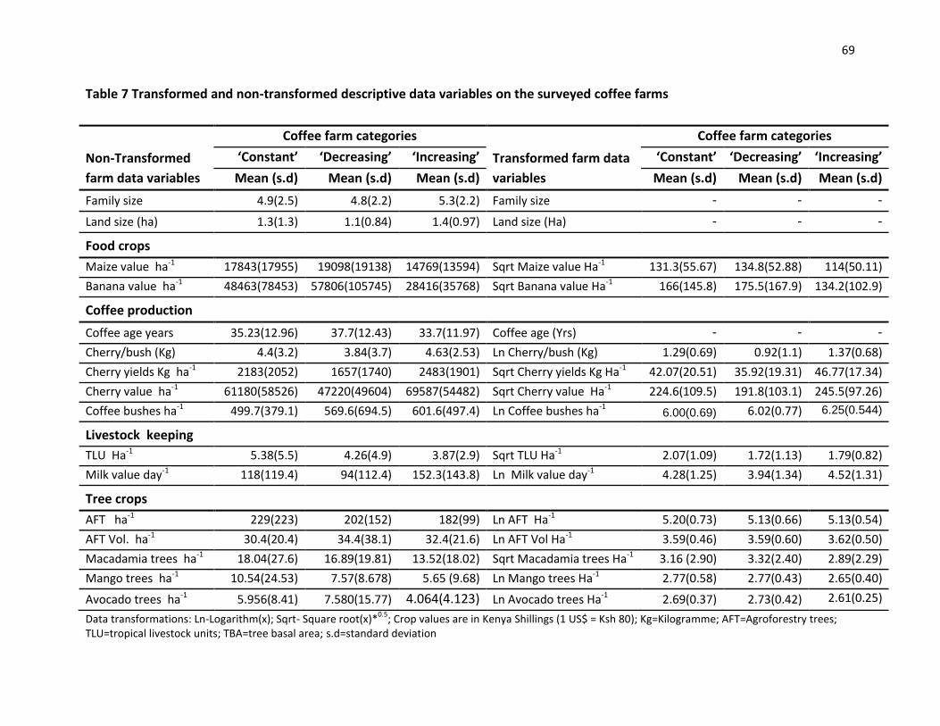
69

Table 7 Transformed and non-transformed descriptive data variables on the surveyed coffee farms

Data transformations: Ln-Logarithm(x); Sqrt- Square root(x)*0.5

; Crop values are in Kenya Shillings (1 US$ = Ksh 80); Kg=Kilogramme; AFT=Agroforestry trees; TLU=tropical livestock units; TBA=tree basal area; s.d=standard deviation

Non-Transformed

farm data variables

Coffee farm categories

Transformed farm data

variables

Coffee farm categories

‘Constant’ ‘Decreasing’ ‘Increasing’ ‘Constant’ ‘Decreasing’ ‘Increasing’

Mean (s.d) Mean (s.d) Mean (s.d) Mean (s.d) Mean (s.d) Mean (s.d)

Family size 4.9(2.5) 4.8(2.2) 5.3(2.2) Family size - - -

Land size (ha) 1.3(1.3) 1.1(0.84) 1.4(0.97) Land size (Ha) - - -

Food crops

Maize value ha-1 17843(17955) 19098(19138) 14769(13594) Sqrt Maize value Ha-1 131.3(55.67) 134.8(52.88) 114(50.11)

Banana value ha-1 48463(78453) 57806(105745) 28416(35768) Sqrt Banana value Ha-1 166(145.8) 175.5(167.9) 134.2(102.9)

Coffee production

Coffee age years 35.23(12.96) 37.7(12.43) 33.7(11.97) Coffee age (Yrs) - - -

Cherry/bush (Kg) 4.4(3.2) 3.84(3.7) 4.63(2.53) Ln Cherry/bush (Kg) 1.29(0.69) 0.92(1.1) 1.37(0.68)

Cherry yields Kg ha-1 2183(2052) 1657(1740) 2483(1901) Sqrt Cherry yields Kg Ha-1 42.07(20.51) 35.92(19.31) 46.77(17.34)

Cherry value ha-1 61180(58526) 47220(49604) 69587(54482) Sqrt Cherry value Ha-1 224.6(109.5) 191.8(103.1) 245.5(97.26)

Coffee bushes ha-1 499.7(379.1) 569.6(694.5) 601.6(497.4) Ln Coffee bushes ha-1 6.00(0.69) 6.02(0.77) 6.25(0.544)

Livestock keeping

TLU Ha-1 5.38(5.5) 4.26(4.9) 3.87(2.9) Sqrt TLU Ha-1 2.07(1.09) 1.72(1.13) 1.79(0.82)

Milk value day-1 118(119.4) 94(112.4) 152.3(143.8) Ln Milk value day-1 4.28(1.25) 3.94(1.34) 4.52(1.31)

Tree crops

AFT ha-1 229(223) 202(152) 182(99) Ln AFT Ha-1 5.20(0.73) 5.13(0.66) 5.13(0.54)

AFT Vol. ha-1 30.4(20.4) 34.4(38.1) 32.4(21.6) Ln AFT Vol Ha-1 3.59(0.46) 3.59(0.60) 3.62(0.50)

Macadamia trees ha-1 18.04(27.6) 16.89(19.81) 13.52(18.02) Sqrt Macadamia trees Ha-1 3.16 (2.90) 3.32(2.40) 2.89(2.29)

Mango trees ha-1 10.54(24.53) 7.57(8.678) 5.65 (9.68) Ln Mango trees Ha-1 2.77(0.58) 2.77(0.43) 2.65(0.40)

Avocado trees ha-1 5.956(8.41) 7.580(15.77) 4.064(4.123) Ln Avocado trees Ha-1 2.69(0.37) 2.73(0.42) 2.61(0.25)

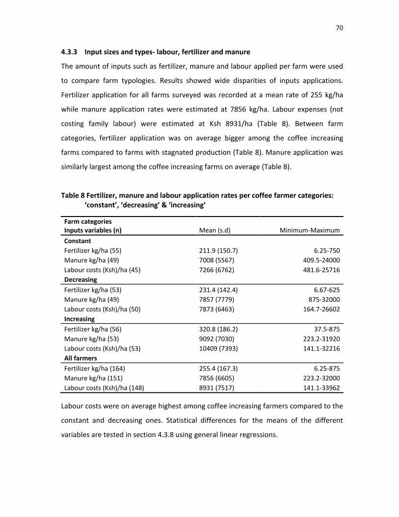
70

4.3.3 Input sizes and types- labour, fertilizer and manure

The amount of inputs such as fertilizer, manure and labour applied per farm were used

to compare farm typologies. Results showed wide disparities of inputs applications.

Fertilizer application for all farms surveyed was recorded at a mean rate of 255 kg/ha

while manure application rates were estimated at 7856 kg/ha. Labour expenses (not

costing family labour) were estimated at Ksh 8931/ha (Table 8). Between farm

categories, fertilizer application was on average bigger among the coffee increasing

farms compared to farms with stagnated production (Table 8). Manure application was

similarly largest among the coffee increasing farms on average (Table 8).

Table 8 Fertilizer, manure and labour application rates per coffee farmer categories: ‘constant’, ‘decreasing’ & ‘increasing’

Farm categories Inputs variables (n) Mean (s.d) Minimum-Maximum

Constant Fertilizer kg/ha (55) 211.9 (150.7) 6.25-750

Manure kg/ha (49) 7008 (5567) 409.5-24000 Labour costs (Ksh)/ha (45) 7266 (6762) 481.6-25716 Decreasing

Fertilizer kg/ha (53) 231.4 (142.4) 6.67-625 Manure kg/ha (49) 7857 (7779) 875-32000 Labour costs (Ksh)/ha (50) 7873 (6463) 164.7-26602 Increasing

Fertilizer kg/ha (56) 320.8 (186.2) 37.5-875 Manure kg/ha (53) 9092 (7030) 223.2-31920 Labour costs (Ksh)/ha (53) 10409 (7393) 141.1-32216 All farmers

Fertilizer kg/ha (164) 255.4 (167.3) 6.25-875 Manure kg/ha (151) 7856 (6605) 223.2-32000 Labour costs (Ksh)/ha (148) 8931 (7517) 141.1-33962

Labour costs were on average highest among coffee increasing farmers compared to the

constant and decreasing ones. Statistical differences for the means of the different

variables are tested in section 4.3.8 using general linear regressions.

71

4.3.4 Smallholder enterprise diversification

Farm crop enterprises recorded within all surveyed coffee farms showed a diversity of

7.1 (s.d = 1.71). The farm with the least crop diversity had two crop types while the farm

with highest diversity had 12 agricultural crop types. The ten most prevalent agricultural

crops on smallholder coffee farms represent 88% of all crop types surveyed on all farms.

These crops were maize, beans, banana, avocado, macadamia, mango, beans, papaw,

Irish potatoes and Khat (Table 9).

Table 9 Farmer preference scores on major enterprises on farm. Enterprises were arbitrary selected given their prominence on surveyed farms.

Percentage (%) of farmers allocating an enterprise given score

(5 = Highest score; 0,1 = lowest score)

Farm enterprises (N) 5 4 3 2 1 0 Total

Coffee (180) 52 20 18 9 1 - 100

Livestock (166) 52 24 14 7 2 - 100

Maize (165) 30 14 25 20 10 - 100

Trees (156) 44 14 21 16 4 1 100

Banana (154) 31 15 27 18 9 1 100

Beans (129) 27 14 21 19 19 - 100

Tea (36) 28 31 31 11 - - 100

Potato (36) 19 17 28 25 11 - 100

Vegetables (31) 32 16 26 10 13 3 100

Fruits (26) 19 23 19 23 15 - 100

Macadamia (24) 13 17 58 4 8 - 100

Napier (21) 43 29 10 14 5 - 100

Cajanas (17) 12 18 6 24 41 - 100

Catha edulis (12) 25 33 - 25 8 8 100

Cowpeas (6) - - - 33 67 - 100

Cassava (5) 20 - 20 20 40 - 100

Sweet potato (4) 25 - - - 75 - 100

Yams (3) - 33 - - 67 - 100

Arrow roots (3) - 33 - - 67 - 100

Black beans (3) 33 33 - - 33 - 100

Sorghum (3) - - 33 33 33 - 100

All enterprises 37 18 21 15 9 0.00 100

N = number of farms surveyed. Percentages in bold shows the highest score attributed to an enterprise

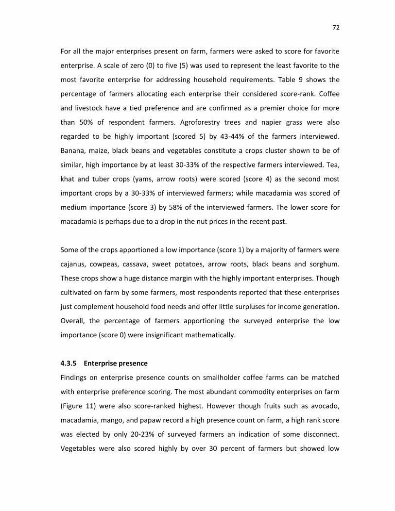
72

For all the major enterprises present on farm, farmers were asked to score for favorite

enterprise. A scale of zero (0) to five (5) was used to represent the least favorite to the

most favorite enterprise for addressing household requirements. Table 9 shows the

percentage of farmers allocating each enterprise their considered score-rank. Coffee

and livestock have a tied preference and are confirmed as a premier choice for more

than 50% of respondent farmers. Agroforestry trees and napier grass were also

regarded to be highly important (scored 5) by 43-44% of the farmers interviewed.

Banana, maize, black beans and vegetables constitute a crops cluster shown to be of

similar, high importance by at least 30-33% of the respective farmers interviewed. Tea,

khat and tuber crops (yams, arrow roots) were scored (score 4) as the second most

important crops by a 30-33% of interviewed farmers; while macadamia was scored of

medium importance (score 3) by 58% of the interviewed farmers. The lower score for

macadamia is perhaps due to a drop in the nut prices in the recent past.

Some of the crops apportioned a low importance (score 1) by a majority of farmers were

cajanus, cowpeas, cassava, sweet potatoes, arrow roots, black beans and sorghum.

These crops show a huge distance margin with the highly important enterprises. Though

cultivated on farm by some farmers, most respondents reported that these enterprises

just complement household food needs and offer little surpluses for income generation.

Overall, the percentage of farmers apportioning the surveyed enterprise the low

importance (score 0) were insignificant mathematically.

4.3.5 Enterprise presence

Findings on enterprise presence counts on smallholder coffee farms can be matched

with enterprise preference scoring. The most abundant commodity enterprises on farm

(Figure 11) were also score-ranked highest. However though fruits such as avocado,

macadamia, mango, and papaw record a high presence count on farm, a high rank score

was elected by only 20-23% of surveyed farmers an indication of some disconnect.

Vegetables were also scored highly by over 30 percent of farmers but showed low

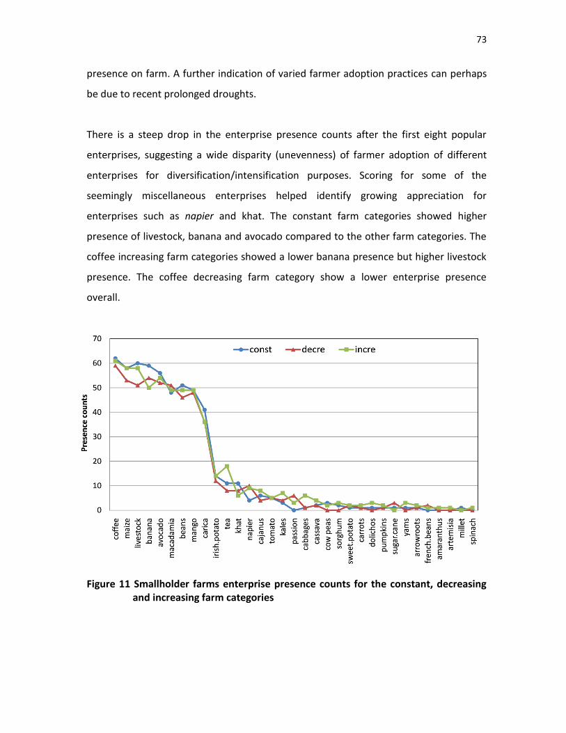
73

presence on farm. A further indication of varied farmer adoption practices can perhaps

be due to recent prolonged droughts.

There is a steep drop in the enterprise presence counts after the first eight popular

enterprises, suggesting a wide disparity (unevenness) of farmer adoption of different

enterprises for diversification/intensification purposes. Scoring for some of the

seemingly miscellaneous enterprises helped identify growing appreciation for

enterprises such as napier and khat. The constant farm categories showed higher

presence of livestock, banana and avocado compared to the other farm categories. The

coffee increasing farm categories showed a lower banana presence but higher livestock

presence. The coffee decreasing farm category show a lower enterprise presence

overall.

Figure 11 Smallholder farms enterprise presence counts for the constant, decreasing and increasing farm categories

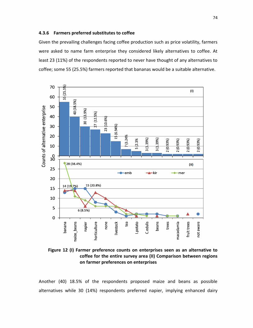
74

4.3.6 Farmers preferred substitutes to coffee

Given the prevailing challenges facing coffee production such as price volatility, farmers

were asked to name farm enterprise they considered likely alternatives to coffee. At

least 23 (11%) of the respondents reported to never have thought of any alternatives to

coffee; some 55 (25.5%) farmers reported that bananas would be a suitable alternative.

Figure 12 (I) Farmer preference counts on enterprises seen as an alternative to coffee for the entire survey area (II) Comparison between regions on farmer preferences on enterprises

Another (40) 18.5% of the respondents proposed maize and beans as possible

alternatives while 30 (14%) respondents preferred napier, implying enhanced dairy

75

keeping as possible alternatives (Figure 12I). Data comparisons between coffee districts

clearly showed that banana is the most preferred alternative for the Meru region but is

less favoured in Embu and Kirinyaga regions rivaled by maize and beans (Figure 12II).

There is a high preference for napier grass (implying dairy keeping) for Embu and high

preference for horticulture (mainly tomato, kales) for Kirinyaga (Figure 12II).

4.3.7 Factors driving smallholder enterprise choice

To assess the relationship between various factors having a role in smallholder

enterprise productivity pair-wise correlation was assessed on selected variates at 5%

significance level. Variables measuring farm resource size such as land size, family size,

agroforestry tree ha-1, tree basal area ha-1, cherry production, coffee bush ha-1 and

livestock enterprise TLU ha-1, milk value day-1 were tested for association (Table 10).

Additionally, farm inputs variables such as manure, fertilizer and labour costs were

correlated with other variables used to assess farm production (Table 11).

Results showed some evidence that maize value obtained per hectare is negatively

correlated to household size and land size. Maize is the staple food for most households

and extensification is constrained by input costs. There is some evidence that maize

value significantly increases with higher tree basal area (TBA), number of coffee bushes

and banana value per hectare. A higher banana value ha-1 suggests that more inputs can

be afforded for maize production. It also in a way complements maize as the main

staple food crop. Moreover, a high banana value is positively associated with the size of

tropical livestock units kept per hectare. This is perhaps due to the fact that banana

stems are valued as fodder supplement for livestock kept under zero grazing systems.

Correlation of banana value with family size, land size, agroforestry tree ha-1 and coffee

bushes ha-1 returned an expected negative correlation, even though not significant at

0.05 level.

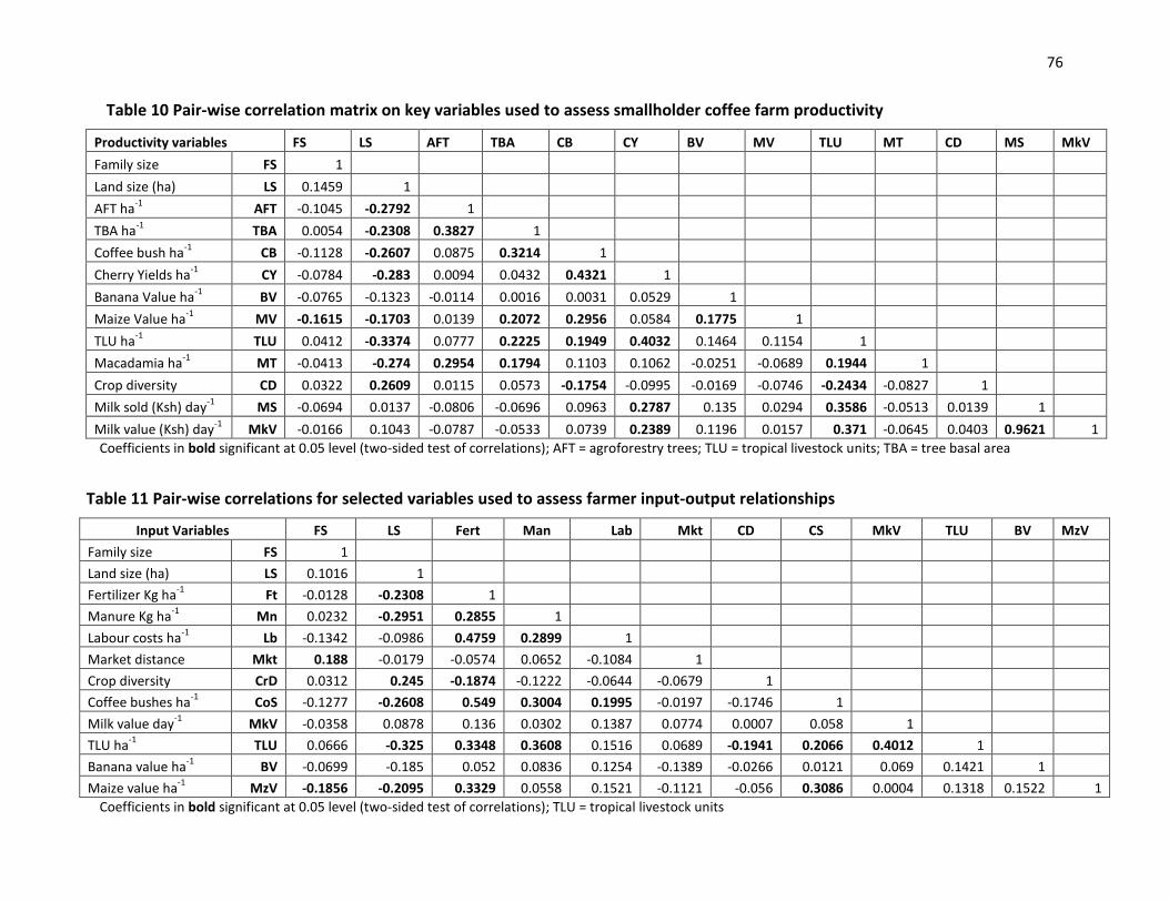
76

Table 10 Pair-wise correlation matrix on key variables used to assess smallholder coffee farm productivity

Productivity variables FS LS AFT TBA CB CY BV MV TLU MT CD MS MkV

Family size FS 1 Land size (ha) LS 0.1459 1

AFT ha-1

AFT -0.1045 -0.2792 1 TBA ha

-1 TBA 0.0054 -0.2308 0.3827 1

Coffee bush ha-1

CB -0.1128 -0.2607 0.0875 0.3214 1 Cherry Yields ha

-1 CY -0.0784 -0.283 0.0094 0.0432 0.4321 1

Banana Value ha-1

BV -0.0765 -0.1323 -0.0114 0.0016 0.0031 0.0529 1 Maize Value ha

-1 MV -0.1615 -0.1703 0.0139 0.2072 0.2956 0.0584 0.1775 1

TLU ha-1

TLU 0.0412 -0.3374 0.0777 0.2225 0.1949 0.4032 0.1464 0.1154 1 Macadamia ha

-1 MT -0.0413 -0.274 0.2954 0.1794 0.1103 0.1062 -0.0251 -0.0689 0.1944 1

Crop diversity CD 0.0322 0.2609 0.0115 0.0573 -0.1754 -0.0995 -0.0169 -0.0746 -0.2434 -0.0827 1 Milk sold (Ksh) day

-1 MS -0.0694 0.0137 -0.0806 -0.0696 0.0963 0.2787 0.135 0.0294 0.3586 -0.0513 0.0139 1

Milk value (Ksh) day-1

MkV -0.0166 0.1043 -0.0787 -0.0533 0.0739 0.2389 0.1196 0.0157 0.371 -0.0645 0.0403 0.9621 1

Coefficients in bold significant at 0.05 level (two-sided test of correlations); AFT = agroforestry trees; TLU = tropical livestock units; TBA = tree basal area

Table 11 Pair-wise correlations for selected variables used to assess farmer input-output relationships

Input Variables FS LS Fert Man Lab Mkt CD CS MkV TLU BV MzV

Family size FS 1 Land size (ha) LS 0.1016 1

Fertilizer Kg ha-1

Ft -0.0128 -0.2308 1 Manure Kg ha

-1 Mn 0.0232 -0.2951 0.2855 1

Labour costs ha-1

Lb -0.1342 -0.0986 0.4759 0.2899 1 Market distance Mkt 0.188 -0.0179 -0.0574 0.0652 -0.1084 1

Crop diversity CrD 0.0312 0.245 -0.1874 -0.1222 -0.0644 -0.0679 1 Coffee bushes ha

-1 CoS -0.1277 -0.2608 0.549 0.3004 0.1995 -0.0197 -0.1746 1

Milk value day-1

MkV -0.0358 0.0878 0.136 0.0302 0.1387 0.0774 0.0007 0.058 1 TLU ha

-1 TLU 0.0666 -0.325 0.3348 0.3608 0.1516 0.0689 -0.1941 0.2066 0.4012 1

Banana value ha-1

BV -0.0699 -0.185 0.052 0.0836 0.1254 -0.1389 -0.0266 0.0121 0.069 0.1421 1 Maize value ha

-1 MzV -0.1856 -0.2095 0.3329 0.0558 0.1521 -0.1121 -0.056 0.3086 0.0004 0.1318 0.1522 1

Coefficients in bold significant at 0.05 level (two-sided test of correlations); TLU = tropical livestock units

77

Results showed that reduced land size accelerates intensification (i.e. value per

hectare) using agroforestry trees, coffee bushes, banana, maize and livestock

enterprises. Crop diversification is significantly enhanced by bigger land sizes. Higher

coffee and livestock intensity nonetheless significantly reduces agricultural crop

diversity on farm while a higher maize and banana value will also reduce farmer crop

diversification even though analyzed data is inconclusive. Finally, crop diversity is

reduced by lower labour costs and market distance even though collected evidence

was not significant.

Key input applications such as fertilizer, manure are significantly constrained on large

farm sizes. Labour inputs are shown to be constrained even though not significantly.

However labour costs can significantly affect fertilizer application rates implying

higher costs could seriously influence farm nutrient status. Labour costs as expected

were positively related to the number of coffee stems per hectare. Other results

showed a negative correlation between farmer labour expenditure and distance to

the nearest market outlet and levels of crop diversification even though not

significant at 0.05 level. Fertilizer application rates increases significantly with the

number of coffee stems per farm, maize value realized per hectare and amounts of

manure applied per hectare. Distance covered by households to the nearest market

showed a negative correlation with fertilizer application rates even though not

significantly. Fertilizer application was also reduced by higher crops diversity within

smallholder farms. On the other hand, data revealed that manure ha-1 is positively

associated with labour expenditure per hectare, coffee bushes ha-1, livestock units’

ha-1 and banana value ha-1. Like fertilizer, manure application is significantly reduced

with higher agricultural crop diversification.

4.3.8 General linear regression analysis

The effects of present coffee production trends and farm size on smallholder farm

intensification were investigated using a general linear regression model (Table 12).

The effects of coffee production trends were modeled using the farm categories-

‘constant’, ‘decreasing’ and ‘increasing’ as predictor variates. Farm size (ha) was then

added to this ‘trend’ model to assess its effects as it was found to be significantly

78

associated with most variables. Coefficients of the model containing farm size were

then used to analyse differences between the three coffee production trends.

Response variates selected for regressions were identified by pair-wise correlations

(Table 10 and 11). These were coffee bush ha-1, fertilizer kg ha-1, labour costs Ksh ha-1

and non labour costs Ksh Yr-1, tree volume farm-1, avocado tree ha-1 and milk value

sold day-1 (transformed by natural logarithm, Ln) and cherry value ha-1, maize value

ha-1, banana value ha-1 and TLU ha-1 (transformed by taking square root). Shapiro-

Wilk tests for normality on all variables showed P < 0.001 suggesting they were

unlikely from a normal distribution hence the transformations (Royston, 1993).

The ‘constant’ farm category was fixed as the model reference/constant. Fisher’s

Least Significance Difference procedure was then used to compare significant

differences between coffee production categories at P < 0.05 and P < 0.1 level.

Models regressing cherry value ha-1, milk value sold day-1, fertilizer Kg ha-1, non-

labour costs Yr-1 and avocado tree ha-1 against coffee production trends were

significant at 0.05 level. Regressions models on coffee bush ha-1, labour costs Ksh Yr-1

and maize value ha-1 were significant at 0.1 level. All the models showed that farm

size effect was highly significant at P < 0.05 except for avocado tree ha-1 (Table 12).

Results showed significant differences between farm categories considering outputs

such as cherry value ha-1, milk value sold per day, number of avocado trees ha-1 and

inputs such as fertilizer applied in Kg ha-1 and labour and non labour costs per farm

per year. Measures of intensification such as tropical livestock units ha-1, maize value

ha-1, banana value ha-1 and agroforestry tree volume farm-1 were however not

significantly different for farms with the different coffee production trends.

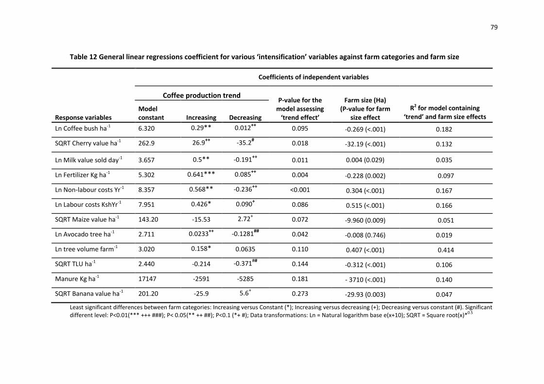
79

Table 12 General linear regressions coefficient for various ‘intensification’ variables against farm categories and farm size

Response variables

Coefficients of independent variables

Coffee production trend

P-value for the model assessing

‘trend effect’

Farm size (Ha) (P-value for farm

size effect

R2 for model containing ‘trend’ and farm size effects

Model constant Increasing Decreasing

Ln Coffee bush ha-1 6.320 0.29** 0.012++ 0.095 -0.269 (<.001) 0.182

SQRT Cherry value ha-1 262.9 26.9++

-35.2#

0.018 -32.19 (<.001) 0.132

Ln Milk value sold day-1 3.657 0.5** -0.191++ 0.011 0.004 (0.029) 0.035

Ln Fertilizer Kg ha-1 5.302 0.641*** 0.085++ 0.004 -0.228 (0.002) 0.097

Ln Non-labour costs Yr-1 8.357 0.568** -0.236++ <0.001 0.304 (<.001) 0.167

Ln Labour costs KshYr-1 7.951 0.426* 0.090+ 0.086 0.515 (<.001) 0.166

SQRT Maize value ha-1 143.20 -15.53 2.72+ 0.072 -9.960 (0.009) 0.051

Ln Avocado tree ha-1 2.711 0.0233++ -0.1281

## 0.042 -0.008 (0.746) 0.019

Ln tree volume farm-1 3.020 0.158* 0.0635 0.110 0.407 (<.001) 0.414

SQRT TLU ha-1 2.440 -0.214 -0.371## 0.144 -0.312 (<.001) 0.106

Manure Kg ha-1 17147 -2591 -5285 0.181 - 3710 (<.001) 0.140

SQRT Banana value ha-1 201.20 -25.9 5.6+ 0.273 -29.93 (0.003) 0.047

Least significant differences between farm categories: Increasing versus Constant (*); Increasing versus decreasing (+); Decreasing versus constant (#). Significant different level: P<0.01(*** +++ ###); P< 0.05(** ++ ##); P<0.1 (*+ #); Data transformations: Ln = Natural logarithm base e(x+10); SQRT = Square root(x)*

0.5

80

Coffee bushes ha-1 for farms with increasing coffee production was significantly

different from the constant and decreasing ones (P < 0.05). In fact results showed

that on average farms increasing coffee farming have 17% (P < 0.05) more coffee

bushes ha-1 than constant farms and 5.5% (P < 0.05) more bushes compared to the

farms on a decreasing trend. Though coffee bushes ha-1 on coffee decreasing farms

were 12.3% higher than the constant ones, data analysis did not show evidence of

significant differences.

In terms of cherry value ha-1, results were robust to show that cherry value for the

increasing farms are significantly different (P < 0.05) from those of decreasing farms

but not so for the constant farms. In fact cherry value for the coffee decreasing

farms was significantly lower (P < 0.1) compared to the constant farms. Analysis

showed that both cherry value ha-1 and coffee bushes ha-1 are significantly (P <

0.001) lower in bigger farm sizes measured in hectares. This is perhaps due to the

high costs of labour and non-labour inputs required for coffee farming at larger

scale.

Farm intensification with dairy farming activities revealed that milk value sold per

day for the coffee increasing farms were significantly different from the constant and

the decreasing ones. Farms switching to increased coffee production trends

recorded a 22.5 % (P < 0.05) higher milk value sold per day compared to the constant

farms; and a 38.3 % (P < 0.05) higher value compared to the coffee decreasing farms.

The coffee constant farms recorded a 20% higher milk value compared to the coffee

decreasing farms. This finding was however not statistically significant at 0.1 level.

Results showed that milk outputs could nonetheless be increased with bigger farm

sizes.

On the other hand, avocado fruit farming, popular in smallholder coffee systems

showed a significantly higher (31.8%, P < 0.05) tree intensity per hectare for farms

with constant/stagnated coffee production trends compared to the increasing ones.

Avocado trees per hectare were significantly higher (46.4%; P < 0.05) in coffee

decreasing farms compared to the increasing farms. Results however showed that

81

avocado intensification is significantly reduced in bigger farm sizes. Other results

showed that total tree volume maintained on farm though not different by farm

categories would be significantly increased by bigger farm sizes.

Coffee farms intensification using maize (maize value ha-1) and banana (banana value

ha-1) were not different by farm categories but showed declining and increasing

trends for farms with increasing and decreasing coffee production trends. Results

further showed that larger farm sizes would significantly decrease maize (P = 0.027)

and banana (P = 0.020) value per hectare. Both enterprises have a fairly high input

demand. Results demonstrated that fertilizer application (Kg ha-1) were significantly

higher (33.9 %) for the coffee increasing farms compared to the constant farms; and

27.9 % higher compared to the coffee decreasing farms (P < 0.05). Fertilizer

application on the coffee decreasing farms were 8.4 % higher compared to the

constant farms. This finding was nonetheless not significantly different.

Measurements of non-labour input costs such as pesticides, seeds and others,

showed that, coffee increasing farms record significantly higher costs compared to

the constant farms (14.2 %, P < 0.05) and 12.9%, (P < 0.05) more costs compared to

the decreasing farms. The coffee decreasing farms recorded lower non labour costs

though higher (1.44 %; P > 0.1) than the constant farms. Coffee farms further

showed a significantly high labour costs (30.2%) incurred per year for farms showing

increasing coffee production compared to the constant ones; and 24.4% more costs

compared to farms on a decreasing trend (P < 0.1). Labour costs for the decreasing

farms were 7.7 % higher but not significantly different from the constant ones.

Results confirmed expected trend that bigger farm sizes will significantly increase

costs of labour and non-labour costs and more specifically reduce fertilizer

application rates per hectare. Manure application was also found to decline

significantly with bigger farm sizes. In fact all farm types whether increasing or

decreasing on coffee production had declining manure application rates perhaps

suggesting its limited use compared to chemical fertilizers. These results were

however not statistically different.

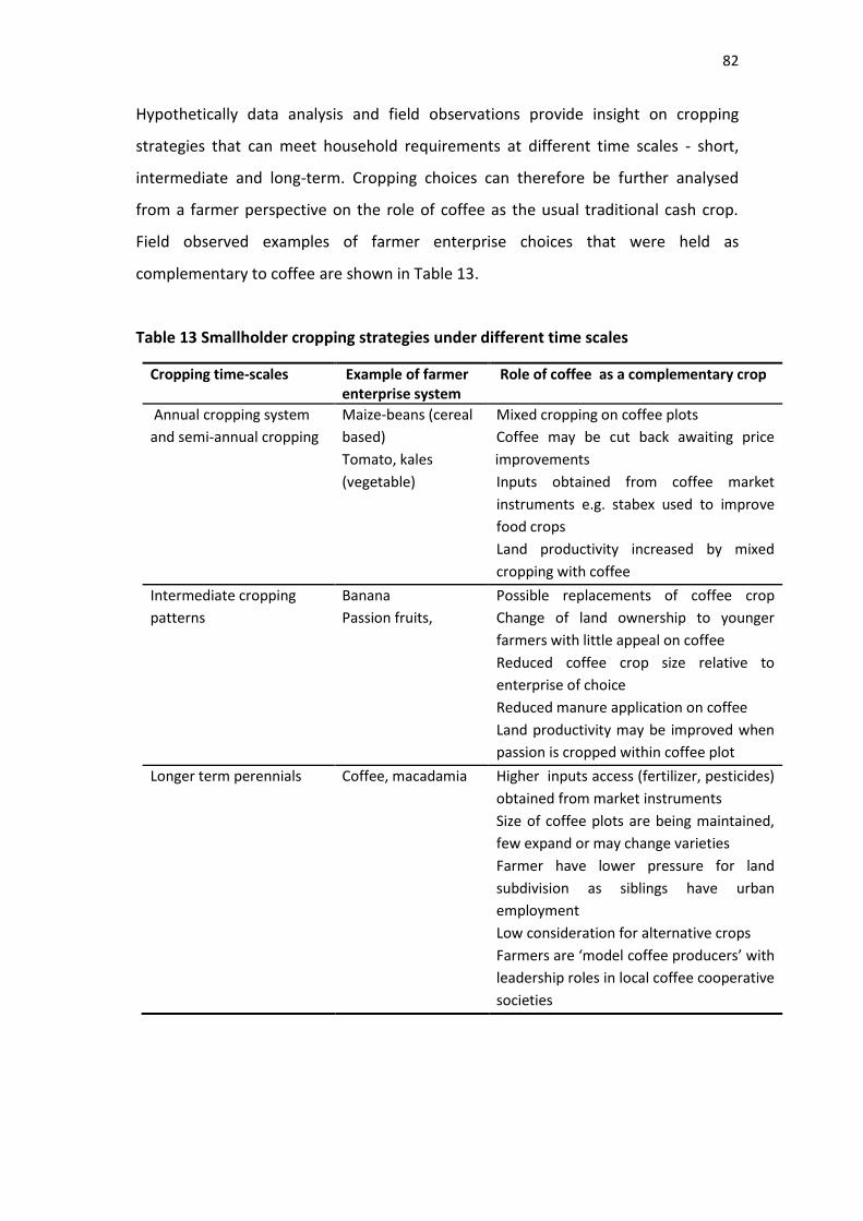
82

Hypothetically data analysis and field observations provide insight on cropping

strategies that can meet household requirements at different time scales - short,

intermediate and long-term. Cropping choices can therefore be further analysed

from a farmer perspective on the role of coffee as the usual traditional cash crop.

Field observed examples of farmer enterprise choices that were held as

complementary to coffee are shown in Table 13.

Table 13 Smallholder cropping strategies under different time scales

Cropping time-scales Example of farmer enterprise system

Role of coffee as a complementary crop

Annual cropping system

and semi-annual cropping

Maize-beans (cereal

based)

Tomato, kales

(vegetable)

Mixed cropping on coffee plots

Coffee may be cut back awaiting price

improvements

Inputs obtained from coffee market

instruments e.g. stabex used to improve

food crops

Land productivity increased by mixed

cropping with coffee

Intermediate cropping

patterns

Banana

Passion fruits,

Possible replacements of coffee crop

Change of land ownership to younger

farmers with little appeal on coffee

Reduced coffee crop size relative to

enterprise of choice

Reduced manure application on coffee

Land productivity may be improved when

passion is cropped within coffee plot

Longer term perennials Coffee, macadamia Higher inputs access (fertilizer, pesticides)

obtained from market instruments

Size of coffee plots are being maintained,

few expand or may change varieties

Farmer have lower pressure for land

subdivision as siblings have urban

employment

Low consideration for alternative crops

Farmers are ‘model coffee producers’ with

leadership roles in local coffee cooperative

societies

83

4.4 DISCUSSION

Uncertainty in coffee profitability has been contributed by buyer driven chains with

producers having little influence in the market chains. This situation suggests that

farmers can expect persistent price fluctuations. Though it’s clear that at a micro-

level, diversified farm enterprises are part of farmer risk avoidance strategies there

are challenges to prescribing credible alternative to coffee or enhancing coffee

productivity.

Development of successful smallholder coffee productivity forecasts requires

identification of factors that influence changes in agronomical practices.

Smallholders are nonetheless heterogeneous and show complexities of farming

practices (Stroebel, 2004). Previous empirical studies have used data collected from

random samples to analyze and construct farm typologies (Valbuena et al., 2008;

Carmona et al., 2010; Titonnell et. al., 2010). In this study, a sampling strategy that

characterized existing farm typologies was used to determine farmer enterprise

adoption behaviour. Essentially, farmer historical coffee production records were

used to depict production trends as increasing, decreasing or maintaining more or

less the same level of production. Data sources to categorize sample farmers were

mainly from coffee cooperatives societies. Using simple descriptive statistics such as

means with standard deviations, paired correlations and general linear regressions,

performance of farms showing different coffee production behavior were made.

Results were clear that smallholder farms intensification is aligned to farmer coffee

production decision on whether to increase or decrease coffee production. To some

extent other farm enterprise productivity and diversification pursuits are also

pegged on this behavior since farm productivity was shown to be strongly associated

with labour and non labour inputs including fertilizer affordability. Marenya and

Barret (2009) have showed that in Western Kenya, smallholder production response

to fertilizer at the levels they can afford do not justify application.

The differentiation of coffee productivity in terms of coffee bushes ha-1 and cherry

value ha-1 between the farm categories revealed that the coffee increasing farms

84

were significantly different from the constant and decreasing farms however there

were weak differences between the constant and the decreasing farms. These

results are suggestive of farmers’ uncertainty on future coffee production. Results

demonstrated that farm output measures such as cherry value ha-1, the number of

high value tree crops such as avocado ha-1 and milk output sold per day as useful

indicators depicting farm productivity differences. These differences are in addition

reinforced by farmer inputs affordability particularly on fertilizers, labour and other

non labour inputs such as pesticides and seeds.

Results comparing the constant, decreasing, and increasing farm categories were

inconclusive on the hypothesis that smallholders with stagnated or decreasing coffee

yield productivity record higher enterprise intensification rates with maize, banana,

livestock and agroforestry trees. Analysis showed that farmers decreasing coffee

production realize significantly lower cherry value and have smaller farm sizes and

households; but larger banana and maize value which were however not significantly

different to the other farm categories. Milk value sold per day was also on the

decline per unit suggesting lesser dairy keeping activities compared to the coffee

increasing farms. The size of agroforestry tree volumes was slightly bigger than other

farm categories. Further, these farmers incur lower labour costs, have lower manure

application rates and not much dairy production. They nonetheless appear to use a

higher diversity of crops to substitute decreased coffee farming.

On the other hand, farmers interested in expanding coffee production are cushioned

to some extent by productive milk enterprises. They also have larger land areas

which allow them to have some diversity of other crops without impinging on coffee.

They can afford higher fertilizer application and labour costs somewhat subsidized by

larger household sizes. Comparatively, evidence suggests that coffee decreasing

farms seem to be shifting more into banana and maize than farmers who are

expanding coffee production. For these farmers, maize and banana are seen as

alternatives. In fact banana has a much higher value on coffee decreasing farms than

those expanding the coffee enterprise.

85

There is evidence of farmer response to shrinking farm sizes and lost coffee yield

productivity. Findings suggest that farmers with larger farm sizes are more likely to

maintain and increase their investment in coffee enterprise, especially if they also

have other important income sources like milk. On the other hand, coffee is

decreasing on smaller farms suggesting that with greater land subdivision there is

greater farmer interests on other crops like banana and maize unless profitability for

coffee were to increase. Smaller farmers inadvertently face more challenges to

maintain coffee production instead opting for other crops that provide food security.

These farmers also show higher levels of livestock keeping and agroforestry trees to

serve as self- insurance for the household. In self-insurance, people exchange some

forgone expected earnings for reduced income variability by selecting a portfolio of

assets and activities with a low or negative correlation of incomes.

Overall farm typology analysis confirm that farmers rationally allocate assets across

activities to equalize marginal returns in the face of quasi fixed complementary

assets (e.g land) or mobility barriers to expand existing (farm or non-farm)

enterprises (Barrett, 2001). For the poorest this may mean highly diversified

portfolios with low marginal returns, or desperation led diversification (Reardon et

al., 2000; Barrett et al., 2006).

4.5 CONCLUSIONS

This study has provided insights on farmer strategies to meet household

requirements in circumstances of uncertainty for major cash crop farming such as

coffee. Land size, coffee production (number of bushes, cherry yields ha-1), livestock

units, agroforestry trees, banana, maize value and nutrient (manure and fertilizer)

and labour and non labour inputs were identified as significant factors that influence

coffee farms productivity behaviour and can therefore distinguish farm typologies.

Though farm diversification strategies are found to be similar especially in terms of

agroforestry activities, it is apparent that coffee production is decreasing in smaller

farms compared to where it is increasing. It is also clear that inputs such as fertilizer

application are tremendously reduced with declining coffee production raising

concerns that smallholder coffee farms could decline to low productivity systems. On

86

the other hand continued farm subdivisions and unprofitability could seriously curtail

increased coffee production. Farmers with small farm sizes and declining coffee

production are interested in other crops such as maize and banana that perhaps

offer food security but may not ensure land health. These trends would probably

change with a high profitability shift in coffee. It is therefore critical that policy

makers are aware of these trends in order to support enterprises that are attractive

to farmers. This study nonetheless did not show clear alternatives to coffee farming

even though dairy farming seem to be associated with increased coffee production,

perhaps due to bigger farm sizes.

87

4.6 REFERENCES

Barnett, D, Blake, B and McCarl, BA. 1982. Goal programming via multidimensional

scaling applied to Senegalese subsistence farms. American Journal of Agricultural

Economics, 64: 720–727.

Barrett, CB, Marenya, PP, Mcpeak, J, Minten, B, Murithi, F. Oluoch-Kosura, W. Place,

F. Randrianarisoa, JC, Rasambainarivo, J and Wangila, J. 2006. Welfare dynamics

in rural Kenya and Madagascar. Journal of Development Studies, 42:248–277.

Barrett, CB, Reardon, T and Webb, P 2001. “Nonfarm Income Diversification and

Household Livelihood Strategies in Rural Africa: Concepts, Dynamics, and Policy

Implications.” Food Policy, 26(4): 315-331.

Beets, WC. 1990. Raising and sustaining productivity of smallholder farming systems

in the tropics. AgBe Publishing. Alkmaar, The Netherlands.

Carmona, A, Nahuelhuala, L, Echeverría, C and Báez, A. 2010. Linking farming

systems to landscape change: An empirical and spatially explicit study in

southern Chile. Agriculture, Ecosystems and Environment 139:40–50.

Carter, SE. 1997. Spatial stratification of Western Kenya as a basis for research on

soil fertility management. Agricultural Systems, 55: 45–70.

CRF (Coffee Research Foundation), 2010. Coffee varieties. http://www.crf.co.ke/

Accessed: 12/10/2010.

Crowley, EL and Carter, SE. 2000. Agrarian change and the changing relationships

between toil and soil in Maragoli, Western Kenya (1900–1994). Human Ecology,

28:383–414.

Duvernoy, I. 2000. Use of a land cover model to identify farm types in the Misiones

agrarian frontier (Argentina). Agricultural Systems, 64 (3): 137–149.

Franzel, S. 2004. ‘Use of an indigenous board game, ‘bao’, for assessing farmers’

preferences among alternative agricultural technologies’, Agricultural and

Extension Network Newsletter No. 49. London: Overseas Development Institute.

GenStat Release 12.1 2009. GenStat Twelfth Edition. GenStat Procedure Library

Release PL20.1 VSN International Ltd. www.genstat.co.uk

88

Gill, J. 2000. Generalized Linear Models: A Unified Approach. Sage University Papers

Series on Quantitative applications in the social sciences, series No. 07-134,

Thousands Oaks, Ca: Sage.

GOK (Government of Kenya) 2010. The 2009 Kenya Population and Housing Census.

Volume 1A. Population distribution by administrative units. Kenya National

Bureau of Statistics.

Karanja, AM. 2002. Liberalization and smallholder agricultural development. A case

study of coffee farms in Kenya. PhD thesis, Wageningen University.

Keating et al., 2010. Eco-efficient agriculture, concepts, challenges and

opportunities. Crop Science, 50(2): 109 -119.

Köbrich, C, Rehman, T, Khan, M. 2003. Typification of farming systems for

constructing representative farm models: two illustrations of the application of

multi-variate analyses in Chile and Pakistan. Agricultural Systems, 76 (1): 141–

157.

Lambine, E, Geist, H and Lepers, E. 2003. Dynamics of land-use and land-cover

change in tropical regions. Annual Review of Environment and Resources, 28:

205–241.

Lengkeek, AG and Carsan, S. 2004. The process of participatory tree domestication

project in Meru, Kenya. Development in Practice, 14: 445-451.

Mettrick, H. 1993. Development Oriented Research in Agriculture: an ICRA textbook.

The International Centre for Development Oriented Research in Agriculture

(ICRA), Wageningen, The Netherlands, 290 pp.

Mude, A. 2006. “Weaknesses in Institutional Organization: Explaining the Dismal

Performance of Kenya’s Coffee Cooperatives” Paper presented at International

Association of Agricultural Economists Conference.

Marenya, PP and Barrett CB. 2009. Soil quality and fertilizer use rates among

smallholder farmers in western Kenya. Agricultural Economics, Vol 40:5, 561-572.

Muraya, P, Garlick, C, and Coe, R. 2002. Research data management. Published by

The World Agroforestry Centre (ICRAF) and Statistical Services Centre, The

University of Reading, United Kingdom.

Ovuka, M. 2000. Land use changes in Central Kenya from the 1950s – A possibility to

generalise? GeoJournal, 51: 203–209.

89

PASW statistics 18, 2009. Release 18.0.0 (July 30th, 2009).

Place, F, Barrett, CB, Freeman, AH, Ramisch, JJ and Vanlauwe, B. 2003. Prospects for

integrated soil fertility management using organic and inorganic inputs:

evidence from smallholder African agricultural systems. Food Policy, 28: 365–

378.

Reardon, TJE, Taylor, K, Stamoulis, P, Lanjouw, A and Balisacan. 2000. “Effects of

Nonfarm Employment on Rural Income Inequality in Developing Countries: An

Investment Perspective,” Journal of Agricultural Economics, 51(2): 266-288.

Royston, P.1993. A toolkit for testing for non-normality in complete and censored

samples. The Statistician, 42, 37-43.

Ruben, R and Pender, J. 2004. Rural diversity and heterogeneity in less-favoured

areas: the quest for policy targeting. Food Policy, 29: 303–320.

Shepherd, KD and Soule, MJ. 1998. Assessment of the economic and ecological

impacts of agroforestry and other soil management options on Western Kenyan

farms using a dynamic simulation model. Agriculture Ecosystems and

Environment, 83: 27–42.

Stern, RD, Coe, R, Allan, EF and Dale, IC. 2004. Good statistical practice for natural

resources research. CABI publishing.

Stroebel, A. 2004. Socio-economic complexities of smallholder resource-poor

ruminant livestock production systems in Sub-Saharan, Africa. PHD Thesis,

University of the Free State.

Tittonell, P, Vanlauwe, B, Leffelaar, P, Rowe, E., Giller, K. 2005a. Exploring diversity in

soil fertility management of smallholder farms of Western Kenya. Heterogeneity

at region and farm scales. Agriculture, Ecosystems and Environment, 110: 149–

165.

Tittonell, P, Muriuki, A, Shepherd, KD, Mugendi, D, Kaizzi, KC, Okeyo J, Verchot, L,

Coe, R, Vanlauwe B. 2010. The diversity of rural livelihoods and their influence

on soil fertility in agricultural systems of East Africa – A typology of smallholder

farms. Agricultural Systems, 103: 83–97.

Valbuena, D., Verburg, P, Bregt, A. 2008. A method to define a typology for agent

based analysis in regional land-use research. Agriculture, Ecosystem and

Environment, 128: 27–36.

90

Van de Steeg, J, Verburg, P, Baltenweck, I, Staal, S. 2010. Characterization of the

spatial distribution of farming systems in the Kenyan Highlands. Applied

Geograpphy, 30(2): 239–253.

Waithaka, MM, Thorntorn, PK, Shepherd, KD, and Ndiwa, NN. 2007. Factors affecting

the use of fertilizers and manure by smallholders: the case of Vihiga, western

Kenya. Nutrient Cycling in Agro-ecosystems, 78: 211-224.

Waters, AR. 1972. Change and evolution in the structure of the Kenya coffee

industry. African affairs, Texas A & M University

http://afraf.oxfordjournals.org/content/71/283/163.full.pdf.

Williams, RL. 1972. Jamaican Coffee Supply, 1953-1968. An exploratory study. Social

and Economic Studies, Vol. 21. No.1.

Wilkins, RJ. 2008. Eco-ecofficient approaches to land management: A case for

increased integration of crop animal production systems. Philosophical

Transactions The Royal Society, 63: 517-525.

91

CHAPTER 5 IMPLICATIONS OF DECREASED COFFEE CULTIVATION ON TREE DIVERSITY IN SMALLHOLDER COFFEE FARMS ABSTRACT

African smallholder farming systems are known to maintain a large diversity of

native tree species on farm. A shift in coffee cultivation by smallholder producers is

however suspected to influence the available tree diversity on farm. To provide

current knowledge on how tree diversity is maintained under present coffee

production practices within different agro-ecological zones, this study surveyed 180

farms to determine the diversity of available tree species. Farms were categorised

according to their trends in coffee production such as, increasing, decreasing or

constant. Tree diversity analysis was done using species accumulation curves, rènyi

diversity profiles and species rank abundance. Quasi-Poisson generalized linear

regressions were used to elucidate richness and abundance difference by farm

categories. Results showed that tree diversity per farm was not significantly different

by farm types. Tree individuals within coffee plots among the coffee increasing

farms, were significantly higher than those in the decreasing farms (P = 0.05) and

those of the constant farms. Farm size had a significant effect on tree richnness,

abundance and tree volume/basal area on farm. Shannon diversity index for the

decreasing farms was nonetheless higher than for the decreasing farms. There was

strong evidence (P < 0.001) that species richness in the coffee zone, UM3, is

significantly different from those in UM1 and less so (P = 0.0169) from those in UM2.

Rènyi diversity (H0) ordered as follows: UM3 (H0 = 4.86; richness = 128) > UM2 (H0 =

4.71; richness = 110) > UM1 (H0 = 4.58; richness = 98). UM3 had the largest

proportion (45%) of the most abundant species and hence most un-even. Grevillea

robusta was highly ranked in terms of relative density and dominance across farm

plots at proportions of 41-42%. In conclusion, results suggest that farmers with

larger levels of coffee (Coffea arabica L.) cultivation tend to retain more tree

abundance though not necessarily of high richness on farm. Species richness was

more strongly influenced by type of agro-ecological zones.

92

INTRODUCTION

Smallholder coffee agroforestry systems around Mount Kenya are typical example of

tree rich agro-ecosystems. Derived largely from moist intermediate forests, coffee

farms adjacent to forests often contain tree species richness depicting close

association with species composition in the natural forests (Lengkeek et al., 2006;

Kindt et al., 2007). Coffee agroforests have been shown to be instrumental in

protecting biodiversity and assist in alleviating negative effects of deforestation

(Perfecto et al., 1996). Peeters et al. (2003) have observed that complex agroforests

complement ecological services similar to those provided by natural forests, such as

soil protection through nutrient cycling; water retention and carbon capture. More

importantly, cultivation and retention of naturally regenerated trees in coffee

landscapes, which comprise a significant land-use system in the tropics and sub

tropics, can serve as biological corridors between protected forest areas and farming

landscapes (Schroth and Harvey, 2007).

Recent field evidence suggests that structurally complex habitats also support a

more diverse fauna (Perfecto et al., 2005). For instance, in Latin America, ‘rustic’-

coffee systems contain a great diversity of ants, birds and trees compared to sun-

coffee systems (Rappole et al., 2003). In Brazil, agroforests have been shown to

accumulate intact ant communities that provide natural pest control saving farmers

on pesticide use. Harvey et al. (2008) and Chazdon et al. (2009), illustrate that

conservation approaches that build alliances between ‘human-modified landscapes’

and protected areas tend to enhance biodiversity and to promote sustainable

livelihoods.

Lengkeek et al. (2005), report that farmers can also benefit culturally by maintaining

biological diversity of tree species that ensure productivity and sustainability of their

agroforestry systems. Genetic variation in agricultural landscapes made up by

variation between and within species, helps farmers to manage their inputs in more

efficient ways (Dawson et al., 2009). For instance, a mix of fast growing and slow

growing indigenous timber species can be retained for different market

opportunities such as sawn wood markets; as well as domestic consumption like

93

house building and firewood requirements. In addition, fruit tree species with

different fruiting phenology can better contribute to household food security and

income (Dawson et al., 2009).

In line with this knowledge, approaches such as shade coffee certification have been

advocated to promote preservation of coffee systems biodiversity (Philpott and

Dietsch, 2003). In these schemes, coffee consumers are impressed on the value of

‘shade coffee’- coffee grown under tree canopy as opposed to ‘sun coffee’- coffee

grown without an over-storey. Where practiced, for instance in the Veracruz region

of Mexico, shaded coffee establishment involves placement and maintenance of

young coffee plants under a canopy provided by one or two tree species (Rappole et

al., 2003). In Kenya, tree planting within coffee plots is prominent, though not

necessarily for shade but for tree products and services. Different tree species are

cultivated in mixed or line planting patterns commonly as boundary markers.

Determining what kind of tree canopy management contributes to biodiversity

conservation is critical for increasing consumers’ confidence in shade coffee

certification schemes (Perfecto et al., 2005). For instance, some plantations in

Central America use low density of heavily pruned Inga or Erythrina trees which may

not be as effective at preserving biodiversity compared to ‘rustic’ plantations that

mimic structural complexity of forests (Perfecto et al., 2005). In order to raise the

‘attractiveness’ of shade coffee certification programs, Philpott and Dietsch, (2003)

have recommended provision of financial incentives to farmers to maintain

biodiversity-rich shade farms that also preserve adjacent forest fragments. To keep

farmers from converting more forest to shade coffee, they recommend only

certifying farms that are ten or more years old. The relative impact of converting

natural forest to agroforestry systems has nonetheless not been compared in many

agricultural landscapes (Fitzherbert et al., 2008; Asase and Teteh, 2010). From a

conservation perspective, coffee agroforestry systems should be promoted, but not

at the expense of remaining forest patches (Rappole et al., 2003; Philpott et al.,

2003; Perfecto et al., 2005).

94

Though studying all the factors influencing biodiversity in coffee systems is

challenging, useful lessons from similar agroforests such as cacao (Theobroma cacao

LINN.) and rubber (Hevea brasilensis Muell. Arg) can be inferred. These systems have

been showed to offer more sustainable production systems than pure plantations

systems (Perfecto et al., 2005; Asase and Teteh, 2010). Like coffee, cocoa production

systems are nonetheless being replaced by land-use systems of lower biodiversity

value for instance, in indigenous territories of Talamanca, Costa Rica, despite efforts

to promote cocoa agroforestry as conservation tool (Schroth and Harvey, 2007).

Challenges that negatively affect the promotion of coffee and cocoa agroforests

include; fears of pest and diseases prevalence; expanded human population with

accompanied demand for land; demand for expanded food crop production,

integration of indigenous communities into the cash economy, low prices and poor

market prices for cocoa and coffee (relative to alternative crops).

In order to promote biodiversity in smallholder coffee agroforests of Mount Kenya,

current vegetation with floristic and structural complexity should be enhanced. It is

clear that intensification of the systems with other land uses such as annual cropping

usually involving maize, beans and banana may not be compatible with biodiversity

preservation. Consequently, farm tree domestication activities that enhance farm

tree planting and natural regeneration and at the same time enhance farmer

benefits such as provision of wood and fruits or are beneficial to fauna can have

positive impacts on biodiversity. There are concerns that trees in coffee systems are

propagated with few germplasm sources that are in close vicinity such as

neighboring farms implying that similar patterns of tree diversity on farms can

persist since inter and intra-specific tree diversity is eventually decreased (Lengkeek

et al., 2005).

Few studies are available to show how tree diversity in high potential farming

systems such as Mount Kenya can contribute to biodiversity enhancement with

direct benefits to the farmer. Knowledge gaps abound on farm tree species choices,

management strategies and conservation within fragile habitats and niches. More

95

so, there is need to understand how indigenous species on farm may be managed in

a context of changing land use decisions to cultivate or not cultivate coffee and food

crops such as maize frequently affected by commodity market shocks.

Summarizing patterns of species diversity in relation to the most important factor

structuring plant communities would therefore help reveal the basic patterns of

variation. A small and un-even, tree species population in a given farming landscape

may be dysfunctional by hampering gene migration within a given tree population

thereby increasing chances of genetic erosion (Dawson et al., 2009). There is

however no available evidence to indicate minimum tree densities to be maintained

at a given farming landscape (Lengkeek et al., 2006; Kindt et al., 2007).

The first objective of this study was to investigate agroforestry tree species richness

maintained by coffee farmers under changing coffee yield production trends

categorized as increasing, decreasing or constant. The second objective was to

determine tree diversity patterns maintained under the different coffee agro-

ecological zones (Upper midland 1), 2 and 3 around Mount Kenya. Thirdly, the study

sought to determine gamma diversity for the Mount Kenya coffee system.

It is anticipated that this study findings will contribute towards better awareness

among agricultural practioners and policy makers on the availability and contribution

of tree diversity in smallholder coffee farms. An understanding of the structure and

densities of tree population on farm is especially useful in determining the viability

of trees on agricultural landscape even for conservation. Further, findings could also

inform strategies towards establishing farm based or the so called decentralized tree

germplasm sources by identifying available tree species diversity and their

distribution on coffee farms.

5.1 CONCEPTUAL FRAME

Recent studies on shade coffee document the biodiversity benefits of coffee

agroforestry in various geographic locations. In Mexico, Peeters et al., (2003) report

that diverse shade vegetation yield complimentary products, such as fruits, timber

96

and firewood, which diversify the diet and stabilize incomes for smallholders. The

values of these products have sometimes been found to outweigh gains from coffee

sales. For instance, Beer et al. (1998) shows that coffee estates producing 1380

pounds of coffee ha-1 and shaded with Cordia alliodora (R & P) Oken, a timber

species, have higher profits if coffee price sinks below 60 US$/100 pounds. Peeters

et al. (2003) reports that coffee shaded with any density of Cordia alliodora has

better benefit/cost ratio than in un-shaded coffee estates, although coffee yields are

lower. In Costa Rica, studies have shown that one hectare of coffee plantation with

diverse shade vegetation covers all the necessities of timber, firewood and fruits for

a seven-person peasant family. Simplifying these plantations is reported to be

economically disadvantageous even if coffee production increases (Peeters et al.,

2003).

Quantifying direct benefits households can anticipate from cultivating a diversity of

agroforestry trees can contribute towards preserving and protecting individual

species and their ecosystems (Purvis and Hector, 2000). Comparative measurements

of diversity for multiple locations, groups or times can help answer crucial questions

about how diversity arose and how we might best act to maintain it (Humphries et

al., 1995; Purvis and Hector, 2000). Conceptually, plant diversity can be related to

productivity at different scales: global, regional and experimental (Purvis and Hector,

2000). Figure 1 shows a schematic presentation of these relationships. At a global

scale, from high latitude to the tropics, plant diversity in large areas is positively

related to increasing productivity (Figure 13I). At regional level, (Figure 13II) plant

diversity in small plots is frequently negatively related to increasing productivity,

often as part of a larger unimodal distribution of diversity. The number of species

will at a given scale relate to several factors such as their size. Hence in ecology

studies it’s important to consider the number of individual plants sampled, spatial

heterogeneity and competitive exclusion as productivity increases.

Experimental manipulation of plant diversity within habitats (Figure 13III) reveal that

although relationships vary, productivity tends to increase with diversity owing to

97

increasing complementarities or positive interactions between species and the

greater likelihood of diverse communities containing a highly productive species.

Figure 13 Plant diversity and productivity at different scales (Source: Purvis and

Hector, 2000)

In manipulation experiments, biodiversity is the explanatory variable and

productivity the response, whereas in observational studies the relationship is

usually viewed the other way round as illustrated in Figure (13 III). Abiotic variables

may be responsible for large-scale variation. Nonetheless, evaluation of large or

small - scale effects differ according to species and given field situation.

Benchmarking genetic diversity among the farm tree communities has been poorly

understood aspects for diversity estimation. It is further, not clear to what extent

smallholders are willing to conserve tree diversity due to resource constraints such

as available land per household and possible benefits that can be accrued (Lengkeek

and Carsan, 2004; Simons and Leakey, 2004). The importance of on-farm tree

inventories lies in the information they reveal on the density and the level of

98

aggregation of tree species in farmland. They can also provide insight on the

connectivity, levels of out-crossing and possible inbreeding depression of farm tree

population (Dawson et al., 2009).

Finally, available literature provides useful perspectives for interpreting species

richness data in natural systems. The relation of species richness to species

succession stage, abundance and composition are shown as important in biodiversity

analysis (Grime, 1983; Jongman et al., 1995). For instance large changes in species

richness at a certain stages of the succession does not necessarrily mean large

compositional turnover, since compositional turnover mean a change in species

abundancies which may be uncorrelated with the presences or absences of species.

5.2 MATERIALS AND METHODS

Many factors, such as environmental variation, history of a site and dispersal ability

of different species can be responsible for structuring tree assemblages (Spies,

1998). Species diversity implies the number of categories that can be differentiated

and the proportions (or relative abundance of the number of individuals in each

category (Kindt and Coe, 2005). In more elaborate systems, at least three measures

are used to determine diversity: alpha diversity (species richness of standard site

samples), beta diversity (differentiation between samples along habitat gradients),

and gamma diversity for a geographic area (differentiation between areas at larger

scales) (Bond, 1989).

Species richness and evenness are common methods of quantifying biodiversity even

though quantification is always done with loss of some information (Humphries et

al., 1995; Jongman et al., 1995). Species richness refers to the number of species in a

community; while evenness refers to how species abundances (e.g. the number of

individuals, biomass, and cover) are distributed among the species (Ludwig and

Reynolds, 1988). In forestry, species richness is often regarded as the most

important component of alpha diversity. Tree diversity inventories are therefore

useful in characterizing the demographic shortcomings of agroforests that may

underlie the system (Dawson et al., 2009).

99

The frequency distribution of species abundances is considered a fundamental

characteristic of tree assemblage structure (Sizlinga et al., 2009). Generated species

abundance curve show a log-normal distribution. Relative abundance is an interplay

of many more or less independent factors. On the other hand tree basal area

distribution, matches a geometric distribution of species abundance. This model is

known as the niche pre-emption hypothesis. It assumes that with limited

environmental resources the most dominant species pre-empts a large fraction of

the resources, the next most successful species pre-empts a smaller fraction of the

remaining resources and so forth (Ludwig and Reynolds, 1988).

In this study, tree species counts and tree basal area (tree cross-sectional area at

breast height) are used to analyze tree diversity patterns in smallholder coffee farms.

Diversity is assessed by calculating certain values of inventoried trees (Githae et al.,

2007; Ambinakudige and Sathish, 2009), these are: relative frequency (Rf), which is

the number of farm plots in which a species occurs divided by the total number of

occurrences in plots; Relative density (Rd), which is the number of individuals of a

species divided by the total number of individuals of all species; relative dominance

(RD), which is the basal area of a species divided by the sum of all basal areas for all

species; and importance value (Iv) which is calculated by the summation of Rf + Rd +

RD.

5.2.1 Study area

This study was conducted within the Mount Kenya, smallholder coffee systems (see

chapter 3). The larger Mount Kenya forest biosphere is separated from the coffee

zone by a belt of tea. This biome is a world heritage site exhibiting rare fauna and

flora. Some 882 plant species, belonging to 479 genera and 146 families have been

identified in this ecosystem. Eighty one high altitude plants are endemic to this

system (UNEP, 2005). Three coffee agro-ecological zones namely the upper midland

one (UM1), 2 and 3, constitute the main coffee agro-ecosystems in Kenya (Jaetzold

and Schmidt, 2007). Altitude for coffee growing ranges from 1200 to 1750 m above

sea level. The lower altitude works better if precipitation is above 1200 mm. Annual

mean rainfall is between 1200 and 1800 mm. Mean temperature range is 18.9 to

100

20.7 oC. A small change in diurnal temperature range is anticipated due to prevalent

cloud cover and minimum temperatures compensating for any rises (Jaetzold and

Schimdt, 2007).

The soils are mainly ando-humic nitisols and humic andosols, developed on tertiary

basic igneous rocks. They are characterised by dark reddish brown, to dark brown

colours, with good drainage and extremely deep profile (FAO, 1978). Soil fertility is

however on the decline due to recurrent permanent use over the years with little

recycling of nutrients (see chapter three). Present land use activities other than

coffee production involve growing of vegetables such as French beans, snow peas,

cabbages, kales, bananas, fruits such as passion fruits, avocado, mangoes and food

crops such as maize, beans, Irish potatoes. In the upper midland zone (UM 1), tea

cultivation is also undertaken to a lesser extent. Livestock keeping forms an

important part of smallholder farming. Pure and improved crosses of dairy cattle

such as Ayrshire, Guernsey and Friesian are raised under zero grazing units. Some

farmers also keep bulls (local zebu or crosses) for draft power and serving their cows.

The Mount Kenya coffee zones are largely of high agricultural potential characterized

by high human settlement. Population density exceeding 400 persons per square

kilometer in parts of Embu and Meru central have been recorded (GOK, 2010).

Possible population pressure is driving significant land-use change possibly

influencing farmer land access, availability, and intensification practices.

5.2.2 Farm plots sampling frame

A total of 29 farmer cooperative societies (FCS) effectively covering the coffee

production zone of North-Eastern and Southern Mount Kenya was used to select

farmers. Random samples of 180 farm plots were surveyed during the months of

June to August 2009. Farmer coffee cherry production records were collated at the

FCS level and used to categorize sample farm plots into three groups according to

their ‘coffee trends’ as either ‘increasing’, ‘decreasing’ or `constant’ (see details in

chapter 2). The three types of farm plots were compared and contrasted with

respects to levels of tree diversity maintained. Farm sizes and their slopes were

101

assumed to be similar in most coffee zones and therefore not considered during

sample selection. Coffee, banana and maize farming were assumed to be the most

dominant agricultural cropping patterns present in the Mount Kenya coffee system.

Household interviews, using close and open ended questionnaires were further used

to collect additional farm plot data such as on tree planting practices, farmers’ age,

family size, land size, and size of the coffee enterprise.

The study used ground based methods to enumerate tree species present in

smallholder coffee farms. Tree basal area mensuration (tree cross-sectional area

measured at breast height) was also undertaken. All trees greater than or equal to 5

cm diameter at breast height (DBH) were in fact enumerated. DBH’s were readily

measured using calibrated tree diameter tapes. Trees were defined as all woody

perennials growing to over 1.5 m tall, including exotics (Beentje, 1994; Brown, 1997).

Local names of tallied trees were recorded from farmer interviews. All enumerated

trees were identified to the species level according to Beentje (1994) or Maundu and

Tengnäs (2005). Coffee plants were not classified as agroforestry trees. Two persons

were required to undertake tree inventories by farm walks; simultaneously recording

species presence counts and DBH readings. Farmers’ were requested to facilitate

marking-out of plots boundaries and in species identification in local dialects.

5.2.3 Diversity analysis

Recorded tree species information was termed as ‘coffee farm trees assemblage’

and tabulated into an ecological data matrix. This was subjected to diversity analysis

using BiodiversityR (Kindt and Coe, 2005), based on R statistical software version

2.11.1 (R Development Core Team 2010).

Species patterns are used here to refer to the spatial dispersion of a species within a

given farm and the relationships among many species between farms (Ludwig and

Reynolds, 1988). To investigate species aggregation and levels of dominance, rank

abundance curves and Rènyi diversity profiles were analyzed. Tree abundances

(number of individuals) and basal area (stems area) distributions were calculated to

assess structural complexity and heterogeneity of present farm tree populations

102

(Jongman et al., 1995). All calculations were based on species frequencies. Tree

diversity was assessed by calculating Shannon and inverse-Simpson diversity indices

(Annex 5).

In order to assess tree diversity among farm categories, districts and the different

coffee agro-ecological settings, Rènyi profiles were used to rank sites from low to

high diversity (Kindt and Coe, 2005; Kindt et al., 2006). Rènyi profiles are curves used

to provide information on richness and evenness; they are essentially one of the

diversity ordering techniques (Jongman et al., 1995; Kindt and Coe, 2005). The

profile is calculated from the species proportion and alpha parameter as follows:

Rènyi species diversity ordering for all enumerated species was plotted at scale

values of: 0, 0.25, 0.5, 1, 2, 4, 8 and ∞ as prescribed in BiodiversityR (Kindt and Coe

2005; Jongman et al., 1995). The values are based on parameter ‘alpha’. The profile

value, alpha = 0 provide information on species richness- it equals the logarithm of

species richness (H0 = ln(S). While the profile value, alpha (∞) = infinity provides

information on the proportion of the most dominant species- it is calculated as the

logarithm of 1/proportion of a given species. In summary, Rènyi diversity profiles

calculation includes:

H0 = Ln (Species richness)

H1 = Shannon diversity index

H2 = Ln (Simpson-1)

H∞ = ln (Prop Max-1)

Finally, to analyse tree richness and evenness in the different coffee agro-ecological

zones and coffee farm categories surveyed, sample based species accumulation

curves were plotted. Species accumulation curves show species richness for

103

combinations of sites (in this case farms). These curves portray the average pooled

species richness for all sites together. Average pooled species richness is calculated

because different sites combinations have different species richness (Kindt and Coe,

2005). Quasi-Poisson regression modeling (with a log-link) was used to assess effects

of coffee production trends and farm size on tree diversity, tree volume, coffee bush

and enterprises such as the number of livestock units on farm. The Bray-Curtis and

Kulczynski distances were calculated for academic purposes to examine species

composition for the Meru, Embu and Kirinyaga coffee regions as they are held to be

ecologically similar.

5.3 RESULTS

5.3.1 Farm characteristics

A total of 35820 trees were enumerated from 180 coffee farms. Surveyed farms on

average contain 199 (172.6 - 221.5, P = 0.95) trees; 90 to 100 of the trees are

maintained within coffee plots per farm. Mean species richness per farm was 17

species (15.7 to 18.2 species; P = 0.95). While average tree biomass volumes

accumulated per farm was calculated at 36.31 m3 (31.1- 41.5 m3, P = 95%). Data

analysis showed that only 22.5% of the tree individuals counted on farm was of

indigenous origin. The total area surveyed (combined sample farms) was 224.5

hectares. Farms are on average about 1.2 ha (1.1- 1.4 ha, P = 0. 95) with a family size

of about 5 persons (4.7- 5.4, P = 0.95). Household heads are aging at a mean age of

58 years.

Farmers own about 4.0 tropical livestock units (TLU), and cultivate about 545 (470.8-

619.9, P = 0.95) coffee bushes per hectare; coffee cherry production is 4 kg per bush.

Data analysis showed that coffee bushes distribution on farm is skewed with some

156 (75%) farmers growing between 500 and 750 bushes (Figure 14I). About 40

(22%) farms produce coffee cherry at between 2000-5000 kg ha-1 year-1 indicating

possibilities of high yield production; some 110 (60%) farms reported yields of 1000-

2000 kg of cherry ha-1 year-1 (Figure 14II). Besides coffee, 57.8 % (n = 96) and another

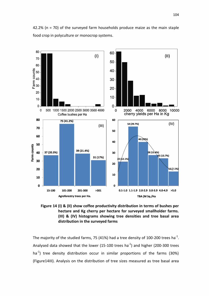
104

42.2% (n = 70) of the surveyed farm households produce maize as the main staple

food crop in polyculture or monocrop systems.

Figure 14 (I) & (II) show coffee productivity distribution in terms of bushes per hectare and Kg cherry per hectare for surveyed smallholder farms. (III) & (IV) histograms showing tree densities and tree basal area distribution in the surveyed farms

The majority of the studied farms, 75 (41%) had a tree density of 100-200 trees ha-1.

Analysed data showed that the lower (15-100 trees ha-1) and higher (200-300 trees

ha-1) tree density distribution occur in similar proportions of the farms (30%)

(Figure14III). Analysis on the distribution of tree sizes measured as tree basal area

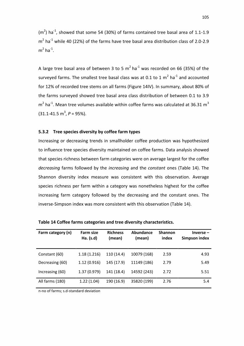
105

(m2) ha-1, showed that some 54 (30%) of farms contained tree basal area of 1.1-1.9

m2 ha-1 while 40 (22%) of the farms have tree basal area distribution class of 2.0-2.9

m2 ha-1.

A large tree basal area of between 3 to 5 m2 ha-1 was recorded on 66 (35%) of the

surveyed farms. The smallest tree basal class was at 0.1 to 1 m2 ha-1 and accounted

for 12% of recorded tree stems on all farms (Figure 14IV). In summary, about 80% of

the farms surveyed showed tree basal area class distribution of between 0.1 to 3.9

m2 ha-1. Mean tree volumes available within coffee farms was calculated at 36.31 m3

(31.1-41.5 m3, P = 95%).

5.3.2 Tree species diversity by coffee farm types

Increasing or decreasing trends in smallholder coffee production was hypothesized

to influence tree species diversity maintained on coffee farms. Data analysis showed

that species richness between farm categories were on average largest for the coffee

decreasing farms followed by the increasing and the constant ones (Table 14). The

Shannon diversity index measure was consistent with this observation. Average

species richness per farm within a category was nonetheless highest for the coffee

increasing farm category followed by the decreasing and the constant ones. The

inverse-Simpson index was more consistent with this observation (Table 14).

Table 14 Coffee farms categories and tree diversity characteristics.

Farm category (n) Farm size Ha. (s.d)

Richness (mean)

Abundance (mean)

Shannon index

Inverse –Simpson index

Constant (60) 1.18 (1.216) 110 (14.4) 10079 (168) 2.59 4.93

Decreasing (60) 1.12 (0.916) 145 (17.9) 11149 (186) 2.79 5.49

Increasing (60) 1.37 (0.979) 141 (18.4) 14592 (243) 2.72 5.51

All farms (180) 1.22 (1.04) 190 (16.9) 35820 (199) 2.76 5.4

n-no of farms; s.d-standard deviation

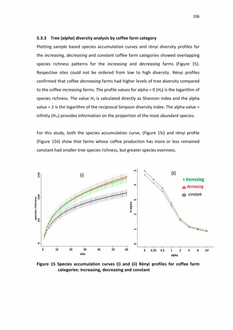
106

5.3.3 Tree (alpha) diversity analysis by coffee farm category

Plotting sample based species accumulation curves and rènyi diversity profiles for

the increasing, decreasing and constant coffee farm categories showed overlapping

species richness patterns for the increasing and decreasing farms (Figure 15).

Respective sites could not be ordered from low to high diversity. Rènyi profiles

confirmed that coffee decreasing farms had higher levels of tree diversity compared

to the coffee increasing farms. The profile values for alpha = 0 (H0) is the logarithm of

species richness. The value H1 is calculated directly as Shannon index and the alpha

value = 2 is the logarithm of the reciprocal Simpson diversity index. The alpha value =

infinity (H∞) provides information on the proportion of the most abundant species.

For this study, both the species accumulation curve, (Figure 15i) and rènyi profile

(Figure 15ii) show that farms whose coffee production has more or less remained

constant had smaller tree species richness, but greater species evenness.

Figure 15 Species accumulation curves (i) and (ii) Rènyi profiles for coffee farm categories: increasing, decreasing and constant

107

Rènyi profile showed that proportions of the most abundant species for the

increasing and decreasing farm categories were similar at 40%. The constant farm

category had higher proportions of the most dominant species at 43% (Table 15).

Table 15 Calculated alpha diversity indices from the constant, decreasing and increasing rènyi profiles

Farm category Species richness

(H0)

Shannon index (H1)

inverse Simpson

(H2)

Proportion (%) of most

abundant species (H∞)

Constant (n = 60) 110 2.59 4.93 0.43 Decreasing (n = 60) 145 2.79 5.48 0.41 Increasing (n = 60) 141 2.72 5.51 0.40

All farms (n = 180) 190 2.76 5.40 0.41

High alpha values indicate higher species richness, conversely; low infinity values

indicate a higher proportion of the dominant species. Examining tree diversity by

Shannon and inverse-Simpson diversity indices showed values of 2.59, 2.79 & 2.72

and 4.93, 5.49 & 5.51; for the constant (n = 60), decreasing (n = 60) and increasing (n

= 60) farm categories, respectively. Rènyi diversity order showed that tree species

evenness was higher in the constant farm category compared to the decreasing and

increasing categories (Figure 15ii).

5.3.4 Effects of coffee production trends on tree diversity

To investigate the effects of coffee production trends (increasing, decreasing, and

constant) and farm size on tree diversity, number of coffee bushes and livestock

units on farm, quasi-Poisson generalized linear regression model (with log-link) was

used (Table 16). The model was preferred instead of a simple linear regression

analysis (Annex 3) as it was found to fit the largely non-random, count data well.

Furthermore, simple linear regression model was found inappropriate when

predicting parameters with non-negative values such as tree richness and

abundances (Kindt and Coe, 2005).

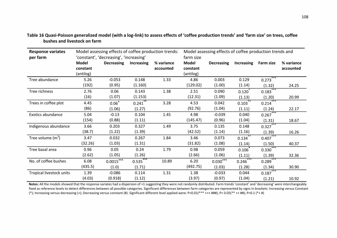
108

Table 16 Quasi-Poisson generalized model (with a log-link) to assess effects of ‘coffee production trends’ and ‘farm size’ on trees, coffee bushes and livestock on farm

Response variates per farm

Model assessing effects of coffee production trends: ‘constant’, ‘decreasing’, ‘increasing’

Model assessing effects of coffee production trends and farm size

Model constant (antilog)

Decreasing Increasing % variance accounted

Model constant (antilog)

Decreasing Increasing Farm size % variance accounted

Tree abundance 5.26 (192)

-0.053 (0.95)

0.148 (1.160)

1.33 4.86 (129.02)

0.003 (1.00)

0.129 (1.14)

0.273***

(1.32) 24.25

Tree richness 2.76 (16)

0.06

(1.07) 0.143

(1.153) 1.38 2.51

(12.31) 0.090 (1.09)

0.120*

(1.13) 0.183

***

(1.20) 20.99

Trees in coffee plot 4.45 (86)

0.06+ (1.06)

0.241** (1.27)

3.28 4.53 (92.76)

0.042 (1.04)

0.103**

(1.11) 0.214***

(1.24) 22.17

Exotics abundance 5.04 (154)

-0.13 (0.88)

0.104 (1.11)

1.45 4.98 (145.47)

-0.039 (0.96)

0.040 (1.04)

0.267***

(1.31) 18.67

Indigenous abundance 3.66 (38.7)

0.203 (1.22)

0.327 (1.39)

1.49 3.75 (42.52)

0.135 (1.14)

0.148 (1.16)

0.327***

(1.39) 16.26

Tree volume (m3) 3.47 (32.26)

0.032 (1.03)

0.267 (1.31)

1.84 3.46 (31.82)

0.073 (1.08)

0.134**

(1.14) 0.407

***

(1.50) 40.37

Tree basal area 0.96 (2.62)

0.05 (1.05)

0.24 (1.26)

1.79 0.98 (2.66)

0.059 (1.06)

0.106*

(1.11) 0.330***

(1.39) 32.36

No. of coffee bushes 6.08 (435.5)

0.0015+++

(1.0)

0.535***

(1.71)

10.89 6.20 (492.75)

0.030+++

(1.03) 0.246

***

(1.28) 0.289

***

(1.34) 30.90

Tropical livestock units 1.39 (4.03)

-0.086 (0.918)

0.114 (1.12)

1.31 1.38 (3.97)

-0.033 (0.97)

0.044 (1.04)

0.187***

(1.21) 10.92 Notes: All the models showed that the response variates had a dispersion of >1 suggesting they were not randomly distributed. Farm trends ‘constant’ and ‘decreasing’ were interchangeably fixed as reference levels to detect differences between all possible categories. Significant differences between farm categories are represented by signs in brackets: Increasing versus Constant (*); Increasing versus decreasing (+); Decreasing versus constant (#). Significant different level applied were: P<0.01(*** +++ ###); P< 0.05(** ++ ##); P<0.1 (*+ #)

109

A suitability assessment of Poisson and quasi-Poisson models revealed that

regressions with Poisson model was inappropriate as the dispersion of the variates

was fixed at 1, whereas the response variates studied had a dispersion parameter >1,

suggesting that individuals were not randomly distributed but clumped.

To compare effects of ‘coffee production trends’ and ‘farm size’ between farm

categories, increasing, decreasing and constant; the categories ‘constant’ and

‘decreasing’ were fixed as references in sequential regressions. Results showed that

present trends in coffee production had no effect on tree richness and abundance on

farm. When combined with ‘farm size’ effect, results showed some evidence (P <

0.1) that tree richness was higher on farms with increasing coffee production

compared to the constant ones. Analysis showed strong evidence (P < 0.05) that

increasing coffee production trends influences current tree abundance within coffee

plots, different from the constant and decreasing farms.

There were no significant effects on coffee production trends on the abundance of

exotic and indigenous trees on the whole farm. The regression coefficient for exotics

was nonetheless negative for coffee decreasing farms suggesting possibilities of

fewer exotic trees when coffee production declines. Other results showed that

present tree volume and basal area on farm is significantly different for farms with

increasing coffee compared to the constant ones. It was clear that farm size has a

strong effect (P < 0.001) on tree volumes and basal area available on farms.

Results further confirmed that coffee bushes were different between the coffee

increasing farms compared to the constant and the decreasing ones (P < 0.001). The

number of bushes in the decreasing farms were however not different from the

constant ones. Finally, results showed that the number of livestock units on farm

was not influenced by current trends of coffee production; however decreasing

coffee production (negative co-efficient) could contribute to declining livestock units.

By and large, results showed that farm size significantly influences (large % of

variance accounted for during regressions) tree diversity, tree volumes, number of

coffee bushes and livestock unit on coffee farms.

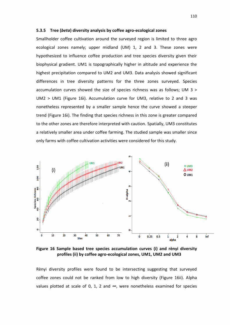
110

5.3.5 Tree (beta) diversity analysis by coffee agro-ecological zones

Smallholder coffee cultivation around the surveyed region is limited to three agro

ecological zones namely; upper midland (UM) 1, 2 and 3. These zones were

hypothesized to influence coffee production and tree species diversity given their

biophysical gradient. UM1 is topographically higher in altitude and experience the

highest precipitation compared to UM2 and UM3. Data analysis showed significant

differences in tree diversity patterns for the three zones surveyed. Species

accumulation curves showed the size of species richness was as follows; UM 3 >

UM2 > UM1 (Figure 16i). Accumulation curve for UM3, relative to 2 and 3 was

nonetheless represented by a smaller sample hence the curve showed a steeper

trend (Figure 16i). The finding that species richness in this zone is greater compared

to the other zones are therefore interpreted with caution. Spatially, UM3 constitutes

a relatively smaller area under coffee farming. The studied sample was smaller since

only farms with coffee cultivation activities were considered for this study.

Figure 16 Sample based tree species accumulation curves (i) and rènyi diversity profiles (ii) by coffee agro-ecological zones, UM1, UM2 and UM3

Rènyi diversity profiles were found to be intersecting suggesting that surveyed

coffee zones could not be ranked from low to high diversity (Figure 16ii). Alpha

values plotted at scale of 0, 1, 2 and ∞, were nonetheless examined for species

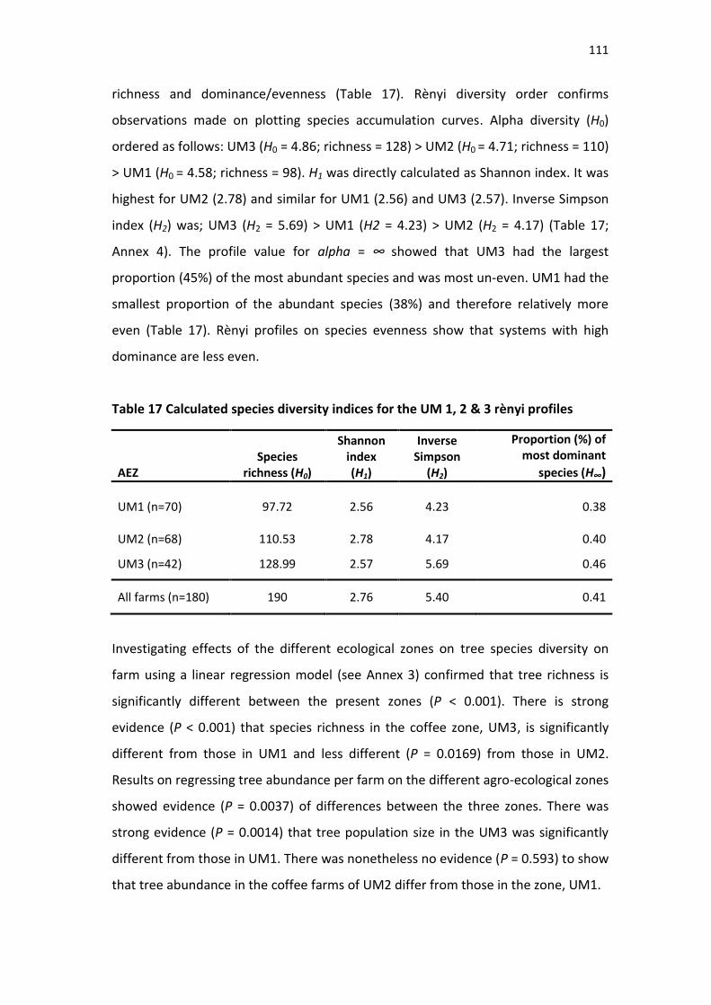
111

richness and dominance/evenness (Table 17). Rènyi diversity order confirms

observations made on plotting species accumulation curves. Alpha diversity (H0)

ordered as follows: UM3 (H0 = 4.86; richness = 128) > UM2 (H0 = 4.71; richness = 110)

> UM1 (H0 = 4.58; richness = 98). H1 was directly calculated as Shannon index. It was

highest for UM2 (2.78) and similar for UM1 (2.56) and UM3 (2.57). Inverse Simpson

index (H2) was; UM3 (H2 = 5.69) > UM1 (H2 = 4.23) > UM2 (H2 = 4.17) (Table 17;

Annex 4). The profile value for alpha = ∞ showed that UM3 had the largest

proportion (45%) of the most abundant species and was most un-even. UM1 had the

smallest proportion of the abundant species (38%) and therefore relatively more

even (Table 17). Rènyi profiles on species evenness show that systems with high

dominance are less even.

Table 17 Calculated species diversity indices for the UM 1, 2 & 3 rènyi profiles

AEZ Species

richness (H0)

Shannon index (H1)

Inverse Simpson

(H2)

Proportion (%) of most dominant

species (H∞)

UM1 (n=70) 97.72 2.56 4.23 0.38

UM2 (n=68) 110.53 2.78 4.17 0.40

UM3 (n=42) 128.99 2.57 5.69 0.46

All farms (n=180) 190 2.76 5.40 0.41

Investigating effects of the different ecological zones on tree species diversity on

farm using a linear regression model (see Annex 3) confirmed that tree richness is

significantly different between the present zones (P < 0.001). There is strong

evidence (P < 0.001) that species richness in the coffee zone, UM3, is significantly

different from those in UM1 and less different (P = 0.0169) from those in UM2.

Results on regressing tree abundance per farm on the different agro-ecological zones

showed evidence (P = 0.0037) of differences between the three zones. There was

strong evidence (P = 0.0014) that tree population size in the UM3 was significantly

different from those in UM1. There was nonetheless no evidence (P = 0.593) to show

that tree abundance in the coffee farms of UM2 differ from those in the zone, UM1.

112

Data analysis to assess whether indigenous tree abundance differ by coffee zones

showed a significant model (P = 0.002). Results revealed strong evidence (P < 0.001)

that zone, UM3 differ from zone UM1; invariably there was weak evidence (P =

0.096) that zone, UM2 differ from UM1 and UM3. Interestingly, when exotic tree

abundance on farm was regressed on the coffee zones, results showed a weak

model (P = 0.0479). There is not strong evidence (P = 0.0269) that exotic tree species

abundance in the zone, UM3 are significantly different from those in UM2 and UM1.

There was no evidence, that average exotic tree populations in UM2 are different

from farms in the zone UM1 or UM3. Other results showed that on average farm

sizes were not significantly different (P = 0.395) between the present coffee zones.

5.3.6 Tree diversity (gamma) for the Mount Kenya coffee ecosystem

A total of 165 species were identified belonging to 127 genera and 56 botanical

families from all the sampled farm plots together (see Annex 2). Some 23 dialect

names of species could not be confirmed using local species identification knowledge

and relevant species literature. The most abundant taxa counted were; Grevillea,

Eucalyptus, Macadamia, Mangifera, Cordia, Carica, Persea, Catha, Cupressus, and

Bridelia. The best-represented botanical families by species counts (in brackets)

were: Fabaceae (20), Rubiacea (10), Euphorbiaceae (10), Moraceae (8), Rutaceae (7),

Combretaceae (7), Anacardiaceae (7), Myrtacea (6), Apocynaceae (6) and Meliaceae

(5) (Figure 17I). Twenty six families are represented by only a single species while

some 17 families are represented by two to four species. Only 11 families are

represented by five or more species counts (Figure 17II).

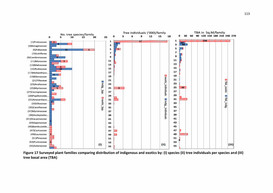
113

Figure 17 Surveyed plant families comparing distribution of indigenous and exotics by: (I) species (II) tree individuals per species and (III) tree basal area (TBA)

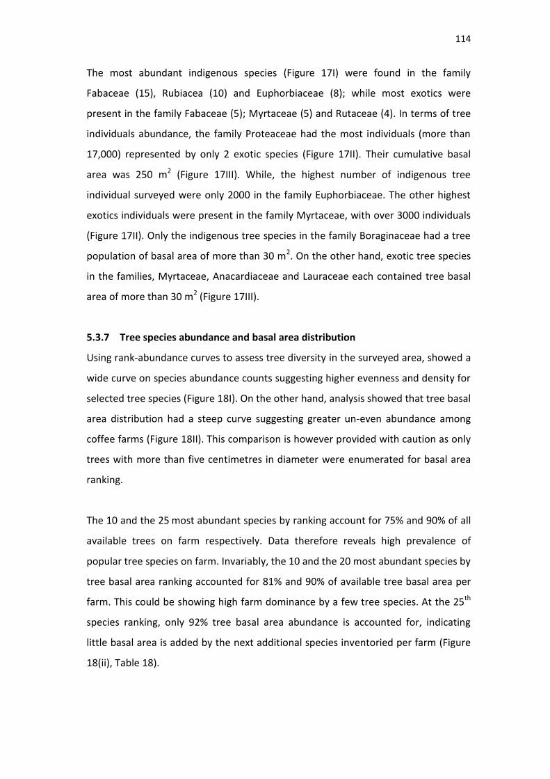
114

The most abundant indigenous species (Figure 17I) were found in the family

Fabaceae (15), Rubiacea (10) and Euphorbiaceae (8); while most exotics were

present in the family Fabaceae (5); Myrtaceae (5) and Rutaceae (4). In terms of tree

individuals abundance, the family Proteaceae had the most individuals (more than

17,000) represented by only 2 exotic species (Figure 17II). Their cumulative basal

area was 250 m2 (Figure 17III). While, the highest number of indigenous tree

individual surveyed were only 2000 in the family Euphorbiaceae. The other highest

exotics individuals were present in the family Myrtaceae, with over 3000 individuals

(Figure 17II). Only the indigenous tree species in the family Boraginaceae had a tree

population of basal area of more than 30 m2. On the other hand, exotic tree species

in the families, Myrtaceae, Anacardiaceae and Lauraceae each contained tree basal

area of more than 30 m2 (Figure 17III).

5.3.7 Tree species abundance and basal area distribution

Using rank-abundance curves to assess tree diversity in the surveyed area, showed a

wide curve on species abundance counts suggesting higher evenness and density for

selected tree species (Figure 18I). On the other hand, analysis showed that tree basal

area distribution had a steep curve suggesting greater un-even abundance among

coffee farms (Figure 18II). This comparison is however provided with caution as only

trees with more than five centimetres in diameter were enumerated for basal area

ranking.

The 10 and the 25 most abundant species by ranking account for 75% and 90% of all

available trees on farm respectively. Data therefore reveals high prevalence of

popular tree species on farm. Invariably, the 10 and the 20 most abundant species by

tree basal area ranking accounted for 81% and 90% of available tree basal area per

farm. This could be showing high farm dominance by a few tree species. At the 25th

species ranking, only 92% tree basal area abundance is accounted for, indicating

little basal area is added by the next additional species inventoried per farm (Figure

18(ii), Table 18).

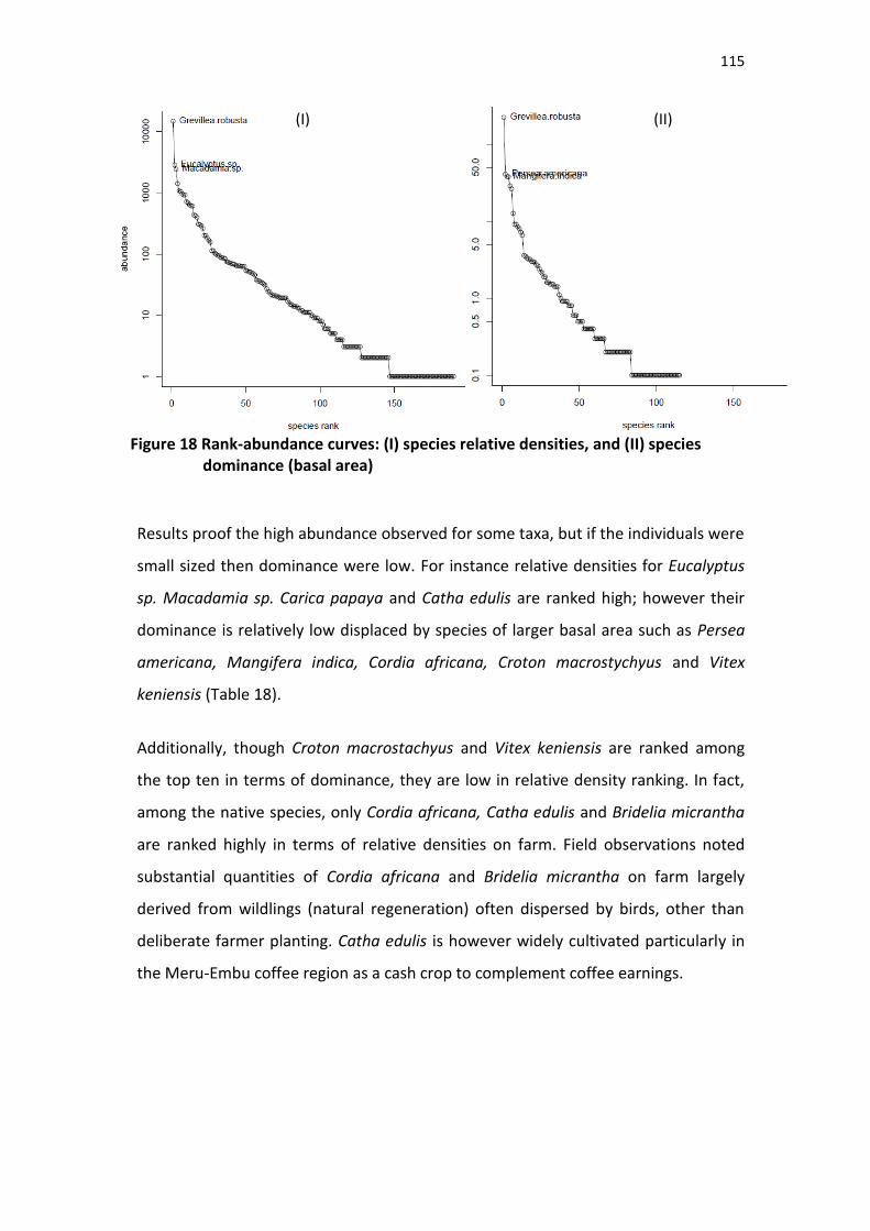
115

Figure 18 Rank-abundance curves: (I) species relative densities, and (II) species

dominance (basal area)

Results proof the high abundance observed for some taxa, but if the individuals were

small sized then dominance were low. For instance relative densities for Eucalyptus

sp. Macadamia sp. Carica papaya and Catha edulis are ranked high; however their

dominance is relatively low displaced by species of larger basal area such as Persea

americana, Mangifera indica, Cordia africana, Croton macrostychyus and Vitex

keniensis (Table 18).

Additionally, though Croton macrostachyus and Vitex keniensis are ranked among

the top ten in terms of dominance, they are low in relative density ranking. In fact,

among the native species, only Cordia africana, Catha edulis and Bridelia micrantha

are ranked highly in terms of relative densities on farm. Field observations noted

substantial quantities of Cordia africana and Bridelia micrantha on farm largely

derived from wildlings (natural regeneration) often dispersed by birds, other than

deliberate farmer planting. Catha edulis is however widely cultivated particularly in

the Meru-Embu coffee region as a cash crop to complement coffee earnings.

(I) (II)

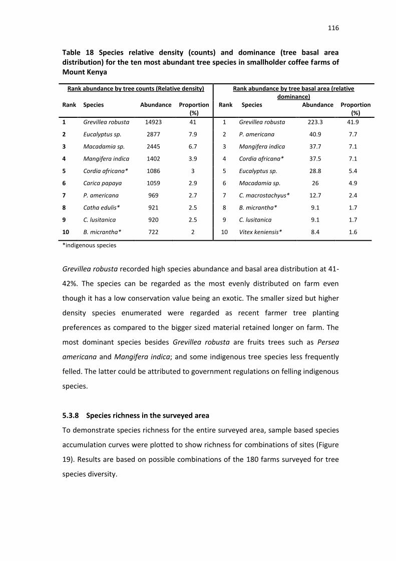
116

Table 18 Species relative density (counts) and dominance (tree basal area distribution) for the ten most abundant tree species in smallholder coffee farms of Mount Kenya

Rank abundance by tree counts (Relative density) Rank abundance by tree basal area (relative dominance)

Rank Species Abundance Proportion (%)

Rank Species Abundance Proportion (%)

1 Grevillea robusta 14923 41 1 Grevillea robusta 223.3 41.9

2 Eucalyptus sp. 2877 7.9 2 P. americana 40.9 7.7

3 Macadamia sp. 2445 6.7 3 Mangifera indica 37.7 7.1

4 Mangifera indica 1402 3.9 4 Cordia africana* 37.5 7.1

5 Cordia africana* 1086 3 5 Eucalyptus sp. 28.8 5.4

6 Carica papaya 1059 2.9 6 Macadamia sp. 26 4.9

7 P. americana 969 2.7 7 C. macrostachyus* 12.7 2.4

8 Catha edulis* 921 2.5 8 B. micrantha* 9.1 1.7

9 C. lusitanica 920 2.5 9 C. lusitanica 9.1 1.7

10 B. micrantha* 722 2 10 Vitex keniensis* 8.4 1.6

*indigenous species

Grevillea robusta recorded high species abundance and basal area distribution at 41-

42%. The species can be regarded as the most evenly distributed on farm even

though it has a low conservation value being an exotic. The smaller sized but higher

density species enumerated were regarded as recent farmer tree planting

preferences as compared to the bigger sized material retained longer on farm. The

most dominant species besides Grevillea robusta are fruits trees such as Persea

americana and Mangifera indica; and some indigenous tree species less frequently

felled. The latter could be attributed to government regulations on felling indigenous

species.

5.3.8 Species richness in the surveyed area

To demonstrate species richness for the entire surveyed area, sample based species

accumulation curves were plotted to show richness for combinations of sites (Figure

19). Results are based on possible combinations of the 180 farms surveyed for tree

species diversity.

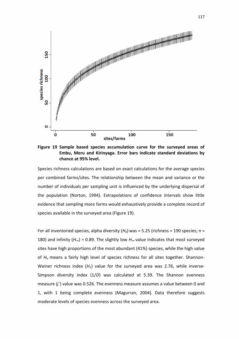
117

Figure 19 Sample based species accumulation curve for the surveyed areas of Embu, Meru and Kirinyaga. Error bars indicate standard deviations by chance at 95% level.

Species richness calculations are based on exact calculations for the average species

per combined farms/sites. The relationship between the mean and variance or the

number of individuals per sampling unit is influenced by the underlying dispersal of

the population (Norton, 1994). Extrapolations of confidence intervals show little

evidence that sampling more farms would exhaustively provide a complete record of

species available in the surveyed area (Figure 19).

For all inventoried species, alpha diversity (H0) was = 5.25 (richness = 190 species; n =

180) and infinity (H∞) = 0.89. The slightly low H∞ value indicates that most surveyed

sites have high proportions of the most abundant (41%) species, while the high value

of Ho means a fairly high level of species richness for all sites together. Shannon-

Weiner richness index (H1) value for the surveyed area was 2.76, while inverse-

Simpson diversity index (1/D) was calculated at 5.39. The Shannon evenness

measure (j´) value was 0.526. The evenness measure assumes a value between 0 and

1, with 1 being complete evenness (Magurran, 2004). Data therefore suggests

moderate levels of species evenness across the surveyed area.

118

Investigating diversity between the main coffee regions, results showed that species

richness (H0) is highest in Meru (4.9; richness = 134), followed by Kirinyaga (4.7

richness = 110) and then Embu (4.6; richness = 99). Moreover, the Kirinyaga coffee

region was showed to have a high proportion of the dominant species (54%; H∞ =

0.6) compared to Embu (35%; H∞ = 1.05) and Meru (33%; H∞ = 1.10). Shannon (H1)

and Simpson (H2) diversity indices however showed higher diversity for Meru (H1 =

2.98; H2 = 7.61) followed by Embu (H1 = 2.66; H2 = 6.35 and Kirinyaga (H1 = 2.22; H2 =

3.28) in that order.

5.3.9 Species diversity prediction

Extrapolated species richness for the entire coffee system surveyed using the first

order and second order Jackknife, Chao and Bootstrap methods, was in the range of

215 to 292 species (Table 19). Bootstrap estimate suggests that sampling captured

about 89% of the species while Jackknife 2 estimate indicates that sampling efforts

captured 66% of the species. Plotted species accumulation curves indeed showed

reduced variability on species presence after 150 sites combinations (Figure 19);

implying lower species richness is captured by extra sampling effort. The sampling

strategy used to survey coffee farms can therefore be regarded to have worked fairly

well having recorded a species richness of 190 species.

Table 19 Species richness prediction for the entire survey area

Prediction method Species richness (all sites combined)

Chao 285

Bootstrap 215

Jackknife1 251

Jackknife2 292

5.3.10 Species composition between coffee regions

As expected, there are dissimilarities in species composition between the three

coffee sub-regions in spite of the dominance of few species at the farm level. The

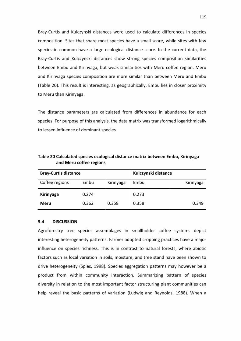
119

Bray-Curtis and Kulczynski distances were used to calculate differences in species

composition. Sites that share most species have a small score, while sites with few

species in common have a large ecological distance score. In the current data, the

Bray-Curtis and Kulczynski distances show strong species composition similarities

between Embu and Kirinyaga, but weak similarities with Meru coffee region. Meru

and Kirinyaga species composition are more similar than between Meru and Embu

(Table 20). This result is interesting, as geographically, Embu lies in closer proximity

to Meru than Kirinyaga.

The distance parameters are calculated from differences in abundance for each

species. For purpose of this analysis, the data matrix was transformed logarithmically

to lessen influence of dominant species.

Table 20 Calculated species ecological distance matrix between Embu, Kirinyaga and Meru coffee regions

Bray-Curtis distance Kulczynski distance

Coffee regions Embu Kirinyaga Embu Kirinyaga

Kirinyaga 0.274 0.273

Meru 0.362 0.358 0.358 0.349

5.4 DISCUSSION

Agroforestry tree species assemblages in smallholder coffee systems depict

interesting heterogeneity patterns. Farmer adopted cropping practices have a major

influence on species richness. This is in contrast to natural forests, where abiotic

factors such as local variation in soils, moisture, and tree stand have been shown to

drive heterogeneity (Spies, 1998). Species aggregation patterns may however be a

product from within community interaction. Summarizing pattern of species

diversity in relation to the most important factor structuring plant communities can

help reveal the basic patterns of variation (Ludwig and Reynolds, 1988). When a

120

species environment is fairly similar, such as in the coffee growing zones, diversity is

called ‘pattern diversity’ (Preston 1948; Spies, 1998).

This study focused on the Mount Kenya coffee zones recently converted from

natural forests (in the last 100-150 years). Coffee farm categories - increasing,

decreasing and constant determined by historical coffee production trends were

analysed for the available tree species diversity. Studied farm types were

significantly different in terms of coffee yield production and the number of coffee

bushes cultivated per farm. Agroforestry tree richness and abundance per farms was

however not significantly different by the categories. Further, data analysis showed

tree individuals maintained within coffee plots per farm were significantly higher in

the coffee increasing farms than the decreasing ones. This suggests a possible

decrease in tree abundance if coffee crop would be reduced on farms. Results

further showed that more than 50% of trees on the surveyed farms are planted

within coffee plots.

Farm size between the increasing and decreasing farms was not significantly

different even though on average, the coffee increasing farms are slightly bigger.

Farm size may therefore not necessarily determine levels of tree abundance and

richness adopted on farm. Rènyi diversity analysis showed that the increasing and

the decreasing farms have similar levels of tree richness and abundance but higher

than the constant farms. The coffee increasing farms on average have higher tree

abundance of similar diversity with the coffee decreasing ones confirming that high

levels of tree abundance do not necessarily imply high level of species richness.

The coffee stagnated farms showed a higher percentage of the most abundant

species perhaps suggesting increased preference of certain species such as Grevillea

that was found to be more abundant.

Though high species richness is recorded in the surveyed coffee farms, this study

confirms uneven species distribution within and between farms (Kindt et al. 2007).

This is probably accelerated by recent market induced changes in agriculture and the

preference of farmers towards fast growing exotics. Analysed data is consistent on

121

rarity of native species as compared to exotics across surveyed farming landscape.

Further, tree basal area distribution even for the dominant species is steeply variable

and uneven among farm plots. This finding suggests increased tree harvesting going

hand in hand with tree species replacement planting.

Coffee plots contain more than half (58%) of all trees present per given farm plot.

Any significant changes in coffee cultivation among farmers will therefore influence

the number of agroforestry trees on farms. Inconclusive evidence suggests that

smallholders with decreased or stagnated coffee production due to reduced coffee

bushes adopt more annual crops and maintain lesser tree richness. Data implies

changes in species selection over time with farmers preferring more exotics than

indigenous species to plant on their farm plots. Grevillea robusta is the most

abundant and dominant species on coffee farms at proportions of 41%.

The presence of indigenous species per farm plot account for about 78% of the

recorded richness, however they are of low, uneven distribution between farms

posing serious demographic implications with regard to genetic integrity. Only Cordia

africana, Croton macrostachyus, Bridelia micrantha and Vitex keniensis ranked

among the 10 most abundant tree species in coffee farm plots. Overall 10 and 25 of

the most abundant species by ranking, account for 75% and 90% of available trees

respectively. Results suggest farmer reliance on relatively few species choices for

tree replacements on farm. It is not clear the extent to which the larger enumerated

tree diversity contributes to households’ livelihood needs and ecological functions

owing to their limited quantities on farm. For instance, though Croton macrostychyus

and Vitex keniensis, are ranked among the top ten in dominance among native

species, they are low in relative densities indicating a low presence of young tree

population. Lower densities of the native species could therefore influence their

genetic integrity in the long run as farmers tend to propagate materials from limited

mother trees on farming landscapes.

Overall, results suggest possible loss of species richness from all study regions. A low

pattern of richness is shown to be associated with higher adoption of exotic species.

122

For instance, species richness is highest in Meru (H0 = 4.9), followed by Kirinyaga (H0

= 4.7) and then Embu (H0 = 4.6). Invariably, the proportion of species domination for

Kirinyaga was 54%; Embu, 35% and Meru, 33%. The results however show an

exception when species richness is assessed by the different coffee agro-ecological

zones. UM3 contains the highest species richness (H0 = 4.91) but also has the highest

proportions of the dominant species (H∞ = 0.77; 46%). UM1 has the lowest richness

(H0= 4.5) but has the least domination by popular species (H∞ = 1.0; 36%). This zone

perhaps has fewer tree compositional changes due to lower reliance on trees

compared to the more prevalent cash crops including tea and horticulture in some

sections. The UM3 on the other hand has fewer cash crops and more annuals

perhaps indicating that more tree abundance and richness are retained to

complement economic benefits.

In terms of species composition, Meru and Kirinyaga coffee sub-regions show

similarities, however there are dissimilarities with Embu, despite geographical

proximity. The significant proportion of dominant species could be associated with

germplasm access, and propagation related constraints influencing farmer species

choices. Largely, planting material for native species is lacking (Lengkeek and Carsan,

2004). Native species are also widely perceived as slow growing with most species

spontaneously inherited from natural regeneration. Further, Grime (1983) reported

that a decrease in community niche space can reduce the number of species due to

ecophysiological constraints. Species with different competitive abilities in relation

to these resources/factors divide the niche space in hierarchical manner (Ludwig and

Reynolds, 1988).

At the botanical families’ level, results revealed skewed patterns of distribution.

Though 56 families were recorded, only 18.5% (11 families) are represented by more

than five species. Nearly half 48%; (26 botanical families) are represented by a single

species while 35% (17 botanical families) are accounted by two to four species.

Presence of a large diversity of plant families, though of skewed distribution, is an

indicator of the potential of coffee system as a reservoir for species diversity on

farm. Despite larger indigenous species records in the families Fabaceae, Rubiaceae

123

and Euphorbiaceae, they are of low individual and tree basal area presence in the

surveyed farms. On the other hand, there are fewer exotic species with larger tree

population (individuals) and tree basal area per family suggestive of expanded

cultivations of selected exotic species. The family Proteacea and Myrtaceae contain

the most available exotic tree population in the surveyed farms.

Tree species balance at the botanical family level is often ignored during

prioritization of domestication activities. How this can be promoted or improved for

purposes of meeting livelihood and conservation objectives, remain an important

research issue. Further, trees in coffee agroforests are largely propagated from

germplasm sources in close vicinity such as neighbor farms. Long term performance

of agroforestry tree population in agricultural systems has therefore been a matter

of concern. A small uneven, tree species population in agricultural landscapes may

be dysfunctional by hampering gene migration within a given tree population

increasing chances of genetic erosion (Dawson et al., 2009). There is however is no

available evidence to indicate minimum tree densities to be maintained at a given

farming landscape (Lengkeek et al., 2005; Kindt et al., 2006).

Mapping and monitoring tree diversity at the farm level is therefore critical in coffee

agroforestry systems so as to understand performance of tree population especially

for germplasm provisioning and their future productivity and adaptive capacity.

Towards this end, agroforestry systems can be used to protect biodiversity and

alleviate the negative effects of deforestation by stimulating natural forest cover

through cultivation of trees with agricultural crops and may serve as biological

corridors between protected areas and non-protected areas (Schroth and Harvey,

2007). Understanding patterns of tree diversity maintained in smallholder systems

provides useful indicators on their productivity assuming that the most diverse

systems are also the most productive.

5.5 CONCLUSIONS

Intensification of coffee farms with high value agricultural enterprises other than

coffee will most likely shift tree species richness in these farms. This study has shown

124

significant presence of exotics such as: grevillea, eucalyptus, macadamia, mango and

avocado indicative of farmer preferences. It is clear that this transition will be

accelerated by decreased coffee cultivation. The reason is that farms immediately

adopt short returns cropping practices to ensure their food security and incomes.

Adoption of fast growing exotic trees is displacing indigenous species such as Croton

macrostychyus and Vitex keniensis. Cordia africana however has significant

abundance within coffee systems perhaps due to its excellent compatibility qualities

with coffee and crop polycultures. Tree abundance and basal area distribution, show

small-sized tree diversity and high relative densities suggesting rapid tree

compositional turnover which imply changing patterns and structure of tree

population on coffee farms. This study has shown that smaller farm size tends to

reduce tree size on farm. Small tree size diversity, unevenly distributed among farms,

has implications if farm tree populations are to be considered for germplasm

provisioning (possible low viability). Further, botanical families are skewed, showing

patterns of distribution that perhaps have been ignored during prioritization of

species for domestication activities. Policy incentives that would promote greater

benefits from indigenous trees will encourage farmers to retain or plant more of

these species. If current trends are unchecked there are risks of lost tree diversity or

poorly performing tree population maintained on smallholder coffee farms.

125

5.6 REFERENCES

Ambinakudige S. and Sathish, BN. 2009. Comparing tree diversity and composition in

coffee farms and sacred forests in the Western Ghats of India. Biodiversity

Conservation, 18: 987–1000.

Asase, A and Tetteh, DA. 2010. The role of complex agroforestry systems in the

conservation of forest tree diversity and structure in southeastern Ghana.

Agroforest Systems, 79: 355–368.

Beentje, HJ. 1994. Kenya Trees, Shrubs and Lianas. National Museums of Kenya,

Nairobi.

Beer, J, Muschler, DK and Somarriba, E. 1998. Shade management in coffee and

cacao plantations. Agroforestry Systems, 38: 139–164.

Brown, S. 1997. Estimating biomass and biomass change of tropical forests: a primer.

FAO Forestry Paper 134. Food and Agriculture Organization of the United

Nations, Rome, Italy.

Bond, WR. 1989. Describing and con-serving biotic diversity. In Biotic Diversity in

Southern Africa: Concepts and Conservation, ed. BJ Huntley, pp. 2-18. Cape

Town: Oxford University Press.

Chazdon, RL, Harvey, CA, Oliver, K, Griffith, D, Ferguson, B, Martinez-Ramos, M. et al.

2009. Beyond reserves: a research agenda for conserving biodiversity in human-

modified tropical landscapes. Biotropica, 41: 142–153.

Dawson, IK, Lengkeek, A, Weber, J, Jamnadass, R. 2009. Managing genetic variation

in tropical trees: linking knowledge with action in agroforestry ecosystems for

improved conservation and enhanced livelihoods. Biodiversity Conservation,

18:969–986.

FAO, 1978. Report on the Agro-ecological Zones Project. Vol. 1. Methodology and

results for Africa. World Soil Resources Report 48/1, FAO, Rome.

Fitzherbert, EB, Struebig, MJ. Morel, A, Danielsen, F, Bru¨hl, CA, Donald, PF and

Phalan, B. 2008. How will oil palm expansion affect biodiversity? Trends in

Ecology and Evolution, 23(10): 538–545.

Githae, EW, Chuah-Petiot, M, Mworia, JK and Odee, DW. 2007. A botanical inventory

and diversity assessment of Mt. Marsabit forest, a sub-humid montane forest in

the arid lands of northern Kenya. African Journal of Ecology, 46: 39–45.

126

Grime, JP. 1983. Plant Strategies and Vegetation Processes. John Wiley and Sons, NY.

GOK (Government of Kenya) 2010. The 2009 Kenya Population and Housing Census.

Volume 1A. Population distribution by administrative units. Kenya National

Bureau of Statistics.

Harvey, C.A., Komar, O., Chazdon, R., Ferguson, B.G., Finegan, B., Griffith, D.M. et al.

2008. Integrating agricultural landscapes with biodiversity conservation in the

Mesoamerican hotspot. Conservation Biology, 22:1.

Humphries, CJ, Williams PH, Vane-Wright, HI. 1995. Measuring Biodiversity Value for

Conservation Author(s): Source: Annual Review of Ecology and Systematics, 26:

93-111.

Jaetzold, R, and Schmidt, H. 2007. Farm management handbook of Kenya (vol.II),

Eastern Kenya, Ministry of Agriculture, Nairobi.

Jongman, RHG, Ter Braak, CJF, Van Tongeren, OFR. 1995. Data analysis in community

and landscape ecology. Cambridge University Press.

Kindt R. and Coe, R. 2005. Tree diversity analysis, A manual and software for

common statistical methods for ecological and biodiversity studies. Nairobi.

World Agroforestry Centre (ICRAF).

Kindt, R, Lillesø, JBP, and Van Breugel P. 2007. Comparisons between original and

current composition of indigenous tree species around Mount Kenya. African

Journal of Ecology, 45: 633–644.

Kindt, R, Van Damme, P. and Simons, AJ. 2006. Tree diversity in western Kenya: using

profiles to characterize richness and evenness. Biodiversity Conservation, 15:

1253–1270.

Lengkeek, AG, and Carsan, S. 2004. The process of participatory tree domestication

project in Meru, Kenya. Development in Practice, 14: 445-451.

Lengkeek, AG, Kindt, R, Van der Maesen LJG, Simons, AJ, and Van Oijen DCC. 2005.

Tree density and germplasm source in agroforestry ecosystems in Meru, Mount

Kenya. Genetic Resources and Crop Evolution, 52: 709–721.

Lengkeek, AG, Muchugi, AM, Agufa, AC, Ahenda, JO, and Dawson, IK. 2006.

Comparing genetic diversity in agroforestry systems with natural forests: A case

study of the important timber tree Vitex fischeri in central Kenya. Agroforestry

Systems, 67:293-300.

127

Ludwig, JA. and Reynolds, JF. 1988. Statistical ecology. A primer on methods and

computing. A Wiley- Interscience publication.

Magurran, A. 2004. Measuring biological diversity. Blackwell Publishing Company,

Malden.

Maundu, P, & Tengnås, B. 2005. Useful Trees and Shrubs for Kenya. World

Agroforestry Centre (ICRAF), Nairobi.

Norton, BG., 1994. "On what we should save: the role of cultures in determining

conservation targets," in P. Forey, et al. (eds), Systematics and Conservation

evaluation.

Peeters, LYK, Soto-Pinto, L, Perales, H, Montoya, G, Ishiki, M. 2003. Coffee

production, timber, and firewood in traditional and Inga-shaded plantations in

Southern Mexico. Agriculture, Ecosystems and Environment, 95: 481–493.

Perfecto, I. Rice T, Greenberg, R, Voorte Van der, M. 1996. Shade coffee: a

disappearing refuge for biodiversity. BioScience, 46: 598–608.

Perfecto, I, Vandermeerb, J, Masa, A, Soto Pinto, L. 2005. Biodiversity, yield, and

shade coffee certification Ecological Economics, 54: 435– 446.

Philpott, S and Dietsch, T. 2003. Coffee and conservation: A global context and the

value of farmer involvement. Conservation Biology, 117(6): 1844-1846.

Purvis, A and Hector, A. 2000. Getting the measure of biodiversity, Nature vol. 405.

Preston, FW 1948. The commonness and rarity of species. Ecology, 29: 254-283.

Rappole, JH. King, DI and Vega Rivera, JH. 2003. Coffee and conservation.

Conservation Biology, 17(1): 334-336.

R Development Core Team, 2010. R: A language and environment for statistical

computing. R Foundation for Statistical Computing, Vienna, Austria. ISBN 3-

900051-07-0. http://www.R-project.org.

Schroth, G and Harvey, CA. 2007. Biodiversity conservation in cocoa production

landscapes: an overview. Biodiversity Conservation, 16: 2237–2244.

Simons, AJ and Leakey, RRB. 2004. Tree domestication in tropical agroforestry.

Agroforestry Systems, 61: 167–181.

Sizlinga, Al, Storch, D, Sizlingova, E, Reif, J and Gaston, JK. 2009. Species abundance

distribution results from a spatial analogy of central limit theorem.

128

Spies, TA. 1998. Forest structure. A key to the ecosystem. Northwest Science, 72: 34-

39.

UNEP, 2005. World Conservation Monitoring Centre, World Heritage sites. Protected

areas and world Heritage.

129

CHAPTER 6

IMPLICATIONS OF CHANGES IN COFFEE PRODUCTIVITY ON SOIL FERTILITY

MANAGEMENT BY SMALLHOLDER COFFEE FARMERS

ABSTRACT

Land fragmentation, over cropping, soil erosion, low fertilizer and manure inputs

have raised concerns that coffee farms around Mount Kenya could rapidly decline to

low production systems. Significant nutrient exports occur through coffee,

horticulture and food crops commonly cultivated. Smallholder decision-making on

soil fertility management is poorly understood, even though it is a key determinant

of the ‘health’ status of their land. Near-infrared spectroscopy (NIR) diagnostic

techniques were used to study soil properties obtained from 94 coffee farms. At

least 189 soil samples randomly collected from coffee plots were scanned for

constituent properties. One third of the samples were identified using Kennerd and

Stone algorithm to aid in calibration. These reference samples were analyzed for

fertility by wet chemistry methods. Partial least square (PLS) regression was used to

run calibration models, giving correlation coefficients between the measured and

PLS predicted soil properties. Results showed strong correlations with all soil

properties (r > 0.70) except for P, Zn and Na confirming the potential of NIR to

accurately predict soil constituents. Principal component analysis (PCA) was then

used to develop three soil nutrient indices (principal components scores) for the

surveyed farms. Collected data was reliable to show that soil organic C, total N and P

were the most deficient across surveyed coffee farms. B prevalence (which is often

ignored as a useful indicator of soil fertility) was identified as a useful nutrient to

monitor acidification in coffee farms and possible effects on the quality of coffee

berries. Results from farmer interviews confirm low rates of manure and fertilizer

application. Finally, results demonstrate the use of NIR techniques to rapidly and

cheaply characterize the nutrient status of smallholder farm. A useful hypothesis

formulated is that smallholders target nutrient application on farm crops with good

market performance.

130

INTRODUCTION

Coffee systems in the Mount Kenya region comprise an important smallholder

agricultural production area in Kenya. Intensive cropping patterns with cash crops

(such as coffee), cereal crops, vegetables and agroforestry trees form the economic

foundation for farmers in these systems. Though the largely volcanic soils have

provided a fertile resource base, increased land fragmentation, over cropping, and

soil erosion have raised concerns on the future productivity of these systems. Low

soil nutrient levels have been associated with low fertilizer inputs, over cropping, soil

dehumification and mineralization (Sanchez, 2002; Tittonell et al., 2005; Muchena et

al., 2005). These factors combined have resulted in declining yields and even crop

composition on farms. Farmer efforts to improve soil fertility involve manure and

chemical fertilizer application albeit below recommended rates (Palm et al., 1997;

Omamo et al., 2002; Swift and Shepherd, 2007). Nutrient depletion rates are farm

specific, depending on the way each particular field has been managed over

decades. Nutrient depletion can produce negative on-farm side effects and

exacerbates off-farm externalities (Place et al., 2005). On-farm effects include less

fodder for cattle, less fuel wood for cooking, and less crop residues and cattle

manure to recycle nutrients. These effects often increase runoff and erosion losses

because there is less plant cover to protect the soils (Sanchez et al., 1997).

Africa loses about 4.4 million tonnes N, 0.5 million tonnes P, and 3 million tonnes K

every year from its cultivated land. These rates are several times higher than the

continent’s annual fertilizer consumption, excluding South Africa: 0.8 million tonnes

N, 0.26 million tonnes P, and 0.2 million tonnes K (Sanchez et al., 2002). Yet analyses

of soil fertility management in Africa often fail to account for links between soil

fertility depletion and factors related to smallholder oriented production patterns

that dominate the continent’s rural landscapes (Carter, 1997; Omamo, et al., 2002;

Swift and Shepherd, 2007).

131

Research and development efforts in the context of Sustainable Land Management

(SLM6), need to focus on how to improve smallholder land quality (soil quality), as

soil can be seen as the most important natural capital owned by smallholders. New

strategies must ensure continued crop productivity in circumstances of low

household incomes to secure nutrient inputs. Agroforestry has been proposed as a

form of land intensification that offers farmers low cost options to improve their

land quality by integrating soil enriching trees that fix atmospheric nitrogen or

through biomass transfer (Swift and Shepherd, 2007). There are however

bottlenecks in selecting species, and designing systems and management regimes,

that optimizes the efficiency of environmental resource capturing and use in a

sustainable manner (Huxley, 1996).

In order to identify strategies that could support maintenance of land quality within

intensive smallholder coffee systems, this study sought to determine soil quality

(nutrient level indicators) and variability on small farms in three coffee producing

areas around Mount Kenya, where declined income from coffee is suspected to

influence farmers’ purchasing power for fertilizers, manure and other inputs. The

hypothesis followed is that, given the declined incomes from coffee farming, there

are intra-household variability in soil nutrient management influencing nutrient

prevalence, and subsequently cash and food crops productivity. Though smallholder

heterogeneity is a given, in terms of production practices, the maintenance of land

quality acts as a common denominator that significantly influences farmer decisions

on crop enterprise. In fact, productivity decline recorded in subsistence crops is

often closely related to a decline in cash crops since invariably, inputs used on cash

crops are shared for subsistence food crop production, therefore indirectly

supporting their production. In situations where farmers continuously maintain low

inputs, the system risks decline to an overall low production system (Place et al.,

2005; Sanchez, 2010).

6 Sustainable land management (SLM) can be defined as the use of land resources such as soils, water, animals

and plants for the production of goods - to meet changing human needs – while assuring the long-term productive potential of these resources, and the maintenance of their environmental functions (SLM-IM Guidelines, ud)

132

Therefore both land-use and soil management influence the amount of nutrients in

soils in many ways, positively as well as negatively. Intra-household differences were

therefore assessed and indicators for the prevalence of farm soil nutrients

developed to characterize smallholder managed soils in coffee systems on the

eastern slopes of Mount Kenya. A description of organic and inorganic fertilizer

inputs further help capture the position of households in accessing key nutrients

inputs via fertilizers and/or animal manure.

6.1 CONCEPTUAL FRAME

Factors most likely to determine soil nutrient flow and out-flows can be divided into

both biological and ecological (biophysical) factors, and socio-economic factors

(Swift and Shepherd, 2007). The biophysical factors are climatic, biological, physical

and chemical characteristics of soil, and the topography, altitude, temperature and

biodiversity (De Jager et al., 1998). Soil fertility loss and land degradation in high

potential systems are often associated with high human population pressure (Carter,

1997; Sanchez et al., 1997). However this observation is also disputed (Omamo,

2002) where small intensified farms are also associated with higher organic and

inorganic nutrient inputs. Cultivation of small farm sizes with similar crops such as

maize and other high input crops can however lead to soil nutrient ‘mining’ and loss

of productivity (Smaling et al., 1997; Shepherd and Walsh, 2007). The difference of

mineral and organic fertilizer inflows and out flows through harvested products and

crop residues removed in a system has been termed as partial nutrient balance.

Conversely, full nutrient balances involve environmental nutrients flows such as from

wet/atmospheric deposition, nitrogen fixation and sedimentation; whereas outflows

occur by leaching, gaseous losses, and soil erosion (Cobo et al., 2010).

The high cost of inorganic nutrients especially chemical fertilizers, in Africa, viewed

as the highest across the world often reduces its use (Mwangi 1996; Omamo, 2001;

Odendo et al., 2007). However, with the right incentives, for instance government

market liberalization, fertilizer use in Kenya and Ethiopia virtually doubled between

the early 1990’s and late 2000’s (Odendo et al., 2007; Haggblade and Jayne,

(u.d))(See Annex 8). Though raising fertilizer use does not automatically contribute

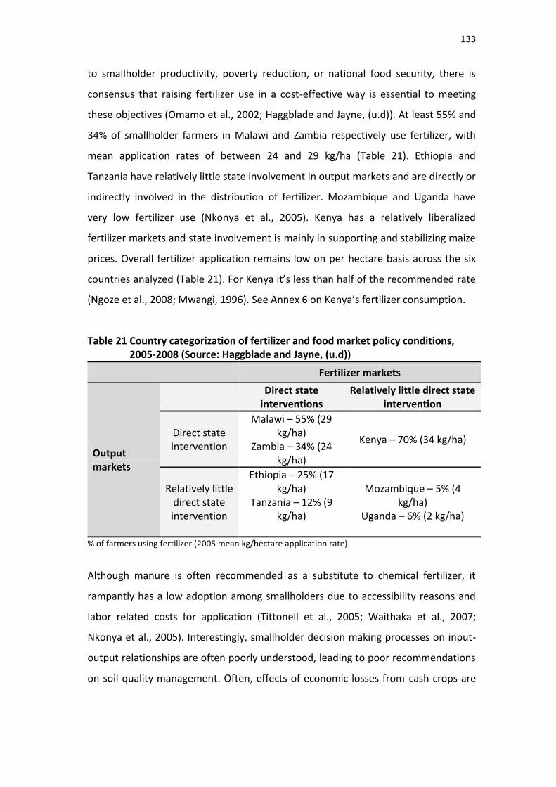
133

to smallholder productivity, poverty reduction, or national food security, there is

consensus that raising fertilizer use in a cost-effective way is essential to meeting

these objectives (Omamo et al., 2002; Haggblade and Jayne, (u.d)). At least 55% and

34% of smallholder farmers in Malawi and Zambia respectively use fertilizer, with

mean application rates of between 24 and 29 kg/ha (Table 21). Ethiopia and

Tanzania have relatively little state involvement in output markets and are directly or

indirectly involved in the distribution of fertilizer. Mozambique and Uganda have

very low fertilizer use (Nkonya et al., 2005). Kenya has a relatively liberalized

fertilizer markets and state involvement is mainly in supporting and stabilizing maize

prices. Overall fertilizer application remains low on per hectare basis across the six

countries analyzed (Table 21). For Kenya it’s less than half of the recommended rate

(Ngoze et al., 2008; Mwangi, 1996). See Annex 6 on Kenya’s fertilizer consumption.

Table 21 Country categorization of fertilizer and food market policy conditions, 2005-2008 (Source: Haggblade and Jayne, (u.d))

Fertilizer markets

Output markets

Direct state interventions

Relatively little direct state intervention

Direct state intervention

Malawi – 55% (29 kg/ha)

Zambia – 34% (24 kg/ha)

Kenya – 70% (34 kg/ha)

Relatively little direct state intervention

Ethiopia – 25% (17 kg/ha)

Tanzania – 12% (9 kg/ha)

Mozambique – 5% (4 kg/ha)

Uganda – 6% (2 kg/ha)

% of farmers using fertilizer (2005 mean kg/hectare application rate)

Although manure is often recommended as a substitute to chemical fertilizer, it

rampantly has a low adoption among smallholders due to accessibility reasons and

labor related costs for application (Tittonell et al., 2005; Waithaka et al., 2007;

Nkonya et al., 2005). Interestingly, smallholder decision making processes on input-

output relationships are often poorly understood, leading to poor recommendations

on soil quality management. Often, effects of economic losses from cash crops are

134

readily linked to aspects of household well-being and rarely on soil fertility

management.

Coffee cultivation around Mount Kenya has had a significant influence on farmers’

incomes for at least forty five years. Its reliance on international market

performance and heavy government control however has important impacts on

levels of returns. The government has traditionally supported the subsector with

hopes of accumulating taxes and enhancing foreign exchange. However in the last

two decades, returns from coffee farming have significantly dissipated with many

farmers opting for alternative cash crops or increased food crop cultivation.

Nonetheless, some farmers are resilient and remain ‘loyal’ to coffee cultivation.

This study assessed soil nutrient status in the Mount Kenya coffee systems with a

history of dependence on coffee cultivation as the main cash crop. Farmer

participation in cash crop marketing arrangements has to a great extent facilitated

their access to fertilizer inputs not only for coffee but also for food crops like maize

(Yamano et al., 2003). In circumstances where markets for coffee decline,

tremendous shocks in terms of inputs that can be afforded are anticipated.

Indirectly, nutrient inputs for food crops such as maize and beans are affected

significantly. Some of the likely scenarios likely to emerge in smallholder systems

with regard to coping with input challenges are presented in Figure 20.

Basically soil nutrient inputs are naturally affected by the soil parent material - in the

Mount Kenya area rich basaltic parent material, volcanic in origin, provides a rich

nutrient base for the newly weathered soils. There however concerns of exacerbated

soil erosion due to cultivation on steep slopes, with poor adoption of soil

conservation measures (Ngoze et al., 2008).

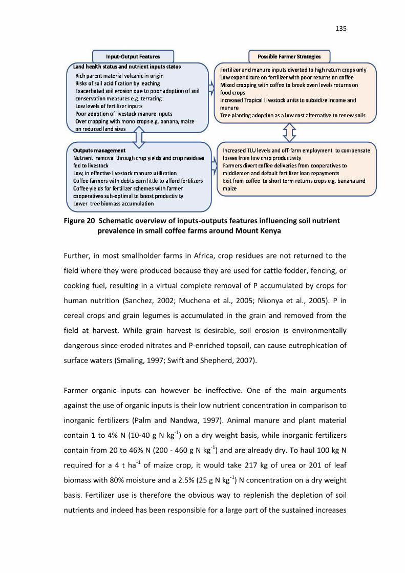
135

Figure 20 Schematic overview of inputs-outputs features influencing soil nutrient

prevalence in small coffee farms around Mount Kenya

Further, in most smallholder farms in Africa, crop residues are not returned to the

field where they were produced because they are used for cattle fodder, fencing, or

cooking fuel, resulting in a virtual complete removal of P accumulated by crops for

human nutrition (Sanchez, 2002; Muchena et al., 2005; Nkonya et al., 2005). P in

cereal crops and grain legumes is accumulated in the grain and removed from the

field at harvest. While grain harvest is desirable, soil erosion is environmentally

dangerous since eroded nitrates and P-enriched topsoil, can cause eutrophication of

surface waters (Smaling, 1997; Swift and Shepherd, 2007).

Farmer organic inputs can however be ineffective. One of the main arguments

against the use of organic inputs is their low nutrient concentration in comparison to

inorganic fertilizers (Palm and Nandwa, 1997). Animal manure and plant material

contain 1 to 4% N (10-40 g N kg-1) on a dry weight basis, while inorganic fertilizers

contain from 20 to 46% N (200 - 460 g N kg-1) and are already dry. To haul 100 kg N

required for a 4 t ha-1 of maize crop, it would take 217 kg of urea or 201 of leaf

biomass with 80% moisture and a 2.5% (25 g N kg-1) N concentration on a dry weight

basis. Fertilizer use is therefore the obvious way to replenish the depletion of soil

nutrients and indeed has been responsible for a large part of the sustained increases

136

in per capita food production in Asia, Latin America, and the temperate region, as

well as in the commercial farm sector in Africa (Sanchez, 2002; Omamo and Mose,

2001; Waithaka et al., 2007).

Though most smallholder farmers in Africa appreciate the value of fertilizers, they

are seldom able to apply them at the recommended rates and at the appropriate

time because of high costs, lack of credit, delivery delays, and low and variable

returns (Sanchez, 2010). Fertilizer application is reported to be highest in highland

systems such as the coffee systems where this study was carried (Omamo, 2001;

Odendo et al., 2007). More recently, fertilizer access by coffee growing farmers is

linked to yield deliveries and coffee market prices. Farmers who accumulate debts

therefore continuously access smaller and smaller fertilizer quantities from their

cooperatives.

The conceptual frame presented here suggests that farmer nutrient application

strategies target only high value cash and food crops. Effects of poor yields from

coffee can therefore depress fertilizer inputs. Farmers will tend to enhance coffee

growing with mixed cropping practices in order to utilize available nutrient. Another

strategy is increased livestock keeping for income and manure. Furthermore,

agroforestry tree planting is adopted as a low cost investment to utilize available

land, perhaps also utilize below surface soil nutrients which are recycled on top soil

by leaf litter for instance by use of Faidherbia albida (ICRAF, 2009).

In economic theory, farmer expenditure on fertilizer and manure nutrient inputs can

be related to total expenditure of income. This is demonstrated through Engels’s

expenditure curve7 (Figure 21); where, y denotes expenditure on fertilizer and χ the

total income (Lewbel, 2006). The postulated model therefore assumes non linear

reciprocal predictors as follows:

7 An Engel’s curve is the function describing how a consumer’s expenditures on some good or services relate to the consumer’s total resource holding. Prices are fixed, so qi = gi(y,z), where qi is the quantity consumed good i, y is income, wealth or total expenditures on goods and services and z is a vector of other characteristics of the consumer such as age and household composition (Lewbel, 2006). The goods are usually aggregate commodities such as total food, clothing or transportation.

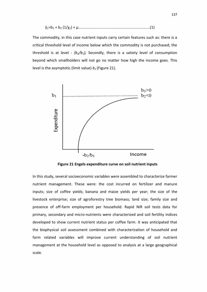
137

ŷ1=b1 + b2 (1/χ1) + μ....................................................................(1)

The commodity, in this case nutrient inputs carry certain features such as: there is a

critical threshold level of income below which the commodity is not purchased; the

threshold is at level - (b2/b1); Secondly, there is a satiety level of consumption

beyond which smallholders will not go no matter how high the income goes. This

level is the asymptotic (limit value) b1 (Figure 21).

Figure 21 Engels expenditure curve on soil nutrient inputs

In this study, several socioeconomic variables were assembled to characterize farmer

nutrient management. These were: the cost incurred on fertilizer and manure

inputs; size of coffee yields; banana and maize yields per year; the size of the

livestock enterprise; size of agroforestry tree biomass; land size; family size and

presence of off-farm employment per household. Rapid NIR soil tests data for

primary, secondary and micro-nutrients were characterized and soil fertility indices

developed to show current nutrient status per coffee farm. It was anticipated that

the biophysical soil assessment combined with characterization of household and

farm related variables will improve current understanding of soil nutrient

management at the household level as opposed to analysis at a large geographical

scale.

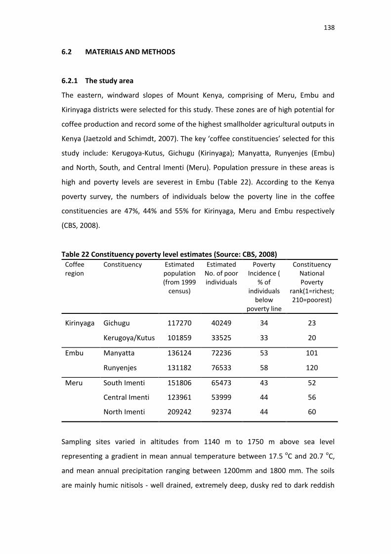
138

6.2 MATERIALS AND METHODS

6.2.1 The study area

The eastern, windward slopes of Mount Kenya, comprising of Meru, Embu and

Kirinyaga districts were selected for this study. These zones are of high potential for

coffee production and record some of the highest smallholder agricultural outputs in

Kenya (Jaetzold and Schimdt, 2007). The key ‘coffee constituencies’ selected for this

study include: Kerugoya-Kutus, Gichugu (Kirinyaga); Manyatta, Runyenjes (Embu)

and North, South, and Central Imenti (Meru). Population pressure in these areas is

high and poverty levels are severest in Embu (Table 22). According to the Kenya

poverty survey, the numbers of individuals below the poverty line in the coffee

constituencies are 47%, 44% and 55% for Kirinyaga, Meru and Embu respectively

(CBS, 2008).

Table 22 Constituency poverty level estimates (Source: CBS, 2008)

Coffee region

Constituency Estimated population (from 1999

census)

Estimated No. of poor individuals

Poverty Incidence (

% of individuals

below poverty line

Constituency National Poverty

rank(1=richest; 210=poorest)

Kirinyaga Gichugu 117270 40249 34 23

Kerugoya/Kutus 101859 33525 33 20

Embu Manyatta 136124 72236 53 101

Runyenjes 131182 76533 58 120

Meru South Imenti 151806 65473 43 52

Central Imenti 123961 53999 44 56

North Imenti 209242 92374 44 60

Sampling sites varied in altitudes from 1140 m to 1750 m above sea level

representing a gradient in mean annual temperature between 17.5 oC and 20.7 oC,

and mean annual precipitation ranging between 1200mm and 1800 mm. The soils

are mainly humic nitisols - well drained, extremely deep, dusky red to dark reddish

139

brown, friable clay, with acidic humic top soil. A detailed description of site

characteristics such as soils, climate, geology and land-use, are described in Jaetzold

and Schimdt (2007).

6.2.2 Farmer sampling strategy

Household sampling involved stratification techniques in three coffee districts of

Embu, Meru and Kirinyaga. Coffee regions largely fall under three agro-ecological

zones namely; Upper midland one (UM1), Upper midland two (UM2) and Upper

midland three (UM3) according to the FAO soil and agro-climatic zones classification

of Kenya (Jaetzold and Schimdt, 2007). Therefore for each zone, existing farmer

cooperative societies were identified and approached for collaboration in the study.

At least 10 farmer coffee cooperative societies per district were approached to

provide a sampling frame covering their respective coffee producing regions.

The coffee societies were requested to provide farmer membership records to be

used as a sampling frame. Farmer membership accounts detailing amounts of coffee

yield deliveries, payments and credit profiles are maintained by the societies.

Written request to the society’s management committee was often required to state

the purpose of the information sought. In a few instances, the research team was

required to hold meeting with the management committee to discuss the purpose of

the study. Most of the societies readily gave consent to collaborating in the study on

meeting their requirements. Findings from the study and especially on the soil test

data were requested once the exercise was complete. Confidentiality of farmer

account information was assured to the management committee. For instance

names of respondents would be replaced with identification codes after data entry

for subsequent analysis.

Random sample farmers were selected a priori in three farmer categories, labeled

‘increasing’, ‘decreasing’ and ‘constant’ according to their levels of coffee cherry

delivery for the period 2000-2008. Soil sampling and household interviews were

conducted for a farmer category in 10 coffee societies, for a total of 30 farmers per

140

district and a total of 90 farmers for the surveyed region. Meru however has a larger

area and three additional societies were approached for sampling. Soil sample

collection was conducted following a pre-determined random sampling scheme

according to the approximate shape of the farm parcel (Stern and Coe, 2004). The

procedure involved demarcating a 5m X 5m quadrat per farm. Quadrat placement

per farm was roughly determined by farm dimensions considered as either ‘thin

rectangular’ or ‘square shaped’. Transects from the centre of a given farm were

used. Assuming a determined random bearing and taking a randomly specified

percentage distance to the edge of the farm, a site for soil sample collection was

defined by a quadrat. Quadrat placement was flexible and could be moved up and

down a land slope depending on site conditions.

Four soil samples were collected per quadrat in the depths of 0-20 cm and 20-40 cm

using soil augers. These were later pooled to obtain a composite of two samples, per

depth per farm. Brown bags were used to collect samples before processing for

laboratory analysis. Sample identification information labels showing farmer name,

depth of sample, date of collection and type of crop on the sample plot were shown

on each sample. A total of 189 soil samples were collected even though only 180

samples were desired. Five extra farms were sampled in the event of poor handling

or loss of samples during field work. Only one sample was lost therefore providing

nine extra samples which were included in the analysis. A map of the Eastern slopes

of Mount Kenya and random farms selected for soil sample collection are presented

in Figure 22.

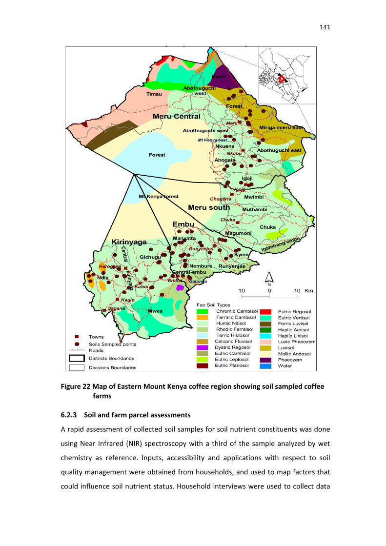
141

Figure 22 Map of Eastern Mount Kenya coffee region showing soil sampled coffee

farms 6.2.3 Soil and farm parcel assessments

A rapid assessment of collected soil samples for soil nutrient constituents was done

using Near Infrared (NIR) spectroscopy with a third of the sample analyzed by wet

chemistry as reference. Inputs, accessibility and applications with respect to soil

quality management were obtained from households, and used to map factors that

could influence soil nutrient status. Household interviews were used to collect data

142

on land management strategies, data on coffee cherry production, food crop yields

and costs of manure and chemical fertilizers applied. Other assembled variables

were: tree basal area (m2), tree volumes (m3) and calculated TLU. These were

correlated with nutrient input and output to explore their inherent correlations. The

following section describes the steps followed on the NIR approach so as to analyze

soil constituents and subsequent development of soil nutrient indices.

6.2.4 Near Infrared (NIR) spectroscopy

NIR spectroscopy is a rapid non-destructive technique recently adopted for

diagnostics of soil chemical constituents (Shepherd and Walsh, 2007). NIR has been

widely used in pharmaceutical and industrial applications for quality control. The

technique show efficiency and cost effectiveness when analyzing organic and

mineral composition of soils (Janik et al., 1995; Shepherd and Walsh, 2002). The

theory provides that derived soil properties may be correlated with the infrared

spectra of constituent components, and the covariance between soil properties and

spectra then modeled by partial least square (PLS) loadings and scores. Factors and

scores are derived independently for each soil property using PLS regressions. This

study used PLS for the qualitative and quantitative study of the prevalence of

nutrients in soils by classifying soil spectra and associated major nutrient elements

by their PLS loadings and scores as described by Shepherd and Walsh (2002). The

next sections demonstrate how NIR diagnostics steps were carried out to analyze soil

samples from small coffee farms in three districts of eastern Mount Kenya.

6.2.5 Sample preparation for NIR spectroscopy

Collected soil samples, in the 0-20 cm and 20-40 cm depths were processed to obtain

only two samples per farm in the respective depths. Processing work involved soil

samples air drying and sieving through a 2 mm sieve. A clean wooden rolling pin was

used to crush course soil material. Samples for laboratory analysis were sub-sampled

using the cone and quarter method. Processed samples were assigned unique

identification for purposes of referencing and then uploaded into ICRAF’s soil

laboratory database. A total of 189 soil samples were processed.

143

Soil sample scanning was done using a Fourier Transform Near Infrared

spectrometer (FT-IR) at wavebands of 4000 cm-1 to 12820 cm-1. Samples were loaded

into glass petri-dishes and scanned in 30 seconds. The resulting spectral signature

display the amount of energy absorbed at each wavelength, responding especially to

the soil organic matter and mineral composition content of a given sample. Spectra

data is multivariate in nature and highly multi-collinear, which makes it difficult to be

analyzed by parametric techniques. Peaks in the regions where absorption features

were found characterize the resulting spectral signature. However noise gets

registered due to instrumental noise and drift, light-scatter and path-length

variations that occur during measurements (Shepherd and Walsh, 2002).

Selected sample spectral signature and demarcated noise free region is shown in

Figure 23. Significant levels of redundancies (noise) in spectral data results in sub-

optimal calibration models to predict constituents in a sample. This is because Partial

Least Squares (PLS) assumes spectral errors are normally distributed throughout the

spectral region. The spectral signatures were therefore assessed for ‘noise’ regions

which were ‘cut off’ so as to remain with data points with significant information

levels. A more accentuated ‘noise free’ spectral signatures for a sample in the

selected spectral region is shown in Figure 24.

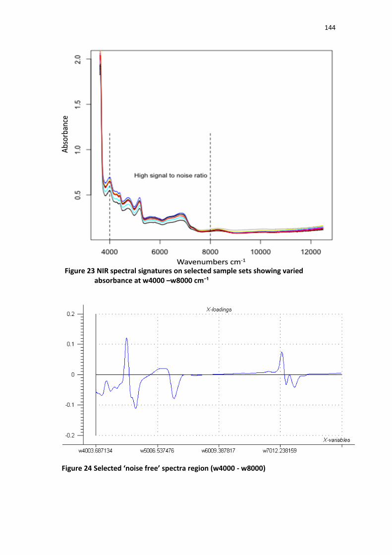
144

Figure 23 NIR spectral signatures on selected sample sets showing varied

absorbance at w4000 –w8000 cm⁻¹

Figure 24 Selected ‘noise free’ spectra region (w4000 - w8000)

145

6.2.6 Reference samples and calibration instruments

When transmittance spectra are converted to absorbance, spectra noise is no longer

constant. This is accentuated in cases where there are large variations in absorbance

(Haaland and Jones, ud). Precision of calibration predictors (spectral data) is

therefore improved by Kennerd and Stone algorithm procedure using R statistical

software. One third of the 189 samples were deemed a suitable calibration set

following ICRAF’s standard procedure (Shepherd and Walsh, 2002). The algorithm

was prescribed to collate 63 reference samples (one third of total samples) from the

entire spectral space based on their relative variation.

Selected samples were submitted for wet chemistry analysis adhering to the

standard soil fertility analysis package by ICRAF for 17 soil properties, namely: pH,

available P, exchangeable K, total N, organic C, Mg, Ca, Na, Mn, S, Cu, B, Zn, Fe, Al,

cation exchange capacity (CEC) and soil electrical conductivity (EC), (ICRAF, 2001).

6.2.7 Spectrometric calibration

Measured soil property values from the wet chemistry procedure were calibrated to

the first derivative of their reflectance spectra using PLS regression. PLS is a

chemometric method to derive prediction models for specific compounds from

spectroscopic data (Haaland and Jones, ud). Full-hold-out-one cross-validation was

done to prevent model over-fitting. PLS regression was applied in constructing linear

predictive models for the 17 soil properties based on their spectra. The multivariate

calibration technique used was principal component regression (PCR), where the X-

scores are chosen to explain as much of factor variation as possible. In this case the

standard reference analysis by wet chemistry was related to their constituent NIR

spectra (Shepherd and Walsh, 2007). This is achieved indirectly by extracting latent

variables from the reference sample factors and responses - in this case the analyzed

14 soil mineral properties together with three fertility factors, CEC, PH and EC. The

approach yields information in the direction of the factor space (Janik et al., 1995;

Shepherd and Walsh, 2007). The 17 factor models were then used to predict

properties for the 189 soil sample sets. Regression analysis was by R statistical

146

software with cross-checks using The Unscrambler software (CAMO, 2006). The

calibration model for C failed to yield consistent outputs using The Unscrambler.

Model calibration sets were assessed based on the coefficient of determination (r2)

and the number of principal components (PC). Model reliability was further assessed

on data transformation by natural log and square root.

To ensure the integrity of selected models, calibration models were built both in

statistical software R and The Unscrambler. Table 23 shows calibration models

constructed in R and in The unscramber. Data transformation was not useful when

using The Unscrambler. Model results however, suggest using natural log for P, S, Zn

could yield slightly better models with r2 improved from 0.16 to 0.65 for P; from 0.41

to 0.52 for S; and r2 0.59 to 0.62 for Zn, using R.

Primary nutrient N, calibrated well, while P and K calibrated poorly in R but showed

fair improvements with the unscramber on the respective natural log (r2 = 0.71; PC =

7) and square root (r2 = 0.71; PC = 6) transformation. The C calibration model was

satisfactory in either transformation but optimized with natural log. Secondary

nutrient models calibrated well except for S, while the precision for micro-nutrients

models was reasonable with the exception of Na, Cu and B the latter showing higher

levels of PCs. Soil PH calibrated well, while CEC showed reasonable results with the

Unscramber. Cross checks on outputs for most of the models in R, showed slightly

higher PCs than in the Unscrambler.

.

147

Table 23 Calibration models showing precision assessed by three methods of data transformations

Primary nutrients Secondary nutrients Indicators Micro nutrients

Transformation N P K C Ca Mg S CEC PH Al Na Mn B Fe Zn

R software

None (r2) 0.85 0.16 0.32 0.78 0.78 0.86 0.41 0.67 0.74 0.77 0.54 0.86 0.74 0.5 0.59

None (PC) 20 3 2 8 15 13 5 10 11 12 7 13 11 6 12

Lnlog (r2) 0.81 0.65 0.34 0.79 0.85 0.76 0.52 0.52 0.73 0.82 0.14 0.55 0.75 0.51 0.62

Lnlog (PC) 16 8 8 8 14 12 5 10 13 15 2 11 14 7 10

SQRT(r2) 0.83 0.44 0.33 0.79 0.89 0.87 0.47 0.62 0.72 0.79 0.09 0.55 0.79 0.51 0.66

SQRT PC 16 5 9 8 15 14 5 10 12 15 2 9 14 8 0.12

The Unscrambler

None (r2) 0.79 -0.4 0.23 0.8 0.76 0.85 0.53 0.75 0.8 0.83 0.107 0.7 0.79 0.67 0.67

None (PC) 8 1 2 7 9 11 5 8 8 10 2 5 11 6 11

Lnlog (r2) 0.81 0.71 0.27 0.85 0.89 0.86 0.62 0.71 0.74 0.82 0.18 0.7 0.82 0.72 0.76

Lnlog (PC) 12 7 2 8 12 12 5 9 8 12 2 4 11 7 9

SQRT (r2) 0.82 0.59 0.71 0.85 0.92 0.88 0.59 0.74 0.79 0.83 0.18 0.71 0.83 0.71 0.73

SQRT PC 8 4 6 8 15 10 5 9 11 12 2 7 14 6 9

None-no data transformation; Lnlog-natural logarithm; SQRT- square root; PC-principal components

148

Overall data transformation by natural log showed slight benefits for calibration

instruments, considering r2 and PC values, and was therefore used to predict

nutrient composition for the spectra data set. Shepherd and Walsh (2007) confirm

that IR spectroscopy in soils show variable performance when predicting for nitrates

and soil available P and K tests, however soil reflectance responds well to key soil

properties that respond to P availability in crops such as mineralogy, organic matter,

clay content and microbial activity.

6.2.8 Data analysis

Soil test data were submitted for principal component analysis8 (PCA), to obtain a

smaller number of artificial variables (called principal components) that account for

most of the variation in the analytical sample (Stern and Coe, 2004). Data reduction

procedures are useful to remove redundant (highly correlated) variables from the

data and obtain a smaller number of uncorrelated variables. PCA was used to

develop soil nutrient indices (principal components) representative of all the soil

samples collected. Essentially, principal components (PC) show levels of soil nutrient

prevalence between farms.

Descriptive and exploratory approaches are used to analyse the relationships

between derived soil PC scores (PC1, PC2 and PC3- the dependent variables) and

composite smallholder household socio-economic variables such as farm size,

amount/value of fertilizer and/or manure applied, tropical livestock units estimates

(TLU), number of coffee bushes, size of tree volumes, and value of maize yield

produced per year. SPSS version 15 was used for biophysical and socio-economic

multivariate data analysis. PCA on soil test data was executed using the unscrambler

version 9.2 or with R software.

8 Principal component can be defined as a linear combination of optimally-weighted observed variables. The words “linear

combination” refer to the fact that scores on a component are created by adding together scores on the observed variables being analysed (Stern and Coe, 2004)

149

6.3 RESULTS

6.3.1 Determining soil nutrient indices

Data values for the seventeen soil properties (pH, P, K, N, C, Mg, Ca, Na, Mn, S, Cu, B,

Zn, Fe, Al, CEC and EC subjected to a principal component analysis, showed high

extracted communality estimates (Annex 7). 9Communalities (always equal to 1)

indicate the amount of variance accounted for in each variable. The score for all

properties was 0.70 to 0.92; except for, K and Zn, which were 0.51 and 0.55; and S

and P, which were 0.62 and 0.64 respectively (Annex 8). This confirmed that

extracted components represent the studied variables well.

The principal axis method was used to extract components, followed by a varimax

(orthogonal) rotation. Only the first four components displayed eigen-values

(accounted variance in the original variables) greater than 1 (PC4=1.8; PC3= 2.04;

PC2= 2.74; PC1=6.8). Results from the scree plot also suggest only the first four

components were meaningful; these were therefore retained for rotation. Extracted

principal components (1 to 4) accounted for 78.3% of total variability in the

submitted data dimension (Annex 7). The rotations maintain the variation explained

by extracted components and is spread more evenly over the components, making

the rotated matrix easier to interpret that the un-rotated one. In Table 24 a

comparison of the rotated and un-rotated extraction matrix is demonstrated.

The rotated component matrices showed better clarity and were used to determine

what the components represent. Using a cut off value of 0.65, a variable item was

said to load to a given component if the factor loading was 0.65 or greater for that

component, and was less than 0.70 for the other principal components (PC). From

this criterion the following was deduced:

i. PC1 is strongly correlated with B, Ca, Mg, Al, Mn, pH, CEC, S, Zn and is

therefore a good indicator of these soil properties

9 Initial communalities are estimates of the variance in each variable accounted for by all components. For principal components extraction, this is always equal to 1.0 for correlation analyses. Extraction communalities are estimates of the variance in each variable accounted for by the components.

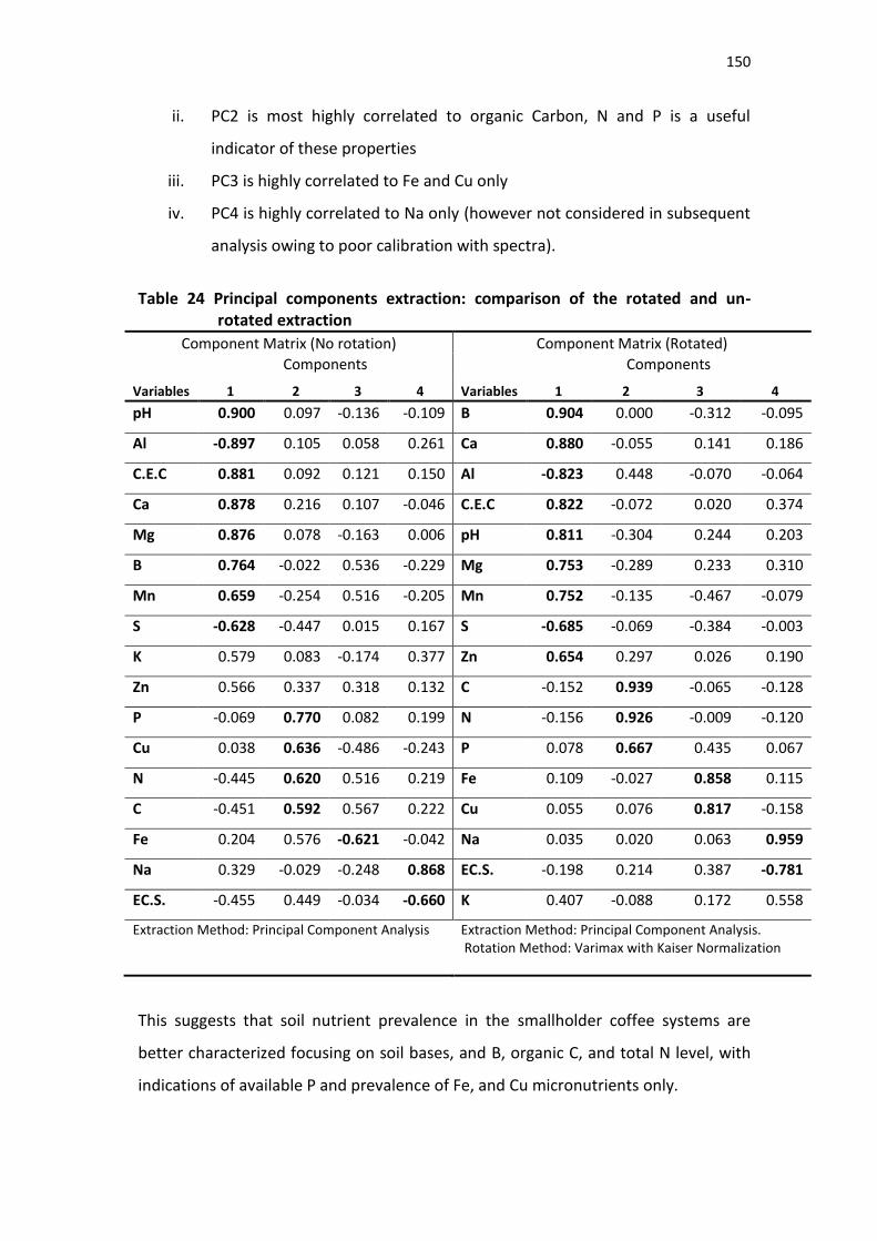
150

ii. PC2 is most highly correlated to organic Carbon, N and P is a useful

indicator of these properties

iii. PC3 is highly correlated to Fe and Cu only

iv. PC4 is highly correlated to Na only (however not considered in subsequent

analysis owing to poor calibration with spectra).

Table 24 Principal components extraction: comparison of the rotated and un-rotated extraction

Component Matrix (No rotation) Component Matrix (Rotated)

Variables

Components Variables

Components

1 2 3 4 1 2 3 4

pH 0.900 0.097 -0.136 -0.109 B 0.904 0.000 -0.312 -0.095

Al -0.897 0.105 0.058 0.261 Ca 0.880 -0.055 0.141 0.186

C.E.C 0.881 0.092 0.121 0.150 Al -0.823 0.448 -0.070 -0.064

Ca 0.878 0.216 0.107 -0.046 C.E.C 0.822 -0.072 0.020 0.374

Mg 0.876 0.078 -0.163 0.006 pH 0.811 -0.304 0.244 0.203

B 0.764 -0.022 0.536 -0.229 Mg 0.753 -0.289 0.233 0.310

Mn 0.659 -0.254 0.516 -0.205 Mn 0.752 -0.135 -0.467 -0.079

S -0.628 -0.447 0.015 0.167 S -0.685 -0.069 -0.384 -0.003

K 0.579 0.083 -0.174 0.377 Zn 0.654 0.297 0.026 0.190

Zn 0.566 0.337 0.318 0.132 C -0.152 0.939 -0.065 -0.128

P -0.069 0.770 0.082 0.199 N -0.156 0.926 -0.009 -0.120

Cu 0.038 0.636 -0.486 -0.243 P 0.078 0.667 0.435 0.067

N -0.445 0.620 0.516 0.219 Fe 0.109 -0.027 0.858 0.115

C -0.451 0.592 0.567 0.222 Cu 0.055 0.076 0.817 -0.158

Fe 0.204 0.576 -0.621 -0.042 Na 0.035 0.020 0.063 0.959

Na 0.329 -0.029 -0.248 0.868 EC.S. -0.198 0.214 0.387 -0.781

EC.S. -0.455 0.449 -0.034 -0.660 K 0.407 -0.088 0.172 0.558

Extraction Method: Principal Component Analysis

Extraction Method: Principal Component Analysis. Rotation Method: Varimax with Kaiser Normalization

This suggests that soil nutrient prevalence in the smallholder coffee systems are

better characterized focusing on soil bases, and B, organic C, and total N level, with

indications of available P and prevalence of Fe, and Cu micronutrients only.

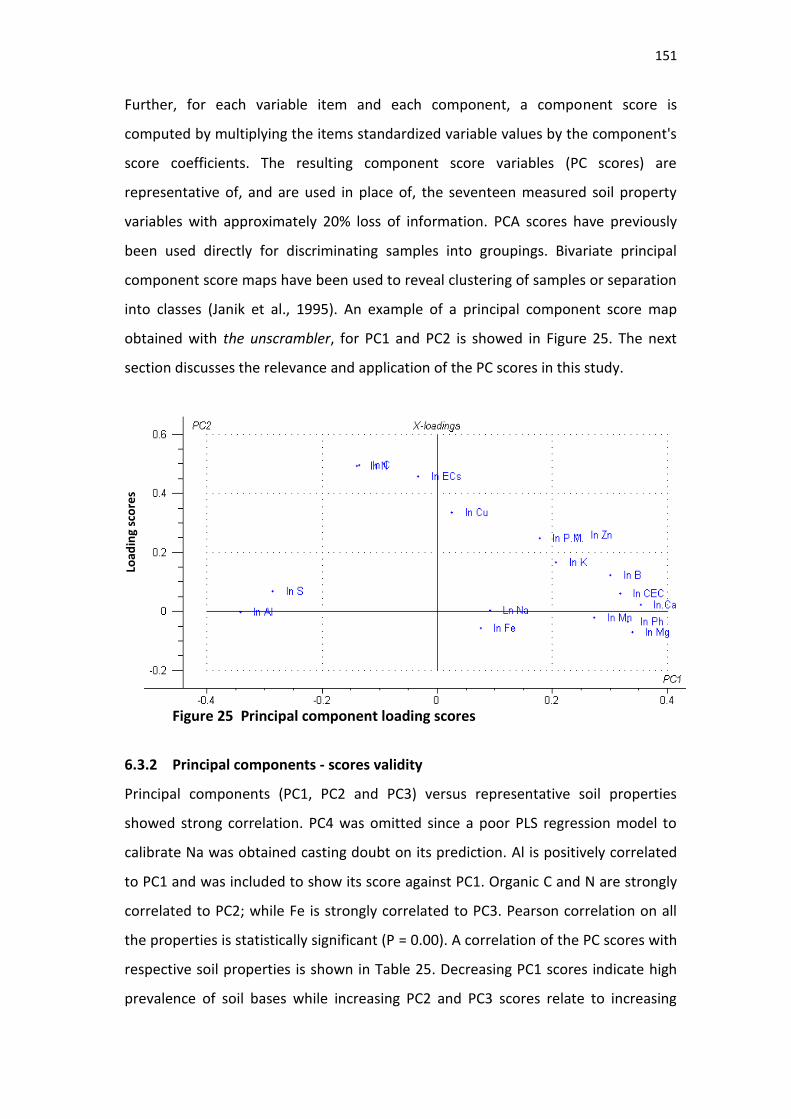
151

Further, for each variable item and each component, a component score is

computed by multiplying the items standardized variable values by the component's

score coefficients. The resulting component score variables (PC scores) are

representative of, and are used in place of, the seventeen measured soil property

variables with approximately 20% loss of information. PCA scores have previously

been used directly for discriminating samples into groupings. Bivariate principal

component score maps have been used to reveal clustering of samples or separation

into classes (Janik et al., 1995). An example of a principal component score map

obtained with the unscrambler, for PC1 and PC2 is showed in Figure 25. The next

section discusses the relevance and application of the PC scores in this study.

Figure 25 Principal component loading scores

6.3.2 Principal components - scores validity

Principal components (PC1, PC2 and PC3) versus representative soil properties

showed strong correlation. PC4 was omitted since a poor PLS regression model to

calibrate Na was obtained casting doubt on its prediction. Al is positively correlated

to PC1 and was included to show its score against PC1. Organic C and N are strongly

correlated to PC2; while Fe is strongly correlated to PC3. Pearson correlation on all

the properties is statistically significant (P = 0.00). A correlation of the PC scores with

respective soil properties is shown in Table 25. Decreasing PC1 scores indicate high

prevalence of soil bases while increasing PC2 and PC3 scores relate to increasing

Load

ing

sco

res

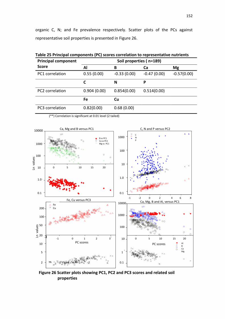
152

organic C, N; and Fe prevalence respectively. Scatter plots of the PCs against

representative soil properties is presented in Figure 26.

Table 25 Principal components (PC) scores correlation to representative nutrients

Principal component Score

Soil properties ( n=189)

Al B Ca Mg

PC1 correlation 0.55 (0.00) -0.33 (0.00) -0.47 (0.00) -0.57(0.00)

C N P

PC2 correlation 0.904 (0.00) 0.854(0.00) 0.514(0.00)

Fe Cu

PC3 correlation 0.82(0.00) 0.68 (0.00)

(**) Correlation is significant at 0.01 level (2 tailed)

Figure 26 Scatter plots showing PC1, PC2 and PC3 scores and related soil

properties

Soil C, N & P versus PC2

-2 2

0.1

6

1.0

10.0

100.0

1000.0

-4 40 8

PC2 scores

Ln v

alu

es (

C, N

& P

)

P

C

N

Soil Fe, Cu vs PC3

20

50

100

-1

200

1 3

5

2

10

-2 20

PC3 scores

Ln v

alu

es

( Fe

, C

u)

Fe

Cu

Fe, Cu versus PC3

Ca, Mg and B versus PC1 C, N and P versus PC2

Lnva

lues

Lnva

lues

PC scores

Soil bases Ca, Mg & B, Al versus PC1

1.0

0.1

5 15

10000.0

0

1000.0

2010

100.0

10.0

ln v

alu

es

(Ca

, Mg

, B &

Al)

PC1 scores

Mg

Ca

B

Al

PC scores

Ca, Mg, B and Al, versus PC1

0.1

10

100

1.0

1000

10000

0.1

1.0

10

100

1000

200

100

50

20

10

5

2

FeCu

-2-1 0 1 2 3

0 5 10 15 20

0 5 10 15 20

0.1

1000

100

10000

1

10

-1 -2 0 2 4 6 8

AlBCaMg

CNP

B vs PC1Ca vs PC1Mg vs PC1

153

6.3.3 Nutrient prevalence in small coffee systems

Data on soil nutrient prevalence is represented by principal components scores for

all soil properties described. These were: PC1 (soil bases and B), PC2 (organic C, total

N and P) and PC3 (Fe and Cu). The PC and constituent nutrients are interchangeably

used in describing soil fertility characteristics of the coffee farms. Indicator scores

were derived by observing entire PC scores range and visually demarcating scores as

low, moderate and high as shown in Table 26.

Table 26 Derived soil nutrient prevalence indicator scores

Nutrient indicators

Indicator scores

high moderate low

PC1 (Ca, Mg, B) <0.0 0.1-5.0 >5.0

PC2( Org. C, N, P) >2.0 0.1-2.0 <0.0

PC3 (Fe, Cu) >2.0 0.1-2.0 <0.0

Analysis of soil nutrients prevalence using the identified indicators (Table 27) showed

64% of the soil test samples had high bases content; only 18% of the samples

showed high organic C content, total N, Fe and Cu. Results showing high bases

content were contrary to expectation, as many of the locations experience high

rainfall with potential leaching. The high score indicates reasonable nutrients stocks

in spite of permanent cultivation practices. Reduced rainfall patterns in the past two

years may also play a contributing factor.

Further analysis showed that nearly half (46%) of the samples tested for organic C

and total N, had low levels of these soil properties. This is perhaps indicative of

available P even though spectra analysis showed high variability. Shepherd and

Walsh (2007) have showed that P dynamics in soils are complex, as they involve both

chemical and biological processes with long-term effects of sorption (fixation) and

desorption (release) processes. Also low concentration and low solubility of P in soils

frequently make P a limiting factor (Sanchez, 2002).

Data suggests C, N and P are by far the most deficient minerals in small coffee farms

as compared to bases at 24% of the samples and Fe, and Cu, at 30% of the samples.

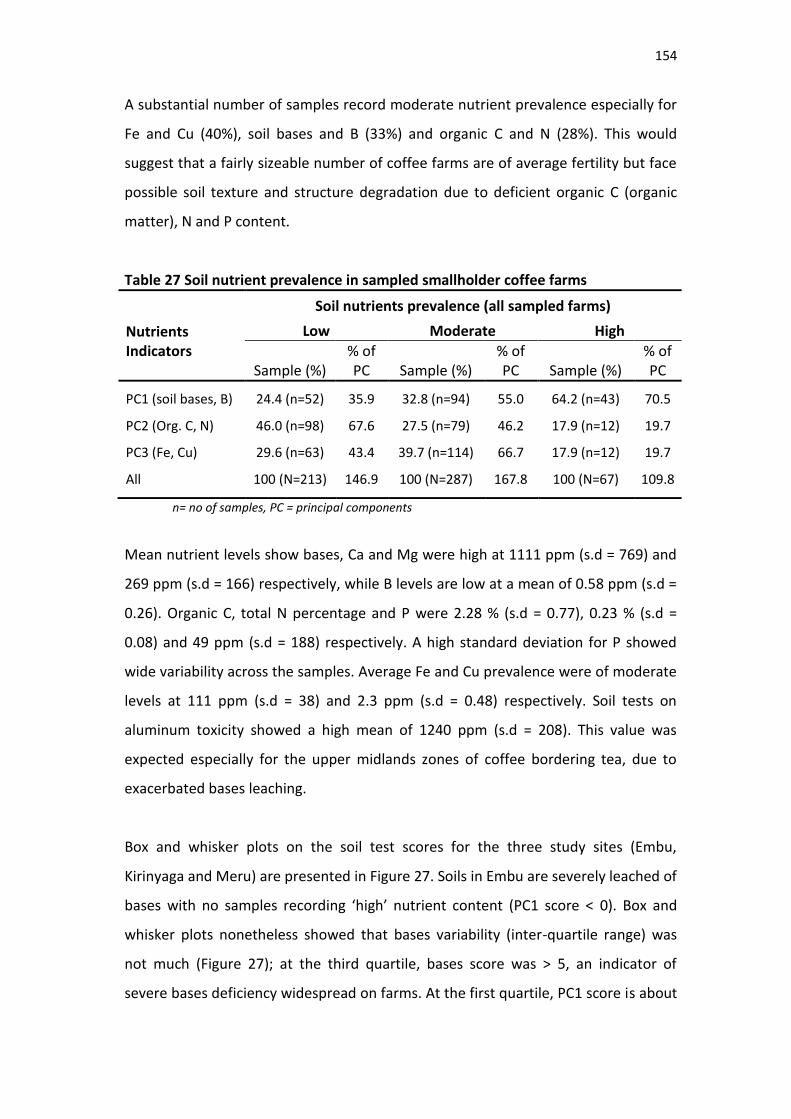
154

A substantial number of samples record moderate nutrient prevalence especially for

Fe and Cu (40%), soil bases and B (33%) and organic C and N (28%). This would

suggest that a fairly sizeable number of coffee farms are of average fertility but face

possible soil texture and structure degradation due to deficient organic C (organic

matter), N and P content.

Table 27 Soil nutrient prevalence in sampled smallholder coffee farms

Nutrients Indicators

Soil nutrients prevalence (all sampled farms)

Low Moderate High

Sample (%) % of PC Sample (%)

% of PC Sample (%)

% of PC

PC1 (soil bases, B) 24.4 (n=52) 35.9 32.8 (n=94) 55.0 64.2 (n=43) 70.5

PC2 (Org. C, N) 46.0 (n=98) 67.6 27.5 (n=79) 46.2 17.9 (n=12) 19.7

PC3 (Fe, Cu) 29.6 (n=63) 43.4 39.7 (n=114) 66.7 17.9 (n=12) 19.7

All 100 (N=213) 146.9 100 (N=287) 167.8 100 (N=67) 109.8

n= no of samples, PC = principal components

Mean nutrient levels show bases, Ca and Mg were high at 1111 ppm (s.d = 769) and

269 ppm (s.d = 166) respectively, while B levels are low at a mean of 0.58 ppm (s.d =

0.26). Organic C, total N percentage and P were 2.28 % (s.d = 0.77), 0.23 % (s.d =

0.08) and 49 ppm (s.d = 188) respectively. A high standard deviation for P showed

wide variability across the samples. Average Fe and Cu prevalence were of moderate

levels at 111 ppm (s.d = 38) and 2.3 ppm (s.d = 0.48) respectively. Soil tests on

aluminum toxicity showed a high mean of 1240 ppm (s.d = 208). This value was

expected especially for the upper midlands zones of coffee bordering tea, due to

exacerbated bases leaching.

Box and whisker plots on the soil test scores for the three study sites (Embu,

Kirinyaga and Meru) are presented in Figure 27. Soils in Embu are severely leached of

bases with no samples recording ‘high’ nutrient content (PC1 score < 0). Box and

whisker plots nonetheless showed that bases variability (inter-quartile range) was

not much (Figure 27); at the third quartile, bases score was > 5, an indicator of

severe bases deficiency widespread on farms. At the first quartile, PC1 score is about

155

4.8 indicating a slight improvement of bases levels but perhaps tending more to

degradation.

Figure 27 Soil nutrient indicators (PC scores) for Embu, Kirinyaga and Meru coffee systems

Soil bases in Kirinyaga samples are most variable with two farms (outliers) showing

excessive score values and hence extremely low bases and severe soil acidification.

However the first quartile of the indicator value was less than zero, while at the third

quartile, PC1 score was about 5 showing a substantial prevalence of moderate levels

of bases. The maximum score value for Kirinyaga was about 12 showing a higher, low

level of bases than Embu at a score of 9. Meru recorded the strongest bases

prevalence with PC1 score of zero at half quartile and a maximum score of 4.9 for

farms with lower bases (Figure 27).

156

Organic C and total N percentage showed similar variability across the three sites. At

the second quartile, all the sites recorded an approximate score value of less than

zero, indicating low nutrient prevalence. The maximum score value was

approximately 3.5 and the minimum was about -3.0. Analysis of Fe and Cu

prevalence for Kirinyaga showed a score of 1.5 at the second quartile, while Embu

showed a score value of approximately zero. Meru showed the smallest variability at

the second quartile at an approximate score value of one (Figure 27). Comparison of

soil fertility by the three farm categories constant, decreasing and increasing showed

more or less similar patterns (Figure 28).

Figure 28 PC scores for the ‘constant’, ‘decreasing’, ‘increasing’ farm categories

Coffee decreasing farms showed PC1 score value of 2 at the first quartile suggesting

only moderate contents of basic soil properties; while for the increasing and

constant categories the score value was about -1 at the first quartile suggesting that

157

fewer than 25% of farms in these farm categories had high bases and low Al

prevalence.

The coffee increasing and decreasing farms had a PC1 score of > 5 at the third

quartile suggesting very low bases and B content, but a high prevalence of Al. The

constant farm category had a score of 4 at the third quartile implying relatively

moderate levels of soil bases and Al. PC2 (Organic C and total N percentage) showed

high variability in the decreasing farm categories with a maximum of about 3 and

minimum score of about -3.5.

The coffee increasing farms showed a PC score of < 0 at the second quartile

suggesting these farms have low organic C, N and P prevalence. All farm categories

showed PC2 score of about 0.1 suggesting only slightly moderate prevalence of

organic C, N and P, at the third quartile. PC3 (Fe and Cu) score variability, though not

of interest, showed low nutrient prevalence for these nutrients at the first quartile

and just moderate levels at the third quartile.

6.3.4 Surveyed households and farm parcel characterization

Typical small coffee farms are characterized by multiple crop and animal enterprises.

Some socio-economic characteristics of the surveyed households are presented in

Table 28. Results showed that heads of households are aging at a mean age of 59

years (s.d = 14); a family size of five persons; and farm parcel of about 1.2 hectares

(s.d = 1.04). There are about 540 coffee bushes per household producing about 4.4

kg of coffee cherry per bush.

Calculated TLU are at a mean of 4 (s.d = 2.6) indicating a relatively strong preference

for livestock farming. Fertilizer and manure application are widely variable per

household demonstrating steep differences in nutrient application rates and perhaps

varied challenges in nutrient accessibility.

Coffee, maize and banana cultivation form important farming activities carried out in

mixed cropping or small monoculture patterns. Soil nutrient assessment as expected

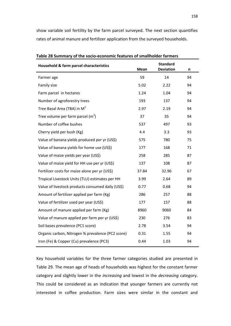
158

show variable soil fertility by the farm parcel surveyed. The next section quantifies

rates of animal manure and fertilizer application from the surveyed households.

Table 28 Summary of the socio-economic features of smallholder farmers

Household & farm parcel characteristics Mean

Standard Deviation n

Farmer age 59 14 94

Family size 5.02 2.22 94

Farm parcel in hectares 1.24 1.04 94

Number of agroforestry trees 193 137 94

Tree Basal Area (TBA) in M2 2.97 2.19 94

Tree volume per farm parcel (m3) 37 35 94

Number of coffee bushes 537 497 93

Cherry yield per bush (Kg) 4.4 3.3 93

Value of banana yields produced per yr (US$) 575 780 75

Value of banana yields for home use (US$) 177 168 71

Value of maize yields per year (US$) 258 285 87

Value of maize yield for HH use per yr (US$) 137 108 87

Fertilizer costs for maize alone per yr (US$) 37.84 32.96 67

Tropical Livestock Units (TLU) estimates per HH 3.99 2.64 89

Value of livestock products consumed daily (US$) 0.77 0.68 94

Amount of fertilizer applied per farm (Kg) 286 257 88

Value of fertilizer used per year (US$) 177 157 88

Amount of manure applied per farm (Kg) 8960 9060 84

Value of manure applied per farm per yr (US$) 230 276 83

Soil bases prevalence (PC1 score) 2.78 3.54 94

Organic carbon, Nitrogen % prevalence (PC2 score) 0.31 1.55 94

Iron (Fe) & Copper (Cu) prevalence (PC3) 0.44 1.03 94

Key household variables for the three farmer categories studied are presented in

Table 29. The mean age of heads of households was highest for the constant farmer

category and slightly lower in the increasing and lowest in the decreasing category.

This could be considered as an indication that younger farmers are currently not

interested in coffee production. Farm sizes were similar in the constant and

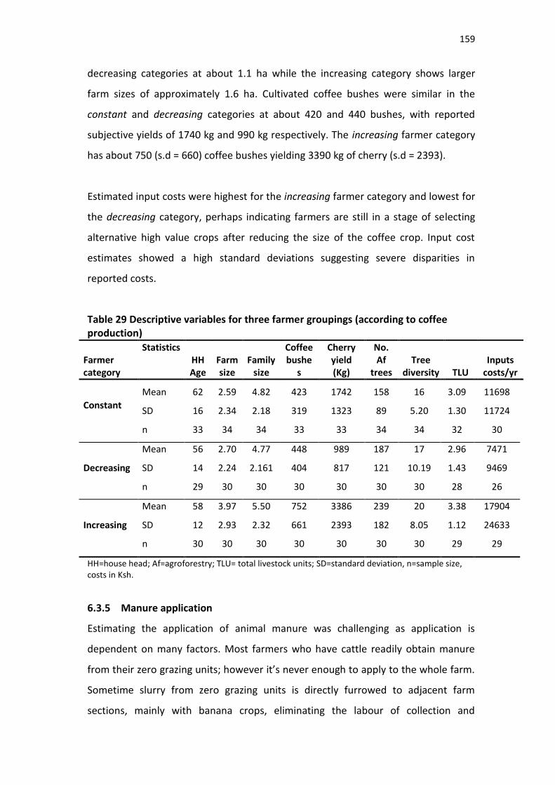
159

decreasing categories at about 1.1 ha while the increasing category shows larger

farm sizes of approximately 1.6 ha. Cultivated coffee bushes were similar in the

constant and decreasing categories at about 420 and 440 bushes, with reported

subjective yields of 1740 kg and 990 kg respectively. The increasing farmer category

has about 750 (s.d = 660) coffee bushes yielding 3390 kg of cherry (s.d = 2393).

Estimated input costs were highest for the increasing farmer category and lowest for

the decreasing category, perhaps indicating farmers are still in a stage of selecting

alternative high value crops after reducing the size of the coffee crop. Input cost

estimates showed a high standard deviations suggesting severe disparities in

reported costs.

Table 29 Descriptive variables for three farmer groupings (according to coffee production)

Farmer category

Statistics HH Age

Farm size

Family size

Coffee bushe

s

Cherry yield (Kg)

No. Af

trees Tree

diversity TLU Inputs

costs/yr

Constant

Mean 62 2.59 4.82 423 1742 158 16 3.09 11698

SD 16 2.34 2.18 319 1323 89 5.20 1.30 11724

n 33 34 34 33 33 34 34 32 30

Decreasing

Mean 56 2.70 4.77 448 989 187 17 2.96 7471

SD 14 2.24 2.161 404 817 121 10.19 1.43 9469

n 29 30 30 30 30 30 30 28 26

Increasing

Mean 58 3.97 5.50 752 3386 239 20 3.38 17904

SD 12 2.93 2.32 661 2393 182 8.05 1.12 24633

n 30 30 30 30 30 30 30 29 29

HH=house head; Af=agroforestry; TLU= total livestock units; SD=standard deviation, n=sample size, costs in Ksh.

6.3.5 Manure application

Estimating the application of animal manure was challenging as application is

dependent on many factors. Most farmers who have cattle readily obtain manure

from their zero grazing units; however it’s never enough to apply to the whole farm.

Sometime slurry from zero grazing units is directly furrowed to adjacent farm

sections, mainly with banana crops, eliminating the labour of collection and

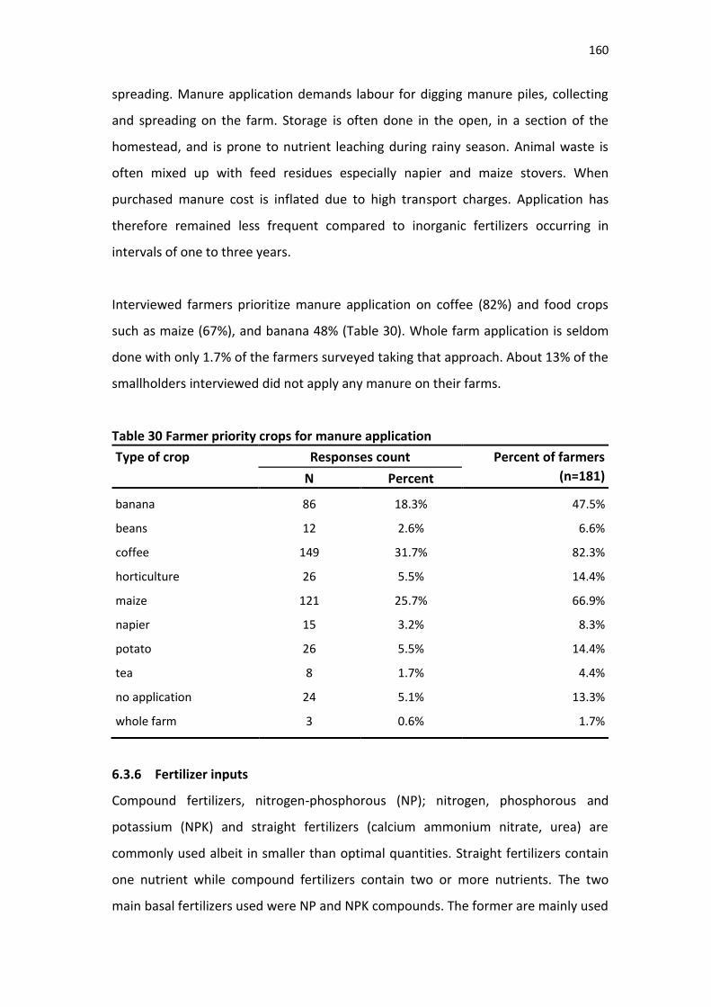
160

spreading. Manure application demands labour for digging manure piles, collecting

and spreading on the farm. Storage is often done in the open, in a section of the

homestead, and is prone to nutrient leaching during rainy season. Animal waste is

often mixed up with feed residues especially napier and maize stovers. When

purchased manure cost is inflated due to high transport charges. Application has

therefore remained less frequent compared to inorganic fertilizers occurring in

intervals of one to three years.

Interviewed farmers prioritize manure application on coffee (82%) and food crops

such as maize (67%), and banana 48% (Table 30). Whole farm application is seldom

done with only 1.7% of the farmers surveyed taking that approach. About 13% of the

smallholders interviewed did not apply any manure on their farms.

Table 30 Farmer priority crops for manure application

Type of crop Responses count Percent of farmers

(n=181) N Percent

banana 86 18.3% 47.5%

beans 12 2.6% 6.6%

coffee 149 31.7% 82.3%

horticulture 26 5.5% 14.4%

maize 121 25.7% 66.9%

napier 15 3.2% 8.3%

potato 26 5.5% 14.4%

tea 8 1.7% 4.4%

no application 24 5.1% 13.3%

whole farm 3 0.6% 1.7%

6.3.6 Fertilizer inputs

Compound fertilizers, nitrogen-phosphorous (NP); nitrogen, phosphorous and

potassium (NPK) and straight fertilizers (calcium ammonium nitrate, urea) are

commonly used albeit in smaller than optimal quantities. Straight fertilizers contain

one nutrient while compound fertilizers contain two or more nutrients. The two

main basal fertilizers used were NP and NPK compounds. The former are mainly used

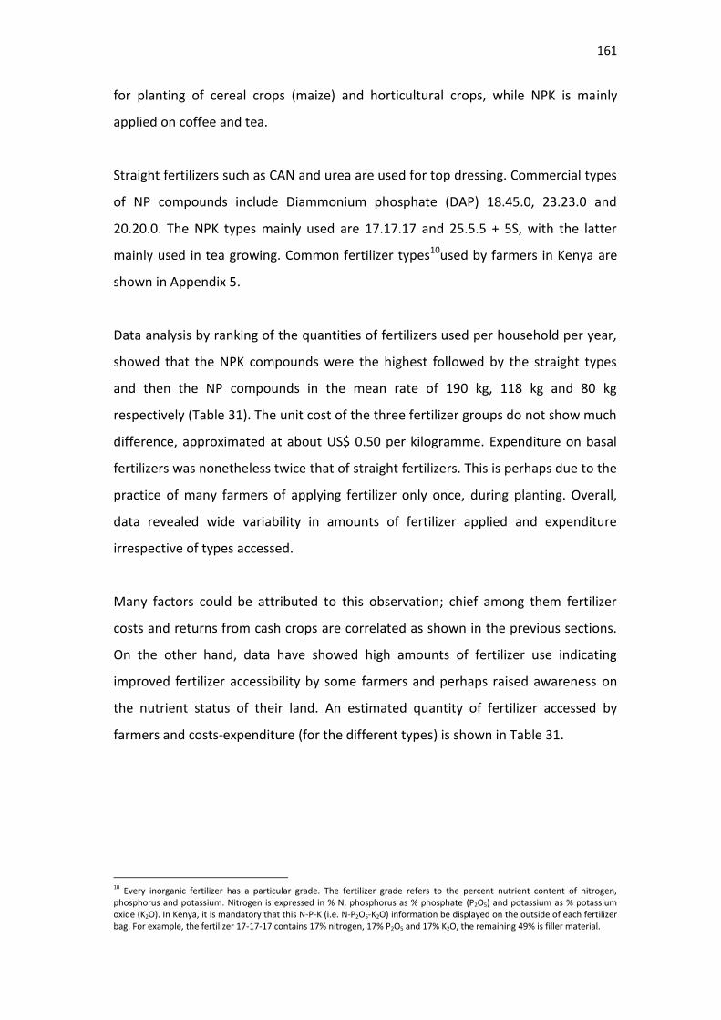
161

for planting of cereal crops (maize) and horticultural crops, while NPK is mainly

applied on coffee and tea.

Straight fertilizers such as CAN and urea are used for top dressing. Commercial types

of NP compounds include Diammonium phosphate (DAP) 18.45.0, 23.23.0 and

20.20.0. The NPK types mainly used are 17.17.17 and 25.5.5 + 5S, with the latter

mainly used in tea growing. Common fertilizer types10used by farmers in Kenya are

shown in Appendix 5.

Data analysis by ranking of the quantities of fertilizers used per household per year,

showed that the NPK compounds were the highest followed by the straight types

and then the NP compounds in the mean rate of 190 kg, 118 kg and 80 kg

respectively (Table 31). The unit cost of the three fertilizer groups do not show much

difference, approximated at about US$ 0.50 per kilogramme. Expenditure on basal

fertilizers was nonetheless twice that of straight fertilizers. This is perhaps due to the

practice of many farmers of applying fertilizer only once, during planting. Overall,

data revealed wide variability in amounts of fertilizer applied and expenditure

irrespective of types accessed.

Many factors could be attributed to this observation; chief among them fertilizer

costs and returns from cash crops are correlated as shown in the previous sections.

On the other hand, data have showed high amounts of fertilizer use indicating

improved fertilizer accessibility by some farmers and perhaps raised awareness on

the nutrient status of their land. An estimated quantity of fertilizer accessed by

farmers and costs-expenditure (for the different types) is shown in Table 31.

10 Every inorganic fertilizer has a particular grade. The fertilizer grade refers to the percent nutrient content of nitrogen, phosphorus and potassium. Nitrogen is expressed in % N, phosphorus as % phosphate (P2O5) and potassium as % potassium oxide (K2O). In Kenya, it is mandatory that this N-P-K (i.e. N-P2O5-K2O) information be displayed on the outside of each fertilizer bag. For example, the fertilizer 17-17-17 contains 17% nitrogen, 17% P2O5 and 17% K2O, the remaining 49% is filler material.

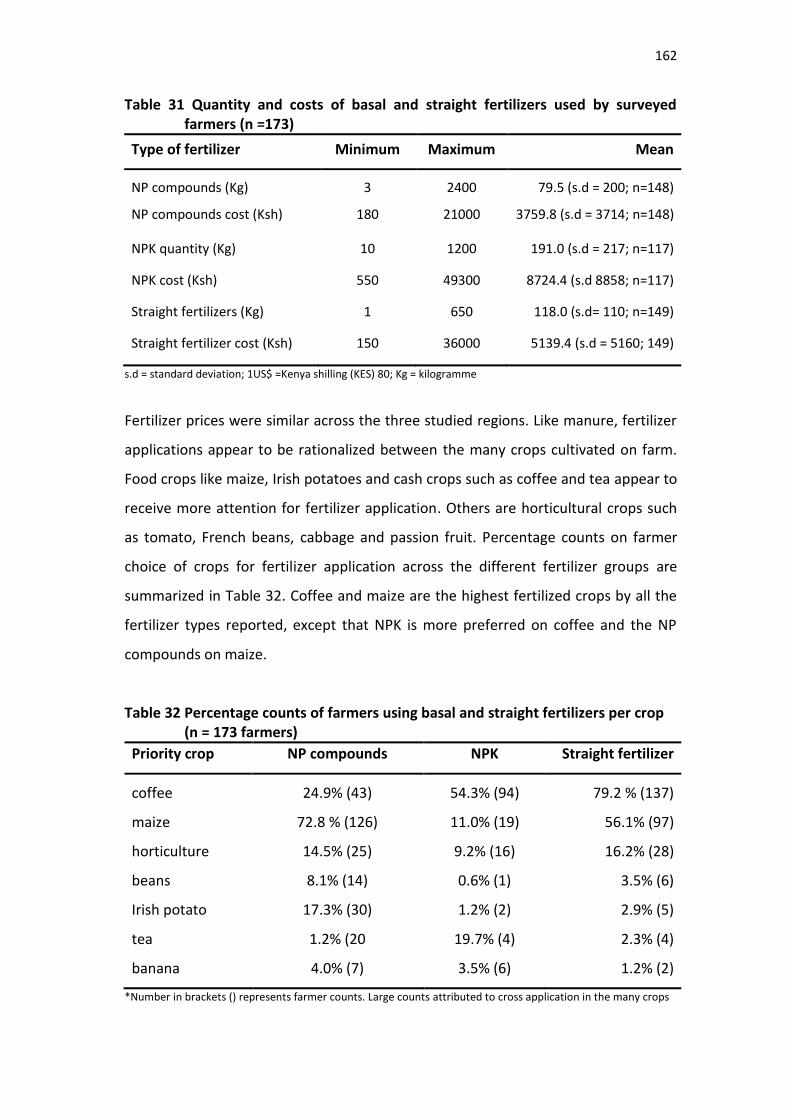
162

Table 31 Quantity and costs of basal and straight fertilizers used by surveyed farmers (n =173)

Type of fertilizer Minimum Maximum Mean

NP compounds (Kg) 3 2400 79.5 (s.d = 200; n=148)

NP compounds cost (Ksh) 180 21000 3759.8 (s.d = 3714; n=148)

NPK quantity (Kg) 10 1200 191.0 (s.d = 217; n=117)

NPK cost (Ksh) 550 49300 8724.4 (s.d 8858; n=117)

Straight fertilizers (Kg) 1 650 118.0 (s.d= 110; n=149)

Straight fertilizer cost (Ksh) 150 36000 5139.4 (s.d = 5160; 149)

s.d = standard deviation; 1US$ =Kenya shilling (KES) 80; Kg = kilogramme

Fertilizer prices were similar across the three studied regions. Like manure, fertilizer

applications appear to be rationalized between the many crops cultivated on farm.

Food crops like maize, Irish potatoes and cash crops such as coffee and tea appear to

receive more attention for fertilizer application. Others are horticultural crops such

as tomato, French beans, cabbage and passion fruit. Percentage counts on farmer

choice of crops for fertilizer application across the different fertilizer groups are

summarized in Table 32. Coffee and maize are the highest fertilized crops by all the

fertilizer types reported, except that NPK is more preferred on coffee and the NP

compounds on maize.

Table 32 Percentage counts of farmers using basal and straight fertilizers per crop (n = 173 farmers)

Priority crop NP compounds NPK Straight fertilizer

coffee 24.9% (43) 54.3% (94) 79.2 % (137)

maize 72.8 % (126) 11.0% (19) 56.1% (97)

horticulture 14.5% (25) 9.2% (16) 16.2% (28)

beans 8.1% (14) 0.6% (1) 3.5% (6)

Irish potato 17.3% (30) 1.2% (2) 2.9% (5)

tea 1.2% (20 19.7% (4) 2.3% (4)

banana 4.0% (7) 3.5% (6) 1.2% (2)

*Number in brackets () represents farmer counts. Large counts attributed to cross application in the many crops

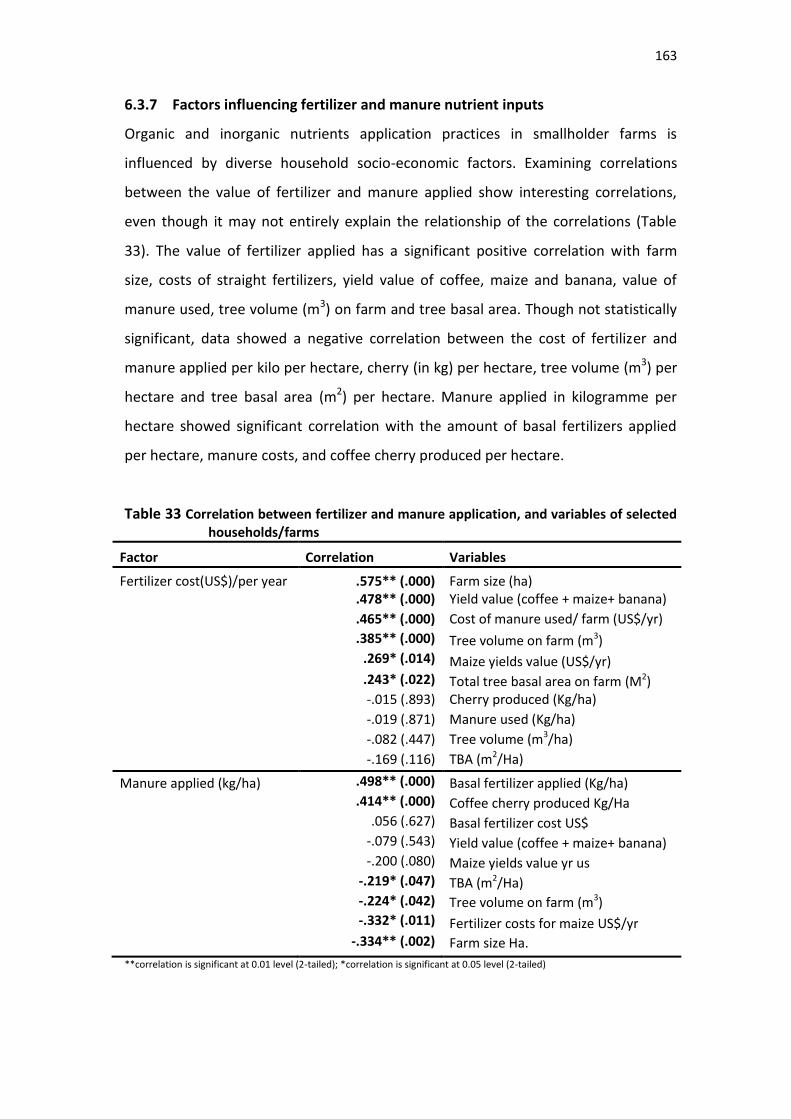
163

6.3.7 Factors influencing fertilizer and manure nutrient inputs

Organic and inorganic nutrients application practices in smallholder farms is

influenced by diverse household socio-economic factors. Examining correlations

between the value of fertilizer and manure applied show interesting correlations,

even though it may not entirely explain the relationship of the correlations (Table

33). The value of fertilizer applied has a significant positive correlation with farm

size, costs of straight fertilizers, yield value of coffee, maize and banana, value of

manure used, tree volume (m3) on farm and tree basal area. Though not statistically

significant, data showed a negative correlation between the cost of fertilizer and

manure applied per kilo per hectare, cherry (in kg) per hectare, tree volume (m3) per

hectare and tree basal area (m2) per hectare. Manure applied in kilogramme per

hectare showed significant correlation with the amount of basal fertilizers applied

per hectare, manure costs, and coffee cherry produced per hectare.

Table 33 Correlation between fertilizer and manure application, and variables of selected households/farms

Factor Correlation Variables

Fertilizer cost(US$)/per year .575** (.000) Farm size (ha) .478** (.000) Yield value (coffee + maize+ banana)

.465** (.000) Cost of manure used/ farm (US$/yr)

.385** (.000) Tree volume on farm (m3)

.269* (.014) Maize yields value (US$/yr) .243* (.022) Total tree basal area on farm (M2) -.015 (.893) Cherry produced (Kg/ha)

-.019 (.871) Manure used (Kg/ha)

-.082 (.447) Tree volume (m3/ha)

-.169 (.116) TBA (m2/Ha)

Manure applied (kg/ha) .498** (.000) Basal fertilizer applied (Kg/ha) .414** (.000) Coffee cherry produced Kg/Ha .056 (.627) Basal fertilizer cost US$ -.079 (.543) Yield value (coffee + maize+ banana) -.200 (.080) Maize yields value yr us -.219* (.047) TBA (m2/Ha) -.224* (.042) Tree volume on farm (m3)

-.332* (.011) Fertilizer costs for maize US$/yr -.334** (.002) Farm size Ha.

**correlation is significant at 0.01 level (2-tailed); *correlation is significant at 0.05 level (2-tailed)

164

There is a negative correlation (statistically significant) between manure application,

and tree basal area, tree volume, fertilizer cost for maize and farm size. This perhaps

is due to targeted application practices practiced by farmers. Trees on farm do not

receive any manure application directly unlike crops, while larger farm sizes have

much smaller proportionate application compared to the smaller farms.

Interestingly, there was no significant correlation between the size of TLU versus the

amount of manure applied, perhaps confirming the limited use of manure or it’s

availability on farm.

6.4 DISCUSSION

Soil fertility between smallholder farms is widely varied - large quantities of nutrients

from small farm parcels are lost through coffee exports, given that inadequate

quantities of manure and fertilizer are presently used to replenish the soil. Sanchez

(2002) estimates a high mean depletion rate of 22 kg of N; 2.5 kg of P, and 15 kg of K

are lost per hectare per year, on cultivated land over the last 30 years in 37 African

countries. This is equivalent to an annual loss of US $4 billion in fertilizer. In Western

Kenya, 80% of the land by smallholders, mainly under maize cultivation is extremely

deficient in P.

Results suggest that nutrient prevalence is closely related to farmers’ choice of crops

and its market performance. Farmers in coffee systems source nutrients from

fertilizers and animal manure to target crops such as coffee, maize, banana, Irish

potato and olericulture. It is clear that fertilizer rather than manure application is

more preferred for annuals than perennials. Fertilizer and manure application are

nonetheless positively correlated suggesting their application complementarities.

Manure application is however negatively correlated to farm size probably indicating

its insufficiency for whole farm application.

Unlike a positive correlation between fertilizer application and farm tree basal area

(m2), manure application was negatively correlated to tree basal area. This is perhaps

suggestive of a wider fertilizer application on farm parcels which benefits trees,

unlike manure application which is limited. Coffee also receives high fertilizer inputs

165

perhaps due to credit facilities from cooperatives and government subsidies under

the ‘economic stimulus programme’. The program more recently provided

smallholders subsidized fertilizers and seeds to compensate for total crop loss

experienced during droughts.

In spite of seemingly sizeable fertilizer and manure application reported by farmers,

soil analysis showed that organic C, total N, and P are the most deficient nutrients in

smallholder coffee farms. Interestingly, the main types of fertilizers consumed by

farmers in the surveyed area and indeed in Kenya are compound fertilizers that

provide both Nitrogen and Phosphate. Macro-nutrient deficiency has severe

productivity implications to farmers and is likely to be exacerbated by nutrients

exports through coffee and increased horticulture farming activities. Bases such as,

Ca, Mg, were satisfactory for Meru but very low in Embu and highly variable in

Kirinyaga. Principal component analysis identified the significance of B prevalence

under PC1 score. B is often an ignored micronutrient in coffee systems despite its

important contribution in ensuring quality coffee yields. Boron was very low (< 0.5

ppm at 75% percentile) in Kirinyaga, followed by Embu and Meru. B assessment in

coffee systems of Ghana showed effects of its low levels on coffee plant growth

since it is associated with plant cell division, lignification and other produce quality. B

is related to the amount of Ca (Ca/B ratio) and is prevalent in low PH soils of less

than 6.5. Its supplementation would therefore be preferred through fertilizer

application other than soil acidification.

Soil fertility management by farm categories showed a slight nutrient decline in the

‘decreasing’ farmer category compared to the ‘increasing’ and ‘constant’ categories.

This is perhaps due to reduced nutrient inputs with less return from coffee; less

fertilizer is received from farmer cooperative society market arrangements since this

is provided against coffee cherry deliveries. Nutrient application has been linked to

household wealth status by Nkonya et al., 2005 who observed that land use systems

for wealthier farmers in Uganda showed higher N and P balances than systems with

poorer farmers.

166

Soil nutrient mining cannot therefore be generalized (Cobo et al., 2010). There is

however a need to use reliable indicators of soil nutrient mining and associated land

degradation. Studies on soil nutrient inflow and outflows have showed that negative

nutrient balances, do not necessarily imply an immediate decline in crop production

as soils with high nutrient stocks can still support continued cultivation for several

years (Palm et al., 1997; de Jager et al., 1998). Hence, the dynamics of soil fertility

decline (i.e. nutrient mining) or recovery (i.e. nutrient accumulation) is better

estimated as a rate of change (proportion) of the total soil nutrient stocks.

6.5 CONCLUSIONS

Through NIR diagnostic tools, soil sample analysis was performed in a relatively rapid

and accurate manner enabling nutrient prevalence assessments in smallholder

coffee farms of Mount Kenya to be determined. Constructed partial least square

calibration models for principal component scores on spectra, showed a high

coefficient of determination (r2 = 0.87) confirming that infrared techniques

adequately accounted for variations in the analyzed samples with only about 13%

loss of information. Predictions for P, Zn, and Na were nonetheless sub-optimal,

probably due to errors in principal components extraction and accuracy of the wet

chemistry soil sample tests. Developed nutrient indicators scores provided a rapid

way of investigating correlations with assembled household socio-economic factors.

Results showed that smallholder coffee farms are deficient in organic C, N and P in

spite of seemingly improved NP-compound fertilizer applications offered through

market instruments in the coffee subsector. Manure application was confirmed to be

insufficient and is negatively correlated to farm size but positively correlated to basal

fertilizer application, indicating possible complementarities. Measurement of

application per household was difficult due to different sources of manure, timing

and measure of application. Labour constraints appeared to impede manure

utilization. Other than an acute deficiency of organic C and total N, sample analysis

showed wide variability of B prevalence across the survey sites, with Kirinyaga

showing the lowest levels in the three sites studied. Even though largely ignored, B is

one of the most important soil micronutrients in coffee systems with prevalence

167

determined by Ca/B ratio. Embu coffee farms were found to be most deficient in

bases followed by Kirinyaga and Meru.

Results are sufficiently robust to suggest that nutrient prevalence in small coffee

farms are associated with application costs of organic manure and fertilizer; yields of

coffee and food-crops; tree basal area and farm size. It is clear that dis-incentives in

the coffee subsector which tends to reduce coffee yield productivity will have

negative effects on fertilizer and manure inputs on smallholder coffee farms.

168

6.6 REFERENCES

Carter, SE. 1997. Spatial Stratification of Western Kenya as a Basis for Research on

Soil Fertility Management. Agricultural Systems 55(1): 45-70.

CAMO Inc. 2006. The Unscrambler user manual. CAMO Inc, Corvallis, OR.

CBS (Central Bureau of Statistics) 2008. Geographic dimensions of well being in

Kenya. ‘Who and where are the poor in Kenya? A constituency level profile Vol. II

Cobo, JG, Dercon, G, Cadisch, G. 2010. Nutrient balances in African land use systems

across different spatial scales: A review of approaches, challenges and progress.

Agriculture, Ecosystems and Environment 136: 1–15.

De Jager, A, Kariuki, I. Matiri, FM. Odendo M, Wanyama, JM. 1998. Linking economic

performance and nutrient balances in different farming systems in Kenya: a

synthesis towards an integrated analysis of economic and ecological

sustainability. Agriculture, Ecosystems and Environment 71: 81–92.

Haaland, DM and Jones, HDT (ud) Weighted partial least squares method to improve

calibration precision for spectroscopic noise-limited data. Sandia National

laboratories, Albuquerqe, NM 87185-0342.

Haggblade S and Jayne, T. (u.d) Fertilizer Marketing in Eastern and Southern Africa.

Policy Synthesis No.1. Common Market for Eastern and Southern Africa

(COMESA) African Agricultural Markets Programme.

http://www.aec.msu.edu/fs2/aamp/seminar_2/Fertilizer_Policy_Synthesis.pdf

(Accessed 18th/09/2011).

Huxley, P. 1996. Biological factors affecting form and functions in woody-non woody

plant mixtures in eds. Ong CK and Huxley P 1996 tree crop interactions- a

physiological approach. Cab International Wallingford, UK.

ICRAF 2001. International Centre for Research in Agroforestry, Laboratory methods

for soil and plant analysis. ICRAF, Nairobi, Kenya.

ICRAF (World Agroforestry Centre) 2009. Creating an Evergreen Agriculture in Africa.

World Agroforestry Centre, Nairobi.

Janik, LJ, Skjemstand, JO and Raven, MD. 1995. Characterization and Analysis of Soils

using Mid-infrared Partial Least Squares .I. Correlations with XRF-determined

Major Element Composition Australian Journal of Soil Research 33:621-36.

169

Jaetzold, R and Schmidt, H. 2007. Farm management handbook of Kenya (vol.II),

Eastern Kenya, Ministry of Agriculture, Nairobi.

Lewbel, A. 2006. Engel curves: entry for the new palgrave dictionary of economics,

Second edition.

Muchena, FN, Onduru, DD, Gachini, GN and De Jager, A. 2005. Turning the tides of

soil degradation in Africa: capturing the reality and exploring opportunities. Land

Use Policy 22:23–31.

Mwangi, W. 1996. Low Use of Fertilizer and Low Productivity in Sub-Saharan Africa.

NRG Paper 96-05. CIMMYT, Mexico, DP.

Ngoze, S, Riha, S, Mbugua, D, Shepherd, KD, Verchot L, Barrett, CB, Lehmann, J,

Wangila, J and Pell, A. 2008. The Impacts of Household Land Use and Socio

Economic Factors on the Soil Fertility of Smallholder Farms in the Highlands of

Kenya. Working Paper. Available : http://ssrn.com/abstract=1141986.

Nkonya, E, Kaizzi, C and Pender, J. 2005. Determinants of nutrient balances in a

maize farming system in eastern Uganda. Agricultural Systems 85:155–182.

Odendo, M, de Groote, H, Wanyama, J, Bett, C and Okuro, J. 2007. Analysis of the

maize seed and fertilizer market in Kenya: a survey of stockists African Crop

Science Conference Proceedings, African Crop Science Society 8:2153-2156.

Omamo, SW. and Mose, LO. 2001. Fertilizer trade under market liberalization:

preliminary evidence from Kenya. Food Policy 26:1–10.

Omamo, SW, Williams, JC, Obare, GA and Ndiwa, NN. 2002. Soil fertility

management on small farms in Africa: evidence from Nakuru District, Kenya.

Food Policy 27:159–170.

Palm, CA. Myers, RJK and Nandwa, SM. 1997. Combined use of organic and inorganic

nutrient sources for soil fertility maintenance and replenishment. In: Buresh, R.J.,

Sanchez, P.A., Calhoun, F. (Eds.), Replenishing Soil Fertility in Africa. Soil Science

Society of America, Madison, Wisconsin.

Place, F. Adato, M, Hebinck, P and Omosa, M. 2005. The impact of agroforestry soil

replenishment practices on the poor in western Kenya. Research report 142

International Food policy Research Institute.

Sanchez, PA. 2002. Soil fertility and hunger in Africa. Science vol. 295. no. 5562 pp.

2019-2020

170

Sanchez, PA. 2010. Tripling crop yields in tropical Africa. Nature Geoscience 3: 299-

300.

Sanchez, PA and Jama B. 2002. Soil fertility replenishment takes off in East and

Southern Africa. In: B. Vanlauwe, J. Diels, N. Sanginga and R. Merck X, Editors,

Integrated Plant Nutrient Management in Sub-Saharan Africa: From Concept to

Practice, CABI, Wallingford pp. 23–46.

Sanchez, PA, Shepherd, KD, Soule, MJ, Place, FM, Buresh RJ, Izac AMI, Mokwunye,

AU, Kwesiga, FR. Ndiritu, CG and Woomer, PL. 1997. Soil ferility replenishment in

Africa: an investment in natural resource capital. In: Buresh, R.J., Sanchez, P.A.,

Calhoun, F. (Eds.), Replenishing SoilFertility in Africa. Soil Science Society of

America, Madison, Wisconsin.

Shepherd, KD and Walsh, MG. 2002. Development of Reflectance Spectral Libraries

for Characterization of Soil Properties. Soil Science Society of America Journal 66:

988–998.

Shepherd, KD and Walsh, MG. 2007. Infrared spectroscopy—enabling an evidence-

based diagnostic surveillance approach to agricultural and environmental

management in developing countries. Journal of Near Infrared Spectroscopy 15:

1-19.

Smaling, EMA, Nandwa, SM and Janssen, BH. 1997. Soil fertility in Africa is at stake.

In: Buresh RJ, Sanchez PA, Calhoun F, (Eds.), Replenishing Soil Fertility in Africa.

Soil Science Society of America, Madison, Wisconsin.

SPSS for windows version 15(2006).

Stern, RD, Coe, R, Allan EF and Dale, IC. 2004. Good statistical practice for natural

resources research. CABI Publishing, CABI.Wallingford Oxfordshire UK.

Swift, MJ and Shepherd, KD. (Eds) 2007. Saving Africa’s Soils: Science and Technology

for Improved Soil Management in Africa. Nairobi: World Agroforestry Centre.

Tittonell, P, Vanlauwe B. Laffelaar, PA, Shepherd, KD and Giller, KE. 2005. Exploring

diversity in soil fertility management of smallholder farms in western Kenya II.

Within farm variability in resource allocation, nutrient flows and soil fertility

status. Agriculture ecosystems and environment 110:166-184.

171

Waithaka, MM, Thornton, PK. Shepherd, KD and Ndiwa, NN. 2007. Factors affecting

the use of fertilizers by smallholders: the case of vihiga, western Kenya. Nutrient.

Cycling in Agroecosytems 78:211-224.

Yamano, T, Jayne, TS and Nyoro, J. 2003. Interlinked Credit and Farm Intensification:

Evidence from Kenya. Selected paper, International Association of Agricultural

Economists meeting, August 16-22, Durban, South Africa.

172

CHAPTER 7

7.0 CONCLUSIONS

This study has illustrated a number of factors associated with smallholder decision

making and transitions within coffee agroforestry systems of Mount Kenya. A better

understanding of farmers’ position with respect to their resources and livelihood

strategies in managing coffee farms under conditions of reduced enterprise

profitability is underscored. These factors were more closely measured by adopting a

farming systems typology that used coffee production to mirror the productivity and

concomitant management behaviour of smallholder coffee farms. The approach was

followed in order to aid the design and implementation of policy concepts that are of

interest to heterogeneous farmers who are often assumed to be a homogeneous

group.

Results from this study imply that policy instruments to substantially increase the

value of maize and banana produced by coffee farmers will have significant

enterprise shifts among farmers with smaller land sizes and already declining or

stagnated coffee production. However measures such as improved dairy production

and returns seem to cushion farmers intending to expand or maintain coffee

production. The typology of coffee farms used to assess smallholder productivity

behavior proposed here may be generalized consistently across coffee landscapes

studied, to contribute to better targeting of innovations. Generally, land size, coffee

production (number of bushes, cherry yields/ha), livestock units, agro forestry trees,

banana, maize value, nutrients (manure and fertilizer) and labour costs influence

farm productivity, and are ideally used to distinguish between farm types.

Smallholder annual crop diversification or intensification practices will most likely

result in lower agroforestry tree species richness and probably landscape domination

by some popular (usually exotic) species. This trend appears to be accelerated by

reduction of the perennial cash crop, namely coffee. Farmer are accumulating more

exotics such as Grevillea robusta, Eucalyptus sp. Macadamia sp. and Mangifera

173

indica on coffee farm plots, thereby displacing usual native species such as Croton

macrostychyus and Vitex keniensis. Cordia africana however shows high abundance

within coffee systems, perhaps due to its excellent compatibility qualities with coffee

and crop polycultures. Tree abundance and basal area distribution show small-tree

diversity and high relative densities suggesting rapid tree compositional turnover.

This implies changing patterns and structures of tree populations on coffee farms.

Small tree-size diversity, unevenly distributed among farms, has implications if farm

tree populations are to be considered for germplasm provisioning (possible low

viability). Further, botanical families are skewed, showing patterns of distribution

that perhaps have been ignored during priority setting of species domestication.

Biophysical assessments of the prevalence of farm nutrients showed that

smallholder coffee farms are primarily deficient in organic C, N and P, in spite of

improved NP-compound fertilizer applications. Manure application is implied to be

largely insufficient and negatively correlated to farm size, but positively correlated to

basal fertilizer application, suggestive of complementarities. Measurement of

manure application per household was noted to be cumbersome due to the many

different sources and timing of application. Assembled data suggests that labour

demands impede manure utilization.

Other than an acute deficiency of organic C and total N, sample analysis showed a

wide variability of B prevalence across the survey sites, with Kirinyaga showing the

lowest levels of the three sites studied. Even though generally ignored, B is one of

the most important soil micro nutrients in coffee systems, with prevalence

determined by the Ca/B ratio. It’s more prevalent in acidic soils. Embu coffee farms

are most deficient in bases followed by Kirinyaga and Meru. Results are sufficiently

robust to suggest that nutrient prevalence in small coffee systems may be associated

with a combination of use of organic manures and fertilizers, yields of coffee and

food-crops, tree basal area, farm size, and costs of fertilizers.

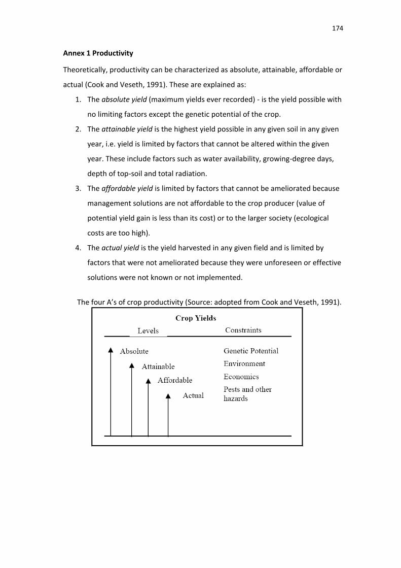
174

Annex 1 Productivity

Theoretically, productivity can be characterized as absolute, attainable, affordable or

actual (Cook and Veseth, 1991). These are explained as:

1. The absolute yield (maximum yields ever recorded) - is the yield possible with

no limiting factors except the genetic potential of the crop.

2. The attainable yield is the highest yield possible in any given soil in any given

year, i.e. yield is limited by factors that cannot be altered within the given

year. These include factors such as water availability, growing-degree days,

depth of top-soil and total radiation.

3. The affordable yield is limited by factors that cannot be ameliorated because

management solutions are not affordable to the crop producer (value of

potential yield gain is less than its cost) or to the larger society (ecological

costs are too high).

4. The actual yield is the yield harvested in any given field and is limited by

factors that were not ameliorated because they were unforeseen or effective

solutions were not known or not implemented.

The four A’s of crop productivity (Source: adopted from Cook and Veseth, 1991).

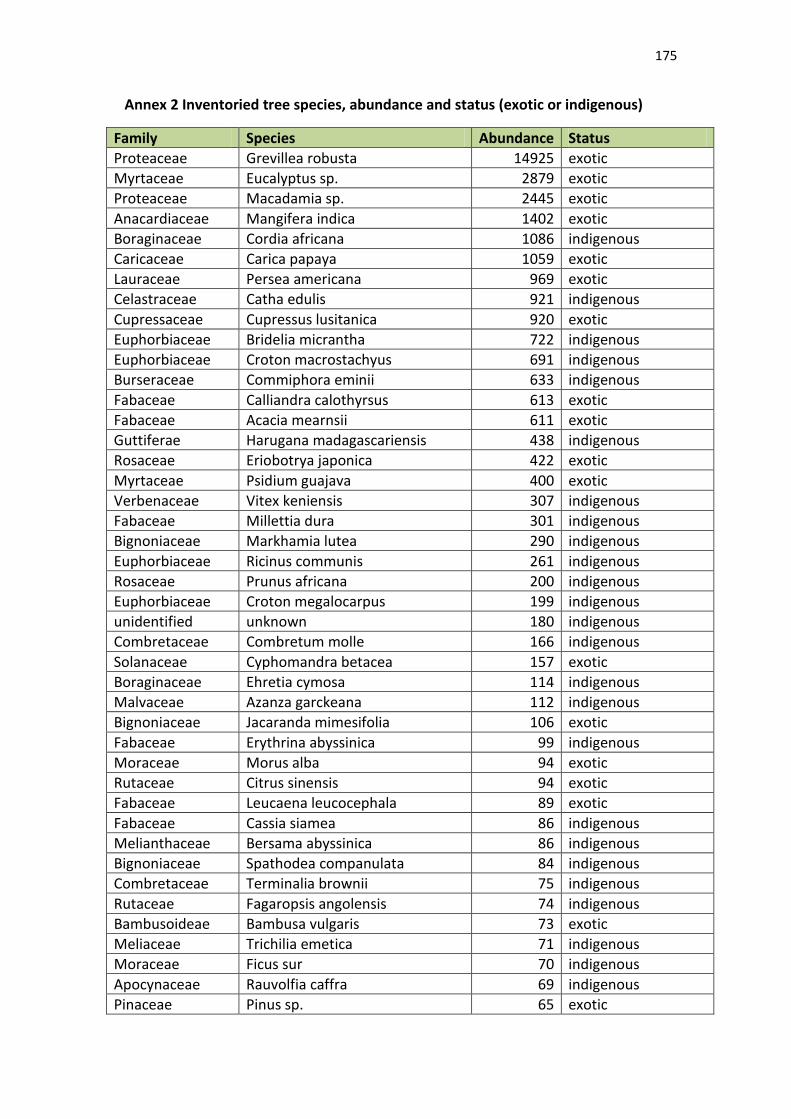
175

Annex 2 Inventoried tree species, abundance and status (exotic or indigenous)

Family Species Abundance Status

Proteaceae Grevillea robusta 14925 exotic

Myrtaceae Eucalyptus sp. 2879 exotic

Proteaceae Macadamia sp. 2445 exotic

Anacardiaceae Mangifera indica 1402 exotic

Boraginaceae Cordia africana 1086 indigenous

Caricaceae Carica papaya 1059 exotic

Lauraceae Persea americana 969 exotic

Celastraceae Catha edulis 921 indigenous

Cupressaceae Cupressus lusitanica 920 exotic

Euphorbiaceae Bridelia micrantha 722 indigenous

Euphorbiaceae Croton macrostachyus 691 indigenous

Burseraceae Commiphora eminii 633 indigenous

Fabaceae Calliandra calothyrsus 613 exotic

Fabaceae Acacia mearnsii 611 exotic

Guttiferae Harugana madagascariensis 438 indigenous

Rosaceae Eriobotrya japonica 422 exotic

Myrtaceae Psidium guajava 400 exotic

Verbenaceae Vitex keniensis 307 indigenous

Fabaceae Millettia dura 301 indigenous

Bignoniaceae Markhamia lutea 290 indigenous

Euphorbiaceae Ricinus communis 261 indigenous

Rosaceae Prunus africana 200 indigenous

Euphorbiaceae Croton megalocarpus 199 indigenous

unidentified unknown 180 indigenous

Combretaceae Combretum molle 166 indigenous

Solanaceae Cyphomandra betacea 157 exotic

Boraginaceae Ehretia cymosa 114 indigenous

Malvaceae Azanza garckeana 112 indigenous

Bignoniaceae Jacaranda mimesifolia 106 exotic

Fabaceae Erythrina abyssinica 99 indigenous

Moraceae Morus alba 94 exotic

Rutaceae Citrus sinensis 94 exotic

Fabaceae Leucaena leucocephala 89 exotic

Fabaceae Cassia siamea 86 indigenous

Melianthaceae Bersama abyssinica 86 indigenous

Bignoniaceae Spathodea companulata 84 indigenous

Combretaceae Terminalia brownii 75 indigenous

Rutaceae Fagaropsis angolensis 74 indigenous

Bambusoideae Bambusa vulgaris 73 exotic

Meliaceae Trichilia emetica 71 indigenous

Moraceae Ficus sur 70 indigenous

Apocynaceae Rauvolfia caffra 69 indigenous

Pinaceae Pinus sp. 65 exotic

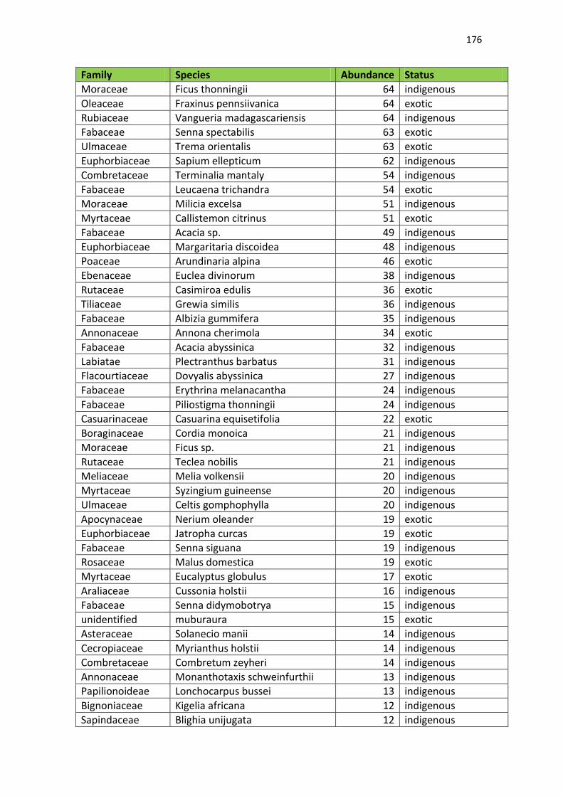
176

Family Species Abundance Status

Moraceae Ficus thonningii 64 indigenous

Oleaceae Fraxinus pennsiivanica 64 exotic

Rubiaceae Vangueria madagascariensis 64 indigenous

Fabaceae Senna spectabilis 63 exotic

Ulmaceae Trema orientalis 63 exotic

Euphorbiaceae Sapium ellepticum 62 indigenous

Combretaceae Terminalia mantaly 54 indigenous

Fabaceae Leucaena trichandra 54 exotic

Moraceae Milicia excelsa 51 indigenous

Myrtaceae Callistemon citrinus 51 exotic

Fabaceae Acacia sp. 49 indigenous

Euphorbiaceae Margaritaria discoidea 48 indigenous

Poaceae Arundinaria alpina 46 exotic

Ebenaceae Euclea divinorum 38 indigenous

Rutaceae Casimiroa edulis 36 exotic

Tiliaceae Grewia similis 36 indigenous

Fabaceae Albizia gummifera 35 indigenous

Annonaceae Annona cherimola 34 exotic

Fabaceae Acacia abyssinica 32 indigenous

Labiatae Plectranthus barbatus 31 indigenous

Flacourtiaceae Dovyalis abyssinica 27 indigenous

Fabaceae Erythrina melanacantha 24 indigenous

Fabaceae Piliostigma thonningii 24 indigenous

Casuarinaceae Casuarina equisetifolia 22 exotic

Boraginaceae Cordia monoica 21 indigenous

Moraceae Ficus sp. 21 indigenous

Rutaceae Teclea nobilis 21 indigenous

Meliaceae Melia volkensii 20 indigenous

Myrtaceae Syzingium guineense 20 indigenous

Ulmaceae Celtis gomphophylla 20 indigenous

Apocynaceae Nerium oleander 19 exotic

Euphorbiaceae Jatropha curcas 19 exotic

Fabaceae Senna siguana 19 indigenous

Rosaceae Malus domestica 19 exotic

Myrtaceae Eucalyptus globulus 17 exotic

Araliaceae Cussonia holstii 16 indigenous

Fabaceae Senna didymobotrya 15 indigenous

unidentified muburaura 15 exotic

Asteraceae Solanecio manii 14 indigenous

Cecropiaceae Myrianthus holstii 14 indigenous

Combretaceae Combretum zeyheri 14 indigenous

Annonaceae Monanthotaxis schweinfurthii 13 indigenous

Papilionoideae Lonchocarpus bussei 13 indigenous

Bignoniaceae Kigelia africana 12 indigenous

Sapindaceae Blighia unijugata 12 indigenous

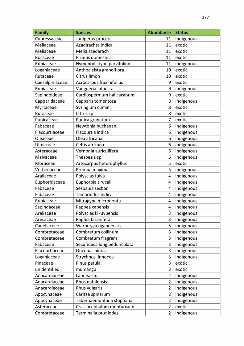
177

Family Species Abundance Status

Cupressaceae Juniperus procera 11 indigenous

Meliaceae Azadirachta indica 11 exotic

Meliaceae Melia azedarach 11 exotic

Rosaceae Prunus domestica 11 exotic

Rubiaceae Hymenodictyon parvifolium 11 indigenous

Loganiaceae Anthocleista grandiflora 10 exotic

Rutaceae Citrus limon 10 exotic

Caesalpiniaceae Acrocarpus fraxinifolius 9 exotic

Rubiaceae Vangueria infausta 9 indigenous

Sapindoideae Cardiospermum halicacabum 9 exotic

Capparidaceae Capparis tomentosa 8 indigenous

Myrtaceae Syzingium cuminii 8 exotic

Rutaceae Citrus sp. 8 exotic

Punicaceae Punica granatum 7 exotic

Fabaceae Newtonia buchananii 6 indigenous

Flacourtiaceae Flacourtia indica 6 indigenous

Oleaceae Olea africana 6 indigenous

Ulmaceae Celtis africana 6 indigenous

Asteraceae Vernonia auriculifera 5 indigenous

Malvaceae Thespesia sp 5 indigenous

Moraceae Artocarpus heterophyllus 5 exotic

Verbenaceae Premna maxima 5 indigenous

Araliaceae Polyscias fulva 4 indigenous

Euphorbiaceae Euphorbia tirucali 4 indigenous

Fabaceae Sesbania sesban 4 indigenous

Fabaceae Tamarindus indica 4 indigenous

Rubiaceae Mitragyna microdonta 4 indigenous

Sapindaceae Pappea capensis 4 indigenous

Araliaceae Polyscias kikuyuensis 3 indigenous

Arecaceae Raphia faranifera 3 indigenous

Canellaceae Warburgia ugandensis 3 indigenous

Combretaceae Combretum collinum 3 indigenous

Combretaceae Combretum fragrans 3 indigenous

Fabaceae Securidaca longipedunculata 3 indigenous

Flacourtiaceae Oncoba spinosa 3 indigenous

Loganiaceae Strychnos innocua 3 indigenous

Pinaceae Pinus patula 3 exotic

unidentified mumangu 3 exotic

Anacardiaceae Lannea sp. 2 indigenous

Anacardiaceae Rhus natalensis 2 indigenous

Anacardiaceae Rhus vulgaris 2 indigenous

Apocynaceae Carissa spinarum 2 indigenous

Apocynaceae Tabernaemontana stapfiana 2 indigenous

Asteraceae Crassocephalum montuosum 2 exotic

Combretaceae Terminalia pruniodes 2 indigenous

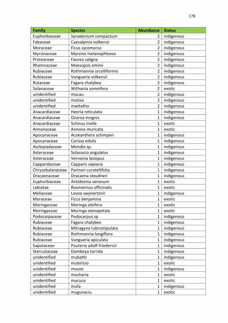
178

Family Species Abundance Status

Euphorbiaceae Synadenium compactum 2 indigenous

Fabaceae Caesalpinia volkensii 2 indigenous

Moraceae Ficus sycomorus 2 indigenous

Myrsinaceae Myrsine melanophloeos 2 indigenous

Proteaceae Faurea saligna 2 indigenous

Rhamnaceae Maesopsis eminii 2 indigenous

Rubiaceae Rothmannia urcelliformis 2 indigenous

Rubiaceae Vangueria volkensii 2 indigenous

Rutaceae Fagara chalybea 2 indigenous

Solanaceae Withania somnifera 2 exotic

unidentified mucau 2 indigenous

unidentified mutiso 2 indigenous

unidentified mwitatho 2 indigenous

Anacardiaceae Heeria reticulata 1 indigenous

Anacardiaceae Ozoroa insignis 1 indigenous

Anacardiaceae Schinus molle 1 exotic

Annonaceae Annona muricata 1 exotic

Apocynaceae Acokanthera schimperi 1 indigenous

Apocynaceae Carissa edulis 1 indigenous

Asclepiadaceae Mondia sp. 1 indigenous

Asteraceae Solanacio angulatus 1 indigenous

Asteraceae Vernonia lasiopus 1 indigenous

Capparidaceae Capparis sepiaria 1 indigenous

Chrysobalanaceae Parinari curatellifolia 1 indigenous

Dracaenaceae Dracaena steudneri 1 indigenous

Euphorbiaceae Antidesma venosum 1 exotic

Labiatae Rosmarinus officinalis 1 exotic

Meliaceae Lovoa swynertonii 1 indigenous

Moraceae Ficus benjamina 1 exotic

Moringaceae Moringa oleifera 1 exotic

Moringaceae Moringa stenopetala 1 exotic

Podocarpaceae Podocarpus sp 1 indigenous

Rubiaceae Fagara chalybea 1 indigenous

Rubiaceae Mitragyna rubrostipulata 1 indigenous

Rubiaceae Rothmannia longiflora 1 indigenous

Rubiaceae Vangueria apiculata 1 indigenous

Sapotaceae Pouteria adolf-friedericii 1 indigenous

Sterculiaceae Dombeya torrida 1 indigenous

unidentified mubathi 1 indigenous

unidentified mubiricio 1 exotic

unidentified mucee 1 indigenous

unidentified mucharia 1 exotic

unidentified mucuca 1 exotic

unidentified mufa 1 indigenous

unidentified mugunaciu 1 exotic

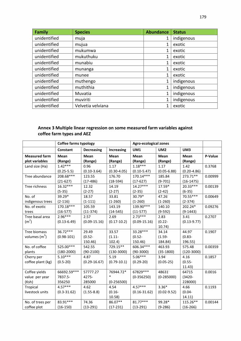
179

Family Species Abundance Status

unidentified muja 1 indigenous

unidentified mujua 1 exotic

unidentified mukumwa 1 exotic

unidentified mukuthuku 1 exotic

unidentified munabiu 1 exotic

unidentified munanga 1 exotic

unidentified munee 1 exotic

unidentified muthengo 1 indigenous

unidentified muthithia 1 indigenous

unidentified Muvatia 1 indigenous

unidentified muviriti 1 indigenous

unidentified Velvetia velviana 1 exotic

Annex 3 Multiple linear regression on some measured farm variables against coffee farm types and AEZ

Coffee farms typology Agro-ecological zones

Constant Decreasing Increasing UM1 UM2 UM3

Measured farm plot variables

Mean (Range)

Mean (Range)

Mean (Range)

Mean (Range)

Mean (Range)

Mean (Range)

P-Value

Land size (Ha) 1.42*** (0.25-5.5)

0.96 (0.10-3.64)

1.17 (0.30-4.05)

1.18*** (0.10-5.47)

1.17 (0.05-6.88)

1.42 (0.20-4.86)

0.3768

Tree abundance 208.68*** (21-627)

123.55 (17-486)

176.70 (18-594)

170.14*** (17-627)

185.84 (9-701)

273.71** (16-1475)

0.00999

Tree richness 16.32*** (5-35)

12.32 (2-27)

14.19.

(2-27) 14.27*** (2-35)

17.59* (2-42)

20.33*** (6-35)

0.00139

No. of indigenous trees

39.29* (2-116)

18.57 (1-111)

33.81 (1-260)

30.79* (1-260)

47.26.

(1-260) 70.55*** (2-374)

0.00649

No. of exotic trees

170.18*** (16-577)

105.59 (11-374)

143.19 (14-545)

139.90*** (11-577)

140.10 (9-592)

202.24* (9-1443)

0.09276

Tree basal area (m

2)

2.96*** (0.13-6.49)

2.57 (0.09-15.16)

2.69 (0.17-10.2)

2.73*** (0.09-15.16)

2.83 (0.22-10.74)

3.41 (0.13-9.77)

0.2707

Tree biomass volumes (m

3)

36.72*** (0.98-101)

29.49 (0.52-150.46)

33.57 (1.11-102.4)

33.28*** (0.52-150.46)

34.14 (1.59-184.84)

44.97.

(0.83-196.55)

0.1907

No. of coffee plants

525.00*** (180-2000)

542.55 (90-2100)

729.15** (130-3000)

606.34*** (90-3000)

463.93 (35-1800)

575.48 (120-3000)

0.00359

Cherry per coffee plant (kg)

5.10*** (0.5-20)

4.87 (0.29-16.67)

5.19 (0.79-10.1)

5.06*** (0.29-20)

3.94.

(0.05-25) 4.16 (0.55-11.43)

0.1857

Coffee yields value per year (Ksh)

66692.59*** 7837.5-356250

57777.27 4275-285000

76944.72** (0-256500)

67829*** (0-356250)

48631.

(0-285000) 64715 (3420-228000)

0.0016

Tropical livestock units

4.57*** (0.3-31.62)

4.62 (1.55-8.8)

4.54 (0.16-10.58)

4.57*** (0.16-31.62)

3.36* (0.02-9.52)

4.66 (0.04-14.11)

0.1193

No. of trees per coffee plot

83.91*** (16-150)

74.36 (13-291)

86.07** (17-231)

81.77*** (13-291)

99.28* (9-286)

115.26** (16-266)

0.00144

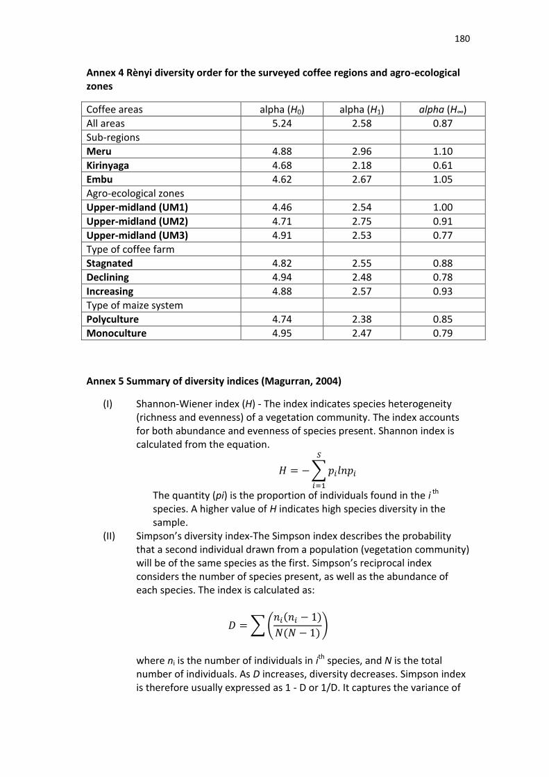
180

Annex 4 Rènyi diversity order for the surveyed coffee regions and agro-ecological zones

Coffee areas alpha (H0) alpha (H1) alpha (H∞)

All areas 5.24 2.58 0.87

Sub-regions

Meru 4.88 2.96 1.10

Kirinyaga 4.68 2.18 0.61

Embu 4.62 2.67 1.05

Agro-ecological zones

Upper-midland (UM1) 4.46 2.54 1.00

Upper-midland (UM2) 4.71 2.75 0.91

Upper-midland (UM3) 4.91 2.53 0.77

Type of coffee farm

Stagnated 4.82 2.55 0.88

Declining 4.94 2.48 0.78

Increasing 4.88 2.57 0.93

Type of maize system

Polyculture 4.74 2.38 0.85

Monoculture 4.95 2.47 0.79

Annex 5 Summary of diversity indices (Magurran, 2004)

(I) Shannon-Wiener index (H) - The index indicates species heterogeneity (richness and evenness) of a vegetation community. The index accounts for both abundance and evenness of species present. Shannon index is calculated from the equation.

∑

The quantity (pi) is the proportion of individuals found in the i th species. A higher value of H indicates high species diversity in the sample.

(II) Simpson’s diversity index-The Simpson index describes the probability that a second individual drawn from a population (vegetation community) will be of the same species as the first. Simpson’s reciprocal index considers the number of species present, as well as the abundance of each species. The index is calculated as:

∑( (

( )

where ni is the number of individuals in ith species, and N is the total number of individuals. As D increases, diversity decreases. Simpson index is therefore usually expressed as 1 - D or 1/D. It captures the variance of

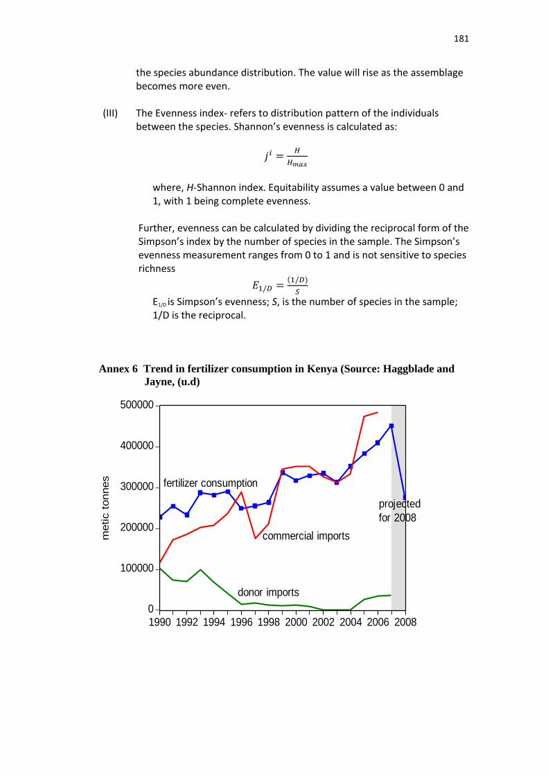
181

the species abundance distribution. The value will rise as the assemblage becomes more even.

(III) The Evenness index- refers to distribution pattern of the individuals

between the species. Shannon’s evenness is calculated as:

where, H-Shannon index. Equitability assumes a value between 0 and 1, with 1 being complete evenness.

Further, evenness can be calculated by dividing the reciprocal form of the Simpson’s index by the number of species in the sample. The Simpson’s evenness measurement ranges from 0 to 1 and is not sensitive to species richness

(

E1/D is Simpson’s evenness; S, is the number of species in the sample; 1/D is the reciprocal.

Annex 6 Trend in fertilizer consumption in Kenya (Source: Haggblade and

Jayne, (u.d)

0

100000

200000

300000

400000

500000

1990 1992 1994 1996 1998 2000 2002 2004 2006 2008

donor imports

commercial imports

fertilizer consumption

projected

for 2008

metic t

onnes

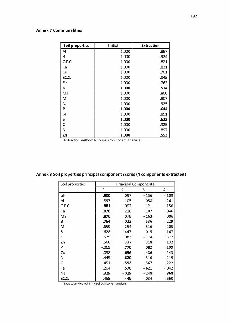
182

Annex 7 Communalities

Soil properties Initial Extraction Al 1.000 .887 B 1.000 .924 C.E.C 1.000 .821 Ca 1.000 .831 Cu 1.000 .701 EC.S. 1.000 .845 Fe 1.000 .762 K 1.000 .514 Mg 1.000 .800 Mn 1.000 .807 Na 1.000 .925 P 1.000 .644 pH 1.000 .851 S 1.000 .622 C 1.000 .925 N 1.000 .897 Zn 1.000 .553 Extraction Method: Principal Component Analysis.

Annex 8 Soil properties principal component scores (4 components extracted)

Soil properties

Principal Components 1 2 3 4

pH .900 .097 -.136 -.109 Al -.897 .105 .058 .261 C.E.C .881 .092 .121 .150 Ca .878 .216 .107 -.046 Mg .876 .078 -.163 .006 B .764 -.022 .536 -.229 Mn .659 -.254 .516 -.205 S -.628 -.447 .015 .167 K .579 .083 -.174 .377 Zn .566 .337 .318 .132 P -.069 .770 .082 .199 Cu .038 .636 -.486 -.243 N -.445 .620 .516 .219 C -.451 .592 .567 .222 Fe .204 .576 -.621 -.042 Na .329 -.029 -.248 .868 EC.S. -.455 .449 -.034 -.660

Extraction Method: Principal Component Analysis

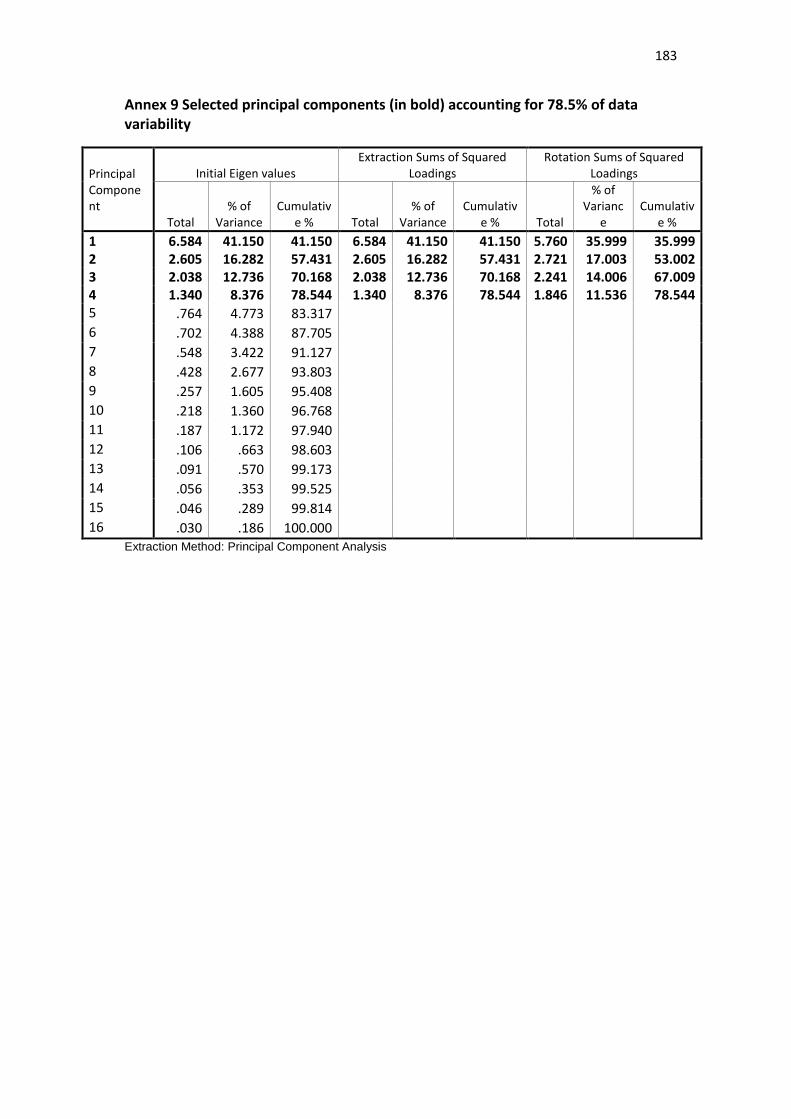
183

Annex 9 Selected principal components (in bold) accounting for 78.5% of data variability

Principal Component

Initial Eigen values Extraction Sums of Squared

Loadings Rotation Sums of Squared

Loadings

Total % of

Variance Cumulativ

e % Total % of

Variance Cumulativ

e % Total

% of Varianc

e Cumulativ

e %

1 6.584 41.150 41.150 6.584 41.150 41.150 5.760 35.999 35.999 2 2.605 16.282 57.431 2.605 16.282 57.431 2.721 17.003 53.002 3 2.038 12.736 70.168 2.038 12.736 70.168 2.241 14.006 67.009 4 1.340 8.376 78.544 1.340 8.376 78.544 1.846 11.536 78.544 5 .764 4.773 83.317 6 .702 4.388 87.705 7 .548 3.422 91.127 8 .428 2.677 93.803 9 .257 1.605 95.408 10 .218 1.360 96.768 11 .187 1.172 97.940 12 .106 .663 98.603 13 .091 .570 99.173 14 .056 .353 99.525 15 .046 .289 99.814 16 .030 .186 100.000

Extraction Method: Principal Component Analysis

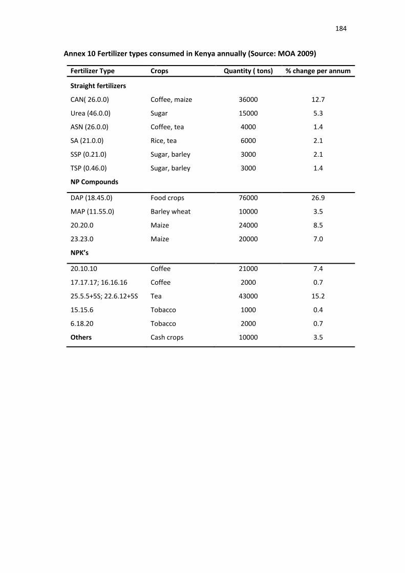
184

Annex 10 Fertilizer types consumed in Kenya annually (Source: MOA 2009)

Fertilizer Type Crops Quantity ( tons) % change per annum

Straight fertilizers

CAN( 26.0.0) Coffee, maize 36000 12.7

Urea (46.0.0) Sugar 15000 5.3

ASN (26.0.0) Coffee, tea 4000 1.4

SA (21.0.0) Rice, tea 6000 2.1

SSP (0.21.0) Sugar, barley 3000 2.1

TSP (0.46.0) Sugar, barley 3000 1.4

NP Compounds

DAP (18.45.0) Food crops 76000 26.9

MAP (11.55.0) Barley wheat 10000 3.5

20.20.0 Maize 24000 8.5

23.23.0 Maize 20000 7.0

NPK’s

20.10.10 Coffee 21000 7.4

17.17.17; 16.16.16 Coffee 2000 0.7

25.5.5+5S; 22.6.12+5S Tea 43000 15.2

15.15.6 Tobacco 1000 0.4

6.18.20 Tobacco 2000 0.7

Others Cash crops 10000 3.5

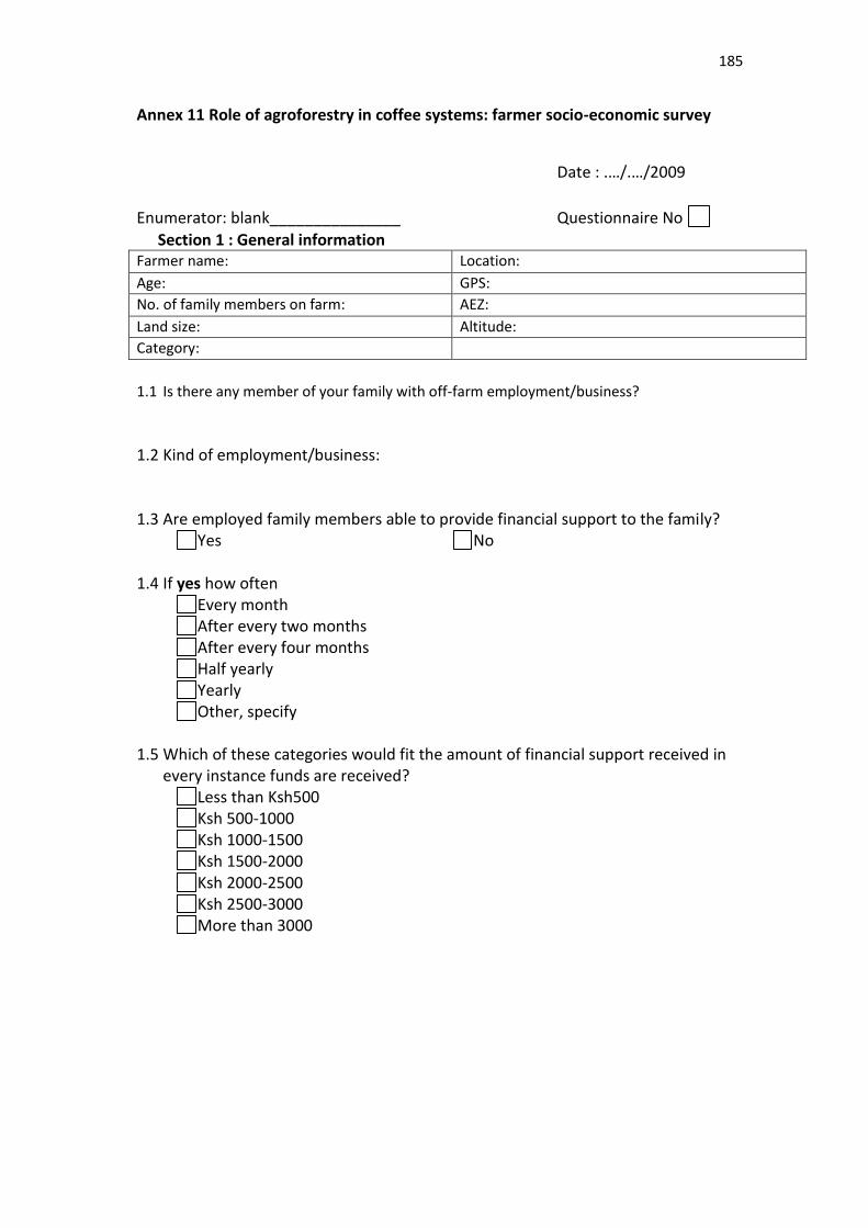
185

Annex 11 Role of agroforestry in coffee systems: farmer socio-economic survey

Date : .…/.…/2009

Enumerator: blank_______________ Questionnaire No

Section 1 : General information Farmer name: Location:

Age: GPS: No. of family members on farm: AEZ:

Land size: Altitude: Category:

1.1 Is there any member of your family with off-farm employment/business?

1.2 Kind of employment/business: 1.3 Are employed family members able to provide financial support to the family?

Yes No 1.4 If yes how often

Every month After every two months After every four months Half yearly Yearly Other, specify

1.5 Which of these categories would fit the amount of financial support received in

every instance funds are received? Less than Ksh500 Ksh 500-1000 Ksh 1000-1500 Ksh 1500-2000 Ksh 2000-2500 Ksh 2500-3000 More than 3000

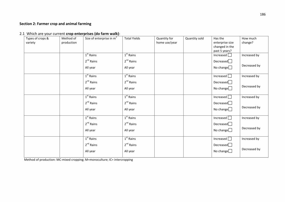
186

Section 2: Farmer crop and animal farming 2.1 Which are your current crop enterprises (do farm walk):

Types of crops & variety

Method of production

Size of enterprise in m2

Total Yields Quantity for home use/year

Quantity sold Has the enterprise size changed in the past 5 years?

How much change?

1st

Rains

2nd

Rains

All year

1st

Rains

2nd

Rains

All year

Increased

Decreased

No change

Increased by

Decreased by

1st

Rains

2nd

Rains

All year

1st

Rains

2nd

Rains

All year

Increased

Decreased

No change

Increased by

Decreased by

1st

Rains

2nd

Rains

All year

1st

Rains

2nd

Rains

All year

Increased

Decreased

No change

Increased by

Decreased by

1st

Rains

2nd

Rains

All year

1st

Rains

2nd

Rains

All year

Increased

Decreased

No change

Increased by

Decreased by

1st

Rains

2nd

Rains

All year

1st

Rains

2nd

Rains

All year

Increased

Decreased

No change

Increased by

Decreased by

Method of production: MC-mixed cropping; M=monoculture; IC= intercropping

187

2.2 Identify inputs and costs for crops enterprises on farm:

Types of crops & variety Kinds of inputs /Costs areas Labour, fertilizer, pesticides

Cost per unit if MC estimate cost of input per unit area

How often Amount spent/production period

* For mixed crops (MC) estimate quantity of shared inputs per unit area; For family labour estimate number of family members for each activity

2.3 What is considered when selecting types of crops to grow on your farm?

Land size Amount of money required to produce Market price Time to produce harvest Labor requirements Other, specify:

2.4 Record farmer livestock enterprise sizes:

Types of livestock enterprise (incl. poultry)

Method of production

Types of breeds No. of livestock Enterprise product (e.g. milk, meat, sale, hire)

Amt of product consumed

Amt of product sold

Price Who owns the livestock

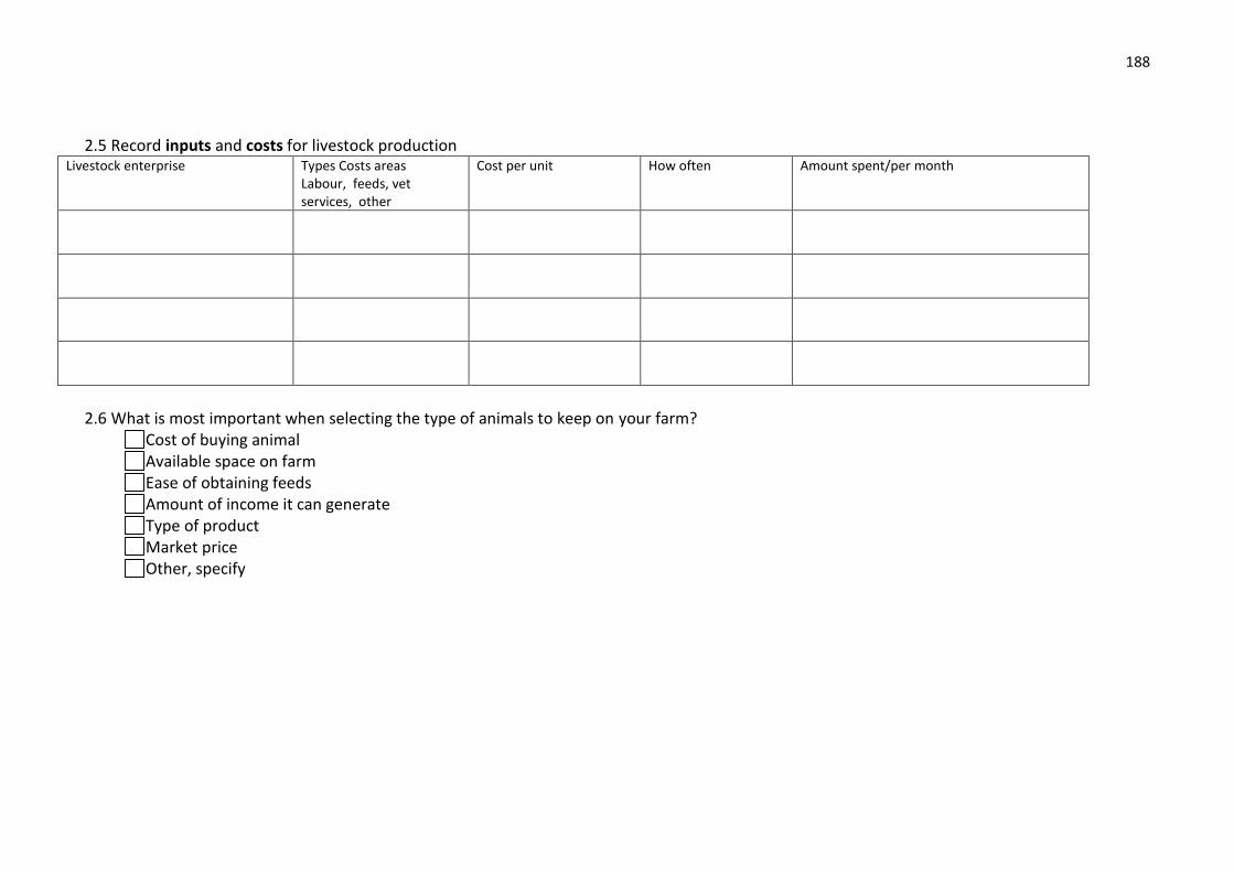
188

2.5 Record inputs and costs for livestock production

Livestock enterprise Types Costs areas Labour, feeds, vet services, other

Cost per unit

How often Amount spent/per month

2.6 What is most important when selecting the type of animals to keep on your farm?

Cost of buying animal Available space on farm Ease of obtaining feeds Amount of income it can generate Type of product Market price Other, specify

189

2.7 Which farm produce is transported to the market?

Produce transported to market

How much How often Distance to nearest market

Transport mode & costs/ unit

Section 3: Coffee Farming 3.1 Assess and record farmer coffee farming activities:

3.2 What changes in farming are considered in times of:

(i) low coffee prices? (ii) high coffee prices?

3.3 What changes in farming activities occur in your location in reaction to changes in coffee prices?

Size of initial coffee crop: acres/ m2

/ no of bushes/ variety Current size of coffee crop in acres/m

2 / no of bushes/Variety

If there is change in size of crop reasons for changed size

In case of variety change what were the reasons?

Size:

Variety:

Spacing:

Yields (kg):

Year planted:

Price/kg:

Size:

Variety:

Spacing:

Yields (kg)/yr:

Year planted:

Price/kg:

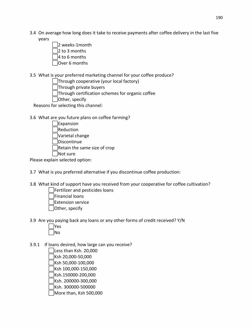
190

3.4 On average how long does it take to receive payments after coffee delivery in the last five years

2 weeks-1month 2 to 3 months 4 to 6 months Over 6 months

3.5 What is your preferred marketing channel for your coffee produce?

Through cooperative (your local factory) Through private buyers Through certification schemes for organic coffee Other, specify

Reasons for selecting this channel: 3.6 What are you future plans on coffee farming?

Expansion Reduction Varietal change Discontinue Retain the same size of crop Not sure

Please explain selected option: 3.7 What is you preferred alternative if you discontinue coffee production: 3.8 What kind of support have you received from your cooperative for coffee cultivation?

Fertilizer and pesticides loans Financial loans Extension service Other, specify

3.9 Are you paying back any loans or any other forms of credit received? Y/N

Yes No

3.9.1 If loans desired, how large can you receive?

Less than Ksh. 20,000 Ksh 20,000-50,000 Ksh 50,000-100,000 Ksh 100,000-150,000 Ksh.150000-200,000 Ksh. 200000-300,000 Ksh. 300000-500000 More than, Ksh 500,000

191

3.9.2 How often? 3.9.3 How is your loan repayment schedule?

On time Written off Delayed Completed Other, specify

Section 4 Tree cultivation: 4.1 Are you considering planting more trees on your farm? Yes No If No, please state reasons: If yes, which ones and by how much? Preferred tree species No. to be planted Source of seedlings

4.2 Assess tree felling, product use, and marketing on farm: Which trees on your farm are harvested for:

Amount of produce for home use

Amount sold for last one year

Price How often? Who are your customers?

Timber:

Fruits:

Fodder:

Firewood pollards:

Medicinals:

Other products:

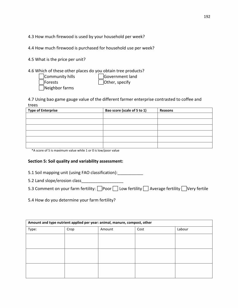
192

4.3 How much firewood is used by your household per week? 4.4 How much firewood is purchased for household use per week? 4.5 What is the price per unit? 4.6 Which of these other places do you obtain tree products?

Community hills Government land Forests Other, specify Neighbor farms

4.7 Using bao game gauge value of the different farmer enterprise contrasted to coffee and trees Type of Enterprise Bao score (scale of 5 to 1) Reasons

*A score of 5 is maximum value while 1 or 0 is low/poor value

Section 5: Soil quality and variability assessment: 5.1 Soil mapping unit (using FAO classification):___________

5.2 Land slope/erosion class__________________

5.3 Comment on your farm fertility: Poor Low fertility Average fertility Very fertile 5.4 How do you determine your farm fertility? Amount and type nutrient applied per year: animal, manure, compost, other

Type: Crop Amount Cost Labour

193

Amount and type of inorganic fertilizer applied per year

Type: Crop Amount Cost Labour

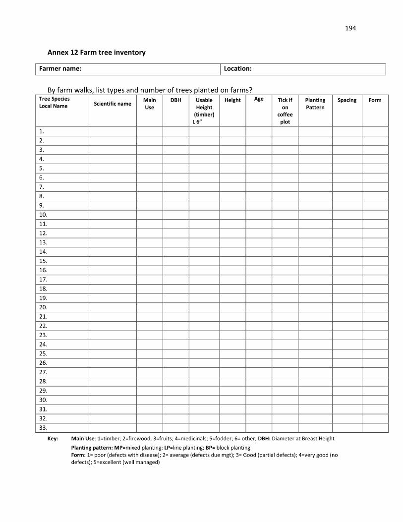
194

Annex 12 Farm tree inventory

Farmer name: Location:

By farm walks, list types and number of trees planted on farms?

Tree Species Local Name Scientific name

Main Use

DBH

Usable Height

(timber) L 6”

Height

Age Tick if on

coffee plot

Planting Pattern

Spacing

Form

1.

2.

3.

4.

5.

6.

7.

8.

9.

10.

11.

12.

13.

14.

15.

16.

17.

18.

19.

20.

21.

22.

23.

24.

25.

26.

27.

28.

29.

30.

31.

32.

33.

Key: Main Use: 1=timber; 2=firewood; 3=fruits; 4=medicinals; 5=fodder; 6= other; DBH: Diameter at Breast Height

Planting pattern: MP=mixed planting; LP=line planting; BP= block planting Form: 1= poor (defects with disease); 2= average (defects due mgt); 3= Good (partial defects); 4=very good (no defects); 5=excellent (well managed)

195

Annex 13 Amount of trees felled (tree stump count on farm)

Species Number of stumps on farm Site

*Site: EB: external boundary; CL: crop land: WL: Woodlot

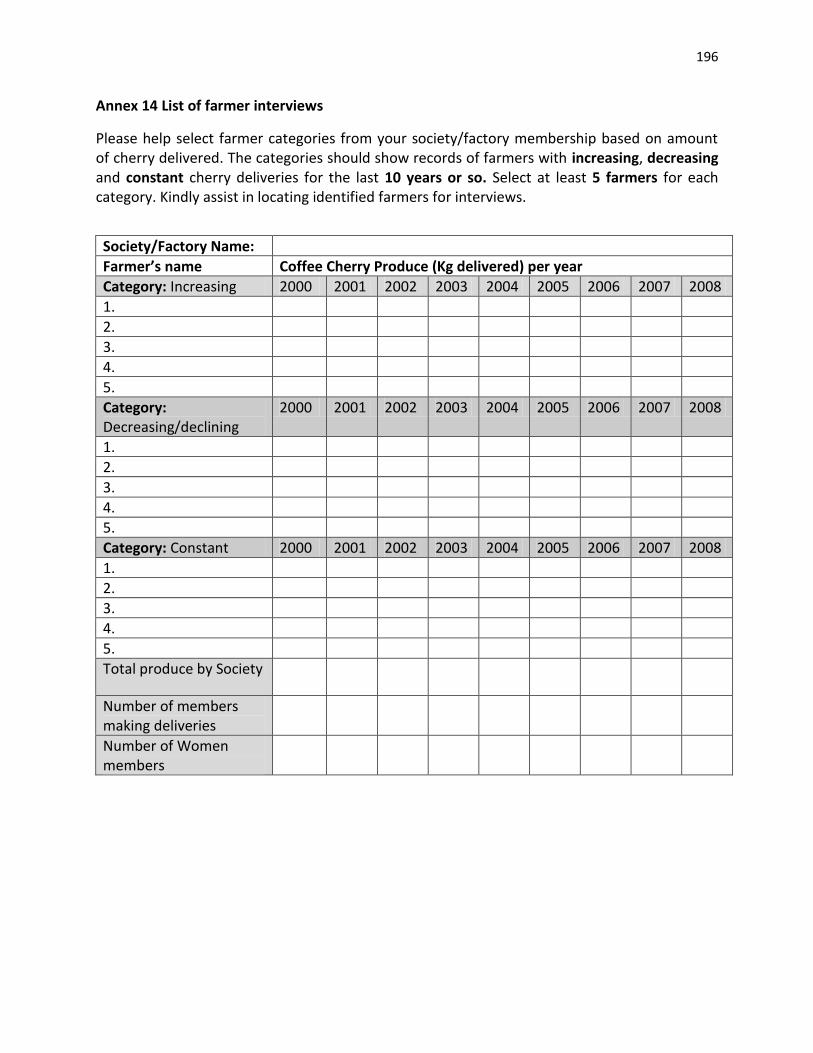
196

Annex 14 List of farmer interviews

Please help select farmer categories from your society/factory membership based on amount of cherry delivered. The categories should show records of farmers with increasing, decreasing and constant cherry deliveries for the last 10 years or so. Select at least 5 farmers for each category. Kindly assist in locating identified farmers for interviews.

Society/Factory Name:

Farmer’s name Coffee Cherry Produce (Kg delivered) per year

Category: Increasing 2000 2001 2002 2003 2004 2005 2006 2007 2008

1.

2.

3.

4.

5.

Category: Decreasing/declining

2000 2001 2002 2003 2004 2005 2006 2007 2008

1.

2.

3.

4.

5.

Category: Constant 2000 2001 2002 2003 2004 2005 2006 2007 2008

1.

2.

3.

4.

5.

Total produce by Society

Number of members making deliveries

Number of Women members

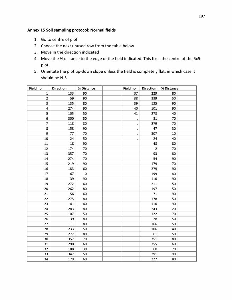
197

Annex 15 Soil sampling protocol: Normal fields

1. Go to centre of plot

2. Choose the next unused row from the table below

3. Move in the direction indicated

4. Move the % distance to the edge of the field indicated. This fixes the centre of the 5x5

plot

5. Orientate the plot up-down slope unless the field is completely flat, in which case it

should be N-S

Field no Direction % Distance

Field no Direction % Distance

1 133 90

37 229 80 2 59 90

38 339 50

3 135 80

39 125 90 4 274 90

40 101 90

5 105 50

41 273 40 6 300 50

. 81 70

7 118 80

. 279 70 8 158 90

. 47 30

9 77 70

. 307 10 10 24 50

. 24 40

11 18 90

48 80 12 174 70

2 70

13 357 70

93 80 14 274 70

54 90

15 219 90

179 70 16 183 60

279 90

17 67 0

199 80 18 39 90

110 90

19 272 60

211 50 20 262 80

197 50

21 56 60

71 90 22 275 80

178 50

23 41 40

110 90 24 283 80

243 20

25 107 50

122 70 26 39 80

28 50

27 11 80

166 50 28 233 50

106 40

29 277 80

61 50 30 357 70

351 80

31 290 60

355 60 32 188 30

60 70

33 347 50

291 90 34 179 60

227 80

198

Annex 16 Soil sampling protocol: Long thin fields

To be used only for rectangular fields where a 5m x 5m plot cannot fit because the field is too long and narrow

1. Go to centre of plot

2. Choose the next unused row from the table below

3. Move in the direction indicated

4. Move the % distance to the edge of the field indicated in the direction indicated.

This fixes the centre of the 5 x 5 plot

5. Orientate the plot up-down slope unless the field is completely flat, in which case it

should be N-S

Field no. left/right distance

Field no. left/right distance

1 Left 50 35 Left 50

2 Right 70 36 Left 50

3 Left 60 37 Left 60

4 Left 0 38 Right 20

5 Left 0 39 Left 20

6 Left 0 40 Right 0

7 Left 10 41 Right 90

8 Right 30 42 Left 10

9 Left 70 43 Left 0

10 Left 40 44 Left 80

11 Right 20 45 Right 30

12 Right 80 46 Left 50

13 Left 20 47 Left 30

14 Left 70 48 Left 90

15 Right 90 49 Right 50

16 Right 10 50 Left 90

17 Right 70 51 Left 60

18 Left 30 52 Left 30

19 Left 30 53 Left 90

20 Right 90 54 Left 10

21 Left 60 55 Left 10

22 Right 90 56 Left 50

23 Right 90 57 Right 0

24 Left 80 58 Right 80

25 Right 90 59 Left 0

26 Left 70 60 Left 70

27 Left 10 61 Right 90

28 Right 80 62 Right 0

29 Right 80 63 Left 50

30 Right 90 64 Left 30

31 Right 60 65 Right 0

32 Right 0 66 Left 90