University of Texas – Department of Mathematics

SATURDAY MORNING MATH GROUPPresents: “Bulls, Bears, and Mathematicians”

By Mike Tehranchi

Disclaimer:

This talk will not teach you how to predict the stock market or get rich quick.

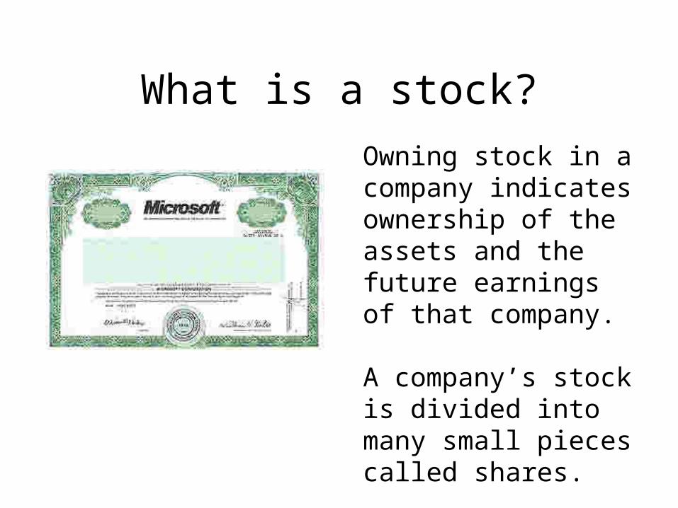
What is a stock?

Owning stock in a company indicates ownership of the assets and the future earnings of that company.

A company’s stock is divided into many small pieces called shares.

Example: Microsoft (MSFT)

The total market value of Microsoft’s assets and potential future earnings is about $272,000,000,000.

There are about 11,000,000,000 shares of Microsoft stock available to buy.

Therefore, the price of one share is about $25.

(By the way, Bill Gates owns more than a billion shares of Microsoft stock!)

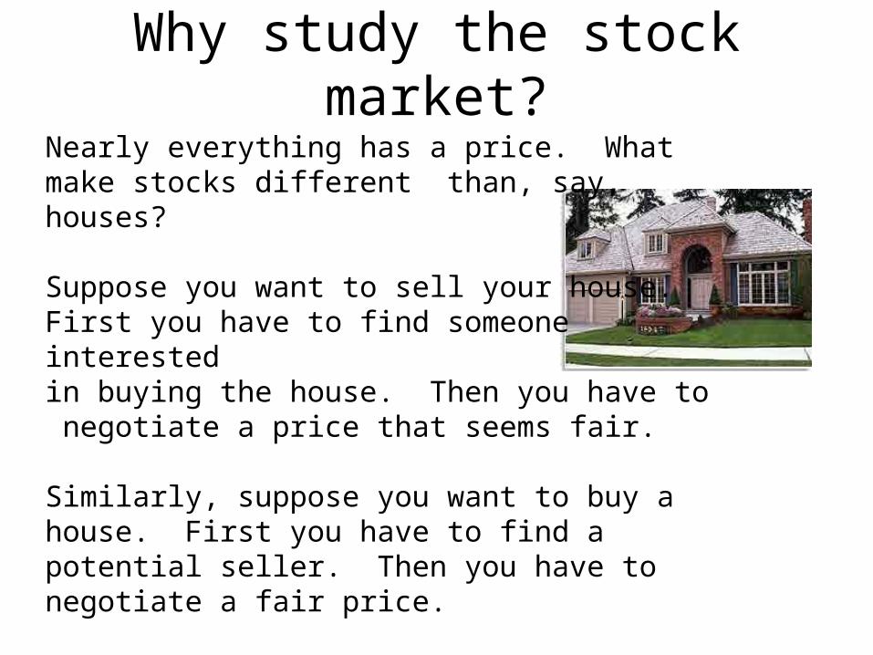
Why study the stock market?

Nearly everything has a price. What make stocks different than, say, houses?

Suppose you want to sell your house.First you have to find someone interested in buying the house. Then you have to negotiate a price that seems fair.

Similarly, suppose you want to buy a house. First you have to find a potential seller. Then you have to negotiate a fair price.

In both cases, the procedure takes a lot of time and money.

On the other hand, buying or selling stock in a company is usually very quick and inexpensive.

Most stock is traded in a stock exchange, so buyers and sellers don’t have to meet or negotiate prices.

Nowadays, you can buy and sell stock over the internet.

Bulls

Price of one share of Microsoft Jan 1996 to Dec 1999

0

10

20

30

40

50

60

70

Jan-96 Jul-96 Jan-97 Jul-97 Jan-98 Jul-98 Jan-99 Jul-99

Bears

0

10

20

30

40

50

60

70

Jan-00 Jul-00 Jan-01 Jul-01 Jan-02 Jul-02 Jan-03 Jul-03

Price of one share of MicrosoftJan 2000 to Nov 2003

Mathematicians

In 1997, Robert Merton and Myron Scholes won the Nobel Prize in Economics for inventing a method to calculate the

price of a stock option. (More on this later.)

Merton Scholes

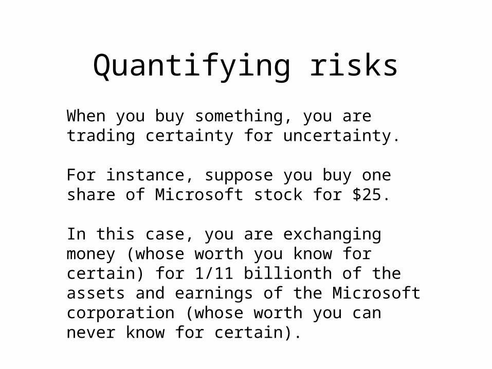
Quantifying risks

When you buy something, you are trading certainty for uncertainty.

For instance, suppose you buy one share of Microsoft stock for $25.

In this case, you are exchanging money (whose worth you know for certain) for 1/11 billionth of the assets and earnings of the Microsoft corporation (whose worth you can never know for certain).

Probability TheoryWe can model risk by appealing to probability theory. Here are some of the ingredients of this theory:

A random variable is a function that assigns a

numerical value to the outcome of an experiment.

Examples of random variables:

The simplest examples come from gambling.

For instance, roll a standard six sided die, and let X be the number that is face up.

Then X is a random variable.

For instance, if you rolled the die very many times, you would see that the random variable X takes the value 2 about one-sixth of the time.

6

1}6{...}2{}1{ XPXPXP

In fact, since all faces are equally likely to occur we have

Here is another example: Deal a two card black jack hand from a standard deck of cards. Let Y be the number of cards worth ten points (10, jack, queen, king) in the hand.

Then Y is a random variable.

As it turns out, it has the

following distribution:

221

20}2{,

221

96}1{,

221

105}0{ YPYPYP

Let Z be a random variable. For every real number z we have the inequality

1}{...}{}{ 21 nzZPzZPzZP

1}{0 zZP

Notice that if a random variable Z takes exactly n values nzzz ,...,, 21

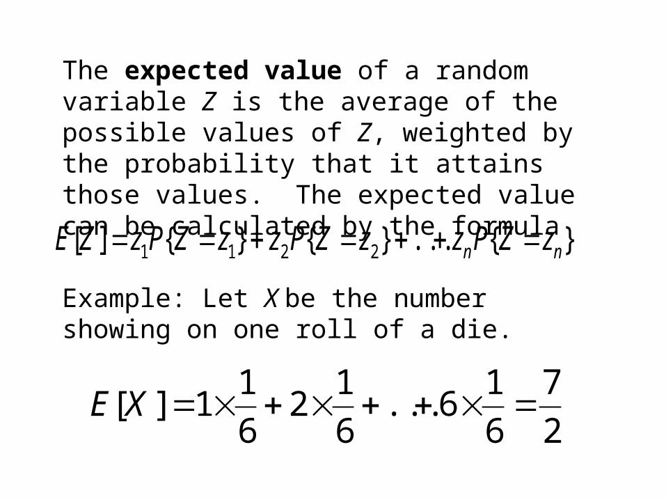
The expected value of a random variable Z is the average of the possible values of Z, weighted by the probability that it attains those values. The expected value can be calculated by the formula

}{...}{}{][ 2211 nn zZPzzZPzzZPzZE

Example: Let X be the number showing on one roll of a die.

2

7

6

16...

6

12

6

11][ XE

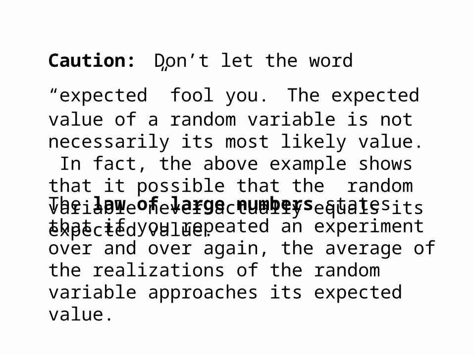
Caution: Don’t let the word “expected” fool you. The expected value of a random variable is not necessarily its most likely value. In fact, the above example shows that it possible that the random variable never actually equals its expected value.

The law of large numbers states that if you repeated an experiment over and over again, the average of the realizations of the random variable approaches its expected value.

Expected value and stocks

.

There are so many factors affecting the value of the assets and earnings of a company that it makes sense to assume that the value is random.

Let Y be a random variable corresponding to the value of one share of a company. Suppose, we know the distribution of Y:

4

3}8{,

4

1}5{ YPYP

4

17

4

38

4

15][ YE

How much should you pay for a share of stock in this company?

A reasonable answer would be the expected value of Y.

The following activity explores this method of calculating a fair price for a risky pay out.

The St. Petersburg Paradox: Game 1Get a partner. Determine who is player #1 and who is player #2.

Player #1 flips a penny. Player #2 writes down the outcome of the flip. H for heads, T for tails.

If the first flip was an H, then the game is over. And player #1 wins $1.

4. If the first flip was a T, then player #1 flips again. If the second flip is an H, then the game is over. Player #1 wins $2.

5. If the second flip is a T, then player #1 flips again. Player #2 should be recording the outcomes.

6. Player #1 continues flipping the coin until they get an H. Player #2 counts the total number of flips. If there are n flips, then Player #1 wins $n.

Here are some examples: Player #1: H Player #2 calculates: $1.  Player #1: T,H Player #2 calculates: $2.  Player #1: T,T,T,T, H Player #2 calculates: $5

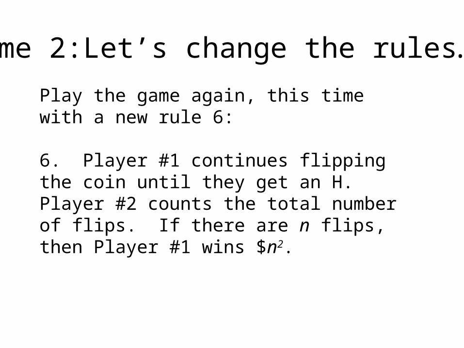
Game 2:Let’s change the rules…

Play the game again, this time with a new rule 6: 6. Player #1 continues flipping the coin until they get an H. Player #2 counts the total number of flips. If there are n flips, then Player #1 wins $n2.

 

Here are some examples:

 

Player #1: T,H Player #2 calculates: $22=$4.

 

Player #1: T,T,T,T,H Player #2 calculates: $52=$25

Play the game again, this time with another rule 6: 6. Player #1 continues flipping the coin until they get an H. Player #2 counts the total number of flips. If there are n flips, then Player #1 wins $2n.

 

Game 3:Let’s change the rules, again…

Here are some examples:

 

Player #1: T,H Player #2 calculates: $22=$4.

 

Player #1: T,T,T,T,H Player #2 calculates: $25=$32

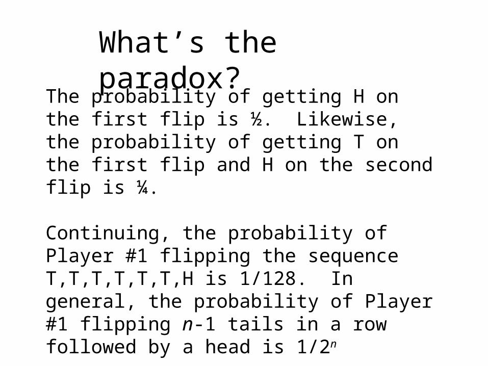
The probability of getting H on the first flip is ½. Likewise, the probability of getting T on the first flip and H on the second flip is ¼.  Continuing, the probability of Player #1 flipping the sequence T,T,T,T,T,T,H is 1/128. In general, the probability of Player #1 flipping n-1 tails in a row followed by a head is 1/2n

What’s the paradox?

Using the formula for expected value, the average winnings in playing Game 1 many times should be

2...2

1...

2

13

2

12

2

11

32

nn

Now let’s look at Game 2. We can calculate the expected value of the winnings in a similar way:

6...2

1...

2

13

2

12

2

11 2

32

222

nn

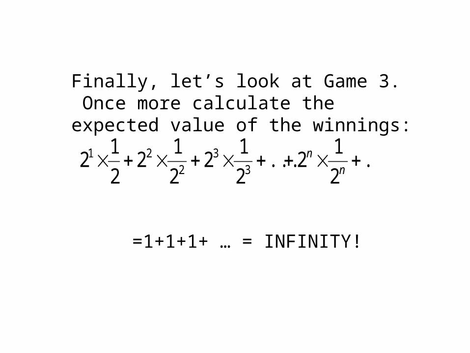
Finally, let’s look at Game 3. Once more calculate the expected value of the winnings:

...2

12...

2

12

2

12

2

12

33

221

nn

=1+1+1+ … = INFINITY!

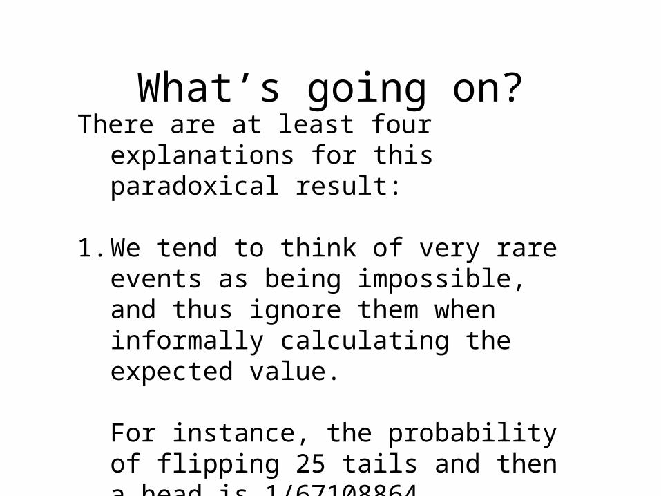
What’s going on?There are at least four explanations for this

paradoxical result:

1. We tend to think of very rare events as being impossible, and thus ignore them when informally calculating the expected value.

For instance, the probability of flipping 25 tails and then a head is 1/67108864. However, in this case you would win $67108864!

2. Let N be the random variable corresponding to the number of flips in a game. The winnings for Game 3 would then be $2N.

For Game 1 we calculated E[N] = 2. It’s tempting to think

42]2[ ][ NENEBut this is false. What’s true is

][2]2[ NENE

3. If you could some how measure happiness, the average person would likely be much happier to win $1,000 than $1. On the other hand, that same person would probably be equally happy to win $1,001,000 and $1,000,000. That is, happiness generally does not increase linearly with wealth.

Thus, in Game 3, you probably don’t want to pay for those really rare events that could make you ridiculously rich, since it wouldn’t make you that much happier than if you were just extremely rich.

4. There’s only about 30 trillion dollars in the entire world economy.

Since 30 trillion is about 245, in the very rare event that you flip 44 tails in a row, you would win all the money in the world!

Stock options

A stock option is a contract that gives the owner the right, but not the obligation, to buy a given stock at fixed price some time in the future.

An important question in financial mathematics is, “What is the fair price of a stock option?”

Merton and Scholes won the Nobel Prize for providing an answer.

How does an option work?

Imagine that the price of a given stock today is $5. And suppose you own the option to buy the stock tomorrow for $6.

Let’s assume that there are two equally likely possibilities. One possibility is that the stock price goes up to $7 tomorrow, and the other possibility is that the stock price drops down to $4 tomorrow.

What if the stock price goes up to $7 tomorrow?

You could exercise your option by buying the stock at the cheaper price of $6. You can then sell the stock back at the market price of $7, pocketing the $1 difference.

What if the price of the stock instead drops to $4?

It wouldn’t make sense to pay $6 for something you can buy for $4, so in this case, you don’t exercise your option. In other words, the option is worthless in this case.

How much would you pay?

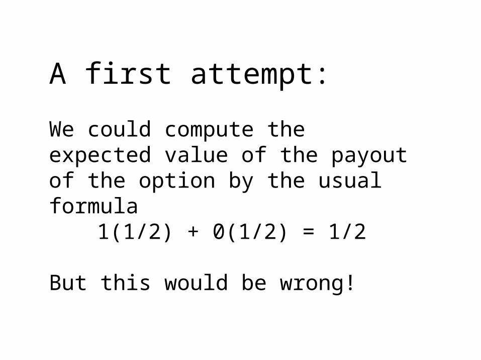
A first attempt:

We could compute the expected value of the payout of the option by the usual formula

1(1/2) + 0(1/2) = 1/2

But this would be wrong!

Suppose that the price of the option was $0.50. Then there is a free lunch available.

Sell three copies of the option and buy the stock. You would receive $1.50 from your sales and you would spend $5 on your purchase, so today you would be down $3.50.

What happens tomorrow?

Case 1: The stock price goes up to $7. In this case, you would have to pay the option holders $1 each, so your total is $7-3 = $4.

Case 2: The stock price goes down to $4. In this case, you would not have to pay the option holders anything, so your total is still $4.

You only spent $3.50, but in both cases you get $4.00 the next day. That’s a free lunch!

The price of the option should be such that there are no free lunches!

Let’s try to compute this price in our example. Let p be the price of the option, to be determined.

Buy a shares of the stock and sell b copies of the option.

You have spent 5a + p b dollars.

Tomorrow you will have 7a + b dollars in Case 1 and 4a in Case 2.

There would be a free lunch if there was a solution to

7a + b > 5a + pb4a > 5a + pb

There is no solution to the two inequalities ifand only if p = 1/3.

We’ve come up with a price for the stock option in the simple case where the stock price can only take three values and moves once a day.

But the real world problem is a lot more involved. Prices change much more frequently and can take on quite a large number of possible values.

The solution to the option price problem involves more technical math in this case, but the same simple idea applies.

log(S(t)/S(0))

-0.5

0

0.5

1

1.5

2

2.5

3

1986 1988 1990 1992 1994 1996 1998 2000 2002

Central Limit Theorem

Let X1, X2, … Xn be n independent random variables with the same distribution. Then the random variable

n

XnEXXXZ n ][...21

is approximately normal if n is large.

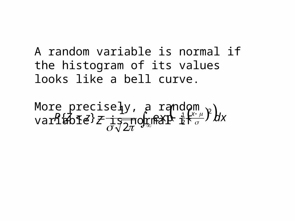
dxzZPz x

2

21exp

2

1}{

A random variable is normal if the histogram of its values looks like a bell curve.

More precisely, a random variable Z is normal if

0

200

400

600

800

1000

1200

1400

1600

1800

2000

-0.045 -0.0357 -0.0264 -0.0171 -0.0078 0.0015 0.0108 0.0201 0.0294 0.0388

Daily returns for MSFTfrom Apr-86 to Nov-03

The Black-Scholes partial differential equation:

Let P(t,x) be the price of a stock option at time t

when the price of the stock is x dollars. Then the following equation holds

rPx

Px

x

Prx

t

P

2

22

2

2

It turns out that the Black-Scholes differential equation is almost exactly the same as the equation from classical physics that describes the distribution of temperature in a material!

Who would have thought that the stock market would have anything to do with physics?