University of Southern Queensland

Faculty of Engineering and Surveying

A laboratory experiment based on the

‘Segway’

Dissertation submitted by

Mr Tshepo D Motswagae

In fulfilment of the requirements of

Courses ENG4111 and 4112 Research Project

Towards the degree of

Bachelor of Engineering (Mechatronics)

Submitted: October 2011

i

ABSTRACT

The use of robots nowadays has become an integral part of our lives. We use them for a

variety of purposes ranging from life saving to entertaining. Due to their growing popularity,

a vast number of research programs have been set up all around the world.

One such case of robotics research that sparked a high level of interest worldwide is the

research on unstable systems such as the inverted pendulum. Since the birth of this ground-

breaking research, many studies have followed thereafter, seeking to integrate or incorporate

the idea with other systems. Some of the fields that are endorsed by the inverted pendulum

research include aero dynamics (landing systems), freight systems and self-balancing robots.

This particular research focuses on the topic of self-balancing robots. It endeavours to explore

and present the design concepts of a two-wheeled self-balancing mobile robot. The main aim

of the research is to construct a working experiment that will be used to assist mechatronics

students to learn principles of control theories at the University of Southern Queensland. It

will also explore ways in which the experiment teachings might best be delivered.

When designing a two-wheeled self-balancing robot it is essential to possess or gain an

understanding of the theories and dynamics of the inverted pendulum as they form the design

basis of the robot. As part of the task, a close study was carried out on the design of the

inverted pendulum. The study helped in deducing the mathematical model of the robot which

subsequently led to the pronouncement of the robot’s state equations and thus allowing for

the simulation to be carried out. It was after the simulation process that the robot was

constructed.

The actual program to control the robot was developed in an Arduino pde platform using C++

language and was controlled by an Arduino microcontroller. The experiment was set up in such a

way that the microcontroller would send monitor signals to the computer to graph the progress of

the robot in real time. This was one way of delivering the teaching aspects of the experiment.

This also allowed the performance of the system to be further analysed by comparing the real

system behaviour with its simulation behaviour. The project is concluded with a revision of each

aspect covered with recommendations for improvement and future areas of investigation.

ii

University of Southern Queensland

Faculty of Engineering and Surveying

ENG4111 Research Project Part 1 &

ENG4112 Research Project Part 2

Limitations of Use

The Council of the University of Southern Queensland, its Faculty of Engineering and

Surveying, and the staff of the University of Southern Queensland, do not accept any

responsibility for the truth, accuracy or completeness of material contained within or

associated with this dissertation.

Persons using all or any part of this material do so at their own risk, and not at the risk of the

Council of the University of Southern Queensland, its Faculty of Engineering and Surveying

or the staff of the University of Southern Queensland.

This dissertation reports an educational exercise and has no purpose or validity beyond this

exercise. The sole purpose of the course pair entitled “Research Project” is to contribute to

the overall education within the student's chosen degree program. This document, the

associated hardware, software, drawings, and other material set out in the associated

appendices should not be used for any other purpose: if they are so used, it is entirely at the

risk of the user.

Professor Frank Bullen

Dean

Faculty of Engineering and Surveying

iii

CERTIFICATION

I certify that the ideas, designs and experimental work, results, analyses and conclusions set out

in this dissertation are entirely my own effort, except where otherwise indicated and

acknowledged.

I further certify that the work is original and has not been previously submitted for assessment in

any other course or institution, except where specifically stated.

Student Name : Tshepo D Motswagae

Student Number: 0050081447

____________________________ Signature

27/10/11

____________________________

Date

iv

Acknowledgements

I would like to extend my thanks to my supervisor Professor John Billingsley for assisting me

with this project throughout the year.

I will also like to thank my dearest friends Nuwan,Shanna,Nathan and Lasni for their

unwavering support.

v

ABSTRACT ................................................................................................................................ i

Limitations of Use...................................................................................................................... ii

CERTIFICATION ................................................................................................................. iii

Acknowledgements ................................................................................................................... iv

CHAPTER 1 INTRODUCTION ............................................................................................... 8

1.1 Introduction ................................................................................................................. 8

1.2 PROBLEM AND TASK ............................................................................................. 9

1.3 PROJECT AIMS, OBJECTIVES AND TIME LINES ............................................... 9

1.4 BACKGROUND ....................................................................................................... 12

1.4.1 Balancing concept ................................................................................................... 12

1.5 METHODOLOGY .................................................................................................... 14

1.6 RISK AND SAFETY ASSESSMENT ..................................................................... 15

1.7 conclusions ................................................................................................................ 15

CHAPTER 2 Literature review ........................................................................................... 16

2.1 Introduction ............................................................................................................... 16

2.2 Existing two wheeled robots ..................................................................................... 16

2.2.1 Segway ............................................................................................................... 16

2.2.2 nBot .................................................................................................................... 17

2.2.3 Emiew ................................................................................................................ 18

2.2.4 Joe ........................................................................................................................... 19

2.2.4 Other Robots ...................................................................................................... 20

2.3 Conclusion ................................................................................................................. 20

CHAPTER 3 SYSTEM DESIGN AND CONFIGURATION ............................................ 21

3.1 Introduction ............................................................................................................... 21

vi

3.2 Hardware design ........................................................................................................ 22

3.2.1 CHASSIS ........................................................................................................... 22

3.2.2 MICROCONTROLLER ................................................................................... 23

3.2.3 SENSORS ......................................................................................................... 24

3.2.4 Accelerometer .................................................................................................... 25

3.2.5 Tilt sensing using the ADXL335 ....................................................................... 26

3.2.6 Gyroscope .......................................................................................................... 28

3.2.7 Angular velocity sensing using the IDG-500..................................................... 29

3.2.8 Motors ............................................................................................................... 30

3.2.9 Motor controller ................................................................................................ 31

3.2.10 Wheels ............................................................................................................ 32

3.2.11 Batteries .......................................................................................................... 32

3.2.12 Hardware configuration ........................................................................................ 33

3.3 Software design ......................................................................................................... 34

3.3 Sensor fusion ............................................................................................................ 36

3.3.1 Introduction ....................................................................................................... 36

3.3.2 Kalman filter ..................................................................................................... 36

3.3.4 Complementary filter ........................................................................................ 40

3.4 Conclusions .............................................................................................................. 43

Chapter 4 SYSTEM MODELLING .................................................................................. 44

4.1 Introduction ............................................................................................................... 44

4.2 Mathematical modelling ............................................................................................ 44

4.3 Controller Design ...................................................................................................... 51

4.4 Stability Analysis ...................................................................................................... 53

4.5 Conclusion ................................................................................................................ 55

CHAPTER 5 SIMULATING THE SYSTEM ..................................................................... 56

5.1 Introduction ............................................................................................................... 56

vii

5.2 Simulation ................................................................................................................ 57

5.3 Conclusion ................................................................................................................. 64

CHAPTER 6 DATA ANALYSIS ........................................................................................ 65

6.1 INTRODUCTION .................................................................................................... 65

6.2 Calibration and tuning ............................................................................................... 65

6.2.1 Accelerometer calibration ................................................................................. 66

6.2.2 Gyroscope calibration ........................................................................................ 67

6.6.3 Complementary filter .................................................................................................. 68

6.3 Robot performance .................................................................................................... 70

CHAPTER 7 CONCLUSIONS AND RECOMMENDATIONS ....................................... 71

7.1 Introduction .............................................................................................................. 71

7.2 Simulation versus actual performance ..................................................................... 71

7.3 Teaching aspects ...................................................................................................... 71

7.4 Results versus Expectations ..................................................................................... 71

7.5 Difficulities experienced ........................................................................................... 72

REFERENCES ........................................................................................................................ 73

APPENDIX A .......................................................................................................................... 74

APPENDIX B .......................................................................................................................... 75

APPENDIX C .......................................................................................................................... 77

C.1 Simulation code ............................................................................................................. 77

C.2 Robot program ............................................................................................................... 85

C.3 APPENDIX -graph code ............................................................................................... 97

8

CHAPTER 1 INTRODUCTION

1.1 Introduction

For the last decade, two wheeled self-balancing robots have become a major topic of research

and study for robotics engineers and enthusiasts (Solerno and Angeles 2007).One of the

reasons why they are heavily explored is because they are believed to be one of the perfect

systems for teaching and applying control theories (Googol technology 2011).Due to their

non-linearity or unstable nature they illustrate various abstract control concepts such as

stability. This research paper will present and explore the design concepts of an experiment

based on a two wheeled self-balancing mobile robot called a Segway. It will further discuss

methods in which the teachings from the experiment might be delivered in the Mechatronics

Practice Unit at the University of Southern Queensland. Apart from learning purposes, when

further pursued, this line of research can also be used to provide an avenue for the acquisition

of modern control systems that may indeed grant stability to many unstable systems that exist

today. Some of the existing non-linear systems that share a common ground with this

research project are automatic aircraft landing systems, missile guidance systems and

mammoth movers such as building movers freight systems.

9

1.2 PROBLEM AND TASK

For many years the inverted pendulum has been the central experiment in the Mechatronics

Practice Unit at the University of Southern Queensland. Now a new balancing experiment has

been proposed based on the concept used on the ‘Segway’. This new supplementary

experiment is believed to be a good model that will add to the existing experiments in the

practise unit. In this proposed experiment the robot has to balance itself on a pair of wheels

either side of its chassis. The balancing of the unit will be governed and assisted by a

combination of sensors connected to a microcontroller. The experiment is set up in such a

way that the monitor’s signals are sent from the robot via a microcontroller and used to plot

its quantities on a computer screen. This provides status of the system versus its time of

travel.

1.3 PROJECT AIMS, OBJECTIVES AND TIME LINES

The main aim of this project in which all others come under, was to construct a new

balancing experiment based on the concept used in the ‘Segway’. A Segway is one of many

self-balancing two-wheeled mobile robots that exist today and is possibly the first one made

that could board a passenger on its carrier. Further information on the Segway will be

covered in the project literature review. Objectives of the research project include the

following.

Conduct a research which will in turn provide direction and also anticipate resources

required to set up this project. Upon completion of this specific objective the best

methods and techniques will be considered and pursued.

Carry out a mathematical model for the system that will define the system’s state

variables and equations.

Simulate the system prior to construction to prove the feasibility of the mathematical

model and the system parameters.

10

Develop algorithm modules which will in turn control the system via a

microcontroller. Test the workability of the selected sensors against their appropriate

algorithm module before incorporating them all together. This will ease the

troubleshooting process.

Assemble the experiment and control it via a microprocessor which will then send

monitor signals to the computer connected to it.

Evaluate the effective performance of the project and there after work on providing

teaching aspects for the practice unit based on the systems performance displayed via

a computer. These include noise correction techniques such as sensor fusion.

If time permits, the experiment will go a step further by replacing the wired links that

connect the experiment with the computer by radio links such as Bluetooth. This

approach will control and monitor the experiment remotely.

The timeline in the following figure 1 contains the chapters that were undertaken and

completed during the course of this project.

11

TASK APRIL MAY JUNE JULY AUGUST SEPTEMBER OCTOBER

1. Introduction

2.Literature

Review

3.System design

and

Configuration

4. System

modelling

5. Simulation

6. Data analysis

7. Conclusions

and

Recommendations

Figure 1.Project time lines

12

1.4 BACKGROUND

1.4.1 Balancing concept

For two-wheeled self-balancing robots, stability is vital as they cannot remain upright

(balanced) without effort. As previously mentioned, their design concepts are mostly derived

from classical robotics research called the inverted pendulum. An inverted pendulum, like its

name suggests, is a pendulum that has its mass above its pivot point and not below like

traditional pendulums (see figure 1.1). A self-balancing robot, such as a Segway, is an

extended version of an inverted pendulum. The two systems could be related on two

accounts; the cart of the inverted pendulum could be related to the wheels and the pole to the

robots chassis (see figure 1.2 and 1.3).

Figure 1.1 Normal and inverted pendulum

Figure 1.2 Inverted pendulum experiment set up

Pole velocity

Mass

Pivoted

point

Pivoted

point

13

Figure 1.3 Two-wheeled self balancing experiment set up

For two systems to be able to balance and thus staying upright at all times, there must be a

thrust applied at their pivot points every time their mass is leaning or falling. This thrust or

torque must always be in the same direction that the mass is falling so that it can induce the

pivot to stay under the body or mass of the system, to maintain balance. For the inverted

pendulum or the robot to move to a pre-defined location or target position from the upright

position (stable position), a specific lean to the direction of the target position has to be

invoked by the wheels or cart. To do so, the wheels have to cautiously roll in the opposite

direction of the target position so as to provide a required lean for the distance.

One analogy that may bring this mechanism to a clear understanding might be of a hand

balancing a stick on it’s a palm as in the illustration below in figure 1.4. One clear issue that

this analogy might help bring to the surface is that as the stick gets reasonably shorter, more

effort will be required to balance it and the opposite is true.

14

Figure 1.4 Hand balancing a stick on a its palm

1.5 METHODOLOGY

The research project is dissected in to seven chapters, each part provide essential lead to the

one before it. This approach consequently contrasted on what was to be done and what was

not done. The first chapter basically introduced the research project and layout the objectives

to be covered by the research. The next chapter which was the literature review provided a

wealth of information on different ways the objectives of the project could be reached. In this

chapter similar previous research project’s success and failures were closely studied. This

chapter basically surfaced the pros and cons of the research project. Chapters that followed

after the literature review were basically implementing what was learned in the literature

review, this consisted of system modelling, construction and analysis of the robot

performance.

Direction of the fall

Direction of the hand (thrust)

15

1.6 RISK AND SAFETY ASSESSMENT

The risks that were evident in this project varied according to the level of lethality. The risk

rankings that were used were as follows; substantial risk, significant risk, slight risk and very

slight risk.

A substantial risk in the project would be an electrical shock from power apparatus and

physical injury from cutting tools, such as wire cutters. Its control measures included wearing

Personal Protection Equipment when using such tools.

A significant risk in the project would the robot colliding with equipment in the lab or even

falling on users. Dangers associated with this kind of risk would be physical injury to users

and lab equipment destruction. Some of the control measures for these dangers were to

reduce the robot’s physical parameters.

A slight risk came from writing the thesis, programme and simulating code for the robot. Eye

strains were the associated risk. The control of the risk was to take occasional breaks.

1.7 conclusions

It is hoped that the results from this research project will be used as a self development

process by allowing mechatronics students at the University of Southern Queensland to learn

control theories through application.

16

CHAPTER 2 Literature review

2.1 Introduction

This chapter assess the literature that is available on the two wheeled balancing robots. It is

necessary for literature review to be conducted before any design could be done. The sole

purpose of this chapter is gain an understanding and appreciation of the already existing two

wheeled balancing robots.

2.2 Existing two wheeled robots

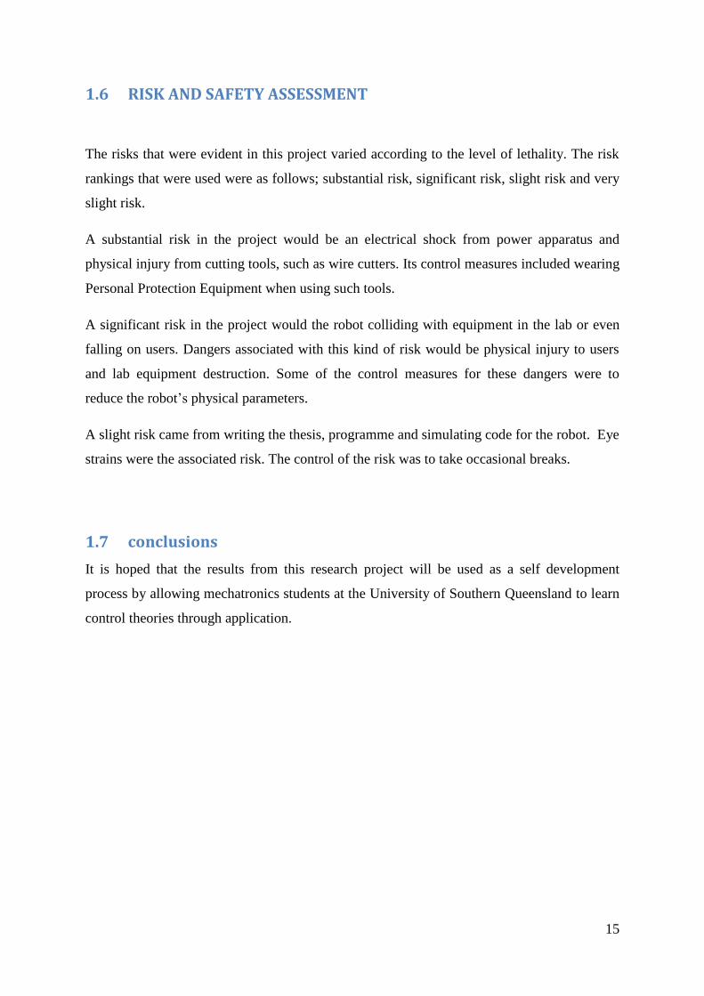
2.2.1 Segway

Segway (Segway 2008) was designed by Dean Kamen and is in its second generation of

commercially available models. This two wheeled robot is promoted as a viable transport

alternative to other mainstream options, see figure 2. Additionally this robot has features

suited to adventure, commuting, law enforcement and transportation in general. It is available

in Australia for a cost range of AU$9385 to AU$10795.

A Segway relies on five gyroscopes and an additional two tilt but for its normal operation it

only needs three gyroscopes to determine the forward and backward tilts angles and the

corresponding rate of its fall. The other two gyroscopes are redundant and only exist for

safety reasons. It uses sensor fusion technique to combine its sensors signals for better signal

quality. The Segway hosts ten on-board microcontrollers to help it to maintain balance and

control.

Manoeuvring the Segway involves manipulation of the handlebars and user controllers which

influences wheel direction. Subsequently, when the rider turns the handle bars the Segway

responds by slowing the rotation speed of the inner wheel, while maintaining the speed of the

other wheel. The machine can also achieve a single axis spin is achieved when it counter-

opposes wheel direction.

17

Figure 2 Segway HTi series two wheeled transport (McComb & Predko 2006)

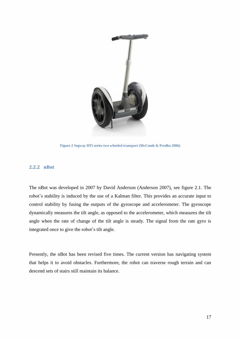
2.2.2 nBot

The nBot was developed in 2007 by David Anderson (Anderson 2007), see figure 2.1. The

robot’s stability is induced by the use of a Kalman filter. This provides an accurate input to

control stability by fusing the outputs of the gyroscope and accelerometer. The gyroscope

dynamically measures the tilt angle, as opposed to the accelerometer, which measures the tilt

angle when the rate of change of the tilt angle is steady. The signal from the rate gyro is

integrated once to give the robot’s tilt angle.

Presently, the nBot has been revised five times. The current version has navigating system

that helps it to avoid obstacles. Furthermore, the robot can traverse rough terrain and can

descend sets of stairs still maintain its balance.

18

Figure 2.1 nBot by David Anderson (Anderson 2007)

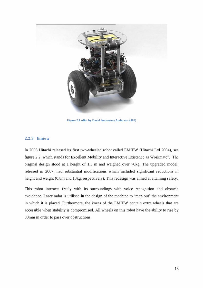
2.2.3 Emiew

In 2005 Hitachi released its first two-wheeled robot called EMIEW (Hitachi Ltd 2004), see

figure 2.2, which stands for Excellent Mobility and Interactive Existence as Workmate”. The

original design stood at a height of 1.3 m and weighed over 70kg. The upgraded model,

released in 2007, had substantial modifications which included significant reductions in

height and weight (0.8m and 13kg, respectively). This redesign was aimed at attaining safety.

This robot interacts freely with its surroundings with voice recognition and obstacle

avoidance. Laser radar is utilised in the design of the machine to ‘map out’ the environment

in which it is placed. Furthermore, the knees of the EMIEW contain extra wheels that are

accessible when stability is compromised. All wheels on this robot have the ability to rise by

30mm in order to pass over obstructions.

19

Figure 2.2 Emiew (Hitachi Ltd 2004)

2.2.4 Joe

Joe is another innovative two wheel balancing robot (figure 2.3). The two decoupled controls

of this robot work side-by-side to; (1) balance the robot and control forward and backward

motion and (2) control shifts about its vertical axis. This radio controlled machine features

the ability to spin around on its vertical axis and perform U-turns. The Joe filters signals from

an accelerometer and rate gyroscope to measure the tilt angle of the robot and produce a tilt

signal. This is used with the motor’s encoders to determine the position of the robot.

Figure 2.3 Joe

20

2.2.4 Other Robots

The internet provides more examples of varying robot constructions, control systems and

materials that can be used. For example, resources such as Lego blocks and other household

materials have been utilised. The incorporation of different mechanisms such as paired Infra-

Red (IR) sensors have been used to determine tilt measurements. The robot tilts in a

particular direction based on the comparisons that the two sensors provide. Linear based

control systems are utilised in many of these designs and for the most part provide a stable

robot.

2.3 Conclusion

Two wheeled balancing robots come in many shapes and forms. Their usage ranges from

transportation to entertainment. As it was discovered in this chapter a Segway is not very

different from the other robots mentioned. It uses gyroscopes and accelerometers like most of

the robots.

21

CHAPTER 3 SYSTEM DESIGN AND CONFIGURATION

3.1 Introduction

The wealth of information provided on the literature review chapter provided an insight on

how the design of the project could be carried out. A commonality between all the designs

conducted by fellow engineers and enthusiasts illustrated in the previous chapter is that, all of

their designs consisted of two main sections; tangible and intangible. The tangible sections

were the robot’s hardware and the intangible sections were the robot’s control systems or

software. The two were integrated together to form a drivable unit.

In this chapter a similar approach will be illustrated. The two fundamental components or

sections that make up the robot will be explored in detail and integrated together to form a

one working unit. The two components are the hardware design and the software design. The

hardware design component will be mainly be focusing on the design of the robot’s physical

structure while the software design component will be focusing on designing the robot’s

control system.

22

3.2 Hardware design

.

The hardware design section of this chapter will capture the design of the robot’s physical

structure. This includes the robot chassis as well as the incorporation of sensors, wheels,

motors, motor controller and the brain of the robot which is the microcontroller on the

chassis.

3.2.1 CHASSIS

The robot chassis is one of the key features of the robot because it is the part that will host

most components of the robot. It should be designed in way that would enable sensors,

battery packs and controllers to be mounted on it without congestion. The chassis was made

in such a way that it resembled a layered cabinet where all the components would fit neatly

within. Wood was chosen to build the chassis because it is lightweight and also it is a non-

electrical conductor, reducing the chances of electrical components short circuiting through

its base. The bottom wooden plate of the chassis was fused with a breadboard for ease of

electrical connection and then the rest of the wood was connected by four threaded steel

wires with nuts. The chassis is rectangular in shape and its dimensions measure

approximately 17 cm by 6.5 cm by 30 cm and weighs about 236 grams. Below is the picture

of the chassis.

Figure 3 Robot chassis

23

3.2.2 MICROCONTROLLER

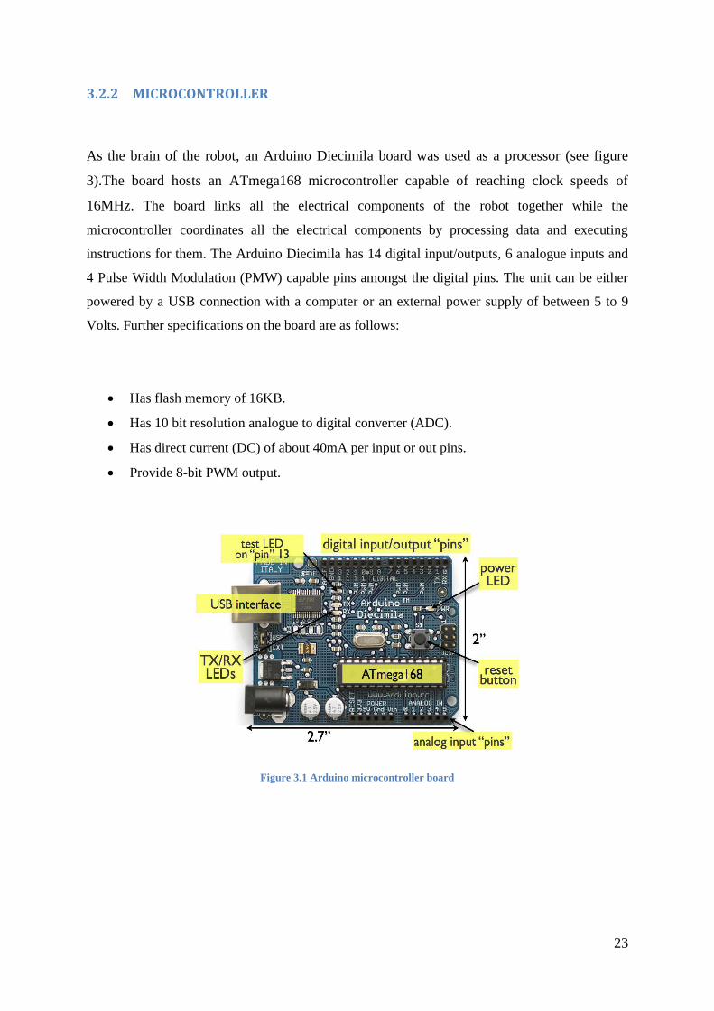
As the brain of the robot, an Arduino Diecimila board was used as a processor (see figure

3).The board hosts an ATmega168 microcontroller capable of reaching clock speeds of

16MHz. The board links all the electrical components of the robot together while the

microcontroller coordinates all the electrical components by processing data and executing

instructions for them. The Arduino Diecimila has 14 digital input/outputs, 6 analogue inputs and

4 Pulse Width Modulation (PMW) capable pins amongst the digital pins. The unit can be either

powered by a USB connection with a computer or an external power supply of between 5 to 9

Volts. Further specifications on the board are as follows:

Has flash memory of 16KB.

Has 10 bit resolution analogue to digital converter (ADC).

Has direct current (DC) of about 40mA per input or out pins.

Provide 8-bit PWM output.

Figure 3.1 Arduino microcontroller board

24

3.2.3 SENSORS

One of the most important tasks of autonomous systems of any kind is to be able to acquire

knowledge about its environment. This can be done through the use of sensors (Ronald

Siegwart et.al 2004). The use of sensors in robotics provides the robots with external physical

information which help these systems to govern themselves accordingly. Without them the

robot would blindly execute instructions without the capacity of re-evaluating its progress

and making adjustments accordingly. From the literature review we learnt of many different

sensors used to balance the two wheeled robots. Some of these sensors were analogue and

some were digital.

Analogue sensors generate a range of continuous signals or values for which the time varying

feature (variable) of the signal is a representation of some other time varying quantity

(Envcoglobal 2009). Although digital sensors generate a range of discrete signals or values

that increase in step sizes, it could also be a simple on or off signal (Seattlerobotics.org

2011).We have also learnt that sensors that are able to measure angular velocity, linear velocity

and acceleration are ideal for providing stability to the two wheeled robots. These sensors include

the likes of an accelerometers, gyroscopes, inclinometers and rotational shaft encoders. In this

project only analogue accelerometers and gyroscopes are going to be used as the robot sensors.

25

3.2.4 Accelerometer

An accelerometer is an electromechanical device that measures inertial acceleration forces.

These forces may be static, like the constant force of gravity pulling at your feet, or they

could be dynamic, caused by moving or vibrating the accelerometer (Dimension Engineering

LLC 2011). By measuring the amount of static acceleration due to gravity, the angle the

device is tilted at with respect to the earth can be found. These devises are susceptible to

noise. This means that they need to be noise corrected if they were to be used to determine

the angle like in this project. Several noise correction techniques will be covered in the

chapters to come.

The model chosen was an ADXL335 accelerometer provided by Sparkfun electronics. It is a

3 axis analogue accelerometer combined with an IDG-500 gyroscope on the same chip. Some

of its features include the following:

+/- 3g acceleration measuring scale range

330 mV/g sensitivity

Outputs 1.65 V for 0g

Operating voltage range of 1.8V to 3.6V

The model is depicted below in figure 3.2

Figure 3.2 ADXL 335 accelerometer (Sparkfun electronics 2011)

26

3.2.5 Tilt sensing using the ADXL335

In order to understand how a 3-axis accelerometer could be used to sense tilt, it is often useful

to visualise an accelerometer as a cube that has pressure sensitive walls with a ball inside it

(instructables 2011). See figure 3.3 below.

Figure 3.3 Accelerometer tilt sensing model (instructables 2011)

If the imaginary cube were to be tilted say at 45 degrees the ball then will exert a force of 1g

or 9.8 m/s2

on the two pressure sensitive walls due to the force of gravity as shown in figure

3.3 above. The results of this placement will be a resultant vector R which is the force

vector that the accelerometer is measuring. See figure 3.4 below

+X +Y

27

Figure 3.4 Accelerometer model(instructables 2011)

Rx, Ry, Rz are projections of the R vector and are the voltage levels that the accelerometer

outputs in each axis due to its placement. These voltage levels are within a predefined range

that will have to be converted to a digital value using an analogue to digital converter (ADC)

module of a microcontroller .By Pythagoras theorem in 3 dimensional it is evident that

R= (Rx) 2+ (Ry)

2+ (Rz)

2 (3.1)

Suppose the values given by the 10 bit ADC module of the microcontroller with a reference

voltage of 3.3V are 584,0,584 bits for Rx, Ry and Rz respectively when the accelerometer is

in position depicted in figure 3.3. Then the voltage that corresponds to the bits in each axis of

the accelerometer is given by the following equation.

refR

1023

VVoltsRi Adc i

(3.2)

The above equation will give 1.88, 0, 1.88 volts for Rx, Ry and Rz respectfully. Each

accelerometer has a zero-g voltage level, this is the voltage that corresponds to 0g. To get a

28

signed voltage values we need to calculate the shift from this level. The 0g voltage for the

ADXL335 model is 1.65 Volts. The equation for calculating the shifts from zero-g voltage

for any accelerometer axis is as follows:

DeltaVoltsRi=VoltsRi –VzeroGref

R1023

VAdc i -VzeroG (3.3)

This will in turn give 0.234V, 0V, 234V as voltage shifts for Rx, Ry and Rz respectively. To

convert the voltage shift to values of g (9.8 m/s2) .This shift values will be divided by the

accelerometer sensitivity which is 0.33 V/g for the ADXL 335 model. So the values for Rx,

Ry and Rz in terms of g will be 0.71g, 0g, 0.71g respectfully.

Now to find the angle Azr in figure 3.4 which is the angle the accelerometer is tilted by

relative to the vertical axis, which relates to the robot’s tilt we would say:

1 1 0.71sin ( ) sin ( ) 45

1

RxAzr Azr

R

degrees (3.4)

2 2 20.71 0 0.71 1R

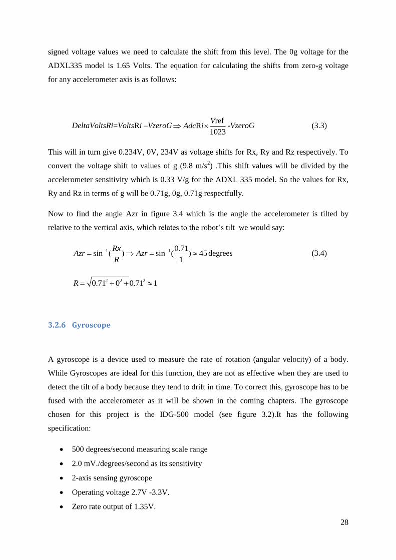
3.2.6 Gyroscope

A gyroscope is a device used to measure the rate of rotation (angular velocity) of a body.

While Gyroscopes are ideal for this function, they are not as effective when they are used to

detect the tilt of a body because they tend to drift in time. To correct this, gyroscope has to be

fused with the accelerometer as it will be shown in the coming chapters. The gyroscope

chosen for this project is the IDG-500 model (see figure 3.2).It has the following

specification:

500 degrees/second measuring scale range

2.0 mV./degrees/second as its sensitivity

2-axis sensing gyroscope

Operating voltage 2.7V -3.3V.

Zero rate output of 1.35V.

29

3.2.7 Angular velocity sensing using the IDG-500

For the purpose of simplicity, the same cube model used for explaining the accelerometer

will be used for the gyroscope as both sensors are in the same chip (see figure 3.5 below).

Figure 3.5 Gyroscope model (instructables 2011)

If Rxz is the projection of the inertial force vector R on the XZ plane and it is the voltage

level that the gyroscope is outputting at that instant, then the rate of change of angle Axz

which is the angle between the Rxz (projection of R on XZ plane) and Z axis will be

represented as (instructables 2011):

1023

VrefAdcRxz VzeroRate

AxzRatesensitivity

Degrees/seconds (3.5)

With VzeroRate, as the voltage that the gyroscope outputs for zero angular rate and AdcRxz,

being the number of bits representing the voltage, then the gyroscope outputs at any

instantaneous time when it is rotated about its y-axis.

30

3.2.8 Motors

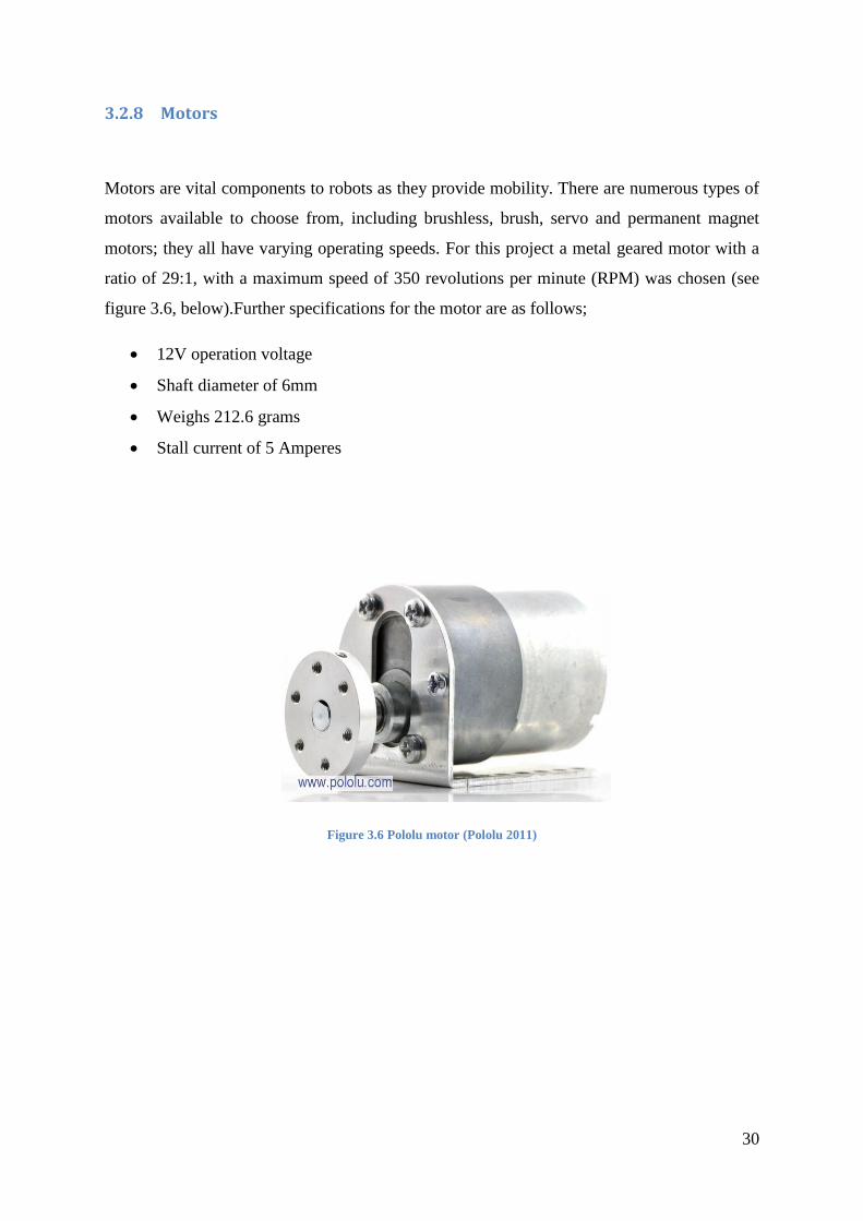
Motors are vital components to robots as they provide mobility. There are numerous types of

motors available to choose from, including brushless, brush, servo and permanent magnet

motors; they all have varying operating speeds. For this project a metal geared motor with a

ratio of 29:1, with a maximum speed of 350 revolutions per minute (RPM) was chosen (see

figure 3.6, below).Further specifications for the motor are as follows;

12V operation voltage

Shaft diameter of 6mm

Weighs 212.6 grams

Stall current of 5 Amperes

Figure 3.6 Pololu motor (Pololu 2011)

31

3.2.9 Motor controller

Motor controllers are essential for this project because they provide necessary control to the

motor’s speed and direction by varying the output voltage signal and setting its polarity

respectively. Without this ability the robot would not be able to switch its motion whenever

its falling in the direction desired. Motor controllers come in different types and are used for

different applications, including Relays and H-bridges (motor bridge).For this project a

custom designed H-bridge was chosen as a motor governor simply because it has the

capability to vary the speed of the motor through a technique called Pulse Width Modulation

(PWM). The magnitude of output voltage provided to the motor by PWM is varied by a duty

cycle, which will be demonstrated shortly. Duty cycle is simply the ratio between the on time

and the off time of a devise for a given period of time (Winans Inc,2011).

Figure 3.7 Pulse width modulation

Figure 3.7 above will be used to illustrate the PWM technique. The microcontroller chosen

for this project runs its PWM at a frequency of about 490Hz with a period cycle of 2

milliseconds used. If figure (a) of figure 3.7 represents 50% duty cycle it means that the

motor is on for 1 millisecond and off for 1 millisecond inside 2 milliseconds span. So its

speed at this instant will be 50% of its maximum (350rpm)

Ton Toff

32

Duty cycle=Ton/(Ton + Toff) * 100%

= 1 /2 * 100%

=50%

Now if 75% is induced it will mean that the on time of the motor is 1.5 milliseconds and off

for 0.5 millisecond within a 2 milliseconds span. This might be the case where the robot has

leaned a bit too much.

Duty cycle=Ton/(Ton + Toff) * 100%

= 1.5 /2 * 100%

=75% of 350 rpm

3.2.10 Wheels

The purpose of wheels is to provide locomotion, traction and to support the robot chassis.

Soft rubber wheels are ideal because they provide better traction on most surfaces and will

eliminate slippage which could distort the robot’s balance. The diameter of the wheel should

sufficient to translate enough torque needed by the robot to correct its tilt. The wheels chosen

were 100 mm in diameter and 10mm wide.

3.2.11 Batteries

As a life source to the robot, 12V-1.2Ah and 9V batteries were used to power the H-bridge

and the microcontroller respectfully.

33

3.2.12 Hardware configuration

Figure 3.8, 3.9 shows a hardware schematic flow diagram and the final design of the robot

respectifully of the robot and its sensors. The motors are connected to the H-bridge (motor

controller) which is in turn connected to the microcontroller. The other two sensors are

connected to the H-bridge via a microcontroller.

Figure 3.9 Robot final hardware design

Encoder wheel(b)

wheel (b)

Figure 3.8 A hardware schematic flow diagram of the robot hardware

Battery supply

Microcontroller

Accelerometer

Gyroscope

H-bridge

Encoder wheel(a)

wheel (a)

Motor (a)

Motor (b)

34

3.3 Software design

The software design phase of this chapter will capture the basic approach taken on how to

program the microcontroller to provide accurate interaction with the hardware and control the

robot accordingly. The microcontroller is required to interpret a collection of sensors and

carry out a series of logical sequences or processes that will dictate the speed and direction of

the motor. The control process was written in such a way that the robot quantities, for

example its angle displacement were displayed or graphed on a computer monitor to ease

teaching aspects. The control process (program) for the robot was written in C++ on an

Arduino pde platform and the simulation was written in visual basic. Both programs are in

Appendix C.

The basic control process for balancing the robot is displaced by a flow chart in figure 3.10

below.

35

Figure 3.10 Robot’s program flow chart

Start

Is the robot

balanced?

Is the robot

falling

forward?

Is the robot

falling

backward?

Turn

wheels

forward

Turn

wheels

backward

NO

NO

YES YES

YES

36

3.3 Sensor fusion

3.3.1 Introduction

Sensor fusion is the integration or the act of combining multiple sensor signals together from

different sources to form a single and more reliable output signal. Reliability and higher

system performance are the main factors driving sensor fusion (Frost & Sullivan 2006).Most

sensors’ reliability is compromised by noise, temperature and long-time usage. These factors

make sensor fusion necessary in this project as the accelerometer is susceptible to noise.

Additionally the accelerometer cannot follow the tilt angle when the robot is rotating or in

motion. While on the other hand the gyroscope can follow the tilt angle perfectly when its

signal is integrated but over time the tilt angle becomes inaccurate because the gyroscope

tends to drift. Therefore, if they are both fused together, they can synchronise and alleviate

these vulnerabilities.

There are many techniques that can be use d to integrate sensor fusion into a system,

including the use of Kalman and complementary filtering. This section of the thesis will

briefly touch upon Kalman filtering and then explore the chosen method for the project which

is the complementary filtering method.

3.3.2 Kalman filter

Kalman filtering is an extensive topic of research and this section will not explore all facets

of the technique.

A Kalman filter is a set of mathematical equations that provides a recursive means of

estimating the states of a process or system (Welch and Bishop, 2006).It was developed in

1960 by Dr. Rudolf E. Kalman for Apollo spacecraft. Since then the Kalman filter has been

implemented in many applications, including the integration of the global position system

(GPS) with the inertial navigation system (INS) to achieve optimal system performance for

positioning.

37

The filter provides an estimation based on the system’s past and present sensor measurements

or values. In other words Kalman filter is a linear optimal observer, and uses all measured

quantities from sensors and computes the best estimation of the system’s state variables. This

approach has been proven to suppress sensor noise and other unwanted system disturbances.

The Kalman filter algorithm fabricates estimated values from a true measured or calculated

sensor value. The algorithm estimates the uncertainty of its predicted value by computing a

weighted average of the predicted value and the true measured sensor value (see figure 3.11).

The most weight is given to the value with the least uncertainty. The estimates produced by

the algorithm tend to be closer to the true values than the original measurements because the

weighted average has a better estimated uncertainty than either of the values that went into

the weighted average (Jay Esfandyari et al. 2011). Kalman filter technique fuses

measurements from sensors according to covariance. Covariance provides a measure of the

strength of the correlation between two or more sets of random variants (Spiegel, M. R. 1992).

Figure 3.11 Kalman filter recursive algorithm (Jay Esfandyari et al. 2011)

38

As compared to other techniques such as complementary filter, the Kalman filter technique

involves an extensive mathematical background like signal processing. The general layout of

the Kalman filter is described in the following state space equation 3.6 and 3.7 (Jay

Esfandyari et al. 2011).

1 1 1k k k kx Ax Bu w (3.6)

k k kz Hx v (3.7)

Where

x is the estimated state of the system in discrete time

B is s an n by l matrix that relates the optional control input u to the state x.

H is an n by m matrix that relates the state to the measurement zk.

wk is the process noise (random variables).

vk is the measurement noise (random variables).

Zk is the measured value

w and v are assumed to be independent of each other, white, and with normal probability

distributions so that,

p(w) ~ N(0, Q)

p(v) ~ N(0, R)

where Q is the process noise covariance matrix and R is the measurement noise covariance

matrix,(see figure 3.11).

To implement this technique to the robot we first have to use equation 3.6 and 3.7 to

construct the robot’s states and have its initial measurements ready. The final tilt angle θ is

the state that we are going to estimate in order to compensate gyroscope for the drift.

Essentially, the accelerometer measurements are going to be used to limit the final tilt angle

so that it will not drift over time due to the gyroscope random drift. Knowing that the angle

provided by the gyroscope sensor is given by the following equation

39

1 0( )gro gro T (3.8)

Where 1 , 0 are final and initial angular velocities for a sampling time T respectively, then

equation 3.8 would become.

( 1) ( )gro k gro k x T b T (3.9)

Where b= 0x , gyroscope dynamic bias and x as gyroscope measurement. From equation 3.4

in the previous section we learnt that the tilt angle measured by the accelerometer from figure

3.4 was given by the equation

Measured tilt Ѳ= 1sin ( )Rx

R

This means that the measurement term for Kalman filter Zk becomes

1sin ( )k k

RxZ

R (10)

Combining this equation 3.6, 3.7, 3.8 and 3.9 we will have the matrix of the form

( 1)

1

1

1

0 1 0

1 0

gro k k

k k

k k

k

k

k

T TX U

b b

Zb

The second step is to obtain the process covariance matrix Q from the offline experiments on

the gyroscope and measurement covariance R from the offline experiments on the

accelerometer. The Kalman filter recursive algorithm depicted in figure 3.11 is computed in

the microprocessor with initial values of X and P being zero. Once the values of Q and R are

fine-tuned, the robot tilt angle from the Kalman filter will always be accurate and will not

drift away.

40

3.3.4 Complementary filter

The term ‘complementary filter’ is often casually used in the literature to refer to any digital

algorithm that serves to ‘blend’ or ‘fuse’ similar or redundant data from different sensors to

achieve a robust estimate of a single state variable. While in the strictest mathematical sense,

it refers to the use of two or more transfer functions, which are mathematical complements of

one another. Thus, if the data from one sensor is operated on by G(s), then the data from the

other sensor is operated on by I-G(s), and the sum of the transfer functions is I; the identity

matrix. In the case of a one-dimensional filter, as will be described in this paper, the identity

matrix reduces to the scalar number one (Paul C. Glasser).A complementary filter consists of

a common low-pass filter for the accelerometer and a high-pass filter for the gyroscope. The

complementary technique or method is easier to understand and implement when compared

to the Kalman filter technique.

If the low-pass and high-pass filters are mathematical complements, then the output of the

filter is the complete reconstruction of the variable being sensed, minus the noise associated

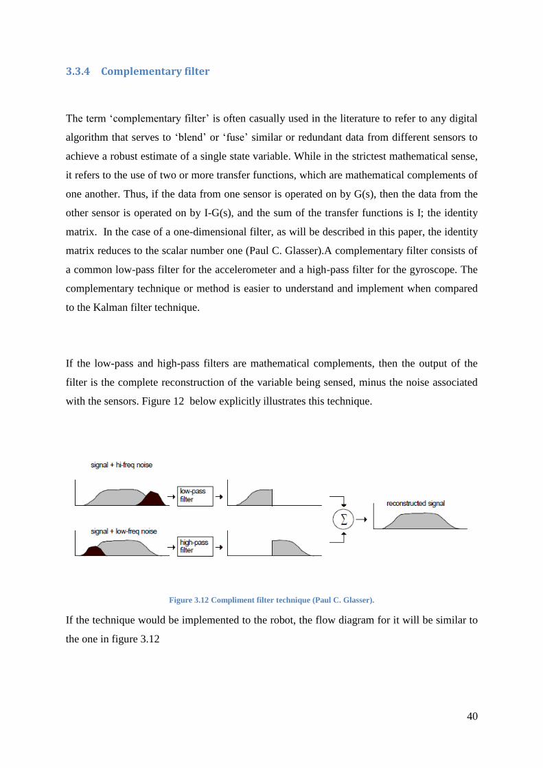
with the sensors. Figure 12 below explicitly illustrates this technique.

Figure 3.12 Compliment filter technique (Paul C. Glasser).

If the technique would be implemented to the robot, the flow diagram for it will be similar to

the one in figure 3.12

41

Figure 3.12 Complimentary filter flow diagram for balancing robot (Jay Esfandyari et al.

2011)

Where

a Is the tilt angle

'

a Is the low passed tilt angle

g Is the integrated tilt angle from the angular velocity signal of the gyroscope

'

g Is the high passed integrated tilt angle from the angular velocity signal of the gyroscope

From the diagram we can see that the final tilt angle will be the sum of '

g and '

a .

='

g + '

a 3.11

The above equation can also be written as

= (1 )g ak k (3.12)

42

Where k is constant between 0 and 1.So if k is 0.90 then equation 12 will become

= 0.90 0.10g a

3.13

If both sensors are sampled at time interval of 0.01 (100Hz), then the time constant of the

filter will be as follows

0.90 0.01

1 1 0.90

k T

k

=0.09 seconds

A complementary filter is a frequency domain filter. This can be explained by the use of the

above time constant value and equation 3.13. At the beginning of this chapter it was

mentioned that the accelerometer cannot follow tilts at fast motion and that the gyroscope

respond better to fast motions. Therefore, this means that for motion that is greater or faster

than 0.09 second time period the gyroscope’s integrated tilt angle θg is weighted more.

Furthermore, the accelerometer noise is filtered out because the values of the accelerometer at

this speed are trusted less for the same reason mentioned above.

When the motion is slower than the 0.09 second time period, the accelerometer tilt

measurement θa has more weight than the θg of gyroscope. So in this case the accelerometer

measurements are trusted more than that of the gyroscope, which tends to reduce the

gyroscope bias drift impact from the vertical point.

This technique was chosen over Kalman filter technique because it is not mathematics

extensive and simple to implement when programming the microcontroller. It is just a line of

code and can be expanded to fuse multiple axis sensors like the one used for this project.

Things to consider when using this technique are as follows. When the zero-rate level or bias

ωX0 of gyroscope is constant and the robot is stationary, the tilt angle from the

complementary filter output will also have a constant offset that can be compensated from the

accelerometer tilt measurement (Shane Colton 2007). If the bias is drifting over time and

temperature, then the error of the tilt angle from the complementary filter will grow over

time. In this case, ωX0 needs to be obtained when the robot is powered on and is stationary to

cancel out gyroscope turn-on to turn-on bias instability. In addition, when the robot is

stationary during the operation, new ωX0 can be obtained — again, periodically to cancel out

bias in-run stability and short-term angular random walk (Jay Esfandyari et al. 2011).

43

3.4 Conclusions

A complementary filter technique was used in the project as opposed to the kalman filter

technique.

44

Chapter 4 SYSTEM MODELLING

4.1 Introduction

This section of the thesis provides the foundation for constructing the robot. A mathematical

model of the robot will be deduced at this stage. The model will provide state equations that

will describe the behaviour of the robot. The model will also aid in developing the robot

controller and be used to simulate the robot. The following free body diagram (FBD) is used

to model the robot.

4.2 Mathematical modelling

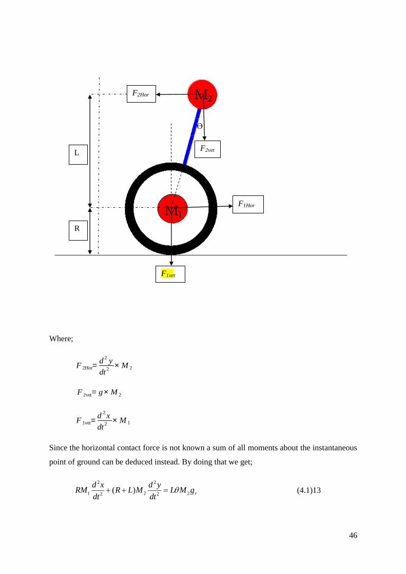
Figure 4 Free body diagram of the segway

45

Where:

M2 is the mass of the robot chassis

M1 is the mass of the wheels and axle

R is the radius of the wheels

L is the length of the stick that connects the chassis and the wheels

ϴ is the angle of the tilt that the chassis and the stick make relative to the vertical axis.

ᵩ is the angle turned by the axle relative to the chassis and stick

χ is the horizontal distance that the wheels made (rolled)

y is the horizontal distance that the top of the stick made

gr the gravity

To keep the modelling simple and manageable a considerable amount of assumptions will be

made that will not drive or blow the modelling out of proportion when made. This will

include the following.

The robot will move only in two dimensions or in one plane, therefore there will be no

steering.

The dynamics of the machine are represented by point masses, namely M1 and M2.

The two motors driving the wheels of the system (robot) are heavily geared and move

symmetrically together as if were one.

All angles made are small, so that their cosine is 1 and their sine is equal to the angle in

radians.

The forces that act on the robot sections are the upper which comprises of the point mass M2

and the lower which comprises of the point mass M1. These are resolved below.

46

Where;

Since the horizontal contact force is not known a sum of all moments about the instantaneous

point of ground can be deduced instead. By doing that we get;

2 2

1 2 22 2( ) r

d x d yRM R L M L M g

dt dt (4.1)13

F 2=d

2y

dt2

× M 2

F 2Hor=d

2y

dt2

× M 2

F 2vet= g× M 2

F 1vet=d

2x

dt2

× M 1

F2Hor

F2vet

ϴ

F1Hor

L

R

F1vet

47

Where x =2

2

d x

dt=R (

2

2

d

dt

+

2

2

d

dt

) 4.2)14

And ÿ= 2

2

d y

dt= x +L

2

2

d

dt

Which then becomes ÿ=2

2

d

dt

(R+L) +R

2

2

d

dt

(4.3)15

Now substituting equation 4.2 and 4.3 in 4.1 becomes

2 2 2 2

1 2 22 2 2 2[ ( )] ( ) [ ( ) ] r

d d d dRM R R L M R L R L M g

dt dt dt dt

2 22 2 2

1 2 1 2 22 2[ ( ) ] [ ( )] r

d dR M M R L R M M R R L L M g

dt dt

(4.4)16

Now the next step is to get an insight about φ. With a heavily geared DC motor of our choice,

we can approximate the motor’s angular speed with an equation of the form;

dau b

dt

(4.5)17

Where

is the rate of rotation in radians per seconds.

u is the proportion of the full drive that is applied.

a is acceleration in radians per (seconds)2and b is simply a gain.

If the motor accelerates to full drive, that is to say when u is 100 percent or simply being 1,

the motor will reach a top speed where now at that top speed the equation above will reduce

to the one below.

d

dt

= 0

Which implies that a(1) = bw when the rate of rotation is no longer changing and that the top

speed will now be represented by the following relation.

48

a

b

Having chosen a motor with a top speed of 5.8 revolutions per second which is 11.6p radians

per second and time constant (1/b) of 0.5seconds, this will mean that

b=2 and

11.6a

b

11.6 (2)a ≅73.30

Substituting a and b in equation 4.5 results in

73.30 2d

udt

................................................................................................(4.6)18

Since is the angle in which the axle turns relative to the chassis or stick, it is clear to see

that its rate of change will be described by the following equation.

d

dt

Also it is clear to see that

2

2

d d

dt dt

........................................................................................................... (4.7)19

Substituting equation 4.7 in to equation 4.6 we get

2

273.30 2

du

dt

Now if we substitute the immediate equation above to equation 4.4, our new final equation

will be

22 2 2

1 2 1 2 22[ ( ) ] (73.30 2 )[ ( )] r

dR M M R L u R M M R R L L M g

dt

49

As a summery from all the equations deduced above, there are now four state equations that

describe the behaviour of the system. These four state equations are deduced from the four

state variables which are φ, ω (from the motor), Ѳ and dѲ/dt (from the chassis).The state

equations are as follows:

d

dt

(4.8)20

d

dt

or2

2

d

dt

or

=2

2 1 2

2 2

1 2

(73.30 2 )[ ( )]

[ ( ) ]

rL M g u R M M R R L

R M M R L

(4.9)21

d

dt

or

= (4.10)22

d

dt

or

=73.30u-2 (4.11)23

The above four equations can be represented in the state-space form as:

A B x x u ( 4.12)

Where, nx R , nu R are the state and control respectively. A Represents a nonlinear

dynamic function matrix while B is a nonlinear input function matrix and the state x, of the

system is as follows:

x

The system’s state space equations in a matrix form is as follows:

2 2

2 1 2 1 2

2 2 2 2 2 2

1 2 1 2 1 2

0 1 0 0 0

2[ ( )] 73.30[ ( )]0 0

( ) ( ) ( )

0 0 0 1 0

0 0 0 2 73.30

rLM g R M M R R L R M M R R L

uR M M R L R M M R L R M M R L

50

For simplicity let

f=LM2 gr

g=R2M1+ M2R(R+L)

h= R2M1+ M2R(R+L)

2

Then the above state space matrix becomes;

0 1 0 0 0

2 73.300 0

0 0 0 1 0

0 0 0 2 73.30

f g g

uh h h

51

4.3 Controller Design

To be able to control the system, feedback has to be applied in order to have a relation that is

able to track how the outputs are affected when the inputs are toggled. Feedback allows the

robot to control its balance and position. To allow feedback to occur the robot has to know

the angle it has tilted and the speed at which it reached this angle. The robot must also know

its current position and the speed it should reach in order to counteract the initial angle

formed and thus reaching its up-right position. This feedback will be of the form;

1 2 3 4a b c d F ax bx cx dx

u u x u

Where a, b, c and d are four constants that might be positive or negative, more about these

constants will be covered as the chapter progress. Inducing the feedback to the state space

equation 4.12 formed in the previous section, make a new closed loop equation of the form;

( )A BF A BF x x x x x

52

And the closed loop matrix is of the form;

0 1 0 0 0 0 0 0

2 73.30 73.30 73.30 73.300 0

0 0 0 1 0 0 0 0

0 0 0 2 73.30 73.30 73.30 73.30

f g ga gb gc gd

h h h h h h

a b c d

0 1 0 0

73.30 73.30 73.30 2 73.30

0 0 0 1

73.30 73.30 73.30 2 73.30

f ga gb gc g gd

h h h h

a b c d

Now the matrix has become the form of Ax x , the stability of the system is now ready to be

analysed. Firstly we must deduce the system characteristic equation. It is essential to find the

system characteristic equation because from it eigen values can be found, which are the roots

of the characteristic polynomial equation of the system. As far as stability of the system is

concerned all the eigen values must have strictly negative real parts, that is, all must lie in the

open left-half complex plane as it show in next section of this chapter.

.

53

4.4 Stability Analysis

To find the characteristics forth order polynomial equation and hence its eigen values, the

equation below is used.

| |A I =0

0 1 0 01 0 0 0

73.30 73.30 73.30 2 73.300 1 0 0

| | det( ) 00 0 1 0

0 0 0 10 0 0 1

73.30 73.30 73.30 2 73.30

f ga gb gc g gd

A I h h h h

a b c d

After some computations the characteristic polynomial will reduce to

4 3 2(119.86 73.3 2) (119.86 73.3 77.8) (5702 155.5) 5702 0b d a c d c

(4.12)

A clear step by step of the deduction of the above equation is carried out in the appendix B

Now, before we deduce the values of the coefficients let us examine what equation (24) tells

us. Firstly, if we look at the last coefficient in the equation, which relates to , which the

angle turned by the wheel (axle) relative to the chassis must be positive. Secondly, if we look

at the coefficient of 3 we immediately notice that the coefficient of the tiltrate ( ) must

exceed that of the angular speed ( ).If we also look at the coefficient 2 we see that the

coefficient of the tilt ( ) must exceed that of wheel angle ( ).Now as an intuitive guess we

expect all the coefficients to be positive, thus making the roots of the system negative. In

other words we expect the drive to follow the coefficients; if the tilt is to the right (positive)

the drive should also be to the right.

To get an approximation of the values of a, b ,c and d a method of ‘pole assignment’ is used,

where values of the roots are chosen and then matched with corresponding coefficients of the

characteristic polynomial.(John Billingsley 2010).If we try four roots of one second we will

get

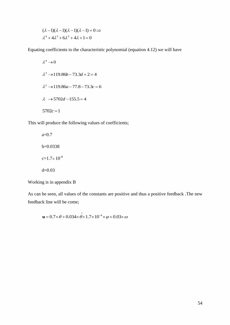
54

4 3 2

( 1)( 1)( 1)( 1) 0

4 6 4 1 0

Equating coefficients to the characteristic polynomial (equation 4.12) we will have

4 0

3 119.86 73.3 2 4b d

2 119.86 77.8 73.3 6a c

5702 155.5 4d

5702 1c

This will produce the following values of coefficients;

a=0.7

b=0.0338

c=1.710-4

d=0.03

Working is in appendix B

As can be seen, all values of the constants are positive and thus a positive feedback .The new

feedback line will be come;

40.7 0.034 1.7 10 0.03 u

55

4.5 Conclusion

The deduced state equation and feedback will be used for simulating the system in the next

chapter to come.

56

CHAPTER 5 SIMULATING THE SYSTEM

5.1 Introduction

Simulations offer a cheap and simple method for forecasting the effectiveness and efficiency of

systems prior to construction.

Simulation of the system was carried out on a visual basic platform and the full code is listed

in appendix C. The dynamics of the system deduced in the previous chapter are now going

used to be used to virtually test the performance of the system against disturbances. Plots of

its distance tilt angle, tilt rate, wheel (axle) angle as well as its angular speed and horizontal

speed will be graphed against the system’s time of travel.

57

5.2 Simulation

The main loop code of its simulation consists of four states equations 8-11 with feedback. It

samples them at a rate of 0.01 of a second. The simulation will kick start with the use of

guess or predicted coefficient of the feedback. The prediction of the coefficient will be

guided by equation 11 which is the system’s characteristics polynomial. Equation 11 dictates

that ‘b’ should be greater than‘d’ and that ‘a’ should be greater than ‘c’. Intuitively if ‘a’

relates to the tilt of the chassis, it is necessary for ‘a’ to be larger than the other coefficients

(biased)because we want the motor to be able to react to the slightest movements of the

angle. By observing the state equations we will choose the coefficient as follows;

a=5

b=1

c=0.8

d=0.3

The main loop for the simulation is of the form.

U = 5 * theta + 1 * dtheta + 0.8 * phi + 0.3 * omega

theta = theta + dtheta * dt

dtheta = dtheta + (3.26 * omega + 78.5 * theta - 119.86 * U) * dt

phi = phi + omega * dt

omega = omega + (73.3 * U - 2 * omega) * dt

Feedback

State equations

58

The pictorial response of the simulation with initial disturbance of phi (wheel-axle angle) as

15 degrees or radians is illustrated below in the graphic user interface (GUI) of the simulation

(see figure 5).

Figure 5 simulation of the system with predicted feedback coefficients

As it can be observed from figure 5 the chosen coefficients make the system rattle back and

forth vigorously in an attempt to balance. It can be observed that the system is under damped

and has a longer settling time.

In our second simulation, the coefficients found by a method of pole assignment are used to

form a new feedback equation line. This new feedback line will replace the previous one

from our last simulation. The response is depicted below in figure 5.1

59

FIGURE 5.1 Figure 5 simulation of the system with deduced feedback coefficients

The new coefficient values of the feedback have improved the system’s rattling back and

forth, but still over shoots, meaning that it still wanders around before it can balance (stop).

That is, it is still under damped. So as our third simulation we are going to use the feedback

coefficients calculated with roots aiming at increasing the system response time. The chosen

roots will be aimed at bringing the robot in a balanced position quickly after been disturbed.

To allow this we will choose a pair of roots of 0.1 and 1 second (John Billingsley 2010).The

equations used in attaining the coefficients are as follows. Full working is in appendix B

4 3 2

( 1)( 1)( 10)( 10) 0

22 141 220 100 0

This gives the coefficient that will form our new feedback line as

U = 1.83 * theta + 0.2 * dtheta + 0.017 * phi + 0.065 * omega

The graph of our new feedback at work is below

60

Figure 5.2 simulation of the system with new feedback coefficients

As it can be observed in the above graph, the new coefficients have improved the system’s

settling time and settling manner. The system now responds more quickly to disturbances and

settles smoothly at its balancing position. It can be said that the system is now critically

damped.

To be able to move the Segway around safely some drive limits/constraints must be declared

in the software. For instance, if we have chosen that our reference angle 0 is when the robot is

vertical, then it must be evident that when the robot’s tilt angle is π/2 (90 degrees) the rider

would have hit the ground. So the best way is to never let it reach that angle by creating some

form of constraint and proportionality between quantities. We must create proportionality

between the robot’s displacement, ground velocity and its tilt.

To allow this we will first have to create an array of target/demanded positions that our robot

is required to go to in steps, then relate the demanded speed that the robot has to travel at for

any given distance error with some form of proportionality. Distance error in this case is the

distance between the demanded and current position.

61

Then to tighten up things we will further relate the ground speed error to the demanded tilt

with some form of proportionality. The robot should know the amount of tilt it should lean

(demanded tilt) in order to correct a certain speed error. Speed error is the difference between

the robot’s current speed and the demanded speed. In other words we want to create a

commonality between the induced demanded tilt angle and the speed ratio.

Last but not least, drive limits to the motor must be induced so as not to let it drive at an

unrealistic speed. When all the above mentioned parameters are set correctly the system

should be able recover smoothly from large distance errors and settle without overshooting its

target position.

We are now going to test the response of the system to disturbances in time of its travel. The

system has an initial disturbance of demanded distance of 0.8 meters. Figure 5.3 below shows

response of the system as it is demanded to travel displacements of 0.8, -0.8 and 0 meters

respectively.

Figure 5.3 simulation of the system with real time response

62

As it can be observed from the above graph, the system now has the capability of recovering

from large errors at a constant 'reasonable' speed, leaning back at a 'reasonable' angle to

decelerate and then settle without an overshoot.

63

64

5.3 Conclusion

The purpose of simulations is to approximate the behaviour of the system virtually before

even the system is constructed. This simulation done in this chapter signify that the real

system with the same parameters used in the simulation can work or function in the real

world.

65

CHAPTER 6 DATA ANALYSIS

6.1 INTRODUCTION

The analysis phase of the project offers an opportunity to review and assess the robots

effectiveness and efficiency in retaining stability and providing locomotion. This phase

permits a comparison to be undertaken between the actual system performances, simulation

and the anticipated project objectives. It is also a stage were self-correction is done through

fine tuning apparatus wherever possible in order to meet the design objective.

6.2 Calibration and tuning

Calibration and tuning of apparatus is necessary because it provides better precision to

targeted goals of the overall system. Often at times poor or incorrect calibration causes

devices or systems to provide inadequate or over responses which often lead to catastrophic

failure and significant damages. So when calibrating one must have a rough idea about the

quality and quantity of their measurements before tuning. This section of the chapter is aimed

at identifying potential benefits that may be acquired through calibrating and tuning the

robot’s components. The calibration will start on sensors used.

66

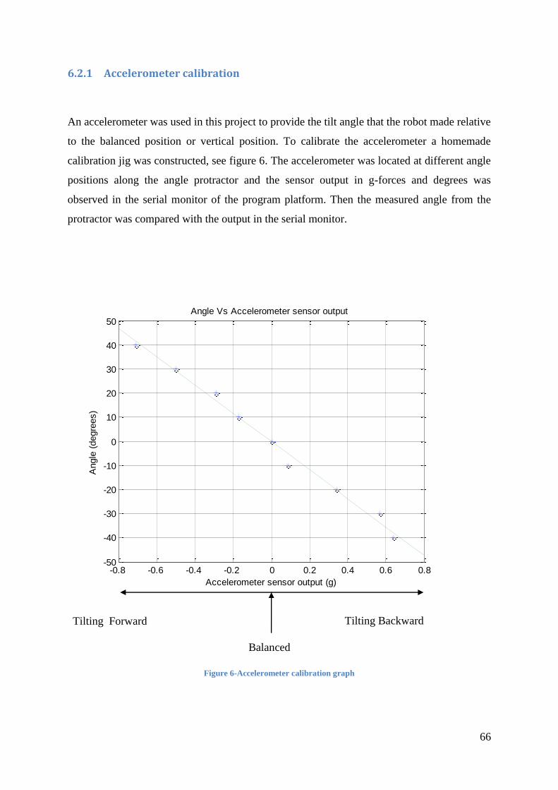
6.2.1 Accelerometer calibration

An accelerometer was used in this project to provide the tilt angle that the robot made relative

to the balanced position or vertical position. To calibrate the accelerometer a homemade

calibration jig was constructed, see figure 6. The accelerometer was located at different angle

positions along the angle protractor and the sensor output in g-forces and degrees was

observed in the serial monitor of the program platform. Then the measured angle from the

protractor was compared with the output in the serial monitor.

Fss

Figure 6-Accelerometer calibration graph

-0.8 -0.6 -0.4 -0.2 0 0.2 0.4 0.6 0.8-50

-40

-30

-20

-10

0

10

20

30

40

50Angle Vs Accelerometer sensor output

Accelerometer sensor output (g)

Angle

(degre

es)

Tilting Forward Tilting Backward

Balanced

67

Equation 6.1 below shows a linear fitted data of the accelerometer’s calibration.

y=-58.7x-0.22

6.2.2 Gyroscope calibration

Figure 6.2 below shows the gyroscope tilt rate against tilt when the robot was made to fall

forward from its upright position and caught before it hit the ground. The data was generated

in the serial monitor of the Arduino pde platform then streamed to excel then was finally

plotted using mat lab.

Figure 6.1 Gyroscope calibration graph

0 10 20 30 40 50 60 70 80-10

0

10

20

30

40

50

60Tilt rate Vs Tilt Angel

Tilt angle (degrees)

Tilt

rate

(degre

es/s

econds)

68

6.6.3 Complementary filter

Figure 6.2 below show the results of a complementary filter that was implemented for the

gyroscope tilt rate and the raw accelerometer angle fusion. The code for the graph and

complimentary filter is in appendix C. The sensors were sampled at 100Hz.The time constant

for the filter was chosen to be 0.49 seconds, see equation below

0.98 0.01

1 1 0.98

k T

k

=0.49 seconds

This meant that for time periods shorter than half a second, the gyroscope integration takes

precedence and the noisy horizontal accelerations are filtered out. For time periods longer

than half a second, the accelerometer average is given more weighting than the gyroscope,

which may have drifted by this point.

Figure 6.2 Complementary filter results

From figure the blue trace is the raw accelerometer tilt angle, the purple trace is the integrated

gyroscope angle and the black trace is the complementary filtered angle angle. As is can be

seen from figure 6.2, the gyroscope integrated angle behave normal then later after some few

seconds it start to drift, that is it does not return to zero angle when the robot is brought back

to its upright position. The raw accelerometer angle tends to be noise when the robot passed a

rough terrain like it was made to. So the best results for the robot tilt angle was brought by

69

the complementary filter because its angle estimate is responsive and accurate and not

sensitive to horizontal accelerations or to gyroscope drift.

70

6.3 Robot performance

The robot’s performance is not up to par. It does balance but it cannot seem to do so without

wobbling vigorously. At this stage it is only feeing back the tilt angle, the tilt rate and not the

linear speed as it was intended. It can recover from tilts of about 15 degrees and not more.

Figure 6.3 shows the robot in action.

71

CHAPTER 7 CONCLUSIONS AND RECOMMENDATIONS

7.1 Introduction

The data analysis performed from the previous chapter was instigated to provide a rational

assessment of the project ability to meet its aims and objectives. This chapter will cover

recommendations for future work and system improvements

7.2 Simulation versus actual performance

The results of the simulation performed in the previous chapter proved that the system is

doable.The simulation was done with the entire robot state variables in tacked in but

unfortunately the real system operated with half of these state variables. The final two which

were supposed to be fed back to the system which are the robot linear speed and position

could not be deduced for the real system because of limited time frame. As for the two other

which were the tilt angle and the tilt rate they behaved as predicted by the simulation.

7.3 Teaching aspects

The teaching aspect will follow a traditional method of the practise unit were students are

given a skeleton code to adjust and make it work.

7.4 Results versus Expectations

At the beginning of the project, the expectations were quite substantial. The goal was to

develop a robot that was so robust that it could recover from significant and deliberately

induced tilt. As problems and difficulties started to become evident in the programming, the

expectations reduced to simply providing a robot that could maintain stability. Incompletion

72

of the program has proved devastating as hence the results are not reflective of the

expectations.

7.5 Difficulities experienced

The difficulty experienced throughout the entire project was learning and implementing the

arduino programming launge with control theories.Consderable amounts of project time was

lost due to this fact. Understading how the sensors worked also proved to be difficult at the

start because the sensor chosen for the project needed to be fused together to work

properly,which was one thing realised a little to late.

73

REFERENCES

1. Ronald Siewart&Illah R.Nourbakhsh,2004, Introduction to Autonomous Mobile Robots,MIT Press

Cambridge,London.

2. Solerno,A and Angeles,J. 2007, A new Family of Two Wheeled Mobile Robots:Modelling and

Controllability.IEEE Transaction of Robotics.

3. Googol Technology (HK), Inverted Pendulum,viewed 22 May

2011,http://www.googoltech.com/uploads/catalog/996/GLIP.PDF

4. McComb, G & Predko, 2006, Robot Builders Bonanza, McGraw-Hill, Sydney.

5. Segway Inc, 2011, Simply moving, viewed 10 March 2011,

<http://www.segway.com/>

6. Anderson, DP, 2007, nBot Balancing Robot, viewed 15 March 2011,

<http://www.geology.smu.edu/~dpa-www/robo/nbot/>

7. John Billingsley, 2010, Essential of Control Techniques and Theory, Taylor and Francis Group,NW.

8. Envco-Environmental Equipment,2009,Analogue sensors,viewed 9 October

2011,<http://www.envcoglobal.com/catalog/water/water-quality-sensors/analogue-sensors>

9. Seattlerobotics,2011,analog and digital sensors,viewed 9 October

2011,<http://www.seattlerobotics.org/encoder/jul97/basics.html>

10. Dimension Engineering LLC,2011, A beginner’s guide to accelerometers,viewed 15 October 2011,<

http://www.dimensionengineering.com/accelerometers.htm>

11. Jay Esfandyari, Roberto De Nuccio, Gang Xu, 2011, Solutions for MEMS sensor fusion,

STMicroelectronics,Coppell, TX USA, viewed on

11October2011,<http://www.electroiq.com/articles/sst/print/volume-54/issue-7/features/cover-

article/solutions-for-mems-sensor-fusion.html>

12. Welch G & Bishop G, 2006, An Introduction to the Kalman Filter,Department of Computer

Science,Chapel Hill.

Frost & Sullivan 2006 Strategic Analysis of the Opportunities and Implications of Automotive Sensor

Fusion,media release,24 May 2006, Market Engineering Spiegel, M. R. 1992, Theory and Problems of

Probability and Statistics, 2nd ed. New York, McGraw-Hill.

13. Shane Colton,2007, The balance filter,Massachusetts Institute of Technology, viwied 12 October

2011,< http://web.mit.edu/scolton/www/filter.pdf>

14. Gadgetgangster 2011, Accelerometer-Gyro-Tutorial,Intructables,viewed 7 October

2011,<http://www.instructables.com/id/Accelerometer-Gyro-Tutorial/ >.

74

APPENDIX A

University of Southern Queensland

FACULTY OF ENGINEERING AND SURVEYING

ENG4111/4112 Research Project

PROJECT SPECIFICATION

FOR: TSHEPO DESMOND MOTSWAGAE

TOPIC: A LABORATORY EXPERIMENT BASED ON SEGWAY

SUPERVISOR: Professor JOHN BILLINGSLEY

SPONSORSHIP: Faculty of Engineering and Surveying

PROJECT AIM: This project aims at constructing an experiment for a mechatronic

practise unit, where a two wheeled self balancing robot will be build on

the principle concepts of a segway.

PROGRAMME: (Issue A, 22/03/2010)

1. Carry out a research based on different techniques of balancing two wheeled robots

and also research on sensors best suited for the design.

2. Carry out background calculations involved in the system and file them as teaching

aspects for the practise unit.

3. Simulate the system prior to construction.

4. Build the system, install appropriate sensors and develop algorithms for controlling

the system via a microprocessor.

75

As time permits

5. Replacement of the wired link by a radio link such as Bluetooth, with a unit self

powered and free standing will be considered.

AGREED (student) (supervisor)

Date: / / 2011 Date: / / 2011

Assistant Examiner:

APPENDIX B

Total weights = 750

Heights = 30cm

Wheel diameter = 90mm

Motor Weight = 514g

Chassis = 236g

76

33

1 0

73.3 73.3 2 73.3

73.3 73.3 2 73.3

73.3 2 73.3 73.3 2 73.3

1

73.3 2 73.3 73.3 2 73.3

73.32 7

M

f ga gb g gd

h h h h h

a b d

gb g gd f ga g gd

h h h h h h h

b d a d

gb

h

2 2

2

22 2

2 73.3 73.3 73.3 2 73.3 73.33.3 1 2 73.3

73.3 2 73.32 73.3 1 73.3

73.32 73.3

bg bgd f ga ag agdd d

h h h h h h

gb f f f gad d

h h h h h

gbd

h

3

33 3 4 2 2

4 3 3 3 2 2

34

2 73.373.3

73.3 2 73.32 73.3 73.3

73.3 73.3 22 73.3 73.3

1 0

73.3 73.3 73.31

73.3 73.3 73.3

f f f gad

h h h h

gb f f f gad d

h h h h h

gb f ga f fd d

h h h h h

M

f ga gb gc

h h h h

a b c

2 2 2 2

73.3 73.3 73.3 73.3

1 1

73.3 73.3 73.3 73.3

73.3 73.3 73.3 73.3 73.31 73.3 1

1

gb gc f ga gc

h h h h h

b c a c

gbc gbc cf gac gacc

h h h h h

2

2

4 3 3 3 2 2 2

4 3 2

73.373.3

73.373.3

73.3 73.3 2 73.32 73.3 73.3 73.3

73.3 73.3 2 73.32 73.3 73.3 73.3

cfc

h

cfc

h

gb f ga f f cfA I d c d

h h h h h h

gb f ga f f cfd c d

h h h h h h

77

APPENDIX C

C.1 Simulation code

' Simulation of the system

' Author: Tshepo Motswagae

Dim theta ' Store for the tilt angle of the stick (theta).

Dim dtheta ' Store for the rate of change of the tilt angle of the stick (dtheta/dt).

Dim phi ' Store for the angle that the wheel has rolled (phi).

Dim omega

Dim x

Dim v

Dim U ' This variable is used to store the amount of motor drive that is

proportional to the maximum drive of the motor.

Dim xdem

Dim vdem

Dim thetadem

Dim dt ' Stores the discrete time between measurements.

Dim T ' The position of the plot.

Dim delay ' Used to cause a delay so that the response can be observed and

studied.

Dim step ' The delay step that alows the simulation speed to be roughly the same

no matter what value dt is set at.

Dim stopit As Boolean ' Used to shut the program down.

78

Private Sub Form_Load() ' Main program routine

Graph.Scale (0, 3)-(100, -3) ' Set the scale of the Graph

Graph.Show ' Show the graph on screen

Graph.Cls ' Make sure that the graph is clear

Graph.Line (0, 0)-(300, 0), vbBlack ' Draw a line on the graph

at 0 vertically and right across the graph

stoppit = False ' Make sure that the program will

run continously.

T = 0 ' Set the graph starting position to 0

dt = 0.0001 ' Set the change in time

theta = 0 ' Set the initial tilt on the stick

dtheta = 0 ' Set the initial rate of change of the tilt

on the stick

phi = 0.3

omega = 0

x = 0 ' Set the initial angle that the wheel has rolled

' Set the initial rate of change of the angle that the

wheel has rolled

U = 0 ' Set the initial proprotion of full

motor drive 0 = none and 1 = full

79

xdem = 0.8 ' This is the initial target angle that the

motor will eventually drive the wheels to

vdem = 0

thetadem = 0 ' Sets the tilt that the system is trying

to target

delay = 0 ' Set the delay counter to 0 so that a

delay will be seen

Do

'Delay the response for visual purposes-----------------------------------------------------------------

-

step = 0.0001 / dt

While delay < 1

delay = delay + step

DoEvents

Wend

'End of the Delay---------------------------------------------------------------------------

'U = 0.8 * theta + 0.0338 * dtheta + 0.00017 * phi + 0.028 * omega 'first u, with

calculated coeffients using pole assignment

' U = 1.83 * theta + 0.2 * dtheta + 0.017 * phi + 0.065 * omega ' secound u, with new better

coeffients

'U = 80 * tilt + 3.38 * tiltrate + 1.7 * angle + 3 * angularvel 'trial an error deduced values

80

'U = 5 * theta + 1 * dtheta + 0.8 * phi + 0.3 * omega 'u with predicted values values

'------------------------------------------------------------------------------------------------

U = 1.83 * (theta - thetadem) + 0.2 * dtheta 'final u used that cater for the limits

'-----------------------------------------------------------------------------------------------

' limits for the motor, for realistic purpose. N.B every motor has a full drive

' If U > 1 Then

' U = 1

' ElseIf U < -1 Then

' U = -1

' Else

' End If

'-------------------------------------------------------------------------------------------------------

'State equations that decribe the system's dynamics

theta = theta + dtheta * dt

dtheta = dtheta + (3.26 * omega + 78.5 * theta - 119.86 * U) * dt

phi = phi + omega * dt

omega = omega + (73.3 * U - 2 * omega) * dt

81

x = 0.1 * (theta + phi)

v = 0.1 * (dtheta + omega)

'-------------------------------------------------------------------------------------------------------

'applying limits to the system for better perfomance on top of its demanded(targets)quantities

vdem = 0.3 * (xdem - x)

If vdem > 10 Then

vdem = 10

ElseIf vdem < -10 Then

vdem = -10

Else

End If

thetadem = 0.4 * (vdem - v)

If thetadem > 0.5 Then

thetadem = 0.5

ElseIf thetadem < -0.5 Then

thetadem = -0.5

Else

End If

Plotdata

82

delay = 0 ' reset delay counter

Loop Until stopit = True ' shut the program if quit button is pressed otherwise keep going

End

End Sub

Sub Plotdata()

Graph.PSet (T, x), vbRed

Graph.PSet (T, v), vbBlue ' Graph speed (v)

'Graph position (x)

Graph.PSet (T, theta), vbCyan ' Graph tilt

Graph.PSet (T, dtheta), vbBlack 'Graph the rate of the tilt

Graph.PSet (T, omega / 4), vbGreen ' Graph the angular velocity of the wheel

Graph.PSet (T, phi / 4), vbMagenta ' Graph the angle that the wheel has rolled

(phi)

If T > 100 Then ' Allow the graph plot to refresh

T = 0

Graph.Cls

Graph.Line (0, 0)-(3000, 0), vbBlack

83

Else

T = T + dt

End If

End Sub

Private Sub Command1_Click()

xdem = -0.8

End Sub

Private Sub Command3_Click() ' Sets the Target angle

when the appropriate button is pressed

xdem = -0.6

End Sub

Private Sub Command4_Click() ' Sets the Target angle

when the appropriate button is pressed

xdem = -0.4

End Sub

Private Sub Command5_Click() ' Sets the Target angle

when the appropriate button is pressed

84

xdem = -0.2

End Sub

Private Sub Command6_Click() ' Sets the Target angle

when the appropriate button is pressed

xdem = 0

End Sub

Private Sub Command7_Click() ' Sets the Target angle

when the appropriate button is pressed

xdem = 0.2

End Sub

Private Sub Command8_Click() ' Sets the Target angle

when the appropriate button is pressed

xdem = 0.4

End Sub

Private Sub Command9_Click() ' Sets the Target angle

when the appropriate button is pressed

85

xdem = 0.6

End Sub

Private Sub Command10_Click() ' Sets the Target angle when

the appropriate button is pressed

xdem = 0.8

End Sub

Private Sub Quit_Click() ' Stops the program after the

main loop has completed

stoppit = True

End

End Sub

C.2 Robot program

//angle and angle rate harnessing

int gyro_pinX = 0; //gyrosope pinX connected to anolog pin 0 of the arduino

int accel_pinX =2;

int accel_pinY =3;

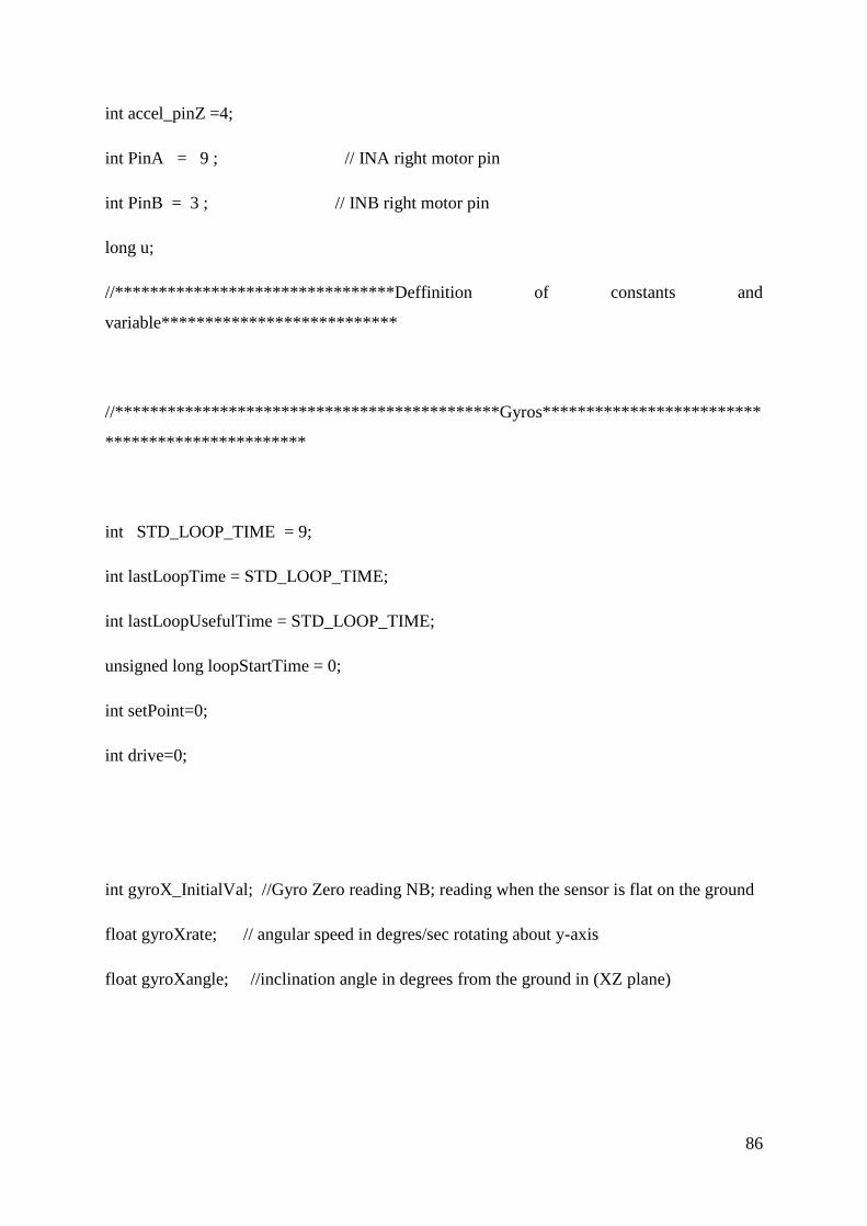
86

int accel_pinZ =4;

int PinA = 9 ; // INA right motor pin

int PinB = 3 ; // INB right motor pin

long u;

//********************************Deffinition of constants and

variable***************************

//********************************************Gyros*************************

***********************

int STD_LOOP_TIME = 9;

int lastLoopTime = STD_LOOP_TIME;

int lastLoopUsefulTime = STD_LOOP_TIME;

unsigned long loopStartTime = 0;

int setPoint=0;

int drive=0;

int gyroX_InitialVal; //Gyro Zero reading NB; reading when the sensor is flat on the ground

float gyroXrate; // angular speed in degres/sec rotating about y-axis

float gyroXangle; //inclination angle in degrees from the ground in (XZ plane)

87

//******************************************Accelerometer********************

******************

int accelX_InitialVal;// Acceloromter (x-axis) value when its flat on the ground ie: its intial

placement

float accelXval; //acclerometer value in g

float accelXangle; //raw acclerometer angle in XZ plane

int accelY_InitialVal;//y-axis

float accelYval; //raw acceleromter value in g

float accelYangle; // acclerometer value in YZ plane

int accelZ_initialVal;//z-axis

float accelZval;

//***********************************Results from the

sensors**********************************

//float xAngle;

float compliAngleX; // filttered angle

//float compliAngleY; //filttered angle

float R;// resultant force vector from the three accelerometer readings[x,y,z]

//(http://demonstrations.wolfram.com/PythagoreanTheorem3D/)

88

//*************************************timing*******************************

*****************

void setup()

{

analogReference(EXTERNAL); //3.3V= Vref (refference voltage)

Serial.begin(115200);

delay(100);//wait for the sensors to calibrate and get ready

//******************All intial sensors values NB:when chip is flat on the

ground******************

gyroX_InitialVal = calibrateGyroX();

// gyroY_InitialVal = calibrateGyroY();

accelX_InitialVal = calibrateAccelX();

accelY_InitialVal = calibrateAccelY();

accelZ_initialVal = calibrateAccelZ();

pinMode(PinA,OUTPUT);

89

pinMode(PinB,OUTPUT);

delay(100);

}

void loop()

{

//***********************Gyro angle

calculation***************************************

gyroXrate =-1.0*((double) ((analogRead(gyro_pinX)-

gyroX_InitialVal)*1.612903));//(gyroXadc-

gryoXIntial)*Vref/1023)/Sensitivity(mV/degree/sec) = AngleRate in degrees per seconds-

(Gyro sensetivity=2mV/o/sec)

gyroXangle=gyroXangle+gyroXrate*lastLoopTime/1000;//Raw angle without any filter

// gyroYrate = -1.0*((double)(((analogRead(gyro_pinY)-

gyroY_InitialVal)*0.003225806)/0.002));//(gyroYadc-

gryoYIntial)*Vref/1023)/Sensitivity(mV/degree/sec) = AngleRate in degrees per seconds-

(Gyro sensetivity=2mV/o/sec)

//gyroYangle=gyroYangle+gyroYrate*dt/1000;//angle Without any filter

90

//************************Accelerometer angle

calculation******************************

accelXval =(double) ((analogRead(accel_pinX)-

accelX_InitialVal)*0.009775169);//(accelXadc-

accelXIntial)*Vref/1023)/Sensitivity(mV/g)=accelXVal in g - (Accelorometer

sensetivity=330mV/g)

accelYval = (double)((analogRead(accel_pinY)-

accelY_InitialVal)*0.009775169);//(accelYadc-

accelYIntial)*Vref/1023)/Sensitivity(mV/g)=accelYVal in g - (Accelorometer

sensetivity=330mV/g)

accelZval = (double)((analogRead(accel_pinZ)-

accelZ_initialVal)*0.009775159);//(accelZadc-

accelZIntial)*Vref/1023)/Sensitivity(mV/g)=accelZVal in g - (Accelorometer

sensetivity=330mV/g)

accelZval++;//will always give 1g in horizontal position

R = sqrt(pow(accelXval,2)+pow(accelYval,2)+pow(accelZval,2));//the force vector

calcuation (R=sqrt(accelXval^2 + accelvalY^2 + accelvalZ^2))

//http://www.instructables.com/id/Accelerometer-Gyro-Tutorial/#step1

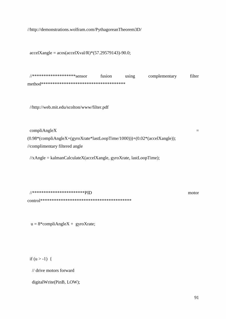
91

//http://demonstrations.wolfram.com/PythagoreanTheorem3D/

accelXangle = acos(accelXval/R)*(57.29579143)-90.0;

//*******************sensor fusion using complementary filter

method*************************************

//http://web.mit.edu/scolton/www/filter.pdf

compliAngleX =

(0.98*(compliAngleX+(gyroXrate*lastLoopTime/1000)))+(0.02*(accelXangle));

//complimentary filtered angle

//xAngle = kalmanCalculateX(accelXangle, gyroXrate, lastLoopTime);

//***********************PID motor

control****************************************

u = 8*compliAngleX + gyroXrate;

if (u > -1) {

// drive motors forward

digitalWrite(PinB, LOW);

92

analogWrite(PinA,255);

}

else if(u<1)

{

digitalWrite(PinA,LOW);

analogWrite(PinB,255);

}

else

{

analogWrite(PinA,0);

analogWrite(PinB,0);

}

//u = abs(u);

//if (u>10) map(u,0,255,0,255);

//u = abs(u);

//u = abs(u);

//map(u,0,255,0,255);

processing();

93

lastLoopUsefulTime = millis()-loopStartTime;

if(lastLoopUsefulTime<STD_LOOP_TIME) delay(STD_LOOP_TIME-

lastLoopUsefulTime);

lastLoopTime = millis() - loopStartTime;

loopStartTime = millis();

}

**********************************************Calibrationn*******************

***********************

//*************************Results from calibrating the sensors********************

//gyros

long resultGyroX;//x-axis

//long resultGyroY;//y-axis

//long resultGyroZ;//z-axis

//accelerometers

long resultAccelX;//x-axis

long resultAccelY;//y-axis

long resultAccelZ;//z-axis

//**************************calibitrating

gyros*************************************

//taking 100 readings when gryo and Accelerometer are at their intial position then averaging

them

94

int calibrateGyroX()

{

for(int i=0;i<100;i++)

{

resultGyroX += analogRead(gyro_pinX);

delay(1);

}

resultGyroX = resultGyroX/100;

return resultGyroX;

}

/*int calibrateGyroY()

{

for(int i=0;i<100;i++)

{

resultGyroY += analogRead(gyro_pinY);

delay(1);

}

resultGyroY = resultGyroY/100;

return resultGyroY;

}

*/

//*********************************calibtrating accelemoter********************

95

int calibrateAccelX()

{

for(int i=0;i<100;i++)

{

resultAccelX += analogRead(accel_pinX);

delay(1);

}

resultAccelX = resultAccelX/100;

return resultAccelX;

}

int calibrateAccelY()

{

for(int i=0;i<100;i++)

{

resultAccelY += analogRead(accel_pinY);

delay(1);

}

resultAccelY = resultAccelY/100;

return resultAccelY;

}

96

int calibrateAccelZ()

{

for(int i=0;i<100;i++)

{

resultAccelZ += analogRead(accel_pinZ);

delay(1);

}

resultAccelZ = resultAccelZ/100;

return resultAccelZ;

}

***************************************Processing/graphing to Arduino

processing***************

//print data to processing

void processing()

{

//***********************angles***************************************

Serial.print(gyroXangle);Serial.print("\t");

//Serial.print(gyroYangle);Serial.print("\t");

Serial.print(accelXangle);Serial.print("\t");

// Serial.print(accelYangle);Serial.print("\t");

97

Serial.print(compliAngleX);Serial.print("\t");

// Serial.print(compliAngleY); Serial.print("\t");

//Serial.print(xAngle);Serial.print("\t");

//*****************************angle rates*********************************

//Serial.print(gyroXrate,0);Serial.print("\t");

/*Serial.print(gyroYrate,0);Serial.print("\t");

Serial.print(accelXval,2);Serial.print("\t");

Serial.print(accelYval,2);Serial.print("\t");

Serial.print(accelZval,2);Serial.print("\t");

*/

//*********************************timing****************************

// Serial.print(lastLoopTime);;Serial.print("\t");

// Serial.print(lastLoopUsefulTime); Serial.print("\t");

Serial.print("\n");

}

C.3 APPENDIX -graph code

import processing.serial.*;

98

Serial arduino;

String stringGyroX;

String stringAccX;

String stringCompX;

String stringKalmanX;

int[] gyroX = new int[600];

float inGyroX;

int[] accX = new int[600];

float inAccX;

int[] compX = new int[600];

float inCompX;

void setup()

{

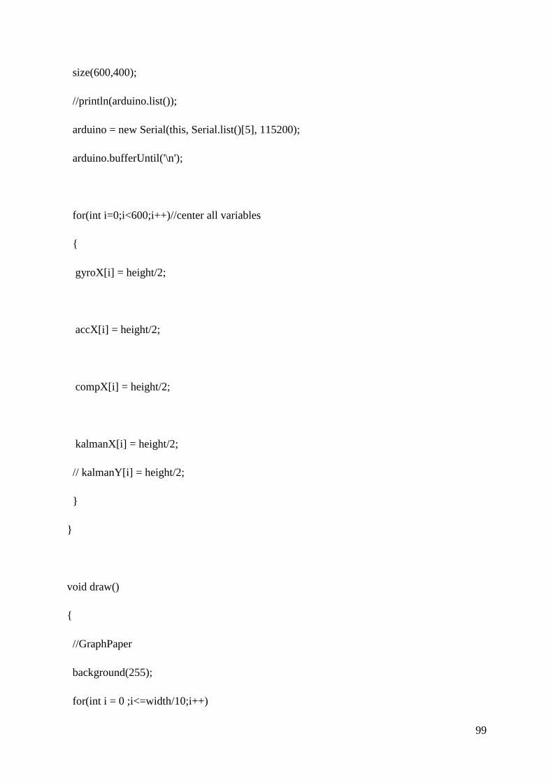
99

size(600,400);

//println(arduino.list());

arduino = new Serial(this, Serial.list()[5], 115200);

arduino.bufferUntil('\n');

for(int i=0;i<600;i++)//center all variables

{

gyroX[i] = height/2;

accX[i] = height/2;

compX[i] = height/2;

kalmanX[i] = height/2;

// kalmanY[i] = height/2;

}

}

void draw()

{

//GraphPaper

background(255);

for(int i = 0 ;i<=width/10;i++)

100

{

stroke(200);

line((-frameCount%10)+i*10,0,(-frameCount%10)+i*10,height);

line(0,i*10,width,i*10);

}

convert();

drawAxisX();

//drawAxisY();

}

void serialEvent (Serial arduino)

{

//get the ASCII strings:

stringGyroX = arduino.readStringUntil('\t');

stringAccX = arduino.readStringUntil('\t');

stringCompX = arduino.readStringUntil('\t');

}

//convert all axis

int maxAngle = -90;

101

void convert()

{

//convert the gyro x-axis

if(stringGyroX != null)

{

//trim off any whitespace:

stringGyroX = trim(stringGyroX);

//convert to an float and map to the screen height:

inGyroX = float(stringGyroX);

inGyroX = map(inGyroX, maxAngle, -maxAngle, 0, height);

gyroX[gyroX.length-1] = int(inGyroX);

}

//convert the accelerometer x-axis

if (stringAccX != null)

{

//trim off any whitespace:

stringAccX = trim(stringAccX);

//convert to an float and map to the screen height:

inAccX = float(stringAccX);

inAccX = map(inAccX, maxAngle, -maxAngle, 0, height);

accX[accX.length-1] = int(inAccX);

}

102

//convert the complementary filter x-axis

if (stringCompX != null)

{

//trim off any whitespace:

stringCompX = trim(stringCompX);

//convert to an float and map to the screen height:

inCompX = float(stringCompX);

inCompX = map(inCompX, maxAngle, -maxAngle, 0, height);

compX[compX.length-1] = int(inCompX);

}

*****************************convert axes*******************

}void drawAxisX()

{

//draw gyro x-axis

noFill();

stroke(127,34,255);//purple

//redraw everything

beginShape();

for(int i = 0; i<gyroX.length;i++){

vertex(i,gyroX[i]);

}

103

endShape();

//put all data one array back

for(int i = 1; i<gyroX.length;i++){

gyroX[i-1] = gyroX[i];

}

//draw acceleromter x-axis

noFill();

stroke(0,129,230);//light blue

//redraw everything

beginShape();

for(int i = 0; i<accX.length;i++){

vertex(i,accX[i]);

}

endShape();

//put all data one array back

for(int i = 1; i<accX.length;i++){

accX[i-1] = accX[i];

}

//draw complementary filter x-axis

noFill();

stroke(0);//black

//redraw everything

beginShape();

104

for(int i = 0; i<compX.length;i++){

vertex(i,compX[i]);

}

endShape();

//put all data one array back

for(int i = 1; i<compX.length;i++){

compX[i-1] = compX[i];

}

/*

}

************************print/graph**********

void printAxis()

{

print(stringGyroX);

print(stringAccX);

print(stringCompX);

}

105