University of Pennsylvania - Finance Department
300
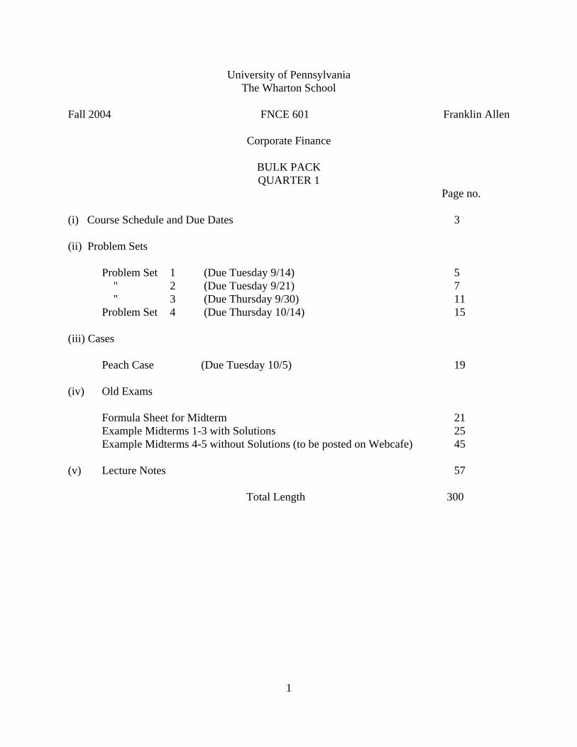
1 University of Pennsylvania The Wharton School Fall 2004 FNCE 601 Franklin Allen Corporate Finance BULK PACK QUARTER 1 Page no. (i) Course Schedule and Due Dates 3 (ii) Problem Sets Problem Set 1 (Due Tuesday 9/14) 5 " 2 (Due Tuesday 9/21) 7 " 3 (Due Thursday 9/30) 11 Problem Set 4 (Due Thursday 10/14) 15 (iii) Cases Peach Case (Due Tuesday 10/5) 19 (iv) Old Exams Formula Sheet for Midterm 21 Example Midterms 1-3 with Solutions 25 Example Midterms 4-5 without Solutions (to be posted on Webcafe) 45 (v) Lecture Notes 57 Total Length 300
Transcript of University of Pennsylvania - Finance Department
1
University of Pennsylvania The Wharton School
Fall 2004 FNCE 601 Franklin Allen Corporate Finance
BULK PACK QUARTER 1
Page no. (i) Course Schedule and Due Dates 3 (ii) Problem Sets Problem Set 1 (Due Tuesday 9/14) 5 " 2 (Due Tuesday 9/21) 7 " 3 (Due Thursday 9/30) 11 Problem Set 4 (Due Thursday 10/14) 15 (iii) Cases Peach Case (Due Tuesday 10/5) 19 (iv) Old Exams Formula Sheet for Midterm 21 Example Midterms 1-3 with Solutions 25 Example Midterms 4-5 without Solutions (to be posted on Webcafe) 45 (v) Lecture Notes 57 Total Length 300

2
INTENTIONALLY BLANK
3
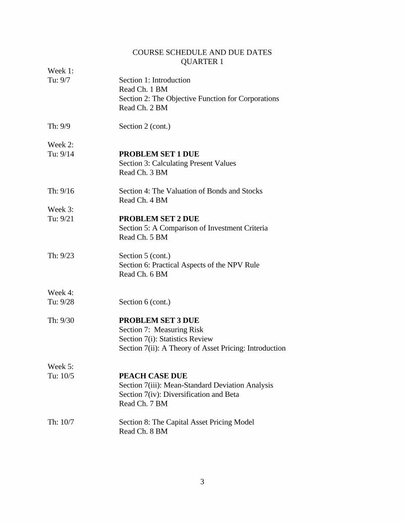
COURSE SCHEDULE AND DUE DATES QUARTER 1 Week 1: Tu: 9/7 Section 1: Introduction Read Ch. 1 BM Section 2: The Objective Function for Corporations Read Ch. 2 BM Th: 9/9 Section 2 (cont.) Week 2: Tu: 9/14 PROBLEM SET 1 DUE Section 3: Calculating Present Values Read Ch. 3 BM Th: 9/16 Section 4: The Valuation of Bonds and Stocks Read Ch. 4 BM Week 3: Tu: 9/21 PROBLEM SET 2 DUE Section 5: A Comparison of Investment Criteria Read Ch. 5 BM Th: 9/23 Section 5 (cont.) Section 6: Practical Aspects of the NPV Rule Read Ch. 6 BM Week 4: Tu: 9/28 Section 6 (cont.) Th: 9/30 PROBLEM SET 3 DUE Section 7: Measuring Risk Section 7(i): Statistics Review Section 7(ii): A Theory of Asset Pricing: Introduction Week 5: Tu: 10/5 PEACH CASE DUE Section 7(iii): Mean-Standard Deviation Analysis Section 7(iv): Diversification and Beta Read Ch. 7 BM Th: 10/7 Section 8: The Capital Asset Pricing Model Read Ch. 8 BM

4
Week 6: Tu: 10/12 Section 8 (cont.) Th: 10/14 PROBLEM SET 4 DUE Section 9: Capital Budgeting and the CAPM Read Ch. 9 BM Week 7: Tu 10/19 Exam Week for MBA Core – No class Th: 10/21 Exam week for MBA Core - No class QUARTER 2 Week 1: Tu: 10/26 Break - No class Th: 10/28 Review Session during regular class Week 2: Mon: 11/1 MIDTERM EXAM 6:15-7:45pm
5
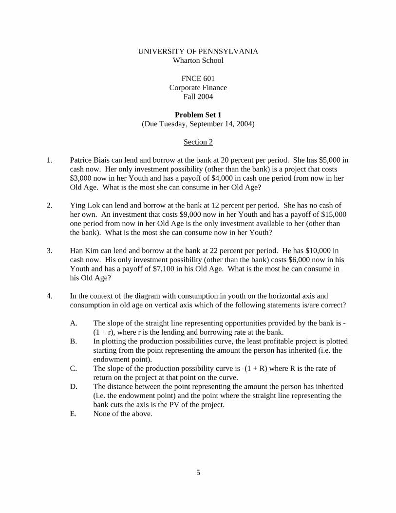
UNIVERSITY OF PENNSYLVANIA Wharton School
FNCE 601
Corporate Finance Fall 2004
Problem Set 1
(Due Tuesday, September 14, 2004)
Section 2 1. Patrice Biais can lend and borrow at the bank at 20 percent per period. She has $5,000 in
cash now. Her only investment possibility (other than the bank) is a project that costs $3,000 now in her Youth and has a payoff of $4,000 in cash one period from now in her Old Age. What is the most she can consume in her Old Age?
2. Ying Lok can lend and borrow at the bank at 12 percent per period. She has no cash of
her own. An investment that costs $9,000 now in her Youth and has a payoff of $15,000 one period from now in her Old Age is the only investment available to her (other than the bank). What is the most she can consume now in her Youth?
3. Han Kim can lend and borrow at the bank at 22 percent per period. He has $10,000 in
cash now. His only investment possibility (other than the bank) costs $6,000 now in his Youth and has a payoff of $7,100 in his Old Age. What is the most he can consume in his Old Age?
4. In the context of the diagram with consumption in youth on the horizontal axis and
consumption in old age on vertical axis which of the following statements is/are correct? A. The slope of the straight line representing opportunities provided by the bank is -
(1 + r), where r is the lending and borrowing rate at the bank. B. In plotting the production possibilities curve, the least profitable project is plotted
starting from the point representing the amount the person has inherited (i.e. the endowment point).
C. The slope of the production possibility curve is -(1 + R) where R is the rate of return on the project at that point on the curve.
D. The distance between the point representing the amount the person has inherited (i.e. the endowment point) and the point where the straight line representing the bank cuts the axis is the PV of the project.
E. None of the above.

6
PROBLEM SET 1 (continued) 5. Which of the following assumptions are necessary to ensure all shareholders will agree
on a firm's capital budgeting decisions if it maximizes NPV? A. The lending rate is equal to the borrowing rate. B. One group of shareholders has different information about the firm's future
prospects than another group. C. The firm is so large that it can influence interest rates. D. There are no frictions. E. None of the above.
Examination Question – Section 2 6. Consider a world with two points in time, t0 and t1. John Lee inherits $5.0 million at t0.
He has three projects he can invest this inheritance in at t0. Project A costs $750,000 at t0 and yields $965,000 at t1. Project B costs $630,000 at t0 and yields $710,000 at t1. Project C costs $350,000 at t0 and yields $370,000 at t1. He can also lend and borrow at a bank at an interest rate of 11 percent.
(a) Which projects should John undertake? (b) What is the largest amount John can consume at t1, given he wishes to consume
$2.4M at t0? (c) How would your answers to (a) and (b) be changed if John could lend to the bank
at 9 percent and borrow from the bank at 13 percent?
7
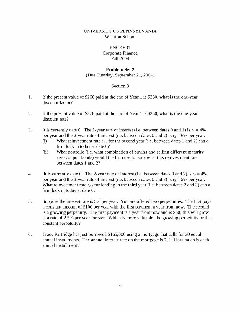
UNIVERSITY OF PENNSYLVANIA Wharton School
FNCE 601
Corporate Finance Fall 2004
Problem Set 2
(Due Tuesday, September 21, 2004)
Section 3 1. If the present value of $260 paid at the end of Year 1 is $230, what is the one-year
discount factor? 2. If the present value of $378 paid at the end of Year 1 is $350, what is the one-year
discount rate? 3. It is currently date 0. The 1-year rate of interest (i.e. between dates 0 and 1) is r1 = 4%
per year and the 2-year rate of interest (i.e. between dates 0 and 2) is r2 = 6% per year. (i) What reinvestment rate r1,2 for the second year (i.e. between dates 1 and 2) can a
firm lock in today at date 0? (ii) What portfolio (i.e. what combination of buying and selling different maturity
zero coupon bonds) would the firm use to borrow at this reinvestment rate between dates 1 and 2?
4. It is currently date 0. The 2-year rate of interest (i.e. between dates 0 and 2) is r2 = 4%
per year and the 3-year rate of interest (i.e. between dates 0 and 3) is r3 = 5% per year. What reinvestment rate r2,3 for lending in the third year (i.e. between dates 2 and 3) can a firm lock in today at date 0?
5. Suppose the interest rate is 5% per year. You are offered two perpetuities. The first pays
a constant amount of $100 per year with the first payment a year from now. The second is a growing perpetuity. The first payment is a year from now and is $50; this will grow at a rate of 2.5% per year forever. Which is more valuable, the growing perpetuity or the constant perpetuity?
6. Tracy Partridge has just borrowed $165,000 using a mortgage that calls for 30 equal
annual installments. The annual interest rate on the mortgage is 7%. How much is each annual installment?
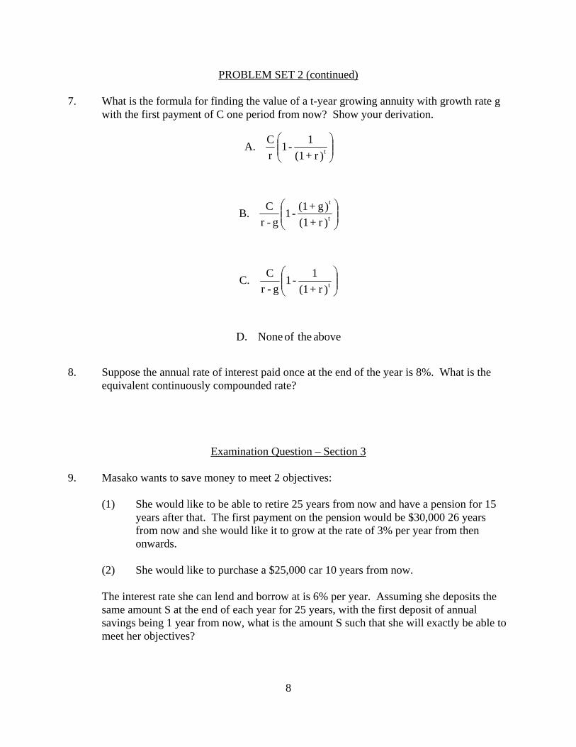
PROBLEM SET 2 (continued) 7. What is the formula for finding the value of a t-year growing annuity with growth rate g
with the first payment of C one period from now? Show your derivation.
⎟⎟⎠
⎞⎜⎜⎝
⎛)r + (1
1 - 1 rC A. t
⎟⎟⎠
⎞⎜⎜⎝
⎛)r + (1)g + (1 - 1
g -r C B. t
t
⎟⎟⎠
⎞⎜⎜⎝
⎛)r + (1
1 - 1g -r
C C. t
above theof None D.
8. Suppose the annual rate of interest paid once at the end of the year is 8%. What is the
equivalent continuously compounded rate?
Examination Question – Section 3
9. Masako wants to save money to meet 2 objectives: (1) She would like to be able to retire 25 years from now and have a pension for 15
years after that. The first payment on the pension would be $30,000 26 years from now and she would like it to grow at the rate of 3% per year from then onwards.
(2) She would like to purchase a $25,000 car 10 years from now. The interest rate she can lend and borrow at is 6% per year. Assuming she deposits the
same amount S at the end of each year for 25 years, with the first deposit of annual savings being 1 year from now, what is the amount S such that she will exactly be able to meet her objectives?
8
PROBLEM SET 2 (continued)
Section 4 10. Why is it usually argued prices in the stock market are equal to the present value of their
payoffs? A. Specialists and other market-makers who post prices set them to be equal to
present values. B. Arbitrage. C. Tax incentives provided by the government. D. None of the above. 11. A bond with par value $1,000 and an annual coupon (i.e. interest payment) of 8%
matures in six years. The current yield on similar bonds is 6%. What is the current price of the bond assuming the first interest payment is a year from now?
12. Company A's dividends are expected to grow at a constant rate of g = 3% Div1 = $35 and
r = 0.08. What is the current price? 13. Company B's dividends are expected to grow at a constant rate of g. P0 = $80; DlV1 =
$5; r = 0.10. What is g?
14. Company C's dividends are expected to grow at a constant rate of g. The company has
just paid a dividend D. What is the price?
g-r
r)+D(1 = P A. 0
g-r
g)+D(1 = P B. 0
g-r
D = P C. 0
D. None of the above
9
PROBLEM SET 2 (continued)15. Company D's dividends are expected to grow at a constant rate of g. It is just about to
pay a dividend D. What is the current price?
g-r
g)+D(1 = P A. 0
g-r
g)+D(1+ D= P B. 0
g-r
D = P C. 0
D. None of the above 16. Suppose there is a perfect capital market with no frictions or taxes. The current price of a
stock is $10 per share. It is just about to go ex-dividend and a dividend of $1 will be paid. People owning the stock at close of trading today will receive a dividend of $1. If somebody buys the stock tomorrow they will not receive the dividend. Irene Lu is certain that the price tomorrow will be $9.25 which implies that there is an arbitrage opportunity. How can she make money by exploiting this arbitrage opportunity?
17. Suppose there is a perfect capital market with no frictions or taxes. Moreover, suppose
there are no arbitrage opportunities remaining in this capital market. The current price of a stock is $15. It is going to pay a dividend of $2. What will the price tomorrow be after it goes ex-dividend?
18. A firm has no growth opportunities and pays out all its earnings as dividends. It's
earnings are expected to stay level in the future at $5 per share. It's current stock price is $60. What is its market capitalization rate?
Examination Question – Section 4 19. (a) The Elephant Corporation pays dividends annually. It's next dividend will be paid
one year from now and is expected to be $10. The dividend will grow at g1 = 15% for two years and then at g2 = 5% forever after that. What is the stock's current price if it's market capitalization rate is 8%?
(b) WVC pays dividends annually. It has just paid a dividend of $3.23 a share. This
dividend is expected to grow at 20% per year for two years, 15% per year for four years after that and then at 3% forever thereafter. Suppose the opportunity cost of capital and hence the discount rate is 10%. What will be the price of a share of WVC?
10

11
UNIVERSITY OF PENNSYLVANIA Wharton School
FNCE 601
Corporate Finance Fall 2004
Problem Set 3
(Due Thursday, September 30, 2004)
Section 51. C0 C1 C2 C3 -200 70 80 100 What is the IRR? 2. C0 C1 C2 C3 -100 80 50 -25 What are the IRR(s) above 0? 3. Two mutually exclusive projects have the following cash flows: C0 C1 IRR A -500 600 20% B -60 80 33% For what range of discount rates between 0 and 50% should B be chosen? 4. Projects A and B have the following cash flows: C0 C1 C2 C3 C4 A (200) 80 60 100 60 B (80) 45 40 0 0 If a company uses the payback rule with a cutoff period of 2 years, which projects would
it accept?
12
PROBLEM SET 3 (continued) 5. Consider the following project. C0 C1 C2 C3 C4 C5 -280 550 -180 250 100 -500 Design an appropriate IRR rule for opportunity costs of capital between 0% and 100%.
(i.e. For which opportunity costs of capital should you accept the project and for which should you reject it?)
Examination Question – Section 5 6. Ashok Narayan has $1,000 to invest. He could invest it in the bank at 10%.
Alternatively he could invest in the following project. C0 C1 C2 C3 C4 -1,000 725 825 875 -1450 (i) What is the IRR between 0 and 10%? (ii) At date 4, how much will Ashok have if he puts his $1,000 in the bank at date 0? (iii) At date 4, how much will Ashok have if he puts his $1,000 in the project at date 0
and puts the cash flows the project generates in the bank? (iv) What is the NPV of the project and how does it relate to your answers in (ii) and
(iii)? Section 6 7. A food processing company has just developed a new kind of soup. It is now trying to
decide whether to build a plant and put the soup into production. In undertaking this capital budgeting exercise which of the following cash flows should be treated as incremental when deciding whether to go ahead and produce the soup?
A. The research and development costs that were incurred developing the soup. B. The value of the land the plant will be built on which is currently owned by the
company. [C - J on the next page]

13
PROBLEM SET 3 (continued) C. The consequent reduction in the sales of the company's existing soup brands.
D. The salvage value of the plant and equipment at the end of its planned life. E. The annual depreciation charge.
F. Marketing expenses for the product. G. A proportion of expenses for the head office assuming these expenses are
independent of whether soup is produced. H. Interest Payments. I. Dividend Payments. J. The expenditures five years from now which will be necessary to ensure the plant
meets regulations which will come into force then. 8. The Follies Company needs to replace some of their lighting equipment. They can either
purchase lights from GE or from Philips. The GE equipment lasts for four years while the Philips equipment lasts for three. The discount rate for this type of project is 10%. The performance of the two types of light is the same. The after tax costs (i.e. all the figures below are negative) at each date are as follows.
t=0 1 2 3 4 GE 50 5 10 15 20 Philips 30 5 5 15 Which is the equipment with the lowest equivalent annual cost? 9. A firm has a choice of undertaking a project now or next year. The cash flows in the two
cases are as follows. t = 0 1 2 3 Start now -10 12 18 0 Start next year 0 -8 13 17 When should the firm undertake the project if the discount rate is 5 percent? 10. ITT is building a new plant to make telephones in South Carolina. The initial working
capital needs of the plant to finance inventory, payroll and so forth are $5M. Each year these needs are expected to increase by 5 percent. After five years the plant will be closed and the working capital recovered. In undertaking a capital budgeting exercise to see whether or not to build the plant, what are the cash flows that should be included to take account of the working capital?

14
PROBLEM SET 3 (continued) Examination Questions - Section 6 11. You are asked to evaluate the following wooden cabinet manufacturing project for a
corporation. Develop a table showing the annual cash flows and calculate the NPV of this project at an 8% discount rate. All figures are given in nominal terms.
20X6 20X7 20X8 Physical Production (cabinets) 3,150 3,750 3,800 Labor Input (hours) 26,000 30,000 31,000 Wood (physical units) 550 630 650 The required investment on 12/31/X5 is $800,000. The firm faces a 34% income tax
rate, and uses straight-line depreciation. The salvage value of the investment which will be received on 12/31/X8 will be one fifth of the initial investment. The price of cabinets on 12/31/X5 will be $250 each and will remain constant in the foreseeable future. Labor costs will be $15 per hour on 12/31/X5 and will increase at 5% per year. The cost for the wood will be $200 per physical unit on 12/31/X5 and will increase at 2% per year. Revenue is received and costs are paid at year's end (i. e. use year-end prices in calculating revenues and costs so, for example, use the 12/31/X6 prices for calculating 19X6 revenues and costs). The firm has profitable ongoing operations so that any losses for tax purposes from the project can be offset against these.
12. The Northwestern Railroad Company is thinking of replacing a locomotive that it
purchased 8 years ago. At that time the projected life of the locomotive was 20 years. It cost $1,325,000 and was expected to have a salvage value of $230,000. It can currently be sold for $745,000. Maintenance costs for the old machine were $133,000 during the last year and are expected to grow at 5% per year. The new locomotive they are thinking of buying has a life of 15 years. It costs $1,640,000 and has an expected salvage value of $195,000. The maintenance costs are expected to be $96,000 during the first year and to grow at 4% thereafter. Both locomotives are expected to generate the same revenues. The firm has a tax rate of 37%. It has profitable ongoing operations and can offset all the costs for tax purposes. It uses straight line depreciation. Assume all cash flows occur at the end of the year. The firm's discount rate for decisions of this type is 12%. Does the old or the new locomotive have the highest equivalent annual cost? Should Northwestern replace the locomotive?
(Hint: Solve in two parts. Treat the opportunity cost of the old locomotive like a
purchase price.)

15
UNIVERSITY OF PENNSYLVANIA Wharton School
FNCE 601
Corporate Finance Fall 2004
Problem Set 4
(Due Thursday, October 14, 2004)
Sections 7 and 8
1. There are four stocks X1, X2, X3 and X4. Each share of X1, X2, X3 and X4 has a payoff of 0 with probability 0.5 and 2 with probability 0.5. The payoffs of X1, X2, X3 and X4 are independent.
(a) What is the mean and standard deviation of each stock? (b) Suppose you buy 1/2 share of X1 and X2, what is the mean and standard deviation of
the portfolio? (c) Suppose you buy 1/3 share of X1, X2 and X3, what is the mean and standard deviation
of the portfolio? (d) Suppose you buy 1/4 share of X1, X2, X3 and X4, what is the mean and standard
deviation of the portfolio? 2. Which of the following statements is/are correct? A. Mean and standard deviation have the same units. B. Mean is a measure of dispersion. C. If two random variables have a negative covariance it means they tend to move in the
opposite direction. D. If two random variables don't move together or in opposite directions on average at all
they have a zero covariance. E. Correlation coefficients must be equal to -1 or +1 or lie in between.
16
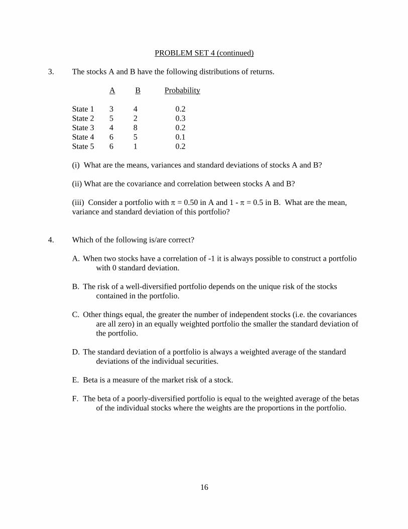
PROBLEM SET 4 (continued) 3. The stocks A and B have the following distributions of returns. A B Probability State 1 3 4 0.2 State 2 5 2 0.3 State 3 4 8 0.2 State 4 6 5 0.1 State 5 6 1 0.2 (i) What are the means, variances and standard deviations of stocks A and B? (ii) What are the covariance and correlation between stocks A and B? (iii) Consider a portfolio with π = 0.50 in A and 1 - π = 0.5 in B. What are the mean,
variance and standard deviation of this portfolio? 4. Which of the following is/are correct? A. When two stocks have a correlation of -1 it is always possible to construct a portfolio
with 0 standard deviation. B. The risk of a well-diversified portfolio depends on the unique risk of the stocks
contained in the portfolio. C. Other things equal, the greater the number of independent stocks (i.e. the covariances
are all zero) in an equally weighted portfolio the smaller the standard deviation of the portfolio.
D. The standard deviation of a portfolio is always a weighted average of the standard
deviations of the individual securities. E. Beta is a measure of the market risk of a stock. F. The beta of a poorly-diversified portfolio is equal to the weighted average of the betas
of the individual stocks where the weights are the proportions in the portfolio.
17
PROBLEM SET 4 (continued) 5. Use EXCEL to answer this question. Stock X has mean return 0.15 and standard
deviation 0.6. Stock Y has mean return 0.10 and standard deviation 0.4. The correlation between them is +0.1. Plot the portfolio locus for these two stocks in mean standard-deviation space with the mean on the vertical axis and the standard deviation on the horizontal axis. Specifically, trace the risk-return tradeoff given by combining these two stocks in varying amounts. Let π represent the proportion of wealth invested in X and 1-π the proportion in Y. Allow π to vary between -0.2 and 1.2 in steps of 0.1. What investments in X and Y do the portfolios with π < 0 and π > 1 correspond to? Attach a copy of your plot of the efficiency locus and the data it is based on with your answers.
6. Suppose that the standard deviation of returns on each individual stock is 80% per annum
and that the covariance between each pair of stocks is 0.25. What is the annual standard deviation of an equally weighted well-diversified portfolio? (Assume 1/N = 0)
7. The risk free rate is 8 percent and the expected return on the market portfolio is 16
percent. What is the expected return on a well-diversified portfolio with a beta of 0.6? 8. Phillippe borrows $15,000 at the risk free interest rate of 5% and invests this together
with $15,000 of his own money in the market portfolio. If the market portfolio has a standard deviation of 15%, what is the standard deviation of the return to his investment?
9. Which of these strategies would offer the same expected return to an investor as a stock
with a beta of 0.5? A. Investing a half of her money in T-bills and investing the remainder in the market
portfolio B. Borrowing an amount equal to one-half of her own resources and investing everything
in the market portfolio C. Borrowing an amount equal to her own resources and investing everything in the
market portfolio D. None of the above
18
PROBLEM SET 4 (continued)
Examination Question – Sections 7 and 8
10. (Parts a, b and c are independent. No information from one should be assumed for the other.)
(a) Suppose there are three types of people in an economy, type A's, B's and C's. There are
also three assets X, Y and Z. Assets X and Y are risky but asset Z is risk free. Type A's hold 45 percent of their portfolios in X, 30 percent in Y and 25 percent in Z. Type B's hold 30 percent of their portfolios in X, 20 percent in Y and 50 percent in Z. Type C's hold 15 percent in X, 10 percent in Y and 75 percent in Z. Are these holdings consistent with the Capital Asset Pricing Model being satisfied? Explain briefly why or why not.
(b) Suppose that the Capital Asset Pricing Model holds. The market portfolio has an
expected return of 0.14 and a standard deviation of 0.35. The risk free rate is 0.05. How could you construct a portfolio having an expected return of 0.20? What are the beta and standard deviation of this portfolio?
(c) You have discovered three portfolios with the following characteristics. Investment Expected Return Beta Unique Risk A 6 percent 0.0 none B 15 percent 1.0 none C 18 percent 1.5 none Plot expected returns against betas for these three portfolios.
(i) Do they all lie on the security market line and is there an arbitrage opportunity available?
(ii) Give a zero-investment, zero-risk portfolio with positive expected return that has either +$1 or -$1 invested in C.
(iii) What is the expected return on the portfolio in (iii)?

19
FNCE 601 Fall 2004 THE PEACH CASE Franklin Allen Instructions: This case will count for 4% of the course grade. It is due on Tuesday, October 5 at 9:00am. It should be uploaded to the FNCE 601 Webcafe site as explained on the next page. The case should be done in groups of three people or less. Each group should include one EXCEL file containing the spreadsheets that are developed to solve the case and a brief one-page write-up explaining what was done. In the write-up state carefully any assumptions that you make in order to be able to solve the problem. The Peach Company is thinking of building a new plant to put the peaches it grows into cans. The plant is expected to last for 20 years. Its initial cost is $20 million. This cost can be depreciated over the full 20-year life of the plant using straight line depreciation. It will require a major renovation which will cost $8 million in real terms after 10 years. This cost of renovation can be depreciated (again using straight line depreciation) over the remaining 10 years of the plant's life. The land the plant is built on could be rented out for $500,000 a year in nominal terms for twenty years. The salvage value of the plant at the end of the twenty years is $3.5 million in nominal terms. This salvage value is attributed to the original expenditure on the plant for tax purposes. There is no salvage value with regard to the renovation. The plant will be able to produce 50 million cans of peaches a year. The price of a can of peaches is currently $0.50. It is expected to grow at a rate of 3% per year in real terms for 6 years and then at 0% in real terms for the remainder of the plant's life. The firm expects to be able to sell all the cans of peaches it can produce. The peaches the firm puts in the cans are grown in the firm's own orchards. If the peaches were not canned they could be sold to supermarkets. The current price they could obtain per peach is $0.1. This price is expected to grow at a rate of 2% in real terms for 5 years and then at 1% in real terms for the next five years and finally at 0% in real terms for the remainder of the plant's life. Each can requires 2.5 peaches to fill it. The raw materials for the cans currently cost $0.05 per can. These costs are expected to remain constant in real terms. The labor required to operate the plant costs a total of $5 million dollars a year in real terms. Initially, the total working capital requirement is $10 million and this is expected to remain constant in real terms. The rate of inflation is expected to be 4% per year for the next four years and 3% per year for the remainder of the plant's life. The firm's total tax rate including local taxes is 38 per cent. The firm expects to make substantial profits on its other operations so that it can offset any losses on the peach canning plant for tax purposes. Its opportunity cost of capital for projects of this type is 14% in nominal terms. Construct two spreadsheets in EXCEL to find the NPV of the peach canning plant. One spreadsheet should be in nominal terms and the other should be in real terms. The value of the real and nominal NPVs should be the same. Should the firm build the plant?

20
GUIDELINES FOR SUBMITTING YOUR CASE STUDY:
1. Assign just one member of your team to create the team’s project folder. Logon to web Café
and click on the Project Folders icon in the FNCE 601 eRoom.
2. Click the Create button below the initial instruction bullets
3. Click on the Folder icon to create a folder to store your project files in.
4. You will be prompted to give your folder a name. Name the folder after the last names of all
group members sorted alphabetically and separated by an underscore, e.g.,
Buffett_Gates_Murdoch.
5. Click the access control button (which can be seen by scrolling down) to view the page in
which you can set the rights for opening and editing the contents of your folder.
6. You should now see the Access Control screen with two drop-down boxes. Use the pick
members icon next to the first drop-down box (the blue button with the two "heads") to
choose the members you want to give access to. Please first click the radio button for
"Coordinators, plus these members." Then select "Instructor," "Teaching Assistants," and
the names of your group members.
7. Click OK on the "Choose Members" screen (the page you are currently viewing), then on the
"Access Control" screen, then on the "Create Folder" screen.
8. You will now see the folder you have created in the Project Folders screen. To put your case
study documents in it, simply click on your folder item and select add file.
9. Pick the file you want to add using the browse function and click OK. You should be able to
see the file you have added in your folder now. Please submit your case solution as one
EXCEL file. This should contain the write-up as well as the spreadsheets. You can make
changes to the existing file using the edit option.
10. You are done! Now, the teaching assistants can view and grade your work online.
IMPORTANT – Please double check that you comply with the following: Only one member
of each group should create the folder for their team. Please avoid multiple folders for the
same team. Do not forget to include the last names of all group members in alphabetical
order when naming your folder. Make sure that you grant opening access to the coordinators.
FORMULA SHEET FOR MIDTERM EXAM Present value formulas:
)r + (1
C = PV tt
tn
1=t∑
Basic formula:
rC = PV
Perpetuity:
g -r
C = PV Growing perpetuity:
)r + (1
1 = r%) ,DF(t years t Discount factor:
21
)r + (1 = r%) ,FV(t years t
Future value factor:
⎟⎟⎠
⎞⎜⎜⎝
⎛
)r + (11 - 1
r1 = %)r ,AF(t years t
Annuity factor:
⎟⎟⎠
⎞⎜⎜⎝
⎛)r + (1)g + (1 - 1
g -r C = PV t
t
Growing annuity:
⎟⎟⎠
⎞⎜⎜⎝
⎛qr + 1 PV= C
qt
t
Interest r per year compounded q times a year for t years:
Ce = PV ttr- c
Continuously compounded:
1 - e =r r); + (1log = r rec
cContinuous/annual relationship
)r + (1
DIV = P tt
1=t0 ∑
∞
Basic stock valuation formula:
g -r
DIV = P 10
Constant growth case: Internal Rate of Return:
C0 + 1 C1 + 1 C2 + . . . + 1 Ct = 0
1 + IRR (1 + IRR)2 (1 + IRR)t
Profitability Index: PI = NPV of project Initial Investment Payback: Payback = Period initial investment is recovered within Average Book Rate of Return: Average book rate of return = Average annual net income Average annual net book value Inflation:
Real discount rate = 1 + nominal rate - 1 1 + inflation rate
Nominal cash flow = Real cash flow × (1 + inflation rate)t
Real cash flow = Nominal cash flow / (1 + inflation rate)t
22
xp = EX ii
n
1=i∑
Statistics formulas: Expectation: )f(xp = ]f(X)[E ii
n
1=i∑
aE(X) = E(aX)If a is constant:
E(Y)+ E(X)= Y)+ E(X
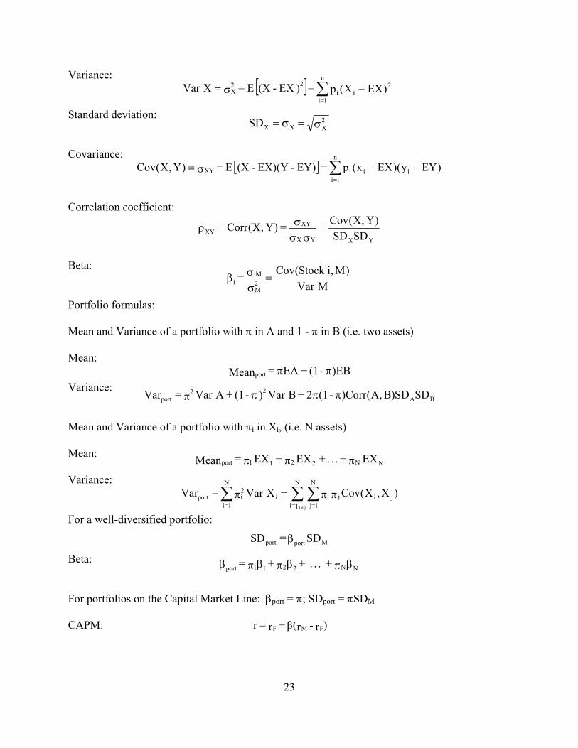
[ ] 2ii
n
1=i
22X )EXX(p = )EX- (X E= XVar −σ= ∑
Variance:
2XXX SD σ=σ=
Standard deviation:
[ ] ∑=
−−σ=n
1iiiiXY )EYy)(EXx(p = EY)- EX)(Y- (X E= )Y,X(Cov
Covariance: Correlation coefficient:
YXYX
XYXY SDSD
)Y,X(Cov = )Y,X(Corr =σσ
σ=ρ
MVar
)M,iStock(Cov = 2M
iMi =
σσβ
Beta: Portfolio formulas: Mean and Variance of a portfolio with π in A and 1 - π in B (i.e. two assets) Mean:
)EB - (1 + EA = Meanport ππ
BA22
port SDSD)B,A()Corr - (12 + BVar) - (1 +AVar = Var ππππVariance: Mean and Variance of a portfolio with πi in Xi, (i.e. N assets)
NN2211port EX + . . . + EX + EX = Mean πππMean:
)X,X(Cov + XVar = Var jiji
N
1=j
N
1=ii
2i
N
1=iport
ji
πππ ∑∑∑≠
Variance:
23
Mportport SD = SD β
For a well-diversified portfolio: βπβπβπβ NN2211port + . . . + + = Beta:
For portfolios on the Capital Market Line: βport = π; SDport = πSDM CAPM: )r - r(β + r =r FMF

24
INTENTIONALLY BLANK
25
UNIVERSITY OF PENNSYLVANIA
FNCE 601 Franklin Allen
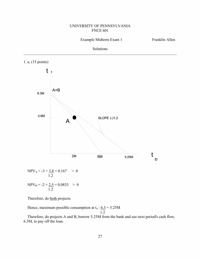
Example Midterm Exam 1 Instructions: You have 1 hour 30 minutes to answer all four questions. All four questions carry equal weight. If anything is unclear, please state carefully any assumptions you make. 1. Consider a world with two points in time t0, t1. Nelly Brown has just inherited $5M. She
has only two projects she can invest in. Project A costs $3M at t0 and pays off $3.8M at
t1. Project B costs $2M at t0 and pays off $2.5M at t1. She can lend and borrow at a bank
at an interest rate of 20 percent. Nelly is only interested in consumption today at t0; she
does not get any utility from consumption at t1.
a. What is the most Nelly can consume at t0? How does she achieve this (i.e. what
projects does she do and how much does she borrow or lend at the bank)?
b. How would your answers to (a) be changed if Nelly could lend to the bank at a
rate of 15 percent but could borrow at 30 percent? 2. Suppose you have decided to start saving money to take a long-awaited world-cruise,
which you want to take 5 years from today. You estimate the amount you will have to pay at that time will be $6000. The savings account you established for your trip offers 16% per annum interest compounded quarterly.
a. How much will you have to deposit each year (at year-end) to have your
$6000 if your first deposit is made 1 year from today and the final deposit is made on the day the cruise departs?
b. How much will you have to deposit each year if your first deposit is made
1 year from today and the final deposit is made 1 year before the cruise departs?
c. How much would you have to deposit each year if your first deposit is
made now and the final deposit is made 1 year before the cruise departs?
26
3. The International Tractor Corporation is considering purchasing personal computers. It can either buy Apple PC’s or IBM PC's. The Apple PC costs $1200 and is expected to last for five years. Annual maintenance costs are $200 per year paid at year's end. The machines are expected to have no salvage value. The IBM PC costs $1800 and is expected to last six years and has annual maintenance costs of $250. It is expected to have a salvage value of $300. The firm estimates its workload is such that it should either buy 400 Apple PC’s or 300 IBM PC's. There is expected to be no technological progress. International Tractor uses straight line depreciation. Both maintenance costs and depreciation are tax-deductible. Its tax rate is 40%. Its discount rate for this type of investment is 8 percent. Should the firm buy Apple PC’s or IBM PC's?
4. a. The respective values of the beta coefficients for the returns on three securities
x,y,z are 1.0, 0.5, and 0.8 when the variance on the market portfolio is equal to 0.0625.
i. What are the respective values of the covariance between each security's
return and the returns on the market portfolio? ii. What would be the value of beta for a portfolio, P, composed equally of
the three securities? iii. What would be the value of the covariance between the returns on the
equally-weighted portfolio P and the return on the market portfolio? b. Joe Smith lives in a country where the assumptions of the capital asset pricing
model are satisfied. There are only two risky securities, Acorn and Bethlehem. Joe has 40 percent of his portfolio in the riskless asset, 35 percent, in Acorn and 25 percent in Bethlehem. If the total value in the entire economy of Acorn is $3.5 million, what is the total value of Bethlehem?
c. The risk-free rate, rf, is 10 percent and the risk premium on the market, (rM - rf), is
expected to be 8.25 percent. Sally Smith is less risk-averse than the average. She
can tolerate beta values up to 1.5. Nevertheless she dislikes holding individually
risky stocks and prefers to borrow and put her holdings in a widely diversified
indexed mutual fund with a beta of 1.0. If she has $10,000 of her own money to
invest in the fund, how much additional money should she borrow to get a
portfolio with a beta of 1.5? What is her expected rate of return?
UNIVERSITY OF PENNSYLVANIA FNCE 601
Example Midterm Exam 1 Franklin Allen
Solutions 1. a. (15 points)
NPVA = -3 + 3.8 = 0.167 > 0 1.2 NPVB = -2 + 2.5 = 0.0833 > 0 1.2 Therefore, do both projects. Hence, maximum possible consumption at to : 6.3 = 5.25M 1.2 Therefore, do projects A and B, borrow 5.25M from the bank and use next period's cash flow, 6.3M, to pay off the loan.
27
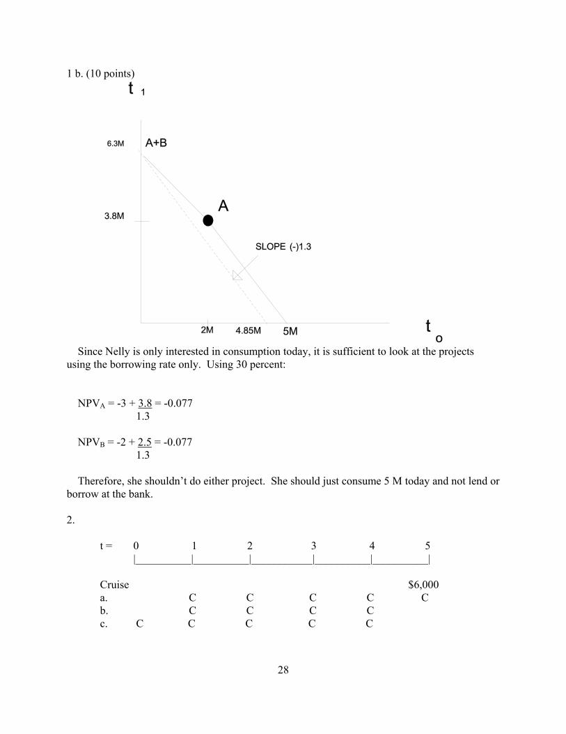
1 b. (10 points)
Since Nelly is only interested in consumption today, it is sufficient to look at the projects using the borrowing rate only. Using 30 percent: NPVA = -3 + 3.8 = -0.077 1.3 NPVB = -2 + 2.5 = -0.077 1.3 Therefore, she shouldn’t do either project. She should just consume 5 M today and not lend or borrow at the bank. 2. t = 0 1 2 3 4 5 |__________|__________|___________|__________|__________| Cruise $6,000 a. C C C C C b. C C C C c. C C C C C
28

29
2a. (8 points) Annual interest rate = (1 + (0.16/4))4 - 1 = 16.99% or 17% PV of cost of cruise = $6000 x (DF 5 yrs, 17%) = $6000 x (0.456) = $2,736 If the person saves C every year, then C x AF(5 yrs., 17%) = $2,736 C = 2,736 = $855.27 3.199 Therefore, you must save $855.27 to finance your trip. 2b. (8 points) In this case C x AF(4 yrs., 17%) = $2,736 C = 2736 = 997.45 2.743 Therefore, you must save $997.45 every year. 2c. (9 points) In this case C + C x AF(4 yrs., 17%) = $2,736 C x [1 + 2.743] = $2,736 C = 2,736 = $730.96 3.743 Therefore, you must save $730.96 every year.
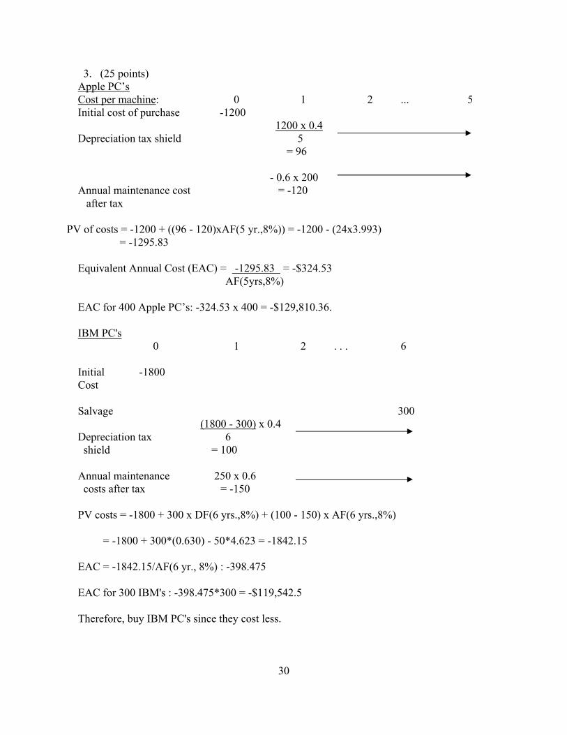
3. (25 points) Apple PC’s Cost per machine: 0 1 2 ... 5 Initial cost of purchase -1200 1200 x 0.4 Depreciation tax shield 5 = 96 - 0.6 x 200 Annual maintenance cost = -120 after tax PV of costs = -1200 + ((96 - 120)xAF(5 yr.,8%)) = -1200 - (24x3.993) = -1295.83 Equivalent Annual Cost (EAC) = -1295.83 = -$324.53 AF(5yrs,8%) EAC for 400 Apple PC’s: -324.53 x 400 = -$129,810.36. IBM PC's 0 1 2 . . . 6 Initial -1800 Cost Salvage 300 (1800 - 300) x 0.4 Depreciation tax 6 shield = 100 Annual maintenance 250 x 0.6 costs after tax = -150 PV costs = -1800 + 300 x DF(6 yrs.,8%) + (100 - 150) x AF(6 yrs.,8%) = -1800 + 300*(0.630) - 50*4.623 = -1842.15 EAC = -1842.15/AF(6 yr., 8%) : -398.475 EAC for 300 IBM's : -398.475*300 = -$119,542.5 Therefore, buy IBM PC's since they cost less.
30

31
4 (a)(i) (3 points) From the definition of β, β = Cov(asset,M) Var(M) Therefore, Cov(asset,M) = β x Var(M) Using this formula for assets X, Y and Z Cov(X, M) = 1 x 0.0625 = 0.0625 Cov(Y, M) = 0.5 x 0.0625 = 0.03125 Cov(Z, M) = 0.8 x 0.0625 = 0.05. (ii) (3 points) Using the formula for the beta of a portfolio
βPORT = πXβX + πYβY + πZβZ
For an equally weighted portfolio, πX = πY = πZ = 1/3
Therefore, βPORT = (1/3) x 1 + (1/3) x 0.5 + (1/3) x 0.8 = 0.767
(iii) (3 points) Using the definition of β
Cov(PORT,M) = βPORT x Var(M) = 0.767 x 0.0625 = 0.0479167
(b) (8 points) Since everybody holds the market portfolio in a CAPM world, everybody must hold Acorn to Bethlehem in the ratio 35/25 = 1.4 Therefore, Total value of Acorn = 1.4 Total value of Bethlehem Therefore, Total value of Bethlehem = 3.5M = $2.5M 1.4 (c) (8 points) She should borrow $5000 and invest it together with her own $10,000 in the widely diversified indexed mutual fund to get a portfolio with beta of 1.5. She is effectively mixing the risk-free asset and the market with 1.5 times her wealth in the market so the beta is 1.5. Then, using the CAPM, ERPORT = 0.10 + 1.5 x 0.0825 = 0.22375

32
INTENTIONALLY BLANK
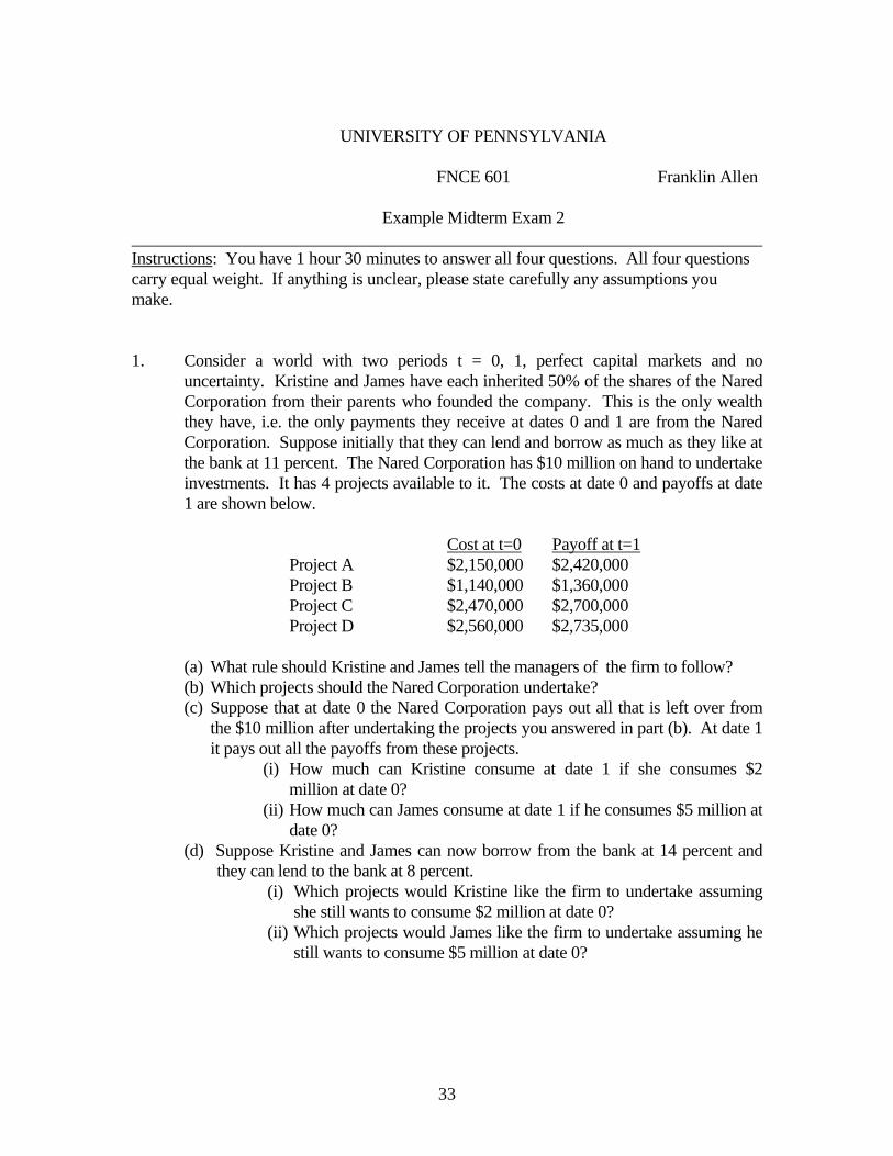
UNIVERSITY OF PENNSYLVANIA FNCE 601 Franklin Allen Example Midterm Exam 2 Instructions: You have 1 hour 30 minutes to answer all four questions. All four questions carry equal weight. If anything is unclear, please state carefully any assumptions you make. 1. Consider a world with two periods t = 0, 1, perfect capital markets and no
uncertainty. Kristine and James have each inherited 50% of the shares of the Nared Corporation from their parents who founded the company. This is the only wealth they have, i.e. the only payments they receive at dates 0 and 1 are from the Nared Corporation. Suppose initially that they can lend and borrow as much as they like at the bank at 11 percent. The Nared Corporation has $10 million on hand to undertake investments. It has 4 projects available to it. The costs at date 0 and payoffs at date 1 are shown below.
Cost at t=0 Payoff at t=1 Project A $2,150,000 $2,420,000 Project B $1,140,000 $1,360,000 Project C $2,470,000 $2,700,000 Project D $2,560,000 $2,735,000
(a) What rule should Kristine and James tell the managers of the firm to follow? (b) Which projects should the Nared Corporation undertake? (c) Suppose that at date 0 the Nared Corporation pays out all that is left over from
the $10 million after undertaking the projects you answered in part (b). At date 1 it pays out all the payoffs from these projects.
(i) How much can Kristine consume at date 1 if she consumes $2 million at date 0?
(ii) How much can James consume at date 1 if he consumes $5 million at date 0?
(d) Suppose Kristine and James can now borrow from the bank at 14 percent and they can lend to the bank at 8 percent.
(i) Which projects would Kristine like the firm to undertake assuming she still wants to consume $2 million at date 0?
(ii) Which projects would James like the firm to undertake assuming he still wants to consume $5 million at date 0?
33
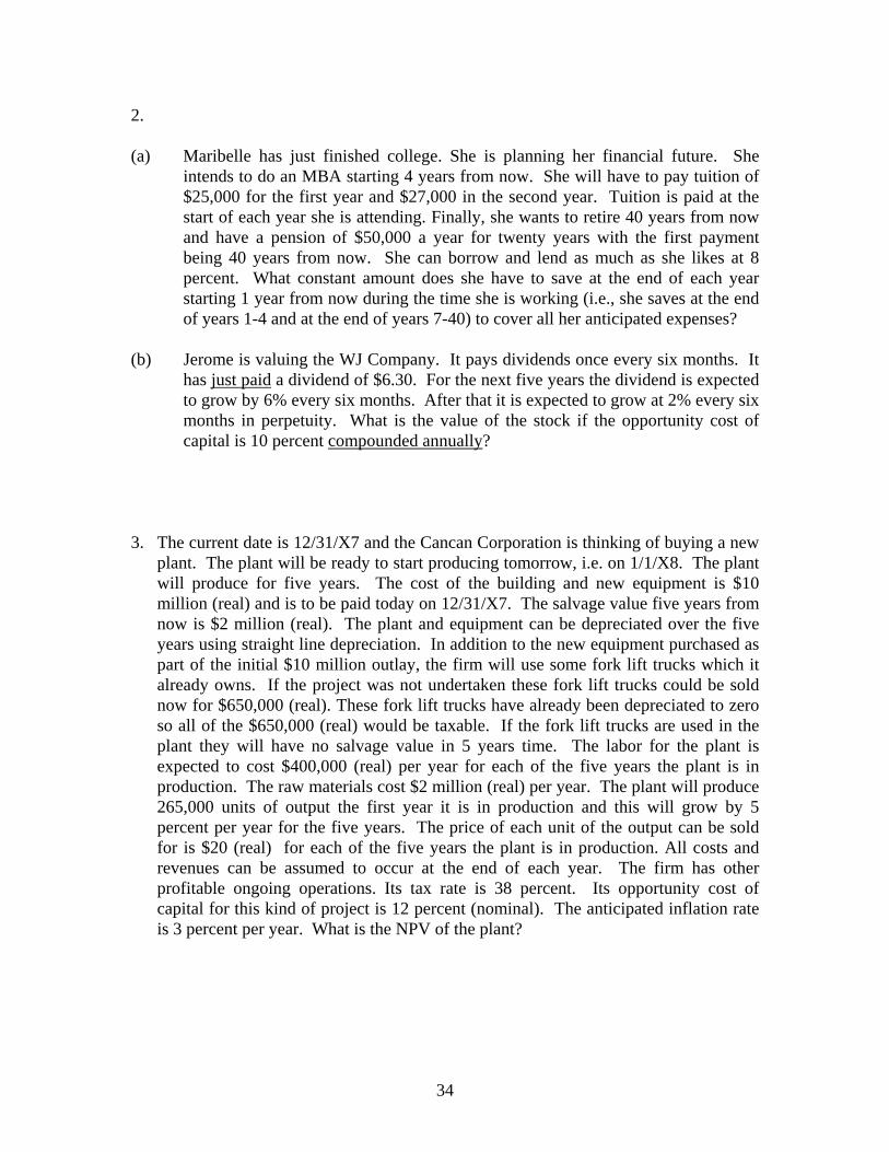
2. (a) Maribelle has just finished college. She is planning her financial future. She
intends to do an MBA starting 4 years from now. She will have to pay tuition of $25,000 for the first year and $27,000 in the second year. Tuition is paid at the start of each year she is attending. Finally, she wants to retire 40 years from now and have a pension of $50,000 a year for twenty years with the first payment being 40 years from now. She can borrow and lend as much as she likes at 8 percent. What constant amount does she have to save at the end of each year starting 1 year from now during the time she is working (i.e., she saves at the end of years 1-4 and at the end of years 7-40) to cover all her anticipated expenses?
(b) Jerome is valuing the WJ Company. It pays dividends once every six months. It
has just paid a dividend of $6.30. For the next five years the dividend is expected to grow by 6% every six months. After that it is expected to grow at 2% every six months in perpetuity. What is the value of the stock if the opportunity cost of capital is 10 percent compounded annually?
3. The current date is 12/31/X7 and the Cancan Corporation is thinking of buying a new
plant. The plant will be ready to start producing tomorrow, i.e. on 1/1/X8. The plant will produce for five years. The cost of the building and new equipment is $10 million (real) and is to be paid today on 12/31/X7. The salvage value five years from now is $2 million (real). The plant and equipment can be depreciated over the five years using straight line depreciation. In addition to the new equipment purchased as part of the initial $10 million outlay, the firm will use some fork lift trucks which it already owns. If the project was not undertaken these fork lift trucks could be sold now for $650,000 (real). These fork lift trucks have already been depreciated to zero so all of the $650,000 (real) would be taxable. If the fork lift trucks are used in the plant they will have no salvage value in 5 years time. The labor for the plant is expected to cost $400,000 (real) per year for each of the five years the plant is in production. The raw materials cost $2 million (real) per year. The plant will produce 265,000 units of output the first year it is in production and this will grow by 5 percent per year for the five years. The price of each unit of the output can be sold for is $20 (real) for each of the five years the plant is in production. All costs and revenues can be assumed to occur at the end of each year. The firm has other profitable ongoing operations. Its tax rate is 38 percent. Its opportunity cost of capital for this kind of project is 12 percent (nominal). The anticipated inflation rate is 3 percent per year. What is the NPV of the plant?
34

4. (a) There are two risky assets X and Y and a risk free asset Z. The means and standard
deviations are as follows. Asset Mean Standard Deviation X 0.15 0.20 Y 0.11 0.30 Z 0.07 0 The correlation of X and Y is -0.1. What is the mean and standard deviation of a
portfolio with 30 percent in X, 45 percent in Y and 25 percent in Z? (b) Suppose the capital asset pricing model holds. The risk free rate is 8 percent. The
expected return on the market portfolio is 16 percent. The standard deviation of the market portfolio is 35 percent. Nola is willing to hold a portfolio with a standard deviation of up to 45 percent but no more than this.
(i) Given this, what is the highest expected return Nola can obtain? (ii) What does the portfolio that allows this expected return consist of if Nola has
wealth of $10,000? (c) You have discovered three well-diversified portfolios with the following characteristics. Portfolio Expected Return Beta A 12% 0.2 B 17% 1.0 C 25% 2.5
(i) Do these three securities lie on the security market line? (ii) Give a zero-investment, zero-risk portfolio with positive expected return that has
either +$1 or -$1 invested in C. (iii) What is the expected return on this portfolio?
35

INTENTIONALLY BLANK
36
UNIVERSITY OF PENNSYLVANIA FNCE 601
Example Midterm Exam 2 Franklin Allen
Solutions
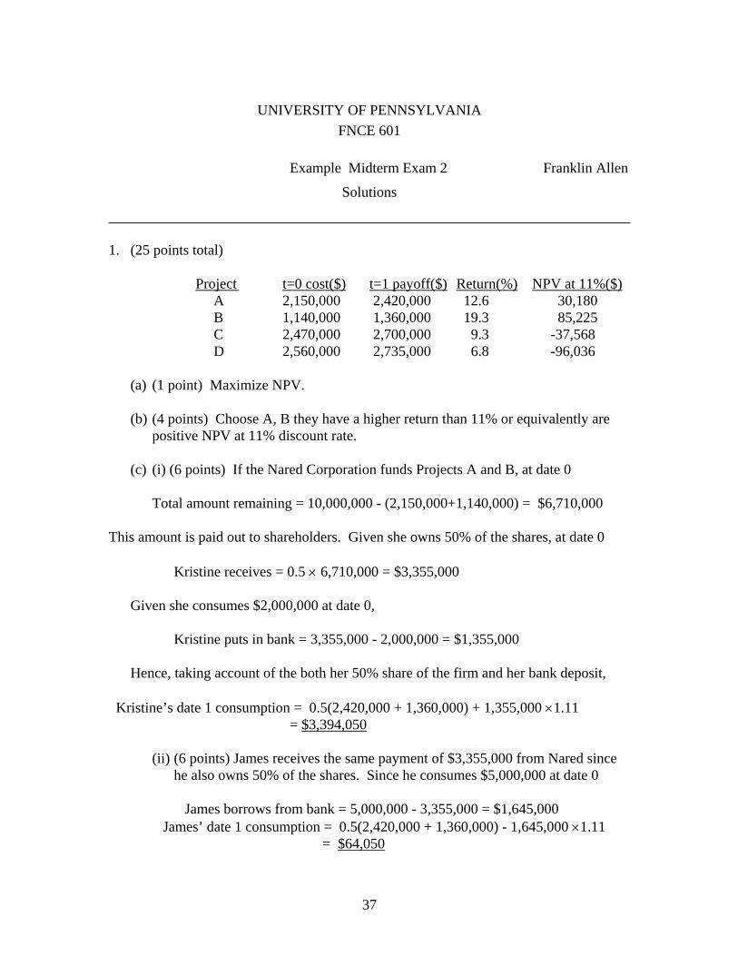
1. (25 points total) Project t=0 cost($) t=1 payoff($) Return(%) NPV at 11%($) A 2,150,000 2,420,000 12.6 30,180 B 1,140,000 1,360,000 19.3 85,225 C 2,470,000 2,700,000 9.3 -37,568 D 2,560,000 2,735,000 6.8 -96,036
(a) (1 point) Maximize NPV. (b) (4 points) Choose A, B they have a higher return than 11% or equivalently are
positive NPV at 11% discount rate. (c) (i) (6 points) If the Nared Corporation funds Projects A and B, at date 0 Total amount remaining = 10,000,000 - (2,150,000+1,140,000) = $6,710,000
This amount is paid out to shareholders. Given she owns 50% of the shares, at date 0
Kristine receives = 0.5 × 6,710,000 = $3,355,000 Given she consumes $2,000,000 at date 0, Kristine puts in bank = 3,355,000 - 2,000,000 = $1,355,000 Hence, taking account of the both her 50% share of the firm and her bank deposit,
Kristine’s date 1 consumption = 0.5(2,420,000 + 1,360,000) + 1,355,000 ×1.11 = $3,394,050
(ii) (6 points) James receives the same payment of $3,355,000 from Nared since he also owns 50% of the shares. Since he consumes $5,000,000 at date 0
James borrows from bank = 5,000,000 - 3,355,000 = $1,645,000 James’ date 1 consumption = 0.5(2,420,000 + 1,360,000) - 1,645,000 ×1.11 = $64,050
37

(d) (i) (4 points) Since Kristine is a lender, the relevant rate for her is the lending rate of 8 percent. She therefore wishes the firm to undertake A, B and C since these are the projects with a higher return than 8 percent.
(ii) (4 points) Since James is a borrower, the relevant rate for him is the borrowing rate of 14 percent. He therefore wishes the firm to undertake B.
2. (a) 15 points t = 0 1… 4 5 6 7… 40 … 59 Tuition 25,000 27,000 Pension 50,000 50,000 Savings S S S S Equating savings with the amount needed gives the equation: S×AF(4yrs,8%)+S×AF(34yrs,8%)×DF(6yrs,8%) = 25,000×DF(4yrs,8%)+27,000×DF(5yrs,8%)+50,000×AF(20yrs,8%)×DF(39yrs,8%) S = $5,762 (b) (10 points) One period = 6 months Interest rate per six months = (1.10)0.5-1= 0.0488 t= just paid 0 1 2… 10 11… ∞ DIV. 6.3 6.3×1.06 6.3×1.062 6.3×1.0610 11.282×1.02 = 6.678 = 11.282 = 11.508
)02.00488.0(508.11
0488.11%)88.4r%,6g,periods10(GAF6.678 = PV 10 −
+==×
= 314.85
38
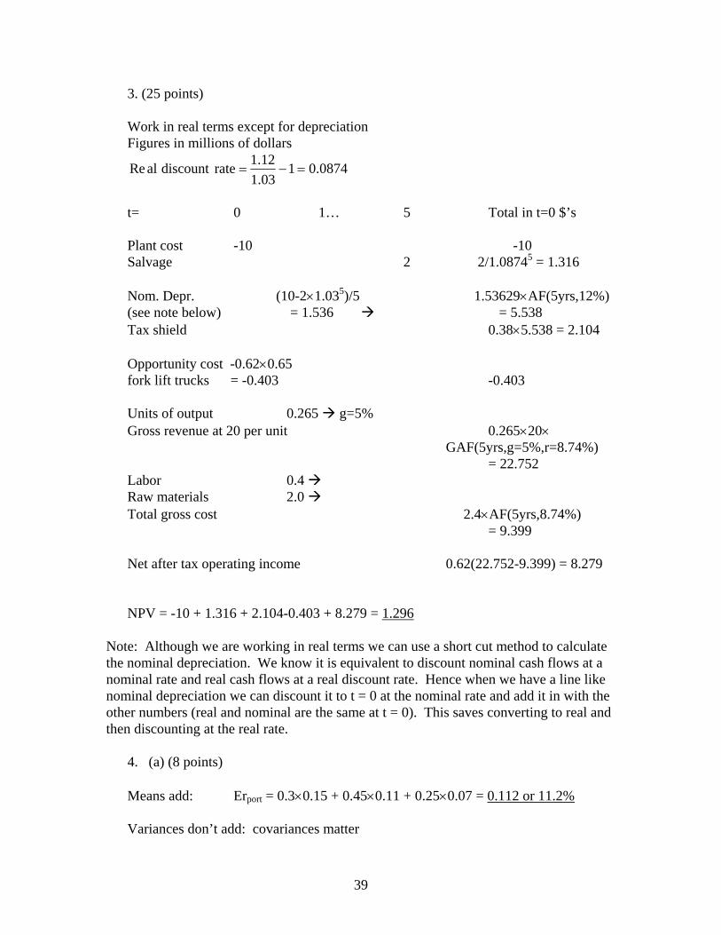
3. (25 points) Work in real terms except for depreciation Figures in millions of dollars
0874.0103.112.1ratediscountalRe =−=
t= 0 1… 5 Total in t=0 $’s Plant cost -10 -10 Salvage 2 2/1.08745 = 1.316 Nom. Depr. (10-2×1.035)/5 1.53629×AF(5yrs,12%) (see note below) = 1.536 = 5.538 Tax shield 0.38×5.538 = 2.104 Opportunity cost -0.62×0.65 fork lift trucks = -0.403 -0.403 Units of output 0.265 g=5% Gross revenue at 20 per unit 0.265×20×
GAF(5yrs,g=5%,r=8.74%) = 22.752 Labor 0.4 Raw materials 2.0 Total gross cost 2.4×AF(5yrs,8.74%) = 9.399 Net after tax operating income 0.62(22.752-9.399) = 8.279 NPV = -10 + 1.316 + 2.104-0.403 + 8.279 = 1.296
Note: Although we are working in real terms we can use a short cut method to calculate the nominal depreciation. We know it is equivalent to discount nominal cash flows at a nominal rate and real cash flows at a real discount rate. Hence when we have a line like nominal depreciation we can discount it to t = 0 at the nominal rate and add it in with the other numbers (real and nominal are the same at t = 0). This saves converting to real and then discounting at the real rate.
4. (a) (8 points) Means add: Erport = 0.3×0.15 + 0.45×0.11 + 0.25×0.07 = 0.112 or 11.2% Variances don’t add: covariances matter
39
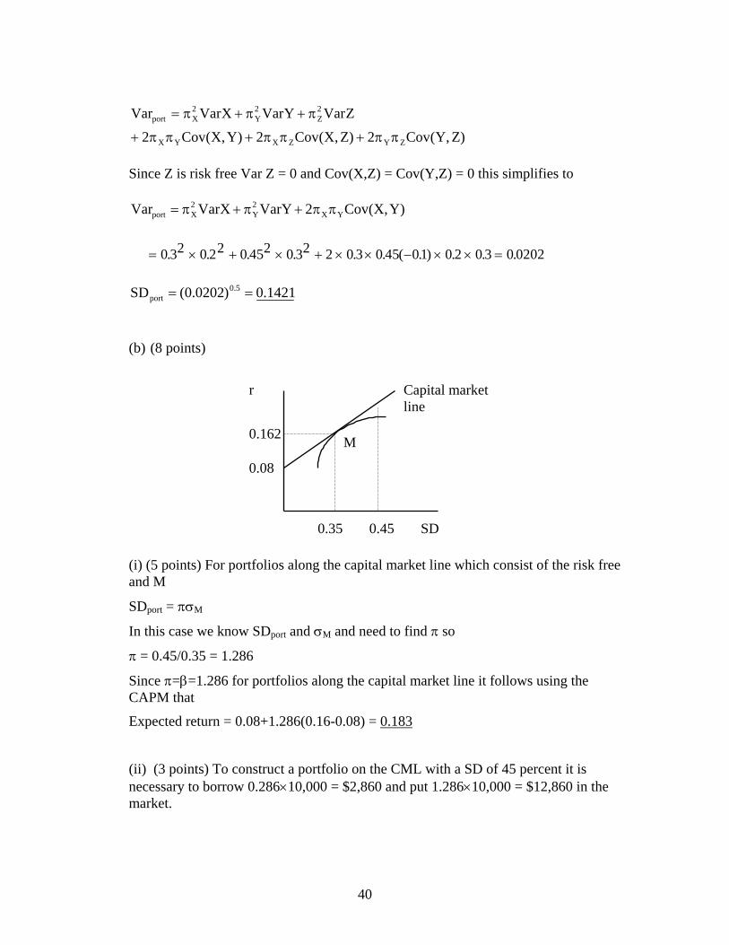
)Z,Y(Cov2)Z,X(Cov2)Y,X(Cov2
ZVarYVarXVarVar
ZYZXYX
2Z
2Y
2Xport
ππ+ππ+ππ+
π+π+π=
Since Z is risk free Var Z = 0 and Cov(X,Z) = Cov(Y,Z) = 0 this simplifies to
)Y,X(Cov2YVarXVarVar YX2Y
2Xport ππ+π+π=
= × + × + × × − × × =0 32 0 22 0 452 0 32 2 0 3 0 45 01 0 2 0 3 0 0202. . . . . . ( . ) . . .
1421.0)0202.0(SD 5.0port ==
(b) (8 points)
M 0.162
0.08
r Capital market line
SD 0.45 0.35
(i) (5 points) For portfolios along the capital market line which consist of the risk free and M
SDport = πσM
In this case we know SDport and σM and need to find π so
π = 0.45/0.35 = 1.286
Since π=β=1.286 for portfolios along the capital market line it follows using the CAPM that
Expected return = 0.08+1.286(0.16-0.08) = 0.183
(ii) (3 points) To construct a portfolio on the CML with a SD of 45 percent it is necessary to borrow 0.286×10,000 = $2,860 and put 1.286×10,000 = $12,860 in the market.
40
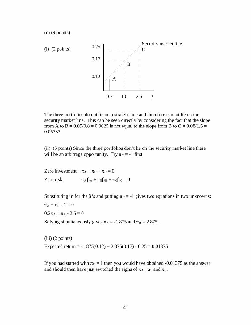
(c) (9 points)
r 0.25
C Security market line
B
A
(i) (2 points)
0.17
0.12
0.2 1.0 2.5 β
The three portfolios do not lie on a straight line and therefore cannot lie on the security market line. This can be seen directly by considering the fact that the slope from A to B = 0.05/0.8 = 0.0625 is not equal to the slope from B to C = 0.08/1.5 = 0.05333.
(ii) (5 points) Since the three portfolios don’t lie on the security market line there will be an arbitrage opportunity. Try πC = -1 first.
Zero investment: πA + πB + πC = 0
Zero risk: πA βA + πBβB + πCβC = 0
Substituting in for the β‘s and putting πC = -1 gives two equations in two unknowns:
πA + πB - 1 = 0
0.2πA + πB - 2.5 = 0
Solving simultaneously gives πA = -1.875 and πB = 2.875.
(iii) (2 points)
Expected return = -1.875(0.12) + 2.875(0.17) - 0.25 = 0.01375
If you had started with πC = 1 then you would have obtained -0.01375 as the answer and should then have just switched the signs of πA, πB and πC.
41

INTENTIONALLY BLANK
42
UNIVERSITY OF PENNSYLVANIA FNCE 601 Franklin Allen Example Midterm Exam 3 Instructions: You have 1 hour 30 minutes to answer all four questions. All four questions carry equal weight. If anything is unclear, please state carefully any assumptions you make. 1. (a) Nicole wishes to save for a pension for her retirement. She plans on retiring
20 years from now. Her desired income for the 25 years following that is $30,000 per year with all pension withdrawals being made at the end of the year and the first being 21 years from now. She also wishes to buy a house 10 years from now which will require $100,000. She can borrow or lend as much as she likes from her bank at 8% per year. What is the constant amount she needs to deposit in the bank as savings each year if the first deposit is made 1 year from now and the last 15 years from now? (Note that all figures are in nominal terms.)
(b) Takuma is valuing the stock of the Paloma Company which manufactures machine tools. The firm is just about to pay a dividend of $2 per share. This is expected to grow at 15% a year for five years, 10% a year for the ten years after that before finally settling down to a growth rate of 5% per year for ever after that. The market capitalization rate of similar stocks is 8%. What is the present value of each share?
2. (a) Consider the following project.
C0 C1 C2 C3 C4 C5 C6 -2,500 2,700 2,900 -3,000 2,600 2,800 -6,000
(i) What is/are the internal rates of return between 0% and 100%? (ii) If the opportunity cost of capital is 5% should the project be undertaken? (iii) If the opportunity cost of capital is 10% should the project be undertaken?
(b) Consider the following two mutually exclusive projects.
C0 C1 C2 C3 A -1,000 700 650 -100 B -1,500 400 400 1,000 For which range of opportunity costs of capital between 0% and 50% should A be
chosen?
43
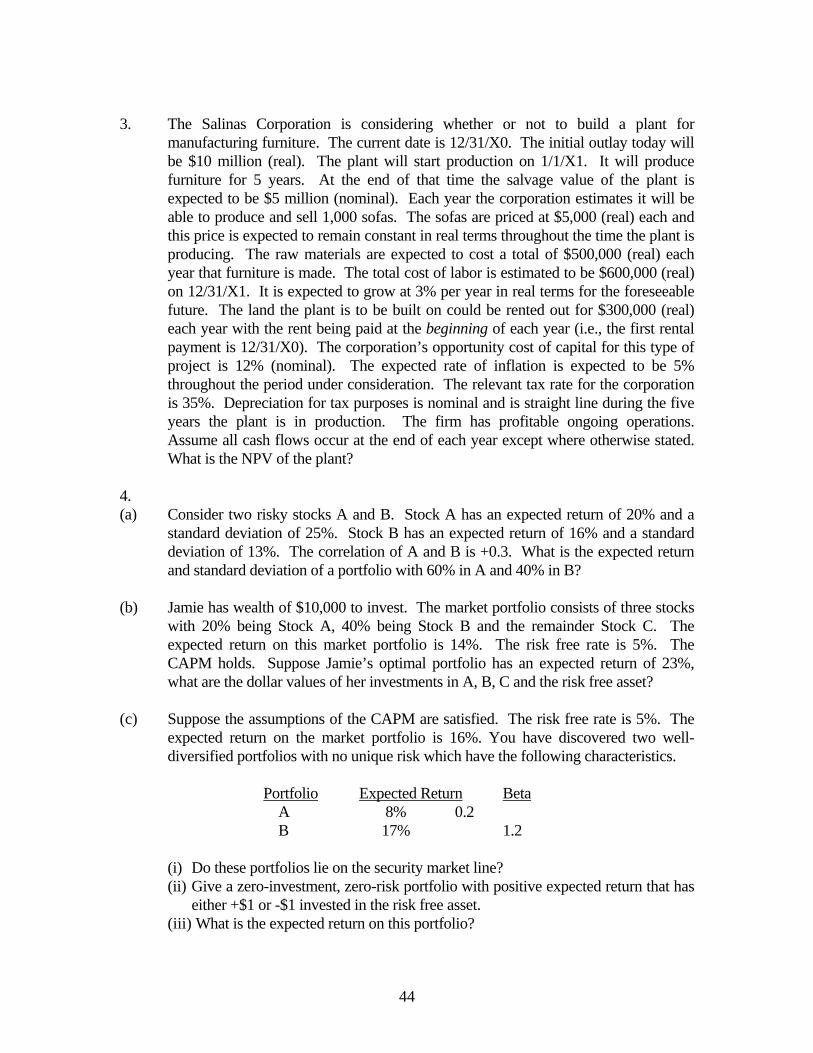
3. The Salinas Corporation is considering whether or not to build a plant for
manufacturing furniture. The current date is 12/31/X0. The initial outlay today will be $10 million (real). The plant will start production on 1/1/X1. It will produce furniture for 5 years. At the end of that time the salvage value of the plant is expected to be $5 million (nominal). Each year the corporation estimates it will be able to produce and sell 1,000 sofas. The sofas are priced at $5,000 (real) each and this price is expected to remain constant in real terms throughout the time the plant is producing. The raw materials are expected to cost a total of $500,000 (real) each year that furniture is made. The total cost of labor is estimated to be $600,000 (real) on 12/31/X1. It is expected to grow at 3% per year in real terms for the foreseeable future. The land the plant is to be built on could be rented out for $300,000 (real) each year with the rent being paid at the beginning of each year (i.e., the first rental payment is 12/31/X0). The corporation’s opportunity cost of capital for this type of project is 12% (nominal). The expected rate of inflation is expected to be 5% throughout the period under consideration. The relevant tax rate for the corporation is 35%. Depreciation for tax purposes is nominal and is straight line during the five years the plant is in production. The firm has profitable ongoing operations. Assume all cash flows occur at the end of each year except where otherwise stated. What is the NPV of the plant?
4. (a) Consider two risky stocks A and B. Stock A has an expected return of 20% and a
standard deviation of 25%. Stock B has an expected return of 16% and a standard deviation of 13%. The correlation of A and B is +0.3. What is the expected return and standard deviation of a portfolio with 60% in A and 40% in B?
(b) Jamie has wealth of $10,000 to invest. The market portfolio consists of three stocks
with 20% being Stock A, 40% being Stock B and the remainder Stock C. The expected return on this market portfolio is 14%. The risk free rate is 5%. The CAPM holds. Suppose Jamie’s optimal portfolio has an expected return of 23%, what are the dollar values of her investments in A, B, C and the risk free asset?
(c) Suppose the assumptions of the CAPM are satisfied. The risk free rate is 5%. The
expected return on the market portfolio is 16%. You have discovered two well-diversified portfolios with no unique risk which have the following characteristics.
Portfolio Expected Return Beta A 8% 0.2 B 17% 1.2
(i) Do these portfolios lie on the security market line? (ii) Give a zero-investment, zero-risk portfolio with positive expected return that has
either +$1 or -$1 invested in the risk free asset. (iii) What is the expected return on this portfolio?
44
UNIVERSITY OF PENNSYLVANIA
FNCE 601 Franklin Allen
Example Midterm Exam 3
Solutions
1. (25 points total)
a) (10 points)
PV(Pension) = ∑=
++
25
120)1(
000,30i
ir = 20)1(
000,30r+
×AF(T=25, r=8%), where AF(25, 8%) =
10.675;
PV(Deposit) = ∑= +
15
1 )1(jjr
D = D×AF(T=15, r=8%), where AF(15,8%) = 8.559; and
PV(House) = 10)1(000,100r+
= 10%)81(000,100
+ = 46,319.35. We know that the annual deposit has
to satisfy the following equation: PV(Deposit) = PV(House) + PV(Pension). Hence we have:
D = 20PV(House) AF(25,8%) 30,000 /(1 8%)
AF(15,8%)+ ⋅ +
=2046,319.35 10.675 30,000 /(1 8%)
8.559+ ⋅ + = $13,439.47
b) (15 points)
From the dividend stream, we have the following equation for PV(stock): P0 = DIV0+GA1(Yr.1~5, g=15%)+GA2(Yr.6~15, g=10%)+GP(Yr.16~∞, g=5%). We also have GA1=DIV1·GAF1(T=5, r=8%, g=15%), where DIV1=2×(1+15%)=2.3;
GA2 = DIV1' · GAF2(T=10, r=8%, g=10%), where DIV1' = 5
5
%)81(%)101(%)151(2
++×+× =
3.011; and GP= DIV1'' · GPF(r=8%, g=5%), where DIV1'' = 15
105
%)81(%)51(1.115.12
++×××
= 3.451. Therefore, P0 = 2 + 12.121 + 30.322 + 115.123 = $159.57
45
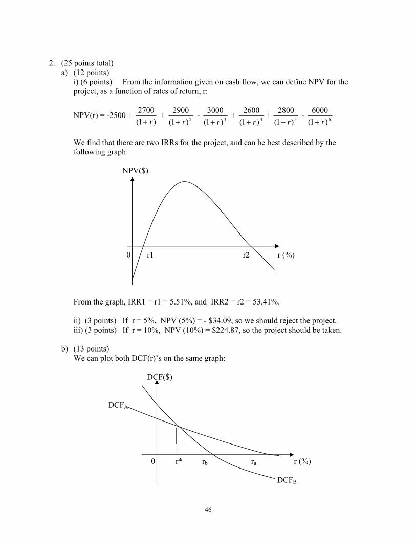
2. (25 points total)
a) (12 points) i) (6 points) From the information given on cash flow, we can define NPV for the project, as a function of rates of return, r:
NPV(r) = -2500 + )1(
2700r+
+ 2)1(2900
r+ - 3)1(
3000r+
+ 4)1(2600
r++ 5)1(
2800r+
- 6)1(6000
r+
We find that there are two IRRs for the project, and can be best described by the following graph:
NPV($)
0 r1 r2 r (%)
From the graph, IRR1 = r1 = 5.51%, and IRR2 = r2 = 53.41%. ii) (3 points) If r = 5%, NPV (5%) = - $34.09, so we should reject the project. iii) (3 points) If r = 10%, NPV (10%) = $224.87, so the project should be taken.
b) (13 points)
We can plot both DCF(r)’s on the same graph: DCF($) DCFA 0 r* rb ra r (%) DCFB
46
We know that r* satisfies the equation: DCFA (r*) = DCFB (r*). Solving this equation with one unknown, we obtain that r* = 2.09%. To do this on your calculator, find the IRR on the incremental cash flows CA – CB. To see why this works, consider the case where we have three dates 0, 1, and 2. We need
A1 A2 B1 B2A0 B02 2
C C C CC C1 r * (1 r*) 1 r * (1 r*)
+ + = + ++ + + +
or equivalently
A1 B1 A2 B2
A0 B0 2
C C C CC C1 r * (1 r*)− −
− + + =+ +
0
so we find r* by solving for IRR for CAt – CBt. From the graph, we observe that when r > r*, DCFA (r*) > DCFB (r*) so for these opportunity costs of capital, NPVA > NPVB . But this does not imply that we should choose project A for all r > r*. In fact, calculating IRR for A yields that when r > 17.93%, NPVA < 0, and it should be rejected. To summarize, when 2.09% < r < 17.93%, project A should be taken.
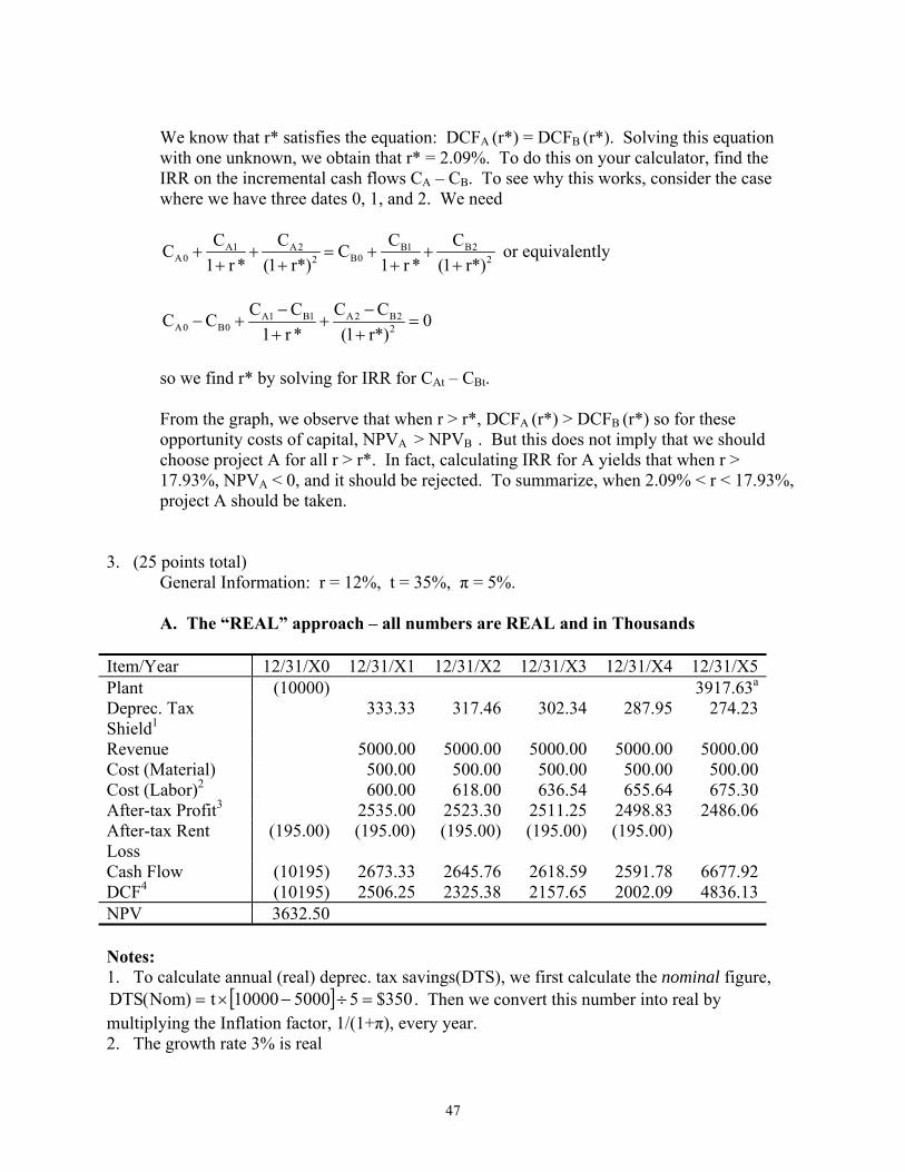
3. (25 points total) General Information: r = 12%, t = 35%, π = 5%.
A. The “REAL” approach – all numbers are REAL and in Thousands
Item/Year 12/31/X0 12/31/X1 12/31/X2 12/31/X3 12/31/X4 12/31/X5Plant (10000) 3917.63a
Deprec. Tax Shield1
333.33 317.46 302.34 287.95 274.23
Revenue 5000.00 5000.00 5000.00 5000.00 5000.00Cost (Material) 500.00 500.00 500.00 500.00 500.00Cost (Labor)2 600.00 618.00 636.54 655.64 675.30After-tax Profit3 2535.00 2523.30 2511.25 2498.83 2486.06After-tax Rent Loss
(195.00) (195.00) (195.00) (195.00) (195.00)
Cash Flow (10195) 2673.33 2645.76 2618.59 2591.78 6677.92DCF4 (10195) 2506.25 2325.38 2157.65 2002.09 4836.13NPV 3632.50 Notes: 1. To calculate annual (real) deprec. tax savings(DTS), we first calculate the nominal figure,
[ ] 350$5500010000t)Nom(DTS =÷−×= . Then we convert this number into real by multiplying the Inflation factor, 1/(1+π), every year. 2. The growth rate 3% is real
47

3. After-tax profit is given by: (Revenue – Total Cost) · (1-t). 4. The real discount factor is given by adjusting the nominal factor using the inflation factor:
.9375.0%51(%)121(
1π1()NDF1(
1RDF =)++
=)++
=
a. This is the real salvage value ( ) 63.391715000 5 =+= π .
B. The “NOMINAL” approach – all numbers are NOMINAL and in Thousands
Item/Year 12/31/X0 12/31/X1 12/31/X2 12/31/X3 12/31/X4 12/31/X5Plant (10000) 5000.00Deprec. Tax Shield1
350.00 350.00 350.00 350.00 350.00
Revenue2 5250.00 5512.50 5788.13 6077.53 6381.41Cost (Material) 2 525.00 551.25 578.81 607.75 638.14Cost (Labor) 2, 3 630.00 681.35 736.87 796.93 861.88After-tax Profit 2611.75 2781.94 2907.09 3037.35 3172.90After-tax Rent Loss
(195.00) (204.75) (214.99) (225.74) (237.02)
Cash Flow (10195) 2807.00 2916.95 3031.35 3150.33 8522.90DCF4 (10195) 2506.25 2325.38 2157.65 2002.09 4836.13NPV 3632.50 Notes: 1. The nominal DTS should be a stream of constants. See note A.1. for calculation. 2. All (real) figures need to be adjusted for inflation. 3. The nominal growth factor is given by the product of real growth factor and inflation factor. 4. Use nominal discount factor, 12%. 4. (25 points total)
a) (5 points) Given the information on return/risk for each stock, we can calculate the return and SD of the portfolio:
%;4.18%164.0%206.0rπrπ )P(R BBAA =⋅+⋅=⋅+⋅=
;0299.013.025.03.04.06.0213.04.025.06.0
)B,A(Covππ2)B(Varπ)A(Varπ)P(VAR2222
BA2
B2
A
=⋅⋅⋅⋅⋅+⋅+⋅=
⋅⋅+⋅+⋅=
%.29.170299.0)P(VAR)P(SD ===
48
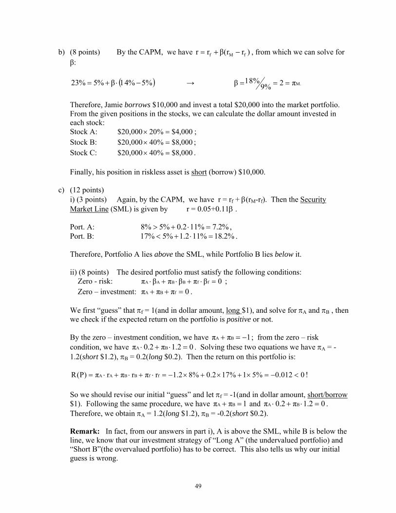
b) (8 points) By the CAPM, we have )rr(βrr fMf −+= , from which we can solve for β:
( )5%−14%⋅+= β%5%23 → .Mπ2β ==9%18%=
Therefore, Jamie borrows $10,000 and invest a total $20,000 into the market portfolio. From the given positions in the stocks, we can calculate the dollar amount invested in each stock: Stock A: 000,4$%20000,20$ =× ; Stock B: 000,8$%40000,20$ =× ; Stock C: 000,8$%40000,20$ =× . Finally, his position in riskless asset is short (borrow) $10,000.
c) (12 points)
i) (3 points) Again, by the CAPM, we have r = rf + β(rM-rf). Then the Security Market Line (SML) is given by r = 0.05+0.11β . Port. A: %2.7%112.0%5%8 =⋅+> , Port. B: %2.18%112.1%5%17 =⋅+< . Therefore, Portfolio A lies above the SML, while Portfolio B lies below it. ii) (8 points) The desired portfolio must satisfy the following conditions: Zero - risk: 0βπβπβπ ffBBAA =⋅+⋅+⋅ ; Zero – investment: 0πππ fBA =++ . We first “guess” that πf = 1(and in dollar amount, long $1), and solve for πA and πB , then we check if the expected return on the portfolio is positive or not. By the zero – investment condition, we have 1ππ BA −=+ ; from the zero – risk condition, we have 02.1π2.0π BA =⋅+⋅ . Solving these two equations we have πA = -1.2(short $1.2), πB = 0.2(long $0.2). Then the return on this portfolio is:
0012.0%51%172.0%82.1rπrπrπ)P(R ffBBAA <−=×+×+×−=⋅+⋅+⋅= ! So we should revise our initial “guess” and let πf = -1(and in dollar amount, short/borrow $1). Following the same procedure, we have 1ππ BA =+ and 02.1π2.0π BA =⋅+⋅ . Therefore, we obtain πA = 1.2(long $1.2), πB = -0.2(short $0.2). Remark: In fact, from our answers in part i), A is above the SML, while B is below the line, we know that our investment strategy of “Long A” (the undervalued portfolio) and “Short B”(the overvalued portfolio) has to be correct. This also tells us why our initial guess is wrong.
49
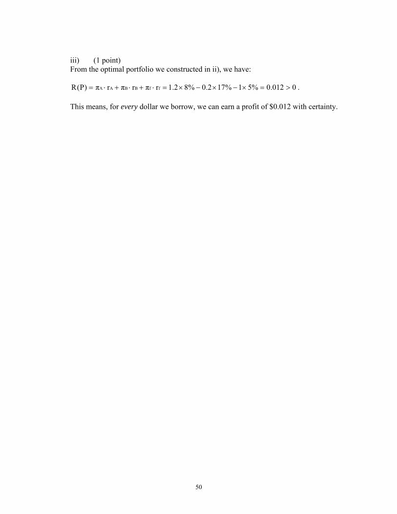
iii) (1 point) From the optimal portfolio we constructed in ii), we have:
0012.0%51%172.0%82.1rπrπrπ)P(R ffBBAA >=×−×−×=⋅+⋅+⋅= . This means, for every dollar we borrow, we can earn a profit of $0.012 with certainty.
50
UNIVERSITY OF PENNSYLVANIA FNCE 601 Franklin Allen Example Midterm Exam 4 Instructions: You have 1 hour 30 minutes to answer all four questions. All four questions carry equal weight. If anything is unclear, please state carefully any assumptions you make. 1. Florencia has no funds of her own. However, she can lend and borrow as much as
she likes at the bank at 7% interest. She has access to some entrepreneurial projects. The cost of these projects at date t = 0 and the revenues they generate at date t = 1 are known with certainty and are listed below.
Project Cost at t = 0 Revenue at t = 1 A 23,000 24,840 B 125,670 145,777 C 320,000 339,200 D 225,000 270,000
(i) Which projects should she undertake? (ii) What is the most she can consume at t = 0 and how much does she need to
lend or borrow in total (including the funding of the projects) at the bank to do this?
(iii) How would your answers to (i)-(ii) be changed if Florencia can lend to the bank at 5% and borrow from the bank at 9%?
2.(a) Bill and Jane are married with one child. The current date is the start of the college
year. All tuition is paid at the start of the year. If their child were to attend college starting now they would have to pay a total of $35,000 now for the year. This cost is expected to grow at 4% per year for the foreseeable future. They anticipate their child will go to college 7 years from now and will attend for four years. They also wish to purchase a house for holidays in the mountains 10 years from now for $350,000. They can lend and borrow as much as they like at 5% per year from their bank. They wish to save S each year with the first deposit now and the last nine years from today. How large should S be in order for them to be able to send their child to college and afford the holiday house in the mountains?
(b) Shaohuan is valuing the FLR Company. Dividends are paid each year. He
anticipates that the first dividend will be $4.30 and will be paid one year from now. This is expected to grow at 25% for the following five years. After that the growth rate is expected to slow down to 15% for the next five years. After that the growth rate of dividends is expected to be 3% forever. What is the value of the stock if the appropriate discount rate is 6%?
51
3. The PYW Corporation is a trucking company that moves household goods long distance. It is thinking of replacing part of its current fleet of trucks. These are currently all Volvos. The firm has narrowed the choice to two models. Both are capable of carrying the same amount of goods. The first is one made by Volvo. This model costs $150,000 (nominal) initially. It is expected to have a life of 5 years with a salvage value of $20,000 (real). The maintenance costs are expected to be $20,000 (real) before tax each year. The second model is one made by Mercedes. This costs $250,000 (nominal) but lasts for 8 years with a salvage value of $35,000 (real). The maintenance costs are expected to be $25,000 (real) before tax each year. The firm uses straight line depreciation and has a total tax rate of 40%. It is anticipated that it will be profitable for the foreseeable future. The firm has a discount rate for this type of project of 12% (nominal). The rate of inflation is expected to be 4% per year. Assume all cash flows occur at the end of each year except where otherwise stated. Which type of trucks should be purchased assuming that similar trucks will be available in the foreseeable future?
4. (The two parts are separate so you cannot use information from one in the other.) (a) Portfolio A has 20 stocks in it and is well diversified. All stocks have equal weights
in the portfolio. The first five stocks have a beta of 0.6. The next five stocks have a beta of 0.8. The remaining 10 stocks have a beta of 1.2. The standard deviation of the market portfolio is 25%. What is the standard deviation of portfolio A?
(b) Suppose the assumptions of the CAPM are satisfied. You have discovered four well-
diversified portfolios with no unique risk. They have the following characteristics. Three of them are correctly priced while one is mispriced.
Portfolio Expected Return Beta A 17% 1.2 B 20% 1.5 C 24% 1.7 D 29% 2.4
(i) Which three portfolios are correctly priced and which is mispriced? (ii) Give a zero-investment, zero-risk portfolio with positive expected return that has
either +$1 or -$1 invested in the mispriced security and which excludes the correctly priced security with the highest expected return.
(iii) What is the expected return on this portfolio?
52
UNIVERSITY OF PENNSYLVANIA FNCE 601 Franklin Allen
Example Midterm Exam 5 Instructions: You have 1 hour 30 minutes to answer all four questions. All four questions carry equal weight. If anything is unclear, please state carefully any assumptions you make. 1.(a) Consider a world with three dates t = 0, 1, and 2, perfect capital markets and no
uncertainty. Haiman has just inherited $0.5 million. She has decided to set up a corporation called Bubble.com. This will manufacture and sell kits of liquid soap and wire frames that will allow children and adults to blow soap bubbles. These kits will be marketed over the internet. Suppose initially she can lend and borrow at the bank at 6 percent per period. Bubble.com has the following projects available.
Project Cost at t = 0 Revenue at t = 1 Revenue at t = 2 Large bubble kit $325,000 $130,000 $260,000 Medium bubble kit $255,000 $128,000 $140,000 Small bubble kit $430,000 $220,000 $270,000
(i) What simple instructions can Haiman give to ensure that the managers she hires create as much wealth as possible for her?
(ii) Which projects should the managers choose to undertake?
(iii) What is the most Haiman can consume at date t = 2 given she wishes to
consume $0.3 million at date t = 0 and $0.2 million at date t = 1? (b) Consider a project with the following cash flows. C0 C1 C2 C3 -850 +5,000 -1,400 -1,500
(i) What, if any, is/are the IRR(s) of this project between 0 and 50 percent? (ii) What is the NPV of the project at 10 percent?
53
2.(a) Srikant is planning his retirement. The rate of interest that he can lend and borrow at
the bank is 6 percent. He would like to retire 20 years from now. He currently has $125,000 in the bank. He intends to buy a car 3 years from now. He estimates it will cost $55,000 then. He would like to buy his mother a house 10 years from now. He estimates it will cost $230,000 then. Srikant wants to have a fixed pension of $100,000 a year with the first payment being 21 years from now and the last being 40 years from now. What is the constant amount he needs to save each year assuming the first time he puts away money is 1 year from now and the last time is 20 years from now?
(b) Sandy is valuing the Halloween Company. It is just about to pay a dividend of $10 per share. This dividend is expected to grow at 15 percent per year for five years and then at 10 percent for the following five years. After that it will grow at 4 percent in perpetuity. What is the current value of a share if the opportunity cost of capital for this type of firm is 12 percent?
3. Over the last five years the Billagong Company has spent $25 million developing a new product called bings. It is considering whether to build a plant in California that will manufacture bings. The current date is 12/31/X0. The cost of the plant is $10 million to be paid now. It will take one year to build. The plant will start producing on 1/1/X2 and the first revenues and costs will be received and paid on 12/31/X2. The plant is expected to produce for three years. It will produce 3 million bings a year. The plant can be depreciated over the three years it is in production. The plant has zero salvage value. The company can sell each bing for $5 and the raw materials will cost $2 per bing in all three years bings are produced. The total labor costs for the first year of production will be $1.5 million (i.e. on 12/31/X2) and these are expected to grow at a rate of 4 percent per year. The land the plant will be built on could be rented out for $500,000 a year with the rent being paid each year at the beginning of the year. The firm already owns some of the machines that it will use for producing the bings. These cost $1 million ten years ago. The $10 million cost of the plant mentioned initially does not include the cost of these machines. These machines are currently fully depreciated and have no market value at all. All figures are in nominal terms and are stated in before tax terms unless otherwise indicated. The firm uses straight-line depreciation and has a tax rate of 35 percent. It has profitable ongoing operations and an opportunity cost of capital for this type of project of 10 percent. What is the NPV of the plant?
54
4. (Parts (a), (b) and (c) are separate so you cannot use information from one in any other.)
(a) Suppose the capital asset pricing model holds. The market portfolio has an expected
return of 15 percent and a standard deviation of 20 percent. The risk free rate is 5 percent.
(i) How would you construct a portfolio on the capital market line (i.e. consisting of
the market portfolio and the risk free asset) with a standard deviation of 65 percent? (ii) What is the expected return on this portfolio? (b) Suppose there are only two risky firms in an economy. The total value of the shares
of firm A is $5 billion and the total value of the shares of firm B is $7 billion. For firm A the standard deviation of the returns on its shares is 20 percent and the expected return is 12 percent. For firm B the standard deviation is 30 percent and the expected return is 16 percent. There is also a risk free asset with a rate of return of 5 percent and total value of $5 billion. The assumptions of the CAPM are satisfied. What is the expected return on a portfolio consisting of 50 percent in the risk free asset and fifty percent in the market portfolio?
(c) Suppose the assumptions of the CAPM are satisfied. You have discovered three
well-diversified portfolios with no unique risk. They have the following characteristics.
Portfolio Expected Return Beta A 6% 0 B 14% 0.8 C 22% 1.2
(i) Can these three investments lie on the security market line? (ii) Give a zero-investment, zero-risk portfolio with positive expected return that has
either +$1 or -$1 invested in portfolio A. (iii) What is the expected payoff on this portfolio?
55

INTENTIONALLY BLANK
56

UNIVERSITY OF PENNSYLVANIA THE WHARTON SCHOOL LECTURE NOTES FNCE 601 CORPORATE FINANCE Franklin Allen Fall 2004 QUARTER 1 - WEEK 1
Tu: 9/7/04 Copyright © 2004 by Franklin Allen

FNCE 601 - Section 1 - Page 1
Section 1: Introduction
Read Chapter 1 BM and Dow Jones reading on Webcafe
Purpose of the Course
The purpose of the course is to give you a framework for thinking about how a firm
should make investment and financing decisions to create value for its shareholders. In order to
do this we will not only need to look at the firm but also to consider how financial markets work
and how investors in those markets should make decisions. By the end of the course you should
have a framework for thinking about business problems.
Reading List
The reading list contains the details of the course.
Study Methods
The material for this course is not the sort that most can absorb easily, especially to start with.
You'll find it helpful at the beginning of the course to read the chapters from the book before we
go through it in class. That way, hopefully, you'll get more from the lectures. As the term
progresses you may find you don't need to do this as much, but at least to start with you should
do so. After we've been through the material in class you should again read the lecture notes and
relevant chapters. You should make sure you understand them, and this may require reading the
material slowly a number of times--it may be necessary to reread certain passages over and over.
You should not get depressed if you can't understand it the first time through. The thing to do is
to try to understand each individual step in an argument one at a time, and then once you've done
that, you'll find you have a better grasp of the idea as a whole. One thing you may find helpful is

FNCE 601 - Section 1 - Page 2
to form study groups and discuss the material together.
Once you've been to class and read through the material, the only way you can be sure you
understand it is to do the problems. Practically every week we will be doing a problem set or
case to be handed in and graded. The problem sets will consist of questions to make sure you
have read the material and questions from old exams so that when you get to the midterm and
final, you'll know what to expect. It's very important that you do the assignments. The problem
sets are the minimum number of problems you should do. If you want to do well in this course,
you should also look at the problems in the backs of the chapters. The special solutions manual
that came shrunk wrap with the book contains fully worked out solutions and you should go
through these, preferably after you have attempted the questions.
For those of you who do not have much previous experience of finance I would
recommend buying Barron’s Dictionary of Financial Terms. There is also a study guide to the
Brealey and Myers that you may find helpful.
It’s up to you whether you bring lecture notes to class. Some people like to make notes
to themselves in the margins. The notes are what I lecture from so some people like to be able to
look back if they missed something. Other people like to sit back and listen knowing that they
don’t have to take notes themselves. Sometimes I’ll ask questions. Don’t look down at the notes
to try and find the answer – try to think it through. If you find yourself getting bored in class or
falling asleep try leaving the notes at home and start taking them yourself. This might not be the
answer but it’s worth a try.
I hope you'll ask questions during lectures. If you don't understand something, it's likely
there are a lot of other people in the room who also haven't understood it. If after you've studied
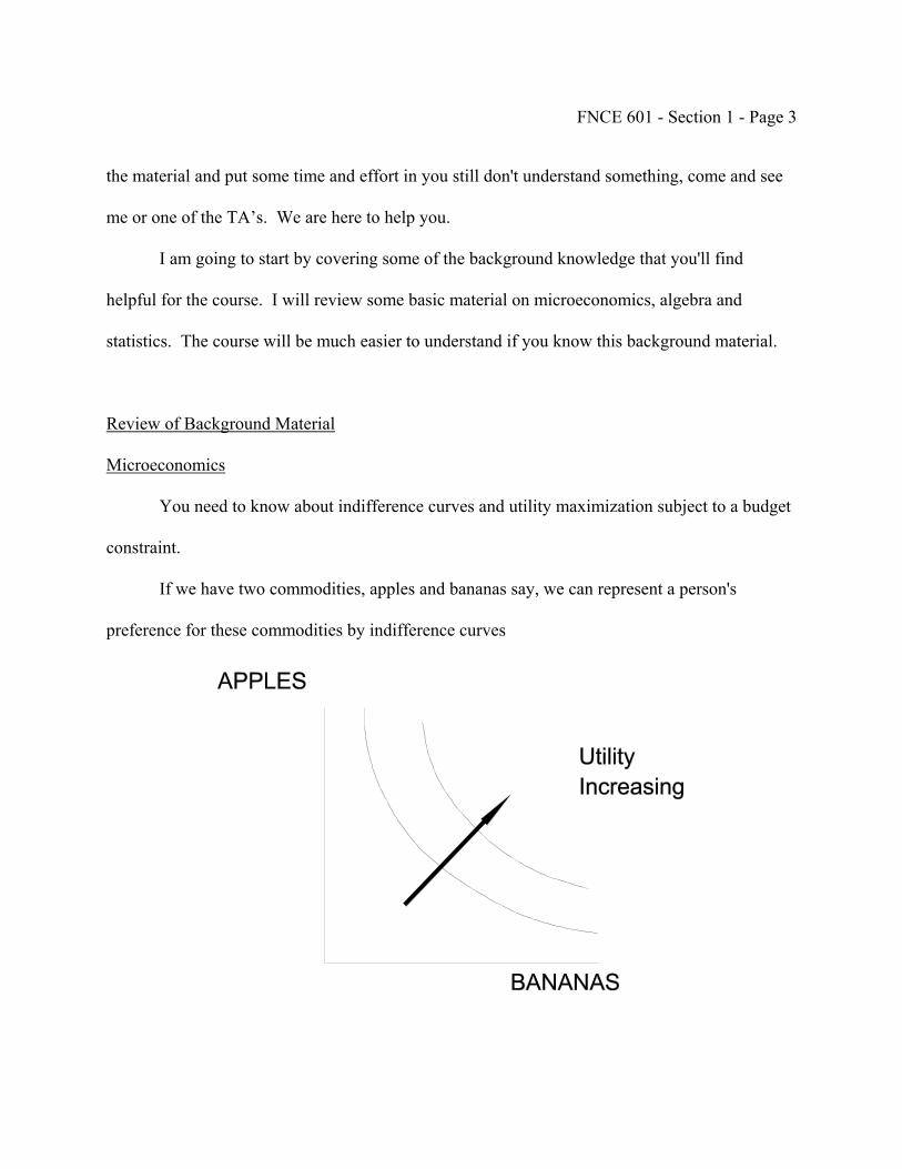
FNCE 601 - Section 1 - Page 3
the material and put some time and effort in you still don't understand something, come and see
me or one of the TA’s. We are here to help you.
I am going to start by covering some of the background knowledge that you'll find
helpful for the course. I will review some basic material on microeconomics, algebra and
statistics. The course will be much easier to understand if you know this background material.
Review of Background Material
Microeconomics
You need to know about indifference curves and utility maximization subject to a budget
constraint.
If we have two commodities, apples and bananas say, we can represent a person's
preference for these commodities by indifference curves

FNCE 601 - Section 1 - Page 4
An indifference curve is the locus of combinations of apples and bananas such that the
person is indifferent. It is assumed more is preferred to less, so moving in a northeasterly
direction utility is increasing.
We are all constrained by a budget constraint: we can't spend more than our income on
apples and bananas. It must be the case that
PA A + PB B ≤ I
where PA, PB are the prices of apples and bananas respectively, A and B are the quantities
purchased, and I is income.
This can be represented on our usual diagram.
If we add indifference curves to this diagram of the budget constraint we can use it to
find the combination of A and B a person will choose if he maximizes his utility.
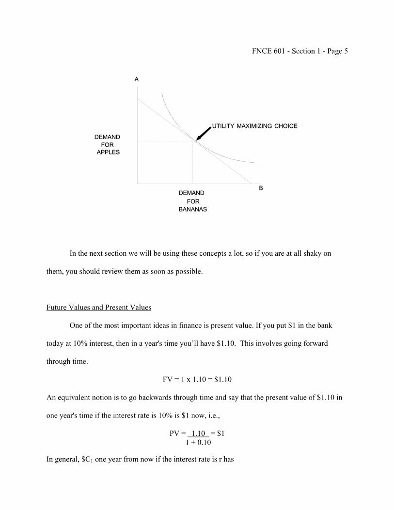
FNCE 601 - Section 1 - Page 5
In the next section we will be using these concepts a lot, so if you are at all shaky on
them, you should review them as soon as possible.
Future Values and Present Values
One of the most important ideas in finance is present value. If you put $1 in the bank
today at 10% interest, then in a year's time you’ll have $1.10. This involves going forward
through time.
FV = 1 x 1.10 = $1.10
An equivalent notion is to go backwards through time and say that the present value of $1.10 in
one year's time if the interest rate is 10% is $1 now, i.e.,
PV = 1.10 = $1 1 + 0.10
In general, $C1 one year from now if the interest rate is r has
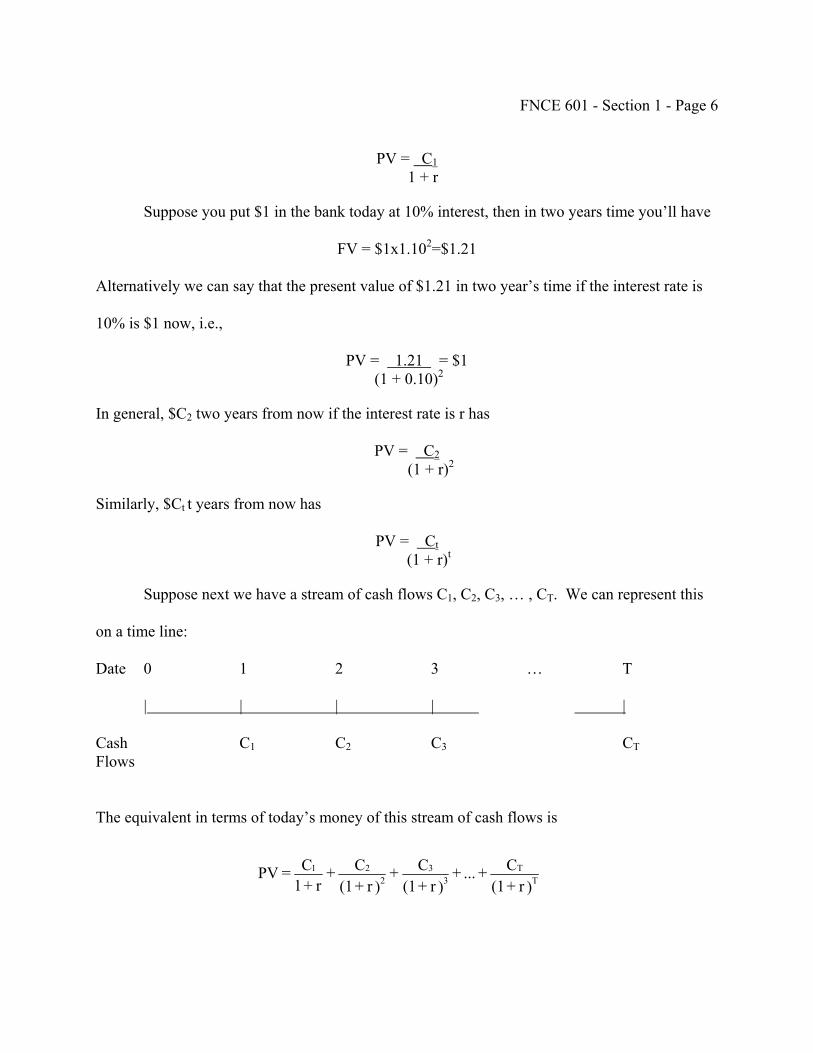
FNCE 601 - Section 1 - Page 6
PV = C1 1 + r
Suppose you put $1 in the bank today at 10% interest, then in two years time you’ll have
FV = $1x1.102=$1.21
Alternatively we can say that the present value of $1.21 in two year’s time if the interest rate is
10% is $1 now, i.e.,
PV = 1.21 = $1 (1 + 0.10)2
In general, $C2 two years from now if the interest rate is r has
PV = C2 (1 + r)2
Similarly, $Ct t years from now has
PV = Ct (1 + r)t
Suppose next we have a stream of cash flows C1, C2, C3, … , CT. We can represent this
on a time line:
Date 0 1 2 3 … T
| | | | |
Cash C1 C2 C3 CT Flows
The equivalent in terms of today’s money of this stream of cash flows is
)r + (1
C + ... + )r + (1
C + )r + (1
C + r + 1
C = PV TT
33
221
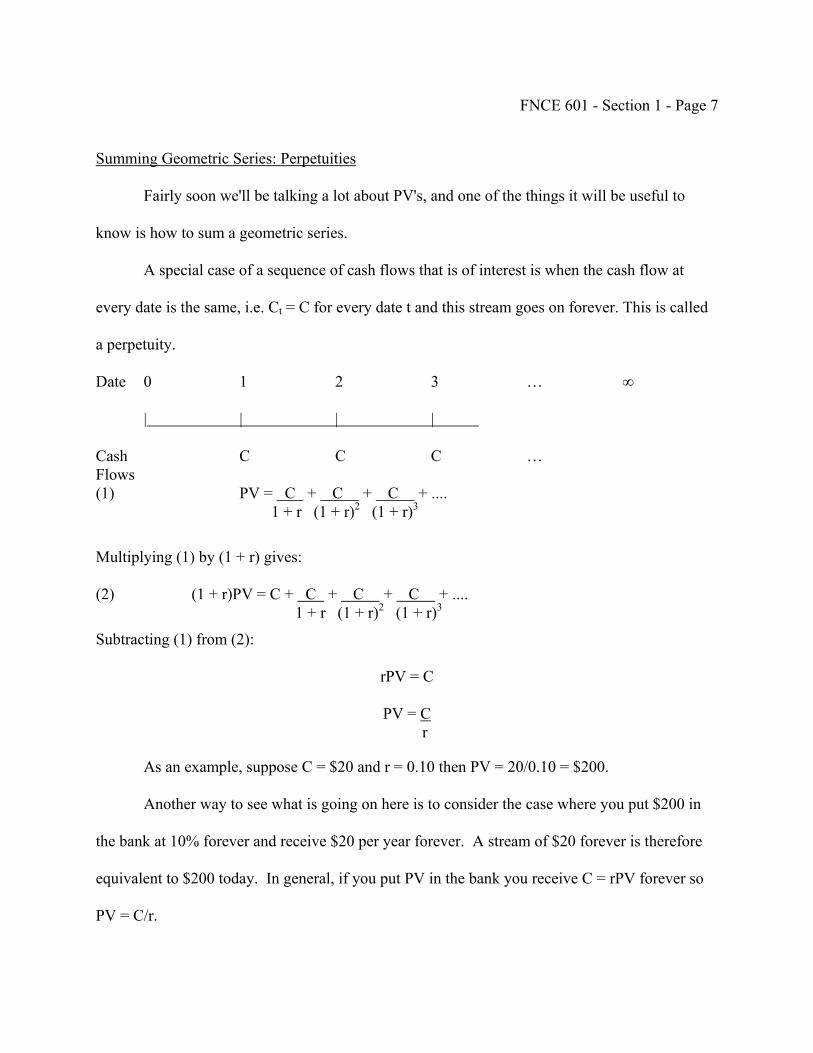
FNCE 601 - Section 1 - Page 7
Summing Geometric Series: Perpetuities
Fairly soon we'll be talking a lot about PV's, and one of the things it will be useful to
know is how to sum a geometric series.
A special case of a sequence of cash flows that is of interest is when the cash flow at
every date is the same, i.e. Ct = C for every date t and this stream goes on forever. This is called
a perpetuity.
Date 0 1 2 3 … ∞
| | | |
Cash C C C … Flows (1) PV = C + C + C + .... 1 + r (1 + r)2 (1 + r)3
Multiplying (1) by (1 + r) gives: (2) (1 + r)PV = C + C + C + C + .... 1 + r (1 + r)2 (1 + r)3
Subtracting (1) from (2):
rPV = C
PV = C r
As an example, suppose C = $20 and r = 0.10 then PV = 20/0.10 = $200.
Another way to see what is going on here is to consider the case where you put $200 in
the bank at 10% forever and receive $20 per year forever. A stream of $20 forever is therefore
equivalent to $200 today. In general, if you put PV in the bank you receive C = rPV forever so
PV = C/r.

FNCE 601 - Section 1 - Page 8
Now that's the last time I'm going to go through the algebra of that or any other
derivation of a formula on the board. In the future I'll just refer you back to this lecture for
perpetuities and give you the general outline for other cases. However at this point you should
memorize the fact that for perpetuities you just divide by the interest rate. There will be
derivations of formulas in the appendix for Section 3 and in the solutions to Problem Set 2. If at
any point you find yourself thinking where does that formula come from you can check it out.
Statistics
We won't be using the statistics for some time and when we get to the point we do need
it, I'll review it. For those of you who want some more time to refresh your memory, I'll just list
the basic concepts you'll need to understand:
Random Variable
Probability
Expectation
The Mean or Average
Variance
Standard deviation
Covariance
Correlation
That's the basic background knowledge you'll need. If you are at all doubtful about any
of the concepts, review them soon.

INTENTIONALLY BLANK
UNIVERSITY OF PENNSYLVANIA THE WHARTON SCHOOL LECTURE NOTES FNCE 601 CORPORATE FINANCE Franklin Allen Fall 2004 QUARTER 1 - WEEK 1 Tu: 9/7/04 and Th: 9/9/04 Copyright © 2004 by Franklin Allen

FNCE 601 - Section 2 - Page 1
PART II. INVESTMENT DECISIONS
Section 2: The Objective Function for Corporations
Read Chapter 2 in BM
Motivation Example
Suppose you are at a GM shareholders' meeting. Three of the shareholders there have
very different ideas about what the firm should do.
Old lady: Wants money now. Wants GM to invest in large cars since this would yield a quick profit.
Little Boy's trust Wants money a long way in the future. Wants GM to invest in fund representative building electric cars. Pension fund Wants money in the medium term. Thinks there will be a very representative serious oil crisis some time in that period. Recommends that GM
build small cars.
What should GM do?
We shall soon be in a position to answer this question.
Net Present Value
Suppose that a firm has a project. To keep it very simple, assume the project has a cost
now and generates a revenue one year from now. The net present value or the NPV as it is
known is net amount generated by the project all evaluated in terms of today’s dollars.
NPV = - Cost + PV(Revenue)
We can think of cost as a negative cash flow and denote it C0 since it occurs now, at time 0, i.e.,
FNCE 601 - Section 2 - Page 2
C0 = - Cost
It's important to note that C0 is a negative number usually. If something costs $2M, then C0 =
-2M.
Also suppose the revenue one year from now is C1
r1C)venue(RePV 1
+=
Substituting we have
r1CCNPV 1
0 ++=
What NPV is measuring is the net amount of wealth in terms of dollars today that the project
creates.
Now, the NPV rule states that if a project has a positive NPV, we should accept it; if it's
negative we should reject it.
NPV Rule: Accept project if NPV > 0.
For example, suppose C1 = 110, r = 10%, and C0 = - 90. Should we accept? Yes, since
NPV = +10. Suppose C0 = - 105. Should we accept? No, since NPV = -5. Using the NPV rule
always leads to an increase in NPV and hence is equivalent to maximizing NPV.
In this section we're going to look at the NPV rule for an individual. Then we'll show
why it's a valid rule for a corporation even though the corporation may be owned by many
different types of people. We're going to do this by considering a simple example.
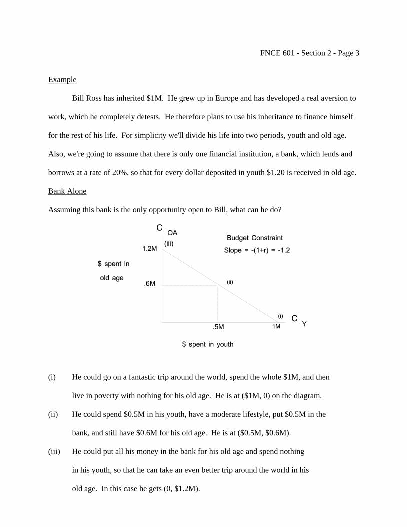
FNCE 601 - Section 2 - Page 3
Example
Bill Ross has inherited $1M. He grew up in Europe and has developed a real aversion to
work, which he completely detests. He therefore plans to use his inheritance to finance himself
for the rest of his life. For simplicity we'll divide his life into two periods, youth and old age.
Also, we're going to assume that there is only one financial institution, a bank, which lends and
borrows at a rate of 20%, so that for every dollar deposited in youth $1.20 is received in old age.
Bank Alone
Assuming this bank is the only opportunity open to Bill, what can he do?
(i) He could go on a fantastic trip around the world, spend the whole $1M, and then
live in poverty with nothing for his old age. He is at ($1M, 0) on the diagram.
(ii) He could spend $0.5M in his youth, have a moderate lifestyle, put $0.5M in the
bank, and still have $0.6M for his old age. He is at ($0.5M, $0.6M).
(iii) He could put all his money in the bank for his old age and spend nothing
in his youth, so that he can take an even better trip around the world in his
old age. In this case he gets (0, $1.2M).
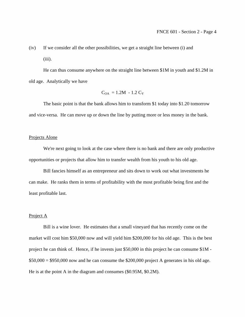
FNCE 601 - Section 2 - Page 4
(iv) If we consider all the other possibilities, we get a straight line between (i) and
(iii).
He can thus consume anywhere on the straight line between $1M in youth and $1.2M in
old age. Analytically we have
COA = 1.2M - 1.2 CY
The basic point is that the bank allows him to transform $1 today into $1.20 tomorrow
and vice-versa. He can move up or down the line by putting more or less money in the bank.
Projects Alone
We're next going to look at the case where there is no bank and there are only productive
opportunities or projects that allow him to transfer wealth from his youth to his old age.
Bill fancies himself as an entrepreneur and sits down to work out what investments he
can make. He ranks them in terms of profitability with the most profitable being first and the
least profitable last.
Project A
Bill is a wine lover. He estimates that a small vineyard that has recently come on the
market will cost him $50,000 now and will yield him $200,000 for his old age. This is the best
project he can think of. Hence, if he invests just $50,000 in this project he can consume $1M -
$50,000 = $950,000 now and he can consume the $200,000 project A generates in his old age.
He is at the point A in the diagram and consumes ($0.95M, $0.2M).

FNCE 601 - Section 2 - Page 5
COA
A 0.2M
CY 0.95M 1M
Project B
Bill is also a gourmet. The next best project he can think of is to run a restaurant in the
town he lives in. He reckons for a $100,000 outlay now he can get $140,000 in his old age. If
he just undertakes this and project A, then he can consume $950,000 - $100,000 = $850,000 now
and $200,000 + $140,000 = $340,000 that the two projects generate in his old age. He is at the
point A + B in the diagram below and consumes ($0.85M, $0.34M).
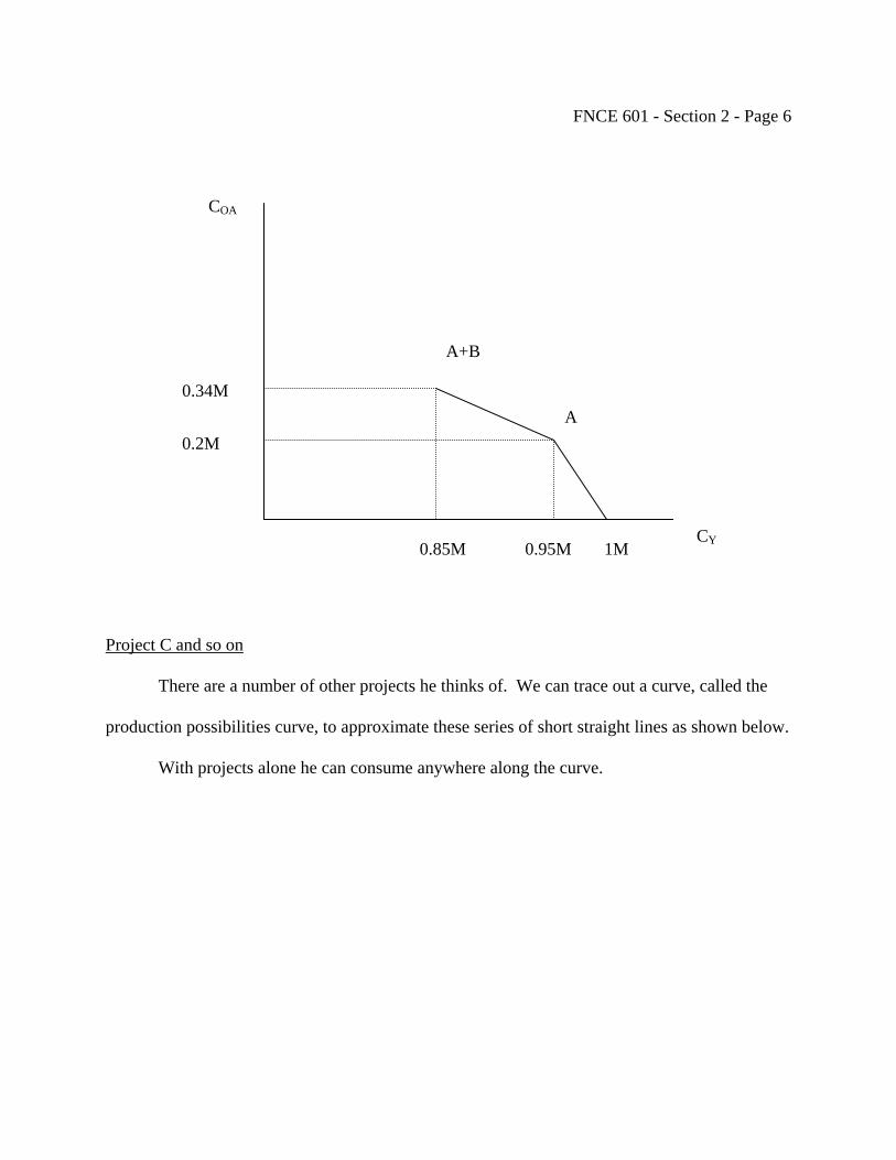
FNCE 601 - Section 2 - Page 6
COA
Project C and so on
There are a number of other projects he thinks of. We can trace out a curve, called the
production possibilities curve, to approximate these series of short straight lines as shown below.
With projects alone he can consume anywhere along the curve.
CY 0.95M
A
1M
A+B
0.2M
0.34M
0.85M
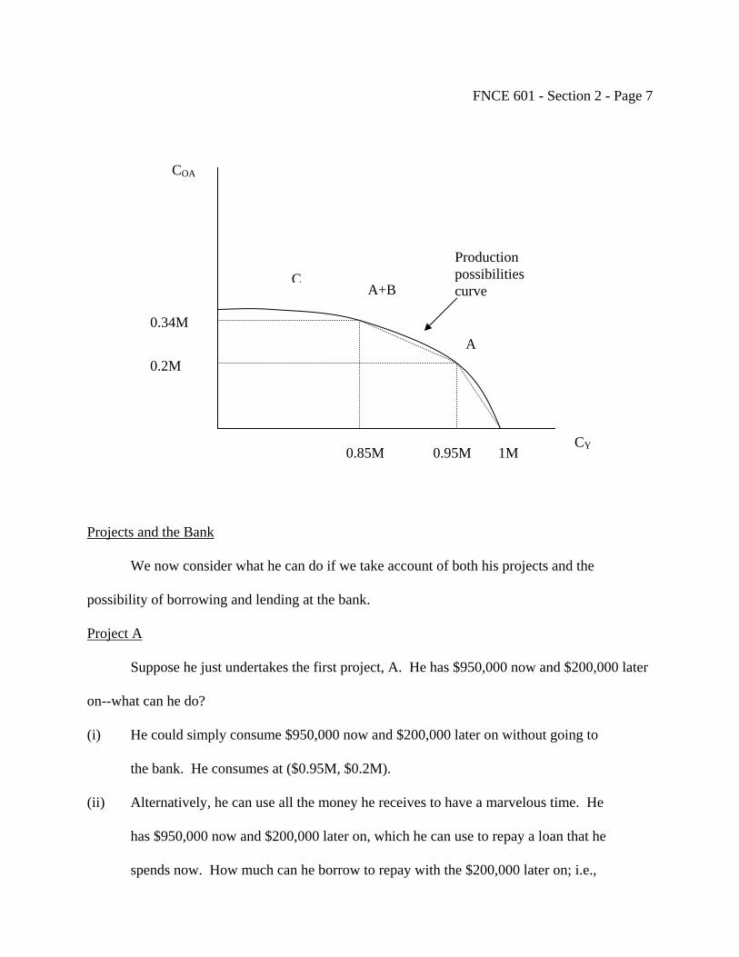
FNCE 601 - Section 2 - Page 7
COA
Projects and the Bank
We now consider what he can do if we take account of both his projects and the
possibility of borrowing and lending at the bank.
Project A
Suppose he just undertakes the first project, A. He has $950,000 now and $200,000 later
on--what can he do?
(i) He could simply consume $950,000 now and $200,000 later on without going to
the bank. He consumes at ($0.95M, $0.2M).
(ii) Alternatively, he can use all the money he receives to have a marvelous time. He
has $950,000 now and $200,000 later on, which he can use to repay a loan that he
spends now. How much can he borrow to repay with the $200,000 later on; i.e.,
CY 0.95M
A
1M
0.2M
A+B
0.85M
Production possibilities Ccurve
0.34M
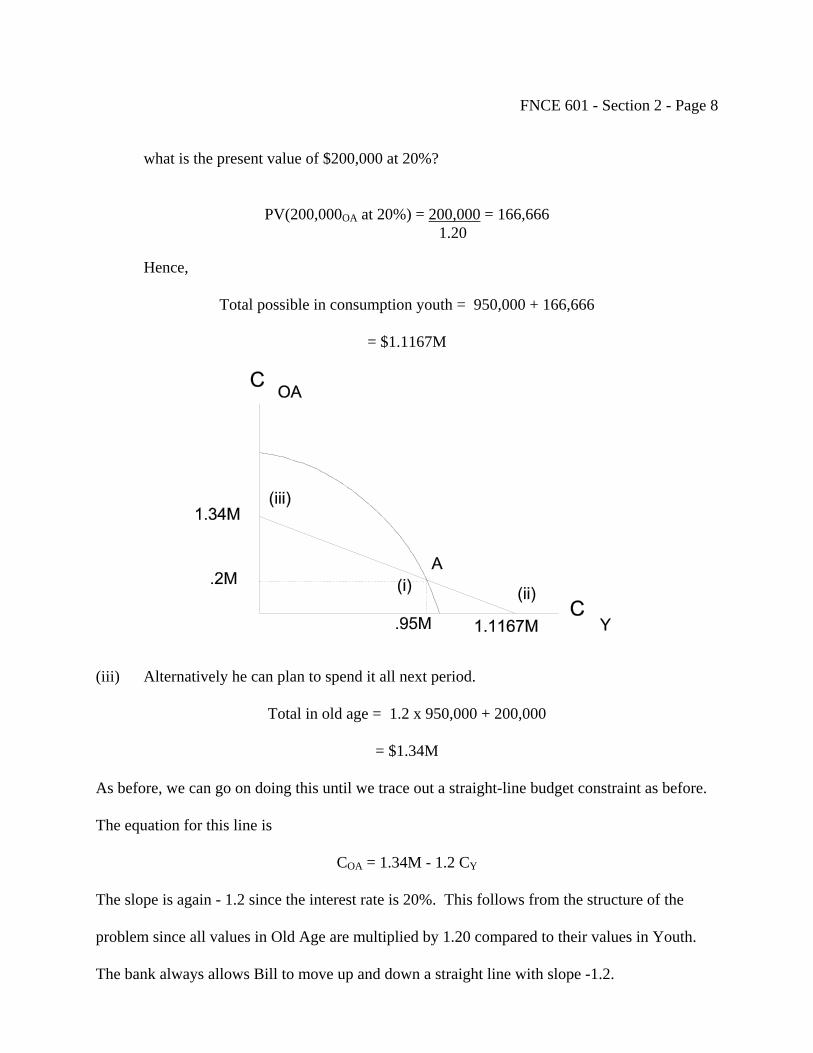
FNCE 601 - Section 2 - Page 8
what is the present value of $200,000 at 20%?
PV(200,000OA at 20%) = 200,000 = 166,666
1.20
Hence,
Total possible in consumption youth = 950,000 + 166,666
= $1.1167M
(iii) Alternatively he can plan to spend it all next period.
Total in old age = 1.2 x 950,000 + 200,000
= $1.34M
As before, we can go on doing this until we trace out a straight-line budget constraint as before.
The equation for this line is
COA = 1.34M - 1.2 CY
The slope is again - 1.2 since the interest rate is 20%. This follows from the structure of the
problem since all values in Old Age are multiplied by 1.20 compared to their values in Youth.
The bank always allows Bill to move up and down a straight line with slope -1.2.

FNCE 601 - Section 2 - Page 9
Project B
Now suppose he undertakes the first and second projects, A and B, so that he produces at
A + B. We can go through the same calculations again and get another line representing his
consumption possibilities.
In this case,
Intercept on COA axis = 1.2 x 850,000 + 340,000 = 1.36 M.
Hence, analytically the budget constraint is given by
COA = 1.36 M - 1.2 CY
We can see that by undertaking the first project he can push out the line representing his
possible consumption, similarly when he undertakes the second project, and so on.
If he prefers more money to less, he is better off if his budget constraint is pushed out
further since this allows him to consume more in both periods. Hence no matter what his
preferences are, he is better off with a budget constraint that is farther out.
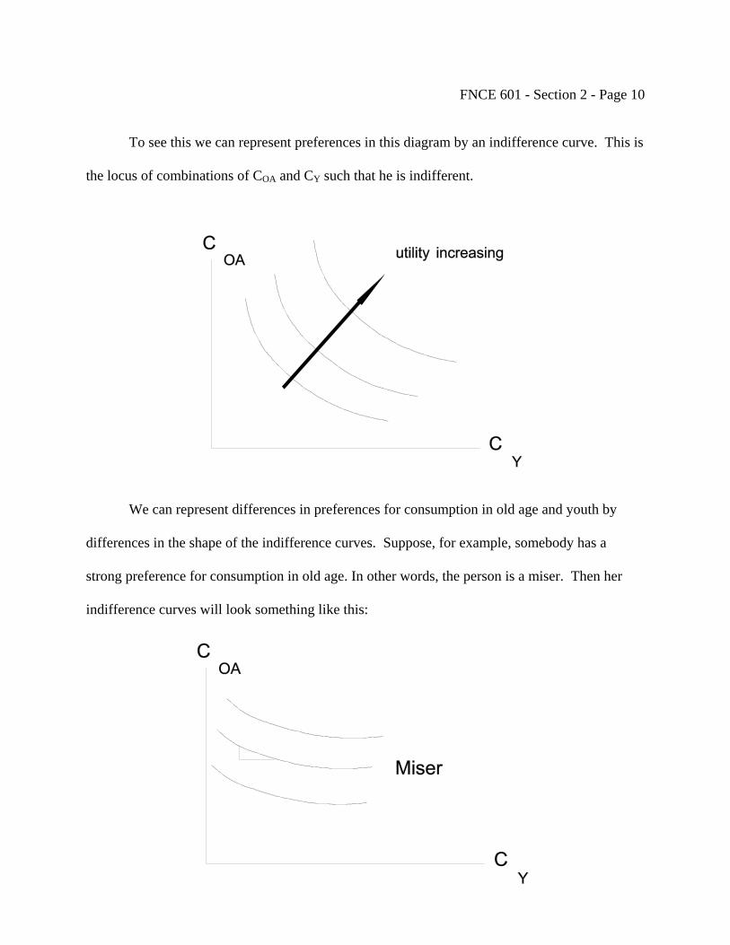
FNCE 601 - Section 2 - Page 10
To see this we can represent preferences in this diagram by an indifference curve. This is
the locus of combinations of COA and CY such that he is indifferent.
We can represent differences in preferences for consumption in old age and youth by
differences in the shape of the indifference curves. Suppose, for example, somebody has a
strong preference for consumption in old age. In other words, the person is a miser. Then her
indifference curves will look something like this:

FNCE 601 - Section 2 - Page 11
Her curves are flat for the following reason. Since she is a miser a small reduction in
consumption in old age must be compensated for by a large increase in youth to make her
indifferent.
Somebody who prefers consumption in his youth, who we shall call a spender, will have
the type of indifference curves below. They are steep because a large reduction in consumption
in old age can be compensated for by a small increase in youth to make him indifferent.
Now if we put budget constraints on these diagrams we can see that pushing a budget
constraint out makes both better off.
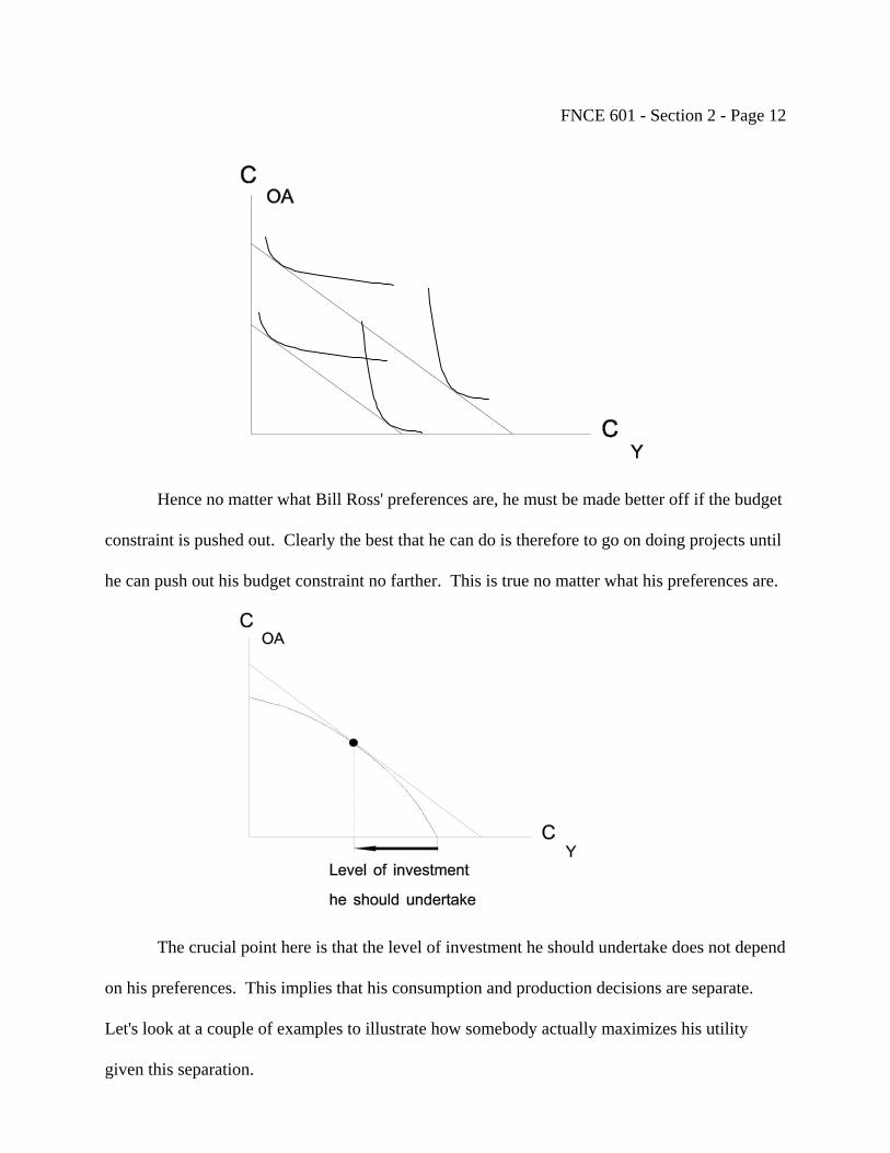
FNCE 601 - Section 2 - Page 12
Hence no matter what Bill Ross' preferences are, he must be made better off if the budget
constraint is pushed out. Clearly the best that he can do is therefore to go on doing projects until
he can push out his budget constraint no farther. This is true no matter what his preferences are.
The crucial point here is that the level of investment he should undertake does not depend
on his preferences. This implies that his consumption and production decisions are separate.
Let's look at a couple of examples to illustrate how somebody actually maximizes his utility
given this separation.
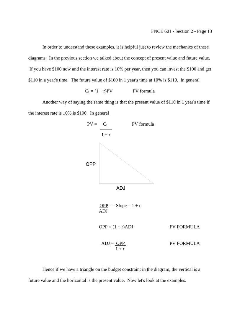
FNCE 601 - Section 2 - Page 13
In order to understand these examples, it is helpful just to review the mechanics of these
diagrams. In the previous section we talked about the concept of present value and future value.
If you have $100 now and the interest rate is 10% per year, then you can invest the $100 and get
$110 in a year's time. The future value of $100 in 1 year's time at 10% is $110. In general
C1 = (1 + r)PV FV formula
Another way of saying the same thing is that the present value of $110 in 1 year's time if
the interest rate is 10% is $100. In general
PV = C PV formula 1 _____ 1 + r
OPP = - Slope = 1 + r ADJ
OPP = (1 + r)ADJ FV FORMULA ADJ = OPP PV FORMULA 1 + r
Hence if we have a triangle on the budget constraint in the diagram, the vertical is a
future value and the horizontal is the present value. Now let's look at the examples.

FNCE 601 - Section 2 - Page 14
Miser - Lends
Spender - Borrows
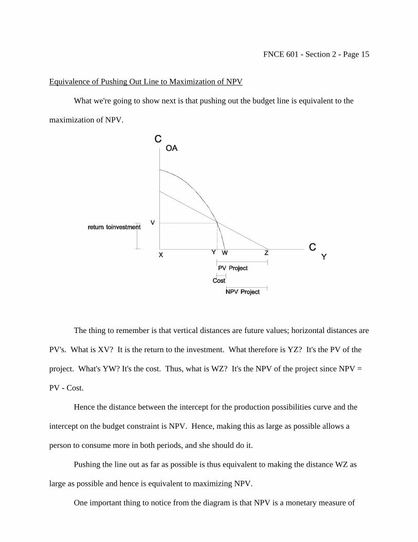
FNCE 601 - Section 2 - Page 15
Equivalence of Pushing Out Line to Maximization of NPV
What we're going to show next is that pushing out the budget line is equivalent to the
maximization of NPV.
The thing to remember is that vertical distances are future values; horizontal distances are
PV's. What is XV? It is the return to the investment. What therefore is YZ? It's the PV of the
project. What's YW? It's the cost. Thus, what is WZ? It's the NPV of the project since NPV =
PV - Cost.
Hence the distance between the intercept for the production possibilities curve and the
intercept on the budget constraint is NPV. Hence, making this as large as possible allows a
person to consume more in both periods, and she should do it.
Pushing the line out as far as possible is thus equivalent to making the distance WZ as
large as possible and hence is equivalent to maximizing NPV.
One important thing to notice from the diagram is that NPV is a monetary measure of
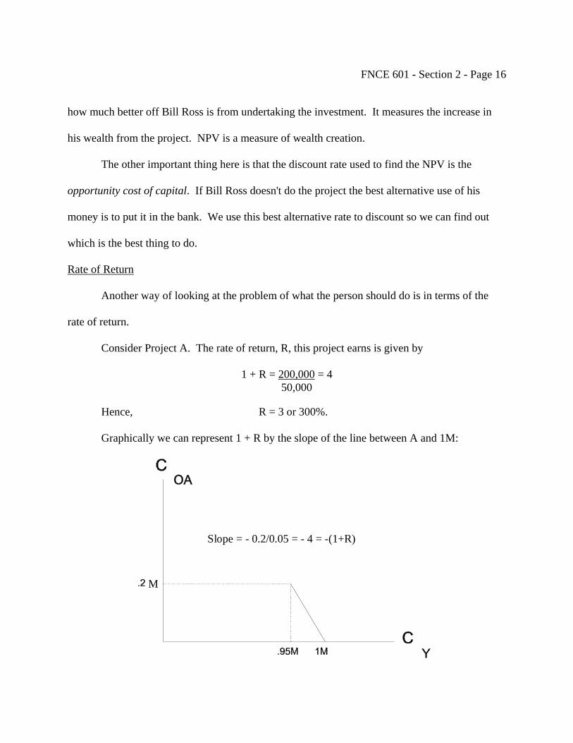
FNCE 601 - Section 2 - Page 16
how much better off Bill Ross is from undertaking the investment. It measures the increase in
his wealth from the project. NPV is a measure of wealth creation.
The other important thing here is that the discount rate used to find the NPV is the
opportunity cost of capital. If Bill Ross doesn't do the project the best alternative use of his
money is to put it in the bank. We use this best alternative rate to discount so we can find out
which is the best thing to do.
Rate of Return
Another way of looking at the problem of what the person should do is in terms of the
rate of return.
Consider Project A. The rate of return, R, this project earns is given by
1 + R = 200,000 = 4 50,000
Hence, R = 3 or 300%.
Graphically we can represent 1 + R by the slope of the line between A and 1M:
Slope = - 0.2/0.05 = - 4 = -(1+R)
M

FNCE 601 - Section 2 - Page 17
With project B the rate of return is given by
1 + R = 140,000 = 1.4 100,000
R = 0.4 or 40%.
Graphically, 1+R is again the slope of the line between B and A.
A
Slope = -0.14/0.1 = -1.4 = -(1+R)
.2M
In the more general case where we have the curve representing the production
possibilities, the rate of return is represented by the slope of the curve.
- (1+R)
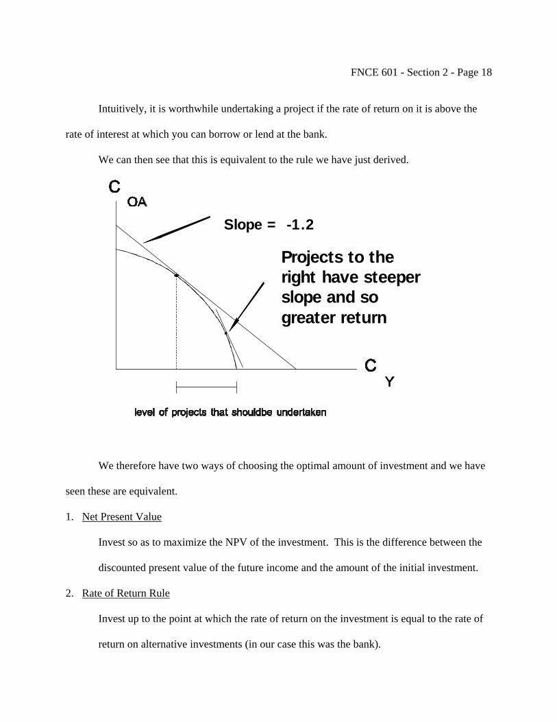
FNCE 601 - Section 2 - Page 18
Intuitively, it is worthwhile undertaking a project if the rate of return on it is above the
rate of interest at which you can borrow or lend at the bank.
We can then see that this is equivalent to the rule we have just derived.
Slope = -1.2
Projects to theright have steeperslope and sogreater return
We therefore have two ways of choosing the optimal amount of investment and we have
seen these are equivalent.
1. Net Present Value
Invest so as to maximize the NPV of the investment. This is the difference between the
discounted present value of the future income and the amount of the initial investment.
2. Rate of Return Rule
Invest up to the point at which the rate of return on the investment is equal to the rate of
return on alternative investments (in our case this was the bank).
FNCE 601 - Section 2 - Page 19
Rules for Managers of Corporations
We have derived these as the rules for an individual to follow when choosing his
investments in real assets. But are they relevant for the type of firm we are interested in where
(i) management and control are separated;
(ii) there are many shareholders who may be very different?
To answer this question, we go back to our example. Here and in fact throughout Part II
we will be assuming that firms are all equity financed. Thus when we talk about borrowing and
lending this refers to shareholders borrowing and lending rather than corporations borrowing and
lending. We consider firms’ borrowing decisions later in the course.
Bill Ross has been thinking a bit about the implementation of these projects and decides
they involve more work than he first thought. He therefore decides to hire managers to
implement the investment in real assets. In order to ensure that they pursue his interests all he
has to do is to tell them to maximize the NPV of the firm, and this will ensure that he can be as
well off as possible.
The important point to note here is:
The decision on how to allocate his consumption between youth and old age is independent of
the need to maximize the NPV of the firm.

FNCE 601 - Section 2 - Page 20
No matter whether he has preferences 1 or 2, he will produce at the point that maximizes
NPV. With preferences 1 he consumes at D. With preferences 2 he consumes at E. Thus
ownership and control can be separated. It is only necessary for the owner to tell the manager to
maximize NPV; the owner doesn't need to give a detailed description of how to run the firm.
The fact that it doesn't matter what Bill Ross' preferences are as far as the production
decision is concerned has very important implications if there is more than one shareholder.
Suppose, that in his father's will, the terms under which Bill Ross inherits, actually say that the
inheritance "is to be divided equally among his children." The $1M figure was based on the
assumption that Bill Ross was the only child. In actual fact it turns out that the father had
another brother, Rex, by a former liaison. His inheritance therefore drops to 0.5M.
Should they change the operation of the firm that Bill Ross has set up? No. Since the
NPV rule we derived was independent of the owner's preferences, it follows that both Bill and
Rex are content to leave the firm the way it is.
Why is this? What is the situation they face? The production possibilities curve is now
half what it was before.
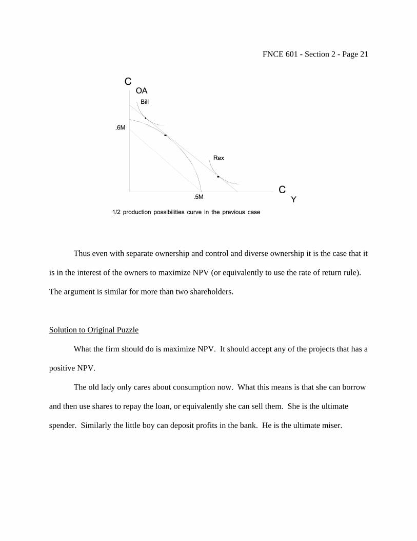
FNCE 601 - Section 2 - Page 21
Thus even with separate ownership and control and diverse ownership it is the case that it
is in the interest of the owners to maximize NPV (or equivalently to use the rate of return rule).
The argument is similar for more than two shareholders.
Solution to Original Puzzle
What the firm should do is maximize NPV. It should accept any of the projects that has a
positive NPV.
The old lady only cares about consumption now. What this means is that she can borrow
and then use shares to repay the loan, or equivalently she can sell them. She is the ultimate
spender. Similarly the little boy can deposit profits in the bank. He is the ultimate miser.
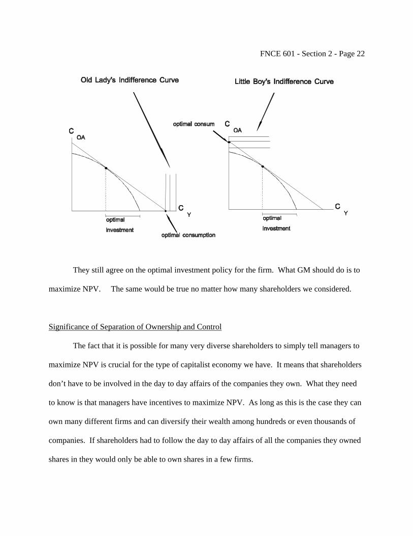
FNCE 601 - Section 2 - Page 22
They still agree on the optimal investment policy for the firm. What GM should do is to
maximize NPV. The same would be true no matter how many shareholders we considered.
Significance of Separation of Ownership and Control
The fact that it is possible for many very diverse shareholders to simply tell managers to
maximize NPV is crucial for the type of capitalist economy we have. It means that shareholders
don’t have to be involved in the day to day affairs of the companies they own. What they need
to know is that managers have incentives to maximize NPV. As long as this is the case they can
own many different firms and can diversify their wealth among hundreds or even thousands of
companies. If shareholders had to follow the day to day affairs of all the companies they owned
shares in they would only be able to own shares in a few firms.
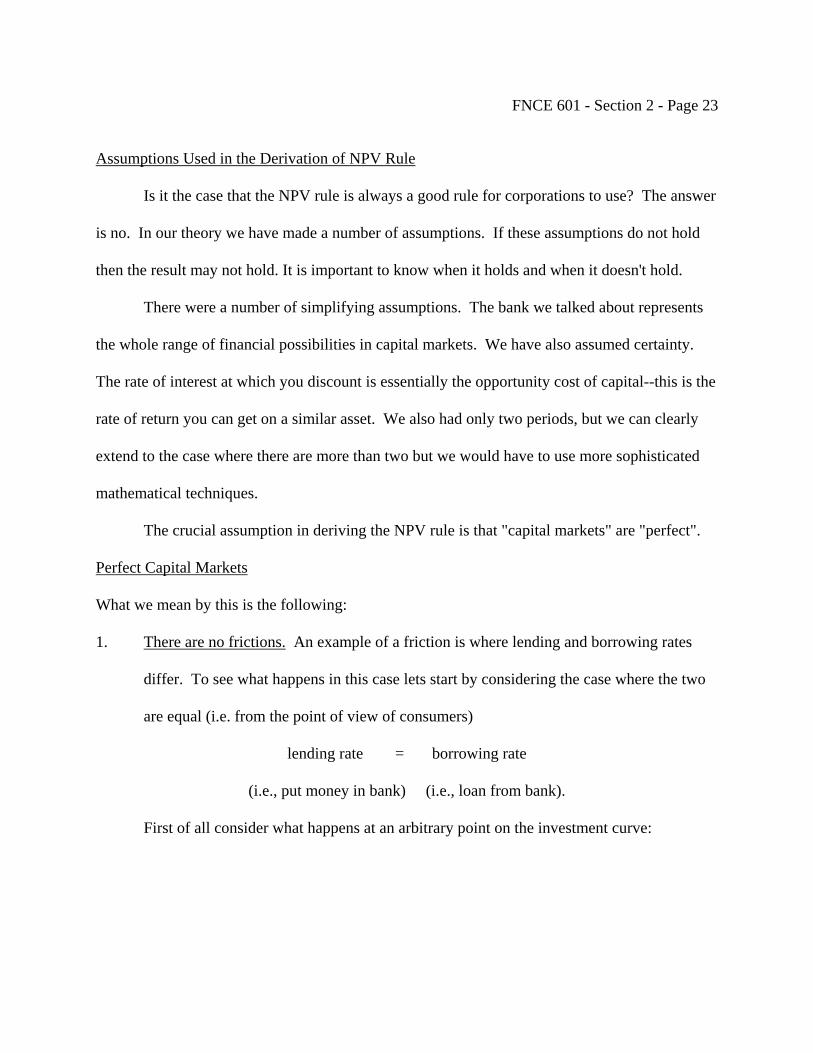
FNCE 601 - Section 2 - Page 23
Assumptions Used in the Derivation of NPV Rule
Is it the case that the NPV rule is always a good rule for corporations to use? The answer
is no. In our theory we have made a number of assumptions. If these assumptions do not hold
then the result may not hold. It is important to know when it holds and when it doesn't hold.
There were a number of simplifying assumptions. The bank we talked about represents
the whole range of financial possibilities in capital markets. We have also assumed certainty.
The rate of interest at which you discount is essentially the opportunity cost of capital--this is the
rate of return you can get on a similar asset. We also had only two periods, but we can clearly
extend to the case where there are more than two but we would have to use more sophisticated
mathematical techniques.
The crucial assumption in deriving the NPV rule is that "capital markets" are "perfect".
Perfect Capital Markets
What we mean by this is the following:
1. There are no frictions. An example of a friction is where lending and borrowing rates
differ. To see what happens in this case lets start by considering the case where the two
are equal (i.e. from the point of view of consumers)
lending rate = borrowing rate
(i.e., put money in bank) (i.e., loan from bank).
First of all consider what happens at an arbitrary point on the investment curve:
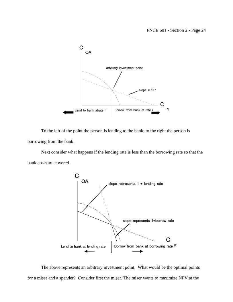
FNCE 601 - Section 2 - Page 24
To the left of the point the person is lending to the bank; to the right the person is
borrowing from the bank.
Next consider what happens if the lending rate is less than the borrowing rate so that the
bank costs are covered.
Lend to bank at lending rate
The above represents an arbitrary investment point. What would be the optimal points
for a miser and a spender? Consider first the miser. The miser wants to maximize NPV at the
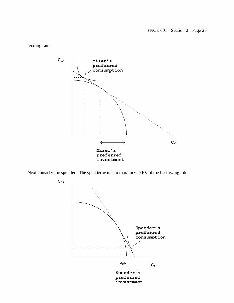
FNCE 601 - Section 2 - Page 25
lending rate.
COA
Next consider the spender. The spender wants to maximize NPV at the borrowing rate.
Miser’s preferred consumption
Miser’s preferred investment
CY
COA
Spender’s preferred consumption
CY
Spender’s preferred investment
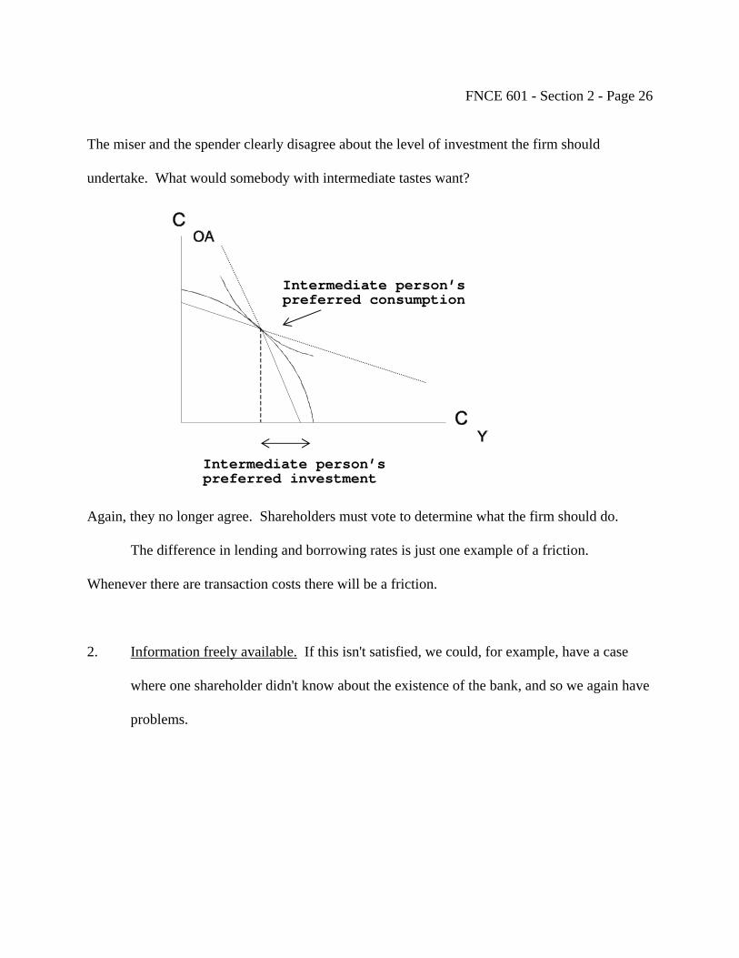
FNCE 601 - Section 2 - Page 26
The miser and the spender clearly disagree about the level of investment the firm should
undertake. What would somebody with intermediate tastes want?
Intermediate person’spreferred investment
Intermediate person’s preferred consumption
Again, they no longer agree. Shareholders must vote to determine what the firm should do.
The difference in lending and borrowing rates is just one example of a friction.
Whenever there are transaction costs there will be a friction.
2. Information freely available. If this isn't satisfied, we could, for example, have a case
where one shareholder didn't know about the existence of the bank, and so we again have
problems.
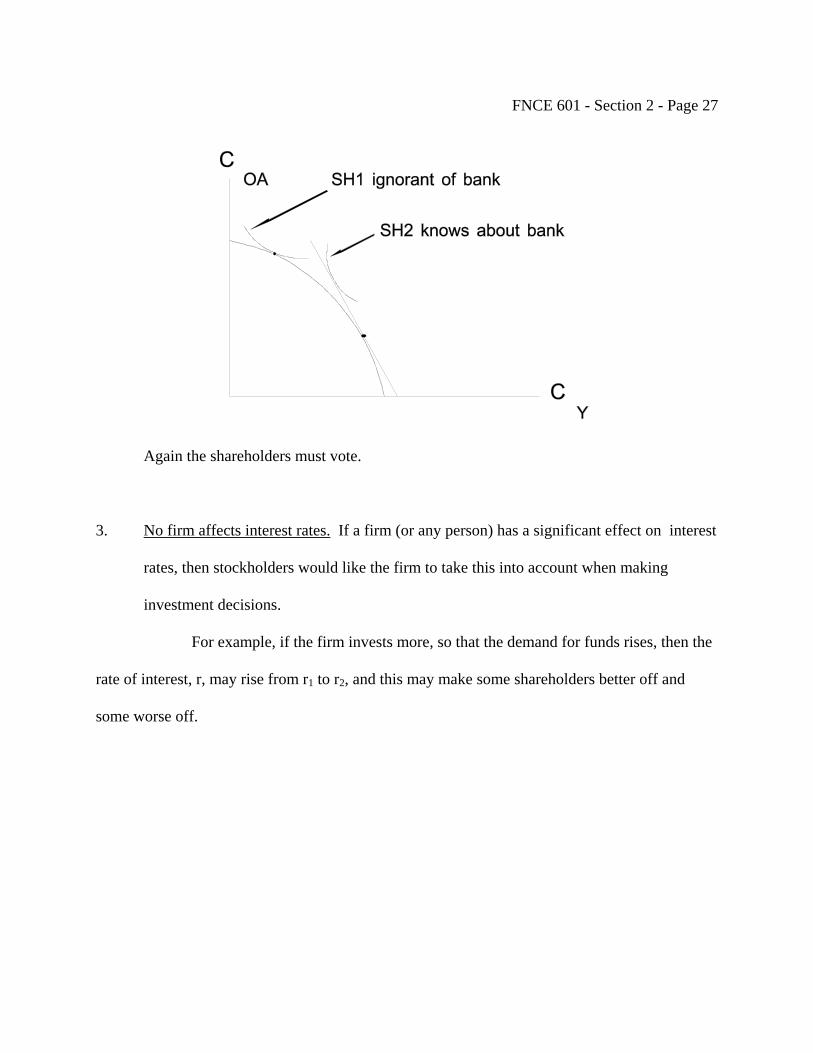
FNCE 601 - Section 2 - Page 27
Again the shareholders must vote.
3. No firm affects interest rates. If a firm (or any person) has a significant effect on interest
rates, then stockholders would like the firm to take this into account when making
investment decisions.
For example, if the firm invests more, so that the demand for funds rises, then the
rate of interest, r, may rise from r1 to r2, and this may make some shareholders better off and
some worse off.

FNCE 601 - Section 2 - Page 28
Situation 1 (r1): One possible leve
Situation 2 (r2): Higher level of in
Once again they no longer agree
prefers Situation 1. Once again shareho
Assessment of Assumptions
Clearly assumptions 1 to 3 aren't
economies, particularly in the U.S., they
assumptions 1 and 2 come close to bein
own most of the stocks in the U.S. For
the third assumption is concerned no co
INV1
INV2l of investment and corresponding interest rate.
vestment and higher corresponding interest rate.
. Shareholder 1 prefers Situation 2 while Shareholder 2
lders must vote on what the firm should do.
entirely satisfied. However, it is the case that in many
come pretty close to being satisfied. The reason that
g satisfied is that rich people and institutional holders
these investors the assumptions are reasonable. As far as
rporations are large enough to affect interest rates so this

FNCE 601 - Section 2 - Page 29
assumption is satisfied. It is for these reasons that we can take the NPV rule as a reasonable
guide for managers to follow at least in the U.S. In a number of other countries, particularly
emerging economies such as Brazil, India and Korea and even a number of Western European
countries such as Germany capital markets are not as perfect. In these cases it is not clear that
maximization of NPV is a sensible goal for corporations with many diverse owners. In such
cases shareholders must get involved in the running of the corporation and vote on what it should
do. This is why family firms, which avoid these issues, are so much more prevalent in such
countries.
Other Aspects of Maximizing NPV
Do Managers Pursue Shareholders Interests?
The analysis above has assumed that managers act in the interests of shareholders. One
of the big debates in recent years has been concerned with whether this is in fact the case. This
is the issue of corporate governance. It has been widely pointed out that in large corporations
there is a tendency for managers to pursue their own interests. This is what is known as an
agency problem. In order to minimize this agency problem managers’ interests must be aligned
with those of shareholders.
One way to do this is to ensure managers have a stake in the firm in terms of direct
ownership of shares and/or stock options. If managers have a substantial portion of their wealth
in the shares of the company they will clearly have an incentive to create wealth for shareholders
by accepting positive NPV projects. Stock options have a similar effect. These allow managers
to buy shares at a fixed price called the exercise price. If the stock price rises above the exercise
price the options clearly become valuable. The managers can buy the shares at the exercise price

FNCE 601 - Section 2 - Page 30
and sell them at the higher market price.
Bonuses are another way that managers can be rewarded for pursuing shareholders’
interests. These are usually based on accounting measures of performance. Since these are not
as good a measure of shareholder wealth as the stock price itself they are often not as effective as
direct ownership of shares or stock options.
Another way of ensuring managers pursue shareholders’ interests is to have an active
market for corporate control. If managers pursue their own interests there is an incentive for an
outside raider to mount a hostile takeover bid and buy the firm. The raider can then fire the
managers and increase the value of the firm.
Should Firms be for Shareholders or All Stakeholders?
Even if the assumptions of the model are satisfied and managers pursue shareholders
interests it is not clear that maximizing NPV is the sole criterion that firms should pursue. A
number of authors have argued that firms should take into account other "stakeholders" in the
firm such as workers, residents around the firms' plants and so on. These are issues on which
there is no wide agreement. You will be discussing this issue at much greater length in the legal
studies and public policy and management core course LGST/PPMT 621.
Different countries have very different views on what the corporation's aim should be.
The German system of codetermination involves workers in large companies having the right to
elect up to half the directors to the supervisory board. In Japan managers usually view the
interests of shareholders to be secondary to those of employees and customers. The appendix (at
the end of the section) outlines the corporate philosophy of Asahi Breweries, which is one of the
major Japanese brewing companies. You can see that shareholders do not get mentioned until
FNCE 601 - Section 2 - Page 31
Section 6 under Social Responsibilities.
Other evidence for the differing views of the role of the firm in different countries are
given in the attached graphs. These are based on interviews with executives from large
companies in the five countries. In the first, where the issue is whose company it is, it can be
seen that Japanese, German and French executives countries view their firms as being for all
stakeholders while the U.S. and U.K. executives view their firms as being for shareholders.
Similarly, when the issue is job security or dividends almost all Japanese executives and the
majority of German and French managers believe job security should come first. Almost all
U.S. and U.K. executives believe dividends should come first.
For the remainder of the course, we shall be taking the objective of the corporation to be
the maximization of NPV or in other words the creation of shareholder wealth. The main point
of this section has been to show the justification of this from the firm perspective.
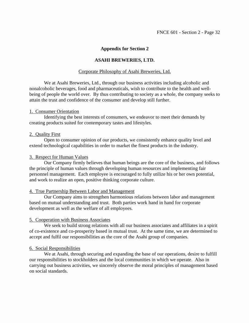
FNCE 601 - Section 2 - Page 32
Appendix for Section 2 ASAHI BREWERIES, LTD. Corporate Philosophy of Asahi Breweries, Ltd. We at Asahi Breweries, Ltd., through our business activities including alcoholic and nonalcoholic beverages, food and pharmaceuticals, wish to contribute to the health and well-being of people the world over. By thus contributing to society as a whole, the company seeks to attain the trust and confidence of the consumer and develop still further. 1. Consumer Orientation Identifying the best interests of consumers, we endeavor to meet their demands by creating products suited for contemporary tastes and lifestyles. 2. Quality First Open to consumer opinion of our products, we consistently enhance quality level and extend technological capabilities in order to market the finest products in the industry. 3. Respect for Human Values Our Company firmly believes that human beings are the core of the business, and follows the principle of human values through developing human resources and implementing fair personnel management. Each employee is encouraged to fully utilize his or her own potential, and work to realize an open, positive thinking corporate culture. 4. True Partnership Between Labor and Management Our Company aims to strengthen harmonious relations between labor and management based on mutual understanding and trust. Both parties work hand in hand for corporate development as well as the welfare of all employees. 5. Cooperation with Business Associates We seek to build strong relations with all our business associates and affiliates in a spirit of co-existence and co-prosperity based in mutual trust. At the same time, we are determined to accept and fulfil our responsibilities as the core of the Asahi group of companies. 6. Social Responsibilities We at Asahi, through securing and expanding the base of our operations, desire to fulfill our responsibilities to stockholders and the local communities in which we operate. Also in carrying out business activities, we sincerely observe the moral principles of management based on social standards.
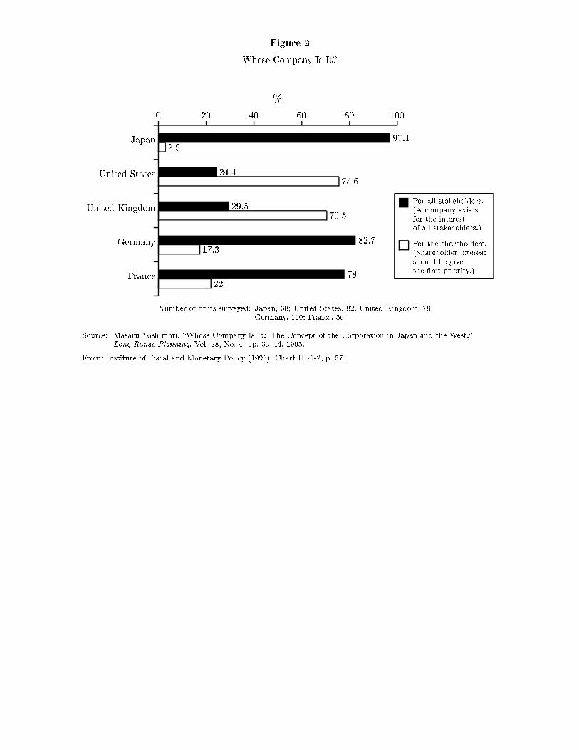
Figure 2
Whose Company Is It?
0 20 40 60 80 100
%
2.9
75.6
70.5
17.3
22
Japan 97.1
United States 24.4
United Kingdom 29.5
Germany 82.7
France 78
Number of �rms surveyed: Japan, 68; United States, 82; United Kingdom, 78;Germany, 110; France, 50.
For the shareholders.(Shareholder interestshould be giventhe �rst priority.)
For all stakeholders.(A company existsfor the interestof all stakeholders.)
Source: Masaru Yoshimori, \Whose Company Is It? The Concept of the Corporation in Japan and the West."Long Range Planning, Vol. 28, No. 4, pp. 33{44, 1995.
From: Institute of Fiscal and Monetary Policy (1996), Chart III-1-2, p. 57.

Figure 3
Job Security or Dividends
0 20 40 60 80 100
%
2.9
89.2
89.3
40.9
39.6
Japan 97.1
United States 10.8
United Kingdom 10.7
Germany 59.1
France 60.4
Number of �rms surveyed: Japan, 68; United States, 83; United Kingdom, 75;Germany, 105; France, 68.
Dividends more important.
Job security more important.
Source: Masaru Yoshimori, \Whose Company Is It? The Concept of the Corporation in Japan and the West."Long Range Planning, Vol. 28, No. 4, pp. 33{44, 1995.
From: Institute of Fiscal and Monetary Policy (1996), Chart III-4-6, p. 84.

INTENTIONALLY BLANK
UNIVERSITY OF PENNSYLVANIA THE WHARTON SCHOOL LECTURE NOTES FNCE 601 CORPORATE FINANCE Franklin Allen Fall 2004 QUARTER 1 - WEEK 2 (part 1) Tu: 9/14/04 Copyright © 2004 by Franklin Allen
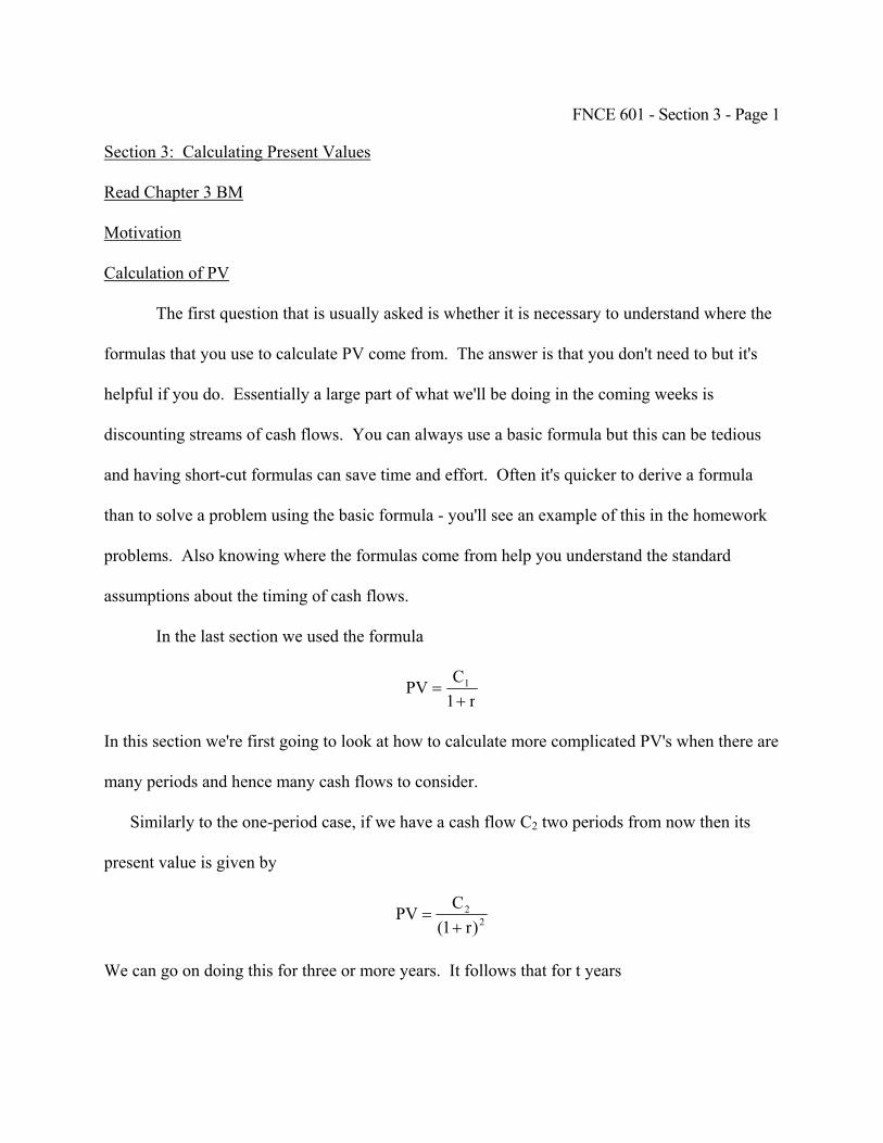
FNCE 601 - Section 3 - Page 1
Section 3: Calculating Present Values
Read Chapter 3 BM
Motivation
Calculation of PV
The first question that is usually asked is whether it is necessary to understand where the
formulas that you use to calculate PV come from. The answer is that you don't need to but it's
helpful if you do. Essentially a large part of what we'll be doing in the coming weeks is
discounting streams of cash flows. You can always use a basic formula but this can be tedious
and having short-cut formulas can save time and effort. Often it's quicker to derive a formula
than to solve a problem using the basic formula - you'll see an example of this in the homework
problems. Also knowing where the formulas come from help you understand the standard
assumptions about the timing of cash flows.
In the last section we used the formula
r1CPV 1
+=
In this section we're first going to look at how to calculate more complicated PV's when there are
many periods and hence many cash flows to consider.
Similarly to the one-period case, if we have a cash flow C2 two periods from now then its
present value is given by
22
)r1(CPV+
=
We can go on doing this for three or more years. It follows that for t years
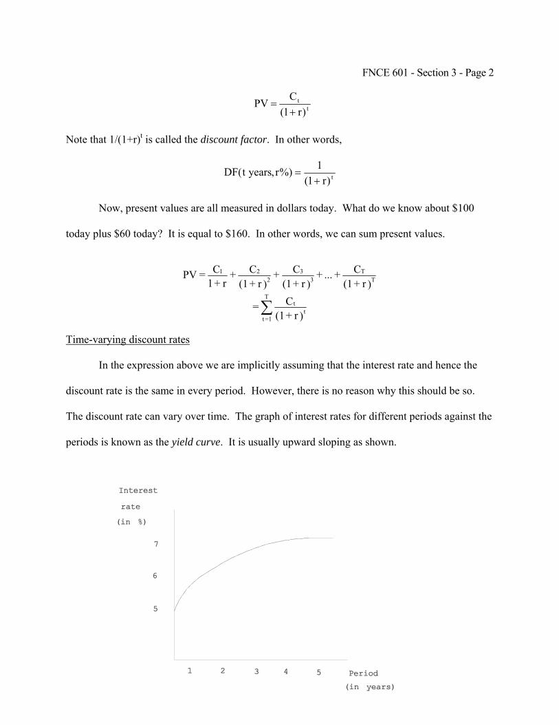
FNCE 601 - Section 3 - Page 2
tt
)r1(CPV+
=
Note that 1/(1+r)t is called the discount factor. In other words,
t)r1(1%)r,yearst(DF+
=
Now, present values are all measured in dollars today. What do we know about $100
today plus $60 today? It is equal to $160. In other words, we can sum present values.
)r + (1
C + ... + )r + (1
C + )r + (1
C + r + 1
C = PV TT
33
221
)r + (1
C = tt
T
1=t∑
Time-varying discount rates
In the expression above we are implicitly assuming that the interest rate and hence the
discount rate is the same in every period. However, there is no reason why this should be so.
The discount rate can vary over time. The graph of interest rates for different periods against the
periods is known as the yield curve. It is usually upward sloping as shown.

FNCE 601 - Section 3 - Page 3
The determinants of the shape of the yield curve such as inflation expectations are
considered in macroeconomics courses. For the moment what we are interested in is the
relationship between rates for different periods. There are two different but equivalent ways of
thinking about what happens when interest rates are different for different periods of time.
Method 1: One possibility is to think in terms of the reinvestment rate. Suppose you are
investing for two periods, for the first one you invest at r1 and for the second one you invest at
r1,2.
t = 0 1 2 |________________________|_______________________| Rate: -------- r1 for period 1 -------> -------- r1,2 period 2 ---------> Investment of 1 becomes 1 + r1 becomes (1 + r1)(1 + r1,2)
Here the present value of a cash flow C2 two periods from now is
PV = C2 ____________ (1)
(1 + r1)(1 + r1,2)
Method 2: The second possibility is to use the two-period interest rate or discount rate r2.
t = 0 1 2 |________________________|_______________________|
Rate: ------------- r2 per period for both periods --------------> Investment of 1 becomes (1 + r2)2
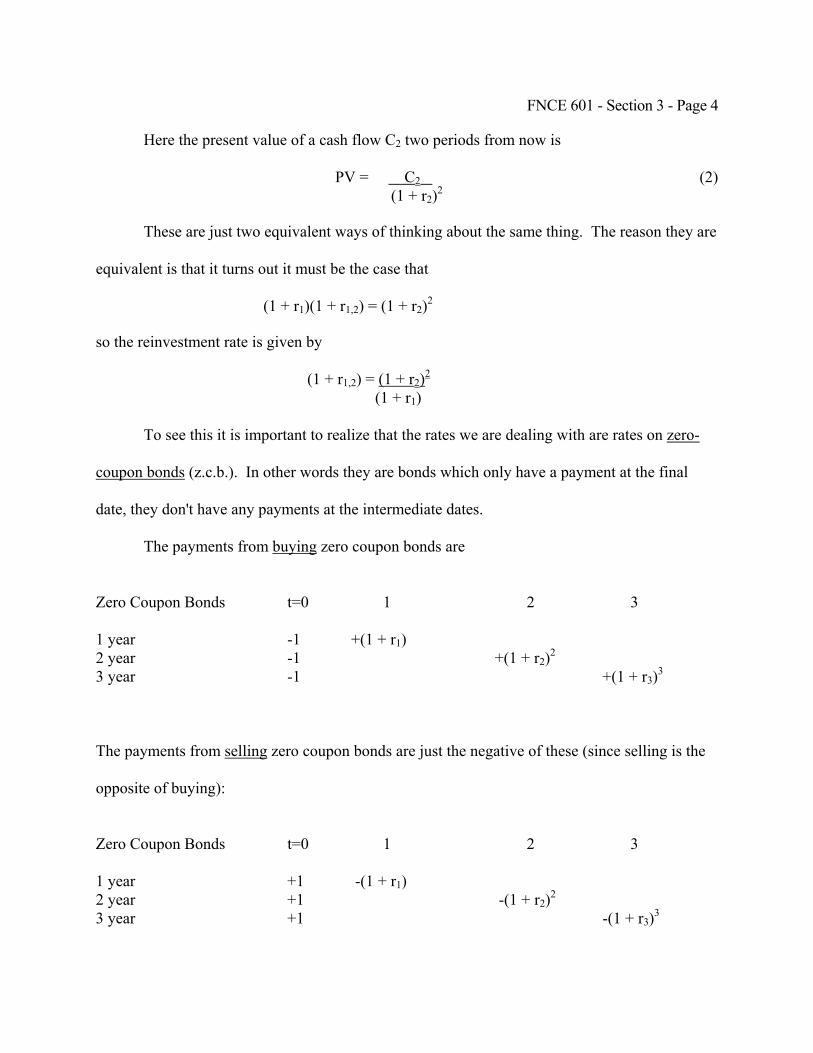
FNCE 601 - Section 3 - Page 4
Here the present value of a cash flow C2 two periods from now is
PV = C2 (2) (1 + r2)2
These are just two equivalent ways of thinking about the same thing. The reason they are
equivalent is that it turns out it must be the case that
(1 + r1)(1 + r1,2) = (1 + r2)2
so the reinvestment rate is given by
(1 + r1,2) = (1 + r2)2
(1 + r1) To see this it is important to realize that the rates we are dealing with are rates on zero-
coupon bonds (z.c.b.). In other words they are bonds which only have a payment at the final
date, they don't have any payments at the intermediate dates.
The payments from buying zero coupon bonds are
Zero Coupon Bonds t=0 1 2 3 1 year -1 +(1 + r1) 2 year -1 +(1 + r2)2
3 year -1 +(1 + r3)3
The payments from selling zero coupon bonds are just the negative of these (since selling is the
opposite of buying):
Zero Coupon Bonds t=0 1 2 3 1 year +1 -(1 + r1) 2 year +1 -(1 + r2)2
3 year +1 -(1 + r3)3
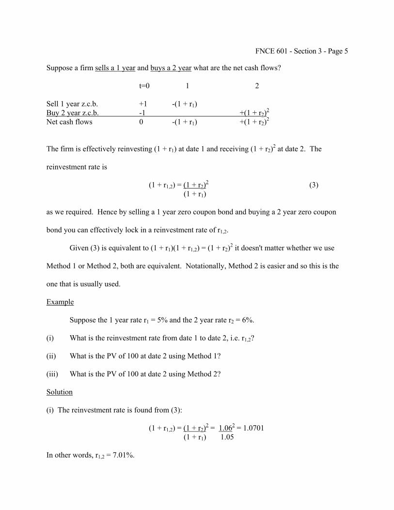
FNCE 601 - Section 3 - Page 5
Suppose a firm sells a 1 year and buys a 2 year what are the net cash flows?
t=0 1 2 Sell 1 year z.c.b. +1 -(1 + r1) Buy 2 year z.c.b. -1 +(1 + r2)2
Net cash flows 0 -(1 + r1) +(1 + r2)2
The firm is effectively reinvesting (1 + r1) at date 1 and receiving (1 + r2)2 at date 2. The
reinvestment rate is
(1 + r1,2) = (1 + r2)2 (3) (1 + r1) as we required. Hence by selling a 1 year zero coupon bond and buying a 2 year zero coupon
bond you can effectively lock in a reinvestment rate of r1,2.
Given (3) is equivalent to (1 + r1)(1 + r1,2) = (1 + r2)2 it doesn't matter whether we use
Method 1 or Method 2, both are equivalent. Notationally, Method 2 is easier and so this is the
one that is usually used.
Example
Suppose the 1 year rate r1 = 5% and the 2 year rate r2 = 6%.
(i) What is the reinvestment rate from date 1 to date 2, i.e. r1,2?
(ii) What is the PV of 100 at date 2 using Method 1?
(iii) What is the PV of 100 at date 2 using Method 2?
Solution
(i) The reinvestment rate is found from (3):
(1 + r1,2) = (1 + r2)2 = 1.062 = 1.0701 (1 + r1) 1.05 In other words, r1,2 = 7.01%.
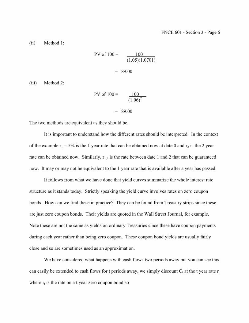
FNCE 601 - Section 3 - Page 6
(ii) Method 1:
PV of 100 = 100 (1.05)(1.0701)
= 89.00 (iii) Method 2:
PV of 100 = 100 (1.06)2
= 89.00 The two methods are equivalent as they should be. It is important to understand how the different rates should be interpreted. In the context
of the example r1 = 5% is the 1 year rate that can be obtained now at date 0 and r2 is the 2 year
rate can be obtained now. Similarly, r1,2 is the rate between date 1 and 2 that can be guaranteed
now. It may or may not be equivalent to the 1 year rate that is available after a year has passed.
It follows from what we have done that yield curves summarize the whole interest rate
structure as it stands today. Strictly speaking the yield curve involves rates on zero coupon
bonds. How can we find these in practice? They can be found from Treasury strips since these
are just zero coupon bonds. Their yields are quoted in the Wall Street Journal, for example.
Note these are not the same as yields on ordinary Treasuries since these have coupon payments
during each year rather than being zero coupon. These coupon bond yields are usually fairly
close and so are sometimes used as an approximation.
We have considered what happens with cash flows two periods away but you can see this
can easily be extended to cash flows for t periods away, we simply discount Ct at the t year rate rt
where rt is the rate on a t year zero coupon bond so
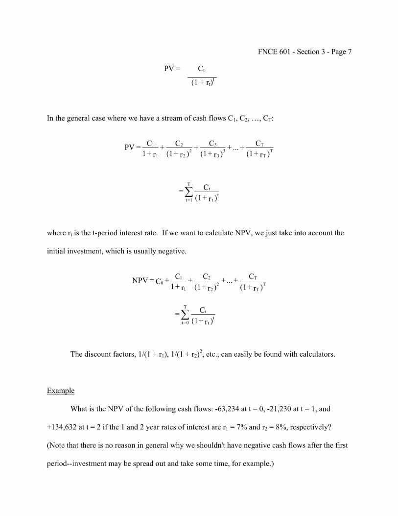
FNCE 601 - Section 3 - Page 7
PV = Ct (1 + rt)t
In the general case where we have a stream of cash flows C1, C2, …, CT:
)r + (1
C + ... + )r + (1
C + )r + (1
C + r + 1
C = PV TT
T3
3
32
2
2
1
1
)r + (1
C = tt
tT
1=t∑
where rt is the t-period interest rate. If we want to calculate NPV, we just take into account the
initial investment, which is usually negative.
)r + (1
C + ... + )r + (1
C + r + 1
C + C = NPV TT
T2
2
2
1
10
)r + (1
C = tt
tT
0=t∑
The discount factors, 1/(1 + r1), 1/(1 + r2)2, etc., can easily be found with calculators.
Example
What is the NPV of the following cash flows: -63,234 at t = 0, -21,230 at t = 1, and
+134,632 at t = 2 if the 1 and 2 year rates of interest are r1 = 7% and r2 = 8%, respectively?
(Note that there is no reason in general why we shouldn't have negative cash flows after the first
period--investment may be spread out and take some time, for example.)
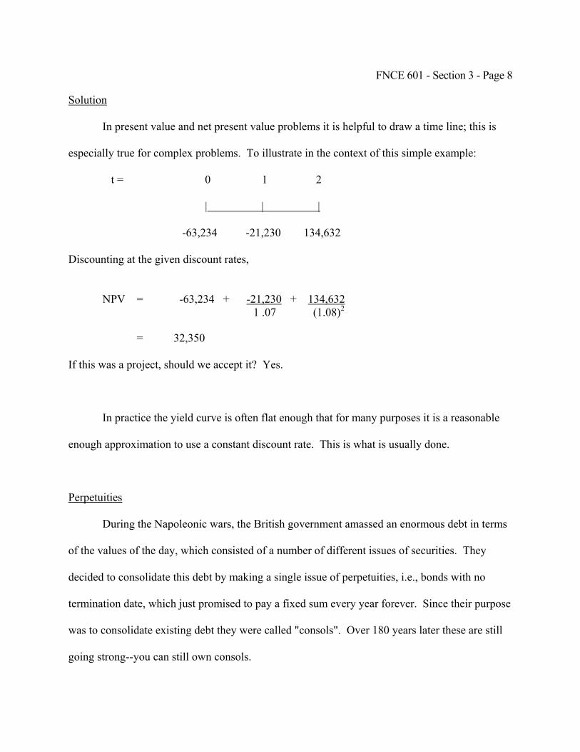
FNCE 601 - Section 3 - Page 8
Solution
In present value and net present value problems it is helpful to draw a time line; this is
especially true for complex problems. To illustrate in the context of this simple example:
t = 0 1 2
| | |
-63,234 -21,230 134,632
Discounting at the given discount rates,
NPV = -63,234 + -21,230 + 134,632 1 .07 (1.08)2
= 32,350
If this was a project, should we accept it? Yes.
In practice the yield curve is often flat enough that for many purposes it is a reasonable
enough approximation to use a constant discount rate. This is what is usually done.
Perpetuities
During the Napoleonic wars, the British government amassed an enormous debt in terms
of the values of the day, which consisted of a number of different issues of securities. They
decided to consolidate this debt by making a single issue of perpetuities, i.e., bonds with no
termination date, which just promised to pay a fixed sum every year forever. Since their purpose
was to consolidate existing debt they were called "consols". Over 180 years later these are still
going strong--you can still own consols.
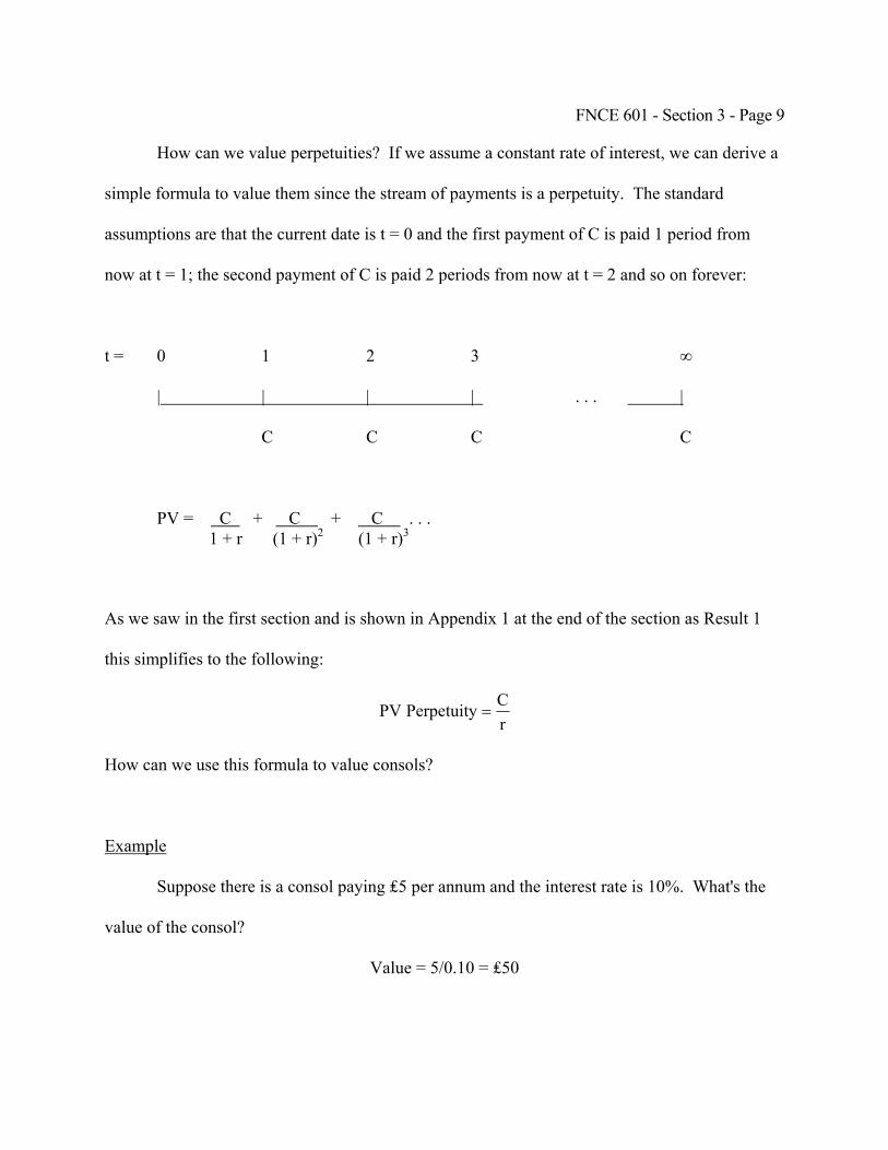
FNCE 601 - Section 3 - Page 9
How can we value perpetuities? If we assume a constant rate of interest, we can derive a
simple formula to value them since the stream of payments is a perpetuity. The standard
assumptions are that the current date is t = 0 and the first payment of C is paid 1 period from
now at t = 1; the second payment of C is paid 2 periods from now at t = 2 and so on forever:
t = 0 1 2 3 ∞
| | | | . . . |
C C C C
PV = C + C + C . . . 1 + r (1 + r)2 (1 + r)3
As we saw in the first section and is shown in Appendix 1 at the end of the section as Result 1
this simplifies to the following:
rCPerpetuityPV =
How can we use this formula to value consols?
Example
Suppose there is a consol paying ₤5 per annum and the interest rate is 10%. What's the
value of the consol?
Value = 5/0.10 = ₤50

FNCE 601 - Section 3 - Page 10
Growing perpetuities
We can use the same trick to value growing perpetuities that we used to value
perpetuities. Suppose we expect the payments to grow at a rate of g forever and the nominal rate
of interest is r. The standard assumptions are that the current date is t = 0 and the first payment
of C is paid 1 period from now at t = 1; the second payment of C(1 + g) is paid 2 periods from
now at t = 2; the third payment of C(1 + g)2 is paid 3 periods from now at t = 3 and so on
forever:
t = 0 1 2 3
| | | | . . .
C C(1+g) C(1+g)2
PV = C + C(1 + g) + C(1 + g)2 + ... 1 + r (1 + r)2 (1 + r)3
It can be seen from Appendix 1, Result 2 that this simplifies to the following:
grCPerpetuityGrowingPV−
=
Example
Suppose we have a growing perpetuity initially paying ₤5 with a growth rate of g = 5%
and interest rate r = 10%. Then
PV = 5 = ₤100 0.10 - 0.05
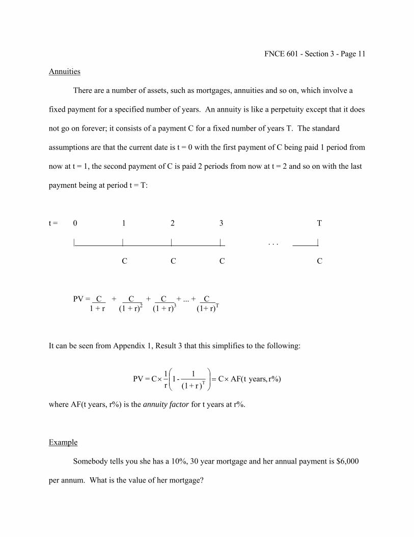
FNCE 601 - Section 3 - Page 11
Annuities
There are a number of assets, such as mortgages, annuities and so on, which involve a
fixed payment for a specified number of years. An annuity is like a perpetuity except that it does
not go on forever; it consists of a payment C for a fixed number of years T. The standard
assumptions are that the current date is t = 0 with the first payment of C being paid 1 period from
now at t = 1, the second payment of C is paid 2 periods from now at t = 2 and so on with the last
payment being at period t = T:
t = 0 1 2 3 T
| | | | . . . |
C C C C
PV = C + C + C + ... + C 1 + r (1 + r)2 (1 + r)3 (1+ r)T
It can be seen from Appendix 1, Result 3 that this simplifies to the following:
%)r,yearst(AFC)r + (1
1 - 1r1C = PV T ×=⎟⎟
⎠
⎞⎜⎜⎝
⎛×
where AF(t years, r%) is the annuity factor for t years at r%.
Example
Somebody tells you she has a 10%, 30 year mortgage and her annual payment is $6,000
per annum. What is the value of her mortgage?
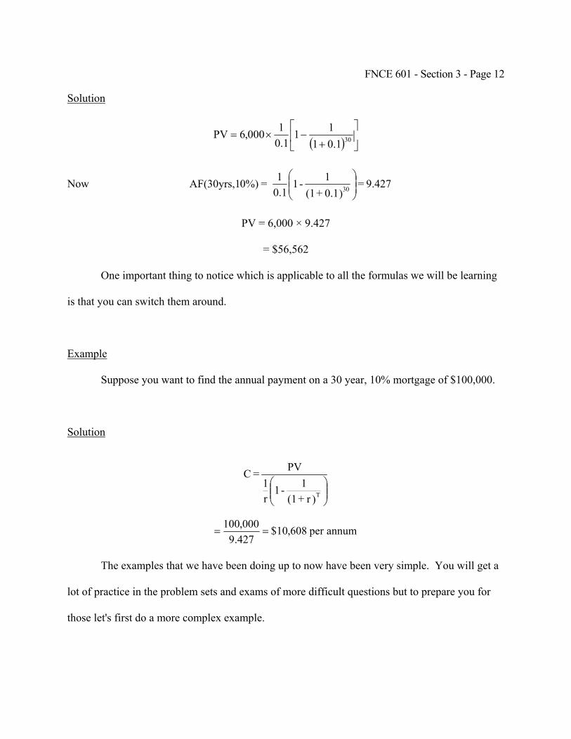
FNCE 601 - Section 3 - Page 12
Solution
( ) ⎥⎦
⎤⎢⎣
⎡
+−×= 301.01
111.0
1000,6PV
Now 9.427 = )0.1 + (1
1 - 10.11 = 0%)AF(30yrs,1 30 ⎟⎟
⎠
⎞⎜⎜⎝
⎛
PV = 6,000 × 9.427
= $56,562
One important thing to notice which is applicable to all the formulas we will be learning
is that you can switch them around.
Example
Suppose you want to find the annual payment on a 30 year, 10% mortgage of $100,000.
Solution
⎟⎟⎠
⎞⎜⎜⎝
⎛)r + (1
1 - 1r1
PV = C
T
annumper608,10$427.9000,100
==
The examples that we have been doing up to now have been very simple. You will get a
lot of practice in the problem sets and exams of more difficult questions but to prepare you for
those let's first do a more complex example.
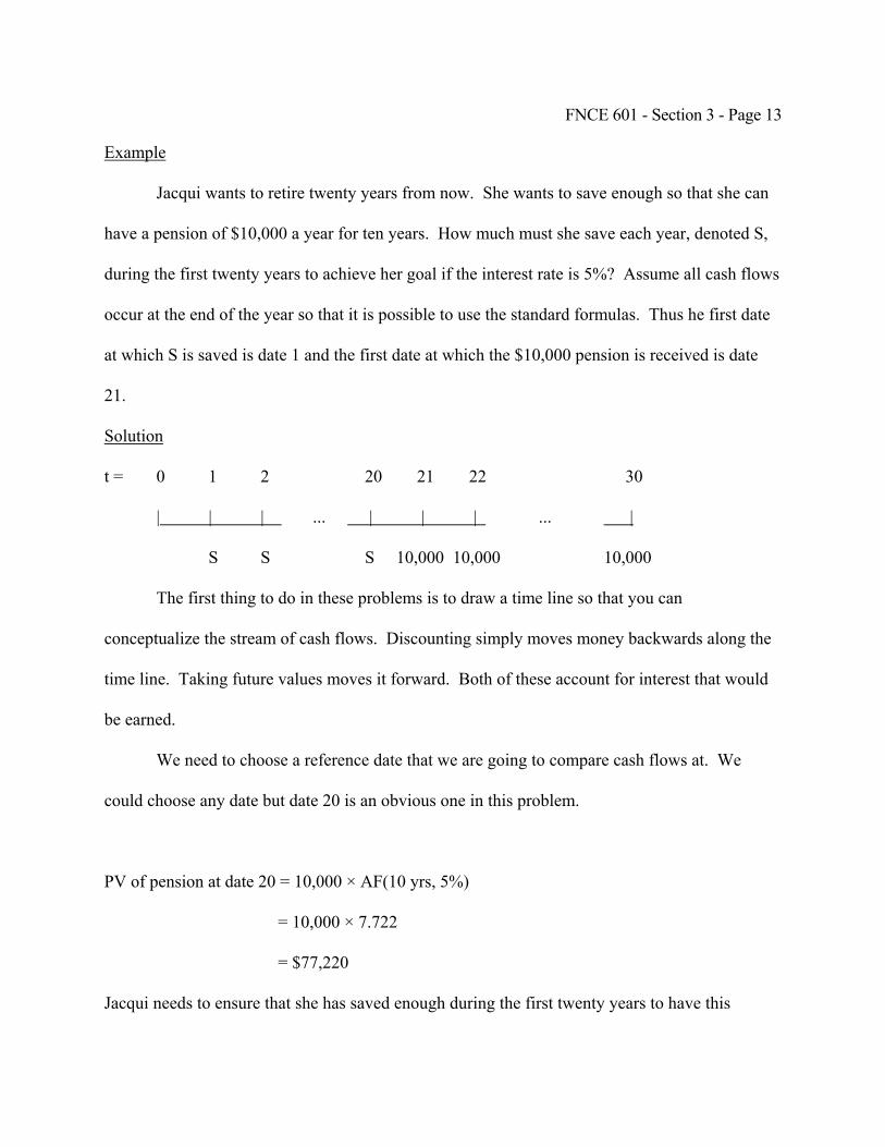
FNCE 601 - Section 3 - Page 13
Example
Jacqui wants to retire twenty years from now. She wants to save enough so that she can
have a pension of $10,000 a year for ten years. How much must she save each year, denoted S,
during the first twenty years to achieve her goal if the interest rate is 5%? Assume all cash flows
occur at the end of the year so that it is possible to use the standard formulas. Thus he first date
at which S is saved is date 1 and the first date at which the $10,000 pension is received is date
21.
Solution
t = 0 1 2 20 21 22 30
| | | ... | | | ... |
S S S 10,000 10,000 10,000
The first thing to do in these problems is to draw a time line so that you can
conceptualize the stream of cash flows. Discounting simply moves money backwards along the
time line. Taking future values moves it forward. Both of these account for interest that would
be earned.
We need to choose a reference date that we are going to compare cash flows at. We
could choose any date but date 20 is an obvious one in this problem.
PV of pension at date 20 = 10,000 × AF(10 yrs, 5%)
= 10,000 × 7.722
= $77,220
Jacqui needs to ensure that she has saved enough during the first twenty years to have this
FNCE 601 - Section 3 - Page 14
amount at date 20.
PV of savings of S for 20 years at date 0 = S × AF(20 yrs, 5%)
= S × 12.462
This is in date 0 dollars. In order to be able to compare this with the 77,722 at date 20 we need
to change it from date 0 dollars into date 20 dollars by taking a future value.
FV of savings of S for 20 years at date 20 = S × 12.462 × (1.05)20
= S × 33.066
Hence to have enough savings to provide the pension Jacqui needs
S × 33.066 = 77,220
Solving gives,
S = 77,220/33.066
= $2,335
Jacqui needs to save $2,335 each year for twenty years to give her a pension of $10,000 a year
for ten years.
Compound Interest
So far we have been assuming interest is paid once a year or, more generally, once a
period. Often interest is paid more frequently than this. What happens if interest is paid more
often, once every six months, say, in which case it is said to be compounded twice?
For example, suppose the interest rate is 10% a year compounded twice. This means 5%
FNCE 601 - Section 3 - Page 15
interest is paid every six months. After one year $1 becomes
1 x (1 + 0.05)2 = 1.1025
That is, we have earned interest on the interest.
If we have 10% compounded four times, we pay 2.5% every quarter. After a year $1
becomes
1 x (1 + 0.025)4 = 1.1038
In general if compounding takes place q times a year and r is the interest rate/year,
q
1 qr1PVC ⎟⎟⎠
⎞⎜⎜⎝
⎛+=
After t periods,
qt
t qr1PVC ⎟⎟⎠
⎞⎜⎜⎝
⎛+=
If compounding takes place continuously so that interest is paid on interest all the time,
so to speak, we get a particularly simple expression. In order to derive this it is necessary to
recall that
m
m m11lime ⎟⎠⎞
⎜⎝⎛ +=
∞→
Taking our formula for discrete compounding and rearranging it we get
⎥⎥⎥
⎦
⎤
⎢⎢⎢
⎣
⎡
⎟⎟⎠
⎞⎜⎜⎝
⎛r/q
1 + 1 PV= Crq rt
t
FNCE 601 - Section 3 - Page 16
Letting m = q/r, we can see that as q approaches infinity and we compound continually
rtm
mtm m11limPVClim
⎥⎥⎦
⎤
⎢⎢⎣
⎡⎟⎠⎞
⎜⎝⎛ +=
∞→∞→
= PVert
Alternatively this can be written
rttrt
t eCeCPV −==
In many circumstances it is much easier to calculate and manipulate these expressions
than their discrete time counterparts. One example is the pricing of options using the Black and
Scholes model that we will be considering later on.
Example 1
Suppose you invest $200 at 12% continuously compounded for two years. What do you
receive at the end of the two years?
Solution
rt = 0.12 × 2 = 0.24
e0.24 = 1.271
C2 = 200 × 1.271 = $254.2
Example 2
What is the PV of $300 in 1 year's time if the interest rate is 5% continuously
compounded?
FNCE 601 - Section 3 - Page 17
Solution
rt = 0.05
e0.05 = 1.051
PV = 300/(1.051) = $285.44
Relationship between continuously compounded and annual rates
If you think back to our original example of investing $1 at 10% compounded twice then
in that case you ended up with $1.1025. The effective annual rate is 10.25%. In other words
10% compounded twice is equivalent to an annual rate of 10.25%. Similarly for any compound
rate, including continuously compounded rates, there is an equivalent annual rate. How do we
go about switching from one to the other?
To distinguish between annual rates and continuous rates, I'm going to use the following
notation from now on:
r - annual rate
rc - continuously compounded rate
Suppose that you invest $1 at an annual rate of r then at the end of the year you have
C1 = 1 + r
If you invest $1 at a continuously compounded rate of rc then at the end of the year you have
e = C r1
c
We want to find the value of r such that it is equivalent to rc; in other words, we wish to find the
value of r and rc such that the C1 you end up with is the same as when you invest at r. Therefore

FNCE 601 - Section 3 - Page 18
equating the C1 you get
r + 1 = erc
1 - e =r rc
or, taking natural logs of the previous equation,
rc = loge(1 + r)
Example 3
(i) If rc = 0.10, what is r?
r = e0.10 - 1 = 1.105 - 1 = 0.105 or 10.5%
(ii) If r = 0.10, what is rc?
rc = loge 1.1 = 0.0953 or 9.53%
This brings us to the end of basic results concerning discounting. Next we turn to using
these ideas to value bonds and stocks.

FNCE 601 - Section 3 - Page 19
Section 3
APPENDIX ON PRESENT VALUE FORMULAS
Result 1: Perpetuities
A perpetuity is a constant payment C every period forever. The standard assumptions are
that the current date is t = 0 and the first payment of C is paid 1 period from now at t = 1; the
second payment of C is paid 2 periods from now at t = 2 and so on, forever. The PV of the
perpetuity is then
PV = C + C + C + ... (1) 1 + r (1 + r)2 (1 + r)3
Multiplying through by 1 + r
(1 + r)PV = C + C + C + ... (2) 1 + r (1 + r)2
Subtracting (1) from (2)
rPV = C
rCPV =
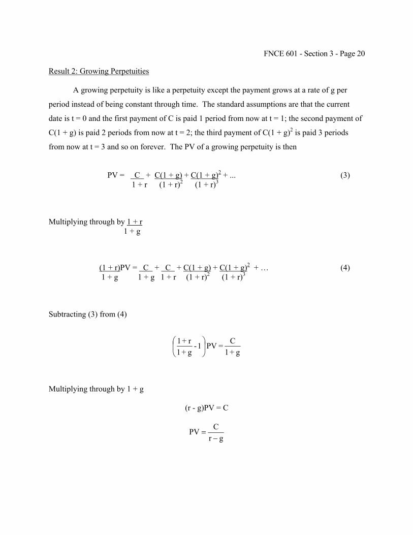
FNCE 601 - Section 3 - Page 20
Result 2: Growing Perpetuities
A growing perpetuity is like a perpetuity except the payment grows at a rate of g per
period instead of being constant through time. The standard assumptions are that the current
date is t = 0 and the first payment of C is paid 1 period from now at t = 1; the second payment of
C(1 + g) is paid 2 periods from now at t = 2; the third payment of C(1 + g)2 is paid 3 periods
from now at t = 3 and so on forever. The PV of a growing perpetuity is then
PV = C + C(1 + g) + C(1 + g)2 + ... (3) 1 + r (1 + r)2 (1 + r)3
Multiplying through by 1 + r 1 + g
(1 + r)PV = C + C + C(1 + g) + C(1 + g)2 + … (4) 1 + g 1 + g 1 + r (1 + r)2 (1 + r)3
Subtracting (3) from (4)
g + 1
C = PV1 - g + 1r + 1
⎟⎠
⎞⎜⎝
⎛
Multiplying through by 1 + g
(r - g)PV = C
grCPV−
=
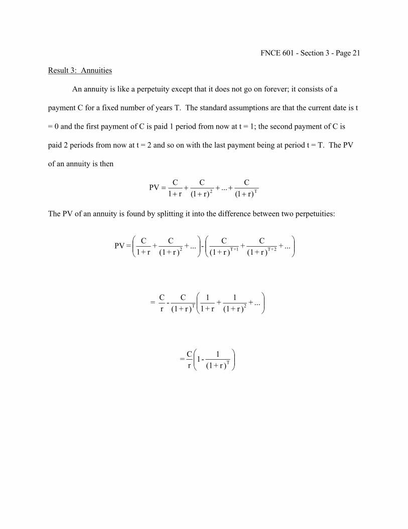
FNCE 601 - Section 3 - Page 21
Result 3: Annuities
An annuity is like a perpetuity except that it does not go on forever; it consists of a
payment C for a fixed number of years T. The standard assumptions are that the current date is t
= 0 and the first payment of C is paid 1 period from now at t = 1; the second payment of C is
paid 2 periods from now at t = 2 and so on with the last payment being at period t = T. The PV
of an annuity is then
T2 )r1(C...
)r1(C
r1CPV
+++
++
+=
The PV of an annuity is found by splitting it into the difference between two perpetuities:
⎟⎟⎠
⎞⎜⎜⎝
⎛⎟⎟⎠
⎞⎜⎜⎝
⎛... +
)r + (1C +
)r + (1C - ... +
)r + (1C +
r + 1C = PV 2+T1+T2
⎟⎟⎠
⎞⎜⎜⎝
⎛... +
)r + (11 +
r + 11
)r + (1C -
rC = 2T
⎟⎟⎠
⎞⎜⎜⎝
⎛)r + (1
1 - 1rC = T
UNIVERSITY OF PENNSYLVANIA THE WHARTON SCHOOL LECTURE NOTES FNCE 601 CORPORATE FINANCE Franklin Allen Fall 2004 QUARTER 1 - WEEK 2 (part 2) Th: 9/16/04 Copyright © 2004 by Franklin Allen
FNCE 601 - Section 4 - Page 1
Section 4: The Valuation of Bonds and Stocks
Read Chapter 4 BM
Motivation Example
Firms A and B have the following stock prices, earnings per share and price/earnings
ratios.
Price EPS Price/EPS
Firm A $100 $10 10
Firm B $100 $5 20
There is no uncertainty associated with either stock.
Which stock would you buy?
It seems as though Firm A is the better buy since you get $10 earnings for every $100
invested whereas with Firm B you get only $5 for every $100 invested. Is this argument correct?
(i) Present Values and Market Values
So far we have been considering present values. Why are we interested in present
values? As we'll see next, present values must be equal to market values in a competitive
market. We shall consider the relationship between market values and present values using the
following example, which is also a useful exercise in calculating PV.
Example 1
A company called the Wensum Bridge Company is to be formed at the end of 20X0 for
the sole purpose of building a bridge across the river Wensum. The contract for the construction
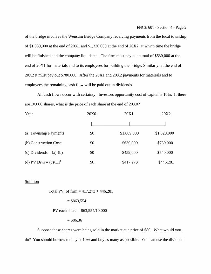
FNCE 601 - Section 4 - Page 2
of the bridge involves the Wensum Bridge Company receiving payments from the local township
of $1,089,000 at the end of 20X1 and $1,320,000 at the end of 20X2, at which time the bridge
will be finished and the company liquidated. The firm must pay out a total of $630,000 at the
end of 20X1 for materials and to its employees for building the bridge. Similarly, at the end of
20X2 it must pay out $780,000. After the 20X1 and 20X2 payments for materials and to
employees the remaining cash flow will be paid out in dividends.
All cash flows occur with certainty. Investors opportunity cost of capital is 10%. If there
are 10,000 shares, what is the price of each share at the end of 20X0?
Year 20X0 20X1 20X2
|__________________|_________________|
(a) Township Payments $0 $1,089,000 $1,320,000
(b) Construction Costs $0 $630,000 $780,000
(c) Dividends = (a)-(b) $0 $459,000 $540,000
(d) PV Divs = (c)/1.1t $0 $417,273 $446,281
Solution
Total PV of firm = 417,273 + 446,281
= $863,554
PV each share = 863,554/10,000
= $86.36
Suppose these shares were being sold in the market at a price of $80. What would you
do? You should borrow money at 10% and buy as many as possible. You can use the dividend
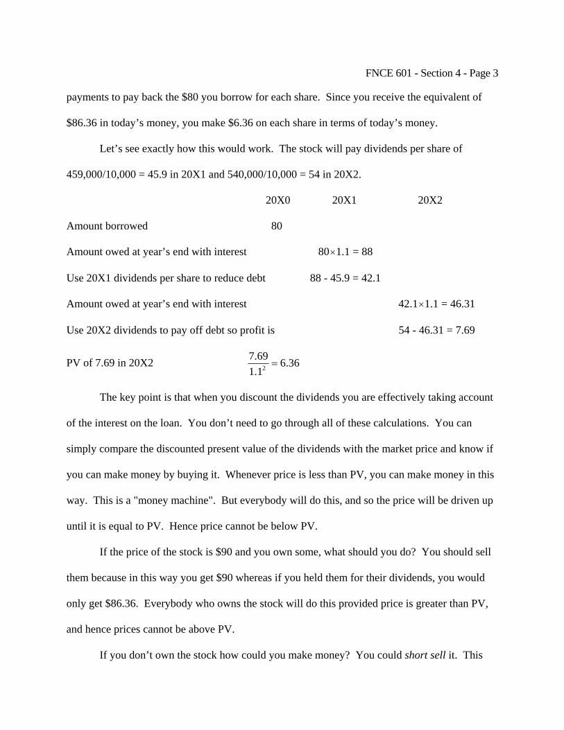
FNCE 601 - Section 4 - Page 3
payments to pay back the $80 you borrow for each share. Since you receive the equivalent of
$86.36 in today’s money, you make $6.36 on each share in terms of today’s money.
Let’s see exactly how this would work. The stock will pay dividends per share of
459,000/10,000 = 45.9 in 20X1 and 540,000/10,000 = 54 in 20X2.
20X0 20X1 20X2
Amount borrowed 80
Amount owed at year’s end with interest 80×1.1 = 88
Use 20X1 dividends per share to reduce debt 88 - 45.9 = 42.1
Amount owed at year’s end with interest 42.1×1.1 = 46.31
Use 20X2 dividends to pay off debt so profit is 54 - 46.31 = 7.69
PV of 7.69 in 20X2 36.61.169.7
2 =
The key point is that when you discount the dividends you are effectively taking account
of the interest on the loan. You don’t need to go through all of these calculations. You can
simply compare the discounted present value of the dividends with the market price and know if
you can make money by buying it. Whenever price is less than PV, you can make money in this
way. This is a "money machine". But everybody will do this, and so the price will be driven up
until it is equal to PV. Hence price cannot be below PV.
If the price of the stock is $90 and you own some, what should you do? You should sell
them because in this way you get $90 whereas if you held them for their dividends, you would
only get $86.36. Everybody who owns the stock will do this provided price is greater than PV,
and hence prices cannot be above PV.
If you don’t own the stock how could you make money? You could short sell it. This
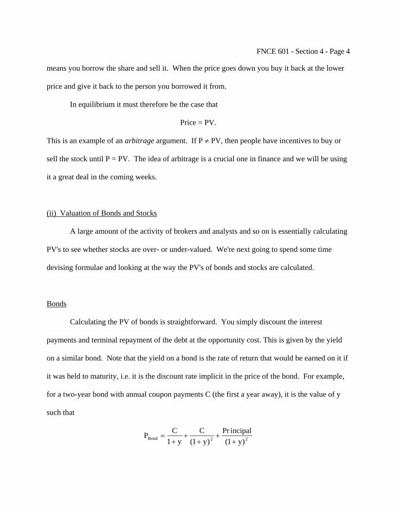
FNCE 601 - Section 4 - Page 4
means you borrow the share and sell it. When the price goes down you buy it back at the lower
price and give it back to the person you borrowed it from.
In equilibrium it must therefore be the case that
Price = PV.
This is an example of an arbitrage argument. If P ≠ PV, then people have incentives to buy or
sell the stock until P = PV. The idea of arbitrage is a crucial one in finance and we will be using
it a great deal in the coming weeks.
(ii) Valuation of Bonds and Stocks
A large amount of the activity of brokers and analysts and so on is essentially calculating
PV's to see whether stocks are over- or under-valued. We're next going to spend some time
devising formulae and looking at the way the PV's of bonds and stocks are calculated.
Bonds
Calculating the PV of bonds is straightforward. You simply discount the interest
payments and terminal repayment of the debt at the opportunity cost. This is given by the yield
on a similar bond. Note that the yield on a bond is the rate of return that would be earned on it if
it was held to maturity, i.e. it is the discount rate implicit in the price of the bond. For example,
for a two-year bond with annual coupon payments C (the first a year away), it is the value of y
such that
22Bond )y1(incipalPr
)y1(C
y1CP
++
++
+=

FNCE 601 - Section 4 - Page 5
Example 2
The Buggy Company has just issued a seven-year $1000 bond. Interest payments of $80
are made at the end of each year, and the $1000 principal must be paid at the end of the seventh
year. If similar bonds are now yielding 6%, what price will the bond sell for?
Solution
t = 0 1 2 6 7
| | | ... | |
Interest 80 80 80 80
Principal 1,000
Cash flows
End of year Amount Discount/Annuity Factors PV
1-7 $80 AF(7 yrs, 6%) = 5.582 446.56
7 $1,000 DF(7 yrs, 6%) = 0.665 665.00
$1,111.56
Hence, the price of the bond = $1,111.56.
What do you think there would be if the bond sold at a price different from $1,111.56?
As in Example 1 there would be arbitrage.
Stock Price and Dividends
The main difference in calculating the PV's of stocks rather than bonds is the difference in the
profiles of earnings.
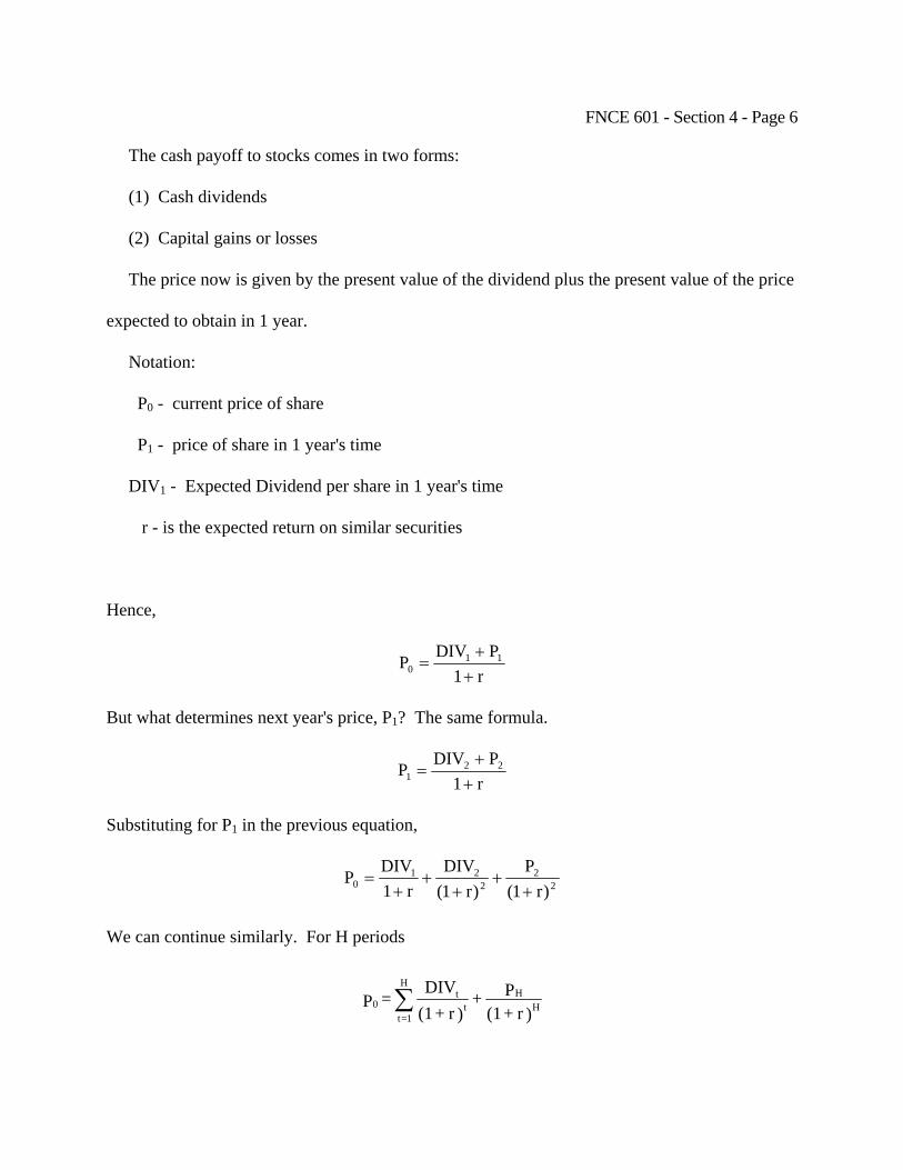
FNCE 601 - Section 4 - Page 6
The cash payoff to stocks comes in two forms:
(1) Cash dividends
(2) Capital gains or losses
The price now is given by the present value of the dividend plus the present value of the price
expected to obtain in 1 year.
Notation:
P0 - current price of share
P1 - price of share in 1 year's time
DIV1 - Expected Dividend per share in 1 year's time
r - is the expected return on similar securities
Hence,
r1PDIVP 11
0 ++
=
But what determines next year's price, P1? The same formula.
r1PDIVP 22
1 ++
=
Substituting for P1 in the previous equation,
22
221
0 )r1(P
)r1(DIV
r1DIVP
++
++
+=
We can continue similarly. For H periods
)r + (1P +
)r + (1DIV
= P HH
tt
H
1=t0 ∑
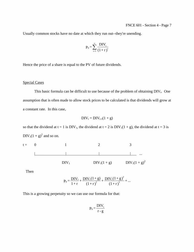
FNCE 601 - Section 4 - Page 7
Usually common stocks have no date at which they run out--they're unending.
)r + (1DIV = P t
t
1=t0 ∑
∞
Hence the price of a share is equal to the PV of future dividends.
Special Cases
This basic formula can be difficult to use because of the problem of obtaining DIVt. One
assumption that is often made to allow stock prices to be calculated is that dividends will grow at
a constant rate. In this case,
DIVt = DIVt-1(1 + g)
so that the dividend at t = 1 is DIV1, the dividend at t = 2 is DIV1(1 + g), the dividend at t = 3 is
DIV1(1 + g)2 and so on.
t = 0 1 2 3
|________________|_________________|________________|___ ...
DIV1 DIV1(1 + g) DIV1(1 + g)2
... + )r + (1
)g + (1DIV + )r + (1
g) + (1DIV + r + 1
DIV = P 3
21
211
0
Then
This is a growing perpetuity so we can use our formula for that:
g -r
DIV = P 10
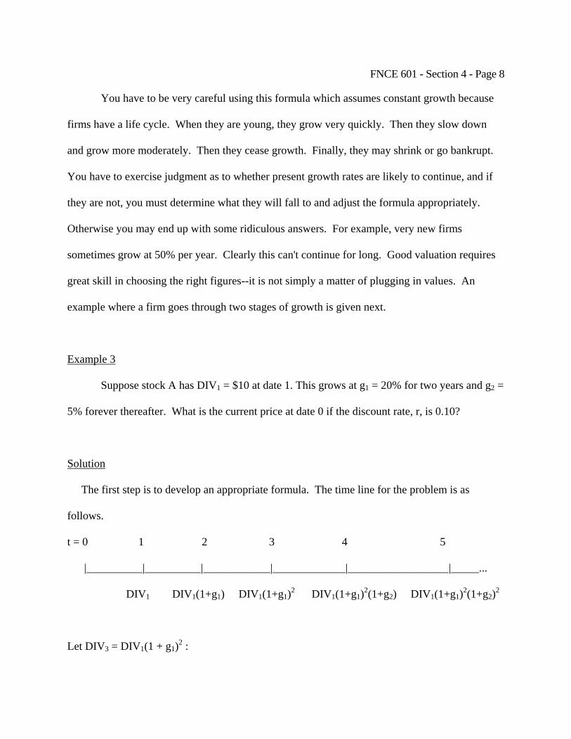
FNCE 601 - Section 4 - Page 8
You have to be very careful using this formula which assumes constant growth because
firms have a life cycle. When they are young, they grow very quickly. Then they slow down
and grow more moderately. Then they cease growth. Finally, they may shrink or go bankrupt.
You have to exercise judgment as to whether present growth rates are likely to continue, and if
they are not, you must determine what they will fall to and adjust the formula appropriately.
Otherwise you may end up with some ridiculous answers. For example, very new firms
sometimes grow at 50% per year. Clearly this can't continue for long. Good valuation requires
great skill in choosing the right figures--it is not simply a matter of plugging in values. An
example where a firm goes through two stages of growth is given next.
Example 3
Suppose stock A has DIV1 = $10 at date 1. This grows at g1 = 20% for two years and g2 =
5% forever thereafter. What is the current price at date 0 if the discount rate, r, is 0.10?
Solution
The first step is to develop an appropriate formula. The time line for the problem is as
follows.
t = 0 1 2 3 4 5
|__________|__________|____________|_____________|__________________|_____...
DIV1 DIV1(1+g1) DIV1(1+g1)2 DIV1(1+g1)2(1+g2) DIV1(1+g1)2(1+g2)2
Let DIV3 = DIV1(1 + g1)2 :
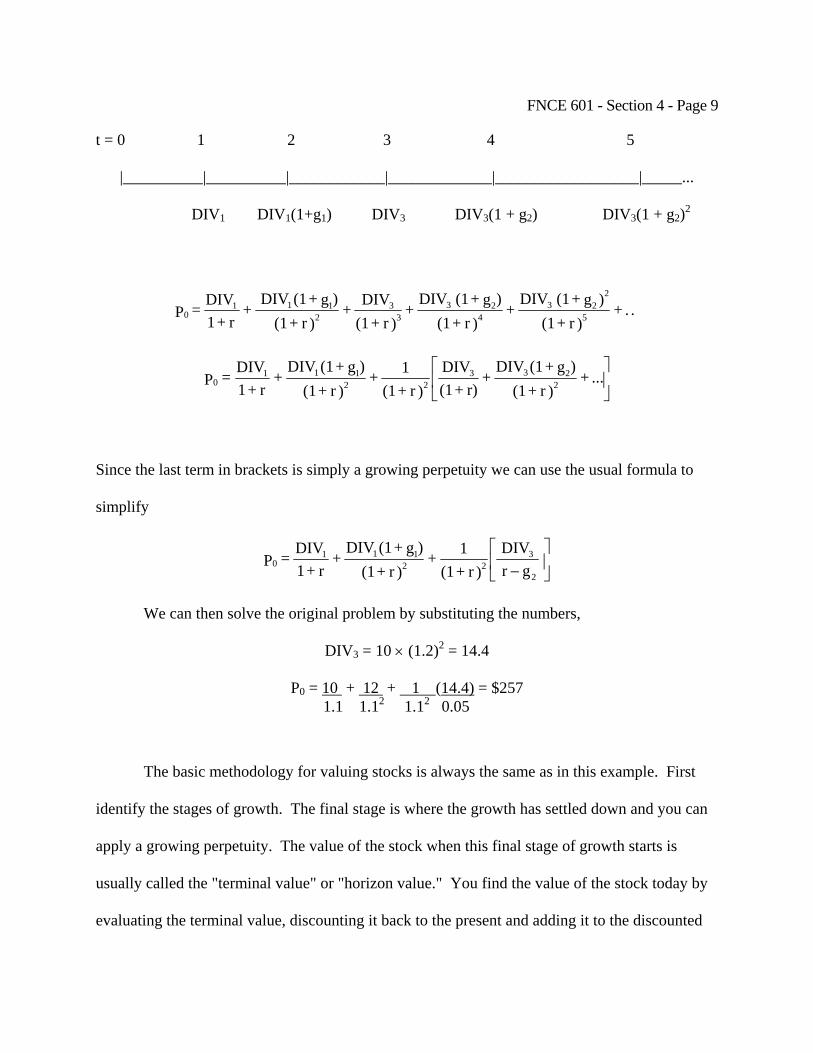
FNCE 601 - Section 4 - Page 9
t = 0 1 2 3 4 5
|__________|__________|____________|_____________|__________________|_____...
DIV1 DIV1(1+g1) DIV3 DIV3(1 + g2) DIV3(1 + g2)2
. . +
)r + (1)g + (1 DIV
+ )r + (1
)g + (1 DIV +
)r + (1DIV +
)r + (1)g + (1 DIV
+ r + 1
DIV = P 5
223
423
33
2111
0
⎥⎦
⎤⎢⎣
⎡... +
)r + (1)g + (1DIV
+ r) + (1
DIV)r + (1
1 + )r + (1
)g + (1DIV +
r + 1DIV=P 2
23322
1110
Since the last term in brackets is simply a growing perpetuity we can use the usual formula to
simplify
⎥⎦
⎤⎢⎣
⎡−
gr
DIV)r + (1
1 + )r + (1
)g + (1DIV +
r + 1DIV=P
2
322
1110
We can then solve the original problem by substituting the numbers,
DIV3 = 10 × (1.2)2 = 14.4
P0 = 10 + 12 + 1 (14.4) = $257 1.1 1.12 1.12 0.05
The basic methodology for valuing stocks is always the same as in this example. First
identify the stages of growth. The final stage is where the growth has settled down and you can
apply a growing perpetuity. The value of the stock when this final stage of growth starts is
usually called the "terminal value" or "horizon value." You find the value of the stock today by
evaluating the terminal value, discounting it back to the present and adding it to the discounted
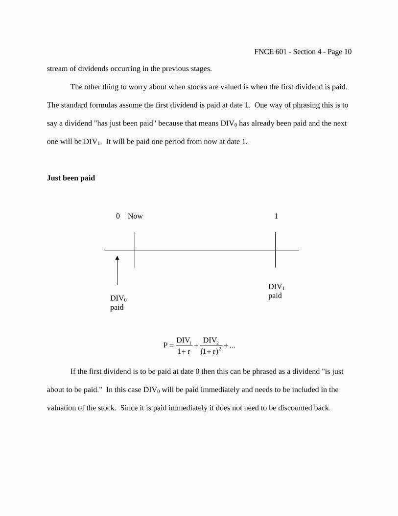
FNCE 601 - Section 4 - Page 10
stream of dividends occurring in the previous stages.
The other thing to worry about when stocks are valued is when the first dividend is paid.
The standard formulas assume the first dividend is paid at date 1. One way of phrasing this is to
say a dividend "has just been paid" because that means DIV0 has already been paid and the next
one will be DIV1. It will be paid one period from now at date 1.
Just been paid
0 Now 1
DIV1paid DIV0
paid
...)r1(
DIVr1
DIVP 221 +
++
+=
If the first dividend is to be paid at date 0 then this can be phrased as a dividend "is just
about to be paid." In this case DIV0 will be paid immediately and needs to be included in the
valuation of the stock. Since it is paid immediately it does not need to be discounted back.

FNCE 601 - Section 4 - Page 11
Just about to be paid
Now 0 1
DIV0 paid
DIV1paid
...)r1(
DIVr1
DIVDIV*P 221
0 ++
++
+=
Note that before the dividend is paid the price P* is higher than the price P just after it is
paid. When the stock goes ex dividend so that the owner no longer has the right to receive the
dividend the price drops by P* - P = DIV0.
Market Capitalization Rates
A concept that is sometimes useful is the notion of market capitalization rates. The market
capitalization rate of a stock is the discount rate such that if the stock's dividends were
discounted at that rate you would obtain the stock's current market price. In other words, the
market capitalization rate is the discount rate implicit in the stock's current market price. It is
like the yield on a bond. For example, for a stock with dividends DIV1, DIV2, and so on, it is the
value of rm such that
...)r1(
DIVr1
DIVP 2m
2
m
1Stock +
++
+=
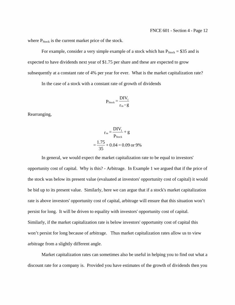
FNCE 601 - Section 4 - Page 12
where PStock is the current market price of the stock.
For example, consider a very simple example of a stock which has PStock = $35 and is
expected to have dividends next year of $1.75 per share and these are expected to grow
subsequently at a constant rate of 4% per year for ever. What is the market capitalization rate?
In the case of a stock with a constant rate of growth of dividends
g - r
DIV = Pm
1Stock
Rearranging,
9%or 0.09 = 0.04+
351.75 =
g + PDIV = r
Stock
1m
In general, we would expect the market capitalization rate to be equal to investors'
opportunity cost of capital. Why is this? - Arbitrage. In Example 1 we argued that if the price of
the stock was below its present value (evaluated at investors' opportunity cost of capital) it would
be bid up to its present value. Similarly, here we can argue that if a stock's market capitalization
rate is above investors' opportunity cost of capital, arbitrage will ensure that this situation won’t
persist for long. It will be driven to equality with investors' opportunity cost of capital.
Similarly, if the market capitalization rate is below investors' opportunity cost of capital this
won’t persist for long because of arbitrage. Thus market capitalization rates allow us to view
arbitrage from a slightly different angle.
Market capitalization rates can sometimes also be useful in helping you to find out what a
discount rate for a company is. Provided you have estimates of the growth of dividends then you
FNCE 601 - Section 4 - Page 13
can always back out the market capitalization rate. There are various ways to find the dividend
growth rate. You can use direct estimates or alternatively you can try to estimate it from how
much the profitability of the investments retained earnings are ploughed back into will allow
dividends to grow. However, we will not go into this in detail since we will argue in Sections 7
and 8 on risk that a better way to get discount rates is to use an asset pricing model.
Stock Price and Earnings Per Share
So far we've looked at stock price and dividends. One of the statistics that is often used
in the financial press and conversation is the ratio of the stock price to earnings per share (P/E
ratio). The motivation example at the beginning of the section is an illustration of how it's used:
investors are advised to buy stocks with low P/E ratios. This is often referred to as “value
investing”. In the early 1990’s there were a number of studies showing that in the long run
investing in low P/E ratios or “value stocks” had given high returns. In the tech boom values
stocks did terribly but more recently they have done relatively well. In the last part of this
section we shall develop the relationship between price and EPS and reconsider our motivation
example in this light. We will try and provide some perspective on how P/E ratios should be
interpreted.
In the last section we looked at price and dividends. The difference between dividends
and EPS is that the former is what's actually paid to stockholders, whereas the latter includes
retained earnings.
We start by considering a firm that does not retain any earnings at all. We can think of it
consisting of a single plant. It does not plow back any earnings and simply produces a constant
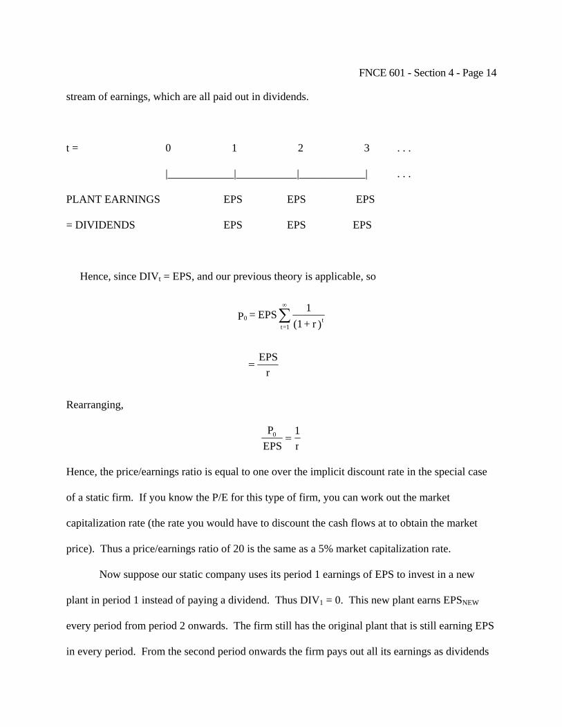
FNCE 601 - Section 4 - Page 14
stream of earnings, which are all paid out in dividends.
t = 0 1 2 3 . . .
|____________|___________|____________| . . .
PLANT EARNINGS EPS EPS EPS
= DIVIDENDS EPS EPS EPS
Hence, since DIVt = EPS, and our previous theory is applicable, so
rEPS
)r + (11 EPS= P t
1=t0
=
∑∞
Rearranging,
r1
EPSP0 =
Hence, the price/earnings ratio is equal to one over the implicit discount rate in the special case
of a static firm. If you know the P/E for this type of firm, you can work out the market
capitalization rate (the rate you would have to discount the cash flows at to obtain the market
price). Thus a price/earnings ratio of 20 is the same as a 5% market capitalization rate.
Now suppose our static company uses its period 1 earnings of EPS to invest in a new
plant in period 1 instead of paying a dividend. Thus DIV1 = 0. This new plant earns EPSNEW
every period from period 2 onwards. The firm still has the original plant that is still earning EPS
in every period. From the second period onwards the firm pays out all its earnings as dividends
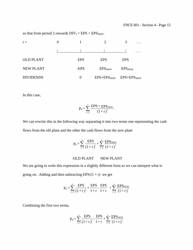
FNCE 601 - Section 4 - Page 15
so that from period 2 onwards DIVt = EPS + EPSNEW.
t = 0 1 2 3 . . .
|____________|____________|___________| . . .
OLD PLANT EPS EPS EPS
NEW PLANT -EPS EPSNEW EPSNEW
DIVIDENDS 0 EPS+EPSNEW EPS+EPSNEW
In this case,
)r + (1 EPS + EPS = P t
NEW
2=t0 ∑
∞
We can rewrite this in the following way separating it into two terms one representing the cash
flows from the old plant and the other the cash flows from the new plant
)r + (1EPS +
)r + (1EPS = P t
NEW
2=tt
2=t0 ∑∑
∞∞
NEW PLANT PLANTOLD
We are going to write this expression in a slightly different form so we can interpret what is
going on. Adding and then subtracting EPS/(1 + r) we get
r + 1EPS -
r + 1EPS +
)r + (1EPS = P t
2=t0 ∑
∞
)r + (1EPS + t
NEW
2=t∑∞
Combining the first two terms,
)r + (1EPS +
r + 1EPS -
)r + (1EPS = P t
NEW
2=tt
1=t0 ∑∑
∞∞

FNCE 601 - Section 4 - Page 16
From our first case with no investment we know the first term is just EPS/r. The second and third
terms taken together are just the NPV of the investment in the new plant in terms of time 0
dollars. Hence we can rewrite the expression as
10 NPVr
EPSP +=
where NPV1 is the NPV of the new plant which is built in the first period. NPV1 is the NPV of
the growth opportunity represented by the new plant.
We have considered a very simple case where we build a plant at date 1 using all the
earnings from the original plant. Now if you go through the same exercise you can see that a
similar conclusion would hold if we used only a proportion of the old plant’s earnings to build
the new plant. For example, if you used half the earnings at date 1 to build the new plant then
everything would be similar except instead of adding and subtracting EPS/(1 + r) so that we
could get our formula we would add and subtract 0.5[EPS/(1 + r)]. We would still get NPV1 as
the final term but now it would be the NPV of the smaller plant. Similarly, if we did the same
exercise using earnings at date 2 to build a plant we would get the same but with NPV2 which
would be the NPV of the date 2 investment. In other words, we can similarly add other possible
projects and go through the same process. We will end up with the formula
NPVGOr
EPSP0 +=
where NPVGO is the net present value of all the growth opportunities of the firm. (Note that
Brealey and Myers uses a slightly different terminology and calls this the present value of
growth opportunities.)
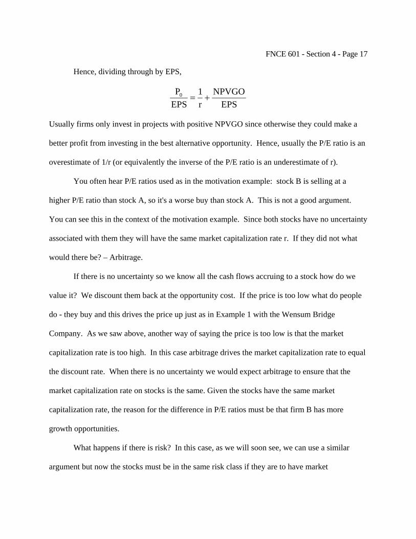
FNCE 601 - Section 4 - Page 17
Hence, dividing through by EPS,
EPSNPVGO
r1
EPSP0 +=
Usually firms only invest in projects with positive NPVGO since otherwise they could make a
better profit from investing in the best alternative opportunity. Hence, usually the P/E ratio is an
overestimate of 1/r (or equivalently the inverse of the P/E ratio is an underestimate of r).
You often hear P/E ratios used as in the motivation example: stock B is selling at a
higher P/E ratio than stock A, so it's a worse buy than stock A. This is not a good argument.
You can see this in the context of the motivation example. Since both stocks have no uncertainty
associated with them they will have the same market capitalization rate r. If they did not what
would there be? – Arbitrage.
If there is no uncertainty so we know all the cash flows accruing to a stock how do we
value it? We discount them back at the opportunity cost. If the price is too low what do people
do - they buy and this drives the price up just as in Example 1 with the Wensum Bridge
Company. As we saw above, another way of saying the price is too low is that the market
capitalization rate is too high. In this case arbitrage drives the market capitalization rate to equal
the discount rate. When there is no uncertainty we would expect arbitrage to ensure that the
market capitalization rate on stocks is the same. Given the stocks have the same market
capitalization rate, the reason for the difference in P/E ratios must be that firm B has more
growth opportunities.
What happens if there is risk? In this case, as we will soon see, we can use a similar
argument but now the stocks must be in the same risk class if they are to have market
FNCE 601 - Section 4 - Page 18
capitalization rates equated. We'll be returning to this soon.
When stock prices accurately reflect the discounted cash flows then we have efficient
markets. This is one of the central ideas in finance and we will consider it in depth in the second
part of the course.
The important point here is that a low P/E ratio probably does not mean a stock is a good
buy, it means the firm has few growth opportunities. It's what is termed an "income stock." If a
firm has a high P/E ratio it probably doesn't mean it is a bad buy it means it has a lot of growth
opportunities - it's what is termed a "growth stock". If these differences occurred because a
stock was over- or under-priced what would happen? There would be arbitrage.
To take an extreme example of a high P/E ratio, what are the earnings of biotechnology
firms early in their history when they are just engaged in research? They are zero but the stock
price is positive so the P/E ratio is infinite. This just reflects the fact that biotech firms have
many growth opportunities. It does not mean they are a bad buy.
Going back to our motivation example the reason the P/E ratios differ is probably
because of a difference in growth opportunities. The market capitalization rates are probably the
same (assuming the stocks have the same risk) so the stocks are equally good buys.
One final point to make here is that we are thinking of EPS as an accurate measure of
cash flow. In fact EPS is an accounting figure, and this may mean many different things in
different companies depending on the conventions and rules the companies adopt. In general
you have to be very careful of accounting figures since often they don't correspond to the notions
that financial economists use. If different firms use different accounting conventions then
clearly their P/E ratios will be different. You must be careful to be using earnings figures

FNCE 601 - Section 4 - Page 19
calculated on a similar basis.

UNIVERSITY OF PENNSYLVANIA THE WHARTON SCHOOL LECTURE NOTES FNCE 601 CORPORATE FINANCE Franklin Allen Fall 2004 WEEK 3 Tu: 9/21/04 and Th: 9/23/04 Copyright © 2004 by Franklin Allen
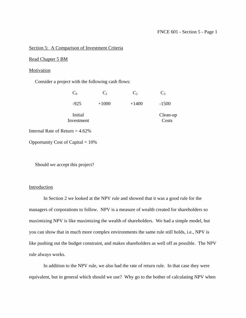
FNCE 601 - Section 5 - Page 1
Section 5: A Comparison of Investment Criteria
Read Chapter 5 BM
Motivation
Consider a project with the following cash flows:
C0 C1 C2 C3 -925 +1000 +1400 -1500 Initial Clean-up Investment Costs
Internal Rate of Return = 4.62%
Opportunity Cost of Capital = 10%
Should we accept this project?
Introduction
In Section 2 we looked at the NPV rule and showed that it was a good rule for the
managers of corporations to follow. NPV is a measure of wealth created for shareholders so
maximizing NPV is like maximizing the wealth of shareholders. We had a simple model, but
you can show that in much more complex environments the same rule still holds, i.e., NPV is
like pushing out the budget constraint, and makes shareholders as well off as possible. The NPV
rule always works.
In addition to the NPV rule, we also had the rate of return rule. In that case they were
equivalent, but in general which should we use? Why go to the bother of calculating NPV when
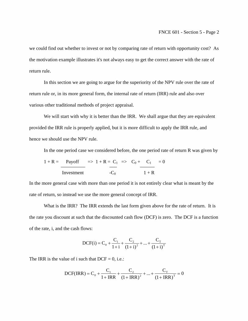
FNCE 601 - Section 5 - Page 2
we could find out whether to invest or not by comparing rate of return with opportunity cost? As
the motivation example illustrates it's not always easy to get the correct answer with the rate of
return rule.
In this section we are going to argue for the superiority of the NPV rule over the rate of
return rule or, in its more general form, the internal rate of return (IRR) rule and also over
various other traditional methods of project appraisal.
We will start with why it is better than the IRR. We shall argue that they are equivalent
provided the IRR rule is properly applied, but it is more difficult to apply the IRR rule, and
hence we should use the NPV rule.
In the one period case we considered before, the one period rate of return R was given by
1 + R = Payoff => 1 + R = C => C + C = 0 1 0 1 __________ ___ ______ Investment -C0 1 + R
In the more general case with more than one period it is not entirely clear what is meant by the
rate of return, so instead we use the more general concept of IRR.
What is the IRR? The IRR extends the last form given above for the rate of return. It is
the rate you discount at such that the discounted cash flow (DCF) is zero. The DCF is a function
of the rate, i, and the cash flows:
TT
221
0 )i1(C...
)i1(C
i1CC)i(DCF
+++
++
++=
The IRR is the value of i such that DCF = 0, i.e.:
0)IRR1(
C...)IRR1(
CIRR1
CC)IRR(DCF TT
221
0 =+
+++
++
+=

FNCE 601 - Section 5 - Page 3
Finding the IRR
The easiest way to find IRR is a calculator. One question that may occur to you is how is
the calculator finding it? To see this, it is helpful to consider what is going on graphically. We
can calculate the DCF at a number of values of the discount rate, join them up and then read off
the value of the discount rate at which DCF = 0. This is the IRR. For example, suppose we have
the following cash flows:
Example 1
C0 C1 -1 +1.1
In this case we have the following values of DCF for various values of i:
i DCF(i)
0 -1 + 1.1 = 0.1
0.05 -1 + (1.1/1.05) = 0.0476
0.1 -1 + (1.1/1.1) = 0
0.15 -1 + (1.1/1.15) = -0.0435
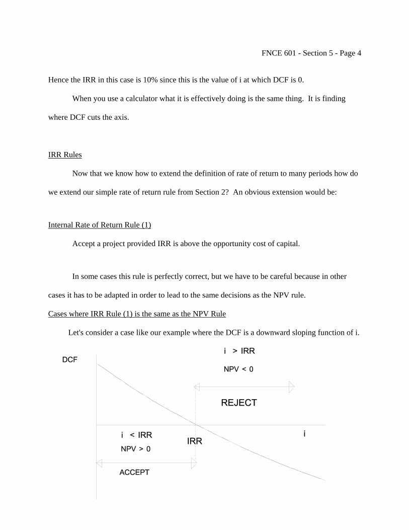
FNCE 601 - Section 5 - Page 4
Hence the IRR in this case is 10% since this is the value of i at which DCF is 0.
When you use a calculator what it is effectively doing is the same thing. It is finding
where DCF cuts the axis.
IRR Rules
Now that we know how to extend the definition of rate of return to many periods how do
we extend our simple rate of return rule from Section 2? An obvious extension would be:
Internal Rate of Return Rule (1)
Accept a project provided IRR is above the opportunity cost of capital.
In some cases this rule is perfectly correct, but we have to be careful because in other
cases it has to be adapted in order to lead to the same decisions as the NPV rule.
Cases where IRR Rule (1) is the same as the NPV Rule
Let's consider a case like our example where the DCF is a downward sloping function of i.

FNCE 601 - Section 5 - Page 5
When does the IRR rule (1) say that we should accept projects? It says we should accept when
the IRR is above the opportunity cost of capital. For example, if the IRR is 10% and the
opportunity cost of capital is 5% we should accept the project. In other words, we should accept
at points to the left of the IRR. We should reject when the IRR is below the opportunity cost of
capital. For example, if the IRR is 10% and the opportunity cost of capital is 15% we should
reject the project. In terms of the diagram we should reject to the right of the IRR.
When does the NPV rule say that we should accept projects? The NPV of a project is
just the DCF where the rate used to discount is the opportunity cost of capital. Keeping with the
same example, when the opportunity cost of capital is 5% it can be seen from the diagram that
the NPV is positive. Hence we should accept. Similarly, we should accept whenever the
opportunity cost of capital is such that NPV is positive. When the opportunity cost of capital is
15% the NPV is negative and we should reject the project. Similarly, we should reject whenever
NPV is negative.
In this case the IRR rule (1) is the same as the NPV rule. In fact it can be seen from the
diagram that whenever the DCF of a project is a downward sloping function of i, the NPV and
the IRR rule (1) give the same result.
When Must IRR Rule (1) Be Adapted to Correspond to the NPV Rule
Now that we have seen that the two rules are the same when DCF is a downward sloping
function of i, when do you think they will differ? Suppose DCF is an upward sloping function of
i:
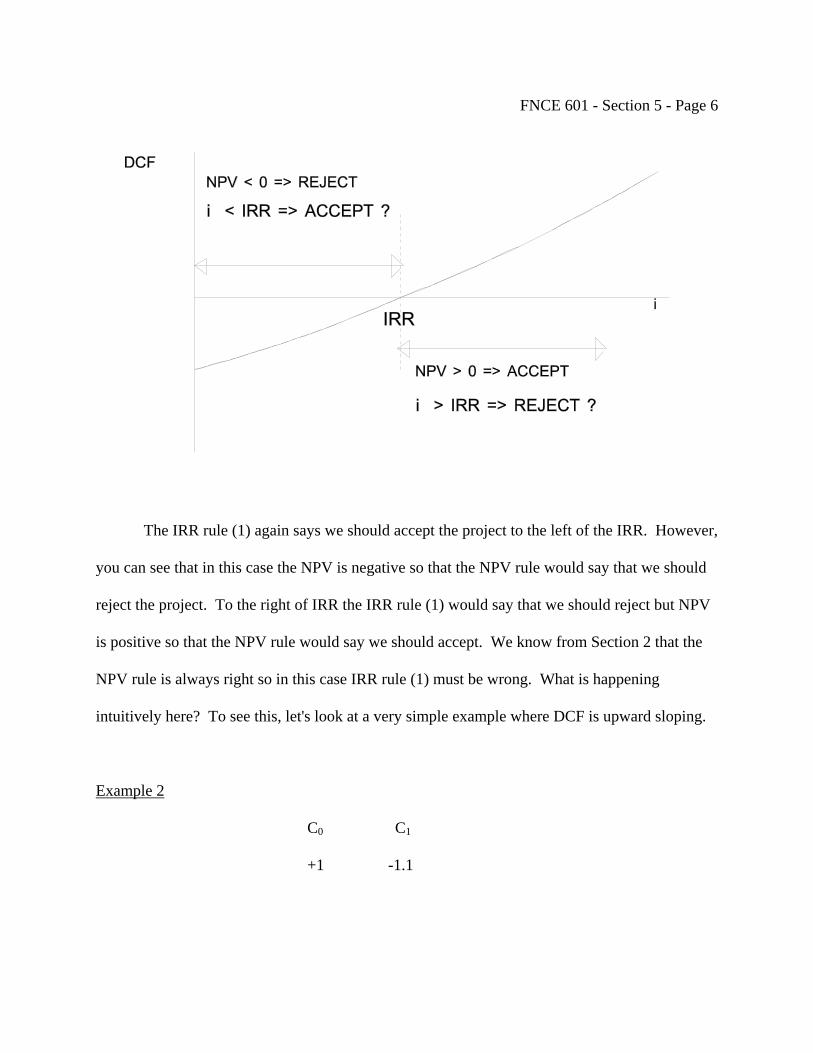
FNCE 601 - Section 5 - Page 6
The IRR rule (1) again says we should accept the project to the left of the IRR. However,
you can see that in this case the NPV is negative so that the NPV rule would say that we should
reject the project. To the right of IRR the IRR rule (1) would say that we should reject but NPV
is positive so that the NPV rule would say we should accept. We know from Section 2 that the
NPV rule is always right so in this case IRR rule (1) must be wrong. What is happening
intuitively here? To see this, let's look at a very simple example where DCF is upward sloping.
Example 2
C0 C1 +1 -1.1

FNCE 601 - Section 5 - Page 7
Notice that this is the same as our original example except that the signs are reversed. Hence the
numerical values of DCF at various values of i will be the same but the signs will be reversed.
i DCF
0 +1 - 1.10 = -0.1
0.05 +1 - (1.1/1.05) = -0.0476
0.10 +1 - (1.1/1.1) = 0
0.15 +1 - (1.1/1.15) = 0.0435
In this case we have the type of relationship depicted above. What is happening? You receive 1
now and pay back 1.1 next period; in other words, you are "borrowing" and the IRR is like a
borrowing rate. Should you try to borrow at a high rate or at a low rate? At a low rate. If you
can borrow at less than the opportunity cost of capital then clearly you can make a profit (i.e.
NPV > 0) and this is what you should do--but this is what the NPV rule is saying.
Consider our original example where DCF is downward sloping:
C0 C1 -1 +1.1
In this case you are laying out $1 now in return for a payment of $1.1 next period. It is
like "lending" and the IRR is like the lending rate. You want to lend at as high a rate of interest
as possible. If the rate you can lend at is greater than the opportunity cost of capital, you can
make a profit so that NPV > 0. Again you can see that the NPV rule is intuitively right.
IRR rule (1) needs to be adapted to take account of whether you are "lending" or
"borrowing". This gives IRR rule (2).
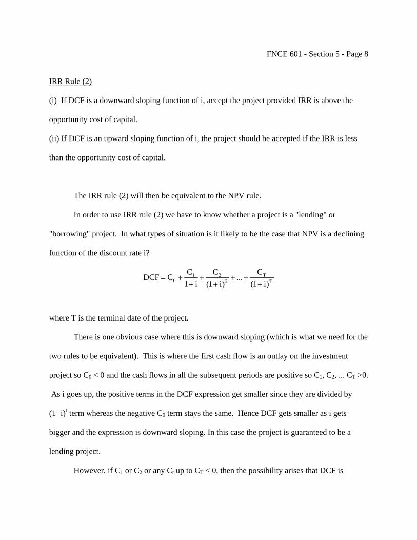
FNCE 601 - Section 5 - Page 8
IRR Rule (2)
(i) If DCF is a downward sloping function of i, accept the project provided IRR is above the
opportunity cost of capital.
(ii) If DCF is an upward sloping function of i, the project should be accepted if the IRR is less
than the opportunity cost of capital.
The IRR rule (2) will then be equivalent to the NPV rule.
In order to use IRR rule (2) we have to know whether a project is a "lending" or
"borrowing" project. In what types of situation is it likely to be the case that NPV is a declining
function of the discount rate i?
TT
221
0 )i1(C...
)i1(C
i1CCDCF
+++
++
++=
where T is the terminal date of the project.
There is one obvious case where this is downward sloping (which is what we need for the
two rules to be equivalent). This is where the first cash flow is an outlay on the investment
project so C0 < 0 and the cash flows in all the subsequent periods are positive so C1, C2, ... CT >0.
As i goes up, the positive terms in the DCF expression get smaller since they are divided by
(1+i)t term whereas the negative C0 term stays the same. Hence DCF gets smaller as i gets
bigger and the expression is downward sloping. In this case the project is guaranteed to be a
lending project.
However, if C1 or C2 or any Ct up to CT < 0, then the possibility arises that DCF is
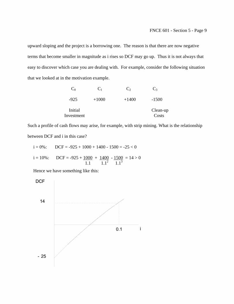
FNCE 601 - Section 5 - Page 9
upward sloping and the project is a borrowing one. The reason is that there are now negative
terms that become smaller in magnitude as i rises so DCF may go up. Thus it is not always that
easy to discover which case you are dealing with. For example, consider the following situation
that we looked at in the motivation example.
C0 C1 C2 C3 -925 +1000 +1400 -1500 Initial Clean-up Investment Costs
Such a profile of cash flows may arise, for example, with strip mining. What is the relationship
between DCF and i in this case?
i = 0%: DCF = -925 + 1000 + 1400 - 1500 = -25 < 0
i = 10%: DCF = -925 + 1000 + 1400 - 1500 = 14 > 0 1.1 1.12 1.13
Hence we have something like this:
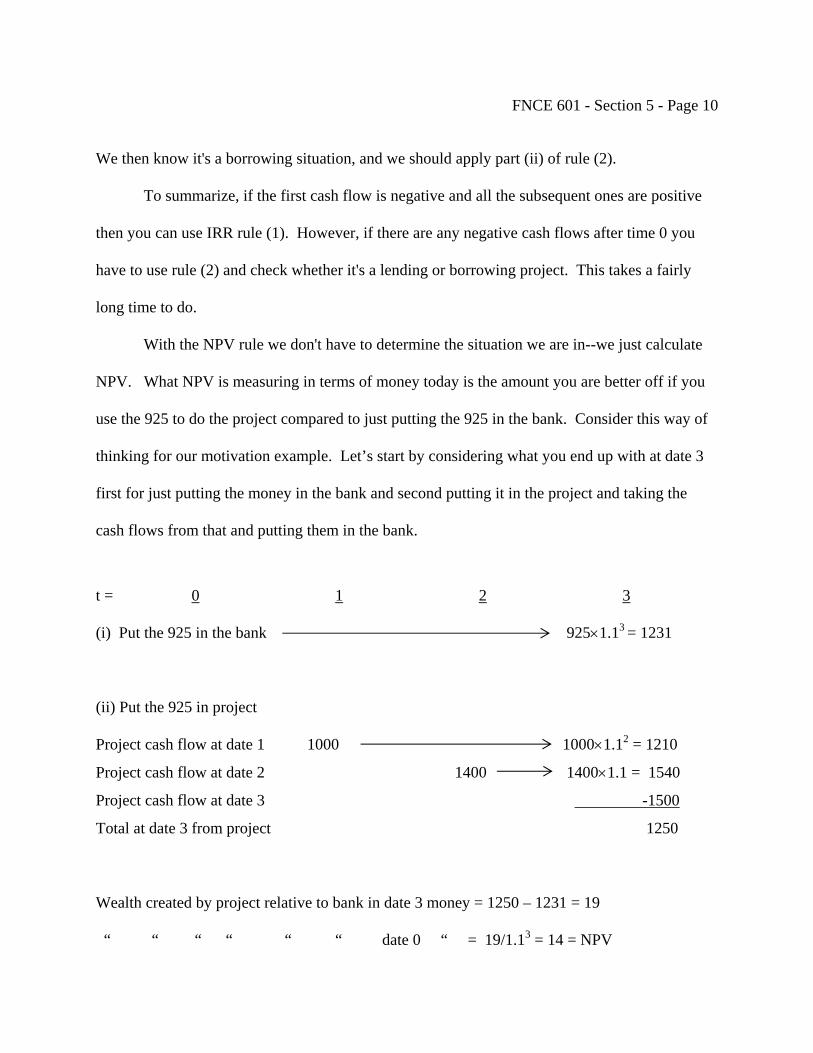
FNCE 601 - Section 5 - Page 10
We then know it's a borrowing situation, and we should apply part (ii) of rule (2).
To summarize, if the first cash flow is negative and all the subsequent ones are positive
then you can use IRR rule (1). However, if there are any negative cash flows after time 0 you
have to use rule (2) and check whether it's a lending or borrowing project. This takes a fairly
long time to do.
With the NPV rule we don't have to determine the situation we are in--we just calculate
NPV. What NPV is measuring in terms of money today is the amount you are better off if you
use the 925 to do the project compared to just putting the 925 in the bank. Consider this way of
thinking for our motivation example. Let’s start by considering what you end up with at date 3
first for just putting the money in the bank and second putting it in the project and taking the
cash flows from that and putting them in the bank.
t = 0 1 2 3
(i) Put the 925 in the bank 925×1.13 = 1231
(ii) Put the 925 in project
Project cash flow at date 1 1000 1000×1.12 = 1210
Project cash flow at date 2 1400 1400×1.1 = 1540
Project cash flow at date 3 -1500
Total at date 3 from project 1250
Wealth created by project relative to bank in date 3 money = 1250 – 1231 = 19
“ “ “ “ “ “ date 0 “ = 19/1.13 = 14 = NPV
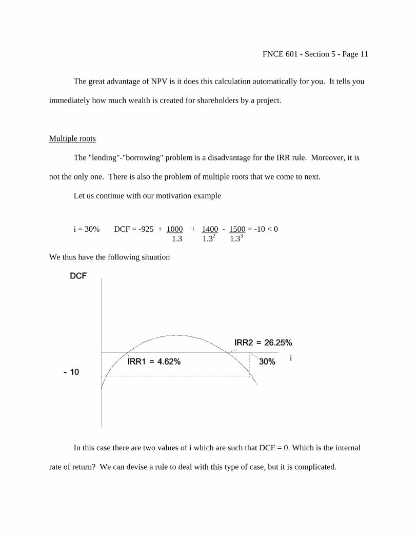
FNCE 601 - Section 5 - Page 11
The great advantage of NPV is it does this calculation automatically for you. It tells you
immediately how much wealth is created for shareholders by a project.
Multiple roots
The "lending"-"borrowing" problem is a disadvantage for the IRR rule. Moreover, it is
not the only one. There is also the problem of multiple roots that we come to next.
Let us continue with our motivation example
i = 30% DCF = -925 + 1000 + 1400 - 1500 = -10 < 0 1.3 1.32 1.33
We thus have the following situation
In this case there are two values of i which are such that DCF = 0. Which is the internal
rate of return? We can devise a rule to deal with this type of case, but it is complicated.

FNCE 601 - Section 5 - Page 12
IRR Rule (3)
(a) If there is just one IRR use IRR rule (2).
(b) Given two IRR: IRR1, and IRR2, there are two possible situations.
(i) If at IRR1, DCF is upward sloping and at IRR2 DCF is downward sloping (i.e. the curve
is n-shaped), then we should accept the project if IRR1 < Opportunity cost of capital <
IRR2. Otherwise, we should reject it.
DCF
(ii) If at IRR1, DCF is downward sloping and at IRR2, DCF is upward sloping (i.e. the curve
is u-shaped), we should accept if the opportunity cost of capital < IRR1 or > IRR2.
Otherwise we should reject it.

FNCE 601 - Section 5 - Page 13
This is obviously an immensely complicated rule to apply. In fact, the problem is even
more serious than this example indicates since in general we may have many more than two
values at which DCF = 0, especially if the project is long-lived and there are many alterations
between +ve and -ve cash flows. For each of these possibilities we will have to develop a version
of our IRR rule.
In situations where the first cash flow is negative and subsequent cash flows are positive
it is fine to use IRR otherwise it is simpler just to calculate NPV.
Mutually Exclusive Projects
Our problems with IRR are not at an end yet. Investment decisions are often concerned
with mutually exclusive projects, that is, ones in which you are choosing among different ways
of doing the same thing. In other words, in some circumstances you can only do one project, you
can't do all of them. An example would be replacing a machine on a production line; there may
be several alternative machines you could potentially use but you can only use one of them to
replace the old one.
It would seem that the appropriate rule in this type of situation is:
"Naive" IRR Rule:
Choose the mutually exclusive project with the highest IRR.
Consider projects A and B depicted below, which are mutually exclusive.
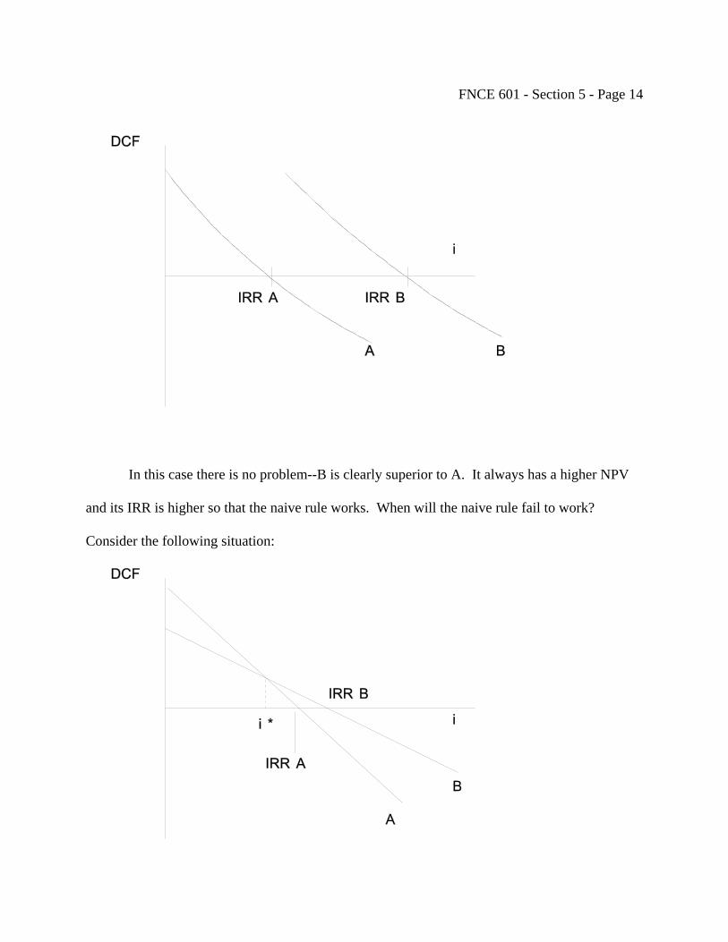
FNCE 601 - Section 5 - Page 14
In this case there is no problem--B is clearly superior to A. It always has a higher NPV
and its IRR is higher so that the naive rule works. When will the naive rule fail to work?
Consider the following situation:

FNCE 601 - Section 5 - Page 15
Which is superior, A or B? In terms of NPV, B is superior when the opportunity cost of
capital is above the crossing point i* and inferior when it is below i*.
In terms of the naive IRR rule, however, B would appear to be superior regardless of i.
What is going on here intuitively? To see this let's consider an example.
Example
Project C0 C1 IRR NPV at 10% NPV at 20% A -1,000 +1,200 20 91 0
B -10 +30 200 17 15
It can be shown that in this example i* = 18.18.
If you graph A and B for NPV against i for this example you get the type of situation
shown above with 10% < i* = 18.18%.
What is happening is a question of relative versus absolute returns. A has a low relative
return but a high absolute return; B has a high relative return but a low absolute return. Given
they're mutually exclusive, you can't do both. What's important is which gives you the highest
absolute return since that's the amount that your budget constraint is pushed out or in other
words the money that actually goes into your pocket. You may be better off investing a large
amount at a low return than a small amount at a high return.
It is possible to fix up the IRR rule by looking at the IRR on incremental cash flows.
This is rather painful and so we will not go through it here. I will leave you to read the details in
the book. It is much simpler just to use NPV.

FNCE 601 - Section 5 - Page 16
One important point to note is that the analysis above assumes perfect capital markets.
This implies that it is possible for the firm to borrow as much as it would like to. If capital
markets are imperfect and the firm is limited in the amount it can borrow there is said to be
“capital rationing.” The way that capital budgeting decisions should be made in this case is
considered further below.
IRR and the Term Structure of Interest Rates
So far we have been assuming that there is just one opportunity cost of capital, which is the
same for every period. However, as we discussed in Section 2 this may not be the case. The
yield curve may not be flat.
In this case the opportunity cost of capital for different periods differs, and we must
calculate NPV using the formula
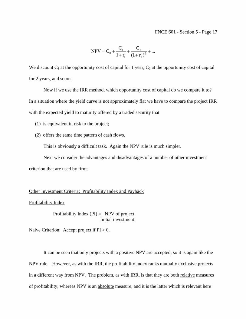
FNCE 601 - Section 5 - Page 17
...)r1(
Cr1
CCNPV 22
2
1
10 +
++
++=
We discount C1 at the opportunity cost of capital for 1 year, C2 at the opportunity cost of capital
for 2 years, and so on.
Now if we use the IRR method, which opportunity cost of capital do we compare it to?
In a situation where the yield curve is not approximately flat we have to compare the project IRR
with the expected yield to maturity offered by a traded security that
(1) is equivalent in risk to the project;
(2) offers the same time pattern of cash flows.
This is obviously a difficult task. Again the NPV rule is much simpler.
Next we consider the advantages and disadvantages of a number of other investment
criterion that are used by firms.
Other Investment Criteria: Profitability Index and Payback
Profitability Index
Profitability index (PI) = NPV of project Initial investment
Naive Criterion: Accept project if PI > 0.
It can be seen that only projects with a positive NPV are accepted, so it is again like the
NPV rule. However, as with the IRR, the profitability index ranks mutually exclusive projects
in a different way from NPV. The problem, as with IRR, is that they are both relative measures
of profitability, whereas NPV is an absolute measure, and it is the latter which is relevant here
FNCE 601 - Section 5 - Page 18
since this determines the amount the budget constraint of shareholders can be shifted outward.
Consider the example we used with IRR and mutually exclusive projects again.
Project C0 C1 NPV at 10% PI
A -1,000 +1,200 91 0.091
B -10 +30 17 1.7
Here we should choose A since this pushes out the budget constraints of shareholders the
farthest. A naive profitability rule which chose the project with the highest PI would give an
incorrect answer; it would say choose B. However, we can again adapt the PI method to deal
with this by looking at the PI of the incremental investment similarly to IRR. Again,
appropriately adapted, PI, like IRR, is not incorrect but NPV is easier to use.
Payback
The payback rule requires that the initial outlay on any project should be recoverable
within some specified cutoff period. The payback period is calculated by counting the number
of years it takes before forecasted cash flows equal the initial investment.
Example
Project C0 C1 C2 C3 Payback NPV @ 10%
A -300 +300 0 0 1 year -27
B -300 +100 +100 +500 3 years 252
FNCE 601 - Section 5 - Page 19
With the payback method we will accept A if the cutoff period is 1 year or over and B if
it is 3 years or over. With NPV, however, we would reject A and accept B. Thus payback can
give incorrect answers to the capital budgeting problem, unlike IRR and PI which were just more
difficult to use.
Why doesn't payback give the same results as NPV? There are three main problems.
(i) The first difference is clearly that with payback no account is taken of the difference in the
value of $'s at different dates. To try and deal with this we could use the discounted payback
method, which takes into account the time value of money, but this still suffers from the other
two defects.
(ii) The second defect is that the cutoff date is fairly arbitrary. If you use the same cutoff,
regardless of the project, then you reject too many long lived projects and accept too many short
lived ones.
There are certain special cases where we can calculate a formula for the optimal cut off
period that corresponds to maximizing NPV, e.g., if flows are spread evenly across the life of the
project, but in general this is not possible.
(iii) The third defect is that it ignores all flows after the cutoff date so there is a bias against long
lived projects.
Does payback have any advantages? One advantage of payback is its ease of calculation
compared to NPV. With short time horizons where things are constantly being replaced and the
projects are small (e.g., office supplies and equipment) it may be worthwhile to use the payback
method because of its ease of computation. In the majority of cases we shouldn't use it though
since, unlike IRR and PI, it gives incorrect answers.

FNCE 601 - Section 5 - Page 20
There are various other criteria that are used for investment decisions. Many are
accounting based such as the book rate of return. These other methods are either difficult to use
or do not correspond to creating wealth for shareholders. I won't go through the deficiencies
here but you can read about them. NPV is better because it is relatively easy to use and directly
measures what we are interested in namely how much wealth is created for shareholders.
Capital Rationing
We have argued above that one of the problems with IRR and PI is that they are relative
measures rather than absolute measures. We suggested it is the absolute amount of money
received that shareholders are interested in so it can be better to take a large investment with a
low rate of return than a small investment with a high rate of return. Implicit in this argument is
the assumption that the firm can invest as much as it wants to. Capital rationing occurs when the
firm has limitations on the capital it can invest that prevent it from undertaking all investment
opportunities with positive net present value that are available. We next consider how
investment decisions should be made in this case.
There are a number of reasons why firms may operate with capital rationing.
Management may believe a rapid expansion will overtax the organization and use a capital
constraint as a proxy in restricting this growth. This is an example of soft rationing, where the
constraint is internally applied.
Because of problems of fraud, people may be reluctant to give any particular firm too
much money. This is an example of hard rationing, which is externally imposed by the market.
In these types of situations, how should the firm make its investment decisions? It is first
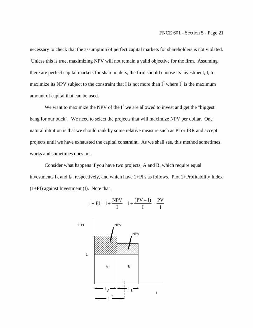
FNCE 601 - Section 5 - Page 21
necessary to check that the assumption of perfect capital markets for shareholders is not violated.
Unless this is true, maximizing NPV will not remain a valid objective for the firm. Assuming
there are perfect capital markets for shareholders, the firm should choose its investment, I, to
maximize its NPV subject to the constraint that I is not more than I* where I* is the maximum
amount of capital that can be used.
We want to maximize the NPV of the I* we are allowed to invest and get the "biggest
bang for our buck". We need to select the projects that will maximize NPV per dollar. One
natural intuition is that we should rank by some relative measure such as PI or IRR and accept
projects until we have exhausted the capital constraint. As we shall see, this method sometimes
works and sometimes does not.
Consider what happens if you have two projects, A and B, which require equal
investments IA and IB, respectively, and which have 1+PI's as follows. Plot 1+Profitability Index
(1+PI) against Investment (I). Note that
IPV
I)IPV(1
INPV1PI1 =
−+=+=+
1+PI
I
A B
NPV
NPV
1
I A I B
I *
FNCE 601 - Section 5 - Page 22
In interpreting this diagram it is helpful to remember that each bar represents a project:
Total Area in each bar = (1+PI) x I
= II
PV×
= PV
Also Unshaded Area = I x 1
= I
Therefore Shaded Area = PV - I
= NPV
Hence the objective of firms is to choose the projects that maximize the total shaded area.
In the diagram above, if the firm is constrained to I*, in this situation it should clearly do A.
Ranking by PI and accepting until the constraint is satisfied works in this case.
If there are three projects A, B and C as below which all require the same investment what
should the firm do?

FNCE 601 - Section 5 - Page 23
1+PI
I
A B
1
I A I B
I *
C
I C
Clearly it should do A and B. Again the rule of ranking by PI and accepting until the
constraint is exhausted works. Is it always the case that the rule works? No! If the projects
require different investments the rule will not work.
I
1+PI
A B C
IIICBA
1
I *
In this case it should do A and C.
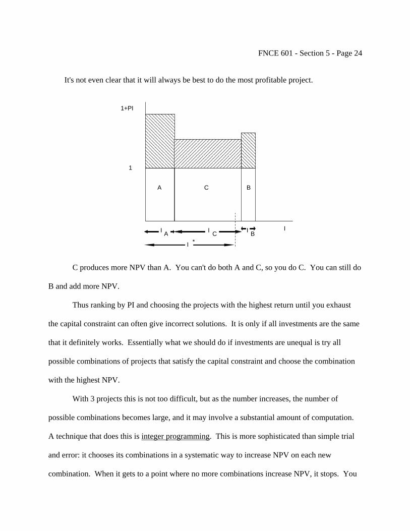
FNCE 601 - Section 5 - Page 24
It's not even clear that it will always be best to do the most profitable project.
1+PI
1
A C B
III BCAI
I *
C produces more NPV than A. You can't do both A and C, so you do C. You can still do
B and add more NPV.
Thus ranking by PI and choosing the projects with the highest return until you exhaust
the capital constraint can often give incorrect solutions. It is only if all investments are the same
that it definitely works. Essentially what we should do if investments are unequal is try all
possible combinations of projects that satisfy the capital constraint and choose the combination
with the highest NPV.
With 3 projects this is not too difficult, but as the number increases, the number of
possible combinations becomes large, and it may involve a substantial amount of computation.
A technique that does this is integer programming. This is more sophisticated than simple trial
and error: it chooses its combinations in a systematic way to increase NPV on each new
combination. When it gets to a point where no more combinations increase NPV, it stops. You

FNCE 601 - Section 5 - Page 25
will be considering integer programming and other optimization methods more in OPIM 621
next semester.

UNIVERSITY OF PENNSYLVANIA THE WHARTON SCHOOL LECTURE NOTES FNCE 601 CORPORATE FINANCE Franklin Allen Fall 2004 QUARTER 1 - WEEK 3 (part 2) and WEEK 4 (part 1) Th: 9/23/04 and Tu: 9/28/04 Copyright © 2004 by Franklin Allen
FNCE 601 – Section 6 – Page 1 Section 6: Practical Aspects of the NPV Rule Read Chapter 6 BM
Motivation
We know how to calculate present values given cash flows but how do you actually evaluate
projects? How do you use accounting data when applying the NPV rule? For example, how do
you do problems like the following example?
Example 1
The Pierpont Company is thinking of building a plant to make trumpets. The plant and
equipment will cost $1 million. It will last for five years and will have no salvage value at the
end of that time. The costs of running the plant are expected to be $100,000 per year. The
revenues from selling the trumpets are expected to be $375,000 per year. All cash flows occur at
the end of the year. The firm uses straight line depreciation. Its corporate tax rate is 35 percent
and the opportunity cost of capital for this project is 10 percent. The projected income
statement for the project is as follows.
Revenues $375,000 Operating Expenses -$100,000 Net Operating Income $275,000 Depreciation -$200,000 Taxable Income $75,000 Taxes -$26,250 Net Income $48,750 Should the firm build the plant?
FNCE 601 - Section 6 - Page 2
Introduction
How do we apply the NPV rule? Discount cash flows. This is all right as far as it goes,
but so far we have not said exactly what we mean by cash flows--what should we include and
what should we not include from accounting data? This is what we're going to consider next.
There are four general rules.
Rule 1: Work with cash flow after taxes, not net income. This is the proper basis for capital
budgeting analysis.
The points to remember are:
(i) Always estimate cash flows on an after-corporate tax basis, since this is what
shareholders are interested in. Hence if the corporate tax rate is denoted tc the
effect of additional gross revenues R is (1-tc)R after tax and the effect of additional
gross costs C is (1-tc)C after tax.
(ii) You have to transform accounting data into cash flows. This is not always easy.
For example, such things as depreciation are not cash flows although the tax
savings due to the tax deductibility of depreciation are. Suppose the corporate tax
rate is tc = 35%. If you have a $100 depreciation deduction it reduces taxable
income by $100 and hence taxes by $35. The value of a tax shield is tc x
Depreciation. Note that it is equivalent to subtract out depreciation then subtract
taxes and finally add back depreciation. This can be seen as follows.
(1-tc)(Net operating income - Depreciation) + Depreciation
= (1-tc)NOI - (1-tc)Depreciation + Depreciation
= (1-tc)NOI + tc x Depreciation
FNCE 601 - Section 6 - Page 3
(iii) Interest and dividends are not cash flows - they are taken account of by
discounting. If they were subtracted out again there would be double counting.
Rule 2: The timing of cash flows is critical. Revenues and costs include cash you have not
received or paid out. You need to adjust for this.
It is important to record cash flows at the time the cash is received or paid out. When
you receive cash, for example, you can earn interest on the money.
Include working capital needs. Since revenues and costs do not correspond to cash flows
we need to adjust for this using working capital. When a new project is undertaken it
may take a while for customers to pay, i.e. the accounts receivable will increase. On the
other hand, the payments associated with the cost of the project may be delayed, i.e. the
accounts payable increases. This offsets the accounts receivable. The difference
between them is a working capital need and this must be financed. Total working capital
taking into account all these kinds of factor is short term assets minus liabilities.
Rule 3: Only incremental cash flows are analyzed (those which occur on the margin because
you invest in the project).
Estimate all the marginal charges that arise if the project is undertaken compared to what
happens if it is not undertaken. In particular
(i) Include all incidental effects. Include all externalities on other parts of the
business. If revenues or costs in any part of the business are affected then care
should be taken to include these incidental marginal effects.
(ii) Forget sunk costs. Sunk costs are expenditures that have already been made.
These are irreversible and should not be included in the cash flows. There's
FNCE 601 - Section 6 - Page 4
nothing you can do about them--bygones are bygones.
(iii) Include opportunity costs. If a firm already owns land that it is considering using
in a project, it should take into account the fact that it could sell the land, raise cash
and invest the money if it does not go ahead with the project. Thus there is an
opportunity cost to the land. The proper comparison is with or without, not before
or after.
(iv) Be careful in the allocation of overhead Fixed costs are allocated by accountants but
they may not correspond to marginal costs borne by the firm. Be careful to adjust
for this.
Rule 4: Be consistent in the treatment of inflation
It is important first to clarify the distinction between nominal and real.
Nominal: The actual number of dollars and the actual interest rates.
Real: Taking into account inflation so that the figures are, in some sense, what would
have happened in the absence of inflation.
The important thing with nominal and real is that, in the context of capital budgeting,
there are two ways of thinking about the same thing. But you must be consistent and stick with
one or the other. Either discount nominal cash flows at a nominal discount rate, or discount real
cash flows at a real discount rate. Provided you do this, it doesn't matter whether you work in
real or nominal terms. Usually in the U.S., Europe and Japan people deal in nominal terms since
this is the form in which the data is presented. However, in high inflation countries such as
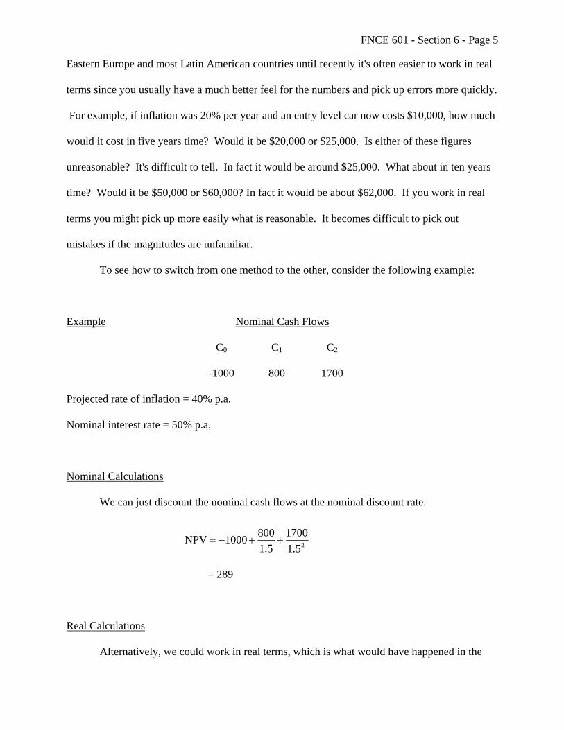
FNCE 601 - Section 6 - Page 5
Eastern Europe and most Latin American countries until recently it's often easier to work in real
terms since you usually have a much better feel for the numbers and pick up errors more quickly.
For example, if inflation was 20% per year and an entry level car now costs $10,000, how much
would it cost in five years time? Would it be $20,000 or $25,000. Is either of these figures
unreasonable? It's difficult to tell. In fact it would be around $25,000. What about in ten years
time? Would it be $50,000 or $60,000? In fact it would be about $62,000. If you work in real
terms you might pick up more easily what is reasonable. It becomes difficult to pick out
mistakes if the magnitudes are unfamiliar.
To see how to switch from one method to the other, consider the following example:
Example Nominal Cash Flows
C0 C1 C2
-1000 800 1700
Projected rate of inflation = 40% p.a.
Nominal interest rate = 50% p.a.
Nominal Calculations
We can just discount the nominal cash flows at the nominal discount rate.
25.11700
5.18001000NPV ++−=
= 289
Real Calculations
Alternatively, we could work in real terms, which is what would have happened in the
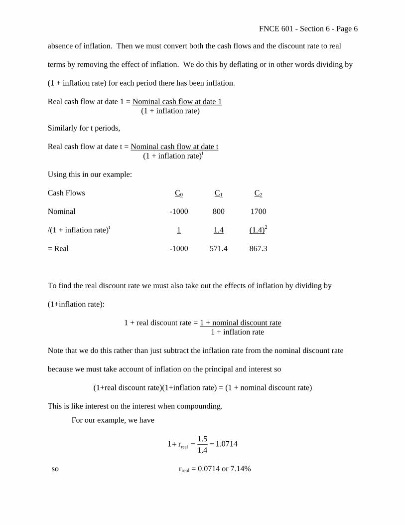
FNCE 601 - Section 6 - Page 6
absence of inflation. Then we must convert both the cash flows and the discount rate to real
terms by removing the effect of inflation. We do this by deflating or in other words dividing by
(1 + inflation rate) for each period there has been inflation.
Real cash flow at date 1 = Nominal cash flow at date 1 (1 + inflation rate)
Similarly for t periods,
Real cash flow at date t = Nominal cash flow at date t (1 + inflation rate)t
Using this in our example:
Cash Flows C0 C1 C2
Nominal -1000 800 1700
/(1 + inflation rate)t 1 1.4 (1.4)2
= Real -1000 571.4 867.3
To find the real discount rate we must also take out the effects of inflation by dividing by
(1+inflation rate):
1 + real discount rate = 1 + nominal discount rate 1 + inflation rate
Note that we do this rather than just subtract the inflation rate from the nominal discount rate
because we must take account of inflation on the principal and interest so
(1+real discount rate)(1+inflation rate) = (1 + nominal discount rate)
This is like interest on the interest when compounding.
For our example, we have
0714.14.15.1r1 real ==+
so rreal = 0.0714 or 7.14%

FNCE 601 - Section 6 - Page 7
Our NPV calculation in real terms is then
2890714.1
3.8670714.1
4.5711000NPV 2 =++−=
To summarize, whether we work in real or nominal doesn't matter. However, we must
not mix them. That's the main thing you have to worry about as far as inflation is concerned. In
practice it's slightly more difficult to implement than this. In particular, you must remember that
the tax code is written in nominal terms, so beware if you're given data (e.g., one of the
homework examination questions) in real terms. In particular be careful to deal with
depreciation properly: work out depreciation in nominal terms since that is how it's specified in
the tax code and then convert to real terms.
Examples
As these general guidelines indicate, capital budgeting is a complicated business. It
requires careful, diligent work and a thorough understanding of the tax code in the country you
are working in. To give you some idea of how to do it, we're going to consider some examples.
Example 1 The Pierpont Company is thinking of building a plant to make trumpets. The plant and equipment will cost $1 million. It will last for five years and will have no salvage value at the end of that time. The costs of running the plant are expected to be $100,000 per year. The revenues from selling the trumpets are expected to be $375,000 per year. All cash flows occur at the end of the year. The firm uses straight line depreciation. Its corporate tax rate is 35 percent and the opportunity cost of capital for this project is 10 percent. The projected income statement for the project is as follows. Revenues $375,000 Operating Expenses -$100,000 Net Operating Income $275,000 Depreciation -$200,000 Taxable Income $75,000 Taxes -$26,250 Net Income $48,750 Should the firm build the plant?
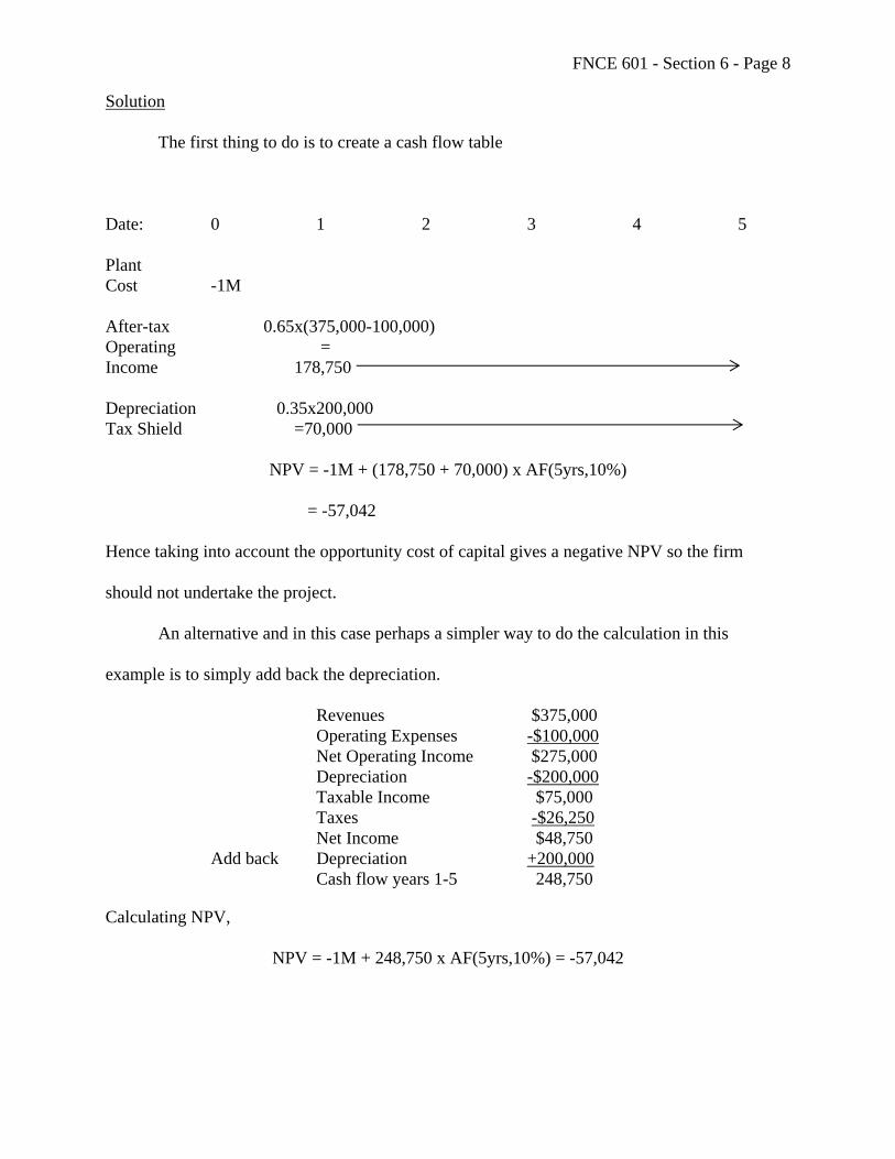
FNCE 601 - Section 6 - Page 8
Solution
The first thing to do is to create a cash flow table
Date: 0 1 2 3 4 5 Plant Cost -1M After-tax 0.65x(375,000-100,000) Operating = Income 178,750 Depreciation 0.35x200,000 Tax Shield =70,000
NPV = -1M + (178,750 + 70,000) x AF(5yrs,10%)
= -57,042
Hence taking into account the opportunity cost of capital gives a negative NPV so the firm
should not undertake the project.
An alternative and in this case perhaps a simpler way to do the calculation in this
example is to simply add back the depreciation.
Revenues $375,000 Operating Expenses -$100,000 Net Operating Income $275,000 Depreciation -$200,000 Taxable Income $75,000 Taxes -$26,250 Net Income $48,750 Add back Depreciation +200,000 Cash flow years 1-5 248,750
Calculating NPV,
NPV = -1M + 248,750 x AF(5yrs,10%) = -57,042
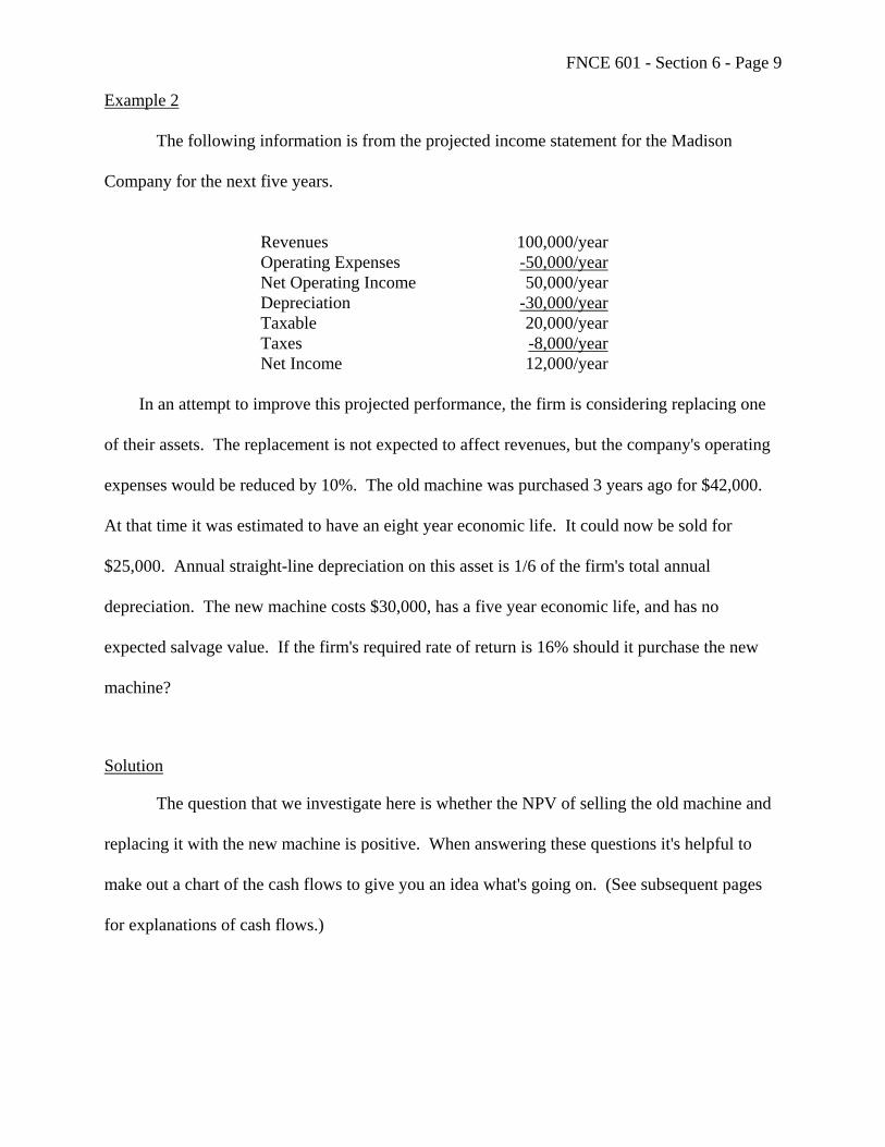
FNCE 601 - Section 6 - Page 9
Example 2
The following information is from the projected income statement for the Madison
Company for the next five years.
Revenues 100,000/year Operating Expenses -50,000/year Net Operating Income 50,000/year Depreciation -30,000/year Taxable 20,000/year Taxes -8,000/year Net Income 12,000/year In an attempt to improve this projected performance, the firm is considering replacing one
of their assets. The replacement is not expected to affect revenues, but the company's operating
expenses would be reduced by 10%. The old machine was purchased 3 years ago for $42,000.
At that time it was estimated to have an eight year economic life. It could now be sold for
$25,000. Annual straight-line depreciation on this asset is 1/6 of the firm's total annual
depreciation. The new machine costs $30,000, has a five year economic life, and has no
expected salvage value. If the firm's required rate of return is 16% should it purchase the new
machine?
Solution
The question that we investigate here is whether the NPV of selling the old machine and
replacing it with the new machine is positive. When answering these questions it's helpful to
make out a chart of the cash flows to give you an idea what's going on. (See subsequent pages
for explanations of cash flows.)
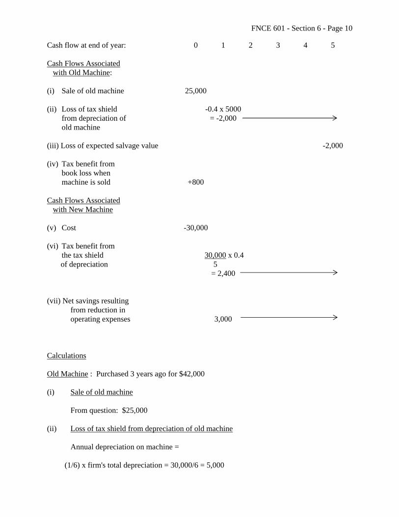
FNCE 601 - Section 6 - Page 10
Cash flow at end of year: 0 1 2 3 4 5
Cash Flows Associated with Old Machine: (i) Sale of old machine 25,000 (ii) Loss of tax shield -0.4 x 5000 from depreciation of = -2,000 old machine (iii) Loss of expected salvage value -2,000 (iv) Tax benefit from book loss when machine is sold +800 Cash Flows Associated with New Machine (v) Cost -30,000 (vi) Tax benefit from the tax shield 30,000 x 0.4 of depreciation 5 = 2,400 (vii) Net savings resulting from reduction in operating expenses 3,000
Calculations
Old Machine : Purchased 3 years ago for $42,000
(i) Sale of old machine
From question: $25,000
(ii) Loss of tax shield from depreciation of old machine
Annual depreciation on machine =
(1/6) x firm's total depreciation = 30,000/6 = 5,000
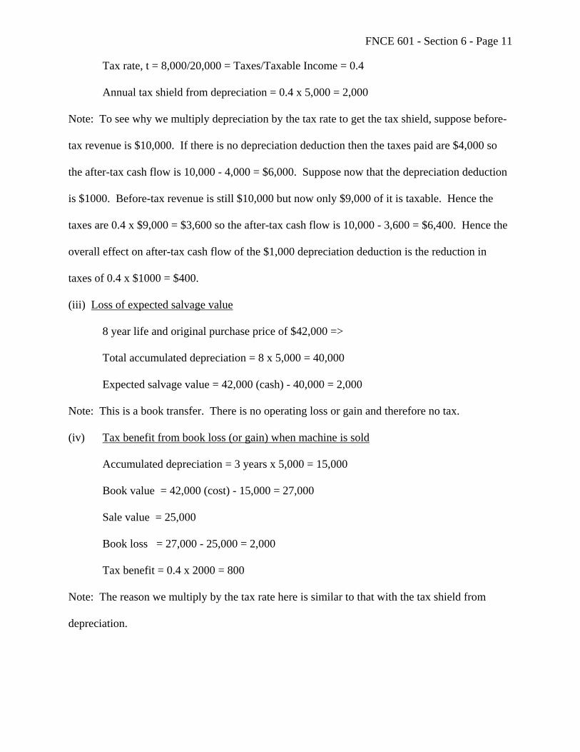
FNCE 601 - Section 6 - Page 11
Tax rate, t = 8,000/20,000 = Taxes/Taxable Income = 0.4
Annual tax shield from depreciation = 0.4 x 5,000 = 2,000
Note: To see why we multiply depreciation by the tax rate to get the tax shield, suppose before-
tax revenue is $10,000. If there is no depreciation deduction then the taxes paid are $4,000 so
the after-tax cash flow is 10,000 - 4,000 = $6,000. Suppose now that the depreciation deduction
is $1000. Before-tax revenue is still $10,000 but now only $9,000 of it is taxable. Hence the
taxes are 0.4 x $9,000 = $3,600 so the after-tax cash flow is 10,000 - 3,600 = $6,400. Hence the
overall effect on after-tax cash flow of the $1,000 depreciation deduction is the reduction in
taxes of 0.4 x $1000 = $400.
(iii) Loss of expected salvage value
8 year life and original purchase price of $42,000 =>
Total accumulated depreciation = 8 x 5,000 = 40,000
Expected salvage value = 42,000 (cash) - 40,000 = 2,000
Note: This is a book transfer. There is no operating loss or gain and therefore no tax.
(iv) Tax benefit from book loss (or gain) when machine is sold
Accumulated depreciation = 3 years x 5,000 = 15,000
Book value = 42,000 (cost) - 15,000 = 27,000
Sale value = 25,000
Book loss = 27,000 - 25,000 = 2,000
Tax benefit = 0.4 x 2000 = 800
Note: The reason we multiply by the tax rate here is similar to that with the tax shield from
depreciation.
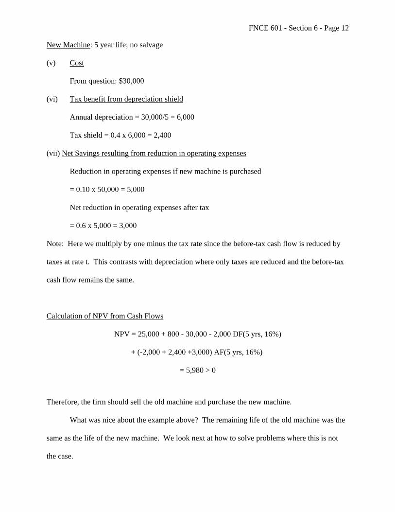
FNCE 601 - Section 6 - Page 12
New Machine: 5 year life; no salvage
(v) Cost
From question: $30,000
(vi) Tax benefit from depreciation shield
Annual depreciation = 30,000/5 = 6,000
Tax shield = 0.4 x 6,000 = 2,400
(vii) Net Savings resulting from reduction in operating expenses
Reduction in operating expenses if new machine is purchased
= 0.10 x 50,000 = 5,000
Net reduction in operating expenses after tax
= 0.6 x 5,000 = 3,000
Note: Here we multiply by one minus the tax rate since the before-tax cash flow is reduced by
taxes at rate t. This contrasts with depreciation where only taxes are reduced and the before-tax
cash flow remains the same.
Calculation of NPV from Cash Flows
NPV = 25,000 + 800 - 30,000 - 2,000 DF(5 yrs, 16%)
+ (-2,000 + 2,400 +3,000) AF(5 yrs, 16%)
= 5,980 > 0
Therefore, the firm should sell the old machine and purchase the new machine.
What was nice about the example above? The remaining life of the old machine was the
same as the life of the new machine. We look next at how to solve problems where this is not
the case.
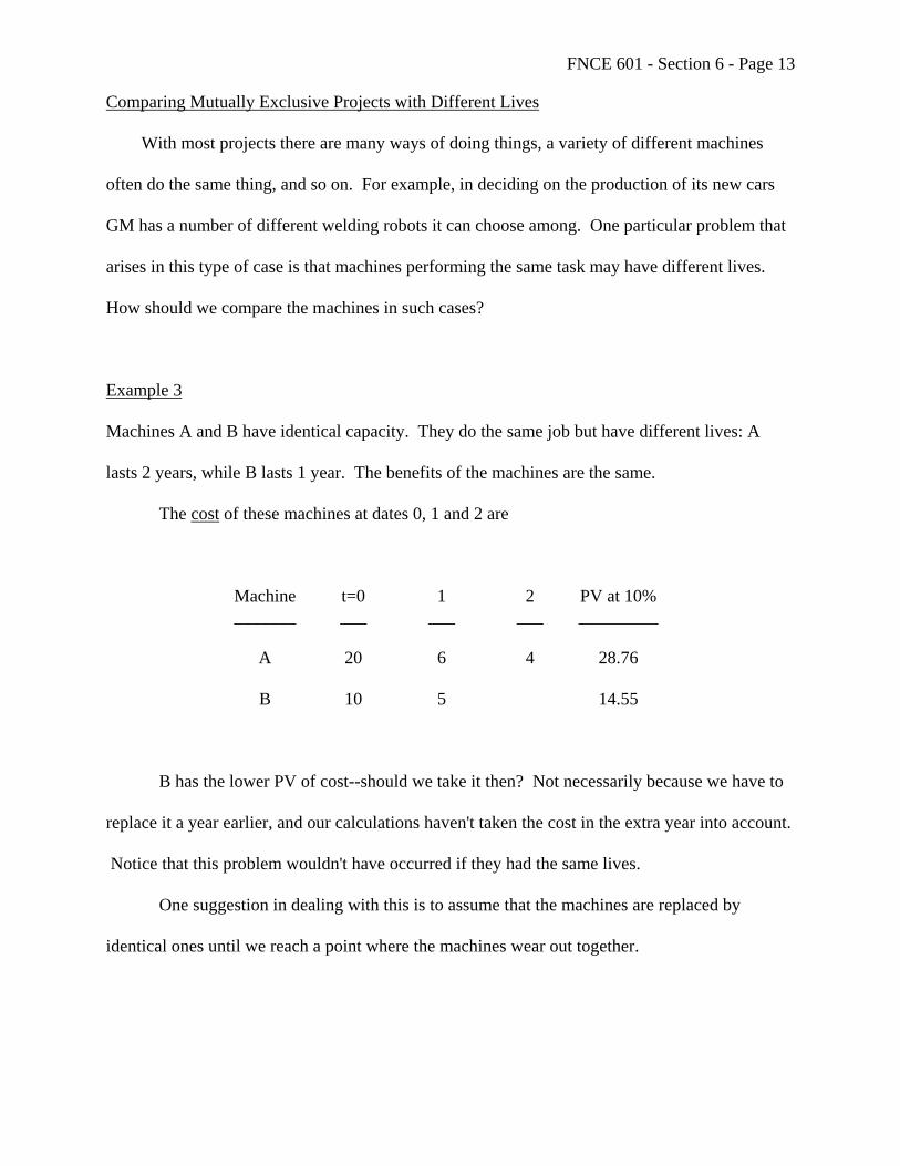
FNCE 601 - Section 6 - Page 13
Comparing Mutually Exclusive Projects with Different Lives
With most projects there are many ways of doing things, a variety of different machines
often do the same thing, and so on. For example, in deciding on the production of its new cars
GM has a number of different welding robots it can choose among. One particular problem that
arises in this type of case is that machines performing the same task may have different lives.
How should we compare the machines in such cases?
Example 3
Machines A and B have identical capacity. They do the same job but have different lives: A
lasts 2 years, while B lasts 1 year. The benefits of the machines are the same.
The cost of these machines at dates 0, 1 and 2 are
Machine t=0 1 2 PV at 10% _______ ___ ___ ___ _________
A 20 6 4 28.76
B 10 5 14.55
B has the lower PV of cost--should we take it then? Not necessarily because we have to
replace it a year earlier, and our calculations haven't taken the cost in the extra year into account.
Notice that this problem wouldn't have occurred if they had the same lives.
One suggestion in dealing with this is to assume that the machines are replaced by
identical ones until we reach a point where the machines wear out together.
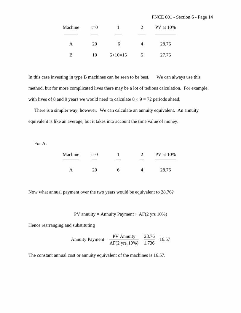
FNCE 601 - Section 6 - Page 14
Machine t=0 1 2 PV at 10% ______ ___ ___ ___ _________
A 20 6 4 28.76
B 10 5+10=15 5 27.76
In this case investing in type B machines can be seen to be best. We can always use this
method, but for more complicated lives there may be a lot of tedious calculation. For example,
with lives of 8 and 9 years we would need to calculate 8 × 9 = 72 periods ahead.
There is a simpler way, however. We can calculate an annuity equivalent. An annuity
equivalent is like an average, but it takes into account the time value of money.
For A:
Machine t=0 1 2 PV at 10% _______ __ __ __ _________
A 20 6 4 28.76
Now what annual payment over the two years would be equivalent to 28.76?
PV annuity = Annuity Payment × AF(2 yrs 10%)
Hence rearranging and substituting
57.16736.1
76.28%)10,yrs2(AF
AnnuityPVPaymentAnnuity ===
The constant annual cost or annuity equivalent of the machines is 16.57.

FNCE 601 - Section 6 - Page 15
t=0 1 2 PV at 10% ___ ___ ___ _________
A 20 6 4 28.76
Annuity 16.57 16.57 28.76
Hence 16.57 is the annuity equivalent of the cost stream of A.
For B,
Annuity Payment = 14.55/0.909 = 16.005
Hence the annuity equivalent, or the equivalent annual cost, of B is 16.005.
t=0 1 PV at 10% __ __ _________
B 10 5 14.55
Annuity 16.005 14.55
In this case 16.005 < 16.57, so again B is preferable.
The annuity equivalent allows us to calculate the constant annual cost of the machines,
and we can compare them on this basis.
Do you think this would be a good methodology for personal computers? Probably not.
Why? What's the implicit assumption here about technological change? We're implicitly
assuming there's no technological change. If there were rapid technological change you'd have
to take that into account by going back to our original overlapping method.
Working Capital
As discussed above, when a new project is undertaken it may take a while for customers to
pay on new sales, i.e. the accounts receivable will increase. The amount of cash that the firm
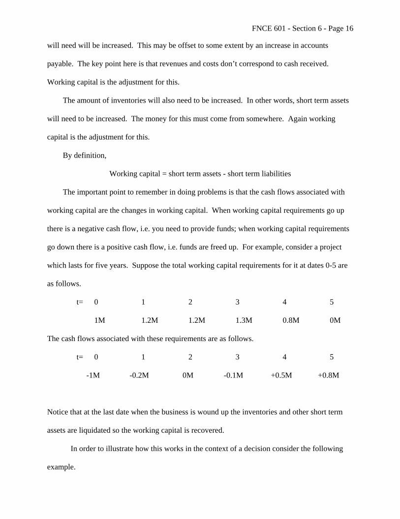
FNCE 601 - Section 6 - Page 16
will need will be increased. This may be offset to some extent by an increase in accounts
payable. The key point here is that revenues and costs don’t correspond to cash received.
Working capital is the adjustment for this.
The amount of inventories will also need to be increased. In other words, short term assets
will need to be increased. The money for this must come from somewhere. Again working
capital is the adjustment for this.
By definition,
Working capital = short term assets - short term liabilities
The important point to remember in doing problems is that the cash flows associated with
working capital are the changes in working capital. When working capital requirements go up
there is a negative cash flow, i.e. you need to provide funds; when working capital requirements
go down there is a positive cash flow, i.e. funds are freed up. For example, consider a project
which lasts for five years. Suppose the total working capital requirements for it at dates 0-5 are
as follows.
t= 0 1 2 3 4 5
1M 1.2M 1.2M 1.3M 0.8M 0M
The cash flows associated with these requirements are as follows.
t= 0 1 2 3 4 5
-1M -0.2M 0M -0.1M +0.5M +0.8M
Notice that at the last date when the business is wound up the inventories and other short term
assets are liquidated so the working capital is recovered.
In order to illustrate how this works in the context of a decision consider the following
example.

FNCE 601 - Section 6 - Page 17
Example 4 The Wharton Olympics Corporation is considering whether to build a new bakery to make
cherry pies. The current date is 12/31/X5. The new bakery will be built over two years and will
be ready to start production on 1/1/X8 and will cease production on 12/31/X9. The investment
for the bakery requires an outlay of $2.5M on 12/31/X5. This expenditure can be depreciated
using straight line depreciation over the two years the bakery is producing. The total salvage
value of all the plant and equipment on 12/31/X9 is expected to be $800,000. The land the
bakery will be built on could be rented out for $200,000 per year before taxes for the four years
from 12/31/X5-12/31/X9 while the bakery is being built and is in production. The bakery will
produce 1.2 million cherry pies per year. These can be sold at $7 per pie. Raw material costs
are $1.20 per pie and the total labor costs are $420,000 per year. These revenues and costs are
expected to be the same for the two years the bakery is in production. The total working capital
required 12/31/X7 to allow inventories to be financed during the first year of production is
$300,000. For the second year the total working capital needs will be 10% higher. When the
plant ceases production all the working capital can be recovered. The firm has a corporate tax
rate of 35 percent. The opportunity cost of capital for the project if it is all equity financed is 12
percent. Assume all cash flows occur at year's end and that the firm has other profitable ongoing
operations.
Solution The table of cash flows for the problem is as follows.

FNCE 601 - Section 6 - Page 18
Item 12/31/X5 12/31/X6 12/31/X7 12/31/X8 12/31/X9 1. Investment -2.5M 2. Salvage Value 0.8M 3. Depr. tax shield 297,500 297,500 [i.e. 0.35(2.5M-0.8M)/2] 4. After tax land rental -130,000 -130,000 -130,000 -130,000 [i.e. -0.65(200,000)] 5. Revenues [i.e. 7(1.2M)] 8.4M 8.4M 6. Raw materials [i.e. 1.2(1.2M)] 1.44M 1.44M 7. Labor costs 0.42M 0.42M 8. Before-tax operating profit 6.54M 6.54M [i.e. line 5 - line 6 - line 7] 9. After-tax operating profit 4.251M 4.251M [i.e. 0.65 x line 8] 10. Total working capital needs 300,000 330,000 0 11. Working capital cash flow -300,000 -30,000 +330,000 12. After tax -2.5M -130,000 -430,000 4.3885M 5.5485M cash flows [i.e. sum of lines 1-4, 9 and 11]
M69.3$121.
5.5485 + 121.
4.3885M + 121.
0.43M - 1.12
0.13M -2.5M - = NPV432=
Finally, consider two more examples to give you some more experience.

FNCE 601 - Section 6 - Page 19
Example 5
Nippon Auto intends to replace one of its plants in the US. It has two mutually exclusive
options. The first, which is codenamed Plan A, is to build a plant on its existing site in Indiana. The
plant will be built on land the company already owns. It is estimated that the land could be currently
sold for an after tax amount of $10 million. Under Plan A the cost of the new plant would be $100
million to be paid now. It is expected to have a life of 15 years and a salvage value of $25 million.
The land can be sold after the fifteen years for an after tax amount of $12 million. Revenues and
costs at the end of the first year are expected to be $30 million and $6 million, respectively. Both are
expected to stay constant for the life of the plant. The second option, which is codenamed Plan B, is
to build a new plant in Alabama. If they choose to do this they will have to buy the land for an after
tax amount of $10 million. The plant will cost $70 million and last for 10 years. At the end of that
time it will have a salvage value of zero and the land can be sold for an after tax amount of $10
million. Revenues and costs at the end of the first year are expected to be $27 million and $6
million, respectively. Both are expected to stay constant for the life of the plant. All figures are in
nominal terms and are stated in before tax terms unless otherwise indicated. The firm uses straight
line depreciation and has a tax rate of 35 percent. It has profitable ongoing operations and an
opportunity cost of capital of 12 percent. Which plant should be chosen if it is anticipated that it will
be replaced by a plant with identical cash flows and this will be repeated for the foreseeable future?
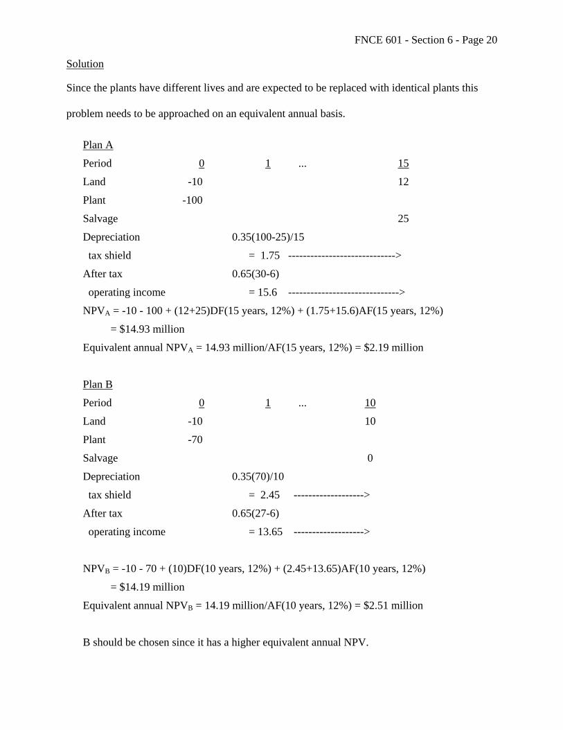
FNCE 601 - Section 6 - Page 20
Solution Since the plants have different lives and are expected to be replaced with identical plants this
problem needs to be approached on an equivalent annual basis.
Plan A
Period 0 1 ... 15
Land -10 12
Plant -100
Salvage 25
Depreciation 0.35(100-25)/15
tax shield = 1.75 ----------------------------->
After tax 0.65(30-6)
operating income = 15.6 ------------------------------>
NPVA = -10 - 100 + (12+25)DF(15 years, 12%) + (1.75+15.6)AF(15 years, 12%)
= $14.93 million
Equivalent annual NPVA = 14.93 million/AF(15 years, 12%) = $2.19 million
Plan B
Period 0 1 ... 10
Land -10 10
Plant -70
Salvage 0
Depreciation 0.35(70)/10
tax shield = 2.45 ------------------->
After tax 0.65(27-6)
operating income = 13.65 ------------------->
NPVB = -10 - 70 + (10)DF(10 years, 12%) + (2.45+13.65)AF(10 years, 12%)
= $14.19 million
Equivalent annual NPVB = 14.19 million/AF(10 years, 12%) = $2.51 million
B should be chosen since it has a higher equivalent annual NPV.
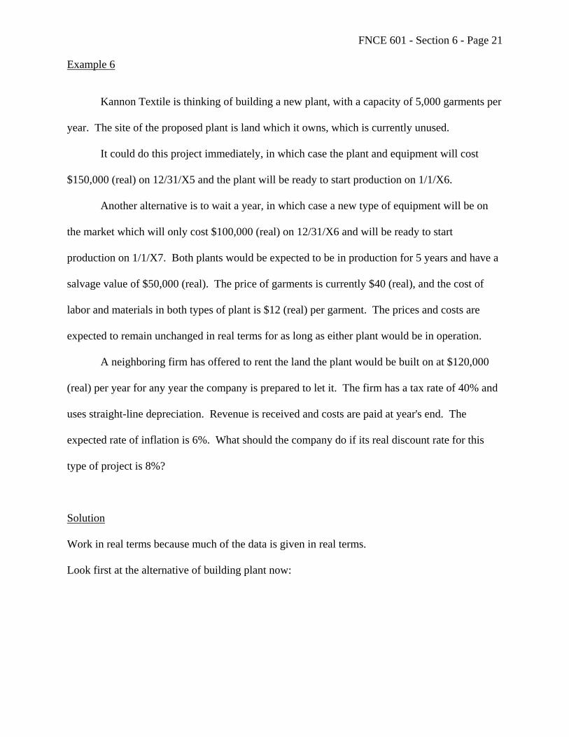
FNCE 601 - Section 6 - Page 21
Example 6
Kannon Textile is thinking of building a new plant, with a capacity of 5,000 garments per
year. The site of the proposed plant is land which it owns, which is currently unused.
It could do this project immediately, in which case the plant and equipment will cost
$150,000 (real) on 12/31/X5 and the plant will be ready to start production on 1/1/X6.
Another alternative is to wait a year, in which case a new type of equipment will be on
the market which will only cost $100,000 (real) on 12/31/X6 and will be ready to start
production on 1/1/X7. Both plants would be expected to be in production for 5 years and have a
salvage value of $50,000 (real). The price of garments is currently $40 (real), and the cost of
labor and materials in both types of plant is $12 (real) per garment. The prices and costs are
expected to remain unchanged in real terms for as long as either plant would be in operation.
A neighboring firm has offered to rent the land the plant would be built on at $120,000
(real) per year for any year the company is prepared to let it. The firm has a tax rate of 40% and
uses straight-line depreciation. Revenue is received and costs are paid at year's end. The
expected rate of inflation is 6%. What should the company do if its real discount rate for this
type of project is 8%?
Solution
Work in real terms because much of the data is given in real terms. Look first at the alternative of building plant now:
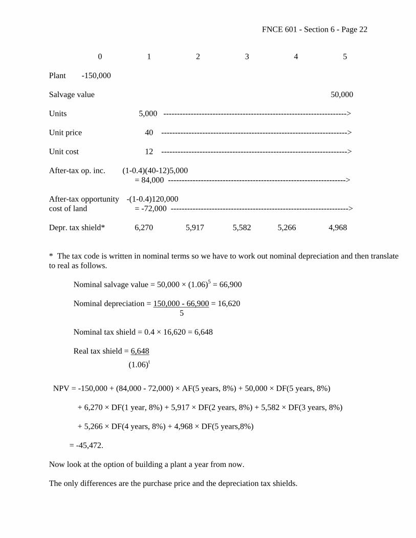
FNCE 601 - Section 6 - Page 22
0 1 2 3 4 5 Plant -150,000 Salvage value 50,000 Units 5,000 -------------------------------------------------------------------> Unit price 40 --------------------------------------------------------------------> Unit cost 12 --------------------------------------------------------------------> After-tax op. inc. (1-0.4)(40-12)5,000 = 84,000 -----------------------------------------------------------------> After-tax opportunity -(1-0.4)120,000 cost of land = -72,000 -----------------------------------------------------------------> Depr. tax shield* 6,270 5,917 5,582 5,266 4,968 * The tax code is written in nominal terms so we have to work out nominal depreciation and then translate to real as follows. Nominal salvage value = 50,000 × (1.06)5 = 66,900 Nominal depreciation = 150,000 - 66,900 = 16,620 5 Nominal tax shield = 0.4 × 16,620 = 6,648 Real tax shield = 6,648
(1.06)t
NPV = -150,000 + (84,000 - 72,000) × AF(5 years, 8%) + 50,000 × DF(5 years, 8%)
+ 6,270 × DF(1 year, 8%) + 5,917 × DF(2 years, 8%) + 5,582 × DF(3 years, 8%) + 5,266 × DF(4 years, 8%) + 4,968 × DF(5 years,8%)
= -45,472. Now look at the option of building a plant a year from now. The only differences are the purchase price and the depreciation tax shields.
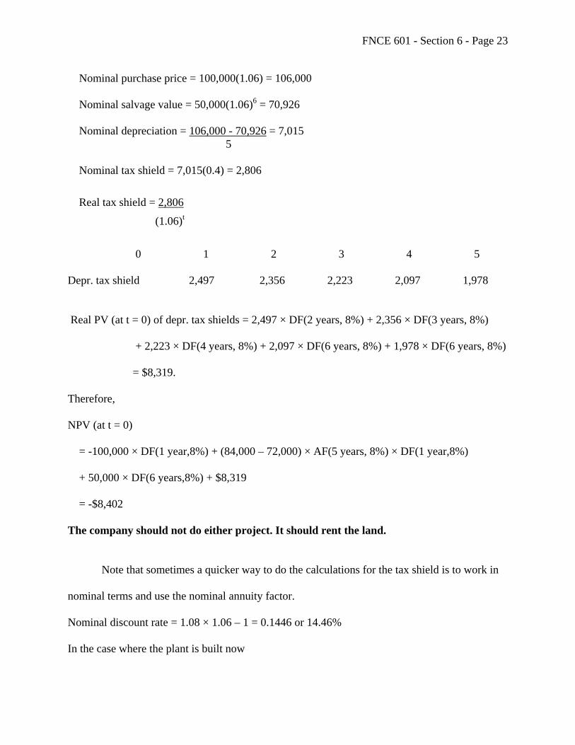
FNCE 601 - Section 6 - Page 23
Nominal purchase price = 100,000(1.06) = 106,000 Nominal salvage value = 50,000(1.06)6 = 70,926 Nominal depreciation = 106,000 - 70,926 = 7,015 5 Nominal tax shield = 7,015(0.4) = 2,806
Real tax shield = 2,806
(1.06)t
0 1 2 3 4 5 Depr. tax shield 2,497 2,356 2,223 2,097 1,978 Real PV (at t = 0) of depr. tax shields = 2,497 × DF(2 years, 8%) + 2,356 × DF(3 years, 8%)
+ 2,223 × DF(4 years, 8%) + 2,097 × DF(6 years, 8%) + 1,978 × DF(6 years, 8%) = $8,319. Therefore, NPV (at t = 0) = -100,000 × DF(1 year,8%) + (84,000 – 72,000) × AF(5 years, 8%) × DF(1 year,8%) + 50,000 × DF(6 years,8%) + $8,319 = -$8,402 The company should not do either project. It should rent the land.
Note that sometimes a quicker way to do the calculations for the tax shield is to work in
nominal terms and use the nominal annuity factor. Nominal discount rate = 1.08 × 1.06 – 1 = 0.1446 or 14.46% In the case where the plant is built now

FNCE 601 - Section 6 - Page 24
PV of tax shield at date 0 = 6,648 × AF(5 years, 14.46%) NPV = -150,000 + (84,000 - 72,000) × AF(5 years, 8%) + 50,000 × DF(5 years, 8%) + 6,648 × AF(5 years, 14.46%) = -45,472. For the alternative where the plant is built 1 year from now PV of tax shield = 2,806 × AF(5 years, 14.46%) × DF(1 year, 14.46%) = 8,319 This may be a slightly quicker method in some circumstances.
Conclusion
This brings us to the end of Section 6 of the course. By this time I hope you have a good
understanding of how to do NPV calculations. If you don't understand what's going on, now is
the time to find out. If you have any problems, come and see me.
So far we have sidestepped the question of uncertainty and this is what we come to next.

INTENTIONALLY BLANK
UNIVERSITY OF PENNSYLVANIA THE WHARTON SCHOOL FNCE 601 FINANCIAL ANALYSIS CORPORATE FINANCE Franklin Allen Fall 2004 QUARTER 1 - WEEK 4 (part 2) and Week 5 (part 1) Th: 9/30/04 and Tu: 10/5/04 Copyright © 2004 by Franklin Allen
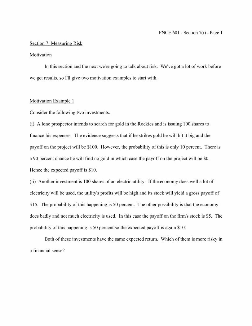
FNCE 601 - Section 7(i) - Page 1
Section 7: Measuring Risk
Motivation
In this section and the next we're going to talk about risk. We've got a lot of work before
we get results, so I'll give two motivation examples to start with.
Motivation Example 1
Consider the following two investments.
(i) A lone prospector intends to search for gold in the Rockies and is issuing 100 shares to
finance his expenses. The evidence suggests that if he strikes gold he will hit it big and the
payoff on the project will be $100. However, the probability of this is only 10 percent. There is
a 90 percent chance he will find no gold in which case the payoff on the project will be $0.
Hence the expected payoff is $10.
(ii) Another investment is 100 shares of an electric utility. If the economy does well a lot of
electricity will be used, the utility's profits will be high and its stock will yield a gross payoff of
$15. The probability of this happening is 50 percent. The other possibility is that the economy
does badly and not much electricity is used. In this case the payoff on the firm's stock is $5. The
probability of this happening is 50 percent so the expected payoff is again $10.
Both of these investments have the same expected return. Which of them is more risky in
a financial sense?

FNCE 601 - Section 7(i) - Page 2
Motivation Example 2
Suppose T-bills are yielding 4%. Is it ever worthwhile investing in a risky stock yielding
a total return (i.e. including dividends and capital gains) of 3%?
What we're going to do over the next two weeks or so is derive a formula for risk
adjusted discount rates of the form
r = rF + β(rM - rF)
where
rF - risk free rate (e.g., T-bill rate)
rM - return on market portfolio (e.g., a value-weighted portfolio of all stocks on the NYSE)
β = Measure of risk = Cov (Stock, Market portfolio) Var (Market portfolio)
Notice that what's important in the measure of risk is covariance with the market
portfolio. You can see from this why we get the results that we do in the motivation examples.
Understanding why covariances matter is the core concept in understanding risk. It is not a
simple idea and we have a lot of ground to cover before you have a full intuitive understanding
of the CAPM and these examples.
Section 7(i): Historical and Statistical Review
Before we go on to deal with risk and asset pricing risk we should start with a brief
historical and statistical review.
The appendix at the end of the section starts with historical data for the US. The first
figure (from the Stocks, Bonds, Bills and Inflation Yearbook for 2003 published by Ibbotson
FNCE 601 - Section 7(i) - Page 3
Associates) shows that there is a vast difference between the returns on different investments.
The second thing to notice is the amount you would have had at the end of 2002 if you had
invested $1 at the beginning of 1926 in various financial instruments. Small stocks in particular
have done very well. Common stocks have also done well. Both have done vastly better than
bonds and bills in the long run. The table on the next page shows this data in a tabular rather
than diagrammatic form.
Jeremy Siegel in his book Stocks for the Long Run has argued that in the short run stocks
and small stocks are much more risky but in the long run (meaning 20 years or more) they are
not so risky and almost always do better than bonds in this period. This view has been criticized
by many because it is based on long run data from one country, the US. In a recent study
Dimson, Marsh and Staunton (2003) have shown that the US experience is an outlier (see
Chapter 3 of their study which is posted on the course website). The next table in the appendix
shows the real return (i.e. taking out the effects of inflation) from investing 1 unit at the end of
1900 and reinvesting all returns until the end of 2003 for stocks and bonds in various places.
Out of 16 countries only three, South Africa, Sweden and Australia did better. The US did better
than the 12 other countries. The next two tables show the same data in terms of geometric and
arithmetic mean returns and the standard deviations. These figures suggest the return on stocks
are not as high as an analysis of the US alone would suggest.
How can these figures be understood? For example, why do different asset classes have
different risks and returns? In order to measure the relationship between risk and return and
develop models which can help us understand what is going on we need some formal statistical
measures.
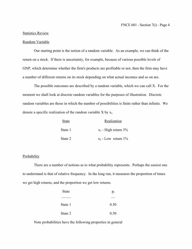
FNCE 601 - Section 7(i) - Page 4
Statistics Review
Random Variable
Our starting point is the notion of a random variable. As an example, we can think of the
return on a stock. If there is uncertainty, for example, because of various possible levels of
GNP, which determine whether the firm's products are profitable or not, then the firm may have
a number of different returns on its stock depending on what actual incomes and so on are.
The possible outcomes are described by a random variable, which we can call X. For the
moment we shall look at discrete random variables for the purposes of illustration. Discrete
random variables are those in which the number of possibilities is finite rather than infinite. We
denote a specific realization of the random variable X by xi.
State Realization
State 1 x1 - High return 3%
State 2 x2 - Low return 1%
Probability
There are a number of notions as to what probability represents. Perhaps the easiest one
to understand is that of relative frequency. In the long run, it measures the proportion of times
we get high returns, and the proportion we get low returns.
State pi _____ __
State 1 0.50
State 2 0.50
Note probabilities have the following properties in general
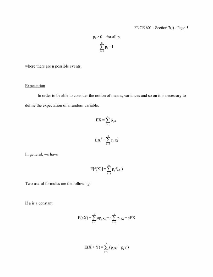
FNCE 601 - Section 7(i) - Page 5
1 = p i
n
1 = i∑
pi ≥ 0 for all pi
where there are n possible events.
Expectation
In order to be able to consider the notion of means, variances and so on it is necessary to
define the expectation of a random variable.
xp = EX ii
n
1 = i∑
xp = EX 2
ii
n
1 = i
2 ∑
In general, we have
)xf(p = ]f(X)[E ii
n
1 = i∑
Two useful formulas are the following:
If a is a constant
aEX = xp a = xap = E(aX) ii
n
1 = iii
n
1 = i∑∑
)yp + xp( = Y)+ E(X iiii
n
1 = i∑
FNCE 601 - Section 7(i) - Page 6
EY+ EX= yp + xp = ii
n
1 = iii
n
1 = i∑∑
The Arithmetic Mean or Average
The first notion we are interested in is the arithmetic mean or average. This is given by
∑ === XxpEXMean ii
e.g.,
EX = 0.5(3) + 0.5(1) = 2%
If you look at the second table on the handout you can see that it gives estimates for the
arithmetic mean of the returns on various financial instruments. Why are these arithmetic means
of interest? They give the best estimate of the mean return if we had invested for a year during
that period.
Variance
We are not only interested in the average value, we are also interested in how much
returns vary. For example, if you invested the money for your tuition this semester last year you
presumably would have liked to know how variable the returns would likely have been. If you
had invested in short term government instruments you could have been fairly sure of meeting
your tuition payment. If you had put it in stocks you might have made a lot of money or you
could have lost a lot of money. To measure variability we use variance
)X - x(p = )X - E(X= = Variance 2
ii
n
1 = i
22X ∑σ
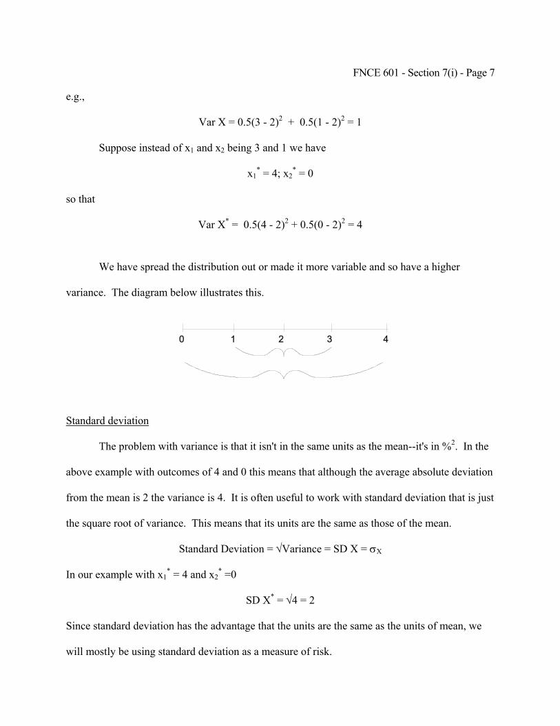
FNCE 601 - Section 7(i) - Page 7
e.g.,
Var X = 0.5(3 - 2)2 + 0.5(1 - 2)2 = 1
Suppose instead of x1 and x2 being 3 and 1 we have
x1* = 4; x2
* = 0
so that
Var X* = 0.5(4 - 2)2 + 0.5(0 - 2)2 = 4
We have spread the distribution out or made it more variable and so have a higher
variance. The diagram below illustrates this.
Standard deviation
The problem with variance is that it isn't in the same units as the mean--it's in %2. In the
above example with outcomes of 4 and 0 this means that although the average absolute deviation
from the mean is 2 the variance is 4. It is often useful to work with standard deviation that is just
the square root of variance. This means that its units are the same as those of the mean.
Standard Deviation = √Variance = SD X = σX
In our example with x1* = 4 and x2
* =0
SD X* = √4 = 2
Since standard deviation has the advantage that the units are the same as the units of mean, we
will mostly be using standard deviation as a measure of risk.
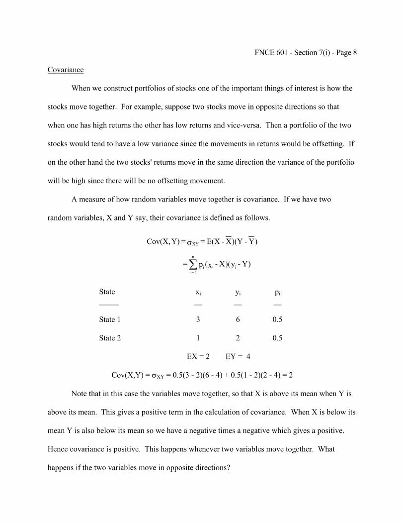
FNCE 601 - Section 7(i) - Page 8
Covariance
When we construct portfolios of stocks one of the important things of interest is how the
stocks move together. For example, suppose two stocks move in opposite directions so that
when one has high returns the other has low returns and vice-versa. Then a portfolio of the two
stocks would tend to have a low variance since the movements in returns would be offsetting. If
on the other hand the two stocks' returns move in the same direction the variance of the portfolio
will be high since there will be no offsetting movement.
A measure of how random variables move together is covariance. If we have two
random variables, X and Y say, their covariance is defined as follows.
)Y - )(YX - E(X= = Y)Cov(X, XYσ
)Y - y)(X - x(p = iii
n
1 = i∑
State xi yi pi _____ __ __ __
State 1 3 6 0.5
State 2 1 2 0.5
EX = 2 EY = 4
Cov(X,Y) = σXY = 0.5(3 - 2)(6 - 4) + 0.5(1 - 2)(2 - 4) = 2
Note that in this case the variables move together, so that X is above its mean when Y is
above its mean. This gives a positive term in the calculation of covariance. When X is below its
mean Y is also below its mean so we have a negative times a negative which gives a positive.
Hence covariance is positive. This happens whenever two variables move together. What
happens if the two variables move in opposite directions?

FNCE 601 - Section 7(i) - Page 9
Example 2
State xi yi pi _____ __ __ __
State 1 3 2 0.5
State 2 1 6 0.5
EX = 2 EY = 4
COV(X,Y) = σXY = 0.5(3 - 2)(2 - 4) + 0.5(1 - 2)(6 - 4) = -2
In this case we have a negative covariance. This is because when X is above its mean Y
is below its mean and vice-versa so in each term we have a positive times a negative which gives
a negative. Thus when variables move in opposite directions they have a negative covariance.
If they are independent and don't tend to move around together or in opposite directions,
then we get some positive terms and some negative terms. When there is no systematic
relationship at all these positive and negative terms tend to cancel out and we get a zero
covariance. When two random variables are independent they have zero covariance.
Correlation
One of the problems with covariance is that its magnitude depends on the units of
measurement. It is not possible to simply deduce from the size of the number how much they
move together. A concept that allows us to do this is the correlation coefficient.
Correlation Coefficient = Corr(X,Y) = ρXY = Cov(X,Y) _____________ SD X × SD Y
Now it can be shown
-1 ≤ ρXY ≤ +1
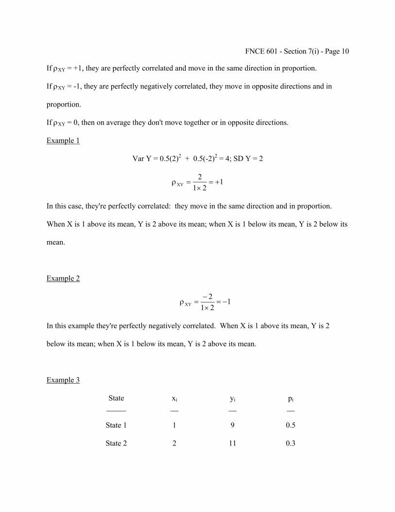
FNCE 601 - Section 7(i) - Page 10
If ρXY = +1, they are perfectly correlated and move in the same direction in proportion.
If ρXY = -1, they are perfectly negatively correlated, they move in opposite directions and in
proportion.
If ρXY = 0, then on average they don't move together or in opposite directions.
Example 1
Var Y = 0.5(2)2 + 0.5(-2)2 = 4; SD Y = 2
121
2XY +=
×=ρ
In this case, they're perfectly correlated: they move in the same direction and in proportion.
When X is 1 above its mean, Y is 2 above its mean; when X is 1 below its mean, Y is 2 below its
mean.
Example 2
1212
XY −=×−
=ρ
In this example they're perfectly negatively correlated. When X is 1 above its mean, Y is 2
below its mean; when X is 1 below its mean, Y is 2 above its mean.
Example 3
State xi yi pi _____ __ __ __
State 1 1 9 0.5
State 2 2 11 0.3
FNCE 601 - Section 7(i) - Page 11
State 3 3 25 0.2
EX = 1.7 EY = 12.8
SD X = 0.781 SD Y = 6.161
Cov(X,Y) = 0.5(1 - 1.7)(9 - 12.8) + 0.3(2 - 1.7)(11 - 12.8)
+ 0.2(3 - 1.7)(25 - 12.8) = 4.34
902.0161.6781.0
34.4XY =
×=ρ
In this case, in state 1when X is 1 – 1.7 = - 0.7 from the average, Y is 9 - 12.8 = -3.8 from
the average; in state 2 when X is 2 – 1.7 = +0.3 from the average, Y is 11 – 12.8 = -1.8 from the
average; in state 3 when X is 3 – 1.7 = +1.3 from the average, Y is 25 – 12.8 = +12.2 from the
average. Thus when one goes up, the other tends to go up, but doesn't always do so. Hence ρXY
is positive but less than one.
Evidence on Covariance and Correlation
As far as the empirical evidence is concerned there are two important conclusions that
can be drawn from the data:
(i) Stock returns are serially uncorrelated or in other words if stock returns are high one year
then you can't use this information to predict whether returns in the subsequent year will be high
or low. This evidence will be important when we talk about market efficiency later in the
course. However, for the moment the one conclusion that is relevant as far as models of asset
pricing is concerned is:
(ii) Within a period most stocks are positively correlated to the market portfolio (e.g. a value-
weighted portfolio of all the stocks on the NYSE).
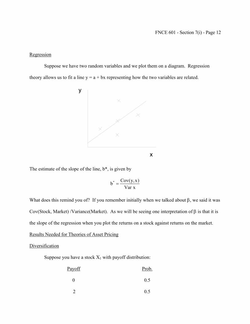
FNCE 601 - Section 7(i) - Page 12
Regression
Suppose we have two random variables and we plot them on a diagram. Regression
theory allows us to fit a line y = a + bx representing how the two variables are related.
The estimate of the slope of the line, b*, is given by
xVar)x,y(Covb* =
What does this remind you of? If you remember initially when we talked about β, we said it was
Cov(Stock, Market) /Variance(Market). As we will be seeing one interpretation of β is that it is
the slope of the regression when you plot the returns on a stock against returns on the market.
Results Needed for Theories of Asset Pricing
Diversification
Suppose you have a stock X1 with payoff distribution:
Payoff Prob.
0 0.5
2 0.5
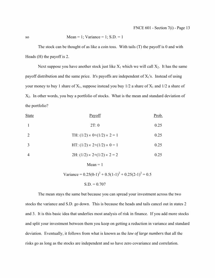
FNCE 601 - Section 7(i) - Page 13
so Mean = 1; Variance = 1; S.D. = 1
The stock can be thought of as like a coin toss. With tails (T) the payoff is 0 and with
Heads (H) the payoff is 2.
Next suppose you have another stock just like X1 which we will call X2. It has the same
payoff distribution and the same price. It's payoffs are independent of X1's. Instead of using
your money to buy 1 share of X1, suppose instead you buy 1/2 a share of X1 and 1/2 a share of
X2. In other words, you buy a portfolio of stocks. What is the mean and standard deviation of
the portfolio?
State Payoff Prob.
1 2T: 0 0.25
2 TH: (1/2) × 0+(1/2) × 2 = 1 0.25
3 HT: (1/2) × 2+(1/2) × 0 = 1 0.25
4 2H: (1/2) × 2+(1/2) × 2 = 2 0.25
Mean = 1
Variance = 0.25(0-1)2 + 0.5(1-1)2 + 0.25(2-1)2 = 0.5
S.D. = 0.707
The mean stays the same but because you can spread your investment across the two
stocks the variance and S.D. go down. This is because the heads and tails cancel out in states 2
and 3. It is this basic idea that underlies most analysis of risk in finance. If you add more stocks
and split your investment between them you keep on getting a reduction in variance and standard
deviation. Eventually, it follows from what is known as the law of large numbers that all the
risks go as long as the stocks are independent and so have zero covariance and correlation.

FNCE 601 - Section 7(i) - Page 14
Nonzero covariance and correlation
Next consider what happens if the two stocks X1 and X2 are perfectly negatively
correlated i.e. ρ = -1. In that case what happens to the portfolio mean, variance and standard
deviation?
State Payoff Prob.
1 2T: 0 0
2 TH: (1/2) × 0+(1/2) × 2 = 1 0.5
3 HT: (1/2) × 2+(1/2) × 0 = 1 0.5
4 2H: (1/2) × 2+(1/2) × 2 = 2 0
Mean = 1
Variance = 0(0-1)2 + 1(1-1)2 + 0(2-1)2 = 0
S.D. = 0
Here you can never get two tails or two heads you always get one head and one tail. Risk
is completely eliminated. In terms of the probability distribution you are putting all the weight
on the mean at 1.
What would happen if you had a negative correlation with -1 < ρ < 0? This case lies in
between the two cases above. For example, if having obtained 1 T the probability of a second T
is 0.25 and similarly having obtained 1 H the probability of a second is also 0.25 it can be shown
the distribution of payoffs is as below and it can be straightforwardly checked the correlation is -
0.5.
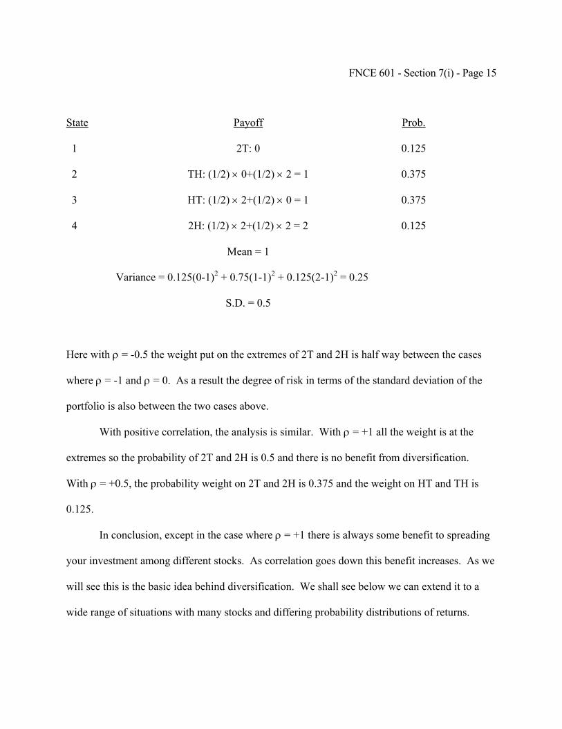
FNCE 601 - Section 7(i) - Page 15
State Payoff Prob.
1 2T: 0 0.125
2 TH: (1/2) × 0+(1/2) × 2 = 1 0.375
3 HT: (1/2) × 2+(1/2) × 0 = 1 0.375
4 2H: (1/2) × 2+(1/2) × 2 = 2 0.125
Mean = 1
Variance = 0.125(0-1)2 + 0.75(1-1)2 + 0.125(2-1)2 = 0.25
S.D. = 0.5
Here with ρ = -0.5 the weight put on the extremes of 2T and 2H is half way between the cases
where ρ = -1 and ρ = 0. As a result the degree of risk in terms of the standard deviation of the
portfolio is also between the two cases above.
With positive correlation, the analysis is similar. With ρ = +1 all the weight is at the
extremes so the probability of 2T and 2H is 0.5 and there is no benefit from diversification.
With ρ = +0.5, the probability weight on 2T and 2H is 0.375 and the weight on HT and TH is
0.125.
In conclusion, except in the case where ρ = +1 there is always some benefit to spreading
your investment among different stocks. As correlation goes down this benefit increases. As we
will see this is the basic idea behind diversification. We shall see below we can extend it to a
wide range of situations with many stocks and differing probability distributions of returns.
FNCE 601 - Section 7(i) - Page 16
Means and Variances of Portfolios
In the case above it was quite a simple task to take the individual stock returns combine
them with the (1/2) and (1/2) weights on the two stocks and work out the payoffs of the portfolio
in each state. From these portfolio payoffs we calculated the mean, variance and standard
deviation of the portfolio. As the number of states becomes larger this procedure of calculating
portfolio payoffs state by state and then calculating the statistics for the portfolio payoff
distribution becomes more and more cumbersome.
An alternative that is considerably easier is just to use the means and standard deviations
of the individual stocks and their covariances or correlations and use them to calculate the mean
and standard deviation of the portfolios. There are some useful formulas which allow us to do
this. We will be using them a lot in the coming weeks. They are derived in the appendix at the
end of the section. These formulas look fearsome but there are only two basic things to
remember.
1. MEANS ADD.
In other words if you invest half your money in stock X1 and the other half in stock X2,
the mean return of the portfolio is simply half the mean of stock X1 and half the mean of stock
X2.
FNCE 601 - Section 7(i) - Page 17
2. VARIANCES DON'T ADD - COVARIANCES MATTER.
In other words if we take the same example of half our money in stock X1 and half in
stock X2, the variance of the portfolio is not just half the variance of stock X1 and half the
variance of stock X2. The reason is that correlations play an important role too as the simple
examples above demonstrated. This is why there is a correlation or covariance term when
calculating the variance of a portfolio.
For the moment the thing to remember is means add but variances and also standard
deviations don't. We will come back to this later on and consider examples to illustrate it.
Statistical Review: Conclusion
This is all the statistics you'll basically need to know. The main thing is to have an
intuitive understanding of what they mean. Arithmetic mean is a measure of how much you can
expect to receive if you hold a stock for a year. The variance and standard deviation are
measures of how variable the returns are likely to be. The higher the variance or standard
deviation the greater the variation. Covariance and correlation are measures of whether two
variables move together or in opposite directions. If they move together covariance and
correlation are positive; if they move in opposite directions covariance and correlation are
negative and if they are independent covariance and correlation are zero. The lower the
correlation the greater the reduction in risk from putting stocks together in a portfolio.
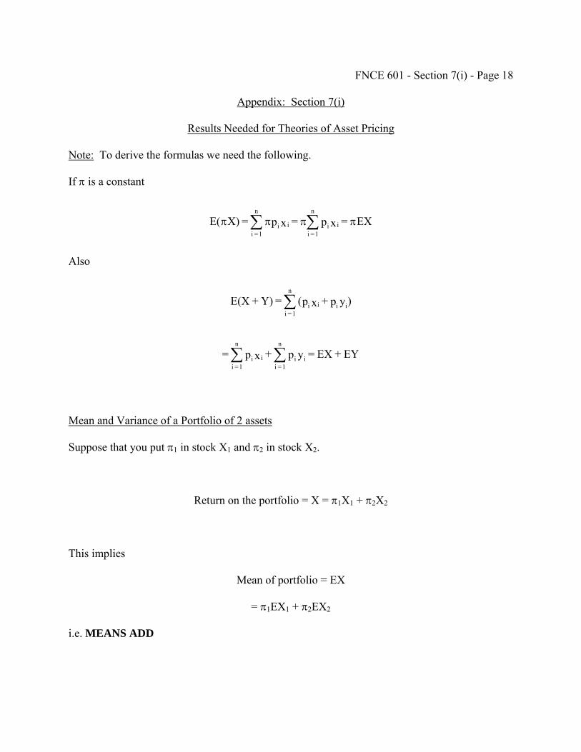
FNCE 601 - Section 7(i) - Page 18
Appendix: Section 7(i)
Results Needed for Theories of Asset Pricing
Note: To derive the formulas we need the following.
If π is a constant
EX = xp = xp = X)E( ii
n
1 = iii
n
1 = i
ππππ ∑∑
Also
)yp + xp( = Y)+ E(X iiii
n
1 = i∑
EY+ EX= yp + xp = ii
n
1 = iii
n
1 = i∑∑
Mean and Variance of a Portfolio of 2 assets
Suppose that you put π1 in stock X1 and π2 in stock X2.
Return on the portfolio = X = π1X1 + π2X2
This implies
Mean of portfolio = EX
= π1EX1 + π2EX2
i.e. MEANS ADD
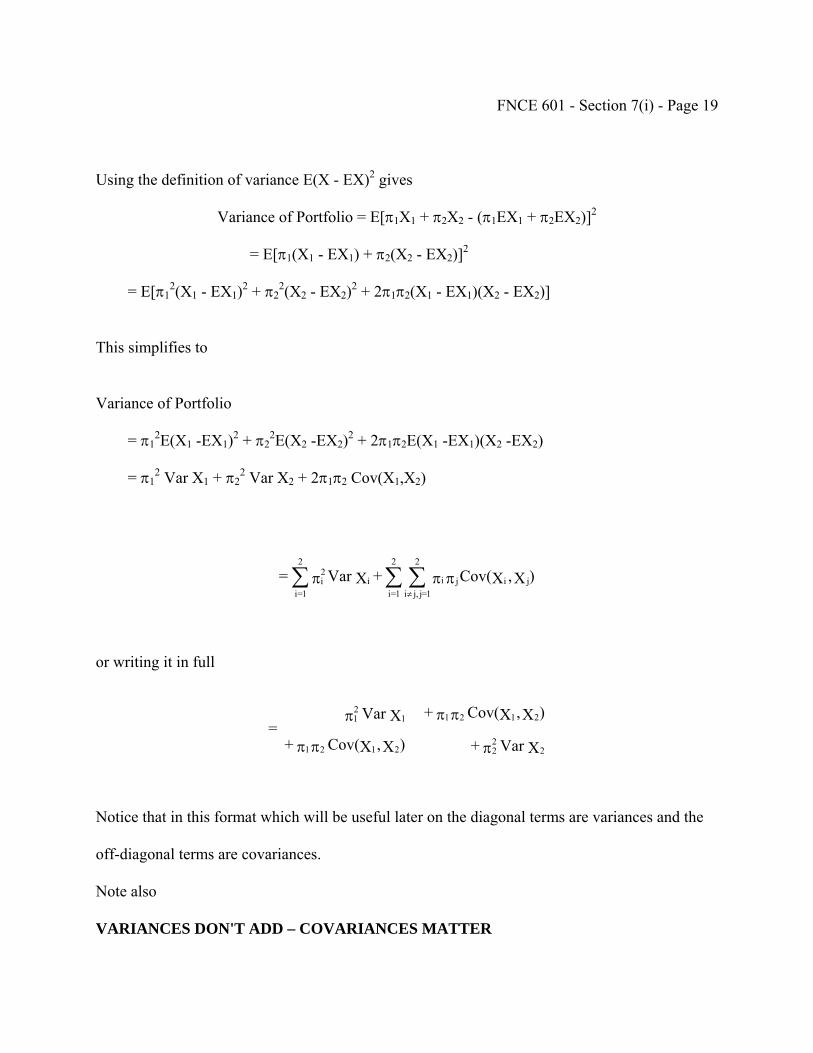
FNCE 601 - Section 7(i) - Page 19
)
Using the definition of variance E(X - EX)2 gives
Variance of Portfolio = E[π1X1 + π2X2 - (π1EX1 + π2EX2)]2
= E[π1(X1 - EX1) + π2(X2 - EX2)]2
= E[π12(X1 - EX1)2 + π2
2(X2 - EX2)2 + 2π1π2(X1 - EX1)(X2 - EX2)]
This simplifies to
Variance of Portfolio
= π12E(X1 -EX1)2 + π2
2E(X2 -EX2)2 + 2π1π2E(X1 -EX1)(X2 -EX2)
= π12 Var X1 + π2
2 Var X2 + 2π1π2 Cov(X1,X2)
X,XCov( + XVar = jiji
2
1=jj,i
2
1=ii
2i
2
1=iπππ ∑∑∑
≠
or writing it in full
XVar + )X,XCov( +
)X,XCov( + XVar =
2222121
2121121
πππ
πππ
Notice that in this format which will be useful later on the diagonal terms are variances and the
off-diagonal terms are covariances.
Note also
VARIANCES DON'T ADD – COVARIANCES MATTER
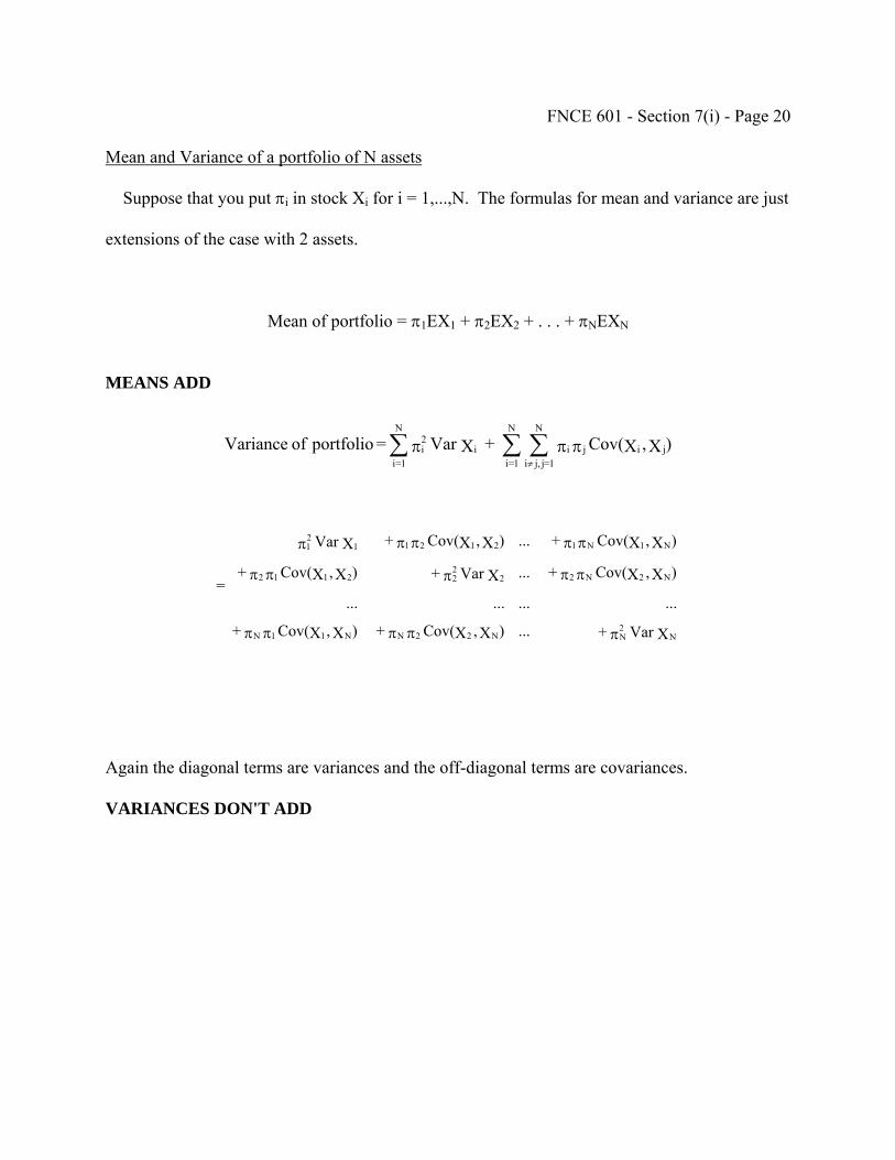
FNCE 601 - Section 7(i) - Page 20
Mean and Variance of a portfolio of N assets
Suppose that you put πi in stock Xi for i = 1,...,N. The formulas for mean and variance are just
extensions of the case with 2 assets.
Mean of portfolio = π1EX1 + π2EX2 + . . . + πNEXN
MEANS ADD
)X,XCov( + XVar = portfolio of Variance jiji
N
1=jj,i
N
1=ii
2i
N
1=iπππ ∑∑∑
≠
XVar + ...)X,XCov( + )X,XCov( +
............
)X,XCov( + ...XVar + )X,XCov( +
)X,XCov( + ...)X,XCov( + XVar
=
N2NN22NN11N
N2N22222112
N1N12121121
πππππ
πππππ
πππππ
Again the diagonal terms are variances and the off-diagonal terms are covariances.
VARIANCES DON'T ADD
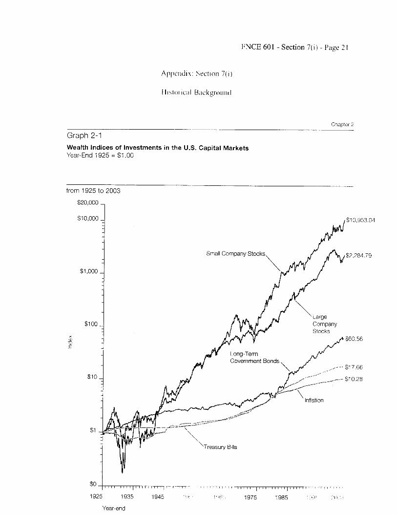
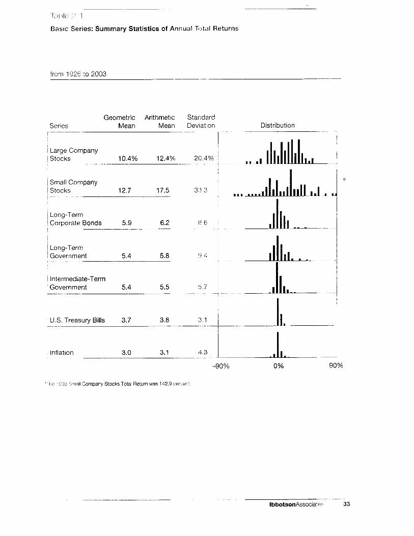
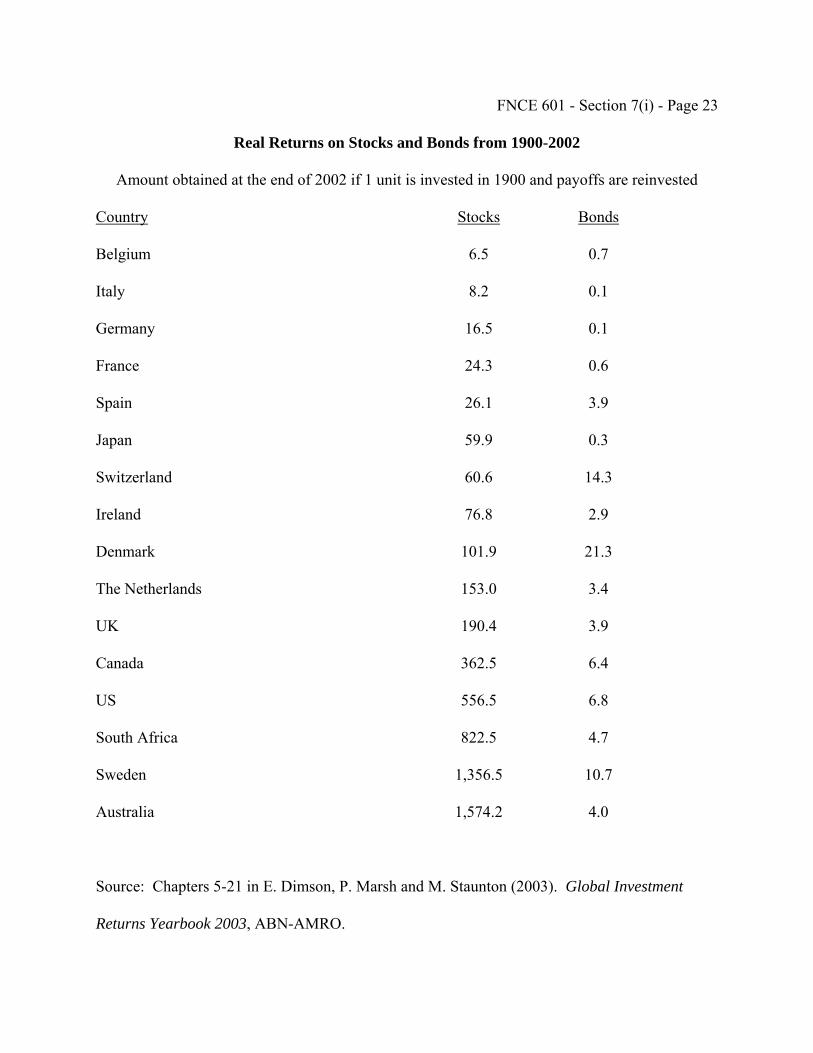
FNCE 601 - Section 7(i) - Page 23
Real Returns on Stocks and Bonds from 1900-2002
Amount obtained at the end of 2002 if 1 unit is invested in 1900 and payoffs are reinvested
Country Stocks Bonds
Belgium 6.5 0.7
Italy 8.2 0.1
Germany 16.5 0.1
France 24.3 0.6
Spain 26.1 3.9
Japan 59.9 0.3
Switzerland 60.6 14.3
Ireland 76.8 2.9
Denmark 101.9 21.3
The Netherlands 153.0 3.4
UK 190.4 3.9
Canada 362.5 6.4
US 556.5 6.8
South Africa 822.5 4.7
Sweden 1,356.5 10.7
Australia 1,574.2 4.0
Source: Chapters 5-21 in E. Dimson, P. Marsh and M. Staunton (2003). Global Investment
Returns Yearbook 2003, ABN-AMRO.
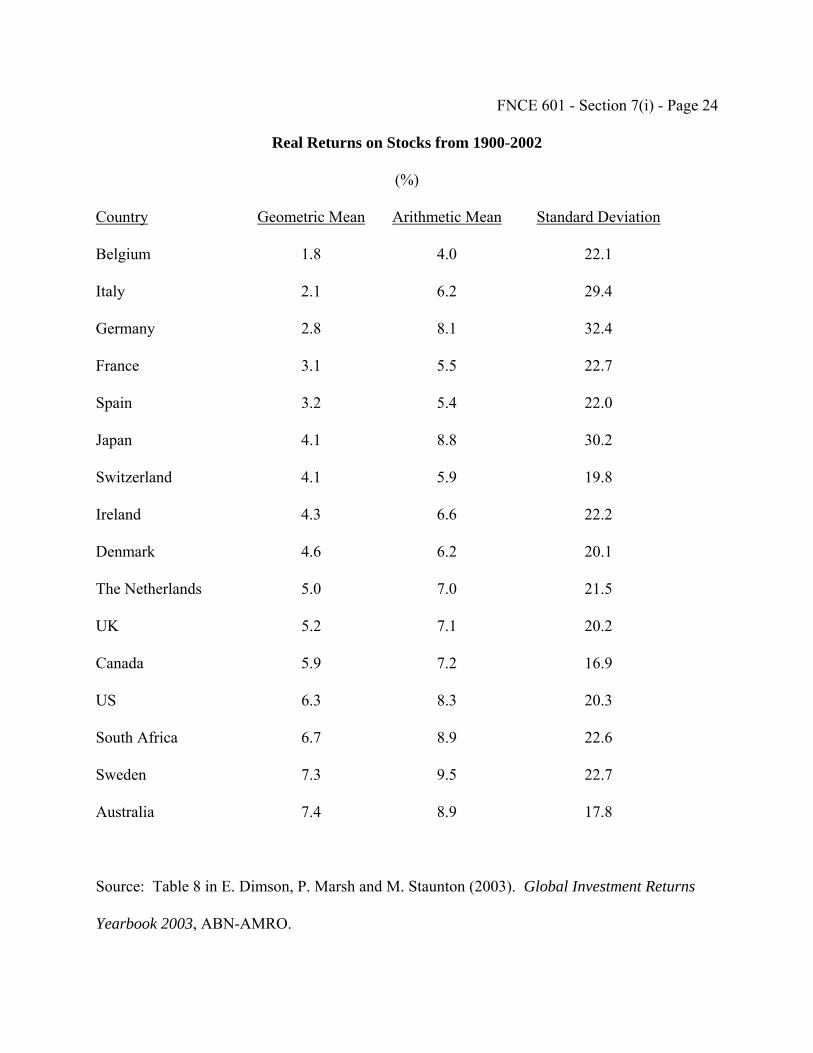
FNCE 601 - Section 7(i) - Page 24
Real Returns on Stocks from 1900-2002
(%)
Country Geometric Mean Arithmetic Mean Standard Deviation
Belgium 1.8 4.0 22.1
Italy 2.1 6.2 29.4
Germany 2.8 8.1 32.4
France 3.1 5.5 22.7
Spain 3.2 5.4 22.0
Japan 4.1 8.8 30.2
Switzerland 4.1 5.9 19.8
Ireland 4.3 6.6 22.2
Denmark 4.6 6.2 20.1
The Netherlands 5.0 7.0 21.5
UK 5.2 7.1 20.2
Canada 5.9 7.2 16.9
US 6.3 8.3 20.3
South Africa 6.7 8.9 22.6
Sweden 7.3 9.5 22.7
Australia 7.4 8.9 17.8
Source: Table 8 in E. Dimson, P. Marsh and M. Staunton (2003). Global Investment Returns
Yearbook 2003, ABN-AMRO.
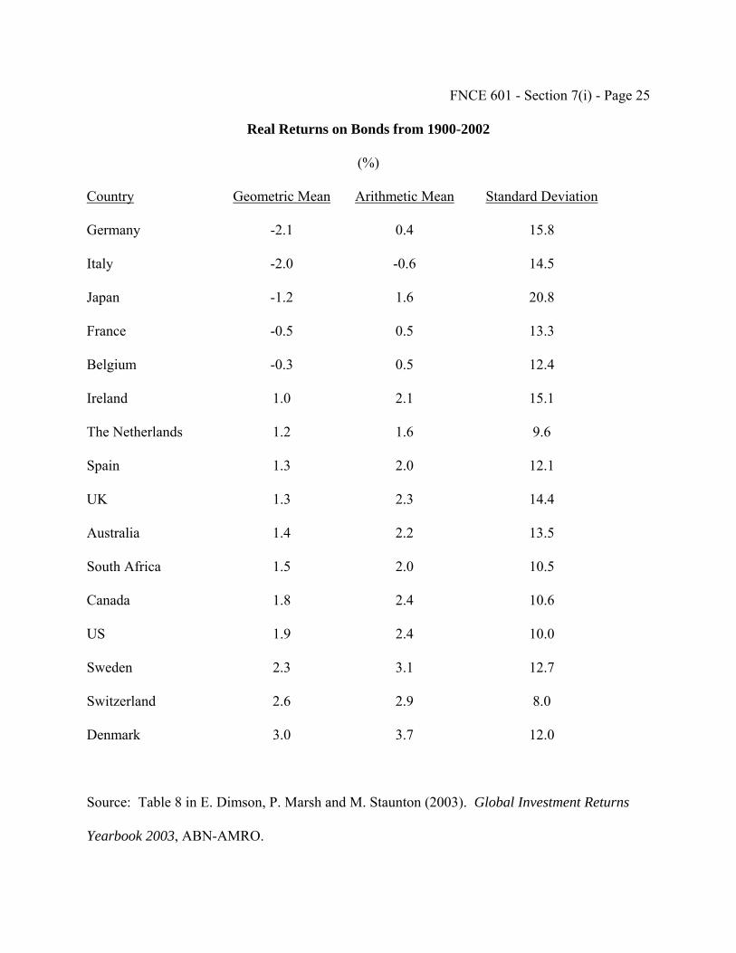
FNCE 601 - Section 7(i) - Page 25
Real Returns on Bonds from 1900-2002
(%)
Country Geometric Mean Arithmetic Mean Standard Deviation
Germany -2.1 0.4 15.8
Italy -2.0 -0.6 14.5
Japan -1.2 1.6 20.8
France -0.5 0.5 13.3
Belgium -0.3 0.5 12.4
Ireland 1.0 2.1 15.1
The Netherlands 1.2 1.6 9.6
Spain 1.3 2.0 12.1
UK 1.3 2.3 14.4
Australia 1.4 2.2 13.5
South Africa 1.5 2.0 10.5
Canada 1.8 2.4 10.6
US 1.9 2.4 10.0
Sweden 2.3 3.1 12.7
Switzerland 2.6 2.9 8.0
Denmark 3.0 3.7 12.0
Source: Table 8 in E. Dimson, P. Marsh and M. Staunton (2003). Global Investment Returns
Yearbook 2003, ABN-AMRO.
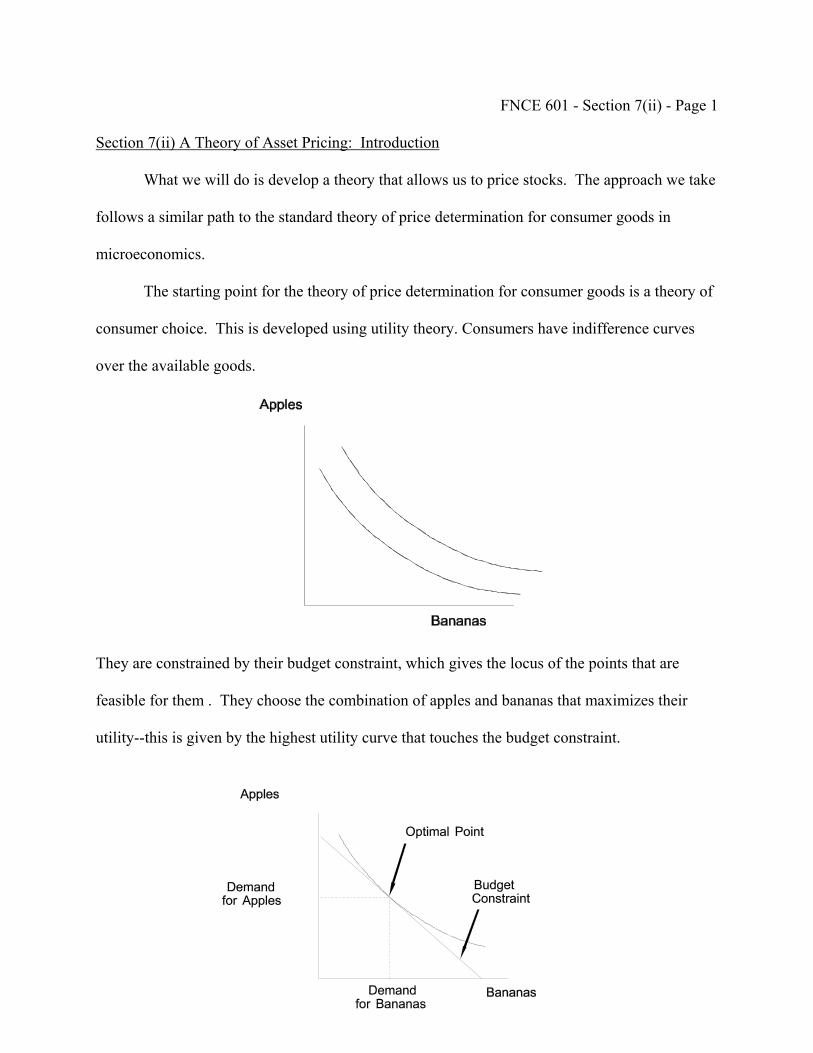
FNCE 601 - Section 7(ii) - Page 1
Section 7(ii) A Theory of Asset Pricing: Introduction
What we will do is develop a theory that allows us to price stocks. The approach we take
follows a similar path to the standard theory of price determination for consumer goods in
microeconomics.
The starting point for the theory of price determination for consumer goods is a theory of
consumer choice. This is developed using utility theory. Consumers have indifference curves
over the available goods.
They are constrained by their budget constraint, which gives the locus of the points that are
feasible for them . They choose the combination of apples and bananas that maximizes their
utility--this is given by the highest utility curve that touches the budget constraint.
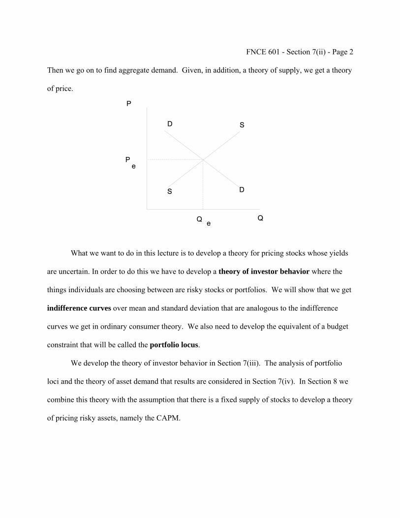
FNCE 601 - Section 7(ii) - Page 2
Then we go on to find aggregate demand. Given, in addition, a theory of supply, we get a theory
of price.
What we want to do in this lecture is to develop a theory for pricing stocks whose yields
are uncertain. In order to do this we have to develop a theory of investor behavior where the
things individuals are choosing between are risky stocks or portfolios. We will show that we get
indifference curves over mean and standard deviation that are analogous to the indifference
curves we get in ordinary consumer theory. We also need to develop the equivalent of a budget
constraint that will be called the portfolio locus.
We develop the theory of investor behavior in Section 7(iii). The analysis of portfolio
loci and the theory of asset demand that results are considered in Section 7(iv). In Section 8 we
combine this theory with the assumption that there is a fixed supply of stocks to develop a theory
of pricing risky assets, namely the CAPM.
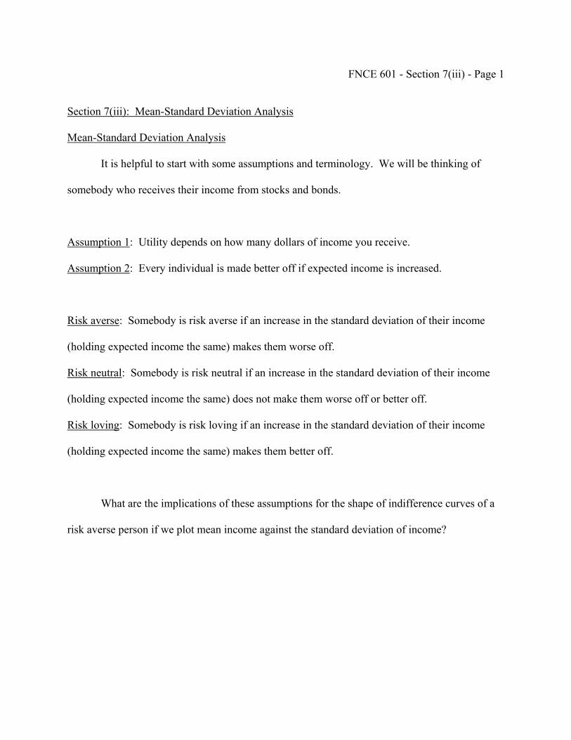
FNCE 601 - Section 7(iii) - Page 1
Section 7(iii): Mean-Standard Deviation Analysis
Mean-Standard Deviation Analysis
It is helpful to start with some assumptions and terminology. We will be thinking of
somebody who receives their income from stocks and bonds.
Assumption 1: Utility depends on how many dollars of income you receive.
Assumption 2: Every individual is made better off if expected income is increased.
Risk averse: Somebody is risk averse if an increase in the standard deviation of their income
(holding expected income the same) makes them worse off.
Risk neutral: Somebody is risk neutral if an increase in the standard deviation of their income
(holding expected income the same) does not make them worse off or better off.
Risk loving: Somebody is risk loving if an increase in the standard deviation of their income
(holding expected income the same) makes them better off.
What are the implications of these assumptions for the shape of indifference curves of a
risk averse person if we plot mean income against the standard deviation of income?
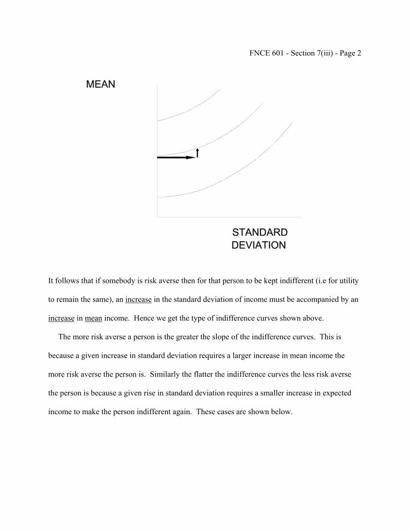
FNCE 601 - Section 7(iii) - Page 2
It follows that if somebody is risk averse then for that person to be kept indifferent (i.e for utility
to remain the same), an increase in the standard deviation of income must be accompanied by an
increase in mean income. Hence we get the type of indifference curves shown above.
The more risk averse a person is the greater the slope of the indifference curves. This is
because a given increase in standard deviation requires a larger increase in mean income the
more risk averse the person is. Similarly the flatter the indifference curves the less risk averse
the person is because a given rise in standard deviation requires a smaller increase in expected
income to make the person indifferent again. These cases are shown below.
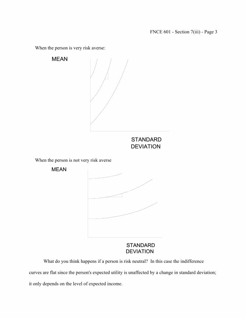
FNCE 601 - Section 7(iii) - Page 3
When the person is very risk averse:
When the person is not very risk averse
What do you think happens if a person is risk neutral? In this case the indifference
curves are flat since the person's expected utility is unaffected by a change in standard deviation;
it only depends on the level of expected income.
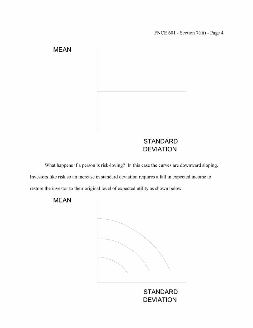
FNCE 601 - Section 7(iii) - Page 4
What happens if a person is risk-loving? In this case the curves are downward sloping.
Investors like risk so an increase in standard deviation requires a fall in expected income to
restore the investor to their original level of expected utility as shown below.
FNCE 601 - Section 7(iii) - Page 5
In what follows we shall be assuming risk aversion so that indifference curves are upward
sloping. The justification for this is that most people appear to be willing to pay to avoid risks
by buying insurance. There are problems with the assumption of risk aversion though. For
example, why do people gamble? In this case they are actually paying to take on a risk which
suggests they are risk loving. The argument that is usually made to explain this is that it's the
utility of going to the casino and actually seeing the wheels go round and the dice roll and so on
that makes gambling attractive rather than the shape of people's utility functions. These factors
are not that important in the context of investing in the stock market. Risk free assets usually
have a lower return than risky assets. This is consistent with people being risk averse.

FNCE 601 - Section 7(iv) - Page 1
Section 7(iv): Diversification and the Measurement of Risk
Read Chapters 7 and 8 BM
Introduction
Suppose we have two stocks, A and B, and preferences as below. Which should be
chosen? Clearly we should choose B.
However, is this the best we can do? No, we may do better by combining the two assets in a
portfolio.
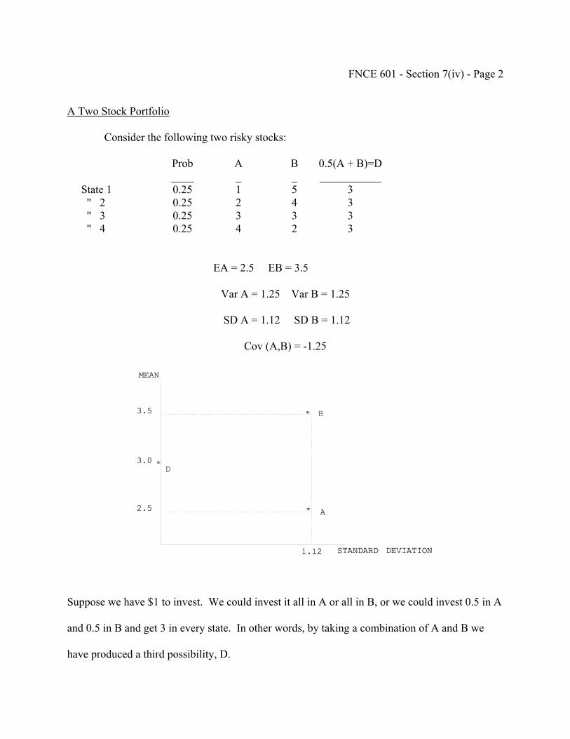
FNCE 601 - Section 7(iv) - Page 2
A Two Stock Portfolio Consider the following two risky stocks: Prob A B 0.5(A + B)=D ____ _ _ ___________ State 1 0.25 1 5 3 " 2 0.25 2 4 3 " 3 0.25 3 3 3 " 4 0.25 4 2 3
EA = 2.5 EB = 3.5
Var A = 1.25 Var B = 1.25
SD A = 1.12 SD B = 1.12
Cov (A,B) = -1.25
Suppose we have $1 to invest. We could invest it all in A or all in B, or we could invest 0.5 in A
and 0.5 in B and get 3 in every state. In other words, by taking a combination of A and B we
have produced a third possibility, D.
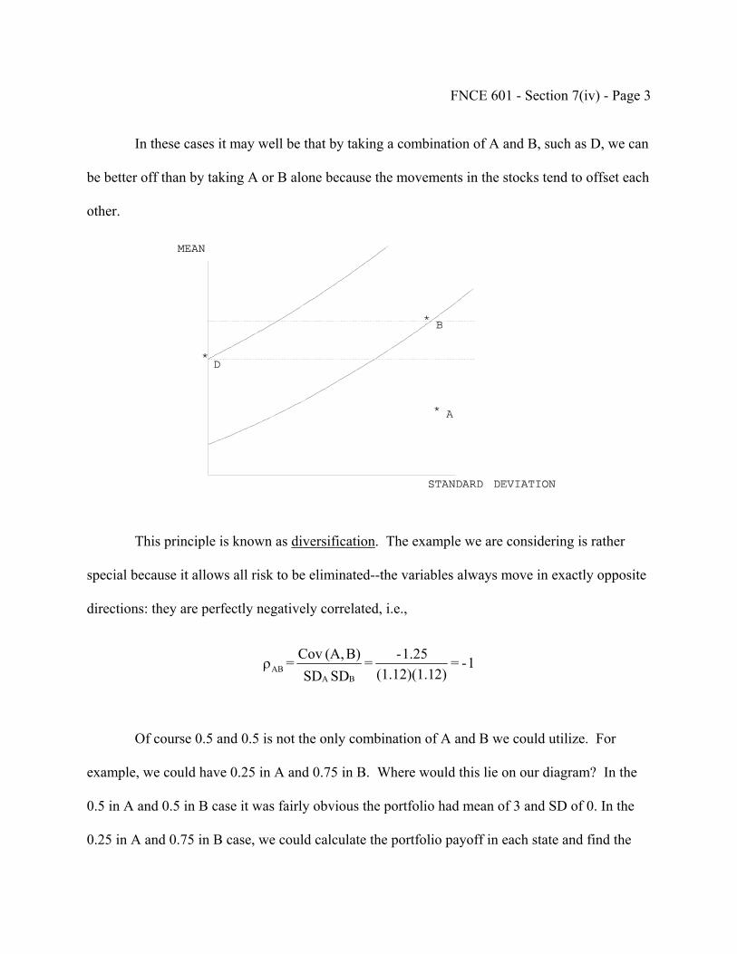
FNCE 601 - Section 7(iv) - Page 3
In these cases it may well be that by taking a combination of A and B, such as D, we can
be better off than by taking A or B alone because the movements in the stocks tend to offset each
other.
This principle is known as diversification. The example we are considering is rather
special because it allows all risk to be eliminated--the variables always move in exactly opposite
directions: they are perfectly negatively correlated, i.e.,
1- = 2)(1.12)(1.1
1.25- = SD SD
B)(A, Cov = BA
ABρ
Of course 0.5 and 0.5 is not the only combination of A and B we could utilize. For
example, we could have 0.25 in A and 0.75 in B. Where would this lie on our diagram? In the
0.5 in A and 0.5 in B case it was fairly obvious the portfolio had mean of 3 and SD of 0. In the
0.25 in A and 0.75 in B case, we could calculate the portfolio payoff in each state and find the

FNCE 601 - Section 7(iv) - Page 4
mean and standard deviation of these payoffs. A quicker method is to use our formulae for the
mean and standard deviation of a portfolio with two stocks which we discussed in Section 2C(i)
to find the mean and standard deviation of this portfolio.
Remember that means add so that:
Mean of portfolio(0.25 in A, 0.75 in B) = 0.25 × EA + 0.75 × EB
= 0.25 × 2.5 + 0.75 × 3.5
= 3.25
Variances do not add they depend on covariance:
Var of portfolio(0.25 in A, 0.75 in B)
= 0.252Var A + 0.752Var B + 2 × 0.25 × 0.75 × Cov(A,B)
= 0.252 × 1.25 + 0.752 × 1.25 + 2 × 0.25 × 0.75 × (-1.25)
= 0.3125
SD of portfolio(0.25 in A, 0.75 in B) = (0.3125)0.5 = 0.56
The point with 0.25 in A and 0.75 in B has mean 3.25 and SD 0.56. It is labeled π =
0.25 in the diagram. Similarly, we can calculate for the portfolio with 0.75 in A and 0.25 in B
that the mean is 2.75 and the standard deviation is 0.56 and it is shown by the point labeled π =
0.75. In general, we can use our formulae to find the mean and SD for all the other possible
values combinations of A and B. We can then use these numbers to plot the portfolio locus
between A and B on our mean-standard deviation diagram.
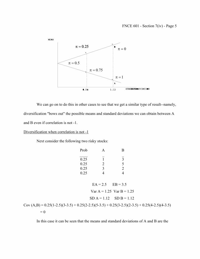
FNCE 601 - Section 7(iv) - Page 5
π = 0.25π = 0.25 π = 0
π = 0.5
π = 0.75
π = 1
We can go on to do this in other cases to see that we get a similar type of result--namely,
diversification "bows out" the possible means and standard deviations we can obtain between A
and B even if correlation is not -1.
Diversification when correlation is not -1
Next consider the following two risky stocks:
Prob A B ____ _ _ 0.25 1 3 0.25 2 5 0.25 3 2 0.25 4 4
EA = 2.5 EB = 3.5
Var A = 1.25 Var B = 1.25
SD A = 1.12 SD B = 1.12
Cov (A,B) = 0.25(1-2.5)(3-3.5) + 0.25(2-2.5)(5-3.5) + 0.25(3-2.5)(2-3.5) + 0.25(4-2.5)(4-3.5)
= 0
In this case it can be seen that the means and standard deviations of A and B are the

FNCE 601 - Section 7(iv) - Page 6
same as before. Now, however, the correlation is
0SDSD
)B,A(Cov
BAAB ==ρ
Whereas with a correlation of -1, the movements in A and B always cancelled out, now it can be
seen that A and B cancel out some of the time but some of the time they do not. Overall, there is
still a benefit from diversification.
Mean of 0.5(A + B) = 3
Variance of 0.5(A + B) = 0.625
SD of 0.5(A + B) = (0.625)0.5 = 0.791
We can see this for mixtures of A and B other than 0.5 and 0.5 using our formulas from the
Appendix to Section 7(i) and plotting the portfolio locus.
ρ = 0
The portfolio locus is still bowed out but not by as much as before. As we increase correlation
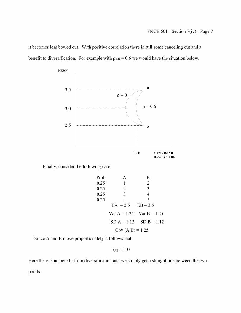
FNCE 601 - Section 7(iv) - Page 7
it becomes less bowed out. With positive correlation there is still some canceling out and a
benefit to diversification. For example with ρAB = 0.6 we would have the situation below.
2.5
3.0
3.5 ρ = 0
ρ = 0.6
Finally, consider the following case.
Prob A B 0.25 1 2 0.25 2 3 0.25 3 4 0.25 4 5 EA = 2.5 EB = 3.5
Var A = 1.25 Var B = 1.25
SD A = 1.12 SD B = 1.12
Cov (A,B) = 1.25
Since A and B move proportionately it follows that
ρAB = 1.0
Here there is no benefit from diversification and we simply get a straight line between the two
points.

FNCE 601 - Section 7(iv) - Page 8
ρ=1
ρ=0
Relationship between ρ and diversification locus
It follows from this analysis that in general the portfolio locus is bowed out and the
degree to which this happens depends on the correlation ρ between the two stocks. Thus we
have:
ρ
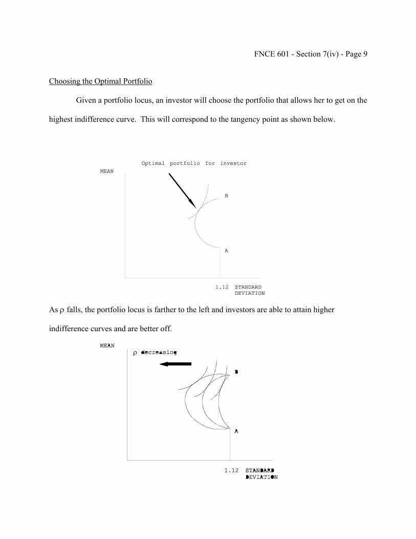
FNCE 601 - Section 7(iv) - Page 9
Choosing the Optimal Portfolio
Given a portfolio locus, an investor will choose the portfolio that allows her to get on the
highest indifference curve. This will correspond to the tangency point as shown below.
As ρ falls, the portfolio locus is farther to the left and investors are able to attain higher
indifference curves and are better off.
ρ
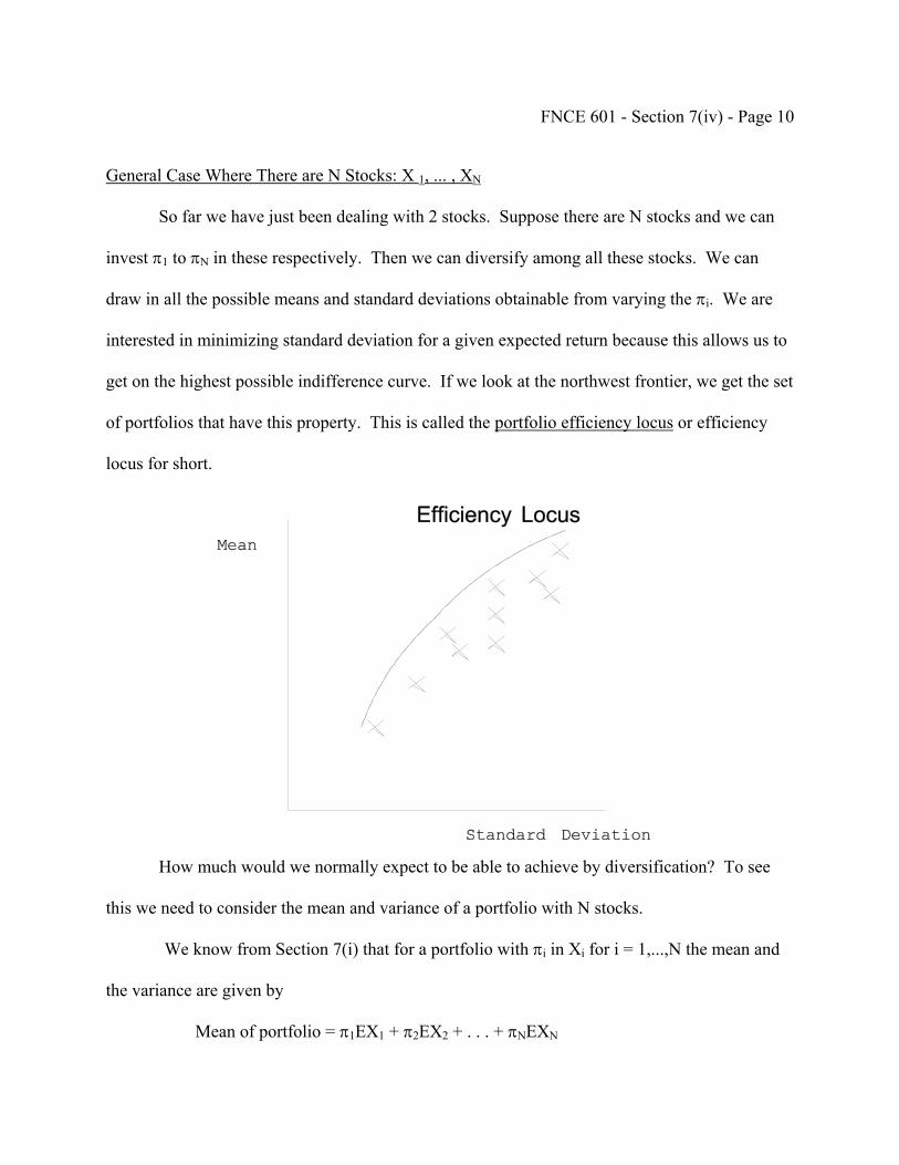
FNCE 601 - Section 7(iv) - Page 10
General Case Where There are N Stocks: X 1, ... , XN
So far we have just been dealing with 2 stocks. Suppose there are N stocks and we can
invest π1 to πN in these respectively. Then we can diversify among all these stocks. We can
draw in all the possible means and standard deviations obtainable from varying the πi. We are
interested in minimizing standard deviation for a given expected return because this allows us to
get on the highest possible indifference curve. If we look at the northwest frontier, we get the set
of portfolios that have this property. This is called the portfolio efficiency locus or efficiency
locus for short.
How much would we normally expect to be able to achieve by diversification? To see
this we need to consider the mean and variance of a portfolio with N stocks.
We know from Section 7(i) that for a portfolio with πi in Xi for i = 1,...,N the mean and
the variance are given by
Mean of portfolio = π1EX1 + π2EX2 + . . . + πNEXN
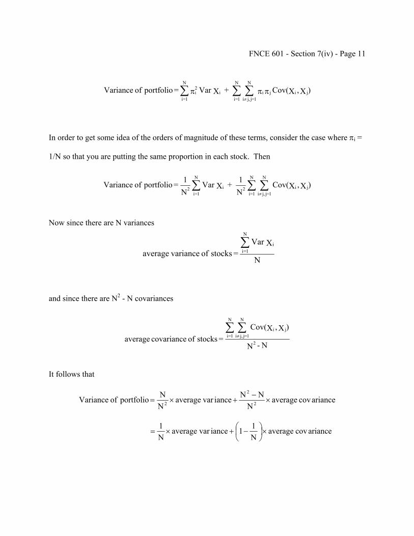
FNCE 601 - Section 7(iv) - Page 11
)X,XCov( + XVar = portfolio of Variance jiji
N
1=jj,i
N
1=ii
2i
N
1=iπππ ∑∑∑
≠
In order to get some idea of the orders of magnitude of these terms, consider the case where πi =
1/N so that you are putting the same proportion in each stock. Then
)X,XCov(
N1 + XVar
N1= portfolio of Variance ji
N
1=jj,i
N
1=i2i
N
1=i2 ∑∑∑
≠
N
XVar = stocks of varianceaverage
i
N
1=i∑
Now since there are N variances
and since there are N2 - N covariances
N - N
)X,XCov( = stocks of covariance average
2
ji
N
1=jj,i
N
1=i∑∑≠
It follows that
ariancecovaverageN
NNiancevaraverageNNportfolioofVariance 2
2
2 ×−
+×=
ariancecovaverageN11iancevaraverage
N1
×⎟⎠⎞
⎜⎝⎛ −+×=
FNCE 601 - Section 7(iv) - Page 12
As N gets large, 1/N → 0 so the first term goes to zero, and the second term approaches
the average covariance. Hence the risk of a well-diversified portfolio depends on the average
covariance of the stocks included.
Variance of portfolio = average covariance of stocks
It's thus the covariances which are the important determinants of the riskiness of a portfolio
rather than the variances.
On the whole would we expect stocks to have a positive or negative covariance?
Because of the business cycle, we would expect firms to have a positive covariance. For
example, when there is a depression, both the auto and the steel industry have low returns and
their stocks therefore have a positive covariance. In fact we know from what we did in the
historical review that they do.
The riskiness of stocks due to the business cycle is known as market risk or systematic
risk, and it can't be diversified away.
Market risk is not the only type of risk associated with stocks considered individually.
There may be changes in returns due to factors only affecting the industry, such as increased
foreign competition, a change in tastes and so on. Or there may be changes due to factors only
affecting a single firm, such as a serious breakdown in a plant or a good or bad decision by a
firm's management. This type of risk is called unique risk or unsystematic risk.
The riskiness of a stock thus has two components: market and unique risk. It is unique
risk that can be diversified away. N used not to have to be very large before unique risk
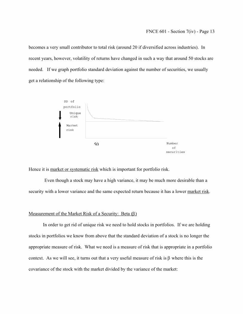
FNCE 601 - Section 7(iv) - Page 13
becomes a very small contributor to total risk (around 20 if diversified across industries). In
recent years, however, volatility of returns have changed in such a way that around 50 stocks are
needed. If we graph portfolio standard deviation against the number of securities, we usually
get a relationship of the following type:
0
Hence it is market or systematic
Even though a stock may
security with a lower variance an
Measurement of the Market Risk
In order to get rid of uniq
stocks in portfolios we know from
appropriate measure of risk. Wh
context. As we will see, it turns
covariance of the stock with the m
5
risk which is important for portfolio risk.
have a high variance, it may be much more desirable than a
d the same expected return because it has a lower market risk.
of a Security: Beta (β)
ue risk we need to hold stocks in portfolios. If we are holding
above that the standard deviation of a stock is no longer the
at we need is a measure of risk that is appropriate in a portfolio
out that a very useful measure of risk is β where this is the
arket divided by the variance of the market:

FNCE 601 - Section 7(iv) - Page 14
βX = Cov(X, Market) = Cov(X, Market) Var M SDM
2
Note that X can be a stock or a portfolio.
Why is beta defined relative to the "market portfolio" which is all the stocks in the
market? The reason this is a useful benchmark is because it is the portfolio where the amount of
unique risk that is diversified away is maximized. On our diagram of unique and market risk it is
the farthest point out on the right hand side.
Well diversified portfolios
50
We denote the market portfolio by M. In this case π1 is the value of the total amount of
stock 1 relative to the total market value. For example, if the total value of stock 1 is 50 million
and the total value of the market portfolio is 1000 billion, then π1 = 50 million/1000 billion.
As a practical matter, when we have gone beyond 50 stocks the added diversification
achieved by going to the market does not reduce variance by a great deal. Portfolios that have a
very small amount of unique risk are called "well-diversified portfolios". These are all the
portfolios out to the right on our diagram.
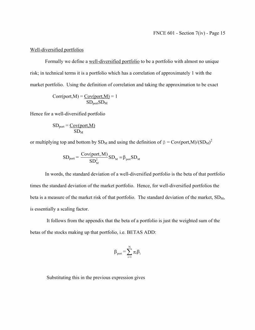
FNCE 601 - Section 7(iv) - Page 15
Well-diversified portfolios
Formally we define a well-diversified portfolio to be a portfolio with almost no unique
risk; in technical terms it is a portfolio which has a correlation of approximately 1 with the
market portfolio. Using the definition of correlation and taking the approximation to be exact
Corr(port,M) = Cov(port,M) = 1 SDportSDM Hence for a well-diversified portfolio SDport = Cov(port,M) SDM
or multiplying top and bottom by SDM and using the definition of β = Cov(port,M)/(SDM)2
SDport = M port M2M
Cov(port,M) SD SDSD
= β
In words, the standard deviation of a well-diversified portfolio is the beta of that portfolio
times the standard deviation of the market portfolio. Hence, for well-diversified portfolios the
beta is a measure of the market risk of that portfolio. The standard deviation of the market, SDM,
is essentially a scaling factor.
It follows from the appendix that the beta of a portfolio is just the weighted sum of the
betas of the stocks making up that portfolio, i.e. BETAS ADD:
βπβ ∑ ii
N
1=iport =
Substituting this in the previous expression gives
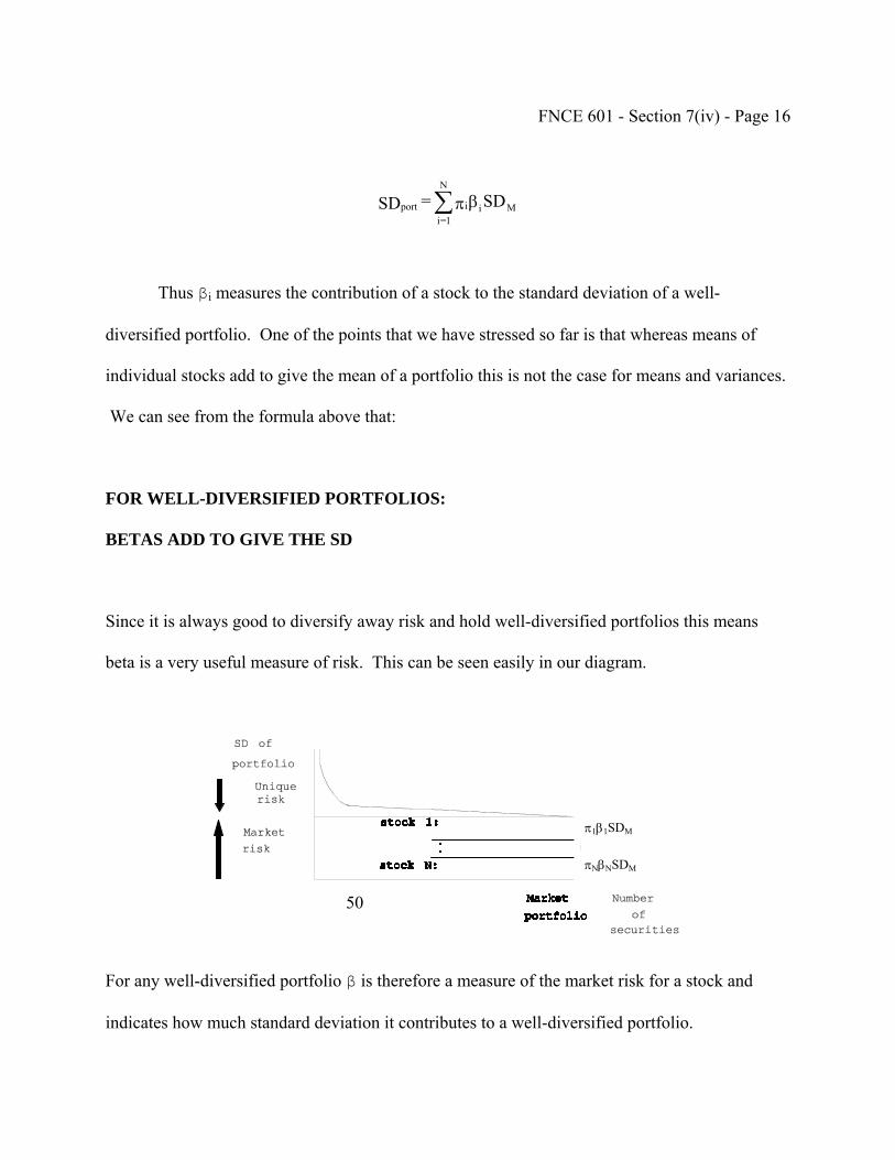
FNCE 601 - Section 7(iv) - Page 16
Mii
N
1=iport SD = SD βπ∑
Thus βi measures the contribution of a stock to the standard deviation of a well-
diversified portfolio. One of the points that we have stressed so far is that whereas means of
individual stocks add to give the mean of a portfolio this is not the case for means and variances.
We can see from the formula above that:
FOR WELL-DIVERSIFIED PORTFOLIOS:
BETAS ADD TO GIVE THE SD
Since it is always good to diversify away risk and hold well-diversified portfolios this means
beta is a very useful measure of risk. This can be seen easily in our diagram.
π1β1SDM
πNβNSDM
50
For any well-diversified portfolio β is therefore a measure of the market risk for a stock and
indicates how much standard deviation it contributes to a well-diversified portfolio.
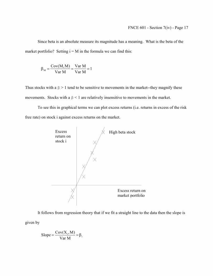
FNCE 601 - Section 7(iv) - Page 17
Since beta is an absolute measure its magnitude has a meaning. What is the beta of the
market portfolio? Setting i = M in the formula we can find this:
MCov(M,M) Var M 1
Var M Var Mβ = = =
Thus stocks with a β > 1 tend to be sensitive to movements in the market--they magnify these
movements. Stocks with a β < 1 are relatively insensitive to movements in the market.
To see this in graphical terms we can plot excess returns (i.e. returns in excess of the risk
free rate) on stock i against excess returns on the market.
Excessreturn onstock i
High beta stock
Excess return onmarket portfolio
It follows from regression theory that if we fit a straight line to the data then the slope is
given by
ii
Cov(X ,M)SlopeVar M
= = β
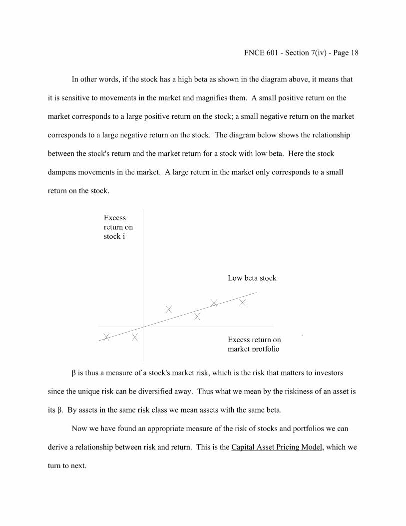
FNCE 601 - Section 7(iv) - Page 18
In other words, if the stock has a high beta as shown in the diagram above, it means that
it is sensitive to movements in the market and magnifies them. A small positive return on the
market corresponds to a large positive return on the stock; a small negative return on the market
corresponds to a large negative return on the stock. The diagram below shows the relationship
between the stock's return and the market return for a stock with low beta. Here the stock
dampens movements in the market. A large return in the market only corresponds to a small
return on the stock.
Excessreturn onstock i
Low beta stock
Excess return onmarket protfolio
β is thus a measure of a stock's market risk, which is the risk that matters to investors
since the unique risk can be diversified away. Thus what we mean by the riskiness of an asset is
its β. By assets in the same risk class we mean assets with the same beta.
Now we have found an appropriate measure of the risk of stocks and portfolios we can
derive a relationship between risk and return. This is the Capital Asset Pricing Model, which we
turn to next.
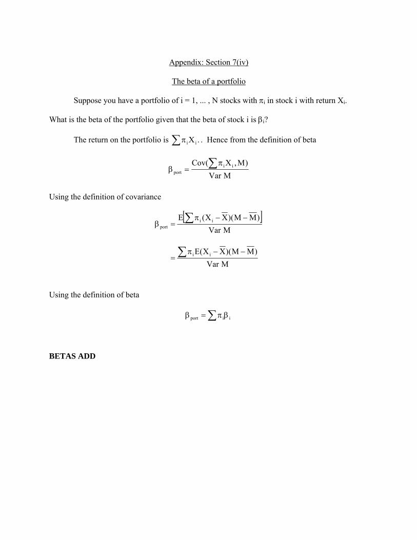
Appendix: Section 7(iv)
The beta of a portfolio
Suppose you have a portfolio of i = 1, ... , N stocks with πi in stock i with return Xi.
What is the beta of the portfolio given that the beta of stock i is βi?
The return on the portfolio is ∑π .Xii . Hence from the definition of beta
MVar)M,X(Cov ii
port∑π
=β
Using the definition of covariance
[ ]
MVar)MM()XX(E ii
port
−−π=β ∑
MVar)MM()XX(E ii −−π
= ∑
Using the definition of beta
∑ βπ=β iiport
BETAS ADD
UNIVERSITY OF PENNSYLVANIA THE WHARTON SCHOOL FNCE 601 CORPORATE FINANCE LECTURE NOTES Franklin Allen Fall 2004 QUARTER 1 - WEEK 5 (part 2) and WEEK 6 (part 1) Th: 10/7/04 and Tu: 10/12/04 Copyright © 2004 by Franklin Allen
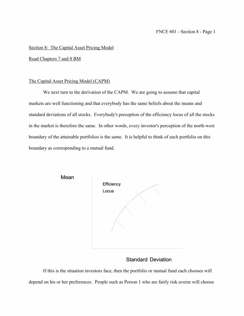
FNCE 601 - Section 8 - Page 1
Section 8: The Capital Asset Pricing Model
Read Chapters 7 and 8 BM
The Capital Asset Pricing Model (CAPM)
We next turn to the derivation of the CAPM. We are going to assume that capital
markets are well functioning and that everybody has the same beliefs about the means and
standard deviations of all stocks. Everybody's perception of the efficiency locus of all the stocks
in the market is therefore the same. In other words, every investor's perception of the north-west
boundary of the attainable portfolios is the same. It is helpful to think of each portfolio on this
boundary as corresponding to a mutual fund.
If this is the situation investors face, then the portfolio or mutual fund each chooses will
depend on his or her preferences. People such as Person 1 who are fairly risk averse will choose
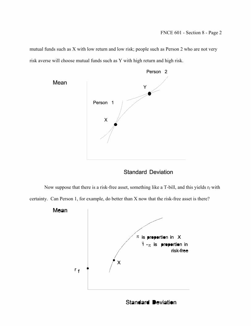
FNCE 601 - Section 8 - Page 2
mutual funds such as X with low return and low risk; people such as Person 2 who are not very
risk averse will choose mutual funds such as Y with high return and high risk.
Now suppose that there is a risk-free asset, something like a T-bill, and this yields rf with
certainty. Can Person 1, for example, do better than X now that the risk-free asset is there?
π
π

FNCE 601 - Section 8 - Page 3
Suppose we hold a portfolio with a proportion π in the mutual fund X which has a mean
return of rX and variance Var X and 1 - π invested in the risk-free asset which has a mean return
of rf and a variance of 0. The covariance of the risk-free asset and X is also 0 since rf -Er f = 0.
What are the mean and standard deviation of this portfolio? Using the formulas for two-security
portfolios from Section 7(iv) with π1 = π and π2 = 1 - π:
Erport = πrX + (1 - π)rf
Varport = π2Var X + (1 - π)2 × 0 + 2π (1 - π) × 0 = π2Var X
SDport = πSDX
The expected return is just a weighted average of rf and rX as you'd expect. The formula
SD = πSDX simply says that if only one of the stocks in a portfolio varies the standard deviation
of the portfolio is the proportion of that stock in the portfolio times the stock's standard
deviation.
As we vary π what do we trace out? To see this suppose rf = 0.05, rX = 0.15, and SDX =
2. Now consider the following.
π = 0.25 rport = 0.075 SDport = 0.5
π = 0.50 rport = 0.100 SDport = 1.0
π = 0.75 rport = 0.125 SDport = 1.5
Hence we trace out a straight line.
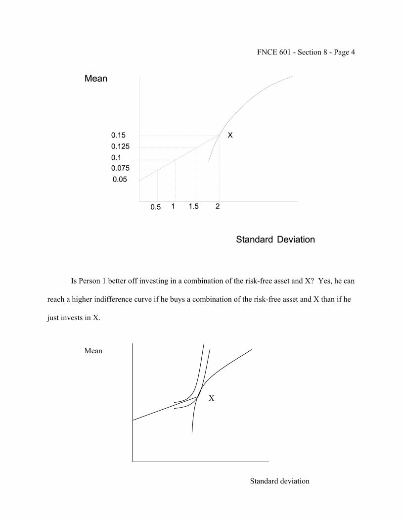
FNCE 601 - Section 8 - Page 4
Is Person 1 better off investing in a combination of the risk-free asset and X? Yes, he can
reach a higher indifference curve if he buys a combination of the risk-free asset and X than if he
just invests in X.
Mean
X
Standard deviation
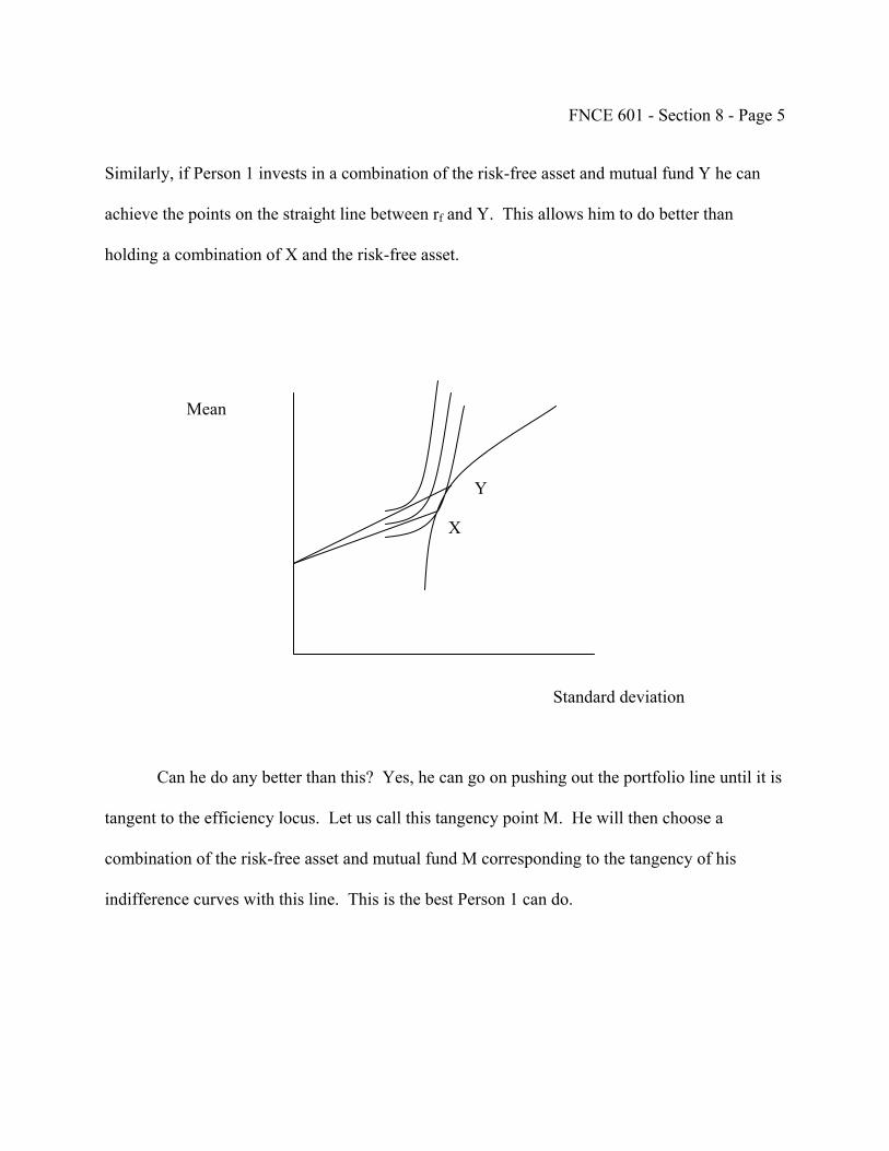
FNCE 601 - Section 8 - Page 5
Similarly, if Person 1 invests in a combination of the risk-free asset and mutual fund Y he can
achieve the points on the straight line between rf and Y. This allows him to do better than
holding a combination of X and the risk-free asset.
Y
X
Mean
Standard deviation
Can he do any better than this? Yes, he can go on pushing out the portfolio line until it is
tangent to the efficiency locus. Let us call this tangency point M. He will then choose a
combination of the risk-free asset and mutual fund M corresponding to the tangency of his
indifference curves with this line. This is the best Person 1 can do.

FNCE 601 - Section 8 - Page 6
What about Person 2, what is the best she can do? Again she will want to push the line
out as far as possible by choosing a combination of the risk-free asset and mutual fund M. Since
the tangency of her indifference curves with the line is at a different point than person 1's, she
will have a different proportion in the risk-free asset and mutual fund M than Person 1, but she
will nevertheless be holding the same two assets.
Notice that people can hold portfolios on the line to the right of M. How? At M they
invest all they have in the portfolio M, i.e., π = 1. To the left of M they put some in the risk-free
asset and π < 1, i.e., they lend. To the right what do you think they do? They borrow to invest in
portfolio M; i.e., they lever themselves and get a higher expected return in exchange for more
risk, i.e. π > 1.
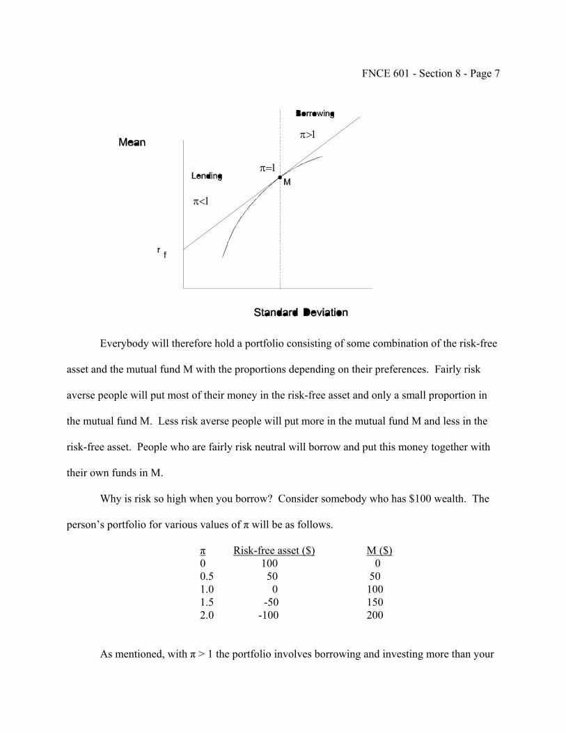
FNCE 601 - Section 8 - Page 7
π=1
π>1
π<1
Everybody will therefore hold a portfolio consisting of some combination of the risk-free
asset and the mutual fund M with the proportions depending on their preferences. Fairly risk
averse people will put most of their money in the risk-free asset and only a small proportion in
the mutual fund M. Less risk averse people will put more in the mutual fund M and less in the
risk-free asset. People who are fairly risk neutral will borrow and put this money together with
their own funds in M.
Why is risk so high when you borrow? Consider somebody who has $100 wealth. The
person’s portfolio for various values of π will be as follows.
π Risk-free asset ($) M ($) 0 100 0 0.5 50 50 1.0 0 100 1.5 -50 150 2.0 -100 200
As mentioned, with π > 1 the portfolio involves borrowing and investing more than your
FNCE 601 - Section 8 - Page 8
wealth in M. Let’s compare π = 1 with π = 2 for the cases where M halves and when it doubles.
Portfolio value when
M doubles M halves
π = 1 $200 $50
π = 2 400 – 100 = $300 100 – 100 = $0
It can be seen that risk increases significantly when you borrow. With π = 1 there’s only 200 –
50 = 150 in variation. However, with π = 2 there’s 300 – 0 = 300 in variation. This is why risk
goes up the more you borrow.
Given that everybody owns the same risky mutual fund M, containing all the stocks in
the market in the same ratios, what do you know about M? In equilibrium, we can show M must
be a replica of the total market; it must have the same proportions in each stock as the total
market. When we introduced β, we talked about riskiness in relation to the market portfolio. It
is the same market portfolio here.
Why must the mutual fund that everybody holds have the same proportions as the market
portfolio?
To see this let M denote the portfolio that everybody holds and suppose that there are n
units in total demanded by people. Then if markets are to clear demand = supply requires:
nM = Market portfolio
or PortfolioMarketn1M =
In other words everybody holds a fraction of the market portfolio.
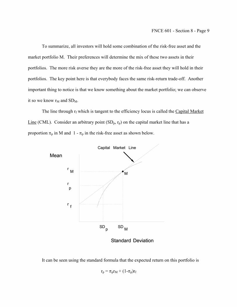
FNCE 601 - Section 8 - Page 9
To summarize, all investors will hold some combination of the risk-free asset and the
market portfolio M. Their preferences will determine the mix of these two assets in their
portfolios. The more risk averse they are the more of the risk-free asset they will hold in their
portfolios. The key point here is that everybody faces the same risk-return trade-off. Another
important thing to notice is that we know something about the market portfolio; we can observe
it so we know rM and SDM.
The line through rf which is tangent to the efficiency locus is called the Capital Market
Line (CML). Consider an arbitrary point (SDp, rp) on the capital market line that has a
proportion πp in M and 1 - πp in the risk-free asset as shown below.
It can be seen using the standard formula that the expected return on this portfolio is
rp = πprM + (1-πp)rf

FNCE 601 - Section 8 - Page 10
= rf + πp(rM - rf) (1)
This can be changed to a more useful form by deriving the relationship between πp and βp. It
was shown in the Appendix for Section 7(iv) last time that ∑ βπ=β .iiport . In this case the
portfolio of interest consists of πp in M and 1 - πp in the risk-free asset. Now it follows from the
definition of beta that βM = 1. Also since rf -r f = 0 it follows that the covariance of the risk-free
asset with the market is zero and hence βrisk-free = 0. Thus
pppp 0)1(1 π=×π−+×π=β (2)
Intuitively, the beta of a portfolio consisting of M that has a beta of 1 and the risk-free
asset that has a beta of 0 is just the proportion invested in M. The more you put in the market the
higher the beta.
Putting (1) and (2) together gives
rp = rf + βp(rM - rf) (3)
What this says is that the expected return on a portfolio along the capital market line with risk βp
is the risk free rate plus βp times the risk premium on the market portfolio (rM - rf). For example,
if somebody puts half their money in the market portfolio, she has half of the risk of the market
and half of the risk premium. We’ve scaled everything relative to the market so it all works out
neatly.
One more step remains before we have the capital asset pricing model. We are going to
argue that the risk premium on any asset or security with riskiness β will be given by β (rM - rf).
The argument is essentially an arbitrage one. You would never hold an asset with
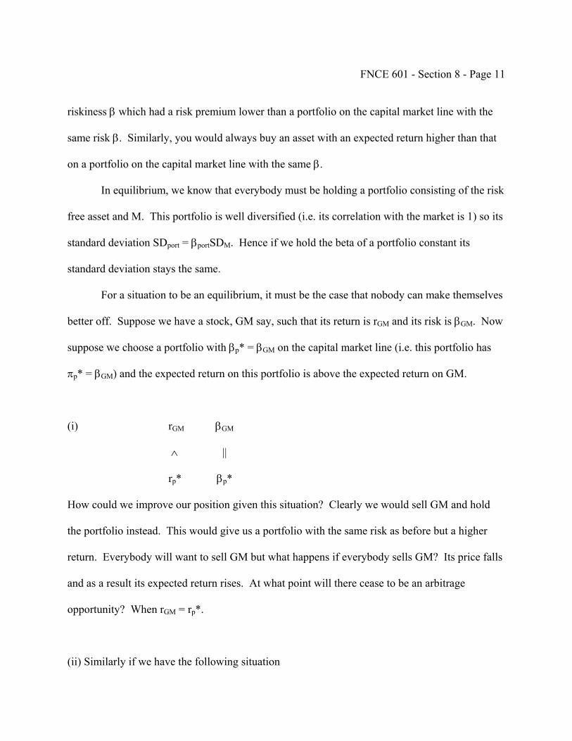
FNCE 601 - Section 8 - Page 11
riskiness β which had a risk premium lower than a portfolio on the capital market line with the
same risk β. Similarly, you would always buy an asset with an expected return higher than that
on a portfolio on the capital market line with the same β.
In equilibrium, we know that everybody must be holding a portfolio consisting of the risk
free asset and M. This portfolio is well diversified (i.e. its correlation with the market is 1) so its
standard deviation SDport = βportSDM. Hence if we hold the beta of a portfolio constant its
standard deviation stays the same.
For a situation to be an equilibrium, it must be the case that nobody can make themselves
better off. Suppose we have a stock, GM say, such that its return is rGM and its risk is βGM. Now
suppose we choose a portfolio with βp* = βGM on the capital market line (i.e. this portfolio has
πp* = βGM) and the expected return on this portfolio is above the expected return on GM.
(i) rGM βGM
∧ ||
rp* βp*
How could we improve our position given this situation? Clearly we would sell GM and hold
the portfolio instead. This would give us a portfolio with the same risk as before but a higher
return. Everybody will want to sell GM but what happens if everybody sells GM? Its price falls
and as a result its expected return rises. At what point will there cease to be an arbitrage
opportunity? When rGM = rp*.
(ii) Similarly if we have the following situation
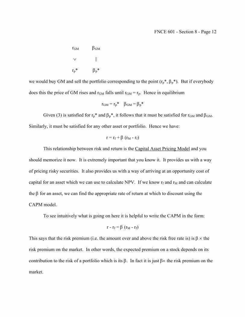
FNCE 601 - Section 8 - Page 12
rGM βGM
∨ ||
rp* βp*
we would buy GM and sell the portfolio corresponding to the point (rp*, βp*). But if everybody
does this the price of GM rises and rGM falls until rGM = rp. Hence in equilibrium
rGM = rp* βGM = βp*
Given (3) is satisfied for rp* and βp*, it follows that it must be satisfied for rGM and βGM.
Similarly, it must be satisfied for any other asset or portfolio. Hence we have:
r = rf + β (rM - rf)
This relationship between risk and return is the Capital Asset Pricing Model and you
should memorize it now. It is extremely important that you know it. It provides us with a way
of pricing risky securities. It also provides us with a way of arriving at an opportunity cost of
capital for an asset which we can use to calculate NPV. If we know rf and rM and can calculate
the β for an asset, we can find the appropriate rate of return at which to discount using the
CAPM model.
To see intuitively what is going on here it is helpful to write the CAPM in the form:
r - rf = β (rM - rf)
This says that the risk premium (i.e. the amount over and above the risk free rate is) is β × the
risk premium on the market. In other words, the expected premium on a stock depends on its
contribution to the risk of a portfolio which is its β. In fact it is just β× the risk premium on the
market.
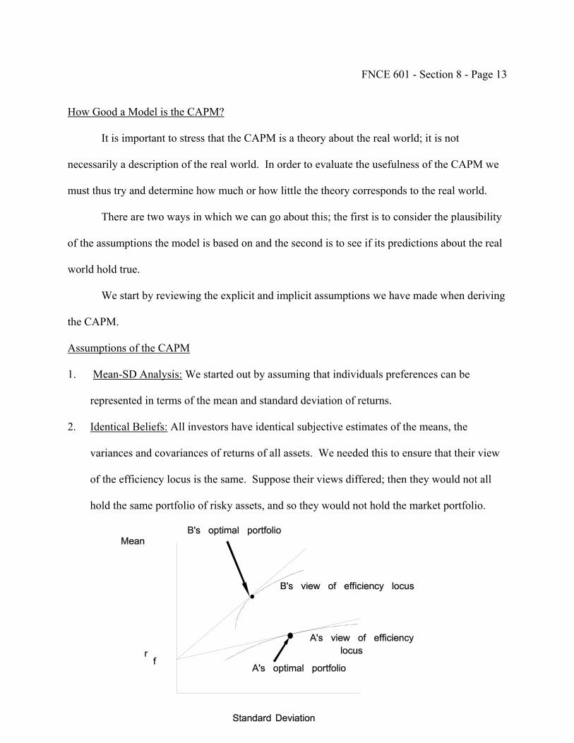
FNCE 601 - Section 8 - Page 13
How Good a Model is the CAPM?
It is important to stress that the CAPM is a theory about the real world; it is not
necessarily a description of the real world. In order to evaluate the usefulness of the CAPM we
must thus try and determine how much or how little the theory corresponds to the real world.
There are two ways in which we can go about this; the first is to consider the plausibility
of the assumptions the model is based on and the second is to see if its predictions about the real
world hold true.
We start by reviewing the explicit and implicit assumptions we have made when deriving
the CAPM.
Assumptions of the CAPM
1. Mean-SD Analysis: We started out by assuming that individuals preferences can be
represented in terms of the mean and standard deviation of returns.
2. Identical Beliefs: All investors have identical subjective estimates of the means, the
variances and covariances of returns of all assets. We needed this to ensure that their view
of the efficiency locus is the same. Suppose their views differed; then they would not all
hold the same portfolio of risky assets, and so they would not hold the market portfolio.
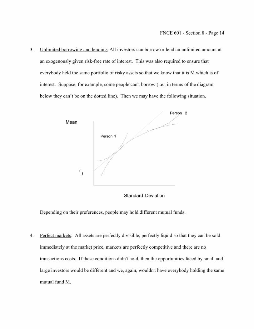
FNCE 601 - Section 8 - Page 14
3. Unlimited borrowing and lending: All investors can borrow or lend an unlimited amount at
an exogenously given risk-free rate of interest. This was also required to ensure that
everybody held the same portfolio of risky assets so that we know that it is M which is of
interest. Suppose, for example, some people can't borrow (i.e., in terms of the diagram
below they can’t be on the dotted line). Then we may have the following situation.
Depending on their preferences, people may hold different mutual funds.
4. Perfect markets: All assets are perfectly divisible, perfectly liquid so that they can be sold
immediately at the market price, markets are perfectly competitive and there are no
transactions costs. If these conditions didn't hold, then the opportunities faced by small and
large investors would be different and we, again, wouldn't have everybody holding the same
mutual fund M.
FNCE 601 - Section 8 - Page 15
5. Same after-tax returns: Taxes must be such that after-tax returns ensure that everybody
faces the same efficiency locus. If this isn't the case then we run into the same type of
problems that we had in 2 when people had different subjective estimates of the means and
variances.
These assumptions are rather strong, which indicates that the model is not likely to be a
perfect description of the real world. But are the divergences from these assumptions such that
they make the model totally useless? To get a better feel for this we turn next to empirical
results to see how serious the strength of the assumptions is.
Empirical Tests of the CAPM
When deriving the CAPM we argued that it must be the case that the expected return on
any asset, security or portfolio must be such that
r = rf + β(rM - rf)
otherwise people wouldn't hold it or would hold more of it until its price changed so that this
condition was satisfied.
If you plot r against β, this is called the Security Market Line (SML). What are the
intercept and slope? The intercept is rf and the slope is (rM - rf).
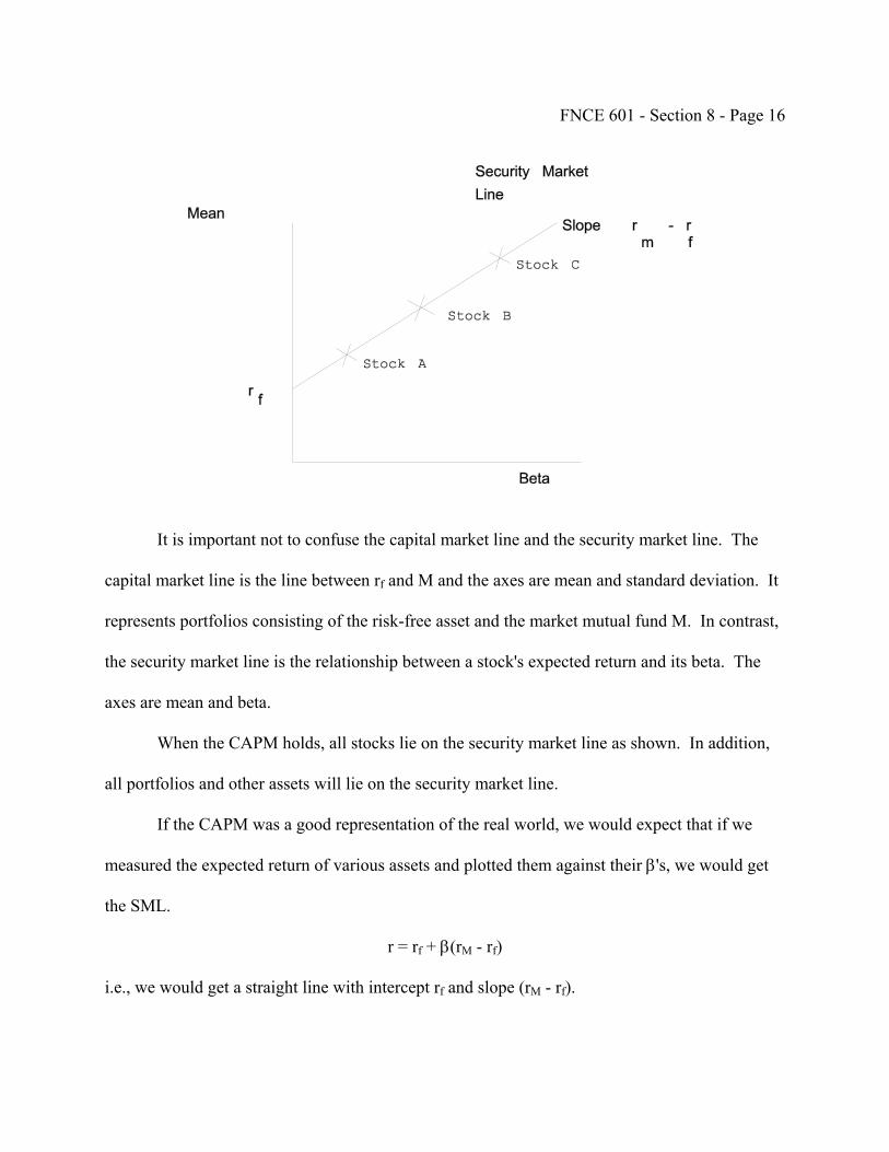
FNCE 601 - Section 8 - Page 16
It is important not to confuse the capital market line and the security market line. The
capital market line is the line between rf and M and the axes are mean and standard deviation. It
represents portfolios consisting of the risk-free asset and the market mutual fund M. In contrast,
the security market line is the relationship between a stock's expected return and its beta. The
axes are mean and beta.
When the CAPM holds, all stocks lie on the security market line as shown. In addition,
all portfolios and other assets will lie on the security market line.
If the CAPM was a good representation of the real world, we would expect that if we
measured the expected return of various assets and plotted them against their β's, we would get
the SML.
r = rf + β(rM - rf)
i.e., we would get a straight line with intercept rf and slope (rM - rf).

FNCE 601 - Section 8 - Page 17
In a classic study, Fama and MacBeth did this for a number of large portfolios. They
used large portfolios to try to minimize the idiosyncratic risk associated with individual
securities. They did this for a number of periods and got the results shown on the diagram at the
end of the section. Obviously the points do not fit perfectly, but on the other hand, they are not
completely different from a straight line.
The CAPM gives some insight into the historical data that we saw initially. As you
would expect from their higher beta stocks have a higher return than bonds. Moreover, small
stocks have a higher beta than large stocks because they are more cyclical. This explains part fot
he higher return that they have. However, as discussed in the book betas cannot fully explain the
difference. It is this kind of anomaly that has lead to the development of other models.
We won't go any further here. If you go on and do more finance, then you'll go into the
CAPM and its validity in much more detail. For the moment a reasonable conclusion to draw
from what we've done is that the CAPM is not ideal but is simple to use and better than nothing.
There have been a number of other asset pricing theories such as Ross' Arbitrage Pricing Theory
(APT) and the Fama-French three factor model. None of these have been sufficiently successful
to supplant the CAPM.
Explaining the Motivation Examples
We initially started off with the puzzles:
1. Which is more risky, investing in gold prospecting or electric utilities? Answer: Electric
utilities.
2. Would you ever invest in a security whose average return was less than that on T-bills?
FNCE 601 - Section 8 - Page 18
Answer: Yes.
The key to understanding these answers is the difference between unique risk and market
risk. Unique risk can be diversified away by holding stocks in a portfolio but market risk cannot.
The gold mining example has a lot of unique risk but no market risk. Since the unique risk can
be diversified away it is not very risky. The electric utilities have market risk. This cannot be
diversified away so they are risky in a financial sense.
In the second example a stock could yield less than T-bills if it had negative market risk.
If it moves in the opposite direction to other stocks then it can reduce the risk of a portfolio.
This means it is very valuable and has a high price or equivalently a low return.
We showed the formal model that captures the notion of diversification and the
difference between unique risk and market risk is the CAPM. For every asset
r = rf + β(rM - rf)
What's important in determining a stock's return is its β because this is what contributes
to the variance of the portfolio. Something with negative covariance with the market is valuable-
-it cuts down risk: when everything else is down, it's up and vice versa. This is good, so it's
valuable, has a high price and therefore a low return.
Understanding the historical data
The CAPM also gives us some insight into the historical data that we looked at initially.
If you think back to the chart on what your wealth would have been if you’d invested $1 in
various instruments you will remember that small stocks had the highest returns, followed by
large stocks, long-term government bonds and T-bills. As you might expect this follows the
FNCE 601 - Section 8 - Page 19
ordering of the stocks betas. Small firm stocks have a larger beta than those of large firms which
in turn have a larger beta than long term government bonds and the zero beta of T-bills. Now
although the ordering is correct the magnitudes of betas are such that they cannot fully explain
the differences in returns. Small stocks have in fact earned even higher returns than their betas
would suggest. Once again the empirical evidence is only partially consistent with the CAPM.
Constructing arbitrage portfolios
An important step in our derivation of the CAPM was the arbitrage argument. It is
helpful in understanding portfolio theory to consider this notion further. Let us start by
reviewing the simple case of a riskless arbitrage where all securities are risk free.
Example 1: Suppose that the borrowing and lending rate is 7%. You discover a risk free one-
year bond which costs $1,000. At the end of the year it will pay a coupon of $80 and principal of
$1,000. It therefore yields 8%. How can you make money? Is the price likely to stay at $1,000?
Clearly, an arbitrage opportunity exists here. The thing to do to make money is to
borrow $1,000 at 7% and invest it in the bond that yields 8%. At the end of the year you will
receive $1,080 and owe the bank $1,070 so you will make a profit of $10. Everybody will try to
do this so the price will go up until the yield on the bond falls to 7% and there are no more
money making opportunities.
1,080P $1,009.351.07
= =
FNCE 601 - Section 8 - Page 20
Arbitrage opportunities such as this will be short-lived. It will not be necessary to wait the full
year. Once the price rises to $1,009.35 (which will be almost immediately) you can repay your
$1,000 loan and keep the $9.35 profit. Notice that this is the same as the $10 you would have
received at the end of the year if you had held the position for the whole year since 10/1.07 =
$9.35.
Example 2: Suppose there are two risk-free one-year bonds A and B that you discover. Bond A
has a current price of $1,000. At the end of the year it will pay a coupon of $50 and principal of
$1,000. It therefore yields 5%. Bond B also has a current price of $1,000. At the end of the
year it will pay a coupon of $60 and principal of $1,000. It therefore yields 6%. How can you
make money? Will this opportunity persist?
Similarly to Example 1, what you would like to do here is borrow at 5% and invest at
6%. Investing at 6% is no problem. All you have to do is buy bond B. How can you borrow at
5%? You can do something called go short in bond A. What this means is that instead of
borrowing money you borrow bond A - you have a negative amount of it. At the end of the time
you have agreed to borrow it for you have to give it back. If any interest becomes due on the
bond during this time you must pay that interest to the person that lent it to you. In this example
you go short in bond A. After you have borrowed it you can sell it at $1,000, take the money
and invest in bond B. Investing in bond B is called going long in bond B.
At the end of the year you receive $60 interest from bond B. You must pay $50 of this to
the person you borrowed bond A from. You can use the $1,000 principal repayment on bond B
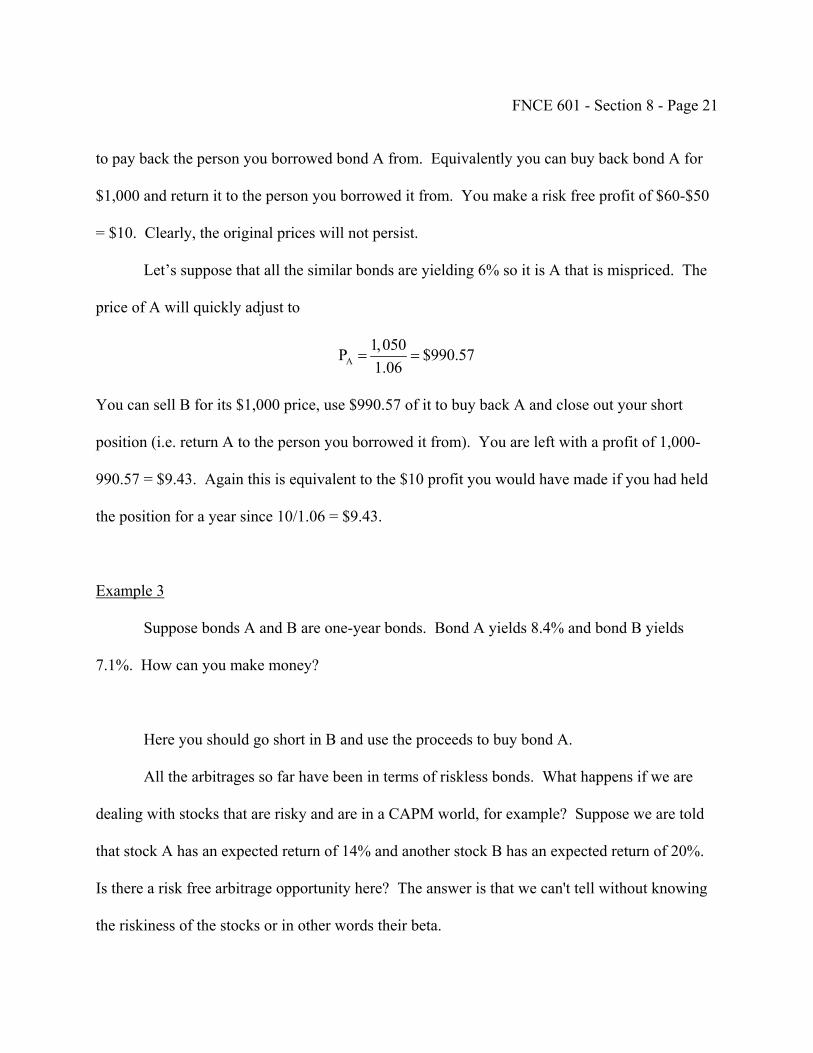
FNCE 601 - Section 8 - Page 21
to pay back the person you borrowed bond A from. Equivalently you can buy back bond A for
$1,000 and return it to the person you borrowed it from. You make a risk free profit of $60-$50
= $10. Clearly, the original prices will not persist.
Let’s suppose that all the similar bonds are yielding 6% so it is A that is mispriced. The
price of A will quickly adjust to
A1,050P $990.571.06
= =
You can sell B for its $1,000 price, use $990.57 of it to buy back A and close out your short
position (i.e. return A to the person you borrowed it from). You are left with a profit of 1,000-
990.57 = $9.43. Again this is equivalent to the $10 profit you would have made if you had held
the position for a year since 10/1.06 = $9.43.
Example 3
Suppose bonds A and B are one-year bonds. Bond A yields 8.4% and bond B yields
7.1%. How can you make money?
Here you should go short in B and use the proceeds to buy bond A.
All the arbitrages so far have been in terms of riskless bonds. What happens if we are
dealing with stocks that are risky and are in a CAPM world, for example? Suppose we are told
that stock A has an expected return of 14% and another stock B has an expected return of 20%.
Is there a risk free arbitrage opportunity here? The answer is that we can't tell without knowing
the riskiness of the stocks or in other words their beta.
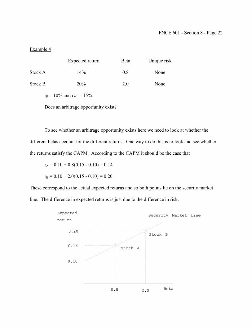
FNCE 601 - Section 8 - Page 22
Example 4
Expected return Beta Unique risk
Stock A 14% 0.8 None
Stock B 20% 2.0 None
rF = 10% and rM = 15%.
Does an arbitrage opportunity exist?
To see whether an arbitrage opportunity exists here we need to look at whether the
different betas account for the different returns. One way to do this is to look and see whether
the returns satisfy the CAPM. According to the CAPM it should be the case that
rA = 0.10 + 0.8(0.15 - 0.10) = 0.14
rB = 0.10 + 2.0(0.15 - 0.10) = 0.20
These correspond to the actual expected returns and so both points lie on the security market
line. The difference in expected returns is just due to the difference in risk.
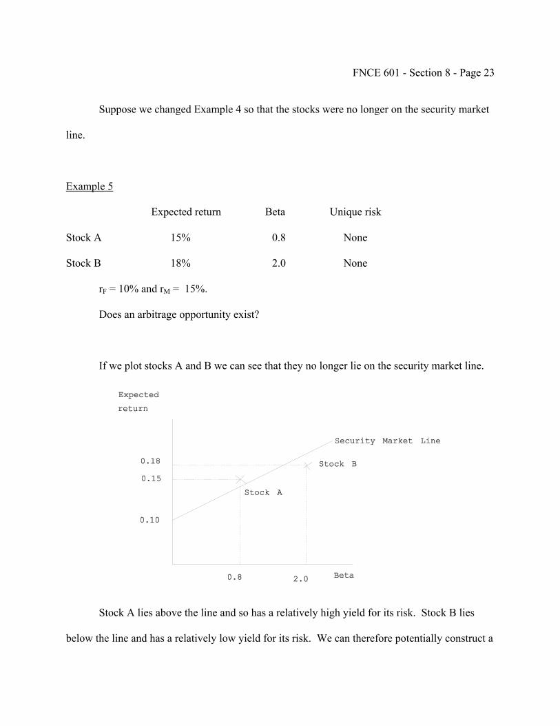
FNCE 601 - Section 8 - Page 23
Suppose we changed Example 4 so that the stocks were no longer on the security market
line.
Example 5
Expected return Beta Unique risk
Stock A 15% 0.8 None
Stock B 18% 2.0 None
rF = 10% and rM = 15%.
Does an arbitrage opportunity exist?
If we plot stocks A and B we can see that they no longer lie on the security market line.
Stock A lies above the line and so has a relatively high yield for its risk. Stock B lies
below the line and has a relatively low yield for its risk. We can therefore potentially construct a

FNCE 601 - Section 8 - Page 24
portfolio that makes money without risk. Note that since the unique risk of both stocks is zero
we only have to worry about the market risk or beta. To have zero market risk we need to
construct a portfolio with zero beta. We know that
βportfolio = πAβA + πBβB.
We need to short B because it has a relatively low yield. Suppose that we set πB = -$1. We are
shorting $1 worth of stock B - in other words we are borrowing it and must pay dividends to the
owner while we hold it and eventually return the share to him. Given πB = -$1, and the values
of πA and πB in the example, it follows that to have a zero risk portfolio
βportfolio = πA x 0.8 + -1 x 2.0 = 0
or πA = 2.0/0.8 = $2.5
By investing $2.5 in A and -$1 in B we have ensured it is a zero risk arbitrage. The net
investment is
πA + πB = 2.5 - 1 = $1.5.
So we are effectively investing 1.5 in a zero beta, i.e. risk free, portfolio. If we were to invest in
the risk free asset we would earn a return of 0.1 x 1.5 = $0.15. In fact our portfolio earns a return
of
Erportfolio = πArA + πBrB = 2.5 x 0.15 - 1 x 0.18 = $0.195.
We have made an excess return of 0.195 - 0.15 = $0.045.
In Example 5 we have to invest something to make an above risk free return. In contrast
in Examples 1-3 we did not need to invest any of our own money - the amount we borrowed was
equal to the amount we invested. This is called a zero-investment portfolio. In order to have a
zero-risk, zero-investment portfolio in our current type of situation we need at least 3 securities.
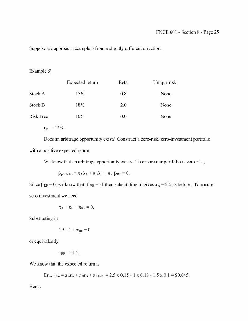
FNCE 601 - Section 8 - Page 25
Suppose we approach Example 5 from a slightly different direction.
Example 5'
Expected return Beta Unique risk
Stock A 15% 0.8 None
Stock B 18% 2.0 None
Risk Free 10% 0.0 None
rM = 15%.
Does an arbitrage opportunity exist? Construct a zero-risk, zero-investment portfolio
with a positive expected return.
We know that an arbitrage opportunity exists. To ensure our portfolio is zero-risk,
βportfolio = πAβA + πBβB + πRFβRF = 0.
Since βRF = 0, we know that if πB = -1 then substituting in gives πA = 2.5 as before. To ensure
zero investment we need
πA + πB + πRF = 0.
Substituting in
2.5 - 1 + πRF = 0
or equivalently
πRF = -1.5.
We know that the expected return is
Erportfolio = πArA + πBrB + πRFrF = 2.5 x 0.15 - 1 x 0.18 - 1.5 x 0.1 = $0.045.
Hence
FNCE 601 - Section 8 - Page 26
πA = $2.5; πB = -$1 and πRF = -$1.5
is a zero-risk, zero-investment portfolio with a positive expected return. Clearly we would not
expect such an opportunity to persist for very long.
The examples above show how arbitrage portfolios can be constructed in simple
situations. In fact whenever 3 securities don't lie on the security market line an arbitrage
opportunity exists; it is not necessary for one of them to be the risk free asset. The examples
above have the special feature that unique risk is zero. When this is not true it is necessary to
work in terms of portfolios where unique risk is diversified away. The stocks that lie off the
security market line must be embedded in diversified portfolios.
Understanding arbitrage is important because much of what investment banks do is to
construct such trading strategies. It is this activity that ensures prices are all the time being
driven into line with present values. The examples above are very simple. When we come to the
section on options you will see other more complicated arbitrage strategies. The whole valuation
of derivative securities of which options are one example is based on arbitrage ideas.
One thing to note is that we have ignored many of the institutional details of short selling
such as collateral. For these see the Appendix.
Concluding remarks
The important lesson of this section is the notion of diversification. You should spread
your investments over a number of alternatives. The CAPM is a formalization of this idea. It
doesn't work that well in terms of providing exact numbers but is a useful starting point
particularly for exercises such as capital budgeting where a rough and ready number is needed.
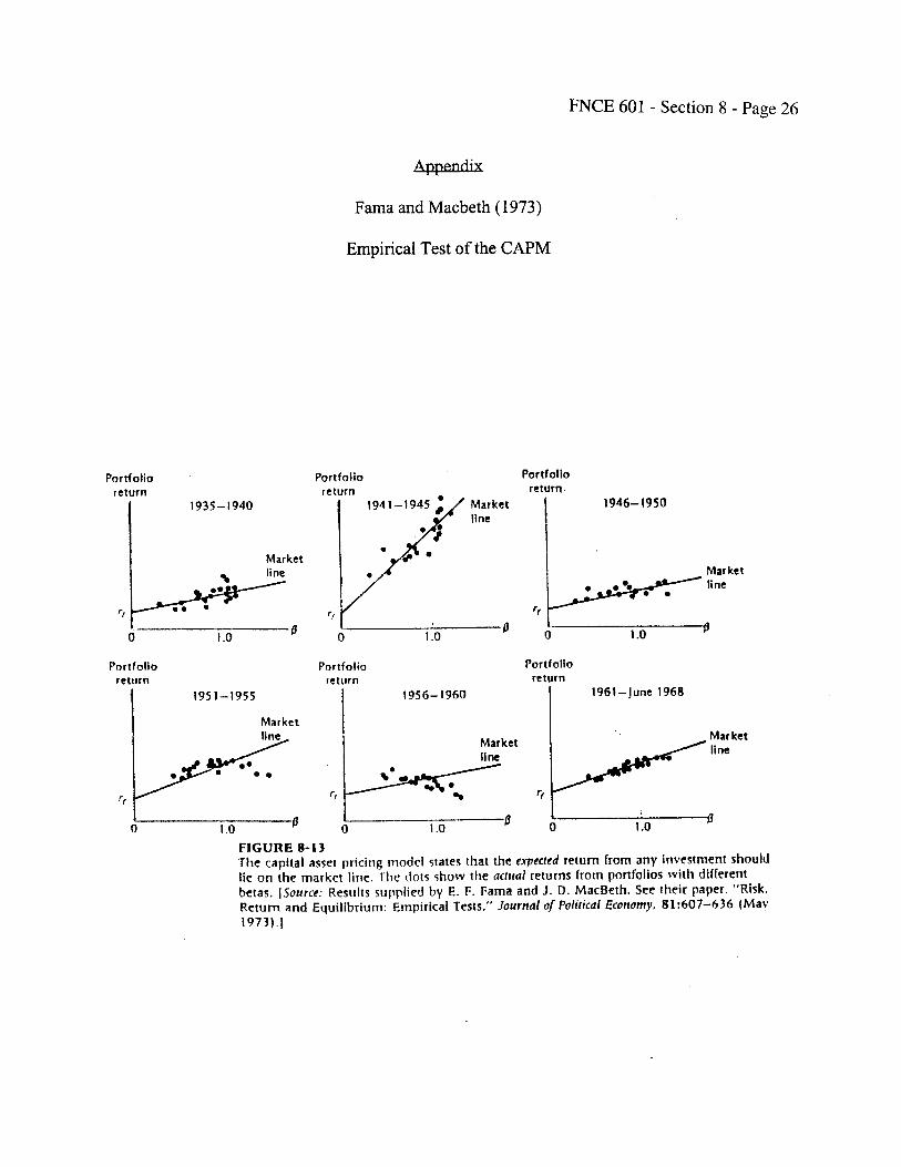
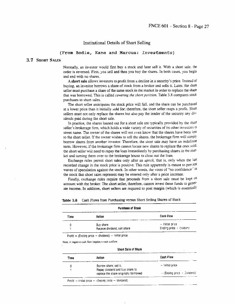

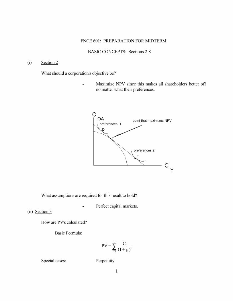
1
FNCE 601: PREPARATION FOR MIDTERM
BASIC CONCEPTS: Sections 2-8 (i) Section 2 What should a corporation's objective be? - Maximize NPV since this makes all shareholders better off
no matter what their preferences.
What assumptions are required for this result to hold? - Perfect capital markets. (ii) Section 3 How are PV's calculated? Basic Formula:
Special cases: Perpetuity
C
COA
Y
point that maximizes NPV
D
E
preferences 1
preferences 2
)r + (1
C = PV tt
tT
1=t∑
2
)r + (1
Dividend = P tt
1=t0 ∑
∞
Growing perpetuity Annuity Growing annuity These all assume payments are made at the end of the year. What happens when payments are made more frequently? - Compounding (iii) Section 4 How do we value bonds and stocks? - Prices of securities must be equal to their PV's. If this wasn't the
case, what would there be? An arbitrage possibility. Basic Formula: Stock with constant growth rate:
If growth is in stages then we have to adapt the basic formula to take account
of this. What do the formulas imply for price/earnings ratios? - If a stock has a high price/earnings ratio does that mean it's a good
buy? No it means it has a lot of growth opportunities.
g-r
Div = P 10
3
(iv) Section 5 Why is NPV the best investment criterion? - Superior to IRR because IRR has following difficulties Lending and borrowing problem Multiple roots Relative measure - Superior to Profitability index because this is Relative measure - Superior also to Payback and accounting measures such as Average
Return on Book because these are incorrect (v) Section 6 How do you make investment decisions using NPV rule? - Discount cash flows - Transform accounting data into cash flows Cash flow = $'s received - $'s paid out Work in after-tax terms Estimate cash flows on an incremental basis Be consistent in your treatment of inflation (vi) Sections 7 and 8 Beta and the Capital Asset Pricing Model Hold stocks in portfolios - Unique risk is diversified away - Market risk remains
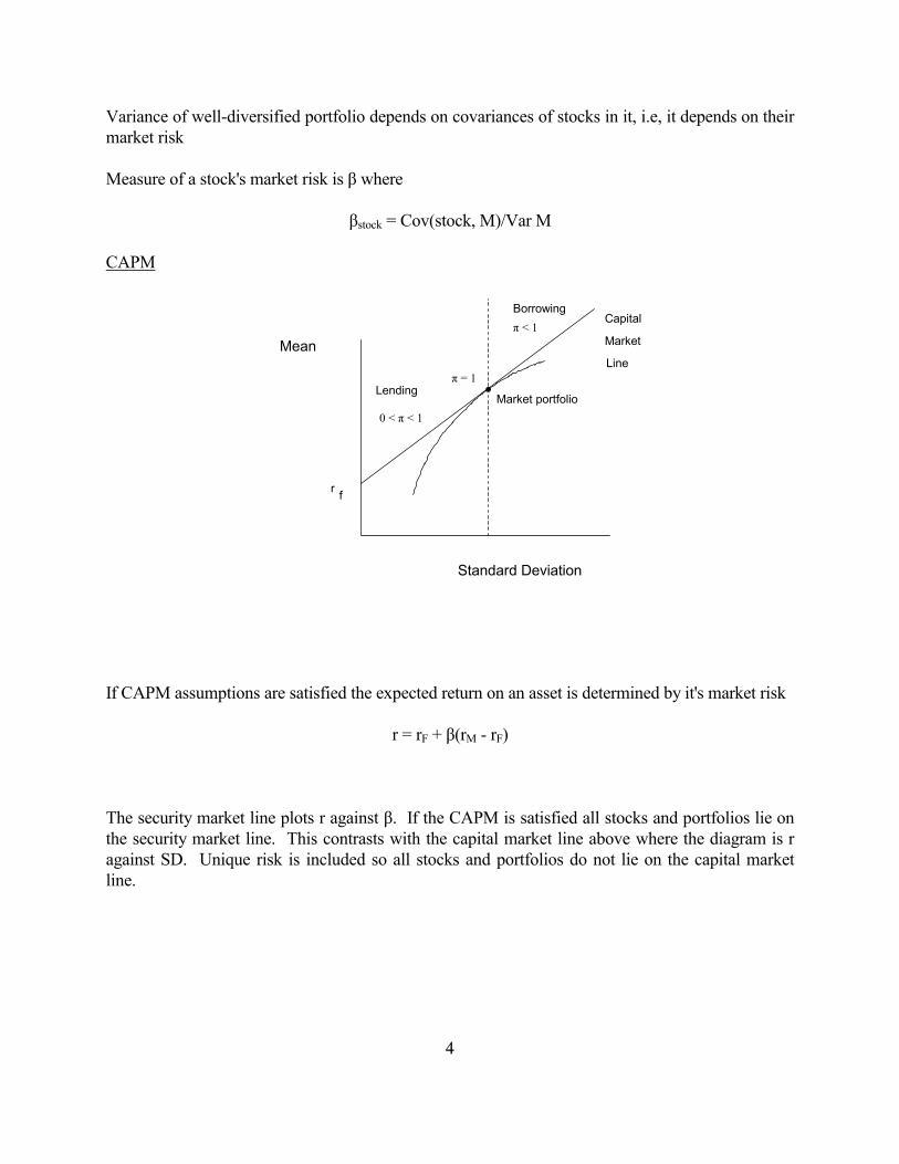
4
Variance of well-diversified portfolio depends on covariances of stocks in it, i.e, it depends on their market risk Measure of a stock's market risk is β where βstock = Cov(stock, M)/Var M CAPM
If CAPM assumptions are satisfied the expected return on an asset is determined by it's market risk r = rF + β(rM - rF) The security market line plots r against β. If the CAPM is satisfied all stocks and portfolios lie on the security market line. This contrasts with the capital market line above where the diagram is r against SD. Unique risk is included so all stocks and portfolios do not lie on the capital market line.
Mean
Standard Deviation
Market portfolio
π = 1
π < 1 Borrowing
Lending
0 < π < 1
r f
Capital
Market
Line

UNIVERSITY OF PENNSYLVANIA THE WHARTON SCHOOL FNCE 601 CORPORATE FINANCE LECTURE NOTES Franklin Allen Fall 2004 QUARTER 1 - WEEK 6 (part 2) Th: 10/14/04 Copyright © 2004 by Franklin Allen
FNCE 601 - Section 9 - Page 1
Section 9: Capital Budgeting and Risk
Read Chapter 9 BM
Motivation Example 1
Macrosoft is a computer software company. It has no debt. The beta of its equity, which
is equal to the beta of its assets since it has no debt, is 1.25. The risk free rate is rF = 5% and the
market risk premium is rM – rF = 8%. Using the CAPM, the opportunity cost of capital for the
firm is 5% + 1.25 x 8% = 15% and this is the discount rate they use for evaluating computer
software projects. Macrosoft is considering a hardware project. It is considering building PC’s
to compete with Dell, Gateway and other PC manufacturers. Suppose the beta of the assets of
these companies that engage in activities similar to this hardware project is 1.83. This
corresponds to an opportunity cost of capital of 5% + 1.83 x 8% = 20%.
Maria Fuentes is the CFO of Macrosoft. She believes that Macrosoft should use 15% as
the discount rate. Her argument is that Macrosoft can raise funds from their shareholders at 15%
and so this is the relevant rate. Ari Silverberg is her deputy. He argues that Macrosoft should
use the rate of 20% since this compensates for the risk that Macrosoft is taking by investing in
the hardware industry.
Who is correct? In evaluating the hardware project should Macrosoft use a discount rate
of 15% or 20%?
Finding the discount rate for a project like the firm
Suppose that we are considering a “pure play” firm like Dell that only invests in one type
of project that is the same as its existing assets. All Dell does is produce PC’s. The discount rate
we should use for a project is the opportunity cost of capital (or as it is often called the cost of
capital). In other words, if the firm didn't do the project it would invest in the best alternative
available and we should use the return on this as the discount rate. In Section 2 there was

FNCE 601 - Section 9 - Page 2
certainty and we simply took the best available alternative. In our initial example this was the
rate at the bank.
What is the best alternative available when there is uncertainty? This depends on the risk
of the project. We should choose the best alternative so that its risk is the same as that of the
project. The CAPM provides a way of doing this. It provides the best available alternative in
the stock market for a similar risk project. If the CAPM holds, then the opportunity cost of
investing in a project with a risk of β is:
r = rF + (Project β)(rM - rF)
This is then the discount rate for the project. If the firm doesn't do the project then it can always
invest in a portfolio with the same β as the project and get a return of r.
There are a number of studies that give some idea of the market return rM. Ibbotson
Associates publishes a book each year that gives the up-to-date figures. For the purposes of this
section we will suppose rF = 0.05 and rM - rF = 0.08. We can also observe rF, the rate on risk
free assets, by looking at that on Treasury bills.
The problem is in finding the project β. For a firm with no debt this is straightforward.
With an all-equity capital structure the earnings from the assets simply flow through to the
equity holders. The riskiness of the assets must be equal to the riskiness of the equity. Hence
for an all-equity firm we can simply get the β of the equity and this will be equal to the β of the
assets or in other words the project β.
How do we measure the β of a firm's equity? We use regression theory. We know from
regression theory that if we plot the returns on a stock Y against the returns on the market and
we fit a straight line by the method of least squares, its slope is given by
β
σ Equitys'Firm2
M
= M)Cov(Y, = b
FNCE 601 - Section 9 - Page 3
Now the statistical problems in measuring betas are significant (see BM Chapter 9). The
easiest way to find a beta is probably to use Bloomberg. So for most companies we can get find
the beta of the company's stock. In the cases where we can't find a precalculated figure we must
go back to the data, fit a regression line for the firm and find our β that way.
One important thing is that regressions are based on historical data. This means that the
β is a measure of risk in the past. However, in analyzing a project we are looking forward so if
we use the β calculated from historic data we are assuming the future will be like the past. This
is a reasonable assumption in many cases but in others it is not. If you think the future riskiness
of a project will be different from the past riskiness you will need to take account of this.
In our Dell example, the beta of its assets of is 1.83. Hence the opportunity cost of
capital for Dell is given by
rDell = 5% + 1.83 x 8% = 20%.
Dell should use a 20% when calculating whether or not a project has a positive NPV and is
worth undertaking.
Example 1
Suppose Dell has a project with a cost at date 0 of $1 million. It foresees three scenarios.
The first is the optimistic scenario and it occurs with probability 0.3. If the product is a big
success the cash flow will be $1.6M at date 1. The second is the moderate scenario and it occurs
with probability 0.5. If the project is a moderate success the cash flow will be $1.2M at date 1.
The third is the pessimistic scenario and it occurs with probability 0.2. If the project is a failure
the cash flow will be $0.8M at date 1.
FNCE 601 - Section 9 - Page 4
Solution
The first step is to calculate the expected cash flow at date 1.
C1 = 0.3×1.6M + 0.5×1.2M + 0.2×0.8M = $1.24M
The next step is to calculate NPV in the usual way.
M033.0$2.1M24.1M1NPV =+−=
If instead of $1.24M the project had an expected cash flow of $1.17M at date 1. Clearly it would
have a negative NPV or equivalently a return of only 17%. It would not be worth undertaking
because Dell would not being compensated for the project’s risk. Dell (or equivalently its
stockholders) would be better off to go into the stock market and buy securities with a beta of
1.83 and have an expected return of 20%.
If a firm has debt then finding the β of the assets is more complicated. When there is
debt the beta of a firm’s equity is different from the beta of its assets. We will consider this at
length when we come to consider capital structure later in the course. For the moment we will
focus on firms that have all equity capital structures so that the beta of the firm’s equity and the
beta of its assets are the same.
Finding the discount rate for a project different from the firm
We are now in a position to answer the question raised in Motivation Example 1.
Suppose that a firm is investing in a project that is different from its current activities such as
Macrosoft investing in hardware rather than software. What is the discount rate, or equivalently
the opportunity cost of capital, for Macrosoft? The key point is that when they are investing in
assets with a beta of 1.83 they must be compensated for that risk. This means that for hardware
projects they should use a discount rate which is the same as Dell’s, i.e. 20%. If they used the
rate for software projects of 15% they might accept projects which did not compensate them for

FNCE 601 - Section 9 - Page 5
the risk they were taking. For example, a project with a 17% rate of return would seem to have a
positive NPV at a 15% discount rate. However, they should reject such projects because they
would have been better off to go out and invest in the stock market in assets with a beta of 1.83
where they could have received a 20% expected return. Macrosoft should use a 20% discount
rate in evaluating hardware projects and a 15% discount rate in evaluating software projects.
Discount rates for Multi-division Firms
How should a multi-division firm calculate its opportunity cost of capital? The principle
is again the same. The rate should reflect the risk being taken by the division. The firm should
not use a rate reflecting the average for the company. Let’s consider an example.
Example 2
Corporal Electric has two divisions. The first division manufactures consumer goods.
The β of firms that only produce consumer goods is 1.0. The second division produces gas
turbines. The β of firms that do this alone is 1.5. The two divisions each constitute 50% of the
firm. The firm has no debt.
The beta of the equity can be found by thinking of the firm as a portfolio of two
divisions.
βE = 0.5x1 + 0.5x1.5 = 1.25
Assuming rF = 0.05 and rM – rF = 0.08 and the CAPM holds it follows that
rE = 0.05 + 1.25 x 0.08 = 0.15.
What rate should the firm use in evaluating projects?
It is helpful to consider the security market line and see how projects lie relative to this.
The expected return on securities with β’s of 1 and 1.5 are 0.05 + 1 x 0.08 = 0.13 and 0.05 + 1.5
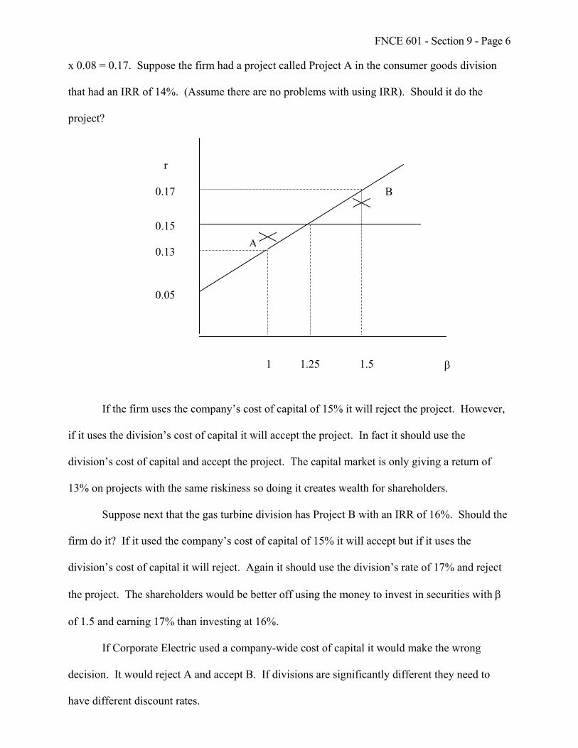
FNCE 601 - Section 9 - Page 6
x 0.08 = 0.17. Suppose the firm had a project called Project A in the consumer goods division
that had an IRR of 14%. (Assume there are no problems with using IRR). Should it do the
project?
B
A
r
0.17
0.13
0.15
0.05
If the firm uses the company’s
if it uses the division’s cost of capital i
division’s cost of capital and accept th
13% on projects with the same riskines
Suppose next that the gas turbin
firm do it? If it used the company’s co
division’s cost of capital it will reject.
the project. The shareholders would b
of 1.5 and earning 17% than investing
If Corporate Electric used a com
decision. It would reject A and accept
have different discount rates.
1 1.25 1.5 β
cost of capital of 15% it will reject the project. However,
t will accept the project. In fact it should use the
e project. The capital market is only giving a return of
s so doing it creates wealth for shareholders.
e division has Project B with an IRR of 16%. Should the
st of capital of 15% it will accept but if it uses the
Again it should use the division’s rate of 17% and reject
e better off using the money to invest in securities with β
at 16%.
pany-wide cost of capital it would make the wrong
B. If divisions are significantly different they need to
FNCE 601 - Section 9 - Page 7
In multi-division firms the key thing is to always evaluate a project using the discount
rate reflecting the risk of the assets that are being invested in. Finding the β for such assets
involves identifying a “pure-play” firm. This is a firm that engages only in a single industry.
The industry of the pure play firm and the project should obviously be the same.
Strategy and Finance
Read Chapter 11 BM
How is it that projects like Project A can have a positive NPV and create wealth for
shareholders? We argue that in capital markets all stocks must lie on the security market line.
Why is it that projects like A do not have to lie on the security market line? In perfect capital
markets competition among arbitrageurs ensures that all stocks lie on the security market line. If
a project is to have a positive NPV it must be due to imperfections in product or input markets.
When a firm has a monopoly over the product market it operates in then it will be able to have
positive NPV projects. Similarly, if the firm is an oligopolist it will also have positive NPV
projects available. In contrast, if a firm is in a perfectly competitive industry it will not have any
positive NPV projects. Any positive NPV projects will be enthusiastically adopted by a number
of firms and prices will be bid down.
Intimately related to the question of identifying positive NPV projects, is the issue of
strategy and finance. In order to have many profitable projects the firm must pursue an overall
strategy that allows it to take advantage of barriers to entry, core competencies and so forth.
Strategic management is concerned with how to find profitable areas.
Good strategy and the existence of positive NPV projects also leads to the notion of
competitive response. One of the most important things in doing good project evaluation is
anticipating competitors’ reactions correctly. It is crucial to take account of such responses
FNCE 601 - Section 9 - Page 8
when forecasting cash flows. The existence of profitable opportunities will encourage entry and
this will lead to the dissipation of profits.
A good example is provided by Bausch and Lomb. This was the leading firm in old style
“hard” contact lenses made from glass. These lasted for a long time but they were difficult to
use. Each night they had to be cleaned in solution and put in a heating machine that would
sterilize them. Bausch and Lomb made a lot of money not only from selling the lenses originally
but also from the sterilizing solutions and machines. They decided not to introduce disposable
contact lenses because of concern about the impact this would have on their existing contact lens
and solutions business. However, in the long run this was a significant mistake as it enabled
Johnson & Johnson to enter the disposable lenses market and gain considerable market share at
Bausch and Lomb’s expense.
Another good example of this problem is IBM. When PC’s were first introduced IBM
was essentially a monopoly. It had a very large market share in mainframes. IBM didn’t
develop PC’s because they thought this would erode sales of mainframes. In the short run this
was a good decision but in the long run it was not. It led to entry by other firms and eroded their
monopoly position.
Fundamental Determinants of Asset β's
So far we have discussed how you can find the β's for already existing lines of business.
You calculate the β's of the assets for firms engaged primarily in this type of business and use
your judgment to adjust for likely future changes.
What do you do if it's a totally new line of business? For example, how should a
company involved in manufacturing mobile phones a few years ago like Motorola or Nokia have
decided what the risk of the business they were investing in was? How should they have decided
FNCE 601 - Section 9 - Page 9
what value of beta to use when they were doing the capital budgeting exercise to see whether it
would be profitable producing them? In such cases it is necessary to have some idea of the
underlying determinants of β's in order to be able to make a judgment.
There are two factors which are usually put forward as being the fundamental
determinants of β's
(i) Correlation with the business cycle
(ii) Technology of production.
Let's look at these in turn.
(i) Correlation with the business cycle
When introducing the notion of market risk we said that correlations between stocks
essentially arose because of the business cycle. Thus you would expect products which are
highly correlated with the business cycle to have high β's. For example, consumer durables,
such as autos, stereos and so on, are likely to be highly cyclical since when times are good
people replace them but when times are bad they make them last a bit longer. Similarly, you
would expect things that people need all the time not to be cyclical and hence have low β's.
(ii) Technology of production
An important distinction economists use when talking about production processes is the
difference between fixed costs and variable costs:
(a) Fixed costs are those which must be paid regardless of output, e.g., rent, basic maintenance,
insurance, and so on.
(b) Variable costs are those that vary with output level, e.g. wages, new materials and so on.

FNCE 601 - Section 9 - Page 10
Fixed costs increase riskiness. To see this consider the extreme case where there are no
fixed costs. In this case price is equal to marginal cost and profits are always equal to zero.
There is then no risk in profits and β = 0. If there are fixed costs then price must be above
marginal cost on average to cover the fixed costs. In this case profits will vary with the number
of units you sell and so the stock will be risky and β > 0.
Having high fixed costs is known as operating leverage. Empirical tests confirm that
companies which have high operating leverage also tend to have high β's.
It is helpful to see the plausibility of these factors by considering some examples of asset
betas (i.e. unlevered to abstract from the effect of debt) from existing industries. A full list can
be obtained from http://pages.stern.nyu.edu/~adamodar/New_Home_Page/datafile/Betas.html .
Industry Asset Betas
Aerospace/Defense 0.57
Banks 0.43
Computer 1.83
Electric Utility 0.33
Electrical Equipment 1.40
Food Processing 0.52
Internet 2.19
Semiconductor Equipment 2.22
Telecom 1.92
Returning to our mobile phone example, what risk do you think firms should have
assigned to the project? The factors determining sales of mobile telephones are presumably
different from regular telephones and more like other electrical equipment. The cost structure is

FNCE 601 - Section 9 - Page 11
also probably similar to these other types of electrical equipment. Now we know that the beta of
firms producing electrical equipment tends to be high. In fact the electrical equipment industry
has had a β of around 1.40. This suggests that the market risk that is associated with mobile
phones should also be high probably the beta should be around 1.40.
Risk Assumptions Implicit in Using CAPM to Calculate Multi-Period Discount Rates
Motivation Example 2
GM is thinking of building a new automobile plant. The cost of this plant is $100M. The
expected cash flow the firm anticipates the plant will generate in each of the three years it will be
in operation is $50M. How should the firm choose its discount rate for this plant?
Time 0 1 2 3
Cash Flow -100M +50M +50M +50M
The firm is confident that economic conditions next year will not be very different from
the current year so that the risk associated with the first-year estimate is fairly minimal.
However, in the second year economic conditions are somewhat more uncertain so the risk
associated with the second-year cash flow estimate is greater than the risk associated with the
first-year estimate. Similarly, in three years time economic conditions could have changed quite
significantly so that the risk associated with the cash flow estimate at this stage is even higher.
The project manager argues that because the risk associated with the estimates of the project's
cash flows increases through time the discount rate the firm uses should be higher the farther
away the cash flow is.
Is the project manager correct?

FNCE 601 - Section 9 - Page 12
The motivation example raises the issue of how we should deal with risk that is changing
over time. One of the assumptions we made with the CAPM, was that it was based on choosing
investments over one period. Many of the projects we will be interested in will obviously be for
more than one period. What are the consequences of using the CAPM to calculate discount rates
for multi-period projects?
First consider the one period case:
r1CPV 1
+=
where )rr(rr FMF −β+=
- What does the rF term adjust for? It adjusts for time.
- What does the β (rM - rF) term adjust for? It adjusts for risk.
Consider next the PV of a second period cash flow:
)r1(C
)r1(1
)r1(CPV 2
22
++=
+=
where r is the same as before.
- How many times are we adjusting for time? We are adjusting for time twice.
- What about risk, how many times are we adjusting for risk? We are using the risk
adjustment factor once in discounting from period 2 to 1, and again in discounting
from period 1 to period 0. We are adjusting for risk twice. We are therefore
implicitly assuming that because the second period cash flow is two periods away,
it is more risky.
FNCE 601 - Section 9 - Page 13
In order to see this more clearly, it is helpful to develop another approach to the problem,
namely, certainty equivalents.
Certainty Equivalents
When considering risky projects, we have so far been evaluating their NPV by taking the
expected cash flows and by making the discount rate depend on the degree of risk. An
alternative method is to adjust the cash flows to their certainty equivalents and discount at the
risk free rate. This is the certainty equivalent approach.
The question we ask to get the certainty equivalent is "What is the smallest certain cash
flow for which you would exchange the risky cash flow C1." This is called the certainty
equivalent and is denoted CEQ1. To get the present value you discount this at the risk free rate.
F
1
r1CEQPV+
=
Similarly for cash flows in other periods. Now we write
CEQ1 = a1 C1
where a1 is the certainty equivalent adjustment factor.
When the CAPM holds, it must be the case that
r1C
r1CEQ 1
F
1
+=
+
Substituting CEQ1 = a1 C1 gives
r1C
r1Ca 1
F
11
+=
+
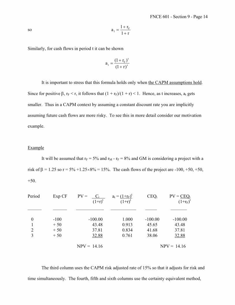
FNCE 601 - Section 9 - Page 14
so r1r1a F
1 ++
=
Similarly, for cash flows in period t it can be shown
t
tF
t )r1()r1(a
++
=
It is important to stress that this formula holds only when the CAPM assumptions hold.
Since for positive β, rF < r, it follows that (1 + rF)/(1 + r) < 1. Hence, as t increases, at gets
smaller. Thus in a CAPM context by assuming a constant discount rate you are implicitly
assuming future cash flows are more risky. To see this in more detail consider our motivation
example.
Example
It will be assumed that rF = 5% and rM - rF = 8% and GM is considering a project with a
risk of β = 1.25 so r = 5% +1.25×8% = 15%. The cash flows of the project are -100, +50, +50,
+50.
Period Exp CF PV = Ct at = (1+rF)t CEQt PV = CEQt (1+r)t (1+r)t (1+rF)t ______ ______ ____________ ___________ _____ _______
0 -100 -100.00 1.000 -100.00 -100.00 1 + 50 43.48 0.913 45.65 43.48 2 + 50 37.81 0.834 41.68 37.81 3 + 50 32.88 0.761 38.06 32.88 NPV = 14.16 NPV = 14.16
The third column uses the CAPM risk adjusted rate of 15% so that it adjusts for risk and
time simultaneously. The fourth, fifth and sixth columns use the certainty equivalent method,

FNCE 601 - Section 9 - Page 15
which in this case since the CAPM holds gives the same answer. The fourth column gives the
certainty equivalent adjustment factors. The fifth column gives the certainty equivalents of the
cash flows and the sixth discounts them at the risk free rate.
It can be seen from the fifth column that even though the expected value of each cash
flow in years 1-3 is 50 the certainty equivalents are 45.65, 41.68 and 38.06 respectively. Hence
by using a constant discount rate you are effectively making a much larger adjustment for risk in
the later cash flows.
Explanation of Motivation Example 2
If the project were something like an automobile plant as in our motivation example, then
this sort of profile would perhaps be reasonable. In 1 year's time the determinants of auto
purchase, are unlikely to be very different from now. If we’re in a boom now it’s likely we’ll be
in a boom then. However, in 2 years they may be somewhat different, and in 3 years they may
be very different. Cash flows 3 years away are thus riskier than in 1 year's time since it is
difficult to predict the direction and magnitude of change in factors affecting demand.
By assuming a constant β you are implicitly assuming that risk grows at a constant rate:
the risk borne per period will be constant, but cumulative risk will grow steadily as you look
further into the future. For many applications, such as the one we discussed, this is not too bad
an assumption.
Situations where constant rate CAPM assumptions are not appropriate
If risk is not increasing at a constant rate, then it is not appropriate to discount in this
way. For example, risk may grow at a faster rate than is implicit in the CAPM assumptions. In
some cases it may grow at a slower rate than is implicit in the CAPM assumptions. In such cases
it is necessary to adapt the certainty equivalent method to adjust the discount rates to fit the
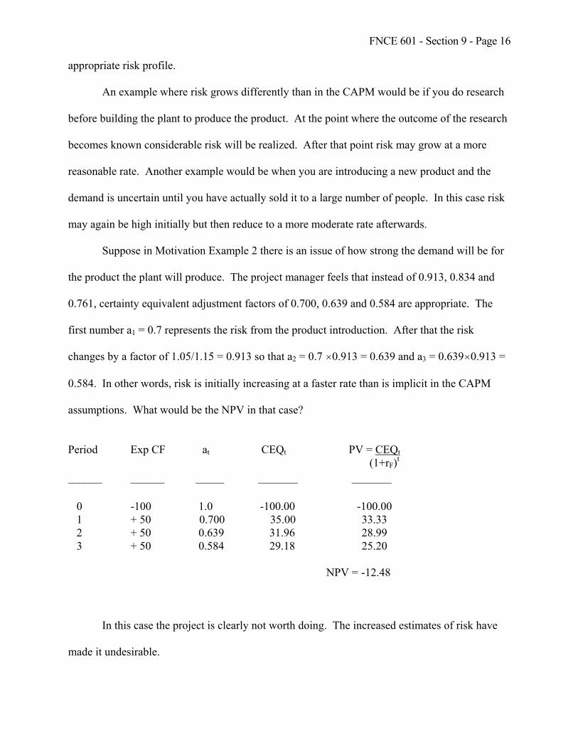
FNCE 601 - Section 9 - Page 16
appropriate risk profile.
An example where risk grows differently than in the CAPM would be if you do research
before building the plant to produce the product. At the point where the outcome of the research
becomes known considerable risk will be realized. After that point risk may grow at a more
reasonable rate. Another example would be when you are introducing a new product and the
demand is uncertain until you have actually sold it to a large number of people. In this case risk
may again be high initially but then reduce to a more moderate rate afterwards.
Suppose in Motivation Example 2 there is an issue of how strong the demand will be for
the product the plant will produce. The project manager feels that instead of 0.913, 0.834 and
0.761, certainty equivalent adjustment factors of 0.700, 0.639 and 0.584 are appropriate. The
first number a1 = 0.7 represents the risk from the product introduction. After that the risk
changes by a factor of 1.05/1.15 = 0.913 so that a2 = 0.7 ×0.913 = 0.639 and a3 = 0.639×0.913 =
0.584. In other words, risk is initially increasing at a faster rate than is implicit in the CAPM
assumptions. What would be the NPV in that case?
Period Exp CF at CEQt PV = CEQt (1+rF)t ______ ______ _____ _______ _______
0 -100 1.0 -100.00 -100.00 1 + 50 0.700 35.00 33.33 2 + 50 0.639 31.96 28.99 3 + 50 0.584 29.18 25.20 NPV = -12.48
In this case the project is clearly not worth doing. The increased estimates of risk have
made it undesirable.
FNCE 601 - Section 9 - Page 17
The main thing to remember here is that discounting at a constant risk adjusted rate
implies that uncertainty is increasing at a steady rate, and if this is not an appropriate
assumption, the result you obtain may be very misleading. In such cases you can use the
certainty equivalent method to adjust appropriately.