UNIVERSITY OF MIAMI

INFANT CRY DETECTION

By

Sunrito Bhattacharya

A THESIS PROJECT

Submitted to the Facultyof the University of Miami

in partial fulfillment of the requirements forthe degree of Master of Science in Music Engineering Technology

Coral Gables, Florida

March 4, 2016

UNIVERSITY OF MIAMI

A Thesis Project submitted in partial fulfillment ofthe requirements for the degree of

Master of Science in Music Engineering Technology

INFANT CRY DETECTION

Sunrito Bhattacharya

Approved:

Prof. William C. PirkleAssociate Professor of Music Engineering

Dr. Shannon de l’EtoileAssociate Dean of Graduate Studies

Dr. Daniel MessingerProfessor of Psychology

Dr. Christopher L. BennettResearch Assistant Professor of Music En-gineering

BHATTACHARYA, SUNRITO M.S., Music Engineering TechnologyMarch 4, 2016

Infant Cry Detection

Abstract of a Master’s Research Project at the University of Miami

Research Project supervised by Prof. William C. PirkleNumber of Pages in Text: [67]

This thesis encompasses modern age feature extraction and machine learningtools for the detection of infant cry signals. In developmental psychology, infantcrying is a measure of distress and an automated tool for measurement is extremelyimportant. Initial testing is done using the MIRToolbox in MATLAB which provedto be non-ideal for real time signal analysis due to slow speed and poor memorymanagement in MATLAB. Thus, a python based real time feature extraction toolLibrosa is used to calculate parameters MFCC, delta-MFCC, pitch, zero-crossing,spectral centroid and energy of the signal. A large chunk of 21 minutes cry signalis used for feature extraction and used for the training of the crying segment. Asimilarly sized non-cry segment consisting of other sounds as speech, baby whim-pering, toy sounds etc. are used to train the non-crying part of the model. A111091 instances and 28 attributes based dataset(.CSV) is developed for our clas-sifier. A Zero-R rule is used for baseline eastablishment, followed by classificationusing a random tree bagger and a multilayer perceptron. An error rate of 2.5 %was achieved using 100 trees and 10 fold cross-validation using random forest and asimilar result was achieved with a MLP with 500 training epochs, 15 hidden layersand 10 fold cross-validation. This is a major improvement over the existing resultsand the methods used for cry detection and much faster in feature extraction andis capable of handling much larger chunks of data for training and testing.

ACKNOWLEDGMENTS

Heads up, this is in the longest section of the thesis. I would like to startby acknowledging Dr. Daniel Messinger without him I could not have been hereand finished this degree. Thank you Dr. Colby Leider for the initial idea andthe introduction to the field of information retrieval. Special thanks to Dr. ChrisBennett for a key idea. Professor Pirkle, thank you for taking me up last minuteand supporting me in every possible way.

I would also like to thank every MuE and GMuE for making this ride a journeyof a lifetime. Thanks to Chris for being the biggest source of motivation andshowing me true work ethics, to AJ for the spunk and various other things, toGyawu for reintroducing us to tadpoles, to Shijia for providing the motivation tostay in academics for a prolonged period of time, to Tom for showing us its nevertoo late, to Akhil for being Akhil, to Kerline for extreme angst, to Tia for showingus true humility and being aggressively nice, to Kathryn for making Miami finallyfeel like home, to Susanta for always hosting me in Tampa and finally to Rhiyafor being the best friend I could ever have. Special thanks to Madhur for all hisPython help and Samarth for being the true father figure - he single handedly gotme through grad school.

Most importantly I would like to thank my family and Suvabrata and SumitaBhattacharya for being role model parents. I definitely got lucky in that depart-ment. Nothing I write here can describe what they have done for me. Thank youTy and Kuttu, for all the love and being the cousins I can always look up to.

Special mention for Innovation Kitchen and Martha for their impeccable CafeCon Leche, S&S diner for sustaining me in most desperate times, to the Yard Housefor the Dark Hour, the lovely people at Crown, Pollo Tropical (the life changer)and to Zuma for still being the place I can’t afford.

iii

DEDICATION

To my grandmom, Ms Mukul Sarkar cause you are the strongest and the mostinspirational person I have ever met.

To India For sustaining me for over two and a half decades.

iv

PREFACE

”The real question is not whether machines think but whether men do. Themystery which surrounds a thinking machine already surrounds a thinking man”,[Skinner, 2014].

v

TABLE OF CONTENTS

ACKNOWLEDGMENTS . . . . . . . . . . . . . . . . . . . . . . . . . . iii

DEDICATION . . . . . . . . . . . . . . . . . . . . . . . . . . . . . . . . . iv

PREFACE . . . . . . . . . . . . . . . . . . . . . . . . . . . . . . . . . . . . v

LIST OF TABLES . . . . . . . . . . . . . . . . . . . . . . . . . . . . . . . ix

LIST OF FIGURES . . . . . . . . . . . . . . . . . . . . . . . . . . . . . . x

CHAPTER

1 Introduction . . . . . . . . . . . . . . . . . . . . . . . . . . . . . . . 1

2 Background and Previous Work . . . . . . . . . . . . . . . . . . 5

2.1 Cry Detection: . . . . . . . . . . . . . . . . . . . . . . . . . . . . 5

2.1.1 Pitch frequency: . . . . . . . . . . . . . . . . . . . . . . . 8

2.1.2 MFCC: . . . . . . . . . . . . . . . . . . . . . . . . . . . . 9

2.1.3 Inharmonicity: . . . . . . . . . . . . . . . . . . . . . . . . 9

2.2 Laughter Detection: . . . . . . . . . . . . . . . . . . . . . . . . . 12

2.2.1 Cepstral Features: . . . . . . . . . . . . . . . . . . . . . . 15

2.2.2 Delta Cepstral Features: . . . . . . . . . . . . . . . . . . 16

2.2.3 Spatial Cues: . . . . . . . . . . . . . . . . . . . . . . . . 16

2.2.4 Modulation Spectrum: . . . . . . . . . . . . . . . . . . . 16

2.3 Environmental Sound Classification: . . . . . . . . . . . . . . . . 17

3 Tools and Methods . . . . . . . . . . . . . . . . . . . . . . . . . . 20

3.1 Tools Used: . . . . . . . . . . . . . . . . . . . . . . . . . . . . . 20

vi

Page

vii

3.1.1 MATLAB and MIRToolBox: . . . . . . . . . . . . . . . . 20

3.1.2 WEKA: . . . . . . . . . . . . . . . . . . . . . . . . . . . 21

3.1.3 LibRosa: . . . . . . . . . . . . . . . . . . . . . . . . . . . 22

3.2 Data Collection and Processing: . . . . . . . . . . . . . . . . . . 24

3.2.1 LENA Recorder: . . . . . . . . . . . . . . . . . . . . . . 24

3.2.2 Data Processing: . . . . . . . . . . . . . . . . . . . . . . 24

3.3 Creation of Data Sets: . . . . . . . . . . . . . . . . . . . . . . . 25

3.3.1 Crying Training Audio: . . . . . . . . . . . . . . . . . . . 25

3.3.2 Non-Crying Training Audio: . . . . . . . . . . . . . . . . 26

3.4 Audio Feature Extraction: . . . . . . . . . . . . . . . . . . . . . 27

3.4.1 MATLAB based extraction: . . . . . . . . . . . . . . . . 27

3.4.2 Librosa based extraction: . . . . . . . . . . . . . . . . . . 28

3.5 Machine Learning: . . . . . . . . . . . . . . . . . . . . . . . . . 29

3.5.1 Zero-R Rule: . . . . . . . . . . . . . . . . . . . . . . . . . 30

3.5.2 Multilayer Perceptron: . . . . . . . . . . . . . . . . . . . 30

3.5.3 Random Forrest Classifier: . . . . . . . . . . . . . . . . . 31

3.5.4 Scikit-learn Integration: . . . . . . . . . . . . . . . . . . . 32

4 Results and Figures . . . . . . . . . . . . . . . . . . . . . . . . . . 33

4.1 MIRToolBox Results: . . . . . . . . . . . . . . . . . . . . . . . . 33

4.1.1 Inharmonicity: . . . . . . . . . . . . . . . . . . . . . . . . 33

4.1.2 Similarity Matrix: . . . . . . . . . . . . . . . . . . . . . . 35

4.1.3 MFCC: . . . . . . . . . . . . . . . . . . . . . . . . . . . . 36

4.1.4 Pitch: . . . . . . . . . . . . . . . . . . . . . . . . . . . . 38

Page

viii

4.1.5 RMS Energy . . . . . . . . . . . . . . . . . . . . . . . . . 40

4.2 Librosa Based Extraction: . . . . . . . . . . . . . . . . . . . . . 41

4.2.1 MFCC, Delta-MFCC, Delta-Delta MFCC: . . . . . . . . 41

4.2.2 Energy: . . . . . . . . . . . . . . . . . . . . . . . . . . . 43

4.2.3 Spectral Centroid: . . . . . . . . . . . . . . . . . . . . . . 45

4.2.4 Zero-Crossing: . . . . . . . . . . . . . . . . . . . . . . . . 46

4.3 Classifiers and Performance: . . . . . . . . . . . . . . . . . . . . 47

4.3.1 Zero-R Classifier: . . . . . . . . . . . . . . . . . . . . . . 47

4.3.2 Multi-Layer Perceptron: . . . . . . . . . . . . . . . . . . 49

4.3.3 Random Forrest Classifier: . . . . . . . . . . . . . . . . . 52

5 Evaluation and Discussions . . . . . . . . . . . . . . . . . . . . . 55

5.1 Receiver Operating Characteristics: . . . . . . . . . . . . . . . . 57

5.2 Cost Function: . . . . . . . . . . . . . . . . . . . . . . . . . . . . 58

5.3 Random Forrest Runtime Analysis: . . . . . . . . . . . . . . . . 60

5.4 Conclusion: . . . . . . . . . . . . . . . . . . . . . . . . . . . . . 60

6 Further Scope . . . . . . . . . . . . . . . . . . . . . . . . . . . . . . 62

LIST OF REFERENCES . . . . . . . . . . . . . . . . . . . . . . . . . . 63

LIST OF TABLES

Table Page

1 Random Forrest Runtime Analysis . . . . . . . . . . . . . . . . 60

ix

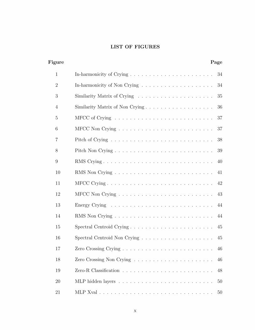
LIST OF FIGURES

Figure Page

1 In-harmonicity of Crying . . . . . . . . . . . . . . . . . . . . . . 34

2 In-harmonicity of Non Crying . . . . . . . . . . . . . . . . . . . 34

3 Similarity Matrix of Crying . . . . . . . . . . . . . . . . . . . . 35

4 Similarity Matrix of Non Crying . . . . . . . . . . . . . . . . . . 36

5 MFCC of Crying . . . . . . . . . . . . . . . . . . . . . . . . . . 37

6 MFCC Non Crying . . . . . . . . . . . . . . . . . . . . . . . . . 37

7 Pitch of Crying . . . . . . . . . . . . . . . . . . . . . . . . . . . 38

8 Pitch Non Crying . . . . . . . . . . . . . . . . . . . . . . . . . . 39

9 RMS Crying . . . . . . . . . . . . . . . . . . . . . . . . . . . . . 40

10 RMS Non Crying . . . . . . . . . . . . . . . . . . . . . . . . . . 41

11 MFCC Crying . . . . . . . . . . . . . . . . . . . . . . . . . . . . 42

12 MFCC Non Crying . . . . . . . . . . . . . . . . . . . . . . . . . 43

13 Energy Crying . . . . . . . . . . . . . . . . . . . . . . . . . . . 44

14 RMS Non Crying . . . . . . . . . . . . . . . . . . . . . . . . . . 44

15 Spectral Centroid Crying . . . . . . . . . . . . . . . . . . . . . . 45

16 Spectral Centroid Non Crying . . . . . . . . . . . . . . . . . . . 45

17 Zero Crossing Crying . . . . . . . . . . . . . . . . . . . . . . . . 46

18 Zero Crossing Non Crying . . . . . . . . . . . . . . . . . . . . . 46

19 Zero-R Classification . . . . . . . . . . . . . . . . . . . . . . . . 48

20 MLP hidden layers . . . . . . . . . . . . . . . . . . . . . . . . . 50

21 MLP Xval . . . . . . . . . . . . . . . . . . . . . . . . . . . . . . 50

x

Figure Page

xi

22 MLP % split . . . . . . . . . . . . . . . . . . . . . . . . . . . . 51

23 RF % split . . . . . . . . . . . . . . . . . . . . . . . . . . . . . 53

24 RF X-Val . . . . . . . . . . . . . . . . . . . . . . . . . . . . . . 54

25 ROC RFl . . . . . . . . . . . . . . . . . . . . . . . . . . . . . . 57

26 ROC MLP . . . . . . . . . . . . . . . . . . . . . . . . . . . . . 58

27 Cost RF . . . . . . . . . . . . . . . . . . . . . . . . . . . . . . . 59

28 Cost MLP . . . . . . . . . . . . . . . . . . . . . . . . . . . . . . 59

1

Introduction

Machine Learning is the modern powerhouse powering everything from

Google to Facebook, from Amazon to Spotify in todays society. Machine learning

systems are used to identify objects in image, transcribe speech to text (or

vice-versa), match news items, posts or products with users interests and select

relevant results of search.

Conventional machine learning techniques were restricted in various ways,

especially in the usage of the natural data in the raw form. For multiple decades,

designing of successful machine learning or pattern recognition systems required

skilled study of the domain in question and design of a feature extractor that

converted the raw data into usable internal representation or a feature vector

from which the learning system can learn patterns and classify it into classes.

A detailed survey has been performed on the traditional machine learning

techniques to measure their efficiency. There is always a trade off on

computational efficiency vs accuracy (when it comes to the traditional methods

since they were designed on much slower computers). Newer, more elaborate

methods of learning, deep neural networks have developed. Hence, they are

explored and their performance is measured against the traditional statistical

machine learning techniques.

The research question is whether automated detection of infant crying can

2

be performed in a principled matter that could be useful to developmental

psychology. Crying is an important parameter since it is an indication of distress

in infants. Recording techniques in this thesis use the Strange Situation

Procedure (SSP). It is a behavioral assessment where the infant is separated from

and reunited with the mother twice and these reunions are referred to as R1 and

R2. Since, experts ratings are time consuming and non-objective in the

assessment of infant behavior, automatic systems are preferred. Thus, an

automatic cry detector is required.

In the past, the cry, laughter and many other specific sound-form

detection was performed in the order of data cleaning, feature extraction, key

feature identification (manually or through data reduction algorithms such as a

the Principal Component Analysis (PCA)), dividing the data for cross-validation

and training and testing a classifier against it. The same route has been followed

in our case where the audio data recorded during a Strange Situation study has

been chopped up into separate cry and non cry segments. Feature extraction has

been performed consisting of MFCC, delta MFCC, pitch, energy, zero crossing,

spectral centroid after frame segmenting the data and they are stored in a CSV

file. For our initial study we perform the feature extraction using MATLAB and

then pass the CSV through the popular machine learning suit called WEKA

(Waikato Environment for Knowledge Analysis) developed by the University of

Waikato, New Zealand. It has been developed using Java and has a wide array of

analytical and visualization tools that can be used for predictive modeling. The

3

CSV is analysed using WEKA to compare various classifier such as the J4.8,

Random Forest Trees and Neural Networks such as the multilayer perceptron.

The theoretical best result achieved was an error rate of 4 % which is a

significant improvement over the existing ones.

The most common learning method is supervised learning. If we consider

the most common image processing problem of breaking down a scene into its

components (for example, a house, a car, trees etc.), we first collect a large set of

images, extract the various features within the images and then store them in a

vector form known as the feature vector. The feature vector is then used to train

a model to identify the quantifiable features. The desired category should ideally

have the highest score but that is not possible without training with an objective

function which stores the error between the measured score and the desired

output score. The machine adjusts its internal parameters to reach the desirable

score; these parameters are often referred to as the weights. These weights are

adjusted to reach a combination that gives us our desired result. In big data

analytics world, there could be millions of such weights and labeled categories.

For the proper adjustment of the weights, the learning algorithm calculates a

gradient vector (usually using the Stochastic Gradient Descent algorithm). The

algorithm indicates by what factor would the change in weight affect the system

and the cost function of the error is minimized by adjusting the weights in the

opposite direction to the gradient vector. Since the 60s, the linear classifiers can

only divide up the input spaces into simple regions divided by the hyperplane.

4

Based on the covariance matrix and the determinants, the hyperplane could be a

hyper-sphere, hyper-ellipse etc [Dow and Penderghest, 2015]. But in our specific

example of speech signals, the model needs to insensitive to irrelevant variations

in the input such as the accent of speech, gender of the speaker etc. Since deep

learning architecture is a multiple stack of various simple learning layers, it often

computes non-linear input-output mappings. and these are impervious to large

irrelevant variations such as the accent or the pitch of the speaker.

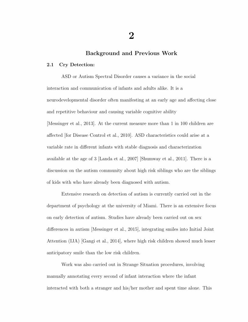
2

Background and Previous Work

2.1 Cry Detection:

ASD or Autism Spectral Disorder causes a variance in the social

interaction and communication of infants and adults alike. It is a

neurodevelopmental disorder often manifesting at an early age and affecting close

and repetitive behaviour and causing variable cognitive ability

[Messinger et al., 2013]. At the current measure more than 1 in 100 children are

affected [for Disease Control et al., 2010]. ASD characteristics could arise at a

variable rate in different infants with stable diagnosis and characterization

available at the age of 3 [Landa et al., 2007] [Shumway et al., 2011]. There is a

discussion on the autism community about high risk siblings who are the siblings

of kids with who have already been diagnosed with autism.

Extensive research on detection of autism is currently carried out in the

department of psychology at the university of Miami. There is an extensive focus

on early detection of autism. Studies have already been carried out on sex

differences in autism [Messinger et al., 2015], integrating smiles into Initial Joint

Attention (IJA) [Gangi et al., 2014], where high risk children showed much lesser

anticipatory smile than the low risk children.

Work was also carried out in Strange Situation procedures, involving

manually annotating every second of infant interaction where the infant

interacted with both a stranger and his/her mother and spent time alone. This

6

task is not only tiresome but also highly cumbersome. This gives rise to the

possible need for the automatic detection of events from an audio signal. There

are existing Digital Language Processing systems such as LENA

[Ford et al., 2008]. It is a natural language processing system which is supposed

to analyze and child and adult vocalization and automatically annotate the

results. It works in terms of feature extraction and then segmentation of audio of

practical noisy environments. The main of objective of LENA is to estimate

Adult Word Counts (AWC), Child Vocalizations (CV), and Conversational Turns

(CT) between the adult and key child. Professional audio transcription was used

while training the model in LENA so that the fine differences between adult and

child speech could be differentiated. Once the difference was established, the

adult and child speech was separately passed through different segmenters and

classifiers. The child speech is differentiated into crying, babble, laughter, etc.

while the adult speech is differentiated into words and they were counted. There

is a separate classifier for non speech signals as well. The hardware used for the

LENA recording is a portable low power recorder using 50 mW power and is

supplied with a 450 mAh battery which lasts it for 16 hours. In case it runs out

of power, the data will not get erased. USB 2.0 is used for communication with

the system.

Specifically, cry detectors have been discussed in various journal papers

over the years. In a paper where baby monitoring through MATLAB graphical

user interface is discussed [Reddy et al., 2014], the primary parameters for

7

feature extraction are discussed. The Magnitude Sum Function is the sum of the

absolute value of the input signal. MSF is not used individually since it gives the

same value for a tired signal and a noisy signal. To overcome this problem it is

used together with pitch and zero crossing. Thus, the next parameter calculated

is pitch. Pitch is a subjective psycho-acoustical feature of a sound which helps us

determine the fundamental frequency of sound. While the natural frequency of

an adult male voice lies between 100-350 Hz, the pitch of a baby crying lies

between 350-500 Hz. In this paper, the pitch is calculated using the Short Term

Auto-correlation Method (S.T.A.C). In terms of finding energy to determine

between noise and tired signal, a slight disparity has been noticed. Usually a

noisy signal has the maximum energy of 170J where a weakest tired signal at

least has an energy of 200J.

In a paper to recognise the baby’s emotions for an automated caregiver

[Yamamoto et al., 2013], a pattern recognition system is developed to find the

various emotions of a baby by studying the inherent patterns within its cry

signals. For training purposes, a 32 dimensional Fast Fourier Transform is used

in the paper. The lack of power in silent regions of the audio signal is subtracted

from the frequency regions of the audio signal. These subtracted values form the

elements of the feature vector. Principal Component Analysis (PCA) is

performed to find the most significant elements. The nearest neighbor criteria is

used to project elements onto the feature space and predict the emotion related

to the babies cry signal. The aim of of the paper is to make a robot recognize the

8

emotions attached to the cry signal so that it could do the needful to ameliorate

the situation.

Rami Cohen and Yazhar Lavner wrote yet another significant paper on

infant cry detection [Cohen and Lavner, 2012]. They developed a particular

algorithm for cry detection especially in situations where the baby was exposed

to danger, for example, in a car. The proposed algorithm can be divided into two

parts. The first part involves feature extraction from the signal which involves

finding the Mel Frequency Cepstral Coefficient and Short term energy from the

signal. A K-NN classifier is used in the second part and it used to classify the cry

signal using the acquired pitch and harmonic info. For the measure of the

robustness of the model and to make sure it works in practical scenarios, various

noisy signal such as road noise, car horns were introduced. A database of cry

signal was also used for evaluation. As popularly stated, an infant cry signal can

be considered as a natural alarm system and can be used to always indicate

discomfort infants [Singer and Zeskind, 2001]. The parameters that are found in

this paper are:

2.1.1 Pitch frequency:

The fundamental frequency f0 is calculated since it is important for

classification purposes. The pitch calculation is based on a combination for

cepstral method [Noll, 1967] and cross-correlation method. The next feature

calculated is the:

9

2.1.2 MFCC:

MFCC [Klautau, 2005] which provides a short term power spectrum of the

signal. MFCC coefficients are calculated by multiplying the each segment of

Short Time Fourier Transform by m triangle shaped segments of band-pass filter

segments with their central frequencies and width arranged according to the mel

scale. The total energy is calculated and a Discrete Cosine Transform (DCT) is

performed to find the MFCC.

2.1.3 Inharmonicity:

It provides of a good indication of the harmonic peaks present in the

signal. DFT of the each analysis frame is calculated and a predefined number of

peaks is considered. The sum of the mod of the highest frequencies of each frame

and the fundamental frequency gives the harmonicity value.

The K-NN classifier classifies the cry sound as a 1 and a no cry segment as

a 0. The testing on the proposed algorithm was performed by passing a 370

second audio out of which 50% was crying. Additive Gaussian Noise was

introduced to test for the robustness of the system. The biggest advantage of this

algorithm is its simplicity and computational efficiency.

Alternate methods for cry detection are explored by Bhagatpatil

Varsharani V, V. M. Sardar [Bhagatpatil and Sardar, ] who consider LPCC

instead of MFCC in an automatic cry detector. There exists a system developed

by Priscilla Dustan called the Dustan Baby Language (DBL) which is yet

another DLP, similar to LENA. It finds out the meaning of baby cries in infants

10

who are between 0-3 months old. According to DBL version, there are five baby

languages: ”neh” means hunger, ”owh” means tired which indicates that the

baby is getting sleepy, ”eh” means the baby wants to burp, ”eairh’ means pain

(wind) in the stomach, and ”heh” means uncomfortable (could be due to a wet

diaper, pain). Like many other elements in nature, infant crying is rhythmic and

periodic in nature which consists of alternating cries and inspirations (breathing

in general). A large amount of air flows through the larynx which causes the

distress signal and there is a repeated opening and closing of the vocal chords

which causes the rhythmic pattern. The parameters that were calculated here for

the cry detection are Zero-Crossing Rate(ZCR) and Fundamental frequency

[Kim et al., 2013], and Fast Fourier Transforms (FFT). Unlike ideal clinical trial

situations which are entirely noise free, this system also aims at robustness in

noisy, real life situations which could be aimed to alert the parents in case of any

physical danger. The system works in two phases, first, when the LPCC

components are calculated, and later when vector quantization is used for the

detection of the cry sounds. During the past studies of cry classification of

normal and abnormal (hypoxia-oxygen lacks) infant was carried by using a neural

network which produced 85% accuracy [Poel and Ekkel, 2006]. The classification

of healthy infants and infants who experienced pain like brain damage, lip cleft

palate, hydrocephalus, and sudden infant death syndrome by using Hidden

Markov Model (HMM) produced 91% accuracy [Lederman et al., 2008]. Neural

network or HMM classifiers have been recurrently used in previous studies. The

11

research towards the identification of DBL infant cries used codebook as a

classifier or pattern identifier which is extracted from the k-means clustering and

MFCC. The automatic recognition of birdsongs using MFCC and Vector

Quantization (VQ) codebook was performed and produced 85% accuracy

[Linde et al., 1980]. So, it is observed that various classifiers and the results and

their usage is entirely dependent on the researcher and the specific task at hand.

In the paper involving an infant codebook and feature vector identification

with MFCC [Renanti et al., 2013], the attempt to automate the Dustan Baby

Language is observed. The codebook is developed using all the baby cry data by

means of K-means clustering. It is a set of vectors that represent the distribution

of a particular sound from a speaker in a sound chamber. Every point of the

codebook is known as a codeword. The distance of incoming sound signals to a

speaker codebook is calculated as the sum of the distances of each frame which is

read to the nearest codeword. Finally, input signal is labeled as speaker

corresponding the smallest codebook distance. Speaker modeling using VQ based

is made by clustering from speaker feature to K which is not overlapping. The

data from the videos from the Dustan Baby Language database is processed to

find the characteristics and results. The data is further divided into training and

testing sets. There are 140 training data sets available and they are differentiated

according to various emotional states of the meaning of the cry. There are 35

testing data sets with 7 infant cries for each type of infant cry. The research

varying frame length: 25 ms/frame length = 275, 40 ms/frame length = 440, 60

12

ms/ frame length = 660, overlap frame: 0%, 25%, 40%, the number of codewords:

1 to 18, except for frame length 275 and overlap frame = 0 using 1 to 29 clusters.

The identification of the infant cry is based on the Euclidean distance.

The problem of detecting speech and other vocalizations in a noisy

environment is a classic signal processing problem and has been previously

addressed by filtering. The most common and effective method was by the use of

Wiener filtering [Lei et al., 2009]. Here, a filter is applied at the front end to

suppress the noise. However, the amplitude and energy had lower energy post

filtering. Banking on the low change of spectral entropy in case the spectral

distribution is maintained constant, mel-frequency filter banks could be applied

for the extraction of speech audio. The use of smarter, multi-layer neural

networks in the recent years have eliminated the need for such signal processing

techniques. Deep networks can parse through the signal and learn to balance

themselves to extract the usable part of the signal, while ignoring the noise.

Thus, they are preferred over signal processing noise removal techniques.

2.2 Laughter Detection:

Keeping the background on cry detection in mind, there lies the necessity

to cover various other soundscapes to diversify our research base and explore the

other modalities that have been used for the identification of various other audio

phenomenons in the world of machine learning. Different de-noising,

classification, clustering, reduction, training and outcomes are achieved through a

wide variety of techniques. Emphasis has always been placed on emotion in

13

infant or human interaction in general. Laughter, being the most positive

emotion known to us, is explored next. A few papers which have used signal

processing-machine learning combinations are picked out and explored.

Mary Tai Knox et al worked on an automatic laughter detection system

using neural networks for the purpose of detection of laughter segments and

speaker recognition [Knox and Mirghafori, 2007]. Previous work had focused and

segmented and identified laughter using various statistical models such as SVM,

HMM and GMM. This paper studies the past work and extends the research to

eliminate the need for the pre-segmentation of the data. Audio communication

usually contains a wealth of information and laughter in general provides

important cues for the emotional state of the speaker

[Truong and Van Leeuwen, 2005]. Laughter detection in general has other

applications such as it provides an important time cue for taking a photo if used

in conjugation with a video camera [Carter, 2000]. The most useful paper on

automatic laughter detection has been present by none other than Ellis et al

[Kennedy and Ellis, 2004] where they studied the detection of overlapped

laughter in various meetings. The data was split into non-overlapping one second

segments, which were then classified based on whether or not multiple speakers

laughed. The support vector machines (SVMs) were trained on four features:

MFCCs, delta MFCCs, modulation spectrum, and spatial cues. A true positive

rate of 87% was achieved during their study. Truong and van Leeuwen

[Knox and Mirghafori, 2007] classified pre-segmented ICSI Meetings data as

14

laughter or speech. The segments were determined prior to training and testing

their system and had variable time durations. The average duration of laughter

and speech segments were 2.21 and 2.02 seconds, respectively. They used

Gaussian mixture models trained with perceptual linear prediction (PLP)

features, pitch and energy, pitch and voicing, and modulation spectrum. They

built models for each of the feature sets. The model trained with PLP features

performed the best at 13.4% EER for the data set. This paper initially

experiments with SVM. The audio had to be segmented to calculate the

statistical features such as the mean and the standard deviation. The offset or

how often the parameters were calculated depended on how often we wanted to

go through the audio to detect the laughter. This gave rise to usual dichotomy of

the accuracy vs the computation complexity trade-off. Small offset also resulted

in much higher storage for the much higher number of statistical features. The

various shortcomings of the SVM such as the need to parse the data into

segments, calculate and store to the disk, parse the statistics of the raw features,

and poor resolution of start and end times were addressed by using a neural

network in this paper. The network was trained with features from a context

window of input frames, thereby obviating the need to compute and store the

mean and standard deviations since the raw data for each frame was included as

a feature. The neural network was used to evaluate the data on a frame-by-frame

basis thus eliminating the need to pre-segment the data, while at the same time

achieving a good resolution to detect laughter. Experiments were performed with

15

MFCC and pitch features. To prevent the common problem of over-fitting in

machine learning and data mining, the data was differentiated into training and

testing.

It is very important to look at the paper published by Ellis et al

[Kennedy and Ellis, 2004] in greater details since it is pivotal in the application

of laughter detection using machine learning. Laughter is automatically detected

in a group setting where more than one person may laugh simultaneously. A

SVM classifier is trained using MFCC, delta MFCC, modulation spectrum and

time delay between two microphones placed on two edges of the desktop. The

ground truth is established using one second long laughter windows and they are

labeled either as laughter event or a non laughter event. We follow it up with

training a support vector machine classifier on the data using some features to

capture the perceptual spectral qualities of laughter (MFCCs, Delta MFCCs),

the spatial cues available when multiple participants are laughing simultaneously,

and the temporal repetition of syllables in laughter (modulation spectrum). The

features calculated are the following:

2.2.1 Cepstral Features:

The mel-frequency cepstral coefficients for each 25ms window with a 10ms

forward shift is calculated. The mean and variance of each coefficient over the

100 sets of MFCCs that are calculated for each one-second window is taken.

16

2.2.2 Delta Cepstral Features:

The delta features are determined by calculating the deltas of the MFCCs

with a 25ms window and 10ms forward shift. The standard deviation of each

coefficient over the 100 sets of Delta MFCCs that are calculated for each

one-second window is taken following that.

2.2.3 Spatial Cues:

The spatial features are calculated by cross-correlating the signals from

two tabletop microphones over 100ms frames with a 50ms forward shift. For each

cross-correlation, we find the normalized maximum and the time delay for the

corresponding for the maximum.

2.2.4 Modulation Spectrum:

They are calculated by taking a one-second waveform, summing the

energy in the 1000Hz - 4000Hz range (since most of the laughter energy is in this

segment) in 20 ms windows, applying a Hanning window, and then taking the

DFT. We use the first 20 coefficients of the DFT as our modulation spectrum

features.

The background provided thus far gives a basic idea of the past and

existing statistical models used in specific sound classification such and cry and

laughter from human sounds. The next goal is to move further into the domain

of machine learning and explore newer forms of classification. In recent years,

there has been a revival in the interest in neural networks in the speech

recognition community [Deng et al., 2013]. While past neural networks could not

17

significantly perform very successful combinations of HMM-GMM models etc,

recent developments have proven otherwise. Primary reason for these are 1)

Making the networks more deeper makes them much more powerful and this gave

rise to the deep neural networks (DNN), 2) Initializing the weights more sensibly

[Hinton et al., 2012] [Mohamed et al., 2012] [Deng et al., 2012] [Yu et al., 2011]

2.3 Environmental Sound Classification:

It is important to cover some of the environment sound classification

techniques since many of the machine learning techniques used for speech

recognition is similar to environmental and urban sound classification. Selina

Chu et al [Chu et al., 2009] in their paper on environmental sound recognition

with time-frequency features discusses the MFCC as a popular method to

describe the audio spectral shape. Environmental sounds such as the chirping of

crickets have a very strong temporal element, however, there exist very few time

domain features to characterize them. Thus, a Matching Pursuit (MP) algorithm

to obtain time-frequency characteristics is used to complement the MFCC. It is

very important to understand that filter-bank based MFCC computation

approximates very important features of the human auditory system. MFCCs

have been shown to work well for structured sounds such as music but they

might degrade in the presence of environmental noise. Thus, MP algorithm is

suggested as an alternative.

The analysis of sound environment in the thesis written by Peltonen

[Peltonen et al., 2002] goes into describe two classification schemes. The first one

18

is the averaging the band-energy ratio and classifying them using a KNN

classifier. The other one uses a combination of MFCCs and band-energy to ratio

as a method for representing sounds in from different frequency ranges.

The department of Music Technology and NYU along with the Center for

Urban Science and Progress (CUSP) has been conducting research in the field of

urban sound acquisition, pattern recognition and classification. Juan Bello et al

recently published an important papers on this area: one of them being on

unsupervised feature learning for urban sound classification

[Salamon and Bello, 2015]. The K-means algorithm is explored in the domain of

urban sound classification. It is used and compared with the existing techniques

such as the MFCC for baseline comparison. While the temporal dynamics did

not show to have a significant effect in natural sounds such as bird song

classification, they played an important role in the urban sound classification

[Stowell and Plumbley, 2014]. As noted, the raw data is never a suitable input to

any form of classifier due to high dimensionality and perceptually similar sounds.

Thus the popular form of learning is to convert the signal into the time-frequency

representations, most commonly MFCC. The log scaled mel spectrogram with 40

components spanning the audio frequency range is calculated using a window and

hop size of 23ms. While these could be directly used as an input, it is proven

that a PCA or ZCA improves the performance by selecting the features which

have a greater effect on the output [Coates and Ng, 2012]. It is very important to

understand that feature learning can be applied to individual frames or

19

alternative frame to form 2D patches. Grouping many frames by concatenating

them together before performing PCA is called shingling. This allows us to learn

features which take into account temporal dynamics. For example, while trying

to differentiate between idling of engines and jackhammers, temporal dynamics

play a huge role since their instantaneous features can be very similar.

3

Tools and Methods

3.1 Tools Used:

A brief introduction to the various tools used for research is given below.

3.1.1 MATLAB and MIRToolBox:

MATLAB is a very popular and the most widely used programming

interface used for signal analysis, data visualization etc. It was developed by

MathWorks and is currently the most commonly used software platform in

academia. Most people have already extensively used it and hence there will be

no detailed discussion on the software package itself. The standard signal

processing toolbox has been utilized in this thesis. It is important to note that a

standout toolbox called the MIRToolBox [Lartillot and Toiviainen, 2007], which

is a set of integrated features written in MATLAB to extract musical and audio

related features, is most commonly used in the field of Musical Information

Retrieval. The MIRToolBox also has dependency on Auditory Toolbox

[Slaney, 1998], NetLab [Nabney, 2002], and SOM-Toolbox [Vesanto et al., 1999].

The MIRToolbox has an object oriented architecture. The superclass from which

all the data and the methods and derived is called mirdata. A hierarchy is

established from the mirdata hyperclass. Most of the analyzed parameters return

a single valued scalar from the frame by frame analysis. However, the non-scalar

features are organized into specialized classes such as the mirautocor,

mirspectrum, mirhisto, mirmfcc, etc. The primary application of MIRToolbox is

21

the easy to use, on the fly feature extraction. Even with the multitude of

advantages presented by this toolbox, its critical drawback is its memory

management. Combined with memory intensive MATLAB application, it

struggles to parse through large data sets when performing frame by frame

analysis even with the default settings. That is why we explore other, faster

feature extractors in the latter stages of our project.

3.1.2 WEKA:

The Waikato Environment for Knowledge Analysis (WEKA)

[Hall et al., 2009] had its inception in 1992. After years of development, it is an

extremely popular machine learning tool written in JAVA and is open to the

public for use. It is not only a conjugation of various machine learning models

but also a platform for independent development for people who want to use

algorithms outside the ones that have already been provided in the software.

Recently, it has reached widespread acceptance in academia and data mining

research due to its easy to use interface and quick results without the need to

write multiple lines of code for machine learning operations. Its sophisticated

modular arrangement is what allows us to build high level functions on top of the

basic structures. The toolkit is easy to expand due to an API, plug-in

mechanism. WEKA also has a very easy to use Graphical User Interface (GUI)

that allows us to use it easily. The main interface we use is called the ”Explorer”.

It is divided into several panels, each of with different stages of machine learning

options. The first panel is called ”Pre-process” which has a group of filters that

22

perform operations on the input file in various file formats such as ”ARFF” and

”CSV”. The next one on the panel is ”classify” gives us access to WEKAs

classification and regression algorithms. By default it runs cross-validation on

datasets preprocessed for predictive performance. It also gives rise to various

graphical models, ROCs and thresholds. Along with supervised algorithms,

WEKA allows unsupervised learning features through the ”cluster” panel. It

provides a simple enough model for the evaluation of the likelihood based on

clustering algorithms and true clustering. Although it is critical to note that the

WEKA clustering algorithms are not as extensively developed as its regression

and classification algorithms.

3.1.3 LibRosa:

LabROSA is a very popular speech processing laboratory run under Dr.

Dan Ellis at the Columbia University. Dr. Brian McFee, in conjugation with

NYU developed a fast, python based package for audio feature extraction

[McFee et al., 2015]. Although MIR is a fairly new field of research (the first

ISMIR conference held back in 2000), there have been various attempts in C++

and MATLAB. However, the scalability, stability and the ease of use left much to

be desired. Due to the data driven nature of MIR research, there has been a

recent shift towards Python due to its data driven architecture and ease of use.

Various machine learning libraries such as scikit-learn, py-brain and theano based

deep learning models have been developed. Irrespective of these developments,

there was a lack of a stable core library for feature extraction in audio which is

23

the very basis of MIR and other machine learning related research. LibRosa

serves this purpose by being a core python library for audio feature extraction.

There are design principles of librosa that need to be discussed with respect to

why it has been exploited as the primary feature extraction tool in this thesis.

First, it has a very low barrier for entry for anyone who is used to MATLAB

based research. There would be very low transition time involved once you get

past the intricacies of installation of any Python based library. Second, there is a

great deal of standardization involved in this package. The variable names,

processes and interfaces have all been standardization for easy of use and lack of

confusion. Third, in most cases there is backward compatibility. The nose

framework in maintained in most modules of feature extraction. Fourth, since

MIR is a new and fast progressing field of research, most of the tools and

methods used are modular. That allows the users add in their own code. Fifth,

the code provided is very readable, developed and constantly updated on

GitHub. Most software practices such as Travis is applied, all functions are

executed in pure Python and documented using Sphinx.

Reason for using LIBROSA:

There was a major need for fast processing of data. MIRToolBox in

MATLAB, although effective, is cursed with slow speed and crippling memory

restrictions. Although various techniques such as dividing the data up into

smaller chunks and iterating them one by one and appending the results were

tried on MIRToolBox, the initial set of data extraction took hours and often

24

crashed in between. Even a test run with mere 3 minutes of crying and

non-crying from the mother-infant reunions took more than an hour to process.

Since, one of the goals of this project is to find computationally efficient ways of

feature extraction in machine learning, LibRosa was tried for quick and efficient

feature extraction.

3.2 Data Collection and Processing:

3.2.1 LENA Recorder:

The data was collected using LENA devices. The LENA recorder is

pocket sized power house. It is as light as 2 ounces, designed to be worn by

children and can record up to 16 hours of audio data. It is made up of a powerful

microprocessor with advanced compression capabilities. It also has audio

components that are similar to hearing aids costing a lot more. The LENA

recorder is inserted into the pocket of an article of LENAs specially-designed

clothing at the beginning of the recording. At the end, it can be plugged into a

computer to extract the audio data from.

3.2.2 Data Processing:

The collected data was stored in uncompressed .wav format. The

sampling rate used as 44.1 KHz and the stereo format was used. The interaction

data was loaded in Audacity and normalized and noisy chunks were removed. It

was later divided into episodes of interaction. Reunion 1 and 2 marked as R1 and

25

R2 were most important since infant reunited with the mother during these

episodes those were the most important part of the research. This is where the

babies often showed elevated levels of emotional response or change in their

current state (going from crying to silent, crying to happy, happy to crying, silent

to crying, playing to silent, playing to happy, etc.). Each episode is about 21

minutes long and each reunion averages around 3 minutes.

3.3 Creation of Data Sets:

A total of 10 subject were used with subject numbers FN005, FN008,

FN049, FN061, FN062, FN069,FN071, FN074, FN082, FN090 for the study.

Separate audio sets are required for the purpose of training and testing our

model after feature extraction. The procedure for creation of those audio sets are

discussed below:

3.3.1 Crying Training Audio:

Initial focus was on R1 and R2 audio sets since they were of primary

interest in the research and they eventually lead on to the use of rest of the data

for the extraction of crying and non-crying parts. But first, pure crying chunks

were extracted from each episode (R1 and R2) and stored in separate audio files.

Sections which lead onto crying, whispering, other disagreeing sounds made by

the baby were NOT considered as a part of crying since we only wanted classify

the sections consists of pure crying. After combining them together there was

approximately 3 minutes of total crying. To expand the data set further, the

process was continued for the entire available audio set. Sections of crying (with

26

some noise associated with the robustness of the model) were extracted from the

database, stored into separate files and combined. The sampling rate and the

stereo functions were maintained during every conversion process. At the end of

the entire procedure there was a total of 20 minutes and 59 seconds of crying

present in a wave file at 44 KHz sampling rate for analysis.

3.3.2 Non-Crying Training Audio:

As previously discussed in the background, there are various methods for

extracting segments marked as non-crying. Then aim was to incorporate every

other sound present in the recordings to train the model to differentiate them

from crying. There was also a need to preserve the temporal nature of the sound

due to the nature of our event classification. Chunks were again extracted from

the mother’s speech, toy sounds, background noise, child whimpering, and other

sounds like instructions, and silence. For the preparation of the non-crying set an

emphasis was placed on the gradual progression of change since whimpering

sometimes leads on to crying and such whimpering was excluded from our

non-crying training set. An analogy of a broad spectrum antibiotic often surfaced

as every other sound that is not crying was divided into separate audio files. The

same process as crying was followed and they were combined into one single file

of length 22 minutes. The length of the file could be questioned since there is the

availability of much larger amount of non crying data. It is interesting to note

that the first non crying data set was as long as approximately 35 minutes. The

reason for the reduced data set would be discussed in the results section.

27

Note: There was no separate procedure followed to make sure that the

segments from the same subject did not form a part of the training and the testing

split.

3.4 Audio Feature Extraction:

The different tools and methods were used for audio feature extraction.

MATLAB based features are used initially and LibRosa based real time

extraction is used after deciding the useful features.

3.4.1 MATLAB based extraction:

For testing and evaluation purposes, initial feature extraction was

performed on MATLAB using the MIRToolBox. The MIRToolBox is often

considered for use only in music worked moderately well on speech/baby sound

signals. The cry segments were loaded individually and iterated through using a

simple loop. The loaded audio was immediately frame segmented using a frame

size of 50ms and a 50% overlap. The frame segmented audio was passed through

the MIRToolBox and mirfeature was performed on them which gave an array of

every feature calculated by MIRToolBox. The features that were considered

based on signal processing experience and past papers are: MFCC, delta-MFCC,

delta-delta-MFCC, Pitch, Zero Crossing, Spectral Brightness, Spectral Centroid,

Kurtosis, RMS energy, roll-off and spectral flux. The features were column wise

exported into a CSV file.

28

3.4.2 Librosa based extraction:

As discussed previously, the need for fast and real time feature extraction

lead us to using LibRosa for the feature extraction in Python. Unlike

MIRToolBox, Librosa has proven to be much better for speech based extraction.

for real time feature extraction, the audio file as a whole is read into librosa and

downsampled to 22k and converted to Mono. It is very important to drop a note

on the sample rate converter used here. The librosa downsampler falls back on

the scikits.samplerate (scikit-learn) and it is a painstakingly slow sample rate

converter. There was a large amount of initial disappointment on the time taken

to downsample 3 minutes of audio while we were utilizing the scikit.samplerate

downsampler. This gave rise to the need for a much low level and faster sample

rate converter.

Libsamplerate:

Libsamplerate aka Secret Rabbit Code (SRC) is a sample rate converter

developed by Erik de Castro Lopo. SRC is capable of arbitrary and time varying

conversions which consists of up-sampling and down-sampling by a factor of 256.

The ratio of the input and the output samples can be irrational numbers. The

conversion ratio can also vary with time for speeding up and slowing down

effects. SRC provides a small number of converters to allow quality vs.

computation cost trade off. The current best converter provides a signal-to-noise

ratio of 145dB with -3dB passband extending from DC to 96% of the theoretical

best bandwidth when input and output sample rates are given. It is written in C

29

and uses wrappers to compile in Python.

Unaltered versions of frame length and overlap space is used from Librosas

default settings. The default frame and hop lengths (how much we can advance

the analysis time origin from frame to frame )are set to 2048 and 512 samples,

respectively. At the default sampling rate of 22050 Hz, this corresponds to

overlapping frames of approximately 93ms, spaced by 23ms. The frames are also

centered by default. For all sliding window analysis, Hanning window is used.

The majority of the feature analysis on Librosa produces a two dimensional array

stored as librosa.ndarray. 12 band MFCCs and delta-MFCCs are extracted using

the spectral features. Zero crossing, RMS calculations are performed next. The

information is stored in 28 columns and unlimited number of rows (based on the

length of the audio) and converted into a CSV. The 28th column of data is used

a class label where A is used to denote crying and B is used to denote non-crying.

Hence, the crying signal is first processed and the features are extracted and

stored into a CSV and class label is marked as A. This is followed by processing

and storing of the information of the non-cry audio samples which are then

appended to the existing CSV and marked as class label B. This entire file would

eventually act as our training set.

3.5 Machine Learning:

Primarily WEKA but also python based machine learning is used. The

machine learning algorithms used are discussed below:

30

3.5.1 Zero-R Rule:

Every machine learning classification problem needs an established

baseline to check the validity the model in use. If the model developed acts worse

than the baseline, it should be immediately discarded. An evenly spread

probability of the classes denotes a non biased data set for training and as a

result a good performance of the trained set on the testing data. The ZeroR rule

is used in WEKA for the establishment of the baseline. As the name suggests,

there are zero rules used for this so this cannot actually be used for classification.

It is a frequency based system where it creates a frequency table for its target

and selects its most frequent value [Fan et al., 2008].

3.5.2 Multilayer Perceptron:

A feed-forward, multi-layered artificial neural network model uses

backpropagation of error to train itself [Rumelhart et al., 1985]. It consists of

multiple neurons connected to each other and are activated by a sigmoid function

which helps them to differentiate between non-linearly separated data. Multilayer

perceptron would be reduced to a perceptron by making the hidden layers equal

to 1. A traditional multilayer perceptron has 3 or more hidden layers and are

considered a form of deep neural network and is one of the simpler deep learning

techniques. The learning actually occurs through the change in weights of the

connection as the error or the deviation of the error is back propagated through

the network. The backpropagation uses a gradient descent algorithm which

effectively minimizes the cost function or the takes the least computationally

31

taxing path (with the accuracy in mind) while backpropagating the error to

reach the fastest way to reach the most accurate result. As the name suggests,

we could easily use an analogy of climbing down from a hill. We try to take the

steepest (fastest) path without sacrificing a sure footing.

3.5.3 Random Forrest Classifier:

It is also commonly referred to as the tree bagging method or the tree

bagger in short [Breiman, 2001]. It selects a n number of random features and

divides the data into those parts while building an ensemble of trees. The trees

are constructed using those features and are grown to the largest possible size.

Two factors are important to notice here. Firstly, the correlation between the

trees increases the error rate in the tree. Secondly, the strength of each individual

tree contributes to the overall classifier performance. When the training set for

the current tree is drawn by sampling with replacement, about one-third of the

cases are left out of the sample. This OOB (out-of-bag) data is used to get a

running unbiased estimate of the classification error as trees are added to the

forest. It is also used to get estimates of variable importance. After each tree is

built, all of the data are run down the tree, and proximities are computed for

each pair of cases. If two cases occupy the same terminal node, their proximity is

increased by one. At the end of the run, the proximities are normalized by

dividing by the number of trees. Proximities are used in replacing missing data,

locating outliers, and producing illuminating low-dimensional views of the data.

32

3.5.4 Scikit-learn Integration:

Scikit-learn is a python based machine learning library widely used for the

use for various classifier and moderately deep neural network implementations. It

is the home for state-of-the-art machine learning algorithms for medium-scale

supervised and unsupervised problems. This package focuses on bringing

machine learning to non-specialists using a general-purpose high-level language.

Although, the majority of the code is written using Python, some of the low level

functions for speed are taken care of by the C++ libraries LibSVM

[Chang and Lin, 2001] and LibLinear [Fan et al., 2008] that provide reference

implementations of SVMs and generalized linear models with compatible licenses.

4

Results and Figures

The results section is divided into the initial MIRToolBox based results,

the Librosa based real-time feature extraction and the performance of various

machine learning and classification algorithms used on the training and the

testing data.

4.1 MIRToolBox Results:

Various features that contributed comparative features are discussed

below. These features have been handpicked after extensive analysis of all

mirfeatures, PCAs and different combinations tried in the past research material.

4.1.1 Inharmonicity:

In-harmonicity is the measure of the deviation of the overtones from the

fundamental frequencies and its integral multiples. The results for small crying

and non crying segments are shows below. The crying segments show a

continuous increase in the in-harmonicity and non-crying display a continuous

decrease. Figures for two short cry and non-crying segments are displayed below:

34

Figure 1: In-harmonicity of Crying

Figure 2: In-harmonicity of Non Crying

35

4.1.2 Similarity Matrix:

The similarity matrix is calculated to measure the autocorrelation in the

signals. In a similarity matrix, self similarity is measured between the data

sequence. The similarity matrix is calculated here under the assumption that the

crying data would have a greater self similarity. The results are depicted below in

crying and non crying data segments below:

Figure 3: Similarity Matrix of Crying

36

Figure 4: Similarity Matrix of Non Crying

4.1.3 MFCC:

The Mel-frequency cepstral coefficient as proven before is a very crucial

model for perceptive (auditory perception) data analysis. Non-scaled MFCCs are

depicted below for crying and non crying data respectively.

37

Figure 5: MFCC Crying

Figure 6: MFCC Non Crying

38

4.1.4 Pitch:

Pitch is the perception of frequency in human beings. As expected from

previous studies, the pitch for crying signal has a much more concentrated

distribution between 350Hz and 600Hz range. An example of the pitch analysis

of the cry signal is shows below in the figure. The non-cry signal however shows

higher variability as expected from the different combination of signals

individually exhibiting a different set of pitches.

Figure 7: Pitch Crying

39

Figure 8: Pitch Non Crying

40

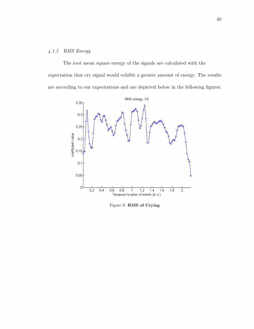
4.1.5 RMS Energy

The root mean square energy of the signals are calculated with the

expectation that cry signal would exhibit a greater amount of energy. The results

are according to our expectations and are depicted below in the following figures:

Figure 9: RMS of Crying

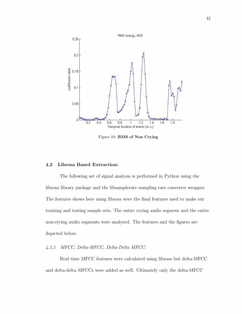
41

Figure 10: RMS of Non Crying

4.2 Librosa Based Extraction:

The following set of signal analysis is performed in Python using the

librosa library package and the libsamplerate sampling rate converter wrapper.

The features shows here using librosa were the final features used to make our

training and testing sample sets. The entire crying audio segment and the entire

non-crying audio segments were analyzed. The features and the figures are

depicted below:

4.2.1 MFCC, Delta-MFCC, Delta-Delta MFCC:

Real time MFCC features were calculated using librosa but delta-MFCC

and delta-delta MFCCs were added as well. Ultimately only the delta-MFCC

42

values are appended to the MFCCs in our training set.

Delta-MFCCs and the delta-delta MFCCs are also known as differential

and acceleration coefficients. The MFCC feature vector describes only the power

spectral envelope of a single frame, but the dynamic information over time

should also be calculated. That is where delta-MFCC comes in. The

corresponding figures for the crying and non-crying segments are shown below:

Figure 11: MFCC Crying

43

Figure 12: MFCC Non Crying

4.2.2 Energy:

The RMS energy and the log-power spectrogram of the crying and

non-crying segments are displayed below:

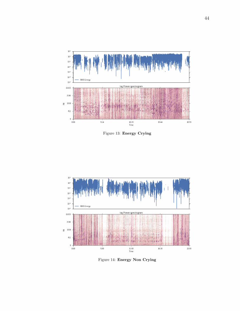
44

Figure 13: Energy Crying

Figure 14: Energy Non Crying

45

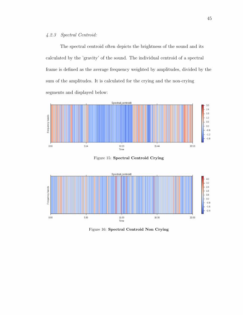
4.2.3 Spectral Centroid:

The spectral centroid often depicts the brightness of the sound and its

calculated by the ’gravity’ of the sound. The individual centroid of a spectral

frame is defined as the average frequency weighted by amplitudes, divided by the

sum of the amplitudes. It is calculated for the crying and the non-crying

segments and displayed below:

Figure 15: Spectral Centroid Crying

Figure 16: Spectral Centroid Non Crying

46

4.2.4 Zero-Crossing:

Zero crossing is the temporal representation of how many times the signal

crosses the zero or the x-axis. It is a method of finding the frequency domain

representation of a time domain signal. It is calculated for the entire crying and

non-crying audio segments and depicted below:

Figure 17: Zero Crossing Crying

Figure 18: Zero Crossing Non Crying

47

4.3 Classifiers and Performance:

The results from the Zero-R method, Tree-bagger classifier and the

multilayer perceptron are depicted below:

4.3.1 Zero-R Classifier:

This method is used for the baseline estimation. Since, our training data

set is roughly a 50/50 mixture of crying and non crying, it should exhibit a

similar split using the Zero R rule. For the simple and less computationally

intensive nature of this model, we use the entire dataset. In our result, it exhibits

a 51.2% and 48.8% split for the crying and non-crying data set. Using the

reduced dataset, we get an even better result. The result for the entire data set

depicted below:

48

Figure 19: Zero R classifier with 10 fold cross-validation and 51.2% Split

49

4.3.2 Multi-Layer Perceptron:

A feed-forward multilayer perceptron with backpropagation of error is

used to classify the reduced dataset with a 10 fold cross-validation. It has 15

hidden layers which essentially depicts the minimum number needed since the

value is the mean of the number of attributes added to the number of classes. It

has a learning rate of 0.3 and a momentum of 0.2 for the backpropagation, a

validation threshold of 20 to terminate for consecutive 20 errors, and finally the

number of training epochs is 500. The time taken to build this model for the

reduced data set is 463.2 seconds and the accuracy achieved is 97.5%. The entire

data set is also processed through a MLP but instead of using the 10 fold cross

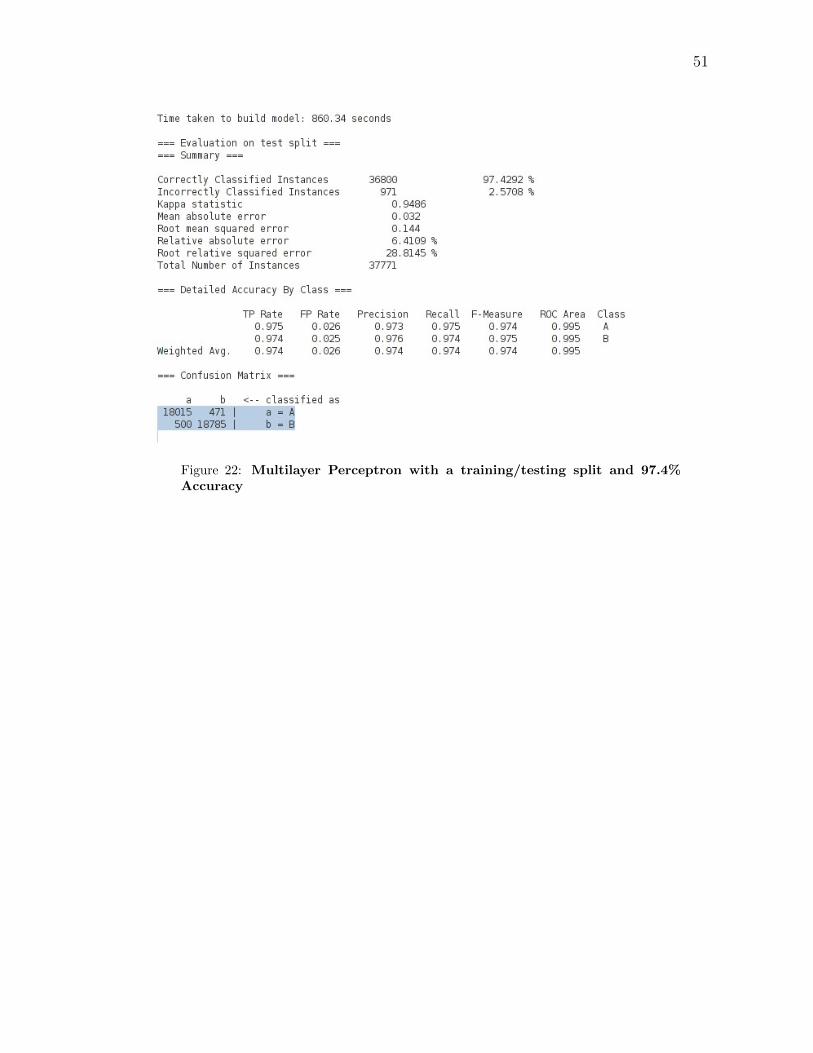
validation, it is processed using a 66/34% training/testing split. The other

parameters remain the same as the whole data set. The results for the reduced

followed by the whole data set are shown below:

50

Figure 20: Multilayer Perceptron with Hidden Layers

Figure 21: Multilayer Perceptron with 10 fold cross validation and 97.5%Accuracy

51

Figure 22: Multilayer Perceptron with a training/testing split and 97.4%Accuracy

52

4.3.3 Random Forrest Classifier:

Two different tree baggers are implemented on two different sets of data

for the evaluation of the classification performance. First, a tree bagger with 100

trees is implemented with 5 random features on the entire data set with a 66/34

percent split between the training the testing data in the model. Due to the large

number of data points, cross-validation either proved to be too time consuming

or too memory intensive. It reached an out of bad error of 0.0257 and the final

classification accuracy was 97.2 %. There were a total of 111091 instances and

the testing was performed on 36728 of them which yielded only 1043

mis-classified instances.

A second tree bagger is used with the reduced data set and a reduced

number of trees. The new number of trees used is 50 while every other parameter

remains unchanged. The results slightly drop due to the 10 fold cross validation

performed on the data but is still at a healthy 96.6 %. The results are depicted

below for a random trial. It is again very important to note that random data

sets are selected every time so there is a slight margin of variability in the results.

The results are showed in the order:

53

Figure 23: Random Forrest with Percentage Split and 97.2 % Accuracy

54

Figure 24: Random Forrest with 10 fold X-Val and 96.6 % Accuracy

5

Evaluation and Discussions

The findings so far are summarized and analyzed below. The first

noticeable observation is the drastic improvement of the sample rate converter

(SRC) due to the libsamplerate wrapper and the source code execution in C.

There was an exponential decrease in the time taken when we implemented the

down-sampler in C. This drastically improved the performance and turned it into

a system that could analyze signals for feature extractions real time.

Based on past experiences and study of signal processing during my

masters degree, combined with the background development of this thesis, I

strongly feel that the features used for extraction are the best options for our

problem.

A major focus of this thesis is to utilize computationally efficient MIR and

feature extractor systems. Librosa was not designed for speech processing and its

the first of a kind implementation of Librosa to extract features from infant cry

signals. The success of this thesis also depicts the robustness of Librosa. It

successfully fills the void of a python based audio feature extraction library in the

area of machine learning. However, the high level nature of python at times

leaves us wanting in terms of sheer computational performance. Using low level

language implementation and using wrappers to execute them Python is also a

very efficient way of running code. Recent implementations on Cython is the best

56

example of this kind of an example. It is very interesting to comment here that

the Pitch estimator of librosa using interpolated STFT as suggested by Julius O

Smith of CCRMA, Stanford was the only unreliable librosa feature. The

performance varied every trial and changing the fmin and fmax values changed

the spread of the pitch entirely. The bug has been reported and is being

currently addressed.

The modular nature of Librosa proves critical in ease of use. It the could

be easily presented in the IPython Notebook format and it would be an ideal

interactive, easy to use interface for re-using the code with the whole project

divided into smaller parts comprising of the results and the output plots.

The need for correct feature selection and a large, non-biased training set

is greatly emphasized. The Zero-R rule is the ideal estimator to judge that. Also,

it is important to note that in such large datasets, over-fitting is a recurrent

issue. To avoid over-fitting, it is critical to make sure that multiple training

samples are not extracted from the same recording. This concept extends to

cross-validation, which is again method for the elimination of over-fitting.

The ensemble bagger and the MLP perform very similarly on our data.

While the MLP used hidden layers and a back-propagation, the ensemble bagger

excels by accumulating a large number of trees together for higher efficiency.

Based on my observations and performance evaluations, I would choose the tree

bagger over the MLP since its easier to train and test. Tree bagger is more time

efficient and it will be faster to use in real life scenarios. It is important to

57

measure the Receiver Operating Characteristics and the Cost Function of the

classifiers for further evaluation and comparison of their performance.

5.1 Receiver Operating Characteristics:

It simply illustrates the performance of a two class (binary) classification

system as its discrimination function is varied through time. The true positive

rate of the classifier (y axis) is plotted against the false positive rate (x axis) to

give a continuous measure of its performance. The ROC characteristics of a

random forest classifier and a MLP are illustrated below:

Figure 25: ROC Random Forest

58

Figure 26: ROC Multilayer Perceptron

5.2 Cost Function:

The Cost function also known as the loss function is a parametric

estimation where the event is a function of the difference of the true and the

estimated value. Therefore, it is the penalty for an incorrect classification. It is

the comparison of the Probability Cost Function and the Normalized Expected

Cost of the decision. The plots for the RF and the MLP are given below. The

left axis represents class A or the right axis represents class B.

59

Figure 27: Cost Random Forrest

Figure 28: Cost Multilayer Perceptron

60

5.3 Random Forrest Runtime Analysis:

A comparison is made between various tree sizes and two different data

sizes for the time training time using the random forest bagging method. A table

is displayed below with all the results:

Table 1: Random Forrest Runtime Analysis

No of Trees Reduced Data Set(s) Whole Data set(s)

10 39.04 64.9420 76.72 122.950 190.9 309.580 301.2 513.4100 371.5 650.5

5.4 Conclusion:

A special emphasis needs to be given to the importance of feature

selection in any machine learning problem. A much higher importance needs to

be placed on the feature selection than on the classifier selection. A classifier can

only be as good as the data presented to it and the entire data presented to it is

determined by the selection and the combination of the features used. For

example, the previous highest accuracy of cry detection stalled at 88-91 % due to

the fact that delta-MFCC and the corresponding temporal changes were never

incorporated into the training data. Incorporation of this feature gave the

performance a significant boost.

Preprocessing, cleaning and proper frame segmentation of data is very

important for the creation of a good feature set as well. In the case of this

project, past findings acted as a good starting point but further experimentations

61

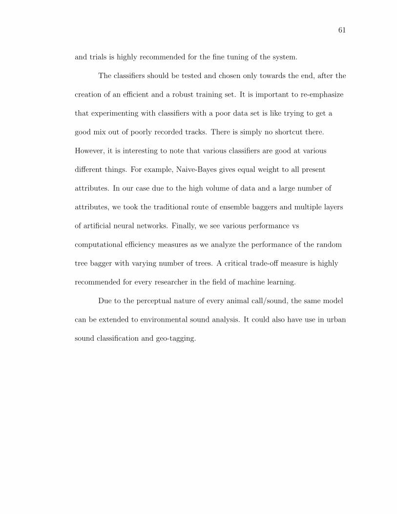
and trials is highly recommended for the fine tuning of the system.

The classifiers should be tested and chosen only towards the end, after the

creation of an efficient and a robust training set. It is important to re-emphasize

that experimenting with classifiers with a poor data set is like trying to get a

good mix out of poorly recorded tracks. There is simply no shortcut there.

However, it is interesting to note that various classifiers are good at various

different things. For example, Naive-Bayes gives equal weight to all present

attributes. In our case due to the high volume of data and a large number of

attributes, we took the traditional route of ensemble baggers and multiple layers

of artificial neural networks. Finally, we see various performance vs

computational efficiency measures as we analyze the performance of the random

tree bagger with varying number of trees. A critical trade-off measure is highly

recommended for every researcher in the field of machine learning.

Due to the perceptual nature of every animal call/sound, the same model

can be extended to environmental sound analysis. It could also have use in urban

sound classification and geo-tagging.

6

Further Scope

This thesis was restricted to the analysis and classification of infant

sounds. The goal is to expand the study into environmental and urban sounds.

The plan to execute a bird sound detector is already in motion and so is the

’dade-box’ project which is going to collect environmental, sonic and geographical

data around the Miami-Dade country and use real-time signal processing and

machine learning algorithms to isolate significant or emergency events such as

accidents or gunshots.

Due to the lack of a NVIDIA GPU on the primary computer, depths of

theano based libraries, Tensor Flow and other deep networks was not executed.

They were studied in details and would constitute the next part of the research

in soundscape analysis and classification. Further classification of cry sounds to

depict the emotional state of the baby (such as hunger, discomfort etc.) have

already been touched upon by other researchers but there is still a large scope of

improvement. Finally, a cry detector and classification app (Android and iOS)

would be a very usable by-product of this thesis and could be seen being used for

not only different kinds of research but also by infant caregivers and mothers who

might leave their phone with their infants for short durations and get updates on

their emotional states on their respective smart watches.

LIST OF REFERENCES

[Bhagatpatil and Sardar, ] Bhagatpatil, M. V. V. and Sardar, V. An automaticinfants cry detection using linear frequency cepstrum coefficients (lfcc).

[Breiman, 2001] Breiman, L. (2001). Random forests. Machine learning,45(1):5–32.

[Carter, 2000] Carter, A. (2000). Automatic acoustic laughter detection.Unpublished Master thesis, Keele University, Staffordshire, UK.

[Chang and Lin, 2001] Chang, C. and Lin, C.-J. (2001). Libsvm: a library forsupport vector machines, h ttp.

[Chu et al., 2009] Chu, S., Narayanan, S., and Kuo, C. J. (2009). Environmentalsound recognition with time–frequency audio features. Audio, Speech, andLanguage Processing, IEEE Transactions on, 17(6):1142–1158.

[Coates and Ng, 2012] Coates, A. and Ng, A. Y. (2012). Learning featurerepresentations with k-means. In Neural Networks: Tricks of the Trade, pages561–580. Springer.

[Cohen and Lavner, 2012] Cohen, R. and Lavner, Y. (2012). Infant cry analysisand detection. In Electrical & Electronics Engineers in Israel (IEEEI), 2012IEEE 27th Convention of, pages 1–5. IEEE.

[Deng et al., 2013] Deng, L., Hinton, G., and Kingsbury, B. (2013). New types ofdeep neural network learning for speech recognition and related applications:An overview. In Acoustics, Speech and Signal Processing (ICASSP), 2013IEEE International Conference on, pages 8599–8603. IEEE.

[Deng et al., 2012] Deng, L., Yu, D., and Platt, J. (2012). Scalable stacking andlearning for building deep architectures. In Acoustics, Speech and SignalProcessing (ICASSP), 2012 IEEE International Conference on, pages2133–2136. IEEE.

[Dow and Penderghest, 2015] Dow, E. M. and Penderghest, T. (2015).Transplanting binary decision trees. Journal of Computer Sciences andApplications, 3(3):61–66.

[Fan et al., 2008] Fan, R.-E., Chang, K.-W., Hsieh, C.-J., Wang, X.-R., and Lin,C.-J. (2008). Liblinear: A library for large linear classification. The Journal ofMachine Learning Research, 9:1871–1874.

64

[for Disease Control et al., 2010] for Disease Control, C. et al. (2010). Autismand developmental disabilities monitoring (addm) network. Retrieved January,19:2010.

[Ford et al., 2008] Ford, M., Baer, C. T., Xu, D., Yapanel, U., and Gray, S.(2008). The lenatm language environment analysis system: Audiospecifications of the dlp-0121. Technical report, Technical Report LTR-03-2).Boulder, CO: Lena Foundation.

[Gangi et al., 2014] Gangi, D. N., Ibanez, L. V., and Messinger, D. S. (2014).Joint attention initiation with and without positive affect: Risk groupdifferences and associations with asd symptoms. Journal of autism anddevelopmental disorders, 44(6):1414–1424.

[Hall et al., 2009] Hall, M., Frank, E., Holmes, G., Pfahringer, B., Reutemann,P., and Witten, I. H. (2009). The weka data mining software: an update. ACMSIGKDD explorations newsletter, 11(1):10–18.

[Hinton et al., 2012] Hinton, G., Deng, L., Yu, D., Dahl, G. E., Mohamed, A.-r.,Jaitly, N., Senior, A., Vanhoucke, V., Nguyen, P., Sainath, T. N., et al. (2012).Deep neural networks for acoustic modeling in speech recognition: The sharedviews of four research groups. Signal Processing Magazine, IEEE, 29(6):82–97.

[Kennedy and Ellis, 2004] Kennedy, L. S. and Ellis, D. P. (2004). Laughterdetection in meetings. In NIST ICASSP 2004 Meeting Recognition Workshop,Montreal, pages 118–121. National Institute of Standards and Technology.

[Kim et al., 2013] Kim, M. J., Kim, Y., Hong, S., and Kim, H. (2013). Robustdetection of infant crying in adverse environments using weighted segmentaltwo-dimensional linear frequency cepstral coefficients. In Multimedia and ExpoWorkshops (ICMEW), 2013 IEEE International Conference on, pages 1–4.IEEE.

[Klautau, 2005] Klautau, A. (2005). The mfcc.

[Knox and Mirghafori, 2007] Knox, M. T. and Mirghafori, N. (2007). Automaticlaughter detection using neural networks. In INTERSPEECH, pages2973–2976.

[Landa et al., 2007] Landa, R. J., Holman, K. C., and Garrett-Mayer, E. (2007).Social and communication development in toddlers with early and laterdiagnosis of autism spectrum disorders. Archives of general psychiatry,64(7):853–864.

[Lartillot and Toiviainen, 2007] Lartillot, O. and Toiviainen, P. (2007). A matlabtoolbox for musical feature extraction from audio. In International Conferenceon Digital Audio Effects, pages 237–244.

65

[Lederman et al., 2008] Lederman, D., Zmora, E., Hauschildt, S.,Stellzig-Eisenhauer, A., and Wermke, K. (2008). Classification of cries ofinfants with cleft-palate using parallel hidden markov models. Medical &biological engineering & computing, 46(10):965–975.

[Lei et al., 2009] Lei, J., Yang, J., Wang, J., and Yang, Z. (2009). A robust voiceactivity detection algorithm in nonstationary noise. In Industrial andInformation Systems, 2009. IIS’09. International Conference on, pages195–198. IEEE.

[Linde et al., 1980] Linde, Y., Buzo, A., and Gray, R. M. (1980). An algorithmfor vector quantizer design. Communications, IEEE Transactions on,28(1):84–95.

[McFee et al., 2015] McFee, B., Raffel, C., Liang, D., Ellis, D. P., McVicar, M.,Battenberg, E., and Nieto, O. (2015). librosa: Audio and music signal analysisin python. In Proceedings of the 14th Python in Science Conference.

[Messinger et al., 2013] Messinger, D., Young, G. S., Ozonoff, S., Dobkins, K.,Carter, A., Zwaigenbaum, L., Landa, R. J., Charman, T., Stone, W. L.,Constantino, J. N., et al. (2013). Beyond autism: a baby siblings researchconsortium study of high-risk children at three years of age. Journal of theAmerican Academy of Child & Adolescent Psychiatry, 52(3):300–308.

[Messinger et al., 2015] Messinger, D. S., Young, G. S., Webb, S. J., Ozonoff, S.,Bryson, S. E., Carter, A., Carver, L., Charman, T., Chawarska, K., Curtin, S.,et al. (2015). Early sex differences are not autism-specific: A baby siblingsresearch consortium (bsrc) study. Molecular autism, 6(1):1.

[Mohamed et al., 2012] Mohamed, A.-r., Dahl, G. E., and Hinton, G. (2012).Acoustic modeling using deep belief networks. Audio, Speech, and LanguageProcessing, IEEE Transactions on, 20(1):14–22.

[Nabney, 2002] Nabney, I. (2002). NETLAB: algorithms for pattern recognition.Springer Science & Business Media.

[Noll, 1967] Noll, A. M. (1967). Cepstrum pitch determination. The journal ofthe acoustical society of America, 41(2):293–309.

[Peltonen et al., 2002] Peltonen, V., Tuomi, J., Klapuri, A., Huopaniemi, J., andSorsa, T. (2002). Computational auditory scene recognition. In Acoustics,Speech, and Signal Processing (ICASSP), 2002 IEEE International Conferenceon, volume 2, pages II–1941. IEEE.

[Poel and Ekkel, 2006] Poel, M. and Ekkel, T. (2006). Analyzing infant criesusing a committee of neural networks in order to detect hypoxia relateddisorder. International Journal on Artificial Intelligence Tools, 15(03):397–410.

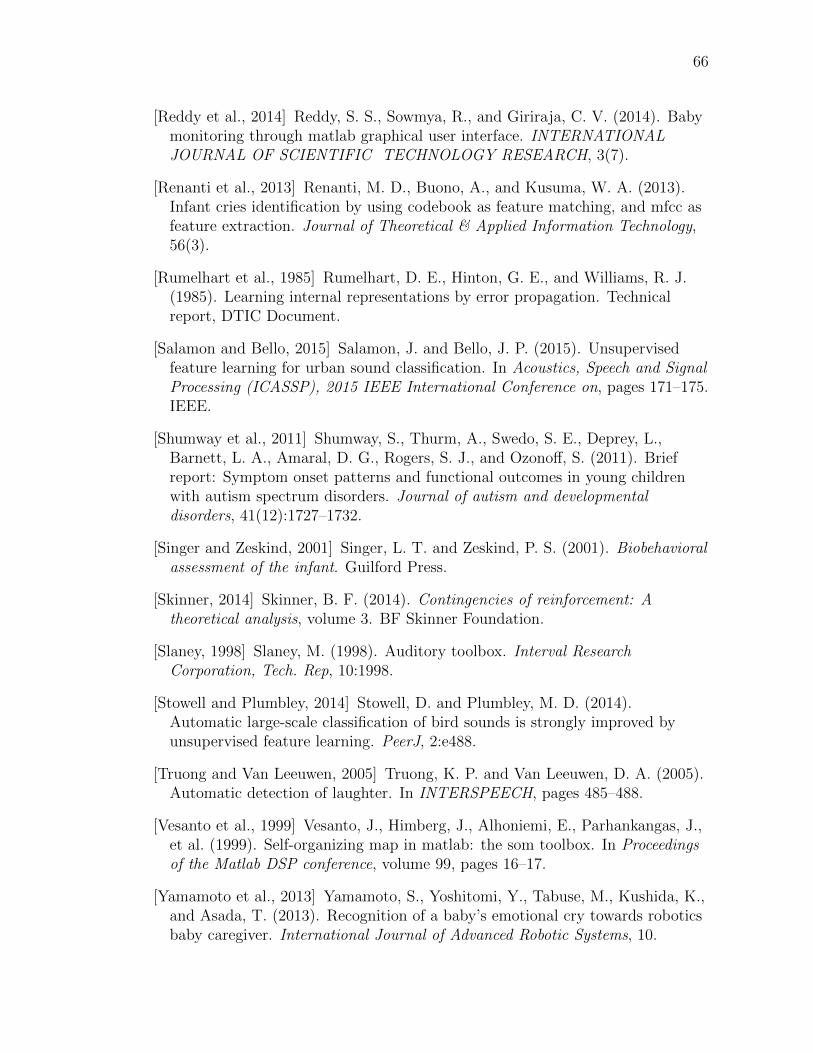
66

[Reddy et al., 2014] Reddy, S. S., Sowmya, R., and Giriraja, C. V. (2014). Babymonitoring through matlab graphical user interface. INTERNATIONALJOURNAL OF SCIENTIFIC TECHNOLOGY RESEARCH, 3(7).

[Renanti et al., 2013] Renanti, M. D., Buono, A., and Kusuma, W. A. (2013).Infant cries identification by using codebook as feature matching, and mfcc asfeature extraction. Journal of Theoretical & Applied Information Technology,56(3).

[Rumelhart et al., 1985] Rumelhart, D. E., Hinton, G. E., and Williams, R. J.(1985). Learning internal representations by error propagation. Technicalreport, DTIC Document.

[Salamon and Bello, 2015] Salamon, J. and Bello, J. P. (2015). Unsupervisedfeature learning for urban sound classification. In Acoustics, Speech and SignalProcessing (ICASSP), 2015 IEEE International Conference on, pages 171–175.IEEE.

[Shumway et al., 2011] Shumway, S., Thurm, A., Swedo, S. E., Deprey, L.,Barnett, L. A., Amaral, D. G., Rogers, S. J., and Ozonoff, S. (2011). Briefreport: Symptom onset patterns and functional outcomes in young childrenwith autism spectrum disorders. Journal of autism and developmentaldisorders, 41(12):1727–1732.

[Singer and Zeskind, 2001] Singer, L. T. and Zeskind, P. S. (2001). Biobehavioralassessment of the infant. Guilford Press.

[Skinner, 2014] Skinner, B. F. (2014). Contingencies of reinforcement: Atheoretical analysis, volume 3. BF Skinner Foundation.

[Slaney, 1998] Slaney, M. (1998). Auditory toolbox. Interval ResearchCorporation, Tech. Rep, 10:1998.

[Stowell and Plumbley, 2014] Stowell, D. and Plumbley, M. D. (2014).Automatic large-scale classification of bird sounds is strongly improved byunsupervised feature learning. PeerJ, 2:e488.

[Truong and Van Leeuwen, 2005] Truong, K. P. and Van Leeuwen, D. A. (2005).Automatic detection of laughter. In INTERSPEECH, pages 485–488.

[Vesanto et al., 1999] Vesanto, J., Himberg, J., Alhoniemi, E., Parhankangas, J.,et al. (1999). Self-organizing map in matlab: the som toolbox. In Proceedingsof the Matlab DSP conference, volume 99, pages 16–17.

[Yamamoto et al., 2013] Yamamoto, S., Yoshitomi, Y., Tabuse, M., Kushida, K.,and Asada, T. (2013). Recognition of a baby’s emotional cry towards roboticsbaby caregiver. International Journal of Advanced Robotic Systems, 10.

67

[Yu et al., 2011] Yu, D., Deng, L., Seide, F. T. B., and Li, G. (2011).Discriminative pretraining of deep neural networks. US Patent App.13/304,643.