June 2004

THE UNIVERSITY OF KANSAS WORKING PAPERS SERIES IN THEORETICAL AND APPLIED ECONOMICS

WORKING PAPER NUMBER 200404

THE UNIVERSITY OF KANSAS WORKING PAPERS SERIES IN THEORETICAL AND APPLIED ECONOMICS

ON USER COSTS OF RISKY MONETARY ASSETS William A. Barnett University of Kansas Shu Wu University of Kansas

On user costs of risky monetary assets

by

William A. Barnett and Shu Wu

University of Kansas, Lawrence, Kansas

June 24, 2004

Forthcoming in the Annals of Finance, volume 1, no. 1.

2

On user costs of risky monetary assets∗

William A. Barnett1 and Shu Wu2

1. Department of Economics, University of Kansas, Lawrence, KS 66045, USA (email: barnett@ku.edu) 2. Department of Economics, University of Kansas, Lawrence, KS 66045, USA (email: shuwu@ku.edu)

Received: revised:

Summary. We extend the monetary-asset user-cost risk adjustment of Barnett, Liu, and

Jensen (1997) and their risk-adjusted Divisia monetary aggregates to the case of multiple

non-monetary assets and intertemporal non-separability. Our model can generate

potentially larger and more accurate CCAPM user-cost risk adjustments than those found

in Barnett, Liu, and Jensen (1997). We show that the risk adjustment to a monetary

asset’s user cost can be measured easily by its beta. We show that any risky non-

monetary asset can be used as the benchmark asset, if its rate of return is adjusted in

accordance with our formula. These extensions could be especially useful, when own

rates of return are subject to exchange rate risk, as in Barnett (2003).

Keywords and Phrases: User costs, Monetary Aggregation, Risk, Pricing kernel, CAPM

JEL Classification Numbers: E41 G12 C43 C22

∗ We thank participants at the 11th Global Finance Annual Conference, Yuqing Huang, and an anonymous

referee for helpful comments and suggestions.

Correspondence to: William A. Barnett

3

1. Introduction

Barnett (1978, 1980, 1997) produced the microeconomic theory of monetary

aggregation under perfect certainty, derived the formula for the user cost of monetary

assets, and originated the Divisia monetary aggregates to track the theory’s quantity and

price aggregator functions nonparametrically. The monetary aggregation theory was

extended to risk by Barnett (1995) and Barnett, Hinich, and Yue (2000). In producing the

Divisia index approximations to the theory’s aggregator functions under risk, Barnett,

Liu, and Jensen (1997) and Barnett and Liu (2000) showed that a risk adjustment term

should be added to the certainty-equivalent user cost in a consumption-based capital asset

pricing model (CCAPM). The risk adjustment depends upon the covariance between the

rates of return on monetary assets and the growth rate of consumption. Using the

components of the usual Federal Reserve System monetary aggregates, Barnett, Liu, and

Jensen (1997) showed, however, that the CCAPM risk adjustment is slight and the gain

from replacing the unadjusted Divisia index with the extended index is usually small. An

overview of the relevant literature is provided in Barnett and Serletis (2000).

The small adjustments are mainly due to the very low contemporaneous

covariance between asset returns and the growth rate of consumption. Under the standard

power utility function and a reasonable value of the risk-aversion coefficient, the low

contemporaneous covariance between asset returns and consumption growth implies that

the impact of risk on the user cost of monetary assets is very small. This finding is closely

related to those in the well-established literature on the equity premium puzzle [see, e.g.,

Mehra and Prescott (1985)], in which it is shown that consumption-based asset pricing

models with the standard power utility function usually fail to reconcile the observed

large equity premium with the low covariance between the equity return and consumption

growth. Many different approaches have been pursued in the literature to explain the

equity premium puzzle. One successful approach is the use of more general utility

functions, such as those with intertemporal non-separability. For example, Campbell and

Cochrane (1999) showed that, in an otherwise standard consumption-based asset pricing

model, intertemporal non-separability induced by habit formation can produce large time-

varying risk premia similar in magnitude to those observed in the data. This suggests that

4

the CCAPM adjustment to the certainty-equivalent monetary-asset user costs can

similarly be larger under a more general utility function than those used in Barnett, Liu,

and Jensen (1997), who assumed a standard time-separable power utility function.

In this paper, we extend the results in Barnett, Liu, and Jensen (1997) to the case

of intertemporal non-separability. We show that the basic result of Barnett, Liu, and

Jensen (1997) still holds under a more general utility function. But by allowing

intertemporal non-separability, our model can lead to substantial, and we believe

accurate, CCAPM risk adjustment, even with a reasonable setting of the risk-aversion

coefficient. We believe that the resulting correction is accurate, since the full impact of

asset returns on consumption is not contemporaneous, but rather spread over time, as

would result from intertemporal non-separability of tastes. This fact has been well

established in the finance literature regarding non-monetary assets, and, as we shall see

below, the risk adjustment to the rates of return on non-monetary assets plays an

important role within the computation of risk adjustments for monetary assets. Hence,

even if intertemporal separability from consumption were a reasonable assumption for

monetary assets, the established intertemporal non-separability of non-monetary assets

from consumption would contaminate the results on monetary assets, under Barnett, Liu,

and Jensen’s (1997) assumption of the conventional fully intertemporally-separable

CCAPM.

We also extend the model in Barnett, Liu, and Jensen (1997) to include multiple

risky non-monetary assets, which are the assets that provide no liquidity services, other

than their rates of return. This extension is important for two reasons. First, it was shown

by Barnett (2003) that the same risk-free benchmark rate cannot be imputed to multiple

countries, except under strong assumptions on convergence across the countries. In the

literature on optimal currency areas and monetary aggregation over countries within a

monetary union, multiple risk-free benchmark assets can be necessary. Even within a

single country that is subject to regional regulations and taxation, Barnett’s (2003)

convergence assumptions for the existence of a unique risk-free benchmark rate may not

hold. Under those circumstances, Barnett (2003) has shown that the theory, under perfect

certainty, requires multiple benchmark rates of return and the imputation of an additional

regional or country subscript to all monetary asset quantities and rates of return, to

5

differentiate assets and rates of return by region or country. Second, the need to compute

a unique risk-free benchmark rate of return, when theoretically relevant, presents difficult

empirical and measurement problems. We rarely observe the theoretical risk-free asset

(in real terms) in financial markets, and hence the risk-free benchmark rate of return is

inherently an unobserved variable that, at best, has been proxied. But we show that the

relationship between the user cost of a monetary asset and a risky “benchmark” asset’s

rate of return holds for an arbitrary pair of a monetary and a risky non-monetary asset.

Because of this fundamental extension, our results on risk adjustment do not depend upon

the existence of a unique risk free rate or the ability to measure such a rate. This

important extension remains relevant, even if all monetary asset rates of return are subject

to low risk, since relevant candidates for the benchmark asset may all have risky rates of

return.

In the asset pricing literature, one of the most popular models is the Capital Asset

Pricing Model (CAPM) developed by Sharpe (1964) and Lintner (1965), among others.

In CAPM, the risk premium on an individual asset is determined by the covariance of its

excess rate of return with that of the market portfolio, or equivalently its beta. The

advantage of CAPM is that it circumvents the issue of unobservable marginal utility, and

the beta can easily be estimated. We show in this paper that there also exists a similar

beta that relates the user cost of an individual monetary asset to the user cost of the

consumer’s wealth portfolio.

The rest of the paper is organized as follows. In the next section, we specify the

representative consumer’s intertemporal optimization problem. The main results are

contained in Section 3, while Section 4 concludes.

2. Consumer’s optimization problem

We use a setup similar to that in Barnett, Liu, and Jensen (1997). We assume that

the representative consumer has an intertemporally non-separable general utility function,

( , , , , )t t t -1 t-nU c c cLm , defined over current and past consumption and a vector of L

current-period monetary assets, 1, 2, ,( , , , )t t t L tm m m ′= Lm . The consumer’s holdings of

6

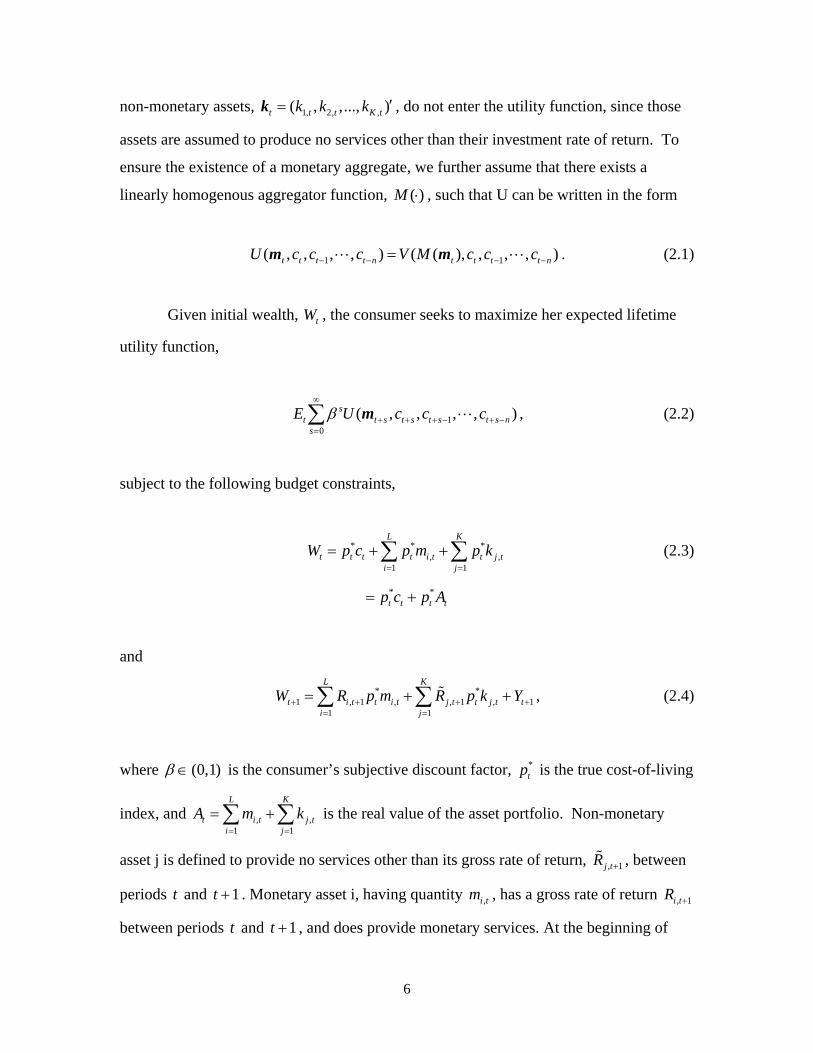
non-monetary assets, 1, 2, ,( , ,..., )t t t K tk k k ′=k , do not enter the utility function, since those

assets are assumed to produce no services other than their investment rate of return. To

ensure the existence of a monetary aggregate, we further assume that there exists a

linearly homogenous aggregator function, ( )M ⋅ , such that U can be written in the form

1 1( , , , , ) ( ( ), , , , )t t t t n t t t t nU c c c V M c c c− − − −=L Lm m . (2.1)

Given initial wealth, tW , the consumer seeks to maximize her expected lifetime

utility function,

10

( , , , , )st t s t s t s t s n

sE U c c cβ

∞

+ + + − + −=∑ Lm , (2.2)

subject to the following budget constraints,

* * *, ,

1 1

L K

t t t t i t t j ti j

W p c p m p k= =

= + +∑ ∑ (2.3)

* *t t t tp c p A= +

and

* *1 , 1 , , 1 , 1

1 1

L K

t i t t i t j t t j t ti j

W R p m R p k Y+ + + += =

= + +∑ ∑ % , (2.4)

where (0,1)β ∈ is the consumer’s subjective discount factor, *tp is the true cost-of-living

index, and , ,1 1

L K

t i t j ti j

A m k= =

= +∑ ∑ is the real value of the asset portfolio. Non-monetary

asset j is defined to provide no services other than its gross rate of return, , 1j tR +% , between

periods t and 1t + . Monetary asset i, having quantity ,i tm , has a gross rate of return , 1i tR +

between periods t and 1t + , and does provide monetary services. At the beginning of

7

each period, the consumer allocates her wealth among consumption, tc , investment in the

monetary assets, tm , and investment in the non-monetary assets, tk . The consumer’s

income from any other sources, received at the beginning of period 1t + , is 1tY + . If any

of that income’s source is labor income, then we assume that leisure is weakly separable

from consumption of goods and holding of monetary assets, so that the function U exists

and the decision exists, as a conditional decision problem. The consumer also is subject

to the transversality condition

*lim 0st t ss

p Aβ +→∞= . (2.5)

The equivalency of the two constraints (2.3) and (2.4) with the single constraint used in Barnett

(1980) and Barnett, Liu, and Jensen (1997) is easily seen by substituting equation (2.3) for period

t+1 into equation (2.4) and solving for *t tp c .

Define the value function of the consumer’s optimization problem to be

1( , , , )t t t t nH H W c c− −= L . Assuming the solution to the decision problem exists, we then

have the Bellman equation

1 1( , , )

{ ( , , , , ) }t t t

t t t t t t n tc

H Sup E U c c c Hβ− − += +Lm k

m , (2.6)

where the maximization is subject to the budget constraints, (2.3) and (2.4).

The first order conditions can be obtained as

* *1 , 1 1t t t j t t tE R p pλ β λ + + +⎡ ⎤= ⎣ ⎦% (2.7)

and

* *, 1 , 1 1t i t t t t i t t tU m E R p pλ β λ + + +⎡ ⎤∂ ∂ = − ⎣ ⎦ , (2.8)

where 1,( , , , )t t t t t nU U c c c− −= Lm and 1( )nt t t t t t t n tE U c U c U cλ β β+ += ∂ ∂ + ∂ ∂ + + ∂ ∂L .

Note that tλ is the expected present value of the marginal utility of consumption, tc . In

8

the standard case in which the instantaneous utility function is time-separable, tλ reduces

to ( , )t t tU c c∂ ∂m .

3. Risk-adjusted user cost of monetary assets

3.1. The theory

As in Barnett, Liu, and Jensen (1997), we define the contemporaneous real user-

cost price of the services of monetary asset i to be the ratio of the marginal utility of the

monetary asset and the marginal utility of consumption, so that

( )

, ,

1, .

t t

i t i t

t t t n

t t t

U Um m

i t U U Untt c c cE

πλβ β+ +

∂ ∂∂ ∂

∂ ∂ ∂∂ ∂ ∂

= =+ + +L

(3.1)

We denote the vector of L monetary asset user costs by 1, 2, ,( , , , )t t t L tπ π π ′= Lπ . With the

user costs defined above, we can show that the solution value of the exact monetary

aggregate, ( )tM m , can be tracked accurately in continuous time by the generalized

Divisia index, as proved in the perfect certainty special case by Barnett (1980).

Proposition 1. Let , ,

, ,1,

i t i tL

l t l tl

mi t m

s π

π=

=∑

be the user-cost-evaluated expenditure share. Under

the weak-separability assumption, (2.1), we have for any linearly homogenous monetary

aggregator function, ( )M ⋅ , that

, ,1

log logL

t i t i ti

d M s d m=

= ∑ , (3.2)

where Mt = M(mt).

Proof. Under the assumption of weak-separability, we have

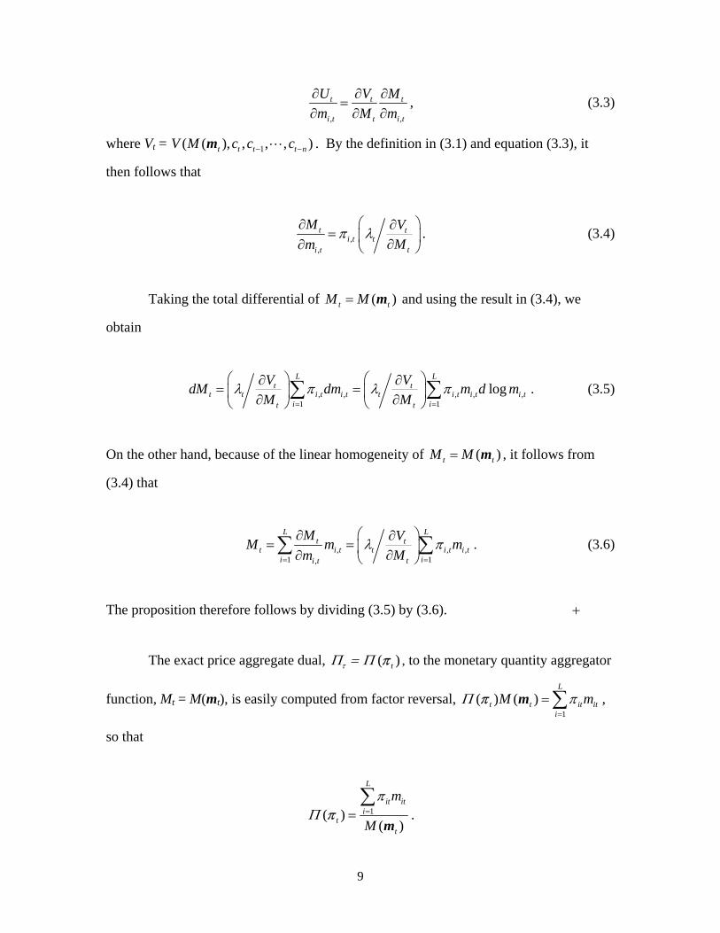
9

, ,

t t t

i t t i t

U V Mm M m∂ ∂ ∂

=∂ ∂ ∂

, (3.3)

where Vt = 1( ( ), , , , )t t t t nV M c c c− −Lm . By the definition in (3.1) and equation (3.3), it

then follows that

,,

t ti t t

ti t

M VMm

π λ⎛ ⎞∂ ∂

= ⎜ ⎟∂∂ ⎝ ⎠. (3.4)

Taking the total differential of ( )t tM M= m and using the result in (3.4), we

obtain

, , , , ,1 1

logL L

t tt t i t i t t i t i t i t

i it t

V VdM dm m d mM M

λ π λ π= =

⎛ ⎞ ⎛ ⎞∂ ∂= =⎜ ⎟ ⎜ ⎟∂ ∂⎝ ⎠ ⎝ ⎠

∑ ∑ . (3.5)

On the other hand, because of the linear homogeneity of ( )t tM M= m , it follows from

(3.4) that

, , ,1 1,

L Lt t

t i t t i t i ti iti t

M VM m mMm

λ π= =

⎛ ⎞∂ ∂= = ⎜ ⎟∂∂ ⎝ ⎠∑ ∑ . (3.6)

The proposition therefore follows by dividing (3.5) by (3.6). +

The exact price aggregate dual, ( )tτΠ = Π π , to the monetary quantity aggregator

function, Mt = M(mt), is easily computed from factor reversal, 1

( ) ( )L

t t it iti

M mΠ π=

=∑π m ,

so that

1( )( )

L

it iti

tt

m

M

πΠ ==

∑π

m.

10

In continuous time, the user cost price dual can be tracked without error by the Divisia

user cost price index

, ,1

log logL

t i t i ti

d s dΠ π=

=∑ .

To get a more convenient expression for the user cost, ,i tπ , we define the pricing

kernel to be

1 1t t tQ β λ λ+ += . (3.7)

Recall that tλ is the present value of the marginal utility of consumption at time t . Hence

1tQ + measures the marginal utility growth from t to 1t + . For example, if the utility

function (2.1) is time-separable, we have that 1 1 1( , )1 ( , )

t t t

t t t

U c ct U c cQ β + + +∂ ∂+ ∂ ∂= m

m , which is the

subjectively discounted marginal rate of substitution between consumption this period

and consumption next period. Clearly 1tQ + is positive, as required of marginal rates of

substitution.

While the introduction of a pricing kernel is well understood in finance, the intent

also should be no surprise to experts in index number theory either. The way in which

statistical index numbers, depending upon prices and quantities, track quantity aggregator

functions, containing no prices, is through the substitution of first order conditions to

replace marginal utilities by functions of relevant prices. This substitution is particularly

well known in the famous derivation of the Divisia index by Francois Divisia (1925). In

our case, the intent, as applied below, is to replace 1tQ + by a function of relevant

determinants of its value in asset market equilibriuim. If we use the approximation that

characterizes CAPM, then the pricing kernel, 1tQ + , would be a linear function of the rate

of return on the consumer’s asset portfolio, At.

11

Using (3.1) and (3.7), the first order conditions (2.7) and (2.8) can alternatively be

written as

1 , 10 1 ( )t t j tE Q r+ += − % , (3.8)

, 1 , 11 ( )i t t t i tE Q rπ + += − , (3.9)

where * *, 1 , 1 1j t j t t tr R p p+ + += %% is the real gross rate of return on non-monetary asset, ,j tk , and

* *, 1 , 1i t i t t t tr R p p+ + += is the real gross rate of return on monetary asset, mi,t, which provides

the consumer with liquidity service.

Equations (3.8) and (3.9) impose restrictions on asset returns. Equation (3.8)

applies to the returns on all risky non-monetary assets, ,j tk ( 1,j K= L ), in the usual

manner. For monetary assets, equation (3.9) implies that the “deviation” from the usual

Euler equation measures the user cost of that monetary asset. To obtain good measures of

the user costs of monetary assets, the non-monetary asset pricing within the asset

portfolio’s pricing kernel, 1tQ + , should be as accurate as possible. Otherwise, we would

attribute any non-monetary asset pricing errors to the monetary asset user costs in (3.9),

as pointed out by Marshall (1997). From the above Euler equations, we can obtain the

following proposition.

Proposition 2. Given the real rate of return, , 1i tr + , on a monetary asset and the real rate

of return, , 1j tr +% , on an arbitrary non-monetary asset, the risk-adjusted real user-cost price

of the services of the monetary asset can be obtained as

, , 1 , , 1,

, 1

(1 ) (1 )i t t j t j t t i ti t

t j t

E r E rE r

ω ωπ + +

+

+ − +=

%

%, (3.10)

where

, 1 , 1( , )i t t t i tCov Q rω + += − (3.11)

and

12

, 1 , 1( , )j t t t j tCov Q rω + += − % . (3.12)

Proof. From the Euler equation (3.8), we have

1 , 1 1 , 11 ( , )t t t j t t t j tE Q E r Cov Q r+ + + += +% % , (3.13)

and similarly from the Euler equation (3.9), we have

, 1 , 1 1 , 11 ( , )i t t t t i t t t i tE Q E r Cov Q rπ + + + += − − . (3.14)

Note that (3.13) implies that

1 , 11

, 1

1 ( , )t t j tt t

t j t

Cov Q rE Q

E r+ +

++

−=

%

%. (3.15)

Hence Proposition 2 follows by substituting 1t tE Q + into (3.14). +

Proposition 2 relates the user cost of a monetary asset to the rates of return on

financial assets, which need not be risk free. It applies to an arbitrary pair of monetary

and non-monetary assets. In fact, observe that the left hand side of equation (3.10) has no

j subscript, even though there are j subscripts on the right hand side. The left hand side of

(3.10) is invariant to the choice of non-monetary asset used on the right hand side, as a

result of equation (3.15), which holds for all j, regardless of i. This result suggests that

we can choose an arbitrary non-monetary financial asset as the “benchmark” asset in

calculating the user costs of the financial assets that provide monetary services, so long as

we correctly compute the covariance, ,j tω , of the return on the non-monetary asset with

the pricing kernel.

Practical considerations in estimating that covariance could tend to discourage use

of multiple benchmark assets. In particular, a biased estimate of ωj,t for a non-monetary

asset j would similarly bias the user costs of all monetary assets, if that non-monetary

asset were used as the benchmark asset in computing all monetary asset user costs.

13

Alternatively, if a different non-monetary financial assets were used as the benchmark

assets for each monetary asset, errors in measuring ωj,t for different j’s could bias relative

user costs of monetary assets.

Nevertheless, in theory it is not necessary to use the same benchmark asset j for

the computation of the user cost of each monetary asset i. In particular, we have the

following corollary.

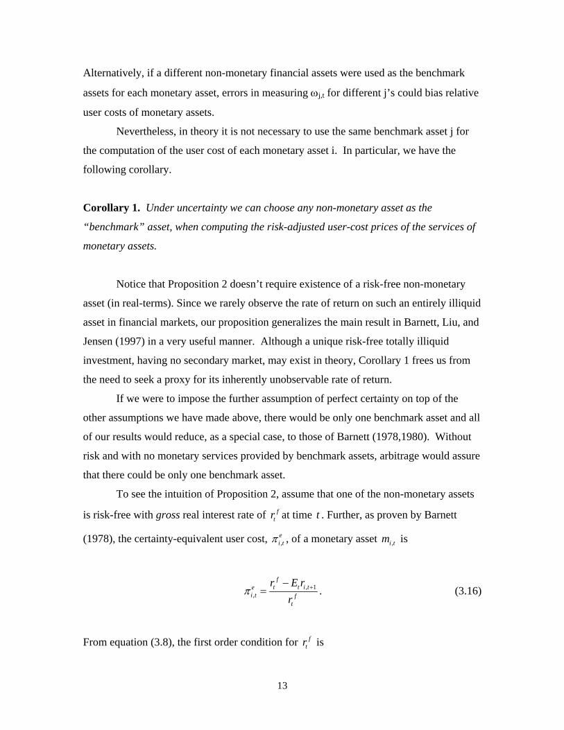
Corollary 1. Under uncertainty we can choose any non-monetary asset as the

“benchmark” asset, when computing the risk-adjusted user-cost prices of the services of

monetary assets.

Notice that Proposition 2 doesn’t require existence of a risk-free non-monetary

asset (in real-terms). Since we rarely observe the rate of return on such an entirely illiquid

asset in financial markets, our proposition generalizes the main result in Barnett, Liu, and

Jensen (1997) in a very useful manner. Although a unique risk-free totally illiquid

investment, having no secondary market, may exist in theory, Corollary 1 frees us from

the need to seek a proxy for its inherently unobservable rate of return.

If we were to impose the further assumption of perfect certainty on top of the

other assumptions we have made above, there would be only one benchmark asset and all

of our results would reduce, as a special case, to those of Barnett (1978,1980). Without

risk and with no monetary services provided by benchmark assets, arbitrage would assure

that there could be only one benchmark asset.

To see the intuition of Proposition 2, assume that one of the non-monetary assets

is risk-free with gross real interest rate of ftr at time t . Further, as proven by Barnett

(1978), the certainty-equivalent user cost, ,ei tπ , of a monetary asset ,i tm is

, 1,

ft t i te

i t ft

r E rr

π +−= . (3.16)

From equation (3.8), the first order condition for ftr is

14

11 ( )ft t tE Q r+= . (3.17)

Hence we have, from the nonrandomness of ftr , that

11

t t ft

E Qr+ = . (3.18)

Replacing 1t tE Q + in (3.9) with 1f

tr, we then have

, 1, , , ,

ft t i t e

i t i t i t i tft

r E rr

π ω π ω+−= + = + , (3.19)

where , 1 , 1( , )i t t t i tCov Q rω + += − . Therefore, ,i tπ could be larger or smaller than the

certainty-equivalent user cost, ,ei tπ , depending on the sign of the covariance between , 1i tr +

and 1tQ + . When the return on a monetary asset is positively correlated with the pricing

kernel, 1tQ + , and thereby negatively correlated with the rate of return on the full portfolio

of monetary and non-monetary assets, the monetary asset’s user cost will be adjusted

downwards from the certainty-equivalent user cost. Such assets offer a hedge against

aggregate risk by paying off when the full asset portfolio’s rate of return is low. In

contrast, when the return on a monetary asset is negatively correlated with the pricing

kernel, 1tQ + , and thereby positively correlated with the rate of return on the full asset

portfolio, the asset’s user cost will be adjusted upwards from the certainty-equivalent user

cost, since such assets tend to pay off when the asset porfolio’s rate of return is high.

Such assets are very risky.

To calculate the risk adjustment, we need to compute the covariance between the

asset return , 1i tr + and the pricing kernel 1tQ + , which is unobservable. Consumption-based

asset pricing models allow us to relate 1tQ + to consumption growth through a specific

utility function. But most utility functions have been shown not be able to reconcile the

15

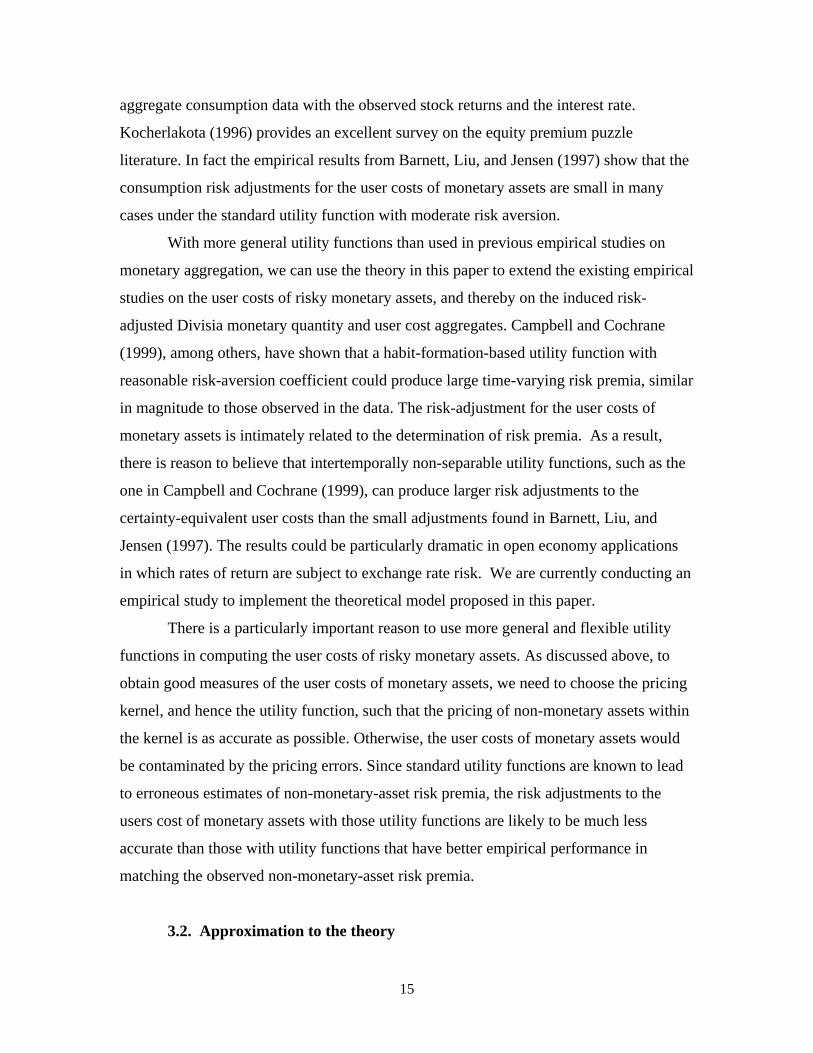
aggregate consumption data with the observed stock returns and the interest rate.

Kocherlakota (1996) provides an excellent survey on the equity premium puzzle

literature. In fact the empirical results from Barnett, Liu, and Jensen (1997) show that the

consumption risk adjustments for the user costs of monetary assets are small in many

cases under the standard utility function with moderate risk aversion.

With more general utility functions than used in previous empirical studies on

monetary aggregation, we can use the theory in this paper to extend the existing empirical

studies on the user costs of risky monetary assets, and thereby on the induced risk-

adjusted Divisia monetary quantity and user cost aggregates. Campbell and Cochrane

(1999), among others, have shown that a habit-formation-based utility function with

reasonable risk-aversion coefficient could produce large time-varying risk premia, similar

in magnitude to those observed in the data. The risk-adjustment for the user costs of

monetary assets is intimately related to the determination of risk premia. As a result,

there is reason to believe that intertemporally non-separable utility functions, such as the

one in Campbell and Cochrane (1999), can produce larger risk adjustments to the

certainty-equivalent user costs than the small adjustments found in Barnett, Liu, and

Jensen (1997). The results could be particularly dramatic in open economy applications

in which rates of return are subject to exchange rate risk. We are currently conducting an

empirical study to implement the theoretical model proposed in this paper.

There is a particularly important reason to use more general and flexible utility

functions in computing the user costs of risky monetary assets. As discussed above, to

obtain good measures of the user costs of monetary assets, we need to choose the pricing

kernel, and hence the utility function, such that the pricing of non-monetary assets within

the kernel is as accurate as possible. Otherwise, the user costs of monetary assets would

be contaminated by the pricing errors. Since standard utility functions are known to lead

to erroneous estimates of non-monetary-asset risk premia, the risk adjustments to the

users cost of monetary assets with those utility functions are likely to be much less

accurate than those with utility functions that have better empirical performance in

matching the observed non-monetary-asset risk premia.

3.2. Approximation to the theory

16

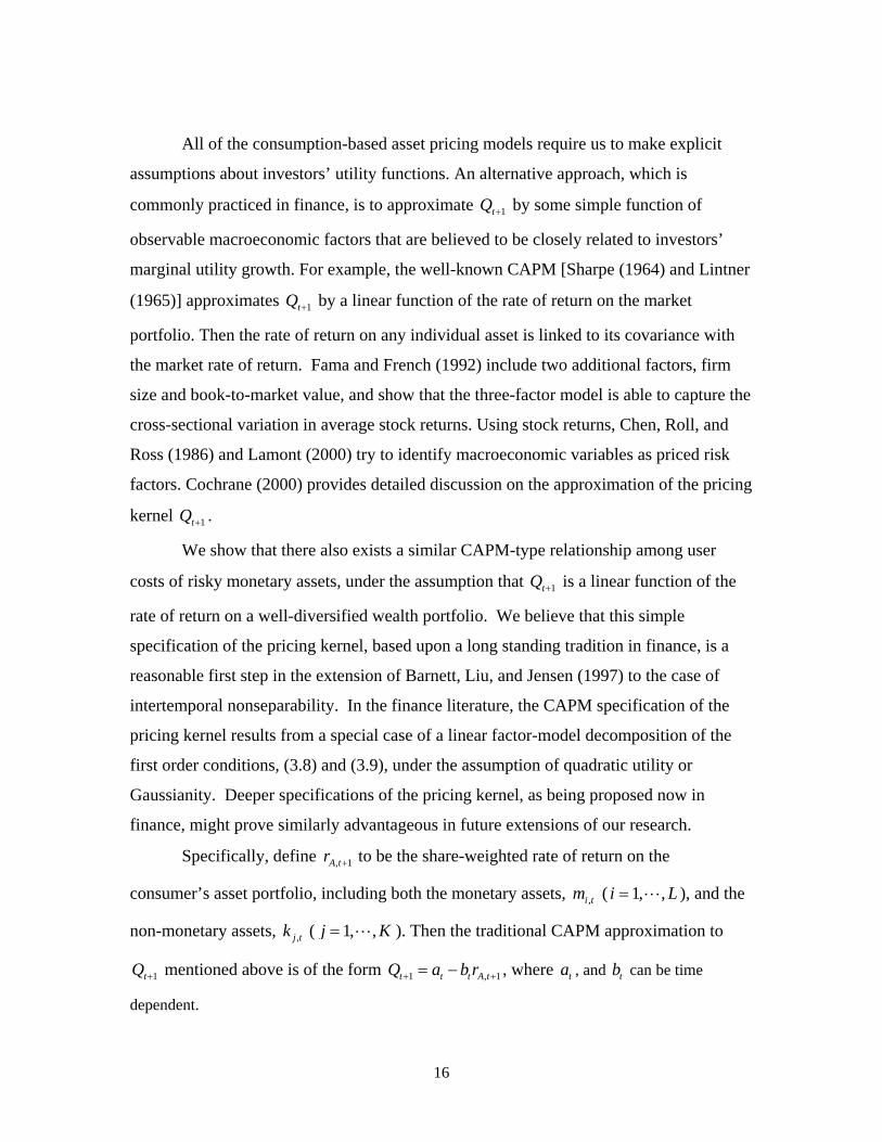
All of the consumption-based asset pricing models require us to make explicit

assumptions about investors’ utility functions. An alternative approach, which is

commonly practiced in finance, is to approximate 1tQ + by some simple function of

observable macroeconomic factors that are believed to be closely related to investors’

marginal utility growth. For example, the well-known CAPM [Sharpe (1964) and Lintner

(1965)] approximates 1tQ + by a linear function of the rate of return on the market

portfolio. Then the rate of return on any individual asset is linked to its covariance with

the market rate of return. Fama and French (1992) include two additional factors, firm

size and book-to-market value, and show that the three-factor model is able to capture the

cross-sectional variation in average stock returns. Using stock returns, Chen, Roll, and

Ross (1986) and Lamont (2000) try to identify macroeconomic variables as priced risk

factors. Cochrane (2000) provides detailed discussion on the approximation of the pricing

kernel 1tQ + .

We show that there also exists a similar CAPM-type relationship among user

costs of risky monetary assets, under the assumption that 1tQ + is a linear function of the

rate of return on a well-diversified wealth portfolio. We believe that this simple

specification of the pricing kernel, based upon a long standing tradition in finance, is a

reasonable first step in the extension of Barnett, Liu, and Jensen (1997) to the case of

intertemporal nonseparability. In the finance literature, the CAPM specification of the

pricing kernel results from a special case of a linear factor-model decomposition of the

first order conditions, (3.8) and (3.9), under the assumption of quadratic utility or

Gaussianity. Deeper specifications of the pricing kernel, as being proposed now in

finance, might prove similarly advantageous in future extensions of our research.

Specifically, define , 1A tr + to be the share-weighted rate of return on the

consumer’s asset portfolio, including both the monetary assets, ,i tm ( 1, ,i L= L ), and the

non-monetary assets, ,j tk ( 1, ,j K= L ). Then the traditional CAPM approximation to

1tQ + mentioned above is of the form 1 , 1t t t A tQ a b r+ += − , where ta , and tb can be time

dependent.

17

Let ,i tφ and ,j tϕ denote the share of ,i tm and ,j tk , respectively, in the portfolio’s

stock value, so that

,i tφ = ,

, ,1 1

i tL K

l t j tl j

m

m k= =

+∑ ∑ = ,i t

t

mA

and

,j tϕ = ,

, ,1 1

j tL K

l t i tl i

k

m k= =

+∑ ∑= ,j t

t

kA

.

Then, by construction, , 1 , , 1 , , 11 1

L K

A t i t i t j t j ti j

r r rφ ϕ+ + += =

= +∑ ∑ % , where

, ,1 1

1L K

i t j ti j

φ ϕ= =

+ =∑ ∑ . (3.20)

Multiplying (3.8) by ,j tϕ and (3.9) by ,i tφ , we have

, 1 , , 10 ( )j t t t j t j tE Q rϕ ϕ+ += − % (3.21)

and

, , , 1 , , 1( )i t i t i t t t i t i tE Q rφ π φ φ+ += − . (3.22)

Summing (3.21) over j and (3.22) over i, adding the two summed equations together, and

using the definition of , 1A tr + , we get

18

, , 1 , 11

1 ( )L

i t i t t t A ti

E Q rφ π + +=

= −∑ . (3.23)

Let , , , , ,1 1

L K

A t i t i t i t j ti j

Π φ π ϕ π= =

= +∑ ∑ % , where ,j tπ% is the user cost of non-monetary asset

j. We define ,A tΠ to be the user cost of the consumer’s asset wealth portfolio. But the

user cost, ,j tπ% , of every non-monetary asset is simply 0, as shown in (3.8), so

equivalently , , ,1

L

A t i t i ti

Π φ π=

=∑ . The reason is that consumers do not pay a price, in terms

of foregone interest, for the monetary services of non-monetary assets, since they provide

no monetary services and provide only their investment rate of return. We can show that

our definition of ,A tΠ is consistent with Fisher’s factor reversal test, as follows.

Result: The pair ( tA , ,A tΠ ) satisfies factor reversal, defined by:

, , , , ,1 1

L K

A t t i t i t j t j ti j

A m kΠ π π= =

= +∑ ∑ % .

Since we know that , 0j tπ =% for all j, factor reversal equivalently can be written as

, , ,1

L

A t t i t i ti

A mΠ π=

=∑ .

The proof of the result is straightforward.

Proof: By the definition of ,i tφ , we have mi,t = ,i t tAφ . Hence, we have

, , , ,1 1

L L

i t i t i t i t ti i

m Aπ π φ= =

=∑ ∑

= , ,1

L

t i t i ti

A π φ=∑ = ,t A tAΠ ,

which is our result. +

19

Observe that the wealth portfolio is different from the monetary services

aggregate, ( )tM m . The portfolio weights in the asset wealth stock are the market-value-

based shares, while the growth rate weights in the monetary services flow aggregate are

the user-cost-evaluated shares.

Suppose one of the non-monetary assets is (locally) risk-free with gross real

interest rate ftr . By substituting equation (3.16) for ,i tπ into the definition of ,A tΠ , using

the definition of , 1A tr + , and letting ftr =E , 1j tr +% for all j, it follows that the certainty

equivalent user cost of the asset wealth portfolio is , 1f

t t A tf

t

r E ret rΑ,Π +−= . We now can prove

the following proposition.

Proposition 3. If one of the non-monetary assets is (locally) risk-free with gross real

interest rate ftr , and if 1 , 1t t t A tQ a b r+ += − , where , 1A tr + is the gross real rate of return on

the consumer’s wealth portfolio, then the user cost of any monetary asset i is given by

, , , , ,( )e ei t i t i t A t A tπ π β Π Π− = − , (3.24)

where ,i tπ and ,A tΠ are the user costs of asset i and of the asset wealth portfolio,

respectively, and , 1,

ft t i t

ft

r E rei t r

π +−= and , 1,

ft t A t

ft

r E reA t r

Π +−= are the certainty-equivalent user costs

of asset i and the asset wealth portfolio, respectively. The “beta” of asset i in equation

(3.24) is given by

, 1 , 1,

, 1

( , )( )

t A t i ti t

t A t

Cov r rVar r

β + +

+

= . (3.25)

Proof. From (3.23) and the definition of ,A tΠ , we have for the wealth portfolio that

, 1 , 1 1 , 11 ( , )A t t t t A t t t A tE Q E r Cov Q rΠ + + + += − − . (3.26)

20

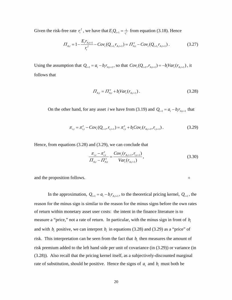
Given the risk-free rate ftr , we have that 1

1 ft

t t rE Q + = from equation (3.18). Hence

, 1, 1, , 1 , 1, , 11 ( ) ( )t A t e

A t t t A t A t t t A tft

E rCov Q r Cov Q r

rΠ Π+

+ + + += − − = − . (3.27)

Using the assumption that 1 , 1t t t A tQ a b r+ += − , so that 1 , 1 , 1( , ) ( )t t A t t t A tCov Q r bVar r+ + += − , it

follows that

, , , 1( )eA t A t t t A tbVar rΠ Π += + . (3.28)

On the other hand, for any asset i we have from (3.19) and 1 , 1t t t A tQ a b r+ += − that

, , 1 , 1 , , 1 , 1( , ) ( , )e ei t i t t t i t i t t t A t i tCov Q r b Cov r rπ π π+ + + += − = + . (3.29)

Hence, from equations (3.28) and (3.29), we can conclude that

, , , 1 , 1

, , , 1

( , )( )

ei t i t t A t i t

eA t A t t A t

Cov r rVar r

π πΠ Π

+ +

+

−=

−, (3.30)

and the proposition follows. +

In the approximation, 1 , 1t t t A tQ a b r+ += − , to the theoretical pricing kernel, 1tQ + , the

reason for the minus sign is similar to the reason for the minus signs before the own rates

of return within monetary asset user costs: the intent in the finance literature is to

measure a “price,” not a rate of return. In particular, with the minus sign in front of tb

and with tb positive, we can interpret tb in equations (3.28) and (3.29) as a “price” of

risk. This interpretation can be seen from the fact that tb then measures the amount of

risk premium added to the left hand side per unit of covariance (in (3.29)) or variance (in

(3.28)). Also recall that the pricing kernel itself, as a subjectively-discounted marginal

rate of substitution, should be positive. Hence the signs of ta and tb must both be

21

positive, and ta must be sufficiently large so that the pricing kernel is positive for all

observed values of , 1A tr + .

Proposition 3 is very similar to the standard CAPM formula for asset returns. In

CAPM theory, the expected excess rate of return, , 1f

t i t tE r r+ − , on an individual asset is

determined by its covariance with the excess rate of return on the market portfolio,

, 1f

t M t tE r r+ − , in accordance with

, 1 , , 1( )f ft i t t i t t M t tE r r E r rβ+ +− = − , (3.31)

where , 1 , 1

, 1

( , ), ( )

f ft i t t M t t

ft M t t

Cov r r r ri t Var r r

β + +

+

− −

−= .

This result implies that asset i’s risk premium depends on its market portfolio risk

exposure, which is measured by the beta of this asset. Our proposition shows that the risk

adjustment to the certainty equivalent user cost of asset i is determined in that manner as

well. The larger the beta, through risk exposure to the wealth portfolio, the larger the risk

adjustment. User costs will be adjusted upwards for those monetary assets whose rates of

return are positively correlated with the return on the wealth portfolio, and conversely for

those monetary assets whose returns are negatively correlated with the wealth portfolio.

In particular, if we find that ,i tβ is very small for all the monetary assets under

consideration, then the risk adjustment to the user cost is also very small. In that case, the

unadjusted Divisia monetary index would be a good proxy for the extended index in

Barnett, Liu, and Jensen (1997).

Notice that Proposition 3 is a conditional version of CAPM with time-varying risk

premia. Lettau and Ludvigson (2001) have shown that a conditional version of CAPM

performs much better empirically in explaining the cross section of asset returns, than the

unconditional CAPM. In fact, the unconditional CAPM is usually rejected in empirical

tests. See, e.g., Breeden, Gibbons, and Litzenberger (1989) and Campbell (1996).

4. Concluding remarks

22

Simple sum monetary aggregates treat monetary assets with different rates of

return as perfect substitutes. Barnett (1978, 1980) showed that the Divisia index, with

user cost prices, is a more appropriate measure for monetary services, and derived the

formula for the user cost of monetary asset services in the absence of uncertainty.

Barnett, Liu, and Jensen (1997) extended the Divisia monetary quantity index to the case

of uncertain returns and risk aversion. For risky monetary assets, however, the magnitude

of the risk adjustment to the certainty equivalent user cost is unclear. Using a standard

time-separable power utility function, Barnett, Liu, and Jensen (1997) showed that the

difference between the unadjusted Divisia index and the index extended for risk is

usually small. However, this result could be a consequence of the same problem that

causes the equity premium puzzle in the asset pricing literature. The consumption-based

asset pricing model with more general utility functions, most notably those that are

intertemporally non-separable, can reproduce the large and time-varying risk premium

observed in the data. We believe that similarly extended asset pricing models will

provide larger and more accurate CCAPM adjustment to the user costs of monetary

assets than those found in Barnett, Liu, and Jensen (1997). The current paper extends the

basic result in Barnett, Liu, and Jensen (1997) in that manner.

How big the risk adjustment should be is an empirical issue. We show in this

paper that for any individual monetary asset, the risk adjustment to its certainty

equivalent user cost can be measured by its beta, which depends on the covariance

between the rate of return on the monetary asset and on the wealth portfolio of the

consumer. This result is analogous to the standard Capital Asset Pricing Model (CAPM).

In practice, if the beta is found to be very small, then the certainty equivalent user cost

would be a good approximation to the true user cost price of the monetary asset services

under uncertainty. In that special case, the unadjusted Divisia index could still be used for

monetary aggregation. We are currently conducting research on the empirical

implications of the models proposed in this paper. Relevant modeling and inference

methodology are available in Barnett and Binner (2004).

Another extension of the current paper could be to introduce heterogeneous

investors, as considered for the case of perfect certainty by Barnett (2003). This

extension can be of particular importance in multicountry or multiregional applications,

23

in which regional or country-specific heterogeneity cannot be ignored. In such cases

regional or national subscripts must be introduced to differentiate goods and assets by

location. With the possibility of regulatory and taxation differences across the

heterogeneous groups, arbitrage cannot be assumed to remove the possibility of multiple

benchmark assets, even under perfect certainty, except under special assumptions on

institutional convergence. See Barnett (2004) regarding those assumptions.

24

References

[1] Barnett, W. A. (1978), “The user cost of money,” Economic Letters 1, 145-149.

Reprinted in W. A. Barnett and A. Serletis (eds.) (2000), The Theory of Monetary

Aggregation, North-Holland, Amsterdam, Chapter 1, 6-10.

Barnett, W. A. (1980), “Economic monetary aggregates: An application of index number

and aggregation theory”, Journal of Econometrics 14, 11-48. Reprinted in W. A. Barnett

and A. Serletis (eds.) (2000), The Theory of Monetary Aggregation, North-Holland,

Amsterdam, Chapter 2, 11-48.

Barnett, W. A. (1995), “Exact aggregation under risk,” in W. A. Barnett, M. Salles, H.

Moulin, and N. Schofield (eds), Social Choice, Welfare and Ethics, Cambridge

University Press, Cambridge, 353-374. Reprinted in W. A. Barnett and A. Serletis (eds.)

(2000), The Theory of Monetary Aggregation, North-Holland, Amsterdam, Chapter 10,

195-206.

Barnett, W. A. (1997), “The microeconomic theory of monetary aggregation,” in W. A.

Barnett (eds), New Approaches to Monetary Economics, Cambridge University Press,

Cambridge, 115-168. Reprinted in W. A. Barnett and A. Serletis (eds.) (2000), The

Theory of Monetary Aggregation, North-Holland, Amsterdam, Chapter 3, 49-99.

Barnett, W. A. (2003), “Aggregation-theoretic monetary aggregation over the Euro area

when countries are heterogeneous,” ECB Working Paper No. 260, European Central

Bank, Frankfurt.

Barnett, W. A. and J. Binner (eds.) (2004), Functional Structure and Approximation in

Econometrics, North-Holland, Amsterdam.

Barnett, W. A., M. Hinich, and P. Yue (2000), “The exact theoretical rational

expectations monetary aggregate,” Macroeconomic Dynamics 4, 197-221.

25

Barnett, W. A. and Y. Liu (2000), “Beyond the risk neutral utility function,” in M. T.

Belongia and J. E. Binner (eds.), Divisia Monetary Aggregates: Theory and Practice,

London, Palgrave, 11-27.

Barnett, W. A., Y. Liu and M. Jensen (1997), “CAPM risk adjustment for exact

aggregation over financial assets,” Macroeconomic Dynamics 1, 485-512. Reprinted in

W. A. Barnett and A. Serletis (eds) (2000), The Theory of Monetary Aggregation, North-

Holland, Amsterdam, Chapter 12, 245-273.

Barnett, W. A. and A. Serletis (eds) (2000), The Theory of Monetary Aggregation, North-

Holland, Amsterdam, Section 3.3, 195-295.

Breeden, D., M. Gibbons and R. Litzenberger (1989), “Empirical tests of the

consumption CAPM,” Journal of Finance 44, 231-262.

Campbell, J. Y. (1996), “Understanding risk and return,” Journal of Political Economy

104, 298-345.

Campbell, J. Y. and J. H. Cochrane (1999), “By force of habit: A consumption-based

explanation of aggregate stock market behavior,” Journal of Political Economy 107, 205-

251.

Chen, N. F., R. Roll and S. Ross (1986), “Economic forces and the stock market,”

Journal of Business 29, 383-403.

Cochrane, J. H. (2000), Asset Pricing, Princeton Press, Princeton, NJ.

Divisia, Francois (1925), “L’Indice Monétaire et la Théorie de la Monnaie,” Revue

d’Economie Politique 39, 980-1008.

26

Fama, E. F. and K. French (1992), “The cross-section of expected stock returns,” Journal

of Finance 47, 427-465.

Kocherlakota, N. (1996), “The equity premium: It's still a puzzle,” Journal of Economic

Literature 34, 43-71.

Lamont, O. (2000), “Economic tracking portfolio”, Journal of Econometrics 105, 161-

184.

Lettau, M. and S. Ludvigson (2001) “Resurrecting the (C)CAPM: A cross-sectional test

when risk premia are time-varying,” Journal of Political Economy 109, 1238-1287

Lintner, J. (1965), “The valuation of risky assets and the selection of risky investments in

stock portfolios and capital budgets,” Review of Economics and Statistics 47, 13 - 37.

Marshall, D. (1997), “Comments on CAPM risk adjustment for exact aggregation over

financial assets,” Macroeconomic Dynamics 1, 513-523.

Sharp, W. F. (1964), “Capital asset prices: A theory of market equilibrium under

conditions of risk,” The Journal of Finance 19, 425–442.