University of Groningen Nanotribology investigations with ...

University of Groningen

Nanotribology investigations with classical molecular dynamicsSolhjoo, Soheil

IMPORTANT NOTE: You are advised to consult the publisher's version (publisher's PDF) if you wish to cite fromit. Please check the document version below.

Document VersionPublisher's PDF, also known as Version of record

Publication date:2017

Link to publication in University of Groningen/UMCG research database

Citation for published version (APA):Solhjoo, S. (2017). Nanotribology investigations with classical molecular dynamics. University ofGroningen.

CopyrightOther than for strictly personal use, it is not permitted to download or to forward/distribute the text or part of it without the consent of theauthor(s) and/or copyright holder(s), unless the work is under an open content license (like Creative Commons).

The publication may also be distributed here under the terms of Article 25fa of the Dutch Copyright Act, indicated by the “Taverne” license.More information can be found on the University of Groningen website: https://www.rug.nl/library/open-access/self-archiving-pure/taverne-amendment.

Take-down policyIf you believe that this document breaches copyright please contact us providing details, and we will remove access to the work immediatelyand investigate your claim.

Downloaded from the University of Groningen/UMCG research database (Pure): http://www.rug.nl/research/portal. For technical reasons thenumber of authors shown on this cover page is limited to 10 maximum.

Download date: 14-03-2022

https://research.rug.nl/en/publications/82129a85-25e6-4ebb-aa45-a3c795ca24d0

Chapter 4 *

Continuum mechanics at the atomic scale: insights into non-adhesive contacts using molecular dynamics simulations

Classical molecular dynamics (MD) simulations were performed to study non–adhesive contact at the atomic scale. Starting from the case of Hertzian contact, it was found that the reduced Young’s modulus 𝐸∗ for shallow indentations scales as a function of, both, the indentation depth and the contact radius. Furthermore, the contact of two representative rough surfaces was investigated: one multi-asperity, Greenwood-Williamson-type (GW-type) rough surface –where asperities were approximated as spherical caps–, and a comparable randomly rough one. The results of the MD simulations were in agreement for both representations and showed that the relative projected contact areas 𝐴rpc were linear functions of nominal applied pressures, even

after the initiation of plastic deformation. When comparing the MD simulation results with the corresponding continuum GW and Persson models, both continuum models were found to estimate the values of 𝐴rpc relatively close to

the MD simulation results.

4.1 Introduction

One of the most important factors investigated in tribological studies is the real contact area 𝐴real, which is typically much smaller than the nominal contact area 𝐴0, due to the roughness of the contacting surfaces. As described in the previous chapter, in macroscopic experiments, the real contact area of the contacting asperities can be usually described as ∑ 𝐴asp = 𝐹∥ 𝜏̅⁄ , where𝐹∥ is

the friction force, and 𝜏̅ is the effective shear strength of the contacting bodies. On the other hand, in continuum contact mechanics models, the contact area is typically defined as a function of separation, normal force, or nominal

* This chapter has been originally published in Journal of Applied Physics 120 (2016) 215102.

68 Chapter 4: Continuum mechanics at the atomic scale

pressure. While such continuum models were developed for macroscopic contacts, advancements in nano-sized devices required researchers to extend continuum theories to the nanoscale. Nevertheless, the atomic resolution of nano-contacts with its inherently discreet nature goes against one of the essential assumptions of continuum theories, namely that the contacting surfaces are continuous. This problem led researchers to study nano-contacts by means of atomistic computer simulation methods, such as molecular dynamics (MD).

MD simulations have been used to describe the contact behavior at different situations: normal or sliding contacts, flat or rough surfaces, with or without adhesion, with or without lubricant, and so on [66, 77-81]. Some researchers went further to compare their simulation results with relevant continuum models; however, discrepancies between the two resulted in a number of extensions to continuum models such as developing an extended version of the Johnson-Kendall-Roberts (JKR) theory [2, 14], and proposing a three-parameter friction law [9]. In a detailed investigation by Luan and Robbins, the breakdown of continuum models for mechanical contact at the atomic scale was demonstrated [3] to be due to the inherent atomic roughness at the contacts; however, Mo et al. [4] later argued that the definition of the real contact area needs to be corrected for the atomic scale, which will result in comparable results with the relevant continuum models. They defined the real contact area as 𝐴real = 𝑁c𝑎𝐴𝑎 , where 𝑁c𝑎 is the number of contacting atoms, and 𝐴𝑎 is the projected area of an individual atom. In chapter 3, different methods for identifying the contacting atoms were further investigated, and argued that the most suitable method for doing so is based on atomic distances, i.e. two atoms are identified as being in contact if their pair-distance is closer than a contact distance 𝑑c. Moreover, it was discussed that the 𝑔(𝑟) curves, depicting the normalized radial distribution function of the system, can be used to define this contact distance as well as the diameter of an individual atom in an adhesive contact.

While the definition of the adhesive contact distance was investigated in detail previously (see chapter 3), the non-adhesive contact distance is not well defined but is very relevant in direct comparisons between atomistic simulations and non-adhesive classical continuum theories. An atom can be identified as being in contact if it is acted upon by a non-zero force from the counterpart. This force-based definition can be translated into a distance-based one in which the governing potential energy needs to be considered. While such definitions have been widely adopted, there is a lack of validating investigations, especially with regard to widely accepted continuum theories.

A short review on non-adhesive contact mechanics 69

4.2 A short review on non-adhesive contact mechanics

Different models have been developed for analyzing non-adhesive contact mechanics, which share some common assumptions: the surfaces are continuous and smooth, each solid can be considered as an elastic half-space, and the strains are small for elasticity to be valid [25]. Moreover, most of the models assume frictionless contact.

The first successful model for analyzing non-adhesive contacts between two solids was published by Hertz [24] (see, e.g., [25] for a review). This model was later adapted and made applicable to adhesive contacts as well, e.g. in the classical JKR [14] and Derjaguin-Muller-Toporov (DMT) [15] theories. Furthermore, the Hertz theory was utilized by Greenwood and Williamson (GW) [82] in their well-known study of rough surface contact, while a ‘competing’ contact mechanics model of rough surfaces was introduced and further developed by Persson [83, 84]; the applicability and limitations of the GW-inspired and Persson models are still debated [85].

4.2.1 The Hertz model

Hertz analytically solved the contact mechanics problem of elliptical point contacts [24]. Assuming the same values of principle radii of curvature for each surface, the area of contact will be circular; therefore, the two contacting surfaces have two radii of curvature of 𝑅1 and 𝑅2, and 𝑅 = (𝑅1

−1 + 𝑅2−1)−1

would be the relative radius of contact. For such a contact, Hertz proposed a pressure distribution of the form 𝑝(𝑟) = 𝑝0(1 − (𝑟 𝑟c⁄ )2)0.5, where 𝑟 is the radial distance of the contact (with 0 at the center of the contact), 𝑝0 is the maximum compressive pressure, and 𝑟c is the radius of the contact area projected on a plane normal to the applied load. The proposed pressure distribution results in the following relations:

𝑟c = (3𝐹⊥𝑅

4𝐸∗)

1 3⁄

, (‎4.1)

and

𝑝0 = (6𝐹⊥𝐸∗2

𝜋3𝑅2)

1 3⁄

, (‎4.2)

with


𝐸∗ = (1 − 휈1

2

𝐸1+

1 − 휈22

𝐸2)

−1

, (‎4.3)

where 𝐹⊥ is the normal applied force, and 𝐸𝑖 and 휈𝑖 are the elastic modulus and the Poisson ratio of the contacting bodies. Moreover, the normal applied force relates to the indentation depth via 𝐹H(𝑑) = 4 3⁄ 𝐸∗𝑅0.5𝑑1.5.

4.2.2 The GW model

Greenwood and Williamson analyzed the non-adhesive contact between rough surfaces by applying Hertzian theory [82]. In their model, the contact of two rough surfaces was simplified as one equivalent elastic rough surface contacting a rigid flat, under the assumption that the final rough surface has an isotropic normal height distribution. Then, they modelled the rough surface as a distribution of 𝑁 asperities having spherical caps with a constant radius. Their original model was developed for non-adhesive and elastic contacts, and ignored all types of interactions between the asperities. At any given separation 𝑠, defined as the distance between the rigid surface and the mean value of the asperity heights, the GW model describes the projected contact area 𝐴GW and the contact normal force 𝐹GW as functions of separation as follows:

𝐴GW = 𝑁 ∫ 𝐴H(ℎ − 𝑠)𝑃(ℎ) dℎ∞

𝑠

, (‎4.4)

and

𝐹GW = 𝑁 ∫ 𝐹H(ℎ − 𝑠)𝑃(ℎ) dℎ∞

𝑠

, (‎4.5)

where ℎ is the asperity height, (ℎ − 𝑠) represents the indentation depth of an asperity, 𝐴H and 𝐹H are the projected contact area and the normal compressive force of each asperity, respectively, calculated from the Hertz model, and 𝑃(ℎ) is the height distribution.

4.2.3 The Persson model

Persson developed a multiscale contact theory by applying a diffusion-like formula to implement scale dependency to his model, which relates the projected contact area of a rigid rough surface contacting an elastic flat surface

A short review on non-adhesive contact mechanics 71

to the applied pressure [83, 84]. The theory was originally developed for non-adhesive contacts, where the rough surface is a quasi self-affine one with an isotropic and normal height distribution. Before the description of the model, let us define the relative projected contact area ratio as 𝐴rpc = 𝐴pc/𝐴0, where

𝐴pc is the projection of the real contact area on a plane normal to the applied

load, and is not to be confused with the area 𝐴H calculated from the Hertz model, and 𝐴0 is the apparent contact area, i.e. 𝐿𝑥 × 𝐿𝑦 , where 𝐿𝑥 and 𝐿𝑦 are

the lateral lengths of the contacting system. In this theory, the projected contact area 𝐴Persson is a function of an

arbitrary length scale 휆, assuming that the original surface is smooth at all length scales below 휆 [86]. This length scale is defined as 휆 = 𝐿 𝑀⁄ , where 𝑀 is called the “magnification level”, and 𝑀 ≥ 1. The magnification level controls the length scale 휆, so that 휆 is the shortest wavelength of roughness that can be resolved at magnification 𝑀 [12]. Although, in theory, the value of 휆 is bounded by the distance between two neighboring atoms, in practice its value cannot be smaller than the lateral resolution of scanning instruments.

In an elastic contact, the relative projected contact area at a given

magnification is defined as 𝐴rpc = ∫ 𝑃(𝑝)∞

0𝑑𝑝, where 𝑝 is the interfacial

contact pressure, and 𝑃(𝑝) is the probability distribution of 𝑝. Persson solved his model, which resulted in the normalized area of real contact

𝐴rpc = erf (𝑃0

2√𝐺), (‎4.6)

with 𝑃0 = 𝐹⊥ 𝐴0⁄ . The magnification dependent “diffusion coeffiecient” 𝐺 was obtained, both, analytically [83, 84] and numerically [12]. Figure ‎4.1 shows a typical power spectral density (PSD) of a quasi self-affine rough surface. For such surfaces, the value of 𝐺 can be calculated from

𝐺 =π

4𝐸∗2 ∫ 𝑞3𝐶(𝑞)d𝑞

𝑀𝑞L

𝑞L

, (‎4.7)

where 𝐶(𝑞) is the PSD of the surface, and 𝑞 is the wavenumber. Note that 𝑀𝑞L ≤ 𝑞S, where 𝑞L = 2𝜋 𝐿⁄ and 𝑞S = 2𝜋 2𝛿⁄ are the wavenumbers corresponding to the largest and shortest wavelengths, respectively, with 𝛿 being the shortest distance between two sampled neighboring point. Comparing (‎4.7) with the second moment of the PSD, it can be shown that

𝐺 = 1 8⁄ 𝐸∗2⟨|∇ℎ|2⟩ (e.g. see [87, 88]), where ⟨|∇ℎ|2⟩ is the mean square gradient of the surface. It should be noted that the values of 𝐺 and ⟨|∇ℎ|2⟩ are dependent on the magnification level 𝑀.


Figure ‎4.1 The schematic power spectral density of a quasi self-affine rough

surface with an isotropic height distribution, plotted in a full logarithmic scale: 𝐶0 is a constant, 𝑞L = 2𝜋 𝐿⁄ and 𝑞S = 2𝜋 𝛿⁄ are the wave numbers corresponding to

the largest and shortest wavelengths, respectively, and 𝑞r is the roll-off wavenumber.

The numerical approach was based on the fitting of a double Gaussian function of the following form to the interfacial stress distribution:

𝑃(𝑝) =1

2√𝜋�̅�(exp (−

(𝑝 − 𝑃0)2

4�̅�) − exp (−

(𝑝 + 𝑃0)2

4�̅�)). (‎4.8)

Theoretically, 𝐺 = �̅�; however, it was shown that the ratio 𝑟 = �̅� 𝐺⁄ varies between 0.5 and 1, suggesting that the theoretical solution requires a correction factor [89].

4.3 Simulation methodology

4.3.1 Overview of numerical experiments

In order to examine the applicability of the Hertz, GW and Persson contact models at the atomic scale, three different systems had to be simulated separately: in the first one, a single asperity comes into contact with a flat substrate; in the other two, a flat substrate touches a GW-type rough surface and a randomly rough surface, respectively. Each of the systems were comprised of a rigid indenter, in the form of a single asperity or a rough

𝐶q

𝑞

𝐶0

𝑞L 𝑞r 𝑞S

𝐶0 𝑞 𝑞r⁄ 𝛽

Simulation methodology 73

surface, and a deformable counterpart constructed from three different layers: (1) the two atomic layers farthest from the contact were fixed to resemble a rigid substrate and provide the needed support, (2) the next four atomic layers were assigned to be the thermostatic layer, and (3) the remaining atoms were Newtonian and formed the free layer. The various studied systems are summarized in Table ‎4.1. Although the geometrical structure of the systems was different in each case, all other parameters were the same in all simulations.

Table ‎4.1 A summary of the different types of the simulated systems in this

chapter, and their placement in the results and discussion section.

System type System snapshot Placement in the text

Single asperity contact

4.4.1 Single asperity contact size effects

GW-type rough contact

4.4.2.1 Multi-asperity rough contact: GW approximation

Randomly rough contact

4.4.2.2 Randomly rough contact

Applying a step size of 10 fs [90], the equations of motion were solved via

~10 nm

~10 nm

~10 nm


the velocity-Verlet algorithm [38]. The temperature of the thermostatic layers was set to 300 K using Berendsen’s thermostat [39]. The systems were equilibrated before the initiation of contact for ~0.5 ns. Moreover, in order to overcome the thermal fluctuations [6], the forces and pressure values were collected by averaging the values over 0.1 ps and 10 ps, respectively. The crystalline direction of [111] was defined as the 𝑧 coordinate direction. Periodic boundary conditions were applied along the lateral directions. Aside from OVITO [40] and ImageJ [68], the post processing analyses were also done by means of a number of codes written explicitly for this purpose in MATLAB (The MathWorks, Inc., Natick, MA).

4.3.2 Potential energies

All of the systems in this investigation were generated of calcium with FCC

crystal structure and a lattice parameter of a0 = 5.5884 Å [91]. Two different types of potential energies were used in this study: one for the atoms of the deformable blocks, and one for the interactions between the counterparts. The atoms of each block were governed by the embedded atom method (EAM) potential [69] with the database developed by Sheng et al. for calcium [91].

In order to replicate a non-adhesive contact, only the repulsive part of the Lennard-Jones (LJ) potential [35] was used:

𝐸(𝑟) = 4휀(𝜎 𝑟⁄ )12, (‎4.9)

where 𝑟 is the distance between the two atoms, 휀 is the depth of the potential well, and 𝜎 is the distance where the potential energy is zero. The LJ parameters for calcium reported by Shu and Davies were used: 휀 =

0.21445 eV and 𝜎 = 3.5927 Å [71]. A cutoff radius of 3𝜎 was applied to the potential. Moreover, the potential was switched off by applying the CHARMM potential switching function [92] from a starting radius of 2.5𝜎. The switch ensures that there is no discontinuity jump in the force field at the cutoff radius. Although a cutoff of 3𝜎 was introduced to the potential, the potential energy would be negligibly small at distances slightly larger than the calcium lattice parameter. Considering the potential energy of the standard LJ formula at a conventional cutoff of 2.5𝜎, i.e. 𝐸(2.5𝜎) ≅ 1 60⁄ 휀, the repulsive part of the

LJ potential shows almost the same value at a distance of ~5.7 Å ≅ 1.6𝜎. It should be noted that the indenter’s response is a function of the applied

interacting potential energy. See Appendix C for further investigations on this topic.

Simulation methodology 75

4.3.3 Single asperity contact

The Hertzian contact model was simulated by bringing a deformable substrate in contact with an atomistic rigid spherical cap. In order to

investigate possible size effects, different radii, ranging between 15 Å and

1000 Å, were used for generating the spherical caps. The caps were generated by bending a crystalline slab: first a crystalline slab with a thickness of three atomic layers was generated, and then the atoms were shifted accordingly to follow the geometry of a spherical cap. In this manner, an atomically smooth surface was generated that would show the most comparable stress distribution conditions with Hertz continuum mechanics [3]. Moreover, the

height of the spherical caps were equal to their radii for 𝑅 ≤ 100 Å, while it

was ~110 Å and 15 Å for 𝑅 = 200 Å and 𝑅 = 1000 Å, respectively. The size of the deformable substrates was different for different contact

radii, in order to decrease the simulation time: each of the deformable parts

contained 76700 atoms (for radii of 15 and 20 Å), 165056 atoms (for radii

from 50 to 200 Å), and 570960 atoms (for the 1000 Å radius), respectively. The spherical cap was moved toward the substrate with a constant velocity of

1 m/s, with a total displacement of ~14 Å.

4.3.4 Multi-asperity contact

The GW contact model was investigated by bringing a rigid rough surface comprising multiple spherical asperity tips in contact with a deformable flat counterpart, as discussed in detail in section ‎4.4.2.1. It should be noted that, assuming no asperity interactions, there is practically no difference between the case where the rough surface is deformable and the flat one is rigid, as in the original GW model, and when the flat surface is deformable and the rough surface is rigid, as is implemented in this investigation.

First, a point cloud was created through generating a rough surface with an

RMS roughness of 10 Å, a radius of 100 Å, and an asperity density of 0.001 Å−2. The generated rough surface had 149 asperities. Then, the surface point cloud was used for constructing an atomic block. To do so, a crystalline cubic bulk

with a lateral size of ~386.7 Å was generated, with [111] along its 𝑧 direction. Then, the height of the surface point cloud was calibrated to have its minimum at a value of a0. Finally, the positions of the atoms of the crystalline bulk were compared with the coordinates of the surface point cloud: the ones located above the surface point cloud were removed, and the remaining constituted a


crystal structure with a rough surface of minimum thickness of a0. It should be noted that the surface point cloud itself was also added as an extra atomic layer to the top of the constructed substrate, in order to keep the substrate’s surface the same as the generated one, with no stepped structure [65].

The counterpart was generated with the same lateral length, but with an atomically flat surface, and a thickness of 18.5 a0, built from 364861 atoms. Because this flat counterpart was meant to be deformable, it was divided into three layers as described in section ‎4.3.1.

4.3.5 Randomly rough contact

A randomly rough contact was simulated for comparison with the multi-asperity contact and, later, with Persson’s model. In order to generate a comparable randomly rough surface, first, the lateral correlation length 휁 of the GW surface was calculated. Then, using the values of 휁 and RMS roughness

of 10 Å, a Gaussian randomly rough surface was generated following the method outlined by Bergström et al. [93]. The surface point cloud was used for building of a system with the same features as those described for the multi-asperity contact. Additional details are given in section ‎4.4.2.2.

4.4 Results and discussion

The results of the single asperity, multi-asperity, and randomly rough contacts are discussed in following sections.

4.4.1 Single asperity contact size effects

The force-displacement curves of a number of contacts with spherical cap indenters of various sizes are shown in Figure ‎4.2. The indenters were moved by controlling their displacement. The results show that larger indenters applied larger forces for the same displacement values. Moreover, a number of load drops are noticeable for all but the largest indenter. In the nanoindentation process, the first load drop indicates the onset of plastic deformation, which is a result of the nucleation of dislocations, and their movement and interactions; readers are referred to the literature [65, 94, 95] for detailed analyses on dislocations behavior during the nanoindentation process. As is shown in Figure ‎4.2, the plastic deformation was initiated at a larger penetration depth as a bigger indenter was used for the simulation.

Results and discussion 77

When fitting the Hertz theory to the elastic part of the force-displacement curves, the reduced Young’s moduli were found to be 𝐸𝑅=100Å

∗ = 23.18 GPa,

and 𝐸𝑅=200Å∗ = 27.17 GPa; however, the fitted constant values could not

correctly describe the systems’ mechanical behavior for the complete range of elastic deformation. The same trend of these results, i.e. the increase in 𝐸∗ for larger indenters, and the inability of describing the contact behavior for the whole range of elastic deformation, can be found in the literature [95]. Therefore, instead of the conventional method of fitting the Hertz theory to the force-displacement curve, the mechanical behavior of the contacts was investigated through their pressure distributions and their comparison with the Hertzian solution (see section ‎4.2.1). It should be noted that the fitting process was done for the range up to and excluding the initiation of plastic deformation. Moreover, these simulations were used to define a contact distance for non-adhesive contacts.

Figure ‎4.2 The variation on the normal forces, normalized by the indenters’ radii,

as a function of displacement. The reference point of the displacement axis is the initial position of the indenter. The dashed lines show the best fits to the curves

of 𝑅 = 100 Å and 𝑅 = 200 Å, based on Hertzian theory. The sudden drops are indications of dislocation sliding in the systems, i.e. the initiation of plastic

deformation [65].

4.4.1.1 The fitting procedure

In order to compare the results with Hertzian mechanics, two conditions were considered for extracting data from the simulations: first, the

0

3

6

9

12

15

18

0 5 10 15

F /

R0

.5 (

nN

/Å0

.5)

Displacement (Å)

1000 Å

200 Å

100 Å

50 Å

20 Å


deformation should be in the elastic regime, i.e. before the onset of plastic deformation, and, also, the stress field initiated at the contact should not extend beyond the substrate so that it could be fully enveloped within the simulation box (see ‎Appendix D).

The Hertz formula for the contact pressure needed to be fitted to the values extracted from the simulations. To do so, the interfacial stress values of the indenters’ atoms were calculated, and the values were saved with 2 decimal place precision. Then, all atoms that had non–zero interfacial stress were selected (see Figure ‎4.3 (a)). The distribution of the interfacial stresses showed two different patterns: one comparable with the Hertz theory, albeit with a “pressure tail” [12], and one with very low stresses distributed sparsely over the contact area. The pressure tail of the first pattern and the second pattern itself, both, have the same justification: the weak interfacial stress values are detectable in the atomistic model due to the applied long-range interaction between the contacting atoms, which is not considered in non-adhesive contact mechanics theories. The pressure tail results from the atoms that are radially far from the center of the contact. On the other hand, the second pattern is mostly a consequence of the weak interactions of the atoms that are radially close to, but vertically far from the center of the contact: these are the atoms of the second atomic layer of the spherical caps. In order to remove the atoms occurring with the second pattern, and which can be considered as false positives, an empirical interacting pressure threshold value of 𝑃i = 0.02 GPa was determined by examining all of the studied systems and identifying the pressure values associated with false positives. This threshold removed false positives and had negligible effect on the pressure tail (see Figure ‎4.3 (a)). After filtering the data using the proposed threshold, the data was smoothened using a moving average filter with a span of 1% of the data points. Finally, the fitting procedure was performed for pressures equal to or greater than the mean pressure of each system. These steps are illustrated in Figure ‎4.3.

4.4.1.2 The contact distance

The Hertz theory was used to define a contact distance by applying a contact pressure 𝑃c: the atoms with interfacial stresses lower than 𝑃c were assigned to be out of contact. This contact pressure was defined by comparing the smoothened pressure distribution of a given simulated system with its corresponding fit, prior to the onset of plastic deformation. The pressure at the fitted contact radius was selected as 𝑃c, and the contacting atoms were


identified by filtering using the corresponding 𝑃c. These atoms were used for defining the contact distance in a two-step procedure. First, the distances between the contacting atoms and the atoms of the substrate were calculated, and, for each atom, the minimum of the distances was selected as its contact distance. Then, the maximum of the contact distances was defined as the contact distance of the system, 𝑑c.

Figure ‎4.3 The interfacial pressure distribution at the contact as a function of

radial distance from the center of the contact was obtained from the atoms of the

spherical caps. This figure corresponds to 𝑅 = 100 Å, at a strain prior to the onset of plastic deformation. (a) The atoms of the cap with a non-zero interfacial stress were selected; the red colored data points were identified as false positives, and were removed by applying an empirical interacting pressure threshold value of

𝑃i = 0.02 GPa. (b) The Hertz theory was fitted to the smoothened interfacial pressure distribution. The interacting atoms are also shown, colored

corresponding to their interfacial pressure values. The fitted contact radius was used to define a contact pressure, as illustrated; this 𝑃c was later used to define the

contact distance, as discussed in section ‎4.4.1.2.

The obtained values of 𝑃c and 𝑑c are summarized in Figure ‎4.4. As the results show, the values of these two parameters vary with the indenter size: the smaller the radius of curvature, the larger the value of 𝑃c, while an inverse behavior can be noticed for the values of 𝑑c. The same behavior has reported by Yang et al. [12] for a system simulated by a multiscale molecular dynamics approach.

By fitting a power law to the obtained contact distances, one can estimate the values of 𝑑c from

𝑑c ≅ 4𝑅0.05. (‎4.10)

0

1

2

3

4

5

0 20 40

Co

nta

ct p

ress

ure

(G

Pa)

Radius (Å)

(a)

0

1

2

3

4

5

0 20 40

Co

nta

ct p

ress

ure

(G

Pa)

Radius (Å)

Smoothened

Hertz fit

5 GPa

0 GPa

𝑃c (b)


Figure ‎4.4 The dependence of the pressure threshold and the contact distance on

the indenter’s radius. The dotted curve and dashed line illustrate the trends.

4.4.1.3 The mechanical behavior

For the simulated material, the values of 𝐸 and 휈 are reported to be 26 GPa and 0.3, respectively [91]. Therefore, the reduced Young’s modulus was calculated to be 𝐸∗ = 𝐸/(1 − 휈2 ) = 28.57 GPa. In order to compare the results with the Hertz theory, the value of the variable 𝐸∗ was estimated based on the pressure distributions at the contacts.

Through the fitting procedure, the contact area and the maximum pressure values were estimated for the Hertz contact. Using the formulae for 𝑟c (‎4.1) and 𝑝0 (‎4.2), one can conclude that

𝐸∗ =𝜋

2𝑝0

𝑅

𝑟c. (‎4.11)

The values of 𝐸∗ for each system were estimated at different values of indenters’ displacement. In order to convert the indenters’ displacement into the indentation depth, the following procedure was followed for all systems. Each system was analyzed at various time steps 𝑡, and, using the fitted values of 𝑝0 and 𝑟c at each time step, the values of the reduced modulus 𝐸𝑡

∗ (using (‎4.11)), the force 𝐹𝑡 = 4 3⁄ 𝐸𝑡

∗𝑅−1𝑟c3 and the interference 𝑑𝑡 = 𝑟c

2 𝑅⁄ were calculated, where the subscript 𝑡 specifies the corresponding time step. Then, the absolute error between the fitted values of force and the simulation results

were calculated via 휀 = |1 − 𝐹𝑡,fit/𝐹𝑡,simulation|. The time step at which the

4

5

6

0

1

2

3

10 100 1000

Co

nta

ct D

ista

nce

(Å

)

Pre

ssu

re T

hre

sho

ld (

GP

a)

Indenter's radius (Å)

Pressure Threshold (GPa)Contact Distance (Å)


absolute error value reached its minimum was selected as the reference point for the conversion of displacement into indentation depth: it was assumed that the actual indentation depth was the value of 𝑑𝑡,fit at the reference point.

Hence, a shift was defined as 𝛿𝑑 = 𝑑𝑡,simulation − 𝑑𝑡,fit, and all displacement

values were shifted using 𝛿𝑑 . In order to make sure that the force was zero at zero indentation depth, a force shift was similarly defined as 𝛿𝐹 = 𝐹(𝑖𝑑 = 0), where 𝑖𝑑 is the newly estimated indentation depth. Therefore, the origins of the force-displacement curves were shifted by the corresponding values of (𝛿𝑑 , 𝛿𝐹) in order to estimate the force-indentation depth curves. These corrective displacement shifts are summarized in Figure ‎4.5.

Figure ‎4.5 The corrective displacement shifts (𝛿𝑑, 𝛿𝐹) as functions of indenter

radius, which were used for the conversion of the force-displacement curves into force–indentation depth ones.

Figure ‎4.6 (a) shows the fitted Young’s moduli: the fitted 𝐸∗ values reveal that this parameter is highly strain-dependent at the very early stages of contact, in contrast to the conventional definition of 𝐸∗ as a constant value. The results show that the contact behaved as “softer” at shallow indentation depths, and the contact’s elastic modulus increased toward the bulk value of 28.57 GPa as the contact approached the point of initiation of plastic deformation. Moreover, it can be seen that the radii of curvature at the contact influenced the fitted 𝐸∗ values; a normalized representation would give a better insight to this effect. Figure ‎4.6 (b) shows the fitted 𝐸∗ values as functions of the normalized indentation depth (𝑑) by the corresponding tip’s radius (𝑅), i.e. 𝑑/𝑅. Figure ‎4.6 (a) reveals that the two smallest contact radii,

namely 15 Å and 20 Å, behaved differently from the other systems.

0

1

2

3

4

5

6

7

0

0.1

0.2

0.3

0.4

0.5

0.6

0.7

10 100 1000


dF

dd

𝛿𝐹

n

N

𝛿𝑑

Å

𝛿𝑑

𝛿𝐹


Figure ‎4.6 Variation of the fitted values of 𝐸∗ as a function of (a) the indentation

depth, and (b) the normalized indentation depth by the corresponding values of the tip’s radius. Note that 𝑖 in R𝑖 indicates the size of contact radius, e.g.

R50 ≡ (𝑅 = 50 Å).

In order to explore these behavior further, the number of interacting atoms (𝑁i), detected based on the pressure threshold of 0.02 GPa (see Figure ‎4.3), were investigated. Figure ‎4.7 shows the values of 𝑁i, normalized with the contacts’ radii, as a function of indentation depth. This figure shows that the number of the interacting atoms was increasing as the indentation depth was

increased. For the smallest contact radius, i.e. 𝑅 = 15 Å, these increments occurred in large steps. These steps became smaller as the indenters were

enlarged, resulting in a linear behavior for 𝑅 ≥ 50 Å. On the other hand, some

fluctuations are visible for the largest system, i.e. 𝑅 = 1000 Å, as is also reflected in Figure ‎4.6 (a). It should be noted that this behavior could also have occurred due to the system’s size and the sampling time: as the systems became larger, their stability was increased, while the sampling time remained the same. Consequently, the extracted data for the smaller systems were essentially an average of all the fluctuating values, while for the largest one, the extracted data needed to be smoothened to filter out the fluctuations. At the same time, it should be noted that a smaller sampling time would potentially reveal fluctuations in the other systems as well.

Although Figure ‎4.6 (b) shows that the values of the fitted 𝐸∗ are not exactly a linear function of 𝑑/𝑅, assuming a linear relation for shallow indentations helps us to predict the values of 𝐸∗. The slope of the fitted 𝐸∗ values versus 𝑑/𝑅, as shown in Figure ‎4.6 (b), was calculated for the ranges of data with the fitted 𝐸∗ ≤ 25 GPa of each system, which corresponds to the

indentation depth of ~4 Å, as shown in Figure ‎4.8. This behavior describes 𝐸∗

0

5

10

15

20

25

30

35

0 2 4 6 8

Fit

ted

𝐸∗

(GP

a)

Indentation depth (Å)

R1000R200R100R50R20R15

(a) 28.57 GPa

0

5

10

15

20

25

30

35

0 0.05 0.1 0.15

Fit

ted

𝐸∗

(GP

a)

d/R

R1000

R200

R100

R50

(b) 28.57 GPa


as a function of indentation depth and the indenter’s radius in the form of

𝐸c∗ = 𝐶 + 𝑚𝑑/𝑅, (‎4.12)

where 𝐶 is a constant found to be ~2.1 GPa, and 𝑚 is a power law function in the form of 𝑚 = 𝐴𝑅𝐵; for the current system, it was found that 𝑚 ≅3.7𝑅1.05 GPa. This empirical formula describes the parameter 𝐸∗ as a function of the contact geometry, i.e. the indenter’s size and the indentation depth, as well as the mechanical properties of the contacting materials.

Figure ‎4.7 The number of interacting atoms (𝑁i), based on the pressure

threshold of 0.02 GPa, normalized by the contact’s radius, i.e. 𝑁i 𝑅⁄ , increases with increasing indentation depth.

Figure ‎4.8 The rate of change of the fitted 𝐸∗ values as a function of the tip’s

radius.

0

1

2

3

4

0 2 4 6 8Indentation depth (Å)

R1000R200R100R50R20R15

𝑁i

𝑅⁄

Å

−1

0

2000

4000

6000

10 100 1000

m=𝐸

∗ /

(d/R

) (G

Pa)


𝑚 ≅ 3.7𝑅1.05 GPa


The value of 𝐸c∗ increases and tends to the bulk value by increasing the

indentation depth up to a finite value, which is ~4 Å in the current study; however, the way 𝐸c

∗ varies as a function of the indenter’s size depends on the value of the exponent 𝐵. While the contact geometry appears directly in the formula for 𝐸c

∗, the mechanical properties of the contacting materials are embedded in the values of constants 𝐴, 𝐵, and 𝐶. The nonzero value of 𝐶, which suggests a finite value of 𝐸∗ at the limiting case of zero indentation depth, is a consequence of defining an interacting pressure threshold 𝑃i = 0.02 GPa for identifying the interacting atoms, and fitting the Hertz formula to the pressure distribution of those atoms. In order to show this effect, let us assume a limiting case of two interacting atoms: for this conceptual system, the Young’s modulus can be defined as 𝐸 = 𝜎eng 휀eng⁄ ,

where 𝜎eng and 휀eng are the engineering stress and engineering strain,

respectively, and which can be rewritten as 𝜎eng = 𝐹⊥ 𝐴𝑎⁄ and 휀eng = 𝛿𝑟 𝑟i⁄ ,

where 𝑟i is the interacting distance between the two atoms, and 𝛿𝑟 is an infinitesimal change in 𝑟i. The Young’s modulus can be rewritten as

𝐸 =𝐹⊥ 𝐴𝑎⁄

𝛿𝑟 𝑟i⁄~

𝑟i

𝐴𝑎∙

𝑑𝐹⊥

𝑑𝑟= 168휀𝜎6𝑟i

−7𝐴𝑎−1; therefore, the Young’s modulus would

have a nonzero value at any interacting distance 𝑟i. In the current study, the interacting distance was defined by an interacting pressure threshold, and by replacing 𝜎eng with 𝑃i, a corresponding contact force can be estimated as

𝐹i = 𝑃i𝐴𝑎 . Then, the interacting force can be calculated as 𝐹(𝑟) = 48휀𝜎12 𝑟13⁄ ,

which results in 𝑟i = 6.417 Å, for 𝐹(𝑟) = 𝐹i (see section ‎4.4.1.4 for the calculation of 𝐴𝑎). Therefore, the corresponding value of the Young’s modulus can be estimated to be 𝐸 ≅ 2.27 GPa. Although this crude estimation of the Young’s modulus, which is close to the value of 𝐸c

∗(𝑑 = 0) = 𝐶 = 2.1 GPa, cannot be directly translated into the contact’s elastic modulus, it appears to justify the nonzero value of the constant 𝐶.

The Hertz formula was solved using the fitted values of 𝐸∗, the bulk value of 𝐸∗ = 28.57 GPa, and the estimated values from (‎4.12), as shown in Figure ‎4.9. As the results show, the fitted values of 𝐸∗ describe best the systems’ behavior through the whole indentation process, as was expected, while the values estimated with (‎4.12) are valid only for very shallow indentation depths. On the other hand, the bulk value of 𝐸∗ = 28.57 GPa appears to fit better to the

results for indentation depths larger than ~4 Å. Therefore, as the results show, assuming the applicability of the Hertz theory at the atomic scale, a redefined value of 𝐸∗ is needed to describe contacts at shallow indentation depths.


Figure ‎4.9 The force–indentation depth curves from simulations were compared

to the Hertz theory using the fitted values of 𝐸∗ based on (‎4.11) (continuous line), the estimated ones from (‎4.12) (large dashed line), and the constant bulk value of

𝐸∗ = 28.57 GPa (small dashed line) for the spherical caps with radii of (a) 50 Å, (b)

100 Å, (c) 200 Å, and (d) 1000 Å. Note that the axes ranges are different.

4.4.1.4 The contact area

In this section, the correctness of the proposed pressure cutoffs was investigated by comparing the Hertz solution with the estimated contact areas based on the contact distances. Hertzian mechanics suggest a relation between the radius of the contact area 𝑟c, the indenter’s radius, and the indentation depth in the form of 𝑑 = 𝑟c

2 𝑅⁄ . The radii of the contact areas for each of the simulated systems were estimated as follows: first, the contacting atoms were identified. Then, the real contact area was estimated via 𝐴real = 𝑁c𝑎𝐴𝑎 , where 𝑁c𝑎 is the number of the contacting atoms, and 𝐴𝑎 is the projected area of an individual atom, estimated from 𝐴𝑎 = 𝜋 4⁄ 𝑑𝑎

2 , where 𝑑𝑎 is the atomic

diameter, which was found to be 3.94 Å, following the method described in Chapter 3. Finally, assuming the contact area to be a circle, the radius of the

0

10

20

30

40

0 2 4 6

Fo

rce

(nN

)


(a) 𝑅 = 50 Å

0

20

40

60

0 2 4 6

Fo

rce

(nN

)


(b) 𝑅 = 100 Å

0

20

40

60

80

0 2 4 6

Fo

rce

(nN

)


(c) 𝑅 = 200 Å

0

50

100

150

200

250

0 2 4 6

Fo

rce

(nN

)


(d) 𝑅 = 1000 Å


contact was calculated. Figure ‎4.10 shows the radii of contact normalized by the indenters’ radii versus the indentation depth.

The results show that the estimated contact areas based on the contact distances were in good agreement with the Hertz solution, which verifies the proposed contact distance definitions, as well as the method used for the conversion of the indenters’ displacement into indentation depth.

Figure ‎4.10 The normalized contact area as a function of indentation depth. The

overestimation of R1000 at large indentation depths could be due to the comparison between 𝐴real (MD simulations) and 𝐴pc (Hertz solution).

4.4.1.5 Contacting atoms versus interacting atoms

The agreement between the estimated contact area and the Hertz solution implies that there is a distinction between the interacting area and the contacting area, where the former can be calculated from the interfacial pressures, and the latter can be estimated based on the defined contact distances; however, one may wonder if these two areas result in the same contact behavior. This issue can be investigated by comparing the number of interacting atoms (𝑁i) and the number of contacting atoms (𝑁c𝑎). Figure ‎4.11 shows that the ratio of 𝑁c𝑎 𝑁i⁄ is very small at the beginning of the contact; however, with increasing indentation depth, 𝑁c𝑎 and 𝑁i changed with different rates in a way that the ratio of 𝑁c𝑎 𝑁i⁄ tended to 1.

0

2

4

6

8

10

12

14

0 2 4 6 8


R1000 R200

R100 R50

R20 R15

Hertz

𝑟 c2

𝑅⁄

Å


Figure ‎4.11 The number of interacting atoms (𝑁i) and the number of contacting

atoms (𝑁c𝑎) change with different rates as the indentation depth increases. It should be noted that the results were smoothened with a moving average filter

with a span of 5% of the data points, in order to remove the fluctuations due to the sampling sizes, as is discussed in ‎4.4.1.3.

Aside from the essentially different behavior of the contact with 𝑅 = 15 Å, the results show a clear size effect: the contact area tends to the interacting area with increasing indenter size. This effect can be related to the atoms responsible for the tail appearing in the pressure distribution, as described in section ‎4.4.1.1: practically, the contact area tends to the interacting area with increasing indenter size as the pressure tail length becomes negligibly small and the pressure distribution increasingly approximates the Hertzian one. More specifically, as the interacting area increases, the contact area increases faster than does the length of the pressure tail. In order to demonstrate this,

the systems were analyzed at a displacement of ~4 Å: the lengths of the pressure tails were estimated via an empirical formula as a function of the indenter radius, as is shown in Figure ‎4.12 (a), which shows that the ratio 𝜌 𝑟𝑐⁄ decreases as the indenter’s size increases. Furthermore, the ratio 𝐴c 𝐴i⁄ can be

predicted by (𝑟c (𝑟c + 𝜌)⁄ )2, where 𝑟c = √𝑅𝑑, with 𝑑 = 4 Å, and 𝜌 = 𝜌1 ln(𝑅) +𝜌2 is the length of the pressure tail, and 𝜌1 and 𝜌2 are the fitted constants. Figure ‎4.12 (b) shows the comparison between the predicted ratios of 𝐴c 𝐴i⁄ and the simulation results.

0

0.2

0.4

0.6

0.8

1

0 5


R1000R200R100R50R20R15

𝑁c

𝑎/𝑁

i


Figure ‎4.12 (a) The length of the pressure tail, 𝜌, was calculated at a

displacement of ~ 4 Å, and described by a natural logarithmic function of the indenter’s radius. Moreover, the figure shows the ratio 𝜌 𝑟c⁄ decreases with

increasing indenter size. (b) The ratio of 𝐴c 𝐴i⁄ of, both, the simulation results and the prediction method are shown. The prediction is based on the Hertz contact

theory, i.e. 𝑟c = √𝑅𝑑, and the values of 𝜌 calculated in (a).

4.4.2 Rough surface contacts

In order to estimate the projected contact area of the rough surface contacts, different approaches were applied, which are summarized in Table ‎4.2. In “projection method”, the mean value of the radius of curvature 𝑅 for the rough surface was estimated; the mean value of the radius of curvature for the constructed surface was estimated through its definition of

𝑹 = |(1 + 𝒛′2)

3 2⁄/𝒛′′|, where 𝒛′ and 𝒛′′ are the first and second derivative of

the surface heights, respectively; then, 𝑅 was defined as √𝑅𝑥 ∙ 𝑅𝑦 . Using the

calculated 𝑅 and (‎4.10), a contact distance was defined in order to identify the contacting atoms. Then, the projected area of the contacting atoms on a plane normal to the applied force, i.e. the 𝑥𝑦 plane in the current study, was estimated as the projected contact area 𝐴pc. The relative contact area was

easily calculated from the ratio 𝐴rpc = 𝐴pc 𝐴0⁄ . In another approach, the GW

model was used for estimating the contact behavior of the rough contacts. To do so, (‎4.4) and (‎4.5) were solved, and the results were normalized with the nominal contact area 𝐴0, in order to achieve the relative projection contact area 𝐴rpc and the nominal pressure, respectively. The value of 𝑅 was

estimated as mentioned above. Moreover, the local maxima were detected and identified as asperities; therefore, the probability distribution function of the

ρ = 3.76 ln(R) - 6.37 0

0.2

0.4

0.6

0.8

1

0

5

10

15

20

10 100 1000

ρ (

Å)

Indenter's radius (Å) 𝜌

𝑟 c⁄

𝜌 𝑟c⁄

(a)

𝜌 Å

0

0.2

0.4

0.6

0.8

1


SimulationPrediction

𝐴c

𝐴i

⁄

(b)

𝑟c

𝑟c + 𝜌

2

101 103 106


asperities could be generated, which was needed for solving the GW model. Finally, for the randomly rough surface, the Persson model, i.e. (‎4.6), was used. The value of the parameter 𝐺 was found from, both, (‎4.7) and (‎4.8). It should be noted that in order to work with (‎4.7), the PSD of the rough surface was needed, which was estimated via with the algorithm described by Persson et al. [96].

The contact behavior of the systems were analyzed using the methods that are summarized in Table ‎4.2, and the results are presented and discussed in the following sections.

Table ‎4.2 The steps of the methods used for estimating the values of the relative

projected contact area.

Projection method

1- Identification of the contacting atoms through the definition of contact distance

2- Visualization of the contacting atoms

3- Analysis of the projection of the contacting atoms on a lateral (𝑥𝑦) plane

GW 1- Detection of the local maxima, and construction of PDF of the identified asperities

2- Solving ( 4.4) and ( 4.5)

Persson I 1- Calculation of the PSD of the rough surface

2- Integration of PSD in the form of ( 4.7)

3- Solving ( 4.6)

Persson II 1- Calculation of the probability distribution of the interfacial pressure values

2- Fitting of the double Gaussian function in the form of ( 4.8) to the interfacial pressure distribution of the system

3- Solving ( 4.6)


4.4.2.1 Multi-asperity rough contact: GW approximation

The generated multi-asperity rough surface, with the estimated probability distribution function (PDF) shown in Figure ‎4.13.

The mean value of the radius of curvature for the constructed surface was

estimated to be ~111 Å, which is slightly larger than the assigned value of

100 Å for the generation of the surface. It should be noted that the estimated

value of 𝑅 = 111 Å was used for working with the GW model.

Figure ‎4.13 (a) The generated GW surface with 𝜎 = 10 Å, 𝑅 = 100 Å, and

휂 ≅ 5 × 10−4 Å−2, and (b) its PDF of asperity heights with 61 detected asperities.

In order to analyze the results, first, the mean plane separation was estimated using the height of the simulation box, the initial thickness of the deformable body, and the asperity mean height of the rough substrate, as demonstrated in Figure ‎4.14. The atomistic system was analyzed by identifying the contacting atoms by applying a contact distance of

𝑑c = 5.062 Å. Using the projection method (see Table ‎4.2) the projected area of the contacting atoms was estimated as the projected contact area 𝐴pc.

Table ‎4.3 shows the projection of the contacting atoms under increasing contact force. The relative projected contact area ratio 𝐴rpc, and the

mechanical response of the contact is shown in Figure ‎4.15. In order to estimate the contact force using the GW model, the reduced

Young’s modulus of 𝐸∗ = 28.57 GPa was used; the reason was the initiation of local plastic deformations, suggesting that the indentation depth for each individual spherical contact was large enough for the bulk value of 𝐸∗ to have been reached. The results are shown in Figure ‎4.16.

0

0.05

0.1

0.15

0.2

0.25

20 40 60 80

PD

F

Asperity Height (Å)

(b) (a)


Figure ‎4.14 The schematic of the GW contact simulations. The separation was

defined as 𝑠 = 𝑍 − (𝐴𝑀 + 𝑇0).

Table ‎4.3 The black dots represent the projection of the contacted atoms of the

GW surface. The first row indicates the contact force in units of nN.

1.49𝑒 − 5 18.15 91.15

228.18

582.30

814.50

T0:

Initial thickness

AM: Asperities’ mean height

Z: S

yst

em’s

hei

ght


Figure ‎4.15 The simulation results of the GW contact. The continuous line shows

the external contact force, while the dots show the value of 𝐴rpc at different values

of separation.

Figure ‎4.16 The relative projected contact area as a function of nominal pressure

for the GW type multi-asperity rough surface.

4.4.2.2 Randomly rough contact

The GW-type surface was analyzed, and its lateral correlation length was

found to be ~23.4 Å. Using this value and 𝜎 = 10 Å, a comparable randomly rough surface with a normal distribution of heights was generated, as shown in Figure ‎4.17.

0

0.1

0.2

0 0.2 0.4 0.6Nominal Pressure (GPa)

Projection Method

GW

𝐴rp

c

0

300

600

900

1200

0 20 40

Fo

rce

(nN

)

Separation (Å)

Force

Initiation of plastic deformation

𝐴rpc

𝐴rp

c


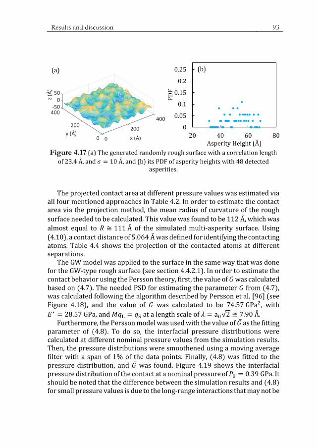
Figure ‎4.17 (a) The generated randomly rough surface with a correlation length

of 23.4 Å, and 𝜎 = 10 Å, and (b) its PDF of asperity heights with 48 detected asperities.

The projected contact area at different pressure values was estimated via all four mentioned approaches in Table ‎4.2. In order to estimate the contact area via the projection method, the mean radius of curvature of the rough

surface needed to be calculated. This value was found to be 112 Å, which was

almost equal to 𝑅 ≅ 111 Å of the simulated multi-asperity surface. Using

(‎4.10), a contact distance of 5.064 Å was defined for identifying the contacting atoms. Table ‎4.4 shows the projection of the contacted atoms at different separations.

The GW model was applied to the surface in the same way that was done for the GW-type rough surface (see section ‎4.4.2.1). In order to estimate the contact behavior using the Persson theory, first, the value of 𝐺 was calculated based on (‎4.7). The needed PSD for estimating the parameter 𝐺 from (‎4.7), was calculated following the algorithm described by Persson et al. [96] (see Figure ‎4.18), and the value of 𝐺 was calculated to be 74.57 GPa2, with

𝐸∗ = 28.57 GPa, and 𝑀𝑞L = 𝑞S at a length scale of 휆 = a0√2 ≅ 7.90 Å. Furthermore, the Persson model was used with the value of �̅� as the fitting

parameter of (‎4.8). To do so, the interfacial pressure distributions were calculated at different nominal pressure values from the simulation results. Then, the pressure distributions were smoothened using a moving average filter with a span of 1% of the data points. Finally, (‎4.8) was fitted to the pressure distribution, and �̅� was found. Figure ‎4.19 shows the interfacial pressure distribution of the contact at a nominal pressure of 𝑃0 = 0.39 GPa. It should be noted that the difference between the simulation results and (‎4.8) for small pressure values is due to the long-range interactions that may not be

0

0.05

0.1

0.15

0.2

0.25

20 40 60 80

PD

F

Asperity Height (Å)

(b) (a)


negligible in the atomistic simulations, but are absent in non-adhesive contact theories [12].

Table ‎4.4 The black dots represent the projection of the contacted atoms of the

randomly rough surface. The first row indicates the contact force in units of nN.

4.64e − 4 12.18 53.36

165.33

446.96

575.32

Figure ‎4.18 The calculated PSD of the randomly rough surface.

𝑞 Å−1

PSD

Å

4

10−2 10−1 100

100

103

10−3

10−6


Figure ‎4.19 The interfacial pressure distribution 𝑃(𝑝) at the nominal pressure of

𝑝0 = 0.39 GPa.

Figure ‎4.20 The relative projected contact area as a function of nominal pressure

for the randomly rough surface.

Figure ‎4.20 compares the contact behavior of the randomly rough surface, estimated using all approaches of Table ‎4.2. As the results show, for light squeezing pressures, the estimations of, both, the Greenwood-Williamson and Persson theories are larger than the results from the projection of the contacting atoms. Moreover, it can be noticed that if the parameter 𝐺 is found using (‎4.8), the Persson model overestimates the contact area at very small

-5

-4

-3

-2

-1

0

0 2 4 6 8 10

SimulationEq. 7

log

10

𝑃𝑝

𝑝 GPa

𝑝0 = 0.39 GPa

0

0.05

0.1

0.15

0.2

0 0.2 0.4 0.6

Nominal Pressure (GPa)

Projection methodGWPersson (Eq.7)Persson (Eq.8)

𝐴rp

c


pressures, and then tends toward the results of the projection method. The reason is that the pressure distribution contains all the interacting atoms, and not only the contacting ones, which affects the fitted values of �̅�; however, with increasing the indentation depth, the number of the contacting atoms tend toward the number of the interacting ones, as was discussed in section ‎4.4.1.5. Therefore, as the nominal pressure increases, the contribution of the contacting atoms will be larger in the pressure distribution, which will be directly reflected in the fitted values of �̅�, and consequently, the description of the Persson model would be closer to the results of the projection method.

4.4.2.2.1 Effects of the length scale on the estimation of the contact behavior

The value of 𝐺 can be defined as 𝐺 = 1 8⁄ 𝐸∗2⟨|∇ℎ|2⟩ (see section ‎4.2.3). Assuming 𝐺 �̅�⁄ = 1, with �̅� being the fitting parameter of (‎4.8), the values of

the contact modulus can be estimated via 𝐸∗ = √8�̅� ⟨|∇ℎ|2 ⟩⁄ ; therefore, the length scale that is used in the calculation of the mean square gradient of the rough surface can affect the estimated value of 𝐸∗. Figure ‎4.21 (a) shows the values of ⟨|∇ℎ|2 ⟩ calculated at different length scales, while the corresponding fitted values of 𝐸∗ at two different length scales are shown in Figure ‎4.21 (b).

Figure ‎4.21 (a) The effect of the length scale on the mean square gradient of the

rough surface. The length scale is defined as 휆 = �̅�𝛿, where 𝛿 = 3.9 Å is the lateral distance between two neighboring atoms of the rough surface. Note that �̅� ≠ 𝑀. (b) The dependence of the fitted values of 𝐸∗ to the nominal pressures using two

different length scales (on the left and right vertical axes).

0

0.2

0.4

0.6

1 2 3 4 5 6

𝛻ℎ

2

log2 �̅�

(a)

휆 = �̅�𝛿 𝛿 = 3.9 Å

0

10

20

30

0

2

4

6

8

10

0 0.2 0.4 0.6Nominal Pressure (GPa)

𝐸∗

GP

a, 𝑀

=2

1

7.4 GPa 𝐸

∗G

Pa

, 𝑀=

25

(b)

26.8 GPa


Considering the calculation method of �̅�, which is performed at the lowest length scale of the system, a reasonable length scale for the calculation of the mean square gradient would be 휆 = 2𝛿; however, this would result in low values of 𝐸∗, as is shown in Figure ‎4.21 (b).

The values of 𝐺 can be calculated at different length scales by assuming that the reduced modulus is 𝐸∗ = 28.57 GPa. It was found that 𝐺(휆 = 26𝛿) =74.28 GPa2 had the closest correspondence to 𝐺 = 74.57 GPa2, which was calculated based on the PSD of the surface with 𝑞S = 2𝜋 2𝛿⁄ . This inconsistency between the length scales could be a consequence of converting

the definition of 𝐺 from the original form of (‎4.7) into 𝐺 = 1 8⁄ 𝐸∗2⟨|∇ℎ|2⟩ using the second moment of the PSD, as described in section ‎4.2.3. Considering the results that are presented in Figure ‎4.20, calculating the theoretical value of 𝐺 in the form of (‎4.7) appears to resolve this issue.

4.4.3 Comparison between studied rough surfaces and their contacts

In order to compare the surfaces, a number of statistical data was calculated for both surfaces, and the results are summarized in Table ‎4.5. Note

that all calculations were performed at a length scale of 휆 = 2𝛿 ≅ 7.8 Å.

Table ‎4.5 The statistical calculated values for the studied rough surfaces.

𝜎 (Å) ⟨|∇ℎ|2⟩ Skewness Kurtosis

GW type 9.82 0.58 −0.64 4.05

Randomly Rough 9.67 0.65 −0.05 3.05

For light squeezing pressures, the rough surface analytical models predict

that the contact area increases linearly with the nominal pressure in the form

of 𝐴rpc = 휅 (𝑃0 (𝐸∗√⟨|∇ℎ|2⟩)⁄ ) [97]. The simulated systems showed the same

behavior as well (see Figure ‎4.22), resulting in a proportionality coefficient of ~6.2, which is larger than the corresponding value of, both, the multi-asperity

models, i.e. √2𝜋, and the Persson theory, i.e. √8 𝜋⁄ [97]. This could be a result of the lateral resolution for the calculation of the mean square gradient of the rough surfaces, as is demonstrated and discussed in section ‎4.4.2.2.1.


Figure ‎4.22 The relative projected contact area as a function of normalized

pressure for both of the simulated systems with rough surface contacts.

4.5 Summary and conclusions

In this chapter, a number of continuum models for non–adhesive contacts were investigated at the atomic scale and it was revealed that the atomistic behavior is rather different from the continuum descriptions, especially at the very first stages of the contact.

First, the Hertz contact model predictions were compared to the simulated force-displacement curves; however, large discrepancies between the two were found. Therefore, the pressure distributions were analyzed instead, in order to calculate the reduced Young’s moduli. It was found that the values of 𝐸∗ were increasing in the form of 𝐸c

∗ = 𝐶 + 𝐴𝑅𝐵−1𝑑 for shallow indentation

depths, of up to ~4 Å in the current study, before they reached a constant value. Contacts with various indenter sizes showed the same trend, except for

the contacts with the indenter radii of 15 Å and 20 Å: these two contacts were different due to their stepped-like increment in the number of interacting atoms. Moreover, it was shown that the contact distance is a function of the indenter’s radius, in the form of 𝑑c ≅ 4𝑅0.05. It should be noted that the results may be different for different systems: in other words, the results could be affected by changing the material, temperature, crystallographic orientation, applied potential energies, and indentation velocity.

Furthermore, the contact behavior of two different types of rough surfaces, a multi-asperity GW-type rough surface and a comparable random one, were

0

0.1

0.2

0 0.01 0.02 0.03

GW type

Randomly Rough

𝐴rp

c

𝑃0 𝐸∗ 𝛻ℎ 2⁄

Summary and conclusions 99

investigated. The contact behavior of both systems were found to be very close. Moreover, the results of the present study show that the relative projected contact area is a linear function of nominal pressure, even after plastic deformation is initiated locally.

The multi-asperity rough surface was studied by the GW theory, and it was found that using the elastic contact modulus of 𝐸∗ = 28.57 GPa, the theory correctly estimates the contact area of the simulated system. Furthermore, both, the GW and Persson theories were used for studying the contact behavior of the randomly rough surface. The results show that the estimation of the contact area in the Persson theory is highly dependent on the method used to calculate the parameter 𝐺: the theory would correctly describe the contact behavior if 𝐺 were calculated using its theoretical solution (‎4.7), or as

the fitting parameter of (‎4.8); however, the relation 𝐺 = 1 8⁄ 𝐸∗2⟨|∇ℎ|2⟩ results in some inconsistency of the length scale, which would be problematic, at least for studying atomistic systems.


This page is intentionally left blank.

University of Groningen Nanotribology investigations with ...

Documents

Transcript of University of Groningen Nanotribology investigations with ...