UNIVERSITY OF CALIFORNIA, IRVINE On the …web.math.ucsb.edu/~shoseto/papers/thesis.pdfCURRICULUM...
99
UNIVERSITY OF CALIFORNIA, IRVINE On the Asymptotic Expansion of the Bergman Kernel DISSERTATION submitted in partial satisfaction of the requirements for the degree of DOCTOR OF PHILOSOPHY in Mathematics by Shoo Seto Dissertation Committee: Professor Zhiqin Lu, Chair Professor Song-Ying Li Professor Jeffrey Streets 2015
Transcript of UNIVERSITY OF CALIFORNIA, IRVINE On the …web.math.ucsb.edu/~shoseto/papers/thesis.pdfCURRICULUM...

UNIVERSITY OF CALIFORNIA,IRVINE
On the Asymptotic Expansion of the Bergman Kernel
DISSERTATION
submitted in partial satisfaction of the requirementsfor the degree of
DOCTOR OF PHILOSOPHY
in Mathematics
by
Shoo Seto
Dissertation Committee:Professor Zhiqin Lu, Chair
Professor Song-Ying LiProfessor Jeffrey Streets
2015

c© 2015 Shoo Seto

DEDICATION
To all my family and friends.
ii

TABLE OF CONTENTS
Page
ACKNOWLEDGMENTS v
CURRICULUM VITAE vi
ABSTRACT OF THE DISSERTATION vii
1 Introduction 1
2 Preliminaries 42.1 Kahler Geometry . . . . . . . . . . . . . . . . . . . . . . . . . . . . . . . . . 4
2.1.1 Kahler Manifolds . . . . . . . . . . . . . . . . . . . . . . . . . . . . . 42.1.2 Calculus on vector bundles . . . . . . . . . . . . . . . . . . . . . . . . 92.1.3 Line bundles . . . . . . . . . . . . . . . . . . . . . . . . . . . . . . . . 102.1.4 Curvature . . . . . . . . . . . . . . . . . . . . . . . . . . . . . . . . . 122.1.5 First Chern Class . . . . . . . . . . . . . . . . . . . . . . . . . . . . . 142.1.6 Example: Complex Projective Space . . . . . . . . . . . . . . . . . . 15
2.2 Kodaira Embedding . . . . . . . . . . . . . . . . . . . . . . . . . . . . . . . 182.3 Polarized Kahler Manifolds . . . . . . . . . . . . . . . . . . . . . . . . . . . . 22
3 The Bergman kernel 253.1 The Bergman Kernel . . . . . . . . . . . . . . . . . . . . . . . . . . . . . . . 25
3.1.1 Bergman kernel on manifolds . . . . . . . . . . . . . . . . . . . . . . 263.1.2 Bergman kernel on the complex projective space . . . . . . . . . . . . 29
3.2 Asymptotic expansion . . . . . . . . . . . . . . . . . . . . . . . . . . . . . . 323.3 Peak Sections . . . . . . . . . . . . . . . . . . . . . . . . . . . . . . . . . . . 343.4 Reduction of the Problem . . . . . . . . . . . . . . . . . . . . . . . . . . . . 393.5 Computation up to first order . . . . . . . . . . . . . . . . . . . . . . . . . . 40
4 Near-Diagonal Expansion 434.1 Bargmann-Fock Model . . . . . . . . . . . . . . . . . . . . . . . . . . . . . . 434.2 Local Construction . . . . . . . . . . . . . . . . . . . . . . . . . . . . . . . . 47
4.2.1 Local Kernel . . . . . . . . . . . . . . . . . . . . . . . . . . . . . . . . 484.2.2 Estimates of local kernel . . . . . . . . . . . . . . . . . . . . . . . . . 50
4.3 Local to Global . . . . . . . . . . . . . . . . . . . . . . . . . . . . . . . . . . 564.4 Higher Order Convergence . . . . . . . . . . . . . . . . . . . . . . . . . . . . 59
iii

5 Off-Diagonal 645.1 Preliminary Discussion . . . . . . . . . . . . . . . . . . . . . . . . . . . . . . 65
5.1.1 Comparison between Bergman and Green kernel . . . . . . . . . . . . 655.1.2 Heat kernel for Lk section . . . . . . . . . . . . . . . . . . . . . . . . 67
5.2 Proof of Theorem 5.0.1 . . . . . . . . . . . . . . . . . . . . . . . . . . . . . . 705.2.1 Perturbation of the Green Operator . . . . . . . . . . . . . . . . . . . 705.2.2 Resolving the singularity . . . . . . . . . . . . . . . . . . . . . . . . . 715.2.3 Estimates . . . . . . . . . . . . . . . . . . . . . . . . . . . . . . . . . 73
6 Appendix 806.1 Useful Formulas . . . . . . . . . . . . . . . . . . . . . . . . . . . . . . . . . . 80
6.1.1 Bound of normalizing constant for peak section . . . . . . . . . . . . 806.1.2 Weitzenbock Formula for LN -valued (0, 1)-forms . . . . . . . . . . . . 816.1.3 ∂ estimate . . . . . . . . . . . . . . . . . . . . . . . . . . . . . . . . . 866.1.4 Hodge Theory and Kahler identities . . . . . . . . . . . . . . . . . . . 876.1.5 Volume Comparison . . . . . . . . . . . . . . . . . . . . . . . . . . . 87
Bibliography 89
iv

ACKNOWLEDGMENTS
First I would like to thank my advisor, Professor Zhiqin Lu, for his guidance, wisdom and pa-tience throughout my graduate years. His constant encouragement and perseverance carriedme through and none of this would have been possible without his support.
I would also like to thank Professors Jeff Streets and Hamid Hezari for allowing me to join inon their projects. I learnt a great deal from them and am very grateful for their friendlinessand willingness to teach me mathematics.
I am also very grateful to have been able to take many courses with Professor Song-Ying Li,who taught my core analysis classes as well as a topics course in several complex variables.I was very lucky to have been enrolled in his courses my first years at UCI.
Thanks to the UCI Mathematics Department and the geometry group for their generoussupport.
Finally, thanks to all my friends for all of your support throughout the years. I would liketo especially thank Hang Xu and Casey Kelleher, for all the math, coffee, fun and adventurethat I don’t intend on stopping with you two.
v

CURRICULUM VITAE
Shoo Seto
EDUCATION
Doctor of Philosophy in Mathematics 2015University of California, Irvine Irvine, California
Master of Science in Mathematics 2011University of California, Irvine Irvine, California
Bachelor of Arts in Mathematics 2009University of California, Berkeley Berkeley, California
RESEARCH EXPERIENCE
Graduate Research Assistant 2009–2015University of California, Irvine Irvine, California
TEACHING EXPERIENCE
Teaching Assistant 2009–2015University of California, Irvine Irvine, California
vi

ABSTRACT OF THE DISSERTATION
On the Asymptotic Expansion of the Bergman Kernel
By
Shoo Seto
Doctor of Philosophy in Mathematics
University of California, Irvine, 2015
Professor Zhiqin Lu, Chair
Let (L, h) → (M,ω) be a polarized Kahler manifold. We define the Bergman kernel for
H0(M,Lk), holomorphic sections of the high tensor powers of the line bundle L. In this
thesis, we will study the asymptotic expansion of the Bergman kernel. We will consider the
on-diagonal, near-diagonal and far off-diagonal, using L2 estimates to show the existence of
the asymptotic expansion and computation of the coefficients for the on and near-diagonal
case, and a heat kernel approach to show the exponential decay of the off-diagonal of the
Bergman kernel for noncompact manifolds assuming only a lower bound on Ricci curvature
and C2 regularity of the metric.
vii
Chapter 1
Introduction
Background and motivation
Let (L, h)→ (M,ω) be a positive Hermitian line bundle over a complex manifold M . Let Lk
be the kth tensor power of L. An active field of research in complex geometry is to analyze
the geometry of the manifold M when k → ∞. A classical result in this direction is the
celebrated Kodaira embedding theorem which states that such manifolds admitting positive
line bundles can be embedded into a projective space of sufficiently high dimension. The
main tools in this analysis are the holomorphic sections H0(M,Lk), which can be used to
construct many objects in geometry, one of them being the Bergman kernel.
The Bergman kernel, as defined classically on pseudoconvex domains Ω ⊂ Cn, is the holo-
morphic integral kernel of the projection operator from square integrable to holomorphic
square integrable functions. Its analogue on complex manifolds can be obtained by replacing
holomorphic functions and the L2 inner product of functions with an L2 inner product in-
duced from the Hermitian metric. In a local neighborhood, we can view holomorphic sections
as local holomorphic functions, an observation we use in Chapter 4.
1

An explicit formula for the Bergman kernel, except for certain cases (c.f. §3.1.2, Lemma
4.1.1), is not possible. However by the works of Zelditch [33] and independently by Catlin
[5], a complete asymptotic expansion of the Bergman kernel on the diagonal was given by
using a result by Boutet de Monvel-Sjostrand on the asymptotics of the Szego kernel. The
coefficients of the asymptotic expansion carry geometric information as demonstrated by Lu
in [19] in which he explicitly computed the first four coefficients. In particular, the second
coefficient is half the scalar curvature of the manifold. This fact was used by Donaldson [11]
demonstrating the stability of polarized manifolds with constant scalar curvature Kahler
metrics. The method employed by Lu in [19] uses certain holomorphic sections called peak
sections constructed by Tian in [31]. These are sections which in a small neighborhood can
be represented by monomials and by Hormander’s ∂-estimate, extend to a global section
with sufficient decay property.
Other methods to the analysis of the Bergman kernel include a heat kernel method by
Dai, Liu, and Ma [9], where they obtained the full off-diagonal asymptotic expansion and
Agmon-type estimates. Their results hold in a more general setting of the Bergman kernel
of the spinc Dirac operator associated to a positive line bundle on a compact symplectic
manifold. Another approach, done by Berman, Berndtsson, and Sjostrand in [3], involves
using microlocal analysis techniques inspired by the calculus of pseudodifferential operators
and Fourier integral operators with complex phase. In this thesis, we consider the diagonal
and the near-diagonal expansion, and the off-diagonal Agmon-type decay estimates.
In chapter 2, we begin by reviewing the fundamentals of Kahler geometry and introduce the
“polarized” setting that we will use. We introduce the primary object of this thesis, the
Bergman kernel in Chapter 3, and discuss the on-diagonal behavior of the Bergman kernel.
We give a computation of the coefficients up to the first order using methods of Tian [31] and
Lu [19]. In Chapter 4, we give an elementary proof of the expansion based on a joint work by
the author with Hezari, Kelleher, and Xu [14]. In Chapter 5, we prove an exponential decay
2

of the Bergman kernel on the off-diagonal using a “perturbation” of the operator approach
as seen in the works of [29].
3

Chapter 2
Preliminaries
2.1 Kahler Geometry
In this chapter, we review the basics of Kahler geometry and set up notations and conventions
which will be used. We focus on the elements of Kahler geometry which will be pertinent to
our analysis of the Bergman kernel for positive line bundles. We refer the reader to [30] for
further detail.
2.1.1 Kahler Manifolds
Let (M,J) be a complex manifold of complex dimension n, where J ∈ End(TM) is the
complex structure. A Hermitian metric on M is a Riemannian metric g such that for
v, w ∈ TM , we have g(v, w) = g(Jv, Jw). Under a holomorphic local coordinate system
(zi)ni=1, g can be written as
g := g(∂i, ∂j)dzi ⊗ dzj := gijdz
i ⊗ dzj,
4

and (gij) can be viewed as an n × n Hermitian matrix. Here and throughout, we will use
the Einstein summation convention for repeated indices. Next define the Kahler form (or
fundamental 2-form) ω by
ω(v, w) :=1
2πg(Jv, w), v, w ∈ TM,
which in local coordinates is given by
ω =
√−1
2πgijdz
i ∧ dzj.
We say a metric is Kahler if dω = 0, and call a manifold equipped with such a metric a
Kahler manifold. The condition dω = 0 in local coordinates is given by
∂kgij = ∂igkj.
An immediate consequence of the symmetries of the metric is the existence of a holomorphic
normal coordinate system.
Lemma 2.1.1 (Holomorphic normal coordinates). At each point x0 on a Kahler manifold
(M, g), there exists a holomorphic coordinate chart (U, (zi)ni=1) centered at x0 such that
gij(x0) = δij and ∂kgij(x0) = 0, for i, j, k ∈ 1, . . . , n.
Proof. Let x0 ∈M . We first choose coordinates (wi)ni=1 centered at x0 such that gij(0) = δij,
which can be found since (gij(0)) is Hermitian symmetric, and expand the metric at 0 to
obtain:
ω =√−1(δij + ∂lgij(0)wl + ∂lgij(0)wl +O(|w|2)
)dwi ∧ dwj.
5
We use the following holomorphic change of variables
Γlij := glq∂jgiq,
wl := zl − 1
2Γlij(0)zizj.
Then
dwl = dzl − Γlij(0)zidzj,
so that
ω =√−1(δij + ∂lgij(0)zl + ∂lgij(0)zl − Γjil(0)zl − Γijl(0)zl +O(|z|2)
)dzi ∧ dzj
=√−1(δij +O(|z|2)
)dzi ∧ dzj.
A crucial point is that for Riemannian metrics normal coordinates can be constructed via
the exponential map, however the coordinates may not be holomorphic, hence we require
the Kahler condition to construct such holomorphic coordinates. The strategy of the proof
of Lemma 2.1.1 can be extended further yielding the result below
Lemma 2.1.2 (K-coordinate system). With the same notation and hypotheses as Lemma
2.1.1, for any choice of pi ∈ Z+ with p =∑n
i=1 pi , there exists a holomorphic coordinate
chart (U, (zi)) centered at x0 ∈M such that
gij(x0) = δij and∂pgij
(∂z1)p1 · · · (∂zn)pn(x0) = 0, for i, j ∈ 1, . . . , n.
In other words, we can find a coordinate system where the derivative of the metric vanishes
for purely holomorphic and purely antiholomorphic directions. These coordinates play an
6

important role in the computation of the coefficients of the Bergman kernel asymptotic
expansion.
The Kahler condition also implies additional basic results in Kahler geometry, known as the
∂∂-lemmas.
Lemma 2.1.3 (Local ∂∂-lemma). Let (M,ω) be a Kahler manifold. For any x0 ∈M , there
is a neighborhood U and a real function ϕ(z, z), called the local Kahler potential, such that
ω =√−1∂∂ϕ.
It can be derived as a special case of the following global version,
Lemma 2.1.4 (Global ∂∂-lemma). Let (M,ω) be a Kahler manifold and [ω] the cohomology
class of (p, q) forms. Given ω, ω′ ∈ [ω] , there exists ϕ ∈ Hp−1,q−1 such that
ω − ω′ = ∂∂ϕ.
Proof. Since ω, ω′ ∈ [ω] there exists α ∈ Λp+q−1 such that
dα = ω − ω′
Decomposing into types α = αp,q−1 + αp−1,q we have
∂αp,q−1 = 0, ∂αp−1,q = 0.
By the Hodge decomposition,
αp−1,q = h+ ∂f
7

where h is ∂-harmonic. Furthermore, on Kahler manifolds,
∆∂h = ∆∂h = 0
so that ∂h = 0. Applying the same argument, αp,q−1 = h+ ∂f , with ∂h = 0, we have
ω − ω′ = dα
= (∂ + ∂)(h+ ∂f + h+ ∂f)
= ∂∂(f − f)
Letting ϕ = f − f , the result follows.
Definition 2.1.1 (Holomorphic Vector Bundle). Let M be a complex manifold. A holomor-
phic vector bundle of rank k over M is a complex manifold E together with a holomorphic
projection map π : E →M satisfying:
1. For any p ∈M , the fiber Ep := π−1(p) is a complex vector space of complex dimension
k.
2. There exists an open covering Ui of M and homeomorphic maps ϕi : π−1(Ui) →
Ui×Ck commuting with the projection to Ui such that for each p ∈ Ui, the restriction
of ϕi|π−1(p) → p × Ck is an isomorphism of the complex vector spaces.
3. On the overlap p ∈ Ui ∩ Uj, the induced transition maps
ϕij(x0) := ϕi ϕ−1j (x0, ·) : Ck → Ck
are holomorphic C-linear maps.
The primary object of study on vector bundles are sections, which can be thought of as
generalization of functions.
8

Definition 2.1.2 (Sections). Let E be a complex vector bundle over M . A section of E is
a map s : M → E such that (π s)(x0) = x0 for all x0 ∈M .
The key idea is that it is a map taking values in E which maps p to objects in the fiber Ep.
The space of smooth sections is denoted at Γ(M,E). In particular, if E is holomorphic, then
we denote H0(M,E) as the space of holomorphic sections. Restricting the vector bundle E
to an open set U ⊂M preserves the vector bundle structure and we can define the space of
sections on the restricted bundle, denoted as Γ(U,E) := Γ(U,E|U).
Definition 2.1.3 (Local frame). The set of sections ei, with each ei ∈ Γ(U,E), is called
a local frame if for each x0 ∈ M the collection ei(x0) forms a basis for the fiber Ex0 as a
vector space.
2.1.2 Calculus on vector bundles
We now introduce the notion of a Hermitian metric on a vector bundle E.
Definition 2.1.4. Let E be a holomorphic vector bundle. A Hermitian metric h of E is
an assignment of a Hermitian inner product h(·, ·) on each Ex0 , which varies smoothly with
respect to x0 ∈M . To be explicit, let ei be a local frame. Then
hij(x0) := h(ei, ej)|x0
where the matrix (hij(x0)) is a Hermitian n× n matrix for each x0.
Connections
Here we introduce the notion of a connection, which is a way to differentiate sections by
“connecting” them between different fibers.
9
Definition 2.1.5 (Connection). Let E → M be a complex vector bundle. A connection D
on E is a C-linear operator
D : Γ(M,E)→ Γ(M,Λ1(E))
satisfying D(fs) = df ⊗ s + fDs for f ∈ C∞(M) and s ∈ Γ(M,E). The connection above
induces a connection on the bundle Λp(E) given by
D : Γ(M,Λp(E))→ Γ(M,Λp+1(E))
by
D(v ∧ s) = dv ∧ s+ (−1)pv ∧Ds,
where v ∈ Γ(M,Λp(E)).
Let (E, h) be a holomorphic vector bundle over a Kahler manifold M . We will focus mainly
on a particular type of connection.
Definition 2.1.6. Let D be a connection satisfying the following conditions:
Dh = 0 (metric compatibility),
DJ = 0 (complex structure compatibility).
Such a connection is called a Hermitian connection.
2.1.3 Line bundles
The following are two important examples of line bundles.
10

Example 2.1.1 (Canonical line bundle). Let M be a complex manifold of dimension n.
The nth exterior power of the holomorphic cotangent bundle forms a line bundle called the
canonical bundle of M
KM := ΛnT ∗(1,0)(M) = det(T ∗(1,0)(M)).
Let Uα, (zi)α be a holomorphic atlas of M . A local holomorphic frame on Uα is given by
(dz1 ∧ . . . ∧ dzn)α and the transition function is given by
(dz1 ∧ . . . ∧ dzn)α = det
(∂ziα∂zjβ
)(dz1 ∧ · · · ∧ dzn)β on Uα ∩ Uβ 6= ∅.
If g is a Hermitian metric on M , then it induces a metrics a natural Hermitian metric on
KM is given by
h = (det g)−1
Its dual, denoted K−1M , is called the anti-canonical bundle.
Example 2.1.2 (Line bundles over CPn). On CPn (defined in 2.1.6), we can construct a line
bundle, called the tautological line bundle or O(−1), by assigning to each point the line that
the point represents and viewing it as a line subbundle of the trivial bundle CPn×Cn+1. To
be precise, let [p] := [p0 : · · · : pn]. Then at [p], attach the line in Cn+1 defined by the vector
〈p0, . . . , pn〉. Let Ui = [p] | pi 6= 0. Since
〈p0, · · · , pn〉 = pi
⟨p0
pi, . . . ,
pnpi
⟩
we can use pi as a local trivialization. Then the transition function gij must satisfy
gij =pipj.
11

Let s ∈ H0(CPn,O(−1)) be a global holomorphic section. Since O(−1) is a subbundle of
the trivial bundle, under a global non-vanishing frame, we can view s as a holomorphic map
s : CPn → Cn+1. The components of s are then holomorphic functions on a compact complex
manifold, hence they must be constant. According to the transition map, on Uα ∩Uβ =6 ∅ it
must satisfy sα = gαβsβ, hence
sαpα
=sβpβ,
which for constants is only satisfied when s = 0.
The dual of O(−1), sometimes called the hyperplane bundle, is denoted O(1) and its tensor
powers O(m) := O(1)m. The transition functions for O(m) are obtained by inversions from
the tautological bundle, i.e.
gmij =
(pjpi
)m.
The global sections of O(m) can be thought of as homogeneous polynomials in p0, . . . , pn of
degree m.
By looking at the transition functions, it can also be shown that KCPn ∼= O(−n− 1).
2.1.4 Curvature
In this subsection, we define and establish the curvature and sign conventions we will use.
Let ∇ be the Levi-Civita connection on a Kahler manifold (M,ω).
Definition 2.1.7 (Curvature Tensor). The curvature tensor R is defined as
R(v1, v2, v3, v4) = g(∇v1∇v2v3 −∇v2∇v1v3 −∇[v1,v2]v3, v4)
12

for vi ∈ TM
On Kahler manifolds, the local coordinate formula for the curvature tensor is greatly sim-
plified due to the compatibility with the complex structure. Let v, w ∈ T 1,0M . Then
∇vw ∈ T 1,0M,
∇vw = 0 = ∇vw.
For local coordinates (zi)ni=1 with coordinate holomorphic vector fields ∂ini=1, the curvature
tensor is determined completely by terms of the form
Rijkl := R(∂i, ∂j, ∂k, ∂l) = −g(∇j∇i∂k, ∂l)
= −gml∂jΓmik
= −∂i∂jgkl + gpq(∂jgpl)(∂kgiq).
Definition 2.1.8 (Ricci and scalar curvature). The Ricci curvature Ric is the trace of the
Riemann curvature tensor and the scalar curvature ρ is the trace of the Ricci curvature, i.e.
Ricij = gklRijkl, (Ricci)
ρ = gijRij. (scalar)
A useful identity for the Ricci curvature which holds for Kahler manifolds is the following
Lemma 2.1.5.
Ricij = −∂i∂j(log det g). (2.1)
13
Proof. Follows from the two identities,
∂j det g = gkl(∂jgkl) det g
∂igkl = −gplgkq(∂igpq)
2.1.5 First Chern Class
We will use the identity (2.1) to define an important cohomology class associated to a
manifold called the (first) Chern class. First define the Ricci form to be
Ric(ω) =
√−1
2πRicij dz
i ∧ dzj = −√−1
2π∂∂ log det g
Let h be another Kahler metric on M . Then dethdet g
be a globally defined function and the
difference of the Ricci forms is given by
Ric(h)− Ric(g) = −√−1∂∂ log
deth
det g
Hence [Ric(g)] ∈ H2(M,R) defines a cohomology class independent of the metric and we
define the first Chern class of M
Definition 2.1.9 (First Chern class of M).
c1(M) = [Ric(g)]
More generally, we can define the first Chern class of a Hermitian line bundle (L, h) as the
cohomology class of form of the line bundle. Let s be a local non-vanishing holomorphic
14

section of L. As in the case for Ricci curvature, the curvature form is locally defined by
F (h) = −√−1∂∂ log h(s)
where h(s) = 〈s, s〉h. Given any other Hermitian metric, it can be written as e−fh for a
globally defined function f and so
F (e−fh)− F (h) =√−1∂∂f
thus we can define the first Chern class of the line bundle L to be the cohomology class
c1(L) =1
2π[F (h)]
By the ∂∂-lemma, we have that every real (1, 1)-form in c1(L) is the curvature of some
Hermitian metric on L. With this viewpoint, we see that the first Chern class of M is the
first Chern class of the anti-canonical bundle of M ,
c1(M) = c1(K−1M ).
2.1.6 Example: Complex Projective Space
The model case of a Kahler manifold which we will consider is the complex projective space,
CPn. It is constructed from Cn+1−0/ ∼, where the equivalence relation is given by p ∼ q
if and only if for p = (p0, · · · , pn), q = (q0, · · · , qn), there is a nonzero complex number
λ ∈ C∗ such that p = λq.
A local coordinate system is given by the following. Let
Ui = [p0 : · · · : pn] ∈ CPn | pi 6= 0
15

for i = 0, · · · , n. Then the map zi given by
zi([p]) =
(p0
pi, · · · , pi
pi, · · · , pn
pi
)
where pipi
is removed, gives a local holomorphic coordinate chart. The holomorphic structure
is the one induced from Cn+1 and the transition maps are easily seen to be holomorphic.
Fubini-Study Metric
A Kahler metric that is commonly equipped to CPn is the Fubini-Study metric.
Definition 2.1.10 (Fubini-Study Metric). Let [p0 : · · · : pn] be homogeneous coordinates
on CPn. The Fubini-Study metric is defined as the 2-form
ωFS :=
√−1
2π∂∂ log(
n∑i=0
|pi|2).
On a neighborhood, say U0 = p0 6= 0, it can be written in local coordinates zi = pip0
ωFS =
√−1
2π∂∂ log(1 +
n∑i=1
|zi|2).
The metric is a homogeneous metric, that is, for any A ∈ U(n + 1) ⊂ Aut(CPn), the
holomorphic automorphism group, acts transitively and leaves the form ωFS invariant. As
such, to check that the form ωFS is indeed a metric, we need to only check that it is positive
definite at one point, say p = [1 : 0 : · · · : 0]. Directly computing, we have
ωFS(p) =
√−1
2π
(δij(1 + |z|2)− zjzi
(1 + |z|2)2
)dzi ∧ dzj|p
=
√−1
2πdzi ∧ dzi > 0
(2.2)
16

Curvature of Fubini-Study metric
As an example, we will compute the curvature terms of the Fubini-Study metric. Using
normal coordinates at the point p = [1 : 0 : · · · : 0], the curvature tensor is given by
Rijkl = −∂k∂lgij.
Using gij given in (2.2), computing while dropping the terms which will evaluate to 0,
−∂k∂l(
δij1 + |z|2
− zjzi(1 + |z|2)2
)∣∣∣∣p
= ∂k
(δijzl
(1 + |z|2)2+
zjδil(1 + |z|2)2
)∣∣∣∣p
= δijδkl + δjkδil
Hence the curvature tensor is given by
Rijkl = gijgkl + gkjgil
and tracing gives the Ricci curvature
Ricij = (n+ 1)gij
and the scalar curvature
ρ = n(n+ 1)
The Fubini-Study metric on CPn is in fact a Kahler-Einstein metric with positive first Chern
class.
17

2.2 Kodaira Embedding
Definition 2.2.1 (Ample line bundle). A line bundle L over M is very ample, if for suitable
sections s0, . . . , sN of L, the Kodaira map
ϕ : M → CPN
p 7→ [s0(p) : . . . : sN(p)]
(2.3)
defines an embedding of M into CPN . A line bundle L is ample if Lk is very ample for
sufficiently large k ∈ Z+.
Theorem 2.2.1 (Kodaira Embedding Theorem). Let L be a line bundle over a compact
complex manifold M. Then L is ample if and only if c1(L) > 0, i.e. L is positive.
Proof for ample implies positive. By the embedding, Lk can be identified with the restriction
of the O(1) bundle of some complex projective space. In particular, Lk is positive. Let h
be the positively curved Hermitian metric of Lk. Then L1k is a positively curved Hermitian
metric on L.
In proving positive implies ample, we first make the following lemma
Lemma 2.2.1. Let L be a positive holomorphic line bundle. If for every x, y ∈ M with
x 6= y and every v ∈ Cn, there exists elements S, T ∈ H0(M,LN) such that S(y) 6= 0,
S(x) = 0, T (x) = 0, and dT (x) = v, then L is ample.
Proof. Let s0, . . . , sN be a basis for H0(M,Lk). Since at each point y ∈ M , we can find a
non-vanishing section s(y) 6= 0, we see that the at least one of si(y) 6= 0, hence the Kodaira
map ϕ (2.6) defined by the basis is well defined. Suppose ϕ(x) = ϕ(y). Then there exists
18

nonzero complex number λ ∈ C∗ such that
(s0(y), · · · , sN(y)) = λ(s0(x), . . . , sN(x))
but this would contradict the existence of a section such that S(x) = 0 and S(y) 6= 0, hence
ϕ is injective. It remains to prove that dϕ is injective, hence we want to show it has maximal
rank. For any x ∈ M , let T1, . . . , Tn be sections of Lk such that Tj(x) = 0 for 1 ≤ j ≤ n.
Let eNL be a local frame at x . Then each Tj has a local representative Tj = tjeNL , where
tj ∈ H0(U). Also let T0 = eNL . By assumption, we can assign for each j, dtj = vj, where
vj is the standard basis vector on Cn. Then define the immersion
x 7→ [T0 : T1 : · · · : Tn : 0 : · · · : 0].
Since the Ti = aijSj, we have the rank of ϕ must be n as well.
Theorem 2.2.2 (L2 estimate construction). Let p1, · · · , ps ∈ M and K1, · · · , Ks ∈ Z+.
Then for k sufficiently large, there is a holomorphic section S ∈ H0(M,Lk) such that at each
pi, S has the prescribed derivatives up to order Ki.
Proof. Let Ui be a coordinate neighborhood of pi, with coordinates (z1, . . . , zn). By pre-
scribed derivatives, we mean to assign the values for a holomorphic function fi at pi,
∂Kifi
∂zk11 · · · ∂zknn
(pi)
Let ηi be a smooth cut-off function whose supports are within Ui and is 1 in a neighborhood
of pi. We then define a global smooth section of Lm by
w =∑i
ηifi.
19

Since we need a global holomorphic section, we consider the ∂ equation
∂f = ∂w
If the solution f exists, then w − f will be holomorphic. To ensure that we have a section
with the required conditions for the derivatives, that is, the vanishing order be at least Ki+1
at each pi.
Consider the Laplace equation
(∂∂∗
+ ∂∗∂)u = ∆∂g = ∂w (2.4)
Taking ∂ on both sides, we have ∂∂∗∂u = 0. Then
0 = (∂u, ∂∂∗∂u) = ‖∂∗∂u‖2
So that ∂∗∂u = 0. Letting ∂
∗u = f , we have
∂f = ∂w.
To solve (2.4), we first use the Weitzenbock formula to get a lower bound estimate for the
first eigenvalue. Let e−ηhk be a Hermitian metric on Lk. For any Lk-valued (0, 1)-form,
aαdzα,
∆∂(aαdzα) = −∇β∇β(aαdz
α) + (Ric)αγaαdzγ +mRic(h)αγaαγdz
γ + (∂α∂γη)aαdzγ
20

Let ψ be an eigensection corresponding to the lowest eigenvalue, λ1. Then
λ1
∫M
‖ψ‖2e−ηdVg =
∫M
〈∆∂(ψ), ψ〉e−ηdVg
≤∫M
‖∇ψ‖2e−ηdVg + (kC1 − C2)
∫M
‖ψ‖2e−ηdVg
for some C1, C2 > 0. Hence λ1 ≥ kC1 − C2. By the first eigenvalue estimate ∆∂u ≥ λ1u,
hence
‖∂w‖2L2,η = ‖∆∂u‖2
L2,η ≥ λ21‖u‖2
L2,η ≥ (kC1 − C2)‖u‖2L2,η
Thus we have
∫M
‖f‖2e−ηdVg =
∫M
‖∂∗u‖2e−ηdVg =
∫M
〈u, ∂∂∗u〉e−ηdVg
≤ ‖u‖L2,η‖∂w‖L2,η ≤‖∂w‖2
L2,η
kC1 − C2
By shrinking the neighborhoods if necessary, we assume that the Ui are all disjoint. Then in
a small neighborhood of pi,
∂(w) =∑i
(∂ηi)fi + ηi(∂fi) = 0.
Hence ‖∂w‖2L2,η < ∞. Now we choose an appropriate cut-off function η for the vanishing
order of f . Consider η to be the function such that at each point near pi,
η(x) = λ log(ri)
where ri is the distance d(x, pi). The value of λ will control the vanishing order of the section.
21

For the integral on the neighborhood Ui, we have
∫Ui
|fi|2e−η =
∫Ui
|fi|2
rλ∼∫ 1
0
|fi|2r2n−1−λ <∞
Since∫ 1
01rp<∞ when p < 1. Let |fi|2 ∼ r2q. Then we require λ− 2q − 2n < 1, so choosing
λ sufficiently large, we can push the vanishing order of fi to be large.
2.3 Polarized Kahler Manifolds
Let L → M be a Hermitian line bundle over M with Hermitian metric h. We say that the
line bundle L is positive if the curvature Ric(h) is positive definite. We define a Kahler form
ωg by the curvature form of L, i.e. for a fixed point p ∈M with local coordinates (zi)ni=1 at
p,
ωg = −√−1
2π
∂2
∂zi∂zjlog hdzi ∧ dzj =
√−1
2πgijdz
i ∧ dzj,
where h is the local representation of the Hermitian metric h. We refer to this setting as
polarized Kahler manifold with polarization L. For each k ∈ Z+, the Hermitian metric
h induces a Hermitian metric hk on Lk := L⊗ · · · ⊗ L︸ ︷︷ ︸k times
. The Hermitian metric hk further
induces an L2 inner product on H0(M,Lk), the space of holomorphic global sections of Lm
as follows: Choose an orthonormal basis Skα of H0(M,Lk). Then define the inner product
〈Skα, Skβ〉L2 :=
∫M
(Skα, Skβ)hk
ωn
n!(2.5)
22

We use the following notations
L2(M,Lk) = f ∈ Γ(M,Lk) | ‖f‖L2 :=
∫M
|f |2hkdVg <∞
H0(M,Lk) = f ∈ L2 | f holomorphic section of Lk
By the Kodaira embedding theorem, for sufficiently high tensor power k, the basis Skα
induces a holomorphic embedding of M into CPN , N + 1 = dimH0(M,Lk) given by the
mapping
ϕk :M → CPN
x 7→ [Sk0 (x) : . . . : SkN(x)]
(2.6)
Let gFS be the standard Fubini-Study metric on CPN , i.e., for homogeneous coordinate
system [Z0 : · · · : ZN ] of CPN ,
ωFS =
√−1
2π∂∂ log
(N∑i=0
|Zi|2)
Definition 2.3.1 (Bergman metric). The 1k-multiple of gFS on CPN restricts to a polarized
Kahler metric 1kϕ∗kgFS on M , where ϕk is the Kodaira map defined above. The metric is
called the Bergman metric with respect to L.
The Bergman metric and polarized metrics are related by the following
Theorem 2.3.1 (Tian). With notation as above,
∥∥∥∥1
kϕ∗kgFS − g
∥∥∥∥C∞
= O
(1
k2
)
Tian [31] originally proved the C2 convergence with remainder O(
1√k
)and was improved
23

to C∞ and O(
1k
)by Ruan [26]. Zelditch [33] and Catlin [5] independently generalized the
above theorem by giving the asymptotic expansion of the Bergman kernel using the Szego
kernel on the unit circle bundle of L∗ over M .
24

Chapter 3
The Bergman kernel
In this chapter, we will introduce the Bergman kernel and and its expansion on the diago-
nal. The first section will define the Bergman kernel, the second section will introduce the
asymptotic expansion and in the third we will give an analysis of it via Tian’s peak sections
[31].
3.1 The Bergman Kernel
In this section, we introduce the primary object of our study, the Bergman kernel. We will
be concerned with the Bergman kernel on manifolds, which is analogous to the classical
Bergman kernel defined on pseudoconvex domains Ω ⊂ Cn. Some literature on the classical
theory can be found in [1], [15].
25

3.1.1 Bergman kernel on manifolds
Let (M,ω) be a compact polarized Kahler manifold with a positive line bundle (L, h) such
that Ric(h) = ω. Let hα be the local representation of the Hermitian metric with respect to
a local frame eL on some neighborhood Uα, that is, hα = h(eL, eL).
By the Hodge theorem, this space is finite-dimensional and a normal family argument shows
that the space is a closed subspace of L2(M,Lm). We then consider the orthogonal projection
Pm : L2(M,Lm)→ H0(M,Lm).
Definition 3.1.1 (Bergman kernel). The holomorphic integral kernel Bk of the projection
is called the Bergman kernel, i.e., for f ∈ L2(M,Lk),
Pk(f)(x) = 〈f(y), Bk(y, x)〉L2
If we choose an orthonormal basis Skα of H0(M,Lk), then the Bergman kernel is given by
Bk(x, y) =∑α
Skα(x)⊗ Skα(y)
Definition 3.1.2. Let Bk(x, x) ∈ Γ(Lk ⊗ Lk) be the Bergman kernel restricted to the
diagonal. The Bergman function, sometimes called density function, B(x) is given by the
point-wise norm, i.e.
B(x) := ‖Bm(x, x)‖hm = |Bm(x, x)|e−kϕ(x),
where B(x, x) is the coefficient function of the Bergman kernel with respect to the frame
ekL ⊗ ekL.
We have an extremal characterization of the Bergman kernel which we will be useful.
26
Lemma 3.1.1. Let B(x) be the Bergman function. Then
B(x) = sup‖s‖L2=1
‖s(x)‖2hk
Proof. We have
B(x) =N∑i=0
‖Si(x)‖2hk ≥ ‖S(x)‖2
hk
for any ‖S(x)‖2L2 = 1, since we can choose an orthonormal basis Sα with S0 = S. For
the converse inequality, let x ∈M and consider the subset Zx ⊂ H0(M,Lk) of sections that
vanish at x. Since B(x) > 0, we know there exists a nonvanishing section S0(x) 6= 0. Then
for any S ∈ H0(M,Lk), consider the decomposition
S(x) = S(x)− λS0(x) + λS0(x)
where λ is chosen so that S(x)− λS0(x) = 0. We see that Zx has codimension one. Let S0
be in the orthogonal complement of Zx and ‖S0‖L2 = 1 and extend to an orthonormal basis
on H0(M,Lk). Then each section orthogonal to S0 vanishes at x so
B(x) = ‖S0(x)‖2hk
which gives us the result.
We first give a rough upper bound of the Bergman kernel.
Lemma 3.1.2 (Uniform upper bound on Bergman function). Let B(x) be the Bergman
function for the Bergman kernel of H0(M,Lk). Then there exists C dependent on M , and
independent of k and x such that
B(x) ≤ Ckn.
27

Proof. We use the extremal characterization of the Bergman function (4.9). On the compact
Kahler manifold M , we fix a finite coordinate cover Uα and also fix a coordinate (zi)ni=1 in
Uα. For each Uα, we have a local Kahler potential ϕ(z). We can assume that U = B(0, 2),
and supz∈B(0,2) |D2ϕ(z)| ≤ C, i.e. the second derivatives are uniformly bounded. Since ϕ
is plurisubharmonic, we can assume the volume form dVg = (√−1
2π∂∂ϕ)n(z) is equivalent to
dVE(z) in B(0, 2).
1 ≥∫B(z0,
1√k
)
|s(z)|2e−kϕ(z)dVg
≥ 1
C1
∫B(z0,
1√k
)
|s(z)|2e−kϕ(z)dVE
≥ 1
C1
e− supB(0,2) |D2ϕ|∫B(z0,
1√k
)
|s(z)|2e−kϕ(z0)−kϕz(z0)(z−z0)−kϕz(z0)(z−z0)dVE
=1
C2
e−kϕ(z0)
∫B(z0,
1√k
)
|s(z)e−kϕz(z0)(z−z0)|2dVE.
Since s(z)e−kϕz(z0)(z−z0) is holomorphic, by the mean-value inequality we have
1
C2
e−kϕ(z0)
∫B(z0,
1√k
)
|s(z)e−kϕz(z0)(z−z0)|2dVE
≥ 1
C3kne−kϕ(z0)|s(z0)|2.
So we have
e−kϕ(z0)|s(z0)|2 ≤ C3kn,
where C3 is uniform for any z0 ∈ B(0, 1) and any s ∈ H0(M,Lk). Taking the supremum
over all such s and a standard finite cover argument yields the desired result.
28

3.1.2 Bergman kernel on the complex projective space
As a concrete example, we will compute the Bergman kernel on the polarized manifold
(CPn,O(1)).
Consider the open set U0 = Z0 6= 0 of CPn. The homogeneous coordinates [1 : z1 : · · · : zn]
give local coordinates (z1, · · · , zn) for U0. Since CPN is a symmetric space, we only need to
consider the Bergman kernel at one point, say [1 : 0 : . . . : 0]. By considering the hyperplane
line bundle O(1) with Hermitian metric h = 11+|z|2 , we consider CPn with the Fubini-Study
metric, which on U0 is represented by
ω =
√−1
2π∂∂ log(1 + |z|2).
The tensor powers of the hyperplane line bundle is denoted O(k) = O(1)k and sections of
the O(k) bundle correspond to k-th degree homogeneous polynomials.
To compute the Bergman kernel, we need to find an orthonormal basis for H0(CPn,O(m)).
Let ρ := 1 + |z|2 and dV0 :=∏n
i=1 dzi ∧ dzi, where the product is the wedge product. We
compute the volume form of the Fubini-Study metric
ωng =
(√−1
2π
)n(∑dzi ∧ dzi
ρ− ∂ρ ∧ ∂ρ
ρ2
)n=n!dV0
ρn− n!|z|2dV0
ρn+1
=
(√−1
2π
)nn!dV0
ρn+1
where we use the fact that (∂ρ ∧ ∂ρ)k = 0 for k > 1.
Next the Hermitian metric hk on U0 can be expressed locally as(
1ρ
)k. Let eL be a frame
on Hk, write zP = zp0
0 · · · zpnn ⊗ eL, P = (p0, p1, . . . pn) ∈ Zn+1 such that |P | =∑pi = k, we
have
29

(zP , zQ) =
∫CPn
zP zQ
(∑|zi|2)k+n+1
dV0
=
∫U0
zp1
1 zq11 · · · zpnn zqnnρk+n+1
dV0
where dV0 =
(√−1
2π
)ndz1 ∧ dz1 · · · dzn ∧ dzn.
By using polar coordinates, we can see that the set zP is orthogonal under the L2 norm.
Hence we compute the norm of each monomial and normalize to form an orthonormal set.
Proposition 3.1.1.
∫Cn
|z1|2p1 · · · |zn|2pn(1 + |z1|2 + . . .+ |zn|2)k+n+1
dV0 =p0!p1! · · · pn!
(n+ k)!
Proof. Changing to polar coordinates, zi = rie√−1θi , we obtain
∫Cn
|z1|2p1 · · · |zn|2pn(1 + |z1|2 + . . .+ |zn|2)k+n+1
dV0 =
∫ ∞0
. . .
∫ ∞0
r2p1+11 · · · r2pn+1
n
(1 + r21 + · · ·+ r2
n)(k+n+1)dr·(∫ 2π
0
dθi
)n
For convenience, we change variables si = r2i to get
1
2n
∫ ∞0
. . .
∫ ∞0
sp1
1 · · · spnn(1 + s1 + . . .+ sn)(k+n+1)
dV (s)
Now consider the integral
∫ ∞0
. . .
∫ ∞0
ds1 . . . dsn(1 + t1s1 + . . .+ tnsn)(n+p0+1)
=p0!
(n+ p0)!t1 · · · tn
30

Then inductively we see that
∂pi
(∂ti)pi
(p0!
(n+ p0)!t1 · · · tn
)=
(−1)pip0!pi!
(n+ p0)!t1 · · · tpi+1i · · · tn
On the other hand, we have
∂pi
(∂ti)pi
(∫ ∞0
. . .
∫ ∞0
ds1 . . . dsn(1 + t1s1 + . . .+ tnsn)(n+p0+1)
)=
∫Rn+
(−1)pi(n+ p0 + 1)(n+ p0 + 2) · · · (n+ p0 + pi)spii
(1 + t1s1 + . . .+ tnsn)(n+p0+pi+1)dV (s)
So
∫Rn+
(−1)k−p0(n+ p0 + 1)(n+ p0 + 2) · · · (n+ k)sp1
1 · · · spnn(1 + s1 + . . . sn)(n+k+1)
dV (s)
=
(∂
∂t1
)p1
. . .
(∂
∂tn
)pn ∫ ∞0
. . .
∫ ∞0
ds1 . . . dsn(1 + t1s1 + . . .+ tnsn)(n+p0+1)
∣∣∣∣(ti=0)
=(−1)(k−p0)(p0)!(p1)! · · · (pn)!
(n+ p0)!
and the result follows.
Using the above, we see that the set
SP =
√(k + n)!
p0! · · · pn!zP eL, zP = zp0
0 · · · zpnn , P = (p0, . . . , pn), |P | = p0 + · · ·+ pn = k
forms an orthonormal basis for H0(CPn,O(k)). The Bergman kernel is then given by
Bk(x, y) =∑|P |=k
SP (x)⊗ SP (y) =∑|P |=k
(k + n)!
P !xPyP eL ⊗ eL
31

Computing the Bergman function, we have
B(x) =∑|P |=k
(k + n)!
P !|xP |2
Which at the origin is (k+n)!k!
. Expanding out the terms in term of the power of k, we have
(k + n)!
k!= kn
(1 +
1
2kn(n+ 1) +O(
1
k2)
)
where we see that the second coefficient is indeed 1/2 of the scalar curvature of CPn.
3.2 Asymptotic expansion
In this section, we discuss the asymptotic expansion of the Bergman kernel. We begin with
the following theorem
Theorem 3.2.1 (Zelditch [33], Catlin [5]). There is a complete asymptotic expansion:
N∑α=0
‖Skα(x)‖2hk = kn
(a0(x) +
a1(x)
k+a2(x)
k2+ · · ·
)
for smooth coefficients aj(x) with a0 = 1. More precisely, for any m
∥∥∥∥∥N∑α=0
‖Skα(x)‖2hm −
∑j<R
aj(x)mn−j
∥∥∥∥∥Cm
≤ CR,mkn−R
where CR,m depends on R,m and the manifold M .
The algorithm to compute the coefficients were given by Lu [19], who also determined the
coefficients to be polynomials in the metric and covariant derivatives of the curvature, and
computed the first 4 coefficients, and extended his computation with Shiffman to the near-
32

diagonal terms. For the near diagonal expansion, it is given in powers of 1√k.
As a corollary of the asymptotic expansion, we give a quick proof of Tian’s theorem, Theorem
2.3.1.
Proof of Theorem 2.3.1. Let Si be an orthonormal basis of H0(M,Lk) and let ϕ : M →
CPN be the associated Kodaira map, see (2.6). Consider homogeneous coordinates [Z0 : · · · :
ZN ] and open set U0 = Z0 6= 0. Then the pullback of the Fubini Study metric by ϕ is
given in local coordinates by
ϕ∗ωFS = ϕ∗√−1
2π∂∂ log
(1 +
n∑i=1
|zi|2)
=
√−1
2π∂∂ log
(|S0|2
|S0|2+|S1|2
|S0|2+ · · ·+ |SN |
2
|S0|2
)= −√−1
2π∂∂ log(|S0|2hk) +
√−1
2π∂∂ logBk
= kω +
√−1
2π∂∂ logBk
where the last line is due to the fact that we are considering a polarized manifold. Using the
asymptotic expansion, we have
√−1
2π∂∂ logBk =
√−1
2π∂∂ log
(kn(
1 +ρ
k+O
(1
k2
)))= O
(1
k
)
Combining with the above, we have
1
kϕ∗ωFS − ω = O
(1
k2
)in C∞
Another immediate corollary that can be obtained is an approximation of the dimension of
space H0(M,Lk) for high tensor powers. More precisely,
33

Corollary 3.2.1. As k →∞, we have
dimH0(M,Lk) = kn∫M
ωn
n!+kn−1
2
∫M
ρωn
n!+O(kn−2)
Proof.
dimH0(M,Lk) =N∑i=0
∫M
|Si|2hk
=
∫M
Bkωn
n!
= kn∫M
(1 +
ρ
2k+O
(1
k2
))ωn
n!
3.3 Peak Sections
We now introduce Tian’s peak section method [31] to compute the coefficients of the asymp-
totic expansion. The peak sections were originally introduced by Tian to prove the following
theorem approximating polarized metrics by a sequence of Bergman metrics:
Let x0 ∈M . Choose local normal coordinates (zi)ni=1 centered at x0 such that the Hermitian
matrix (gij) satisfies
gij(x0) = δij
∂p1+···+pngij(x0)
∂zp1
1 · · · ∂zpnn
= 0
for i, j = 1, . . . , n and any nonnegative integers p1, . . . , pn with p1 + · · ·+pn 6= 0. Next choose
a local holomorphic frame eL of L at x0 such that the local representation function h of the
34

Hermitian metric h has the properties
h(x0) = 1,∂p1+···+pnh
∂zp1
1 · · · ∂zpnn
(x0) = 0
for any nonnegative integers (p1, . . . , pn) with p1 + · · ·+ pn 6= 0.
Lemma 3.3.1 (Peak Sections). Let ck be a sequence such that
limk→∞
cklog(k)α
= 1, α > 1
Suppose Ric(g) ≥ −Kωg, where K > 0 is a constant. For P ∈ Zn+ and an integer p′ > |P |.
Then there is a k > 0 and a holomorphic section SP,k ∈ H0(M,Lk), satisfying
∣∣∣∣∫M
‖SP,k‖2hkdVg − 1
∣∣∣∣ ≤ Ce−18ck (3.1)
Moreover, SP,k can be decomposed as
SP,k = SP,k − uP,k
such that
SP,k(x) = λPη
(k|z|2
ck
)zP ekL =
λP z
P ekL x ∈ |z| ≤√
ck2k
0 x ∈M \ |z| ≤√
ckk
and ∫M
||uP,k||2hkdVg ≤ Ce−18ck
35

where η is a smoothly cut-off function
η(t) =
1 for 0 ≤ t ≤ 1
2
0 for t ≥ 1
satisfying −4 ≥ η′(t) ≥ 0 and |η′′(t)| ≤ 8 and
λ−2P =
∫|z|≤√
ckk
|zP |2akdVg
Proof. Define the weight function
Ψ(z) = (n+ 2p)η
(k|z|2
ck
)log
(k|z|2
ck
)
Where η : R→ R is a smooth cut-off function such that
η(t) =
1 for t < 1
2
0 for t ≥ 1
satisfying −4 ≥ η′(t) ≥ 0 and |η′′(t)| ≤ 8 and |z|2 = |z1|2 + . . . + |zn|2. Directly computing
we have
√−1∂∂Ψ =
√−1(n+ 2p)
[η′′(k|z|2
ck
)k2
c2k
∂|z|2 ∧ ∂|z|2
+η′(k|z|2
ck
)k
ck∂∂|z|2
]log
(k|z|2
ck
)+2 Re
[η′(k|z|2
ck
)k
ck∂|z|2 ∧ ∂ log |z|2
]+ η
(k|z|2
ck
)∂∂ log |z|2
To obtain a lower bound, we first note that√−1∂∂ log(|z|2) is positive definite, hence can be
dropped. According to the support of the cut-off function η and its derivatives, we restrict
36

our attention to the interval ck2k≤ |z|2 ≤ ck
k. In that interval, log
(k|z|2ck
)≤ 0, hence
η′(k|z|2
ck
)log
(k|z|2
ck
)√−1∂∂|z|2 ≥ 0,
thus can be dropped. Continuing the computation, we have
√−1∂∂Ψ(z) ≥ −8k(n+ 2p)
ck
√−1
(k
ck∂|z|2 ∧ ∂|z|2 + ∂|z|2 ∧ ∂ log |z|2
)≥ −24k2(n+ 2p)
c2k
√−1∂|z|2 ∧ ∂|z|2
≥ −24k(n+ 2p)
ck
√−1dzi ∧ dzj
= −48πk(n+ 2p)
ckωg.
Using the above, we have for any unit vector v ∈ T 1,0M and any point p ∈M ,
⟨∂∂Ψ +
2π√−1
(Ric(hk) + Ric(g)
), v ∧ v
⟩≥ k
4‖v‖2
g
For k sufficiently large.
Define the following 1-form
wP =1
4∂(η
(k|z|2
ck
))zp1
1 · · · zpnn ekL
which will serve as the main portion of the peak section. By solving the equation ∂uP = wP ,
we obtain an Lk-valued section uP such that
∫M
‖uP‖2hke−ΨdVg ≤
4
k
∫M
‖wP‖2hke−Ψ
37

Computing out the right hand side to get a more explicit form of the bound, we have
4
k
∫M
||wP ||2hke−ΨdVg =
4
k
∫M
||∂η(k|z|2
ck
)zP ekL||2hke
−ΨdVg
≤ 4
k
∫M
||η′(k|z|2
ck
)kzickzPdziekL||2e−ΨdVg
≤ 16k
c2k
∫ck2k≤|z|2≤ ck
k
|z|2p+2hke−ΨdVg
≤ Ccp−1k
kp
∫ck2k≤|z|2≤ ck
k
hkdV0.
For k large, we expand hk in K-coordinates
hk = e−kϕ = e−k(|z|2+O(|z|4))
so that
∫M
‖uP‖2hke−ΨdVg ≤ C
cp−1+nk
kp+ne−
ck2 .
Since ck ∼ (log k)α, with α > 1, for sufficiently large k, we can obtain the order O(
1kp
)for
any desired p.
Using these peak sections, Tian proved a convergence theorem for Bergman metrics. In
computing the coefficient of the Bergman kernel, we require an orthonormal basis. However,
if we only want to compute up to a certain order, we only require that the sections be “almost
orthogonal”. In that direction, we have a lemma by Tian [31] and generalized by Ruan [26]
Lemma 3.3.2. Let x0 ∈M be fixed. Let SP be a peak section and T ∈ H0(M,Lk). Locally,
T = fekL for a holomorphic function f .
38

1. If zP is not in the Taylor expansion of f at x0, then
(SP , T )hk = O
(1
k
)‖T‖L2 .
2. If f contains no terms zQ such that q < p+ σ in its Taylor expansion at p, then
(SP , T )hk = O
(1
k1+σ/2
)‖T‖L2 .
3.4 Reduction of the Problem
The following reduction used to compute the asymptotic expansion has been given in [19],
and is included here for completeness.
Let S0, . . . , Sd be a basis for H0(M,Lk) such that at x0 ∈M ,
S0(x0) 6= 0
Si(x0) = 0 for i = 1, . . . d
(3.2)
Let S = (S0, . . . , Sd) and define the Gram matrix F = S†S, where the entries are
Fij = 〈Si, Sj〉L2 (3.3)
It is positive definite, since xFx† = ‖Sx†‖2, hence admits a decomposition
F = GG† (3.4)
39

Let H = G−1. Then the entries of SH, i.e.
d∑j=0
HijSj, i = 0, . . . , d (3.5)
form an orthonormal basis of H0(M,Lk). Using this orthonormal basis, the Bergman kernel
at x0 can be reduced to
∑i
‖∑j
HijSj(x0)‖2hk =
∑i
|Hi0|2‖S0(x0)‖2hk (3.6)
Furthermore, if I = F−1, then the (0, 0)th entry is given by
I00 =∑i
|Hi0|2. (3.7)
Hence to compute the asymptotic expansion, we only need to estimate I00 and ‖S0(x0)‖2hk
to the desired order.
3.5 Computation up to first order
With the above considerations, we will compute the diagonal asymptotic expansion up to
first order. It was shown in [19] that I00 = 1+O(
1k3
)hence to compute up to the first order,
we only need to compute λ20. We will need the following integral identity:
Lemma 3.5.1 (Lemma 4.1 [19]). Let A be a symmetric function on 1, . . . , np×1, . . . , np.
Then for any p′ > 0,
∑I,J
∫|z|≤ log k√
k
AI,Jzi1 · · · zipzj1 · · · zjp|z|2qe−k|z|2
dV0
=
(∑I
AI,I
)p!(n+ p+ q − 1)!
(p+ n− 1)!mn+p+q+O
(1
mp′
),
40

where I = (i1, . . . , ip), J = (j1, . . . , jp) and 1 ≤ i1, . . . , ip, j1, . . . , jp ≤ n.
Under normal coordinates and frame,
‖S0‖2hk(x0) = λ2 =
∫|z|2≤ ck
k
hkdVg
=
∫|z|2≤ ck
k
e−kϕ det(g)dV0
=
∫|z|2≤ ck
k
e−kϕelog det(g)dV0
Taking the Taylor expansions with normal coordinates gives
ϕ(z) = |z|2 −Rmijkl
4zizkzjzl +O(|z|5)
and
log det g = −Ricij zizj +O(|z|3).
Therefore
e−kϕ(z) = e−k|z|2
ek4
Rmijkl zizkzjzl = e−k|z|
2
(1 +k
4Rmijkl z
izkzjzl) +O(|z|5)),
and
elog det g = 1− Ricij zizj +O(|z|3).
41

Applying Lemma 3.5.1 and computing up to 1k
order,
∫|z|≤ log k√
k
(1− Ricij zizl +
k
4Rmijkl z
izkzjzl)e−k|z|2
=1
kn(1− ρ
2k) +O
(1
kn+2
).
Inverting the above we have that
λ20 = kn
(1 +
ρ
2k+O
(1
k2
)).
42

Chapter 4
Near-Diagonal Expansion
In this chapter, we provide a proof of the near-diagonal expansion of the Bergman kernel
via a perturbation method given in [14]. We use the observation that the Bergman kernel is
concentrated in the near-diagonal. The first section will review the calculus of the Bargmann-
Fock space. In the second section, we begin by establishing the local setting. There we
will construct our candidate local kernel. The third section will show that the difference
between the candidate kernel with the asymptotic expansion and the global kernel differ by
an decaying term. In the last section, we show the smooth convergence of the asymptotic
expansion.
4.1 Bargmann-Fock Model
The Bargmann-Fock space is the space of entire functions that satisfy the weighted square
integrability condition:
∫Cn|f(z)|2e−|z|2dV <∞.
43

The space F is precisely H0(Cn, |z|2), and is thus a closed linear subspace of the space
L2(Cn, |z|2) with inner product given by
〈f, g〉F :=
∫Cnf(z)g(z)e−|z|
2
dV,
and thus is a Hilbert space. In fact, it is a reproducing kernel Hilbert space on Cn, with
reproducing kernel
RCn(u, v) := eu·v.
We first show that this kernel has the reproducing property on C and then extend this
argument to Cn.
Lemma 4.1.1. On C, the Bargmann-Fock kernel is given by
RC(u, v) := euv.
Proof. Taking some f ∈ H0(C), we consider the inner product against RC. We convert the
resulting integral to polar coordinates and then apply the Cauchy Integral Formula to obtain
〈f(v),RC〉F =√−1
∫Cf(v)euv−|v|
2 dv ∧ dv2π
= − 1
π
∫ ∞0
∫ 2π
0
f(u+ reiθ)eu(u+re−iθ)−|u+reiθ|2 r
2dθdr
= − 1
π
∫ ∞0
re−r2
∫ 2π
0
f(u+ reiθ)e−ureiθ
dθdr
= −f(u)
∫ ∞0
2re−r2
dr
= f(u).
The result follows.
44

Corollary 4.1.1. On Cn, the Bargmann-Fock kernel is given by
RCn(u, v) := eu·v.
Proof. Let u, v ∈ Zn+ with u = (u1, . . . , un) and v = (v1, . . . , vn). Observe that
eu·v =n∏i=1
euivi−|vi|2
.
To demonstrate the reproducing property, we consider f ∈ H0(Cn) and decompose the
integrand of the resulting inner product againsRCn . Applying Lemma ?? to each dimensional
component, we have
〈f(v),RCn〉F =
∫Cnf(v)eu·v−|v|
2
dV
=
∫Cnf(v1, . . . , vn)
(n∏i=i
euivi−|vi|2
)dV
= f(u).
The result follows.
The following lemmas demonstrate the Bargmann-Fock projection of monomials of different
variables.
Lemma 4.1.2. Given some multiindex m ∈ Zn+ the following equality holds.
∫Cnvmeu·v−|v|
2
dV = 0.
45

Proof. By manipulation and an application of Dominated Convergence Theorem,
∫Cnvmeu·v−|v|
2
dV =
∫Cn∂(m)u
[eu·v−|v|
2]dV
= ∂(m)u
[∫Cneu·v−|v|
2
dV
]= 0.
Note that the integral is constant with respect to u, hence the derivative vanishes. The result
follows.
Lemma 4.1.3. The following equality holds, for p, q ∈ Z+ with p ≤ q.
∫Cnvpvqeu·v−|v|
2
dV =
0 if p > q,
q!(q−p)!u
q−p if p ≤ q.
Proof. Again by manipulation and an application of Dominated Convergence Theorem,
∫Cnvpvqeu.v−|v|
2
dV =
∫Cn∂(p)u
[vqeu·v−|v|
2]dV
= ∂(p)u
[∫Cnvqeu·v−|v|
2
dV
]= ∂(p)
u [uq] ,
therefore
∫Cnvpvqeu·v−|v|
2
dV =
0 if p > q,
q!(q−p)!u
q−p if p ≤ q.
Result follows.
46

4.2 Local Construction
The idea is to first construct a local kernel, then use Hormander’s L2-estimates to compare
the local “candidate” Bergman kernel, which by construction will be in the form of an
asymptotic expansion, with the global Bergman kernel. To make precise what we mean by
local construction, we define what we mean by local reproducing property (modulo k−N+1
2 ).
Definition 4.2.1 (Local Reproducing Property). A function QN(x, y) on Ux0×Ux0 which is
holomorphic in x, antiholomorphic in y, is a local reproducing kernel modulo k−N+1
2 on Ux0 ,
if it satisfies the following local reproducing property (modulo k−N+1
2 )
f(x) = 〈χk(y)f(y), QN(y, x)〉L2(Ux,kϕ) +O
(kn−
N+12
)‖f‖L2(Ux,kϕ), f ∈ H0(Ux0),
where χk is a cutoff function supported in a scale ball of radius k−14−ε for some ε > 0
The key here is to show that it is possible to construct such kernel for any N > 0 to be
able to say that Bergman kernel has an asymptotic expansion. To construct such a local
reproducing kernel, we need to consider Bochner coordinates and frames,
Definition 4.2.2 (Bochner coordinates). Let x0 ∈M and Ux0 be a sufficiently small neigh-
borhood which admits a local holomorphic frame eL of L. Define the local Kahler potential
ϕ by
h(eL, eL) = e−ϕ.
Bochner coordinates (zi)ni=1 centered at x0 are special coordinates in which ϕ admits the
following form
ϕ(z) = |z|2 +R(z), R(z) = O(|z|4) (4.1)
47

On a Kahler manifold, we can always find holomorphic Bochner coordinates.
To construct the local reproducing kernel modulo N at a point x0 ∈ M , we begin by
choosing Bochner coordinates and a local trivialization of the bundle. Our cutoff function
χk is chosen to have shrinking support on B(k−14−ε), so that the inner product is localized
near the diagonal and also to ensure that the local rescaled Kahler potential admits an
asymptotic expansion of the form
ϕ(
v√k
):=∣∣∣ v√
k
∣∣∣2(1 +∞∑j=2
aj(v,v)√kj
), k →∞.
This expression is an asymptotic perturbation of∣∣∣ v√
k
∣∣∣2, hence we propose that the local
Bergman kernel admits an asymptotic expansion of the form
K loc(
u√k, v√
k
)= kneuv
(1 +
∞∑j=2
cj(u,v)√kj
), (4.2)
where the cj’s depends on aj and satisfy cj(u, v) = cj(v, u). The reason we propose such an
expansion is that if φ(x) = |x|2, then aj = 0 for all j ≥ 2 and hence cj = 0 for all j ≥ 2
yielding K loc( u√k, v√
k) = kneu·v, which is precisely the rescaling of the kernel of Bargmann-
Fock model k|z|2.
4.2.1 Local Kernel
Existence of coefficients
We first establish some notations. For convenience, we write the volume form as
ωn
n!= ΩdV
48

Let ar,sm be the coefficients in the formal power series expansion of the product
e−kR
(v√k
)Ω(
v√k
)=
∞∑m=0
2m∑r+s=0
ar,sm vrvs√km
, (4.3)
where R(z) was defined in (4.1). The following was shown by the author, with Hezari,
Kelleher, and Xu in [14]
Proposition 4.2.1 (Existence of coefficients (Proposition 2.1 [14]) ). There exist unique
coefficients cp,qj ∈ C depending only on the Kahler potential ϕ such that for any polynomial
F and any N ≥ 0,
F
(u√k
)=
∫CnF
(v√k
)eu·v−|v|
2
(N∑t=0
∑m+j=t
∑p,q
∑r,s
cp,qj ar,sm√kt
upvqvrvs
)dV. (4.4)
Furthermore, the coefficients cp,qj have the following finiteness and “parity property”
1. cp,qm = 0 when |p+ q| > 2m,
2. cp,qm = 0 when |p|+ |q| 6≡2 m.
Remark. When N = 0 the equation reduces to the reproducing property of the Bargmann-
Fock kernel. Also note that the expression in the parenthesis is precisely the truncation up
to k−N/2 of the product
(∞∑j=0
cj(u, v)√kj
)e−kR
(v√k
)Ω(
v√k
).
The key point is that there exists coefficients that reproduce the polynomials each time we
increase the accuracy of the expansion of the volume form. The full proof is provided in [14]
and is purely algebraic relying heavily on the identity given in Lemma 4.1.3.
49

4.2.2 Estimates of local kernel
In this section, we show a series of estimates necessary to show that the coefficients con-
structed perturbing the Bargmann-Fock kernel satisfies the local reproducing property.
Proposition 4.2.2 (Local reproducing property). Let f ∈ H0(B), and cj be the quantities
as found in Proposition 4.2.1. Then for u ∈ B,
f
(u√k
)=
⟨χk
(v√k
)f
(v√k
), eu·v
(N∑j
cj (v, u)√kj
)⟩L2(B(
√k),kϕk(v))
+O(kn−
N+12
)‖f‖L2(B,kϕ).
To show the above, we need to show that we can approximate each term by its series
expansion, and the error term depending on the L2 norm of the function being reproduced.
Lemma 4.2.1 (Remainder of the exponential term). Let M = [N+12ε
] + 1. Then for N ≥ 0
and any f ∈ H0(B),
∫B(√k)χk
(v√k
)f(
v√k
)euv−|v|
2
N∑j=0
cj(u,v)√kj
(e−kR(u√k
)−(e−kR2N+5
(u√k
))M
)Ω(
v√k
)dV
= ‖f‖L2(B,kϕ)O
(kn−
N+12
).
Lemma 4.2.2 (Remainder of determinant). Let M = [N+12ε
] + 1. Then
∣∣∣∣∣∣∫B(√k)χk
(v√k
)f(
v√k
)euv−|v|
2
N∑j=0
cj(u,v)√kj
(e−kR2N+5
(v√k
))M
(Ω− Ω2N+1)(
v√k
)dV
∣∣∣∣∣∣= ‖f‖L2(B,kϕ)O
(kn−
N+12
).
(4.5)
Lemma 4.2.3 (Estimate outside the ball). Let F be a holomorphic polynomial. Then the
50
following estimate holds:
∫Cn
(1− χk
(v√k
))F
(v√k
)euv−|v|
2
(N∑t=0
∑m+j=t
cj(u, v)am(v, v)√kt
)dV
≤ CNkn‖F‖L2(B,kϕ)e
− 132k
12−2ε
.
Given the results above, we prove Proposition 4.2.2.
Proof of Proposition 4.2.2. By Proposition 4.2.1,
F
(u√k
)=
∫CnF
(v√k
)eu·v−|v|
2
(N∑t=0
∑m+j=t
cj(u, v)am(v, v)√kt
)dV,
for all N ≥ 0 and all holomorphic polynomials F . We then split the above to two pieces.
F
(u√k
)=
∫Cn
(1− χk
(v√k
))F
(v√k
)eu·v−|v|
2
(N∑t=0
∑m+j=t
cj(u, v)am(v, v)√kt
)dV
+
∫Cnχk
(v√k
)F
(v√k
)eu·v−|v|
2
(N∑t=0
∑m+j=t
cj(u, v)am(v, v)√kt
)dV.
The first integral is bounded above by CNkn‖f‖L2(B,kϕ)e
− 132k
12−ε from Lemma 4.2.3. For the
second integral, we note that since M = [N+12ε
] + 1 > N/4, and |u| < 1, we have
∣∣∣∣∣(
N∑t=0
∑m+j=t
cj(u, v)am(v, v)√kt
)−
(N∑j=0
cj(u, v)√kj
)(e−kR2N+5
(v√k
))M
Ω2N+1
∣∣∣∣∣≤ CNk
−N+12 |v|4(M+N+1).
Then by applying this to the second integral, and using the Cauchy-Schwarz inequality we
51

get
CNk−N+1
2
∣∣∣∣∫Cnχk
(v√k
)F(
v√k
)|v|4(M+N+1)euv−|v|
2dV
∣∣∣∣≤ CNk−
N+12
(∫Cnχk
(v√k
) ∣∣∣F ( v√k
)∣∣∣2 e−|v|2dV )12(∫
Cnχk
(v√k
) ∣∣∣∣|v|4(M+N+1)euv−|v|22
∣∣∣∣2 dV)1
2
≤ CN‖F‖L2(B,kϕ)kn−N+1
2 .
Hence we obtain the estimate,
F
(u√k
)=
∫Cnχk
(v√k
)F
(v√k
)eu·v−|v|
2
N∑j=0
cj(u, v)√k
(e−kR2N+5
(v√k
))M
Ω2N+1dV
+O(kn−N+1
2 )‖F‖L2(B,kϕ).
Now by applying Lemma 4.2.2 and Lemma 4.2.1, we have
∫Cnχk
(v√k
)F(
v√k
)euv−|v|
2
(N∑j=0
cj(u,v)√kj
)(e−kR2N+5
(v√k
))M
Ω2N+1
(v√k
)dV
=
⟨χk
(v√k
)F(
v√k
), eu·v
(N∑j
cj(u,v)√kj
)⟩L2(B(
√k),kϕ( v√
k))
+ ‖F‖L2(B,kϕ)O(kn−
N+12
).
We can extend to arbitrary f ∈ H0(B) by putting F = fL, letting L → ∞, and using the
uniform convergence of fL. The result follows.
We end this section with the proofs of Lemma 4.2.1, Lemma 4.2.2, and Lemma 4.2.3.
Proof of Lemma 4.2.1. First note that since |v| ≤ k14−ε we have
kR
(v√k
)= O(k−ε).
52

We regroup the quantity
e−kR − e−kR2N+5 = e−kR(1− ek(R−R2N+5)
). (4.6)
By Taylor expansion
k
∣∣∣∣(R−R2N+5)
(v√k
)∣∣∣∣ ≤ k sup|α|=2N+6
|ξ|≤ |v|√k
∣∣∣∣DαR(ξ)
(α)!
∣∣∣∣ ∣∣∣∣ v√k∣∣∣∣α
≤ CNk
(|v|√k
)2N+6
≤ CNk−N+1
2 .
Applying the above to (4.6), we have
∣∣∣∣e−kR(v√k
)− e−kR2N+5
(v√k
)∣∣∣∣ ≤ CNk−N+1
2 . (4.7)
Next we consider the difference
∣∣∣∣e−kR2N+5
(v√k
)−(e−kR2N+5
(v√k
))M
∣∣∣∣ , (4.8)
where M is a fixed constant such that M ≥ N+12ε
.
By
(e−kR2N+5
(v√k
))M
we mean to truncate as
M∑j=0
1
j!
(−kR2N+5
(v√k
))j.
53
Hence we have an estimate
∣∣∣∣e−kR2N+5
(v√k
)−(e−kR2N+5
(v√k
))M
∣∣∣∣ ≤ sup|x|≤|−kR2N+5
(v√k
)|
|x|M+1
(M + 1)!
≤ Ck−εM+1
≤ Ck−N+1
2 .
Combining (4.7) and (4.8), we have
∣∣∣∣e−kR(v√k
)−(e−kR2N+5
(v√k
))M
∣∣∣∣ ≤ CNk−N+1
2 .
Applying our estimate directly to the integral,
∣∣∣∣∣∫Cnχk
(v√k
)f(
v√k
)euv−|v|
2
(N∑j=0
cj(u,v)√kj
)(e−kR
(v√k
)−(e−kR2N+5
(v√k
))M
)Ω(
v√k
)dV
∣∣∣∣∣≤ CNk
−N+12
∫Cn
∣∣∣∣∣χk ( v√k
)f(
v√k
)e−|v|2
2
(N∑j=0
cj(u,v)√kj
)Ω(
v√k
)euv−
|v|22
∣∣∣∣∣ dV≤ CNk
−N+12
(∫Cnχk
(v√k
) ∣∣∣f ( v√k
)∣∣∣2 e−|v|2dV) 12
×
∫Cnχk
(v√k
) ∣∣∣∣∣(
N∑j=0
cj(u,v)√kj
)Ω(
v√k
)euv−
|v|22
∣∣∣∣∣2
dV
12
≤ CNk−N+1
2
(∫Cnχk
(v√k
) ∣∣∣f ( v√k
)∣∣∣2 e−kϕ( v√k
)dV
) 12
×
∫Cnχk
(v√k
) ∣∣∣∣∣(
N∑j=0
cj(u,v)√kj
)Ω(
v√k
)euv−
|v|22
∣∣∣∣∣2
dV
12
≤ CN‖f‖L2(B,kϕ)kn−N+1
2 .
The result follows.
54

Proof of Lemma 4.2.2. We first observe the following estimate
∣∣∣∣(Ω− Ω2N+1)
(v√k
)∣∣∣∣ ≤ sup|α|=2N+2
|ξ|≤∣∣∣ v√
k
∣∣∣
∣∣∣∣DαΩ(ξ)
α!
∣∣∣∣ ∣∣∣∣ v√k∣∣∣∣2N+2
≤ CNk−N+1
2 .
Using the above estimate with a similar manipulation as Lemma 4.2.1 we conclude (4.5).
Proof of Lemma 4.2.3. First note that since |u| ≤ 1 and |v| ≥ 12k
14−ε, we have |u − v| ≥
14k
14−ε. Next we use the identity
∂
(∑i
ev(u−v) 1
ui − vidV
i
)= −nev(u−v)dV,
where dVi
:=(√−1
2π
)ndv1 ∧ dv1 ∧ . . . ∧ dvi ∧ dvi ∧ . . . ∧ dvn ∧ dvn. Integrating by parts, we
have
∫Cn
(1− χk
(v√k
))F
(v√k
)ev(u−v)
N∑t=0
∑m+j=t
cj(u, v)am(v, v)√kt
dV
= − 1
n
∫Cn
(1− χk
(v√k
))F
(v√k
) N∑t=0
∑m+j=t
cj(u, v)am(v, v)√kt
∂
(∑i
ev(u−v) 1
ui − vidV
i
)
= − 1
n
∫CnF
(v√k
)∑i
∂i
(1− χk(v√k
)) N∑t=0
∑m+j=t
cj(u, v)am(v, v)√kt
ev(u−v) 1
ui − vidV.
Iterating the above integration by parts 2N times we obtain
=(−1)2N+1
n2N+1
∫CnF
(v√k
) ∑I=(i1,...,i2N+1)
|I|=2N+1
∂I
(1− χk(v√k
)) N∑t=0
∑m+j=t
cj(u, v)am(v, v)√kt
ev(u−v)
(u− v)IdV.
Since the degrees of am and cj are 2m and 2j respectively, always one differentiation is
applied to 1−χk. Therefore, the integrand is supported on the annulus 12k
14−ε ≤ |v| ≤ k
14−ε.
55

The above integral is then bounded above by
(∫12k
14−ε≤|v|≤k
14−ε
∣∣∣∣F ( v√k
)∣∣∣∣2 e−|v|2dV
×∫
12k
14−ε≤|v|≤k
14−ε
∣∣∣∣∣∣∣∣∣∑
I=(i1,...,i2N+1)
|I|=2N+1
∂I
(1− χk
(v√k
)) N∑t=0
∑m+j=t
cj(u, v)am(v, v)√kt
e|u|2−|u−v|2
2
(u− v)I
∣∣∣∣∣∣∣∣∣2
dV
12
≤ CNkn‖F‖L2(B,kϕ)e
− 132k
12−2ε
.
The result follows
4.3 Local to Global
Now that we have constructed the local kernel, we will use Hormander’s estimate to con-
struct a global holomorphic section such that the contribution of the terms outside the local
neighborhood is negligible to the asymptotic expansion. This will prove the existence of the
asymptotic expansion. Recall that the norm of Bk as a section of the bundle Lk ⊗ Lk is the
Bergman function B (Definition 3.1.2). Hence in local coordinates
B(x) = |Bk(x, x)|hk = |Bk(x, x)|e−kϕ(x),
where Bk(x, x) is the coefficient function of the Bergman kernel with respect to the frame
ekL ⊗ eLk. We also have an extremal characterization of the Bergman function given by
B(x) = sup‖s‖L2≤1
|s(x)|2hk , (4.9)
where s ∈ H0(M,Lk).
Let Bk(x, y) = Bk,y(x) be the global Bergman kernel of H0(M,Lk). We view Bk,y(x) as a
56

section of Lk⊗Lky. We shall use Bk(x, y) for the local representation of Bk(x, y) with respect
to the frame eL(x)k ⊗ eL(y)k.
Theorem 4.3.1 (Local to global). The following equality relates the truncated local Bergman
kernel
Block,N
(u√k,v√k
)= kneu·v
N∑j=0
cj(u, v)√kj
to the global Berman kernel Bk.
Bk
(u√k,v√k
)= Bloc
k,N
(u√k,v√k
)+O
(k2n−N+1
2
).
Proof. Fix u, v ∈ B. We apply the local reproducing property to the global Bergman kernel
f(w) = Bk, u√k(w) = Bk(w,
u√k)
Bk
(v√k,u√k
)=
⟨χk(w)Bk
(w,
u√k
), Bloc
k,N
(w,
v√k
)⟩L2(B,kϕ(w))
+O(kn−
N+12
)‖Bk, u√
k‖L2(B,kϕ).
By the reproducing property, we obtain from Lemma 3.1.2,
‖Bk, u√k‖2L2(B,kϕ) ≤ ‖Bk, u√
k‖2L2 = Bk
(u√k,u√k
)= B
(u√k
)ekϕk(u) ≤ Ckn,
where Bk, u√k(w) means section with respect to w and local coefficient function with respect
to u. Thus we have
Bk
(v√k,u√k
)=
⟨χk(w)Bk
(w,
u√k
), Bloc
k,N
(w,
v√k
)⟩L2(B,kϕ(w))
+O(k2n−N+1
2
).
We next estimate the difference of the local Bergman kernel with the projection of the local
57

kernel.
gk,v
(w√k
):= χk
(w√k
)Block,N
(w√k,v√k
)−⟨χk(x)Bk
(x,
w√k
), Bloc
k,N
(x,
v√k
)⟩L2(B,kϕ(x))
= χk
(w√k
)Block,N
(w√k,v√k
)−⟨χk(x)Bloc
k,N
(x,
v√k
), Bk
(x,
w√k
)⟩L2(B,kϕ(x))
We can regard gk,v as a global section of Lk because of the cut-off function χk. Since
⟨χkB
lock,N, v√
k, Bk, u√
k
⟩L2
= PH0
(χkB
lock,N, v√
k
),
where PH0 is the Bergman projection and gk,v is the L2-minimal solution to
∂gk,v = ∂(χkB
lock,N, v√
k
).
Now we estimate ∂(χkBloc
k,N,v√k
).
∂(χkB
lock,N, v√
k
)∣∣∣w√k
=
(∂ (χk)B
lock,N, v√
k+ χk∂
(Bloc
k,N,v√k
))∣∣∣∣w√k
= ∂ (χk)Bloc
k,N,v√k
∣∣∣∣w√k
.
We note that ∂
(Bloc
k,N,v√k
)= 0 because Bloc
k,N is holomorphic. The term ∂ (χk) on the right
hand side ensures |w − v| ≥ 14k
14−ε, and |w| ≤ k
14−ε. Furthermore, since Bloc
k,N, v√k
( w√k) =
O(ewv|vw|2N
), and because
|ewv|2e−|w|2 = e2 Rewv−|w|2 = e−|w−v|2+|v|2 ≤ Ce−
116k
12−2ε
,
58

we obtain
∥∥∥∂(χk)Block,N, v√
k
∥∥∥L2(M,Lk)
≤ Ce−132k
12−2ε
.
So by the Hormander’s L2-estimate, the following inequality holds uniformly for v ∈ B,
‖gk,v‖L2(M,Lk) ≤ Ce−132k
12−2ε
. (4.10)
By the same argument as in the Lemma 3.1.2 above, for all u ∈ B we obtain the uniform
estimate
∣∣∣gk,v ( u√k
)∣∣∣ ≤ Ce−164k
12−2ε
.
This concludes the estimate
∣∣∣∣Block,N
(u√k,v√k
)−Bk
(u√k,v√k
)∣∣∣∣ ≤ Ck2n−N+12 ,
uniformly for all u, v ∈ B.
4.4 Higher Order Convergence
As the Cm norms depend on the choice of coordinates, we must give some care when dis-
cussing the convergence in higher order. The local kernel that we have constructed is an
expansion at one point p ∈ M . We now show the regularity of the local kernel depending
on the point p.
59

We have shown that at a point p ∈M
|Bk(p+ z, p+ w)−Block,N(p, z, w)| ≤ Cp,N
kN+1−2n, d(z, w) <
1√k.
In fact, the Cp,N depends on the local potential, that is,
Cp,N ≤ sup|α|≤α(N)x∈Bp(2δ)
|Dαϕ(x)|
We first would like to show that given a point q ∈ Bp(δ), the constant Cp,N is uniform in
that neighborhood, i.e.
|Bk(q + z, q + w)−Block,N(q, z, w)| ≤ Cp,N
kN+1−2n, d(z, w) <
1√k.
Consider a smooth family of Bochner coordinates. The existence of such a coordinate is
given, for example in [18]. Then consider a finite cover of M by Bp(2δ) of fixed radius. Then
for q ∈ Bp(2δ), we have
supBq(δ)
|Dαϕ| ≤ C supBp(2δ)
|Dαϕ|,
where C is independent of q, and the derivatives Dα on the left correspond to the Bochner
coordinates centered at p and the right corresponds to the Bochner coordinates centered at
q.
To show the convergence for higher order derivatives with respect to the variable p, we first
apply the Bochner-Martinelli formula to the difference of the local kernel and the global
kernel.
60

We recall that
Lemma 4.4.1 (Bochner-Martinelli kernel). For w, z ∈ Cn, we define the Bochner-Martinelli
kernel, M(w, z)
M(w, z) =(n− 1)!
(2π√−1)n
1
|z − w|2n∑
1≤j≤n
(wj − zj)dw1 ∧ dw1 ∧ · · · ∧ dwj ∧ · · · ∧ dwn ∧ dwn
Suppose that f ∈ C∞(D) where D is a domain in Cn with piecewise smooth boundary. Then
for z ∈ D,
f(z) =
∫∂D
f(w)M(w, z)−∫D
∂f(w) ∧M(w, z).
Now let p ∈ M and consider Bochner coordinates (z1, · · · , zn) centered at p. The Bergman
kernel and the local kernel are both objects that depend on the base point and two argu-
ments,i.e.
Kk(p, z, w) := Kk(p+ z, p+ w)
By polarizing in the p variable and considering the almost holomorphic extension, we may
view the kernel as
Bk(p, q, z, w) := Bk(p+ z, q + w)
Let
fk(p, q, z, w) = Bk(p, q, z, w)−Block,N(p, q, z, w)
be the difference between the global and local kernel. Note that fk is defined for q, p+ z, q+
61
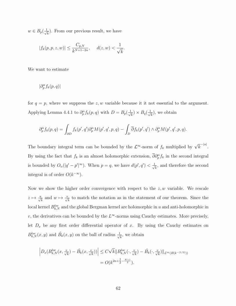
w ∈ Bp(1√k). From our previous result, we have
|fk(p, p, z, w)| ≤ Cp,NkN+1−2n
, d(z, w) <1√k.
We want to estimate
|∂αp fk(p, q)|
for q = p, where we suppress the z, w variable because it it not essential to the argument.
Applying Lemma 4.4.1 to ∂αp fk(p, q) with D = Bp(1√k)×Bq(
1√k), we obtain
∂αp fk(p, q) =
∫∂D
fk(p′, q′)∂αpM(p′, q′, p, q)−
∫D
∂fk(p′, q′) ∧ ∂αpM(p′, q′, p, q).
The boundary integral term can be bounded by the L∞-norm of fk multiplied by√k−|α|
.
By using the fact that fk is an almost holomorphic extension, ∂∂αp fk in the second integral
is bounded by Oα(|q′ − p′|∞). When p = q, we have d(p′, q′) < 1√k, and therefore the second
integral is of order O(k−∞).
Now we show the higher order convergence with respect to the z, w variable. We rescale
z 7→ u√k
and w 7→ v√k
to match the notation as in the statement of our theorem. Since the
local kernelBlock,N and the global Bergman kernel are holomorphic in u and anti-holomorphic in
v, the derivatives can be bounded by the L∞-norms using Cauchy estimates. More precisely,
let Dx be any first order differential operator of x. By using the Cauchy estimates on
Block,N(x, y) and Bk(x, y) on the ball of radius 1√
k, we obtain
∣∣∣Dx(Block,N(x, v√
k)− Bk(x,
v√k))∣∣∣ ≤ C
√k‖Bloc
k,N(·, v√k)− Bk(·, v√
k)‖L∞(B(k−(1/2)))
= O(k2n+12−N+1
2 ).
62

The above holds for x ∈ B(12k−1/2), hence we have
∣∣∣Dx(Block,N( u√
k, v√
k)− Bk(
u√k, v√
k))∣∣∣ = O(k2n+
12−N+1
2 ).
By similar argument, we can obtain the same estimates for the holomorphic variables y.
Now let Dα be any α-th degree differential operator with respect to x or y. By iterating the
previous argument, we obtain the following
|Dα(Block,N −Bk)| ≤ O(k
|α|2
+2n−N+12 ).
Hence we obtain the smooth convergence of the Bergman kernel asymptotics.
63

Chapter 5
Off-Diagonal
In this section we prove the rapid decay of the Bergman kernel on the off-diagonal. We will
prove the following We prove the off-diagonal estimate of the Bergman kernel.
Theorem 5.0.1. Let (L, h) → (M,ω) be a positive line bundle over a complete (not nec-
essarily compact) Kahler manifold of dimension n. Assume the Ricci curvature is bounded
from below, Ric(g) ≥ −Kω and assume the metric is only C2. Let Bk(x, y) be the Bergman
kernel for H0L2(M,Lk). For d(x, y) > 1, there exists ε0 > 0 such that the following off-
diagonal decay holds:
‖Bk(x, y)‖ ≤ C vol(Bx(1))−1 vol(By(1))−1e−ε0√kd(x,y).
We actually only require the distance d(x, y) to be greater than some positive constant
independent of k.
The study of the off-diagonal behavior has gained interest due to a conjecture by Zelditch,
which relates the decay rate of the Bergman kernel with the regularity of the metric.
Conjecture 1 ([7] page 2). Let d(x, y) ≥ δ > 0. The Bergman kernel decays at a rate
64

O(e−ck) for some c = c(δ) > 0 if and only if the metric potential ϕ is real analytic.
Results regarding the off-diagonal Agmon estimates in the compact setting can be found in
[7], [8], [9], [22], [25].
5.1 Preliminary Discussion
5.1.1 Comparison between Bergman and Green kernel
For compact manifolds by the Hodge decomposition, any smooth section f ∈ Γ(M,Lk) can
be decomposed into its harmonic and ∂∗
exact component,
f = fh + ∂∗f1.
Define the ∂-Laplacian on LN -valued 0-forms (sections) and (0, 1)-forms by
∆0 := ∂∗∂
∆1 := ∂∗∂ + ∂∂
∗.
This gives us a decomposition of the identity operator into
I − Pk = ∆0G0 = ∂∗∂G0,
where Pk is the Bergman projection and G0 is the Green operator of ∆0 for sections Γ(M,Lk).
Now we assume that M is noncompact. By restricting ourselves to ΓL2(M,Lk), we can
obtain the same Hodge decomposition as above by the spectral theorem.
We will need the following identity to commute the ∂ operator and the resolvent of ∆i in
65

our estimates.
Lemma 5.1.1. Let ∆0 and ∆1 be the Laplacian for ΓL2(M,Lk) and ΓL2(M,Λ0,1(M)⊗ Lk)
respectively. For α > 0 and s > 0, we have
∂(∆0 + α)−s = (∆1 + α)−s∂,
on the algebra C∞0 (M) of smooth function with compact support.
Proof. For any f ∈ C∞0 (M), we define the operator
At := e−t(∆1+α)∂ − ∂e−t(∆0+α).
Taking the derivative, we have
dAtf
dt= −(∆1 + α)Atf,
where we use that fact that ∂∆0 = ∆1∂. Since A0f = 0, since the Ricci curvature is bounded
below, by [10] we have by the uniqueness of the solution of the heat equation, Atf = 0 for
all t and f ∈ C∞0 (M). Multiplying the equality through by ts−1 and integrating both sides
we have
∫ ∞0
ts−1e−t(∆1+α)∂dt =
∫ ∞0
∂e−t(∆0+α)ts−1dt,
gives us the result.
Now on ΓL2(M,Lk), we have the following decomposition
I − Pk = ∆G0 = ∂∗∂G0 = ∂
∗G1∂.
66
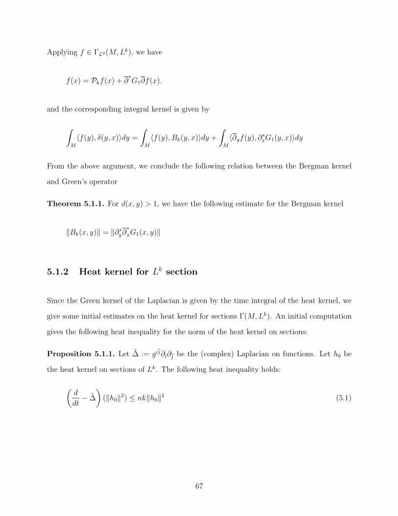
Applying f ∈ ΓL2(M,Lk), we have
f(x) = Pkf(x) + ∂∗G1∂f(x).
and the corresponding integral kernel is given by
∫M
〈f(y), δ(y, x)〉dy =
∫M
〈f(y), Bk(y, x)〉dy +
∫M
〈∂yf(y), ∂∗xG1(y, x)〉dy
From the above argument, we conclude the following relation between the Bergman kernel
and Green’s operator
Theorem 5.1.1. For d(x, y) > 1, we have the following estimate for the Bergman kernel
‖Bk(x, y)‖ = ‖∂∗y∂∗xG1(x, y)‖
5.1.2 Heat kernel for Lk section
Since the Green kernel of the Laplacian is given by the time integral of the heat kernel, we
give some initial estimates on the heat kernel for sections Γ(M,Lk). An initial computation
gives the following heat inequality for the norm of the heat kernel on sections:
Proposition 5.1.1. Let ∆ := gij∂i∂j be the (complex) Laplacian on functions. Let h0 be
the heat kernel on sections of Lk. The following heat inequality holds:
(d
dt− ∆
)(‖h0‖2) ≤ nk‖h0‖2 (5.1)
67

Proof. Viewing h0 ∈ Γ(Lk) we directly calculate:
∆(‖h0‖2) = gij∂i∂j〈h0, h0〉
= gij(〈∇i∇jh0, h0〉+ 〈h0,∇i∇jh0〉
)+ ‖∇h0‖2 + ‖∇h0‖2
The first term, the rough Laplacian is equal to the ∂-Laplacian,
gij〈∇i∇jh0, h0〉 = −〈∆0h0, h0〉.
For the second term, due to the inner product being Hermitian, we require the use of the
Ricci formula to commute the covariant derivatives. This yields
[∇i,∇j]h0 = −kRic(h)ijh0.
Then
gij〈h0,∇i∇jh0〉 = 〈h0, gji∇j∇ih0〉 − nk‖h0‖2 = 〈h0,∆0h0〉 − nk‖h0‖2.
Combining everything together, we have
∆0(‖h0‖2) ≥ −〈∆0(h0), h0〉 − 〈h0,∆0h0〉 − nk‖h0‖2 + ‖∇h0‖2 + ‖∇h0‖2
≥ d
dt(‖h0‖2)− nk‖h0‖2.
By rescaling, we get the heat inequality
(d
dt− ∆
)(e−nkt‖h0‖2) ≤ 0.
68

Hence by a semigroup domination argument [12], we have the estimate
‖h0‖ ≤ enkt2 |k0|. (5.2)
We can see that we get an exponential growth with respect to t.
It was shown in [27] that for the heat kernel on functions k0, there exists constants β1, C1 <∞
such that
k0(t, x, y) ≤ C1
vol(Bx(√t))
12 vol(By(
√t))
12
e− d
2(x,y)C14t eβ1t
Combining with our initial heat kernel estimate, we have
‖h0(t, x, y)‖ ≤ C1
vol(Bx(√t))
12 vol(By(
√t))
12
e− d
2(x,y)C14t eC2nkt
for some C2 > 0.
By a volume comparison argument from (6.6), there exists β2, C3 <∞ such that
vol(Bx(√t))−1/2 vol(By(
√t))−1/2 ≤ C3
vol(Bx(1))supt−n, 1eβ2d(x,y)
By an application of Cauchy’s inequality, for any γ ∈ R,
e− d(x,y)2
4C4t ≤ e−γd(x,y)eC4γ2t (5.3)
With the above considerations, we obtain
‖h0(t, x, y)‖ ≤ C3
vol(Bx(1))supt−n, 1e(β2−γ)d(x,y)e(C4γ2+C2nk)t (5.4)
69

5.2 Proof of Theorem 5.0.1
5.2.1 Perturbation of the Green Operator
We consider the class of functions
Ψ := ψ ∈ C1(M) | |∇ψ|2 ≤ c20k,
where c0 > 0 is a constant to be determined later. The choice of k in the upper bound will
also become evident in §5.2.4. Then we have that
infψ(x)− ψ(y) | ψ ∈ Ψ = −c0
√kd(x, y),
for any x, y ∈M . Let
φ(x) = vol(Bx(1))−12 .
First note that the integral kernel for the operator
A := φ−1eψ∂∗∆−1
1 ∂eψφ−1,
is given by
A(x, y) = φ−1(x)eψ(x)∂∗x∂∗yG(x, y)e−ψ(y)φ−1(y).
We want to show a uniform upper bound for A(x, y) when d(x, y) > 1 so that
‖∂∗x∂∗yG(x, y)‖ ≤ Cφ(x)φ(y)eψ(y)−ψ(x).
70

Varying over ψ ∈ Ψ yields
‖∂∗x∂∗yG(x, y)‖ ≤ Cφ(x)φ(y)e−c0√kd(x,y) for d(x, y) > 1,
and Theorem 5.1.1 will imply the off-diagonal decay of the Bergman kernel. Note that we
allow C to be at most polynomial growth in k, as a proper choice of the constant in the
exponent will absorb the polynomial term. In the following, we will use a resolvent identity
to obtain a kernel identity and provide the necessary bounds.
5.2.2 Resolving the singularity
We consider the following resolvent and corresponding Green kernel for the operator (∆i+α):
(∆i + α)−s−1f(x) =
∫M
(Gα,s(y, x), f(y))dy
:=1
Γ(s+ 1)(
∫ ∞0
hi(t, y, x)e−αttsdt, f(y))dy
i = 0, 1. We abuse the notation for the Green kernel as it will be clear from context which we
are using. By choosing an appropriately large α > 0, we can “push away” the exponential
growth in k. The exponent s is used to remove the singularity of the heat kernel when t = 0
for x = y. To introduce such a term, we use the following resolvent identity:
∆−11 = (∆1 + α)−1 + α(∆1 + α)−1∆−1
1
= (∆1 + α)−1 + α(∆1 + α)−1/2∆−11 (∆1 + α)−1/2
71

By iterating, we obtain
∆−11 = (∆1 + α)−1 + α(∆1 + α)−2 + · · ·+ α2n+3(∆1 + α)−2n−4
+ α2n+4(∆1 + α)−n−2∆−11 (∆1 + α)−n−2.
(5.5)
Perturbing the operator, we get
A = φ−1eψ∂∗∆−1
1 ∂e−ψφ−1 =2n+3∑p=0
αpφ−1eψ∂∗(∆1 + α)−(p+1)∂e−ψφ−1
+ α2n+4φ−1eψ∂∗(∆1 + α)−n−2∆−1
1 (∆1 + α)−n−2∂e−ψφ−1.
We can see that we have two cases to consider
1. As := φ−1eψ∂∗(∆1 + α)−s∂e−ψφ−1
2. B := φ−1eψ∂∗(∆1 + α)−n−2∆−1
1 (∆1 + α)−n−2∂e−ψφ−1
where As is singular if s ≤ n. For the first case, we use Lemma 5.1.1 and we have
As(x, y) = φ−1eψ∂∗(∆1 + α)−s∂e−ψφ−1
= φ−1eψ∂∗∂(∆0 + α)−se−ψφ−1
= φ−1eψ∆0(∆0 + α)−se−ψφ−1
= φ−1eψ(∆0 + α)−s+1e−ψφ−1 − αφ−1eψ(∆0 + α)−se−ψφ−1.
Inserting this into the above identity leads to a cancellation in all the middle terms. The
leading term becomes the delta kernel, which vanishes for d(x, y) > 0. Hence we have the
operator identity
A = φ−1eψIe−ψφ−1 − α2n+4φ−1eψ(∆0 + α)−2n−4e−ψφ−1 + α2n+4B.
72

Let A(x, y) and B(x, y) be the kernel of the operator A and B respectively. We then have
the kernel identity
A(x, y) = −α2n+4φ−1(x)eψ(x)Gα,2n+3(x, y)e−ψ(y)φ−1(y) + α2n+4B(x, y).
for d(x, y) > 0.
5.2.3 Estimates
Since the α terms will be at most a polynomial in k, we will incorporate it into the exponential
decaying term.
Lemma 5.2.1. There exists α > 0 and C ≤ ∞ such that for ψ ∈ Ψ,
supx,y‖φ−1(x)eψ(x)Gα,2n+3(x, y)e−ψ(y)φ−1(y)‖ ≤ C.
Proof. We modify Lemma 6.6 and consider both the volume of x and y so
vol(B√t(x))−1/2 vol(B√t(y))−1/2 ≤ C2φ(x)φ(y) supt−n, 1,
Applying the heat kernel estimates, we have
‖Gα,2n+3(x, y)‖
≤ C3φ(x)φ(y)
∫ ∞0
supt−n, 1e−γd(x,y)t2n+3e(C4γ2+C2nk−α)t
≤ C5φ(x)φ(y)e−γd(x,y),
for any γ and α > C4γ2 + C2nk.
73

Using this, we have a bound on the Green function
supx,y‖φ−1(x)eψ(x)Gα,2n+3(y, x)e−ψ(y)φ−1(y)‖
≤ C supx,y
e−γ+c0√kd(x,y)
≤ C.
By choosing appropriate γ.
Next we consider the L1 → L∞ bound for the B operator. This would imply the same bound
on the kernel B(x, y). We first show the following lemma
Lemma 5.2.2. There exists α > 0 and C <∞ such that for all ψ ∈ Ψ
supx∈M
φ−2(x)
∫M
‖Gα,n(x, y)‖2e2(ψ(x)−ψ(y))dy ≤ C
Proof. We repeat the steps of the previous lemma and applying Lemma 6.6 to obtain
‖Gα,n(x, y)‖
≤ C3φ2(x)
∫ ∞0
suptn, 1e−γd(x,y)e(C4γ2+C2nk−α)t
≤ Cφ2(x)e−γd(x,y).
74

Again, by choosing appropriate α. Then by direct computation,
φ−2(x)
∫M
‖Gα,s(x, y)‖2e2(ψ(x)−ψ(y))dy
≤ Cφ2(x)
∫M
e−2(γ−β2−c0√k)d(x,y)dy
≤ C∞∑j=1
e−2(γ−β2−c0√k)(j−1) Vol(Bj(x))
Vol(B1(x))
≤ C
∞∑j=1
jne−2(γ−β2−c0√k)(j−1)e(n−1)
√Kj
where the second to last inequality is obtained by splitting the integral as M =⋃∞j=1y | j−
1 ≤ d(x, y) ≤ j and the last inequality is by volume comparison. The series is convergent
when
2(γ − β2 − c0
√k) > (n− 1)
√K. (5.6)
Hence we choose γ which satisfies the above.
Decomposing B = Aα,2TψAα,1 where
Aα,2 := φ−1eψ∂∗(∆1 + α)−n−1e−ψ
Aα,1 := eψ(∆1 + α)−n−1∂e−ψφ−1
Tψ := eψ∆−11 e−ψ
Lemma 5.2.3. There exists some α ≥ 0 and C > 0 such that
‖Aα,1‖1,2 ≤ C
‖Aα,2‖2,∞ ≤ C.
Proof. Let Gα,n+1(x, y) be the Green kernel from (∆0 + α)−n−2. By direct computation, we
75

have
∫M
‖∂xGα,n+1(x, y)‖2e2(ψ(x)−ψ(y))dx
≤ 8c20k
∫M
e2(ψ(x)−ψ(y))‖Gα,n+1(x, y)‖2dx
+
∫M
e2(ψ(x)−ψ(y))(Gα,n+1(x, y), ∂∗x∂xGα,n+1(x, y))dx
Now using Lemma 5.1.1, we have
‖eψ∂(∆0 + α)−n−2e−ψφ−1‖1,2
=
(∫M
‖eψ(x)∂(∆0 + α)−n−2(e−ψφ−1u)(x)‖2dx
) 12
=
(∫M
∥∥∥∥eψ(x)∂x
(∫M
(Gα,n+1(y, x)e−ψ(y)φ−1(y), u(y))dy
)∥∥∥∥2
dx
) 12
≤ supyφ−1(y)
(∫M
‖∂Gα,n+1(x, y)‖2e2(ψ(x)−ψ(y))dx
) 12
≤ supyφ−1(y)
(∫M
e2(ψ(x)−ψ(y))‖∂Gα,n+1(x, y)‖2dx
) 12
≤ supyφ−1(y)
(8c2
0k
∫M
e2(ψ(x)−ψ(y))‖Gα,n+1(x, y)‖2dx
+
∫M
e2(ψ(x)−ψ(y))(Gα,n+1(x, y),∆1Gα,n+1(x, y))dx
) 12
When the Laplacian acts on the Green kernel, we have
∆∂,xGα,s(x, y) =
∫ ∞0
∆∂,xk(t, x, y)e−αttsdt
= −∫ ∞
0
(∂tk(t, x, y))e−αttsdt
76

Integrating by parts,
=
∫ ∞0
k(t, x, y)sts−1e−αtdt−∫ ∞
0
αk(t, x, y)e−αttsdt
= sGα,s−1(x, y)− αGα,s(x, y).
Inserting the identity, we have
∫M
e2(ψ(x)−ψ(y))(Gα,n+1(x, y),∆∂,xGα,n+1(x, y))dx
= −(n+ 1)
∫M
e2(ψ(x)−ψ(y))(Gα,n+1(x, y), Gα,n(x, y))dx
+ α
∫M
e2(ψ(x)−ψ(y))‖Gα,n+1(x, y)‖2dx
≤ (α− n+ 1
2)
∫M
e2(ψ(x)−ψ(y))‖Gα,n+1(x, y)‖2dx
− n+ 1
2
∫M
e2(ψ(x)−ψ(y))‖Gα,n(x, y)‖2dx
Hence combining we obtain
‖eψ∂(∆ + α)−n−1e−ψφ−2‖21,2
≤ supyφ−1(y)(8c2
0k + α− n+ 1
2)
∫M
e2(ψ(x)−ψ(y))‖Gα,n+1(x, y)‖2dx
− n+ 1
2
∫M
e2(ψ(x)−ψ(y))‖Gα,n(x, y)‖2dx
≤ supyφ−2(y)(8c2
0k + α− n+ 1
2)
∫M
e2(ψ(x)−ψ(y))‖Gα,n+1(x, y)‖2dx
+ supyφ−2(y)
n+ 1
2
∫M
e2(ψ(x)−ψ(y))‖Gα,n(x, y)‖2dx.
Lemma 5.2.2 gives us the upper bound. For the Aα,2, we note that the dual operator
A∗α,1 = φ−1e−ψ∂∗(∆ + α)−n−1eψ has the operator bound ‖A∗α,1‖2,∞ ≤ C for ψ ∈ Ψ, hence
varying over the class of functions in Ψ, we obtain the same bound for Aα,2.
77

Next we show the L2 → L2 bound of Tψ.
Lemma 5.2.4. Assume that the Ricci curvature of M has a lower bound. Then for suffi-
ciently large k and for ψ ∈ Ψ, we have
‖Tψ‖2,2 ≤ C <∞.
Proof. Define the operator
Tψ′:= eψ∆1e
−ψ −∆1.
By the Weitzenbock formula, we have
∆1 = −∇2 + E = −∇2 + k ω + Ric(M).
We denote ∆ = −∇2 to be the rough Laplacian. Then we can write
Tψ′= eψ∆e−ψ − ∆.
For any Lk-valued (0, 1) form u, we have
(Tψ′u, u) = (∇(e−ψu),∇(eψu))− (∇u,∇u)
≤ c20k
∫M
‖u‖2 + 2 Im
(∫M
∇ψ∇u u)
Using the Cauchy inequality, using the fact that |∇ψ| ≤ bk, we have
‖(Tψ′u, u)‖ ≤ 4c20k
∫M
‖u‖2 +1
2
∫M
‖∇u‖2.
78

Since the Ricci curvature has a lower bound −K, integrating the Weitzenbock formula gives
∫M
‖∇u‖2 ≤∫M
〈∆1u, u〉+K
∫M
‖u‖2 − k∫X
‖u‖2.
In summary, we have
|(Tψ′u, u)| ≤ 1
2(∆1u, u) + (4c2
0k +K − k)
∫M
|u|2,
and for c0 <12, we have
|(Tψ′u, u)| ≤ 1
2(∆1u, u)
for k sufficiently large.
We have
|((∆1 + Tψ′)u, u)| ≥ |(∆1u, u)| − |(Tψ′u, u)|
≥ 1
2|(∆1u, u)|
≥ ck(u, u).
A lower bound for the quadratic form of an operator implies an upper bound for its inverse.
Here we see that the order c0
√k is necessary in our choice of the class of functions Ψ.
Combining Lemmas 5.2.1, 5.2.3, and 5.2.4 proves Theorem 5.0.1.
79

Chapter 6
Appendix
6.1 Useful Formulas
6.1.1 Bound of normalizing constant for peak section
Lemma 6.1.1.
∫r2pe−mr
2
rdr = − 1
2me−mr
2
p∑k=0
p!
(p− k)!mkr2(p−k) (6.1)
Corollary 6.1.1. Let P ∈ Zn+ and use the following notations: P ! = p1! · · · pn! and p =
p1 + · · ·+ pn
∫Cn|zP |2e−m|z|2dV0 =
P !
mn+p(6.2)
Corollary 6.1.2 (lower bound for integral). Let cm →∞
∫|z|≤ cm√
m
|zP |2e−m|z|2dV0 ≥C
mn+p(6.3)
80

Proof. By using (6.1.1), we have
∫cm√m≥|z1||z1|2p1e−m|z1|
2
dV0
=π
mp1+1e−cm
p1∑k=0
p1!
(p1 − k)!c2(p1−k)m
≤ p1!π
mp1+1
p1∑k=0
c2(p1−k)m
ec2m
≤ (p1 + 1)!π
mp1+1
c2p1m
ec2m
For large t 0, we have
tp1
et<
1
(p1 + 1)π(6.4)
So taking m sufficiently large, we have
∫cm√m≥|z1||z1|2p1e−m|z1|
2
dV0 ≤C1
mp1+1(6.5)
for Cn1 < |P | Then we have
∫|z|≤ cm√
m
|zP |2e−m|z|2dV0 =
∫Cn|zP |2e−m|z|2dV0 −
∫|z|≥ cm√
m
|zP |2e−m|z|2dV0
≥ P !
mn+p− C1
mn+p=
C
mn+p
6.1.2 Weitzenbock Formula for LN-valued (0, 1)-forms
We define the covariant derivative for holomorphic indices of LN -valued (0, q)-forms as
81
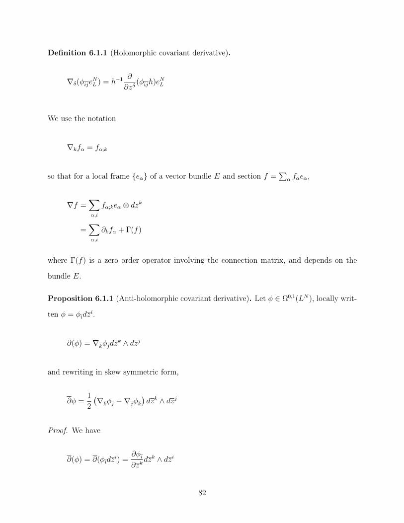
Definition 6.1.1 (Holomorphic covariant derivative).
∇δ(φijeNL ) = h−1 ∂
∂zδ(φijh)eNL
We use the notation
∇kfα = fα;k
so that for a local frame eα of a vector bundle E and section f =∑
α fαeα,
∇f =∑α,i
fα;keα ⊗ dzk
=∑α,i
∂kfα + Γ(f)
where Γ(f) is a zero order operator involving the connection matrix, and depends on the
bundle E.
Proposition 6.1.1 (Anti-holomorphic covariant derivative). Let φ ∈ Ω0,1(LN), locally writ-
ten φ = φidzi.
∂(φ) = ∇kφjdzk ∧ dzj
and rewriting in skew symmetric form,
∂φ =1
2
(∇kφj −∇jφk
)dzk ∧ dzj
Proof. We have
∂(φ) = ∂(φidzi) =
∂φi∂zk
dzk ∧ dzi
82

On the other hand, we have by definition:
∇kφi =∂φi∂zk− φjΓ
j
ki
So that
∂φi∂zk
= ∇kφi + φjΓj
ki
substituting the above to the first equation yields
∂(φ) = (∇kφi + φjΓj
ki)dzk ∧ dzi
By the alternating 2-form and the symmetry of Γkij, we have
Γkij = 0
which gives us the result.
We now show the formula for the ∂∗
operator for LN -valued (0, 1) and (0, 2)-forms.
Lemma 6.1.2 (∂∗
for LN -valued (0, 1)-forms).
∂∗(φidz
i ⊗ eNL ) = −gji ∂∂zj
(φi)eNL − gjiφi
∂h
∂zjh−1eNL = −gji∇j(φie
NL )
Lemma 6.1.3 (∂∗
for LN -valued (0, 2)-forms).
(∂∗φ)pdz
p = −2gli(∇∂l(φipeNL )− φijgkpgsjΓksleNL )dzp
83

Proof. We use the defining relation (∂∗(φij), ηk) = (φij,
∂ηk∂zl
). Expanding, we obtain
(φij,∂ηk∂zl
) =2
∫M
φij∂ηk∂zl
gligkjh det gdVE
= −2
∫M
ηk∂
∂zl(φijg
ligkjh det g)dVE
and
(∂∗(φij), ηk) =
∫M
gkm(∂∗φ)mηkh det gdVE
Comparing coefficients, we have
−2gkm∂
∂zl(φijg
ligkjh det g) = (∂∗φ)mh det g
The left hand side splits into
−gkm∂
∂zl(φijg
ligkjh det g) = −∂φij∂zl
gligkmgkjh det g
− φijgkjgkmh∂
∂zl(gli det g)
− gkmφij∂gkj
∂zlglih det g
− φijgkmgligkj∂h
∂zldet g
The second term vanishes due to the Kahler symmetries, and we simplify the remaining
terms:
−gkm∂
∂zl(φijg
ligkjh det g) = −∂φim∂zl
glih det g
+ gliφijgkpgsjΓksl det g
− φim∂lh det g
84
Using the covariant derivative identity, we have
(∂∗φ)m = −2gli(∇l(φime
NL )− φijgkmgsjΓksleNL )
Lemma 6.1.4. Let φ ∈ Ω0,1(LN). Under normal coordinates, we have
∂∂∗(φ) = −gji
(∇k∇j(φie
NL ))dzk = −
∑k,j
(∇j∇k(φke
NL ))dzj
and
∂∗∂(φ) = −
∑k,j
∇k∇k(φjeNL ) +∇k∇j(φke
NL )
Lemma 6.1.5 (Ricci Formula). Let φ be a LN -valued (0, 1)-form, i.e. φ = φαldzl ⊗ eα
[∇k,∇j]φαl
= φiRijkl + φl Ric(h)kj
Proof. First calculate in normal coordinates
∇k∇j(φl) = ∇k(∂φl∂zj− φmΓm
jl)
=∂2φl∂zk∂zj
− φm∂Γm
jl
∂zk
Next we calculate the opposite term
∇j∇k(φl) = ∇j(∂φl∂zk
+ φldzl ∂h
∂zkh−1)
=∂2φl∂zj∂zk
+ φl∂2h
∂zk∂zjh−1.
85
Combining the terms yields
[∇k,∇j](φl) = φiRijkl + φl Ric(h)kj
Proposition 6.1.2 (Weitzenbock Formula for LN -valued (0, 1)-forms.).
∆∂(φ) = ∂∂∗
+ ∂∗∂(φ)
=∑k,j,i
−∇k∇k(φj) +∇k∇j(φk)−∇j∇k(φk)
=∑k,j,i
(−∇k∇k(φj) + φi Ric(g)ij + φk Ric(h)kj
)dzj ⊗ eNL
6.1.3 ∂ estimate
The following Hormander’s L2-estimate for the ∂-equation is used:
Theorem 6.1.1. Let (M,ω) be a complete Kahler manifold, and let L→M be Hermitian
line bundle with Hermitian metric h. Assume that the curvature Ric(h) ≥ Cω is positive
for some C > 0. Then there is an integer N0 depending on M,L and h such that for any
N ≥ N0, the following holds: for any g ∈ L2(M,∧0,1M ⊗Lm) satisfying ∂g = 0, there exists
f ∈ L2(M,Lm) such that ∂f = g and
∫M
|f |2hmdVg ≤1
C
∫M
|g|2hmdVg
where C is the same constant as in the hypothesis.
86
6.1.4 Hodge Theory and Kahler identities
Theorem 6.1.2 (Hodge Theorem). Let E be a Hermitian vector bundle over a compact
Hermitian manifold X. For p, q ≥ 0, let
Hp,q(X,E) = φ ∈ Γ(X,Ωp,q(E)) | ∆∂φ = 0
i.e. the harmonic (p, q) forms. Then
1. dimHp,q(X,E) <∞;
2. For any η ∈ Γ(X,Ωp,q(E)), we have
η = ηh + ∂η1 + ∂∗η2,
where ηh is harmonic.
On Kahler manifolds, we have the equivalence between the different Laplacians.
∆∂ = ∆∂ =1
2∆d
6.1.5 Volume Comparison
Proposition 6.1.3 (Bishop Volume Comparison). Let M be a complete n-dimensional
Riemannian manifold such that Ric ≥ −K. Let BK(r) be a ball in the Riemannian space
form of constant sectional curvature − Kn−1
. Then
Vol(B(r)) ≤ Vol(BK(r))
87

We have
ωnsn ≤ Vol(BK(s)) ≤ ωns
ne√
(n−1)Ks.
For any ball Bx(r) ⊂M , we have
Vol(Bx(s))
Vol(Bx(s′))≤ Vol(BK(s))
Vol(BK(s′)), 0 < s′ < s < 2r.
Hence we deduce that
Vol(Bx(s)) ≤ Vol(Bx(s′))( ss′
)ne√
(n−1)Ks, 0 < s′ < s < 2r.
Setting d = d(x, y), we can compare the volume of balls centered at points as follows,
Vol(By(s)) ≤ Vol(Bx(d+ s))
≤ Vol(Bx(s′))
(d+ s
s′
)ne√
(n−1)K(d+s), 0 < s′ < s < r, y ∈ B
Let φ(x) = Vol(Bx(1))−12 . Combining the above, there exists β2, C2 <∞ such that
Vol(Bx(√t))−1/2 Vol(By(
√t))−1/2 ≤ C2φ
2(x) supt−n2 , 1eβ2d(x,y) (6.6)
88

Bibliography
[1] K. Adachi. Several complex variables and integral formulas. World Scientific PublishingCo. Pte. Ltd., Hackensack, NJ, 2007.
[2] S. Alexakis and K. Hirachi. Integral Kahler invariants and the Bergman kernel asymp-totics for line bundles. 2015.
[3] R. Berman, B. Berndtsson, and J. Sjostrand. A direct approach to Bergman kernelasymptotics for positive line bundles. Ark. Mat., 46(2):197–217, 2008.
[4] T. Bouche. Asymptotic results for Hermitian line bundles over complex manifolds: theheat kernel approach. In Higher-dimensional complex varieties (Trento, 1994), pages67–81. de Gruyter, Berlin, 1996.
[5] D. Catlin. The Bergman kernel and a theorem of Tian. In Analysis and geometry inseveral complex variables (Katata, 1997), Trends Math., pages 1–23. Birkhauser Boston,Boston, MA, 1999.
[6] M. Christ. Slow off-diagonal decay for Szego kernels associated to smooth Hermitian linebundles. In Harmonic analysis at Mount Holyoke (South Hadley, MA, 2001), volume320 of Contemp. Math., pages 77–89. Amer. Math. Soc., Providence, RI, 2003.
[7] M. Christ. Off-diagonal decay of Bergman kernels: On a conjecture of Zelditch. 2013.
[8] M. Christ. Upper bounds for Bergman kernels associated to positive line bundles withsmooth Hermitian metrics. 2013.
[9] X. Dai, K. Liu, and X. Ma. On the asymptotic expansion of Bergman kernel. J.Differential Geom., 72(1):1–41, 2006.
[10] J. Dodziuk. Maximum principle for parabolic inequalities and the heat flow on openmanifolds. Indiana Univ. Math. J., 32(5):703–716, 1983.
[11] S. K. Donaldson. Scalar curvature and projective embeddings. I. J. Differential Geom.,59(3):479–522, 2001.
[12] H. Donnelly and P. Li. Lower bounds for the eigenvalues of Riemannian manifolds.Michigan Math. J., 29(2):149–161, 1982.
89
[13] R. Hempel and J. Voigt. The spectrum of a Schrodinger operator in Lp(Rν) is p-
independent. Comm. Math. Phys., 104(2):243–250, 1986.
[14] H. Hezari, C. Kelleher, S. Seto, and H. Xu. Asymptotic expansion of the Bergmankernel via perturbation of the Bargmann-Fock model. 2014.
[15] S. G. Krantz. Geometric analysis of the Bergman kernel and metric, volume 268 ofGraduate Texts in Mathematics. Springer, New York, 2013.
[16] C.-j. Liu. The asymptotic Tian-Yau-Zelditch expansion on Riemann surfaces with con-stant curvature. Taiwanese J. Math., 14(4):1665–1675, 2010.
[17] C.-J. Liu and Z. Lu. Asymptotic Tian-Yau-Zelditch expansions on singular Riemannsurfaces. J. Fixed Point Theory Appl., 10(2):327–338, 2011.
[18] C.-J. Liu and Z. Lu. Abstract Bergman kernel expansion and its applications. 2014.
[19] Z. Lu. On the lower order terms of the asymptotic expansion of Tian-Yau-Zelditch.Amer. J. Math., 122(2):235–273, 2000.
[20] Z. Lu and G. Tian. The log term of the Szego kernel. Duke Math. J., 125(2):351–387,2004.
[21] Z. Lu and S. Zelditch. Szego kernels and Poincare series. 2014.
[22] X. Ma and G. Marinescu. The Spinc Dirac operator on high tensor powers of a linebundle. Math. Z., 240(3):651–664, 2002.
[23] X. Ma and G. Marinescu. Generalized Bergman kernels on symplectic manifolds. C. R.Math. Acad. Sci. Paris, 339(7):493–498, 2004.
[24] X. Ma and G. Marinescu. The first coefficients of the asymptotic expansion of theBergman kernel of the Spinc Dirac operator. Internat. J. Math., 17(6):737–759, 2006.
[25] X. Ma and G. Marinescu. Holomorphic Morse inequalities and Bergman kernels, volume254 of Progress in Mathematics. Birkhauser Verlag, Basel, 2007.
[26] W.-D. Ruan. Canonical coordinates and Bergmann [Bergman] metrics. Comm. Anal.Geom., 6(3):589–631, 1998.
[27] L. Saloff-Coste. Uniformly elliptic operators on Riemannian manifolds. J. DifferentialGeom., 36(2):417–450, 1992.
[28] B. Shiffman and S. Zelditch. Asymptotics of almost holomorphic sections of ample linebundles on symplectic manifolds. J. Reine Angew. Math., 544:181–222, 2002.
[29] K.-T. Sturm. On the Lp-spectrum of uniformly elliptic operators on Riemannian man-ifolds. J. Funct. Anal., 118(2):442–453, 1993.
[30] G. Szekelyhidi. An introduction to extremal Kahler metrics, volume 152 of GraduateStudies in Mathematics. American Mathematical Society, Providence, RI, 2014.
90

[31] G. Tian. On a set of polarized Kahler metrics on algebraic manifolds. J. DifferentialGeom., 32(1):99–130, 1990.
[32] H. Xu. A closed formula for the asymptotic expansion of the Bergman kernel. Comm.Math. Phys., 314(3):555–585, 2012.
[33] S. Zelditch. Szego kernels and a theorem of Tian. Internat. Math. Res. Notices, (6):317–331, 1998.
91