University of Bradford eThesis

University of Bradford eThesis This thesis is hosted in Bradford Scholars – The University of Bradford Open Access repository. Visit the repository for full metadata or to contact the repository team

© University of Bradford. This work is licenced for reuse under a Creative Commons

Licence.

https://bradscholars.brad.ac.uk/

http://creativecommons.org/licenses/by-nc-nd/3.0/




ADVANCED CONTROLLERS FOR BUILDING ENERGY

MANAGEMENT SYSTEMS

Advanced controllers based on traditional mathematical methods (MIMO P+I,

state-space, adaptive solutions with constraints) and intelligent solutions (fuzzy

logic and genetic algorithms) are investigated for humidifying, ventilating

and air-conditioning applications

by

Abu Bakar MHD. GHAZALI, MSc

A Thesis Submitted for the

Degree of Doctor of Philosophy

Department of Electronic and Electrical Engineering

University of Bradford

1996

ADVANCED CONTROLLERS FOR BUILDING ENERGY MANAGEMENT

SYSTEMS

Abu Bakar MED GHAZALI

Keywords: Building energy management systems; humidification, ventilation and air- conditioning; multi-input/multi-output (MIMO) systems; multivariable P+I controllers; state-space methods; modal control; constrained adaptive control; fuzzy logic controllers; genetic algorithms.

ABSTRACT

This thesis presents the design and implementation of control strategies for building energy management systems (BEMS). The controllers considered include the multi PI- loop controllers, state-space designs, constrained input and output MIMO adaptive controllers, fuzzy logic solutions and genetic algorithm techniques. The control performances of the designs developed using the various methods based on aspects such as regulation errors squared, energy consumptions and the settling periods are investigated for different designs. The aim of the control strategy is to regulate the room temperature and the humidity to required comfort levels.

In this study the building system under study is a3 input/ 2 output system subject to external disturbances/effects. The three inputs are heating, cooling and humidification, and the 2 outputs are room air temperature and relative humidity. The external disturbances consist of climatic effects and other stochastic influences. The study is carried out within a simulation environment using the mathematical model of the test room at Loughborough University and the designed control solutions are verified through experimental trials using the full-scale BMS facility at the University of Bradford.

ACKNOWLEDGEMENTS

I wish to express my sincere thanks and gratitude to my supervisor Prof. G. S. Virk for

his continued support, advice, and guidance throughout the duration of this work. My

thanks are also extended to Prof. J. G. Gardiner, Head of the department, for his

administrative support and Dr. D. Azzi for his help in setting the BEMS test room at the

Bradford University.

I would also like to express my gratitude to the Malaysian Goverment and the Malaysian

Institute of Nuclear Technology Research (MINT) in particular for the financial support

throughout this period of study.

Last but not least, my gratitude goes to my parents, my wife and my childrens for their

never ending support, patience and prayer.

III

TABLE OF CONTENTS

Chapter 1: Introduction .............................................................................................. 1

1.1 Building energy management systems ....................................................................... 3

1.2 Current control techniques ....................................................................................... 4

1.2.1 On/off control ................................................................................................... 4

1.2.2 PID control ....................................................................................................... 5

1.2.3 Optimal start/stop ............................................................................................. 7

1.3 The current status of BEMS ..................................................................................... 8

1.4 The potential for model-based control ...................................................................... 9

1.5 Work in this thesis ................................................................................................. 11

Chapter 2: 'The Simulation Environment ................................................................. 13

2.1 Office zone test system .......................................................................................... 13

2.2 Discrete transfer function model ............................................................................. 16

2.3 Validation of the models ........................................................................................ 18

2.3.1 Step responses ................................................................................................ 18

2.3.2 On/off control strategy .................................................................................... 21

2.3.2.1 Simulation studies ................................................................................. 24

2177 Mndel nerformance ............................................................................... 28

2.4 Conclusions ........................................................................................................... 30

Chapter 3: Multi-input Multi-output P+I Controls ................................................. 31

3.1 Single PI-loop controller ........................................................................................ 32

3.2 Multi PI-loop controller ......................................................................................... 34

3.3 Multi PI-loop tuning methodology ......................................................................... 40

3.3.1 Simulation results ............................................................................................ 43

3.4 Methodology to minimise the number of PI controllers ......................................... .. 46

3.5 Conclusions ......................................................................................................... .. 48

Chapter 4: State-Space Methods .............................................................................. 50

4.1 State-space representation .................................................................................... .. 50

4.2 State-feedback design .......................................................................................... .. 58

4.2.1 Pole-placement design by state feedback ....................................................... .. 61

4.2.2 Multistage design procedure for state feedback ............................................ ..

69 4.3 Output feedback design .................................................... ................................ ..

82

4.3.1 Pole-placement design by output feedback ..................................................... .. 83 4.4. Practical aspects of the state-space method ......................................................... ..

88 4.5 Conclusions ......................................................................................................... ..

90

Chapter 5: MIMO Adaptive Control with Constrained Inputs ............................ .. 91

5.1 Statement of the problem ..................................................................................... .. 93

5.2 Multivariable adaptive control law ........................................................................ ..

95 5.3 Multivariable parameter estimation .......................................................................

101 5.4 MIMO adaptive controller for the office zone system ...........................................

105 5.4.1 The objective function

................................................................................... 106

5.4.2 Input and output constraints .......................................................................... 111

5.4.3 Quadratic programming 112 113 5.5 Simulation results .................................................................................................

IV

5.6 Conclusions ......................................................................................................... 126

Chapter 6: Fuzzy Logic Controllers ........................................................................ 128

6.1 Design of the FLC ................................................................................................

129 6.1.1 FLC based on proportional action .................................................................

130 6.1.2 FLC based on P+I control ...........................................................................

138 6.2 Defuzzification process ........................................................................................

141 6.2.1 Calculation of the FLC outputs ......................................................................

143 6.3 Simulation results .................................................................................................

146 6.4 Conclusions .........................................................................................................

153

Chapter 7: Genetic Algorithms for BEMS ............................................................. 154

7.1 GA methodology ................................................................................................. 155

7.1.1 Initialisation .................................................................................................. 156

7.1.2 Encoding ....................................................................................................... 15 6

7.1.3 Evaluation ..................................................................................................... 157

7.1.4 Genetic operators .......................................................................................... 158

7.1.5 Convergence ................................................................................................. 160

7.2 Controller based on GA .......................................................................................

160 7.3 Multi-proportional loop controller ........................................................................

161 7.3.1 Initial population ...........................................................................................

163 7.3.2 Reproduction ................................................................................................

164 7.3.3 Crossover ......................................................................................................

166 7.3.4 Mutation

....................................................................................................... 166

7.3.5 Convergence .................................................................................................

167 7.3.6 Tuning of the proportional gains ....................................................................

167 7.3.7 Simulation results ..........................................................................................

169 7.4 Improved FLC using GA technique ......................................................................


180 7.5 GA for adaptive control .......................................................................................

184 7.5.1 Convergence .................................................................................................


187 7.6 Smoothing of GA solutions ..................................................................................

192 7.7 Conclusions .........................................................................................................

197

Chapter 8: Real-time Controls ................................................................................ 199

8.1 Multi PI-loop controller ....................................................................................... 201

8.2 Constrained input MIMO adaptive controller ....................................................... 203

8.3 Fuzzy logic controller .......................................................................................... 207

8.4 Genetic algorithm ................................................................................................. 210

8.5 Commercial controller .......................................................................................... 212

8.6 Discussion of Results ........................................................................................... 214

8.7 Conclusions ......................................................................................................... 219

Chapter 9: Conclusions and Future Work ............................................................. 220

9.1 Future work ......................................................................................................... 223

Bibliographies .......................................................................................................... 226

Appendix A ............................................................................................................. 234

V

Chapter 1

Introduction

A modern building : )mprises many control loops which when combined, create an

environment in which employees can work in safety and comfort, and provides a stable

environment for storing valuable assets such as documents, plants and works of art. In

addition other benefits to be derived from a well controlled building is the ability to save

on the ever increasing operating costs by looking for ways in which to minimise energy

consumption as well as addressing environmental concerns by minimising the release of

carbon dioxide to the atmosphere since the built sector is a major consumer of energy.

These facts are in agreement with the resolution from the 1992 Earth Summit in Rio on

Climate Change where it was agreed that we should return emissions of CO2 to their

1990 levels by the year 2000.

Other benefits to result from a well-operated building are that the improved

conditions leads to greater occupant productivities, preventative maintenance can be

employed thereby reducing maintenance cost because of the experience gain through the

additional monitoring of components in the building environmental system, and enables

the analyses of the data from all the control systems to aid decision making for future

operation of the building. Moreover, there are a number of concepts in building

1

management systems (BMSs) which lead to the `intelligent building' (Hamblin, 1995);

the essential idea here is that the building (through its BMS) will be ̀ intelligent" enough

to respond and adapt automatically to the requirement of its users. This includes not only

the working environment conditions but the systems concerning lighting, voice and data

communications and security. When these buildings actually arrive they will provide the

end user with greater functionality. One interesting example of this intelligence could be

the use of solar blinds whose control based on whether it is more cost effective to use

electrical energy to provide the additional cooling due to the increased heat generated by

the increase in the internal lighting levels and `intelligent' lighting systems have been

suggested which are controlled by internal and external ambient light levels (Hamblin,

1995).

Intelligent control systems for buildings have a big market, especially in the

developed countries. For example, the UK market for total value-added intelligent

building controls (IBCs) in 1993 was £283 million (McHale, 1995) and is likely to be

maintained for several years. So this fact justifies the investment in further research that

is essential to improve IBC systems.

The main objectives in this field at the moment are to maintain comfortable internal

working environments for the occupants in the building and to reduce overall building

energy consumptions. These objectives have been satisfied in general by improving the

insulation, since this is one of the most cost-effective measures. Other improvements

which have been made are to the plant efficiency, to the design of the building and

services systems, and an increased overall awareness of the need to conserve energy on

the part of the occupants. Computer-assisted control in the form of building energy

management systems is already widespread, but further research is needed to develop the

2

application of this modern technology to its full potential. These systems are not only

able to control the heating, ventilating and air conditioning (HVAC) plant, but are also

able to integrate lighting, fire detection, security, and energy tariffing features.

1.1. Building energy management systems

Intelligent building controls are also known as building energy management systems

(BEMS) or building management systems (BMS) in general mean the use of digital

computer technology for monitoring the status of buildings and their services systems,

and then implementing appropriate control action based on the measured data (Loveday

and Virk, 1992a). Such systems have been in existence since the early 1970s, and have

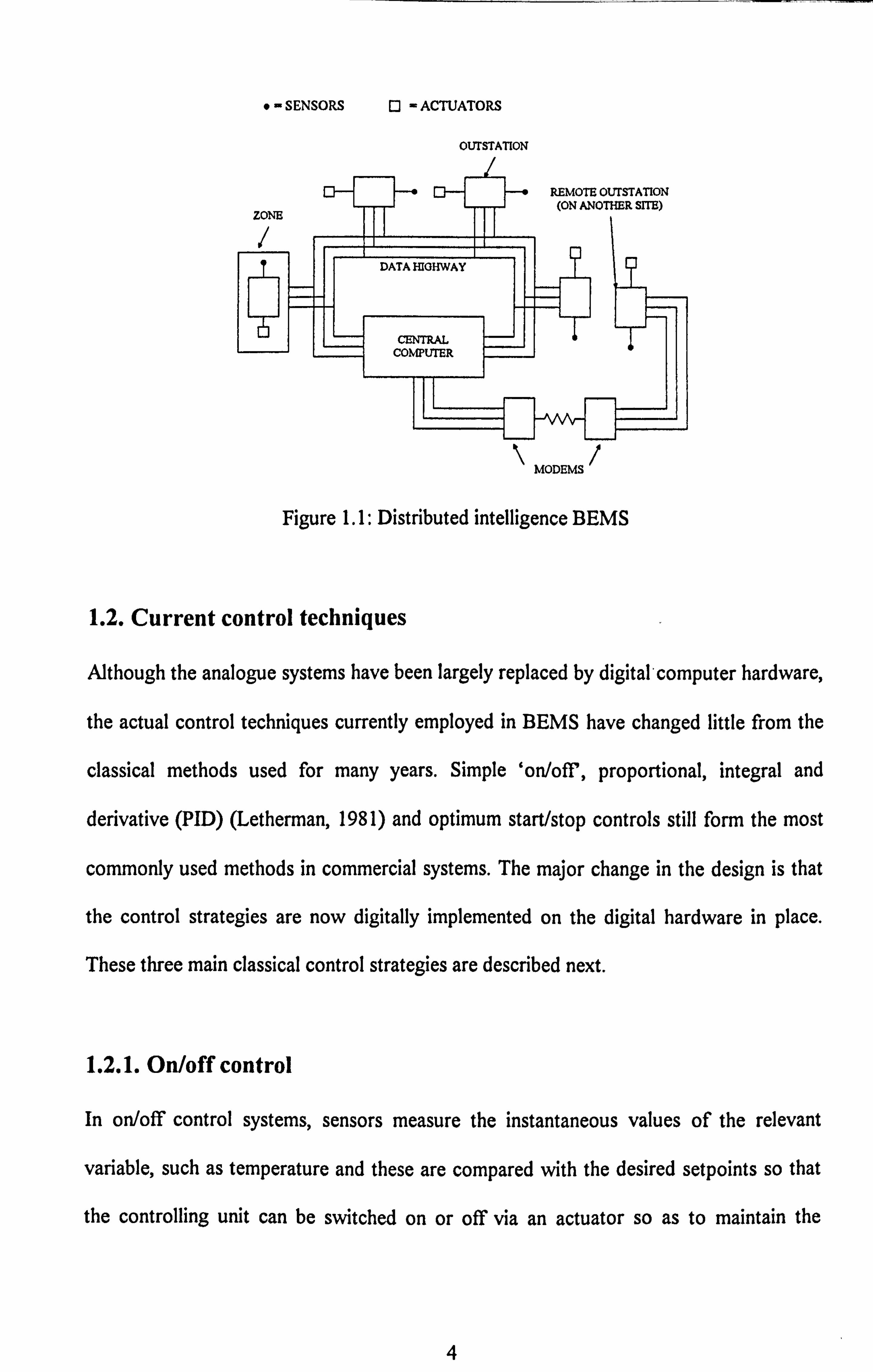
evolved into distributed intelligence systems as shown in Figure 1.1 where we can see a

number of outstations linked together to form a network which is connected to a central

supervisory computer (usually a personal computer) via a data highway. Each outstation

has its own processor to monitor and control the local zones (local loops), and the

sensor's signals are sent to a local processor which then operate the inputs and actuators

to control the operation. Sensors in these systems include thermisters to measure the

temperature, flowmeters for measuring flows of air and/or water, and rh sensors for

measuring relative humidity. The inputs and actuators consist of heaters, coolers and

humidifiers as well as dampers which regulate the flow of air in and out of the occupied

rooms. The remote outstations can be connected via modem links, if necessary, to form

larger networks for controlling large buildings and complexes.

3

"- SENSORS Q -ACTUATORS

OUTSTATION

REMOTE OUTSTATION

ZONE (ON ANOTHER SITE)

DATA HIGHWAY

CENTRAL COMPUTER

MODEMS

Figure 1.1: Distributed intelligence BEMS

1.2. Current control techniques

Although the analogue systems have been largely replaced by digital-computer hardware,

the actual control techniques currently employed in BEMS have changed little from the

classical methods used for many years. Simple 'on/off, proportional, integral and

derivative (PID) (Letherman, 1981) and optimum start/stop controls still form the most

commonly used methods in commercial systems. The major change in the design is that

the control strategies are now digitally implemented on the digital hardware in place.

These three main classical control strategies are described next.

1.2.1. On/off control

In on/off control systems, sensors measure the instantaneous values of the relevant

variable, such as temperature and these are compared with the desired setpoints so that

the controlling unit can be switched on or off via an actuator so as to maintain the

4

required conditions. In practice, the on/off strategy is implemented by having two

setpoints, one an upper and the other a lower. To explain the on/off operation we

consider a temperature regulation system, and assume that the temperature is initially

lower than both of these points. The strategy then is to keep the heater on until the

measured temperature reaches the higher limit TuPP,,, at which point the heater is

switched off; This causes the temperature to decay (normally), and when the measured

temperature reaches the lower threshold T, oWe ,,,

the heater is switched on again. This

hytheresis (T,, PP,, -TI.,, tt)

in the switching on and switching off points is useful in order to

avoid continual on/off switching of the heater or whatever the controlling device is.

1.2.2. PID control

The PID controller is also known as the three-term controller, since its output is made up

of three terms that are functions of its input; the first term is proportional to the input,

the second is proportional to the integral of the input and the third is proportional to the

derivative of the input. The function of each of these three terms can be explained by

considering a simple unity feedback closed-loop system for controlling the temperature in

a building zone, as illustrated in Figure 1.2.

Kp TEMPERATURE ACIVAL

REQUIRED ERROR

DYNAMICS ZONE

K, INTEGRATE . i. "

HEATER/ OF TEMP.

+ rEMP. COOLER BUILDING ZONE

KD DIFFERENTIATE

Figure 1.2: PID controller in a temperature control feedback loop

5

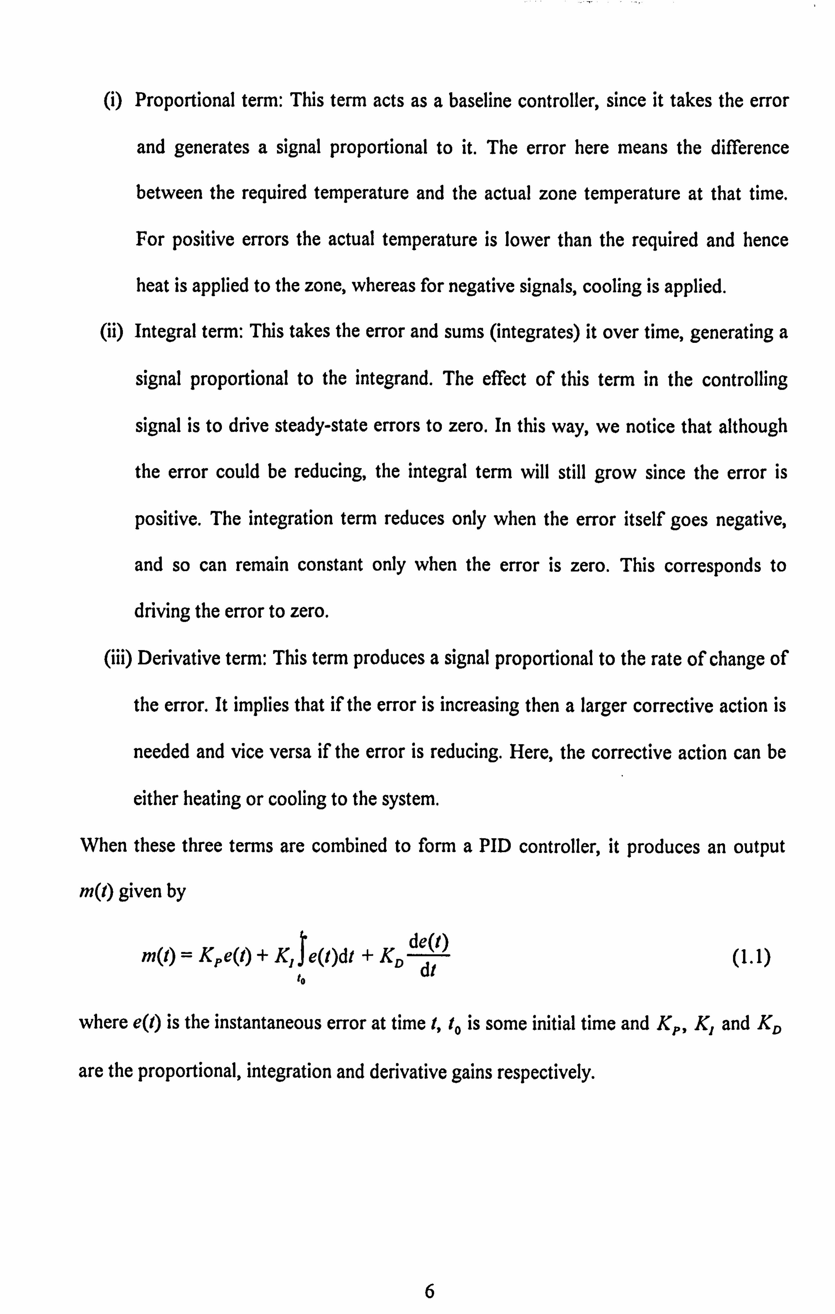
(i) Proportional term: This term acts as a baseline controller, since it takes the error

and generates a signal proportional to it. The error here means the difference

between the required temperature and the actual zone temperature at that time.

For positive errors the actual temperature is lower than the required and hence

heat is applied to the zone, whereas for negative signals, cooling is applied.

(ii) Integral term: This takes the error and sums (integrates) it over time, generating a

signal proportional to the integrand. The effect of this term in the controlling

signal is to drive steady-state errors to zero. In this way, we notice that although

the error could be reducing, the integral term will still grow since the error is

positive. The integration term reduces only when the error itself goes negative,

and so can remain constant only when the error is zero. This corresponds to

driving the error to zero.

(iii) Derivative term: This term produces a signal proportional to the rate of change of

the error. It implies that if the error is increasing then a larger corrective action is

needed and vice versa if the error is reducing. Here, the corrective action can be

either heating or cooling to the system.

When these three terms are combined to form a PID controller, it produces an output

m(l) given by

m(t) = Kpe(t) + K, 1

e(t)dt + KD de(t)

to dt (1.1)

where e(t) is the instantaneous error at time t, to is some initial time and Kp, K, and KD

are the proportional, integration and derivative gains respectively.

6

"1ý, '-11- ý-- "1-, 11 1,,, 1 -11 --II

In the commissioning phase of a BEMS, the PID controller in each zone is tuned by

performing certain tests on the zone. Such tests are to determine the settings of K,,, K,

and KD normally via a well known method due to Ziegler and Nichols (1942).

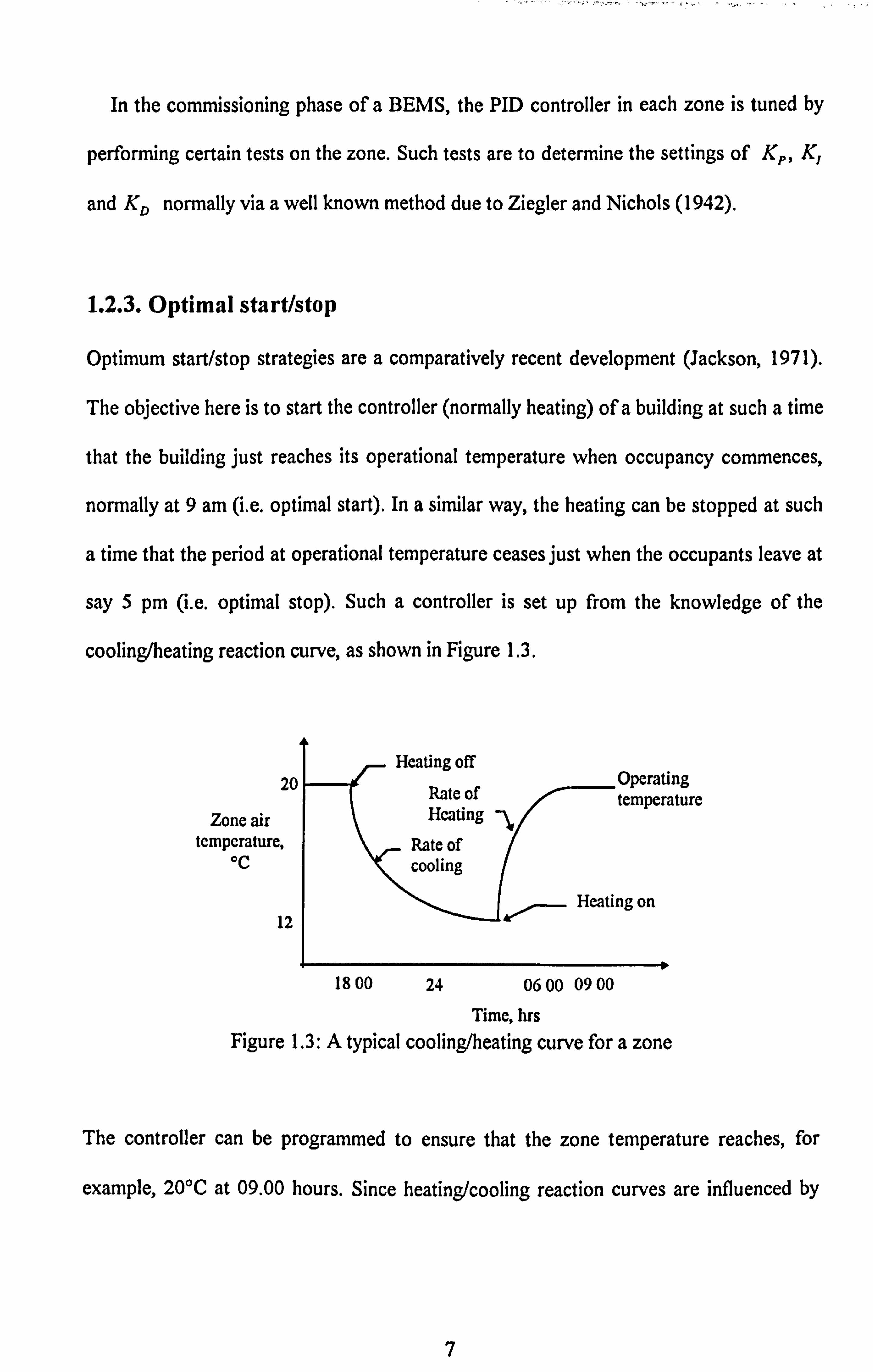
1.2.3. Optimal start/stop

Optimum start/stop strategies are a comparatively recent development (Jackson, 1971).

The objective here is to start the controller (normally heating) of a building at such a time

that the building just reaches its operational temperature when occupancy commences,

normally at 9 am (i. e. optimal start). In a similar way, the heating can be stopped at such

a time that the period at operational temperature ceases just when the occupants leave at

say 5 pm (i. e. optimal stop). Such a controller is set up from the knowledge of the

cooling/heating reaction curve, as shown in Figure 1.3.

201

Zone air temperature,

CC

12

Heating off Operating

Rate of temperature Heating

_ Rate of cooling

f- Heating on

18 00 24 06 00 09 00

Time, hrs Figure 1.3: A typical cooling/heating curve for a zone

The controller can be programmed to ensure that the zone temperature reaches, for

example, 20°C at 09.00 hours. Since heating/cooling reaction curves are influenced by

7

external temperature, some controllers have an external temperature sensor and its

relation to the plant output rate can be programmed by the user.

1.3. The current status of BEMS

The development of BEMS or BMS has been closely allied to advances in the

microelectronics technology (Rouse, 1990) and the stage has now been reached where

direct digital control (DDC) techniques have displaced analogue technology as the most

common methods for plant control in buildings. Advances in BMSs, likes other areas,

have also faced difficulties and these can be identified into three major issues (Rouse,

1990):

a) Cabling difficulties: the increased quantities of cables and data place a larger burden

on the existing methods used for ducting and networking. Optical fibre technology is

likely to offer a solution.

b) Compatibility: at present, it is not possible to interface BEMS hardware from different

manufacturers. A widespread adoption of the draft communication standard should

solve this problem; however there is not much interest for BMS manufacturers to

pursue this route.

c) Commissioning: this is an expensive and time-consuming process, Although dedicated

controllers for individual plant items are designed and configured, this still leaves the

final tuning of the control loops to be carried out on-site.

Current research might offer solutions to some of these problems, in particular that of

commissioning. For example, Haves and Dexter (1991) have been investigating the use

of simulation models to emulate the behaviour of the building/HVAC system; such

models serve as a means for laboratory testing the performance of a BMS. Similar

8

emulators have been developed at the National Institute of Standards and Technology

(NIST), USA and at Honeywell Controls, Wisconsin, USA. More recently, methods for

developing self-tuning PID controllers for HVAC systems have been receiving attention

(Dexter et at., 1990). The impact of artificial intelligence (AI), not only on

commissioning, but also on system diagnostics and data management, is also being

highlighted (Culp et al., 1990; Loveday and Virk, 1992a). However, the potential for

improvement to the control algorithms has until now received limited attention. As

already mentioned the control methods in BMS have mainly consisted of classical on/off

or PID (Ziegler and Nichols, 1942) techniques. Optimum start/stop control (Jackson,

1971; Fielden and Ede, 1982; Murdoch et al., 1990) has been recently applied in digital

form. Some fundamental prototyping of advanced controller strategies have also been

investigated; Dexter and Trewhella (1990) have looked at the use of rule-based

controllers employing fuzzy logic and its relevance to computer-based facilities

management; Ling and Dexter (1994) have used a fuzzy rule-based supervisor to

evaluate control performance and to adjust the temperature setpoint within a given

comfort band. The full potential for advanced control in buildings via a BMS still remains

to be investigated.

1.4. The potential for model-based control

The development of modelling and control techniques have traditionally been closely

coupled; the main reason for this coupling is the need for a better understanding of the

systems and processes before effective control can be designed and implemented. A

mathematical model which describes a system's dynamical behaviour can be derived

using stochastic identification techniques (see for example Ljung, 1987; Norton, 1986);

9

these are well known to many control system practitioners but have not been throughly

applied to the building services sector. This is a great shame because model-based

controls are deemed to be especially appropriate here; among the reasons for this are the

following (Virk et al., 1992 ):

(i) Buildings possess slow dynamical effects and long dead times can also be present

which give rise to large overshoots and undershoots in traditional PID controlled

systems.

(ii) Buildings are multivariable in nature, since many inputs (causes such as climatic

conditions, heat supplied and incidental gains) affect the many outputs (effects such

as temperatures, humidities, and air flow rates in many zones).

(iii) Buildings can be subject to significant stochastic disturbance effects; these include

fluctuations in occupancy levels, ventilation rate variations and climatic changes.

The model-based method has the capacity to improve the setpoint regulation as well

as reduce the energy consumption because of the ability of the model to make accurate

forecasts. Research on a laboratory-scale test system has shown that by employing a

generalised minimum variance (GMV) controller design with an off-line model the air

temperature can be regulated more effectively together with energy savings of 16% as

compared to classical PID control (Virk et al., 1990). The potential of advanced control

for the full-scale situations has also been investigated by other researchers (see for

example Zaheer-Uddin, 1990; Athienitis, 1988; Penkan, 1990; Coley and Penkan, 1992).

The main approach has been to derive the models of the air dynamics in the building

using physical reasoning, and implement a model-based control strategy to improve the

overall system performance. It is well known that a simple process model can be used for

10

in an on-line manner to tune a few parameters which are then used for control in an

adaptive manner (Penman, 1990).

In a recent SERC report, Loveday and Virk (1992b) have demonstrated that

multivariable stochastic identification techniques can be used to model a zone's thermal

and moisture behaviour in a full-scale building. The model determined in this way can be

used to accurately predict the air temperature and relative humidity in the zone over

short term (10-20 minutes) and long term (several days) time horizons. Short term

prediction errors have been shown to be well within ±0.25°C in 19°C and ±0.6%rh in 53

%rh whereas long term prediction errors have been found to be within ±0.8°C and 1.3%

rh. Such accurate predictions clearly show that the modelling approach is suitable for this

application area and that research effort should be utilised to assess the full potential of

advanced modelling and subsequent model-based solutions for the building services

sector.

1.5. Work in this thesis

The works presented in this thesis is the continuation of the efforts made by Loveday and

Virk (1992b); as mentioned earlier, they have derived a multivariable model which

accurately describes the dynamical behaviour within a typical office zone due to the

effects of a heating, cooling and humidifying plant as well as climatic disturbances and

other influences. The detailed explanation on the design and validation of this model is

presented in chapter 2. By utilising this model, we will develop several advanced control

strategies; some of these will be based on classical methods such as multi-input multi-

output proportional and integration output (MIMO P+I) controllers, others will utilise

modern mathematical modelling methods and are based on state-space and constrained

11

input adaptive controlled methods. In addition we will develop novel solutions based

upon recent intelligent methods using fuzzy logic and genetic algorithmic techniques for

humidifying, ventilating and air-conditioning applications. These methods and their

solutions designed are tested within a simulation environment to regulate the air

temperature and relative humidity form the main component in this thesis. These

simulations of the solutions designed are carried out using MATLAB.

In addition to the simulation results the designed MIMO P+I and constrained input

adaptive controllers and the fuzzy logic and GA based solutions are implemented upon

the Bradford BMS research facility to yield encouraging results in term of output

regulations and energy consumptions when compared with the commercial PI controller.

12

Chapter 2

The Simulation Environment

In this chapter the design and modelling of the office zone which is used in our studies is

described. The office zone system and it's associated equipment were built, installed and

commissioned at Loughborough University, United Kingdom, and the modelling work

was funded by the Science and Engineering Research Council (SERC) under Research

Contract GR/F/02014.

2.1. Office zone test system

In the study made by Loveday and Virk (1992b), the office zone and HVAC plant is

modelled as a3 input/2 output system subject to external disturbances/effects, as

depicted in Figure 2.1. The three inputs are the heater, cooler and humidifier, and the

two outputs are the test room air temperature and relative humidity. The external

disturbances consist of climatic effects such as external air temperature and humidity, and

solar gain and other stochastic influences include the number of occupants in the room

and the frequency of the opening and closing of the door.

13

INPUTS DISTURBANCES OUTPUTS

e. g. climate

Heating Office Zone/ Zone temperature

Cooling HVAC Zone relative humidity Humidifying

Figure 2.1: Block diagram of the Office-zone system

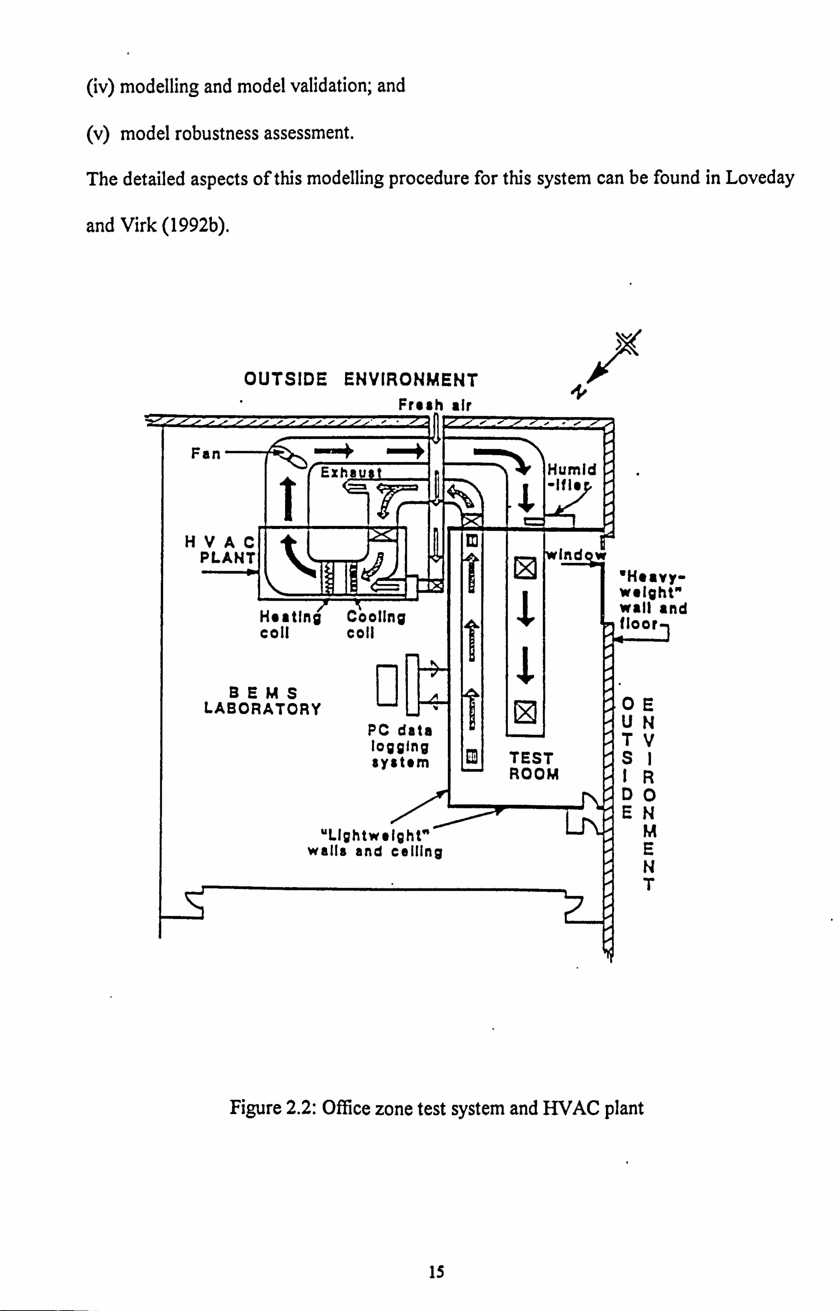
The office zone comprises a full-scale room and dedicated HVAC plant as shown in

Figure 2.2. The room, of dimensions 5.4 metres long by 3.25 metres wide by 3 metres

high, simulates an office comprising three internal walls and a fourth, outside, wall. The

latter is south-west facing and contains a small doubled-glazed window. The chamber

was equipped with a dedicated heating, ventilating and air-conditioning (HVAC) plant,

comprising cooling coils, electrical heating elements and a humidifier. The heat output, of

5kW rating, is regulated by a phase control module driven by an analogue input of 0-5

volts. The cooling unit is of conventional direct expansion type with compressor rating of

2.6kW and the control of the cooling coils is via TTL on/off logic. The humidifier unit is

of 2.7kW rating and again controlled by TTL on/off logic.

The methodology used to identify the multivariable model which describes the test

room's air temperature and moisture behaviour follows the procedure advocated by

many practitioners in this field (see for example Ljung, 1987; Norton, 1986; Virk et al,

1995). The procedure consists of the following sequential operations to be carried out on

the system in question.

(i) single input step response tests;

(ii) single input pseudo random binary sequence (PRBS) response tests;

(iii) multi-input PRBS response tests;

14

(iv) modelling and model validation; and

(v) model robustness assessment.

The detailed aspects of this modelling procedure for this system can be found in Loveday

and Virk (1992b).

OUTSIDE ENVIRONMENT

Fresh air

Fan

HVAC PLANT

H. atin Coil

BEMS LABORATORY

-4 Ethe

ýv

ti

Humid rr- 2

Ii

Cooling coil

PC data logging system

'Lightweight" walls and ceiling

m

® Ind

1 TEST ROOM

'Heavy- weight" wall and floor-,

OE UN TV S

R DO EN

M E N T

Figure 2.2: Office zone test system and HVAC plant

15

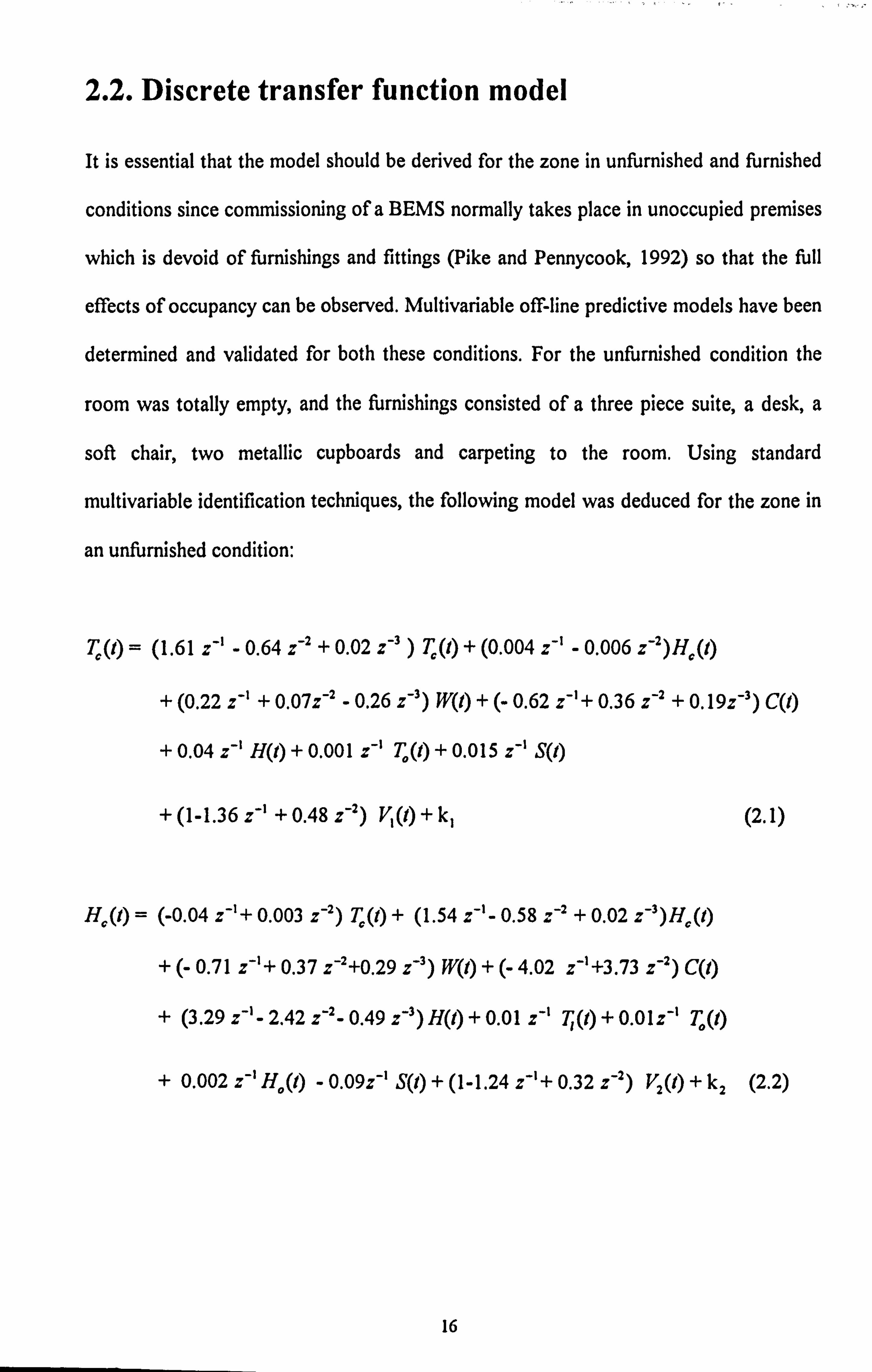
2.2. Discrete transfer function model

It is essential that the model should be derived for the zone in unfurnished and furnished

conditions since commissioning of a BEMS normally takes place in unoccupied premises

which is devoid of furnishings and fittings (Pike and Pennycook, 1992) so that the full

effects of occupancy can be observed. Multivariable off-line predictive models have been

determined and validated for both these conditions. For the unfurnished condition the

room was totally empty, and the furnishings consisted of a three piece suite, a desk, a

soft chair, two metallic cupboards and carpeting to the room. Using standard

multivariable identification techniques, the following model was deduced for the zone in

an unfurnished condition:

Tc (t) _ (1.61 z'' - 0.64 z'2 + 0.02 z'3) T (t) + (0.004 z'' - 0.006 z'2) Hý (t)

+ (0.22 z'' + 0.072-2 -0.26 z-3) W(t) + (- 0.62 z-'+ 0.36 z-Z + 0.19z-3) C(t)

+ 0.04 z'1 H(t) + 0.001 z-' To(t) + 0.015 z-' S(t)

+(1-1.36 z-' + 0.48 z-2) V1(t)+k, (2.1)

Hi(t) _ (-0.04 z"'+ 0.003 z-2) T, (t) + (1.54 z-'- 0.58 z-Z + 0.02 z-')HH(t)

+ (- 0.71 z-'+ 0.37 z-2+0.29 z-3) W(t) + (- 4.02 z-1+3.73 z'2) C(l)

+ (3.29 z-'- 2.42 z-2- 0.49 z"3) H(t) + 0.01 z"' T (t) + 0.01 z'' T, (t)

+ 0.002 z-' H, (t) - 0.09z-' S(t) + (1-1.24 z-'+ 0.32 z"2) V2(t) + k2 (2.2)

16

for t=T, 2T, 3T,.., kT, ... where T, is the office-zone air temperature in °C and Hl is

the relative humidity in %rh, T, is the temperature (in °C) of the laboratory which

surrounds the office-zone, W is the heat input rate in kW, C is the cooling input rate in

kW, H is the power input rate to produce moisture for the office-zone in kW, T. is the

outside air temperature in °C, H. is the outside air relative humidity in %rh, S is the total

solar irradiance in Wm-and V, and Vz are white noise processes to represent

unmodelled stochastic influences and k, and k2 are constants. Here, the term z is the

normal discrete operator, i. e. z-1 f(t) = f(t-T), where T is the sampling interval equal to 5

minutes.

For the furnished zone, the following model was deduced:

Ti (t) _ (1.66 z"' - 0.69 z-2+0.031 z'') T , (I) +(0.004 z-' - 0.003 z-2) He (t)

+ (0.19 z"' + 0.092'2 - 0.26 z'3) W(t) + (- 0.59 z"'+ 0.29 z-2 + 0.252-3) C(t)

+ 0.004 z-' H(t) + 0.001 z"' T, (I) + 0.021 z"' S(t)

+ (1-1.22 z'' + 0.30 z_2) Y (t) + k, (2.3)

Hc (t) = (-0.011 z'' + 0.015 z'2) Tc (t) + (-1.52 z-'+ 0.56 z'2 - 0.03 z'3) Hc (t)

+ (- 0.61 z''+ 0.16 z"2+0.34 z"3) W(t) + (- 2.89 z''+2.98 z"2) C(t)

+ (2.69 z-'- 2.37 z"2- 0.23 z-3) H(t) + 0.004 z'' T (t) + 0.006z-' T, (t)

+ 0.002 z-' Ha(t) + (1- 0.91 z-'+ 0.03 z-2) V2(t) + k2 (2.4)

Note that equations (2.1), (2.2), (2.3) and (2.4) are models for normalised values, that is,

each term has had its mean value removed. The mean value of T, H, W, C, H, T,, T,,

17

Ho and S for these equations are 17.95°C, 53.26%rh, 2.52kW, 0.91kW, 1.08kW,

20.13°C, 1.53°C, 89.19%rh and 0.05 Wm-2 respectively.

2.3. Validation of the models

Both models have been validated and for completeness, we present two simple tests to

compare the predictions from the model with data obtained through experiment. The first

test is to simulate step responses and the second is to assess setpoint regulation using the

on/off control strategy.

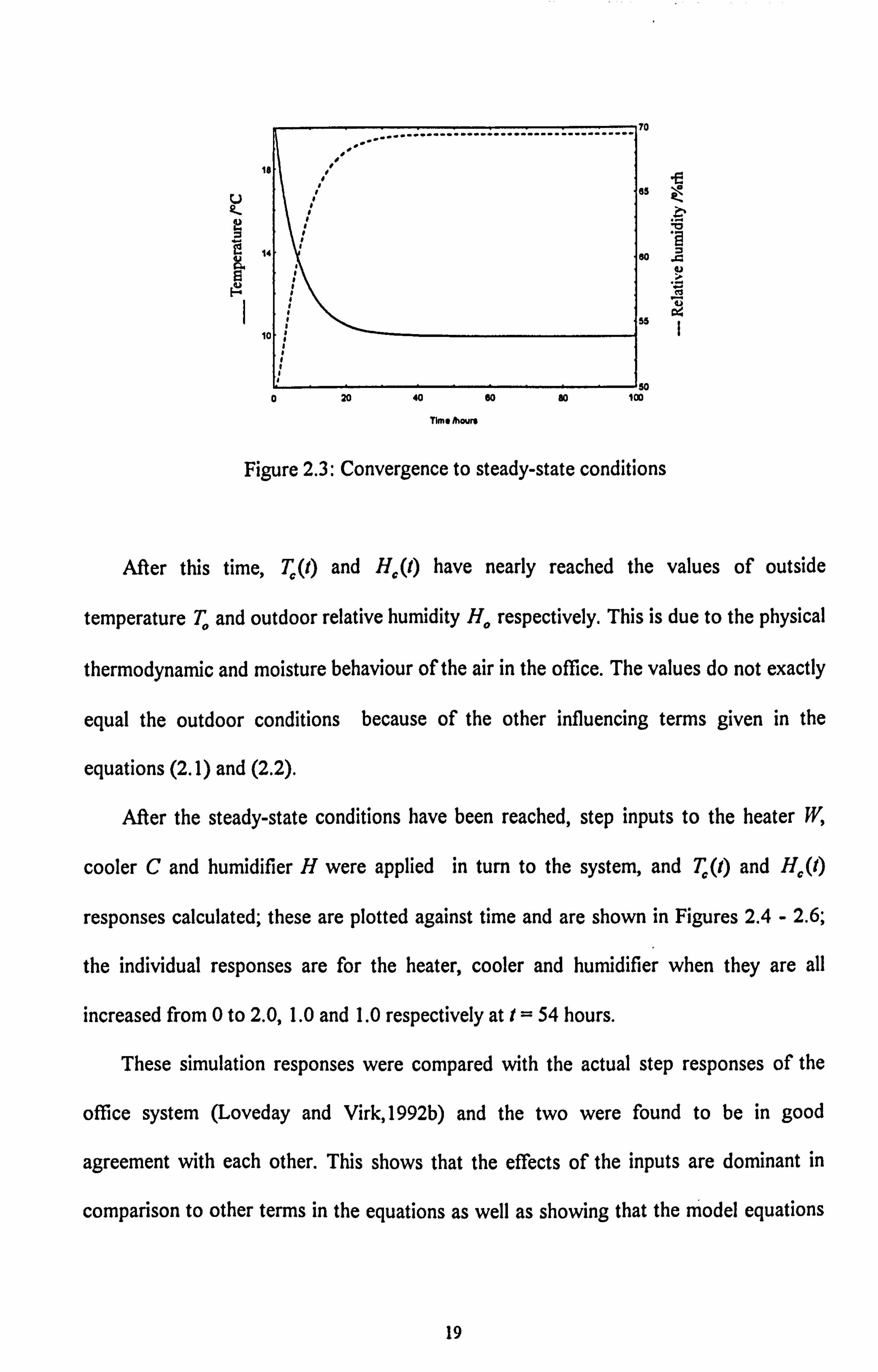
2.3.1. Step responses

Although the model relates to data obtained from the full-scale environmental chamber

operating at some state and under certain climatic influences, it can be used, to an initial

approximation, to simulate the room air temperature and relative humidity for any

arbitrary condition. Since the simulated conditions will inevitably differ from those under

which the data was collected it is necessary to let the model reach some nominal steady

state condition before the simulation is carried out. This was done by making simplifying

assumptions on the influencing terms, namely that the climatic effects T, To, H. and S

were constant at 20°C, 10°C and 70%rh, 0Wm-Z respectively and the other external

influences V, and VZ, and the control inputs were assumed to be zero. The simulated

results are shown in Figure 2.3 where it can be seen that the time needed to reach steady

state conditions is approximately 30 hours and these values are 9.9°C and 69.5%rh for

the temperature and the relative humidity respectively.

18

, U

w

L1 14

1o ;

f 0 20 40 00 00 100

Time ihoun

Figure 2.3: Convergence to steady-state conditions

t

.ý

.ý x I

After this time, T, (t) and Hi(t) have nearly reached the values of outside

temperature To and outdoor relative humidity H. respectively. This is due to the physical

thermodynamic and moisture behaviour of the air in the office. The values do not exactly

equal the outdoor conditions because of the other influencing terms given in the

equations (2.1) and (2.2).

After the steady-state conditions have been reached, step inputs to the heater W,

cooler C and humidifier H were applied in turn to the system, and T, (t) and Hi(t)

responses calculated; these are plotted against time and are shown in Figures 2.4 - 2.6;

the individual responses are for the heater, cooler and humidifier when they are all

increased from 0 to 2.0,1.0 and 1.0 respectively at t= 54 hours.

These simulation responses were compared with the actual step responses of the

office system (Loveday and Virk, 1992b) and the two were found to be in good

agreement with each other. This shows that the effects of the inputs are dominant in

comparison to other terms in the equations as well as showing that the model equations

19

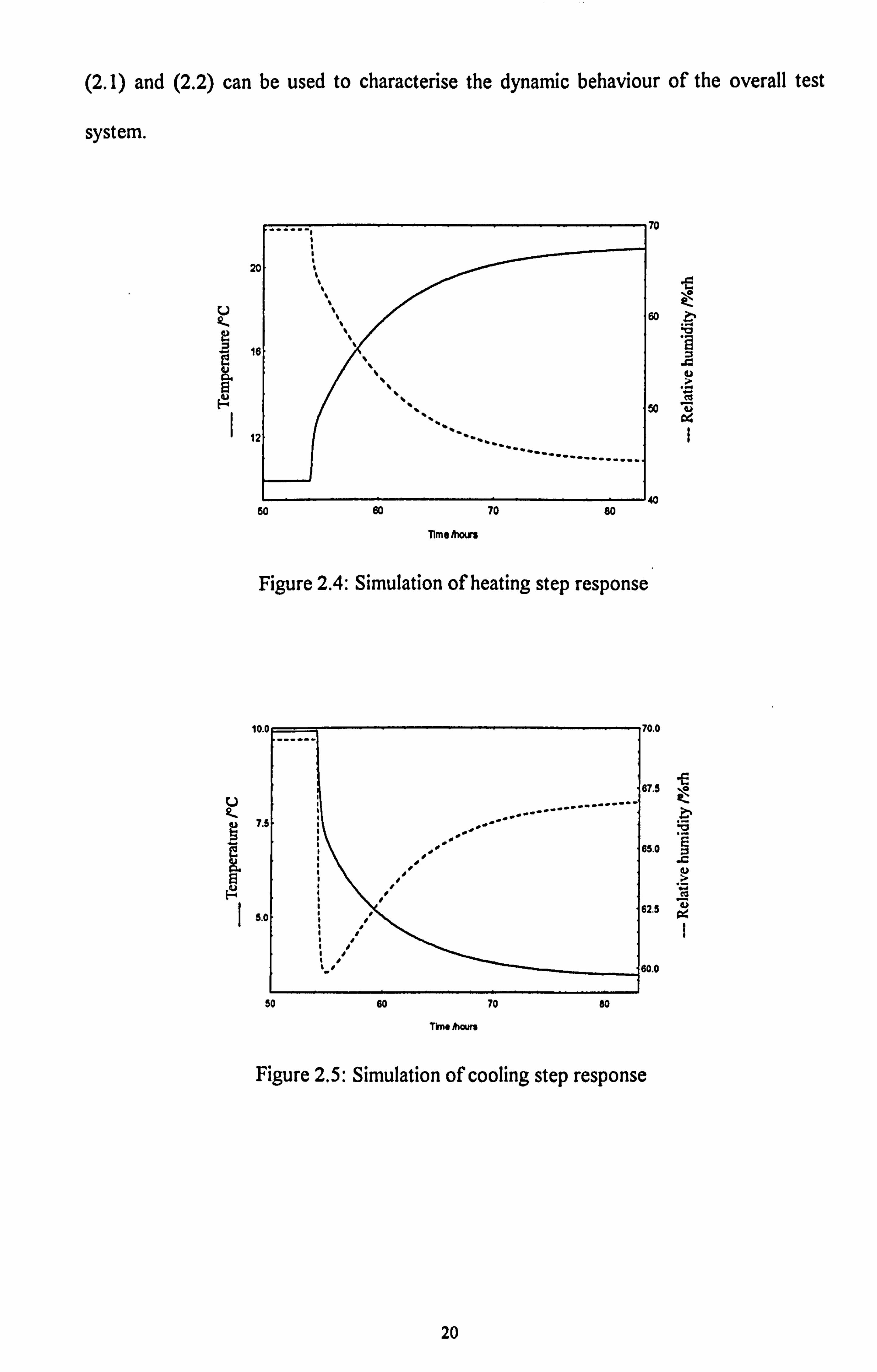
(2.1) and (2.2) can be used to characterise the dynamic behaviour of the overall test

system.

U

Eý

U

:o

50

12

v

AR

50 60 70 80

Time Awes

Figure 2.4: Simulation of heating step response

1 F, 4 07.0

i

65.0

i

S,

I.

50 60 70 60

TM. Aaun

Figure 2.5: Simulation of cooling step response

.a t

ýv .ý

u . ý, d a I

f

b

s a d x

20

U

2

d a 2 9.1

TWm Mours

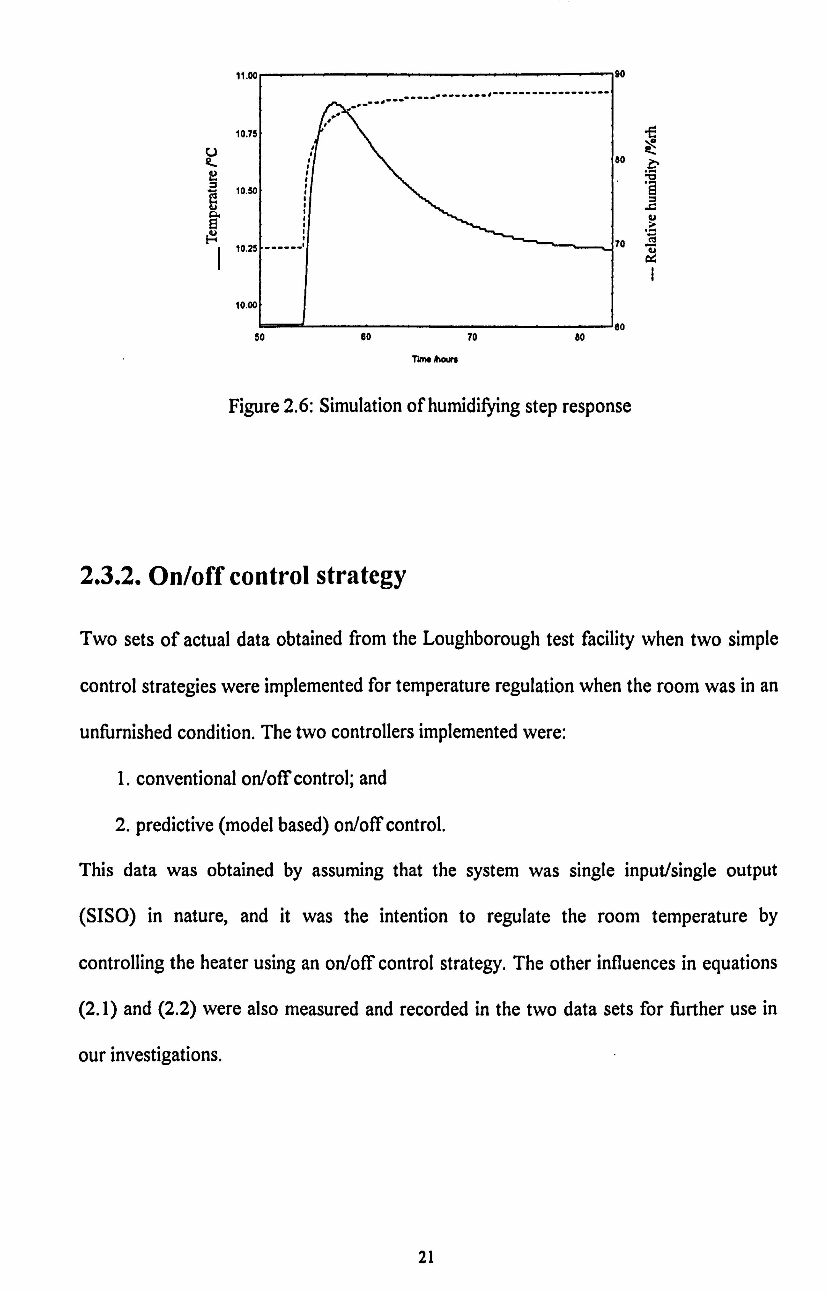
Figure 2.6: Simulation of humidifying step response

2.3.2. On/off control strategy

-fý

.ý

oG I

Two sets of actual data obtained from the Loughborough test facility when two simple

control strategies were implemented for temperature regulation when the room was in an

unfurnished condition. The two controllers implemented were:

1. conventional on/off control; and

2. predictive (model based) on/off control.

This data was obtained by assuming that the system was single input/single output

(SISO) in nature, and it was the intention to regulate the room temperature by

controlling the heater using an on/off control strategy. The other influences in equations

(2.1) and (2.2) were also measured and recorded in the two data sets for further use in

our investigations.

21

50 60 70 60

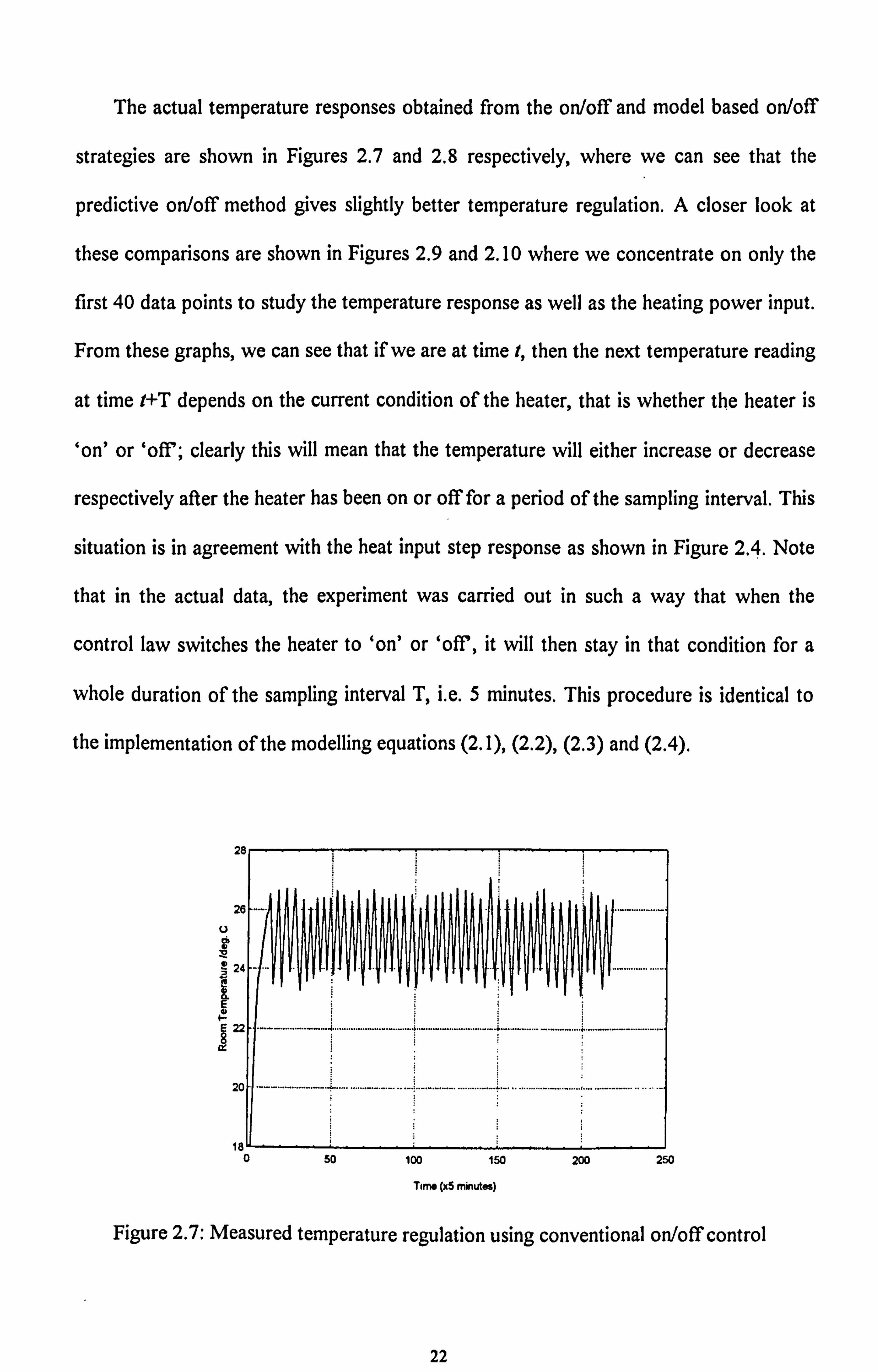
The actual temperature responses obtained from the on/off and model based on/off

strategies are shown in Figures 2.7 and 2.8 respectively, where we can see that the

predictive on/off method gives slightly better temperature regulation. A closer look at

these comparisons are shown in Figures 2.9 and 2.10 where we concentrate on only the

first 40 data points to study the temperature response as well as the heating power input.

From these graphs, we can see that if we are at time t, then the next temperature reading

at time t+T depends on the current condition of the heater, that is whether the heater is

òn' or òff; clearly this will mean that the temperature will either increase or decrease

respectively after the heater has been on or off for a period of the sampling interval. This

situation is in agreement with the heat input step response as shown in Figure 2.4. Note

that in the actual data, the experiment was carried out in such a way that when the

control law switches the heater to òn' or òff, it will then stay in that condition for a

whole duration of the sampling interval T, i. e. 5 minutes. This procedure is identical to

the implementation of the modelling equations (2.1), (2.2), (2.3) and (2.4).

U

0

E 0 E

ö

Time (x5 minutes)

Figure 2.7: Measured temperature regulation using conventional on/off control

22

0 SO 100 150 200 250

28 U

O

E 24 O

E 8

22

i{ i

{ .......................... ........... ................. +.....................

.... _. J........ _......... _. _.... _..... y..... _.... _. _. _............... ii i

i s i

ii i ij

1

Time (x5 minutes)

Figure 2.8: Measured temperature regulation using predictive on/off control

30

20 ------ .... __... .. _... _. _. _. ............... _ _. _. w...... ...... Room temperature PC ----- HepterlkW

-------------ýý -"--+ j--"" ---ter "--+ +'-+ i

0 0 10 20 30 40

Time Ix5 minutes

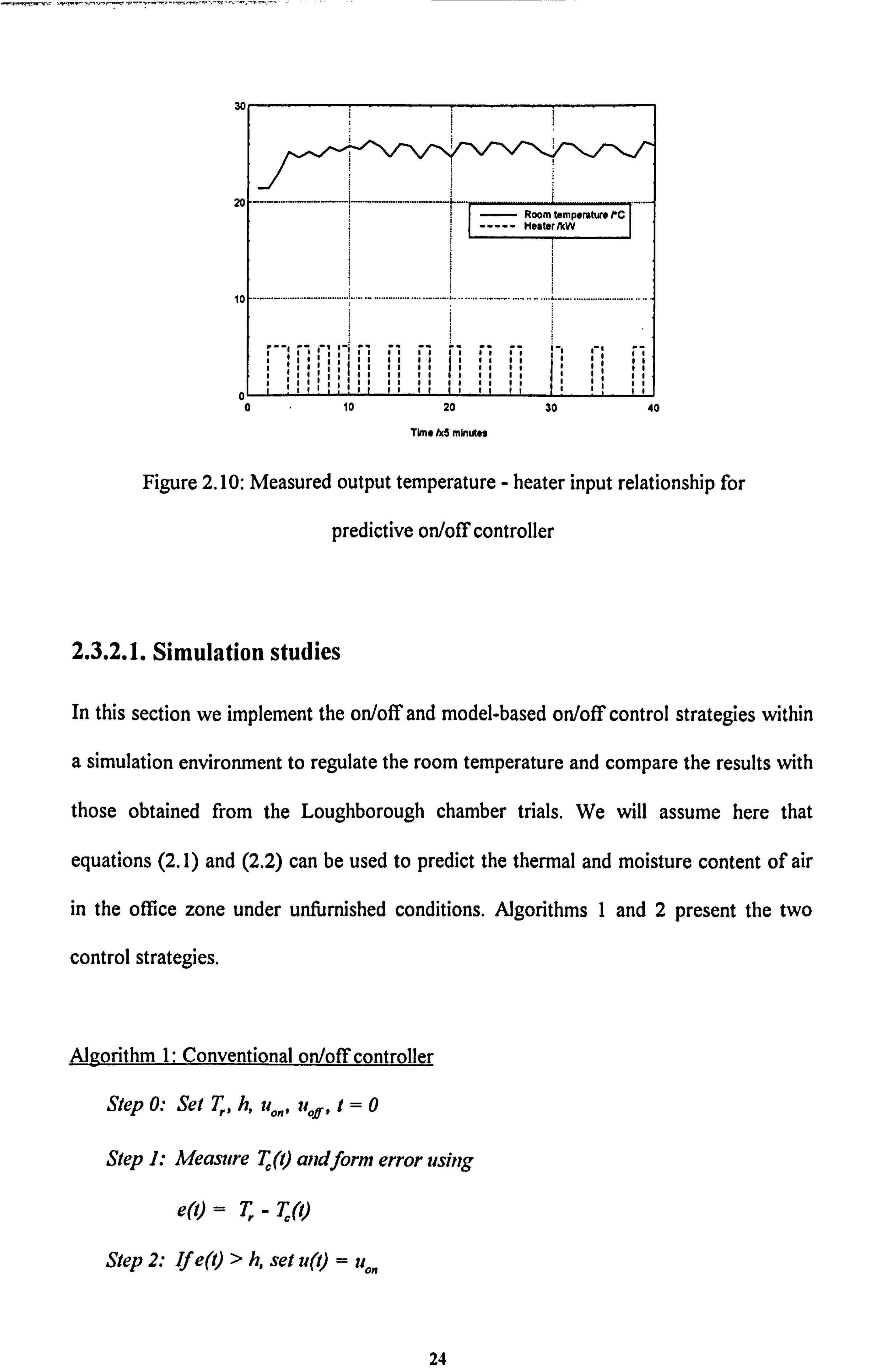
Figure 2.9: Measured output temperature - heater input relationship for

on/off controller

23

3C

20 Room temperature P

i ----- Heater AW

10 -. _. _. _.......................... i......

.__.. .. _ ............. _. _. _.:....... ..... _. _. _...... ........ ..... ....................... ....

1 ( 1 II 11 11 11 11111,1 11

11 11 1

1111I 11111 11 11

1111 1111 1 1

ý1 I1I 11 1, 1

111111111 1 1

11 111111

1 I 11 11 1 I 11 1

1I A

11 1 1111 111

0 10 20 30 40

This /x5 mfnuta

Figure 2.10: Measured output temperature - heater input relationship for

predictive on/off controller

2.3.2.1. Simulation studies

In this section we implement the on/off and model-based on/off control strategies within

a simulation environment to regulate the room temperature and compare the results with

those obtained from the Loughborough chamber trials. We will assume here that

equations (2.1) and (2.2) can be used to predict the thermal and moisture content of air

in the office zone under unfurnished conditions. Algorithms 1 and 2 present the two

control strategies.

Algorithm _1:

Conventional on/off controller

Step 0: Set T,, h, uo,,, uof., 1=0

Step 1: Measure T, (1) and form error using

e(t) = T, -T (t)

Step 2: If e(t) > h, set u(t) = ua,,

24

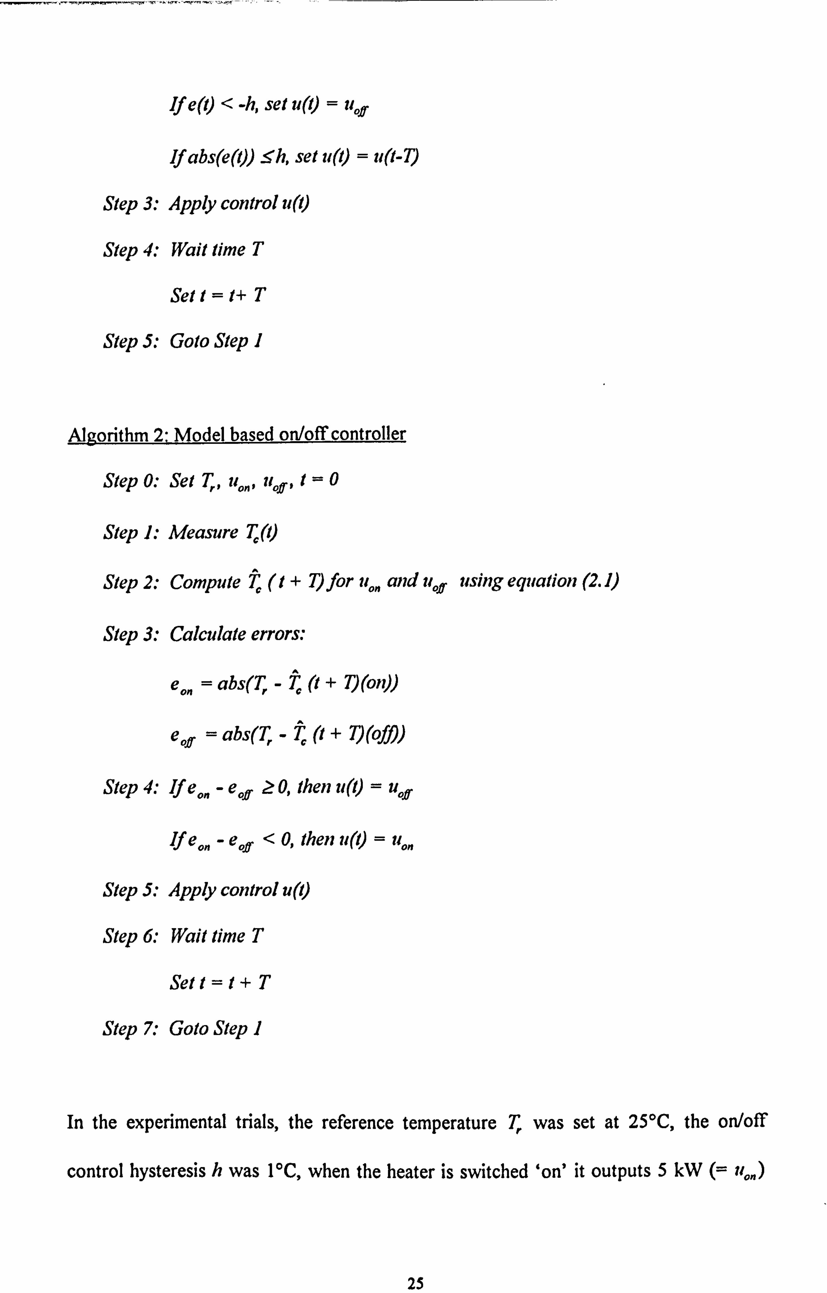
Ife(t)<-h, set u(t)=uoff

If abs(e(t)) Sh, set u(t) = u(t-T)

Step 3: Apply control u(t)

Step 4: Wait time T

Sett=t+T

Step 5: Goto Step 1

Alszorithm 2: Model based on/off controller

Step 0: Set T,, uon, u,, ff, t=0

Step 1: Measure T, (1)

Step 2: Compute T (t + T) for uo� and uoff using equation (2.1)

Step 3: Calculate errors: A

eon = abs(T, -T (t + T)(on))

eoff = abs(T, -T (t + T)(off))

Step 4: If ea� - eo8 z 0, then u(t) = uof

If e, � - eof < 0, then u(t) = uo�

Step 5: Apply control u(t)

Step 6: Wait time T

Sett=t+T

Step 7: Goto Step 1

In the experimental trials, the reference temperature T, was set at 25°C, the on/off

control hysteresis h was 1°C, when the heater is switched ̀ on' it outputs 5 kW (_ ; io�)

25

and when it is ̀ off it gives out 0 kW (= uoff) and the sampling interval T was 5 minutes.

These conditions are utilised for the simulations as well where the control law decides

whether the heater is `on' or `oif, and the test room temperature is calculated via

equations (2.1) and (2.2).

Obviously the measured temperatures in Step 1 of the algorithm need to be

modified, for the simulation runs in that these temperatures are obtained via the model,

rather than by measurement. The climatic terms in these equations are taken as these

measured during the actual conventional on/off trials. For convenience, we assume that

the white noise processes V, and Vz have the form of pseudo random binary sequences

(PRBS) (Godfrey, 1980) generated using 6 shift registers; the two levels of these PRBSs

were assumed to equal 0.25 or -0.25 thus giving V, = ±0.25°C and V2 = ±0.25%rh.

These represent 25 percent of noise level into the system as discussed by Loveday and

Virk (1992b).

For the initial conditions, we use the first 3 data points from the measured data, and

the simulation trial commences at iteration t= 4T to cater for the delayed terms in the

model's equations. A simulation program was developed and a typical simulated trial is

shown in Figure 2.11 where we can see that the overall system performance is slightly

different from those obtained via the experimental trials (Figure 2.7). This is due to the

fact that the accuracy of the model diminishes as the difference between the setpoint and

the average room temperature grows significantly large. Moreover, the air dynamics in

the room are nonlinear in nature (Loveday and Virk, 1992) but these nonlinearities are

being approximated by the linear model equations (2.1) - (2.4). Consequenctly the model

is a linearised approximation at a particular situation and model prediction will degraded

when it is used away from this operating point. In Loveday and Virk (1992b), the

26

average temperature was measured to be 19.2°C and the mean error between predicted

and measured temperatures for 25% noise level was ±0.86°C. Furthermore, the

stochastic noise levels in the actual measurements was unknown and the 25% noise level

used in the simulation environment is arbitrary. However, the result does show that the

model can approximate the real life situation quite well and therefore can be used for

determining the on/off control strategy for a real HVAC system.

28

26

U

24

a E22

20

1e, 0 50 100 150 200 250

Time (x5 minutes)

Figure 2.11: Simulated temperature regulation performance using on/off

control

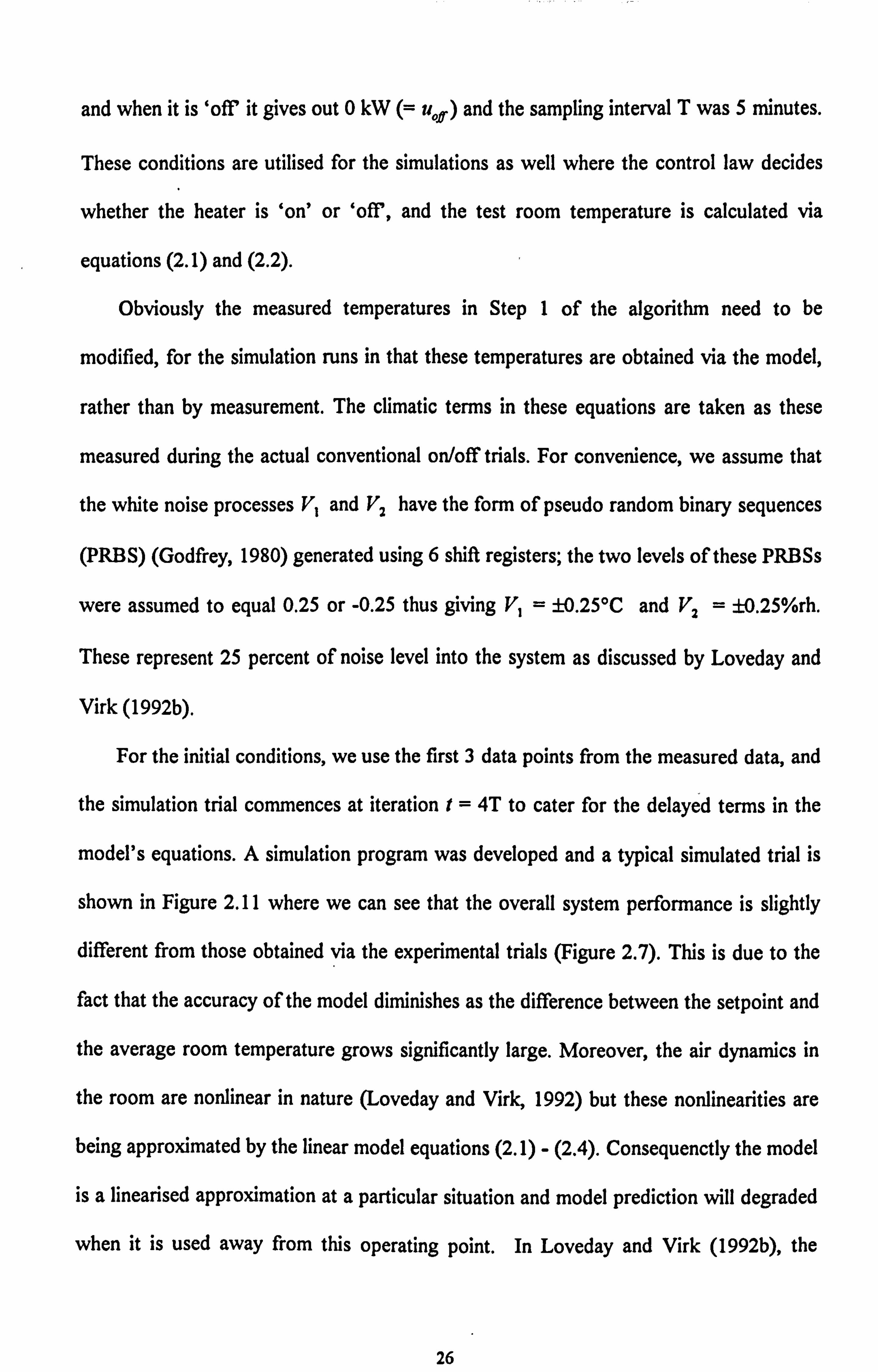
A similar approach as for the conventional on/off controller was applied for the

predictive on/off control strategy; again T , (I) is calculated via equations (2.1) and (2.2).

In Step 2, the predicted room temperature T , (l +T) is computed for the heater turned on

and off. Here, we use the model to predict the output if the heater was on (u = ua�) and if

it was off (= uoff). The input which gives a smaller error at the next sampling instant is

27

chosen and applied into the system. The climatic terms in the model equations are those

measured during the Loughborough chamber trials and similar V, and V2 processes as

applied for the conventional on/off simulations were used. The simulated results are

shown in Figure 2.12 where we can see that the control performance is again a little

different from the actual result (Figure 2.8) but there is considerable agreement; again for

the same reasons as for the standard on/off strategy.

2

U Z;

ä

23

21L 0

_I-, __ 50 100 950 200 250

Time (x5 minutes)

Figure 2.12: Simulated temperature regulation using the predictive on/off

strategy

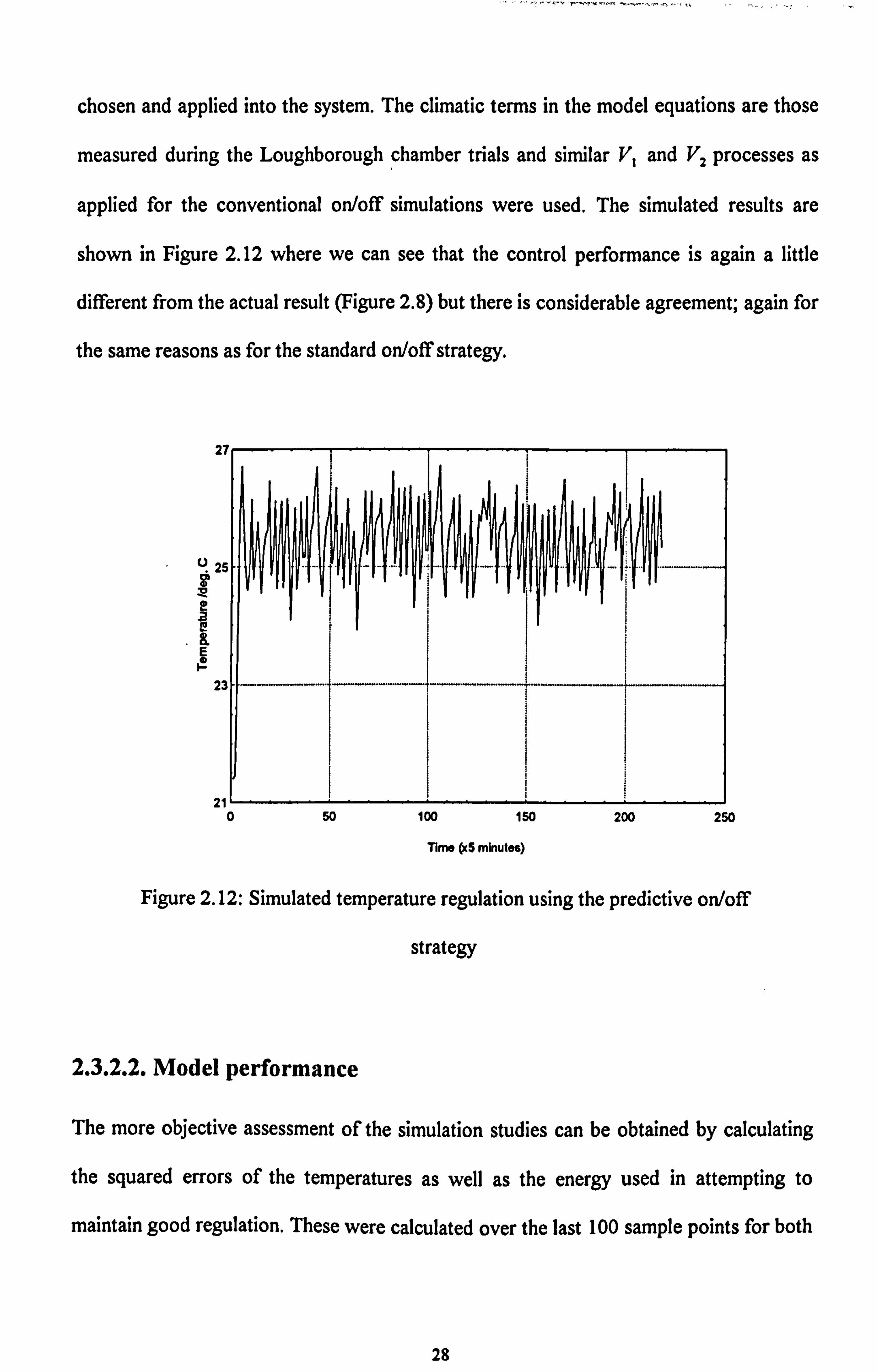
2.3.2.2. Model performance

The more objective assessment of the simulation studies can be obtained by calculating

the squared errors of the temperatures as well as the energy used in attempting to

maintain good regulation. These were calculated over the last 100 sample points for both

28

controllers and the results are summarised in Table 2.1. For an ideal case, the simulated

result via the model would be identical to the experimental results obtained through

measurements.

Table 2.1: Assessment of simulated and experimental studies

Control

strategy

Methodology Temp. errors

squared, , C2

Energy used,

kWh

Conventional Experimental 107.36 18.75

on/off Simulation 123.89 18.17

Predictive Experimental 68.79 8.75

on/off Simulation 66.61 9.58

From Table 2.1, we can see that the simulation accuracies are quite acceptable since the

regulation errors squared and the energies consumed for both control strategies

calculated via the model are similar to the actual experimental results obtained from the

Loughborough research chamber. The predictive on/off controller is superior in both the

energy used and the regulation errors hence demonstrating the value of model-based

control strategies even when very simple decision making is being carried out.

Our main conclusions here are that the performance of the unfurnished model used

in the simulations imply that it can be used quite adequately to describe the temperature

and relative humidity of the air in the test room due to heating inputs, as well as the

climatic disturbances. The model's performance due to the cooling as well as the

humidifying inputs were not analysed here because no experimental data was available

29

for comparative purposes, but the full model validation has been presented in Loveday

and Virk (1992b). This model will be used in this thesis for the application of advanced

controllers for building management systems. The furnished model (equations (2.3) and

(2.4)) are not used for this purpose because the control law for this condition will be

largely identical to that deduced using the unfurnished model. This is because both

models have similar structure and the only difference is the coefficient for each term in

the model; thus we would expect to give different magnitudes of the controller's tuning

parameters.

2.4. Conclusions

This chapter has demonstrated that the use of the model can be used to assess model-

based control strategies and the results achieved are very close to those obtained from

carrying out experimental trials on the Loughborough test chamber. In view of the

similarities we can conclude that the model can be used within a simulated environment

to develop and test new advanced control algorithms and to assess their suitability for the

BMS application area.

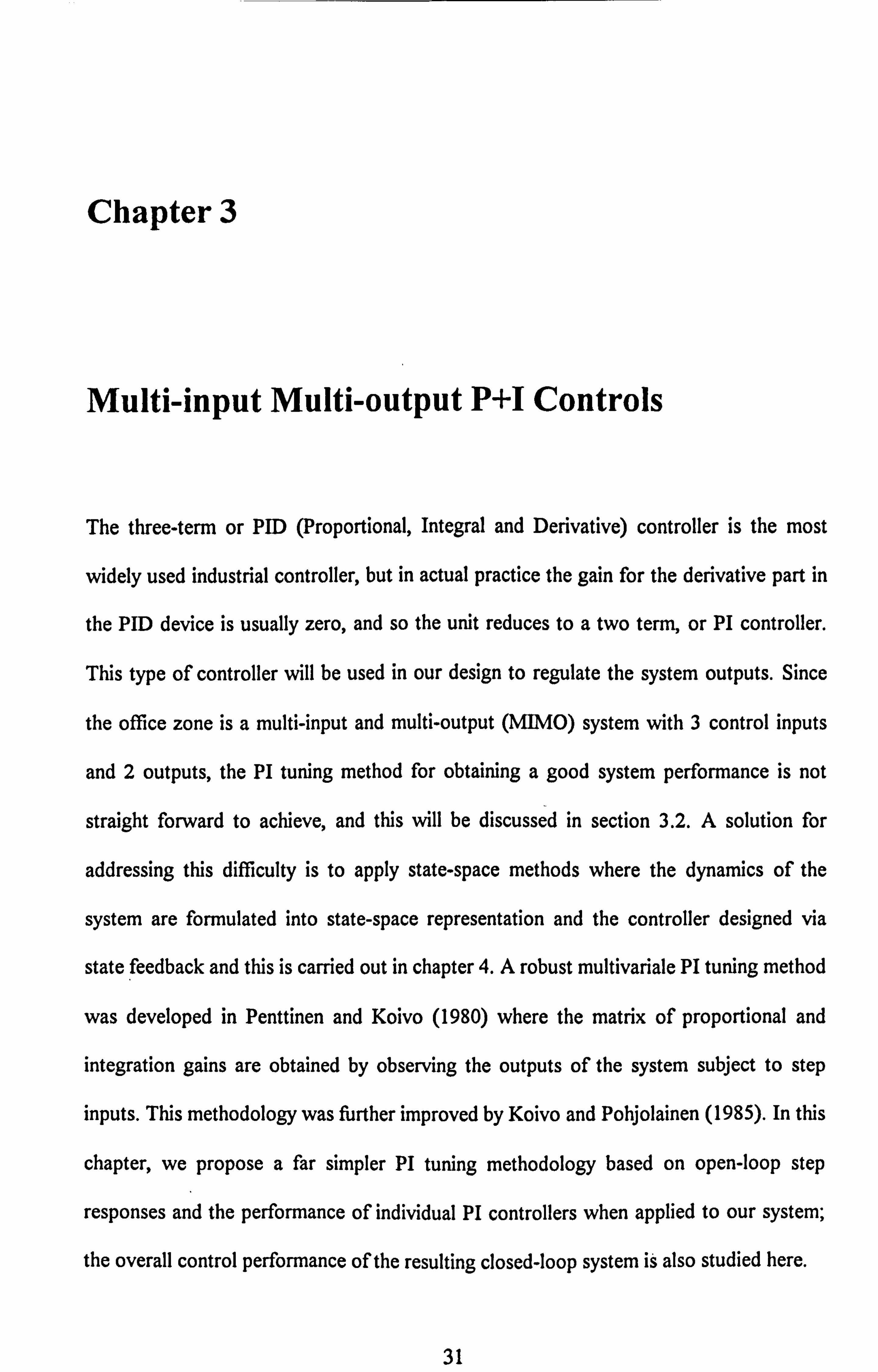
Chapter 3

Multi-input Multi-output P+I Controls

The three-term or PID (Proportional, Integral and Derivative) controller is the most

widely used industrial controller, but in actual practice the gain for the derivative part in

the PID device is usually zero, and so the unit reduces to a two term, or PI controller.

This type of controller will be used in our design to regulate the system outputs. Since

the office zone is a multi-input and multi-output (MIMO) system with 3 control inputs

and 2 outputs, the PI tuning method for obtaining a good system performance is not

straight forward to achieve, and this will be discussed in section 3.2. A solution for

addressing this difficulty is to apply state-space methods where the dynamics of the

system are formulated into state-space representation and the controller designed via

state feedback and this is carried out in chapter 4. A robust multivariale PI tuning method

was developed in Penttinen and Koivo (1980) where the matrix of proportional and

integration gains are obtained by observing the outputs of the system subject to step

inputs. This methodology was further improved by Koivo and Pohjolainen (1985). In this

chapter, we propose a far simpler PI tuning methodology based on open-loop step

responses and the performance of individual PI controllers when applied to our system;

the overall control performance of the resulting closed-loop system is also studied here.

31

Since the dynamics of building zone are described by discrete modelling equations

(2.1) and (2.2), this chapter, as well as the remainder of the thesis, will design several

types of controller using the digital format. Our discussion commences with the design of

a single PI-loop controller and this is followed by developing our multi PI-loop tuning

methodology for the HVAC/office zone system.

3.1. Single PI-loop controller

In a controlled system, we require that the system output y(t) tracks the setpoint r(t) so

that the error e(t) reduces to zero at steady-state conditions. So the aim here is to find

out the appropriate setting of the proportional, Kp, and integration, K,, gains as well as

the upper, Im, and lower, -IM, limits of the integral term so that the system output

critically follows the setpoint. A well known method for obtaining the Kp and K, is

given by the tuning rules of Ziegler and Nichols (1942) which require closed-loop and/or

open-loop step responses of the system. For the setting of 1., we must ensure that the

integral term does not grow too large thereby swamping the proportional term.

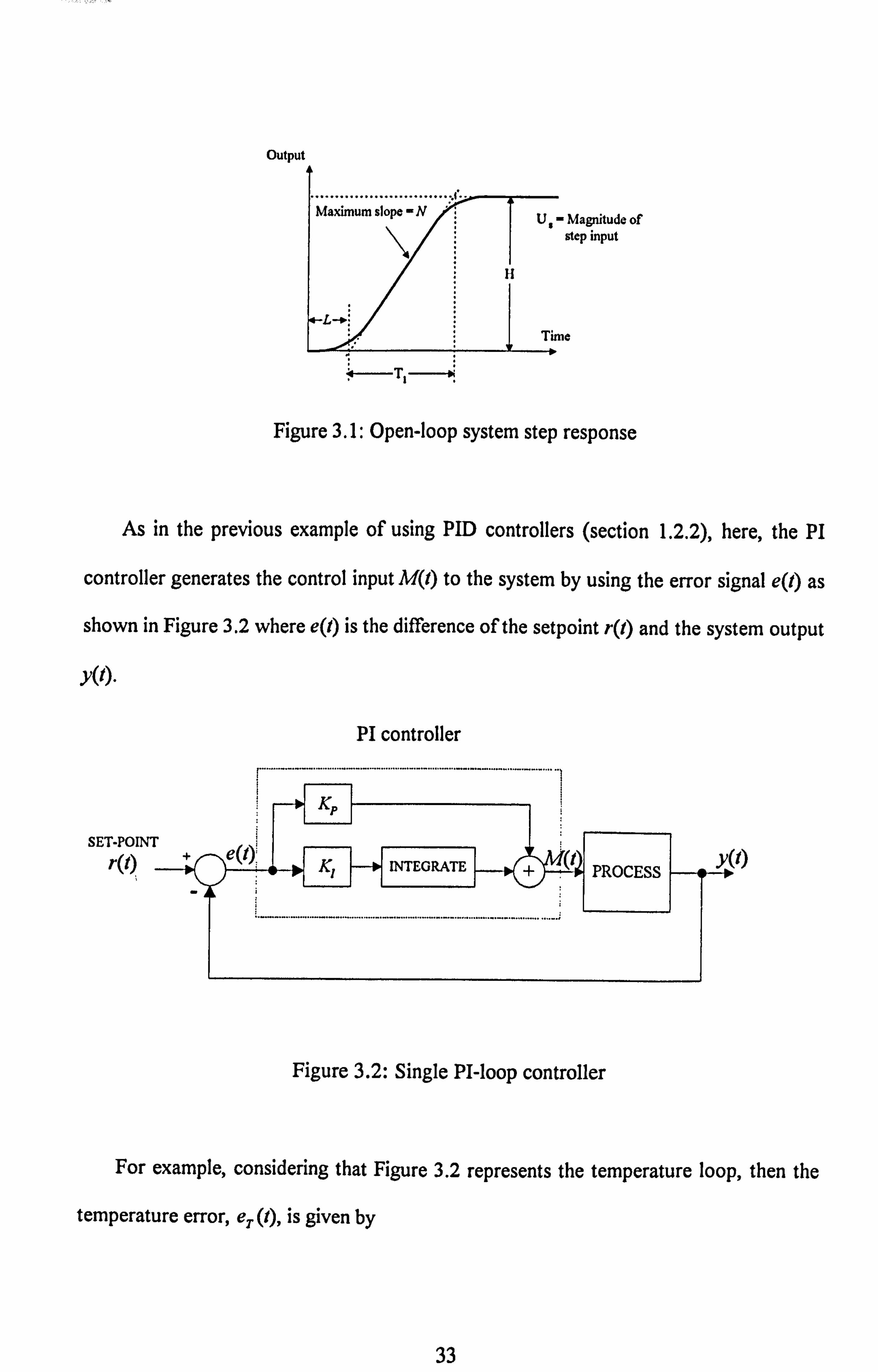
For our case, the open-loop system step response of each control input is carried out

as explained in section 2.3.1 and the PI gains are given by

K _-0.9Ü, (3.1) P NL

and

0.3Kp K, =L (3.2)

where U., N and L can be obtained from the open-loop system step response of Figures

2.4,2.5 and 2.6 and the terms are defined as in Figure 3.1.

32

Output

......................... .... Maximum slope eNU. - Magnitude of step input

H

Time

f-Tý-

Figure 3.1: Open-loop system step response

As in the previous example of using PID controllers (section 1.2.2), here, the PI

controller generates the control input M(t) to the system by using the error signal e(t) as

shown in Figure 3.2 where e(t) is the difference of the setpoint r(t) and the system output

y(t)

PI controller

SET-POINT

r(t) _

Figure 3.2: Single PI-loop controller

Y(I)

For example, considering that Figure 3.2 represents the temperature loop, then the

temperature error, e,. (1), is given by

33

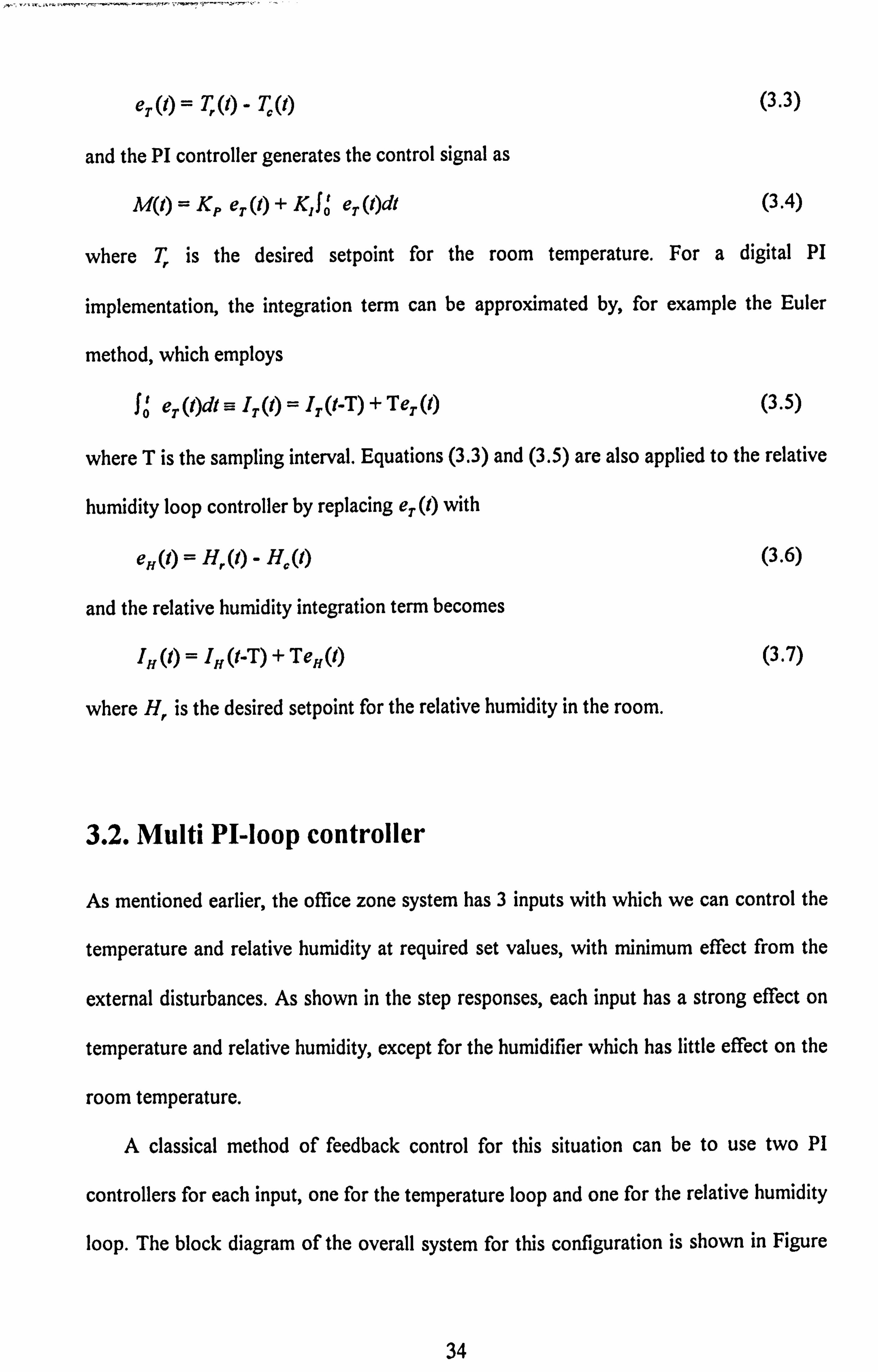
eT (t) = T, (t) - Tý (t) (3.3)

and the PI controller generates the control signal as

M(t) =Kpe,. (t) + K, jö eT (t)dt (3.4)

where T, is the desired setpoint for the room temperature. For a digital PI

implementation, the integration term can be approximated by, for example the Euler

method, which employs

ft eT (t)dt = IT (t) = IT (t-T) +Te,. (t) (3.5)

where T is the sampling interval. Equations (3.3) and (3.5) are also applied to the relative

humidity loop controller by replacing eT (1) with

elf (t) = H. (t) - H, (t)

and the relative humidity integration term becomes

1H (t) =IH (t-T)+TeH(t)

where H, is the desired setpoint for the relative humidity in the room.

3.2. Multi PI-loop controller

(3.6)

(3.7)

As mentioned earlier, the office zone system has 3 inputs with which we can control the

temperature and relative humidity at required set values, with minimum effect from the

external disturbances. As shown in the step responses, each input has a strong effect on

temperature and relative humidity, except for the humidifier which has little effect on the

room temperature.

A classical method of feedback control for this situation can be to use two PI

controllers for each input, one for the temperature loop and one for the relative humidity

loop. The block diagram of the overall system for this configuration is shown in Figure

34

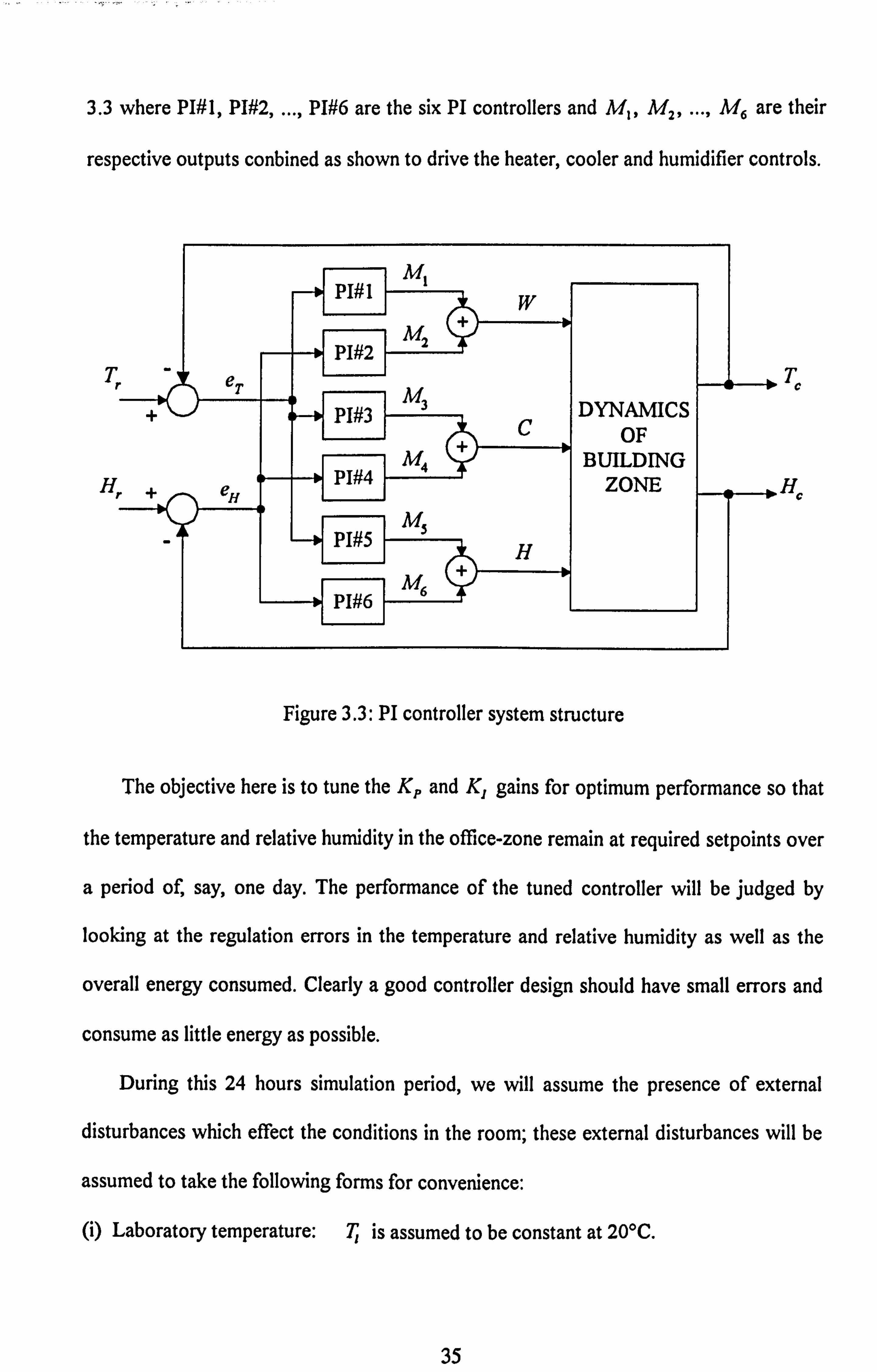
3.3 where PI#1, PI#2, ..., PI#6 are the six PI controllers and Ml, M2, ..., M6 are their

respective outputs conbined as shown to drive the heater, cooler and humidifier controls.

Tr

+

H, +

M1 PI# 1 W 4

M+ 2 PI#2 _ eT Tc

M 3 PI#3 DYNAMICS OF

M4 + BUILDING

eH PI#4 ZONE H,

MS PI#S H

6 M PI#6

Figure 3.3: PI controller system structure

The objective here is to tune the Kp and K, gains for optimum performance so that

the temperature and relative humidity in the office-zone remain at required setpoints over

a period of, say, one day. The performance of the tuned controller will be judged by

looking at the regulation errors in the temperature and relative humidity as well as the

overall energy consumed. Clearly a good controller design should have small errors and

consume as little energy as possible.

During this 24 hours simulation period, we will assume the presence of external

disturbances which effect the conditions in the room; these external disturbances will be

assumed to take the following forms for convenience:

(i) Laboratory temperature: T is assumed to be constant at 20°C.

35

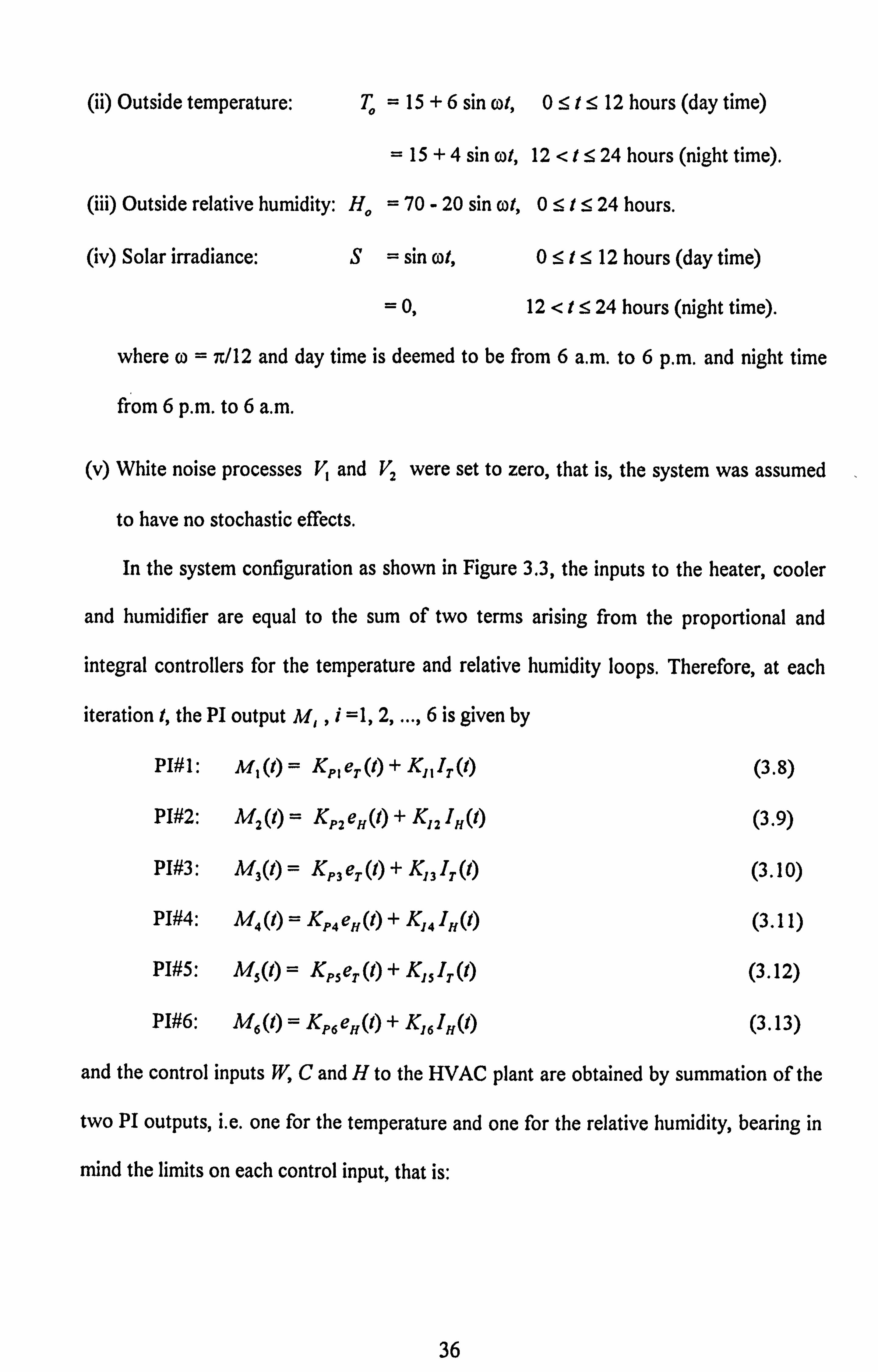
(ii) Outside temperature: T. = 15 +6 sin cot, 051: 5 12 hours (day time)

= 15 +4 sin wt, 12 < t: 5 24 hours (night time).

(iii) Outside relative humidity: H,, = 70 - 20 sin cot, 0S1: 5 24 hours.

(iv) Solar irradiance: S= sin cot, 0 <_ 1: 9 12 hours (day time)

= 0,12 <tS 24 hours (night time).

where co = 7/12 and day time is deemed to be from 6 a. m. to 6 p. m. and night time

from 6 p. m. to 6 a. m.

(v) White noise processes V, and VZ were set to zero, that is, the system was assumed

to have no stochastic effects.

In the system configuration as shown in Figure 3,3, the inputs to the heater, cooler

and humidifier are equal to the sum of two terms arising from the proportional and

integral controllers for the temperature and relative humidity loops. Therefore, at each

iteration t, the PI output M, ,i =1,2,..., 6 is given by

PI#1: M, (t) = KP, er (t) + K,, Ir (t) (3.8)

PI#2: M2(1) = Kp2e1, (1) +K12 IH(1) (3.9)

PI#3: M3(t) = KP3 er (1) + K, 3 IT (t) (3.10)

PI#4: M4 Q) = KP4ee(t) + K, 4IN(t) (3.11)

PI#5: M5(t) = Kpser(1) + K, slr(') (3.12)

PI#6: M6(t) = KP6e1(t) + K, 61H(t) (3.13)

and the control inputs W, C and H to the HVAC plant are obtained by summation of the

two PI outputs, i. e. one for the temperature and one for the relative humidity, bearing in

mind the limits on each control input, that is:

36

Heater: WO)" M, (t) + M2 (t), 05 W(t) S 5.0

Cooler: C(t) = M3(t) + M4(t), 05 C(t) 5 2.7

Humidifier: H(t) = M5(t) + M6(t), 0: 5 H(t) 5 2.6

(3.14)

(3.15)

(3.16)

The Ziegler and Nichols (1942) tuning rules were followed using the open loop

system step responses and applied to the system; however it was found that these tuning

rules lead to poor control as shown in Figure 3.4, where we have assumed setpoints of

25°C and 50%rh for the temperature and relative humidity respectively. In the simulation

of step responses, we assume that the climatic disturbances T,, To, H. and S are constant

at 20°C, 10°C and 70%rh and OWm'Z respectively and the stochastic effects V, and V2

are zero.

Homer IkW "--" CeeNr MW

Hum' IIf kW

3

jýlý li IIIýt

=4I IIII

iýIýý!

II (II ýIý{t

Ilj I

I: 11: I ý' hlt

II I1 I' I Ilf

oI 0 100 200 200

Tlm1 b6m0 a. s

60

C 100 200 300

TIP* he mW,, Hs

a) Control inputs b) System outputs

Figure 3.4: Performance of 6 PIs tuned via the standard Ziegler-Nichols

method (no noise)

37

I

100 700

T- &S . 0.. m

PI #1

300 0

I F

-x

I

-L 0 100 700 700 0 100 }00 000

Twýý h6 ýnln T-. hS wnht

PI#3 PI#4

I I I

0 100 700 X00 0 100 700 0I

T-MS. 0l T-hS wýuN

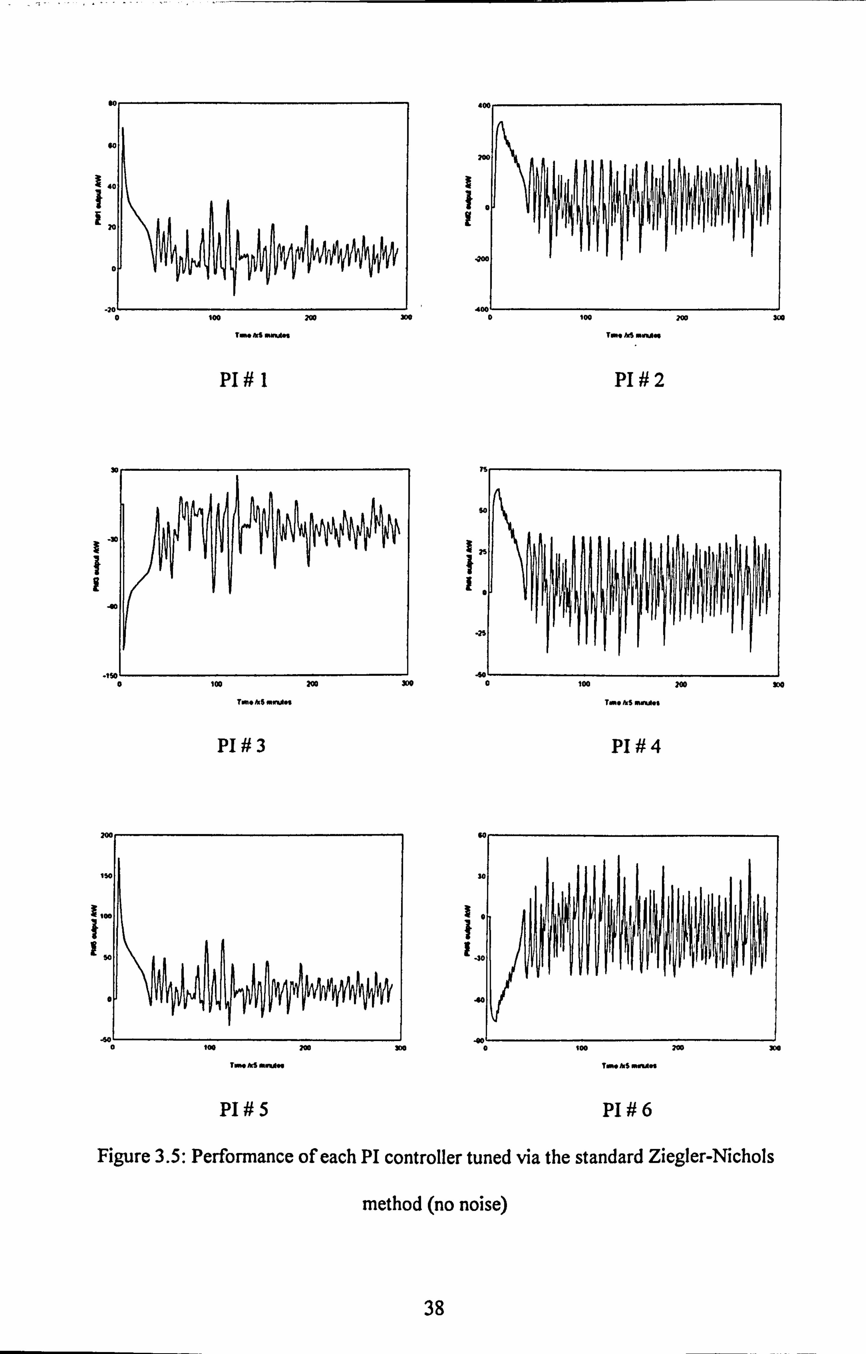
PI#5 PI#6

Figure 3.5: Performance of each PI controller tuned via the standard Ziegler-Nichols

method (no noise)

38

o +oo )oo wo

Twn M -AM

PI #2

PI

Controller

N

(°C/h)

L

(h)

U:

(kW)

Kp

(kW/°C)

K,

(kW/°C_h)

PI#1 6.16 0.038 1.250 4.81 38.0

PI#3 -5.27 0.017 0.675 -6.78 -119.7

PI#5 0.71 0.060 0.650 6.83 34.1

a). Temperature loop

PI

Controller

N

(%rh/h)

L

(h)

U.

(kW)

Kp

(kW/%rh)

K,

(kW/%rh_h)

PI#2 -11.20 0.017 1.250 -5.91 -104.2

PI#4 -33.90 0.017 0.675 -1.10 -19.4

PI#6 25.78 0.017 0.650 1.33 23.5

b). Relative humidity loop

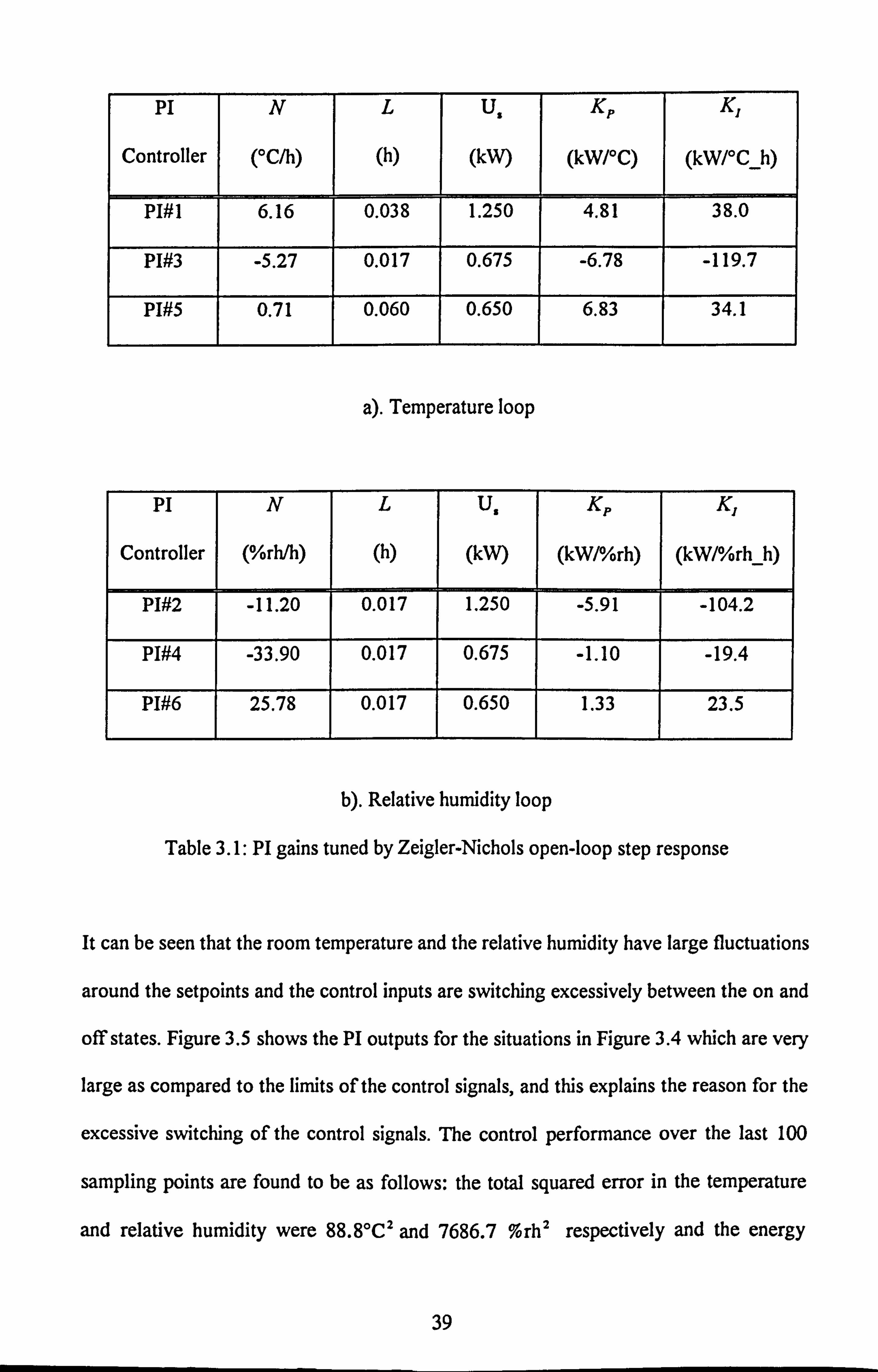
Table 3.1: PI gains tuned by Zeigler-Nichols open-loop step response

It can be seen that the room temperature and the relative humidity have large fluctuations

around the setpoints and the control inputs are switching excessively between the on and

off states. Figure 3.5 shows the PI outputs for the situations in Figure 3.4 which are very

large as compared to the limits of the control signals, and this explains the reason for the

excessive switching of the control signals. The control performance over the last 100

sampling points are found to be as follows: the total squared error in the temperature

and relative humidity were 88.8°C2 and 7686.7 %rh2 respectively and the energy

39

consumed by the heater, cooler, and humidifier were 29.8,5.9 and 11.7 kWh

respectively.

Here, the Kp and K, values of each loop for the three control inputs were obtained

from equations (3.1) and (3.2) respectively by using the data from the individual step

responses by increasing the controlled inputs from 50% to 75% of their maximum

powers; the values are given in Table 3.1. The PI controllers obtained in this way lead to

the poor performance shown in Figure 3.4 because the system is essentially multivariable

in nature whereas the traditional Ziegler-Nichols method applies only to single

input/single output systems. In other words, the Kp and KI values given by the Ziegler-

Nichols method is only valid if all the loops are independent of each other and do not

apply to the multivariable case. In view of this it was decided to investigate an interactive

methodology for tuning the PI gains in the multivariable situation so that the resulting

controllers can yield better performances. However, we found that developing a

multivariable PI loop tuning proved extremely difficult and the results were not

acceptable due to large control input switchings. In view of this a more simpler detuning

methodology to modify the Ziegler-Nichols gain was investigated and developed for the

MIMO case. This is discussed next.

3.3. Multi PI-loop tuning methodology Since our system has three control inputs, namely the heater, cooler and humidifier, and

two outputs, namely the room temperature and the relative humidity, with the PI control

structure as shown in Figure 3.3, then the tuning procedure which is suitable to our setup

needs be developed so that the interaction effects are included in the tuning.

40

As shown in Figures 3.4 and 3.5, the PI output swings are very large as compared to

their respective control limits but the controHer is still able to regulate the air temperature

and relative humidity in the room at their setpoints. This means that the Zeigler-Nichols

tuning methodology is applicable in this multivariale system but it needs modification to

improve the output regulations. It is straight forward to deduce that the large controller

switchings are due to the large Ziegler-Nichols K. and K, gains for this system and

thus, it indicates that a methodology should be developed to reduce these gains. Clearly,

for a good control system, the output of individual PI controllers should not exceed the

permitted control limit, namely, the output of the controllers PI#I and PI#2, PIO and

1`194, and PI#5 and PI#6 should be regulating in the range of the heater, cooler and

humidifier control limits respectively without any constraints implemented during the

process controls. Based on these facts, we propose a simple method to recalculate the PI

gains to improve the results obtained via Ziegler-Nichols methodology for this

multivariable system and the method is given as follows:

First of all, we reduce the average individual PI output swings to within its control

limit. This is done by reducing the output of controllers P191 and PI#2 to the range

of 0-5 kW since they apply to the heater. Similarly, PIO and PI#4 outputs are

reduced to 0-2.7 W, and PI#5 and PI#6 outputs to 0-2.6 kW since they control

the cooler and humidifier respectively. These reduction factors, of dimensionless

units and positive sign, can be obtained by dividing the control limit with the average

PI output swing at steady state condition of the individual PI controller and are used

to modify the gains Kp and K, so that the PI outputs fall into the control limits. The

average PI output swings can be graphically estimated from Figure 3.5 and the

modified PI gains, namely, KpM and K. are calculated by multiplying the Ziegler-

Nichols PI gains Kp and K, with their respective reduction factors.

The results are summarised in Table 3.2. As an example, let us calculate the modified

Ziegler-Nichols gains, KFM and K. for controller PI#1. The reduction gain equals the

heater limit (5 kW) divided by the averaged PI#1 output swing (20 kW) at steady state

condition which is equal to 0.25. Then, applying the above method, we calculate:

KPM = Kp x 0.25 = 1.2 kW/°C and Klm = K, x 0.25 = 9.8 kW/°C h.

A similar calculation can be performed to the remaining PI gains in the system in order to

obtain their modified Ziegler-Nichols (Z-N) gains.

PI Ziegler-Nichols Average Reduction Modified Z-N

Controller Kp

(kW/°C)

Kf

(kW/°C_h)

output

swing (kW)

factor KPM

(kW/°C)

K

(kW/°C_h)

PI#1 4.81 38.0 20 0.2500 1.20 9.8

PI#3 -6.78 -119.7 40 0.0675 -0.46 -8.1

PI#5 13.73 68.7 40 0.0650 0.89 4.5

a) Temperature loop

PI Ziegler-Nichols Average Reduction Modified Z-N

Controller Kp

(kW/%rh)

K,

(kW/%rh_h)

output

swing (kW)

factor KFM

(kW/%rh)

KIM

(kW/%rh_h)

PI#2 -5.91 -104.2 350 0.0140 -0.08 -1.5

PI#4 -1.10 -19.4 70 0.0386 -0.04 -0.75

PI#6 1.33 23.5 70 0.0371 0.05 0.87

b) Relative humidity loop

Table 3.2: Modified Zeigler-Nichols PI gains

3.3.1. Simulation results

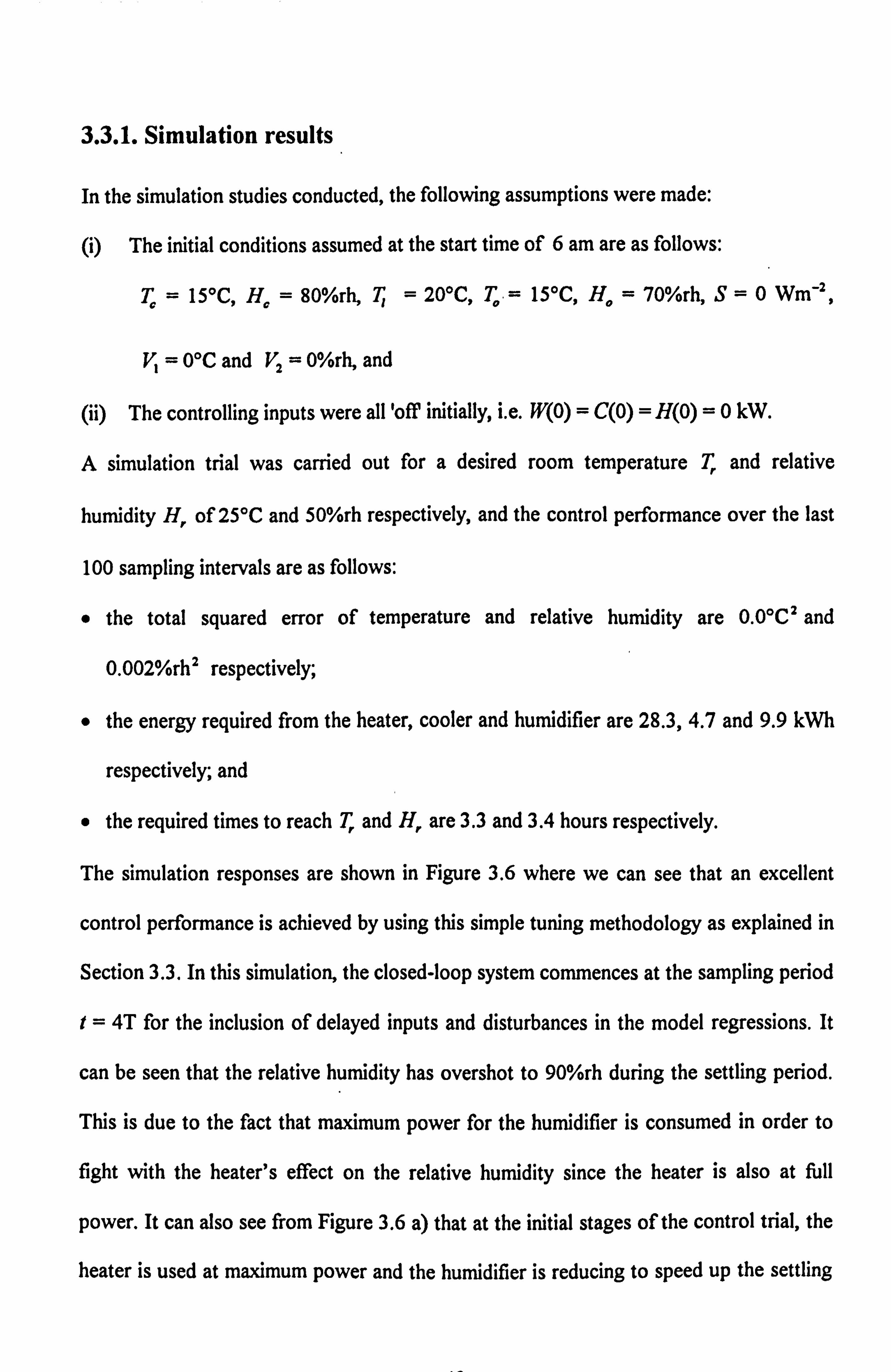
In the simulation studies conducted, the following assumptions were made:

(i) The initial conditions assumed at the start time of 6 am are as follows:

, T0 = 15°C, H0 = 80%rh, T= 20°C, T.. = 15°C, H. = 70%rh, S=0 WM-2

V. = 0°C and YZ = O%rh, and

(ii) The controlling inputs were all 'off initially, i. e. W(O) = C(O) = H(O) =0 kW.

A simulation trial was carried out for a desired room temperature T, and relative

humidity H, of 25°C and 50%rh respectively, and the control performance over the last

100 sampling intervals are as follows:

" the total squared error of temperature and relative humidity are 0.0°C2 and

0.002%rh2 respectively;

" the energy required from the heater, cooler and humidifier are 28.3,4.7 and 9.9 kWh

respectively; and

" the required times to reach T, and H, are 3.3 and 3.4 hours respectively.

The simulation responses are shown in Figure 3.6 where we can see that an excellent

control performance is achieved by using this simple tuning methodology as explained in

Section 3.3. In this simulation, the closed-loop system commences at the sampling period

t= 4T for the inclusion of delayed inputs and disturbances in the model regressions. It

can be seen that the relative humidity has overshot to 90%rh during the settling period.

This is due to the fact that maximum power for the humidifier is consumed in order to

fight with the heater's effect on the relative humidity since the heater is also at full

power. It can also see from Figure 3.6 a) that at the initial stages of the control trial, the

heater is used at maximum power and the humidifier is reducing to speed up the settling

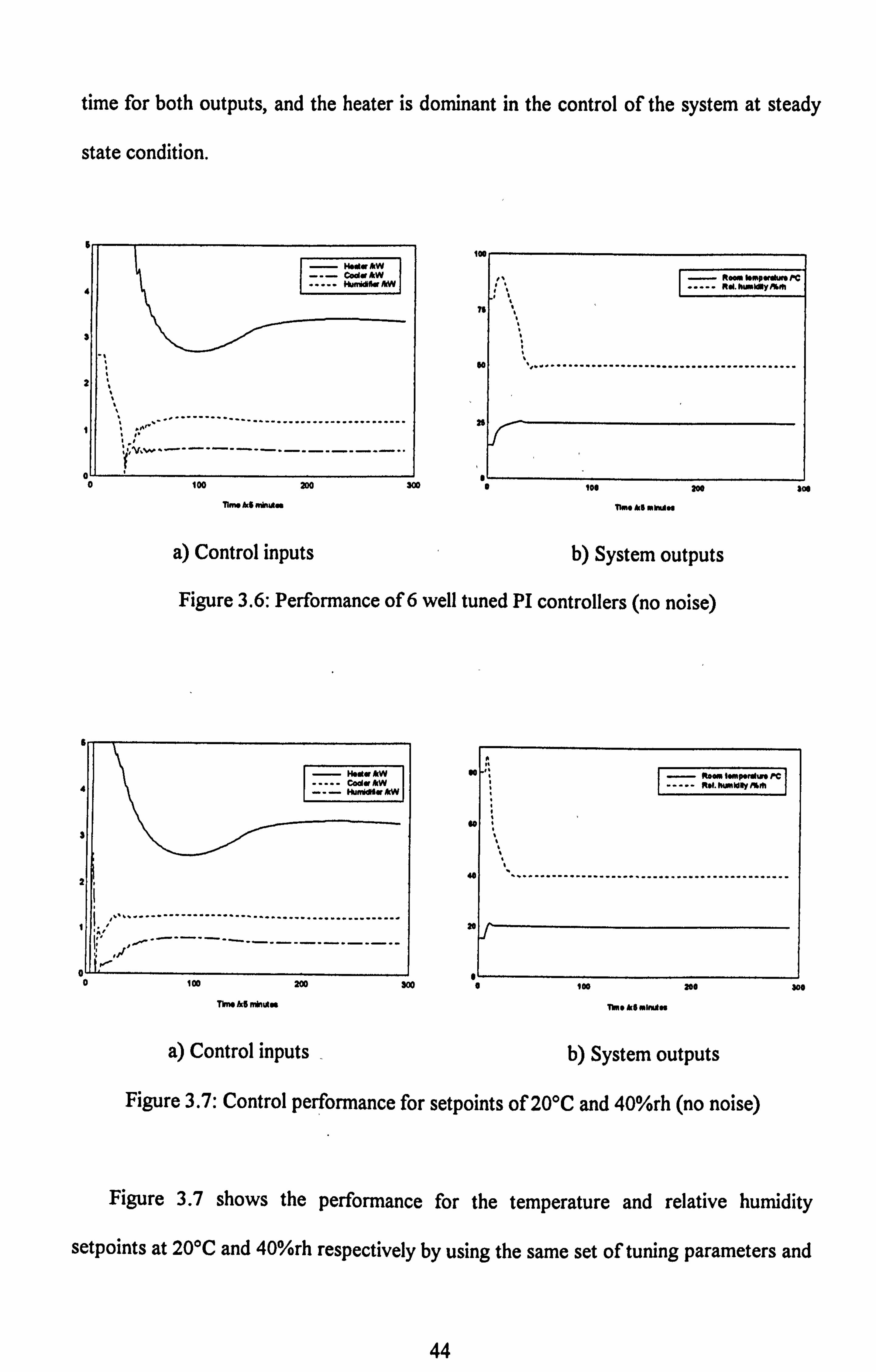
time for both outputs, and the heater is dominant in the control of the system at steady

state condition.

N"ff dW Ceda&W

.. _. Hlnidllfr W

. ý- --------------------------------------

4

bmpwdwo PC .... RN. hiwWly /1H11

1 ...............................................

161

.L 0 100 2o0 wo o toe 200

T hm ht Minuw 11ne we wawa


Figure 3.6: Performance of 6 well tuned PI controllers (no noise)

s

IMtr la:.:

4 Coda

-. I+Jmkla

2.

' ....... ---- ....................................

a

308

p- Ro. Iu I«np r is K "" Rsi NI n101q I%M

a

40

.L o Iro 200 300 100 200

TrIO 15 minus 7Yne Ich rowan


Figure 3.7: Control performance for setpoints of 20°C and 40%rh (no noise)

30"

Figure 3.7 shows the performance for the temperature and relative humidity

setpoints at 20°C and 40%rh respectively by using the same set of tuning parameters and

44

initial conditions. It was found that the control performances over the last 100 sampling

points are as follows:

" the heater, cooler and humidifier consumed energies of 27.6,10.3 and 5.6 kWh

respectively;

" the total temperature and the relative humidity squared errors are 0.0°C2 and

0.002%rh2 respectively; and

" the required times to reach T, and H, are 1.6 and 2.5 hours respectively.

To add a degree of realism into our simulation studies, we can insert some white

noise processes V, and V2 so that occupancy and other stochastic effects can be

included in the analysis. For convenience pseudo random binary sequences (PRBS)

generated using 6 shift registers with magnitudes V= ±0.5°C and VZ = ±0.5%rh, were

used as the noise processes. These represent large disturbances and consequently should

effect the dynamic behaviour of the system quite significantly. These terms were then

included into the system of identical settings as used in Figure 3.6. The simulated result is

shown in Figure 3.8 where the control performances for the last 100 sampling intervals

are as follows:

" the heater, cooler and humidifier consumed 28.7,5.7 and 10.8 kWh respectively; and

9 the total temperature and the humidity squared errors are 81.00C2 and 3098.5%rh2

respectively.

These results show that the regulated errors have became sizeable as expected due to the

disturbances which are not taken into account by the PI controllers. The situation can be

improved by using an advanced model-based method such as a MIMO adaptive

controller (Chapter 5) or a more intelligent solution such as a fuzzy logic controller

45

(Chapter 6) or a genetic algorithm optimisation technique (Chapter 7) which can attempt

to correct for these stochastic effects.

- H. r. Aw --- cod. Mw

w. rw

Rom IsmpwiIn PC 1ý1 -- RN. ýuýIAýY AIT

1

0 iro 200 wo 0 100 200 300

Tkm h6 nüi im

a) Control inputs

T i"he . lna""

b) System outputs

Figure 3.8: Control performance with noise

3.4. Methodology to minimise the number of PI controllers

-It is worthwhile to reduce thenumber of PI controllers used in the overall system so that

excessive hardware is not used; to do this objectively requires the use of each PI

controller to be justified by quantifying the benefits achieved by its inclusion.

We present a possible strategy by considering our results in Section 3.3. From

Figures (3.6a) and (3.7a) and that the required control inputs are different for the two

setpoints considered, namely (T, Hj are required to be at (250C, 50%rh) and at

(20"C, 40%rh). In addition the contribution from each PI controller to the system during

the control process is analysed and only those "units which are active are selected for

particular situations.

For example, let us consider the results for the setpoints (20'C, 40%rh); from

Figure 3.7 a), we can see that at the steady-state condition, the lowest energy is required

from the humidifier, i. e. only 20% of it's maximum power. Therefore, we can ignore

PI#5 and PI#6. Moreover, P1#1 and PI#4 form the majority of the control actions used in

the system, and so the controllers PI#2 and PIO can be ignored. Therefore, as a possible

solution for this setpoint we can use only 2 PI controllers, one for the heater and one for

the cooler with the output ranges set to 0-5.0 kW and 0-2.6 M for PI#1 and PI#4

respectively.

When this solution is tested we observe an excellent controlled response as shown in

Figure 3.8; the performance over the last 100 sampling intervals are as follows:

9 the heater and cooler consumed energies of 20.6 and 4.1 kWh respectively; and

9 the total temperature and the humidity squared errors are O. OoC2 and 0.001%rh 2

respectively,

which is in fact a better performance from that achieved using the six controllersl

6

IMýn AW

`- Coda AW

2\

--------------------- --

0

- Ros r.. O.. rwI rC

"""" RN 111w11ay K/11

.................................................

o too 200 300 e

TYný k6 minutw ý

a) Control inputs

10o 201 700

Time A. $ mwes

b) System outputs

Figure 3.9: Control performance using 2 PI controllers (PI# I and PI#4)

47

We also found that this controller is also capable of maintaining the system at the

setpoints of 201C < T, < 25"C and 30%rh < H, < 45%rh, for which the output squared

errors are quite small.

Also consider the second situation from Section 3.3 where we have a setpoint of

(25"C, 50%rh). In this case it was found that the lowest energy is required from the

cooler. Moreover, the presence of the cooler will require more energy from the heater in

order to maintain the required setpoints. Therefore, we can ignore the cooler as well as

the controllers PIO and PI#4. When this is done we found that the control performance

is deteriorated and the performance over the last 100 sampling intervals are as follows:

* the heater and humidifier consumed energies of 23.0 and 5.6 kWh respectively; and

o the total temperature and the humidity squared errors are 11.9"C' and 241.0%rh2

respectively

which are still within a comfort zone. In another word, It is also possible to use the

heater and the humidifier only to regulate the temperature and the relative hunUity at

25°C and 50%rh respectively.

3.5. Conclusions

In this chapter a simple yet effective tuning methodology of multi PI-loop controllers for

our HVAC plant /office zone system is described. It has been shown that good control

performances can be achieved by using the proportional and integration gains tuned by

this method. Although the methodology is specific to this application it is hoped it can be

generalised to cover a wider range of situations.

48

The methodology is also useful for minimising the number of PI controllers that are

necessary for effective results. It is found that only two PI controllers are required for

good temperature and relative humidity regulation; one is for the heater (driven by the

temperature loop) and the other for the cooler (driven by the rh loop).

49

Chapter 4

State-Space Methods

In the previous chapters, the simulation and control of air conditioned systems using

discrete transfer function has been discussed. Another recent development in control

theory is to use state-space representations which allow more insight into the internal

behaviour of the system under study (see for example Friedland, 1986). To undertake

this type of study it is necessary to convert the transfer function form of model equations

(2.1) and (2.2) into a state-space representation. We begin our discussions concerning

the state-space analysis by first deriving a suitable state-space fonnat for our HVAC

system.

4.1. State-space representation

The normal approach employed to obtain a state-space description is to define the state

variables as delayed versions of the system output (T, and H,, in our case). Following

this methodology we define the state variables as

Y, (1) = TT (t-2T), x2 (t) = T, (t-T), Y3(l) = TT (1),

Y4(t) = H,, (1-2T), iFs (t) = H, (1-T) and Y6(1) = H, (1)

where upon it is straightforward to deduce the individual state equations as:

50

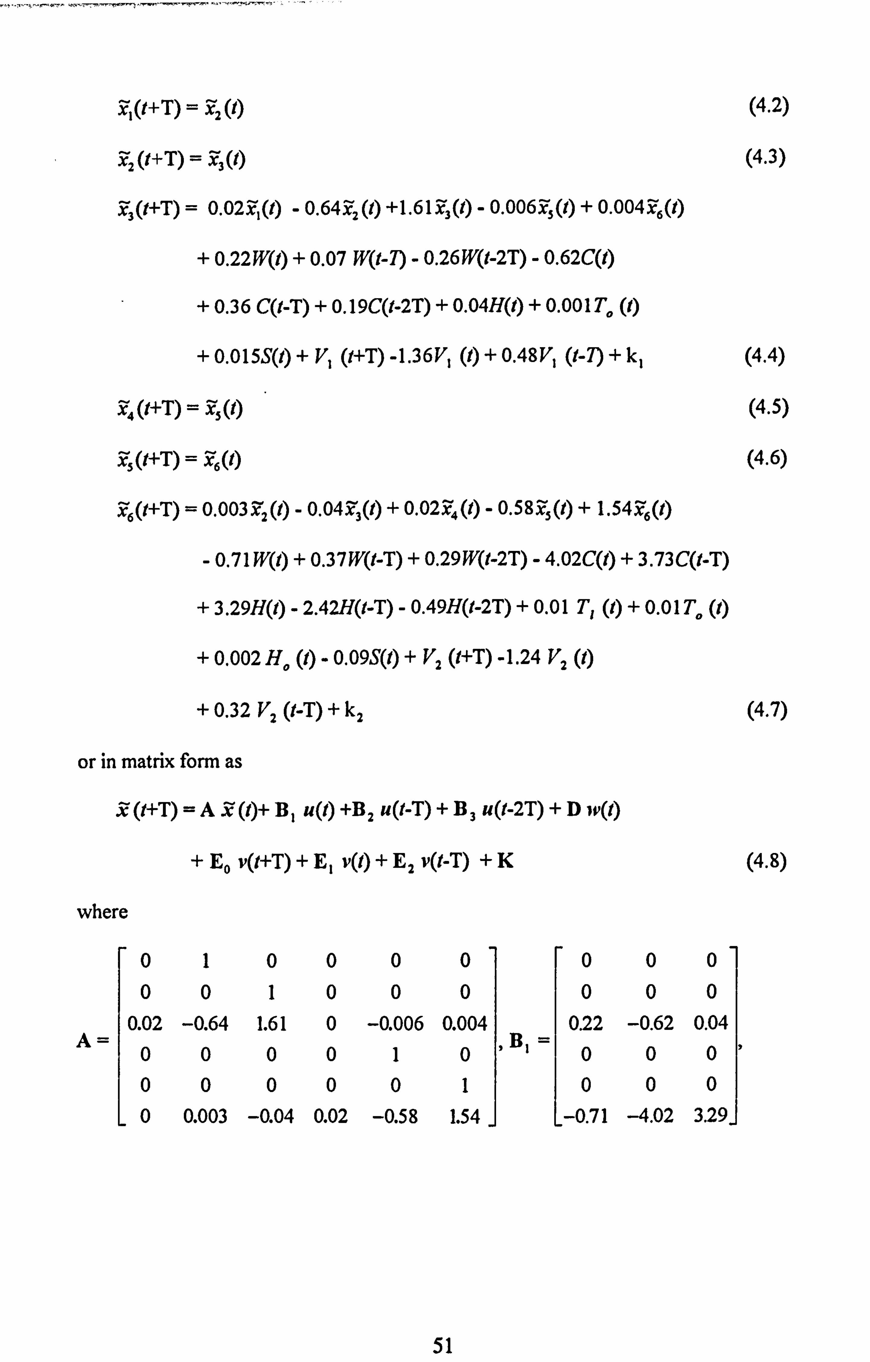
z(t+T) = z2 (t) (4.2)

z2 Q+ T) = z3 (t) (4.3)

ý3(t+T) = 0.02iý, (I) - 0.64Y2(t) +1.61Y3(l) - 0.006Y3(l) + 0.004Y(, (I)

0.22W(l) + 0.07 W(I-7) - 0.26W(t-2T) - 0.62C(l)

0.36 Qt-T) + 0.19Qt-2T) + 0.04H(t) + 0. OOITý, (t)

0.015S(t) + V, (t+T) -1.36VI (t) + 0.48VI (t-7) + k, (4.4)

z4 (t+T) = zs (t) (4.5)

zs(t+T) = zb(t) (4.6)

iý6(t+T) = 0.003Z2(t) - 0.04Z3(t) + 0.02Z4(t) - 0.58Z5(t) + 1.54Z6(t)

- 0.71 W(f) + 0.37W(t-T) + 0.29W(I-2T) - 4.02C(l) + 3.73C(I-T)

3.29H(l) - 2.42H(I-T) - 0.49H(t-2T) + 0.0 1 T, (1) + 0.0 1 T,, (t)

0.002 H� (t) - 0.09S(t) + V2 (t+T) -1.24 V2 (t)

+ 0.32 V2 (t-T) + k2 (4.7)

or in matrix form as

.Z (t+T) =AZ (t)+ B, u(t) +B 2 u(t-T) +B3 u(t-2T) +D iv(t)

+ Eo v(t+T) + E, v(l) + E2 v(t-T) +K (4.8)

where

0 1 0 0 0 0 0 0 0 0 0 1 0 0 0 0 0 0

0.02 -0.64 1.61 0 -0.006 0.004 0.22 -0.62 0.04 A IBI 31 0 0 0 0 1 0 0 0 0

0 0 0 0 0 1 0 0 0

L0 0.003 -0.04 0.02 -0.58 1.54 j L-0.71 -4.02 3.29_j

51

000 000 00

000 000 00

0.07 0.36 0 -0.26 0.19 0 10 B2=

000 2B3= 000 E0 oo

000 000 00

LO. 37 3.73 -2.42j L Q29 0 -0.49j LO IJ

0000 00 00

0000 00 00

0 0.001 0 0.015 -1.36 0 0.48 0 D= 9E1 = >

E2 = 2 0000 00 00

0000 00 00

LO-01 0.01 0.002 -0.09j L0 -1.24j L00.32j

X,

0 X2 T, w

k, X3 T. 0x U= C, )P= H,, and v

121 V X4

L-H-j

IV

0 'ý5 LS J

Lk2. J L 3F6.

J

From equation (4.1), the output equation becomes

. v(t) = T°(t)

= z3(1) [H,

(1) x6(t)

or in compact form as

y(t)=Cz(r)

where

001000

(4.9)

Equation (4.8) is not in standard form in which the state-space equations are

normally presented; the reason is that there are terms explicitly present which are

dependent on delayed value ý of the inputs and noise. It is possible to transform this form

52

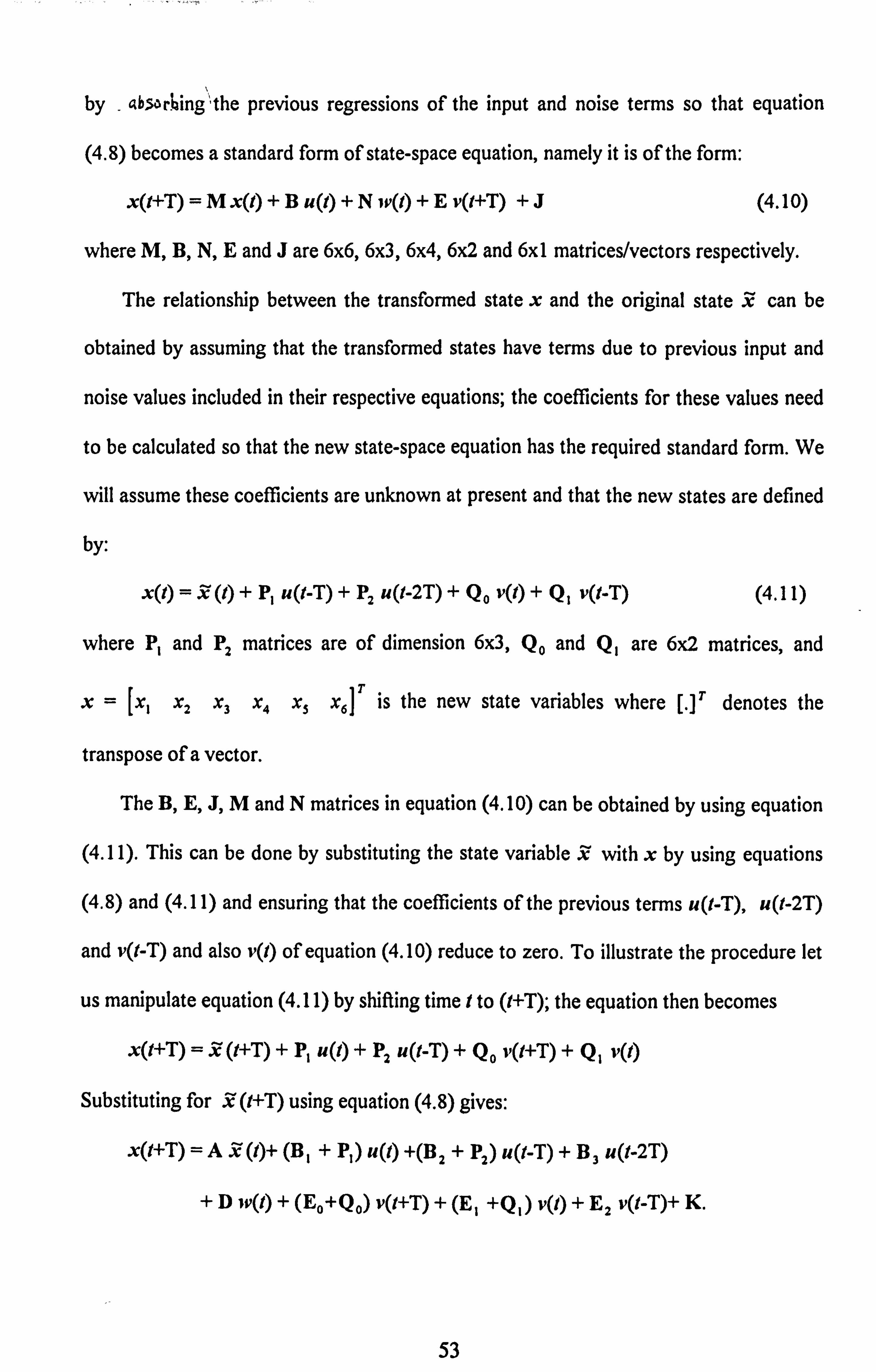
by - absarbing"the previous regressions of the input and noise terms so that equation

(4.8) becomes a standard form of state-space equation, namely it is of the form:

x(I+T) =M x(l) +B u(t) +N jp(l) +E v(/+T) +J (4.10)

where M, B, N, E and J are 6x6,60,6A, 6x2 and 6xI matrices/vectors respectively.

The relationship between the transformed state x and the original state 3ý can be

obtained by assuming that the transformed states have terms due to previous input and

noise values included in their respective equations; the coefficients for these values need

to be calculated so that the new state-space equation has the required standard form. We

will assume these coefficients are unknown at present and that the new states are defined

by:

x(t) =X (t) + P, u Q-T) + P2 u Q-2T) +Q0 v(t) +Q, v(t-T) (4.11)

where P, and P, matrices are of dimension 60, Q0 and Q, are 6x2 matrices, and

X= [XI

X2 X3 X4 X5 X6 ]T is the new state variables where [. ]

T denotes the

transpose of a vector.

The B, E, J, M and N matrices in equation (4.10) can be obtained by using equation

(4.11). This can be done by substituting the state variable X with x by using equations

(4.8) and (4.11) and ensuring that the coefficients of the previous terms u(I-T), u(I-2T)

and v(t-T) and also vQ) of equation (4.10) reduce to zero. To illustrate the procedure let

us manipulate equation (4.11) by shifting time I to (I+T); the equation then becomes

x(t+T) = X(t+T) + P, u(t) + P2 u(t-T) + Qo v(t+T) + Q, v(t)

Substituting for X (I+T) using equation (4.8) gives:

x(t+T) = A. W (1)+ (B I+ P) u(t) +(B 2+ P2) u(t-T) +B3 u(I-2T)

D iv(t) + (EO+Qo) v(t+T) + (EI +Q, ) v(t) + E2 v(t-T)+ K.

53

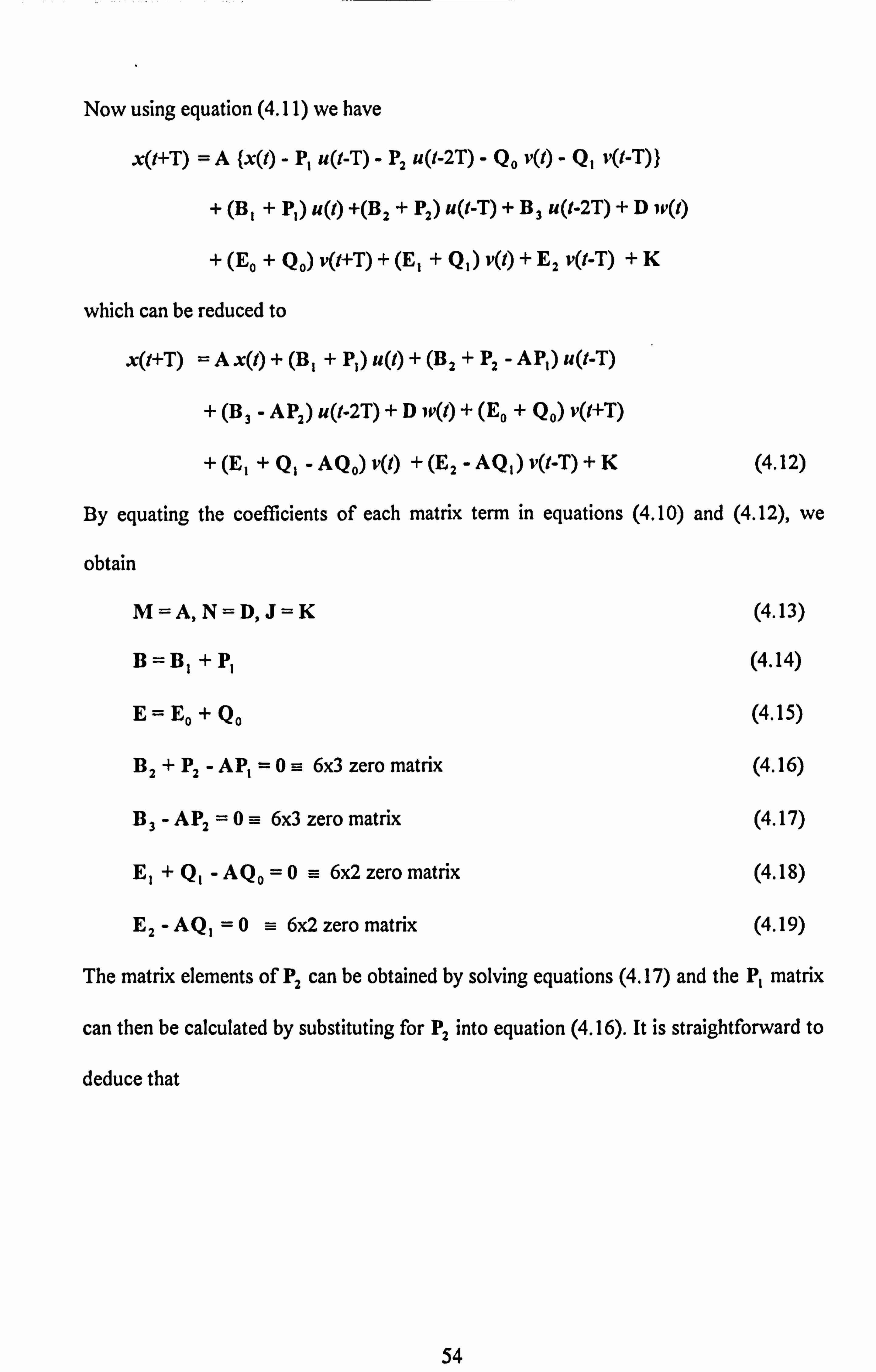
Now using equation (4.11) we have

x(I+T) =A (x(l) - P, u(I-T) - P2u(t-2T) - Q0 v(1) - Q, v(I-T))

+ (B I+ P) u(t) +(B2+ P2) u(I-T) + B3u(I-2T) +D jp(l)

+ (EO + QO) v(I+T) + (El + Q, ) v(1) + E2 VQ-T) +K

which can be reduced to

xQ+T) =A x(l) + (BI + P) u(I) + (B2 + P2 - AP) u(t-T)

+ (B 3-A P2) u(I-2T) +D jv(l) + (E,, + Qj v(t+T)

+ (El + Q, - AQO) v(l) + (E2 - AQ, ) v(I-T) +K (4.12)

By equating the coefficients of each matrix term in equations (4.10) and (4.12), we

obtain

M=A, N=D, J=K (4.13)

B=Bl +Pj (4.14)

E= Eo + Qo (4.15)

B2 + P2 - AP, =0 =- 60 zero matrix (4.16)

B3- AP2 =0 =- 60 zero matrix (4.17)

El + Q, - AQO =0a 6x2 zero matrix (4.18)

E2 -AQ, =0 =- 6x2zero matrix (4.19)

The matrix elements of P. can be obtained by solving equations (4.17) and the P, matrix

can then be calculated by substituting for P, into equation (4.16). It is straightforward to

deduce that

54

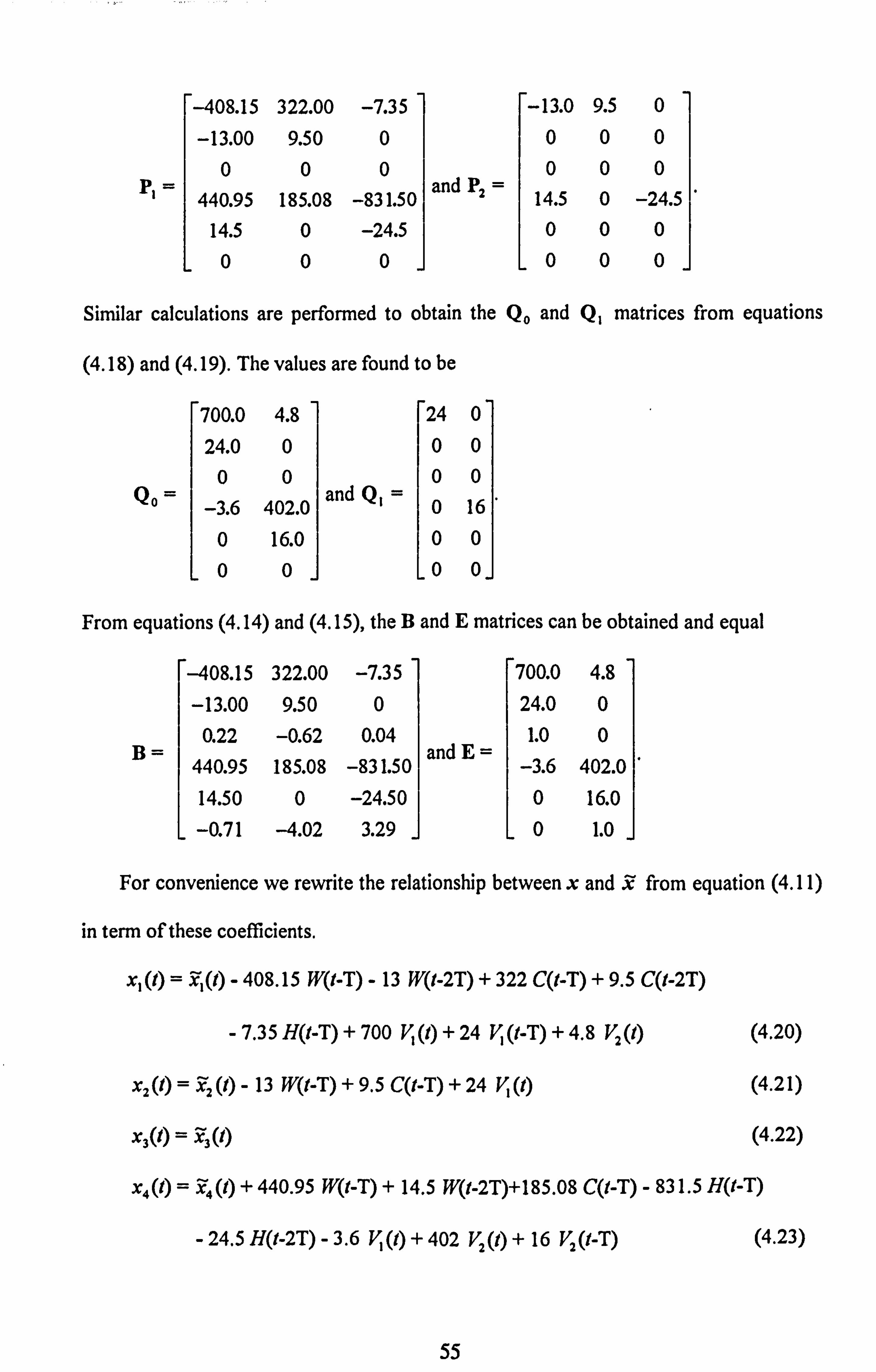
-408.15 322.00

- 13.00 9.50 00

p 440.95 185.08

14.5 0

L00

-7.35 -- 13.0 9.5 0

0 000

0 000 and P2

-831.50 14.5 0 -24.5 -24.5 000

0J L000J

Sin-dlar calculations are performed to obtain the Q, and Q, matrices from equations

(4.18) and (4.19). The values are found to be

700.0 4.8 24 0

24.0 0 00 00 00

QO -3.6 402 .0

and Q, 0 16

0 16.0 00

L00j L00J

From equations (4.14) and (4.15), the B and E matrices can be obtained and equal

-408.15 322.00 -7.35 700.0 4.8

-13.00 9.50 0 24.0 0 0.22 -0.62 0.04 1.0 0

B and E 440.95 185.08 -831.50 -3.6 402.0 14.50 0 -24.50 0 16.0

L -0.71 -4.02 3.29 j L01.0 j

For convenience we rewrite the relationship between x and 9 from equation (4.11)

in term of these coefficients.

x, (t) = YI(l) - 408.15 W(I-T) - 13 W(I-2T) + 322 C(t-T) + 9.5 CQ-2T)

- 7.3 5 H(I-T) + 700 V, (t) + 24 V, (t-T) + 4.8 V2 (t) (4.20)

(4.21) 2 (1)

- 13 W(I-T) + 9.5 CQ-T) + 24 V, (t)

"ý 'F3 (1) (4.22) X30) "

x4(l) = Z4(l) + 440.95 W(I-T) + 14.5 W(I-2T)+185.08 C(I-T) - 831.5 H(t-T)

- 24.5 H(1-2T) - 3.6 V, (1) + 402 V2 (1) + 16 V2 (t-T) (4.23)

55

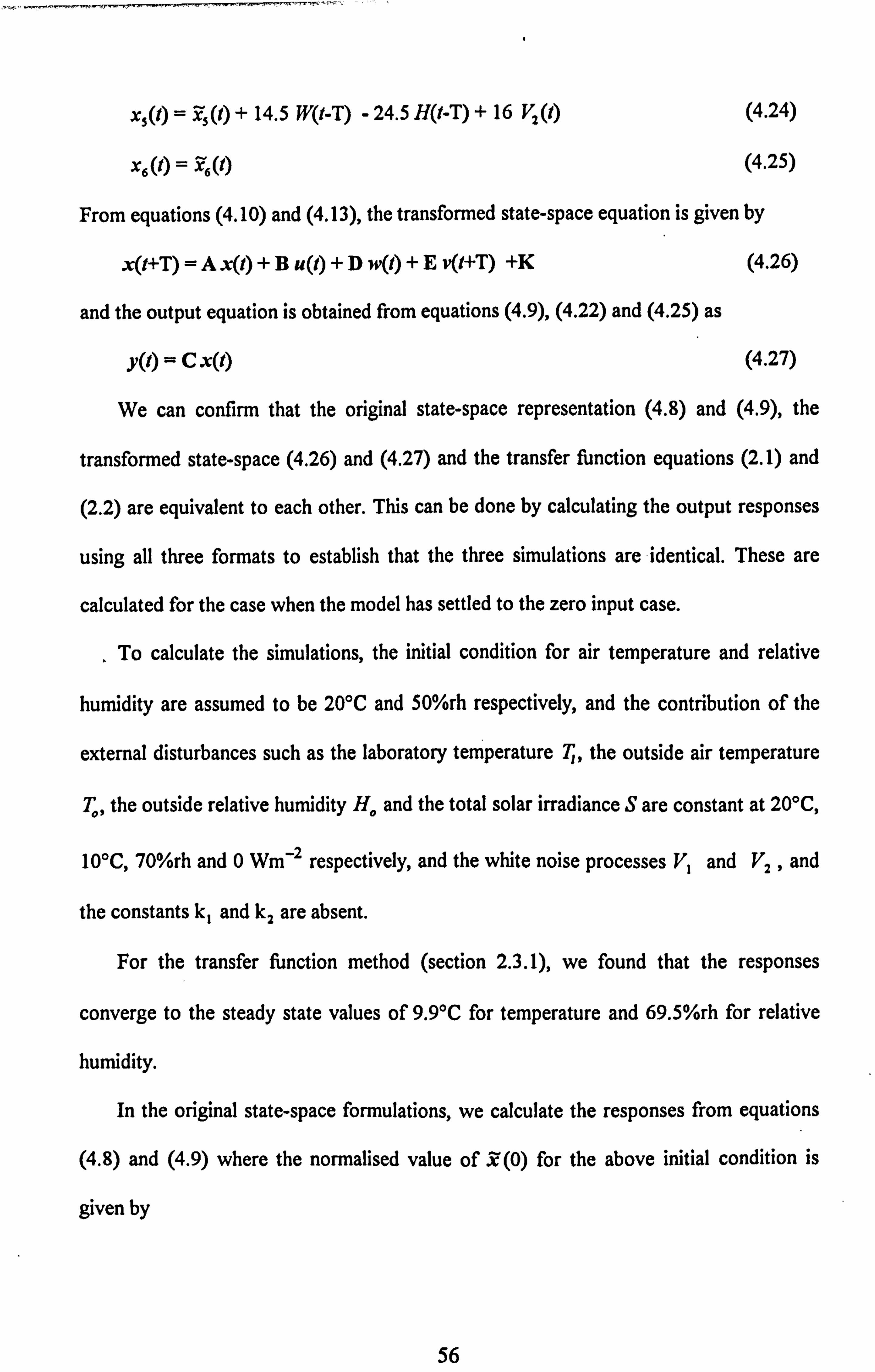
x, (t) = iý5(t) + 14.5 W(t-T) - 24.5 H(I-T) + 16 V2(1) (4.24)

x6 (t) = X6 (t) (4.25)

From equations (4.10) and (4.13), the transformed state-space equation is given by

x(I+T) =A x(t) +B u(o +D w(t) +E v(t+T) +K (4.26)

and the output equation is obtained from equations (4.9), (4.22) and (4.25) as

y(t) =C x(t) (4.27)

We can confirm that the original state-space representation (4.8) and (4.9), the

transformed state-space (4.26) and (4.27) and the transfer function equations (2.1) and

(2.2) are equivalent to each other. This can be done by calculating the output responses

using all three formats to establish that the three simulations are -identical. These are

calculated for the case when the model has settled to the zero input case.

. To calculate the simulations, the initial condition for air temperature and relative

humidity are assumed to be 200C and 50%rh respectively, and the contribution of the

external disturbances such as the laboratory temperature T,, the outside air temperature

T, the outside relative humidity H. and the total solar irradiance S are constant at 20"C, 0

10"C, 70%rh and 0 Wm-2 respectively, and the white noise processes V, and V2 , and

the constants k, and k2are absent.

For the transfer function method (section 2.3.1), we found that the responses

converge to the steady state values of 9.9'C for temperature and 69.5%rh for relative

humidity.

In the original state-space formulations, we calculate the responses from equations

(4.8) and (4.9) where the normalised value of X(O) for the above initial condition is

given by

56

X (0) = [2.05 2.05 2.05 -3.26 -3.26 -3.26] 7 (4.28)

The simulated results via this state-space equation can easily be shown to give the same

response as the transfer function method. In a similar way the transformed state-space

representation can also be shown to give the same response. It should be noted that

before the state-space method can be applied, the initial values of the state vector in the

function should be calculated using equation (4.20) - (4.25) by assuming that the

controlling inputs have not been applied. Identical output responses to those shown in

Figure 2.3 were obtained for all the three methods and hence we can conclude

equivalence of the approaches. -

Next, we design a control system whereby the output is required to track the desired

setpoints; we will use the pole placement method and modal control techniques to obtain

the desired dynamic behaviour of the system and the final value theorem to calculate the

feedforward matrix needed to achieve zero steady state error. We select two structures

for the closed-loop control system, one using state feedback and the other using output

feedback in achieving these objectives.

57

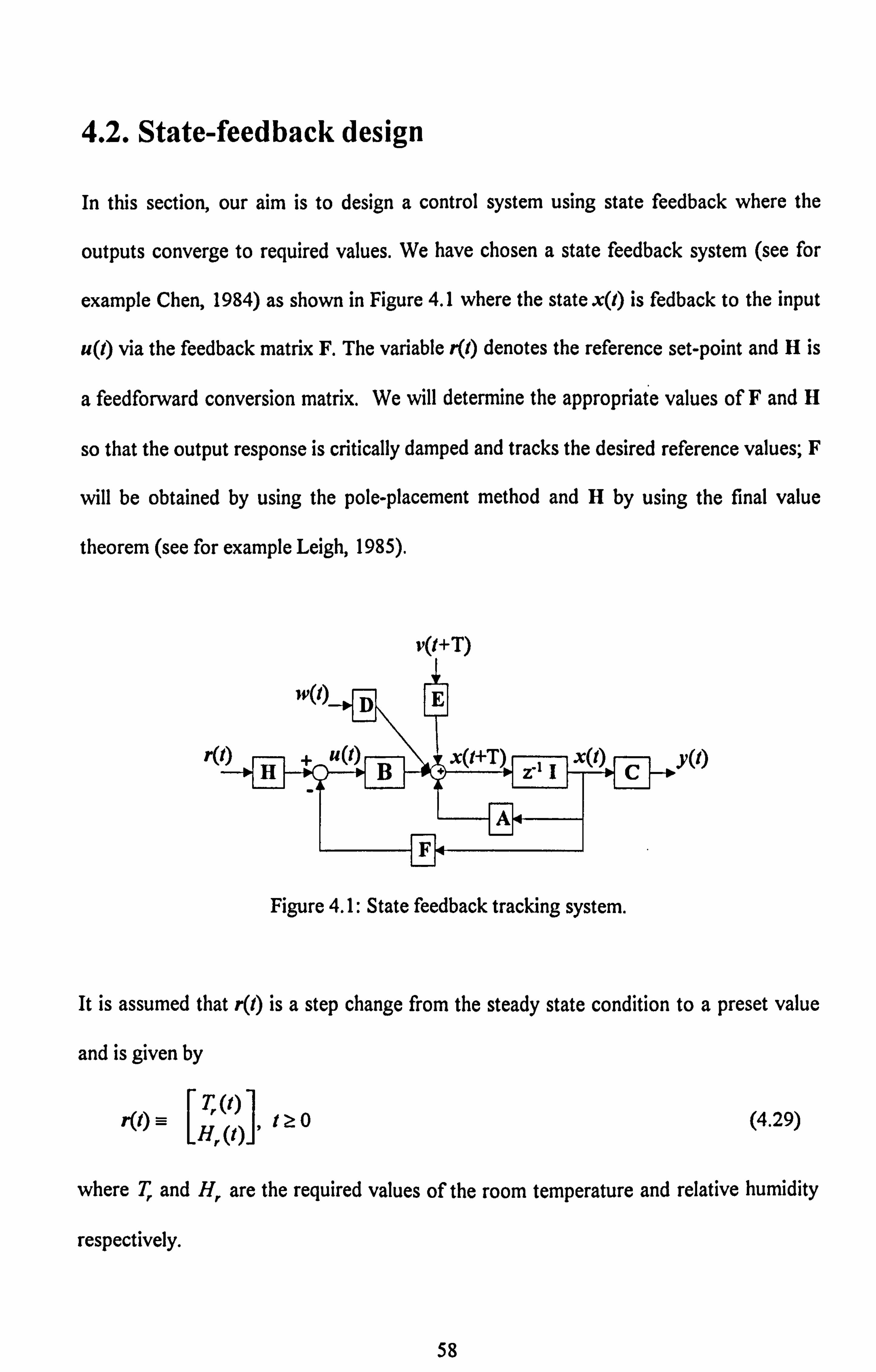
4.2. State-feedback design

In this section, our aim is to design a control system using state feedback where the

outputs converge to required values. We have chosen a state feedback system (see for

example Chen, 1984) as shown in Figure 4.1 where the state x(l) is fedback to the input

u(I) via the feedback matrix F. The variable r(I) denotes the reference set-point and H is

a feedforward conversion matrix. We will determine the appropriate values of F and H

so that the output response is critically damped and tracks the desired reference values; F

will be obtained by using the pole-placement method and H by using the final value

theorem (see for example Leigh, 1985).

v(t+T)

w(r).

H+B x(I+T Z-1 IC Y(l)

FA ---]

Figure 4.1: State feedback tracking system.

It is assumed that r(l) is a step change from the steady state condition to a preset value

and is given by

-[T, W

týto r(t) = (4.29)

where T, and H, are the required values of the room temperature and relative humidity

resPectively.

58

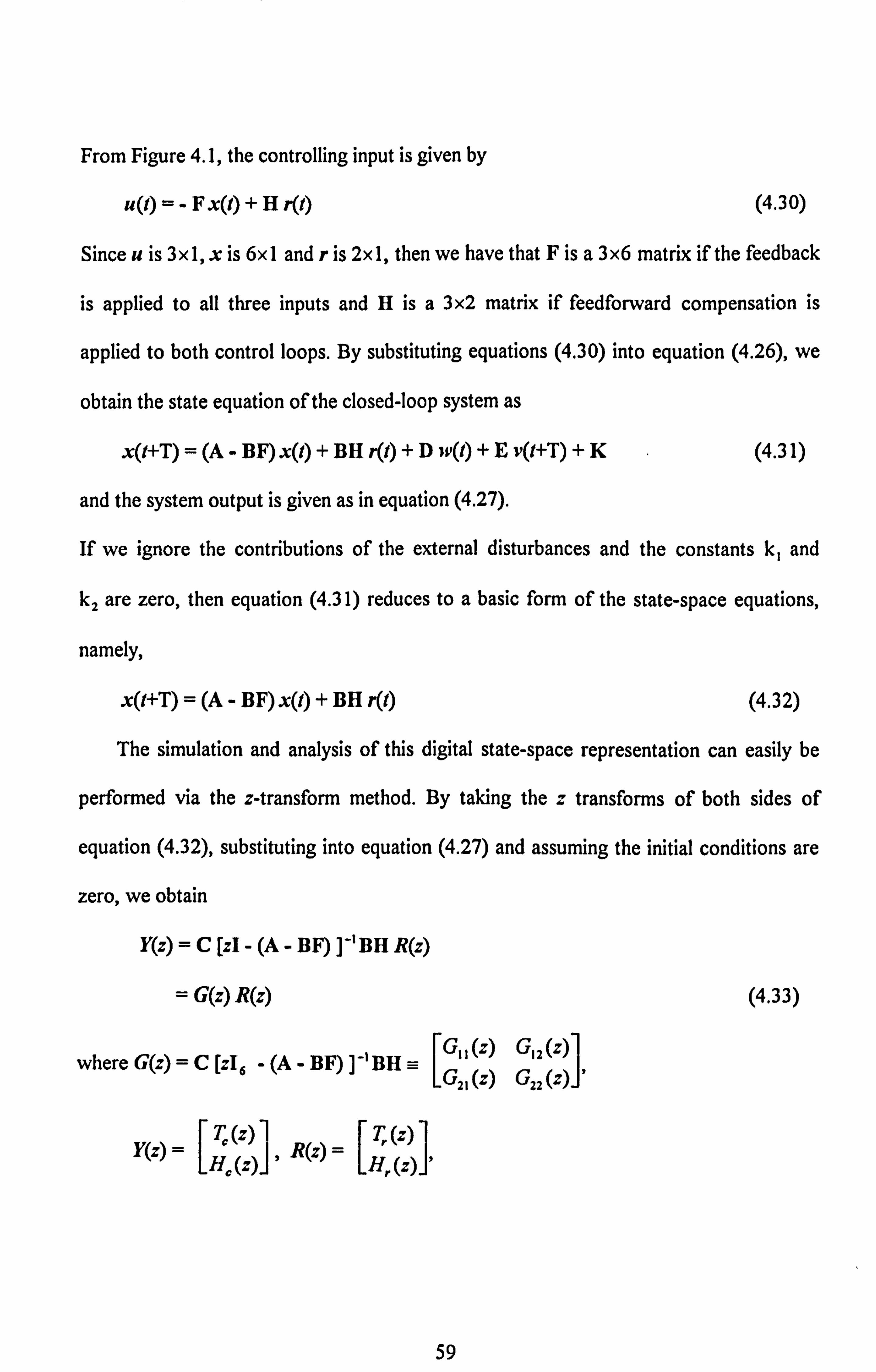
From Figure 4.1, the controlling input is given by

u(t) =- Fx(l) +H r(l) (4.30)

Since u is 3xI, x is 6x I and r is 2x 1, then we have that F is a3 x6 matrix if the feedback

is applied to all three inputs and H is a 3x2 matrix if feedforward compensation is

applied to both control loops. By substituting equations (4.30) into equation (4.26), we

obtain the state equation of the closed-loop system as

x(I+T) = (A - BF) x(l) + BH r(l) + D)P(I) +E v(I+T) +K (4.31)

and the system output is given as in equation (4.27).

If we ignore the contributions of the external disturbances and the constants k, and

k2 are zero, then equation (4.3 1) reduces to a basic form of the state-space equations,

namely,

x(t+T) = (A - BF) x(t) + BH r(l) (4.32)

The simulation and analysis of this digital state-space representation can easily be

performed via the z-transform method. By taking the Az transforms of both sides of

equation (4.32), substituting into equation (4.27) and assuming the initial conditions are

zero, we obtain

Y(z) =C [zl - (A - BF) ]-'BH R(z)

= G(z) R(z)

where G(z) C [zl, -(A-BF)]-'BH=- G,, (z) G,

2(Z) [G2,

(z) G. 2

(z)]'

Te (z T (z Y(z)

[ )], R(z)= r

)I H, (z) H. (z)j'

(4.33)

59

and 16 is a 6x6 identity matrix, G, I) G121, G2,

and G22

are the individual input/output

polynomials. Equation (4.33) can easily be transformed into the time domain by the

method of residues, and the solution is given by

6

y(kT)= lim: -,,,

(z-pi) G(z)R(z) Zk-I for k=o, 1,2, (4.34)

where A are the closed loop poles. Thus, the responses of the room temperature T, (kT)

and the relative huýnidity H, (kT) are given by

Tc (kT) =[ gill pl k +g112 p2 k +gl 13 p3 k+ 9114 Ak+ glis PS k

k ]T p3 k 9116 Ar W) +[ gl2l PI k +9122 P2 k +9123

g124 p4 k+ g125 p5 k+ 9126 P6 k] Hr(kT) (4.35)

Hý, (kT) =[ 9211 Pl k +9212 p2 k +g213 p3 k +9214 p4 k+ g215 p5 k

9216 Ak IT, W) + 19221 Ak+ 9222 Ak+ 9223 Ak

9224 Ak+ g225 p5 k+ 9226 P6 k]H

r(kT) (4.36)

for k=1,2,3,... g, I 1,.., 9110 91210-2 9120 921111"') 92,6 and 9221

P-ý g226 are calculated

from equation (4.34) by factorising the numerator and denominator of the individual

input/output polynomials G,,, G12, G2, and G22 respectively.

At steady state, we require the output to equal the reference input; hence by

applying the final value theorem (see for example Leigh, 1985) to equation (4.33) and

assuming that r(t) is a unit step function at t=0, we obtain

im I : -*I

*ý' ( G(z) 'I)=I

or

C[I,, -(A-BF)]-'BH=12

where12 is aW identity matrix.

(4.37)

60

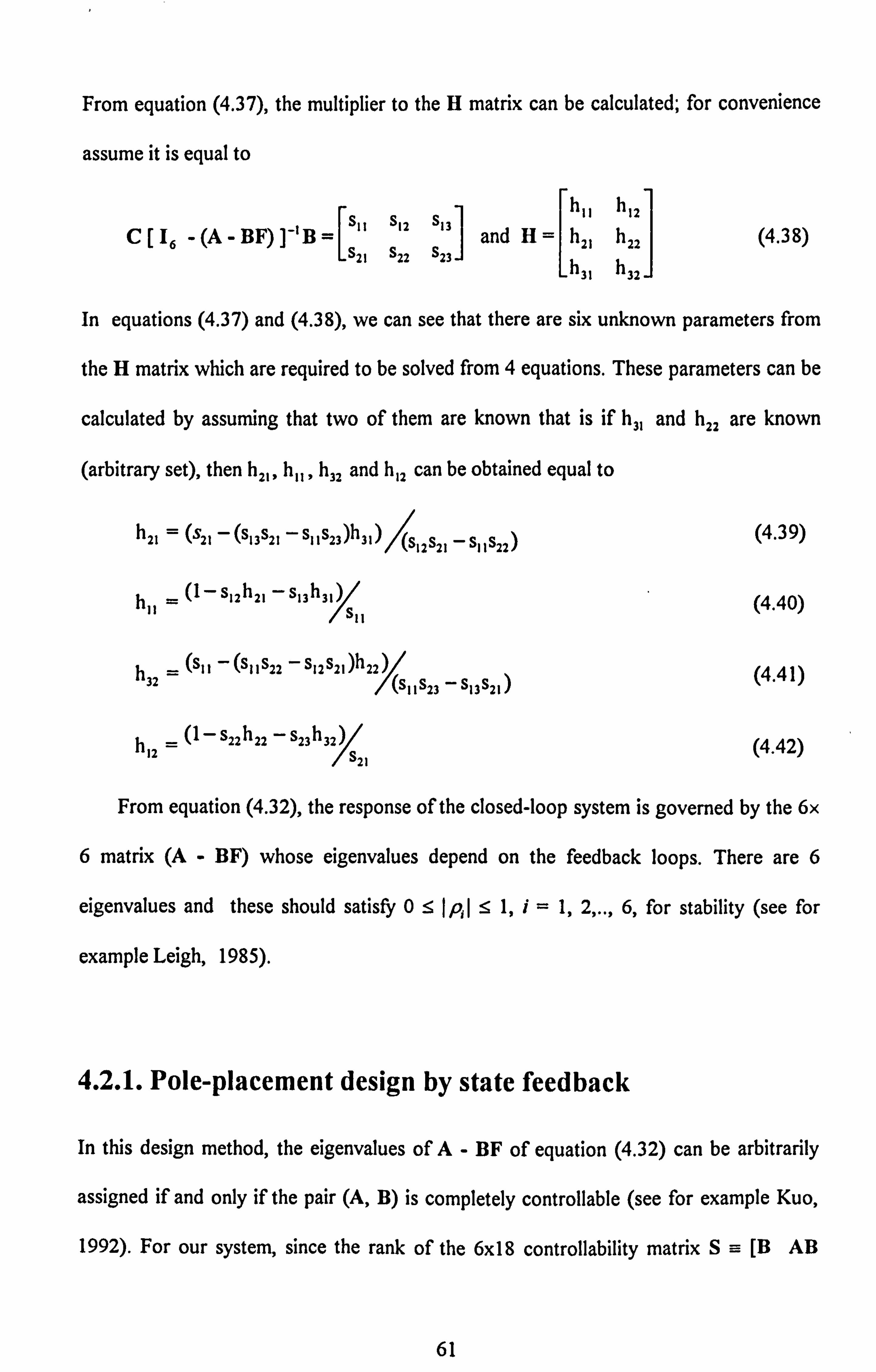
From equation (4.37), the multiplier to the H matrix can be calculated; for convenience

assume it is equal to

C[ 16 - (A - BF) ]-'B =" S21

S12 s hl, h12

"] and H h2l h22 S22 S23

_h3l h32-

(4.38)

In equations (4.37) and (4.38), we can see that there are six unknown parameters from

the H matrix which are required to be solved from 4 equations. These parameters can be

calculated by assuming that two of them are known that is if h3, and h22 are known

(arbitrary set), then h2,, h1110 h32 and h, can be obtained equal to

h -'ý ( 21 -

(SI 3S21 - Sl I S23)h 21 's 31)

/(Sl

2 S21 - Sl I S22 (4.39)

hil = (I - sl, h2, - SIA YSII

(4.40)

h32 = (Sll -(SlIS22 -Sl2S21)h2

%(SlIS23

- S13S21 )

h12 -": (l-S22h22

-S23h3 ý /S21

(4.42)

From equation (4.32), the response of the closed-loop system is governed by the 6x

6 matrix (A - BF) whose eigenvalues depend on the feedback loops. There are 6

eigenvalues and these should satisfy 0 -, e, I p, 1 :51, i=1,2,.., 6, for stability (see for

example Leigh, 1985).

4.2.1. Pole-placement design by state feedback

In this design method, the eigenvalues of A- BF of equation (4.32) can be arbitrarily

assigned if and only if the pair (A, B) is completely controllable (see for example Kuo,

1992). For our system, since the rank of the 6x18 controllability matrix SM [B AB

61

A2B.. A5 B] is 6, then the system is completely state controllable. The design problem

is to find the feedback matrix F such that the control input u of equation (4.30) places

the eigenvalues of A- BF at arbitrarily assigned positions in the z-plane.

Let us construct , a, single-input system from equation (4.26) by temporarily

ignoring the contributions of the external disturbances ip and v, and the constant K; it

then becomes

x(t+T) =A x(l) + B* u(t) (4.43)

where B*u=Bu, and the 6x I matrix B' is defined as

B*=Bw (4.44)

where w is a vector of dimension (3xl) for our case. This vector must be chosen so that

the pair (A, B) is controllable. Then, we can apply the feedback of the single-input, F',

which is defined as

u(t) = -F* x(t) (4.45)

to place the eigenvalues of A- B* F' at the same locations as those of A- BF. Then,

the problem becomes that of designing the state feedback for the single-input system of

equation (4.43). Once the feedback matrix F* is determined, F is given by

F= wF'

since BF= B' F4

(4.46)

It is apparent that in general w is not unique, and it only has to satisfy the condition that

(A, Bw) is controllable. For our case, let us assume that w= [10 10 1], r, it is found

that the determinant of controllability matrix S =- JB' AB' .. A'B'j = -0.47 #0 and

is therefore nonsingular. Thus, the pair (A, B') is controllable. The characteristic

equation of the open-loop system is given by

62

I Z16 -Al =z6 - 3.15 z' + 3.70 Z4 -1.96 z' + 0.43 z' - 0.02 z+0.0004

= Z6 + a. z' + a, z4+ a4 Z3+ a3 Z2+ a2 z+ a, (4.47ý

If the desired poles of the closed-loop system are distinct at say p, = 0.4,0.5,0.6,0.7,

0.8 and 0.9 for stability of the system, then the characteristic equation of A- B' F*

becomes

1 z16 -A+ BA Fo 1= (z - 0.4)(z - 0.5)(z - 0.6)(z - 0.7)(z - 0.8)(z - 0.9)

= Z6 + a6 z' + a, Z4 + a4 Z3 + a3 Z2 + a2z+ a, (4.48)

which is equal to

IZ'6 -A+B*F*I=z6-3.90z5+6.25 Z4 -5.27 z' - 2.46 z2

- 0.60 z+0.06 (4.49)

The elements of F* can be calculated via the formula:

F'=[(M ST )-'(a -a)] r (4.50)

which is of dimension M. The detailed derivation of this formula can be found in Kuo

(1992).

The parameters on the right-hand side of equation (4.50) when applied to our system

with the prescribed poles become

1 0 0 0 0 0

-3.15 1 0 0 0 0 3.70 -3.15 1 0 0 0

M -1.96 3.70 -3.15 1 0 0, 0.43 -1.96 3.70 -3.15 1 0

L-0.02 0.43 -1.96 3.70 -3.15 Ij

-3.90 6.25 -5.27 -2.46 -0.60 0.06 ]r

and

-3.15 3.70 -0.96 0.43 -0.02 0.0004 ] 7'

63

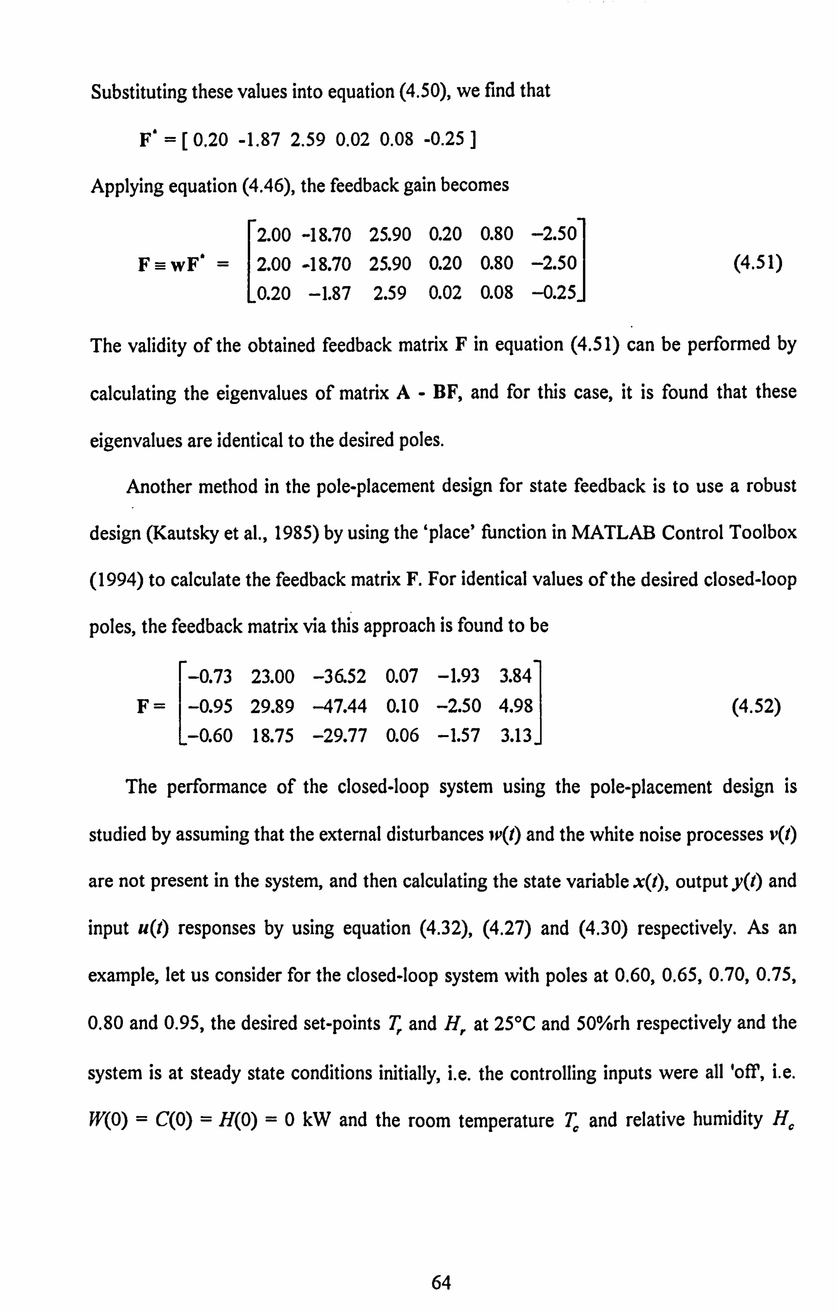
Substituting these values into equation (4.50), we find that

F4 =[0.20 -1.87 2.59 0.02 0.08 -0.25 1

Applying equation (4.46), the feedback gain becomes

2.00 -18.70 25.90 0.20 0.80 -2.50 F =- wF* 2.00 -18.70 25.90 0.20 0.80 -2.50 (4.51)

0.20 -1.87 2.59 0.02 0.08 -0.25-

The validity of the obtained feedback matrix F in equation (4.51) can be performed by

calculating the eigenvalues of matrix A- BF, and for this case, it is found that these

eigenvalues are identical to the desired poles.

Another method in the pole-placement design for state feedback is to use a robust

design (Kautsky et al., 1985) by using the 'place' function in MATLAB Control Toolbox

(1994) to calculate the feedback matrix F. For identical values of the desired closed-loop

poles, the feedback matrix via this approach is found to be

-0.73 23.00 -36.52 0.07 -1.93 3.84

F= -0.95 29.89 -47.44 0.10 -2.50 4.98 (4.52)

--0.60 18.75 -29.77 0.06 -1.57 3.13.

The performance of the closed-loop system using the pole-placement design is

studied by assuming that the external disturbances ip(t) and the white noise processes v(1)

are not present in the system, and then calculating the state variable x(l), output y(t) and

input u(I) responses by using equation (4.32), (4.27) and (4.30) respectively. As an

example, let us consider for the closed-loop system with poles at 0.60,0.65,0.70,0.75,

0.80 and 0.95, the desired set-points T, and H, at 25*C and 50%rh respectively and the

system is at steady state conditions initially, i. e. the controlling inputs were all 'off, i. e.

W(O) = C(O) = H(O) =0 kW and the room temperature T, and relative humidity H.,

64

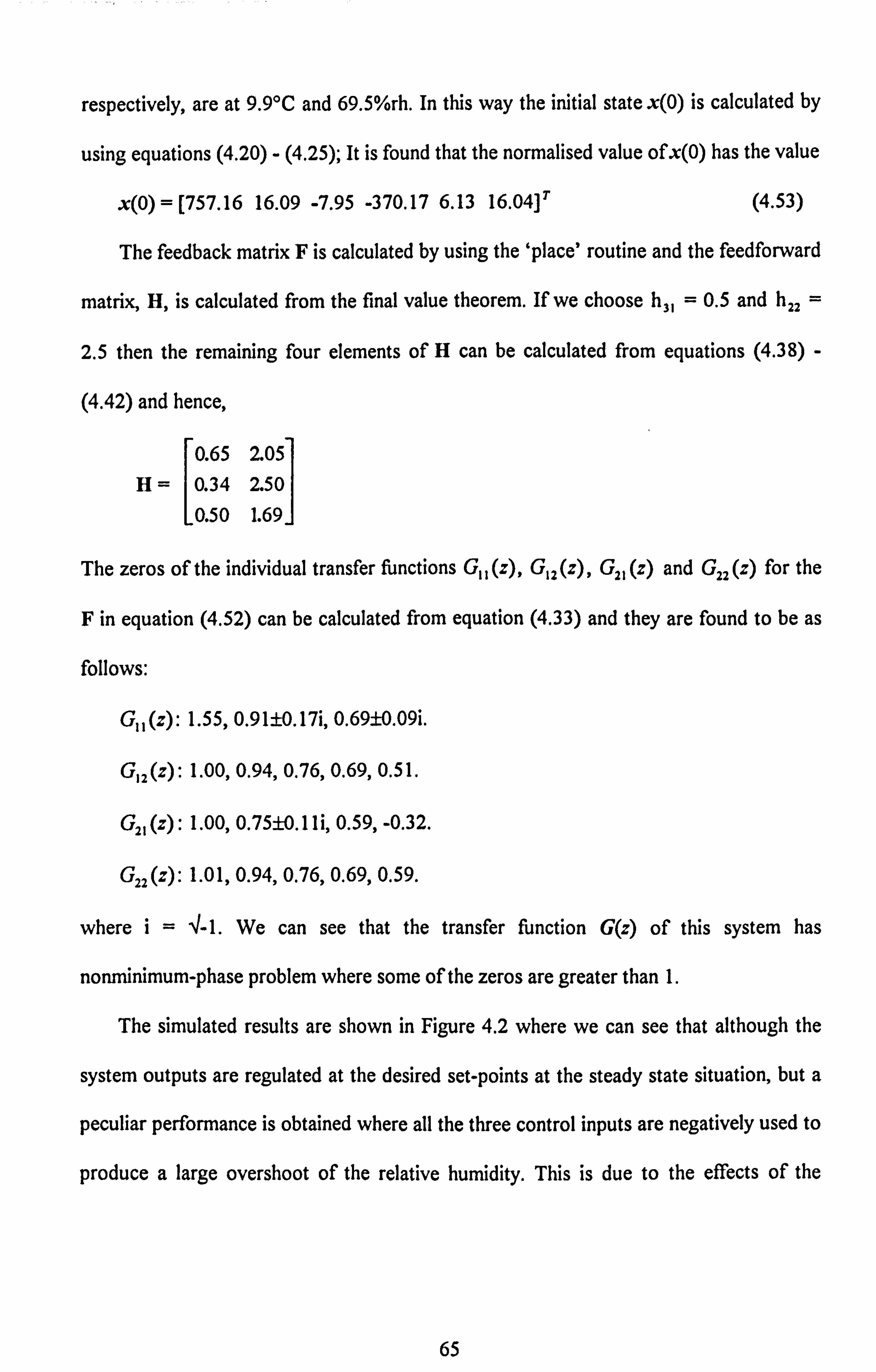
respectively, are at 9.9'C and 69.5%rh. In this way the initial state x(O) is calculated by

using equations (4.20) - (4.25); It is found that the normalised value ofx(O) has the value

x(O) = [757.16 16.09 -7.95 -370.17 6.13 16.04] 7 (4.53)

The feedback matrix F is calculated by using the 'place' routine and the feedforward

matrix, H, is calculated from the final value theorem. If we choose h3, : -- 0.5 and h22 =

2.5 then the remaining four elements of H can be calculated from equations (4.38) -

(4.42) and hence,

0.65 2.05 H 0.34 2.50

0.50 1.69

The zeros of the individual transfer functions G,, (z), G,, (z), G2, (z) and G,, (Z) for the

F in equation (4.52) can be calculated from equation (4.33) and they are found to be as

follows:

G, , 1.55,0.91±0.17i, 0.69±0.09i.

G12 (Z): 1.00,0.94,0.76,0.69,0.5 1.

(z): 1.00,0.75±0.1 1 i, 0.59, -0-32.

G22 (Z): 1-01,0.94,0.76,0.69,0.5 9.

where i= 4-1. We can see that the transfer function G(z) of this system has

nonminimum-phase problem where some of the zeros are greater than 1.

The simulated results are shown in Figure 4.2 where we can see that although the

system outputs are regulated at the desired set-points at the steady state situation, but a

peculiar performance is obtained where all the three control inputs are negatively used to

produce a large overshoot of the relative humidity. This is due to the effects of the

65

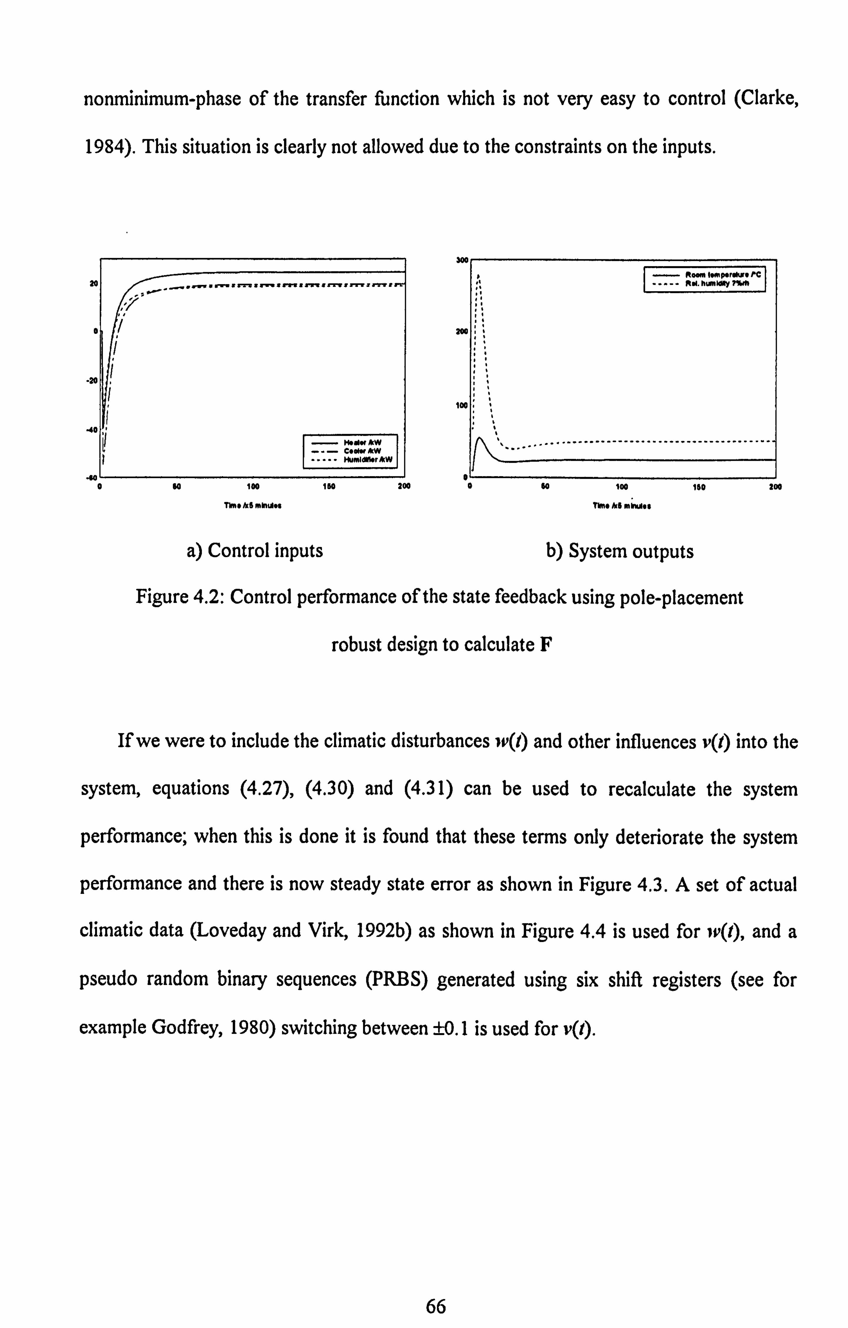
nonminimum-phase of the transfer function which is not very easy to control (Clarke,

1984). This situation is clearly not allowed due to the constraints on the inPuts.

......................

-20

-40

W-I. Wi

Ft"o Impordwe PC R. I. hMMY r"

200

00

................................................

.L so 100 ISO 200 0 60 ISO ISO

Tkn* AS miniAs Time ks Meuse


Figure 4.2: Control performance of the state feedback using pole-placement

robust design to calculate F

200

If we were to include the climatic disturbances jvQ) and other influences vQ) into the

system, equations (4.27), (4.30) and (4.31) can be used to recalculate the system

performance; when this is done it is found that these terms only deteriorate the system

performance and there is now steady state error as shown in Figure 4.3. A set of actual

climatic data (Loveday and Virk, 1992b) as shown in Figure 4.4 is used for jv(l), and a

pseudo random binary sequences (PRBS) generated using six shift registers (see for

example Godfrey, 1980) switching between ±0. I is used for v(1).

66

ffý

"0.1w COGWAw mmmm" NW

00

00

.................................... .......... 0 50 100 ISO 200 0 so 100 ISO 200

Time f's m1mdom Tký. &S mWM"


Figure 4.3: Control performance of the state feedback with disturbance and noise present

03

02

0,

ol 0

............................................. L. 0b. IMIMMUM rc oumift I-pwatum rc OutsMs mi. huldly ^rh

so i0o 150 200 0 so IN ISO

TW. 1.5 ýWKA. s nme MG MIM0.8

a) Solar irradiance b) other climatic disturbances

Figure 4.4: Actual climatic data used in the simulation studies

200

The results do not make any sense in practice, since all the three control inputs are

beyond the permitted ranges and they are 'fighting one anotherý', that is excessive

heating is used because the cooling is excessive and vice versa, etc. This type of result is

also obtained when F is calculated using equations (4.46) and (4.50). Furthermore, we

also found that the magnitude of the control inputs are determined by the desired pole

67

locations; the near the locations are to the origin in z-plane, the larger the required

control inputs and the larger the 'overshoot', and vice versa. In another words, if we

require a fast output response then a large control signal is needed but the priority

criteria as to which control signals should be used is not clearly shown by this

methodology and hence the above conflicts; this fact is important to highlight in actual

situations in order that the total energy consumption is minimised.

We notice that the two techniques of pole-placement design presented here although

commonly used, do not consider the constraints on the control inputs; the methods are

however extremely powerful for designing control systems with the desired closed-loop

poles. In order for arbitrary pole placement to be possible, the system must be completely

state controllable and the magnitude of the control input must be unbounded (Ogata,

1987). Our control inputs, namely, the heater W, cooler C and humidifier H have limits

of 0-5. Op 0-2.7 and 0-2.6 kilowatts respectively, and hence the normal pole-

placement design for calculating the feedback matrix F is not applicable in our situation.

In another word, the closed-loop poles A can not be simply chosen to lie at any arbitrary

locations in z-plane. This is obvious since we can not expect infinitely fast behaviour

when we have finite limits on the control signals.

Furthermore when we are dealing with mutli-input applications it is not obvious

which input should be used to modify which eigenvalue. In theory if the system is

controllable using only one input then feedback is required only on this loop but in

practice there are constraints present on most control systems and these restrict the

general results which are possible. For example using the 'place' function leads to very

peculiar results which look good at a quick glance but when they were studied more

closely it transpires that the control inputs were being used incorrectly - the negative of

68

the heating input is used for the cooling and the negative of the cooling input is used for

the heating. Large signals for the heating and the cooling were again being displayed to

give rapid response and as already mentioned there was considerable wastage in energy

cancellation of the heating with cooling inputs. The 'place' routine merely attempts to

achieve the desired pole locations and no sense is made of the final result. Clearly, in

practice we do not have negative heating or negative cooling signals and the strategy can

not be implemented.

In order that sensible state-feedback designs can be carried out in multivariable

application it is necessary to use an iterative design procedure where each individual

control loop is closed in sequence and the most appropriate eigenvalues set at each stage.

Modal control offers a suitable methodology in this respect and we discuss it next.

4.2.2. Multistage design procedure for state feedback

In view of the above problems with the standard state feedback method we discuss the

multi-stage procedure presented in Porter and Crossley (1972). This approach utilises the

mode controllability matrix (D at each stage to determine the number of modes to be

controlled by each control loop. The details of the method are now presented.

First of all, the input matrix B is partitioned into its elemental column vectors; for

our case this is as follows

B=[b, b2 b3l (4.54)

as there are three inputs. The state equation (4.26) with the input terms partitioned in this

way become

69

xQ+T) =A x(l) +bIW (1)+ b2 C(t) +b At) +D w(t) +E v(t+T) +K

or 3

x(I+T)=Ax(l)+I: bi Ui(t)+Dit, (I)+Ev(I+T)+K i=l

where it, = W, U2 =C and u3= H.

(4.55)

In this section, our aim is to design a control law for which we can alter one or more

eigenvalues of the plant matrix namely A, to the desired eigenvalues of the closed-loop

system, provided that the appropriate modes are controllable. The design method

involved in this control law, known as multi-stage modal control, will be applied to our

system with the structure as shown in Figure 4.1, to calculate the feedback matrix F.

Let us define the control signal as

K, v ji)T X(j), 1,2, (4.56)

where r is the number of control inputs (equal to three in our case), v, () is the j-th

eigenvector of the transposed plant matrix (= associated with the control input u,,

K, is thej-th proportional controller gain and n is the number of modes of an appropriate

selection for the i-th control input u,.

By substituting the expression for u, given in equation (4.56) into equation (4.55)

we then have the effect of the control input u, to change the plant matrix y, to the new

plant matrix which is given by

n

+bi2: Kjv(j'), r (i=1,2,..., r-1) (4.57) j=l

where

xv, (4.58)

70

Theref Y) ore, the effect of using n eigenvectors v, (i = 1,2, ..., n) is to change the

eigenvalues X, of xV, to some new values pj of and the eigenvectors uj of W, to

some corresponding new eigenvectors wi of leaving the remaining (m - n) pairs of

eigenvalues and eigenvectors of the plant matrix of the uncontrolled system unchanged.

For our case, m=6, which is the number of eigenvalues of the plant matrix xV, .

Let us we define uJI) = gTx(l) then from equation (4.56), we have

n

gi I: Kv, (4.59) J=l

where g, is the i-th feedback vector associated with uj.

The proportional controller gain Ki can be derived in term of the eigenvalues of y, and

the required eigenvalues of xV,., of i-th input, then equation (4.59) becomes

n

n II(Pk

T k=l gi

n

(D() k llk-ýIj)

k-l, k*i

(4.60)

where pk (k =1,2,..., n) are the desired closed-loop poles of the new plant matrix

1,2,.., 6) are the eigenvalues of plant matrix A, (D(') is the k-th element of the k

appropriate mode-controllability matrix, (D,, and n is obtained on the basis of the

magnitudes of the elements of (D,, in view of the form of equation (4.60).

The vector g, is related to the feedback matrix F via equations (4.30) and (4.56)

and is given by

rT TJT F=- [g, 92 93 (4.61)

The v(') vectors are the columns of the modal matrix, Vi of equation (4.60), which

is defined as the eigenvector of the transposed plant matrix (= %pir ), associated with the

71

i-th stage of the design procedure. By substituting g, from equation (4.59) into equation

(4.57), we have

Wi., -2 Wi + bi gir (i =1,2,..., r-1) (4.62)

The mode-controllability matrix, (D,, associated with the i-th stage of the design

procedure is given by the equation

(Di = ViT Bi Q=1,2,..., r) (4.63)

It is well known (see for example Porter and Crossley, 1972) that if we premultiply

the eigenvector of W, (= Uj ) by the transposed eigenvector of W, (= V) we will

obtain an identity matrix of order equal to rank of %V,; in mathematical form this can be

written as

V, T U, = 16

where

[VI(l) V2 (i) V3(i) V4(') v, (')

v6(')] for i=1,2,3

and

Ui -= [Ul(i)

U2(i) U3(i) U4(i) US(i) U6(i] for i=1,2,3

(4.64)

The relationship in equation (4.64) is important to confirm first before proceeding to the

next stage of the design procedure. If this relation does not comply (due to incorrect

normalisation of the eigenvectors) then further rescaling of the V matrix with respect to

the U matrix needs to be carried out.

The eigenvalues A of A are calculated and are equal to 0.99,0.94,0.61,0.54,0.03

and 0.04. It is desired to move these eigenvalues to the required locations as well as

ensuring that the output will track the reference inputs.

72

As an example, let us consider the desired locations, p, are at 0.5,0.6,0.7,0.8,

0.85 and 0.9 and the modal control design stage input sequence is ( W, C, H), that is the

heater input feedback design is carried out first followed by the cooler and then the

humidifier feedback design is carried out last. In this case the mode-controllability matrix

(D, is obtained from equation (4.63) and is equal to

0.25 -0.22 -0.07 -0.038 0.32 -0.92

1.89 -6.38 2.28

-6.74 -11.64 14.23 365.99 -345.85 93.71

-437.83 -209.75 853.151

We can determine the modes to be controlled by the heater by examining the rows of the

(D, matrix. It is clearly indicated that the first and fifth modes would be chosen since the

first and the fifth elements in the first column are dominant, i. e.

10.25 1> 1-0.221,10.25 1> 1-0.071

and

1365.99 1> 1-345.85 1,1365.99 1> 193.711.

Therefore, the W input should be used to move the first and fifth eigenvaluesA = 0.99

and ý=0.03 to the required valuesA = 0.5 and p5= 0.85 respectively. Thus, by using

equation (4.60), we can calculate the feedback vector, g,, which is given by

(I)T (I)T

91 = (p, - AXP,

- AM

+ (p,

- -ý)(P, -, QV5

0.25(, ý -A) 365.99(A -, Q

= [-0.05 1.48 -2.36 0.01 -0.18 0.34] (4.65)

After completing the first stage of the design, equation (4.62) can be used to calculate

the modified plant matrix, W2by using

I gT W2-2 A+bI (4.66)

73

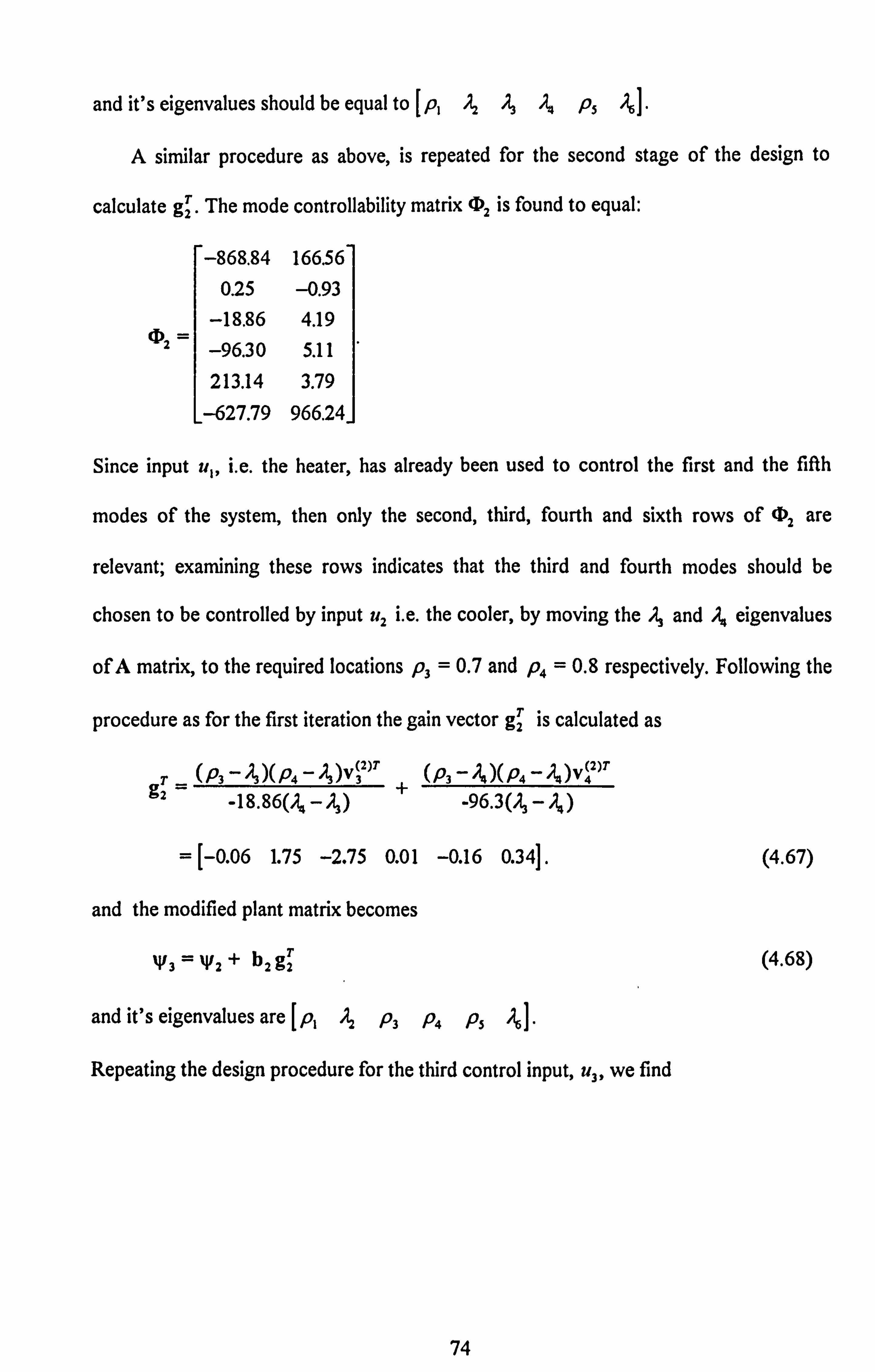
and it's eigenvalues should be equal to [p, ýýý p5 ý].

A sirnilar procedure as above, is repeated for the second stage of the design to

calculate g. The mode controllability matrix 02 is found to equal: 2

-868.84 166.56 0.25 -0.93

-18.86 4.19 (D2 96.30 5.11

213.14 3.79

L-627.79 966.24J

Since input u,, i. e. the heater, has already been used to control the first and the fifth

modes of the system, then only the second, third, fourth and sixth rows of ID2 are

relevant; examining these rows indicates that the third and fourth modes should be

chosen to be controlled by input U2 i. e. the cooler, by moving the ý and ý eigenvalues

of A matrix, to the required locations p3 = 0.7 and p4= 0.8 respectively. Following the

procedure as for the first iteration the gain vector g' is calculated as

(2)T (2)l

9r (A -'ý)(A - 'UV3 +

(A _fU(P4 -'ýM

2 -18.86(, ý -, Q -96.3(, ý -, ý)

= [-0.06 1.75 -2.75 0.01 -0.16 0.34]. (4.67)

and the modified plant matrix becomes

T W3 W2+ b292

and it's eigenvalues are [p, ý pý p,, p, ý].

Repeating the design procedure for the third control input, u3, we find

(4.68)

74

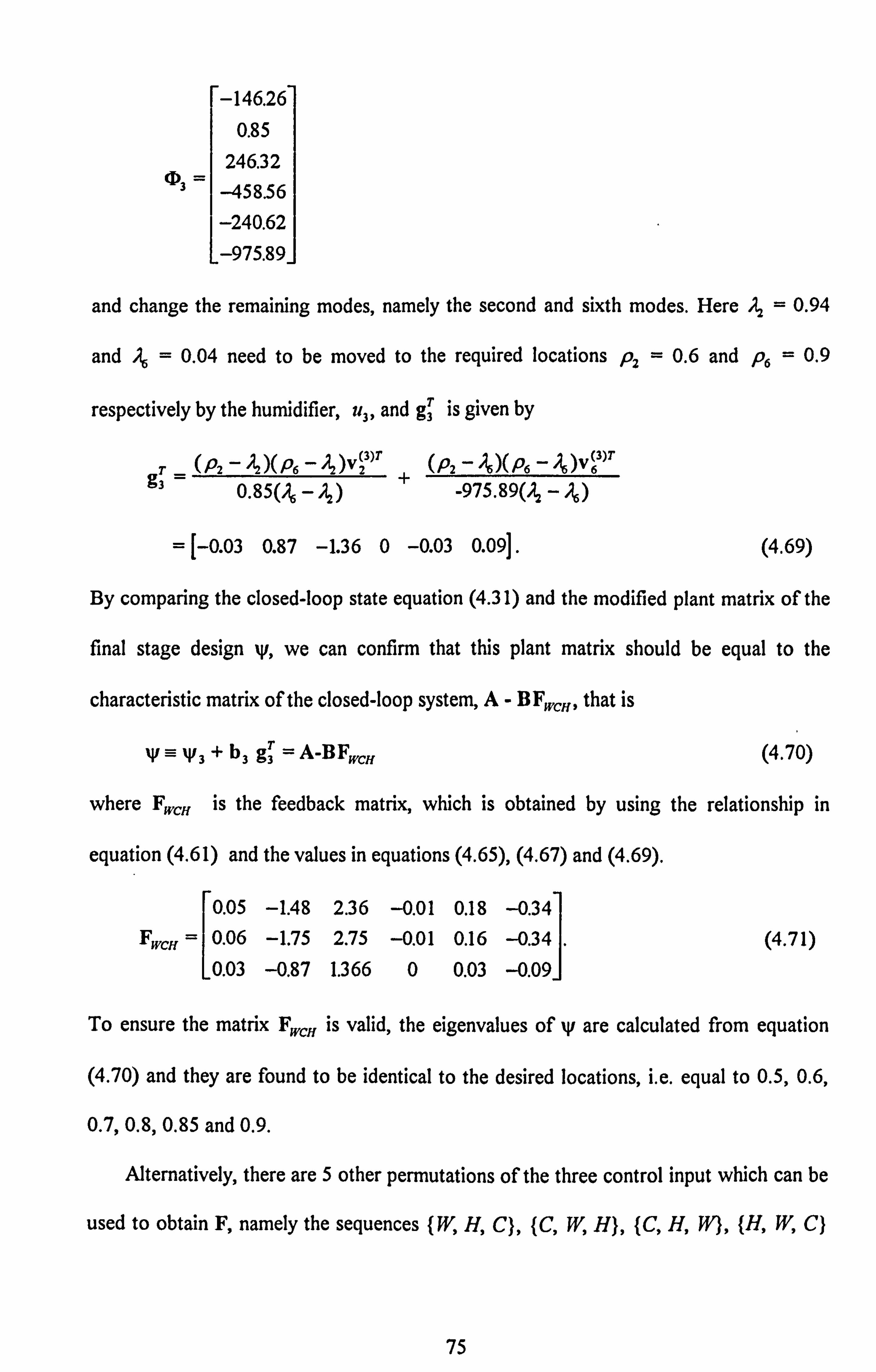
-146.26 0.85

246.32 (D3 ý

-458.56

-240.62

--975.89-1

and change the remaining modes, namely the second and sixth modes. Here ý=0.94

and ý=0.04 need to be moved to the required locations p2 = 0.6 and p. = 0.9

respectively by the hutrMfier, UP and g' is given by 3

(3)T 3)T T=

(P2 - 'ýXP6 - JUV2 (P2 -'U(P6 - 'OV(6

93 0.85(. ý -, ý) + -975.89(, ý -, ý)

= [-0.03 0.87 -1.36 0 -0.03 0.09]. (4.69)

By comparing the closed-loop state equation (4.3 1) and the modified plant matrix of the

final stage design %V, we can confirm that this plant matrix should be equal to the

characteristic matrix of the closed-loop system, A- BFcff, that is

-W+bT= A-BFwcH ý33 93 (4.70)

where Fcff is the feedback matrix, which is obtained by using the relationship in

equation (4.6 1) and the values in equations (4.65), (4.67) and (4.69).

0.05 -1.48 2.36 -0.01 0.18 -0.34 Fwc, ff = 0.06 -1.75 2.75 -0.01 0.16 -0.34 (4.71)

0.03 -0.87 1.366 0 0.03 -0.09-

To ensure the matrix FcH is valid, the eigenvalues of V are calculated from equation

(4.70) and they are found to be identical to the desired locations, i. e. equal to 0.5,0.6,

0.71,0.8,0.85 and 0.9.

Alternatively, there are 5 other permutations of the three control input which can be

used to obtain F, namely the sequences (W, H, C), (C, W, H), {C, H, W), (H, W, C)

75

and (H, C, 91. In other words the order in which the control input designs are carried

out alter the solution obtained. To illustrate this we discuss the design procedure for the

(C, W, H) sequence. We can apply the same strategy as above, for which the closed-

loop poles, p3 and p, are used to calculate g, ' using the cooler, p, and p, are for g, '

using the heater and p2 and p, are for g' using the humidifier. For this sequence, the 3

eigenvector of the first stage, V, is identical to the previous example, i. e. equal to the ,

eigenvectors of A' and the mode controllability vector 0, is given by

01 = VJ b2 =[ -0.22 0.32 -6.38 -11.64 -345.85 -209.75 ]r

and the feedback vector for the cooler g' and the modified plant matrixW2 respectively, 2

are given by

Mr I)T I=

(A - -ý)(Pl -'OV3 (A-ý4)(A-'QV4( 92

-6.3 8 (, ý -ý) -T-

-1 1.64(, ý - ý4)

= [0.03 -1.01 1.60 0 0.11 -0.22]

and T W2 o A+ b292

For the second stage of the design, these parameters are given by

02 = V2r b, =[0.38 -1.30 -198.2 -365.4 519.3 -344.5 ]T

(, Dl )V (2)7 ý)( ý)V(2)T TI pi P5

-5 91 0.38(, ý -A) + 519.3(A -, ý)

= [-0.02 0.47 -0.45 0.01 -0.20 0.201

+bT W3 "2 W2 191

and for the final stage of the design, we have

03= V3Tb3= [ 571.0 -2.3 -1172.6 -4042.4 -2371.2 598.4 ]"

76

(P2 _, ý)(P6 _, ý)V, I)T (P2 -'ý)(A +

-2.3 (, ý 598.4(, ý

= [-0.02 0.37 -0.45 0 -0.13 0.16]

W-+b"= A-BFcwH = W3 3 93

where Fcm is the feedback matrix for the input sequence (C, W, HI is equal to

-0.03 1.01 -1.60 0 -0-11 0.22

Fc; vn 0.02 -0.47 0.45 -0.01 0.20 -0.20 (4.72)

0.02 -0.37 0.45 0 0.13 -0.16-

Once again, it was found that the required poles of the closed-loop system, A- BFcn,

are equal to the desired locations.

Similarly, if we choose the input sequence as (H, C, 91 then the modified plant

matrices become

W2,,, 2 A+bT= W2 + b2 gT and W-+b, gr = A-BFHcw (4.73) 3 93 , W3 2ý W3 I

and the feedback matrix, F,,, in equation (4.67) is different from FcH and Fcm,

although the poles of the closed-loop system are identical to the desired locations.

By using the feedback matrix F from one of these input sequences and assuming that

the initial conditions and the desired setpoints are identical to the example in the pole-

placement design (section 4.2.1), we can calculate the output response y(l) from the state

equations (4.31) for the system with disturbances, and equation (4.32) for the system

without disturbances, and the output equation (4.27). The control input u(I) is calculated

from equation (4.30) where the feedforward matrix H is obtained from the final value

theorem (equations (4.38) - (4.42)). It is straightforward to deduce that a suitable value

of H for the feedback matrix Fwcff is

77

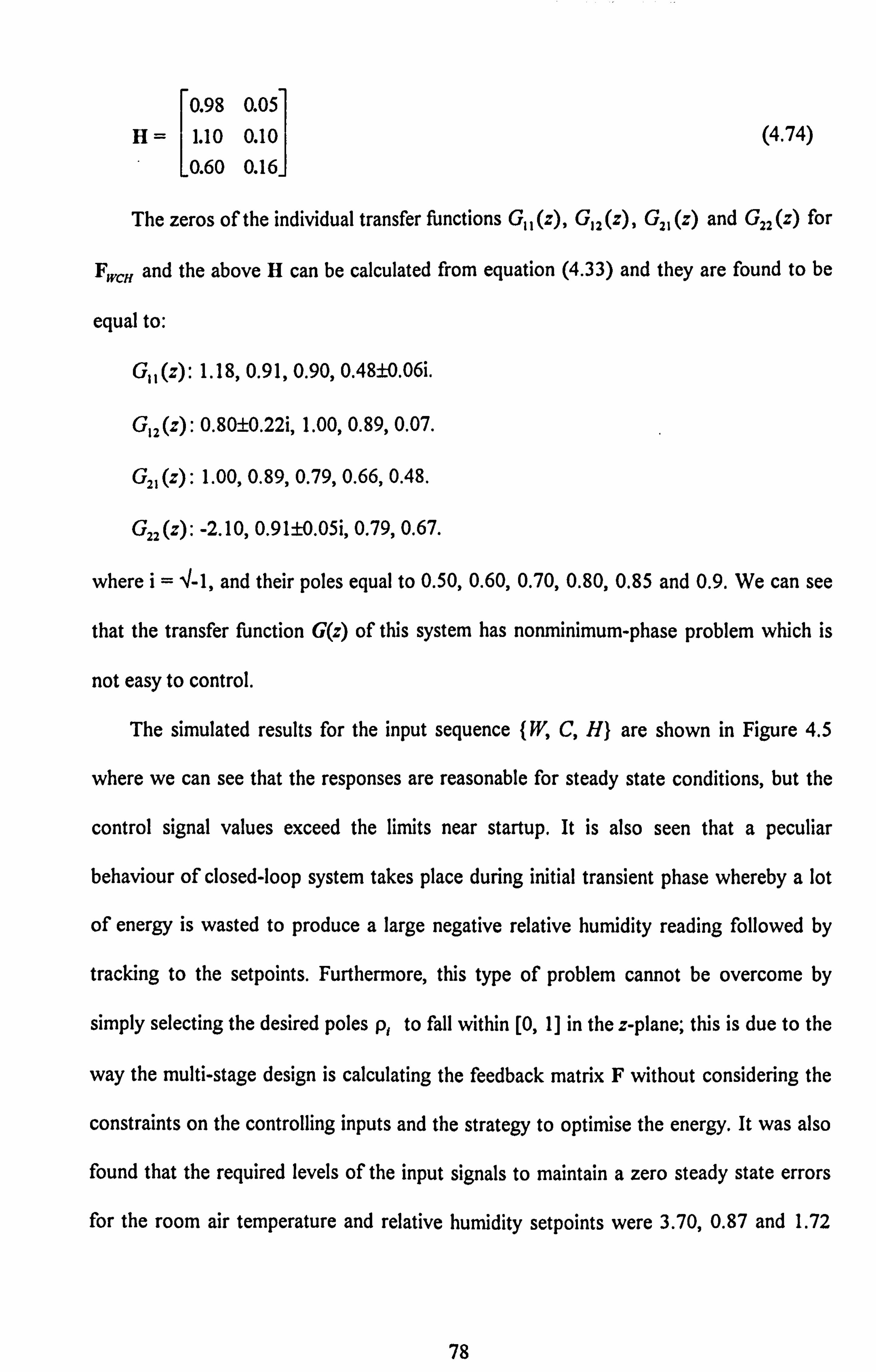
0.98 0.05 H 1.10 0.10

0.60 0.16

(4.74)

The zeros of the individual transfer functions G, , (z), G, 2(z), G2, (z) and G22 (Z) for

Fwcff and the above H can be calculated from equation (4.33) and they are found to be

equal to:

G, , (z): 1.18,0.91,0.90,0.48±0.0 i.

G12(Z): 0.80±0.22i, 1.00,0.89,0.07.

G2, (z): 1.00,0.89,0.79,0.66,0.48.

G22 (Z): -2.10,0.91±0.05i, 0.79,0.67.

where i= 4-1, and their poles equal to 0.50,0.60,0.70,0.80,0.85 and 0.9. We can see

that the transfer function G(z) of this system has nomninimum-phase problem which is

not easy to control.

The simulated results for the input sequence (W, C, H) are shown in Figure 4.5

where we can see that the responses are reasonable for steady state conditions, but the

control signal values exceed the liýnits near startup. It is also seen that a peculiar

behaviour of closed-loop system takes place during initial transient phase whereby a lot

of energy is wasted to produce a large negative relative hutnýidity reading followed by

tracking to the setpoints. Furthermore, this type of problem cannot be overcome by

simply selecting the desired poles p, to fall within [0,1] in the z-plane; this is due to the

way the multi-stage design is calculating the feedback matrix F without considering the

constraints on the controlling inputs and the strategy to optimise the energy. It was also

found that the required levels of the input signals to maintain a zero steady state errors

for the room air temperature and relative humidity setpoints were 3.70,0.87 and 1.72

78

kW for the heater, cooler and hutnidifier respectively. This is acceptable since the

temperature setpoint is higher than the ambient temperature. For the other control input

perinutation designs, the required powers for zero steady state errors are given in Table

4.1. In the calculation of the feedback matrix F for these sequences, we can observe that

the heater, cooler and humidifier were always used to move the plant matrix eigenvalues

A and ý, 23 and ý, and ý and ý to the desired closed loop poles p, and p, p3 and

p, and p2 and p6 respectively but the calculation of the feedback vectors g, ' via the

heater, g, ' via the cooler and g, ' via the hutnidifier were carried out by following the

input design sequences where the mode controllability vectors 01,02 and03 are different

for one sequence to the others; and hence gives different values in the feedback matrix F.

We then would expect to obtain different combinations of the required control signals W,

C and H at steady state conditions and these are shown in Table 4.1. We can see that

excessive powers are required for the input design sequence numbers 3,4,5, and 6

where the control inputs are fighting one another to maintain the desired setpoints;

excessive heating requires more cooling and humidifying and vice versa. This situation is

not recommended in practice since minimal cost of operation is the main target of the

operators.

By studying the results of these different design we can obtain the optimal solution

in the sense of minimal energy consumption; it is clear that the (W, C, H) sequence is the

best one for this design because the energy is minimal and all the three inputs fall within

the permitted limits. This sequence is not optimal for all situations; when the closed loop

poles are allocated to the positions 0.3,0A, 0.5,0.6,0.7 and 0.8 the modal control

design procedure gives the best sequence as (H, C, W) although the inputs still control

the same modes, namely the heater (modes I and 5), cooler (modes 3 and 4) and the

79

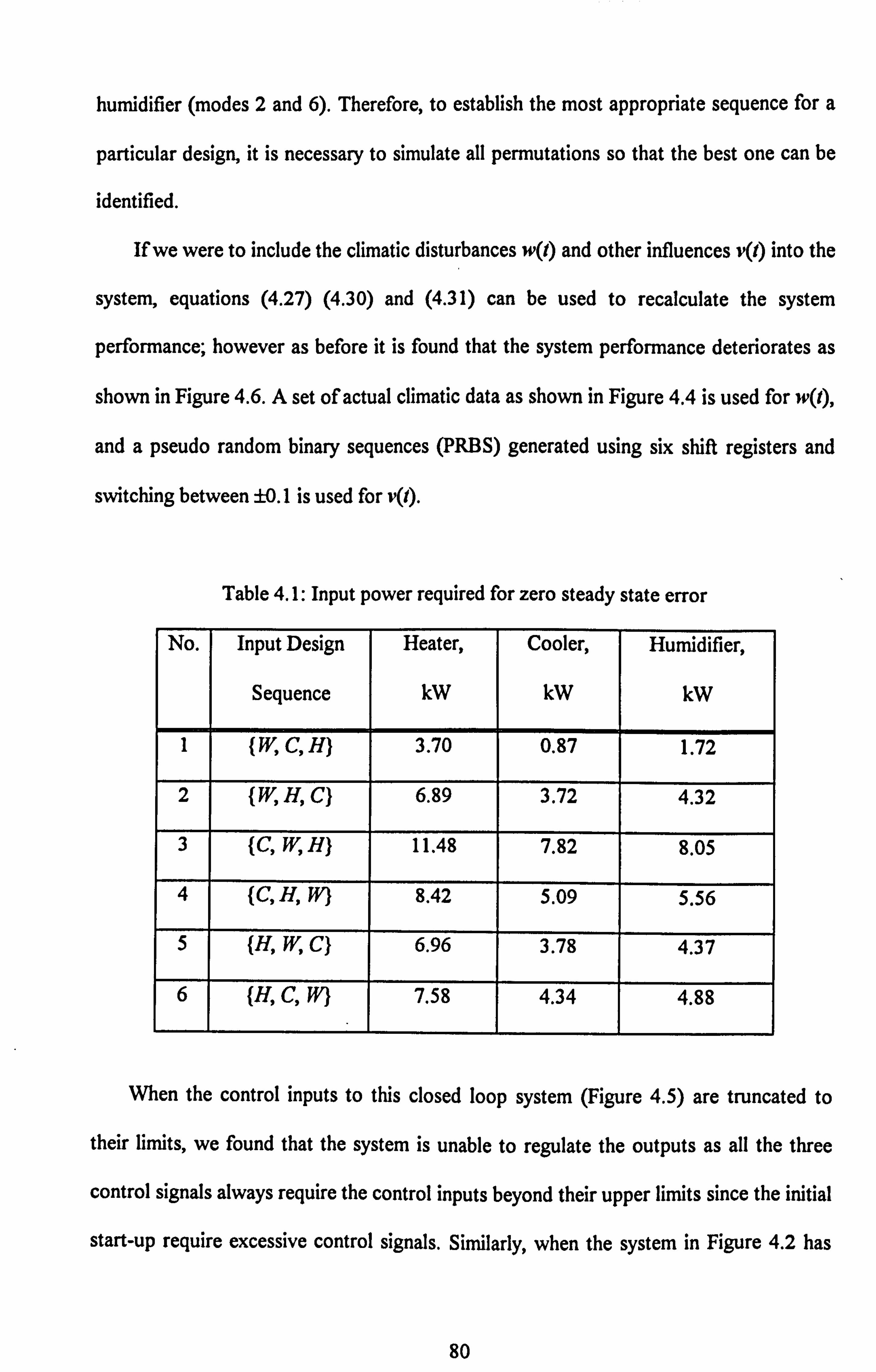
hun-ddifier (modes 2 and 6). Therefore, to establish the most appropriate sequence for a

particular design, it is necessary to simulate all permutations so that the best one can be

identified.

If we were to include the climatic disturbances w(l) and other influences v(1) into the

system, equations (4.27) (4.30) and (4.31) can be used to recalculate the system

performance; however as before it is found that the system performance deteriorates as

shown in Figure 4.6. A set of actual climatic data as shown in Figure 4.4 is used for w(l),

and a pseudo random binary sequences (PRBS) generated using six shift registers and

switching between ±0. I is used for v(l).

Table 4.1: Input power required for zero steady state error

No. Input Design

Sequence

Heater,

kW

Cooler,

kW

Humidifier,

kW

I ( W, C, H) 3.70 0.87 1.72

2 (W, H, Q 6.89 3.72 4.32

3 (C, W, H) 11.48 7.82 8.05

4 (C, H, Jn 8.42 5.09 5.56

5 (H, W, Q 6.96 3.78 4.37

6 (H, C, W) 7.58 4.34 4.88

When the control inputs to this closed loop system (Figure 4.5) are truncated to

their limits, we found that the system is unable to regulate the outputs as all the three

control signals always require the control inputs beyond their upper limits since the initial

start-up require excessive control signals. Similarly, when the system in Figure 4.2 has

80

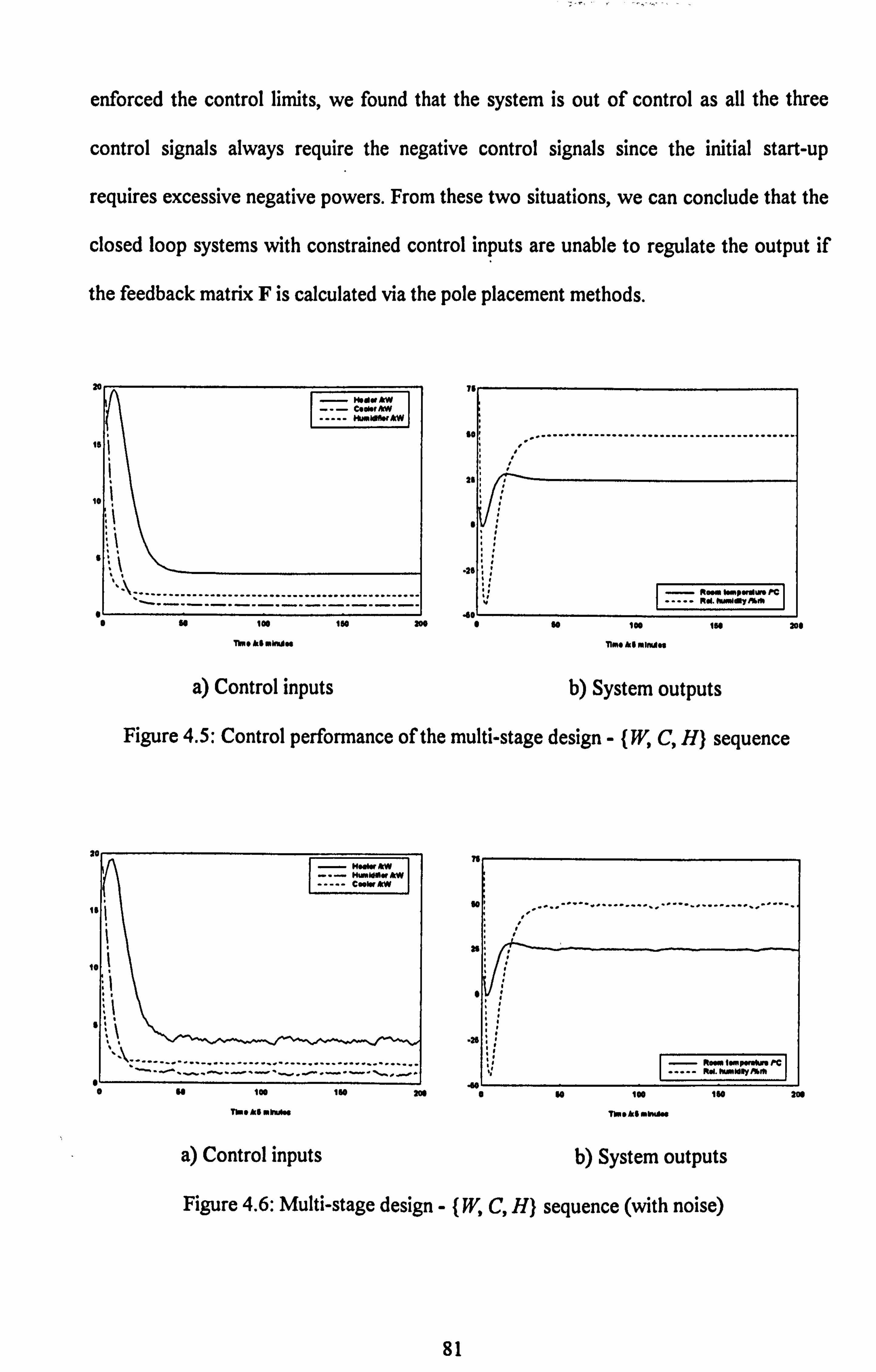
enforced the control limits, we found that the system is out of control as all the three

control signals always require the negative control signals since the initial start-up

requires excessive negative powers. From these two situations, we can conclude that the

closed loop systems with constrained control inputs are unable to regulate the output if

the feedback matrix F is calculated via the pole placement methods.

"1 '5

10

Colbf^W HM~-"

... ... ... ... ... ... ...

76

so .............................................

21

. 26''

U 100 ISO no 0 100 1" 208

Time ks MWA008 IIM* &I Mir""


Figure 4.5: Control performance of the multi-stage design -(W, C, H) sequence

M-1dow kw C""mlwWA,, rWw

I

Is I

I.

------------ ----------- ....................

100 160 208

11'. 0 As MWA"

so ................... ....... ......... .......

35

it. " I. P PC

100 lea 209

Thpokgmbkfiw


Figure 4.6: Multi-stage design - (W, C, H) sequence (with noise)

81

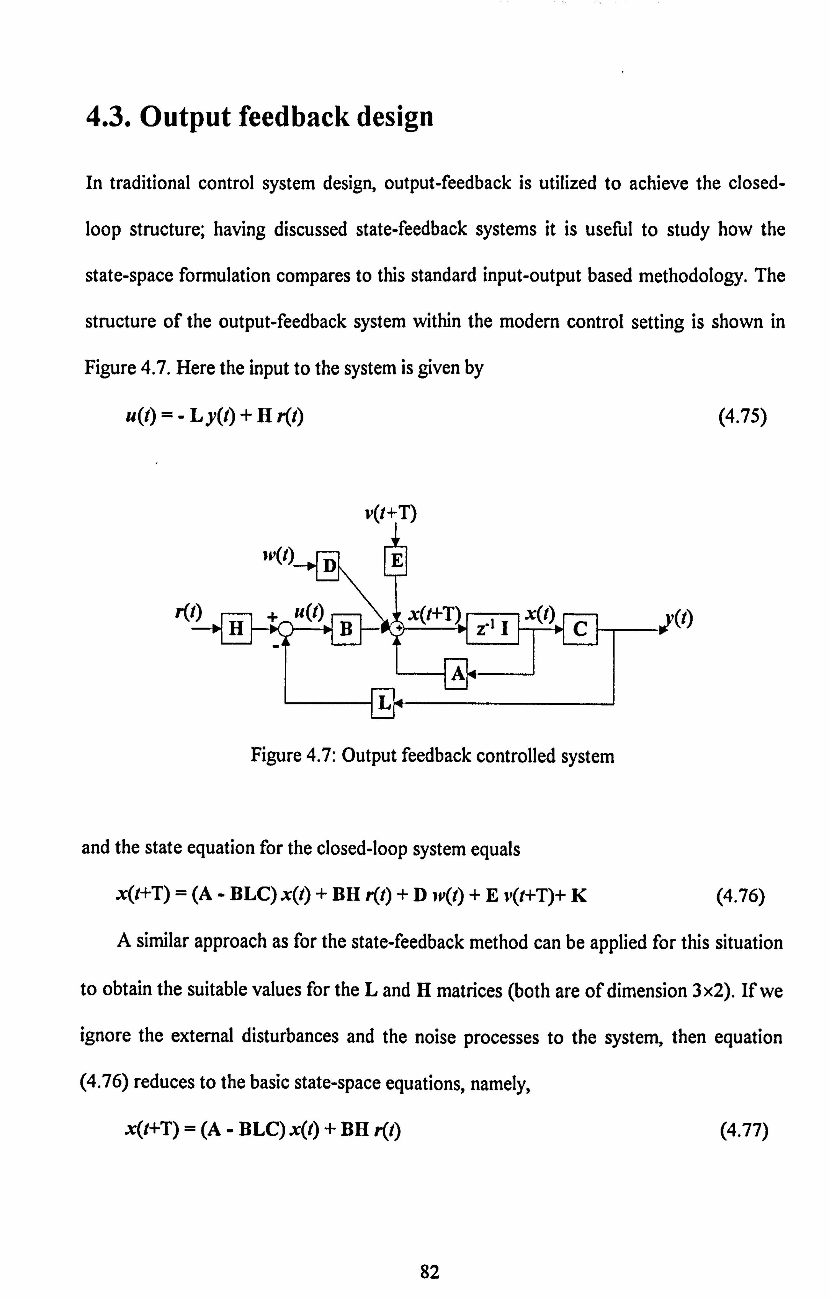
4.3. Output feedback design

In traditional control system design, output-feedback is utilized to achieve the closed-

loop structure; having discussed state-feedback systems it is useful to study how the

state-space formulation compares to this standard input-output based methodology. The

structure of the output-feedback system within the modern control setting is shown in

Figure 4.7. Here the input to the system is given by

u(t) =- Ly(l) +H r(l)

v(t+T)

Figure 4.7: Output feedback controlled system

and the state equation for the closed-loop system equals

1)

(4.75)

x(I+T) = (A - BLQ x(l) + BH r(l) +D ip(l) +E v(I+T)+ K (4.76)

A similar approach as for the state-feedback method can be applied for this situation

to obtain the suitable values for the L and H matrices (both are of dimension 3x2). If we

ignore the external disturbances and the noise processes to the system, then equation

(4.76) reduces to the basic state-space equations, namely,

x(I+T) = (A - BLQ x(l) + BH r(l) (4.77)

82

As in section 4.2, the H matrix in equation (4.77) can be calculated using the final value

theorem to achieve zero steady-state error. From equations (4.27) and (4.77), the z

transform of the output becomes

Y(z) =C[ zl - (A - BLQ ]-' BH R(z) (4.78)

and applying the final value theorem we obtain

(4.79) [I - (A - BLQ ]-l BH 12

so that the system output equals the desired set point. Equation (4.79) can be used to

calculate the H matrix by defining

[I - (A - BLQ ]-l B tll t12 t13 It2l

t22 t23 (4.80)

and assuming that two of the matrix elements of H are known. As in section 4.2, if h3l

and h22 are known, then h., 9hI19

h32 and h,, can be calculated using equations (4.39) -

(4.42) by replacing s with t.

4.3.1. Pole-placement design by output feedback

The design of the output feedback controller can be carried out in a manner similar to

that of the state-feedback control. Since equation (4.76) is equivalent to the state

equation of a closed-loop system with state-feedback gain LC and the pair (A, B) is

completely controllable, then this gain can be solved directly from equation (4.50). Thus,

we have

LaC= [(M ST )-' (a - a)]T

and the output feedback gain

L= wl:

(4.80)

(4.81)

83

Since the right-hand side of equation (4.80) is of dimension N6 and from equation (4.9),

C is defined by C=0000], then the vector 1: should be of dimension 10

00100

I x2 and let us define I: a[ 1*, 12* ] and hence, I: C =[1, * 00 1*2 '0 0 ]. The a vector

can be calculated from equation (4.80) where the right-hand side becomes

[(M S' )-' (a - a)]' =[1, * 001*, 00].

The term (M S' )-' can be calculated and for convenience, let it equal

Zil Z12 Z13 Z14 Z15 Z16

Z21 Z22 Z23 Z24 Z25 Z26

(m sr YI= Z31 Z32 Z33 Z34 Z35 Z36

we then have Z41 Z42 Z43 Z44 Z43 Z46

Z51 Z52 Z53 Z54 Z55 Z56

IZ61 Z62 Z63 Z64 Z65 Z66 J

Zil Z12 Z13 Z14 ZIS Z16 a, -a, Z21 Z22 Z23 Z24 Z23 Z26 a, -a, 0 Z31 Z32 Z33 Z34 Z35 Z36 a4 -a4 0

(4.82) Z41 Z42 Z43 Z44 Z45 Z46 a3-a3 12

Z51 Z32 Z53 Z54 Z55 Z56 a2-a2 0 Z61 Z62 Z63 Z64 Z65 Z66J Lai-aij LOJ

By substituting w= [w, W2 W3 I I' into equation (4.8 1), we have

Wl"l W112

W21, W21; (4.83)

-W311 W31'2

-

and the characteristic equation of the closed-loop system is

1 Z'6 -A+BLCI= 1 Z16 -A+Bäl: C 1 =O (4.84)

Since the rank of B (= 3) is greater than that of C (= 1), we cannot arbitrarily assign

all the elements of w if we wish to arbitrarily assign a maximum number of eigenvalues of

the closed-loop system. But if all the three elements of w were arbitrarily assigned so that

84

the pair (A, B') is controllable then applying equation (4.82), we then have only 2 out of

6 elements of a to be chosen so that the closed-loop system is stable. The remaining

elements can be obtained from the rows of which the right-hand side of equation (4.82)

are zero, i. e. the second, third, fifth and sixth equations. These a elements will determine

the eigenvalues of the system, namely p,, p2, p3, p, p, and p6,, through the closed-

loop characteristic equation (4.77) of which it can be factorized as:

1 zl, -A+ BLC 1m (Z - PJXZ - PYZ - PYZ - AXZ - PJXZ - P6) =

or equivalently, IzI.

-A+BLCI=-z 6+a6Z5+ a5 Z4 + a4 Z3 + a3 Z2 + a2 Z+ al =0

where a, = p, p2p3p4p5p6, etc.

The elements of 1:, i. e. I' and 12* can be calculated from the first and the fourth elements

of the left-hand side of equation (4.82).

As mentioned earlier, the conditions for stability of the desired closed-loop system is

that the absolute eigenvalues should be 0<Ip, I<1, i=1,2, ..., 6. - We can see that a,

in terms of p, are not linearly related. Therefore, we must find the 2 starting elements of

a so that the system's stability as well as equation (4.82) are satisfied, before being used

to obtain 1: and hence the output feedback gain L.

As an example, we can again use w= [10 10 I]T because it makes the pair (A,

B) controllable. Let us assume that the values of a3 and a4 are known, then from

equation (4.82), we can calculate the remaining a's by solving 4 unknown parameters

such as a, . a2, a5 and a6 from 4 linear equations. It is found that a solution for

stability of the closed-loop system is as follows: a3 and a4l. respectively, equal to

-0.040 and -0.783, which gives a,, a2, a, and a6, respectively, equal to -0.00 1,0.25 1,

85

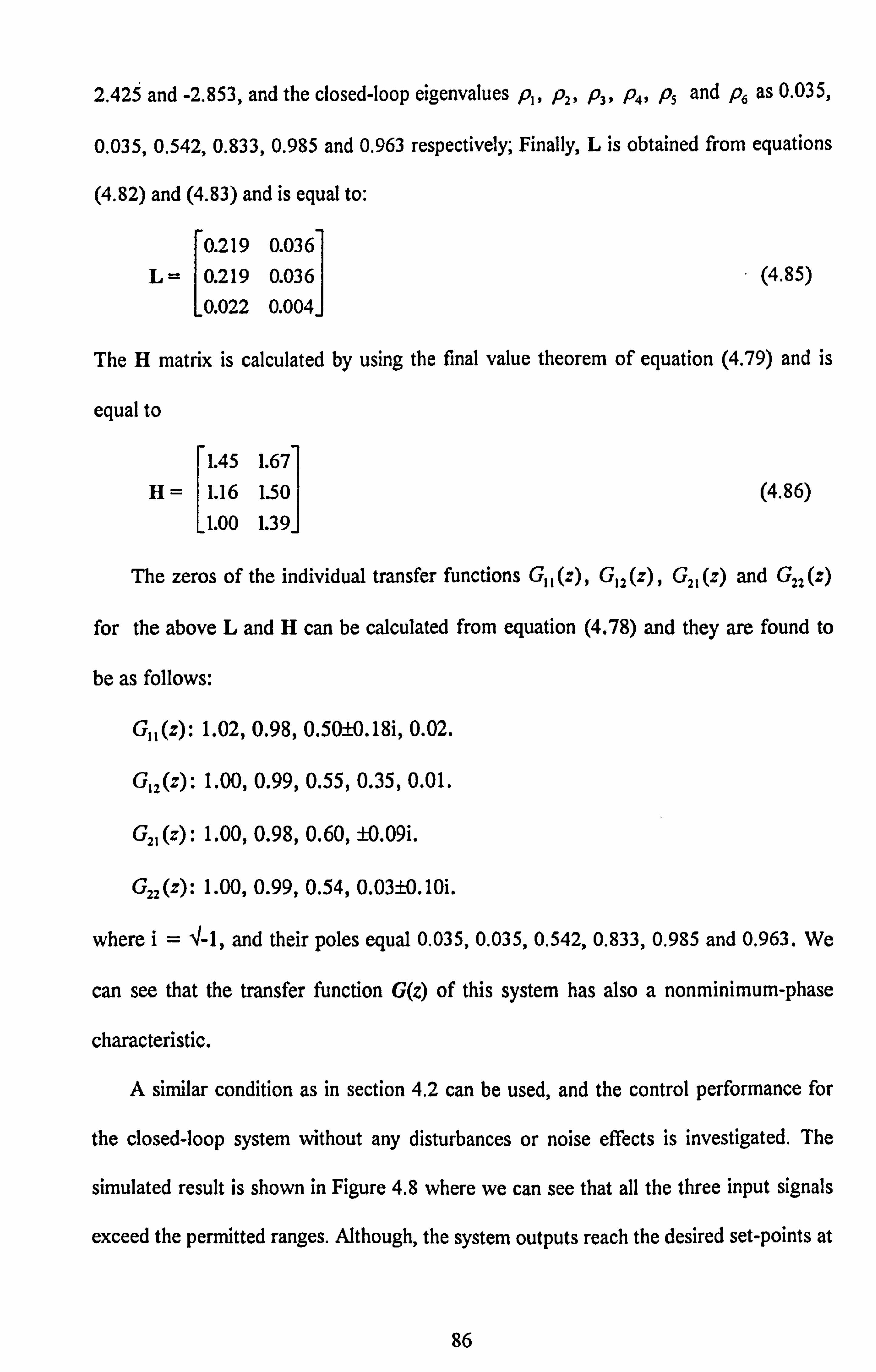
2.425 and -2.853, and the closed-loop eigenvalues p,, p2, p3, p4, p, and p6 as 0.035,

0.035,0.542,0.833,0.985 and 0.963 respectively; Finally, L is obtained from equations

(4.82) and (4.83) and is equal to:

0.219 0.036 L= 0.219 0.036

0.022 0.004

(4.85)

The H matrix is calculated by using the final value theorem of equation (4.79) and is

equal to

1.45 1.67 H 1.16 1.50

1.00 1.39

(4.86)

The zeros of the individual transfer functions G, , (z), G, 2 W, G2, (z) and G22 (Z)

for the above L and H can be calculated from equation (4.78) and they are found to

be as follows:

Gl, (z): 1.02,0.98,0.50±0.18i, 0.02.

G,, (z): 1.00,0.99,0.55,0.35,0.01.

G2, (z): 1.00,0.98,0.60, ±0.09i.

G22 (Z): 1.00,0.99,0.54,0.03±0.10i.

where i= 4-1, and their poles equal 0.035,0.035,0.542,0.833,0.985 and 0.963. We

can see that the transfer function G(z) of this system has also a nonminimum-phase

characteristic.

A similar condition as in section 4.2 can be used, and the control performance for

the closed-loop system without any disturbances or noise effects is investigated. The

simulated result is shown in Figure 4.8 where we can see that all the three input signals

exceed the permitted ranges. Although, the system outputs reach the desired set-points at

86

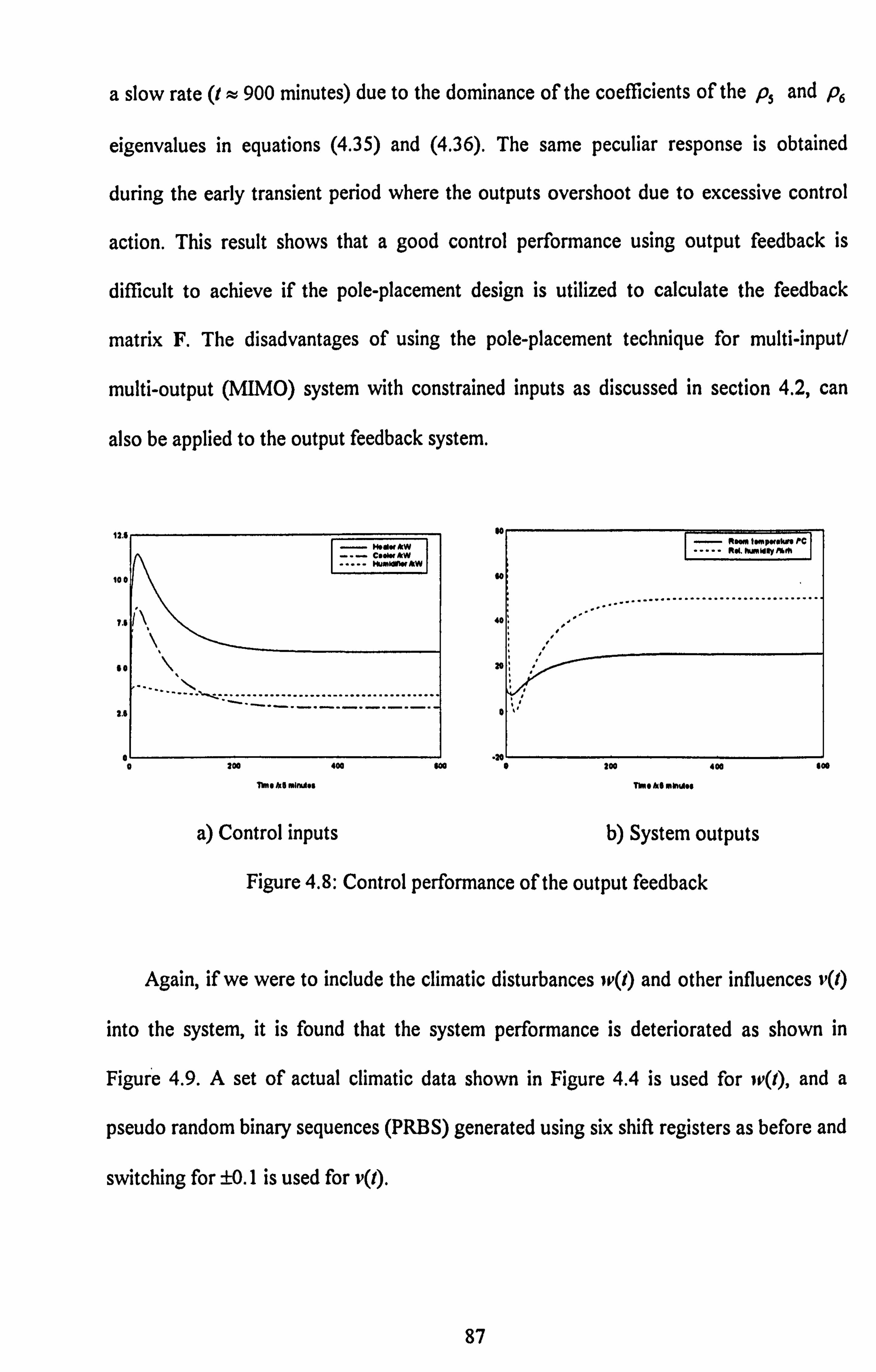
a slow rate (t; -- 900 minutes) due to the dominance of the coefficients of the p, and p6

eigenvalues in equations (4.35) and (4.36). The same peculiar response is obtained

during the early transient period where the outputs overshoot due to excessive control

action. This result shows that a good control performance using output feedback is

difficult to achieve if the pole-placement design is utilized to calculate the feedback

matrix F. The disadvantages of using the pole-placement technique for multi-input/

multi-output (MIMO) system with constrained inputs as discussed in section 4.2, can

also be applied to the output feedback system.

12.5

100

7.6

so

Hd. kw

C.. Wkw muokwwkw

200 400 640

nme *5 MINAS$

a) Control inputs

........................................

400 on

b) System outputs

Figure 4.8: Control performance of the output feedback

Again, if we were to include the climatic disturbances ip(l) and other influences v(1)

into the system, it is found that the system performance is deteriorated as shown in

Figur e 4.9. A set of actual climatic data shown in Figure 4.4 is used for w(f), and a

pseudo random binary sequences (PRBS) generated using six shift registers as before and

switching for ±0. I is used for vQ).

87

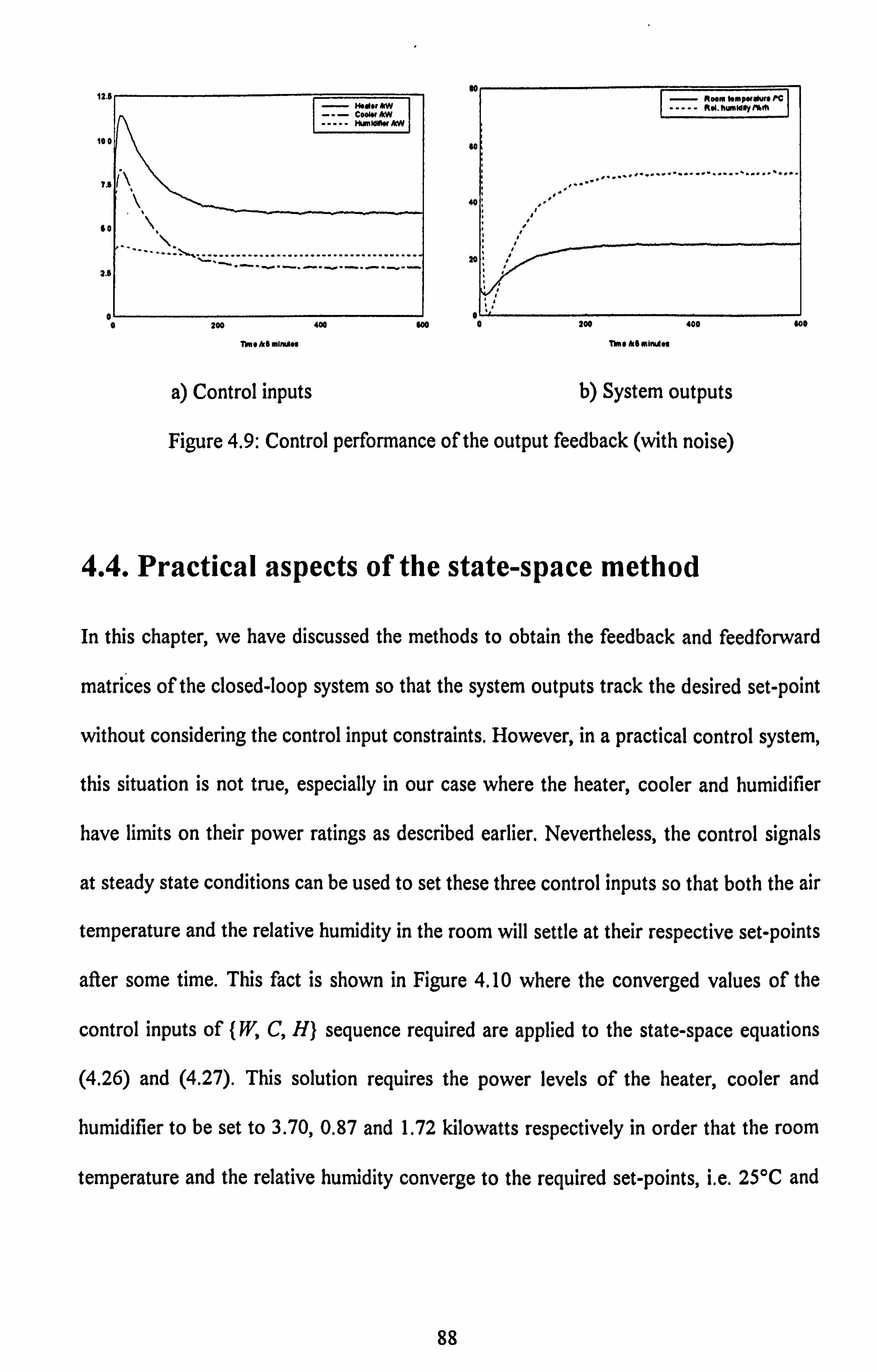
co" okw HM~AW

0011

Go ---------------

2.6

200 400 400 0 200 400

Th 0 A. 6 mImges Tee eh 0 wimoot

- RMM I. mpswI PG

. E.. "


Figure 4.9: Control performance of the output feedback (with noise)

4.4. Practical aspects of the state-space method

so*

In this chapter, we have discussed the methods to obtain the feedback and feedforward

matrices of the closed-loop system so that the system outputs track the desired set-point

without considering the control input constraints. However, in a practical control system,

this situation is not true, especially in our case where the heater, cooler and humidifier

have limits on their power ratings as described earlier. Nevertheless, the control signals

at steady state conditions can be used to set these three control inputs so that both the air

temperature and the relative humidity in the room will settle at their respective set-points

after some time. This fact is shown in Figure 4.10 where the converged values of the

control inputs of (W, C, H) sequence required are applied to the state-space equations

(4.26) and (4.27). This solution requires the power levels of the heater, cooler and

humidifier to be set to 3.70,0.87 and 1.72 kilowatts respectively in order that the room

temperature and the relative humidity converge to the required set-points, i. e. 25T and

88

50%rh respectively. Identical responses as in Figure 4.10 are also obtained when the

simulation trial is carried out via the original model equations (2.1) and (2.2).

Rol. humidity /%rh Room temperature PC

----------------------------------------

0 200 400 Goo

Tim txS mlnLAos

Figure 4.10: System response for steady state values for the control inputs

In the calculation of the control inputs W, C and H from the modal controller, the

climatic disturbances )P(I) and the stochastic noises v(1) were not included into the

system. When these terms are present, such as the laboratory temperature, the outside

temperature, the outside humidity and the solar irradiance are constant at 20"C, IOIC,

70%rh and OWm-' respectively and the other stochastic effects are ignored, we found

that the temperature and the humidity converged to 25.4"C and 51.8%rh respectively

due to the calculated feedback, F, and feedforward, H, matrices were based on the plant,

A. and input, B, matrices only. This shows thauthe method to calculate F by temporarily

ignoring these external disturbances is acceptable for this example since the steady state

values are slightly different from the required setpoints.

89

4.5. Conclusions

This chapter has discussed the state-space methodology for solving the control problems

in the building energy management application area. The techniques such as the pole-

placement design and the modal control do not consider the constrained input situations

as well as the strategies for control input optimization. Therefore, both methods are at

first sight unable to achieve a good control performance in realistic applications.

However, the results can be used to get an idea of the control signal ratios for the

required set-points and the desired poles.

More advanced methods such as using MIMO adaptive control with constrained

inputs or more intelligently, the fijzzy logic and genetic algorithm techniques can be

utilized to solve this type of control problems; these are discussed in the remaining

chapters.

90

Chapter 5

MIMO Adaptive Control with Constrained

Inputs

In most control systems, the main problem is to design a control strategy which has the

ability to adjust itself according to the changing properties of the controlled processes

and the restrictions on the signals. A relatively new approach, namely, adaptive control,

can provide the ability to carry out such designs. These control systems can be divided

into two main groups, namely, feedforward and feedback adaptive controllers (Isermann

et al., 1992). Feedforward adaptive control systems are based on the fact that the

changing properties of the plant can be monitored by measurement of the signals acting

on the process. If the process behaviour changes cannot be determined directly by

measurement of external process signals, the feedback type of adaptive controllers

should be used. Amongst many types of feedback adaptive controller, the model

identification adaptive controllers (MIACs), sometimes also called self-optimising

controllers or self-tuning controllers are well known to control practitioners.

Numerous papers discuss the MIMO adaptive controllers, but many of them deal

with only square systems, i. e. the number of inputs equals the number of outputs (see for

91

examples Borrisson, 1979; Elliott et al., 1984; Mohtadi et al., 1986). Mikles (1990) has

developed a multivariable self-tuning controller based on the pole-placement design

which is suitable for nonsquare systems but it does not consider any constraints on the

control inputs. A number of papers deal with constrained inputs for designing MIMO

adaptive controllers. Most of these are based on the dynamic matrix control approach

(DMC) developed by Cutler and Ramaker (1980) which use the predicted output errors

in the presence of physical constraints. Some of them use saturated inputs instead of the

actual computed inputs (see for examples Ohkawa and Yonezawa, 1982; Payne, 1986).

Another approach is to re-compute the reference model whenever the computed control

input is out of the permitted input range (see Ortega et al., 1984).

In this chapter, we present a MIAC with input and output constraints, which are

usually found in real systems. The theory of designing the control law for the adaptation

mechanism presented here is based on the methods developed by Dion et al. (199 1), and

for the process model identification, a multivariable recursive least square method is used

(see for examples Mikles, 1990; Peterka, 1975). In applying this control law, the control

input is computed on a receding horizon principle, based on the generalized predictive

control methodology (Clarke et al., 1987). The constraints on the inputs are not only

applied to the present control input but also to future computed control inputs. All these

control inputs are not actually applied since, at each sampling time, only the current

computed constrained input is applied. However, it may be noticed in the proposed

algorithm, that the current control input has been computed under the hypothesis that the

future control inputs and/or their derivatives also satisfy the constraints. The adaptive

constrained control problem is then solved iteratively, using classical "quadratic

programming with constrainte' methods (see for example Fletcher, 198 1).

92

The proposed algorithm can deal with nonsquare systems which is suitable for our

system with 3 control inputs and 2 outputs (Figure 2.1). These inputs have physical

limitations on their maximum power ratings, as well as the power changes between the

sampling periods that they can provide to the system. Furthermore, it may also be

required to set the output ranges as required in the algorithm.

This chapter is organised as follows: we present the theory of the control law

developed by Dion et al and then follow this by it's application in our BEMS. The

theory begins with a statement of the problem and then it's solution for this application.

5.1. Statement of the problem

Let us consider the following multivariable process model:

A(z-')y(t) = B(z-)u(t) (5.1)

where

I+A, z-' +... + A, z-"

B, z-1 +... + B,, z-"

are (p x p) and (p x m) polynomial matrices respectively, n is an upper bound on the

observability index of the process model, I is (p x p) identity matrix, u(I) and y(I) are,

respectively, the input and output vectors, and for convenience, the term - is defined

slightly different from other type of controllers in this thesis, that is z-'Rt) = Rt-1) where

the sampling interval T is assumed to be unity.

The control objectives are the following: tA

Let us consider the following finite horizon quadratic criterion:

93

N

J(I) = 1: (y(l+j)-ym(t+j))TR (y(l+j)-ym(t+j)) J-1

N Ar

J: A UT(t +j_ 1) Q, Au(t+j-l)+EuT(i +j- 1) Q, u(I +j- 1) (5.2) i=l J-1

where N is the prediction horizon, (y. (1)) is the output reference vector sequence, A is

the difference operator (I - z-')I, and R, Q, and Q2 are the weighting factors on the

predicted output error, rate of predicted input and the predicted input respectively and L41 S+

they are positive definite matrices. We can see from the du nf-ýav, (5.2) that the first,

second and third terms on the right hand side of the equation deal with the predicted cost

of regulation errors, the rate of energy consumed and the actual energy consumed

respectively; these are all variables which we intend to minimise. The weight Q, on the

input increments Au incorporates some integral action of the predicted input and the

weight Q2 on the input u allows one to save control energy when we have degrees of

freedom on the inputs.

We require that, at each time 1, the control inputs that minimise the quadratic

criterion J(I) and satisfy constraints on the inputs and outputs of the following type:

Cäut 2. v. (0, offl, t) D(O)y, 2: yfy (0, offl, t)

where

(5.3)

AU, [AUT(j), ... , AUT(I+N-1)] (I x Nm) is the predictions in the rate of change

of the control sequence from the current time (1) to the future time Q+N-1).

ytT [yT(I + 1), ... , y(1 +, N)] (I x Np) is the predictions of the output y from

time (1+1) to time Q+N).

94

O= [A, q ...

A#,, BI, ... , BJT (n(p +m) xp) is the matrix of coefficients in the

process model.

ý' (t) = [-y'(t), ... , -y'(t - u'(t -n+ 1)] (5.4)

C, D(O, V. () and V., () depend on the constraints and will be specified later.

The inequalities given by equation (5.3) can express different types and

combinations of constraints on u(. ) and y(. ); for instance constraints on the magnitude of

u and y, the magnitude of the derivatives of u and y or on some linear combination of u

and

5.2. Multivariable adaptive control law

When the A, and B, parameter matrices are known, we can transform the above

problem, i. e. minimisation of the objective (5.2) while satisfying the Process dynamics

(5.3) into a classical one, namely, quadratic minimisation with constraints. The control

law is then computed, using quadratic programming methods with constraints.

Let us first build general j-step ahead predictors with the following Bezout

identities:

I=E, (z-) A (z-) A+F, (z-') z-J, forj = 1, ... ,N (5.5)

where E, (z-') and F, (z-') are polynomial matrices defined by

Ej (Z-') =1+ EIJ z-1 +... + E, ý, z-J"

(z-) = FI + Ff z-' +... + F�l z-' i (5.6)

These polynomial matrices are uniquely defined by A(z-), A, and the prediction horizon

By postmultiplyingy(t +J) into equation (5.5) we get

95

yQ +j) = E, (z-')A(z-') Ay(I +J) + F, (z-') z-iy(t+j)

Using equation (5.1) on the first term on the right hand side gives

y(t +J) = Ej(z-1) B(z-1) Au(t +J) + F, (z-)y(t) forj = 1, ... ,N (5.7)

Defining Gi(z-') as E, (z-) B(z-') and letting

Go' z-' + GJ z-' +... + G.,., -, z-j-"

we have the following set of predictors

y(t + 1) = Go' Au(I) + (z G'(z-') - Go) Au(l) + F, (z-') Y(t)

y(t + 2) = (Go + G, z-') Au(I + 1) + (z G'(z-') - Gý' - G, z-' ) Au(I + 1)

+ F, (z-')y(t)

(5.8)

Ar- I

G, "z-1 Au(I+N-I)+(zG"(z-')-I: G, z-')Au(I+N-1) 1-0

+ F, (z-)y(t). (5.9)

It is easily shown (Clarke et al., 1987) that

2= Go = Go'= Go ... = GON-1 = GON

G, =G 12 =G 13 ... = Gj'

G, v-, = GNAr-I ,

The set of equations (5.9) can then be rewritten in a condensed form:

96

G,, Au,

where

(5.11)

yt = ly, (t + 1), Y, (I + N)]

Au, r = [Au r (1), A u'(1 +N- 1)] (5.12)

f, = IfIT(l), ... I

RT (1) 1

(z GJ(z-') - 2GJ

Z-') Au(t +j -1) + F, (z-')y(t) (5.13) i=O

Go G, Go

G, um =- (Np xA I).

G, Go

-GAr-I GN-2

a G, Go

The term U, Au, contains present and future inputs, and the term f, contains present

and past outputs (up to time 1), and past inputs (up to time I- 1).

The quadratic criterion (5.2) can then be rewritten as

Al) = (YI - yMt 'ý(Yt - yMt +A Ut (5.15) T TQI A Ut + U: )2Ut

where

R= diag (R, R) (Np x NP)

C), = diag (Q,,..., Qj) (NM x NM)

U2 = diag (Q2,..., Q2) (Nm x Nm)

T [. V T (I + I), ...

(I XN ,y+, N)] p XMI MM

U, (I x Nnl). (5.16) U'Q + N- 1)]

Defining W,, as [uT(t -

1), UT(I UT(t _ 1)] (1 x Nm), u, may be rewritten as:

97

Ut = HN AUt + WI-I

where

lux (Nm x Nm)

Using equation (5.11), the criterion (5.15) becomes

(GN A u,

+Au, "U, A u, + u, rUu,

Now, using equation (5.17) we have

JQ) = (GN A u, + yA,,, ) T k(Uv A u, + f, - yxf, ) +Au T) IA

(5.17)

+&uITH NT L-) 2 H- + 2AurH-T- (5.18) Af

A Us t NQ2'Tt-I + Wt-ICIA-1

The control law input implemented at time I is the control at time Q-1) plus the change

needed to maintain the required objective, that is:

u(t) = u(I - 1) + Au(l) (5.19)

where the change in the control signals, Au(I) is obtained by minimisation of the

objective (5.2) while satisfying equation (5.3), and can be expressed as:

min (AuT T Au, - 210T Au, ) (5.20) 'Nut

subject to the constraints (5.3).

where T jK 1, a1 (5.21) I'y ,N N+ul+jT

17 (Alm x Np) -2 uIN ?2N

CIT =H (I x Nni) (5.22) (YA,

tt - ft)

T 1ý UN - wsý-l U2

N*

98

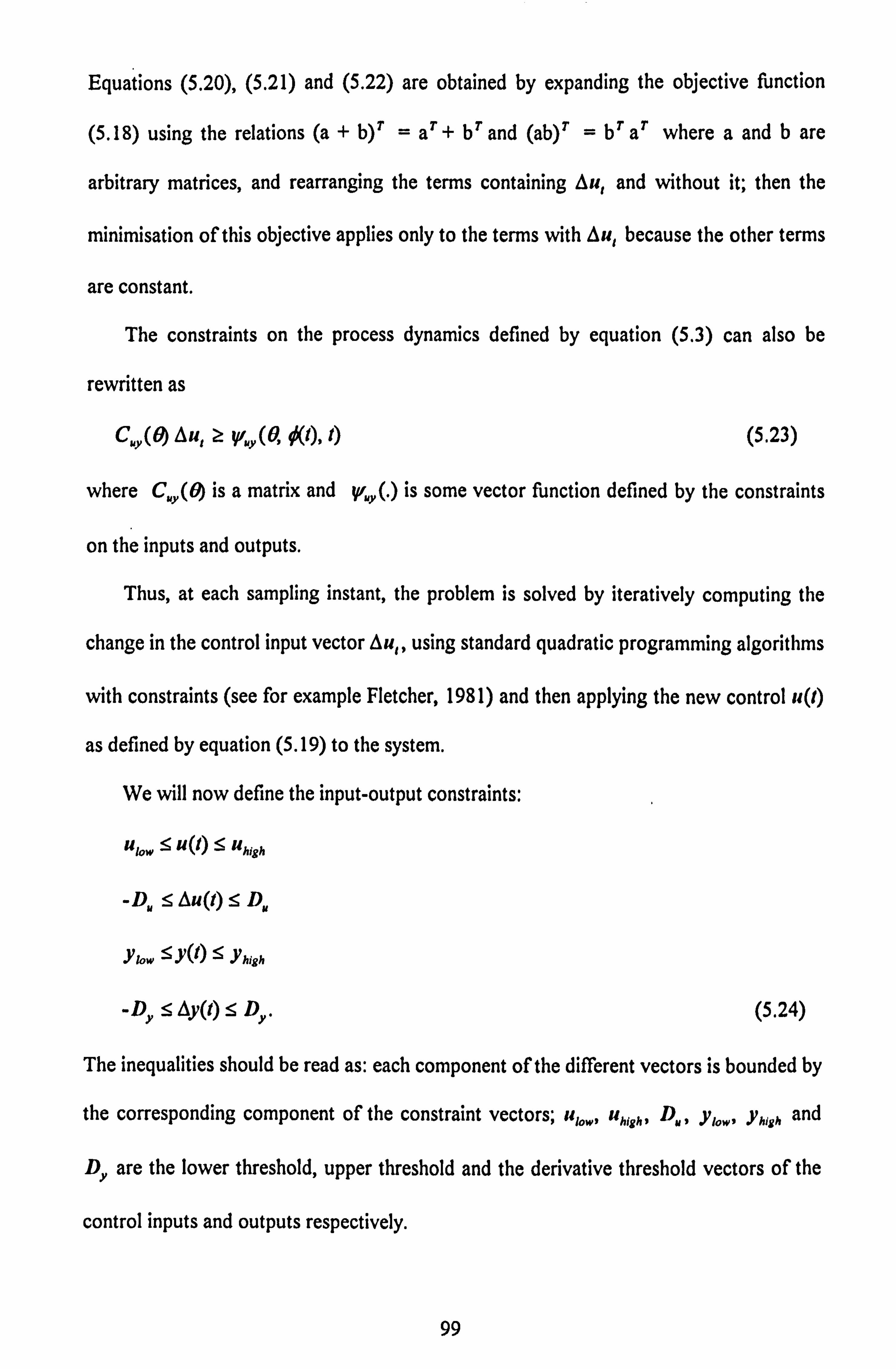
Equations (5.20), (5.21) and (5.22) are obtained by expanding the objective function

(S. 18) using the relations (a + b)' = a' +V and (ab)' =V a' where a and b are

arbitrary matrices, and rearranging the terms containing Au, and without it; then the

minimisation of this objective applies only to the terms with Au, because the other terms

are constant.

The constraints on the process dynamics defined by equation (5.3) can also be

rewritten as

C. Y(ü) Au, 2ý v/. Y (0, offl, t) (5.23)

where C., (O is a matrix and Vf. y(. ) is some vector function defined by the constraints

on the inputs and outputs.

Thus, at each sampling instant, the problem is solved by iteratively computing the

change in the control input vector Au, using standard quadratic programming algorithms

with constraints (see for example Fletcher, 1981) and then applying the new control u(I)

as defined by equation (5.19) to the system.

We will now define the input-output constraints:

Ulow U (1) :5 Uhigh

Au(t): g D.

Yk,. !" YQ) :5 Aligh

-D.,: 5 Ay(t).: 5 Dy. (5.24)

The inequalities should be read as: each component of the different vectors is bounded by

the corresponding component of the constraint vectors; ulow, uhighl D., y1o., yh,, h and

D. are the lower threshold, upper threshold and the derivative threshold vectors of the

control inputs and outputs respectively.

99

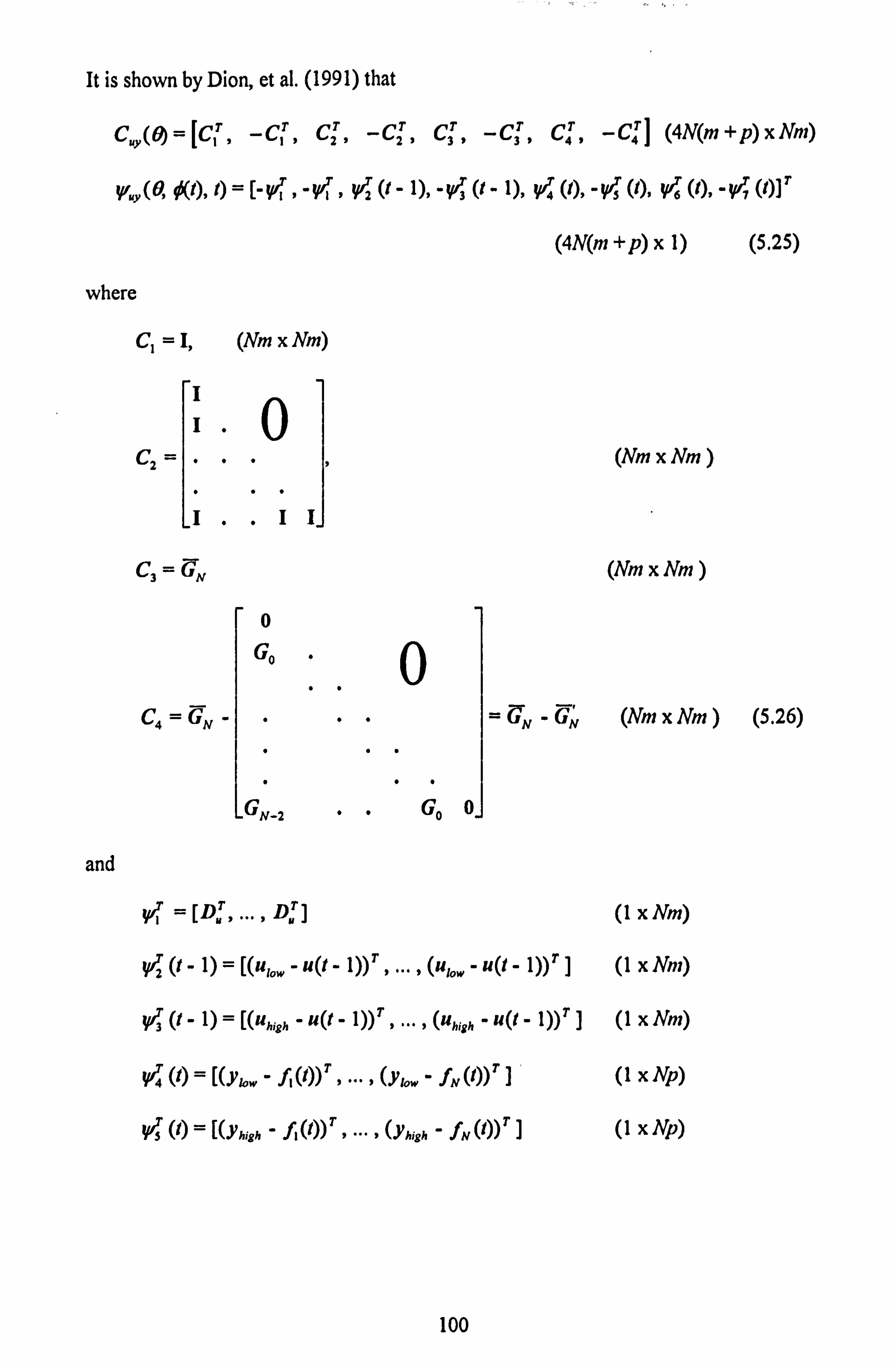
It is shown by Dion, et al. (1991) that

_[CTý _CIT, T

-CT 7 CUY(O ý- AjTI (4N(m + p) x Arm) CT Tj

21 -C21 C3 3 11

C4 C4

r 7' rII Vr2 1), ' , 3r 0" 1)) VIT Q)P ' VOS (')' K11T V'uy (0,0(t), 0 V1 V/ IQ4 'T (A

(4N(m +p) x 1) (5.25)

where

C, =1, (Nm x Nm)

0

C2 (Nm x Nm)

LI

3 Ar (Nni x Nm) C '?; r

0

Gý 0

C4 N, (Nm x Arm (5.26) UN UN

-GN-2 Go Oj

and

V71 =[ DT,, D. r (I x Nm)

T (I x Nni) V2 (t - 1) Rulow U(t 1))T (Ulow

- U(t - 1))T ]

T_ 1) [(Uhigh U(t 1))7' p

(Uhigh ,U (t 7' (t (I x Nm)

f W I(Ylow - l(t))T V4 ... I (Ykl. A (0) TI (I x NP)

T VS (1) [(Yhigh - fl (0) T2 (Yhigh A (0) TI (I x NP)

100

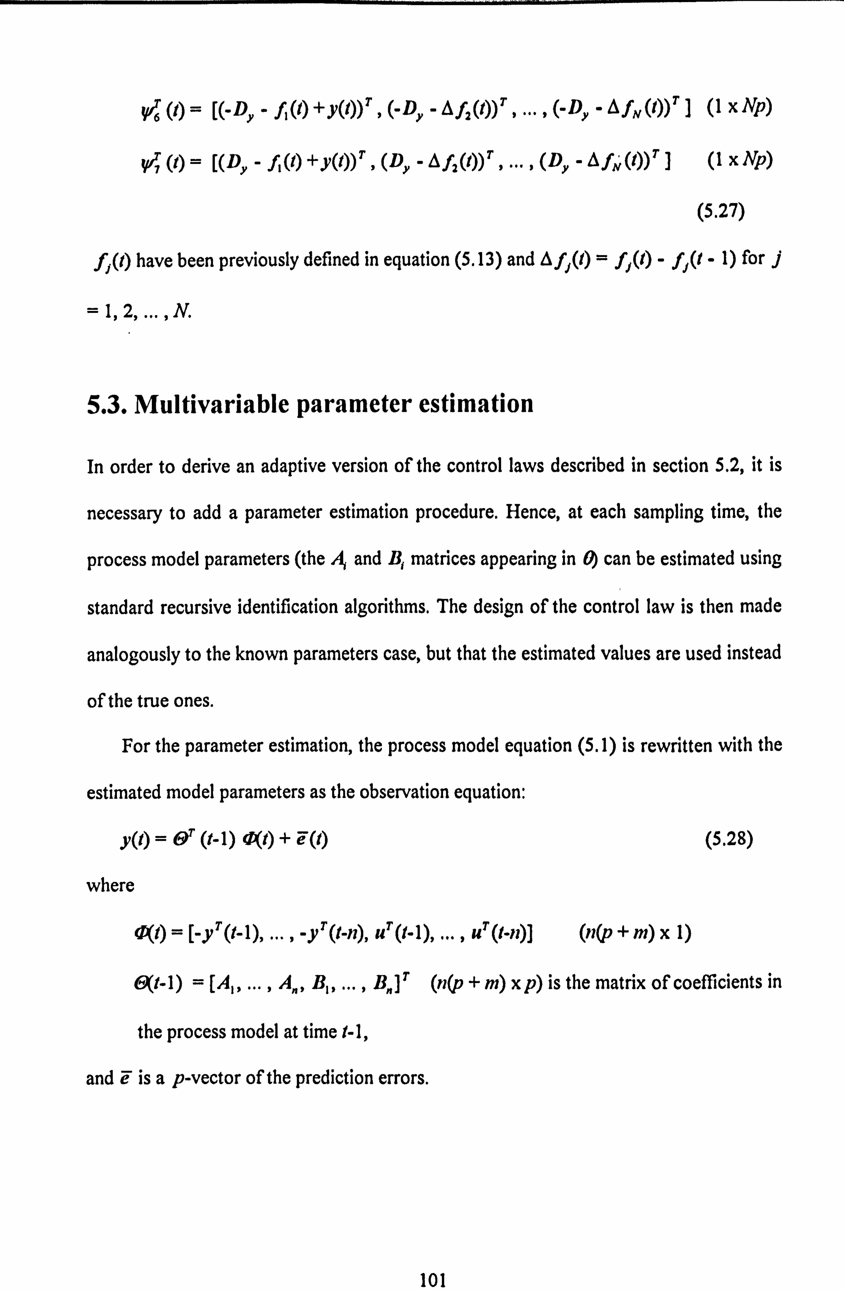
V/6 (1) = [(-Dy - fl(l) +y(l))T, (-Dy -Af2(t))T9..., (-DY-Afv(l))Tl (IXNP)

Wl' (1) = [(Dy - f, (t) + y(l)) T, (Dy -A f2 (1)), ... ,

(Dy -A fý (1)) 7] (I x NP)

(5.27)

fj(t) have been previously defined in equation (5.13) and Af, (I) = fj(1) - fj(I - 1) for

= 1,2,...,

5.3. Multivariable parameter estimation

In order to derive an adaptive version of the control laws described in section 5.2, it is

necessary to add a parameter estimation procedure. Hence, at each sampling time, the

process model parameters (the A and B, matrices appearing in 0 can be estimated using

standard recursive identification algorithms. The design of the control law is then made

analogously to the known parameters case, but that the estimated values are used instead

of the true ones.

For the parameter estimation, the process model equation (5.1) is rewritten with the

estimated model parameters as the observation equation:

er (t- I) At) F(t) (5.28)

where

qt) = [-y'(t- 1), ... , -y'(1-n), u(1- 1), ... , u(1-n)] (11(p + M) x 1)

e(t- i) = [A,, ... , A., BI, ... , B,, ]' (n(p + m) x p) is the matrix of coefficients in

the process model at time 1-1,

and F is a p-vector of the prediction errors.

0

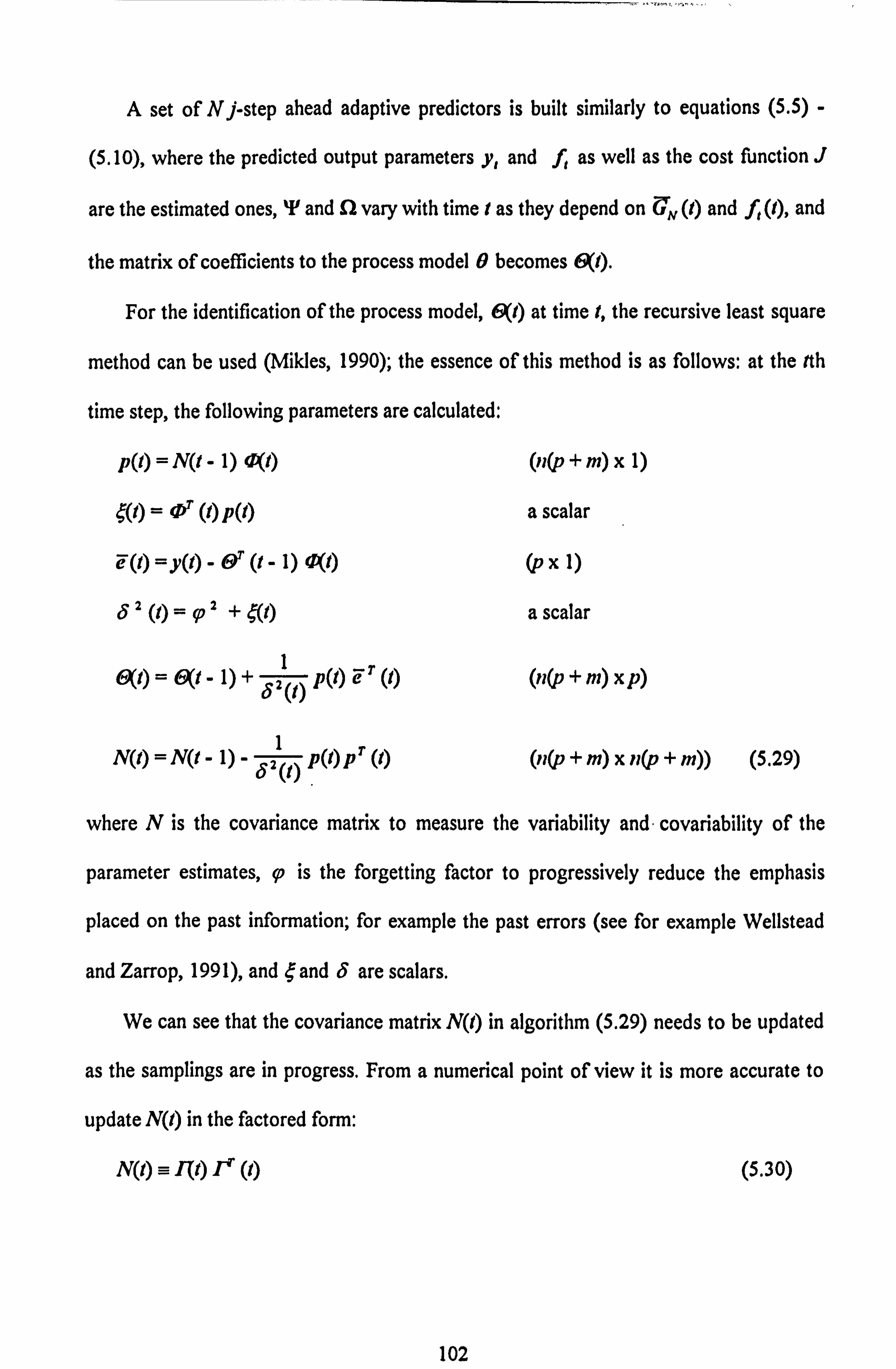
A set of Nj-step ahead adaptive predictors is built similarly to equations (5.5) -

(5.10), where the predicted output parameters y, and f, as well as the cost function J

are the estimated ones, T and fl vary with time I as they depend on U. (1) and ft (1), and

the matrix of coefficients to the process model 0 becomes 6(1).

For the identification of the process model, 6(1) at time 1, the recursive least square

method can be used (Mikles, 1990); the essence of this method is as follows: at the tth

time step, the following parameters are calculated:

p(t) = N(I - 1) (V(t)

41) = (v (1) p(l)

F(I) =Y(I) - eT (t

- 1) 41(t)

j' (1) = q7 ' 41)

(? I(P + M) x

a scalar

(p x

a scalar

ew = e(t - I) +1 82(j) P(l)

1) p(l) P, (1) NQ) = NQ - 1) -

(11(p + m) x P)

(11(p + M) x n(p + M)) (5.29)

where N is the covariance matrix to measure the variability and - covariability of the

parameter estimates, p is the forgetting factor to progressively reduce the emphasis

placed on the past information; for example the past errors (see for example Wellstead

and Zarrop, 199 1), and ý and 8 are scalars.

We can see that the covariance matrix NQ) in algorithm (5.29) needs to be updated

as the samplings are in progress. From a numerical point of view it is more accurate to

update N(l) in the factored form:

I(t) 1r (, ) (5.30)

102

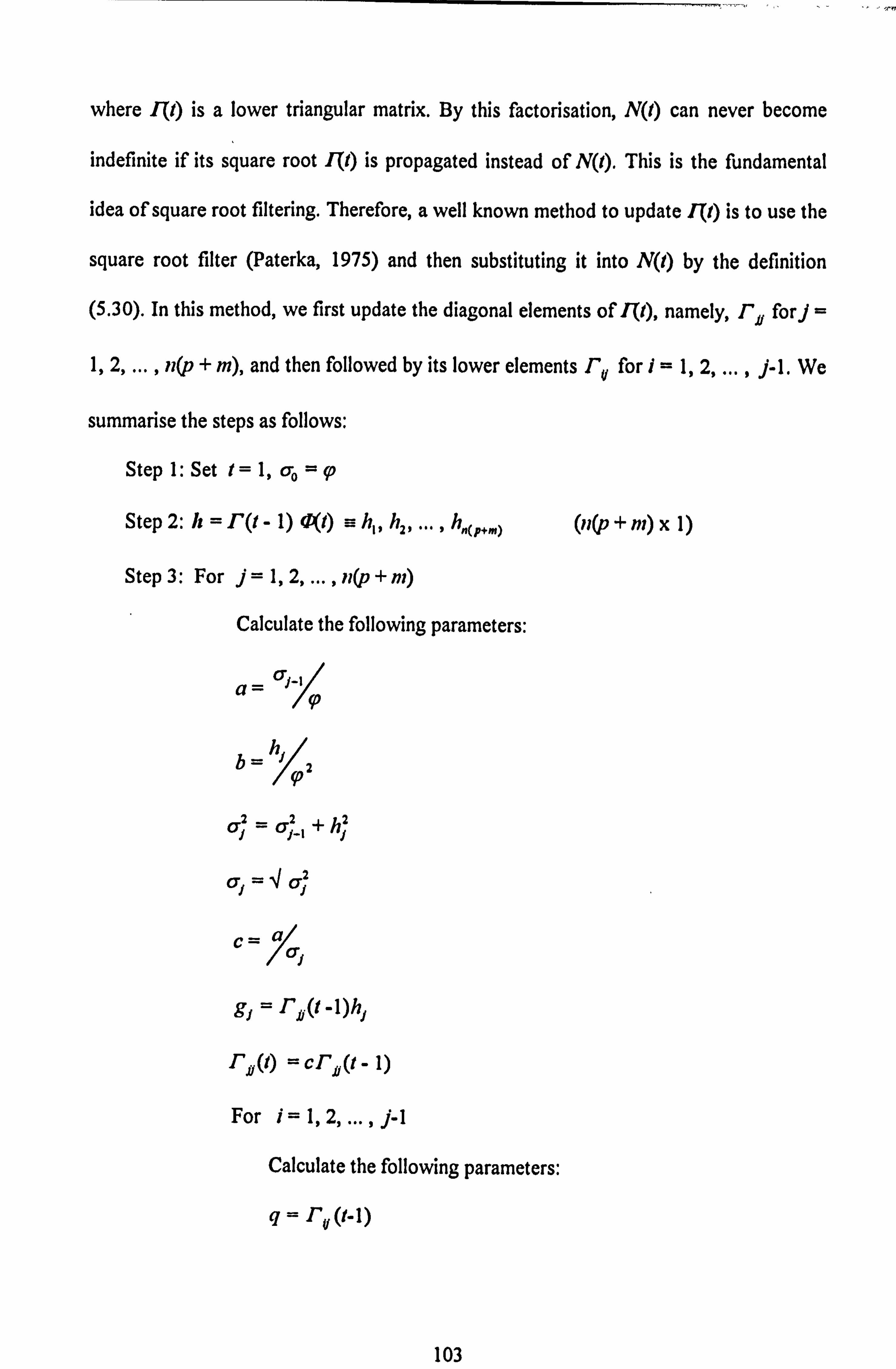
where F(I) is a lower triangular matrix. By this factorisation, N(I) can never become

indefinite if its square root I(I) is propagated instead of NQ). This is the fundamental

idea of square root filtering. Therefore, a well known method to update ITI) is to use the

square root filter (Paterka, 1975) and then substituting it into N(I) by the definition

(5.30). In this method, we first update the diagonal elements of 111), namely, I-ji forj =

1,2, ... , ii(p + m), and then followed by its lower elements I-, for i=1,2, ... , j-1. We

summarise the steps as follows:

Step 1: Set t=1, ao = ip

Step 2: h= ro - i) ow a h., h2, ... , h,, (P,. ) (II(P + m) x 1)

Step 3: For j=1,2, ... , ii(p + m)

Calculate the following parameters:

ail 9 a=9

b Y92

(7j a; -, + hj'

2 j aj a

C= A

gj = r,, (t -I)h,

r., (t) = cr,, (t - i)

For i=1,2,..., j-1

Calculate the following parameters:

q=r,, Q- 1)

103

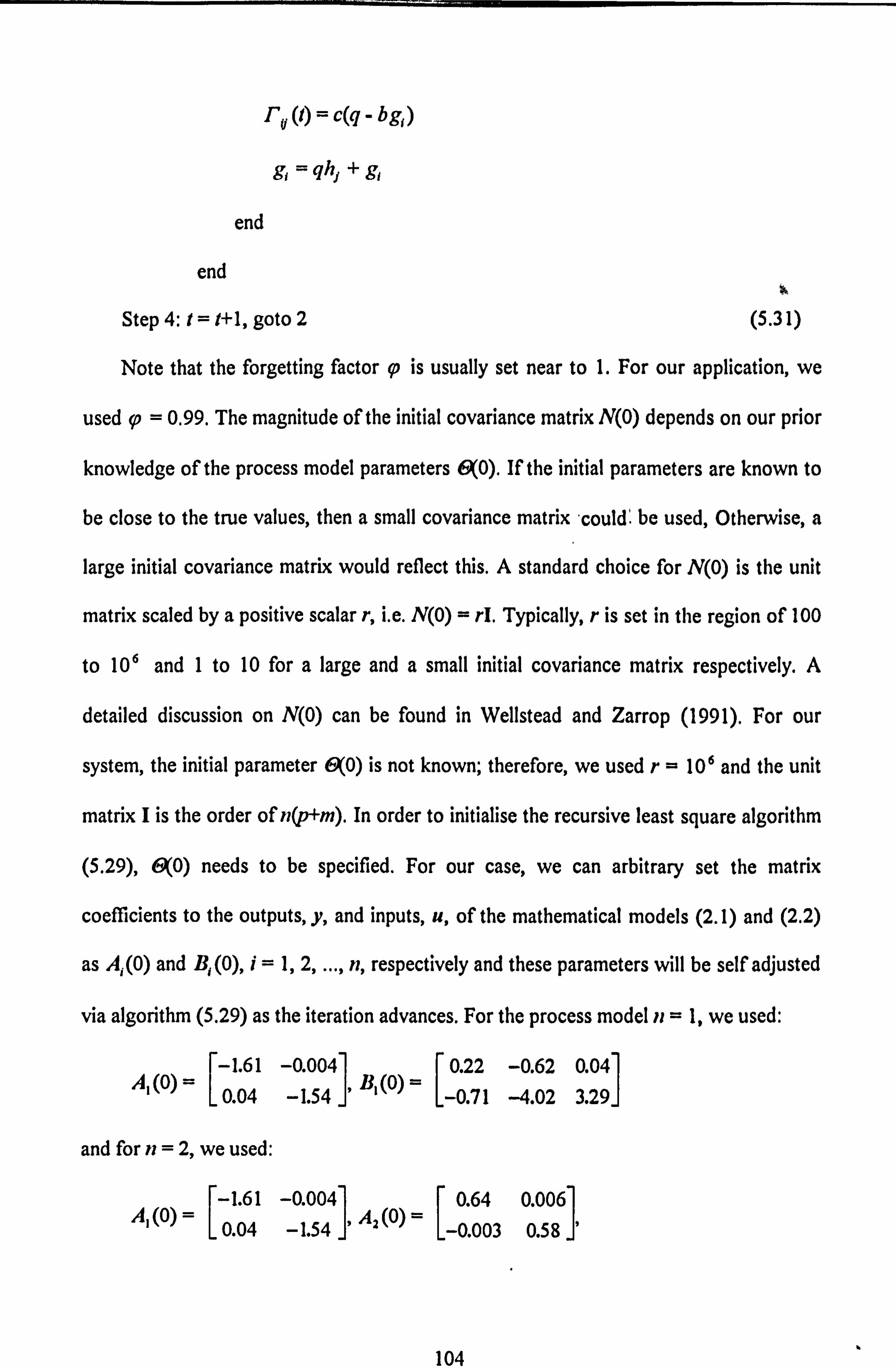
ru (1) = c(q - bg, )

end

gi = qhj + gi

end

Step 4: t= t+1, goto 2 (5.31)

Note that the forgetting factor q) is usually set near to 1. For our application, we

used (p = 0.99. The magnitude of the initial covariance matrix N(O) depends on our prior

knowledge of the process model parameters 0(0). If the initial parameters are known to

be close to the true values, then a small covariance matrix -could' be used, Otherwise, a

large initial covariance matrix would reflect this. A standard choice for N(O) is the unit

matrix scaled by a positive scalar r, i. e. N(O) = rl. Typically, r is set in the region of 100

to 10' and I to 10 for a large and a small initial covariance matrix respectively. A

detailed discussion on N(O) can be found in Wellstead and Zarrop (1991). For our

system, the initial parameter 6(0) is not known; therefore, we used r= 10' and the unit

matrix I is the order of n(p+m). In order to initialise the recursive least square algorithm

(5.29), 09(0) needs to be specified. For our case, we can arbitrary set the matrix

coefficients to the outputs, y, and inputs, u, of the mathematical models (2.1) and (2.2)

as A, (0) and B, (0), i=1,2, ..., n, respectively and these parameters will be self adjusted

via algorithm (5.29) as the iteration advances. For the process model it = 1, we used:

1.61 A. (0)

0.04

and for n=2, we used:

1.61 A, (0)

0.04

-0.004 0.22 -0.62 0.04]

-1.541 , B, (0) =

[-0.71

-4.02 3.29

-0.004 0.64 0.006 A2 (0) =i8

-1.54

l' 1-0.003

0.5

l'

I

B. (0) = 0.22 -0.62 0.04

1B_

rO. 07 0.36 0- etc.

[-0.71

-4.02 3.29] JO) = LO. 37 3.73 -2.42]'

5.4. MIMO adaptive controller for the office zone

system

The MIMO adaptive controller developed in sections 5.2 and 5.3 can be applied for the

office zone system, consisting of three inputs (m = 3) and two outputs (p = 2). The block

diagram of the system is depicted in Figure 2.1 where the climatic disturbances and other

stochastic influences present in the system are clearly shown.

Y'P) Control law AU(I)

I Pararnctcr estimation, AandB

Controller III Office zone/ Y(I) U(I) I HVAC plant

Disturbanccs

Figure 5.1: MIMO adaptive control scheme for the office zone system

The block diagram of MIMO adaptive controller is shown in Figure 5.1 where the

parameter estimation of the polynomial matrices, A and B are first calculated before

being used in the control law. The main objective of this controller system is to calculate

105

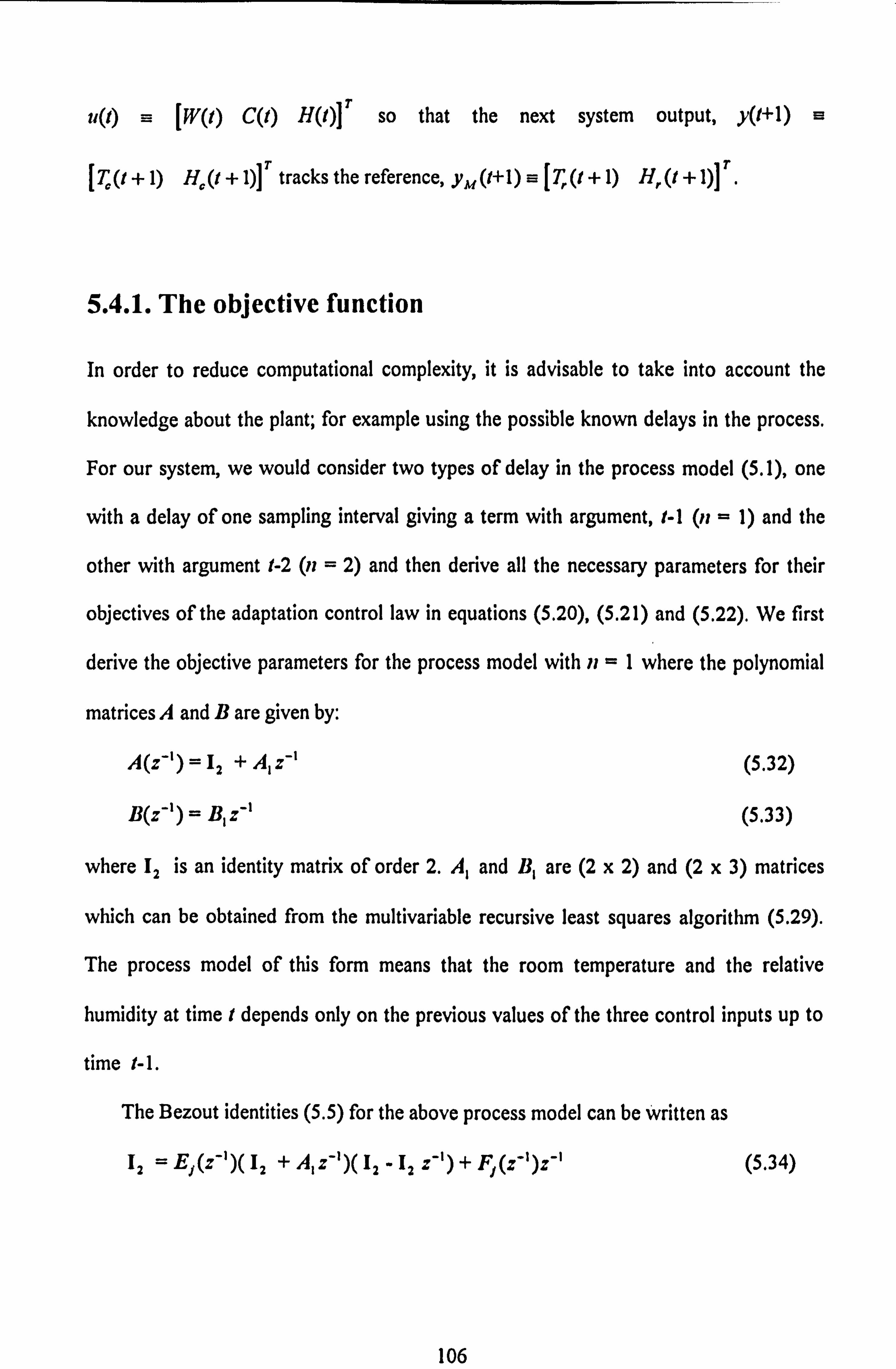
u(t) a [W(t) C(t) H(t)lr so that the next system output, y(t+l) is

[T, (t+l) H, (t + If tracks the reference, ym(t+l) -= [T, (t+l) H, (t+l)]".

5.4.1. The objective function

In order to reduce computational complexity, it is advisable to take into account the

knowledge about the plant; for example using the possible known delays in the process.

For our system, we would consider two types of delay in the process model (5.1), one

with a delay of one sampling interval giving a term with argument, 1-1 (it = 1) and the

other with argument 1-2 (11 = 2) and then derive all the necessary parameters for their

objectives of the adaptation control law in equations (5.20), (5.21) and (5.22). We first

derive the objective parameters for the process model with Yi =I where the polynomial

matrices A and B are given by:

A(z-')= 12 + A, z-' (5.32)

B, z-' (5.33)

where 12 is an identity matrix of order 2. A, and B, are (2 x 2) and (2 x 3) matrices

which can be obtained from the multivariable recursive least squares algorithm (5.29).

The process model of this form means that the room temperature and the relative

humidity at time I depends only on the previous values of the three control inputs up to

time 1- 1.

The Bezout identities (5.5) for the above process model can be Written as

12 = E, (z-')(1, + Az-1)(I,, I, z J(z )z (5.34) -1) +F -1 -1

106

Equation (5.34) is a linear diophantine equation (see for example Kucera, 1979) and it

can be solved by using elementary row operations. It is straightforward to deduce that a

minimum degree solution for the polynomial matrices E, (z-') and F, (z-') can be

obtained if we make (see Mikles and Meszoros, 1991),

Ej(z-1) = 12 and Fj(z-') = FOJ + Fiz-' (5.35)

Then equation (5.34) becomes

12 12 + (A, - 12 + Foi)z -A, + Fli)f' (5.36)

Equation (5.36) is true if the coefficients of z-1 and ý' on the right hand side of the

equation are W zero matrices, we then have

Fi=l -A FIJ=Al 021P

and F, (z-) = (12 - A) + A, z-1 forj = 1,2, ..., N (5.37)

Now, we calculate the polynomial GJ(z-') from equation (5.8) which is given by

Gi(z-') = E, (z-') B(z-1) = B, z-'

and for the prediction horizon N=5, we obtain

UN

L0

and

(lox 15)

(2 x 1) fj (1) (12 - A) y(l) + A, y(t - 1), j=1,2,3,4,5

(5.38)

(5.39)

From the definition of R, Q, and Q2 in equation (5.16), T in equation (5.21) and f17' in

equation (5.22) can be obtained as follows:

107

BITRBI+QI+5Q2 4Q2

TO) 3 Q2

2 Q2

L Q2

4Q2 BITRBI+QI+4Q2

3Q2 2Q2 Q2

2Q2 2 Q2 2Q2

BI'RBI+QI+2Q2 Q2

3 Q2 3 Q2

B17RBI+QI+3Q2 2 Q2 Q2

Q2 Q2 Q2 Q2

BITRBI+Q, +Q2 I

(15 x 15)

(yu Q+ 1) -fl(t))' RBI-5ur(t- I) Q, (ymQ + 2) -f2 (1))'RBI- 4ur(I - I)Q2 (ym(1+3)-f3(t))' RBI -3 ur (t - 1) Q2 (I x 15)

(ym(t+4)-f4(t))r RBI-2uT(t- I)Q2

L (Ym (t + 5) - fs (t)) 7RBI - u'(t - 1) Q2

For it =I and N=2, these parameters are calculated to equal:

fj (t) (12 - A) y(t) + A, y(t - 1), j=1,2 (2 x 1)

TO) BTRB, +Q, +2Q2

TRB Q2

(6 x 6) Q2 B, I+QI+Q2

fIT (ym(t+1)-fl(t))T RBI-2 UT (t 1) Q2

(I x 6) (ym (I + 2) -

f2 (t))T "I - UT (t 1) Ow2

I

(5.40)

(5.41)

Similar calculations can also be performed to obtain the objective parameters for the

process model with ii =2 and the prediction horizon N= 5. We then found:

F (z-') = 02 -A, )+(A, -A, )z-'+A2 Z-2 forj = 1,2, i

108

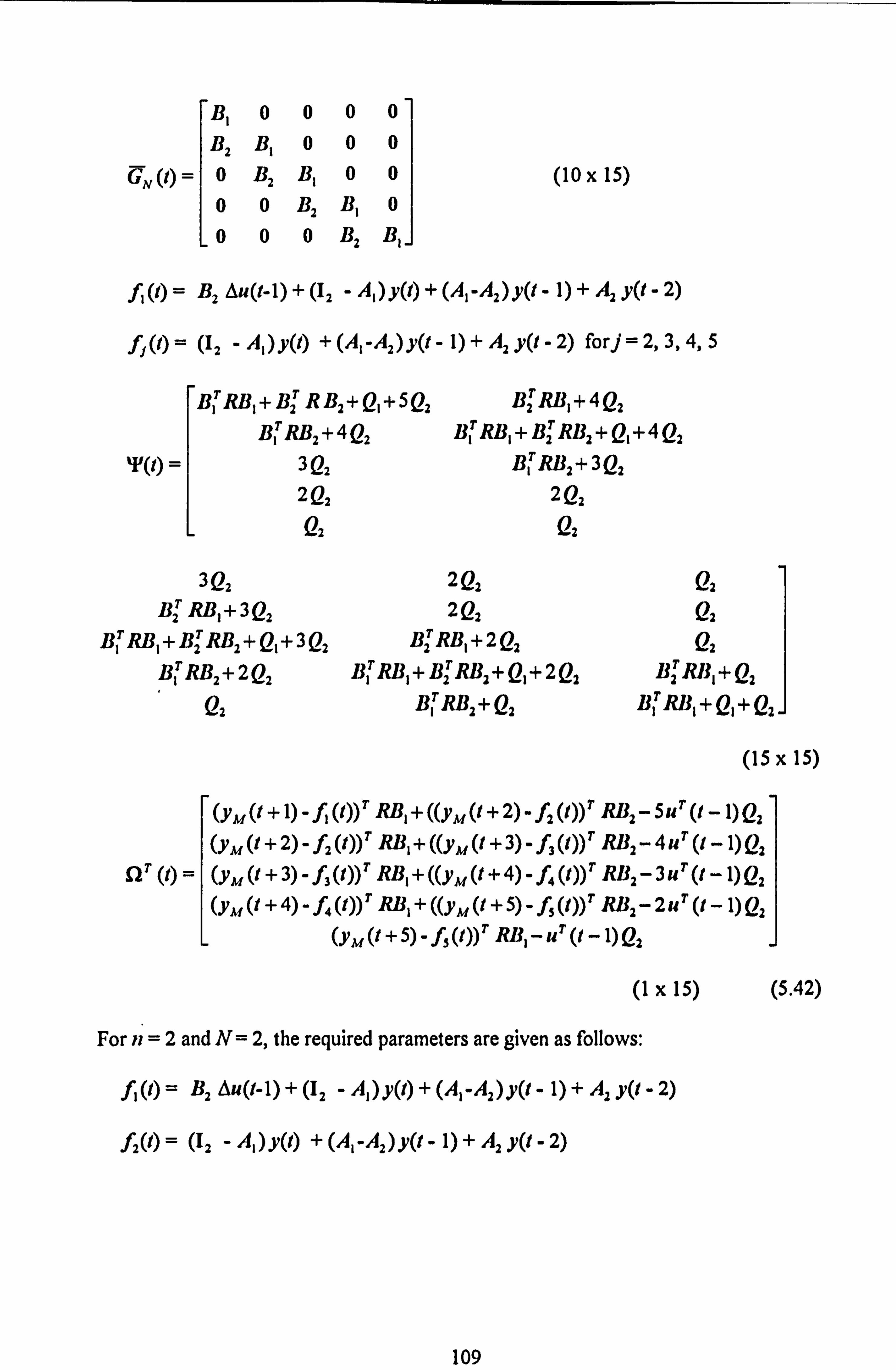
B, 0 0 0 0 B2 B, 0 0 0

GN 0 B2 B, 0 0 (10 x 15)

0 0 B2 B, 0

L0 0 0 B2 B,

fl(l)= 2 AU(t-l) + 02

- A) y(t) + (A, -A2) YQ " 1) + A, y(t - 2)

fj (1) ý (12 - A) y(l) + (A, -A2) Al - 1) + A2 y(I - 2) forj = 2,3,4,5

B, TRB, +B, TRB2+QI+5Q2

BITRB2+4Q2 TO) 3 Q2

2 Q2 Q2

3Q2 B2r RBI +3 Q2

BI'RBI + B2T RB, + Q, +3 Q2

BT I RB2+2Q2 Q2

B2rRBI+4 2

BIT RBI + B2T RB2+QI+4Q2 BITRB2+3Q2

2Q2 Q2

2Q2 2Q2

B2r RBI +2 Q2 BITRBI+B2TRB2+QI+2Q2

BITRB2+Q2

Q2 Q2 Q2

B2T RIJ, + Q2 B, rRll, +Q, +Q2j

(15 x 15)

(ym(t+1) -fl(t))r RBI+((ym(t+2)-f2(t))" JW2-Sur(t- I) Q2

(ym (t + 2) - f2 (t))7RB, + ((yu (t + 3) - f3(l)) " RB2-4ur(t-I)Q2

flr(t)= (ym(t+3)-f3(t))' RBI + ((ym Q+ 4) - f4(t)) " RB2-3ur(t -I) Q2 (ym(t +4)-f4(t))T, ", +((Ym(t +5)-f5(t))7"2-2uT Q -I) Q2

L (yw (t + 5) w f5 (t)) r RBI - u'(t - 1) Q2

(I x 15)

For ii =2 and N=2, the required parameters are given as follows:

)y(t -+ A2 y(t B2 AU(1-1) + (12 - A)y(l) + (A, -A2

f2Q) ý-' (12 - A) y(t) + (A, -A2)YQ - 1) + A2 y(I - 2)

(5.42)

109

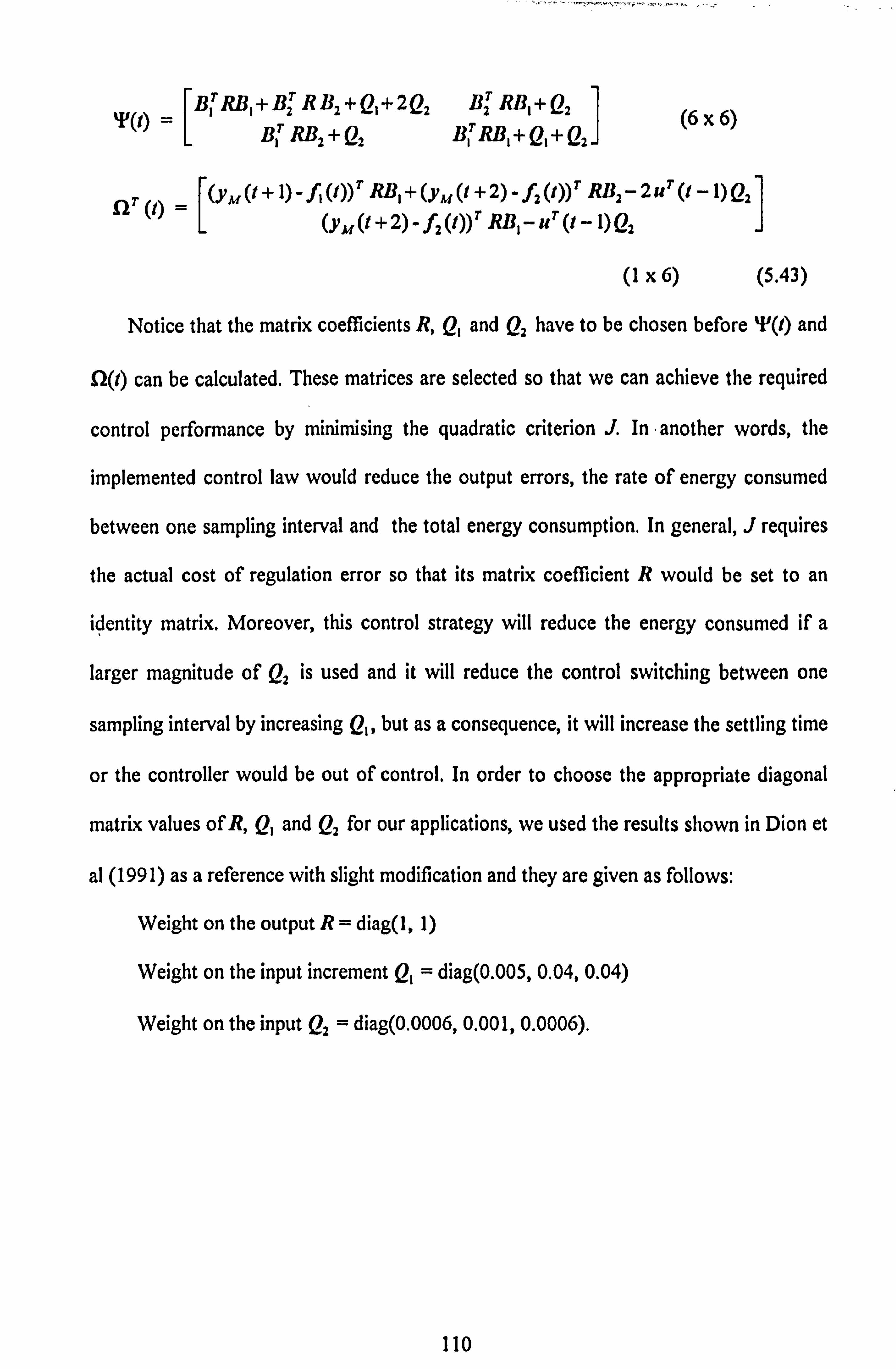
BITRBI+B2TRB2+QI+2Q2 B2TRB, +(? 2 (6 x 6) BIT RB2 + Q2 BITRBI+QI+Q2]

(yw Q+ 1) - f, (1))r JWI + (yw Q+ 2) - f2 (t))r RB2 -2 ur Q- 1) Q2

(ym(1+2)-f2 (1))' JWI - u'(1 - 1) Q2

I

(I x 6) (5.43)

Notice that the matrix coefficients R, Q, and Q2 have to be chosen before T(I) and

0(1) can be calculated. These matrices are selected so that we can achieve the required

control performance by minimising the quadratic criterion J. In -another words, the

implemented control law would reduce the output errors, the rate of energy consumed

between one sampling interval and the total energy consumption. In general, J requires

the actual cost of regulation error so that its matrix coefficient R would be set to an

identity matrix. Moreover, this control strategy will reduce the energy consumed if a

larger magnitude of Q, is used and it will reduce the control switching between one

sampling interval by increasing Q1, but as a consequence, it will increase the settling time

or the controller would be out of control. In order to choose the appropriate diagonal

matrix values of R, Q, and Q2 for our applications, we used the results shown in Dion et

al (199 1) as a reference with slight modification and they are given as follows:

Weight on the output R= diag(l, 1)

Weight on the input increment Q, = diag(O. 005,0.04,0.04)

Weight on the input Q2= diag(O. 0006,0.001,0.0006).

110

5.4.2. Input and output constraints

Let us define the control input changes, Au(I) m [AWQ) AC(I) AH(I)IT and the

output changes, Ay(l) a [AT, (I) AH, (1)17'. For the input constraints, the heater W,

cooler C and humidifier H have limits of 5.0,2.7 and 2.6 kilowatts respectively.

Therefore, from the definitions in equation (5.28), we have Uhlh = [5.0 2.7 2.6]T and

u, = [0 0 0]'. We also need to set the maximum permissible change in the control

input between sampling intervals, D.; let this equal [2 1 ]IT.

For the output constraints, these limits are selected using common sense reasoning

as follows: y,,,, = [40 1001

T, yl,,,, = [0 O]T, and Dy = [10 10]T, i. e. the ranges of

the room temperature and the relative humidity are 0- 40'C and 0- 100%rh; and their

maximum permissible changes in one sampling interval are IOT and 10%rh respectively.

The matrix C,, Y(o and vector yi. Y(O,

0(l), 1) for the prediction horizon N=2 are

calculated from equations (5.25), (5.26) and (5.27) where it is straightforward to show

that the matrices C,, C2, C3 and C4 are of dimensions (6 x 6), (6 x 6), (6 x 6) and (4 x

6) respectively, and the vectors V, , V2, V/3, V4, v/s, V. and V7 are of dimensions (6 x

(6 x 1), (6 x 1), (4 x 1), (4 x 1), (4 x 1) and (4 x 1) respectively, thus giving the

matrix C. Y(O

is of dimension (40 x 6) and the vector V. Y(O, 0(l), 1) is of dimension (40 x

1). The required (6 x 1) predicted incremental inputs Au, is given by

Au, =[, &W(l) AC(I) &H(l) AW(t+l) AC(t+l) AH(1+1)lr

Therefore, in this case we require to obtain 6 unknown parameters, i. e. AW(l), AC(l), ...,

AH(1+1), with conditions (5.20) subjects to 40 constraints, at each sampling time.

III

Similarly, for the prediction horizon N=5, the size of C.., (0 and V., (0,0(1), t) are

of dimensions (100 x 15) and (100 x 1) respectively and the required Au, is of dimension

(15 x 1) and is given by

Am, = [AW(t) AC(t) AH(t)

AH(t + 3) AW(t + 4) AC(t + 4) AH(t + 4) T

In this case we require to obtain 15 unknown parameters, i. e. AW(l), AC(l), ..., AH(1+4)

with conditions (5.20) subjects to 100 constraints, at each sampling time.

5.4.3. Quadratic programming

If equations (5.20) - (5.22) are fulfilled the optimality conditions given by the Kuhn-

Tucker conditions (see for example Koo, 1977), and it is possible to calculate Au, by

using a quadratic programming method. The standard notation of quadratic

programming is to find a solution for x* from

minimize q(x) xGx + gx x

subject to Ax:: 5 b. (5.44)

where A and G are (r x s) and (s x s) matrices respectively.

Under this notation, equation (5.23) can be written as

- C. y (ü) A ul :9- vf. y

(0, offl, t) (5.45)

and for the case in section 5.3, matrices G and A, and vectors x and b from equation

(5.44) can be given as follows:

G= 2'F (5.46)

gr = -20T (5.47)

112

A= -C., Y(o (5.48)

vf. y (0, offl, 1) (5.49)

X=[X,, x,,, '., x, ]r, forN=2 (5.50)

where

x, =A W(t), x2 = AC(t), ... , x. = AH(t + 1)

and x=[xl, x 2'j -. x,, ]7, forN=S

where

A w(t)3 x2 «=, äc(t), ***, x, ,= AH(t + 4).

In the MATLAB language, a function called 'qp' can be used to calculate the solution x.

Finally, we are only interested in obtaining the values of x,, X2 andX3. since these

values are required to update u(I) from the relationship

U(I) = U(I - 1) + AU(I) (5.19)

where

AU(I)=[XI X2 X317 (5.52)

5.5. Simulation results

The developed MIMO adaptive control theory described in sections 5.2 - 5.4. is used

to control the room temperature and the relative humidity by simultaneously calculating

the three input signals to regulate the HVAC plant. It is assumed that the plant dynamics

follow the model equations (2.1) and (2.2), and the adaptive process model is of the form

of equations (5.32) and (5.33).

113

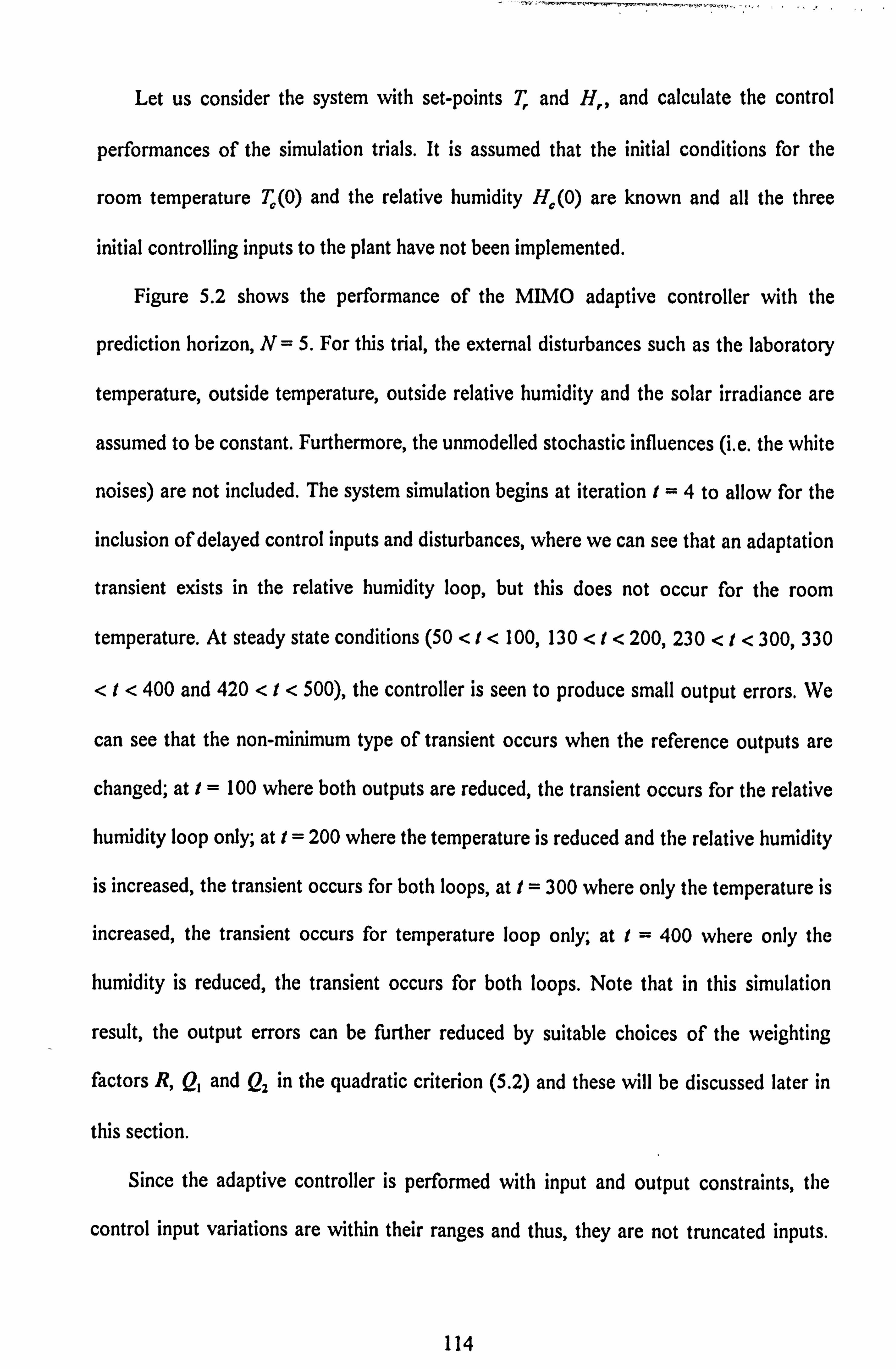
Let us consider the system with set-points T, and H, and calculate the control

performances of the simulation trials. It is assumed that the initial conditions for the

room temperature TJO) and the relative humidity HJO) are known and all the three

initial controlling inputs to the plant have not been implemented.

Figure 5.2 shows the performance of the MIMO adaptive controller with the

prediction horizon, N=5. For this trial, the external disturbances such as the laboratory

temperature, outside temperature, outside relative humidity and the solar irradiance are

assumed to be constant. Furthermore, the unmodelled stochastic influences (i. e. the white

noises) are not included. The system simulation begins at iteration I=4 to allow for the

inclusion of delayed control inputs and disturbances, where we can see that an adaptation

transient exists in the relative humidity loop, but this does not occur for the room

temperature. At steady state conditions (50 <I< 100,130 <I< 200,230 <i< 300,330

<I< 400 and 420 <I< 500), the controller is seen to produce small output errors. We

can see that the non-minimum type of transient occurs when the reference outputs are

changed; at I= 100 where both outputs are reduced, the transient occurs for the relative

hurnidity loop only; at I= 200 where the temperature is reduced and the relative humidity

is increased, the transient occurs for both loops, at I= 300 where only the temperature is

increased, the transient occurs for temperature loop only; at I= 400 where only the

humidity is reduced, the transient occurs for both loops. Note that in this simulation

result, the output errors can be further reduced by suitable choices of the weighting

factors R, Q, and Q, in the quadratic criterion (5.2) and these will be discussed later in

this section.

Since the adaptive controller is performed with input and output constraints, the

control input variations are within their ranges and thus, they are not truncated inputs.

114

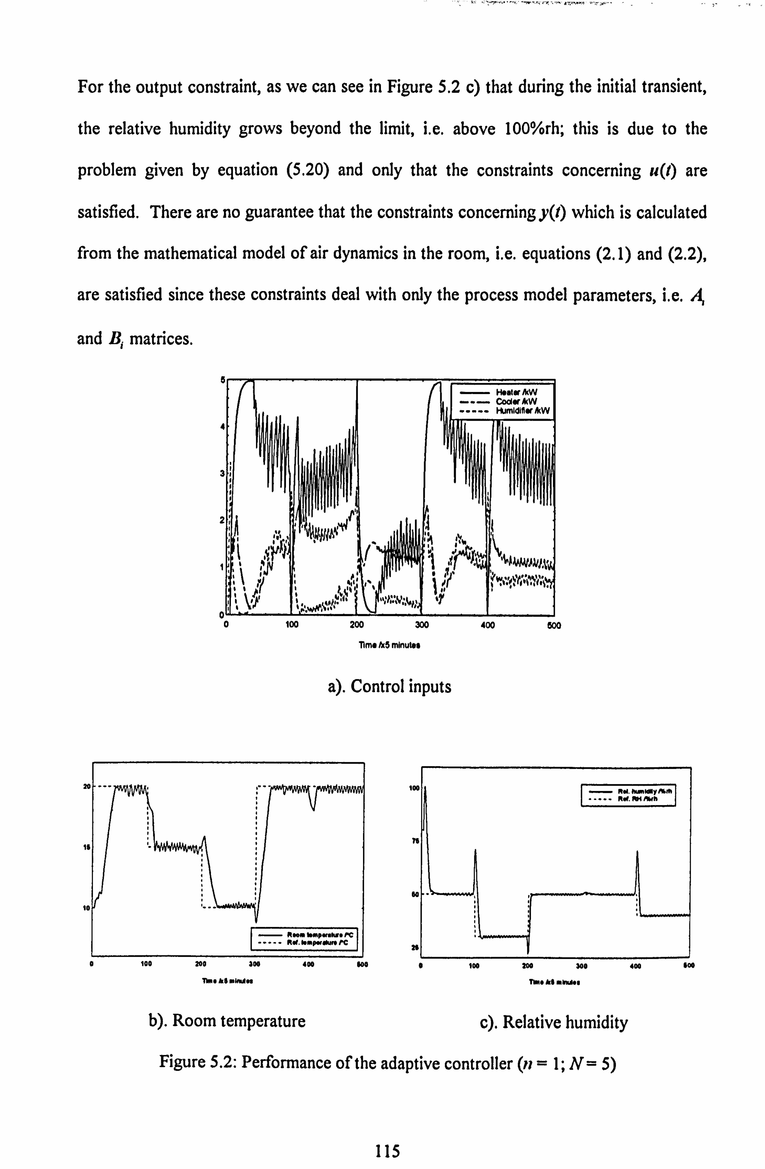
For the output constraint, as we can see in Figure 5.2 c) that during the initial transient,

the relative humidity grows beyond the limit, i. e. above 100%rh; this is due to the

problem given by equation (5.20) and only that the constraints concerning u(I) are

satisfied. There are no guarantee that the constraints concerningy(l) which is calculated

from the mathematical model of air dynamics in the room, i. e. equations (2.1) and (2.2),

are satisfied since these constraints deal with only the process model parameters, i. e.

and B, matrices.

Hester fkW CoderAW Humldifier AM

4,

3-:

2

0 100 200 3W

lime fX5 minutes

a). Control inputs

20

Is

10 ..

ft"m bffip-hg* PC ad. bmpmuo PC

00 MM

-- "-, - ' 0'

400 500

I

a 100 200 3" 400 Goo 0 i0o 200 300 400 goo

rMaksiaw"" Time kI oft"m

b). Room temperature c). Relative humidity

Figure 5.2: Performance of the adaptive controller (ii = 1; N= 5)

115

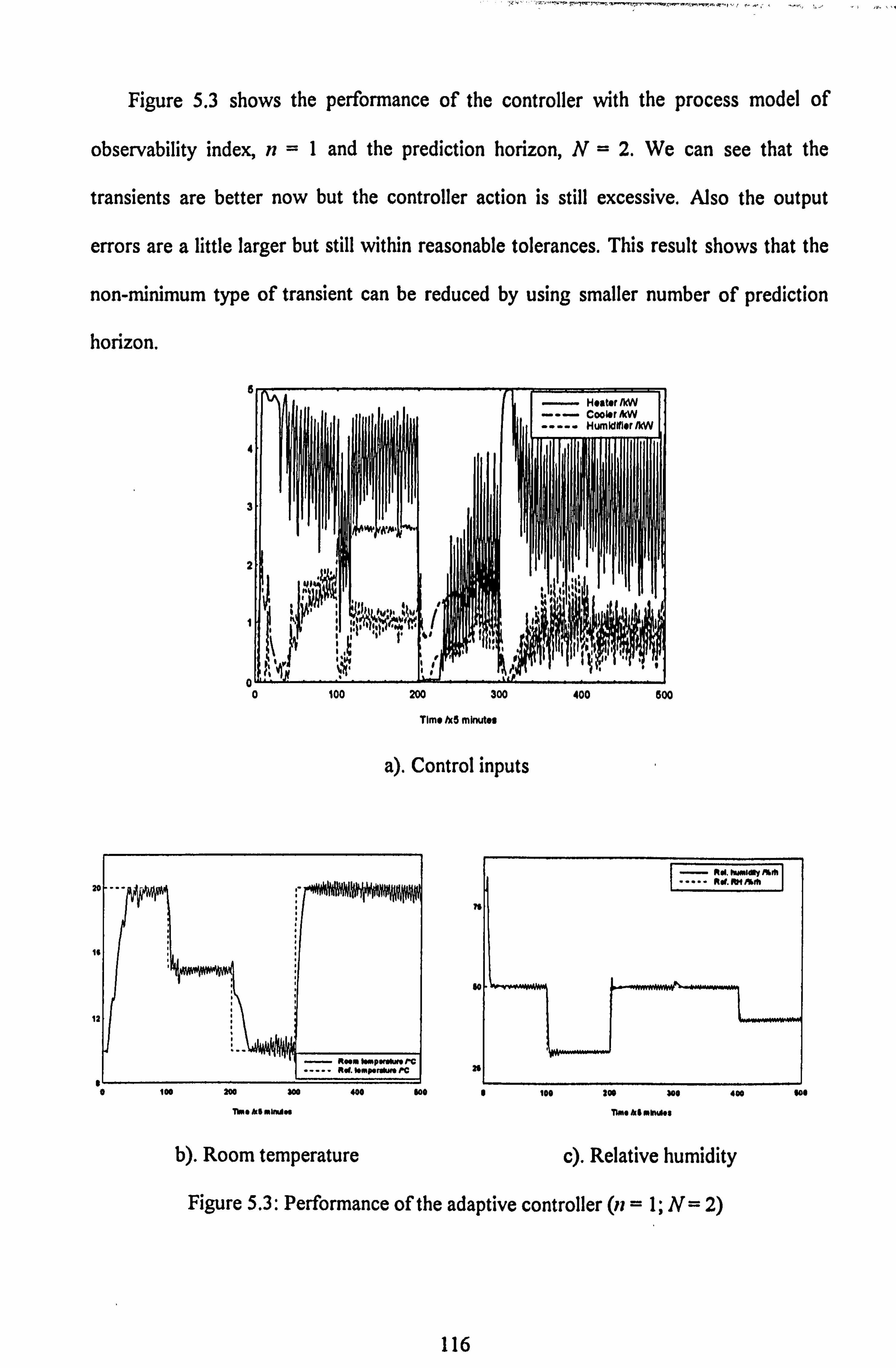
Figure 5.3 shows the performance of the controller with the process model of

observability index, n=I and the prediction horizon, N=2. We can see that the

transients are better now but the controller action is still excessive. Also the output

errors are a little larger but still within reasonable tolerances. This result shows that the

non-minimum type of transient can be reduced by using smaller number of prediction

horizon.

a

4

3

20

Is

12

Heater/M Coolor&W Humldlflor/kW

100 200 300

Time N5 mWes

a). Control inputs

400 500

ft so, hummy

....... Id. RH fkfh

"It

100 200 300 400 Soo 100 300 300 400 too

-nMG, w$MV"" 7UM4*6Mw"$



116

The simulation trials are also carried out for the process model of observability

index, it =2 with identical parameter values as used for Figures (5.2). The result is

shown in the Figure 5.4 where we can see the non-minimum type of transients still exists

during the step change of the setpoints but the output regulation as well as the control

input switching were very much improved as compared to the result for ii = 1. Similarly,

we found that these transients are reduced when the prediction horizon, N, equals 2, and

this is shown in Figure 5.5. The steady state performance over 100 data points, for

example, from 101st to 200th iterations are calculated and found to be as follows:

e the required control input energies are 27.7,7.2 and 11.5 kWh for the heater, cooler

and humidifier respectively;

* the output squared errors are OYC' and 1.3%rh' for the temperature and relative

humidity respectively; and

e the required times to reach the temperature and relative humidity setpoints are 1.7 and

0.8 hours respectively.

The values of the estimated parameters for the on-line process model with n=2 and

N=2, namely A,, , ý, B, and B2, were calculated; the results are presented in Figure

5.6 where we can see that how the adaptive system responds to stepwise reference

signals and to changes in the incremental control inputs via the presented control law.

Here, the estimated parameters are defined as follows:

A, = [a:

: a:, 2 A2 =

[a2,,

a2 a22 a221

a2,2 B,

bIll a222

I' [b,

21

b112 b, 13

I

and b122 b123 J

B2= b 211

b212 b213 lb221

b222 b 2231

117

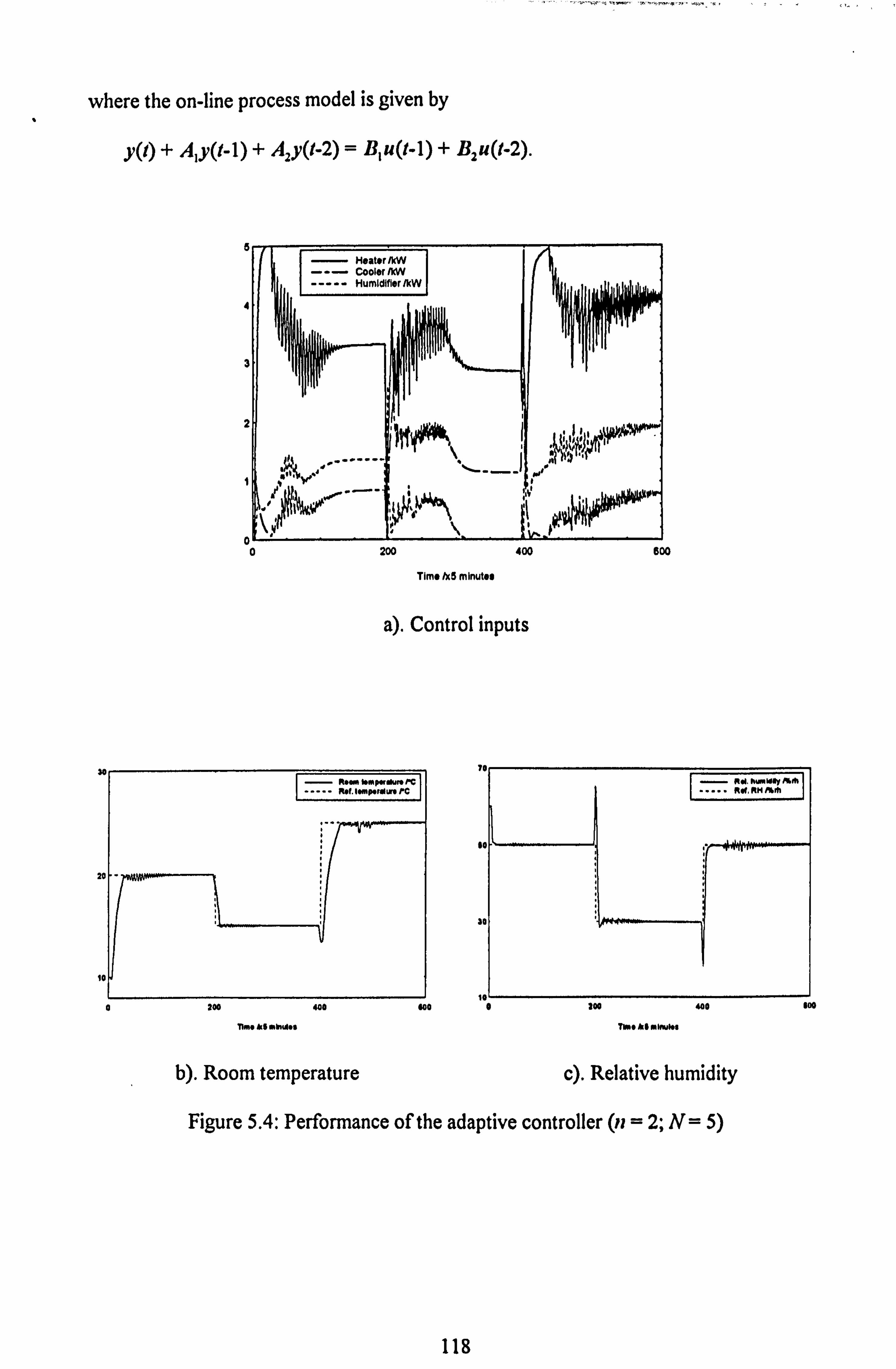
where the on-line process model is given by

y(I) + Aly(t-1) + A2y(I-2) = B, u(t-1) + Bu(I-2).

5

4

3

0

20

10

r

30

200 400 600 300 400 Boo

Time *5 Obwes TURO As Owwwo


Figure 5A Performance of the adaptive controller (n = 2; N= 5)

Rom bmpw Rof. lomporours PC

118

200 4W Ow

Timo NS m1nutes

a). Control inputs

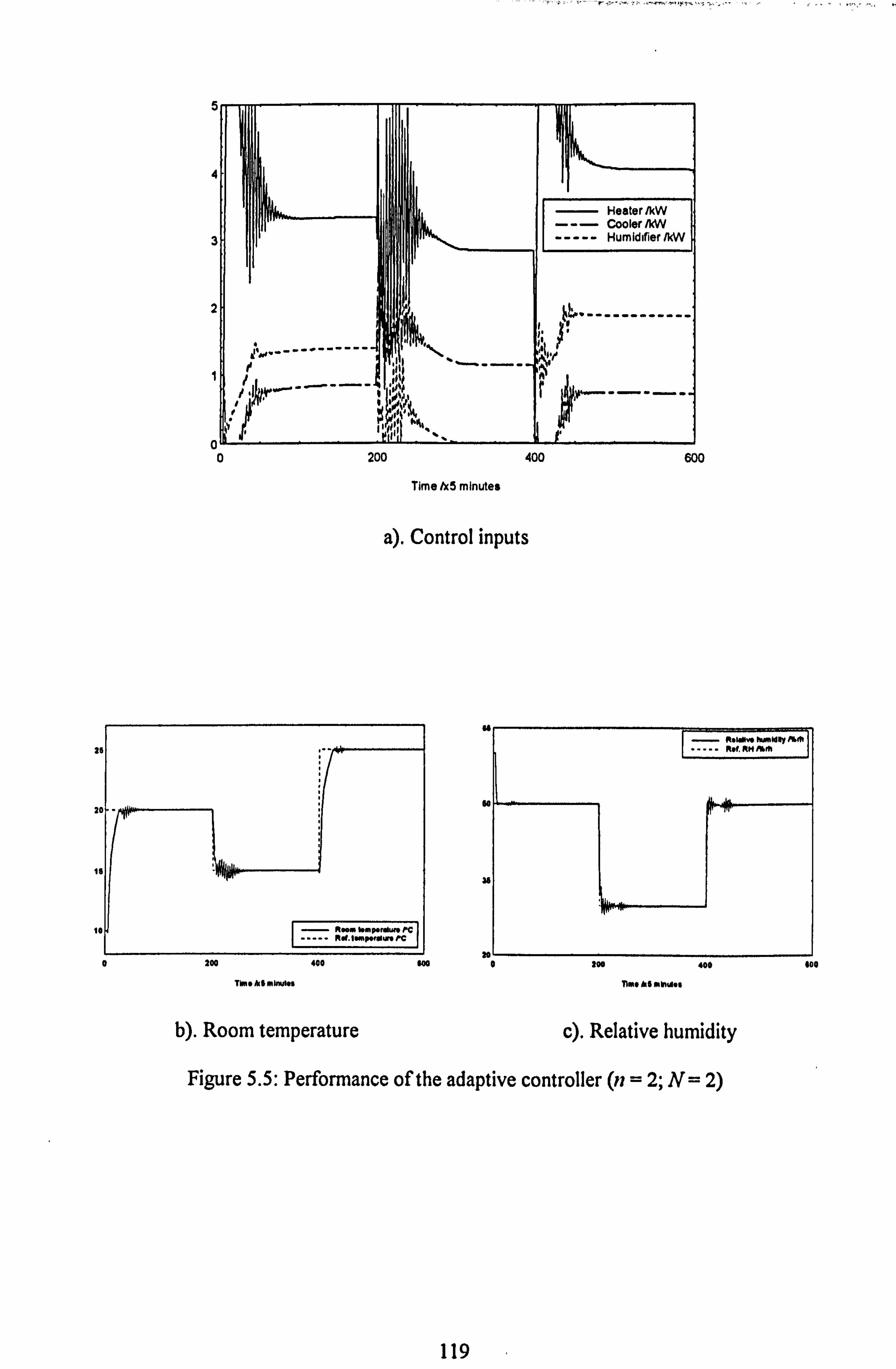
HeaterlkW Cooler/kW Humidifier fkW

------------- -------------

0 200 400 600

Time Ix5 minutes

a). Control inputs

5

4

3

25

20 Wo,

15 q"lgr

10 ll-*" PC Rd. J-pmý PC

0

-;. = N, &* Rot. RM phrft

200 400 $00 0 200 400

Thee h& mWes Time AS 011"W. 6



400

119

----------------- P-! 3, w ...............

i ý ir F 122 a a, 2, ,, 2

Ilk I

. ..... . ..... .

Ii ý

1

VIV ------- 4 a 111

200 400 go*

Tim tAS MkPASI

a) A1

5.0

2.5

. 2.6

. 6.0, 0

------------------ r- -7 bill b113 b123

... ... ... ...

121 11112 122

------- N

......... I ................. ..................

a, 22

4.30 221

4AG

a2,, no cm so@

T"Ohlo"Wel

b) A2

b223

of.

b b2 211 213 12 ....... Li b222

.................

b22

. 0.6

-1.0

-1.9 200 400 600 0 200

Tlmo ke mwÄtt TWAO ke rAwAge

c) B, d) B2

400 on

Figure 5.6: Parameter estimation values for the process model (n = 2; N= 2)

Now, we present the effect to the control performances as the weighting factors R,

Q, and Q2 are changed. We can use the controller parameters as used to obtain Figure

5.3 for comparison purposes. The simulation results are shown in Figures 5.6,5.7 and

5.8 when only R is reduced to diag(O. 8,0.8), when only Q, is increased to diag(O. 05,

0.4) 0.4), i. e. 10 times larger than the previous value, and when only Q. is increased to

diag(O. 006,0.01,0.006), i. e. 10 times larger than the previous value, respectively. We

can see that the difference in the control performances as compared to that shown in

120

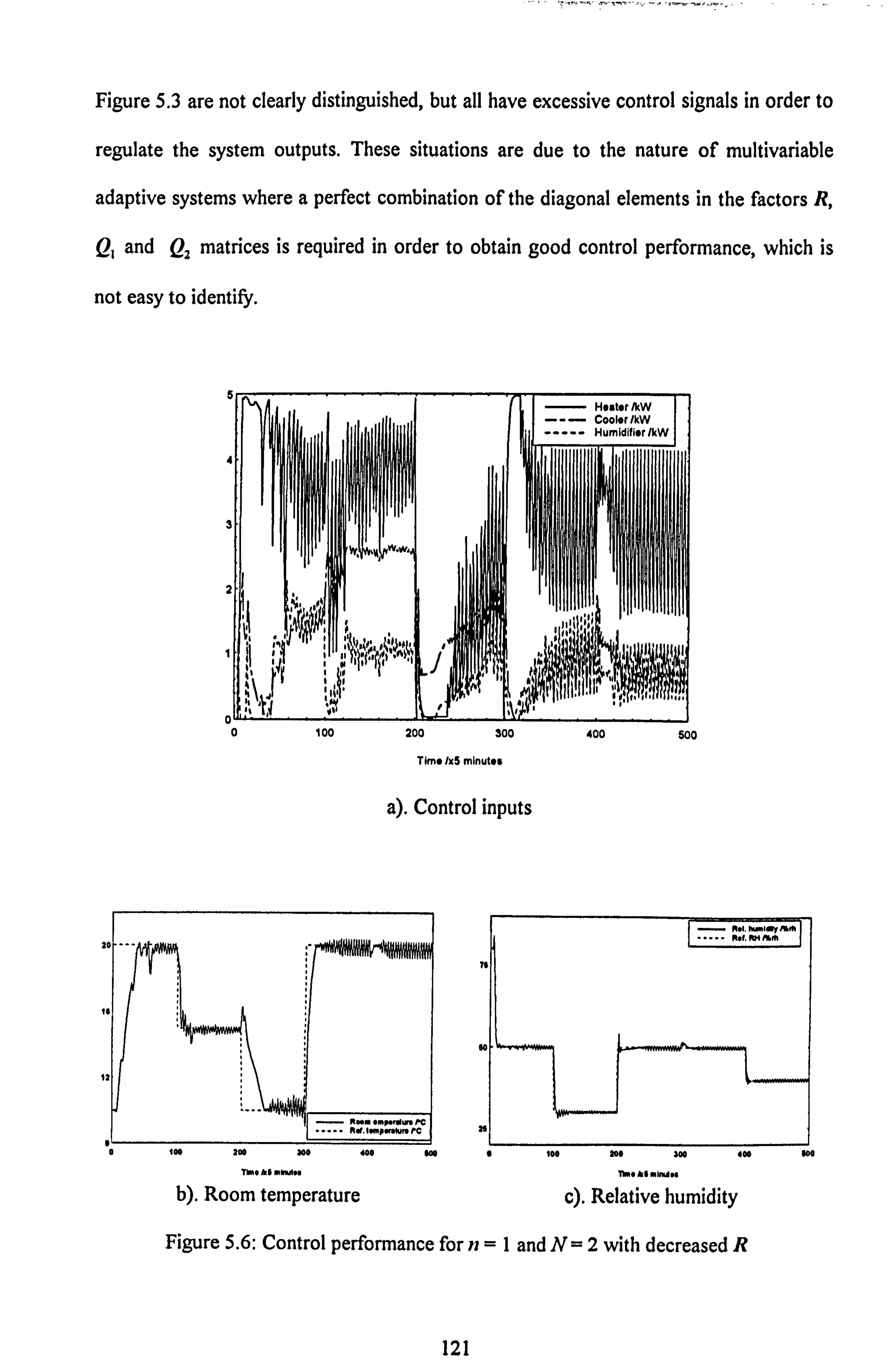
Figure 5.3 are not clearly distinguished, but all have excessive control signals in order to

regulate the system outputs. These situations are due to the nature of multivariable

adaptive systems where a perfect combination of the diagonal elements in the factors R,

Q, and Q, matrices is required in order to obtain good control performance, which is

not easy to identify.

Hester /kW Coolor/kW

----- Humidifier AW

4

3

W. Wq

2

0 100 200 300

Tim* /x5 minutes

a). Control inputs

20 ----

PC ..... Ref. Impmw

:

P: c

400 Soo

"... -. dty FA of. 104 FAM

76

26

Ice 200 300 400 goo 0 100 200 300 400 Soo

TWA$ hS MWA" roe &S MWMDG


Figure 5.6: Control performance for ?i=I and N=2 with decreased R

121

5

4

3

2

I

A

Heater AW Cooler/kW Humidifier /kW

to

0 100 200 300

Time Ix5 minutes

a). Control inputs

'I

100 200 300 400 Goo 1 100 too 300 400 M

Tim *5 mWoA. s TIMO Al MIMAeS


Figure 5.7: Control performance for n=I and N=2 with increased Q,

400 500

Ror, RH fhfh-

n

so

25

122

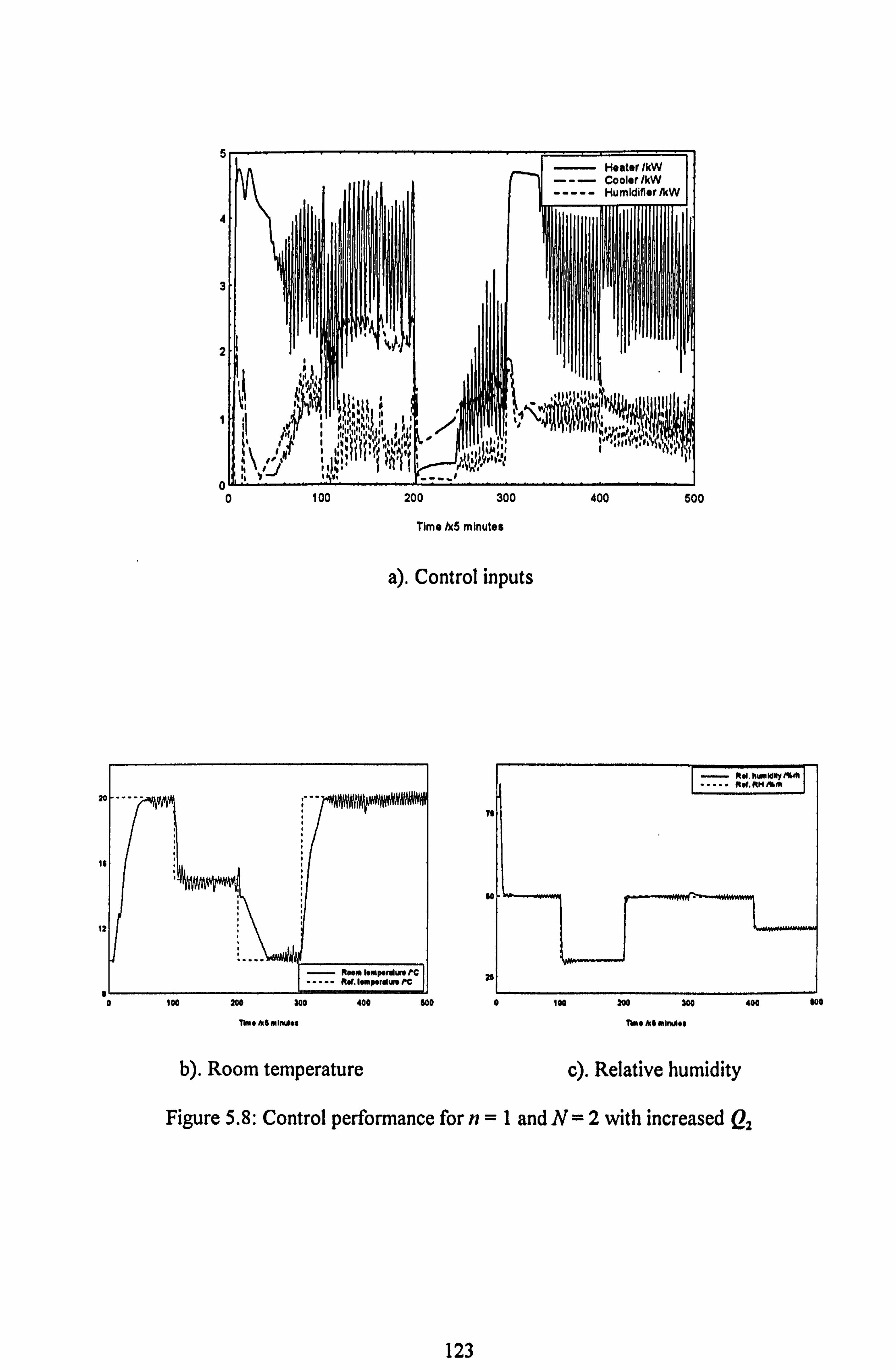
5

4

3

2

I

Heater /kW Cooler/kW

----- Humidifier/M

:ý1 '10 Oil

0 100 200 300

Time /x5 minutes

a). Control inputs

20 ------...

Is

12

R"m bmp*rdm PC OW. Imperdmpc

400 500

- Rol, tiwiddyt%fh ft«. RM Phrh

100 200 Soo 400 Goo 0 100 200 300 400 too

71MO&SMIrass rA@*$f"iMA*M


Figure 5.8: Control performance for n=I and N=2 with increasedQ2

123

Another possible approach to reduce the controller switching actions is to reduce

the maximum permissible control changes D.. To demonstrate this, a simulation trial is

carried out as for the conditions in Figure 5.3, except that the room temperature and the

relative humidity reference setpoints are arbitrary set at 20'C and 40%rh respectively,

and the maximum permissible control changes D. are smaller as compared to the one

used to obtain Figure 5.3, say, equals [0.5 0.3 0.3]r. The results are shown in Figure

5.9 where we can see that the output errors as well as the controllers switching at steady

state conditions are reduced as compared to Figure 5.3 due to the smaller changes

allowed in the control inputs. The steady state performance over the last 100 sampling

intervals are as follows:

9 the required control input energies are 33.7,15.7 and 12.8 kWh for the heater, cooler


e the output squared errors are 1.4*C' and 1.8%rh' for the temperature and relative


9 the required times to reach the temperature and relative humidity setpoints are 5.0 and


From this result, we notice that a disadvantage of this approach is that the temperature

settling time is longer as compared to Figure 5.3 which is due to smaller amount of

increment of the heater between one sampling interval.

Nevertheless, D. may also have the lower limit at which the value lower than this

causes the controller's out of control. One of the lower limit was found to be D. =

[0.2 0.1 O. I]T

124

Figure 5.10 shows the performance of the MIMO adaptive controller (ii =I and

N= 2) for the system with the actual climatic disturbances as shown in Figure 4.4, and

for convenience, pseudo random binary sequences (PRBS) generated using 6 shift

registers (Godfrey, 1980) and switching between ±0.5 were used as the stochastic noises

included. We can see that the system performance is significantly degraded as compared

to the system with constant disturbances and no noise case and this is to be expected.

The steady state performance over the last 100 sampling intervals are as follows:

* the required control input energies are 35.3,5.6 and 15.3 kWh for the heater, cooler


4P the output squared errors are 53. IoC2 and 71.1%rh' for the temperature and relative


* the required times to reach the temperature and relative humidity setpoints are 6.7 and


H= *. 111 CH H * 111 =

.

Rom Imporowe lb-1 'o Rol. hmidly I%fh

.................................................

9 so lw 160 2m 0 so 100 140

Tbm ta Minute nm@A. 601euel

a). Control inputs b). System outputs

Figure 5.9: Control performance for n=1, N= 2 and with reduced D,

200

125

This result shows that the output regulation and the controller switching at steady state

condition were improved as compared to Figure 5.3, although the total controlling input

energy is about 1.2 times greater as compared to the multi PI-loop controller using 6 PI

units (see section 3.3.1). As before, this performance can be improved further by suitable

additional tuning of the weighting factors R, Q, and Q2 in the quadratic criterion, J(I).

omwlkw cmis, okw 14MIdMrAtW

Rol, hwl" I%rh

0, 100 ISO 200 go IN IN

Thno k5 minLdes inmoksmimAss

a). Control inputs b). System outputs

Figure 5.10: Control performance for ii = 1, N=2 (with noise)

5.6. Conclusions

This chapter has discussed a multivariable adaptive control algorithm based on the

generalized predictive control methodology which explicitly takes into account natural

constraints on the input and output signals. The process model with observatory indexes

of ii =I and n=2 were used to describe the dynamic processes of a heating, ventilating

and air-conditioning plant consisting three control inputs and two outputs. From the

results presented in Section 5.5, we can conclude that the selected process models

together with the designed control law and the selected constraints are well suited to

126

controlling the overall system. The controller performance can be improved by suitable

choice of the weighting factors R, Q, and Q2 in the quadratic criterion as well as the

prediction horizon, N, and the maximum permissible changes in the control input, D..

Moreover, it may be possible to improve the system performance by selecting different

prediction horizons for the predicted output y, rate of predicted input Au and predicted

input u terms in the quadratic criterion J. For example, a smaller prediction horizon for

Au and u will reduce the non-minimum phase overshoot effects in the output responses

as well as stabilising the controller signals. This require reformulating the problem so that

a suitable control law can be calculated; this will obviously be different from the law

presented here.

127

Chapter 6

Fuzzy Logic Controllers

In recent years there has been growing interest in using fuzzy logic for the design of

control systems. The advantage of using these techniques is that it is easy to apply

heuristic knowledge and 'Wle-of-thumb" experiences without involving tedious

mathematical analysis. Fuzzy controllers are usually based on expert knowledge that is

given by linguistic rules (Zadeh, 1975), and many successful applications have been

reported. One such application is in an air-conditioning plant (Ling and Dexter, 1994)

where a rule-based supervisor is used to select a setpoint for the zone temperature which

satisfies the majority of the occupants in the building as well as minimising the cost of

operating the air-handling-unit (AHU); the results show that a significant cost savings

without unacceptable increases in discomfort levels can be achieved. Furthermore, the

solution was also able to compensate for day-to-day variations in conditions to maintain

the control performance.

In view these encouraging results it is worthwhile to investigate the potential of

fuzzy logic for HVAC applications; this was carried out and discussed here. We will

design a fuzzy logic controller (FLC) which is based on the output errors to control an

office zone system. The overall control objective is assumed to be to maintain acceptable

128

levels for the room temperature and the relative humidity variations as well as minimizing

the energy costs of operating the HVAC plant.

6.1. Design of the FLC

Most FLCs developed so far employ error and error rates about a setpoint as their

driving inputs (Ying et al., 1990). For our case, since the system has two setpoints,

namely, the air temperature and the relative humidity in the test room, then using a

similar reasoning we require four inputs; two from the output errors and two from the

error rates, in order to calculate the three control signals to drive the HVAC plant using

the fuzzy method.

Another FLC design is to employ fuzzy versions of the three terms in the PID

controller (He et al., 1993). For our system, the PID-based fuzzy controller requires six

inputs where two inputs are required for each term. Thus, the size of the fuzzy rules

which depend on the number of crisp inputs, become quite large and the time required

for calculating the control decision will be longer.

In this chapter, we present two types of FLC design; the first design is based on the

proportional (P) controller and the second type is based on the Proportional and Integral

(PI) controller. Both designs employ incremental control rather than the actual input so

that integral action to eliminate steady state errors can be easily deployed. The three

control input increments, namely, the heater increment dW, the cooler increment dC and

the humidifier increment dH, are defined by:

dW(l) = WQ) - W(I-T) (6.1)

dC(l) = C(l) - C(I-T) (6.2)

129

dH(t) = H(t) - H(t-T) (6.3)

respectively.

6.1.1. FLC based on proportional action

In this design, the system structure is shown in Figure 6.1 where the FLC employs only

the proportional term with gain Kp is assumed to be unity to simplify the design. The

required parameters are the output errors, namely the error signals in the air temperature

eTQ) and the relative humidity e, (I) for which the FLC calculates the three control

increments. The design follows the three main steps in fuzzy controller design, that is,

fuzzification, control rule evaluation and defuzzification.

For the fuzzification process, singleton error signals are 'fuzzified" into membership

functions as shown in Figure 6.2. Both the error signals e. and e,, are assumed to have

five membership values: Negative Large (NL), Negative Small (NS), Zero (Z), Positive

Small (PS) and Positive Large (PL) and the controller output increments have three

membership functions: Negative (N), Zero (Z) and Positive (P). The constants I 1) 129 139

SIP S2P S3P ZIP Z2. x,,, n., n, z,, z., z, p,, p.. and x. used in the definition of the

membership functions shown in Figure 6.2 are chosen in accordance to the possible

ranges in the error signals and the maximum possible controller changes, which will be

fixed after being determined. Note that the constants I 10 129

.., x. used in the two sets of

the error signals can be different in general (according to the dynamics of the office

zone), but we assume them to be the same here in order to simplify the design and

notation in the following discussions.

130

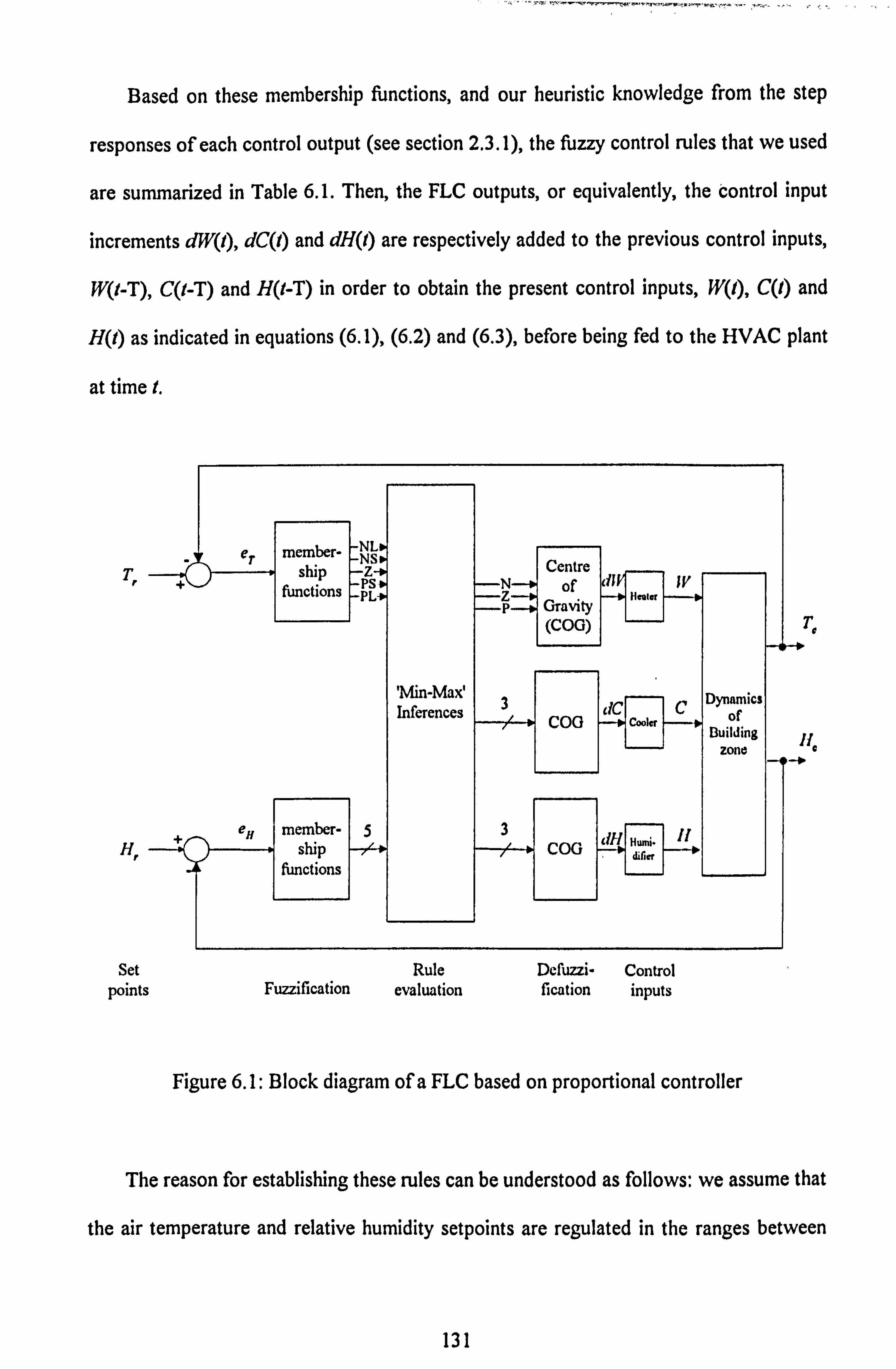
Based on these membership functions, and our heuristic knowledge from the step

responses of each control output (see section 2.3.1), the fuzzy control rules that we used

are summarized in Table 6.1. Then, the FLC outputs, or equivalently, the control input

increments M(I), dC(l) and dH(t) are respectively added to the previous control inputs,

W(I-T), QI-T) and H(I-T) in order to obtain the present control inputs, WQ), C(l) and

H(I) as indicated in equations (6.1), (6.2) and (6.3), before being fed to the HVAC plant

at time t.

e e r member- shi

NS -Z-01 Centre p T,

+ PS * functions --PL-o -N 1, Of fit IV -Z 1, Heat" _P 0 Gravity

(COG) T.

'Min-Ma)e 3 Dynamics

Inferences Xc C of COG Cooler Building

zone

eH member- 5 +

3 H, ship __Vý r r COG Ila

functions

Set Rule Defuzzi- Control points Fuzzification evaluation fication inputs

Figure 6.1: Block diagram of a FLC based on proportional controller

The reason for establishing these rules can be understood as follows: we assume that

the air temperature and relative humidity setpoints are regulated in the ranges between

131

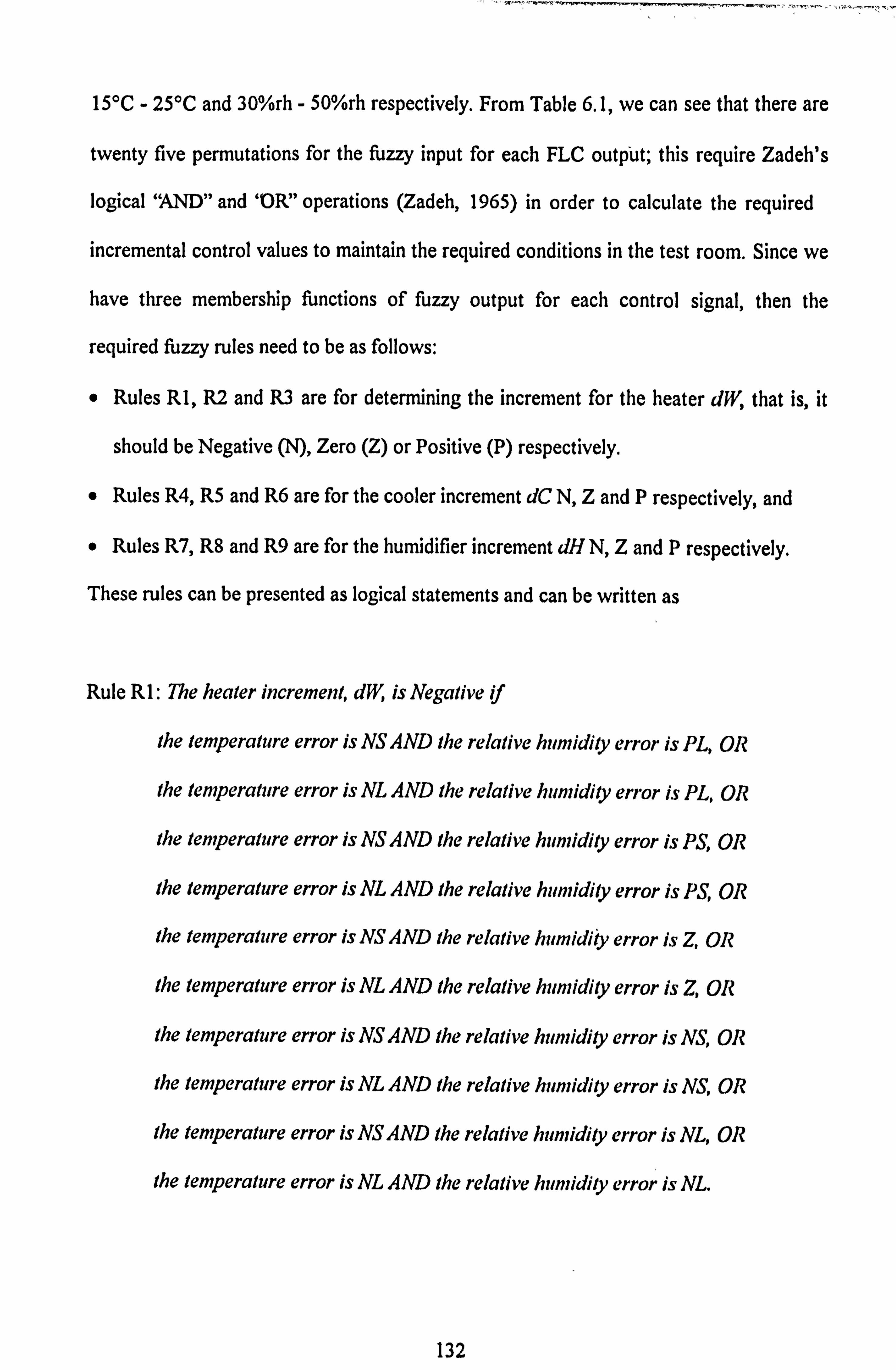
IPC - 25*C and 30%rh - 50%rh respectively. From Table 6.1, we can see that there are

twenty five permutations for the fuzzy input for each FLC output; this require Zadeh's

logical 'AND" and 'OlVoperations (Zadeh, 1965) in order to calculate the required

incremental control values to maintain the required conditions in the test room. Since we

have three membership functions of fuzzy output for each control signal, then the

required fuzzy rules need to be as follows:

o Rules RI, R2 and R3 are for determining the increment for the heater dW, that is, it

should be Negative (N), Zero (Z) or Positive (P) respectively.

9 Rules R4, R5 and R6 are for the cooler increment dC N, Z and P respectively, and

o Rules R7, R8 and R9 are for the humidifier increment dH N, Z and P respectively.

These rules can be presented as logical statements and can be written as

Rule R 1: The heater increment, dW, is Negative if

the temperature error is NS AND the relative humidity error is PL, OR

the temperature error is NL AND the relative humidity error is PL, OR

the temperature error is NS AND the relative humidity error is PS, OR

the temperature error is NL AND the relative humidity error is PS, OR

the temperature error is NSA ND the relative humidiiy error is Z OR

the temperature error is NL AND the relative humidity error is Z OR

the temperature error is NS AND the relative humidity error is NS, OR

the temperature error is NL AND the relative humidity error is NS, OR

the temperature error is NS AND the relative humidity error is NL, OR

the temperature error is NL AND the relative humidity error is NL.

132

NL NS FL PS PL

1 r---i\ A, lz

AA-

10. -11 -12 S1 -13 'S2 -ZI S31 S3 ZI S2 13 Sl 12 11

Z2 0 eýl) and e, (I)

errors

a) Fuzzy input sets

n. zi n. z. p, Z, PM Xv

Controller outputs dW, X and dH (kW)

b) Fuzzy output sets

Figure 6.2: Fuzzy membership functions

Rule R2: Vie heater increment, dW, is Zero if

the temperature error is PS AND the relative humidity error is PL, OR

the temperature error is Z AND the relative humidity error is PL, OR

the temperature error is Z AND the relative humidity error is PS, OR

the temperature error is Z AND the relative humidity error is Z OR

the temperature error is Z AND the relative humidity error is NS, OR

the temperature error is Z AND the relative humidity error is NL.

133

ýL Negative Zero Positive

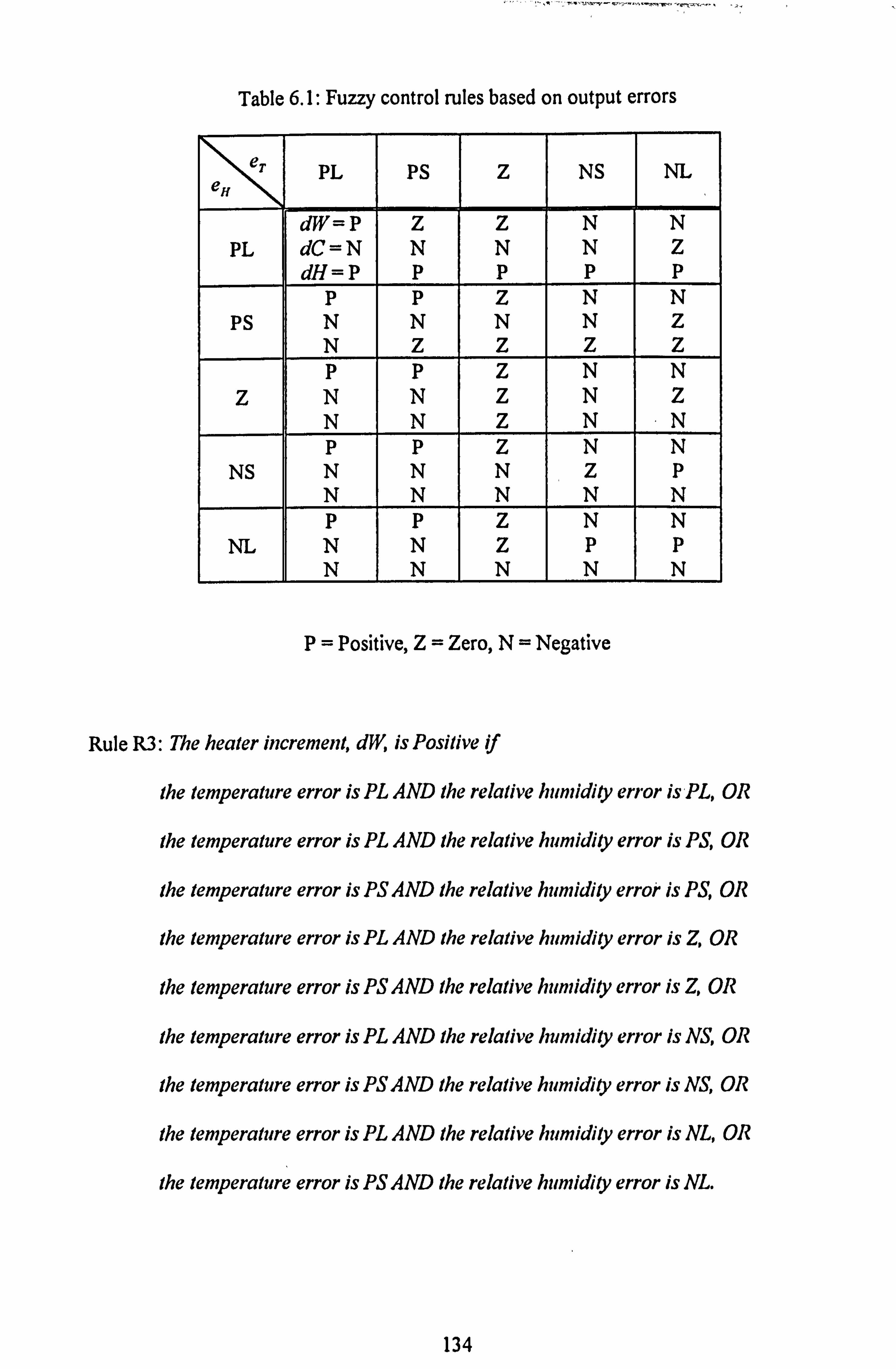
Table 6.1: Fuzzy control rules based on output errors

e,. PL PS Z NS NL eH

dW= P Z Z N N PL dC=N N N N Z

dH =P P p P P P P Z N N

PS N N N N Z N Z Z Z Z P p Z N N

Z N N Z N Z N N Z N N P P Z N N

NS N N N Z P N

-N N N N

P P Z N N NL N N Z P P

N N N N N

P= Positive, Z= Zero, N= Negative

Rule R3: Yhe heater increment, dW, is Positive if

the temperature error is PL AND the relative humidity error is ýPL, OR

the temperature error is PL AND the relative humidity error is PS, OR

the temperature error is PS AND the relative humidity error is PS, OR

the temperature error is PL AND the relative humidity error is Z OR

the temperature error is PS AND the relative humidity error is Z OR

the temperature error is PL AND the relative humidity error is NS, OR

the temperature error is PS AND the relative humidity error is NS, OR

the temperature error is PL AND the relative humidity error is NL, OR

the temperature error is PS AND the relative humidity error is NL.

134

Rule R4: The cooler increment, dC, is Negative if

the temperature error is PL AND the relative humidity error is PL, OR







the temperature error is NS AND the relative humidity error is PS, OR



the temperature error is NS AND the relative humidity error is Z OR

the temperature error is PL AND the relative humidity error is NS, OR




the temperature error is PS AND the relative humidity error is NL.

Rule R5: The cooler increment, dC, is Zero if

the temperature error is NL AND lhe relative humidity error is PL, OR



the temperature error is NL AND the relative humidity error is Z OR


135

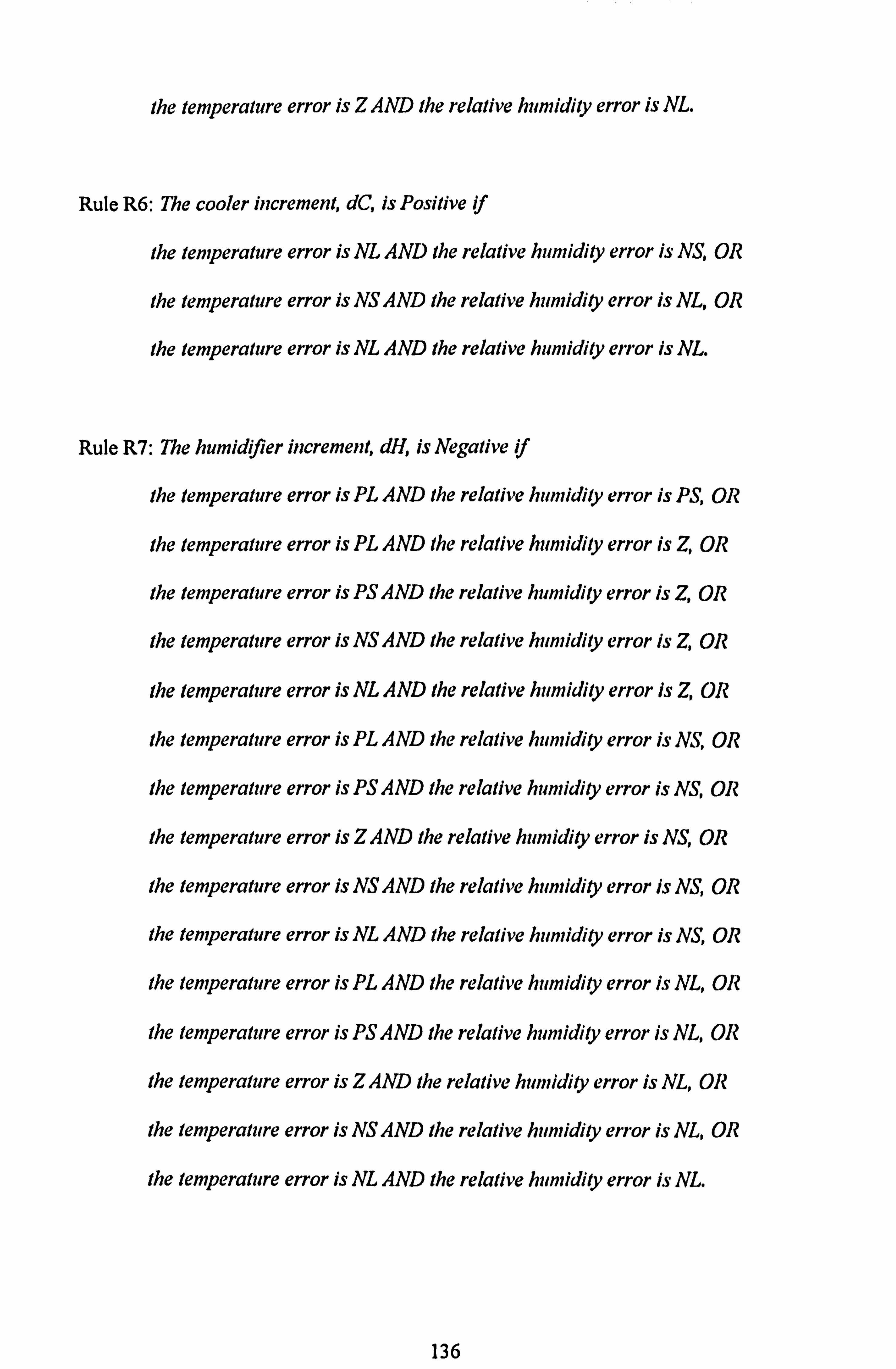
the temperature error is Z AND the relative humidity error is NL.

Rule R6: The cooler increment, dC, is Positive if

the temperature error is NL AND the relative humidity error is NS, OR

the temperature error is NS AND the relative hmidity error is NL, OR


Rule R7: The humidifier increment, dH, is Negative if




the temperature error is NS AND the relative hunddify error is Z OR

the temperature error is NL AND the relative humidity error Is Z OR

the temperature error is PL AND the relative hunddity error is NS, OR




the temperature error is NL AND the relative humidify error is NS, OR


the temperature error is PS AND the relative humidity error is NL, OR

the temperature error is Z AND the relative humidity error is NL, OR

the temperature error is NS AND the relative humidity error is NL, OR


136

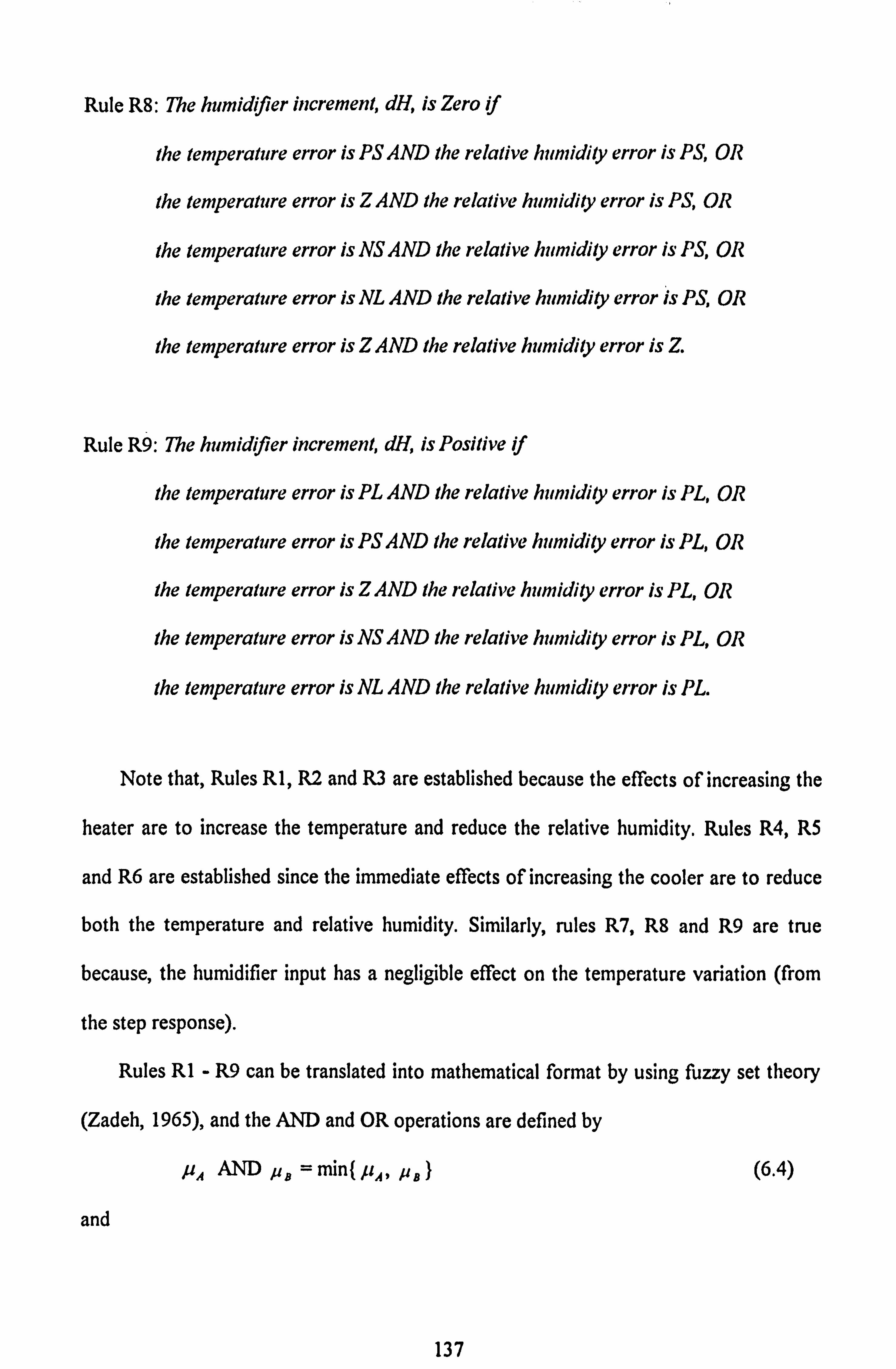
Rule R8: The humidifier increment, dH, is Zero if



the temperature error is NS AND the relative humidify error is PS, OR


the temperature error is Z AND the relative humidity error is Z.

Rule R9: Ae humidifier increment, dH, is Positive if

the temperature error is PL AND the relative humidity error is PL, OR




the temperature error is NL AND the relative humidity error is PL.

Note that, Rules RI, R2 and R3 are established because the effects of increasing the

heater are to increase the temperature and reduce the relative humidity. Rules R4, R5

and R6 are established since the immediate effects of increasing the cooler are to reduce

both the temperature and relative humidity. Similarly, rules R7, R8 and R9 are true

because, the hurnidifier input has a negligible effect on the temperature variation (from

the step response).

Rules RI - R9 can be translated into mathematical format by using fuzzy set theory

(Zadeh, 1965), and the AND and OR operations are defined by

JUA ANDu,, =min( PAI PS)

and

(6.4)

137

, uA ORu,, =--max( pA, uB) (6.5)

for any two membersWp functions u,, and p,, on fuzzy subsets A and B respectively.

For our case, this theory can be interpreted as follows: for each fuzzy output membership

function, the minimum value of the rule strength, p, from each pair of the fuzzy input

membership functions of e., and eH, as indicated in the fuzzy rules with the statement

'AND' is first obtained, and then these minimum values are sorted to get the largest

value amongst them via the statement 'OR' in the rule. Therefore, this value is the rule

strength or the degree of membership for that particular fuzzy output membership

function.

6.1.2. FLC based on P+I control

In this design, both the output errors e,, (I) and e, Q) and the integration errors I., (l) and

IH(I) are fed into the FLC as shown in Figure 6.3.

The integration terms in discrete form are defined by equations (3.4) and (3.5); a

well known method to avoid these terms from growing excessively is to apply upper and

lower limits, namely ±I7. and ±Iffm for the room temperature and relative humidity

respectively. These limits are incorporated into the fuzzy input scaling factors where 1TAI

("C-h) and I., (%rh_h) respectively are both set equal to I, (Figure 6.2 a)).

138

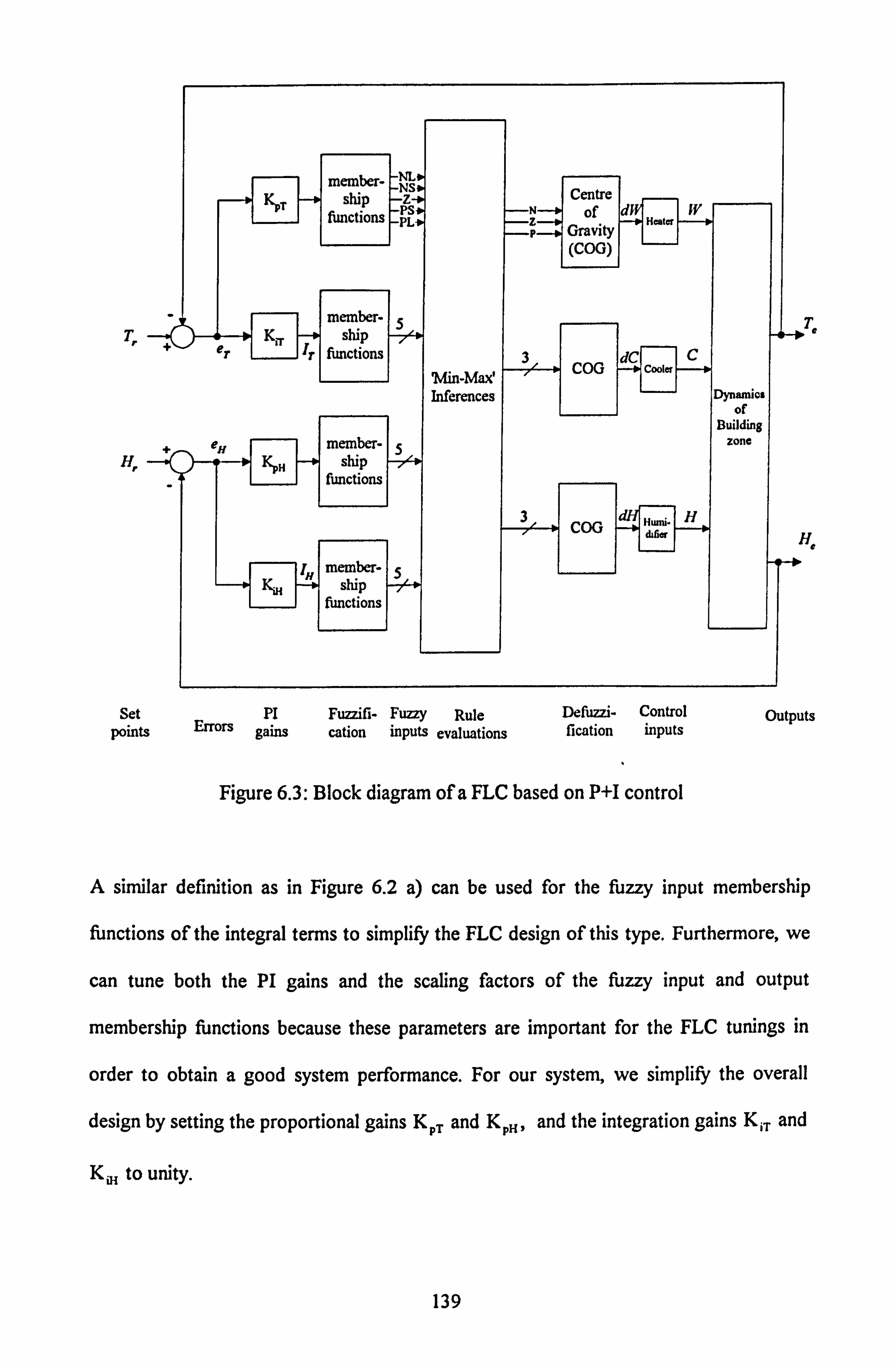
membership

fimctions

member- 5 T. -. sbip "P

ýerIr

fimctions 3

Inferences

member- 15

fimctions ship r

3

gjý - member K it ship

functions

Centre of

Gravity (COG)

jdCj COO cooler

cor difier

Set PI Fuzzifi- Fuzzy Rule Defuzzi. Control points Errors gains cation inputs evaluations fication inputs

I

Figure 6.3: Block diagram of a FLC based on P+I control

i. e

of Building

zone

J1

Outputs

A similar definition as in Figure 6.2 a) can be used for the flizzy input membership

functions of the integral terms to simplify the FLC design of this type. Furthermore, we

can tune both the PI gains and the scaling factors of the fuzzy input and output

membership functions because these parameters are important for the FLC tunings in

order to obtain a good system performance. For our system, we simplify the overall

design by setting the proportional gains KpT and KPH, and the integration gains KiT and

KjH to unity.

139

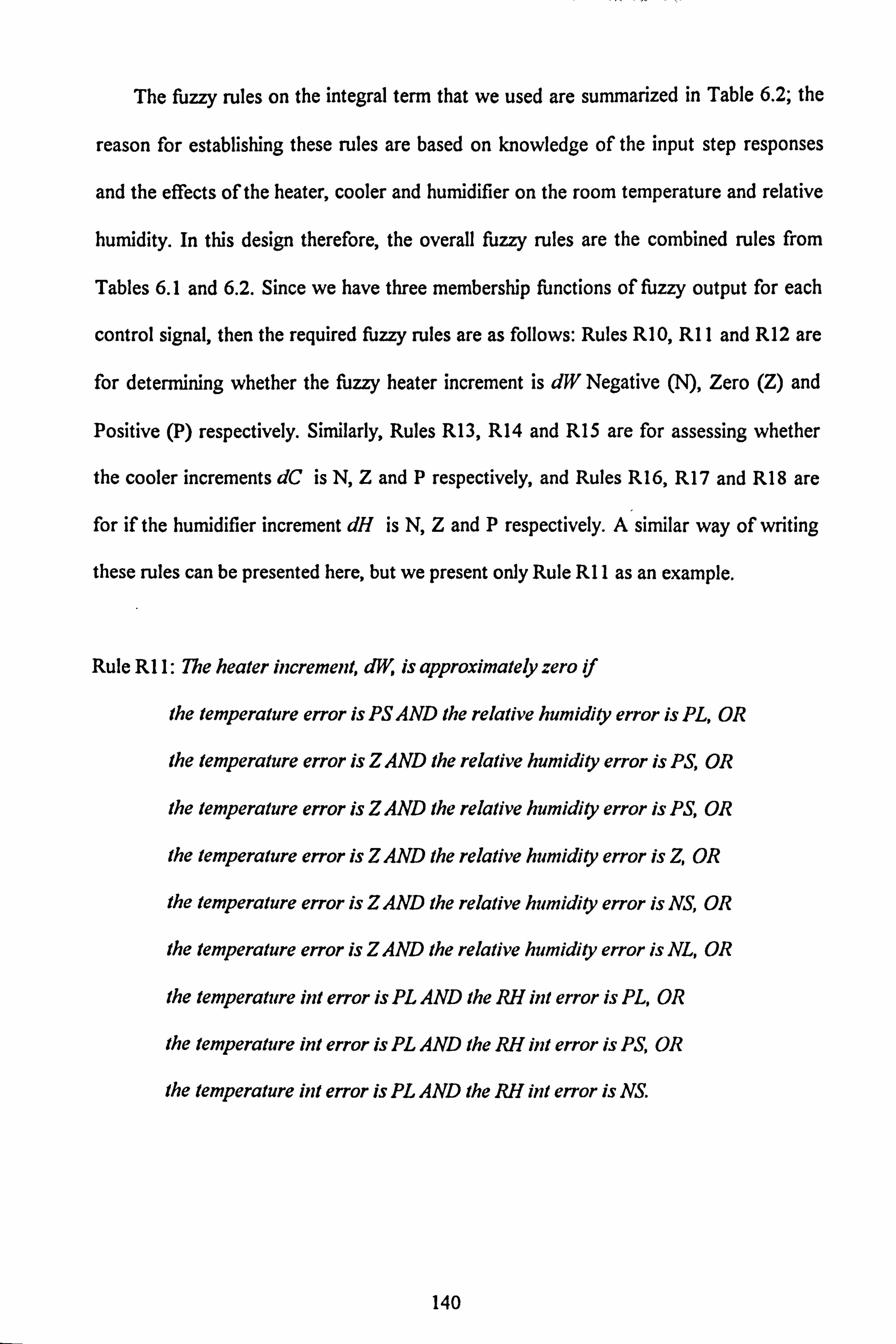
The fuzzy rules on the integral term that we used are summarized in Table 6.2; the

reason for establishing these rules are based on knowledge of the input step responses

and the effects of the heater, cooler and humidifier on the room temperature and relative

humýidity. In this design therefore, the overall fuzzy rules are the combined rules from

Tables 6.1 and 6.2. Since we have three membership functions of fuzzy output for each

control signal, then the required fuzzy rules are as follows: Rules RIO, RI I and R12 are

for determining whether the fuzzy heater increment is dW Negative (N), Zero (Z) and

Positive (P) respectively. Similarly, Rules R13, R14 and R15 are for assessing whether

the cooler increments dC is N, Z and P respectively, and Rules R16, R17 and R18 are

for if the humidifier increment dH is N, Z and P respectively. A similar way of writing

these rules can be presented here, but we present only Rule RI I as an example.

Rule RI 1: Yhe heater increment, dW, is approximately zero if






the temperature error is Z AND the relative humidity error is NL, OR

the temperature int error is PL AND the RH int error is PL, OR

the temperature int error is PL AND the RH int error is PS, OR

the temperature int error is PL AND the RH int error is NS.

140

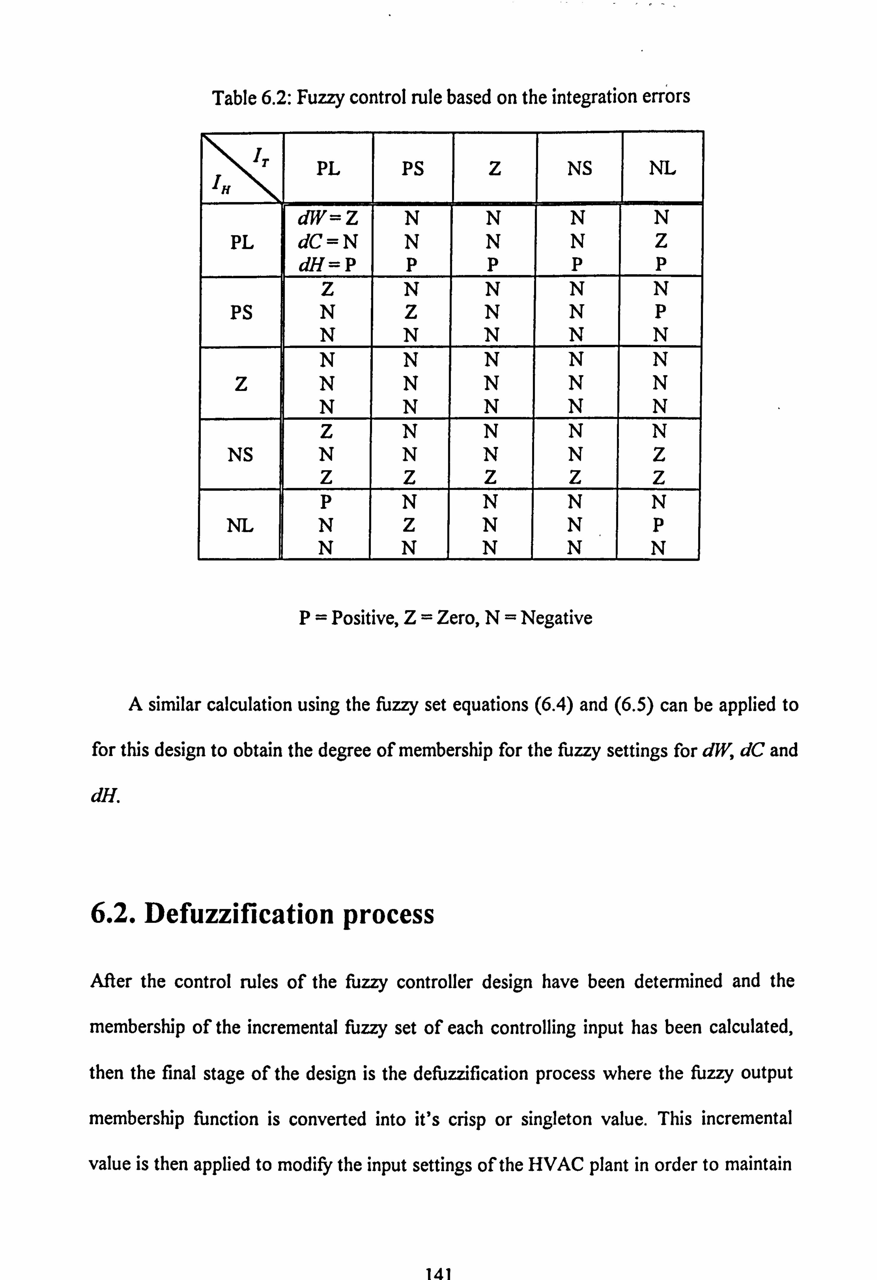
Table 6.2: Fuzzy control rule based on the integration errors

PL PS Z NS 1

NL

dW= Z N N N N PL dC=N N N N Z

___ dH=P p p P p

_ Z N N N N PS N Z N N P

N N N N N N N N N N

Z N N N N N N N N N N Z N N N N

NS N N N N Z Z Z Z Z Z p N N N N

NL N Z N N P N N N N N

P= Positive, Z= Zero, N= Negative

A similar calculation using the fuzzy set equations (6.4) and (6.5) can be applied to

for this design to obtain the degree of membership for the fuzzy settings for dW, dC and

dFl.

6.2. Defuzzification process

After the control rules of the fiizzy controller design have been determined and the

membership of the incremental fuzzy set of each controlling input has been calculated,

then the final stage of the design is the defuzzification process where the fuzzy output

membership function is converted into it's crisp or singleton value. This incremental

value is then applied to modify the input settings of the HVAC plant in order to maintain

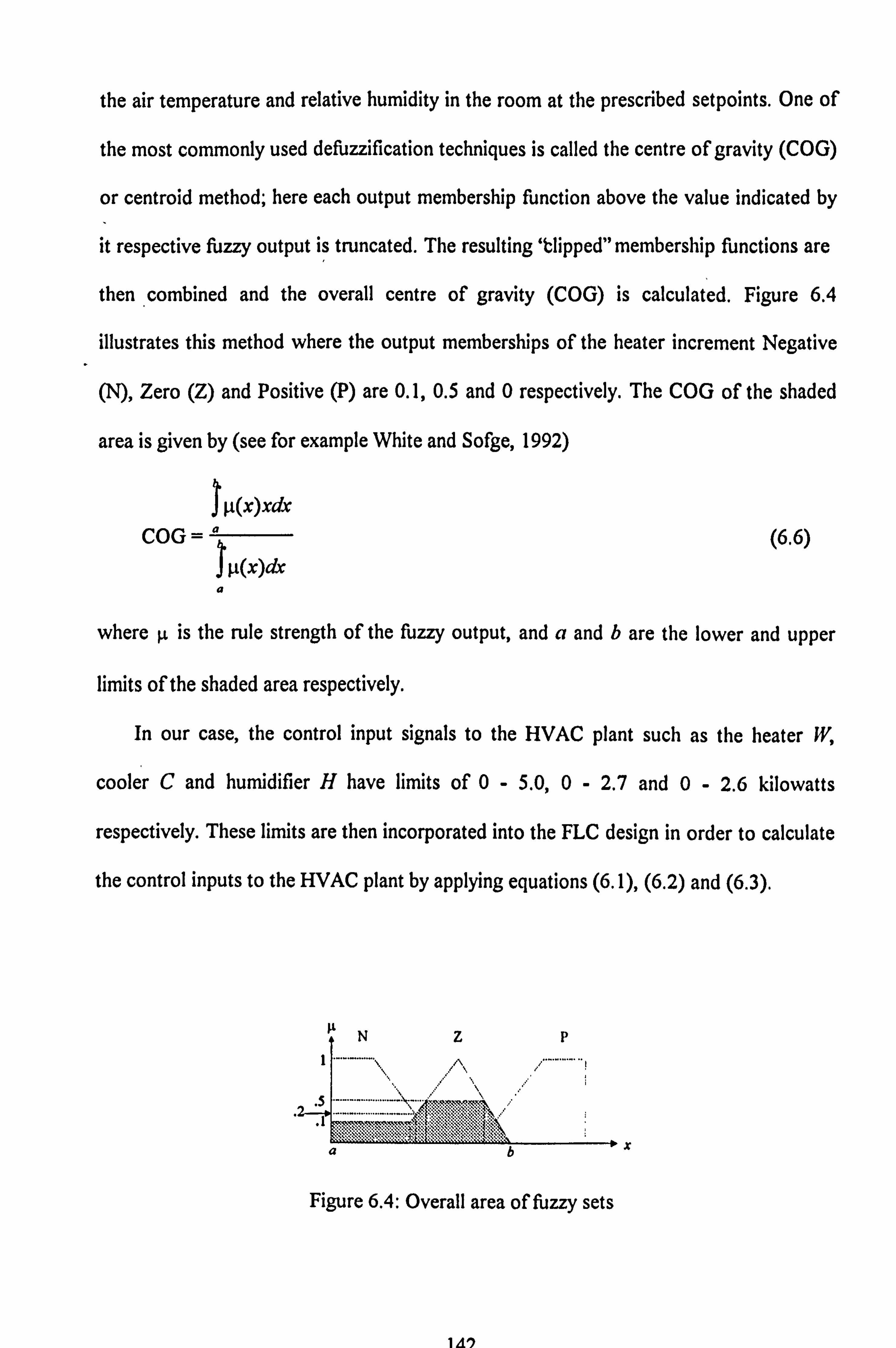
the air temperature and relative humidity in the room at the prescribed setpoints. One of

the most commonly used defuzzification techniques is called the centre of gravity (COG)

or centroid method; here each output membership function above the value indicated by

it respective fuzzy output is truncated. The resulting 'blipped" membership functions are

then combined and the overall centre of gravity (COG) is calculated. Figure 6.4

illustrates this method where the output memberships of the heater increment Negative

(N), Zero (Z) and Positive (P) are 0.1,0.5 and 0 respectively. The COG of the shaded

area is given by (see for example White and Sofge, 1992)

lp(x)xdc

COG=' lp(x)dx

a

(6.6)

where ýt is the rule strength of the fuzzy output, and a and b are the lower and upper

limits of the shaded area respectively.

In our case, the control input signals to the HVAC plant such as the heater W,

cooler C and humidifier H have limits of 0-5.0,0 - 2.7 and 0-2.6 kilowatts

respectively. These limits are then incorporated into the FLC design in order to calculate

the control inputs to the HVAC plant by applying equations (6.1), (6.2) and (6.3).

x

Figure 6A Overall area of fuzzy sets

ýt XT

6.2.1. Calculation of the FLC outputs

In general, the control performance of the FLC design depends on the number of fuzzy

input and output membership functions, the domain and shape of each membership

function, and the way the control rule is evaluated. There are many ways of combining

the above considerations, but let us consider that for our system, the room temperature

error range of -0.51C to 0.5"C corresponds to the fuzzy membership Z, between OT to

2*C is PS, 0"C to -2*C is NS, and an error greater than IT is PL and lower than -I T

is NL. Similarly, these conditions are also applied to the relative humidity error. For

these definitions, the chosen membership functions used in the design are shown in Table

6.3. Moreover, the domains of the fuzzy output membership functions: Negative, Zero

and Positive are given in Table 6.4. Note that the dimension for the values in Table 6.3

can be either ̀C or %rh, as explained in Section 6.1.

In the tuning of the presented controllers, we used the actual output and integral

errors for fuzzification process and therefore the proportional and integration gains for

these designs are unity. We can improve these designs for other gains as well since the P

and I terms in P+I controllers linearly correspond to the output and integral errors

respectively.

Table 6.3: Scaling factor of fuzzy input membership functions

Fuzzyinput NL and PL NS and PS z

scaling factor 11 12 13 S, S2 S3 Z, Z2

Range 100.0 2.0 1.0 2.0 1.0 0 0.5 0

Table 6A Scaling factors for the fuzzy output membership functions

Fuzzy controller Negative (N) Zero (Z) Positive (P)

output (M) X, n. nr zi zm zf p, P, X.

dW -0.20 -0.14 0 -0.14 0 0.14 0 0.14 0.20

dC -0.20 -0.14 0 -0.14 0 0.14 0 0.14 0.20

dH -0.20 -0.14 1 0 -0.14 0 0.18 1 0 0.18

As an example, let us assume that the output errors, e. (1) and e,, (1) at time I are

-0.2"C and 0.64%rh respectively. From the fuzzification process and using the scaling

factors in Table 6.3 for Figure 6.2, we can calculate the degree of membership, p, for

each fuzzy input. We found that for this value of e,.; PL, PS, Z, NS and NL have values

of 0,0,0.6,0.2 and 0 respectively. Similarly, for e. equal to 0.64%rh the corresponding

values are 0,0.64,0,0 and 0. By applying the fuzzy rules RI, R2, ..., R9 and the min-

max inferences of equations (6.4) and (6.5) to these fuzzy inputs, we can obtain the

degree of membership for all our fuzzy output incremental settings: N, Z and P of each

controller's output. The details of the calculations are as follows:

i). Heater increment, dW

max(rnin(0.2,0), niin(0,0), min(0.2,0.64), min(0,0.64), min(0.2,0), min(0,0), min(0.2,0), min(0,0), min(0.2,0), i-ni-n(0,0» max{O, 0,0.2,0,0,0,0,0,0,0) = 0.2

gz = maximin(0,0), min{0.6,0), min(0.6,0.64), min(0.6,0), min(0.6,0), rain{0.6,0»

= max{O, 0,0.6,0,0,0) = 0.6

gp = max{min(0,01, min{O, 0.64), nun(0,0.64), min(0.6,0), inin(0,0), min{O, 0.2), min(0,0), min(0,0), min(0,0.64»

= max{O, 0,0,0,0,0,0,0,0) =0

144

ii). Cooler increment, X

gn max(min(0,01, min(0,0), min(0.6,0), min(0.2,0), min(0,0.64), min(0,0.64), min{0.6,0.64), min(0.2,0.64), min(0,0), min(0,0), min(0.2,0), min(0,0), min(0,0), min(0.6,0), min(0,0). � Hn{O, 0» max(0,0,0,0,0,0,0.6,0.2,0,0,0,0,0,0,0,0) = 0,6

gz = max{rnin{0,0), min(0,0.64), min(0.6,0), min{O, 0), min{0.2,0), min{0.6,0»

= max{O, 0,0,0,0,0) =0

gp = max(min(0,0), min(0.2,0), min(0,0» = max(0,0,0) =0

iii). Humidifier increment, dH

gn = max{niin(0,0.641, min{O, 0), min{O, 0), min(0.2,0), inin(0,0), min(0,0), min(0,0), min(0.6,0), min(0.2,0) min(0,0), min(0,0), min(0,0), min(0.6,0), min(0.2,0), min(0,01)

= max (0,0,0,0,0,0,0,0,0,0,0,0,0,0,0) =0

g, = max{ min{O ' 0.64), min(0.6,0.64), min{0.2,0.64), i-nih(0,0.64), min(0.6,0»

= max (0,0.6,0.2,0,0) = 0.6

gp = max(rnin(0,0), rnin(0,0), min(0.6,0), min(0.2,0), min10,0»

= max (0,0,0,0,0) =

Now, we can calculate the physical values of dW, dC and dH via the defuzzification

process. By using the scaling factors in Table 6.4, we find that XV, dC and dH are

-0.018, -0.116 and 0.095 kW respectively. If the previous control inputs W, C, H to the

plant are 4.936,0.478 and 0.076 kW respectively, then using equations (6.1), (6.2) and

(6.3), their present values become 4.918,0.362 and 0.171 kW respectively.

145

6.3. Simulation results

In this section, we present some simulation results using the FLC developed in Section

6.1. In these simulations, the system performance for step reference inputs is studied. As

before, our objectives of the design are:

1) to obtain minimal output errors at steady state conditions,

2) to minimise the overall energy consumption of the HVAC plani, and

3) possess fast settling time i. e. the time required to reach the setpoints from an initial

condition should be as fast as possible.

A simulation program was developed by applying the fuzzy design procedures

presented in Section 6.1 and the scaling factors in Tables 6.2,6.3 and 6.4. In the

simulation, we assume that the air dynamics of the room follows equations (2.1) and

(2.2). Moreover, the climatic disturbances such as the laboratory temperature, T, ,

outside air temperature, T,, , outside relative humidity, H,, , and total solar irradiance, S,

are assumed to be constant at 20"C, 15T, 80%rh and O. IWm-' respectively, and the

white noise processes, V, and V2 , and the constants, k, and k, , are zero. Note that the

fuzzy input domains as presented in Table 6.3 are arbitrarily chosen as discussed in

Section 6.2.1 but the fuzzy output domains in Table 6.4 were obtained after several

simulations trials carried out for the above conditions so that the desired overall control

performances can be achieved.

The system performances can be judged by calculating the magnitude of the errors

of the actual room temperature and relative humidity from the setpoints as well as

deducing the energies consumed by the system. Let us consider tile system under the

setpoints of 25'C and 50%rh for the room temperature and relative humidity

146

respectively, and their initial values are assumed to be at 15T and 80%rh respectively.

Moreover, all the three control inputs to the plant have not been used initially. The

simulated results are shown in Figure 6.5; the control performance calculated over the

last 100 data points after steady state had been reached and the following results are

obtained:

* the required control input energies are 22.3,0 and 5.4 kWh for the heater, cooler and

humidifier respectively;

* the output squared errors are 0.2"C' and 2.8%rh' for the temperature. and relative


the required times to reach the temperature and relative humidity setpoints are 5.8 and


We can see that excellent control regulation has been achieved from this tYpe of FLC.

We found that the heater consumed more power and the cooler was not used in all the

simulation periods; this is reasonable since the temperature setpoint of 25T is much

higher than the ambient temperature (equal to 9.9C as discussed in Section 2.3.1).

Figure 6.6 shows that the good regulation performance of the system is maintained

even when climatic disturbances (see section 4.2.1) and white noise processes are

included in the analysis. The disturbances for the noise terms were inserted in the form of

pseudo random binary sequences (PRBS) generated using 6 bits shift register (Godfrey,

1980) with 10% of magnitude, i. e. their values were ±0.1. The control performance at

steady state conditions for these situations are calculated over the last 100 data points

and found to be as follows:

* the required control input energies are 28.2,0 and 6.8 kWh for the heater, cooler and

humidifier respectively; and

147

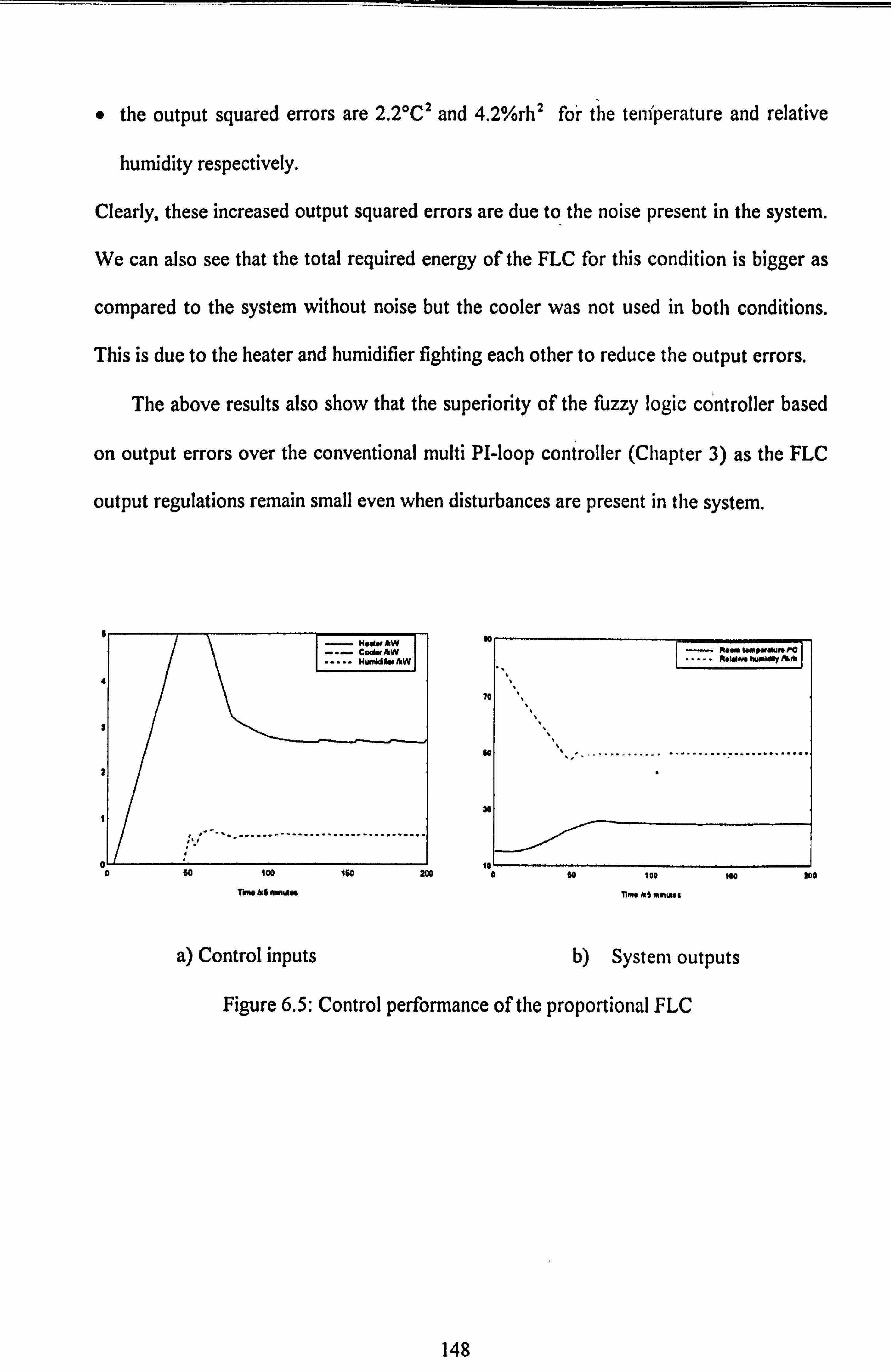
the output squared errors are 2.2"C' and 4.2%rh' fo'r the teniperature and relative

humidity respectively.

Clearly, these increased output squared errors are due to the noise present in the system.

We can also see that the total required energy of the FLC for this condition is bigger as

compared to the system without noise but the cooler was not used in both conditions.

This is due to the heater and humidifier fighting each other to reduce the output errors.

The above results also show that the superiority of the fuzzy logic controller based

on output errors over the conventional multi PI-loop controller (Chapter 3) as the FLC

output regulations remain small even when disturbances are present in the system.

-He" AW COOW&W

II

51

so 100 460 200

Thm Ad mmam

vu PC ZMW hu. WNY PAM

so ............. ..........................

30

10 0 so 100 184 200

mm* ki .. w..


Figure 6.5: Control performance of the proportional FLC

148

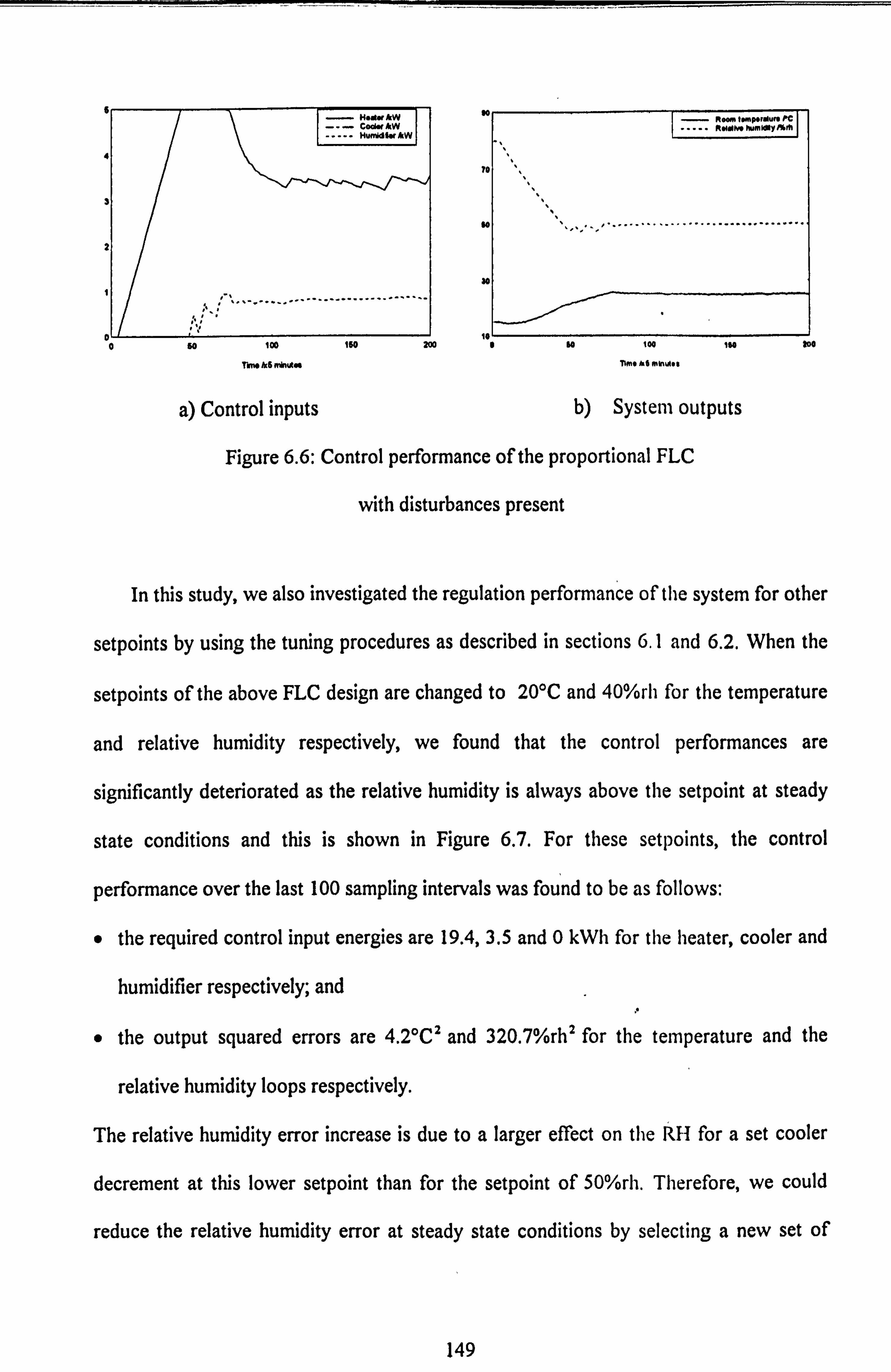
6

4

3

-H. Ntw AW --- COOW AM ----- HwrJdW AIW

I'll, 114,1

.....................................

Rý Imperalum PC II

'0 ,,

.............. ....................

Tkm M trftga -nme 1.5 Minw. 8


Figure 6.6: Control performance of the proportional FLC

with disturbances present

oo

In this study, we also investigated the regulation performance of the system for other

setpoints by using the tuning procedures as described in sections 6.1 and 6.2. When the

setpoints of the above FLC design are changed to 20'C and 40%rh for the temperature

and relative humidity respectively, we found that the control performances are

significantly deteriorated as the relative humidity is always above tile setpoint at steady

state conditions and this is shown in Figure 6.7. For these setpoints, the control

performance over the last 100 sampling intervals was found to be as follows:

" the required control input energies are 19.4,3.5 and 0 kWh for tile heater, cooler and


" the output squared errors are 4.2"C' and 320.7%rh' for the temperature and the

relative humidity loops respectively.

The relative hurnidity error increase is due to a larger effect on tile RH for a set cooler

decrement at this lower setpoint than for the setpoint of 50%ril. Therefore, we could

reduce the relative humidity error at steady state conditions by selecting a new set of

149

fuzzy output scaling factors as shown in Table 6.5 'where only the fuzzy output

membership functions of the cooler, namely z, p. and x. are increased to 0.21,0.21

and 0.3 M

edw H C. w HundSorAW

l VVv-1A IV\ v V l

-

A-M om, wwm PC

10

0 50 100 ISO 200 a so 104 IN 200

Thm AKS minta no t. % mmfi. v

a) Control inputs b) Systern outputs

Figure 6.7: Control performance of the proportional FLC (setpoints change)

Table 6.5: Scaling factors for the fijzzy output membership functions

Fuzzy controller Negative (N) Zero (Z) Positive (P)

output (W) X) nm nr zI zm Zr p, P, X.

dW -0.20 -0.14 0 -0.14 0 0.14 0 0.14 0.20

dC -0.20 -0.14 0 -0.14 0 0.21 0 0.21 0.30

dH -0.20 -0.10 0 -0.10 0 0.18 0 0.18 0.25

The simulated result for this redesigned FLC is shown in Figure 6.8 where we can

see that all the three signals are required to regulate the systern outputs. The control

performance of the controller was calculated for the last 100 iterations of the simulation

trial; the value of the squared errors were found to be 0.4"C' and ý 3.9%rh 2 for the

ISO

temperature and relative humidity respectively which is almost similar to the result

obtained from the previous fuzzy settings, but the energies consumed by the heater,

cooler and hunUifier were relatively large at 24.5,8.0 and 3.5 kWh respectively. We can

see that the three control inputs are fighting one another in order to regulate the two

outputs.

6

4

3

-Hmtw AW Coolw IkW

..... Humidiw*W

70

GO

so lw 150 200

Time ýk6 ninutes

30

S so IN ISO 200

Tlýf AS MirAA. 8


Figure 6.8: Control performance of the proportional FLC with redesigned fuzzy

membership functions

I

For the FLC based on a P+I design, the control performance is shown in Figure 6.9

where identical climatic disturbances and white noise processes as earlier are applied.

The scaling factors for the P+I terms (as indicated in Tables 6.3 and 6.6) are uged in this

design. Again, the ftizzy input domains of the integral terms IT and 11, as presented in

Table 6.6 were obtained after several simulation trials 'so that the desired output

regulations can be achieved.

151

mom Impordum PC ROIGINORL"Imly/%gh

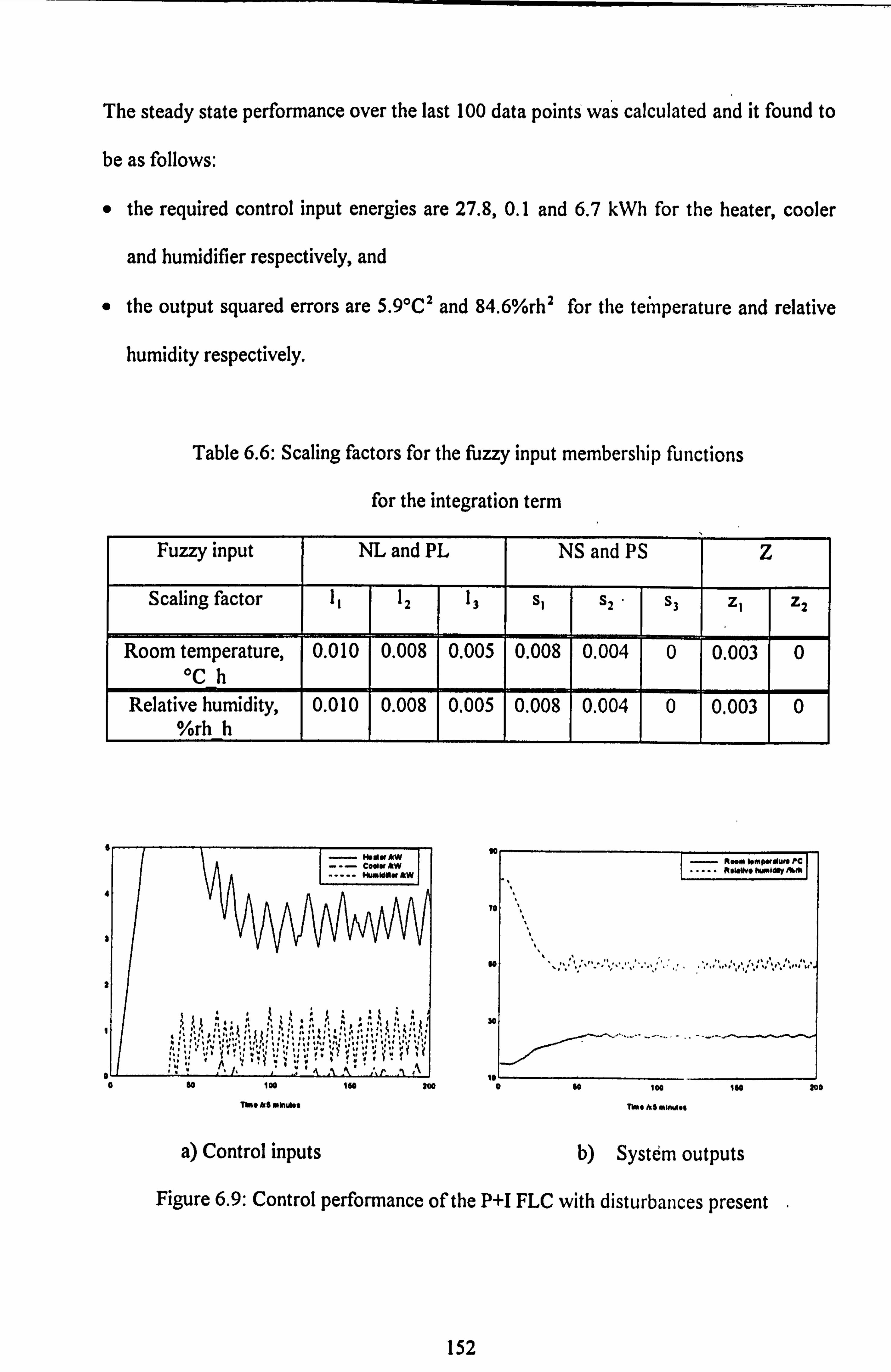
The steady state performance over the last 100 data points was calculated and it found to

be as follows:

" the required control input energies are 27.8,0.1 and 6.7 kWh for the heater, cooler

and humidifier respectively, and

" the output squared errors are 5.9C' and 84.6%rh 2 for the teinperature and relative


Table 6.6: Scaling factors for the fuzzy input membership functions

for the integration term


Scaling factor 11 12 13 S, S2 S3 ZI Z2

Room temperature, 'C h

0.010 0.008 0.005 0.008 0.004 0 0.003

I

0

Relative humidity, %rh h

0.010 0.008

I

0.005 0.008 0.004 0 0.003 I 0

I

.... AIW muffildo1w &W

61

aI

li

""I" "I

I "" I

'A' '

" I' ""tA" I' .A

- .. m I, mp«lw$ PC IuIdlIy m

so 100 160 too 0 so 100 iso 300

Thme *6 MIM"I TIMG 1.5 Mir". $

a) Control inputs b) Syst6m outputs

Figure 6.9: Control performance of the P+I FLC with disturbaiices present

152

We can see that the output regulation at steady state conditions is acceptable but

degraded as compared to that obtained through the proportional FLC. This is because

the proportional FLC in fact. also contains integral action as it is implemented with

incremental control. If it was a true proportional only FLC the performance would be

inferior with steady-state error due to the zero type number of the system and controller

configuration. Both results for the proportional and P+I FLCs can be improved further

by modifying the overall fuzzy rules as well as the scaling factors for the fuzzy input and

output membership functions.

We have also designed other types of FLC based on the PID controller, such as

employing P+D or P+I+D terms, and found that the required FLC tunings are more

difficult to achieve and extensive simulation trials are needed in order to achieve a good

design. This problem is due to our system being multivariable, and many parameters are

involved in the tuning process which are quite difficult to carry out in practice.

From the results presented here, we have faced a difficulty of obtaining the

appropriate values of the fuzzy membership functions where extensive simulation trials

are needed to achieve the desired FLC control 'performance. To improve the situation,

we propose the use of genetic algorithm (GA) optimisation techniques to automatically

search these functions, and this is discussed in Chapter 7.

6.4. Conclusions

This chapter has shown that good control performances can be achieved by using fuzzy

logic controllers (FLC) based on proportional techniques with incremental control, when

applied to a HVAC plant /office zone system having three inputs and two outputs. These

153

good results have also been obtained using a P+I FLC but P+D and P+I+D controllers

require more effort in tuning them in order to achieve a good result. These practical

aspects are considered in Chapter 7.

153A

Chapter 7

Genetic Algorithms for BEMS

The genetic algorithm based method (GA) is a global search technique which uses

natural selection and genetics. It searches from a population of solutions, by using

random choice as a selection tool to obtain the best solution, The first thorough

treatment of the use of genetic algorithms was given by Holland (1975) but a more upto

date description of the theory and application of GA methods may be found in Goldberg

(1989). Examples of the use of GAs in control applications are given in Waddicor

(1993), McGregor et al (1992) and Etter et al (1992).

These algorithms operate on a population of character strings in much the same way

as genetic action operates on chromosomes in a population of organisms. GAs enforces a

Darwinian "survival of the fittesf' strategy among a population of strings. In every

generation, a new set of strings is created using parts of the fittest individuals from the

previous generation. The algorithms use past information efficiently to explore new

regions of decision space with a high probability of finding improved performances.

GAs are different from typical search methods in three primary ways, namely,

1. they work with a coding of the parameter set rather than with the actual

parameters,

154

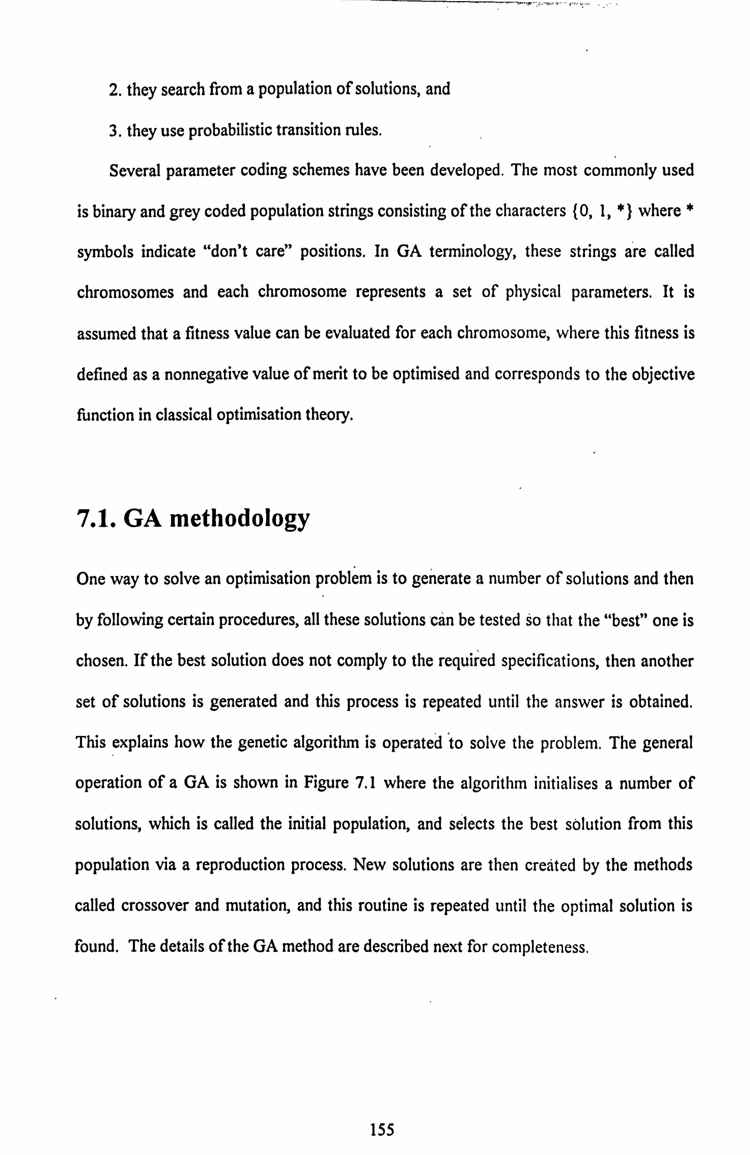
2. they search from a population of solutions, and

3. they use probabilistic transition rules.

Several parameter coding schemes have been developed. The most commonly used

is binary and grey coded population strings consisting of the characters (0,1, *) where *

symbols indicate "don't care"' positions. In GA terminology, these strings are called

chromosomes and each chromosome represents a set of physical parameters. It is

assumed that a fitness value can be evaluated for each chromosome, where this fitness is

defined as a nonnegative value of merit to be optimised and corresponds to the objective

function in classical optimisation theory.

7.1. GA methodology

One way to solve an optimisation problem is to generate a number of solutions and then

by following certain procedures, all these solutions6n be tested so that the "best" one is

chosen. If the best solution does not comply to the required specifications, then another

set of solutions is generated and this process is repeated until the answer is obtained.

This explains how the genetic algorithm is operated 'to solve the problem. The general

operation of a GA is shown in Figure 7.1 where the algorithm initialises a number of

solutions, which is called the initial population, and selects the best solution from this

population via a reproduction process. New solutions are then created by the methods

called crossover and mutation, and this routine is repeated until the optimal solution is

found. The details of the GA method are described next for completeness,

155

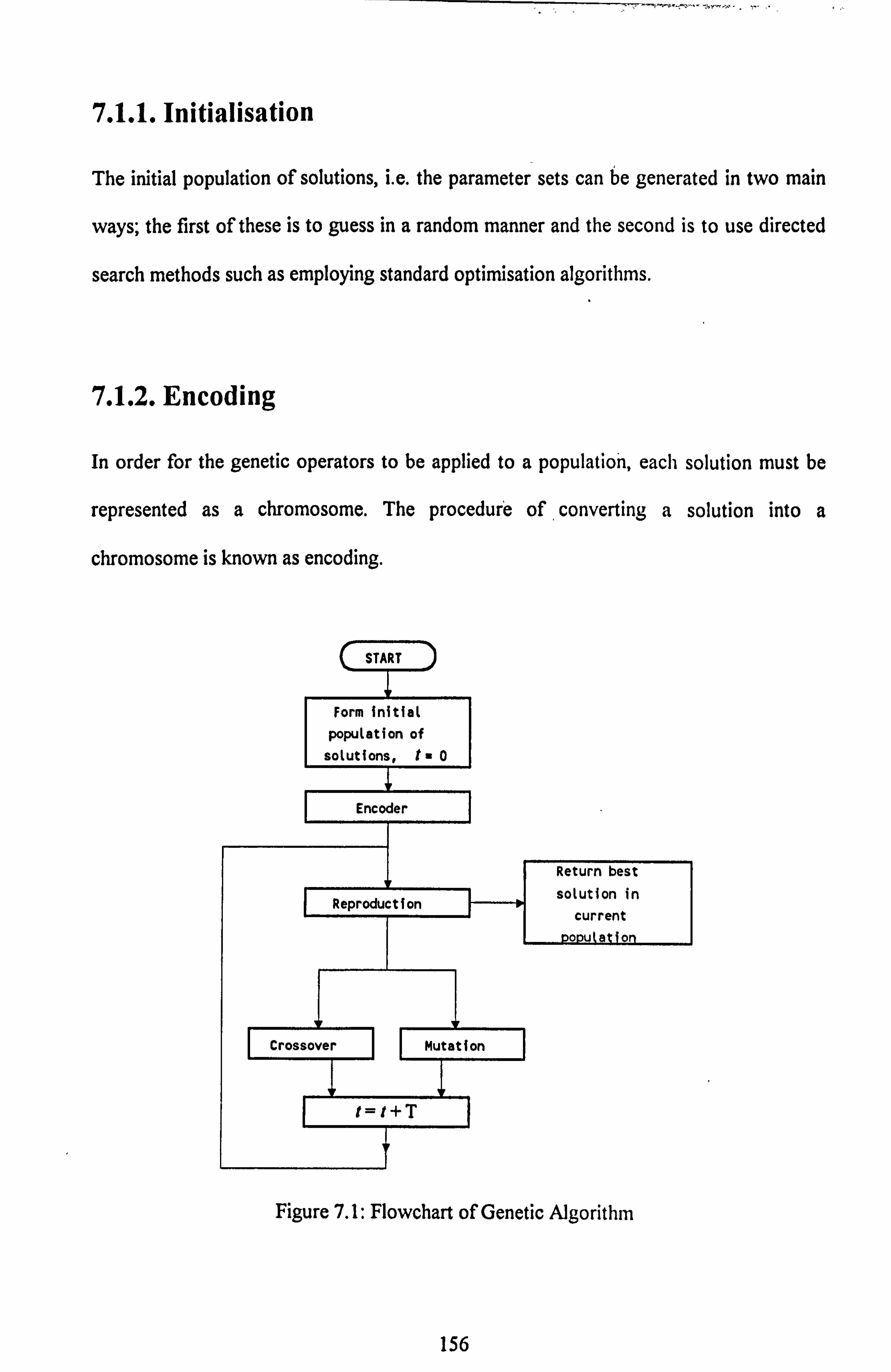
7.1.1. Initialisation

The initial population of solutions, i. e. the parameter sets can be generated in two main

ways; the first of these is to guess in a random manner and the second is to use directed

search methods such as employing standard optimisation algorithms.

7.1.2. Encoding

In order for the genetic operators to be applied to a population, each solution must be

represented as a chromosome. The procedure of . converting a solution into a

chromosome is known as encoding.

Figure 7.1: Flowchart of Genetic AJgorithm

156

The encoding procedure varies according to the type of problem being considered

and nature of the solution being sought; for a solution which is specified as a set of

parameters expressed as floating point numbers, the following procedure may be used.

However before encoding can take place, it is necessary to determine the minimum and

maximum values for each parameter as well as the number of possible values it may take.

This corresponds to the resolution R and is set to 2 n_l, where n is a positive integer.

Each parameter value may then be normalised to a value in tile range 0-R, by using

NormalisedValue OriginalFalue - Minimum Value

xR (7.1) Maximum Value - Minimum Value

This normalised value is rounded to the nearest integer, which is then expressed in binary

logic-or base 2 arithmetic. The result is a chromosome with a word length (number of

bits) equal to 1092(R+I); Figure 7.2 shows this procedure more clearly where the integer

n=4, i. e. 4 bit string of each of the three parameters, namely X,, X2 and X3, and their

resolution, R, are calculated to equal 15. The normalised values can be calculated from

equation (7.1) where the maximum values are 5.0,2.7 and 2.6 for x,, x, and X3

respectively and their minimum values are zero. When all the parameters within a set of

solutions have been converted to strings, the strings are concatenated to produce the

chromosome of length S, where S represents the number in the parameter set, and for

this example, S =12.

7.1.3. Evaluation

The performance for each chromosome is evaluated by calculating the fitness function

for its parameter set which is obtained by performing the reverse of the above encoding

process.

157

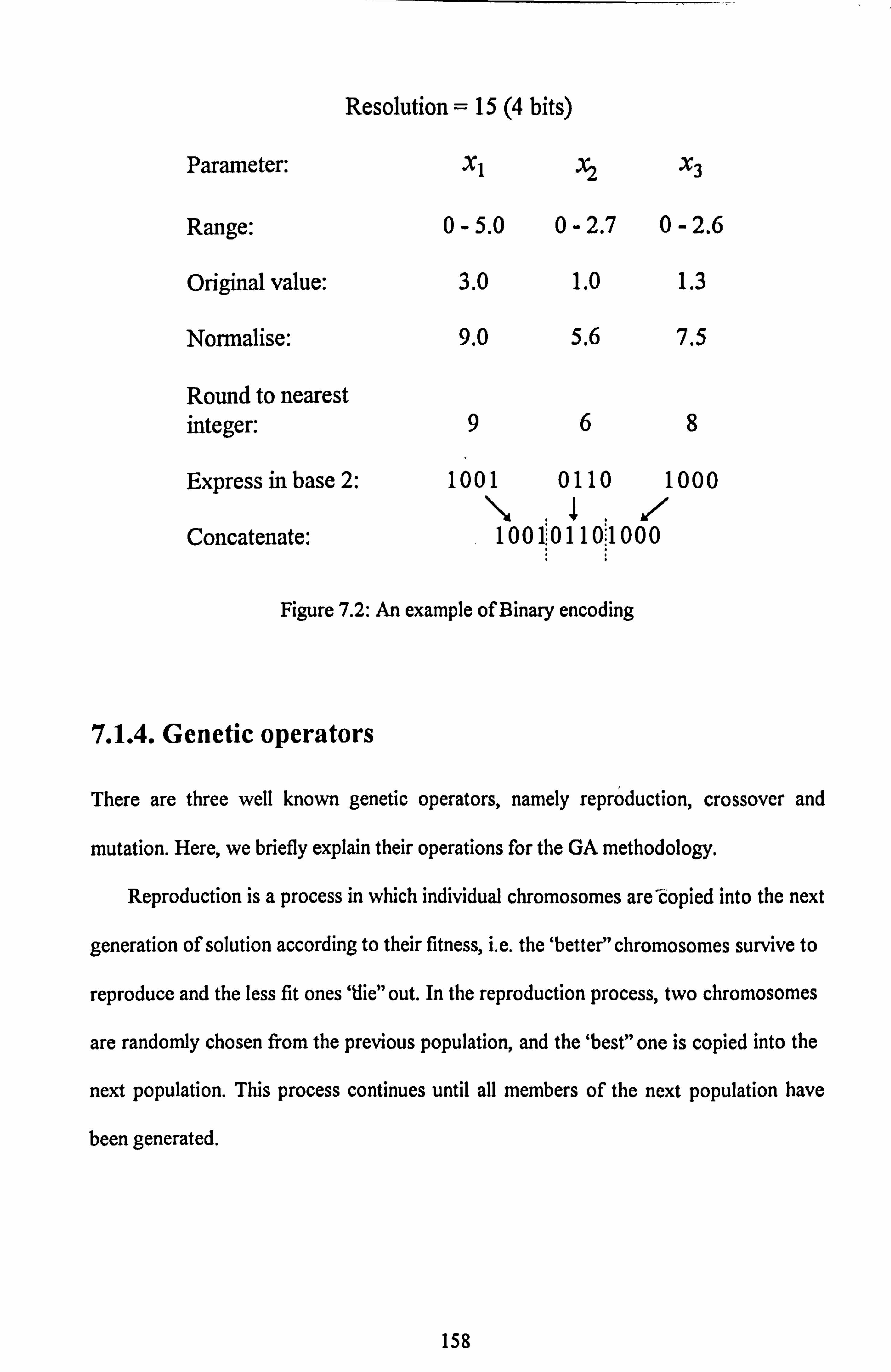
Resolution = 15 (4 bits)

Parameter: XI X2

Range: 0-5.0 0-2.7

Original value: 3.0 1.0

Normalise: 9.0 5.6

Round to nearest

X3

0-2.6

1.3

7.5

integer: 968

Express in base 2: 1001 0110 1000 \, I. z

Concatenate: 10011011011000

Figure 7.2: An example of Binary encoding

7.1.4. Genetic operators

There are three well known genetic operators, namely reproduction, crossover and

mutation. Here, we briefly explain their operations for the GA methodology.

Reproduction is a process in which individual chromosomes are -copied into the next

generation of solution according to their fitness, i. e. the 'bettee, chromosomes survive to

reproduce and the less fit ones 'Uie" out. In the reproduction process, two chromosomes

are randomly chosen from the previous population, and the 'best" one is copied into the

next population. This process continues until all members of the next population have

been generated.

158

After reproduction, simple crossover of the genes 'occ6rs in two steps. First, the

members of the newly reproduced chromosomes are "mated" randomly and crossover is

then accomplished by

(i). randomly selecting a number of positions in the chromosome (usually over half of

the bits in a chromosome); and

(ii). swapping all the succeeded positions, thus creating two new chromosomes.

Old 10011101 1 10 01 Jill 0 11 1 11

chromosomes 110 00 111 .......... I

CROSSOVER

New 11010111

chromosomes 10 00 110 1

7-7777'. '-

MUTATION

Ioo1; 1"-1,1! 10

Figure 7.3: Crossover and Mutation operators

In the mutation process, we randomly change the value of a specific chromosome

(bit); this is usually applied to only a few positions in the chromosomes of the new

population, for example, a ratio of the order I in every 1000 is normally applied. A

randon-Ay selected bit is flipped, i. e., if its value is 0, it becomes 1, and vice versa. This

operation, when used sparingly, ensures that potentially useful information in a string

position is not lost forever.

The crossover and mutation operators in a binary code are shown in Figure 3 where

we can see that the crossover rate is 5 out of 8 bits (60%) and takes place at bit positions

2,3,5j, 7 and 8 and the mutation is at position 6 from the left.

159

7.1.5. Convergence

All GAs eventually produce a population in which the best chromosonie is identical to

that obtained from the previous generations. At this point, the GA is said to have

converged, and this chromosome represents the optimal solution to the problem.

7.2. Controller based on GA

In the control of a HVAC plant/office zone system, we require that the room

temperature T, and relative humidity H. track their' respective setpoints 7, ' and H, and

the output errors, namely e,. and e,, should be as small as possible at steady state

conditions. Therefore, the objective is to simultaneously minimise e7. and eH, which are

defined by equations (3.3) and (3.4).

There are other ways to define the objective function for the above HVAC plant. I

For example, to minimise the total energy consumption in applying the controlling inputs,

namely, the heater W, cooler C and humidifier H while maintaining tile output errors to

within an acceptable limit. The objective function for thiý definition may be difficult to

formulate due to the plant being multivariable in nature and optimisation of many

parameters would be required. Thus, we restrict our discussion to tile earlier definition

for simplicity and investigate the system performance of different fitness functions, and

different setpoints.

In this chapter, we present the use of GA techniques to solve the problem of

determining the three strategies for calculating the control inputs to drive the HVAC

160

plant/office zone system. The first type is to apply the structure of a multi-proportional

loop controller where the GA is used to tune the proportional gains. The second type

will be to search the best combination of fuzzy membership functions so that the control

performance of the FLC based on output errors is improved and the third type minimises

the predicted system output errors at time I+T and the GA is used to obtain the best

combination of the three control inputs at each time step 1. This adaptive type of

controller is further improved by the use of hybrid GA techniques to reduce the control

input switching problems encountered earlier in our research.

7.3. Multi-proportional loop controller

In this type of controller, the requirement is to tune the proportional gains so that the

system output closely tracks the desired setpoint. For our application, the block diagram

of the overall control system as shown in Figure 3.3 can be used to solve this problem

where all the PI controllers are replaced by simple proportional controllers. For this

configuration, the control inputs W(I), CQ) and H(I) can be calculated by summing the

proportional terms obtained from the temperature and relative humidity loops limited by

their respective input constraints, namely,

W(t)=Kple7. (t)+Kp2eH(t)s 0: ý5W(t): 55,0 (7.2)

C(t) = KP3 eT (t) + KP4 eH (1), 0': 5 C(t): 5 2.7 (7.3)

HQ) = KP5 eT (1) +KP6eH(l), 0: 5C(l): 5 2.6 (7.4)

where KpI, KP22 **o

Kp, are the proportional gains f6r th6 controllers #1, #2, ..,

#6

respectively.

161

The design problem here is to tune these gains by the GA method so that the output

errors are as small as possible at steady state conditions. This can be done by first

applying the main information about the input step responses as discussed in chapters 2

and 3; note the sign of gains Kp,, Kps and Kp, should be positive and those of Kp2, KP3

and Kp, negative in order to reduce the errors. Moreover, since the majority of the

modified Ziegler-Nichols proportional gains, as presented in Chapter 3 fall in the range

between 0 and 1, we assume that these gains lie in this range. Then, the GA optimisation

technique described in section 7.1 can be adopted for this case by ititroduciný a set of

individual chromosomes pj, j= lp 2, ..., M which belong to the population P(i) at

generation i and the following steps are implemented in order to determine the gains:

Proportional GA algorithm

Step 1. Select a random initial population PQ) comprising M solutions satisfying the

above assumption, i. e. 0 :51K, I :ý1,1 =Pl, P2, .., P6. Set the encoding

resolution R for each gain, and the crossover and the mutation rates. Initialise

the generation i=0.

Step 2. Encoding: Perform the encoding procedure for each solution, i. e. the parameter

set (KPI

3, KP2$KP3)KP4, K, Kpj is converted into a chromosome, as shown

in Figure 7.2.

Step 3. Calculate the parameter set for each chromosome by performing the reverse of

the encoding process.

Step 4. Reproduction: Calculate the fitness function for each chromosome and

generate the population PQ+l) of M chromosomes according to the

reproduction procedure.

162

Step 5. Go to Step 6 or Step 7 randomly.

Step 6. Crossover: Mate the members of PQ) at random, and carry out the crossover

operation at random for each pair of chromosomes. We then have 2M

chromosomes for population P(i+l), that is M chromosonýes belong to the

parent and M chromosomes belonging to the offspring. Go to, Step 8.

Step 7. Mutation: Select at random a chromosome fiom the population P(i), Carry out

the mutation operation for that chromosome, we th6n have an offspring

chromosome and the population PQ+l) contains ýf+l chromosomes.

Step 8. Set i=i+I and Goto Step 3.

The above steps are iterated until the fitness function of the best chromosome at

generation i converges to a minimal value. The details of each step in the algorithm are

explained next.

7.3.1. Initial population

The initial population is generated by using a random selection method. In our

application, the multi-proportional loop controller requires 6 gains in the range between

0 and 1, then using the MATLAB language, this population can be generated using the

"rand" function; hence P(O) = rand(6, M); this generates random numbers between 0-I

of equal opportunity. Thus, we have a population of P of dimension 6xM and pj is the

jth. column vector of P for thejth. parameter set (Kf,, KpJ2ý ..,

Kpj6) where j= 1,2, ...,

M. In the genetic algorithm, the physical value of the parameter set is encoded into a

chromosome. If the encoding resolution is 15, then we have a4 bit string for each input

163

(see Figure 7.2) and these strings are concatenated to'produce a chromosbme of length

24 bits with the first, second, third, fourth, fifth and sixth four bits represent the gains

Kpj, 9

KP29KP3) KPO Kps and KP6 respectively. If the required encoding resolution is

255, i. e. 8 bit words, then each chromosome will be 48 bits long.

The size of the population M is normally set between 20 to 80 in order to obtain

"enough variety" of chromosomes and ensuring that the computational requirements do

not become excessive; it is obvious that, the larger the M the longer the simulation

period.

7.3.2. Reproduction

In the reproduction process, two chromosomes ar6 s6lected at randoin from the

population PQ) and these compete through a fitness function for survival to the next

generation. The fitter chromosome will be selected and the weaker one will die. This

process is repeated for other pairs of chromosomes until we obtain a total number of M

chromosomes for the population P(i+l).

The fitness function (normally known as the objective function in the field of

optimisation) plays an important factor for the system to converge, it has to be

formulated in such a way that both the system outputs should converge to the required

setpoints at steady state conditions. A sensible choice for the fitness function, fi, for the

chromosome pi is the summation of the absolute room temperature and relative

humidity errors. In this way larger values will indicate a poor solution and smaller errors

a good one. A convenient way of combining the temperature and hunlidity errors is as

follows:

164

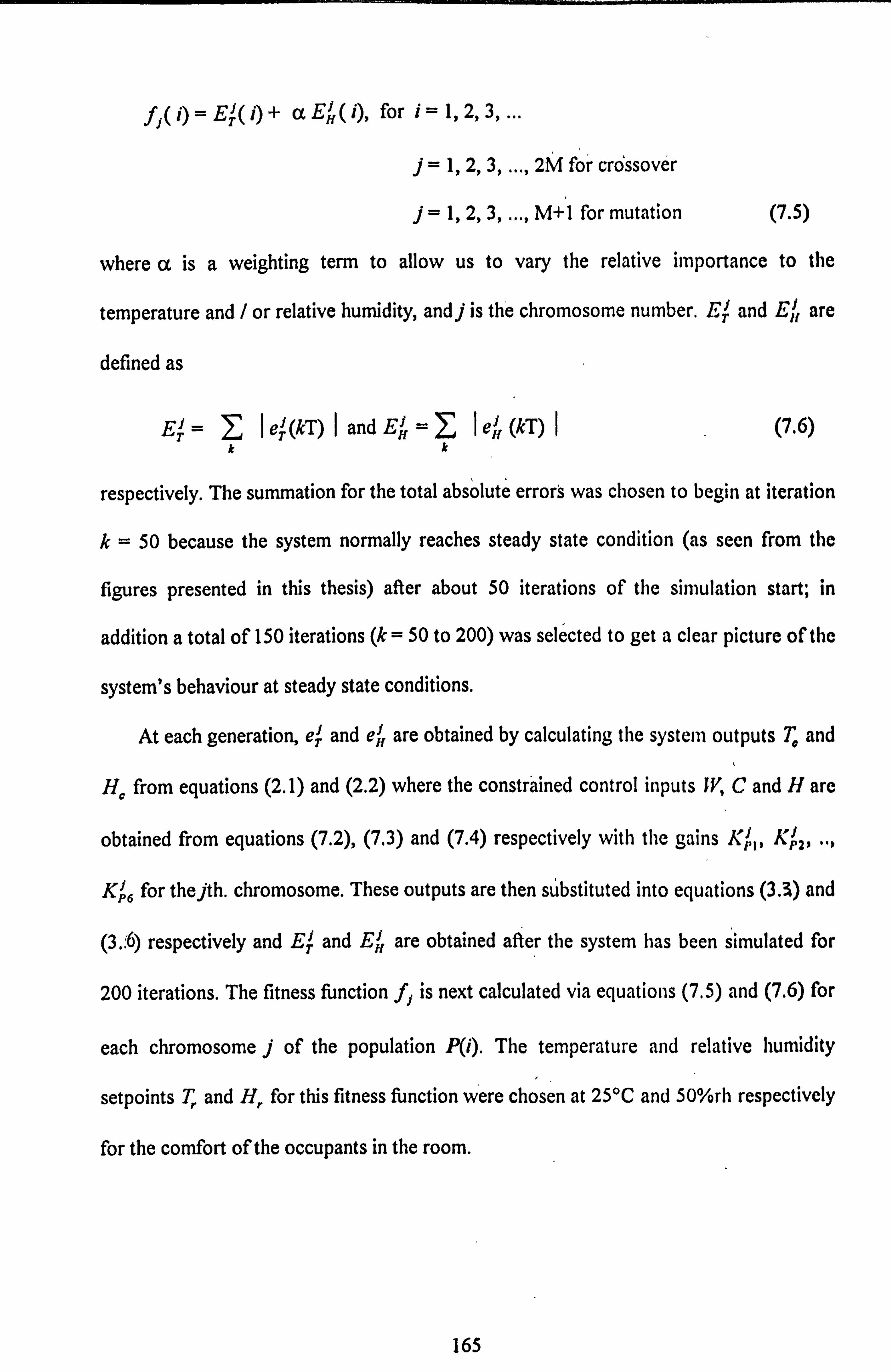
fj(i) = ETJ(i)+ ccEHJ ( i), for i=1,2,3, TH

1,2,3, ..., 2M for crdssover

1,2,3, ..., M+l for mutation (7.5)

where a is a weighting term to allow us to vary the relative importance to the

temperature and / or relative humidity, andj is the chromosome number. EJ and EJ, are

defined as

Ei eJ (kT) I and EJ, ei (kT) (7.6) TT kk

respectively. The summation for the total absolute errors was chosen to begin at iteration

k= 50 because the system normally reaches steady state condition (as seen from the

figures presented in this thesis) after about 50 iterations of the simulation start; in

addition a total of 150 iterations (k = 50 to 200) was selected to get a clear picture of the

system's behaviour at steady state conditions.

At each generation, e' and ei are obtained by calculating tile system outputs T, and I

H from equations (2.1) and (2.2) where the constrained control inputs JV, C and H are

i obtained from equations (7.2), (7.3) and (7.4) respectively with the gains KpJ,, KP29 "t

Kpi 6 for thejth. chromosome. These outputs are then substituted into equations (M) and

(3.. "6) respectively and E. J and E. J are obtained after the system has been simulated for 11

200 iterations. The fitness function fj is next calculated via equations (7.5) and (7.6) for

each chromosome j of the population PQ). The temperature and relative humidity

setpoints T, and H, for this fitness function were chosen at 25"C and 50%rh respectively

for the comfort of the occupants in the room.

165

In the reproduction process, all the chromosomes at geheration i compete for

survival and the M chromosomes with the smallest Values of fitness functions are

selected to win the competition and survive for the next generation. a

7.3.3. Crossover

The crossover operation is performed through the example in Figure 7.3, where two

offspring chromosomes are produced from any pair of parent chromosomes of

population PQ) after being crossovered. It is normally over half of the number of bits in a

chromosome which take part in the crossover operation. For example, if the resolution

for each gain is 15, and the crossover rate, cr, is IY24, then there are 15 OLIt of 24 bits of

each chromosome to be involved in this operation: The actual bit positions which

crossover in each pair of the parent chromosomes are randomly chosen.

7.3.4. Mutation

The mutation operation is usually selected at a very low rate of occurrence in most

applications because otherwise the method reduces to a random search; normally at one

in a thousand bit positions of the parent chromosomes are chosen to nlutate in this way.

As an example, for our case, if the number of population M is 20, and the chromosome

length is 24 bits, then the chances of a bit in a chrornosome', b,, j=1,2,..., 20; k=1,29

..., 24, to alter it's value is Xso. This probability is also called the mutation rate, mr. If

the mutation rate is Am, that is about half of V48o, an average possibility for mutation to

occur in Step 6 of the algorithm is in every other iteration.

166

7.3.5. Convergence

For the fitness function described in section 7.3.2, the GA is assumed to have converged

when the lowest value of the fitness function f, at generAtion i reduces to a minimum. It

is clear that the fitness function is monotone decreasing, that is i): 5 f, ( 1 -1) for all i.

The number of generations after which the GA should be terminated is determined by the

value of the fitness function and when an acceptable level for the output errors has been

reached.

7.3.6. Tuning of the proportional gains

In the GA tuning process, we assume that the initial conditions of the room temperature,

T (0), and relative humidity, HJO), are at 15*C and 60%rh respectively, and all the 0

three control inputs to the plant are zero. For convenience, the clinuitic disturbances such

as the laboratory temperature, T,, outside air temperature, T., outside relative humidity,

H, total solar irradiance, S, are assumed to be constant at 20*C, I SIT, 70%rh and 0.1

WM-2 respectively, and the unmodelled stochastic influences, V, and ý"2 are not present.

The desired setpoints T,. and H, are assumed to be 25'C and 50%rh respectively. The

weighting term a in the fitness function from equation (7.5) is normally less than I

because the temperature is normally more important from an occupant comfort

viewpoint than the relative humidity.

167

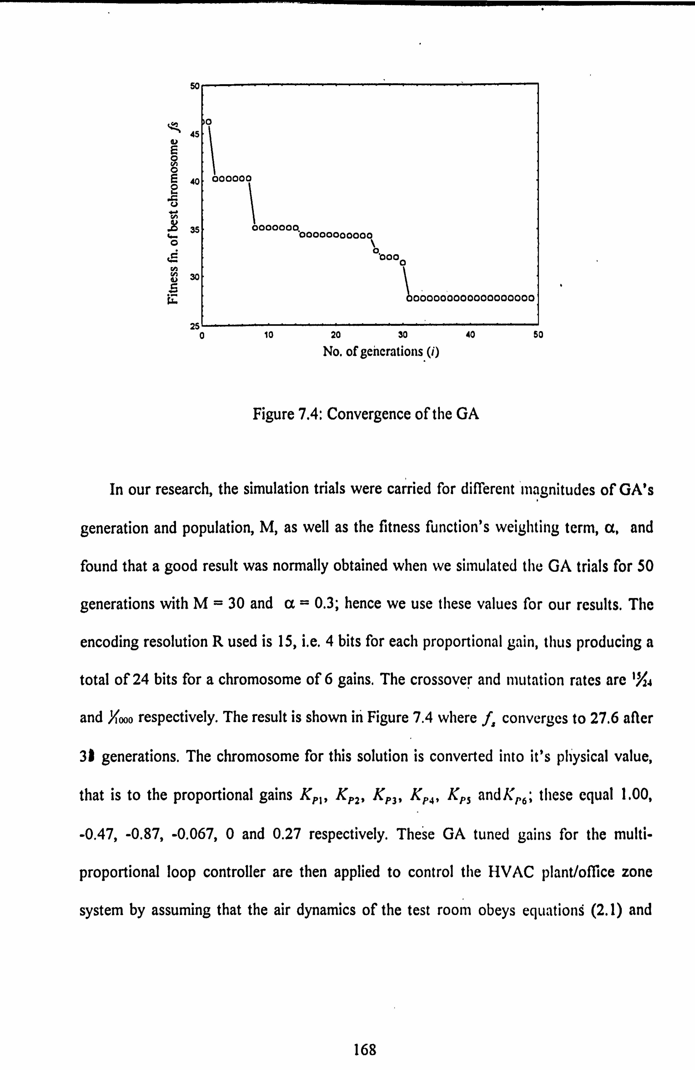
so

45

40

35

30

1. i- L000,00000000000001 25L

0 10 20 30 40 50

No. of gchcrations (i)

Figure 7A Convergence of the GA

In our research, the simulation trials were carried for different'niagnitudes of GA's

generation and population, M, as well as the fitness function's weighting term, a, and

found that a good result was normally obtained when we simulated the GA trials for 50

generations with M= 30 and cc = 0.3; hence we use these values for our results. The

encoding resolution R used is 15, i. e. 4 bits for each proportional gain, thus producing a

total of 24 bits for a chromosome of 6 gains, The crossover and mutation rates are IY24

and Ylooo respectively. The result is shown in Figure 7.4 where f, convergcs to 27.6 after

31 generations. The chromosome for this solution is converted into it's physical value,

that is to the proportional gains KpI, KP2 ,K P3 ,K P4 ,

Kp5 andKP6; these equal 1.00,

-0.47, -0.87, -0.067,0 and 0.27 respectively. These GA tuned gains for the multi-

proportional loop controller are then applied to control the HVAC plant/oflice zone

system by assuming that the air dynamics of the test room obeys equatioM (2.1) and

168

(2.2), and the three control inputs can be calculated via equations (7.2), (7.3) and (7.4)

using these gains. The simulation results are presented next.


The performance indexes such as the output error, the energy consumption and the

settling period, of this multi-proportional loop controller is investigated via simulation

studies where the setpoints, the climatic disturbances and other stochastic cffects are

identical to those described in section 7.3.6. A simulated result is shown in Figure 7.5

where we can see that a good control performance is achieved for tile setpoints ( T,, H, )

at (25*C, 50%rh), and the system has small steady state errors as shown in Table 7.1.

It is worthwhile to compare this GA tuned controller with the conventional Ziegler-

Nichols (1942) method for this multivariable system. For the open-loop step responses as

discussed in Chapter 3, the proportional gains for this rhethod is given by Kp = Us NL

where U., N and L are as previously defined;, these gains are calculated for the six

proportional controllers and found to equal 5.34, -7.53 and 15.26 kW/*C for K,,, Kp3

and Kp,, and -6.57, -1.17 and 1.48 kW/O/orh fd-r K. 2, K. 4 and K. 6 respectively. A

simulation result for this method is shown in Figure 7.6 wherethe control performance is

poor as compared to the results obtained via the GA tuned controller. We can see that

the room temperature and the relative humidity have large fluctuations around tile set-

point of 25C and 50%rh respectively and the control inputs are switching excessively

between the on and off states.

169

5

4

3

Nfttw Aw C*oW)kW Hýiclflw AW

---------------------- ------------------------------------

7"Poravile PC

"a met. RH. O%lh

-------------------

so 100 150 2DO 0 to 100 160

Thm hS ngmdes Tim &G ftmles


Figure 7.5: Proportional GA tuned controller for T, = 25"C; H, = 50%rh

Humkow AW

Codw AW

M

- PC

so

0 60 100 160 200 0 It 100 10 lot

Thm &S min. &" TIMSASOM. A. s


Figure 7.6: Performance of multi-proportional controller via Ziegler-Nieliols tuned gains

As discussed in Chapter 3, this poor performance can be improved by modifying the

Ziegler-Nichols tuned gains. When these are carried out, we found that the modified

proportional gains, Kp,, equal 0.45, -0.418 and 0.51 kW/'C for controllers #1, #3 and

#5, and -0.047, -0.047 and 0.049 kW/l/orh for controllers #2, #4 and #6 rcspectively. A

simulated result for this case is shown in Figure 7.7 where the control performance is still

170

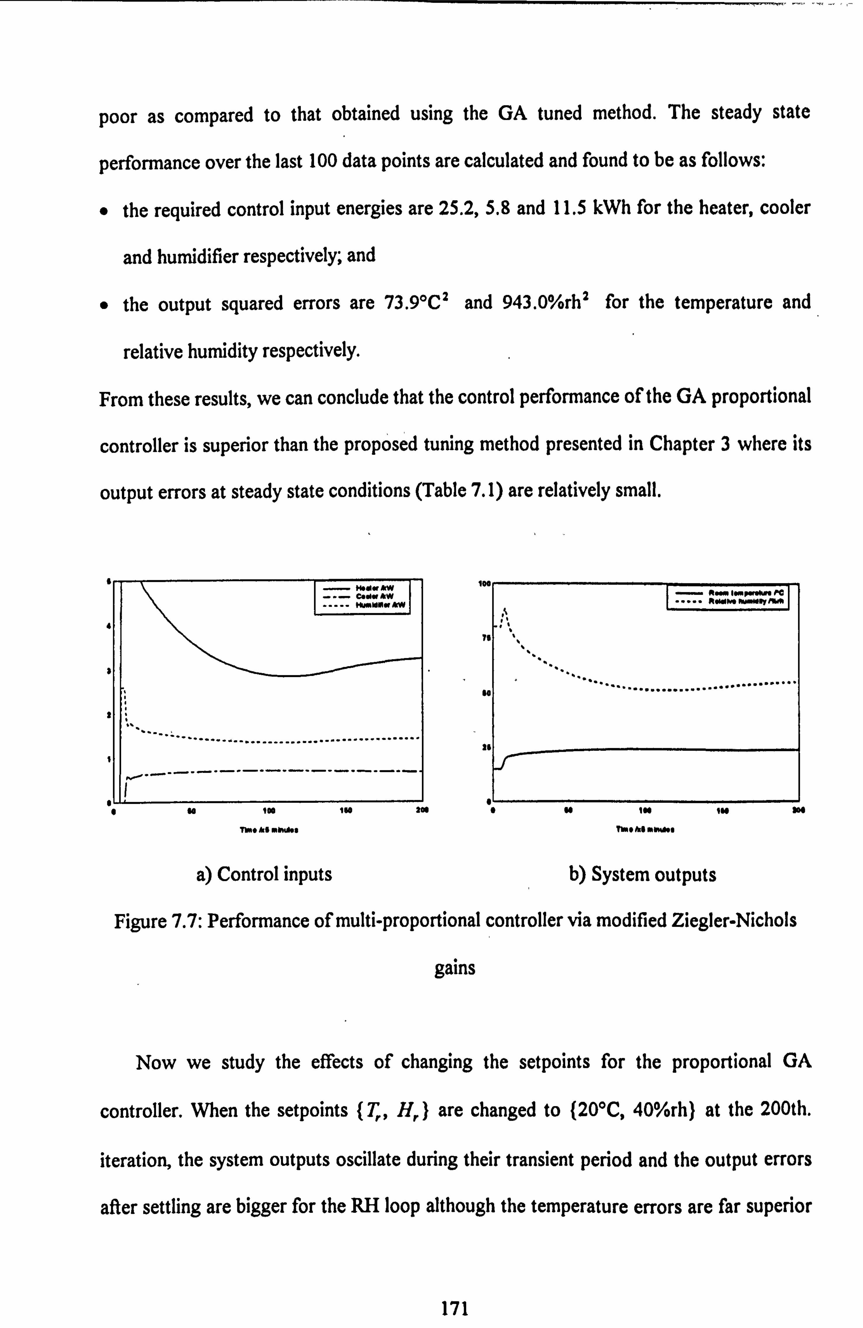
poor as compared to that obtained using the GA tuned method. The steady state

performance over the last 100 data points are calculated and found to be as follows:

e the required control input energies are 25.2,5.8 and 11.5 kWh for the heater, cooler

and humidifier respectively; and

the output squared errors are 73 goC2 and 943.0%rh2 for the temperature and

relative humidity respectively.

From these results, we can conclude that the control performance of the GA proportional

controller is superior than the proposed tuning method presented in Chapter 3 where its

output errors at steady state conditions (Table 7.1) are relatively small.

Co WAW mm MWAN

.................................................. --------

------------------

J!

ptwwo ft"W" AWN

..............................................

so 100 ISO 209 # so I" IN 204

Tbn* At mkw, %s Two he Oft"s


Figure 7.7: Performance of multi-proportional controller via modified Ziegler-Nichols

gains

Now we study the effects of changing the setpoints for the proportional GA

controller. When the setpoints (T, H, ) are changed to (20*C, 40%rh) at the 200th.

iteration, the system outputs oscillate during their transient period and the output errors

after settling are bigger for the RH loop although the temperature errors are far superior

171

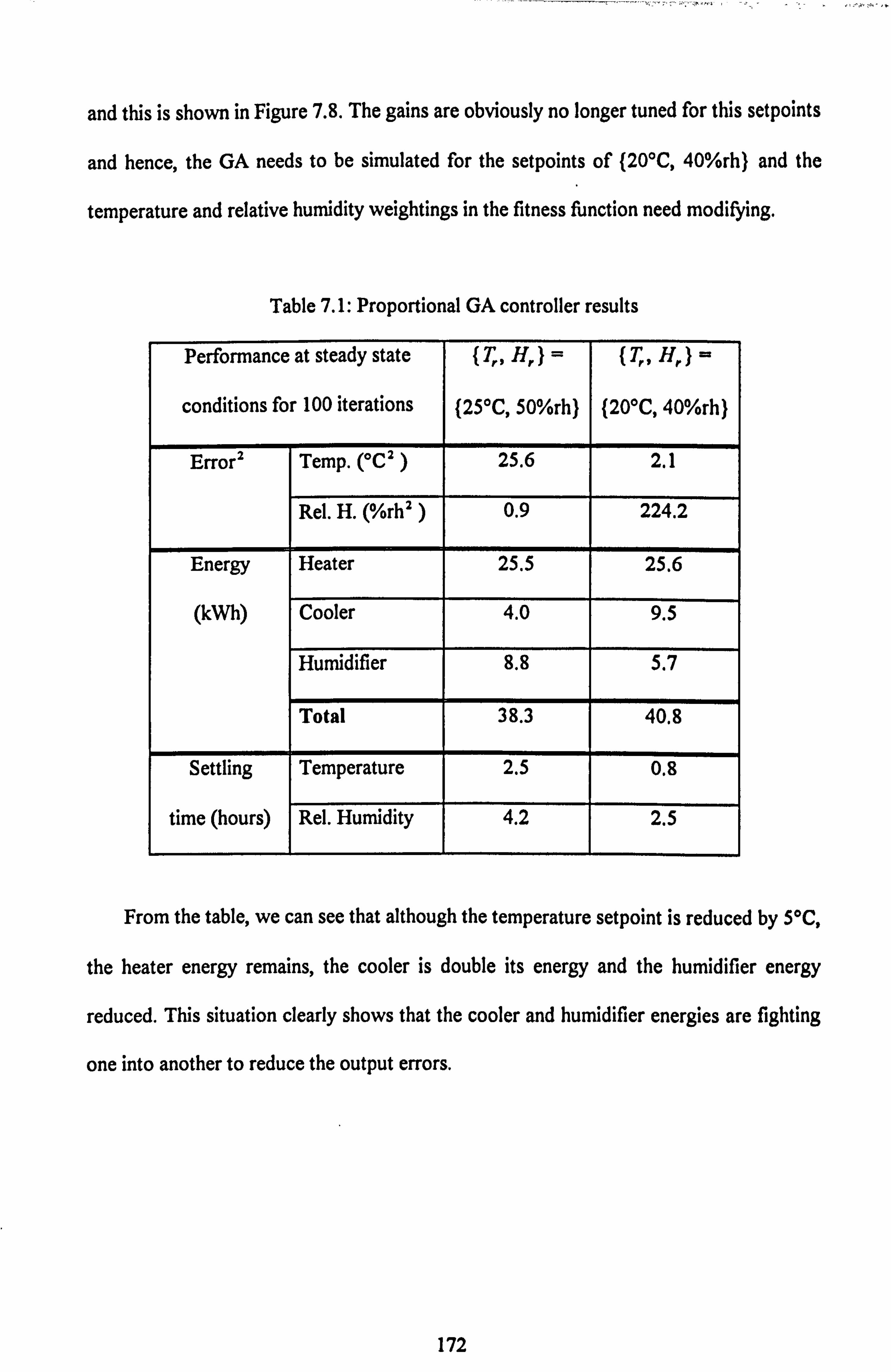
and this is shown in Figure 7.8. The gains are obviously no longer tuned for this setpoints

and hence, the GA needs to be simulated for the setpoints of (20T, 40%rh) and the

temperature and relative humidity weightings in the fitness function need modifying.

Table 7.1: Proportional GA controller results

Performance at steady state

conditions for 100 iterations

{ T, H, )=

(25'C, 50%rh)

( T, H, )=

{20*C, 40%rh)

Error 2 Temp. ("C' ) 25.6 2.1

Rel. H. (%rh' 0.9 224.2

Energy Heater 25.5 25.6

(kWh) Cooler 4.0 9.5

Humidifier 8.8 5.7

Total 38.3 40.8

Settling Temperature 2.5 0.8

time (hours) Rel. Humidity 4.2 2.5

From the table, we can see that although the temperature setpoint is reduced by 511C,

the heater energy remains, the cooler is double its energy and the humidifier energy

reduced. This situation clearly shows that the cooler and hunUifier energies are fighting

one into another to reduce the output errors.

172

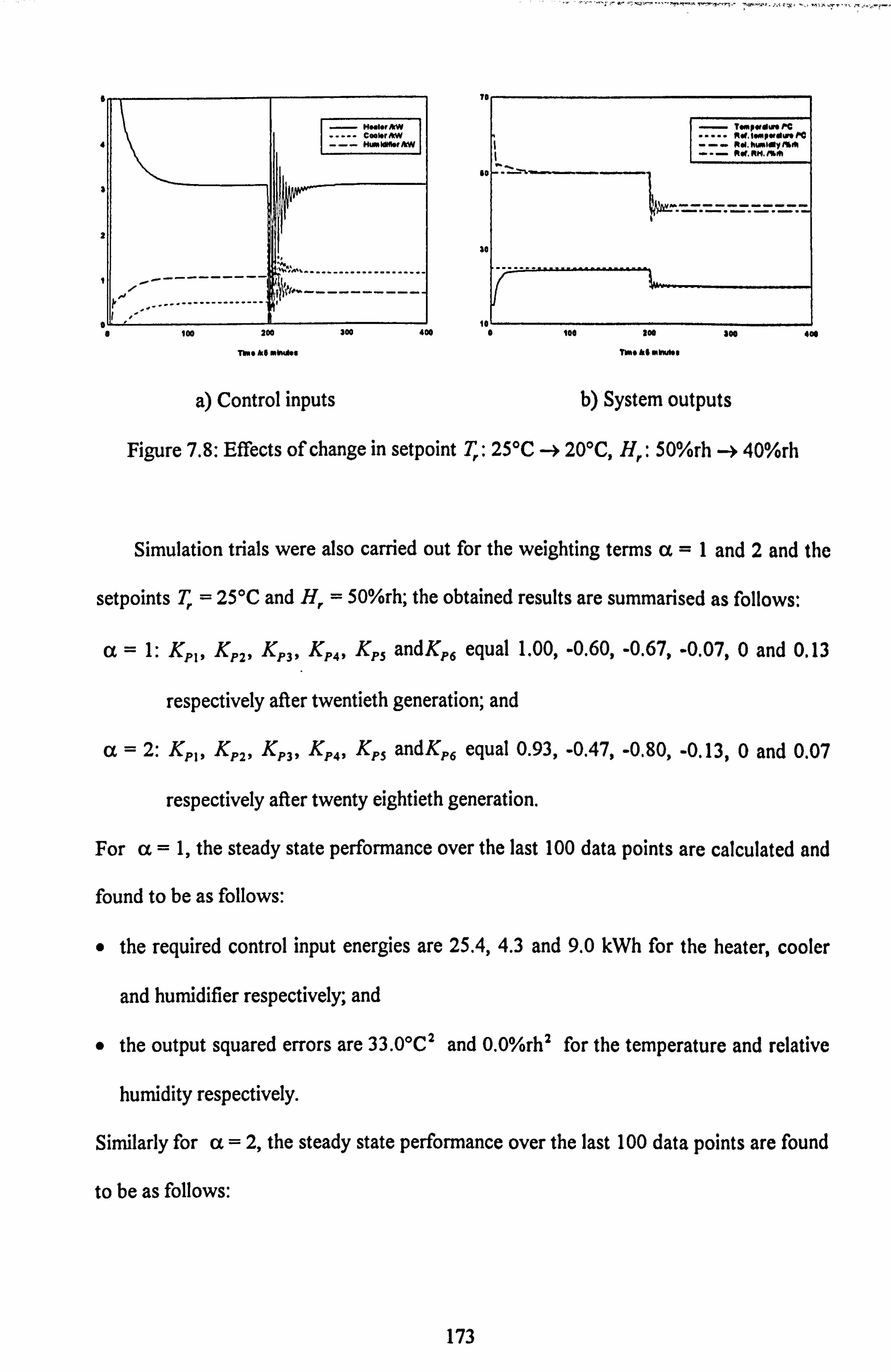
- pI_I., *w - CI. r*W

HlW

----------- --------------

-------------------

. I- Tompgo"Pe Rlf, I"PW40M 0.0

o g

Time MG mWdes Time h$ mWAse


Figure 7.8: Effects of change in setpoint T,: 25'C -ý 20"C, H,: 50%rh -> 40%rh

400

Simulation trials were also carried out for the weighting terms ot =I and 2 and the

setpoints T, = 25C and H, 50%rh; the obtained results are summarised as follows:

X '-: 1: KKKKK andKp, equal 1.00, -0.60, -0.67, -0.07,0 and 0.13 PIP P29 P3 31 P4 P5

respectively after twentieth generation; and

a=2: KPI, KP2, KP3

11 KP4$ Kps andKp, equal 0.93, -0.47, -0.80, -0.131 0 and 0.07

respectively after twenty eightieth generation.

For a=1, the steady state performance over the last 100 data points are calculated and

found to be as follows:

" the required control input energies are 25.4,4.3 and 9.0 kWh for the heater, cooler


" the output squared errors are 33 OoC2 and 0.0%rh 2 for the temperature and relative


Similarly for cc = 2. the steady state performance over the last 100 data points are found

to be as follows:

173

* the required control input energies are 25.7,4.2 and 9.0 kWh for the heater, cooler


9 the output squared errors are 27.8 oC2 and 1.0%rh 2 for the temperature and relative

hun-Mty respectively.

We can see that the three weighting terms, namely cc = 1,2 and 0.3, give relatively

large temperature errors at steady state conditions. This drawback could be improved by

selecting a larger GA resolution, R and this is demonstrated in Section 7.5. The results

also show that the control performances for the proportional GA controllers for the three

selected cts are similar although the gain combinations are different. This demonstrates

the randomisation of the GA approaches where a number of optimal solutions can be

obtained.

The parameter set (K,,,, K, K, K, Kp5, Kp, ) for several setpoints are

searched for by this GA methodology and the results are presented in Table 7.2. We can

use this table to set the proportional gains for the desired setpoints or to re-tune the

controller when a new setpoint is required. Furthermore, we can interpolate these gains

for intermediate setpoints. For example, if the required references T, and H, are 22*C

and 40%rh respectively, then we could use the gains for the setpoints ( T, H, )= (20T,

40%rh) with KpI could be slightly greater than 1, say, 1.2"C/kW to increase the heating

signal due to increased sensitivity of controller #1 so that the temperature could track its

setpoint at steady state conditions.

174

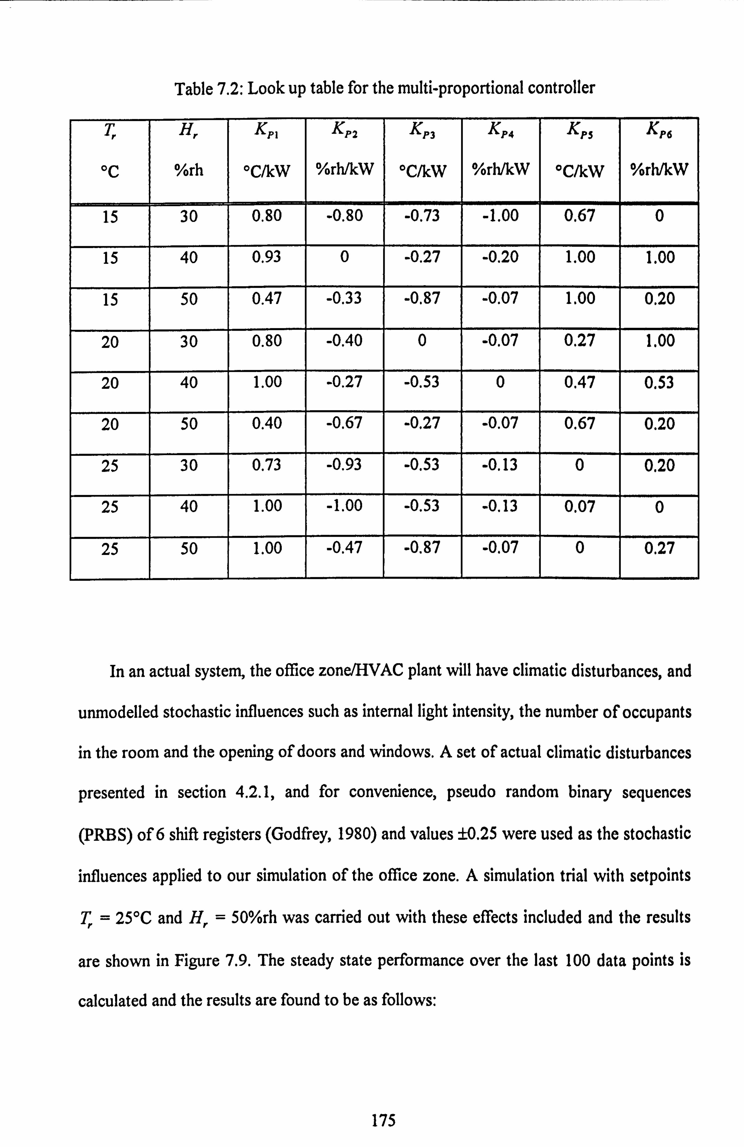
Table 7.2: Look up table for the multi-proportional controller

T,

oc

H,

%rh

Kp,

`C/kW

KP2

%rh/kW

KP3

'C/kW

KP4

%rh/kW

KP5

OC/kW

KP6

%rh/kW

15 30 0.80 -0.80 -0.73 -1.00 0.67 0

15 40 0.93 0 -0.27 -0.20 1.00 1.00

15 50 0.47 -0.33 -0.87 -0.07 1.00 0.20

20 30 0.80 -0.40 0 -0.07 0.27 1.00

20 40 1.00 -0.27 -0.53 0 0.47 0.53

20 50 0.40 -0.67 -0.27 -0.07 0.67 0.20

25 30 0.73 -0.93 -0.53 -0.13 0 0.20

25 40 1.00 -1.00 -0.53 -0.13 0.07 0

25 50 1.00 -0.47 -0.87 -0.07 0 0.27

In an actual system, the office zoneAFIVAC plant will have climatic disturbances, and

unmodelled stochastic influences such as internal light intensity, the number of occupants

in the room and the opening of doors and windows. A set of actual climatic disturbances

presented in section 4.2.1, and for convenience, pseudo random binary sequences

(PRBS) of 6 shift registers (Godfrey, 1980) and values ±0.25 were used as the stochastic

influences applied to our simulation of the office zone. A simulation trial with setpoints

T= 25"C and H, = 50%rh was carried out with these effects included and the results r

are shown in Figure 7.9. The steady state performance over the last 100 data points is

calculated and the results are found to be as follows:

175

the required control input energies are 29.2,2.3 and 8.1 kWh for the heater, cooler


the output squared errors are 78.0"C' and 111.7%rh' for the temperature and


This result shows that the control performance has deteriorated as expected. Looking at

the control inputs we can observe excessive switching which is highly undesirable and

commonly encounted in systems subject to stochastic influences. There are several

method for handling this problem; these range from inserting a weighting term into the

fitness function to penalise excessive controller switching or simply inserting a smoothing

filter.

CooWAM ----- HuidOW &W

Eým

i0o lu 200

11.0 As obufts

0

Redow himpersour PC 111161.1111,41 humidly

100 ISO so@


Figure 7.9: Proportional GA controller with climatic and stochastic disturbances

We introduce two different low-pass filters for performing the smoothing, namely,

Filter I. Uf Q) = (U(t) + U(t - T)Y2

Filter II. Uf (t) = (u(t) + 2u(t - T) + U(t - 2T)Y4

176

where uf is the filtered input and u is the control input vector consisting of W, C and H

which is calculated from equations (7.2), (7.3) and (7.4) respectively. Here Filter I

assumes a simple averaging over two consecutive control values whereas Filter 11 does

this over three inputs. Simulation trials were carried out for this controller by using the

filtered input, uf, and for the gains chosen for the setpoints (T, H, ) = {25"C, 50%rh)

with the prescribed conditions; the results show that both filters reduce the excessive

switching of the control inputs as well as the output regulations and this is shown in

Figure 7.10. For the controller with Filter I, the steady state performance over the last

100 data points are found to be as follows:

4, the required control input energies are 29.1,2.2 and 8.0 kWh for the heater, cooler


e the output squared errors are 71.9"C' and 73.2%rh' for the temperature and relative

hunýidity respectively,

and for the controller with Filter II, the steady state performance over the last 100 data

points are found to be as follows:

9 the required control input energies are 30.3,3.6 and 9.0 kWh for the heater, cooler


* the output squared errors are 126.51C' and 12.4%rh' for the temperature and


When the steady state performances of these controllers are compared, we found that the

proportional GA controller with Filter I is better since it consumed lower energy as well

as improved regulation.

177

-Hootw AW codw &W HýMw AM

- 'AI'

0 so IUD im Tkno Ais MN"«

a) Control inputs

Room lomporalurs PC

100 Ise 304 Thns A. $ mlovAss

2W

b) System outputs

Figure 7.10: Improving the proportional GA controller by Filter II

The results in Table 7.1 and Figure 7.6 show that the proportional GA tuned

controller gives a good control performance only for the setpoint at which the GA was

used to calculate the gains. The control performance deteriorates when the setpoints are

changed. This demonstrates the main disadvantage in using the structure of proportional

controller where the values are only accurate for the tuned setpoints and some

modification needs to be made to remedy this shortcoming.

7.4. Improved FLC using GA technique

There are many methods of improving the basic GA procedure presented in Section 7.3,

for example we could extend the work to PID controllers, consider a state-space GA

solution or integrate GAs with neural networks for advanced intelligent BEMS control.

This opens up a vast area of research in itself and could be worthy of a whole project;

instead we consider integrating the fuzzy logic approach presented in Chapter 6 with the

genetic algorithm method to access whether an improved solution can be realised. In

178

particular we will use the GA optimisation techniques to adjust the fuzzy membership

functions so that the control performance of the FLC can be improved (see for example

Genshe and Yinhai, 1993). In our case, we implement the GA method to adjust the

tuning parameters of the FLC based on output errors as described in chapter 6. Recall

that this controHer has 5 fuzzy input membership functions for each of the 2 output

errors and 3 ftizzy output membership functions for each of the 3 incremental control

signals as shown in Figure 6.1 to make a total of 19 fuzzy membership functions. These

functions need to be optimised so that the required FLC's performance is as good as it

can be to reduce the output errors, consume minimal energy and have fast settling

periods as compared to the ordinary FLC.

We now consider the example shown in Figure 6.5 where a good performance has

been achieved but we assume that it could be further improved by using the GA method.

Therefore, most of the scale factor settings in the fuzzy membership functions can be

fixed as they are in order to reduce the complexity of designing the GA operators. For

this reason we have chosen the 10 fuzzy input membership functions to be fixed at the

values shown in Table 6.3, and the fuzzy output membership functions in Figure 6.2b)

for each incremental control signal are defined by

i) z, = n., n, = z. = p, =0 and x. =

nm = 0.7x, and p. = 0.7x.; and

iii) the incremental control limits are 0.1 :! g x, :50.5 and 0.1 < x. :! ý. 0.5.

The objective here is to obtain the best set of x, and x. for the three incremental control

signals, i. e. dW, dC and dH so that the controller"s performance is optimised. This can be

done by concatenating them into a parameter set (xlw2 xuwý x1c, x., c, xuf, x.. ) where

x, x, and x,, are the lower limits, and x.,, x,, c and x., are the upper limits of the

179

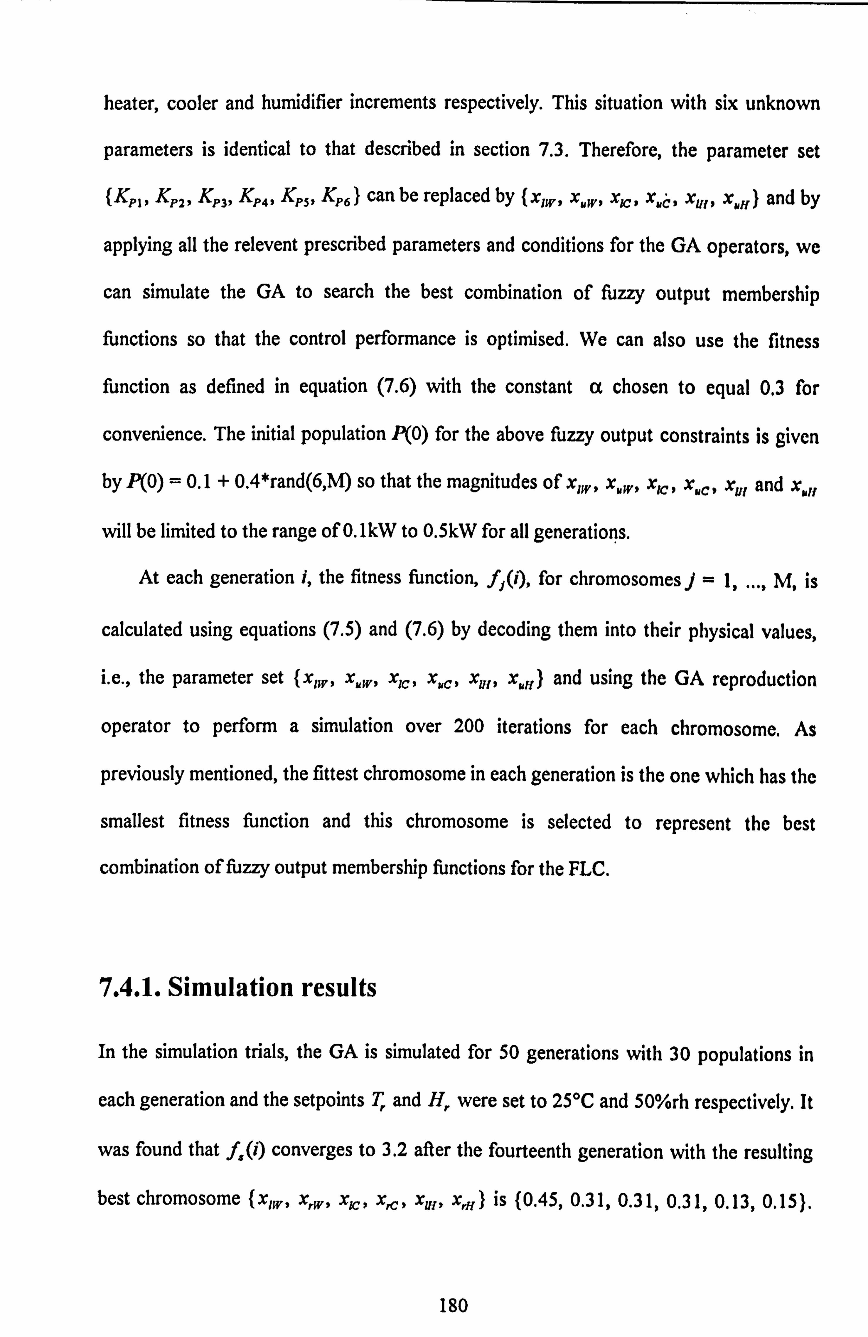
heater, cooler and humidifier increments respectively. This situation with six unknown

parameters is identical to that described in section 7.3. Therefore, the parameter set

fKpIp K P2 , KP3, KP49KPSKP6) can be replaced by (xlw, xw, x1c, x. & . x,,, x.. ) and by

applying all the relevent prescribed parameters and conditions for the GA operators, we

can simulate the GA to search the best combination of fiazy output membership

functions so that the control performance is optimised. We can also use the fitness

function as defined in equation (7.6) with the constant cc chosen to equal 0.3 for

convenience. The initial population P(O) for the above fuzzy output constraints is given

by P(O) = 0.1 + 0.4*rand(6, M) so that the magnitudes of xlw, x.,, x1c, x. c, xul and x.,,

will be lin-&ed to the range of O. lkW to 0.5kW for all generatiops.

At each generation i, the fitness function, fi(i), for chromosomes j=1, ..., M, is

calculated using equations (7.5) and (7.6) by decoding them into their physical values,

i. e., the parameter set {xlw, xw, x1c, x,, c, x1m, x.. ) and using the GA reproduction

operator to perform a simulation over 200 iterations for each chromosome. As

previously mentioned, the fittest chromosome in each generation is the one which has the

smallest fitness function and this chromosome is selected to represent the best

combination of fuzzy output membership functions for the FLC.


In the simulation trials, the GA is simulated for 50 generations with 30 populations in

each generation and the setpoints T, and H, were set to 25T and 50%rh respectively. It

was found that f, (i) converges to 3.2 after the fourteenth generation with the resulting

best chromosome {xlw, x,, w, x1c, xc, xul, x,,,, ) is (0.45,0.31p 0.31p 0.31.9 0.139 0.15).

180

By using the definition of the fuzzy outputs for this FLC design we can calculate n. and

p. for each incremental control input and the results are shown diagrammatically in

Figure 7.11. Analysis of this diagram as well as comparison to the ordinary FLC's output

membership functions as presented Table 6.4 is difficult to perform here since many

tuning parameters and rules are involved, and the GA only presents one of many minimal

solutions. If the conditions are maintained as before and the GA simulation trial is carried

out for the second attempt, we could obtain a new set fx,,, x,.,, x1c, xc, xvj, x,, j) of

minimal solution which would also give a good control performance. Therefore, we

could have more than one 'best" combination of the FLC tuning parameters to give

similar control performances by using the GA method.

zp

-0.45 -0.32 0 0.22 0.31

zp

-0.31 -0.22 0 0.22 0.31

Nz

-0.13 -0.09 0 0.11 0.15

a) Heater (M) b) Cooler (M) c) Humidifier (kW)

Figure 7.11: Incremental fuzzy output membership functions via GA

The GA solution was utilised in the FLC and the simulated results are shown in

Figure 7.12; the control performance calculated over the last 100 data points after steady

state had been reached gives the following results:

e the required control input energies are 22.3,0 and 5.3 kWh for the heater, cooler and


* the output squared errors are O. I'C' and 2.1%rh' for the temperature and relative


181

These results are slightly better than those obtained from the ordinary FLC discussed in

Chapter 6. Clearly, the GA optimisation could be introduced to several stages within the

fuzzification and defuzzification processes and potentially further improvements could be

made.

Hoda ArW Coda #kW 6 ko dcl a ArW

RýI-Pwwm. oc

60 Iw ISO 200 6 so 180 160

Tb- A. 6 ndnAft TImehOMORt"I


Figure 7.12: FLC + GA based controller performance

309

When the setpoints T, and H, are changed to 20T and 40%rh respectively, the GA

produces the best parameter set equal to (0.10,0.50,0.45,0.45,0.10,0.45) after twenty

three generations; this is shown diagrammatically in Figure 7.13. For this situation, the

control perfonnance over the last 100 data points after settling is as follows:

o the required control input energies are 19.9,3.6 and 0 kWh for the heater, cooler and


* the output squared errors are 24.9"C2 and 62.2%rh' for the temperature and relative

hunýidity respectively.

The results have clearly degraded as before and some modification to the procedure

needs to be made so that setpoint changes can be accommodated. A better result could

182

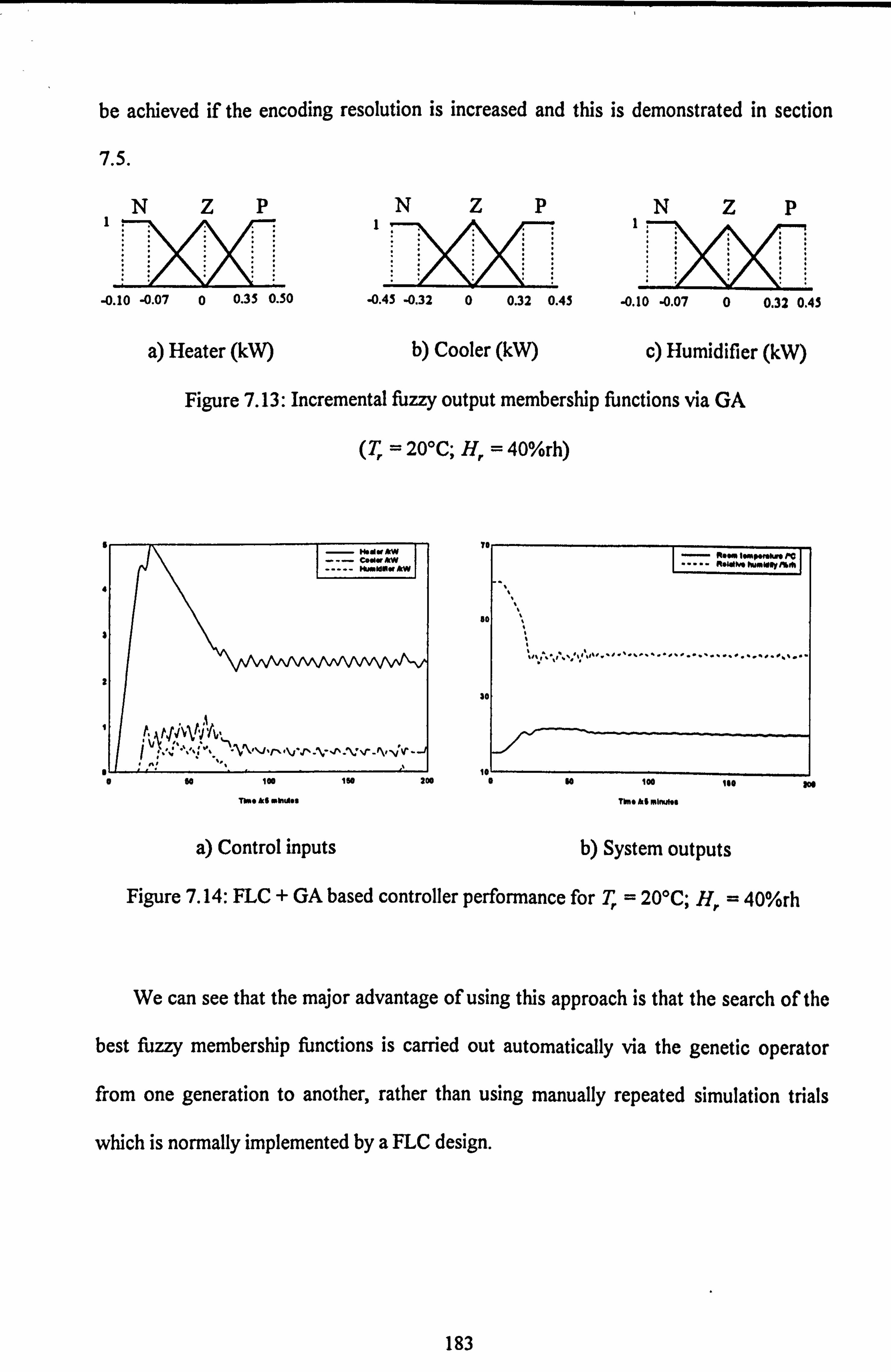
be achieved if the encoding resolution is increased and this is demonstrated in section

7.5.

INzp

-0.10 -0.07 0 0.35 0.50 -0.45 -0.32 0 0.32 0.43

a) Heater (W) b) Cooler (W) c) Humidifier (W)

Figure 7.13: Incremental fuzzy output membership functions via GA

(T, = 20*C; H, = 40%rh)

IW AM C. M. AM MMIdOW AW

3L

fiý%tj A `1ý,

100 IN 200

Time &S . 1n. A. s

30

-0.10 -0.07 0 0.32 0.45

ýlw PC

100 ISO 10 Thh* k$ minuf9a


Figure 7.14: FLC + GA based controller performance for T, = 20*C; H, = 40%rh

We can see that the major advantage of using this approach is that the search of the

best ffizzy membership functions is carried out automatically via the genetic operator

from one generation to another, rather than using manually repeated simulation trials

which is normally implemented by a FLC design.

183

7.5. GA for adaptive control

In this application, we will use the advantage of one-step ahead predictions from the

mathematical model (2.1) and (2.2) to forecast the air temperature and relative humidity in

the test room if certain inputs are applied. To implement this using GAs, we present M

solutions for the control inputs W, C, and H at time t (each one represents an individual

chromosome p, j=1,2, ..., M which belongs to the population PQ)). The GA operators

are then applied to the population P(t) to generate new populationP(t+T) at time I+T. We

summarise the GA algorithm as follows:

Step 1. Select a random initial populationP(l) of solutions satisfying the input constraints,

i. e. W, C and H have linýts of 5.0,2.7 and 2.6 kilowatts respectively. Set the

resolution, R, the crossover, the mutation rates, the sample time T, and set t=0.

Step 2. Encodin : Encode the control inputs f W, C, H) into a chromosome.

Step 3. Calculate the controls (W, C, H) for individual chromosomes by reversing the

encoding process.

Step 4. Reproduction: Calculate the fitness function for individual chromosomes and

generate the population PQ+T) according to the reproduction procedure. The

controls JW, C, H) having the fittest chromosome from population P(t+T) is

selected and applied to the HVAC plant at time t.

Step 5. Go to Step 6 or Step 7 randon-Ay.

Step 6. Crossove : Mate the members of P(t) at random, and carry out the crossover

operation randomly for each pair of chromosomes to generate 2M chromosomes

for populationP(t+T). Go to step 8.

184

I- Step 7. Mutation: Select at random a chromosome from the population P(I) and carry out

the mutation operation for that chromosome.

Step 8. Set I=t+T and Goto Step 3.

The initial population is generated by using a random method; for our application we

require 3 control inputs of different ranges and using the MATLAB language, the initial

population can be generated using P(O) = [5*rand(l, NI); 2.7*rand(l, M); 2.6*rand(l,

M). Thus, P is a RM matrix and pj is thejth. column vector of P, and we represent the

jth. parameter set by (Wi, Ci, Hi), j=1,2, ..., M. If the encoding resolution is ISP

then we have a4 bit string for each input and then these strings are concatenated to

produce a chromosome of length 12 bits. If the required encoding resolution is 255, i. e. an

8 bit word length then the chromosome will have a length of 24 bits.

As before, the reproduction process selects two solutions as potential parents which

compete for survival; this is repeated until we obtain M chromosomes in the population

PQ+T). The best chromosome amongst them is selected and decoded into {W, C, H)

before being applied to the HVAC plant at time t.

The fitness function is again formulated so that both the room temperature and

relative humidity track the setpoints as the GA is advancing from a generation P(t) to the

next generation P(t+T). As before we propose the fitness function, fi, for the

chromosome pi by

fj Q) ei (t+T) +aI ei (t+T) t=0, T, 2T, 3 T, TH

1,2,3, ..., 2M for crossover

1,2,3, ..., M+l for mutation (7.7)

185

where eTi and eJ are the predicted output errors at time I+T and can be obtained from

equations (2.1), (2.2), (3.2) and (3.5), and a is a weighting factor as before. The

controls (Wi (1), CJ (t), Hi (t)) for chromosome j can be used to calculate thcir fitness

functions via equation (7.7); the chromosome having the lowest fitness function f, is

selected for applying to the HVAC plant at time t. Note each time step is now a gencration

within this GA setting.

7.5.1. Convergence

The GA is assumed to have converged when the output errors eT and c,, become zero and

steady state conditions have been reached; this can be written as:

lim,, e(t) = (7.8)

where e= eT ]. Ideally, the controlling inputs W, C and H are constant at steady state

[e,,

conditions, so that the system outputs remain at their setpoints and the best chrornosonics

in any generation within this period are identical to each other, i. e. the GA operators will

not produce any better solutions; this situation is identical to that shown in Figurc 7.4

where the best fitness function, fQ), at generation t remains constant at this minimal

condition.

When the climatic and stochastic disturbances are present in the system, tile GA

operator will produce a better chromosome even at the steady state condition; here the

method is reacting to noise to reduce the error.

186


Let us consider the system under the setpoints T, and H, and calculate the performances

for the last 100 generations (sampling periods) of the simulation trials. We assume that the

initial conditions for the room temperature, T, (O), and relative humidity, 11. (0), arc

known and all the three controlling inputs to the plant are zero.

A number of simulation trials were carried out to get the best value of cc in the ritncss

function and it was found that an appropriate value of (x is between 0.13 to 0.14. Valucs

beyond this range lead to the system going out of control where the output errors are very

large at steady state conditions. This value is also tested for the system with other pairs of

{T,, H, ), such as (20'C, 40%rh), (15"C, 60%rh) and (150C, 30%rh), as wcll as for

different initial conditions such as TJO) = 35"C and H, (O) = 100%rh.

The simulation results showed that the control performance for all the trials wcre

acceptable and the system outputs converged to the desired setpoints. We can conclude

that this cc value can be used for any set of {T,, H, TJO), H,, (O)) within the ranges of

PC to 35"C for room temperature and 10%rh to 100%rh for relative humidity. An

example of the system performance is shown in Figure 7.15 where the corresponding

values for {T,, H, TJO), H, (O)) aref 15T, 30%rh, 350C, 100%rh). From this figure, we

can see that although the system outputs are quite smooth at steady state conditions, all

three control inputs have large fluctuations and excessive controller switching is again

seen. This can be tackled as discussed in Section 7.6.

All the above simulation trials were carried out by setting the resolution R to 15, the

crossover rate cr = Y12

and the population size M= 20. Furthermore, we assume that the

,,, H,, and S, are constant at 201C, I OIC, 100%rh and climatic disturbances such as T,, T

187

0.1 WM-2 respectively, and the unmodelled stochastic influences, V, and V, wcrc

absent.

--*Won po

...........

0 be tot 144 >O 11.4 ke obe, "o


Figure 7.15: Adaptive GA controller performance

[: ý.: Aw coolm kw "Widmier *W

----------- --

............ a so 100 150 Z

71me A5 mkAos a

: No tomow*. O. OKI kW^OV AW%

so

,5

.L 60 100 tu me

Im* &0 wow"


Figure 7.16: Adaptive GA controller vAth enhanced resolution

An improvement to the GA design can be made by increasing the resolution, R. By

selecting R= 255 for each control input, and applying the above procedure and

conditions, a simulation trial was carried out and the result is shown in Figure 7.16. We

188

so 100 160 200

1.5 mi.. I. 4

can see that all the three control input variations are significantly reduced and the systcm

'(0), outputs at steady state conditions are improved; this result shown is for (T,, H, T,

{15'C, 30%rh, 35"C, 100%rh), and cr = IY24. For this case, the control

performance over the last 100 data points after settling is as follows:

*" the required control input energies are 25.2,18.3 and 1.8 kWh for the heater, cooler


* the output squared errors are 0.1"C' and 0.9%rh' for the temperature and rclativc


The results show that an excellent output regulation has been achieved by this controller

but it wastes a lot of energy from the heater and cooler in order to maintain the sctpoints.

When the same climatic disturbances as in section 4.2.1 are present in the systcm, the

performance is as shown in Figure 7.17 the control inputs are switching more but the

system output responses appear unchanged.

In a real system, the HVAC plant will have climatic disturbances, and unmodellcd

stochastic influences such as people in the room and the opening and closing of doors and

windows. For convenience, these influences are included here in the form of pscudo

random binary sequences (PRBS) of 6 shift registers and values ±0.1. For this situation, a

simulation trial was carried out and the results are shown in Figure 7.18 where the control

performance over the last 100 data points after settling is as follows:

9 the required control input energies are 34.0,17.4 and 3.4 kWh for the heatcr, coolcr

and hun-ýidifier respectively; and

* the output squared errors are OXC' and 1.9%rh' for the temperature and relative

hunýidity respectively.

189

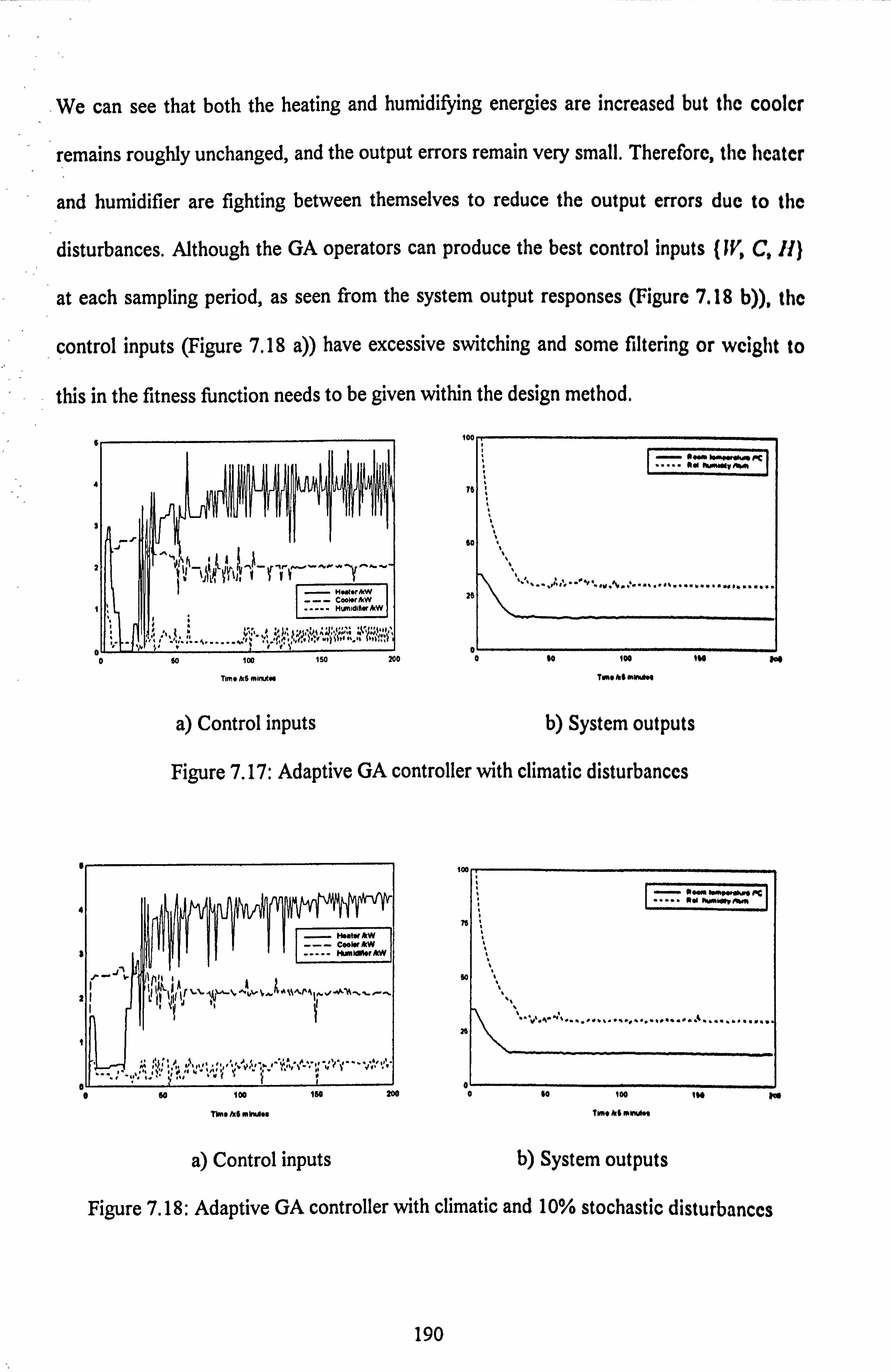
-We can see that both the heating and humidifying energies are increased but the cooler

remains roughly unchanged, and the output errors remain very small. Therefore, tile heater

and humidifier are fighting between themselves to reduce the output errors due to the

disturbances. Although the GA operators can produce the best control inputs (IV, C, H)

at each sampling period, as seen from the system output responses (Figure 7.18 b)), the

control inputs (Figure 7.18 a)) have excessive switching and some filtering or weight to

this in the fitness function needs to be given within the design method.

-.

---r I- - H.. t. rAW

CoI. rAW " Htndifl. AW

60

25

0

PC

.......... ..................

No$ 100 150 0 so Ica IVA

TO. 1.5 WIIA" T"s fts ONUO


Figure 7.17: Adaptive GA controller with climatic disturbances

H.. I. cW

I I! !II IEd0&«u1cw

_______I 1 'N --

I ni

'

- I--,

.0

�

.L 0w 100 159 zm 9 be 100 tu

Tl, Aeixe. b". u Two ki Mumm$ tot


Figure 7.18: Adaptive GA controller with climatic and 10% stochastic disturbances

190

Figure 7.19 shows another good regulation result of this type of adaptive controller

where the setpoints have changed from {25*C, 50%rh) to {20*C, 40%rh) aftcr the two

hundreth generation. For this case the initial conditions for T, (O) and 11, (0) wcre sct at

IPC and 60%rh respectively, and the climatic and 25% stochastic disturbances are

assumed to be present. We can see that the system outputs follow the sctpoints quite

quickly but the control switching remains a problem. This is due to the fact that the

control strategy is always searching for the best solution to minimise the output crrors

and no emphasis to control switching is assumed. This needs to be remedied in any

practical solution based on GAs.

a) Control inputs

100 to@ wo 400

, h. 0 ärt ob""

so

so Ab^

ad

io

b) Systcm outputs

Figure 7.19: Adaptive GA controller with setpoint change

The control performance at steady state conditions for the setpoints (T,, 11, )-

{25"C, 50%rh} over 100 data points after settling is as follows:

* the required control input energies are 25.4,2.9 and 7.9 kWh for the heater, cooler and


191

0 100 200 300 400

Ilme ke mkxdot

e the output squared errors are 2.7'C' and 71.9%rh' for the temperature and relative


We can see that this performance is similar to that obtained from the control stratcgics

presented earlier in this thesis; the multi PI-loop controllers (Chapter 3), Constraincd

inputs MIMO adaptive control (Chapter 5) and fuzzy logic controller (Chapter 6); hence

there is potential for the GA approach.

7.6. Smoothing of GA solutions

As presented in section 7.5, GAs can be used to regulate the system outputs at the dcsircd

setpoints to within acceptable limits at steady state conditions, but the variation of tile

control inputs with respect to time is excessive. This problem is due to the GA working on

the basis of randomly generated solutions where the designed fitness function does not

relate between one generation to the next. This causes large variations in tile control

inputs which are not recommended in practice because this will reduce the life span of the

control actuators. To overcome this problem, we propose the introduction of a smoothing

routine within the GA presented in Section 7.5 (Davis, 1991); one way of achieving thi's

smoothing is to use a digital filter. The smoothing is introduced to the control stratcSy

whenever appropriate to suppress the switching of control signal when it exceeds beyond

the perniissible lirftits. The low pass filter is designed by defining two difTcrcnt valucs of

the control input, namely Au and Aul where

Au = ju.. (t) - u(t-T)i (7.9)

Au' = ju(t-T) - u(t-2T)i

192

where u.. = W, Cý,, , H,. is the control input vector which is obtained by the GA and 9

u is the required control input vector consisting of W, C and H. The requirement of the

system is that if Au is less than AW by a certain amount then US4 Wis

applied at time

otherwise the filtered control input, uf, will be used. In a mathematical form, this can be

written as

u(t) = ug, '

(t), Au <ß Au,

uf (1), otherwise.

where 0<6<I defines the permitted level of input switching (this could be different

value for each control input). Let 8,, J62 and . 83 be the levels for the heater, coolcr and

humidifier respectively, then we have

W(t) = wg"(t), AW < fl, Awl

W (t), otherwise. f

C Cga (0) AC "ýý P2 ACP

(7i2)

Cf (1), otherwise.

H(t) = Hý, ý, (t), AH< ß3AH'

= H., (t), otherwise. (7.14)

and the system outputs T, (I+T) and H, (I+T) are re-calculated by applying tile

mathematical model equations (2.1) and (2.2). These fl-values will also indirectly increase

the output errors since the GA control inputs, Wg., Cga and Ha are supposedly the best

solutions to regulate the system outputs optimally.

Now, we define the filtering control inputs, Wf , Cf and Hf . It is important to decide

the level of suppression which is needed so that good overall control performance is

193

maintained. For example, if the suppression is very large then the system output

regulation becomes poor and the system may even go out of control. Here, we use Filtcrs

I and II as described in Section 7.3.7 with slightly different notations as follows:

Filter I. Uf (t) = {Uý. (t) + U(t - T)Y2

Filter H. Uf (1) = (Usa W+ 2u(t - 1) + u(t - 2T)Y4

The control performances for the adaptive controllers using Filters I and 11 witil

identical fl-values are shown in Figures 7.20 and 7.21 respectively where their output

regulations as well as the magnitudes of the control input fluctuations were found to be

similar; therefore, the comparison of performances between the two adaptive GA

controllers are difficult to analyse here due to the GA method operating on the basis of

randon-dy minimal solutions. To present them quantitatively, we calculate tile

performances for Figure 7.20 at steady state conditions where the setpoints ( T, 11, )

equal {20'C, 40%rh); the performances over the last 100 data points were found to be as

follows:

o the required control input energies are 29.4,10.9 and 6.9 kWh for the heater, cooler


e the output squared errors are 0.4"C' and 41.9%rh' for the temperature and relative


We can see that the switching of the control inputs have been significantly reduced but the

output errors at steady state error are slightly degraded as compared to the original GA

controller. Nevertheless, these errors are still acceptable and overall we conclude that the

solutions have been enhanced due to the filtering.

194

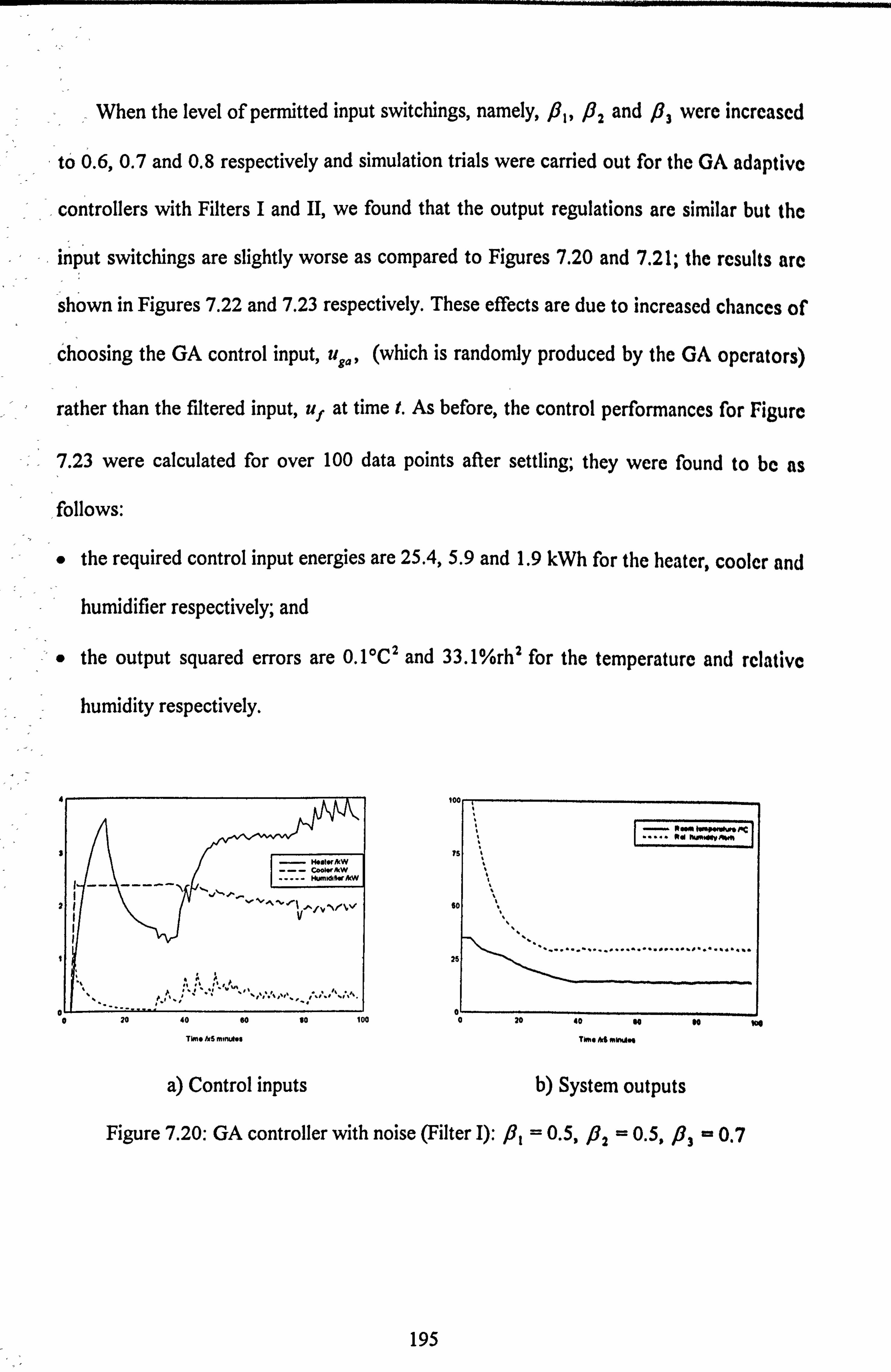
When the level of permitted input switchings, namely, fl,, 82 and 6, were increased

to 0.6,0.7 and 0.8 respectively and simulation trials were carried out for the GA adaptive

-Iý. controllers with Filters I and II, we found that the output regulations are similar but the

input switchings are slightly worse as compared to Figures 7.20 and 7.21; the results are

shown in Figures 7.22 and 7.23 respectively. These effects are due to increased chances of

choosing the GA control input, u,,,,, (which is randon-dy produced by the GA opcrators)

rather than the filtered input, uf at time t. As before, the control performances for Figurc

7.23 were calculated for over 100 data points after settling; they were found to be as

follows:

o the required control input energies are 25.4,5.9 and 1.9 kWh for the heater, cooler and


Ie the output squared errors are O. IoC2 and 33.1%rhl for the temperature and rclativc

hunUity respectively.

C. ~&W "*""*w

...........

.............................

.L 0 79 40 so so lug 9 20 40 we

TW* 1.6 ., m*. s Two he MW%A"


Figure 7.20: GA controller with noise (Filter 1): 81 =2 0.5, P2= 0.5, P3= 0.7

195

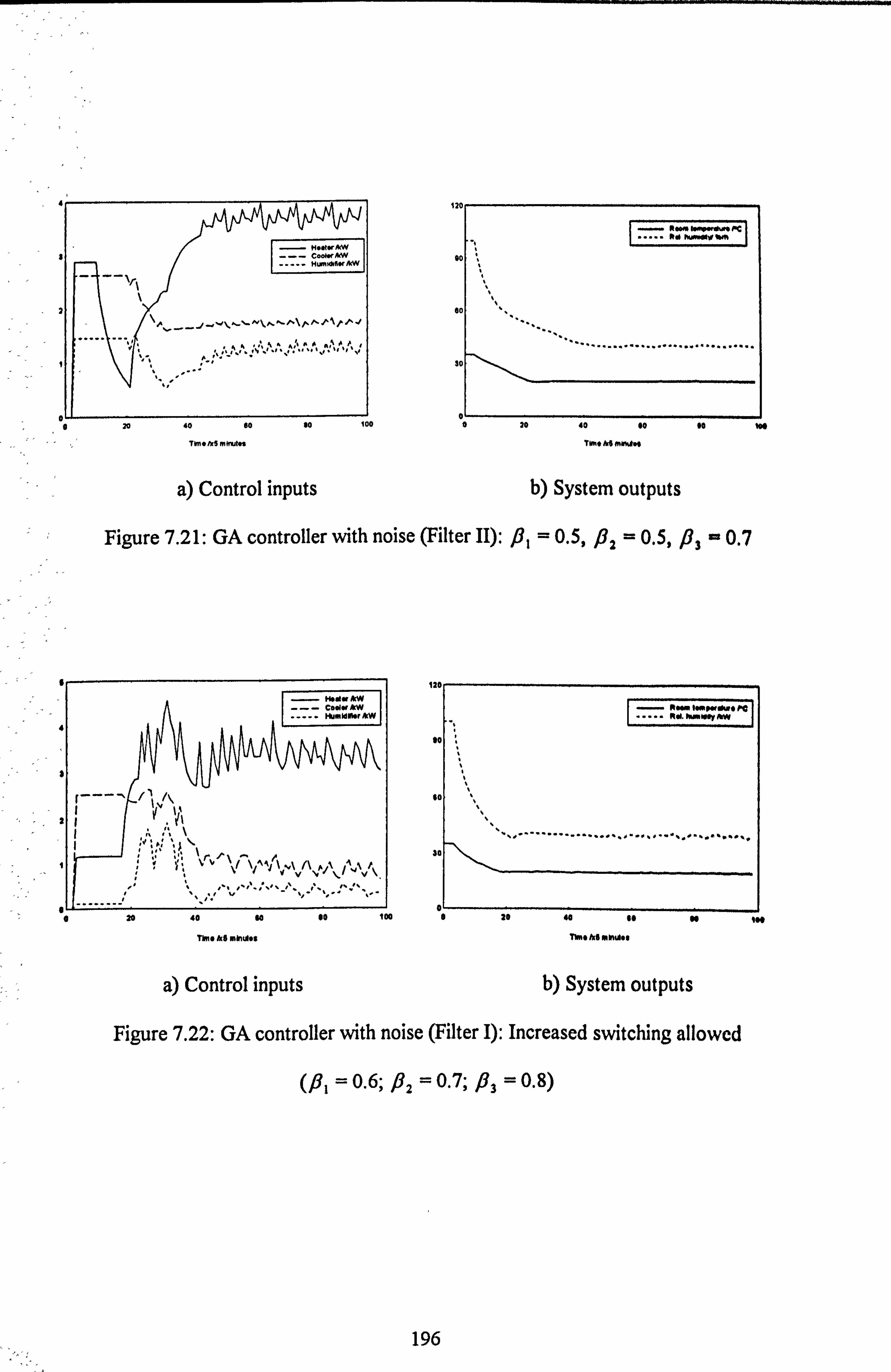
- CoMfliW

-

1. - 'ý --,, 'lý

110

........................................

100


Figure 7.21: GA controller with noise (Filter II): P, = 0.5, fl2= 0.59 #63-0.7

4

-I

t.

CO. l« AM

__ 7-- [-ý-7- 1, «- 1

Hu. Idr4rAN

----'1 1A

I f- V

Li I 0 I"

to so

Thme &5 mlmdes 11MOMMMwes


Figure 7.22: GA controller with noise (Filter 1): Increased switching allowed

(fl, = 0.6; )62= 0.7; 83 = 0.8)

196

----------

a- 20 40 Go so

Ti- MS . U. o

I R"m woo

. kmw"&Al so so

.......................... ...........

30

20 40 of

Time *I obwAss


Figure 7.23: GA controller with noise (Filter II): Increased svvitching allowed

(fl, = 0.6; #82 = 0.7: fl3 = 0.8)

7.7. Conclusions

In this chapter, the use of GA techniques to solve the problem of determining tile three

control inputs for the HVAC plant/office zone system are presented. The first solution

-proportional loop controller where the GA method is used to tune presented uses a multi

the six proportional gains. The second solution uses GAs to search the best combination

of fuzzy membership functions so that the control performance of a FLC based on output

errors is improved. The third GA-based solution minimises the predicted system output

errors at the next time instant t+T. This adaptive type controller is further improved by

employing a smoothing technique.

The GA proportional controller gives good results when regulating to tile sctpoints

used in the tuning but the performance deteriorates as the setpoints are changed. This

demonstrates a weakness in using the conventional controller such as a PID structure

197

where retuning is necessary. This difficulty can be overcome by using interpolation

ý 'techniques to modify the controller gains as the setpoints are changed.

It is found that the performance of the fuzzy logic controller presented in Chapter 6 is

improved when the membership functions are chosen using a genetic search procedure.

The adaptive GA controller gives good results even when the setpoints are changcd.

The excessive switching of the inputs is shown to be reduced by applying a smoothing

technique using digital filters.

198

, Chapter 8

Real-time Controls

The control systems described in the previous chapters are further investigatcd for their

performances within in a real-time control situation, namely on the newly commissiond

BEMS laboratory at the University of Bradford. The facility comprises a full-scale thrce

roomed office set up with its own variable air volume (VAV) HVAC plant. The dctailcd

specifications of the laboratory are presented in Appendix A, and the task 11cre is to 0

regulate the air temperature and relative humidity in Room I at their dcsired sctpoints by

controlling the main heater, W,,,, cooler, C, and humidifier, H; the performances of the

multi PI-loop controller, the constrained input and output adaptive controllcr, the fuzzy

logic controller and the GA-based controllers are assessed here. For thi's purposc, a

minor modification needs to be made to the respective simulation software prcscntcd

earlier, namely that the computer needs to be interfaced to sensors and actuator drivers.

The sampling interval T was chosen to be 5 minutes for all experiments to allow

reasonable changes in the outputs due to a change in the three control inputs. During the

experiments, all the three reheaters were switched off, the fresh air intake and tile

discharge dampers were fully open and the return damper was closed to allow significant

climatic disturbances to the room via the fresh intake. Moreover, the VAV I damper,

199

D,, was arbitrarily chosen to be 70% opened. The air pressure in the room was assumcd

to be constant due to the automatic control of the fresh air intake and discharge fans by

the Caradon Trend equipment. Moreover, the laboratory activities in the thrce rooms

were like those found in ordinary office buildings where occupants move around and go

in and out from the room, and the light intensity varies due to occupancy. Thesc

disturbances are treated as stochastic effects to the system in the following discussions.

8.1. Multi PI-loop controller

For tuning the PI controller parameters, open loop step responses were carried out on

the test room where the control inputs were increased from 50% to 75% of tlicir

maximum power to give the required parameters N and L for PI#1, PI#2, - PI#6; these

parameters are given in Table 8.1 and the PI gains Kp and K. are then calculated via

the Zeigler-Nichols equations (3.1) and (3.2) for each controller. An experimental testing

of the multi PI-loop controller was then carried out for a duration when steady state

conditions were reached, say after 5 hours; this allows us to graphically estimate tile

average output swings and gives the modified PI gains Kp,, and K,,, as discussed in

Chapter 3. The results are summarised in Table 8.1.

A number of experiments to assess the controller's performance were carried out by

using the modified PI gains Kp,, and K,,, and a sample trial is presented in Figure 8.1;

this experiment began at 5 p. m. on 24th. February, 1996 and logging lasted for a period

of 24 hours with setpoints of 22*C and 40%rh for the temperature and relative humidity

respectively. We can see that an acceptable regulation has been achieved by this

200

controller and the performance over the last 100 sampling intervals is calculated to be as

follows:

0 the required control input energies are 27.0,0 and 37.5 kWh for the heater, cooler


0 the output squared errors are 247.3"C' and 400.8%rh' for the temperature and the


Table 8.1: Ziegler-Nichols and modified PI gains via open loop step responses

Temperature loop

PI #

N

(-CIh)

L

(11)

us

(M)

Kp

(kWrC)

K,

(M/'Cý h)

Ave. output swing (M)

Rcduct.

factor

Kpx,

(kW/*C)

KLtj

(,, W,. C

1 0.66 0.025 1.13 61.4 736.8 420 0.0107 0.657 7.88

3 -0.99 0.017 0.75 -40.1 -707.8 400 0.0075 -0.301 -5.31

51 0.21 1 0.033 1 1.13 1 146.1 1 1328.2 800 0.0056 1 0.81-8 7.44

Relative humidity loop

PI N

(%rh/h)

L

(h)

us

(kW)

Kp

(kW'"*rh)

K,

(kW/O/orILh)

Ave. output

imn g W)

s(wk

Rcduct.

factor

K.,, tt

(kw/O /orli)

KLw

W Xprhýh) (k, '/0

2 -4.47 0.025 1.13 -9.1 -108.7 330 0.0136 -0.124 -1.48

4 -4.60 0.017 0.75 -8.6 -152.3 400 0.0075 -0.065 -1.14

61 13.0 1 0.033 1 1.13 2.4 21.5 70

__O.

0643 1 0.154- Fl. 38

201

We can see that the humidifier was used at its maximum power to fight the heating

energy; the result was that the energy was wasted and clearly this is not recommended

from the user viewpoint. Moreover, the cooler was not used in this trial because the

desired room temperature was higher than the outside temperature which was on average

at approximately 6'C

This result shows that the proposed multi PI-loop tuning methodology to modify tile

Ziegler-Nichols PI gains as described in Chapter 3 is practically applicable for the actual

control of HVAC systems and may be useful for controlling other multivariable systems

as well.

-----------------------------------------------

21; 1

Hurtgd$w&W

....... ....

10 Is ZD 25

Tbno Awan Ilms Rok"


Figure 8.1: Performance of the multi PI-loop controller with 6 PI units

$

We notice that the maximum slopes of the step responses, N, for this system are less

than the values obtained for the Loughborough BEMS system (Table 3.1). This is due to

the fact that although the heating, cooling and humidifying powers for both facilities arc

similar the total air volume of the three rooms (Appendix A) is much larger in

202

comparison to that in the test room at Loughborough and also the thermal structure of

the two offices are quite different.

8.2. Constrained input MIMO adaptive controller

The constrained input NIB40 adaptive controller described in sections S. I-5.4 was ncxt

implemented for real-time control of the test room. In this implementation, it is assumcd

that the on-line process model with observability indices n=I and 2 are adquate to

describe the conditions in the room.

The experimental results for n=I are shown in Figures 8.2 and 8.3 where wc can

see that this type of controller is capable of controlling the air temperature and rclative

humidity within the room. Figure 8.2 represents the result of a trial using the controllcr

with a prediction horizon N=5, and the maximum permissible change in the control

inputs, D. = [0.5 0.5 0.5] rM The trial began at 6 p. m. on 14th. October, 1995 and

logging lasted for a period of 12 hours with the room temperature and relative humidity

setpoints chosen at 221C and 45%rh respectively. The control performance ovcr the last

100 sampling intervals are found to be as follows:

0 the required control input energies are 18.0,15.6 and 28.1 kWh for the licatcr,

cooler and hun-Mifier respectively; and

0 the output squared errors are 6 OoC2 and 134.8%rh 2 for the temperature and


Figure 8.3 represents the result of an experiment using the controlicr %vith a

prediction horizon N=2, and the maximum permissible change in the control inputs 1).

203

[1 2 1]7' M The experiment began at 6 p. m. on 4th. September, 1995 and a

logging period of 15 hours was used with the room temperature and relative humidity

setpoints chosen to be 22'C and 50%rh respectively. The control performance over the

last 100 sampling intervals are found to be as follows:

the required control input energies are 22.7,3.8 and 22.6 kWh for the heater, coolcr


the output squared errors are 38.0 "C' and 177.7 %rh' for the temperature and tile


The large output fluctuations are due to the larger changes allowed here with those

used for Figure 8.2.

------------------------

AW AW ----- H.. MwAtW

rE

---: -

...................................

69a9

ryno Amn Timokma


Figure 8.2: Constrained input NID40 controller results (n = 1; N=5;

[0.5 0.5 0.5 7' )

to

204

gum woovowo PC

.,, I. ; ".

4' 0 0., 11,4 . -Pic "Nfi II1 . 06 4 rýj 0., ý ,s. 0, .1v "I# .. 1 04

SOL 10 1*

11"AMM Time Atom


Figure 8.3: Constrained input NIIMO controller results (n 1; N= 2, D.

The experiments were also carried out for the on-line process model of obscrvability

index, n2 and a prediction horizon, N 2. One of the experiment began at 5 p. m. on

23rd. February, 1996 and a logging period of 24 hours was used with the room

temperature and relative humidity setpoints chosen to be 22'C and 40%rh respectively.

The result is shown in Figure 8.4 where the control performance over the last 100

sampling intervals are found to be as follows:

the required control input energies are 19.0,1.5 and 29.7 kWh for the heater, cooler


the output squared errors are 10.4 'C' and 50.2 %rh' for the temperature and


We can see in this experimental trial that during the transient period, the heater is

switched on to its maximum power to increase the temperature and followed by tile

humidifier which increases the relative humidity that was initially at 16.1%rh. Tile

controller took 3 hours to reach the relative humidity setpoint of 40%rh.

205

H. M. AW CaoWAW HufWdgw AW

4 -0 , -, - Z V

40

30

20

Time Two "WS


Figure 8A Constrained input MIMO controller results (n 2; N 2; D. r

8.3. Fuzzy logic controller

In the implementation of the fuzzy logic design f or real-time control of the conditions

within the room, we only require the knowledge of each control input's step response to

estimate the outputs at the next time step. This knowledge is then applied to design tile

fuzzy evaluation rules for this system; the step test experiments were carded out for

Room I and it was found that the responses were similar to those obtained using the

Loughborough model equations (2.1) and (2.2) as presented in Chapter 2. Since tile

physical structure and air volume in Room I of the Bradford facility is quite di crcnt IT

from the test room in Lougborough, it was felt necessary to construct new fuzzy input

and output membership functions.

A number of experiments were carried out on the room by using the FLC design

based on the proportional fuzzy logic controller where the fuzzy rules in Table 6.1. tile

fuzzy input and output membership functions in Tables 8.2 and 8.3 respectively arc

206

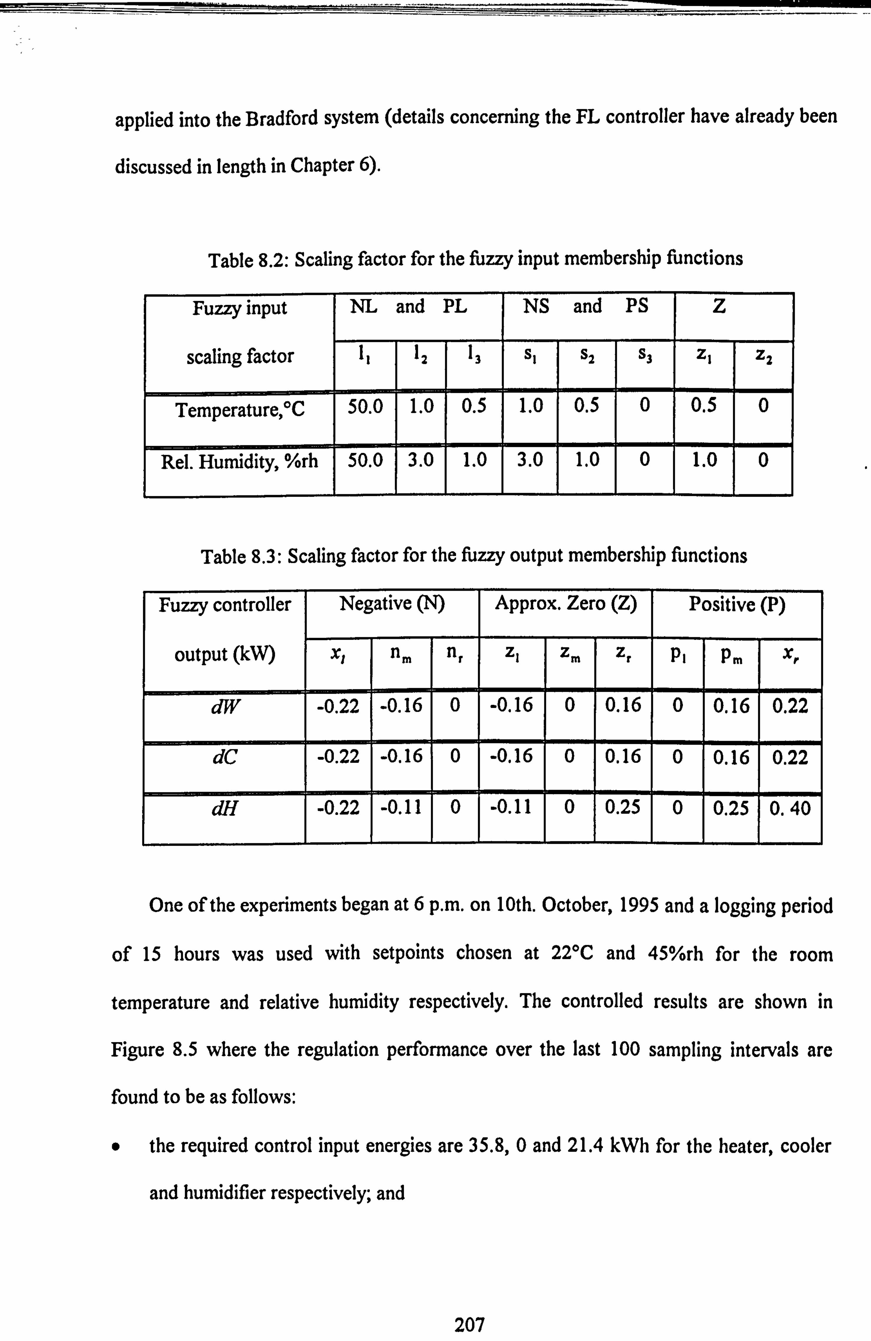
applied into the Bradford system (details concerning the FL controller have already been

discussed in length in Chapter 6).

Table 8.2: Scaling factor for the fuzzy input membership functions


scaling factor 11 12 13 S, S2 S3 Z, Z2

Temperature, "C 50.0 1.0 0.5 1.0 0.5 0 0.5 0

Rel. Humidity, %rh 50.0 3.0 1.0 3.0 1.0 0 1.0-1 0

Table 8.3: Scaling factor for the fuzzy output membership functions

Fuzzy controller Negative (N) Approx. Zero (Z) Positive (P)

output (M) X, n. n, ZI zm zr Pi P. XF

dW -0.22 1 -0.16 0 -0.16 0

1

0.16 0 0.16 0.22

dC -0.22 -0.16 0

I -0.16

-

0 0.16

I

0 0.16

I

0.22

dH -0.22 -0.11 01 -0.11 0 0.25 0 0.25 1 0.40

One of the experiments began at 6 p. m. on 10th. October, 1995 and a logging period

of 15 hours was used with setpoints chosen at 22"C and 45%rh for the room

temperature and relative humidity respectively. The controlled results are shown in

Figure 8.5 where the regulation performance over the last 100 sampling intervals are

found to be as follows:


and hurnidifier respectively; and

207

the output squared errors are 2. OoC2 and 34.6%rh' for the temperature and


The controller investigations were also carried out for the PI-based FLC using tile

design presented in Section 6.1.2 where the fuzzy membership functions from Tables 6.7,

8.2 and 8.3, and the combined ffizzy rules from Tables 6.1 and 6.2 were applied. A trial

began at 6 p. m. on 15th. October, 1995 and logging lasted for a period of 23 hours with

the setpoints chosen at 220C and 45%rh for the room temperature and relative humidity

respectively. The experimental results are shown in Figure 8.6 where the control

performance over the last 100 sampling intervals are found to be as follows:



the output squared errors are 3 OoC2 and 33.4%rh 2 for the temperature and relative

hunUity respectively.

: �-;

: '! ---c. aw

HuW

Thhe

Regales M@""%MWjAW%

TWO News


Figure 8.5: Performance of the proportional fuzzy logic controller

208

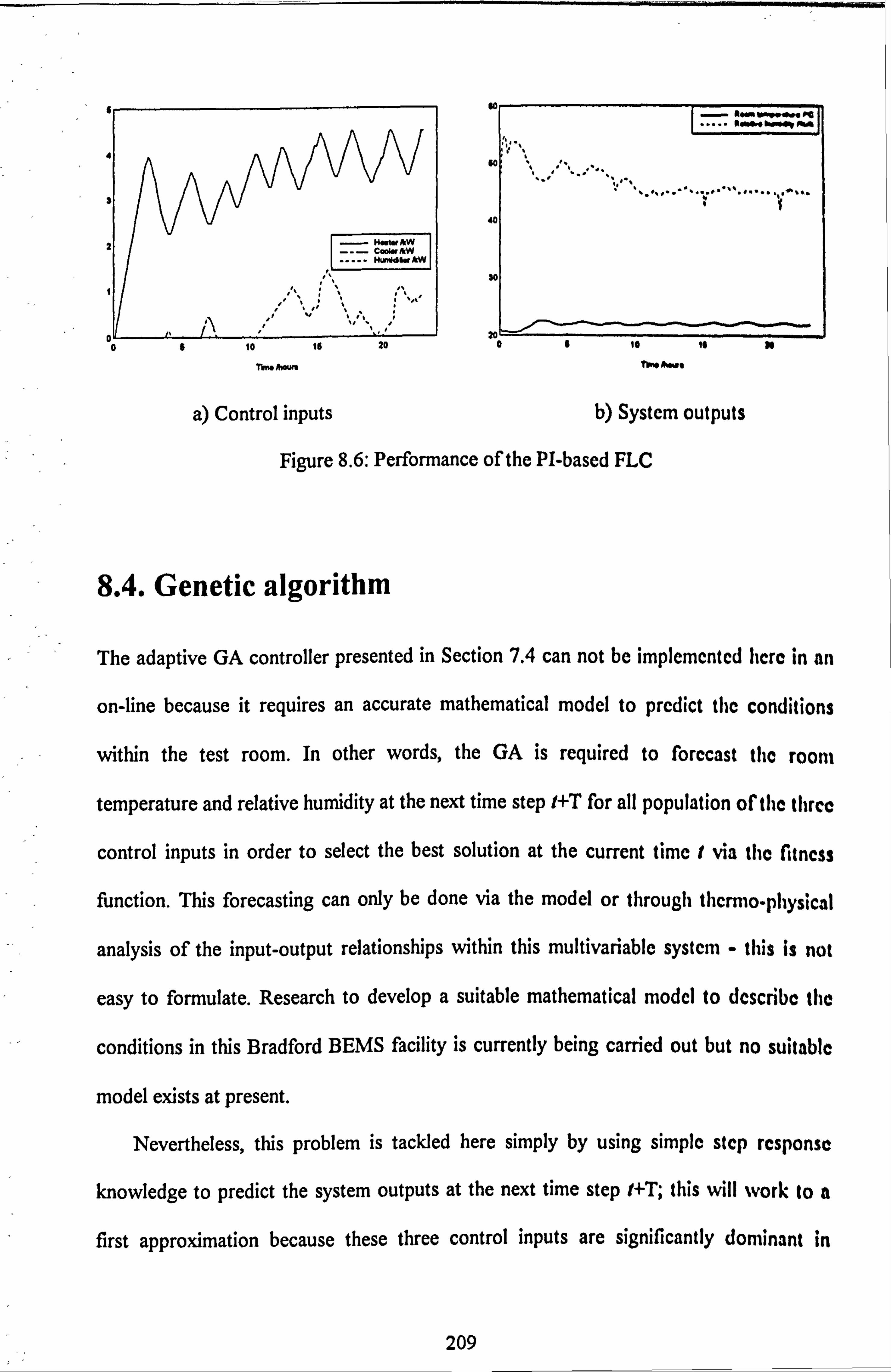
Hoew --- cooler

HuRdd

10 10 Thm Awn

a) Control inputs

so ohm* ba"It ft^

60

40

30

20 aa 16 to 22

nme Nut

b) Systcm outputs

Figure 8.6: Performance of the PI-based FLC

8.4. Genetic algorithm

The adaptive GA controller presented in Section 7.4 can not be implemcntcd licre in an

on-line because it requires an accurate mathematical model to prcdict the conditions

within the test room. In other words, the GA is required to forccast the room

temperature and relative humidity at the next time step I+T for all population or tile tllrce

control inputs in order to select the best solution at the current time t via tile fitncss

function. This forecasting can only be done via the model or through thcrtno-physlIcal

analysis of the input-output relationships within this multivariable system - this is not

easy to formulate. Research to develop a suitable mathematical modcl to describe tile

conditions in this Bradford BEMS facility is currently being carried out but no suitable

model exists at present.

Nevertheless, this problem is tackled here simply by using simple step response

knowledge to predict the system outputs at the next time step I+T; this will %vork to a

first approximation because these three control inputs are significantly dominant in

209

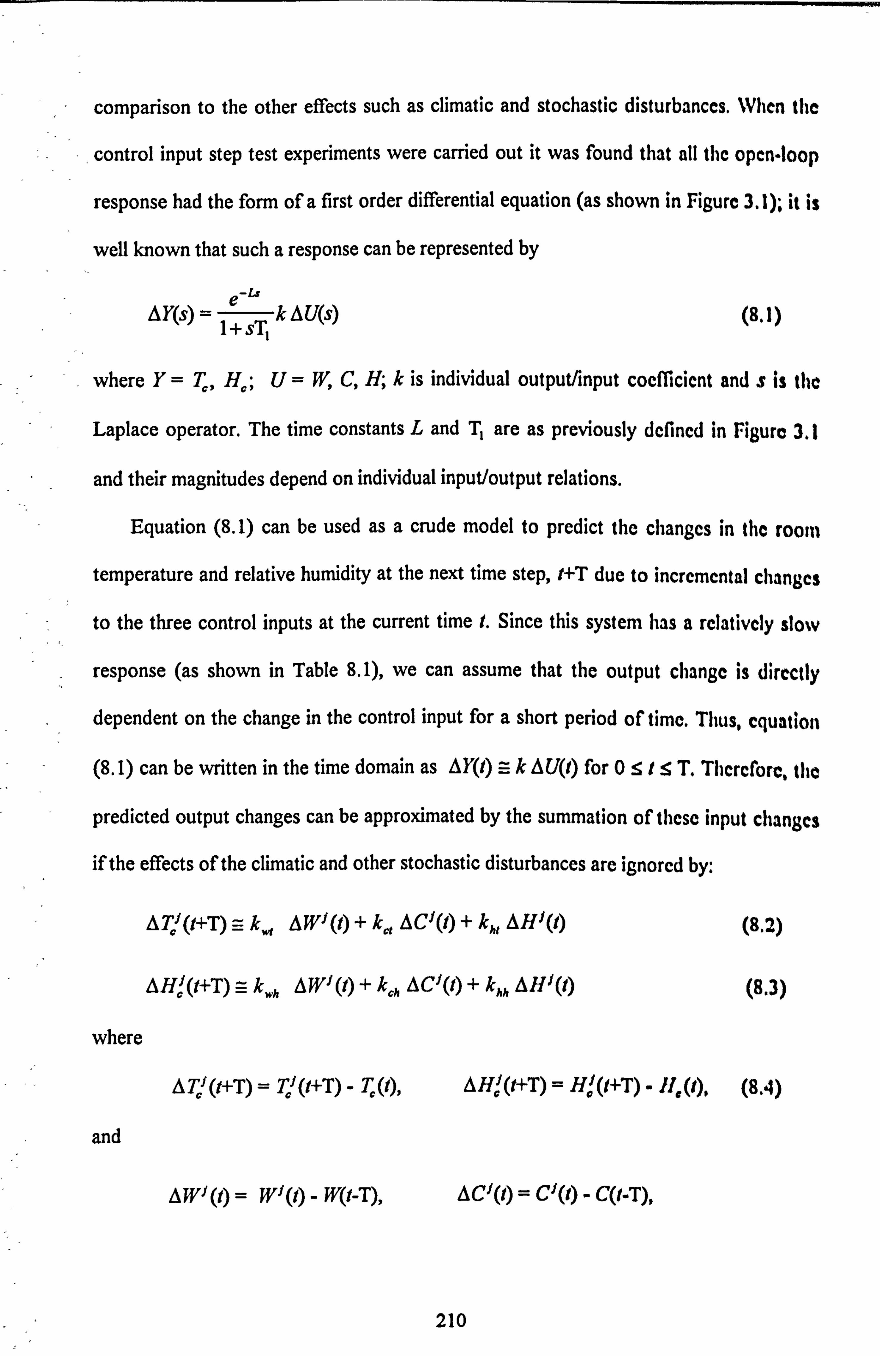
comparison to the other effects such as climatic and stochastic disturbanccs. When the

control input step test experiments were carried out it was found that all the opcn-loop

response had the form of a first order differential equation (as shown in Figure 3.1), it is

well known that such a response can be represented by

-Li AY(s) = -k AU(s)

I+sT,

where Y=T, H,; U=W, C, H; k is individual outputfinput coefficient and s is the

Laplace operator. The time constants L and T, are as previously defincd in Figure 3.1

and their magnitudes depend on individual input/output relations.

Equation (8.1) can be used as a crude model to predict the changes in the room

temperature and relative hun-ddity at the next time step, I+T due to incremcntal changcs

to the three control inputs at the current time 1. Since this system has a relatively slow

response (as shown in Table 8.1), we can assume that the output change is directly

dependent on the change in the control input for a short period of time. Thus, cquation

(8.1) can be written in the time domain as AY(I) =- kAU(I) for 0: 5 1: 5T. Thmforc, the

predicted output changes can be approximated by the summation of these input changn

if the effects of the climatic and other stochastic disturbances are ignored by:

AT, i(I+T) =- k., AWJ(t) + k,, ACi(l) + kh, AHJ(f)

AH, i(t+T) =- kh AWi(l) + kh ACi(l) + khhAHI(l)

(8.1)

(8.2)

(8.3)

where

A T", (t+T) = T'll (I+T) - T, (I)p A Hji (t+T) = Hi (t+T) - 11, (t), (8.4)

and

Awl(t) = WI(l) - WO-T)l ACI(t) = CIO) - CO-T)l

210

AHJQ) = HJ(t) - H(t-T), (8.5)

Here, j is the 'label number"of the chromosome in the GA, and IVJ(I), CJ(I) and 111(t)

are the physical values of jth chromosome at generation 1. We can assume that the

coefficients to control input changes k k.,.,, khh are constant for a period between

one sampling instant and the next, t to I+T. For our applications, we propose to calculate

these coefficients by using the results from the mid-range step responses (50% to 75% of

the maximum power) as described in section 8.1; the values were found to be:

kwt = 0.126, kct = -0.028, kht = 0.015 (TAW).

kwh -0.60, kch=

-0.127$, khh= 0.956 (%rh/kW).

The predicted room temperature TJ(t+T) and relative humidity Hj' I(t+T) arc thcn

calculated for all the chromosomes pi via equation (8.4) and the fitness function

evaluated using equation (7.3) with 9 equals 0.13 since this value is suitable for tile

simulation environment (Chapter 7). The best control input setting at generation t is tlIcn

chosen and applied into the Bradford HVAC system.

HUIWdfiý IkW COOIWA. W H"tw)kW

i, i" i F, I. I I m

a9 12

Tl. *)hwm tot #m"


Figure 8.7: Performance of the adaptive GA controller

4*

- ----------

. I-

211

By using this approximation, experimental trials were carried out and one sample

run is shown in Figure 8.7 where we can see that the GA controller is capable of

regulating the air temperature and relative humidity of the main room. The cxpedment

began at 6 p. m. on 4th. September, 1995 and logging lasted for a period of 12 hours and

the desired setpoints were chosen at 22T and 50%rh for the temperature and humiWity

respectively. The control performance over the last 100 sampling intervals are found to

be as follows:

0 the required control input energies are 15.7,2.4 and 33.6 kWh for the ficatcr, coolcr


the output squared errors are 16.7 oC2 and 387.8%rh 2 for the tcmpcraturc and

relative hun-ýidity respectively.

8.5. Commercial controller

It is worthwhile to compare the advanced controllers designed here with a comincrcial

controller which was installed for the Bradford BEMS Laboratory wlicn it was

commissioned. The control strategy of the commercial controller is dividcd into two

parts; the first part is to regulate the AHU supply air temperature, T,, and the rctum

relative humidity, RH,, by controlling the main heater, JV., cooler, C, humidificr, 11,

fresh air damper, Df, return damper, D,, and discharge damper, Dd; the second pirt is

for the individual office rooms, that is, to maintain the air temperature and rclative

humidities at their setpoints by controlling the reheater and damper in the VAV Box for

each room.

212

The aim of the control strategy is to regulate the room temperature and the humidity

-to within required comfort levels. The air pressure in this system is kept constant via tile

AHU supply fan, Fs, and the extract fan, Fe, which correspond to controlling tile

dampers Df, D, and D.. The setpoints were chosen as 170C and 40%rh for the AIIU

supply air temperature and return relative humidity, and 221C and 45%rh for the air

temperature and humidity respectively of the three rooms (such values are typical for

offices). The experiment was carried out on 21st. November, 1995 and the result is

shown in Figure 8.8. We can see that the room temperature is regulated at tile dcsircd

value but the relative humidity does not reach its setpoint, this could be due to poor

tuning of the PI controllers at the commissioning stage of the system, The control

performance over the last 100 sampling intervals are found to be as follows:

S

.

the required control input energies are 0,0,2.5 and 8.8 kWh for the main licatcr,

cooler, humidifier and the reheater #1 (in VAV Box 1) respectively; and

the output squared errors are 26.8"C' and 7567.3%rhl for the tcrnpcraturc and


Note that the control system is designed in such a way that the amount of intake and

discharge dampers (in %) are identical but the return damper is (100% - intakc danipcr).

For this experiment, the average intake and discharge dampers opening were round to be

at 40% and the return damper at 60%, and the average damper opening in VAV Box

was 40%.

213

Room tomperahme IIC ----- RA humIddy I%fh

a 1.0

too

16 % .401 V%

20

,. L 10

Time fturs

20 30

Figure 8.8: Control performance of the Concord PI controllcr

8.6. Discussion of Results

The experimental results of all the controllers as presented earlier need to be compared in

order to choose the best one. The results such as the errors squared of the system's

output and its energy consumption are surnmarised in Table 8.4 so that the control

performances can easily be analysed.

We can see that the Proportional and PI-based fuzzy logic controllers give smallest

output errors as compared to the other controllers. This is followed by the constrained

input MIMO adaptive controllers and then the adaptive GA-bascd controller. Tile multi

PI-loop controller is the worst amongst the designed controllers since it gives tile

greatest output errors and the temperature is mostly slightly below the setpoint but it is

still better than the commercial PI controller in term of the relative humidity error.

214

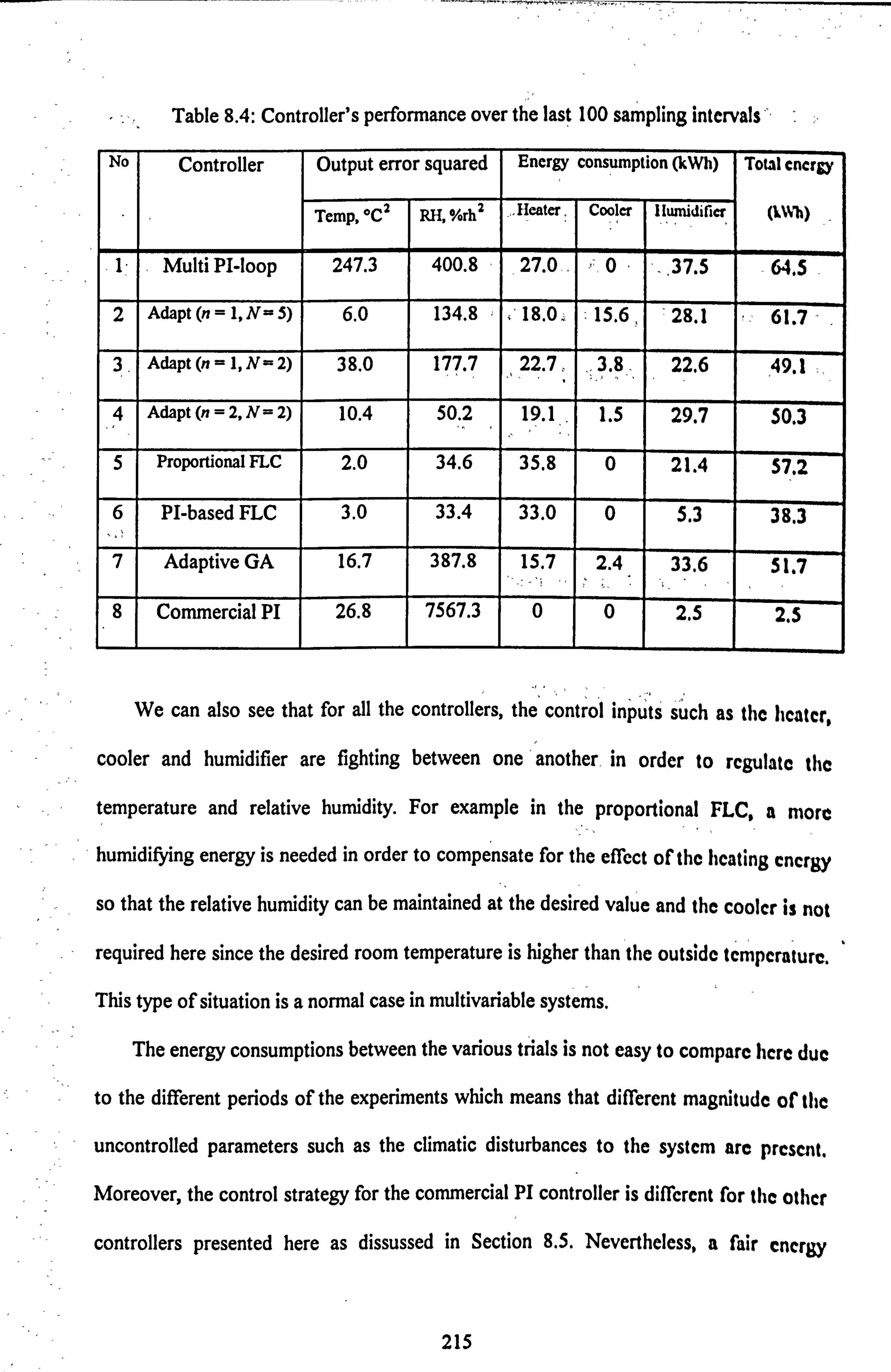
Table 8A Controller's performance over the last 100 sampling intervals

No Controller Output error squared Encrgy consumption (kWh) Total cnergy

Temp, *C 2 RH, %rh 2 --fleater,

Cooler llwnidirler

Multi PI-loop 247.3 400.8 27.0, 0 -, 37.5 -64.5 2 Adapt (n = 1, N= 5) 6.0 134.8 18.0., 15.6, 28.1 61.7-

3', Adapt (n = 1, N= 2) 38.0 177.7 22.7, 3.8, 22.6 49.1

,4 Adapt (n = 2, N= 2) 10.4 50.. 2 19.11, 1.5 29.7 50.3

5 Proportional FLC 2.0 34.6 35.8 0 21.4 57.2

6 PI-based FLC 3.0 33.4 33.0 0 5.3 38.3

7 Adaptive GA 16.7 387.8 15.7 2.4. 33,6 51.7

.8 Commercial PI 26.8 7567.3 0 0 2.5 2.5

We can also see that for all the controllers, the , contro .I inputs' such as the heater,

cooler and humidifier are fighting between one 'another, in order to rcgulatc tile

temperature and relative humidity. For example in the proportional FLC, a more

humidifying energy is needed in order to compensate for the effect of the heating cncrgy

so that the relative humidity can be maintained at the desired value and the coolcr is not

required here since the desired room temperature is higher than the outside tcmperature,

This type of situation is a normal case in multivariable systems.

The energy consumptions between the various trials is not easy to compare licre due

to the different periods of the experiments which means that different magnitude or tile

uncontrolled parameters such as the climatic disturbances to the system are prcscnt.

Moreover, the control strategy for the commercial PI controller is diffcrcnt for the other

controllers presented here as dissussed in Section 8.5. Nevertheless, a fair cncrgy

215

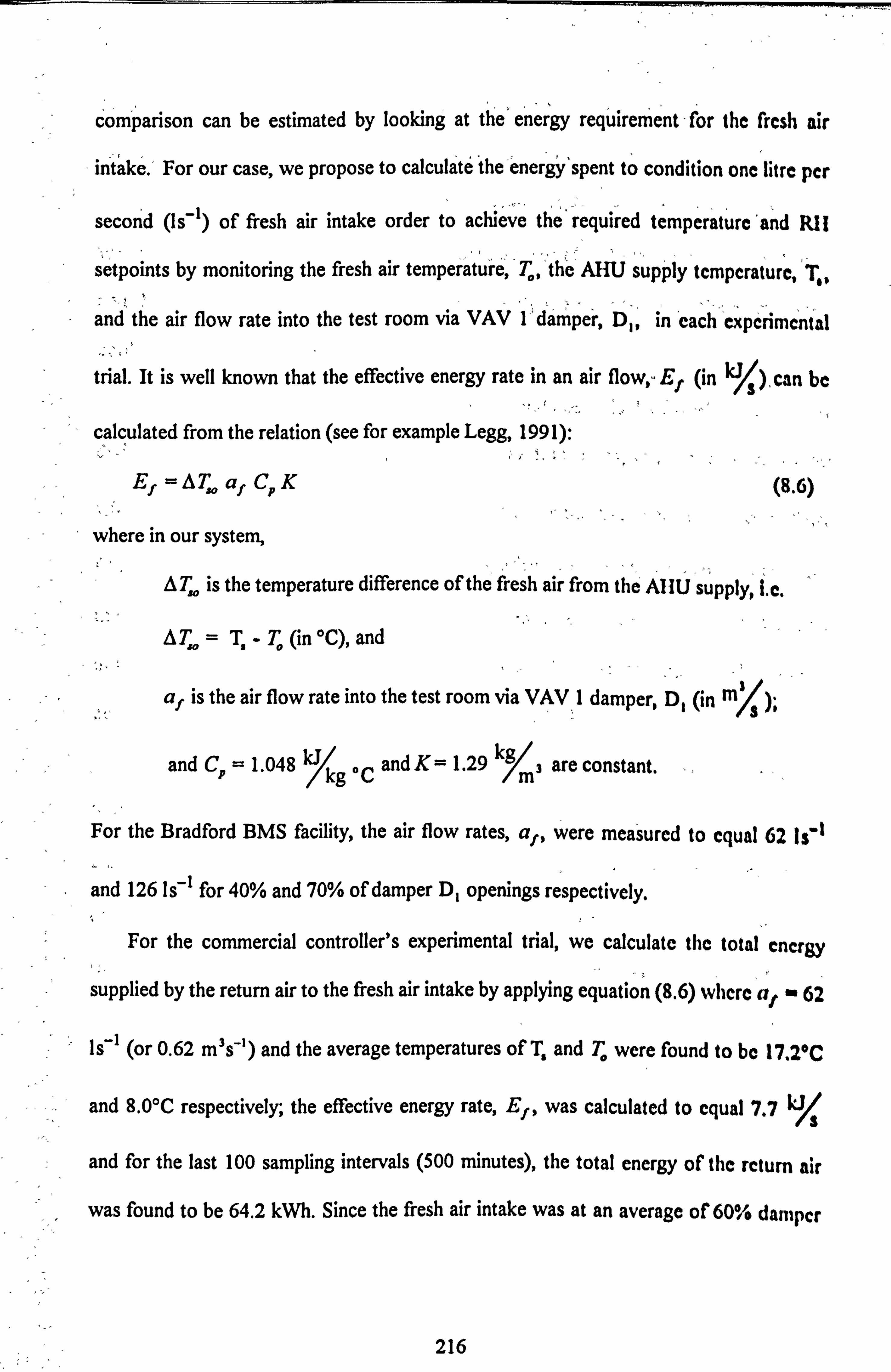
c om . panson can be estimated by looking at tfie'energy requirement -for the fresh air

intake. ' For our case, we propose to calculate *the -energý'spent to condition one litre per

second (Is-1) of fresh air intake order to achieve the'required temperature'and R11

setpoints by monitoring the fresh air temperature, - T., 'th'e- AHU supply tcmpcratureý T.,

and' the air flow rate into the test room via VAV I'damper, D1, ineach expcnme I nt I al

trial. It is well known that the effective energy rate in an air flow, - Er (in 0/, ), can be

calculated from the relation (see for example Legg, 199 1)

Ef = AT,,, a. CP K (8.6)

where in our system,

is the temperature difference of th AT e fresh air from the'AIJU supply, i. e.

AT,,, = T. - T. (in T), and

af is the air flow rate into the test room via VAV, I damper, 'D (in My,

andC,, =1.048kj, ý

, andK=1.29 kg/

3 are constant. /kg C /M

For the Bradford BMS facility, the air flow rates, af, were measured to equal 62 Is-'

and 126 Is-' for 40% and 70% of damper D, openings respectively.

For the commercial controller's experimental trial, we calculate the total cncrgy

supplied by the return air to the fresh air intake by applying equation (8.6) whcrc a,, w 62

Is-I (or 0.62 m's-') and the average temperatures of T, and T. were found to be 17.2*C

and 8.0"C respectively; the effective energy rate, Ef, was calculated to equal 7.7 U/S

and for the last 100 sampling intervals (500 minutes), the total energy of the return air

was found to be 64.2 kWh. Since the fresh air intake was at an average of 60% danipcr

216

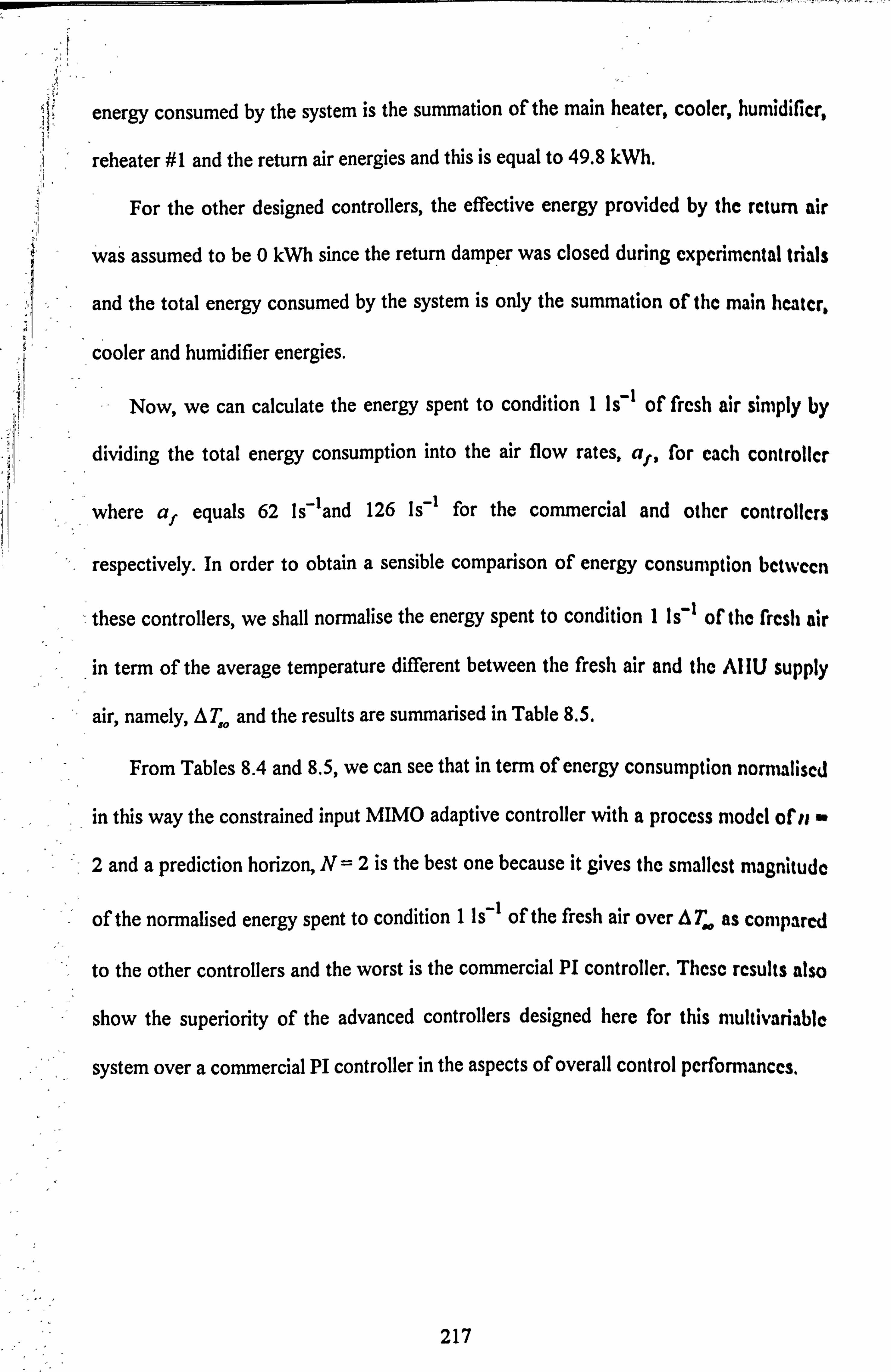
energy consumed by the system is the summation of the main heater, coolcr, humidifier,

reheater #1 and the return air energies and this is equal to 49.8 kWh.

For the other designed controllers, the effective energy provided by the rcturn air

was assumed to be 0 kWh since the return damper was closed during cxpcrimcntal trials

and the total energy consumed by the system is only the summation of the main hCater.

cooler and humidifier energies.

Now, we can calculate the energy spent to condition I Is of fresh air simply by

dividing the total energy consumption into the air flow rates, af, for each controlicr

where af equals 62 Is-land 126 Is-' for the commercial and othcr controlIcTs

respectively. In order to obtain a sensible comparison of energy consumption boween

these controllers, we shall normalise the energy spent to condition II s-I or the ricst, air

in term of the average temperature different between the fresh air and the AIIU supply

air, namely, AT,,, and the results are summarised in Table 8. S.

From Tables 8.4 and 8.5, we can see that in term of energy consumption normalised

in this way the constrained input MIMO adaptive controller with a process modd of it ---

2 and a prediction horizon, N= 2 is the best one because it gives the smallest magnitude I

of the normalised energy spent to condition I IS-' of the fresh air over AT. as compared

to the other controllers and the worst is the commercial PI controller. Thcse rcsults also

show the superiority of the advanced controllers designed here for this multivariable

-- system over a commercial PI controller in the aspects of overall control pufornianccs,

217

, Table 8.5: Normalised energy spent to condition, I Is-' of the fresh air ovcr

h 49.8 U. bu 5U F/. 2 9.2 0.087

8.7. Conclusions

This chapter has presented the control performances of several advanced controllers to

regulate the conditions within the Bradford plant/office zone system; in particular the

multi PI-loop controller, the constrained input MIMO adaptive control, the fuzzy logic

controller and the genetic algorithm-based controllers which have been discussed in

previous chapters have been experimentally verified. The results show that tile multi 1)1.

loop controller with 6 PI units, the fijzzy logic controller and the constrained input

adaptive controller can achieve good regulation control performances. The adaptive GA.

Controller No.

(from Table 8.4)

Total

energy, kWh

Energy / fresh

air, kWh/ IS-'

T.

Oc

T.

Oc Oc

Energy/ fresh air +, &T

kWh/ Is -1 PC

1 64.5 0.51 6.0 21.9 15.9 0.032

2 61.7 0.49 11.2 21.8 10.6 0.046

3 49.1 0.39 12.1 21.9 9.8 0.040

4 50.3 0.40 5.6 22.0 16.4 0.024

5 57.2 0.45 11.9 22.1 10.2 0.044

6 38.3 0.30 12.1 21.9 9.8 0.031

7 51.7 0.41 12.2 22.2 10.0 0.041

8 49.8 0.8 8.0 t

17.2 9.2 0.087

218

based controller is also capable of regulating the system outputs at their desired

setpoints, but it is felt that its performance could be improved if a more accurate

mathematical model which can describe the conditions in the room is available.

219

Chapter 9

Conclusions and Future Work

The main objectives of the research presented in this thesis have been to investigate the

design of advanced controllers which are suitable for building energy management

systems (BEMS). These include the multi PI-loop controller, state feedback in the state-

space, the constrained input NUMO adaptive controller, the fuzzy logic-based controller

and the genetic algorithm optimisation technique. The control performances based on the

system's output errors squared, the energy consumptions and the settling period have

been investigated for different parameters and rules to assess their effect on the

performances.

In this research, the BEMS under study is presented as a3 input/2 output system

subject to external disturbances and effects. The three inputs are the heater, cooler and

humidifier, and the two outputs are the test room's air temperature and relative humidity.

The external disturbances consist of climatic effects, incidental gains due to occupancy

and other stochastic influences. The study is carried out within a simulation environment

using the mathematical model which describes the conditions within the BMS test room

facility at the University of Loughborough; some of the controllers developed are also

tested in a real-time situation to control the experimental BEMS Laboratory at the

220

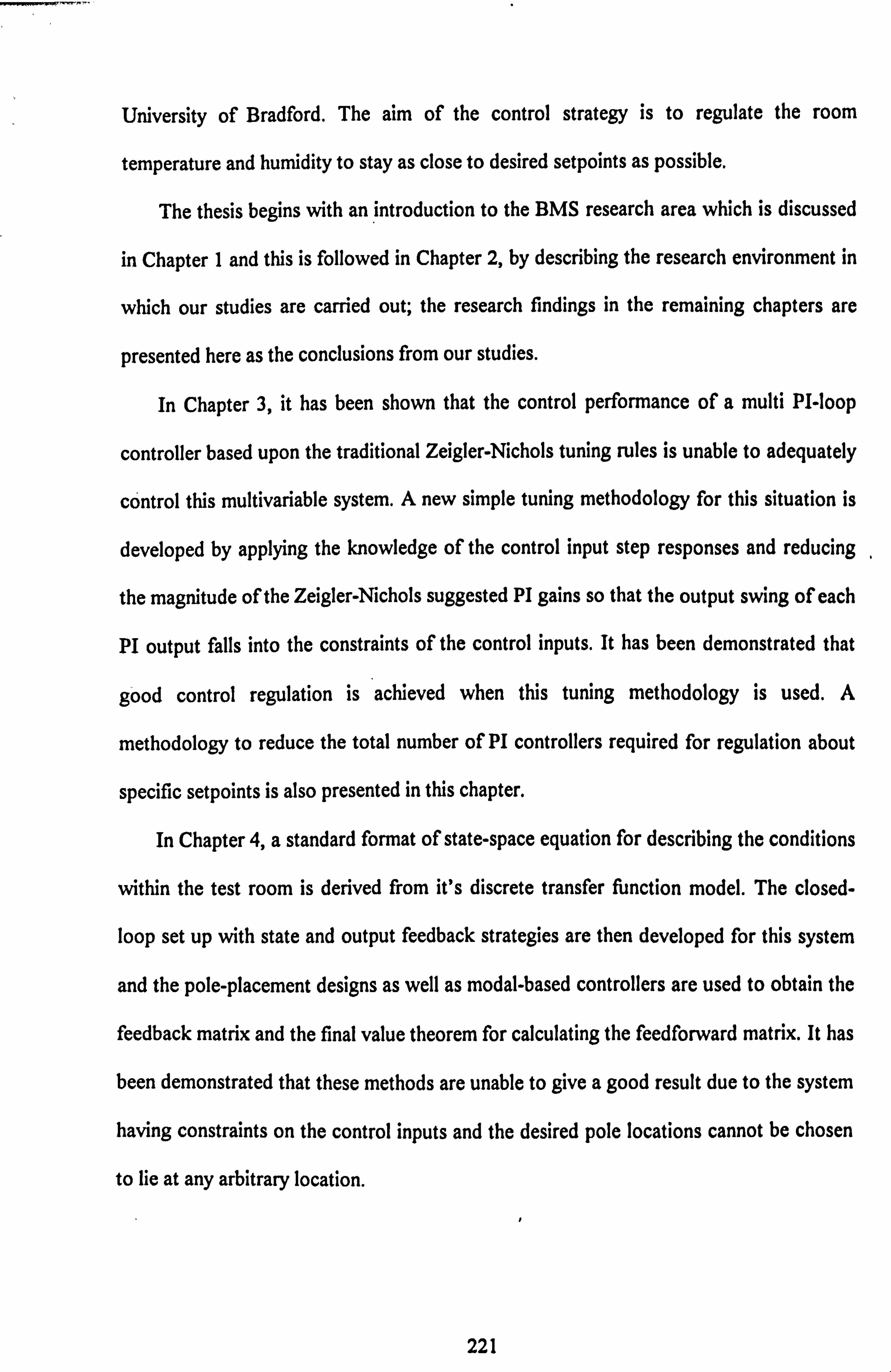
University of Bradford. The aim of the control strategy is to regulate the room

temperature and humidity to stay as close to desired setpoints as possible.

The thesis begins with an introduction to the BMS research area which is discussed

in Chapter I and this is followed in Chapter 2, by describing the research environment in

which our studies are carried out; the research findings in the remaining chapters are

presented here as the conclusions from our studies.

In Chapter 3, it has been shown that the control performance of a multi PI-loop

controller based upon the traditional Zeigler-Nichols tuning rules is unable to adequately

control this multivariable system. A new simple tuning methodology for this situation is

developed by applying the knowledge of the control input step responses and reducing

the magnitude of the Zeigler-Nichols suggested PI gains so that the output swing of each

PI output falls into the constraints of the control inputs. It has been demonstrated that

good control regulation is achieved when this tuning methodology is used. A

methodology to reduce the total number of PI controllers required for regulation about

specific setpoints is also presented in this chapter.

In Chapter 4, a standard format of state-space equation for describing the conditions

within the test room is derived from it's discrete transfer function model. The closed-

loop set up with state and output feedback strategies are then developed for this sYstem

and the pole-placement designs as well as modal-based controllers are used to obtain the

feedback matrix and the final value theorem for calculating the feedforward matrix. It has

been demonstrated that these methods are unable to give a good result due to the system

having constraints on the control inputs and the desired pole locations cannot be chosen

to lie at any arbitrary location.

221

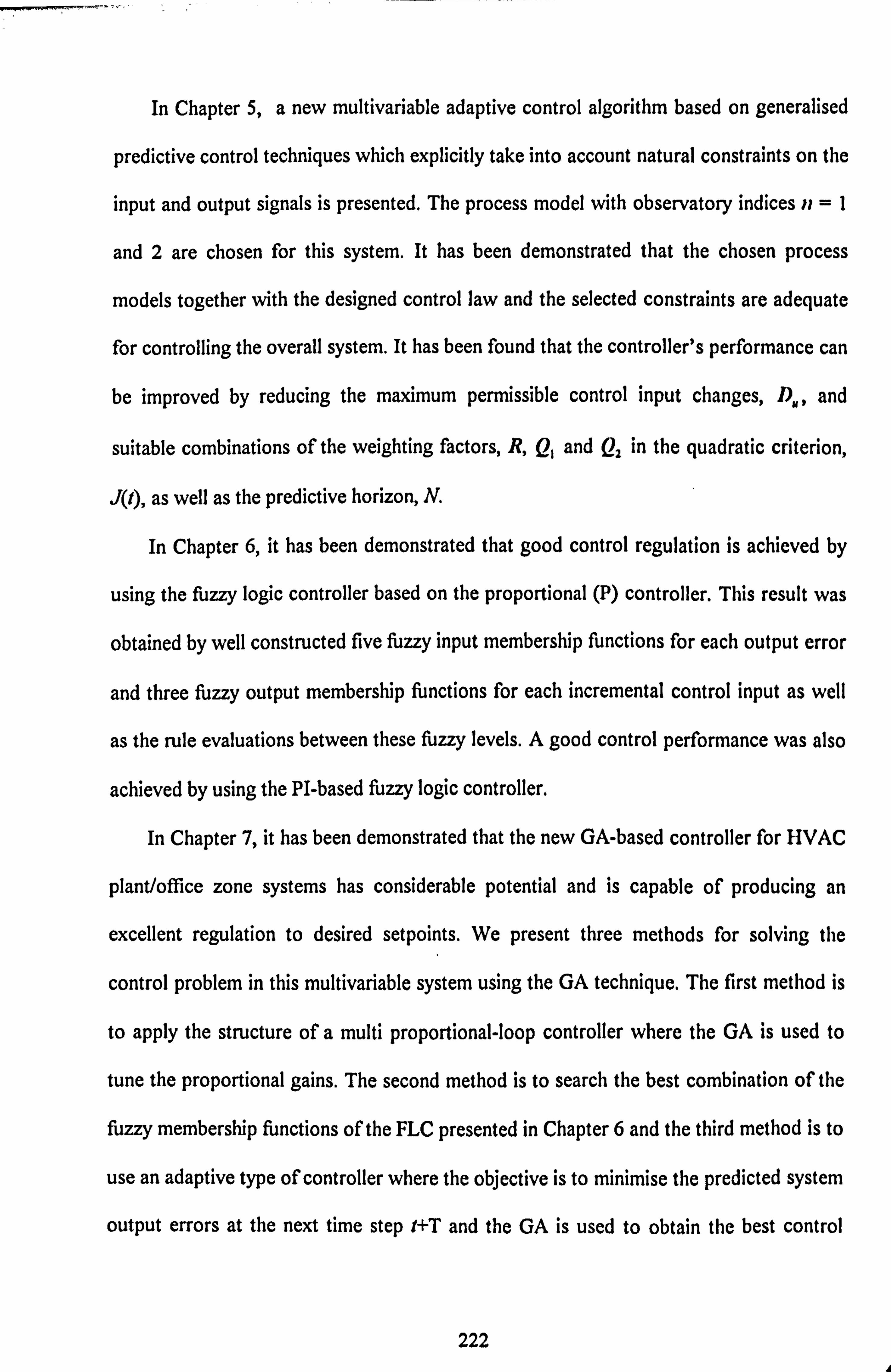
In Chapter 5, a new multivariable adaptive control algorithm based on generalised

predictive control techniques which explicitly take into account natural constraints on the

input and output signals is presented. The process model with observatory indices it =I

and 2 are chosen for this system. It has been demonstrated that the chosen process

models together with the designed control law and the selected constraints are adequate

for controlling the overall system. It has been found that the controller's performance can

be improved by reducing the maximum permissible control input changes, D., and

suitable combinations of the weighting factors, R, Q, and Q, in the quadratic criterion,

J(I), as well as the predictive horizon, N.

In Chapter 6, it has been demonstrated that good control regulation is achieved by

using the fuzzy logic controller based on the proportional (P) controller. This result was

obtained by well constructed five fuzzy input membership functions for each output error

and three fuzzy output membership functions for each incremental control input as well

as the rule evaluations between these fijzzy levels. A good control performance was also

achieved by using the PI-based fuzzy logic controller.

In Chapter 7, it has been demonstrated that the new GA-based controller for IIVAC

plant/office zone systems has considerable potential and is capable of producing an

excellent regulation to desired setpoints. We present three methods for solving the

control problem in this multivariable system using the GA technique. The first method is

to apply the structure of a multi proportional-loop controller where the GA is used to

tune the proportional gains. The second method is to search the best combination of the

fuzzy membership functions of the FLC presented in Chapter 6 and the third method is to

use an adaptive type of controller where the objective is to minimise the predicted system

output errors at the next time step I+T and the GA is used to obtain the best control

222

inputs at the current time 1. It has been found that all these three GA-based methods have

produced good control results. The third method has an advantage in the sense that it can

adapt to the changing of the setpoints as well as to the external disturbances effecting the

system without deteriorating the control performance. This approach is further improved

by applying a smoothing operation by using a moving average digital filter to suppress

the excessive control input fluctuation whenever these grow beyond maximum

permissible limits at each sampling instant.

The advanced controllers presented in this thesis are further verified by testing them

within a real-time control situation where experimental trials were carried out on the full-

scale Bradford BEMS Laboratory. For this system, the HVAC plant/office zone system

was configured to have an identical number of inputs and outputs as used in tile

simulation environment and the actual climatic disturbances and other influences present

in the system. It has been demonstrated that the developed controllers, except the state-

space-based ones, are capable of regulating the air temperature and relative humidity of

the test room by simultaneously controlling the main heater, cooler and humidifier. Note

that the state-space method was not experimentally tested on the Bradford BMS due to

the lack of a suitable mathematical model for the Bradford BMS test. facility.

9.1. Future work

An important aspect of this work is that the research was started with a known

dynamical model of a test room and the main objective of the selected control systems

was to mýinimise the closed-loop system output errors. With this model, we can study

many other control objectives; for example to minimise the energy consumption as well

223

as the output errors by modifying the FLC rule evaluations as well as designing a suitable

fitness function of the GA controller presented in Section 7.4.

There are many other advanced methods that are suitable for solving the control

regulation problem within this multivariable system. Such methods are the improved

fuzzy logic controller using genetic algorithm, see for example Genshe and Xinhai

(1993); neural network (NN) and neuro-fijzzy controllers, see for example White and

Sofge (1992). Fuzzy logic controllers for BEMS could also be based on commercial

controller strategies. For example, the strategy of the one installed at the Bradford test

facility as explained in Section 8.5 where the fuzzy logic methods decision can be used to

obtain the fresh air intake and the three main control inputs as well as the damper's

opening and the rebeater for individual office rooms.

The method of obtaining the feedback matrix in a closed-loop system with

constrained control inputs should be developed so that the outputs are critically tracking

the setpoints. It has been found that this can be achieved by making some of the closed-

loop poles A, i=1,2, .., 6 lie on the real-imaginary axis with I pi 1 :51 (Virk and

Ghazali, 1994).

Another important research area needing attention is to design a fault diagnosis

system for BEMS applications via a simulation environment since the air dynamics in

rooms can be known from mathematical models. A possible way of implementing this

could be to apply a set of input and output related data from a normally operating system

as a reference and then training a neural network using faulty input/output data. This

trained NN can accurately predict the system outputs under normal and failed conditions,

and hence can be used to detect a variety of faults. This can be further extended to

224

designing a control reconfiguration system in the case of system failure so that the over

system remains functional.

225

BIBLIOGRAPHIES

ASTROM, K. J., C. C. HANG, P. PERSSON, AND W. K. HO (1992). Towards

Intelligent PID Control. Automatica, Vol. 28, No. 1, pp. 1-9.

ATHIENITIS, A. K. (1988). A predictive control algorithm for massive buildings.

ASHRAE Transactions, Vol. 94, pt. 2, pp. 1050-1068.

BORRISON, U. (1979). Self-tuning regulators for a class of multivariable systems.

Automatica, vol. 15, pp. 209-215.

CBEN, C. T. (1984). Linear System Theory and Design. Holt, Rinehart and Winston

Series, pp. 372-373.

CLARKE, D. W. (1984). Self-tuning control of nonminimum-phase systems.

Automatica, Vol. 20, No. 5, pp. 501-517.

CLARKE, D. W., C. MOHTADI AND P. S. TUFFS (1987). Generalized predictive

control - part I: The basic algorithm; part II: extension and interpretation.

Automatica, 23, pp. 137-160.

COLEY, D. A. AND J. M. PENKAN (1992). Second order system identification in the

thermal response of real buildings. Paper 11: Recursive formulation for on-line

building energy management and control, Building and Etivironment, Vol. 27, No.

3, pp. 169-277.

CULP, C., J. HEBERL, L. NORTORD, P. BROTHERS AND J. D. HALL (1990). The

impact of Al technology within the HVAC industry. ASHRAE 32.12, pp. 12-22.

226

CUTLER, C. R. AND B. L. RAMAKER (1980). Dynamic matrix control -a computer

control algorithm. J. A. C. C.: Joint Automatic Control Conference, San Francisco,

paper WP5-B.

DAVIS, L. (ed. ) (1991). Handbook of genetic algorithms. Van Nostrand Reinhold.

DEXTER, A. L., G. GENG AND P. HAVES (1990). The application of self-tuning PID

control to HVAC systems. IEE Colloquium on Control hi Building Ener&T

Management Systems, IEE Digest 1990 093 May, 1990.

DEXTER, A. L. AND D. W. TREWHELLA (1990). Building control systems: fuzzy

rule-based approach to performance assessment. Buildhig Serv. Evig. Res.

TechnoL, 11(4), 115-124.

DION, J. M., L. DUGARD, A. FRANCO, N. M. TRI AND D. REY (199 1). 'MIMO

adaptive constrained predictive control case study: An environmental test chamber.


ELLIOTT, H., W. A. WOLOVICH AND M. DAS (1984). Arbitrary adaptive pole

placement for linear multivariable systems. IEEE Traw. Automatic Cowrol, Vol.

AC-29, No. 3.

ETTER, D. M., M. J. HICKS AND K. H. CHO (1992). Recursive adaptive filter design

using an adaptive genetic algorithm. in Proc. IEEE, IM. Coitf. Acoustics, SI)eech,

andSignalProcessing, 1992, Vol. 2, pp. 635-638.

FIELDEN, C. J. AND T. 1. EDE (1982). Computer based energy management in

buildings. West Bvrleet: Pitman Abba Consultants Automation.

FLETCHER, R. (1981). Practical methods of optimization, Vol. 2: Constrained

optimization. Wiley, Chichester.

227

FRIEDLAND, B. (1986). Control system design: An introduction to state space

methods. McGraw 011, Inc.

GENSHE, C AND C. XINHAI (1993). Improved fuzzy logic controller using genetic

algorithm and its application to spacecraft rendezvous. IEEE, TENCON'93, Beijing.

GHAZALI, A. B. (1994). Advanced Intelligent Control and Fault Diagnosis in Building

Energy Management Systems (BEMS). PhD Proposal, Dept. of Electrical

Engineering, Univ. of Bradford.

GODFREY, K. R. (1980). Correlation Methods. Aulonialica, Vol. 16, pp. 527-534,

Pergamon Press Ltd.

GOLDBERG, D. E. (1989). Genetic algorithms in search, optimization and machine

learning. Reading, M. A.: Addison-Wesley.

HAMBLIN, J. (1995). Why control your buildings? Ehergy Efficiemy Yearbook 1995,

Energy Systems Trade Association (ESTA), Gloucestershire, UK. pp. 28-29.

HAVES, P. AND A. L. DEXTER (1991). Use of a building emulator to evaluate control

strategies implemented in commercial BEMS. Proc. BuIldhig Divirownewal

Performance BEP '91, University ofKent, Canterbury, pp. 31.4 1.

HE, S. Z, S. TAN, F. L. XU AND P. Z. WANG (1993). Fuzzy self-tuning of PID

controllers. Fuzzy Sets atid Systems, 56, pp. 37-46, North Holland.

HOLLAND, J. H. (1975). Adaptation in natural and artificial systems. Ann Arbor, MI:

Univ. of Michigan Press.

ISERMANN, R., K. H. LACHMANN AND D. MATCO (1992). Adaptive control

systems. Prentice Hall Ltd.

JACKSON, T. B. (1971). The theory and economics and optimum start programming of

heating plant. Itist. ofHeating and Ventilating E tigineers Joumal, 3 9, A24-3 8.

228

KAUTSKY, J., N. K. NICHOLS AND P. V. DOOREN (1985). Robust Pole

Assigrunent in Linear State Feedback. Int. J Control, Vol. 41, no. 5, pp. 1129-

1155.

KOIVO, H. N. AND S. POEIJOLAINEN (1985). Tuning of multivariable Pl-cOntrollers

for unknown systems with input delay. Automatica, Vol. 2 1, No. 1, pp. 81-9 1.

KOO, D. (1977). Element of optimization: with application in economic and business.

Heidelberg Science Library.

KUO, B. C. (1992). Digital Control systems, 2nd ed. Saunder College Publishing, pp.

556-563.

KUCERA, V. (1979). Discrete Linear Control; the Polynomial Equation Approach. John

Wiley & Sons.

LEGG, R. C. (1991). Air Conditioning Systems. BT Batsford.

LEIGH, J. R. (1985). Applied Digital Control: Theory, Design and Implementation.

Prentice/Hall International.

LETHERMAN, K. M. (1981). Automatic Controls for Heating and Air-Conditioning.

Per, gamon Press, Oxford.

LING, K. V. AND A. L. DEXTER (1994). Expert control of air-conditioning plant.


LJUNG, L. (1987). System Identification: Theory for the User. Prentice Hall,

Englewood Cliffs, New Jersey.

LOVEDAY, D. L., J. Y. M. CHEUNG AND G. S. VIRK (1990). Building Energy

Management Using Advanced Mathematical Models. Proc. 'Facilities Management

International'; Building Performance Volume, 'Building as Energy Systeme,

paper 2.33, Glasgow,

229

LOVEDAY, D. L. AND G. S. VIRK (1992a). Artificial Intelligence for Buildings.

Jounial ofApp. Energy, Vol. 4 1, No. 3, pp. 201-22 1.

LOVEDAY, D. L. AND G. S. VIRK (1992b). Final Report to the Science and

Engineering Research Council, Research Contract GR/F/02014: The Effectiveness

of Predictive Control Applied to Warm Air Heating Systems For Commercial

Building. August 1989 - August 1992.

MACLAY, D. AND R. DOREY (1993). Applying genetic search techniques to drive

train modeling. IEEE Control System, pp. 50-55.

MATLAB User Guide (1994). The MathWorks Inc., 24 Prime Park Way, Natick, MA.

MCHALE, A. (1995). Major changes ahead in the controls industry. Eviergy Effidemy

Yearbook 1995, EnerV Systems Trade Association (ESTA), Gloucestershire, UK,

p. 4.

MCGREGOR, D. R., M. 0. ODETAYO AND D. DASGUPTA (1992). Adaptive

control of a dynamic system using genetic-based methods. in Proc. IEEE lilt.

Symp. Intelligent Control 1992, pp. 521-525.

MIKLES, J. (1990). A multivariable self-tuning controller based on pole-placement

design. Automatica, Vol. 26, No. 2, pp. 293-302.

MIKLES, J. AND A. MESZOROS (1991). A decoupling pole-placement controller for a

class of multivariable systems. Problem of control and htformation Theory, Vol.

20(4), pp. 291-298.

MOHTADI, C., S. L. SHAH AND D. W. CLARKE (1986). Generalized predictive

control of multivariable systems. Report no. OUEL 1640/86, Dept. Eng. Science,

Univ. of Oxford, U. K

230

MURDOCH, N., J. M. PENMAN AND G. 1. LIVERMORE (1990). Emperical and

theoretical optimum start algorithms. Building Serv. Eng. Res., Technol, 11 (3), 97-

103.

NISHIKAWA, Y., N. SANNOMIYA, T. OHTA AND H. TANAKA (1984). A Method

for Auto-tuning of PID Control Parameters. Automatica, Vol. 20, No. 3, pp. 321-

332.

NORTON, J. P. (1986). An Introduction to Identification. Academic Press, London.

OGATA, K. (1987). Discrete-Time Control Systems. Prentice/Hall International, p. 668.

OHKAWA, F. AND Y. YONEZAWA (1982). A discrete model reference adaptive

control system for a plant with input amplitude constraints. Int. J Control. 36,

747-753.

ORTEGA, R., M. M'SAAD AND C. CANUDAS (1984). Practical requirements and

theoritical results in robust adaptive control. Preprints IFAC 91h World Congr.,

Budapest, Vol. VII, 189-195.

PATERKA, V. (1975). A square root filter for real-time multivariable regression.

Kybernelica, 11,55-67.

PAYNE, A. N. (1986). Adaptive one-step-ahead control subject to an input amplitude

constraints. hil. J ControL 43,1257.

PENKAN, J. M. (1990). Second order system identification in the thermal response of a

working school. Buildhig and Etivironmetit, Vol. 25, pp. 105-110.

PENMAN, I. M. (1990). Real time thermal modelling and the control of buildings. Proc.

Congress International de Domonique, Rennes, 27-29 June.

PENTTINEN, J. AND H. N. KOIVO (1980). Multivariable tuning regulators for

unknown systems. Automatica, Vol. 16, pp. 393-398.

231

PIKE AND PENNYCOOK (1992). Commissioning of BEMs -A Code of Practice;

Application Handbook AH 2/92. Building Services Research and Information

Association, Brockwell.

PORTER, B. AND R. CROSSLEY (1972). Modal Control, Theory and Applications,

Taylor and Francis Ltd.

ROUSE, K. (1990). Future trends in building energy management. Energy World,

176(3), 11-13.

SHAW, M. R. (1987). Applying Expert Systems to Environmental Management and

Control Problems. Building Research Establishment, U. K., pp. 113 -125.

SONNOMIYA, N. AND H. IIMA (1992). Genetic algorithm approach to a production

ordering problem in an assembly process with buffers. IFAC Information cono-ol

problems in Maitufacturitig Techtioloýg, Toranto, Canada,

VIRK, G. S., J. Y. M. CHEUNG AND D. L. LOVEDAY (1990). The Role of Control

Technology for Energy Savings in Buildings. IEE, Colloquium "SCADA and

EnerwManagement Systems", Digest No. 1990/173, pp. 3/1 - 3/7.

VIRK, G. S., J. Y. M. CHEUNG AND D. L. LOVEDAY (1992). Advanced controllers

for the built environment. Proc. Canadian Conf. on Industrial A wontation, Vol. 2,

pp. 34.17-34.21, Montreal, June.

VIRK, G. S. AND A. B. GHAZALI (1994). State Space Methods in Building Systems

Control. Research Report No. 529, Department of Electronic and Electrical

Engineering, University of Bradford, U. K, January.

VIRK, G. S., D. L. LOVEDAY AND J. Y. M. CHEUNG (1995). Practical stochastic

multivariable identification for buildings. J Applied Mathematical Modelling, Vol.

19, October.

232

WADDICOR, 1. (1993). A genetic algorithm for PID controller tuning. M. Sc

clessertation, Dept. of Control Engineering, Univ. of Bradford.

WELLSTEAD, P. E. AND M. B. ZARROP (1991). Self-tuning Systems: Control and

Signal Processing. John Wiley & Sons, Chichester. pp. 80-81,150.

VVHITE, D. A. AND D. A. SOFGE (Ed. ) (1992). Handbook of Intelligent Control:

Neural, Fuzzy and Adaptive Approaches. Van Nostrand Reinhold, N. Y.

YING, H., W. SILER AND J. J. BUCKLEY (1990). Fuzzy control theory: a nonlinear

case. Automatica. Vol. 26, No. 3, pp. 5 13-520.

ZADEH, L. A. (1965). Fuzzy Sets. Inf. Control. 8,3 3 8.

ZADEH, L. A. (1975). The concept of a linguistic variable and its applications to

approximate reasoning. Infonnation Sciences, Vol. 8, pp. 199-249.

ZABEER-UDDIN, M. (1990). Combined energy balance and recursive least squares

method for identification of system parameters. ASHRAE Traiisactions, Vol, 96,

pt. 2, pp. 239-244.

ZIEGLER, J. G. AND N. B. NICHOLS (1942). Optimum settings for automatic

controllers. ASME Trans., 64,759-768.

233

Appendix A: BMS Research Laboratory (Room DI. 02, University

of Bradford)

The laboratory comprises three office rooms with its own dedicated HVAC plant. The

rooms consist of Room I having dimensions of 7.42 metres in length, 2.92 metres in

width and 2.80 metres in height, Room 2 having dimensions of 4.12 metres in length,

2.92 metres in width and 3.12 metres in height and Room 3 having dimensions of 3.14

metres in length, 2.92 metres in width and 3.12 metres in height. The plant, of VAV

(Variable Air Volume) type, comprise a main heater having 4.5kW rating, a

cool er/dehumidifier of 3kW rating and a humidifier of 4.5kW (6kg steam/hr) rating and

they are driven by a control module where the input signals are given in percentage of

maximum power rating. In addition, Each room is serviced by a VAV box which consists

of an air damper and a reheater. Reheaters of 3kW capacity are installed for Room I and

Room 2, and Room 3 has a reheater of 2kW capacity. The air handling unit (AHU) is

located in the false ceiling of the main room and data monitoring and control functions

are performed using Caradon Trend BMS equipment.

The control of each of the VAV boxes and the AHU is carried out by a separate IQ

module and the strategy implemented at commissioning consists of using the AHU to

regulate the temperature of the air supplied to VAV boxes and the moisture content of

the return air from all three rooms. Each VAV box controller will use the reheater and

the damper to increase or reduce, respectively, the room temperature as required. The

block diagram of the BEMS Research laboratory is shown in Figure AI and the symbols

in the diagram are explained below.

234

Svstem inputs

Wi control input to heating device (i = m, 1,2,3 = main heater, reheaters 1,2,3).

H control input to humidifier.

C control input to cooler/dehumidifier.

Di control input to damper (i = 1,2,3, f, r, d= VAVI, VAV2, VAV3, fresh air, return, discharge).

F. control input to supply fan.

F. control input to extract fan.

Svstem outputs

Tj space temperature (i = 1,2,3, o, p, r, s, si = Rooms 1,2,3, outside, re-heat, return, ANU supply, supply to VAV i).

RHj space relative hunUity (i = 1,2,3, o, r, s= Rooms 1,2,3, outside, return, AHU supply).

Li light level (i = outside, inside).

Si sensor (i = p, vi = duct pressure, velocity VAV i).

I

235

II To

, RHO

w 4ýýt

Df ý]

Wm

TP

c

Fs

ITS

sp

D1

W,

Ts 1

svlF ROOM 1

T, RH,

Outside

Dr

S

-. 1:

I Dd r--j

Fe i

Corridor

Extract from false ceiling above . each room (through grills)

Figure AI: Block diagram of Bradford BMS iesearch facility

236

W2

D2

<- Tr RHr

R001SI 2

T2

RH2

W, T, RH3

iEs D3

ROOM 3

University of Bradford eThesis

Documents

Transcript of University of Bradford eThesis