University of Birmingham

Utilisation of ensemble empirical modedecomposition in conjunction with cyclostationarytechnique for wind turbine gearbox fault detectionRoshanmanesh, Sanaz; Hayati, Farzad; Papaelias, Mayorkinos

DOI:10.3390/app10093334

License:Creative Commons: Attribution (CC BY)

Document VersionPublisher's PDF, also known as Version of record

Citation for published version (Harvard):Roshanmanesh, S, Hayati, F & Papaelias, M 2020, 'Utilisation of ensemble empirical mode decomposition inconjunction with cyclostationary technique for wind turbine gearbox fault detection', Applied Sciences, vol. 10,no. 9, 3334. https://doi.org/10.3390/app10093334

Link to publication on Research at Birmingham portal

General rightsUnless a licence is specified above, all rights (including copyright and moral rights) in this document are retained by the authors and/or thecopyright holders. The express permission of the copyright holder must be obtained for any use of this material other than for purposespermitted by law.

•Users may freely distribute the URL that is used to identify this publication.•Users may download and/or print one copy of the publication from the University of Birmingham research portal for the purpose of privatestudy or non-commercial research.•User may use extracts from the document in line with the concept of ‘fair dealing’ under the Copyright, Designs and Patents Act 1988 (?)•Users may not further distribute the material nor use it for the purposes of commercial gain.

Where a licence is displayed above, please note the terms and conditions of the licence govern your use of this document.

When citing, please reference the published version.

Take down policyWhile the University of Birmingham exercises care and attention in making items available there are rare occasions when an item has beenuploaded in error or has been deemed to be commercially or otherwise sensitive.

If you believe that this is the case for this document, please contact UBIRA@lists.bham.ac.uk providing details and we will remove access tothe work immediately and investigate.

Download date: 12. Dec. 2021

applied sciences

Article

Utilisation of Ensemble Empirical ModeDecomposition in Conjunction with CyclostationaryTechnique for Wind Turbine Gearbox Fault Detection

Sanaz Roshanmanesh 1,†,‡ and Farzad Hayati 2,‡ and Mayorkinos Papaelias 1,*,†,‡

1 School of Metallurgy and Materials, University of Birmingham, Birmingham B15 2TT, UK;s.roshanmanesh@bham.ac.uk

2 School of Engineering, University of Birmingham, Birmingham B15 2TT, UK; f.hayati@bham.ac.uk* Correspondence: m.papaelias@bham.ac.uk† Current address: School of Metallurgy and Materials, University of Birmingham, Birmingham B15 2TT, UK.‡ These authors contributed equally to this work.

Received: 26 March 2020; Accepted: 8 May 2020; Published: 11 May 2020�����������������

Abstract: In this paper the application of cyclostationary signal processing in conjunction withEnsemble Empirical Mode Decomposition (EEMD) technique, on the fault diagnostics of wind turbinegearboxes is investigated and has been highlighted. It is shown that the EEMD technique togetherwith cyclostationary analysis can be used to detect the damage in complex and non-linear systemssuch as wind turbine gearbox, where the vibration signals are modulated with carrier frequenciesand are superimposed. In these situations when multiple faults alongside noisy environment arepresent together, the faults are not easily detectable by conventional signal processing techniquessuch as FFT and RMS.

Keywords: EMD; EEMD; cyclostationary; gearbox; wind turbine; condition monitoring

1. Introduction

With the wind energy global installed capacity reaching 651 GW in 2019 [1], effective remotecondition monitoring and predictive maintenance strategies for wind turbines are becoming moresignificant attracting increased attention. Wind turbines are typically expected to have a design lifespanof 20–25 years. However, they rarely meet this target without major overhauls, particularly in theirdrivetrain [2]. Gearbox faults and failures take considerable time to repair. Hence, they result inmajor downtime and loss of production capacity leading to increased maintenance costs for wind farmoperators [3–6].

Direct drive wind turbine designs remove the need for a gearbox. However, the power convertersof direct drive wind turbines are among the most frequent failing components which cumulativelyresult in excessive downtime [7,8]. Thus, the failure rate of power electronics in direct drive windturbines greatly exceeds the failure rate of the gearbox in geared wind turbines [8]. Nonetheless,due to the advantages and disadvantages of each design, technology forecasts suggest that both gearedand direct drive wind turbines will continue to be used in the future [9].

Unlike simple gearboxes used in conventional steady-state machinery, the vibration signalsrecorded from the gearbox of a wind turbine can be contaminated resulting in erroneous interpretationof the data acquired. Wind turbine gearboxes have very complex designs, comprising many differentgears and bearings resulting in the vibration of different parts of the gearbox to superimpose inthe recorded vibration signal with multiple frequency and amplitude modulations occurring. Hence,it is very challenging to detect a developing fault in its early stages using conventional signal processingtechniques such as Fast Fourier Transform or RMS [10]. Moreover, once a fault is detected it is extremely

Appl. Sci. 2020, 10, 3334; doi:10.3390/app10093334 www.mdpi.com/journal/applsci

Appl. Sci. 2020, 10, 3334 2 of 15

important from a maintenance point of view to evaluate the severity. Identifying a defect alone is notsufficient for a wind farm operator in order to decide if maintenance is required. In addition, if it isdeemed that maintenance is required it is very important to identify when it should be carried outwithout risking loss of production and expensive outages. Gearboxes are rarely available as spareparts and therefore it can take several months before a spare gearbox can become available. Therefore,it is critical for wind farm operators to pinpoint the exact gearbox component affected by the faultand quantify its severity in order to accurately plan maintenance without the risk of loss of production.

The cyclostationary signal processing technique is a very powerful tool for fault detection inrotating machinery. Moreover, it can be utilised to evaluate the severity of developing faults in rollingelements and bearings. However, as it has been suggested by Dong and Chen [11], this technique isnot very successful in complex systems when multiple gears and bearings are present.

Here we have investigated the suitability of combining two advanced signal processing techniquesfor the purpose of fault detection in the gearbox of wind turbines. These techniques are known as CyclicSpectral Analysis and Ensemble Empirical Mode Decomposition (EEMD), which will be explained inmore details in the next section. It should be stressed, that wind turbines operate in variable loadingconditions and therefore, the accurate evaluation of the severity of faults is very challenging [12].Moreover, false indications of non-existent faults are not uncommon when using conventional signalprocessing techniques.

2. Theory

2.1. Cyclic Spectral Analysis

The concept of cyclostationary signals has been around for almost 40 years [13,14]. In recentyears, the theory of cyclostationary signals has been increasingly used in the field of mechanicalfault detection. Vibration signals extracted from bearings and rotating machines are non-stationarysignals containing some hidden periodicities in their background. To extract the periodicity manysignal processing tools are available. The cyclostationary signal analysis technique is one of the mostpowerful techniques from those currently available [15]. The statistics of cyclostationary signals haveperiodicity with respect to time [10]. Currently, second-order cyclostationarity which is known as cycliccorrelation [10] has an important role in practical application. Despite the strengths of this techniqueand its popularity in signal processing of rotating machinery, it has not attracted much attention inthe field of wind turbine condition monitoring and signal processing. To describe this technique westart with a random process.

In general, a random process will have a time-varying autocorrelation:

Rx(t, τ) = E{

x(

t +τ

2

)x∗(

t− τ

2

)}(1)

where E{. . . } denotes the mathematical expectation operator, and τ is the time delay.If the autocorrelation is considered periodic with a period of T0, the ensemble average can be estimatedwith a time average as below:

Rx(t, τ) = limN→∞

N

∑n=−N

x(

t + nT0 +τ

2

)x∗(

t + nT0 −τ

2

)(2)

The autocorrelation function in Equation (1) can be written in form of Fourier series due toits periodicity

Rx(t, τ) = ∑α

Rαx(τ)e

j2παt (3)

Appl. Sci. 2020, 10, 3334 3 of 15

where α = m/T0 and m ∈ Z. Combining the above equation with the Equation (2), the Fouriercoefficients can be written as below

Rαx(τ) = lim

T→∞

1T

∫ T2

− T2

x(

t +τ

2

)x∗(

t− τ

2

)ej2παt dt

=⟨

x(

t +τ

2

)x∗(

t− τ

2

)ej2παt

⟩t

(4)

where Rαx(τ) is known as cyclic autocorrelation function with α being the cyclic frequency. The 〈. . . 〉

symbol represents the time averaging operator. Next, to obtain the cyclic spectrum, the Fouriertransform can be applied to the cyclic autocorrelation function with respect to the time delay τ, yielding

Sαx( f ) =

∫ ∞

−∞Rα

x(τ)e−j2π f τ dτ (5)

that is known as cyclic spectrum or the spectral correlation function.In this work the Welch’s averaged periodogram technique has been used, that due to its high

computational efficiency is one of the most common estimators for cyclic spectrum [16].The cyclic coherence that measures the strength of the correlation between spectral components

distanced by cyclic frequencies can be calculated using [16]

Cαx( f ) =

Sαx( f )√

S0x( f + α/2)S0

x( f − α/2)(6)

2.2. Empirical Mode Decomposition

The Empirical Mode Decomposition (EMD) is the fundamental part of a technique known asHilbert–Huang Transform that is an empirical data analysis technique, developed in late 1990s byHuang et al. [17–19]. Unlike other techniques such as Fourier or Wavelet Transforms, that use priorknowledge or fixed basis to decompose the signal, EMD derives its basis adaptively from the dataitself and does not rely on any prior knowledge [20]. This technique is based on an assumption thatany data is consisting of a set of simple intrinsic modes of oscillations [21].

The EMD decomposition process, decomposes the original signal into a set of signals known asIntrinsic Mode Functions (IMFs). This is accomplished by a novel process known as sifting, whichis repeatedly applied to the signal until it converges on criteria that define an IMF [20]. The EMDsifting process extracts the fastest varying component first and continues to the next IMF. The processproduces a finite number of IMFs before converging itself.

The extracted IMFs represent simple oscillatory functions with different time-scale. Each IMFby definition will have the same number of extrema and zero-crossings or differ at most by one.Furthermore, the mean value of the envelopes of local maxima and local minima of IMFs are zero atany given point [21]. The technique to calculating the IMFs are briefly explained here but for moredetails and derivations on the technique one can refer to [17,21].

The first step to calculate the IMF is to find all the local maxima points of the signal and connectthem using cubic spline to obtain the upper envelope of the signal. The same procedure is appliedto the local minima points to obtain the lower envelope. Next, the mean value of the two envelopesis calculated. The first component of the signal is calculated by subtracting the obtained mean fromthe original signal

h1(t) = x(t)−m1(t) (7)

where x(t) is the original signal and m1 is the calculated mean. If the calculated component h1 meetsthe IMF criteria, then it will be the first IMF. However if the calculated component does not meetthe requirement of an IMF, the procedure is repeated again by replacing the original signal x(t) with h1.

Appl. Sci. 2020, 10, 3334 4 of 15

This cycle is repeated until the calculated component meets the IMF criteria. It is then marked asthe first IMF (c1) and subtracted from the original signal.

xnew(t) = x(t)− c1(t) (8)

After this step, the original signal x(t) is replaced with the new signal xnew(t) and the wholeprocedure is repeated to calculate the next IMFs. The remaining signal after calculating the last IMF iscalled the residual signal r(t) and can be used to reconstruct the original signal using the calculatedIMFs using

x(t) =n

∑i=1

ci(t) + r(t) (9)

where n represent the number of calculated IMFs. This process is summarised in Figure 1.

Start

Input signal r0 = x(t), i = 1

Set hi(k−1) = ri−1, k = 1

Find the local exermas of hi(k−1)

Obtain upper and lower envelopes

Calculate the mean mi(k−1)

Calculate hi,k = hi(k−1) −mi(k−1)

is hik an IMF? k = k + 1

Obtain the ith IMF ci = hik

Set ri+1 = ri − ci

ri+1 extermas > 1

Set resedual r(t) = ri+1

i = i + 1

Stop

no

yes

yes

no

Figure 1. The procedure to obtain Intrinsic Mode Functions (IMFs) using Empirical Mode Decomposition(EMD) technique, adapted from [22]. Refer to the text for more details.

Appl. Sci. 2020, 10, 3334 5 of 15

Although this technique is very effective in decomposing non-linear and non-stationary signals,it suffers from certain problems such as end effect or mode mixing (aliasing) which was noted byHuang himself [19]. One solution to avoid the mode mixing problem is to use a newly proposedtechnique known as Ensemble EMD (EEMD) [23]. This technique uses noise assisted analysis to solvethe problem of mode mixing in the EMD algorithm.

This can be done by adding White Gaussian noise to the signal. Consider adding noise tothe proposed signal for M times and each time decomposing the signal using EMD technique. Each newsignal can be presented as

xi(t) = x(t) + wi(t) (10)

where wi(t) represents the i-th added white noise to the original signal x(t) and xi(t) is the generatednoisy signal. Using Equation (9) we can reconstruct the i-th noisy signal as

xi(t) =n

∑j=1

cij + ri(t) (11)

where cij is the j-th calculated IMF of noisy signal xi(t) and ri(t) is the residual signal. Now we canensemble the corresponding IMF over noisy signals to obtain the resulting IMFs

cj =1M

M

∑i=1

cij + r(t) (12)

where M is the total number of times that the white noise was added to the signal. The accuracy ofthe result obtained using EEMD is highly dependent on the number of ensemble and the amplitudeof the added noise (ε). Using a well-established statistical rule such as Equation (13), the standarddeviation of error (εn) in the final IMFs can be calculated [23].

εn =ε√N

(13)

3. Measurement Setup

The evaluation of the proposed technique was done using three different testing setups. Initially,a lightly contaminated signal recorded from a simple rolling element bearing was used to evaluatethe performance of the cyclostationary analysis, as well as its combination with EEMD.

Next, a more complex scenario was considered with a signal recorded from an input shaft ofa 3-stage gearbox in a mock-up wind turbine. Finally, the data recorded from the gearbox of a realwind turbine, during full load operation, was used to evaluate the performance of the technique. Eachof these three setups is detailed below.

3.1. Rolling Element Test Rig

A simple customised test rig shown in Figure 2 was used for bearing test at the University ofBirmingham. The test rig consists of an AC motor rotating a shaft via pulley and belt. A controlledload was applied to the rolling element under investigation. The speed of the bearing was monitoredusing a tachometer. The sensor which was used to record the vibration signal was a high frequency712F accelerometer by Wilcoxon Corporation with a nominal range of 3 Hz to 25 KHz.

Appl. Sci. 2020, 10, 3334 6 of 15

AC Motor

Belt

Load

AccelerometerBearing

Tachometer

Controlled Load

Accelerometer

Bearing

Figure 2. Test-rig used to measure the vibration of rolling elements. The figure on the left showingthe complete setup and the image on the right is zoomed in on the rolling element under the test.

3.2. Tidal Turbine Gearbox Test Rig

The test rig used for these measurements has been developed by TWI Ltd. in the UKand the University of Brunel in an effort to replicate a geared tidal turbine with the ability to besubmerged into the water. The test rig consists of a 3-phase 750 Watt AC motor controlled by a VariableFrequency Driver (VFD) capable of running at 1500 rpm, a 3-stage spur and helical parallel gearboxwith a ratio of approximately 1:69 and 3 blades at the main shaft turning at approximately 22 rpm.The tidal turbine gearbox test rig setup is shown in Figure 3.

3 PhaseMotor

Accelerometers

3 StageGearbox

Blades AC Motor

Accelerometers

Gearbox

BladesFigure 3. The test setup used to measure the vibration of the simple gearbox. On the left the systemwith 3 blades is visible and on the right a different setup with a single blade is shown.

This test rig is instrumented with two accelerometers in X and Y directions mounted on the inputshaft of the gearbox (i.e., slow speed shaft) over the bearing to record vibration data of the gear box.The sensors used are AC 150-2C accelerometer by Connection Technology Centre Inc with a nominalrange of 1 Hz to 10 kHz.

3.3. Wind Turbine Gearbox

Vibration data were recorded from an operational industrial wind turbine at full load usingan INGESYS system manufactured by INGETEAM Service, Spain. The monitored wind turbine hada rated power of 850 kW with a 3-stage planetary gearbox and a ratio of approximately 1:62. The windturbine was known to be due for maintenance and it had some gear teeth wear and bearing damage atthe planetary stage.

Appl. Sci. 2020, 10, 3334 7 of 15

The INGESYS monitoring system was installed in an industrial cabinet in the nacelle ofthe wind turbine. It consists of the power supply, communications and vibration acquisition system.During testing it was connected to the ground data recording unit using fibre optic.

In order to measure vibrations in the drive-train, 8 piezoelectric accelerometers were used. Two ofthem were specifically selected to measure low vibration frequencies in the main shaft. The twotypes of the accelerometer sensors that were used are PRE-1010-MS and PRE-1030-MS by IMI Sensorscapable of covering the range of 0.5 Hz to 10 kHz and 2 Hz to 10 kHz, respectively. These sensorswere installed on both radial and axial directions on the main shaft, planetary stage, high speedshaft and the generator. Some of the accelerometers installed on the wind turbine gearbox are shownin Figure 4.

Accelerometer

Gearbox

Radial Accelerometer

Generator

Axial Accelerometer

Figure 4. The radial vibration sensor installed near the planetary gear on the left and both axialand radial vibration sensors installed on the generator drive end on the right.

4. Results and Discussions

4.1. Rolling Element Analysis

Two identical tapered roller bearing with different induced faults were used in this setup. The firstroller bearing was damaged on its both outer races and the second roller bearing was scuffed onthe roller surface as shown in Figure 5. Each scuffed roller was placed in one of the bearing races.The recorded signal from these bearings was also expected to be contaminated with some noiseoriginating from the AC motor, pulley, belt and other nearby bearings used in the test-rig itself.The characteristic frequencies of the rolling element used for the experiments using the customisedtest rig at the University of Birmingham are summarised in Table 1.

Figure 5. The induced scuffing on the bearing outer race (left) and the roller (right).

Appl. Sci. 2020, 10, 3334 8 of 15

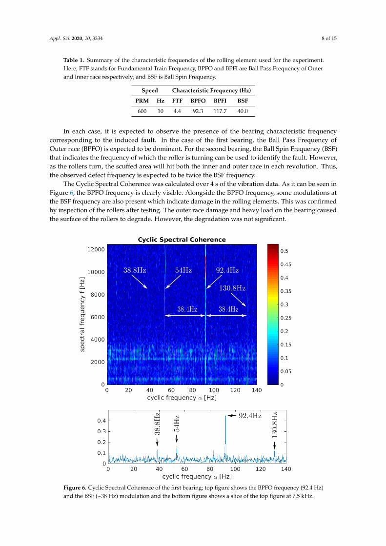
Table 1. Summary of the characteristic frequencies of the rolling element used for the experiment.Here, FTF stands for Fundamental Train Frequency, BPFO and BPFI are Ball Pass Frequency of Outerand Inner race respectively; and BSF is Ball Spin Frequency.

Speed Characteristic Frequency (Hz)

PRM Hz FTF BPFO BPFI BSF

600 10 4.4 92.3 117.7 40.0

In each case, it is expected to observe the presence of the bearing characteristic frequencycorresponding to the induced fault. In the case of the first bearing, the Ball Pass Frequency ofOuter race (BPFO) is expected to be dominant. For the second bearing, the Ball Spin Frequency (BSF)that indicates the frequency of which the roller is turning can be used to identify the fault. However,as the rollers turn, the scuffed area will hit both the inner and outer race in each revolution. Thus,the observed defect frequency is expected to be twice the BSF frequency.

The Cyclic Spectral Coherence was calculated over 4 s of the vibration data. As it can be seen inFigure 6, the BPFO frequency is clearly visible. Alongside the BPFO frequency, some modulations atthe BSF frequency are also present which indicate damage in the rolling elements. This was confirmedby inspection of the rollers after testing. The outer race damage and heavy load on the bearing causedthe surface of the rollers to degrade. However, the degradation was not significant.

38.4Hz

92.4Hz54Hz38.8Hz

130.8Hz

38.4Hz

38.8Hz

54Hz

130.8Hz92.4Hz

Figure 6. Cyclic Spectral Coherence of the first bearing; top figure shows the BPFO frequency (92.4 Hz)and the BSF (~38 Hz) modulation and the bottom figure shows a slice of the top figure at 7.5 kHz.

Appl. Sci. 2020, 10, 3334 9 of 15

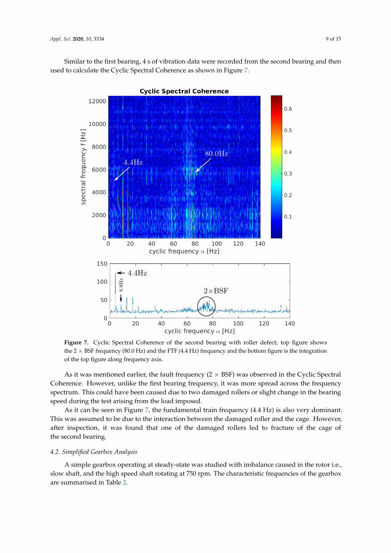
Similar to the first bearing, 4 s of vibration data were recorded from the second bearing and thenused to calculate the Cyclic Spectral Coherence as shown in Figure 7.

80.0Hz4.4Hz

8.8Hz

4.4Hz

2×BSF

Figure 7. Cyclic Spectral Coherence of the second bearing with roller defect; top figure showsthe 2 × BSF frequency (80.0 Hz) and the FTF (4.4 Hz) frequency and the bottom figure is the integrationof the top figure along frequency axis.

As it was mentioned earlier, the fault frequency (2 × BSF) was observed in the Cyclic SpectralCoherence. However, unlike the first bearing frequency, it was more spread across the frequencyspectrum. This could have been caused due to two damaged rollers or slight change in the bearingspeed during the test arising from the load imposed.

As it can be seen in Figure 7, the fundamental train frequency (4.4 Hz) is also very dominant.This was assumed to be due to the interaction between the damaged roller and the cage. However,after inspection, it was found that one of the damaged rollers led to fracture of the cage ofthe second bearing.

4.2. Simplified Gearbox Analysis

A simple gearbox operating at steady-state was studied with imbalance caused in the rotor i.e.,slow shaft, and the high speed shaft rotating at 750 rpm. The characteristic frequencies of the gearboxare summarised in Table 2.

Appl. Sci. 2020, 10, 3334 10 of 15

Table 2. The characteristic frequencies of the used gearbox at 740 rpm speed. Here the GAPF standsfor Gear Assembly Phase Frequency.

Feature Frequency (Hz)

Output Shaft 12.53rd Stage Gear-mesh 337.5

Interim Shaft 3.552nd Stage Gear-mesh 35.5

Slow Shaft 0.831st Stage Gear-mesh 11.6

1st GAPF 5.8Input Shaft 0.18

The Cyclic Spectral Coherence was calculated using 4 s vibration signals. The calculated resultsare presented in Figure 8. As the induced fault was imbalance, modulations and cyclic behaviour atthe gear-mesh (GM) frequency of the first stage of the gearbox (10.5 Hz) were caused.

10.5Hz 10.5Hz

10.5Hz10.5Hz

3.5Hz

5.3Hz

(a) (b)

(c) (d)

(e) (f)

Figure 8. Cyclic Spectral Coherence of unbalanced condition. From left to right the top row showsthe original signal and filtered signal using Wavelet Daubechies-3 (db3) filter. The middle row isthe first and second IMFs and the bottom row is 6th and 8th IMFs.

Appl. Sci. 2020, 10, 3334 11 of 15

As it can be seen in Figure 8a, the result from the analysis of the original raw signal is less clearin comparison with the bearing test. For comparison purposes, the analysis was also applied tothe de-noised signal using the Wavelet de-noising technique. This was carried out using Daubechies-3wavelet. However, de-noising the signal worsened the Cyclic Spectral Coherence result as it is shownin Figure 8b.

Using the EEMD technique, the signal was decomposed into 8 IMFs and the Cyclic SpectralCoherence of each IMF was calculated. The result of the first two IMFs is presented in Figure 8c,drespectively. As it can be seen, the result is slightly less contaminated compared with the rawand de-noised signal. However, more interestingly, in Figure 8e,f which shows the result on the 6thand 8th IMFs two other frequencies are visible. These frequencies are the first stage GAPF frequency(5.3 Hz) and the second stage rotational frequency (3.5 Hz).

The presence of both first stage gear mesh and GAPF cyclic behaviour clearly indicatesthe imbalance applied to the first stage. The existence of the second stage rotational frequencycould as well indicate the imbalance. Nonetheless, it can also show the normal vibration contaminatingthe signal.

4.3. Wind Turbine Gearbox Analysis

The studied gearbox in this part contained 11 different types of bearings. Including the correspondingfrequencies of the gears, more than 50 different frequencies of interest were available to analyse.In the present study only the result corresponding to the planetary stage of the gearbox and its bearingdefect are shown.

The vibration signal used to analyse the bearing defect at the planetary stage was obtained fromthe Radial sensor placed at the planetary stage of the gearbox.

The damaged bearing was a cylindrical roller bearing with its characteristic frequencies listed inTable 3. Given the wind turbine working at full rated load, the planets were turning at around 1.07 Hz.The other frequency of interest in the planetary stage fault is the gear-mesh of the planets which wascalculated to be 140.84 Hz. The next nearest calculated frequencies to this frequency were 99.1 Hzand 192.5 Hz belonging to the intermediate and high-speed shaft bearings.

Table 3. The unit characteristic frequencies and the operation characteristic frequencies of the bearingused for the planets in the monitored gearbox.

Speed Characteristic Frequency (Hz)

PRM Hz FTF BPFO BPFI BSF

60 1.00 0.405 5.676 8.323 2.55064 1.07 0.433 6.057 8.881 2.721

As it can be seen in the Figure 9a,b, the gear-mesh of the planets (140.8 Hz) are present in bothspectra, indicating possible damage in the planetary gear. It is also evident that the cyclic spectralcoherence of the first IMF of the signal is considerably less contaminated with noise originating fromother gears.

Appl. Sci. 2020, 10, 3334 12 of 15

(a) (b)

(c) (d)

Figure 9. Cyclic Spectral Coherence of vibration signal recorded from planetary gearbox of windturbine. From left to right the top row shows analysis on the original signal and its first IMF showingthe gear-mesh of the planets. Similarly, the bottom row is the analysis of the same signal (downsampled) and its first IMF showing the BPFI of the bearing of the planet.

Similarly in the Figure 9c,d, the Ball Passing Frequency of Inner race (BPFI) at 8.8 Hz is distinctlyvisible. The other closest present frequencies to this frequency are 7 Hz and 9.5 Hz correspondingto the sun gear defect and carrier bearing frequencies. Again, similar to the gear mesh analysisthe cyclostationary analysis on the first IMF of the signal shown in Figure 9d shows less artefactsrelated to the other gears.

For comparison purposes, the same signal recorded from the planetary stage was also analysedusing FFT, Hilbert transform and Cepstrum that are commonly used in condition monitoringand fault detection. As it can be seen in Figure 10a,b the gear-mesh frequency is not detectablein the applied Cepstrum, FFT or Hilbert analysis while the cyclic spectral coherence enhanced withEEMD preconditioning was able to detect it. Similarly, Figure 10c,d show the same analysis applied tothe signal to detect BPFI frequency. Similar to the gear mesh analysis, the BPFI frequency was notdetected using either Cepstrum or FFT analysis. Although, the Hilbert transform analysis showssome peaks around the BPFI frequency, the amplitude of the peaks are not very significant which canlead to underestimation of the severity. Again, using the cyclic spectral coherence with EEMD the BPFIfrequency was detected clearly reducing the likelihood of underestimation of the severity of the defect.

Appl. Sci. 2020, 10, 3334 13 of 15

(a) (b)

(c) (d)

Figure 10. Conventional techniques applied to vibration signal recorded from planetary gearboxof wind turbine with bearing and gear defect. (a) The Cepstral analysis on the original signal withred dashed line on 7.1 ms representing the gear-mesh of the planets at 140.8 Hz. (b) The Hanningwindowed single sided FFT amplitude of both original signal and its Hilbert transform with the reddashed line on 140.8 Hz corresponding to the plants gear-mesh. (c) Same as (a) with the red dashedline showing BPFI of the bearing of planets at 114 ms or 8.8 Hz. (d) Same as (b) with the red dashedline showing BPFI of the bearing of planets at 8.8 Hz.

5. Conclusions

The rapid growth in the use of wind turbines combined with their operation under severe loadingconditions has increased the need for efficient condition monitoring technologies. Early fault detectionis important for wind farm operators in order to improve predictive maintenance strategies, reduceunexpected downtime and associated repair costs. Continuously variable operation of the windturbines and complexity of the multi-stage gearboxes employed makes it very challenging to detectdeveloping faults particularly during the early stages of evolution.

The cyclostationary technique has been proven to be a very effective tool to detect faults inrotating machinery. However as the complexity of the system increases, the performance of thistechnique degrades and the results get contaminated with various artefacts coming from differentparts of the system.

In this paper the Ensemble Empirical Mode Decomposition technique was used to preconditionthe vibration signal prior to perform the cyclostationary technique. It has been shown that thiscan improve the performance of the cyclostationary technique and reduce the contamination inthe resulting analysed signals.

The Ensemble Empirical Mode Decomposition technique is a very powerful method that hasnot been fully explored in the field of wind turbine condition monitoring. The present study hasshown the potential of this technique to be employed in conjunction with other techniques to enhance

Appl. Sci. 2020, 10, 3334 14 of 15

the overall performance of various signal processing techniques in wind turbine gearbox conditionmonitoring. The ability of this technique to separate the signal into its intrinsic modes, as it wasdemonstrated in this paper, opens new opportunities in advanced signal processing that are yet to beexplored in more depth.

Author Contributions: S.R. and F.H. developed and carried out the signal processing methodology employed inthe study, M.P. organised and led the experiments carried out. All authors have read and agreed to the publishedversion of the manuscript.

Funding: This research was partially funded by European Union’s Seventh Framework grant number 322430.

Acknowledgments: The authors would like to thank the several industrial partners anonymised in this paper dueto confidentiality reasons for their support. The authors would also like to thank TWI Limited, Brunel Universityand INGETEAM service for their assistance with some of the tests. The authors are indebted to the EC for partiallyfunding this research as part of the OPTIMUS FP7 industrial collaborative project.

Conflicts of Interest: The authors declare no conflict of interest.

Abbreviations

The following abbreviations are used in this manuscript:

BPFI Ball Pass Frequency of Inner raceBPFO Ball Pass Frequency of Outer raceBSF Ball Spin FrequencyEEMD Ensemble Empirical Mode DecompositionEMD Empirical Mode DecompositionFTF Fundamental Train FrequencyGM Gear-meshGAPF Gear Assembly Phase FrequencyIMF Intrinsic Mode Function

References

1. Global Wind Statistics. Global Wind Report 2019. Available online: https://gwec.net/global-wind-report-2019 (accessed on 15 April 2020).

2. Barszcz, T. Vibration-Based Condition Monitoring of Wind Turbines, 1st ed.; Springer: Switzerland, 2019;doi:10.1007/978-3-030-05971-2. [CrossRef]

3. Pérez, J.M.P.; Márquez, F.P.G.; Tobias, A.; Papaelias, M. Wind turbine reliability analysis. Renew. Sustain.Energy Rev. 2013, 23, 463–472. [CrossRef]

4. Márquez, F.P.G.; Tobias, A.M.; Pérez, J.M.P.; Papaelias, M. Condition monitoring of wind turbines: Techniquesand methods. Renew. Energy 2012, 46, 169–178. [CrossRef]

5. Zhou, J.; Roshanmanesh, S.; Hayati, F.; Junior, V.J.; Wang, T.; Hajiabady, S.; Li, X.; Basoalto, H.; Dong, H.;Papaelias, M. Improving the reliability of industrial multi-MW wind turbines. Insight-Non Test. Cond. Monit.2017, 59, 189–195. [CrossRef]

6. Ferrando Chacon, J.L.; Andicoberry, E.A.; Kappatos, V.; Papaelias, M.; Selcuk, C.; Gan, T.H. An experimentalstudy on the applicability of acoustic emission for wind turbine gearbox health diagnosis. J. Low Freq. NoiseVib. Act. Control 2016, 35, 64–76. [CrossRef]

7. Fischer, K.; Pelka, K.; Puls, S.; Poech, M.H.; Mertens, A.; Bartschat, A.; Tegtmeier, B.; Broer, C.; Wenske, J.Exploring the Causes of Power-Converter Failure in Wind Turbines based on Comprehensive Field-Dataand Damage Analysis. Energies 2019, 12, 593. [CrossRef]

8. Junior, V.J.; Zhou, J.; Roshanmanesh, S.; Hayati, F.; Hajiabady, S.; Li, X.; Dong, H.; Papaelias, M. Evaluationof damage mechanics of industrial wind turbine gearboxes. Insight-Non Test. Cond. Monit. 2017, 59, 410–414.[CrossRef]

9. Van de Kaa, G.; van Ek, M.; Kamp, L.M.; Rezaei, J. Wind turbine technology battles: Gearbox versus directdrive-opening up the black box of technology characteristics. Technol. Forecast. Soc. Chang. 2020, 153, 119933.[CrossRef]

Appl. Sci. 2020, 10, 3334 15 of 15

10. Feng, Z.; Chu, F. Cyclostationary Analysis for Gearbox and Bearing Fault Diagnosis. Shock Vib. 2015, 2015.doi:10.1155/2015/542472. [CrossRef]

11. Dong, G.; Chen, J. Investigation into various techniques of cyclic spectral analysis for rolling element bearingdiagnosis under influence of gear vibrations. J. Phys. Conf. Ser. 2012, 364, 012039. [CrossRef]

12. Romero, A.; Lage, Y.; Soua, S.; Wang, B.; Gan, T.H. Vestas V90-3MW wind turbine gearbox health assessmentusing a vibration-based condition monitoring system. Shock Vib. 2016, 2016, 6423587. [CrossRef]

13. Gardner, W.A. (Ed.) An Introduction to Cyclostationary Signals. In Cyclostationarity in Communicationand Signal Processing; IEEE Press: New York, NY, USA, 1994; Chapter 1, pp. 1–90.

14. Giannakis, G.B. Cyclostationary Signal Analysis. In The Digital Signal Processing Handbook; Madisetti, V.K.,Williams, D.B., Eds.; IEEE Press: New York, NY, USA, 1997; Chapter 17.

15. Ishak, G.; Raad, A.; Antoni, J. Analysis of Vibration Signals Using Cyclostationary Indicators; Institute ofTechnology of Chartres: Chartres, France, 2013.

16. Antoni, J. Cyclic spectral analysis in practice. Mech. Syst. Signal Process. 2007, 21, 597–630. [CrossRef]17. Huang, N.E.; Long, S.R.; Shen, Z. The Mechanism for Frequency Downshift in Nonlinear Wave Evolution.

In Advances in Applied Mechanics; Academic Press: London, UK, 1996; Volume 32, pp. 59–117. [CrossRef]18. Huang, N.E.; Shen, Z.; Long, S.R.; Wu, M.C.; Shih, H.H.; Zheng, Q.; Yen, N.C.; Tung, C.C.; Liu, H.H.

The empirical mode decomposition and the Hilbert spectrum for nonlinear and non-stationary time seriesanalysis. Proc. R. Soc. Lond. A Math. Phys. Eng. Sci. 1998, 454, 903–995. [CrossRef]

19. Huang, N.E.; Shen, Z.; Long, S.R. A New View of Nonlinear Water Waves: The Hilbert Spectrum. Annu. Rev.Fluid Mech. 1999, 31, 417–457. [CrossRef]

20. Kizhner, S.; Blank, K.; Flatley, T.; Huang, N.E.; Patrick, D.; Hestnes, P. On the Hilbert-Huang TransformTheoretical Developments. 2005. Available online: https://ntrs.nasa.gov/search.jsp?R=20050210067(accessed on 20 April 2018).

21. Huang, N.E. Introduction to the Hilbert-huang Transform and Its Related Mathematical Problems.In Hilbert-Huang Transform and Its Applications, 2nd ed.; Huang, N.E., Shen, S.S.P., Eds.; World Scientific:Singapore, 2014; Chapter 1, pp. 1–26._0001. [CrossRef]

22. Lei, Y.; Lin, J.; He, Z.; Zuo, M.J. A review on empirical mode decomposition in fault diagnosis of rotatingmachinery. Mech. Syst. Signal Process. 2013, 35, 108–126. [CrossRef]

23. Wu, Z.; Huang, N.E. Ensemble Empirical Mode Decomposition: A Noise-Assisted Data Analysis Method.Adv. Adapt. Data Anal. 2009, 1, 1–41. [CrossRef]

c© 2020 by the authors. Licensee MDPI, Basel, Switzerland. This article is an open accessarticle distributed under the terms and conditions of the Creative Commons Attribution(CC BY) license (http://creativecommons.org/licenses/by/4.0/).