University of Alberta...determine concentration profiles during the sedimentation processes....

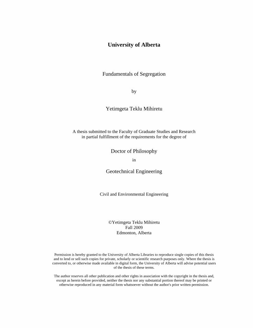
University of Alberta

Fundamentals of Segregation

by

Yetimgeta Teklu Mihiretu

A thesis submitted to the Faculty of Graduate Studies and Research in partial fulfillment of the requirements for the degree of

Doctor of Philosophy

in

Geotechnical Engineering

Civil and Environmental Engineering

©Yetimgeta Teklu Mihiretu Fall 2009

Edmonton, Alberta

Permission is hereby granted to the University of Alberta Libraries to reproduce single copies of this thesis and to lend or sell such copies for private, scholarly or scientific research purposes only. Where the thesis is

converted to, or otherwise made available in digital form, the University of Alberta will advise potential users of the thesis of these terms.

The author reserves all other publication and other rights in association with the copyright in the thesis and,

except as herein before provided, neither the thesis nor any substantial portion thereof may be printed or otherwise reproduced in any material form whatsoever without the author's prior written permission.

EXAMINING COMMITTEE

Dr. Rick Chalaturnyk, Supervisor, Civil and Environmental Engineering Dr. Dave Sego, Civil and Environmental Engineering Dr. William McCaffrey, Chemical and Materials Engineering Dr. Robert Driver, Civil and Environmental Engineering Dr. Ernest Yanful, External Examiner, University of Western Ontario

DEDICATION

To My wife Aparna and my son Aaron

and to My parents Ayelech and Teklu

ABSTRACT A common challenge during deposition of slurries is segregation as large particles settle

through the matrix of fines and water. Whether segregation occurs or not depends on the

grain size distribution of the solids, the void ratio or solids content and the rheological

properties of the fines-water matrix.

The rheological characterization of slurry composed of different grain sizes and varying

water chemistry was investigated. The vane yield stress was used to characterize different

slurries composed of clay, silt and sand materials. Semi-empirical fractal theory showed

good agreement with experimental data for fine slurry. Comparison of yield stress at

same concentration but different composition showed a decreasing trend as the

composition of either silt or sand material increases. The pore-water effect was studied

for representative kaolinite slurry. The yield stress was insensitive for pH values in the

acidic and neutral range, while in the basic range it showed significant response

depending upon the type of the chemical used to achieve the pH: Ca(OH)2 and NaOH.

A modified segmented standpipe was designed and used in a series of experiments to

determine concentration profiles during the sedimentation processes. Analyses of the

solid content profiles and sand content profiles in the standpipes indicated a capture of

sand particles which could be correlated to the yield stress of the fines matrix. Theoretical

calculations, however, showed over-prediction of the captured sand size. A correction

factor of about 0.2 was applied.

Flume test on a high solid content slurries showed that the dynamic segregation is

governed by all the factors governing the static case. Beaching profile shapes were not a

necessary indication of segregating and non-segregating type of slurries. Modified

version plastic theory for flow slides was used to characterise profile shape.

Computational fluid dynamics approaches based on kinetic theory and bi-viscous model

analysis were implemented and showed a reasonable capability in modelling segregation

when compared with experimental results. A statistical formulation for segregation index,

SI, was proposed. The index accounts for variation in depth of samples. Finally

recommendations for future research are proposed based on the observations and findings

made from the study.

ACKNOWLEDGMENTS I would like to thank my supervisor, Dr. Rick J. Chalaturnyk for his advice and

consummate support during the periods of the research and study. I cannot thank him

enough for his kindness, support and friendship right from the beginning.

I am grateful to Dr. J. Don Scott for his advice and guidance through his vast experience

in Oil Sands study. I am also thankful to my friends with whom I have had inspiring and

learning discussions.

I would like to thank also Gerry Cyre, Steve Gamble, Christine Hereygers, Gilbert Wong

and Ken Leung for their laboratory and technical support throughout the experimental

work.

The support from Oil Sands Tailings Research Facility (OSTRF) is greatly appreciated. I

want to thank also Alberta Research Council (ARC) for the use of their RS Soft Solid

Tester Rheometer.

I am indebted to M.techs Teklu Birru and Tesfaye Sabir for their invaluable guide and

assistance I simply took for granted.

At last but not least, I am also highly indebted to my parents and family for their

continuous love, patience and support.

TABLE OF CONTENTS

1. INTRODUCTION ...................................................................................... 1

1.1 General...................................................................................................................... 1 1.2 Motivation of Study .................................................................................................. 3 1.3. Objective of the Research Program ......................................................................... 6 1.4 Statement of the Problem.......................................................................................... 6 1.5. Organization of the thesis ........................................................................................ 7 1.6 Scope of the thesis .................................................................................................... 7 1.7. References................................................................................................................ 8

2. LITERATURE REVIEW ......................................................................... 11

2.1 General.................................................................................................................... 11 2.2 Theoretical Background.......................................................................................... 14

2.2.1 Suspension properties ...................................................................................... 14 2.2.2 Theory of Sedimentation.................................................................................. 15 2.2.3 Kynch theory of batch sedimentation .............................................................. 17

2.4. Experimental and model studies ............................................................................ 18 2.4.1 Monodisperse Suspension................................................................................ 18 2.4.2 Bi-disperse suspension..................................................................................... 21 2.4.3 Poly-disperse suspension ................................................................................. 21

2.5 Granular Flow and Segregation .............................................................................. 23 2.6. Segregation Study in Tailing Management............................................................ 26

2.6.1 Oil Sand Fine Tails .......................................................................................... 27 2.6.2 Soil Structure-Behaviour Diagram .................................................................. 29 2.6.3. Use of admixtures ........................................................................................... 31

2.7. References.............................................................................................................. 32 3. GEOTECHNICAL AND RHEOLOGICAL CHARACTERIZATION... 43

3.1 Introduction............................................................................................................. 43 3.2 Previous works (Literature review and Background) ............................................. 43 3.3 Theoretical Considerations ..................................................................................... 48

3.3.1 Rheological Characteristics ............................................................................. 48 3.3.2 Empirical models for flow curve ..................................................................... 50 3.3.3. The principle of yield stress calculation based on vane method..................... 51

3.4 Materials and Experimental Methods ..................................................................... 53 3.5 Results and discussion Section ............................................................................... 56

3.5.1 Test of the working principle........................................................................... 56 3.5.2 Comparison of vane yield stress with rheological model ................................ 63 3.5.3 The effect of pore water chemistry .................................................................. 65 3.5.4 Rheological measurements of oil sands tailings .............................................. 68

3.6 Summary and Conclusion ....................................................................................... 69 3.7. References.............................................................................................................. 70

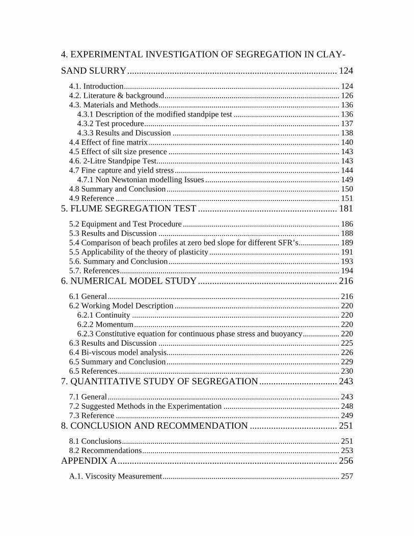
4. EXPERIMENTAL INVESTIGATION OF SEGREGATION IN CLAY-

SAND SLURRY......................................................................................... 124

4.1. Introduction.......................................................................................................... 124 4.2. Literature & background...................................................................................... 126 4.3. Materials and Methods......................................................................................... 136

4.3.1 Description of the modified standpipe test .................................................... 136 4.3.2 Test procedure................................................................................................ 137 4.3.3 Results and Discussion .................................................................................. 138

4.4 Effect of fine matrix.............................................................................................. 140 4.5 Effect of silt size presence .................................................................................... 143 4.6. 2-Litre Standpipe Test.......................................................................................... 143 4.7 Fine capture and yield stress ................................................................................. 144

4.7.1 Non Newtonian modelling Issues .................................................................. 149 4.8 Summary and Conclusion ..................................................................................... 150 4.9 Reference .............................................................................................................. 151

5. FLUME SEGREGATION TEST ........................................................... 181

5.2 Equipment and Test Procedure ............................................................................. 186 5.3 Results and Discussion ......................................................................................... 188 5.4 Comparison of beach profiles at zero bed slope for different SFR’s.................... 189 5.5 Applicability of the theory of plasticity ................................................................ 191 5.6. Summary and Conclusion.................................................................................... 193 5.7. References............................................................................................................ 194

6. NUMERICAL MODEL STUDY........................................................... 216

6.1 General.................................................................................................................. 216 6.2 Working Model Description ................................................................................. 220

6.2.1 Continuity ...................................................................................................... 220 6.2.2 Momentum..................................................................................................... 220 6.2.3 Constitutive equation for continuous phase stress and buoyancy.................. 220

6.3 Results and Discussion ......................................................................................... 225 6.4 Bi-viscous model analysis..................................................................................... 226 6.5 Summary and Conclusion ..................................................................................... 229 6.5 References............................................................................................................. 230

7. QUANTITATIVE STUDY OF SEGREGATION................................. 243

7.1 General.................................................................................................................. 243 7.2 Suggested Methods in the Experimentation ......................................................... 248 7.3 Reference .............................................................................................................. 249

8. CONCLUSION AND RECOMMENDATION ..................................... 251

8.1 Conclusions........................................................................................................... 251 8.2 Recommendations................................................................................................. 253

APPENDIX A............................................................................................. 256

A.1. Viscosity Measurement....................................................................................... 257

A.2. Procedure ............................................................................................................ 257 A.3. Calibration........................................................................................................... 258 A.4. Viscosity measurement ....................................................................................... 259 A5 Rheological Measurements of Tailings Materials ................................................ 264

APPPENDIX B........................................................................................... 296

Equation derivation for settling of sphere in a fluid with yield stress ........................ 297 APPENDIX C ............................................................................................. 301

C.1. Effect of Mixing on Segregation......................................................................... 302 C.2. Procedure............................................................................................................. 302 C.3. Results and discussion......................................................................................... 303 C.4. Summary and conclusion .................................................................................... 304

Appendix D................................................................................................. 312

Segregation Index Calculation.................................................................................... 313 Statistical Comparisons of Model fits......................................................................... 315

LIST OF TABLES Table 3-1 Models of fluid characterization....................................................................... 50 Table 3-2 Material Properties ........................................................................................... 53 Table 3-3 Dimensions of the vanes used in yield stress measurement ............................. 54 Table 3-4 Test schedule for vane shear experiment.......................................................... 56 Table 3-5 Summary of yield stress based on measured maximum torque ....................... 57 Table 3-6 Range of fine sizes according to different references ...................................... 61 Table 3-7 Comparison of yield stress as obtained from different methods ...................... 64 Table 3- 8 Statistical comparison of rheological model fits ............................................. 65 Table 5-1 Design test solid contents and sand fine ratio for flume segregation test ...... 187 Table A-1 Calibration Template for analyzing calibration results ................................. 260 Table A- 2 Mature Fine Tailings sample properties as-received. ................................... 264 Table A- 3Table A-3 Solid content of samples at different bulk densities..................... 264 Table C-1 Test schedule for turbulent mixing and standpipe test .................................. 303 Table D-1 Segregation index calculation for testing at 15 sec ....................................... 314 Table D-2 Flume test Segregation Index (SI) calculations............................................. 314 Table D- 3 AICc Calculation for 40% kao slurry ........................................................... 316 Table D- 4 AICc Calculation for 50% kao-sil slurry...................................................... 317

LIST OF FIGURES Figure 2-1 Forces acting on spherical particle in a liquid................................................. 36 Figure 2-2 Batch settling curve (from Diplas and Papanicolaou 1997)............................ 37 Figure 2-3 Segregation process during sedimentation of binary species suspension ....... 38 Figure 2-4 Formation of zones in sedimentation of poly-disperse suspension (after

Mirza and Richardson 1973).......................................................................... 39 Figure 2-5 Deposition mechanism in tailings impoundment (after Yong 1984) .............. 40 Figure 2-6 Tailing Design Diagram showing different Boundaries (after (Fine

Tailings Fundamentals Consortium 1995)..................................................... 41 Figure 2-7 Shifting of Segregation Boundary due to addition of flocculant (after

(Chalaturnyk and Scott 2001))....................................................................... 42 Figure 3-1 Flow Curves for different non-Newtonian materials. (a) Viscoplastic;

(b) Bingham plastic (c) Pseudoplastic (d) Newtonian (e) Dilatant ................ 74 Figure 3-2 Vane Geometry ............................................................................................... 75 Figure 3-3 Grain size distribution of the material used to prepare the slurry ................... 76 Figure 3-4 Comparison of design and achieved sample solid content for kaolinite

slurry .............................................................................................................. 77 Figure 3-5 Relationship between maximum torque and geometrical parameter for

kaolinite slurry(50%w/w) at shear rates (a) 0.01/s and (b) 0.02/s ................. 78 Figure 3-6 Relationship between maximum torque and modified geometrical

parameter for kaolinite slurry (50%w/w) at shear rates 0.01/s and 0.02/s, when the shear surface is at diameter 5% larger than the vane diameter.......................................................................................................... 80

Figure 3-7 Yield stress variation with solid content at different shearing rate................. 81 Figure 3-8 Variation of %Torque (reference 5mNm) with time for 30%s, kaolinite

slurry at different rates ................................................................................... 82 Figure 3-9 Variation of shear stress with time for kaolinite slurry (30%s) at

different rates ................................................................................................. 83 Figure 3-10 Variation of shear stress(SS) and % Torque(%M) with time for 50%-

kaolinite slurry @ a rate 0.01/s ...................................................................... 84 Figure 3-11 Variation of shear stress with time for kaolinite slurry (40%s) at

different rates ................................................................................................. 85 Figure 3-12 Variation of % Torque with time for kaolinite slurry (40%s) at

different rates ................................................................................................. 86 Figure 3-13 Variation of shear stress with time for kaolinite slurry (50%s) at


different rates ................................................................................................. 88 Figure 3-15 Variation of shear stress with time for kaolinite slurry (55%s) at


different rates ................................................................................................. 90

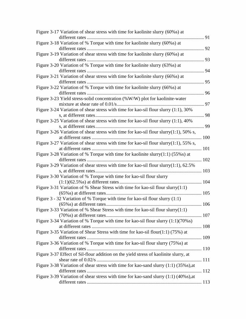
Figure 3-17 Variation of shear stress with time for kaolinite slurry (60%s) at different rates ................................................................................................. 91

Figure 3-18 Variation of % Torque with time for kaolinite slurry (60%s) at different rates ................................................................................................. 92





Figure 3-23 Yield stress-solid concentration (%W/W) plot for kaolinite-water mixture at shear rate of 0.01/s........................................................................ 97

Figure 3-24 Variation of shear stress with time for kao-sil flour slurry (1:1), 30% s, at different rates.......................................................................................... 98

Figure 3-25 Variation of shear stress with time for kao-sil flour slurry (1:1), 40% s, at different rates.......................................................................................... 99

Figure 3-26 Variation of shear stress with time for kao-sil flour slurry(1:1), 50% s, at different rates ........................................................................................... 100

Figure 3-27 Variation of shear stress with time for kao-sil flour slurry(1:1), 55% s, at different rates ........................................................................................... 101

Figure 3-28 Variation of % Torque with time for kaolinite slurry(1:1) (55%s) at different rates ............................................................................................... 102

Figure 3-29 Variation of shear stress with time for kao-sil flour slurry(1:1), 62.5% s, at different rates........................................................................................ 103

Figure 3-30 Variation of % Torque with time for kao-sil flour slurry (1:1)(62.5%s) at different rates .................................................................... 104

Figure 3-31 Variation of % Shear Stress with time for kao-sil flour slurry(1:1) (65%s) at different rates............................................................................... 105

Figure 3 - 32 Variation of % Torque with time for kao-sil flour slurry (1:1) (65%s) at different rates............................................................................... 106

Figure 3-33 Variation of % Shear Stress with time for kao-sil flour slurry(1:1) (70%s) at different rates............................................................................... 107

Figure 3-34 Variation of % Torque with time for kao-sil flour slurry (1:1)(70%s) at different rates ........................................................................................... 108

Figure 3-35 Variation of Shear Stress with time for kao-sil flour(1:1) (75%) at different rates ............................................................................................... 109

Figure 3-36 Variation of % Torque with time for kao-sil flour slurry (75%s) at different rates ............................................................................................... 110

Figure 3-37 Effect of Sil-flour addition on the yield stress of kaolinite slurry, at shear rate of 0.02/s ....................................................................................... 111

Figure 3-38 Variation of shear stress with time for kao-sand slurry (1:1) (35%s),at different rates ............................................................................................... 112

Figure 3-39 Variation of shear stress with time for kao-sand slurry (1:1) (40%s),at different rates ............................................................................................... 113

Figure 3-40 Variation of shear stress with time for kao-sand mix (1:1), 50%s, at different shear rates...................................................................................... 114

Figure 3-41 Shear stress variation with time for kosand mix(1:1), 60%s, at different rates ............................................................................................... 115

Figure 3-42 Effect of Sand addition on the yield stress of kaolinite slurry, at shear rate of 0.02/s................................................................................................. 116

Figure 3-43 Shear Variation with time for different compositions at 60% solids @ 0.02/s ............................................................................................................ 117

Figure 3-44 Flow curve for kaolinite slurry 40%s(w/w) and Herschel-Bulkley (HB)model fit with KHB=2.855, n=0.3105 and τy=11.49 Pa ....................... 118

Figure 3-45 Flow curve for kaolinite slurry 40%s(w/w) and Casson’s model fit with Kc=0.0248, and τc=12.1466 Pa............................................................ 119

Figure 3-46 Flow curve for kaolinite Sil flour(1:1) slurry 50%s(w/w) and Herschel-Bulkley (HB)model fit with KHB=1.056, n=0.6429 and τy=11.0 Pa .................................................................................................... 120

Figure 3-47 Flow curve for kaolinite Sil-flour(1:1) slurry 50%s(w/w) and Casson’s model fit with Kc=0.0593, and τc=10.131 Pa ............................... 121

Figure 3-48 Variation shear stress at different pH values for kaolinite slurry @50% s ........................................................................................................ 122

Figure 3-49 The variation of yield stress with pH for kaolinite slurry 50% s ................ 123 Figure 4-1Grain size distribution of test materials ......................................................... 158 Figure 4-2 Schematic drawing (left) and picture (right) of modified standpipe............. 159 Figure 4-3 Ternary diagram for a slurry ......................................................................... 160 Figure 4-4 Solid and sand content profile of slurry at SFR=1, FWR=10 and an initial

solids content of 18.8% at different elapsed times ................................................. 161 Figure 4-5 Solid and sand content profile of slurry at SFR=1, FWR=15 and an initial










solids content of 46.9% at different elapsed times ................................................. 172

Figure 4-15 Solid and sand content profile of slurry at SFR=4, FWR=20 and an initial solids content of 55.6% at different elapsed times ................................................. 173

Figure 4-16 Yield stress measurement (left) and rheogram (right) with Herschel-Bulkley model fit .................................................................................................................. 174

Figure 4-17 Solid and sand content profile in different composition of clay and silt size composition at a time of 15 min ............................................................................. 175

Figure 4- 18 Solid and sand content profile of kaolin sand slurry at constant fine water ratio of 20% and different sand fine ratio ............................................................... 176

Figure 4- 19 Solid and sand content profile of kaolin sand slurry at constant fine water ratio of 30%and different sand fine ratio ................................................................ 177

Figure 4- 20 Solid and sand content profile of kaolin sand slurry at constant fine water ratio of 45% and different sand fine ratio ............................................................... 178

Figure 4-21 Solid content profiles of Figure 4.19 after being renormalized with respect to the initial solid content ratio ................................................................................... 179

Figure 4-22 Solid content profiles of Figure 4.20 after being renormalized with respect to the initial solid content ratio ................................................................................... 180

Figure 5-1 Master Beach Profile for Equation 5.3...........................................................197 Figure 5-2 Schematic of flume apparatus ....................................................................... 198 Figure 5-3 Solid and Sand content profile along the flume length test1, 57.17%s,

SFR=1, zero-slope........................................................................................ 199 Figure 5-4 Solid and Sand content profile along the flume length test1, 57.2%s,

SFR=1, slope 5% ......................................................................................... 200 Figure 5-5 Solid and Sand content profile along the flume length test1, 57.14%s,

SFR=1, slope =10% ..................................................................................... 201 Figure 5- 6 Beach profile along the flume length test set 1 at different slopes .............. 202 Figure 5-7 Solid and sand content profiles of standpipe test on material collected

from flume downstream end ........................................................................ 203 Figure 5-8 Beach profile along the flume length for test set 2 (57.75%s, SFR=2) at

different slopes............................................................................................. 204 Figure 5-9 Solid and sand content profile for sample deposit in a standpipe at the

5% slope- flume end .................................................................................... 205 Figure 5-10 Solid and Sand content profile for sample deposited in a standpipe

after exited from the 10% slope-flume end.................................................. 206 Figure 5-11 Beach profile along the flume length test set 3 (55.6%s, SFR=4) at

different slopes............................................................................................. 207 Figure 5-12 Solid and sand content profile along the flume length test set 3 and

zero bed slope............................................................................................... 208 Figure 5-13 Solid and sand content profile along the flume length test set 3 and

5% bed slope ( 55.6%s, SFR=4) .................................................................. 209 Figure 5-14 Solid and sand content profile along the flume length test set 3 and

10% bed slope (design slurry: 55.6%s, SFR=4) .......................................... 210 Figure 5-15 Solid and sand content profile for sample deposit in a standpipe at the

zero- slope- flume end. (design slurry: 55.6%s, SFR= 4)............................ 211 Figure 5-16 Solid and sand content profile for sample deposit in a standpipe at the

10%- slope- flume end. (design slurry: 55.6%s, SFR= 4) ........................... 212

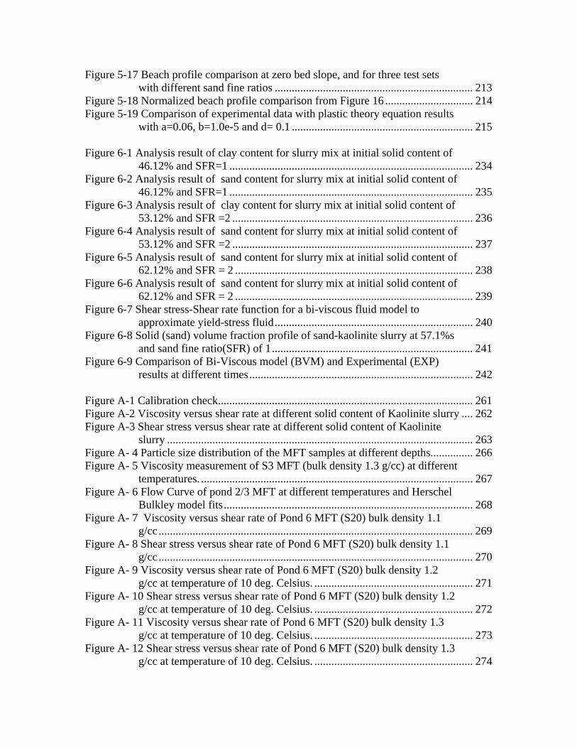
Figure 5-17 Beach profile comparison at zero bed slope, and for three test sets with different sand fine ratios ...................................................................... 213

Figure 5-18 Normalized beach profile comparison from Figure 16 ............................... 214 Figure 5-19 Comparison of experimental data with plastic theory equation results

with a=0.06, b=1.0e-5 and d= 0.1 ................................................................ 215 Figure 6-1 Analysis result of clay content for slurry mix at initial solid content of

46.12% and SFR=1 ...................................................................................... 234 Figure 6-2 Analysis result of sand content for slurry mix at initial solid content of

46.12% and SFR=1 ...................................................................................... 235 Figure 6-3 Analysis result of clay content for slurry mix at initial solid content of

53.12% and SFR =2 ..................................................................................... 236 Figure 6-4 Analysis result of sand content for slurry mix at initial solid content of

53.12% and SFR =2 ..................................................................................... 237 Figure 6-5 Analysis result of sand content for slurry mix at initial solid content of

62.12% and SFR = 2 .................................................................................... 238 Figure 6-6 Analysis result of sand content for slurry mix at initial solid content of

62.12% and SFR = 2 .................................................................................... 239 Figure 6-7 Shear stress-Shear rate function for a bi-viscous fluid model to

approximate yield-stress fluid...................................................................... 240 Figure 6-8 Solid (sand) volume fraction profile of sand-kaolinite slurry at 57.1%s

and sand fine ratio(SFR) of 1....................................................................... 241 Figure 6-9 Comparison of Bi-Viscous model (BVM) and Experimental (EXP)

results at different times............................................................................... 242 Figure A-1 Calibration check.......................................................................................... 261 Figure A-2 Viscosity versus shear rate at different solid content of Kaolinite slurry .... 262 Figure A-3 Shear stress versus shear rate at different solid content of Kaolinite

slurry ............................................................................................................ 263 Figure A- 4 Particle size distribution of the MFT samples at different depths............... 266 Figure A- 5 Viscosity measurement of S3 MFT (bulk density 1.3 g/cc) at different

temperatures. ................................................................................................ 267 Figure A- 6 Flow Curve of pond 2/3 MFT at different temperatures and Herschel

Bulkley model fits........................................................................................ 268 Figure A- 7 Viscosity versus shear rate of Pond 6 MFT (S20) bulk density 1.1

g/cc ............................................................................................................... 269 Figure A- 8 Shear stress versus shear rate of Pond 6 MFT (S20) bulk density 1.1

g/cc ............................................................................................................... 270 Figure A- 9 Viscosity versus shear rate of Pond 6 MFT (S20) bulk density 1.2

g/cc at temperature of 10 deg. Celsius. ........................................................ 271 Figure A- 10 Shear stress versus shear rate of Pond 6 MFT (S20) bulk density 1.2

g/cc at temperature of 10 deg. Celsius. ........................................................ 272 Figure A- 11 Viscosity versus shear rate of Pond 6 MFT (S20) bulk density 1.3

g/cc at temperature of 10 deg. Celsius. ........................................................ 273 Figure A- 12 Shear stress versus shear rate of Pond 6 MFT (S20) bulk density 1.3

g/cc at temperature of 10 deg. Celsius. ........................................................ 274

Figure A- 13 Viscosity versus shear rate of Pond 6 MFT (S20) bulk density 1.4 g/cc at temperature of 10 deg. Celsius. ........................................................ 275

Figure A- 14 Shear stress versus shear rate of Pond 6 MFT (S20) bulk density 1.4 g/cc at temperature of 10 deg. Celsius. ........................................................ 276













Figure A- 27 Viscosity versus shear rate of Pond 6 MFT (S42) bulk density 1.3g/cc at temperature of 10 deg. Celsius. ................................................... 289


Figure A- 29 Viscosity versus shear rate of Pond 6 MFT (S42) bulk density 1.4g/cc at temperature of 10 deg. Celsius. ................................................... 291


Figure A- 31 Viscosity versus shear rate of thickener underflow fines at different solid content. ................................................................................................ 293

Figure A- 32 Shear stress versus shear rate of thickener underflow fines at different solid contents................................................................................. 294

Figure A- 33 Yield stress measurement of thickener underflow fines at solid content of 35% and pH of 12 achieved by Ca(OH)2 and NAOH additions. ...................................................................................................... 295

Figure B-1 Free body diagram of a sphere of radius R suspended in a fluid ................. 297

Figure B-2 Drag coefficient versus Reynolds number without taking yield stress into account (Data from Dedegil, 1986, Valentik and Whitmore, 1965)..... 299

Figure B-3 Drag coefficient versus Reynolds number taking yield stress into account (Data from Dedegil, 1986, Valentik and Whitmore, 1965)............ 300

Figure C-2 SEM image of sand particles passing 250micron sieve and retained in

125 mm sieve ............................................................................................... 305 Figure C-3 SEM image of sand particles passing 425 micron sieve and retained in

250micron sieve ........................................................................................... 306 Figure C-4 SEM image of sand particles passing 2 mm sieve and retained in 425

mm sieve ...................................................................................................... 307 Figure C-5 Solid and Sand Content Profiles; (a) and (b) for DS1, (c) and (d) for

DS2, (e) and (f) for DS3............................................................................... 308 Figure C-6 Sedimentation of sample for test sets DS1 after mixing .............................. 309 Figure C-7 Sedimentation of sample for test sets DS2 after mixing .............................. 310 Figure C-8 Sedimentation of samples for test sets DS3 after mixing............................. 311

1

CHAPTER 1

1. INTRODUCTION

1.1 General Segregation is a phenomenon by which certain sizes or components with similar

properties tend to preferentially collect in one or another physical zone of the assembly.

Segregation commonly occurs in many natural and man-made processes: the sorted layers

of magma, rock or ice avalanches, and seasonal stream deposits are a few among many

natural events. In industry, where bulk materials are handled and transported, segregation

may result in poor product quality as in pharmaceutical, ceramic, cement and food

processing. On the other hand ore extraction processes exploit the advantage of

differential settling. In oil sands extraction process, the bitumen is separated as a froth

which floats to the surface; the coarse sand settles to the bottom and is removed. A

portion of this slurry, known as middling, is removed from the central portion of the

vessel, and is further processed.

Since segregation is a common problem of profound significance that touches many

disciplines, it has been a subject of interest to mathematicians, physicists, engineers and

industrial community. The studies are associated with different problems as

sedimentation, consolidation, fluidization, erosion and mass transport (Pane and

Schiffman, 1997). The study of segregation in civil engineering is relevant in sediment

transport (Graf 1973), mud flow (Coussot 1997) and in granular flow problems (Savage

1979). Current development in the subject matter has extended to the application in rock

(ice) avalanches, debris flow, sand dunes and oil sands waste management.

While sedimentation and consolidation have received a great deal of treatment in soil

engineering, the emphasis has been mainly on fine and uniform soils. The consolidation

theory treats the small displacement of soil as a result of water drainage by the excess

pore pressure development. The groundwater and seepage studies are concerned with the

relative movement of liquids to the soil grains. The flow of the soil grains with the

2

interacting fluid medium as multiphase flow appears to be still on the course of

development.

The disposal of high water content soil like materials and the reclamation of disturbed

land have been recognized as a major challenge to geotechnical engineers (Krizek, 2000).

He further stressed that growing safety issues such as risk-free environment and public

safety and the need to integrate reclamation into the planning and design process dictate

that much more remains to be done. Two major challenges were identified with mine

wastes; the large volume they occupy and the great variability in properties. According to

his estimate the annual total worldwide mine waste is in the order of a billion cubic

meters or more, and the impoundments for these wastes are among the largest in the

world.

With respect to oil sand tailings in Alberta, Morgenstern and Scott (1997) indicated that

at the early stage of mine development, the storage volume required by tailings is three

times the volume of oil sand mined and processed. These large volumes of tailings and

their segregating characteristics were less understood and posed design and planning

problems early in the history of oil sands mining. According to their report, the Syncrude

tailings pond, which was designed to provide storage for 550 x 106 m3 of sand, 370 x

106m3 of fine tails and 50 x 106 m3 of water, required a construction of 18km dyke

ranging from 32 m to 90 m in final height occupying a surface area of 22km2.

The most convenient and economical method for mining waste disposal is to impound

them hydraulically. However such disposal schemes commonly yield settling of coarse

and large size particles on the dyke beaches and transport of fine particles farther in the

pond forming fine tailings. The major problems associated with a segregating type of

tailings are:

• High operating costs

• Large volume to store and high lease costs

• Liquefaction susceptibility of sand beaches and low strength

• Toxicity and high environmental risks

3

• Slow settling rate and thus less quantity of release water to recycle

• Monitoring cost and difficulty in long term reclamation of the land

• Difficulty of mining the ores underneath the pond.

Cooper (1988) pointed out that the successful management of large dam tailings storage

implicitly requires an understanding of the mechanics of slurry flow, the principles of

drainage and consolidation and importantly, the development of the strength of the

tailings. He also listed the most relevant geotechnical parameters which influence tailings

storage construction: bearing capacity, moisture content/compactive effort relationship,

permeability, shrinkage, consolidation, rate of loss of moisture (from beach area). It is

necessary that the planning, design, operation, and reclamation of impoundment areas

containing tailings be dealt not necessarily with traditional geotechnical approaches but

rather it should involve expertise from other disciplines.

1.2 Motivation of Study For the oil sands mining process, approximately 15 to 20 percent of the ore results in

bitumen concentrate; the rest of the bulk material ends up as waste material. Such large

quantity of waste cannot be disposed to the local environment, due to the presence of

some constituents, which are not compatible with the environment. Thus safe disposal is

a critical requirement and in most cases, the waste materials or tailings, are discharged

into a tailings pond. The major concern upon deposition is that the coarse materials

segregate and form a beach close to the dyke while the fine materials are transported

further to the middle of the pond where they remain in suspension and undergo extremely

slow sedimentation. This disposal scheme is accompanied by some consequences; such

as leachate, liquefaction susceptibility and poor reclamation of release water for recycling

due to the very slow settling rate in the pond.

Moreover the large volume occupied by the tailing ponds incur significant cost on lease

and monitoring of the surroundings for any associated risks such as stability of dykes and

seepage to the local groundwater system. Caughill (1992) remarked that the solution to

such tailing problems should ideally include, one-step disposal, a reclaimable surface,

4

low cost and high safety, reclaim of water, leachate control and reduction in total storage

volume.

Hence, the handling of mine waste seeks an optimal disposal scheme. Production of non

segregating tailings is currently viewed as a solution to either the existing tailing

management challenges or future planning. Achievement of non-segregating tailings

requires a fundamental understanding of the behavior of the constituents and the

governing mechanisms involved.

Generally, the mechanisms which govern the segregation process are still not well

defined, owing to the complex nature of the process where particle features such as

particle size and distribution, shape, density, chemical affinity and many others contribute

to the complexity. The subject has been regarded as an engineering frontier by some

(Savage 1979) and as the focus of debate among others (Edwards and Grinev 2003).

Boogerd et al. (2001) have gone further to question whether something is missed. There

exists no unified model which can predict the occurrence of segregation while

incorporating all relevant factors over the wide range of flow regimes. Attempts,

however, have been made to characterise dominant mechanisms over narrow ranges of

conditions.

The segregation process, primarily, occurs under subaqueous and subaerial environment.

The sedimentation process refers closely to the former and granular flow to the latter.

When solid phases interact with fluid, e.g., water, sedimentation / segregation occur by

the action of gravity due to size or density differences among particles. The subject of

sedimentation involving suspensions containing mixed particle sizes is not well

developed, and reliable relationships have not been available. This is because of the wide

range of particles sizes, the variety of particles shapes, and the complex nature of the

hydrodynamic and physicochemical phenomena which governs particle-fluid and

particle-particle behaviour (Selim et al., 1983). Nevertheless, it is common among

engineers to deal with their complex problems in some pragmatic way based on

experimental evidence and past experience. For example, Terzaghi et al. (1995) stated

5

that success in geotechnical engineering, more than any other field of civil engineering,

depends on practical experience. i.e., experience has tailored the practice.

It appears that the study of sedimentation with application to industrial process has

received wide treatment in chemistry or chemical engineering and mining engineering.

The works in these areas can be seen mostly as experimental study supplemented by

semi-empirical models or simulation (Richardson and Zaki 1954); (Barnea and Mizrahi

1973); (Lockett and Al-Habboby 1973); (Lockett and Al-Habboby 1974); (Garside and

Al-Dibouni 1977); (Mirza and Richardson 1979); (Selim et al. 1983); (Zimmels 1983).

Some study in the subject matter has also been made in the geotechnical field with

emphasis, however, on certain soil types, namely, fine clays (McRoberts and Nixon

1976); (Been and Sills 1981); (Tan et al. 1990); (Toorman 1996); (Pane and Schiffman

1997); (Toorman 1999).

Soil, as encountered in nature, is rarely uniform and dealing with this heterogeneity in

mine waste management is an issue where the mine processing industry produces large

volumes of waste. The development of effective disposal schemes for this situation has

become a major challenge to the geotechnical engineer. For example, Eckert et al. (1996)

described the nature of the sedimentation/consolidation process in oil sand tailings as

very complex, due to the presence of ultra-fines and some chemicals, and the

sedimentation/consolidation process is expected to take very long time (centuries).

While most of the forgoing studies presented are associated with a quasi-static

environment, the sedimentation /segregation phenomenon is also common in the process

of mixing, transportation and deposition. These processes are collectively referred to as

dynamic segregation. Some valuable contributions on dynamic segregation are found in

sediment transport studies in hydraulic engineering (Graf,1973), (Vanoni et al. 1975),

(Garde and Ranga Raju, 1977), and (Choux and Druitt 2002).

The investigation made by Kuepper (1991) has indicated the existence of segregation

(hydraulic sorting) of the hydraulic fill both in laboratory and field experimentation.

6

While her work typically dealt with the hydraulic deposition of segregating slurries, it

was mentioned that non-segregating slurries exhibit non-Newtonian rheology.

Morgenstern and Kuepper (1988) stressed that the ability to forecast and control grain

size separation is still limited. They further suggest the need for greater understanding of

the process. Such insights have notable significance in this research as to identify which

rheological characteristics, under segregating and non-segregating regimes, slurries may

exhibit, and their significance in the prediction models. Consequently, the stimulus for

this study comes from a desire to make available fundamental principles which contribute

to the basic understanding of the segregation process.

1.3. Objective of the Research Program The objective of this research program is to establish the fundamental factors controlling

segregation mechanisms in oil sand tailings under static and dynamic (shear) conditions.

The principal factors that will be studied include:

• The viscous and chemical nature of the fluid medium (Pore fluid).

• The grain-size distribution.

• Mechanical/shearing action.

• Flow mechanism.

1.4 Statement of the Problem The gap-graded nature of oil sand tailings stream accounts for the segregation of fines

from the sand grains. Accumulation of segregated fine tailings results in a large volume

of stable suspension with little release water and insignificant consolidation, incurring

increased operating costs and long term reclamation (Fine Tailings Fundamentals

Consortium 1995). The very stable nature of fine tailings is attributable to the gelation

characteristics of the ultrafines (<3μm) and the chemical composition of the pore water.

The effect of ultra fines on the macroscopic behaviour of fine tailings is manifested by

the rheological properties of the slurry. Rheological studies suggest that fine tailings

exhibit non-Newtonian characteristics. The significance of non-Newtonian behaviour has

7

also been indicated by Scott et al. (1985), who have explained in their experimental result

that the rheological (‘gel’, their term) strength of the slurry contributes to the capture of

sand grains resulting in non-segregating mixes.

Research dealing with the application of rheology of fines in segregation studies is not

well established and rarely linked to the hydrodynamics of the process. While

categorisation of the grain sizes of the tailing materials into two major divisions as fines

and sands appears simple and easy from practical point of view, the impact of such bulk

division is, however, unexplained. Since segregation by size is the major phenomena,

study of wide spectrum of sizes is necessitated. Nevertheless, there exists no adequate

research tool to provide data in the process of segregation. The different flow regimes

under which segregation occurs need also further investigation.

1.5. Organization of the thesis

A summarized outline is presented briefly as follows. The thesis comprises the following

chapters:

Chapter 1 Introduction

Chapter 2 Literature review

Chapter 3 Geotechnical and rheological characterization

Chapter 4 Static sedimentation/segregation experiments

Chapter 5 Flume segregation test

Chapter 6 Numerical modeling studies

Chapter 7 Quantitative analysis

Chapter 8 Conclusion and recommendation

1.6 Scope of the thesis

The material and rheological characterization tests are carried out with the available

laboratory equipment. All static standpipe tests are completed with one or two litre

standpipes and a custom-designed standpipe developed during this research program.

Even though the chemical interactions have influence on the macroscopic behaviour, the

8

microscopic influences due to chemical flocculent or coagulant addition are precluded in

this study. Moreover the water to be used in the standpipe test is tap water. Tailing

release water is used in all experiments involving tailing materials only. In the case of

examining some particular phenomena, the materials to be used may not be exactly

similar to the tailing materials, substitute materials are used as an option, keeping the

properties as closely similar as possible to that of tailing materials. In the dynamic

experimentation, the flume test is used. The study of segregation under pipe flow

conditions are not in the scope of this study. The concept of ‘similarity of process’ as

justified by Kuepper (1991) is applied in the experimental program of this research.

Time-dependent rheological properties, like creep and thixotropy are known to have

some influence on the long-term process of segregation; however, since the focus of the

current research is on immediate or short-term segregation mechanism, these rheological

characteristics are not investigated in this research study.

1.7. References Barnea, E., and Mizrahi, J. 1973. A Generalized Approach to the Fluid Dynamics of

Particulate Systems

Part 1. General Correlation for Fluidization and Sedimentation in Solid Multiparticle

Systems. The Chemical Engineering Journal, 5: 171-189.

Been, K., and Sills, G.C. 1981. Self-Weight Consolidation of soft soils: an experimental

and theoretical study. Geotechnique, 31(4): 519-535.

Boogerd, P., Scarlett, B., and Brouwer, R. 2001. Recent modelling of sedimentation of

suspended particles, A Survey. Irrigation and Drainage, 50: 109-128.

Caughill, D.L. 1992. Geotechnics of Non-segregating Oil Sands Tailings. MSc thesis,

University of Alberta, Edmonton.

Choux, C.M., and Druitt, T.H. 2002. Analogous study of particle segregation in

pyroclastic density currents, with implications for the emplacement mechanisms

of large ignimbrites. Sedimentology, 49: 907-926.

9

Cooper, D. 1988. Tailings management in Australia. In Hydraulic Fill Structures,

Speciality Conference. Edited by D.J.A. Van Zyl and S.G. Vick. Fort Collins.

ASCE, pp. 130-141.

Coussot, P. 1997. Mudflow Rheology and Dynamics. A.A.Balkema.

Eckert, W.F., Masliyah, J.H., Gray, M.R., and Fedorak, P.M. 1996. Prediction of

Sedimentation and Consolidation of Fine Tails. AIChE Journal, 42(4): 960-972.

Edwards, S.F., and Grinev, D.V. 2003. Statistical mechanics of granular materials:stress

propagation and distribution of contact forces. Granular Matter, 4(4): 147-153.

Fine Tailings Fundamentals Consortium, F. 1995. Clark Hot Water Extraction Fine

Tailings. In Advances in Oil Sand Tailings Research. Alberta Department of

Energy, Oil Sands and Research Division., Edmonton.

Garde, R.J., and Ranga Raju, K.G. 1977. Mechanics of sediment transportation and

alluvial stream problems. Wiley Eastern Ltd.

Garside, J., and Al-Dibouni, M.R. 1977. Velocity-Voidage Relationships for Fluidzation

and Sedimentation in Solid-Liquid Systems. Ind.Eng.Chem.,Process Des. Dev.,

16(2): 206-214.

Graf, W.H. 1973. Hydraulics of Sediment Transport. McGraw-Hill.

Krizek, R.J. 2000. Geotechnics of High Water Content Materials. In Geotechnics of High

Water Content Materials, ASTM STP 1374. Edited by T.B. Edil and P.J. Fox.

West Conshohocken, PA. ASTM.

Krizek, R.J. 2004. Slurries in Geotechnical Engineering, College Station, Texas.

Kuepper, A.A.G. 1991. Design of Hydraulic Fill. PhD, University of Alberta,

Edmonton,Canada.

Lockett, M.J., and Al-Habboby, H.M. 1973. Differential Settling by Size of Two Particles

in A Liquid. Trans.Instn.Chem.Engrs, 51: 281-292.

Lockett, M.J., and Al-Habboby, H.M. 1974. Relative Particle Velocities in Two-Species

Settling. Powder Technology, 10: 67-71.

McRoberts, E.C., and Nixon, J.F. 1976. A theory of soil sedimentation. Can.Geotech.J.,

13: 294-310.

Mirza, S., and Richardson, J.F. 1979. Sedimentation of Suspensions of Particles of Two

or More Sizes. Chemical Engineering Science, 34: 447-454.

10

Morgenstern, N.R., and Kuepper, A.A.G. 1988. Hydraulic Fill Structures- A Perspective.

In Hydraulic Fill Structures, Speciality Conference. Edited by D.J.A. Van Zyl and

S.G. Vick. Fort Collins. ASCE, pp. 1-31.

Morgenstern, N.R., and Scott, J.D. 1997. Oil Sand Geotechnique. Geotechnical News:

102-109.

Pane, V., and Schiffman, R.L. 1997. The permeability of clay suspension. Geotechnique,

47(2): 273-288.

Richardson, J.F., and Zaki, W.N. 1954. Sedimentation and Fluidization: Part I.

Trans.Instn.Chem.Engrs, 32: 35-78.

Savage, S.B. 1979. Gravity flow of cohesionless granular material in chutes and channels.

Journal of Fluid Mechanics, 92: 53-96.

Scott, J.D., Dusseault, M.B., and Carrier, W.D. 1985. Behaviour of the

clay/bitumen/water sludge system from oil sands extraction plants. Applied Clay

Science, 1: 207-218.

Selim, M.S., Kothari, A.C., and Turian, R.M. 1983. Sedimentation of Multisized Particles

in Concentrated Suspensions. AIChE Journal, 29(6): 1029-1038.

Tan, T.-S., Yong, K.-Y., Leong, E.-C., and Lee, S.-L. 1990. Sedimentation of Clayey

Slurry. J. Geot. Engrg., ASCE, 116(6): 885-898.

Terzaghi, K., Peck, R.B., and Mesri, G. 1995. Soil Mechanics in Engineering Practice.

John Wiley & Sons.

Toorman, E.A. 1996. Sedimentation and self-weight consolidation:general unifying

theory. Geotechnique, 46(1): 103-113.

Toorman, E.A. 1999. Sedimentation and self-weight consolidation: constitutive equations

and numerical modelling. Geotechnique, 49(6): 709-726.

Vanoni, V.A., Anderson, A.G., Kennedy, J.F., Woodruff, N.P., Chepil, W.J., Zingg,

A.W., Shen, H.W., Karaki, S., Chamberlain, A.R., Albertson, M.L., Harleman,

D.R.F., and Happ, S.C. 1975. Chapter II- Sediment Transportation Mechanics. In

Sedimentation Engineering. ASCE. pp. 17-315.

Zimmels, Y. 1983. Theory of Hindered Sedimentation of Polydisperse Mixtures. AIChE

Journal, 29(4): 669-676.

11

CHAPTER 2

2. LITERATURE REVIEW

2.1 General

The utilization of natural resources has enabled humankind to reach the current level of

development. All the inorganic part of the resources are derived from the earth’s crust,

the thin shell that coats our planet to a depth of 13km (Kelly and Spottiswood 1982). The

ores, however, are not ready-to-use in their original form. Their extraction and process

involves different level of effort and operation. Only small portion of the ore results in

concentrate, the remaining bulk of material is disposed. The mineral processing industry,

in general, has put a greater demand on solid-liquid separation equipment in recent years.

This trend has been partly due to environmental consideration and partly due to technical

issues and cost efficiencies (Pearse et al. 2001).

Most of the attention in geotechnical engineering has been focused on the behaviour of

mass of soil grains. Terzaghi’s early works primarily deal with the post-sedimentation

behaviour of the soil i.e., after the formation of soil, or more specifically after the

development of effective stress. The flow of liquid, through porous media has been

another part where considerable development has been achieved. When it comes to the

movement of the solid grains with the fluid, a multi-phase, multi-component flow, little

emphasis is observed as to the involvement of geotechnical engineers. Lately, the area

has attracted attention in the resource development and management in highly demanding

areas such as handling and depositing mine tailings. Some of the subjects of interest are

sedimentation or consolidation of fine slurry, stability of impoundment, ground water

contamination, liquefaction susceptibility and slurry handling (segregation), and

reclamation.

Numerous disciplines are concerned with the relative motion which can be established

between a fluid phase and a suspended solid phase. These disciplines include

geotechnical engineering, sedimentology and chemical (mechanical) engineering and

12

environmental engineering, and the associated problems relate to sedimentation,

consolidation, fluidization, erosion and mass transport (Pane and Schiffman 1997).

The phenomena of segregation, though unnoticed, may trace back to the era of earth crust

formation, where the main geologic event, volcanic eruption, exploded off the magma

and then fall-out scoria, the lava flow and the ashes form a segregated deposit (Fisher and

Schmincke 1984). The other most common event is sediment transport by streams. The

streams carry large load of sediments whereby small sediment loads are transported long

distance while the larger ones settle to the bed en-route. As aggradations (rise in bed

level) occur usually at downstream sides and such events takes place over seasons form a

bed which is sorted of different particle sizes. More common is also the occurrence of

segregation as debris flow takes place. The dangers caused by debris flow are attributable

to the large boulders which segregate due to their high inertia.

When we consider the segregation phenomena in the industrial sector, the importance of

segregation occurrence cannot be understated. Its occurrence is either desired or vice

versa. The mineral industry exploits the phenomena of segregation to separate different

particle sizes from the ore slurry, whereas, some industries, like the pharmaceutical,

ceramic, paints and some others, do not want the mixed slurry to segregate. This becomes

evident when one simply recognizes the fact that particulates are universally found as

constituents of most commonly used items, which are produced within extensive complex

industries, i.e., agriculture, ceramics, chemicals, energy, geological systems, mining,

pharmaceuticals, plastics, pollution control systems, and powder metallurgy.

One may define the term segregation as a tendency for certain sizes or components with

similar properties to preferentially collect in one or another physical zone of collective

(de Silva et al. 1999). The study of segregation may be viewed from two perspectives,

namely the sedimentation process and granular flow. In both scenarios, the segregation

phenomena occur when there is a size, density or other physical property (say angle of

repose) difference among the mixed constituents, (more than or equal to two parts).

13

The process of sedimentation of particles dispersed in a fluid is one of great practical

importance (Kynch 1952). Sedimentation is involved to various degrees of importance.

For example, transportation and agitation of slurries depend on the prevention of settling

of the suspended solids. Classification, fluidization and elutriation operations are

designed to meet the sedimentation characteristics of the particulates. Phase separation in

solvent extraction depends on the distribution of dispersed phase in the mixer settler.

Thickening and centrifugation are controlled by sedimentation. Density of reactors that

utilize counter-current flow of phases involve consideration of sedimentation (Zimmels

1983).

Lockett and Al-Habboby (1973) stated that there seems little prospect at the present time

of dealing with the hydrodynamics of binary particles-liquid mixture in a fundamental

way. This notion is still shared today as the current developments could not provide us

with the thorough theoretical background. Different factors account for the settling

characteristics in a suspension, such as hydrodynamic effect of the system, concentration,

or geometric packing of the suspended particles and interaction between the liquid and

the particles.

Some semi-empirical approaches have been provided to describe the mechanism of

segregation. Such models, however, are specific to the test conditions and subjected to

different limitation. For example, no sedimentation model is available for predicting the

sedimentation characteristics of dense suspension. Selim et al. (1983) stated that

sedimentation in a concentrated suspension of particles is a broad subject because of the

wide range of particle sizes, the variety of particle shapes, and the complex nature of the

hydrodynamic and physicochemical phenomena which govern particle-fluid and particle-

particle behaviour. The subject of sedimentation involving suspensions containing mixed

particle sizes is not well developed, and reliable relationships are not available.

Natural and industrial processes generally involve many particles with wide distribution

of sizes. Sedimentation in such systems results in particle classification by size, and

models capable of describing settling in such concentrated mixed particle size system are

14

needed in assessing industrial operations such as separation, and particle fractionation

and natural processes involving sedimentation.

Despite an overwhelming appearance of literature in the last five decades, relationships

between identified mechanisms are ambiguous, experimental data is scarce and is subject

to some limitation, and there is no generally accepted model capable of predicting the

occurrence of segregation over the wide spectrum of possible flow regimes. These issues

bring to bear scientific as well as technical questions, such as the existence of “universal”

mechanism of segregation, their measurement and quantification, the effect of mean flow

and particle fluctuation, the evolution of microstructure, and the feasibility of developing

a unified model.

While the underlying focus of the research is the study of segregation, with particular

attention on oil sands tailings, an effort has also been made to base the study from an

integrated theoretical background, experimental studies to date and numerical studies.

This literature review attempts to cover some of the developments made so far in an

extensive manner in an effort to bridge the whole spectrum of the segregation process.

2.2 Theoretical Background

2.2.1 Suspension properties

Suspensions are a heterogeneous mix of fluid and solid grains exhibiting different

interactions like liquid molecule interaction, fine solid particle interaction, friction or

collision between grains, particle-water flow, etc. (Coussot 1997).

The interaction within water, commonly known as hydrodynamic interaction, takes place

due to momentum transfer as a result of molecular motion. When colloidal particles (1nm

to 10μm in size range), collide with the fluid molecules surrounding them, a chaotic

motion called Brownian motion results. Van der Waals forces are major forms of

15

interaction between atoms, molecules, or particles. These forces result from dipole or

induced-dipole interactions at the atomic level. Colloidal particles have a large number of

atoms or molecules and thus exhibit larger van der Waal forces. These forces consist of

three major categories known as Keesom interactions (permanent dipole/permanent

dipole interactions), Debye interactions (permanent dipole/induced dipole interactions),

and London interactions (induced dipole/ induced dipole interactions) (Hiemenz and

Rajagopalan 1997).

Electrical interaction among colloidal particles in a suspension influences a particle

stability, and interaction with surrounding particle or fluid. Electrical double layer is

formed due to non-uniform distribution of ions around a charged particle

(Elimelech et al. 1995). At the surface of the mono-layers of clay particles, adsorbed

exchangeable cations may slightly diffuse in the liquid (water), while remaining attracted

by, and thus close to, the particle surface. In parallel some ions of opposite charges which

should be repelled from the surface, will tend to get closer to the surface in order to

compensate for the diffusion of the exchangeable cations. This leads to the formation of

an electric double-layer made up of the charged surface and a neutralizing excess of

counter-ions (exchangeable cations) over the co-ions distributed in a diffuse manner

(Coussot 1997).

When particles come into contact, they aggregate and/or deposit and surface contacts

between grains will result in deformation at contact locations. The deformation at contact

location can be elastic, viscous, plastic or other complex deformation types.

2.2.2 Theory of Sedimentation

The process of sedimentation involves the dispersion of particulate materials in a fluid

and the settling process that the particles undergo due to different action such as viscous,

traction and particle interaction.

16

The settling of a single sphere in an unbounded fluid represents the simplest case of

solid/liquid sedimentation (Chen 1994). When a single spherical particle is suspended at

rest in a liquid, it experiences two opposing forces: buoyant force, BF, and gravitational

force, GF as shown in Figure 2-1. The unbalanced force, called drag force, FD, is caused

due to difference between the density of solids and the liquids. The drag force increases

with an increase in particle velocity.

The drag reduces the acceleration and finally the particle settles at constant terminal

velocity. The particle then comes to equilibrium due to driving force (GF –BF) and the

drag force, FD. The drag force is given by:

FD = V(ρs-ρl)g (2.1)

This relationship holds for a particle in an infinite fluid and depends on the Reynolds

number. Reynolds number is given by:

Re= ρlusr dp/μ (2.2)

where

dp=diameter of particle;

usr= relative velocity between particle and liquid;

ρl = density of liquid; and

μ = viscosity of liquid.

For laminar flow the drag force is given by Stokes as:

FD=3πμdpu∞ . (2.3)

Equation (2.3) gives an approximate result. For better accuracy, reference could be made

to an equation provided by Proudman and Pearson, provided in literature by (Chen 1994):

FD=3πμdpu∞ [1+3/16∗Re+9/160*(Re)2ln{Re/2}+….] . (2.4)

17

The drag coefficient CD is obtained by dividing the drag force by ρlusr2/2 and by the area

of the body projected onto the plane normal to usr.

42

22psrl

DD du

FC

πρ= (2.5 a)

Which together with Equations.(2.2) and (2.4) and setting usr =uf, becomes

...2

RelnRe2027

29

Re24

+⎭⎬⎫

⎩⎨⎧++=DC (2.5.b)

For normal sedimentation equipment, the second and third terms can be ignored , thus the

equation reduces to,

Re24

=DC . (2.5.c)

From Equations (2.4) and (2.5c) one can get the following expression,

μ

ρρ18

)(2 gdu lsp −

=∞ (2.6)

This equation gives the terminal velocity of a single particle in an infinite fluid medium,

in laminar flow condition. Equation (2.6) is commonly used to estimate the size of a

particle in the sedimentation test.

When other particles are present, the settling of a single particle is affected by the

neighbouring particles and the concentration in the liquid. Group effects are presented in

the following sections.

2.2.3 Kynch theory of batch sedimentation

18

Kynch (1952) provided a theory of sedimentation for incompressible materials based

entirely on the continuity equation. An analogy of sound propagation has been used to

derive the equation. The theory was developed based on the following assumptions:

• The suspension is ideal

• The concentration of particles is constant at any horizontal cross section in the

column.

• The suspension has a homogeneous initial concentration φo.

• At the bottom of the container there is a continuous but extremely rapid increase of

concentration from φo to the final concentration of φ∞.

The main advantage of the Kynch equation is that the results obtained from a single batch

test can be used to describe the settling process of the slurry at different initial solids

concentration.

The Kynch theory does not account for the effect of the compression zone on the settling

behaviour. Tiller (1981) modified Kynch theory to include the effect of the rising

sediment layer at the bottom of the cylinder by considering the characteristics, which

propagate within the second falling rate region and originate from the sediment-

suspension interface. Later works by Tiller (1981) and Fitch (1983) dealt with relations

for average solid concentration within the suspension region. The major drawback of the

theory is that it requires prior knowledge of the height of variation of the mud line and

sediment-suspension interfaces with time. Such information, however, is not known

beforehand and is typically part of the solution (Diplas and Papanicolaou 1997). It also

deals only with mono-disperse suspensions (Figure 2-2).

2.4. Experimental and model studies

2.4.1 Monodisperse Suspension

19

In the forgoing discussion the settling velocity of single particle was shown to depend on

the diameter, the density of particles and density and viscosity of the fluid. When more

particles are present, the settling velocity will also depend on the concentration of the

particles, due to the mutual interactions among particles. And earlier experimental work

indicated that as the concentration increases, the settling velocity decreases. Mono-

disperse suspension refers to the presence of relatively similar particle sizes in the

suspension.

When closely sized particles are distributed in a suspension, there is development of a

visible interface after the commencement of settling. As the concentration of particles

increases, the particles exhibit joint descent. Such phenomenon is known as hindered

settling.

The sedimentation rate of particles in a concentrated suspension is always less than the

settling rate of a single particle in isolation. This is partly because the downward

movement of particles causes an equal volumetric flow rate of displaced fluid relative to

which the particles must move. Furthermore, for a given relative velocity, the average

velocity gradients, and hence shear stresses, will be greater in a concentrated suspension

(Mirza and Richardson 1979). The hindrance effect in a multi-particle system is due to

the following major effects (Barnea and Mizrahi 1973):

(i) The pseudo-hydrostatic effect that occurs when the average effective hydrostatic

pressure gradient of the suspension is greater than that of the fluid alone, and

consequently the effective buoyancy is greater;

(ii) The momentum transfer effect that occurs when the presence of other particles affects

the mechanism between each particle and the fluid medium. This effect is related to the

increase of the “apparent” bulk viscosity of the suspension; and

(iii) The “wall hindrance” effect that occurs when significant wall effects are detectable

even when a single particle is settling in a vessel whose diameter is larger than the

particle size by one or two orders of magnitude.

20

The most familiar expression for settling velocity is the Richardson and Zaki equation

(Richardson and Zaki 1954). The equation relates the settling velocity of the interface(us)

with the terminal (free settling) velocity of a single particle(ut) given by Equation (2.7):

us = ut(1-φs)n . (2.7)

where

us= mean settling rate of particles (particle-supernatant interface) in a container in the

presence of many others,

ut= terminal (free settling) velocity of a single representative particle, that is ,us,

when φs=0,under otherwise similar conditions. (It is constant for a given solid-liquid

system),

φs= volumetric concentration of particles. It is equal to C/ρs,

C= mass concentration of particles,

ρs = density of particles

n= a constant.

Richardson and Zaki (Richardson and Zaki 1954) gave the different expression to

calculate “n” for different range of Reynolds number.

n = 4.65 +19.5 dp /D for Re<2.0

= (4.35+17.5dp/D )Re-0.03 for 0.2<Re<1.0

= (4.45+18dp/D)Re-0.1 for 1<Re<200

= 4.45Re-0.1 for 200<Re<500

= 2.39 for Re> 500

The Richardson and Zaki equation is perhaps the most widely used form of equation,

which predicts correct behaviours for most regions. The main drawback is that it over

predicts values of us/ut values and discontinuity of the us/ut versus Re at Reynolds

numbers of 0.2, 1.0 and 500 with further discontinuity at 200 if the wall effect is taken

into account (Garside and Al-Dibouni 1977).

21

Barnea and Mizrahi (1973) presented a review of different preceding researches and

provided the following expression for the creeping flow range, based on their analysis of

data from various authors:

( )( ) ( ){ }

2

1 3

11 exp 5 / 3 1

s

t

uu

φφ φ φ

−=

+ − . (2.8)

Further attempts have been made by Garside and Al-Dibouni (1977) to achieve greater

accuracy and convenient use. They presented two correlations: correlations based on

logistic curve and a correlation of Richardson and Zaki type.

2.4.2 Bi-disperse suspension

In binary suspension, where two distinct particle sizes of equal density are involved, the

sedimentation process will results in four zones, from top to bottom, clear liquid,

suspension of smaller particle size only, suspension of both particle size (with

concentration equal to initial concentration) and at the bottom, the sediment (Mirza and

Richardson 1979). A typical sedimentation process for bi-disperse suspension is shown in

Figure 2-3.

For such suspensions a number of experimental works and corresponding model works

have been completed (Smith 1965; Smith 1966); (Mirza and Richardson 1979); (Selim et

al. 1983); (Patwardhan and Tien 1985); (Davis and Gecol 1994). Cheung et al. (1996)

provided different models which were used to predict experimental data. The models are

limited to dilute concentration of suspension and subject to the experiment condition.

Since the above model developments consider mostly ideal conditions for which surface

properties of fine particles are not present, their application need to be considered with

care if particles of colloidal nature and large density are considered.

2.4.3 Poly-disperse suspension

22

Poly-disperse suspensions consist of more than two species of particle sizes. Though

some extension of models from bi-disperse suspension were made, no experimental result

exists to compare the prediction. Some of the literature providing models can be referred

to (Smith 1967);(Masliyah 1979);(Mirza and Richardson 1979);(Selim et al. 1983).

Typical schematic for ideal sedimentation of poly-disperse suspension is shown in Figure

2-4.

Other than the above phenomenological kinematic approach, model studies based on

particulate multiphase fluid dynamics have been available in recent years. Some

developments in this respect could be referenced to the works of Gidaspow (1994),

Montante et al.(2001), Sha et al. (2001) and Loth et al.( 2006) to mention only the few.

Moreover, discrete element models, another branch of study which deals with

discontinuum approaches to modeling, are also available in the study of segregation. The

main feature of DEM is that the collision and interaction of particles with their

environment is captured by the contact force law of physics. The DEM has great

application in study of mixing and segregation of granular particles. Also with the

development of commercial software packages there is growing interest in this direction

and their application tend to be promising. Recent developments in advanced

computation make the study based on numerical modeling more promising. Particularly,

the development of discrete element codes as applied to granular flow and segregation

have received the latest attention.

Most of the DEM models ignore the hydrodynamic drag effect of the fluid, as they deal

on either quasi-static situation or granular flow cases where the air drag effect is

neglected. Lately, some models have attempted to account for hydrodynamic effects

(Kenji Iimura et al. 1998), (Iimura et al. 1998), (Asmar et al. 2002). The work of Asmar

et al. (2002) introduces an index, generalized mean mixing index, GMMI, to quantify the

degree of segregation.

23

2.5 Granular Flow and Segregation

One of the challenges of geotechnical engineers is the problem associated with granular

motion state, which are commonly categorized in three regimes: Static, slowly

deforming, and rapidly flowing. Although much effort have been put into the research,

determination of the regime of motion remains far from perfect mainly due to the

complexity of the problem.

Granular materials have been the subject of much research since the time of Coulomb.

Some success has been achieved in understanding the mechanisms involved in the

physical interaction of the grains as a discrete solids. The theoretical and experimental

works so far are subject to some limitation and their application is restrictive. The

problem of granular materials when stripped down to fundamental physics, it is quite

complex and novel (Edwards and Grinev 2003).

Granular materials behave as a solid and liquid. For example, when placed on inclined

plane they resist flow and stay at equilibrium, whereas when the angle is greater than the

angle of repose then, the grains start to flow. de Silva et al. (1999) explained the

phenomena of segregation in granular flow under three major circumstances: segregation

mechanism, a localized event which leads to the separation of components; a segregating

process, a situation in which the mechanisms become active; and handling regimes as

circumstances which promote or reduce the effect of various segregation mechanisms.

As different mechanisms of segregation, they listed rolling, sieving, push-away, angle of

repose, percolation, displacement, trajectory, air current, fluidization, impact,

concentration driven displacement, agglomeration and Embedding. Detailed explanation

can be found in de Silva et al.(1999).

The mechanism of percolation may be activated by spontaneous conditions, vibrations or

local shear (de Silva et al 1999), (Vallance and Savage, 1999). Spontaneous inter-particle

percolation is defined as the drainage of small particles through a static arrangement of

24

larger particles. In a gravitational field the fine-grained particles will move downward so

that the upper portions of a material will have relatively small proportion of fine grained

particles and lower part of the material will have large proportions. The fine-grained

particle will be concentrated in the direction of flow, if a fluid is forced through the

material. Consideration of triangular arrangement of three large particles having

diameter, D, indicates the upper limit of 0.155D as the maximum size of the smaller

percolating particles.

Referring to the dimensional analysis of Bridgwater and others, Vallance and Savage

(1999) provided the following relationship for percolation velocity was developed:

( )

12

, ,2

c dfnDgD

ε ν⎛ ⎞= ⎜ ⎟⎝ ⎠

(2.9)

where

c is the percolation velocity of small particles;

g is the gravitational constant;

d/D is the diameter ratio of the percolating to static particles;

ε is the coefficient of restitution; and;

ν is the solid fraction.

Generally, c increases as d/D increases; c goes to zero as ε goes to 1 and c increases in

the radial direction as ν increases.

They compared their experimental observation, that denser particle of the same size as

the bed particles are migrating downward on shaking whereas Williams (1963) observed

that large particles migrate to the top of the bed and increasing the density of the particles

enhance the upward migration. But the observation by Rippie and others (Rippie et al.

1964) showed that threefold contrast in density resulted in no segregation. The

contradictory observation maybe due to the experimental methods adopted.

25

Vallance and Savage (1999) stated that segregation patterns and velocity profiles

observed in steady, uniform, chute-flow experiments, having solid fraction of 0.4 or

greater, results from kinetic sieving, attenuated by diffusive mixing in high energy flow

and by viscosity or buoyancy in flows with liquid present. Kinetic sieving comprises two

processes: 1) flow subjected to shear strain, small and large particles percolate

downwards into the void spaces that periodically open beneath them. The small particles

percolate downward much more frequently than the large particles; and 2) the expulsion

of individual particles out of their layers into adjacent layers owing to contact forces.

Expulsion can occur in either direction and does not have to be size preferential.

The well known problem of size segregation is the so called “Brazil Nut effect” where

large particles placed at the bottom of the vibrating bed tends to come to the top, while

the smaller particles percolate to the bottom. Important discussion about the different

hypotheses, for example, regarding the upward migration of larger particle in vibrational

segregation have been presented by Vallance and Savage (1999).

The two hypothesis presented are of intuitive and probabilistic explanation. The first one,

according to Williams, suggests that as the particles are jostled small voids periodically

open beneath the large particle and small particles owing to interlocking and compression

of them by the large particle, the small particles are unlikely to move once in place

beneath the large particles.

The other hypothesis, purported by Rosato and coworkers Rosato et al. (1986), is that

several small particles beneath the large particle would have to be moved simultaneously

in order to create a void large enough for it to fit into, but only one particle would have to

be moved to create such a void beneath a small particle. Therefore, the probability of

opening a void space that is big enough for large particles to fall into is considerably less

than that of opening a void big enough a small particle to fall into. Thus, the larger

particles will tend to migrate upward because probability favours small particles filling

voids beneath them.

26

2.6. Segregation Study in Tailing Management

Virtually no mineral is extracted as a final product. It needs to pass through many steps

generally referred to as mineral processing. The methods of extraction involve mostly

chemical and physical processes. The mining industry produces huge volume of mineral

wastes. Thus waste disposal has become a major concern in the mineral processing. The

cost involved in waste disposal has become a challenge, due to a growing environmental

concern marked by stringent regulation.

The waste material from processing comes mostly in the form of slurry. Disposal of these

materials requires construction of large impoundments. The disadvantage of such

impoundment includes deeper burial of potential ore bodies, high cost of construction and

maintenance of the dam, slow rate of consolidation of fines and lack of environmental

appeal (Scott and Cymerman 1984).

The tailing stream is transported by pipeline to the tailings pond, where upon disposal the

coarse particles settle close to the beach while the fine particles are carried to the centre

of the pond. Such deposition results in segregation of the tailings materials. The

deposition mechanism is shown in Figure 2-5.

Geotechnical engineers are involved in a variety of processes such as waste handling

methods, waste embankment stability, pollution control and reclamation. The common

deposition methods of hydraulic fill construction are (1) spigotting and single point

discharge, (2) cycloning, and (3) cell construction. Details of the discussion can be found

in (Morgenstern and Scott, 1999). Such deposition method mostly results in segregation

of mixtures, which is not desirable in many aspects. The innovative method introduced by

Robinsky (1999), referred to as thickened tailing disposal, is a major success in

mitigating the problem of segregation. The solid content at which thickened tailings are

discharged is about 65% solids.

27

Fine tailings are characterized by high moisture content and low permeability. Such fine

tails may be resulting from segregation in a settling pond. And the geo-environmental

problem associated with such wastes is of considerable challenge. Large volumes of fine

tailings are produced when sedimentary deposits as oil sands, bauxite and phosphate ore

are produced (Morgenstern and Scott 1999).

After bitumen extraction, the tailings are transported hydraulically as slurries of process

water, bitumen-free solids, and unrecovered hydrocarbons to the tailing retention ponds.

The coarser solids settle out relatively rapidly and are used for the construction of

containment dykes and beaches for the resulting ponds. Water and fines, not retained with

coarse solids, enter the pond where further settling and slow consolidation process

continue, with the release water for recycle back to the plant (MacKinnon and Sethi

1999).

2.6.1 Oil Sand Fine Tails Oil sands are unconsolidated sandstone deposits of a very heavy hydrocarbon: bitumen.

Oil sands deposits are present in many locations around the world and appear to be

similar in many respects, occurring along the rim of major sedimentary basins, mainly in

either fluvial or deltaic environment containing sands of high porosity and permeability

(Shaw et al. 1996).

The oil sands contribute about one-third of Canada’s supply of oil (Fine Tailings

Fundamentals Consortium, 1995). The province of Alberta has the largest reserve of oil

sands with the major oil sand deposits in Athabasca, Cold Lake, Wabasca and Peace

River areas. The deposits in Fort McMurray area occur at shallow depth which allowed

surface mining for recovery. The Suncor mine, Syncrude mine and Albian Sands are the

major operators in the area, with other operators to follow.

The oil sands consist of sands with silt, clay, water and bitumen filling the intergranular

spaces. The silts and clay particles together with the barren interbeds become dispersed

28

during the Clark Hot Water Extraction (CHWE) extraction process and largely

accumulate as fine tails deposits in the tailings settling basins.

The Athabasca Oil Sand deposit is the largest of Alberta’s four oil sand deposits and it

contains approximately one trillion barrels of bitumen in place. Based on surface

mineable areas only, the recoverable reserves are estimated at 33 billion barrels of

bitumen. Commercial surface mine operations in the Athabasca oil sands currently

produce over 700 million barrels of Synthetic Crude Oil (SCO) per year. This is

undertaken by: 1) Suncor Inc. which began operation in 1967 and currently produces

about 5 million cubic meters of SCO per year and (2) Syncrude Canada Ltd. which began

operation in 1978 and currently produces approximately 10 million cubic meters of SCO

per year. Albian sand has started operation in 2002. Canadian Natural Resources Limited

(CNRL) started production in 2009. Shell Jackpine mines and Imperial Oil, Kearl Oil

Sands Project will join the operation in the coming years. All companies employ surface

mining methods to obtain the oil sand ore and then transport it to a plant for extraction.

For oil sand extraction, about 80% of the ore is waste solid, the largest component of

which is sand, with the remaining fines, composed of clays silts and very fine sands.

From tailings management perspective, it is the fines fraction and its resulting stable

suspension (fine tails) that are posing major concerns regarding oil sands development.

The suspended solids fraction of the tailing ponds has been the focus of most of the long

term environmental concern regarding tailings management (MacKinnon and Sethi

1999).

The major geo-environmental concern is the presence of complex mixture of carboxylic

acids known as naphthenic acid and selenium. If the deposit is segregated and such toxic

substances may percolate into the ground water system causing ground water pollution.

Continuing research that has been taking place at the University of Alberta, CANMET

and Syncrude Canada Ltd. are the most significant one so far and considerable

development has been attained.

29

Scott and Cymerman (1984) also introduced a schematic diagram called Sand-Fines-

Water (SFW) diagram, in order to analyze and explain the different properties and

behaviour of slurries composed of coarse and fine mineral matter. The diagram is used

for predicting and planning disposal methods for most slurry. In the diagram, a specific

amount of water (fluid), fine solids and coarse solid in slurry are plotted as a point.

2.6.2 Soil Structure-Behaviour Diagram In soil engineering, the USCS classification use of ternary diagram is common. The

ternary diagram is subdivided into different categories based on the composition of clay,

silt and sand in a given soil sample. The application of ternary diagram for clay-water-

sand slurry characterization appeared in the work of Charles and Charles (1971). The

three axes plot the three compositions of the ingredients (clay, water, sand) of the slurry.

Any point on the diagram sum up to give 100%.

The ternary diagram illustrated in Figure 2-6 appears to be first introduced at the

University of Alberta by Scott and Chichak (1983) with a substitute of clay by fines.

Scott and Cymerman (1984) initially named this schematic diagram as Sand-Fines-Water

(SFW) diagram. Later the ternary diagram was modified to a tailing design diagram

(TDD), with a replacement of water content axis by fines-water ratio. It is also named

Slurry Properties Diagram by Morgenstern and Scott (1999). It is now know generally as

the Soil Structure-Behavior Diagram (SSBD).

It has become a valuable tool to analyze and explain the different properties and behavior

of slurry composed of coarse and fine mineral matter. The diagram is applied for

predicting and planning disposal methods for most slurry. The single ternary diagram

eliminates the need for multiple two dimensional plots (Morgenstern and Scott 1999);

(Scott 1999). In the diagram, the solid content is plotted on the left side, the fine water

ratio on the right side and fine content at the bottom axes, ranging from 0 to 100%.

There is no collective agreement on the dividing line between the fines and coarse

particles. Some suggestion to mention are the #200 sieve (74 micron), #325 sieve (44

30

micron) and 22 micron at Syncrude. (Chalaturnyk and Scott 2001) and (Whipple 1997)

put the silt and clay range of the grain size distribution curve as that of fines. It has been

observed that the boundary definitions vary depending upon the operational significance.

With the help of the SSBD, it is possible to show the sedimentation/ consolidation

boundary, segregating and non-segregating boundary, pumpable and nonpumpable

boundaries, liquid-solid boundary, sand matrix-fine matrix boundaries, For example, the

segregation limit is taken as the line above which coarse particles settle preferentially

with respect to the clay particle.

Other properties which could be explained through the SSBD are sedimentation

/consolidation, compressibility, permeability, and undrained shear strength. Its

application is reported to have contributed to the understanding of different properties

and enhanced some planning activities. It is reported that the use of such diagram by

Syncrude has enhanced the research and testing of tailing materials and economic

advantage thereof.

The tailing stream composition is falling in the segregating part of the SSBD. To mitigate

segregation, methods needs to be adopted say by lowering of the water content of the

tailing (thickening) or by increasing the fine contents, or doing both.

The amount of fine particles in tailing has been shown to be of important significance,

such as permeability, liquefaction susceptibility and some chemical effect on

flocculation, thixotropic and rheological properties of the slurries (Chalaturnyk and Scott

2001). They provided detailed explanation of TDD. They also indicated that

determination of segregation boundary is an issue of fine capture.

In defining the segregation boundary, the definition of average solid content and

segregation index has been introduced. The average solids contents with time is given by

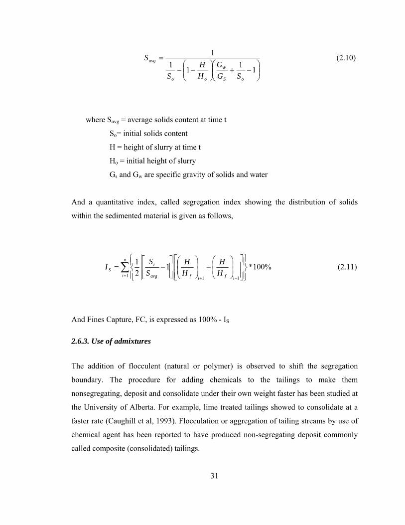
31

⎟⎟⎠

⎞⎜⎜⎝

⎛−+⎟⎟

⎠

⎞⎜⎜⎝

⎛−−

=

11111

oS

W

oo

avg

SGG

HH

S

S (2.10)

where Savg = average solids content at time t

So= initial solids content

H = height of slurry at time t

Ho = initial height of slurry

Gs and Gw are specific gravity of solids and water

And a quantitative index, called segregation index showing the distribution of solids

within the sedimented material is given as follows,

∑= −+ ⎪⎭

⎪⎬⎫

⎪⎩

⎪⎨⎧

⎥⎥⎦

⎤

⎢⎢⎣

⎡⎟⎟⎠

⎞⎜⎜⎝

⎛−⎟

⎟⎠

⎞⎜⎜⎝

⎛

⎥⎥⎦

⎤

⎢⎢⎣

⎡−=

n

i ififavg

iS H

HHH

SS

I1 11

%100*121 (2.11)

And Fines Capture, FC, is expressed as 100% - IS

2.6.3. Use of admixtures

The addition of flocculent (natural or polymer) is observed to shift the segregation

boundary. The procedure for adding chemicals to the tailings to make them

nonsegregating, deposit and consolidate under their own weight faster has been studied at

the University of Alberta. For example, lime treated tailings showed to consolidate at a

faster rate (Caughill et al, 1993). Flocculation or aggregation of tailing streams by use of

chemical agent has been reported to have produced non-segregating deposit commonly

called composite (consolidated) tailings.

32

2.7. References Asmar, B. N., P. A. Langston, et al. (2002). "A generalized mixing index in distinct

element method simulation of vibrated particulate beds." Granular Matter 4: 129-

138.

Barnea, E. and J. Mizrahi (1973). "A Generalized Approach to the Fluid Dynamics of

Particulate Systems


Systems." The Chemical Engineering Journal 5: 171-189.

Chalaturnyk, R. J. and J. D. Scott (2001). Soil Structure Behaviour Diagram. High

Density and Paste Tailings 2001.

Charles, M. E. and R. A. Charles (1971). The use of heavy media in the pipeline transport

of particulate solids. Advances in Solid-Liquid flow in pipes and its application. I.

Zandi, Pergamon Press Inc.: 187-197.

Chen, W. a. S. K. J. (1994). Sedimentation. Handbook of Powder Science. noname: 635-

682.

Cheung, M. K., R. L. Powell, et al. (1996). "Sedimentation of Noncolloidal Bidisperse

Suspension." AIChE Journal 42(1): 271-276.

Coussot, P. (1997). Mudflow Rheology and Dynamics, A.A.Balkema.

Davis, R. H. and H. Gecol (1994). "Hindered Settling Function with No Empirical

Parameters for Polydisperse Suspensions." AIChE Journal 40(3): 570-575.

de Silva, S., A. Dyroy, et al. (1999). Segregation Mechanism and Their Quantification

using Segregation Testers. Proceedings of the IUTAM Symposium on

Segregation in Granular Flows, Cape May, NJ, Kluwer Academic Publishers.

Diplas, P. and A. N. Papanicolaou (1997). "Batch Analysis of Slurries in Zone Settling

Regime." J. Environmental Engg., ASCE 123(7): 659-667.

Edwards, S. F. and D. V. Grinev (2003). "Statistical mechanics of granular

materials:stress propagation and distribution of contact forces." Granular Matter

4(4): 147-153.

33

Fine Tailings Fundamentals Consortium, F. (1995). Clark Hot Water Extraction Fine

Tailings. Advances in Oil Sand Tailings Research. Edmonton, Alberta

Department of Energy, Oil Sands and Research Division. I.

Fisher, R. V. and H.-U. Schmincke (1984). Pyroclastic Rocks, Springler-Verlag Berlin

Heidelberg.

Fitch, B. (1983). "Kynch Theory and Compression Zones." AIChE Journal 29(6): 940-

947.

Garside, J. and M. R. Al-Dibouni (1977). "Velocity-Voidage Relationships for

Fluidzation and Sedimentation in Solid-Liquid Systems." Ind.Eng.Chem.,Process

Des. Dev. 16(2): 206-214.

Gidaspow, D. (1994). Multiphase Flow and Fluidization. San Diego, Academic Press.

Kelly, E. G. and D. J. Spottiswood (1982). Introduction to Mineral Processing, John

Wiley & Sons, Inc.

Kenji Iimura, H. Nakagawa, et al. (1998). "Deformation of aggregates depositing on a

plate in a viscous fluid simulated by modified discrete element method."

Advanced Powder Technology 9(4): 345-361.

Kynch, G. J. (1952). "A Theory of Sedimentation." Trans.Faraday Soc. 48: 166-176.

Lockett, M. J. and H. M. Al-Habboby (1973). "Differential Settling by Size of Two

Particles in A Liquid." Trans.Instn.Chem.Engrs 51: 281-292.

Loth, E., G. Tryggvason, et al. (2006). Chapter 13 Modeling. Multiphase Flow

Handbook. C. T. Crowe. Boca Raton, Taylor & Francis Group, LLC: 13-1-13-

150.

MacKinnon, M. and A. Sethi (1999). A Comparison of Physical and Chemical Properties

of the Tailings Pond at the Syncrude and Suncor Oil Sands Plants. Professional

Development Course on Liquid Solid Separation, Aug. 21-22,1999. Quebec City.

Masliyah, J. H. (1979). "Hindered settling in a multi-species particle system." Chemical

Engineering Science 34: 1166-1168.

Mirza, S. and J. F. Richardson (1979). "Sedimentation of Suspensions of Particles of Two

or More Sizes." Chemical Engineering Science 34: 447-454.

34

Montante, G., G. Micale, et al. (2001). "Experiments and CFD Predictions of Solid

Particle Distribution in a Vessel Agitated with Four Pitched Blade Turbines."

Institution of Chemical Engineers, Trans IChemE 79(Part A): 0263-8762/01.

Morgenstern, N. R. and J. D. Scott (1999). Geotechnics of Fine Tailing Management.

Professional Development Course on Liquid Solid Separation, Aug. 21-22 1999.

Quebec City.

Pane, V. and R. L. Schiffman (1997). "The permeability of clay suspensions."

Geotechnique 47(2): 273-288.

Patwardhan, V. S. and C. Tien (1985). "Sedimentation and Liquid Fluidization of Solid

Particles of Different Sizes and Densities." Chemical Engineering Science 40(7):

1051-1060.

Pearse, M. J., S. Weir, et al. (2001). "Advances in Mineral Flocculation." Minerals

Engineering 14(11): 1505-1511.

Richardson, J. F. and W. N. Zaki (1954). "Sedimentation and Fluidization: Part I."

Trans.Instn.Chem.Engrs 32: 35-78.

Savage, S. B. (1979). "Gravity flow of cohesionless granular material in chutes and

channels." Journal of Fluid Mechanics 92: 53-96.

Scott, J. D. (1999). The Tailing Design Diagram. Professional Development Course on

Liquid Solid Separation, Aug. 21-22, 1999. Quebec City.

Scott, J. D. and M. F. Chichak (1983). Initial segregation Tests. Edmonton, Syncrude

Canada Ltd.

Scott, J. D. and G. J. Cymerman (1984). Prediction of Viable Tailing Disposal Methods.

Proceeding of a Symposium: Sedimentation consolidation models: Prediction and

Validation., San Fransisco, California, ASCE.

Selim, M. S., A. C. Kothari, et al. (1983). "Sedimentation of Multisized Particles in

Concentrated Suspensions." AIChE Journal 29(6): 1029-1038.

Sha, Z., S. Palosaari, et al. (2001). "CFD Simulation of Solid Suspension in a Stirred

Tank." J. Chemical Engineering of Japan 34(5): 621-626.

Shaw, R. C., L. L. Schramm, et al. (1996). Suspensions in the Hot Water Flotation

Process for Canadian Oil Sands. 'Suspensions: Fundamentals and Applications in

35

the Petroleum Industry' in Advances in Chemistry series 251. L. L. Schramm.

Washington,DC, American Chemical Society. 251: 639-675.

Smith, T. N. (1965). "The Differential Sedimentation of Particles of Two Different

Species." Trans.Instn.Chem.Engrs 43: T69-T73.

Smith, T. N. (1966). "The Sedimentation of Particles having a Dispersion of Sizes."

Trans.Instn.Chem.Engrs 44: T153-T157.

Smith, T. N. (1967). "The Differential Sedimentation of Particles of Various Species."

Trans.Instn.Chem.Engrs 45: T311-T313.

Suthaker, N. N. (1995). Geotechnics of Oil sand Tailings. Civil and Environmental

Engineering. Edmonton, University of Alberta.

Tiller, F. M. (1981). "Revision of Kynch Sedimentation Theory." AIChE Journal 27(5):

823-829.

Vallance, J. W. and S. B. Savage (1999). Particle Segregation in Granular Flows Down

Chutes. Proceedings of the IUTAM Symposium on Segregation in Granular

Flows, Cape May, NJ, Kluwer Academic Publishers.

Whipple, K. X. (1997). "Open-Channel Flow of Bingham Fluids: Application in Debris-

Flow Research." The Journal of Geology 105: 243-262.

Zimmels, Y. (1983). "Theory of Hindered Sedimentation of Polydisperse Mixtures."

AIChE Journal 29(4): 669-676.

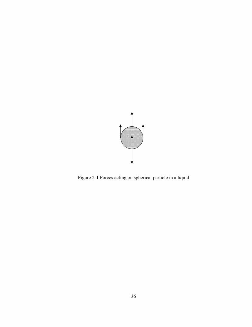
36

Figure 2-1 Forces acting on spherical particle in a liquid

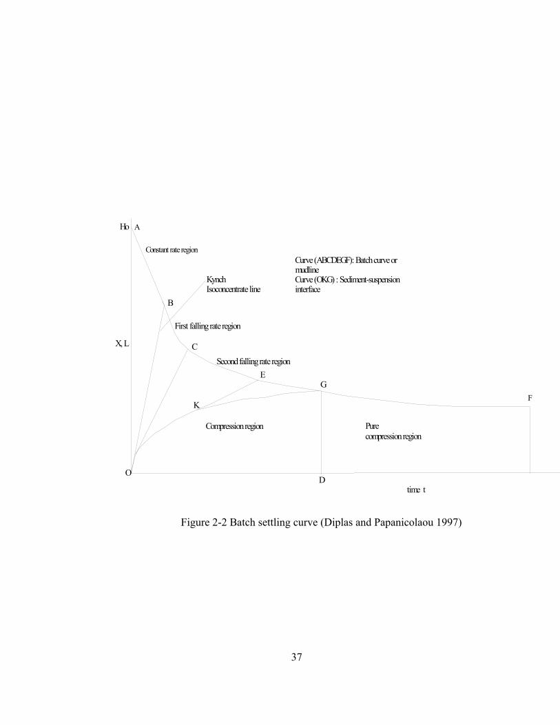
37

Compression region Purecompression region

First falling rate region

Second falling rate region

Constant rate region

Kynch Isoconcentrate line

Ho

Curve (ABCDEGF): Batch curve or mudlineCurve (OKG) : Sediment-suspension interface

A

B

C

EG

K

O

time t

F

D

X, L

Figure 2-2 Batch settling curve (Diplas and Papanicolaou 1997)

38

Figure 2-3 Segregation process during sedimentation of binary species suspension

Clear liquid

Smaller particles suspension

Sediment

Suspension of both particle sizes

39

Figure 2-4 Formation of zones in sedimentation of poly-disperse suspension (after Mirza

and Richardson 1973)

Sediment

Contains all sizes a-M

Contains all sizes b-M

Contains only smaller particles (M)

Clear liquid

Zone m

Zone m-1

Zone 1

u c,a,m

u c,b,m-1

u c,M-1,2

u c,M,1

Settling velocities of interfaces

40

Figure 2-5 Deposition mechanism in tailings impoundment (after Yong 1984)

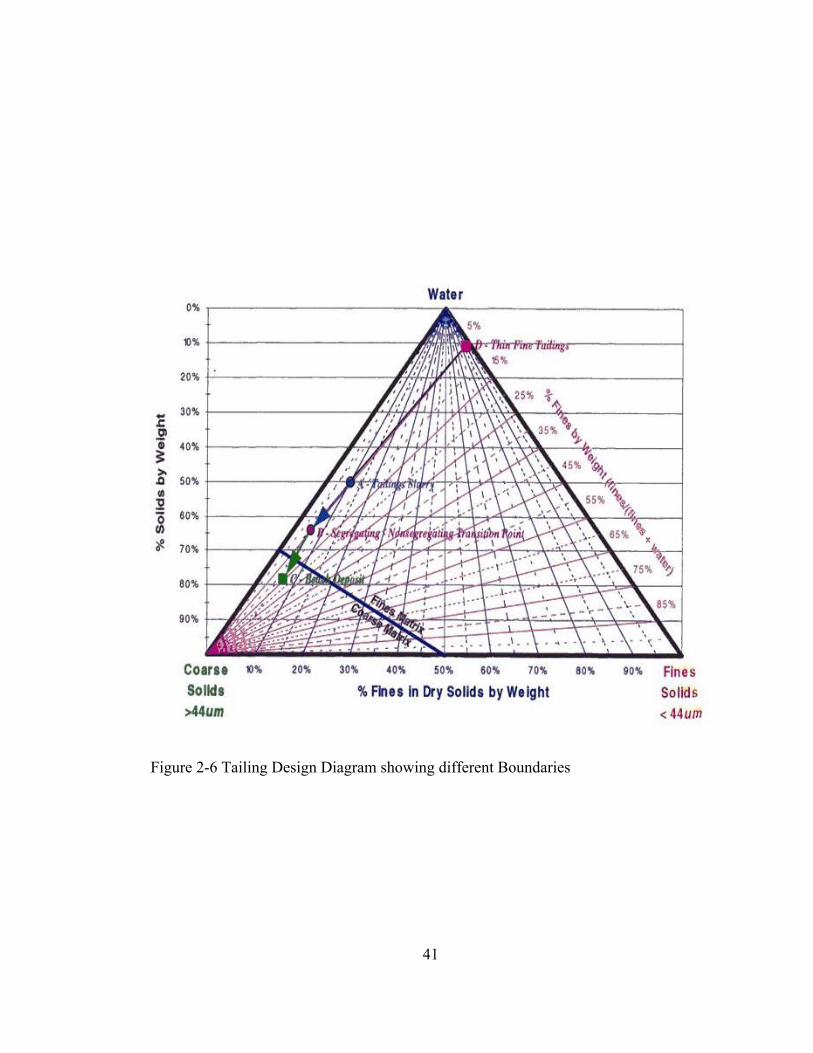
41

Figure 2-6 Tailing Design Diagram showing different Boundaries

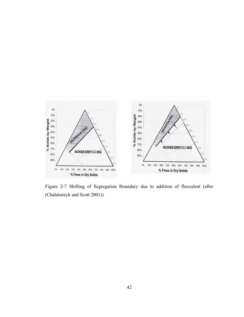
42

Figure 2-7 Shifting of Segregation Boundary due to addition of flocculent (after

(Chalaturnyk and Scott 2001))

43

CHAPTER 31

3. GEOTECHNICAL AND RHEOLOGICAL CHARACTERIZATION

3.1 Introduction

The constitutive behaviour of mixtures involving different phases is a subject of great

complexity. The complex mixtures of solids and fluids exhibit behaviour different from

Newtonian fluids. Fluids which deviate from Newtonian behaviour are referred to

commonly as non-Newtonian fluids. These materials may involve two or three phases.

The study of these mixed phases has shown significance in many fields: the economical

and efficient transportation of solids in mining industry, hydraulic dredging, debris and

mud flow researches, chemical and processing industries, biomedical and genetic

engineering process (Charles and Charles (1971), Govier and Aziz (1972),

Coussot (1997), Whipple (1997), Kessel and Fontijn (2000) and Chhabra (1993).

3.2 Previous works (Literature review and Background)

Characterization of the rheological behaviour of non-Newtonian fluids has become very

important from an engineering perspective. Rheological characterization provides

necessary tools for flow behaviour prediction, quality control and comparison. As

Zhou et al. (2001) described, understanding the rheological behaviour of concentrated

suspensions is of importance in the analysis and control of the properties of the

suspensions so that they display well-defined and desired flow behaviour. One

application is to establish criteria for controlling rheological properties and physical

stability of a suspension so as to increase the maximum packing volume with desired

1 A version of this chapter has been published. Mihiretu, Y.M., Chalaturnyk, R.J., Scott, J.D. Proc. of 58th Canadian Geotechnical Conference, Saskatoon, Saskatchewan, 2005. And in Mihiretu, Y.M, Chalaturnyk, R.J., Scott, J.D. Proc. of 1st International Oil Sands Tailings Conference, Edmonton, 2008.

44

fluidity, while maintaining sufficient stability against sedimentation, aggregation, and

agglomeration of the particles. They also provided different aspects of application of

rheological studies.

For such purpose, quite a number of models relating shear stress with shearing rate are

available. The parameters that are usually required in the models are the apparent yield

stress, plastic viscosity and flow indices. The required parameters are determined from

laboratory or field experiments and curve fitting techniques. It appears that, compared to

other parameters in the model, there is remarkable interest in measuring yield stress.

Houwink (1937) reported that even in crystalline bodies, migration of atoms takes place

without application of any tension (stress). Such migration results in plastic deformation.

And he concludes that no yield stress exists. Vocadlo and Charles (1971) discussed the

difficulties involved in defining yield stress from a “strength of materials” perspective

and signified the distinction between solids and fluids. Chhabra (1993) concluded that

viscoplastic fluids, which are characterized by the existence of yield stress, are not really

a fluid according to strict physical definition. Barnes and Walter (1985) argued that the

yield stress is a “myth” which has provided a point of controversy among researchers.

Hartnett and Hu (1989) conducted a falling ball experiment in an aqueous 2500wppm

Carbopol 960 solution. They tracked the movement of the nylon ball for several months

and observed that the ball is essentially at rest from an engineering perspective. Thus they

concluded that yield stress is an engineering reality. Their conclusion contradicted the

hypothesis of Barnes and Walter (1985) and leads to further debate on the subject in the

literature (Astarita (1990), Schurz (1990), Evans (1992), Schurz (1992).

Later, Barnes (1999) provided a comprehensive review of the yield stress where he

emphasized that there is no true yield stress and flow exists beyond the yield stress.

Reference was even made to Reiner (1969) :” In reality there is no rigid boundary

between solids and liquids. Παντα ρει (Panta rhei), everything flows, as Heraclitus

(495B.C.) said.” in reinforcing his argument. According to Barnes (1999), the definition

45

of (apparent) yield stress is a mathematical curve-fitting constant, used along with other

parameters to produce an equation to describe the flow curve of a material over a limited

range of shear rates. While Vocadlo and Charles (1971) have marked the value of

distinction between “fluid” and “solid” “if it enable us to place common materials

unambiguously in one category or the other on the basis of experimental tests. However,

this is only possible interpretation through personal judgment based on time of

observation, time of service, predicted permanent deformation, etc.”

Despite the controversy resident in the subject of yield stress, it can be seen that there is

an apparent agreement with regard to the time frame to which test conditions are

predominantly considered. For example, Houwink (1937) highlighted that in a practical

experiment carried out rapidly, a yield value can be observed. He further stressed the

significance of the inclusion of the rate of testing in the reporting of the experimental

results. Barnes (1999) reported his consent with the argument of Harnett and Hu (1989)

that liquid could be assumed to have yield stress when it comes to a reasonable length

and time scale. Astarita (1990) provided a review of the arguments of Barnes and Walter

(1985) and Harnett and Hu (1989) and provided a discussion on the relative nature of

time and length scales.

As Evans (1992) concluded, the dispute is more of accepting one’s definition or not. Thus

in common engineering practice, the yield stress is pragmatically significant and the

application is investigated with the intent of characterizing the flow behaviour of

suspension in short test duration. The concept of creep appears to be of less significance

at least in the context of studies which involve short duration of experimentation. The

number and variety of attempts to measure yield stress signifies how the pragmatic

approach is prevalent in these types of experiments.

The most common method for computing the yield stress is back extrapolation of the

flow curve to zero shear rate from rheometer data. As such, extrapolated results have

been used to check the yield stress measurement made by other apparatus. Because this

46

method is a curve fitting procedure, direct experimental measurement of yield stress has

received attention amongst researchers.

Charm and Kurland (1967) have devised a glass capillary tube to measure the yield stress

of blood. They found good agreement with the back extrapolated yield value of

rheometer tests.

Scott et al. (1985) conducted rheological tests on sludge from oil sands. They used a

conventional rheometer and back extrapolated the flow curve to zero shear rate to

determine yield stress (or gel strength, as they called it). They observed over the range of

their study that the addition of sand effects in reducing the apparent viscosity and yield

stress. They remarked that the development of gel strength can be beneficial if it is

desirable to suspend a granular phase such as sand in the sludge by mixing.

Locat and Demers (1988) studied the rheological properties of sensitive clays. They were

able to establish a relationship: plastic viscosity vs. liquidity index and remoulded shear

strength (yield stress) vs. liquidity index.

Wuensch (1990) used a falling ball viscometer to find the two parameters of a Bingham

fluid: yield stress and plastic viscosity simultaneously. While the results compare well

with the working theory, it is unclear why comparison was not made with those of other

conventional rheological experiments. Schurz (1990) introduced a rolling ball method of

yield stress measurement. He showed that when a ball rolls down a curved groove, the

acting shear stress is proportional to the position at which the ball comes to standstill.

Rajani and Morgenstern (1991) conducted slump test to measure the yield stress of

mortar and Devon silt. They compared their result with the falling cone tests. They

concluded that slump test is a viable method for determining the yield stress of

geotechnical material of Bingham fluid type. Zreik et al. (1995) devised a falling cone

test to measure undrained shear strength (yield stress) of remolded marine clay. They

found good match between the results from their experiment and theoretical prediction.

47

Coussot and Boyer (1995) conducted inclined plane tests to determine the yield stress of

mud mixtures at different solid concentrations. They found good agreement between

inclined plane test and rheometrical test data for Herschel-Bulkley model fitting fluids.

Kessel and Fontijn (2000) devised a miniature sounding probe to measure the yield stress

of freshly deposited sediments. They measured as small a yield stress value as 1 Pa. Their

rationale not to use conventional rheometer techniques were that: 1) the increase in

effective stress with depth cannot be accounted for; and 2) the sample is reconstituted

while injecting into the rheometer.

The vane shear method, which was initially devised to measure the undrained shear

strength of cohesive soils in geotechnical engineering (Osterberg 1956), has been adopted

to the yield stress measurement of soft solids and slurry (Keentok, 1982); (Nguyen and

Boger, 1985); (Turian et al. 1993). The method has demonstrated itself to be a reliable

technique for the measurement of yield stress.

By use of similar device, Turian and coworkers, Turian et al.,(1992, 1993, 2002), were

able to characterize and control the properties of coal-water fuel mixtures. They indicated

that yield stress is an effective property which indicates the existence of structure within

the composite material and, therefore, its value provides a measure of relative strength of

the two phase structure. They added further that, in general, effective properties of

composite materials depend upon pertinent properties of the continuous and the dispersed

phases, their concentrations and the geometrical arrangement of the dispersed phase

within the mixture.

Many slurry flows in nature (e.g. mudflow, debris flow, erosion), in industrial processing

(mixing handling and processing) and in industrial waste management (tailing transport

and disposal) involve different grain size composition and water chemistry. In the

literature, however, little emphasis has been given to the study of rheological properties

of such material. This may be due to the fact that measurement difficulties are

predominantly hindering. Kuepper (1991) has indicated that non-segregating slurries are

48

characterized by an increased viscosity and display a non-Newtonian rheology. Mining

wastes (tailings) need to be handled and transported before they are deposited into a

pond. It is desirable for the tailings disposal scheme to have rheological properties which

are stable, easily transportable and yielding low volume at storage. The measurement of

yield stress has become very significant parameter in evaluating the geotechnical

suitability of deposits. Thus proper characterization of rheological behaviour is valuable

tool in all processes involving their management.

The purpose in this chapter is to investigate the significance of yield stress, as rheological

parameter, in characterizing the properties of different mixes of grains sizes (clay, silt and

sand) when they form a non-segregating (stable) slurry. Thus the composition,

concentration and porewater chemistry effects are examined.

3.3 Theoretical Considerations

3.3.1 Rheological Characteristics

Fluids of any type may exhibit one of the following flow behaviour types: Newtonian,

non-Newtonian or Viscoelastic. Detailed discussions about these materials can be found

in Wilkinson (1960), Shamlou (1988) or Chhabra (1993). A brief explanation of flow

behaviour is presented below.

Newtonian fluids are fluids in which the viscosity is constant and satisfy the complete

Navier-Stokes equations (i.e. in simple shear, deviatoric normal stresses are identically

zero). Non-Newtonian fluids are those whose flow curve exhibit non-linear relationship.

Linear flow curve that does not pass through the origin are also aligned in the non-

Newtonian category.

The most common non-Newtonian flow behaviour can be put in three categories

1. Time independent (viscous) fluids:

49

Fluid of this type can be described by flow properties independent of time. The

constitutive rheological equation can be written as

)(γτ &f= (3.1)

These fluids maybe further subdivided into

(a) Shear thinning or pseudoplastic

For this fluids, the ratio of instantaneous shear stress to shear rate, called

‘apparent viscosity’ drops as the shear rate increases. Most commonly

encountered time independent fluids fall in this category. Some examples are

inks, paints, clay suspensions, paper pulp, emulsions, oils and greases.

(b) Shear thickening (dilatant)

The ’apparent viscosity’ increases as shear rate increases and there is no yield

stress. Some paints, concentrated suspension of solids, plastisols and

quicksands are of the dilatant type.

(c) Viscoplastic

These fluids are characterized by yield stress which must be exceeded before

flow commences. The mathematical models to characterize such flow

behaviour are mainly the Bingham, Hershel-Bulkley, or Casson models.

Figure 3-1 shows the rheograms for these different fluid types.

2. Time dependent fluids:

For these types of materials, the shear flow properties depend on both the shear rate

and the time of shearing. They are mainly subdivided into:

(a) Thixotropic (breakdown of structures by shear)

If the apparent viscosity decreases with time for a given shear rate, then the fluid

is said to exhibit thixotropy.

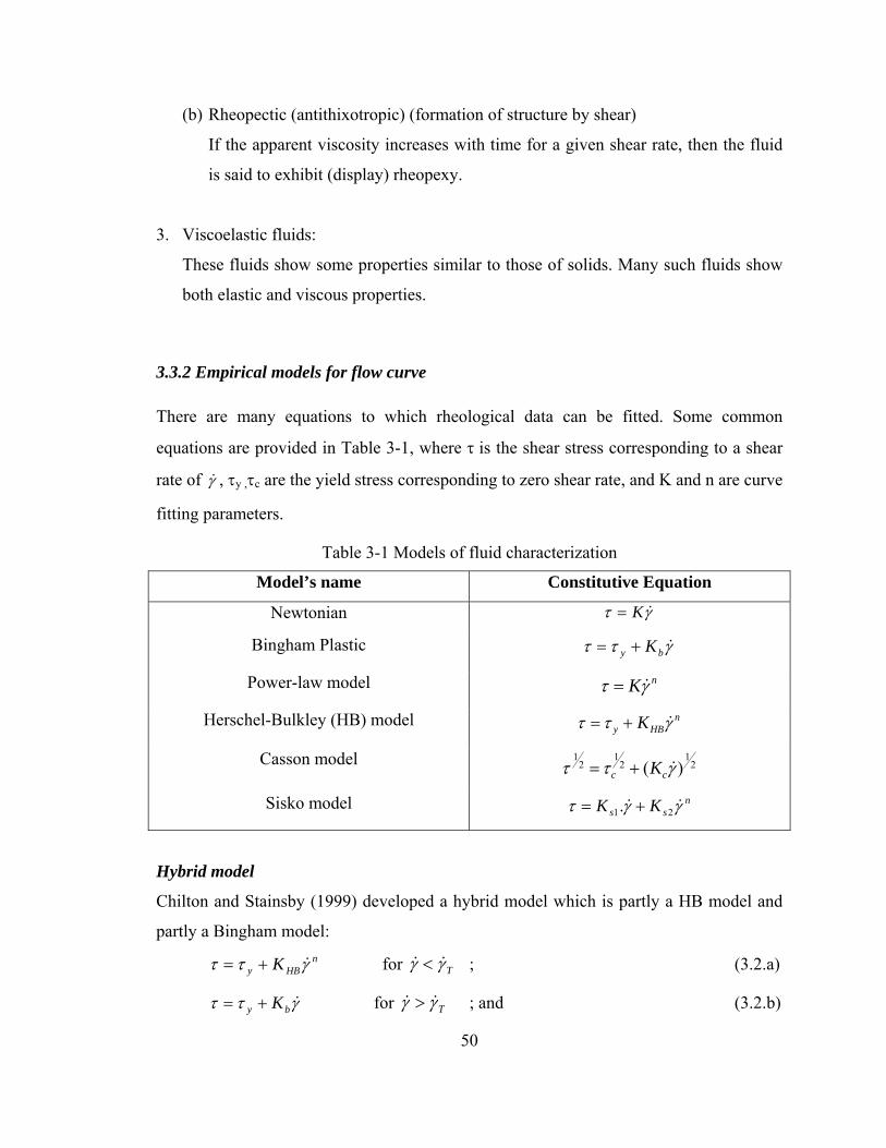
50

(b) Rheopectic (antithixotropic) (formation of structure by shear)

If the apparent viscosity increases with time for a given shear rate, then the fluid

is said to exhibit (display) rheopexy.

3. Viscoelastic fluids:

These fluids show some properties similar to those of solids. Many such fluids show

both elastic and viscous properties.

3.3.2 Empirical models for flow curve There are many equations to which rheological data can be fitted. Some common

equations are provided in Table 3-1, where τ is the shear stress corresponding to a shear

rate of γ& , τy ,τc are the yield stress corresponding to zero shear rate, and K and n are curve

fitting parameters.

Table 3-1 Models of fluid characterization

Model’s name Constitutive Equation

Newtonian γτ &K=

Bingham Plastic γττ &by K+=

Power-law model nKγτ &=

Herschel-Bulkley (HB) model nHBy K γττ &+=

Casson model 21

21

21

)( γττ &cc K+=

Sisko model nss KK γγτ && 21. +=

Hybrid model

Chilton and Stainsby (1999) developed a hybrid model which is partly a HB model and

partly a Bingham model: n

HBy K γττ &+= for Tγγ && < ; (3.2.a)

γττ &by K+= for Tγγ && > ; and (3.2.b)

51

nTHByT K γττ &+= = Tby K γτ &+ ; (3.2.c)

where the transitional shear strain rate ( Tγ& ) is derived from the rheometer data.

The first three parameters τ y, KHB and n are obtained from the best fit of HB model to all

of the data and using the standard method. The two additional parameters, τ y and Kb are

obtained by fitting a straight line to the high-strain tail of the viscometer data (Chilton

and Stainsby 1999).

3.3.3. The principle of yield stress calculation based on vane method

The vane shear apparatus is made of four thin blades welded to a cylindrical shaft at right

angle to each other as shown in Figure 3-2. The shaft is coupled to a motor at the top

which drives the system. The yield value is the shear stress corresponding to the observed

maximum torque. The yield stress is calculated by assuming that the sample yields along

a cylindrical surface (and two circular ends) circumscribed by the length and diameter of

the vane.

In performing the test, the vane is immersed into the sample slowly and a torque is

applied to rotate the vane. Measurement of torque as a function of time is made. If the

sample has yield stress, a maximum torque is observed after some time has elapsed. The

maximum torque corresponds to the critical force required to overcome the strength of

the sample. The maximum developed reaction (force) per unit area along the shear

surface is thus the rheological yield stress.

The total torque (T) experienced by the shaft, when the vane is set in motion at a constant

speed, can be given by the sum of the reactions at cylindrical surface, top and bottom face

of the cylinder as follows:

∫∫∫ ++=2/

0

2/

00

D

t

D

b

H

s dTdTdTT (3.3.a)

52

= )2()2()(2

2/

0

2/

00

rdrrrdrrdHDD D

t

D

bs

H

πτπτπτ ∫∫∫ ++ ; (3.3.b)

where Ts is due to shearing on the cylindrical area formed by the shear surface and Tb and

Tt are due to shearing on the bottom and top ends of the cylindrical shear surface

respectively. And τs, τb and τt are the corresponding shear stress on the respective

surfaces.

It is assumed that the shear stress on the cylindrical surface be constant. Also the shear

stress at the top and bottom surfaces are taken to be the same, i.e., τb = τt = τe thus

Equation (3.3 b) results in:

∫+=2/

0

22 )2(*22

D

es drrHDT τπτπ (3.4)

The exact variation of the shear stress at top and bottom are not exactly known. If an

arbitrary power relationship is assumed (Nguyen and Boger 1985), τe can be written as

s

m

e Drr ττ ⎟

⎠⎞

⎜⎝⎛=

2)( , for 2

0 Dr ≤≤ (3.5)

Substituting Equation (3.5) in (3.4) and integrating one gets

ss mDHDT τπτπ

)3(22

32

++= (3.6)

or smDHDT τπ

⎥⎦⎤

⎢⎣⎡

++=

31

23 (3.7)

If the shear stress on the ends is assumed to be constant and the same as the cylindrical

surface shear, then m=0. This has been proven experimentally by Nguyen and Boger

(1985) for flocculated bauxite residue slurries.

Thus, equation (3.7) reduces to

53

sDHDT τπ

⎥⎦⎤

⎢⎣⎡ +=

31

23 (3.8)

Equation (3.8) is the widely used equation in the calculation of yield stress, τy = τs. If H/D

is set to 2:1, the yield stress in terms of maximum torque and D is given as:

max3

67y

TD

τπ

= (3.9)

where τy is the yield stress, Tmax is the maximum torque, and D is the vane diameter.

3.4 Materials and Experimental Methods

The choice of material for this experimentation is based on the following criteria:

availability, quality and repeatability of the working sample, and proximity to the real

material, in particular tailings from the oil sands industry. Consequently, the materials

chosen for geotechnical/rheological experiments are kaolinite, sil-sand rock flour, and

sand. The kaolinite material and the sil-sand rock flour are obtained from Sil-Industrial

Minerals Inc. The material properties for the studied materials are summarized in Table

3-2 below:

Table 3-2 Material Properties

Material Specific Gravity D50(μm)

Kaolinite

Sil flour

Sand

2.70

2.67

2.66

~<1

~16

~200

Moreover, the liquid limit and the plastic limit of kaolinite are (55.2%) and (29.5%)

respectively. The silt size sil-sand rock flour (Sil flour) exhibits no plasticity. The

ambient temperature during the test is 20+1oC. The grain size distributions of the

materials used in the experiment are shown in Figure 3-3.

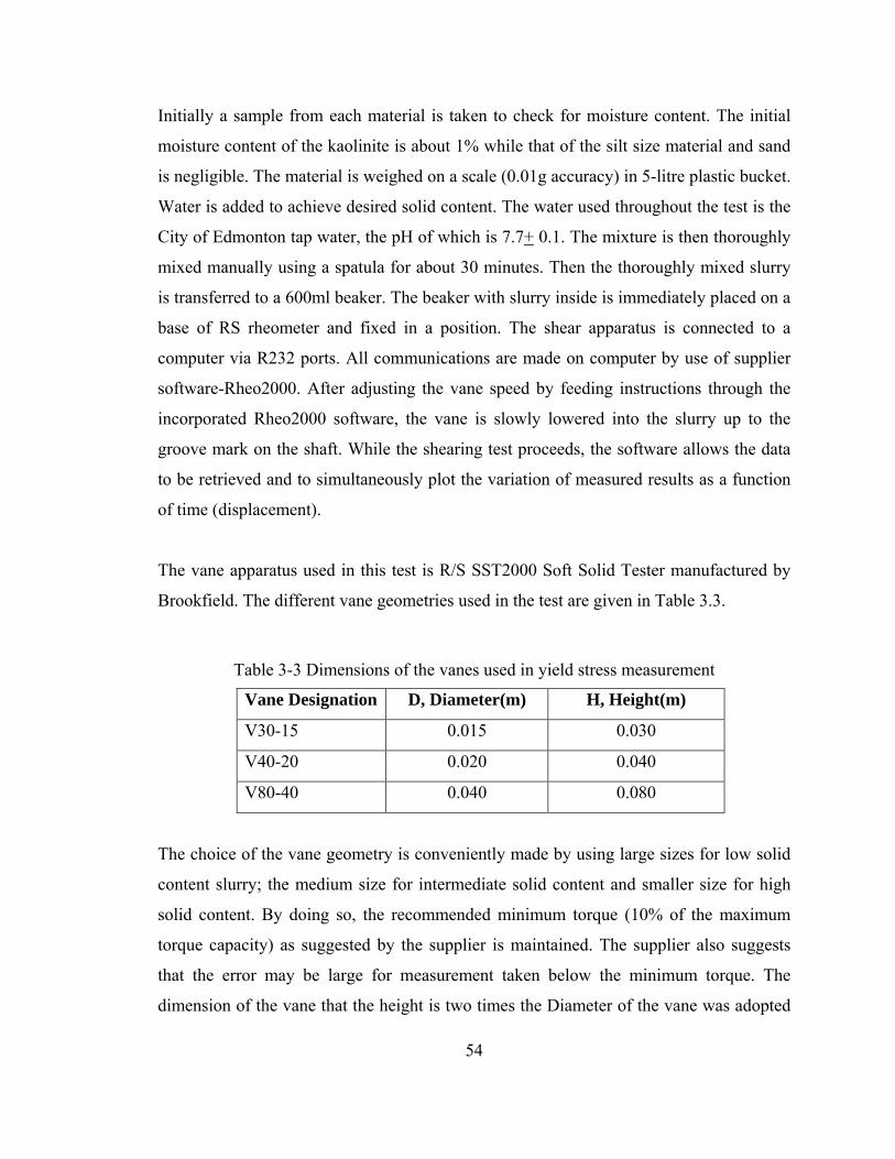
54

Initially a sample from each material is taken to check for moisture content. The initial

moisture content of the kaolinite is about 1% while that of the silt size material and sand

is negligible. The material is weighed on a scale (0.01g accuracy) in 5-litre plastic bucket.

Water is added to achieve desired solid content. The water used throughout the test is the

City of Edmonton tap water, the pH of which is 7.7+ 0.1. The mixture is then thoroughly

mixed manually using a spatula for about 30 minutes. Then the thoroughly mixed slurry

is transferred to a 600ml beaker. The beaker with slurry inside is immediately placed on a

base of RS rheometer and fixed in a position. The shear apparatus is connected to a

computer via R232 ports. All communications are made on computer by use of supplier

software-Rheo2000. After adjusting the vane speed by feeding instructions through the

incorporated Rheo2000 software, the vane is slowly lowered into the slurry up to the

groove mark on the shaft. While the shearing test proceeds, the software allows the data

to be retrieved and to simultaneously plot the variation of measured results as a function

of time (displacement).

The vane apparatus used in this test is R/S SST2000 Soft Solid Tester manufactured by

Brookfield. The different vane geometries used in the test are given in Table 3.3.

Table 3-3 Dimensions of the vanes used in yield stress measurement

Vane Designation D, Diameter(m) H, Height(m)

V30-15 0.015 0.030

V40-20 0.020 0.040

V80-40 0.040 0.080

The choice of the vane geometry is conveniently made by using large sizes for low solid

content slurry; the medium size for intermediate solid content and smaller size for high

solid content. By doing so, the recommended minimum torque (10% of the maximum

torque capacity) as suggested by the supplier is maintained. The supplier also suggests

that the error may be large for measurement taken below the minimum torque. The

dimension of the vane that the height is two times the Diameter of the vane was adopted

55

from the original vanes used by Cadling and Odenstad (1950) referred in Flaate(1966). It

is for the purpose of having as small area-ratio as possible. The area ratio is defined as the

cross-sectional area of the vane cross-section and stem in percentage of the cross-

sectional area of circumscribed cylinder. It is suggested that the area ratio should not be

higher than about 15 percent (Flaate 1966).

In some cases also viscosity measurements are taken to plot flow curve from which the

yield stress is approximated by extrapolating the flow curve to zero shear rates. The

viscometer used for this test is the Brookfield DV-II Viscometer. Unlike the vane shear

apparatus, the viscometer is not supplied with software. However, quality data acquisition

is achieved through Microsoft windows Hyper Terminal Communication Program.

Further discussion about viscosity calibration and measurements is provided in Appendix

A.

The slurry composition was prepared in three ingredient categories (i) kaolinite only, (ii)

kaolinite and Sil flour mix and (iii) kaolinite and sand mixes. The solid content and

proportions are also varied.

The shear rate is set to 6 speeds, i.e., 0.01, 0.02, 0.03, 0.1, 0.2, 0.3 /s. After each test is

completed, samples are taken to check the design solid content. The comparison is carried

out based on designed solid content and achieved solid content. Figure 3-4 provides a

representative plot of these comparisons and illustrates that excellent control on sample

solid contents can be achieved during the experimental program.

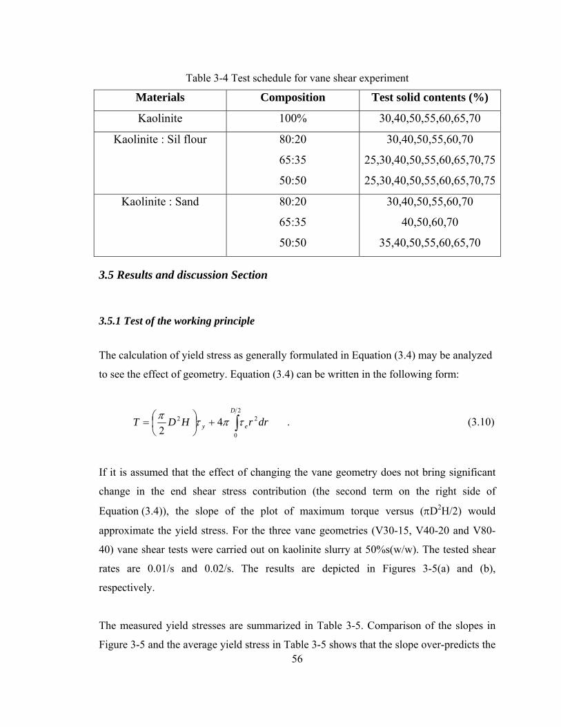
56

Table 3-4 Test schedule for vane shear experiment

Materials Composition Test solid contents (%)

Kaolinite 100% 30,40,50,55,60,65,70

Kaolinite : Sil flour 80:20

65:35

50:50

30,40,50,55,60,70

25,30,40,50,55,60,65,70,75

25,30,40,50,55,60,65,70,75

Kaolinite : Sand 80:20

65:35

50:50

30,40,50,55,60,70

40,50,60,70

35,40,50,55,60,65,70

3.5 Results and discussion Section

3.5.1 Test of the working principle

The calculation of yield stress as generally formulated in Equation (3.4) may be analyzed

to see the effect of geometry. Equation (3.4) can be written in the following form:

∫+⎟⎠⎞

⎜⎝⎛=

2

0

22 42

D

ey drrHDT τπτπ . (3.10)

If it is assumed that the effect of changing the vane geometry does not bring significant

change in the end shear stress contribution (the second term on the right side of

Equation (3.4)), the slope of the plot of maximum torque versus (πD2H/2) would

approximate the yield stress. For the three vane geometries (V30-15, V40-20 and V80-

40) vane shear tests were carried out on kaolinite slurry at 50%s(w/w). The tested shear

rates are 0.01/s and 0.02/s. The results are depicted in Figures 3-5(a) and (b),

respectively.

The measured yield stresses are summarized in Table 3-5. Comparison of the slopes in

Figure 3-5 and the average yield stress in Table 3-5 shows that the slope over-predicts the

57

yield stress by about 10%. The linear fit along the three points suggests that the end

contribution is constant instead of being a functional relationship with yield value.

Alternatively, Bowles (1977) has suggested that the diameter of the shear surface

associated with the vane may be larger than the vane diameter by about 5%. If this

suggestion is examined with the geometry of the shear surface and the corresponding

graph similar to Figure 3-5 is shown in Figure 3-6.

Table 3-5 Summary of yield stress based on measured maximum torque

Yield Stress (Pa) Vane Shear Rate at 0.01/s Shear Rate at 0.02/s V30-15 81.36 83.07 V40-20 78.27 78.83 V80-40 74.09 74.85 Average 77.91 78.92

Comparison of average measured value (Table 3-5) and the slopes in Figure 3-6 show a

very good agreement. While the foregoing analysis indicates the top and bottom ends

contribute about 10% of the total resistance; this effect however can be ignored if the

diameter of shear surface is at 5% more diameter than the vane diameter as illustrated in

Figure 3-6.

(1) Kaolinite Slurry

Since yield-stress is defined as the shear stress that must be exceed prior to flow

initiation, attempts to measure such quantity would ideally be made at static condition

(zero shear rate). However, it is technically impossible to undertake static test. The

convenient and indirect way in any rheometrical experimentation is to back extrapolate

the shear stress-shear rate plot to zero shear rate to determine the yield stress. The closer

the shear rates are towards zero the better is the yield stress approximation. Similarly,

direct yield stress measurements using the vane method need to be conducted at lower

speed. Tests at lower speed minimizes the influence of viscous resistance and instrument

inertia on the measured maximum torque (Dzuy and Boger 1985). They suggested that

58

the rotational speed be less that 10rpm and showed experimental results at 0.1rpm.

Common vane test in geotechnical engineering practice use rotating speed of 0.167 rpm

or 1% /minute. Osterberg (1956) and Turian et al. (1993) employed a rotational speed of

0.3rpm in their studies. Coussot (1997) suggested a speed, in terms of shear rate, of

0.01/s. In this research, tests were conducted at six speeds between 0.01/s and 0.3/s.

For kaolinite, Figure 3-7 shows the variation of yield stress with solids content over the

six rotational speeds chosen for this research. At 70.4% solid content it was not possible

to measure yield stress at shear rate higher than 0.02/s, since the maximum torque

capacity of the machine was exceeded. Except the readings at 66.3% solid content, the

yield stress shows an increasing trend as the shear rate increases.

Additional insight into the behavior of these slurries can be found by plotting the

variation of torque with time for specific solid contents. Figures 3-8 and 3-9 show the

variation of the torque and shear stress of 30%s-kaolinite slurry at different shear rates. In

Figure 3-8, the torque is expressed as the percentage of the reference torque, which is

5mNm in all cases. The readings are more reliable when the torque is greater than 10% of

the reference, i.e., 0.5mNm (according to manufacturer recommendation). These figures

show that with minor exceptions, there is an increasing trend in the torque and shear

stress with the shearing rate. A similar trend has also been reported by Biscontin and

Pestana (2001).

A closer examination of Figures 3-8 and 3-9 shows that the pattern of variation of shear

stress is similar to that of the torque. The shear stress is automatically calculated

according to the principle discussed in Section 3.3.3 and illustrated in Equation (3.8) or

(3.9). The torque is plotted together to check the compliance with minimum torque

requirement. Otherwise the shear stress plot is sufficient to determine the yield stress.

Thus the yield stress is approximated as the maximum shear stress from the shear stress

vs. time plot. A typical plot for 50%s kaolinite slurry is shown in Figure 3-10.

59

Figures 3-11 to Figures 3-22 show the plots of shear stress and moment at different shear

rates and different solid content. What is remarkably observable in these figures is that

the time to yield at lower shear rates is longer than those of the faster rates. The longer

time is obviously due to slow movement of the vane to bring the material to shear.

Moreover, as the shear rate increases and the solid content increases the stress vs. time

variation tends to be nearly constant, indicative of stable plastic behaviour. The increase

of yield stress with increasing shear rate shows that yield stress is not unique with respect

to shear rate. However, the yield stress corresponding to lower shear rates are nearly the

same indicating that the measurements should be conducted at lower shear rates as far as

possible.

Based on these experimental results, a relationship between the yield stress and solid

content can be established. Figure 3-23 shows the measured yield stress for different solid

content of kaolinite slurry at a shear rate of 0.01/s. The smallest solid content at which the

yield measurement starts is 30%. At this solid content, it is possible to keep the

suspension stable with insignificant settlement during the shearing experiment. As the

solid content increase, the yield strength shows a faster increasing trend.

There are different ways in which yield stress is correlated to the solid concentration of

the slurry. Kao et al. (1975) provided a theoretical equation for Bingham type fluids that

dimethyldichlorosilicate glass beads in glycerol show dependence of yield stress on the

square of solid concentration. Smith and Bruce (1979) provided an empirical equation

which showed the following a cubic relationship:

τo=k’ (φ-φo)3 , (3.11)

where k’ and φo are empirical constants. Other types of empirical equations have been

discussed in Turian et al. (1992) and Turian et al (1993).

60

The influence of fractal structure of suspended flocs on the yield stress has been

presented by Kranenburg (1994). He provided the following relationship of yield stress

with excess density and fractal dimension D.

Day

−Δ 32

~ ρτ (3.12)

For this experimental work, in which the yield stress is conveniently plotted as a function

of the solid content (s) of the slurry, the above relation can be rewritten in terms of solid

content and specific gravity (Gs) as follows:

D

s

sy SGS

GSA

−

⎥⎦

⎤⎢⎣

⎡−+

−=

32

)1()1(

τ , (3.13)

where A is fitting parameter.

The above equation is fitted into the yield stress solid content relationship as shown in

Figure 3-23 with A= 13620 and a fractal dimension (D=2.67). Excellent agreement is

observed between the experimental results and the theoretical fit. Kessel and

Fontijn (2000) have estimated the fractal dimension of china clay as D=2.68 which

corresponds very closely to the fractal dimension obtained for kaolinite (D=2.67).

(2) Kaolinite and Sil flour

This component of the research was completed to examine the effect of silt size particles

on the rheological strength of a kaolinite-sil flour slurry mix. Commonly, clay and silt are

categorized as fine particles. Different categories of fine classifications are available in

different references. Some of the classifications of fines by grain size are shown in

Table 3-6 below. The particles in a suspension may have different grain size composition.

There is a common trend to consider sand sizes as coarse and silt and clay size as fines.

61

Table 3-6 Range of fine sizes according to different references

Size (micron) of fines Reference

< 22 Syncrude Canada Ltd.

< 30 (Stein 1986) ; (Shamlou 1988)

< 40 (Coussot 1997)

< 44 U of A, Geotechnical Centre

<75 Unified Soil Classification System

Figures 3-24 to 3-36 depict the shear stress and % torque of kaolinite-sil flour (1:1) mix

at different solid content. It is observed that at 30% and 40% solid content, the shear

stress measurement show very scattered readings (Figures 3-24 and 3-25). The scatter in

measurement is attributed to the unstable (segregating) nature of the slurry. Also the

measured % torque was less than 10% for solid contents below 50% (inclusive) which

contrasts the kaolinite only tests where reliable torque measurements were obtained at the

same solid contents. While the yield stress is generally less than that of kaolinite-only

slurry, it is possible to achieve, however, workable solid content up to 75% solids. In case

of kaolinite only slurry, the 70% solids is very stiff and measurements were not possible.

The dependence of yield stress on the shear rate is also clearly visible as the solid content

increases. Here also there is a trend of an increase in yield stress as shear rate increases.

Except at 75% solids, the higher shear rates result in the gentle slope, in some of the data

nearly horizontal, are visible.

Also the proportion of kaolinite and sil-flour has been varied to a proportion 65:35 and

80:20 (kaolinite: sil-flour). A comparative plot is summarized in Figure 3-37 for tests

conducted at a shear rate 0.02/s. In general, similar trends are observed at other shear

rates. The addition of more silt size particles show a decreasing effect on the yield stress

at the same time the maximum solid content at which yield stress reach ‘infinite’ value is

shifted toward high solid content. This is consistent with the observation made by

Kleinecke (1988) who has shown a tendency toward more shear thinning with increased

62

filler content. He has also observed a decrease of elastic properties with increasing filler

content.

(3) Kaolinite and Sand

Since the objective of this research is studying the fundamentals of segregation, it is

relevant to study the rheological behavior of typical segregating mixtures. Consequently,

kaolinite mixed with sand at mixture ratios of 50:50, 65:35 and 80:20 (kaolinite:sand)

have been tested. The solid content at which segregation began to cease was observed to

be 35%. Figure 3-38 shows the shear stress variation with time for this solid content.

While scatter in the data begins to stabilize (due to the minimized segregation), Figure 3-

38 clearly shows the very small shear stress magnitudes that were measured and the

cyclic behaviour in the shear stress measurements. A modest increase in solids content,

from 35% to 40%, produces more stable shear stress readings, as illustrated in Figure 3-

39. For both these solids contents, it is important to note that the magnitude of the

measured shear stresses are very small and are less than the suggested minimum of 10%

of the maximum torque.

Increasingly stable (from a segregation perspective) slurry is attainable at 50% solid

content. Figure 3-40 shows the shear stress variation at this solid content. Above 50% s,

all the samples tested, i.e., 55% 60%, 65% and 70% show very stable shear stress

reading, a representative plot is shown at 60%s in Figure 3-41.

The variation of yield stress as a function of solid content is shown in Figure 3-42. The

solid composition is varied at different kaolinite and sand proportion. The results

illustrated in Figure 3-42 show that as the proportion of sand in the kaolinite-sand mix

increases the yield stress of the mixture decreases.

Comparing Figure 3-29 and Figure 3-42, it is apparent that the yield stress is more

dependent on the finest size of the grains present in the slurry indicating that the clay

sizes have a predominant effect on the yield stress characteristics of a slurry. Zhou et al.

63

(2001) have indicated that the yield stress is inversely proportional to the square of

particle size. The current research results are in support of their statement. The coarse

grains are in essence “inactive” relative to their contribution to the yield stress of the

slurry. Suspension yield stress depends on solid concentration, particle size, shape and

size distribution and in general, suspension chemistry (Nguyen and Boger, 1985).

Also to observe is the magnitude of variation with time at nearly similar solid

concentration, a plot is shown in Figure 3-43. A comparison is made at 60%s (w/w) for

which the addition of sil flour and sand substitute 50% of the kaolinite material. The silt

size addition reduces the yield stress by nearly half.

Similarly, the addition of the sand reduces the yield stress by nearly a factor of 20. This

result is consistent with the work of Scott et al. (1985) who indicated that the yield stress

and apparent viscosity reduce with the addition of sand materials.

The significant application is thus in order to get significant yield stress the presence of

fines, particularly the clay size is very important. At the same time addition of larger sizes

makes the slurry flow easy at high solid content, suggesting that filler addition is more

workable than kaolinite slurry alone.

Another significant contribution of yield stress is the minimization of settling of larger

grains suspended in the fine matrix. Scott et al. (1985) have discussed such application in

their study of oil sand sludge. They indicated that the yield stress development is

beneficial to suspend a granular phase such as sand in sludge by mixing. They noted that

a more profound understanding of the microscopic behaviour of the sludge system is

worthy of pursuit.

3.5.2 Comparison of vane yield stress with rheological model

In the conventional rheological tests, the viscometer data are used to plot a flow curve of

shear stress vs. shear rate. The extrapolation of the flow curve to zero shear rate provides

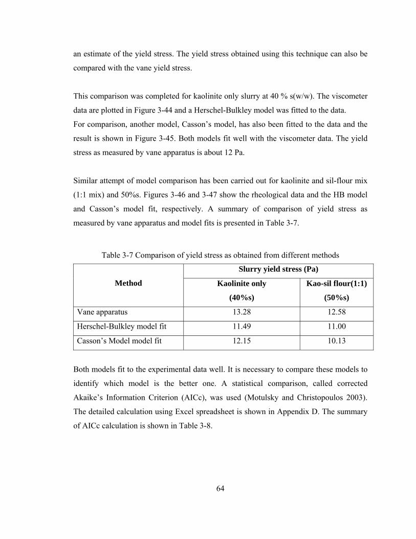
64

an estimate of the yield stress. The yield stress obtained using this technique can also be

compared with the vane yield stress.

This comparison was completed for kaolinite only slurry at 40 % s(w/w). The viscometer

data are plotted in Figure 3-44 and a Herschel-Bulkley model was fitted to the data.

For comparison, another model, Casson’s model, has also been fitted to the data and the

result is shown in Figure 3-45. Both models fit well with the viscometer data. The yield

stress as measured by vane apparatus is about 12 Pa.

Similar attempt of model comparison has been carried out for kaolinite and sil-flour mix

(1:1 mix) and 50%s. Figures 3-46 and 3-47 show the rheological data and the HB model

and Casson’s model fit, respectively. A summary of comparison of yield stress as

measured by vane apparatus and model fits is presented in Table 3-7.

Table 3-7 Comparison of yield stress as obtained from different methods

Slurry yield stress (Pa)

Method Kaolinite only

(40%s)

Kao-sil flour(1:1)

(50%s)

Vane apparatus 13.28 12.58

Herschel-Bulkley model fit 11.49 11.00

Casson’s Model model fit 12.15 10.13

Both models fit to the experimental data well. It is necessary to compare these models to

identify which model is the better one. A statistical comparison, called corrected

Akaike’s Information Criterion (AICc), was used (Motulsky and Christopoulos 2003).

The detailed calculation using Excel spreadsheet is shown in Appendix D. The summary

of AICc calculation is shown in Table 3-8.

65

Table 3- 8 Statistical comparison of rheological model fits

AICc Slurry Description

H-B Model Casson’s Model

Evidence Ratio

Kao-Slurry (40%s) 9.022 7.465 0.211

Kao-Sil Slurry(50%s) 2.992 2.409 0.558

Table 3-8 shows that for both slurries, Casson’s model has lower AICc that Herschel-

Bulkley (H-B) model. Therefore, Casson model fit the data better than H-B model.

Furthermore, the evidence ratio shows that the Casson’s model is 21% better that H-B

model for the Kao-slurry at 40%solids and 56%.better than H-B model, for Kao-sil slurry

at 50% solids.

Such an outcome seems to be in support of some studies made by different researchers.

For example, Want et al. (1982) reported that excellent agreement has been observed in

the yield stress values measured directly by the vane in comparison with other indirect

techniques, for concentrated red mud suspensions at solids concentration higher than 62%

by weight. Dzuy and Boger (1985) measured the yield stress of flocculated bauxite

residue slurries. They found the yield stress measured with vane test to be in good

agreement with the results obtained by the more conventional rheological methods. They

suggested further that the dubious nature of the true yield stress often associated with the

laborious but indirect rheological approach can be avoided.

3.5.3 The effect of pore water chemistry

Different observations are made with regard to the effect of pore water chemistry on the

yield stress. Turian et al. (1993) have tested the yield stress of coal water mixture in the

acidic range and showed that the yield stress increases with acidity. Bourret et al. (1988)

studied the pH effect on a narrow range of 6 to 8. They observed an increase in shear

stress for increase in pH.

66

Whereas Zhou et al. (2001) have shown that the yield stress of a zirconia suspension is

maximum as the pH approach to the neutral pH region and decreases as pH moves to

lower and higher values.

Tseng and Wu (2003), when comparing the settling rates of Al2O3 suspensions at pH 2

and pH 11, found that the faster settling rate at the higher pH is due to prevailing

attractive van der Waals force over the interparticle potential. They also reported that the

interparticle attraction would compete with the gravitational force during sedimentation.

The kaolinite slurry at different pH level is tested to see the effect pore water chemistry

on the slurry yield stress. The pH is varied by adding diluted HCl acid solution to achieve

lower pH and Ca(OH)2 /NaOH solution to achieve higher pH.

The shear stress variation at different pH condition is shown in Figure 3-48. Figure 3-49

show yield stress as a function of pH at a solid content of 50% kaolinite slurry. The yield

stress seems to show moderate increase by decrease in the pH. This observation is in

some way in support of the data presented on Leda Clays by (Torrance and Pirnat, 1984).

They stated that the greater yield stress below about pH 7 exhibited by lower salinity

material suggest that the hydrogen ions and the polyvalent ions released by acid attack on

the mineral had a greater effect when the competition from other ions was weakest. They

further discussed that the edges of clay minerals are positively charged below the

isolectric point pH. The interaction with negatively charged mineral particles increases

below the isolectric point. Such a reaction, along with changing ion saturation, partially

explain the increased yield stress as the pH decreased. The edge faces of kaolinite are

positively charged in acidic condition (Schofield and Samson, 1953). The high yield

value and viscosity of slightly acidic, salt-free suspensions is ascribed to exhibit high

yield and viscosity was ascribed to attraction between positive crystal edges and negative

crystal faces, possibly giving rise to a cubic card-house structure (Houwink and De

Decker 1971).

67

The increase in yield stress at pH 12 as achieved by the addition of Ca2+, can be

explained through the ion exchange properties of the kaolinite slurry. The source of ion

exchange can be (i) broken bonds that give rise to unsatisfied negative charges to be

balanced by adsorbed cations and (ii) the hydrogen of exposed hydroxyls, which may be

replaced by exchangeable cation.

The diffuse double layer at clay surfaces consists of the lattice charge and compensating

counterions, which reside in the liquid immediately adjacent to the particles. Counterions

are subject to two opposing tendencies (i) electrostatic attraction to negatively charged

clay surface and (ii) diffusion from high concentration at the particle surface to low

concentration in the bulk solution. Diavalent ions are attracted to the surface with a force

twice as great as that of monovalent ions. Thus, in a divalent ion system, the diffuse

double layer is more compressed. With an increase in the electrolyte concentration of the

solution, the tendency of counterions to diffuse away from the surface is diminished and

the diffuse double layer is further compressed. Consequently, the thin diffuse double

layer enhance further attraction of clay particles and then flocculation.

The clay slurry prepared at the pH 12 using NaOH shows different shear stress values.

The shear stress is almost diminished and shows no distinct yield stress point. Instead the

shear stress shows a slight increase in shear stress with time. The addition of sodium

hydroxide causes the number of positive charges to be reduced to the point where the

edge faces on which they occur are no longer capable of attracting the negatively charged

cleavage surface of adjacent crystals. The interparticle repulsive forces, due to the net

negative charges, are then adequate to maintain complete dispersion. ((Schofield and

Samson 1953). The gradual rise in shear thickening could be due to the mechanical action

that realign the particle arrangement and give rise to some attraction between adjacent

particles.

Zhou et al. (2001) stated that the nature and magnitude of forces acting in the flow system

and the resulting microstructure are responsible for the complicated rheological

responses. They explained the existence of three kinds of forces which coexist to various

68

degrees in flowing suspensions: hydrodynamic forces, Brownian forces and colloidal

force. It is believed that the complex interaction of these forces account for the

remarkably different rheological behaviour at higher pH.

3.5.4 Rheological measurements of oil sands tailings

Oil sands tailings samples were obtained from Suncor Energy Inc (Suncor). and Albian

Sands Energy (Albian). The tailing sample obtained from Suncor is a mature fine tailings

(MFT) from pond 6 at three depths and the sample obtained from Albian is thickener

underflow.

The test data are presented in Appendix A5. The data indicate that rheological properties

are dependent on temperature, grain size distribution and porewater chemistry. These

observations indicate that the surrogate tailings material used can be further used to

understand the fundamental factors and mechanisms in the study.

The Albian thickener underflow at 35% solids content (Figure A-33) exhibited a different

rheological response versus the kaolinite slurry (Figure 4-58) when treated with Ca(OH)2

and NaOH at pH 12. This drop in yield stress when for the sample treated with Ca(OH)2

can be ascribed to the process used to produce bitumen. Albian sands use non-caustic

sodium citrate to extract the bitumen from the oil sand. The tailing from this non-caustic

process thus include sodium citrate. Sodium citrate forms a complex with calcium,

apparently so stable that adsorption of this calcium by the clay particles is drastically

depressed. The anticoagulant action of sodium citrate was due to the depression of

calcium ions (Hussey et al. 1950).

The yield stress measurement shows different pattern depending upon grain composition

and concentration. Such properties can be used in the process involving the transport and

deposition of slurry, where control of the quality of materials need to be quickly achieved

by comparing the yield stress measurement with the set target yield stress. In this respect,

the sensitivity of the yield stress to any ingredients change and relatively very short

69

duration of the test suggest that it can be used as a viable and quick controlling means in

large scale slurry handling processes. In settling behaviour of slurry, the significance of

yield stress accounts for the effect of fine matrix on the rheological models and that need

to be accounted for in the flow characteristics. This application is discussed in detail in

the ensuing chapters.

3.6 Summary and Conclusion

The yield stress as a parameter of rheological characterization has been investigated using

the vane shear apparatus. A test on the working principle of the apparatus has indicated

that there exists good repeatability of measurements and less effect of the ends (about

10% of the total yield stress). The yield stress is shown to be predominantly dependent on

the surface property of the very fine particles, namely clay size. Changing the

composition of slurry by adding silt size or sand size particle accounts for reduced yield

stress and consequent decrease in the stiffness of the slurry at very high solid content. By

addition of more sand, however, at higher solid contents, results in dilatant behaviour of

the slurry. Consideration of fines as silt and clay appears insufficient unless the clay and

silt composition are specified in the fines.

As there exists no standard rate of shearing, different rates have been tested. Increasing

the shearing rate has shown generally an increase in yield stress. However at low shear

rates between 0.01/s and 0.03/s the yield stress shows good repeatability. The

experiments suggest that shear rates below 0.03/s can be used to measure the yield stress.

Fractal theory fit has been applied to fit to experimental results and very good match is

observed.

For the solid content tested (50%s), an important observation is made that kaolinite slurry

is affected by the pH of the pore fluid medium. Reference to pH alone is not sufficient

without stating the mineralogy of the solution. It is observed that, at similar pH of 12 but

70

prepared from different solution have shown very different shear properties, thus

mineralogy need also be specified together with pH.

3.7. References

Astarita, G., 1990. "The engineering reality of the yield stress". Journal of Rheology, 34(2): 275-277.

Barnes, H.A., 1999. "The yield stress-a review or -everything flows?" J. Non-Newtonian

Fluid Mech., 81: 133-178. Barnes, H.A. and Walter, K., 1985. "The yield stress myth?" Rheol Acta, 24: 323-326. Biscontin, G. and Pestana, J.M., 2001. "Influence of Peripheral Velocity on Vane Shear

Strength of an Artificial Clay". Geotechnical Testing Journal, 24(4): 423-429. Bourret, B., Rueda-Rodriguez, C., Fortune, R. and Bardet, L., 1988. "Comportement

rheologique de sols d'acide polysilicique. I. Influence des facteurs pH,concentration et temps". Rheol Acta, 27: 52-60.

Bowles, J.E., 1977. Foundation Analysis and Design. McGraw-Hill, 749 pp. Charles, M.E. and Charles, R.A., 1971. The use of heavy media in the pipeline transport

of particulate solids. In: I. Zandi (Editor), Advances in Solid-Liquid flow in pipes and its application. Pergamon Press Inc., pp. 187-197.

Charm, S.E. and Kurland, G.S., 1967. "Static Method for determining Blood Yield

Stress". Nature, 216: 1121-1123. Chhabra, R.P., 1993. Bubbles,Drops, and Particles in Non-Newtonian Fluids. CRC Press,

Inc., 417 pp. Chilton, R.A. and Stainsby, R., 1999. A comparison of scale-up procedures for turbulent

non-Newtonian pipe flow, Hydrotransport 14. BHR Group, pp. 223-237. Coussot, P., 1997. Mudflow Rheology and Dynamics. A.A.Balkema. Coussot, P. and Boyer, S., 1995. "Determination of yield stress fluid behaviour from

inclined plane test". Rheol Acta, 34: 534-543.

71

Dzuy, N.Q. and Boger, D.V., 1985. "Direct Yield Stress Measurement with the Vane Method". Journal of Rheology, 29(3): 335-347.

Evans, I.D., 1992. "On the nature of the yield stress". Journal of Rheology, 36(7): 1313-

1316. Govier, G.W. and Aziz, K., 1972. The flow of complex mixtures in pipes. Van Nostrand

Reinhold Company, N.Y. Hartnett, J.P. and Hu, R.Y.Z., 1989. "The Yield Stress-An Engineering Reality". Journal

of Rheology, 33(4): 671-679. Houwink, R., 1937. Elasticity, Plasticity and Structure of Matter. Cambridge University

Press, 376 pp. Houwink, R., and De Decker, H.K. 1971. Elasticity, Plasticity and Structure of Matter.

Cambridge University Press, London. Hussey, C. V., A. J. Quick, et al. (1950). "Effect of Sodium Citrate and Heparin on

Removal of Calcium from Blood and Serrum by Amberlite." J.Biol.Chem. 184(1): 105-108.

Kao, S.V., Nielsen, L.E. and Hill, C.T., 1975. "Rheology of Concentrated Suspension of

spheres:II Suspension Agglomerated by an Immiscible Second Liquid". Journal of Colloid and Interface Science., 53(3): 367-373.

Keentok, M., 1982. "The measurement of the yield stress of liquids". Rheol Acta, 21:

325-332. Kessel, T.v. and Fontijn, H.L., 2000. "Miniature sounding tests on soft saturated cohesive

soils." Geotechnique, 50(5): 537-546. Kleinecke, K.-D., 1988. "Zum Einfluss von Fuellstoffen auf das rheologishe Verhalten

von hochmolekularen Polyethylenschmelzen I. Das Fliessverhalten in Sher-und Dehnstroemungen". Rheol Acta, 27: 150-161.

Kranenburg, C., 1994. "The Fractal Structure of Cohesive Sediment Aggregates".

Estuarine,Coastal and Shelf Science, 39: 451-460. Kuepper, A.A.G., 1991. Design of Hydraulic Fill. PhD Thesis, University of Alberta,

Edmonton,Canada, 525 pp. Locat, J. and Demers, D., 1988. "Viscosity, yield stress, remolded strength and liquidity

index relationships for sensitive clays". Can.Geotech.J., 25: 799-806.

72

Motulsky, H.J., and Christopoulos, A. 2003. Fitting models to biological data using linear and non-linear regression: A practical guide to curve fitting. Graphpad Software Inc., San Diego, CA.

Nguyen, Q.D. and Boger, D.V., 1985. "Direct Yield Stress Measurement with the Vane

Method". Journal of Rheology, 29(3): 335-347. Osterberg, O.J., 1956. Introduction, Symposium on vane shear testing of soils. ASTM,

Atlanta City, N.J., pp. 1-8. Rajani, B. and Morgenstern, N.R., 1991. "On the yield stress of geotechnical materials

from the slump test". Can.Geotech.J., 28: 457-462. Reiner, M., 1969. Deformation,Strain and Flow. H.K.Lewis & Co. Ltd., 347 pp. Schofield, R.K., and Samson, H.R. 1953. The Deflocculation of Kaolinite Suspensions

and the Accompanying Change-Over from Positive to Negative Chloride Adsorption. Clay Minerals, 2: 45-51.

Schurz, J., 1990. "The yield stress- An empirical reality". Journal of Rheology, 29: 170-

171. Schurz, J., 1992. "A yield value in a true solution?" Journal of Rheology, 36(7): 1319-

1321. Scott, J.D., Dusseault, M.B. and Carrier, W.D., 1985. "Behaviour of the

clay/bitumen/water sludge system from oil sands extraction plants". Applied Clay Science, 1: 207-218.

Shamlou, P.A., 1988. Handling of Bulk Solids. Butterworth& Co.Ltd, London, 193p pp. Smith, T.N. and Bruce, C.A., 1979. "Intrinsic Viscosities and Other Rheological

Properties of Flocculated Suspension of Nonmagnetic and Magnetic floc." Journal of Colloid and Interface Science, 72(1): 13-26.

Stein, H.N., 1986. Rheological Behavior of Suspensions. In: N.P. Cheremisinoff (Editor),

Encyclopedia of Fluid Mechanics, pp. 3-48. Torrance, J.K., and Pirnat, M. 1984. Effect of pH on the Rheology of Marine Clay from

the site of the south Nation River, Canada, Landslide of 1971. Clays and Clay Minerals, 32(5): 384-390.

Tseng, W.J. and Wu, C.H., 2003. "Sedimentation, rheology and particle packing structure

of aqueous Al2O3 suspension". Ceramic International, 29: 821-828.

73

Turian, R.F., Attal, J.F., Sung, D. and Wedgewood, L.E., 2002. "Properties and rheology of coal-water mixtures using different coals". Fuel, 81: 2019-2033.

Turian, R.M., Fakhreddine, M.K., Avramidis, K.S. and Sung, D.-J., 1993. "Yeild stress of

coal-water mixtures". Fuel, 72(9): 1305-1315. Turian, R.M., Hsu, F.-L., Avramidis, K.S., Sung, D.-J. and Allendorfer, R.K., 1992.

"Settling and Rheology of Suspensions of Narrow-Sized Coal Particles". AIChE Journal, 38(7): 969-987.

Vocadlo, J.J. and Charles, M.E., 1971. "Measurement of Yield Stress of Fluid-like

Viscoplastic Substances". Can.J.Chem. Eng., 49: 576-582. Want, F.M., Colombera, P.M., Nguyen, Q.D. and Boger, D.V., 1982. Pipeline design for

the transport of high density bauxite residue slurries, Proc.8th Int. Conf. Hydraulic Transport of Solids in Pipes-Hydrotransport 8. BHRA Fluid Eng., Johannesburg, pp. 249-262.

Whipple, K.X., 1997. "Open-Channel Flow of Bingham Fluids: Application in Debris-

Flow Research". The Journal of Geology, 105: 243-262. Wilkinson, W.L., 1960. Non-Newtonian Fluids:Fluid mechanics, mixing and heat

transfer. International series of monographs on chemical engineering, 1. Pergamon Press, 138 pp.

Wuensch, O., 1990. "Experimentelle Bestimmung Binghamisher Stoffparameter". Rheol

Acta, 29: 163-169. Zhou, Z., Scales, P.J. and Boger, D.V., 2001. "Chemical and physical control of the

rheology of concentrated metal oxide suspensions." Chemical Engineering Science, 56: 2901-2920.

Zreik, D.A., Ladd, C.C. and Germaine, J.T., 1995. "A new fall cone device for measuring

the undrained strength of very weak cohesive soils." Geotechnical Testing Journal, 18(4): 472-482.

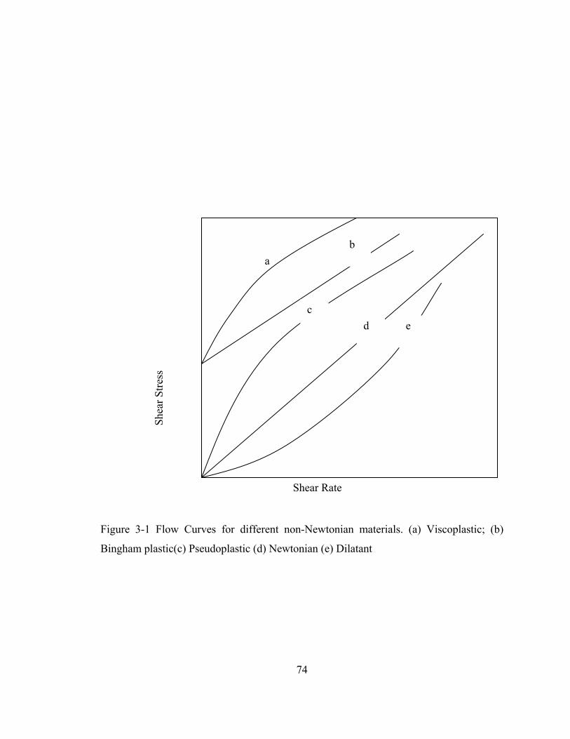
74

Figure 3-1 Flow Curves for different non-Newtonian materials. (a) Viscoplastic; (b)

Bingham plastic(c) Pseudoplastic (d) Newtonian (e) Dilatant

a

Shea

r Stre

ss

e

b

c d

Shear Rate

75

Figure 3-2 Vane Geometry

H

D

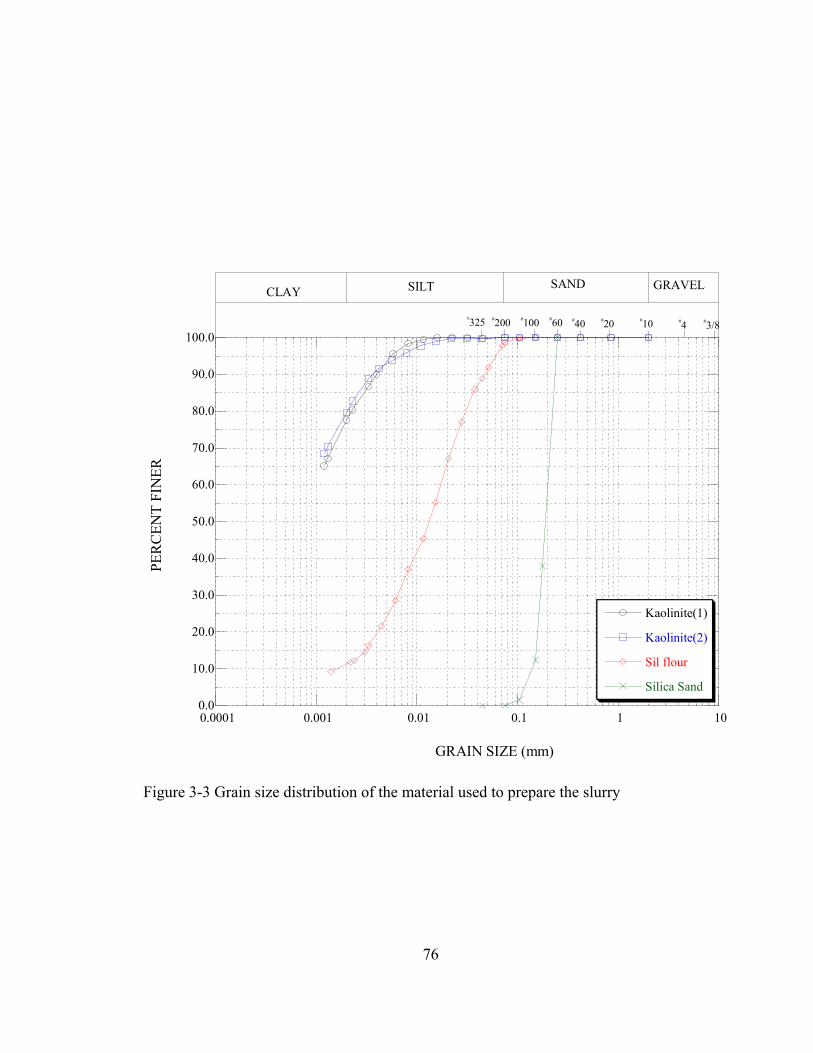
76

0.0

10.0

20.0

30.0

40.0

50.0

60.0

70.0

80.0

90.0

100.0

0.0001 0.001 0.01 0.1 1 10

Kaolinite(1)

Kaolinite(2)

Sil flour

Silica Sand

PER

CEN

T FI

NER

GRAIN SIZE (mm)

SILT SAND GRAVELCLAY

#200 #100 #60 #40 #20 #10 #4 #3/8#325

Figure 3-3 Grain size distribution of the material used to prepare the slurry

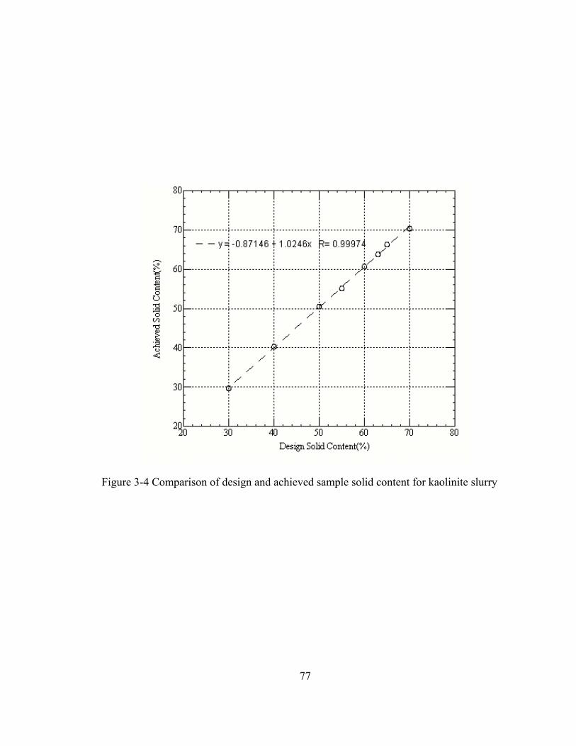
77

Figure 3-4 Comparison of design and achieved sample solid content for kaolinite slurry

78

(a)

y = 86.518xR2 = 0.9999

0

0.005

0.01

0.015

0.02

0 0.0001 0.0002 0.0003

πD2H/2 (m3)

Max

.Tor

que(

Nm

)

0.01/s

b)

y = 87.398xR2 = 0.9999

0

0.005

0.01

0.015

0.02

0 0.0001 0.0002 0.0003

πD2H/2 (m3)

Max

.Tor

que

(Nm

)

0.02/s

Figure 3-5 Relationship between maximum torque and geometrical parameter for

kaolinite slurry(50%w/w) at shear rates (a) 0.01/s and (b) 0.02/s

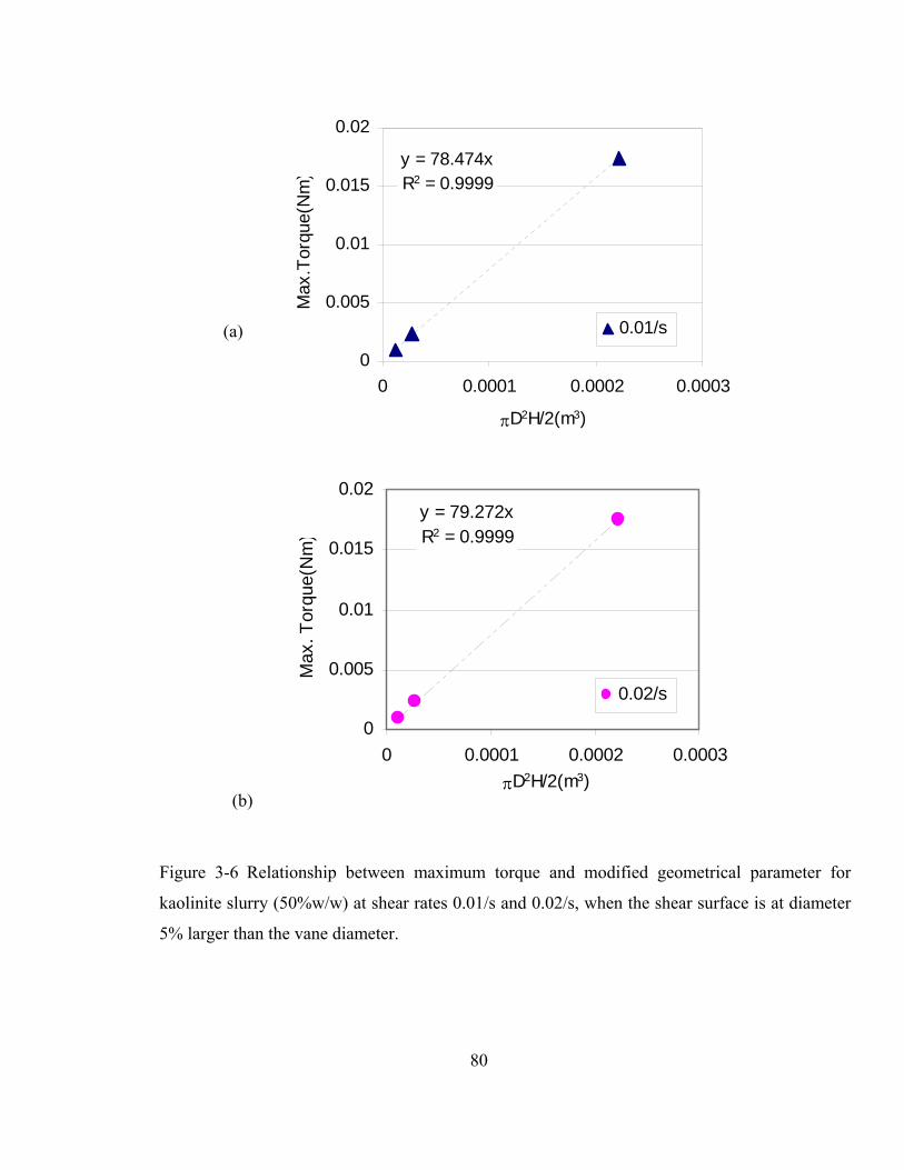
80

y = 78.474xR2 = 0.9999

0

0.005

0.01

0.015

0.02

0 0.0001 0.0002 0.0003

πD2H/2(m3)

Max

.Tor

que(

Nm

)0.01/s

y = 79.272xR2 = 0.9999

0

0.005

0.01

0.015

0.02

0 0.0001 0.0002 0.0003πD2H/2(m3)

Max

. Tor

que(

Nm

)

0.02/s

Figure 3-6 Relationship between maximum torque and modified geometrical parameter for

kaolinite slurry (50%w/w) at shear rates 0.01/s and 0.02/s, when the shear surface is at diameter

5% larger than the vane diameter.

(b)

(a)

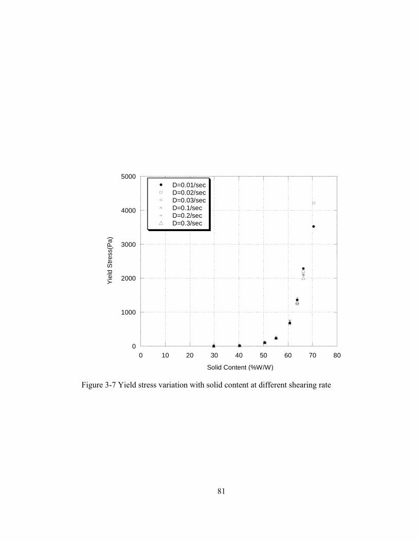
81

0

1000

2000

3000

4000

5000

0 10 20 30 40 50 60 70 80

@

D=0.01/secD=0.02/secD=0.03/secD=0.1/secD=0.2/secD=0.3/sec

Yiel

d S

tress

(Pa)

Solid Content (%W/W)

Figure 3-7 Yield stress variation with solid content at different shearing rate

82

0

5

10

15

20

0 20 40 60 80 100 120 140

Time(sec)

%To

rque

0.01/s 0.02/s 0.03/s 0.1/s 0.2/s 0.3/s

Figure 3-8 Variation of %Torque (reference 5mNm) with time for 30%s, kaolinite

slurry at different rates

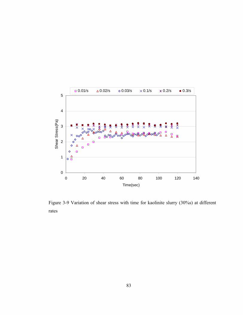
83

0

1

2

3

4

5

0 20 40 60 80 100 120 140

Time(sec)

She

ar S

tress

(Pa)

0.01/s 0.02/s 0.03/s 0.1/s 0.2/s 0.3/s

Figure 3-9 Variation of shear stress with time for kaolinite slurry (30%s) at different

rates

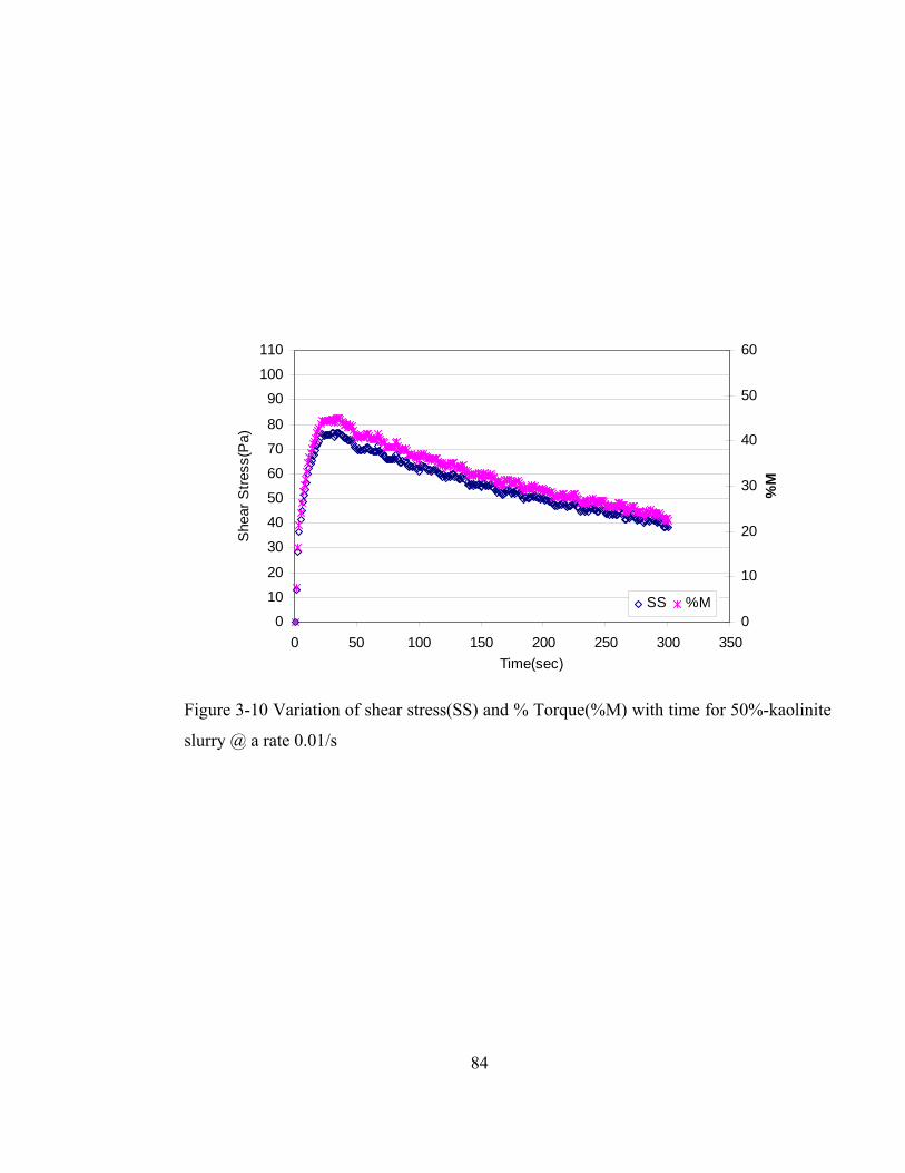
84

0

10

20

30

40

50

60

70

80

90

100

110

0 50 100 150 200 250 300 350Time(sec)

She

ar S

tress

(Pa)

0

10

20

30

40

50

60

%M

SS %M

Figure 3-10 Variation of shear stress(SS) and % Torque(%M) with time for 50%-kaolinite

slurry @ a rate 0.01/s

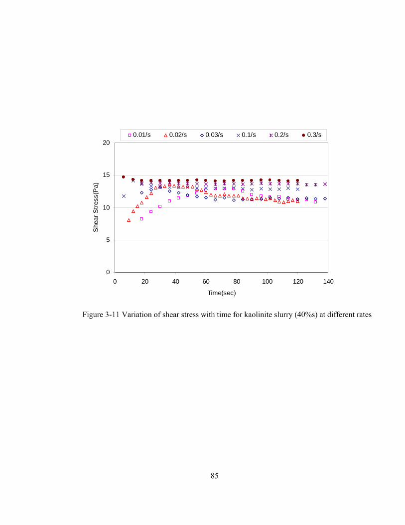
85

0

5

10

15

20

0 20 40 60 80 100 120 140

Time(sec)

She

ar S

tress

(Pa)

0.01/s 0.02/s 0.03/s 0.1/s 0.2/s 0.3/s

Figure 3-11 Variation of shear stress with time for kaolinite slurry (40%s) at different rates

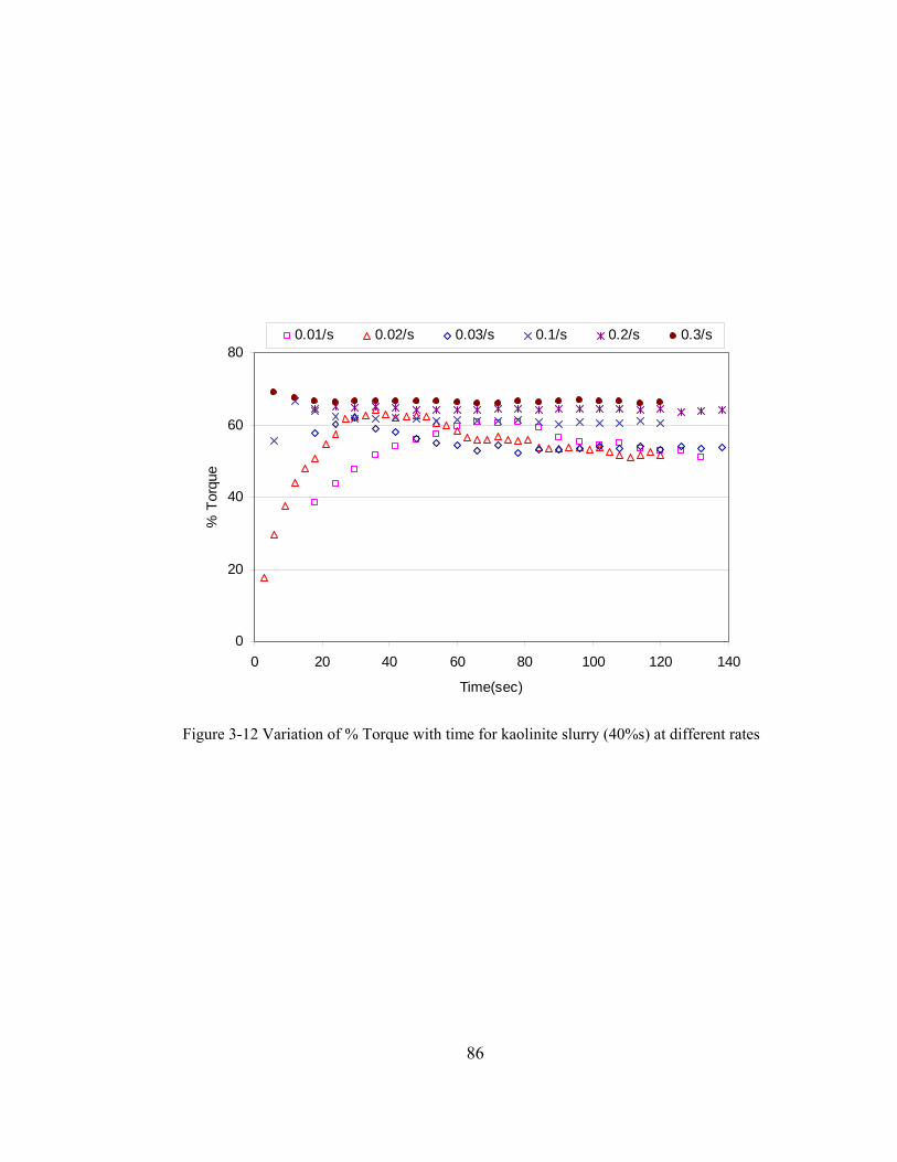
86

0

20

40

60

80

0 20 40 60 80 100 120 140

Time(sec)

% T

orqu

e

0.01/s 0.02/s 0.03/s 0.1/s 0.2/s 0.3/s

Figure 3-12 Variation of % Torque with time for kaolinite slurry (40%s) at different rates

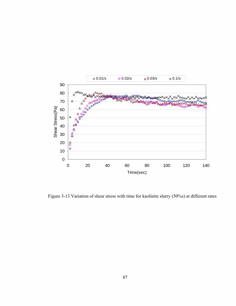
87

0

10

20

30

40

50

60

70

80

90

0 20 40 60 80 100 120 140

Time(sec)

She

ar S

tress

(Pa)

0.01/s 0.02/s 0.03/s 0.1/s


88

0

10

20

30

40

50

60

0 20 40 60 80 100 120 140

Time(sec)

%To

rque

0.01/s 0.02/s 0.03/s 0.1/s


89

0

50

100

150

200

250

300

0 20 40 60 80 100 120 140

Time(sec)

She

ar S

tress

(Pa)

0.01/s 0.02/s 0.03/s 0.1/s 0.2/s


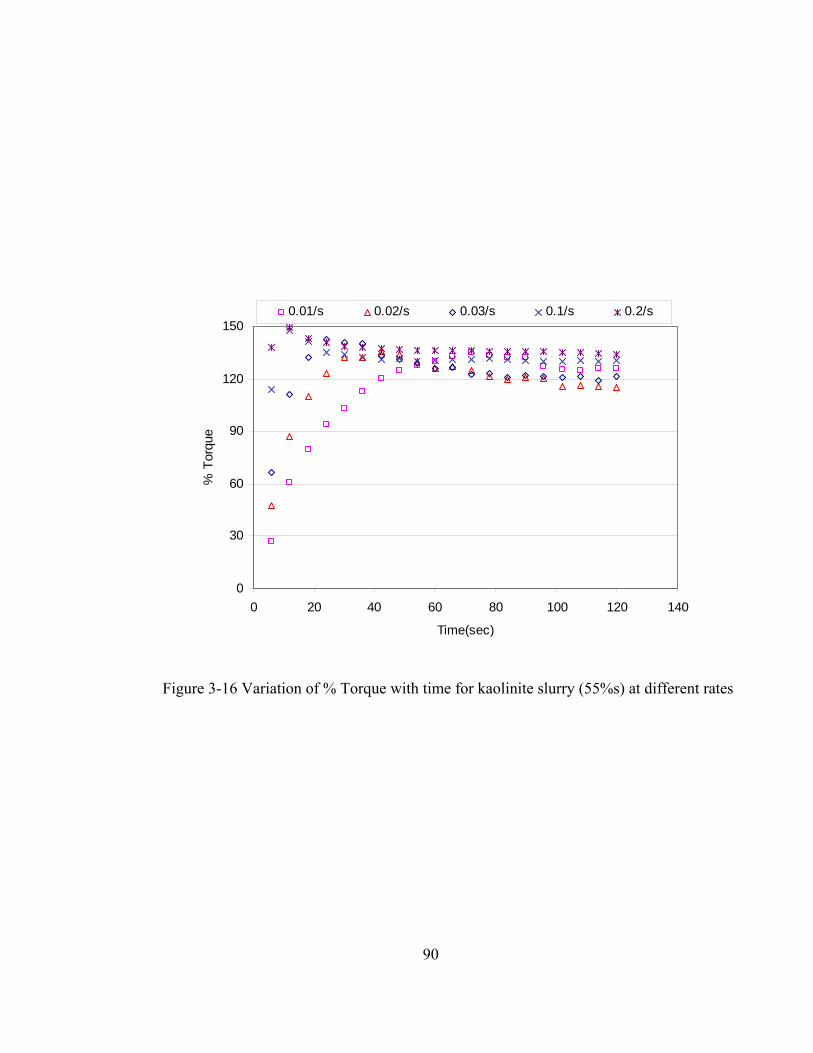
90

0

30

60

90

120

150

0 20 40 60 80 100 120 140

Time(sec)

% T

orqu

e

0.01/s 0.02/s 0.03/s 0.1/s 0.2/s


91

0

100

200

300

400

500

600

700

0 20 40 60 80 100 120 140

Time(sec)

She

ar S

tress

(Pa)

0.01/s 0.02/s 0.03/s 0.1/s 0.2/s 0.3/s


92

0

100

200

300

400

500

0 20 40 60 80 100 120 140

Time(sec)

% T

orqu

e

0.01/s 0.02/s 0.03/s 0.1/s 0.2/s 0.3/s


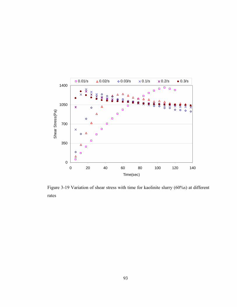
93

0

350

700

1050

1400

0 20 40 60 80 100 120 140

Time(sec)

She

ar S

tress

(Pa)

0.01/s 0.02/s 0.03/s 0.1/s 0.2/s 0.3/s


rates

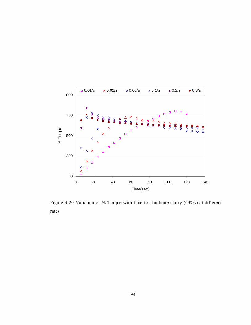
94

0

250

500

750

1000

0 20 40 60 80 100 120 140

Time(sec)

% T

orqu

e

0.01/s 0.02/s 0.03/s 0.1/s 0.2/s 0.3/s

Figure 3-20 Variation of % Torque with time for kaolinite slurry (63%s) at different

rates

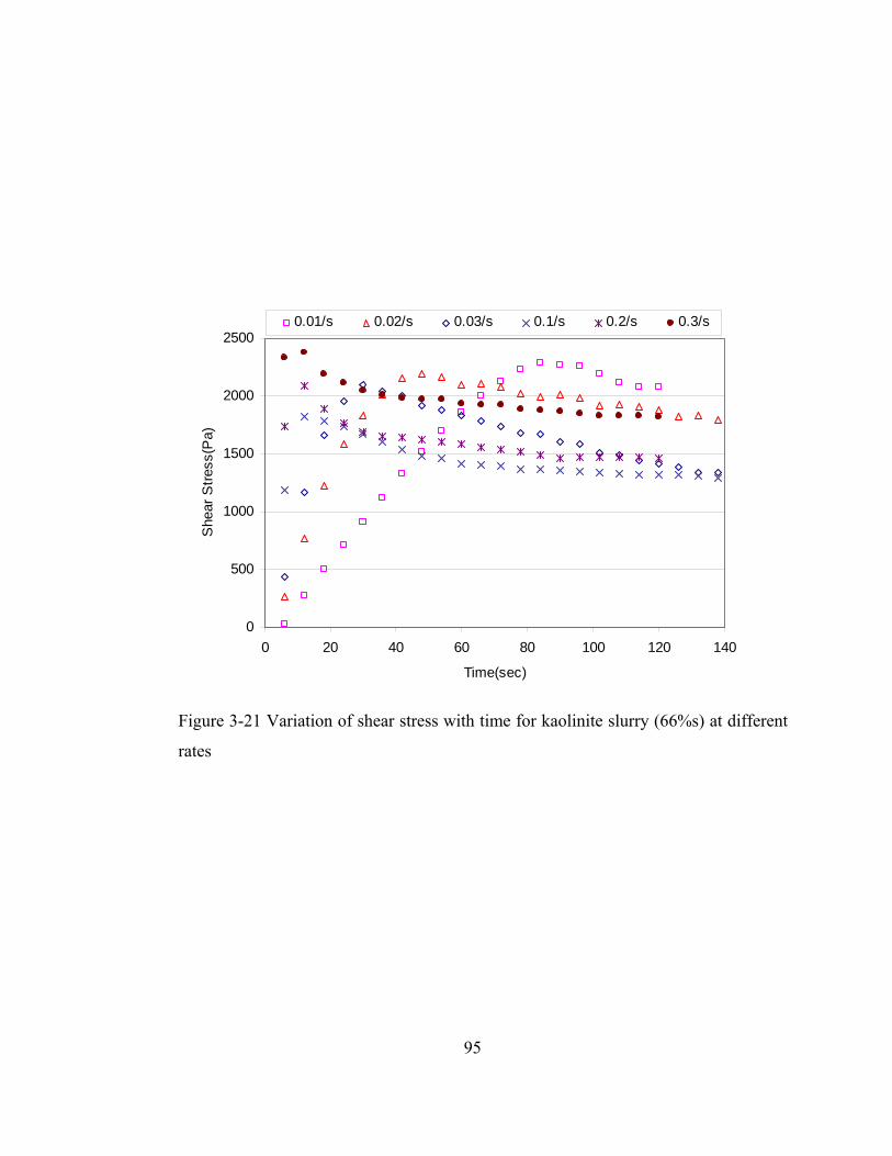
95

0

500

1000

1500

2000

2500

0 20 40 60 80 100 120 140

Time(sec)

She

ar S

tress

(Pa)

0.01/s 0.02/s 0.03/s 0.1/s 0.2/s 0.3/s


rates

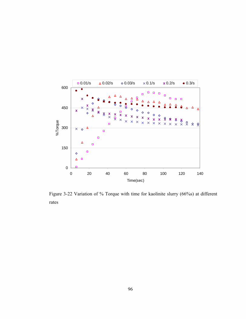
96

0

150

300

450

600

0 20 40 60 80 100 120 140

Time(sec)

%To

rque

0.01/s 0.02/s 0.03/s 0.1/s 0.2/s 0.3/s

Figure 3-22 Variation of % Torque with time for kaolinite slurry (66%s) at different

rates

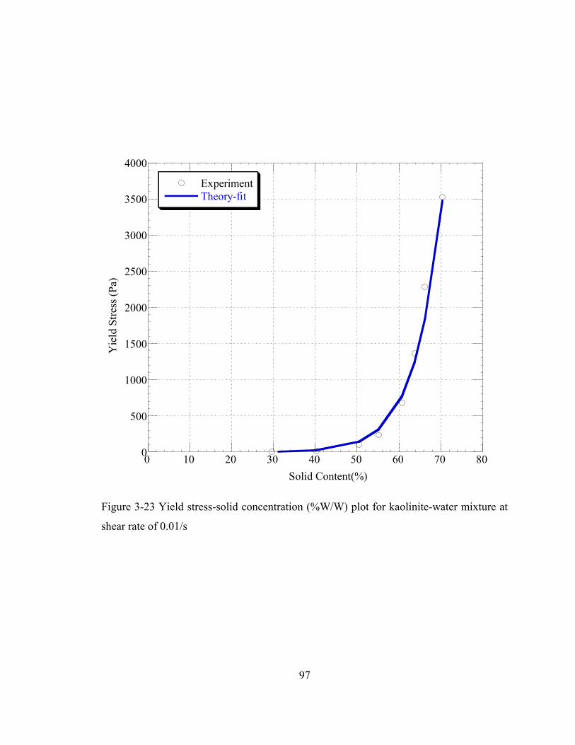
97

0

500

1000

1500

2000

2500

3000

3500

4000

0 10 20 30 40 50 60 70 80

ExperimentTheory-fit

Yie

ld S

tress

(Pa)

Solid Content(%)

Figure 3-23 Yield stress-solid concentration (%W/W) plot for kaolinite-water mixture at

shear rate of 0.01/s

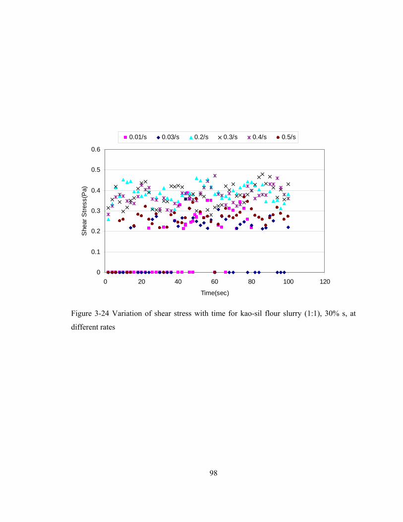
98

0

0.1

0.2

0.3

0.4

0.5

0.6

0 20 40 60 80 100 120

Time(sec)

She

ar S

tress

(Pa)

0.01/s 0.03/s 0.2/s 0.3/s 0.4/s 0.5/s

Figure 3-24 Variation of shear stress with time for kao-sil flour slurry (1:1), 30% s, at

different rates

99

0

1

2

3

4

5

0 20 40 60 80 100 120 140

Time(sec)

She

ar S

tress

(Pa)

0.01/s 0.1/s 0.2/s 0.3/s 0.4/s 0.5/s

Figure 3-25 Variation of shear stress with time for kao-sil flour slurry (1:1), 40% s, at

different rates

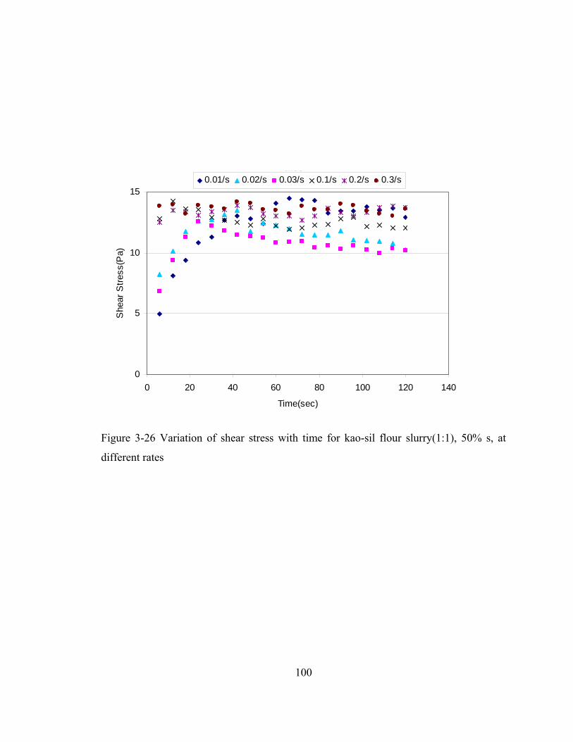
100

ates

0

5

10

15

0 20 40 60 80 100 120 140

Time(sec)

She

ar S

tress

(Pa)

0.01/s 0.02/s 0.03/s 0.1/s 0.2/s 0.3/s

Figure 3-26 Variation of shear stress with time for kao-sil flour slurry(1:1), 50% s, at

different rates

101

0

10

20

30

40

50

0 20 40 60 80 100 120 140

Time(sec)

She

ar S

tress

(Pa)

0.01/s 0.02/s 0.03/s 0.1/s 0.2/s 0.3/s

Figure 3-27 Variation of shear stress with time for kao-sil flour slurry(1:1), 55% s, at

different rates

102

0

10

20

30

0 20 40 60 80 100 120 140

Time(sec)

%To

rque

0.01/s 0.02.s 0.03/s 0.1/s 0.2/s 0.3/s

Figure 3-28 Variation of % Torque with time for kaolinite slurry(1:1) (55%s) at different

rates

103

( ) @

0

50

100

150

200

250

300

350

0 50 100 150(Time(s)

She

ar S

tress

(Pa)

0.01/s 0.02/s 0.03/s 0.1/s 0.2/s 0.3/s

Figure 3-29 Variation of shear stress with time for kao-sil flour slurry(1:1), 62.5% s, at

different rates

104

q ( ) @

010

203040

506070

8090

0 50 100 150(Time(s)

% T

orqu

e

0.01/s 0.02/s 0.03/s 0.1/s 0.2/s 0.3/s

Figure 3-30 Variation of % Torque with time for kao-sil flour slurry (1:1)(62.5%s) at

different rates

105

0

50

100

150

200

250

300

0 20 40 60 80 100 120

Time(sec)

She

ar S

tress

(Pa)

0.01/s 0.02/s 0.03/s 0.1/s 0.2/s 0.3/s

Figure 3-31 Variation of % Shear Stress with time for kao-sil flour slurry(1:1) (65%s) at

different rates

106

0

20

40

60

80

100

0 20 40 60 80 100 120

Time(sec)

%To

rque

0.01/s 0.02/s 0.03/s 0.1/s 0.2/s 0.3/s

Figure 3 - 32 Variation of % Torque with time for kao-sil flour slurry (1:1) (65%s) at

different rates

107

0

200

400

600

800

1000

0 20 40 60 80 100 120

Time(sec)

She

ar S

tress

(Pa)

0.01/s 0.02/s 0.03/s 0.1/s 0.2/s 0.3/s

Figure 3-33 Variation of % Shear Stress with time for kao-sil flour slurry(1:1) (70%s) at

different rates

108

0

100

200

300

0 20 40 60 80 100 120

Time(sec)

% T

orqu

e

0.01/s 0.02/s 0.03/s 0.1/s 0.2/s 0.3/s

Figure 3-34 Variation of % Torque with time for kao-sil flour slurry (1:1)(70%s) at

different rates

109

0

500

1000

1500

2000

2500

3000

3500

4000

0 50 100 150 200 250 300

Time(sec)

She

ar S

tress

(Pa)

0.02/s 0.03/s 0.1/s 0.2/s 0.3/s

Figure 3-35 Variation of Shear Stress with time for kao-sil flour(1:1) (75%) at different

rates

110

0

100

200

300

400

500

600

700

800

900

1000

0 50 100 150 200 250 300

Time(sec)

She

ar S

tress

(Pa)

0.02/s 0.03/s 0.1/s 0.2/s 0.3/s

Figure 3-36 Variation of % Torque with time for kao-sil flour slurry (75%s) at different

rates

111

0

500

1000

1500

2000

2500

3000

3500

4000

25 35 45 55 65 75Solid Content(%W/W)

Yiel

d St

ress

(Pa)

kaolinte only20%Sil-flr35%Sil-flr50%Sil-flr

Figure 3-37 Effect of Sil-flour addition on the yield stress of kaolinite slurry, at shear rate

of 0.02/s

112

0

0.4

0.8

1.2

0 50 100 150 200 250 300Time(sec)

She

ar S

tress

(Pa)

0.01/s 0.02/s 0.03/s 0.1/s 0.2/s 0.3/s

Figure 3-38 Variation of shear stress with time for kao-sand slurry (1:1) (35%s),at

different rates

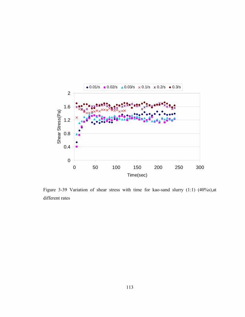
113

0

0.4

0.8

1.2

1.6

2

0 50 100 150 200 250 300Time(sec)

She

ar S

tress

(Pa)

0.01/s 0.02/s 0.03/s 0.1/s 0.2/s 0.3/s

Figure 3-39 Variation of shear stress with time for kao-sand slurry (1:1) (40%s),at

different rates

114

rates.

0

2

4

6

0 50 100 150 200 250 300Time(sec)

Shea

r Stre

ss(P

a)

0.01/s 0.02/s 0.03/s 0.1/s 0.2/s 0.3/s

Figure 3-40 Variation of shear stress with time for kao-sand mix (1:1), 50%s, at different

shear rates

115

0

5

10

15

20

25

30

35

40

45

0 50 100 150 200 250 300Time(sec)

She

ar S

tress

(Pa)

0.01/s 0.02/s 0.03/s 0.1/s 0.2/s 0.3/s

Figure 3-41 Shear stress variation with time for kosand mix(1:1), 60%s, at different rates

116

0

500

1000

1500

2000

2500

3000

3500

4000

4500

25 35 45 55 65 75Solid Content(%W/W)

Yie

ld S

tress

(Pa)

kaolinte only20%Sand35%Sand50%sand

Figure 3-42 Effect of Sand addition on the yield stress of kaolinite slurry, at shear rate

of 0.02/s

117

0

100

200

300

400

500

600

700

0 20 40 60 80 100 120 140Time (sec)

She

ar S

tress

(Pa) kaolinite only

kaolinite+silflourkaolinite&sand

Figure 3-43 Shear Variation with time for different compositions at 60% solids @ 0.02/s

118

0

5

10

15

20

25

0 10 20 30 40 50 60 70 80

Shear Rate(1/s)

She

ar S

tress

(Pa)

HB model fit

Figure 3-44 Flow curve for kaolinite slurry 40%s(w/w) and Herschel-Bulkley (HB)model

fit with KHB=2.855, n=0.3105 and τy=11.49 Pa

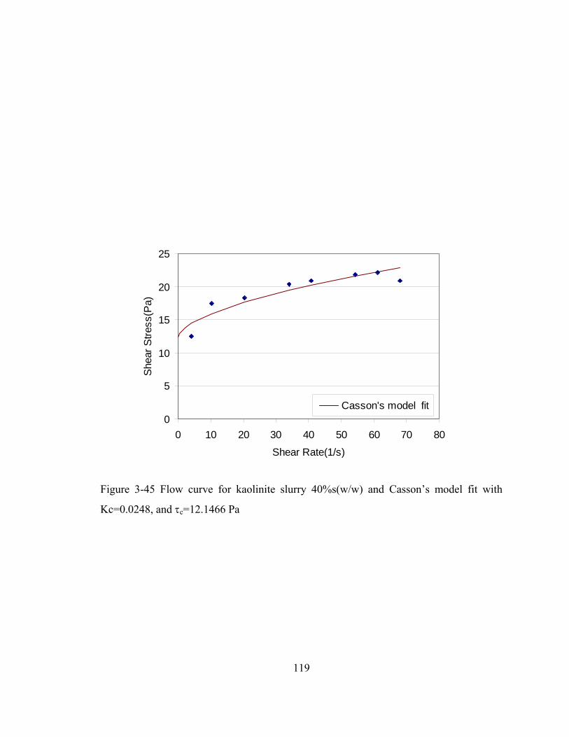
119

0

5

10

15

20

25

0 10 20 30 40 50 60 70 80

Shear Rate(1/s)

Shea

r Stre

ss(P

a)

Casson's model fit

Figure 3-45 Flow curve for kaolinite slurry 40%s(w/w) and Casson’s model fit with

Kc=0.0248, and τc=12.1466 Pa

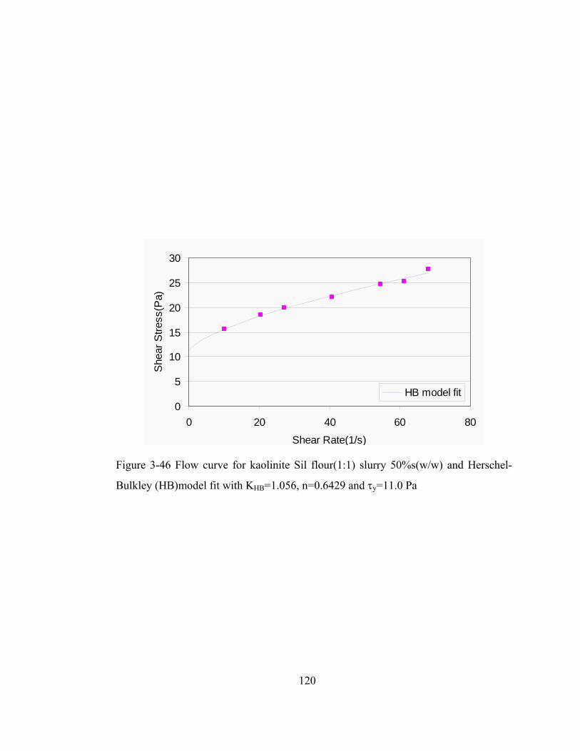
120

0

5

10

15

20

25

30

0 20 40 60 80

Shear Rate(1/s)

She

ar S

tress

(Pa)

HB model fit

Figure 3-46 Flow curve for kaolinite Sil flour(1:1) slurry 50%s(w/w) and Herschel-

Bulkley (HB)model fit with KHB=1.056, n=0.6429 and τy=11.0 Pa

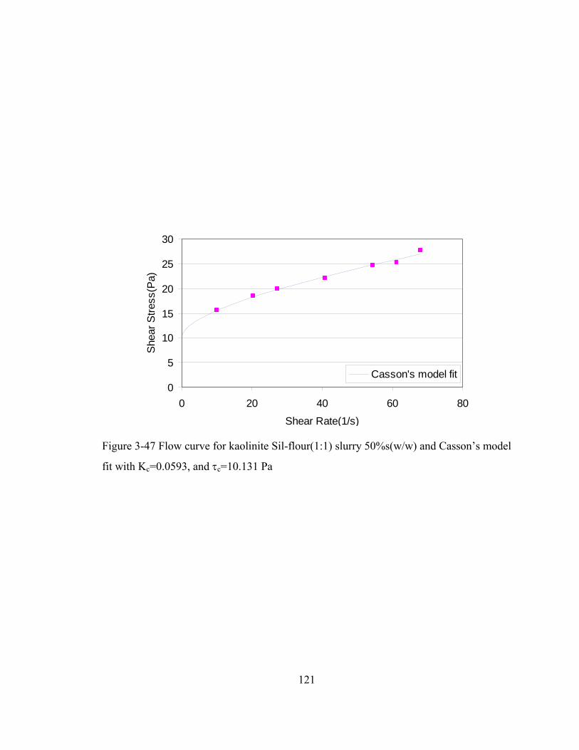
121

0

5

10

15

20

25

30

0 20 40 60 80

Shear Rate(1/s)

She

ar S

tress

(Pa)

Casson's model fit

Figure 3-47 Flow curve for kaolinite Sil-flour(1:1) slurry 50%s(w/w) and Casson’s model

fit with Kc=0.0593, and τc=10.131 Pa

122

0

20

40

60

80

100

120

140

0 100 200 300 400 500 600 700

Time(sec)

She

ar S

tress

(Pa)

pH=3 pH=4.43 pH=5.58 pH=7.8 pH=9 pH=10.05 pH=12_Ca(OH)2 pH=12_NaOH

Figure 3-48 Variation shear stress at different pH values for kaolinite slurry @50% s

123

0.00

40.00

80.00

120.00

160.00

0 2 4 6 8 10 12 14

pH

Yie

ld S

tress

(Pa)

Figure 3-49 The variation of yield stress with pH for kaolinite slurry 50% s

124

CHAPTER 42

4. EXPERIMENTAL INVESTIGATION OF SEGREGATION IN CLAY-SAND SLURRY

4.1. Introduction

Segregation, as a ubiquitous phenomenon, occurs in many natural and man-made

processes: the sorted layers of magma fall out, stone rings in permafrost, rock avalanches,

and seasonal stream deposits are few among many natural events. In industrial processes,

where bulk materials are handled, transported, and stored segregation usually results in

poor quality of product as in pharmaceutical, ceramic, cement and food processing. On

the other hand ore extraction process exploits the advantage of differential settling. In oil

sands extraction process, for example, the bitumen is separated as a froth which floats to

the surface; the coarse sand settles to the bottom and is removed. A portion of this slurry,

known as middling, is removed from the central portion of the vessel, and is further

processed.

Segregation, in the context of its use here, may be described as a phenomenon by which

certain sizes or components with similar properties tend to preferentially collect in one or

another physical zone of a collective (de Silva, 1999). It may occur due to differences in

size, density ,shape, surface roughness, elastic modulus, voidage and many others, among

which size difference is the most dominant Williams (1976), Rhodes (1998), Vallance

and Savage (1999).

The segregation process, primarily, occurs under sub-aerial and sub-aqueous

environment. The granular flow refers closely to the former and sedimentation process to

the latter. The granular flow, where the bulk volume of the particulate materials are

involved, is by itself a wide and complex subject, and it is not in the intent of this work to

2 A version of this chapter has been published. Mihiretu, Y.M., Chalaturnyk, R.J., Scott, J.D. Proc. of 59th Canadian Geotechnical Conference, Vancouver, British Columbia, 2006.

125

cover it. However, some theoretical and experimental treatments may be found in the

works of Savage and his co-workers; Savage and Lun (1988), Savage (1993), Vallance

and Savage (1999), de Silva et al.(1999), Williams (1976) and others.

The study of sedimentation is important, because it is either desired (bitumen extraction,

filtration, thickening, consolidation, tailings management) or unwanted (industrial

applications: pharmaceutical, ceramic, paints). Sedimentation process takes places when

particles settle/segregate through a fluid medium mainly under the action of gravity. This

process has been understood since the early times when human beings started to crush

and wash mineral ores to extract the concentrate. Later the invention of thickeners and

their wide use has in the meantime facilitated the scientific studies in the subject. A

comprehensive historical survey of the development has been provided by Buerger and

Wendland (2001).

The subject of sedimentation involving suspensions containing mixed particle sizes is not

well developed, and reliable relationships have not been available. This is because of the

wide range of particle sizes, the variety of particle shapes, and the complex nature of the

hydrodynamic and physicochemical phenomena which govern particle-fluid and particle-

particle behaviour (Selim et al., 1983). In their critical review on this subject, Boogerd et

al. (2001) remarked that although much effort has been applied in past decades, no

fundamental breakthrough has been achieved. Nevertheless, it is not uncommon among

engineers/ researchers to deal with their complex problems in some pragmatic way based

on experimental evidences, past experience and theoretical and empirical models.

Mitigation or control of either natural or industrial processes involving segregation thus

requires a fundamental understanding.

In a fresh formation of deposits in practice and in most laboratory experimentation,

sedimentation and consolidation are concurrent processes which may be difficult to treat

independently. However, occasionally the term sedimentation and consolidation are used

with ambiguity. In the commonest use of geotechnical engineering, we refer to

sedimentation as a tendency of the solid phase to settle to a deposition state in the

126

direction of dominant acting force (mainly gravity, centrifuge) whereas consolidation

refers to the settlement of the deposited material as a result of removal of liquid material

(water) due to the dissipation of excess pore pressure and development of effective stress.

Study of segregation as it is dealt with in this work focuses on the fundamental aspects of

the sedimentation/ consolidation process which involve wide size range. It will be

worthwhile to recapitulate the research made in these aspects in different areas and then

proceed with the objectives outlined for this work.

4.2. Literature & background

When solid phases interact with fluids, sedimentation/segregation occurs by the action of

gravity due to size or density differences among particles. The classic study of

sedimentation is attributed to G.G. Stokes in 1851. He derived an equation relating the

terminal velocity of a sphere in fluid with the density difference between the solid and

liquid, diameter of sphere and viscosity of the fluid. Though his equation was derived for

a single sphere, it is applied to very dilute suspension, where the inter-particle

interactions are assumed to be negligible and free settling of particles takes place. It is

this basic idea that is still being used today as a means of grain size determination in the

basic soil mechanics (Bowles 1986).

When the concentration of particles increases, the interaction among the particles also

increase and a hindered settling mode is observed. After the invention of thickener in

1905, the application of hindered settling process received wide attention. However the

operational systems were more of an art than a practice based on basic scientific

understanding (Concha and Buerger 2002). It appears that the study of sedimentation

with application to industrial processes has received greater treatment in chemistry or

chemical engineering and mining engineering, probably driven by the demand for

optimal design and operation in the filtration and separation industry. The works in these

areas can be seen mostly as experimental study supplemented by semi-empirical models

or simulation.

127

Coe and Clevenger (1916) identified different settling zones in batch settling of slimes

containing wide range of sizes and they used the observed experimental data in the design

of thickener. There existed no systematic theory until the time when Kynch (1952)

introduced his new theory of sedimentation. The principle of continuity and the

assumption that the velocity of propagation of concentration waves depends only on the

local concentration constitute the main framework of his theoretical formulation. His

theory is later revisited and revised by Tiller (1981) to account for the effect of rising

sediment.

Richardson and Zaki (1954) summarized preceding studies which applied modified forms

of Stokes’ equation in the prediction of the settling rates of suspension of fine and

uniform particles. They argued that the previous assumptions that the effective

gravitational force acting on a particle in a suspension is determined by the density of the

suspension and that the drag on the particle is a function of the apparent viscosity cannot

be true for a suspension of uniform particles. They stated that in the suspension of

uniform particle, each particle settles at the same rate and displaces its own volume of

liquid and they conclude that for a suspension of uniform particles, the use of an effective

viscosity of the suspension is not valid. They provide the widely cited equation which

relates the settling velocity of uniform suspension to the terminal settling velocity of a

single particle (‘relative velocity’, a term used by Happel (1958)-‘velocity ratio’ seems

more appropriate- and the porosity raised to a constant. The constant is a slope obtained

from the log-log plots of settling velocity versus the porosity.

Happel (1958) developed a mathematical free surface model, in which the relative

velocity is dependent upon some function of the diameter ratio of the spherical bulb

encasing the particle to the diameter of the particle. He showed that the model fitted

experimental data in the dilute and concentrated suspension ranges.

Barnea and Mizrahi (1973) produced a comprehensive survey of published works and

introduced an empirical equation for the relative velocity also as a function of particle

128

volume fraction. The relative velocity matches a unit value when the concentration

reduced to infinite dilution, which is the theoretical value. Most important assumptions in

their study were: no flocculation and aggregation were considered, the relative positions

of the particles in the clouds are completely random, with segregation and wall effects

being ignored.

Garside and Al-Dibouni (1977) also analyzed the experimental results of their

predecessors and conducted experiments. They noticed significant curvature on a log-log

plot of settling velocity versus porosity at high voidage (volume fraction of non-solids)

values and in the turbulent regions. They provide a logistic curve fit for the Richardson

and Zaki’s constant as a function of the Reynolds number.

Studies have been extended to systems of the bi-disperse and poly-disperse suspension,

which are practically the situations encountered in many industrial operations. In these

types of suspensions, the significance of segregation becomes apparent. Lockett and Al-

Habboby (1973) conducted experiments on bi-disperse system. Their hypothesis was that

in the settling of the bi-disperse system, containing particles with the same density but

different in size, different zones would appear: from top to bottom, clear liquid zone,

zone containing only smaller particles, and a zone containing both large and small

particles. They extended the Richardson-Zaki equation to the bi-disperse case, and found

a good fit to their experimental data; however, significant over-prediction is visible when

they compared the same model with previously published experimental data. Mirza and

Richardson (1979) extended this principle to poly-disperse cases.

Masliyah (1979), developed a model by applying steady state momentum balance to

poly-disperse suspensions, as it was derived for mono-disperse suspension in Wallis

(1969). The model applies for both size and density differences of particles in the

suspension. The density difference for a particle size under consideration is its density

minus the density of a mixture of the pure fluid and smaller particles present locally.

Selim et al. (1983) also developed a model for poly-disperse suspension based on the

Garside and Al-Dibouni (1977) approach. They tested their model with bi-disperse

129

suspension and found good agreement. However their model was criticized for some

deviations in limiting cases (Doheim et al. 1997) and an error in the formulation

(Stamatakis and Tien 1988). Stamatakis also examined some of the cited models in

literature. They commented that the models have little difference and it is the ease of

computation that mandates the merits of the correlations. Other experimental and model

studies in bidisperse and polydisperse suspensions, also available in literature, are due to

(Zimmels 1983) (Patwardhan and Tien 1985); (Law, 1987); (Zimmels, 1988);

(Stamatakis and Tien 1988); (Smith 1997); (Buerger et al. 2000).

Batchelor (1982), from a colloidal science perspective, developed a theory of

sedimentation based on two-sphere hydrodynamics accounting for effects of relative

movement of particles due to gravity, the inter-particle force and Brownian diffusion. He

investigated the effect of interaction and inter-particle forces between pairs of particle

and obtained formula for the average speed of particles (which are correct to the first

power of the volume fraction of the particles). His equation introduces dimensionless

sedimentation coefficient which is a function of size ratio and reduced density ratio. The

theory has been also interpreted/ analyzed numerically (Batchelor and Wen 1982).

A comprehensive review on the development of the non-colloidal sedimentation at low

Reynolds number is presented by Davis and Acrivos (1985). They also give attention to a

case of enhanced sedimentation in inclined channels which is a rare case appearing in

literature. They conclude in their review by recommending further research to reach a

relation of the macroscopic properties of a sedimenting polydisperse suspension to the

local microphysical interaction between the different particles. Davis and Gecol (1994)

proposed a hindered settling function which looks like a hybrid/coupling between

Richardson-Zaki model and Batchelor’s model. By putting the sedimentation coefficient

of Batchelor’s theory in to the exponent of Richardson and Zaki’s exponential term, they

managed to avoid the empirical parameter involved. They compared their model with

dilute bi-disperse experimental results and found good agreement. They also suggest that

their model be tested for complex cases involving broader range of particle size and

130

densities. The above survey indicates that the emphasis is mainly on the sedimentation of

non-colloidal particles in a liquid.

Shen et al. (1994) clearly indicated that the most readily understood situation is of

particles without an appreciable affinity for one another. This situation is not always

realized, however. The flocculation of particles into aggregates or gel-like networks

complicates the processing of a variety of materials including foods, soils, ceramic

powders, and chemical/biological waste product.

Coe and Clevenger (1916) noticed that, in metallurgical practice, slime pulp consists of

water, finely divided sand or granular particles, and colloidal material. In their different

settling zones, they generally took that the granular material falls directly to the bottom

immediately, and eliminated from consideration, and implicitly, not contribute to the

mechanism. They identified different settling zone in batch settling of slimes containing

wide range of sizes and used the observed experimental data in the design of thickener.

For flocculated suspensions, Michaels and Bolger (1962) correlated experimental data by

means of a modified form of the Richardson-Zaki equation. They suggested a structural

model for the settling of fine kaolin particles in which primary particles are grouped into

small clusters (called flocs). They assumed that each floc was spherical in shape, and that

the water within it moved with it and there was flow of liquid around the flocs, but no

flow through them. While it is clear that these assumptions cannot exactly represent the

actual situation, they lead nevertheless to an equation which is useful for data correlation,

and which indicates, at least qualitatively, how the flocculation affects the settling

process. Michaels and Bolger (1962) analyses also show why critical concentration is

much lower for flocculated than for non-flocculated suspensions. If the flocs are truly

spherical and closely-sized, the critical concentration would be expected to correspond to

a floc volume fraction in the order of 0.64 (random-packed equal spheres).

Landman and White (1992, 1994) discussed the phenomenological approach to the study

of flocculated suspensions. They highlighted the importance of rheology and stressed the

131

importance of three rheological parameters: compressive yield stress, the hindered

settling factor and the dynamic compressibility. They have shown the application of

phenomenological compressional rheology of flocculated suspensions to gravity

thickening and pressure filtration. Green et al. (1996) presented an experimental

procedure of determining the compressive yield stress.

Phillips (1997) reviewed briefly the sedimentation behaviour of colloidal particles. He

based his discussion on Batchelor’s sedimentation theory. He discussed that attraction

between colloidal particles reduces the concentration dependence of velocity. He noticed

also that the concentration dependence of the sedimentation dynamics in the case of non-

spherical particles has hardly been investigated, and according to him, is a major

challenge in colloidal sedimentation.

Li and Mehta (1998) assessed the hindered settling formulation to fluid mud-like

suspension and derived an analytical equation from the continuity equation by applying

Darcy’s law to the seepage velocity of upward moving displaced water. They estimated

the permeability from the Hagen-Poiseulle viscous flow equation.

In the geotechnical field, the study of sedimentation seems to have got relatively little

attention. Traditionally soil mechanics is related to the post-sedimentation stage, i.e. after

the formation of soils. Primarily, since the early works of Karl Terzaghi, the treatment of

soil-water interaction is mainly considered as the water is moving through the pore space

of stationary soil grains, namely consolidation or/and seepage. Imai (1980) wrote that our

attention has been hitherto concentrated on the soil behaviour after soil formation, and the

behaviour before the soil formation has been overlooked in geotechnical engineering,

although its knowledge may be invaluable to practical designs of land-filling work,

disposal work by sedimentation and so on. The processes which govern the sedimentation

process are either implicitly related to the Stokes’ law or simply overlooked (McRoberts

and Nixon 1976). However, as the geotechnical engineers encounter more complex

phenomena, it has necessitated revisiting the basic process to understand the involved

mechanisms.

132

The well-established consolidation theory in geotechnical engineering has been basically

developed for solving settlement of foundations on clays (Terzaghi 1943). In essence, the

theory is subjected to many simplifying assumptions such as constant permeability,

constant compressibility, and validity of Darcy’s law. These assumptions are only

satisfied approximately in practice (Gibson et al. 1967). In a latter study, Gibson et al.

(1967) developed a finite non-linear consolidation equation of saturated clays which

accounts for the changes in soil compressibility and permeability.

It is through the early work of McRoberts and Nixon (1976) that the theory of

sedimentation was brought to the attention of geotechnical engineers. They introduced, in

extended form, the Kynch theory of sedimentation to settling of soil particles. They

related the development of effective stress and then the consolidation process with

formation of soil and at the same time questioned which concentration level of dispersion

is referred to as ‘soil’ in geotechnical sense. They argue that the sedimentation theory

governs the behaviour of soil grains-water mixtures at concentration ranges immediately

less than the concentration range appropriate for consolidation. Pane and

Schiffman (1997) have estimated a void ratio in the range of 30 to 40 for the formation of

soil from their experimentation in Kaolin sedimentation.

Been and Sills (1981) completed laboratory tests on sedimentation of soft soils (kaolin

and clayey silt mud). They used a non-destructive method (X-ray) to obtain the density

profile of a settling mud. They assessed segregation during settling. They observed that

significant proportion of the silt particles settled through the mud to the base. The

segregation is very visible when the mud was dispersed with sodium hexametaphosphate,

showing that flocculation plays an important role in segregation. In their theoretical

explanation to their experimental results, they introduced imaginary overburden to the

consolidation equation. However, this approach was challenged by Tan et al (1990), due

to the situation that the process is hindered settling rather than a consolidation process.

Buerger et al. (2000) were able to capture the shape of the concentration profile by use of

the phenomenological sedimentation theory, though involving rough estimates. On the

133

other hand, their measurements show the development of excess pore pressure, which is a

sufficient condition to assume the mud as a soil and then consequently apply the

consolidation theory.

Imai (1980, 1981) has completed experimental studies on the behaviour of soft soil. He

examined the settling characteristics as affected by clay mineralogy, concentration and

salt content of water. He identified the major settling stages in three zones: zone settling,

flocculated free settling and consolidated settlings. Tan et al. (1990) presented the effect

of grain size distribution, pH and flocculent on the settling characteristics of clay slurry.

They observed non-Newtonian behaviour from rheological study conducted on the

sediment. By spreading sand on the surface of the sediment, they demonstrated that

capture of the sand due to gain in strength of sediment. In another study, Tan et al. (1990)

modified the Kynch theory to flocculated clay sedimentation by use of momentum

equation and empirical formulation for permeability.

The traditional consolidation theory deals with situations where the initial conditions are

well known. The question [to geotechnical engineers] would be what if the initial

conditions are by themselves undergoing a process, such as is the case in freshly

deposited sediments. Then necessity of sedimentation (hindered settling) with the

consolidation process becomes evident. Studies which combine sedimentation and

consolidation process appeared in the 1980’s. Pane and Schiffman (1985) proposed a

simplified constitutive formulation for the total stress by introducing interaction

coefficient to the effective stress. Incorporating the constitutive equation into Gibson et

al.'s (1967) finite strain consolidation theory, they form an equation which can model

simultaneous sedimentation and consolidation of saturated soils.

In a separate study in the fluid mechanics area, Auzerais et al. (1988) developed a

phenomenological theory of the sedimentation and consolidation theory of concentrated

suspensions using the equation of motion for the fluid-particle system, including all the

forces active in both the settling and sediment phase. Their analysis predicts

concentration profiles of the whole process (sedimentation/consolidation) for both stable

134

and flocculated suspensions. Eckert et al. (1996) have shown that the governing equation

for consolidation as developed by Gibson et al. (1967) in soil mechanics and the fluid

dynamic equation of Auzerais et al. (1988) are the same equations formulated from a

different frame of reference.

Similarily, Toorman (1996,1999), Diplas and Papanicolaou (1997), Karl and Wells

(1999) and Buerger (2000) have developed phenomenological models to approach the

sedimentation/ consolidation problem. Stamatakis and Tien (1992) also presented an

approximate approach of sedimentation/ consolidation dealing with polydispersity.

Fitch (1975) offered an opinion that although some success was achieved in the

development of sedimentation/consolidation equations, that the literature of this era

should be understood as primarily elaboration of Kynch theory, rather than an

explanation of reality.

The wide grain size distribution influencing the size segregation is long understood in

practice. These effects are counteracted by the increase of particles’ concentration

(Barnea and Mizrahi 1973). The brief review above show that a great deal of effort has

been put into the sedimentation /consolidation study. The effect of grain size was

considered somehow by account of poly-dispersity. Falk and Umberto (2002), in their

review, noted that previous researchers considered size ratio of about 2 to 3. In their

experimental work they considered a wider grain size distribution ranging in four

decades. Shih et al. (1987), for example, mentioned a typical size distribution of particles

in coal liquids to range from 2 through 20 micron. They formulated a general multiphase

hydrodynamic model for multi-sized particles. They attempted to include, fluid-particle

interaction, solid compressive stress, particle to particle interaction and other forces. They

were somehow able to capture the concentration profiles with some deviations. In related

studies, Stamatakis and Tien (1988) and Al-Naafa and Selim (1992) reported that the

effect of fine particles presence in the suspension, are accounted for by considering

equivalent viscosity of suspension of slow settling particles and fluid medium.

135

Colloidal systems display complex rheological behaviour related to their thermodynamic

non-ideality. These systems depart from Newtonian behaviour, often exhibiting yield

stress, before deforming continuously as a liquid. Flocculated suspensions respond

elastically to small deformations with moduli that depend strongly on the volume fraction

of particles (Russel et al. 1989). It is also apparent that the studies in colloidal

sedimentation mainly emphasize on the compressive yield stress in conformance to the

hindered settling/ consolidation approach (Bergsroem et al. (1992), Landman et al.

(1988), Landman and White (1994), Shen et al. (1994) and Chu et al. (2002).

The important observation from the above review of the literature indicates that the

rheological properties of the flocculated slurry are considered in the sediment zone only.

A remaining question is how the rheological characteristics of a slurry affect the settling

zone. In a different study in non-Newtonian fluid mechanics there is a clear account of

different rheological approach in that the significant presence of fine particles contribute

to the rheological characteristics of the whole suspension system Valentik and Whitmore

(1965), Ansley and Smith (1967), Chhabra et al. (1992), Saha et al. (1992), and Coussot

(1997).

The properties of mine tailings, particularly, oil-sands tailings in Northern Alberta,

Canada, present complex practical challenges due to the fact that there exists segregating

disposal behavior (Kuepper 1991), a large volume of waste materials (Fine Tailings

Fundamentals Consortium 1995), and very slow sedimentation /consolidation

(Eckert et al. 1996). At the same time safe disposal being a major environmental

requirement, handling, storing and monitoring have posed major challenges to the

geotechnical engineers. Consequently, it has become necessary to understand the major

physical process involved in the tailing disposal schemes.

Despite the fact that important developments have been seen in the study of

sedimentation/ segregation in particulate form or in colloidal form separately, there exists

very little information in the literature on the results of studies on the constitutive

influence of a slurries composition (i.e. fine and coarse particles) on the

136

sedimentation/segregation behaviour. Moreover, information on the interaction or

progress with time of the segregation process involving slurries with a wide particle size

distribution is hard to find in the literature.

The theme of this work is thus to examine the segregation phenomena experimentally and

theoretically with emphasis on identifying the effect of grain size composition commonly

classified in geotechnical engineering as clay, silt and sand. It will also be attempted to

investigate the concentration level at which the rheological properties of fines play a

significant role.

4.3. Materials and Methods

The materials used in the experimental program are mainly kaolinite clay, silica sand

(180-250 micron size) and sil-flour which was used as a silt size material. The particle

size distribution for each material is shown in Figure 4-1. The liquid and plastic limits of

kaolinite are 55.2% and 29.5% respectively. The silt size, sil-flour exhibits no plasticity.

The ambient temperature during experimentation is 20+2o C.

The material is weighed on to a scale (0.01g accuracy) in 5-litre plastic pail. The water,

which is added to achieve a desired solid content, is Edmonton City tap water, the pH of

which is 7.7+0.2. Two types of standpipes are used in this experiment: a modified type 5-

litre standpipe or 2-litre standpipes. The choice is made in such a way that slurries that

are expected to exercise relatively high settling rates are tested with the modified

standpipe, whereas those slurries expected to have a relatively slow settling rate are tested

with 2-litre standpipes.

4.3.1 Description of the modified standpipe test

The modified stand pipe test designed for this study is shown schematically and in picture

in Figure 4-2. The material used to manufacture the modified standpipe is transparent

Plexiglas, with a thickness of 10 mm. The standpipe was designed to enable the

137

development of segregation with time to be studied and to provide sufficient sample

volume of each “element” for concentration profiling. Wall effects have been minimized

by specifying relatively large dimensions for the width and depth of the cell.

4.3.2 Test procedure

After initial mixing of all the ingredients of the slurry, the sample is thoroughly mixed for

about 15 to 20 min in a pail. The mixed slurry is transferred into the modified standpipe

and stirred again in the standpipe for about 5 to 10 minutes to insure uniform distribution

of the slurry. Then the sliding plates are pushed into the standpipe at a chosen time. The

driving of the sliding plates takes about 10 sec to completely form different sections of

the height for sampling. Then each section from top down is pumped out of the standpipe

and transferred into aluminum tray. Whenever pumping becomes difficult due to high

solid content, samples were scooped with large spoons fitted on extension rods. After wet

mass measurement, the material is put into the oven overnight. The following day dry

mass is measured. After that the material is soaked in water in order that the fines can be

easily washed out. The fine washing is carried out through the 44micron sieve. After

ensuring that all fines are washed out, by visual observation that clear water come

through the bottom of the sieve, the retained sand is transferred into the tray and put in

the oven overnight. The next day, dry mass measurement is conducted. Material loss is

encountered occasionally due to splashing during stirring or leak while driving the slicing

gates. Finally the mass balance before and after the test is checked. If the loss of material

is greater than 5 %, the test is repeated.

The test programs as well as interpretation of the results will be described using the

ternary diagram (or soil structure behaviour diagram) as shown in Figure 4-3. The

definitions for the variables used in the soil structure behavior diagram (SSBD) are the

following:

Solid content, s = (weight of dry sample–weight of tray)/(weight of wet

sample-weight of tray)*100

138

Sand content, SC = (weight of dry sample after washing- weight of tray)/

(weight of wet sample-weight of tray) *100

Solid content = weight of solid in a slurry/ (weight of wet slurry)

Sand content (%) = (sand/(sand + fine))*100 (weight basis)

Fine content: = fine /(sand +fine) = 100-SC

Sand Fine Ratio (SFR) = weight of Sand/ weight of Fine (weight basis)

Volumetric solid content =Volume of Solid/ total volume of slurry.

4.3.3 Results and Discussion

The compositions for all tests are identified in Figure 4-3 as small red points. For

modified standpipe experimentation the design of testing is made according to SFR 1, 2,

4 and FWR at 10, 15, 20, 30 and 40%.

(i) Test of Sand Fine Ratio, SFR=1

Figure 4-4 shows the test results for the temporal behavior of slurry with a target initial

solid content of 18.8%s. Figure 4-4 illustrates the change in solids content and sand

content profiles at 15 second intervals from an elapsed time of 15 seconds to 90 seconds.

The solid content profile shows that there exist two distinct regions of concentration,

mainly a high concentration region at the bottom and an upper low concentration region.

The corresponding sand content profile reveals that the sand has settled almost

immediately to the bottom. Though not easily visible in the solid content profile, the sand

content shows a decreasing trend in the upper segments. Also visible in the sand profile is

that the change in sand content takes place in the intermediate section and the top section

remains nearly the same.

With slight increase in the fine content to 15% FWR, Figure 4-5 shows the concentration

variation clearly both in terms of solid content and sand content. The time progress of

sedimentation shows the increase in concentration at the bottom and drop in

concentration at the upper section. Also observed here is that the trend of the time

139

progress of sedimentation showing the concentration profile with respect to the total solid

and sand show similar trend.

Figure 4-6 shows the results at FWR of 20 and solid content of 33.3%. The profile at this

test condition shows an overlapping tendency for both solid content and sand content

profiles for the times of test. Unlike the previous testing, there is no sharp increase at the

bottom in this test. Also the gradient of the profiles seem to be smooth throughout the

depth. The solid concentration profile for the 30sec test seem to be deviating towards a

less concentration level, this could be attributed to experimental errors.

As the initial solid content as well as FWR increases to 46.2% and 30% respectively, the

solid content and sand content profiles show nearly vertical profile as shown in Figure 4-

7. Despite the extended time of testing to 180sec, the sedimentation process during this

time does not produce any visible segregating tendency.

When the FWR is raised to 40% and the solid content to 57.1%, the slurry is very dense

and longer testing time up to 24hrs is allowed. As shown in Figure 4-8, the solid content

profiles and sand content profiles are nearly vertical in all cases. A small deviation of

solid content profile at 18hrs reading has been attributed to experimental errors.

(ii) Test of Sand Fine Ratio, SFR = 2

As the sand proportion is increased (i.e. SFR increased from 1 to 2), evolution of the

sedimentation/ segregation process, as illustrated in Figure 4-9, remains visible for the

first 30 seconds but thereafter, the solid concentration profile remains essentially

unchanged. In contrast, the evolution in the sand content profile continues to show

changes well past 60 seconds, indicating that sand segregation is occurring with relative

negligible changes in solids content. For the case with an SFR = 1 (Figure 4-4), the

evolution of the sand content profile was not as apparent as for SFR = 2. This is likely

just due to the higher sand concentration at an SFR = 2 allowing this behavior to be

captured in the modified standpipe.

140

When the FWR is raised to 15% (Figure 4-10), the profiles at different times get closer

and become a gentle slope, both with respect to solid content and sand content. A similar

trend is also to see for FWR of 20 (Figure 4-11). Nearly vertical profile appears when the

FWR is raised to 30% (Figure 4-12). The sand content shows very little deviation

vertical-wise for the test duration of 240sec (4min).

(iii) Test of Sand Fine Ratio, SFR=4

For the three tests conducted at SFR=4, the effect of sand content is clearly magnified at

the low solid content as shown in Figure 4-13. The increase of FWR by small amount

produced gentle slope in both solid and sand content profiles. This result indicate that the

effect of granular packing contribution to the interaction and consequent reduction in

segregation trend (Figure 4-14).

Due to high solid content, longer testing interval was allowed to the test condition shown

in Figure 4-15. There appears no segregation within the first 4hrs of testing time. For

longer testing times, 12hrs and 24 hrs, the departure from verticality is noticeable.

However, this is due to settlement of the whole suspension and clear water formation at

the top section, and increase in solid content. While the solid concentration profile shows

significant increase in solid content of the deposit after 12 hrs, only slight change is

visible at the bottom section with respect to the sand content. This maybe an indication

that the sand is captured in the fine matrix and the sedimentation takes place en-masse.

4.4 Effect of fine matrix

At low solid concentration, there is immediate settling of the sand and at the same time

there are some particles retained in the top sections. The question would be why do not

all sand particles do not settle. If we assume the fine particles form part of the fluid

medium, the equivalent viscosity of the suspension may be estimated using the Einstein’s

141

(1906, 1911) equation, described as Equation (4.1) or that of Thomas (1965) described as

Equation 4.2 which was widely used and tested to fit available data reasonably. For

10%w/w solid content the difference is about 2.0% [1.87 exact]. Consequently, Thomas’s

equation was used in this research.

(1 2.5 )effμ μ φ= + (4.1)

Thomas (1965) provided an extended empirical form of the equation as:

2(1 2.5 10.05 0.00273exp(16.6 ))effμ μ φ φ φ= + + + (4.2)

where μeff. the suspension viscosity , μ is the viscosity of the medium (water in this case)

and φ is the volume fraction of the solids in the suspension.

For laminar motion (Re<1), the transition region (1 < Re>1000) and the turbulent region

(Re>1000) the settling velocity is defined as follows:

Laminar motion [ Re 1dVρμ

= < ],

2( )

18s

og du ρ ρ

μ−

= (=>Stokes’ law) ; (4.3)

Transition region [1<Re<1000],

0.72 1.18

0.45

( )0.20( / )

so

g du ρ ρρ μ ρ

⎡ ⎤−= ⎢ ⎥

⎣ ⎦ ; (4.4)

and turbulent motion [Re> 800],

0.50

0.5( )1.74 sou g dρ ρ

ρ⎡ ⎤−

= ⎢ ⎥⎣ ⎦

. (4.5)

Since cases of dilute suspensions are being examined, an assumption that sand particles

settle individually may be acceptable and the settling velocity calculation for a particle

may be used conveniently. The Reynolds number and velocity for sand particle settling

through kaolinite+water suspension are calculated to be 6.34 and 3.13cm/s respectively,

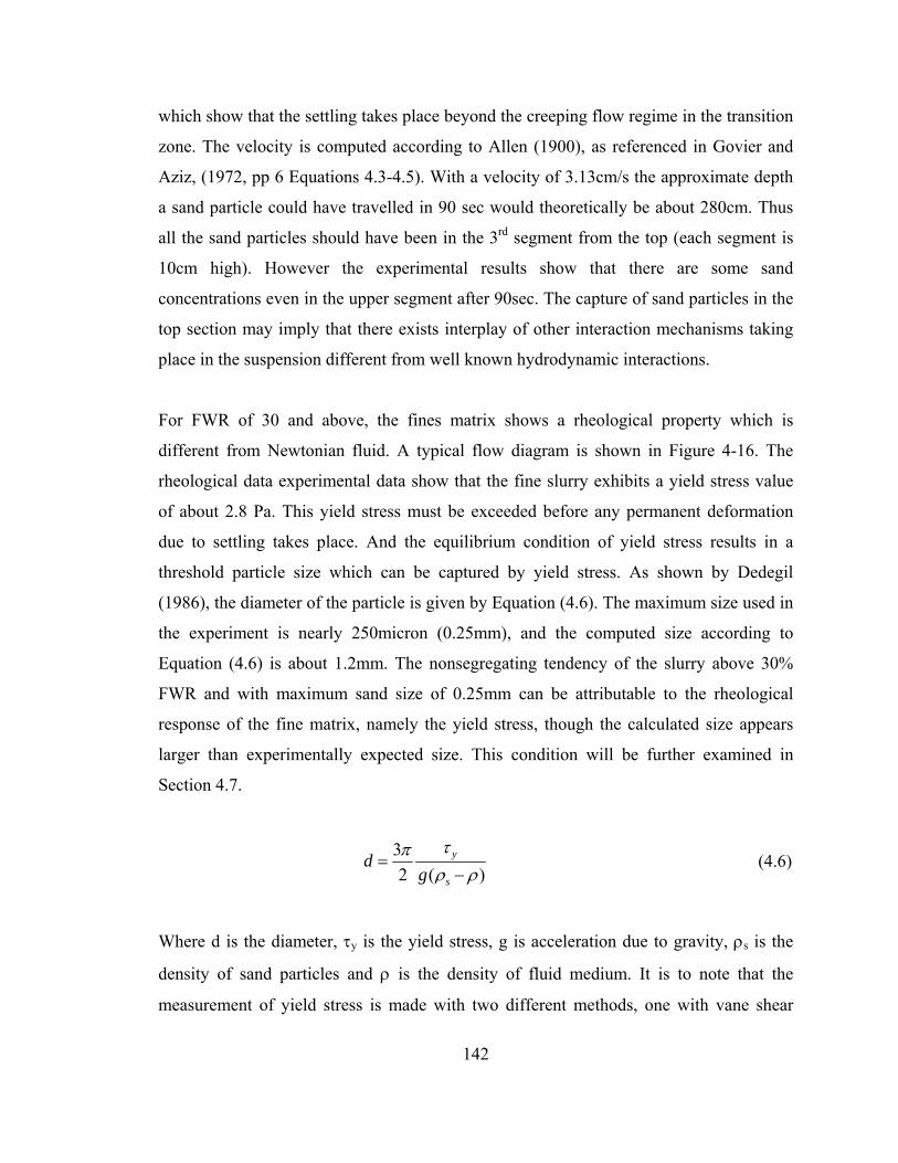
142

which show that the settling takes place beyond the creeping flow regime in the transition

zone. The velocity is computed according to Allen (1900), as referenced in Govier and

Aziz, (1972, pp 6 Equations 4.3-4.5). With a velocity of 3.13cm/s the approximate depth

a sand particle could have travelled in 90 sec would theoretically be about 280cm. Thus

all the sand particles should have been in the 3rd segment from the top (each segment is

10cm high). However the experimental results show that there are some sand

concentrations even in the upper segment after 90sec. The capture of sand particles in the

top section may imply that there exists interplay of other interaction mechanisms taking

place in the suspension different from well known hydrodynamic interactions.

For FWR of 30 and above, the fines matrix shows a rheological property which is

different from Newtonian fluid. A typical flow diagram is shown in Figure 4-16. The

rheological data experimental data show that the fine slurry exhibits a yield stress value

of about 2.8 Pa. This yield stress must be exceeded before any permanent deformation

due to settling takes place. And the equilibrium condition of yield stress results in a

threshold particle size which can be captured by yield stress. As shown by Dedegil

(1986), the diameter of the particle is given by Equation (4.6). The maximum size used in

the experiment is nearly 250micron (0.25mm), and the computed size according to

Equation (4.6) is about 1.2mm. The nonsegregating tendency of the slurry above 30%

FWR and with maximum sand size of 0.25mm can be attributable to the rheological

response of the fine matrix, namely the yield stress, though the calculated size appears

larger than experimentally expected size. This condition will be further examined in

Section 4.7.

32 ( )

y

s

dg

τπρ ρ

=−

(4.6)

Where d is the diameter, τy is the yield stress, g is acceleration due to gravity, ρs is the

density of sand particles and ρ is the density of fluid medium. It is to note that the

measurement of yield stress is made with two different methods, one with vane shear

143

apparatus and the other with conventional viscosity measurement with a rheogram plot

extrapolating to zero shear, gave similar yield stress value.

4.5 Effect of silt size presence

In soil mechanics, clay and silt sizes are generally grouped as fine soils. Such

classification was examined in rheological characterization part in the previous chapter.

The presence of silt size is observed to decrease the yield strength of the fine matrix. As

yield stress is more attributed to the ultra fine clay particles, inclusion of larger sizes tend

to minimize the bonding of clay particles and consequently reduce the yield strength. The

different composition of clay and silt at initial total solid content of 33.3% is shown in

Figure 4-17. The clay and silt size particle composition is varied at 100% clay, 80% clay

& 20% silt size, 65% clay & 35% silt size and 50% clay & 50% silt size. The figure

clearly shows that despite similar solid content in all tests, the sedimentation results in a

segregating concentration profile both in solid content and sand profiles. This kind of

phenomena is indirectly observed in the rheological characterization of slurries. Thus it

can be ascribed that the sedimentation process to be in direct relation to the rheological

property of the suspension (slurry). This is a clear demonstration that the fine clay size

presence contribute to the settling properties quite significantly depending upon the

concentration level. At dilute concentration ranges (about FWR < 20) the effect is not

visible. As the fine concentration gets larger, the dominant effect of clay particle presence

comes into play.

The results discussed above clearly indicate the contribution of fines (clay) in the

sedimentation process. It is worthwhile then to investigate further the fine matrix effect

on the sedimentation process with significant presence of fines and also allowing longer

testing time. Thus some more tests were conducted on a 2-litre standpipe. Details of the

results will be presented as follows.

4.6. 2-Litre Standpipe Test

144

To examine further the effect of fine on the sedimentation process, 2 litre standpipe tests

were conducted. At low FWR there is clear indication that sand particles easily settle

through the suspension leading to two distinct regions: sand with little clay particle

presence at the bottom and clay particles at the top. This is clearly visible at FWR less

than 20% (Figure 4-18). However, as the FWR is increased the sediment profile seems to

be controlled by the fine particle presence. This is seen in Figures 4-19 and 4-20 where

the profile at same FWR but different solid content shows similar pattern in profile

indicating the FWR after certain limits (i.e. FWR value of 30) controls the sedimentation

process. The sand particles are captured throughout the fine matrix.

A remarkable observation for slurries beyond a FWR of 30% is that the solid content

profile at different SFR but same FWR exhibit similar shape in profile. It is also observed

that the distance between the curves is in the proportion of the initial solid content. If the

different curves are normalized to the initial solid content they all fall into a close band at

a single location. Figures 4-21 and 4-22 show the normalized plots for FWR of 30 and 45

respectively.

4.7 Fine capture and yield stress

The theoretical size, as obtained by Equation 4.6, seems to give larger sizes than those

observed experimentally. Thus detailed experimentation was carried to check the validity

of the theoretical formulation in the testing programs. The sand sizes are divided into

different size range in order to minimize averaging over a wide size range.

Also in order to analyze the segregating profile of the sedimentation experiment, a

statistical approach, i.e., standard deviation which is referred in here as Segregation Index

(SI) is used. Details of its formulation are found in Chapter 7.

An SI with respect to solid and SI with respect to sand can be computed. For this test

series, it is assumed that an SI of 5 with respect to solids and an SI of 2.5 with respect to

sand in solids can provide a reasonable indicator of non-segregation.

145

Detailed experimental observations on four size ranges of sand indicate that the size

captured is actually less than the one calculated from yield stress Equation (4.6). Thus a

correction factor is applied as indicated in Equation (4.7). It can be seen from the

summary of results provided in Table 4-1; the correction factor is always less than one

indicating that the theoretical value over-predicts the size that can be held by yield stress.

The difference gets larger as the size increases.

dmeasured = K * dtheoretical. (4.7)

Table 4-1 Fine capture at different grain size range of sand particles

Size range (μm) SI (total solid) SI (sand in solids) FWR K

150-180 5.0 0.75 30 0.24

250-300 3.7 1.23 32 0.25

600-850 3.4 0.42 38 0.16

1180-2000 1.8 0.44 42 0.15

The correction factor K as in Equation (4.7) is higher at lower FWR and vise versa. It is

clear that the capture size for fine slurry increases with increase in fines solid content.

However the theoretical prediction is found to over-predict the size of sand that can be

captured. This is shown by the value of K found for the kaolinite slurry. On the average

the K value is 0.2. Such experimental results cast doubt on the purely theoretical formulation. In order to

help us compare our result with those found in literature a yield parameter defined in

Equation (4.8) was chosen to give better comparison.

( )

y

s

Ygd

τρ ρ

=−

(4.8)

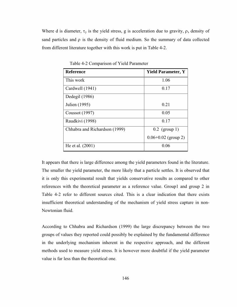
146

Where d is diameter, τy is the yield stress, g is acceleration due to gravity, ρs density of

sand particles and ρ is the density of fluid medium. So the summary of data collected

from different literature together with this work is put in Table 4-2.

Table 4-2 Comparison of Yield Parameter

Reference Yield Parameter, Y

This work 1.06

Cardwell (1941) 0.17

Dedegil (1986)

Julien (1995)

0.21

Coussot (1997) 0.05

Raudkivi (1998) 0.17

0.2 (group 1) Chhabra and Richardson (1999)

0.06+0.02 (group 2)

He et al. (2001) 0.06

It appears that there is large difference among the yield parameters found in the literature.

The smaller the yield parameter, the more likely that a particle settles. It is observed that

it is only this experimental result that yields conservative results as compared to other

references with the theoretical parameter as a reference value. Group1 and group 2 in

Table 4-2 refer to different sources cited. This is a clear indication that there exists

insufficient theoretical understanding of the mechanism of yield stress capture in non-

Newtonian fluid.

According to Chhabra and Richardson (1999) the large discrepancy between the two

groups of values they reported could possibly be explained by the fundamental difference

in the underlying mechanism inherent in the respective approach, and the different

methods used to measure yield stress. It is however more doubtful if the yield parameter

value is far less than the theoretical one.

147

Based on major features of the physical process investigated in this test program, some

preliminary classification of a slurry property can be made. Three main regions are

shown in Figure 4-3. Region A is a dilute zone where the inertia of sand particles is very

large and consequently settles to the bottom of the standpipe immediately. In this region

conventional Newtonian particulate fluid mechanics may be applied. This is an area

where most sedimentation studies fall. It is in this area that segregation is more prevalent.

In region B the surface properties of fine particles, namely clays, come into play. In this

region non-Newtonian behaviour is predominantly observed. The microscopic interaction

can be explained in terms of a collective macroscopic behaviour in some rheological

form. For the fine slurry we tested the rheological model which better suit for the fine

slurry is Herschel-Bulkley model. Slurries in this region are apparently less studied.

The bottom region C is a solid and semi-solid region where more soil-like behaviour is

exhibited. This region is a high solid content area and consequently has less likelihood of

segregation. Long term effects, such as consolidation, creep or stability issues that are

significant in this region.

In the experimental observations made in this study, for low solid contents and a wide

size distribution, segregation is almost instantaneous occurring in the first minutes

following mixing (deposition). As the solids content increases, the effect is counteracted

by particle interactions. These phenomena have been also understood in practice and the

most readily understood situation is the interaction of particles without an appreciable

affinity for one another. This situation is not always realized.

In a study of oil sands tailings, Scott et al. (1985) explained that the sand grains remain

suspended due largely to gel strength. They present rheological characteristics of the

material they investigated. From their results, the material shows pseudo-plastic

behaviour. The significance of understanding the sedimentation and strength

characteristics of slurry has also been discussed by Tan et al. (1990). They observed that

at the end of settling, the water content of slurry is still much higher that the liquid limit

(to be called soil in soil mechanics sense) and the slurry are still fluid-like. In their study

148

about the behaviour of clay, they noticed that fines slurry exhibit non-Newtonian

behaviour with some threshold yield strength. They demonstrated the significance of

yield stress by pouring sand on to the surface of sediments and observed retained sand

particles. They also emphasized that yield strength, though small in conventional soil

mechanics sense, is significant in soil treatment. Despite such an understanding, the

mechanistic explanation of the phenomena was not available. It was Dedegil (1986) who

presented the equation which explain the phenomena theoretically. However, our

experimental results indicate that the theoretical formulation generally give larger size. A

correction factor in the range of 0.15 to 0.25 needs to be applied for the sand particle size

ranges in this experiment.

Russel et al. (1989) have indicated that flocculated suspensions respond elastically to

small deformations with moduli that depend strongly on the volume fraction of particles.

During sedimentation involving fine colloidal particles sizes, the concentration profile of

a sediment changes with depth and time. During such process water is displaced and

particles rearrange and settle into a more structured and stable form. At the same time, it

is also apparent that the yield stress would change with depth and time. How the

development of the network structure affects the yield stress of the fine matrix and also

the interaction mechanism with the coarse particle present is far from clear, and merits

further research.

An important practical case in the direction of this study will be the oil sands tailings, in

northern Alberta, Canada. Since the beginning of commercial extraction of bitumen there

exist a large volume of tailings material disposed into ponds that is filling rapidly and

dewatering slowly. As conventional disposal schemes produce segregating tailings, the

produced fine tailing in the pond are settling or consolidating at a very slow rate and may

even take longer time even estimated in centuries (Eckert et al. 1996).

The Fine Tailings Fundamentals Consortium (1995) has reported on the unusual

properties of fine tailings and concluded that it is predominantly associated with the

gelation characteristics of an ultra-fine, colloidal(< 0.3 micron) solids’ fraction. And the

149

presence of ultra-fines in oil sands fine tailings account for more than 90% of its water

holding capacity. In the same compendium it was lucidly put that complete understanding

of tailing behaviour requires knowledge of ultra-fines content, the in-situ environment in

the parent ore, and process or pond water chemistry. Some efforts to create non-

segregating tailings were focused on changing the floc structure of the fine tailings such

as addition of divalent ions (flocculants), freeze-thaw and other treatment process.

It is apparent that despite some understanding about some rheological characterization,

the application to the fine tailings sedimentation/consolidation behaviour should be a

subject of further study. Experimental observations made in this study with some testing

on actual tailings materials indicate that such phenomena may be significant. It is

believed that proper treatment of rheological properties could give better understanding

of the existing challenges in tailings. One of the possible solutions to the existing fine

tailings problems is, for example, the in-situ treatment of the fine tailings or mature fine

tailings (MFT). In order to improve the consolidation process, internal surcharge by sand

grains could be applied if the rheological properties of fine tailings are adequately

recognized.

4.7.1 Non Newtonian modelling Issues

Experimental study of sedimentation of a single particle in non-Newtonian fluid was

initially made by Valentik and Whitmore (1965) Further developments by Ansley and

Smith (1967), Dedegil (1986), and Machac et al. (1995) were significant contributions in

the field. An experimental investigation of hindered settling in power-law liquids was

conducted by Chhabra et al. (1992) and they extended Newtonian models to interpret

their experimental data. Although the subject has been brought to attention fundamentally

for almost four decades, very little information is available in the literature. This is likely

attributable to insufficient experimental data in the area and/or to the lack of adequate

research tools.

150

In the chemical engineering literature, consolidation of flocculated suspensions has

received a great deal of attention. Field studied and model developments have also been

shown to match experimental results Auzerais et al. (1988), Buscall and White (1987),

Landman and White (1994), Eckert et al. (1996), and Green et al. (1996) ). There is a

tendency to believe that a linear relationship exists between the compressive yield stress

and the rheological yield stress. Floc formation and restructuring mechanism and the

process taking place remains not well understood. The presence of a yield stress, a

subject of debate though, at the early stage of sedimentation before the onset of

consolidation seems to be unaccounted for. Also the presence of coarse, surface free

grains adds to the complication the sedimentation mechanism. At current stage, thus, a

sedimentation/ consolidation model comprising wide grain size range and incorporating

surface properties of fine particles is seemingly unavailable. Also experimental data on

the consolidation of fine and coarse mixtures at different composition are not available in

the surveyed geotechnical references.


In this study of segregation experimental results show the early stages of segregation

process. It is observed that at low solid content and low FWR the sand settles to the bed

immediately. However, there exist some sand particles within the slurry after some time

has elapsed which can not be explained by available hydrodynamic analysis.

The sedimentation tests on different grain-size composition are exhibiting some kind of

direct response analogy to the yield stress rheological characterization observation made

in accompanying test program.

It is also observed that in all test ranges conducted, there is a tendency that the fine

content controls the concentration profile of the sedimentation involving clay and sand

particle concentrations.

151

The impact of constant Fine Water Ratio are significant above the FWR value of 30%

where the slurry begins to exhibit yield stress and the effects are remarkably

demonstrated through the normalized plot which fairly bring all test point, at different

solid content but similar FWR, to the same curve(band).

The theoretical size from yield stress equilibrium, though conservative, is shown to over-

estimate the size observed through experiment. Also a quantitative interpretation tool has

been applied to analyze the experimental observation.

4.9 Reference

Al-Naafa, M.A., and Selim, M.S. 1992. Sedimentation of Monodisperse and Bidisperse

Hard-Sphere Colloidal Suspensions. AIChE Journal, 38(10): 1618-1630.

Ansley, R.W., and Smith, T.N. 1967. Motion of Spherical Particles in a Bingham Plastic.

AIChE Journal, 13(6): 1193-1196.

Auzerais, F.M., Jackson, R., and Russel, W.B. 1988. The resolution of shocks and the

effects of compressible sediments in transient settling. J.Fluid Mech., 195: 437-

462.

Barnea, E., and Mizrahi, J. 1973. A Generalized Approach to the Fluid Dynamics of

Particulate Systems


Systems. The Chemical Engineering Journal, 5: 171-189.

Batchelor, G.K. 1982. Sedimentation in a dilute polydisperse system of interacting

spheres.Part 1. General theory. J. Fluid. Mech., 124: 329-528.

Batchelor, G.K., and Wen, C.-S. 1982. Sedimentation in a dilute polydisperse system of

interacting spheres. Part 2. Numerical results. J.Fluid Mech., 124: 495-528.

Been, K., and Sills, G.C. 1981. Self-Weight Consolidation of soft soils: an experimental

and theoretical study. Geotechnique, 31(4): 519-535.

Bergsroem, L., Schilling, C.H., and Aksay, I.A. 1992. Consolidation Behavior of

Flocculated Alumina Suspensions. J.Am.Ceram. Soc., 75(12): 3305-3314.

152

Boogerd, P., Scarlett, B., and Brouwer, R. 2001. Recent modelling of sedimentation of

suspended particles, A Survey. Irrigation and Drainage, 50: 109-128.

Bowles, J.E. 1986. Engineering Properties of soils and their measurements. McGraw-Hill

Book Co., Singapore.

Buerger, R. 2000. Phenomenological foundation and mathematical theory of

sedimentation-consolidation process. Chemical Engineering Journal, 80: 177-188.

Buerger, R., and Wendland, W.L. 2001. Sedimentation and suspension flows: Historical

perspectives and some recent developments. Journal of Engineering Mathematics,

41: 101-116.

Buerger, R., Concha, F., and Tiller, F.M. 2000a. Application of the phenomenological

theory to several published experimental cases of sedimentation processes.

Chemical Engineering Journal, 80: 105-117.

Buerger, R., Concha, F., K.-K., F., and H., K.K. 2000b. Numerical simulation of the

settling of polydisperse suspensions of spheres. Powder Technology, 113: 30-54.

Buscall, R., and White, L.R. 1987. The Consolidation of Concentrated Suspension: Part

1.- The Theory of Sedimentation. J.the Chemical Society. Faraday transaction I,

83: 873-891.

Chalaturnyk, R.J., and Scott, J.D. 2001. Soil Structure Behaviour Diagram. In High

Density and Paste Tailings 2001. May 10-11, 2001.

Channell, G.M., and Zukoski, C.F. 1997. Shear and compressiv rheology of aggregated

Alumina suspension. AIChE Journal, 43(7): 1700-1708.

Charles, M.E., and Charles, R.A. 1971. The use of heavy media in the pipeline transport

of particulate solids. In Advances in Solid-Liquid flow in pipes and its

application. Pergamon Press Inc. pp. 187-197.

Chhabra, R.P., Unnikrishnan, A., and Unnikrishnan Nair, V.R. 1992. Hindered settling in

Non-Newtonian Power Law Liquids. Can.J.Chem. Eng., 70: 716-720.

Chu, C.P., Ju, S.P., Lee, D.J., and Mohany, K.K. 2002. Batch Gravitaational

Sedimentation of Slurries. J. Coll. Inter. Science, 245: 178-186.

Coe, H.S., and Clevenger, G.H. 1916. Methods for Determining the Capacities of Slime-

Settling Tanks. Trans. Am. Inst. of Minining Engrs., LV: 356-384.

153

Concha, F., and Buerger, R. 2002. A Century of Research in Sedimentation and

Thickening. KONA(20): 38-70.


Davis, R.H., and Acrivos, A. 1985. Sedimentation of non-colloidal particles at low

Reynolds number. Ann. Rev. Fluid Mech., 17: 91-118.

Davis, R.H., and Gecol, H. 1994. Hindered Settling Function with No Empirical

Parameters for Polydisperse Suspensions. AIChE Journal, 40(3): 570-575.

de Silva, S., Dyroy, A., and Enstad, G.G. 1999. Segregation Mechanism and Their

Quantification using Segregation Testers. In Proceedings of the IUTAM

Symposium on Segregation in Granular Flows. Edited by A.D. Rosato and B.

D.L. Cape May, NJ. Kluwer Academic Publishers, pp. 11-29.

Dedegil, M.Y. 1986. Drag Coefficient and Settling Velocity of Particles in non-

Newtonian Suspension. In International Symposium on Slurry Flows. Edited by

M.C. Roco and W. W. Anaheim, California. ASME, Vol.38, pp. 9-15.

Diplas, P., and Papanicolaou, A.N. 1997. Batch Analysis of Slurries in Zone Settling

Regime. J. Environmental Engrg., ASCE, 123(7): 659-667.

Doheim, M.A., Abu-Ali, M.H., and Mabrouk, S.A. 1997. Investigation and modelling of

sedimentation of mixed particles. Powder Technology, 91: 43-47.

Eckert, W.F., Masliyah, J.H., Gray, M.R., and Fedorak, P.M. 1996. Prediction of

Sedimentation and Consolidation of Fine Tails. AIChE Journal, 42(4): 960-972.

Falk, V., and Umberto, D.O. 2002. A polydisperse sedimentation and Polydisperse

Packing Models. Powder Technology, 128: 229-235.

Fine Tailings Fundamentals Consortium, F. 1995. Clark Hot Water Extraction Fine

Tailings. In Advances in Oil Sand Tailings Research. Alberta Department of

Energy, Oil Sands and Research Division., Edmonton.

Fitch, B. 1975. Current Theory and Thickener Design (1975)- Part 1. Filtration &

Separation(July/August).

Garside, J., and Al-Dibouni, M.R. 1977. Velocity-Voidage Relationships for Fluidzation

and Sedimentation in Solid-Liquid Systems. Ind.Eng.Chem.,Process Des. Dev.,

16(2): 206-214.

154

Gibson, R.E., England, G.L., and Hussey, M.J.L. 1967. The theory of 0ne-dimensional

consoldation of saturated clays. Geotechnique, 17: 261-273.

Green, M.D., Eberl, M., and Landman, K.A. 1996. Compressive Yield Stress of

Flocculated Suspensions: Determination via Experiment. AIChE Journal, 42(3):

2308-2318.

Happel, J. 1958. Viscous Flow in Multiparticle Systems: Slow Motion of Fluids Relative

to Beds of Spherical Particles. AIChE Journal, 4(2): 197-201.

Imai, G. 1980. Settling Behaviour of Clay Suspension. Soils and Foundations, 20(2): 61-

77.

Imai, G. 1981. Experimental studies on Sedimentation Mechanism and Sediment

Formation of Clay Materials. Soils and Foundations, 21(1): 7-20.

Karl, J.R., and Wells, S.A. 1999. Numerical Model of Sedimentation/Thickening With

Inertial Effects. Journal of Environmental Engineering, 125(9): 792-806.

Kezdi, A. 1974. Handbook of Soli Mechanics,Vol.1, Soil Physics. Elsevier

Sci.Publishing.


Edmonton,Canada.

Kynch, G.J. 1952. A Theory of Sedimentation. Trans.Faraday Soc., 48: 166-176.

Landman, K.A., and White, L.R. 1992. Determination of the Hindered Settling Factor for

Flocculated Suspensions. AIChE Journal, 38(2): 184-192.

Landman, K.A., and White, L.R. 1994. Solid/Liquid Separation of Flocculated

Suspensions. Adances in Colloid and Interfaces Sciences, 51: 175-246.

Landman, K.A., White, L.R., and Buscall, R. 1988. The Continuous-Flow Gravity

Thickener: Steady State Behavior. AIChE Journal, 34(2): 239-252.

Li, Y., and Mehta, A.J. 1998. Assessment of hindered settling of fluid mudlike

suspension. J.Hydr.Engrg.,ASCE, 124(2): 176-178.

Lockett, M.J., and Al-Habboby, H.M. 1973. Differential Settling by Size of Two Particles

in A Liquid. Trans.Instn.Chem.Engrs, 51: 281-292.

Machac, I., Ulbrichova, I., Elson, T.P., and Cheesman, D.J. 1995. Fall of spherical

particles through non-Newtonian suspensions. Chemical Engineering Science,

50(20): 3323-3327.

155

McRoberts, E.C., and Nixon, J.F. 1976. A theory of soil sedimentation. Can.Geotech.J.,

13: 294-310.

Michaels, A.S., and Bolger, J.S. 1962. Settling rates and sediment volumes of flocculated

kaolin suspensions. I &EC Fundamentals, 1(1): 24-33.

Mirza, S., and Richardson, J.F. 1979. Sedimentation of Suspensions of Particles of Two

or More Sizes. Chemical Engineering Science, 34: 447-454.

Morgenstern, N.R., and Scott, J.D. 1999. Geotechnics of Fine Tailing Management. In

Professional Development Course on Liquid Solid Separation, Aug. 21-22 1999,

Quebec City.

Pane, V., and Schiffman, R.L. 1985. A note on sedimentation and consolidation.

Geotechnique, 35(1): 69-72.

Pane, V., and Schiffman, R.L. 1997. The permeability of clay suspension. Geotechnique,

47(2): 273-288.

Patwardhan, V.S., and Tien, C. 1985. Sedimentation and Liquid Fluidization of Solid

Particles of Different Sizes and Densities. Chemical Engineering Science, 40(7):

1051-1060.

Phillips, A.P. 1997. Colloidal sedimentation (and filtration). Current Opinion in Colloid

& Interface Science, 2: 200-206.

Richardson, J.F., and Zaki, W.N. 1954. Sedimentation and Fluidization: Part I.

Trans.Instn.Chem.Engrs, 32: 35-78.

Russel, W.B., Saville, D.A., and Schowalter, W.R. 1989. Colloidal Dispersions.

Cambridge University Press, Cambridge.

Saha, G., Purohit, N.K., and Mitra, A.K. 1992. Spherical particle terminal settling

velocity and drag in Bingham liquids. Int. J. Miner. Process., 36: 273-281.

Savage, S.B., and Lun, C.K.K. 1988. Particle size segregation in inclined chute flow of

dry cohesionless granular solids. J.Fluid Mech., 189: 311-335.

Scott, J.D. 1999. The Tailing Design Diagram. In Professional Development Course on

Liquid Solid Separation, Aug. 21-22, 1999, Quebec City.

Scott, J.D., and Chichak, M.F. 1983. Initial segregation Tests, Report Sludge Stand Pipe

Testing Contract Agreement C2919-55, Syncrude Canada Ltd., Edmonton.

156

Scott, J.D., and Cymerman, G.J. 1984. Prediction of Viable Tailing Disposal Methods. In

Proceeding of a Symposium: Sedimentation consolidation models: Prediction and

Validation. Edited by R.N. Yong and F.C. Townsend. San Fransisco, California.

ASCE, pp. 522-544.

Scott, J.D., Dusseault, M.B., and Carrier, W.D. 1985. Behaviour of the

clay/bitumen/water sludge system from oil sands extraction plants. Applied Clay

Science, 1: 207-218.

Selim, M.S., Kothari, A.C., and Turian, R.M. 1983. Sedimentation of Multisized Particles

in Concentrated Suspensions. AIChE Journal, 29(6): 1029-1038.

Selley, R.C. 1976. An Introduction to Sedimentology. Academic Press, London.

Shen, C., Russel, W.B., and Auzerais, F.M. 1994. Colloidal Gel FIltration: Experiment

and Theory. AIChE Journal, 40(11): 1876-1891.

Shih, Y.T., Gidaspow, D., and Wasan, D.T. 1987. Hydrodynamics of Sedimentation of

Multisized Particles. Powder Technology, 50: 201-215.

Smith, T.N. 1997. Differential settling of a binary mixture. Powder Technology, 92: 171-

178.

Stamatakis, K., and Tien, C. 1988a. Dynamics of Batch Sedimentation of Polydispersed

Suspensions. Powder Technology, 56: 105-117.

Stamatakis, K., and Tien, C. 1988b. Additional work on the gravity of suspension

containing heavy and light particles. Chemical Engineering Science, 22(2): 445-

448.

Stamatakis, K., and Tien, C. 1992. Batch Sedimentation Calculations-The Effect of

Compressible Sediment. Powder Technology, 72(3): 227-240.

Tan, T.-S., Yong, K.-Y., Leong, E.-C., and Lee, S.-L. 1990a. Behaviour of Clay Slurry.

Soils and Foundations, 30(4): 105-118.

Tan, T.-S., Yong, K.-Y., Leong, E.-C., and Lee, S.-L. 1990b. Sedimentation of Clayey

Slurry. J. Geot. Engrg., ASCE, 116(6): 885-898.

Terzaghi, K. 1943. Theoretical Soil Mechanics. John Wiley and Sons, New York.

Terzaghi, K., Peck, R.B., and Mesri, G. 1995. Soil Mechanics in Engineering Practice.

John Wiley & Sons.

157

Tiller, F.M. 1981. Revision of Kynch Sedimentation Theory. AIChE Journal, 27(5): 823-

829.

Toorman, E.A. 1996. Sedimentation and self-weight consolidation:general unifying

theory. Geotechnique, 46(1): 103-113.

Toorman, E.A. 1999. Sedimentation and self-weight consolidation: constitutive equations

and numerical modelling. Geotechnique, 49(6): 709-726.

Valentik, L., and Whitmore, R.L. 1965. The terminal velocity of spheres in Bingham

Plastics. Brit.J.Appl.Phys/, 16: 1197-1203.

Vallance, J.W., and Savage, S.B. 1999. Particle segregation in granular flow down

chutes. In IUTAM Syposium on Segregation in Granular flow. Edited by A.D.

Rosato and D.L. Blackmore. Cape May, NJ. Kluwer Academic Publishers, pp. 31-

51.

Wallis, G.B. 1969. One-Dimensional Two Phase Flow. McGraw Hill, New York.

Whipple, K.X. 1997. Open-Channel Flow of Bingham Fluids: Application in Debris-

Flow Research. The Journal of Geology, 105: 243-262.

Williams, J.C. 1976. The Segregation of Particulate Material.A Review. Powder

Technology, 15: 245-251.

Zimmels, Y. 1983. Theory of Hindered Sedimentation of Polydisperse Mixtures. AIChE

Journal, 29(4): 669-676.

158

0 . 0

1 0 . 0

2 0 . 0

3 0 . 0

4 0 . 0

5 0 . 0

6 0 . 0

7 0 . 0

8 0 . 0

9 0 . 0

1 0 0 . 0

0 .0 0 0 1 0 .0 0 1 0 .0 1 0 .1 1 1 0

K ao li n ite ( 1 )

K ao li n ite ( 2 )

S il f lo u r

S il ic a S a n d

PER

CEN

T FI

NER

G R A IN S IZ E (m m )

S I L T S A N D G R A V E LC L A Y

Figure 4-1Grain size distribution of test materials

159

Figure 4-2 Schematic drawing (left) and picture (right) of modified standpipe

Sliding plates

Note: All dimensions are in mm

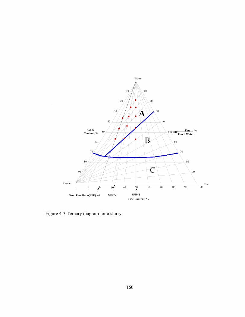
160

Fine Content, %

Water

Coarse Fine

10

20

30

40

50

60

80

70

90

SolidsContent, %

10

20

30

40

50

60

70

80

90

Fine Fine+ Water

, %

0 10 20 30 40 50 60 70 80 90 100

Sand Fine Ratio(SFR) =4 SFR=2 SFR=1

FWR=

A

B

C

Figure 4-3 Ternary diagram for a slurry

161

, ,

05

101520253035404550

0 10 20 30 40 50

Solid Content (%)

Hei

ght(c

m)

15sec 30sec 45sec 60sec 90sec

05

101520253035404550

0 20 40 60 80 100

Sand Content (%)

Hei

ght(c

m)


Figure 4-4 Solid and sand content profile of slurry at SFR=1, FWR=10 and an initial

solids content of 18.8% at different elapsed times

162

( )

0

5

10

15

20

2530

35

40

45

50

0 10 20 30 40 50Solid Content (%)

Hei

ght(c

m)


, , ( )

0

5

1015

2025

30

3540

45

50

0 20 40 60 80 100Sand Content (%)

Hei

ght(c

m)




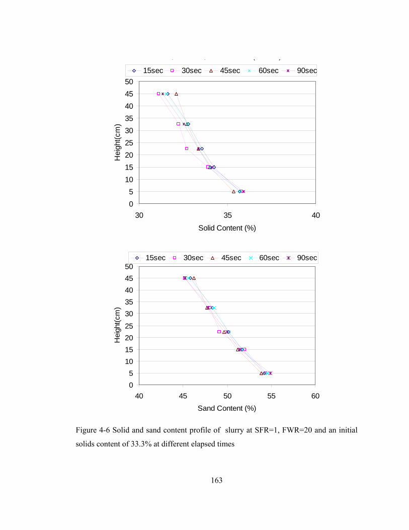
163

, , ( )

05

101520253035404550

30 35 40

Solid Content (%)

Hei

ght(c

m)


05

10152025

3035404550

40 45 50 55 60

Sand Content (%)

Hei

ght(c

m)




164

0

5

10

15

20

25

30

35

40

45

50

45 46 47 48 49 50Solid Content (%)

Hei

ght(c

m)


0

5

10

15

20

25

30

35

40

45

50

45 47 49 51 53 55Sand Content (%)

Hei

ght(c

m)




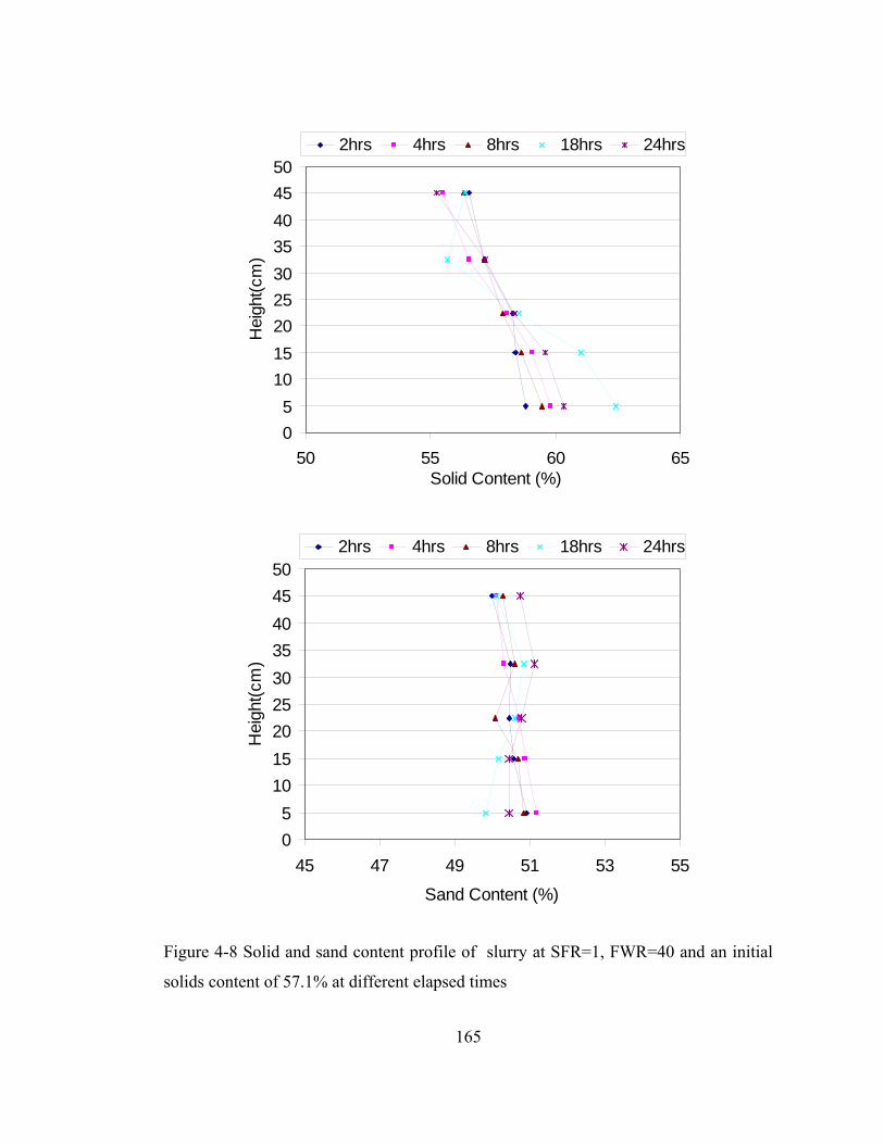
165

05

101520253035404550

50 55 60 65Solid Content (%)

Hei

ght(c

m)

2hrs 4hrs 8hrs 18hrs 24hrs

05

101520253035404550

45 47 49 51 53 55

Sand Content (%)

Hei

ght(c

m)

2hrs 4hrs 8hrs 18hrs 24hrs



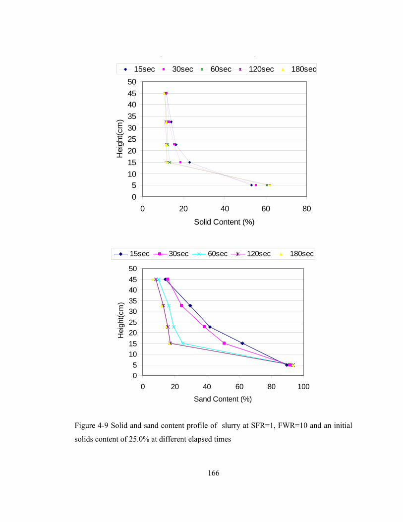
166

, ,

05

101520253035404550

0 20 40 60 80

Solid Content (%)

Hei

ght(c

m)


05

101520253035404550

0 20 40 60 80 100Sand Content (%)

Hei

ght(c

m)




167

0

5

10

15

20

25

30

35

40

45

50

40 45 50

Solid Content (%)

Hei

ght(c

m)


0

5

10

15

20

25

30

35

40

45

50

60 62 64 66 68 70Sand Content (%)

Hei

ght(c

m)




168

0

5

10

15

20

25

30

35

40

45

50

40 45 50

Solid Content (%)

Hei

ght(c

m)


0

5

10

15

20

25

30

35

40

45

50

60 62 64 66 68 70Sand Content (%)

Hei

ght(c

m)




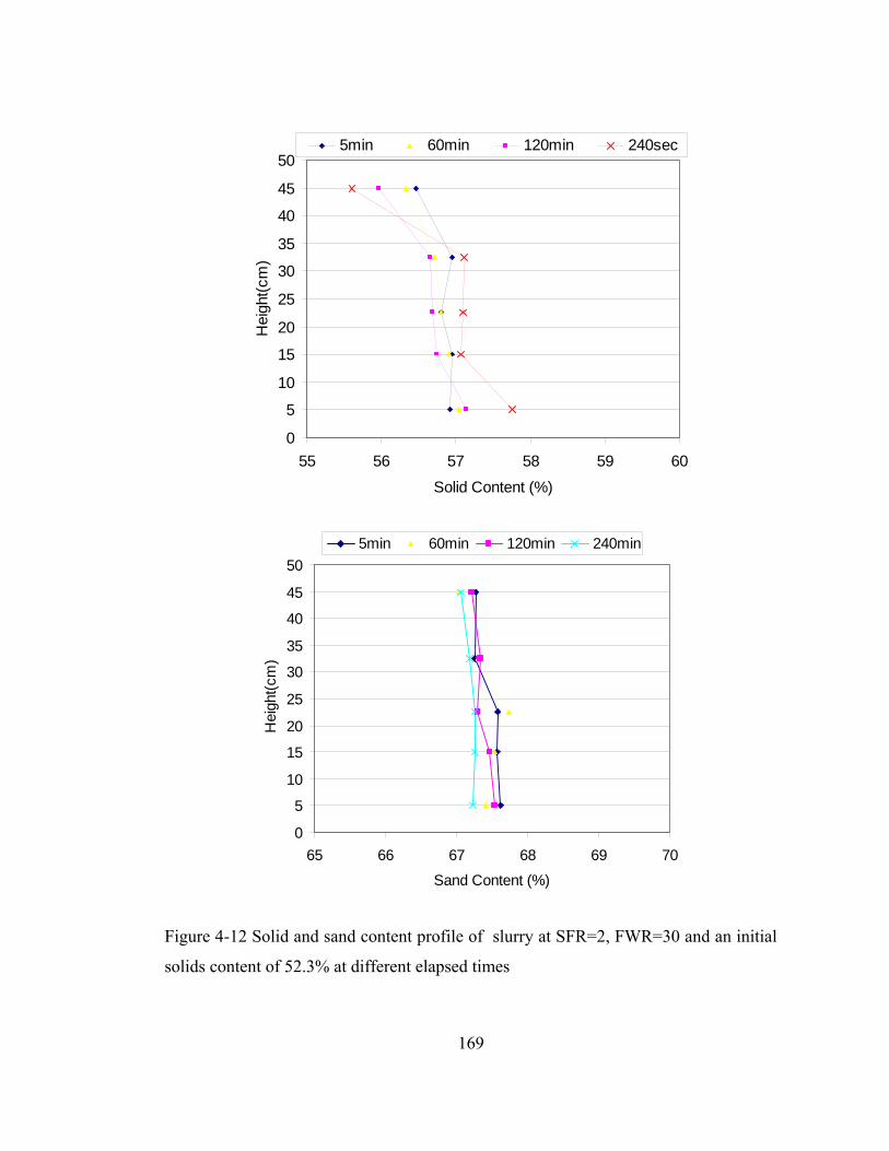
169

0

5

10

15

20

25

30

35

40

45

50

55 56 57 58 59 60

Solid Content (%)

Hei

ght(c

m)

5min 60min 120min 240sec

0

5

10

15

20

25

30

35

40

45

50

65 66 67 68 69 70

Sand Content (%)

Hei

ght(c

m)

5min 60min 120min 240min



171

05

101520253035404550

0 20 40 60 80

Solid Content (%)

Hei

ght(c

m)


, ,

05

101520253035404550

0 20 40 60 80 100 120

Sand Content (%)

Hei

ght(c

m)




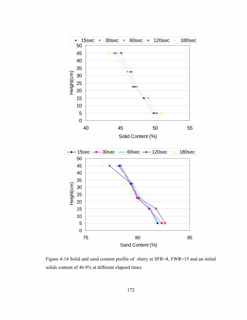
172

05

101520253035404550

40 45 50 55

Solid Content (%)

Hei

ght(c

m)


( p )

05

101520253035404550

75 80 85Sand Content (%)

Hei

ght(c

m)




173

05

101520253035404550

0 20 40 60 80

Solid Content (%)

Hei

ght(c

m)

1hr 2hr 4hr 12hrs 24hrs

05

101520253035404550

0 20 40 60 80 100

Sand Content (%)

Hei

ght(c

m)

1hr 2hrs 4hrs 12hrs 24hrs



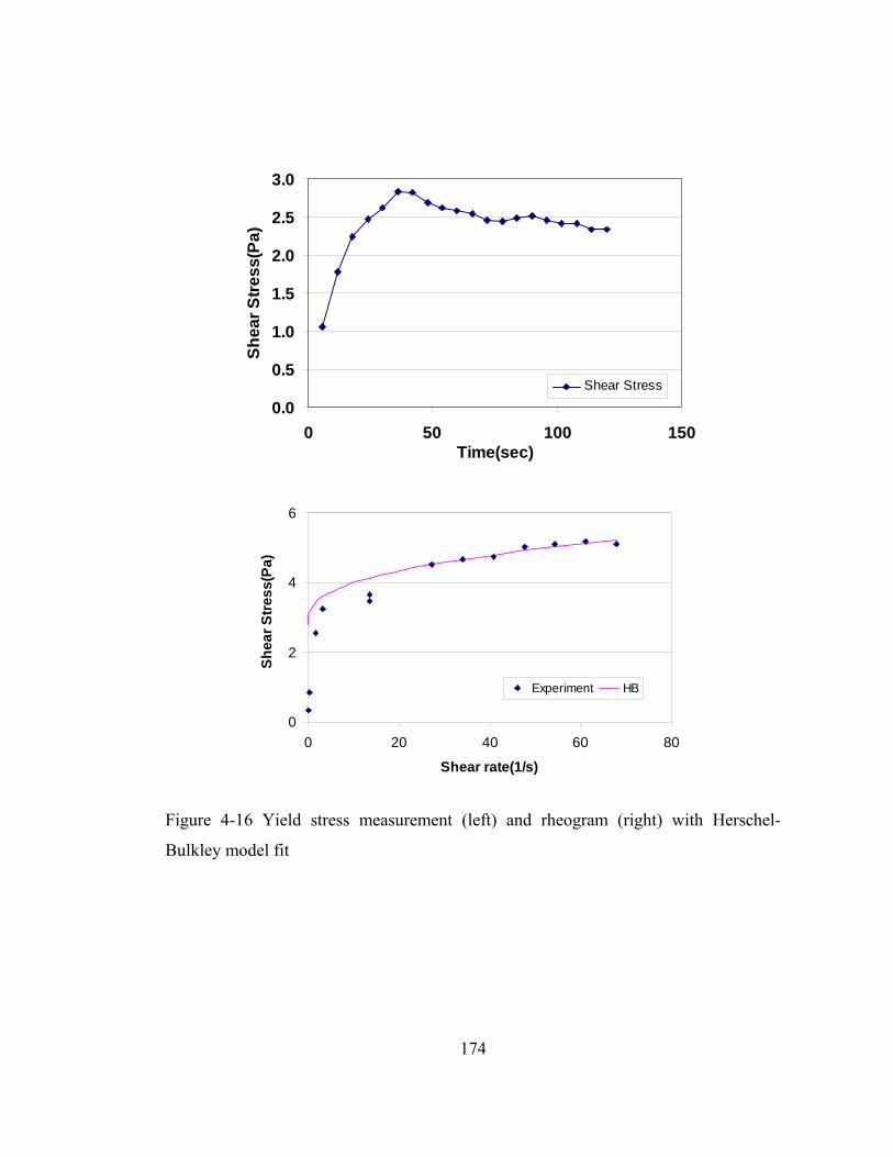
174

0.0

0.5

1.0

1.5

2.0

2.5

3.0

0 50 100 150Time(sec)

Shea

r Stre

ss(P

a)

Shear Stress

0

2

4

6

0 20 40 60 80

Shear rate(1/s)

Shea

r Stre

ss(P

a)

Experiment HB

Figure 4-16 Yield stress measurement (left) and rheogram (right) with Herschel-

Bulkley model fit

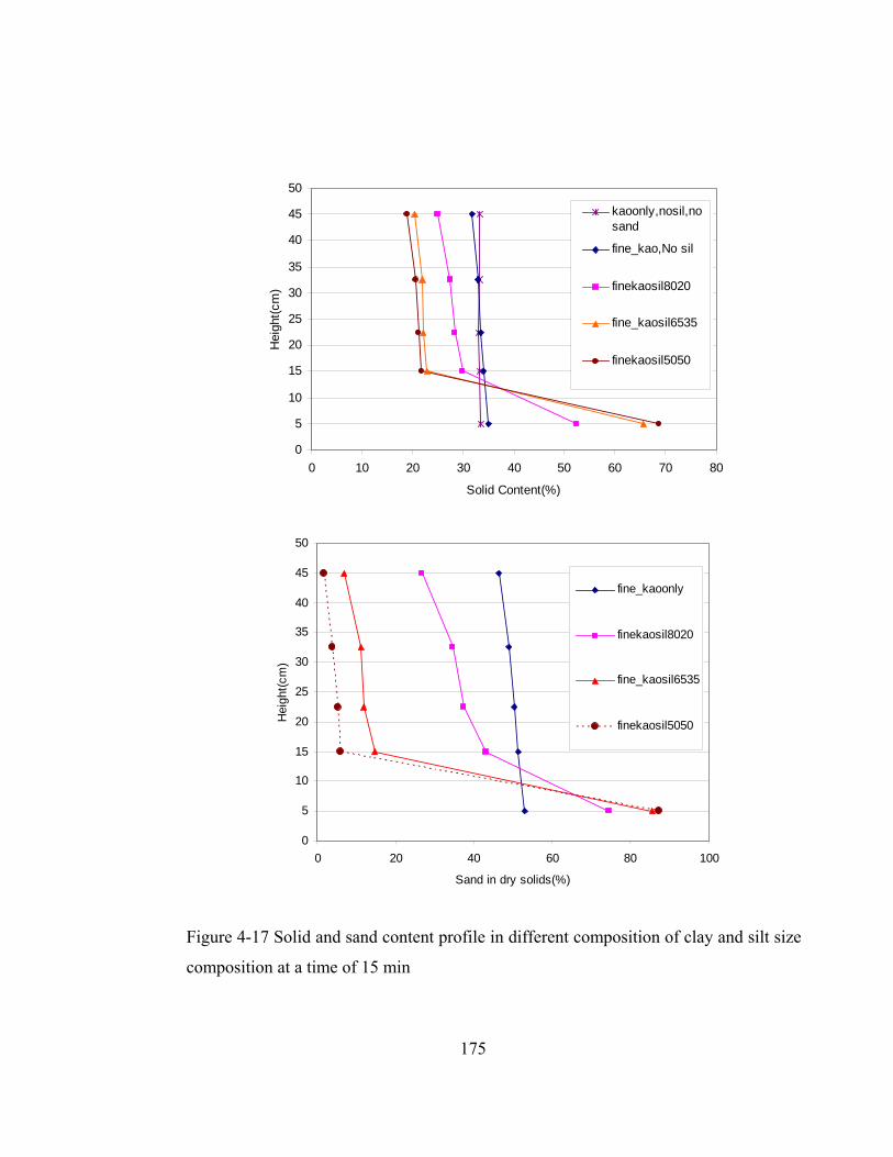
175

0

5

10

15

20

25

30

35

40

45

50

0 10 20 30 40 50 60 70 80

Solid Content(%)

Hei

ght(c

m)

kaoonly,nosil,nosand

fine_kao,No sil

finekaosil8020

fine_kaosil6535

finekaosil5050

0

5

10

15

20

25

30

35

40

45

50

0 20 40 60 80 100

Sand in dry solids(%)

Hei

ght(c

m)

fine_kaoonly

finekaosil8020

fine_kaosil6535

finekaosil5050

Figure 4-17 Solid and sand content profile in different composition of clay and silt size

composition at a time of 15 min

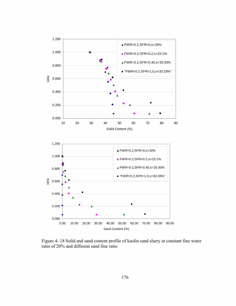
176

0.000

0.200

0.400

0.600

0.800

1.000

1.200

10 20 30 40 50 60 70 80 90

Solid Content (%)

H/H

fFWR=0.2,SFR=0,s=20%

FWR=0.2,SFR=0.2,s=23.1%

FWR=0.2,SFR=0.40,s=25.93%

"FWR=0.2,SFR=1.0,s=33.33%"

0.000

0.200

0.400

0.600

0.800

1.000

1.200

0.00 10.00 20.00 30.00 40.00 50.00 60.00 70.00 80.00 90.00

Sand Content (%)

H/H

f

FWR=0.2,SFR=0,s=20%

FWR=0.2,SFR=0.2,s=23.1%

FWR=0.2,SFR=0.40,s=25.93%

"FWR=0.2,SFR=1.0,s=33.33%"

Figure 4- 18 Solid and sand content profile of kaolin sand slurry at constant fine water ratio of 20% and different sand fine ratio

177

0.000

0.200

0.400

0.600

0.800

1.000

1.200

10 20 30 40 50 60 70 80

Solid Content (%)

H/H

f

FWR=0.3, SFR=0,s=30.0%

FWR=0.3, SFR=0.2,s=33.96%

FWR=0.3,SFR=0.6,s=40.67%

FWR=0.3,SFR=1.0,s=46.15%

0.000

0.200

0.400

0.600

0.800

1.000

1.200

0.00 5.00 10.00 15.00 20.00 25.00 30.00 35.00 40.00 45.00 50.00

Sand Content (%)

H/H f

SFR=0.20,s=38.11%

SFR=0.63,s=47.14%

SFR=1.00,s=46.15%

Figure 4- 19 Solid and sand content profile of kaolin sand slurry at constant fine water ratio of 30%and different sand fine ratio

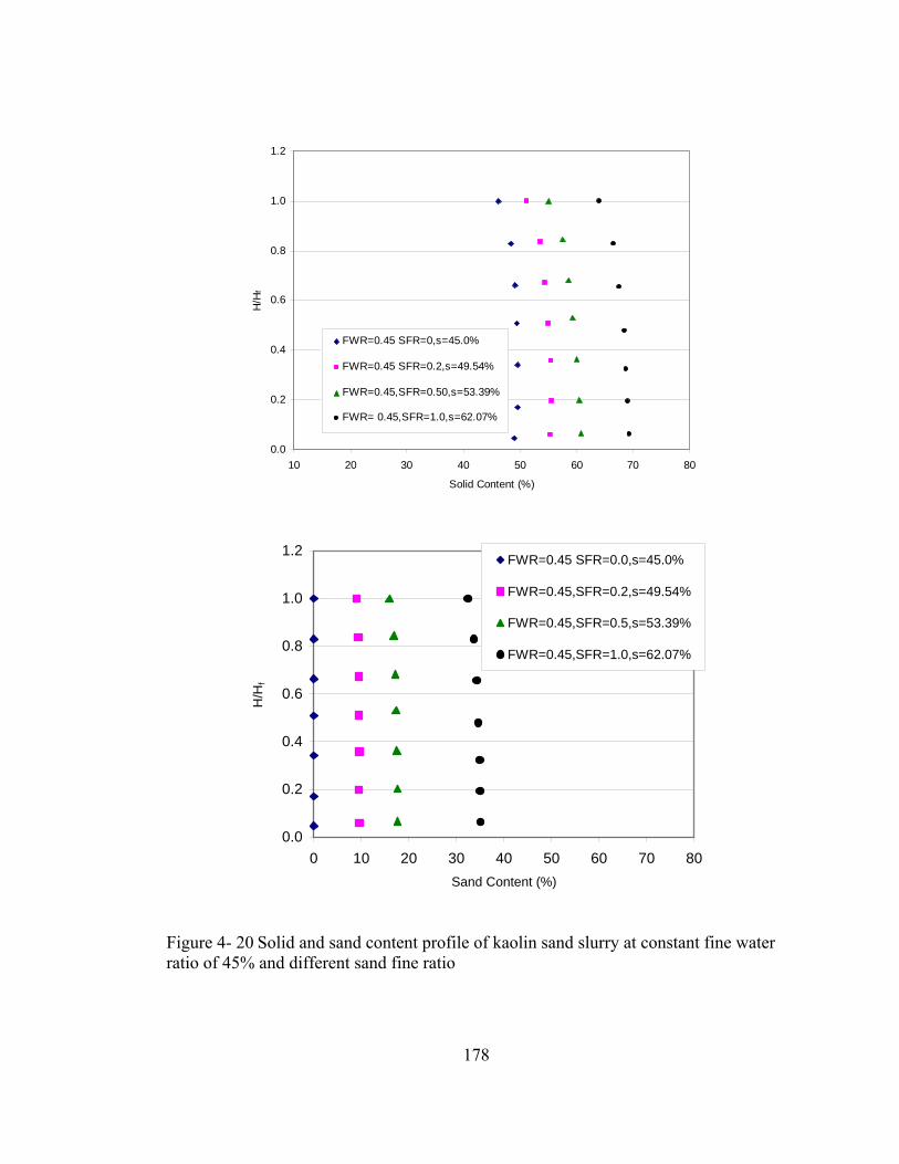
178

0.0

0.2

0.4

0.6

0.8

1.0

1.2

10 20 30 40 50 60 70 80

Solid Content (%)

H/H

f

FWR=0.45 SFR=0,s=45.0%

FWR=0.45 SFR=0.2,s=49.54%

FWR=0.45,SFR=0.50,s=53.39%

FWR= 0.45,SFR=1.0,s=62.07%

0.0

0.2

0.4

0.6

0.8

1.0

1.2

0 10 20 30 40 50 60 70 80Sand Content (%)

H/H

f

FWR=0.45 SFR=0.0,s=45.0%

FWR=0.45,SFR=0.2,s=49.54%

FWR=0.45,SFR=0.5,s=53.39%

FWR=0.45,SFR=1.0,s=62.07%

Figure 4- 20 Solid and sand content profile of kaolin sand slurry at constant fine water ratio of 45% and different sand fine ratio

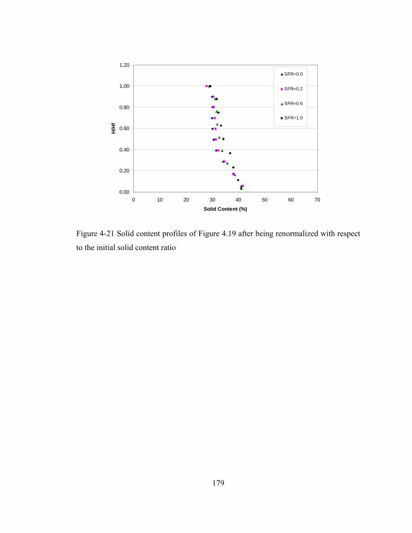
179

0.00

0.20

0.40

0.60

0.80

1.00

1.20

0 10 20 30 40 50 60 70

Solid Content (%)

H/H

f

SFR=0.0

SFR=0.2

SFR=0.6

SFR=1.0

Figure 4-21 Solid content profiles of Figure 4.19 after being renormalized with respect

to the initial solid content ratio

180

0.00

0.20

0.40

0.60

0.80

1.00

1.20

0 10 20 30 40 50 60 70 80

Solid content(%)

H/H

f

SFR=0.0

SFR=0.2

SFR=0.4

SFR=1.0

Figure 4-22 Solid content profiles of Figure 4.20 after being renormalized with respect

to the initial solid content ratio

181

CHAPTER 53

5. FLUME SEGREGATION TEST 5.1 General Segregation through the process of transport or flow commonly occurs in both natural

and man-made processes. Natural processes include rock avalanches, debris flows,

pyroclastic flows and sediment transport by rivers. These processes are commonly of

devastating nature and are the cause of many disasters in mountainous communities.

Because of the high and intermittent socio-economic impacts involved, some effort have

been made to understand the formation, transport and deposition of solid particle-fluid

mixtures (Hungr and Morgenstern 1984), (Iverson 1997), (Iverson and Delinger 2001)

(Coussot 1997), (Choux and Druitt 2002), (McLeod et al. 1999) to name only a few.

In man-made processes, the study of complex mixtures is of great significance in many

aspects. In mining operation, for example, the disposal scheme involves hydraulic

transport of the slurry to a disposal site. The transported material is then deposited into an

impoundment where it will eventually settle and consolidate under self weight and

surcharge of subsequently placed materials. Hydraulic transport is the most common way

of conveying of solid particles. Proper mix proportion, solid concentration, and other

geometrical and flow parameters are important component to be studied for efficient

transport of bulk material.

Regardless of the environment of occurrence, the mechanism for the segregation process

appears to be governed by the same physics of either grain-grain interaction or grain-fluid

interaction. The understanding of the mechanics is still in the realm of limited success.

3 A version of this chapter has been published. Mihiretu, Y.M., Chalaturnyk, R.J., Scott, J.D. Proc. of 60th Canadian Geotechnical Conference, Ottawa, Ontario, 2007.

182

Morgenstern and Kuepper (1988) defined hydraulic segregation as the process of

deposition of particles of different sizes at different distances from the deposition point.

Larger particles tend to deposit soon after being discharged, while smaller particles can

be carried by the flow and deposited further down-slope. They also stressed that the

ability to forecast and control grain size separation is still limited and greater

understanding of this process is needed.

In hydraulic engineering solid-liquid mixtures are studied mainly in the area of sediment

transport. Sediment transport involves bed load or suspension. Sediments are further

studied into two broad classes: coarse or cohesionless and fine or cohesive types. The

coarse sediment refers to mainly sand and gravel while the fine (cohesive) sediment is

mainly a mixture of silt and clay, for which cohesive bonds between particles are

significant and affect the sediment properties. The cohesive forces are due to attractive

intermolecular forces and electrochemical forces. Partheniades and Paaswell (1970)

explained that cohesive forces in the sediment are dependent on the fluid quality and have

time dependent behaviour. Cohesive sediments behaviour in a flow field is a subject of

complexity and most sediment transport studies relate almost exclusively to non-cohesive

sediments (Raudkivi 1998). From practical point of view, sediment transport rate is of

great importance to assess sediment yield, siltation of a reservoir, stability of beds and

banks, and dredging in different water bodies. Sediment transport rate is the total weight

of grains passing through a section per unit time, and is the product of the weight of

moving grains present in the water over a unit area times the velocity at which they move

(Dyer 1986).

Quantification of the relationship between water flow and sediment transport rate have

been made from studies made on rivers, channels and flumes. According to Dyer (1986)

the formulae for sediment transport rate fall into three basic groups:

1. Experimental (e.g. Meyer-Peter and Mueller 1948)–number of flume test and

empirical relationship.

183

2. Theoretical. (e.g. (Einstein 1950) and (Bagnold 1956, 1966)–basic physics of

the movement of individual grains. –relations developed.

3. Dimensional analysis (Yalin 1977), (Ackers and White 1973)-sediment flow

variables are grouped together in a dimensionless numbers.

More detailed discussion on sediment transport rate is available in some standard text

books like (Graf 1971), (Yalin 1977), (Chanson 1999) and (Chang 1988). While the

sediment transport problems are conventionally associated with land erosion, rivers and

coastlines, the same physical concepts apply to many industrial and chemical processes as

well (Raudkivi 1998).

Graf (1973) showed that for purely cohesive material the Shield’s parameter can be

equated with the coefficient of cohesion of the material (C0):

00( )s

Cd

τγ γ

=−

, (5.1)

where τ0 is γ *Rh*S, γs is the solids unit weight, γ is the unit weight of the fluid , d is the

diameter of particle, Rh is hydraulic radius and S is the slope of the bed.

Graf also discussed that the critical shear stress for cohesionless material is a function of

particle size whereas for cohesive soils the critical shear stress is a function of both

particle size and coefficient of cohesion. ”…The shear stress of cohesive material

depends on the composition of the different fractions (clay, and non-clay minerals and

organic matter), the particle-size distribution and particles’ shape, the packing, and

probably on other items. Also geologic events, such as compression or stratification, may

be of importance.” He also asserts that the critical shear stress depends on the Plasticity

Index (PI). In a conclusion, he remarked that erosion of cohesive soils takes place in

aggregates rather than particle by particle. It was observed that a well-defined interface

exist between the flocculated cohesive material-frequently referred to as fluid mud-and

184

the overlying water. Raudkivi (1998) mentioned that only about 10% of clay will suffice

to assume control of the soil properties.

Partheniades and Paaswell (1970) defined critical shear stress as the stress for which the

bed material was in general motion and provided a relationship between critical shear

stress and plasticity index.

0.84

0 0.0034( )PIτ = (5.2)

with τo in psf.

Flume studies have been major experimental means to study sediment transport

behaviour (de Groot et al. 1988), (McLeod et al. 1999), (Parson et al. 2001). Wilson

(1991) describes flume as any artificial channel carrying flow with a free surface, which

is commonly known by open –channel flow.

de Groot et al. (1988) conducted field and laboratory investigation to study slope and

density of dams constructed by hydraulic fill of fine sand. An important result of their

study is a formula for the equilibrium slope, defined as the slope at which sedimentation

and erosion are in balance. They also reported that the viscosity at concentration of

30%(vol), the apparent viscosity is about 4 times the viscosity of clear water. In a laminar

flow the sand grains are supported by mutual collisions and in turbulent regions the

grains are kept in suspension by turbulent diffusion. In their study of density current,

sedimentation and flow slide processes, using laboratory prototype test, they found out

that the underwater slope is mainly a function of grain size and sand transport rate. They

stressed that grain size is of primary importance.

Kuepper (1991) studied the deposition mechanism of hydraulic fills both in the laboratory

and field experimentation. She adopted ‘similarity of process’ approach for the laboratory

system in which the performance of the laboratory study is made similar in terms of

process to the general system being studied. This kind of approach mainly serves the

185

purpose of studying the deposition mechanics rather than extrapolation of results from

laboratory to field. She also discussed that hydraulic sorting (segregation) is more

pronounced for high flow rates, lower slurry concentration and relatively small flow

velocity on the beach.

Blight (1987) discussed two important aspect of depositional profile of slurry material. At

lower solid concentration, larger particles settle out higher up the beach while finer

particles will travel further toward the pool. Such deposition formed can be shown in a

master profile (Figure 5-1) which is given by the Equation (5.3)

1ny x

H L⎛ ⎞= −⎜ ⎟⎝ ⎠

(5.3)

He also observed that beyond a certain solids concentration, the flow regime changes and

instead of progressive particle sorting occurring, with the average particle size decreasing

towards the pool, the slurry starts to flow as a homogeneous material. He found for fly

ash slurry that 40%s marks the change from a ‘particle settling’ to a ‘mud flow’

condition. Below 40%s is a particle settling regime, under which most conventional

tailings dam operate; and above this solid content is the mud-flow regime, under which

thickened discharge type dams operate.

Fourie (1988) also conducted flume beaching tests on three tailings, i.e., bauxite tailings,

nickel ore slurry and coal tailings. Beach profiles as obtained from his experiment are

convex upward unlike those reported by Blight (1987) as concave upward. He discussed

that tailings which produced a value for ‘n’ less than unity (resulting in convex upward

profiles), little or no segregation occurs and vise versa.

Kuepper's (1991) flume experimental data also show concave upward beach profile. She

also observed that the beach profile is steeper for larger slurry concentrations, smaller

flow rates and larger mean grain diameter. Also the field test beach profile show concave

upward shape. In a discussion about the occurrence of segregating behavior, she

186

described that the fluid and solid phases interact by retaining separate identities, and the

slurry viscosity remains similar to that of the carrier fluid. This latter remark is, however,

in contradiction with the experimental observations in this study, as discussed in

Chapter 3.

Some similarity of beaching profile can be observed from the flow of ice sheet as

presented in (Paterson 1969). He showed a slightly different form of Equation (5.3).

For granular flow at uniform steady condition, Pouliquen (1999) proposed semi-empirical

normalized differential equation to predict the shape of granular front on an inclined

plane. The basis of the formulation lies in empirical friction factor at the base, and steady

equilibrium condition along the flume length.

The study of dynamic processes that involve fluid-particle and particle-particle

interaction is greatly relevant. Morgenstern (1985) pointed out that the design of tailings

handling systems requires an appreciation of processes at the boundary between fluid

mechanics and soil mechanics.

It is of an interest to study whether high concentration slurry would exhibit a segregating

behavior when the slurry is subjected to flow condition. The objective of this

experimentation is to study the occurrence of segregation in a dynamic environment.

Since segregating type experiments both in the laboratory and in the field are done

extensively by other researchers e.g. (Kuepper 1991), the subject of this study here

emphasizes on the segregation behavior of relatively non-segregating slurry when

subjected to a dynamic flow mechanism.

5.2 Equipment and Test Procedure

The flume has an overall length of 244cm and 11.5cm wide. It is wholly made of plexi-

glass. At one end of the flume, a compartment was segmented to serve as a reservoir with

a sluicing gate at the downstream side. The dimension of the reservoir was 33.4cm

187

length, 21.8cm deep and 11.5cm wide. The schematic showing the flume set up is shown

in Figure 5-2. An overflow pipe which limits the depth of the slurry level at 20cm is

provided at the middle of the reservoir. Thus a reservoir can handle about 7.7 liter of

slurry volume, when the gate is closed. The slope of the flume bed can be adjusted by the

jack table that supports one edge of the flume.

The test materials are kaolinite clay material, sand and tap water. Similar procedure as in

standpipe test was followed in the preparation of the slurry. A total volume of 15litre

slurry was prepared for the initial flume experiment. For the subsequent test the material

left over after sampling is collected and remixed after adjusting the proportion to meet the

required solid content.

The slurry was poured into the reservoir while the gate was closed. Then the gate was

opened to 2.3cm height and the slurry material was discharged. At the same time the

reservoir was fed with slurry until the total of 15litre is poured into it. The discharge was

so instantaneous that it makes it measurement of the flow rate very difficult.

The depth of profile is measured along the flume length at selected positions. Then after

the deposited material is sectioned by cork plates and from each section samples are

withdrawn at the top half and bottom half for solid and sand content determination. The

design solid contents and SFR are summarized in Table 5-1. The major distinction among

the three test set is the SFR as the solid content is slightly varied.

Table 5-1 Design test solid contents and sand fine ratio for flume segregation test

Test Set No. Design Solid (%) SFR Bed slopes (degrees)

1 57.14 1 0, 5, 10

2 56.25 2 0, 5, 10

3 55.56 4 0, 5, 10

188

5.3 Results and Discussion

The solid and sand content profiles at three bed slopes are shown from Figure 5-3 to

Figure 5-5. There is no observable segregation along the flume length both in term of

solid content and sand content. Figure 5-6 show the beach profile for test set 1 at three

bed slopes. The negative value in distance corresponds to the profile height at the middle

of reservoir behind the gate. For 0% slope, the material is fully deposited inside the flume

without reaching the flume end.

As the bed slope is increased, the beach height is reduced and the material reaches the

flume end. The profiles generally exhibit convex upward shape which is consistent with

other observation made on non-segregating type slurries (Fourie 1988). Moreover the

slurry material that left the flume were collected into standpipe and allowed to stay

overnight and tested for solid content and sand content. Representative standpipe data

from slurry material that left the 10%-slope flume is indicated in Figure 5-7.

Similar beach profile comparison for test set 2 (SFR=2) is shown in Figure 5-8. While the

effect of the bed slope can be clearly seen by the remarkable difference in the profiles, the

effect of SFR is remarkably seen by the less amount of material left in the flume (or

simply reduced flume height as compared to SFR=1)

The standpipe test solid content and sand content profile on the slurry material which left

the flume for 5% and 10% slopes are indicated in Figure 5-9 and Figure 5-10

respectively. These profiles also show that the slurry material is relatively non-

segregating after 24 hrs.

For SFR equals to 4 a comparison of beach profile at different slope is shown in Figure 5-

11. Reduced height was observed for zero slope bed set up. Also the difference between

189

zero slope beach profile and 5% profile is only up to about half-way of flume length then

overlaps for the rest of flume length up to the exit point. The 10% slope is exhibiting a

humpy profile towards the end of the flume. This phenomenon appears to be an

indication of ripple formation. If the flume had enough length and large volumes of slurry

material were input, the ripple formation might have been possible. A single formation of

such ripple may be because of limited amount of slurry. During the experimentation

small wavy patterns were visible.

After beaching on the flume, water release at the top surface is visible. The solid and sand

content profiles for zero bed-slope along the flume length are shown in Figure 5-12. In

this profile there is an indication of segregation at the sampling positions. The increase in

solid content is related to the surface water release after deposit formation.

Similar profile trends are observed for 5% and 10% bed slopes which are shown in Figure

5-13 and Figure 5-14 respectively. Furthermore the standpipe solid and sand content

profile, after 24hrs on the slurry material that exited at the flume end, are shown in Figure

5-15, for zero-bed slope and in Figure 5-16, for 10% bed slope. The segregating trend

was remarkably seen in both cases.

5.4 Comparison of beach profiles at zero bed slope for different SFR’s

The design solid contents of the three test sets summarized in Table 5-1 are in close

proximity, the maximum difference between solid contents of test set 1 and test set 3 is

about 2.8%. This would allow us in an approximate manner to compare the beach profile

at similar bed slope but different sand fine ratios. Figure 5-17 shows the beach profile

comparison at zero bed slope but different SFR. The information that can be tractable

from such comparison is that it is the fine content that controls the shape of the profile.

On a normalized scheme the three test plot in a banded location and equation (a) has also

been fitted to the normalized plot. The values of the exponent ‘n’ are 0.4929 for TS1,

0.4706 for TS2 and 0.4762 for TS3. Such banded profile has been explained by Blight

190

(1987) as a master profile. Such a master profile plot obscure the information about the

ingredient composition by normalizing the plot and fitting exponential curve to the plot.

Blight (1987) also discussed two phenomena which are closely related to the master

profile concept. (i) The profile appears to be generated by gravitational sorting of particle

sizes (ii) the resultant gradient of particle sizes down the beach produces a gradient of

permeability.

The depiction of the test results as a master profile gives a vital information about the

segregating/ non-segregating condition. When the master profile is convex upward, the

slurry is of non-segregating type, whereas, when the beach profile is concaving upward,

there is a tendency of segregation. This phenomena has been reported by Fourie (1988).

The experimental results in this test program agree with these observations partially. It

can be seen that for the sand-fine ratio of one and two, there is almost no segregation.

When the sand-fine ratio is four there is segregation both in the beach deposit and

standpipe test. The shape of the beach profile looks convex upward and is in close band

on master profile though.

Such process can be related to the rheological behavior of the slurry in that the flow and

deformation nature of slurry is governed by fluid-particle and particle-particle

interactions. At large concentration and significant presence of fine material, mainly clay,

the slurry behaves as pseudo-one-phase fluid. The major contributor to the deformation

nature in such a case will be the yield stress. Such effects have been reported in some

natural debris flow. For example, Parson et al. (2001), reported that the Acuabona debris-

flow channel in the Alps exhibit the grain-fluid transition as silty fine material extracted

from the eroded marl. They explained that the fine material acts to lubricate for the flow,

increasing run out exhibiting non-Newtonian behaviour.

Iverson (1997) showed different depositional characteristics as influenced by grain

composition and water saturation. He also asserted that grain size segregation mechanism

in debris flows may be complicated and may involve more than one process. The general

191

flow condition in this experiment is unsteady and of short residence time. If the flow is

assumed to be a function of instantaneous depth in the reservoir, the discharge velocity is

approximately a function of square root of depth in the reservoir. With increase in bed

slope, the flow velocity increase. Consequently the shear stress and turbulence intensity

induced by the flow reduces the yield stress further, leaving small volume of material left

in the flume. The decrease of yield stress due to increase in velocity was also reported by

Song and Chiew (1997).

Franzini (2002) wrote that from a mechanical point of view, clays and silts concentration

increases the cohesion of the water-sediment mixture, provided by the electrochemical

interaction of very fine particles so that coarser particles are held in suspension by matrix

strength. He dealt however with the sediments without cohesive particles. The fall

velocity of sand particles can also be reduced by the presence of silt or clay particles as

explained in de Groot et al. (1988). In case of tailing disposal schemes also, the volume

of tailings to be stored is sensitive to the fines content and the densities that these fines

will attain (Morgenstern 1985). Hence, the experimental observations clearly demonstrate

that presence of fines both in the static and dynamic condition influences the segregation

mechanism.

5.5 Applicability of the theory of plasticity

Most of the observed beach profile formed from deposition of non-segregating slurries,

have shapes that look similar to mud flow and glacier flow tongues. It is of practical

interest to see if the theory developed for the study of flow tongues work for this

experimental study.

Brueckl and Scheidegger (1973) applied theory of plasticity to study slow mud flows.

The theory they used was a modified version of the theory of (Nye 1951) for glaciers.

Based on Mohr-Coulomb constitutive relationship and equilibrium and assumptions they

derived equation for the profile of the mud flow. The formulation they arrived is of the

form given in Equation (5.4):

192

0sCdh rch hdx

εγ γ

⎛ ⎞± − + =⎜ ⎟

⎝ ⎠ , (5.4)

where

1 w hsh

γ γε β φγ

⎛ ⎞= − −⎜ ⎟

⎝ ⎠ , and (5.5)

c is the internal cohesion of the flow material, cs, cohesion at slip plane β angle of

inclination of the slip plane, γ, bulk unit weight and γw, weight of pore water, h, height of

flowing material measured normal to slip plane and r is a factor which is π /2 when the

shear stress at the base is equal to c or 2 when the base shear is much less than c.

Equation (5.4) may be rewritten as:

dh ah bdx h d

+=

+ , (5.6)

where a is ε, b is cs/γ and d is +rc/γ .

This is a non-linear ordinary differential equation if the parameters a, b and d are

assumed constant. Some kind of such assumption appeared in the works of Brueckl and

Scheidegger (1973).

Equation (5.6) was tested for one of the 5% slope experimental result on Figure 5-6., with

solid content 57.1% and SFR=1. A software program called FlexPDE 5 was used to solve

Equation 5.6, with assumed values for the constants a, b, and d. Figure 5-19 shows a

comparison of results from the solution of Equation (5.6) with experimental data.

Equation (5.6) appears to under-predict the beach profile close to the exit point and match

fairly well at the other locations. While at this stage the equation was fitted with assumed

constant parameter values and it is encouraging to capture the profile in part.

Due to scale effect and short retention time the degree of dynamic shearing /segregation

might have been limited and instantaneous. From practical point of view, the master

193

profile could provide information about actual deposition from small scale laboratory

tests.

Wilson (1976) describes flume transport with homogeneous slurry flow usually involving

longer distances and flatter slopes than the coarse-particle case. These slurries are

comprised of partially processed materials or, more typically, tailings being transported to

retention areas. Observation in this testing program is not completely in support of his

statements. As the sand fine ratio increases the flow exhibit fast flow rate and flatter slope

at deposition are also observed.

As Mehta (1984) pointed two decades ago, the linkage between sediment rheology,

aggregation dynamics and the settling behavior needs to be explored further at a basic

level, in order to reduce the current level of empiricism in evaluating the settling velocity.

The test conducted is primarily an initiative to understand the occurrence of segregation

in non-Newtonian regime. Due to the complexity of the process and limited resources at

the time of testing, flow characteristics and segregation impacts were not examined to full

extent. Rather it is recommended that further work be extended with more details.

5.6. Summary and Conclusion

All beach profiles at zero bed-slope testing condition exhibit a convex upward and higher

beach profile with non-segregating trend. As the slope is increased the beach profile

exhibits nearly parallel to bed profile. The less segregation nature may be attributed not

only to the fine-matrix but also to the length of the flume i.e., shorter flume length imply

less residence time, less interaction and reduced segregation. The material flows farther

as the sand fine ratio is increased indicating that the presence of fine influence highly

both the beach profile and flow characteristics of the slurry. That a master beach profile is

convex upward is not necessarily an indication on non-segregating slurry mix. As the

sand fine ratio increases segregation is more likely.

194

Non-linear differential equations based on the theory of plasticity show good comparison

with experimental data, nonetheless, the parameter need to be studied further to minimize

the level of simplifications adopted.

5.7. References

Blight, G.E. 1987. The concept of the master profile for tailings dam beaches. In

Prediction and Performance in Geotechnical Engineering. Edited by R.C. Joshi

and F.J. Griffiths. Calgary.

Brueckl, E., and Scheidegger, A.E. 1973. Application of the theory of plasticity to slow

mud flows. Geotechnique, 23(1): 101-107.

Chang, H.H. 1988. Fluvial Processes in River Engineering. John WIley & Sons, Inc.,

New York.

Chanson, H. 1999. The Hydraulics of Open Channel Flow. John Wiley & Sons Inc., NY.

Choux, C.M., and Druitt, T.H. 2002. Analogous study of particle segregation in

pyroclastic density currents, with implications for the emplacement mechanisms

of large ignimbrites. Sedimentology, 49: 907-926.


de Groot, N.B., Heezen, F.T., Mastebergen, D.R., and Stefess, H. 1988. Slope and

Densities of hydraulically placed Sands. In Hydraulic Fill Structures, Speciality

Conference. Edited by D.J.A. Van Zyl and S.G. Vick. Fort Collins. ASCE, pp. 32-

50.

Dyer, K.R. 1986. Coastal and Estuarine Sediment Dynamics. John Wiley & Sons,

Chichester.

Fourie, A. 1988. Beaching and Permeability Properties of Tailings. In Hydraulic Fill

Structures, Speciality Conference. Edited by D.J.A. Van Zyl and S.G. Vick. Fort

Collins. ASCE, pp. 142-154.

Franzini, L. 2002. On the variablility of the sediment concentration in currents on steep

slopes: a simplified approach? Physic and Chemistry of the Earth, 27: 1551-1555.

Graf, W.H. 1973. Hydraulics of Sediment Transport. McGraw-Hill.

195

Hungr, O., and Morgenstern, N.R. 1984. Experiments on the flow behaviour of granular

materials at high velocity in an open channel. Geotechnique, 34(3): 405-413.

Iverson, R.M. 1997. The Physics of debris flows. Review of Geophysics, 35(3): 245-296.

Iverson, R.M., and Delinger, R.P. 2001. Flow of variabily fluidized granular masses

across three-dimensional terrain 1: Coulomb mixture theory. Journal of

Geophysical Research, 106(B1): 537-552.


Edmonton,Canada.

McLeod, P., Carey, S., and Sparks, R.S.J. 1999. Behaviour of particle-laden flows into

the ocean,experimental simulation and geological implications. Sedimentology,

46: 523-536.

Mehta, A.J. 1984. Summary. In Estuarine Cohesive Sediment Dynamics. Edited by A.J.

Mehta. Tampa, Florida. Springer-Verlag, Vol.14, pp. 467-468.

Morgenstern, N.R. 1985. Geotechnical aspects of environmental control. Edited by

P.c.o.X. ICSMFE. Proc.of the 11th Int. conf. Soil Mechs. Found. Eng. A.A

Balkema, Vol.1, pp. 155-186.

Morgenstern, N.R., and Kuepper, A.A.G. 1988. Hydraulic Fill Structures- A Perspective.

In Hydraulic Fill Structures, Speciality Conference. Edited by D.J.A. Van Zyl and

S.G. Vick. Fort Collins. ASCE, pp. 1-31.

Parson, J.D., Whipple, K.X., and Simoni, A. 2001. Experimental Study of the Grain-

Flow, Fluid-Mud Transition in Debris Flows. The Journal of Geology, 109: 427-

447.

Partheniades, E., and Paaswell, R.E. 1970. Erodibility of Channels with Cohesive

Boundary. J.of Hydraulics Division, Proc. of ASCE, 96(HY3): 755-771.

Paterson, W.S.B. 1969. The Physics of Glaciers. Pergamon Press Ltd., Oxford.

Pouliquen, O. 1999. On the shape of granular front down rough inclined planes. Phys.

Fluids, 11(7): 1956-1958.

Raudkivi, A.J. 1998. Loose Boundary Hydraulics. A.A. Balkema, Rotterdam.

Song, T., and Chiew, Y.-M. 1997. Settling Characteristics of Sediments in Moving

Bingham Fluid. J.Hydr.Engrg.,ASCE, 123(9): 812-815.

196

Wilson, K.C. 1976. A unified physically-based analysis of solid-liquid pipeline flow. In

Proceedings of the 4th International Conference on Hydraulic transport of solids.

Cranefield, UK. BHRA Fluid Engineering, Vol.Paper A2, pp. 1-16.

Wilson, K.C. 1991. Slurry Transport in Flumes. In Slurry Handling: Design of Solid-

Liquid Systems. Elsevier Applied Science. pp. 167-180.

L

X

Y

197

Figure 5-1 Master Beach Profile for Equation 5.3

198

C D F G HE

Sliding gate

EndB

Overflowduct

Sampling locations

Flow direction

33.4 210 cm

11.5

21.8

(B) Plan View

(A) Side View

NOTE: All dimensions are in cm

Reservoir

Figure 5-2 Schematic of flume apparatus

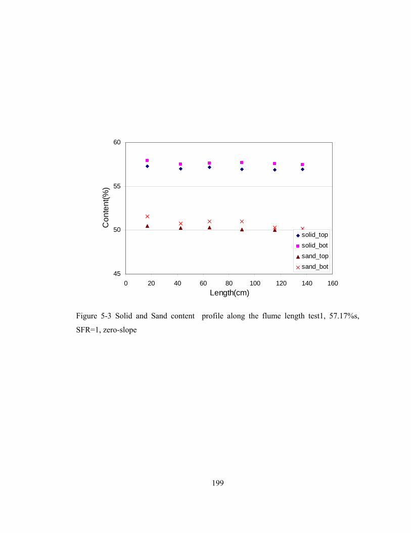
199

45

50

55

60

0 20 40 60 80 100 120 140 160Length(cm)

Con

tent

(%)

solid_topsolid_botsand_topsand_bot

Figure 5-3 Solid and Sand content profile along the flume length test1, 57.17%s,

SFR=1, zero-slope

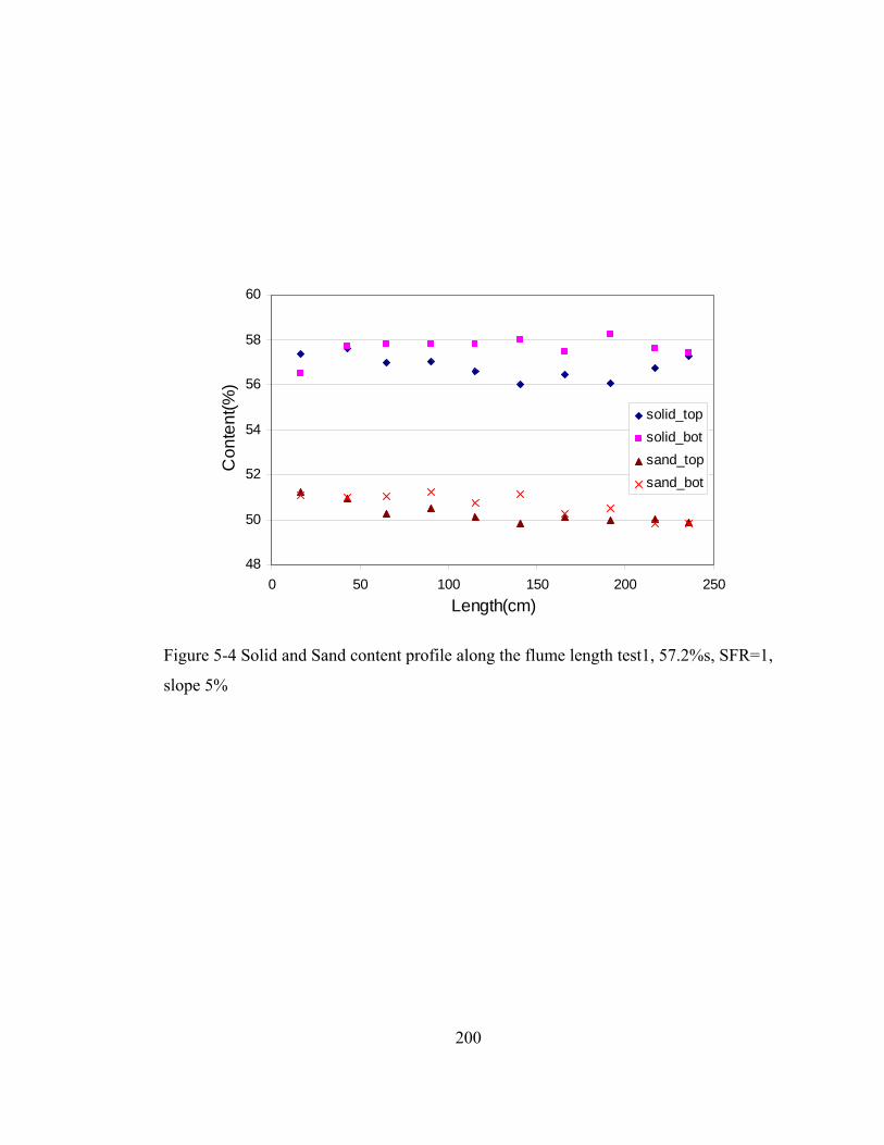
200

48

50

52

54

56

58

60

0 50 100 150 200 250Length(cm)

Con

tent

(%)


Figure 5-4 Solid and Sand content profile along the flume length test1, 57.2%s, SFR=1,

slope 5%

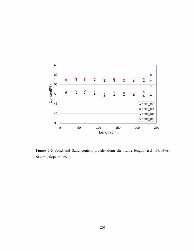
201

35

40

45

50

55

60

65

0 50 100 150 200 250Length(cm)

Con

tent

(%)


Figure 5-5 Solid and Sand content profile along the flume length test1, 57.14%s,

SFR=1, slope =10%

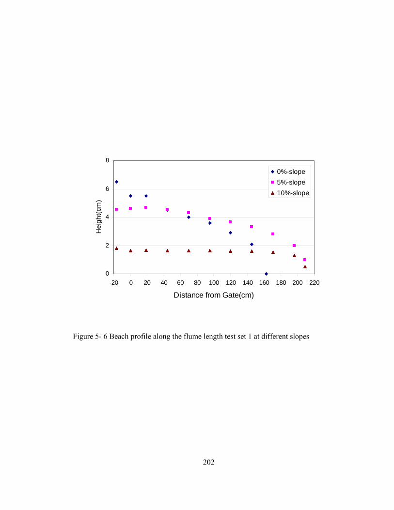
202

0

2

4

6

8

-20 0 20 40 60 80 100 120 140 160 180 200 220

Distance from Gate(cm)

Hei

ght(c

m)

0%-slope5%-slope10%-slope

Figure 5- 6 Beach profile along the flume length test set 1 at different slopes

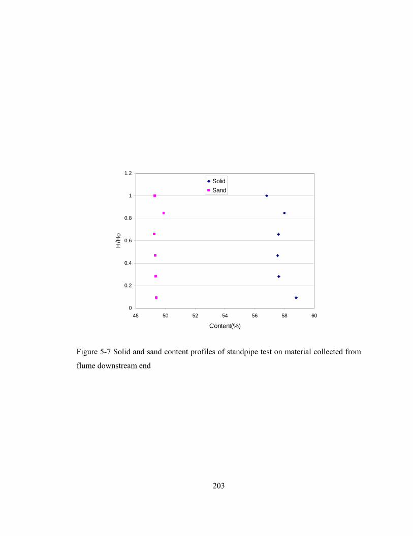
203

0

0.2

0.4

0.6

0.8

1

1.2

48 50 52 54 56 58 60

Content(%)

H/H

o

SolidSand

Figure 5-7 Solid and sand content profiles of standpipe test on material collected from

flume downstream end

204

0

2

4

6

-20 0 20 40 60 80 100 120 140 160 180 200 220


Hei

ght(c

m)

0% slope5%-slope10%-slope

Figure 5-8 Beach profile along the flume length for test set 2 (57.75%s, SFR=2) at

different slopes

205

0

0.2

0.4

0.6

0.8

1

1.2

30 40 50 60 70

Content(%)

H/H

f

SolidSand

Figure 5-9 Solid and sand content profile for sample deposit in a standpipe at the 5%

slope- flume end

206

0

0.2

0.4

0.6

0.8

1

1.2

20 30 40 50 60 70 80

Content(%)

H/H

f

SolidSand

Figure 5-10 Solid and Sand content profile for sample deposited in a standpipe after

exited from the 10% slope-flume end

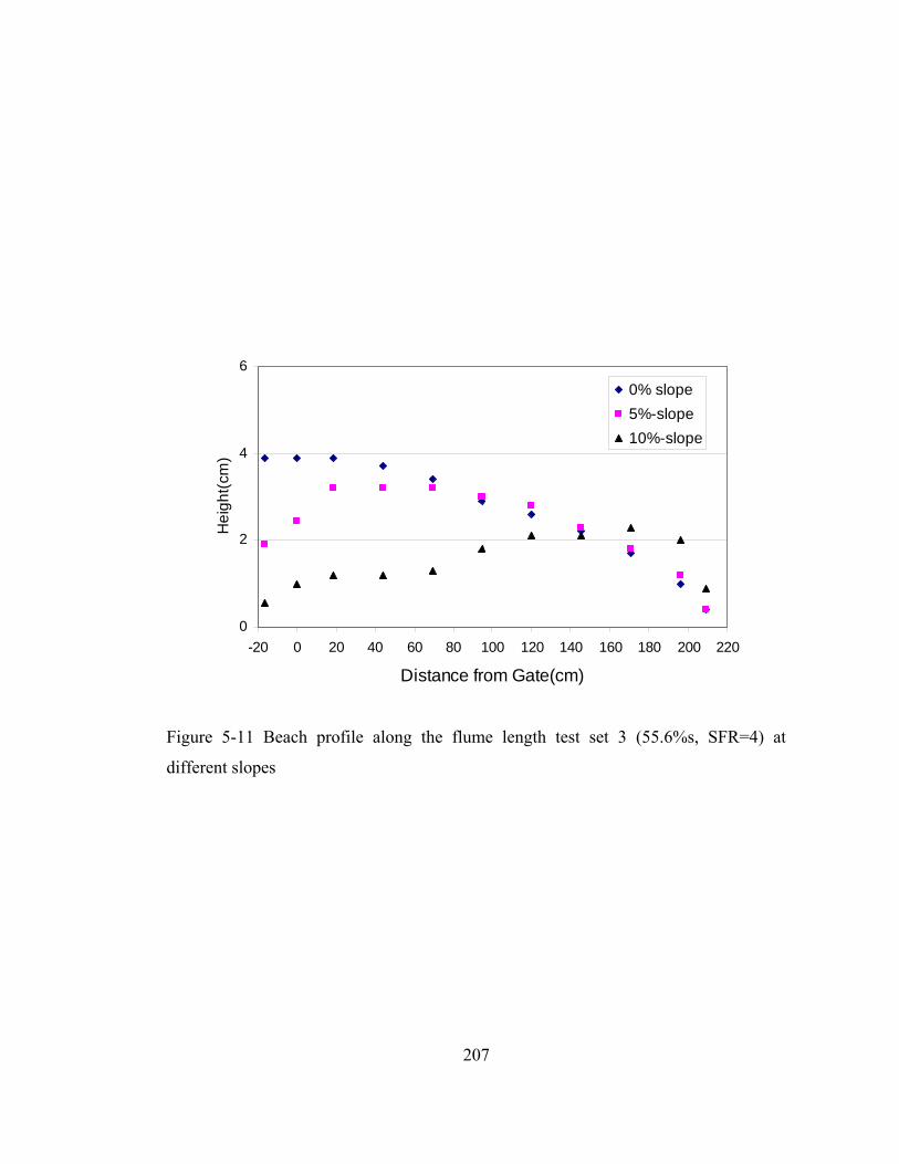
207

0

2

4

6

-20 0 20 40 60 80 100 120 140 160 180 200 220


Hei

ght(c

m)

0% slope5%-slope10%-slope

Figure 5-11 Beach profile along the flume length test set 3 (55.6%s, SFR=4) at

different slopes

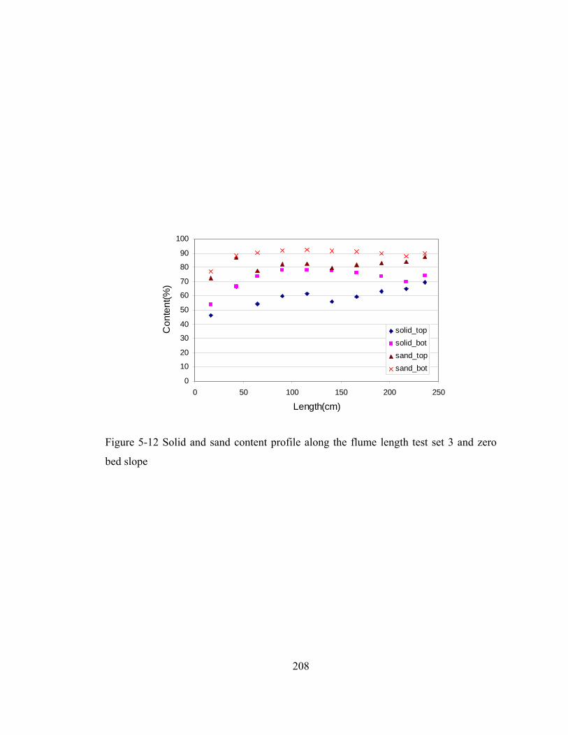
208

0

10

20

30

40

50

60

70

80

90

100

0 50 100 150 200 250

Length(cm)

Con

tent

(%)


Figure 5-12 Solid and sand content profile along the flume length test set 3 and zero

bed slope

209

0

10

20

30

40

50

60

70

80

90

100

0 50 100 150 200 250

Length(cm)

Con

tent

(%)


Figure 5-13 Solid and sand content profile along the flume length test set 3 and 5%

bed slope ( 55.6%s, SFR=4)

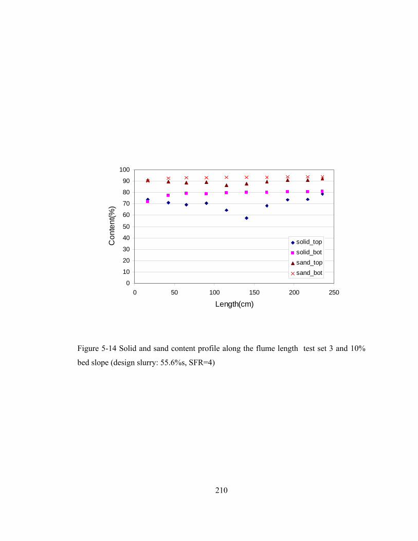
210

0

10

20

30

40

50

60

70

80

90

100

0 50 100 150 200 250

Length(cm)

Con

tent

(%)


Figure 5-14 Solid and sand content profile along the flume length test set 3 and 10%

bed slope (design slurry: 55.6%s, SFR=4)

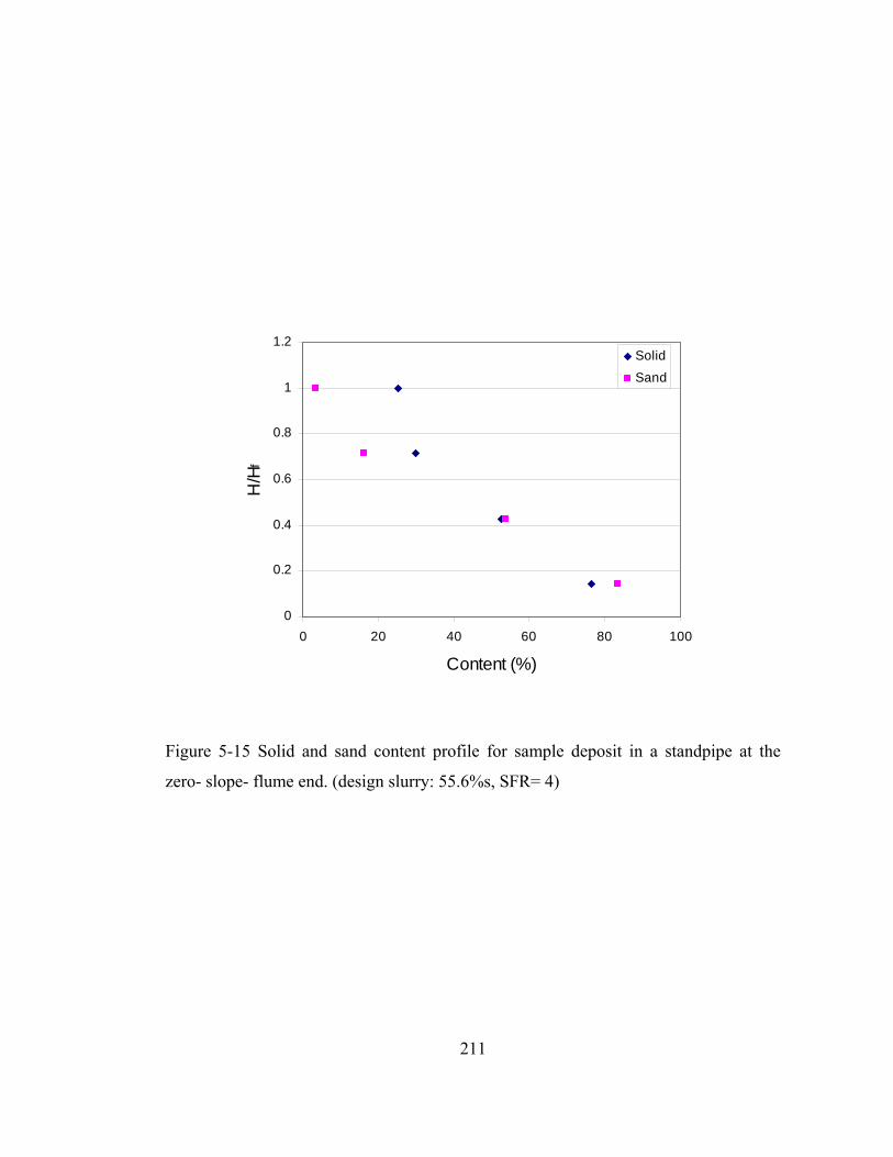
211

0

0.2

0.4

0.6

0.8

1

1.2

0 20 40 60 80 100

Content (%)

H/H

f

Solid

Sand

Figure 5-15 Solid and sand content profile for sample deposit in a standpipe at the

zero- slope- flume end. (design slurry: 55.6%s, SFR= 4)

212

0

0.2

0.4

0.6

0.8

1

1.2

0 20 40 60 80 100

Content (%)

H/H

f

Solid

Sand

Figure 5-16 Solid and sand content profile for sample deposit in a standpipe at the

10%- slope- flume end. (design slurry: 55.6%s, SFR= 4)

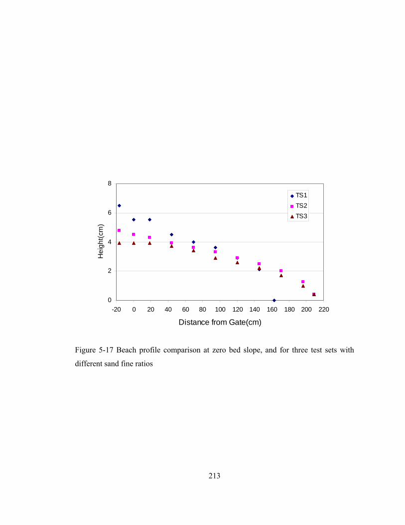
213

0

2

4

6

8

-20 0 20 40 60 80 100 120 140 160 180 200 220


Hei

ght(c

m)

TS1TS2TS3

Figure 5-17 Beach profile comparison at zero bed slope, and for three test sets with

different sand fine ratios

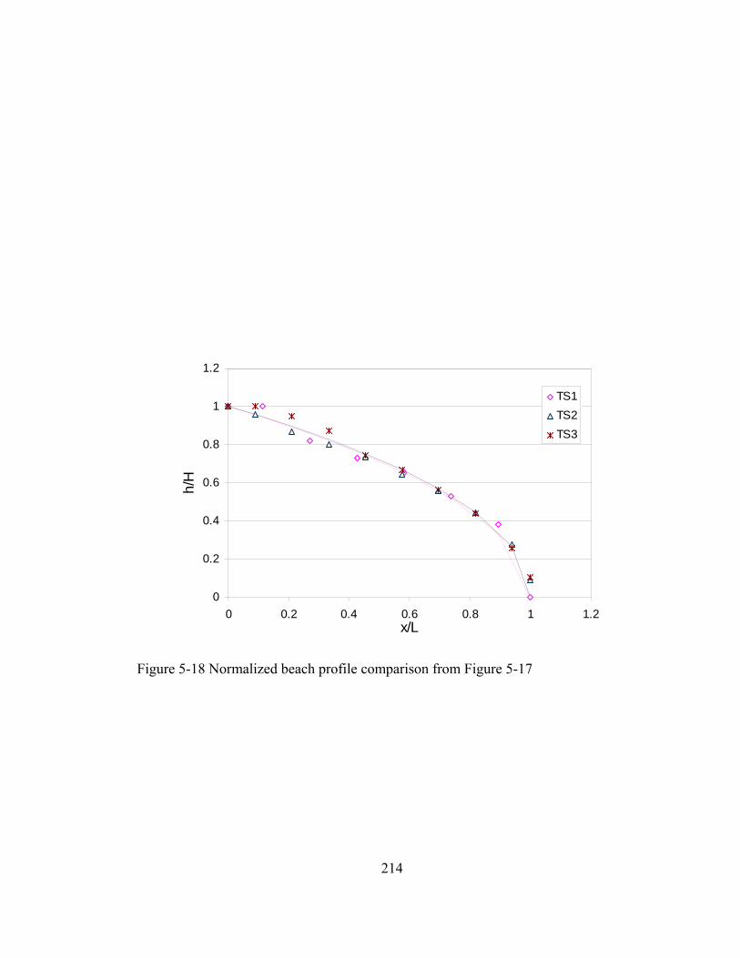
214

0

0.2

0.4

0.6

0.8

1

1.2

0 0.2 0.4 0.6 0.8 1 1.2x/L

h/H

TS1TS2TS3

Figure 5-18 Normalized beach profile comparison from Figure 5-17

215

0

1

2

3

4

5

6

0 50 100 150 200 250Distance from flume exit (cm)

Hei

ght (

cm)

ExperimentEq.(5.6)

Figure 5-19 Comparison of experimental data with plastic theory equation results with

a=0.06, b=1.0e-5 and d= 0.1

216

CHAPTER 6

6. NUMERICAL MODEL STUDY

6.1 General Numerical modeling is essentially an exercise by which we seek to provide some form of

functional relationship among important governing variables. Numerical modeling has

become a great tool in modern science and engineering. When appropriately formulated,

modeling has some powerful features which are impossible otherwise to deal with by

experimental means, such as: when experimental data give limited results, rather than

variable physical process, when sampling methods used in the experiment disturb the

physical process, and when future prediction of the physical process is of interest.

In the 42nd Rankine lecture, Potts (2003) addressed the different applications of numerical

analysis in geotechnical engineering. He discussed that numerical analysis has led to

economical design. He pointed out that the ability for a numerical analysis to reflect field

condition depends on the ability of the constitutive models to represent real soil

behaviour.

The range of applications in geotechnical engineering is very wide but the emphasis of

this study will be focused on the sedimentation/consolidation or more specifically

segregation which involves multiphase system. Multiphase flow consists of mixtures of

different phases. The different phases refer to solid, liquid and gases. Multiphase flow

forms can be gas-liquid, gas-solid, liquid-solid or a mixture of the three phases. They

occur almost in any natural and man-made processes.

It is the liquid-solid flow that would be a primary interest here where such flows are

regarded as slurry flows. The solid-liquid slurry mix commonly consists of particles of

different size and density. The solid particles may segregate due to differences in size or

217

density. Due to the complexities in modeling multiphase fluids, some simplifying

assumptions are commonly made to overcome the theoretical and computational

difficulties (Elimelech et al. 1995). Model studies, providing systematic information on

well-defined systems, can usefully contribute to the greater understanding of real process.

The modeling works carried out to capture or simulate the segregation phenomena are

mainly developed based on the continuum or discontinuum approach. When the

interstitial fluid presence is dominant, the continuum approach is the common one.

Whereas discontinuum methods appears to dominate the cases of granular flows

mechanism. In the continuum case, the early models appear with the sedimentation,

which are based on the theories presented in Chapter 2. There is a report by

Selim et al. (1983) that the sedimentation of poly-disperse system were made by one of

the co-worker - Kothari(1981). Zimmels (1988), provided a computer model for non-

steady sedimentation of polydisperse mixture. The model uses the principle of tracing

positions and concentrations of all particle fractions which constitute a distribution, given

the initial conditions and elapsed time.

Concha et al. (1992) presented a model which simulates the settling of mixtures of ideal

polydisperse suspension based on Kynch sedimentation process. In their model, the solid

concentration and solid-fluid flux relationships are derived from the Kynch sedimentation

process and the constitutive equation for the relative solid-fluid velocities from the well

known Richardson and Zaki equation as proposed by Masliyah (1979). Most of the

existing models for sedimentation deal with the settling velocity. However, it is the solid

concentration profile that provides more information for characterizing sedimentation

process as a function of time (Quispe et al. 2000).

Stamatakis and Tien (1992) provided an algorithm which predicts the sedimentation of

the polydisprsed suspension. Eckert et al. (1996) developed a model predicting

sedimentation and consolidation of fine tails using experimental results from centrifuge.

They used curve fitting techniques to determine the state functions. They also showed

that the governing equation for consolidation used in soil mechanics area and the fluid

218

dynamics equations can be shown to yield the same formulation. The model applies to

only fine tailings part where the coarse grains were discarded. Masala (1998) developed

the coupled sedimentation consolidation model. The inherent derivation in the approach

is based on the assumption that the suspension is ‘slow-settling’ (‘non-segregating’

dispersions, colloidal suspension, etc). It is developed for mono-dispersed type of

suspensions only and requires calibration with experimental data.

The case of aerodynamic consideration as fluid was seen in a work by Mudryy et al.

(1999). They used finite element code based on distributed Lagarangian

multiplier/method (DLM) to study the motion of flowing powders in the regime where

the aerodynamic forces are important. They modeled the air-flow using the Navier-Stokes

equation. They have demonstrated that aerodynamic forces cause mixing when the

particles are identical, and segregation when the particles are different in density. The

non-Newtonian flow of open-channel flow modeling appeared in the work of Sadd and

Gao (1997) and Whipple (1997).

In the discontinuum approach, the most widely used method is the distinct or discrete

element method (DEM). The method has proved its power of application in modeling

mixing and segregation. The DEM has been applied for quasi-static cases (Cundall and

Strack 1979) and for granular flows by (Yamane 1999); (Ristow 1999);(Kenji Iimura et

al. 1998); (Cleary et al. 1998); (Cleary 2001);(Asmar et al. 2002). The works of Ristow,

Yamane and Cleary have focused on a rotating cylinder (drum). Cundall (2001) presented

a comparison of continuum and discontinuum with emphasis on the geotechnical example

of soils and rocks.

The main feature of DEM is that the collision and interaction of particles with their

environment is captured by the contact force law of physics. The particles are regarded as

soft or hard, depending upon the modelers’ preference. The soft-particle model allows

simultaneous and prolonged contact between the particles, which is applicable in quasi-

static and rapid flow problems. It was applied first for soil mechanics by Cundall and

Strack (1979). Others contributions appear in different literature (Oda 1997), (Sadd and

219

Gao 1997). The hard-particle model takes the interaction of particles as binary and

instantaneous collision, which uses the principle of impact dynamics. The model was first

applied for granular flow by Campbell (Shen and Babic 1999). Backgrounds of the

important developments in DEM models can be found in (Cundall and Strack 1979);

(Kenji Iimura et al. 1998);(Shen and Babic 1999);(Cleary et al. 1998); (Cleary 2001).

Since granular particles which are subjected to segregation are individual grains the

consideration of the discrete element method which bases the system of solution on

discontinuum appears to be promising. The DEM has made its way from research tool to

a vital tool in industrial simulation. The problem associated with DEM is the high

computational time and difficulty of properly representing the field condition. The

computation time is directly proportional to the displacement modeled (Cundall 2001).

For large mobility involved in segregation situations, this may be a bad news. But the

development of powerful computers may overcome such difficulties.

Most of the DEM models ignore the fluid drag effect of the fluid, as they deal on either

quasi-static situation or granular flow cases where the air drag effect is neglected. Lately

some models have attempted to account for hydrodynamic effects (Kenji Iimura et al.

1998), (Asmar et al. 2002), (Limtrakul et al. 2003).

A discrete element method approach to model the behaviour of clay has been presented

by Anandarajah (1994). The model considers the inter-particle mechanical and

physicochemical repulsive force while ignoring the attractive forces. The model indicates

some insight into the application of DEM in simulating the fundamental stress-strain

behaviour of cohesive soils.

Even though the phenomenon of segregation in sedimentation process is one of the little

understood subjects, there has been considerable effort to explain the process

mathematically.

220

It will be shown here the application of available models to match experimental results.

In this respect the approach for the investigation of numerical studies of segregation is the

model developed in particulate fluid mechanics. The underlying principle in the theory is

the conservation of mass (continuity) and conservation of momentum according to

Gidaspow (1994) with supplements from ANSYS CFX manual will be presented

hereunder in view of kinetic theory.

6.2 Working Model Description

6.2.1 Continuity

( )i ii i i i

i

U mt x

φ ρ φ ρ∂ ∂+ =

∂ ∂& (6.1)

where φi and ρi are the volume fraction and density of the ith component, Ui is the

velocity vector and the term on the right side mi is user specified mass source.

6.2.2 Momentum

( ) ( ) . ( )i i i

i i i j i i i i B j i j jj

U U U F U U m Ut x

φ ρ φ ρ φ ρ τ β∂ ∂+ = + ∇ + − +

∂ ∂& (6.2)

where βB is the fluid-particle friction coefficient.

6.2.3 Constitutive equation for continuous phase stress and buoyancy

[ ]. 2c c c c c cP U I Sτ ξ μ= − + ∇ + (6.3)

where

1 1( ) .2 3

Tc c c cS U U U I⎡ ⎤= ∇ + ∇ − ∇⎣ ⎦ (6.3a)

/c cF g φ= (6.3b)

6.2.4 Constitutive equation for solid phase stress and buoyancy

221

[ ]. 2s s s s s sP U I Sτ ξ μ= − + ∇ + (6.4)

1 1( ) .2 3

Ts s s sS U U U I⎡ ⎤= ∇ + ∇ − ∇⎣ ⎦ (6.4a)

(1 / )c c sF g ρ ρ= − (6.4b)

6.2.5 Solids Phase Stress:

A) Solid Phase Pressure –Empirical Constitutive Equation

( ) ( )s s s s s sP P P Gφ φ φ= ⇒ ∇ = ∇ (6.5)

( )( ) s smCs oG G e φ φφ −= (6.5a)

Where G(φs) is the Elastic Modulus Go is the reference Elasticity Modulus, C is the

compaction modulus, and φsm is the maximum packing parameter.

In ANSYS-CFX the Gidaspow model is implemented with the option of specifying the

reference Elasticity Modulus and Compaction Modulus. Direct option for Elasticity

modulus is also available.

B) Solid Phase Pressure -Kinetic Theory Models

The kinetic theory model for solid pressure is a modified form of the equation of state for

ideal gases by accounting for inelastic collisions, and maximum solid packing.

[1 2(1 ) ]s s s o sP e gρ φ φ= Θ + + (6.6)

where Θ is the granular temperature, e is the coefficient of restitution for solid-solid

collisions and go is the radial distribution function given as:

Gidaspow (1994)

222

1 3 10.6(1 ( / ) ]o s smg φ φ −= − (6.7)

Lun and Savage (1986)

2.5(1 ( / )] sm

o s smg φφ φ −= − (6.8)

As φs approaches φsm, go tends to infinity, such singularity is being removed in ANSYS

CFX by the form of equation as

3

1 2 3( ) ( ) ( )]o o s c s c s cg C C C Cφ φ φ φ φ φ= + − + − + − (φs ≥ φc ) (6.9)

Where φc=φsm-0.001, C0=1079, C1= 1.08 x 106, C2=1000C1 and C3=1000C2

C) Solids Phase Bulk Viscosity:

20

4 (1 )3s s s pd g eξ φ ρ

πΘ

= + (6.10)

D) Solids Phase Shear Viscosity:

2

20 0

0

2 4 41 (1 ) (1 )(1 ) 5 5

dilss s s s pe g d g e

e gμ

μ φ φ ρπΘ⎡ ⎤= + + + +⎢ ⎥+ ⎣ ⎦

(6.11)

where μsdil is Solid Phase Dilute Viscosity given as:

596dils s pdπμ ρ= Θ (6.12)

6.2.6 Granular Temperature:

223

(A) Algebraic Equilibrium Model

Granular temperature may be computed from the assumption of local equilibrium in a

transport equation model, i.e.

isij s

j

Uproduction Dissipationx

τ γ∂= ⇒ =

∂ (6.13)

Where τsij denotes the shear stress tensor (Equation 6.4), and

2 20

43(1 ) .s s sp

e g Ud

γ φ ρπ

⎛ ⎞⎛ ⎞Θ= − Θ − ∇⎜ ⎟⎜ ⎟⎜ ⎟⎜ ⎟⎝ ⎠⎝ ⎠

(6.14)

Thus

22. ( . )3

ji isij s s s s

j i j

UU UP U Ux x x

τ μ ξ μ⎛ ⎞∂∂ ∂ ⎛ ⎞= − ∇ + + + − ∇⎜ ⎟ ⎜ ⎟⎜ ⎟∂ ∂ ∂ ⎝ ⎠⎝ ⎠

(6.15)

2 2s s sProduction P D S Dμ λ⇒ = − + + (6.16)

Where

23s s sλ ξ μ= − , .D U= ∇ and

2

2 12

ji

j i

UUSx x

⎛ ⎞∂∂= +⎜ ⎟⎜ ⎟∂ ∂⎝ ⎠

(6.16a)

In order to determine Θs from (Equation 6.13), the dependence of solids pressure and

shear bulk viscosities on Θs is taken into account, i.e.,

, ,s sP μ ξ∝ Θ ∝ Θ ∝ Θ (6.17)

So one may write:

0s sP P= Θ , 0s sμ μ= Θ , s soξ ξ= Θ and s soλ λ= Θ (6.18)

224

Substituting (6.18) into (Equation 6.16), one gets

2 2

0 0 0( )s s sProduction D S P Dλ μ= + Θ − Θ

P PA B= Θ − Θ (6.19)

Where: 2 2

0 0 0P s sA D Sλ μ= + ≥ and 0P sB P D= (6.20)

Equation (6.14) can also be expressed as

3 2

D DDissipation A B= Θ − Θ (6.21)

Where:

4 0D Ds

A Cd π

= ≥ , D DB C D= and 2 203(1 ) 0D s sC e gφ ρ= − ≥ (6.22)

Equating (Equation 6.19) and (Equation 6.21) gives 3 2

P P D DA B A BΘ − Θ = Θ − Θ (6.23)

Dividing both sides of Equation (6.23) by Θ yields the following quadratic equation

( ) 0D P D PA B B AΘ + − Θ − = (6.24)

For the strict case of coefficient of restitution less than unity and when Ap> 0, a positive

solution for Θ can be found as:

2( ) 4

2D P D P D P

D

B B B B A AA

− + − +Θ = (6.25)

or 2

2( ) 42

D P D P D P

D

B B B B A AA

⎛ ⎞− + − +⎜ ⎟Θ =⎜ ⎟⎝ ⎠

(6.25a)

225

It has been observed that the algebraic equilibrium can give ‘unphysically’ large granular

temperatures in regions of low solid particle volume concentration. ANSYS CFX

recommends that user specified upper bound be set.

(B) Zero-Equation Model

An algebraic model for granular temperature as proposed by Ding and Gidaspow is given

as:

2 2115(1 ) pd S

eΘ =

− (6.26)

In the following section numerical simulation for a sedimentation experiment on 5 litre

segmented stand pipe will be presented.

6.3 Results and Discussion ANSYS-CFX software is applied for this purpose. Such experimentation would enable us

to observe the segregation process in a simulated manner. In the case of complex

rheological model, for which it is difficult to model using the conventional CFD software

method, approximate methods such as bi-viscous methods may be applied. Figure 6-1

shows short duration numerical analysis result of sand clay slurry mixed at a total solid

content of about 46% and sand fine ratio of 1. The figure indicates clay content profile at

different times. The analysis time was up to about 3min.

It is observed that during the analysis time there is little change in solid content with

respect to clay. It shows only slight changes: a decrease at the bottom and an increase at

the top sections. In the middle it keeps the initial solid content. Also similar trend but

reverse profile is shown in Figure 6-2. The analysis result indicate that there is

segregation, i.e. an increase in sand content and decrease in clay content at bottom and

vice versa at the top part.

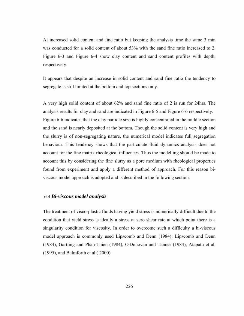
226

At increased solid content and fine ratio but keeping the analysis time the same 3 min

was conducted for a solid content of about 53% with the sand fine ratio increased to 2.

Figure 6-3 and Figure 6-4 show clay content and sand content profiles with depth,

respectively.

It appears that despite an increase in solid content and sand fine ratio the tendency to

segregate is still limited at the bottom and top sections only.

A very high solid content of about 62% and sand fine ratio of 2 is run for 24hrs. The

analysis results for clay and sand are indicated in Figure 6-5 and Figure 6-6 respectively.

Figure 6-6 indicates that the clay particle size is highly concentrated in the middle section

and the sand is nearly deposited at the bottom. Though the solid content is very high and

the slurry is of non-segregating nature, the numerical model indicates full segregation

behaviour. This tendency shows that the particulate fluid dynamics analysis does not

account for the fine matrix rheological influences. Thus the modelling should be made to

account this by considering the fine slurry as a pore medium with rheological properties

found from experiment and apply a different method of approach. For this reason bi-

viscous model approach is adopted and is described in the following section.

6.4 Bi-viscous model analysis

The treatment of visco-plastic fluids having yield stress is numerically difficult due to the

condition that yield stress is ideally a stress at zero shear rate at which point there is a

singularity condition for viscosity. In order to overcome such a difficulty a bi-viscous

model approach is commonly used Lipscomb and Denn (1984); Lipscomb and Denn

(1984), Gartling and Phan-Thien (1984), O'Donovan and Tanner (1984), Atapatu et al.

(1995), and Balmforth et al.( 2000).

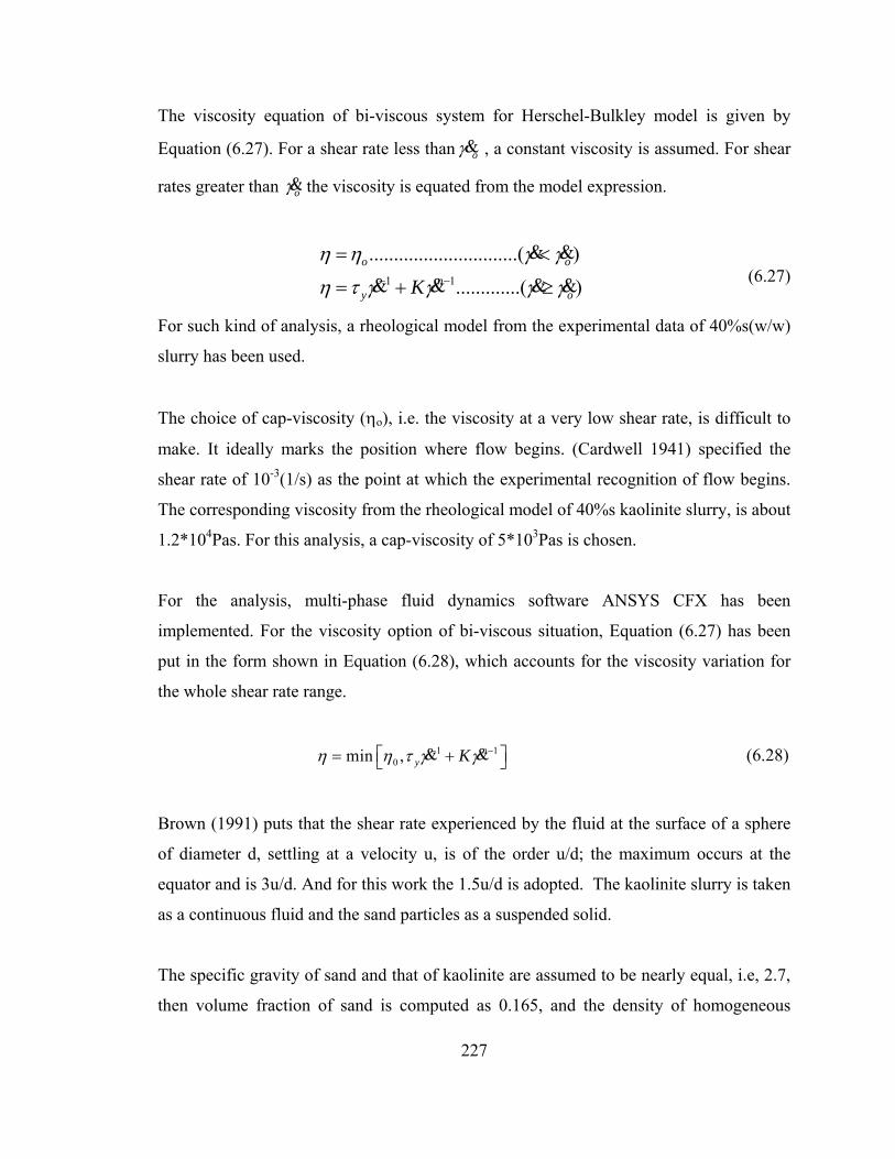
227

The viscosity equation of bi-viscous system for Herschel-Bulkley model is given by

Equation (6.27). For a shear rate less than oγ& , a constant viscosity is assumed. For shear

rates greater than oγ& the viscosity is equated from the model expression.

1 1

..............................( )

.............( )o o

ny oK

η η γ γ

η τ γ γ γ γ− −

= <

= + ≥

& &

& & & & (6.27)

For such kind of analysis, a rheological model from the experimental data of 40%s(w/w)

slurry has been used.

The choice of cap-viscosity (ηo), i.e. the viscosity at a very low shear rate, is difficult to

make. It ideally marks the position where flow begins. (Cardwell 1941) specified the

shear rate of 10-3(1/s) as the point at which the experimental recognition of flow begins.

The corresponding viscosity from the rheological model of 40%s kaolinite slurry, is about

1.2*104Pas. For this analysis, a cap-viscosity of 5*103Pas is chosen.

For the analysis, multi-phase fluid dynamics software ANSYS CFX has been

implemented. For the viscosity option of bi-viscous situation, Equation (6.27) has been

put in the form shown in Equation (6.28), which accounts for the viscosity variation for

the whole shear rate range.

1 10min , n

y Kη η τ γ γ− −⎡ ⎤= +⎣ ⎦& & (6.28)

Brown (1991) puts that the shear rate experienced by the fluid at the surface of a sphere

of diameter d, settling at a velocity u, is of the order u/d; the maximum occurs at the

equator and is 3u/d. And for this work the 1.5u/d is adopted. The kaolinite slurry is taken

as a continuous fluid and the sand particles as a suspended solid.

The specific gravity of sand and that of kaolinite are assumed to be nearly equal, i.e, 2.7,

then volume fraction of sand is computed as 0.165, and the density of homogeneous

228

kaolinite slurry is about 1337kg/m3. It is observed that the cap-viscosity predominate the

viscosity used in the model, indicating that the shear rate is very small to take up the

rheological model. Thus one may increase the cap-viscosity value in case of

unsatisfactory results. Such action was not needed in this work.

Figure 6-8 shows the comparison of the solid content profile for 24hrs simulation. The

simulation results indicate that it is only at the top and bottom parts that small variation in

concentration results. Also comparison with experimental data in terms of sand solid

content is shown in Figure 6-9. From this figure it is to observe that both experimental

and model result fall in a close band except at the top and bottom. The trend indicated by

the bi-viscous model analysis indicates that at the top decrease in the sand content and at

the bottom an increase in sand content. This is somehow reasonable.

Even though the choice of viscosity was made about half of the definition value, it still

gives satisfactory results. The other limitation to the choice of bi-viscous model is that at

a very small shear rate, the viscosity may be very high that the numerical scheme

becomes very stiff yielding no result. Thus the choice of cap-viscosity as indicated in

Equation (6.28) depends not only on the defined value but also on the computational

limits of applied schemes. From this work, it is encouraging to have a comparable bi-

viscous model to the experimental result. It is also not fully conclusive at this stage since

one needs to deal within the limits of using this approach..

It is apparent from the results that the fine matrix contribute to the capture of larger size

particles (sand) with regard to the time span to which the test has been carried to identify

the effect of stress degradation at the sedimentation stage and compaction as

consolidation takes place require further examination.

The study of sand settling in fine slurry has two major applications such as transport of

coarse particles carried by fine medium and treatment of poorly consolidating tailings

ponds. The transport of coarse particle with fine medium produces easily transportable,

non-segregating and relatively high solid content material, which require reduced

229

impoundment volume. On the other hand tailings ponds are known for their very slow

consolidation and very little release water. In such cases understanding the mechanism of

inter-particle and fluid-particle interaction helps one to implement an effective way of

material handling and deposition.

For example, internal surcharge of fine tailings by coarse sand material assist the

consolidation process. At the same time optimum application can be made if the rheology

of the mixture is properly understood. The same may apply also in case of capping of soft

sediment by sand, or handling of dredged material in coastal areas. Also the presence of

coarse particle give improved strength of the deposited material which help the

reclamation process and closure plans.

The implementation of the mechanism into a numerical scheme is still at developing

stage mainly due to the complexity of the mechanism involved and a limited

understanding in that respect. With the available knowledge and some simplifying

assumption it is possible to model physical phenomena. The use of bi-viscous model is a

typical example of a simplifying assumption. Moreover, no theoretical account has been

given for some visible physical phenomena such as stress degradation with time and

channelling, indicating that there exist still more research need in the area.

The numerical simulation of the motion of particles in a fluid during sedimentation

process is a very difficult problem that until today has not been solved to entire

satisfaction (Quispe et al. 2000). This statement appears to be very true and concurring.


The principles of particulate fluid mechanics were applied to match the experimental

results in this study. The numerical simulations as developed in computational fluid

mechanics were the basis of the study. Commercial software package, ANSYS-CFX, was

implemented for this study.

230

The kinetic theory model was implemented in the solid phase pressure in the study. For

slurries exhibiting yield stress a bi-viscous approach was applied to account for the effect

of yield stress.

Numerical simulations involve some simplifying assumptions either due to lacking

physics or computational difficulties. Comparison of numerical results with experimental

data showed encouraging outcomes.

It is recommended that additional numerical study be implemented to further explain the

mechanics involved such as concurrent development stress degradation and stress build-

up during sediment formation.

Shaughnessy et al. (2005) states that although the use of CFD may become widespread it

will never totally replace physical experimentation. This notion is applicable and shared

in this research work.

6.5 References Anandarajah, A. (1994). "Discrete-Element Method for simulating Behaviour of

Cohesive Soil." Journal of Goetechnical Engineering 120(9): 1593-1613.

Asmar, B. N., P. A. Langston, et al. (2002). "A generalized mixing index in distinct

element method simulation of vibrated particulate beds." Granular Matter 4: 129-

138.

Atapatu, D. D., R. P. Chhabra, et al. (1995). "Creeping sphere motion in Herschel-

Bulkley fluids: flow field and drag." J.Non-Newtonian Fluid Mech. 59: 245-265.

Balmforth, N. J., A. S. Burbidge, et al. (2000). "Visco-Plastic models of isothermal lava

domes." J. Fluid. Mech. 403: 37-65.

Brown, N. P. (1991). The Settling Behaviour of Particles in Fluids. Slurry Handling:

Design of Solid-Liquid Systems. N. P. Brown and N. I. Heywood, Elsevier

Applied Science: 17-40.

231

Cardwell, W. T., Jr (1941). Drilling-Fluid Viscometry. Drilling and Production Practice,

New York, American Petroleum Institute.

Cleary, P. (2001). "Modelling comminution devices using DEM."

Int.J.Numer.Anal.Meth.Geomech., 2001 25: 83-105.

Cleary, P., G. Metcalfe, et al. (1998). "How well do discrete granular flow models

capture the essentials of mixing processes?" Applied Mathematical Modelling 22:

995-1008.

Concha, F., C. H. Lee, et al. (1992). "Settling velocities of particular systems. Part 8.

Batch sedimentation of polydispersed suspensions." International Journal of

Mineral Processing 35: 159-175.

Cundall, P. A. (2001). "A discontinuous future for numerical modelling in

geomechanics?" Geotechnical Engineering 149(1): 41-47.

Cundall, P. A. and O. D. L. Strack (1979). "A Discrete Numerical Model for Granular

Assemblies." Geotechnique 29(1): 47-65.

Eckert, W. F., J. H. Masliyah, et al. (1996). "Prediction of Sedimentation and

Consolidation of Fine Tails." AIChE Journal 42(4): 960-972.

Elimelech, M., J. Gregory, et al. (1995). Particle Deposition and Aggregation. Woburn,

MA, Butterworth-Heinemann.

Gartling, D. K. and N. Phan-Thien (1984). "A Numerical Simulation of a Plastic Fluid in

a Parallel-Plate Plastometer." J.Non-Newtonian Fluid Mech. 14: 347-360.

Gidaspow, D. (1994). Multiphase Flow and Fluidization. San Diego, Academic Press.

Kenji Iimura, H. Nakagawa, et al. (1998). "Deformation of aggregates depositing on a

plate in a viscous fluid simulated by modified discrete element method."

Advanced Powder Technology 9(4): 345-361.

Limtrakul, S., A. Chalermwattanatai, et al. (2003). "Discrete particle simulation of solids

motion in a gas-solid fluidized bed." Chemical Engineering Science 58: 915-921.

Lipscomb, G. G. and M. M. Denn (1984). "Flow of Bingham Fluids in Complex

Geometries." J.Non-Newtonian Fluid Mech. 14: 337-346.

Masala, S. (1998). "Numerical simulation of sedimentation and consolidation of fine

tailings". Civil and Environmental Engineering. Edmonton, University of Alberta.

232

Mudryy, R., P. Singh, et al. (1999). Air Entrainment and segregation in powder flow.

Proceedings of the IUTAM Symposium on Segregation in Granular Flows, Cape

May, NJ, Kluwer Academic Publishers.

Oda, M. (1997). A Micro-Deformation model for Dilatancy of Granular Materials.

Proceeding of A Syposium on: Mechanics of Deformation and Flow of Particulate

Materials, Evanston, Illinois, ASCE.

O'Donovan, E. J. and R. I. Tanner (1984). "Numerical Study of The Bingham Squeeze

Film Problem." J.Non-Newtonian Fluid Mech. 15: 75-83.

Potts, D. M. (2003). "Numerical analysis: a virtual dream or practical reality?"

Geotechnique 53(6): 535-573.

Quispe, J., F. Concha, et al. (2000). "Discrete sedimentation model for ideal

suspensions." Chemical Engineering Journal 80: 135-140.

Ristow, G. H. (1999). Mixing and Segregation in Rotating Drums. Proceedings of the

IUTAM Symposium on Segregation in Granular Flows, Cape May, NJ, Kluwer

Academic Publishers.

Sadd, M. H. and J. Y. Gao (1997). The Effect of particle Damage on Wave Propagation

in Granular Materials. Proceeding of A Syposium on: Mechanics of Deformation

and Flow of Particulate Materials, Evanston, Illinois, ASCE.

Selim, M. S., A. C. Kothari, et al. (1983). "Sedimentation of Multisized Particles in

Concentrated Suspensions." AIChE Journal 29(6): 1029-1038.

Shaughnessy, E. J., I. M. Katz, et al. (2005). Introduction to Fluid Mechanics. New York,

Oxford University Press.

Shen, H. H. and M. Babic (1999). Rapid Flow of Granular Materials. Mechanics of

Granular Materials. M. Oda and K. Iwashita. Rotterdam, A.A. Balkema: 319-377.

Stamatakis, K. and C. Tien (1992). "Batch Sedimentation Calculations-The Effect of

Compressible Sediment." Powder Technology 72(3): 227-240.

Whipple, K. X. (1997). "Open-Channel Flow of Bingham Fluids: Application in Debris-

Flow Research." The Journal of Geology 105: 243-262.

Yamane, K. (1999). DEM study of segregation in a rotating cylinder. Proceedings of the

IUTAM Symposium on Segregation in Granular Flows, Cape May, NJ, Kluwer

Academic Publishers.

233

Zimmels, Y. (1988). "Simulation of Nonsteady Sedimentation of Polydisperse Particle

Mixture." Powder Technology 56: 227-250.

234

0.00

0.10

0.20

0.30

0.40

0.50

0.60

0.00 5.00 10.00 15.00 20.00 25.00 30.00

Clay solid content(%)

Hei

gnt (

m)

Init30sec60sec90sec120sec180sec

Figure 6-1 Analysis result of clay content for slurry mix at initial solid content of

46.12% and SFR=1

235

0.00

0.10

0.20

0.30

0.40

0.50

0.60

0.00 10.00 20.00 30.00 40.00 50.00 60.00

Sand solid content(%)

Hei

gnt (

m)

Init30sec60sec90sec120sec180sec

Figure 6-2 Analysis result of sand content for slurry mix at initial solid content of 46.12%

and SFR=1

236

0.00

0.10

0.20

0.30

0.40

0.50

0.60

10.00 12.00 14.00 16.00 18.00 20.00 22.00 24.00

Clay solid content (%)

Hei

ght (

m)

init15sec30sec60sec90sec120sec180sec

Figure 6-3 Analysis result of clay content for slurry mix at initial solid content of 53.12%

and SFR =2

237

0.00

0.10

0.20

0.30

0.40

0.50

0.60

10.00 20.00 30.00 40.00 50.00 60.00 70.00 80.00

Sand solid content (%)

Heig

ht (m

)

init15sec30sec60sec90sec120sec180sec


and SFR =2

238

0.00

0.10

0.20

0.30

0.40

0.50

0.60

0.00 10.00 20.00 30.00 40.00 50.00 60.00 70.00 80.00 90.00

Clay solid content (%)

Heig

ht (m

)

init1hr2hrs4hrs12hrs24hrs

Figure 6-5 Analysis result of clay content for slurry mix at initial solid content of 62.12%

and SFR = 2

239

0.00

0.10

0.20

0.30

0.40

0.50

0.60

0.00 20.00 40.00 60.00 80.00 100.00 120.00

Sand solid content(%)

Heig

ht (m

)

init1hr2hrs4hrs12hrs24hrs


and SFR = 2

240

Shear Rate

Shea

r Str

ess/

Vis

cosi

ty

Viscosity

Shear Stress

Figure 6-7 Shear stress-Shear rate function for a bi-viscous fluid model to approximate

yield-stress fluid

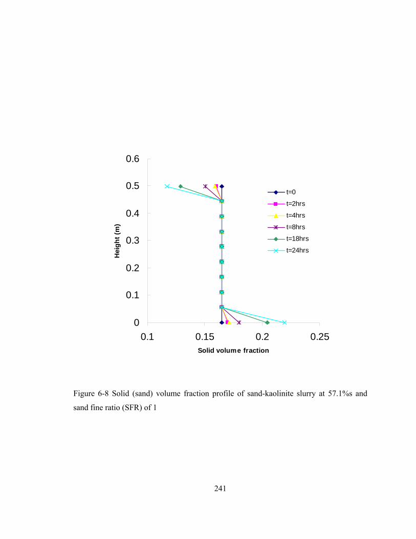
241

0

0.1

0.2

0.3

0.4

0.5

0.6

0.1 0.15 0.2 0.25Solid volume fraction

Hei

ght (

m)

t=0

t=2hrs

t=4hrs

t=8hrs

t=18hrs

t=24hrs

Figure 6-8 Solid (sand) volume fraction profile of sand-kaolinite slurry at 57.1%s and

sand fine ratio (SFR) of 1

242

0

0.1

0.2

0.3

0.4

0.5

0.6

45 50 55

Sand Content(%)

Hei

ght (

m)

BVM-2hrs

EXP-2hrs

BVM-8hrs

EXP-8hrs

BVM-24hrs

EXP-24hrs

Figure 6-9 Comparison of Bi-Viscous model (BVM) and Experimental (EXP) results at

different times

243

CHAPTER 74

7. QUANTITATIVE STUDY OF SEGREGATION

7.1 General As there is limited understanding in the subject matter of segregation, there is a need to

quantify the degree of segregation or mixing so that some form of quality control or

common way of describing the effect of different mechanisms is achieved. The degree of

mixing or segregation is expressed commonly by measuring the statistical variation of

composition using the standard deviation (Buslik (1950), Lacey (1954), Fuerstenau and

Fouladi (1967) and Liss et al. (2004) ).

Segregation and mixing, as two opposing phenomena, have prevailed in many industrial

processes which are involved in the separation or blending of different ingredients. In the

industry it is necessary to have some means of quantifying the quality of mixing so that,

for example, the required performance of a mixer can be specified and then measured

(Asmar et al. 2002).

According to Davies (1971) mixing of solids is defined as an operation by which two or

more solid materials in particulate form are intermingled randomly in the mixer by the

random movement of particles. Lacey (1954) assumed that in all mixers, mixing is

achieved by one or more of the following:

(a) Convective mixing: Transfer of groups of particles from one location to another

(b) Shear mixing: Setting up of slipping planes within the mass of material

(c) Diffusive mixing: Diffusion of individual particles over newly developed

surfaces.

These mechanisms control mixing to a varying degree depending on the modes of

operation of the mixer. De-mixing usually accompanies mixing and two mechanisms are

4 A version of this chapter has been published. Mihiretu, Y.M., Chalaturnyk, R.J., Scott, J.D. Proc. of 61st Canadian Geotechnical Conference, Edmonton, Alberta, 2008.

244

proposed to describe these effect. The first is the percolation mechanism relating to the

slipping of smaller particles through the voids created by the larger particles. The other

mechanisms results from differences in trajectories of materials falling at an angle during

free flight.

In the case where different phases are involved in the mixtures, differences in mobility of

the particles usually yields the sorting of particles. The sedimentation process and

multiphase flows in which different composition of properties involved, the occurrence of

segregation is more likely depending upon the concentration and flow characteristics.

Differences in size, density or shape are the main factors which contribute to the

segregation of the mixture. It is widely accepted that difference in size may be the most

dominant factor (Fan et al. 1970); (Rhodes 1998); (Vallance and Savage 1999).

Gravitational settling consisting of particles of different mobility results in segregation of

particles. It would be of practical significance to express the degree of segregation in

somewhat quantitative manner. An expression as such may provide a common basis for

comparison and assessment of the quality of data output.

A quantitative index, called Segregation Index, has been in use by research group at

University of Alberta, Suthaker (1995), Tang (1997) and Chalaturnyk and Scott (2001).

The index is calculated based on total solid content for the depth profile after

sedimentation test is completed. Another term related to Segregation Index (SI) is the

fines capture, FC, given as100-SI (refer to Equations (2.10) and (2.11)). The segregation

boundary, which divides the segregating type of slurry and the otherwise, is the fine

capture value of 95. A value of fine capture less than 95 is categorized as segregating

mix. Such an index calculation is in agreement with the definition of segregation as given

by Kuepper (1991) where segregation was defined as “the tendency of solid fraction (or

part of it) to settle, creating a concentration gradient within the mass”. The segregation

index constructed on the overall solid content may somehow indicate the size segregation

245

indirectly, one finds, however, some difficulty in communicating with other experimental

results (Kenney and Westland 1992) (Kaushal and Tomita 2002).

Davies (1971) presented an index for degree of mixing for samples of similar size as:

M = S / σR , (7.1)

where S is the estimated standard deviation and σR is standard deviation for completely

random mixtures. The standard deviation S (for unbiased estimation) given by Equation

(7.1) is

2

1( )

1

n

ii

x xS

n=

−=

−

∑ . (7.2)

Amongst the most popular indices using standard deviation is Lacey’s index (Lacey

1954), which defines a mixing index M, based on the number of particles in a sample, as

2 2

2 2o

o R

S SMS S

−=

− , (7.3)

where So2 is the variance for completely segregated mixture, SR

2 is the variance for

completely random mixture and S2 is the variance of the mixture between fully random

and completely segregated mixtures. This index suffers from three drawbacks: it is

limited to same size particles, very sensitive near the completely segregated state, and

relatively insensitive in the final stage of mixing (Fan et al. 1970);(Davies 1971);

(Williams 1976) and (Asmar et al. 2002).

Asmar et al. (2002) introduced an index called Genaralised Mean Mixing Index (GMMI)

in their Discrete Element Method (DEM) simulations. The GMMI in one of the axes

direction, say z, is defined as:

246

1 1( ) ( )

k

n Nj ref refj k

i

z z z zGMMIz

n N= =

⎡ ⎤ ⎡ ⎤− −⎢ ⎥ ⎢ ⎥=⎢ ⎥ ⎢ ⎥⎣ ⎦⎣ ⎦

∑ ∑ (7.4)

where n is the number of particles of type I, N is the total number of particles, z is the z-

coordinate of the position of the particle centre and zref is the reference z-coordinate.

The GMMI will be the average of the calculations in three directions. The use the index

appears simple, however, its application is limited to DEM simulation where the position

of individual particles is known.

In the study of segregation of granular filter materials, Kenney and Westland (1992)

applied the term Segregation Index and Relative Segregation Index to determine the

extent of segregation. They carried out the rotary-drum test, in which the drum is half

filled with soil sample and tumbled. After the test, they divide the drum into three parts,

inner 25% volume, the middle 50% and the outer 25%. Grain size analysis is carried out

for samples taken from each component and plotted as percent finer vs. grain size. They

determined the logarithmic mean particle size (using Popovics’ equation), and they

defined Segregation Index as follows:

SI = log(dc/df) (7.5)

Where dc and df are logarithmic mean particle sizes of the coarse and fine zones,

respectively. They defined Relative Segregation Index (RSI), as the ratio of SI (test) to

the Segregation Index calculated for the state of perfect segregation, SIp.

RSI = SI(test)/SIp (7.6)

They found that the middle 50% volume is characterised by similar grain size distribution

as that of the initial sample. The definition of fines and coarses, according to their work,

is relative to test material, (e.g., sand may be fine for gravel and sand mix) as the division

247

contains all particles which lie in the inner 25% and the outer 25% volume respectively.

They reported that it is only under perfect segregation that complete sorting according to

size may be achieved. The application of their approach to design of a filter in

embankment dam is discussed by Milligan (2003). It is also shown that for grain size

distribution varying in two decades; segregation is independent of grain size and grain

size distribution. The idea of separating in different zones after the test and undertaking

the grain size distribution seems attractive to be applied for other similar cases as well.

Other similar studies in bulk material handling (granular mixing) were using index

calculation based on statistical means. According to Lacey (1954), it is generally agreed

that the most useful way of expressing degree of mixture is by measuring the statistical

variation of composition among samples drawn from it. A summary of different mixing

indexes as used by different authors are presented by Hastie and Wypych (1999). Fan et

al. (1970), referring the works of Lawrence and Beddow (1969), stated that particle

density and shape were found to have little effect upon the extent of segregation.

A term degree of mixedness, as it is used by Fuerstenau and Fouladi (1967) for the study

of packed particles of two different sizes, is defined as

o

Mσσ

−= 1 (7.7)

where M is the degree of mixedness, σ, is the observed standard deviation of sample

taken from the mixture; σo is the expected standard deviation of samples taken before any

mixing had occurred and is given by

)1( ppo −=σ (7.8)

where p is the mass fraction of larger particles in the mixture.

248

Yamane (1999) defined Segregation Index, which is a different version of Equation (7.7).

His index is equivalent to 1-M.

A standard deviation approach was followed by Liss et al. (2004). They introduced

Relative Standard Deviation (RSD) to characterize the relative degree of segregation. The

form of the expression is shown in Equation (7.9):

2

1( )

1

n

ii

xRSD

n

μ=

−=

−

∑ , (7.9)

where n is the number of samples taken, μ is the mean value of all the samples, and xi is

the value of the ith sample. RSD ranges between the limits 0, perfect mix, and 1,

completely segregated.

The above survey of literature shows that there is no universally accepted index. Most of

the proposed mixing indices are developed for binary solid-mixtures and are based on

statistical analysis, mostly the standard deviation, variance or coefficient of variation.

7.2 Suggested Methods in the Experimentation

The uniformly mixed slurry is poured into standpipe then after the sedimentation process

is complete, the release water is decanted and the sediment is divided into different layers

and samples for moisture content and grain size analysis. From the grain size analysis, it

is possible to estimate the composition of each size in the different layers.

The profile of concentration of each particle size is plotted, which indicate the extent of

segregation with respect to size groups. It is believed that a quantitative description of the

extent of segregation may give some form of comparison for different test conditions.

The following index, Segregation Index (SI), is proposed for the works that follow.

249

( )2

2 i ii i

i

i

h Sh S

hSI

h

⎛ ⎞⎜ ⎟−⎜ ⎟⎝ ⎠=

∑∑ ∑∑

(7.10)

where Si is the solid content of sample section with height of hi. This equation takes the

variability of sampling depths into account by weighing them in their separate section (hi)

by assuming that the sample represents a section height from which it is taken

Such an index calculation can also be used for a test which involves different size group.

It can also be applied to dynamic segregation cases.

The advantages of the proposed equation are:

- simple and very convenient to calculate

- it can be applied to multi-size particle presence

- it can account the sampling depth variation.

It is to notice that indices which are statistical in nature are basically different forms of

mean deviation, standard deviation or variance. Representative spread sheet calculations

are presented in Appendix D.

7.3 Reference

Asmar, B.N., Langston, P.A., and Matchett, A.J. 2002. A generalized mixing index in distinct element method simulation of vibrated particulate beds. Granular Matter, 4: 129-138.

Buslik, D. 1950. Mixing and Sampling with Special Reference to Multi-Sized Granular Material. ASTM Bulletin: TP92-TP99.

Chalaturnyk, R.J., and Scott, J.D. 2001. Soil Structure Behaviour Diagram. In High Density and Paste Tailings 2001. May 10-11, 2001.

Davies, G.S. 1971. Mixing of solids. In Particle Technology. Edited by D. Venkateswarlu and A. Prabhakara Rao. Madras, India, pp. 497-508.

Fan, L.T., Chen, S.J., and Watson, C.A. 1970. Solids Mixing. In Ann. Rev. Ind.& Engrg Chemistry. Edited by V.W. Weekman(Jr). American Chemical Society, pp. 22-56.

Fuerstenau, D.W., and Fouladi, J. 1967. Degree of Mixedness and Bulk Density of Packed Particles. Ceramic Bulletin, 46(9): 821-823.

250

Hastie, D.B., and Wypych, P.W. 1999. Segregation During Gravity Filling of Storage Bins. In Proceedings of the IUTAM Symposium on Segregation in Granular Flows. Edited by A.D. Rosato and B. D.L. Cape May, NJ. Kluwer Academic Publishers, pp. 61-72.

Kaushal, D.R., and Tomita, Y. 2002. Solid concentration profile and pressure drop in pipe line flow of multisized particulate slurries. International Journal of Multiphase Flow, 28: 1697-1717.

Kenney, T.C., and Westland, J. 1992. Laboratory study of segregation of granular filter materials. In Filters in Geotechnical and Hydraulic Engineering. Edited by J. Brauns, M. Heibaum, and U. Schuler. Karlsruhe, Germany. A.A. Balkema, pp. 313-319.

Kuepper, A.A.G. 1991. Design of Hydraulic Fill. PhD, University of Alberta, Edmonton,Canada.

Lacey, P.M.C. 1954. Development in the theory of particle mixing. Journal of appl. Chem., 4: 257-268.

Liss, E.D., Conway, S.L., Zega, J.A., and Glasser, B.J. 2004. Segregation of Powders during Gravity Flow through Vertical Pipes. Pharmaceutical Technology, February: 78-96.

Milligan, V. 2003. Some uncertainities in Embankment Dam Engineering. J.Geotech.&Geoenvironmental Engrg., ASCE, 129(5): 785-797.

Rhodes, M. 1998. Introduction to Particle Technology. John Wiley &Sons,, Chichester, England.

Saileswaren, N., and Panchanathan, V. 1971. Packing Characteristics of nonspherical particles. In Particle Technology. Edited by D. Venkateswarlu and A. Prabhakara Rao. Indian Institute of Technology, Madras, pp. 106-120.

Suthaker, N.N. 1995. Geotechnics of Oil sand Tailings. PhD thesis, University of Alberta, Edmonton.

Tang, J. 1997. Fundamental behaviour of Composite Tailings. MSc thesis, University of Alberta, Edmonton.

Williams, J.C. 1976. The Segregation of Particulate Material.A Review. Powder Technology, 15: 245-251.

Yamane, K. 1999. DEM study of segregation in a rotating cylinder. In Proceedings of the IUTAM Symposium on Segregation in Granular Flows. Edited by A.D. Rosato and B. D.L. Cape May, NJ. Kluwer Academic Publishers, Vol.321-326.

251

CHAPTER 8

8. CONCLUSION AND RECOMMENDATION

8.1 Conclusions

A convenient and economical method of mine wastes disposal is to impound them

hydraulically. However such disposal methods commonly yield segregation, i.e, settling

of coarse and large size particles on the dyke beaches and transport of fine particles

farther in the pond forming fine tailings. The research was aimed at establishing the

fundamental factors that control the segregation mechanism in the oil sands tailings.

Rheological characterization was carried out on slurry to examine the effect of grain size,

void ratio and porewater chemistry. Rheological properties were shown to be highly

influenced by grain size composition, solid content (void ratio) and porewater chemistry.

Generally, yield stress increases with increase in total solid content. Slurries at the same

solid content but different sand-to-fine ratio show difference in yield stress, the higher the

sand fine ratio the lesser the yield stress.

Comparisons of yield measurement using vane method and model fit of the conventional

viscometer rheogram was showed satisfactory results. Herschel-Bulkley and Casson’s

model were used to fit the rheogram data. A statistical analysis was carried out to choose

the better model. And for the test conditions, the Casson’s model appear to fit the data

better than Herschel-Bulkley model.

The relationship between yield stress and solid content for fine slurry was presented. with

a model fit based on the fractal theory. Porewater chemistry effect was studied by varying

the pH of the pore fluid medium. The yield stress was mildly influence in the acidic range

by showing a moderate increase with increase in acidity. A significant change in yield

252

stress was observed at pH 12 when a slurry was treated with Ca(OH)2 and NaOH.,

indicating that higher yield stress in the case of Ca(OH)2 addition versus diminished or no

distinct yield stress in the case of NaOH-based pore fluid medium. Thus surface

properties of clay particles and the surrounding fluid medium chemistry influence the

flow/rheological properties. Reference to pH alone is not sufficient without stating the

mineralogy of the solution. The higher yield stress is an indication of the potential of the

fine matrix to capture coarse particle (sand) and mitigate segregation.

Rheological studies with oil sands tailings presented similar rheological trends as those of

kaolinite slurries. It is therefore suggested that proceeding with the surrogate tailings

materials for the rest of the experimental program would be reasonable to understand the

segregation mechanism. The potential drawback for the surrogate tailing material is the

lack of bitumen traces that is found oil sands tailings.

A custom-designed standpipe was used in a series of experiments to determine

concentration profiles during the sedimentation process. Standpipe tests at low solid

content and low Fine Water Ratio indicated that the sand particles settle to the bed

immediately. However, there existed some sand particles even at the upper section after

some time has elapsed. The capture mechanism is correlated to the rheological property

of the fine matrix. The fine content was found to control the shape of concentration

profile.

It was observed that surface properties of the fine matrix was modified by the addition of

intermediate size (silt size) particles in that the settling rate (water release) was improved

and the degree of segregation was minimized. The intermediate size serves as surface

property modifier and internal surcharge.

The sediment profile of the segregating type of slurries is controlled by the clay water

ratio. Segregating slurries at same clay water ratio exhibit similar deposit profile after

sedimentation.

253

Theoretical formulation for coarse size capture by the yield stress of the fine matrix was

presented. It was found that the theoretical formulation over-predicted the size of coarse

particle that can be captured by the yield stress of the fine matrix. A correction factor was

used to the theoretical size to match with experimental observation. The correction factor

was compared with other data in the literature and there exist wide difference. Thus the

correction factor is rather an indication of a “missing physics” that need yet to be

explained well.

Flume test was conducted to study the effect of flow and shearing on relatively non-

segregating slurry mixes. The shape at deposition and flow rate were observed to be

governed by the solid content, sand fine ratio, bed inclination, and discharge from the

reservoir. As the sand fine ratio increases, the beach profile followed nearly a parallel

trend to bed slope. The tendency to segregate was also high when the sand fine ratio

increases. A simplified form of non-linear first order differential equation derived from

the theory of plasticity was applied to study the profile of a beach formed from flume test.

Numerical simulation using Computational Fluid Dynamic (CFD) software was used to

supplement the experimental work. The CFD method implemented the kinetic theory

approach and resulted in segregating slurry for all range of test. A different approach

using a bi-viscous model was adopted for non-segregating type slurries and reasonable

match was achieved.

A general purpose quantitative index was introduced to identify whether slurry is

segregating or not. The important feature of the index is that it accounts for the thickness

the sample is drawn from. Furthermore, the application of the proposed index can be

extended to a dynamic segregation conditions.

8.2 Recommendations

Rheological studies indicate the huge impact they have on the segregation properties of

tailings. To practical cases, it is suggested that tailings materials are rheologically

254

calibrated comparing with their sand fine ratio, and solid contents. Once this is done, it

may provide in-situ quality control method identifying whether the slurry has segregation

potential or not.

The basic mechanism of segregation is still not well understood. It appears that the

motion of individual particles within a group settling needs to be understood. It is

suggested that small beads or balls with embedded signal/frequency emitter, which is

varied according to different size groups involved, be allowed to settle in the slurry. The

motion of individual particles then can be tracked by their respective signals. This

method could be used both in the static and dynamic environment. Such approach could

supply the data we need to understand the process of segregation. It may require

collaboration with expertise in electrical signal system.

When the solid content of a slurry is above 40% and it is allowed to settle, there are

channels along the height of standpipe and lava domes at the interface between release

water and suspension. There is no study made on the impact of these micro-channels on

the process of sedimentation/ consolidation. Detailed examination of the effects is need.

The fine particles are the major contributors of the rheological properties that govern the

segregation process. Application of fractal theory in rheological characterization need

further study to minimize the level of empiricism involved. The same recommendation

also goes for the application of plastic theory in the study of beach profile.

The effect of pore fluid chemistry on the segregation properties of slurries need to be

further investigated in terms of ion exchange capacity in the range of slurry solid

contents. Furthermore, the effect of trace bitumen in the segregation mechanism of oil

sands tailings needs to be studied.

Also a sedimentation and consolidation model which work for segregating slurries need

to be developed. The challenging issue in the modeling would be the moving boundary

255

problem between the sediment and the suspension and the different size distribution

involved in the process.

Moreover, in sediment formation the concurrent process of stress degradation and stress

build-up are not well understood and further research to understand the physics involved

is recommended.

There have been reports that pipeline transport of non-segregating slurry results in

segregating slurry at the deposition. More study to better understand the flow mechanism

in pipeline transport is required. Moreover, the idea of mobile thickener that avoids

transporting high solid content by pipeline should be a subject of future research.

The theory of sedimentation and consolidation which involve segregation and the

complexities of fine matrix rheology require more study and further theory improvement.

256

APPENDIX A

257

A.1. Viscosity Measurement ASTM D 4016-02 defined coefficient of viscosity as the ratio between the applied stress

and the rate of shear. This coefficient is a measure of the resistance to flow of the liquid.

It is commonly called the viscosity of the liquid. The cgs unit of viscosity is 1g/cm.c

(1dyne/s cm2) and is called a poise (P). Viscosities of thin liquids are normally given in

hundredth of a poise or centipoises (cP). The SI unit of viscosity is 1Pa.s (1 N.s./m2) and

is equal to 10P, or 1000cP.

A.2. Procedure

Brookfield manual (No. M/97-164-D1000) provides the following general procedure for

viscosity measurements. Brookfield recommends the use of a 600 ml Low Form Griffin

beaker when using LV/RV/HA/HB spindles.

1. Mount the guardleg on the DV-II+ Viscometer (LV and RV series).

2. Insert and center spindle in the test material until the fluid's level is at the

immersion groove on the spindle's shaft. With a disc-type spindle, it is necessary

to tilt the spindle slightly while immersing to avoid trapping air bubbles on its

surface. Attach the spindle to the lower shaft of the viscometer. Lift the shaft

slightly, holding it firmly with one hand while screwing the spindle on with the

other (note left-hand thread). Avoid putting side thrust on the shaft. Verify the

proper spindle immersion depth and that the viscometer is level.

3. The process of selecting a spindle and speed for an unknown fluid is normally

trial and error. An appropriate selection will result in measurements made

between 10-100 on the instrument % torque scale. Two general rules will help in

the trial and error process.

258

1) Viscosity range is inversely proportional to the size of the spindle.

2) Viscosity range is inversely proportional to the rotational speed.

To measure high viscosity, choose a small spindle and/or a slow speed. If the

chosen spindle/speed results in a reading above 100%, then reduce the speed or

choose a smaller spindle.

Experimentation may reveal that several spindle/speed combinations will produce

satisfactory results between 10-100%. When this circumstance occurs, any of the

spindles may be selected. Non-Newtonian fluid behavior can result in the

measured viscosity changing if the spindle and/ or speed is changed.

Allow time for the indicated reading to stabilize. The time required for

stabilization will depend on the speed at which the Viscometer is running and the

characteristics of the sample fluid. For maximum accuracy, readings below 10%

should be avoided.

4. Press the MOTOR ON/OFF/ESCAPE key and turn the motor “OFF” when

changing a spindle or changing samples. Remove spindle before cleaning.

5. Interpretation of results and the instrument's use with non-Newtonian and

thixotropic materials is discussed in the booklet, "More Solutions to Sticky

Problems", and in Appendix C, Variables in Viscosity Measurements.

A.3. Calibration

The Calibration was carried out with the standard fluid provided by the manufacturer,

Brookfield Engineering Laboratories. A calibration template obtained from manufacturer

website was used in analyzing calibration results. Table A-1 shows the calibration

analysis of the viscometer used in the measurement program. Figure A-1 shows a

calibration check chart, that shows viscosity measurement at different rate. The data plot

259

falls well within the manufacturer’s acceptable ranges, validating the use of the

viscometer for test.

A.4. Viscosity measurement

After the calibration check viscosity measurements took place and sample results are

presented below. Figure A-2 shows viscosity versus shear rate relationships for a range of

solid contents from 25% to 45 % solid contents of kaolinite slurry. And Figure A-3 shows

a corresponding shear stress versus shear rate relationship for same range of solid

contents of kaolinite slurry used through the experimental program.

260

Table A-1 Calibration Template for analyzing calibration results

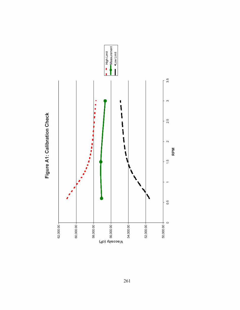
261

Figure A-1 Calibration check

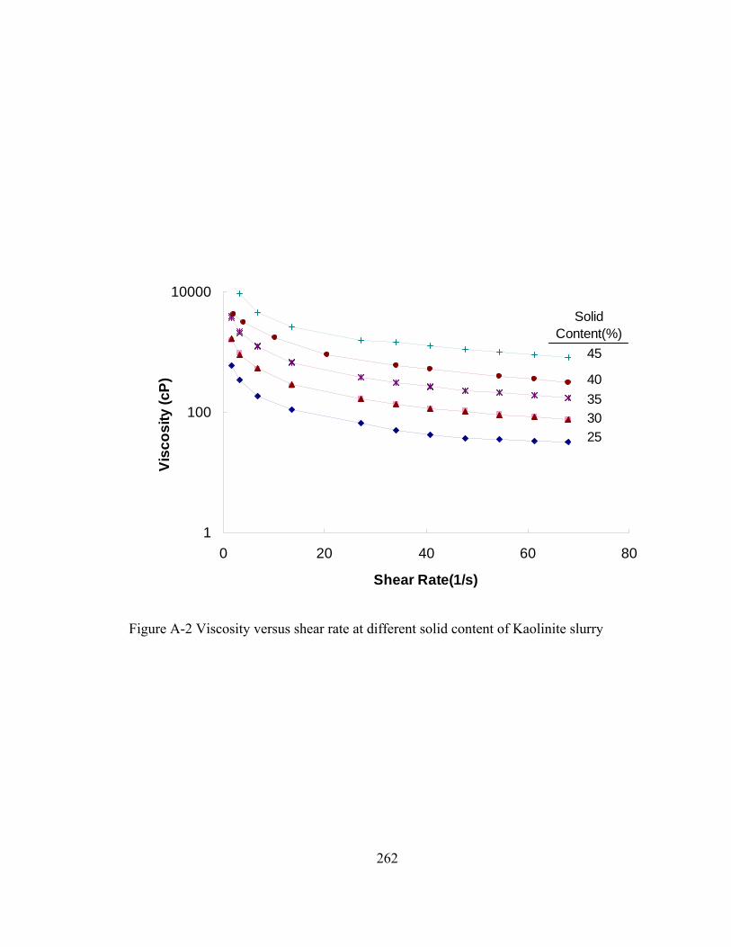
262

1

100

10000

0 20 40 60 80

Shear Rate(1/s)

Visc

osity

(cP)

45

Solid Content(%)

40353025

Figure A-2 Viscosity versus shear rate at different solid content of Kaolinite slurry

263

1

10

100

0 20 40 60 80

Shear Rate(1/s)

She

ar S

tress

(Pa)

25

30

35

40

45

Solid Content(%)

Figure A-3 Shear stress versus shear rate at different solid content of Kaolinite slurry

264

A5 Rheological Measurements of Tailings Materials

i) Suncor Mature Fine Tailings

Mature fine tailings (MFT) samples were received from Suncor MFT (Pond 6) and Pond

2/3. Three set of samples identified as S20, S30 and S42, the digits after the letter S

designate the depth in feet from which the samples were taken. Table A-2 shows sample

properties as-received.

Table A-3 summarizes the measured solid content at targeted bulk density of tailings

slurry for the three set of samples. Tailings release water sample was received to prepare

a slurry mix with a desired slurry mix. The measured pH of the release water was 8.73.

Particle size distributions of the tailings materials at different depths were carried out and

are shown in Figure A-4.

Table A- 2 Mature Fine Tailings sample properties as-received.

Sample Description pH Solid content (by weight)

S20 8.07 23.07 S30 7.71 31.75 S42 7.49 38.15

Table A- 3 Solid content of samples at different bulk densities.

Bulk Density S20 S30 S42 Average

1.5 57.3 57.8 57.8 57.6 1.4 48.0 51.4 49.2 49.5 1.3 41.5 43.6 41.6 42.2 1.2 29.7 30.0 30.4 30.1 1.1 16.3 15.7 16.8 16.3

Viscosity measurement Temperature Effect

265

The effect of temperature was studied on S30 (middle depth, 30ft) sample at three

temperatures, 10, 20 and 30 degree Celsius. The samples have a constant bulk density of

1.3g/cc. Figure A-5 shows the data plots.

Figure A-6 shows another rheogram for samples obtained from Suncor pond 2/3 tested at

different temperature at bulk density of 1.3 g/cc.

Figures A-7 to A-30 show the rheological data plots at different depths and bulk densities

ranging from 1.1 g/cc to 1.4 g/cc tested temperature of 10 degree Celsius.

266

0.0

10.0

20.0

30.0

40.0

50.0

60.0

70.0

80.0

90.0

100.0

0.0001 0.001 0.01 0.1 1 10

Depth 20ft

Depth 30ft

Depth 42ft

PER

CEN

T FI

NER

GRAIN SIZE (mm)

SILT SAND GRAVELCLAY

#200 #100 #60 #40 #20 #10 #4 #3/8#325

Figure A- 4 Particle size distribution of the MFT samples at different depths.

267

0

2000

4000

6000

8000

10000

12000

14000

0 10 20 30 40 50 60 70 80

Shear rate(1/s)

Visc

osity

(cP)

smp1temp10smp2temp10smp3temp10smp1temp20smp2temp20smp1temp30smp2temp30

Figure A- 5 Viscosity measurement of S3 MFT (bulk density 1.3 g/cc) at different temperatures.

268

0

10

20

30

40

50

60

70

0 10 20 30 40 50 60 70 80

Shear rate (1/s)

Shea

r Str

ess(

dyne

/cm

^2)

Experiment(temp=8)HB Model fit(temp=8)Experiment(temp=15)HB Model fit(temp=15)Experiment(temp=20)HB Model fit(temp=20)

Figure A- 6 Flow Curve of pond 2/3 MFT at different temperatures and Herschel Bulkley model fits

269

0

20

40

60

80

100

120

140

160

0 20 40 60 80

Shear rate(1/s)

Visc

osity

(cP)

bd11smp1 bd11smp2 bd11smp3

Figure A- 7 Viscosity versus shear rate of Pond 6 MFT (S20) bulk density 1.1 g/cc

270

0

10

20

30

40

50

0 20 40 60 80

Shear rate(1/s)

Shea

r Str

ess(

dyne

/cm

^2)

smp1 smp2 smp3

Figure A- 8 Shear stress versus shear rate of Pond 6 MFT (S20) bulk density 1.1 g/cc

271

0

200

400

600

800

1000

1200

1400

1600

1800

2000

0 20 40 60 80

Shear rate(1/s)

Visc

osity

(cP)


Figure A- 9 Viscosity versus shear rate of Pond 6 MFT (S20) bulk density 1.2 g/cc at temperature of 10 deg. Celsius.

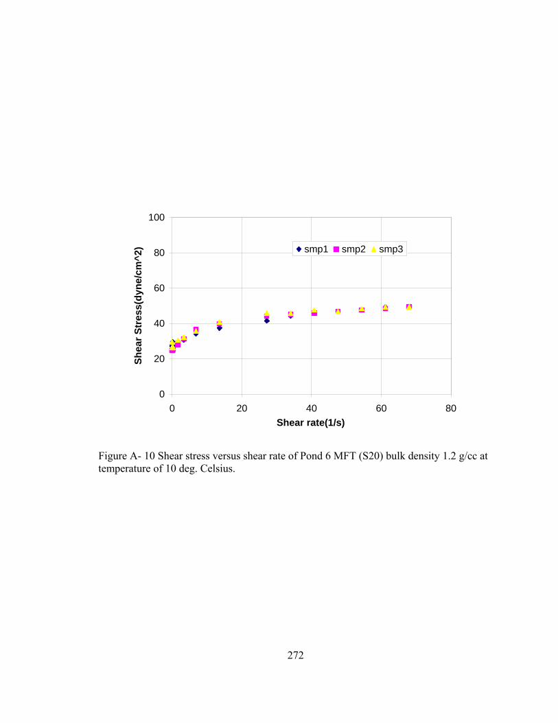
272

0

20

40

60

80

100

0 20 40 60 80Shear rate(1/s)

Shea

r Str

ess(

dyne

/cm

^2) smp1 smp2 smp3

Figure A- 10 Shear stress versus shear rate of Pond 6 MFT (S20) bulk density 1.2 g/cc at temperature of 10 deg. Celsius.

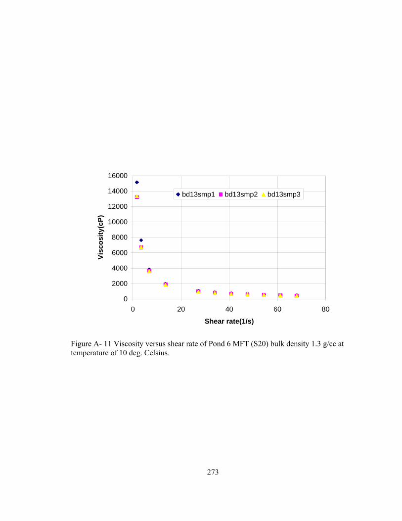
273

0

2000

4000

6000

8000

10000

12000

14000

16000

0 20 40 60 80

Shear rate(1/s)

Visc

osity

(cP)



274

0

50

100

150

200

250

300

350

400

0 20 40 60 80

Shear rate(1/s)

Shea

r Str

ess(

dy/c

m^2

)

smp1 smp2 smp3


275

0

5000

10000

15000

20000

25000

30000

35000

40000

45000

0 20 40 60 80

Shear rate(1/s)

Visc

osity

(cP)



276

0

100

200

300

400

500

600

700

800

900

0 20 40 60 80

Shear rate(1/s)

Shea

r Str

ess(

dy/c

m^2

)

smp1 smp2 smp3


277

0

100

200

300

400

500

600

0 20 40 60 80

Shear rate(1/s)

Visc

osity

(cP)

bd11sample1 bd11sample2 bd11sample3


278

0

5

10

15

20

0 20 40 60 80

Shear rate(1/s)

Shea

r str

ess(

dy/c

m^2

)



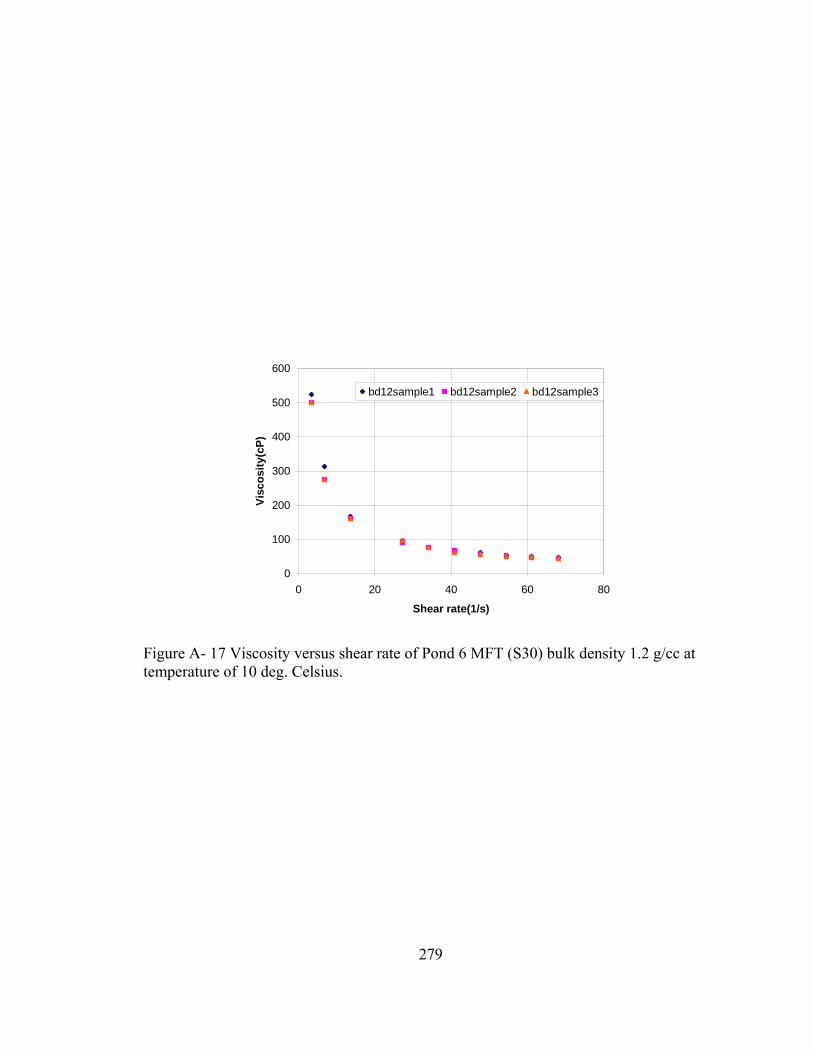
279

0

100

200

300

400

500

600

0 20 40 60 80

Shear rate(1/s)

Visc

osity

(cP)



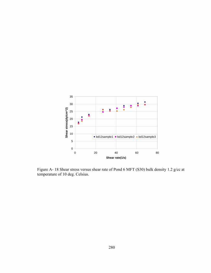
280

0

5

10

15

20

25

30

35

0 20 40 60 80

Shear rate(1/s)

Shea

r str

ess(

dy/c

m^2

)



281

0

1000

2000

3000

4000

5000

6000

0 20 40 60 80

Shear rate(1/s)

Visc

osity

(cP)



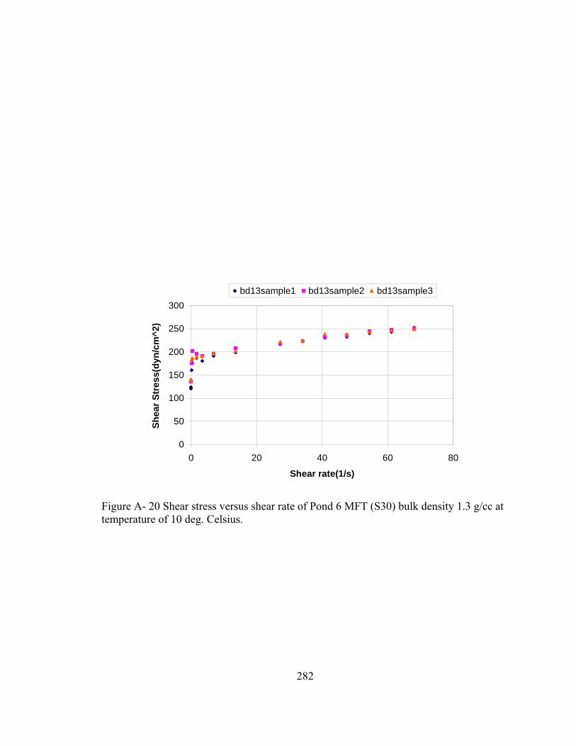
282

0

50

100

150

200

250

300

0 20 40 60 80

Shear rate(1/s)

Shea

r Str

ess(

dyn/

cm^2

)



283

0

500

1000

1500

2000

2500

3000

3500

4000

4500

5000

0 20 40 60 80

Shear rate(1/s)

Visc

osity

(cP)



284

0

50

100

150

200

250

300

350

400

450

0 20 40 60 80

Shear rate(1/s)

Shea

r Str

ess(

dyne

/cm

^2)



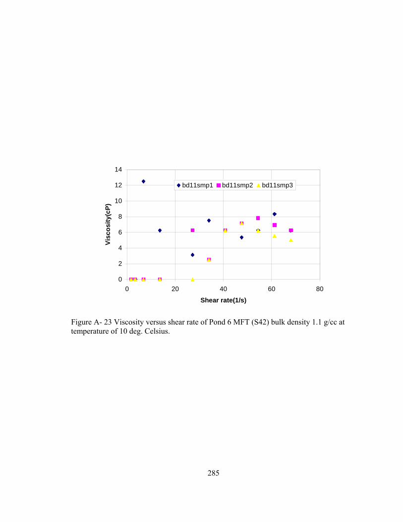
285

0

2

4

6

8

10

12

14

0 20 40 60 80

Shear rate(1/s)

Visc

osity

(cP)



286

0

2

4

6

8

10

0 20 40 60 80

Shear rate(1/s)

Shea

r Str

ess(

dy/c

m^2

)

smp1 smp2 smp3


287

0

100

200

300

400

500

600

700

0 20 40 60 80

Shear rate(1/s)

Visc

osity

(cP)



288

0

10

20

30

40

0 20 40 60 80

Shear rate(1/s)

Shea

r Str

ess(

dy/c

m^2

) smp1 smp2 smp3


289

0

500

1000

1500

2000

2500

3000

3500

0 20 40 60 80

Shear rate(1/s)

Visc

osity

(cP)


Figure A- 27 Viscosity versus shear rate of Pond 6 MFT (S42) bulk density 1.3g/cc at temperature of 10 deg. Celsius.

290

0

10

20

30

40

50

60

70

80

90

100

0 20 40 60 80

Shear rate(1/s)

Shea

r Str

ess(

dy/c

m^2

)

smp1 smp2 smp3


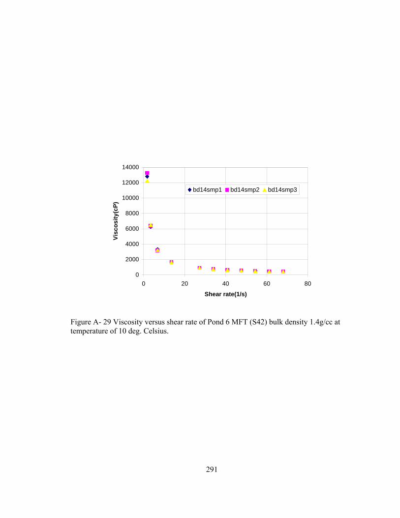
291

0

2000

4000

6000

8000

10000

12000

14000

0 20 40 60 80

Shear rate(1/s)

Visc

osity

(cP)


Figure A- 29 Viscosity versus shear rate of Pond 6 MFT (S42) bulk density 1.4g/cc at temperature of 10 deg. Celsius.

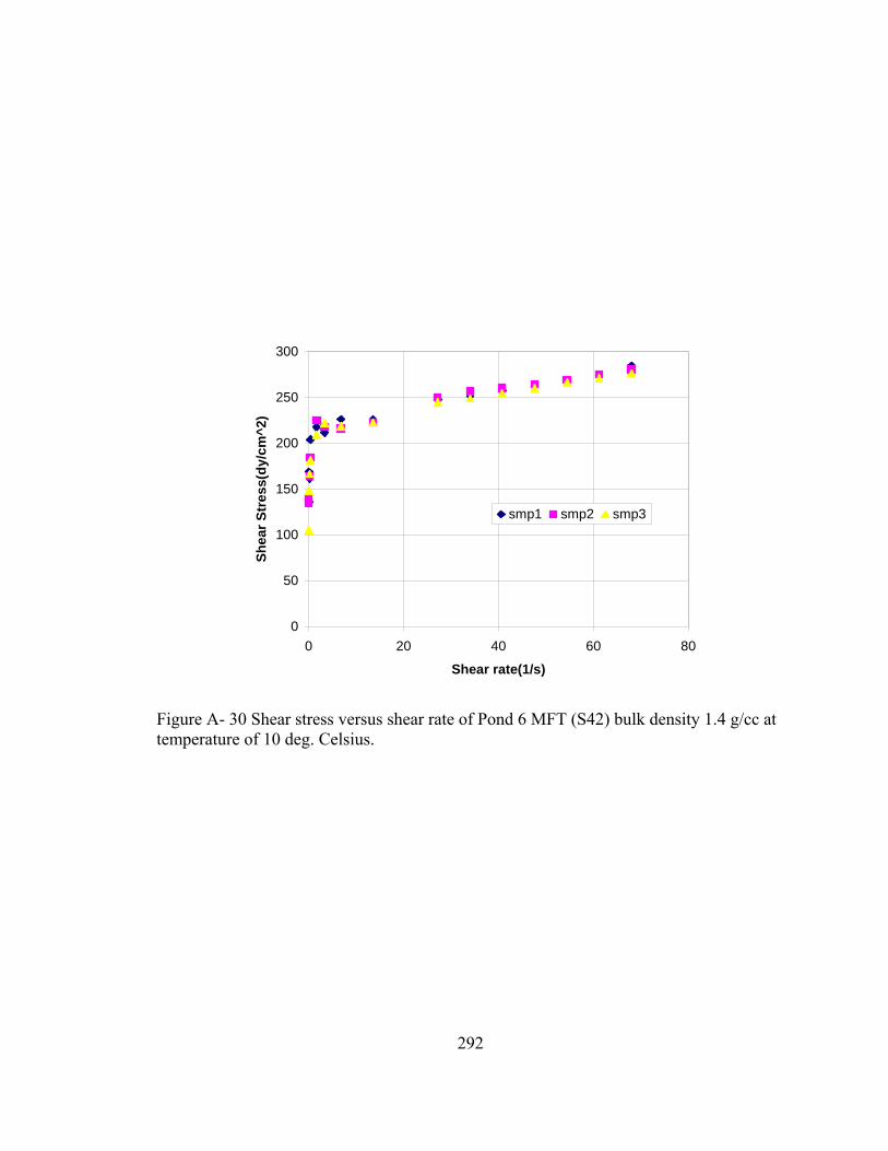
292

0

50

100

150

200

250

300

0 20 40 60 80

Shear rate(1/s)

Shea

r Str

ess(

dy/c

m^2

)

smp1 smp2 smp3


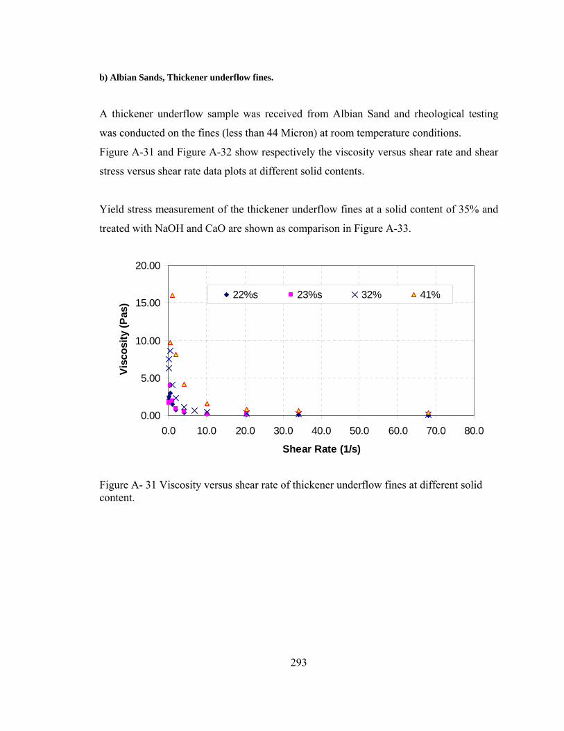
293

b) Albian Sands, Thickener underflow fines.

A thickener underflow sample was received from Albian Sand and rheological testing

was conducted on the fines (less than 44 Micron) at room temperature conditions.

Figure A-31 and Figure A-32 show respectively the viscosity versus shear rate and shear

stress versus shear rate data plots at different solid contents.

Yield stress measurement of the thickener underflow fines at a solid content of 35% and

treated with NaOH and CaO are shown as comparison in Figure A-33.

0.00

5.00

10.00

15.00

20.00

0.0 10.0 20.0 30.0 40.0 50.0 60.0 70.0 80.0

Shear Rate (1/s)

Visc

osity

(Pas

)

22%s 23%s 32% 41%

Figure A- 31 Viscosity versus shear rate of thickener underflow fines at different solid content.

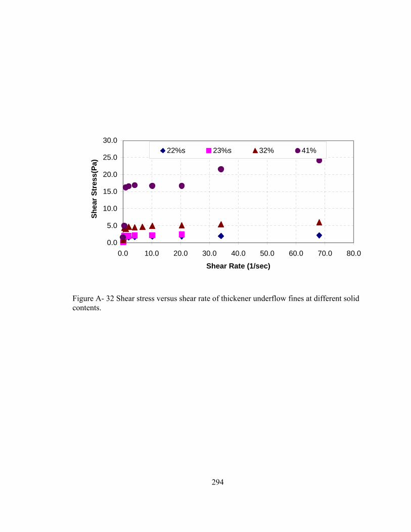
294

0.0

5.0

10.0

15.0

20.0

25.0

30.0

0.0 10.0 20.0 30.0 40.0 50.0 60.0 70.0 80.0

Shear Rate (1/sec)

Shea

r Str

ess(

Pa)

22%s 23%s 32% 41%

Figure A- 32 Shear stress versus shear rate of thickener underflow fines at different solid contents.

295

0

1

2

3

4

5

6

7

0 100 200 300 400 500 600 700

Time(s)

Shea

r Stre

ss(P

a)

Ca(OH)2NaOH

Figure A- 33 Yield stress measurement of thickener underflow fines at solid content of 35% and pH of 12 achieved by Ca(OH)2 and NAOH additions.

296

APPPENDIX B

297

Equation derivation for settling of sphere in a fluid with yield stress

Figure B-1 Free body diagram of a sphere of radius R suspended in a fluid

Integration of the tangential force over the surface gives:

( )2

2

0 0

sin sintF R d dπ π

τ θ θ θ φ= ∫ ∫

22 2

0 0

sinR d dπ π

τ θ θ φ= ∫ ∫

2

0

1 cos 222

R dπ θπτ θ−

= ∫

= 2 2Rπ τ (B.1) Or in terms of the yield stress τy

= 2 2y Rπ τ (B.2)

The buoyant weight of the sphere is given as

θ

φ

y

x

z

Ft

(ρs-ρ)g

298

= 34 ( )3 sR gπ ρ ρ− (B.3)

Where ρs is the density of the sphere and ρ is the density of the fluid. Equating Equation (B.2) to Equation (B.3) results in:

34 ( )

y

s

Rg

τπρ ρ

=−

(B.4)

Or in terms of Diameter

( )32

y

s

Dτπ

ρ ρ=

− (B.5)

Equation (B.5) is the same as Equation 4.6 in Chapter 4.

Dedegil (1986) examined Equation (B.5) with data of Valentik and Whitmore (1965)

from experiment on settling of spheres in Bingham fluids. The relationship between drag

coefficient (CD) and Reynolds number (Re) from the same data are shown in Figure B-2

without taking yield stress into account and in Figure B-3 by taking the yield stress into

account.

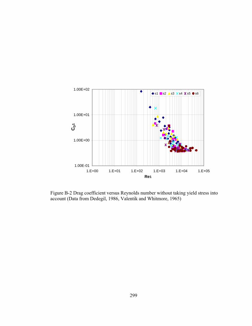
299

1.00E-01

1.00E+00

1.00E+01

1.00E+02

1.E+00 1.E+01 1.E+02 1.E+03 1.E+04 1.E+05Re1

CD

1

s1 s2 s3 s4 s5 s6

Figure B-2 Drag coefficient versus Reynolds number without taking yield stress into account (Data from Dedegil, 1986, Valentik and Whitmore, 1965)

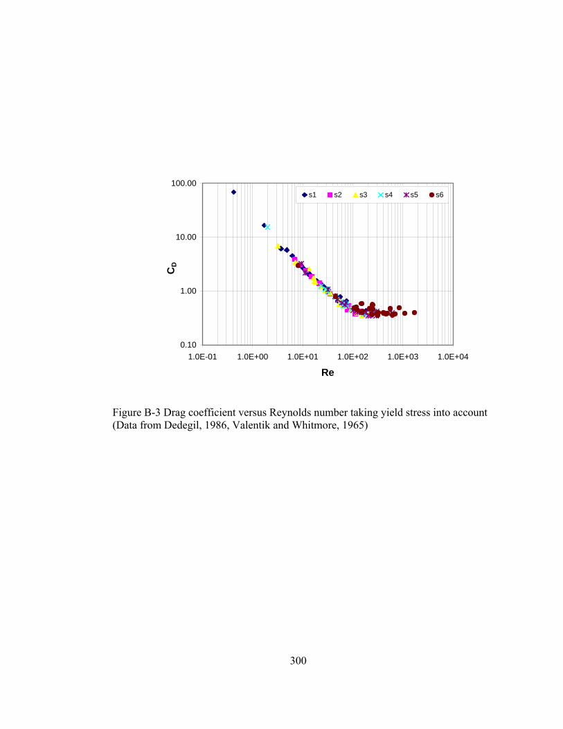
300

0.10

1.00

10.00

100.00

1.0E-01 1.0E+00 1.0E+01 1.0E+02 1.0E+03 1.0E+04

Re

CD

s1 s2 s3 s4 s5 s6

Figure B-3 Drag coefficient versus Reynolds number taking yield stress into account (Data from Dedegil, 1986, Valentik and Whitmore, 1965)

301

APPENDIX C

302

C.1. Effect of Mixing on Segregation

The objective of the testing program is to examine the effect of initial turbulent mixing on

static (standpipe) segregation on relatively non-segregating slurries. For this testing, three

test schedules as shown in Table C-1 were made. The test was to investigate the effect of

thorough mixing of slurry at different mixing duration followed by standpipe test.

C.2. Procedure

The slurry is initially mixed to a desired solid content and sand fine ratio in a 5 litre pail

manually using spatula until homogeneity was achieved and then the mixed slurry was

transferred to a 1 litre beaker, which was part of the Philadelphia Mixer. The mixer speed

was controlled by computer. For a given speed a measured torque was recorded by

manufacturer-installed software in the controlling computer. The shaft was rotating at

constant speed for a specified period of mixing; the slurry is then transferred to a

standpipe and allowed to settle until the sedimentation process is near completion.

Different mixing times were adopted to see the effect of duration of mixing. On the other

hand, a separate standpipe test was conducted on the similar slurry sample with no

mixing to serve as a reference.

Figure C-1 to Figure C-3 show the Scan Electron Microscopy (SEM) image of sand

particles at different sizes ranges as retained on certain sieves from grain size analysis.

The speed of the impeller was set at 1080 rpm for all tests. And only mixing time was

varied on a sample with same solid content and sand fine ratios.

The following table shows the sample used in the testing.

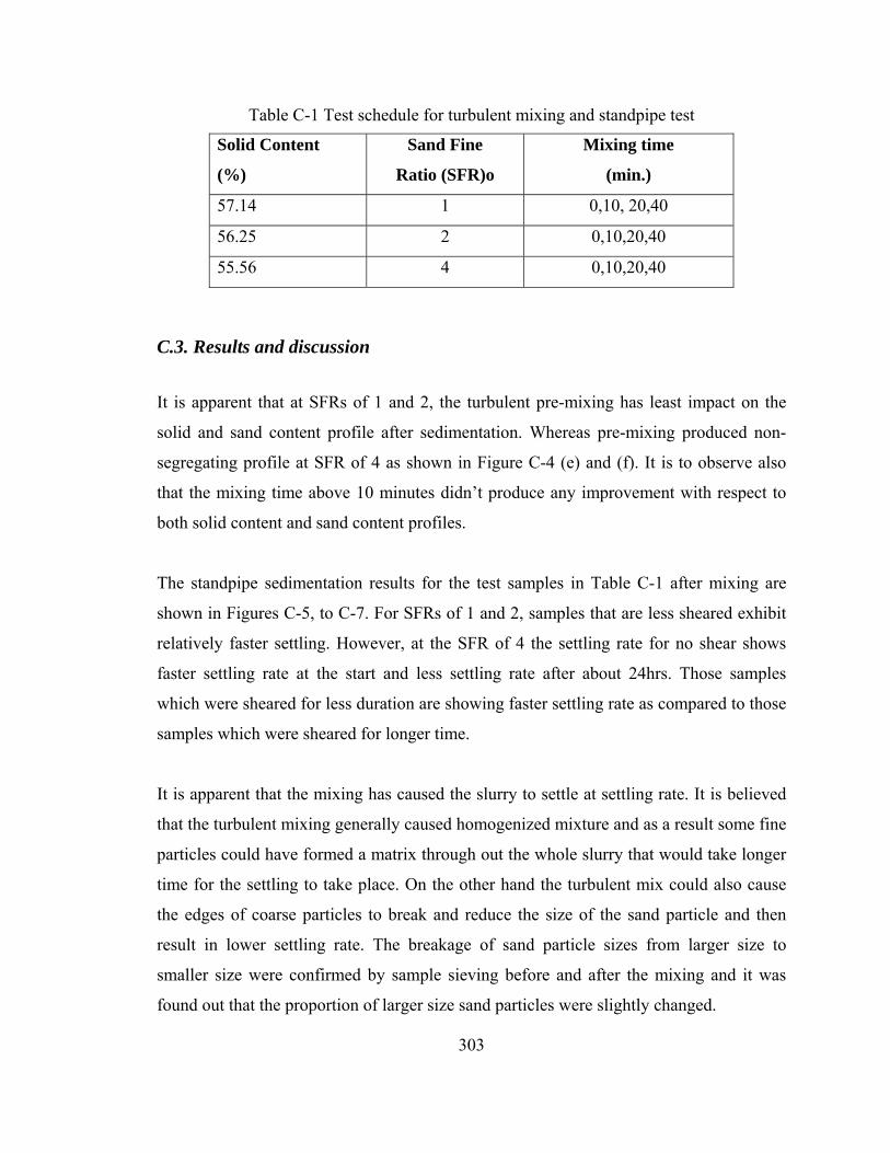
303

Table C-1 Test schedule for turbulent mixing and standpipe test

Solid Content

(%)

Sand Fine

Ratio (SFR)o

Mixing time

(min.)

57.14 1 0,10, 20,40

56.25 2 0,10,20,40

55.56 4 0,10,20,40

C.3. Results and discussion

It is apparent that at SFRs of 1 and 2, the turbulent pre-mixing has least impact on the

solid and sand content profile after sedimentation. Whereas pre-mixing produced non-

segregating profile at SFR of 4 as shown in Figure C-4 (e) and (f). It is to observe also

that the mixing time above 10 minutes didn’t produce any improvement with respect to

both solid content and sand content profiles.

The standpipe sedimentation results for the test samples in Table C-1 after mixing are

shown in Figures C-5, to C-7. For SFRs of 1 and 2, samples that are less sheared exhibit

relatively faster settling. However, at the SFR of 4 the settling rate for no shear shows

faster settling rate at the start and less settling rate after about 24hrs. Those samples

which were sheared for less duration are showing faster settling rate as compared to those

samples which were sheared for longer time.

It is apparent that the mixing has caused the slurry to settle at settling rate. It is believed

that the turbulent mixing generally caused homogenized mixture and as a result some fine

particles could have formed a matrix through out the whole slurry that would take longer

time for the settling to take place. On the other hand the turbulent mix could also cause

the edges of coarse particles to break and reduce the size of the sand particle and then

result in lower settling rate. The breakage of sand particle sizes from larger size to

smaller size were confirmed by sample sieving before and after the mixing and it was

found out that the proportion of larger size sand particles were slightly changed.

304

C.4. Summary and conclusion

Non-segregating slurry samples at different SFRs show no segregating trend when they

are turbulently mixed at different duration. The mixing generally produces improved non-

segregating profiles as compared to no mixing cases. It was found out from sedimentation

tests that turbulent mixing produce a slow water release rate as compared to static tests.

However, as the SFR increase such the above conclusion may not be concurred.

The effect of turbulent mixing is a combination of the following:(i) homogenizing the

slurry to a better non-segregating one (ii) breakage of large size sand grains into smaller

sizes and further assist in homogenizing.

305

Figure C-1 SEM image of sand particles passing 250micron sieve and retained in 125 mm sieve

306

Figure C-2 SEM image of sand particles passing 425 micron sieve and retained in 250micron sieve

307

Figure C-3 SEM image of sand particles passing 2 mm sieve and retained in 425 mm sieve

308

(a)

0

0.2

0.4

0.6

0.8

1

1.2

10 30 50 70

Solid Content (%)

H/H

fNo Shear10min shear20min shear40min shear

(b)

0

0.2

0.4

0.6

0.8

1

1.2

10 20 30 40

Sand Content (%)

H/H

f

No Shear

10min shear

20min shear

40min shear

(c)

0.0

0.2

0.4

0.6

0.8

1.0

1.2

10 30 50 70 90

Solid Content (%)

H/H

f

No Shear

10min shear

20min shear

40min shear

(d)

0.0

0.2

0.4

0.6

0.8

1.0

1.2

10 20 30 40 50

Sand Cont ent (%)

No Shear

10min shear

20min shear

40min shear

(e)

0.0

0.2

0.4

0.6

0.8

1.0

1.2

10 30 50 70 90

Solid Content (%)

H/H

f

No Shear10min shear20min shear40min shear

(f)

0.0

0.2

0.4

0.6

0.8

1.0

1.2

10 30 50 70 90

Sand Content (%)

H/H

f

No Shear10min shear20min shear40min shear

Figure C-4 Solid and Sand Content Profiles; (a) and (b) for DS1, (c) and (d) for DS2, (e)

309

and (f) for DS3

0.40.50.60.70.80.9

1

0 2000 4000 6000 8000 10000 12000

Time(sec)

H/H

f

No Shear 10min shear 20min shear 40min shear

Figure C-5 Sedimentation of sample for test sets DS1 after mixing

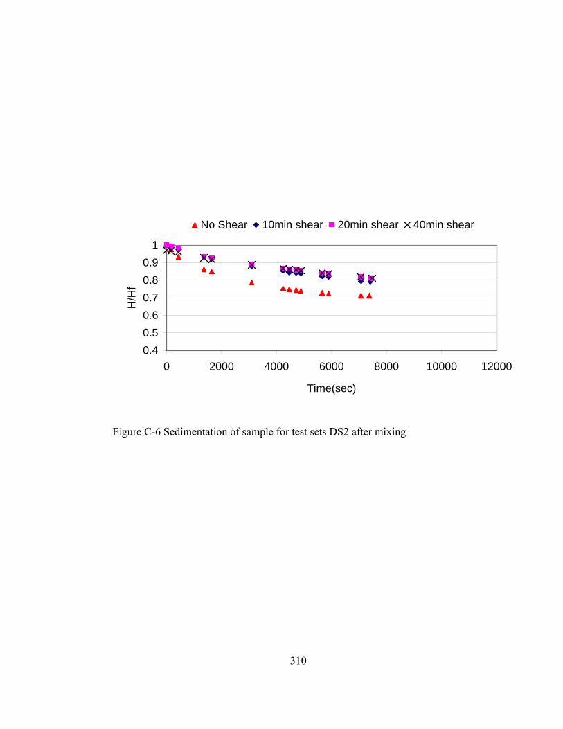
310

0.40.50.60.70.80.9

1

0 2000 4000 6000 8000 10000 12000

Time(sec)

H/H

f


Figure C-6 Sedimentation of sample for test sets DS2 after mixing

311

0.4

0.5

0.6

0.7

0.8

0.9

1

0 1000 2000 3000 4000 5000 6000 7000

Time(sec)

H/H

f


Figure C-7 Sedimentation of samples for test sets DS3 after mixing

312

Appendix D

313

Segregation Index Calculation

The proposed Segregation Index calculation in Chapter 7 is:

( )2

2 i ii i

i

i

h Sh S

hSI

h

⎛ ⎞⎜ ⎟−⎜ ⎟⎝ ⎠=

∑∑ ∑∑

(7.10)

Equation 7.10 may also be expressed as:

( )2

i i avg

i

H S SSI

H−

=∑

∑ (7.10 a)

Both Equation 7.10 and Equation 7.10.a can be worked out in a spreadsheet and similar

results will serve as a check.

The following spreadsheet example illustrates the calculation of SI for sand content

profile shown in Figure 4-4.

Table D.2 provides summary of SI calculation for flume segregation test in Chapter 5.

The Hi in this case refers to the sectional length of the flume from which sample was

taken.

314

Table D-1 Segregation index calculation for testing at 15 sec

Si Hi SiHi SiHi2 Hi(Si-Savg)2

7.619912 10 76.19912 580.6307 5802.338 15.9997 10 159.997 2559.904 2467.493 25.37764 10 253.7764 6440.248 400.7284 27.02631 10 270.2631 7304.213 219.1783 82.51621 10 825.1621 68089.25 25814.79

Sum 50 1585.398 84974.25 34704.53

Savg 31.70796

SI1 = 26.3456 SI2 = 26.3456 Check

Table D-2 Flume test Segregation Index (SI) calculations

Solid Content(%w)

Flume Slope (degree)

SFR SI

57.6 0 1 0.5 57.6 5 1 0.5 57.6 10 1 1.0 57.9 0 2 1.2 57.9 5 2 1.8 57.9 10 2 3.6 55.5 0 4 3.7 55.5 5 4 3.2 55.5 10 4 5.5

315

Statistical Comparisons of Model fits

The following procedure was modified from (Motulsky and Christopoulos 2003).

1. Fit the one of the models using non-linear regression.

2. Look at the results non-linear regression and write down the sum-of-squares (SS)

3. Define N to be the number of data points. Be sure to account for replicates

properly.

4. Define K to be the number of parameters fit by non-linear regression plus 1.

Donot count parameters that are constrained to constant values. If in doubt, count

the number of distinct Standard Error (SE) reported by non-linear regression, then

add 1 to get the value of K.

5. Compute AICc

2 ( 1)ln 21c

SS K KAIC N KN N K

+⎛ ⎞= ⋅ + +⎜ ⎟ − −⎝ ⎠

6. Repeat steps 1-5 with the other model

7. The model with lower AICc is more likely to be correct

8. Calculate the evidence ratio from the difference in AICc scores

0.51.

cAICEvidence Ratioe− Δ=

Table D-3 presents the summary of AICc computation for kao-slurry at 40% solids using

Excel spread sheet. And Table D-4 presents the summary of AICc computation for kao-

sil slurry at 50% solids.

In summary ,the AICc value is lower for Casson model in both tables, indicating that

Casson’s model represent the data better that Hershel-Bulkley (H-B) model.

316

Table D- 3 AICc Calculation for 40% kao slurry

Shear Rate (1/s) SS (Pa)

HB Model Casson's Model SS(H-B) SS(Casson)

4.08 12.49 15.91 14.47 11.682 3.902 10.2 17.42 17.36 15.91 0.003 2.293 20.4 18.27 18.77 17.61 0.252 0.434 34 20.4 20.02 19.39 0.142 1.017

40.8 20.91 20.52 20.17 0.152 0.546 54.4 21.85 21.36 21.59 0.236 0.066 61.2 22.19 21.73 22.25 0.210 0.004 68 20.91 22.07 22.89 1.352 3.906

SUM 14.028 12.168 N 8 SE 1.777 0.544 0.431

K 1.544 1.431

AIC 7.581 6.216 AICc 9.022 7.465 Lower AICc

Evidence Ratio 0.211

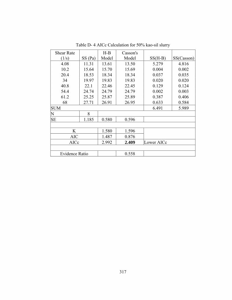
317

Table D- 4 AICc Calculation for 50% kao-sil slurry

Shear Rate (1/s) SS (Pa)

H-B Model

Casson's Model SS(H-B) SS(Casson)

4.08 11.31 13.61 13.50 5.279 4.816 10.2 15.64 15.70 15.69 0.004 0.002 20.4 18.53 18.34 18.34 0.037 0.035 34 19.97 19.83 19.83 0.020 0.020

40.8 22.1 22.46 22.45 0.129 0.124 54.4 24.74 24.79 24.79 0.002 0.003 61.2 25.25 25.87 25.89 0.387 0.406 68 27.71 26.91 26.95 0.633 0.584

SUM 6.491 5.989 N 8 SE 1.185 0.580 0.596

K 1.580 1.596

AIC 1.487 0.876 AICc 2.992 2.409 Lower AICc

Evidence Ratio 0.558

University of Alberta...determine concentration profiles during the sedimentation processes....

Documents

Transcript of University of Alberta...determine concentration profiles during the sedimentation processes....