University Calculus Supplement TI-89
65
1 A Calculator Supplement for Calculus University Calculus: Elements with Early Transcendentals (WMU edition) Regular Section Edition, TI-89 version Dennis Pence Western Michigan University Table of Contents Chapter 0 – An Overview of the TI-89 (TI-92, Voyage 200) §1. Settings, Layout, Operating Systems, Desktop §2. Home Screen Operations §3. Functions, Tables, and Gr aphs §4. Entering Data, Performing a Regression §5. Solving Equations §6. Programming §7. Saving Your Work in a Text Fil e §8. Units §9. Connecting to a Computer, Ot her Applications Chapter 1 –Functions and Limits §1. Entering and Storing Functions §2. Composition of Functions and Inverse Functions §3. Trigonometric Functions §4. Average Rate of Change §5. Using Tables to Investigate Limits §6. Symbolic Limits Chapter 2 – Differentiation §1. The Derivative Definition §2. Graphical Derivatives §3. Numerical Derivatives §4. Exploring Differenti ation Rules wit h the Calc ulator §5. Implicit Functions and Plotting §6. Implicit Differentiation §7. Taylor Polynomials Chapter 3 – Applications of Derivatives §1. Zooming to See Asymptotes §2. Points of Inflection §3. Maxima and Minima §4. Parameterization of Plane §5. Newton’s Method Chapter 4 – Integration §1. Two Notat ions for Antiderivatives §2. Riemann Sums and the Sigma Notation §3. Symbolic Integrals
-
Upload
andreazevedorj -
Category
Documents
-
view
221 -
download
0
Transcript of University Calculus Supplement TI-89

8/3/2019 University Calculus Supplement TI-89
http://slidepdf.com/reader/full/university-calculus-supplement-ti-89 1/65
1
A Calculator Supplement for CalculusUniversity Calculus: Elements with Early Transcendentals (WMU edition)
Regular Section Edition, TI-89 version
Dennis Pence
Western Michigan University
Table of Contents
Chapter 0 – An Overview of the TI-89 (TI-92, Voyage 200)§1. Settings, Layout, Operating Systems, Desktop§2. Home Screen Operations§3. Functions, Tables, and Graphs§4. Entering Data, Performing a Regression
§5. Solving Equations§6. Programming§7. Saving Your Work in a Text File§8. Units§9. Connecting to a Computer, Other Applications
Chapter 1 –Functions and Limits§1. Entering and Storing Functions§2. Composition of Functions and Inverse Functions§3. Trigonometric Functions§4. Average Rate of Change§5. Using Tables to Investigate Limits
§6. Symbolic LimitsChapter 2 – Differentiation
§1. The Derivative Definition§2. Graphical Derivatives§3. Numerical Derivatives§4. Exploring Differentiation Rules with the Calculator§5. Implicit Functions and Plotting§6. Implicit Differentiation§7. Taylor Polynomials
Chapter 3 – Applications of Derivatives§1. Zooming to See Asymptotes
§2. Points of Inflection§3. Maxima and Minima§4. Parameterization of Plane§5. Newton’s Method
Chapter 4 – Integration§1. Two Notations for Antiderivatives§2. Riemann Sums and the Sigma Notation§3. Symbolic Integrals
8/3/2019 University Calculus Supplement TI-89
http://slidepdf.com/reader/full/university-calculus-supplement-ti-89 2/65
2
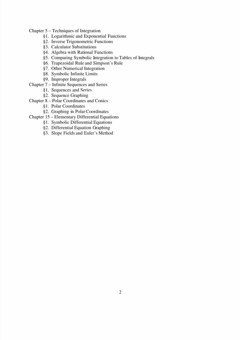
Chapter 5 – Techniques of Integration§1. Logarithmic and Exponential Functions§2. Inverse Trigonometric Functions§3. Calculator Substitutions§4. Algebra with Rational Functions
§5. Comparing Symbolic Integration to Tables of Integrals§6. Trapezoidal Rule and Simpson’s Rule§7. Other Numerical Integration§8. Symbolic Infinite Limits§9. Improper Integrals
Chapter 7 – Infinite Sequences and Series§1. Sequences and Series§2. Sequence Graphing
Chapter 8 – Polar Coordinates and Conics§1. Polar Coordinates§2. Graphing in Polar Coordinates
Chapter 15 – Elementary Differential Equations§1. Symbolic Differential Equations§2. Differential Equation Graphing§3. Slope Fields and Euler’s Method

8/3/2019 University Calculus Supplement TI-89
http://slidepdf.com/reader/full/university-calculus-supplement-ti-89 3/65
3
Chapter 0
Overview of the TI-89 (TI-92 Plus, Voyage 200)
This chapter provides a brief introduction to some of the features of this family of
graphing/symbolic calculators that relate to pre-calculus material. For the most part, wedemonstrate with the TI-89 (including the TI-89 Titanium), which is the most common choicefor students at WMU. The TI-92 Plus (no longer made) and the Voyage 200 provide the samecapabilities in a larger-sized model with a QWERTY keyboard. If you have not alreadypurchased your calculator, you might want to consider the Voyage 200. For only about $50more, you get more memory, several cost applications, a larger keyboard and screen, and theGraphLink cable to connect to your computer. The newest TI-89 Titanium also has morememory and included is a USB connection cable to connect to your computer. See the TexasInstruments Calculator web site for the latest information about what is available for this family.http://education.ti.com
1. Settings, Layout, Operating Systems, Desktop
TI-89 Home Screen Applications List Mode Settings
When you press the ON button (lower left), a TI-89 generally comes on in what is called theHOME screen as in the first figure above. You will do immediate computations in the commandline at the bottom of the screen. Results will appear in the middle region, which is called the“history” area, and many commands can be obtained by pressing one of the function keys F1-F8,which are blue keys below the screen. The different “screens” of the calculator are calledapplications. Press the blue APPS key to bring up the list of applications as in the second figureabove. Note that additional applications can be loaded into the calculator, and they will appearunder the heading 1:FlashApps. Press the MODE key to bring up the first page (of three) of various settings for the calculator.
TI-89 and Voyage 200 Desktop Home Screen

8/3/2019 University Calculus Supplement TI-89
http://slidepdf.com/reader/full/university-calculus-supplement-ti-89 4/65
4
A Voyage 200 and the TI-89 Titanium generally come on with an icon desktop displaying theapplications. This can be turned off in a page 3 mode setting, but it includes a possible clock inthe corner which is nice. Press ENTER with an icon highlighted to move to that application. Asyou see in the figure above, the Voyage 200 comes with some additional flash applications (mostof which can be added to a TI-89). The APPS key brings you back to the icon desktop.
You adjust the contrast of the screen by holding the green “diamond” key and pressing the “+”
key to darken and the “−” key to lighten. If you need to keep increasing the contrast, this is asign that your battery is low. A low battery signal will also come on as a warning and certainlinking operations will not be allowed when the battery is low.
This family of calculators uses flash ROM, enabling all of the code in the calculator to beupgraded. Texas Instruments calls the software running the calculator the operating system orOS. You can check at the TI web site (http://education.ti.com) for the newest OS version and fornew applications available for downloading. You will need a computer and the GraphLink cable(or the TI-89 USB cable) to download new things from the web site. You can also get a new OS
and free applications from another calculator (of the same model). Press F1 A: About to seewhat version you have.
See http://education.ti.com and look for DOWNLOADS to find the latest OS for you calculator.A new OS might fix bugs that have been discovered, add new commands, and help to makesome of the new applications possible. You can also find the various applications mentioned inthis document at that location as well.
The ESC key is very important for escaping out of some situation. If you pull up a menu anddecide not to select anything, press ESC to back out of the menu (or submenu). In manysituations, the display will give you the option to ENTER to save or confirm and ESC to cancelout of that process. For example, none of the changes you make in the MODE pages take effectuntil you press ENTER=save, with ESC=cancel as an option.

8/3/2019 University Calculus Supplement TI-89
http://slidepdf.com/reader/full/university-calculus-supplement-ti-89 5/65
5
2. Home Screen Operations
ENTER in AUTO ♦ENTER in AUTO
The default Exact/Approx mode setting is AUTO, and this allows many computations to be doneexactly. The command F1 8:Clear Home erases the “history” area. When you want a decimalapproximation in this mode setting, just press the “green diamond” key before the ENTER key to
get “APPROX ≈”, rather than changing the mode setting.
Notice below the command line some of the mode settings are displayed. In the figures above,the MAIN indicates we are in the main folder, RAD indicates radian angle mode, AUTOindicates the exact/approx mode, FUNC indicates function graphing is selected, and the 3/30 inthe first two figures indicates that the history contains 3 items out of the 30 that will beremembered (with more or less possible as a format setting).
Variable names can be up to 8 characters long and must begin with a letter. Usually we usesingle letter names for true variables in our algebraic expressions, and we use longer names forprograms and other things we wish to keep. The F6 2:New Problem command is a very niceway to start fresh. It clears the history, clears out all variables named by a single letter (as doesF6 1:Clear a-z…), and deselects all functions and plots in graphing.
Notice in the first figure above, we have used “implied multiplication” when we typed thecoefficients of the polynomial. In the last figure, we needed the multiplication symbol between“a” and “x” and between “b” and “x” because typing “ax” and “bx” would have been interpretedas new variable names.

8/3/2019 University Calculus Supplement TI-89
http://slidepdf.com/reader/full/university-calculus-supplement-ti-89 6/65
6
You notice that after you press ENTER, the last command stays in the command line, but it is allhighlighted. If you simply start typing, the new typing replaces the highlighted expression. If,instead, you want to edit the last line, press the left or right cursor keys to move the insertionpoint to that end and remove the highlighting. Then you can edit the expression. The “back
arrow” ← key is a destructive backspace command. Above that key, the command “green
diamond” DEL above the back arrow is a destructive forward movement. By default, any typingthat you do is inserted where the blinking vertical bar appears in the command line. Pressing 2nd
INS above the back arrow is a toggle converting between the insert entry mode and the typeoverentry mode (blinking space).
After entering a command (as in the first figure above), you can simply press “+” to do acontinuation calculation. If you press any command requiring an argument before the command(like “+”), the calculator assumes you wish to use the last answer. In the second figure, we see ithas added “ans(1)” in front of the “+” that we typed to indicate this. When you want the lastanswer (and any one stored in the history) somewhere else in the command line, use ANS (abovethe negation key). Just edit “ans(1)” to have another number if you want to go back more thanone answer.
When you use the up cursor, you move up into the history area and highlight results (on theright) and command lines (on the left by a ). You sometimes must do this to scroll sideways toread all of a long result. Pressing ENTER while something in the history is highlighted causes itto be pasted into the command line as figure one and two above. Thus you should never need toretype anything you can see!! While the cursor is anywhere in the history area, you can pressESC to jump down to the command line without pasting anything there.
Holding the “up arrow” ↑ key and then cursoring in the command line allows you to selectivelyhighlight a part of the command line. Under F1 Tools, you will find that you have Cut, Copy,and Paste much like on a computer.
8/3/2019 University Calculus Supplement TI-89
http://slidepdf.com/reader/full/university-calculus-supplement-ti-89 7/65
7
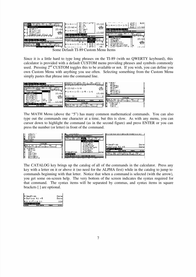
Some Default TI-89 Custom Menu Items
Since it is a little hard to type long phrases on the TI-89 (with no QWERTY keyboard), thiscalculator is provided with a default CUSTOM menu providing phrases and symbols commonlyused. Pressing 2nd CUSTOM toggles this to be available or not. If you wish, you can define youown Custom Menu with anything you use often. Selecting something from the Custom Menusimply pastes that phrase into the command line.
The MATH Menu (above the “5”) has many common mathematical commands. You can alsotype out the commands one character at a time, but this is slow. As with any menu, you cancursor down to highlight the command (as in the second figure) and press ENTER or you canpress the number (or letter) in front of the command.
The CATALOG key brings up the catalog of all of the commands in the calculator. Press anykey with a letter on it or above it (no need for the ALPHA first) while in the catalog to jump tocommands beginning with that letter. Notice that when a command is selected (with the arrow),you get some on-screen help. The very bottom of the screen indicates the syntax required forthat command. The syntax items will be separated by commas, and syntax items in squarebrackets [ ] are optional.

8/3/2019 University Calculus Supplement TI-89
http://slidepdf.com/reader/full/university-calculus-supplement-ti-89 8/65
8
You can store a number in a variable name either with the F4 1:Define command or the STO
key (which appears on the screen only as the arrow →). Then whenever you use that name, thevalue is immediately used. The F4 4:DelVar command is used to delete the definitions for thesevariable names. Note that F6 1:Clear a-z… and 2:NewProblem will not clear these longervariable names. Suggestion: Never store a number in the variables x, y, z, or t because we oftenuse these letters for algebra variables. There is too great a chance you will forget to delete thembefore you want to use them as an undefined variable.
Alternatives to “storing a number in x” are better. The “with” command is a vertical bar | key,and it allows a value to be substituted in for a variable temporarily without permanently storingthat value in the variable name. When we define a function, then we can simply evaluate thefunction without storing anything permanently in the variable name.
3. Functions, Tables, and Graphs
FUNCTION graphing Y= Editor Home
A formula entered into the Y= Editor (which you can get to via APPS 2:Y= Editor or via “greendiamond” F1) is then available to you in the Home screen.
TblSet Table Table (scrolled down)
8/3/2019 University Calculus Supplement TI-89
http://slidepdf.com/reader/full/university-calculus-supplement-ti-89 9/65
9
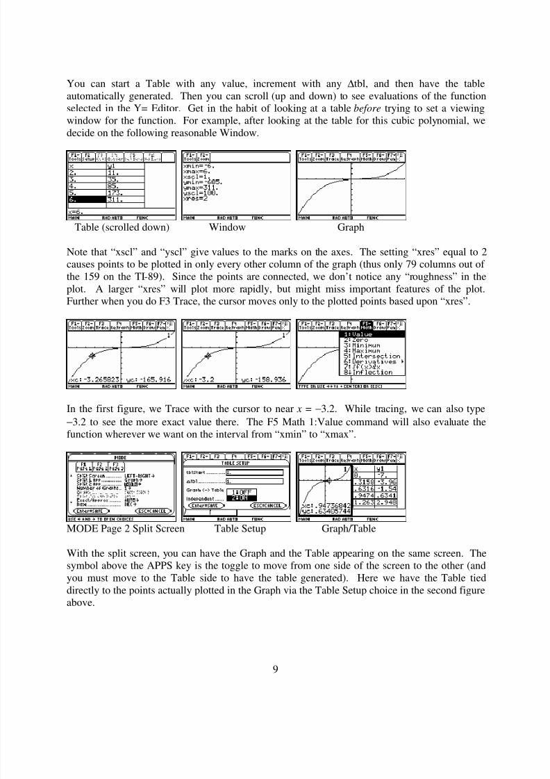
You can start a Table with any value, increment with any ∆tbl, and then have the tableautomatically generated. Then you can scroll (up and down) to see evaluations of the functionselected in the Y= Editor. Get in the habit of looking at a table before trying to set a viewingwindow for the function. For example, after looking at the table for this cubic polynomial, we
decide on the following reasonable Window.
Table (scrolled down) Window Graph
Note that “xscl” and “yscl” give values to the marks on the axes. The setting “xres” equal to 2causes points to be plotted in only every other column of the graph (thus only 79 columns out of
the 159 on the TI-89). Since the points are connected, we don’t notice any “roughness” in theplot. A larger “xres” will plot more rapidly, but might miss important features of the plot.Further when you do F3 Trace, the cursor moves only to the plotted points based upon “xres”.
In the first figure, we Trace with the cursor to near x = −3.2. While tracing, we can also type−3.2 to see the more exact value there. The F5 Math 1:Value command will also evaluate thefunction wherever we want on the interval from “xmin” to “xmax”.
MODE Page 2 Split Screen Table Setup Graph/Table
With the split screen, you can have the Graph and the Table appearing on the same screen. Thesymbol above the APPS key is the toggle to move from one side of the screen to the other (andyou must move to the Table side to have the table generated). Here we have the Table tieddirectly to the points actually plotted in the Graph via the Table Setup choice in the second figureabove.

8/3/2019 University Calculus Supplement TI-89
http://slidepdf.com/reader/full/university-calculus-supplement-ti-89 10/65
10
Functions can be defined in the Home screen, but we can only graph a formula appearing in oneof the function slots of the Y= Editor. (You can define a function with one of these function slotvariable names in the Home screen.) When more than one functions is selected, we may want to
change the F6 Style to be able to tell them apart. In the Y= Editor, F4 will change whether afunction slot is selected or not.
Notice that the default Line Style and “xres = 2” do not do such a great job plotting the tangentfunction. Generally we wish to avoid the false “near vertical” lines near vertical asymptotes.The Dot Style avoids this. [For OS 3.0 or higher, you can turn on the GRAPH FORMAT“Discontinuity Dection ON” to avoid these false vertical lines.]
8/3/2019 University Calculus Supplement TI-89
http://slidepdf.com/reader/full/university-calculus-supplement-ti-89 11/65
11
The “when” command gives us a way to do piecewise-defined functions, if there are not toomany pieces. The Dot Style is also usually best for such piecewise-defined functions, whichmay not be continuous between the pieces.
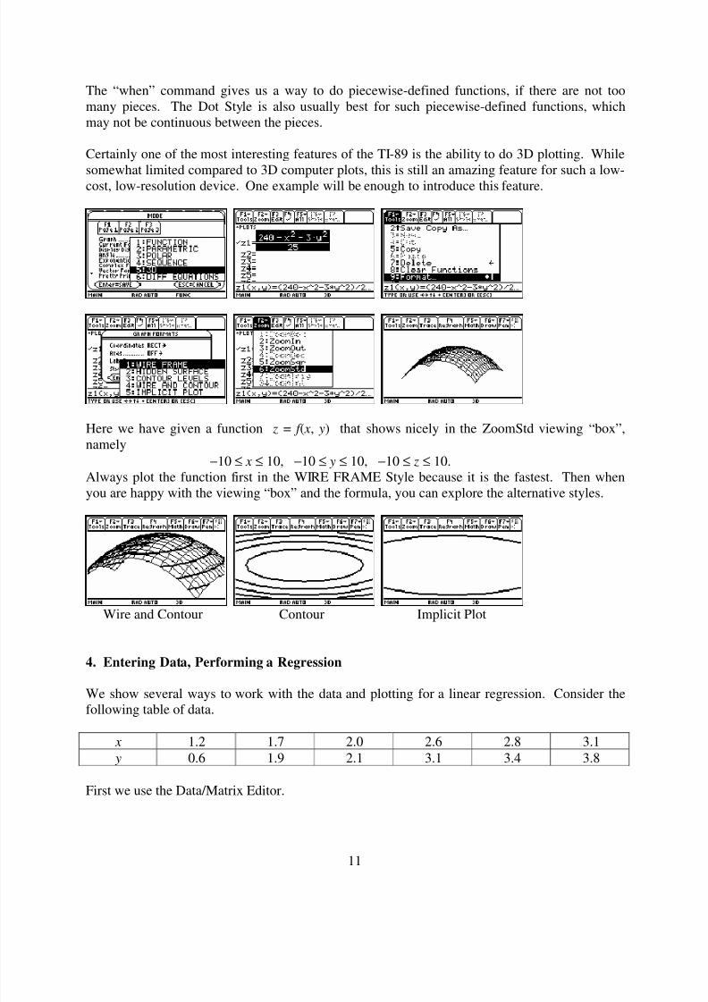
Certainly one of the most interesting features of the TI-89 is the ability to do 3D plotting. While
somewhat limited compared to 3D computer plots, this is still an amazing feature for such a low-cost, low-resolution device. One example will be enough to introduce this feature.
Here we have given a function z = f ( x, y) that shows nicely in the ZoomStd viewing “box”,namely
−10 ≤ x ≤ 10, −10 ≤ y ≤ 10, −10 ≤ z ≤ 10.Always plot the function first in the WIRE FRAME Style because it is the fastest. Then whenyou are happy with the viewing “box” and the formula, you can explore the alternative styles.
Wire and Contour Contour Implicit Plot
4. Entering Data, Performing a Regression
We show several ways to work with the data and plotting for a linear regression. Consider thefollowing table of data.
x 1.2 1.7 2.0 2.6 2.8 3.1
y 0.6 1.9 2.1 3.1 3.4 3.8
First we use the Data/Matrix Editor.

8/3/2019 University Calculus Supplement TI-89
http://slidepdf.com/reader/full/university-calculus-supplement-ti-89 12/65
12
F2 Plot Setup F1 Define
ENTER, then ESC Y= F2 9:ZoomData
It takes all of this to get the scatter plot of the data. Notice that performing ZoomData after thePlot 1 has been defined gives a nice viewing window for the plot (we are back in Functiongraphing).
Return to current data F5 Calculate
Current Stat Vars Y= Editor Graph and F3 Trace
Above we see the steps to calculate the linear regression, store the formula in slot y1(x), and thenlook at the graph with both the scatter plot and the regression line. Most people found thisstatistical process a little cumbersome compared to the more advanced statistics on the TI-83. TIhas also offered a free flash application called the Statistics List Editor with all of the power and

8/3/2019 University Calculus Supplement TI-89
http://slidepdf.com/reader/full/university-calculus-supplement-ti-89 13/65
13
ease of use of the TI-83 (and even additional statistical commands). Most new TI-89’s comewith this flash application loaded, and anyone can download it from the web site.
APPS 1:FlashApps Type data in lists
Statistics, including linear regression, can also be done in the CellSheet flash application, whichgives a mini-spreadsheet for this family of calculators. The CellSheet costs extra for the TI-89but comes loaded in a Voyage 200.
5. Solving Equations
We can solve some equations exactly with the symbolic command F2 1:solve( in the Homescreen. We can also solve equations numerically in the Numeric Solver application. We canalso graph both side of an equation, and seek an intersection point. We demonstrate an exampleof each method.
8/3/2019 University Calculus Supplement TI-89
http://slidepdf.com/reader/full/university-calculus-supplement-ti-89 14/65
14
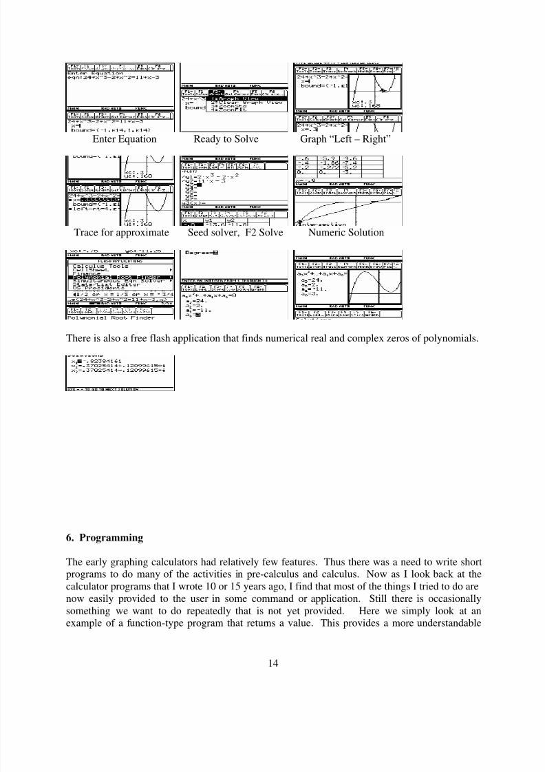
Enter Equation Ready to Solve Graph “Left – Right”
Trace for approximate Seed solver, F2 Solve Numeric Solution
There is also a free flash application that finds numerical real and complex zeros of polynomials.
6. Programming
The early graphing calculators had relatively few features. Thus there was a need to write shortprograms to do many of the activities in pre-calculus and calculus. Now as I look back at thecalculator programs that I wrote 10 or 15 years ago, I find that most of the things I tried to do arenow easily provided to the user in some command or application. Still there is occasionallysomething we want to do repeatedly that is not yet provided. Here we simply look at anexample of a function-type program that returns a value. This provides a more understandable
8/3/2019 University Calculus Supplement TI-89
http://slidepdf.com/reader/full/university-calculus-supplement-ti-89 15/65
15
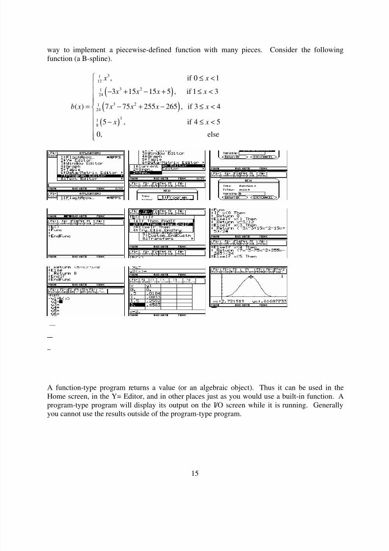
way to implement a piecewise-defined function with many pieces. Consider the followingfunction (a B-spline).
( )( )
( )
3112
3 21
24
3 2124
318
, if 0 1
3 15 15 5 , if 1 3
( ) 7 75 255 265 , if 3 4
5 , if 4 5
0,
x x
x x x x
b x x x x x
x x
≤ <
− + − + ≤ <
= − + − ≤ <
− ≤ <
else
A function-type program returns a value (or an algebraic object). Thus it can be used in theHome screen, in the Y= Editor, and in other places just as you would use a built-in function. Aprogram-type program will display its output on the I/O screen while it is running. Generallyyou cannot use the results outside of the program-type program.

8/3/2019 University Calculus Supplement TI-89
http://slidepdf.com/reader/full/university-calculus-supplement-ti-89 16/65
16
7. Saving Your Work in a Text File
You may do a sequence of command lines in the Home screen that you would like to save forlater use. Perhaps you have not finished, but you need to do something else with the calculatornow. Perhaps the sequence is appropriate to use again and again (somewhat like a program).
We show here how to save the command lines represented in the history.
Give name to text F1 8:ClearHome
Notice that the actual value was inserted wherever we used the ANS key or a continuationcomputation. This text file can be edited, perhaps to put “ans(1)” into these places. With thecursor within some line in the text, press F4 Execute to have that command line (preceded withthe “C:”) executed back in the Home screen. Most of the time, we select under F3 View 1:Scriptview to split the screen vertically so that we can see both the text file and the Home screen result.
8. Units
Calculations for science and engineering always involve units. Mathematics instructors are oftenguilty of ignoring units (really they just assume they are correct). The calculator has severalfeatures that help you work with units and standard constants. First, there is a Page 3 Modesetting for the default unit system. The first two choices are the metric system (SI for SystemInternational) and the English system. Above the “3” key is the Units command to bring up theunits menu. They have tried to give you units in the order most often needed (not alphabetical),so explore what is given.

8/3/2019 University Calculus Supplement TI-89
http://slidepdf.com/reader/full/university-calculus-supplement-ti-89 17/65
17
You type a number and then attach the unit after it. It is easier to get the unit designation fromthe menu. You can also type the symbols, but notice that all unit designations begin with an“underbar”. In the third figure above we have attached miles to 3. The calculator automaticallyconverts the result to the mode-specified unit system, here to meters.
You can also convert from one unit to another in the same category. Simply type the desirednumber, attach the original unit, press the “bold arrow” above the MODE key, and attach thenew unit desired.
If you assign units to objects in an algebraic expression, as in the second figure above, the“solved” variable will be given the appropriate units (in the mode-selected system). For somestrange reason, temperature conversion does not work in the same way. Look in the CATALOGfor the command tmpCnv().
The first line of the units menu gives many common constants from science and engineering.For example “_Gc” is Newton’s universal gravitation constant which in the SI system equals
6.67259E−11 in m3 /(kg-s2).
9. Connecting to a Computer, Other Applications
All TI graphing calculators come with a short cable to connect one calculator to anothercalculator. A GraphLink cable is for connecting the calculator to a computer. Older GraphLink cables (grey and black) plug into the COM port of a PC or the modem port of a Macintosh. Thenewer GraphLink cables (silver) use a USB connection (for both PC’s and Macintoshes). Youwill need such a cable to upgrade the OS or to download new applications. You can also save
8/3/2019 University Calculus Supplement TI-89
http://slidepdf.com/reader/full/university-calculus-supplement-ti-89 18/65
18
your work (text files, programs, functions) on the computer. All of the figures in this documenthave been obtained using the GraphLink connection. The Voyage 200 comes with theGraphLink cable and software. TI-89 users may want to purchase a GraphLink cable (about$20). The newest TI-89 includes a mini USB connection and a cable to connect to the USB portof a computer. The latest computer software for connection with the GraphLink cable can
always be downloaded for free from the TI web site (http://education.ti.com). The Arts andSciences Computing Labs on the third floor of Rood Hall have GraphLink cables for both PC’sand Macintoshes and the required software on the server. On the new engineering campus, theCEAS computer lab has the required software on the server and you may check out a USBGraphLink cable from the desk.
We have already mentioned two flash applications that are free, the Statistics List Editor and thePolynomial Root Finder. Other free flash applications available now for the TI-89 are CalculusTools, Finance, Simultaneous Equation Solver, Symbolic Math Guide, Study Cards, and USPresidents. Cost flash applications include CellSheet (mini spread sheet $15), Equation Writer($15), EE200 (circuit analysis $20), ME*Pro (mechanical engineering $50), EE*Pro (electrical
engineering $50), The Geometer’s Sketchpad ($30), and Cabri Geometry ($30). Some of thesecost applications come preloaded in the Voyage 200. Recently they have added a free Organizer(address/phone and calendar/appointment book) for this family of calculators. Seehttp://education.ti.com in the area for DOWNLOADS for your calculator model to find out whatis available.

8/3/2019 University Calculus Supplement TI-89
http://slidepdf.com/reader/full/university-calculus-supplement-ti-89 19/65
19
Chapter 1
Functions and Limits
Function is a data type in the TI-89. There are many things that we can do with certain
functions. This is loosely coordinated with Chapter 1 of the text University Calculus: Elementswith Early Transcendentals (WMU edition), by Hass, Weir, and Thomas, Pearson CustomPublishing.
1. Entering and Storing Functions
In the Home screen we can store a formula for a function using the Define command or theSTO key. We can use any variable name (up to eight characters beginning with a letter) as thename for the function.
Custom menu items
Notice in the first row of figures that we define a function f ( x), which we can evaluate usingfunction notation. In the second row of figures, we name an expression instead. To evaluate anexpression, use the vertical bar to temporarily assign a value to x. Pressing the VAR-LINKkeystroke brings up a list of all the variables defined, the data type, and the bytes of storagerequired. While a variable in the VAR-LINK list is highlighted, you can press F6 Contents tosee one screen of the definition or program (which is usually enough to remember what you havestored here). If you press ENTER while the name is highlighted, the name will be pasted into thecommand line. If you press the destructive back arrow while the name is highlighted, you can
delete the object from memory.
8/3/2019 University Calculus Supplement TI-89
http://slidepdf.com/reader/full/university-calculus-supplement-ti-89 20/65
20
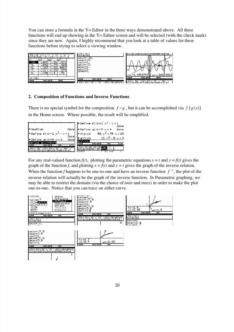
You can store a formula in the Y= Editor in the three ways demonstrated above. All threefunctions will end up showing in the Y= Editor screen and will be selected (with the check mark)since they are new. Again, I highly recommend that you look at a table of values for thesefunctions before trying to select a viewing window.
2. Composition of Functions and Inverse Functions
There is no special symbol for the composition f g , but it can be accomplished via ( )( ) f g x
in the Home screen. Where possible, the result will be simplified.
For any real-valued function f (t ), plotting the parametric equations x = t and y = f (t ) gives thegraph of the function f , and plotting x = f (t ) and y = t gives the graph of the inverse relation.
When the function f happens to be one-to-one and have an inverse function 1 f − , the plot of the
inverse relation will actually be the graph of the inverse function. In Parametric graphing, wemay be able to restrict the domain (via the choice of tmin and tmax) in order to make the plotone-to-one. Notice that you can trace on either curve.

8/3/2019 University Calculus Supplement TI-89
http://slidepdf.com/reader/full/university-calculus-supplement-ti-89 21/65
21
In Function graphing mode, the calculator provides a command to have the inverse relation as a“drawn” object. However “drawn” objects cannot be traced, and they disappear when the graphis re-plotted for any reason. It is also hard to restrict the domain in Function graphing mode.
For very simple functions (little more than linear polynomials), the solve command in the Homescreen can enable us to find the formula for the inverse function.
3. Trigonometric Functions
The calculator provides the trigonometric functions for the sine, cosine, and tangent. It alsoprovides an inverse function for each (on a suitably restricted domain). The other trigonometricfunction can be computed from these, but it might be nice to have them defined permanently. If we use variable names longer than one letter, then the commands in the F6 Clean Up menu likeNewProb will not delete these functions.
ZoomTrig y = cot( x)

8/3/2019 University Calculus Supplement TI-89
http://slidepdf.com/reader/full/university-calculus-supplement-ti-89 22/65
22
ZoomTrig y = sec( x) ZoomTrig y = csc( x)
We can also compute the inverse functions for the cotangent, secant, and cosecant functions interms of the inverse trigonometric functions provided. There is simply a question of the mostdesirable domain and range. For example, if we desire the inverse cotangent, we consider thefollowing algebra.
1 1 1
1cot( )
tan( )
1tan( )
1 1tan implying that cot ( ) tan
y x x
x y
x y y y
− − −
= =
=
= =
Most people do not like this choice of range for the inverse cotangent (and it leaves the problem
of what to do with 1cot (0)− ).
As in many computer languages, we use “acot” as the variable name for the inverse cotangent orarccotangent, and then “asec” and “acsc” for the remaining inverse functions. Make thefollowing definitions to have these functions.
Define acot(y)=when(y<0,tan−−−−1(1/y)+ππππ,when(y>0, tan−−−−1(1/y),ππππ/2))
Define asec(y)= cos−−−−1(1/y)
Define acsc(y)= sin−−−−1(1/y)
When you want to use these functions, you can either type the name or you can get it from yourVAR-LINK list of all of your variables as in the last figure above.

8/3/2019 University Calculus Supplement TI-89
http://slidepdf.com/reader/full/university-calculus-supplement-ti-89 23/65
23
By the way, all of the above steps are not needed if you will simply upgrade your OS to at leastversion 2.08 where the “other” trigonometric functions and their inverses have been included.Since the variable names “cot”, “sec”, and “csc” become reserved words in the newer versions of the operating system, you will not be allowed to keep programs around with these names.Further for OS 3.0 and later (which is only available for the TI-89 Titanium and the Voyage
200), you can turn on the Graph Formatting option for “discontinuity detection” to avoid thevertical asymptotes rather than needing to us the “dot” style for graphing the discontinuoustrigonometric functions.
TI-89 Titanium OS 3.10, cotangent and inverse cotangent provided in the catalog
4. Average Rate of Change
The concept of average velocity and average rate of change for a function : n f →
R R involve
the formula
( ) ( )2 1
2 1
f t f t
t t
−
−
.
For a given vector-valued function, we can do numerical and symbolic computations directlywith this formula.
After using the formula directly a few times, you might seek a shortcut. This is such animportant concept, that the average rate of change is given as a command. The easiest way tofind this command is to use the CATALOG (pressing the key with “A” above it to move to thepart of the catalog with commands beginning with “A”).

8/3/2019 University Calculus Supplement TI-89
http://slidepdf.com/reader/full/university-calculus-supplement-ti-89 24/65
24
As with many commands which we are just starting to use, we can make sure of what thecommand is doing by applying the command to undefined variables.
5. Using Graphs and Tables to Investigate Limits
The limit concept is first intuitively approached by looking at graphs. Consider the piecewise-defined function
2
, 1( )
, 1
x x f x
x x
<=
≤
where the most interesting question is what happens when x approaches 1.
−1 ≤ x ≤ 2, −1 ≤ y ≤ 4 0.8 ≤ x ≤ 1.2, 0.8 ≤ y ≤ 1.44
Thus there is graphical evidence that 1lim ( ) 1 x f x→ = and that this function is continuous. We canalso explore this limit numerically in a table. For limits, it is best to select the “ASK” mode forthe Table Setting involving the independent variable. Clear the Table of old results, and enter in x-values approaching 1 (both above and below).
The most interesting limits arise from taking the average rate of change over a smaller andsmaller interval. E.g.
( ) ( )0 0
0limh
f x h f x
h→
+ −where ( )
1
1 f x
x=
−and 0 2 x = .

8/3/2019 University Calculus Supplement TI-89
http://slidepdf.com/reader/full/university-calculus-supplement-ti-89 25/65
25
The numerical evidence seems to suggest that the limit here is about 1− .
6. Symbolic Limits
In the Home screen, we can actually ask the calculator to find symbolic limits. It knows thepatterns and rules to find many limits exactly. Appropriately the limit command is in the F3Calculus menu (as well as in the CATALOG).
The optional last argument for the limit command gives one-sided limits (with the limit from theleft if the number is negative and with the limit from the right if the number is positive).

8/3/2019 University Calculus Supplement TI-89
http://slidepdf.com/reader/full/university-calculus-supplement-ti-89 26/65
26
Chapter 2
Differentiation
We consider in this chapter symbolic and numerical computations related to the differentiation
rules. We also explore implicit functions and implicit differentiation a little more than the textdoes. This is loosely coordinated with Chapter 2 of the text University Calculus: Elements with
Early Transcendentals (WMU edition), by Hass, Weir, and Thomas, Pearson Custom Publishing.
1. The Derivative Definition
Highly interesting to us now are limits involving the definition of the derivative.
The history indicates that a limit does not exist by the notation “undef”.
2. Graphical Derivatives
While looking at the graph of a function, we can evaluate the derivative at any point on the graphor have a tangent line drawn. We consider first real-valued functions.
The tangent line produced by the F5 MATH command is a drawn object on the plot. Thus youcannot trace along the tangent line, and this line will disappear when you make any change to thegraph (zoom, scroll, change the functions selected, or change the window). You would need totype the tangent line as a Y= function to get an active graph including it.

8/3/2019 University Calculus Supplement TI-89
http://slidepdf.com/reader/full/university-calculus-supplement-ti-89 27/65
27
after a ZoomBox
3. Numerical and Symbolic Derivatives
From the derivative definition, we know that a derivative (if it exists) can be approximated bythe following.
0 00
( ) ( )( )
f x h f x f x
h
+ −′ ≈
When h = r > 0, this is called a forward difference approximation 0 0( ) ( ) f x r f x
r
+ −, and when
h = −r < 0, this is called a backward difference approximation
0 0 0 0( ) ( ) ( ) ( ) f x r f x f x f x r
r r
− − − −=
−.
The command “averRG(f(x),x,h)” gives us a convenient way to compute these. In general, oneof these approximations will tend to be larger than the derivative and the other will tend to besmaller. Thus it is reasonable to expect the average of the two to be a more accurateapproximation.
Centered Difference Approximation
0 0 0 0 0 01 1
2 2
( ) ( ) ( ) ( ) ( ) ( )
2
f x h f x f x f x h f x h f x h
h h h
+ − − − + − −+ =
This numerical approximation is provided by the F3 Calc command A : nDeriv(Note that all of these derivative approximations can always be computed, even when thederivative does not exist (or even later when there is no rule to find the derivative).
Default h = 0.001

8/3/2019 University Calculus Supplement TI-89
http://slidepdf.com/reader/full/university-calculus-supplement-ti-89 28/65
28
The symbolic derivative operation is provided in the F3 Calc menu by the command 1 : d (differentiate. Note that you can also get this command on the keyboard (2
nd“8”) and that this is
a special “slanted” character on the command line, which is different from the letter “d”. Wewill explore the symbolic derivative command more in the next chapter.
3. Exploring Differentiation Rules with the Calculator
Warning: The fact that the TI-89 “knows” the differentiation rules does not relieve you of the
responsibility to learn them for yourself . Once you become fairly proficient at differentiation by
hand, you can write down the derivative much faster than you can type in the function and havethe calculator do it. Most instructors will want to test your knowledge of the rules of differentiation in the absence of the tool. Use the tool only as an aid while you are learning therules.
We explore various ways to see that the calculator knows the following rules:
Theorem Suppose that c is a real number, that f and g are real-valued functions so that
f’ and g’ are defined at x, and that n is a positive integer. Then
(a) ( ) ( ) ( )c f x c f x′ ′= . (Multiple rule)
(b) ( ) ( ) ( ) ( ) f g x f x g x′ ′ ′+ = + . (Sum rule)
(c) ( ) ( ) ( ) ( ) ( ) ( ) f g x f x g x f x g x′ ′ ′= + . (Product rule)
(d )( ) 1
n
nd x
n xdx
−=

8/3/2019 University Calculus Supplement TI-89
http://slidepdf.com/reader/full/university-calculus-supplement-ti-89 29/65
29
When we ask to the calculator to differentiate something undefined, it tends to indicate what itwill do as far as it can. Effectively the “rules” above allow us to differentiate any polynomial.With a little practice, you can write down the derivative of a polynomial much faster than youcan type in the original polynomial. You can use the calculator to check while you are firstlearning, but as soon as possible, you will want to loose your dependency upon the tool to do
simple derivatives.
Certainly the calculator knows and can implement the quotient rule and the chain rule. It canactually “show you” the abstract quotient rule (using undefined functions) but it needs to knowthe “outer function” to proceed with the chain rule.
5. Implicit Functions and Plotting
Up until now, you have tended to only work with functions for which you have a simple explicitformula (such as can be easily typed into the Y= Editor). We now start to work with functionswhich may not have such a simply-found formula. Consider the set of all pairs ( x, y) in the planesatisfying the equation
3 3 6 x y xy+ = .
You can easily verify that the pair (3, 3) is in this set. We wish to claim that if you specify an x-value near 3, then there is a corresponding y-value (also near 3) that still solves the equation. Wecan use the numerical solver to see how this works for a few values.
Theorem If f and g are a real-valued functions defined on appropriate subsets of R and
differentiable at t, then
(a)[ ]
2
( ) ( ) ( ) ( )( )
( )
f g x f x f x g x D x
g g x
′ ′ −=
(Quotient Rule)
(b) ( ) ( )( ) ( )( ) ( ) ( ) ( ) D f g x D f g x f g x g x′ ′= = (Chain Rule)

8/3/2019 University Calculus Supplement TI-89
http://slidepdf.com/reader/full/university-calculus-supplement-ti-89 30/65
30
APPS Numeric Solver APPS Numeric Solver Enter equation(APPS Desktop ON) (APPS Desktop OFF)
Enter desired x-value Enter “seed” y-value Press F2 Solve
Enter x-value and “seed” Press F3 Solve Once more
We say that the equation 3 3 6 x y xy+ = implicitly defined a function near the solution pair (3, 3).
What we want to do now is to get a plot of this function on the calculator. The trick is to makeuse of a command line version of this numeric solver, which can be found in the catalog.
Command in CATALOG “Seed” is last argument as “y=3” 0 ≤ x ≤ 4.5, 0 ≤ y ≤ 3.5,Press TRACE, type x = 3
It is strongly suggested that you do not make your initial viewing window too large. Also since
it takes a very long time to do this plotting, select xres = 2 or 3 to reduce the number of pointsplotted (and the time). [You must turn “Discontinuity detection” OFF in OS 3.0 or higher to getthis xres setting option.] Finally select the DOT style because this function might not be definedfor the whole x-range given (the one above is not), and the LINE style might “drop down” toanother implicit function defined by the same equation.
To get a larger plot of the solution set for this equation, we expand the viewing window a littleand put in some additional numeric solver commands with different seeds.

8/3/2019 University Calculus Supplement TI-89
http://slidepdf.com/reader/full/university-calculus-supplement-ti-89 31/65
31
Voyage 200 screen, Y= Editor −4.5 ≤ x ≤ 4.5, −3.5 ≤ y ≤ 3.5, xres = 2 (plots slowly!)
From the plot, we can guess that for x = 3 there will actually be three different solutions forpossible y-values which solve the equation. We can go back to the interactive numeric solver
and try these alternate seeds to find that y = 3 or about 1.8541019662496 or −4.8541019662499.
The TI-89 has implicit plotting as a style in 3D graphing mode, but you cannot easily add thetangent line or trace along the curve (as we will want to do in the next section), so the above
seems better for a Calculus 1 class.
Select 3D graphing z1=x^3+y^3−6x*y F1 Format Style −4.5 ≤ x ≤ 4.5, −3.5 ≤ y ≤ 3.5
6. Implicit Differentiation
Once you get a rough understanding of implicitly-defined functions, then you can ask for howwe can find the derivative for such a function. It turns out that this usually ends up to beimplicitly-defined as well. For illustration purposes, we go through the steps for what is called
implicit differentiation for 3 3 6 x y xy+ = .
( )
( )( )
2 2
2 2
2 2
22 2
2 22
3 3 6 6
3 6 6 3
3 6 6 3
3 26 3 2
3 6 23 2
dy dy x y y x
dx dx
dy dy y x y x
dx dx
dy y x y x
dx
y xdy y x y x
dx y x y x y x
+ = +
− = −
− = −
−− −= = =
− −−
In particular, since we know that (3, 3) solves the original equation (giving us the “top” functionin our plot), then we can compute the derivative there.

8/3/2019 University Calculus Supplement TI-89
http://slidepdf.com/reader/full/university-calculus-supplement-ti-89 32/65
32
2
23, 3
2(3) (3 )1
(3 ) 2(3) x y
dy
dx = =
−= = −
−
In a similar fashion, we can find the derivatives at the other solutions corresponding to x = 3.2
2
3, 1.8541019662496
2(1.8541019662496 ) (3 )2.06524758425
((1.8541019662496) ) 2(3) x y
dy
dx = =
−= =
−
2
23, 4.8541019662499
2( 4.8541019662499 ) (3 )1.06524758425
(( 4.8541019662499) ) 2(3 ) x y
dy
dx = =−
− −= = −
− −
We now add the tangent lines (for the “top” function and the “middle” function) to the plot wehave of this curve.
Although it might be more trouble than it is worth, it is possible to get the calculator to dosymbolic implicit differentiation. At least you can use it to confirm some of your hand work asyou are first learning to do implicit differentiation. To accomplish this, we need to convince thecalculator that y is some unknown function of x. We do this by replacing the single letter y bythe notation y( x). The result of differentiating such an equation has the derivative of thisunknown function y( x) in it. Unfortunately we can “solve” for such an unknown derivative in
the result. However we can substitute a new variable name (we use yp below) for this derivative.Then we solve for yp.
8/3/2019 University Calculus Supplement TI-89
http://slidepdf.com/reader/full/university-calculus-supplement-ti-89 33/65
33
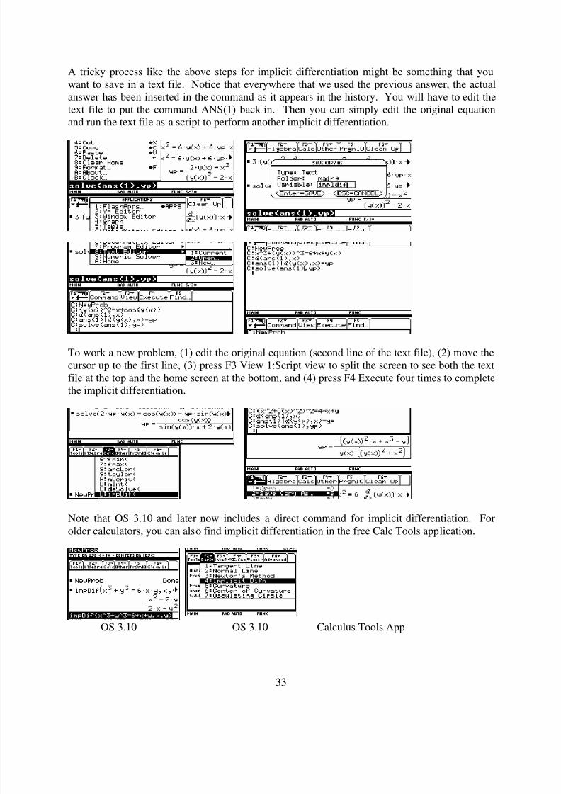
A tricky process like the above steps for implicit differentiation might be something that youwant to save in a text file. Notice that everywhere that we used the previous answer, the actualanswer has been inserted in the command as it appears in the history. You will have to edit thetext file to put the command ANS(1) back in. Then you can simply edit the original equationand run the text file as a script to perform another implicit differentiation.
To work a new problem, (1) edit the original equation (second line of the text file), (2) move thecursor up to the first line, (3) press F3 View 1:Script view to split the screen to see both the textfile at the top and the home screen at the bottom, and (4) press F4 Execute four times to completethe implicit differentiation.
Note that OS 3.10 and later now includes a direct command for implicit differentiation. Forolder calculators, you can also find implicit differentiation in the free Calc Tools application.
OS 3.10 OS 3.10 Calculus Tools App

8/3/2019 University Calculus Supplement TI-89
http://slidepdf.com/reader/full/university-calculus-supplement-ti-89 34/65
34
7. Taylor Polynomials
There is a nice command to generate a Taylor polynomial of any order for a function centered atany point.
To improve the speed of plotting, generate the polynomials in the home screen , copy and pastethe results in the Y= Editor for graphing. If you put the taylor command in the Y= Editor, thepolynomial is re-generated again for every point plotted (making plotting extremely slow).
F2 Zoom 7:ZoomTrig

8/3/2019 University Calculus Supplement TI-89
http://slidepdf.com/reader/full/university-calculus-supplement-ti-89 35/65
35
Chapter 3
Applications of Derivatives
For the activities in this chapter, the various graphing capabilities of the calculator will be used.
This is loosely coordinated with Chapter 3 of the text University Calculus: Elements with EarlyTranscendentals (WMU edition), by Hass, Weir, and Thomas, Pearson Custom Publishing.
1. Zooming to See Asymptotes
Asymptotes can roughly be described as observing how the graph of a function behaves assomething goes to infinity. Since the viewing window is always finite in every direction,calculator and computer graphs have a difficult time accurately representing either vertical orhorizontal asymptotes. In particular, the two pieces of a vertical asymptote (where the functionis not continuous) may be connected by a near vertical line segment which makes the plot appear
continuous. Remember that in the default style (line), the calculator plot evaluates the functionat a finite number of points, plots these points in the graph, and then connects the points (inorder) with line segments. If the two plotted points lie on different sides of a vertical asymptote,then we would like to remove the line segment.
Consider1
( )2
f x x
=−
for viewing window 10 10, 10 10 x y− ≤ ≤ − ≤ ≤ (ZoomStd).
If we press F3 Trace and move with the cursor keys to the plotted point with the largest x less
than 2, we find the plotted point (1.89873, −9.875) near the bottom of the viewing window.Moving with the right cursor key once to the smallest x greater than 2, we find the plotted point(2.02532, 39.5) well above the viewing window. The near vertical line in the plot attempts toconnect these two points. All of the above plots have xres = 1. Making xres larger than 1 cangive a plot looking even worse with the connecting line segment looking less vertical (seebelow). [Discontinuity detection in OS 3.10 eliminates the need to use xres and dot style here.]
xres = 3 Style Line xres = 1 Style Dot 8 12, 10 10 x y− ≤ ≤ − ≤ ≤
8/3/2019 University Calculus Supplement TI-89
http://slidepdf.com/reader/full/university-calculus-supplement-ti-89 36/65
36
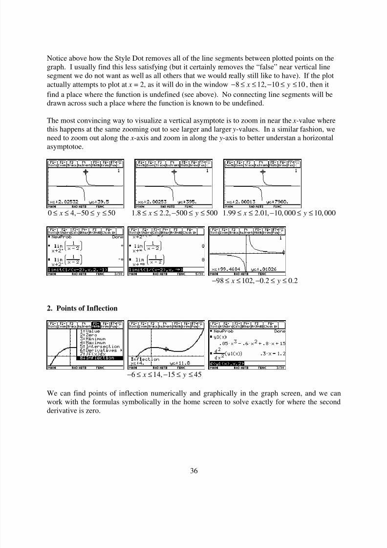
Notice above how the Style Dot removes all of the line segments between plotted points on thegraph. I usually find this less satisfying (but it certainly removes the “false” near vertical linesegment we do not want as well as all others that we would really still like to have). If the plotactually attempts to plot at x = 2, as it will do in the window 8 12, 10 10 x y− ≤ ≤ − ≤ ≤ , then it
find a place where the function is undefined (see above). No connecting line segments will bedrawn across such a place where the function is known to be undefined.
The most convincing way to visualize a vertical asymptote is to zoom in near the x-value wherethis happens at the same zooming out to see larger and larger y-values. In a similar fashion, weneed to zoom out along the x-axis and zoom in along the y-axis to better understan a horizontalasymptotoe.
0 4, 50 50 x y≤ ≤ − ≤ ≤ 1.8 2.2, 500 500 x y≤ ≤ − ≤ ≤ 1.99 2.01, 10,000 10,000 x y≤ ≤ − ≤ ≤
98 102, 0.2 0.2 x y− ≤ ≤ − ≤ ≤
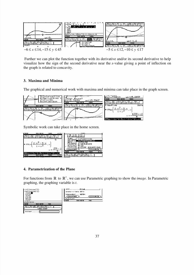
2. Points of Inflection
6 14, 15 45 x y− ≤ ≤ − ≤ ≤
We can find points of inflection numerically and graphically in the graph screen, and we canwork with the formulas symbolically in the home screen to solve exactly for where the secondderivative is zero.
8/3/2019 University Calculus Supplement TI-89
http://slidepdf.com/reader/full/university-calculus-supplement-ti-89 37/65
37
6 14, 15 45 x y− ≤ ≤ − ≤ ≤ 5 12, 10 17 x y− ≤ ≤ − ≤ ≤
Further we can plot the function together with its derivative and/or its second derivative to helpvisualize how the sign of the second derivative near the x-value giving a point of inflection onthe graph is related to concavity.
3. Maxima and Minima
The graphical and numerical work with maxima and minima can take place in the graph screen.
Symbolic work can take place in the home screen.
4. Parametrization of the Plane
For functions from R to 2R , we can use Parametric graphing to show the image. In Parametric
graphing, the graphing variable is t .

8/3/2019 University Calculus Supplement TI-89
http://slidepdf.com/reader/full/university-calculus-supplement-ti-89 38/65
38
Often when plotting a two-dimensional image, we might be happier using a plot with equally-scaled axes. The F2 Zoom 5:ZoomSqr command will widen the range of either the x-axis or the y-axis so that we see everything we saw before only in window with equally-scaled axes. Thenthis plot will look like a circle.
We can also use parametric graphing to simulate some motion problems. Suppose that2( ) 5 40 16h t t t = + − describes the height of a ball (in feet) thrown straight up at time t = 0 after t
seconds. We can provide an animation of the motion, the image of h, and the graph of h. Noticewe have set tmax below to correspond with the time when the ball hits the ground.
Animation (part way up)
Path (partially drawn) Graph of h
8/3/2019 University Calculus Supplement TI-89
http://slidepdf.com/reader/full/university-calculus-supplement-ti-89 39/65
39
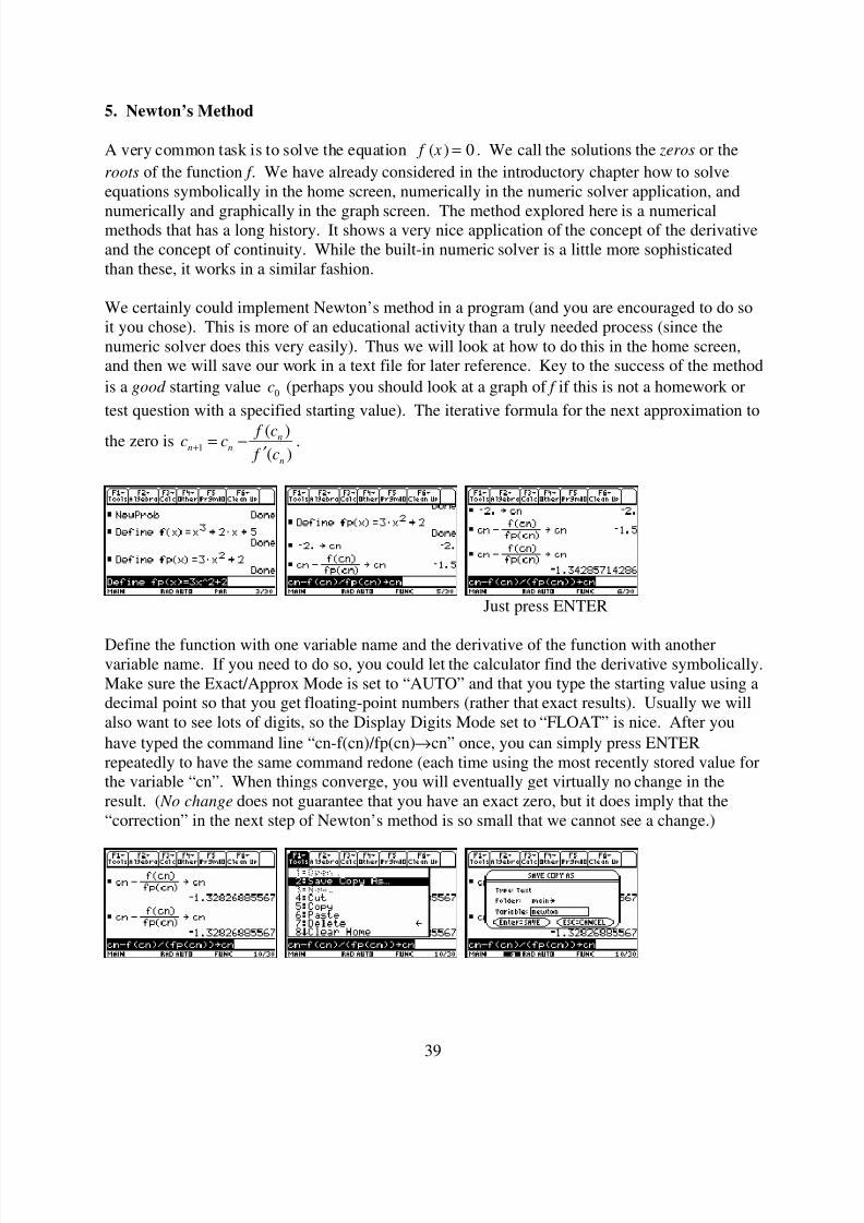
5. Newton’s Method
A very common task is to solve the equation ( ) 0 f x = . We call the solutions the zeros or the
roots of the function f . We have already considered in the introductory chapter how to solveequations symbolically in the home screen, numerically in the numeric solver application, and
numerically and graphically in the graph screen. The method explored here is a numericalmethods that has a long history. It shows a very nice application of the concept of the derivativeand the concept of continuity. While the built-in numeric solver is a little more sophisticatedthan these, it works in a similar fashion.
We certainly could implement Newton’s method in a program (and you are encouraged to do soit you chose). This is more of an educational activity than a truly needed process (since thenumeric solver does this very easily). Thus we will look at how to do this in the home screen,and then we will save our work in a text file for later reference. Key to the success of the method
is a good starting value 0c (perhaps you should look at a graph of f if this is not a homework or
test question with a specified starting value). The iterative formula for the next approximation to
the zero is 1( )( )
nn n
n
f cc c f c
+ = −′
.
Just press ENTER
Define the function with one variable name and the derivative of the function with anothervariable name. If you need to do so, you could let the calculator find the derivative symbolically.Make sure the Exact/Approx Mode is set to “AUTO” and that you type the starting value using adecimal point so that you get floating-point numbers (rather that exact results). Usually we willalso want to see lots of digits, so the Display Digits Mode set to “FLOAT” is nice. After you
have typed the command line “cn-f(cn)/fp(cn)→cn” once, you can simply press ENTERrepeatedly to have the same command redone (each time using the most recently stored value forthe variable “cn”. When things converge, you will eventually get virtually no change in theresult. ( No change does not guarantee that you have an exact zero, but it does imply that the“correction” in the next step of Newton’s method is so small that we cannot see a change.)

8/3/2019 University Calculus Supplement TI-89
http://slidepdf.com/reader/full/university-calculus-supplement-ti-89 40/65
40
We save the work in the history section by the command F1 2: Save Copy As. The dialog boxwill ask you to provide a name for the resulting text file. Here we give it the name “newton”.This process will save the work, even if you clear the history area.
Press the APPS key and select the Text Editor. Choose to open the text we named “newton”. In
this Text Editor, we can edit the file to change the starting value or to change the function and itsderivative. Press F3 View to choose a Split view so that we can see both this text file (at the top)and the home screen (at the bottom). Move the cursor to some command line (with a beginningC:) and press F4 Execute to paste that command into the home screen and have it executed.
Respond with ESC Repeatedly press F4
We finish this section by noting that some of the features and characteristics of Newton’s methodare present in the numeric solver available as an application. If you type a “good” starting valueinto the variable in the numeric solver before pressing F2 Solve, you effectively tell the internalalgorithm to start its iteration with the given value. This can help it to converge more rapidly,much as in Newton’s method. There is also the option to specify an interval (the default bound
={−1.E14,1.E14} is effectively no bound at all). The internal algorithm stays within the intervalgiven.
8/3/2019 University Calculus Supplement TI-89
http://slidepdf.com/reader/full/university-calculus-supplement-ti-89 41/65
41
Chapter 4
Integration
For the activities in this chapter, the various graphing, numerical, and symbolic capabilities of
the calculator will be used. This is loosely coordinated with Chapter 4 of the text UniversityCalculus: Elements with Early Transcendentals (WMU edition), by Hass, Weir, and Thomas,Pearson Custom Publishing.
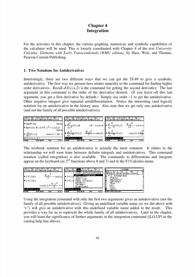
1. Two Notations for Antiderivatives
Interestingly, there are two different ways that we can get the TI-89 to give a symbolicantiderivative. The first way we present here relates naturally to the command for finding higherorder derivatives. Recall d (f(x),x,2) is the command for getting the second derivative. The lastargument in this command is the order of the derivative desired. (If you leave off this last
argument, you get a first derivative by default.) Simply use order −1 to get the antiderivative.Other negative integers give repeated antidifferentiation. Notice the interesting (and logical)notation for an antiderivative in the history area. Also note that we get only one antiderivative(and not the family of all possible antiderivatives).
The textbook notation for an antiderivative is actually the most common. It relates to therelationship we will soon learn between definite integrals and antiderivatives. This commandnotation (called integration) is also available. The commands to differentiate and integrateappear on the keyboard (as 2nd functions above 8 and 7) and in the F3 Calculus menu.
Using the integration command with only the first two arguments gives an antiderivative (not thefamily of all possible antiderivatives). Giving an undefined variable name (as we did above with“c”) will give an antiderivative with this undefined variable name added to the result. Thisprovides a way for us to represent the whole family of all antiderivatives. Later in the chapter,you will learn the significance of further arguments in the integration command ([LO,UP] in thecatalog help line above).

8/3/2019 University Calculus Supplement TI-89
http://slidepdf.com/reader/full/university-calculus-supplement-ti-89 42/65
42
2. Riemann Sums and the Sigma Notation
Definite integrals are defined by means of a limit of Riemann sums, and one of the ways toapproximate a definite integral is to use some kind of Riemann sum. There are several ways tocompute Riemann sums on the TI-89/Voyage 200 family of calculators.
A general Riemann sum approximating ( )b
a f x dx∫ is defined in terms of a partition { }i x of the
interval [ ],a b into subintervals [ ] [ ] [ ] [ ]0 1 1 2 1 1, , , , , , , , ,i i n n x x x x x x x x− −… … and in terms of a
selection of evaluation points { }is with [ ]1,i i is x x−∈ for 1, 2, ,i n= … . Namely,
( )1
1
( ) ( ) .n
b
i i ia
i
f x dx f s x x −=
≈ −∑∫
Each term in the sum can be interpreted as the area of a rectangle with width ( )1i i x x −− and
“signed” height ( ).i f s Special cases include selecting 1i is x −= (left endpoints), i is x= (right
endpoints), or 1
2i i
i x xs − += (midpoints). Often the partition points { }i x are equally spaced
across the interval, giving ( )1i i x x x−− = ∆ for all 1, 2, , .i n= … First we show how to compute a
general Riemann sum (no special assumptions) using lists.
Start by storing the formula for ( ) f x . Store the partition points { }i x in a list, say l1. (Note that
variable names must begin with a letter, and so the first character in the name of this list is the
letter “l” , not the number “1”.) Store the selection points { }is in another list, say l2. Then take
advantage of the list operations to compute the Riemann sum in the HOME screen. Applying a
function to a list gives a list of evaluations. The command ∆List computes a list of the
differences (i.e. ( )1i i x x −− ). Multiplying two lists of equal length, gives a list where like terms in
the two lists have been multiplied. Finally the sum command sums the terms in a list.
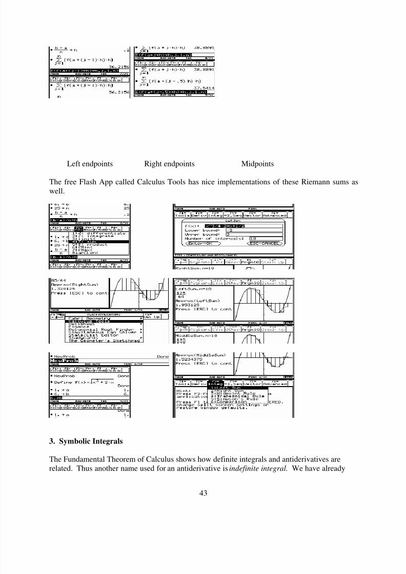
If you desire an equally spaced partition with special evaluation points (left endpoints, rightendpoints, midpoints), there are simpler ways to have the calculator compute these.
8/3/2019 University Calculus Supplement TI-89
http://slidepdf.com/reader/full/university-calculus-supplement-ti-89 43/65
43
Left endpoints Right endpoints Midpoints
The free Flash App called Calculus Tools has nice implementations of these Riemann sums aswell.
3. Symbolic Integrals
The Fundamental Theorem of Calculus shows how definite integrals and antiderivatives arerelated. Thus another name used for an antiderivative is indefinite integral. We have already

8/3/2019 University Calculus Supplement TI-89
http://slidepdf.com/reader/full/university-calculus-supplement-ti-89 44/65
44
seen this integration command used to find antiderivatives in the first section of this chapter.The same command will find definite integrals if we specify the interval of integration. Makesure the Exact/Approximate mode is set to AUTO or EXACT so that we can see exactintegration answers.
Indefinite Integral Exact Definite Integral Approximate Definite Integral
[Press ENTER.] [Press ♦ENTER.]
Thus you can use the calculator to check your hand work using the Fundamental Theorem of calculus. Usually the calculator can do a symbolic problem if you can do it by hand. If theintegrand in a definite integral does not have an elementary antiderivative (or the calculator
cannot find one), the AUTO mode will automatically switch to a numerical approximation (usinga method a little more accurate and efficient than Riemann sums).
[Press ENTER.] Using unknown f Using unknown g

8/3/2019 University Calculus Supplement TI-89
http://slidepdf.com/reader/full/university-calculus-supplement-ti-89 45/65
45
Chapter 5
Techniques of Integration
Most of the activities in this chapter involve functions where you really need the calculator toevaluate the functions. This is loosely coordinated with Chapter 5 of the text University
Calculus: Elements with Early Transcendentals (WMU edition), by Hass, Weir, and Thomas,Pearson Custom Publishing.
1. Logarithmic and Exponential Functions
The TI-89/Voyage 200 offers the natural logarithm function and the natural exponential functionon the keyboard. Many people do not know that the common logarithm function is alsoavailable in the CATALOG (or you can just type log). [In the newer OS versions, you can evenget logarithms to other bases by typing “log(x,b)”, where 0, 1b b> ≠ is the desired base.
However you seldom have a need for this feature in Calculus.]
Base e Base e Base 10
2. Inverse Trigonometric Functions
If you have upgraded your OS to at least 2.08 or higher, then you have not only all of thetrigonometric functions, but also all of the inverse trigonometric functions as well. The ones notprinted on the keyboard can be found in the CATALOG.
Notice that you will get the error message “Non-real result” if you get outside of the domain of some of the inverse trigonometric functions (assuming your MODE setting for Complex Formatis REAL). All of the trigonometric functions have generalizations to domains of complexnumbers, and the calculator is programmed to handle when the Complex Format is selected tosomething other than REAL. You may use these functions using complex numbers in a latermathematics or physics or engineering course.
8/3/2019 University Calculus Supplement TI-89
http://slidepdf.com/reader/full/university-calculus-supplement-ti-89 46/65
46
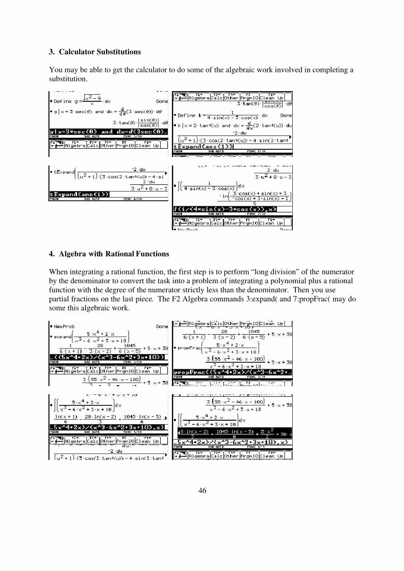
3. Calculator Substitutions
You may be able to get the calculator to do some of the algebraic work involved in completing asubstitution.
4. Algebra with Rational Functions
When integrating a rational function, the first step is to perform “long division” of the numeratorby the denominator to convert the task into a problem of integrating a polynomial plus a rationalfunction with the degree of the numerator strictly less than the denominator. Then you use
partial fractions on the last piece. The F2 Algebra commands 3:expand( and 7:propFrac( may dosome this algebraic work.
8/3/2019 University Calculus Supplement TI-89
http://slidepdf.com/reader/full/university-calculus-supplement-ti-89 47/65
47
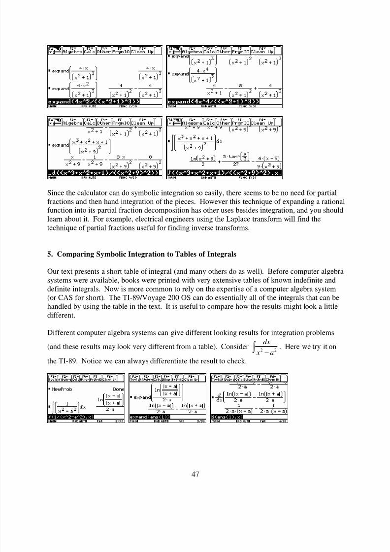
Since the calculator can do symbolic integration so easily, there seems to be no need for partialfractions and then hand integration of the pieces. However this technique of expanding a rationalfunction into its partial fraction decomposition has other uses besides integration, and you shouldlearn about it. For example, electrical engineers using the Laplace transform will find thetechnique of partial fractions useful for finding inverse transforms.
5. Comparing Symbolic Integration to Tables of Integrals
Our text presents a short table of integral (and many others do as well). Before computer algebrasystems were available, books were printed with very extensive tables of known indefinite and
definite integrals. Now is more common to rely on the expertise of a computer algebra system(or CAS for short). The TI-89/Voyage 200 OS can do essentially all of the integrals that can behandled by using the table in the text. It is useful to compare how the results might look a littledifferent.
Different computer algebra systems can give different looking results for integration problems
(and these results may look very different from a table). Consider2 2
dx
x a−∫ . Here we try it on
the TI-89. Notice we can always differentiate the result to check.
8/3/2019 University Calculus Supplement TI-89
http://slidepdf.com/reader/full/university-calculus-supplement-ti-89 48/65
48
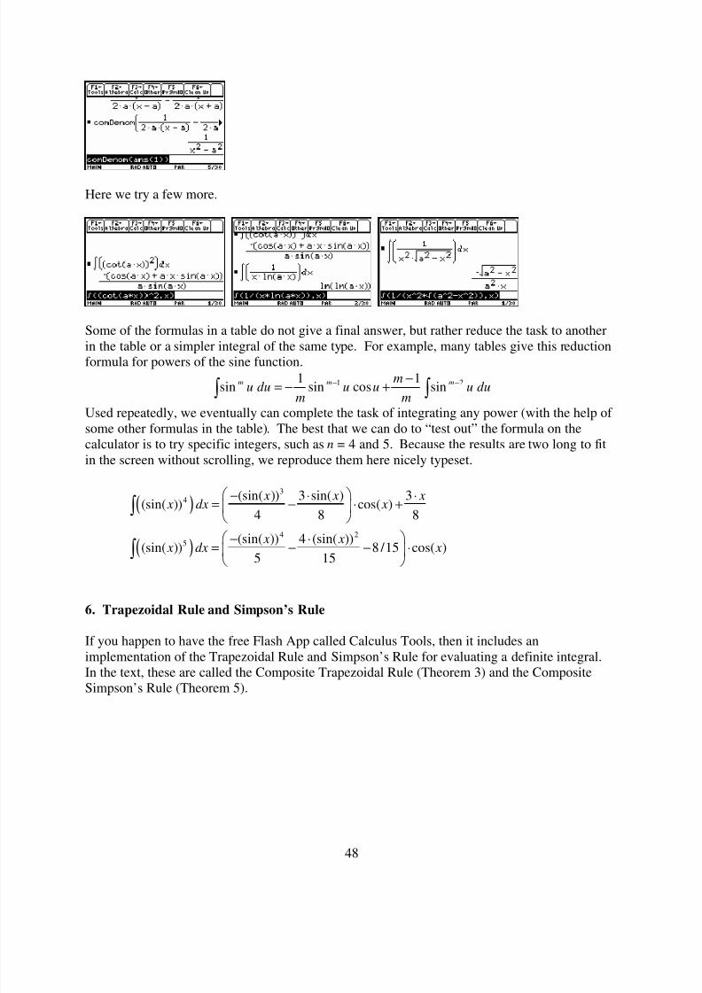
Here we try a few more.
Some of the formulas in a table do not give a final answer, but rather reduce the task to another
in the table or a simpler integral of the same type. For example, many tables give this reductionformula for powers of the sine function.
1 21 1sin sin cos sinm m mm
u du u u u dum m
− −−= − +∫ ∫
Used repeatedly, we eventually can complete the task of integrating any power (with the help of some other formulas in the table). The best that we can do to “test out” the formula on thecalculator is to try specific integers, such as n = 4 and 5. Because the results are two long to fitin the screen without scrolling, we reproduce them here nicely typeset.
( )3
4 (sin( )) 3 sin( ) 3(sin( )) cos( )
4 8 8
x x x x dx x
− ⋅ ⋅= − ⋅ +
∫
( )4 2
5 (sin( )) 4 (sin( ))(sin( )) 8 /15 cos( )
5 15
x x x dx x
− ⋅= − − ⋅
∫
6. Trapezoidal Rule and Simpson’s Rule
If you happen to have the free Flash App called Calculus Tools, then it includes animplementation of the Trapezoidal Rule and Simpson’s Rule for evaluating a definite integral.In the text, these are called the Composite Trapezoidal Rule (Theorem 3) and the CompositeSimpson’s Rule (Theorem 5).
8/3/2019 University Calculus Supplement TI-89
http://slidepdf.com/reader/full/university-calculus-supplement-ti-89 49/65
49
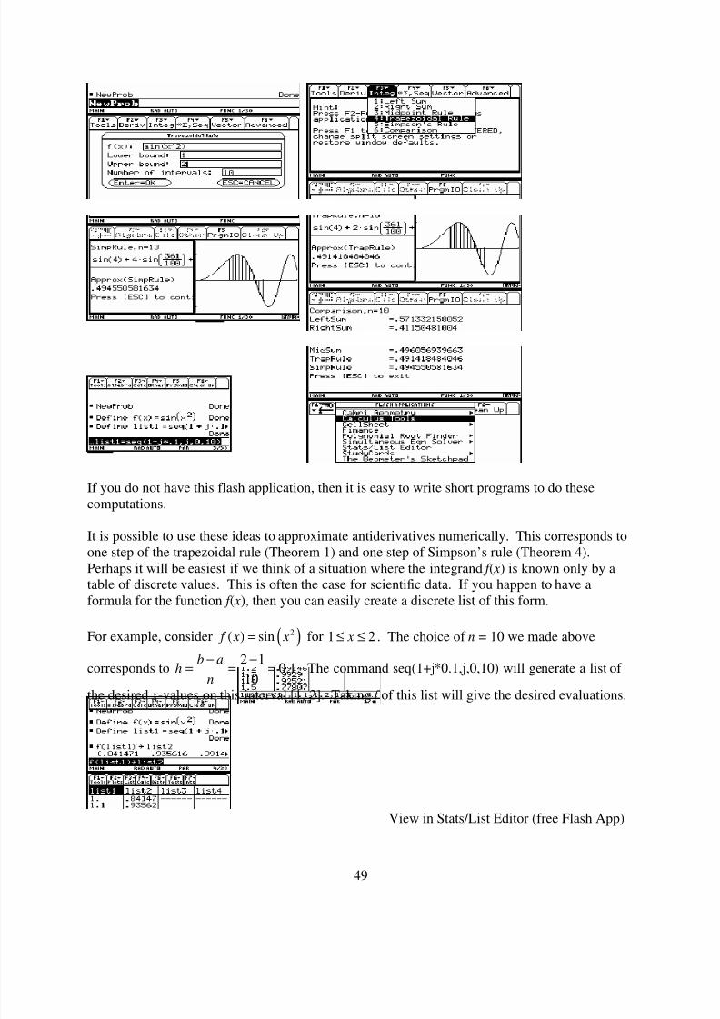
If you do not have this flash application, then it is easy to write short programs to do thesecomputations.
It is possible to use these ideas to approximate antiderivatives numerically. This corresponds toone step of the trapezoidal rule (Theorem 1) and one step of Simpson’s rule (Theorem 4).Perhaps it will be easiest if we think of a situation where the integrand f ( x) is known only by atable of discrete values. This is often the case for scientific data. If you happen to have aformula for the function f ( x), then you can easily create a discrete list of this form.
For example, consider ( )2( ) sin f x x= for 1 2 x≤ ≤ . The choice of n = 10 we made above
corresponds to2 1
0.110
b ah
n
− −= = = . The command seq(1+j*0.1,j,0,10) will generate a list of
the desired x-values on this interval [1, 2]. Taking f of this list will give the desired evaluations.
View in Stats/List Editor (free Flash App)

8/3/2019 University Calculus Supplement TI-89
http://slidepdf.com/reader/full/university-calculus-supplement-ti-89 50/65
50
This information will most often be displayed in a book or on your paper in a table.
x f ( x)
1.0 0.841471
1.1 0.935616
1.2 0.9914581.3 0.992904
1.4 0.925212
1.5 0.778073
1.6 0.549355
1.7 0.248947
1.8 −0.098249
1.9 −0.451466
2.0 −0.756802
We are interested in approximating 1 ( )
x
f t dt ∫ for the same set of x-values as used in the tableabove, using only the numbers available in the table. This is easy to do for x = 1 because
1
1( ) 0 f t dt =∫ . For x = 1.1, we use one trapezoid to approximate
1.1
1
(1) (1.1)( ) (0.1)
2
f f f t dt
+≈∫
and get 0.088854. In a similar fashion, we can use another trapezoid to approximate1.2
1.1
(1.1) (1.2)( ) (0.1) 0.096354
2
f f f t dt
+≈ ≈∫ . Thus to get
1.2
1( ) 0.088854 0.096354 0.185208 f t dt ≈ + ≈∫ .
All of this can be done in the home screen as illustrated below. If the number n is small, these
step-by-step calculations are reasonable to do.
Obviously what we want to do is to automate this process a little. The commandseq((list2[j]+list2[j+1])*0.1/2,j,1,10)
will generate a sequence of numbers representing the individual trapezoid approximations
1 1( ) ( )( ) (0.1)
2
j
j
x j j
x
f x f x f t dt
+ ++≈∫ .
The MATH menu, List submenu command cumSum(above list ) will give the cumulative sum wedesire to approximate
1 1
11
( ) ( )( ) (0.1)
2
j j
xk k
k
f x f x f t dt
+ +
=
+≈ ∑∫ .

8/3/2019 University Calculus Supplement TI-89
http://slidepdf.com/reader/full/university-calculus-supplement-ti-89 51/65
51
Finally we append the initial zero to the list to get a final list of the same length as the originallists. This command is augment({0}, above list )
x f ( x)1
( ) x
f t dt ∫ (Trapezoidal)
1.0 0.841471 0
1.1 0.935616 0.088854
1.2 0.991458 0.185208
1.3 0.992904 0.284426
1.4 0.925212 0.380332
1.5 0.778073 0.465496
1.6 0.549355 0.531868
1.7 0.248947 0.571783
1.8 −0.098249 0.579318
1.9 −0.451466 0.551832
2.0 −0.756802 0.491418
Notice that the final answer in the last column is the Trapezoidal Rule computation from theCalculus Tools choice we did at the very beginning.
Implementing Simpson rule step-by-step is similar. The one different feature here is that ournew column is not complete. The approximation we use is
2 1 2( ) 4 ( ) ( )( ) ( )
3
j
j
x j j j
x
f x f x f x f t dt h
+ + ++ +≈∫ ,
giving us only partial definite integrals over “double” subintervals.
augment(cumSum(seq((list2[j]+4*list2[j+1]+list2[j+2])*0.1/2,j,1,10,2)))
Notice that we use an additional argument in the sequence command to indicate that the index j
goes from 1 to 10 in steps of 2.

8/3/2019 University Calculus Supplement TI-89
http://slidepdf.com/reader/full/university-calculus-supplement-ti-89 52/65
52
x f ( x)1
( ) x
f t dt ∫ (Simpson)
1.0 0.841471 0
1.1 0.935616
1.2 0.991458 0.185846
1.3 0.9929041.4 0.925212 0.382123
1.5 0.778073
1.6 0.549355 0.535018
1.7 0.248947
1.8 −0.098249 0.583248
1.9 −0.4514662.0 −0.756802 0.494551
Again notice that the value at the bottom of the last column is the Simpson rule approximationfrom Calculus Tools that we did at the very beginning of this section.
You may want to put these steps into a short program or save the history as a text file to morequickly do the step-by-step trapezoidal rule and the step-by-step Simpson’s rule repeatedly fornew problems.
The discrete computations in this section work very nicely in a spreadsheet. If you have theCellSheet (it comes on the Voyage 200), you can experiment with alternative ways toaccomplish the step-by-step trapezoidal rule and step-by-step Simpson’s rule in the spreadsheetthat is available on this device.
7. Other Numerical Integration
There are more efficient and accurate algorithms for numerical integration than the compositetrapezoidal rule and the composite Simpson’s rule. One feature often put in these moresophisticated algorithms is an adaptive process to estimate the error made for the particularproblem given. The algorithm then adjusts the step-size h as it works along the interval toachieve a desired accuracy. TI uses such an adaptive numerical integration routine internally,and it works to try to achieve 6 significant digits of accuracy on this family of calculators. Thuswhen display digits is set to the default FLOAT 6 mode, you can generally expect all of thedisplayed digits in a numerical integration computation to be correct. If you display more digitsthan 6, you cannot assume all the additional digits are correct.

8/3/2019 University Calculus Supplement TI-89
http://slidepdf.com/reader/full/university-calculus-supplement-ti-89 53/65
53
It is generally better to use the internal numerical integration (either the nInt( command or the
regular integration command with a ♦ENTER) rather than the composite trapezoidal rule or thecomposite Simpson’s rule. The best advice is to use one of these simple numerical integrationroutines only when the specific routine is specified. Generally in a textbook problem or a testquestion, the instruction will tell you not only the method (trapezoidal or Simpson) but also the
step size.
8. Symbolic Infinite Limits
The TI-89 can handle many limits involving infinity. It is not a good idea to jump to conclusionsabout the value for infinite limits based upon numerical evidence. However the same theoremsyou are learning about how to handle infinite limits can be implemented in the symbolic part of
the calculator. Notice that you can find “∞” on the keyboard, and infinity is a possible output if you have the Exact/Approx mode set to either AUTO or EXACT.
9. Improper Integrals
Since the evaluation of improper integrals generally involves a symbolic integration followed bysome evaluation of an infinite limit, it is not a surprise that the TI-89 can do many of these.

8/3/2019 University Calculus Supplement TI-89
http://slidepdf.com/reader/full/university-calculus-supplement-ti-89 54/65
54
Chapter 7
Sequences and Series
The activities in this chapter present symbolic, numerical, and graphical activites involving
sequences and series. This is loosely coordinated with Chapter 7 of the text UniversityCalculus: Elements with Early Transcendentals (WMU edition), by Hass, Weir, and Thomas,Pearson Custom Publishing.
1. Sequences and Series
It is possible to work with finite sequences and series using lists. This may be enough torecognize patterns.
The F3 Calc command 4:Σ( sum allows some symbolic results. Some special infinite series canbe evaluated.
The ability of the calculator to evaluate symbolic limits means it will be useful for some of thelimits needed in the ratio test for power series. This has been further facilitated in the CalculusTools flash application (free from http://education.ti.com). You will not get much credit usingonly the application (because your instructor will want to see that you understand the ratio test),but you can check your work with this flash application.
8/3/2019 University Calculus Supplement TI-89
http://slidepdf.com/reader/full/university-calculus-supplement-ti-89 55/65
55
2. Sequence Graphing
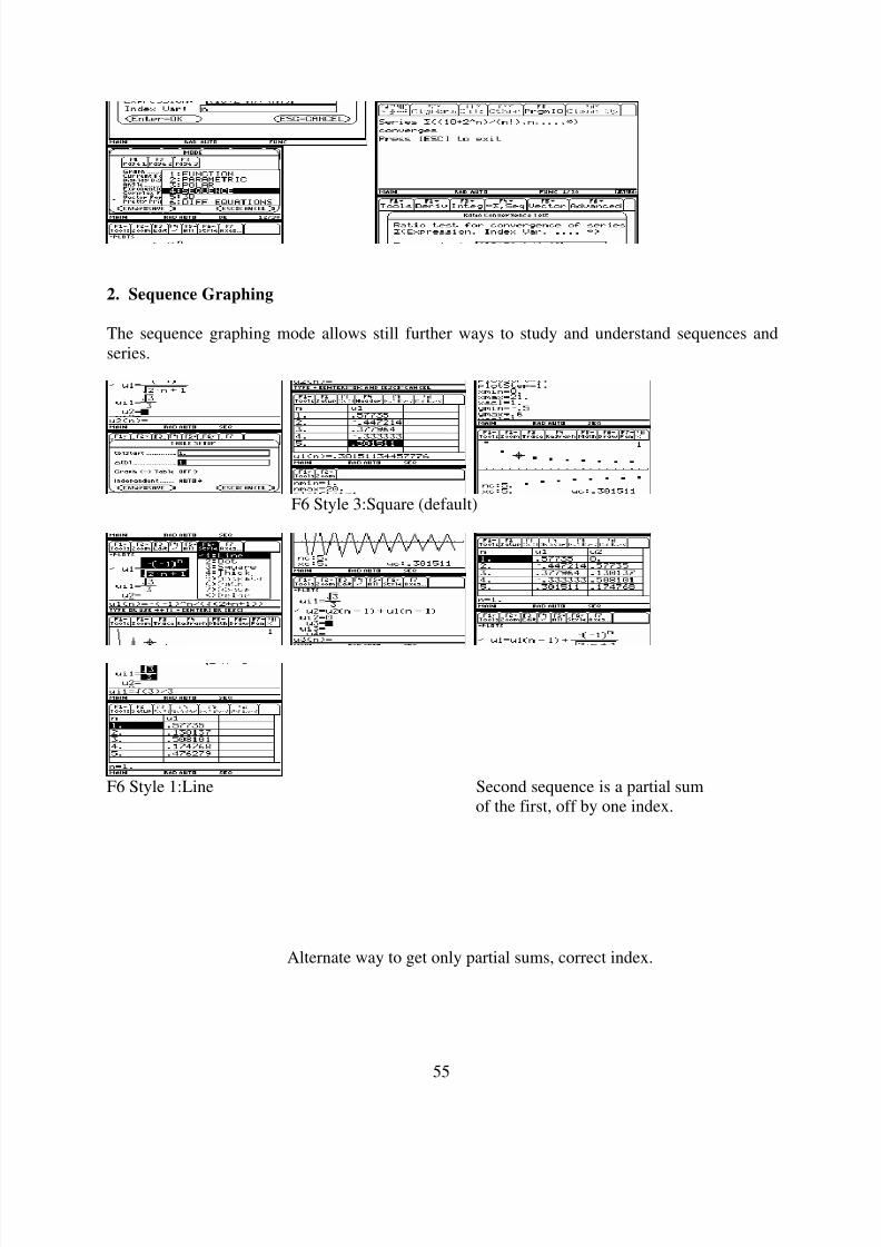
The sequence graphing mode allows still further ways to study and understand sequences andseries.
F6 Style 3:Square (default)
F6 Style 1:Line Second sequence is a partial sumof the first, off by one index.
Alternate way to get only partial sums, correct index.

8/3/2019 University Calculus Supplement TI-89
http://slidepdf.com/reader/full/university-calculus-supplement-ti-89 56/65
56
Alternate way with Line Style Evaluation of alternate way in HOME screen

8/3/2019 University Calculus Supplement TI-89
http://slidepdf.com/reader/full/university-calculus-supplement-ti-89 57/65
57
Chapter 8
Polar Coordinates and Conics
The activities in this chapter show polar coordinates and polar graphing. This is loosely
coordinated with Chapter 8 of the text University Calculus: Elements with Early Transcendentals(WMU edition), by Hass, Weir, and Thomas, Pearson Custom Publishing.
1. Polar Coordinates
Since the TI-92, this family of graphing calculators (including the TI-89 and the Voyage 200 thatreplaced the TI-92) has offered some nice features relating to polar coordinates. In the MATHmenu, the 2:Angle submenu, you will find several commands for converting between rectangularand polar coordinates. Note: The “angles” will automatically be in the Angle MODE (eitherradians or degrees).
Old TI-92, in RAD Angle MODE Conversions (in radians)
Switching to DEG Angle MODE Conversions (in degrees)
2. Graphing in Polar Coordinates
There is a polar equation graphing mode that allows the graphing of polar equations that can besolved for r , i.e. where r can be expressed in a formula in terms of θ . We demonstrate belowwith several examples. For the first example, note that the calculator is in DEG Angle MODE(which is usually not what we want in a calculus course). Note also that for polar graphing, wewill typically want to have equally-scaled axes (which we get with the ZoomSqr command fromthe ZOOM menu).

8/3/2019 University Calculus Supplement TI-89
http://slidepdf.com/reader/full/university-calculus-supplement-ti-89 58/65
58
In calculus, we are much more likely to want to work in RAD Angle MODE. Here are a fewexamples.

8/3/2019 University Calculus Supplement TI-89
http://slidepdf.com/reader/full/university-calculus-supplement-ti-89 59/65
59
For the polar equation 2 4sin(2 )r θ = , we plot the two possible solutions for r .
θ min = 0, θ max = π , xmin = −3.7699, xmax = 3.76099, ymin = −1.6119, ymax = 1.6119

8/3/2019 University Calculus Supplement TI-89
http://slidepdf.com/reader/full/university-calculus-supplement-ti-89 60/65
60
Chapter 15
Elementary Differential Equations
The activities in this chapter present some additional things that we can now do with differential
equations on this family of calculators. This is loosely coordinated with Chapter 15 of the textUniversity Calculus: Elements with Early Transcendentals (WMU edition), by Hass, Weir, andThomas, Pearson Custom Publishing.
1. Symbolic Differential Equations
Many calculus texts present one method for solving some first-order differential equations,namely the “method of separation of variables.” Assuming you can do the “separation”algebraically by hand, the task reduces to two indefinite integration problems. Obviously thesymbolic integration on the TI-89 can be helpful.
Consider ( )2 3 0dy y xy xdx+ + = . Working by hand we find
( )3 2
3 2
dy x y y
dx
ydy dx
y x
+ = −
+= −
with the last line showing the separation of the two variables. Integrating both sides can be doneby hand or by the calculator.
Letting ck e= ± and dropping the absolute value, we would generally express the solution as
2 3 y x y e k = , which implicitly defines y as a function of x. The calculator can directly solve some
differential equations, including the example above in a similar fashion. The command deSolvecan be found in the F3 Calc menu or in the catalog.

8/3/2019 University Calculus Supplement TI-89
http://slidepdf.com/reader/full/university-calculus-supplement-ti-89 61/65
61
Notice the arbitrary constant in the general solution is represented by the variable “@1” in theoutput. Here the calculator is not as careful with absolute values as we were above.
We can also ask the calculator to give us the symbolic solution for the general differentialequation, namely ( ) ( ) y t k y t b′ = + . The command deSolve can be used to solve for a particular
solution for such an equation with an initial condition. Notice below when we solve the generallogistic differential equation, we cannot use the variable names “c1” and “c2” because they arereserved variables use by the system (for the columns in a data set or matrix). We use “cc1” and“cc2” instead.
The command deSolve can solve some second-order differential equations as well. If it cannotsolve a differential equation, it will just repeat the problem back as a result. Even when it can
solve a problem with an implicit solution (such as ( )sin 2 y y t ′ = + below), the solution may not
be all that useful.
2. Differential Equation Graphing
There is a differential equation graphing mode that allows the numerical solution for first-orderdifferential equations with one or more initial conditions. We demonstrate below for a singleequation first.
Consider ( )sin 2 , (0) 3.1 y y t y′ = + =
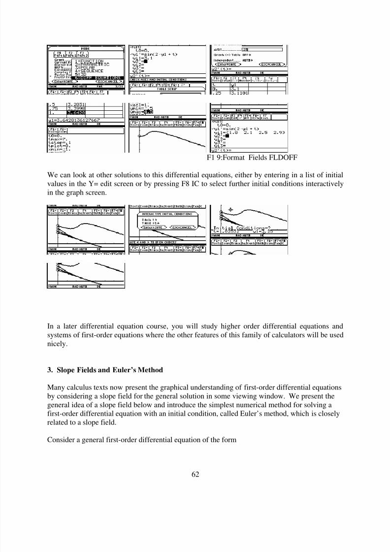
8/3/2019 University Calculus Supplement TI-89
http://slidepdf.com/reader/full/university-calculus-supplement-ti-89 62/65
62
F1 9:Format Fields FLDOFF
We can look at other solutions to this differential equations, either by entering in a list of initialvalues in the Y= edit screen or by pressing F8 IC to select further initial conditions interactively
in the graph screen.
In a later differential equation course, you will study higher order differential equations andsystems of first-order equations where the other features of this family of calculators will be usednicely.
3. Slope Fields and Euler’s Method
Many calculus texts now present the graphical understanding of first-order differential equationsby considering a slope field for the general solution in some viewing window. We present thegeneral idea of a slope field below and introduce the simplest numerical method for solving afirst-order differential equation with an initial condition, called Euler’s method, which is closelyrelated to a slope field.
Consider a general first-order differential equation of the form

8/3/2019 University Calculus Supplement TI-89
http://slidepdf.com/reader/full/university-calculus-supplement-ti-89 63/65
63
( )( ) , ( )dy
t f t y t dt
= .
Suppose the graph of the solution passes through the point (a, b), i.e. when t = a then y(a) =b.We know from the differential equation that the solution must have ( ) ( , ) y a f a b′ = . Given a
desired viewing window, we construct a grid of points in the rectangle. We treat the coordinates
of each point in our grid as the pair (a, b), and we draw a short line segment through the gridpoint with the slope ( ) ( , ) y a f a b′ = that the solution must have (if it goes through that grid
point).
Sample Grid (Grid ON) DE with no initial condition F1 9:Format Field SLPFLD
(default grid, not as before)
For example, one of the grid points used in the last image seems to be about (0.87, 2.79). Thus
that line segment is drawn with slope approximately sin(2*2.79 + 0.87) ≈ 0.166
F2 Zoom ZoomBox More detail Add initial condition y(0) = 3.1
Here we reproduce the slope filed for ( )2
( ) 2 ( ) ( )P t P t P t ′ = − .
y’(0) = {0.05, 0.5, 1.0, 3.0, 4.0}
TI uses an adaptive Runge-Kutta routine to numerically approximate the solutions in thesedifferential equation plots by default. This routine works to try to get plotted points with anaccuracy of diftol, a parameter you can set in the Window screen. The parameter fldres in theWindow screen sets the grid spacing for the slope filed. The defaults which often work nicelyare diftol = 0.001 and fldres = 14 (giving a 14 by 7 array of slope lines in the slope field).
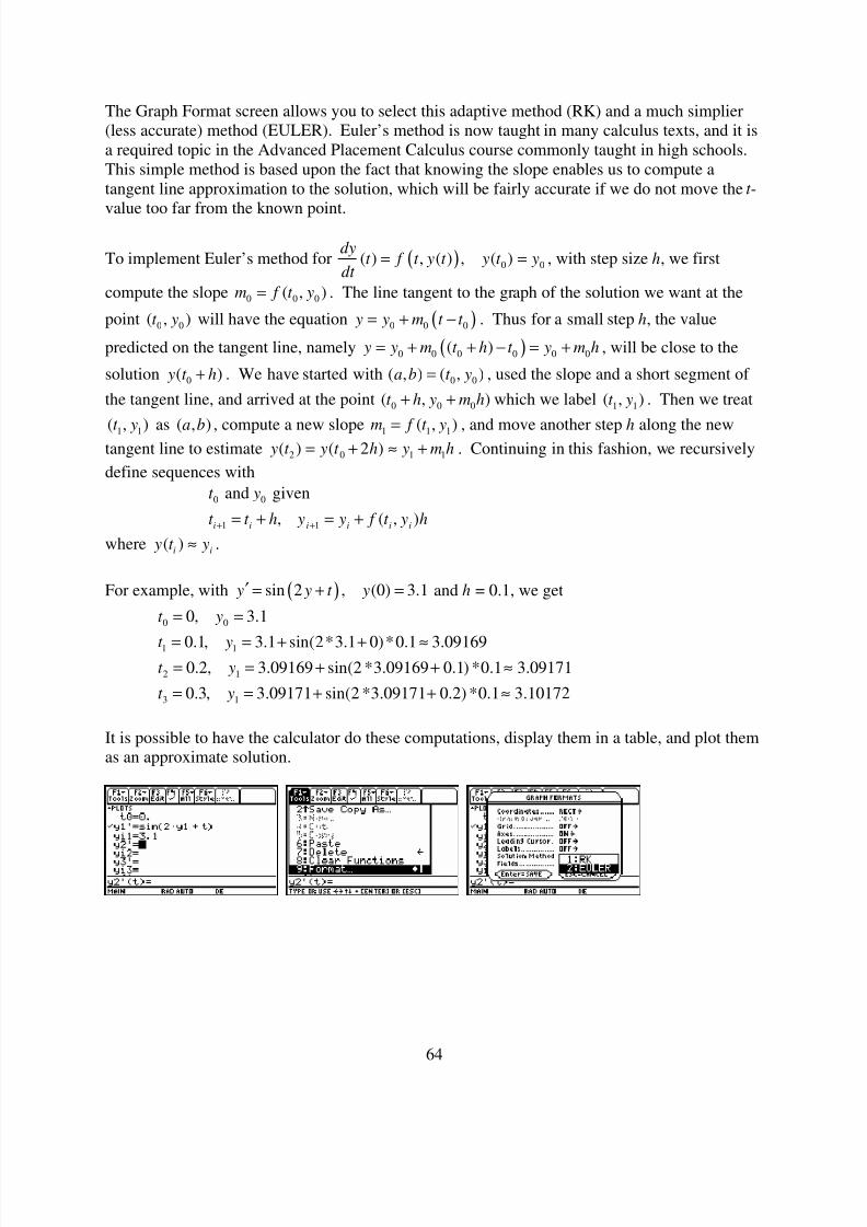
8/3/2019 University Calculus Supplement TI-89
http://slidepdf.com/reader/full/university-calculus-supplement-ti-89 64/65
64
The Graph Format screen allows you to select this adaptive method (RK) and a much simplier(less accurate) method (EULER). Euler’s method is now taught in many calculus texts, and it isa required topic in the Advanced Placement Calculus course commonly taught in high schools.This simple method is based upon the fact that knowing the slope enables us to compute atangent line approximation to the solution, which will be fairly accurate if we do not move the t -
value too far from the known point.
To implement Euler’s method for ( ) 0 0( ) , ( ) , ( )dy
t f t y t y t ydt
= = , with step size h, we first
compute the slope 0 0 0( , )m f t y= . The line tangent to the graph of the solution we want at the
point 0 0( , )t y will have the equation ( )0 0 0 y y m t t = + − . Thus for a small step h, the value
predicted on the tangent line, namely ( )0 0 0 0 0 0( ) y y m t h t y m h= + + − = + , will be close to the
solution 0( ) y t h+ . We have started with 0 0( , ) ( , )a b t y= , used the slope and a short segment of
the tangent line, and arrived at the point 0 0 0( , )t h y m h+ + which we label 1 1( , )t y . Then we treat
1 1( , )t y as ( , )a b , compute a new slope 1 1 1( , )m f t y= , and move another step h along the newtangent line to estimate 2 0 1 1( ) ( 2 ) y t y t h y m h= + ≈ + . Continuing in this fashion, we recursively
define sequences with
0 0
1 1
and given
, ( , )i i i i i i
t y
t t h y y f t y h+ += + = +
where ( )i i y t y≈ .
For example, with ( )sin 2 , (0) 3.1 y y t y′ = + = and h = 0.1, we get
0 0
1 1
2 1
3 1
0, 3.1
0.1, 3.1 sin(2*3.1 0)*0.1 3.091690.2, 3.09169 sin(2 *3.09169 0.1) *0.1 3.09171
0.3, 3.09171 sin(2 *3.09171 0.2) *0.1 3.10172
t y
t yt y
t y
= =
= = + + ≈= = + + ≈
= = + + ≈
It is possible to have the calculator do these computations, display them in a table, and plot themas an approximate solution.
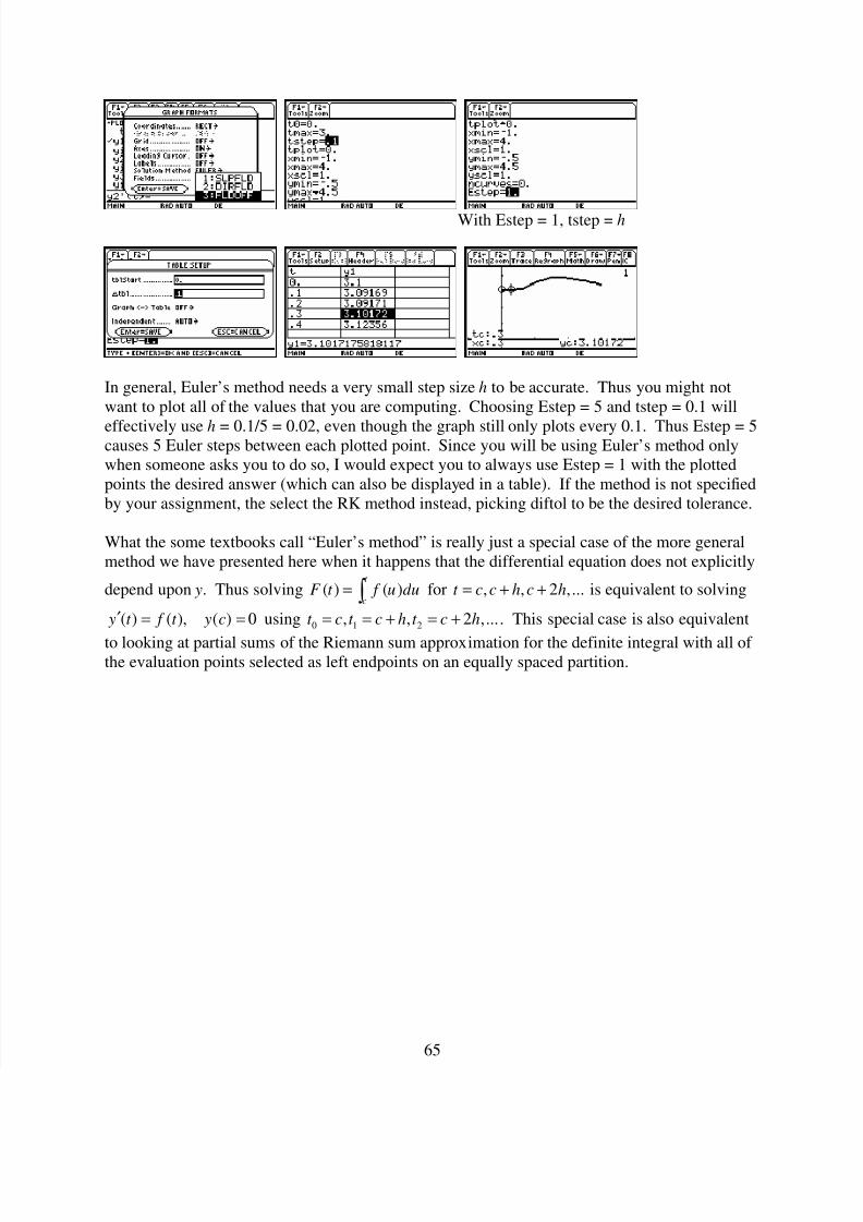
8/3/2019 University Calculus Supplement TI-89
http://slidepdf.com/reader/full/university-calculus-supplement-ti-89 65/65
With Estep = 1, tstep = h
In general, Euler’s method needs a very small step size h to be accurate. Thus you might notwant to plot all of the values that you are computing. Choosing Estep = 5 and tstep = 0.1 will
effectively use h = 0.1/5 = 0.02, even though the graph still only plots every 0.1. Thus Estep = 5causes 5 Euler steps between each plotted point. Since you will be using Euler’s method onlywhen someone asks you to do so, I would expect you to always use Estep = 1 with the plottedpoints the desired answer (which can also be displayed in a table). If the method is not specifiedby your assignment, the select the RK method instead, picking diftol to be the desired tolerance.
What the some textbooks call “Euler’s method” is really just a special case of the more generalmethod we have presented here when it happens that the differential equation does not explicitly
depend upon y. Thus solving ( ) ( )t
cF t f u du= ∫ for , , 2 ,...t c c h c h= + + is equivalent to solving
( ) ( ), ( ) 0 y t f t y c′ = = using 0 1 2, , 2 ,...t c t c h t c h= = + = + . This special case is also equivalent
to looking at partial sums of the Riemann sum approximation for the definite integral with all of the evaluation points selected as left endpoints on an equally spaced partition.