University at Buffalo, State University of New York USAsrihari/CSE574/Chap4/4.4-Laplace.pdf ·...

The Laplace Approximation

Sargur N. Srihari University at Buffalo, State University of New York

USA

Topics in Linear Models for Classification •  Overview 1. Discriminant Functions 2. Probabilistic Generative Models 3. Probabilistic Discriminative Models 4. The Laplace Approximation 5. Bayesian Logistic Regression

2

Machine Learning Srihari

Topics in Laplace Approximation

•  Motivation •  Finding a Gaussian approximation: 1-D case •  Approximation in M-dimensional space •  Weakness of Laplace approximation •  Model Comparison using BIC


3

What is Laplace Approximation? •  The Laplace approximation framework aims to

find a Gaussian approximation to a continuous distribution


4

Why study Laplace Approximation?

•  We shall discuss Bayesian treatment of logistic regression –  It is more complex than the Bayesian treatment of

linear regression –  In particular we cannot integrate exactly

•  In ML we need to predict a distribution of the output that may involve integration


5

Bayesian Linear Regression •  Recapitulate:

–  in Bayesian linear regression we integrate exactly:


6

p(t | t,α,β)= p(t|w,β) ⋅p(w|t,α,β)dw∫

p(t |x,w,β) = N(t |y(x,w),β−1) p(w|t)=N(w|mN,SN) mN=β SNΦTt

SN-1=α I+β ΦTΦ

p(t |x, t,α,β) = N(t |m

NTφ(x),σ

N2 (x)) where σ

N2 (x) =

1β

+φ(x)TSNφ(x)

y(x,mN)= k(x,x

n)tn

n=1

N

∑ k(x,x’)=βφ (x)TSNφ (x’) SN-1= S0

-1+ βΦTΦ ⎟⎟⎟⎟⎟

⎠

⎞

⎜⎜⎜⎜⎜

⎝

⎛

=Φ

−

−

)x()x(

)x()x(...)x()x(

10

20

111110

NMN

M

φφ

φφφφ

Equivalent Kernel

Gaussian posterior: Gaussian noise:

Predictive Distribution::

Result of integration:

p(w)=N (w|m0 ,S0) S0=α-1I

Gaussian prior:

Bayesian Logistic Regression

•  In Bayesian treatment of Logistic regression – we cannot directly integrate over the parameter

vector w since the posterior is not Gaussian •  It is therefore necessary to introduce some form

of approximation •  Later we will consider analytical approximations

and numerical sampling


7

Approximation due to intractability •  Bayesian logistic regression

– Prediction p(Ck|x) involves integrating over w

– Convolution of Sigmoid-Gaussian is intractable •  It is not Gaussian-Gaussian as in linear regression

•  Need to introduce methods of approximation •  Approaches

– Analytical Approximations •  Laplace Approximation

– Numerical Sampling 8


p(C1 |φ, t) ! σ (wTφ)p(w)dw∫

Laplace approximation framework

•  Simple but widely used framework •  Aims to find a Gaussian approximation to a

probability density defined over a set of continuous variables

•  Method aims specifically at problems in which the distribution is unimodal

•  Consider first the case of single continuous variable


9

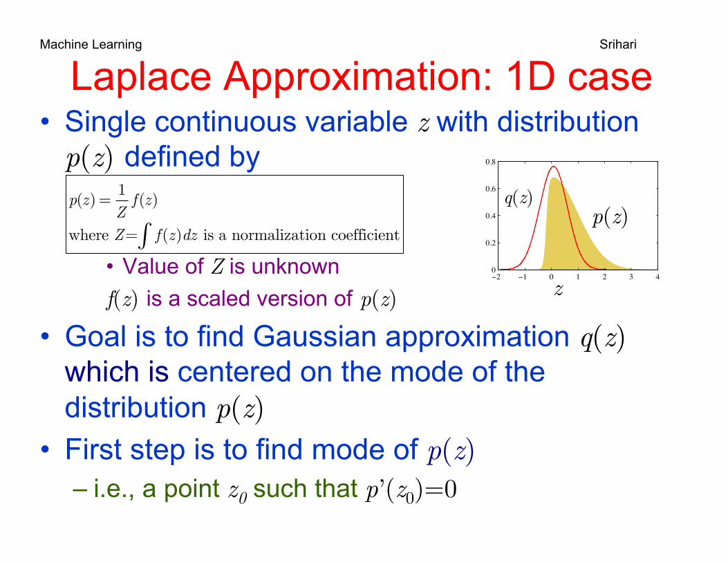
Laplace Approximation: 1D case •  Single continuous variable z with distribution

p(z) defined by

•  Value of Z is unknown f(z) is a scaled version of p(z)

•  Goal is to find Gaussian approximation q(z) which is centered on the mode of the distribution p(z)

•  First step is to find mode of p(z) –  i.e., a point z0 such that p’(z0)=0

p(z) =1Z

f (z)

where Z= f (z)dz ∫ is a normalization coefficient

!2 !1 0 1 2 3 40

0.2

0.4

0.6

0.8


q(z) p(z)

z

Quadratic using Taylor’s series •  A Taylor’s series expansion of f (x) centered

on the mode x0 has the power series

–  f (x) is assumed infinitely differentiable at x0 – Note that when x0 is the maximum f’(x0)=0 and

that term disappears •  A Gaussian f (x) has the property that lnf (x)

is a quadratic function of x – We will use a Taylor’s series approximation of the

function ln f (z) and use only the quadratic term


11

f (x) = f (x

0)+

f '(x0)

1!x −x

0( )+f ''(x

0)

2!x −x

0( )2+

f (3)(x0)

3!x −x

0( )3+ ...

Animation

Finding mode of a distribution •  Find point z0 such that p’(z0)=0,

– Or equivalently

•  Approximate f (z) using 2nd derivative p’’(z0) – Logarithm of Gaussian is a quadratic. – Use Taylor expansion of ln f (z)centered at mode z0

df (z)dz

z=z0

= 0

€

ln f (z) ≈ ln f (z0) − 12A(z − z0)2

where A = −d2

dz2 ln f (z)z= z0

First order term does not appear since z0 is a local maximum and f ’(z0)=0


A is the second derivative of logarithm of scaled p(z)

!2 !1 0 1 2 3 40

0.2

0.4

0.6

0.8

q(z) p(z)

z

Final form of Laplacian (one dim)

•  Taking exponential

•  To Normalize f (z) we need Z

• The normalized version of f(z) is q(z) = 1

Zf (z) = A

2π!

"#

$

%&1/2

exp −A2(z− z0 )

2()*

+,-~ N(z | z0,A

−1)

€

f (z) ≈ f (z0)exp −A2(z − z0)

2$ % &

' ( )


•  Approximation of f(z):

Z = f(z)dz∫ ≈ f(z0) exp -

A2

(z - z0)2⎧

⎨⎩

⎫⎬⎭∫ dz = f(z0)

(2π)1/2

A1/2

Assuming ln f(z) to be quadratic

€

ln f (z) ≈ ln f (z0) − 12A(z − z0)2

where A = −d2

dz2 ln f (z)z= z0

Laplace Approximation Example

!2 !1 0 1 2 3 40

0.2

0.4

0.6

0.8

14

!2 !1 0 1 2 3 40

10

20

30

40

p(z)

Mode of p(z)

Laplace Approx (Gaussian)

Negative Logarithms


Gaussian approximation will only be well-defined if its precision A>0, or second derivative of f (z) at point z0 is negative

Applied to distribution where is sigmoid

p(z)α exp(−z2 / 2)σ (20z + 4)

σ

f (z) = exp(−z 3 / 2)σ(20z + 4)

Z = f (z)dz∫

Laplace’s Method •  Approximate integrals of the form

– Assume f(x) has global maximum at x0•  Then f(x0) >> other values of f(x)

– with eMf(x) growing exponentially with M

•  So enough to focus on f(x) at x0

•  As M increases, integral is well-approximated by a Gaussian

•  Second derivative appears in denominator •  Proof involves Taylor’s series expansion of

f(x) at x0


15

eMf (x )a

b

∫ dx

M=0.5

M=3

Laplace Approx: M-dimensions •  Task: approximate p(z)=f(z)/Z defined over

M-dim space z •  At stationary point z0 the gradient vanishes •  Expanding around this point

– where A is the M x M Hessian matrix

•  Taking exponentials


16

∇f (z )

ln f (z) ln f (z0 ) −

12(z − z0 )

T A(z − z0 )

A = −∇∇ ln f (z) |z=z0

f (z) f (z0 )exp −

12(z − z0 )

T A(z − z0 )"#$

%&'

Normalized Multivariate Laplacian

17

Z = f (z)dz∫

≈ f (z0 ) exp - 12

(z − z0 )T A(z − z0 )$%&

'()∫ dz

= f (z0 ) (2π )M /2

| A |1/2


q(z) = 1Zf (z) =

A 1/2

(2π )M /2 exp −12

(z − z0 )T A(z − z0 )#$%

&'(

=N(z|z0,A-1)

•  Distribution q(z) is proportional to f(z) as

Steps in Applying Laplace Approx.

1.  Find the mode z0

– Run a numerical optimization algorithm 2.  Evaluate Hessian matrix A at that mode

•  Many distributions encountered in practice are multimodal – There will be different approximations according to

which mode considered – Z of the true distribution need not be known to apply

Laplace method


18

Weakness of Laplace Approx.

•  Directly applicable only to real variables – Based on Gaussian distribution

•  May be applicable to transformed variable –  If 0≤τ<∞ then consider Laplace approx of ln τ

•  Based purely on a specific value of the variable •  Variational methods have a more global

perspective


19

Approximating Z

20


•  As well as approximating the distribution p(z) we can also obtain an approximation to the normalizing constant Z

•  Can use this result to obtain an approximation

to model evidence that plays a central role in Bayesian model comparison

Z = f (z)dz∫ ! f (z0 ) exp − 1

2(z − z0 )T A(z − z0 )⎧

⎨⎩

⎫⎬⎭∫ dz

=f (z0 ) (2π )M /2

| A |1/2

Model Comparison and BIC

21


•  Consider data set D and models {Mi} having

parameters {θi} •  For each model define likelihood p(D|θi,Mi) •  Introduce prior p(θi|Mi) over parameters •  Need model evidence p(D|Mi) for various

models

Model Comparison and BIC

22

p(D) = p(D |θ)p(θ)dθ∫

For a given model from sum rule


ln p(D)=ln f (θ)dθ∫

=ln f (θmap ) (2π )M /2

| A |1/2

$

%&

'

()

= lnp(D|θmap ) + ln p(θmap ) + M2

ln2π − 12

ln | A |

Identifying f(θ)=p(D|θ)p(θ) and Z=p(D) and using Z = f (z0 )(2π )M /2

| A |1/2

where θmap is the value of θ at the mode of the posterior A is Hessian of second derivatives of negative log posterior

Occam factor that penalizes model complexity

Bayes Information Criterion (BIC)

•  N is the number of data points •  M is the no of parameters in θ •  Compared to AIC given by ln p(D|wML)-M BIC penalizes model complexity more heavily


23

lnp(D) ≈ lnp(D|θmap) -

12M lnN

Assuming broad Gaussian prior over parameters & Hessian is of full rank, approximate model evidence is

Weakness of AIC, BIC

•  AIC and BIC are easy to evaluate •  But can give misleading results since

– Hessian matrix may not have full rank since many parameters not well-determined

•  Can obtain more accurate estimate from

•  Used in the context of neural networks


24

ln p(D)= lnp(D|θmap ) + ln p(θmap ) + M2

ln2π − 12

ln | A |

Summary •  Bayesian approach for logistic regression is

more complex than for linear regression – Since posterior over w is not Gaussian

•  Predictive Distribution needs an integral over parameters – Simplified when Gaussian

•  Laplace approximation fits the best Gaussian – Defined for both univariate and multivariate

•  Normalization term is useful as BIC criterion •  AIC and BIC are simple but not accurate


25

University at Buffalo, State University of New York USAsrihari/CSE574/Chap4/4.4-Laplace.pdf ·...

Documents

Transcript of University at Buffalo, State University of New York USAsrihari/CSE574/Chap4/4.4-Laplace.pdf ·...