Universität Tübingen - uni-goettingen.de Küchlin, WSI und STZ OIT, Uni Tübingen 28.07.2015 2 SR...

SR

Automated Theorem Proving – Foundations of SAT-Solving –

July 2015

Wolfgang Küchlin

Symbolic Computation Group Wilhelm-Schickard-Institute of Informatics

Faculty of Mathematics and Sciences

Universität Tübingen

Steinbeis Transferzentrum Objekt- und Internet-Technologien (OIT)

[email protected] http://www-sr.informatik.uni-tuebingen.de

Wolfgang Küchlin, WSI und STZ OIT, Uni Tübingen 28.07.2015 2 SR

Contents

Propositional Resolution Theorem Proving by Deduction From 2 clauses C1 and C2, deduce new resolvent clause R

where C1 ∧ C2 ⊨ R, hence {C1, C2 } ≡ {C1, C2, R } Prove SAT(ℱ)=false by deducing ⊥ (represented by unsatis-

fiable empty clause { } =: □) since ℱ ≡ ℱ ∪ { } ≡ ℱ ∧ ⊥ ≡ ⊥

Elementary DPLL SAT-Solving The historical Davis-Putnam-Logemann-Loveland Method Compute SAT(F) in place by

• Trying some variable assignment x=true • Computing other variable assignments as immediate consequences • Carrying on, until success, or backtracking to x=false.


The Resolution Rule

(sole) inference rule:

where C´ = C ⋃ {ℓ} and D´ = D ⋃ {¬ℓ} are clauses. The resolvent R = C ⋃ D is deduced by resolving parent clauses

C´ and D´ on the literal ℓ. We write {C´, D´} ⊢ R. Examples:

ResDC

}{D}{C∪

¬∪∪

v}{x,u}{v}u,{x,

v}u,y,{x,z}v,{u,z}y,{x,

¬¬¬

¬¬¬


Example: Resolution proof-tree

F3={{x,y},{x,¬y,z},{¬x},{¬y,¬z}} {x,y} {x,¬y,z} {x,z} {¬x} {x,y} {¬x} {z} {¬y,¬z} {y} {¬y} □


Clauses and Implications, Soundness, Completeness A clause embeds a variety of implications:

Example: (x ∨ y ∨ z) ≡ ¬(¬x ∧ ¬y) ∨ z ≡ (¬x ∧ ¬y → z) But also: (x ∨ y ∨ z) ≡ ¬(¬x) ∨ (y ∨ z) ≡ (¬x → y ∨ z)

Resolution represents deduction of implications Parent clauses (A ∨ x) and (B ∨ ¬x), resolvent (A ∨ B) (A ∨ x) ≡ (¬(¬A) ∨ x) ≡ (¬A → x) (B ∨ ¬x) ≡ (x → B) From (¬A → x) and (x → B) follows (¬A → B) ≡ (¬(¬A) ∨ B) ≡ (A ∨ B)

The resolution calculus is sound (sound). For all sets ℱ of clauses and all clauses D, we have: ℱ ⊢*Res D implies ℱ ⊨ D

Hence: ℱ ⊢*Res D implies ℱ ≡ ℱ ∪ D Theorem: the resolution calculus is refutation complete:

ℱ ⊨ ⊥ implies ℱ ⊢*Res □


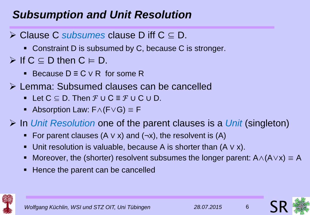
Subsumption and Unit Resolution

Clause C subsumes clause D iff C ⊆ D. Constraint D is subsumed by C, because C is stronger.

If C ⊆ D then C ⊨ D. Because D ≡ C ∨ R for some R

Lemma: Subsumed clauses can be cancelled Let C ⊆ D. Then ℱ ∪ C ≡ ℱ ∪ C ∪ D. Absorption Law: F∧(F∨G) ≡ F

In Unit Resolution one of the parent clauses is a Unit (singleton) For parent clauses (A ∨ x) and (¬x), the resolvent is (A) Unit resolution is valuable, because A is shorter than (A ∨ x). Moreover, the (shorter) resolvent subsumes the longer parent: A∧(A∨x) ≡ A Hence the parent can be cancelled


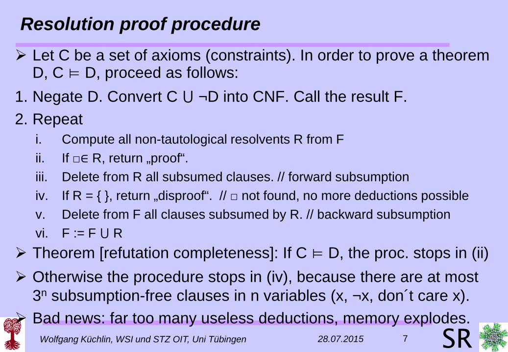
Resolution proof procedure Let C be a set of axioms (constraints). In order to prove a theorem

D, C ⊨ D, proceed as follows: 1. Negate D. Convert C ⋃ ¬D into CNF. Call the result F. 2. Repeat

i. Compute all non-tautological resolvents R from F ii. If □∈ R, return „proof“. iii. Delete from R all subsumed clauses. // forward subsumption iv. If R = { }, return „disproof“. // □ not found, no more deductions possible v. Delete from F all clauses subsumed by R. // backward subsumption vi. F := F ⋃ R

Theorem [refutation completeness]: If C ⊨ D, the proc. stops in (ii) Otherwise the procedure stops in (iv), because there are at most

3n subsumption-free clauses in n variables (x, ¬x, don´t care x). Bad news: far too many useless deductions, memory explodes.


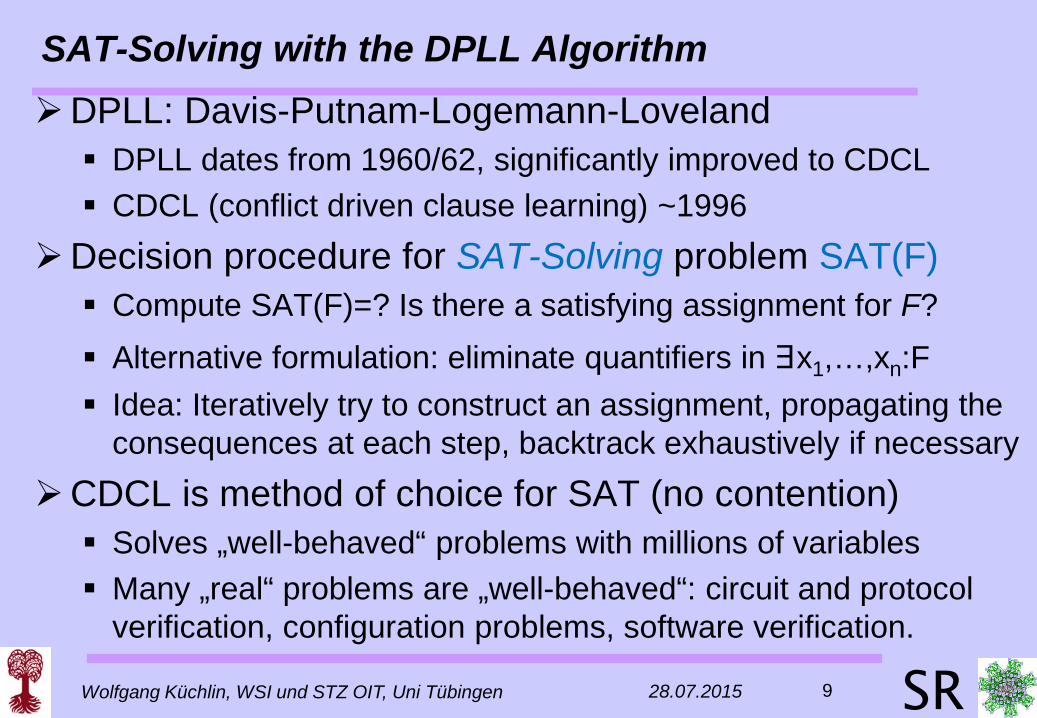
SAT-Solving with the DPLL Algorithm DPLL: Davis-Putnam-Logemann-Loveland DPLL dates from 1960/62, significantly improved to CDCL CDCL (conflict driven clause learning) ~1996

Decision procedure for SAT-Solving problem SAT(F) Compute SAT(F)=? Is there a satisfying assignment for F? Alternative formulation: eliminate quantifiers in ∃x1,…,xn:F Idea: Iteratively try to construct an assignment, propagating the

consequences at each step, backtrack exhaustively if necessary CDCL is method of choice for SAT (no contention) Solves „well-behaved“ problems with millions of variables Many „real“ problems are „well-behaved“: circuit and protocol

verification, configuration problems, software verification.


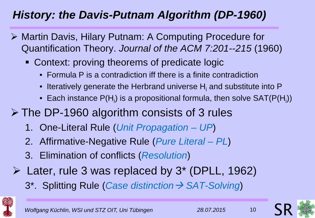
History: the Davis-Putnam Algorithm (DP-1960)

Martin Davis, Hilary Putnam: A Computing Procedure for Quantification Theory. Journal of the ACM 7:201--215 (1960) Context: proving theorems of predicate logic

• Formula P is a contradiction iff there is a finite contradiction • Iteratively generate the Herbrand universe Hi and substitute into P • Each instance P(Hi) is a propositional formula, then solve SAT(P(Hi))

The DP-1960 algorithm consists of 3 rules 1. One-Literal Rule (Unit Propagation – UP) 2. Affirmative-Negative Rule (Pure Literal – PL) 3. Elimination of conflicts (Resolution)

Later, rule 3 was replaced by 3* (DPLL, 1962) 3*. Splitting Rule (Case distinction SAT-Solving)



Rule 1 (One-Literal Clauses) a) F is inconsistent, if it contains two unit clauses {p} and {¬p} b) Else, if F contains a unit clause {p}, then delete all clauses

containing p, and delete ¬p from all clauses. The result F´ is inconsistent iff F is inconsistent. a) The case of a unit clause {¬p} is analogous to (b). If F´ is empty, then F is consistent.

• All clauses were deleted, hence all are satisfied.

Rule 2 (Affirmative-Negative Rule) If an atom p appears only positively (affirmative) or only

negatively, then delete all clauses containing p. The result F´ is inconsistent iff F is inconsistent. If F´ is empty, then F is consistent.



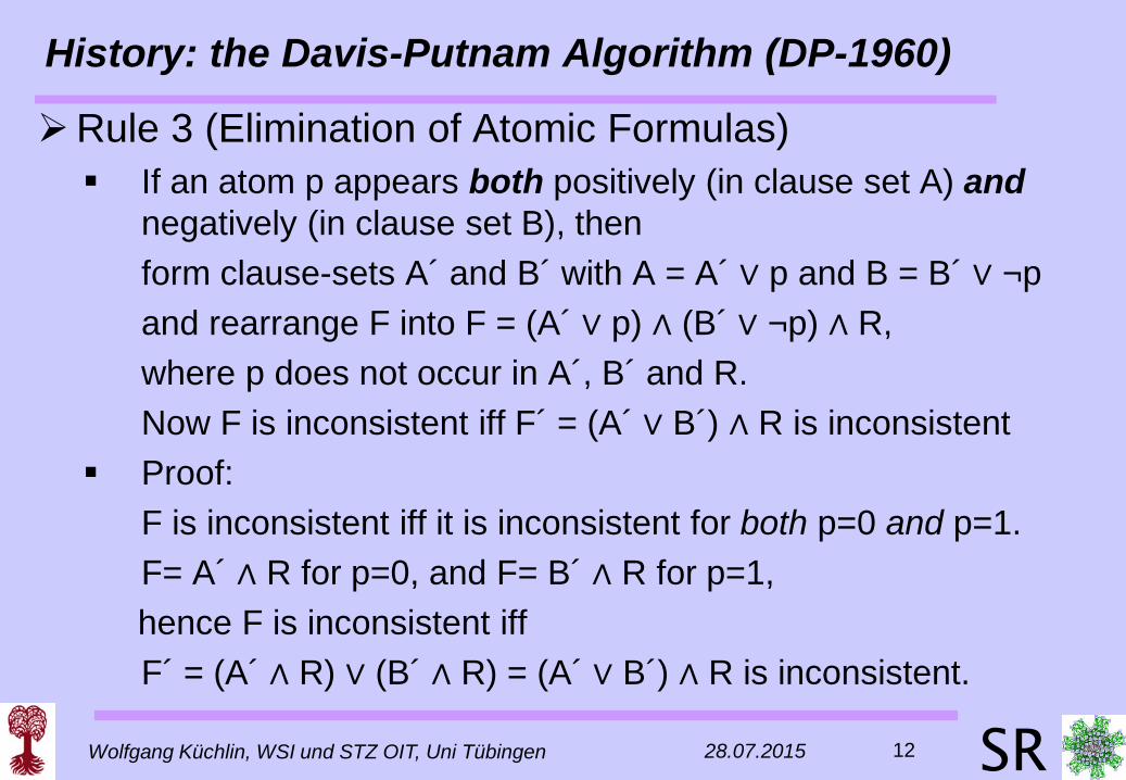
Rule 3 (Elimination of Atomic Formulas) If an atom p appears both positively (in clause set A) and

negatively (in clause set B), then form clause-sets A´ and B´ with A = A´ ∨ p and B = B´ ∨ ¬p and rearrange F into F = (A´ ∨ p) ∧ (B´ ∨ ¬p) ∧ R, where p does not occur in A´, B´ and R. Now F is inconsistent iff F´ = (A´ ∨ B´) ∧ R is inconsistent Proof: F is inconsistent iff it is inconsistent for both p=0 and p=1.

F= A´ ∧ R for p=0, and F= B´ ∧ R for p=1, hence F is inconsistent iff F´ = (A´ ∧ R) ∨ (B´ ∧ R) = (A´ ∨ B´) ∧ R is inconsistent.



Implementation of Rule 3 (Eliminating Atomic Formulas) Rearrange F into F = (A´ ∨ p) ∧ (B´ ∨ ¬p) ∧ R F is inconsistent iff F´ = (A´ ∨ B´) ∧ R is inconsistent In short: factor out p and resolve on p. (A´ ∨ B´) consists of all

resolvents between clauses in A and clauses in B. • Ex.: (a ∨ p) ∧ (b ∨ p) ∧ (c ∨ ¬p) ∧ (d ∨ ¬p) = [(a ∧ b) ∨ p] ∧ [(c ∧ d) ∨ ¬p]

Form (a ∧ b) ∨ (c ∧ d) = (a ∨ c) ∧ (a ∨ d) ∧ (b ∨ c) ∧ (b ∨ d). These are exactly the resolvents. The parent clauses can be deleted: if (a ∧ b) is satisfied in F´, then F is satisfied by additionally setting p=0, and analogously, if (c ∧ d) is satisfied in F´, then we may set p=1 to satisfy F.

Rule 3 yields a quantifier elimination (QE) procedure ∃p,x1,…,xn:F ≡ ∃x1,…,xn:F´ ≡ …. ≡ B, where B∈ {⊤,⊥}

Bad news: clauses get longer, and clause set explodes, and F´ = (A´ ∨ B´) ∧ R is no longer in CNF, needs fresh CNF conversion


Example: the Davis-Putnam Algorithm (DP-1960)

The DP-Algorithm consists of 3 rules 1. One-Literal (Unit Propagation – UP) 2. Affirmative-Negative (Pure Literal – PL) 3. Elimination of conflicts (Resolution)

Example S0 = {{x, y, z}, {¬x, y, z}, {¬x}, {z, ¬y}} 1c (UP of ¬x): S1 = {{y, z}, {z, ¬y}} 3 (resolution on y): S2 = {{z}, {z}} = {{z}} 2 (PL of z}: S3 = { }, hence consistent.

Rule 3 renders DP-1960 inefficient In order to eliminate p from F, ALL resolvents over p have to be

computed. This leads to an explosion of new clauses.


The Davis-Logemann-Loveland Algorithm (DPLL 1962) Martin Davis, George Logemann, and Donald Loveland. A Machine Program for

Theorem Proving. Communications of the ACM 5:394—397 (1962).

Rule 3* (Splitting Rule, replaces Rule 3) If p occurs both positively and negatively in F, rearrange F into

F = (A ∨ p) ∧ (B ∨ ¬p) ∧ R, where p does not occur in R. F is inconsistent iff both (A ∧ R) and (B ∧ R) are inconsistent Proof: F is inconsistent iff it is inconsistent for both p=0 and for

p=1. Now F= A ∧ R for p=0, and F= B ∧ R for p=1. Implementation of Rule 3* Set p=1 and p=0 one after another in F (e.g. as unit clauses) Do not form new clauses, instead perform unit propagation. Clauses are shortened, sometimes eliminated, the problem is

simplified, especially through unit propagation.


History: The Davis-Logemann-Loveland Algorithm


The DPLL Algorithm (of 1962)

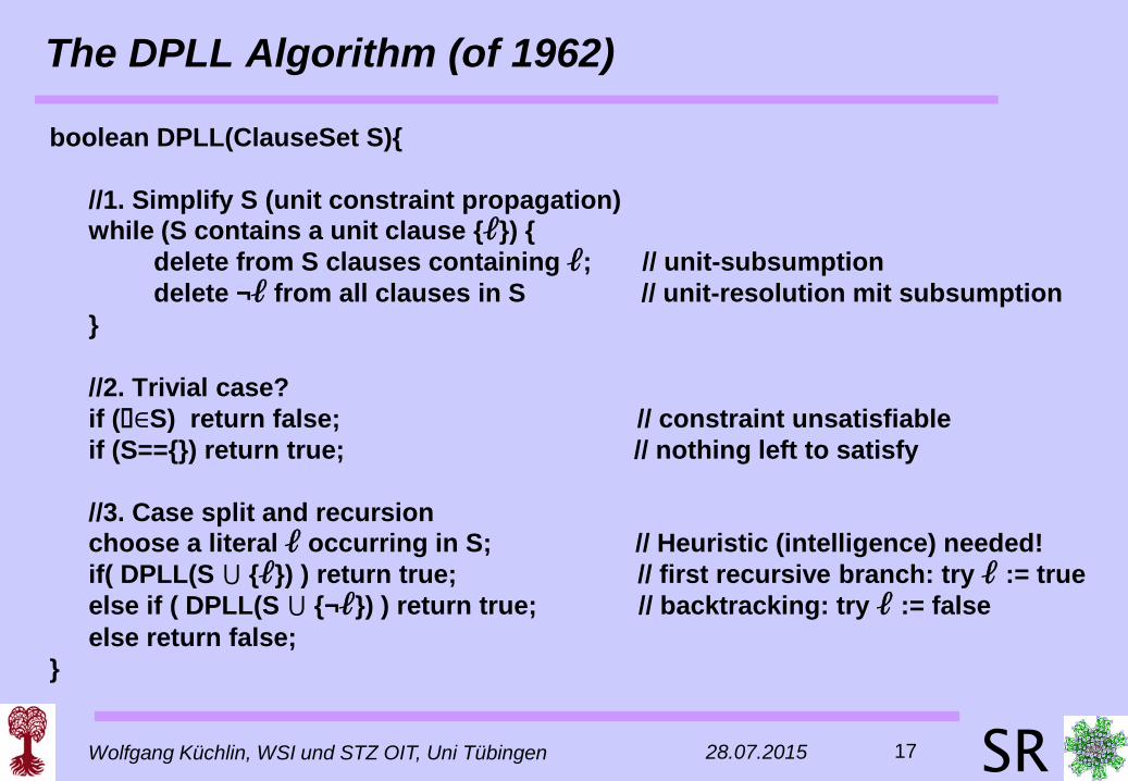
boolean DPLL(ClauseSet S){ //1. Simplify S (unit constraint propagation) while (S contains a unit clause {ℓ}) { delete from S clauses containing ℓ; // unit-subsumption delete ¬ℓ from all clauses in S // unit-resolution mit subsumption } //2. Trivial case? if (�∈S) return false; // constraint unsatisfiable if (S=={}) return true; // nothing left to satisfy //3. Case split and recursion choose a literal ℓ occurring in S; // Heuristic (intelligence) needed! if( DPLL(S ⋃ {ℓ}) ) return true; // first recursive branch: try ℓ := true else if ( DPLL(S ⋃ {¬ℓ}) ) return true; // backtracking: try ℓ := false else return false; }


Observations for DPLL in practice

No deduction of new clauses No dynamic storage allocation

Algorithm lives (and dies) with unit propagation UP dominates run-time in practice (> 90% UP). This is necessarily so:

• With 100 variables there are 2100 cases without UP • With complete UP there are only 99 propagations • Typical value in practice: 90 propagations, 210 remaining cases

Lesson from practice (and secret behind DPLL) Only few decisions are essential, the remaining cases follow

as immediate consequences, ruling out many theoretical alternatives.


Example: SAT-Solving with DPLL

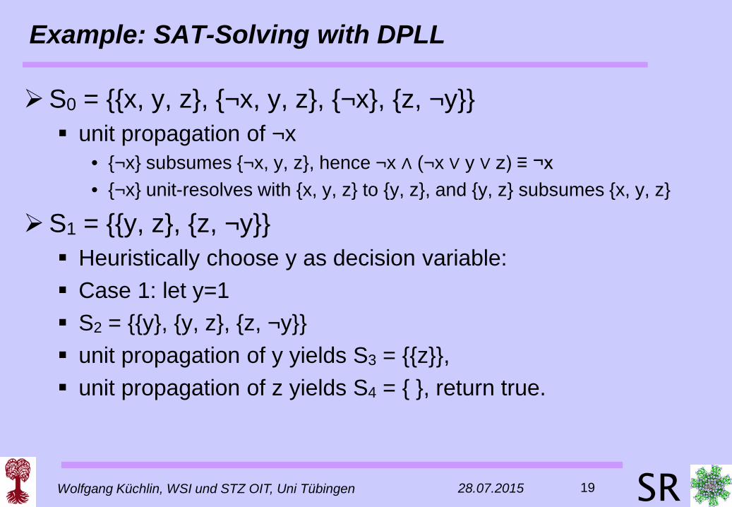
S0 = {{x, y, z}, {¬x, y, z}, {¬x}, {z, ¬y}} unit propagation of ¬x

• {¬x} subsumes {¬x, y, z}, hence ¬x ∧ (¬x ∨ y ∨ z) ≡ ¬x • {¬x} unit-resolves with {x, y, z} to {y, z}, and {y, z} subsumes {x, y, z}

S1 = {{y, z}, {z, ¬y}} Heuristically choose y as decision variable: Case 1: let y=1 S2 = {{y}, {y, z}, {z, ¬y}} unit propagation of y yields S3 = {{z}}, unit propagation of z yields S4 = { }, return true.


Variable Selection Heuristics for DPLL

Some Heuristics for variable selection: Coose the literal which occurs most often.

• Then the formula is simplified in the most places

Choose a literal L from 2-clause (binary clause) {K, ¬L}. • Then K=1 if L=1, resp. L=0 if K=0, because clause encodes (L → K) • Clever choice of K resp. L immediately leads to UP, eliminating a decision

Choose a literal from a short(est) clause. • Will soon produce a binary clause, then a UP

For each literal L, compute how F would be shortened by UP after assigning L. Choose that L which has the greatest effect.

• This simplifies F most before the next decision.


Correctness of DPLL

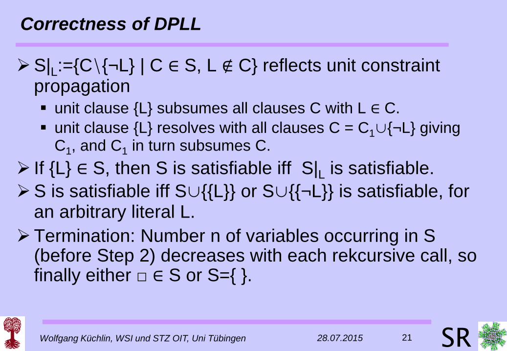
S|L:={C∖{¬L} | C ∈ S, L ∉ C} reflects unit constraint propagation unit clause {L} subsumes all clauses C with L ∈ C. unit clause {L} resolves with all clauses C = C1∪{¬L} giving

C1, and C1 in turn subsumes C. If {L} ∈ S, then S is satisfiable iff S|L is satisfiable. S is satisfiable iff S∪{{L}} or S∪{{¬L}} is satisfiable, for

an arbitrary literal L. Termination: Number n of variables occurring in S

(before Step 2) decreases with each rekcursive call, so finally either □ ∈ S or S={ }.


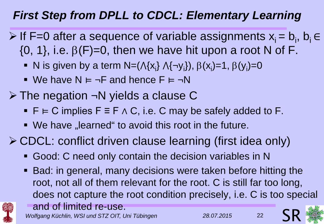
First Step from DPLL to CDCL: Elementary Learning

If F=0 after a sequence of variable assignments xi = bi, bi ∈ {0, 1}, i.e. β(F)=0, then we have hit upon a root N of F. N is given by a term N=(⋀{xi} ⋀{¬yi}), β(xi)=1, β(yi)=0 We have N ⊨ ¬F and hence F ⊨ ¬N

The negation ¬N yields a clause C F ⊨ C implies F ≡ F ∧ C, i.e. C may be safely added to F. We have „learned“ to avoid this root in the future.

CDCL: conflict driven clause learning (first idea only) Good: C need only contain the decision variables in N Bad: in general, many decisions were taken before hitting the

root, not all of them relevant for the root. C is still far too long, does not capture the root condition precisely, i.e. C is too special and of limited re-use.


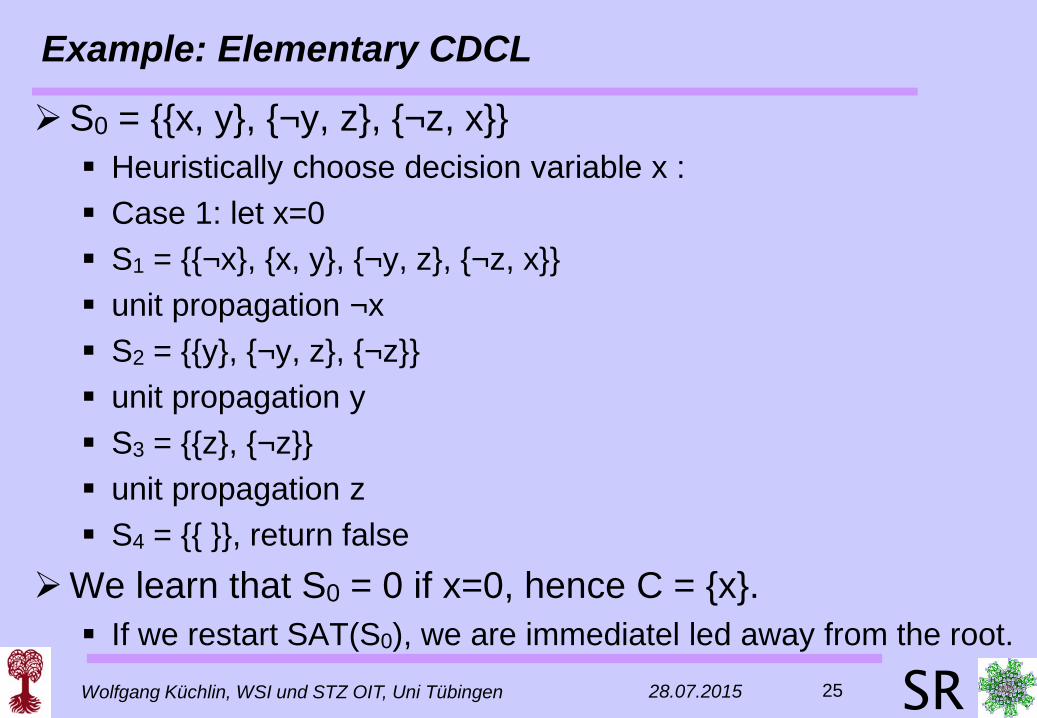
Example: Elementary CDCL

S0 = {{x, y}, {¬y, z}, {¬z, x}} Heuristically choose decision variable x : Case 1: let x=0 S1 = {{¬x}, {x, y}, {¬y, z}, {¬z, x}} unit propagation ¬x S2 = {{y}, {¬y, z}, {¬z}} unit propagation y S3 = {{z}, {¬z}} unit propagation z S4 = {{ }}, return false

We learn that S0 = 0 if x=0, hence C = {x}. If we restart SAT(S0), we are immediatel led away from the root.


Example: Elementary CDCL

Analysis of example S0 = {{x, y}, {¬y, z}, {¬z, x}} x y z S0

0 0 0 0 0 0 1 0 0 1 0 0 0 1 1 0 1 0 0 1 1 0 1 1 1 1 0 0 1 1 1 1

In the future, the learned clause C = {x} directs us away from any of those 4 roots E.g. after a fresh call and attempted propagations ¬z und ¬y

From the previous variable assignments we learned: we hit the root N=(x=0, y=1, z=1).

Since x was the only decision variable, we further learn that N is part of a cluster of 4 roots.


Principle of Learning in CDCL

Key insight: start learning process with conflict clause K Conflict clause (failure clause) K is the clause which becomes

empty in Step 2 of DPLL, i.e. β(K)=0, which is always due to a unit propagation in Step 1 (decisions never fail a clause).

As a consequence of a decision, some clause R („reason“-clause) became unit and forced L=1 for a literal L in R.

As an immediate consequence, K failed, i.e. the sole remaining literal L´ in unit clause K was forced to L´=0.

Hence L und L´ are complementary literals and R and K have a resolvent without this literal. Since K and R were unit, this resolvent is also a failure clause K´ (under the current assignment).

Now iterate the process …. (there are still some open details)


Example: Principle of Learning in CDCL

S0 = {{x, y}, {¬y, z}, {¬z, x}} Heuristically choose decision variable x: Case 1: Let x=0 S1 = {{¬x}, {x, y}, {¬y, z}, {¬z, x}} unit propagation ¬x (reason for ¬x is decision x=0) S2 = {{y}, {¬y, z}, {¬z}} unit propagation y (reason for y is R1={x, y}). S3 = {{z}, {¬z}}. unit propagation z (reason for z is R2={¬y, z})) S4 = {{ }}, return false (failure clause is K={¬z, x})

We have β({¬z, x}) = 0. Resolution with R2= {¬y, z} yields {¬y, x}, further resolution with R1= {x, y} yields K´={x}.


Example: Principle of Learning in CDCL

Analysis of Example S0 = {{x, y}, {¬y, z}, {¬z, x}} x y z S0

0 0 0 0 0 0 1 0 0 1 0 0 0 1 1 0 1 0 0 1 1 0 1 1 1 1 0 0 1 1 1 1

Future hits into cluster N´´= (x=0) (e.g. by a different UP sequence) are precluded by learned clause K´ = {x}.

From failure clause K={¬z, x} we learn: we hit the cluster of roots N=(x=0, z=1)

After resolution of K with R2={¬y, z} we learn {¬y, x}, i.e. N´= (x=0, y=1) is a ``neighboring´´ cluster of roots.

After resolution with R1={x, y} we learn {x} with cluster N´´= (x=0).


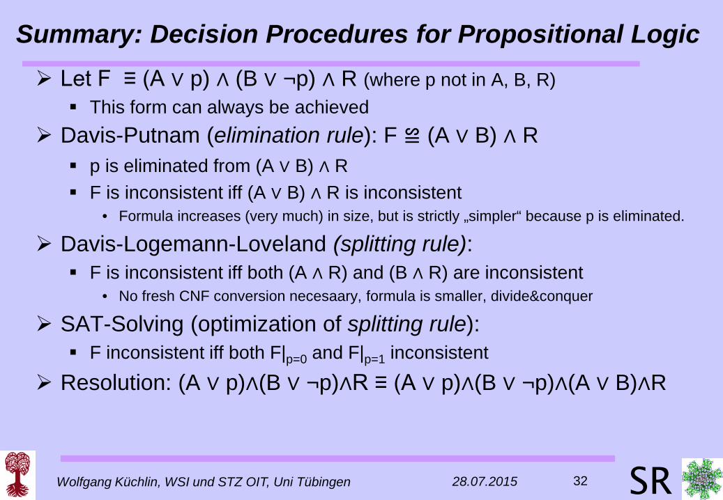
Summary: Decision Procedures for Propositional Logic Let F ≡ (A ∨ p) ∧ (B ∨ ¬p) ∧ R (where p not in A, B, R)

This form can always be achieved Davis-Putnam (elimination rule): F ≌ (A ∨ B) ∧ R

p is eliminated from (A ∨ B) ∧ R F is inconsistent iff (A ∨ B) ∧ R is inconsistent

• Formula increases (very much) in size, but is strictly „simpler“ because p is eliminated.

Davis-Logemann-Loveland (splitting rule): F is inconsistent iff both (A ∧ R) and (B ∧ R) are inconsistent

• No fresh CNF conversion necesaary, formula is smaller, divide&conquer

SAT-Solving (optimization of splitting rule): F inconsistent iff both F|p=0 and F|p=1 inconsistent

Resolution: (A ∨ p)∧(B ∨ ¬p)∧R ≡ (A ∨ p)∧(B ∨ ¬p)∧(A ∨ B)∧R

Universität Tübingen - uni-goettingen.de Küchlin, WSI und STZ OIT, Uni Tübingen 28.07.2015 2 SR...

Documents

Transcript of Universität Tübingen - uni-goettingen.de Küchlin, WSI und STZ OIT, Uni Tübingen 28.07.2015 2 SR...