UNIVERSITI PUTRA MALAYSIA

DEVELOPMENT AND APPLICATION OF A FINITE ELEMENT DISTRIBUTED RAINFALL RUNOFF SIMULATION MODEL

HUANG YUK FENG

FK 2000 57

DEVELOPMENT AND APPLICATION OF A FINITE ELEMENT DISTRIBUTED RAINFALL RUNOFF SIMULATION MODEL

By

HUANG ¥UK FENG

Thesis Submitted in Fulfilment of the Requirement for the Degree of Master of Science in the Faculty of Engineering

U niversiti Putra Malaysia

December 1000

Dedicated To

My Beloved Grandmother, Mother, Sisters, Brothers,

And In Memory of My Beloved Father

11

Abstract of thesis presented to the Senate ofUniversiti Putra Malaysia in fulfilment of the requirement for the degree of Master of Science

DEVELOPMENT AND APPLICATION OF A FINITE ELEMENT DISTRIBUTED RAINFALL-RUNOFF SIMULATION MODEL

By

HUANG YUK FENG

December 2000

Supervisor : Ir. Dr. Lee Teang Sbui

Faculty : Engineering

A detenninistic model to simulate rainfall runoff from pervious and

impervious swfaces is presented. With precipitation excess as input, the swface

runoff model is based on a one-dimensional, variable width, kinematic wave

approximation to the St Venanfs equation and Manning's equation, and was used

to mathematically route overland and channel flow using the finite element

method. The Galerkin's residual finite element formulation utilizing linear and

quadratic one-dimensional Lagrangian elements is presented for the spatial

discretization of the nonlinear kinematic runoff equations. Temporal excess rainfall

discretization using linear transition over two time steps was used to eliminate

abrupt discontinuities in excess rainfall intensities. The system of nonlinear

equations was solved using successive substitutions employing Thomas algorithm

and Gaussian elimination. The whole formulation was set up using the MapBasic

and Map Info Geographical Information System.

111

A laboratory rainfall runoff physical model was set up for observation data

in order to test the numerical model. Parameters considered include, surface

roughness, plane slope, constant or changing rainfall intensities. Maximum

infiltration, overland flow discharge, and overland with channel flow discharge

were observed for model verification. Finite element simulations have been shown

to compare favourably with observed laboratory data. Linear element simulation

was found to give results as accurate as the quadratic element simulation. The

increased number of elements employed in the model to simulate runoff from a

homogenous surface did not give any obvious added advantage. While maximum

time step increment for computation is given by the Courant Criterion, it is

however, always recommended that as small a time increment is to be used to

eliminate any oscillatory instability. Time increment for channel flow routing was

found to be always smaller when compared to lateral overland flow. Thus, the

chosen time step increment for channel flow routing must be a common factor of

that of lateral overland flow in order to satisiY the linear interpolation of overland

outflow hydrograph as input into the channel. For laboratOly scale catchments,

problems of big physical elemental interface roughness differences (eg. 0.033 for

bare soil surface upstream and 0.300 for grass surface downstream) can result in

small wavy oscillatory at the rising limb. On the contrary, when the upstream

roughness is larger then the downstream TOughness, such discrepancies do not

appear in the simulation. Differences in elemental interface slope (eg. 5% and 10%

bare soil surfaces) can be catered for rather well in the model.

A hypothetical watershed and imaginary tropical rainstorm was also studied

to veriiY the capability of the model in larger runoff catchments. Channels, which

iv

are initially dry or with existing flows can be simulated incorporating additional

rainfiill. Large catchments with large physical elemental roughness and slope

differences can be well simulated by the model to give typical hydrograph

characteristics, without oscillations, evident in laboratory scale tests.

v

Abstrak tesis yang dikemukakan kepada Senat Universiti Putra Malaysia sebagai memenuhi keperluan untuk Ijazah Master Sains

PEMBANGUNAN DAN PENGGUNAAN MODEL UNSUR TERHINGGA TERAGIH PENYELAKUAN UUJAN-AIR LARIAN

Oleh

HUANG YUK FENG

Disember 2000

Penyelaras : Ir. Dr. Lee Teang Shui

Fakulti : Kejuruteraan

Sebuah model berketentuan demi untuk menyelaku air larian hujan dari

permukaan telap dan tak telap telah dikemukakan. Dengan kelebihan hujan sebagai data

masukan ke dalam model, model air larian permukaan adalah berdasarkan pendekatan

ombak-kinematik kepada persamaan St Venant yang berdimensi satu, lebar bolehubah

dan persamaan Manning. lanya digunakan untuk mengira seeara matematik, aliran

permukaan dan aHran saluran dengan kaedah unsur terhingga. Formulasi unsur terhingga

berbaki Galerkin berdasar unsur-unsur Lagrangian satu dimensi lelurus dan kuadratik

dipersembahkan demi untuk pembahagian secara ruang persamaan air larian kinematik

tak Ielurus. Pembahagian kelebihan hujan semasa dengan menggunakan peralihan lelurus

diantara dua langkah masa berturutan digunakan untuk menghapuskan dadakan yang

disebabkan tak berterusan dalam kelebihan hujan. Sistem persamaan tak lelurus

diselesaikan dengan menggunakan penggantian berturut-turut berasas algoritma Thomas

VI

dan penghapusan Gaussian. Pembentukan persamaan-persamaan keseluruhannya

diaturcarakan dengan MapBasic dan Sistem Matlumat Geografi, MapInfo.

Sebuah model air larian hujan fizikal makmal dibentukkan demi untuk menguji

kebolehan model. Parameter-parameter yang dipertimbangkan termasuk kekasaran

permukaan, kecerunan, keamatan hujan tetap atau berubah-ubah. Penyusupan maxima,

hasil larian air permukaan dan hasil larian air saluran serta permukaan dicerapkan untuk

pengesahan model. Kaedah penyelakuan unsur terhingga telah menunjukkan

perbandingan yang baik dengan data makmal. Penyelakuan unsur lelurus menghasilkan

keputusan setepat penyelakuan unsur kuadratik. Pertambahan bilangan unsur yang

digunakan dalam model tidak menunjukkan sebarang kelebihan. Sementara nilai langkah

masa tokokan untuk pengiraan dalam model boleh dikirakan mengikut Kriteria Courant,

ianya disyorkan langkah masa yang lebih kecil boleh digunakan demi untuk

menghapuskan ketakstabilan ayunan. Nilai tokokan masa untuk aliran saluran adalah

sentiasa lebih keeil dibandingkan dengan nilai yang digunakan pada permukaan sisi. Oleh

sebab itu, pilihan tokokan masa untuk saluran mestilah merupakan factor sepunya kepada

yang digunakan untuk aliran permukaan sisi, demi untuk memenuhi kehendak interpolasi

lelurus bagi grathidro sebagai data masukan ke dalam saluran. Bagi tadahan berskalar

makmal, masalah penggunaan dua nilai kekasaran yang berlainan untuk unsur-unsur

berdekatan (contohnya, 0.300 untuk permukaan rumput dan 0.033 untuk permukaan

tanah terdedah) ialah berlakunya dadakan pada lengkung menaik grathidro. Sebaliknya,

perbezaan kecerunan permukaan diantara dua unsur (contohnya, 5% dan 10% kecerunan

untuk permukaan tanah terdedah) boleh diatasi dengan baik dalam model.

vii

Sebuah kawasan tadahan hipotesis dan andaian hujan tropikal juga dikaji untuk

membuktikan kebolehan model untuk kawasan yang sewajah. Saluran-saluran yang pada

awalnya dalam keadaan yang kering atau berair boleh dipenyelakukan bersamaan dengan

hujan tambahan yang masuk padanya. Tadahan besar yang berair, kekasaran unsur dan

kecerunan fizikal yang perbezaannya besar boleh diramalkan dengan model dan

menghasilkan sebuah grafhidro yang khusus tanpa dadakan yang sentiasa wujud dalam

kajian makmal.

viii

ACKNOWLEDGEMENTS

First and foremost, I would like to express my sincere appreciation and

gratitude to my project supervisor, Ir. Dr. Lee Teang Shui for his guidance and

help throughout the duration of this research.

I would like also to take this opportunity to thank my research committee

group members, Associate Professor Kwok Chee Van, Associate Professor Ir. Dr.

Mohd. Amin Mohd. Soom, and Ir. Dr. Hiew Kim Loi (Deputy Director-General I,

Department of Irrigation and Drainage Malaysia) for their valuable help and

support. I am indebted to the Universiti Putra Malaysia for funding this study

through the P ASCA scheme fellowsbip. I also wish to record my appreciation to

Associate Professor Dr. Shattri Mansor for bis valuable help as the chairman of my

viva examination.

Last but not least, I would like to extend my appreciation to my family for

their encouragement and support throughout my study at UPM.

ix

J certify that an Examination Committee met 011 19 December, 2000 to conduct the final examination of I-luang Yuk Feng, on his Master of Science thesis entitled "Development and Application of A Finite Element Distributed Rainfall Runoff Simulation Model" in accordance with Universiti Pertanian Malaysia (Higher Degree) Act 1980 and Universiti Pertanian Malaysia (Higher Degree) Regulations 1981 _ The committee recommends that the candidate be awarded the relevant degree_ Members of the Examination Committee are as follows:

SHA'f'fRI MANSOR, Ph.D Associate Professor Faculty of Engineering Universiti Putra Malaysia (Chairman)

JR. I,EE TEANG SHUI, Pb.D Faculty of Engineering Universiti Putra Malaysia (Member)

KWOK CHEE Y AN Associate Professor Faculty of Engineering Universiti Putra Malaysia (Member)

IR. MOHO. AMJN MOHO. SOOM, Ph.D Associate Professor I Faculty of Engineering Universiti Putra Malaysia (Member)

IR. "lEW KIM LOt, Ph.D Deputy Director-General I Department of Irrigation and Drainage MaJaysia (Member)

GHAZA J MOHA YIDIN, Pb.D. Profe or I Deputy Dean of Graduate School Universiti Putra Malaysia

Date: 2 1 DEC 2000

x

This thesis submitted to the Senate of Universiti Putra Malaysia has been accepted as fulfilment of the requirement for the degree of Master of Science.

� KAMISWA�.D. Associate Professor Deputy Dean of Graduate School Universiti Putra Malaysia

Date: 11 1 JAN 2001

xi

DECLARATION

I hereby declare that the thesis is based on my original work except for quotations and citations, which have been duly acknowledge. I also declare that it has not been previously or concurrently submitted for any other degree at UPM or other institutions.

HUANG YUK FENG

Date: �/,�/�

xii

TABLE OF CONTENTS

Page

DEDICATION ii ABSTRACT iii ABSTRAK vi ACKNO�EDGEMENTS IX APPROVAL SHEETS X DECLARATION FORM xii LIST OF TABLES xv LIST OF FIGURES xvi LIST OF PLATES xix LIST OF ABBREVIATIONS xx

CHAPTER

I INTRODUCTION 1 Background of Study 1 Statement of Problem 3 Objectives 5 Significance of Project 5 Scope ofWorlc 6

II LITERATURE REVIEW 7 Rainfall-Discharge Relationship 7 Hydrograph Analysis 10 brlilttation 12 Flow Routing 13

Saint-Venant Equations 15 Kinematics Wave Theory 19

Watershed Modeling 21

III MODEL DEVELOPMENT 30 Kinematics Wave Theory and Equations 31 Finite Element Method and Solution 33

Approximation for Overland and Channel Flows 33 Finite Element Formulation 36

Determination of Time Increment 48 Temporal Excess Rainfall Discretization 50 Structure of Model Package 51

xiii

IV LADORA TORY TESTING 54 Laboratory Apparatus and Ammgemelll 55

Rainfall Simulator 55 Runoff Basin 58 Discharge Measurement 60 Infiltration-Percolation Water Measurement 61

Experiment Procedure 62 Range of Experimental Conditions 64

V DATA INPUT AND PROGRAM EXECUTION 69 Data Input 69 Program Execution 74

VI RESULTS AND DISCUSSIONS 78 Laboratory Simulation Results and Discussion 78

Effective Rainfall 79 Time Increment Selection 86 Selection of Surface Roughness Used in the Simulation Results 91 Effects of Number of Elements and Element Length Used 93 Linear versus Quadratic Interpolation Function Models 98 Accuracy. Stability, and Convergence of the Simulated Results versus Observed Results 101

Natural Catchment 107 Varying Catchment Topography 110 Channels with Existing Flows 112

VII SUMMARY, CONCLUSIONS AND RECOMMENDATIONS 116 Summary 116 Conclusions 117 Recommendations 118

REFERENCES 120 APPENDICES 125 BIODATA OF THE AUTHOR 160

XlV

LIST OF TABLES

Table Page

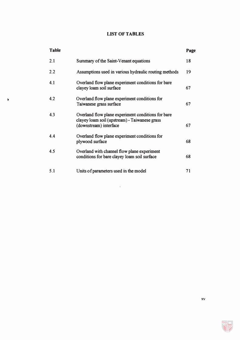
2. 1 Summary of the Saint-Venant equations 1 8

2.2 Assumptions used in various hydraulic routing methods 19

4. 1 Overland flow plane experiment conditions for bare clayey loam soil surface 67

4.2 Overland flow plane experiment conditions for Taiwanese grass surface 67

4.3 Overland flow plane experiment conditions for bare clayey loam soil (upstream) - Taiwanese grass (downstream) interface 67

4.4 Overland flow plane experiment conditions for plywood surface 68

4.5 Overland with channel flow plane experiment conditions for bare clayey loam soil surface 68

5.1 Units of parameters used in the model 7 1

xv

LIST OF FIGURES

Figure Page

2.1 Hydrograph corresponding to a long stonn 8

2.2 Components of the hydrograph 9

2.3 Hydrograph definition 1 1

3 . 1 Representations for Overland and Channel Flows 35

3.2 Finite Element Discretization 38

3.3 Finite element library 39

3.4 Excess rainfall linear transition 5 1

3.5 Flow-chart of model execution sequence 53

4. 1 Schematic diagram of the rainfiill-runoff laboratory physical model 56

4.2 Schematic diagram of sprinkler setting 57

5 . 1 An example of the digitized map of the laboratory setting with Maplnfo table 70

5.2 Table ofn, s, w, and L input for a 2-element overland flow strip 71

S.3 Excess rainfall input table in accordance to the linear transition method 72

5.4 MapBasic program execution for a 2-element channel 7S

5.5 Dialog Box for number of elements used 76

5.6 Error Message 76

5.7 Display of hydro graphs for different nodes 77

6 . 1 Excess Rainfall Hyetograph and Discharge Hydrograph for 5% slope bare soil (n = 0.033) overland flow with rainfiill intensity 2.67xlO·3 mlmin 80

6.2 Excess Rainfall Hyetograph and Discharge Hydrograph for 5% slope bare soil (n:= 0.033) overland flow with rainfilll intensity 2.67xlO-3, 2.25xlO-3, 1 .44xlO-3 mlmin 82

xvi

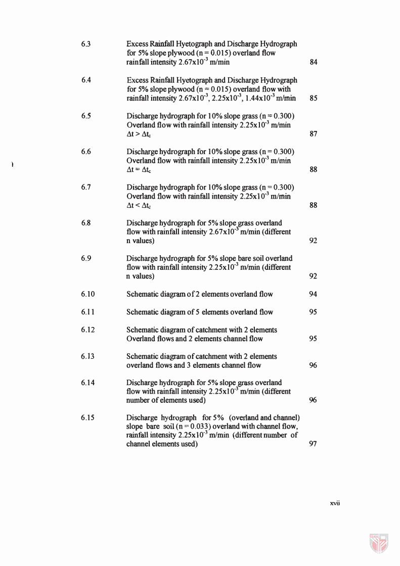
6.3 Excess Rainfall Hyetograph and Discharge Hydrograph for 5% slope plywood (n = 0.015) overland flow with rainfall intensity 2.67x1O-3 mlmin 84

6.4 Excess Rainfall Hyetograph and Discharge Hydrograph for 5% slope plywood (n:::;: 0.015) overland flow with rainfall intensity 2.67xl O·3, 2.25xlO·3, 1 .44xlO-3m1min 85

6.5 Discharge hydrograph for 1 0% slope grass (n ::;: 0.300) Overland flow with rainfall intensity 2.25xlO-3 mlmin .1t> .1tc 87

6.6 Discharge hydrograph for 10% slope grass (n = 0.300) Overland flow with rainfall intensity 2.25xI0-3 mlmin .1t:::;: .1tc 88

6.7 Discharge hydrograph for 10% slope grass (n:::;: 0.300) Overland flow with rainfall intensity 2.25xl 0-3 mlmin .1t <.1tc 88

6.8 Discharge hydro graph for 5% slope grass overland flow with rainfall intensity 2.67xlO-3 mlmin (different n values) 92

6.9 Discharge hydro graph for 5% slope bare soil overland flow with rainfall intensity 2.25xlO-3 mlmin (different n values) 92

6. 10 Schematic diagram of 2 elements overland flow 94

6. l 1 Schematic diagram of 5 elements overland flow 95

6.12 Schematic diagram of catchment with 2 elements Overland flows and 2 elements channel flow 95

6.13 Schematic diagram of catchment with 2 elements overland flows and 3 elements channel flow 96

6. 14 Discharge hydrograph for 5% slope grass overland flow with rainfall intensity 2.25xl 0-3 mlmin (different number of elements used) 96

6 . 15 Discharge hydrograph for 5% (overland and channel) slope bare soil (n = 0 .033) overland with channel flow, rainfall intensity 2.25xlO-3 mlmin (different number of channel elements used) 97

xvii

6.16 Discharge hydrograph for 5% slope grass overland flow with rainfall intensity 2.25xlO-3 mlmin, linear and quadratic 2 elements simulation 99

6.17 Discharge hydrograph for 5% slope grass overland flow with rainfall intensity 2.25xlO·3 mlmin, linear and quadratic 5 elements simulation 99

6.18 Discharge hydrograph for 5% (overland and channel) slope bare soil (n:::: 0.033) overland flow with channel flow, rainfall intensity 2.25xlO·3 mlmin, linear and quadratic 2 elements channel simulation 100

6.19 Illustrated of actual and assumed excess rainfall pattern 103

6.20 Discharge hydrograph for 5% slope bare soil (upstream, n == 0.033) and grass (downstream, n == 0.300) interface overland flow with rainfall intensity 2.25xI0· mlmin lOS

6.21 Discharge hydrograph for 5% slope bare soil (upstream, n = 0.033) and grass (downstream, n = 0.300) interface overland flow with rainfall intensity 2 .25xl 0.3 mlmin, two sets of different roughness 106

6.22 Schematic of a fictitious large natural catchment 107

6.23 Comparison of natural catchment hydrograph for two Different rainfall intensities 108

6.24 Oscillatory effects not evident in large scale overland component with different roughness coefficient values amongst the elements in the overland system 110

6.25 Oscillatory effects not evident in large scale overland component with different roughness coefficient values and slopes amongst the elements in the overland system 111

6.26 Oscillatory effects not evident in large-scale catchment with different roughness coefficient values and slopes amongst the elements in the channel system 112

6.27 Simulation of catchment discharge for channel without! with existing flows (lower volume) 113

6.28 Simulation of catchment discharge for channel without! with existing flows (higher volume) 114

xviii

LIST OF PLATES

Plate Page

4.1 RainfaJ)-runofflaboratory model with rainfall simulator 57

4.2 Water pump, water tanks, and gate and ball valves 58

4.3 Runoff basin for overland flow simulation 59

4.4 Runoffbasin for overland with channel flow simulation 60

4.5 Surface runoff collection 61

4.6 Infiltration-percolation collection 62

4.7 Runoffbasin with bare clayey loam soil surface 65

4.8 Runoffbasin with Taiwanese Grass surface 65

4.9 Runoffbasin with bare clayey loam soil (upstream)-Taiwanese grass (downstream) interface 66

xix

Qfc Qfo Q A P w R 1. ERF V N q S n n � L\t L\tc 1:c lmax 1

NOTATION

Channel Flow Overland Flow Discharge Wetted Area Channel Wetted Area Perimeter Overland Element Width Hydraulic Radius Element Length Excess Rainfall Flow Velocity Interpolation Function Lateral Inflow Plane Slope Roughness Coefficient Number of Nodes In An Element The Smallest Element Length Time Increment Courant Time Increment Time of Concentration Maximum Rainfall Intensity Rainfall Intensity

xx

CHAPTER 1

INTRODUCTION

Background of Study

The objective of a hydrologic system analysis is to study the system

operations and predict its output, for example, an outflow hydrograph. In general, a

hydrologic system model is an approximation of the actual system, in which its

inputs and outputs are measurable hydrologic variables and are linked by a set of

equations. The hydrologic system's synthesis and prediction are the most essential

activities in '.he design of water resources systems.

The derivation of relationship between the rainfall over a catchment area

and the resulting flow in the river system is a fundamental problem in any

hydrologic study. Estimating runoff or discharge from rainfall measurements is

needed for the assessment of water resources and flood prediction. The noticeable

increase in the frequency and magnitude of floods in recent years has further

prompted the examination of the hydrologic impact of land-use and land-use

changes in a watershed.

Flood forecasting is an important issue in engineering hydrology. The

information obtained from the forecasting is primarily needed for the design of

hydraulic structures. The quantity of runoff resulting from a given rainfall event

depends on a number of factors such as antecedent moisture content of soil, land­

use, slope of catchment, as well as intensity, distribution, and duration of the

rainfall. Thus, linking of the geomorphologic parameters with the hydrological

characteristics of the basin can provide a simple way to tmderstand the hydrologic

behavior of the watershed.

The advent of the high-speed digital computer with a large capacity of data

storage has stimulated research in many disciplines, including the hydrological

process simulation in hydrologic studies. The principal techniques of hydrological

modeling make use of the two powerful facilities of the digital computer, the

ability to carry out vast numbers of iterative calculations and the ability to answer

the specifically designed interrogations. Complex theories describing hydrologic

processes are now applied using computer simulations and, vast quantities of

observed data are reduced to swnmary statistic for better Wlderstanding of

hydrologic phenomena and for establishing hydrologic design level. More

sophisticated approaches are now feasible, thus enabling the hydrological

processes to be simulated more precisely.

2

The relatively recent introduction of Geographic Infonnation System (GIS)

into hydrologic modeling has provided the means of an efficient use of spatial data.

The development in GIS and microcomputer technology has enhanced the

capabilities to handle large database describing the detailed spatial configuration ('If

land surface. With these facilities of technology, a watershed can be divided into a

number of elements, and a single value of a land surface parameter is assigned to

each element. In other words, it provides a digital representation of watershed

characteristics used in hydrologic modeling. GIS also provides the storage and

preprocessing capabilities for the data needed in analysis and displays the results in

the tabular and maps fonn for analysis purpose and visual representation.

Statement of Problem

Mathematical modeling to predict the hydrologic response of a watershed

system has been the subject of many researches in recent years. Many of these

hydrologic models are lumped parameter models in which the flow is calculated as

a function 0 f time alone and at a particular location. The flow of water through the

soil and stream channels of a watershed is a distributed process, since the flow rate,

velocity, and depths usually show temporal and spatial variation throughout the

watershed. Therefore, estimates of flow rate or water discharge at any location in

the chatmel system can be obtained using a distributed modeL By using this type of

model, the flow rate can be computed as a function of space and time, rather than

of time alone as in a lumped model.

3

The distributed model can be used to describe the transfonnation of stonn

rainfall into runoff over a watershed to produce a flow hydro graph for the

watershed outlet, and then to take this hydro graph as lateral input into a river

system and route it to the downstream end. By using this type of model, it provides

for more reliable temporal and spatial data, and the effects of land-use changes as

can be reflected in the nmoff hydro graph.

Most of the hydraulic models require a large number of input data and

might produce a large set of output data. Using GIS technology as an underlying

platfonn for hydraulic models provides an effective integration mechanism for

performing large-area surface water and drainage management studies. A complex,

large-area, multi-basin drainage study requires significant effort in tenns of data

organization, development of models� and presentation of results. To overcome

these problems and difficulties, a GIS system can be used to organize, store, and

display spatial (maps) and non-spatial (characteristic) data for the study.

Although a lot of advanced and useful hydrograph models have been

developed for this purpose in other countries, but almost none of them can be

applied directly in our country without major modification or proper calibration

and verification. Some of the models are developed specifically for their own

applications of a particular geomorphology and climate, and they are also not

economical to purchase. Due to the different climate and topography in our humid

and tropical country compare to the foreign country, a lot of the developed models

cannot be applied directly and it is suggested that we should develop our own

model, which is suited for our country's environment.

4