UNIVERSITÉ DU QUÉBEC À MONTRÉAL TROIS...
225
UNIVERSITÉ DU QUÉBEC À MONTRÉAL TROIS ESSAIS SUR LA GESTION DES RISQUES FINANCIERS: CAS DE L'INDUSTRIE PÉTROLIÈRE AMÉRICAINE THÉSE PRÉSENTÉE COMME EXIGENCE PARTIELLE DU DOCTORAT EN ADMINISTRATION PAR MOHAMED MNASRI MAI 2014
-
Upload
duongtuong -
Category
Documents
-
view
213 -
download
0
Transcript of UNIVERSITÉ DU QUÉBEC À MONTRÉAL TROIS...
UNIVERSITÉ DU QUÉBEC À MONTRÉAL
TROIS ESSAIS SUR LA GESTION DES RISQUES FINANCIERS: CAS DE
L'INDUSTRIE PÉTROLIÈRE AMÉRICAINE
THÉSE
PRÉSENTÉE COMME EXIGENCE PARTIELLE
DU DOCTORAT EN ADMINISTRATION
PAR
MOHAMED MNASRI
MAI 2014

UNIVERSITÉ DU QUÉBEC À MONTRÉAL
THREE ESSAYS ON CORPORATE RISK MANAGEMENT: THE CASE OF U.S OIL AND
GAS INDUSTRY
DISSERTATION
PRESENTED IN PARTIAL FULFILLMENT OF THE REQUIREMENTS FOR THE
DEGREE OF DOCTOR OF PHILOSOPHY IN ADMINISTRATION
BY
MOHAMED MNASRI
MAY 2014

REMERCIEMENTS
Louange à Allah Le Tout Miséricordieux Le Très Miséricordieux
Au terme de cette thèse, je souhaite tout d’abord remercier chaleureusement, M. Jean-
Pierre Gueyie et M. Georges Dionne, mes directeurs de thèse pour la qualité de leur
encadrement, leurs conseils avisés, et leurs qualités humaines d'écoute et de compréhension.
J’éprouve une sincère gratitude envers vous mes chers professeurs.
Par ailleurs, j’exprime ma gratitude à M. Tim Rene Adam, M. Hatem Ben Ameur, et M.
Sedzro Komlan qui m’ont fait l’honneur de participer à l’évaluation de ma thèse.
Mes vifs remerciements vont également à mes amis et compagnons des années au
doctorat: Abdelmajid, Wejdi, et Salma. Je n’oublierai toutefois pas monsieur Maher Kooli
ainsi que tout le personnel du Département de finance de l’UQAM.
Je garde mes remerciements amoureux pour mon épouse Khaoula qui m’a soutenu au
quotidien durant toutes ces années. À mon très cher petit prince Mounib, je te demande
pardon pour mon absence durant tes débuts dans la vie. Mes remerciements amoureux
s’adressent aussi à mes parents et à mon cher oncle Cheikh Borni pour leur soutien moral qui
a favorisé l’aboutissement de ce projet. Qu’ils trouvent tous dans cette thèse le témoignage de
mon amour et ma profonde reconnaissance.

TABLE DES MATIÈRES
LISTE DES FIGURES .................................................................................................................... vii
LISTE DES TABLEAUX ............................................................................................................... viii
RÉSUMÉ .......................................................................................................................................... x
ABSTRACT .................................................................................................................................... xii
INTRODUCTION GÉNÉRALE ........................................................................................................ 1
CHAPITRE I
ARTICLE 1 ..................................................................................................................................... 12
ABSTRACT .................................................................................................................................... 14
1.1 Introduction ............................................................................................................................... 15
1.2 Related Literature and Hypotheses ............................................................................................. 19
1.2.1 Correlation between Internal Cash Flows and Investment Opportunities ............................ 19
1.2.2 Production Function Characteristics .................................................................................. 20
1.2.3 Overinvestment Problem ................................................................................................... 22
1.2.4 Compensation Policy and Ownership Structure ................................................................. 22
1.2.5 Tax Incentives .................................................................................................................. 23
1.2.6 Control Variables .............................................................................................................. 24
1.3 Data and Dependent Variables.................................................................................................... 32
1.3.1 Data Construction ............................................................................................................. 32
1.3.2 Dependent Variables: Construction and Characteristics ..................................................... 33
1.3.3 Econometric Methodologies .............................................................................................. 37
1.3.4 Dynamic Generalized Ordered Specification for Hedging Instrument Choice ..................... 38
1.3.5 Dynamic Multinomial Specification for Hedging Portfolio Choice..................................... 39
1.4 Results and Discussion ............................................................................................................... 40
1.4.1 Descriptive Statistics: Independent Variables .................................................................... 42
1.4.2 Multivariate Results .......................................................................................................... 46
1.5 Concluding remarks ................................................................................................................... 68
APPENDIX 1.1
HOW DO FIRMS HEDGE RISKS? EMPIRICAL EVIDENCE FROM US OIL AND GAS
PRODUCERS ................................................................................................................................. 70
v
APPENDIX 1.2
UNIVARIATE ANALYSIS ............................................................................................................. 73
REFERENCES ................................................................................................................................ 87
CHAPITRE II
ARTICLE 2 ..................................................................................................................................... 91
ABSTRACT .................................................................................................................................... 93
2.1 Introduction ............................................................................................................................... 94
2.2 Hypotheses ................................................................................................................................ 97
2.2.1 Financial distress .............................................................................................................. 97
2.2.2 Market conditions ............................................................................................................. 98
2.2.3 Hedging contract features................................................................................................ 100
2.2.4 Underinvestment costs .................................................................................................... 101
2.2.5 Production characteristics ............................................................................................... 102
2.2.6 Other control variables .................................................................................................... 103
2.3 Sample construction and characteristics .................................................................................... 104
2.3.1 Sample construction ........................................................................................................ 104
2.3.2 Sample characteristics ..................................................................................................... 108
2.4 Econometric methodology ........................................................................................................ 112
2.5 Univariate results ..................................................................................................................... 112
2.6 Maturity structure of corporate risk management ...................................................................... 119
2.7 Robustness checks ................................................................................................................... 129
2.7.1 Maturity choice at the inception of the hedging contract .................................................. 129
2.7.2 Determinants of the early termination decision of hedging contracts ................................ 132
2.8 Real implications of hedging maturity choice ........................................................................... 136
2.8.1 Effects of hedging maturity on stock return sensitivity ..................................................... 137
2.8.2 Effects of hedging maturity on stock volatility sensitivity ................................................ 140
2.9 Concluding Remarks ................................................................................................................ 141
APPENDIX 2.1
FIRST STEP OF THE TWO-STEP HECKMAN REGRESSIONS WITH SAMPLE
SELECTION: DETERMINANTS OF THE OIL OR GAS HEDGING DECISION ......................... 143
APPENDIX 2.2
SUMMARY OF OUR PREDICTIONS AND FINDINGS .............................................................. 145
REFERENCES .............................................................................................................................. 149

vi
CHAPITRE III
ARTICLE 3 ................................................................................................................................... 153
ABSTRACT .................................................................................................................................. 155
3.1 Introduction ............................................................................................................................. 156
3.2 Real implications of corporate risk management: a review ........................................................ 160
3.2.1 Risk management, firm value and risk ............................................................................. 160
3.2.2 Risk management and firm cost of capital ....................................................................... 161
3.3 Sample construction and characteristics .................................................................................... 163
3.3.1 Data collection ................................................................................................................ 163
3.3.2 Descriptive statistics: Firms and loans’ characteristics ..................................................... 163
3.3.3 Descriptive statistics: Oil and gas hedging activities ........................................................ 168
3.4 Empirical results ...................................................................................................................... 171
3.4.1 Univariate analysis.......................................................................................................... 172
3.4.2 Risk management and firm performance ......................................................................... 173
3.4.3 Risk management and firm risk ....................................................................................... 179
3.4.4 Risk management and external financing ......................................................................... 186
3.5 Concluding Remarks ................................................................................................................ 193
APPENDIX 3.1
VARIABLES’ DEFINITIONS, CONSTRUCTION AND DATA SOURCES ................................. 194
APPENDIX 3.2
SIMULTANEOUS EQUATION ANALYSIS OF HEDGING EXTENT AND THE
RETURN ON EQUITY ................................................................................................................. 198
REFERENCES .............................................................................................................................. 201
CONCLUSION ............................................................................................................................. 204
RÉFÉRENCES .............................................................................................................................. 207

LISTE DES FIGURES
Figure ............................................................................................................................. Page
1.1 Frequency of use by hedging strategy over 1998-2010 for gas hedging ................. 36
1.2 Frequency of use by hedging strategy over 1998-2010 for oil hedging ................... 36
2.1 Non-monotonic relationship between hedging maturity and leverage for
gas hedgers ..........................................................................................................123
2.2 Non-monotonic relationship between hedging maturity and leverage for oil hedgers............................................................................................................124
2.3 Non-monotonic relationship between hedging maturity and gas spot prices for
gas hedgers ..........................................................................................................126
2.4 Non-monotonic relationship between hedging maturity and oil spot prices for oil hedgers............................................................................................................127

LISTE DES TABLEAUX
Table Page
1.1 Variables definitions, construction and data sources ............................................... 29
1.2 Distribution of hedging decisions by firm–quarter .................................................. 33
1.3 Hedging instruments used by oil and gas producers ................................................ 34
1.4 Hedging strategies adopted by oil and gas producers .............................................. 35
1.5 Summary statistics for firm financial and operational characteristics ...................... 43
1.6 Hedging instrument choice by gas hedgers ............................................................. 47
1.7 Hedging instrument choice by oil hedgers .............................................................. 49
1.8 Hedging portfolio choice by gas hedgers ................................................................ 55
1.9 Hedging portfolio choice by oil hedgers ................................................................. 57
1.10 Hedging intensity by derivative by gas hedgers ...................................................... 62
1.11 Hedging intensity by derivative by oil hedgers ....................................................... 64
2.1 Variable definitions and construction, and data sources .........................................106
2.2 Weighted-average maturity by hedging instrument (in years) ................................109
2.3 Summary statistics for sample firms financial and operational characteristics ........111
2.4 Characteristics of oil and gas producers and market conditions by hedging
maturity ...............................................................................................................115
2.5 Contract features by hedging maturity ...................................................................118
2.6 Maturity structure by gas hedgers .........................................................................120
2.7 Maturity structure by oil hedgers...........................................................................121
2.8 Maturity choice at the inception of hedging contracts by gas hedgers ....................130
2.9 Maturity choice at the inception of hedging contracts by oil hedgers .....................131
2.10 Determinants of early termination of hedging contracts by gas hedgers .................133
2.11 Determinants of early termination of hedging contracts by oil hedgers ..................135
2.12 Effect of hedging maturity on stock return and volatility sensitivity ......................139
3.1 Summary statistics for sample firms ......................................................................165

ix
3.2 Summary statistics for loan characteristics ............................................................168
3.3 Distribution of hedging decisions by firm–quarter .................................................169
3.4 Hedging instruments used by oil and gas producers ...............................................169
3.5 Summary statistics of hedging ratios by horizon ....................................................170
3.6 Univariate tests .....................................................................................................173
3.7 Simultaneous equation analysis of hedging extent and realized selling prices ........175
3.8 Simultaneous equation analysis of hedging extent and the return on asset ..............178
3.9 Simultaneous equation analysis of hedging extent and firm idiosyncratic risk ........181
3.10 Simultaneous equation analysis of hedging extent and firm systematic risk ...........185
3.11 Simultaneous equation analysis of hedging extent and firm leverage .....................188
3.12 Simultaneous equation analysis of hedging extent and loan spread ........................191

RÉSUMÉ
La présente thèse se compose de trois chapitres qui portent sur la gestion des risques
financiers dans les entreprises non-financières. Les différents tests empiriques que nous y
effectuons sont basés sur un large panel de 6,326 observations trimestrielles. Ce panel comporte des données détaillées concernant les positions de couverture d’un échantillon de
150 compagnies pétrolières américaines et ce, entre 1998 et 2010.
Le premier chapitre contribue à la littérature en apportant des réponses à la question relative aux déterminants du choix des stratégies de couverture. Une telle question qui a été
relativement abordée sur le plan théorique mais peu d’évidences empiriques sont fournies vu
le manque de données détaillées sur la structure des stratégies de couverture ou les difficultés
de les avoir. Dans l’ensemble, les résultats obtenus prouvent que le choix de la stratégie de couverture est influencé par les dépenses d’investissement et la corrélation entre ces dépenses
et les flux monétaires générés par l’entreprise.
Le choix de la stratégie est aussi très relié aux prix au comptant (spot), à leur volatilité, ainsi qu’aux prix anticipés. De surcroit, les contraintes financières jouent un rôle important
dans la détermination de la nature de la couverture. Finalement, les caractéristiques de la
production, telles que la diversification géographique et l’incertitude dans la production, influencent aussi le choix de la stratégie de la couverture.
Le deuxième chapitre contribue à la littérature en donnant des premiers constats
empiriques au regard du choix de la structure de maturité des positions de couverture. Les
résultats montrent une relation non-monotone entre la maturité de la couverture et la probabilité de la détresse financière. Cette non-monotonicité existe aussi entre la maturité et
les prix au comptant.
Les résultats indiquent aussi que la maturité de la couverture est positivement reliée à l’incertitude dans la production, à la corrélation entre les prix de ventes et les quantités
produites, et à la volatilité des prix au comptant du pétrole et du gaz. Les entreprises semblent
encore aligner la maturité de leurs positions de couverture avec celles de leurs actifs (réserves
de pétrole et de gaz) et dettes.
L’aversion au risque du gestionnaire n’a pas un effet significatif sur le choix de la
maturité. Finalement, le deuxième chapitre présente une première évidence empirique
concernant l’impact de la maturité sur les rendements de l’action de l’entreprise.
Le troisième chapitre réexamine l’hypothèse de la prime liée à la gestion des risques
financiers. Une estimation en équations simultanées par la méthode des triples moindres
carrés est utilisée pour pallier le problème d’endogénéité entre la décision de couverture et d’autres décisions financières de l’entreprise. Les résultats montrent que les entreprises, qui
se couvrent contre les fluctuations des prix du pétrole et du gaz, réalisent des prix de vente
xi
sensiblement plus élevés qui vont rehausser les résultats comptables. De surcroit, la
couverture est associée à une réduction du risque total et du risque spécifique de l’entreprise.
Finalement, les entreprises qui gèrent leurs risques financiers accèdent à plus de financement
externe mais non pas à moindre coût.
Mots clés: Gestion des risques financiers, choix des instruments dérivés, stratégie de
couverture, maturité, résiliation prématurée, implications réelles, création de valeur,
réduction de risque, industrie pétrolière et gazière.

ABSTRACT
This thesis consists of three essays on corporate risk management. It uses a new hand-
collected dataset on the hedging activities of 150 US oil and gas producers during the period
1998-2010.
The first chapter examines the determinants of hedging strategy choice. Several
theoretical studies investigate this issue; however, little empirical evidence is given. In this
regard, this chapter adds to the hedging literature by exploring the implications of some theoretical predictions related to derivative choice that have not been explored yet. We use
different dynamic discrete choice frameworks with random effects to mitigate unobserved
heterogeneity and state dependence. Our evidences suggest that hedging strategy is strongly
influenced by investment opportunities, the correlation between generated cash flows and investment expenditures, oil and gas market conditions, financial constraints, production
specificities (i.e., production uncertainty, production flexibility, and price-quantity
correlation), and managerial risk aversion.
The second chapter investigates how firms design the maturity of their hedging programs,
and the real effects of maturity choice on firm value and risk. This chapter contributes to the
literature by providing first empirical evidences on the determinants of the hedging maturity structure. We then study the determinants of the maturity choice at the inception of hedging
contracts and the motivations of the early termination of outstanding contracts. We find that
hedging maturity is influenced by investment opportunities, the correlation between
generated cash flows and investment expenditures, oil and gas market conditions, production specificities (i.e., production uncertainty and price-quantity correlation), and hedging contract
features (i.e., strike price and remaining maturity).
Our results also indicate an interesting non-monotonic relationship between hedging maturity and measures of financial distress. Oil and gas producers tend to align their hedging
maturity with expected life duration of oil and reserves and weighted-average maturity of
debt. Finally, we show that longer hedging maturities could attenuate the sensitivity of stock
returns to oil and gas price fluctuations.
In the third chapter, we examine whether derivative use has real implications on firm
value and risk. Previous hedging literature leads to fairly mixed and controversial results.
Therefore, we revisit the hedging premium question for non-financial firms after controlling for potential shortcoming sources detected in previous studies. Particularly, we control for the
endogeneity problem between derivative use decision and other firm’s financial policies. We
also control for sample selection bias by selecting firms within the same industry. Other forms of non-financial hedging are further considered (i.e., operational hedging).

xiii
We find that oil and gas hedging allows firms to realize higher selling prices and higher
accounting performance. More importantly, results show that firm’s total and idiosyncratic
risks are significantly reduced by oil and gas hedging. Finally, results indicate that hedging
eases access to higher debt financing, however with no real effects on debt cost. In sum, these real effects of hedging should lead to valuation gains for shareholders.
Keywords: Risk management, derivative choice, hedging strategy, maturity choice, early termination, real implications, value creation, risk reduction, oil and gas industry.

INTRODUCTION
Dans le monde sans friction de Modigliani et Miller (1958), la gestion des risques
financiers s’avère infructueuse car elle ne génère pas une augmentation de la valeur pour
l’entreprise. Toutefois, dans le monde réel imparfait, la gestion des risques au moyen
d'instruments financiers dérivés devient de plus en plus répandue. En juin 2013, la Banque
des Règlements Internationaux (BRI) a publié des statistiques révélatrices qui montrent que
les entreprises non-financières détenaient des montants notionnels de 10.6 trillions de dollars
et de 35.8 trillions de dollars de produits financiers dérivés sur les devises et les taux
d’intérêt, respectivement. À cette même date, les contrats de gré à gré sur les matières
premières avaient un encours notionnel d'environ 2 trillions de dollars, l’or non compris. Au
début du millénaire, ces chiffres étaient d’environ 2.8 trillions, 5.5 trillions et 0.3 trillions de
dollars pour les produits financiers dérivés sur les devises, les taux d’intérêt et les matières
premières.
De surcroit, les études empiriques révèlent que les entreprises non-financières recourent
davantage aux produits financiers dérivés pour couvrir leurs expositions aux différents
risques financiers (voir par exemple, Haushalter, 2000; Jin et Jorion, 2006 et Kumar et
Rabinovitch, 2013 pour l’industrie pétrolière). Dans une perspective internationale, Bartram,
Brown, et Fehle (2009) trouvent que 60% des 7,319 firmes étudiées, issues de 50 pays
différents, utilisent des instruments financiers dérivés sur des devises, des taux d’intérêt ou
des matières premières.
La présente thèse répond à deux questions relatives à la gestion des risques financiers par
les entreprises non-financières. La première question portera sur l’architecture des
programmes de couverture des risques financiers et plus spécifiquement sur (i) les
déterminants du choix de la stratégie de couverture et (ii) les déterminants du choix de
l’horizon de la couverture. Le premier volet relatif au choix des stratégies sera traité dans le
premier chapitre. Le deuxième volet portant sur le choix de l’horizon de la couverture sera
abordé dans le deuxième chapitre. La deuxième question qui fera l’objet du troisième

2
chapitre portera sur les implications réelles de la gestion des risques financiers sur la valeur et
le risque de l’entreprise. Pour ce faire, les différents tests empiriques dans cette thèse sont
basés sur des données détaillées concernant les positions de couverture d’un échantillon de
150 compagnies pétrolières américaines durant la période allant de 1998 à 2010.
1- Les déterminants de la gestion des risques financiers1
Il importe, à ce niveau, de rappeler les déterminants et les motivations de la gestion des
risques financiers au sein des entreprises non-financières pour mieux situer la thèse dans son
contexte. La littérature financière se base sur l’existence des frictions (taxes, coûts d’agence,
coûts de la détresse financière, l’asymétrie de l’information, …) dans le monde réel pour bâtir
un cadre théorique des motivations de la gestion des risques financiers. Ces motivations
pourront être classées en deux grandes catégories. La première catégorie considère la gestion
des risques financiers comme étant un moyen de création et de maximisation de la valeur de
l’entreprise, et la deuxième catégorie relie la gestion des risques à la maximisation de l’utilité
des gestionnaires des entreprises.
Les motivations liées à la maximisation de la valeur stipulent que la gestion des risques
réduit la variabilité des flux monétaires et plus particulièrement elle évite les grandes pertes.
Par conséquent, la gestion des risques réduit les coûts anticipés de la détresse financière
(Mayers et Smith, 1982; Stulz, 1984; Smith and Stulz, 1985; Stulz, 1996). La réduction de la
probabilité de la détresse financière et des coûts qui lui sont rattachés permettra à l’entreprise
d’accéder à un financement extérieur plus élevé et moins coûteux. L’augmentation de la
capacité d’endettement de l’entreprise se traduira par une augmentation de la valeur de celle-
ci et ce à travers : (i) Les économies d’impôts liées à la déductibilité des intérêts financiers
(Smith et Stulz, 1985; Leland, 1998; Ross, 1996; Graham et Rogers, 2002). (ii) Une meilleure
coordination entre le financement et l’investissement ce qui permettrait d’éviter le problème
du sous-investissement (Bessembinder, 1991; Froot, Scharfstein et Stein, 1993).
1 Voir Aretz et Bartram (2010).

3
La réduction de la variabilité des flux monétaires aidera encore l’entreprise à avoir les
fonds internes nécessaires pour le financement des projets ayant des retombées financières
positives. Les effets bénéfiques de la gestion des risques s’accentuent davantage dans le cas
des entreprises ayant des opportunités d’investissement substantielles et faisant face à un coût
de financement externe élevé (Smith et Stulz, 1985; Froot, Scharfstein et Stein, 1993; Gay et
Nam; 1998).
La gestion des risques permet aussi de réduire les coûts reliés au problème d’agence. En
effet, le gestionnaire avec des flux monétaires plus stables est moins enclin de se comporter
d’une manière opportuniste par le biais d’un transfert des risques (risk-shifting) qui va à
l’encontre des intérêts des créanciers de l’entreprise.
De même, la gestion des risques augmente la valeur de l’entreprise en diminuant ses
dettes sous forme de taxes à payer. Smith et Stulz (1985) démontrent qu’une entreprise,
assujettie à un taux de taxation qui croît avec l’augmentation de ses résultats comptables
(fonction de taxation convexe), pourra diminuer les taxes à payer par le biais de la gestion des
risques financiers. En effet, la gestion des risques atténuera la variabilité des résultats
comptables avant impôts diminuant ainsi les taxes dues. Par conséquent, l’allégement du
fardeau fiscal à long terme permettra de rehausser la valeur de l’entreprise. Cet argument a
été validé empiriquement dans les études subséquentes (Nance, Smith et Smithson, 1993;
Graham et Smith, 1999; Graham et Rogers, 2002).
Un deuxième courant, dans la littérature, relie la gestion des risques financiers au
comportement des gestionnaires qui ont un penchant pour la maximisation de leur utilité. Les
arguments avancés s’insèrent dans le cadre du problème principal-agent entre les
gestionnaires et les actionnaires (Jensen et Meckling, 1976). En effet, l’ancienneté dans le
travail, la réputation, l’expertise (ces facteurs représentent le capital humain du gestionnaire)
et encore la détention directe des actions de l’entreprise font en sorte que la richesse
personnelle du gestionnaire soit étroitement reliée à la valeur de l’entreprise. Tous ces
facteurs combinés à l’incapacité du gestionnaire à diversifier sa richesse personnelle (carrière
dans l’entreprise) l’incitent à entreprendre des activités de gestion des risques financiers pour
couvrir sa propre richesse et non pas pour maximiser celle des actionnaires. Pour pallier à ce

4
problème Stulz (1984) et Smith et Stulz (1985) suggèrent l’inclusion des options d’achat des
actions de l’entreprise comme composante de la rémunération des gestionnaires. Les résultats
empiriques concernant cet argument sont controversés. Par exemple, Tufano (1996) confirme
cette hypothèse alors que Haushalter (2000) ne trouve pas une relation directe entre la gestion
des risques et la valeur des actions détenues par le gestionnaire.
2- Les déterminants du choix de la stratégie de couverture
Comme déjà mentionné, une riche littérature a permis de mieux comprendre les
motivations de la gestion des risques et ses vertus pour les entreprises non-financières.
Cependant, une moindre attention a été accordée à la manière dont on doit gérer les risques
financiers. En effet, à part les quelques travaux théoriques en rapport avec les déterminants
du choix de la stratégie de couverture, on distingue une seule étude empirique menée par
Adam (2009) pour le secteur de l’or. Encore, les constats empiriques révèlent que les
entreprises, dans le même secteur d’activité, adoptent des stratégies de couverture différentes
alors qu’elles font face à la même source de risque. Ainsi, le premier chapitre de cette thèse
aura comme objectif de combler le manque d’études empiriques en rapport avec les
déterminants du choix de la stratégie de couverture. Plus particulièrement, nous vérifierons la
validité empirique de certaines prédictions émanant des travaux théoriques.
La littérature financière classifie les instruments financiers dérivés en deux grandes
catégories: (i) les instruments dérivés qui ont un profil de gain (payoff) ayant une relation
linéaire avec le prix de l’actif sous-jacent. Les contrats swap et les contrats à terme (de gré à
gré ou les contrats futures) font partie de cette catégorie. L’initiation de ce genre
d’instruments ne génère pas de paiement. La deuxième catégorie englobe les instruments
financiers dérivés dont le profil de gain a une relation non-linéaire avec le prix de l’actif
sous-jacent. Ces instruments non-linéaires englobent les options d’achat, les options de vente
et d’autres produits avec une structure relativement plus complexes (les collars, les strangles,
...). Les instruments non-linéaires génèrent le paiement d’une prime à l’initiation.

5
L’analyse de la dynamique des stratégies de couverture adoptées par les entreprises dans
notre échantillon révèle un constat très important relatif à la persistance dans les choix
effectués par les gestionnaires. En effet, ces derniers maintiennent leurs stratégies de
couverture pour des périodes relativement longues. Ceci pose un défi au niveau de l’approche
économétrique à adopter. Nous avons ainsi opté pour des méthodologies économétriques
dynamiques dérivées des modèles appliqués aux choix discrets à savoir le modèle probit
ordonné et le modèle logit multinomial.
Nos tests empiriques révèlent que les stratégies non-linéaires sont positivement corrélées
avec les opportunités d’investissement. En effet, les entreprises ayant des dépenses élevées en
termes d’exploration et de développement des réserves de gaz et de pétrole font recours à
plus de stratégies non-linaires. Ce constat corrobore la prédiction théorique de Froot, Stein, et
Scharfstein (1993) et les résultats d’Adam (2009) pour le secteur de l’or. Dans ce même
contexte, les résultats montrent qu’une corrélation positive entre les dépenses en capital et les
flux monétaires générés incitera les entreprises à utiliser davantage les produits linéaires (les
contrats swap). Les résultats démontrent aussi que les stratégies linéaires sont positivement
corrélées avec les prix au comptant (spot) du pétrole et du gaz alors que les stratégies non-
linéaires sont plus liées au niveau de la volatilité de ces prix au comptant et aux prix anticipés
dans le futur.
Les producteurs de pétrole et de gaz qui ont une plus grande diversification géographique
dans leurs opérations de production font plus recours aux stratégies non-linéaires. Ce résultat
est conforme à l’argument de la flexibilité de la production avancé par Moschini et Lapan
(1992). La flexibilité dans la production est considérée comme étant une option réelle avec un
payoff non-linéaire (convexe) nécessitant une stratégie non-linéaire pour la couvrir. Une
corrélation positive entre les prix de vente et les quantités produites encourage le recours aux
stratégies linéaires comme stipulé dans la littérature (Brown et Toft, 2002; Gay, Nam, et
Turac, 2002). De plus, une plus grande incertitude dans les quantités produites motive le
recours aux stratégies non-linéaires. L’incertitude dans la production accentue la convexité de
l’exposition globale de l’entreprise, ce qui nécessite le recours aux stratégies avec un payoff
convexe tel que suggéré par Moschini et Lapan (1995) et Brown et Toft (2002).
6
Les résultats donnent une première évidence empirique de l’impact du problème de
surinvestissement, tel que identifié par Morellec et Smith (2007), sur le choix de la stratégie
de couverture. Lorsque la variabilité des flux monétaires générés par l’entreprise est grande,
les stratégies linéaires permettront de mieux les stabiliser et réduire ainsi les flux monétaires
disponibles aux gestionnaires. En concordance avec les prédictions de Smith et Stulz (1985),
nos résultats démontrent qu’un gestionnaire détenant une plus grande part d’actions de
l’entreprise a tendance à recourir aux contrats swap. Au contraire, si le gestionnaire détenait
plus d’options d’achat d’actions de l’entreprise, il aurait plus d’incitation à utiliser des
stratégies non-linéaires. Les entreprises qui ont un ratio d’endettement plus élevé, mais pas
encore en détresse financière, ont tendance à utiliser les stratégies linéaires. Ces entreprises
cherchent plus à stabiliser leurs revenus pour faire face aux paiements induits par leur
endettement élevé. Par contre, les entreprises qui sont déjà en situation de détresse financière
recourent davantage aux stratégies non-linéaires en guise de comportement de transfert de
risque (risk-shifting) tel que identifié dans la littérature (Jensen et Meckling, 1976; Adler et
Detemple, 1988).
3- Les déterminants de l’horizon de la couverture
Un autre volet de l’architecture ou du design de la stratégie de gestion des risques
financiers a été largement ignoré dans la littérature qui se focalise plus sur les explications de
l’étendue de la couverture et ses implications. Il s’agit du choix de l’horizon lors de
l’initiation du programme de couverture, des ajustements à apporter par la suite, de la
résiliation prématurée des contrats de couverture en place et le remplacement de ceux déjà
expirés. La littérature théorique a ignoré tous ces aspects car elle traite des modèles statiques
qui sont préconisés souvent sur une seule période de temps et qui assument que la décision de
couverture est irréversible et sans coûts.2 Les études empiriques ont aussi ignoré ce volet vu
l’indigence des données pertinentes et les difficultés d’y accéder.
2 Par exemple les modèles développés par Smith et Stulz (1985), Froot, Scharfstein, et Stein (1993) et Adam
(2002).

7
Récemment, Fehle et Tsyplakov (2005) ont comblé le manque de prédictions théoriques
concernant la structure de maturité de la couverture. Ils ont bâti un modèle dynamique en
temps continu dans lequel l’entreprise pourrait ajuster son ratio de couverture ainsi que la
maturité des instruments qu’elle utilise en réponse aux fluctuations des prix de son produit.
Leur modèle produit un certain nombre de nouvelles prédictions théoriques concernant le
choix de la maturité à l’initiation de la couverture et les ajustements à apporter par la suite
tels que la résiliation prématurée et le remplacement des positions expirées.
Le deuxième chapitre de la thèse a pour objectif de combler le manque d’études
empiriques relatives aux déterminants du choix de la maturité à l’initiation de la couverture
ainsi que son évolution dans le temps. De surcroit, ce chapitre examine les implications
réelles de la maturité de la couverture sur la valeur et le risque de l’entreprise. Pour ce faire,
nous retiendrons les différentes prédictions théoriques émanant du modèle de Fehle et
Tsyplakov (2005), ci-dessus mentionné, et nous les supplémentons par d’autres hypothèses
relatives aux caractéristiques du programme d’investissement de l’entreprise, la maturité de
ses actifs et dettes, les taxes, et l’aversion au risque du gestionnaire.
Les résultats révèlent des effets opposés des caractéristiques du programme
d’investissement sur la maturité de la couverture. En effet, les entreprises avec des grandes
opportunités d’investissement font recours à des positions de couverture avec des longues
maturités pour avoir une meilleure harmonisation entre les dépenses en capital et les flux
monétaires générés à l’interne. Cependant, une corrélation positive entre les dépenses
d’investissement et les flux monétaires muni les entreprises d’une diversification naturelle
qui diminuera la probabilité d’un sous-financement et donc favorisera l’utilisation des
positions de couverture plus courtes.
Les tests empiriques démontrent aussi un constat très révélateur. Il s’agit de la relation
non-monotone (concave) entre la maturité de la couverture et la probabilité de la détresse
financière. Ce constat corrobore la prédiction théorique de Fehle et Tsyplakov (2005) qui
stipule que les entreprises qui sont loin de la détresse financière et celles qui sont proches de
la détresse financière adopteront des stratégies de couverture de courte durée. Cependant,
nous avons trouvé que les entreprises, qui sont déjà en détresse financière et qui encourent

8
des grandes pertes en termes de flux monétaires, font davantage recours aux options de vente
avec des maturités plus longues pour se couvrir. Ce résultat contredit la prédiction théorique
de Fehle et Tsyplakov (2005) mais il est justifié par un comportement de transfert de risque
(risk-shifting).
De surcroit, nos résultats indiquent qu’une plus grande incertitude dans la production
incite les entreprises à utiliser des couvertures de longue maturité. Ce constat infirme la
prédiction théorique de Brown et Toft (2002) affirmant que l’incertitude dans la production
rend les entreprises réticentes à couvrir leurs expositions les plus lointaines. Comme attendu,
une corrélation positive entre les prix au comptant et les quantités produites, favorise
l’implémentation de couvertures avec de longues durées pour éviter les variations dans les
flux monétaires. La maturité de la couverture semble aussi avoir une relation non-monotone
avec les prix au comptant du pétrole et du gaz et elle est positivement corrélée avec la
volatilité de ces prix au comptant. Ces deux derniers constats corroborent avec les prédictions
de Fehle et Tsyplakov (2005).
Les résultats indiquent encore que les entreprises ayant une plus grande convexité dans
leur fonction de taxation utilisent davantage des couvertures de longue durée afin de profiter
des économies d’impôts liées à la gestion des risques tel que stipulé dans la littérature
(Graham et Smith, 1999; Graham et Rogers, 2002). Les résultats prouvent aussi que les
entreprises alignent la maturité de leurs positions de couverture avec celles de leurs actifs (les
réserves de pétrole et de gaz) et dettes. Finalement, ce deuxième chapitre documente une
première évidence empirique de l’impact de la structure de maturité de la couverture sur la
valeur et le risque de l’entreprise. À cet égard, nos résultats montrent que les couvertures
avec de longues échéances sont capables d’atténuer la sensibilité des rendements des actions
aux fluctuations des prix du pétrole et du gaz. Cependant, l’effet sur la volatilité des
rendements est statistiquement insignifiant.
9
4- Les implications réelles de la gestion des risques financiers
Partant des imperfections qui entachent le monde réel, une large littérature s’est donné
pour objectif de mettre en évidence les vertus et les bienfaits de la gestion des risques
financiers pour les entreprises non-financières et, par conséquent, pour leurs actionnaires.
Selon cette littérature, la gestion des risques contribue à la création de valeur, entre autres, en
réduisant la probabilité de la détresse financière, en évitant le problème de sous-
investissement, en diminuant les taxes à payer, et en empêchant les problèmes d’agence.
Toutefois, les résultats et constats empiriques restent largement controversés et non
concluants. Par exemple, Allayannis et Weston (2001), Graham et Rogers (2002), Carter,
Rogers, et Simkins (2006), Adam et Fernando (2006), et Bartram, Brown, et Conrad (2011)
font partie d’un courant qui, dans la littérature, confirme l’hypothèse selon laquelle la gestion
des risques est créatrice de valeur pour l’entreprise. Par contre, les résultats d’autres études
empiriques menées par Hentschel et Kothari (2001), Guay et Kothari (2003), Jin et Jorion
(2006), et Fauver et Naranjo (2010) n’appuient pas cette hypothèse.
Aretz et Bartram (2010) font une revue exhaustive de cette littérature et ils renvoient la
contradiction entre les résultats empiriques, principalement, à un problème d’endogénéité
entre la décision d’utiliser les instruments financiers dérivés en vue de faire de la couverture
et autres décisions financières dans l’entreprise. De surcroit, selon ces auteurs, ce problème
d’endogénéité se trouve aggravé par un autre problème fondamental d’identification où les
déterminants de la décision de couverture sont en même temps des déterminants d’autres
décisions financières. Encore, la gestion des risques est une stratégie multidimensionnelle qui
incorpore d’autres aspects outre l’usage des instruments dérivés. En effet, la gestion
opérationnelle des risques (operational hedge) est vue comme un moyen complémentaire de
couverture qui pourrait expliquer les effets faibles de la gestion des risques par les
instruments financiers dérivés (Guay et Kothari, 2003). Finalement, Aretz et Bartarm (2010)
mettent de l’avant une source supplémentaire de divergence et d’ambigüité dans les résultats
empiriques. Il s’agit de la difficulté à identifier avec précision l’étendue de la couverture.
Ceci est dû essentiellement au fait que les entreprises utilisent plutôt des portefeuilles
d’instruments différents (hedging mix) que des instruments individuels.

10
Partant de tous ces constats, le troisième chapitre vise à revisiter la question de la prime
liée à la gestion des risques financiers tout en prenant en compte les différentes sources de
divergence susmentionnées. Pour surmonter le problème d’endogénéité, nous considérons les
effets de rétroaction mutuelle entre la décision de couverture et les autres décisions
financières dans l’entreprise. Nous utiliserons ainsi l’approche des triples moindres carrés
(Three-Stage Least Squares, 3-SLS) pour l’estimation des équations simultanées. La méthode
des triples moindres carrés a l'avantage essentiel de considérer la corrélation entre les résidus
des équations estimées, par conséquent, elle conduit à des estimations plus efficientes. De
surcroit, le biais de sélection est minimisé dans nos tests empiriques car les entreprises, dans
notre échantillon, appartiennent à la même industrie, elles sont exposées à la même source de
risque (les prix du pétrole et du gaz) et elles différent considérablement en termes de
comportements de couverture tel que suggéré par Jin et Jorion (2006). Encore, nous prenons
en considération l’existence de la gestion d’autres risques financiers (le taux d’intérêt et le
taux de change) et la diversification géographique comme moyen de couverture
opérationnelle. Finalement, les tests sont réalisés en utilisant l’étendue global du portefeuille
de couverture ainsi que par instrument (contrats swap, options de vente, et les costless
collars).
Dans l’ensemble, les résultats obtenus montrent que la couverture a des effets positifs sur
les prix de vente, ce qui se traduira par une amélioration dans les rendements des actifs
(return on asset) et des capitaux propres (return on equity). En outre, la couverture réduit
sensiblement le risque total et le risque idiosyncratique de l’entreprise. Ces résultats
corroborent ceux rapportés par Guay (1999) et Bartram, Fehle, et Conrad (2011). À l’instar
d’Adam (2009), la couverture n’entraîne pas une augmentation du coût des capitaux propres
car elle n’augmente pas le risque systématique (coefficient beta) de l’entreprise. Finalement,
la couverture semble augmenter la capacité d’endettement de l’entreprise tel que prôné par la
littérature (Stulz, 1984; Smith et Stulz, 1985; Stulz, 1996; Garham et Rogers, 2002).
Cependant, dans notre échantillon, la couverture s’avère sans impact réel sur le coût de la
dette pour les entreprises. Ceci contredit les récents résultats rapportés par Campello, Lin,
Ma, et Zou (2011) pour le cas de la couverture des taux d’intérêt et des taux de change, et
Kumar et Rabonovitch (2013) pour la couverture des prix du pétrole et du gaz. Kumar et

11
Rabonovitch (2013) n’ont pas pris en considération le problème d’endogénéité dans leur
régression.
Le reste de la thèse est divisé de la façon suivante: un premier chapitre qui explore les
déterminants du choix de la stratégie de couverture. Le second examine les déterminants du
choix de la maturité de la couverture ainsi que ses implications réelles sur la valeur et le
risque de l’entreprise. Le troisième chapitre revisite la question de la prime associée à la
gestion des risques financiers pour les entreprises non-financières. Finalement, une dernière
partie est consacrée à la synthèse des résultats et à la conclusion.

CHAPITRE I
ARTICLE 1

HOW DO FIRMS HEDGE RISKS?
EMPIRICAL EVIDENCE FROM US OIL AND GAS PRODUCERS
Mohamed Mnasri
Ph. D. Candidate
ESG-UQÀM
Georges Dionne
Canada Research Chair in Risk Management,
HEC Montréal, CIRRELT, and CIRPÉE
Jean-Pierre Gueyie
Associate Professor,
Department of Finance
Université du Québec à Montréal
ABSTRACT
This paper investigates the determinants of hedging strategy choice. We introduce
different dynamic discrete choice frameworks with random effects to mitigate unobserved
heterogeneity and state dependence. Using a new dataset on the hedging activities of 150 US oil and gas producers, we find strong evidence that hedging strategy is influenced by
investment opportunities, the correlation between generated cash flows and investment
expenditure, oil and gas market conditions, financial constraints, and oil and gas production specificities (i.e., production uncertainty, production flexibility, and price-quantity
correlation).
Keywords: Risk management, derivative choice, hedging strategy, oil and gas industry.
JEL classification: D8, G32.

1.1 Introduction
To date, scant empirical research has attempted to explore how hedging programs are
structured by non-financial firms (e.g., Tufano, 1996; Géczy, Minton, and Schrand, 1997;
Brown, 2001; Adam, 2009). The goal of this study is to add to the literature by shedding light
on how firms hedge risks. We also study the determinants and consequences of their choices.
We answer the following question: What are the determinants of hedging strategy choice? It
is important to understand why firms within the same industry and with the same risk
exposure vastly differ in terms of their hedging strategy. Differences in firms’ hedging
practices seem to come from differences in firm-specific characteristics rather than
differences in their underlying risk exposures. Therefore, explaining how firms structure their
hedging portfolios and measuring their related economic effects should provide a better
understanding of how hedging affects corporate risk and value.
This study contributes to the literature on corporate hedging in several ways. We use an
extensive and new hand-collected dataset on the risk management activities of 150 US oil
and gas producers with quarterly observations over the period 1998 to 2010. Our data,
collected from publicly disclosed information, avoid the non-response bias associated with
questionnaires and provide detailed information about hedging activities. Moreover, unlike
previous studies on risk management in the oil and gas industry, our dataset is quarterly
rather than annual and covers a far longer period. In addition, we study the hedging activities
of both commodities, oil and gas, separately, which gives deeper insight into oil and gas
producers’ hedging dynamics. Finally, our study period coincides with the application of the
new derivative accounting standard (Financial Accounting Standards Board 133) in the
United States, which is expected to influence corporate risk management starting from 1998:
Bodnar, Hayt, and Marston (1998) find that 80% of the Wharton Survey respondents
expressed concern regarding the accounting treatment of derivatives.
16
In addition, we innovate in terms of the econometric methodology to better capture
hedging dynamism and improve the reliability of the statistical inference of our findings. We
consider derivative choice as a multi-state process and examine the effects of firm-specific
characteristics and oil and gas market conditions on the choice of hedging strategy. To
alleviate the effects of unobserved individual heterogeneity and state dependence3, we use
dynamic discrete choice methodologies with random effects that account for the initial
condition problem. We thus distinguish the effects of past hedging strategy choice and
observable and unobservable firm characteristics on current hedging behavior. We use a
dynamic generalized random effects ordered probit model to analyze why firms chose linear
or non-linear instruments. This model explores the determinants of hedging strategies based
on one instrument only (i.e., swap contracts only, put options only, costless collars only). In
addition, we use a dynamic random effects mixed multinomial logit (MMNL) to explore the
determinants of hedging strategies based on a combination of two or more instruments (i.e.,
hedging portfolios). For the multinomial mixed logit, we chose swap contracts as our base
outcome, which allows us to determine why firms chose hedging portfolios with payoffs
departing from strict linearity.
Our comprehensive dataset allows us to reliably test the empirical relevance of some
theoretical arguments and predictions related to derivative choice that have not been explored
yet. In particular, we test the implications of the prediction of Froot, Scharfstein, and Stein
(1993) related to the impact of the correlation between internally generated cash flows and
investment opportunities. Further, our dataset allows us to verify the implications of
production characteristics (i.e., production flexibility and quantity–price correlation) as
suggested by Moschini and Lapan (1992), Brown and Toft (2002) and Gay, Nam, and Turac
(2002, 2003). We also test the empirical relevance of the overinvestment problem (i.e., free
cash flow agency problem) as theorized by Morellec and Smith (2007) and identified
empirically by Bartram, Brown, and Fehle (2009), namely that large profitable firms with
few investment opportunities face overinvestment problems. We test the real implication of
managerial risk aversion and tax function convexity on derivative choice. We revisit other
predictions explored by Adam (2009). In particular, we investigate the effects of production
3 The current state depends on last period’s state, even after controlling for unobserved heterogeneity.

17
uncertainty, financial constraints, oil and gas market conditions, and industrial diversification
on derivative choice. Finally, we investigate the impacts of the existence of other hedgeable
risks—that is, interest rate (IR), foreign exchange (FX) and basis risks.
Our results reveal significant state dependence effects in the hedging strategy that should
be accounted for when studying firms’ risk management behaviors. Accounting for this state
dependence allows us to better distinguish the effects of observable and unobservable
characteristics on hedging preferences. Consistent with the theoretical predictions of Froot,
Scharfstein, and Stein (1993), we find that positive correlation between internally generated
cash flows and investment expenditures motivates oil and gas producers to rely more on
hedging strategies with linear-like payoffs (i.e., swap contracts only, costless collars only or a
mixture of swaps and collars) and to avoid put options. This positive correlation provides oil
and gas producers with a natural hedge (i.e., natural diversification) and linear strategies
could provide value-maximizing hedges.
Results further indicate that oil and gas producers with higher geographical dispersion in
their production activities tend to use put options only or sometimes a mixture of swaps and
collars, and to avoid swap contracts only. This finding corroborates the production flexibility
argument of Moschini and Lapan (1992), in that the firm is able to alter its production
parameters after observing the future price of the output. The geographical dispersion allows
producers to shift their production operations between different locations with different cost
structure and operational characteristics. This operational flexibility could be seen as a real
option with convex payoffs requiring non-linear hedging strategies. Results further show that
when gas production and gas spot prices are positively correlated, gas producers tend to
hedge more with swaps only to stabilize firm’s cash flows because quantities and prices are
moving in the same direction. This empirical evidence supports the theoretical prediction by
Brown and Toft (2002) and Gay, Nam, and Turac (2002, 2003).
Multivariate results also give empirical evidence of the role of the overinvestment
problem arising from the free cash flow agency theory (e.g., Jensen, 1986). Overinvestment
is positively related to the use of swap contracts only or collars only and negatively related to
put options only. This finding is consistent with the theoretical prediction of Morellec and

18
Smith (2007). More linear instruments stabilize generated cash flows and prevent the
managerial affinity to overinvest. However, the impact of overinvestment problem on put
options combined with swaps is mixed. In sum, these results give the first direct evidence of
the real implications of the overinvestment problem on hedging behavior.
Regarding managerial risk aversion, we find that managerial option-holding is positively
related to the use of put options (only or in combination with swaps), and managerial
stockholding is positively associated with swap contracts. These latter findings corroborate
the theoretical predictions (e.g., Smith and Stulz, 1985) and show that a manager with higher
stockholding seeks complete insulation of firm value from the source of risk. On the contrary,
higher option-holding motivates managers to accept more variability in firm value.
Interestingly, we find that costless collars are positively related to both managerial
stockholding and option-holding. Results pertaining to tax function convexity are mixed. As
predicted, oil and gas producers with more tax loss carryforwards tend to use put options only
or collars only and to avoid swaps only. Tax loss carryforwards seem to motivate firms to
tolerate more variability in their pre-tax incomes because they could use this tax shield to
decrease their future tax liabilities.
Oil and gas producers that are more leveraged but not yet close to financial distress tend
to use more swap contracts to ensure predetermined revenues. More solvent producers
generally use collars only and avoid swaps only. In line with the risk-shifting theory,
producers close to financial distress use put options only or hedging portfolios with non-
linear payoffs (swaps in combination with put and/or collars). We also find that investment
opportunities are positively related to hedging strategies with non-linear payoffs. This result
is consistent with the argument of Froot, Scharfstein, and Stein (1993) and the empirical
finding of Adam (2009) that firms with larger investment programs tend to use non-linear
strategies to preserve any upside potential and ensure sufficient internal financing of future
investment expenditures. The results further emphasize the real implications of market
conditions on derivative choice and show that put options and costless collars are positively
related to price volatility and anticipated prices, and swap contracts are positively related to
spot prices.

19
As predicted, our results suggest that production uncertainty is positively related to the
use of non-linear hedging strategies because this uncertainty adds more convexity to the
firm’s total exposure (e.g., Moschini and Lapan, 1995; Brown and Toft, 2002). Results
related to the variability in production costs are significant and mixed. With regard to the
existence of additional hedgeable risks, we find that FX risk is significantly related to the use
of put options only or collars in combination with swaps. Basis risk is more related to swaps
only. Interest rate risk has significant but mixed impacts. Consistent with Adam (2009), we
find that more focused oil and gas producers tend to use more non-linear strategies. Finally,
we test the robustness of the results using continuous measures of instrument intensity (i.e.,
derivative notional position scaled by the aggregate hedging portfolio) and find similar
results.
The remainder of the paper is divided into five sections. Section I reviews the existing
theoretical and empirical studies and states our hypotheses. Section II describes our data and
dependent variables. Section III presents the retained econometric methodologies. Section IV
reports our results, discussions, and robustness checks. Section V concludes the paper.
1.2 Related Literature and Hypotheses
In this section, we review the related literature, develop our testable hypotheses, and
discuss the construction of independent variables.
1.2.1 Sensitivity of Firm’s Revenues and Investment Costs to the Risk Exposure
Froot, Scharfstein, and Stein (1993) argue that when revenues and investment costs have
similar sensitivities to changes in the underlying risk factor, linear strategies alone can
provide value-maximizing hedges. Otherwise, firms should use non-linear strategies to
achieve more optimal hedging strategies. In the oil and gas industry, contemporaneous oil
and gas prices determine the cash flows generated from operations. These prices also dictate
future rents associated with the exploration, development, and acquisition of oil and gas
reserves. We therefore posit:

20
HYPOTHESIS 1: When revenues and investment costs have equal sensitivities to
commodity price movements, oil and gas producers are more likely to use linear hedging
strategies. Otherwise, non-linear strategies may be required to achieve optimal hedge.
To test the empirical relevance of this hypothesis, we simply calculate the correlation
coefficients between firm’s revenues and investment costs4. Firm’s revenues are measured by
free cash flow before capital expenditures, as in Lehn and Poulsen (1989)5. These free cash
flows are not contaminated by the monetary effects of hedging because these effects are
reported in comprehensive income as suggested by the new derivative accounting standard
FASB 133 effective since 1998. Investment costs are measured by the ratio of the cost
incurred over net property, plant, and equipment at the beginning of the quarter. In the oil and
gas industry, the cost incurred includes the total costs of oil and gas property acquisition,
exploration, and development. For each firm, these correlation coefficients are calculated by
taking all the observations available until the current quarter.
1.2.2 Production Function Characteristics
Moschini and Lapan (1992) conclude that when the firm has sufficient production
flexibility (in the sense that it is able to change its production parameters after observing the
future price of the output, and assuming that this future price is unbiased), it should make use
of options by shorting a put and call option with the same strike price and maturity (i.e.,
shorting a straddle position). In contrast, when all the production parameters are fixed ex-ante
(before observing the future price of the output), there is no production flexibility and options
will be useless. Generally, oil and gas firms operate in different regions of the world, with
operating costs varying significantly between regions due to variations in domestic factors
costs (i.e., salary, royalties, taxes, transportation costs...). This geographical dispersion of oil
and gas reserves could be seen as production flexibility because firms can adjust their
4 As robustness checks, we follow Tufano (1996) and estimate these sensitivities in a more direct manner that will
be discussed later. 5 Lehn and Poulsen (1989) calculate free cash flow before investment expenditures as operating income before
depreciation less total income taxes plus changes in the deferred taxes from the previous quarter to the current quarter less gross interest expenses on short- and long-term debt less the total amount of preferred dividends less
the total dollar amount of dividends declared on common stock.

21
production capacity in each geographic location with different production costs in relation to
the anticipated commodity prices to preserve their profit margins. This operative flexibility is
thus a real option that has a convex payoff by definition and requires non-linear instruments
to be hedged. Hence we propose:
HYPOTHESIS 2: Oil and gas producers with higher production flexibility (i.e.,
geographical diversification of oil and gas production) are more likely to use non-linear
instruments.
We measure the geographical diversity of oil or gas production as one minus the
Herfindahl index. A higher value implies that the oil or gas production has greater
geographical dispersion and hence the firm has more production flexibility (see Table 1.1 for
more details).
Moreover, the theoretical works of Brown and Toft (2002) and Gay, Nam, and Turac
(2002, 2003) emphasize that the impact of price risk and production uncertainty on derivative
choice is closely related to the level of the correlation between the output quantities and
current prices. In fact, a positive correlation will increase the volatility of revenues because
quantities and prices are moving in the same direction. A negative correlation will reduce
variability in revenues and produce a natural hedge for the firm, but overhedging (i.e., when
the sold quantities under forward/futures contracts are higher than produced quantities, and
prices are rising) is then more likely to happen and hence non-linear instruments are more
advantageous.
HYPOTHESIS 3: Oil and gas producers with a negative quantity–price correlation are
more likely to use non-linear instruments because overhedging is more likely. Conversely,
firms with a positive quantity–price correlation are more likely to use linear instruments to
reduce the volatility of their revenues.
We calculate the correlation coefficient between quantities of daily oil (gas) production
and oil (gas) spot prices. For each firm, the correlation coefficients are constructed with all
the observations of daily production and spot prices available until the current quarter.

22
1.2.3 Overinvestment Problem
Morellec and Smith (2007) show that the firm’s hedging policy is derived not only by the
underinvestment incentives arising from shareholder–debtholder conflict but also by the
overinvestment incentives arising from shareholder–manager conflict. The overinvestment
problem is due to the managerial tendency to overinvest because managers derive private
benefits from the investment. This problem is more observable in the case of firms with
larger free cash flows and fewer investment opportunities. Morellec and Smith’s (2007)
argument is consistent with the empirical evidence reported by Bartram, Brown, and Fehle
(2009), that large profitable firms with fewer growth options tend to hedge more, a finding
that runs counter to the financial distress and underinvestment hypotheses. To reduce the
costs of both overinvestment and underinvestment, Morellec and Smith (2007) suggest that
the optimal hedging policy must reduce free cash flow volatility. Hence we posit:
HYPOTHESIS 4: Oil and gas producers with large free cash flows and fewer
investment opportunities are more likely to use linear instruments because of their capability
to decrease free cash flow volatility to avoid the overinvestment problem.
The overinvestment problem is measured by a binary variable that takes the value of one
when the ratio of free cash flows scaled by the book value of total assets and investment
opportunities are, respectively, above and below the industry’s median and zero otherwise.
1.2.4 Compensation Policy and Ownership Structure
In a value-maximizing framework, Stulz (1984) points out the crucial role of managerial
compensation contracts in optimal hedging policies. In a subsequent seminal work, Smith and
Stulz (1985) show that if the manager’s end-of-period utility is a concave function of the
firm’s end-of-period value, the optimal hedging policy involves complete insulation of the
firm’s value from underlying risks (if feasible). Accordingly, a risk-averse manager owning a
significant fraction of the firm’s shares is unlikely to hold a well-diversified portfolio and
hence has more incentives to use linear hedging strategies. Linear strategies can better
eliminate the volatilities of the firm’s payoffs that directly affect the manager’s wealth.

23
Smith and Stulz (1985) contend that if a manager’s end-of-period utility is a convex
function of a firm’s end-of-period value, the manager has less incentive to completely
eliminate underlying risks. The more a compensation package includes stock option grants,
the more a manager’s utility tends to be a convex function of firm value and hence the
manager has more motivation to use non-linear instruments that reduce rather than eliminate
the volatility of the firm’s payoffs.
HYPOTHESIS 5: Oil and gas producers with large manager shareholding are more
likely to use linear instruments. Conversely, oil and gas producers with large stock option
compensation are more likely to use non-linear instruments.
We focus on chief executive officer (CEO) compensation packages because the CEO
plays a crucial role in corporate hedging decisions. We measure the manager’s firm-specific
wealth by the logarithm of one plus the market value of common shares held by the CEO at
the end of each quarter. Following Tufano (1996), we use the logarithm specification to
reflect the idea that managerial risk aversion should decrease as firm-specific wealth
increases. We also use the number of options held by the firm’s CEO at the end of each
quarter. To check whether the hedging strategy choice is due to poorly diversified risk-averse
managers, Tufano (1996) controls for the existence of outside blockholders and argues that
they should be well-diversified investors less interested in risk hedging. We subsequently
control for the existence of outside blockholders by using the percentage of common shares
held by institutional investors.
1.2.5 Tax Incentives
The tax argument for corporate hedging was analyzed by Mayers and Smith (1982),
Smith and Stulz (1985), and Graham and Smith (1999) among others. The latter show that, in
the presence of a convex tax function, hedging reduces the variability of pre-tax firm values
and reduces the expected corporate tax liability. As for the choice of what derivative
instruments to use, we expect firms with a convex tax function to use linear instruments
because of their ability to eliminate the volatility of pre-tax incomes and we predict:
24
HYPOTHESIS 6: Oil and gas producers in the convex tax region are more likely to use
linear instruments and those with more tax loss carryforwards are likely to use non-linear
instruments more often.
Because the sample consists of US firms, we compute a proxy for tax function convexity
based on the simulation procedure proposed by Graham and Smith (1999) to measure the
expected percentage of tax savings arising from a 5% reduction in the volatility of pre-tax
income. This measure is already applied in some empirical research, as in the work of
Campello et al. (2011) and Dionne and Triki (2013). We also use the book value of tax loss
carryforwards scaled by the book value of total assets to control for any disincentive to
stabilize the pre-tax income because firms could use this tax shield to minimize their future
tax liabilities. Graham and Rogers (2002) argue that tax loss carryforwards are uncorrelated
with tax function convexity. We therefore predict that firms with higher tax loss
carryforwards tend to use non-linear hedging strategies.
1.2.6 Control Variables
We include the following control variables, as in Adam (2009).
1.2.6.1 Financial Constraints
In Jensen and Meckling’s (1976) risk shifting (or asset substitution) approach, the
convexity of shareholders’ utility motivates them to increase risk when the firm nears
bankruptcy. It is then expected that highly distressed firms have more incentives to use non-
linear hedging strategies that increase rather than eliminate the firm’s payoff volatility. Adam
(2002) extends the work of Froot, Scharfstein, and Stein (1993) to an inter-temporal setting
and argues that hedging strategy depends on the firm’s credit risk premium. When this
premium is relatively low, the firm buys put options to avert a shortfall in future cash flows
to fund its future investment programs. Firms with large credit risk premiums tend to hedge
with concave strategies that involve selling call options. In intermediate cases between those
two situations, Adam (2002) confirms that hedging portfolios will contain both convex and

25
concave strategies (i.e., costless collars). He also asserts that unlevered firms with low levels
of non-hedgeable risks are more likely to use linear hedging strategies, as suggested by Adler
and Detemple (1988). Altogether, we predict that oil and gas producers that are either far
from financial distress or deep in financial distress are more likely to use non-linear hedging
strategies, while producers between those two extremes tend to use linear instruments and
costless collars.
We construct the following three variables as proxies for financial distress. (1) Following
Drucker and Puri (2009) and Campello et al. (2011), we implement the distance to default
(DTD) as a measure of the future likelihood of default. The DTD is a market-based measure
originating from Merton’s (1974) approach and used by Moody’s KMV, as described by
Crosbie and Bohn (2003) (see Table 1.1 for more details). (2) Leverage is measured as the
ratio of long-term debt in current liabilities plus one-half of long-term debt over the book
value of total assets. (3) Financial constraint is measured by a binary variable that takes the
value of one when both the leverage ratio and quick ratio are, respectively, above and below
the industry’s median and zero otherwise, in line with Dionne and Garand (2003).
1.2.6.2 Investment Expenditures
Froot, Scharfstein, and Stein (1993) argue that when future capital expenditures are a
non-linear function of some hedgeable risk, then a non-linear strategy is required. Adam
(2009) studies the options used in gold-mining firms and maintains that firms facing large
capital expenditures that are a non-linear function of gold prices are more likely to use an
insurance strategy (i.e., buying put options). It is expected that oil and gas producers with
larger investment opportunities are more likely to use non-linear hedging strategies because
they face non-linear capital expenditures that depend on oil and gas prices. In addition, non-
linear instruments allow for future upside benefits.

26
We measure future investment opportunities with the following two proxies: 1) the ratio
of the cost incurred over net property, plant, and equipment at the beginning of the quarter
and 2) the quantity of proved undeveloped reserves for oil and gas, respectively.6 These
reserves could be seen as unexercised real options (Grullon, Lyandres, and Zhdanov, 2012)
because oil and gas producers have the option but not an obligation to produce their
undeveloped reserves after paying development costs.
1.2.6.3 Oil and Gas Market Conditions
Dolde (1993), Stulz (1996), and Bodnar, Hayt, and Marston (1998), in their surveys of
corporate risk management practices, argue that managers incorporate their market views of
future price movements by frequently altering either the size or the timing of their hedging
positions. Stulz (1996) reports strong evidence of this view, which he refers to as speculative
hedging. Empirically, Brown (2001) finds that the convexity of the hedging portfolios tends
to be lower when the exchange rate volatility is higher relative to the FX exposures for near-
term horizons, and it will be higher when the forward exchange rate is anticipated to be
higher. Adam (2009) concludes that the option position is negatively related to gold spot
price and uncorrelated with gold price volatility and gold basis (i.e., the difference between
the forward and spot prices of gold). Accounting for oil and gas production uncertainties (i.e.,
quantity risk), we expect that the non-linearity of the hedging strategy will be positively
related to oil and gas price volatility and anticipated prices, and negatively related to oil and
gas spot prices.
We extract the oil and gas spot prices observed at the end of each quarter from the
Bloomberg Financial Markets database. We use the West Texas Intermediate crude oil (WTI)
index as a proxy for oil spot prices. For natural gas spot prices, we use the average index
established by the Bloomberg Financial Markets database from different location indices
(Gulf Coast, Henry Hub, Rocky Mountains, etc.). We calculate the volatility of oil and gas
6 Undeveloped reserves are expected to be recovered (1) from new wells on undrilled acreage, (2) from deepening existing wells to a different reservoir, or (3) where a relatively large expenditure is required to (a) recomplete an existing well or (b) install production or transportation facilities for primary or improved recovery projects
(World Petroleum Council).

27
for each quarter as the standard deviation of daily spot prices within the quarter. For future oil
and gas prices, we use (i) the Bloomberg NYMEX Crude Oil 12-Month Strip futures price,
and (ii) the Bloomberg NYMEX Henry Hub Natural Gas 12-Month Strip futures price. These
two indices are established by the Bloomberg Financial Markets database as the arithmetic
averages of oil (gas) futures contract prices over the next 12 months.
1.2.6.4 Additional Risks
Moschini and Lapan (1995), Franke, Stapleton, and Subrahmanyam (1998), Brown and
Toft (2002), and Gay, Nam, and Turac (2002, 2003) predict that when a firm is facing
increasing non-hedgeable risks, its total exposure becomes non-linear and optimal hedging
should be non-linear. Adler and Detemple (1988) show in a portfolio context that borrowing
or short selling constraints can create non-linear exposures and hence non-linear instruments
are required to implement optimal hedging. Indeed, Brown and Toft (2002) show that in the
presence of hedgeable risks that are not hedged for some reason, firms are more likely to use
non-linear instruments. Empirically, Brown (2001) finds no significant relation between FX
exposure volatility and the use of non-linear strategies and Adam (2009) asserts that gold
production risk does not appear to motivate the use of options.
Firms operating in the petroleum industry face several risks in addition to oil and gas
price risks. Some of these additional risks are non-hedgeable with current marketable
derivative instruments. These include quantity risk caused by uncertainties in the quantities
produced and production cost risk due to variability in production costs. Additional risks—
FX risk, IR risk, and basis risk—could be hedged with marketable derivatives. Therefore, we
predict that oil and gas producers facing additional hedgeable and non-hedgeable risks have
more incentive to use non-linear instruments because their total exposure becomes non-
linear.

28
Production uncertainty is measured by the coefficient of variation of the time series of
daily production for oil and gas, respectively. The production cost risk is measured by the
coefficient of variation of cash costs given by the barrel of oil equivalent (BOE).7 For each
firm, we calculate these coefficients of variation based on available observations until the
current quarter. The FX risk, IR risk, and basis risk are measured by dummy variables, where
each dummy variable takes the value of one if the firm hedges the given risk and zero
otherwise.
1.2.6.5 Industrial Diversification
Another aspect of production flexibility comes from the complementary nature of oil and
gas operations. Hence, firms operating in both the oil and gas segments could be seen as
practicing industrial diversification. We construct two additional indices measuring the
fraction of revenues derived from oil and gas production separately. These indices allow us to
distinguish between producers operating primarily in the oil segment and those operating
primarily in the gas segment.
Table 1.1 summarizes the definitions, construction, and data sources of the variables.
Table A.1.1 (Appendix) summarizes the theoretical predictions arising from the literature
review and illustrates their expected empirical implications, which we investigate for each of
the hedging strategies adopted by oil and gas producers.
7 The lifting costs per BOE are given on an annual basis. We repeat the annual observations for each quarter of the same fiscal year. Oil and gas producers typically quote production in BOEs. Naturally, one barrel of oil = 1
BOE. For natural gas production, 6,000 cubic feet (Mcf) of gas is counted as one BOE.

29
Table 1.1 Variables definitions, construction and data sources
Variable
definition
Variable name Construction Data source
Variables that proxy for hedging activity
Hedging dummy GAS_HEDG, OIL_HEDG,
IR_HEDG, FX_HEDG,
BASIS_HEDG
For Commodity Risk, FX, and IR hedging activities for a specified fiscal quarter. This variable is coded as follows: 0 (no
hedging), 1(hedging).
10-K and 10-
Q reports
Variables that proxy for tax advantage of hedging
Tax loss
carryforwards
TLCF Book value of the TLCF scaled by the book value of total assets Compustat
Tax save TAX_SAVE Tax liability saving arising from a reduction of 5% of taxable income (Graham and Smith, 1999). Compustat
Variables that proxy for financial distress costs
Leverage LEV Book value of long-term debt in current liabilities + one-half of long-term debt scaled by the book value of total assets. Compustat
Distance to default DTD Market-based measure of default risk based on Merton’s (1974) approach and used by Moody’s KMV. The DTD is equal to
a
a a
V D
V , where D is defined as long-term debt in current liabilities plus one-half of long-term debts,
aV is the market value of
assets, and is one-year asset volatility. The quantities aV and are unobservable and are approximated from Merton’s
(1974) model by using the market value and volatility of equity, the three-month Treasury bill rate, and debts (D). See Crosbie
and Bohn (2003) for more details on the construction of the DTD.
Manually
constructed
Financial
constraint
CONSTRAINT Binary variable. It equals 1 when both the leverage ratio and quick ratio are, respectively, above and below the industry’s
median and 0 otherwise.
Compustat
Cash cost CASH_COST Production cost of a BOE Bloomberg and
10-K reports
Variables that proxy for underinvestment costs
Investment
opportunities
(IOs)
INV_OPP Total costs incurred in oil and gas property acquisition, exploration, and development, scaled by net property, plant, and
equipment at the beginning of the quarter.
Bloomberg and
10-K reports
Correlation FCF
and IOs
COR_IO_FCF Correlation coefficient between free cash flow and investment opportunities. This coefficient is calculated for each firm by
using all the observations until the current quarter.
Bloomberg and
10-K reports
Undeveloped
proved reserves
(oil)
UND_OIL Quantity of proved undeveloped oil reserves at the end of the quarter (in millions of barrels). Bloomberg and
10-K reports
Undeveloped
proved reserves
(gas)
UND_GAS Quantity of proved undeveloped gas reserves at the end of the quarter (in billions of cubic feet). Bloomberg and
10-K reports
Continued

30
Table 1.1-Continued
Variable definition Variable
name
Construction Data source
Variables that proxy for overinvestment
Overinvestment problem OVER_INV Binary variable. It equals 1 when both the ratio of free cash flows scaled by the book value of total assets and
investment opportunities are, respectively, above and below the industry’s median and 0 otherwise.
Compustat
Variables that proxy for production characteristics
Fraction of revenues from
oil production
OIL_REV Equals the fraction of oil production (i.e., oil daily production in BOEs, divided by daily oil and gas production in
BOEs) multiplied by the fraction of oil and gas revenues (oil and gas revenues divided by the firm’s total revenues).
Bloomberg and 10-K
reports
Fraction of revenues from
gas production
GAS_REV Equals the fraction of gas production (i.e., gas daily production in BOEs, divided by daily oil and gas production in
BOEs) multiplied by the fraction of oil and gas revenues (oil and gas revenues divided by the firm’s total revenues).
Bloomberg and 10-K
reports
Herfindahl index (oil
production)
HERF_OIL Equals 1-
2
1
N
i
i
q
q, where
iq is the daily oil production in region i (Africa, Latin America, North America, Europe,
and the Middle East) and q is total daily oil production.
Bloomberg and 10-K
reports
Herfindahl index (gas
production)
HERF_GAS Equals 1-
2
1
N
i
i
g
g, where
ig is the daily gas production in region i (Africa, Latin America, North America,
Europe, and the Middle East) andig is total daily gas production.
Bloomberg and 10-
K reports
Oil production
uncertainty
UNCER_OIL Coefficient of variation of daily oil production. This coefficient is calculated for each firm by using all the
observations of daily oil production until the current quarter.
Bloomberg and 10-
K reports
Gas production
uncertainty
UNCER_GAS Coefficient of variation of daily gas production. This coefficient is calculated for each firm by using all the
observations of daily gas production until the current quarter.
Bloomberg and 10-
K reports
Cash cost variability COST_CV Coefficient of variation of the cash (lifting) cost, by BOE. This coefficient is calculated for each firm by all the
observations of cash costs until the current quarter.
Bloomberg and 10-
K reports
Price–quantity correlation
(oil)
PQ_COR_OIL Correlation coefficient between daily oil productions and oil spot prices. Bloomberg and 10-
K reports
Price–quantity correlation
(gas)
PQ_COR_GAS Correlation coefficient between daily gas productions and gas spot prices. Bloomberg and 10-
K reports
Variables that proxy for firm size
Sales SALES Total revenues from oil and gas sales (in millions of dollars) Compustat
Market value MKT_VALUE Number of common shares outstanding * end-of-quarter per share price (in millions of dollars). Compustat
Oil reserves RES_OIL Quantity of the total proved developed and undeveloped oil reserves (in millions of barrels). Bloomberg and 10-
K reports
Gas reserves RES_GAS Quantity of the total proved developed and undeveloped gas reserves (in billions of cubic feet). Bloomberg and 10-
K reports
Continued

31
Table 1.1-Continued
Variable definition Variable
name
Construction Data source
Variables that proxy for managerial risk aversion
Market value of CEO
shareholding
MV_CS_CEO Measured by the logarithm of 1 plus the market value of common shares held by the CEO at the end of each quarter. Thomson
Reuters
# CEOs stock options OPT_CEO Number of CEO stock options (in thousands). Thomson
Reuters
Variables that proxy for information asymmetry
% Institutions shareholding %_CS_INST Percentage of institutions’ common shares held. Thomson
Reuters
Variables that proxy for market conditions
Oil future price FUTURE_OIL Average oil future prices for exchange-traded futures for the next 12 months. Bloomberg
Oil spot price SPOT_OIL Oil spot price represented by the WTI in the NYMEX. Bloomberg
Gas future price FUTURE_GAS Average gas future prices for exchange-traded futures for the next 12 months. Bloomberg
Gas spot price SPOT_GAS Constructed as an average index established from principal locations’ indices in the United States (Gulf Coast,
Henry Hub, etc.)
Bloomberg
Oil price volatility VOL_OIL Historical volatility (standard deviation) using the spot price of the previous 60 days. Bloomberg
Gas price volatility VOL_GAS Historical volatility (standard deviation) using the spot price of the previous 60 days. Bloomberg
Variables that proxy for hedging substitutes
Quick ratio Q_RATIO Cash and cash equivalents scaled by current liabilities. Compustat
Book value of convertible debts BVCD Book value of convertible debts scaled by the book value of total assets. Compustat

32
1.3 Data and Dependent Variables
1.3.1 Data Construction
The oil and gas industry is an excellent laboratory to test the different corporate risk
management motivations and implications, for several reasons. First, firms in this industry
share homogeneous risk exposures (i.e., fluctuations in crude oil and natural gas prices).
Hence, diversity in the hedging strategies implemented should not come from differences in
risk exposure, but is more likely to result from differences in firm characteristics. Second, the
existence of financial derivatives on crude oil and natural gas offers these firms several price
hedging methods. Futures contracts and options in oil and gas are traded in the NYMEX and
forward contracts and swaps are traded in the over-the-counter market. Third, improvements
in accounting disclosure related to oil- and gas-producing activities have made operational
data available, pertaining to exploration, production and reserve quantities, cash costs, and so
on.
A first list of 413 US oil and gas producers with the primary Standard Industrial
Classification (SIC) code 13118 was extracted from Bloomberg. Only firms that met the
following criteria were retained: They have at least five years of historical data on oil and gas
reserves during the period 1998 to 2010, the 10-K and 10-Q reports are available from the
EDGAR website, and the firm is covered by COMPUSTAT. The filtering process produced a
final sample of 150 firms with an unbalanced panel of 6,326 firm–quarter observations. To
our knowledge, this sample is the most recent and the largest in the empirical literature on
risk management in the oil and gas industry.9
8 The SIC code 1311, Crude Petroleum and Natural Gas, comprises companies primarily involved in the operation of properties for the recovery of hydrocarbon liquids and natural gas. 9 Jin and Jorion (2006) study a sample of 119 US oil and gas producers with 330 firm–year observations over the
period 1998 to 2001. Haushalter (2000) uses a sample of 100 U.S oil and gas producers with 292 firm–year observations over the period 1992 to 1994. Haushalter, Heron, and Lie (2002) use a sample of 68 US oil producers with 155 firm–year observations over the period 1992 to 1994.
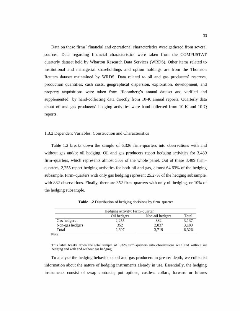
33
Data on these firms’ financial and operational characteristics were gathered from several
sources. Data regarding financial characteristics were taken from the COMPUSTAT
quarterly dataset held by Wharton Research Data Services (WRDS). Other items related to
institutional and managerial shareholdings and option holdings are from the Thomson
Reuters dataset maintained by WRDS. Data related to oil and gas producers’ reserves,
production quantities, cash costs, geographical dispersion, exploration, development, and
property acquisitions were taken from Bloomberg’s annual dataset and verified and
supplemented by hand-collecting data directly from 10-K annual reports. Quarterly data
about oil and gas producers’ hedging activities were hand-collected from 10-K and 10-Q
reports.
1.3.2 Dependent Variables: Construction and Characteristics
Table 1.2 breaks down the sample of 6,326 firm–quarters into observations with and
without gas and/or oil hedging. Oil and gas producers report hedging activities for 3,489
firm–quarters, which represents almost 55% of the whole panel. Out of these 3,489 firm–
quarters, 2,255 report hedging activities for both oil and gas, almost 64.63% of the hedging
subsample. Firm–quarters with only gas hedging represent 25.27% of the hedging subsample,
with 882 observations. Finally, there are 352 firm–quarters with only oil hedging, or 10% of
the hedging subsample.
Table 1.2 Distribution of hedging decisions by firm–quarter
Hedging activity: Firm–quarter
Oil hedgers Non-oil hedgers Total
Gas hedgers 2,255 882 3,137
Non-gas hedgers 352 2,837 3,189
Total 2,607 3,719 6,326 Note:
This table breaks down the total sample of 6,326 firm–quarters into observations with and without oil hedging and with and without gas hedging.
To analyze the hedging behavior of oil and gas producers in greater depth, we collected
information about the nature of hedging instruments already in use. Essentially, the hedging
instruments consist of swap contracts; put options, costless collars, forward or futures

34
contracts, and three-way collars. Table 1.3 presents a breakdown of the frequency of use for
each hedging instrument. The most common hedging vehicles are swap contracts, with
45.58% (45.25%) of use in gas (oil) hedging. The second most frequently used instrument is
the costless collar, with 37.19% (37.11%) for gas (oil) hedging. Next are put options, with
10.55% for gas hedging and 11.85% for oil hedging. The least used instruments are forward
or futures contracts, with only 3.25% (2.78%) for gas (oil) hedging, and three-way collars,
with only 3.42% (3.02%) for gas (oil) hedging. These observations show that oil and gas
producers adopt quite similar strategies in their oil and gas hedging and that they prefer more
swap contracts and costless collars.
Table 1.3 Hedging instruments used by oil and gas producers
Gas hedging Oil hedging
Financial instrument
Number of
firm–quarters Percentage of use
Number of
firm–quarters Percentage of use
Swap contracts 2,255 45.58% 1,711 45.25%
Put options 522 10.55% 448 11.85%
Costless collars 1,840 37.19% 1,403 37.11%
Forwards or futures 161 3.25% 105 2.78% Three-way collars 169 3.42% 114 3.02%
Total 4,947 100% 3,781 100% Note:
This table reports the different types of financial instruments used by the sample firms that report oil and gas hedging activities in a given firm–quarter observation. The values for each instrument indicate the number of firm–quarters and the fraction (in percentage) of use.
We now analyze hedging strategies and, to save space, we skip observations related to
forward/futures contracts, which account for only 3.25% of gas hedging activity and 2.78%
of oil hedging activity. We also omit observations related to three-way collars, because they
are used in only 3.42% of cases for gas hedging activity and 3.02% for oil hedging. Table 1.4
shows that two major hedging behaviors are adopted by oil and gas hedgers: the use of only
one hedging instrument and the use of more than one hedging instrument simultaneously to
form hedging portfolios with different payoff structures. Table 1.4 illustrates that swap
contracts are used separately 45% of the time, with put options 6% of the time, costless
collars 41% of the time, and put options and costless collars simultaneously 8% of the time.
Put options are employed separately 29% of the time, with swap contracts 24% of the time,
costless collars 14% of the time, and simultaneous swaps and collars 33% of the time. In

35
addition, costless collars are used separately 36% of the time, with swaps 50% of the time,
put options 4% of the time, and simultaneous swaps and puts 10% of the time.
Table 1.4 Hedging strategies adopted by oil and gas producers
Panel A: Gas hedging strategies
Swap only Put only Collar only Swap+put Swap+collar Put+collar Swap+put+collar
Number of firm–quarters 932 126 582 137 999 72 187
Percentage of use
Swap contracts 41.33% 6.08% 44.30% 8.29%
Put options 24.14% 26.25% 13.79% 35.82%
Costless collars 31.63% 54.29% 3.91% 10.16%
Panel B: Oil hedging strategies
Swap only Put only Collar only Swap+put Swap+collar Put+collar Swap+put+collar
Number of firm–quarters 849 150 577 99 627 63 136
Percentage of use
Swap contracts 49.62% 5.79% 36.65% 7.95%
Put options 33.48% 22.10% 14.06% 30.36%
Costless collars 41.13% 44.69% 4.49% 9.69%
Note:
This table reports the hedging strategies adopted by the sample firms. An oil and gas producer can use one or more instruments simultaneously. Overall, we distinguish seven hedging strategies: swap contracts only, put options only, costless collars only, swaps and puts, swaps and collars, puts and collars, and swaps, put, and collars for oil hedgers and gas hedgers, respectively. The value for each strategy represents the number of firm–quarter observations in which a firm reports the use of that strategy. The percentage of use for each instrument represents the number of firm–quarters of use of a given strategy scaled by the total number of firm–quarters of use of that instrument as given in Table 1.3.
Figures 1.1 and 1.2 show how these hedging strategies evolve over time and highlights
some important facts. Use of swaps only declines starting 1999, particularly for gas hedging.
The decrease in swap use seems to be compensated by an increase in collars use separately or
in combination with swaps. The use of put options only or in combination with swaps is
stable over time, in particular for gas hedging. Turning to the distribution of notional quantity
for each hedging portfolio (i.e., a combination of instruments), we find significant variations
in the time-series distribution of notional quantities between instruments.

36
Figure 1.1 Frequency of use by hedging strategy over 1998-2010 for gas hedging
Figure 1.2 Frequency of use by hedging strategy over 1998-2010 for oil hedging
0%
10%
20%
30%
40%
50%
60%
70%
80%
90%
100%
Gas hedging
Swap only Put only Swap and Put
Collar only Swap and Collar Collar and Put
Swap, Collar and Put
0%
10%
20%
30%
40%
50%
60%
70%
80%
90%
100%
Oil hedging
Swap only Put only Swap and Put
Collar only Swap and Collar Collar and Put
Swap, Collar and Put

37
1.3.3 Econometric Methodologies
The transition probabilities reported in Table A.1.2 show extreme state dependence in the
derivative choice for the sample hedgers. The elements of Table A.1.2 could be interpreted as
conditional probabilities under the Markov model. The magnitude of the diagonal elements
clearly shows the persistence or state dependence in hedging strategy choice. Persistence in
hedging behavior arises from two main sources. One possibility is that persistence is caused
by unobserved decision-maker-specific preferences for derivatives that are time invariant,
which creates unobserved time-invariant individual heterogeneity (i.e., spurious state
dependence, as noted by Heckman, 1981). Alternatively, persistence can be due to
unobserved but time-variant characteristics of hedging strategies, which creates true state
dependence. These unobserved time-variant characteristics could be transaction costs,
liquidity risk, counterparty risk, and accounting concerns associated with different hedging
instruments.
To disentangle the effects of unobserved individual heterogeneity and state dependence,
we employ several dynamic discrete choice frameworks with random effects, retaining a
first-order Markov process (i.e., including the first lagged dependent variable) and accounting
for the initial condition problem. We consider derivative choice as multi-state process and
examine the effects of investment opportunities, taxes, agency costs, distress costs,
managerial risk aversion, overinvestment, production function characteristics, and market
conditions on the choice of hedging strategy. Estimating these econometric dynamic settings
allows us to distinguish the effects of past hedging strategy choice and observable and
unobservable firm characteristics on current hedging behavior.
To control for the possibility of sample selection bias, the estimation of all our models is
derived in the context of two-step Heckman regression with selection. This procedure
captures the sequential decisions of oil and gas producers: a first decision to hedge or not and
a second decision about the nature of the hedging strategy. In the first step, we follow the
literature and model hedging activity as a function of variables that are proposed to be
determinants of the hedging decision: tax incentives, leverage, liquidity, cash costs, book
value of convertible debt, firm market value (size), sales (market risk exposure), and oil and

38
gas reserve quantities (substitute to hedging). Table A.1.3 reports the estimation results of the
first step, which allow us to obtain the estimated inverse Mills ratio for the second step. We
observe that almost all variables are statistically significant and with appropriate signs,
consistent with the previous literature on the decision to hedge (Tufano, 1996; Graham and
Rogers, 2002; Campello et al, 2011; Dionne and Triki, 2013).
1.3.4 Dynamic Generalized Ordered Specification for Hedging Instrument Choice
This model is used for hedging strategies based on one instrument only, as identified in
Table 1.4 (i.e., swap contracts only, put options only, and costless collars only). We include
the first lagged value of the dependent variable to account for this state dependence in
hedging strategy choice. This model is flexible and relaxes the single index or parallel-line
assumption (i.e., same coefficient vector for all categories of the dependent variable) by
making threshold parameters a linear function of the covariates (Maddala, 1983; Terza,
1985). We order hedging instruments in terms of their payoff non-linearity as follows: (1) put
options only, (2) costless collars only, and (3) swaps only. The starting point for the
econometric model is an unobserved latent dependent variable *
( , )i th that describes the choice
of hedging instrument, given that possible choices are , 1, 2, 3i th . The reduced form of
the estimated model is
*
, , , 1 , 1, , : 1, , , i t i t i t i t i ih X h u i N t T
(1)
where ,i tX is a set of observed exogenous variables related to investment program
specificities, taxes, financial distress costs, managerial risk aversion, overinvestment
problem, production function characteristics, and market conditions, which may be associated
with the hedging strategy choice of firm i at time t. In addition, ,i tX includes the inverse
Mills ratio from the first step of the Heckman regression with sample selection. iu is firm-
specific factor that is time invariant and thus represents unobserved individual heterogeneity;
and , i t
is the idiosyncratic error term that is assumed to be strictly exogenous, normally
39
distributed, and uncorrelated across firms and time. , 1i th is the observed instrument choice in
the previous period that allows state dependence to be captured.
To overcome the initial condition problem, we parameterize the unobserved individual
heterogeneity iu as in the work of Wooldridge (2002):
1 ,0 2 1, , , i i i iu h X i N (2)
where ,0ih is the first observation of hedging strategy choice for firm i.
iX and is a set of
means over the sample period of the exogenous variables of firm i (i.e., ,i tX ); and is
assumed to be distributed as ( ) and independent of the exogenous variables, the initial
condition, and the error term ( ). Because the latent outcome *
,i th is not observed, only an
indicator of the hedging instrument in which the latent variable falls is observed:
*
, 1 , if , i t j i t jh j h (3)
where the j with 1, 2, 3j are the threshold parameters. We allow these threshold
parameters to be a linear function of the observable characteristics ,i tX ,
, 1i th , ,0ih , and
iX .
The conditional probability of observing each category 1, 2, 3j is then given by an
augmented generalized ordered probit with random effects including the lagged dependent
variable and the initial observation. This approach, as for Williams (2006), leads to the
estimation of 1J (J is the number of categories) dynamic random effects probit models.
The first model contrasts category 1 with categories 2, , J ; the second model contrasts
categories 1 and 2 with categories 3, , J The model 1J does the same regarding
categories 1, , 1 J versus category J. For each model among the 1J dynamic random
effects probit models, the current and lower-coded categories are recorded to 0 (i.e., reference
group) and higher categories are recorded to 1. Therefore, positive coefficients mean that
higher values on the explanatory variable are more related to higher categories than the
40
current one. Negative coefficients indicate that higher values on the explanatory variable are
more related to the current or lower-coded category. This model could be estimated by
Gauss–Hermite quadrature10
(see Boes, 2007 for more detail).
1.3.5 Dynamic Multinomial Specification for Hedging Portfolio Choice
Here we focus our attention on hedging portfolio choice (i.e., simultaneously using more
than one instrument). Table 1.4 reveals that these hedging portfolios are constructed mainly
from combinations of swap contracts with put options and/or costless collars. The transition
probabilities reported in Table A.1.2 indicate higher persistence in these hedging portfolios,
which motivates the use of a dynamic multinomial choice framework. Our econometric
framework takes the form of a dynamic MMNL with random coefficients and correlated
random effects.
We allow random effects to be correlated with the firm’s time-variant characteristics.
This specification is less restrictive than in a standard random effects model because it does
not exhibit the restrictive assumption of independence from irrelevant alternatives and is
more consistent with the random utility maximization assumption. The mixed logit also
effectively captures random taste variation and habit formation. The utility for firm i from
choosing hedging portfolio j at time t, , is given by11
:
( ) (4)
where ,i tX is a set of observed exogenous variables related to hedging portfolio choice as
in equation (1) with unknown weight j, and is a binary dummy variable indicating
lagged hedging portfolio choice with parameter j, with if firm i chooses
hedging portfolio j at time 1t and otherwise. Oil and gas producers have a set
of four alternative hedging portfolios: swap contracts only 1j , which is our base
10 The model is estimated using a STATA user-written program regoprob2 developed by Pfarr, Schmid, and
Schneider (2010) based on Gauss-Hermite quadrature.
11 The notation in this section is largely adapted from Zucchelli, Harris, and Xueyan (2012).
41
outcome in the model; swap contracts combined with put options 2j ; swap contracts
combined with costless collars 3j ; and swap contracts combined with put options and
costless collars 4j . Here ,i ju represents firm i and alternative j specific factors that are
time invariant (i.e., unobserved heterogeneity). ( ) are modeled as random
effects by assuming that they come from a trivariate normal distribution. The term is an
idiosyncratic error term that is assumed to be independent from everything else in the model;
it follows a Gumbel distribution.
Assume that at each time period 1t a firm chooses the hedging portfolio associated
with the highest level of utility. Then, if for all 1, , k j k J .
Hence, the probability of making choice j at time conditional on ,i tX , , and
,i ju
takes the following logit form:
( | ) ( )
∑ ( )
(5)
For identification purposes, all coefficients for the first category 1j and its
unobserved heterogeneity are set to zero (i.e., hedging with swap contracts only). We assume
that the individual unobserved heterogeneity for the remaining three hedging portfolios
follows a trivariate normal distribution with zero mean and a variance–covariance matrix
with non-zero correlation across unobserved heterogeneity for alternative hedging portfolios.
Train (2009) suggests approximating the sample likelihood (SL) for the multinomial logit
with random effects using simulated maximum likelihood methods.12
To account for the
initial condition problem, we parameterize the distribution of the individual unobserved
heterogeneity for each firm as a function of the means of the exogenous variables over the
sample period and the hedging portfolio choice in the initial period.
12 The model is estimated using a user-written STATA program mixlogit by Arne Risa Hole (2007) that
implements simulation using Halton sequences. We use 200 Halton draws.
42
1.4 Results and Discussion
1.4.1 Descriptive Statistics: Independent Variables
Descriptive statistics are computed for the pooled dataset. Table 1.5 presents summary
statistics for the financial and operational characteristics of the 150 US oil and gas producers
in the sample. The findings suggest that US oil and gas producers are intensive hedgers. In
fact, the hedging indicator variables show that gas hedging occurred in 49.58% of the firm–
quarters in the sample and oil hedging occurred in 41.21% of the firm–quarters. In addition,
IR, FX, and basis risk hedging occurred, respectively, in 17.18%, 4.5%, and 9.48% of the
firm–quarters.

43
Table 1.5 Summary statistics for firm financial and operational characteristics
Variables Obs Mean Median 1
st quartile 3
rd quartile STD
Variables that proxy for hedging activity
GAS_HEDG 6,326 0.496 0.000 0.000 1.000 0.500
OIL_HEDG 6,326 0.412 0.000 0.000 1.000 0.492
BASIS_HEDG 6,326 0.095 0.000 0.000 0.000 0.293
IR_HEDG 6,326 0.172 0.000 0.000 0.000 0.377
FX_HEDG 6,326 0.045 0.000 0.000 0.000 0.207
Variables that proxy for underinvestment costs
INV_OPP 6,006 0.224 0.075 0.041 0.129 3.619
UND_OIL 6,326 95.153 2.109 0.118 19.106 450.444
UND_GAS 6,326 503.631 31.799 2.742 193.048 2028.157
COR_IO_FCF 6,196 0.055 0.046 -0.179 0.305 0.383
Variables that proxy for overinvestment
OVER_INV 5,855 0.259 0.000 0.000 1.000 0.438
Variables that proxy for tax advantage
TLCF 6,066 0.134 0.000 0.000 0.064 0.438
TAX_SAVE 6,160 0.052 0.048 0.029 0.070 0.051
Variables that proxy for financial distress costs
DTD 5,686 2.234 2.052 1.323 2.862 1.361
LEV 6,063 0.158 0.142 0.053 0.220 0.153
CONSTRAINT 6060 0.321 0.000 0.000 1.000 0.467
CASH_COST 6,241 9.860 7.527 4.684 12.230 8.441
Variables that proxy for managerial risk aversion
MV_CS_CEO 6,326 28.983 1.125 0.000 11.563 152.159
OPT_CEO 6,326 174.386 0.000 0.000 120.000 681.760
Variables that proxy for information asymmetry
%_CS_INST 6,326 0.372 0.299 0.000 0.742 0.353
Variables that proxy for production characteristics
UNCER_OIL 6,058 0.416 0.313 0.141 0.587 0.388
PQ_COR_OIL 6,119 0.229 0.455 -0.287 0.723 0.587
UNCER_GAS 6,078 0.408 0.303 0.146 0.582 0.359
COST_CV 6,167 0.292 0.252 0.148 0.396 0.556
PQ_COR_GAS 6,112 0.154 0.230 -0.174 0.504 0.419
OIL_REV 6,204 0.351 0.273 0.107 0.526 0.350
GAS_REV 6,204 0.519 0.566 0.242 0.785 0.311
HERF_GAS 6,180 0.063 0.000 0.000 0.000 0.183
HERF_OIL 6,178 0.100 0.000 0.000 0.000 0.233
Variables that proxy for firm size
MKT_VALUE 5,922 6,439.084 268.290 47.502 1,625.050 33,014.790
SALES 6,326 1,379.558 22.071 2.762 162.717 7,771.860
RES_OIL 6,326 276.710 8.010 0.948 53.352 1,277.726
RES_GAS 6,326 1,504.194 99.463 13.711 571.699 5,888.217
Variables that proxy for hedging substitutes BVCD 6,065 0.025 0.000 0.000 0.000 0.102
Q_RATIO 6,069 1.555 0.275 0.079 0.850 5.334

44
Note:
This table provides financial and operational statistics for the 150 US oil and gas producers for the period 1998 to 2010. The terms GAS_HEDG, OIL_HEDG, IR_HEDG, FX_HEDG, and BASIS_HEDG are dummy variables for gas, oil, IR, FX, and basis risk hedging. Here TLCF stands for tax loss carry-forwards s scaled by the book value of total assets; TAX_SAVE for the expected percentage of tax savings; LEV for the leverage ratio; DTD for the distance-to-default; CASH_COST for the production cost per BOE; INV_OPP for investment opportunities;
COR_IO_FCF for the correlation between free cash flows and investment opportunities; UND_OIL and UND_GAS for undeveloped proved oil (in millions of barrels) and gas (in billions of cubic feet) reserves, respectively; OVER_INV for the overinvestment problem; OIL_REV and GAS_REV for fractions of revenues from oil and gas production, respectively; HERF_OIL and HERF_GAS for the geographical dispersion of oil and gas production, respectively; UNCER_OIL and UNCER_GAS for the production uncertainty for oil and gas, respectively; PQ_COR_OIL and PQ_COR_GAS for the quantity–price correlation for oil and gas, respectively; SALES for sales; MKT_VALUE for common shares market value (in millions of dollars); RES_OIL and RES_GAS for the total reserves of oil and gas, respectively; MV_CS_CEO for the market value of common shares held by the
firm CEO (in millions of dollars); OPT_CEO for the number of stock options held by the firm CEO (in thousands); %_CS_INST for the percentage of common shares held by institutional investors; Q_RATIO for the quick ratio; BVCD for the book value of convertible debts scaled by the book value of total assets; and COST_CV for the coefficient of variation of the cash cost per BOE.
The measure of firms’ investment programs shows that oil and gas producers are also
intensive investors. On average, firms expend the equivalent of 22.37% of the book value of
their net property, plant, and equipment in exploration and reserve acquisition and
development. The correlation between internal cash flows and investment opportunities has a
mean (median) of 0.055 (0.046), with one-fourth of these firms having a correlation less than
-0.18 and another fourth with a correlation greater than 0.30. The tax preference item,
measured by the ratio of the book value of TLCFs scaled by the book value of total assets,
has a mean (median) of 13.42% (0.00%). The expected tax saving benefits of hedging have a
mean (median) of 5.24% (4.80%), which is quite close to the findings of Graham and Smith
(1999).
The DTD of the sample has a mean (median) of 2.234 (2.052), which reflects little
variation in the financial safety of the oil and gas producers in the sample. Those results are
similar to statistics reported by Drucker and Puri (2009) and Campello et al. (2011). Oil and
gas producers maintain low leverage levels, with a mean (median) of 15.8% (14.2%).
Overall, oil and gas producers maintain relatively high cash balance levels (quick ratio) and
have quite similar cash costs (lifting cost per BOE). The statistics also indicate that in 32% of
the firm–quarters in our sample, producers are financially constrained, with a leverage ratio
and quick ratio that are, respectively, above and below the industry’s median. Managers’

45
stock and option ownership varies considerably, with a mean (median) of $28.983 million
($1.125 million) for stockholding and 174,386 (0.000) options. Institutional ownership has a
mean (median) of 37.17% (29.86%) and varies from no institutional ownership for the first
quartile to higher than 74% for the top quartile of the firm–quarters in the panel. The market
value of firms’ outstanding common shares shows that the oil and gas industry mainly
comprises relatively small firms and a few large producers. In addition, this market value
varies strongly within the sample, with a mean (median) of $6.44 billion ($268 million). The
same conclusion is validated by the means and medians of oil and gas sales and reserve
quantities.
The two Herfindahl indices, measuring the geographical dispersion of the daily
production of oil and gas, respectively, indicate that oil- and gas-producing activities are
largely concentrated in the same region. The mean Herfindahl index is 0.06 for daily oil
production and 0.10 for daily gas production. The results further show that oil and gas
producers derive almost 87% of their total revenues from oil and gas production. On average,
gas production contributes to 52% of total revenue and oil production to 32%. Production
uncertainty, measured by the coefficient of variation in daily production, has a mean
(median) of 0.41 (0.31) for oil and 0.41 (0.30) for gas production. In addition, the coefficient
of variation of the cash cost per BOE has a mean (median) of 0.29 (0.25). This finding
implies that oil and gas producers face higher additional risks related to input costs and
output quantities.

46
1.4.2 Multivariate Results13
1.4.2.1 Hedging Instrument Choice
In this section, we investigate the empirical relevance of our hypotheses for hedging
strategies based on one instrument only, as identified in Table 1.4 (i.e., swap contracts only,
put options only, and costless collars only). The three hedging instruments are classified in
terms of their linearity as follows: 1) put options, 2) costless collars, and 3) swap contracts.
By nature, costless collars are situated between strict linear instruments (i.e., swap contracts)
and strict non-linear instruments (i.e., put options). We use the dynamic generalized random
effects ordered probit in equation (1). Tables 1.6 and 1.7 report the regression results of this
model for four specifications for oil and gas hedgers separately. For each specification, we
report the estimations EQ1 and EQ2, where EQ1 estimates put options versus swap contracts
and costless collars and EQ2 estimates swap contracts versus put options and costless collars.
The inspection of regressions reported in Tables 1.6 and 1.7 clearly demonstrates state
dependence in derivative choice. Hence, the coefficients of the lagged dependent variable for
all the specifications are significant at the 1% level. Investigation of the coefficients of the
initial observations further shows that this state dependence is more evident with significant
coefficients at conventional levels. These findings show that managers maintain almost
invariable hedging strategies for subsequent periods and suggest that recognition of the state
dependence phenomenon would provide insight into management behavior and refines the
association between each hedging instrument and observed firm characteristics, market
conditions, and measures of managerial risk aversion.
13 Appendix A discusses the results of our univariate analysis. Tables A.1.4 to A.1.7 report descriptive statistics of the independent variables and test for differences between the means and medians of the relevant variables for gas and oil hedgers separately. The univariate analysis is carried out by derivative instruments (Tables A.1.4 and
A.1.5) and by hedging portfolios (Tables A.1.6 and A.1.7).

47
Table 1.6 Hedging instrument choice by gas hedgers
Model 1 Model 2 Model 3 Model 4
Independent variables EQ1 EQ2 EQ1 EQ2 EQ1 EQ2 EQ1 EQ2
CONSTANT -1.2893 -1.8507** 2.5375* -3.4419*** 1.7583* -1.3599** 4.6938*** -0.9407
(1.461) (0.796) (1.325) (0.852) (1.036) (0.676) (1.124) (0.834)
LAG_LINEARITY 0.9050*** 0.5171*** 0.7999*** 0.5536*** 0.8237*** 0.5241*** 0.8176*** 0.5656***
(0.098) (0.047) (0.095) (0.050) (0.096) (0.049) (0.092) (0.049)
LINEARITY_0 0.4744*** 0.3447*** 0.2875*** 0.2460*** 0.2316 0.1781* 0.3004*** 0.2747***
(0.132) (0.070) (0.104) (0.061) (0.168) (0.105) (0.105) (0.067)
COR_IO_FCF 0.8547** 0.3906* 0.4023 0.5527*** 0.9114*** 0.2810 0.4913* 0.3787*
(0.341) (0.203) (0.354) (0.205) (0.339) (0.214) (0.283) (0.194)
HERF_GAS -1.5110* -1.2259 -1.1656 -1.5755
(0.845) (1.209) (0.880) (1.473)
PQ_COR_GAS 0.4927* 0.1033 0.3515 0.2871
(0.298) (0.213) (0.284) (0.211)
OVER_INV 0.3928* 0.1315 0.1286 0.1932
(0.238) (0.148) (0.228) (0.147)
OPT_CEO -0.0019 -0.0070*** -0.0078** -0.0056*** -0.0046 -0.0053*** -0.0070** -0.0051***
(0.003) (0.002) (0.003) (0.002) (0.003) (0.002) (0.003) (0.002)
MV_CS_CEO 7.6396* 0.0335 14.2617** 0.7586 15.7783** 0.2278 13.4854** 1.3690
(4.556) (0.816) (7.154) (0.907) (7.945) (0.890) (6.313) (0.958)
%_CS_INST 2.4206*** -0.2793 2.5528*** -0.1002
(0.578) (0.336) (0.629) (0.360)
TAX_SAVE 2.7050 -3.9638** 4.4549 -3.9816***
(4.009) (2.002) (3.688) (1.480)
TLCF -0.3503 -1.2245** -0.0821 -1.1772**
(0.408) (0.542) (0.375) (0.541)
LEV 0.6896 0.0879 1.5010 -0.1194
(0.974) (0.488) (0.969) (0.487)
CONSTRAINT -0.2590 -0.1184 -0.3311* -0.0560
(0.207) (0.132) (0.190) (0.125)
DTD -0.1458 -0.1894*** -0.1075 -0.1983***
(0.104) (0.059) (0.105) (0.062)
INV_OPP 0.1880 -1.7308*** -0.2869 -1.7637***
(0.642) (0.528) (0.708) (0.618)
UND_GAS 0.1043 -0.1332 1.2887** -0.0904
(0.254) (0.115) (0.518) (0.111)
VOL_GAS -0.4262*** -0.2158** -0.3275** -0.2768***
(0.140) (0.098) (0.128) (0.100)
FUTURE_GAS 0.0257 -0.3946*** 0.0513 -0.4428***
(0.085) (0.062) (0.081) (0.062)
SPOT_GAS 0.0003 0.1799*** -0.0116 0.1992***
(0.065) (0.052) (0.064) (0.051)
UNCER_GAS -2.8398*** -0.9969** -3.2470*** -1.7510***
(0.807) (0.419) (0.848) (0.519)
COST_CV 1.5396* 1.1404** 1.3530* 1.3005*** 1.4621* 1.0445**
(0.786) (0.462) (0.766) (0.488) (0.760) (0.478)
OIL_HEDG 0.8111*** 0.0291
(0.208) (0.139)
IR_HEDG -0.8117*** -0.0132
(0.252) (0.167)
FX_HEDG -0.5379 0.2274
(0.792) (0.565)
BASIS_HEDG -0.1312 0.2792
(0.454) (0.255)
GAS_REV -0.9040 -1.9288*** 0.2793 -2.1248***
(0.759) (0.573) (0.717) (0.567)
IMR_GAS -0.3785 0.7645*** -0.2795 0.1406 -0.3495 0.7458** 0.0165 0.1285
(0.450) (0.276) (0.411) (0.271) (0.410) (0.296) (0.384) (0.203)
Rho 0.7364***
(0.028)
0.8564***
(0.017)
0.7452***
(0.027)
0.8092***
(0.019)
Observations 1,630
-691.9547
-938.0734
492.2374
0.0000
1,601
-642.5038
-948.0657
611.1238
0.0000
1,597
-673.5852
-897.5861
448.0017
0.0000
1,615
-663.3446
-963.1919
599.6946
0.0000
Log-likelihood (LL)
LL constant only
Wald stat.
Significance
48
Notes:
This table reports the coefficient estimates of the dynamic generalized random effects ordered probit model for the hedging instrument choice for the subsample of gas hedgers. The dependent variables are the hedging instruments classified in terms of the linearity of their final payoffs: (1) put options only, (2) costless collars only, and (3) swap contracts only. The term LAG_LINEARITY is the lagged dependent variable; LINEARITY_0 is the initial condition; COR_IO_FCF for the correlation between free cash flows and investment opportunities; HERF_GAS for the geographical dispersion of gas production; PQ_COR_GAS for the gas quantity–price correlation; OVER_INV for overinvestment; OPT_CEO for the number of stock options held by the CEO; MV_CS_CEO for the market value of common shares held by the CEO; %_CS_INST for the percentage of common shares held by
institutional investors; TAX_SAVE for the expected percentage of tax savings; TLCF stands for TLCFs scaled by the book value of total assets; LEV for the leverage ratio; CONSTRAINT for financial constraints; DTD for the DTD; INV_OPP for investment opportunities; UND_GAS for undeveloped proved gas reserves; FUTURE_GAS, SPOT_GAS, and VOL_GAS for gas future and spot prices and volatility, respectively; UNCER_GAS for gas production uncertainty; COST_CV for the coefficient of variation of the cash cost per BOE; OIL_HEDG, IR_HEDG, FX_HEDG, and BASIS_HEDG are dummy variables for oil, IR, FX, and basis risk hedging, respectively; GAS_REV for revenues from gas production; and IMR_GAS for the inverse Mills ratio from the first-step Heckman regression (Table A.1.3). The coefficients of the exogenous variables’ means are not reported here
for conciseness and are available upon request. Standard errors are in parentheses. The superscripts ***, **, and * indicate significance at the 1%, 5%, and 10% levels, respectively. EQ1 estimates put options (recorded to 0) versus collars and swaps (recorded to 1) and EQ2 estimates put options and collars (recorded to 0) versus swaps (recorded to 1).

49
Table 1.7 Hedging instrument choice by oil hedgers
Model 1 Model 2 Model 3 Model 4
Independent variables EQ1 EQ2 EQ1 EQ2 EQ1 EQ2 EQ1 EQ2
CONSTANT 1.5749 1.6030* -1.8533 -0.3196 0.2078 0.8690 -2.2690* -0.7764
(1.120) (0.958) (1.193) (0.896) (0.813) (0.630) (1.255) (0.863)
LAG_LINEARITY 0.8105*** 0.4950*** 0.7590*** 0.5549*** 0.7930*** 0.5448*** 0.8104*** 0.5218***
(0.084) (0.049) (0.084) (0.049) (0.084) (0.049) (0.083) (0.049)
LINEARITY_0 -0.0451 0.1490** -0.0091 0.2210*** 0.3347*** 0.6320*** 0.0037 0.1660**
(0.087) (0.067) (0.100) (0.077) (0.090) (0.080) (0.097) (0.070)
COR_IO_FCF -0.4057 0.5639** -0.3155 0.9665*** -0.2421 0.5257** -0.3260 0.6227***
(0.284) (0.249) (0.291) (0.240) (0.286) (0.248) (0.271) (0.226)
HERF_OIL -1.9644** -1.8431*** -1.5977 -2.0155***
(0.844) (0.546) (1.041) (0.606)
PQ_COR_OIL -0.2065 0.1530 -0.4315 0.0947
(0.289) (0.182) (0.274) (0.181)
OVER_INV 0.4060** 0.0342 0.5614*** 0.1129
(0.202) (0.151) (0.207) (0.153)
OPT_CEO 0.0066 0.0027 0.0061 -0.0004 0.0099** 0.0006 0.0068 -0.0012
(0.005) (0.003) (0.005) (0.003) (0.004) (0.003) (0.005) (0.003)
MV_CS_CEO -0.0796 -0.5522 4.0040* 0.0796 -0.2164 -0.6244 2.3725 -0.0503
(1.784) (0.802) (2.312) (0.846) (2.010) (0.853) (1.960) (0.832)
%_CS_INST 0.1454 -0.1763 0.2683 -0.1662
(0.522) (0.366) (0.541) (0.396)
TAX_SAVE 16.3462*** -2.4470 14.6409*** -2.1517
(4.821) (1.505) (4.681) (1.618)
TLCF -0.6855 -2.8766*** -0.8622 -2.2270***
(0.490) (0.683) (0.547) (0.711)
LEV 0.3348 2.0412** -0.4624 2.5572***
(1.211) (0.808) (1.171) (0.784)
CONSTRAINT -0.2526 0.1381 -0.2456 0.0197
(0.214) (0.135) (0.203) (0.134)
DTD 0.2232** -0.2352*** 0.2040** -0.2818***
(0.096) (0.066) (0.098) (0.071)
INV_OPP 0.1216 -1.2814*** 0.1710 -1.3633***
(0.579) (0.451) (0.536) (0.442)
UND_OIL 1.0730 3.3914* 4.8559** 1.3811
(2.690) (1.925) (2.373) (1.858)
VOL_OIL -0.0250 -0.0522** -0.0303 -0.0237
(0.031) (0.022) (0.032) (0.024)
FUTURE_OIL -0.1159*** -0.0149 -0.1175*** -0.0571**
(0.033) (0.023) (0.032) (0.023)
SPOT_OIL 0.1097*** 0.0148 0.1094*** 0.0504**
(0.033) (0.022) (0.031) (0.022)
UNCER_OIL -1.5136** 0.6957* -2.3282*** 0.5672
(0.637) (0.380) (0.663) (0.408)
COST_CV 3.1899*** -1.1992* 1.0124 -1.5153*** 3.1940*** -0.2282
(0.936) (0.646) (0.848) (0.523) (0.876) (0.637)
GAS_HEDG 0.8166*** 0.1904
(0.252) (0.190)
IR_HEDG 0.8970*** 0.3789**
(0.270) (0.162)
FX_HEDG -1.1081*** 0.5099
(0.413) (0.371)
BASIS_HEDG 0.0767 1.0981***
(0.333) (0.195)
OIL_REV -1.7321** 1.3136** -2.0957** 0.6999
(0.784) (0.586) (0.819) (0.580)
IMR_OIL -1.1546** 0.2843 -0.5734 1.1021*** -0.8629 0.3470 -1.0220** 0.8544***
(0.512) (0.307) (0.576) (0.367) (0.541) (0.342) (0.404) (0.293)
Rho 0.7852***
(0.021)
0.7754***
(0.027)
0.7775***
(0.024)
0.7747***
(0.024)
Observations 1,572
-685.9948
-945.5503
519.1109
0.0000
1,547
-659.9249
-878.7359
437.6220
0.0000
1,550
-654.5332
-884.8251
460.5838
0.0000
1,564
-660.7962
-894.4599
467.3274
0.0000
Log-likelihood (LL)
LL constant only
Wald stat.
Significance

50
Note:
This table reports the coefficient estimates of the dynamic generalized random effects ordered probit model for the hedging instrument choice for the subsample of oil hedgers. The dependent variables are the hedging instruments classified in terms of the linearity of their final payoffs: (1) put options only, (2) costless collars only, and (3) swap contracts only. The term LAG_LINEARITY is the lagged dependent variable; LINEARITY_0 is the initial condition; COR_IO_FCF for the correlation between free cash flows and investment opportunities; HERF_OIL for the geographical dispersion of oil production; PQ_COR_OIL for the oil quantity–price correlation; OVER_INV for overinvestment; OPT_CEO for the number of stock options held by the CEO; MV_CS_CEO for the market
value of common shares held by the CEO; %_CS_INST for the percentage of common shares held by institutional investors; TAX_SAVE for the expected percentage of tax savings; TLCF stands for TLCFs scaled by the book value of total assets; LEV for the leverage ratio; CONSTRAINT for financial constraints; DTD for the DTD; INV_OPP for investment opportunities; UND_OIL for undeveloped proved oil reserves; FUTURE_OIL, SPOT_OIL, and VOL_OIL for oil future and spot prices and volatility, respectively; UNCER_OIL for oil production uncertainty; COST_CV for the coefficient of variation of the cash cost per BOE; GAS_HEDG, IR_HEDG, FX_HEDG, and BASIS_HEDG are dummy variables for gas, IR, FX, and basis risk hedging, respectively; OIL_REV for revenues from oil production; and IMR_OIL for the inverse Mills ratio from the first-
step Heckman regression (Table A.1.3). The coefficients of the exogenous variables’ means are not reported here for conciseness and are available upon request. Standard errors are in parentheses. The superscripts ***, **, and * indicate significance at the 1%, 5%, and 10% levels, respectively. EQ1 estimates put options (recorded to 0) versus collars and swaps (recorded to 1) and EQ2 estimates put options and collars (recorded to 0) versus swaps (recorded to 1).
Pertaining to the first hypothesis, the proxy COR_IO_FCF for the correlation between
free cash flows and the firm’s investment programs are significantly positively related to
linear instruments, as predicted. For the subset of gas hedgers, COR_IO_FCF is related
positively to swaps and collars. Particularly for oil hedgers, the association between this
correlation and swaps is more evident. Overall, these findings empirically validate our
Hypothesis 1 that firms with higher correlation between internal cash flows and future
investment opportunities are more likely to use linear instruments because they benefit from a
natural hedge and linear strategies suffice to provide value-maximizing hedges.
Economically, it appears that oil and gas prices have a simultaneous positive impact on firm’s
generated cash flows and rents associated with future investment expenditures, and provide
producers with a natural diversification.
In line with the production flexibility argument of Moschini and Lapan (1992), the results
confirm our Hypothesis 2 and show that greater geographical diversification in production
activities is associated more with the use of non-linear instruments. We find that geographical
diversification in gas production (HERF_GAS) is more related to the use of put options and
diversification in oil production (HERF_OIL) is associated with the use of put options and
costless collars. However, the impact of geographical diversification is economically and
51
statistically more significant for oil hedgers. Oil and gas producers seem to consider
geographical dispersion in their production operations as a real option requiring that non-
linear instruments be used to hedge. Whereas Moschini and Lapan (1992) suggest that
production flexibility motivates firms to sell convexity (i.e., selling put and call options), we
find that it motivates firms to go long in put options.
Results pertaining to the quantity–price correlation indicate that when gas production
quantities and spot prices are positively correlated (PQ_COR_GAS), gas producers tend to
hedge more with swaps and collars as predicted in Hypothesis 3. Despite its low statistical
significance, this result is consistent with the conjectures of Brown and Toft (2002) and Gay,
Nam, and Turac (2002, 2003) that when production quantity and spot prices are positively
correlated, overhedging is less likely and linear instruments could achieve optimal hedging.
Oil quantity–price correlation (PQ_COR_OIL) has no significant impact on hedging
instrument choice. Although with similar production uncertainties, oil hedgers and gas
hedgers react differently to the price–quantity correlation.
Overinvestment (OVER_INV), a problem identified by Morellec and Smith (2007) and
Bartram, Brown, and Fehle (2009), seems to be largely supported by the multivariate results.
Overinvestment is more likely for large, profitable firms that have fewer investment
opportunities. Managers at these firms tend to overinvest because they derive private benefits
from the investment. Overinvestment is significantly positively related to swap contracts and
costless collars for oil hedgers, in particular. Consistent with our Hypothesis 4, when
overinvestment is more likely, firms tend to use more linear instruments and to avoid put
options. In the context of shareholder–manager conflict, hedging with linear instruments
allows firms to attenuate the variability in their generated cash flows, which would benefit
the managers who tend to overinvest. To our knowledge, the overinvestment problem has not
been empirically investigated in the corporate risk management context.14
14 As a robustness check, we proxy the overinvestment problem by creating a dummy variable that equals one for firms whose ratio of free cash flow to total assets is in the top quartile and zero otherwise. We interact and interact
this dummy variable with investment opportunities and obtain the same results.

52
Regarding managerial risk aversion, particularly for gas hedgers, the results show that a
CEO with higher firm-specific wealth (MV_CS_CEO) tends to use swap contracts and
collars, and to avoid put options, as predicted in Hypothesis 5. Results also suggest that CEO
option holding (OPT_CEO) is significantly negatively related to the use of swaps.
Interestingly, we find that managerial stockholding and option-holding are strongly positively
related to costless collars. A possible explanation for this finding is linked to the payoff
structure of costless collars (i.e., buying put options and selling call options, which creates a
linear-like payoff structure). Overall, the latter findings are consistent with the literature
(Smith and Stulz, 1985), in which a risk-averse manager with higher stockholding tends to
use linear instruments and to avoid non-linear ones. Managers with a convex payoff (i.e.,
higher option holding levels) will do the converse. The percentage of institutional
shareholding (%_CS_INST) is significantly positively related to the use of swaps and collars.
This finding could be explained by the fact that institutional investors act like risk-averse
managers and seek higher insulation of firm value from the source of risk.
The empirical implications with respect to the convexity of the tax function (TAX_SAVE)
are unclear. Although TAX_SAVE has a significant positive impact on the use of swap
contracts and costless collars for oil hedgers as predicted, it is more related to collars and put
options for gas hedgers. TLCF appears to be more associated with the use of collars and put
options. Altogether, tax function convexity and TLCF seem to be more related to the use of
collars.
The results pertaining to financial constraints show, particularly for oil hedgers, that swap
contracts are positively related to leverage ratio (LEV) in a significant manner. In light of
descriptive statistics (i.e., leverage ratio has a mean (median) of 15.8% (14.2%)). This finding
corroborates the theoretical predictions of Adam (2002) and Adler and Detemple (1988) that
linear instruments are optimal for average or no financial constraints. Results further show
that more solvent oil and gas producers (i.e., with a higher DTD) tend to use costless collars.
This finding indicates again that more leveraged firms tend to lock in predetermined
revenues, while more solvent ones tolerate more variability in their future revenues by
avoiding strict linear hedging strategies. In line with risk-shifting theory (Jensen and
53
Meckling (1976)), the results show that gas hedgers close to financial distress
(CONSTRAINT) use more put options.
Interestingly, the results emphasize the fact that investment opportunities (INV_OPP)
appear to be more associated with the use of costless collars and put options. Overall, these
findings are consistent with Froot, Scharfstein, and Stein’s (1993) argument that firms with
larger investment programs tend to use more non-linear instruments, along with the empirical
findings of Gay and Nam (1998) and Adam (2002, 2009). Further, undeveloped proved oil
and gas reserves (UND_GAS and UND_OIL) seem to be more related to the use of swap
contracts and costless collars. One explanation could be that because oil and gas producers
already have larger undeveloped reserves, they face less pressure related to future
development expenditures.
The results pertaining to the impact of market conditions are highly consistent with
predictions. Accordingly, higher volatility (VOL_GAS and VOL_OIL) and higher anticipated
future prices (FUTURE_GAS and FUTURE_OIL) are related to the use, in particular, of put
options and collars. These findings mean that in a higher volatility environment or when
prices are anticipated to be higher, oil and gas producers are more interested in maintaining
any potential upside risk than protecting downside risk. Our findings contradict those of
Brown (2001), who finds a negative association between volatility and the convexity of the
hedging portfolio, and those of Adam (2009), who finds no significant relation between
volatility and option use. As predicted, increasing spot prices (SPOT_GAS and SPOT_OIL)
motivate firms to use swap contracts to lock in predetermined higher prices because they are
anticipating that prices will decline in the future. These findings highlight the significant role
of market conditions in derivative choice, which may explain firm hedging behavior.
Interestingly, the association between higher production uncertainty (UNCER_GAS and
UNCER_OIL) and the use of put options is as predicted and is significant.15
Overall, these
findings contradict the empirical results of Brown (2001) and Adam (2009), who find no
significant relation between firm’s exposure fluctuation and option use, and corroborate the
15
Model 1 in Table 1.11 illustrates an unexpected positive coefficient for oil production uncertainty and swap use,
albeit with a lower significance level.

54
theoretical predictions of Moschini and Lapan (1995), Brown and Toft (2002), and Gay,
Nam, and Turac (2002, 2003). The results further show that when oil and gas producers
hedge simultaneously both commodities and basis risk (GAS_HEDG, OIL_HEDG and
BASIS_HEDG), they tend to use more swaps and collars. A possible explanation for this
finding could be that hedging the primary source of business risk (i.e., oil or gas price risk)
attenuates the non-linearity of the firm’s total exposure, which makes non-linear instruments
less optimal.
Regarding IR risk and production cost variability (COST_CV), the results are significant
and mixed. For oil hedgers, hedging FX risk is linked more to put options. Producers
primarily engaged in gas production (i.e., with a higher GAS_REV) tend to use more put
options or collars. In addition, producers primarily engaged in oil production (i.e., with a
higher OIL_REV) tend to use more put options. This result is consistent with the empirical
finding of Adam (2009), who confirms that more focused gold-mining firms are 30% more
likely to use options strategies than diversified firms are.
1.4.2.2 Hedging Portfolio Choice
Tables 1.8 and 1.9 report the estimation results of the determinants of hedging portfolio
choice for many specifications of the dynamic random effects MMNL model. The estimation
was carried out for the subset of oil hedgers and gas hedgers separately. Because the main
focus here is on oil and gas producers’ rationales for choosing hedging portfolios with
payoffs that depart from linearity to non-linearity (by combinations of swap contracts with
put options and/or costless collars), swap contracts are chosen as our base outcome and all
the results must be interpreted relative to choosing swap contracts. However, the level of
non-linearity depends on the percentage of the notional hedged quantity of each instrument
forming the portfolio. Table A.1.8 summarizes those hedging portfolios and breaks down the
notional quantity hedged between the different instruments.

55
Table 1.8 Hedging portfolio choice by gas hedgers
Model 1 Model 2 Model 3 Model 4
Dependant variables
Swaps +
Put options
Swaps +
Collars
Swaps +
Collars +
Put options
Swaps +
Put options
Swaps +
Collars
Swaps +
Collars +
Put options
Swaps +
Put options
Swaps +
Collars
Swaps +
Collars +
Put options
Swaps +
Put options
Swaps +
Collars
Swaps +
Collars +
Put options
(I) (II) (III) (IV) (V) (VI) (VII) (VIII) (IX) (X) (XI) (XII)
COR_IO_FCF 0.1587 -0.4873 0.5000 0.4293 -0.2054 1.4151** 0.2622 -0.3965 0.6820 0.3626 -0.1519 1.3159**
(0.798) (0.353) (0.659) (0.846) (0.353) (0.665) (0.807) (0.346) (0.636) (0.872) (0.350) (0.657)
HERF_GAS 5.6000 0.6124 3.8470 6.6783 0.3125 3.7546
(5.830) (1.491) (3.026) (5.612) (1.498) (3.056) PQ_COR_GAS -0.2411 -0.6961* -1.4700** -0.2072 -0.7796** -1.5082**
(0.819) (0.392) (0.716) (0.854) (0.396) (0.728)
OVER_INV -1.5085** 0.0040 0.6479 -1.6354** -0.0560 0.4625
(0.690) (0.251) (0.480) (0.737) (0.248) (0.472) OPT_CEO -0.0117 0.0009 0.0065* -0.0140 0.0028 0.0003 -0.0128 0.0004 0.0051 -0.0141 0.0031 0.0002
(0.012) (0.002) (0.004) (0.013) (0.002) (0.002) (0.013) (0.002) (0.004) (0.013) (0.002) (0.002)
MV_CS_CEO -4.0146 1.0181 -0.0421 -7.2996 1.3072 1.5108 -5.2502 1.0619 0.2951 -9.9613 0.9361 0.7024
(7.073) (1.086) (3.629) (9.097) (1.259) (3.059) (8.163) (1.104) (3.310) (11.096) (1.264) (3.270) %_CS_INST 0.5147 1.4699** -0.1865 0.5325 1.3982** -0.3489
(1.583) (0.591) (1.018) (1.630) (0.600) (1.013)
TAX_SAVE -11.3358 2.0227 -8.8088 -11.8664 2.0916 -7.6186
(13.873) (1.387) (10.348) (14.014) (1.409) (9.719) TLCF 0.5614 0.3886 0.9566 1.0216 0.3481 1.6292
(1.739) (0.954) (1.851) (1.919) (0.971) (1.739)
LEV -0.7111 -3.2276** -0.8418 -1.0500 -3.2655** -1.5442
(1.735) (1.350) (2.114) (1.789) (1.346) (2.243) CONSTRAINT 0.0067 0.6903*** -0.6279 0.0198 0.6756*** -0.5603
(0.566) (0.228) (0.389) (0.593) (0.230) (0.383)
DTD -0.2966 0.0443 -0.1564 -0.3682 0.0544 -0.0632
(0.207) (0.089) (0.168) (0.231) (0.089) (0.166) INV_OPP 2.2211** 1.8193** 2.1679* 1.6198 1.9128 0.8811
(1.112) (0.788) (1.136) (1.380) (1.173) (0.930)
UND_GAS -1.3290 0.0593 -0.1530 -1.2261 0.0909 0.1699
(1.271) (0.153) (0.341) (1.952) (0.164) (0.340) VOL_GAS 0.4982 0.2629* 0.3655 0.5271 0.3138** 0.3294
(0.387) (0.157) (0.298) (0.395) (0.159) (0.300)
FUTURE_GAS 0.0064 0.2581** 0.2822 -0.0390 0.2500** 0.2701
(0.299) (0.104) (0.198) (0.316) (0.104) (0.191) SPOT_GAS -0.0106 -0.1080 -0.1661 0.0384 -0.0983 -0.1576
(0.244) (0.088) (0.183) (0.256) (0.088) (0.175)
UNCER_GAS 1.1570 1.8972*** 5.5793*** 0.8685 2.0719*** 4.9724***
(1.776) (0.682) (1.406) (1.911) (0.756) (1.648) COST_CV -3.9733* -0.7083 0.8668 -2.2789 -0.1849 1.2712 -2.7916 -0.4681 1.2027
(2.095) (0.757) (0.993) (1.586) (0.721) (0.991) (1.816) (0.720) (0.939)
OIL_HEDG -0.1000 0.4263 1.2311**
(0.590) (0.273) (0.562) IR_HEDG 1.1310 0.3743 1.1073**
(0.915) (0.247) (0.478)
FX_HEDG 0.3080 0.4211 1.0414
(2.064) (0.498) (0.863) BASIS_HEDG -2.1393 0.0652 0.0929
(1.422) (0.295) (0.586)
GAS_REV 7.1128*** 1.9334* 1.7740 9.0750*** 1.5953 2.7445
(2.496) (0.987) (2.037) (3.066) (1.058) (2.125) IMR_GAS 0.8591 -0.8247 -0.6898 0.2746 -0.6466 -1.3389 0.4013 -1.1196** -0.2771 0.1380 -0.6983 -1.6001
(1.098) (0.514) (1.000) (1.173) (0.610) (1.112) (1.141) (0.568) (1.077) (1.240) (0.651) (1.139)
LAG 4.8491*** 3.8356*** 3.1484*** 4.2207*** 3.8633*** 3.2324*** 4.6935*** 3.8528*** 3.0547*** 4.1282*** 3.8411*** 3.2357***
(0.525) (0.180) (0.388) (0.557) (0.189) (0.387) (0.650) (0.183) (0.371) (0.682) (0.189) (0.373) LAG_0 -0.1002 0.2200 2.3247** 2.9400* -0.4745 3.1734*** 0.0418 0.6110 2.2957** 3.2006 0.2136 2.8169***
(1.005) (0.765) (0.926) (1.669) (1.143) (0.980) (1.275) (1.018) (0.929) (2.300) (1.031) (0.889)
uj -8.0634* -8.1426*** -4.0618 -10.7790 -4.0450* -6.1800 -5.1669 -4.7398*** -0.6227 -7.3354 -1.9742 -4.3276 (4.719) (2.061) (4.035) (6.655) (2.333) (4.841) (4.489) (1.801) (3.562) (7.457) (2.346) (3.998)
Sigma_uj 1.9645*** 1.3458*** 2.4797*** 2.2569*** 1.4661*** 2.0832*** 2.3419*** 1.3438*** 1.9622*** 3.0565** 1.5299*** 1.9774***
(0.456) (0.202) (0.450) (0.649) (0.221) (0.432) (0.707) (0.202) (0.439) (1.262) (0.239) (0.399)
Rho_1_2
Rho_1_3
Rho_2_3
0.935
0.993
0.897
0.154
0.793
0.705
0.735
0.999
0.734
0.410
0.929
0.715
Observations Log-likelihood (LL)
LL constant only
Wald stat.
Significance
2,188 -889.3674
-945.7635
112.7922
0.0000
2,168 -860.5163
-910.7239
100.4151
0.0000
2,134 -875.4408
-920.7931
90.7046
0.0000
2,168 -870.0853
-920.4412
100.7117
0.0000
56
Note:
This table reports the means of the coefficient estimates of the dynamic random effects MMNL to select one of three hedging portfolios—(1) swap and put options, (2) swaps and collars, and (3) swaps, put options, and
costless collars—for the subsample of gas hedgers. The base case is using swap contracts only. COR_IO_FCF for the correlation between free cash flows and investment opportunities; HERF_GAS for the geographical dispersion of gas production; PQ_COR_GAS for the gas quantity–price correlation; OVER_INV for overinvestment; OPT_CEO for the number of stock options held by the CEO; MV_CS_CEO for the market value of common shares held by the CEO; %_CS_INST for the percentage of common shares held by institutional investors; TAX_SAVE for the expected percentage of tax savings; TLCF stands for TLCFs scaled by the book value of total assets; LEV for the leverage ratio; CONSTRAINT for financial constraints; DTD for the DTD; INV_OPP for investment opportunities; UND_GAS for undeveloped proved gas reserves; FUTURE_GAS, SPOT_GAS, and
VOL_GAS for gas future and spot prices and volatility, respectively; UNCER_GAS for gas production uncertainty; COST_CV for the coefficient of variation of the cash cost per BOE; OIL_HEDG, IR_HEDG, FX_HEDG, and BASIS_HEDG are dummy variables for oil, IR, FX, and basis risk hedging, respectively; GAS_REV for revenues from gas production; IMR_GAS for the inverse Mills ratio from the first-step Heckman regression (Table A.1.3); LAG for the lagged dependent variable; and LAG_0 for the first observation. The coefficients of the exogenous variables’ means are not reported here for conciseness and are available upon request. Standard errors are in parentheses. The superscripts ***, **, and * indicate significance at the 1%, 5%, and 10% levels, respectively.

57
Table 1.9 Hedging portfolio choice by oil hedgers
Model 1 Model 2 Model 3 Model 4
Dependant variables
Swaps + Put options
Swaps + Collars
Swaps +
Collars + Put options
Swaps + Put options
Swaps + Collars
Swaps +
Collars + Put options
Swaps + Put options
Swaps + Collars
Swaps +
Collars + Put options
Swaps + Put options
Swaps + Collars
Swaps +
Collars + Put options
(I) (II) (III) (IV) (V) (VI) (VII) (VIII) (IX) (X) (XI) (XII)
COR_IO_FCF -2.7309 -0.0486 0.0425 -4.2599** -0.1835 -0.4804 -2.7180 0.1298 0.2752 -2.8437* 0.0247 -0.3498 (1.850) (0.431) (0.746) (1.688) (0.436) (0.707) (1.910) (0.429) (0.752) (1.511) (0.435) (0.699)
HERF_OIL -0.9574 2.7762*** 0.9429 -1.2176 3.0714*** 1.5233
(3.814) (1.045) (1.827) (3.727) (1.063) (1.807)
PQ_COR_OIL -1.8948 0.2817 0.2435 -1.8978 0.2664 -0.0109 (1.661) (0.328) (0.700) (1.485) (0.328) (0.661)
OVER_INV 2.3335* 0.2800 -0.6270 2.4165** 0.2073 -0.5909
(1.192) (0.299) (0.545) (1.149) (0.293) (0.542)
OPT_CEO 0.0501** -0.0022 0.0043 0.0400* 0.0012 0.0015 0.0592*** -0.0040 0.0050 (0.020) (0.005) (0.014) (0.021) (0.003) (0.003) (0.021) (0.005) (0.013)
MV_CS_CEO -8.0300 2.2892* 0.2434 -7.7560 1.4191 0.0496 -8.0806 2.6113** 1.0862
(16.948) (1.331) (5.148) (16.331) (1.392) (4.682) (18.848) (1.327) (4.826)
%_CS_INST 2.8521 0.0920 -0.2079 (2.903) (0.712) (1.330)
TAX_SAVE 17.8661** 1.9370 -4.4769 16.8294* 1.7214 -1.7231
(8.191) (2.306) (12.410) (9.588) (2.381) (11.280)
TLCF -0.1810 1.3681 -0.5394 0.8270 1.5653 -0.3020 (4.333) (1.346) (2.631) (5.048) (1.305) (2.595)
LEV -8.0969 0.0268 1.4242 -7.2524 -0.1088 0.7652
(7.121) (1.632) (2.607) (6.500) (1.568) (2.440)
CONSTRAINT 0.6528 -0.0117 0.8732* 0.3328 -0.0198 0.9003** (0.897) (0.274) (0.447) (0.840) (0.271) (0.433)
DTD -0.1652 -0.0162 0.1090 -0.0758 -0.0232 0.0347
(0.411) (0.120) (0.227) (0.439) (0.122) (0.229)
INV_OPP 1.2251 1.3159* 1.7185* 0.3801 0.8754 1.0355 (1.463) (0.712) (0.895) (1.800) (0.742) (0.824)
UND_OIL 11.4982 0.7859 2.0579 6.3964 1.7266 4.5504
(23.887) (3.407) (5.484) (15.515) (3.483) (5.058)
VOL_OIL 0.1668 -0.0308 0.0071 0.2411 -0.0416 -0.0356 (0.135) (0.042) (0.083) (0.167) (0.045) (0.082)
FUTURE_OIL 0.3404* -0.0169 0.0927 0.2288* -0.0142 0.0749
(0.177) (0.038) (0.074) (0.127) (0.038) (0.071)
SPOT_OIL -0.2962* 0.0299 -0.0789 -0.2091* 0.0297 -0.0630 (0.162) (0.038) (0.073) (0.122) (0.038) (0.070)
UNCER_OIL -0.8425 -1.3400 -0.4906 0.7025 -2.3167** -0.3717
(2.567) (0.819) (1.399) (2.413) (0.922) (1.408)
COST_CV -7.5344 0.0743 -0.7213 -4.3151 1.5133 1.3351 (5.694) (0.337) (1.109) (4.412) (0.996) (1.027)
GAS_HEDG -0.3332 0.4399 2.9815**
(1.382) (0.557) (1.451)
IR_HEDG -0.4810 0.1372 0.7083 (1.132) (0.304) (0.517)
FX_HEDG -3.2237 1.3204** 0.5769
(4.656) (0.672) (1.107)
BASIS_HEDG -1.8850 -0.5905 -0.4051 (1.690) (0.363) (0.710)
OIL_REV 2.2294 0.7476 3.1159 0.7369 0.5417 1.1714
(4.157) (1.303) (2.416) (4.063) (1.284) (1.993)
IMR_OIL 0.2289 -1.1030* -1.8762 1.6797 0.2603 0.4796 -0.2946 -0.7839 -1.8701 0.3296 0.3457 0.2947 (1.817) (0.659) (1.238) (2.578) (0.772) (1.110) (1.939) (0.705) (1.208) (2.019) (0.730) (1.082)
LAG 4.6163*** 3.6750*** 3.2885*** 4.1698*** 3.6499*** 3.3325*** 4.3804*** 3.6805*** 3.3783*** 3.6572*** 3.6687*** 3.3198***
(0.932) (0.225) (0.449) (0.837) (0.232) (0.431) (0.940) (0.228) (0.441) (0.696) (0.226) (0.429)
LAG_0 (X) (X) -0.1268 (X) (X) 1.6318 (X) (X) -0.0691 (X) (X) 0.2900 (1.513) (1.380) (1.372) (1.632)
uj -3.3900 -10.3039*** -8.4440** -22.7548 0.6415 3.2016 2.9837 -5.2764** -2.5449 1.0114 1.2818 2.2034
(8.459) (2.883) (4.183) (16.762) (4.123) (5.998) (9.226) (2.270) (3.115) (14.282) (3.290) (4.274) Sigma_uj 3.2093** 2.0000*** 2.3607*** 6.2914** 2.3399*** 2.9545*** 3.8441** 1.9688*** 2.1166*** 7.1710** 2.4725*** 3.0574***
(1.634) (0.322) (0.559) (2.586) (0.381) (0.578) (1.933) (0.327) (0.487) (3.266) (0.393) (0.614)
Rho_1_2
Rho_1_3
Rho_2_3
0.498
0.862
0.860
0.312
0.786
0.832
0.237
0.652
0.891
0.484
0.855
0.867
Observations
Log-likelihood (LL) LL constant only
Wald stat.
Significance
1,632
-619.8875 -668.3723
96.9697
0.0000
1,650
-628.8506 -705.3281
152.9549
0.0000
1,605
-615.5335 -670.4718
109.8766
0.0000
1,678
-653.7601 -740.2093
172.8985
0.0000

58
Note:
This table reports the means of the coefficient estimates of the dynamic random effects MMNL to select one of the following three hedging portfolios—(1) swap and put options, (2) swaps and collars, and (3) swaps, put
options, and costless collars—for the subsample of oil hedgers. The base case is using swap contracts only. COR_IO_FCF for the correlation between free cash flows and investment opportunities; HERF_OIL for the geographical dispersion of oil production; PQ_COR_OIL for the oil quantity–price correlation; OVER_INV for overinvestment; OPT_CEO for the number of stock options held by the CEO; MV_CS_CEO for the market value of common shares held by the CEO; %_CS_INST for the percentage of common shares held by institutional investors; TAX_SAVE for the expected percentage of tax savings; TLCF stands for TLCFs scaled by the book value of total assets; LEV for the leverage ratio; CONSTRAINT for financial constraints; DTD for the DTD; INV_OPP for investment opportunities; UND_OIL for undeveloped proved oil reserves; FUTURE_OIL,
SPOT_OIL, and VOL_OIL for oil future and spot prices and volatility, respectively; UNCER_OIL for oil production uncertainty; COST_CV for the coefficient of variation of the cash cost per BOE; GAS_HEDG, IR_HEDG, FX_HEDG, and BASIS_HEDG are dummy variables for gas, IR, FX, and basis risk hedging, respectively; OIL_REV for revenues from oil production; IMR_OIL for the inverse Mills ratio from the first-step Heckman regression (Table A.1.3); LAG for the lagged dependent variable; and LAG_0 for the first observation. The coefficients of the exogenous variables’ means are not reported here for conciseness and are available upon request. Standard errors are in parentheses. The superscripts ***, **, and * indicate significance at the 1%, 5%, and 10% levels, respectively, and (X) indicates that the variable was omitted by STATA software during the regression because of co-linearity.
Tables 1.8 and 1.9 report the estimated coefficients’ means for explanatory variables, as
well as estimated means (uj), estimated standard deviations (Sigma_uj), and correlation
coefficients (Rho_1_2, Rho_1_3, and Rho_2_3) of unobserved heterogeneity terms for the
remaining three hedging portfolios, namely (1) swap contracts combined with put options,
(2) swap contracts combined with costless collars, and (3) swap contracts combined with put
options and costless collars. The results (see the lower parts of Tables 1.8 and 1.9) show a
statistically non-zero standard deviation of the unobserved heterogeneity effects justifying the
random effects specification. They also indicate higher correlations between the random
effects of the three hedging portfolios for gas and oil hedgers, respectively. This higher
correlation of the random effects across hedging portfolios implies that the firm-specific
unobserved factors driving hedging portfolio choices overlap but are not the same. This
finding appears to suggest that firm-specific random effects are a crucial element to consider
and that our model should outperform other models without random effects.
Lagged hedging portfolio choice exhibits a great degree of persistence in all hedging
portfolios. Results related to the correlation between internal cash flows and investment
opportunities are mixed. Although, this correlation is negatively related to put options in a
statistically significant manner for oil hedgers as predicted, it is positively related to the use

59
of put options and collars for gas hedgers. The results further indicate that oil hedgers with
greater geographical diversification tend to include costless collars in their hedging
portfolios. For gas hedgers, geographic diversification has the predicted positive sign but
with no significant impact. Consistent with the theoretical predictions of Brown and Toft
(2002) and Gay, Nam, and Turac (2002, 2003) and previous findings, the positive price–
quantity correlation for gas hedgers appears to have a significant negative impact on the use
of put options and/or collars in combination with swaps. Hence, gas producers with a higher
positive price–quantity correlation tend to use swap contracts only, to mitigate adverse
movements in revenues because prices and quantities are moving in the same direction.
However, there is no evidence of this relation for oil hedgers.
The impact of the overinvestment problem on hedging portfolio choice is mixed.
Although overinvestment is significantly negatively associated with put options for the subset
of gas hedgers as predicted, it appears to be positively related to put options for oil hedgers.
Consistent with the prediction, CEO option-holding is positively related to the use of put
options in a statistically significant manner (particularly for oil hedgers). Consistent with our
findings in the previous section, a CEO’s equity stake value in a firm is positively related to
the use of collars. Overall, these results are consistent with Smith and Stulz’s (1985)
prediction. In addition, gas hedgers with higher percentages of institutional shareholding tend
to use collars in combination with swaps. Contrary to expectations, tax function convexity is
positively associated with the use of put options in addition to swaps for the subset of oil
hedgers. TLCFs appear to have no real impact on hedging portfolio choice.
The results also show, particularly for gas hedgers, that collars are negatively related to
leverage in a statistically significant manner. This finding suggests that gas producers that are
more leveraged but not yet in financial distress tend to lock in predetermined revenues to
satisfy their future commitments by resorting to swap contracts. The financial constraint
proxy seems to be significantly related to the use of put options and/or collars. This finding
corroborates risk-shifting theory. Surprisingly, DTD appears to have no real impact on
hedging portfolio choice. In line with Froot, Scharfstein, and Stein (1993) and Adam (2009),
the results show that investment opportunities are significantly positively related to the
inclusion of put options and/or collars in hedging portfolios in addition to swap contracts.

60
This result confirms our findings in the dynamic ordered probit model. The results further
show that undeveloped oil and gas reserves have no significant impact on hedging portfolio
choice.
Gas future prices and gas price volatilities are significantly positively associated with
costless collars. Furthermore, the results show that put options are negatively related to oil
spot prices and positively impacted by oil future prices. These findings, pertaining to market
conditions, corroborate our predictions and are consistent with the dynamic ordered probit
model above. For the subset of gas hedgers, gas production uncertainty seems to be
significantly positively related to the use of put options and collars, as predicted. Conversely,
oil production uncertainty is negatively related to collars. However, production cost risk (i.e.,
cash cost variability) appears to be significantly negatively related to the use of put options
for the subset of gas hedgers.
The results further show that the existence of additional hedgeable risk (i.e., FX and IR
risk) is significantly positively related to the use of put options and/or collars in addition to
swaps. This finding corroborates the theoretical predictions of Moschini and Lapan (1995),
Brown and Toft (2002), and Gay, Nam, and Turac (2002, 2003) that additional risks make
total exposure non-linear and therefore the hedging strategy should also tend to be non-linear.
Surprisingly, producers more engaged in natural gas production tend to use more put options
or collars in addition to swaps. This result is consistent with our previous results and those of
Adam (2009).
1.4.2.3 Robustness Checks: Hedging Intensity by Derivative
Results in previous sections are based on discrete choice models where each hedging
strategy is represented by a binary variable regardless of the quantity hedged. We now check
the robustness of our results by constructing continuous measures of hedging intensity of
using each of the major derivatives: swap contracts, put options and costless collars. Hedging
61
intensity is measured by the ratio of derivative notional16
position scaled by the total hedged
quantity (i.e., the aggregate hedging portfolio). Going into further details, we distinguish
between hedging intensities for the current fiscal year (i.e., Year_0) and those for the
following fiscal years. For swaps and collars, we consider the subsequent three fiscal years
(i.e., Year_1-3). For put options, two fiscal years ahead are considered (i.e., Year_1-2)
because hedging activity for farther horizons are rare. This distinction gives deeper insight
into hedging dynamism. We then run random-effects tobit regressions and correct standard
errors for within-firm correlation (clustering) and heteroskedasticity using the Huber-White-
Sandwich estimator.17
The independent variables used in these regressions are measured at the
end of the previous quarter.
Overall, results reported in Table 1.10 for gas hedgers and Table 1.11 for oil hedgers are
consistent with predictions and our previous findings. As predicted, gas hedgers with positive
correlation between generated cash flows and investment expenditures tend to intensify their
swap positions and to rely less on collars. However, impacts of this positive correlation are
more evident for farther horizons (Year_1-3). Results also show that put option intensity
increases with geographical diversification in gas production activities for both near (Year_0)
and longer hedging terms (Year_1-2). This empirical evidence corroborates our prediction
and findings in the ordered probit specification. Counter to our predictions, for the three-year
horizon, swap intensity becomes negatively related to gas price-quantity correlation. Results
reported in Table 1.10, for gas hedgers, indicate that the overinvestment problem has
significant positive impacts on swaps’ intensity for the current year horizon and significant
negative impacts on put option positions for the current and subsequent years. These results
confirm earlier findings for gas hedgers.
16
We follow Haushalter (2000) and use notional quantities for put options because we lack detailed information
to calculate a delta-percentage for these options. At least, we have three attributes of our sample that could mitigate this shortcoming in our study: (i) put options are used on average in 11% (12%) of firm-quarters with gas (oil) hedging, (ii) put options are used most often with either swap/or collars, and (iii) the fraction of the quantity hedged by put options does not exceed 40% (50%) for gas (oil). 17
The model is estimated using adaptive quadrature implemented in Stata by a program GLLAMM (Generalized
Linear Latent and Mixed Models) using 30 integration points. For more details see Rabe-Hesketh, S., Skrondal, A.
and Pickles, A. (2005).

62
Table 1.10 Hedging intensity by derivative by gas hedgers
Swap contracts Put options Costless collars Dependent variables Year_0 Year_0 Year_1-3 Year_1-3 Year_0 Year_0 Year_1-2 Year_1-2 Year_0 Year_0 Year_1-3 Year_1-3
I II III IV V VI VII VIII IX X XI XII
CONSTANT 0.4110*** 0.5412*** 0.4928*** 0.6281*** -1.1255*** -0.9992*** -1.4147*** -1.3139*** -0.0585 -0.1945** -0.1823 -0.3376***
(0.092) (0.087) (0.094) (0.089) (0.219) (0.170) (0.326) (0.232) (0.098) (0.094) (0.125) (0.120)
COR_IO_FCF 0.1017 0.0914 0.1802** 0.1541** 0.0727 0.0538 0.0010 -0.0350 -0.1423* -0.1072 -0.2226** -0.1626
(0.065) (0.068) (0.071) (0.074) (0.149) (0.137) (0.191) (0.180) (0.082) (0.079) (0.102) (0.100)
HERF_GAS 0.0345 0.0872 -0.3556 -0.2617 0.8300* 0.8089* 1.8384** 1.8794** -0.2995 -0.3327 0.0700 -0.0769
(0.268) (0.263) (0.282) (0.270) (0.468) (0.468) (0.870) (0.810) (0.371) (0.360) (0.571) (0.561)
PQ_COR_GAS -0.0841 -0.0368 -0.2262** -0.1553* -0.1528 -0.1385 -0.0940 -0.0697 0.0789 0.0062 0.1644 0.0221
(0.080) (0.081) (0.095) (0.094) (0.206) (0.218) (0.248) (0.252) (0.105) (0.107) (0.129) (0.126)
OVER_INV 0.0699* 0.0666 0.0636 0.0563 -0.1896*** -0.1828** -0.2679** -0.2406** -0.0146 -0.0037 -0.0052 0.0165
(0.042) (0.042) (0.053) (0.050) (0.073) (0.074) (0.120) (0.117) (0.050) (0.049) (0.063) (0.058)
MV_CS_CEO -0.2633 -0.1801 -0.3615 -0.2267 -1.7726 -1.4764 -1.3869 -1.1762 0.3996 0.2071 0.6805*** 0.4513*
(0.231) (0.219) (0.233) (0.236) (1.098) (0.954) (0.996) (0.919) (0.249) (0.258) (0.261) (0.272)
OPT_CEO -0.0004** -0.0004* 0.0001 0.0002 -0.0002 -0.0002 -0.0008 -0.0008 0.0003* 0.0002 -0.0001 -0.0002*
(0.000) (0.000) (0.000) (0.000) (0.001) (0.001) (0.001) (0.001) (0.000) (0.000) (0.000) (0.000)
TLCF -0.0459 -0.1002 0.0516 -0.0175 0.2095 0.1730 0.4036*** 0.2596* -0.0661 -0.0018 -0.0965 0.0126
(0.103) (0.101) (0.144) (0.146) (0.148) (0.167) (0.124) (0.140) (0.100) (0.102) (0.153) (0.167)
TAX_SAVE -0.1325 -0.1613 -0.3655 -0.4136 -0.0607 -0.0694 -0.1804 -0.0941 0.3442 0.4974* 0.4831* 0.6895**
(0.222) (0.250) (0.253) (0.299) (0.739) (0.722) (1.057) (0.978) (0.247) (0.265) (0.256) (0.270)
LEV 0.1691 0.2278 -0.1696 -0.2198 -0.1478 -0.2780
(0.160) (0.169) (0.413) (0.559) (0.232) (0.267)
CONSTRAINT 0.0022 0.0194 0.0243 0.0332 0.0171 -0.0498
(0.034) (0.041) (0.078) (0.098) (0.038) (0.048)
INV_OPP 0.0683 0.1008 0.0753 0.2799** -0.0578 -0.1370
(0.080) (0.070) (0.140) (0.139) (0.105) (0.103)
VOL_GAS -0.0661*** -0.0667*** 0.0339 -0.0143 0.1032*** 0.0940***
(0.021) (0.022) (0.045) (0.071) (0.024) (0.029)
SPOT_GAS 0.0140 0.0269** 0.0443* 0.0754** -0.0263** -0.0414***
(0.010) (0.012) (0.024) (0.036) (0.011) (0.015)
FUTURE_GAS -0.0394** -0.0588*** -0.0467 -0.0965* 0.0711*** 0.0963***
(0.017) (0.019) (0.036) (0.053) (0.019) (0.025)
UNCER_GAS 0.0066 -0.0804 0.2437 0.0637 0.1913 0.2638*
(0.110) (0.102) (0.278) (0.387) (0.121) (0.140)
Sigma_u 0.4948*** 0.4958*** 0.5593*** 0.5478*** 0.9021*** 0.8933*** 1.0349*** 1.0306*** 0.5727*** 0.5561*** 0.7105*** 0.6900***
(0.044) (0.043) (0.051) (0.048) (0.087) (0.084) (0.126) (0.123) (0.053) (0.050) (0.063) (0.059)
Log (Sigma_e) -0.9662*** -0.9732*** -0.9597*** -0.9729*** -0.5709*** -0.5704*** -0.4711*** -0.4901*** -0.8132*** -0.8288*** -0.7682*** -0.7956***
(0.056) (0.056) (0.056) (0.056) (0.095) (0.094) (0.125) (0.116) (0.045) (0.045) (0.053) (0.051)
Observations 2,990 2,990 2,226 2,226 2,990 2,990 2,223 2,223 2,990 2,990 2,226 2,226
Uncensored Obs 2093 2093 1558 1558 476 476 241 241 1696 1696 1180 1180
Censored Obs 897 897 668 668 2514 2514 1982 1982 1294 1294 1046 1046
Number of firms 108 108 108 108 108 108 108 108 108 108 108 108
Log Likelihood -1703.2744 -1687.3005 -1319.5858 -1294.7091 -949.0272 -948.6661 -572.9526 -564.9747 -1909.1494 -1871.1233 -1446.4524 -1399.9256

63
Note:
This table reports the coefficient estimates of the random effects tobit models. The dependent variables are the hedging intensity by derivative instrument (swap contracts, put options, and costless collars) for the subsample of gas hedgers: Year_0, Year_1-2, and Year_1-3 are hedging intensities for the current fiscal year, the subsequent two years, and the subsequent three years, respectively. Independent variables, measured at the end of the previous quarter, are: COR_IO_FCF for the correlation between free cash flows and investment opportunities; HERF_GAS for the geographical dispersion of gas production; PQ_COR_GAS for the gas quantity–price correlation; OVER_INV for overinvestment; MV_CS_CEO for the market value of common shares held by the CEO; OPT_CEO for the number of stock options held by the CEO; TLCF stands for TLCFs scaled by the book value of
total assets; TAX_SAVE for the expected percentage of tax savings; LEV for the leverage ratio; CONSTRAINT for financial constraints; INV_OPP for investment opportunities; FUTURE_GAS, SPOT_GAS, and VOL_GAS for gas future and spot prices and volatility, respectively; UNCER_GAS for gas production uncertainty. Standard errors, corrected for heteroskedasticity and clustering using Huber-White-Sandwich estimator, are in parentheses. The superscripts ***, **, and * indicate significance at the 1%, 5%, and 10% levels, respectively. Sigma_u and Sigma_e stand for the standard deviations of random-effects and error terms, respectively.
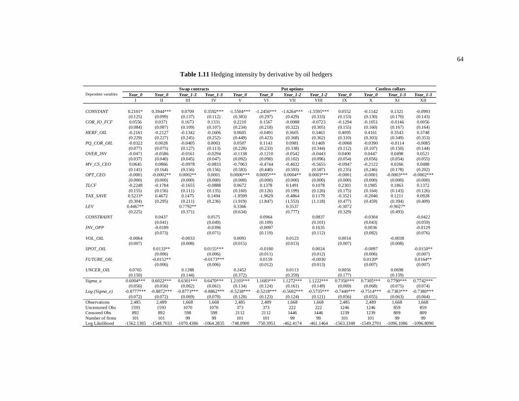
64
Table 1.11 Hedging intensity by derivative by oil hedgers
Swap contracts Put options Costless collars Dependent variables Year_0 Year_0 Year_1-3 Year_1-3 Year_0 Year_0 Year_1-2 Year_1-2 Year_0 Year_0 Year_1-3 Year_1-3
I II III IV V VI VII VIII IX X XI XII
CONSTANT 0.2101* 0.3944*** 0.0709 0.3592*** -1.5504*** -1.2456*** -1.6264*** -1.5595*** 0.0552 -0.1142 0.1321 -0.0993
(0.125) (0.099) (0.137) (0.112) (0.383) (0.297) (0.429) (0.333) (0.153) (0.130) (0.170) (0.143)
COR_IO_FCF 0.0556 0.0371 0.1673 0.1331 0.2210 0.1567 -0.0088 -0.0723 -0.1294 -0.1051 -0.0146 0.0056
(0.084) (0.087) (0.109) (0.107) (0.234) (0.218) (0.322) (0.305) (0.155) (0.160) (0.167) (0.164)
HERF_OIL -0.2161 -0.2127 -0.1342 -0.1606 0.0605 -0.0491 0.3605 0.3463 0.4095 0.4161 0.3543 0.3748
(0.229) (0.227) (0.245) (0.252) (0.449) (0.423) (0.368) (0.362) (0.310) (0.303) (0.349) (0.353)
PQ_COR_OIL -0.0322 0.0028 -0.0405 0.0003 0.0507 0.1143 0.0981 0.1469 -0.0068 -0.0390 -0.0114 -0.0085
(0.077) (0.075) (0.127) (0.113) (0.228) (0.233) (0.338) (0.344) (0.112) (0.107) (0.150) (0.144)
OVER_INV -0.0471 -0.0586 -0.0161 -0.0294 -0.1138 -0.1210 -0.0542 -0.0443 0.0400 0.0447 0.0498 0.0521
(0.037) (0.040) (0.045) (0.047) (0.092) (0.090) (0.102) (0.096) (0.054) (0.056) (0.054) (0.055)
MV_CS_CEO 0.0645 0.0866 -0.0978 -0.0833 -0.7063 -0.4744 -0.4632 -0.5655 -0.0947 -0.2122 0.0266 0.0488
(0.141) (0.164) (0.156) (0.156) (0.583) (0.440) (0.593) (0.587) (0.235) (0.246) (0.178) (0.202)
OPT_CEO -0.0001 -0.0002** 0.0002** 0.0001 0.0006*** 0.0005*** 0.0004** 0.0003*** -0.0001 -0.0001 -0.0003*** -0.0002***
(0.000) (0.000) (0.000) (0.000) (0.000) (0.000) (0.000) (0.000) (0.000) (0.000) (0.000) (0.000)
TLCF -0.2248 -0.1784 -0.1655 -0.0888 0.0672 0.1378 0.1491 0.1078 0.2303 0.1985 0.1863 0.1372
(0.155) (0.156) (0.111) (0.135) (0.160) (0.126) (0.199) (0.126) (0.175) (0.164) (0.143) (0.126)
TAX_SAVE 0.5213* 0.4672 0.1475 0.1494 -1.9599 -1.9629 -0.4864 0.1179 -0.3521 -0.2046 0.1211 0.0928
(0.304) (0.295) (0.211) (0.236) (1.919) (1.847) (1.553) (1.118) (0.477) (0.459) (0.394) (0.409)
LEV 0.4467** 0.7792** 0.3366 0.3537 -0.3072 -0.9027*
(0.225) (0.371) (0.634) (0.777) (0.329) (0.493)
CONSTRAINT 0.0437 0.0575 0.0964 0.0837 -0.0304 -0.0422
(0.041) (0.049) (0.109) (0.101) (0.043) (0.059)
INV_OPP -0.0189 -0.0396 -0.0097 0.1635 0.0036 -0.0129
(0.073) (0.071) (0.119) (0.112) (0.082) (0.076)
VOL_OIL -0.0064 -0.0033 0.0091 0.0123 0.0014 -0.0038
(0.007) (0.008) (0.015) (0.013) (0.007) (0.008)
SPOT_OIL 0.0133** 0.0155*** -0.0180 0.0024 -0.0097 -0.0150**
(0.006) (0.006) (0.011) (0.012) (0.006) (0.007)
FUTURE_OIL -0.0152** -0.0173*** 0.0159 -0.0030 0.0120* 0.0164**
(0.006) (0.006) (0.012) (0.013) (0.007) (0.007)
UNCER_OIL 0.0765 0.1288 0.2452 0.0113 0.0056 0.0698
(0.150) (0.144) (0.372) (0.359) (0.177) (0.159)
Sigma_u 0.6004*** 0.6022*** 0.6301*** 0.6470*** 1.2103*** 1.1683*** 1.1272*** 1.1222*** 0.7356*** 0.7305*** 0.7790*** 0.7742***
(0.056) (0.056) (0.062) (0.061) (0.134) (0.124) (0.161) (0.149) (0.069) (0.068) (0.075) (0.074)
Log (Sigma_e) -0.8777*** -0.8872*** -0.8773*** -0.8862*** -0.5238*** -0.5218*** -0.5692*** -0.5735*** -0.7440*** -0.7514*** -0.7383*** -0.7380***
(0.072) (0.072) (0.069) (0.070) (0.128) (0.123) (0.124) (0.121) (0.056) (0.055) (0.063) (0.064)
Observations 2,485 2,489 1,668 1,668 2,485 2,489 1,668 1,668 2,485 2,489 1,668 1,668
Uncensored Obs 1593 1593 1070 1070 373 373 222 222 1246 1246 859 859
Censored Obs 892 892 598 598 2112 2112 1446 1446 1239 1239 809 809
Number of firms 101 101 99 99 101 101 99 99 101 101 99 99
Log Likelihood -1562.1385 -1548.7033 -1070.4386 -1064.2835 -748.0900 -750.3951 -462.4174 -461.1464 -1563.3348 -1549.2701 -1096.1086 -1096.8090

65
Note:
This table reports the coefficient estimates of the random effects tobit models. The dependent variables are the hedging intensity by derivative instrument (swap contracts, put options, and costless collars) for the subsample of
oil hedgers: Year_0, Year_1-2, and Year_1-3 are hedging intensities for the current fiscal year, the subsequent two fiscal years, and the subsequent three fiscal years, respectively. Independent variables, measured at the end of the previous quarter, are: COR_IO_FCF for the correlation between free cash flows and investment opportunities; HERF_OIL for the geographical dispersion of oil production; PQ_COR_OIL for the oil quantity–price correlation; OVER_INV for overinvestment; MV_CS_CEO for the market value of common shares held by the CEO; OPT_CEO for the number of stock options held by the CEO; TLCF stands for TLCFs scaled by the book value of total assets; TAX_SAVE for the expected percentage of tax savings; LEV for the leverage ratio; CONSTRAINT for financial constraints; INV_OPP for investment opportunities; FUTURE_OIL, SPOT_OIL, and VOL_OIL for oil
future and spot prices and volatility, respectively; UNCER_OIL for oil production uncertainty. Standard errors, corrected for heteroskedasticity and clustering using Huber-White-Sandwich estimator, are in parentheses. The superscripts ***, **, and * indicate significance at the 1%, 5%, and 10% levels, respectively. Sigma_u and Sigma_e stand for the standard deviations of random-effects and error terms, respectively.
Results further indicate, for gas hedgers, that collar intensity increases with managerial
stockholding for the three-year horizon. Interestingly, managerial option-holding has a
significant negative impact on swaps and collars’ notional quantities, and significant positive
effects on put option intensity. The impacts of option-holding on swaps and put options are
evident for near and farther horizons. For collars, this effect is evident only for more distant
horizons. These finding corroborate our earlier results, and give empirical evidence of the
impact of managerial risk aversion on firms’ hedging behaviors. Oil hedgers and gas hedgers
in the progressive tax region tend to intensify their swap and collar positions respectively. As
predicted, the positive relation between tax loss carryforwards and put options is more
evident with the tobit model, particularly for gas hedgers. This latter finding corroborates
Graham and Rogers (2002) conjecture that tax loss carryforwards capture a separate non-tax
influence on firm’s hedging behavior. In addition, higher level of tax loss carryforwards
means that the firm recently accumulated losses and is more likely to be in financial distress.
Consequently, firm’s manager enters costly non-linear hedging (put options) as risk-shifting
strategy.

66
Consistent with previous results, more leveraged oil hedgers tend to rely more on swap
contracts and less on collars. Investment opportunities have a significant positive impact on
put options’ intensity for more distant horizons to avoid costly external financing and the
underinvestment problem, as documented in our earlier results. For both Year_0 and Year_1-
3 horizons, results support previous findings and show that swap (collar) intensity decreases
(increases) with gas price volatility and oil and gas anticipated future prices, and increases
(decreases) with oil and gas spot prices. Unlike findings in previous sections, results further
indicate that put option intensity increases (decreases) with gas spot (future) prices. One
explanation could be that in high spot prices environments, oil and gas producers tend to take
larger put option positions to lock-in the current prices because they believe that prices are
more likely to decrease in the future. Conversely, firms tend to hedge less by costly put
options when future prices are anticipated to increase because shortfalls in future inflows are
less likely and hedging needs are less pressing. Surprisingly, put option positions are not
affected by gas price volatility or oil market conditions. Gas production uncertainty appears
to be positively related to larger collars positions as in our earlier results.
Following Adam (2009), we re-estimate the random-effects tobit models using alternative
measures of hedging intensity of put options and costless collars. Put options and collars’
intensity are measured by
and
respectively.
Results reported in Table A.1.9 show some noticeable differences with the results of the
mixed multinomial logit18
. We find an unpredictable negative impact of diversification in oil
activities on put options’ intensity for the Year_1-2 horizon. Gas diversification loses its
statistical significance. However, this finding corroborates the multinomial logit results. The
negative association between managerial stockholding and put options’ extent is now more
evident as predicted. Moreover, oil hedgers with tax loss carry forwards rely more on collars.
Consistent with the multinomial logit results, tax function convexity is significantly
positively related to put options for Year_1-2 horizon, however, counter the prediction.
Unlike multinomial logit models, for gas hedgers, put options are no longer positively related
to investment opportunities but they are now significantly positively correlated to gas price
18
Results using these alternative measures of hedging intensities could be seen as robustness checks of results of
the mixed multinomial logit for hedging portfolios.
67
volatility. For oil hedgers, oil spot and future prices have no longer significant impact on put
options’ intensity.
Table A.1.10 summarizes our predictions and findings arising from the models used in
the previous sections.
1.4.2.4 Robustness Checks: Other Specifications
In this section, we check the robustness of our previous results to other specifications
related to hedging strategies classification and some variables construction. First, we classify
hedging strategies into two categories: linear and non-linear. Linear strategies include swap
contracts, forward and futures. Non-linear strategies comprise put options, costless collars
and three-way collars. We after distinguish between firms using only linear strategies, a
combination of linear and non-linear strategies, and only non-linear strategies. As before, we
use a dynamic mixed multinomial logit for this new specification of the hedging strategies.
The use of linear strategies only is the base case. We also recalculate the correlations between
spot prices and produced quantities (PQ_COR_GAS and PQ_COR_OIL) and the coefficients
of variation of produced quantities (UNCER_GAS and UNCER_OIL) and cash costs
(COST_CV) based on rolling windows of eight quarterly observations.
Finally, we calculate the sensitivities of revenues and investment costs to the risk
exposure in a more direct manner to test the argument of Froot, Scharfestein, and Stein
(1993) exposed in HYPOTHESIS 1. We then calculate the correlation between firm’s free
cash flows (as previously defined) and oil (gas) spot prices. For the sensitivity of investment
costs, we calculate the correlation between capital expenditures and oil (gas) spot prices.
These coefficients of correlation are calculated at the end of each quarter using rolling
windows of eight quarterly observations. Subsequently, we calculate the absolute value of the
differential between both sensitivities of free cash flows and investment costs (i.e., sensitivity
of investment costs minus the sensitivity of free cash flows). A smaller differential means
that firm’s revenues and investment costs have closer sensitivities to oil (gas) prices and
bigger differential means dissimilar sensitivities. We predict a positive sign for the absolute
values of these differentials in sensitivities (DIFF_GAS and DIFF_OIL).

68
Table A.1.11 reports the regression results for oil and gas hedgers separately and shows
noticeable differences with previous results related to hedging portfolio choice using a mixed
multinomial logit (Table 1.8 and Table 1.9). Surprisingly, differentials in sensitivities of
firm’s revenues and investment costs have no significant impact on the hedging strategy
choice. Higher geographical diversity in oil production activities appears to be positively
related to the use of non-linear strategies as predicted. The newly calculated variables,
namely the correlation between produced quantities and spot prices, the production
uncertainty, and cash cost risk, lose their significant impacts. Results related to managerial
risk aversion and tax arguments are mixed. As predicted, the CEOs option-holding and tax
loss carry-forwards are positively related to the use of non-linear strategies. However, CEOs
shareholding and tax save measure have unpredicted positive association with non-linear
strategies. Financial constraints measures have no real impacts on strategy choice. Consistent
with predictions and previous results, investment opportunities, gas price volatility and gas
future prices are positively related to the use of non-linear strategies. The results further show
that when oil and gas producers hedge simultaneously both commodities and basis risks, they
tend to use more linear strategies because the firm’s aggregate exposure becomes less non-
linear (e.g., Brown and Toft, 2002).
1.5 Concluding remarks
A rich body of empirical literature on corporate risk management explores the incentives,
determinants, and virtues of hedging. While this empirical literature comprehensively
answers why firms hedge risks and identifies the determinants of hedging extent and effects,
the question of how firms hedge risks has been of lesser concern. Using a unique, hand-
collected dataset of detailed, publicly available quarterly information on the risk management
activities of 150 US oil and gas producers during the period from 1998 to 2010, we extend
the empirical literature by investigating the determinants of hedging strategy choice.
Overall, our results show that the state dependence or preference characteristic in hedging
strategy choice must be considered when explaining firm hedging behavior. We find that a
positive correlation between internal funds and capital expenditures is positively related to

69
the use of more linear hedging strategies because oil and gas producers are naturally
diversified. In addition, we observe that geographic diversification in oil and gas production
significantly affect the manner in which producers hedge their exposures. This operative
flexibility is related to hedging strategies with payoffs departing from strict linearity. As
predicted, the price–quantity correlation appears to impact the derivative choice in a
significant manner and is associated positively with swap use for gas hedging particularly.
Overinvestment appears to be a real concern when choosing hedging strategies and it
motivates the use of more swap contracts only or collars only.
In line with our predictions, we find that CEOs with higher shareholding use more linear
strategies and CEOs with higher option holding tend to use more hedging portfolios with
non-linear payoffs. Surprisingly, the results show that higher stockholding and option holding
are both positively related to the use of collars only. The presence of institutional investors
also affects hedging programs. Tax function convexity has a significant and mixed impact on
derivative choice. Tax loss carryforwards are negatively associated with the use of swap
contracts as predicted.
Results further indicate that oil and gas producers that are more leveraged but not yet in
financial distress tend to use swap contracts more frequently because they are seeking
predetermined revenues to satisfy their future debt commitments. More solvent oil and gas
producers tend to use collars only and to avoid swaps only. Consistent with risk-shifting
theory, we find that oil and gas producers close to financial distress use more hedging
portfolios with non-linear payoffs. Investment opportunities are related to more non-linear
hedging strategies. Further, we find that hedging strategy choice is strongly correlated with
the economic conditions of the oil and gas market (i.e., spot prices, future expected prices,
and volatilities). Results pertaining to additional non-hedgeable risks (i.e., quantity and cost
uncertainty) and additional hedgeable risks (FX, IR, and basis risks) indicate that these risks
play an important role in hedging choices. More focused oil and gas producers tend to use
more non-linear strategies. Finally, we check the robustness of our empirical findings using
continuous measures of hedging intensity by instrument.

APPENDIX 1.1
HOW DO FIRMS HEDGE RISKS?
EMPIRICAL EVIDENCE FROM US OIL AND GAS PRODUCERS

71
Table A.1.1 Summary of empirical predictions
Theoretical predictions Author(s) Swap
contracts
only
Put
options
only
Costless
collars
only
Swaps
and put
options
Swaps
and collars
Swaps, put
options and
collars
Collars
and put
options
Correlation between internal funds
and investment opportunities
(expenditures)
Froot, Scharfstein, and Stein (1993)
+ - -/+ - -/+ - -
Production flexibility Moschini and Lapan (1992) - + + + + + +
Quantity–price correlation Brown and Toft (2002); Gay, Nam, and Turac (2002,
2003). + - -/+ - -/+ - -
Overinvestment (Free cash flow
agency problem)
Jensen (1986); Morellec and Smith (2007); Bartram,
Brown, and Fehle (2009) + - + - + - -
Managerial shareholding Smith and Stulz (1985); Tufano (1996) + - -/+ - -/+ - -
Managerial option holding Smith and Stulz (1985); Tufano (1996) - + -/+ + -/+ + +
Tax function convexity Mayers and Smith (1982); Smith and Stulz (1985) + - -/+ - -/+ - -
Financial constraints Adler and Detemple (1988) - + + + + + +
Financial constraints Adam (2002) + - + + + + +
Investment opportunities
(expenditures) Froot, Scharfstein, and Stein (1993) - + -/+ + -/+ + +
Market conditions:
Spot prices
Future prices
Volatilities
Adam (2009)
+
-
-
-
+
+
-
+
+
-
+
+
-
+
+
-
+
+
-
+
+
Existence of additional hedgeable and
non-hedgeable risks
Moschini and Lapan (1995); Franke, Stapleton, and
Subrahmanyam (1998); Brown and Toft (2002); and
Gay, Nam, and Turac (2002, 2003).
- + -/+ + -/+ + +
Note:
This table summarizes the empirical predictions for each of the seven hedging strategies adopted by US oil and gas producers.

72
Table A.1.2 Transition probabilities matrix for oil and gas hedging strategies
Put only Put+collar Put+swap Collar only Collar+put+swap Collar+swap Swap only Total
Panel A: Gas hedging strategies (%)
Put only 85.45 3.64 4.55 2.73 0.91 1.82 0.91 100
Put+collar 8.57 71.43 0.00 11.43 5.71 2.86 0.00 100
Put+swap 3.76 0.00 84.96 0.75 3.76 0.75 6.02 100
Collar only 0.73 1.81 0.00 87.84 0.73 7.62 1.27 100
Collar+put+swap 1.10 2.20 0.55 1.10 79.67 14.29 1.10 100
Collar+swap 0.00 0.10 0.10 4.29 1.99 88.28 5.23 100
Swap only 0.11 0.21 0.54 0.86 0.11 5.91 92.27 100
Panel B: Oil hedging strategies (%)
Put only 89.76 3.94 2.36 0.00 0.79 0.79 2.36 100
Put+collar 5.17 72.41 1.72 13.79 6.90 0.00 0.00 100
Put+swap 3.13 0.00 87.50 0.00 6.25 0.00 3.13 100
Collar only 0.18 1.10 0.00 90.83 0.73 6.42 0.73 100
Collar+put+swap 0.00 3.91 2.34 0.78 79.69 12.50 0.78 100
Collar+swap 0.17 0.00 0.17 6.35 1.67 85.45 6.19 100
Swap only 0.24 0.00 0.48 1.19 0.36 4.30 93.44 100
Table A.1.3 First step of the two-step Heckman regression with sample selection:
Determinants of the oil or gas hedging decision
Dependent variables Oil hedge Gas hedge
(I) (II)
TAX_SAVE 0.9005** 0.1232
(0.366) (0.428)
LEVERAGE 1.5843*** 1.9170***
(0.091) (0.096)
CASH_COST 0.0398*** 0.0605***
(0.003) (0.005)
BVCD -1.2947*** -1.2417***
(0.246) (0.214)
Q_RATIO -0.1056*** -0.1288***
(0.014) (0.014)
RESERVE -0.0009*** -0.0001***
(0.000) (0.000)
MKT_VALUE 0.3924*** 0.5700***
(0.043) (0.043)
SALES 0.1994*** 0.0894***
(0.019) (0.017)
CONSTANT -2.2678*** -2.1663***
(0.088) (0.089)
Observations 5,798 5,798
Pseudo-R squared 0.3025 0.3129
Chi squared 2399.4838 2512.4946
Significance 0.0000 0.0000
Note:
This table reports the coefficients estimates of the probit model. The dependent variable is the hedging decision dummy varia ble, which
takes the value of one if the firm has oil or gas hedging position, respectively, for the quarter and zero otherwise. The independent
variables are TAX_SAVE for the expected percentage of tax savings, LEVERAGE for the leverage ratio measured by the book value of
long-term debt scaled by the book value of total assets, CASH_COST for the production cost per BOE, BVCD for the book value of
convertible debts scaled by the book value of total assets, Q_RATIO for the quick ratio measured by the book value of cash and the
equivalent of cash scaled by the book value of current liabilities, RESERVE for the quantities of proved reserves for oil (for oil hedgers)
and gas (for gas hedgers), MKT_VALUE for the logarithm of the market value of common shares outstanding (i.e., closing price at the
end of the quarter multiplied by the number of common shares outstanding), and SALES for the logarithm of sales at the end of the
quarter. Standard errors are in parentheses. The superscripts ***, **, and * indicate significance at the 1%, 5%, and 10% levels,
respectively.

APPENDIX 1.2
UNIVARIATE ANALYSIS

74
Univariate Analysis
Tables A.1.4 and A.1.5 report descriptive statistics of the independent variables and tests
of differences between the means and medians of relevant variables by derivative instruments
for gas and oil hedgers separately. The means are compared by using a t-test assuming
unequal variances; the medians are compared by using a non-parametric Wilcoxon rank-sum
Z-test and two-sided p-values. As discussed, we retain only the three major derivative
instruments: put options, costless collars, and swap contracts (the three instruments
correspond to more than 93% of all oil and gas hedging). These major instruments could be
classified according to their payoff linearity. Put options are the most non-linear instruments,
swap contracts are the most linear, and costless collars fall in between. Overall, the univariate
results support the premise that firms with greater investment opportunities tend to use more
non-linear instruments (i.e., put options and costless collars) than linear instruments (i.e.,
swap contracts).
Unexpectedly, higher undeveloped proved oil and gas reserves appear to be associated
more with the use of swap contracts. On average, firms using more swap contracts and
costless collars seem to have a higher correlation between internal cash flows and investment
opportunities than those using put options as predicted. Interestingly, the univariate results
support the prediction that large profitable oil and gas producers with fewer growth options
tend to use more linear instruments to avoid the overinvestment problem, as suggested by
Morellec and Smith (2007) and Bartram, Brown, and Fehle (2009).
The results related to tax incentives are mixed. Although tax function convexity and tax
preference items (i.e., TLCFs) tend to be more related to the use of swaps for the subsample
of oil hedgers as predicted, they are unpredictably more associated with put options and
costless collars for the subsample of gas hedgers. On average, users of put options have a
relatively lower DTD and lower leverage ratios. Interestingly, these findings suggest that
there is a non-monotonic relation between the use of put options and firm financial health.
Hence, firms either close to or far from financial distress tend to use more non-linear hedging
strategies. In contrast, swap contracts are associated more with relatively higher DTDs and
higher leverage ratios.

75
On average, swap contracts are associated with a higher CEO equity stake value in the
firm, as predicted. Unexpectedly, put options are associated with fewer CEO option holdings,
particularly for the subsample of oil hedgers. The results also show that a higher percentage
of institutional shareholding is more related to the use of put options and costless collars. The
results of the means comparison concerning the impact of additional non-hedgeable risks
(i.e., production uncertainty, cash cost risk) are mixed. Although higher cash cost risk is more
related to the use of costless collars and put options as predicted, oil and gas production
uncertainties seem to be more associated with the use of swaps.
The results for the price–quantity correlation and geographical and industrial
diversification are mixed. However, the use of put options is more closely related to a lower
price–quantity correlation and higher geographical diversification for the subsample of gas
hedgers, as predicted. The use of put options by oil hedgers is more strongly associated with
a higher price–quantity correlation and lower geographical diversification. Tests further show
that firms operating primarily in gas production use more collars and those operating
primarily in oil production use more put options. Surprisingly, the results show no significant
differences in the economic conditions of the oil and gas markets between swap contracts and
put options. In fact, higher volatility, higher spot prices, and higher future prices are largely
associated with the use of costless collars.
We now analyze financial and operational characteristics by hedging portfolios when oil
and gas hedgers use more than one instrument simultaneously. Tables A.1.6 and A.1.7 report
univariate results related to those portfolios. We retain comparisons involving the next two
hedging portfolios: swaps combined with put options versus swaps combined with costless
collars. The first portfolio is supposed to have a more non-linear payoff. As predicted, the
results show that users of swap and collar portfolios have lower investment opportunities and
larger undeveloped proved oil and gas reserves. Unexpectedly, swap and collar portfolios are
associated with a lower correlation between internal cash flows and investment opportunities,
lower expected tax savings, and lower tax preference items (TLCFs). In addition, users of
swap and collar portfolios have fewer financial constraints coupled with a higher DTD and
lower leverage ratios.

76
Consistent with the predictions, swap and collar portfolios are associated with a higher
CEO equity stake value in the firm. Counter to predictions, these portfolios seem to be
associated with higher stock option holding. As predicted, the results indicate that swap and
collar portfolios are related to lower production uncertainty and a higher price–quantity
correlation. Nonetheless, swaps and collars portfolios’ users have higher cash cost variability
and greater geographical diversification, contradicting the conjecture. For the subsample of
gas hedgers, the univariate results show, unexpectedly, that swaps and collars portfolios are
associated with higher gas price volatility and with higher gas future prices. As predicted,
swaps and collars portfolios are related to higher gas spot prices.

77
Table A.1.4 Financial and operational characteristics of gas hedgers, by hedging instrument
Gas hedging instruments firm–quarter
Swap Put Collar Swap vs put Swap vs collar Collar vs put
Variable Obs Mean Median Obs Mean Median Obs Mean Median t-Stat p-Value Z-Score p-Value t-Stat p-Value Z-Score p-Value t-Stat p-Value Z-Score p-Value Variables that proxy for hedging activity
OIL_HEDG 932 0.630 1.000 126 0.540 1.000 582 0.741 1.000 1.906 0.059 -1.955 0.051 -4.593 0.000 4.464 0.000 -4.172 0.000 -4.479 0.000
BASIS_HEDG 932 0.152 0.000 126 0.063 0.000 582 0.060 0.000 3.585 0.000 -2.683 0.007 6.003 0.000 -5.431 0.000 0.140 0.889 0.143 0.886
IR_HEDG 932 0.276 0.000 126 0.159 0.000 582 0.196 0.000 3.267 0.001 -2.803 0.005 3.625 0.000 -3.514 0.000 -1.015 0.311 -0.964 0.335 FX_HEDG 932 0.065 0.000 126 0.040 0.000 582 0.003 0.000 1.339 0.182 -1.122 0.262 7.329 0.000 -5.876 0.000 2.056 0.042 3.726 0.000
Variables that proxy for underinvestment costs
INV_OPP 927 0.092 0.068 126 0.129 0.086 555 0.116 0.086 -2.101 0.038 3.401 0.001 -2.974 0.003 4.841 0.000 0.679 0.498 0.207 0.836
UND_OIL 932 40.745 4.170 126 26.793 17.597 582 19.549 4.569 2.648 0.009 2.394 0.017 5.535 0.000 0.522 0.602 1.494 0.137 3.042 0.002 UND_GAS 932 371.744 89.290 126 228.131 124.412 582 193.096 46.350 2.827 0.005 -1.433 0.152 5.204 0.000 -5.830 0.000 0.677 0.499 2.540 0.011
COR_IO_FCF 932 0.146 0.154 126 -0.026 0.018 582 0.087 0.086 5.188 0.000 4.860 0.000 3.114 0.001 3.063 0.002 -3.435 0.000 -3.743 0.000
Variables that proxy for overinvestment
OVER_INV 932 0.328 0.000 126 0.230 0.000 552 0.225 0.000 2.411 0.017 2.221 0.026 4.402 0.000 4.249 0.000 0.132 0.895 0.134 0.894
Variables that proxy for the tax advantage of hedging
TLCF 928 0.044 0.000 126 0.092 0.000 571 0.085 0.000 -3.087 0.002 3.737 0.000 -3.547 0.000 4.563 0.000 0.343 0.732 1.143 0.253
TAX_SAVE 928 0.047 0.044 126 0.052 0.052 573 0.054 0.050 -1.733 0.084 3.266 0.001 -2.790 0.005 5.011 0.000 -0.551 0.582 0.305 0.761
Variables that proxy for financial distress costs DTD 915 2,338 2,206 126 2,148 2,105 564 2,150 2,123 2.1573 0.0321 0.929 0.353 2.930 0.003 1.910 0.056 -0.027 0.978 0.098 0.922
CONSTRAINT 928 0.471 0.000 126 0.405 0.000 571 0.375 0.000 1.411 0.160 1.397 0.162 3.686 0.000 3.645 0.000 0.620 0.536 0.627 0.531
LEV 928 0.207 0.185 126 0.163 0.180 571 0.209 0.170 4.491 0.000 2.514 0.012 -0.248 0.804 1.454 0.146 -4.155 0.000 -1.360 0.174
Variables that proxy for managerial risk aversion MV_CS_CEO 932 42.241 4.151 126 6.578 4.007 582 44.470 3.394 5.800 0.000 1.635 0.102 -0.214 0.830 2.561 0.010 -4.469 0.000 -0.095 0.924
OPT_CEO 932 229952 5000 126 173357 22500 582 197251 0.000 1.406 0.161 0.026 0.979 0.805 0.420 2.209 0.027 -0.457 0.647 1.382 0.167
Variables that proxy for information asymmetry %_CS_INST 932 0.451 0.475 126 0.557 0.663 582 0.493 0.543 -3.227 0.002 3.440 0.001 -2.294 0.022 2.228 0.026 1.868 0.063 2.003 0.045
Variables that proxy for production characteristics
UNCER_OIL 887 0.409 0.286 126 0.365 0.358 562 0.435 0.374 1.768 0.079 0.138 0.890 -1.558 0.120 3.620 0.000 -2.802 0.006 -2.327 0.020
PQ_COR_OIL 900 0.213 0.450 126 0.330 0.579 562 0.375 0.565 -2.172 0.031 2.516 0.012 -5.520 0.000 5.637 0.000 -0.815 0.417 -0.660 0.509
UNCER_GAS 932 0.409 0.308 126 0.335 0.224 582 0.379 0.294 2.493 0.014 -2.714 0.007 1.781 0.075 -0.767 0.443 -1.445 0.150 -2.470 0.014 PQ_COR_GAS 932 0.225 0.312 126 0.024 0.027 582 0.249 0.374 5.232 0.000 -5.039 0.000 -1.187 0.235 2.192 0.028 -5.651 0.000 -5.449 0.000
COST_CV 913 0.243 0.194 126 0.260 0.217 568 0.275 0.262 -0.955 0.341 0.737 0.461 -3.856 0.000 4.167 0.000 -0.865 0.388 -1.443 0.149
OIL_REV 926 0.254 0.204 126 0.391 0.416 582 0.324 0.299 -6.245 0.000 -6.180 0.000 -6.183 0.000 -6.776 0.000 2.995 0.003 3.137 0.001
GAS_REV 926 0.587 0.656 126 0.562 0.541 582 0.638 0.638 1.139 0.255 1.702 0.088 -3.852 0.000 -1.885 0.059 -3.535 0.000 -3.693 0.000 HERF_GAS 932 0.044 0.000 126 0.142 0.000 582 0.028 0.000 -4.598 0.000 -5.443 0.000 2.735 0.006 4.623 0.000 5.407 0.000 8.358 0.000
HERF_OIL 897 0.100 0.000 126 0.140 0.000 567 0.085 0.000 -1.707 0.089 -2.584 0.009 1.324 0.186 2.498 0.012 2.302 0.022 4.245 0.000
Variables that proxy for market conditions
VOL_OIL 929 3.200 2.371 126 3.123 2.233 581 3.520 2.674 0.306 0.760 -0.070 0.944 -2.117 0.035 3.147 0.002 -1.490 0.138 -1.896 0.058 SPOT_OIL 929 49.140 35.760 126 47.959 32.520 581 54.813 56.500 0.450 0.654 -0.428 0.669 -3.816 0.000 4.139 0.000 -2.531 0.012 -2.912 0.004
FUTURE_OIL 929 49.212 33.311 126 47.983 30.298 581 54.985 58.710 0.454 0.651 -0.227 0.821 -3.785 0.000 4.068 0.000 -2.512 0.013 -2.758 0.006
VOL_GAS 929 0.687 0.456 126 0.784 0.543 581 0.828 0.695 -1.840 0.068 2.277 0.023 -4.766 0.000 5.532 0.000 -0.796 0.427 -0.850 0.395
SPOT_GAS 929 4.833 4.602 126 5.139 4.830 581 5.674 5.700 -1.256 0.211 1.326 0.185 -6.302 0.000 7.163 0.000 -2.116 0.036 -2.555 0.011 FUTURE_GAS 929 5.340 5.070 126 5.677 5.149 581 6.467 6.213 -1.441 0.152 1.704 0.088 -8.443 0.000 8.888 0.000 -3.242 0.001 -3.259 0.001
Note:
This table reports the univariate analysis results for the independent variables proposed to explain the use of hedging instruments by gas hedgers. The terms OIL_HEDG, IR_HEDG, FX_HEDG, and BASIS_HEDG are dummy variables for
gas, oil, IR, FX, and basis risk hedging, respectively; TLCF stands for TLCFs scaled by the book value of total assets; TAX_SAVE for the expected percentage of tax savings; LEV for the leverage ratio; DTD for the DTD; CONSTRAINT for
financial constraints; INV_OPP for investment opportunities; COR_IO_FCF for the correlation between free cash flows and investment opportunities; UND_OIL and UND_GAS for the undeveloped proved reserves of oil and gas,
respectively; OVER_INV for overinvestment; OIL_REV and GAS_REV for the fraction of revenues from oil and gas production, respectively; HERF_OIL and HERF_GAS for the geographical dispersion of oil and gas production, respectively;
UNCER_OIL and UNCER_GAS for the production uncertainty for oil and gas, respectively; COST_CV for the coefficient of variation of the cash cost per BOE; PQ_COR_OIL and PQ_COR_GAS for the quantity–price correlation for oil and
gas, respectively; MV_CS_CEO for the market value of common shares held by the CEO; OPT_CEO for the number of stock options held by the CEO; %_CS_INST for the percentage of common shares held by institutional investors;
FUTURE_OIL, SPOT_OIL, and VOL_OIL for oil future and spot prices and volatility, respectively; and FUTURE_GAS, SPOT_GAS, and VOL_GAS for gas future and spot prices and volatility. The means are compared by using a t-test,
assuming unequal variances; the medians are compared by using the non-parametric Wilcoxon rank sum Z-score. Two-sided p-values are reported.

78
Table A.1.5 Financial and operational characteristics of oil hedgers, by hedging instrument
Oil hedging instruments firm–quarter
Swap Put Collar Swap vs put Swap vs collar Collar vs put
Variable Obs Mean Median Obs Mean Median Obs Mean Median t-Stat p-Value Z-Score p-Value t-Stat p-Value Z-Score p-Value t-Stat p-Value Z-Score p-Value Variables that proxy for hedging activity
OIL_HEDG 849 0.826 1.000 150 0.787 1.000 577 0.818 1.000 1.084 0.280 -1.145 0.252 0.370 0.712 -0.371 0.711 -0.843 0.400 -0.874 0.382
BASIS_HEDG 849 0.221 0.000 150 0.060 0.000 577 0.045 0.000 6.693 0.000 -4.579 0.000 10.578 0.000 -9.150 0.000 0.702 0.484 0.761 0.447
IR_HEDG 849 0.335 0.000 150 0.080 0.000 577 0.243 0.000 9.254 0.000 -6.290 0.000 3.810 0.000 -3.724 0.000 -5.704 0.000 -4.361 0.000
FX_HEDG 849 0.121 0.000 150 0.093 0.000 577 0.012 0.000 1.063 0.289 -0.982 0.326 9.021 0.000 -7.582 0.000 3.347 0.001 5.286 0.000
Variables that proxy for underinvestment costs
INV_OPP 842 0.105 0.073 146 0.118 0.070 560 0.130 0.080 -0.767 0.444 0.333 0.739 -1.979 0.048 1.724 0.085 -0.617 0.538 -0.868 0.385
UND_OIL 849 43.351 6.178 150 44.958 12.545 577 46.770 6.332 -0.250 0.803 1.161 0.246 -0.604 0.546 -2.189 0.029 -0.239 0.812 2.388 0.017
UND_GAS 849 441.004 112.765 150 344.652 57.215 577 362.649 56.098 1.503 0.134 -3.289 0.001 1.615 0.107 -5.990 0.000 -0.256 0.798 0.413 0.680 COR_IO_FCF 849 0.125 0.095 150 0.072 0.041 577 0.042 0.058 1.838 0.067 1.589 0.112 4.192 0.000 3.477 0.000 1.014 0.311 0.488 0.625
Variables that proxy for overinvestment
OVER_INV 838 0.285 0.000 146 0.226 0.000 558 0.339 0.000 1.554 0.122 1.475 0.140 -2.106 0.035 -2.123 0.034 -2.809 0.005 -2.607 0.009
Variables that proxy for the tax advantage of hedging TLCF 844 0.077 0.000 146 0.045 0.000 577 0.101 0.000 2.762 0.006 -5.196 0.000 -1.794 0.073 0.119 0.905 -3.491 0.001 -5.390 0.000
TAX_SAVE 845 0.052 0.048 146 0.046 0.047 577 0.045 0.044 2.298 0.022 -1.871 0.061 3.689 0.000 -3.825 0.000 0.373 0.710 0.372 0.710
Variables that proxy for financial distress costs DTD 819 2.390 2.530 146 2.127 2.048 576 2.276 2.214 2.893 0.004 2.159 0.031 1.748 0.080 1.250 0.211 -1.604 0.109 -1.393 0.164
CONSTRAINT 844 0.515 1.000 146 0.301 0.000 577 0.310 0.000 5.118 0.000 4.776 0.000 7.939 0.000 7.665 0.000 -0.207 0.836 -0.207 0.836
LEV 844 0.214 0.191 146 0.136 0.134 577 0.184 0.154 8.539 0.000 7.166 0.000 3.776 0.000 6.904 0.000 -4.699 0.000 -2.818 0.005
Variables that proxy for managerial risk aversion MV_CS_CEO 849 68.804 4.661 150 11.598 3.572 577 53.203 3.731 5.402 0.000 2.819 0.005 1.163 0.245 2.773 0.005 -4.847 0.000 -0.996 0.319
OPT_CEO 849 230427 75000 150 98734 0.000 577 99958 0.000 5.855 0.000 4.976 0.000 8.080 0.000 7.221 0.000 -0.065 0.948 -0.533 0.594
Variables that proxy for information asymmetry %_CS_INST 849 0.505 0.602 150 0.519 0.672 577 0.559 0.668 -0.452 0.652 1.016 0.310 -2.974 0.003 4.146 0.000 -1.220 0.224 -1.536 0.125
Variables that proxy for production characteristics
UNCER_OIL 846 0.408 0.288 150 0.332 0.259 577 0.460 0.448 2.821 0.005 -1.670 0.095 -2.972 0.003 5.176 0.000 -4.743 0.000 -5.824 0.000
PQ_COR_OIL 849 0.237 0.459 150 0.363 0.638 577 0.416 0.589 -2.461 0.015 3.912 0.000 -6.420 0.000 6.331 0.000 -1.039 0.300 0.419 0.675
UNCER_GAS 840 0.413 0.260 150 0.354 0.335 570 0.408 0.322 2.266 0.024 -0.618 0.537 0.282 0.778 2.552 0.011 -2.092 0.037 -1.836 0.066 PQ_COR_GAS 849 0.203 0.287 150 0.127 0.214 577 0.257 0.363 1.932 0.055 -1.531 0.126 -2.675 0.008 2.974 0.003 -3.252 0.001 -2.866 0.004
COST_CV 844 0.191 0.220 150 0.263 0.216 560 0.310 0.300 -1.629 0.104 0.791 0.429 -2.812 0.005 7.862 0.000 -2.790 0.006 -3.606 0.000
OIL_REV 842 0.311 0.250 145 0.459 0.519 577 0.387 0.320 -7.388 0.000 -7.340 0.000 -5.435 0.000 -5.751 0.000 3.389 0.008 4.215 0.000
GAS_REV 842 0.520 0.573 145 0.454 0.454 577 0.561 0.612 3.599 0.000 3.511 0.000 -2.715 0.006 -2.475 0.013 -5.554 0.000 -5.602 0.000 HERF_GAS 845 0.080 0.000 150 0.098 0.000 570 0.039 0.000 -1.013 0.312 -0.429 0.668 4.781 0.000 5.839 0.000 3.362 0.000 4.401 0.000
HERF_OIL 849 0.110 0.000 150 0.129 0.000 577 0.089 0.000 -0.822 0.412 -1.050 0.2936 1.785 0.074 2.253 0.024 1.745 0.082 2.547 0.011
Variables that proxy for market conditions
VOL_OIL 849 3.272 2.371 150 3.469 2.445 576 3.864 3.271 -0.764 0.446 0.785 0.433 -3.741 0.000 6.566 0.000 -1.475 0.141 -2.804 0.005 SPOT_OIL 849 47.999 32.520 150 51.612 44.600 576 59.790 61.050 -1.366 0.174 0.527 0.598 -8.101 0.000 8.483 0.000 -3.022 0.003 -3.788 0.000
FUTURE_OIL 849 47.768 30.298 150 51.797 46.388 576 60.371 64.847 -1.496 0.136 0.763 0.445 -8.410 0.000 8.366 0.000 -3.115 0.002 -3.642 0.000
VOL_GAS 849 0.710 0.458 150 0.747 0.526 576 0.857 0.760 -0.795 0.428 1.181 0.238 -4.972 0.000 6.216 0.000 -2.257 0.025 -2.386 0.017
SPOT_GAS 849 4.945 4.740 150 5.194 5.050 576 5.852 5.771 -1.042 0.299 0.720 0.471 -6.735 0.000 7.199 0.000 -2.639 0.009 -3.189 0.001 FUTURE_GAS 849 5.443 5.106 150 5.804 5.388 576 6.654 6.280 -1.557 0.121 1.581 0.114 -9.217 0.000 9.483 0.000 -3.520 0.001 -3.621 0.000
Note:
This table reports the univariate analysis for the independent variables proposed to explain the use of the hedging instrument by oil hedgers. The terms GAS_HEDG, IR_HEDG, FX_HEDG, and BASIS_HEDG are dummy variables for gas, oil,
IR, FX, and basis risk hedging; TLCF stands for TLCFs scaled by the book value of total assets; TAX_SAVE for the expected percentage of tax savings; LEV for the leverage ratio; DTD for the DTD; CONSTRAINT for financial constraints;
INV_OPP for investment opportunities; COR_IO_FCF for the correlation between free cash flows and investment opportunities; UND_OIL and UND_GAS for the undeveloped proved reserves of oil and gas, respectively; OVER_INV for
overinvestment; COST_CV is the coefficient of variation of the cash cost per BOE; OIL_REV and GAS_REV for the fraction of revenues from oil and gas production, respectively; HERF_OIL and HERF_GAS for the geographical dispersion
of oil and gas production, respectively; UNCER_OIL and UNCER_GAS for the production uncertainty for oil and gas, respectively; PQ_COR_OIL and PQ_COR_GAS for the quantity–price correlation for oil and gas, respectively;
MV_CS_CEO for the market value of common shares held by the CEO; OPT_CEO for the number of stock options held by the CEO; %_CS_INST for the percentage of common shares held by institutional investors; FUTURE_OIL,
SPOT_OIL, and VOL_OIL for oil future and spot prices and volatility, respectively; and FUTURE_GAS, SPOT_GAS, and VOL_GAS for gas future and spot prices and volatility, respectively. The means are compared by using a t-test
assuming unequal variances; the medians are compared by using the non-parametric Wilcoxon rank sum Z-score. Two-sided p-values are reported.
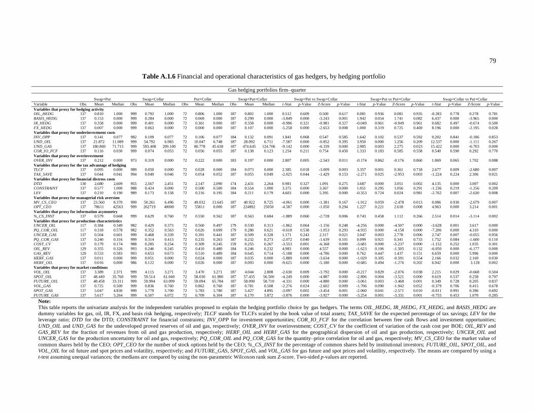
79
Table A.1.6 Financial and operational characteristics of gas hedgers, by hedging portfolio
Gas hedging portfolios firm–quarter
Swap+Put Swap+Collar Put+Collar Swap+Put+Collar Swap+Put vs Swap+Collar Swap+Put vs Put+Collar Swap+Collar vs Put+Collar
Variable Obs Mean Median Obs Mean Median Obs Mean Median Obs Mean Median t-Stat p-Value Z-Score p-Value t-Stat p-Value Z-Score p-Value t-Stat p-Value Z-Score p-Value
Variables that proxy for hedging activity OIL_HEDG 137 0.810 1.000 999 0.792 1.000 72 0.806 1.000 187 0.802 1.000 0.512 0.609 0.500 0.617 0.081 0.936 0.081 0.935 -0.283 0.778 0.278 0.781
BASIS_HEDG 137 0.153 0.000 999 0.284 0.000 72 0.069 0.000 187 0.299 0.000 -3.849 0.000 -3.243 0.001 1.942 0.054 1.741 0.082 6.437 0.000 -3.965 0.000
IR_HEDG 137 0.358 0.000 999 0.401 0.000 72 0.361 0.000 187 0.358 0.000 -0.996 0.321 -0.981 0.327 -0.049 0.961 -0.049 0.961 0.682 0.497 -0.674 0.500
FX_HEDG 137 0.007 0.000 999 0.063 0.000 72 0.000 0.000 187 0.107 0.000 -5.258 0.000 -2.653 0.008 1.000 0.319 0.725 0.469 8.196 0.000 -2.195 0.028
Variables that proxy for underinvestment costs
INV_OPP 137 0.141 0.077 982 0.109 0.077 72 0.106 0.077 184 0.132 0.091 1.841 0.068 0.547 0.585 1.642 0.102 0.537 0.592 0.202 0.841 -0.186 0.853
UND_OIL 137 21.872 11.089 999 54.792 6.983 72 10.047 6.748 187 28.092 6.711 -7.587 0.000 -0.852 0.395 3.950 0.000 1.256 0.209 12.537 0.000 -1.111 0.267
UND_GAS 137 180.869 71.715 999 593.408 209.100 72 80.778 45.638 187 474.645 124.706 -9.142 0.000 -6.339 0.000 2.985 0.003 2.275 0.023 15.422 0.000 -6.703 0.000 COR_IO_FCF 137 0.116 0.030 999 0.074 0.053 72 0.056 0.055 187 0.138 0.123 1.254 0.211 0.754 0.450 1.333 0.183 0.585 0.558 0.540 0.590 0.292 0.770
Variables that proxy for overinvestment
OVER_INV 137 0.212 0.000 973 0.319 0.000 72 0.222 0.000 183 0.197 0.000 2.807 0.005 -2.543 0.011 -0.174 0.862 -0.176 0.860 1.869 0.065 1.702 0.088
Variables that proxy for the tax advantage of hedging TLCF 137 0.095 0.000 989 0.050 0.000 72 0.028 0.000 184 0.073 0.000 2.385 0.018 -3.009 0.003 3.357 0.001 0.361 0.718 2.677 0.009 -2.680 0.007
TAX_SAVE 137 0.044 0.041 994 0.049 0.046 72 0.054 0.052 187 0.055 0.049 -2.025 0.044 -1.429 0.153 -2.271 0.025 -2.953 0.003 -1.224 0.224 2.306 0.021
Variables that proxy for financial distress costs
DTD 130 2,680 2,609 955 2,567 2,451 72 2,147 2,090 174 2,431 2,264 0.981 0.327 1.091 0.275 3.687 0.000 3.051 0.002 4.135 0.000 3.007 0.002 CONSTRAINT 137 0.577 1.000 988 0.424 0.000 72 0.500 0.500 184 0.554 1.000 3.375 0.000 3.367 0.000 1.051 0.295 1.056 0.291 -1.236 0.219 -1.256 0.209
LEV 137 0.210 0.190 989 0.173 0.158 72 0.216 0.195 184 0.211 0.179 4.603 0.000 5.395 0.000 -0.353 0.724 0.024 0.981 -2.762 0.007 -2.630 0.008
Variables that proxy for managerial risk aversion MV_CS_CEO 137 23.560 8.370 999 50.261 6.496 72 49.032 13.645 187 40.922 8.725 -4.061 0.000 -1.381 0.167 -1.912 0.059 -2.478 0.013 0.086 0.930 -2.679 0.007 OPT_CEO 137 78611 42563 999 262719 40000 72 55811 0.000 187 224892 25050 -4.587 0.000 -1.050 0.294 1.227 0.221 2.618 0.008 4.963 0.000 3.214 0.001
Variables that proxy for information asymmetry
%_CS_INST 137 0.579 0.668 999 0.629 0.760 72 0.550 0.562 187 0.563 0.684 -1.889 0.060 -2.728 0.006 0.743 0.458 1.112 0.266 2.514 0.014 -3.114 0.002
Variables that proxy for production characteristics UNCER_OIL 117 0.384 0.349 982 0.429 0.373 72 0.560 0.497 179 0.530 0.313 -1.862 0.064 -1.156 0.248 -4.256 0.000 -4.507 0.000 -3.628 0.001 3.617 0.000
PQ_COR_OIL 117 0.318 0.578 982 0.352 0.563 72 0.626 0.699 179 0.286 0.621 -0.618 0.538 -1.053 0.293 -4.935 0.000 -4.158 0.000 -7.206 0.000 4.310 0.000
UNCER_GAS 137 0.504 0.601 999 0.468 0.339 72 0.391 0.441 187 0.509 0.328 1.171 0.243 2.317 0.021 3.047 0.003 2.778 0.006 2.747 0.007 -0.055 0.956
PQ_COR_GAS 137 0.240 0.316 999 0.314 0.413 72 0.235 0.263 187 0.232 0.273 -2.072 0.040 -1.639 0.101 0.099 0.921 0.341 0.733 1.752 0.084 -1.600 0.110 COST_CV 137 0.179 0.174 988 0.285 0.254 72 0.309 0.245 159 0.255 0.267 -3.553 0.001 -6.368 0.000 -3.681 0.000 -5.237 0.000 -1.152 0.252 1.035 0.301
OIL_REV 129 0.355 0.326 993 0.246 0.245 72 0.410 0.480 184 0.246 0.232 4.983 0.000 4.557 0.000 -1.623 0.106 -1.505 0.132 -6.050 0.000 -6.177 0.000
GAS_REV 129 0.533 0.583 993 0.653 0.673 72 0.510 0.489 184 0.645 0.714 -5.188 0.000 -4.786 0.000 0.762 0.447 1.437 0.151 6.659 0.000 5.996 0.000
HERF_GAS 137 0.011 0.000 999 0.051 0.000 72 0.024 0.000 187 0.035 0.000 -5.889 0.000 -3.634 0.000 -1.029 0.305 -0.591 0.554 2.166 0.032 2.169 0.030 HERF_OIL 137 0.016 0.000 986 0.122 0.000 72 0.026 0.000 187 0.093 0.000 -9.625 0.000 -5.180 0.000 -0.685 0.494 -1.276 0.202 6.942 0.000 3.128 0.002
Variables that proxy for market conditions VOL_OIL 137 3.389 2.371 999 4.115 3.271 72 3.470 3.271 187 4.044 2.808 -2.630 0.009 -3.792 0.000 -0.217 0.829 -2.076 0.038 2.215 0.029 -0.668 0.504
SPOT_OIL 137 48.449 35.760 999 59.514 61.040 72 58.030 61.980 187 57.435 56.500 -4.249 0.000 -4.887 0.000 -2.896 0.004 -3.521 0.000 0.619 0.537 0.258 0.797 FUTURE_OIL 137 48.458 33.311 999 59.994 63.099 72 59.094 65.784 187 58.090 58.710 -4.331 0.000 -4.880 0.000 -3.061 0.003 -3.468 0.001 0.349 0.728 0.205 0.837
VOL_GAS 137 0.725 0.500 999 0.836 0.760 72 0.862 0.760 187 0.781 0.508 -2.276 0.024 -2.602 0.009 -1.706 0.090 -1.942 0.052 -0.379 0.706 0.415 0.678
SPOT_GAS 137 5.047 4.830 999 5.779 5.700 72 5.783 5.780 187 5.427 4.895 -3.097 0.002 -3.454 0.001 -2.060 0.041 -2.571 0.010 -0.011 0.991 0.396 0.692
FUTURE_GAS 137 5.617 5.264 999 6.507 6.072 72 6.709 6.304 187 6.170 5.872 -3.876 0.000 -3.927 0.000 -3.254 0.001 -3.331 0.001 -0.755 0.453 1.070 0.285
Note:
This table reports the univariate analysis for the independent variables proposed to explain the hedging portfolio choice by gas hedgers. The terms OIL_HEDG, IR_HEDG, FX_HEDG, and BASIS_HEDG are
dummy variables for gas, oil, IR, FX, and basis risk hedging, respectively; TLCF stands for TLCFs scaled by the book value of total assets; TAX_SAVE for the expected percentage of tax savings; LEV for the
leverage ratio; DTD for the DTD; CONSTRAINT for financial constraints; INV_OPP for investment opportunities; COR_IO_FCF for the correlation between free cash flows and investment opportunities;
UND_OIL and UND_GAS for the undeveloped proved reserves of oil and gas, respectively; OVER_INV for overinvestment; COST_CV for the coefficient of variation of the cash cost per BOE; OIL_REV and
GAS_REV for the fraction of revenues from oil and gas production, respectively; HERF_OIL and HERF_GAS for the geographical dispersion of oil and gas production, respectively; UNCER_OIL and
UNCER_GAS for the production uncertainty for oil and gas, respectively; PQ_COR_OIL and PQ_COR_GAS for the quantity–price correlation for oil and gas, respectively; MV_CS_CEO for the market value of
common shares held by the CEO; OPT_CEO for the number of stock options held by the CEO; %_CS_INST for the percentage of common shares held by institutional investors; FUTURE_OIL, SPOT_OIL, and
VOL_OIL for oil future and spot prices and volatility, respectively; and FUTURE_GAS, SPOT_GAS, and VOL_GAS for gas future and spot prices and volatility, respectively. The means are compared by using a
t-test assuming unequal variances; the medians are compared by using the non-parametric Wilcoxon rank sum Z-score. Two-sided p-values are reported.
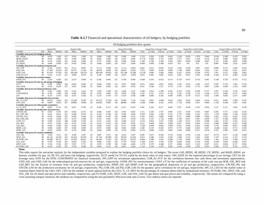
80
Table A.1.7 Financial and operational characteristics of oil hedgers, by hedging portfolio
Oil hedging portfolios firm–quarter
Swap+Put Swap+Collar Put+Collar Swap+Put+Collar Swap+Put vs Swap+Collar Swap+Put vs Put+Collar Swap+Collar vs Put+Collar
Variable Obs Mean Median Obs Mean Median Obs Mean Median Obs Mean Median t-Stat p-Value Z-Score p-Value t-Stat p-Value Z-Score p-Value t-Stat p-Value Z-Score p-Value
Variables that proxy for hedging activity
OIL_HEDG 99 0.879 1.000 627 0.955 1.000 63 0.968 1.000 136 0.949 1.000 -2.253 0.026 -3.100 0.002 -2.249 0.026 -1.970 0.049 -0.544 0.588 -0.479 0.632
BASIS_HEDG 99 0.020 0.000 627 0.290 0.000 63 0.063 0.000 136 0.324 0.000 -11.719 0.000 -5.737 0.000 -1.271 0.207 -1.418 0.156 6.319 0.000 3.864 0.000
IR_HEDG 99 0.374 0.000 627 0.442 0.000 63 0.175 0.000 136 0.456 0.000 -1.290 0.199 -1.269 0.204 2.901 0.004 2.698 0.007 5.125 0.000 4.097 0.000
FX_HEDG 99 0.000 0.000 627 0.056 0.000 63 0.000 0.000 136 0.037 0.000 -6.084 0.000 -2.408 0.016 NA NA NA NA 6.084 0.000 1.923 0.054
Variables that proxy for underinvestment costs
INV_OPP 99 0.146 0.079 622 0.131 0.081 61 0.113 0.058 133 0.114 0.064 0.653 0.515 0.636 0.525 1.182 0.239 1.987 0.047 0.898 0.371 1.638 0.101
UND_OIL 99 27.384 25.029 627 64.751 12.526 63 48.239 8.048 136 48.647 12.061 -7.072 0.000 0.248 0.804 -1.748 0.085 0.644 0.520 1.311 0.194 0.161 0.872
UND_GAS 99 81.416 57.054 627 436.400 136.510 63 300.440 44.932 136 322.188 62.288 -13.250 0.000 -5.883 0.000 -2.421 0.018 -0.328 0.743 1.451 0.151 3.466 0.001 COR_IO_FCF 99 0.181 0.133 627 0.090 0.070 63 0.100 0.085 136 0.074 -0.004 2.814 0.005 2.400 0.016 1.961 0.051 1.445 0.148 -0.365 0.716 -0.481 0.630
Variables that proxy for overinvestment
OVER_INV 99 0.242 0.000 621 0.273 0.000 61 0.295 0.000 132 0.166 0.000 -0.668 0.505 -0.652 0.514 -0.720 0.472 -0.733 0.463 -0.346 0.729 -0.355 0.722
Variables that proxy for the tax advantage of hedging TLCF 99 0.100 0.000 624 0.062 0.000 62 0.068 0.000 133 0.072 0.000 1.874 0.064 0.063 0.950 1.150 0.252 1.189 0.235 -0.347 0.730 1.304 0.192
TAX_SAVE 99 0.055 0.059 627 0.053 0.049 61 0.060 0.065 136 0.057 0.050 0.531 0.596 1.371 0.170 -1.167 0.245 -1.713 0.087 -2.095 0.038 -3.324 0.001
Variables that proxy for financial distress costs
DTD 99 2.243 2.082 610 2.532 2.423 58 2.296 2.299 122 2.404 2.327 -2.483 0.014 -2.289 0.022 -0.276 0.782 -0.309 0.757 1.427 0.158 1.318 0.187 CONSTRAINT 99 0.545 1.000 624 0.463 0.000 62 0.452 0.000 133 0.639 1.000 1.520 0.131 1.523 0.128 1.156 0.249 1.155 0.248 0.172 0.863 0.174 0.862
LEV 99 0.215 0.197 624 0.181 0.166 62 0.233 0.194 133 0.220 0.196 3.988 0.000 4.140 0.000 -0.885 0.378 -0.212 0.832 -2.903 0.005 -2.671 0.007
Variables that proxy for managerial risk aversion MV_CS_CEO 99 24.552 2.642 627 55.189 8.789 63 49.133 21.196 136 53.081 7.155 -3.265 0.001 -2.608 0.010 -1.963 0.053 -2.465 0.014 0.411 0.681 -1.289 0.197 OPT_CEO 99 53879 23333 627 228965 25000 63 610305 0.000 136 485481 0.000 -3.598 0.000 -2.261 0.024 -1.718 0.090 1.813 0.069 -1.165 0.248 3.301 0.001
Variables that proxy for information asymmetry
%_CS_INST 99 0.662 0.715 627 0.621 0.760 63 0.560 0.512 136 0.477 0.441 1.402 0.163 0.517 0.605 2.207 0.029 2.103 0.036 1.527 0.131 1.603 0.109
Variables that proxy for production characteristics UNCER_OIL 92 0.502 0.376 627 0.455 0.375 63 0.446 0.447 124 0.367 0.202 1.311 0.192 1.747 0.081 1.331 0.185 0.193 0.847 0.292 0.771 -1.182 0.237
PQ_COR_OIL 93 0.415 0.651 627 0.448 0.670 63 0.553 0.748 124 0.399 0.650 -0.550 0.583 -1.493 0.135 -1.737 0.085 -2.552 0.011 -1.759 0.082 -1.760 0.078
UNCER_GAS 99 0.593 0.649 627 0.483 0.340 63 0.408 0.439 136 0.480 0.353 3.329 0.001 5.698 0.000 4.717 0.000 4.080 0.000 2.263 0.025 -0.625 0.532
PQ_COR_GAS 99 0.218 0.284 627 0.274 0.368 63 0.324 0.441 136 0.137 0.103 -1.431 0.155 -1.726 0.084 -2.109 0.037 -2.067 0.039 -1.327 0.188 -0.801 0.423 COST_CV 99 0.285 0.252 604 0.366 0.256 63 0.312 0.243 136 0.286 0.221 -2.155 0.032 -1.017 0.309 -1.104 0.272 -1.019 0.308 1.426 0.155 -1.011 0.312
OIL_REV 86 0.523 0.583 625 0.353 0.329 63 0.516 0.574 134 0.457 0.452 6.212 0.000 5.903 0.000 0.207 0.835 0.594 0.552 -6.900 0.000 -6.257 0.000
GAS_REV 86 0.430 0.396 625 0.564 0.609 63 0.446 0.397 134 0.517 0.548 -5.358 0.000 -4.841 0.000 -0.531 0.595 -0.832 0.405 5.750 0.000 4.827 0.000
HERF_GAS 99 0.096 0.000 627 0.062 0.000 63 0.072 0.000 136 0.063 0.000 1.568 0.119 0.160 0.873 0.773 0.440 0.543 0.587 -0.468 0.641 0.713 0.476 HERF_OIL 99 0.020 0.000 627 0.154 0.000 63 0.066 0.000 136 0.136 0.000 -9.116 0.000 -2.815 0.005 -1.845 0.068 0.415 0.678 3.452 0.000 2.435 0.015
Variables that proxy for market conditions VOL_OIL 99 4.343 3.271 627 4.180 3.307 63 4.487 3.471 136 4.233 3.307 0.420 0.675 -0.364 0.716 -0.264 0.792 -1.234 0.217 -0.714 0.477 -1.256 0.209
SPOT_OIL 99 60.126 62.910 627 62.934 65.870 63 67.144 69.890 136 59.592 61.045 -0.871 0.386 -1.052 0.293 -1.609 0.110 -1.832 0.067 -1.257 0.213 -1.372 0.170 FUTURE_OIL 99 60.689 66.721 627 63.458 66.815 63 68.344 71.653 136 60.521 63.973 -0.849 0.398 -1.041 0.298 -1.736 0.085 -1.973 0.049 -1.441 0.154 -1.494 0.135
VOL_GAS 99 0.794 0.543 627 0.853 0.760 63 0.868 0.760 136 0.778 0.543 -1.038 0.301 -1.043 0.297 -0.828 0.409 -0.736 0.462 -0.199 0.843 -0.036 0.971
SPOT_GAS 99 5.554 5.530 627 5.937 5.771 63 5.870 5.780 136 5.384 4.602 -1.379 0.170 -1.486 0.137 -0.804 0.423 -1.021 0.307 0.211 0.834 0.137 0.891
FUTURE_GAS 99 6.414 6.129 627 6.729 6.280 63 6.816 6.213 136 6.067 5.264 -1.159 0.249 -1.079 0.281 -1.042 0.299 -1.035 0.301 -0.281 0.779 -0.352 0.725
Note:
This table reports the univariate analysis for the independent variables proposed to explain the hedging portfolio choice by oil hedgers. The terms GAS_HEDG, IR_HEDG, FX_HEDG, and BASIS_HEDG are
dummy variables for gas, oil, IR, FX, and basis risk hedging, respectively; TLCF stands for TLCFs scaled by the book value of total assets; TAX_SAVE for the expected percentage of tax savings; LEV for the
leverage ratio; DTD for the DTD; CONSTRAINT for financial constraints; INV_OPP for investment opportunities; COR_IO_FCF for the correlation between free cash flows and investment opportunities;
UND_OIL and UND_GAS for the undeveloped proved reserves for oil and gas, respectively; OVER_INV for overinvestment; COST_CV for the coefficient of variation of the cash cost per BOE; OIL_REV and
GAS_REV for the fraction of revenues from oil and gas production, respectively; HERF_OIL and HERF_GAS for the geographical dispersion of oil and gas production, respectively; UNCER_OIL and
UNCER_GAS for the production uncertainty for oil and gas, respectively; PQ_COR_OIL and PQ_COR_GAS for the quantity–price correlation for oil and gas, respectively; MV_CS_CEO for the market value of
common shares held by the CEO; OPT_CEO for the number of stock options held by the CEO; %_CS_INST for the percentage of common shares held by institutional investors; FUTURE_OIL, SPOT_OIL, and
VOL_OIL for oil future and spot prices and volatility, respectively; and FUTURE_GAS, SPOT_GAS, and VOL_GAS for gas future and spot prices and volatility, respectively. The means are compared by using a
t-test assuming unequal variances; the medians are compared by using the non-parametric Wilcoxon rank sum Z-score. Two-sided p-values are reported.

81
Table A.1.8 Fraction of the notional position by instrument
Panel A: Gas hedging (%)
Strategy Swap+put Swap+collar Collar+put Swap+put+collar
Instrument Swap Put Swap Collar Collar Put Swap Put Collar
Mean 59.3 40.7 53.1 46.9 58.2 41.8 33.1 19.3 47.7
Median 64.9 35.1 55 45 60 40 30.6 13.8 46.5
SD 26.3 26.3 30 30 20.8 20.8 24.2 15.9 25.3
Min 7.2 0.5 0.2 0 2.6 1.1 0.1 0.4 3.1
Max 99.5 92.8 100 99.8 98.9 97.4 91.7 66.4 96.9
Panel B: Oil hedging (%)
Strategy Swap+put Swap+collar Collar+put Swap+put+collar
Instrument Swap Put Swap Collar Collar Put Swap Put Collar
Mean 48.7 51.3 50.7 49.3 62.3 37.7 36.5 17.9 45.6
Median 49.2 50.8 51.6 48.4 66.6 33.4 30.3 15.8 48.6
SD 25.2 25.2 28.1 28.1 27 27 26.2 12.8 26.5
Min 4.4 2.3 0.02 1.3 0.5 2.1 1.4 0.5 0.8
Max 97.7 95.6 98.7 99.8 97.9 99.5 93 62.9 93.6
Note:
For a given hedging strategy, this table gives summary statistics of the fraction of notional position hedged by each
instrument.

82
Table A.1.9 Alternative measures of hedging intensity for put options and costless collars
Panel A : Gas hedgers Panel B : Oil hedgers
Dependent Put options Costless Collars Put options Costless collars
variables Year_0 Year_0 Year_1-2 Year_1-2 Year_0 Year_0 Year_1-3 Year_1-3 Year_0 Year_0 Year_1-2 Year_1-2 Year_0 Year_0 Year_1-3 Year_1-3
I II III IV V VI VII VIII IX X XI XII XIII XIV XV XVI
CONSTANT -1.1717*** -1.3428*** -1.6028*** -1.4833*** 0.0583 -0.0911 -0.1704 -0.3098** -1.3926*** -1.3176*** -2.3438*** -2.2462*** 0.1854 -0.0136 0.2970 -0.0412
(0.416) (0.327) (0.519) (0.357) (0.096) (0.104) (0.125) (0.131) (0.532) (0.391) (0.843) (0.706) (0.157) (0.131) (0.181) (0.151)
COR_IO_FCF 0.1889 0.1356 0.0985 0.0467 -0.2190** -0.2029** -0.2869*** -0.2538** 0.0694 0.0596 -0.1706 -0.1892 -0.1136 -0.1073 -0.0685 -0.0759
(0.184) (0.185) (0.224) (0.233) (0.086) (0.084) (0.107) (0.106) (0.370) (0.332) (0.453) (0.414) (0.138) (0.142) (0.165) (0.161)
HERF 0.1668 0.0718 0.7633 0.6845 0.0057 -0.0163 0.5394 0.4166 -0.0375 -0.1613 -0.4240 -0.5851** 0.4422 0.4460 0.2076 0.2301
(0.198) (0.202) (0.584) (0.735) (0.371) (0.368) (0.496) (0.476) (0.158) (0.213) (0.285) (0.295) (0.315) (0.307) (0.415) (0.421)
PQ_COR 0.0325 0.0341 0.3054 0.2790 0.0677 -0.0131 0.2090 0.0695 0.2388 0.2175 0.7028 0.8461 -0.0016 -0.0287 0.0180 0.0150
(0.274) (0.273) (0.222) (0.229) (0.106) (0.108) (0.131) (0.130) (0.238) (0.246) (0.445) (0.546) (0.109) (0.104) (0.151) (0.144)
OVER_INV -0.1763 -0.1934 -0.3713** -0.3583** -0.0626 -0.0414 -0.0321 -0.0118 0.1103 0.1222 0.1715 0.2083 0.0260 0.0421 0.0167 0.0341
(0.139) (0.138) (0.154) (0.148) (0.051) (0.052) (0.067) (0.065) (0.115) (0.093) (0.145) (0.158) (0.053) (0.056) (0.055) (0.060)
MV_CS_CEO -7.2211*** -8.1855*** -5.8748* -6.7628* 0.3991* 0.2208 0.6221** 0.4073 -1.1286 -0.6299 -1.8382 -1.7448 -0.1821 -0.2979 0.0864 0.0647
(2.776) (2.872) (3.173) (3.688) (0.240) (0.246) (0.267) (0.277) (1.681) (1.283) (1.980) (2.084) (0.220) (0.229) (0.182) (0.199)
OPT_CEO 0.0046*** 0.0052*** 0.0020 0.0025 0.0002 0.0001 -0.0001 -0.0003** -0.0003 -0.0009 0.0009 0.0004 -0.0000 -0.0001 -0.0002** -0.0002**
(0.002) (0.002) (0.002) (0.002) (0.000) (0.000) (0.000) (0.000) (0.003) (0.003) (0.002) (0.001) (0.000) (0.000) (0.000) (0.000)
TLCF 0.7291* 0.7143 0.1714 0.1692 0.0615 0.1107 0.0178 0.0442 0.3235 0.3675 -0.4729 -0.3537 0.4176* 0.3761 0.4181*** 0.3237*
(0.430) (0.446) (0.330) (0.472) (0.139) (0.144) (0.382) (0.403) (0.493) (0.421) (0.544) (0.438) (0.239) (0.229) (0.143) (0.170)
TAX_SAVE -0.1927 0.0434 0.4917 0.6787 0.1422 0.2926 0.3213 0.5257** 0.6516 -0.0437 1.4569* 1.4740* -1.0031 -0.7576 -0.3454 -0.2575
(0.747) (0.602) (0.403) (0.470) (0.205) (0.223) (0.258) (0.265) (1.330) (1.679) (0.848) (0.798) (0.628) (0.571) (0.438) (0.474)
LEV -0.4121 0.0492 -0.1781 -0.2774 -1.1310 -0.7271 -0.3780 -1.1906**
(0.646) (0.509) (0.227) (0.275) (1.010) (1.129) (0.356) (0.569)
CONSTRAINT -0.0277 0.0087 0.0277 -0.0019 -0.1153 -0.0928 -0.0181 -0.0492
(0.097) (0.092) (0.042) (0.058) (0.140) (0.108) (0.047) (0.069)
INV_OPP 0.1081 0.1261 0.0759 -0.0762 -0.0153 0.0481 0.1094 0.1156
(0.073) (0.095) (0.119) (0.119) (0.085) (0.079) (0.074) (0.076)
VOL 0.1447*** 0.0952 0.1088*** 0.0962*** -0.0057 -0.0052 0.0056 -0.0023
(0.046) (0.076) (0.022) (0.026) (0.023) (0.013) (0.007) (0.010)
SPOT 0.0304 0.0575 -0.0240** -0.0394** -0.0181 0.0022 -0.0079 -0.0120
(0.031) (0.050) (0.012) (0.017) (0.020) (0.018) (0.007) (0.007)
FUTURE 0.0215 -0.0294 0.0696*** 0.0943*** 0.0157 -0.0043 0.0104 0.0141*
(0.049) (0.068) (0.020) (0.027) (0.020) (0.021) (0.007) (0.008)
UNCER 0.4377 0.3380 0.2195* 0.3460** 0.0604 0.3074 0.0189 0.0604
(0.498) (0.622) (0.133) (0.151) (0.524) (0.514) (0.175) (0.183)
Sigma_u 1.2473*** 1.3003*** 1.3545*** 1.3219*** 0.5619*** 0.5467*** 0.6978*** 0.6728*** 1.4802*** 1.4422*** 2.1420*** 2.1317*** 0.7061*** 0.7017*** 0.7365*** 0.7309***
(0.149) (0.189) (0.225) (0.203) (0.049) (0.046) (0.061) (0.055) (0.233) (0.187) (0.517) (0.455) (0.070) (0.069) (0.078) (0.075)
Log (Sigma_e) -0.8832*** -0.8778*** -0.7993*** -0.8008*** -0.8889*** -0.9043*** -0.8129*** -0.8322*** -0.6398*** -0.6362*** -0.8650*** -0.8715*** -0.8186*** -0.8262*** -0.7867*** -0.7828***
(0.138) (0.143) (0.172) (0.174) (0.047) (0.047) (0.054) (0.054) (0.182) (0.172) (0.196) (0.181) (0.056) (0.055) (0.071) (0.071)
Observations 1,143 1,143 776 776 2,388 2,388 1,790 1,790 1,043 1,047 627 627 1,976 1,979 1,322 1,322
Uncensored Obs 247 247 127 127 1459 1459 975 975 219 220 124 124 1095 1095 717 717
Censored Obs 896 896 649 649 929 929 815 815 824 827 503 503 881 884 605 605
Number of firms 89 89 76 76 104 104 102 102 75 75 64 64 97 97 92 92
Log Lik -346.9759 -347.0528 -210.5145 -209.6560 -1458.8852 -1427.6203 -1151.9868 -1123.2630 -356.5632 -360.7287 -174.2065 -173.5380 -1230.7488 -1216.7463 -867.6313 -870.2438
Note:
This table reports the coefficient estimates of the random effects tobit models. The dependent variables are the ratios of (i) put option notional position scaled by the sum of swap and put option’s notional positions, and (ii) costless collar
notional position scaled by the sum of swap and collar’s notional positions: Year_0, Year_1-2, and Year_1-3 are hedging intensities for the current fiscal year, the subsequent two fiscal years, and the subsequent three fiscal years, respectively.
Independent variables, measured at the end of the previous quarter, are: COR_IO_FCF for the correlation between free cash flows and investment opportunities; HERF for the geographical dispersion of oil (gas) production; PQ_COR for the
oil (gas) quantity–price correlation; OVER_INV for overinvestment; MV_CS_CEO for the market value of common shares held by the CEO; OPT_CEO for the number of stock options held by the CEO; TLCF stands for TLCFs scaled by the
book value of total assets; TAX_SAVE for the expected percentage of tax savings; LEV for the leverage ratio; CONSTRAINT for financial constraints; INV_OPP for investment opportunities; FUTURE, SPOT, and VOL for oil (gas) future and
spot prices, and volatility, respectively; UNCER for oil (gas) production uncertainty. Standard errors, corrected for heteroskedasticity and clustering using Huber-White-Sandwich estimator, are in parentheses. The superscripts ***, **, and *
indicate significance at the 1%, 5%, and 10% levels, respectively. Sigma_u and Sigma_e stand for the standard deviations of random-effects and error terms, respectively.

83
Table A.1.10 Summary of our predictions and findings
Hedging strategies based on one instrument only Hedging portfolios Hedging intensity
Econometric Models Dynamic RE Generalized Ordered Probit Dynamic RE Mixed Multinomial Logit RE Tobit
Hedging strategies
Put
versus
swap and collar
Put and collar
versus
swap
Swaps and
put
options
Swaps
and
collars
Swaps, put
options, and
collars
Swap contracts Put
options
Costless
collars
Correlation between
internal funds and
Investment programs
Predicted + + - - - + - ?
Gas Hedgers +*** +*** + - +** +** -/+ -**
Oil Hedgers - +*** -** -/+ -/+ + -/+ -/+
Oil and gas production characteristics
Geographic diversification Predicted - - + + + - + ?
Gas Hedgers -* - + + + -/+ +** -/+
Oil Hedgers -** -*** - +*** + - -/+ +
Price–quantity Predicted + + - - - + - ?
correlation Gas Hedgers +* + - -** -** -*** - +
Oil Hedgers - + - + -/+ -/+ + -
Free cash flow agency problem
Overinvestment Predicted + + - - - + - ?
Gas Hedgers +* + -** -/+ + +* -*** -/+
Oil Hedgers +*** + +** + - - - +
Managerial risk aversion
Managerial shareholding Predicted + + - - - + - ?
Gas Hedgers +** + - + -/+ - - +***
Oil Hedgers +* -/+ - +** + -/+ -/+
Managerial option- Predicted - - + + + - + ?
holding Gas Hedgers -** -*** - + +* -** - -*/+*
Oil Hedgers +** -/+ +*** -/+ + -**/+** +*** -***
Tax function convexity
Tax save Predicted + + - - - + - ?
Gas Hedgers + -*** - + - - - +***
Oil Hedgers +*** - +** + - +* -/+ -/+
Tax loss carry forwards Predicted - - + + + - + ?
Gas Hedgers - -** + + + -/+ +*** -/+
Oil Hedgers - -*** -/+ + - - + +
Financial constraints
Leverage Predicted + + - - - + - ?
Gas Hedgers + -/+ - -** - + - -
Oil Hedgers -/+ +*** - -/+ + +** + -*
Distance to default Predicted - - + + + - + ?
Gas Hedgers - -*** - + - n/a n/a n/a
Oil Hedgers +** -*** - - + n/a n/a n/a
Continued

84
Table A.1.10-Continued
Hedging strategies based on one instrument only Hedging portfolios Hedging intensity
Econometric Models Dynamic RE Generalized Ordered Probit Dynamic RE Mixed Multinomial Logit RE Tobit
Hedging strategies
Put
versus
swap and collar
Put and collar
versus
swap
Swaps and
put
options
Swaps
and
collars
Swaps, put
options, and
collars
Swap contracts Put
options
Costless
collars
Financial constraint Predicted - - + + + - + ?
Gas Hedgers -* - + +*** - + + -/+
Oil Hedgers - + + - +** + + -
Investment programs and real options
Investment opportunities Predicted - - + + + - + ?
Gas Hedgers -/+ -*** +** +** +* + +** -
Oil Hedgers + -*** + +* +* - -/+ -/+
Undeveloped Predicted - - + -/+ + - + ?
reserves Gas Hedgers +** - - + -/+ n/a n/a n/a
Oil Hedgers +** +* + + + n/a n/a n/a
Oil and gas market conditions
Spot price Predicted + + - - - + - -
Gas Hedgers -/+ +*** -/+ - - +** +** -***
Oil Hedgers +*** +** -* + - +*** -/+ -**
Future price Predicted - - + + + - + +
Gas Hedgers + -*** -/+ +** + -*** -* +***
Oil Hedgers -*** -** +* - + -*** -/+ +**
Price volatility Predicted - - + + + - + +
Gas Hedgers -*** -*** + +** + -*** -/+ +***
Oil Hedgers - -** + - -/+ - + -/+
Additional risk
Production uncertainty Predicted - - + + + - + ?
Gas Hedgers -*** -*** + +*** +*** -/+ + +*
Oil Hedgers -*** +* -/+ -** - + + +
Production cost Predicted - - + + + - + ?
variability Gas Hedgers +* +*** -* - + n/a n/a n/a
Oil Hedgers +*** -*** - + -/+ n/a n/a n/a
Industrial diversification
Industrial diversification Predicted - - + + + - + ?
Gas Hedgers -/+ -*** +*** +* + n/a n/a n/a
Oil Hedgers -** +** + + + n/a n/a n/a
Note This table presents a summary of our predictions and findings pertaining to the hypotheses tested in our models. The superscripts ***, **, and * mean that the sign is significant at the 1%, 5%, and 10% levels, respectively; ? means that we are
unable to make a prediction about the sign associated with the hedging strategy (particularly for costless collars only); -/+ means that the given variable takes the minus sign in some specifications and the plus sign in others, but with no
significant effects. n/a stands for non-available and means that the given variable is not included in the regression. RE stands for random effects.
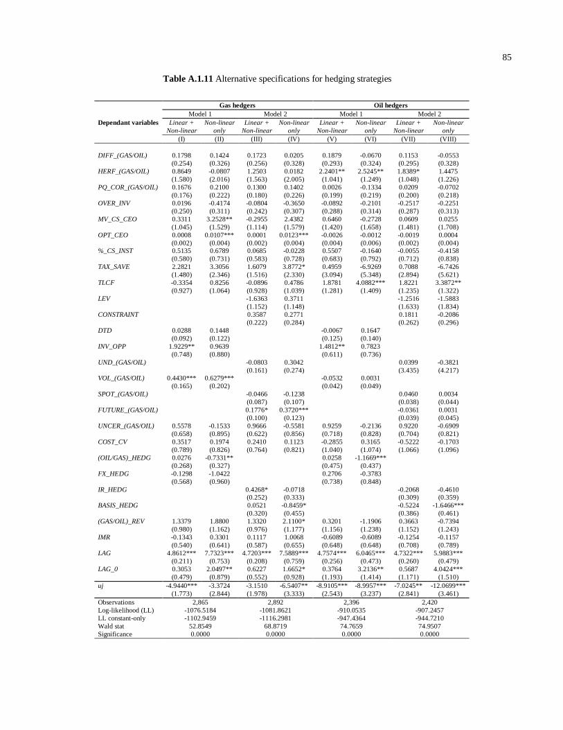
85
Table A.1.11 Alternative specifications for hedging strategies
Gas hedgers Oil hedgers
Model 1 Model 2 Model 1 Model 2
Dependant variables Linear +
Non-linear
Non-linear
only
Linear +
Non-linear
Non-linear
only
Linear +
Non-linear
Non-linear
only
Linear +
Non-linear
Non-linear
only
(I) (II) (III) (IV) (V) (VI) (VII) (VIII)
DIFF_(GAS/OIL) 0.1798 0.1424 0.1723 0.0205 0.1879 -0.0670 0.1153 -0.0553
(0.254) (0.326) (0.256) (0.328) (0.293) (0.324) (0.295) (0.328)
HERF_(GAS/OIL) 0.8649 -0.0807 1.2503 0.0182 2.2401** 2.5245** 1.8389* 1.4475
(1.580) (2.016) (1.563) (2.005) (1.041) (1.249) (1.048) (1.226)
PQ_COR_(GAS/OIL) 0.1676 0.2100 0.1300 0.1402 0.0026 -0.1334 0.0209 -0.0702
(0.176) (0.222) (0.180) (0.226) (0.199) (0.219) (0.200) (0.218)
OVER_INV 0.0196 -0.4174 -0.0804 -0.3650 -0.0892 -0.2101 -0.2517 -0.2251
(0.250) (0.311) (0.242) (0.307) (0.288) (0.314) (0.287) (0.313)
MV_CS_CEO 0.3311 3.2528** -0.2955 2.4382 0.6460 -0.2728 0.0609 0.0255
(1.045) (1.529) (1.114) (1.579) (1.420) (1.658) (1.481) (1.708)
OPT_CEO 0.0008 0.0107*** 0.0001 0.0123*** -0.0026 -0.0012 -0.0019 0.0004
(0.002) (0.004) (0.002) (0.004) (0.004) (0.006) (0.002) (0.004) %_CS_INST 0.5135 0.6789 0.0685 -0.0228 0.5507 -0.1640 -0.0055 -0.4158
(0.580) (0.731) (0.583) (0.728) (0.683) (0.792) (0.712) (0.838)
TAX_SAVE 2.2821 3.3056 1.6079 3.8772* 0.4959 -6.9269 0.7088 -6.7426
(1.480) (2.346) (1.516) (2.330) (3.094) (5.348) (2.894) (5.621)
TLCF -0.3354 0.8256 -0.0896 0.4786 1.8781 4.0882*** 1.8221 3.3872**
(0.927) (1.064) (0.928) (1.039) (1.281) (1.409) (1.235) (1.322)
LEV -1.6363 0.3711 -1.2516 -1.5883
(1.152) (1.148) (1.633) (1.834)
CONSTRAINT 0.3587 0.2771 0.1811 -0.2086
(0.222) (0.284) (0.262) (0.296)
DTD 0.0288 0.1448 -0.0067 0.1647
(0.092) (0.122) (0.125) (0.140)
INV_OPP 1.9229** 0.9639 1.4812** 0.7823
(0.748) (0.880) (0.611) (0.736)
UND_(GAS/OIL) -0.0803 0.3042 0.0399 -0.3821
(0.161) (0.274) (3.435) (4.217) VOL_(GAS/OIL) 0.4430*** 0.6279*** -0.0532 0.0031
(0.165) (0.202) (0.042) (0.049)
SPOT_(GAS/OIL) -0.0466 -0.1238 0.0460 0.0034
(0.087) (0.107) (0.038) (0.044)
FUTURE_(GAS/OIL) 0.1776* 0.3720*** -0.0361 0.0031
(0.100) (0.123) (0.039) (0.045)
UNCER_(GAS/OIL) 0.5578 -0.1533 0.9666 -0.5581 0.9259 -0.2136 0.9220 -0.6909
(0.658) (0.895) (0.622) (0.856) (0.718) (0.828) (0.704) (0.821)
COST_CV 0.3517 0.1974 0.2410 0.1123 -0.2855 0.3165 -0.5222 -0.1703
(0.789) (0.826) (0.764) (0.821) (1.040) (1.074) (1.066) (1.096)
(OIL/GAS)_HEDG 0.0276 -0.7331** 0.0258 -1.1669***
(0.268) (0.327) (0.475) (0.437)
FX_HEDG -0.1298 -1.0422 0.2706 -0.3783
(0.568) (0.960) (0.738) (0.848)
IR_HEDG 0.4268* -0.0718 -0.2068 -0.4610 (0.252) (0.333) (0.309) (0.359)
BASIS_HEDG 0.0521 -0.8459* -0.5224 -1.6466***
(0.320) (0.455) (0.386) (0.461)
(GAS/OIL)_REV 1.3379 1.8800 1.3320 2.1100* 0.3201 -1.1906 0.3663 -0.7394
(0.980) (1.162) (0.976) (1.177) (1.156) (1.238) (1.152) (1.243)
IMR -0.1343 0.3301 0.1117 1.0068 -0.6089 -0.6089 -0.1254 -0.1157
(0.540) (0.641) (0.587) (0.655) (0.648) (0.648) (0.708) (0.789)
LAG 4.8612*** 7.7323*** 4.7203*** 7.5889*** 4.7574*** 6.0465*** 4.7322*** 5.9883***
(0.211) (0.753) (0.208) (0.759) (0.256) (0.473) (0.260) (0.479)
LAG_0 0.3053 2.0497** 0.6227 1.6652* 0.3764 3.2136** 0.5687 4.0424***
(0.479) (0.879) (0.552) (0.928) (1.193) (1.414) (1.171) (1.510)
uj -4.9440*** -3.3724 -3.1510 -6.5407** -8.9105*** -8.9957*** -7.0245** -12.0699***
(1.773) (2.844) (1.978) (3.333) (2.543) (3.237) (2.841) (3.461)
Observations 2,865
-1076.5184
-1102.9459
52.8549
0.0000
2,892
-1081.8621
-1116.2981
68.8719
0.0000
2,396
-910.0535
-947.4364
74.7659
0.0000
2,420
-907.2457
-944.7210
74.9507
0.0000
Log-likelihood (LL)
LL constant-only
Wald stat
Significance

86
Note:
This table reports the means of the coefficient estimates of the dynamic random effects MMNL to select one of the following two hedging strategies—(1) linear and non-linear strategies, and (2) only non-linear strategies—for the gas hedgers and oil hedgers separately. The base case is using only linear strategies. DIFF_GAS (OIL) is the absolute value of differentials in firm’s revenues and investment costs sensitivities to gas (oil) price fluctuations; HERF_GAS (OIL) for the geographical dispersion of gas (oil) production; PQ_COR_GAS (OIL) for the gas (oil) quantity–price correlation calculated using rolling windows of eight quarterly observations; OVER_INV for overinvestment; OPT_CEO for the number of stock options held by the CEO; MV_CS_CEO for the market value of common shares held
by the CEO; %_CS_INST for the percentage of common shares held by institutional investors; TAX_SAVE for the expected percentage of tax savings; TLCF stands for TLCFs scaled by the book value of total assets; LEV for the leverage ratio; CONSTRAINT for financial constraints; DTD for the DTD; INV_OPP for investment opportunities; UND_GAS (OIL) for undeveloped proved gas (oil) reserves; FUTURE_GAS (OIL), SPOT_GAS (OIL), and VOL_GAS (OIL) for gas (oil) future and spot prices and volatility, respectively; UNCER_GAS (OIL) for gas (oil) production uncertainty measured by the coefficient of variation of daily produced quantities using rolling windows of eight quarterly observations; COST_CV for the coefficient of variation of the cash cost per BOE using rolling windows of eight quarterly observations; GAS(OIL)_HEDG, IR_HEDG, FX_HEDG, and BASIS_HEDG are dummy variables for gas (oil), IR, FX, and basis risk hedging, respectively; GAS(OIL)_REV for revenues from gas (oil) production; IMR for the inverse Mills ratio
from the first-step Heckman regression (Table A.1.3); LAG for the lagged dependent variable; and LAG_0 for the first observation. The coefficients of the exogenous variables’ means are not reported here for conciseness and are available upon request. Standard errors are in parentheses. The superscripts ***, **, and * indicate significance at the 1%, 5%, and 10% levels, respectively.

REFERENCES
Adam, T., 2002, Risk management and the credit risk premium, Journal of Banking and
Finance 26, 243–269.
Adam, T., 2009, Capital expenditures, financial constraints, and the use of options, Journal of Financial Economics 92, 238–251.
Adler, M., and J.B. Detemple, 1988, Hedging with futures and options, Studies in Banking
and Finance 5, 181–197.
Bartram, S.M., G.W. Brown, and F.R. Fehle, 2009, International evidence on financial
derivative usage, Financial Management 38, 185–206.
Bodnar, G.M., G.S. Hayt, and R.C. Marston, 1998, 1998 Survey of financial risk
management by US nonfinancial firms, Financial Management 27, 70–91.
Boes, S., 2007, Three essays on the econometric analysis of discrete dependent variables,
Working paper, University of Zürich.
Brown, G.W., 2001, Managing foreign exchange risk with derivatives, Journal of Financial Economics 60, 401–448.
Brown, G.W., and K.B. Toft, 2002, How firms should hedge, Review of Financial Studies 15,
1283–1324.
Campello, M.,C. Lin, Y. Ma, and H. Zou, 2011, The real and financial implications of
corporate hedging, Journal of Finance 66 (5), 1615–1647.
Crosbie, P.J., and R.J. Bohn, 2003, Modeling Default Risk (KMV, San Francisco).
Dionne, G., and M. Garand, 2003, Risk management determinants affecting firms’ values in the gold mining industry: New empirical results, Economics Letters 79, 43–52.
Dionne, G., and T. Triki, 2013, On risk management determinants: What really matters?
European Journal of Finance 19, 145–164.
Dolde, W., 1993, The trajectory of corporate financial risk management, Journal of Applied
Corporate Finance 6, 33–41.
Drucker, S., and M. Puri, 2009, On loan sales, loan contracting, and lending relationships,
Review of Financial Studies 22, 2835–2872.

88
Financial Accounting Standards Board, 1998, Accounting for derivative instruments and
hedging activities, Statement No. 133.
Franke, G., R.C. Stapleton, and M.G. Subrahmanyam, 1998, Who buys and who sells
options: The role of options in an economy with background risk, Journal of Economic Theory 82, 89–109.
Froot, K.A., D.S. Scharfstein, and J.C. Stein, 1993, Risk management: Coordinating
corporate investment and financing policies, Journal of Finance 48, 1629–1658.
Gay, G.D., and J. Nam, 1998, The underinvestment problem and corporate derivatives use,
Financial Management 27, 53–69.
Gay, G.D., J. Nam, and M. Turac, 2002, How firms manage risk: The optimal mix of linear
and non-linear derivatives, Journal of Applied Corporate Finance 14, 82–93.
Gay, G.D., J. Nam, and M. Turac, 2003, On the optimal mix of corporate hedging
instruments: Linear versus non-linear derivatives, Journal of Futures Markets 23,
217–239.
Géczy, C., B.A. Minton, and C. Schrand, 1997, Why firms use currency derivatives, Journal
of Finance 52, 132–154.
Graham, J., and C.W. Smith, 1999, Tax incentives to hedge, Journal of Finance 54, 2241–2262.
Graham, J.R., and D.A. Rogers, 2002, Do firms hedge in response to tax incentives? Journal
of Finance 57, 815–839.
Grullon, G., E. Lyandres, and A. Zhdanov, 2012, Real options, volatility, and stock returns, Journal of Finance 67, 1499–1537.
Haushalter, D., 2000, Financing policy, basis risk, and corporate hedging: Evidence from oil
and gas producers, Journal of Finance 55, 107–152.
Haushalter, D., R.A. Heron, and E. Lie, 2002, Price uncertainty and corporate value, Journal
of Corporate Finance 8, 271–286.
Heckman, J., 1981, The incidental parameters problem and the problem of initial conditions
in estimating a discrete time–discrete data stochastic process, in C.F. Manski and D. McFadden, eds.: Structural Analysis of Discrete Data with Econometric Applications
(MIT Press, Cambridge, MA).
Hole, A. R., 2007, Fitting mixed logit models by using maximum simulated likelihood, Stata Journal 7, 388-401.

89
Jensen, M., 1986, Agency costs of free cash flow, corporate finance and takeovers, American
Economic Review 76, 323–329.
Jensen, M.C., and W.H. Meckling, 1976, Theory of the firm: Managerial behavior, agency
costs and ownership structure, Journal of Financial Economics 3, 305-360.
Jin, Y., and P. Jorion, 2006, Firm value and hedging: Evidence from U.S. oil and gas
producers, Journal of Finance 61, 893–919.
Lehn, K., and A. Poulsen, 1989, Free cash flow and stockholder gains in going private transactions, Journal of Finance 44, 771–788.
Maddala, G., 1983, Limited-Dependent and Qualitative Variables in Econometrics
(Cambridge University Press, Cambridge).
Mayers, D., and C.W. Smith, 1982, On the corporate demand for insurance, Journal of Business 55, 281–296.
Merton, R.C., 1974, On the pricing of corporate debt: The risk structure of interest rates,
Journal of Finance 29, 449-470.
Morellec, E., and C. W. Smith, 2007, Agency conflicts and risk management, Review of
Finance 11, 1–23.
Moschini, G., and H. Lapan, 1992, Hedging price risk with options and futures for the competitive firm with production flexibility, International Economic Review 33,
607–618.
Moschini, G., and H. Lapan, 1995, The hedging role of options and futures under joint price,
basis, and production risk, International Economic Review 36, 1025–1049.
Pfarr, C., Schmid, A. and U. Schneider, 2010, REGOPROB2: Stata module to estimate
random effects generalized ordered probit models (update), Statistical Software
Components, Boston College Department of Economics.
Rabe-Hesketh, S., Skrondal, A. and Pickles, A. (2005). Maximum likelihood estimation of
limited and discrete dependent variable models with nested random effects. Journal
of Econometrics 128 (2), 301-323.
Smith, C.W., and R.M. Stulz, 1985, The determinants of firms’ hedging policies, Journal of Financial and Quantitative Analysis 20, 391–405.
Stulz, R.M., 1984, Optimal hedging policies, Journal of Financial and Quantitative Analysis
19, 391–405.
Stulz, R.M., 1996, Rethinking risk management, Journal of Applied Corporate Finance 9, 8–
24.

90
Terza, J., 1985, Ordinal probit: A generalization, Communications in Statistics–Theory and
Methods 14, 1–11.
Train, K.E., 2009, Discrete Choice Methods with Simulation (Cambridge University Press,
Berkeley).
Tufano, P., 1996, Who manages risk? An empirical examination of risk management
practices in the gold mining industry, Journal of Finance 51, 1097–1137.
Williams, R., 2006, Generalized ordered logit: Partial proportional odds models for ordinal dependent variables, Stata Journal 6 (1), 58–82.
Wooldridge, J.M., 2002, Econometric Analysis of Cross Section and Panel Data (MIT Press,
Cambridge).
Zucchelli, E., M. Harris, and Z. Xueyan, 2012, Ill-health and transitions to part-time work and self-employment among older workers, Working paper, Centre for Health
Economics, University of York.

CHAPITRE II
ARTICLE 2

THE MATURITY STRUCTURE OF CORPORATE HEDGING:
THE CASE OF THE U.S. OIL AND GAS INDUSTRY
Mohamed Mnasri
Ph. D. Candidate
ESG-UQÀM
Georges Dionne
Canada Research Chair in Risk Management,
HEC Montréal, CIRRELT, and CIRPÉE
Jean-Pierre Gueyie
Associate Professor,
Department of Finance
Université du Québec à Montréal

ABSTRACT
This paper investigates how firms design the maturity of their hedging programs, and the
real effects of maturity choice on firm value and risk. Using a new dataset on hedging
activities of 150 U.S. oil and gas producers, we find strong evidence that hedging maturity is influenced by investment programs, market conditions, production specificities, and hedging
contract features. We also give empirical evidence of a non-monotonic relationship between
hedging maturity and measures of financial distress. We further investigate the motivations of early termination of contracts. Finally, we show that longer hedging maturities could
attenuate the impacts of commodity price risk on firm value and risk.
Keywords: Risk management, maturity choice, early termination, economic effects, oil and
gas industry.
JEL classification: D8, G32.
2.1 Introduction
We explore a new channel in corporate risk management literature through which firms
could create value and reduce risk by considering the following questions: How far ahead do
firms hedge? What are the determinants of the maturity structure of firms’ hedging
programs? What are the economic effects of hedging maturities on firm value and risk?
These questions are still largely unexplored because of the lack of empirical analysis due to
limitations of the data. Using an extensive and new hand-collected dataset on the risk
management activities of 150 U.S. oil and gas producers with quarterly observations over the
period 1998-2010, we fill this gap in the literature and answer the above questions. It is
important to understand why firms within the same industry and with the same risk exposure
differ in terms of their hedging maturity structure.
We contribute to the literature on corporate hedging in several ways. Our first
contribution is to provide empirical evidence of the rationales and determinants of the
maturity structure of hedging contracts at inception; we also study the rationales for early
termination of hedging contracts, and the real implications of maturity choice on firm value
and risk. We hence add new significant results to the empirical literature; the scant empirical
studies discuss the maturity structure of hedging in a largely descriptive manner.19
In
19 Dolde (1993) surveys the hedging practices of 244 Fortune 500 companies and finds that the common practice
is to hedge cash flow exposures within a horizon of two to four quarters. In line with Dolde (1993), Tufano (1996) provides statistics about the percentage of the production hedged for North American gold mining firms for 1991-1993, and finds that they hedge 61.2% of their gold production for the current year (1991) and 10% and 11% for the subsequent two years. In a Wharton survey of financial risk management practices and derivatives of 399 U.S. non-financial firms, Bodnar et al., (1998) report that 82% of the questioned firms use foreign currency derivatives with an initial maturity of 91 days or less, and only 12% use foreign currency derivatives with maturities exceeding 3 years. They also find that hedging ratios at longer maturities decreased dramatically during 1998. Adam and Fernando (2006 and 2008) study the cash flow gains from selective hedging for a sample
of 92 North American gold producers from 1989 to 1999 and report descriptive statistics of hedging ratios up to five years. They find that gold producers use hedging programs with one-year maturities in 90% of firm-quarters with non-zero hedging with a mean hedging ratio of 54% of expected gold production, hedging programs with three-year maturities in 51% of hedging quarters with an average hedging ratio of 25%, and programs with five-year maturities in 18% with an average hedging ratio of 28%. They also point out that near-term hedging ratios are more volatile than those with longer horizons. Carter, Rogers, and Simkins (2006) investigate the jet fuel hedging activities of U.S. airline firms during 1992-2003 and find that hedging maturities vary significantly between firms (e.g., from one year to six years ahead) and that hedging ratios of the next year’s fuel consumption
are very disparate (e.g., from 1% to 43%).

95
addition, our data collected from publicly disclosed information avoid the non-response bias
associated with questionnaires and provide detailed information about real hedging activities.
Finally, we study hedging activities of both commodities (oil and gas) separately, which
gives deeper insight into oil and gas producers’ hedging dynamics.
Consistent with our predictions, results of our base model (i.e., Dynamic System-GMM
Panel Model) show that oil and gas producers, having substantial growth options, use
hedging contracts with longer maturities to avoid shortfalls in their future cash flows. We
also find that oil and gas producers with a higher positive correlation between their
investment expenditures and internal cash flows tend to use short-term hedging contracts
because they benefit from a natural hedge. In line with Fehle and Tsyplakov’s (2005)
prediction, we give strong evidence of the non-monotonic (concave) relationship between
measures of the likelihood of financial distress (i.e., leverage) and hedging maturity. This
non-monotonic relationship means that hedging maturities increase and then decrease with
the likelihood of financial distress.
Results also indicate that distressed oil and gas producers (i.e., with insufficient liquidity)
enter long-term put options as a risk-shifting (asset substitution) strategy. Costly put options
with long maturities increase rather than eliminate the firm’s payoff volatility and decrease
assets available for debtholders. Results further show that oil and gas producers with higher
cash flow volatility, due to higher production uncertainty and/or higher price-quantity
correlation, tend to use farther hedging positions to avoid shortfalls in their future revenues.
We also observe strong evidence of the impact of market conditions on hedging maturity
choice. Oil and gas price volatilities are significantly positively related to longer maturities
hedging, as predicted by Fehle and Tsyplakov (2005). Accordingly, higher price volatility
makes firms reluctant to incur costly early termination of their hedging contracts unless spot
prices increase significantly. We further verify that when future prices are expected to be
higher, firms tend to use short-term hedging. Consistent with Fehle and Tsyplakov (2005),
we find empirical evidence of a non-monotonic (concave) relationship between oil and gas
spot prices and hedging maturities.

96
Results show that the hedging contract features (i.e., moneyness, strike price) have an
evident impact on maturity choice. As predicted, oil and gas producers keep in-the-money
hedging contracts until they mature and terminate out-of-the-money contracts early. Results
further imply that a hedging contract initiated at a sufficiently higher strike price is more
likely to be kept for longer periods. Consistent with our prediction, tax function convexity
motivates the use of long-term contracts and tax loss carry-forwards seem to be a disincentive
to hedge longer exposures because they could be used as a caution to reduce firms’ future tax
liabilities. With respect to asset-liability management, we find that oil and gas producers seek
to match the maturities of their hedging and of their oil and gas developed reserves (i.e.,
assets) and debt.
Results are largely robust to other data collection criteria. Specifically, we use maturity
choice at inception of the hedging contracts and find results largely similar to those of our
base specification (i.e., Dynamic System-GMM Panel Model). Our results are validated again
when we study the determinants of the early termination of hedging contracts. Finally, we
give novel evidence of the impact of hedging maturity on firm value and risk, and find that
long-term hedging lowers the sensitivity of the stock return to changes in gas prices, in
particular. However, we find no significant impact on sensitivity to oil and gas price
volatility.
The rest of the paper is organized as follows. In Section 2, we state our hypotheses. In
Section 3, we describe our data, and dependent and independent variables. Section 4 presents
the retained econometric methodology. Section 5 reports univariate results and Section 6
investigates the empirical evidence of the maturity structure of corporate risk management. In
Section 7, we test the robustness of our results by exploring the determinants of maturity
choice at the inception of hedging contracts and the determinants of early termination of
outstanding hedging contracts. We then investigate the real implications of hedging maturity
choice empirically in Section 8, and Section 9 concludes the paper.

97
2.2 Hypotheses
The lack of testable theoretical predictions on hedging maturity structure was
compensated by Fehle and Tsyplakov (2005). They present an infinite-horizon continuous
time model of a firm that can adjust the hedge ratio and maturity of its hedging instruments
dynamically in response to fluctuations in firm output price. Their model is calibrated to
replicate empirical observations for a gold mining firm and produces a number of new
theoretical predictions pertaining to the optimal timing, adjustment, and rollover of hedging
contracts and their maturities, which we will describe in depth to develop our hypotheses in
this section and test empirically after.
2.2.1 Financial distress
A large body of the empirical literature has analyzed the positive relationship between
financial constraints and firms’ hedging activities (e.g., Nance et al., 1993; Géczy et al.,
1997; Tufano, 1996; Gay and Nam, 1998; Adam, 2002, 2009). In line with this extant
literature, Fehle and Tsyplakov (2005) analyzed the implications of financial distress on risk
management adjustments. Based on simulations of output (gold) spot prices, they find a non-
monotonic relationship between hedging maturity and measures of the probability of
financial distress. This non-monotonicity means that hedging maturity first increases and then
decreases with the probability of financial distress. To put it another way, firms near distress
are often observed with short-run hedging contracts, and may terminate longer contracts at a
high cost as a result of risk-shifting behavior. Firms far from distress opt for short-term
contracts because of the low marginal benefits of hedging for wealthy firms (e.g., Stulz,
1996).
Fehle and Tsyplakov (2005) also find that financial distress costs are negatively related to
hedging maturity. Their simulations show that firms with high distress costs tend to use
shorter maturity hedging. Thus, distress costs increase when the firm’s cash inflows (i.e., its
selling prices) are insufficient to cover production costs and debt payments. Hence we posit:

98
HYPOTHESIS 1: Hedging maturity is negatively related to (i) either high or low likelihood
of financial distress, and (ii) higher distress costs.
To verify the empirical relevance of this prediction we use the following two measures of
the distress likelihood: (1) the leverage ratio as measured by the book value of long-term debt
in current liabilities plus half of long-term debt scaled by book value of total assets as used by
Moody’s-KMV, and (2) distance-to-default, which is a market-based measure originating
from Merton’s (1974) approach. This measure gives the number of standard deviations that
the firm is away from default (Crosbie and Bohn, 2003). We also use leverage squared and
distance-to-default squared to capture non-linearity between financial soundness and hedging
maturity. We predict a positive sign for the leverage ratio and distance-to-default and a
negative sign for their squared values.
Following Fehle and Tsyplakov’s (2005) methodology, we measure firm’s incurred
distress costs by the following product [ ] [ ] where is an
indicator function and Liquidity is the quick ratio (i.e., cash and cash equivalents scaled by
the book value of current liabilities). We use the quick ratio because a firm could use this
liquidity as a caution to repay future debt requirements (see Dionne and Triki, 2013). M is the
median quick ratio of the oil and gas industry. [ ]
and 0 otherwise. [ ] means that a firm incurs distress costs that are
proportional to the shortfall of its realized selling prices compared with its production costs
and debt payments . These realized prices20
include the monetary effects of hedging
activities, if any. The letter is for cash cost.21
Debt payments are measured by the quarterly
interest expenses and the outstanding proportion of long-term debt to current liabilities at the
end of the quarter, and are represented by . The variables , and are expressed per
Barrel of Oil Equivalent (BOE). Therefore, a firm incurs distress costs when its liquidity is
below the industry’s median and its actual cash inflows (i.e., realized selling prices net of
20
Firms disclose their realized selling prices for oil and gas, respectively, on an annual basis. For each firm, we
repeat the annual observation for each quarter of the same fiscal year. These realized prices include the monetary
effects of the firm’s hedging activities if any. 21
Cash costs are disclosed annually. For each firm, we repeat the same observation for each quarter of the same
fiscal year.

99
production costs) are insufficient to meet debt requirements. These distress costs may entail
higher future external financing costs.
2.2.2 Market conditions
The corporate hedging literature shows that market conditions, namely spot prices and
their volatilities, play a crucial role in why firms hedge, how much they hedge, and how they
hedge (see for instance Bodnar et al., 1998; Stulz, 1996; Brown and Toft, 2002; Adam,
2009). Fehle and Tsyplakov (2005) investigate the evolution of risk management contracts
and the spot price history by simulating the stochastic process of the gold spot price.
Basically, they find strong evidence of a non-monotonic relationship between spot price and
hedging contract maturity. This means that when spot prices are very high or low, firms
choose short maturity hedging. As for Hypothesis 1, when spot prices are very high (low), the
likelihood of distress is very low (high). For the range of spot prices between these two
extremes, firms tend to adjust their risk management instruments more frequently and then
tend to enter into newly initiated contracts with longer maturities.
Moreover, Fehle and Tsyplakov (2005) find that firms with higher price volatility tend to
choose longer hedging contracts. In a higher price uncertainty environment, firms tend to
refrain from costly early termination of their outstanding contracts unless spot prices increase
significantly. These firms often conclude long-run contracts. In addition, we expect that when
future prices are anticipated to be higher, firms tend to terminate their outstanding contracts
and initiate new risk management contracts with higher exercise prices. Moreover, the newly
initiated contracts will be for short-term maturities to prevent them from being worthless in
the future. We therefore posit:
HYPOTHESIS 2: Hedging maturity is negatively related to (i) either very high or very low
spot prices, and (ii) higher anticipated prices. Conversely, firms prefer longer maturity
contracts when price volatility is higher.

100
We extract the oil and gas spot prices observed at the end of each quarter from the
Bloomberg Financial Markets database.22
We calculate the volatility of oil and gas for each
quarter as the standard deviation of daily spot prices within the quarter. As a proxy for the
future tendency of oil and gas prices, we calculate an expected return by [ ] [ ]
where and are respectively the prices of 12-month Futures23
contracts and the spot
prices observed at the end of quarter t. We expect a positive sign for spot prices and
volatilities, and a negative sign for spot prices squared and expected returns [ ].
2.2.3 Hedging contract features
Fehle and Tsyplakov (2005) find that features of existing hedging contracts, namely
moneyness, remaining maturity and strike price, play an important role in optimal rollover
and adjustment decisions. Regarding these features, they derive the following prediction that
we will investigate empirically.
HYPOTHESIS 3: Hedging contracts initiated at higher strike prices are more likely to be
kept until maturity because they are more likely to be in the money for a longer period.
As proxy for the strike price at initiation of the hedging contracts, we calculate the mean
of the spot price during the quarter of the initiation. This proxy will give the information on
the level of the strike price of the initiated contract. The moneyness is calculated by the strike
price as previously mentioned minus the mean spot price in the current quarter. We predict a
positive sign for both strike price and moneyness.
22 We use the West Texas Intermediate crude oil (WTI) index as proxy for the oil spot prices. For natural gas spot
prices, we use an average index established by Bloomberg Financial Markets database from different location indices (Gulf Coast, Henry Hub, Rocky Mountains, etc.). 23 For future oil and gas prices, we use (i) Bloomberg NYMEX Crude Oil 12-Month Strip futures price, and (ii)
Bloomberg NYMEX Henry Hub Natural Gas 12-Month Strip futures price. These two indices are established by
the Bloomberg Financial Markets database as the arithmetic averages of oil (gas) futures contract prices over the
next 12 months.
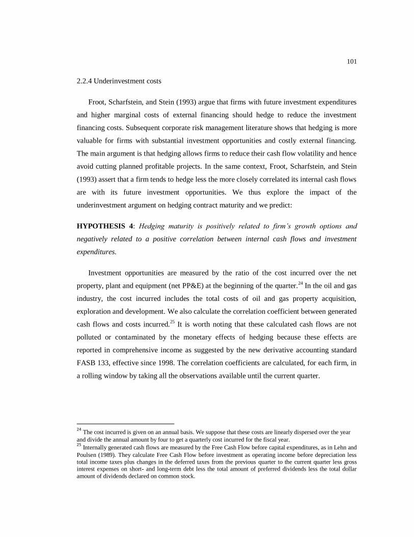
101
2.2.4 Underinvestment costs
Froot, Scharfstein, and Stein (1993) argue that firms with future investment expenditures
and higher marginal costs of external financing should hedge to reduce the investment
financing costs. Subsequent corporate risk management literature shows that hedging is more
valuable for firms with substantial investment opportunities and costly external financing.
The main argument is that hedging allows firms to reduce their cash flow volatility and hence
avoid cutting planned profitable projects. In the same context, Froot, Scharfstein, and Stein
(1993) assert that a firm tends to hedge less the more closely correlated its internal cash flows
are with its future investment opportunities. We thus explore the impact of the
underinvestment argument on hedging contract maturity and we predict:
HYPOTHESIS 4: Hedging maturity is positively related to firm’s growth options and
negatively related to a positive correlation between internal cash flows and investment
expenditures.
Investment opportunities are measured by the ratio of the cost incurred over the net
property, plant and equipment (net PP&E) at the beginning of the quarter.24
In the oil and gas
industry, the cost incurred includes the total costs of oil and gas property acquisition,
exploration and development. We also calculate the correlation coefficient between generated
cash flows and costs incurred.25
It is worth noting that these calculated cash flows are not
polluted or contaminated by the monetary effects of hedging because these effects are
reported in comprehensive income as suggested by the new derivative accounting standard
FASB 133, effective since 1998. The correlation coefficients are calculated, for each firm, in
a rolling window by taking all the observations available until the current quarter.
24
The cost incurred is given on an annual basis. We suppose that these costs are linearly dispersed over the year
and divide the annual amount by four to get a quarterly cost incurred for the fiscal year. 25
Internally generated cash flows are measured by the Free Cash Flow before capital expenditures, as in Lehn and
Poulsen (1989). They calculate Free Cash Flow before investment as operating income before depreciation less total income taxes plus changes in the deferred taxes from the previous quarter to the current quarter less gross interest expenses on short- and long-term debt less the total amount of preferred dividends less the total dollar
amount of dividends declared on common stock.

102
2.2.5 Production characteristics
Several studies,26
mostly theoretical, have investigated the role of characteristics of
production activity on firm’s hedging behavior. These studies demonstrate the importance of
production uncertainty (i.e., quantity risk) and the correlation between produced quantities
and spot prices on firm’s hedging programs (i.e., hedging extent and strategy choice). We
explore the effects of these characteristics on hedging maturity choice. By deriving the
optimal hedge analytically, Brown and Toft (2002) show that firms tend to hedge less for
longer exposures because of the difficulty in forecasting their future produced quantities
accurately.
These theoretical models also highlight the important impact of the correlation between
produced quantities and spot prices on hedging decisions. Brown and Toft (2002) and Gay,
Nam, and Turac (2002, 2003) find that firms with a negative price-quantity correlation
benefit from a natural hedge with declining quantities and increasing prices, and vice versa.
On the contrary, a positive price-quantity correlation leads to higher variations in firm’s cash
flows because both prices and quantities are moving in the same direction. Hence we
propose:
HYPOTHESIS 5: Hedging maturity is negatively related to production uncertainty and
positively related to price-quantity correlation.
For each firm, we measure production uncertainty by the coefficient of variation of daily
production27
for oil and gas respectively by taking all the observations available until the
current quarter. We calculate the correlation coefficient between daily oil (gas) production
and oil (gas) spot prices by taking all the firm’s observations available until the current
quarter.
26 These studies include Moschini and Lapan (1995), Brown and Toft (2002), Gay, Nam, and Turac (2002, 2003)
and Adam (2009). 27
Daily production for oil and gas, respectively, are disclosed by firms annually. We repeat the annual
observation for each quarter of the same fiscal year.

103
2.2.6 Other control variables
We include the following control variables largely retained in the corporate risk
management literature.
2.2.6.1 Managerial risk aversion
As proxy for managerial risk aversion, we include the number of options and the market
value28
of the firm’s stocks held by the CEO. According to Smith and Stulz (1985), managers
should undertake hedging activities more actively if their utility is a concave function of firm
value, and they should be reluctant to engage risk management activities if their utility is a
convex function of the firm’s value. Therefore, we predict that a CEO owning a significant
fraction of the firm’s common shares tends to use hedging contracts with longer maturities
because he would like to insulate the firm value from the underlying risks. Conversely, we
expect a CEO with significant option holdings to tolerate more volatility in firm value, and
consequently prefer short-term hedging contracts.
2.2.6.2 Tax incentives
The tax argument for corporate hedging is accounted for using a simulation procedure
proposed by Graham and Smith (1999) to measure the expected percentage of tax savings
arising from a 5% reduction in the volatility of pre-tax income. The tax argument means that
hedging increases the firm’s after-tax value when its local tax function is convex. A firm will
thus hedge more extensively when its taxable income is in the progressive region of the tax
structure. We expect firms with higher tax function convexity to use hedging contracts with
longer maturities that would increase the tax benefits of hedging. We also use the book value
of tax loss carry-forwards scaled by the book value of total assets. Graham and Rogers (2002)
argue that tax loss carry-forwards are uncorrelated with tax function convexity, and that this
28
We use the number of options held by the firm’s CEO at the end of each quarter and we measure the CEO’s
firm-specific wealth by the logarithm of one plus the market value of common shares held by the CEO at the end of each quarter. We use the logarithm specification of the market value of common shares held by CEOs to reflect
the fact that the CEOs’ risk aversion should decrease as their firm-specific wealth increases (Tufano, 1996).

104
variable might measure other corporate characteristics. Thus, we expect that it represents a
disincentive to hedge because firms could use this tax shield to minimize their future tax
liabilities. Therefore, we predict that firms with higher tax loss carry-forwards tend to use
short-term hedging contracts.
2.2.6.3 Asset-Liability Management
Asset-Liability Management is also accounted for in our analysis. Maturity matching is a
common best practice in corporate finance. We use the following two measures: (1) a
weighted average maturity of debt. This average maturity is calculated as the book value-
weighted average maturities of debt that mature within one, two, three, four and five years29
;
and (2) an expected life duration (in years) of developed reserves for oil and gas separately.
This expected life duration is calculated by dividing the current quantity of oil (gas)
developed reserves by the current annual oil (gas) production. These two variables allow us
to capture any maturity matching between both the hedging strategy and the firm’s assets
(proven reserves, which are the most important components of an oil and gas producer’s
assets) and hedging strategy and the firm’s future debt commitments.
2.3 Sample construction and characteristics
2.3.1 Sample construction
This study is implemented on a sample of 150 US oil and gas producers over the period
of 1998 to 2010. The oil and gas industry is an excellent laboratory to test corporate risk
management motivations and implications for several reasons. First, firms in this industry
share homogenous risk exposures (i.e. fluctuations in crude oil and natural gas prices).
Hence, diversity in hedging strategies implemented does not come from differences in risk
exposure, but is more likely to result from differences in firm characteristics. Second, the
existence of financial derivatives on crude oil and natural gas offer these firms several price
29 These items are disclosed by COMPUSTAT on an annual basis. We repeat the annual observation for each
quarter of the same fiscal year.
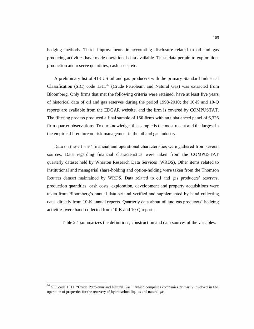
105
hedging methods. Third, improvements in accounting disclosure related to oil and gas
producing activities have made operational data available. These data pertain to exploration,
production and reserve quantities, cash costs, etc.
A preliminary list of 413 US oil and gas producers with the primary Standard Industrial
Classification (SIC) code 131130
(Crude Petroleum and Natural Gas) was extracted from
Bloomberg. Only firms that met the following criteria were retained: have at least five years
of historical data of oil and gas reserves during the period 1998-2010; the 10-K and 10-Q
reports are available from the EDGAR website, and the firm is covered by COMPUSTAT.
The filtering process produced a final sample of 150 firms with an unbalanced panel of 6,326
firm-quarter observations. To our knowledge, this sample is the most recent and the largest in
the empirical literature on risk management in the oil and gas industry.
Data on these firms’ financial and operational characteristics were gathered from several
sources. Data regarding financial characteristics were taken from the COMPUSTAT
quarterly dataset held by Wharton Research Data Services (WRDS). Other items related to
institutional and managerial share-holding and option-holding were taken from the Thomson
Reuters dataset maintained by WRDS. Data related to oil and gas producers’ reserves,
production quantities, cash costs, exploration, development and property acquisitions were
taken from Bloomberg’s annual data set and verified and supplemented by hand-collecting
data directly from 10-K annual reports. Quarterly data about oil and gas producers’ hedging
activities were hand-collected from 10-K and 10-Q reports.
Table 2.1 summarizes the definitions, construction and data sources of the variables.
30
SIC code 1311 ‘‘Crude Petroleum and Natural Gas,’’ which comprises companies primarily involved in the operation of properties for the recovery of hydrocarbon liquids and natural gas.

106
Table 2.1 Variable definition, construction and data sources
Variable definition Variable name Construction Data source
Variables that proxy for tax advantage of hedging
Tax loss carry-forwards TLCF Book value of the TLCF scaled by the book value of total assets Compustat
Tax save TAX_SAVE Tax liability saving arising from a 5% reduction in taxable income (Graham and Smith, 1999). Compustat
Variables that proxy for financial distress costs
Leverage LEV Book value of long-term debt in current liabilities + one-half of long-term debt scaled by the book value of total assets. Compustat
Distance-to-default DTD Market-based measure of default risk based on Merton’s (1974) approach and used by Moody’s KMV. The DTD is equal to
a
a a
V D
V, where D is defined as long-term debt in current liabilities plus one-half of long-term debt,
aV is the market value of
assets, and is one-year asset volatility. The quantities aV and are unobservable and are approximated from Merton’s
(1974) model by using the market value and volatility of equity, the three-month Treasury bill rate, and debt (D). See Crosbie and
Bohn (2003) for more details on the construction of the DTD.
Manually
constructed
Financial distress costs DIST_COSTS Measured by [ ] [ ] where Liquidity is the quick ratio, M is the median quick ratio of the oil
and gas industry, are the realized selling prices, are production costs, and debt payments. , and are expressed per Barrel of Oil Equivalent. [ ] and 0 otherwise.
Manually
constructed
Cash cost CASH_COST Production cost of a BOE Bloomberg and
10-K reports
Variables that proxy for underinvestment costs
Investment opportunities
(IOs)
INV_OPP Total costs incurred in oil and gas property acquisition, exploration, and development, scaled by net property, plant, and
equipment at the beginning of the quarter.
Manually
constructed
Correlation between
investment expenditures
and free cash flows.
COR_CI_CF Correlation coefficient between free cash flow and costs incurred. This coefficient is calculated for each firm by using all the
observations until the current quarter.
Manually
constructed
Variables that proxy for production characteristics
Oil production
uncertainty
PROD_CV_OIL Coefficient of variation of daily oil production. This coefficient is calculated for each firm by using all the observations of daily
oil production until the current quarter.
Manually
constructed
Gas production
uncertainty
PROD_CV_GAS Coefficient of variation of daily gas production. This coefficient is calculated for each firm by using all the observations of daily
gas production until the current quarter.
Manually
constructed
Price–quantity
correlation (oil)
COR_PQ_OIL Correlation coefficient between daily oil production and oil spot prices. Manually
constructed
Price–quantity
correlation (gas)
COR_PQ_GAS Correlation coefficient between daily gas production and gas spot prices. Manually
constructed
Continued

107
Table 2.1-Continued
Variable
definition
Variable name Construction Data source
Variables that proxy for firm size
Sales SALES Total revenues from oil and gas sales (in millions of dollars) Compustat
Market value MKT_VALUE Number of common shares outstanding * end-of-quarter per share price (in millions of dollars). Compustat
Oil reserves RES_OIL Quantity of the total proven developed and undeveloped oil reserves (in millions of barrels). Bloomberg and 10-K
reports
Gas reserves RES_GAS Quantity of the total proven developed and undeveloped gas reserves (in billions of cubic feet). Bloomberg and 10-K
reports
Variables that proxy for managerial risk aversion
Market value of CEO shareholding CEO_CS Measured by the logarithm of 1 plus the market value of common shares held by the CEO at the end of
each quarter.
Thomson Reuters
# CEOs stock options CEO_OPT Number of CEO stock options (in thousands). Thomson Reuters
Variables that proxy for market conditions
Oil expected return OIL_RET Measured by [ ] [ ] where and are respectively the oil prices of 12-month Futures
contracts and the oil spot prices observed at the end of quarter t.
Manually constructed
Oil spot price OIL_SPOT Oil spot price represented by the WTI in the NYMEX. Bloomberg
Gas expected return GAS_RET Measured by [ ] [ ] where and are respectively the gas prices of 12-month Futures
contracts and the gas spot prices observed at the end of quarter t.
Manually constructed
Gas spot price GAS_SPOT Constructed as an average index established from principal locations’ indices in the United States (Gulf
Coast, Henry Hub, etc.)
Bloomberg
Oil price volatility OIL_VOL Historical volatility (standard deviation) using the spot price of the previous 60 days. Manually constructed
Gas price volatility GAS_VOL Historical volatility (standard deviation) using the spot price of the previous 60 days. Manually constructed
Variables that proxy for the asset-liability management
Weighted-average maturity of debt (in
years)
DEBT_MAT Calculated as the book value-weighted average maturities of debt that mature within one, two, three, four
and five years.
Manually constructed
Expected life duration of oil and gas
reserves (in years)
RES_MAT_(OIL/GAS) Calculated by dividing the current quantity of oil (gas) developed reserves by the current annual oil (gas)
production.
Manually constructed
Variables that proxy for hedging contract features
Contract strike price STRIKE Measured by the average spot price during the quarter of the initiation of the hedging contract Manually constructed
Contract moneyness MONEYNESS Calculated as the contract strike price minus the average spot price during the current quarter Manually constructed
Variables that proxy for hedging substitutes
Quick ratio Q_RATIO Cash and cash equivalents scaled by current liabilities. Compustat
Book value of convertible debt BVCD Book value of convertible debt scaled by the book value of total assets. Compustat
108
2.3.2 Sample characteristics
2.3.2.1 Descriptive statistics: Dependent variable
Our dependent variable is hedging maturity measured by the average remaining maturity
weighted by the hedged notional quantity as follows:
∑
∑
, (1)
where is the weighted-average remaining maturity for firm i at quarter t and
hedging instrument j. The hedging instrument could be swap contracts, put options, costless
collars, forward or future contracts and 3-way collars. is the hedged notional quantity31
for instrument j and horizon T. T departs from the current fiscal year to five years ahead. We
retain a maximum of five years because we rarely find firms with hedging positions
exceeding this horizon. k takes the value of 1 at the beginning of the current fiscal year or a
fraction of the year otherwise (e.g., 0.75 for nine months).
Table 2.2 contains descriptive statistics of the weighted-average hedging maturity by
hedging instruments for oil and gas hedgers separately. Overall, Table 2.2 shows that gas
hedgers and oil hedgers adopt quite similar hedging horizons for each hedging instrument.
For example, the average remaining maturity for swap contracts is 1.286 (1.227) years for gas
(oil) hedgers. For put options, the remaining maturity is, on average, 1.023 (1.083) years for
gas (oil) hedgers. Moreover, statistics show little variation of average remaining maturities
across instruments. Swaps contracts and 3-way collars seem to have the longest average
remaining maturity with respectively 1.286 and 1.187 years for gas hedgers, and 1.227 and
1.448 years for oil hedgers. Forward and future contracts appear to have the nearest average
31
We follow Haushalter (2000) and use notional quantities for put options because we lack detailed information
to calculate a delta-percentage for these options. At least, we have three attributes of our sample that could
mitigate this shortcoming in our study: (i) put options are used on average in 11% (12%) of firm-quarters with gas
(oil) hedging, (ii) put options are used with either swap/or collars most, and (iii) the fraction of the quantity
hedged by put options does not exceed 40% (50%) for gas (oil).

109
remaining maturities with 0.856 (0.818) years for gas (oil) hedgers. We also calculate the
average remaining maturity for oil (gas) hedging portfolios that include two or more
instruments simultaneously. Hedging portfolios have an average remaining maturity of 1.222
(1.204) years for gas (oil) hedgers. Hedging horizons therefore seem to not differ
significantly across oil and gas and across hedging instruments. Statistics related to hedging
maturities reported in Table 2.2 are in line with previous empirical findings that firms tend to
hedge near-term positions.
Table 2.2 Weighted-average maturity by hedging instrument (in years)
Hedging Instrument Obs % of use Mean Median 1st quartile 3rd quartile Min Max Std Dev
Panel A: Gas hedgers
Swap contracts 2255 45.58% 1.286 1.161 0.894 1.582 0.250 5 0.651 Costless Collars 1840 37.19% 1.156 1.032 0.822 1.404 0.250 4.190 0.539 Put options 522 10.55% 1.023 1 0.750 1.273 0.250 3.220 0.538 Forwards or Futures 161 3.25% 0.856 0.914 0.616 1.002 0.250 1.942 0.330
3-way Collars 169 3.42% 1.187 1.096 0.881 1.427 0.250 3.101 0.511
Gas hedging portfolio
maturity
3137 1.222 1.111 0.906 1.478 0.250 5 0.559
Panel B: Oil hedgers Swap contracts 1711 45.25% 1.227 1.061 0.750 1.530 0.250 3.758 0.644 Costless Collars 1403 37.11% 1.221 1.050 0.799 1.500 0.250 4.439 0.621 Put options 448 11.85% 1.083 1 0.750 1.416 0.250 2.970 0.548
Forwards or Futures 105 2.78% 0.818 0.750 0.500 1 0.250 1.750 0.332 3-way Collars 114 3.02% 1.448 1.230 0.855 1.840 0.250 4.212 0.878
Oil hedging portfolio
maturity
2607 1.204 1.061 0.820 1.489 0.250 3.935 0.575
Table 2.2 also shows that gas hedging occurred in 3137 firm-quarters (49.58% of the
firm-quarters in the sample) and oil hedging occurred in 2607 firm-quarters (41.21% of the
firm-quarters in the sample). Table 2.2 presents a breakdown of the frequency of use for each
hedging instrument. The most common hedging vehicles used in the oil and gas industry are
swap contracts, with 45.58% (45.25%) of use in gas (oil) hedging. The second most
frequently used instrument is costless collars, with 37.19% (37.11%) for gas (oil) hedging.
Next are put options, with 10.55% for gas hedging and 11.85% for oil hedging. The least
used instruments are forward or futures contracts, with only 3.25% (2.78%) for gas (oil)
hedging and 3-way collars, with only 3.42% (3.02%) for gas (oil).

110
2.3.2.2 Descriptive statistics: Independent variables
Descriptive statistics are computed on the pooled dataset. Table 2.3 gives the mean,
median, 1st quartile, 3
rd quartile and standard deviation for the 150 U.S. oil and gas producers
in the sample. Statistics show that oil and gas producers expend, on average, the equivalent of
22.37% of the book value of their net property, plant and equipment in exploration and
reserve acquisition and development. The correlation between internal cash flows and
investment expenditures has a mean (median) of 0.307 (0.373), with one fourth of the sample
having a correlation less than -0.015 and another fourth a correlation greater than 0.70. These
two specificities of the firm’s investment programs create opposite effects on the hedging
needs of oil and gas producers because investment expenditures accentuate these needs and a
higher positive correlation attenuates them. The two measures of financial constraints,
namely distance-to-default and the leverage ratio, indicate that oil and gas producers have a
relatively solid financial situation. Distance-to-default and leverage ratio have, respectively, a
mean (median) of 2.234 (2.052) and 15.8% (14.2%), which reflects little variation in the
financial solvency of the sample firms.32
Surprisingly, statistics indicate that oil and gas
producers in financial distress (i.e., with liquidity below the industry’s median, and realized
selling prices insufficient to cover production costs and debt requirements) incurred on
average distress costs of 2.3$/BOE. However, 75% of the sample does not incur any distress
costs, and only a few producers have insufficient operating income to meet their debt
commitments.
32
Drucker and Puri (2009) examine the secondary market for loan sales in the USA over the 1999-2004 period.
Using a sample of 7261 loans, they find a mean (median) for Distance-to-Default of 2.304 (1.929). Campello et al. (2011) study the implications of hedging for corporate financing and investment. Using a dataset of 1185 firms over the period 1996-2002, they find a mean (median) for the Distance-to-Default of 2.464 (1.861).

111
Table 2.3 Summary statistics for sample firms financial and operational characteristics
Variable Obs Mean Median 1st quartile 3
rd quartile Std. Dev
Variables that proxy for underinvestment costs INV_OPP 6,006 0.224 0.075 0.041 0.129 3.619
COR_CI_CF 6,196 0.307 0.373 -0.015 0.693 0.452 Variables that proxy for financial distress costs DTD 5,686 2.234 2.052 1.323 2.862 1.361 LEV 6,063 0.158 0.142 0.053 0.220 0.153 DIS_COSTS 6,298 2.347 0 0 0 16.957
Variables that proxy for production characteristics PROD_CV_OIL 6,058 0.416 0.313 0.141 0.587 0.388
COR_PQ_OIL 6,119 0.229 0.455 -0.287 0.723 0.587 PROD_CV_GAS 6,078 0.408 0.303 0.146 0.582 0.359 COR_PQ_GAS 6,112 0.154 0.230 -0.174 0.504 0.419
Variables that proxy for managerial risk aversion CEO_CS 6,326 28.983 1.125 0.000 11.563 152.159 CEO_OPT 6,326 174.386 0.000 0.000 120.000 681.760
Variables that proxy for tax advantage TLCF 6,066 0.134 0.000 0.000 0.064 0.438 TAX_SAVE 6,160 0.052 0.048 0.029 0.070 0.051 Variables that proxy for the asset-liability management DEBT_MAT 6,116 2 2 0 3.349 1.640 RES_MAT_OIL 6,157 9.055 7.542 5.050 10.639 10.846 RES_MAT_GAS 6,180 9.506 7.476 5.206 10.439 10.657
Note:
This table provides financial and operational statistics for the 150 US oil and gas producers for the period 1998-2010. INV_OPP for investment opportunities; COR_CI_CF for the correlation between free cash flows and cost incurred; DTD for distance-to-default; LEV for the leverage ratio measured by the sum of long-term debt in current liabilities plus one-half long-term debt scaled by book value of total assets; DIS_COSTS for distress costs (in $); PROD_CV_OIL and PROD_CV_GAS measure the production uncertainty for oil and gas respectively; COR_PQ_OIL and COR_PQ_GAS measure the quantity-price correlation for oil and gas respectively; CEO_CS for the market value of common shares held by firm’s CEO (in MM$); CEO_OPT for the number of stock options
held by firm’s CEO (in 000); TLCF for tax loss carry-forwards scaled by the book value of total assets; TAX_SAVE for the expected percentage of tax saving; DEBT_MAT is the long-term debt maturity (in years); RES_MAT_OIL and RES_MAT_GAS are the expected life of proven oil and gas reserves (in years).
Statistics further show higher production uncertainty, as measured by the coefficient of
variation in daily production, with a mean (median) of 0.41 (0.31) for oil and 0.41 (0.30) for
gas production respectively. Interestingly, the price-quantity correlation is relatively positive
with a mean (median) of 0.23 (0.45) for oil and 0.15 (0.23) for gas. The higher level of
production uncertainty and the positive price-quantity correlation create additional variability
in generated cash flow, and consequently greater hedging needs for oil and gas producers.
The tax preference item, measured by the ratio of the book value of tax loss carry-forwards
scaled by the book value of total assets, has a mean (median) of 13.42% (0.00%). The
112
expected tax saving benefits of hedging have a mean (median) of 5.24% (4.80%), which are
quite similar to the findings of previous studies. The manager’s stock and option ownership
varies considerably, with a mean (median) of 28.983 MM$ (1.125 MM$) for stockholding
and 174,386 (0.000) for options. Debt maturity has a mean and median of 2 years. Oil and
gas proven reserves have almost similar expected life durations, with a mean (median) of 9
(7) years.
2.4 Econometric methodology
The inspection of the time series characteristics of the remaining hedging maturity by
instrument shows a higher first-order serial correlation ranging from 0.8 to 0.9. This
motivates the modeling of the hedging behavior within a dynamic rather than a static
framework. The general model of the data-generating process is as follows:
| | (
) (2)
where is the remaining maturity for hedging instrument j used by firm i at
time t. Hedging instrument j might be swaps contracts, put options, costless collars,
forward and future contracts, or 3-way collars. is the observation on the
same series for the same firm in the previous period. is a set of observed
exogenous variables related to investment programs, financial distress, taxes,
managerial risk aversion, production function characteristics, oil and gas market
conditions and asset-liability management, which may be associated with hedging
maturity choice for instrument j by firm i at time t. also includes the Inverse
Mills Ratio coming from the first step of the Heckman regression with sample
selection. contains hedging contract j features at time t, namely, moneyness and
strike price. is the unobserved firm-instrument specific effects and is the
disturbance term that is assumed to be independent across firms with
113
( ) ( ) ( ) .
We follow Arellano and Bover (1995) and Blundell and Bond (1998) in estimating the
model in equation (2) by a Dynamic System-GMM Panel Model (SYS-GMM hereafter). We
choose this special econometric specification because other econometric frameworks (e.g.,
OLS, 2SLS and Within Group estimates) lead to asymptotically inefficient estimates as
mentioned by Bond (2002), especially for small time-series panel data. Moreover, we prefer a
SYS-GMM specification over the Difference-GMM, developed by Arellano and Bond
(1991), because the latter model suffers from poor finite sample properties in terms of bias
and precision, especially when the series are close to a random-walk, as was subsequently
well documented by Blundell and Bond (1998).
A SYS-GMM33
estimate for dynamic panel data combines moment conditions for the
model in first difference with moment conditions for the model in level which improves the
estimates even when the series are very persistent. We use two-step estimation, which leads
to standard errors that are theoretically robust to heteroskedasticity and arbitrary patterns of
autocorrelation within individuals, but they are downward biased, as suggested by Roodman
(2009a). To control for this bias, we implement the Windmeijer (2005) correction for the
potential downward bias in the standard errors produced by two-step estimation. In addition,
two-step estimation allows a robust Hansen J-test, which is not available in one-step
estimation. Following the good practice guideline suggested by Roodman (2009a, 2009b),
we report statistics that allow us to test the validity of the econometric specification of the
estimated SYS-GMM Model.
To control for the possibility of sample selection bias, the estimation of all our models
was derived in the context of the Two-Step Heckman Regression with Selection. This
procedure captures the sequential decisions of oil and gas producers: a first decision to hedge
or not and a second decision about the nature of the hedging strategy. In the first step, we
follow the literature and model the existence of hedging activity as a function of variables
33
We estimate the model in equation (2) with the user-written command xtabond2 in Stata Software developed by Roodman
(2009b).

114
that are conjectured to be determinants of the hedging decision: tax incentives, leverage ratio,
liquidity, cash costs, convertible debt, firm market value, sales to capture the market risk
exposure of firms, and oil and gas reserves quantities that should be qualified as hedging
substitutes. Table A.2.1 reports the estimation results of the first step. We observe that almost
all variables are statistically significant and with appropriate signs, as already obtained in the
previous literature on the decision to hedge (Tufano, 1996; Graham and Rogers, 2002;
Campello et al., 2011; Dionne and Triki, 2013).
2.5 Univariate results
Table 2.4 presents our univariate results, comparing oil and gas producers’ characteristics
and market conditions, based on the remaining maturities of hedging portfolios (i.e., a
simultaneous combination of hedging instruments). We then classify the remaining weighted-
average maturities as (1) short-term maturities (i.e., below one year ahead), (2) medium-term
maturities (i.e., between one and two years ahead), and (3) long-term maturities, exceeding
two years ahead. Tests of differences between means and medians of relevant variables
contrast short- and medium-terms to long-term maturities and are conducted for gas and oil
hedgers separately. Comparison of means is constructed using a t-test assuming unequal
variances; comparison of medians is constructed using a non-parametric Wilcoxon rank-sum
Z-test and two-sided p-values are computed.
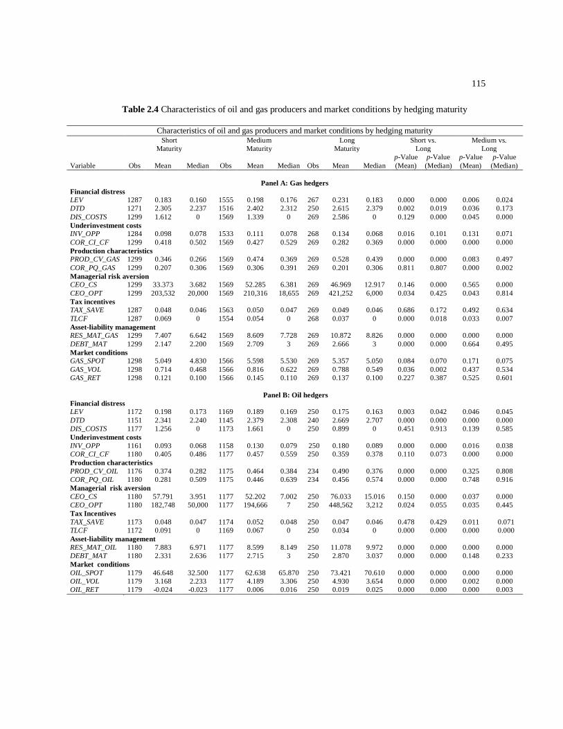
115
Table 2.4 Characteristics of oil and gas producers and market conditions by hedging maturity
Characteristics of oil and gas producers and market conditions by hedging maturity
Short
Maturity
Medium
Maturity
Long
Maturity
Short vs.
Long
Medium vs.
Long
Variable Obs Mean Median Obs Mean Median Obs Mean Median
p-Value
(Mean)
p-Value
(Median)
p-Value
(Mean)
p-Value
(Median)
Panel A: Gas hedgers
Financial distress
LEV 1287 0.183 0.160 1555 0.198 0.176 267 0.231 0.183 0.000 0.000 0.006 0.024
DTD 1271 2.305 2.237 1516 2.402 2.312 250 2.615 2.379 0.002 0.019 0.036 0.173
DIS_COSTS 1299 1.612 0 1569 1.339 0 269 2.586 0 0.129 0.000 0.045 0.000
Underinvestment costs INV_OPP 1284 0.098 0.078 1533 0.111 0.078 268 0.134 0.068 0.016 0.101 0.131 0.071
COR_CI_CF 1299 0.418 0.502 1569 0.427 0.529 269 0.282 0.369 0.000 0.000 0.000 0.000
Production characteristics
PROD_CV_GAS 1299 0.346 0.266 1569 0.474 0.369 269 0.528 0.439 0.000 0.000 0.083 0.497
COR_PQ_GAS 1299 0.207 0.306 1569 0.306 0.391 269 0.201 0.306 0.811 0.807 0.000 0.002
Managerial risk aversion
CEO_CS 1299 33.373 3.682 1569 52.285 6.381 269 46.969 12.917 0.146 0.000 0.565 0.000
CEO_OPT 1299 203,532 20,000 1569 210,316 18,655 269 421,252 6,000 0.034 0.425 0.043 0.814
Tax incentives
TAX_SAVE 1287 0.048 0.046 1563 0.050 0.047 269 0.049 0.046 0.686 0.172 0.492 0.634
TLCF 1287 0.069 0 1554 0.054 0 268 0.037 0 0.000 0.018 0.033 0.007
Asset-liability management
RES_MAT_GAS 1299 7.407 6.642 1569 8.609 7.728 269 10.872 8.826 0.000 0.000 0.000 0.000
DEBT_MAT 1299 2.147 2.200 1569 2.709 3 269 2.666 3 0.000 0.000 0.664 0.495
Market conditions
GAS_SPOT 1298 5.049 4.830 1566 5.598 5.530 269 5.357 5.050 0.084 0.070 0.171 0.075
GAS_VOL 1298 0.714 0.468 1566 0.816 0.622 269 0.788 0.549 0.036 0.002 0.437 0.534
GAS_RET 1298 0.121 0.100 1566 0.145 0.110 269 0.137 0.100 0.227 0.387 0.525 0.601
Panel B: Oil hedgers
Financial distress LEV 1172 0.198 0.173 1169 0.189 0.169 250 0.175 0.163 0.003 0.042 0.046 0.045
DTD 1151 2.341 2.240 1145 2.379 2.308 240 2.669 2.707 0.000 0.000 0.000 0.000
DIS_COSTS 1177 1.256 0 1173 1.661 0 250 0.899 0 0.451 0.913 0.139 0.585
Underinvestment costs
INV_OPP 1161 0.093 0.068 1158 0.130 0.079 250 0.180 0.089 0.000 0.000 0.016 0.038
COR_CI_CF 1180 0.405 0.486 1177 0.457 0.559 250 0.359 0.378 0.110 0.073 0.000 0.000
Production characteristics
PROD_CV_OIL 1176 0.374 0.282 1175 0.464 0.384 234 0.490 0.376 0.000 0.000 0.325 0.808
COR_PQ_OIL 1180 0.281 0.509 1175 0.446 0.639 234 0.456 0.574 0.000 0.000 0.748 0.916
Managerial risk aversion
CEO_CS 1180 57.791 3.951 1177 52.202 7.002 250 76.033 15.016 0.150 0.000 0.037 0.000
CEO_OPT 1180 182,748 50,000 1177 194,666 7 250 448,562 3,212 0.024 0.055 0.035 0.445
Tax Incentives
TAX_SAVE 1173 0.048 0.047 1174 0.052 0.048 250 0.047 0.046 0.478 0.429 0.011 0.071
TLCF 1172 0.091 0 1169 0.067 0 250 0.034 0 0.000 0.000 0.000 0.000
Asset-liability management
RES_MAT_OIL 1180 7.883 6.971 1177 8.599 8.149 250 11.078 9.972 0.000 0.000 0.000 0.000
DEBT_MAT 1180 2.331 2.636 1177 2.715 3 250 2.870 3.037 0.000 0.000 0.148 0.233
Market conditions
OIL_SPOT 1179 46.648 32.500 1177 62.638 65.870 250 73.421 70.610 0.000 0.000 0.000 0.000
OIL_VOL 1179 3.168 2.233 1177 4.189 3.306 250 4.930 3.654 0.000 0.000 0.002 0.000
OIL_RET 1179 -0.024 -0.023 1177 0.006 0.016 250 0.019 0.025 0.000 0.000 0.000 0.003

116
Note:
This table provides the mean and median values of firms’ financial and operational characteristics and market conditions
according to the weighted-average maturity of the hedging portfolio. For each firm-quarter with hedging activity, a hedging
portfolio maturity is classified as short-term maturity if it is below one year ahead, a medium-term maturity if it is between one
and two years ahead, and a long-term maturity if it exceeds two years ahead. INV_OPP for investment opportunities;
COR_CI_CF for the correlation between free cash flows and cost incurred; DTD for distance-to-default; LEV for the leverage
ratio measured by the sum of long-term debt in current liabilities plus one-half long-term debt scaled by book value of total
assets; DIS_COSTS for distress costs (in $); PROD_CV_OIL and PROD_CV_GAS measure production uncertainty for oil and
gas respectively; COR_PQ_OIL and COR_PQ_GAS measure the quantity-price correlation for oil and gas respectively;
CEO_CS for the market value of common shares held by firm’s CEO (in MM$); CEO_OPT for the number of stock options held
by firm’s CEO (in 000); TLCF for tax loss carry-forwards scaled by the book value of total assets; TAX_SAVE for the expected
percentage of tax saving; DEBT_MAT is the long-term debt maturity (in years); RES_MAT_OIL and RES_MAT_GAS are the
expected life of proven oil and gas reserves (in years); GAS_SPOT and OIL_SPOT are spot prices; GAS_VOL and OIL_VOL are
historical volatilities of spot prices over the current quarter; GAS_RET and OIL_RET are oil and gas returns measured by log(12-
month future price/spot price). Comparison of means is constructed using a t-test assuming unequal variances; comparison of
medians is constructed by using the non-parametric Wilcoxon rank sum Z-score. Two sided p-values are reported.
The univariate tests show considerable number differences between firm-quarters with
long-term maturities and those with short- or medium-term maturities for oil hedgers and gas
hedgers separately. Table 2.4 Panel A reports results pertaining to the subsample of gas
hedgers and Panel B presents results for oil hedgers. Results show that oil and gas producers
with higher distance-to-default tend to choose longer maturities. Results related to the
leverage ratio are mixed. Although the higher leverage ratio is more related to longer
maturities for gas hedgers, it seems to be more associated with shorter maturities for oil
hedgers. Counter to our predictions, higher distress costs are more related to long-run
contracts for gas hedgers. Consistent with our predictions, results further show that oil and
gas producers with higher growth opportunities prefer long-run hedging contracts, and that
higher correlation between free cash flows and investment expenditures motivates the use of
short- and medium-term contracts.
Univariate tests also show that oil and gas producers with higher production uncertainty
tend to use long maturity contracts. This is inconsistent with the prediction that higher
production uncertainty makes firms reluctant to make a large hedge for more distant
exposures. We find that price-quantity correlation is more closely related to medium-term
contracts for gas hedgers, and to long-term contracts for oil hedgers. In sum, these findings
corroborate our prediction that firms with higher price-quantity correlation tend to use longer
maturities because their cash flows are more volatile. Consistent with our prediction, the
Wilcoxon test for difference in medians shows that higher CEO stake value in the firm is

117
more related to long maturity contracts. In contrast, higher CEO option-holdings are
associated with long-term contracts, which contradicts the prediction that a manager with a
convex utility in firm value has a disincentive to undertake corporate hedging.
Univariate tests pertaining to tax incentives indicate that medium-term hedging is related
to a higher percentage of tax savings for oil hedgers. Consistent with our prediction, oil and
gas producers with higher tax loss carry-forwards tend to use short maturity hedging. In
addition, oil and gas producers with remaining longer maturities of debt and proven reserves
tend to choose long-run contracts. This corroborates the asset-liability management
argument. As predicted, results pertaining to market conditions suggest that higher spot
prices and volatilities are more associated with medium-term contracts for gas hedgers and
longer contracts for oil hedgers. Conversely, when oil future prices are anticipated to be
higher, oil hedgers tend to prefer long maturity contracts.
Table 2.5 presents our results, comparing the moneyness and strike prices of hedging
instruments based on their remaining maturities. Table 2.5 Panel A reports results pertaining
to gas hedgers and Panel B presents results for oil hedgers. For conciseness, we concentrate
our analysis on the three major hedging instruments used by oil and producers: swap
contracts, put options and costless collars.34
For oil hedgers, we find that swap contracts with
the longest maturities have the lowest moneyness as measured by the strike price minus the
spot price. One explanation would be that firms are reluctant to exit out-of-the-money swaps
prior to the agreed-upon termination date due to the termination costs. Consistent with our
prediction, results also show that higher strike prices are more related to medium-term swaps
for gas hedgers and to long-term swaps for oil hedgers. We further find that higher
moneyness and strike prices are more related to medium-term put options in the case of gas
hedging. As predicted, longer term put options are more associated with higher strike prices
for oil hedgers. Consistent with predictions, longer term collars are related to higher
moneyness and strike prices for both oil and gas hedgers.
34
We skip the observations related to forward/futures contracts because they contribute to only 3.25% of gas
hedging activity and 2.78% of oil hedging activity. We also omit observations related to three-way collars because
they are used in only 3.42% of cases for gas hedging activity and 3.02% of cases for oil hedging.

118
Table 2.5 Contract features by hedging maturity
Contract features by hedging maturity
Short
Maturity
Medium
Maturity
Long
Maturity
Short vs.
Long
Medium vs.
Long
Variable Obs Mean Median Obs Mean Median Obs Mean Median
p-value
(Mean)
p-value
(Median)
p-value
(Mean)
p-value
(Median)
Panel A: Gas hedgers
Swap contracts
MONEYNESS 903 -0.187 0 1069 -0.029 0 282 -0.127 0 0.580 0.171 0.344 0.176
STRIKE 903 5.054 5.261 1069 5.506 5.511 282 5.108 5.261 0.744 0.532 0.012 0.011
Put options
MONEYNESS 306 -0.005 0 184 0.121 0 27 -0.480 0 0.108 0.395 0.043 0.018
STRIKE 306 5.263 5.407 184 5.849 6.114 27 4.865 4.706 0.273 0.369 0.011 0.028
Costless collars
MONEYNESS 869 0.040 0 859 0.052 0 111 0.777 0 0.002 0.000 0.003 0.000
STRIKE 869 5.491 5.484 859 6.203 6.164 111 7.457 7.161 0.000 0.000 0.000 0.000
Panel B: Oil hedgers
Swap contracts
MONEYNESS 794 -2.689 -0.622 706 -2.681 0 211 -5.186 0 0.019 0.300 0.031 0.103
STRIKE 794 41.656 31.155 706 56.059 58.095 211 65.592 64.952 0.000 0.000 0.000 0.000
Put options
MONEYNESS 230 -1.428 0 188 0.760 0 27 2.043 0 0.389 0.143 0.751 0.514
STRIKE 230 49.356 38.314 188 63.068 60.048 27 66.512 59.956 0.011 0.013 0.599 0.675
Costless collars
MONEYNESS 663 -2.676 -0.263 589 -3.016 0 151 5.298 0 0.000 0.004 0.000 0.015
STRIKE 663 50.717 48.305 589 60.551 60.048 151 77.451 63.335 0.000 0.000 0.000 0.000
Note:
This table provides the mean and median values of the hedging instruments features (i.e., moneyness and strike price) according to its weighted-average maturity. Hedging instruments
are swap contracts, put options, and costless collars. Strike price is measured by the average spot price during the quarter of initiation of the hedging contract. Moneyness is calculated as
the contract strike price minus the average spot price during the current quarter. For each instrument, a hedging maturity is classified as short-term maturity if it is below one year
ahead, a medium-term maturity if it is between one and two years ahead, and a long-term maturity if it exceeds two years ahead. Comparison of means is constructed using a t-test
assuming unequal variances; comparison of medians is constructed by using the non-parametric Wilcoxon rank sum Z-score. Two sided p-values are reported.
119
2.6 Maturity structure of corporate risk management
To investigate the determinants of hedging maturity choice by oil and gas producers, we
estimate the dynamic panel regression using a two-step SYS-GMM35
model as presented
previously. In these regressions, the weighted-average remaining maturity is regressed on
variables that measure underinvestment costs, financial distress costs, production function
characteristics, managerial risk aversion, tax incentives, market conditions, asset-liability
management and contract features. Many specifications of the SYS-GMM are estimated for
the subset of oil hedgers and gas hedgers separately and for the following major hedging
instruments used: swap contracts, put options and costless collars. We based our analysis on
remaining maturity by instrument rather than the whole hedging portfolio to get more insights
into the hedging dynamics of oil and gas producers.
35
Following the good practice guideline suggested by Roodman (2009a and 2009b), we use all available lags of
the dependent variables as instruments to retain more information. We also apply a collapsing technique to avoid instrument proliferation that weakens the Hansen test instrument validity. We further report: (i) the number of instruments generated for the regression, (ii) the Hansen J-test statistics and p-value, and (iii) the Arellano-Bond
test for a second-order serial correlation in residuals (i.e., AR (2) test).

120
Table 2.6 Maturity structure by gas hedgers
(1) (2) (3) (4) (5) (6) (7) (8) (9) (10) (11) (12) Variables Swap
contracts Swap
contracts Swap
contracts Swap
contracts Put
options Put
options Put
options Put
options Costless collars
Costless collars
Costless collars
Costless collars
INV_OPP 0.3292*** 0.3468*** 0.2735** 0.3192*** 0.0695 0.0634 (0.089) (0.082) (0.114) (0.108) (0.086) (0.079) COR_CI_CF -0.0437 -0.0026 -0.1851** -0.2055** -0.0028 0.0599 (0.042) (0.048) (0.081) (0.099) (0.044) (0.043) LEV 1.3438*** 1.4572*** 1.3907*** 3.2410*** 0.8867*** 1.0542*** (0.280) (0.281) (0.424) (0.600) (0.184) (0.175) LEV_SQUARE -0.9482*** -1.1349*** -1.3725 -5.4469*** -0.5349*** -0.6324*** (0.360) (0.402) (0.866) (1.456) (0.130) (0.170) DTD 0.0994*** 0.0115 0.1499*** (0.029) (0.050) (0.032) DTD_SQUARE -0.0087* 0.0062 -0.0237*** (0.005) (0.008) (0.006) DIS_COSTS 0.0041 0.0028 0.0069 0.0081* 0.0014 0.0001 (0.003) (0.004) (0.005) (0.005) (0.001) (0.002) PROD_CV_GAS 0.0734 0.1487** 0.0923 0.0765 0.1273*** 0.1439*** (0.051) (0.057) (0.101) (0.102) (0.047) (0.052) COR_PQ_GAS 0.0550 -0.0073 0.0071 0.0110 0.0940** 0.0031 (0.051) (0.045) (0.083) (0.078) (0.042) (0.039) GAS_VOL 0.0555*** 0.0541*** 0.1128*** 0.1287*** 0.0482** 0.0425** (0.019) (0.020) (0.029) (0.030) (0.019) (0.019) GAS_RET -0.1307* -0.1572** -0.4896*** -0.4689*** -0.2587*** -0.2710*** (0.070) (0.069) (0.142) (0.130) (0.070) (0.076) GAS_SPOT 0.1309*** 0.1457*** 0.0997*** (0.016) (0.029) (0.017) GAS_SPOT_SQUARE -0.0080*** -0.0074*** -0.0047*** (0.001) (0.002) (0.001) MONEYNESS 0.0144* 0.0209*** 0.0158 0.0161 0.0109 0.0142* (0.008) (0.008) (0.017) (0.015) (0.008) (0.008) STRIKE 0.0299*** 0.0384*** 0.0222*** (0.007) (0.011) (0.007) TLCF -0.3411*** -0.3849*** -0.3462*** -0.4941*** -0.0611* -0.1061** (0.062) (0.142) (0.050) (0.178) (0.036) (0.041) TAX_SAVE -0.0491 0.2914 0.0389 1.9730** 0.4577 0.7561** (0.140) (0.235) (0.848) (0.764) (0.409) (0.340) DEBT_MAT 0.0396*** 0.0368*** 0.0082 -0.0146 0.0307*** 0.0337*** (0.012) (0.012) (0.016) (0.018) (0.010) (0.010) RES_MAT_GAS 0.0184*** 0.0188*** 0.0212*** 0.0208*** 0.0228*** 0.0200*** (0.004) (0.005) (0.006) (0.006) (0.004) (0.005) CEO_CS 0.1218 0.1756 -0.2095 0.2573 0.1841 0.1322 (0.114) (0.154) (0.330) (0.326) (0.148) (0.121) CEO_OPT 0.0001 0.0001 -0.0002 0.0001 -0.0002*** -0.0001** (0.000) (0.000) (0.000) (0.000) (0.000) (0.000) IMR 0.1829*** 0.1002** 0.1202** 0.2569*** 0.1225* 0.0851 0.1181* 0.2251*** 0.1288*** 0.0583 0.0597 0.1734*** (0.047) (0.047) (0.057) (0.063) (0.065) (0.083) (0.061) (0.082) (0.047) (0.046) (0.049) (0.051) LAG_1 0.5597*** 0.5836*** 0.5834*** 0.5742*** 0.4892*** 0.5592*** 0.5120*** 0.4766*** 0.5816*** 0.6043*** 0.5918*** 0.6044*** (0.053) (0.044) (0.051) (0.050) (0.080) (0.094) (0.074) (0.081) (0.049) (0.051) (0.053) (0.047) LAG_2 -0.0289 (0.022)
Observations 2,123 2,129 2,096 2,108 480 485 478 480 1,726 1,746 1,699 1,745 Number of firms 99 100 99 99 44 49 43 44 93 95 93 94 Number of instruments 63.0000 61.0000 63.0000 62.0000 63.0000 61.0000 63.0000 62.0000 63.0000 61.0000 63.0000 62.0000 F statistic 409.4175 705.0217 428.2656 433.7338 173.8287 182.3584 227.4729 200.8200 412.9824 570.3112 601.2629 575.2583 p value F statistic 0.0000 0.0000 0.0000 0.0000 0.0000 0.0000 0.0000 0.0000 0.0000 0.0000 0.0000 0.0000 Hansen J statistic 63.8114 53.8975 62.5987 59.8964 36.6077 30.6516 36.9887 33.0220 60.9116 52.6989 56.9287 60.2093 p value of Hansen statistic 0.1074 0.3641 0.1279 0.1595 0.9356 0.9893 0.9295 0.9761 0.1613 0.4082 0.2640 0.1769 AR(2) test statistic -1.4614 -1.3744 -1.6156 -0.7854 -0.6087 -0.9605 -0.3671 -1.4434 -1.3989 -0.8421 -1.3168 -1.5502 p value of AR(2) statistic 0.1439 0.1693 0.1062 0.4322 0.5427 0.3368 0.7136 0.1489 0.1618 0.3997 0.1879 0.1211 Sigma_e 0.3393 0.4425 0.3471 0.3459 0.3049 0.4605 0.3100 0.3164 0.3175 0.4135 0.3194 0.3277
Note:
This table provides the two-step SYS-GMM results for the determinants of the weighted-average remaining maturity for swap contracts, put options and
costless collars respectively. The results are for the subsample of gas hedgers. INV_OPP for investment opportunities; COR_CI_CF for the correlation
between free cash flows and cost incurred; LEV for the leverage ratio measured by the sum of long-term debt in current liabilities plus one-half long term
debt scaled by book value of total assets; LEV_SQUARED is the leverage ratio squared; DTD for distance-to-default; DTD_SQUARED for the distance to
default squared; DIS_COSTS for distress costs (in $/BOE); PROD_CV_GAS measures gas production uncertainty; COR_PQ_GAS measures the gas
quantity-price correlation; GAS_VOL for gas price volatility; GAS_RET for gas return as measured by log(gas 12-month future price/gas sport price);
GAS_SPOT and GAS_SPOT_SQUARED are for gas spot price and gas price squared; MONEYNESS measured by the contract strike price minus the
average spot price during the current quarter; STRIKE is the contract’s strike price; TLCF for tax loss carry-forwards scaled by the book value of total
assets; TAX_SAVE for the expected percentage of tax saving; DEBT_MAT is the long-term debt maturity (in years); RES_MAT_GAS are the expected life
of proven oil and gas reserves (in years); CEO_CS for the market value of common shares held by firm’s CEO (in logarithm); CEO_OPT for the number of
stock options held by firm’s CEO (in 000); IMR is the inverse Mills Ratio (Table A.2.1); LAG_1 is the dependent variable first lag; LAG_2 is the dependent
variable second lag (used when there is second-order serial correlation in the error term). Standard errors are clustered by firm and incorporate the
Windmeijer (2005) correction, in parentheses. ***Significant at the 1% level, ** Significant at the 5% level, * Significant at the 10% level.

121
Table 2.7 Maturity structure by oil hedgers
(1) (2) (3) (4) (5) (6) (7) (8) (9) (10) (11) (12) Variables Swap
contracts Swap
contracts Swap
contracts Swap
contracts Put
options Put
options Put
options Put
options Costless Collars
Costless Collars
Costless Collars
Costless Collars
INV_OPP 0.2623** 0.2200** 0.5839** 0.5923** 0.1001* 0.0916* (0.129) (0.110) (0.222) (0.235) (0.052) (0.052) COR_CI_CF -0.1294*** -0.0818* 0.0487 0.0533 0.0213 0.0302 (0.048) (0.048) (0.076) (0.094) (0.052) (0.059) LEV 0.5090* 0.8594*** 1.5182* 1.6283** 1.1577*** 0.8237*** (0.265) (0.256) (0.803) (0.760) (0.348) (0.208) LEV_SQUARE -0.2940 -0.7017** -1.5120 -1.3516 -1.4545*** -0.9989*** (0.402) (0.349) (2.053) (1.702) (0.522) (0.292) DTD 0.0729** 0.2709*** 0.1614*** (0.029) (0.075) (0.055) DTD_SQUARE -0.0049 -0.0474*** -0.0230** (0.003) (0.015) (0.010) DIS_COSTS 0.0011 -0.0006 0.0146*** 0.0103*** 0.0003 0.0005 (0.002) (0.003) (0.003) (0.003) (0.003) (0.003) PROD_CV_OIL 0.1090* 0.1260* 0.0089 0.0109 -0.0404 -0.0797 (0.065) (0.065) (0.119) (0.104) (0.062) (0.059) COR_PQ_OIL 0.0590 0.0001 0.0217 -0.0442 0.0983** 0.0427 (0.037) (0.038) (0.084) (0.084) (0.048) (0.046) OIL_VOL 0.0189*** 0.0206*** 0.0159** 0.0205** 0.0133** 0.0170*** (0.005) (0.005) (0.007) (0.008) (0.005) (0.006) OIL_RET -0.0313 0.0165 -0.3799 -0.3938 -0.2188 -0.0051 (0.195) (0.209) (0.495) (0.504) (0.230) (0.215) OIL_SPOT 0.0149*** 0.0043 0.0080*** (0.002) (0.003) (0.002) OIL_SPOT_SQUARE -0.0001*** -0.0000 -0.0000** (0.000) (0.000) (0.000) MONEYNESS 0.0028** 0.0033*** 0.0015 0.0031 0.0037*** 0.0044*** (0.001) (0.001) (0.002) (0.002) (0.001) (0.001) STRIKE 0.0057*** 0.0037*** 0.0033*** (0.001) (0.001) (0.001) TLCF -0.3940*** -0.5680*** -0.2640*** -0.4791*** -0.0531 -0.0813 (0.082) (0.134) (0.062) (0.163) (0.059) (0.052) TAX_SAVE 0.1945 0.1802 0.1319 0.9001 0.1094 0.0787 (0.154) (0.140) (0.612) (0.583) (0.286) (0.273) DEBT_MAT 0.0416*** 0.0420*** 0.0280 -0.0006 0.0310*** 0.0260** (0.013) (0.013) (0.019) (0.020) (0.011) (0.010) RES_MAT_OIL 0.0311*** 0.0272*** 0.0119** 0.0052 0.0182*** 0.0161*** (0.004) (0.004) (0.006) (0.007) (0.005) (0.004) CEO_CS -0.1633 -0.0628 -0.3542 -0.3388 -0.0665 -0.1324 (0.137) (0.139) (0.318) (0.343) (0.140) (0.146) CEO_OPT 0.0002* 0.0002 -0.0001 0.0001 -0.0001 -0.0001 (0.000) (0.000) (0.000) (0.000) (0.000) (0.000) IMR 0.1311** 0.1470** 0.1049* 0.2848*** 0.1382** 0.2096*** 0.0121 0.1800*** 0.2054*** 0.1265** 0.1797** 0.1946*** (0.059) (0.071) (0.060) (0.062) (0.059) (0.066) (0.052) (0.052) (0.068) (0.049) (0.068) (0.044) LAG_1 0.5630*** 0.5548*** 0.5728*** 0.5490*** 0.4645*** 0.5872*** 0.4760*** 0.5211*** 0.5858*** 0.6228*** 0.5745*** 0.6256*** (0.039) (0.046) (0.042) (0.046) (0.063) (0.062) (0.084) (0.076) (0.040) (0.041) (0.039) (0.035) LAG_2 -0.0496** -0.0696*** -0.0432** -0.0529** (0.020) (0.023) (0.020) (0.020)
Observations 1,593 1,608 1,572 1,608 402 417 393 414 1,331 1,351 1,311 1,351 Number of firms 88 89 88 89 36 40 35 37 81 81 81 81 Number of instruments 63.0000 61.0000 63.0000 62.0000 57.0000 57.0000 57.0000 56.0000 63.0000 61.0000 63.0000 62.0000 F statistic 293.9642 413.6701 255.7297 280.9298 128.4730 176.0464 102.0687 336.8433 280.2979 444.6558 275.8100 318.6617 p value F statistic 0.0000 0.0000 0.0000 0.0000 0.0000 0.0000 0.0000 0.0000 0.0000 0.0000 0.0000 0.0000 Hansen J statistic 51.8717 51.3504 55.6423 54.2101 29.0451 28.2022 27.3456 35.4909 59.4069 46.4226 56.9199 53.5233 p value of Hansen statistic 0.4007 0.4206 0.2708 0.3170 0.9688 0.9865 0.9825 0.8441 0.1960 0.6558 0.2642 0.3777 AR(2) test statistic -1.0896 0.1353 -1.2967 -0.7639 0.5991 1.4030 1.0248 1.2104 0.8288 0.2945 0.9272 1.0881 p value of AR(2) statistic 0.2759 0.8923 0.1947 0.4449 0.5491 0.1606 0.3055 0.2261 0.4072 0.7684 0.3538 0.2766 Sigma_e 0.3144 0.4310 0.3160 0.3163 0.3038 0.4969 0.3079 0.3177 0.3374 0.4834 0.3324 0.3533
Note:
This table provides the two-step SYS-GMM results for the determinants of the weighted-average remaining maturity for swap contracts, put options and
costless collars respectively. The results are for the subsample of oil hedgers. INV_OPP for investment opportunities; COR_CI_CF for the correlation between
free cash flows and cost incurred; LEV for the leverage ratio measured by the sum of long-term debt in current liabilities plus one-half long term debt scaled by
book value of total assets; LEV_SQUARED is the leverage ratio squared; DTD for distance-to-default; DTD_SQUARED for distance-to-default squared;
DIS_COSTS for distress costs (in $/BOE); PROD_CV_OIL measures oil production uncertainty; COR_PQ_OIL measures the oil quantity-price correlation,
OIL_VOL for oil price volatility; OIL_RET for oil return as measured by log(oil 12-month future price/oil sport price); OIL_SPOT and OIL_SPOT_SQUARED
are for oil spot price and oil price squared; MONEYNESS measured by the contract strike price minus the average spot price during the current quarter;
STRIKE is the contract’s strike price; TLCF for tax loss carry-forwards scaled by the book value of total assets; TAX_SAVE for the expected percentage of tax
saving; DEBT_MAT is the long-term debt maturity (in years); RES_MAT_OIL are the expected life of proven oil and gas reserves (in years); CEO_CS for the
market value of common shares held by firm’s CEO (in logarithm); CEO_OPT for the number of stock options held by firm’s CEO (in 000); IMR is the inverse
Mills Ratio (Table A.2.1); LAG_1 is the dependent variable first lag; LAG_2 is the dependent variable second lag (used when there are second order serial
correlation in the error term). Standard errors are clustered by firm and incorporate the Windmeijer (2005) correction, in parentheses. ***Significant at the 1%
level, ** Significant at the 5% level, * Significant at the 10% level.

122
The results in Tables 2.6 (gas hedgers) and 2.7 (oil hedgers) are generally consistent with
hypotheses pertaining to underinvestment costs. In particular, oil and gas producers with
higher future investment opportunities (INV_OPP) tend to use longer term swap contracts,
put options and costless collars. Oil and gas producers with substantial growth opportunities
employ hedging contracts with longer maturities to reduce any shortfall in their future cash
flows and hence avoid both cutting planned investment programs and costly external
financing. We also find a significant negative effect of the correlation between investment
expenditures and internally generated cash flows (COR_CI_CF) and hedging contract
horizon because firms benefit from a natural hedge. We find that the remaining maturities of
put options and swap contracts decline with this positive correlation for gas hedgers and oil
hedgers respectively. The impacts on costless collars’ maturities are mixed and insignificant.
Interestingly, results reveal opposite effects of firm’s investment specificities on hedging
maturity structure: growth options accentuate future funding needs and a positive correlation
dampens this need. These opposite effects are essentially driven by the simultaneous positive
impacts of current oil and gas prices on future investment opportunities and present cash
inflows.
The results pertaining to financial distress give strong evidence of the non-monotonic
relationship between hedging horizons and the likelihood of financial distress. In line with
Fehle and Tsyplakov’s (2005) prediction, we find that the leverage ratio (LEV) and the
leverage squared (LEV_SQUARE) have highly significant positive and negative coefficients
respectively for both subsets of gas hedgers and oil hedgers, for the three hedging
instruments.36
These non-monotonic (concave) relationships mean that hedging maturities
should first increase and then decrease with the likelihood of financial distress. To further
investigate this non-monotonic relationship empirically, we use an alternative robust measure
of the likelihood of financial distress, namely, distance-to-default. Interestingly, results show
that remaining maturity should increase and decrease with the distance to default. Generally,
we find that Distance-to-Default (DTD) and its squared value (DTD_SQUARE) are
respectively significantly positively and negatively related to hedging instrument maturity.
The non-monotonic relationship between hedging maturity and leverage ratio is shown, for
36
As robustness checks, we measure the leverage ratio by: (i) long-term debt in current liabilities plus long-term
debt scaled by total assets, (ii) long-term debt scaled by total assets. Results are the same.
123
each hedging instrument, in Figure 2.1 for gas hedgers and in Figure 2.2 for oil hedgers.
These figures show that this non-monotonic relationship is more pronounced for put options
for gas hedgers and for costless collars for oil hedgers.
Figure 2.1 Non-monotonic relationship between hedging maturity and leverage for gas hedgers
Note:
This figure illustrates the relation between hedging maturity and leverage ratio by: with and coming from the estimation of our base model SYS-GMM in table 6.
The coefficients and equal 1.45 and -1.13 for swap contracts, 3.24 and -5.44 for put options, and 1.05
and -0.63 for costless collars (see Table 6 Columns 4, 8 and 12). For Fehle and Tsyplakov (2005), and equal 0.70 and -0.69 (see Table 15, pp.40 from Fehle and Tsyplakov, 2005).
Mat
uri
ty (i
n y
ear
)
Leverage
Gas hedgers: Non-monotonic relation between hedging maturity and leverage
Swap contracts
Put options
Costless collars
Fehle and Tsyplakov(2005)

124
Figure 2.2 Non-monotonic relationship between hedging maturity and leverage for oil hedgers
Note:
This figure illustrates the relation between hedging maturity and leverage ratio by: with and coming from the estimation of our base model SYS-GMM in Table 7. The coefficients and equal 0.86 and -0.70 for swap contracts, 1.63 and -1.35 for put options, and 0.82
and -1.00 for costless collars (see Table 7 Columns 4, 8 and 12). For Fehle and Tsyplakov (2005), and equal 0.70 and -0.69 (see Table 15, pp.40 from Fehle and Tsyplakov, 2005).
In contrast with our hypotheses, we find that distressed oil and gas producers incurring a
higher dollar loss per Barrel of Oil Equivalent (DIS_COSTS) tend to use put options with
longer maturities. This empirical finding contradicts the simulation results of Fehle and
Tsyplakov (2005), who find that firms incurring higher distress costs tend to use short-term
hedging contracts. A possible explanation comes from Jensen and Meckling’s (1976) risk
shifting (or asset substitution) approach. By entering costly long-term put options, distressed
oil and gas producers increase rather than eliminate the firm’s payoff volatility, decrease
assets available for debtholders and preserve any upside potential for shareholders.
Results further indicate that oil and gas producers with higher production uncertainty
(PROD_CV_OIL and PROD_CV_GAS) tend to use long-term swap contracts and costless
collars. The impact on put options’ maturities is also positive but not significant. This finding
contradicts Brown and Toft (2002), who assert that higher production uncertainty makes
firms reluctant to hedge farther exposures. As predicted, we find that higher price-quantity
Mat
uri
ty (i
n y
ear
)
Leverage
Oil hedgers: Non-monotonic relation between hedging maturity and leverage
Swap contracts
Put options
Costless collars
Fehle and Tsyplakov(2005)

125
correlations (COR_PQ_OIL and COR_PQ_GAS) motivate oil and gas hedgers to use more
distant costless collar positions. A higher price-quantity correlation induces higher firm cash
flow volatility because both prices and quantities are moving in the same direction.
Altogether, we find that oil and gas producers with higher cash flow volatility, due to higher
production uncertainty and/or higher price-quantity correlation, tend to use longer hedging
positions to avoid shortfalls in their future revenues.
The results for variables pertaining to market conditions are highly consistent with our
predictions. We find that oil and gas price volatilities (OIL_VOL and GAS_VOL) are
significantly positively related to longer maturities for the three hedging instruments. This
corroborates the simulation results of Fehle and Tsyplakov (2005), namely that in a higher
price fluctuation environment, firms tend to refrain from costly early termination of their
outstanding contracts unless spot prices increase significantly. We further find that when
future gas prices are expected to be higher, as measured by GAS_RET, gas hedgers tend to
use short-term hedging. This is consistent with the prediction that when future prices are
expected to be higher, firms tend to terminate their outstanding contracts and initiate new
hedging contracts with higher exercise prices. In addition, these newly initiated contracts
have short maturities to prevent them from being worthless in the future. Surprisingly,
expected tendency in future oil prices, as measured by OIL_RET, has the predicted negative
sign but no significant impact.37
Our results also provide strong evidence of a non-monotonic relationship between spot
prices and hedging maturities, as conjectured by Fehle and Tsyplakov (2005). We find that
oil and gas spot prices (OIL_SPOT and GAS_SPOT) and the spot prices squared
(OIL_SPOT_SQUARE and GAS_SPOT_SQUARE) have highly significant positive and
negative coefficients respectively, yielding a non-monotonic relationship. Accordingly, when
spot prices are either very high or very low, firms are more likely to choose short-term
hedging contracts. This corroborates the non-monotonic relationship between financial
distress likelihood measures (i.e., leverage ratio and distance-to-default) and hedging
37 We further investigate the effects of anticipated oil and gas prices, as observed in the future contracts market,
on hedging maturity choice by using the following Futures terms: three, six, fifteen, eighteen and twenty four
months ahead. Our results are unchanged with 12-month future contracts.

126
maturity. When spot prices are very high or low, firms are more likely to be far from or deep
in financial distress respectively. Figures 3 and 4 show the non-monotonic relationship
between hedging maturity and spot prices for gas hedgers and oil hedgers separately. The
non-monotonic relationship is more evident for swap contracts for oil hedgers.
Figure 2.3 Non-monotonic relationship between hedging maturity and gas spot prices for gas hedgers
Note:
This figure illustrates the relation between hedging maturity and leverage ratio by: with and coming from the estimation of our base model SYS-GMM in Table 6. The coefficients and equal 0.131 and -0.008 for swap contracts, 0.146 and -0.007 for put options, and 0.100 and -0.005 for costless collars (see Table 6 Columns 2, 6 and 10).
Mat
uri
ty (i
n y
ear
)
Gas spot price ($/MMBTU)
Gas hedgers: Non-monotonic relation between hedging maturity and gas spot price
Swap contracts
Put options
Costless collars

127
Figure 2.4 Non-monotonic relationship between hedging maturity and oil spot prices for oil hedgers
Note:
This figure illustrates the relation between hedging maturity and leverage ratio by: with and coming from the estimation of our base model SYS-GMM in Table 7. The coefficients and equal 0.015 and -0.0001 for swap contracts, 0.0043 and -0.00000185 for put options, and 0.008 and -0.00004 for costless collars (see Table 7 Columns 2, 6 and 10).
Hedging contract features appear to have an evident impact on hedging maturity choice.
Results show that swap contracts and costless collars with higher MONEYNESS (e.g., strike
prices higher than current spot prices) tend to have longer maturities. For put options,
moneyness has the predicted sign but no significant impact. As predicted, oil and gas
producers keep in-the-money hedging contracts until they mature and early terminate out-of-
the-money contracts. Results also indicate that when hedging contracts are initiated at
sufficiently higher prices (STRIKE) they are more likely to be kept for longer periods.
Mat
uri
ty (i
n y
ear
)
Oil spot price ($/barrel)
Oil hedgers: Non-monotonic relation between hedging maturity and oil spot
price
Swap contracts
Put options
Costless collars
128
Consistent with our expectations, we find that oil and gas producers with higher tax loss
carry-forwards (TLCF) choose short-term hedging maturities. Tax loss carry-forwards thus
seem to be a disincentive to hedge longer exposures because they reduce firms’ future tax
liabilities. This corroborates the argument of Graham and Rogers (2002) that tax loss carry-
forwards are uncorrelated with tax function convexity. As predicted, results further show a
significant positive association between tax function convexity (TAX_SAVE) and put option
and costless collar maturities for gas hedgers, in particular. For oil hedgers, the tax function
convexity measure has the predicted sign but no significant impact.
Results for variables pertaining to asset-liability management are as predicted. We find
that oil and gas producers with longer average debt maturity (DEBT_MAT) tend to use more
distant swap and collar positions.38
Average debt maturity appears to have no significant
impact on put option maturity. We document strong evidence of a positive impact of the
expected life duration of proven oil and gas reserves (RES_MAT_OIL and RES_MAT_GAS)
on maturities of the three hedging instruments. These results suggest that oil and gas
producers seek to match the maturities of their hedging and the maturities of their assets and
debt. The CEO’s stake value in the firm (CEO_CS) seems to have no impact on hedging
maturity choice. CEO option-holding has a mixed impact. Although CEO option-holding
(CEO_OPT) is negatively related to collar maturities for gas hedgers, it is positively related
to swap maturities for oil hedgers.
38 We use an alternative measure of average debt maturity as described by Eisdorfer (2008). The firm’s average
debt maturity is estimated by: ̂
( ) where TD, STD, and LTD are the book values of total,
short-term, and long-term debt. Our results are the same.
129
2.7 Robustness checks
In this section, we investigate the empirical relevance of our predictions and our previous
findings by: (i) studying maturity choice at hedging contract inception, (ii) and investigating
the determinants of the early termination of outstanding hedging contracts.
2.7.1 Maturity choice at the inception of the hedging contract
We skim the time series of the weighted-average maturity by hedging instrument and
detect initiation dates by choosing observations where the observed maturity at time T is
superior to the one at time T-1. We run a pooled cross-sectional time-series regression of the
weighted-average maturities at the inception dates on firm’s fundamentals, production
function characteristics and oil and gas market conditions. Table 2.8 and 2.9 report the
regression results for gas hedgers and oil hedgers separately.
130
Table 2.8 Maturity choice at the inception of hedging contracts by gas hedgers
(1) (2) (3) (4) (5) (6) (7) (8) (9) (10) (11) (12) Variables Swap
contracts Swap
contracts Swap
contracts Swap
contracts Put
options Put
options Put
options Put
options Costless collars
Costless collars
Costless collars
Costless collars
INV_OPP 0.0026 0.0146 -0.0512 -0.0371 0.1862** 0.1876** (0.109) (0.111) (0.140) (0.151) (0.082) (0.079) COR_CI_CF -0.2297*** -0.2398*** -0.4763*** -0.4721*** -0.0388 -0.0025 (0.063) (0.071) (0.120) (0.137) (0.055) (0.058) LEV -0.5737* -0.9896** 1.9823** 1.5209 0.4274 0.7591** (0.343) (0.408) (0.784) (1.168) (0.329) (0.357) LEV_SQUARE 1.0634*** 1.1176*** -2.5490** -2.8874 -0.3952 -0.6584* (0.306) (0.333) (1.280) (2.469) (0.320) (0.359) DTD -0.0023 -0.1624 0.0425 (0.040) (0.119) (0.064) DTD_SQUARE 0.0025 0.0253 -0.0085 (0.006) (0.021) (0.010) DIS_COSTS 0.0057** 0.0055** 0.0036 0.0056 0.0015 0.0010 (0.003) (0.002) (0.005) (0.005) (0.002) (0.002) PROD_CV_GAS 0.0294 0.0257 0.2925** 0.2413** 0.2699*** 0.2538*** (0.054) (0.057) (0.114) (0.121) (0.057) (0.060) COR_PQ_GAS -0.1624** -0.1725** -0.1216 -0.1775* 0.0628 0.0392 (0.072) (0.067) (0.092) (0.091) (0.053) (0.052) GAS_VOL -0.0259 -0.0364 0.0072 -0.0135 0.0377 0.0317 (0.041) (0.039) (0.055) (0.053) (0.038) (0.038) GAS_RET 0.0015 -0.0392 -0.1774 -0.1942 -0.0055 -0.0033 (0.132) (0.126) (0.170) (0.163) (0.100) (0.099) GAS_SPOT -0.0159 0.0524 0.0654** (0.035) (0.040) (0.027) GAS_SPOT_SQUARE 0.0010 -0.0028 -0.0032 (0.003) (0.003) (0.002) STRIKE -0.0141 0.0260** 0.0278*** (0.010) (0.012) (0.009) TLCF -0.5876*** -0.5165*** -0.7963*** -0.6928*** -0.0835 -0.1434 (0.142) (0.147) (0.198) (0.208) (0.152) (0.152) TAX_SAVE -1.4783* -1.5711* -0.1894 -0.3458 0.2650 0.2519 (0.873) (0.841) (0.878) (0.831) (0.201) (0.214) DEBT_MAT 0.0152 0.0188 0.0068 -0.0029 0.0242** 0.0229** (0.013) (0.013) (0.020) (0.020) (0.011) (0.012) RES_MAT_GAS 0.0142*** 0.0120*** 0.0320*** 0.0281*** 0.0128** 0.0122** (0.005) (0.004) (0.007) (0.007) (0.005) (0.005) CEO_CS 0.2019 0.1969 -0.0600 0.1344 0.4796** 0.4417** (0.258) (0.269) (0.297) (0.360) (0.205) (0.205) CEO_OPT 0.0007 0.0008 -0.0001 0.0004 0.0001 0.0001 (0.001) (0.001) (0.002) (0.002) (0.000) (0.000) IMR -0.3736*** -0.2885*** -0.3237*** -0.3941*** -0.0970 -0.3959*** -0.3236*** -0.2614 -0.3176*** -0.2978*** -0.3778*** -0.2299*** (0.060) (0.057) (0.060) (0.071) (0.112) (0.108) (0.095) (0.158) (0.070) (0.073) (0.065) (0.080) CONSTANT 1.6506*** 1.6762*** 1.5977*** 1.8711*** 0.6523*** 1.4443*** 1.3201*** 1.2623*** 1.0725*** 1.1194*** 1.1399*** 1.0577*** (0.112) (0.124) (0.115) (0.147) (0.194) (0.181) (0.212) (0.261) (0.098) (0.096) (0.109) (0.121)
Observations 733 735 726 735 168 168 167 163 603 608 597 607 R-squared 0.0799 0.0825 0.0649 0.0948 0.2083 0.2047 0.1947 0.1898 0.1236 0.0872 0.1220 0.0888
Note: This table provides pooled cross-sectional time-series regressions of the determinants of the weighted-average remaining maturity for
swap contracts, put options and costless collars respectively. The results are for the subsample of gas hedgers. INV_OPP for investment
opportunities; COR_CI_CF for the correlation between free cash flows and cost incurred; LEV for the leverage ratio measured by the sum
of long-term debt in current liabilities plus one-half long-term debt scaled by book value of total assets; LEV_SQUARED is the leverage
ratio squared; DTD for distance-to-default; DTD_SQUARED for distance-to-default squared; DIS_COSTS for distress costs (in $/BOE);
PROD_CV_GAS measures gas production uncertainty; COR_PQ_GAS measures the gas quantity-price correlation; GAS_VOL for gas
price volatility; GAS_RET for gas return as measured by log(gas 12-month future price/gas sport price); GAS_SPOT and
GAS_SPOT_SQUARED are for gas spot price and gas price squared; MONEYNESS measured by the contract strike price minus the
average spot price during the current quarter; STRIKE is the contract’s strike price; TLCF for tax loss carry-forwards scaled by the book
value of total assets; TAX_SAVE for the expected percentage of tax saving; DEBT_MAT is the long-term debt maturity (in years);
RES_MAT_GAS are the expected life of proven oil and gas reserves (in years); CEO_CS for the market value of common shares held by
firm’s CEO (in logarithm); CEO_OPT for the number of stock options held by firm’s CEO (in 000); IMR is the inverse Mills Ratio
(Table A.2.1). Robust standard errors using Huber-White-Sandwich estimator are in parentheses. ***Significant at the 1% level, **
Significant at the 5% level, * Significant at the 10% level.
131
Table 2.9 Maturity choice at the inception of hedging contracts by oil hedgers
(1) (2) (3) (4) (5) (6) (7) (8) (9) (10) (11) (12) Variables Swap
contracts Swap
contracts Swap
contracts Swap
contracts Put
options Put
options Put
options Put
options Costless collars
Costless collars
Costless collars
Costless collars
INV_OPP 0.1860 0.2165 0.3426** 0.3949*** 0.2728*** 0.2879*** (0.154) (0.142) (0.157) (0.145) (0.104) (0.104) COR_CI_CF -0.2169*** -0.2177*** -0.1492 -0.1486 -0.0184 -0.0360 (0.063) (0.065) (0.124) (0.125) (0.075) (0.086) LEV -1.3732*** -0.2853 -1.8256 -0.2747 -0.3317 -0.3262 (0.403) (0.378) (1.277) (1.569) (0.425) (0.478) LEV_SQUARE 1.0744*** -0.0052 3.5507 1.2990 0.0682 0.1122 (0.377) (0.342) (3.041) (3.217) (0.500) (0.543) DTD 0.1393*** 0.2988*** 0.1412** (0.035) (0.101) (0.065) DTD_SQUARE -0.0098*** -0.0515*** -0.0200* (0.003) (0.015) (0.010) DIS_COSTS 0.0018 0.0029* 0.0085* 0.0119*** -0.0003 0.0007 (0.002) (0.002) (0.005) (0.004) (0.001) (0.001) PROD_CV_OIL 0.3939*** 0.3406*** -0.1638 -0.1586 -0.1665* -0.1750* (0.089) (0.087) (0.125) (0.112) (0.095) (0.094) COR_PQ_OIL -0.0259 0.0060 -0.0359 -0.0879 0.1208*** 0.1039** (0.042) (0.037) (0.088) (0.079) (0.047) (0.048) OIL_VOL 0.0126 0.0279** 0.0155 0.0294** 0.0032 0.0094 (0.011) (0.011) (0.013) (0.013) (0.013) (0.013) OIL_RET 1.0026*** 0.9922*** -0.1797 0.1297 1.3909*** 1.5355*** (0.359) (0.348) (0.562) (0.589) (0.419) (0.424) OIL_SPOT 0.0222*** 0.0058 0.0105** (0.003) (0.005) (0.004) OIL_SPOT_SQUARE -0.0001*** -0.0000 -0.0000 (0.000) (0.000) (0.000) STRIKE 0.0100*** 0.0039** 0.0049*** (0.001) (0.002) (0.001) TLCF -0.4943*** -0.4607*** -0.6377*** -0.6094** -0.2474*** -0.2038*** (0.133) (0.136) (0.215) (0.261) (0.079) (0.077) TAX_SAVE 0.0044 -0.0476 0.8006 0.6848 -0.1129 -0.7660 (0.208) (0.211) (1.408) (1.555) (1.037) (1.001) DEBT_MAT 0.0212 0.0196 0.0128 0.0093 0.0296* 0.0328** (0.014) (0.014) (0.025) (0.026) (0.015) (0.016) RES_MAT_OIL 0.0272*** 0.0234*** 0.0132** 0.0108** 0.0051 0.0039 (0.004) (0.004) (0.006) (0.005) (0.005) (0.005) CEO_CS -0.1867 -0.1990 0.0916 -0.0315 0.0717 0.1074 (0.229) (0.230) (0.673) (0.696) (0.321) (0.323) CEO_OPT 0.0006 0.0007 0.0002 0.0002 0.0004 0.0004 (0.000) (0.000) (0.000) (0.000) (0.000) (0.000) IMR -0.2008** 0.0349 -0.0675 0.0230 -0.4435*** -0.3672*** -0.3348*** -0.3689** -0.2096*** -0.0748 -0.1387* -0.1324 (0.091) (0.087) (0.083) (0.094) (0.121) (0.105) (0.086) (0.147) (0.077) (0.080) (0.081) (0.083) CONSTANT 1.2574*** 0.6425*** 0.6798*** 0.9784*** 1.5144*** 1.3262*** 0.9009*** 1.3511*** 1.4490*** 0.8816*** 1.1732*** 1.1215*** (0.117) (0.115) (0.121) (0.133) (0.241) (0.198) (0.215) (0.322) (0.123) (0.127) (0.143) (0.144)
Observations 562 570 557 570 128 132 126 129 433 436 430 436 R-squared 0.1874 0.2042 0.1950 0.2045 0.2062 0.2111 0.2643 0.2148 0.0952 0.1078 0.1129 0.1046
Note:
This table provides pooled cross-sectional time-series regressions of the determinants of the weighted-average remaining maturity for swap contracts, put
options and costless collars respectively. The results are for the subsample of oil hedgers. INV_OPP for investment opportunities; COR_CI_CF for the
correlation between free cash flows and cost incurred; LEV for the leverage ratio measured by the sum of long-term debt in current liabilities plus one-half
long-term debt scaled by book value of total assets; LEV_SQUARED is the leverage ratio squared; DTD for distance-to-default; DTD_SQUARED for
distance-to-default squared; DIS_COSTS for distress costs (in $/BOE); PROD_CV_OIL measures oil production uncertainty; COR_PQ_OIL measures the
oil quantity-price correlation; OIL_VOL for oil price volatility; OIL_RET for oil return as measured by log(oil 12-month future price/oil sport price);
OIL_SPOT and OIL_SPOT_SQUARED are for oil spot price and oil price squared; MONEYNESS measured by the contract strike price minus the average
spot price during the current quarter; STRIKE is the contract’s strike price; TLCF for tax loss carry-forwards scaled by the book value of total assets;
TAX_SAVE for the expected percentage of tax saving; DEBT_MAT is the long-term debt maturity (in years); RES_MAT_OIL are the expected life of
proven oil and gas reserves (in years); CEO_CS for the market value of common shares held by firm’s CEO (in logarithm); CEO_OPT for the number of
stock options held by firm’s CEO (in 000); IMR is the inverse Mills Ratio (Table A.2.1). Robust standard errors using Huber-White-Sandwich estimator
are in parentheses. ***Significant at the 1% level, ** Significant at the 5% level, * Significant at the 10% level.

132
In line with the baseline model (i.e., SYS-GMM), results illustrate the opposite effects of
investment program specificities and the non-monotonic relationship between new contracts’
maturities and measures of likelihood of financial distress (LEV and DTD). Distress costs and
production uncertainty have the same positive impact on hedging maturities of newly
initiated contracts. Results also indicate that the maturities of newly initiated hedging
contracts are increasing with strike prices and reserves’ expected life duration, and decreasing
with tax loss carry-forwards. The coordination between debt maturity and newly initiated
collars is again confirmed but it disappears for initiated swaps. Results further show, for gas
hedgers, that managers with a higher stake value in the firm prefer long-term collars, as
predicted.
However, impacts of leverage ratio and gas price-quantity correlation on maturities of
newly initiated swaps contradict our previous findings. Surprisingly, oil and gas market
conditions largely lose their effect on hedging contract maturity at initiation. The non-
monotonic relationship with spot prices appears to exist only for newly initiated swaps’
maturities for oil hedgers. Dissimilar to baseline model results, oil hedgers tend to initiate
longer maturity swaps and collars when anticipated oil prices are increasing. One possible
explanation for this finding could be that, when oil prices are anticipated to be high in the
near term (e.g., we use 12-month future contracts), firms believe that they are more likely to
decline in the long run (i.e., mean reversion); hence they tend to initiate long-term hedging
contracts to lock-in higher strike prices.39
Managerial option-holding appears to have no
significant impact on maturity choice at the inception of hedging contracts.
2.7.2 Determinants of the early termination decision of hedging contracts
Termination of a hedging contract is considered as an early termination when the
outstanding hedging contract has a remaining weighted-average maturity equal to or above
six months. For each instrument, we create a dummy variable that takes the value of one
when we pick up observations of no-hedging preceded by an outstanding hedging with
39 We use the following Futures’ terms for anticipated oil and gas prices, as observed in the future contracts market: three, six, fifteen, eighteen and twenty-four months ahead. We observe changes only for put option
maturities, which become significantly negatively affected by three- and six-month gas future prices, as predicted.

133
remaining maturity equal to or above six months and zero otherwise. We run pooled cross-
sectional time-series probit regressions of these dummy variables on firm fundamentals,
production characteristics and oil and gas market conditions. Tables 2.10 and 2.11 report the
regression results for gas hedgers and oil hedgers separately.
We find strong evidence of a non-monotonic (convex) relationship between early
termination of swap contracts and leverage ratio, in particular.40
This finding means that early
termination of swap contracts decreases then increases with the probability of financial
distress. Put options and costless collars also exhibit a non-monotonic (convex) relationship
with financial leverage but with lower statistical significance. This empirical evidence
corroborates our previous findings. Price-quantity correlations are negatively related to early
termination. This is in line with predictions and previous findings that firms with positive
price-quantity correlation tend to use longer hedging positions because their generated cash
flows are more volatile.
Consistent with our previous findings, higher oil and gas price volatilities prevent the
early termination of hedging positions. Results further indicate that when future oil prices are
anticipated to be higher, firms tend to early terminate their outstanding swap contracts to
profit from the rising prices or to lock in higher strike prices for new contracts. Results again
show an evident non-monotonic (convex) relationship between early termination and oil and
gas spot prices. When oil and gas prices attain higher levels, outstanding hedging contracts
are actively terminated and might be replaced by new contracts with higher strike prices.
40 We also use distance-to-default and find similar results.

134
Table 2.10 Determinants of early termination of hedging contracts by gas hedgers
(1) (2) (3) (4) (5) (6)
Variables Swap
contracts
Swap
contracts
Put
options
Put
options
Costless
collars
Costless
collars
OPP_INV 0.2358 -0.3690 0.0856 (0.284) (0.790) (0.273) COR_CI_CF -0.0556 0.1147 -0.1326 (0.115) (0.221) (0.138) LEV -2.9846*** -4.1255* -0.5718 (0.795) (2.176) (0.863) LEV_SQUARE 1.8096*** 4.4556 0.5257 (0.664) (3.985) (0.628) DIS_COSTS -0.0083 -0.0161 0.0040 (0.007) (0.016) (0.004) PROD_CV_GAS 0.0479 -0.4728 -0.1927 (0.144) (0.291) (0.154) COR_PQ_GAS -0.1553 -0.2885 -0.2564* (0.144) (0.182) (0.145) GAS_VOL -0.5007*** -0.1973 -0.2868** (0.144) (0.204) (0.137) GAS_RET 0.1737 -0.1456 0.2358 (0.328) (0.388) (0.315) GAS_SPOT -0.1848*** -0.3378*** -0.3630*** (0.068) (0.108) (0.081) GAS_SPOT_SQUARE 0.0061 0.0223*** 0.0195*** (0.005) (0.007) (0.006) MONYNESS -0.1084 -0.2623 0.2060 (0.185) (0.404) (0.164) REMAINING_MAT -0.4496* -1.2286*** -1.1152*** (0.261) (0.396) (0.299) TAX_SAVE -0.4619 -0.4984 -0.3618 (1.036) (4.009) (0.834) DEBT_MAT -0.0580* -0.0016 -0.0345 (0.030) (0.051) (0.033) RES_MAT_GAS 0.0106 -0.0073 0.0146* (0.007) (0.021) (0.009) CEO_CS -1.7609 -13.9335* -3.0740* (1.456) (7.343) (1.864) CEO_OPT -0.0007 0.0009 -0.0039* (0.001) (0.001) (0.002) CONSTANT -1.1494*** -0.7850*** -0.5415 -0.3609 -1.5494*** -0.2803 (0.167) (0.210) (0.354) (0.385) (0.232) (0.251)
Observations 2,312 2,342 559 564 1,865 1,905 Pseudo-R squared 0.0762 0.0569 0.2174 0.0883 0.1527 0.1002 Chi-squared 34.5827 45.6079 44.9633 16.3846 32.6056 45.0865
Significance 0.0001 0.0000 0.0000 0.0593 0.0002 0.0000
Note:
This table provides pooled cross-sectional time-series PROBIT regressions of the determinants of the early termination of swap
contracts, put options and costless collars respectively. The results are for the subsample of gas hedgers. INV_OPP for
investment opportunities; COR_CI_CF for the correlation between free cash flows and cost incurred; LEV for the leverage ratio
measured by the sum of long-term debt in current liabilities plus one-half long-term debt scaled by book value of total assets;
LEV_SQUARED is the leverage ratio squared; DIS_COSTS for distress costs (in $/BOE); PROD_CV_GAS measures gas
production uncertainty; COR_PQ_GAS measures the gas quantity-price correlation; GAS_VOL for gas price volatility;
GAS_RET for gas return as measured by log(gas 12-month future price/gas sport price); GAS_SPOT and
GAS_SPOT_SQUARED are for gas spot price and gas price squared; MONEYNESS measured by the contract strike price minus
the average spot price during the current quarter; STRIKE is the contract’s strike price; REMAINING_MAT is the remaining
maturity at the termination date (in years); TAX_SAVE for the expected percentage of tax saving; DEBT_MAT is the long-term
debt maturity (in years); RES_MAT_GAS are the expected life of proven oil and gas reserves (in years); CEO_CS for the market
value of common shares held by firm’s CEO (in logarithm); CEO_OPT for the number of stock options held by firm’s CEO (in
000); Robust standard errors using Huber-White-Sandwich are in parentheses. ***Significant at the 1% level, ** Significant at
the 5% level, * Significant at the 10% level.

135
Table 2.11 Determinants of early termination of hedging contracts by oil hedgers
(1) (2) (3) (4) (5) (6)
Variables Swap
contracts
Swap
contracts
Put
options
Put
options
Costless
collars
Costless
collars
OPP_INV -0.3025 0.1810 0.2939 (0.446) (0.424) (0.241) COR_CI_CF -0.0697 0.3345 0.0397 (0.147) (0.259) (0.138) LEV -3.2636*** -3.2577 -2.3780** (1.109) (3.305) (1.043) LEV_SQUARE 2.6593*** 2.4391 1.9671 (0.931) (7.625) (1.219) DIS_COSTS -0.0302 -0.0131 0.0029 (0.027) (0.013) (0.005) PROD_CV_OIL 0.0381 -0.0322 -0.3278 (0.206) (0.414) (0.208) COR_PQ_OIL -0.2531** -0.3286* -0.3523*** (0.127) (0.183) (0.116) OIL_VOL -0.1040** -0.0170 -0.1482** (0.053) (0.040) (0.059) OIL_RET 3.0460*** 1.3630 1.9779 (0.921) (1.426) (1.214) OIL_SPOT -0.0441*** -0.0290*** -0.0463*** (0.009) (0.010) (0.007) OIL_SPOT_SQUARE 0.0002*** 0.0002** 0.0002*** (0.000) (0.000) (0.000) MONYNESS -0.4600*** -0.0167 -0.0452 (0.097) (0.027) (0.030) REMAINING_MAT -0.8982*** -1.0269** -0.8855*** (0.285) (0.456) (0.282) TAX_SAVE 0.9225 6.3143* 1.1954 (0.890) (3.477) (1.130) DEBT_MAT -0.0075 -0.2048*** -0.0156 (0.039) (0.062) (0.034) RES_MAT_OIL 0.0186 -0.0957 -0.0152 (0.012) (0.064) (0.015) CEO_CS -1.2290 -1.0270 -1.0966 (1.137) (2.493) (0.709) CEO_OPT -0.0008 0.0006 -0.0025 (0.002) (0.001) (0.003) CONSTANT -1.0042*** -0.4612* -0.2718 -0.6973* -0.5360* -0.1093 (0.256) (0.264) (0.686) (0.382) (0.275) (0.239)
Observations 1,747 1,792 446 471 1,435 1,471 Pseudo-R squared 0.1385 0.3535 0.2079 0.1282 0.1570 0.1770 Chi-squared 37.2153 108.8693 20.0476 25.2569 34.1545 73.2886
Significance 0.0000 0.0000 0.0176 0.0027 0.0001 0.0000
Note:
This table provides pooled cross-sectional time-series PROBIT regressions of the determinants of the early termination of swap
contracts, put options and costless collars respectively. The results are for the subsample of oil hedgers. INV_OPP for
investment opportunities; COR_CI_CF for the correlation between free cash flows and cost incurred; LEV for the leverage ratio
measured by the sum of long-term debt in current liabilities plus one-half long-term debt scaled by book value of total assets;
LEV_SQUARED is the leverage ratio squared; DIS_COSTS for distress costs (in $/BOE); PROD_CV_OIL measures oil
production uncertainty; COR_PQ_OIL measures the oil quantity-price correlation; OIL_VOL for oil price volatility; OIL_RET
for oil return as measured by log(oil 12-month futures price/oil sport price); OIL_SPOT and OIL_SPOT_SQUARED are for oil
spot price and oil price squared; MONEYNESS measured by the contract strike price minus the average spot price during the
current quarter; STRIKE is the contract’s strike price; REMAINING_MAT is the remaining maturity at the termination date (in
years); TAX_SAVE for the expected percentage of tax saving; DEBT_MAT is the long-term debt maturity (in years);
RES_MAT_OIL is the expected life of proven oil and gas reserves (in years); CEO_CS for the market value of common shares
held by firm’s CEO (in logarithm); CEO_OPT for the number of stock options held by firm’s CEO (in 000); Robust standard
errors using Huber-White-Sandwich are in parentheses. ***Significant at the 1% level, ** Significant at the 5% level, *
Significant at the 10% level
.

136
Results also show that in-the-money swap contracts are less likely to be prematurely
terminated by oil hedgers. The remaining maturity of hedging contracts is statistically
negatively related to early termination, namely contracts with longer remaining maturity are
less likely to be prematurely terminated. Possible explanations could be that the early
termination of longer contracts generates higher termination costs, and/or for longer
maturities market conditions could improve over the remaining life of the contract, which
becomes more beneficial for hedgers. The impact of debt maturity on early termination is
negative as predicted but significant only in cases of swap contracts for gas hedgers and put
options for oil hedgers. Unexpectedly, higher percentages of tax save motivates the early
termination of put options by oil hedgers, and longer gas reserves duration motivates the
early termination of collar positions. As predicted, managers with higher stockholding tend to
maintain their outstanding hedging contracts, in particular put options and collars.
2.8 Real implications of hedging maturity choice
In this section, we extend the controversial existing literature that focuses on the
relationship between corporate hedging and firm risk and value. One strand of this empirical
literature finds no support for the risk reduction argument and firm value maximization
theory (see for instance Hentschel and Kothari, 2001; Guay and Kothari, 2003; Jin and
Jorion, 2006; Fauver and Naranjo, 2010). In contrast, another strand of the literature shows
that firm’s derivative transactions translate into increases in shareholder value (Allayannis
and Weston, 2001; Graham and Rogers, 2002; Carter, Rogers, and Simkins, 2006; Adam and
Fernando, 2006; Bartram, Brown, and Conrad, 2011). Other studies give empirical evidence
of risk reduction associated with derivative usage (e.g., Guay, 1999; Allayannis and Ofek,
2001; Bartram, Brown, and Conrad, 2011). Aretz and Bartram (2010) review the existing
empirical literature on corporate hedging firm value and risk.
We complement the empirical literature by going into further detail and investigating the
real implications of the maturity structure of corporate risk management on: (1) firms’ stock
return sensitivity to changes in oil and gas prices; (2) firms’ stock volatility sensitivity to oil
and gas price volatilities. In addition, our study does not suffer from the endogeneity concern
related to derivatives use as advanced by Jin and Jorion (2006) to explain the controversial
results in the literature. This is because we select firms within the same industry; they have

137
the same exposure to commodity risks and they differ vastly in terms of their hedging
behaviors. To our knowledge, no empirical study to date gives direct evidence of the effects
of maturity structure of corporate hedging on firm value and risk.
2.8.1 Effects of hedging maturity on stock return sensitivity
Our tests expand on that of Jin and Jorion (2006), who run pooled cross-sectional time-
series regressions of firms’ stock returns on the market and oil and gas price changes, and
control for commodity risk hedging and proven oil and gas reserves. We estimate the
following models with interaction variables reflecting the impact of hedging maturity in oil
beta:
( ∑
)
(3)
and a symmetric equation for gas beta. , i tR is the total stock rate of return for firm i in
month t, , m tR is the monthly return of the S&P 500 index, , oil tR is the monthly rate of
change in the price of the NYMEX WTI crude oil near-month futures contract, , gas tR is the
monthly rate of change in the price of the NYMEX Henry Hub natural gas near-month
futures contract. are three variables reflecting outstanding maturities for swap
contracts, put options and costless collars at the end of the previous month for oil (gas)
hedgers.41
Oil reserve/MVE (gas reserve/MVE) are the discounted dollar values of oil (gas)
developed reserves divided by the market value of equity.42
The presented model in (3)
allows us to detect the impact of the maturity structure on the sensitivity of firm’s stock
return to changes in oil and gas prices. We then predict negative signs on the maturities of the
three hedging strategies (i.e., swaps, put, and collars). Oil and gas reserves should have
41 We collect hedging strategy observations on a quarterly basis. For the first two months of each fiscal quarter, we repeat the observations at the end of the previous fiscal quarter. We then suppose that hedging strategies outstanding at the end of the previous fiscal quarter are effective until the end of the current fiscal quarter when we update the observations with the new information reported by firms. 42 We calculate developed oil and gas reserve quantities on a quarterly basis by considering production,
development, and acquisition and exploration activities. For the first two months of each fiscal quarter, we repeat the observations at the end of the previous fiscal quarter. Following SFAS No. 69 and SEC regulations, we calculate a standardized measure of discounted future net cash flows from developed reserves by considering current oil and gas prices, current production quantities and costs, and a discounting rate of 10%. The ratio of reserve/MVE is updated monthly by considering the firm’s new stock, oil and gas prices.

138
positive signs because a greater ratio of reserve/MVE induces greater exposure to oil and gas
price fluctuations. We include firm fixed effects and correct standard errors for within-firm
correlation (clustering) and heteroskedasticity using the Huber-White-Sandwich estimator.
We further include the inverse Mills ratios coming from the Heckman first-step for both
subsets of oil hedgers and gas hedgers.
Panel A of Table 2.12 reports the estimations of the model in (3). Columns (1) and (2) of
Panel A display the estimation of models with interaction variables between the remaining
maturity of the hedging portfolio (i.e., weighted-average maturity of all outstanding hedging
instruments) at the end of the previous month and the monthly rate of change in the prices of
the NYMEX oil and gas futures contracts for subsets of gas hedging and oil hedging
separately. Results show that these interaction variables have the predicted negative sign.
However, this negative relationship is statistically significant only for gas hedgers. Longer
hedging maturities could lower the sensitivity of stock return to changes in gas prices. Going
further in detail, Column (3) of Panel A indicates that swap contracts and costless collars
positions with the longest maturities could achieve the lowest sensitivity of stock return to
changes in gas prices. Put options have the predicted negative sign but no significant impact.
For oil hedgers, the three hedging instruments have no significant impact on the sensitivity of
stock return to changes in oil prices as observed for the oil hedging portfolio (Column 4).
Consistent with Rajgopal (1999), and Jin and Jorion (2006), results show that greater oil
and gas reserves accentuate a stock’s exposure to oil and gas price fluctuations. We repeat
our regressions and replace the ratio of reserve/MVE by the production mix, namely the ratio
of the daily gas or oil production quantity divided by the total daily oil and gas production,
and find similar results. The coefficients of the production mix ratios are positive, as
predicted, and have higher economic significance.

139
Table 2.12 Effect of hedging maturity on stock return and volatility sensitivity
Panel A
Return Sensitivity
Panel B
Volatility Sensitivity
(1) (2) (3) (4) (5) (6) (7) (8)
Variables
Gas
Hedgers
Oil
Hedgers
Gas
Hedgers
Oil
Hedgers
Gas
Hedgers
Oil
Hedgers
Gas
Hedgers
Oil
Hedgers
(R/SIG)_MKT 1.0155*** 1.0723*** 1.0143*** 1.0700*** 1.2699*** 1.3036*** 1.2679*** 1.3037***
(0.046) (0.049) (0.046) (0.049) (0.052) (0.059) (0.053) (0.058)
(R/SIG)_OIL 0.2730*** 0.3190*** 0.2743*** 0.2806*** 0.2081*** 0.1944*** 0.2082*** 0.2215***
(0.023) (0.056) (0.023) (0.045) (0.035) (0.052) (0.035) (0.049)
(R/SIG)_GAS 0.2418*** 0.1916*** 0.2152*** 0.1920*** 0.0250 0.0459*** 0.0408** 0.0458***
(0.042) (0.016) (0.033) (0.016) (0.020) (0.012) (0.017) (0.012)
HEDG_PORT_MAT x -0.0791*** -0.0562 0.0170 0.0182
(R/SIG)_(OIL/GAS) (0.023) (0.037) (0.015) (0.029)
SWAP_MAT x -0.0410*** -0.0258 0.0092 0.0125
(R/SIG)_(OIL/GAS) (0.016) (0.028) (0.012) (0.030)
PUT_MAT x -0.0273 0.0474 -0.0301 0.0036
(R/SIG)_(OIL/GAS) (0.027) (0.061) (0.022) (0.045)
COLLAR_MAT x -0.0401** -0.0262 0.0015 -0.0230
(R/SIG)_(OIL/GAS) (0.019) (0.027) (0.013) (0.023)
RES_MVE (OIL/GAS) x 0.0623*** 0.0433** 0.0621*** 0.0433**
R_(OIL/GAS) (0.020) (0.020) (0.021) (0.020)
MKT_VALUE 0.0000*** 0.0000*** 0.0000*** 0.0000***
(0.000) (0.000) (0.000) (0.000)
LEV 0.5839*** 0.5250*** 0.5829*** 0.5169***
(0.084) (0.106) (0.084) (0.105)
DTD -0.0797*** -0.0823*** -0.0801*** -0.0827***
(0.009) (0.009) (0.009) (0.009)
Q_RATIO -0.0213*** -0.0212** -0.0206*** -0.0207**
(0.007) (0.009) (0.007) (0.009)
IMR 0.0080 -0.0014 0.0077 -0.0011 0.1145*** 0.0895** 0.1112*** 0.0826*
(0.011) (0.010) (0.011) (0.010) (0.036) (0.045) (0.036) (0.046)
CONSTANT 0.0059 0.0133** 0.0060 0.0131** 0.1920*** 0.1976*** 0.1952*** 0.2030***
(0.006) (0.006) (0.006) (0.006) (0.046) (0.050) (0.046) (0.049)
Obs (firm-month) 8,581 7,145 8,581 7,145 8,582 7,150 8,582 7,150
R-squared (within) 0.1840 0.1883 0.1838 0.1884 0.4718 0.4992 0.4720 0.4995
Number of clusters 106 99 106 99 106 99 106 99
F statistic 164.2872 131.2653 125.1299 100.1854 116.2512 114.0222 100.3655 95.3091
Rho 0.0381 0.0325 0.0383 0.0326 0.2148 0.2099 0.2157 0.2103
Sigma_U 0.0300 0.0275 0.0300 0.0275 0.1266 0.1221 0.1269 0.1222
Sigma_E 0.1505 0.1498 0.1506 0.1498 0.2421 0.2369 0.2420 0.2369
Note:
This table reports the coefficient estimates of the fixed effects regressions of the effect of hedging strategy choice on firm’s
return and risk. The dependent variables are (i) the total stock rate of return for firm i in month t (Panel A), and (ii) the total
stock risk measured by the annualized standard deviation of stock daily returns for firm i during month t (Panel B). R_MKT is
the monthly rate of return in the S&P500 index. R_OIL is the monthly rate of change of the NYMEX near-month futures
contract for oil. R_GAS is the monthly rate of change of the NYMEX near-month futures contract for natural gas. SIG_MKT is
the annualized standard deviation of the market index daily returns during the month t. SIG_OIL and SIG_GAS are the
annualized standard deviations of the oil (gas) daily returns during the month t (e.g., R_OIL and R_GAS). HEDG_PORT_MAT is
the remaining maturity of the hedging portfolio observed at the end of the previous month T-1. SWAP_MAT, PUT_MAT,
COLLAR_MAT are the remaining maturities observed at the end of the previous month t-1. RES_MVE stands for the lagged
value of the ratio of discounted dollar value of oil (gas) developed reserves divided by the market value of equity MKT_VALUE
measured by the logarithm of the market value of common shares outstanding (e.g., closing price at the end of the month
multiplied by the number of common shares outstanding). LEV for the leverage ratio measured by the book value of long-term
debt in current liabilities plus one-half long-term debt scaled by the book value of total assets; Q_RATIO for the quick ratio
measured by the book value of cash and equivalent of cash scaled by the book value of current liabilities; DTD for distance-to-
default; IMR is the Inverse Mills Ratio for oil hedgers and gas hedgers respectively coming from the Heckman first-step (Table
A.2.1). Standard errors, corrected for heteroskedasticity and clustering using Huber-White-Sandwich estimator, are in
parentheses. ***Significant at the 1% level, ** Significant at the 5% level, * Significant at the 10% leve

140
2.8.2 Effects of hedging maturity on stock volatility sensitivity
This sub-section provides detailed evidence of the relation of firms’ total risk measured
by the annualized stock return volatility, and firms’ hedging strategies. Our aim is to examine
which hedging maturity better mitigates the effects of the exposure to oil (gas) price
volatilities on firms’ total risk. Following Guay (1999), we partition the total stock return
volatility into market risk, oil and gas risks and firm-specific risk. We then estimate the
following model with interaction variables for oil hedgers:
( ∑ )
∑ (4)
and a symmetric equation for gas hedgers where , i t
is the annualized standard deviation
of daily stock returns for firm i during month t to capture the aggregate firm risk, ,m t
is the
annualized standard deviation of daily S&P 500 index returns during month t, , oil t
are , gas t
are the annualized standard deviations of daily returns of the NYMEX WTI crude oil and
Henry Hub natural gas near-month futures contracts during month t. are
outstanding remaining maturities as previously defined. are a set of exogenous
variables related to firms’ characteristics. We retain firm size, leverage and liquidity, which
Bartram, Brown and Stulz (2012) find to be important determinants of both firm total risk
and systematic risk. We also use Distance-to-Default, defined above, and the inverse Mills
ratios coming from the Heckman first-step for both subsets of oil hedgers and gas hedgers
respectively. This specification partitions total stock return volatility into firm-specific
exposures to oil and gas volatilities, global market index risk and firm-specific
characteristics. We include firm fixed effects and correct standard errors for within-firm
correlation (clustering) and heteroskedasticity using the Huber-White-Sandwich estimator.
Panel B of Table 2.12 reports the estimations of the model in (4). Panel B also shows the
estimation of models with interaction variables between the remaining maturity of the
hedging portfolio at the end of the previous month and annualized standard deviations for oil
and gas NYMEX contracts respectively (Column 5 and 6). Overall, results show that these
interaction variables, in all specifications, have no statistically significant effects on the
sensitivity of stock volatility to commodity price risk. Results also suggest that larger firms

141
with higher financial leverage have higher return volatility, and firms with higher
Distance-to-Default and carrying higher cash balances have lower stock return volatility.
2.9 Concluding Remarks
A substantial body of the corporate risk management literature has increased our
understanding of the motivations, virtues and value implications of hedging. This literature
derives its theoretical or empirical predictions based on hedging extent or hedging activity
participation. Due to the lack of data, the empirical maturity structure of corporate risk
management is discussed in a largely descriptive manner. In this study, we go beyond the
classical questions in the corporate hedging literature and investigate the following questions:
How far ahead do firms hedge? What are the determinants of the maturity structure of firms’
hedging programs? and What are the economic effects of hedging maturities on firm value
and risk?
Using an extensive and new hand-collected dataset on the risk management activities of
150 U.S. oil and gas producers and the empirical predictions of Fehle and Tsyplakov (2005),
we find that the maturity structure of corporate hedging is positively influenced by firms’
investment opportunities. Results also show that a positive correlation between investment
expenditure and generated cash flows gives firms a natural hedge and motivates the use of
short-term contracts. We provide strong evidence that hedging maturities should increase and
then decrease with the likelihood of financial distress, as conjectured by Fehle and Tsyplakov
(2005). Highly distressed oil and gas producers should enter long-term put options as a risk-
shifting strategy. Results indicate that oil and gas producers with higher cash flow volatility
tend to use longer maturity hedging to avoid shortfalls in their future cash flows.
Interestingly, we observe strong evidence of the impact of market conditions on hedging
maturity choice. We give empirical evidence of a non-monotonic relationship between oil
and gas spot prices and hedging maturities, as suggested by Fehle and Tsyplakov (2005). In
addition, hedging contract features (i.e., moneyness, strike price) have an evident impact on
maturity choice. Regarding asset-liability management, oil and gas producers appear to match
the maturities of their hedging positions and the maturities of their assets and debt. Tax
function convexity seems to influence the maturity structure of firm’s hedging. We also give

142
the first direct evidence of the motivations for early termination of hedging contracts,
which appears to be strongly influenced by the likelihood of financial distress, spot prices and
their volatilities, price-quantity correlation, and the remaining maturities of contracts. We
also find evidence of a non-monotonic (convex) relationship between early termination and
financial leverage and spot prices. Table A.2.2 summarizes our predictions and findings
arising from the baseline model (i.e., SYS-GMM), maturity choice at inception of the
hedging contract, and early termination of contracts. Overall, this table shows that our
findings are stable and consistent across these tests. Finally, we explore the real effects of
hedging maturity on firm value and risk, and provide empirical evidence that long-term
hedging lowers the sensitivity of the stock return to changes in gas prices in particular.
APPENDIX 2.1
FIRST STEP OF THE TWO-STEP HECKMAN REGRESSIONS WITH SAMPLE
SELECTION: DETERMINANTS OF THE OIL OR GAS HEDGING DECISION

144
Table A.2.1: First Step of the Two-Step Heckman regressions with sample selection:
Determinants of the oil or gas hedging decision
Variable Oil hedge Gas hedge
TAX_SAVE 0.9005** 0.1232
(0.366) (0.428)
LEVERAGE 1.5843*** 1.9170***
(0.091) (0.096)
CASH_COST 0.0398*** 0.0605***
(0.003) (0.005)
BVCD -1.2947*** -1.2417***
(0.246) (0.214)
Q_RATIO -0.1056*** -0.1288***
(0.014) (0.014)
RES_(OIL/GAS) -0.0009*** -0.0001***
(0.000) (0.000)
MKT_VALUE 0.3924*** 0.5700***
(0.043) (0.043)
SALES 0.1994*** 0.0894***
(0.019) (0.017)
CONSTANT -2.2678*** -2.1663***
(0.088) (0.089)
Observations 5,798 5,798
Pseudo-R squared 0.3025 0.3129
Chi-squared 2399.4838 2512.4946
Significance 0.0000 0.0000
Note: This table reports the coefficients estimates of the Probit model. The dependent variable is the hedging decision
dummy variable that takes the value of 1 if the oil and gas producer have any oil and gas hedging position for the quarter and 0 otherwise. The independent variables are: TAX_SAVE for the expected percentage of tax saving; LEVERAGE for the leverage ratio measured by the book value of long-term debt scaled by the book value of total assets; CASH_COST is the production cost per Barrel of Oil Equivalent (BOE); BVCD for the book value of convertible debt scaled by the book value of total assets. Q_RATIO for the quick ratio measured by the book value of cash and equivalent of cash scaled by the book value of current liabilities; RES_OIL and RES_GAS are the quantities of proven reserves for oil (for oil hedgers) and gas (for gas hedgers); MKT_VALUE measured by the logarithm of the market value of common shares outstanding (i.e., closing price at the end of the quarter
multiplied by the number of common shares outstanding); SALES measured by the logarithm of sales at the end of the quarter. Standard errors are in parentheses. ***Significant at the 1% level, ** Significant at the 5% level, * Significant at the 10% level.

APPENDIX 2.2
SUMMARY OF OUR PREDICTIONS AND FINDINGS

146
Table A.2.2 Summary of our predictions and findings
Hedging maturity structure Baseline model: SYS-GMM
Maturity choice at the inception of the hedging contract
Early termination of the hedging contract
Hedging strategies
Swap contracts
Put options
Costless Collars
Swap contracts
Put options
Costless collars
Swaps contracts
Put options
Costless collars
Investment programs and real options
Investment opportunities Predicted + + + + + + - - -
Gas Hedgers +*** +*** + + - +** + - +
Oil Hedgers +** +** +* + +*** +*** - + +
Correlation between internal funds and Investment programs
Predicted - - - - - - + + +
Gas Hedgers - -** -/+ -*** -*** - - + -
Oil Hedgers -*** + + -*** - - - + +
Oil and gas market conditions
Spot price Predicted + + + + + + - - -
Gas Hedgers +*** +*** +**** - + +** -*** -*** -***
Oil Hedgers +*** + +*** +*** + +** -*** -*** -***
Spot price squared Predicted - - - - - - + + +
Gas Hedgers -*** -*** -*** + - - + +*** +***
Oil Hedgers -*** - -** -*** - - +*** +** +***
Return Predicted - - - - - - + + +
Gas Hedgers -** -*** -*** -/+ - - + - +
Oil Hedgers -/+ - - +*** -/+ +*** +*** + +
Price volatility Predicted + + + + + + - - -
Gas Hedgers +*** +*** +** - -/+ + -*** - -**
Oil Hedgers +*** +** +*** +** +** + -** - -**
Oil and gas production function characteristics
Production uncertainty Predicted - - - - - - + + +
Gas Hedgers +** + +*** + +** +*** + - -
Oil Hedgers +* + - +*** - -* + - -
Price–quantity Predicted + + + + + + - - - correlation Gas Hedgers + -/+ +** -** -* + - - -* Oil Hedgers + -/+ +** -/+ - +*** -** -* -***
Continued

147
Table A.2.2-Contunied
Hedging maturity structure Baseline model: SYS-GMM
Maturity choice at the inception of the hedging contract
Early termination of the hedging contract
Hedging strategies
Swap contracts
Put options
Costless Collars
Swap contracts
Put options
Costless collars
Swaps contracts
Put options
Costless Collars
Financial distress
Leverage Predicted + + + + + + - - - Gas Hedgers +*** +*** +*** -** +** +** -*** -* - Oil Hedgers +*** +** +*** -*** - - -*** - -**
Leverage squared Predicted - - - - - - + + + Gas Hedgers -*** -*** -*** +*** -** -* +*** + + Oil Hedgers -** - -*** +*** + + +*** + +
Distance to default Predicted + + + + + + - - - Gas Hedgers +*** + +*** - - + n/a n/a n/a Oil Hedgers +** +*** +*** +*** +*** +** n/a n/a n/a
Distance to default Predicted - - - - - - + + + squared Gas Hedgers -* + -*** + + - n/a n/a n/a Oil Hedgers - -*** -** -*** -*** -* n/a n/a n/a
Distress costs Predicted - - - - - - + + + Gas Hedgers + +* + +** +** + - - + Oil Hedgers -/+ +*** + +* +*** -/+ - - +
Contract features
Moneyness Predicted + + + + + + - - - Gas Hedgers +*** + +* n/a n/a n/a - - + Oil Hedgers +*** + +*** n/a n/a n/a -*** - -
Strike price Predicted + + + + + + - - -
Gas Hedgers +*** +*** +*** - +** +*** n/a n/a n/a Oil Hedgers +*** +*** +*** +*** +** +*** n/a n/a n/a
Remaining maturity Predicted - - - Gas Hedgers -* -*** -*** Oil Hedgers -*** -** -***
Continued

148
Table A.2.2-Contunied
Hedging maturity structure Baseline model: SYS-GMM
Maturity choice at the inception of the hedging contract
Early termination of the hedging contract
Hedging strategies
Swap contracts
Put options
Costless Collars
Swap contracts
Put options
Costless collars
Swaps contracts
Put options
Costless collars
Tax incentives
Tax loss carry-forwards Predicted - - - - - - + + + Gas Hedgers -*** -*** -** -*** -*** - n/a n/a n/a Oil Hedgers -*** -*** - -*** -*** -*** n/a n/a n/a
Tax save Predicted + + + + + + - - - Gas Hedgers -/+ +** +** -* - + - - - Oil Hedgers + + + -/+ + - + +* +
Asset-liability management
Debt maturity Predicted + + + + + + - - - Gas Hedgers +*** -/+ +*** + -/+ +** -* - -
Oil Hedgers +*** -/+ +*** + + +** - -*** -
Reserve expected life Predicted + + + + + + - - - Gas Hedgers +*** +*** +*** +*** +*** +** + - +* Oil Hedgers +*** +** +*** +*** +** + + - -
Managerial compensation policy
Managerial shareholding Predicted + + + + + + - - - Gas Hedgers + -/+ + + -/+ +** - -* -* Oil Hedgers - - - - -/+ + - - -
Managerial option Predicted - - - - - - + + + holding Gas Hedgers + -/+ -*** + -/+ + - + -* Oil Hedgers +* -/+ - + + + - + -
Note: This table presents a summary of our predictions and findings pertaining to the hypotheses tested. The superscripts ***, **, and * mean that the sign is significant at the 1%, 5%, and 10% levels, respectively; -/+ means that the given variable takes the minus sign in some specifications and the plus sign in others, but with no signifi cant effects; n/a stands for non-available and means that the given variable is not included in the regression.

RÉFÉRENCES
Adam, T., 2002, Risk management and the credit risk premium, Journal of Banking and
Finance 26, 243–269.
Adam, T., 2009, Capital expenditures, financial constraints, and the use of options, Journal of Financial Economics 92, 238–251.
Adam, T., and C.S. Fernando, 2008, Can companies use hedging programs to profit from the
market? Evidence from gold producers, Journal of Applied Corporate Finance 20 (4), 91–102.
Adam, T., and C.S. Fernando, 2006, Hedging, speculation, and shareholder value, Journal of
Financial Economics 81, 283–309.
Allayannis, G., and E. Ofek, 2001, Exchange rate exposure, hedging, and the use of foreign currency derivatives, Journal of International Money and Finance 20, 273–296.
Allayannis, G., and J.P. Weston, 2001, The use of foreign currency derivatives and firm market value, Review of Financial Studies 14, 243–276.
Arellano, M., and O. Bover, 1995, Another look at the instrumental variable estimation of error-components models. Journal of Econometrics 68, 29–51.
Arellano, M., and S. Bond, 1991, Some tests of specification for panel data: Monte Carlo
evidence and an application to employment equations. Review of Economic Studies
58, 277–98.
Aretz, K., and S.M. Bartram, 2010, Corporate hedging and shareholder value, Journal of
Financial Research 33, 317–371.
Bartram, S.M., G.W. Brown, and R.M. Stulz, 2012, Why are U.S. stocks more volatile?
Journal of Finance 67, 1329–1370.
Bartram, S.M., G.W. Brown, and J. Conrad, 2011, The effects of derivatives on firm risk and value, Journal of Financial and Quantitative Analysis 46, 967–999.
Bodnar, G.M., G.S. Hayt, and R.C. Marston, 1998, 1998 Survey of financial risk management by US nonfinancial firms, Financial Management 27, 70–91.
Bond, S. R., 2002, Dynamic panel data models: a guide to micro data methods and practice, Portuguese Economic Journal 1, 141–162.

150
Brown, G.W., and K.B. Toft, 2002, How firms should hedge, Review of Financial Studies
15, 1283–1324.
Blundell, R., and S. Bond, 1998, Initial conditions and moment restrictions in dynamic panel data models. Journal of Econometrics 87, 115–43.
Campello, M.,C. Lin, Y. Ma, and H. Zou, 2011, The real and financial implications of corporate hedging, Journal of Finance 66 (5), 1615–1647.
Carter, D.A., D. Rogers, and B.J. Simkins, 2006, Does hedging affect firm value? Evidence
from the US airline industry, Financial Management 35, 53–87.
Crosbie, P.J., and R.J. Bohn, 2003, Modeling Default Risk (KMV, San Francisco).
Dionne, G., and T. Triki, 2013, On risk management determinants: What really matters?
European Journal of Finance 19, 145–164.
Dolde, W., 1993, The trajectory of corporate financial risk management. Journal of Applied
Corporate Finance 6 (3), 33–41.
Drucker, S., and M. Puri, 2009, On loan sales, loan contracting, and lending relationships, Review of Financial Studies 22, 2835–2872.
Eisdorfer, A., 2008, Empirical evidence of risk-shifting in financially distressed firms, Journal of Finance 63, 609–637.
Fauver, L., and A. Naranjo, 2010, Derivative usage and firm value: The influence of agency
costs and monitoring problems, Journal of Corporate Finance 16, 719–735.
Fehle, F., and S. Tsyplakov, 2005, Dynamic risk management: Theory and evidence, Journal
of Financial Economics 78, 3–47.
Froot, K.A., D.S. Scharfstein, and J.C. Stein, 1993, Risk management: Coordinating
corporate investment and financing policies, Journal of Finance 48, 1629–1658.
Gay, G.D., J. Nam, and M. Turac, 2003, On the optimal mix of corporate hedging
instruments: Linear versus non-linear derivatives, Journal of Futures Markets 23,
217–239.
Gay, G.D., J. Nam, and M. Turac, 2002, How firms manage risk: The optimal mix of linear
and non-linear derivatives, Journal of Applied Corporate Finance 14, 82–93.
Gay, G.D., and J. Nam, 1998, The underinvestment problem and corporate derivatives use,
Financial Management 27, 53–69.
Géczy, C., B.A. Minton, and C. Schrand, 1997, Why firms use currency derivatives, Journal

151
of Finance 52, 132–154.
Graham, J., and C.W. Smith, 1999, Tax incentives to hedge, Journal of Finance 54, 2241–
2262.
Graham, J.R., and D.A. Rogers, 2002, Do firms hedge in response to tax incentives? Journal
of Finance 57, 815–839.
Guay, W.R., 1999, The impact of derivatives on firm risk: An empirical examination of new
derivatives users, Journal of Accounting and Economics 26, 319–351.
Guay, W. R., and S. P. Kothari, 2003, How much do firms hedge with derivatives? Journal
of Financial Economics 70, 423–461.
Haushalter, D., 2000, Financing policy, basis risk, and corporate hedging: Evidence from oil
and gas producers, Journal of Finance 55 (1), 107–152.
Hentschel, L., and S.P. Kothari, 2001, Are corporations reducing or taking risks with
derivatives? Journal of Financial and Quantitative Analysis 36, 93–118.
Jensen, M.C., and W.H. Meckling, 1976, Theory of the firm: Managerial behavior, agency costs and ownership structure, Journal of Financial Economics 3, 305-360.
Jin, Y., and P. Jorion, 2006, Firm value and hedging: Evidence from U.S. oil and gas producers, Journal of Finance 61, 893–919.
Lehn, K., and A. Poulsen, 1989, Free cash flow and stockholder gains in going private
transactions, Journal of Finance 44, 771–788.
Merton, R.C., 1974, On the pricing of corporate debt: The risk structure of interest rates,
Journal of Finance 29, 449-470.
Moschini, G., and H. Lapan, 1995, The hedging role of options and futures under joint price,
basis, and production risk, International Economic Review 36, 1025–1049.
Rajgopal, S., 1999. Early evidence on the informativeness of the SEC’s market risk
disclosures: The case of commodity price risk exposure of oil and gas producers,
Accounting Review 74, 251–280.
Roodman, D., 2009a, How to do xtabond2: an introduction to difference and system GMM in
Stata.Stata Journal 9, 86–136.
Roodman, D., 2009b, A note on the theme of too many instruments. Oxford Bulletin of
Economics and Statistics 71, 135–158.

152
Smith, C.W., and R.M. Stulz, 1985, The determinants of firms’ hedging policies, Journal of
Financial and Quantitative Analysis 20, 391–405.
Stulz, R.M., 1996. Rethinking risk management. Journal of Applied Corporate Finance 9, 8–24.
Tufano, P., 1996. Who manages risk? An empirical examination of risk management practices in the gold mining industry. Journal of Finance 51, 1097–1137.
Windmeijer, F., 2005, A finite sample correction for the variance of linear efficient two-step
GMM estimators. Journal of Econometrics 126, 25–51.

CHAPITRE III
ARTICLE 3

VALUE AND RISK EFFECTS OF CORPORATE HEDGING:
SOME EVIDENCE FROM THE U.S. OIL AND GAS INDUSTRY
Mohamed Mnasri
Ph. D. Candidate
ESG-UQÀM
Georges Dionne
Canada Research Chair in Risk Management,
HEC Montréal, CIRRELT, and CIRPÉE
Jean-Pierre Gueyie
Associate Professor,
Department of Finance
Université du Québec à Montréal

ABSTRACT
This paper revisits the question of whether derivative use has real implications on firm
value and risk. In light of the controversial results of the previous research, this paper revisits
the hedging premium question for firms. We control for the endogeneity problem between derivatives use decision and other firm’s financial policies. Using a new dataset on the
hedging activities of 150 U.S. oil and gas producers, we find that hedging allows firms to
realize higher selling prices and therefore higher accounting performance. We also find evidence of a significant risk reduction related to hedging. Finally, results show that hedging
eases access to higher debt level, but with no real effects on loan spread. These real
implications of hedging should translate into value gains for shareholders.
Keywords: Corporate risk management, real implications, value creation, risk reduction, hedging benefits, oil and gas industry.
JEL classification: D8, G32.

3.1 Introduction
In the frictionless world of Modigliani and Miller (M&M) (1958), there are no rationales
for corporate risk management because it does not enhance firm value. However, risk
management through derivative instruments becomes increasingly widespread in the
imperfect real world where hedging activity has become very important. The Bank of
International Settlements (BIS) reports that, by the end of June 2013, notional amounts
outstanding of $10.6 trillion and $35.8 trillion for, respectively, over-the-counter foreign
exchange (FX) and interest rate (IR) derivatives held by non-financial entities. At the same
date, over-the-counter commodity contracts have a notional amount outstanding of about $2
trillion, gold not included. At the beginning of the millennium, these figures were only about
$2.8 trillion, $5.5 trillion, and $0.3 trillion for FX, IR and commodity contracts (gold not
included). Empirical evidences (e.g., Haushalter, 2000, Jin and Jorion, 2006, Kumar and
Rabinovitch, 2013) show increasing fraction of production protected from price fluctuations
using derivatives for the petroleum industry, for example.43
In the last three decades, growing risk management literature has emerged motivated by
data availability and particularly improvements in theoretical backgrounds of corporate
demand for protection. Mayers and Smith (1982), Stulz (1984), and Smith and Stulz (1985)
are first to build a hedging theory relying on the introduction of frictions into the perfect
world of M&M, and show that market frictions (e.g., bankruptcy costs, tax shields, agency
costs) enable firms to create value by hedging actively. The subsequent empirical literature
extends the knowledge on hedging determinants (e.g., Nance, Smith, and Smithson, 1993,
Mian, 1996, Tufano, 1996, Haushalter, 2000). More recent lines in the literature focus on
hedging value and risk implications for firms (e.g., Guay, 1999, Allayannis and Weston,
2001, Jin and Jorion, 2006). Yet, empirical findings on value implications of risk
management are fairly mixed and inconclusive. Methodological problems related to
43
Haushalter (2000) reports an average fraction of production hedged of 30% for each year 1992, 1993, and 1994.
Jin and Jorion (2006) find that an average firm hedge 33% (41%) of next-year oil (gas) production. Kumar and Rabinovitch (2013) report an average fraction of production hedged of 46% for the current quarter. Their measure combines both oil and gas production. We provide more details on our sample firms’ hedging ratios in subsequent
section.

157
endogeneity of derivative use and other firm’s decisions, sample selection, sample size, and
the existence of other potential hedging mechanisms (e.g., operational hedge) are often
blamed for these mixed empirical evidences.
This paper revisits the question of hedging virtues in a more comprehensive and
multifaceted manner for a sample of U.S oil and gas producers. To better gauge the real
implications of hedging, we examine its effects on the following firm characteristics: 1)
realized oil and gas prices.44
Oil and gas prices constitute the primary source of market risk
for firms in the petroleum industry. Direct impacts of hedging activities would be
materialized in firm’s revenues throughout its output prices. To the best of our knowledge,
this study gives the first direct evidence of the hedging effects on firm’s output selling prices.
2) Firm’s accounting performance as measured by the return on equity and the return on
asset. We check whether hedging effects translates into higher accounting profits. 3) Firm
risk as measured by its total, idiosyncratic, and systematic risk. One would expect that
hedging should attenuate firm’s exposure to the underlying market risk factor which leads to
lower firm riskiness. In doing so, we verify particularly if firms are hedging or speculating by
using derivatives. 4) Firm external financing. We assess if hedging eases firm’s access to
higher debt financing or not. In addition, we check if hedging is valued by lenders. Do
hedgers obtain lower loan spread than non-hedgers? Prior literature suggests that hedging
should lower the probability of left-tail outcomes which reduces expected costs related to
financial distress and bankruptcy, and consequently firm’s ability to raise external funds
increases (e.g., Smith and Stulz, 1985, Stulz, 1996).
Endogeneity of hedging decision is a major concern for any study in corporate risk
management. To overcome this first source of inconsistency in empirical literature, we
consider the feedback effects between hedging and other firm’s financial decisions. We then
use simultaneous equations setting based on three-stage least squares (3-SLS).45
The 3-SLS
44
These realized selling prices include the monetary effects of hedging activities, if any. Fortunately,
COMPUSTAT database gives historical data on oil and gas selling prices realized by producers on quarterly basis from 2002. 45
Geczy, Minton, and Schrand (1997) use a two-stage least square (2-SLS) for currency derivative use and capital
structure decisions. Graham and Rogers (2002) also use similar approach to link the hedging extent and debt ratio. Dionne and Triki (2013) use a minimum distance procedure to estimate a simultaneous system linking
hedging extent and leverage ratio.

158
estimation has the crucial advantage of considering cross-equation correlation in residuals.
Therefore, it leads to more efficient estimations. Moreover, the endogeneity problem is
minimized in our tests because the sample selection bias should be alleviated by selecting
firms from the same industry; they bear important commodity risk exposures and vastly differ
in terms of their hedging behavior as in Jin and Jorion (2006).
Prior literature analyzes either binary variables indicating whether a firm uses derivatives,
or sometimes aggregate hedging positions and percentage of production hedged. We go
beyond the aggregate feature of the hedging and use detailed information on positions by
derivative instrument in use (i.e., swap contracts, put options, and costless collars). We then
link the hedging extent by instrument to the retained measure of firm characteristics. To gain
further insight, we study the hedging activities of commodities, oil and gas, separately. In
doing so, our study identifies more precise mechanism of how hedging affects firm value and
risk.
Our evidences suggest that gas hedgers earn noticeably higher gas selling prices. Oil
hedging seems to have no real effects on oil prices. For individual instrument, results indicate
that costless collars and particularly put options positions are successful hedging strategies.
For oil hedging, using swap contracts appears to be loser strategy. Surprisingly, results
suggest that oil and gas producers do not frequently adjust their hedging positions in response
to their realized prices. More importantly, we find strong evidence that hedging translates
into higher accounting performance, as measured by the return on asset and the return on
equity, suggesting that hedging enhances the shareholders wealth. The increase in accounting
profitability is more attributable to put options. Results show a bi-directional effect signifying
that oil and gas producers with higher accounting performance increase swap contracts
positions for gas hedging and reduce their collars positions for oil hedging.
Consistent with prior literature (e.g., Guay, 1999; Bartram, Brown, and Conrad, 2011),
we find that hedging reduces firm total and idiosyncratic risk. This reduction is statistically
and economically significant. The reduction is more attributable to swap contracts for gas
hedging and to put options for oil hedging. In addition, interest rate hedging participates in
this reduction with significant negative impact on firm risk. Interestingly, firms with higher

159
riskiness tend to cut their swap and collar positions and to increase gas hedging with put
options. This finding implies that firms with more volatile value tend to engage in risk-
shifting strategies. Pertaining to firm systematic risk, we find that only collars have a
negative impact on firm market beta, but with a low statistical significance (10% level). All
the other hedging extent measures have no significant effect on firm systematic risk. Overall,
this finding suggests that firms’ cost of equity does not increase due to hedging as suggested
by Adam and Fernando (2006), who do not find a positive effect of gold hedging on firm’s
market beta. This finding also suggests that any potential positive effects associated with oil
and gas hedging should translate into value enhancement for shareholders because there is no
off-setting increase in the required cost of equity. Firms with higher systematic risk tend to
increase their collar positions and to reduce their put option positions.
Regarding firm debt capacity, we find that oil and gas hedging eases the access to debt
financing. The results are statistically and economically significant and consistent with the
hypothesis that hedging reduces the expected cost of financial distress and therefore increases
firm debt capacity (Stulz, 1984; Smith and Stulz, 1985; Stulz, 1996). Interest rate hedging
also has similar positive effects on firm’s debt level. The increase in firm access to debt
financing should translate into higher firm value throughout the tax-savings related to debt as
suggested by Leland (1998), Ross (1996) and Graham and Rogers (2002). We also find
strong evidence of a positive feedback effect that runs from leverage to hedging extent.
Pertaining to the cost of debt financing, results indicate that oil hedging with collars lowers
the loan spread but oil hedging with swaps increases this spread. The net effect of oil hedging
portfolio is insignificant. Surprisingly, the hedging of foreign exchange risk noticeably
reduces loan spread and interest rate hedging has no real effects. Results further show that
higher loan spread implies higher hedging extent by swap contract particularly.
The remainder of this paper is organized as follows. Section 2 reviews related literature.
Section 3 describes the sample, explains the construction of variables, and provides summary
statistics. Section 4 discusses our univariate and multivariate results. Section 5 concludes the
paper.
160
3.2 Real implications of corporate risk management: a review
3.2.1 Risk management, firm value and risk
One strand of the corporate hedging literature finds no support for the risk reduction
argument and firm value maximization theory. Using a sample of 425 large US corporations
from 1991 to 1993, Hentschel and Kothari (2001) find that derivative users display
economically small difference in their stock return volatility compared with non-users, even
for firms with larger derivatives holdings. Guay and Kothari (2003) study the hedging
practices of 234 large non-financial firms, and find that the magnitude of the derivative
positions is economically small compared to firm-level risk exposures and movements in
equity values. Jin and Jorion (2006) revisit the question of the hedging premium for a sample
of 119 US oil and gas producers from 1998 to 2001. Although they find that oil and gas betas
are negatively related to hedging extent, they show that hedging has no discernible effect on
firm value. Fauver and Naranjo (2010) study derivative usage by 1,746 US firms during
1991-2000, and assert that firms with greater agency and monitoring problems exhibit an
economically significant negative association of 8.4% between firms’ Tobin’s Q and
derivative usage.
In contrast, Tufano (1998) studies hedging activities of 48 North American gold mining
firms from 1990 through March 1994, and finds that gold firm exposures (i.e., gold betas) are
negatively related to the firm’s hedging production. Guay (1999) looks at a sample of 254
non-financial corporations that began using derivatives in the fiscal year 1991, and reports
that new derivative users experience a statistically and economically significant 5% reduction
in stock return volatility compared to a control sample of non-users. Using a sample of S&P
500 non-financial firms for 1993, Allayannis and Ofek (2001) find strong evidence that
foreign currency hedging reduces firms’ exchange-rate exposure. Allayannis and Weston
(2001) give the first direct evidence of the positive relation between currency derivative
usage and firm value (as defined by Tobin’s Q) and show that for a sample of 720 non-
financial firms, the market value of foreign currency hedgers is 5% higher on average than
for non-hedgers.

161
Carter, Rogers, and Simkins (2006) investigate jet fuel hedging behavior of firms in the
US airline industry during 1993-2003, and find an average hedging premium of 12%-16%.
Adam and Fernando (2006) examine the outstanding gold derivative positions for a sample of
92 North American gold mining firms for the period 1989-1999 and obtain that derivatives
use translates into value gains for shareholder since there is no offsetting increase in firm’s
systematic risk. Bartram, Brown, and Conrad (2011) explore the effect of derivative use on
firm risk and value for a large sample of 6,888 non-financial firms from 47 countries during
2000-2001. Their evidence suggests that using derivatives reduces both total risk and
systematic risk, and is associated with higher firm value, abnormal returns, and larger profits.
Recently, Choi, Mao, and Upadhyay (2013) examine the financial and operational
hedging activities of 73 U.S pharmaceutical and biotech firms during 2001-2006. They find
that hedging is associated with higher firm value and that this enhancement is larger for firms
subject to higher information asymmetry and larger growth options. They estimate that the
hedging premium for their sample is about 13.8%. Perez-Gonzales and Yun (2013) exploit
the introduction of weather derivatives in 1997 as a natural experiment for a sample of energy
firms. They find evidence of positive effects of weather derivative use on firm’s value as
measured by the market to book ratio.
3.2.2 Risk management and firm cost of capital
Mayers and Smith (1982) and Smith and Stulz (1985) argue that hedging should reduce
financial distress costs by lowering the probability of left-tail outcomes, and therefore
enhance firm value. The association between hedging and debt financing is examined in
many empirical studies. Dolde (1995) and Haushalter (2000) find that leverage ratio increases
hedging intensity. On the contrary, another strand in the literature finds no support for this
conjecture (e.g., Nance, Smith, and Smithson, 1993, Allayannis and Ofek, 2001). Another
line of theory suggests that corporate risk management increases firm’s debt capacity. Stulz
(1996), Ross (1996), and Leland (1998) assert that corporate risk management enables firm to
increase its debt capacity, and therefore firm’s value increases due to tax-related benefits of
debt (i.e., interest deduction).

162
To control for potential endogeneity of derivative use and capital structure decisions,
some empirical works examine the association between hedging and leverage in a
simultaneous equations framework. Gezcy, Minton, and Shrand (1997) run a set of
simultaneous equations and find no evidence of feedback effects between firm’s derivative
use and debt level. On the contrary, Graham and Rogers (2002) also use the same
simultaneous equations procedure for a different sample and find strong positive mutual
effects between derivatives use and debt capacity of the firm. They also verify that leverage
increases due to hedging, which enhances firm value by approximately 1.1% throughout the
tax-related savings from debt financing. Dionne and Triki (2013) estimate simultaneously the
derivative use and capital structure decisions for a sample of North American gold mining
firms. Their findings provide evidence of a positive impact of leverage ratio on gold hedged
quantity. However, they find no bi-directional effects because hedging does not increase debt
capacity of their sample firms.
Lin, Philips, and Smith (2008) examine theoretically and empirically the interaction
between hedging, investment, and financing decisions. From a simultaneous equations
setting, their findings are consistent with the debt capacity argument for hedging. That is,
there is a significant positive bi-directional effect between firm’s hedging and leverage.
Regarding the cost of capital, Gay, Lin, and Smith (2011) investigate the relation between
derivative use and firm’s cost of equity. From a large sample of non-financial firms during
the two sub-periods 1992-1996 and 2002-2004, they find that hedgers have lower cost of
equity than non-hedgers by about 24-78 basis points. This reduction comes essentially from
lower market betas for derivative users. Their results are robust to endogeneity concern
related to derivative use and capital structure decisions. Campello, Lin, Ma, and Zou (2011)
examine a large sample of 2,718 loan contracts signed by 1,185 firms and find that hedging
interest rate and foreign exchange risk noticeably reduces the cost of debt, measured by the
loan spread, by about 53 basis points which corresponds to a reduction of 28% of the average
loan spread (188 basis points). Recently, Kumar and Rabinovitch (2013) find evidence of
cost of debt reduction due to oil and gas hedging for a sample of 41 U.S. oil and gas
producers during 1996-2008. Their estimated reduction in cost of borrowing is about 27.3
basis points, which translates into an average reduction of 14.26% in loan spread.

163
3.3 Sample construction and characteristics
3.3.1 Data collection
We begin our sampling by a first list of 413 US oil and gas producers with the primary
Standard Industrial Classification (SIC) code 1311.46
Next, we retain firms which are covered
by COMPUSTAT, have at least five years of historical data on oil and gas reserves during the
period 1998 to 2010, and have their 10-K and 10-Q reports available from the EDGAR
website. Our final sample consists of 150 firms with an unbalanced panel of 6,326 firm–
quarter observations.
Data regarding financial characteristics are retrieved from the COMPUSTAT quarterly
dataset held by Wharton Research Data Services (WRDS). Operational and geographic
segment data are taken from the SEGMENT files of COMPUSTAT. Other items related to
institutional shareholdings are from the Thomson Reuters dataset maintained by WRDS. Data
related to oil and gas production quantities, cash costs, geographical dispersion in production
activities are taken from Bloomberg’s annual dataset and verified and completed by hand-
collecting data directly from 10-K annual reports. Daily stock return data comes from the
CRSP dataset held by WRDS and daily closing prices of oil and gas Future contracts are
from the web site of the Energy Information Administration. We obtain loan contracts data
for our sample firms from Loan Pricing Corporation’s Dealscan database held by WRDS.
Characteristics on loan contracts include loan spread, maturity, size, types, and purposes. Our
final loan sample contains a total of 694 loan contracts signed by 115 firms. Quarterly data
about oil and gas producers’ hedging activities were hand-collected from 10-K and 10-Q
reports.
3.3.2 Descriptive statistics: Firms and loans’ characteristics
Table 3.1 presents summary statistics for firms and loan contracts characteristics in the
sample. Statistics show that gas hedging and oil hedging occurred in 49.58% and 41.21% of
46 The SIC code 1311, Crude Petroleum and Natural Gas, comprises companies primarily involved in the
operation of properties for the recovery of hydrocarbon liquids and natural gas.

164
the firm–quarters in the sample, respectively. 55.15% of the sample firm-quarters hedge gas
and/or oil. These proportions are somewhat lower than proportions reported in Jin and Jorion
(2006), who examine a sample of 119 U.S oil and gas producers from 1998 to 2001 (their
corresponding proportions are 51.12%, 43.33% and 62.42%). In addition, IR and FX risk
hedging occurred, respectively, in 17.18% and 4.5% of the firm–quarters.
Table 3.1 also reports summary statistics on firms’ financial characteristics such as firm
size (market value of assets) and sales. Mean and median values of these characteristics show
that our sample comprises relatively small firms and a few large producers. On average,
73.5% of total assets are fixed assets as indicated by the tangibility measure (net PPE scaled
by total assets) since oil and gas industry is highly capital intensive. This latter percentage is
somewhat lower than the 83% reported in Kumar and Rabinovitch (2013) for a sample of 41
U.S oil and gas producers for the period 1996-2008. Sample firms derive, on average, 87% of
their revenues from oil and gas production, with 35% from oil and 52% from gas production,
and 87% of their sales are in the U.S market.

165
Table 3.1 Summary statistics for sample firms
Variables Obs Mean Median 1
st quartile 3
rd quartile Std. Dev
Variables that proxy for hedging activity
GAS_HEDG 6,326 0.496 0 0 1 0.500
OIL_HEDG 6,326 0.412 0 0 1 0.492
OIL/GAS_HEDG 6,326 0.551 1 0 1 0.497
IR_HEDG 6,326 0.172 0 0 0 0.377
FX_HEDG 6,326 0.045 0 0 0 0.207
Variables that proxy for underinvestment costs
INV_OPP 6,006 0.224 0.075 0.041 0.129 3.619
Variables that proxy for tax advantage
TLCF 6,066 0.134 0 0 0.064 0.438
TAX_SAVE 6,160 0.052 0.048 0.029 0.070 0.051
Variables that proxy for financial constraints
DTD 5,686 2.234 2.052 1.323 2.862 1.361
SIGMA_ASSET 5,675 0.492 0.395 0.276 0.588 0.341
LEVERAGE 6,063 0.289 0.263 0.095 0.407 0.261
Q_RATIO 6,069 1.555 0.275 0.079 0.850 5.334
CASH_COST 6,241 9.860 7.527 4.684 12.230 8.441
Variables that proxy for information asymmetry
%_CS_INST 6,326 0.372 0.299 0.000 0.742 0.353
Variables that proxy for production characteristics
UNCER_OIL 6,058 0.416 0.313 0.141 0.587 0.388
PQ_COR_OIL 6,119 0.229 0.455 -0.287 0.723 0.587
UNCER_GAS 6,078 0.408 0.303 0.146 0.582 0.359
PQ_COR_GAS 6,112 0.154 0.230 -0.174 0.504 0.419
HERF_GAS 6,180 0.063 0 0 0 0.183
HERF_OIL 6,178 0.100 0 0 0 0.233
Variables that proxy for revenues characteristics
SALES 6,147 1,419.332 24.062 3.370 170.193 7,880.685
OIL&GAS_REV 6,216 0.864 1 0.981 1 0.284
OIL_REV 6,204 0.351 0.273 0.107 0.526 0.350
GAS_REV 6,204 0.519 0.566 0.242 0.785 0.311
US_SALES 6,304 0.870 1 0.926 1 0.279
OIL_PRICE 3,012 54.658 54.570 33.645 69.225 23.660
GAS_PRICE 3,000 5.653 5.510 4.190 6.925 2.253
Variables that proxy for firm size
TANGIBILITY 6,033 0.735 0.811 0.644 0.879 0.200
SIZE 5,920 9,782.407 480.944 91.262 2,901.530 44,541.910
Variables that proxy for firm performance and risk
BETA_MKT 5,097 0.895 0.830 0.272 1.449 1.050
BETA_OIL 5,097 0.201 0.141 -0.045 0.421 0.510
BETA_GAS 5,097 0.086 0.063 -0.054 0.210 0.338
RISK_TOTAL 5,099 0.577 0.467 0.334 0.682 0.384
RISK_SPECIFIC 5,099 3.307 2.769 1.990 1.966 2.071
ROE 6,060 0.024 0.023 -0.014 0.054 2.079
ROA 6,061 -0.002 0.009 -0.007 0.024 0.093
EBITDA 6,053 0.030 0.040 0.014 0.063 0.100
Note:
This table provides financial and operational statistics for the 150 US oil and gas producers for the period 1998 to 2010. All
variables’ definitions and construction are in Table A.3.1 (Appendix.)

166
The Table shows that oil and gas producers maintain low leverage levels (book value of
debt in current liabilities plus book value of long term debt scaled by total assets), with a
mean (median) of 29% (26%), have distance to default with a mean (median) of 2.234
(2.054), and have asset volatility with a mean (median) of 49% (39%). These latter figures
are quite similar to those reported by Campello et al. (2011). Table also reports summary
statistics on stocks’ market betas, and oil and gas betas, calculated on quarterly basis based
on three factors market model constituted by daily market returns and daily changes in oil
and gas near-month Future contracts prices. Our sample firms have a systematic risk (market
beta), oil beta, and gas beta with mean (median) of 0.89 (0.83), 0.20 (0.14), and 0.08 (0.06)
respectively. Our sample has higher systematic risk then corresponding market beta reported
in Jin and Jorion (2006) and Haushalter, Heron, and Lie (2002). Oil beta estimates are in line
with those reported in the two previous studies. On average, gas beta is significantly lower
than oil beta indicating that stock returns are more sensitive to fluctuations in oil prices.
Pertaining to firm aggregate risk as measured by annualized standard deviations of daily
returns calculated in quarterly basis, statistics indicate a volatility of equity of about 0.58. We
also follow previous literature (e.g., Hentschel and Kothari, 2001; Bartram, Brown, and
Conrad, 2011) and standardize equity volatility by market index volatility as a measure of the
firm’s idiosyncratic risk. This measure avoids the potential bias from spurious correlation
between risk management activities and overall market volatility. Sample firms appear to
have substantial idiosyncratic risks with an average return volatility which is more than three
times the market volatility. These two latter figures are relatively similar to those reported in
Bartram, Brown, and Conrad (2011) for their international sample. The Table also reports
summary statistics on firm profitability as measured by the return on equity (net income
scaled by market value of equity) and the return on asset (net income scaled by total assets),
and other firm operational characteristics such as production uncertainty (coefficient of
variation of daily production), geographical diversification in production activities and the
price-quantity correlation.

167
Table 3.2 reports summary statistics on loan characteristics. The average loan spread,
based on DealScan’s all in spread drawn47
, is 201 basis points over LIBOR and with a
median of 162.5 basis points.. Loan size has a mean (median) of $645 million ($275 million)
and the loan maturity has a mean (median) of 1,246 days or about 41.5 months (1,275 days).
The average spread loan and maturity is relatively higher than corresponding spreads
reported in Kumar and Rabinovitch (2013), who report an average loan spread of 191.67 for a
sample of 41 U.S oil and gas producers for the period 1996-2008, and the loan maturity is
quite similar to the maturity reported in this same study. In addition, Table 3.2 reports
statistics related to loan type and loan primary purpose (dummy variable for each type (5
types) and purpose (6 purposes)). 72.5% of loans in the sample are revolver loans (70.1% are
revolvers longer than one year and 2.4% revolvers shorter than one year) and 12.8% are term
loans, whereas the remainder is 364-day facilities and others. Regarding loans’ purposes,
about 41% of loans in the sample are for general corporate purposes, 24% are for working
capital financing, 16% are for project financing, and 10.5% are for debt repayment.
47
All-In Spread Drawn: Describes the amount the borrower pays in basis points over LIBOR for each dollar
drawn down. This measure adds the spread of the loan with any annual (or facility) fee paid to the bank group
(Loan Pricing Corporation Deal Scan).

168
Table 3.2 Summary statistics for loan characteristics
Variables Obs Mean Median 1st quartile 3rd quartile Std. Dev
LOAN SPREAD (all-in spread
drawn)
615 200.781 162.500 112.500 250 165.566
LOAN SIZE ($Mill)
692 645.662 275 100 600 1,382.889
MATURITY (in days)
654 1,246 1,275 900 1800 570
LOAN TYPES REVOLVER (>1 year)
692 0.704 1 0 1 0.456
REVOLVER (<1
year)
692 0.021 0 0 0 0.145
364-DAY FACILITY
692 0.083 0 0 0 0.277
TERM LOAN 692 0.128 0 0 0 0.335 LOAN PURPOSES
CORPORATE 692 0.406 0 0 1 0.491 WORK CAP 692 0.241 0 0 0 0.428
DEBT REPAY 692 0.105 0 0 0 0.307 PROJECT FINANCE
692 0.161 0 0 0 0.368
BACKUP LINE 692 0.063 0 0 0 0.244 Variables that proxy for macro controls CREDIT SPREAD 6,194 1.065 0.91 0.81 1.18 0.494 TERM SPREAD 6,194 1.370 1.56 0.14 2.58 1.218
Note:
This table provides summary statistics on 692 lean contracts in our sample. All variables’ definitions and construction are in Table A.3.1.
3.3.3 Descriptive statistics: Oil and gas hedging activities
Table 3.3 shows that oil and gas producers report hedging activity for 3,489 firm–
quarters, which represent almost 55% of the whole panel of 6,326 firm–quarters. Gas hedging
occurs in 3,137 firm–quarters or almost 50% of the whole sample and oil hedging takes place
in 2,607 firm–quarters or almost 41% of the sample. Oil and gas producers report hedging
activities for both oil and gas in about 2,255 firm–quarters. Regarding the nature of hedging
instruments in use, Table 3.4 shows that the most common hedging vehicles are swap
contracts, with 45.58% (45.25%) of use in gas (oil) hedging. The second most frequently
used instrument is the costless collar, with 37.19% (37.11%) for gas (oil) hedging. Next are

169
put options, with 10.55% for gas hedging and 11.85% for oil hedging. The least hedging
instruments in use are forward or futures contracts, with only 3.25% (2.78%) for gas (oil)
hedging, and three-way collars, with only 3.42% (3.02%) for gas (oil) hedging.
Table 3.3 Distribution of hedging decisions by firm–quarter
Hedging activity: Firm–quarter
Oil hedgers Non-oil hedgers Total
Gas hedgers 2,255 882 3,137 Non-gas hedgers 352 2,837 3,189 Total 2,607 3,719 6,326
Note:
This table breaks down the total sample of 6,326 firm–quarters into observations with and without oil hedging and with and without gas hedging.
Table 3.4 Hedging instruments used by oil and gas producers
Gas hedging Oil hedging
Financial instrument Number of firm–
quarters Percentage of use Number of
firm–quarters Percentage of use
Swap contracts 2,255 45.58% 1,711 45.25% Put options 522 10.55% 448 11.85% Costless collars 1,840 37.19% 1,403 37.11% Forwards or futures 161 3.25% 105 2.78% Three-way collars 169 3.42% 114 3.02%
Total 4,947 100% 3,781 100%
Note:
This table reports the different types of financial instruments used by the sample firms that report oil and gas hedging activities in a given firm–quarter observation. The values for each instrument indicate the number of firm–quarters and the fraction (in percentage) of use.
Table 3.5 shows descriptive statistics for hedging ratios by horizon as measured by the
fraction of production hedged.48
Statistics on aggregate hedging (aggregate hedging portfolio
for oil and gas production respectively) ratios by horizon show that firms in the sample hedge
their commodity exposures for the current fiscal year to five years ahead. The average
hedging ratio for near-term exposures (i.e., hedging ratio for the remaining time of the current
fiscal year) is around 51% for gas hedging and 46% for oil hedging. These figures are in line
with the corresponding average fraction of production of 46% reported in Kumar and
Rabinovitch (2013), who calculate their fractions of production hedged for the current
48 We follow Haushalter (2000) and use notional quantities to measure the Fraction of Production Hedged (FPH)
by horizon.
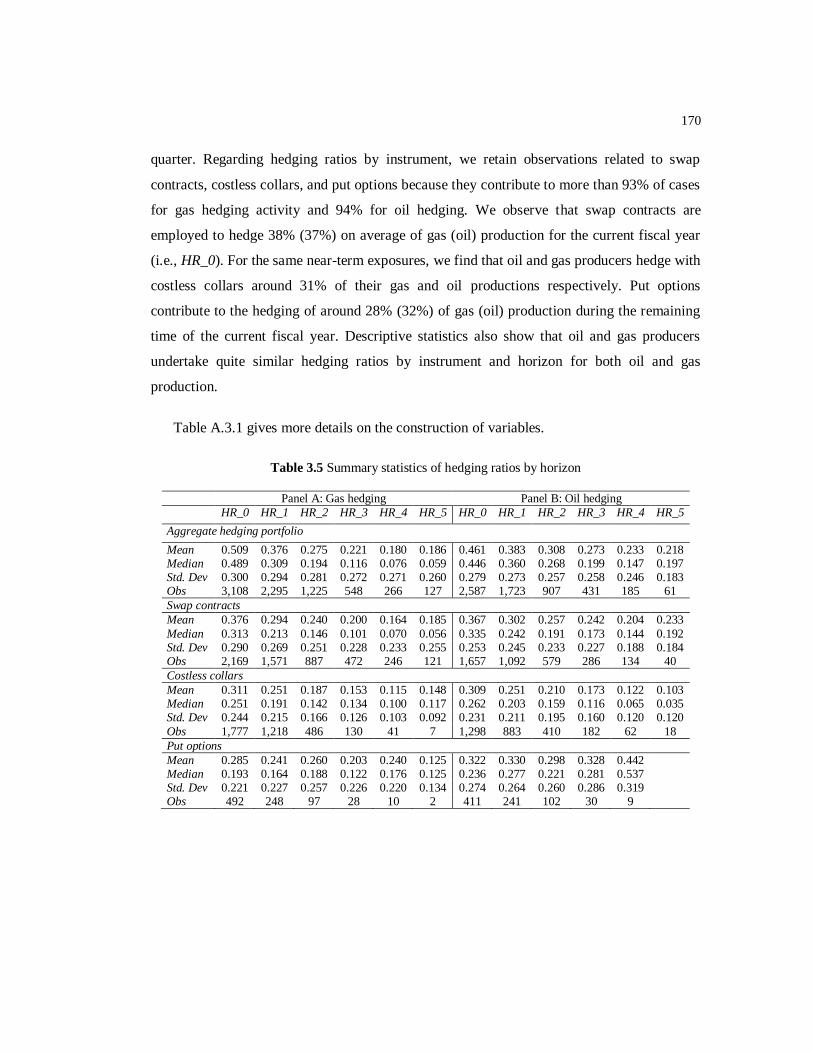
170
quarter. Regarding hedging ratios by instrument, we retain observations related to swap
contracts, costless collars, and put options because they contribute to more than 93% of cases
for gas hedging activity and 94% for oil hedging. We observe that swap contracts are
employed to hedge 38% (37%) on average of gas (oil) production for the current fiscal year
(i.e., HR_0). For the same near-term exposures, we find that oil and gas producers hedge with
costless collars around 31% of their gas and oil productions respectively. Put options
contribute to the hedging of around 28% (32%) of gas (oil) production during the remaining
time of the current fiscal year. Descriptive statistics also show that oil and gas producers
undertake quite similar hedging ratios by instrument and horizon for both oil and gas
production.
Table A.3.1 gives more details on the construction of variables.
Table 3.5 Summary statistics of hedging ratios by horizon
Panel A: Gas hedging Panel B: Oil hedging
HR_0 HR_1 HR_2 HR_3 HR_4 HR_5 HR_0 HR_1 HR_2 HR_3 HR_4 HR_5
Aggregate hedging portfolio
Mean 0.509 0.376 0.275 0.221 0.180 0.186 0.461 0.383 0.308 0.273 0.233 0.218 Median 0.489 0.309 0.194 0.116 0.076 0.059 0.446 0.360 0.268 0.199 0.147 0.197 Std. Dev 0.300 0.294 0.281 0.272 0.271 0.260 0.279 0.273 0.257 0.258 0.246 0.183 Obs 3,108 2,295 1,225 548 266 127 2,587 1,723 907 431 185 61
Swap contracts
Mean 0.376 0.294 0.240 0.200 0.164 0.185 0.367 0.302 0.257 0.242 0.204 0.233
Median 0.313 0.213 0.146 0.101 0.070 0.056 0.335 0.242 0.191 0.173 0.144 0.192 Std. Dev 0.290 0.269 0.251 0.228 0.233 0.255 0.253 0.245 0.233 0.227 0.188 0.184 Obs 2,169 1,571 887 472 246 121 1,657 1,092 579 286 134 40
Costless collars
Mean 0.311 0.251 0.187 0.153 0.115 0.148 0.309 0.251 0.210 0.173 0.122 0.103 Median 0.251 0.191 0.142 0.134 0.100 0.117 0.262 0.203 0.159 0.116 0.065 0.035 Std. Dev 0.244 0.215 0.166 0.126 0.103 0.092 0.231 0.211 0.195 0.160 0.120 0.120
Obs 1,777 1,218 486 130 41 7 1,298 883 410 182 62 18
Put options
Mean 0.285 0.241 0.260 0.203 0.240 0.125 0.322 0.330 0.298 0.328 0.442 Median 0.193 0.164 0.188 0.122 0.176 0.125 0.236 0.277 0.221 0.281 0.537 Std. Dev 0.221 0.227 0.257 0.226 0.220 0.134 0.274 0.264 0.260 0.286 0.319 Obs 492 248 97 28 10 2 411 241 102 30 9

171
3.4 Empirical results
In this section, we first carry out univariate tests to compare firm-quarters with and
without oil and/or gas hedging in terms of firm and loan characteristics. We then perform
more rigorous multivariate tests to examine the effects of hedging on firm performance, risk,
debt capacity, and external financing costs. To account for the potential endogeneity and bi-
directional causality between firm’s derivative use and other decisions, we conduct all our
multivariate tests on a simultaneous equations setting by the three-stage least squares (3-SLS)
technique. We also control for the endogeneity problem by examining firms in the same
industry; they have the same exposure to commodity price risk and they differ vastly in terms
of their hedging behavior. Relative to other empirical studies, we minimize the endogeneity
which is a real concern for any study dealing with financial decision-making channels inside
firms.
To gain further insight, we decompose the aggregate oil and gas hedging positions and
investigate the real implications of each hedging instrument separately, namely swap
contracts, costless collars, and put options. We then perform pairwise simultaneous equation
regressions. In the first equation, each measure of firm performance, risk, debt capacity, and
external financing costs enters as an endogenous variable supplemented by appropriate
control variables that have been shown elsewhere to be associated with the retained measure
(e.g., Campello et al, 2011). In the second equation, we include the hedge ratio of the
aggregate hedging portfolio or by instrument as endogenous variables.49
As control variables for the hedge ratio equation, we include the leverage, the quick ratio,
sales (in logarithm), variables related to tax incentives (tax save measure and tax loss carry
forward), oil and gas spot prices and their volatilities, variables related to production
characteristics (price-quantity correlation, quantity risk, and geographical diversification). All
control variables enter the regressions in lagged values to better alleviate the endogeneity
problem. Finally, all regression have firm and time fixed effects by including dummy
variables for each firm and quarter.
49
We only consider hedging ratios for the remaining period of the current fiscal year (HR_0).

172
3.4.1 Univariate analysis
Table 3.6 presents the results comparing the characteristics of firms and loans for firm-
quarters with and without oil and/or gas hedging in place. A Wilcoxon test for difference in
medians shows considerable differences between firm-quarters with and without hedging.
Consistent with the previous literature, we find that hedgers are much larger than non-
hedgers, more leveraged, and have higher asset tangibility, as well as lower asset volatility
and higher distance-to-default. We also find that hedgers have higher oil and gas selling
prices and higher accounting performance as measured by the ROE, ROA, and EBITDA.
Moreover, hedgers exhibit higher stock return sensitivity to the market index return, and
oil and gas price fluctuations as measured by their respective betas. One possible explanation
is that hedgers are much larger in terms of size and sales, and then have higher exposure to
both market index and commodity price fluctuations. However, this higher sensitivity to
market index fluctuations does not translate into higher stock return volatility because
hedgers have lower stock return volatility and lower idiosyncratic risk. These findings are
quite similar to those in Hentschel and Kothari (2001), who find that hedgers have higher
market beta and lower idiosyncratic risk. More importantly, hedgers have access to larger
loans with longer maturities. Comparison of medians further indicates that hedgers pay
higher spread loan of 25 basis points, which is around 12.5% of the sample mean spread of
200 basis points. However, this difference in median spreads is not significant at
conventional levels.
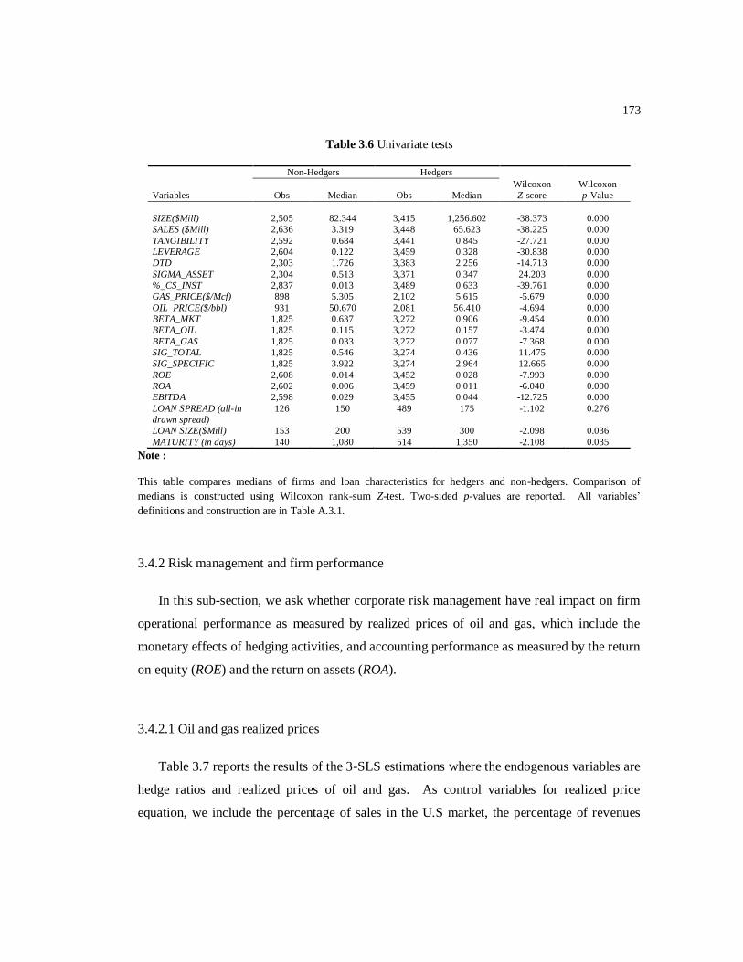
173
Table 3.6 Univariate tests
Non-Hedgers Hedgers
Variables
Obs
Median
Obs
Median
Wilcoxon
Z-score
Wilcoxon
p-Value
SIZE($Mill) 2,505 82.344 3,415 1,256.602 -38.373 0.000
SALES ($Mill) 2,636 3.319 3,448 65.623 -38.225 0.000
TANGIBILITY 2,592 0.684 3,441 0.845 -27.721 0.000
LEVERAGE 2,604 0.122 3,459 0.328 -30.838 0.000
DTD 2,303 1.726 3,383 2.256 -14.713 0.000
SIGMA_ASSET 2,304 0.513 3,371 0.347 24.203 0.000
%_CS_INST 2,837 0.013 3,489 0.633 -39.761 0.000
GAS_PRICE($/Mcf) 898 5.305 2,102 5.615 -5.679 0.000
OIL_PRICE($/bbl) 931 50.670 2,081 56.410 -4.694 0.000
BETA_MKT 1,825 0.637 3,272 0.906 -9.454 0.000
BETA_OIL 1,825 0.115 3,272 0.157 -3.474 0.000
BETA_GAS 1,825 0.033 3,272 0.077 -7.368 0.000
SIG_TOTAL 1,825 0.546 3,274 0.436 11.475 0.000
SIG_SPECIFIC 1,825 3.922 3,274 2.964 12.665 0.000
ROE 2,608 0.014 3,452 0.028 -7.993 0.000
ROA 2,602 0.006 3,459 0.011 -6.040 0.000
EBITDA 2,598 0.029 3,455 0.044 -12.725 0.000
LOAN SPREAD (all-in
drawn spread)
126 150 489 175 -1.102 0.276
LOAN SIZE($Mill) 153 200 539 300 -2.098 0.036
MATURITY (in days) 140 1,080 514 1,350 -2.108 0.035
Note :
This table compares medians of firms and loan characteristics for hedgers and non-hedgers. Comparison of
medians is constructed using Wilcoxon rank-sum Z-test. Two-sided p-values are reported. All variables’
definitions and construction are in Table A.3.1.
3.4.2 Risk management and firm performance
In this sub-section, we ask whether corporate risk management have real impact on firm
operational performance as measured by realized prices of oil and gas, which include the
monetary effects of hedging activities, and accounting performance as measured by the return
on equity (ROE) and the return on assets (ROA).
3.4.2.1 Oil and gas realized prices
Table 3.7 reports the results of the 3-SLS estimations where the endogenous variables are
hedge ratios and realized prices of oil and gas. As control variables for realized price
equation, we include the percentage of sales in the U.S market, the percentage of revenues

174
from oil (gas) production, quantity of oil (gas) daily production, oil (gas) spot prices and
volatilities, and oil (gas) production uncertainty.
Panel A of Table 3.7 shows a significant positive impact of the hedging intensity on gas
realized prices. Not only is this effect is statistically significant, it is moreover economically
important. The estimated coefficient (Table 3.7, Column 1) implies that gas hedgers with an
average hedging intensity earn about 1.6$/Mcf (1000 cubic feet) more than non-hedgers (=
3.1212×0.51, where 0.51 is the mean intensity for the aggregate hedging portfolio for gas
production reported in Table 3.7). Relative to the average gas realized price of 5.653$/Mcf,
this represents an increase of about 28% (=1.6$/5.653$). Regarding hedging intensity by
instrument, Panel A of Table 3.7 shows that costless collars and put options have a
statistically and economically significant positive impacts on gas realized prices. The average
hedging ratio by costless collars contribute to an increase of 1.57$/Mcf (=5.067×0.31, where
0.31 is the mean intensity for costless collars). The average hedging intensity of put options
contribute to an increase of 4.4$/Mcf (=15.685×0.285, where 0.285 is the mean intensity for
put options). Relative to the average realized price for gas, this represents an increase of
about 28% (=1.57$/5.653$) for costless collars and 78% (=4.4$/5.653$) for put options.

175
Table 3.7 Simultaneous equation analysis of hedging extent and realized selling prices
Panel A: Gas hedging Panel B: Oil hedging
Hedging
portfolio
Swap
contracts
Costless
collars
Put
options
Hedging
portfolio
Swap
contracts
Costless
collars
Put
options
(1) (2) (3) (4) (5) (6) (7) (8)
Equation 1: Gas (oil) realized price is the dependent variable
HEDGE RATIO 3.1212*** 1.7610 5.0670*** 15.6856*** -1.5077 -13.6491* 31.7962** 37.6445
(0.636) (1.086) (1.052) (4.532) (6.240) (7.815) (15.433) (27.412)
US_SALES -0.1348 0.0299 -0.2277 0.9045* -0.1479 -0.7447 1.4297 -0.9089
(0.316) (0.319) (0.274) (0.547) (1.117) (0.868) (2.002) (0.968)
GAS(OIL)_REV -0.9514*** -0.8529*** -0.7843** -1.6267*** -4.8646** -3.9697** -7.7759*** -3.0073
(0.299) (0.287) (0.307) (0.483) (1.908) (1.893) (2.420) (2.309)
GAS(OIL)_PROD 0.0000 0.0000 -0.0000 -0.0002 0.0050 0.0004 0.0270* 0.0006
(0.000) (0.000) (0.000) (0.000) (0.007) (0.005) (0.014) (0.005)
VOL_GAS(OIL) 0.4057*** 0.3974*** 0.3517*** 0.4209** 0.8812*** 0.8871*** 0.8212*** 0.9239*** (0.127) (0.121) (0.132) (0.179) (0.104) (0.105) (0.119) (0.117)
SPOT_GAS(OIL) 0.5476*** 0.5673*** 0.5304*** 0.6280*** 0.6306*** 0.6321*** 0.6155*** 0.6255***
(0.021) (0.019) (0.023) (0.033) (0.012) (0.011) (0.014) (0.012)
UNCER_GAS(OIL) 0.0967 0.4415*** -0.0235 -0.1194 2.2169 3.3285** 1.7319 0.5338
(0.170) (0.150) (0.187) (0.268) (1.594) (1.471) (1.393) (1.734)
CONSTANT 1.8708*** 1.4943*** 2.2458*** 0.2226 10.1957*** 10.3343*** 10.6866*** 11.0354***
(0.461) (0.452) (0.438) (0.774) (2.357) (2.208) (2.995) (2.342)
Observations 2,880 2,880 2,880 2,880 2,870 2,870 2,870 2,870
R-squared 0.6562 0.6857 0.6194 0.3234 0.8638 0.8593 0.8303 0.8436
Chi_2 5890.2460 6432.0301 5451.4366 2982.9911 18209.7200 17607.2953 14597.0219 15774.1048
p-value 0.0000 0.0000 0.0000 0.0000 0.0000 0.0000 0.0000 0.0000
Equation 2: Hedge ratio is the dependent variable
GAS(OIL)_PRICE -0.0470 0.0017 0.0088 -0.0530 -0.0232 -0.0137 -0.0244 0.0087
(0.062) (0.048) (0.048) (0.032) (0.020) (0.015) (0.015) (0.010)
TAX_SAVE 0.0064 -0.0526 0.0673 -0.0000 -0.0020 -0.0075 0.0050 0.0050
(0.070) (0.053) (0.045) (0.037) (0.063) (0.035) (0.075) (0.014)
TLCF -0.0366* -0.0005 -0.0246* -0.0037 -0.0423 -0.0567** 0.0382 0.0192 (0.022) (0.017) (0.014) (0.011) (0.037) (0.028) (0.030) (0.017)
VOL_GAS(OIL) 0.0137 -0.0041 0.0044 0.0206 0.0208 0.0126 0.0217 -0.0094
(0.031) (0.024) (0.025) (0.016) (0.017) (0.013) (0.013) (0.008)
SPOT_GAS(OIL) 0.0264 0.0023 -0.0027 0.0231 0.0153 0.0088 0.0156 -0.0054
(0.033) (0.026) (0.026) (0.017) (0.013) (0.009) (0.010) (0.006)
Q_RATIO -0.0017 -0.0007 -0.0011 -0.0009 -0.0010 -0.0011 0.0005 0.0006
(0.001) (0.001) (0.001) (0.001) (0.001) (0.001) (0.001) (0.001)
SALES 0.0665*** 0.0128 0.0359*** 0.0261*** 0.0209 -0.0032 0.0278* 0.0082
(0.017) (0.013) (0.013) (0.009) (0.019) (0.013) (0.016) (0.008)
LEVERAGE 0.1009*** 0.0939*** -0.0004 -0.0329* 0.0401 0.0611** -0.0084 -0.0173
(0.038) (0.029) (0.026) (0.020) (0.037) (0.027) (0.037) (0.015)
PQ_COR_GAS(OIL) -0.0795*** -0.0819*** -0.0048 -0.0331** 0.0108 0.0150 -0.0618** -0.0026
(0.028) (0.021) (0.020) (0.015) (0.029) (0.020) (0.028) (0.015)
UNCER_GAS(OIL) 0.0495** -0.0341* 0.0475** 0.0343*** 0.1742*** 0.1168*** 0.0531 0.0155
(0.025) (0.019) (0.020) (0.013) (0.051) (0.038) (0.039) (0.026) HERF_GAS(OIL) -0.3132*** -0.1308* -0.1899*** -0.0422 -0.2708*** -0.1340*** -0.0504 0.0136
(0.098) (0.075) (0.073) (0.051) (0.078) (0.050) (0.064) (0.021)
CONSTANT -0.3636*** -0.1207** -0.2869*** -0.0379 0.0058 0.1054 0.0531 -0.1266*
(0.062) (0.048) (0.047) (0.032) (0.147) (0.110) (0.110) (0.073)
Observations 2,880 2,880 2,880 2,880 2,870 2,870 2,870 2,870
R-squared 0.6381 0.6251 0.5097 0.0523 0.2018 0.2892 -0.7790 0.1042
Chi_2 5480.4338 4807.6629 2985.9036 1126.6518 1569.8011 1287.8327 826.4356 1106.3186
p-value 0.0000 0.0000 0.0000 0.0000 0.0000 0.0000 0.0000 0.0000

176
Note:
This table presents the results of 3-SLS simultaneous equations estimation linking hedging extent with oil and gas realized prices to account for endogeneity between the two variables. The dependent variable in Equation 1 is gas (oil) realized prices. The dependent variable in Equation 2 is the hedging extent (for the aggregate hedging portfolio and by instrument). The estimation is done for gas hedging (Panel A) and oil hedging (Panel B), separately. All independent variables enter regressions with lagged values. All variables’ definitions and construction are detailed in Table A.3.1. All regressions have firm and time fixed effects (not reported for conciseness). The t-statistics are into parentheses. ***Significant at the 1% level, ** Significant at the 5% level, * Significant at the 10% level.
Surprisingly, Panel B of Table 3.7 indicates that aggregate hedging portfolio of oil
production has no real effects on oil realized prices. However, results further show that
hedging oil production by swap contacts leads to a significant reduction in oil realized prices
of about 5$/barrel (=-13.649×0.367, where 0.367 is the mean intensity for swap contracts) or
equivalently a reduction of about 9.14% of the average realized price of 54.658$/barrel. On
the contrary, costless collars contribute to an important increase of about 9.856$/barrel in oil
realized prices or 18% of the average oil price. Overall, hedging instruments departing from
strict linearity (i.e., put options and costless collars) have the highest positive impacts on
realized prices. These instruments allow firms to profit from any potential upside. Although,
swap contracts permit firms to fix their selling prices, they deprive them from any important
increase in prices.
Results also indicate no bi-directional causality between realized prices and hedging
intensities. In fact, oil and gas producers appear to not consider realized prices when
adjusting their hedging intensities and strategies. Regarding control variables in price
equations, we find that firms deriving most of their revenues from either oil or gas earn lower
realized prices. Realized prices also are significantly positively related to spot prices and their
volatilities, and to production uncertainty.
3.4.2.2 Accounting performance
We carry out 3-SLS regressions where the endogenous variables are hedge ratios and one
of the two measures of firm accounting profit: 1) return on equity (ROE) , and 2) return on
asset (ROA). We obtain qualitatively similar results. We focus on the ROA results reported in
177
Table 3.8 to save space (results related to the ROE are tabulated in Table A.3.2). As control
variables for ROA equation, we include the firm size (in logarithm), the leverage ratio, the
percentage of revenues from oil and gas production, the percentage of sales in the U.S
market, investment expenditures, production cost per barrel of oil equivalent, and
institutional shareholding.
Panel A of Table 3.8 shows a significant positive impact of gas hedging intensity on firm
ROA. Specifically, the ROA for gas hedgers increases by a significant 4.99 basis points
(0.0499%) for each 1% increase in the aggregate hedging portfolio of gas production. Given
the average ratio of 51% for gas hedging portfolio, this translates into a higher ROA of about
255 basis points or 2.55%, which places the firm in the top quartile in term of ROA. Panel A
of Table 3.8, for gas hedging, further indicates that 1% increase in hedging intensity by swap
contracts, collars, and put options leads to an increase in ROA of 8.28, 7.39, and 23.36 basis
points respectively. Results related to oil hedging reported in Panel B also show a significant
increase of 9.67 basis points in ROA for each 1% increase in the hedged fraction of oil
production. The positive impact on ROA from oil hedging comes particularly from costless
collars and put options with 33.37 and 118.02 basis points respectively. More importantly, we
find that most beneficial effects come from put options. This corroborates the results with
realized prices. However the impact of put options is statistically insignificant for oil realized
prices while it is highly significant for ROA. These findings support the hedging premium
hypothesis, that is corporate risk management translates into higher firm value and
performance.

178
Table 3.8 Simultaneous equation analysis of hedging extent and the return on asset
Panel A: Gas hedging Panel B: Oil hedging
Hedging
portfolio
Swap
contracts
Costless
collars
Put
options
Hedging
portfolio
Swap
contracts
Costless
collars
Put
options
(1) (2) (3) (4) (5) (6) (7) (8)
Equation 1: Return on asset is the dependent variable
HEDGE RATIO 0.0499*** 0.0828** 0.0739** 0.2336*** 0.0967*** 0.0307 0.3373*** 1.1802***
(0.014) (0.034) (0.032) (0.086) (0.030) (0.035) (0.092) (0.455)
SIZE 0.0015 0.0025** 0.0026** 0.0025** -0.0002 0.0025* 0.0003 0.0003
(0.001) (0.001) (0.001) (0.001) (0.002) (0.001) (0.002) (0.001)
OIL&GAS_REV -0.0005 0.0001 0.0001 0.0001 -0.0017 -0.0029 -0.0004 0.0001
(0.002) (0.002) (0.003) (0.003) (0.004) (0.003) (0.005) (0.003)
US_SALES 0.0053 0.0102** 0.0059 0.0042 0.0040 0.0030 0.0128 0.0052
(0.004) (0.005) (0.005) (0.006) (0.006) (0.005) (0.008) (0.005)
INV_OPP -0.0009** -0.0004 -0.0012* -0.0013* -0.0012* -0.0015** -0.0011 -0.0000 (0.000) (0.000) (0.001) (0.001) (0.001) (0.001) (0.001) (0.002)
%_CS_INST -0.0128*** -0.0147*** -0.0150*** -0.0126*** -0.0111** -0.0113*** -0.0242*** -0.0076
(0.003) (0.005) (0.004) (0.004) (0.004) (0.004) (0.007) (0.005)
CASH_COST -0.0005*** -0.0004*** -0.0007*** -0.0007*** -0.0013*** -0.0011*** -0.0016*** -0.0007***
(0.000) (0.000) (0.000) (0.000) (0.000) (0.000) (0.000) (0.000)
LEVERAGE -0.0197*** -0.0227*** -0.0138*** -0.0136*** -0.0138*** -0.0090* -0.0063 -0.0169*
(0.005) (0.006) (0.004) (0.004) (0.005) (0.005) (0.006) (0.010)
CONSTANT -0.0040 -0.0169 -0.0095 -0.0157 0.0192 -0.0080 0.0160 0.0006
(0.010) (0.012) (0.012) (0.012) (0.015) (0.013) (0.016) (0.016)
Observations 5,248 5,248 5,248 5,248 5,256 5,256 5,256 5,256
R-squared 0.3014 0.2638 0.3001 0.2065 0.2302 0.3524 -0.3815 -3.4052
Chi_2 2681.3427 2602.7059 2645.0520 2476.6849 2463.7534 2931.4679 1395.3654 745.4809
p-value 0.0000 0.0000 0.0000 0.0000 0.0000 0.0000 0.0000 0.0000
Equation 2: Hedge ratio is the dependent variable
ROA 3.4610*** 2.8830*** -0.5095 0.3242 -1.8996*** -0.6351 -1.9086*** 0.3255
(0.966) (0.798) (0.585) (0.319) (0.563) (0.406) (0.410) (0.225)
TAX_SAVE 0.0169 -0.0380 0.0956** 0.0034 0.0351 0.0281 0.0180 -0.0012 (0.047) (0.037) (0.042) (0.020) (0.060) (0.043) (0.042) (0.009)
TLCF -0.0227** -0.0141 -0.0112 0.0012 -0.0183 -0.0413*** 0.0174** 0.0010
(0.011) (0.009) (0.010) (0.005) (0.012) (0.009) (0.009) (0.002)
VOL_GAS(OIL) 0.0558*** 0.0197 0.0361*** 0.0024 -0.0004 0.0022 -0.0064*** 0.0011
(0.018) (0.015) (0.011) (0.006) (0.003) (0.002) (0.002) (0.001)
SPOT_GAS(OIL) -0.0014 -0.0057* 0.0073*** -0.0031** 0.0020*** 0.0008*** 0.0013*** -0.0001
(0.004) (0.003) (0.002) (0.001) (0.000) (0.000) (0.000) (0.000)
Q_RATIO -0.0012** -0.0008* -0.0001 -0.0002 -0.0009 -0.0009* 0.0002 0.0001
(0.001) (0.000) (0.000) (0.000) (0.001) (0.001) (0.000) (0.000)
SALES 0.0431*** 0.0142*** 0.0291*** 0.0056** 0.0436*** 0.0162*** 0.0257*** 0.0030*
(0.007) (0.005) (0.004) (0.002) (0.005) (0.004) (0.004) (0.002)
LEVERAGE 0.2083*** 0.1678*** 0.0281* 0.0124 0.0552*** 0.0873*** -0.0188 0.0103
(0.026) (0.022) (0.016) (0.009) (0.021) (0.015) (0.015) (0.008)
PQ_COR_GAS(OIL) -0.0172* -0.0144* 0.0028 -0.0094** -0.0030 -0.0037 -0.0018 0.0000
(0.009) (0.007) (0.008) (0.004) (0.009) (0.006) (0.006) (0.002) UNCER_GAS(OIL) 0.0736*** 0.0308** 0.0335*** 0.0145** 0.0525*** 0.0422*** 0.0059 0.0006
(0.015) (0.012) (0.013) (0.006) (0.014) (0.010) (0.010) (0.003)
HERF_GAS(OIL) -0.1624*** -0.0692** -0.1357*** 0.0509*** -0.0707** -0.0976*** 0.0350 0.0055
(0.038) (0.029) (0.031) (0.015) (0.035) (0.025) (0.024) (0.005)
CONSTANT -0.4151*** -0.1337*** -0.2891*** -0.0283 -0.4770*** -0.2185*** -0.2304*** -0.0212
(0.063) (0.052) (0.039) (0.021) (0.049) (0.036) (0.036) (0.019)
Observations 5,248 5,248 5,248 5,248 5,256 5,256 5,256 5,256
R-squared 0.4504 0.3531 0.4394 0.2861 0.4937 0.5068 0.1787 0.3964
Chi_2 6255.2466 4760.0622 4189.0354 2253.7585 5861.9751 5548.0440 2528.5586 3618.6994
p-value 0.0000 0.0000 0.0000 0.0000 0.0000 0.0000 0.0000 0.0000

179
Note:
This table presents the results of 3-SLS simultaneous equations estimation linking hedging extent with firm’s return on asset (ROA) to account for endogeneity between the two variables. The dependent variable in Equation 1 is the ROA measured by net income divided by total assets. The dependent variable in Equation 2 is the hedging extent (for the aggregate hedging portfolio and by instrument). The estimation is done for gas hedging (Panel A) and oil hedging (Panel B), separately. All independent variables enter regressions with lagged values. All variables’ definitions and construction are detailed in Table A.3.1. All regressions have firm and time fixed effects (not reported for conciseness). The t-statistics are into parentheses. ***Significant at the 1% level, ** Significant at the 5% level, * Significant at the 10% level.
Results also indicate feedback effects between firm ROA and hedging intensities. Firms
with higher accounting profitability tend to hedge more their gas production. An increase of
1% in ROA motivates firms to increase their gas aggregate hedging of about 3.46%.
Interestingly, this increase is only significant for swap contracts. This testifies that more
profitable firms are under pressure to maintain their accounting performance. Unpredictably,
ROA appears to have significant negative impacts on oil hedging intensities. In fact, an
increase of 1% in ROA motivates firms to cut their oil hedging of about 1.90%. This
reduction is only significant for costless collars positions. One possible explanation comes
from our previous regressions related to oil and gas prices, where we find that oil hedging has
negative but insignificant effects on oil realized prices. This may motivate manager, who
believes that oil hedging is less appealing, to cut oil hedging to maintain firm performance.
Pertaining to control variables in ROA equations, we find that larger firms have higher
performance. ROA appears to be negatively related to the investment expenditures,
institutional shareholding, production costs, and leverage.
3.4.3 Risk management and firm risk
This sub-section provides detailed evidence on the mutual effects between firms’ hedging
activities and firms risk characteristics. Specifically, we check whether firms use derivatives
primarily to hedge their exposures. We would expect higher hedging intensity to be
associated to lower firm’s risk. Conversely, if firms use derivative primarily to speculate, we
would expect higher hedging intensity to be related to higher firm’s risk. We then examine
real implications of firm’s hedging on the two following measures of firm risk:1) firm
idiosyncratic risk as measured by standardized equity volatility and 2) firm systematic risk as

180
measured by its market beta (Table A.3.1 gives details on the construction of these
measures).
3.4.3.1 Firm idiosyncratic risk
We perform simultaneous equations regressions where the endogenous variables are
firm’s idiosyncratic risk as previously defined and hedge ratios. We make a logarithm
transformation for the idiosyncratic risk because of its right-skewed distribution and to ease
interpretation of results. Table 3.9 reports the results and show statistically significant
estimated coefficients for oil and gas hedging portfolios, with 1% increase in hedging
portfolio intensity inducing a reduction in firm’s idiosyncratic risk of about 0.41% and 0.48%
for gas and oil respectively. However, gas hedging effect has stronger statistical significance.
Results related to hedging ratios by instrument indicate that swap contracts are effective
vehicles to reduce firm’s idiosyncratic risk: 1% increase in swap intensity implies a reduction
in idiosyncratic risk of about 1.43% and 1% for gas hedging and oil hedging respectively.
More importantly, put options appear to provide firms with the highest reduction in
idiosyncratic risk: with 1% increase in intensity leads to a significant reduction of about 4.8%
of oil hedging, however with statistical significance at 10% level. For gas hedging, put
options also have important negative effects on idiosyncratic risk of about -1.26%.
Surprisingly, costless collars appear to be positively associated with firm’s risk with an
estimated positive coefficient of 1.775. Overall, these findings are consistent with one strand
of the literature which testifies that corporations use derivative to hedge and then reduce
firm’s riskiness (e.g., Stulz, 1996, Bartram, Brown, and Conrad, 2011, among others).
Clearly, our results produce evidence that our sample firms do not speculate on commodity
market movements.
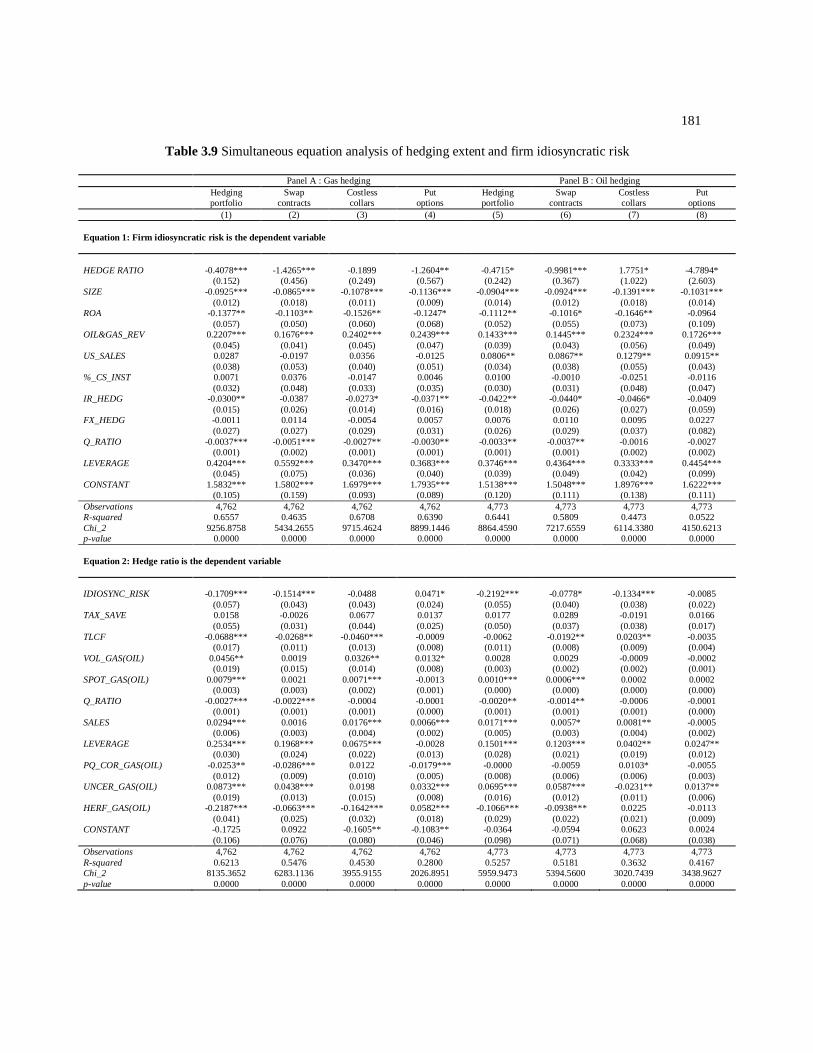
181
Table 3.9 Simultaneous equation analysis of hedging extent and firm idiosyncratic risk
Panel A : Gas hedging Panel B : Oil hedging
Hedging
portfolio
Swap
contracts
Costless
collars
Put
options
Hedging
portfolio
Swap
contracts
Costless
collars
Put
options
(1) (2) (3) (4) (5) (6) (7) (8)
Equation 1: Firm idiosyncratic risk is the dependent variable
HEDGE RATIO -0.4078*** -1.4265*** -0.1899 -1.2604** -0.4715* -0.9981*** 1.7751* -4.7894*
(0.152) (0.456) (0.249) (0.567) (0.242) (0.367) (1.022) (2.603)
SIZE -0.0925*** -0.0865*** -0.1078*** -0.1136*** -0.0904*** -0.0924*** -0.1391*** -0.1031***
(0.012) (0.018) (0.011) (0.009) (0.014) (0.012) (0.018) (0.014)
ROA -0.1377** -0.1103** -0.1526** -0.1247* -0.1112** -0.1016* -0.1646** -0.0964
(0.057) (0.050) (0.060) (0.068) (0.052) (0.055) (0.073) (0.109)
OIL&GAS_REV 0.2207*** 0.1676*** 0.2402*** 0.2439*** 0.1433*** 0.1445*** 0.2324*** 0.1726***
(0.045) (0.041) (0.045) (0.047) (0.039) (0.043) (0.056) (0.049)
US_SALES 0.0287 -0.0197 0.0356 -0.0125 0.0806** 0.0867** 0.1279** 0.0915**
(0.038) (0.053) (0.040) (0.051) (0.034) (0.038) (0.055) (0.043)
%_CS_INST 0.0071 0.0376 -0.0147 0.0046 0.0100 -0.0010 -0.0251 -0.0116
(0.032) (0.048) (0.033) (0.035) (0.030) (0.031) (0.048) (0.047)
IR_HEDG -0.0300** -0.0387 -0.0273* -0.0371** -0.0422** -0.0440* -0.0466* -0.0409
(0.015) (0.026) (0.014) (0.016) (0.018) (0.026) (0.027) (0.059)
FX_HEDG -0.0011 0.0114 -0.0054 0.0057 0.0076 0.0110 0.0095 0.0227
(0.027) (0.027) (0.029) (0.031) (0.026) (0.029) (0.037) (0.082)
Q_RATIO -0.0037*** -0.0051*** -0.0027** -0.0030** -0.0033** -0.0037** -0.0016 -0.0027
(0.001) (0.002) (0.001) (0.001) (0.001) (0.001) (0.002) (0.002)
LEVERAGE 0.4204*** 0.5592*** 0.3470*** 0.3683*** 0.3746*** 0.4364*** 0.3333*** 0.4454***
(0.045) (0.075) (0.036) (0.040) (0.039) (0.049) (0.042) (0.099)
CONSTANT 1.5832*** 1.5802*** 1.6979*** 1.7935*** 1.5138*** 1.5048*** 1.8976*** 1.6222***
(0.105) (0.159) (0.093) (0.089) (0.120) (0.111) (0.138) (0.111)
Observations 4,762 4,762 4,762 4,762 4,773 4,773 4,773 4,773
R-squared 0.6557 0.4635 0.6708 0.6390 0.6441 0.5809 0.4473 0.0522
Chi_2 9256.8758 5434.2655 9715.4624 8899.1446 8864.4590 7217.6559 6114.3380 4150.6213
p-value 0.0000 0.0000 0.0000 0.0000 0.0000 0.0000 0.0000 0.0000
Equation 2: Hedge ratio is the dependent variable
IDIOSYNC_RISK -0.1709*** -0.1514*** -0.0488 0.0471* -0.2192*** -0.0778* -0.1334*** -0.0085
(0.057) (0.043) (0.043) (0.024) (0.055) (0.040) (0.038) (0.022)
TAX_SAVE 0.0158 -0.0026 0.0677 0.0137 0.0177 0.0289 -0.0191 0.0166
(0.055) (0.031) (0.044) (0.025) (0.050) (0.037) (0.038) (0.017)
TLCF -0.0688*** -0.0268** -0.0460*** -0.0009 -0.0062 -0.0192** 0.0203** -0.0035
(0.017) (0.011) (0.013) (0.008) (0.011) (0.008) (0.009) (0.004)
VOL_GAS(OIL) 0.0456** 0.0019 0.0326** 0.0132* 0.0028 0.0029 -0.0009 -0.0002
(0.019) (0.015) (0.014) (0.008) (0.003) (0.002) (0.002) (0.001)
SPOT_GAS(OIL) 0.0079*** 0.0021 0.0071*** -0.0013 0.0010*** 0.0006*** 0.0002 0.0002
(0.003) (0.003) (0.002) (0.001) (0.000) (0.000) (0.000) (0.000)
Q_RATIO -0.0027*** -0.0022*** -0.0004 -0.0001 -0.0020** -0.0014** -0.0006 -0.0001
(0.001) (0.001) (0.001) (0.000) (0.001) (0.001) (0.001) (0.000)
SALES 0.0294*** 0.0016 0.0176*** 0.0066*** 0.0171*** 0.0057* 0.0081** -0.0005
(0.006) (0.003) (0.004) (0.002) (0.005) (0.003) (0.004) (0.002)
LEVERAGE 0.2534*** 0.1968*** 0.0675*** -0.0028 0.1501*** 0.1203*** 0.0402** 0.0247**
(0.030) (0.024) (0.022) (0.013) (0.028) (0.021) (0.019) (0.012)
PQ_COR_GAS(OIL) -0.0253** -0.0286*** 0.0122 -0.0179*** -0.0000 -0.0059 0.0103* -0.0055
(0.012) (0.009) (0.010) (0.005) (0.008) (0.006) (0.006) (0.003)
UNCER_GAS(OIL) 0.0873*** 0.0438*** 0.0198 0.0332*** 0.0695*** 0.0587*** -0.0231** 0.0137**
(0.019) (0.013) (0.015) (0.008) (0.016) (0.012) (0.011) (0.006)
HERF_GAS(OIL) -0.2187*** -0.0663*** -0.1642*** 0.0582*** -0.1066*** -0.0938*** 0.0225 -0.0113
(0.041) (0.025) (0.032) (0.018) (0.029) (0.022) (0.021) (0.009)
CONSTANT -0.1725 0.0922 -0.1605** -0.1083** -0.0364 -0.0594 0.0623 0.0024
(0.106) (0.076) (0.080) (0.046) (0.098) (0.071) (0.068) (0.038)
Observations 4,762 4,762 4,762 4,762 4,773 4,773 4,773 4,773
R-squared 0.6213 0.5476 0.4530 0.2800 0.5257 0.5181 0.3632 0.4167
Chi_2 8135.3652 6283.1136 3955.9155 2026.8951 5959.9473 5394.5600 3020.7439 3438.9627
p-value 0.0000 0.0000 0.0000 0.0000 0.0000 0.0000 0.0000 0.0000

182
Note:
This table presents the results of 3-SLS simultaneous equations estimation linking hedging extent with firm idiosyncratic risk to account for endogeneity between the two variables. The dependent variable in Equation 1 is the firm idiosyncratic risk measured by stock return volatility divided by market return volatility. The dependent variable in Equation 2 is the hedging extent (for the aggregate hedging portfolio and by instrument). The estimation is done for gas hedging (Panel A) and oil hedging (Panel B), separately. All independent variables enter regressions with lagged values. All variables’ definitions and construction are detailed in Table A.3.1. All regressions have firm and time fixed effects (not reported for conciseness). The t-statistics are into parentheses. ***Significant at the 1% level, ** Significant at the 5% level, * Significant at the 10% level.
Surprisingly, results show significant negative effects of idiosyncratic risk on hedging
intensities. These negative effects are about 17 and 22 basis points for gas and oil hedging
portfolios, respectively. For individual instruments, we find that firms with higher levels of
idiosyncratic risks tend to reduce their swap and collar positions particularly: 1% increase in
firm’s idiosyncratic risk commits gas hedgers to reduce their swap positions by about 15
basis points. More importantly, gas hedgers increase their put options positions by about 5
basis points for each 1% increase in firm’s idiosyncratic risk. Similarly, oil hedgers reduce
their swap positions by about 8 basis points and their collar positions by about 13 basis points
for each 1% increase in idiosyncratic risk.
Two plausible explanations, for the intriguing reduction in swap positions and increase in
put option positions as firm’s risk increases, come from the risk-shifting theory (e.g., Jensen
and Meckling, 1976; Myers, 1977). In fact, as the idiosyncratic risk increases, firm’s value
becomes more volatile (and more leveraged) and the option character of stocks (e.g., Merton,
1974) becomes more important. Shareholders, then, have incentives to let firm value under
exposure by reducing swap positions to increase firm’s riskiness and to transfer wealth from
debt holders to equity owners. In addition, as firms’ risk increases, managers tend to enter in
costly non-linear hedging positions (put options) as risk-shifting behavior.
Regarding control variables, IR hedging seems to have a significant negative effect on
firm’s idiosyncratic risk. This finding reiterates the hypothesis that risk management could
reduce firm’s idiosyncratic risk (e.g., Guay, 1999). Finally, firm’s idiosyncratic risk seems to
be significantly negatively related to firm’s size, profitability, and liquidity. On the contrary,
more leveraged firms with lower diversification (industrial and geographical) exhibit higher
idiosyncratic risk. Finally, we repeat the same regressions with the annualized standard

183
deviations of stock returns (with logarithmic transformation because of its distribution is
strongly right-skewed). Results are qualitatively the same.
3.4.3.2 Firm systematic risk
Univariate tests show higher market betas for oil and gas hedgers. At first glance, one
would suspect that derivative use causes firm systematic risk to increase and consequently
firm cost of equity to be higher. As Adam and Fernando (2006) point out, any positive link
between hedging and firm’s systematic risk implies higher cost of equity implying that the
potential positive cash flows related to hedging would not translate into higher value gains
for shareholders. Therefore, we inspect in a more rigorous manner the potential effects
between hedging intensity and firm’s systematic risk. First, we follow previous studies (e.g.,
Jin and Jorion, 2006) and estimate a market model that includes the market index and the
rates of change in NYMEX near-month Future contracts for oil and gas respectively. The
model is estimated in a quarterly frequency using daily returns of firms’ stocks and of market
index. We use the CRSP NYSE/AMEX/Nasdaq composite value-weighted index as a market
measure. We use also daily rates of change in near-month contract prices for oil and gas. To
avoid the non-trading biases related to daily data (Scholes and Williams, 1977), we
supplement the contemporaneous daily return by one lead and lag return for the market index,
oil, and gas returns.50
Beta for each factor (market, oil, and gas) is obtained by summing the
estimated coefficients on the contemporaneous, lead, and lagged return.
Next, we estimate simultaneous equations where the endogenous variables are firm’s
systematic risk (quarterly stock market betas) and hedge ratios to control for possible
simultaneity. Results are reported in Table 3.10. Interestingly, estimated coefficients for both
hedging portfolios of oil and gas productions have negative signs but with no statistical
significance at conventional levels. We find no evidence that oil and gas hedging increases
systematic risk for our sample firms. Therefore, the positive effects, in terms of realized
prices and ROA found in the previous section, should translate into value gains for
50
See Dimson (1979) and Fowler and Rorke (1984) for more details.

184
shareholders. More importantly, Panel A of Table 3.10 indicates that hedging gas production
by costless collars has a significant (at the level of 10%) negative impact on firm’s systematic
risk. This finding suggests that hedging gas production by collars would attenuate cost of
equity for oil and gas producers. Results further show no evident effects for swap contracts or
put options.
Regarding the feedback effects, results reveal that 1% increase in systematic risk commits
firms to increase their collar positions by about 6 basis points for oil hedging and gas hedging
respectively. This increase in collar intensity should be interpreted in light of the previously
documented negative effect of collars on systematic risk. Similarly, 1% increase in
systematic risk leads to a reduction of 4 basis points in put option positions for oil hedging.
One possible explanation is that by cutting option positions, managers are trying to attenuate
the volatility effects of such non-linear hedging instruments.
For control variables in the systematic risk equation, we find that IR hedging reduces
systematic risk which confirms that financial hedging has risk reduction virtues as claimed by
one strand of the related literature (see Panel A, Column 1 and 2). We also find that more
profitable oil and gas producers bear noticeably lower systematic risk. On the contrary,
systematic risk appears to be significantly positively related to firm size, leverage and more
noticeably to the percentage of institutional shareholding. These latter findings give evidence
that the higher systematic risk observed for oil and gas hedgers comes essentially form their
larger size, higher leverage ratio, and more importantly their higher percentage of
institutional shareholding (see univariate tests).
Similarly, we assess whether derivative use is positively related to firm’s exposure to oil
and gas price fluctuations. Univariate results show that hedgers have significantly higher
exposure to oil and gas price fluctuations as measured by their respective betas from the
market model estimated previously. That is, if firms in our sample use derivative to speculate,
and then to increase their commodity exposures, we should expect a significant positive
effects of hedging on oil and gas betas.

185
Table 3.10 Simultaneous equation analysis of hedging extent and firm systematic risk
Panel A : Gas hedging Panel B : Oil hedging
Hedging
portfolio
Swap
contracts
Costless
collars
Put
options
Hedging
portfolio
Swap
contracts
Costless
collars
Put
options
(1) (2) (3) (4) (5) (6) (7) (8)
Equation 1: Firm systematic risk is the dependent variable
HEDGE RATIO -0.3490 -0.7219 -1.1071* -0.9299 -0.1881 -0.7111 1.1821 3.5165
(0.350) (0.828) (0.620) (1.325) (0.589) (0.795) (1.999) (4.793)
SIZE 0.0898*** 0.0701** 0.1141*** 0.1028*** 0.0765** 0.0809*** 0.0658** 0.0742***
(0.028) (0.033) (0.026) (0.021) (0.033) (0.025) (0.032) (0.024)
ROA -0.5143*** -0.4836*** -0.5489*** -0.5734*** -0.3939*** -0.3443** -0.2851** -0.4452**
(0.136) (0.133) (0.145) (0.146) (0.138) (0.136) (0.136) (0.219)
OIL&GAS_REV 0.1318 0.0887 0.1053 0.0944 0.0440 0.0052 0.0268 0.0718
(0.104) (0.096) (0.108) (0.100) (0.102) (0.103) (0.101) (0.111)
US_SALES 0.0083 -0.1019 0.0085 0.1116 -0.1031 -0.1138 -0.1461 -0.1042
(0.088) (0.114) (0.095) (0.111) (0.089) (0.091) (0.100) (0.096)
%_CS_INST 0.3181*** 0.3738*** 0.3135*** 0.2225*** 0.2911*** 0.2782*** 0.2927*** 0.2957***
(0.076) (0.100) (0.080) (0.075) (0.079) (0.076) (0.097) (0.092)
IR_HEDG -0.0689* -0.1063** -0.0256 -0.0110 -0.0680 -0.0948 -0.0038 -0.0223
(0.035) (0.053) (0.035) (0.035) (0.047) (0.059) (0.046) (0.107)
FX_HEDG 0.0103 0.0456 0.0116 -0.0069 0.0033 0.0209 -0.0312 -0.0386
(0.064) (0.067) (0.071) (0.065) (0.069) (0.070) (0.065) (0.158)
Q_RATIO 0.0031 0.0027 0.0034 0.0038 0.0030 0.0025 0.0040 0.0035
(0.003) (0.003) (0.003) (0.003) (0.003) (0.003) (0.003) (0.003)
LEVERAGE 0.1484 0.2095 0.1145 0.0613 0.1733* 0.2434** 0.1482* 0.0677
(0.104) (0.131) (0.089) (0.089) (0.089) (0.102) (0.084) (0.159)
CONSTANT 0.5563** 0.7600** 0.3915* 0.4707** 0.7158** 0.6664*** 0.9274*** 0.7890***
(0.243) (0.298) (0.226) (0.199) (0.296) (0.246) (0.260) (0.200)
Observations 4,673 4,673 4,673 4,673 4,684 4,684 4,684 4,684
R-squared 0.3712 0.3557 0.3438 0.3700 0.3739 0.3605 0.3413 0.2503
Chi_2 2750.1957 2565.1182 2682.2338 2820.6103 2781.0386 2687.9323 2523.1622 2441.6563
p-value 0.0000 0.0000 0.0000 0.0000 0.0000 0.0000 0.0000 0.0000
Equation 2: Hedge ratio is the dependent variable
BETA_MKT -0.0609 -0.0486 0.0649** -0.0387** -0.0268 -0.0255 0.0540* -0.0115
(0.040) (0.033) (0.031) (0.017) (0.044) (0.034) (0.031) (0.019)
TAX_SAVE 0.0144 -0.0245 0.0776 0.0092 0.0052 0.0151 -0.0003 0.0015
(0.058) (0.045) (0.047) (0.025) (0.058) (0.043) (0.035) (0.025)
TLCF -0.0883*** -0.0492*** -0.0536*** 0.0027 -0.0124 -0.0241** 0.0142 0.0052
(0.018) (0.014) (0.015) (0.008) (0.013) (0.010) (0.009) (0.006)
VOL_GAS(OIL) 0.0546** 0.0133 0.0654*** -0.0102 0.0087*** 0.0053*** 0.0013 0.0000
(0.022) (0.018) (0.017) (0.009) (0.002) (0.002) (0.002) (0.001)
SPOT_GAS(OIL) 0.0063 0.0011 0.0121*** -0.0047*** 0.0010** 0.0004 0.0009** 0.0000
(0.004) (0.003) (0.003) (0.002) (0.000) (0.000) (0.000) (0.000)
Q_RATIO -0.0017** -0.0014** -0.0006 -0.0001 -0.0010 -0.0010 -0.0004 0.0001
(0.001) (0.001) (0.001) (0.000) (0.001) (0.001) (0.001) (0.000)
SALES 0.0431*** 0.0121*** 0.0163*** 0.0063*** 0.0317*** 0.0107*** 0.0114*** 0.0032
(0.006) (0.004) (0.004) (0.002) (0.005) (0.004) (0.004) (0.002)
LEVERAGE 0.2005*** 0.1465*** 0.0442** 0.0181* 0.0792*** 0.0994*** -0.0146 0.0199**
(0.024) (0.020) (0.018) (0.010) (0.023) (0.018) (0.016) (0.010)
PQ_COR_GAS(OIL) -0.0127 -0.0182* 0.0147 -0.0101** 0.0069 0.0019 0.0000 -0.0039
(0.012) (0.009) (0.010) (0.005) (0.009) (0.007) (0.005) (0.004)
UNCER_GAS(OIL) 0.0990*** 0.0649*** 0.0233 0.0260*** 0.0757*** 0.0565*** 0.0052 0.0045
(0.018) (0.014) (0.014) (0.008) (0.015) (0.011) (0.009) (0.006)
HERF_GAS(OIL) -0.2429*** -0.1110*** -0.1723*** 0.0477*** -0.1189*** -0.1095*** 0.0091 0.0104
(0.043) (0.033) (0.034) (0.018) (0.033) (0.025) (0.020) (0.014)
CONSTANT -0.3931*** -0.1051** -0.2974*** 0.0092 -0.3752*** -0.1593*** -0.2008*** -0.0125
(0.059) (0.049) (0.045) (0.025) (0.057) (0.044) (0.040) (0.025)
Observations 4,673 4,673 4,673 4,673 4,684 4,684 4,684 4,684
R-squared 0.6206 0.5620 0.4010 0.2456 0.5686 0.5296 0.3477 0.4252
Chi_2 7734.6309 6059.0298 3530.4441 1929.6447 6178.7115 5290.8280 2890.6784 3490.3474
p-value 0.0000 0.0000 0.0000 0.0000 0.0000 0.0000 0.0000 0.0000

186
Note:
This table presents the results of 3-SLS simultaneous equations estimation linking hedging extent with firm systematic risk to account for endogeneity between the two variables. The dependent variable in Equation 1 is the
firm systematic risk measured by stock market beta. The dependent variable in Equation 2 is the hedging extent (for the aggregate hedging portfolio and by instrument). The estimation is done for gas hedging (Panel A) and oil hedging (Panel B), separately. All independent variables enter regressions with lagged values. All variables’ definitions and construction are detailed in Table A.3.1. All regressions have firm and time fixed effects (not reported for conciseness). The t-statistics are into parentheses. ***Significant at the 1% level, ** Significant at the 5% level, * Significant at the 10% level.
In unreported results, we repeat the same simultaneous equations estimation with oil and
gas betas as endogenous variables with hedge ratios. Results reveal insignificant feedback
effects between oil and gas betas and hedging intensity. Although, these findings are
inconsistent with the hypothesis that hedging should reduce firm’s exposure to the underlying
risk (e.g., Tufano, 1998, Allayannis and Ofek, 2001, Jin and Jorion, 2006), they do not
provide evidence of a speculative behavior of our sample firms.
3.4.4 Risk management and external financing
In this sub-section, we examine the potential feedback effects between corporate risk
management and 1) capital structure decisions, and 2) external financing costs.
3.4.4.1 Firm debt capacity
In line with the existing literature (e.g., Froot, Stein, and Sharfstein, 1993, Stulz. 1996,
Leland, 1998, Graham and Rogers, 2002, Dionne and Triki, 2013, Bartram, Brown, and
Fehle, 2009), we investigate jointly commodity hedging and debt level of firms. We, then,
estimate simultaneous regressions where the endogenous variables are hedge ratio and
leverage ratio as measured by the book value of long term debt plus debt in current liabilities
scaled by book value of assets. We supplement the leverage equations by the following
control variables: firm size (in logarithm), asset volatility, asset tangibility measuring the
firm’s collateral value, firm profitability measured by the EBITDA, and dummy variables for
IR hedging and FX hedging.

187
Interestingly, Table 3.11 shows statistically and economically significant effects of oil
and gas hedging on firms’ leverage ratios. The estimated coefficients indicate that a 1%
increase in the aggregate hedging ratio of gas (oil) production translates into a 13 (25.51)
basis points in leverage ratio. These figures are larger than the 3 basis points reported in
Bartram, Brown, and Fehle (2009) for commodity hedging, and are relatively smaller than 32
basis points documented in Graham and Rogers (2002) for IR and FX hedging. For gas
hedging, a 1% increase in swap contract and put option intensity leads to an increase of about
28 and 97 basis points in leverage ratio.
For oil hedging, a 1% increase in swap contract, costless collar, and put option intensity
allows firms to attain higher leverage ratios of about 29, 62, and 218 basis points. More
importantly, put options appear to allow firms to access higher levels of external financing.
One explanation of this finding could be that put option users are often wealthy firms having
better access to debts. Relative to the average hedging ratio, a firm can attain higher leverage
levels of about 6.63% (=13 basis points × 51%) and about 12% (=25.51 basis points × 47%)
for gas hedging and oil hedging respectively. This explains the important gap between
median leverage of hedgers and non-hedgers (33% versus 12%).
These documented findings corroborate earlier empirical results and theoretical
conjectures by Smith and Stulz (1985), Froot, Stein, and Sharfstein (1993), Stulz (1996),
Ross (1996), Leland (1998), and Graham and Rogers (2002), namely financial hedging
improves firm’s debt capacity by reducing the probability of left-tail (lower-tail) outcomes
and expected costs of bankruptcy. In doing so, corporate risk management increases firm
value throughout the following three channels: 1) tax advantages of interest deduction (Ross,
1996, Leland, 1998, Graham and Rogers, 2002), 2) project financing (Froot, Stein,
Sharfstein, 1993, Stulz, 1996, Graham and Rogers, 2002), and 3) firm monitoring provided
by debt financing which commits manager to improve efficiency (Stulz, 1996).
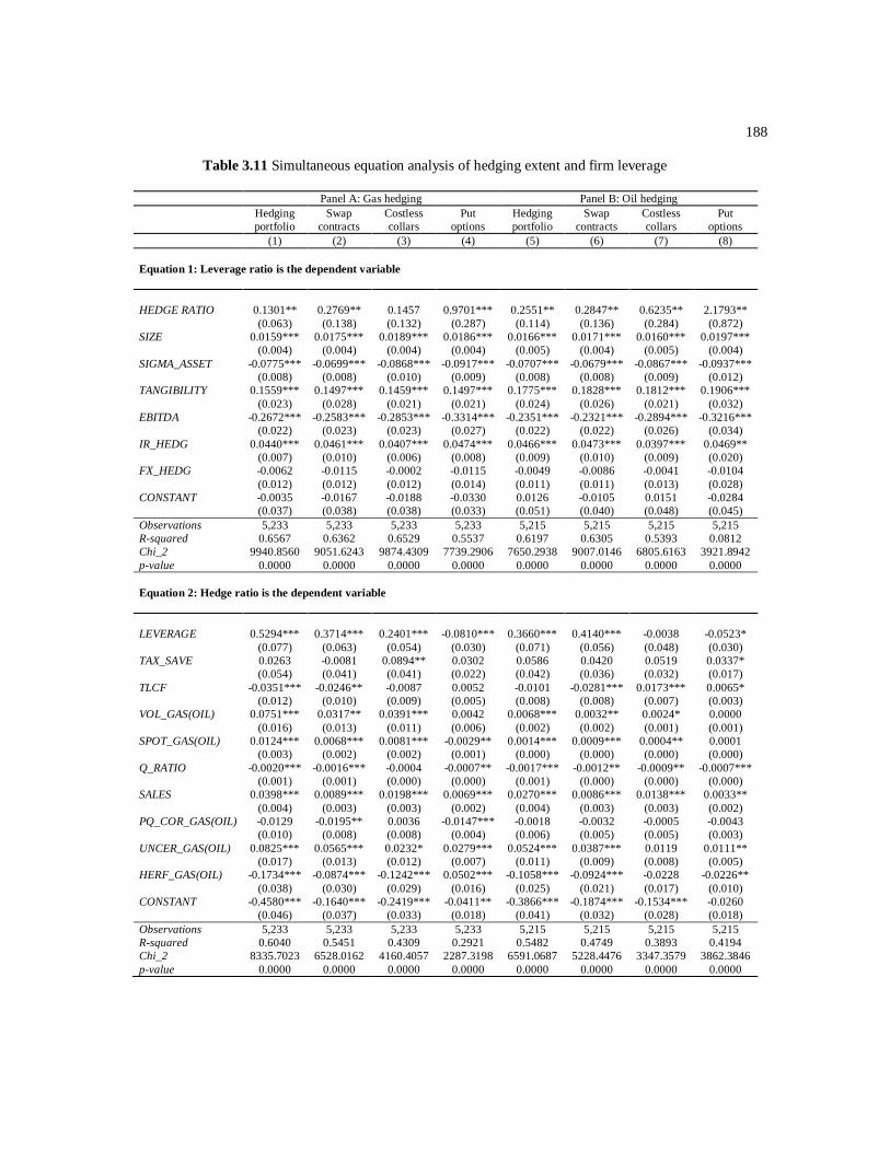
188
Table 3.11 Simultaneous equation analysis of hedging extent and firm leverage
Panel A: Gas hedging Panel B: Oil hedging
Hedging
portfolio
Swap
contracts
Costless
collars
Put
options
Hedging
portfolio
Swap
contracts
Costless
collars
Put
options
(1) (2) (3) (4) (5) (6) (7) (8)
Equation 1: Leverage ratio is the dependent variable
HEDGE RATIO 0.1301** 0.2769** 0.1457 0.9701*** 0.2551** 0.2847** 0.6235** 2.1793**
(0.063) (0.138) (0.132) (0.287) (0.114) (0.136) (0.284) (0.872)
SIZE 0.0159*** 0.0175*** 0.0189*** 0.0186*** 0.0166*** 0.0171*** 0.0160*** 0.0197***
(0.004) (0.004) (0.004) (0.004) (0.005) (0.004) (0.005) (0.004)
SIGMA_ASSET -0.0775*** -0.0699*** -0.0868*** -0.0917*** -0.0707*** -0.0679*** -0.0867*** -0.0937***
(0.008) (0.008) (0.010) (0.009) (0.008) (0.008) (0.009) (0.012)
TANGIBILITY 0.1559*** 0.1497*** 0.1459*** 0.1497*** 0.1775*** 0.1828*** 0.1812*** 0.1906***
(0.023) (0.028) (0.021) (0.021) (0.024) (0.026) (0.021) (0.032)
EBITDA -0.2672*** -0.2583*** -0.2853*** -0.3314*** -0.2351*** -0.2321*** -0.2894*** -0.3216***
(0.022) (0.023) (0.023) (0.027) (0.022) (0.022) (0.026) (0.034)
IR_HEDG 0.0440*** 0.0461*** 0.0407*** 0.0474*** 0.0466*** 0.0473*** 0.0397*** 0.0469**
(0.007) (0.010) (0.006) (0.008) (0.009) (0.010) (0.009) (0.020)
FX_HEDG -0.0062 -0.0115 -0.0002 -0.0115 -0.0049 -0.0086 -0.0041 -0.0104
(0.012) (0.012) (0.012) (0.014) (0.011) (0.011) (0.013) (0.028)
CONSTANT -0.0035 -0.0167 -0.0188 -0.0330 0.0126 -0.0105 0.0151 -0.0284
(0.037) (0.038) (0.038) (0.033) (0.051) (0.040) (0.048) (0.045)
Observations 5,233 5,233 5,233 5,233 5,215 5,215 5,215 5,215
R-squared 0.6567 0.6362 0.6529 0.5537 0.6197 0.6305 0.5393 0.0812
Chi_2 9940.8560 9051.6243 9874.4309 7739.2906 7650.2938 9007.0146 6805.6163 3921.8942
p-value 0.0000 0.0000 0.0000 0.0000 0.0000 0.0000 0.0000 0.0000
Equation 2: Hedge ratio is the dependent variable
LEVERAGE 0.5294*** 0.3714*** 0.2401*** -0.0810*** 0.3660*** 0.4140*** -0.0038 -0.0523*
(0.077) (0.063) (0.054) (0.030) (0.071) (0.056) (0.048) (0.030)
TAX_SAVE 0.0263 -0.0081 0.0894** 0.0302 0.0586 0.0420 0.0519 0.0337*
(0.054) (0.041) (0.041) (0.022) (0.042) (0.036) (0.032) (0.017)
TLCF -0.0351*** -0.0246** -0.0087 0.0052 -0.0101 -0.0281*** 0.0173*** 0.0065*
(0.012) (0.010) (0.009) (0.005) (0.008) (0.008) (0.007) (0.003)
VOL_GAS(OIL) 0.0751*** 0.0317** 0.0391*** 0.0042 0.0068*** 0.0032** 0.0024* 0.0000
(0.016) (0.013) (0.011) (0.006) (0.002) (0.002) (0.001) (0.001)
SPOT_GAS(OIL) 0.0124*** 0.0068*** 0.0081*** -0.0029** 0.0014*** 0.0009*** 0.0004** 0.0001
(0.003) (0.002) (0.002) (0.001) (0.000) (0.000) (0.000) (0.000)
Q_RATIO -0.0020*** -0.0016*** -0.0004 -0.0007** -0.0017*** -0.0012** -0.0009** -0.0007***
(0.001) (0.001) (0.000) (0.000) (0.001) (0.000) (0.000) (0.000)
SALES 0.0398*** 0.0089*** 0.0198*** 0.0069*** 0.0270*** 0.0086*** 0.0138*** 0.0033**
(0.004) (0.003) (0.003) (0.002) (0.004) (0.003) (0.003) (0.002)
PQ_COR_GAS(OIL) -0.0129 -0.0195** 0.0036 -0.0147*** -0.0018 -0.0032 -0.0005 -0.0043
(0.010) (0.008) (0.008) (0.004) (0.006) (0.005) (0.005) (0.003)
UNCER_GAS(OIL) 0.0825*** 0.0565*** 0.0232* 0.0279*** 0.0524*** 0.0387*** 0.0119 0.0111**
(0.017) (0.013) (0.012) (0.007) (0.011) (0.009) (0.008) (0.005)
HERF_GAS(OIL) -0.1734*** -0.0874*** -0.1242*** 0.0502*** -0.1058*** -0.0924*** -0.0228 -0.0226**
(0.038) (0.030) (0.029) (0.016) (0.025) (0.021) (0.017) (0.010)
CONSTANT -0.4580*** -0.1640*** -0.2419*** -0.0411** -0.3866*** -0.1874*** -0.1534*** -0.0260
(0.046) (0.037) (0.033) (0.018) (0.041) (0.032) (0.028) (0.018)
Observations 5,233 5,233 5,233 5,233 5,215 5,215 5,215 5,215
R-squared 0.6040 0.5451 0.4309 0.2921 0.5482 0.4749 0.3893 0.4194
Chi_2 8335.7023 6528.0162 4160.4057 2287.3198 6591.0687 5228.4476 3347.3579 3862.3846
p-value 0.0000 0.0000 0.0000 0.0000 0.0000 0.0000 0.0000 0.0000

189
Note:
This table presents the results of 3-SLS simultaneous equations estimation linking hedging extent with firm leverage to account for endogeneity between the two variables. The dependent variable in Equation 1 is the firm leverage ratio measured by the book value of long-term debt + debt in current liabilities divided by total assets. The dependent variable in Equation 2 is the hedging extent (for the aggregate hedging portfolio and by instrument). The estimation is done for gas hedging (Panel A) and oil hedging (Panel B), separately. All independent variables enter regressions with lagged values. All variables’ definitions and construction are detailed in Table A.3.1. All regressions have firm and time fixed effects (not reported for conciseness). The t-statistics are into parentheses. ***Significant at the 1% level, ** Significant at the 5% level, * Significant at the 10% level.
Results also show statistically and economically significant positive impacts of leverage
ratio on hedging intensity as suggested by the previous literature and particularly Haushalter
(2000) for oil and gas industry. As leverage increases, firms tend to intensify their hedging by
swap contracts and collars, and to reduce put option intensity. In light of the median leverage
of 33% for hedgers, these latter findings are consistent with Adam (2002) prediction, namely
when credit premium is moderately large, firms tend to use linear approximation of their
hedging strategies. Control variables in leverage equations have predicted signs. Leverage is
positively related to firm size and collateral value (asset tangibility), and negatively related to
asset volatility and firm profitability. More importantly, we find that IR hedging has a
significant positive effect on leverage ratio as predicted (Graham and Rogers, 2002). This
latter finding reiterates the conjecture that financial hedging improves firm’s debt capacity.
3.4.4.2 Cost of external financing
In the previous sub-section, we find that hedging eases the access to external funds. We
now turn our attention to the cost of external financing. We do this by explicitly connecting
hedging and loan spread. It is expected that hedging by reducing the probability of left-tail
realizations and preventing agency costs related to risk-shifting, should improve loans
contracting terms. We then estimate simultaneous regressions where the endogenous
variables are hedge ratios and loan spreads. We largely follow the empirical specification
adopted by Campello et al (2011) and take the logarithm of loan spread to alleviate the
effects of extreme values in the spread sample. We also control for loan characteristics
(logarithm of loan size (in Mill $), logarithm of loan maturity (in days), types, and purposes),
macroeconomic variables (credit and term spreads), and firm specific characteristics (firm
190
size (in logarithm), firm profitability, leverage, asset tangibility, asset volatility, dummy
variables for IR hedging and FX hedging).
Results reported in Panel A of Table 3.12 show insignificant effects of gas hedging on
loan spreads. Contrary to our prediction, results in Panel B indicate that loan spread is
positively related to swap contract intensity for oil hedging. In fact, average (oil) hedgers
with swap contracts are charged loan spreads that are 35.23% higher than those charged to
non-hedgers (= 0.96 × 0.367, where 0.367 is the mean intensity for swap contracts for oil
hedging). This finding contradicts the estimated reduction of 28% in loan spread reported by
Campello et al (2011) for average IR/FX hedgers. It also contradicts spread reduction of
17.5% documented in Kumar and Rabinovitch (2013) for average oil and gas hedgers.
As predicted, average oil hedgers with costless collars are charged loan spreads that are
42.87% lower than those charged to non-hedgers. Relative to the average loan spread of
about 201 basis points, swap contracts lead to an increase of about 71 basis points in loan
spread and collars reduce this spread by about 86 basis points. Collar effects corroborate
Campello et al (2011) and Kumar and Rabinovitch (2013) findings, with a higher figure. Due
to these conflicting effects of swap and collars, the aggregate hedging portfolio of oil
production has a negative but insignificant effect on loan spread.
Results further indicate a significant positive effect of loan spread on oil and gas hedging
ratios: a 1% increase in loan spread implies an increase of about 10 and 17 basis points in the
aggregate hedging portfolio of gas and oil production, respectively. Concerning hedging
intensity by instrument, we find that loan spread have a particular positive impact on the
extent of swap contracts for both panels of gas hedgers and oil hedgers, and a negative effect
on put options for gas hedgers. Interestingly, these findings are consistent with our previous
results related to leverage effects on hedging instruments that is leverage impacts in a
positive manner swap contracts and in a negative manner put options. Regarding control
variables in the loan spread equation, we find that firms with farther loan maturities are
charged higher spread because banks require liquidity premium for long-term debts. The loan
size has a negative impact on spreads which might reflect economies of scale in bank lending
(Campello et al., 2011).

191
Table 3.12 Simultaneous equation analysis of hedging extent and loan spread
Panel A: Gas hedging Panel B: Oil hedging
Hedging
portfolio
Swap
contracts
Costless
collars
Put
options
Hedging
portfolio
Swap
contracts
Costless
collars
Put
options
(1) (2) (3) (4) (5) (6) (7) (8)
Equation 1: Loan spread (in log) is the dependent variable
HEDGE RATIO 0.0024 0.3610 -0.4071 -0.9874 -1.1985 0.9601* -1.3829** -2.6801
(0.455) (0.383) (0.637) (1.186) (1.102) (0.520) (0.592) (2.592)
MATURITY 0.0722* 0.0717* 0.0773** 0.0729** 0.1033* 0.0697** 0.0835** 0.0889
(0.037) (0.038) (0.037) (0.035) (0.054) (0.035) (0.042) (0.056)
LOAN SIZE -0.1193*** -0.1165*** -0.1227*** -0.1199*** -0.1463*** -0.1132*** -0.1264*** -0.1267***
(0.020) (0.019) (0.020) (0.022) (0.026) (0.019) (0.022) (0.045)
CREDIT_SPREAD -0.0705 -0.0827 -0.0611 -0.0546 -0.0665 -0.0641 -0.0595 -0.0426
(0.120) (0.126) (0.173) (0.136) (0.158) (0.113) (0.150) (0.212)
TERM_SPREAD 0.0924 0.0917 0.0748 0.0744 0.0801 0.0912 0.0780 0.0660
(0.145) (0.146) (0.179) (0.158) (0.208) (0.138) (0.157) (0.312)
SIZE -0.0516 -0.0528 -0.0489 -0.0471 -0.0193 -0.0573 -0.0501 -0.0278
(0.054) (0.042) (0.038) (0.043) (0.074) (0.037) (0.041) (0.101)
EBITDA 0.0606 0.0560 0.0869 0.1072 0.3584 0.0955 0.1710 0.2582
(0.317) (0.307) (0.332) (0.314) (0.506) (0.304) (0.348) (0.395)
TANGIBILITY 0.1611 0.1401 0.1171 0.0363 0.1260 0.1149 0.2032 0.0344
(0.314) (0.254) (0.224) (0.277) (0.484) (0.210) (0.240) (0.528)
LEVERAGE 0.9767*** 0.9433*** 1.0255*** 1.0404*** 1.3803*** 0.7802*** 1.0516*** 1.3125***
(0.181) (0.142) (0.161) (0.145) (0.420) (0.172) (0.168) (0.450)
SIGMA_ASSET 0.2650* 0.2782** 0.2555* 0.2341* 0.2739 0.2236* 0.2646* 0.2283
(0.137) (0.141) (0.136) (0.137) (0.193) (0.127) (0.145) (0.272)
IR_HEDG -0.0156 -0.0137 -0.0113 -0.0113 -0.0030 -0.0110 -0.0105 0.0005
(0.041) (0.040) (0.043) (0.039) (0.054) (0.039) (0.043) (0.111)
FX_HEDG -0.2069** -0.1912** -0.1969** -0.1792** -0.2329** -0.1782** -0.1940** -0.2091*
(0.091) (0.086) (0.086) (0.082) (0.107) (0.082) (0.089) (0.122)
CONSTANT 5.2432*** 5.1720*** 5.1791*** 5.1801*** 4.8489*** 5.1269*** 5.0058*** 4.7316***
(0.687) (0.509) (0.544) (0.675) (1.097) (0.510) (0.571) (1.623)
Observations 541 541 541 541 534 534 534 534
R-squared 0.8494 0.8441 0.8399 0.8406 0.7055 0.8107 0.7681 0.6975
Chi_2 3047.9566 3011.8708 2872.3926 2905.3416 1181.2056 2519.4797 2033.2960 1339.3020
p-value 0.0000 0.0000 0.0000 0.0000 0.0000 0.0000 0.0000 0.0000
Equation 2: Hedge ratio is the dependent variable
LOAN SPREAD 0.1044** 0.0718* 0.0409 -0.0311* 0.1712*** 0.0671* 0.0408 0.0154
(0.044) (0.037) (0.032) (0.018) (0.052) (0.037) (0.032) (0.026)
LEVERAGE 0.1986** 0.0555 0.0948 0.0860** 0.1169 0.1295* -0.0091 0.1058**
(0.090) (0.076) (0.066) (0.036) (0.107) (0.076) (0.066) (0.053)
TAX_SAVE 0.3760 -0.1202 0.8059** -0.0992 0.5504 -0.1226 0.7335*** 0.0629
(0.426) (0.354) (0.314) (0.163) (0.401) (0.301) (0.277) (0.187)
TLCF -0.3438*** -0.3322*** 0.0134 -0.0405 -0.0330 -0.0615 0.0871 -0.0289
(0.111) (0.093) (0.081) (0.042) (0.103) (0.079) (0.069) (0.051)
VOL_GAS(OIL) 0.0635 0.0391 -0.0291 0.0328 0.0177 0.0116 -0.0009 -0.0039
(0.052) (0.044) (0.038) (0.021) (0.015) (0.011) (0.009) (0.008)
SPOT_GAS(OIL) 0.0215** 0.0021 0.0210*** -0.0014 0.0019 0.0022*** 0.0006 0.0003
(0.010) (0.008) (0.007) (0.004) (0.001) (0.001) (0.001) (0.001)
Q_RATIO -0.0032 -0.0030 0.0004 -0.0004 0.0049 -0.0041 0.0023 0.0033
(0.004) (0.004) (0.003) (0.002) (0.005) (0.003) (0.003) (0.002)
SALES 0.0303 -0.0137 0.0307** 0.0047 0.0666*** -0.0070 0.0270** 0.0215**
(0.019) (0.016) (0.014) (0.008) (0.019) (0.014) (0.012) (0.009)
PQ_COR_GAS(OIL) 0.0465 0.0221 0.0390 -0.0043 -0.0699** -0.0416 -0.0092 -0.0195
(0.048) (0.040) (0.035) (0.018) (0.035) (0.025) (0.021) (0.015)
UNCER_GAS(OIL) -0.0251 -0.1263** 0.0129 0.0617** 0.1594*** -0.0690* 0.0987*** 0.0458*
(0.073) (0.061) (0.053) (0.028) (0.058) (0.041) (0.036) (0.024)
HERF_GAS(OIL) -0.1714 -0.0225 -0.2496** 0.1397** 0.2155* -0.2045** 0.2473*** 0.1170**
(0.151) (0.125) (0.111) (0.059) (0.121) (0.093) (0.082) (0.059)
CONSTANT -0.7495*** -0.0690 -0.4682** -0.0622 -1.4643*** -0.0667 -0.6226*** -0.3800**
(0.291) (0.246) (0.214) (0.116) (0.337) (0.241) (0.211) (0.164)
Observations 541 541 541 541 534 534 534 534
R-squared 0.7027 0.6844 0.6288 0.5313 0.5981 0.6135 0.5887 0.5630
Chi_2 1280.2745 1181.1841 914.8622 620.2128 807.5248 863.8695 761.5915 700.2860
p-value 0.0000 0.0000 0.0000 0.0000 0.0000 0.0000 0.0000 0.0000

192
Note:
This table presents the results of 3-SLS simultaneous equations estimation linking hedging extent with loan spread to account for endogeneity between the two variables. The dependent variable in Equation 1 is the loan spread (in
logarithm). The dependent variable in Equation 2 is the hedging extent (for the aggregate hedging portfolio and by instrument). The estimation is done for gas hedging (Panel A) and oil hedging (Panel B), separately. All independent variables enter regressions with lagged values. All variables’ definitions and construction are detailed in Table A.3.1. All regressions have firm and time fixed effects (not reported for conciseness). The t-statistics are into parentheses. ***Significant at the 1% level, ** Significant at the 5% level, * Significant at the 10% level.
In addition, more leveraged firms with higher asset volatility are charged higher loan
spread to account for the incremental credit risk related to newly issued loans. More
importantly, firms with FX hedging are charged lower loan spreads. The reduction due to FX
hedging ranges from 18 to 23 basis points, which implies a reduction of about 9% to 11.5%
of the average loan spread (201 basis points). Surprisingly, IR hedging has negative but
insignificant estimated coefficients. These latter findings are consistent with findings in
Campello et al (2011) for IR/FX hedging, however these authors do not consider IR hedging
and FX hedging separately in their model. These findings also could explain the divergence
of our results from those in Kumar and Rabinovitch (2013), who do not control for IR and/or
FX hedging in their regressions.

193
3.5 Concluding Remarks
Many empirical studies on corporate risk management explore the question of whether
derivatives have value and risk implication on firms. Results have been largely controversial.
Using a new dataset of detailed information on the hedging activities of 150 U.S. oil and gas
producers during the period from 1998 to 2010, this papers revisits the hedging premium
question. We use simultaneous equation regressions to control for the endogeneity feature of
derivative use decision. This study examines the links between oil and gas hedging and
multiple measures of firm performance, risk and debt characteristics. Furthermore, we go
beyond the aggregate feature of hedging activity and examine the real implications by
derivative instrument used by our sample firms.
On the whole, we provide novel evidence of the real impact of hedging on firm’ output
realized selling prices, and show that hedging significantly increases gas realized prices. In
addition, we find that higher realized prices are more related to costless collars and put
options. Hedging also appears to be positively associated with firm’s accounting
performance. Our results also show that oil and gas hedging is significantly negatively related
to total and idiosyncratic risk suggesting that our sample firms hedge and not speculate with
derivatives. We further find insignificant effects of hedging on systematic risk suggesting that
hedging does not increase the cost of equity for hedgers. Interestingly, we find that oil and
gas hedging facilitates the access to more debt financing but not at a lower cost. In fact, we
find a significant positive association between hedging and debt but there are no real impacts
on loan spread. Finally, the welfare effects of hedging on realized prices, accounting
performance, risk, and debt capacity of firms should translate into value gains for
shareholders.

APPENDIX 3.1
VARIABLES’ DEFINITIONS, CONSTRUCTION AND DATA SOURCES
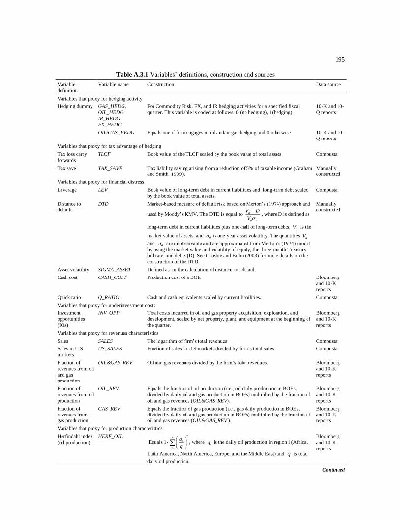
195
Table A.3.1 Variables’ definitions, construction and sources
Variable
definition
Variable name Construction Data source
Variables that proxy for hedging activity
Hedging dummy GAS_HEDG,
OIL_HEDG
IR_HEDG,
FX_HEDG
For Commodity Risk, FX, and IR hedging activities for a specified fiscal
quarter. This variable is coded as follows: 0 (no hedging), 1(hedging).
10-K and 10-
Q reports
OIL/GAS_HEDG Equals one if firm engages in oil and/or gas hedging and 0 otherwise 10-K and 10-
Q reports
Variables that proxy for tax advantage of hedging
Tax loss carry
forwards
TLCF Book value of the TLCF scaled by the book value of total assets Compustat
Tax save TAX_SAVE Tax liability saving arising from a reduction of 5% of taxable income (Graham
and Smith, 1999).
Manually
constructed
Variables that proxy for financial distress
Leverage LEV Book value of long-term debt in current liabilities and long-term debt scaled
by the book value of total assets.
Compustat
Distance to
default
DTD Market-based measure of default risk based on Merton’s (1974) approach and
used by Moody’s KMV. The DTD is equal to a
a a
V D
V , where D is defined as
long-term debt in current liabilities plus one-half of long-term debts, aV is the
market value of assets, and is one-year asset volatility. The quantities aV
and are unobservable and are approximated from Merton’s (1974) model
by using the market value and volatility of equity, the three-month Treasury
bill rate, and debts (D). See Crosbie and Bohn (2003) for more details on the
construction of the DTD.
Manually
constructed
Asset volatility SIGMA_ASSET Defined as in the calculation of distance-tot-default
Cash cost CASH_COST Production cost of a BOE Bloomberg
and 10-K
reports
Quick ratio Q_RATIO Cash and cash equivalents scaled by current liabilities. Compustat
Variables that proxy for underinvestment costs
Investment
opportunities
(IOs)
INV_OPP Total costs incurred in oil and gas property acquisition, exploration, and
development, scaled by net property, plant, and equipment at the beginning of
the quarter.
Bloomberg
and 10-K
reports
Variables that proxy for revenues characteristics
Sales SALES The logarithm of firm’s total revenues Compustat
Sales in U.S
markets
US_SALES Fraction of sales in U.S markets divided by firm’s total sales Compustat
Fraction of
revenues from oil
and gas
production
OIL&GAS_REV Oil and gas revenues divided by the firm’s total revenues. Bloomberg
and 10-K
reports
Fraction of
revenues from oil
production
OIL_REV Equals the fraction of oil production (i.e., oil daily production in BOEs,
divided by daily oil and gas production in BOEs) multiplied by the fraction of
oil and gas revenues (OIL&GAS_REV).
Bloomberg
and 10-K
reports
Fraction of
revenues from
gas production
GAS_REV Equals the fraction of gas production (i.e., gas daily production in BOEs,
divided by daily oil and gas production in BOEs) multiplied by the fraction of
oil and gas revenues (OIL&GAS_REV ).
Bloomberg
and 10-K
reports
Variables that proxy for production characteristics
Herfindahl index
(oil production)
HERF_OIL Equals 1-
2
1
N
i
i
q
q, where
iq is the daily oil production in region i (Africa,
Latin America, North America, Europe, and the Middle East) and q is total
daily oil production.
Bloomberg
and 10-K
reports
Continued

196
Table A.3.1-Continued
Variable
definition
Variable name Construction Data source
Herfindahl index
(gas production)
HERF_GAS Equals 1-
2
1
N
i
i
g
g, where
ig is the daily gas production in
region i (Africa, Latin America, North America, Europe, and
the Middle East) andig is total daily gas production.
Bloomberg and 10-
K reports
Oil production
uncertainty
UNCER_OIL Coefficient of variation of daily oil production. This
coefficient is calculated for each firm by using all the
observations of daily oil production until the current quarter.
Bloomberg and 10-
K reports
Gas production
uncertainty
UNCER_GAS Coefficient of variation of daily gas production. This
coefficient is calculated for each firm by using all the
observations of daily gas production until the current quarter.
Bloomberg and 10-
K reports
Price–quantity
correlation (oil)
PQ_COR_OIL Correlation coefficient between daily oil productions and oil
spot prices.
Bloomberg and 10-
K reports
Price–quantity
correlation (gas)
PQ_COR_GAS Correlation coefficient between daily gas productions and
gas spot prices.
Bloomberg and 10-
K reports
Gas daily
production
GAS_PROD Measured in millions of cubic feet. The observations are
given on an annual basis. We repeat the annual observations
for each quarter of the same fiscal year
Bloomberg and 10-
K reports
Oil daily
production
OIL_PROD Measured In thousands of barrels. The observations are given
on an annual basis. We repeat the annual observations for
each quarter of the same fiscal year
Bloomberg and 10-
K reports
Variables that proxy for firm size
Firm size SIZE The logarithm of (number of common shares outstanding *
end-of-quarter per share price) + book value of asset – book
value of equity.
Compustat
Tangibility TANGIBILITY Net property, plant, and equipment scaled by book value of
asset.
Compustat
Profitability EBITDA Earnings before interest, tax, depreciation, and amortization
scaled by book value of total asset.
Compustat
Variables that proxy for information asymmetry
% Institutions
shareholding
%_CS_INST Percentage of institutions’ common shares held. Thomson Reuters
Variables that proxy for market conditions
Oil spot price SPOT_OIL Oil spot price represented by the WTI in the NYMEX. Bloomberg
Gas spot price SPOT_GAS Constructed as an average index established from principal
locations’ indices in the United States (Gulf Coast, Henry
Hub, etc.)
Bloomberg
Oil price
volatility
VOL_OIL Historical volatility (standard deviation) using the spot price
of the previous 60 days.
Bloomberg
Gas price
volatility
VOL_GAS Historical volatility (standard deviation) using the spot price
of the previous 60 days.
Bloomberg
Firm’s stock return characteristics
Stock market
beta, oil beta, and
gas beta
BETA_MKT,
BETA_OIL,
BETA_GAS
Calculated from the market model supplemented by changes
in near-month NYMEX future contracts for gas and oil. The
model is estimated on quarterly basis using daily return of
firm’s stock and market index as measured by the CRSP
value weighted index.
CRSP and US
energy information
administration
Total volatility SIG_TOTAL Standard deviation of daily stock return calculated on
quarterly basis
CRSP
Idiosyncratic risk SIG_SPECIFIC Equals the ratio of stock return volatility divided by market
index volatility calculated from daily returns and on quarterly
frequency.
CRSP
Continued
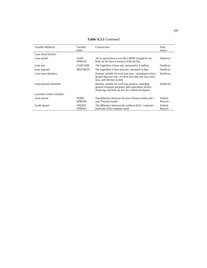
197
Table A.3.1-Continued
Variable definition Variable
name
Construction Data
source
Loan characteristics
Loan spread LOAN
SPREAD
All-in spread drawn over the LIBOR charged by the
bank for the drawn fraction of the facility.
DealScan
Loan size LOAN SIZE The logarithm of loan size, measured in $ million DealScan
Loan maturity MATURITY The logarithm of lean maturity, measured in days DealScan
Loan types dummies Dummy variable for each loan type: including revolver
greater than one year, revolver less than one year, term
loan, and 364-day facility
DealScan
Loan purposes dummies Dummy variable for each loan purpose, including
general corporate purposes, debt repayment, project
financing, and back-up line for commercial papers
DealScan
economic control variables
Term spread TERM
SPREAD
The difference between 10-year Treasury bonds and 1-
year Treasury bonds
Federal
Reserve
Credit spread CREDIT
SPREAD
The difference between the yields on BAA corporate
bond and AAA corporate bond
Federal
Reserve

APPENDIX 3.2
SIMULTANEOUS EQUATION ANALYSIS OF HEDGING EXTENT AND THE
RETURN ON EQUITY

199
Table A3.2 Simultaneous equation analysis of hedging extent and the return on equity
Panel A: Gas hedging Panel B: Oil hedging
Hedging
portfolio
Swap
contracts
Costless
collars
Put
options
Hedging
portfolio
Swap
contracts
Costless
collars
Put
options
(1) (2) (3) (4) (5) (6) (7) (8)
Equation 1: Return on equity is the dependent variable
HEDGE RATIO 0.1287** 0.1511 0.2389** 0.6130* 0.1732* -0.1195 1.1123*** 3.5196**
(0.056) (0.135) (0.115) (0.333) (0.101) (0.133) (0.326) (1.369)
SIZE 0.0019 0.0073 0.0007 0.0026 -0.0031 0.0049 -0.0037 -0.0014
(0.004) (0.005) (0.004) (0.004) (0.005) (0.005) (0.006) (0.004)
OIL&GAS_REV 0.0168 0.0166 0.0290** 0.0252** 0.0306** 0.0285** 0.0447*** 0.0291**
(0.011) (0.010) (0.012) (0.012) (0.012) (0.012) (0.017) (0.014)
US_SALES 0.0255 0.0529*** 0.0284 0.0215 0.0364* 0.0345* 0.0679** 0.0329
(0.017) (0.020) (0.020) (0.027) (0.019) (0.019) (0.029) (0.022)
INV_OPP 0.0024 0.0023 0.0008 0.0008 -0.0006 -0.0001 0.0017 0.0006
(0.002) (0.002) (0.003) (0.002) (0.003) (0.003) (0.004) (0.002)
%_CS_INST -0.0359*** -0.0481*** -0.0266* -0.0228 -0.0225 -0.0289* -0.0741*** -0.0180
(0.013) (0.016) (0.016) (0.015) (0.015) (0.015) (0.024) (0.019)
CASH_COST -0.0018*** -0.0014*** -0.0019*** -0.0020*** -0.0027*** -0.0021*** -0.0041*** -0.0012*
(0.000) (0.000) (0.001) (0.001) (0.000) (0.000) (0.001) (0.001)
LEVERAGE -0.0340* -0.0332 -0.0232 -0.0212 -0.0060 0.0167 0.0035 -0.0155
(0.018) (0.023) (0.016) (0.016) (0.016) (0.019) (0.020) (0.027)
CONSTANT -0.0332 -0.0979* -0.0281 -0.0556 -0.0051 -0.0867* 0.0213 -0.0321
(0.041) (0.050) (0.043) (0.044) (0.051) (0.046) (0.057) (0.051)
Observations 5,237 5,237 5,237 5,237 5,243 5,243 5,243 5,243
R-squared 0.1439 0.1432 0.1237 0.0990 0.1483 0.1563 -0.5663 -2.8136
Chi_2 1074.4425 1065.2208 1050.0986 1049.0043 1078.8284 1069.5052 601.7645 405.3583
p-value 0.0000 0.0000 0.0000 0.0000 0.0000 0.0000 0.0000 0.0000
Equation 2: Hedge ratio is the dependent variable
ROE 0.7946*** 0.7271*** -0.0613 0.1230 -0.6089*** -0.1689 -0.6758*** 0.1090
(0.285) (0.238) (0.184) (0.102) (0.219) (0.152) (0.171) (0.084)
TAX_SAVE 0.0254 -0.0442 0.1009** 0.0049 0.0566 0.0302 0.0418 0.0024
(0.051) (0.041) (0.041) (0.021) (0.060) (0.041) (0.048) (0.011)
TLCF -0.0259** -0.0189** -0.0077 -0.0007 -0.0244** -0.0428*** 0.0250** 0.0022
(0.012) (0.009) (0.009) (0.005) (0.012) (0.009) (0.010) (0.002)
VOL_GAS(OIL) 0.0523*** 0.0158 0.0360*** 0.0011 0.0043 0.0041** -0.0027 0.0006
(0.018) (0.015) (0.012) (0.006) (0.003) (0.002) (0.002) (0.001)
SPOT_GAS(OIL) -0.0015 -0.0063* 0.0069*** -0.0033** 0.0019*** 0.0008*** 0.0013*** -0.0001
(0.004) (0.003) (0.003) (0.001) (0.000) (0.000) (0.000) (0.000)
Q_RATIO -0.0015** -0.0011** -0.0001 -0.0002 -0.0010 -0.0009* 0.0002 0.0001
(0.001) (0.001) (0.000) (0.000) (0.001) (0.000) (0.001) (0.000)
SALES 0.0471*** 0.0166*** 0.0268*** 0.0040* 0.0366*** 0.0119*** 0.0232*** 0.0029
(0.006) (0.005) (0.004) (0.002) (0.005) (0.004) (0.004) (0.002)
LEVERAGE 0.1606*** 0.1285*** 0.0315** 0.0107 0.0626*** 0.0859*** 0.0005 0.0047
(0.022) (0.019) (0.014) (0.008) (0.021) (0.014) (0.016) (0.008)
PQ_COR_GAS(OIL) -0.0133 -0.0145* 0.0052 -0.0084** -0.0003 -0.0035 0.0010 0.0001
(0.010) (0.008) (0.008) (0.004) (0.009) (0.006) (0.007) (0.002)
UNCER_GAS(OIL) 0.0815*** 0.0381*** 0.0358*** 0.0146** 0.0433*** 0.0373*** -0.0100 -0.0035
(0.017) (0.014) (0.013) (0.007) (0.014) (0.010) (0.011) (0.003)
HERF_GAS(OIL) -0.1938*** -0.0966*** -0.1402*** 0.0537*** -0.0893** -0.1068*** 0.0447 0.0085
(0.040) (0.032) (0.031) (0.016) (0.036) (0.025) (0.028) (0.007)
CONSTANT -0.4248*** -0.1340*** -0.2753*** -0.0160 -0.4538*** -0.1972*** -0.2352*** -0.0163
(0.060) (0.050) (0.039) (0.021) (0.053) (0.037) (0.041) (0.020)
Observations 5,237 5,237 5,237 5,237 5,243 5,243 5,243 5,243
R-squared 0.5002 0.3687 0.4472 0.2802 0.4473 0.4962 0.0099 0.4060
Chi_2 7119.2985 5188.3519 4236.8553 2279.4582 5446.2599 5464.6774 2066.6122 3863.1885
p-value 0.0000 0.0000 0.0000 0.0000 0.0000 0.0000 0.0000 0.0000

200
Note:
This table presents the results of 3-SLS simultaneous equations estimation linking hedging extent with firm’s return on equity (ROE) to account for endogeneity between the two variables. The dependent variable in Equation
1 is the ROE measured by net income divided by book value of equity. The dependent variable in Equation 2 is the hedging extent (for the aggregate hedging portfolio and by instrument). The estimation is done for gas hedging (Panel A) and oil hedging (Panel B), separately. All independent variables enter regressions with lagged values. All variables’ definitions and construction are detailed in Table A.3.1. All regressions have firm and time fixed effects (not reported for conciseness). The t-statistics are into parentheses. ***Significant at the 1% level, ** Significant at the 5% level, * Significant at the 10% level.

REFERENCES
Adam, T., and C.S. Fernando, 2006, Hedging, speculation, and shareholder value, Journal of
Financial Economics 81, 283–309.
Adam, T., 2002, Risk management and the credit risk premium, Journal of Banking and
Finance 26, 243–269.
Allayannis, G., and E. Ofek, 2001, Exchange rate exposure, hedging, and the use of foreign
currency derivatives, Journal of International Money and Finance 20, 273–296.
Allayannis, G., and J.P. Weston, 2001, The use of foreign currency derivatives and firm
market value, Review of Financial Studies 14, 243–276.
Bartram, S.M., G.W. Brown, and J. Conrad, 2011, The effects of derivatives on firm risk and
value, Journal of Financial and Quantitative Analysis 46, 967–999.
Bartram, S.M., G.W. Brown, and F.R. Fehle, 2009, International evidence on financial
derivative usage, Financial Management 38, 185–206.
Campello, M.,C. Lin, Y. Ma, and H. Zou, 2011, The real and financial implications of corporate hedging, Journal of Finance 66 (5), 1615–1647.
Carter, D.A., D. Rogers, and B.J. Simkins, 2006, Does hedging affect firm value? Evidence
from the US airline industry, Financial Management 35, 53–87.
Choi, J.J.,C. X. Mao, and A. D. Upadhyay, 2013, Corporate risk management under
information asymmetry, Journal of Business Finance and Accounting 40, 239–271.
Crosbie, P.J., and R.J. Bohn, 2003, Modeling Default Risk (KMV, San Francisco).
Dimson, E., 1979, Risk measurement when shares are subject to infrequent trading, Journal of Financial Economics 7, 197–226.
Dionne, G., and T. Triki, 2013, On risk management determinants: What really matters?
European Journal of Finance 19, 145–164.
Dolde, W., 1995, Hedging, leverage and primitive risk, Journal of Financial Engineering 4,
187–216.
Fauver, L., and A. Naranjo, 2010, Derivative usage and firm value: The influence of agency
costs and monitoring problems, Journal of Corporate Finance 16, 719–735.
202
Fowler, D. J., and C. H. Rorke, 1983, Risk measurement when shares are subject to
infrequent trading: Comment, Journal of Financial Economics 12, 279–283.
Froot, K.A., D.S. Scharfstein, and J.C. Stein, 1993, Risk management: Coordinating
corporate investment and financing policies, Journal of Finance 48, 1629–1658.
Gay, G.D., C. M. Lin, and S. D. Smith, 2011, Corporate derivatives use and the cost of
equity, Journal of Banking and Finance 35, 1491-1506.
Géczy, C., B.A. Minton, and C. Schrand, 1997, Why firms use currency derivatives, Journal
of Finance 52, 132–154.
Graham, J.R., and D.A. Rogers, 2002, Do firms hedge in response to tax incentives? Journal
of Finance 57, 815–839.
Guay, W.R., 1999, The impact of derivatives on firm risk: An empirical examination of new
derivatives users, Journal of Accounting and Economics 26, 319–351.
Guay, W. R., and S. P. Kothari, 2003, How much do firms hedge with derivatives? Journal of Financial Economics 70, 423–461.
Haushalter, D., R.A. Heron, and E. Lie, 2002, Price uncertainty and corporate value, Journal
of Corporate Finance 8, 271–286.
Haushalter, D., 2000, Financing policy, basis risk, and corporate hedging: Evidence from oil
and gas producers, Journal of Finance 55 (1), 107–152.
Hentschel, L., and S.P. Kothari, 2001, Are corporations reducing or taking risks with derivatives? Journal of Financial and Quantitative Analysis 36, 93–118.
Jensen, M.C., and W.H. Meckling, 1976, Theory of the firm: Managerial behavior, agency
costs and ownership structure, Journal of Financial Economics 3, 305-360.
Jin, Y., and P. Jorion, 2006, Firm value and hedging: Evidence from U.S. oil and gas
producers, Journal of Finance 61, 893–919.
Kumar, P., and R. Rabinovitch, 2013, CEO entrenchment and corporate hedging: Evidence
from the oil and gas industry, Journal of Financial and Quantitative Analysis 48, 887–917.
Leland, Hayne E., 1998, Agency costs, risk management, and capital structure, Journal of
Finance 53, 1213-1243.
Mayers, D., and C.W. Smith, 1982, On the corporate demand for insurance, Journal of
Business 55, 281–296.

203
Merton, R.C., 1974, On the pricing of corporate debt: The risk structure of interest rates,
Journal of Finance 29, 449-470.
Mian, S., 1996, Evidence on corporate hedging policy, Journal of Financial and Quantitative
Analysis 31, 419-439.
Modigliani, M., and M. Miller, 1958, The cost of capital, corporate finance and theory of
investment, American Economic Review 48, 261–297.
Myers, S.C., 1977, Determinants of corporate borrowing, Journal of Financial economics 5, 147–175.
Nance, D.R., C.W Smith, and C.W. Smithson, 1993, On the determinants of corporate
hedging, Journal of Finance 48, 267–284.
Pérez-Gonzalez, F., and H. Yun, 2013, Risk management and firm value: Evidence from
weather derivatives, Journal of Finance 68, 2143–2176.
Ross, M.P., 1996. Corporate Hedging: What, Why and How? Working paper, University of
California, Berkeley.
Scholes, M. S., and J. Williams., 1977. Estimating Betas from Nonsynchronous Data, Journal of Financial Economics 5, 309-327.
Smith, C.W., and R.M. Stulz, 1985, The determinants of firms’ hedging policies, Journal of
Financial and Quantitative Analysis 20, 391–405.
Stulz, R. M., 1996, Rethinking risk management, Journal of Applied Corporate Finance 9, 8-
24.
Stulz, R.M., 1984, Optimal hedging policies, Journal of Financial and Quantitative Analysis 19, 391–405.
Tufano, P., 1998, The determinants of stock price exposure: Financial engineering and the
gold mining industry, Journal of Finance 53, 1015-52.
Tufano, P., 1996, Who manages risk? An empirical examination of risk management
practices in the gold mining industry, Journal of Finance 51, 1097–1137.

CONCLUSION
Malgré son impertinence dans le monde parfait de Modigliani et Miller (1958), la gestion
des risques financiers est devenue une pratique usuelle dans un grand nombre d’entreprises
non-financières (Bartram, Brown, et Fehle, 2009). La littérature a bien amélioré notre
compréhension des motivations de la gestion des risques et de ses vertus potentielles en
termes de création de la valeur pour l’entreprise et, par conséquent, pour les actionnaires.
Toutefois, il importe de remarquer que cette littérature, surtout celle empirique, nous éclaire
peu sur les déterminants du choix de la stratégie de couverture à adopter par les entreprises.
De surcroit, cette littérature ne dit presque rien sur la manière de choisir les maturités des
positions de couverture et leur évolution dans le temps. À ce niveau, le manque de modèle
théorique a été comblé par Fehle et Tsyplakov (2005). Finalement, les résultats empiriques
relatifs aux implications et retombées de la gestion des risques sur l’entreprise restent
largement controversés et non-concluants.
Parmi les raisons déjà avancées par Aretz et Bartram (2010) pour expliquer ces
controverses, on trouve les difficultés à déterminer avec précision l’étendue de la couverture
vu que les entreprises utilisent des portefeuilles complexes incorporant une multitude
d’instruments qui différent en termes des coûts d’initiation, profil de gain (payoff), maturité,
comptabilisation, etc. Grâce aux données très détaillées, collectées manuellement, sur les
positions de couverture d’un échantillon de 150 compagnies pétrolières américaines, le but de
cette thèse est de contribuer à la littérature en préconisant des réponses surtout au regard des
déterminants du choix de la stratégie et de la maturité de la couverture. Vu le manque
d’évidences empiriques portant sur ces deux aspects, nous croyons qu’il n’est pas inutile
d’apporter une nouvelle contribution à la littérature dans ce sujet. Encore, nous croyons que,
revisiter la question de la prime liée à la gestion des risques est toujours indispensable,
surtout à la lumière des différentes critiques méthodologiques et les limitations au niveau des
données qui restreignent la pertinence des résultats empiriques obtenus.

205
Dans le premier chapitre, nous avons examiné la validité empirique de certaines
prédictions émanant des travaux théoriques en rapport avec les déterminants du choix des
stratégies de couverture. Un défi d’ordre méthodologique s’est posé vu la persistance dans le
choix des stratégies. Cette persistance a motivé le recours à une modélisation économétrique
dynamique appliquée aux modèles aux choix discrets. Dans l’ensemble, les résultats obtenus
montrent que les entreprises qui font face à plus de dépenses d’investissement utilisent plus
les stratégies non-linéaires. Toutefois, une corrélation positive entre ces dépenses
d’investissement et les flux monétaires générés à l’interne incite davantage l’utilisation des
stratégies linéaires. Les stratégies non-linéaires sont aussi positivement corrélées avec la
diversification géographique et l’incertitude dans la production. Cependant, une corrélation
positive entre les prix de vente et les quantités produites motive le déploiement des stratégies
linéaires pour stabiliser les flux monétaires.
Les résultats donnent aussi une première évidence empirique de l’impact du problème de
surinvestissement qui favorise l’utilisation des stratégies linéaires. La fonction d’utilité du
gestionnaire averse au risque joue un rôle important dans la détermination de la stratégie de
couverture. Si sa fonction d’utilité est concave (plus d’actions), le gestionnaire choisirait les
stratégies linéaires. Si sa fonction d’utilité est convexe (plus d’options d’achat), il aurait
tendance à préférer les stratégies ayant un payoff convexe. Les entreprises les plus endettées,
mais pas encore en détresse financière, cherchent à stabiliser leurs flux monétaires avec
particulièrement les contrats swap. Les entreprises en détresse financière font plutôt du
transfert de risque avec les options de vente.
Le deuxième chapitre investigue particulièrement la validité empirique des prédictions
théoriques émanant du modèle de Fehle et Tsyplakov (2005) ainsi que d’autres hypothèses
liées au programme d’investissement de l’entreprise, à la maturité de ses actifs et ses dettes,
aux taxes, et à l’aversion au risque du gestionnaire. Le constat le plus important révélé par les
résultats est celui de la relation non-monotone qui existe entre la maturité de la couverture et
la probabilité de la détresse financière. Cette non-monotonicité existe aussi entre la maturité
et les prix au comptant du pétrole et du gaz. Les résultats montrent aussi que la maturité de la
couverture est positivement corrélée à l’incertitude dans la production, à la corrélation entre
les prix de vente et les quantités produites, et à la volatilité des prix au comptant.
206
Les entreprises ayant de grandes dépenses d’investissement privilégient les couvertures
avec de longues maturités pour aboutir à une meilleure coordination des dépenses en capital
et du financement. Toutefois, une corrélation positive entre les dépenses d’investissement et
les flux monétaires, incite les entreprises à utiliser des couvertures plus courtes. Les résultats
montrent encore que les entreprises alignent la maturité de leurs positions de couverture avec
celles de leurs actifs et leurs dettes. Enfin, une première investigation empirique des effets de
la maturité de la couverture sur la valeur et le risque de l’entreprise, démontre que les
positions de couverture avec des échéances plus lointaines assurent une meilleure réduction
de la sensibilité des rendements de l’action aux fluctuations des prix du pétrole et du gaz.
Dans le troisième chapitre, nous réexaminons l’hypothèse de la prime liée à la gestion des
risques financiers. Pour pallier aux critiques adressées aux résultats déjà obtenus dans la
littérature, nous prenons en compte particulièrement le problème d’endogénéité de la décision
de couverture avec d’autres aspects de la politique financière de l’entreprise via une
estimation en équations simultanées par la méthode des triples moindres carrés. Nous avons
aussi contrôlé pour l’existence d’autres couvertures telles que celles relatives aux taux
d’intérêt et aux taux de change, et aussi l’existence d’autres types de couverture
opérationnelle sous forme de diversification géographique, par exemple.
Les résultats révèlent que la gestion des risques a des effets positifs particulièrement sur
les prix de vente du gaz. Ces effets positifs se répercutent favorablement sur la performance
comptable de l’entreprise. De plus, la couverture permet de réduire significativement la
volatilité des rendements des actions de l’entreprise ainsi que son risque résiduel. La
couverture n’est pas associée à une augmentation du risque systématique. Cela signifie que la
présence de la gestion des risques financiers n’incite pas les investisseurs à demander un taux
de rendement plus élevé pour détenir l’action de l’entreprise. De surcroit, la gestion des
risques augmente la capacité de l’entreprise à contracter des dettes mais sans effets directs
(positif ou négatif) sur le coût de cet endettement.

RÉFÉRENCES
Adam, T., 2002, Risk management and the credit risk premium, Journal of Banking and
Finance 26, 243–269.
Adam, T., 2009, Capital expenditures, financial constraints, and the use of options, Journal of Financial Economics 92, 238–251.
Adam, T., and C.S. Fernando, 2008, Can companies use hedging programs to profit from the
market? Evidence from gold producers, Journal of Applied Corporate Finance 20 (4), 91–102.
Adam, T., and C.S. Fernando, 2006, Hedging, speculation, and shareholder value, Journal of
Financial Economics 81, 283–309.
Adler, M., and J.B. Detemple, 1988, Hedging with futures and options, Studies in Banking and Finance 5, 181–197.
Allayannis, G., and E. Ofek, 2001, Exchange rate exposure, hedging, and the use of foreign
currency derivatives, Journal of International Money and Finance 20, 273–296.
Allayannis, G., and J.P. Weston, 2001, The use of foreign currency derivatives and firm
market value, Review of Financial Studies 14, 243–276.
Arellano, M., and O. Bover, 1995, Another look at the instrumental variable estimation of error-components models. Journal of Econometrics 68, 29–51.
Arellano, M., and S. Bond, 1991, Some tests of specification for panel data: Monte Carlo
evidence and an application to employment equations. Review of Economic Studies
58, 277–98.
Aretz, K., and S.M. Bartram, 2010, Corporate hedging and shareholder value, Journal of
Financial Research 33, 317–371.
Bartram, S.M., G.W. Brown, and R.M. Stulz, 2012, Why are U.S. stocks more volatile? Journal of Finance 67, 1329–1370.
Bartram, S.M., G.W. Brown, and J. Conrad, 2011, The effects of derivatives on firm risk and
value, Journal of Financial and Quantitative Analysis 46, 967–999.
Bartram, S.M., G.W. Brown, and F.R. Fehle, 2009, International evidence on financial derivative usage, Financial Management 38, 185–206.

208
Bessembinder, H., 1991, Forward contracts and firm value: investment incentive and
contracting effects, Journal of Financial and Quantitative Analysis 26, 519–532.
Bodnar, G.M., G.S. Hayt, and R.C. Marston, 1998, 1998 Survey of financial risk management by US nonfinancial firms, Financial Management 27, 70–91.
Boes, S., 2007, Three essays on the econometric analysis of discrete dependent variables,
Working paper, University of Zürich.
Bond, S. R., 2002, Dynamic panel data models: a guide to micro data methods and practice,
Portuguese Economic Journal 1, 141–162.
Brown, G.W., 2001, Managing foreign exchange risk with derivatives, Journal of Financial Economics 60, 401–448.
Brown, G.W., and K.B. Toft, 2002, How firms should hedge, Review of Financial Studies 15,
1283–1324.
Blundell, R., and S. Bond, 1998, Initial conditions and moment restrictions in dynamic panel
data models. Journal of Econometrics 87, 115–43.
Campello, M.,C. Lin, Y. Ma, and H. Zou, 2011, The real and financial implications of
corporate hedging, Journal of Finance 66 (5), 1615–1647.
Carter, D.A., D. Rogers, and B.J. Simkins, 2006, Does hedging affect firm value? Evidence
from the US airline industry, Financial Management 35, 53–87.
Choi, J.J.,C. X. Mao, and A. D. Upadhyay, 2013, Corporate risk management under
information asymmetry, Journal of Business Finance and Accounting 40, 239–271.
Crosbie, P.J., and R.J. Bohn, 2003, Modeling Default Risk (KMV, San Francisco).
Dimson, E., 1979, Risk measurement when shares are subject to infrequent trading, Journal
of Financial Economics 7, 197–226.
Dionne, G., and M. Garand, 2003, Risk management determinants affecting firms’ values in
the gold mining industry: New empirical results, Economics Letters 79, 43–52.
Dionne, G., and T. Triki, 2013, On risk management determinants: What really matters?
European Journal of Finance 19, 145–164.
Dolde, W., 1995, Hedging, leverage and primitive risk, Journal of Financial Engineering 4, 187–216.
Dolde, W., 1993, The trajectory of corporate financial risk management, Journal of Applied
Corporate Finance 6, 33–41.

209
Drucker, S., and M. Puri, 2009, On loan sales, loan contracting, and lending relationships,
Review of Financial Studies 22, 2835–2872.
Eisdorfer, A., 2008, Empirical evidence of risk-shifting in financially distressed firms,
Journal of Finance 63, 609–637.
Fauver, L., and A. Naranjo, 2010, Derivative usage and firm value: The influence of agency
costs and monitoring problems, Journal of Corporate Finance 16, 719–735.
Fehle, F., and S. Tsyplakov, 2005, Dynamic risk management: Theory and evidence, Journal
of Financial Economics 78, 3–47.
Financial Accounting Standards Board, 1998, Accounting for derivative instruments and hedging activities, Statement No. 133.
Fowler, D. J., and C. H. Rorke, 1983, Risk measurement when shares are subject to
infrequent trading: Comment, Journal of Financial Economics 12, 279–283.
Franke, G., R.C. Stapleton, and M.G. Subrahmanyam, 1998, Who buys and who sells
options: The role of options in an economy with background risk, Journal of
Economic Theory 82, 89–109.
Froot, K.A., D.S. Scharfstein, and J.C. Stein, 1993, Risk management: Coordinating
corporate investment and financing policies, Journal of Finance 48, 1629–1658.
Gay, G.D., C. M. Lin, and S. D. Smith, 2011, Corporate derivatives use and the cost of
equity, Journal of Banking and Finance 35, 1491-1506.
Gay, G.D., J. Nam, and M. Turac, 2003, On the optimal mix of corporate hedging
instruments: Linear versus non-linear derivatives, Journal of Futures Markets 23,
217–239.
Gay, G.D., J. Nam, and M. Turac, 2002, How firms manage risk: The optimal mix of linear
and non-linear derivatives, Journal of Applied Corporate Finance 14, 82–93.
Gay, G.D., and J. Nam, 1998, The underinvestment problem and corporate derivatives use,
Financial Management 27, 53–69.
Géczy, C., B.A. Minton, and C. Schrand, 1997, Why firms use currency derivatives, Journal
of Finance 52, 132–154.
Graham, J., and C.W. Smith, 1999, Tax incentives to hedge, Journal of Finance 54, 2241–2262.
Graham, J.R., and D.A. Rogers, 2002, Do firms hedge in response to tax incentives? Journal
of Finance 57, 815–839.
210
Grullon, G., E. Lyandres, and A. Zhdanov, 2012, Real options, volatility, and stock returns,
Journal of Finance 67, 1499–1537.
Guay, W.R., 1999, The impact of derivatives on firm risk: An empirical examination of new
derivatives users, Journal of Accounting and Economics 26, 319–351.
Guay, W. R., and S. P. Kothari, 2003, How much do firms hedge with derivatives? Journal of
Financial Economics 70, 423–461.
Haushalter, D., 2000, Financing policy, basis risk, and corporate hedging: Evidence from oil and gas producers, Journal of Finance 55, 107–152.
Haushalter, D., R.A. Heron, and E. Lie, 2002, Price uncertainty and corporate value, Journal
of Corporate Finance 8, 271–286.
Heckman, J., 1981, The incidental parameters problem and the problem of initial conditions in estimating a discrete time–discrete data stochastic process, in C.F. Manski and D.
McFadden, eds.: Structural Analysis of Discrete Data with Econometric Applications
(MIT Press, Cambridge, MA).
Hentschel, L., and S.P. Kothari, 2001, Are corporations reducing or taking risks with
derivatives? Journal of Financial and Quantitative Analysis 36, 93–118.
Hole, A. R., 2007, Fitting mixed logit models by using maximum simulated likelihood, Stata Journal 7, 388-401.
Jensen, M.C., 1986, Agency costs of free cash flow, corporate finance and takeovers,
American Economic Review 76, 323–329.
Jensen, M.C., and W.H. Meckling, 1976, Theory of the firm: Managerial behavior, agency costs and ownership structure, Journal of Financial Economics 3, 305-360.
Jin, Y., and P. Jorion, 2006, Firm value and hedging: Evidence from U.S. oil and gas
producers, Journal of Finance 61, 893–919.
Kumar, P., and R. Rabinovitch, 2013, CEO entrenchment and corporate hedging: Evidence
from the oil and gas industry, Journal of Financial and Quantitative Analysis 48,
887–917.
Lehn, K., and A. Poulsen, 1989, Free cash flow and stockholder gains in going private transactions, Journal of Finance 44, 771–788.
Leland, Hayne E., 1998, Agency costs, risk management, and capital structure, Journal of
Finance 53, 1213-1243.
Lin, C.M., R. Philips, and S. D. Smith, 2008, Hedging, financing, and investment decisions:
theory and empirical tests, Journal of Banking and Finance 32, 1566–1582.

211
Maddala, G., 1983, Limited-Dependent and Qualitative Variables in Econometrics
(Cambridge University Press, Cambridge).
Mayers, D., and C.W. Smith, 1982, On the corporate demand for insurance, Journal of
Business 55, 281–296.
Merton, R.C., 1974, On the pricing of corporate debt: The risk structure of interest rates,
Journal of Finance 29, 449-470.
Mian, S., 1996, Evidence on corporate hedging policy, Journal of Financial and Quantitative Analysis 31, 419-439.
Modigliani, M., and M. Miller, 1958, The cost of capital, corporate finance and theory of
investment, American Economic Review 48, 261–297.
Morellec, E., and C. W. Smith, 2007, Agency conflicts and risk management, Review of Finance 11, 1–23.
Moschini, G., and H. Lapan, 1995, The hedging role of options and futures under joint
price, basis, and production risk, International Economic Review 36, 1025–1049.
Moschini, G., and H. Lapan, 1992, Hedging price risk with options and futures for the
competitive firm with production flexibility, International Economic Review 33,
607–618.
Myers, S.C., 1977, Determinants of corporate borrowing, Journal of Financial economics 5,
147–175.
Nance, D.R., C.W Smith, and C.W. Smithson, 1993, On the determinants of corporate
hedging, Journal of Finance 48, 267–284.
Pérez-Gonzalez, F., and H. Yun, 2013, Risk management and firm value: Evidence from
weather derivatives, Journal of Finance 68, 2143–2176.
Pfarr, C., Schmid, A. and U. Schneider, 2010, REGOPROB2: Stata module to estimate
random effects generalized ordered probit models (update), Statistical Software
Components, Boston College Department of Economics.
Rabe-Hesketh, S., Skrondal, A. and Pickles, A. (2005). Maximum likelihood estimation of
limited and discrete dependent variable models with nested random effects. Journal
of Econometrics 128 (2), 301-323.
Rajgopal, S., 1999, Early evidence on the informativeness of the SEC’s market risk
disclosures: The case of commodity price risk exposure of oil and gas producers,
Accounting Review 74, 251–280.

212
Roodman, D., 2009a, How to do xtabond2: an introduction to difference and system GMM in
Stata.Stata Journal 9, 86–136.
Roodman, D., 2009b, A note on the theme of too many instruments. Oxford Bulletin of Economics and Statistics 71, 135–158.
Ross, M.P., 1996. Corporate Hedging: What, Why and How? Working paper, University of California, Berkeley.
Scholes, M. S., and J. Williams., 1977. Estimating Betas from Nonsynchronous Data, Journal
of Financial Economics 5, 309-327.
Smith, C.W., and R.M. Stulz, 1985, The determinants of firms’ hedging policies, Journal of Financial and Quantitative Analysis 20, 391–405.
Stulz, R.M., 1996, Rethinking risk management, Journal of Applied Corporate Finance 9, 8–
24.
Stulz, R.M., 1984, Optimal hedging policies, Journal of Financial and Quantitative Analysis
19, 391–405.
Terza, J., 1985, Ordinal probit: A generalization, Communications in Statistics–Theory and Methods 14, 1–11.
Train, K.E., 2009, Discrete Choice Methods with Simulation (Cambridge University Press,
Berkeley).
Tufano, P., 1998, The determinants of stock price exposure: Financial engineering and the
gold mining industry, Journal of Finance 53, 1015-52.
Tufano, P., 1996, Who manages risk? An empirical examination of risk management
practices in the gold mining industry, Journal of Finance 51, 1097–1137.
Williams, R., 2006, Generalized ordered logit: Partial proportional odds models for ordinal
dependent variables, Stata Journal 6 (1), 58–82.
Windmeijer, F., 2005, A finite sample correction for the variance of linear efficient two-step GMM estimators. Journal of Econometrics 126, 25–51.
Wooldridge, J.M., 2002, Econometric Analysis of Cross Section and Panel Data (MIT Press,
Cambridge).
Zucchelli, E., M. Harris, and Z. Xueyan, 2012, Ill-health and transitions to part-time work
and self-employment among older workers, Working paper, Centre for Health
Economics, University of York.


![GUIDE DU CHANTIER Mars 2014. 1] Le chantier en quelques chiffres 115 MILLIONS DEUROS TTC dINVESTISSEMENT 1 AN DETUDES 2 ANS DE CHANTIER 13 000 M2 DE SURFACES.](https://static.fdocuments.in/doc/165x107/551d9dbb497959293b8de917/guide-du-chantier-mars-2014-1-le-chantier-en-quelques-chiffres-115-millions-deuros-ttc-dinvestissement-1-an-detudes-2-ans-de-chantier-13-000-m2-de-surfaces.jpg)