Search Engines & Question Answering Giuseppe Attardi Università di Pisa.
Upload
truongthuanCategory
view
218download
0
Università di Pisa
Facoltà di Scienze Matematiche Fisiche e Naturali
Corso di Laurea Specialistica in Scienze Fisiche
Anno Accademico 2006-2007
Tesi di Laurea Specialistica
The HAM-SAS Seismic Isolation System for the Advanced LIGO
Gravitational Wave Interferometers
Candidato Alberto Stochino
Relatori Riccardo De Salvo
(California Institute of Technology)
Francesco Fidecaro
(Università di Pisa)

Ai miei genitori e ai miei fratelli


Abstract
The three LIGO interferometers are full operative and under science run sinceNovember 2005. The acquired data are integrated with those obtained by th Virgoexperiment within an international cooperation aimed to maximize the efforts forthe detection of gravitational waves.
From 2001 LIGO I is expected to be shut down and the construction and com-missioning of Advanced LIGO to start. The objective of the new generation in-terferometers is a ten times greater sensibility with the purpose to extend of afactor of a thousand the space volume covered and to increase of the same orderof magnitude the probability to detect events.
To increase the sensibility in the band below 40 Hertz, the main source ofnoise that Advanced LIGO have to face is the seismic noise. In this perspective,the SAS group (Seismic Attenuation Systems) of LIGO has developed a class oftechnologies on which the HAM-SAS system is based. Designed for the seismicisolation of the output mode cleaner optics bench and more in general for allthe HAM vacuum chambers of LIGO, HAM-SAS, with little variations, can beextended to the BSC chambers as well.
In HAM-SAS the legs of four inverted pendulums form the stage of attenu-ation of the horizontal degrees of freedom. Four GAS filters are included insidea rigid intermediate structure called Spring Box which is supported by the in-verted pendulums and provide for isolation of the vertical degrees of freedom.The geometry is such that the horizontal degrees of freedom and the vertical onesare separate. Each GAS filter carries an LVDT position sensor and an electro-magnetic actuator and so also each leg of the inverted pendulums. Eight steppermotors guarantee the DC control of the system.
A prototype of HAM-SAS has been constructed in Italy, at Galli & Morelli andthen transferred to Massachusetts Institute of Technology in the US to be testedinside the Y-HAM vacuum chamber of the LIGO LASTI laboratory.
The test at LASTI showed that the vertical and horizontal degrees of free-dom are actually uncoupled and can be treated as independent. It was possible toclearly identify the modes of the system and assume these as a basis by which tobuild a set of virtual position sensors and a set of virtual actuators from the realones, respect with which the transfer function of the system was diagonal. Insidethis modal space the control of the system was considerably simplified and moreeffective. We measured accurate physical plants responses for each degree of free-dom and, based on these, designed specific control strategies. For the horizontaldegrees of freedom we implemented simple control loops for the conservation ofthe static position and the damping of the resonances. For the vertical ones, be-

yond these functions, the loops introduced an electromagnetic anti-spring effectand lowered the resonance frequency.
The overall results was the achievement of the LIGO seismic attenuation re-quirements within the sensibility limits of the geophone sensors used to measuredthe performances.
The entire project, from the construction to the commissioning, occurred withina very tight time schedule which left scarce possibility to complete the expectedmechanical setup. The direct access to the system became much rarer once theHAM chamber had been closed and the vacuum pumped. Some of the subsystems(among which the counterweights for the center of percussion of the pendulumsand the “magic wands”) could not be implemented and several operations of op-timization (i.e. the lower tuning of the vertical GAS filters’ resonant frequenciesand the tilts’ optimization) had no chance to be completed. Moreover the LASTIenvironment offered a seismically unfortunate location if compared with the sitesof the observatories for which HAM-SAS have been designed. Nonetheless theperformances measured on the HAM-SAS prototype were positive and the ob-tained results very encouraging and leave us confident to be further improved andextended by keeping working on the system.
2

Riassunto(Italian Abstract)
La presente tesi di laurea è il risultato della partecipazione del candidato allosviluppo del sistema HAM-SAS per l’attenuazione del rumore sismico negli in-terferometri di Advanced LIGO.
I tre interferometri nei due osservatori di LIGO sono ormai operativi e in con-tinua presa dati dal Novembre del 2005. I dati acquisiti sono integrati con quelliottenuti dal progetto Virgo nell’ambito di una cooperazione internazionale volta amassimizzare gli sforzi per la rivelazione delle onde gravitazionali.
A partire dal 2011 sono previsti la dismessa di LIGO I e l’inizio dell’installazionee messa in funzione di Advanced LIGO. L’obiettivo degli interferometri di nuovagenerazione è una sensibilità dieci volte maggiore con lo scopo di estendere di unfattore mille il volume di spazio coperto e di incrementare dello stesso ordine digrandezza la probabilità di rivelazione di eventi.
Per aumentare la sensibilità nella banda sotto 10 Hertz la principale fontedi rumore che Advanced LIGO deve fronteggiare è il rumore sismico. In taleprospettiva, il gruppo SAS (Seismic Attenuation Sistems) di LIGO ha sviluppatoun insieme di tecnologie sulle quali si basa il sistema HAM-SAS, progettato perl’isolamento sismico del banco ottico dell’output mode cleaner e più in generaleper tutte le camere a vuoto HAM di LIGO.
In HAM-SAS le gambe di quattro pendoli invertiti costituiscono lo stadio diattenuazione dei gradi di libertà orizzontali (yaw e le due traslazioni sul piano).Quattro filtri GAS sono contenuti all’interno di una struttura rigida intermediachiamata Spring Box che poggia sui pendoli invertiti e provvedono all’isolamentodei gradi di libertà verticali (traslazione verticale e le inclinazioni). La geometriaè tale che i gradi di libertà orizzontali e quelli verticali risultano separati. Ognifiltro GAS è accompagnato da un sensore di posizione LVDT e da un attuatoreelettromagnetico e così anche ogni gamba dei pendoli invertiti. Otto stepper mo-tors permettono il controllo di posizione statica del sistema.
Un prototipo di HAM-SAS è stato realizzato in Italia e quindi trasportatopresso il Massachusetts Institute of Technology negli Stati Uniti d’America peressere testato entro la camera a vuoto Y-HAM dell’interferometro da 15 metri delLIGO LASTI Laboratory.
La collaborazione del candidato al progetto è cominciata nel 2005 con lo stu-dio di uno dei sottosistemi di HAM-SAS, le cosiddette “magic wands”, oggettodella tesi di laurea di primo livello e ora parte integrante della tecnica SAS.Nell’Agosto del 2006 un maggiore coinvolgimento è cominciato con la parte-cipazione alle varie fasi di costruzione del sistema presso le officine meccaniche
3
della Galli e Morelli di Lucca. Il contributo alla costruzione in Italia ha incluso:il design di alcuni elementi, il processo di produzione dell’acciaio maraging perle lame dei filtri GAS, l’assemblaggio dell’intero sistema in tutte le sue parti mec-caniche inclusi sensori, attuatori elettromagnetici e stepper motors e le caratteriz-zazioni preliminari dei pendoli invertiti e dei filtri GAS. Il sistema è stato inoltreinteramente sottoposto ai processi di trattamento per la compatibilità con gli am-bienti ad ultra alto vuoto dell’interferometro e in questa fase un contributo sonostati i test spettroscopici tramite FT-IR dei campioni ricavati dal sistema. Du-rante l’assemblaggio definitivo in camera pulita, come spiegato nell’elaborato,l’impegno è andato dal tuning dei filtri GAS, alla distribuzione precisa dei carichisui pendoli invertiti e alla messa a punto del sistema per la correzione del tiltverticale.
All’MIT, a cominciare da Dicembre 2006, il candidato ha rappresentato il pro-getto HAM-SAS per tutta la sua durata. Qui si è occupato, assieme al gruppoSAS, di tutte le fasi dell’esperimento, dal setup dell’elettronica e della meccanicaal commissioning del sistema per raggiungere i requisiti di progetto, passandoper la creazione del sistema di acquisizione dati, i controlli, l’analisi dei dati el’interpretazione dei risultati.
I test a LASTI hanno mostrato che, grazie alla particolare geometria del sis-tema, i gradi di libertà orizzontali e quelli verticali sono disaccoppiati e possonoessere trattati come indipendenti. E’ stato possibile identificare chiaramente imodi del sistema e assumerli come base con cui costruire un set di sensori diposizione virtuali e un set di attuatori virtuali a partire da quelli reali, rispettoai quali la funzione di trasferimento del sistema fosse diagonale. All’interno diquesto spazio modale il controllo del sistema è risultato notevolmente semplifi-cato e più efficace. Abbiamo misurato accurate physical plant responses per ognigrado di libertà e, sulla base di queste, disegnato specifiche tipologie di controllo.Per i gradi di libertà orizzontali si sono utilizzati semplici loops di controllo peril mantenimento della posizione statica e il damping delle risonanze. Per quelliverticali in più a queste funzioni, i loops introducevano un effetto di antimollaelettromagnetica e abbassavano le frequenze di risonanza.
Il risultato complessivo è stato il raggiungimento dei requisiti di attenuazionesismica di LIGO per il banco ottico entro i limiti di sensibilità dei sensori geofoniutilizzati.
L’intero progetto, dalla produzione al commissioning, si è svolto secondo unprogramma dai tempi contingentati che ha lasciato scarsa possibilità di completarefino in fondo il setup meccanico previsto. L’accesso diretto al sistema è diventatomolto più raro una volta richiusa la camera HAM nell’interferometro e pompatoil vuoto. Alcuni dei sottosistemi (tra cui i contrappesi per il centro di percussionedei pendoli e le “magic wands”) non hanno potuto essere installati e diverse op-erazioni di ottimizzazione (come l’abbassamento delle frequenze dei filtri GAS
4

verticali e dei pendoli invertiti e l’ottimizzazione dei tilt) non hanno potuto esserecompletate. Inoltre l’ambiente di LASTI ha offerto una locazione sismicamentepoco favorevole se confrontata alle sedi degli osservatori per le quali HAM-SASera stato progettato. Nondimeno le performance ottenute dal prototipo di HAM-SAS sono state positive e i risultati ottenuti molto incoraggianti e ci lascianofiduciosi della possibilità che possano essere ulteriormente migliorati e ampliatidai lavori ancora in corso.
5

6
AknowledgementsThis thesis is the result of a significant experience, for my education as a physicistand my life overall. I am indebted to all the people who made it possible, whogave me a lot of valuable support during my work and also so much good timeboth in Lucca and Boston. I’d like to acknowledge them here.
First of all I want to thank my supervisors Riccardo De Salvo, who gave methis opportunity and has constantly and strongly supported my work teaching mean innumerable amount of things, and Francesco Fidecaro, who first introducedme to Virgo and LIGO. I would not be writing these lines if it wasn’t for them.
The construction of HAM-SAS demanded a great effort and I have to thankCarlo Galli, Chiara Vanni e Maurizio Caturegli from Galli & Morelli. It wouldnot have been possible without their deep commitment, and I would not have hadsuch a good time in Lucca without them.
I also want to thank the many people of the HAM-SAS team for their contin-uous support during the project and for introducing me to the LIGO systems andin particular: Virginio Sannibale, Dennis Coyne, Yoichi Aso, Alex Ivanov, BenAbbott, Jay Heefner, David Ottaway, Myron MacInnis, Bob Laliberte. It was apleasure to work with them.
The LIGO department at MIT has been my house for eight months. I have tothank all the people there for their hearty hospitality and Marie Woods deservesa special thank for being always so kind and helping me with my relocation andmy staying at MIT. I want also to thank: Richard Mittleman for being alwaysavailable in the lab and his support in writing this thesis; Fabrice Matichard for allhis valuable tips of mechanical engineering and for our enjoyable coffee breaksin the office; Brett Shapiro, Thomas Corbitt and Pradeep Sarin for their help andpleasant company in the control room.I also want to thank MIT for letting me experience its exciting atmosphere for allthese months.
I have to thank the LIGO Project, Caltech and the National Science Foundationfor granting my visitor program, and in particular David Shoemaker and AlbertLazzarini. I’m also grateful to the Italian INFN for granting the beginning of myprogram.
I want to thank Luca Masini for all his logistic support in Pisa for this thesis.It would not even be printed without him.
The LIGO Observatories were constructed by the California Institute of Tech-nology and Massachusetts Institute of Technology with funding from the NationalScience Foundation under cooperative agreement PHY 9210038. The LIGO Lab-oratory operates under cooperative agreement PHY-0107417. This paper has beenassigned LIGO Document Number LIGO-P070083-00-R.

2

Contents
1 Gravitational Waves Interferometric Detectors 51.1 Gravitational Waves . . . . . . . . . . . . . . . . . . . . . . . . . 51.2 Interferometric Detectors . . . . . . . . . . . . . . . . . . . . . . 7
1.2.1 The LIGO Interferometers . . . . . . . . . . . . . . . . . 91.3 Seismic Noise . . . . . . . . . . . . . . . . . . . . . . . . . . . . 10
1.3.1 Passive Attenuation . . . . . . . . . . . . . . . . . . . . . 12
2 HAM Seismic Attenuation System 172.1 Seismic Isolation for the OMC . . . . . . . . . . . . . . . . . . . 182.2 System Overview . . . . . . . . . . . . . . . . . . . . . . . . . . 202.3 Vertical Stage . . . . . . . . . . . . . . . . . . . . . . . . . . . . 20
2.3.1 The GAS filter . . . . . . . . . . . . . . . . . . . . . . . 222.3.2 Equilibrium point position to load dependence . . . . . . 262.3.3 Resonant frequency to load variation . . . . . . . . . . . . 272.3.4 Thermal Stability . . . . . . . . . . . . . . . . . . . . . . 282.3.5 Quality Factor to Frequency Dependence . . . . . . . . . 302.3.6 The “Magic Wands” . . . . . . . . . . . . . . . . . . . . 312.3.7 Vertical Modes of the System . . . . . . . . . . . . . . . 322.3.8 Tilt stabilizing springs . . . . . . . . . . . . . . . . . . . 34
2.4 Horizontal Stage . . . . . . . . . . . . . . . . . . . . . . . . . . 352.4.1 Inverted Pendulums . . . . . . . . . . . . . . . . . . . . . 362.4.2 Response to Ground Tilt . . . . . . . . . . . . . . . . . . 402.4.3 Horizontal Normal Modes of the System . . . . . . . . . 41
2.5 Sensors and actuators . . . . . . . . . . . . . . . . . . . . . . . . 412.6 Spring Box Stiffeners . . . . . . . . . . . . . . . . . . . . . . . . 44
3 Mechanical Setup and Systems Characterization 453.1 GAS Filter Tuning . . . . . . . . . . . . . . . . . . . . . . . . . 453.2 Tilt Correcting Springs . . . . . . . . . . . . . . . . . . . . . . . 463.3 IP setup . . . . . . . . . . . . . . . . . . . . . . . . . . . . . . . 53
3.3.1 Load equalization on legs . . . . . . . . . . . . . . . . . 53
3

3.3.2 IP Load Curve . . . . . . . . . . . . . . . . . . . . . . . 553.3.3 IP Counterweight . . . . . . . . . . . . . . . . . . . . . . 57
3.4 Optics Table Leveling . . . . . . . . . . . . . . . . . . . . . . . . 57
4 Experimental Setup 594.1 LIGO Control and Data System (CDS) . . . . . . . . . . . . . . . 594.2 Sensors setup . . . . . . . . . . . . . . . . . . . . . . . . . . . . 60
4.2.1 LVDTs . . . . . . . . . . . . . . . . . . . . . . . . . . . 614.2.2 Geophones . . . . . . . . . . . . . . . . . . . . . . . . . 674.2.3 Tilt coupling . . . . . . . . . . . . . . . . . . . . . . . . 694.2.4 Optical Lever . . . . . . . . . . . . . . . . . . . . . . . . 694.2.5 Seismometer . . . . . . . . . . . . . . . . . . . . . . . . 70
5 HAM-SAS control 755.1 Optics Table Control . . . . . . . . . . . . . . . . . . . . . . . . 755.2 Diagonalization . . . . . . . . . . . . . . . . . . . . . . . . . . . 76
5.2.1 Measuring the sensing matrix . . . . . . . . . . . . . . . 775.2.2 Measuring the driving matrix . . . . . . . . . . . . . . . . 785.2.3 Experimental diagonalization . . . . . . . . . . . . . . . 795.2.4 Identifying the normal modes . . . . . . . . . . . . . . . 835.2.5 Actuators calibration . . . . . . . . . . . . . . . . . . . . 845.2.6 System Transfer Function . . . . . . . . . . . . . . . . . 85
5.3 Control Strategy . . . . . . . . . . . . . . . . . . . . . . . . . . . 855.3.1 Control topology . . . . . . . . . . . . . . . . . . . . . . 855.3.2 Static Position Control (DC) . . . . . . . . . . . . . . . . 865.3.3 Velocity Control (Viscous Damping) . . . . . . . . . . . . 875.3.4 Stiffness Control (EMAS) . . . . . . . . . . . . . . . . . 87
6 System Performances 976.1 Measuring the HAM-SAS Performances . . . . . . . . . . . . . . 97
6.1.1 Power Spectrum Densities . . . . . . . . . . . . . . . . . 976.1.2 Transmissibility and Signal Coherence . . . . . . . . . . . 98
6.2 Evaluating the Seismic Performances . . . . . . . . . . . . . . . . 996.3 Experimental Results . . . . . . . . . . . . . . . . . . . . . . . . 100
6.3.1 Passive Attenuation . . . . . . . . . . . . . . . . . . . . . 1016.3.2 Getting to the Design Performances . . . . . . . . . . . . 1036.3.3 Lowering the Vertical Frequencies . . . . . . . . . . . . . 1056.3.4 Active Performance . . . . . . . . . . . . . . . . . . . . . 105
6.4 Ground Tilt . . . . . . . . . . . . . . . . . . . . . . . . . . . . . 107
7 Conclusions 115
4


Chapter 1
Gravitational Waves InterferometricDetectors
According to general relativity theory gravity can be expressed as a spacetimecurvature[1]. One of the theory predictions is that a changing mass distributioncan create ripples in space-time which propagate away from the source at thespeed of light. These freely propagating ripples in space-time are called gravita-tional waves. Any attempts to directly detect gravitational waves have not beensuccessful yet. However, their indirect influence has been measured in the binaryneutron star system PSR1913+16 [2].
This system consist of two neutron stars orbiting each other. One of the neu-tron stars is active and can be observed as a radio pulsar from earth. Since theobserved radio pulses are Doppler shifted by the orbital velocity, the orbital pe-riod and its change over time can be determined precisely. If the system behavesaccording to general relativity theory, it will loose energy through the emission ofgravitational waves. As a consequence the two neutron stars will decrease theirseparation and, thus, orbiting around each other at a higher frequency. From theobserved orbital parameters one can first compute the amount of emitted gravita-tional waves and then the inspiral rate. The calculated and the observed inspiralrates agree within experimental errors (better than 1%).
1.1 Gravitational WavesGeneral Relativity predicts gravitational waves as freely propagating ‘ripples’ inspace-time [3]. Far away from the source one can use the weak field approx-imation to express the curvature tensor gµν as a small perturbation hµν of theMinkowski metric ηµν:
gµν = ηµν + hµν with∣∣∣hµν∣∣∣ � 1 (1.1)
5
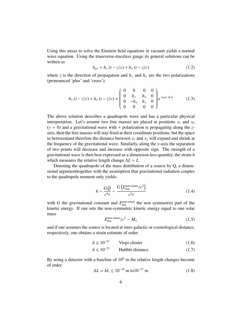
Using this ansaz to solve the Einstein field equations in vacuum yields a normalwave equation. Using the transverse-traceless gauge its general solutions can bewritten as
hµν = h+ (t − z/c) + h× (t − z/c) (1.2)
where z is the direction of propagation and h+ and h× are the two polarizations(pronounced ‘plus’ and ‘cross’):
h+ (t − z/c) + h× (t − z/c) =
0 0 0 00 h+ h× 00 −h× h+ 00 0 0 0
e (iωt−ikx) (1.3)
The above solution describes a quadrupole wave and has a particular physicalinterpretation. Let’s assume two free masses are placed at positions x1 and x2
(y = 0) and a gravitational wave with + polarization is propagating along the z-axis, then the free masses will stay fixed at their coordinate positions, but the spacein between|and therefore the distance between x1 and x2 will expand and shrink atthe frequency of the gravitational wave. Similarly, along the y-axis the separationof two points will decrease and increase with opposite sign. The strength of agravitational wave is then best expressed as a dimension-less quantity, the strain hwhich measures the relative length change ∆L = L.
Denoting the quadrupole of the mass distribution of a source by Q, a dimen-sional argument|together with the assumption that gravitational radiation couplesto the quadrupole moment only yields:
h ∼GQc4r∼
G(Enon-simm
kin /c2)
c2r(1.4)
with G the gravitational constant and Enon-simmkin the non symmetrict part of the
kinetic energy. If one sets the non-symmetric kinetic energy equal to one solarmass
Enon-simmkin /c2 ∼ M� (1.5)
and if one assumes the source is located at inter-galactic or cosmological distance,respectively, one obtains a strain estimate of order
h . 10−21 Virgo cluster (1.6)
h . 10−23 Hubble distance. (1.7)
By using a detector with a baseline of 104 m the relative length changes becomeof order:
∆L = hL . 10−19 m to10−17 m (1.8)
6

This is a rather optimistic estimate. Most sources will radiate significantly lessenergy in gravitational waves.
Similarly, one can estimate the upper bound for the frequencies of gravita-tional waves. A gravitational wave source can not be much smaller than itsSchwarzshild radius 2GM/c2, and cannot emit strongly at periods shorter thanthe light travel time 4πGM/c3 around its circumference. This yields a maximumfrequency of
f ≤c3
4πGM∼ 104 Hz
M�M
(1.9)
From the above equation one can see that the expected frequencies of emittedgravitational waves is the highest for massive compact objects, such as neutronstars or solar mass black holes.
Gravitational waves are quite different from electro-magnetic waves. Mostelectro-magnetic waves originate from excited atoms and molecules, whereas ob-servable gravitational waves are emitted by accelerated massive objects. Also,electro-magnetic waves are easily scattered and absorbed by dust clouds betweenthe object and the observer, whereas gravitational waves will pass through themalmost unaffected. This gives rise to the expectation that the detection of grav-itational waves will reveal a new and different view of the universe. In particu-lar, it might lead to new insights in strong field gravity by observing black holesignatures, large scale nuclear matter (neutron stars) and the inner processes ofsupernova explosions. Of course, stepping into a new territory also carries thepossibility to encounter the unexpected and to discover new kinds of astrophysi-cal objects.
1.2 Interferometric DetectorsAn interferometer uses the interference of light beams typically to measure dis-place ments. An incoming beam is split so that one component may be used as areference while another part is used to probe the element under test The changein interference pattern results in a change in intensity of the output beam whichis detected by a photodiode. By using the wavelength of light as a metric in-terferometers can easily measure distances on the scales of nanometers and withcare much more sensitive measurements may be made. The light source used isa laser, a highly collimated single frequency light making possible very sensitiveinterference fringes.
In a Michelson interferometer the laser beam is split at the surface of the beamsplitter (BS) into two orthogonal directions. At the end of each arm a suspendedmirror reflects the beam back to the BS. The beams reflected from the arms re-combine on the BS surface. A fraction of the recombined beam transmits through
7

CHAPTER �� THE DETECTION OF GRAVITATIONAL WAVES �
Laser
Detector
Beamsplitter
Figure ���� A Michelson interferometer�
����� Interferometeric Detectors
An interferometer uses the interference of light beams typically to measure displace�
ments� An incoming beam is split� so that one component may be used as a reference
while another part is used to probe the element under test� The change in interfer�
ence pattern results in a change in intensity of the output beam which is detected
by a photodiode� By using the wavelength of light as a metric� interferometers can
easily measure distances on the scales of nanometres and� with care� much more
sensitive measurements may be made� The light source used is a laser� a highly col�
limated� single frequency light� making possible very sensitive interference fringes�
Dierent con�gurations can be used to measure angles� surfaces� or lengths�
The use of interferometers to detect gravity waves was originally investigated by
Forward and Weiss in the �����s���� ���� To use an interferometer to detect gravity
waves� two masses are set a distance apart� each resting undisturbed in inertial
space� When a gravity wave passes between the masses� the masses will be pushed
and pulled� By measuring the distance between these two masses very accurately�
the very small eect of the gravity waves may be detected� The simplest Michelson
interferometer is shown in �gure ���� The input beam is split at a beamsplitter�
sending one half of the light into each arm� Fortuitously� the quadrupole moment
Figure 1.1: Scheme of a basic Michelson interferometer.
the BS and the rest is reflected from it. The intensity of each recombined beamis determined by the interferometer conditions and is detected by a photo detector(PD) that gives the differential position signal from the apparatus.
A Michelson interferometer can detect gravitational waves from the tidal ac-tion on the two end mirrors. The change of the metric between the two mirrorbecause of a gravitational wave causes a phase shift detectable by the interferom-eter.
The optimal solution would be to build Michelson interferometers with armsas long as 1/2 of the GW wavelength, which would require hundreds or thousandsof km. Folding the light path into an optical cavity (Fabry-Perot) is the solutionapplied to solve the problem.
The interferometric signal can be detected most sensitively by operating theinterferometer on a dark fringe, when the resulting intensity at the photodetector isa minimum. Since power is conserved, and very little light power is lost in passingthrough the interferometer, most of the input laser power is reflected from theinterferometer back towards the input laser. Since increasing laser power resultsin better sensitivity rather than ’waste’ this reflected power, a partially transmittingmirror can be placed between the input laser and the beam splitter. This allowsthe entire interferometer to form an optically resonant cavity with a potentiallylarge increase in power in the interferometer. This is called power recycling andis shown schematically by the mirror labeled PR in fig.1.2.
Based on this idea several interferometric detectors have been built in theworld: a 3 Km detector in Italy (VIRGO) [40], a 600 m in Germany (GEO600)[41], a 300 m in Japan (TAMA) [42] and two twin 4 Km and a 2 Km in USA
8

CHAPTER �� THE DETECTION OF GRAVITATIONAL WAVES ��
PR
SR
Figure ���� Power and signal recycling in a simple Michelson interferometer� MirrorPR re�ects any exiting laser power back into the interferometer� while mirror SRre�ects the output signal back into the system�
a Fabry�Perot cavity relies on having a partially transmitting optic� which restricts
the material used in the mirror to be transmissive and to have very low absorption�
In addition� systems using Fabry�Perot cavities have the additional di�culty that
the the cavities must be maintained on resonance� resulting in more complicated
control systems�
Power Recycling Signal Recycling and Other Con�gurations
The interferometric signal can be detected most sensitively by operating the inter�
ferometer on a dark fringe� when the resulting intensity at the photodetector is a
minimum� Since power is conserved� and very little light power is lost in passing
through the interferometer� most of the input laser power is re�ected from the in�
terferometer back towards the input laser� Since increasing laser power results in
better sensitivity section ������� rather than �waste� this re�ected power� a partially
transmitting mirror can be placed between the input laser and the beam splitter�
This allows the entire interferometer to form an optically resonant cavity� much like
the Fabry�Perot cavities discussed earlier� with a potentially large increase in power
in the interferometer� This is called power recycling� and is shown schematically by
the mirror labelled PR in �gure ����
Figure 1.2: Power and signal recycling in a simple Michelson interferometer. MirrorPR reflects any exiting laser power back into the interferometer, while mirror SRreflects the output signal back into the system.
(LIGO) [17]. Virgo e LIGO are fully active, LIGO at nominal sensitivity andVirgo approaching it. All four observatories Virgo, LIGO and GEO are takingdata as an unified network since May 2007.
1.2.1 The LIGO Interferometers
The LIGO Project consists of two observatories, one in Hanford, Washington, andthe other in Livingston, Louisiana, 3000 Km far away from each other (fig.1.5)[47]. The Virgo interferometer, Located in Cascina, Italy, has 3 km long arms,while the smaller GEO in Hanover, Germany, has 800 m arms and no FP cavities.The four interferometers operate together and share data to maximize the effort todetect gravitational waves.
The two LIGO interferometers, with 4 Km long arms, operate in coincidenceto reject local noise sources. Gradual improvement of the different parts of thedetector are planned in forthcoming years; in LIGO the currently considered up-grades concern the laser (higher power), the mirror substrate, the mirror suspen-sion (fused silica) and the seismic isolation system (this thesis is a contribution tothe new seismic isolation system development). The spectral sensitivity curve ofLIGO I is shown in fig.1.3 along with the contribution of the different sources ofnoise.
The low frequency limit of the detector is set by the cut-off of the “seismicwall”, located for LIGO I above 40 Hz. At higher frequencies the sensitivityof the interferometer is limited from 40 to 120 Hz by the thermal noise of themirror suspension. Above 120 Hz the shot noise dominates. Figure 1.4 shows thesensitivity improvement expected from LIGO II, whose start-up is scheduled for
9

AJW, LIGO SURF, 6/16/06
Initial LIGO Sensitivity Goal
Strain sensitivity < 3x10-23 1/Hz1/2
at 200 HzDisplacement Noise
» Seismic motion» Thermal Noise» Radiation Pressure
Sensing Noise» Photon Shot Noise» Residual Gas
Facilities limits much lower
BIG CHALLENGE:reduce all other (non-fundamental, or technical) noise sources to insignificance
Figure 1.3: Initial LIGO strain sensitivity curve.
2011. [43].
1.3 Seismic NoiseSeismic motion is an inevitable noise source for interferometers built on the Earth’scrust. The signal of an interferometer caused by the continuous and randomground motion is called seismic noise. The ground motion transmitted throughthe mechanical connection between the ground and the test masses results in per-turbations of the test masses separation.
Since the ground motion is of the order of 10−6 m at 1 Hz and the expectedGW signal is less than 10−18 m, we need attenuation factors of the order of 10−12.
As the amplitude of the horizontal ground motion in general is larger at lowerfrequencies, the seismic motion will primarily limit the sensitivity of an interfer-ometer in the low frequency band, usually below several tens of Hertz1.
1Below 10 Hz the seismically induced variations of rock density produce fluctuations of theNewtonian attraction to the test mass that bypass any seismic attenuation system (Newtoniannoise) and overwhelm any possible GW signal.
10

LIGO-T010075-00-D
page 3 of 24
mal noise•
Residual gas:
beam tube pressure, 10
–-9
torr, H
2
The strain sensitivity estimate for an interferometer using fused silica test masses is given inAppendix A.
3.2. Non-gaussian noise
Care must be taken in designing the interferometer subsystems to avoid potential generation ofnon-gaussian noise (avoiding highly stressed mechanical elements, e.g.).
3.3. Availability
The availability requirements for initial LIGO, specified in the
LIGO Science Requirements Doc-ument
, E950018-02-E, are applied to the advanced LIGO interferometers; in short:
• 90% availability for a single interferometer (integrated annually); minimum continuous operating period of 40 hours
• 85% availability for two interferometers in coincidence; minimum continuous operating period of 100 hours
• 75% availability for three interferometers in coincidence; minimum continuous operating period of 100 hours
101
102
103
104
10−25
10−24
10−23
10−22
10−21
Frequency (Hz)
h(f)
/ H
z1/
2Quantum Int. thermal Susp. thermalResidual Gas Total noise
Figure 1. Current estimate of the advanced LIGO interferometer strain sensitivity, calculated usingBENCH, v. 1.10. The design uses 40 kg sapphire test masses, signal recycling, and 125 W inputpower. The neutron-star binary inspiral detection range for a single such interferometer is 209 Mpc.
Figure 1.4: Advanced LIGO strain sensitivity curve.
A typical model for the power spectrum of the ground motion for above 100mHz is given by
x = a/ f 2 [m/√
Hz] (1.10)
where a is a constant dependent on the site and varies from 10−7 to 10−9. Themodel assumes the motion to be isotropic in the vertical and horizontal directions.
The surface waves that originate the seismic ground motion are a composedof Rayleigh waves (a mix of longitudinal and transversal waves that originate thehorizontal displacement) and Lowes waves (transverse waves that originate thevertical motion). The ground can also have an angular mode of motion, with notranslation. There is no direct measurement of the power spectrum associated tothis kind of seismic motions, so a typical way to have an estimation is to considerthe only contributions given by the vertical component of Rayleigh waves:
θ =2π f
cS v. (1.11)
θ and S v are the angular power spectrum ([rad/√
Hz]) and the vertical power spec-trum ([m/
√Hz]), c is the local speed of the seismic waves. This depends mainly
on the composition of the crust and it is also a function of the frequency. Lowerspeeds correspond to larger amplitude of the ground tilt, then the lowest valuescan be used to set an upper limit [23].
11
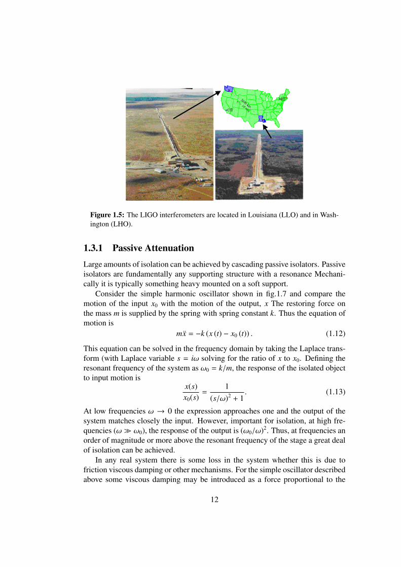
Figure 1.5: The LIGO interferometers are located in Louisiana (LLO) and in Wash-ington (LHO).
1.3.1 Passive Attenuation
Large amounts of isolation can be achieved by cascading passive isolators. Passiveisolators are fundamentally any supporting structure with a resonance Mechani-cally it is typically something heavy mounted on a soft support.
Consider the simple harmonic oscillator shown in fig.1.7 and compare themotion of the input x0 with the motion of the output, x The restoring force onthe mass m is supplied by the spring with spring constant k. Thus the equation ofmotion is
mx = −k (x (t) − x0 (t)) . (1.12)
This equation can be solved in the frequency domain by taking the Laplace trans-form (with Laplace variable s = iω solving for the ratio of x to x0. Defining theresonant frequency of the system as ω0 = k/m, the response of the isolated objectto input motion is
x(s)x0(s)
=1
(s/ω)2 + 1. (1.13)
At low frequencies ω → 0 the expression approaches one and the output of thesystem matches closely the input. However, important for isolation, at high fre-quencies (ω � ω0), the response of the output is (ω0/ω)2. Thus, at frequencies anorder of magnitude or more above the resonant frequency of the stage a great dealof isolation can be achieved.
In any real system there is some loss in the system whether this is due tofriction viscous damping or other mechanisms. For the simple oscillator describedabove some viscous damping may be introduced as a force proportional to the
12

Figure 1.6: Recent sensitivity curve of the main operating GW interferometrs: GEO,LIGO (LLO and LHO), Virgo.
relative velocity, Fv = −γ (x − x0). This represents for example the motion of thisoscillator in air. Then the transfer function from ground input to mass output is
x(s)x0(s)
=2η(s/ω0) + 1
(s/ω)2 + 2η(s/ω0) + 1(1.14)
where the damping ratio η is given for this viscously damped case by η = γ/2mω0.Particularly for systems with very little damping the system is often parametrizedwith the quality factor of the resonance, the Q rather than the damping ratio η,where
Q =12η. (1.15)
The response of a system with Q ≈ 10 is shown in fig.1.8. There are two im-portant characteristics of the magnitude of the frequency response in contrast toa system with infinite Q. First, the height of the resonant peak at ω0 is roughlyQ times the low frequency response. Second, the response of the system is pro-portional to (ω0/ω)2 above the resonant frequency up to about a frequency Qω0.Above this point the system response falls only as 1/ω. These conclusions aredrawn for viscously damped systems. For low loss systems for any form of loss,
13

Figure 1.7: A one dimensional simple harmonic oscillator with spring constant k andmass m The mass is constrained to move frictionlessly in one direction horizontal
CHAPTER �� MECHANICAL SUSPENSION IN INTERFEROMETERS ��
Q��
Q
� ���
� ���
Transfer Function of a Damped Simple Harmonic Oscillator
Frequency �����
jX�
X�j
���������
���
���
���
����
����
����
Figure ���� Response of a simple harmonic isolator with �nite Q
with the quality factor of the resonance� the Q� rather than the damping ratio� ��
where
Q "�
��� ����
The response of a system with Q � �� is shown in �gure ���� There are two im�
portant characteristics of the magnitude of the frequency response in contrast to a
system with in�nite Q� Firstly� the height of the resonant peak at �� is roughly Q
times the low frequency response� Secondly� the response of the system is propor�
tional to ������ above the resonant frequency up to about a frequency Q��� Above
this point� the system response falls only as ���� These conclusions are drawn for
viscously damped systems� For low loss systems� for any form of loss� the system
response will fall proportionally to ���� for frequencies a decade or more above the
resonant frequency�
Passive isolation has a number of advantages in comparison to �active� isolation
stages to be discussed shortly� A system is passive in that it supplies no energy to the
system and thus requires no energy source� Because it adds no energy to the system�
it is guaranteed to be stable� As it has fewer components than an active system�
it can be considered more mechanically and electrically reliable� Its performance is
Figure 1.8: Response of a simple harmonic isolator with finite Q.
the system response will fall proportionally to 1/ω2 for frequencies a decade ormore above the resonant frequency.
Passive isolation has a number of advantages. A system is passive in that itsupplies no energy to the system and thus requires no energy source as opposedto an active system, which senses the mechanical energy fed into the system andcounter it with external forces. Because it adds no energy to the system, it isguaranteed to be stable. As it has fewer components than an active system, it canbe considered more mechanically and electrically reliable. Its performance is notsensor or actuator limited.
The required seismic attenuation is obtained using a chain of mechanical os-cillators of resonant frequency lower than the frequency region of interest. In thehorizontal direction the simple pendulum is the most straightforward and effec-tive solution: the suspension wire has a negligible mass and the attenuation factorbehaves like 1/ f 2 till the first violin mode of the wire (tens or hundreds of Hertz).Thus, with reasonable pendulum lengths (tens of cm), good attenuation factorscan be easily achieved in the frequency band of interest (above 10 Hz) for the x
14

and y directions. A simple pendulum is even more effective for the yaw mode;torsional frequencies of few tens of millihertz are easy to be obtained. A masssuspended by a wire has also two independent degrees of freedom of tilt, the pitchand the roll; low resonant frequencies (<0.5 Hz) and high attenuation factors forthese modes are obtained by attaching the wire as close as possible to the centerof mass of the individual filters.
The difficult part in achieving high isolation in all the 6 d.o.f.s is to gener-ate good vertical attenuation. The vertical noise is, in principle, orthogonal tothe sensitivity of the interferometer. Actually the 0.1-1% of the vertical motionis transferred to the horizontal direction at each attenuation stage by mechanicalimperfections, misalignments and, ultimately (at the 10−4 level), by the non par-allelism of verticality (the Earth curvature effects) on locations kilometers apart.The vertical attenuation then becomes practically as important as the others.
In the gravitational wave detectors, every test mass is suspended by a pendu-lum to behave as a free particle in the sensitive direction of the interferometer. Thetypical resonant frequency of the pendulum is 1 Hz. In such a case, at 100 Hz, thelowest frequency of the GW detection band, the attenuation factor provided in thependulum is about 10−4. From the simple model of the seismic motion (eq.1.10),neglecting the vertical to horizontal cross-couplings, and assuming a quiet sitea = 10−9, the motion of the test mass induced by the seismic motion reaches theorder of 10−13m/
√Hz, corresponding to a strain h ∼ 10−16 to 10−15 depending n
the scale of the detector. This is far above the required level (typically at least10−21 in strain), and the attenuation performance needs to be improved. This im-provement can be easily achieved by connecting the mechanical filters in series. Inthe high frequency approximation, the asymptotic trend of the attenuation factorimproves as 1/ωn where n is the number of the cascaded filters. Thence by addinga few more stages above the mirror suspension, one can realize the required at-tenuation performance by simply using the passive mechanics. An example ofthis strategy are the stack system composed by layers of rubber springs and heavystainless steel blocks interposed between the mirror suspension system and theground in LIGO, TAMA300 and GEO600.
Another way to improve the isolation performance is to lower the resonantfrequency of the mechanics. By shifting lower the resonant frequencies, one cangreatly improve the attenuation performance at higher frequency. Virgo utilizedthis approach and realized extremely high attenuation performance starting at lowfrequency (4 to 6 Hz) with the a low frequency isolation system coupled to amulti-stage suspension system called Supper Attenuator (SA) [31].
15

16

Chapter 2
HAM Seismic Attenuation System
The configuration of advanced LIGO is a power-recycled and signal-recycledMichelson interferometer with Fabry-Perot cavities in the arms - i.e., initial LIGO,plus signal recycling. The principal benefit of signal recycling is the ability to re-duce the optical power in the substrates of the beamsplitter and arm input mirrors,thus reducing thermal distortions due to absorption in the material. To illustratethis advantage, the baseline design can be compared with a non-signalrecycledversion, using the same input laser power but with mirror reflectivities re-optimized.The signal recycled design has a (single interferometer) NBI (Neutron Binary In-spiral) range of 200 Mpc, with a beamsplitter power of 2.1 kW; the non-SR designhas a NBI range of 180 Mpc, but with a beamsplitter power of 36 kW. Alterna-tively, if the beamsplitter power is limited to 2.1 kW, the non-SR design wouldhave a NBI range of about 140 Mpc.
An important new component in the design is an output mode cleaner. Theprincipal motivation to include this is to limit the power at the output port to amanageable level, given the much higher power levels in the interferometer com-pared to initial LIGO.
With an output mode cleaner all but the TEM00 component of the contrastdefect would be rejected by a factor of ∼1000, leaving an order 1 mW of carrierpower. The OMC will be mounted in-vacuum on a HAM isolation platform, andwill have a finesse of order 100 to give high transmission (>99 percent) for theTEM00 mode and high rejection (>1000) of higher order modes.
Earlier attempts to implement an external OMC failed because of seismicnoise couplings. It was found necessary to implement a seismic attenuated, in-vacuum OMC and detection diodes.
17

LIGO-T010075-00-D
page 5 of 24
4.1. Signal recycling configuration
The configuration of the advanced interferometers is a power-recycled and signal-recycled Mich-elson interferometer with Fabry-Perot cavities in the arms–i.e., initial LIGO, plus signal recycling.Mirror reflectivities are chosen based on thermal distortion and other optical loss estimates, andaccording to the optimization of NBI detection. To limit system complexity, the signal recycling isnot required to have broad tuning capability
in situ
(i.e., no compound signal recycling mirror; norany kind of ‘multi-disc cd player’ approach, involving multiple signal recycling mirrors on a car-ousel), though it may have some useful tunability around the optimal point.
The principal benefit of signal recycling is the ability to reduce the optical power in the substratesof the beam splitter and arm input mirrors, thus reducing thermal distortions due to absorption inthe material. To illustrate this advantage, the baseline design can be compared with a non-signal-recycled version, using the same input laser power but with mirror reflectivities re-optimized. Thesignal recycled design has a (single interferometer) NBI range of 200 Mpc, with a beamsplitterpower of 2.1 kW; the non-SR design has a NBI range of 180 Mpc, but with a beamsplitter powerof 36 kW. Alternatively, if the beamsplitter power is limited to 2.1 kW, the non-SR design wouldhave a NBI range of about 140 Mpc.
T=0.5%
OUTPUT MODECLEANER
INPUT MODECLEANER
LASER MOD.
T=7%
SAPPHIRE, 31.4CMφ
SILICA, HERAEUS SV 35CMφ
SILICA, LIGO I GRADE~26CMφ
125W 830KW
40KG
PRM
SRM
BSITM ETM
GW READOUT
PD
T~6%
ACTIVE
CORRECTIONTHERMAL
Figure 2. Basic layout of an advanced LIGO interferometer.Figure 2.1: Basic layout of an advanced LIGO interferometer.
2.1 Seismic Isolation for the OMCIsolation of the LIGO II optics from ambient vibration is accomplished by theseismic isolation systems which must provide the following functions:
• provide vibration isolated support for the payload(s)
• provide a mechanical and functional interface for the suspensions
• provide adequate space and flexibility for mounting of components (suspen-sions and auxiliary optics) and adequate space for access to components
• provide coarse positioning capability for the isolated supports/platforms
• provide external actuation suitable for use by the interferometer’s globalcontrol system to maintain long-term positioning and alignment
• provide means for the transmission of power and signals from control elec-tronics outside the vacuum chambers to the suspension systems and anyother payloads requiring monitoring and/or control
18
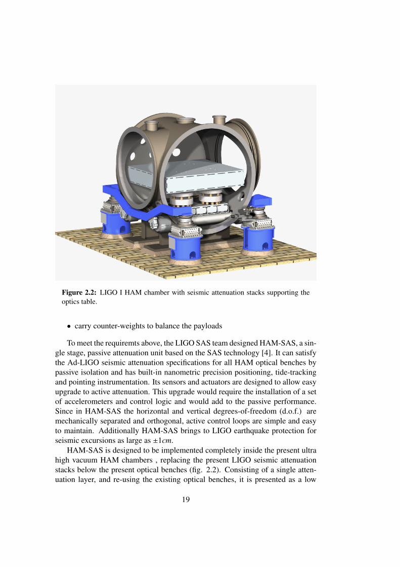
Figure 2.2: LIGO I HAM chamber with seismic attenuation stacks supporting theoptics table.
• carry counter-weights to balance the payloads
To meet the requiremts above, the LIGO SAS team designed HAM-SAS, a sin-gle stage, passive attenuation unit based on the SAS technology [4]. It can satisfythe Ad-LIGO seismic attenuation specifications for all HAM optical benches bypassive isolation and has built-in nanometric precision positioning, tide-trackingand pointing instrumentation. Its sensors and actuators are designed to allow easyupgrade to active attenuation. This upgrade would require the installation of a setof accelerometers and control logic and would add to the passive performance.Since in HAM-SAS the horizontal and vertical degrees-of-freedom (d.o.f.) aremechanically separated and orthogonal, active control loops are simple and easyto maintain. Additionally HAM-SAS brings to LIGO earthquake protection forseismic excursions as large as ±1cm.
HAM-SAS is designed to be implemented completely inside the present ultrahigh vacuum HAM chambers , replacing the present LIGO seismic attenuationstacks below the present optical benches (fig. 2.2). Consisting of a single atten-uation layer, and re-using the existing optical benches, it is presented as a low
19

cost and less complex alternative to the Ad-LIGO baseline with three-stage activeattenuation system [5, 6].
Also HAM-SAS is based on an technology akin to the multiple pendulumsuspensions that it supports, thus offering a coherent seismic attenuation systemto the mirror suspension.
Even though the specific design is adapted to the HAM vacuum chambers, theSAS system was designed to satisfy the requirements of the optical benches of theBSC chambers as well. HAM-SAS can be straightforwardly scaled up to isolatethe heavier BSC optical benches.
Unlike the baseline Ad-LIGO active system, HAM-SAS does not require in-strumentation on the piers [9, 10].
2.2 System OverviewHAM-SAS is composed of three parts:
• a set of four inverted pendulums (IP) for horizontal attenuation supportedby a base plate;
• a set of four geometric anti spring (GAS) springs for vertical attenuation ,housed in a rigid “spring box”;
• eight groups of nm resolution linear variable differential transformers (LVDT),position sensors and non-contacting actuators for positioning and pointingof the optical bench. Micropositioning springs ensure the static alignmentof the optical table to micrometric precision even in the case of power loss.
The existing optical bench is supported by a spring-box composed by twoaluminum plates and the body of four GAS springs (fig. 2.3, 2.4). The GASsprings support the bench on a modified kinematical mount; each filter is pro-vided with coaxial LVDT position sensors and voice coil actuators, and parasitic,micrometrically tuned, springs to control vertical positioning and tilts. The springbox is mounted on IP legs that provide the horizontal isolation and compliance.The movements of the spring-box are also controlled by four groups of co-locatedLVDT position sensors, voice coil actuators and parasitic springs. The IP legs bolton a rigid platform which rests on the existing horizontal cross beam tubes.
2.3 Vertical StageThe vertical stage of HAM-SAS consist of the Spring Box. Inside of it, four GASfilters are held rigidly together to support the load of the optics table and to provide
20

Figure 2.3: HAM-SAS assembly. From bottom to top: base plate, IP legs, spring boxwith GAS filters, optics table. The red weights on top represent the actual payload.
Figure 2.4: Spring Box assembly.
21

Figure 2.5: HAM-SAS still in the clean romm at the production site before the bak-ing process. The spring box is tight to the base plate by stainless stell columns. Thetop plate is bolt to the spring box for the transfer.
the vertical seismic isolation. The interface between the optical table and the GASfilters is an aluminum plate with four stainless steel pins sticking down from thecorners, each with a particularly shaped bottom mating surface, according to ascheme of the distribution and positioning of the load known as quasi-kinematicmount. Two opposite ones are simple cylinders with a flat bottom surface, theother two have one conical hollow and a narrow V-slot respectively. Each of theGAS filter culminates in a threaded rod having a hardened ball bearing sphereembedded at the top. The quasi-kinematic configuration is such that the table’spins mate to the filters’ spheres thus precisely positioning the table while avoidingto over-constrain it . The contact point between the spheres and the surfaces letthe table free to tilt about the horizontal axis.
2.3.1 The GAS filter
The GAS filter (fig. 2.6) consists of a set of radially-arranged cantilever springs,clamped at the base to a common frame ring and opposing each other via a centraldisk or keystone. The blades are flat when manufactured and under load bendlike a fishing rod. We used modified Monolithic GAS (MGAS) filters [12]. Asthe MGAS the tips of the crown of blades are rigidly connected to the centraldisk supporting the payload. Instead of being made by a large, single sheet ofbent maraging, we bolted the tips of independent blades to a central “keystone”.Being built of different parts the spring is not, strictly speaking, “monolithic”,but it shares all the performance improvements of the monolithic spring. For
22
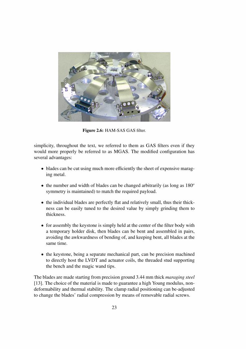
Figure 2.6: HAM-SAS GAS filter.
simplicity, throughout the text, we referred to them as GAS filters even if theywould more properly be referred to as MGAS. The modified configuration hasseveral advantages:
• blades can be cut using much more efficiently the sheet of expensive marag-ing metal.
• the number and width of blades can be changed arbitrarily (as long as 180o
symmetry is maintained) to match the required payload.
• the individual blades are perfectly flat and relatively small, thus their thick-ness can be easily tuned to the desired value by simply grinding them tothickness.
• for assembly the keystone is simply held at the center of the filter body witha temporary holder disk, then blades can be bent and assembled in pairs,avoiding the awkwardness of bending of, and keeping bent, all blades at thesame time.
• the keystone, being a separate mechanical part, can be precision machinedto directly host the LVDT and actuator coils, the threaded stud supportingthe bench and the magic wand tips.
The blades are made starting from precision ground 3.44 mm thick maraging steel[13]. The choice of the material is made to guarantee a high Young modulus, non-deformability and thermal stability. The clamp radial positioning can be-adjustedto change the blades’ radial compression by means of removable radial screws.
23

10−1
100
101
102
−70
−60
−50
−40
−30
−20
−10
0
10
20
Frequency [Hz]
Mag
nitu
de [d
B]
Figure 2.7: GAS filter transmissibility measured at Caltech in 2005 on a three blade,3mm thick bench prototype [14]
At frequencies lower than a critical value the GAS filter’s vertical transmissi-bility1 from ground to the payload has the typical shape of a simple second orderfilter’s transfer function (2.7). The amplitude plot is unitary at low frequencies,then has a resonance peak then followed by a trend inversely proportional to thesquare of the frequency. Above a critical frequency the amplitude stops decreas-ing and plateaus. This high frequency saturation effect is due to the distributedmass of the blades; the transmissibility of a compound pendulum has the samefeatures.
A typical GAS filter can achieve -60 dB of vertical attenuation in its simpleconfiguration, this performance can be improved to -80 dB with the application ofa device called “Magic Wand” (see sec.2.3.6).
An effective low frequency transmissibility for the GAS filter is2
Hz(ω) =ω2
0(1 + iφ) + βω2
ω20(1 + iφ) + ω2
, (2.1)
1In Linear Time Invariant systems, the so called transfer function H(s) relates the Laplacetransform of the input i(s) and the output o(s) of a system, i.e. o(s) = H(s)i(s) or o(s)/i(s) = H(s).The transmissibility, a dimensionless transfer function where the input and the output are thesame type of dynamics variables (position, velocity, or acceleration), is therefore the appropriatequantity to use when measuring the attenuation performance of a mechanical filter.
2Since the GAS filter is designed to work under vacuum the viscous damping term has beenneglected.
24

Figure 2.8: GAS Springs Model
where ω20 is the angular frequency of the vertical resonance, φ the loss angle ac-
counting for the blades’ structural/hysteretic damping and β is a function of themass distribution of the blades.
A simple way to model the GAS filter is to represent the payload of mass m0
suspended by a vertical spring of elastic constant kz and rest length l0z and by twohorizontal springs opposing each other of constant kx and rest length l0x (fig.2.8).The angle made by the horizontal springs is θ and it is zero at the equilibriumpoint when the elongations of the springs are zeq and x0 for the vertical and thehorizontal respectively. The equation of motion for the system is then:
mz = kz(zeq − z − l0z) − kx(lx − l0x) sin θ − mg (2.2)
where lx =
√x2
0 + z2 is the length of the horizontal spring. Approximating sin θto z/x0 for small angles (2.2) reduces to
mz = kz(zeq − z − l0z) − kx
(1 −
l0x
x0
)z − mg. (2.3)
We can see that at the first order the system behaves like a linear harmonicoscillator with effective spring constant
ke f f = kz + kx −kxl0x
x0. (2.4)
The last term of (2.4) is referred as the Geometric Anti-Spring contribute becauseit introduces a negative spring constant into the system. As consequence of it theeffective stiffness is reduced, and so the resonant frequency, by just compressing
25
the horizontal springs. The system’s response is then that of a second order lowpass filter with a very low resonance frequency of the order of 0.1 Hz. Comparedwith an equivalent spring with the same frequency, it is much more compact andwith motion limited to only one direction.
2.3.2 Equilibrium point position to load dependence
According to this model, at the equilibrium point the vertical spring holds alonethe payload and we have that
zeq =m0gkz+ l0z (2.5)
from which the equation of motion becomes
mz = kz
(m0gkz− z
)− kxz − kxl0x
z√x2
0 + z2− mg. (2.6)
We can find how, in the small angle approximation, the position of the equilibriumpoint changes in correspondence of a variation of the payload’s mass when m =m0 + δm in the equation of motion (2.6). We obtain:
δm = −kz + kx
gz +
kxl0x
gz√
x20 + z2
. (2.7)
Defining the compression asl0x − x0
l0x(2.8)
we have that the position of the equilibrium point changes for different valuesof compression as in fig.2.9. As shown in the model, above a critical value ofthe compression the system has three equilibrium points in correspondence of thesame payload, two are stable and one unstable. In this condition we say that thesystem is bi-stable. This implies that in case of very low frequency tuning of theGAS filter one has to avoid that the dynamic range of the system does not includemultiple equilibrium points in order to avoid bi-stability3.
3The optimal tune of the filter is very close to this critical compression value (at the criticalpoint the recalling force of the spring and its mechanical noise transmission is null), but bi-stabilitycannot be tolerated.
26

−40 −30 −20 −10 0 10 20 30 40−300
−200
−100
0
100
200
300
Load Variation [Kg]
Wor
king
Poi
nt[m
m]
1 %19 %30 %
Figure 2.9: Equilibrium Point displacement for a variation of the payload’s massin correspondence of several compressions. The compression ratio in the legend isdefined as (l0x − x0)/(l0x).
2.3.3 Resonant frequency to load variation
Linearizing (2.6) it is possible to define the effective spring constant of the systemcorrespondent to a change in the payload’s mass as the derivative of the total forceapplied to it as evaluated at the equilibrium point:
ke f f (z) = −(∂ f∂z
)= kz + kx
(1 −
l0xx20
(x20 + z2)3/2
)(2.9)
where f is equal to the right side of 2.6. The plot on fig.2.10 shows the effect ofthe bi-stability as negative values of the square of the resonant frequency whenthe compression exceeds the critical value.
It is possible to extract the relation between resonant frequency and workingpoint position when m = δm + m0 is evaluated at the equilibrium point (fig.2.11)obtaining:
ω =
√ke f f
m=
kz − kx
(l0x x2
0
(x20+z2)3/2 − 1
)m0 −
zg
(kx + kz −
kxl0x√x2
0+z2
)
1/2
. (2.10)
Plot 2.11 shows the frequency as a function of the equilibrium point. The curvescorresponding to different compressions of the blades tend asymptotically to the
27

−40 −30 −20 −10 0 10 20 30 40−2
−1
0
1
2
3
4
5
Load Variation [Kg]
Squ
are
Res
onan
t Fre
quen
cy [H
z]2
1 %19 %30 %
Figure 2.10: Dependence of the squared resonant frequency to the variation of thepayload’s mass at the equilibrium point.
straight lines forming a sharp V for values of the compression closer to the criticaland also the minimum for each compression slowly changes position.
2.3.4 Thermal StabilityOnce the compression and the payload is fixed, the system can be regarded as asoft linear spring which supports the payload. The thermal stability of the GAScan be studied under this approximation, valid in a small range around the workingposition [23]. In the GAS at the equilibrium, the entire vertical force of the systemcomes from the elasticity of the blade, and the working (equilibrium) positionis determined by a balance of the stiffness and the payload weight. From theequation (2.4), the variation of the effective spring for a given perturbation of thetemperature ∆T is
∆ke f f = ∆kz +
(1 −
l0x
x0
)∆kx −
kx
x0∆l0 +
kxl0x
x20
∆x0 (2.11)
in which we can separate the contribution of the physical expansion of the bladesand the frame ring from the change on the elasticity due to the temperature depen-dence of the Young modulus E as in the following:
∆ke f f =
{[kz +
(1 −
l0x
x0
)kx
]δEblade
E−
kx
x0l0x
(δLblade − δL f rame
)}∆T. (2.12)
28

−0.4 −0.3 −0.2 −0.1 0 0.1 0.2 0.30
0.2
0.4
0.6
0.8
1
1.2
1.4
Position [m]
Res
onan
t Fre
quen
cy [H
z]1 %10%15%19 %
Figure 2.11: Resonant frequency to equilibrium position for several values of com-pression. The minimum moves from the original position.
The geometrical contribution depends on the differential thermal expansion coeffi-cient of the blade and the frame (filter body). Assuming the use of maraging steelfor the blade, and of aluminum for the frame, the difference of their expansioncoefficients will be of order of 10−6.
∆ke f f =
[ke f f
(δEE
)blade−
kx
x0l0x
(δLblade − δl f rame
)]∆T. (2.13)
In the case of HAM-SAS, the relative variation of the Young modulus of maragingsteel for a Kelvin degree is about 3×10⁻⁴, the effective elastic constant of the fourfilters in parallel for a mass of about 1 ton and a resonant frequency of 200 mHzis 1.6 × 10³N/m. By assuming 9.0% of compression and substituting the parame-ters used in the plots above and the properties of maraging steel, one obtains thefollowing formula to estimate the variation of the effective spring constant:
∆ke f f = −
[(0.5)elasticity +
(10−3
)expansion
]∆T [N/m]. (2.14)
From the previous we can estimate the change in mass necessary to keep at thesame height the working point of the GAS filter as:
∆m =(∆ke f f
ke f f
)M∆T (2.15)
which turns out to be very useful to evaluate the environmental condition in whichthe actuators have sufficient authority to compensate for the temperature varia-tions.
29

���������������������
���������������������
����������������������������������������������������������������������������������������
����������������������������������������������������������������������������������������
meff
z0 payload
to the
Clamp
BladeIeffCounterweight
Clamp
Ll
Pivotμm, I
Pivotz
Figure 2.12: Rigid body representation of the GAS filter with a COP compensationwand. For sake of simplicity just one blade and one wand are sketched. Because ofits distributed mass, the low frequency blade’s dynamics can be approximated witha rigid body with effective mass and moment of inertia rotating about an horizontalaxis. A wand with a counterweight connected as shown in the figure, provides a wayof properly tune the center of percussion and remove the transmissibility saturation.
It is important to note that although the thermal sensitivity grows rapidly asthe resonant frequency is brought near zero, the correction authority requirementis independent of the frequency tune of the filter.
The GAS effect only reduces the elastic return forces, but cannot affect thehysteresis forces. As the critical compression level is approached, the hysteresistakes a progressively dominating role. From the static point of view, just prior tobistability, hysteresis makes the oscillator indifferent. From the dynamical pointof view hysteresis can turn the 1/ f 2 GAS filter TF behavior into a less favorable1/ f [34].
2.3.5 Quality Factor to Frequency DependenceFrom equation 2.4 we can deduce the dependence of the Q factor of the GASoscillator associating loss angles φ to each of the spring constants of our modeland to the overall effective constant. We can then write:
ke f f = kz (1 + iφz)(1 −
l0x
x0
)+ kx (1 + iφx) = keff (1 + iφeff) (2.16)
where the tildes mark the real part of the quantities. From the previous it followsthat:
φeff =kzφz (1 − l0x/x0) + kxφx
keff. (2.17)
Considering that keff = kz (1 − l0x/x0) + kx = Mω2 and that Q = 1/φ we have:
Q =ω2
ω2 − cQz. (2.18)
30

From 2.18 it follows that in the low frequency limit for ω → 0 it is Q ∝ ω2. Thisimplies that for very low frequency of tuning the Q drops naturally for histereticcauses and no damping is necessary [53].
2.3.6 The “Magic Wands”The term β in (2.1) that limits the attenuation of GAS filters at high frequenciesoriginates by the mass distribution in the blades and can be eliminated by theCenter Of Percussion correction. The COP and its effect can be exemplified bya compound pendulum constrained to move in the horizontal direction. Whenthe suspension point is forced to oscillate, in the high frequency limit, the pendu-lum body pivots around a fixed point, which is the COP. In the same way, if animpulsive force is applied along the COP the suspension point remains fixed.
A solution has been designed [15], [14] and it consists of a device that ismounted in parallel to the GAS springs. It consists essentially of a wand hingedto the filter frame ring and the central keystone. Attached to one end is a counter-weight whose function is to move the wand’s COP out of the pivot.
A reasonably accurate dynamical description of the system, which accountsfor the internal vibrational modes, can be obtained simply by considering thecurved blades as an elastic structure. However the low frequency dynamics andthe transmissibility saturation of the GAS filter with the wand can be easily andaccurately described in the rigid body approximation (see figure 2.12). In thisregime, the blade is represented as a vertical spring of spring constant kz; its dis-tributed mass is an effective rigid body with mass me f f , horizontal principal mo-ment of inertia Ie f f , with center of mass at distance le f f from the wand’s pivot. Thewand is modeled as a hollow cylinder of lenght d, moment of inertia I and massm, with a point-like counterweight of mass µ at one end. The distances along thewand from the pivot to the counterweight and to the wand’s tip are respectivelyl and L. The payload can be simply modeled with a point-like mass M. Underthese assumptions, the Lagrangian for small oscillations of the system is
L =12
Mz2 +12µ
(lL
z −L + l
Lz0
)2
+ (2.19)
12
me f f
(le f f
Lz −
L − le f f
Lz0
)2
+Ie f f
2L2 (z − z0)2 +
12
m(2L − d
2Lz +
d2L
z0
)2
+I
2L2 (z − z0)2 −
12
k(z − z0)2
where z is the generalized coordinate orthogonal to the constraints necessary to
31
describe the system’s dynamics, and z0 is the coordinate of the suspension point.The spring constant k is complex and can be rewritten as k = kz(1 + iφ) wherethe term φ and k are both real and have been introduced ad hoc to account for thestructural damping, which is the dominant dissipation mechanism of the blades.The gravitational potentials have not been included because they only fix the equi-librium position of the system and do not affect the dynamical solution.
Computing the Euler-Lagrange equation and solving it in the frequency do-main, we obtain the vertical transmissibility Hz(ω) of the mechanical system:
Hz(ω) =z(ω)z0(ω)
=ω2
0 − Aω2
ω20 − Bω2
in which:
A =d2
4L2 −d
2L+
Ie f f
mL2 +I
mL2 −me f f le f f
mL+
me f f l2e f f
mL2 +µl2
mL2 +µlmL
B = 1 +Mm+
d2
4L2 −dL+
Ie f f
mL2 +I
mL2 +me f f l2
e f f
mL2 +µl2
mL2
ω20 =
kz (1 + iφ)m
From (2.20) it follows that, in the limit ω → ∞, H(w) → A/B and a plateauappears in the transmissibility at high frequency. In principle it can be canceledreducing A to zero by tuning the counterweight’s moment of inertia µl2. WhenA , 0, because µl2 is either too small or too large, a complex conjugate zeropair appears in the transfer function and we say the system is under- or over-compensated respectively. Ideally neglecting the internal modes and setting thesystem at the transition between under-compensation and overcompensation, awell-tuned wand should be able to restore the theoretical 1/ω2 trend at the highfrequencies [15].
2.3.7 Vertical Modes of the System
The HAM-SAS’ vertical degrees of freedom can be simply modeled by a tableheld by four vertical springs. Each of them represents a GAS filter with an equaleffective spring constant k1, k2, k3, k4 and has null rest lengths. Let the tern (z, θ, φ)represent the coordinates of the system, M the total mass of the table, Iθ and Iφthe momentums of inertia of the table along the x axis and the y axis respectively,and l the table’s half length. We can deduce the equation of motion from theLagrangian of the system L = T −U in which the kinetic and the potential energy
32

Figure 2.13: "Magic Wand" designed for HAM-SAS. Presently not yet installed inthe system. They can provide an additional order of magnitude in vertical attenuation.
can be written as:
2T = Mz2 + Ixθ2 + Iyφ
2 (2.20)
2U = k1z21 + k2z2
2 + k3z23 + k4z2
4. (2.21)
zi are the elongations of the springs and can be written in terms of the coordinateof the system as:
z1 = z − lθ − lφ (2.22)z2 = z + lθ − lφ (2.23)z3 = z + lθ + lφ (2.24)z4 = z − lθ + lφ. (2.25)
Solving the equations of Eulero-Lagrange for the system we can write:
[M] x = Kx (2.26)
33

Figure 2.14: Dynamical model of the optics table.
where x represents the vector of the coordinates, [M] represents the inertia and Kis the stiffness matrix of the system:
K =
k1 + k2 + k3 + k4l2 (−k1 + k2 + k3 − k4) l
2 (−k1 + k2 + k3 + k4)l2 (−k1 + k2 + k3 − k4) l2(k1 + k2 + k3 + k4) l
2 (k1 − k2 + k3 − k4)l2 (−k1 + k2 + k3 + k4) l
2 (k1 − k2 + k3 − k4) l2(k1 + k2 + k3 + k4)
.(2.27)
From 2.27 the modes of the system correspond to the eigenvectors of K:
Kξ = λξ (2.28)
and the correspondent frequencies can be obtained from the relative eigenvalues:
ω20i =
λi
Mi. (2.29)
In the simple case in which the four spring constants are equal to each other theeigenfrequencies are:
ωz =
(4kM
)1/2
; ωx =
(2kl2
Ix
)1/2
; ωy =
(2kl2
Iy
)1/2
. (2.30)
From (2.30) we can see that the two angular frequencies depend on the system’smomentums of inertia and the two modes are degenerate in case of symmetry.
2.3.8 Tilt stabilizing springsIn general the table will not rest horizontally because of torques originated by theweight distributions and differences in the spring constants. Unlike the BSC case,in the HAM chambers the load is located above the seismic attenuation stage andthe effective tilt rotation axis. This torque is in competition with the stabilizingcomponent of the GAS springs. The GAS springs, though, are tuned to be veryweak, therefore the destabilizing torque eventually dominates and would resultin an unstable equilibrium. This problem was overseen in the initial design andsimulations, and discovered during initial tests. To solve this problem a systemof correcting springs has been introduced in the design of HAM-SAS in order toadd stiffness on the angular DOFs (see fig. 2.15). A vertical shaft was connected
34

Figure 2.15: Scheme of the tilt correcting springs added between the top plate andthe spring box.
to the underside of the top plate, attaching a cross of four springs connected tothe four corners of the spring box. The four springs hook to four wires and fourtuning screws to reach the spring box corners and allow fine tilt tuning.
The four tilt correcting springs work inevitably as a spring in parallel to theGAS springs and add stiffness in the vertical degree of freedom as well. Thespring constant of this effective vertical parallel spring is
k(z)tilt = 4
(1 −
l0
x0
)k (2.31)
where l0 is the springs’ rest length, x0 the spring elongation at the working pointand k their spring constant. k(z)
tilt can be made small keeping the working pointlength close to the rest length. Since the springs work in tension, x0 cannot bereduced arbitrarily but has to be always greater than l0 in all the dynamical rangeof the system.
The additional,and unwanted vertical stiffness can be cancelled by a small, insitu, correction compression of the GAS springs4.
2.4 Horizontal StageThe horizontal stage of HAM-SAS is based on four inverted pendulums that sup-port the spring box. Each of them is constituted by an aluminum hollow cylinder,448 mm long, 50 mm diameter and walls 1 mm thick hinged to the base plate by amaraging steel flex joint with diameter of 95 mm over the length of 50 mm5. This
4At this time, there has not been occasion for this fine adjustment yet.5The angular elasticity of this flex joint was calculated to balance the inverted pendulum desta-
bilization stiffness (−Mgh) for a mass of 250 kg per leg (1 ton total) over the 491 mm effective IPleg.
35

Figure 2.16: Supporting system for the spring box.
flex joint works in compression. The connection to of the Spring Box is obtainedby mean of a particular mechanical system (fig.2.16). In correspondence of eachattachment point the spring box is provided with a small steel bridge that hangsfrom a tensional flex joint made of a short maraging steel wire 30 mm long and3 mm diameter. The wire hangs from the IP’s leg cap. The bridge is providedwith 4 screws, two pushing and two pulling from the spring box plate. This ar-rangement permits to tune the height of the attachment point of the leg and thus tocompensate for spring box warping or differences on the leg’s length and equallydistribute the load between them (see section 3.3.1 for the process of tuning).
2.4.1 Inverted Pendulums
The inverted pendulums (IP) are designed to provide the seismic isolation alongthe horizontal directions. An IP is a compound pendulum hinged to the groundby a flex joint in such a way that the center of mass is above the pivot. Themodel represented in fig.2.17 illustrates how it works. M is the mass that has tobe isolated from the ground and it is connected to a rigid leg with momentum ofinertia I, mass m and length l by a flex joint producing an elastic force to whichcorresponds a complex spring constant κ = κ0(1 + iφ), where the imaginary termis introduced to take into account the structural damping. With these parameters
36

Figure 2.17: Inverted Pendulum Model
the equation of motion for the mass along the θ axis is then:
Iθ = −κθ + Mgl sin θ (2.32)
which describes an harmonic oscillator with effective spring constant
κe f f = κ − Mgl. (2.33)
From (2.33) we can see that the gravitation term Mgl acts like an anti-spring andreduces the overall stiffness and thus the resonant frequency.
The physics of the system is well described by the potential energy:
U =12κθ2 + Mgl(cos θ − 1) w
1κe f f θ
2 + Mglθ4
4!O(θ6). (2.34)
In the small angle approximation and for κ > 0 the quadratic term of the potentialdominates and the system is a simple oscillator. By reducing the value of κ thepotential “flattens” around θ = 0 and this corresponds to small restoring forcesand small resonant frequency. When κe f f ≈ 0 the quartic term dominates at smallangles. When gravity begin dominate (κe f f . 0, θ = 0 is no more a point of stableequilibrium. U(θ) has two minima at
θ = ±
√12−κe f f
Mgl. (2.35)
When κe f f � 0 the potential is always negative and the system is unstable.
37

−0.5 −0.4 −0.3 −0.2 −0.1 0 0.1 0.2 0.3 0.4 0.5−1
−0.8
−0.6
−0.4
−0.2
0
0.2
0.4
0.6
0.8
1x 10
−3
θ [rad]
U/k
eff
Mgl/k = 0.5Mgl/k = 0.99Mgl/k = 1Mgl/k = 1.1Mgl/k = 1.2
Figure 2.18: The reduced potential energy Upot/κ is plotted for different values ofthe gravity elastic ratio Rge = Mgl/κ. For R � 1 the system is far from instability; orR & 1 the system becomes bi-stable; for R � 1 there is no stable equilibrium pointand the system collapses.
Referring to the IP linear displacement x measured at its top (x = lθ) and tothe linear stiffness k = κ/l2, the equation of motion for the variable x and in caseof small displacements is:
Mx = −(k −
Mgl
)x + O(x3) = ke f f x + O(x3). (2.36)
When ke f f > 0, the system is an oscillator resonating at frequency:
f0 =1
2π
√kM−
gl. (2.37)
In principle, by properly tuning the spring stiffness and the suspended load onecan obtain arbitrarily resonant frequency.
We can describe the dynamical behavior of the IP in the frequency domain bythe Lagrangian of the system:
L =12
Mv2 +12
Iθ2 +12
mv2cm −
12
kl2θ2 − mhzcm − Mgz (2.38)
38

−150
−100
−50
0
50
Mag
nitu
de (
dB)
10−2
10−1
100
101
102
−180
−135
−90
−45
0
Pha
se (
deg)
Bode Diagram
Frequency (rad/sec)
B=10−3
B=10−4
B=0
Figure 2.19: IP Transmissibility for different values of B/C.
from which we can obtain the transmissibility as following:
x(ω)x0(ω)
=A + Bω2
A −Cω2 (2.39)
A =
[4ω2
0 − 1 −2gl− 4M −
4Mm−
4gMml
](2.40)
B =
[1 − 4
Iml2
](2.41)
C =
[1 + 4
Iml2 + 4
Mm
]. (2.42)
It is clear from (2.39) that the inverted pendulum acts as a second order low passfilter respect to the ground motion.
Similarly to the GAS filter case (see sec.2.3.6) the presence of the ω2 term inthe numerator of (2.39) introduces a plateau of the transmissibility at high frequen-cies and thus a saturation in the isolation performance. The effect arises becauseof the mismatch of the center of percussion with the hinging point. The way to
39

Figure 2.20: IP counterweight to compensate the COP effect.
overcome the limitation consists then in adding a counterweight to bring the COPto the ground level, that is to say canceling the term B in (2.39) [31].
The plateau level expected with the unbalanced 200 g legs is calculated to beat -80 dB. The implementation of the counterweight is expected to increase theattenuation power by 20 dB with just 90% compensation of the COP effect, a verysimple balancing to obtain6.
2.4.2 Response to Ground Tilt
When the ground tilts by and angle Θ with respect to the vertical axis, it simplyintroduces an additional external force −kθΘ to the system. If this contribution isincluded by the equation of motion 2.39 we have:
x =A + Bω2
A −Cω2 x0 +kθ/l2
A −Cω2Θ (2.43)
where kθ/l2 is the equivalent spring constant for the translational motion x.With an IP perfectly tuned so that κeff = 0 (κ = Mgl), the spring box would
respond like a mass on a perfectly friction-less flat table.
6For the HAM-SAS prototype a suitable counterweight was designed and built, but never putin operation for lack of time.
40

Figure 2.21: Dynamical model for the horizontal degrees of freedoom
2.4.3 Horizontal Normal Modes of the SystemWe can study the horizontal degrees of freedom with a simple model. The en-semble spring box plus optics table is regarded as a rigid body on the horizontalplane supported by four soft springs with constant k1, . . . , k4 and null rest lengths(fig.2.21). According to this model the system has three normal modes resultingfrom the overimposition of two translations along the horizontal plane and onerotation around the vertical axis.
The motion of the rigid mody is defined by a vector containing the positions(x,y,φ) in a Cartesian system of coordinates. Considering the elementary displace-ments, one obtains the stiffness matrix of the system:
K =
−k1 − k2 − k3 − k4 0 −k2 + k4
0 −k1 − k2 − k3 − k4 −k1 + k3
−k2 + k4 −k1 + k3 -k1 − k2 − k3 − k4
(2.44)
where the mass, the momentum of inertia and the radius of the rigid body areassumed as unity for simplicity. In the case in which k1 = k3 and k2 = k4 thenormal modes coincide with two pure translations and a rotation.
2.5 Sensors and actuatorsIn HAM-SAS the spring box is mechanically constrained to movements in thehorizontal plane (x-y and yaw) while the optical bench only moves in the remain-ing three degrees of freedom (z, pitch and roll) with respect to the spring box.
41

Figure 2.22: Horizontal coil actuator and LVDT.
The 6 by 6 positioning and control matrix then naturally and conveniently splitsinto two independent three degree-of-freedom matrices. Sensors and actuators areco-located to roughly diagonalize the controls within each of the three degree-of-freedom matrices.
Instrumentation for sensing and actuation is applied in groups of four, even ifeach system has only three degrees-of-freedom. This arrangement was chosen be-cause of the rectangular symmetry of the vacuum chamber support feed-throughsand of the optical bench. Four instruments for three degrees of freedom form aredundant system, one of the instruments can be ignored, or three diagonalizedvirtual sensors can be synthesized from the four actual ones. The redundancy ofthe sensor/actuators also makes that if one of the instruments fails, the SAS canstill operate normally, by simply changing the diagonalization matrix (The subjectis extensively discussed in sec. 5.2).
An LVDT [33] (Linear Variable Differential Transformer) is constituted bythree coaxial coils, two large ones wire in series, coiled in opposite direction,which are mounted on a reference structure and act as receiver and a smaller coil,which is the emitting coil, positioned between the larger two and fastened to themoving mechanical component. The central emitting coil is driven by a sinu-soidal signal with frequency between 10 kHz and 20 kHz. The coils are made inKapton-coated copper wire wound around a peek support. The clearance betweenthe large coils was sufficient to allow 10 mm movements in all directions. The po-sition measurement is obtained by measuring in a lock-in amplifier the amplitudeand sign of the voltage generated in the receiving coils by the emitting coil. Ob-
42

LIGO LIGO-T03xxxx-00-D
25
Figure 22, 7th cut perimeter
Figure 2.23: Simulations of the internal modes of the spring box brought to theintroduction of later stiffenere into the structure.
viously the measured voltage depends on the magnetic coupling of the two coilsand the right choice of the geometry permits a 1 percent linearity over a region ofmore than a few centimeters at low gain. At high gain the readout range is stronglyreduced to improve the sensitivity to a nm. This resolution exceeds the stabilityof the floor and is deemed sufficient to satisfy the Ad-LIGO specs. Another im-portant function of the LVDTs is to provide the position memory needed to bringthe table back into the original alignment after interventions on the optics.
The horizontal-direction dynamic actuators are specially designed, noncon-tacting, “racetrack” voice coils (fig.2.22). The choice of wire diameter and of ma-terials (kapton and peek) is made so that the coils can, in non condition, (includeda railed power supply) over-heat and get damaged or, worse, pollute the vacuumsystem. The geometry of the “racetrack” and of the magnetic yoke are designedto deliver constant force within better than a percent over a field of movements of10 mm in diameter in the horizontal plane. They deliver force sufficient to dealwith tidal movements and thermal excursions of 10 K with less than a mW ofmaximum power dissipation. They are capable of positioning the table within theresolution of the LVDT position sensors.
The vertical direction dynamic actuators have similar performance, but moretraditional design, non-contacting voice coils.
Micrometrically and remotely controlled stepper motors are used to null thestatic current of the dynamic actuators. This solution has multiple advantages. It
43

maintains alignment within a few microns even in the event of complete powerloss, it makes in-vacuum power consumption practically negligible, and, by re-ducing the force requirements on the actuators to mN levels, it allows the use ofvery low authority drivers, thus minimizing their actuation noise.
2.6 Spring Box StiffenersEarly simulations of the HAM SAS spring box showed that the spring box hasundesirable low frequency resonances [11]. A study was carried out to find easysolutions to stiffen the table and mitigate the possible problem (fig.2.23).
It was noted how some modes had relatively large relative movements betweenthe IP support points of the spring box and the GAS support points of the opticaltable. Two kinds of stiffeners, C-profile plates mounted at the periphery of thespring box, where they can be installed easily were tried. The result was thatsome frequencies actually decrease because of the added mass and some increase.The stiffeners were included in the design because it caused the most worrisomeresonances to increase in frequency.
44

Chapter 3
Mechanical Setup and SystemsCharacterization
The two main subsystems of HAM-SAS are the GAS filters and the Inverted Pen-dulums. As discussed in the previous chapter, the firsts are responsible for thevertical degrees of freedom, the seconds control the horizontal ones. The overallperformance of the system depends equally on the performance of each of the twoparts, and on their mutual interactions. During the mechanical setup, we set eachof them in its optimal configuration and then integrated the whole system. Weassembled the GAS filters with the appropriate compression of the blades, tunedand equalized their resonant frequencies and working points. For the inverted pen-dulums we measured the spring constant of the flex joints and found the optimalload for the best horizontal seismic attenuation performance. We then installed thespring box with the GAS filters on the IPs, taking care of equally distributing theload on each leg. The mechanical setup continued with the system installed insidethe HAM chamber at LASTI with the leveling of the optics table, the stabilizationof the tilts and the final tunings.
3.1 GAS Filter TuningThe GAS filters performs at best if tuned to the lowest possible frequency whichstill prevents them from becoming bi-stable1. As shown in 2.11, the resonant fre-
1This bench tuning is made mechanically, exciting the oscillations and measuring their ring-down. Because of damping approaching critical levels and hysteresis, it is impossible in thisconfiguration to read the filter resonance at the lowest frequencies and tune the filters to lowerlevels. Also the tune may be slightly changed by the bake-out procedures, and the overall verticalstiffness may change when the four filters are assembled into the spring box and the tilt stabi-lization mechanism is implemented. Once fully installed, with full fledged sensing and actuationcapabilities, a much more precise mechanical tune of the filters and the overall system is possible.
45
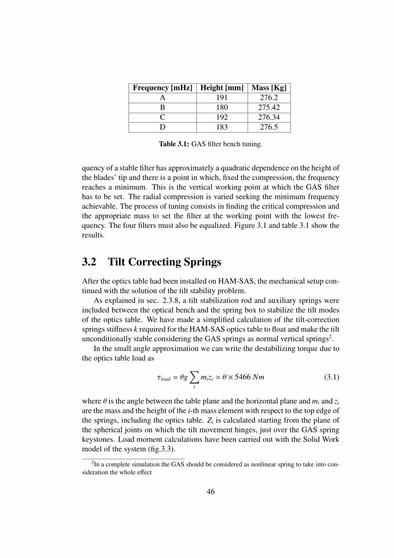
Frequency [mHz] Height [mm] Mass [Kg]A 191 276.2B 180 275.42C 192 276.34D 183 276.5
Table 3.1: GAS filter bench tuning.
quency of a stable filter has approximately a quadratic dependence on the height ofthe blades’ tip and there is a point in which, fixed the compression, the frequencyreaches a minimum. This is the vertical working point at which the GAS filterhas to be set. The radial compression is varied seeking the minimum frequencyachievable. The process of tuning consists in finding the critical compression andthe appropriate mass to set the filter at the working point with the lowest fre-quency. The four filters must also be equalized. Figure 3.1 and table 3.1 show theresults.
3.2 Tilt Correcting SpringsAfter the optics table had been installed on HAM-SAS, the mechanical setup con-tinued with the solution of the tilt stability problem.
As explained in sec. 2.3.8, a tilt stabilization rod and auxiliary springs wereincluded between the optical bench and the spring box to stabilize the tilt modesof the optics table. We have made a simplified calculation of the tilt-correctionsprings stiffness k required for the HAM-SAS optics table to float and make the tiltunconditionally stable considering the GAS springs as normal vertical springs2.
In the small angle approximation we can write the destabilizing torque due tothe optics table load as
τload = θg∑
i
mizi ' θ × 5466 Nm (3.1)
where θ is the angle between the table plane and the horizontal plane and mi and zi
are the mass and the height of the i-th mass element with respect to the top edge ofthe springs, including the optics table. Zi is calculated starting from the plane ofthe spherical joints on which the tilt movement hinges, just over the GAS springkeystones. Load moment calculations have been carried out with the Solid Workmodel of the system (fig.3.3).
2In a complete simulation the GAS should be considered as nonlinear spring to take into con-sideration the whole effect
46

16 17 18 19 20 21 22 23 24 25180
200
220
240
260
280
300
320
X: 20.04Y: 191.4
GAS Filter A
Height [mm]
Fre
quen
cy [H
z]
15 16 17 18 19 20 21 22 23 24 25
180
200
220
240
260
280
300GAS Filter B
Height [mm]
Fre
quen
cy [H
z]
X: 19.95Y: 179.7
14 16 18 20 22 24 26 28180
200
220
240
260
280
300
320
340
360
X: 19.8Y: 191.7
GAS Filter C
Height [mm]
Fre
quen
cy [H
z]
14 15 16 17 18 19 20 21 22 23 24180
200
220
240
260
280
300
320
X: 20.29Y: 182.6
GAS Filter D
Height [mm]
Fre
quen
cy [H
z]
Figure 3.1: GAS filters Frequency vs Height experimental curves.
47

10 20 30 40 50 60 70 80 90
1
1.5
2
2.5
3
3.5
4y
Exponential Curve Fitting
Time [s]
Am
plitu
de [V
olts
]
y(x)=a*exp(b*x)+c a=3.46+/-0.02 b=-0.024+/-0.003 c=0.59+/-0.09
Figure 3.2: The plot shows the fit with an exponential decay for the oscillation am-plitude of the GAS filter A of HAM-SAS tuned at 245 Hz. The result is a qualityfactor of about 42. It was believed to be quite an high value,after that measurementthe compression was increased to reduce the frequency.
A compensating torque is introduced by the GAS and it is approximately equalto
τGAS = 2kGAS θl2 ' θ × 464 Nm (3.2)
where
l2 =√
Dx2 + Dy2, kGAS =16π2 f 2
0
MLOAD. (3.3)
In the calculations we have assumed a resonance frequency f0 = 0.2 Hz3. Thisstabilization force is negligible, and will tend to zero as the GAS resonance fre-quency is tuned towards zero. The force applied by the tilt-stabilizing springs isF = kx with x = θh. The tilt stabilizing torque that it provides is proportional toh, the height of the tilt stabilization rod. The effect of the tilt-stabilizing springscan be written as
τ = 2kθh2 ' kθ × 0.151Nm (3.4)
where h = 0.275 m is the distance between the plane of tilt-correction springs andthe assembly hinging point and k is the stiffness of the used springs4.
In order to have a stable equilibrium position we need to have
τ + τGAS = τLOAD. (3.5)
Substituting in the expression we get
k ' 33100N/m. (3.6)3This was the initial tune of the GAS filters, before bakeout.4This is not necessarily the actual distance from the center of rotation.
48

ElementMass (Pounds)
Mass (Kg)
Z (Inches) Z (m)
Vertical Moment (kg m)
Dominant Material
Density (kg)
Volume (m^3)
Bouyant Mass (Kg)
Optical Table 841.00 378.45 0.00 0.00 0.00 Aluminium 2700.00 0.1402 0.16820.00 0.00 0.0000
H1 Geophone 25.00 11.25 4.00 0.10 1.14 Mixed 0.0030 0.0036H2 Geophone 25.00 11.25 4.00 0.10 1.14 Mixed 0.0030 0.0036H3 Geophone 25.00 11.25 4.00 0.10 1.14 Mixed 0.0030 0.0036V1 Geophone 25.00 11.25 5.00 0.13 1.43 Mixed 0.0031 0.0037V2 Geophone 25.00 11.25 5.00 0.13 1.43 Mixed 0.0031 0.0037V3 Geophone 25.00 11.25 5.00 0.13 1.43 Mixed 0.0031 0.0037
0.00 0.00 0.0000Triple_Suspended 9.00 32.52 0.83 7.43 Aluminium 2200.00 0.0041 0.0049Triple_Non_Suspended 36.00 15.28 0.39 13.97 Aluminium 2700.00 0.0133 0.0160
0.0000Raised_Mass (Leg Element #1) 610.00 274.50 18.50 0.47 128.99 Stainless 8000.00 0.0343 0.0412Mass_Riser 22.00 7.75 0.20 4.33 Stainless 8000.00 0.0028 0.0033Leg Element #3 233.50 105.08 1.35 0.03 3.60 Stainless 8000.00 0.0131 0.0158Clamp Risers 13.64 0.00 0.00 Stainless 8000.00 0.0017 0.0020Counterweight 45.45 0.00 0.00 Stainless 8000.00 0.0057 0.0068Optics Table Adaption Plate 112.00 0.00 0.00 Aluminium 2700.00 0.0415 0.0498
TOTAL 1063.62 166.04 0.2748 0.3298
Worst Case TableMass Element Susp. Type Susp. Mass Sus. Height Non Susp. Mass Non Susp. Mass Height Total Mass Mass MomentMC1 MC Triple 9 0.826 36 0.388 45 21.402MC2 MC Triple 9 0.826 36 0.388 45 21.402MMT3 RM Triple 38.3 0.796 40.4 0.537 78.7 52.1816RM MC Triple 9 0.826 36 0.388 45 21.402Totals 65.3 213.7 116.3876
HAM SAS InitialBSC Leg Element 1 277 0.4699 277 130.1623LOS Cage 22 0.19685 22 4.3307Total 0.66675 299 134.493
HAM SAS TripleBSC Leg Element 1 277 0.4699 277 130.1623LOS Cage 22 0.19685 22 4.3307MC Triple MC Triple 9 0.826 36 0.388 45 21.402Total 344 155.895
Figure 3.3: Mass Properties of the HAM Table load as extracted from the SolidWorks model. One shows the effective buoyant mass of the load on the GAS springs.The effective buoyant mass of the system is 0.32 kg. The second shows verticalmoments in the worst case scenario for Advanced LIGO (i.e. HAM 2 with a stablesignal recycling geometry).
Assuming an ideal zero GAS resonance frequency (τGAS = 0) we get a slightlyhigher required stiffness
k ' 36150N/m. (3.7)
Note that four springs are mounted in a cross configuration. By symmetrytwo springs can always be considered orthogonal to any considered tilt, while theother two can be considered along the tilt. Therefore the effective stiffness in thetilt stabilization is twice the stiffness of a single spring, as long as the springs areunder some tension.
The effect of the angular stiffness of the GAS springs was not consideredin this initial calculation because the GAS springs support the optical table viaspheres in groves that nominally do not transmit torque. This effect was then
49

Figure 2: 3.0 mm wire spring stiffness measurement
Figure 3: 2.5 mm wire spring stiffness measurement Figure 3.4: 2.5 mm wire spring stiffness measurement
calculated and added and resulted being non negligible 5.To calculate the stiffness of a generic helical spring we can use the relation
k =Gd4
nD3 (3.8)
where d is the wire diameter, D is the average spring diameter, n is the windingnumber and G is a constant proportional to the material shear modulus. G wasdetermined experimentally from a measurement of a spring.
Figures 3.4 and 3.5 show respectively the stiffness measurements for a spring,with d = 2.5 mm, n = 20.75 windings and for a spring with d = 3 mm and n = 18windings. The average winding diameter was D = 16.8 mm for both springs.From the two measurements we get
G ' 1.26 · 1010 N/m2 (3.9)
5The real problem came because when ordering the correction springs, we accidentally droppeda factor of ten from the calculation above and ordered softer springs. When we started the tuningwe had available several sets of springs between 6,600 N/m (each) and 23,000 N/m. This mistake,composed with an unfortunate loose screw in the assembly of the tilt stabilization rod caused a lotof confusion.
50
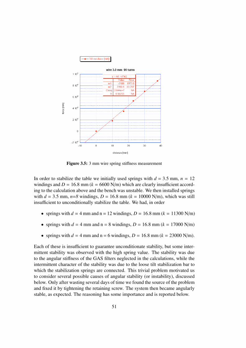
Figure 2: 3.0 mm wire spring stiffness measurement
Figure 3: 2.5 mm wire spring stiffness measurement
Figure 3.5: 3 mm wire spring stiffness measurement
In order to stabilize the table we initially used springs with d = 3.5 mm, n = 12windings and D = 16.8 mm (k = 6600 N/m) which are clearly insufficient accord-ing to the calculation above and the bench was unstable. We then installed springswith d = 3.5 mm, n=8 windings, D = 16.8 mm (k = 10000 N/m), which was stillinsufficient to unconditionally stabilize the table. We had, in order
• springs with d = 4 mm and n= 12 windings, D = 16.8 mm (k = 11300 N/m)
• springs with d = 4 mm and n = 8 windings, D = 16.8 mm (k = 17000 N/m)
• springs with d = 4 mm and n = 6 windings, D = 16.8 mm (k = 23000 N/m).
Each of these is insufficient to guarantee unconditionate stability, but some inter-mittent stability was observed with the high spring value. The stability was dueto the angular stiffness of the GAS filters neglected in the calculations, while theintermittent character of the stability was due to the loose tilt stabilization bar towhich the stabilization springs are connected. This trivial problem motivated usto consider several possible causes of angular stability (or instability), discussedbelow. Only after wasting several days of time we found the source of the problemand fixed it by tightening the retaining screw. The system then became angularlystable, as expected. The reasoning has some importance and is reported below.
51

By this time we had remade the stiffness calculations and we knew that eventhe stiffest springs available were not sufficient. We conjectured correctly that themissing angular stiffness was contributed by the GAS springs angular stiffness,but the reason why we encountered only some angular stability at all might be inthe friction in the spherical joints that couples in part of the GAS angular stiffness.We also considered the fact that the GAS springs are not linear and become stifferas they stray away from the equilibrium point. This contribution turned out to benon relevant.
Simulations made with linear springs showed that if the spherical joints areeliminated, the table is perfectly stable with softer tilt correction springs, while iffrictionless spherical joints are introduced, the table becomes angularly unstable6.
Sufficient friction of the spherical joints but only as long as the sphere of thejoint sticks to it siege. Evidently the that stick and slip in the joint this gave us theobserved stability.
In order to answer the question, we went back to the lab and measured thetorsional rigidity of GAS springs. We mounted a rigid lightweight carbon fibershaft to a two blade GAS spring keystone. The blade is a close relative to theHAM-SAS’(a two blade version, in which we could measure independently thestiffness along and across the blades, with equal length blades, but 10% narrowerand a few percents thinner than in HAM-SAS). The torque is applied at 600 mmfrom the keystone with a string, a pulley, and approximately 156 g masses. Thetorsional angle was measured on photos comparing the angle between the shaftand a ruler marks on the wall in the background. The measurement was made firstalong the blades, and then repeated transversally.
We found a longitudinal angular elastic constant for a pair of GAS bladesequal to
klθ = (53 ± 5) N/rad (3.10)
ktθ = (72 ± 5) N/rad. (3.11)
A GAS filter has four pairs of blades spaced at 45 degrees, therefore the angularelastic constant of a filter is
kθ = 2(53 + 72) = (394 ± 10) N/rad (3.12)
that is for the whole spring box it would be kθ = (1572 ± 40)Nm/rad. These num-bers have to include a factor of 1.25 accounting for the different blade thickness(2.22 mm thick in the bench prototype, 2.39 mm in HAM-SAS) and 1.16 for the
6In the simulation the system is described with two bodies, the optics table and a massive base,and four springs with a diagonal stiffness matrix (108, 108, kGAS ) that connects the two bodies.The motion of the base respect to a generic inertial frame (ground) is not constrained.
52

blades width (80 instead of 69 mm). We also had to account for the number ofblades in the filters. Then we have for the LASTI case:
kθ = (2280 ± 40) N/rad. (3.13)
This torque represents roughly 40% of the torque necessary to stabilize the opticstable tilt. The second possible source of stability may be that in GAS springs theresonant frequency is function of the distance x from the spring optimal workingpoint (see fig.3.1):
f = a + bx2. (3.14)
We can write the elastic constant of an oscillator as k = c f 2, equating we get:
k = c21 + 2c1c2x2 + c2
2x4. (3.15)
Then the potential energy of a GAS spring would lead also to higher than quadraticterms
UGAS = kGAS x2 = c21x2 + 2c1c2x4 + c2
2x6 (3.16)
which may contribute to the stability. This contribution will not eliminate the needfor the stabilization bar.
3.3 IP setupThe IPs are made of four allow aluminum tubes 0.491 mm long and 1 mm thick.They are supported by 8 mm thick, 50 mm long maraging steel cylindrical flexjoints through an apposite holding cup. This flex joint (working under compres-sion) provides the mechanical angular stiffness of the IP mechanism. A thin, neg-ligible stiffness flex joint, working under tension, connects the head of each IP legto the spring box. The IP setup required: the equalization of the load between thefour legs;; the measurement of the resonant frequencies of the horizontal transla-tional modes of the spring box and the correspondent load curve; the choice of thecenter of percussion correcting counterweight.
3.3.1 Load equalization on legsEven though the parts involved in the IPs are machined to a high precision theUHV baking processing inevitably introduces some warping. We found the springbox to be more warped than the height tolerancies of the four legs. A new ad-justable support system was then introduced to solve that problem.
The way we measured the individual leg load was measuring the frequencyof the lowest rigid body mode of the legs. This corresponds to the “banana”
53

Figure 3.6: IP Leg First Banana Mode
mode of the main flex joint and leg’s body together with the upper and lower flexjoint deforming in an "S" shape. Because it works in tension, the small flex jointacquires a transversal stiffness Mg/l (where m is the applied load and l is the 30mm joint’s length; see fig. 3.6). The varying transversal stiffness affects the leg’sresonance frequency, therefore we can make sure that the load is equalized on thefour legs by making sure that the four legs have the same banana mode resonantfrequency.
The frequency measurement was performed as shown in fig.3.7. A magnetwas attached at some point on the leg (i.e. the support upper cup, see fig. 3.7) anda coil cut from by a small commercial voice speaker was held in front of it fromthe spring box frame. The measurement was made analyzing the spectrum of theinduced current on the coils after hitting the leg. The current passed through acushy amplifier and low pass filter as well. Under the load of the spring box, thelegs were equalized to the frequencies showed in tab.3.2.
leg 1st frequency0 2211 2182 2203 218
Table 3.2: Legs first banana mode frequency.
54
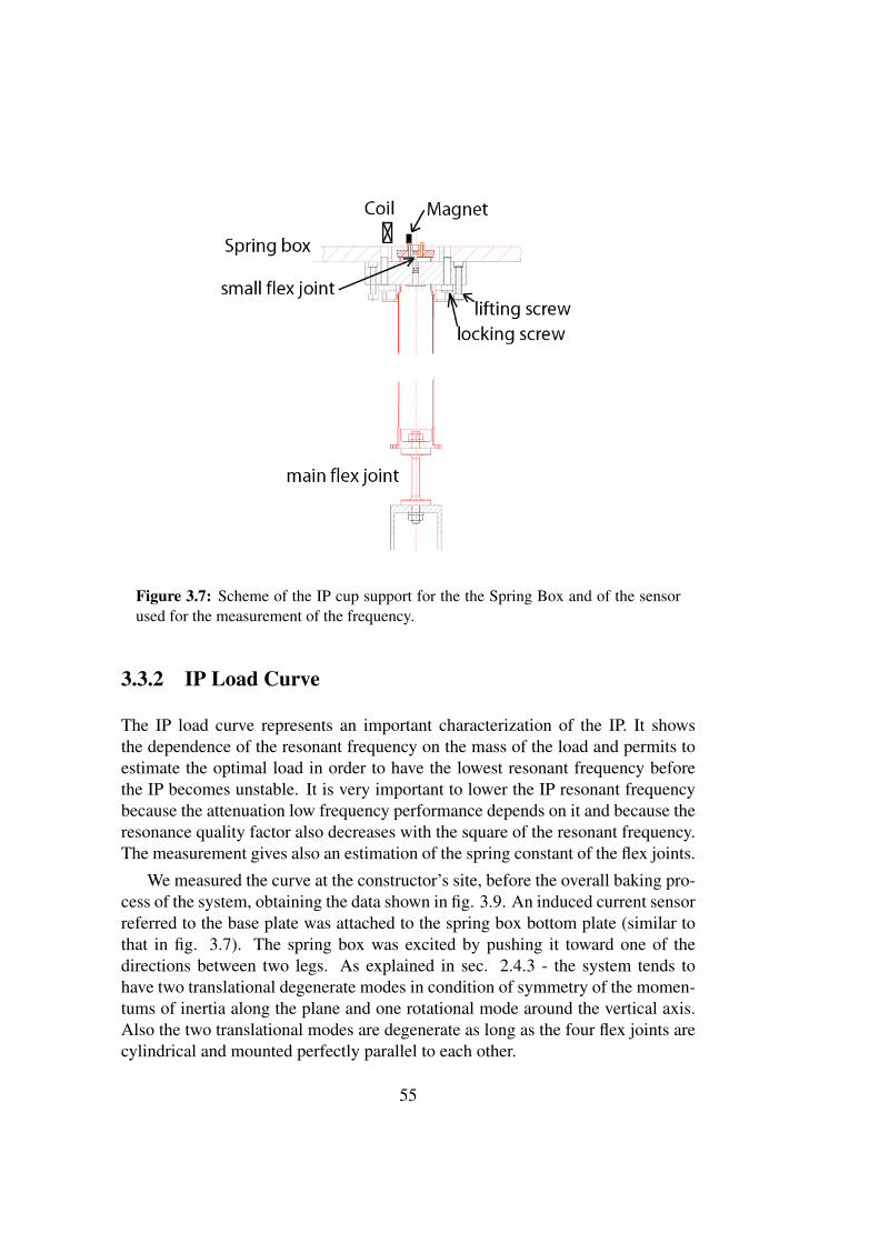
Figure 3.7: Scheme of the IP cup support for the the Spring Box and of the sensorused for the measurement of the frequency.
3.3.2 IP Load Curve
The IP load curve represents an important characterization of the IP. It showsthe dependence of the resonant frequency on the mass of the load and permits toestimate the optimal load in order to have the lowest resonant frequency beforethe IP becomes unstable. It is very important to lower the IP resonant frequencybecause the attenuation low frequency performance depends on it and because theresonance quality factor also decreases with the square of the resonant frequency.The measurement gives also an estimation of the spring constant of the flex joints.
We measured the curve at the constructor’s site, before the overall baking pro-cess of the system, obtaining the data shown in fig. 3.9. An induced current sensorreferred to the base plate was attached to the spring box bottom plate (similar tothat in fig. 3.7). The spring box was excited by pushing it toward one of thedirections between two legs. As explained in sec. 2.4.3 - the system tends tohave two translational degenerate modes in condition of symmetry of the momen-tums of inertia along the plane and one rotational mode around the vertical axis.Also the two translational modes are degenerate as long as the four flex joints arecylindrical and mounted perfectly parallel to each other.
55

0 0.2 0.4 0.6 0.8 1 1.2−85
−80
−75
−70
−65
−60
−55
−50
−45
−40
−35
Frequency (kHz)
Pow
er/fr
eque
ncy
(dB
/Hz)
Power Spectral Density Estimate via Welch
0 0.2 0.4 0.6 0.8 1 1.2−75
−70
−65
−60
−55
−50
−45
−40
−35
−30
−25
Frequency (kHz)
Pow
er/fr
eque
ncy
(dB
/Hz)
Power Spectral Density Estimate via Welch
Leg 0 Leg 1
0 0.2 0.4 0.6 0.8 1 1.2−85
−80
−75
−70
−65
−60
−55
−50
−45
−40
−35
Frequency (kHz)
Pow
er/fr
eque
ncy
(dB
/Hz)
Power Spectral Density Estimate via Welch
0 0.2 0.4 0.6 0.8 1 1.2−90
−85
−80
−75
−70
−65
−60
−55
−50
−45
−40
Frequency (kHz)
Pow
er/fr
eque
ncy
(dB
/Hz)
Power Spectral Density Estimate via Welch
Leg 2 Leg 3
Figure 3.8: PSDs of the four IP legs after the optimization of the load distribuition.
56

300 400 500 600 700 800 900 1000 11000.1
0.2
0.3
0.4
0.5
0.6
0.7
0.8
0.9
1
Mass [Kg]
Fre
quen
cy [H
z]y(x) = 1 / 6.28⋅sqrt((a / 0.491^2 − (1.5 / ...a = 5373R = 0.99719 (lin)
Figure 3.9: IP load curve fit.
Fitting the data with the expression of the frequency
f0 =1
2π
√kθl2 −
(m2 + M
)gl
M(3.17)
where M is the load mass, m = 1.5 Kg is the leg mass of the four legs includingits heads and l = 0.491 is the IP length, we found kθ = 5373 ± 25. The criticalmass of about 1100 Kg was found calculating the intersection of the fit at zerofrequency
3.3.3 IP CounterweightThe IP conuterweight, designed to bring the theoretical attenuation preformancefrom 80 dB to 100 dB, were not mounted on the HAM SAS for lack of time.
A mechanical (non numeric) simulation was used for a rough estimation ofthe counterweight mass and gave a counterweight of ∼150 g.
A specialized sliding table, built to precisely measure the necessary counter-weight was built and could never used.
3.4 Optics Table LevelingOnce that the optics table was floating upon the GAS springs it is important toensure its horizontality.
57

The first step of the leveling was done with a simple bubble level and adjustingthe weights distribution on top of the table. A finer adjustment was made usingan optical level and a combination of small mass positioning and the vertical ac-tuators. Four vertical rulers, previously inter-calibrated, were installed on the fourcorners of the table and the optical level referred to the plumb line. From theMEDM control interface of the ADC (see sec. 4.1) the coil actuators were indi-vidually with DC currents until the same height was read on the rulers from theoptical level. With the table leveled, the LVDT voltages were acquired as refer-ence point and the values taken into account as offsets to be subtracted out of thefour vertical position signals. After this subtraction, zero vertical voltage or fourequal voltages in the four LVDTs was then assumed to signal horizontality of thetable.
Figure 3.10: HAM-SAS inside the HAM chamber with the optics table and the tripleon it.
58
Chapter 4
Experimental Setup
The particular prototype of HAM-SAS, object of this thesis, was specifically de-signed to support the optics tables of the output mode cleaner of Enhanced LIGOeven though the design of the system is almost the same for all the HAM cham-bers of the Advanced LIGO interferometers. The tests performed at LASTI wereaimed to reproduce those conditions. A triple pendulum, one of the main elementsof the Advanced LIGO optics suspensions, was installed on the table (fig.4.2) andseveral weights were arranged to simulate the same mass distribution and heightof the center of mass. Six Mark Products L4-C geophone sensors were placed tomonitor the six degrees of freedom of the table and, from outside the chamber, anoptical lever to monitor the triple. Guralp CMG-T40 seismometers measured theseismic motion of the ground.
4.1 LIGO Control and Data System (CDS)
The HAM-SAS control and data systems (CDS) are designed according to theLIGO CDS standard and based on the EPICS system1. In the front end computerEPICS provides a platform for the execution of the control and monitor programs.The code is written in C by a Matlab Simulink interface in which sensors, ac-tuators and channels have a graphical representation and the controls are imple-mented in the topology of the connections among the elements (figure.4.13 shows
1EPICS is a set of Open Source software tools and applications, written by the Los Alamosand Argonne National laboratories, which provide a software infrastructure for use in buildingdistributed control systems to operate devices such as Particle Accelerators, Large Experimentsand major Telescopes. Such distributed control systems typically comprise tens or even hundredsof computers, networked together to allow communication between them and to provide controland feedback of the various parts of the device from a central control room, or even remotely overthe internet.
59

Figure 4.1: Optics table and weight distribution installed on HAM-SAS inside theLASTI HAM vacuum chamber.
the scheme of the Simulink code we wrote for HAM-SAS). The MEDM softwareprovides a graphical command interface (fig.4.3).
4.2 Sensors setup
Several kind of sensors are involved in the HAM-SAS tests : LVDTs, L4C geo-phones, Guralp seismometers, QPDs. The LVDTs are position sensors while geo-phones and Guralps are velocity sensors. The LVDT are relative sensors, whichmeans that they measure the position (or velocity) from the relative displacementof a test mass from their reference frame. The sensor frame and the test mass forman harmonic oscillator. The frame follows the system whose position x0 is the onethat has to be measured. In a way that changes depending on the particular kindconsidered, the sensor measures the relative position (x − x0) of the mass to theframe. From the equation of motion of the test mass
mx = −k(x − x0), (4.1)
60

Figure 4.2: Triple pendulum and sketch of a representing model. The triple pendu-lum is the last stage of the seismic isolation. Its role is to filter the high (>10Hz)frequencies noise using three stages of passive isolation in the horizontal directionsand two stages of isolation in the vertical one [44].
neglecting for simplicity any dissipation mechanism, we can obtain the frequencyresponse between the relative displacement and the reference frame:
x0
x − x0=ω2
0 − ω2
ω2 . (4.2)
The function in (4.2) depends on the resonant frequency of the system and givesthe calibration of the sensor. Multiplying it by the output signal (x − x0) we obtainthe position of the reference2.
4.2.1 LVDTsAs already mentioned, eight LVDTs are used for position control in HAM-SAS.The LVDTs (Linear Variable Differential Transformers, [33]) are displacementsensors constituted by a primary and two secondary windings. The primary wind-ing is fed with an audio frequency (usually in the range 10-20 kHz) sinusoidal
2In the same way all HAM-SAS, together with its LVDTs, could be considered as a big dis-placement sensors for the ground, that is a seismometer.
61

Figure 4.3: HAM-SAS MEDM interface. The platform is represented by the grayrectangle. At the corners, with simbols Vx, are the LVDT sensors, actuators andstepper motors of each GAS filter. The black circles represent the IP legs and havesimilar sensors and actuators panels.
signal. The secondary winding is composed by two identical coaxial and rigidlyinterconnected coils, wound in opposite directions. The primary coil general sitsin the center between the two secondaries, coaxially oriented. When the primarywinding is longitudinally displaced by of an amount ∆x, a current with the samefrequency of the primary signal and modulated in amplitude proportionally to ∆xis induced in the secondary winding. A mixer is then required to demodulate thesecondary signal and produce a DC output proportional to ∆x. Translations in theother directions, in first approximation, induce no signal.
A VME LVDT driver board is used in HAM-SAS control. The LVDT boardspecifications are:
• 8 independent channels, first channel set as master in master-slave triggerconfigurations;
• individually tunable coil excitation levels;
• individually tunable sensor coil read-back amplifier gains;
62

Figure 4.4: Horizontal LVDT scheme. The bracket (269, 270) and (243) supportsthe primary coil (244) hanging from the springs box. The twin secondary coils arewound on the same cylinder (245) supported by the bracket (246) to the base. Thecalibration was made measuring the distance between (245) and (246 ,271) with acaliber for several given static position of the spring box.
• One single-ended output per channel for signal monitoring3;
• One single-ended input, for external oscillator operation;
• One single-ended output, for inter-board synchronization;
• Master-slave/asynchronous operation selectable through onboard jumpers;
• External/internal oscillator operation selectable through onboard jumpers;
• ± 22Vpp primary output voltage;
• ±15V - ±18 V Supply operating voltage;
• 3 24-pin connectors for LVDT primary winding excitations, LVDT sec-ondary winding readbacks, ADC.
3The internal oscillator of the first readout circuit can be used as a master for the channel ofthe boards and to slave all other boards used in the system.
63
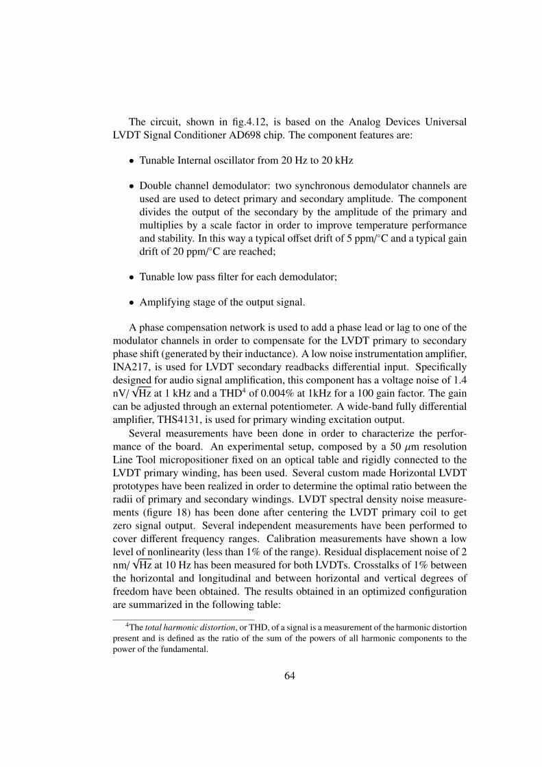
The circuit, shown in fig.4.12, is based on the Analog Devices UniversalLVDT Signal Conditioner AD698 chip. The component features are:
• Tunable Internal oscillator from 20 Hz to 20 kHz
• Double channel demodulator: two synchronous demodulator channels areused are used to detect primary and secondary amplitude. The componentdivides the output of the secondary by the amplitude of the primary andmultiplies by a scale factor in order to improve temperature performanceand stability. In this way a typical offset drift of 5 ppm/◦C and a typical gaindrift of 20 ppm/◦C are reached;
• Tunable low pass filter for each demodulator;
• Amplifying stage of the output signal.
A phase compensation network is used to add a phase lead or lag to one of themodulator channels in order to compensate for the LVDT primary to secondaryphase shift (generated by their inductance). A low noise instrumentation amplifier,INA217, is used for LVDT secondary readbacks differential input. Specificallydesigned for audio signal amplification, this component has a voltage noise of 1.4nV/√
Hz at 1 kHz and a THD4 of 0.004% at 1kHz for a 100 gain factor. The gaincan be adjusted through an external potentiometer. A wide-band fully differentialamplifier, THS4131, is used for primary winding excitation output.
Several measurements have been done in order to characterize the perfor-mance of the board. An experimental setup, composed by a 50 µm resolutionLine Tool micropositioner fixed on an optical table and rigidly connected to theLVDT primary winding, has been used. Several custom made Horizontal LVDTprototypes have been realized in order to determine the optimal ratio between theradii of primary and secondary windings. LVDT spectral density noise measure-ments (figure 18) has been done after centering the LVDT primary coil to getzero signal output. Several independent measurements have been performed tocover different frequency ranges. Calibration measurements have shown a lowlevel of nonlinearity (less than 1% of the range). Residual displacement noise of 2nm/√
Hz at 10 Hz has been measured for both LVDTs. Crosstalks of 1% betweenthe horizontal and longitudinal and between horizontal and vertical degrees offreedom have been obtained. The results obtained in an optimized configurationare summarized in the following table:
4The total harmonic distortion, or THD, of a signal is a measurement of the harmonic distortionpresent and is defined as the ratio of the sum of the powers of all harmonic components to thepower of the fundamental.
64
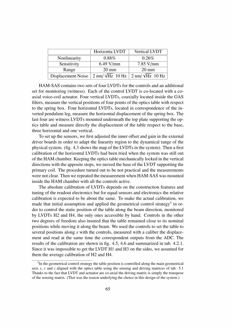
Horizonta LVDT Vertical LVDTNonlinearity 0.88% 0.26%Sensitivity 6.49 V/mm 7.85 V/mm
Range 20 mm 20 mmDisplacement Noise 2 nm/
√Hz 10 Hz 2 nm/
√Hz 10 Hz
HAM-SAS contains two sets of four LVDTs for the controls and an additionalset for monitoring (witness). Each of the control LVDT is co-located with a co-axial voice-coil actuator. Four vertical LVDTs, coaxially located inside the GASfilters, measure the vertical positions of four points of the optics table with respectto the spring box. Four horizontal LVDTs, located in correspondence of the in-verted pendulum leg, measure the horizontal displacement of the spring box. Thelast four are witness LVDTs mounted underneath the top plate supporting the op-tics table and measure directly the displacement of the table respect to the base,three horizontal and one vertical.
To set up the sensors, we first adjusted the inner offset and gain in the externaldriver boards in order to adapt the linearity region to the dynamical range of thephysical system. (fig. 4.3 shows the map of the LVDTs in the system). Then a firstcalibration of the horizontal LVDTs had been tried when the system was still outof the HAM chamber. Keeping the optics table mechanically locked in the verticaldirections with the apposite stops, we moved the base of the LVDT supporting theprimary coil. The procedure turned out to be not practical and the measurementswere not clear. Then we repeated the measurement when HAM-SAS was mountedinside the HAM chamber with all the controls active.
The absolute calibration of LVDTs depends on the construction features andtuning of the readout electronics but for equal sensors and electronics the relativecalibration is expected to be about the same. To make the actual calibration, wemade that initial assumption and applied the geometrical control strategy5 in or-der to control the static position of the table along the beam direction, monitoredby LVDTs H2 and H4, the only ones accessible by hand. Controls in the othertwo degrees of freedom also insured that the table remained close to its nominalpositions while moving it along the beam. We used the controls to set the table toseveral positions along x with the controls, measured with a caliber the displace-ment and read at the same time the correspondent outputs from the ADC. Theresults of the calibration are shown in fig. 4.5, 4.6 and summarized in tab. 4.2.1.Since it was impossible to get the LVDT H1 and H3 on the sides, we assumed forthem the average calibration of H2 and H4.
5In the geometrical control strategy the table position is controlled along the main geometricalaxis x, y and z aligned with the optics table using the sensing and driving matrices of tab. 5.1Thanks to the fact that LVDT and actuator are co-axial the driving matrix is simply the transposeof the sensing matrix. (Thzt was the reason underlying the choice in this design of the system.)
65

−2 −1.5 −1 −0.5 0 0.5 1 1.5 2 2.5
x 104
73
74
75
76
77
78
79LVDT H2
DAC [counts]
Pos
ition
[mm
]y(x) = a0 + a1⋅xa0 = 75.521a1 = 0.00014514
R = 0.99594 (lin)
Figure 4.5: H2 LVDT calibration results. The fit gives a coefficient of 0.18 µm/count
−2 −1.5 −1 −0.5 0 0.5 1 1.5 2 2.5
x 104
71
72
73
74
75
76
77
78LVDT H4
DAC [counts]
Pos
ition
[mm
]
y(x) = a0 + a1⋅xa0 = 74.81a1 = −0.00018137
R = 0.99949 (lin)
Figure 4.6: H2 LVDT calibration results. The fit gives a coefficient of 0.14 µm/count
66

LVDT Slope Uncertainty Calibration Uncertainty[#] [Counts/um] [Counts/um] [um/Counts] [um/Counts]V1 -4.7281 0.0498 -0.2115 0.0022V2 4.9162 0.0559 0.2034 0.0023V3 -4.6772 0.032 -0.2138 0.0015V4 -5.4043 0.0552 -0.185 0.0019H1 -6.1255 – -0.16325 –H2 6.8898 0.0785 -0.14514 0.0017H3 -6.1255 – 0.16325 –H4 -5.5135 0.0628 0.18137 0.0021
Each vertical LVDTs have been calibrated with the system inside the chamber.The vertical LVDT is mounted with two sets of three screws in push-pull mode, toset the electrical zero of the LVDTs at the mechanical working point of the GASfilters. With the optics table and the spring box mechanically locked in all thedirections, the support of the LVDT secondary coil was released and moved by adefinite number of turns of its holding screws. From the pitch step we measuredthe displacements and, at the same time, the readouts from the ADC.
Unfortunately, due to their remote positioning, there was no direct way tocalibrate the witness LVDTs. They could only be cross calibrated from the controlLVDT readout for various position settings.
4.2.2 GeophonesSix geophones are placed on the optics table. As shown in fig. 4.1, three of them,the horizontal, are aligned parallel to the table’s plane, in a pinwheel configura-tion and the other three, the vertical, are orthogonal to the plane, arranged in atriangular configuration. The configuration is such that they can be sensitive to allthe six degrees of freedom.
The geophones are relative velocity sensors. The test mass inside is a mag-net connected to the sensor’s frame by a spring and its velocity is monitored theinduced current on a coaxial coil mounted on the frame. In order to pass fromvelocity to position a calibration filter has to be applied to the signal. The filteris designed on the frequency domain and then implemented on MEDM whichprovides for the transformation into the time domain. In the frequency domain,the position can be obtained from the velocity simply by dividing by ω, corre-sponding to the introduction of a pole at zero frequency. The actual calibration weimplemented is described in table 4.2.2:
With the geophones calibrated to measure the positions, we can decouple thesignals to obtain the coordinates of the system along the six degrees of freedom.
67

Poles Zeroes Gain0.50 (3) 0.2847±i*1.0625 0.0129
Table 4.1: Calibration transfer function of the geophones in the zpk format. The threepoles at 50 mHz have to be considered like they were poles at zero. The reason forthe shift is to avoid the saturation that would happen because of the DC componentof the signal from the geophones. Basically the calibration divides by the frequencyto obtain from a velocity a signal proportional to the changing position. Then thedouble pole at zero frequency and the complex zero at about 1 Hz transform therelative displacement of the test mass into absolute position of the reference.
−0.8 −0.6 −0.4 −0.2 0 0.2 0.4 0.6 0.8−0.8
−0.6
−0.4
−0.2
0
0.2
0.4
0.6
0.8
H1(−0.7874,−0.7112) +Y V1(0.8382,−0.7366) +Z
H2(−0.762,0.7366) +X
V2(−0.8382,0.0254) +Z H3(0.8382,0) −Y
V3(0.8382,0.7366) +Z
Figure 4.7: Mapping of the geophones on the table
Be g = (h1, h2, h3, v1, v2, v3) and r = (x, y, z, , θy, θz) the vectors with the single sig-nals from the geophones and the coordinates of the system respectively. Referringto the mapping of the sensors in fig.4.7 we have that:
h1
h2
h3
v1
v2v3
=
0 1 0 0 0 H(x)1
1 0 0 0 0 −H(y)2
0 -1 0 0 0 −H(x)3
0 0 1 V (y)1 −V (x)
1 00 0 1 V (y)
2 −V (x)2 0
0 0 1 V (y)3 −V (x)
3 0
xyzθx
θyθz
. (4.3)
Inverting the matrix in (4.3) and substituting the coordinates of the sensors wefind the decoupling matrix.
68

Figure 4.8: Model to explain the tilt to horizontal coupling in the horizontal geo-phones on the optics table.
4.2.3 Tilt couplingThe horizontal geophones response depends also on the tilt motion of the opticstable. As a matter of fact, they measure as horizontal displacement part of what isactually tilt of the optics table. This can be clearly understood if in the model weconsider also a rotation of the plane with the geophone as shown in fig.4.8. Theoverall frequency response include an additional term due to the coupling betweenof the tilt into the horizontal sensors:
x0
x − x0=
(ω2
0 − ω2
ω2
)horizontal
+
(gω2
θ
x − x0
)tilt coupling
. (4.4)
The term becomes more important at low frequency where it easily dominates overthe real horizontal motion. If it were possible to have an independent measure ofthe tilt, this effect could be taken into account and subtracted out6.
4.2.4 Optical LeverAn optical lever provides for an independent measurement of yaw and one of thetilt modes of the optics table. A diode laser, positioned on top of a pier just outsidethe HAM chamber, emits a beam that enters the chamber through a glass portholeand hits the mirror in the middle of the bottom mass of the triple pendulum.7 Thereflected beam reaches the center of a QPD (Quadruple Photo-Detector) sensorplaced right next of the laser source. A QPD is made of a four quadrant photodiodein which each quadrant gives a voltage proportional to the inpinging power. Thesignal share between the four channels depends on the position hit by the beamspot (fig.4.9). The linearity range and sensitivity of this detector depend on thelaser spot size.
6As is, in certain conditions can dominate the measurement and give an overestimated seismicinduced motion.
7The triple pendulum is frozen with respect to the optical bench for this measurement.
69

Figure 4.9: QPD sensor. The signal from each quadrant is proportional to the areacovered by the beam spot (red). The coordinates of the beam spot’s center are givenby the differences between the output signals.
The optical lever is set up with the table mechanically locked in all the degreesof freedom. In that condition the beam spot’s center is made to coincide with thecenter of the QPD, equalizing the signal from the quadrants by changing the ofthe QPD. From the vector with the four signals, the pitch and yaw angles can beobtained by the following decoupling matrix:
(θyθz
)=
2l
(1 1 -1 -11 -1 1 -1
) Q1
Q2
Q3
Q4
. (4.5)
in which l ' 1.2 m is the arm lever starting from the middle of the table to the QPDsensor. The output voltage to position calibration is obtained by micrometricallymoving the quadrant photodiode.
4.2.5 Seismometer
Three Guralps seismometers are placed around the HAM chamber as shown infig. 4.10. They are velocity sensors that means that in order to obtain a signalproportional to the position of the ground, they have to have a calibration functionsimilar to that implemented on the geophones. Table 4.2.5 contains the details ofthe calibration function.
Each of them provides for three output signals correspondent to three or-thogonal directions, two horizontal and one vertical called respectively North-South(NS), East-West (EW), Vertical (V). Six of the nine signals are used to mea-sure the motion of the ground around the HAM chamber along the six degrees offreedom.
70
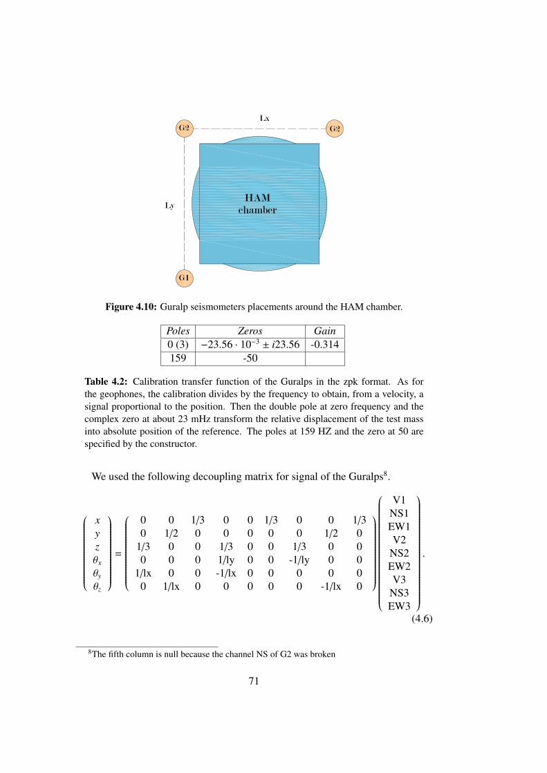
Figure 4.10: Guralp seismometers placements around the HAM chamber.
Poles Zeros Gain0 (3) −23.56 · 10−3 ± i23.56 -0.314159 -50
Table 4.2: Calibration transfer function of the Guralps in the zpk format. As forthe geophones, the calibration divides by the frequency to obtain, from a velocity, asignal proportional to the position. Then the double pole at zero frequency and thecomplex zero at about 23 mHz transform the relative displacement of the test massinto absolute position of the reference. The poles at 159 HZ and the zero at 50 arespecified by the constructor.
We used the following decoupling matrix for signal of the Guralps8.
xyzθx
θyθz
=
0 0 1/3 0 0 1/3 0 0 1/30 1/2 0 0 0 0 0 1/2 0
1/3 0 0 1/3 0 0 1/3 0 00 0 0 1/ly 0 0 -1/ly 0 0
1/lx 0 0 -1/lx 0 0 0 0 00 1/lx 0 0 0 0 0 -1/lx 0
V1NS1EW1V2
NS2EW2V3
NS3EW3
.
(4.6)
8The fifth column is null because the channel NS of G2 was broken
71

Y end HAM Vacuum System
Horz LVDT and Coils4 eachVac Breakout X4
Vert LVDT and Coils4 eachVac Breakout X4
Witness LVDTs4 eachX4
Brea
kout
Boa
rd
Coil Driver
Interface
LVDT Driver
Bre
akou
t Boa
rd
LVDT Driver
Stepper
Stepper
Stepper
Stepper
Stepper
Stepper
Stepper
Stepper
Ste
pper
Inte
rface
Step
per I
nter
face
Motor Controller X4
Motor Controller X4
HAM SASCPU, Anti-Alias, Anti-
Image, ADCs, DACs, BIO
Guralp Interface
X end HAM HEPI Controls
L-4C6 each
STS-2
HAM SAS Controls Block Diagram
QPD
W
hite
ning QPD
QPD
QPD
W
hite
ning QPD
QPD
Coil Driver
Guralp Seismometer
Figure 4.11: HAM SAS Controls Block Diagram.
72

5 5
4 4
3 3
2 2
1 1
DD
CC
BB
AA
Sezio
ne C
anal
e 11
MW
0206
20
LVD
T D
RIV
ER
12
CA
NA
LI
1113
Frid
ay, J
une
30, 2
006
A00
Title
Size
Doc
umen
t Num
ber
Rev
Dat
e:S
heet
of
+14
+14
LVD
T IN
11-
EX
C C
ON
N 1
1+
AD
C C
ON
N 1
1+
-14
SYN
C L
O/D
X
EX
C C
ON
N 1
1-
-14
LVD
T IN
11+
AD
C C
ON
N 1
1-
-14
+14
-14
+14
-14
+14
-14
+14
R11
11R
0
R11
0939
0R
+-
U11
03O
P27
326
7 4
J110
1S
IGN
AL
MO
NIT
OR
1
2
R11
1039
0R
C11
1210
0nF
C11
1410
0nF
C11
04C
Myl
ar
+
+-
-
U11
06TH
S41
311
2
3
4 5
6
8
R11
05R
S
+
C11
1310
uF
U11
02A
D69
8
1
13
15
16
14 18
2024
28
17
19
10
11
2221 23 5 6
7
8
2 3
-VCC
-BIN
-AIN
+AIN
+BIN
-AC
OM
P
AFILT1SIGREF
+VCC
+AC
OM
P
AFILT2
BFILT1
BFILT2
FEE
DB
AC
K
OU
TFIL
T
SIG
OU
TLE
V1
LEV
2
FREQ1
FREQ2
EX
C1
EX
C2
U11
04SS
M21
42 12
4
56
78
C11
081u
F M
ylar
C11
06C
Myl
ar
R11
12R
1R
1102
1K
C11
05C
Myl
ar
C11
0322
uF
RV
1104
100K
25T
RV
1101
100R
25T
C11
093.
3nF
Myl
ar
U11
05SS
M21
42 12
4
56
78
RV
1102
RT
25T
+
C11
1510
uF
C11
0110
0nF
R11
0739
0R
SW
1101
SYN
C IN
T/E
XT
21 3
54 6
R11
0410
K
C11
111u
F M
ylar
C11
0210
0nF
C11
1010
0nF
Myl
ar
C11
071u
F M
ylar
R11
06
200R
R11
0839
0R
GA
IN
GA
IN+ -
U11
01IN
A21
73 1 8 2
7
5
4
6
R11
0110
K
RV
1103
5K 2
5T
R11
0310
K
Figure 4.12: LVDT driver board master channel
73

Bad
Lin
k
site
=M1
rate
=2K
dcui
d=22
gds_
node
_id=
4cd
sPar
amet
ers
Bad
Lin
k
HA
MY
_WIT
_SM
atrix
In1
In2
In3
In4
In5
In6
Out
1
Out
2
Out
3
Out
4
Out
5
Out
6
HA
MY
_WIT
_MO
N
In1
In2
In3
In4
Out
1
Out
2
Out
3
Out
4
HA
MY
_WIT
Bad
Lin
k
HA
MY
_V_S
Mat
rix
Bad
Lin
k
HA
MY
_V_D
Mat
rix
In1
In2
In3
In4
Out
1
Out
2
Out
3
Out
4
HA
MY
_VS
EN
S
In1
In2
In3
In4
Out
1
Out
2
Out
3
Out
4
HA
MY
_VC
OM
P
In1
In2
In3
In4
Out
1
Out
2
Out
3
Out
4
HA
MY
_VA
CT
In1
In2
In3
In4
Out
1
Out
2
Out
3
Out
4
HA
MY
_STE
P2
In1
In2
In3
In4
Out
1
Out
2
Out
3
Out
4
HA
MY
_STE
P1
IN1
IN2
IN3
IN4
OU
T1
OU
T2
OU
T3
HA
MY
_QP
D4
IN1
IN2
IN3
IN4
OU
T1
OU
T2
OU
T3
HA
MY
_QP
D3
IN1
IN2
IN3
IN4
OU
T1
OU
T2
OU
T3
HA
MY
_QP
D2
IN1
IN2
IN3
IN4
OU
T1
OU
T2
OU
T3
HA
MY
_QP
D1
Bad
Lin
k
HA
MY
_H_S
Mat
rix
Bad
Lin
k
HA
MY
_H_D
Mat
rix
In1
In2
In3
In4
Out
1
Out
2
Out
3
Out
4
HA
MY
_HS
EN
S
In1
In2
In3
In4
Out
1
Out
2
Out
3
Out
4
HA
MY
_HC
OM
P
In1
In2
In3
In4
Out
1
Out
2
Out
3
Out
4
HA
MY
_HA
CT
Bad
Lin
k
HA
MY
_GU
RA
LP_R
Mat
rix
In1
In2
In3
In4
In5
In6
Out
1
Out
2
Out
3
Out
4
Out
5
Out
6
HA
MY
_GU
RA
LP3
In1
In2
In3
In4
In5
In6
Out
1
Out
2
Out
3
Out
4
Out
5
Out
6
HA
MY
_GU
RA
LP2
In1
In2
In3
In4
In5
In6
Out
1
Out
2
Out
3
Out
4
Out
5
Out
6
HA
MY
_GU
RA
LP1
In1
In2
In3
In4
In5
In6
Out
1
Out
2
Out
3
Out
4
Out
5
Out
6
HA
MY
_GU
RA
LP
In1
In2
In3
In4
In5
In6
In7
In8
Out
1
Out
2
Out
3
Out
4
Out
5
Out
6
Out
7
Out
8
HA
MY
_CO
ILM
ON
Out
1
Out
2
Out
3
HA
MY
_CA
L
Bad
Lin
k
DA
C_0
DA
C
AD
C S
elec
tor
AD
C S
elec
tor
AD
C S
elec
tor
AD
C S
elec
tor
AD
C S
elec
tor
AD
C S
elec
tor
AD
C S
elec
tor
AD
C S
elec
tor
AD
C S
elec
tor
AD
C S
elec
tor
AD
C S
elec
tor
AD
C S
elec
tor
AD
C S
elec
tor
AD
C1
adc_
1
AD
C0
adc_
0
<adc
_1_2
8>
<adc
_1_2
9>
<adc
_1_3
0>
<adc
_1_3
1>
<adc
_0_0
>
<adc
_0_1
>
<adc
_0_2
>
<adc
_0_3
>
<adc
_0_4
>
<adc
_0_5
>
<adc
_0_6
>
<adc
_0_7
>
<adc
_0_8
>
<adc
_0_9
>
<adc
_0_1
0>
<adc
_0_1
1>
<adc
_0_1
2>
<adc
_0_1
3>
<adc
_0_1
4>
<adc
_0_1
5>
<adc
_0_1
6>
<adc
_0_1
7>
<adc
_0_1
8>
<adc
_0_1
9>
<adc
_0_2
0>
<adc
_0_2
1>
<adc
_0_2
2>
<adc
_0_2
3>
<adc
_0_2
4>
<adc
_0_2
5>
<adc
_0_2
6>
<adc
_0_2
7>
<adc
_0_2
8>
<adc
_0_2
9>
<adc
_1_1
6>
<adc
_1_1
7>
<adc
_1_1
8>
<adc
_1_1
9>
<adc
_1_2
0>
<adc
_1_2
1>
<adc
_1_2
2>
<adc
_1_2
3><a
dc_1
_0>
<adc
_1_1
>
<adc
_1_2
>
<adc
_1_3
>
<adc
_1_4
>
<adc
_1_5
>
<adc
_1_6
>
<adc
_1_7
>
<adc
_1_2
4>
<adc
_1_2
5>
<adc
_1_2
6>
<adc
_1_2
7>
<adc
_1_1
2>
<adc
_1_1
3>
<adc
_1_1
0>
<adc
_1_1
5>
<adc
_1_9
>
<adc
_1_8
>
<adc
_1_1
4>
<adc
_1_1
1>
Figure 4.13: Simulink representation of the HAM-SAS front end code
74

Chapter 5
HAM-SAS control
5.1 Optics Table Control
The optics table is a 6 degree of freedom mechanical system: 6 independent sen-sors are required to fully determine its position and 6 independent actuators tomove it. Each physical sensor is, in principle, sensitive to movements in all the 6normal modes (which in the following will be often referred to as x, y, θz, z, θx, θy,although they do not correspond necessarily to pure translations and rotations). Inthe same way, each actuator will generate movements of the optics table involv-ing a mix of the 6 modes. The basic idea of the HAM-SAS controls is to treatas separate the horizontal from the vertical DOFs and to diagonalize the sensingand control actions: the aim is to pass from the sensors/actuators space, to a spacewhere each normal mode is independently sensed and acted upon. Mathemati-cally, this means to realize a coordinate transformation for each group of degreesof freedom such that the equations of motions get the form:
xi + ω2i xi = qi (5.1)
where xi (for i = 1; 2; 3) is a normal mode coordinate, ωi/2π is the resonantfrequency of the i − th mode and qi is the generalized force corresponding to thecoordinate xi [45, 31]. Experimentally this means to find 3 linear combinations ofthe sensor outputs, defined virtual sensors, each sensitive to a single normal modeand, correspondingly, 3 linear combinations of the excitation coil currents (virtualactuators) which excite each mode separately. In control theory terminology, thismeans to break down a multiple in-multiple out (MIMO) system into many singlein-single out (SISO) systems. The control of a SISO system is much easier: everymode is controlled by an independent feedback loop, simplyfing greately the loopdesign and the seismic requirements.
75

5.2 DiagonalizationThe GAS filters support the optics table in such a way that the relative movementof the suspension points respect to the spring box is mostly limited to the verticaldirection. This significantly reduces the coupling between the horizontal DOFs ofthe table (x, y and roll) and the verticals (z, pitch, yaw) and allows to treat themseparately into two stages. Let us consider only one stage, i.e. the horizontal.
Be u(s) the vector containing the Laplace transform of the positions of thefour LVDT sensors, and v(s) the vector with the transforms of the forces exertedby the actuators. We have that
u = H v (5.2)
where H is a 4×4 matrix in which the generic element hi j represents the transferfunction between the actuator j and the sensor i. Neglecting the vertical to thehorizontal couplings, each of these transfer functions can be written as a linearcombination of three oscillators, one for each of the normal modes of the system:
hi j(s) =ui(s)v j(s)
=
3∑k=0
a(i j)k
ω20k
s2 + ω20k + iω2
0kφk(5.3)
where a(i j)k is the coupling coefficient for the k-th mode, ω0k the mode’s resonant
frequency. For hi j(iω) we can expect the shape resulting from three overimposedharmonic oscillator functions to look like the graph in fig.5.1.
We have that u ∈ U, sensors space, and v ∈ V , actuators space. It is possibleto pass to basis for U and for V such that the transfer function matrix H becomesdiagonal. With this choice of basis each sensor is a modal sensor which is sensitiveto only one of the normal modes of the system. In the same way each actuatorbecomes a modal actuator wich is able to act only on one mode. In the newcoordinates
x = Hq (5.4)
hi j(s) =xi(s)q j(s)
= bk hi j(s) δi jk (5.5)
where δi jk is the Kronecker tensor. Be S and D the basis change matrices for Uand V representing the sensing matrix and driving matrix respectively. We havethat:
x = Su (5.6)v = Dq (5.7)
Su = HD−1v (5.8)
which makesH = S−1HD−1 (5.9)
76

10−1 100−40
−30
−20
−10
0
10
20M
agni
tude
(dB
)
Bode Diagram
Frequency (Hz)
Figure 5.1: Typical real sensor to actuator transfer function.
5.2.1 Measuring the sensing matrixBeing u = S−1x we know that the column vectors of S−1 represent the relativesensitivy of the real sensors to each single mode. The only matrix we can measuredirectly is H but we can reduce it to a matrix physically equivalent to S−1. Wechoose one of the real actuators, say v1, and use it to excite the system. Wethen measure all the quantities hi1(ωk) in correspondence of the three resonantfrequencies of the three modes of interest. Taking the imaginary part of thesenumbers we can build the matrix
M =
= [h11(ω1)] · · · = [h11(ω3)]
......
= [h31(ω1)] · · · = [h31(ω3)]
(5.10)
and it can be shown that S−1 and M are equivalent and differ only for a scale factorthat multiplies each column.
In fact, let us define S−1 = {σi j} and D−1 = {∆i j}. From 5.9 and 5.5 we canwrite
hi j(s) =3∑
k=1
σikhkk∆k j. (5.11)
At the resonance ωk
hkk(iωk) ≈ =[hkk(iωk)] = −bkQk (5.12)
77

Figure 5.2: Diagonalization scheme
hi j(iωk) = −σikbkQk∆k j (5.13)
and this means that
M =
−σ11 b1 Q1 ∆11 · · · −σ13 b3 Q3 ∆31
......
−σ31 b1 Q1 ∆11 · · · −σ33 b3 Q3 ∆31
= [α1 σ
(1), α2 σ(2), α3 σ
(3)].
(5.14)S−1 and M are equivalent because the α factors only change the length of theeigenvectors but not their relative angles. Physically those factors only set theglobal sensitivity of the sensors to each mode but do not change the relative sen-sitivity among the sensors to one mode.
The same consideration holds if instead of v1 we had chosen an other actu-ator to evaluate the matrix. As long as the system is linear, no matter how weexcite a mode, we can get different α values but the ratios between the conversioncoefficients in each column of M rest the same.
5.2.2 Measuring the driving matrixNow, since we have defined the modal sensors, we can measure the driving matrixfrom their relation with the real actuators
x = HD−1 v = N v (5.15)
by simply measuring the ratios
xi(iω)v j(iω)
= ni j (5.16)
at a fixed frequency. Even though N(s) is frequency dependent all the dependenceis in H. Since H is a diagonal matrix, N and D−1 are equivalent. The only specifi-cation is that the test frequency at which the measurement is made must be lowerthan all the resonant frequencies in order to neglect the imaginary part of ni j andhave only real numbers to build the matrix.
78

1/4 1/4 1/4 1/41/2 0 −1/2 00 1/2 0 −1/20 0 0 0
1/4 1/2 0 01/4 0 1/2 01/4 −1/2 0 01/4 0 −1/2 0
Vertical Sensing Vertical Driving
0 1/2 0 1/2
1/2 0 1/2 01/4 −1/4 −1/4 1/40 0 0 0
0 1/2 1/4 01/2 0 −1/4 00 1/2 −1/4 0
1/2 0 1/4 0
Horizontal Sensing Horizontal Driving
Table 5.1: Geometrical diagonalization matrices
5.2.3 Experimental diagonalization
Experimentally the diagonalization of sensors and actuators is an iterative process.The two procedure can be reiterated many times until the virtual sensors are welldecoupled and sensitive to the normal modes of the system. On each iteration thevirtual sensors are assumed to be real and the new sensing and driving matricesobtained have to be multiplied to the left of the old ones.
For each of the stages we started the diagonalization from the geometricalsensing and driving matrices. That immediately reduced the redundancy of thesensors and actuators. As discussed in sec. 2.4.3, from the symmetry of thesystem, we expected the modes to be two pure translations and a pure rotation andthus the transfer function to be not too far from being already diagonal with thatchoice of base. For the vertical DOFs we chose two main axis along the diagonalsof the table and the third one along the vertical direction as eigenaxis. For thehorizontals, we considered two translational modes along x and y and a rotationalmode around the vertical axis. The corresponding matrices are shown in tab 5.1.
For each stage, either horizontal or vertical, we measured the transfer functionsbetween one virtual actuator and all the virtual sensors of the same stage of DOFs.We extracted the imaginary parts in correspondence of the peaks for each sensorand with these we wrote S−1. Then we inverted it to obtain S and transformed to a4×4 matrix filling the last column and row with zeros. Finally we multiplied thisto the left of the geometric sensing matrix obtaining a new one. The procedurewas repeated for each actuator and the obtained matrices were averaged using the
79

−0.12 0.32 1 0.33
1 0.44 −0.42 0.15−0.27 1 0.30 −1
0 0 0 0
0.04 1 −0.20 00.46 0.74 0.94 0
1 −0.04 0.15 00.57 0.21 −1 0
Vertical Sensing Vertical Driving
−1 0.81 −0.15 0.07
0.76 1 0.32 0.52−0.37 −0.30 −1 1
0 0 0 0
−1 0.83 −0.41 0
0.50 0.92 0.14 0−0.63 0.76 −1 00.13 1 0.73 0
Horizontal Sensing Horizontal Driving
Table 5.2: Measured sensing and driving matrices.
norm of the columns as weight. Figures 5.2.3 and 5.2.3 show the transfer functionsfor the excitation of the Y an Z geometrical virtual actuators respectively.
The inverse of the driving matrix was obtained exciting each geometric vir-tual actuator one at a time at a fixed low frequency and measuring the transfercoefficients1 between the virtual sensors as obtained from the new sensing matrix.Then it was inverted, converted to a 4×4 matrix filling the last column and rowwith zeros and multiplied by the driving matrix.
The amplitude chosen for the excitations determined the signal to noise ratioand the quality of the measurements. The measured matrices are shown in fig.5.2.
The most troublesome to measure was the vertical driving matrix. The trans-fer coefficients have been always characterized by not negligible imaginary partseven if they were measured at frequencies much lower than the resonances. Thereason is probably in a certain amount of coupling with the horizontal DOFs in-troduced by exciting the table in the range of frequencies where the horizontalresonances occur. This supposed coupling did not produced the same problem inthe measurement of the horizontal driving matrix probably because the verticalresonances are all well above the horizontal ones. When the imaginary parts wereabout the same as the real, the simple transpose of the sensing matrix turned outto be more effective than the measured driving matrix to control the modes. Thereason for this is that the vertical actuators are perfectly aligned with the vertical
1The transfer coefficient is the value of a transfer function at a given point.
80

T0=16/06/2007 15:36:06 Avg=3
Frequency (Hz)
-110
Mag
nit
ud
e (d
B)
-50
-45
-40
-35
-30
-25
-20
-15
Transfer function
T0=16/06/2007 15:36:06 Avg=3
X/Y
YY
TZ/Y
Transfer function
T0=16/06/2007 15:36:06 Avg=3
Frequency (Hz)
-110
Imag
inar
y
-0.2
-0.15
-0.1
-0.05
-0
0.05
0.1
0.15
Transfer function
T0=16/06/2007 15:36:06 Avg=3
X/Y
YY
TZ/Y
Transfer function
Figure 5.3: Magnitude and imaginary part of the transfer function between the geo-metrical horizontal DOFs and the geometrical virtual actuator Y. In the peaks of theimaginary parts we get the frequencies of the horizontal modes: 38 mHz; 60 mHz;75 mHz.
81

T0=16/06/2007 22:38:02 Avg=3
Frequency (Hz)
Mag
nit
ud
e (d
B)
-50
-40
-30
-20
-10
Transfer function
T0=16/06/2007 22:38:02 Avg=3
Z/Z
Tx/Z
TY/Z
Transfer function
T0=16/06/2007 22:38:02 Avg=3
Frequency (Hz)
Imag
inar
y
-0.2
-0.1
0
0.1
0.2
Transfer function
T0=16/06/2007 22:38:02 Avg=3
Z/Z
Tx/Z
TY/Z
Transfer function
Figure 5.4: Magnitude and imaginary part of the transfer function between the geo-metrical vertical DOFs and the virtual geometrical actuator Z. The frequency of themodes are: 146 mHz; 198 mHz; 250 mHz.
82

0.81 1 0.50−1 0.60 −0.60−0.98 0.04 1
0.65 1 0.07
1 −0.98 0.200.30 −0.10 −1
Vertical Modes Horizontal Modes
Table 5.3: Inverse of the measured sensing matrices. The columns define the eigen-modes of the system. For the vertical the frequencies are: 146 mHz, 198 mHz,250 mHz respectively. For the horizontal they are: 38 mHz, 60 mHz, 75 mHz.
LVDTs and, for construction reasons, they must share almost the same calibrationcurrent-force among each other.
Figure 5.8,5.9 shows the comparison between the LVDT spectra as obtainedby the real sensors, the geometric virtual sensors and the diagonalized sensors.
5.2.4 Identifying the normal modesFrom section 5.2.1 it follows that the columns of the inverse of the measuredsensing matrix S−1 represent the eigenmodes of the system in the basis of thespace in which the matrix is measured. In the case of the geometrical basis, thecolumns represent the projection of the modes on the x, y and θz conventional axischosen for HAM-SAS.
Table 5.3 contains the vertical and horizontal inverse of the sensing matriceswith the eigenmodes as column vectors in the geometric basis representation. Thecalibration of the LVDT sensors and the inclusion of the arm lengths in the ge-ometrical matrices are essential for the modes to be interpreted in that basis. Inparticular, in the horizontal matrix the first row has to be intended as meters alongx, the second as meters along y and the third as radiants around z. In the verticalmatrix, the first row represent meters of transaltion along z. The second is the onewe called θx (even though it corresponds to a rotation around the diagonal withLVDT sensors V1 and V3) and the third is θy (corresponding to the opposite diag-onal, between V2 and V4). A more realistic comparison between the geometricalprojections of the modes could be done looking at the energies stored in each ofthem, which can be estimated from the products of the square of the amplitudesfor the mass of the system in the case of the translation components, and for themoments of inertia for the rotations: Mx2, My2 Izθ
2z , Mz2, Ixθ
2x, Iyθ
2y .
In the vertical matrix, the ratio between the third and the second rows’ com-ponents represents the direction of the eigenaxis in the horizontal plane measuredfrom the first diagonal. From the measured matrices we have that the first moderoughly corresponds to a rotation around the actual y axis plus a translation along
83

z. The second is mostly a vertical translation plus a rotation around the first di-agonal. The third is a vertical translation plus a rotation around an axis which iscloser to the first diagonal than to the second2.
The horizontal matrix was closer to expectations than the vertical. The thirdcolumn contains a mode which is almost a pure rotation around z. The secondis mostly a translation at about 45 degrees between the x and y axis. The firstis a mix of a translation along an axis somewhere in between x and y axis and arotation around the vertical axis.
5.2.5 Actuators calibrationThe actuators redundancy allows driving modes which applies null resultant forceand null resultant torque to the optics table. In case of equal calibrations betweenthe actuators, these modes are represented by the vector wh = (1,−1,−1, 1) forthe horizontal actuators and by the vector wv = (1,−1, 1,−1) for the vertical ac-tuators (in the vertical case these modes are called saddle or pringle modes3. Thegeometric diagonalization of the driving matrix excludes actuators’ combinationsthat could drive as pringle modes, as long as the actuators have the same forcecalibration. Geometrically the image of the vertical matrix Dv is a 3-dim spaceorthogonal to the actuation vector wv and the image of Dh is orthogonal to wh. Ifthe orthogonality is not guaranteed each of the actuators applies a different forcefor the same current. Thus the scalar product between the pringle vector and thecolumns of the driving matrix tells us about the actuators’ calibration.
From 5.2 we have from the vertical driving matrix:
Dv(1) · wv = 0.67
Dv(2) · wv = 0.00 (5.17)
Dv(3) · wv = 0.00
and from the horizontal:
Dh(1) · wh = 0.00
Dh(2) · wh = 0.00 (5.18)
Dh(3) · wh = 0.00
2These asymmetries can be explained with a transversal stress applied mostly on the GAS filternumber 1 (which is forced to work crookedly) by an error in assembly. Testing this hypothesiswould require disassembly and reassembly of the system, which could not be performed for lackof time.
3The reason is that they would tend to bend the table in a way similar to the shape of a horsesaddle or of a pringle potate chip.
84
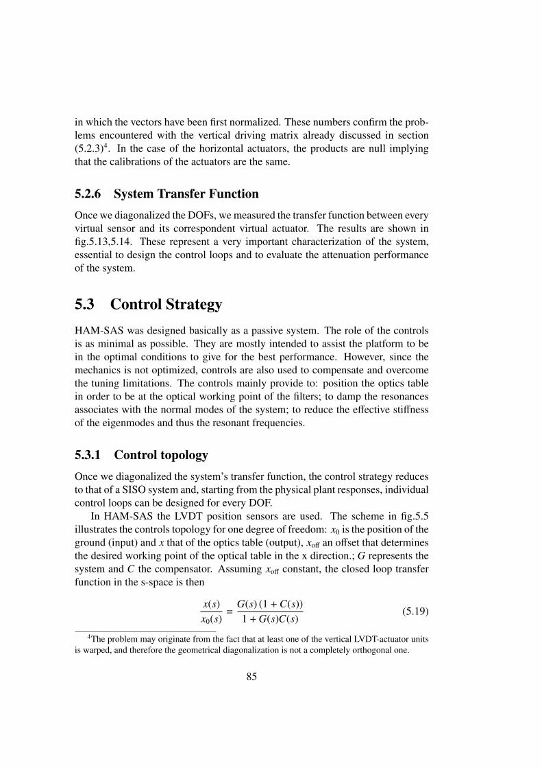
in which the vectors have been first normalized. These numbers confirm the prob-lems encountered with the vertical driving matrix already discussed in section(5.2.3)4. In the case of the horizontal actuators, the products are null implyingthat the calibrations of the actuators are the same.
5.2.6 System Transfer FunctionOnce we diagonalized the DOFs, we measured the transfer function between everyvirtual sensor and its correspondent virtual actuator. The results are shown infig.5.13,5.14. These represent a very important characterization of the system,essential to design the control loops and to evaluate the attenuation performanceof the system.
5.3 Control StrategyHAM-SAS was designed basically as a passive system. The role of the controlsis as minimal as possible. They are mostly intended to assist the platform to bein the optimal conditions to give for the best performance. However, since themechanics is not optimized, controls are also used to compensate and overcomethe tuning limitations. The controls mainly provide to: position the optics tablein order to be at the optical working point of the filters; to damp the resonancesassociates with the normal modes of the system; to reduce the effective stiffnessof the eigenmodes and thus the resonant frequencies.
5.3.1 Control topologyOnce we diagonalized the system’s transfer function, the control strategy reducesto that of a SISO system and, starting from the physical plant responses, individualcontrol loops can be designed for every DOF.
In HAM-SAS the LVDT position sensors are used. The scheme in fig.5.5illustrates the controls topology for one degree of freedom: x0 is the position of theground (input) and x that of the optics table (output), xoff an offset that determinesthe desired working point of the optical table in the x direction.; G represents thesystem and C the compensator. Assuming xoff constant, the closed loop transferfunction in the s-space is then
x(s)x0(s)
=G(s) (1 +C(s))1 +G(s)C(s)
(5.19)
4The problem may originate from the fact that at least one of the vertical LVDT-actuator unitsis warped, and therefore the geometrical diagonalization is not a completely orthogonal one.
85
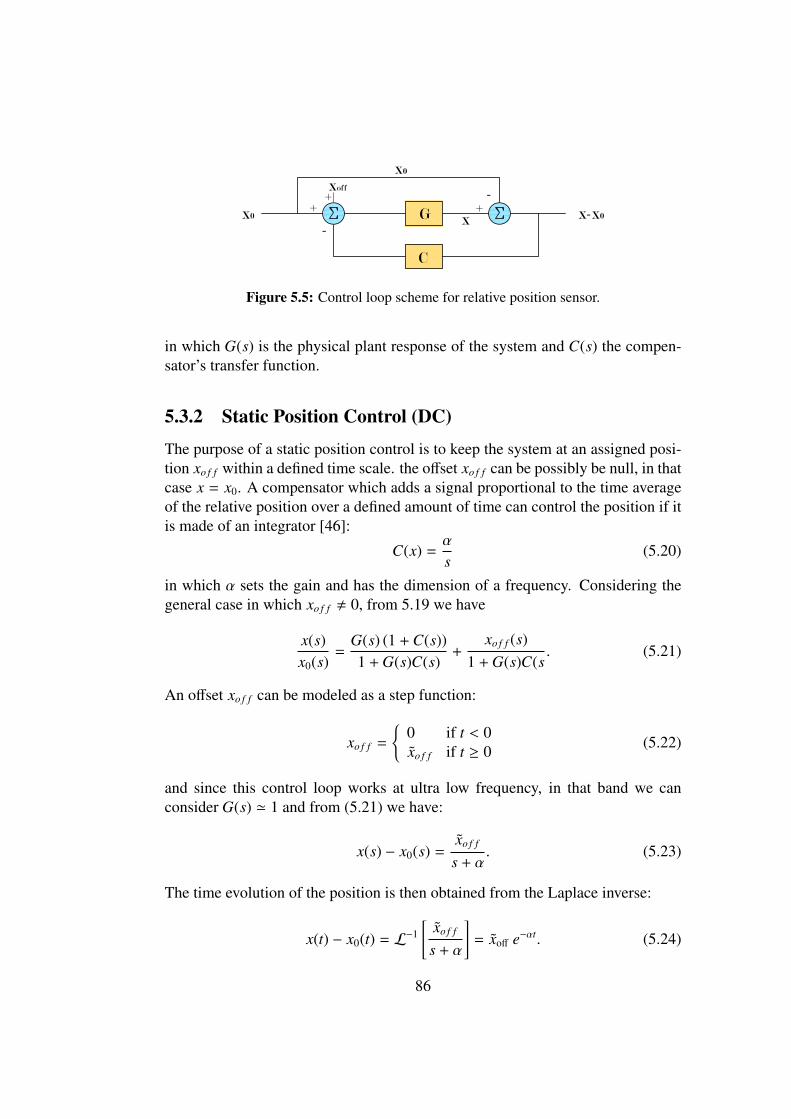
Figure 5.5: Control loop scheme for relative position sensor.
in which G(s) is the physical plant response of the system and C(s) the compen-sator’s transfer function.
5.3.2 Static Position Control (DC)
The purpose of a static position control is to keep the system at an assigned posi-tion xo f f within a defined time scale. the offset xo f f can be possibly be null, in thatcase x = x0. A compensator which adds a signal proportional to the time averageof the relative position over a defined amount of time can control the position if itis made of an integrator [46]:
C(x) =α
s(5.20)
in which α sets the gain and has the dimension of a frequency. Considering thegeneral case in which xo f f , 0, from 5.19 we have
x(s)x0(s)
=G(s) (1 +C(s))1 +G(s)C(s)
+xo f f (s)
1 +G(s)C(s. (5.21)
An offset xo f f can be modeled as a step function:
xo f f =
{0 if t < 0xo f f if t ≥ 0 (5.22)
and since this control loop works at ultra low frequency, in that band we canconsider G(s) ' 1 and from (5.21) we have:
x(s) − x0(s) =xo f f
s + α. (5.23)
The time evolution of the position is then obtained from the Laplace inverse:
x(t) − x0(t) = L−1[
xo f f
s + α
]= xoff e−αt. (5.24)
86

We have that α defines the time constant of the process (τ = 1/α) and the loopbandwidth. The unity gain is obtained solving
|G(s)C(s)| '∣∣∣∣∣αs
∣∣∣∣∣ = 1 (5.25)
which places the unitary gain at:
fu.g =α
2π. (5.26)
Since the open loop transfer function G(s)C(s) has a phase smaller than -180degrees above the resonant frequency of G(s), the Nyquist criterion then requiresfu.g to be lower than the resonance of the system G(s) in order for the system tobe stable.
5.3.3 Velocity Control (Viscous Damping)A velocity control is used to apply viscous damping to the system. A force pro-portional to the relative velocity (x− x0) is realized by means of a derivative com-pensator of the form
C(s) = γs (5.27)
In particular the quality factor of the system can be reduced by γ since we havethat:
Q =ω0mγ. (5.28)
5.3.4 Stiffness Control (EMAS)The Electro-Magnetic Anti-Spring strategy (EMAS) was already developed aspart of the SAS technology but it has been applied for the first time extensivelyand by mean of a digital feedback control system in HAM SAS. At the basis of thestrategy is the introduction into the system actuation of a positive feedback signalfrequency independent, which is equivalent to a spring with repulsive stiffness andcompetes with the mechanical spring constant to lower the overall stiffness of themode. The control loop topology is shown in fig.5.6. The transfer function atclosed loop is:
x(s)x0(s)
=G(s) (1 − k)1 − kG(s)
. (5.29)
Assuming a simple pendulum physical plant response like
G(s) =ω2
0
ω20 − ω
2(5.30)
87

Figure 5.6: Electromagnetic Anti-Spring (EMAS) control loop. A pure gain, fre-quency indipendent, is fedback into the system to reduce the stiffness.
Figure 5.7: Scheme of the control configuration for the measurement of the physicalplant as modified by the introduction of the EMAS. The precise measurement wouldbe given exciting after the integrator and measuring the ratio out/A. Since the testpoints are only in some fixed locations according to the the front end code, the bestpossible measurement is made exciting right before the physical plant G from theratio A/exc. This ratio well approximates G’ except for the DC value.
the closed loop transfer function becomes
Gc.l(s) =ω2
0 (1 − k)
ω20 (1 − k) − ω2
(5.31)
which is equivalent to a system with a reduced resonant frequency
ω′
0 = ω0
√1 − k (5.32)
that is to a system with a reduced stifness.In order to measure the new physical plant response including the effect of
the EMAS we followed the scheme in fig. 5.7. The table has always to be atthe working point height, thus a position control must be included in parallel tothe anti-spring. Ideally, the precise way to measure the new plant G
′
would beexciting right after the integrator and then it would be G
′
= out/A. Since EPICS
88

allows only a limited number of test points, one has to find the best location intothe system’s map to measure the transfer function. According to the front endcode and to the available test points the closest thing to G
′
that we could measurewas A/exc. This ratio well approximates G
′
for low gain of the integrator but itstill differs for the DC value. The result of one of this kind of measurement forthe z emas is shown in fig.5.12.
89

10−2
10−1
100
10−2
100
102
104
106
108
Frequency [Hz]
Am
plitu
de [A
U/s
qrt(
Hz)
]
Normal Mode MGAS Table
T0=28/03/2007 14:51:30 Avg=1 BW=0.0117187
Frequency (Hz)
-110
Mag
nit
ud
e
1
10
Power spectrum - Geometrical Modes
T0=28/03/2007 14:51:30 Avg=1 BW=0.0117187
TX
TY
Z
Power spectrum - Geometrical Modes
Figure 5.8: Modal vertical LVDT power spectra. The upper plot shows the signalsfrom the virtual sensors after the diagonalization. Each sensors senses much moreonly one of the three resonances. Still, mostly on the first two resonances a little ofcoupling persists. The lower plot shows the spectra from the virtual sensors beforethe diagonalization, when they were aligned to the geometrical directions. The plotsrefer to an early configuration of the system when the resonances were at slightlydifferent frequencies and the LVDT still not calibrated.
90

T0=18/06/2007 15:37:05 Avg=10 BW=0.0117187
Frequency (Hz)
-210 -110
Mag
nit
ud
e
10
210
Power spectrum
T0=18/06/2007 15:37:05 Avg=10 BW=0.0117187
TZ
X
Y
Power spectrum
Figure 5.9: Modal horizontal LVDT power spectra. In this case the diagonalizationof the sensors is very good and the three virtual sensors sense almost only one modeeach.
91

*T0=20/03/2007 04:06:16 *Avg=14/Bin=11L BW=0.0117178
Frequency (Hz)
-210 -110 1 10 210
Mag
nit
ud
e
-110
1
10
210
Power spectrum
*T0=20/03/2007 04:06:16 *Avg=14/Bin=11L BW=0.0117178
M1:SAS-HAMY_HSENS_H2_OUT
M1:SAS-HAMY_HSENS_H2_OUT(REF1)
Power spectrum
*T0=20/03/2007 04:06:16 *Avg=14/Bin=11L BW=0.0117178
Frequency (Hz)
-210 -110 1 10 210
Mag
nit
ud
e
-110
1
10
Power spectrum
*T0=20/03/2007 04:06:16 *Avg=14/Bin=11L BW=0.0117178
M1:SAS-HAMY_HSENS_H1_OUT
M1:SAS-HAMY_HSENS_H1_OUT(REF0)
Power spectrum
*T0=20/03/2007 04:06:16 *Avg=14/Bin=11L BW=0.0117178
Frequency (Hz)
-210 -110 1 10 210
Mag
nit
ud
e
-110
1
10
Power spectrum
*T0=20/03/2007 04:06:16 *Avg=14/Bin=11L BW=0.0117178
M1:SAS-HAMY_HSENS_H3_OUT
M1:SAS-HAMY_HSENS_H3_OUT(REF2)
Power spectrum
*T0=20/03/2007 04:06:16 *Avg=14/Bin=11L BW=0.0117178
Frequency (Hz)
-210 -110 1 10 210
Mag
nit
ud
e
-110
1
10
Power spectrum
*T0=20/03/2007 04:06:16 *Avg=14/Bin=11L BW=0.0117178
M1:SAS-HAMY_HSENS_H4_OUT
M1:SAS-HAMY_HSENS_H4_OUT(REF3)
Power spectrum
Figure 5.10: The plots show the horizontal LVDTS before (red curves) and after(blu curves) closing local damping control loops on each horizontal actuator (eachactuator is controlled indipendently by the others). The sensors were not calibratedyet and the optics table was mechanically locked.
T0=05/07/2007 21:45:18 Avg=1
Time (s)
0 50 100 150 200 250 300
Sig
nal
-900
-800
-700
-600
-500
-400
-300
-200
-100
0
Time series
T0=05/07/2007 21:45:18 Avg=1
M1:SAS-HAMY_VSENS_V2_O
Time series
Figure 5.11: The plot shows the position control while it brings the table position asread by one of the vertical LVDT to a given position.
92

T0=18/05/2007 15:46:10 Avg=3
Frequency (Hz)
-210 -110 1 10 210
Mag
nit
ud
e (d
B)
-80
-60
-40
-20
0
Transfer function - Z
T0=18/05/2007 15:46:10 Avg=3
EMAS OFF
EMAS ON
Transfer function - Z
Figure 5.12: The plot shows the effect of an EMAS control applied to the Z modewith kEMAS = 7. The frequency is shifted from about 200 mHz to about 40 mHz.The blue (with EMAS) and red (with EMAS) have different DC values because ofthe way the modified physical plant response is measured according to the availableEPICS test points.
93

10−2
10−1
100
101
−100
−80
−60
−40
−20
0
Mag
nitu
de [d
B]
X Mode Frequency fx = 37 mHz
10−2
10−1
100
101
−400
−300
−200
−100
0
Frequency [Hz]
Pha
se [D
eg]
10−2
10−1
100
101
−100
−80
−60
−40
−20
0
Mag
nitu
de [d
B]
Y Mode Frequency fy = 59 mHz
10−2
10−1
100
101
−200
−150
−100
−50
Frequency [Hz]
Pha
se [D
eg]
10−2
10−1
100
101
−100
−80
−60
−40
−20
0
Mag
nitu
de [d
B]
TZ Mode Frequency fθz = 74 mHz
10−2
10−1
100
101
−1000
−800
−600
−400
−200
Frequency [Hz]
Pha
se [D
eg]
Frequency [Hz]
Figure 5.13: Diagonal transfer functions for the horizontal degrees of freedom fittedby a pendulum function.
94
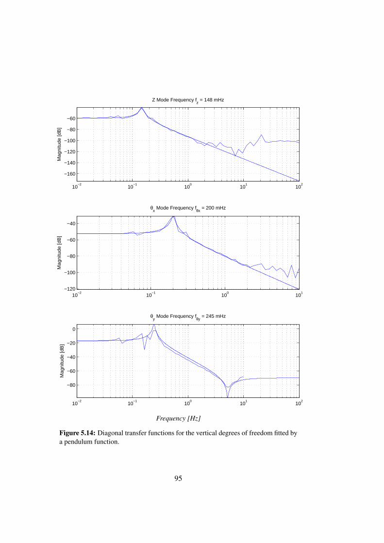
10−2
10−1
100
101
102
−160
−140
−120
−100
−80
−60
Mag
nitu
de [d
B]
Z Mode Frequency fz = 148 mHz
10−2
10−1
100
101
102
−600
−500
−400
−300
−200
−100
0
Frequency [Hz]
Pha
se [D
eg]
10−2
10−1
100
101
−120
−100
−80
−60
−40
Mag
nitu
de [d
B]
θx Mode Frequency fθx
= 200 mHz
10−2
10−1
100
101
−200
−100
0
100
200
300
Frequency [Hz]
Pha
se [D
eg]
10−2
10−1
100
101
102
−80
−60
−40
−20
0
Mag
nitu
de [d
B]
θy Mode Frequency fθy
= 245 mHz
10−2
10−1
100
101
102
−150
−100
−50
0
Frequency [Hz]
Pha
se [D
eg]
Frequency [Hz]
Figure 5.14: Diagonal transfer functions for the vertical degrees of freedom fitted bya pendulum function.
95

96

Chapter 6
System Performances
In this chapter we present the latest experimental results from the HAM-SASexperiment. First we introduce the quantities by which we measured the per-formances of the system. We discuss the attenuation performance achieved, thestrategy adopted for the controls and the issue about the very low frequency dis-placement noise observed.
6.1 Measuring the HAM-SAS PerformancesBefore discussing the performances of the system, we want to clarify the defini-tions and the properties of the quantities that we are going to consider. Since weare here interested in seismic attenuation performances, the observable that wehave in mind is always a coordinate position.
6.1.1 Power Spectrum DensitiesBe x(t) the coordinate describing the system in the time domain [16]. Its powerspectrum density is defined as the Fourier transform
Px ( f ) =1/√
2πx ∗ x (0)
∫ +∞
−∞
x ∗ x (τ) (τ) e−2πiωtdτ (6.1)
in which x ∗ x (τ) is the autocorrelation function of x(t) which is defined as:
x ∗ x (τ) =∫ +∞
−∞
x (t) x (t + τ) dt (6.2)
From Parseval’s theorem the root mean square value of x is connected to the powerspectrum by:
xr.m.s. =
√∫ +∞
−∞
Px ( f ) d f (6.3)
97

We rather work with an object derived from the power spectrum: the amplitudespectral density1. It is simply defined as the square root of the power spectrum:
S ( f ) =√
Px ( f ). (6.4)
and its dimensions are [x]/√
Hz. The advantage of this object is that the unitmatches better what we measure with the sensors (i.e. meters).
The spectrum measurements on HAM-SAS data have been made with an FFTMatlab based software tool, averaging over many measurements. The averagedspectra are accompanied by the root mean square of the measurement, intendedas the standard deviation on the points j of the set at frequency i:
S r.m.s.( fi) =
√√√1N
N∑j=1
(S ( fi) − S j( fi)
). (6.5)
The spectrum r.m.s. represents a useful parameter for the evaluation of the mea-surement noise.
6.1.2 Transmissibility and Signal CoherenceThe particular transfer functions in which both the input and the output quantitiesare dynamic variables as position, velocity or acceleration are called transmis-sibilities. We evaluated the seismic performance of HAM-SAS measuring thetransmissibilities of the system for each degree of freedom. They were obtainedsimply dividing the Fourier transform of the output signal from the geophones onthe optics table by the input signal from the Guralp seismometers on the ground,both of them corresponding to the same degree of freedom.
Experimentally the input and output of a transmissibility measurement can bedisturbed by noise and the ratio between the two relative spectra does not neces-sarily represent the transfer function of the system. In LTI system theory (LinearTime Invariant), it can be demonstrated [48] that two signal x (t) and y (t) are cor-related if and only if it is possible to define a function H (t) such that:
y (t) = H (t) ∗ x (t) ⇒ Y (ω) = H (ω) X (ω) . (6.6)
To evaluate the quality of the measured ratio between the two spectra as actuallyrepresenting the transfer function, for the measurements on HAM-SAS, we haveconsidered the coherence function to evaluate the correlation between the signal.The coherence Cxy (ω) between x and y is defined as
Cxy (ω) =
∣∣∣Rxy (ω)∣∣∣2
Xx (ω) Yy (ω)(6.7)
1Although we often improperly refer to it as power spectrum or just spectrum.
98

Frequency (Hz)
-210 -110 1 10 210
Mag
nit
ud
e
-1110
-1010
-910
-810
-710
-610
Power spectrum
HAM Requirements
LLO Seismic Reference
Power spectrum
Figure 6.1: Advanced LIGO HAM requirements for the displacement noise of thePower Recycling and Output Mode Cleaner and model of Livingston seismic powerspectrum.
where Rxy (ω) is the Fourier transform of the cross-correlation function between xand y, defined as
Rxy (τ) = x ∗ y (τ) . (6.8)
The coherence is a real function between zero and one. It is one if x and y arecorrelated. On the other hand, when x and y are uncorrelated (i.e., y is a noiseprocess not derived from x), the coherence converges to zero at all frequencies.
6.2 Evaluating the Seismic PerformancesThe Advanced LIGO HAM requirements [49] set a reference to evaluate theHAM-SAS seismic performances and they represented the ultimate goal of thesystem commissioning. In particular the constraints for the Power Recycling andMode Cleaner optics set a displacement noise limit of 2 × 10⁻⁷ m/
√Hz in the
0.1-0.2 Hz band, 4 × 10⁻¹⁰ m/√
Hz at 600 mHz and 3 × 10⁻¹¹ m/√
Hz above 20Hz (fig.6.1). The conditions have been defined according to a model of the groundseismic spectra at both of the sites, Hanford (LHO) and Livingston (LLO) [50].The horizontal and vertical ground noise are considered equal and expressed, inthe frequency range 100mHz < f < 40Hz, as a polynomial expansion in logspace:
log xg ( f ) = p1(log f
)n+ p2
(log f
)n−1+ . . . + pn log f + pn+1 (6.9)
where xg is the displacement spectral density. Because the average ground noise atthe two observatories and at MIT differ significantly, three separate ground noise
99

Figure 6.2: Ground noise models for the Hanford (LHO), Livingston (LLO) andLASTI sites. Each curve was obtained by a polynomial fit of the seismometer data.The plot shows LASTI as a noisier location than the sites in the horizontal and verticalDOF.
models are estimated for LHO, LLO and LASTI; these are shown in fig.6.2. In themodels the ground noise input is assumed to be the same for all three translationaldegrees of freedom.
6.3 Experimental Results
We want here to show and discuss some of the latest power spectra and trans-missibilities which illustrate the status of the system performances in the presentconfiguration.
As we explained in chapter 5, the roles of the control system are two: tokeep the platform at the working point in order to have the best passive isolatingperformance and to actively assist the mechanics in attenuating the seismic noise.We will see here the effect of these different strategies.
100
6.3.1 Passive AttenuationAs explained in chapter 3, both the IPs and the GAS filter were set to perform atbest at their correspondent working point2. Because of absolute and differentialthermal drifts of the apparatus, ground movements and tilts (tidal movements,water table variations, movements of heavy loads on the floor and in the buildingvicinities, diurnal and seasonal differential heating and cooling of the facilitiesetc.)3, only position control can guarantee and maintain a perfect alignment ofthe optical table. The very low tuning of the resonant frequencies exacerbatesthese drifts both in the vertical and horizontal directions.4. Misalignments caneven bring to instabilities because of recoil effects between the spring box and thependulums.
From the measured physical plant responses (see sec. 5.2.6), we designedstatic positioning control loops (DC) with a very low unitary gain frequency (u.g.f.)of about 1 mHz by which we obtained the power spectrum of fig. 6.3, basicallyleaving the system free to move at all frequencies .
The structure between 10 and 20 Hz is typical of all the measurements. Itcorresponds to a internal mechanical resonance of the system which we had notime to identify and damp. We believe it is likely due to either the tilt correctingsprings or the wire by which they pull the central column. When the HAM cham-ber was still open, it was in part, but not totally, attenuated by magnetic dampers(see fig.6.4). It is expected to be fixed with properly designed dampers and/orredesigned springs.
Below about 400 mHz the transmitted seismic motion of the uncontrolled sys-tem amplitude becomes higher than the requirements, especially for x, and under100 mHz, where the horizontal displacement becomes greater than 1 µm/
√Hz.
In particular we notice three peaks between 100 and 300 Hz correspondent to theresonances of the vertical DOFs. These resonances enter in every degree of free-dom because of couplings between different degrees of freedom. They actuallycause a larger appparent displacement in the horizontal than in the vertical. Theactual coupling originates likely in recoil effects between the spring box and theoptics table. It must be considered that the table with all its payload has a masswhich is three times that of the spring box and the center of mass is located 50cm over the pivot point of the GAS filters. The mechanical solution foreseen for
2As part of the lower frequency tuning process, optimization of the GAS system would haverequired a complete frequency versus load scan of the vertical degree of freedom, to set the payloadat the GAS minimum frequency point. Even this step was not performed for lack of time.
3The effects of creep [47] in the SAS structure have been neutralized by prolonged bakingunder load after assembly.
4This, as well as time constraints, is the reason why, in absence of working controls of thestatic positioning, in the first implementation we chose a conservative tune of both GAS filters andthe IP table, at twice or more of achievable frequencies.
101

Frequency (Hz)
-210 -110 1 10 210
Mag
nit
ud
e [u
m/s
qrt
(Hz)
]
-610
-510
-410
-310
-210
-110
1
10
Power spectrum - Sunday-May-20-2007 - Only very weak DC controls
HAM requirements
M1:SEI-HMX_GEO_X
M1:SEI-HMX_GEO_RY
M1:SEI-HMX_GEO_Z
Power spectrum - Sunday-May-20-2007 - Only very weak DC controls
Figure 6.3: Optics table displacement power spectrum of the x, z and yaw (θz) de-grees of freedom. Only weak DC control loops are closed. The straight line is theHAM requirement refernce. The spectrum can be considered as a measurement ofthe passive performance of HAM-SAS.
this problem is to implement a lower tuning of the vertical frequencies, by an ad-ditional compression of the GAS filters’ blades (or by EMAS control), until thenatural larger damping at lower frequency neutralizes these resonances.
As already pointed out in sec. 4.2.3, the geophones are inertial sensors andthus affected by tilt-to-horizontal coupling. For this reason in x and y spectra,especially at low frequency, where we suspect the effect to be more important,we cannot distinguish between the actual horizontal motion and what is angularmotion of the vertical DOFs sensed as horizontal motion. Under 100 mHz themeasurements from the geophones have then to be considered with that caveat. Asexplained in sec. 4.2.3, the tilt contribution could be subtracted out of x if we hadan independent and reliable measure of it. The tilt signal is useful for subtractionfrom the horizontal signal if it is coherenthas coherence with the horizontal signal.But neither the tilt measured by the vertical geophones (i.e. Ry in fig.6.3), northe optical lever were found to be coherent with the horizontal signal. For thegeophones the reason is that their sensitivity decreases significantly below 100 Hzwhereas a very high accuracy would be needed to measure a tilt angle from the
102

Figure 6.4: Damper magnets installed to attenuate the wire and tilt correctionspring’s resonance.
difference of two vertical signals5.
6.3.2 Getting to the Design Performances
The HAM SAS mechanics is equivalent to that of an extremely large seismometer.Its mass is basically completely inertial at high frequency, while in the low fre-quency band it moves around under the influence of tilt for the horizontal directionand in a way which is also affected by the hysteresis of the materials used to buildits flexures. Like the mass of any horizontal accelerometer, the dominant frac-tion of its horizontal residual motion is excited by ground tilt. Ideally, this sortof random motion, in absence of any damping mechanism, would be enhancedindefinitely as the resonance frequencies are tuned toward zero frequency6. If asuitable evaluation of the ground tilt were available, the part induced by the tilt ofthe residual motion could be eliminated by feed-forward controls7.
Without any closed loops on the system, the LVDT signals from HAM SASare equivalent to those of an array of seismometers (fig.6.5). Then the controlstrategy consists in having no control at high frequency, where its attenuationperformance corresponds to the sensitivity limit of seismometers and geophones,and to reduce the residual motion by tying the system to ground at the lowestfrequencies by means of LVDT signal feedbacks. The LVDTs, being relativeposition sensors, are not directly influenced by tilts. Important is the choice ofof filters and of the optimal u.g.f. to avoid feeding LVDT and actuation noise tothe high frequency side, where the performance is already equivalent to that of an
5This is basically the same reason why it is not easy to have reliable tilt-seismometer sensors.6The limit case, for zero frequency tune, is that of a mass on a completely frictionless table,
which would move to infinity for even the slightest table tilt7The feed-forward filtering is an alternative for feedback for the seismic noise attenuation when
a signal correlated to the noise is available. The idea is to produce a secondary noise source suchthat it cancels the effect of the primary noise at the location of the error sensors.
103

T0=29/06/2007 03:06:20 Avg=100 BW=0.0117187
Frequency (Hz)
-210 -110 1 10 210
Mag
nit
ud
e
-410
-310
-210
-110
1
10
Power spectrum
T0=29/06/2007 03:06:20 Avg=100 BW=0.0117187
LVDT mode ’X’
LVDT mode ’Y’
LVDT mode ’Tz’
Guralp X
Power spectrum
Figure 6.5: The Guralps’ and the LVDTs’ signal match at high frequency. HAM-SAS and the optics table can bee considered as afree mass in that range and thus therelative position signal from the LVDTs follows the ground movement. (The unit onthe Y-axis is µm/
√Hz).
ideal seismometer. The process is analogous to, and shares the same noise sourcesof an active attenuation system, where the signal of position sensors is used tostabilize the r.m.s. displacement at the lowest frequencies, and which is blendedinto the signal of the best available seismometer above a critical frequency. In bothactive and passive systems the amount of low frequency r.m.s. residual motion isdetermined by the u.g.f., and in both systems the horizontal residual motion canideally be reduced by means of tilt meter signals.
The low frequency seismic residual motion can be amplified by the qualityfactor of the mechanical resonances of the system. The effects of these resonancesin SAS can be eliminated in two ways. The resonances can be damped - likein most seismometers - by electromagnetic damping, or by driving the motionresonances sufficiently low in frequency that the quality factor drops. If the qualityfactor becomes smaller than 1, the system is completely dominated by tilt and bythe internal forces in its flexure materials.
SAS has two ways to control its resonant frequencies. First the frequenciesare minimized mechanically, by increasing the load of the IP tables and the ra-dial compression of the GAS filters as close as possible to the critical point. This
104
process is practically limited only by the onset of hysteresis. After getting to thelimits of the mechanical tuning, the resonance frequencies can be further reducedby means of the electromagnetic spring control system (EMAS)8. Since strongEMAS can reintroduce control noise, it is first important to mechanically min-imize the frequency resonances9. An other benefit of minimizing the resonantfrequencies is that the actuator authority requirements are reduced, and thus alsothe noise re-injection due to the electronics.
6.3.3 Lowering the Vertical FrequenciesIt is know that for oscillators at very low frequency hysteresis becomes an impor-tant effect and that the quality factor scales with the square of the frequency (seesec. 2.3.5, [53]). Thus we implemented the Electro-Magnetic Anti-Spring (seesec.5.3.4) controls system to the vertical degrees of freedom with the purpose todamp the vertical resonance and to increase the attenuation factor. Figure (6.6)shows the results of this strategy. The vertical frequencies are all shifted below100 mHz and the vertical power spectrum easily meets the requirements. All theresonant frequencies of the six modes are then concentrated in the low frequencyregion. As a consequence the effect of the coupling between the horizontal and thevertical DOFs and tilt became more and more important the measured horizontaldisplacement exceeds the requirements.
We tried to damp the resonances at low frequencies with damping controlloops in every DOF but the price for an appreciable reduction of the horizontal dis-placement was a large control bandwidth and then a significant noise re-injectedabove 1 Hz.
Also, the EMAS made the system less stable and a small environmental changelike a person walking close by the HAM chamber could trigger an instability inthe loops.
6.3.4 Active PerformanceWe found that the best performance can be achieved with only position controlsand damping controls in parallel, tuned in order to have u.g.f. between about 0.5and 1 Hz. Optimizing the gains and the bandwidth for each loop, we ensured thestability and reduced the noise re-injection at high frequency as much as possible(fig. 6.8). The results for x and z are shown in fig.6.11.
8The EMAS springs are a more complex system, but have the advantage that they can be easilycoupled with very low u.g.f. static positioning feedback, to counter the otherwise dominatinghysteresis effects.
9In the present tests the mechanical tuning was halted roughly twice above previously achievedlevels
105
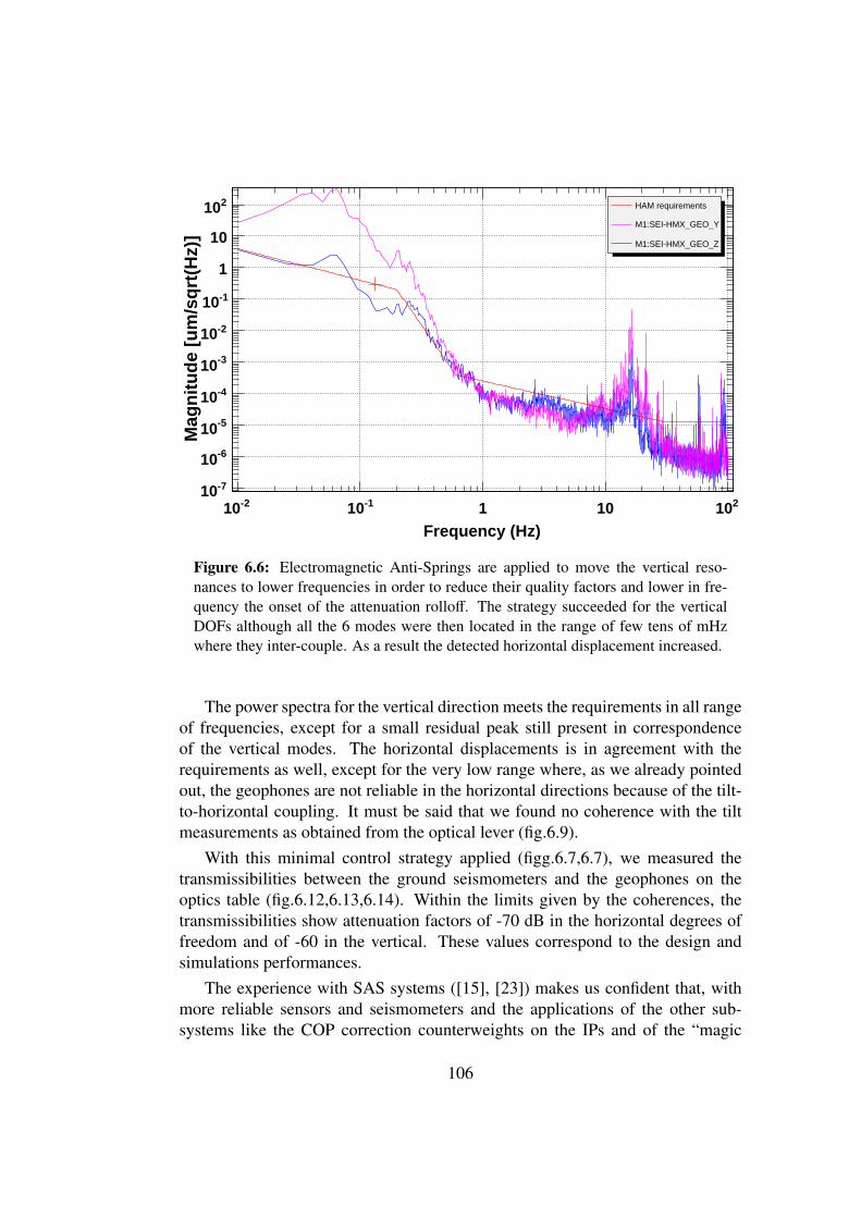
Frequency (Hz)
-210 -110 1 10 210
Mag
nit
ud
e [u
m/s
qrt
(Hz)
]
-710
-610
-510
-410
-310
-210
-110
1
10
210
Power spectrum
HAM requirements
M1:SEI-HMX_GEO_Y
M1:SEI-HMX_GEO_Z
Power spectrum
Figure 6.6: Electromagnetic Anti-Springs are applied to move the vertical reso-nances to lower frequencies in order to reduce their quality factors and lower in fre-quency the onset of the attenuation rolloff. The strategy succeeded for the verticalDOFs although all the 6 modes were then located in the range of few tens of mHzwhere they inter-couple. As a result the detected horizontal displacement increased.
The power spectra for the vertical direction meets the requirements in all rangeof frequencies, except for a small residual peak still present in correspondenceof the vertical modes. The horizontal displacements is in agreement with therequirements as well, except for the very low range where, as we already pointedout, the geophones are not reliable in the horizontal directions because of the tilt-to-horizontal coupling. It must be said that we found no coherence with the tiltmeasurements as obtained from the optical lever (fig.6.9).
With this minimal control strategy applied (figg.6.7,6.7), we measured thetransmissibilities between the ground seismometers and the geophones on theoptics table (fig.6.12,6.13,6.14). Within the limits given by the coherences, thetransmissibilities show attenuation factors of -70 dB in the horizontal degrees offreedom and of -60 in the vertical. These values correspond to the design andsimulations performances.
The experience with SAS systems ([15], [23]) makes us confident that, withmore reliable sensors and seismometers and the applications of the other sub-systems like the COP correction counterweights on the IPs and of the “magic
106

T0=05/07/2007 20:48:06 M1SAS.al.txtT0=05/07/2007 20:48:06 M1SAS.al.txtT0=05/07/2007 20:48:06 M1SAS.al.txt
Frequency (Hz)
-310 -210 -110 1 10 210
Mag
nit
ud
e (d
B)
5
10
15
20
25
30
35
40
Transfer function
T0=05/07/2007 20:48:06 M1SAS.al.txt
DC-damper X
Transfer function
T0=05/07/2007 20:48:06 M1SAS.al.txtT0=05/07/2007 20:48:06 M1SAS.al.txtT0=05/07/2007 20:48:06 M1SAS.al.txt
Frequency (Hz)
-310 -210 -110 1 10 210
Ph
ase
(deg
)
-100
-80
-60
-40
-20
0
20
40
60
Transfer function
T0=05/07/2007 20:48:06 M1SAS.al.txt
D-damper C X
Transfer function
T0=05/07/2007 20:48:06 M1SAS.al.txtT0=05/07/2007 20:48:06 M1SAS.al.txtT0=05/07/2007 20:48:06 M1SAS.al.txt
Frequency (Hz)
-310 -210 -110 1 10 210
Mag
nit
ud
e (d
B)
5
10
15
20
25
30
35
40
Transfer function
T0=05/07/2007 20:48:06 M1SAS.al.txt
DC-damper X
Transfer function
T0=05/07/2007 20:48:06 M1SAS.al.txtT0=05/07/2007 20:48:06 M1SAS.al.txtT0=05/07/2007 20:48:06 M1SAS.al.txt
Frequency (Hz)
-310 -210 -110 1 10 210
Ph
ase
(deg
)
-100
-80
-60
-40
-20
0
20
40
60
Transfer function
T0=05/07/2007 20:48:06 M1SAS.al.txt
D-damper C X
Transfer function
Figure 6.7: The plot shows the transfer function amplitude and phase of the positionand damping combined control for the horizontal mode X that we applied to obtainthe performances which met the seismic attenuation requirements. The same filtershape, but with different gains and locations of poles and zeros adapted to the specificphysical plant responses are applied to the other modes.
wands” on the GAS filters, these performance could be extended to -100 dB in thehorizontal DOF and -80 dB in the vertical while minimizing the low frequencyr.m.s.residual motion at the same time.
6.4 Ground Tilt
Even if the displacement noise at very low frequency can be significantly attenu-ated by the damping controls, the source of much of the measured horizontal geo-phone noise still remains not definitely identified. The seismic noise measured bythe seismometers does not explain it unless it comes from angular seismic noise,which the seismometers would not sense.
According to the model of section 2.4.2 the response of the IPs to the groundtilt is
x =A + Bω2
A −Cω2 x0 +kθ/l2
A −Cω2Θ (6.10)
107

T0=05/07/2007 20:51:00 M1SAS.al.txt
Frequency (Hz)
-310 -210 -110 1 10 210
Mag
nit
ud
e (d
B)
-140
-120
-100
-80
-60
-40
-20
0
20
40
Transfer function
T0=05/07/2007 20:51:00 M1SAS.al.txt
DC-damper X
Transfer function
T0=05/07/2007 20:51:00 M1SAS.al.txt
Frequency (Hz)
-310 -210 -110 1 10 210
Ph
ase
(deg
)
-250
-200
-150
-100
-50
0
Transfer function
T0=05/07/2007 20:51:00 M1SAS.al.txt
D-damper C X
Transfer function
Figure 6.8: The plot shows the Bode plot of the open loop transfer function GC forthe x degree of freedom. The same strategy is applied to all the DOFs. The u.g.f.is chosen as a trade off between the necessity to damp the low frequency resonancesand the re-injection of high frequency noise. In this case u.g.f.=100 mHz.
where Θ represent the angular spectrum of the ground. Since direct and accu-rate measurements of the ground tilt do not exist, the classical model, very oftenadopted to have an estimation, relies on the Rayleigh waves propagation model.In it, as discussed in the first chapter, the ground tilt noise spectrum is proportionalto the vertical component of Rayleigh waves divided by the propagation speed. Asdiscussed in chapter 1, the coupling factor between the nominal ground tilt Θ andits translational motion X0 varies from 10−3 to 10−1 rad/m and thus, ideally, thecontribute should be negligible. However the model does not take into accountlocal environmental factors like the wind and anthropogenic activities which cantilt the local structures (buildings) and are more likely to make the contributiondominant at very low frequencies. The experience from the HAM-SAS prototypeand the seismic team at Virgo ([52]) reinforce that hypothesis, although the ulti-mate proof will come when reliable tilt-seismomters will be available. Both LIGOand Virgo are now strongly involved in the development of such sensors.
108

T0=29/06/2007 06:38:13 Avg=40 BW=0.0117187
Frequency (Hz)
-210 -110 1 10 210
Co
her
ence
0
0.1
0.2
0.3
0.4
0.5
0.6
0.7
0.8
0.9
1
Coherence
T0=29/06/2007 06:38:13 Avg=40 BW=0.0117187
QPD YAW / GEOPHONES Y
QPD YAW / GEOPHONES X
Coherence
Figure 6.9: Coherence between the pitch as measured by the optical lever and thehorizontal degress of fredom as measured by the geophones.
*T0=17/06/2007 20:40:04 *Avg=10 *BW=0.0117187
Frequency (Hz)
-210 -110 1 10 210
Mag
nit
ud
e [u
m/s
qrt
(Hz)
]GE
-610
-510
-410
-310
-210
-110
1
Power spectrum
*T0=17/06/2007 20:40:04 *Avg=10 *BW=0.0117187
GEOPHONE X
GEOPHONE Y
GEOPHONE Rz
Power spectrum
Power spectrum
Figure 6.10: Geophones noise floor measured disconnecting the sensors from thereadout board.
109

*T0=24/06/2007 06:57:48 *Avg=17/Bin=11L *BW=0.0117178
Frequency (Hz)
-210 -110 1 10 210
Mag
nit
ud
e [u
m/s
qrt
(Hz)
]
-810
-710
-610
-510
-410
-310
-210
-110
1
10
Power spectrum
*T0=24/06/2007 06:57:48 *Avg=17/Bin=11L *BW=0.0117178
GURALP X
GEOPHONE X
HAM REQUIREMENTS
Power spectrum
*T0=24/06/2007 06:57:48 *Avg=17/Bin=11L *BW=0.0117178
Frequency (Hz)
-210 -110 1 10 210
Mag
nit
ud
e [u
m/s
qrt
(Hz)
]
-710
-610
-510
-410
-310
-210
-110
1
Power spectrum
*T0=24/06/2007 06:57:48 *Avg=17/Bin=11L *BW=0.0117178
GURALP Z
GEOPHONE Z
HAM REQUIREMENTS
Power spectrum
Figure 6.11: The plot shows the power spectrum on the x direction (upper plot) andof the vertical direction z (lower plot) each one compared with the reference givenby the correspondent displacement spectra from the seismometers on the ground (redcurves) and the HAM requirements. DC, damping and Resonance Gain controls areactive.
110

T0=24/06/2007 06:57:48 Avg=17/Bin=11L BW=0.0117178
Frequency (Hz)
-210 -110 1 10 210
Mag
nit
ud
e (d
B)
-100
-80
-60
-40
-20
0
20
40
Transfer function
T0=24/06/2007 06:57:48 Avg=17/Bin=11L BW=0.0117178
GEOPHONE X/ GURALP X
Transfer function
T0=24/06/2007 06:57:48 Avg=17/Bin=11L BW=0.0117178
Frequency (Hz)
-210 -110 1 10 210
Co
her
ence
0
0.1
0.2
0.3
0.4
0.5
0.6
0.7
0.8
0.9
1
Coherence
T0=24/06/2007 06:57:48 Avg=17/Bin=11L BW=0.0117178
GEOPHONE X / GURALP X
Coherence
Figure 6.12: Active performance. Horizontal Transmissibility along x. The coher-ence is often low but -70 dB are reached at 4 Hz. The geophone noise floor is reachedat about 20 Hz
111

T0=24/06/2007 06:57:48 Avg=17/Bin=11L BW=0.0117178
Frequency (Hz)
-210 -110 1 10 210
Mag
nit
ud
e (d
B)
-100
-80
-60
-40
-20
0
20
Transfer function
T0=24/06/2007 06:57:48 Avg=17/Bin=11L BW=0.0117178
GEOPHONE Y / GURALP Y
Transfer function
T0=24/06/2007 06:57:48 Avg=17/Bin=11L BW=0.0117178
Frequency (Hz)
-210 -110 1 10 210
Co
her
ence
0
0.1
0.2
0.3
0.4
0.5
0.6
0.7
0.8
0.9
1
Coherence
T0=24/06/2007 06:57:48 Avg=17/Bin=11L BW=0.0117178
GEOPHONE Y / GURALP Y
Coherence
Figure 6.13: Active performance. Horizontal Transmissibility along y. In this casethe coherence is higher than for x and the measurement is less noisy. Also in this casean attenuation of -70 dB is reached at 4 Hz. The geophone noise floor is reached atabout 20 Hz.
112

T0=24/06/2007 06:57:48 Avg=17/Bin=11L BW=0.0117178
Frequency (Hz)
-210 -110 1 10 210
Mag
nit
ud
e (d
B)
-80
-60
-40
-20
0
20
Transfer function
T0=24/06/2007 06:57:48 Avg=17/Bin=11L BW=0.0117178
GEOPHONE Z / GURALP Z
Transfer function
T0=24/06/2007 06:57:48 Avg=17/Bin=11L BW=0.0117178
Frequency (Hz)
-210 -110 1 10 210
Co
her
ence
0
0.1
0.2
0.3
0.4
0.5
0.6
0.7
0.8
0.9
1
Coherence
T0=24/06/2007 06:57:48 Avg=17/Bin=11L BW=0.0117178
GEOPHONE Z / GURALP Z
Coherence
Figure 6.14: Active performance. Vertical transmissibility along z. In the verticaldirection the coherence is almost zero at very low frequency but is good above. Asa result we have a cleaner measurement than the horizontal ones. An attenuation of-60 dB is reached at 10 Hz, then the geophone noise floor is reached
113

114
Chapter 7
Conclusions
HAM-SAS represents the convergence of more than ten years of R&D carriedout at LIGO by the SAS group to develop passive and ’soft’ solutions for theseismic isolation systems of Advanced LIGO. The several technologies producedand the know-how acquired in the past years merged into one complex systemdesigned for a specific task in the intermediate and advanced interferometers. TheHAM-SAS first item produced served as a test bench for the SAS systems forAdvanced LIGO, to prove to measure up the leap from the lab to the site, fromsingle separate systems to a multi stage reliable attenuator for an actual high-requirement optical bench. The results discussed in this thesis show that HAM-SAS was able to accomplish that task. We proved that the system is able to supportand control the HAM optics table in in a facility similar to those of the sites thatthe LASTI vacuum chambers reproduces. We showed that along each degree offreedom the system, in its passive configuration, responds like a second orderfilter with attenuation that manifestly falls as 1/ω2 up to 10 Hz, reaching -60 dBin the vertical and -70 dB in the horizontal. Above that frequency the attenuationis limited by the familiar plateaus produced by the center of percussion effectof inverted pendulums and GAS filters. This made us confident that, having thepossibility to implement the SAS solutions for this limitations, an additional orderof magnitude in attenuation could be likely achieved in all directions.
The geometry of the system allowed us to apply straightforward control strate-gies. Vertical and horizontal degrees of freedom are in first approximation inde-pendent in most of the frequency range. For both the horizontal and the verticalstages we treated each mode individually and designed control loops to damp theresonances and control the static position. With such limited bandwidth controlswe could bring the displacement noise power spectrum of the platform to meet theAdvanced LIGO requirements for the HAM chambers practically at all frequen-cies. Since the controls inevitably re-inject some noise at high frequency, a furtherimprovement of the performance would come from setting the vertical modes at
115

lower frequencies by re-tuning the GAS filters, improving the tilt correction sys-tem and adding some mass to the IP table. Since the Q factors reduce with ω2 weexpect that the reduction of the resonant frequencies will also reduce or eliminatethe need for viscous resonance damping.
The residual motion at very low frequency, especially in the horizontal de-grees of freedom, was larger than expected. In that frequency region we foundthe sensitivity limit of the geophone sensors and of the seismometers which madehard to clearly distinguish between the contribution from the environment andthe part played by the system. We suspect the role of the ground angular noiseto be determinant in overwhelming the sensor signals. Unfortunately no reliablemeasurement of the angular spectrum could be obtainable from the available seis-mometers on ground. The issue of the seismic angular noise touches HAM-SASbut it is getting growing attention from both LIGO and Virgo in view of advancedsuspensions.
HAM-SAS showed very interesting performances as a seismic attenuation sys-tem. It was a complex project and it happened within a very tight time schedulethat did not leave sufficient room for the complete optimization of the system. Aswe could expect from a prototype, we encountered many problems and difficul-ties, but we solved many and we learned from each of them becoming confidentin the HAM SAS potentialities as a platform for seismic isolation in AdvancedLIGO.
116

Bibliography
[1] A. Einstein Approximative integration of the field equations of gravitationin The Collected Papers of Albert Einstein, pp. 201-210, Princeton Univer-sity Press, 1987.
[2] R. Hulse and J. Taylor, Discovery of a pulsar in a binary system, The As-trophysical Journal, vol. 195, pp. L51-L53, 1975.
[3] L. D. Landau and E. M. Lifshitz, The Classical Theory of Fields, PergamonPress
[4] DeSalvo R., Passive, non-linear, mechanical structures for seismic attenu-ation 5th ASME Int. Conf. on Multibody Systems, Nonlinear Dynamics andControls (Long Beach, CA, 24-28 Sept.), and references therein (LIGO-P050001-00-D).
[5] Robertson N et al 2004 Proc. SPIE 5500 81-91 .
[6] Abbott R et al, Seismic isolation enhancement for initial advanced LIGO,Class. Quantum. Grav. 21 S915-921
[7] Wang C. et al, Constant force actuator for gravitational wave detectorsseismic attenuation systems, Nucl. Instrum. Methods A 489 563-9.
[8] Tariq H et al, The linear variable differential transformer (LVDT) positionsensor for gravitational wave interferometer low-frequency controls, Nucl.Instrum. Methods A 489 570-6 .
[9] C. Hardham et al, Quiet Hydraulic Actuators for LIGO,Proceedings ofControl of Precision Systems, ASPE Topical Meeting, April 2001.
[10] C. Hardham et al, Multi-DOF Isolation and Alignment with Quiet Hy-draulic Actuators, LIGO-P040021-00-R.
[11] Yumei Huang, Virginio Sannibale, Valerio Boschi, Dennis Coyne, RiccardoDeSalvo, Spring box simulations, LIGO Document LIGO-T03xxxx-yy-D
117

[12] G. Cella, V. Sannibale, R. De Salvo, S. Màrka, A. Takamori, MonolithicGeometric Anti-Spring Blades, gr-qc/0406091, NIM A 540 (2005) 502-519.
[13] S. Braccini, F. Frasconi, et al., The maraging-steel blades of the Virgo superattenuator, Meas. Sci. Technol. 11 (2000) 467-476.
[14] A. Stochino, Performance Improvement of the Geometric Anti Spring(GAS) Seismic Filter for Gravitational Waves Detectors, SURF-LIGO 2005Final Report, LIGO-P050074-00-R.
[15] A. Stochino, R. De Salvo, Y. Huang, V. Sannibale, Improvement of theseismic noise attenuation performance of the Monolithic Geometric AntiSpring filters for Gravitational Wave Interferometric Detectors, NIM, ac-cepted for publication (2007)
[16] Peter R. Saulson, Foundamentals of Inteferometric Gravitational WavesDetector, World Scientific.
[17] A. Abramovici et al., Science 256 (1992) 325.
[18] The VIRGO Collaboration, VIRGO Final Design Report, (1997).
[19] K. Danzmann et al., Max-Plank-Institut fur Quantenoptik Report, (1994).
[20] K. Tsubono, Gravitational Wave Experiments, World Scientific, pp.122(1995).
[21] C. Casciano, Seismic Isolation for the Test Masses of the VIRGO Gravita-tional Wave Antenna, PhD Thesis, University of Pisa (2002).
[22] M. Barton, A. Bertolini, E. Black, G. Cella, E. Cowan, E. D’ambrosio, R.DeSalvo, K. Libbrecht, V. Sannibale, A. Takamori, N. Viboud, P. Willems,H. Yamamoto, Proposal of a Seismic Attenuation System (SAS) for theLIGO Advanced Configuration (LIGO-II), T990075-00, 1999, LIGO In-ternal Note.
[23] A. Takamori, et al., Mirror Suspension System for the TAMA SAS, Class.Quantum Grav. 19, 1615, (2002).
[24] Gravitational Wave Detection II, Proceedings of the 2nd TAMA Interna-tional Workshop held 19-22 October, 1999 in Tokyo, Japan. UniversalAcademy Press Frontiers Science Series Edited by S. Kawamura and N.Mio. 32 (2000) 311.
118

[25] G. Cella, R. DeSalvo, V. Sannibale, H. Tariq, N. Vibound, and A. Takamori,Nucl. Instrum. Meth. A, 487, 652, (2002).
[26] A. Bertolini, G. Cella, R. DeSalvo, and V. Sannibale, Nucl. Instrum. Meth.A, 435, 475, (1999).
[27] H. Brody, The sweet spot of a baseball bat, American Journal of Physics,54(7), 640-643 (1986).
[28] G. Losurdo, et al.: An inverted pendulum pre-isolator stage for VIRGOsuspension system, Rev. Sci. Instrum., 70, 2507-2515 (1999).
[29] G. Cella, V. Sannibale et al., Monolithic geometric anti-spring blades,Nucl. Instr. and Met. A 540 (2005) 502-519.
[30] M. Ando, A. Bertolini, G. Cella, R. DeSalvo, Report to NSF on the TAMA-SAS Passive Seismic Attenuation Chain Test for the Tokyo University 3 me-ter Interferometer, LIGO-T010006-00-R.
[31] G. Losurdo, Ultra-Low Frequency Inverted Pendulum for the VIRGO TestMass Suspension, Tesi di Dottorato di Ricerca in Fisica, Scuola NormaleSuperiore di Pisa - Classe di Scienze, Italia Ottobre 1998.
[32] P. Raffai, et al., Inverted Pendulum as Low Frequency Pre-Isolation forAdvacned Gravitational Wave Detectors, submitted to LSC.
[33] H. Tariq, et al. The Linear Variable Differential Transformer (LVDT) Posi-tion Sensor for Gravitational Wave Interferometer Low-frequency Controls,Nuclear Instruments and Methods in Physics Research Section A, Volume489, Issue 1-3, p. 570-576.
[34] M. Mantovani, R. DeSalvo, One Hertz Seismic Attenuation for Low Fre-quency Gravitational Waves Interferometers, accepted for publication onNucl. Instr. and Meth. (2005).
[35] A. Bertolini et al, Design and prototype tests of a seismic attenuation sys-tem for the advanced-LIGO output mode cleaner, Class. Quantum Grav. 23S111-S118, (2006).
[36] Ligo Internal Document, D051100 to 051199 (2006)
[37] M. Husman, Suspension and Control for Interferometric GravitationalWave Detectors, Ph.D. Thesis, University of Glasgow (2000).
119

[38] V. Sannibale et al., A new seismic attenuation filter stage (MGASF) foradvanced gravitational wave interferometers detectors, submitted to NIM(2006).
[39] M.Beccaria, et al., Nuc. Intrum. Meth. in Phys. Res. A., 394,397-408(1997).
[40] C. Bradaschia, et al., Nucl. Instrum. Meth. A, 289, 518 (1992).
[41] J. Hough, K. Danzmann, et al., GEO600 Proposal, unpublished (1994).
[42] K. Kuroda, et al., in Proceedings of the 1st International Conference onGW: Sources and Detectors, eds. F. Fidecaro, I. Ciufolini, World Scientific,Singapore (1997). (1994).
[43] LIGO Scientific Collaboration, ed. P Fritschel, Advanced LIGO SystemsDesign, LIGO Document T010075-00-D (2001).
[44] Torrie C.I., Development of the suspensions for the GEO 600 gravitationalwave detector, PhD thesis, (2000), University of Glasgow.
[45] H. Goldstein, Classical Mechanics, Addison-Wesley.
[46] J. J. D’Azzo, C. H. Houpis, S. N. Sheldon, Linear Control System Analysisand Design with Matlab, Fifth Edition, Marcel Dekker, Inc. (2003)
[47] A. Bertolini, High sensitivity accelerometers for gravity experiments, PhD.Thesis, University of Pisa, LIGO-P010009-00-Z
[48] Julius O. Smith III, Mathematics of the Discrete Fourier Transform (DFT),with Audio Applications, Second Edition, W3K Publishing, 2007.
[49] P. Fritschel, HAM Seismic Isolation Requirements, LIGO Internal Docu-ment T060075-00-D, (2006)
[50] P. Fritschel et al., Seismic Isolation Subsystem Design Requirements Docu-ment, LIGO Internal Note E990303-00-D, (2001)
[51] J. Peterson, Observations and Modeling of Seismic Background Noise,USGS Report 93-322 (1993)
[52] G. Losurdo, MIT Lunch Talk, May 17th 2007, LIGO MIT
120

[53] R. De Salvo, S. Marka, K. Numata, V. Sannibale, A. Takamori, H. Tariq,E.J. Ugas, T. Yoda, Y. Aso, A. Bertolini, Study of quality factor and hys-teresis associated with the state-of-the-art passive seismic isolation systemfor Gravitational Wave Interferometric Detectors., Nucl. Instrum. Meth. A538:526-537, 2005
121