UNIVERSITA DEGLI STUDI DI` CAGLIARI - Dottorati di ricerca · 2016-05-23 · pute variational...
115
UNIVERSIT ` A DEGLI STUDI DI CAGLIARI Facolt` a di Scienze Matematiche, Fisiche e Naturali Dipartimento di Fisica PhD Thesis PhD School in Physical Sciences and Technologies PhD Course in Nuclear, Subnuclear Physics and Astrophysics XXI Cycle (2005-2008) First ab–initio, variational ro–vibrational spectra of the C 2 H 2 molecule Advisor: Prof. Luciano Burderi Candidate: Andrea Urru Co-advisor: Dr. Giacomo Mulas
Transcript of UNIVERSITA DEGLI STUDI DI` CAGLIARI - Dottorati di ricerca · 2016-05-23 · pute variational...

UNIVERSITA DEGLI STUDI DICAGLIARI
Facolta di Scienze Matematiche, Fisiche e Naturali
Dipartimento di Fisica
PhD Thesis
PhD School in Physical Sciences and TechnologiesPhD Course in Nuclear, Subnuclear Physics
and Astrophysics
XXI Cycle (2005-2008)
First ab–initio, variational ro–vibrational spectraof the C2H2 molecule
Advisor: Prof. Luciano Burderi Candidate: Andrea Urru
Co-advisor: Dr. Giacomo Mulas

Typeset in LATEX by Andrea Urru
December 2, 2008

To my family

4

Presentation
The availability of theoric accurate spectra of low-mass cool stars, the most numerous,
will be necessary to maximise the scientific return of space mission Gaia (see figures 1
and 2) (1) of ESA (European Space Agency). The satellite launch is scheduled to take
place ‘no later than’ 2012 (2). Gaia’s payload consists of three instruments: an astro-
nomic instrument, a multi-band photomer and a spectrometer that will continuously
and repeatedly scan the sky during the 5-yr mission. The definition and optimization
studies for the Gaia satellite spectrograph, “the radial velocity spectrometer” (RVS),
converged in late 2002 with the adoption of the instrument baseline. The RVS is an
integral field spectrograph: it uses neither slits nor fibres, but disperses all of the light
entering its 2.00◦ × 1.61◦ field of view with a resolving power R = λ∆λ
= 11500 over
the wavelength range [848, 878] nm. On average, each source will be observed 102
times over this period. The RVS will collect the spectra of about 100-150 million stars
up to magnitude V ≃ 17− 18. Moreover, for R ≥ 10000, numerous lines contained in
the RVS infrared wavelenght range are unblended and it becomes possible to deter-
mine the individual abundances of several chemical species and in particular of alpha
elements (e.g. magnesium, silicon). The RVS is an integral field spectrograph. As
a consequence, in regions of high stellar density, the spectra of neighbouring sources
will overlap and the mean rate of overlap grows linearly with resolution. Numerical
simulations have shown that it will be possible, to a certain extent, to deconvolve the
stacked spectra (see (3; 4; 5)).
The cool stars, known being the most numerous, are dominated by molecular
absorption and, in particular for carbon stars (stars with a photospheric abundance
of Carbon grater than that of oxygen), one needs to consider triatomic species such as
HCN and HNC (6), and C3 (7). For some dwarfs molecules larger than triatomics
are known to form: methane and acetylene are thought to be particular important for
carbon stars (7). Given that the computed rotation-vibration line lists for triatomic
species have contained between 10 and 500 million distinct transitions, line lists for
these polyatomic molecules will need to consider many billions of transitions. So far
no comprehensive line list exists for any species larger than triatomic. C2H2 is known

6
Figure 1: Gaia satellite service module

7
Figure 2: Gaia satellite focal plane
to be abundant in cool carbon stars (see figure 3), the wavelength of the cis bending
fundamental is close to that of HCN at 13.71 µm (729.2 cm−1) (8). However, no
extensive data set for acetylene is currently in the public domain, so it has not been
used in the computation of syntetic spectra. The inclusion of such data would be likely
to significantly change the model atmosphere and synthetic spectrum. My work in
this thesis aims at assembling the computational tools needed to calculate such a
complete database of intensity transitions for acetylene molecule, with the prospect
of including them in model atmospheres of cool stars.
Overview of this thesis
The first chapter introduces the theoretical machinery which can be used to com-
pute variational spectra of a tetratomic molecule, based on ab initio calculations.
The second chapter gives a general overview on the state of the art of rovibrational
spectroscopy of the acetylene molecule, introducing the available experimental and
theoretical data on which the present work can be based. The following chapter de-
scribes our calculations, along with a description of the existing codes which have
been used in the computation of the energy levels of the acetylene (wavr4 code)

8
Figure 3: ISO SWS spectra taken towards 12 YSO’s (young stellar objects). TheHCN and C2H2 bending mode are indicated. Figure taken from Lahuis and vanDishoeck [(9)]

9
and the new codes developed for the calculation of transition dipole moments of this
molecule, which are not yet available in the literature. The fourth chapter compares
our calculations with experimental lists of rovibrational lines in two parallel bands.
The last chapter presents the conclusions of the work and the way forward that this
work opens for the near future.

10

Contents
1 Calculating the spectra of tetratomic molecules 13
1.1 Introduction . . . . . . . . . . . . . . . . . . . . . . . . . . . . . . . . . 13
1.2 Solution of the electronic problem . . . . . . . . . . . . . . . . . . . . . 14
1.3 Solution of the nuclear problem . . . . . . . . . . . . . . . . . . . . . . 16
1.3.1 Coordinate systems . . . . . . . . . . . . . . . . . . . . . . . . . 18
1.4 Choice of the basis functions . . . . . . . . . . . . . . . . . . . . . . . . 20
1.4.1 Angular basis . . . . . . . . . . . . . . . . . . . . . . . . . . . . 21
1.4.2 Radial basis . . . . . . . . . . . . . . . . . . . . . . . . . . . . . 22
1.5 Solution of the complete problem . . . . . . . . . . . . . . . . . . . . . 23
1.6 Method of solution: the dvr technique . . . . . . . . . . . . . . . . . . 25
1.6.1 Numerical computation of matrix elements and DVR . . . . . . 26
2 The C2H2 System 29
2.1 Fundamentals of C2H2 spectroscopy . . . . . . . . . . . . . . . . . . . . 29
2.1.1 Vibrational motion . . . . . . . . . . . . . . . . . . . . . . . . . 30
2.1.2 Rotational motion . . . . . . . . . . . . . . . . . . . . . . . . . 32
2.1.3 Parity . . . . . . . . . . . . . . . . . . . . . . . . . . . . . . . . 33
2.1.4 Nuclear Spin Statistics . . . . . . . . . . . . . . . . . . . . . . . 33
2.1.5 Transition intensity and selection rules . . . . . . . . . . . . . . 35
2.1.6 Calculation of the line strength . . . . . . . . . . . . . . . . . . 35
2.1.7 Rotational Selection Rules and Honl-London factors . . . . . . . 37
2.2 Existing Data . . . . . . . . . . . . . . . . . . . . . . . . . . . . . . . . 38
2.2.1 Experimental data: the HITRAN Database . . . . . . . . . . . 39
2.2.2 Theoretical data: Potential Energy Surfaces . . . . . . . . . . . 41
2.2.3 Dipole Moment surfaces . . . . . . . . . . . . . . . . . . . . . . 42
2.2.4 State of the art of variational C2H2 spectra . . . . . . . . . . . 43
3 Calculations 45
3.1 The wavr4 code . . . . . . . . . . . . . . . . . . . . . . . . . . . . . . 45

12 Contents
3.1.1 Implementation details . . . . . . . . . . . . . . . . . . . . . . . 48
3.1.2 Calculation of energy levels . . . . . . . . . . . . . . . . . . . . 50
3.2 Purely vibrational transitions . . . . . . . . . . . . . . . . . . . . . . . 52
3.2.1 The Dipole code . . . . . . . . . . . . . . . . . . . . . . . . . . 52
3.2.2 Results . . . . . . . . . . . . . . . . . . . . . . . . . . . . . . . . 54
3.3 Calculation of rotational constant B . . . . . . . . . . . . . . . . . . . . 59
4 Results vs HITRAN 89
4.1 Calculations of line intensities . . . . . . . . . . . . . . . . . . . . . . . 89
4.1.1 The (3ν4 + ν5)0 cold band . . . . . . . . . . . . . . . . . . . . . 90
4.1.2 The (ν3) fundamental hot band . . . . . . . . . . . . . . . . . . 91
5 Conclusions and perspectives 95
5.1 Example synthetic opacities . . . . . . . . . . . . . . . . . . . . . . . . 96
5.2 Forthcoming work . . . . . . . . . . . . . . . . . . . . . . . . . . . . . . 97

Chapter 1
Calculating the spectra oftetratomic molecules
1.1 Introduction
The theoretical study of many topics in quantum chemistry is based on the study of
a complete molecular Hamiltonian. Within the framework of nonrelativistic quantum
mechanics the three-dimensional time-indipendent Schrodinger equation is:(
T + U(r))
Ψ(r) = EΨ(r) (1.1)
The attempt to compute the eigenvalues and eigenfunctions must begin with the
construction of an appropriate representation of the Hamiltonian. By quantizing the
classical energy in Hamilton form one obtains a molecular Hamilton operator where
R and r are the coordinate vector of nuclei and electrons (ions) respectively. The
Hamiltonian H is a sum of five terms. They are:
1) The kinetic energy operators for each nucleus in the system
Tn = −∑
i
~
2Mi
∇2(Ri) (1.2)
2) The kinetic energy operators for each electron in the system
Te = −∑
i
~
2me
∇2(ri) (1.3)
3) The potential energy between the electrons and nuclei, the total electron-nucleus
Coulombic attraction in the system
Uen = −∑
i
∑
j
Zie2
4πǫ0|Ri − rj|(1.4)

14 Chapter 1. Calculating the spectra of tetratomic molecules
4) The potential energy arising from Coulombic electron-electron repulsions
Uee =1
2
∑
i
∑
j 6=i
e2
4πǫ0|ri − rj|(1.5)
5) The potential energy arising from Coulombic nuclei-nuclei repulsions (nuclear re-
pulsion energy)
Unn =1
2
∑
i
∑
j 6=1
ZiZje2
4πǫ0|RI −Rj|(1.6)
Here Mi is the mass of nucleus i, Zi and Zj are the atomic numbers of nucleus i and
j and me is the mass of electron.
1.2 Solution of the electronic problem
The determination of the energy and wavefunction of the molecular system is a hard
task because it is a many-body system. This complete problem is more easily solved
if it can be separated in smaller problems. The Born-Opphenheimer (10) or adi-
abatic approximation allows to separate the electronic and nuclear problems. This
approximation is an important tool of quantum chemistry, without it only the light-
est molecules could be handled. The success of the Born-Oppenheimer approximation
is due to the high ratio between nuclear and electronic masses. The heavier nuclei
move more slowly than the lighter electrons. From a conceptual point of view, this
approximation amounts to assuming that the nuclear motion is so slow, with respect
to the one of the electrons, that the electrons behave, at any given moment, as if
the nuclei had been fixed at their instantaneous position for an infinite time. In the
framework of this approximation, one therefore proceeds first to consider a purely
electronic Hamiltonian He(R) which depends on the nuclear coordinates only as fixed
parameters.
He(R) = Te + Uen + Uee + Unn, (1.7)
where we remark that obviously
H = He(R) + TN . (1.8)
The interacting electrons thus move in the Coulomb potential of the nuclei clamped
at certain positions in space. One has to solve a Schrodinger equation that involves
only the electronic degrees of freedom for any fixed configuration of the molecule:
He(R)|φn(R) >= ǫn(R)|φn(R) >, (1.9)

1.2. Solution of the electronic problem 15
where we have noted explicitly that the electronic Hamiltonian He, its eigenstates
ǫn(R) and eigenvalues φn(R) depend on the particular nuclear configuration. We
note that the electronic eigenstates for any fixed choice of the positions of the nuclei
forms a complete set of basis for the electrons. So we can write:
Ψ(r,R) =∑
m
φm(r;R)ηm(R) (1.10)
where the functions φm depends on R only as external parameters and the coefficients
ηm are functions of R. So the complete Schrodinger equation of our system can be
written:
(TN + He)Ψ(r,R) = EΨ(r,R). (1.11)
If we now assume that the (parametric) dependence of φm(r;R) is weak, then Tn
approximately commutes with φm(r;R), i. e. we can neglect the action of the op-
erator Tn on φm(r;R). This assumption is exactly the mathematical expression of
the Born–Oppenheimer approximation. Under this approximation, we can rewrite
Eq. 1.11 as
(TN + He)Ψ(r,R) = (TN + He)∑
m
φm(r;R)ηm(R) =
∑
m
φm(r;R)TNηm(R) +∑
m
ηm(R)Heφm(r;R) =
∑
m
φm(r;R)TNηm(R) +∑
m
ηmǫn(R)φm(r;R). (1.12)
Multiplying on the left by φ∗j(r;R), integrating over the electronic degrees of freedom
and making use of the orthonormality of the φ functions, we obtain
(TN + ǫn(R))ηj(R) = Eηj(R), (1.13)
i. e. we obtain a new Schrodinger equation for the nuclei alone,
HN |ΨN >= E|ΨN >, (1.14)
with an effective Hamiltonian HN defined as
HN = TN + ǫn(R). (1.15)
The electronic degrees of freedom do not explicitly appear anymore, the effect of the
electrons on nuclear motion being entirely contained in the effective potential ǫn(R).
The hypersurfaces defined by ǫn(R) are, for this reason, called potential energy sur-
faces (P.E.S.). We remark that the electronic wavefunctions, i. e. the eigenfunctions

16 Chapter 1. Calculating the spectra of tetratomic molecules
of the electronic problem described by Eq. 1.9, are not needed to study the nuclear
motion, but only the eigenvalues. The importance of this remark is that it enables us
to use relatively simpler approaches to solve the electronic problem, such as Density
Functional Theory (DFT) (see references (11; 12)) which trade a higher computational
efficiency in calculating accurate potential energy surfaces, in exchange of giving up
the knowledge of the electronic wavefunctions. The eigenvalue E in Eq. 1.14 is the
total energy of the molecule, including contributions from both electronic and nuclear
degrees of freedom.
1.3 Solution of the nuclear problem
The next step is to solve Eq. 1.14 for the nuclear motion, which is itself still a com-
plicated, many–body problem. The traditional approach, very effective for semi-rigid
molecules, is to choose a co–moving reference system, bound to the equilibrium config-
uration of nuclei, and express all nuclear coordinates as functions of the Euler angles
(13) of this system and of the displacements from the equilibrium positions. If the
latter displacements are small, the effective potential is well represented by its Taylor
expansion around its minimum, considering the terms of higher order than the leading
quadratic ones as small perturbations. In this case, a natural choice of co–moving axes
is given by the Eckart conditions (see Sect. 2.1.6) (14), and a natural choice of internal
degrees of freedom is given by the normal coordinates of the natural harmonic modes.
With this choice, one obtains a formally simple expression of the classical nuclear ki-
netic energy term, which can then be quantised using either the Podolsky formalism
(15) or going through the straightforward but cumbersome algebra of quantising in
cartesian coordinates and changing variables after quantisation:
H =∑
α,β
µαβPαPβ−∑
α
hαPα +1
2
∑
α,β
µ1/2pαµαβµ−1/2pβ +
1
2
∑
k
µ1/2pkµ−1/2pk + ǫn(R),
(1.16)
where Pα and Pβ are the components of the total angular momentum and pα and
pβ are the components of angular momentum arising from vibrations alone. Also
the indices α, β denote the x, y or z axes of the body–fixed system, and µ is the
determinant of the coefficients µαβ (functions only of the normal coordinates). Here
hα =1
2
∑
β
[
2µαβ pβ + (pβµαβ) + µαβµ1/2(
pβµ−1/2
)]
(1.17)
in which pβ operates only on what is included in the parentheses. In practice, if the
oscillations are small, the terms predominant in the Hamiltonian are of zero-order and

1.3. Solution of the nuclear problem 17
the terms of superior order are considered as small perturbations. The perturbation
theory is well known and its application to molecular rotation and vibration, up
to second order, is well explained in the book of Papousek and Aliev (16). If the
oscillations are of large amplitude or the potential energy is strongly anharmonic,
the perturbation terms are not small. Hence the perturbation series may converge
slowly or not converge at all. In such cases a variational approach is preferable. This
approach entails
1. choosing a complete (in principle) basis set to represent the Banach space of the
nuclear wavefunctions;
2. representing all wavefunctions and operators in this basis;
3. truncating this basis set to a finite number of functions, which define a subspace
of the total space of nuclear wavefunctions;
4. projecting all wavefunctions and operators to this subspace;
5. the infinite eigenvalue problem in Eq. 1.14 is thus replaced by the approximated
problem of finding eigenvalues and eigenvectors of the finite hamiltonian matrix
which results from applying steps 2 and 4 to the operator HN defined in Eq. 1.15.
The designation “variational” applies because in this truncated basis the energy eigen-
values are all larger than or equal to the corrisponding exact eigenvalues: ENI ≥ Ei,
where Ei are the true eigenvalues. The accuracy of this method is tightly related to
the error implied in the truncation of the basis set and the subsequent projection to
the corresponding reduced subspace. In principle, any complete basis set will work
equally well, if enough basis functions are retained. On the other hand, the larger is
the basis set, the larger is the truncated hamiltonian matrix to be diagonalised. There-
fore, choosing a “good” basis set is crucial to achieve an acceptable level of accuracy
with a feasible computational cost. “Good” in this case means several things:
1. the number of basis functions needed to accurately represent the eigenfunctions
must be as close as possible to the number of such eigenfunctions;
2. the truncated hamiltonian matrix must be as simple as possible first to calculate
and then to diagonalise;
In principle, one can definitely use, as such a basis set, the eigenfunctions of the
rigid–rotor, harmonic approximation problem, i. e. the result of considering the
zero–order approximation of Eq. 1.16. Indeed this was done, (17; 18), as it is a

18 Chapter 1. Calculating the spectra of tetratomic molecules
Figure 1.1: Representation of the space–fixed and body–fixed reference frames, andconsequent definition of the Euler angles
natural choice and it results in a relatively easy evaluation of many matrix elements,
for which analytic expressions can be found (19). Unfortunately, if large amplitude
oscillations are involved such a basis set fails miserably the first requirement for a
“good” basis set, i. e. a very large number of basis functions is required to obtain
convergence for a small number of eigenfunctions (see e. g. 20).
1.3.1 Coordinate systems
Coordinate systems based on generalized orthogonal vectors have become a very pop-
ular choice in dealing with wide-amplitude motions in polyatomic systems. Recently
M. Mladenovic (21) gave a concise account of this approach together with a detailed
descriptions of applications to some molecules. The definition of generalized orthogo-
nal vectors is tightly connected to the general expression of the quantum–mechanical
nuclear kinetic energy when generalised internal coordinates are introduced instead of
simple cartesian coordinates for the nuclei. The internal geometry of a molecule com-
posed of n atoms is generally represented by first choosing a number n− 1 of vectors
di which uniquely specify it (such as Radau vectors, Jacobi vectors etc. see Sect. 3.1).
The fact that they are n− 1 accounts for having taken out the degrees of freedom of
translation of the center of mass of the system. Then one of the vectors, which we
take to be d1, is arbitrarily chosen as the z–axis of an orthogonal set of co–moving,
body–fixed axes x, y, and z. This defines two of the Euler angles of the body–fixed
system, namely φ and θ (see Fig. 1.1). A second vector d2 is then arbitrarily chosen
to define the (zx) molecular plane, which is spanned by d1 and d2. This uniquely
defines the line of nodes and thus the third Euler angle χ (see Fig. 1.1). Such a choice,

1.3. Solution of the nuclear problem 19
or embedding, of co–moving, body–fixed axes is different from the Watson–Eckart def-
inition (see Eq. 1.16 above) which is the usual choice for semirigid molecules. While
it loses the intuitive physical meaning of the axes coincident, to first order, with the
principal axes of inertia of the molecule, it is convenient for a choice of “good” gen-
eralised coordinates as defined previously. Analytical expressions of the orthogonal
transformations connecting the space–fixed and the body–fixed reference frames, as
functions of the Euler angles so defined, can be found, for example, in the work of M.
Mladenovic (21). We can then take, as generalised internal coordinates:
1. the three Euler angles φ, θ and χ;
2. the n− 1 lengths qα of the vectors di;
3. the n − 2 bending θj angles between each of the vectors di and the vector d1,
with 2 ≤ i ≤ n− 1;
4. the n−3 torsion χk dihedral angles between the planes (d1d2) and (d1di), with
3 ≤ i ≤ n− 1.
With such a choice, it turns out (22) that one can write
TN = Tstr + Tang, (1.18)
where Tstr contains no angular variables and Tang contains the contribution due to
internal and overall (i. e. the Euler angles) rotational degrees of freedom. Very
generally, one can write
Tstr = − ~2
2M
(
n−1∑
α=1
1
µqα
∂2
∂q2α
+n−1∑
α,β 6=α
Fαβ∂2
∂qα∂qβ
)
. (1.19)
Internal coordinates qα chosen such that each of the kinetic coupling constants Fαβ are
equal to zero constitute an important subgroup of possible descriptions of the internal
geometry. The qα are defined to be a set of generalized orthogonal coordinates (21) if
and only if
Fαβ = 0 ∀α, β. (1.20)
One of the most attractive features of generalised orthogonal coordinates is the sim-
plicity of the kinetic energy operator:
TN =1
2M
n−1∑
α=1
[
− ~2
µqα
(
∂2
∂q2α
+2
qα
∂
∂qα
)
+1
µqαq2α
l2α
]
, (1.21)

20 Chapter 1. Calculating the spectra of tetratomic molecules
with the reduced masses µqαand internal angular momenta lα as defined in (21).
Eq. 1.21 results from all mixed terms in Tstr vanishing, thanks to Eq. 1.20. This is
the so–called maximally separable form, in which
Tstr =1
2M
n−1∑
α=1
[
− ~2
µqα
(
∂2
∂q2α
+2
qα
∂
∂qα
)]
(1.22)
and
Tang =1
2M
n−1∑
α=1
[
1
µqαq2α
l2α
]
. (1.23)
There is not a unique choice of generalized orthogonal coordinates for a given molecu-
lar system; indeed, four different possibilities are described for a tetratomic molecule
by e. g. Gatti (23). A detailed expression of the resulting Tang can be found in Eq. 37
of (21), and we report it here for convenience of the reader
Tang = −~2 1
2f(d2, d1)
[
∂2
∂θ21
+ cot θ1∂
∂θ1
− 1
sin2 θ1
(Jz − lz)2
~2
]
+
1
2
n−2∑
2
f(d2, d1)l2i +
1
2MµRR2[J2 − 2(Jz − lz)2 − 2Jzlz +
2∑
i,j>i
lizljz − (J−l− + J+l+) + (l+ − J−)
(
−~∂
∂θ1
+ cot θ1(lz − Jz)
)
+
(l− − J+)
[
~∂
∂θ1
+ cot θ1(lz − Jz)
]
+∑
i,j>i
(l+i l−j + l−i l
+j )] (1.24)
where f(d2, d1) is the reduced mass of the bending coordinate θ1:
f(di, d1) =1
M
(
1
µdid2
i
+1
µRd21
)
, (1.25)
J is the total angular momentum in the body-fixed frame and J± are the correspond-
ing raising and lowering operators.
1.4 Choice of the basis functions
Within this choice of generalised coordinates, we can appropriately select an appro-
priate complete basis set. This is usually taken to be a direct product of a complete
basis in the stretching coordinates Φα times a complete basis in the rotation–angular
coordinates Φang.
|Φ〉 =∏
|Φang〉 |Φα〉 (1.26)
.

1.4. Choice of the basis functions 21
1.4.1 Angular basis
Suitable rotation–angular basis sets in the body-fixed reference frame can be found
in Eq. 30 of (21)
P|k−K|l1
(cos θ1)
[
n−2∏
i=2
Y ki
li(cos θi, χi)
]
|J,K,M〉 (1.27)
where P kl (cos θ) are normalized associated Legendre functions (24), and Y ki
li(cos θi, χi)
are spherical harmonics (24) with Condon-Shortley phase convention (25)
Y ki
li(cos θi, χi) = (−1)(ki+|ki|)/2P ki
li(cos θi)
1√2πeikiχi (1.28)
and
| JKM〉 =
[
2J + 1
8π2
]1/2
DJ∗M,K(φ, θ, χ) = (−1)M−K
[
2J + 1
8π2
]1/2
DJ−M,−K(φ, θ, χ)
(1.29)
are the (normalised) symmetric-top eigenfunctions depending only of the Euler angles.
The quantum numbers of the projection of the total angular momentum J onto the
Z-axis of the space-fixed and onto the z-axis of the body-fixed frame are M and K,
respectively. The definition of the Wigner expansion coefficients DJ∗M,K(φ, θ, χ) can be
found e. g. in Zare (26). The associate Legendre function in cosθ1 is of the order
|k −K|, where k stands for
k =n−2∑
i=2
ki. (1.30)
If we consider inversion through the origin of tha spatial coordinates, it be verified
that the action of the spatial inversion Iv on the basis functions Eq.1.27 is given by
IvP|k−K|l1
[
n−2∏
i=2
Y ki
li
]
|J,K,M〉 = P|k−K|l1
[
n−2∏
i=2
(−1)kiY −ki
li
]
(−1)J+K |J,−K,M〉. (1.31)
Since the molecular Hamiltonian is invariant under Iv , it is convenient to replace the
basis functions from Eq. 1.27 with parity–adapted basis functions constructed with
the help of Eq. 1.31. Total angular momentum J , its space-fixed projection M , and
parity p (see Sect. 2.1.3) are strictly conserved quantum numbers for eigenstates of
an n-atomic molecule, i.e., all matrix elements of H are diagonal in J , M , and p. The
parity-adapted basis functions for tetratomic molecules are written in the following
manner:
AJpKkjl = NKkP
|k−K|
j [Y kl |J,K,M〉+ (−1)J+K+k+pY −k
l |J,−K,M〉 (1.32)

22 Chapter 1. Calculating the spectra of tetratomic molecules
BJpKkjl = NKkP
k+K
j [Y kl |J,−K,M〉+ (−1)J+K+k+pY −k
l |J,K,M〉 (1.33)
where NKk is a normalization factor. The parity-adapted functions AJpKkjl and BJp
Kkjl
are eigenfunctions of Iv with the eigenvalues (−1)p (see Sect. 2.1.3), where p is 0 and
1 for even and odd parity, respectively. In Eqs 1.32 and 1.33, K and k take only
positive values. To avoid considering twice the same basis functions the values K = 0
or/and k = 0 are included only for one type of basis set, e.g. BJpKkjl from Eq. 1.33.
The functions AJpKkjl and BJp
Kkjl correspond to the cases when the z-projections of the
J and l are of the same and opposite sign, respectively.
1.4.2 Radial basis
A “good” basis set for the stretching generalised coordinates qα is given by Morse-
oscillator-like functions or spherical-oscillator functions. Morse-oscillator-like func-
tions are defined as (27)
β1/2Nnα exp(−y/2)y(α+1)/2Lαn(y) (1.34)
where
y = α exp[−β(r − re)],
α =4De
β,
β = ωe
(
µ
2De
)1/2
,
Lαn(y) is a Laguerre polynomial, µ is the reduced mass associated with the radial
distance r and Nnα is a normalization factor. The parameters re, ωe and De are
equilibrium distance, fundamental frequency and dissociation energy, respectively. In
the case where the distance r can be zero, spherical-oscillator functions (28) are a
better choice:√
2β1/4Nnη +1
2exp(−y/2)y(η+1)/2L(η+1)/2
n (y), (1.35)
where y = βr2, β = (µωe)1/2. The reason for this is that the kinetic energy operator
has an analytical singularity at qα = 0, which exactly cancels out when it operates on
a spherical-oscillator function in qα = 0. The action of the operator TN on functions
of the rotation–angular basis set of Eq.1.27 is given in Eq. 38 of (21). The choice of
generalized orthogonal coordinates and of a basis set of the kind shown above gives a
huge advantage, because the resulting matrix representation of TN is block–diagonal
and can thus be more easily computed, stored and diagonalised.

1.5. Solution of the complete problem 23
1.5 Solution of the complete problem
A simplistic approach, from this point on, would be to simply truncate the direct
product basis set obtained above with some suitable recipe, and brute–force diago-
nalise the resulting finite–sized matrix representation of the hamiltonian. However, a
computationally much more effective approach is to proceed by a number of subse-
quent partial diagonalisations and truncations (29), which we briefly outline here. We
have seen that, if generalised orthogonal coordinates are chosen, the nuclear kinetic
energy operator is expressed in its maximally separable form, in which the momenta
conjugate each coordinate appears in distinct terms of a sum and are never mixed,
i. e.
TN =∑
i
Ti, (1.36)
where each Ti contains the conjugate momentum of the ith generalised coordinate
only. The technique of subsequent truncation and diagonalisation takes advantage of
this by considering auxiliary hamiltonian operators, obtained from the complete one
by omitting some of the Ti’s. To elucidate the procedure, we use as an example the
procedure followed e. g. in the wavr4 (see Sect. 3.1 code (30). We first consider the
auxiliary hamiltonian operator H1 obtained by omitting all the Ti’s corresponding to
stretching coordinates, i. e. we completely omit Tstr. Moreover, we also only include in
H1 the terms of Tang which are diagonal in the K quantum number (see the definition
of K above)
H1 = TKang(qα) + ǫN (qα, θi, χj) . (1.37)
The operator H1 is therefore, by definition, diagonal in the stretching coordinates,
with which it commutes, and in K; qα and K only appear as parameters. H1 only
operates on rotation–angular coordinates, and an eigenvalue problem can be posed
and solved, in the rotation–angular space, for each acceptable value (as parameters)
of the stretching coordinates qα and of K:
H1
∣
∣ψi1
⟩
= Ei1 (qα, K)
∣
∣ψi1
⟩
, (1.38)
where eigenvalues and eigenvectors depend on the values of the parameters. We now
express both the operator H1 and the ket in the rotation–angular basis set defined in
Eqs. 1.32 and 1.33. Since the total angular momentum J is conserved, H1 is naturally
separated in distinct, block–diagonal submatrices, one for each value of the conserved
quantum number J . If the parity–adapted basis set was chosen, each of these blocks
is further separated in odd and even parity sub–blocks.

24 Chapter 1. Calculating the spectra of tetratomic molecules
At this point, the first basis truncation is applied on the rotation-angular basis
set, usually by adopting a threshold on the eigenvalues E1 and choosing accordingly
which basis set vectors to keep (31). As a result of this truncation, the representation
of H1 becomes a finite–sized hermitian matrix, whose elements can be analytically or
numerically evaluated and whose eigenvalues and eigenvectors can be numerically de-
termined. These eigenvalues and eigenvectors depend, as parameters, on the stretch-
ing coordinates qα and on K. Such eigenvectors are then used to construct a new
basis set, i. e. replacing the initial rotation–vibration functions in the direct product
of Eq. 1.26.
The next step is to consider a new auxiliary hamiltonian operator H2 obtained by
adding to H1 one (or more) of the Ti’s. For the sake of clarity, as an example, without
loss of generality, we can assume
H2 = H1 + T1. (1.39)
We then proceed to express this operator in the new basis set we obtained in the
previous step. H1 is diagonal, by definition, in this basis set, while T1 operates only
on the |Φ1〉 vectors in the direct product defining the basis set, and is diagonal in all
the others. As before, an eigenvalue problem can be posed and solved, this time in
the space of rotation–angular coordinates plus the q1 stretching coordinate, for each
acceptable value (as parameters) of the remaining stretching coordinates qα (i e. with
α 6= 1) and of K:
H2
∣
∣ψi2
⟩
= Ei2 (qα(α 6= 1), K)
∣
∣ψi2
⟩
. (1.40)
As before, again, the basis set chosen ensures that this hamiltonian matrix H2 has a
block–diagonal form, with a relatively small number of off–diagonal nonzero elements.
Now another basis truncation is applied, this time in the space of the q1 stretching
coordinate, again based on an appropriate threshold in Ei2 (31). This results in a
finite–sized representation of H2 whose eigenvalues and eigenvectors can, as before,
be numerically determined. These eigenvalues and eigenvectors depend, as param-
eters, on the remaining stretching coordinates qα and on K. Again as before, such
eigenvectors are now used to construct a new basis set, i. e. replacing the initial ro-
tation–vibration functions |Φang〉 and the stretching function in q1, |Φ1〉, in the direct
product of Eq. 1.26.
This procedure is again iterated, adding each time one (or more) of the initially
omitted pieces of the complete HN which acts only on part of the generalised coor-
dinates and which, until this point, were considered as parameters in the auxiliary
hamiltonian Hn−1 of the previous step. In our example, these are the remaining Ti’s

1.6. Method of solution: the dvr technique 25
and the part of Tang non–diagonal in the quantum number K (which is usually added
last). Each time, the resulting new auxiliary hamiltonian Hn is expressed in the basis
set obtained by the direct product of the eigenvectors of Hn−1 and the remaining
|Φα〉, and by construction this is block–diagonal and contains few nonzero offdiagonal
elements. Hn is indeed non–diagonal only in the space of the coordinates which are
acted upon by the operators added to go Hn−1 → Hn; truncation in the basis set
of such coordinates makes the representation of Hn finite, and enables us to obtain
its eigenvalues and eigenvectors. This procedure is iterated until, as a last step, the
complete HN is obtained and can be diagonalised. The basis set therefore changes
for each subsequent intermediate step; in particular, the basis set which is used for
the final step of expressing and diagonalising the complete HN is very different from
the initial one, as expressed in Eq. 1.26, which was the straight direct product of
separate basis sets in the subspaces of various generalised coordinates. If required, it
is formally straightforward to reconstruct the expression of the final eigenvectors in
the initial basis, by tracing back the definition of each intermediate basis set (see e. g.
31).
The (approximated) representation of nuclear rovibrational operators and vectors
in finite, truncated basis sets, as described above, is usually called a Variational
Basis Representation (VBR). In order to practically solve the sequence of eigenvalue
problems above, one usually has to resort to more numerical approximations, e. g. in
the numerical evaluation of all the integrals involved in obtaining the matrix elements
of the various Hn operators to be diagonalised. This will be dealt with in next section.
1.6 Method of solution: the dvr technique
In the previous section we have outlined the formal procedure which is followed for
a variational solution of the nuclear motion of a molecule. In this section we delve
into details, specifying how numerical calculations are carried out. In particular, we
have seen that to solve the variational problem we set up iteratively a number of
eigenvalue problems, followed by truncations. We will now specify how we set up
each of those eigenvalue problems. Let’s therefore consider a generic Hamiltonian H
operator (which may be one of the intermediate “effective” ones (e.g. as H1 in Eq.
1.37 or H2 in Eq. 1.39 and so on) or the complete one. Upon choosing a suitable basis
set (as detailed in the previous section), we must proceed to build the corresponding
matrix representation H of the aforementioned H operator.

26 Chapter 1. Calculating the spectra of tetratomic molecules
1.6.1 Numerical computation of matrix elements and DVR
Quite generally, the matrix elements of any linear operator H in a basis consisting of
some functions φN is defined by integrals of this type:
Hij =
∫
dxφ∗iHφj, (1.41)
with i, j =1,. . . .N. In some cases (e. g. for the operator TKang and the angular basis set
given in the previous section) an analytical expression can be conveniently obtained for
the matrix elements. Otherwise the latter have to be obtained by numerical evaluation
of the corresponding integrals. This is usually the case for the effective potential
energy operator ǫN (qα, θi, χj). If the functions to be integrated are polynomials,
the most straightfoward approach to evaluate the resulting integrals is to use some
numerical integration scheme, such as Gaussian quadrature (32).
Gaussian quadrature rules are a standard topic of numerical analysis, see e.g.
(33; 34) or the books by Evans (35) and Stroud and Secrest (36). The idea is to
replace the integral of a function by the sum of the values it takes over a suitably
chosen finite grid of points, multiplied by appropriate weighting coefficients, i. e.
I =
∫ b
a
ω(x)f(x) dx ≈N−1∑
α=0
Wα f(xα) (1.42)
where the N abscissae xα and the N weights Wα are chosen so that formula (1.42) is
exact if f(x) is a polynomial of degree up to 2N −1. In particular, the general theory
tells us that the xα are the N roots of the N -th degree orthogonal polynomial on [a, b]
with respect to the weight function ω(x), while the weights Wα can be equivalently
expressed by several formulae one of which is (35)
(Wα)−1 =N−1∑
j=0
pj(xα)2 (1.43)
where pj(x) if the normalised j-th degree orthogonal polynomial on [a, b] with respect
to the weight ω(x). This numerical quadrature scheme is exactly coincident with the
formal integral for all polynomials up to degree 2N − 1 (32), it is an approximation
in other cases.
The numerical quadrature scheme is a well–defined scalar product in and of itself,
and can therefore be used to define a Hilbert space replacing the scalar product defined
as an integral; the two Hilbert spaces are exactly coincident in the (finite) subspace of
polynomials for which the Gaussian quadrature was defined. This Hilbert space, ob-
tained by the replacement of the Gaussian quadrature scheme as scalar product in the

1.6. Method of solution: the dvr technique 27
place of the corresponding integral, is called finite basis representation (FBR). Consid-
ering only the finite subspace in which the FBR is exactly coincident with the original
Hilbert space, it is easily demonstrated (37) that the polynomials of this subspace are
uniquely determined by the values they take when evaluated on the finite grid of points
defined by the corresponding Gaussian quadrature scheme. Such N–tuples of values
can be considered themselves a vector space, which is isomorphic to the subspace
of polynomials. The scalar product, in this space, is given by the Gaussian quadra-
ture formula and is therefore extremely simple. The representation of vectors in the
Hilbert space by a pointwise representation on a set of N coordinate points is called a
discrete variable representation (DVR) (37). If we now consider a given, generic linear
operator H, its representation will be slightly different between the VBR, which uses
the scalar product as defined in the original Hilbert space, and the FBR, which uses
the scalar product as defined by the Gaussian quadrature scheme. On the other hand,
the DVR and FBR are just different (indeed isomorphic) representations of the same
approximation to the variational basis representation (VBR): they contain exactly the
same information and imply exactly the same approximations. However The DVR
representation offers the advantage of greatly simplifying calculating the matrix el-
ements corresponding to many operators, since non–differential operators (e. g. the
effective potential) are diagonal in this representation.
If the Hilbert space one begins with is a direct product of subspaces, one can
independently choose a DVR or FBR representation for each subspace, depending on
what is more convenient. In the specific case of tetra–atomic molecules, we follow (30)
and use a FBR for the angular basis, to exploit the simplicity of analytical expressions
for the matrix elements of the angular kinetic energy operator, and a DVR for the
radial basis, for computational convenience.
The definition of DVRs is related to the specific set of polynomial functions for
which the Gaussian quadrature scheme is tailored, i. e. on the basis set of the underly-
ing (isomorphic) FBR. For the case we are interested in, the basis set is some family of
classical orthogonal polynomials (harmonic oscillator functions-Hermite polynomials,
Legendre polynomials, Laguerre polynomials), with the appropriate weight functions.
For a given base of N classical orthogonal polynomials and their appropriate weight
functions φGiN , an orthogonal transformation exists which connects the DVR represen-
tation of an element of this space as the values it takes on the N Gaussian quadrature
points and the FBR representation in terms of the N coefficients of its expression as
a linear combination of the basis functions. As an example, for a 1–dimensional FBR

28 Chapter 1. Calculating the spectra of tetratomic molecules
this orthogonal transformation is explicitly given as
TGiα =
[
φGi
(
xGα
)] (
ωGα
)1/2(1.44)
where xGα N and ωG
α are the grid points and weights of the Gaussian quadrature scheme
associated to the basis functions φGi N . The TG
iα matrix can be used to convert between
the matrix representations of the same operators in the FBR and DVR. This is partic-
ularly evident if one considers a non–differential operator V . Its matrix representation
in the FBR is given by definition as
(
V FBR)
ij=
N∑
α=1
φGi
(
xGα
)
V(
xGα
)
φGj
(
xGα
)
ωGα (1.45)
=N∑
α=1
[
φGi
(
xGα
)] (
ωGα
)1/2V(
xGα
) [
φGj
(
xGα
)] (
ωGα
)1/2(1.46)
=N∑
α=1
TGiαV
(
xGα
)
TGjα (1.47)
=N∑
α,β=1
TGiα
(
V DVR)
αβTG
jβ (1.48)
= TGVDVRTGT, (1.49)
where clearly(
V DVR)
αβ= V
(
xGα
)
δαβ (1.50)
thereby making also explicit the fact that the matrix representation of any such oper-
ator will be diagonal in the DVR. Therefore the eigenvalue problems can be achieved
and one would solve it with any efficient and useful algebric algorithm for this purpose.

Chapter 2
The C2H2 System
2.1 Fundamentals of C2H2 spectroscopy
We will here recall some basic notions on molecular spectroscopy which are useful
to treat the C2H2 molecule. The spectroscopy of polyatomic molecules has much
more variety than the spectroscopy of diatomic molecules. Generally, the molecular
transitions can be grouped in three classes:
(1) transitions involving different electronic states, typically occurring in the optical
and ultraviolet wavelength range,
(2) transitions in which the electronic state does not change, but vibrational (and
possibly rotational) states do, typically occurring in the infrared range,
(3) transitions in which neither the electronic nor the vibrational states change, but
rotational states do, typically occurring in the far infrared and microwave range.
Such a description is strictly valid only as far as the molecular states can be factorised
in an electronic, a vibrational and a rotational wave function. Even when such a de-
scription is not assumed, as is our case, it still useful to interpret spectra. In such
a case, a “real” state, obtained without assuming e. g. rotational and vibrational
motions to be separable, is labelled according to the “approximated” state to which
it is closer. When perturbation theory is applicable, this labelling is completely un-
ambiguous, since states are then labelled according to the unperturbed states they
result from. For highly excited states, when perturbation theory is ineffective or in-
applicable, the unperturbed state corresponding to a “real” one is usually chosen as
the one with the largest projection, but this can be somewhat ambiguous.

30 Chapter 2. The C2H2 System
2.1.1 Vibrational motion
The acetylene molecule C2H2 is a linear polyatomic molecule and here we just deal
with its infrared bands, the rotation-vibrations transitions. The vibration-rotation
transitions of a linear polyatomic molecule closely resemble those of diatomic molecules.
The molecular symmetry of linear polyatomic molecules is either D∞h or C∞v (38).
The acetylene molecule H−C ≡ C−H has D∞h = C∞v⊗Ci symmetry and possesses
seven vibrational degrees of freedom giving rise to five normal modes of vibration rep-
resented in figure 2.1.
Figure 2.1: Normal vibration modes of acetylene C2H2. The harmonic frequenciesare from [(39)] (12C2H2); [(40)] (12C2D2); [(41)] (13C2H2); [(42)] (12C2HD); and [(43)](12C13
2 CH2).
The modes can be classified as stretching modes and bending modes. The bending
modes are always doubly degenerate with two modes associated with one frequency.
The number and types of normal modes can be quickly determined for all linear
molecules. If there are N atoms, then there will be N − 1 stretch frequencies and[(3N − 5− (N − 1)]
2= N − 2 bending frequencies, so there are 2N − 3 normal fre-
quencies. Thus C2H2 has 5 normal frequencies. Each normal mode is represented by
a simple harmonic oscillator and the vibrational energy is given by a sum over 2N −3
normal modes as:
E(νi) =2N−3∑
i=1
hνi(vi +di
2) (2.1)
where each normal mode i has a frequency νi and a vibrational quantum number vi
and di is the degeneracy (i. e. 1 for stretching modes, 2 for bending modes). The

2.1. Fundamentals of C2H2 spectroscopy 31
numbering of the modes is determined by the conventional order of the irriducibile
representations in the D∞h character table of Herzberg (44). These vibrational modes
are identified by the approximate quantum numbers ν1, ν2, ν3, ν4 and ν5. The funda-
mental five vibrational modes, illustred in figure 2.1, are:
(1) the symmetric C −H stretch ν1 at 3397cm−1
(2) the C ≡ C stretch ν2 at 1982cm−1
(3) the antisymmetric C −H stretch ν3 at 3317cm−1
(4) the trans bend H↓ − C ≡ C −H ν4 at 609cm−1
(5) thecis bend H↓ − C ≡ C −H↓ ν5 at 729cm−1
To designate the vibrational states, the series of vibrational quantum numbers of
normal modes in the harmonic approximation (ν1, ν2, ν3 . . . ) is often used, such as
011 for HCN molecule and 01100 for C2H2. Degenerate vibrational modes (ν4 and
ν5) have an additional complication because they have vibrational angular momentum
l in addition to the rotational angular momentum R. When only vibrational and
rotational angular momenta are present, as is the case for the electronic ground state
of C2H2, the total angular momentum J is given by
J = R + l. (2.2)
The vibrational angular momentum l in linear molecules is directed along the molec-
ular axis and takes integer values in steps of 2, i. e. l =, νi, νi − 2,. . . 1 or 0.
Figure 2.2: Representation of the clockwise and counterclockwise motion of the nucleiin a linear molecule like acetylene
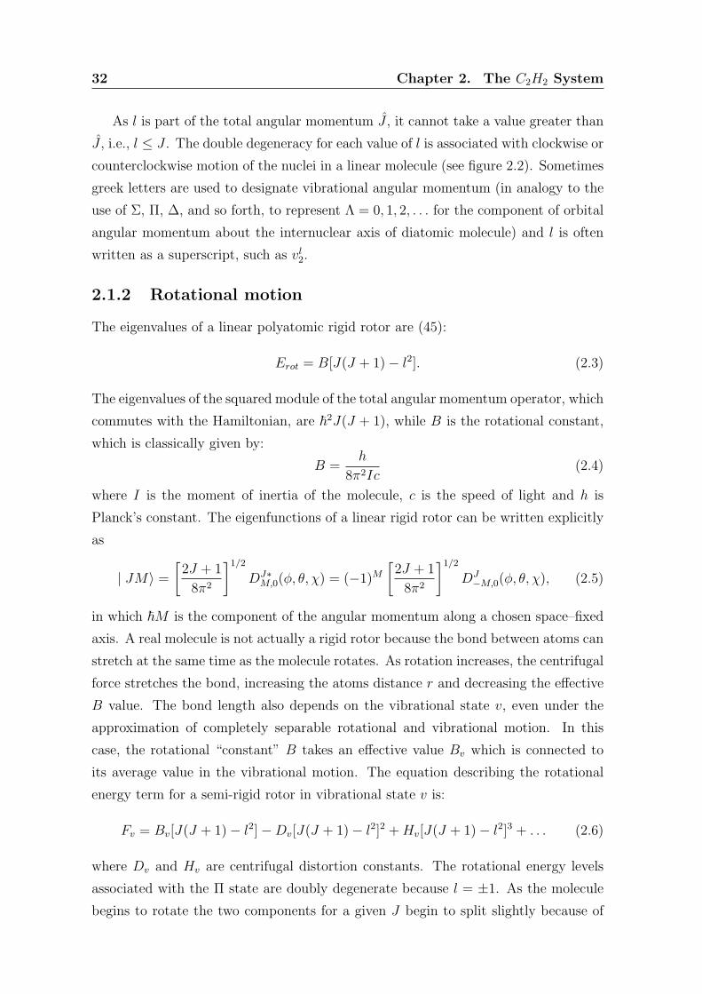
32 Chapter 2. The C2H2 System
As l is part of the total angular momentum J , it cannot take a value greater than
J , i.e., l ≤ J . The double degeneracy for each value of l is associated with clockwise or
counterclockwise motion of the nuclei in a linear molecule (see figure 2.2). Sometimes
greek letters are used to designate vibrational angular momentum (in analogy to the
use of Σ, Π, ∆, and so forth, to represent Λ = 0, 1, 2, . . . for the component of orbital
angular momentum about the internuclear axis of diatomic molecule) and l is often
written as a superscript, such as vl2.
2.1.2 Rotational motion
The eigenvalues of a linear polyatomic rigid rotor are (45):
Erot = B[J(J + 1)− l2]. (2.3)
The eigenvalues of the squared module of the total angular momentum operator, which
commutes with the Hamiltonian, are ~2J(J + 1), while B is the rotational constant,
which is classically given by:
B =h
8π2Ic(2.4)
where I is the moment of inertia of the molecule, c is the speed of light and h is
Planck’s constant. The eigenfunctions of a linear rigid rotor can be written explicitly
as
| JM〉 =
[
2J + 1
8π2
]1/2
DJ∗M,0(φ, θ, χ) = (−1)M
[
2J + 1
8π2
]1/2
DJ−M,0(φ, θ, χ), (2.5)
in which ~M is the component of the angular momentum along a chosen space–fixed
axis. A real molecule is not actually a rigid rotor because the bond between atoms can
stretch at the same time as the molecule rotates. As rotation increases, the centrifugal
force stretches the bond, increasing the atoms distance r and decreasing the effective
B value. The bond length also depends on the vibrational state v, even under the
approximation of completely separable rotational and vibrational motion. In this
case, the rotational “constant” B takes an effective value Bv which is connected to
its average value in the vibrational motion. The equation describing the rotational
energy term for a semi-rigid rotor in vibrational state v is:
Fv = Bv[J(J + 1)− l2]−Dv[J(J + 1)− l2]2 +Hv[J(J + 1)− l2]3 + . . . (2.6)
where Dv and Hv are centrifugal distortion constants. The rotational energy levels
associated with the Π state are doubly degenerate because l = ±1. As the molecule
begins to rotate the two components for a given J begin to split slightly because of

2.1. Fundamentals of C2H2 spectroscopy 33
the interaction of rotational (J) and vibrational (l) angular momenta. The splitting
∆ν is proportional to
∆ν = qJ(J + 1) (2.7)
and q is called the l-type doubling constant.
2.1.3 Parity
It is useful to use parity labels to distinguish the two nearly degenerate levels for each
J . The two most common varieties are total parity and rotationless e/f parity. Total
parity can be either positive “+” (upper sign) or negative “−” (lower sign). Total
parity considers the effect of inversion of all coordinates in the laboratory frame of
the total wavefunction Ψtot. Total parity is commonly used to label the energy levels
of atoms as well as the rotational energy levels of diatomic and linear molecules. The
total parity of a linear molecule wavefunction alternates with J for a Σ+ state. Since
this alternation of total parity with J occurs for all electronic states, it is convenient to
factor out the J dependence and designate those rotational levels with a total parity
of +(−1)J as e parity and those with a total parity of −(−1)J as f parity (for half-
integer J a total parity of +(−1)J− 1
2 corresponds to e and −(−1)J− 1
2 to f). The e/f
parity is thus a J indipendent parity labeling scheme for rovibronic wavefunctions.
All Σ+ rotational energy levels, therefore, have e parity, while all Σ− rotational energy
levels have f parity. The e/f parity labels correspond to the residual intrinsic parity
of a rotational level after the −(−1)J part has been removed. For Π states all of the
rotational energy levels occur as e/f pairs. The one-photon, electric-dipole selection
rules + ↔ − is derived by recognizing that the parity of the dipole moment µ (see
Eq. 2.13) is −1, while the parity of the transition moment integral must be +1.
2.1.4 Nuclear Spin Statistics
An additional symmetry requirement is associated with the constraint placed on
molecular wavefunctions by the Pauli exclusion principle. Because identical nuclei
are indistinguishable, a symmetry operation exchanging them must either leave the
total wavefunction Ψtot (including nuclear spin) unchanged or only change its sign. If
P12 is the operator which exchanges identical nuclei, then the Pauli exclusion principle
requires that
P12Ψtot = ±Ψtot. (2.8)
For particles with integer nuclear spin in units of ~ (I = 0, ~, 2~, . . .), for which
Bose–Einstein statistics apply, the sign in equation 2.8 must be positive (+1), while

34 Chapter 2. The C2H2 System
for particles with half-integer nuclear spin (I =~
2,3~
2,5~
2, . . .) Fermi–Dirac statistics
apply, and the sign must be negative. The total wavefunction, if the interaction
between nuclear magnetic momenta and electronic motion is small (it always is), can
be written as a product of a nuclear spin part ψspin and a space part, ψspace ≡ ψ,
Ψtot = ψspaceψspin = ψψspin, (2.9)
so that the effect of P12 on either part can be examined separately. When P12 operates
on the “normal” space part of the total wavefunction of a symmetric linear molecule
P12ψ = ±ψ, (2.10)
the + levels are labeled as symmetric or s, and − as antysymmetric or a. The nature
of the nuclear spin part of Ψtot depends on the particular nuclei under consideration.
In the acetylene molecule or molecules of D∞h symmetry, the nuclear spin of 12C is
zero, while that of 1H is~
2. P12, when acting on C2H2, exchanges two identical C
atoms (bosons, “+” sign) and two identical H atoms (fermions, “-” sign), resulting
in an overall “-” sign. The total wavefunctions must therefore obey the equation
P12Ψtot = −Ψtot. (2.11)
This means that s symmetry spatial wavefunctions must be combined with antysym-
metric spin functions, while a symmetry spatial wavefunctions are combined with
symmetric spin functions. From standard rules on the combination of angular mo-
menta, combining two spin zero and two spin~
2particles results in a triply degenerate
state of spin ~ of even parity and in a single state of zero spin, of odd parity. There-
fore, the energy levels with a spatial symmetry, which must combine with the nuclear
triplet spin states, have statistical weights three times those of the s levels, which
must combine with the singlet nuclear spin state. This means that, all other things
being equal, the transitions from a levels are three times as intense as are those from
s levels. Note that s and a labels describe the wavefunction exclusive of nuclear spin.
The selection rules on s and a are s ↔ s and a ↔ a for transitions. The levels
with the larger nuclear spin weighting are designed ortho (spin triplets), while the
levels with the smaller weighting are designed para (spin singlet). The spatial part of
the wavefunction must hence be symmetric with respect to exchange of the identical
nuclei if the spin state is para and anti–symmetric if the spin state is ortho.

2.1. Fundamentals of C2H2 spectroscopy 35
2.1.5 Transition intensity and selection rules
Given two specific energy states of the molecule, the line line strenght S(f ← i) of an
electric dipole transition is defined as
S(f ← i) =∑
Φ′,Φ′′∑
A=X,Y,Z
|〈Φ′|~µA|Φ′′〉|2 (2.12)
where Φ′ and Φ′′ are states corresponding to the energies E ′ and E ′′, respectively. In
this equation µA is the component of the molecular dipole moment operator along the
A axis (A = X,Y orZ); the X,Y, Z system having origin at the molecular center of
mass and space fixed orientation. This operator is given by
~µA =∑
j
ejAj (2.13)
with ej and Aj as the charge and A coordinate of the jth particle in the molecule,
where j runs over all nuclei and electrons. It is clear that S(f ← i) must be completely
invariant with respect to all symmetries of the molecule. In terms of symmetry groups,
this implies that the product of the symmetries of the Φ′ and Φ′′ states must include
the symmetry of ~µA at least for one of the values of A, so that the overall integral can
be totally symmetric. This selection rule based on symmetry species is rigorous, and is
strictly valid regardless e. g. of the assumed separability of electronic, vibrational and
rotational degrees of freedom. If separability, or harmonicity of vibrational motion is
assumed, more stringent selection rules can be derived, which are approximate, whose
accuracy depends on that of the underlying assumptions.
2.1.6 Calculation of the line strength
For a neutral molecule the value of 〈Φ′|µA|Φ′′〉 is indipendent of the origin of the axis
system used for µ and, therefore, one is free to choose this origin at one’s convenience.
It is advantageous, when evaluating S(f ← i), to express µA in terms of the dipole
referred to the body-fixed axes µbf (µx, µy, µz). The molecule fixed axis system (x, y, z)
can be viewed as a rotated version of the space fixed axis system (X,Y, Z), where the
rotation that turns X,Y, Z into x, y, z is defined by the three Euler angles (φ, θ, χ)
(see Sect. 1.3.1). To specify the orientation of the molecule-fixed frame with respect
to the space-fixed one, is a process called ‘embedding’. The specific embedding used
in our calculations is described in Sect. 1.3. Consequently, we obtain the following
relation between the µbf and the µA.
µA =∑
l
[D10,t(φ, θ, χ)]∗µbf (2.14)

36 Chapter 2. The C2H2 System
where we put the explicit expression of the orthogonal rotation matrix transforming
µbf in µA, in terms of the Wigner expansion coefficients (see Sect. 1.4.1 and (26)).
The quantum numbers of the projection of the total angular momentum J onto the
Z-axis of the space-fixed and onto the z-axis of the body-fixed frame are M and K
respectively. Moreover, the body-fixed wavefunctions are given as a linear combina-
tion of products of angular momentum eigenfunctions and vibrational basis functions
expressed with respect to 3N − 5 internal coordinates. In general, any given state of
the molecule can always be expressed in the form
Ψ(JMV ) =
(
2J + 1
8π2
)1/2∑
k,v
cJkVv φJk
v (q) | JMk〉. (2.15)
Substituting Eqns. 2.15 and 2.14 in Eq. 2.12, assuming isotropy of space (i. e. no
magnetic fields) and making use of the algebraic properties of the Wigner coefficients
one can obtain (46)
S(f ← i) = (2J ′ + 1)(2J ′′ + 1)×
× |∑
k′,v′,k′′,v′′
∑
t
(−1)k′
cJ′k′v′
v′
⋆cJ
′′k′′v′′
v′′
(
J ′ 1 J ′′
k′ t (−k′′)
)
〈φJ ′,k′
v′ | µbf,t | φJ ′′,k′′
v′′ 〉 |2
(2.16)
If the vibrational and rotational parts of the motion are well separated, it is possible
(47) to choose the components of the wavefunctions so that they can be written more
simply as
Ψ(JMV ) =
(
∑
v
aVv φv(q)
)(
∑
k
bJk|JMk〉)
. (2.17)
In the limit of small displacements from equilibrium, this separation is exact. This is
obtained using the embedding defined by the Eckart conditions (47):
∑
i
miri,e × ri = 0;∑
i
miri = 0 (2.18)
where mi is the mass and ri the position (ri,e at equilibrium) of particle i. With
the above equation, the expression of the line strenght in Eq. 2.16 factorises in a part
involving only vibrational coordinates and a part involving only rotational coordinates,
i. e.
S(f ← i) = (2J ′ + 1)(2J ′′ + 1)×
× |∑
t
∑
v′,v′′
aV ′
v′
⋆aV ′′
v′′ 〈φv′ | µbf,t | φv′′〉∑
k′,k′′
(−1)k′
bJ′k′⋆
bJ′′k′′
(
J ′ 1 J ′′
k′ t (−k′′)
)
|2 .
(2.19)

2.1. Fundamentals of C2H2 spectroscopy 37
When the sum over t is restricted to only one value (as is frequently the case for
symmetry reasons, as for C2H2, when at most one of them at a time is nonzero, for a
given transition), this can be rewritten as
S(f ← i) = SRot(J′′, J ′)SV ib(V
′′, V ′) (2.20)
where
SV ib(V′′, V ′) = |〈V ′|µbf |V ′′〉|2 = |〈V ′|µbf,t|V ′′〉|2 (2.21)
and SRot(J′′, J ′) are algebraic coefficients which are completely determined by the
rotational quantum numbers of the levels involved in the transition and by the value
of t for which 〈V ′|µbf ,l |V ′′〉 is not zero.
A transition with the emission or absorption of radiation can occur between the
vibrational states V ′ and V ′′ if |〈V ′|µbf,t|V ′′〉|2 is different from zero for at least one t.
This can occur only if the product 〈V ′|µbf,t|V ′′〉 is totally symmetric with respect to
all symmetries of the molecule. This leads to selection rules which are rigorous and
therefore always valid regardless of simplifying assumptions (48). More restrictive
vibrational selection rules can be derived upon assuming the harmonic approximation
to hold, and the electric dipole moment to be well described by its first–order Taylor
expansion around the equilibrium position of the nuclei. The SRot(J′′, J ′) are called
the Honl–London coefficients (49).
2.1.7 Rotational Selection Rules and Honl-London factors
We have seen above that, under some simplifying assumptions, the line strength can
be factorised in a vibrational term SV ib(V′′, V ′) and a rotational term SRot(J
′′, J ′),
called Honl–London coefficient. We will now list the relevant selection rules and
Honl–London coefficients for the case of a linear, symmetric molecule such as C2H2.
The general transition selection rules can be summerized as (45):
1) ∆l = 0 with l = 0. This is the parallel transition of the Σ+ → Σ+ type for
stretching modes with P (∆J = −1) and R branches (∆J = +1).
2) ∆l = ±1. This is a perpendicular transition type for bending modes such as
Π→ Σ, ∆→ Π, and so forth, with P and R branches (∆J = ±1) and a strong
Q branch (∆J = 0).
3) ∆l = 0 with l 6= 0. These are transitions of the type Π → Π, ∆ → ∆, and so
forth with P and R branches (∆J = ±1) and weak Q branches (∆J = 0). The
Q branch lines of these bands are rarely observed.

38 Chapter 2. The C2H2 System
The terms parallel and perpendicular are used because the transition dipole moment
is either parallel (µz) or perpendicular (µx and µy) to the molecular symmetry axis,
conventionally labelled as the z-axis. By using the Honl–London, the intensities of
individual lines can be approximately reduced to a single band intensity which repre-
sents the intensity of the whole band. LJ,∆J is defined as
LJ,∆J=−1 =(J − l∆l)(J − l∆l − 1)
2J(P-branch) (2.22)
LJ,∆J=0 =(2J + 1)(J − l∆l)(J + l∆l + 1)
(2J)(J + 1)(Q-branch) (2.23)
LJ,∆J=+1 =(J + l∆l + 2)(J + l∆l + 1)
2(J + 1)(R-branch) (2.24)
for perpendicular bands (∆l = ±1) and
LJ,∆J=−1 =(J + l∆l)(J − l∆l)
J. (P-branch) (2.25)
LJ,∆J=0 =(2J + 1)(l∆l)2
(J)(J + 1)(Q-branch) (2.26)
LJ,∆J=+1 =(J − l∆l + 1)(J + l∆l + 1)
(J + 1)(R-branch). (2.27)
for parallel bands (∆l = 0).
2.2 Existing Data
The infrared spectroscopy of acetylene molecule C2H2 is important for atmospheric,
planetary and astrophysical applications. This molecule is present as a trace con-
stituent in the upper atmosphere of the giant planets where it comes from methane
photodissociation. Thus the strong Q-branch of the ν5 fundamental band, around
13.6µm, was early on observed in the emission spectra of the giant planets (50; 51).
The stratospheric distribution of acetylene in Uranus was deducted from spectra ob-
tained with the infrared space observatory (ISO) instrument (52). In 1981, the first
vertical profile of C2H2 was obtained from balloon flight spectra (Denver University)
around 13.6µm by Goldman et al.(53). Finally, acetylene, was observed in the cir-
cumstellar shell of cool carbon stars such as IRC+10216, and in interstellar clouds,
through spectra recorded in the 3µm region of the ν3 fundamental band (54; 55), and
in the 13.6µm region of the ν5 fundamental band (56; 8). The C2H2 molecule is also
interesting for testing theoretical approaches. Detailed theoretical considerations on
acetylene can be found in the book by Herman et al. (57), supplemented by statistical
and dynamical interpretation (58).

2.2. Existing Data 39
2.2.1 Experimental data: the HITRAN Database
HITRAN (59) is an acronym for high-resolution transimission molecular absorption
database and it is a compilation of spectroscopic parameters that a variety of com-
puter codes use to predict and simulate the trasmission and emission of light in the
atmosphere.
Figure 2.3: HITRAN homepage
The database is a long-running project started by the Air Force Cambridge Re-
search Laboratories (AFCRL) in the late 1960’s in response to the need for the detailed
knowledge of the infrared properties of the atmosphere. Spectroscopic data concern-
ing acetylene were introduced in the HITRAN database (molecule number 26) as early
as the 1986 edition (60). The 2000 HITRAN edition, last updated in 2004, contains
essentially all available experimental data on the vibrational spectra of the acetylene
molecule (see Fig. 2.4). The 13.6µm and 3µm (61; 62; 63) spectral regions of interest

40 Chapter 2. The C2H2 System
Figure 2.4: Spectrum of C2H2 from the HITRAN 2004 database. Top panel showsthe overall spectrum, while the remaining four panels zoom in over individual bands.Data are in cm/molecule vs. microns.

2.2. Existing Data 41
were represented, using the pioneering work of Varanasi et al. (64) and Rinsland et
al. (54) for the line position and for the line intensities, Devi et al. (65) for the
air-broadening coefficients, and Varanasi et al. (64; 66) for the self-broadening coeffi-
cients and the temperature dependence of air-broadening coefficients. More than 670
line intensities of nine perpendicular bands of acetylene are measured in the 2.5µm
(67) spectral region and also the last work of Lyulin et al. (68) extended the previous
measurements of the line intensities of acetylene, in the 1.9µm and 1.7µm spectral
regions, in order to elaborate a complete database for this molecule.
2.2.2 Theoretical data: Potential Energy Surfaces
Potential energy surfaces (P.E.S.) have been derived, from ab initio calculations, for
acetylene molecule spanning the acetylene and vinylidene minima and isomerization
barrier. A potential energy function for the ground state surface of C2H2 was con-
structed by Carter and Mills (69) in 1980. The method to calculate this P.E.S. is
based on a many-body expansion of the potential, so that the asymptotic limits of
the surface corresponding to all possible molecular dissociations are automatically cor-
rect. The 2- and 3-body terms have been obtained by preliminary investigation of the
ground state surfaces of CH2 and C2H. A 4-body term has been derived which repro-
duces the energy, geometry and harmonic force field of C2H2. Certain discrepancies
in this potential were removed by Halonen et al. (70) in 1982, in particular to include
the ab initio calculations by Dykstra and Schaefer (71) on the vinylidene-acetylene
transition state, and also to reproduce a known barrier on the HC +CH dissociation
pathway. Two types of potential models for acetylene were investigated in this work.
The models are developed and tested by comparison between variational calculations
for the stretching vibrational term values and available spectroscopic data. The first is
a simple bond potential model with harmonic interbond coupling terms, the C−H(D)
and C − C bonds being treated as Morse and harmonic oscillators respectively. The
second model uses a modification of the potential designed by (69) to describe both
the parent molecules and exactly their dissociation fragments CH2(CD2), C2H(C2D),
CH(CD), C2 and H2(D2). The most accurate presently available potential energy
surface was recently obtained by the Bowman group (see references (72; 73; 74)).
This P.E.S., accurately explained in the work of Zou and Bowman (74), is an ac-
curate, least–squares fit to nearly 10.000 symmetry-equivalent, ab initio electronic
calculations obtained at the coupled-cluster singles, doubles (triples) CCSD(T) level
of theory, with an aug-cc-pVTZ gaussian basis set (75), using molpro (76). At first
the geometries and normal-mode frequencies of acetylene, vinylidene and the isomer-

42 Chapter 2. The C2H2 System
ization saddle point were determined. The permutational symmetry of the molecule
with respect to interchange of the two H atoms or the two C atoms was exploited
to generate additional points to be used in the fitting. To fit the electronic energies,
one needs to select coordinates that display the permutational symmetry. A set of
coordinates that explicitly do this are the six internuclear distances; r3 and r6 are the
distances between the two carbon atoms and the two hydrogen atoms, respectively;
r1 and r4 are the distances between hydrogen atom one and carbon atom two, re-
spectively, and r2 and r5 are the distances between hydrogen atom two and carbon
atom one and two, respectively. The functional form of the fitted potential is a direct
product, multinomial in Morse variables for ri, i = 1−5, and a standard displacement
variable for r6. Explicitly
V (r1 − r6) =∑
n=0
Cn(r6 − r6e)n6
5∏
i=1
(1− e−α(ri−rie))ni , (2.28)
where n is the set of integers n1 − n6. The sum of these integers is restricted to be
less than or equal to four, an thus there are 210 terms in the above expression. The
standard choice of α equal to one was made, and for the four CH distances rie equals
3.13789 bohr. This is the average of the equilibrium value of the two CH bond lengths
for a given C atom for acetylene. The values for the two other reference distances, r3e
and r6e, are 2.27712 and 6.27578 bohr, respectively. These are the equilibrium CC
and HH bond lengths for acetylene.
More recently, a new semi–empirical potential energy surface was obtained by Xu
et al. (77), based on the ab initio calculations of (74) with the addition of empirical
scaling for the stretching coordinates. The parameters of the empirical scaling func-
tions were determined to obtain the best fit of variational energy levels with respect
to their experimental values.
2.2.3 Dipole Moment surfaces
At the moment, no dipole moment surfaces (D.M.S.) for acetylene are available in the
literature. Professor Baas Braams of the Department of Mathematics and Computer
Science, Emory University (Atlanta, USA) derived a series of D.M.S.s, based on ab
initio calculations, obtained in a similar way as the P.E.S by Zou and Bowman (74),
i. e. by fitting a parametrised analytical expression to a grid of values of the dipole
moment. He obtained different grids spanning various portions of the nuclear config-
uration space of C2H2, with different samplings, using different levels of theory. For
calculations involving highly excited vibrational states of acetylene, the best available

2.2. Existing Data 43
level of theory is Density Functional Theory, using the hcth147 functional (78) and the
cc-pvtz (75) gaussian basis set. The dipole moment is represented in the functional
form
~µ =∑
i
w(i) · ~x(i) (2.29)
where w(i) is the effective charges of the i–th nucleus, and ~x(i) is its position vector.
The w(i) are represented by polynomials, whose coeffiecients are determined by a
least squares system where the data are the ab initio computed dipole moments. The
effective charges are scalar quantities and are invariant under rotations, translations,
and inversions of the geometry under permutations of like nuclei. The dipole moment
thus defined is therefore a vector itself, and by construction it has all the appropriate
symmetry and transformation properties. For the case of a neutral system, such as
neutral C2H2, the dipole moment must be invariant under translation. To enforce
neutrality, for each configuration the equation∑
i
w(i) = 0 is included in the least
squares system. This means that the charge of the system is neither strictly zero nor
even constant for varying nuclear configurations, but only approximately so: charge
results to be zero with the same accuracy with which the ab initio computed dipole
moments are fitted. This also means that the fitted dipole moment is not strictly
invariant under translations. The safest and most consistent choice is therefore to
assume the origin of the reference system coincident with the center of mass of the
nuclei. The resulting parametrised D.M.S. was kindly made available by prof. Braams
in the form of Fortran 90 modules.
2.2.4 State of the art of variational C2H2 spectra
Acetylene has been studied extensively (79; 80; 81), at low vibrational energy (see e. g.
Herman et al. (57) and references therein). There are been fewer studies of acetylene
at energies approaching the barrier to isomerization and still fewer of vinylidene.
The work most relevant to the understanding of intramolecular energy flow has been
reviewed by Jacobson and Field (82). More recent full–dimentional calculations of
purely vibrational states were performed by Xu et al. (83) and by Kozin et al. (31).
The latter authors performed their calculations using the wavr4 code, to which the
following Sect. 3.1 is devoted. Variational transition intensities for C2H2 are not yet
available in the literature, and are indeed the purpose of the present work.

44 Chapter 2. The C2H2 System

Chapter 3
Calculations
Our goal is ultimately to calculate detailed lists of rovibrational transitions, includ-
ing energies and intensities, among accurate states obtained via variational methods.
As previously mentioned, there are currently no such results in the literature yet for
C2H2. Having no previous results to benchmark and validate a full calculation of this
kind, we decided to proceed in progressive steps and, at first, restrict our variational
calculations to rotationless states (i. e. J = 0) and purely vibrational transitions.
This reduces vastly the computational investment, while still enabling us to validate
the newly developed part in the codes we used. On the other hand, it should be un-
derstood that some vibrational states, namely those with nonzero vibrational angular
momentum, cannot be represented at all with a basis set composed only of states
with zero total angular momentum. Those levels, and transitions involving them, are
simply not computed. This notebly includes fundamental bending transitions, since
for them the upper state has vibrational angular momentum l = ±1. Only overtones
and combination bands of bending transitions can be computed, i. e. those in which
(in the harmonic approximation) the occupation numbers of bending modes change
by an even number (i. e. at least 2).
3.1 The wavr4 code
The computational program wavr4 (30) calculates the bound ro-vibrational levels
and wavefunctions of a tetraatomic system based on the well-established technique
of sequential diagonalization and truncation (29). The theoretical framework is de-
scribed in Sect. 1.3, while in the present section we describe its specific implemen-
tation. Wavr4 is a general suite of computer programs which utilizes a class of
coordinate system based on generalized orthogonal vectors. The program offers a
choice of coordinate systems based on Radau (84), Jacobi (85), diatom-diatom (86)

46 Chapter 3. Calculations
Figure 3.1: Coordinate system supported by WAVR4. The position of the pointsCM12, CM123, CM34, B and M are defined in Ref.(21)
and orthogonal satellite vectors (87), (88). The corresponding analytical expressions
of the orthogonal vectors ~q1, ~q2, ~q3 in terms of the atom position vectors ~r′1, ~r′2, ~r′3
are summarized in figure 3.2. The use of orthogonal vectors makes the Hamiltonian
structure very simple and yet allows a variety of possible choices of coordinate sys-
tem. Several possibilities relevant to acetylene are presented in fig 3.1. The HC−CHdiatom-diatom coordinates correspond to traditional valence coordinate in the limit
that masses of atoms 1 and 4 are small compared to those of atoms 2 and 3. Note that
the Hamiltonians are equally rigorous in all three coordinate representations shown in
Fig. 3.1. The angular coordinates (see equations 1.27, 1.32 and 1.33) are treated us-
ing a finite basis representation (F.B.R.) based on product of spherical harmonics. A
discrete variable representation (D.V.R.) based on Morse-oscillator-like (see equation
1.4.2) is used for the radial coordinates. Matrix elements are computated using an ef-
ficient Gaussian quadrature (see Sect. 1.6.1) in the angular coordinates and the DVR
approximation in the radial cooordinates. The full basis so are a product of the FBR
angular basis and a radial DVR basis. The solution of the secular problem is carried
through a series of intermediate diagonalisations and truncations. In particular, it
proceeds through 4 phases, which are described in detail in (31).

3.1. The wavr4 code 47TABLESTABLE I. Atom position vectors f~r01; ~r02; ~r03; ~r04g in terms of the orthogonal internal vectorsf~q1; ~q2; ~q3g for tetratomic molecules. Here mij = mi+mj , m123 = m12+m3, and M = m123+m4.The constant � for the Radau vectors is given by Eq. (2) and the constant � for the orthogonalizedsatellite vectors by Eq. (4).Jacobi vectors Radau vectors~r01 m2m12 ~q1 � m3m123 ~q2 � m4M ~q3 qm4M [(1� �m23)~q1 + �m2~q2 + �m3~q3 ]~r02 � m1m12 ~q1 � m3m123 ~q2 � m4M ~q3 qm4M [�m1~q1 + (1� �m13)~q2 + �m3~q3 ]~r03 m12m123 ~q2 � m4M ~q3 qm4M [�m1~q1 + �m2~q2 + (1� �m12)~q3]~r04 m123M ~q3 � 1pm4 M (m1~q1 +m2~q2 +m3~q3)diatom+diatom vectors orthogonalized satellite vectors~r01 m2m12 ~q1 � m34M ~q3 1m12 qm34M [(m12 +m2�)~q1 �m2�~q2]~r02 � m1m12 ~q1 � m34M ~q3 1m12 qm34M [�m1�~q1 + (m12 +m1�)~q2]~r03 � m4m34 ~q2 + m12M ~q3 � m4m34 ~q3 � 1pm34M (m1~q1 +m2~q2)~r04 m3m34 ~q2 + m12M ~q3 m3m34 ~q3 � 1pm34M (m1~q1 +m2~q2)
7Figure 3.2: Atom position vectors ~r′1, ~r′2, ~r′3, ~r′4 in terms of the orthogonal internalvectors ~q1, ~q2, ~q3 for tetratomic molecules. Here mij = mi + mj, m123 = m12 +m3 and M = m123 + m4. The constant α for the Radau vectors is given by α =
1m123
(
1−√
Mm4
)
and the constant β for the orthogonalized satellite vectors is given
by β =√
MM34
− 1

48 Chapter 3. Calculations
3.1.1 Implementation details
The WAVR4 code allows the use of all three coordinate systems and implied symme-
tries of the molecule in question. Indeed, acetylene is invariant under the operations of
inversion and permutation of the hydrogens P (HH) and the carbons P (CC). Thus
the total symmetry group of acetylene is G8 (38). The diatom-diatom coordinate
system easily supports the operations of inversion and simultaneous permutation of
carbons and hydrogens, P (CC)× P (HH). These two operations generate the group
G4 which is a subgroup of G8. Having reduced symmetry is not a problem if only
low-lying energy levels are of interest. However, for highly excited energy levels the
isomerization to vinylidene becomes feasible thus connecting two equivalent acety-
lene geometries. Therefore the full symmetry should be properly accounted for and
this is done most readily using the coordinates shown in Fig 3.1 (Jacobi vectors and
orthogonal-satellite vectors). The original wavr4 code supported only inversion sym-
metry and the symmetry operations which reverse a vector connecting two identical
atoms. The current version has been modified (89) to make use of hydrogen permu-
tation symmetry P (HH).
The code is parallelized using OpenMP compiler directives thus allowing the com-
pilation of the same code in both serial and parallel modes. When the parallel mode
is being used then a parallel diagonalizer is used in phase three. Another advan-
tage of using OpenMP is that it supports dynamic scheduling for the parallel section
of the code. This makes it possible to have a varied job load for computations at
each grid point and still achieve reasonable load balancing per CPU on average. The
main limitation of OpenMP is that parallelism is only achieved on symmetric multi-
processing (SMP) computers, and not in clusters in which computing nodes do not
share the same memory and run the same instance of the same operating system.
In contrast, however, the implementation of a parallelization strategy using standard
message passing interface (MPI) would have had to employ a fixed (within each run of
the code) number of selected eigenstates for every grid point to achieve load balancing
(90).
One of the crucial choices in the calculation is the selection of the energy cutoffs
required by the diagonalization-truncation method at each phase. If the cutoffs are
too high, then the optimized basis set is very large and the final matrix is too big for
direct diagonalization methods. If, however, the cutoffs are too low, then at a given
radial grid point, all the angular eigenvalues may be above the cutoff, so that the whole
radial grid point is effectively discarded. The lack of essential grid points may result
in severe errors in the DVR energies. Therefore the choice must be a balance between

3.1. The wavr4 code 49
the basis set size (and hence computer time) and the desired accuracy. Depending
on the size of the angular basis, the computation of the three-dimensional angular
integrals of the potential function is the most time-consuming part of the calculation.
A major advantage of Eq. 1.21 is that it helps separate radial and angular co-
ordinates, because no mixed derivative angular-radial operators are present. Thus if
the radial motion is treated in the discrete variable representation (DV R), the whole
problem can be effectively constructed from a set of angular subproblems. Further-
more the use of the DV R approximation for the potential energy requires only the
angular integrals to be computed explicitily.
The size of the primitive basis is necessarily very big. If we had a pure DV R
basis, we could use methods which do not require explicit storage of the Hamiltonian
matrix for finding eigenvectors. Unfortunately the nondirect product part of the
basis cannot be transformed effectively to a DV R and so integration of the angular
potential function must be performed. To make the calculation as efficient possible,
the potential can be expanded in the angular functions defined by Eq. 1.27 at every
radial pair, so that angular integrals can be computed analytically. However for
C2H2 the best ratio of performance to accuracy was found with direct integration of
the potential function using Gaussian quadrature on a minimal number of quadrature
points. This was achieved by implementing an algorithm which takes into account the
symmetry properties of the product of two primitive basis functions. The summation
is performed only over half of the quadrature points but it uses the symmetric part
of the potential if the product is symmetric and the asymmetric part if the product
is asymmetric. In choosing the number of quadrature points, we used the minimum
number of points required to mantain the orthogonality of the basis functions. These
numbers are jmax+1, kmax+1 and lmax+1 for the coordinates θ1, φ and θ2 respectively,
where
1) θ1 is the angle between q3 and q1 (0 ≤ θ1 ≤ π);
2) θ2 is the angle between q3 and q2 (0 ≤ θ2 ≤ π);
3) φ is the second polar angle defining the direction of q2 in the body-fixed frame
defined by q3 and q1,
namely
4) select z-axis along q3 vector;
5) select x-axis such that zx plane is defined by vectors q3 and q1, and the angle θ1
is less than π;

50 Chapter 3. Calculations
6) select y-axis so that the axis system is right handed.
The program is written in Fortran 90, taking full advantage of dynamic memory
allocation. All variables are explicitly declared. Wavr4 requires an input file for
all runs. The units are: energies expressed as the equivalent wavenumbers in cm−1,
lengths in A, angles in radians, masses in unified atomic mass units.
3.1.2 Calculation of energy levels
Below we present details of calculations using the diatom-diatom coordinates system.
All calculations have been performed using the recent ab initio potential of Zou and
Bowman (74) and, for the first time, a new potential describing better the isomer-
ization between acetylene and vinylidene (77). Details on the potential of Zou and
Bowman has been discussed in previous chapter. The calculations were carried out at
Daresbury Laboratory, Warrington, UK on the “cseem64t” cluster composed by 32
compute nodes, each of which being a dual–processor dual–core Xeon 5160 3.0 GHz
with 8 GBytes of RAM (91).
The calculations were performed in the diatom-diatom HC −CH general orthog-
onal coordinates, using six radial functions in each CH coordinate and nine radial
functions in the CC coordinate. The parameters used for CH stretching Morse-
oscillator–like functions were re = 1.164A, we = 2900cm−1 and De = 36000cm−1;
the parameters for CC stretching were re = 1.4135A, we = 2000cm−1 and De =
55000cm−1. The bending basis set was defined by jmax = lmax = 26 and kmax = 7.
These quantum numbers defined 4460 bending functions which are totally symmet-
ric with respect to the inversion. Thus the total size of the primitive basis set was
1445040. To contract this basis set, up to 300 optimized bending functions were
selected for each radial grid point during phase one with an upper energy cutoff of
30000 cm−1 and up to 450 functions during phase two with an energy cutoff of 30000
cm−1. The computation of all 1400 (phase three) states symmetric and asymmetric
with total angular momentum J = 0 (with respect to P (HH) permutation) took a
total of 28 hours on a node of the “cseem64t” cluster. The zero-point energy (ZPE)
and the lowest 40 excited states energy are presented in table 3.1.
The complete list of calculated energy states is available online (see reference
(94)). Our results are clearly compatible with previously published theoretical (31)
and experimental (57; 92; 93) results.

3.1. The wavr4 code 51
N◦ Assignment Eth1 Eth
2 Eexp
ν1, ν2, ν3, νl44 , ν
l55 (cm−1) (cm−1) (cm−1)
0 ZPE 5715.51 0, 0, 0, 20, 00 1203.5 1228.9 1230.82 0, 0, 0, 11, 1−1 1311.6 1323.4 1328.13 0, 0, 0, 00, 20 1448.6 1438.4 1449.04 0, 1, 0, 00, 00 1950.7 1973.4 1974.35 0, 0, 0, 40, 00 2419.0 2488.4 2487.06 0, 0, 0, 31, 1−1 2519.5 2566.2 2560.67 0, 0, 0, 22, 2−2 2632.1 2650.0 2648.28 0, 0, 0, 20, 20 2675.9 2691.6 2683.89 0, 0, 0, 11, 3−1 2772.0 2754.8 2757.810 0, 0, 0, 00, 40 2922.3 2868.1 2879.911 0, 1, 0, 20, 00 3143.5 3191.1 3180.812 0, 0, 1, 00, 00 3241.1 3248.2 3316.913 0, 1, 0, 11, 1−1 3254.3 3280.7 3281.914 1, 0, 0, 00, 00 3371.1 3375.1 3372.415 0, 1, 0, 00, 20 3379.2 3390.2 3420.516 0, 0, 0, 60, 00 3642.6 3770.9 3767.017 0, 0, 0, 51, 1−1 3735.0 3833.1 3818.418 0, 0, 0, 42, 2−2 3839.6 3900.5 3884.019 0, 2, 0, 00, 00 3886.0 3930.7 3933.820 0, 0, 0, 40, 20 3911.9 3969.8 3940.321 0, 0, 0, 22, 4−2 4096.2 4069.2 4060.022 0, 0, 0, 20, 40 4170.6 4141.0 4124.623 0, 1, 0, 40, 00 4349.5 4377.4 4415.624 0, 0, 0, 00, 60 4406.2 4440.2 4293.125 0, 0, 1, 20, 00 4417.7 4444.4 4489.126 0, 1, 0, 31, 1−1 4447.3 4513.6 4658.327 0, 0, 1, 11, 1−1 4525.3 4540.0 4609.328 1, 0, 0, 20, 00 4546.6 4574.5 4570.029 0, 1, 0, 22, 2−2 4556.2 4593.4 4589.830 0, 1, 0, 20, 20 4595.6 4632.9 4634.431 1, 0, 0, 11, 1−1 4656.5 4656.8 4673.632 0, 0, 1, 00, 20 4671.1 4676.3 4727.133 0, 1, 0, 11, 3−1 4691.1 4694.5 4710.734 1, 0, 0, 00, 20 4803.5 4791.5 4800.235 0, 1, 0, 00, 40 4834.2 4806.8 4848.936 0, 0, 0, 80, 00 4871.0 5070.0 5068.537 0, 0, 0, 71, 1−1 4954.9 5117.4 5098.438 0, 2, 0, 11, 1−1 5158.1 5228.2 5230.039 0, 0, 0, 53, 3−3 5161.4 5228.6 5254.540 0, 1, 1, 00, 00 5200.0 5265.2 5260.0
Table 3.1: Calculated differencies of vibrational energy levels from ZPE (Eth1 and Eth
2
with (74) and (77) potential respectively) and comparison with experimental data(Eexp) [(see references (57), (92) and (93))]

52 Chapter 3. Calculations
3.2 Purely vibrational transitions
In Sect. 2.12 we summarised the calculation of the integrated intensity of a transition.
We here recall that, assuming separability of vibrational and rotational motion, the
line strength for a given transition can be factorised as
S(f ← i) = SRot(J′′, J ′)SV ib(V
′′, V ′) (3.1)
where
SV ib(V′′, V ′) = |〈V ′|µbf |V ′′〉|2. (3.2)
We restricted the basis set, in the variational calculation, to include only |JKM〉functions for which J = 0. This means the only the single |000〉 angular function is
included, which is indeed a constant. The wavefunctions of the rotationless states re-
sulting from our variational calculation are therefore independent of the Euler angles,
and coincident with the purely vibrational wavefunction. SV ib(V′′, V ′) can therefore be
obtained by performing the integration of |〈V ′|µbf,t|V ′′〉|2 (where t = x, y, z) directly
on the wavefunctions resulting from the variational calculation, over all molecular
coordinates except the Euler angles. Moreover, since for all the states we calculated
the total vibrational angular momentum l = 0, we can only have transitions for which
l = 0, ∆l = 0, i. e. parallel transitions (see selection rules in Sect. 2.1.7). This implies
that we only need to compute integrals like
〈V ′|µbf,t=z|V ′′〉, (3.3)
where the z axis of the Eckart embedding is conventionally chosen along the molecular
symmetry axis. For low–energy vibrational states of C2H2 this is very nearly (but not
exactly!) coincident with the direction of the C–C bond, which in turn is convention-
ally chosen as the z axis of the diatom–diatom embedding we used for the wavr4
calculations. It is therefore tempting to just perform the integral 〈V ′|µbf,z|V ′′〉 with
the µbf,z component in this latter embedding. This is not strictly correct, as shown
in detail in (46), and we will indeed always consider the z component of the dipole
moment in the Eckart embedding.
3.2.1 The Dipole code
The actual calculation of the integrals mentioned in the previous Section was im-
plemented in Fortran 90. This was done in collaboration with Dr. Igor Kozin of
Daresbury Laboratory, Warrington, UK, during my visit at Department of Physics
and Astronomy of University College London (UCL) by working with Prof. Jonathan

3.2. Purely vibrational transitions 53
Tennyson. The calculation of the integrals proceeds in two steps. In the first step,
the wavefunctions produced by phase 3 of the wavr4 code are converted to the more
convenient representation in the primitive basis set φα. This means that all of the
integrals like Eq. 3.3 can be represented as a linear combination of all the integrals of
the form
〈φα|µbf,t=z|φβ〉, (3.4)
which can then be conveniently expressed in the form of a matrix multiplication.
As we mentioned in Sect. 3.1, only the angular part of the primitive basis functions
(i. e. the one depending on the Euler angles) is represented in the FBR form, while
the basis functions involving the internal molecular coordinates are in DVR form.
This has the twofold implication that the integrals in Eq. 3.4 are actually computed
as simple sums over gaussian grids and that for their implementation we could take
advantage of the well–tested corresponding parts in wavr4, adapting them for the
present purpose. On the other hand, wavefunctions and integrals are expressed in
diatom–diatom coordinates. The Fortran 90 modules provided by Prof. Baas Braams
yield the 3–D components of µbf in the same embedding of the input molecular coor-
dinates, while we need to compute the z component of µbf in the Eckart embedding.
The appropriate rotation of µbf was achieved by making use of a numeric transforma-
tion implemented in a Fortran 90 module kindly made available by Dr Edit Matyus
of Institute of Chemistry, Eotvos University, Budapest, Hungary (95).
The calculation of the integrals in Eq. 3.4, as explained above, implies, in practice,
computing the integrand over a grid of points (specified by the DVR representation
of the primitive basis set) and summing the results. The computational problem is
therefore naturally broken in a very large number of small, independent subproblems of
very nearly equal computational cost. This is particularly suitable for parallelisation,
using either OpenMP and MPI. In this case, since dynamic load balancing at run time
does not offer particular advantages, we chose to use MPI, which enabled us to take
advantage of a wider range of parallel supercomputers in contrast to OpenMP, which
can only exploit parallelism in SMP computers. Since the parallelisation strategy uses
processors to grid mapping, the best load balancing is achieved by using a number
of processors which is a divisor of the total radial grid size (see Sect. 1.4.2). In our
case, since we used a grid with 6 ∗ 6 ∗ 9 = 324 points, “good” numbers of processors
are e. g. 162, 108 etc.. Figure 3.3 shows the scaling properties of a large run of the
Dipole code with different numbers of processing units, ranging from 27 to 108 cores.
The blue line shows the perfect linear scaling, while the red line shows the observed
one. While scaling is not perfect (presumably due to some overhead in partitioning

54 Chapter 3. Calculations
the problem among jobs and collecting the results), it is parallel (and close) to the
nominal one, showing that the Dipole code can efficiently scale up to at least some
hundreds of processors.
0.4
0.6
0.8
1
1.2
1.4
1.6
1.8
2
20 30 40 50 60 70 80 90 100 110
tota
l C
PU
tim
e (
ho
urs
)
number of CPU cores
theoric scalingmpi scaling
Figure 3.3: Running times for a large Dipole code run, MPI version, with varyingnumbers of CPU cores. The blue line show the perfect linear scaling extrapolatedfrom the run using the smallest number of processors (27 CPU cores). The red lineshows real running times for 27, 36, 54 and 108 CPU cores.
3.2.2 Results
We used the Dipole code to compute SV ib(V′′, V ′) for all the couples of states resulting
from the previous run of wavr4. Table 3.2 reports a sample of the transitions among
the first few tens of states having nonzero intensity. The first column from the left in
the table identifies the vibrational states involved in the transition; the second column
lists the calculated vibrational energy difference in wavenumbers (cm−1); the third col-
umn gives the calculated SV ib(V′′, V ′) (in units of elementary electronic charges · A2
).
States are here simply labelled by numbers in order of increasing energy, and are
listed, for cross–reference, in Table 3.3. The first column from the left in Table 3.3
gives the number identifiyng the state; the second gives the vibrational energy of the
state with respect to the ground state; the third column gives the expectation value

3.2. Purely vibrational transitions 55
of the rotational constant < B > in that state (see next section). which we use to
estimate the effective Bv (see Eq. 2.6 in Sect. 2.1.2). The complete list of calculated
parallel vibrational transitions is available online (see reference (96)).
Table 3.2: A sample of the transitions among the first few tens ofstates having nonzero intensity. Columns are, from left to right:identification of the vibrational states involved, calculated vibra-tional energy difference, and calculated SV ib(V
′′, V ′).
Transition ∆ Energy Line strength(cm−1) ((e·A)2)
1 → 3 1311.5770 0.0011 → 7 2519.4822 2.5 · 10−7
1 → 10 2772.0035 7 · 10−8
1 → 13 3241.0504 0.000791 → 14 3254.3348 0.00151 → 18 3734.9991 6 · 10−11
1 → 22 3955.6108 1.1 · 10−10
1 → 23 3999.7215 2 · 10−12
1 → 26 4246.5770 1.6 · 10−10
1 → 29 4417.7154 2.3 · 10−6
1 → 30 4447.3147 2.8 · 10−7
1 → 35 4656.4795 2.9 · 10−7
1 → 36 4671.1114 7.6 · 10−8
1 → 37 4691.0767 8.4 · 10−9
2 → 3 108.0469 0.000772 → 7 1315.9521 0.00182 → 10 1568.4734 2.1 · 10−9
2 → 13 2037.5203 6.6 · 10−9
2 → 14 2050.8047 1 · 10−5
2 → 18 2531.4690 1.5 · 10−6
2 → 22 2752.0807 3 · 10−8
2 → 23 2796.1914 6 · 10−8
2 → 26 3043.0469 7.5 · 10−11
2 → 29 3214.1853 0.00172 → 30 3243.7846 0.000192 → 35 3452.9494 2.1 · 10−6
2 → 36 3467.5813 8.5 · 10−7
3 → 4 137.0592 0.000793 → 5 639.1326 3.8 · 10−6
3 → 6 1107.4482 1.4 · 10−6
3 → 8 1320.4789 0.00283 → 9 1364.3699 3.6 · 10−7
3 → 11 1610.7538 4 · 10−9
3 → 12 1831.8771 3.8 · 10−7
3 → 15 2059.5095 1.3 · 10−6
3 → 16 2067.6368 6.9 · 10−6
3 → 17 2330.9855 2.3 · 10−12
3 → 19 2527.9914 1.4 · 10−6
3 → 20 2574.3849 1.2 · 10−10
3 → 21 2600.3037 1.8 · 10−10
3 → 24 2784.6144 1.9 · 10−7
3 → 25 2859.0174 3.3 · 10−10
continued on next page

56 Chapter 3. Calculations
Table 3.2 – continued from previous page
Transition ∆ Energy Line strength(cm−1) ((e·A)2)
3 → 27 3037.8863 4.8 · 10−10
3 → 28 3094.6617 2.7 · 10−11
3 → 31 3213.7305 0.00163 → 32 3235.0080 0.00013 → 33 3244.6691 0.000343 → 34 3284.0013 1.5 · 10−8
4 → 7 1070.8460 2.7 · 10−7
4 → 10 1323.3673 0.00194 → 13 1792.4142 2.7 · 10−8
4 → 14 1805.6987 2.8 · 10−6
4 → 18 2286.3630 1.5 · 10−10
4 → 22 2506.9747 3.4 · 10−7
4 → 23 2551.0853 2.7 · 10−7
4 → 26 2797.9409 2.2 · 10−7
4 → 29 2969.0793 1.9 · 10−9
4 → 30 2998.6785 2.2 · 10−11
4 → 35 3207.8433 0.000354 → 36 3222.4753 0.00145 → 7 568.7726 8.3 · 10−8
5 → 10 821.2939 9.6 · 10−8
5 → 13 1290.3408 0.000825 → 14 1303.6252 0.000225 → 18 1784.2896 1.2 · 10−11
5 → 22 2004.9013 2.5 · 10−11
5 → 23 2049.0119 3 · 10−11
5 → 26 2295.8675 1.4 · 10−10
5 → 29 2467.0059 2.5 · 10−7
5 → 30 2496.6051 1.3 · 10−7
5 → 35 2705.7699 1 · 10−9
5 → 36 2720.4019 4 · 10−8
6 → 7 100.4571 0.00146 → 10 352.9783 3.6 · 10−9
6 → 13 822.0252 3.3 · 10−8
6 → 14 835.3097 1.8 · 10−8
6 → 18 1315.9740 0.00256 → 22 1536.5857 1.7 · 10−7
6 → 23 1580.6963 3 · 10−8
6 → 26 1827.5519 6.6 · 10−11
6 → 29 1998.6903 1.7 · 10−5
6 → 30 2028.2895 1.6 · 10−5
6 → 35 2237.4543 1.2 · 10−8
6 → 36 2252.0863 7.5 · 10−9
7 → 8 112.5737 0.00197 → 9 156.4647 0.000257 → 11 402.8485 2.9 · 10−10
7 → 12 623.9719 6.5 · 10−6
7 → 15 851.6043 9.9 · 10−9
7 → 16 859.7316 1.6 · 10−8
7 → 17 1123.0803 3.4 · 10−6
7 → 19 1320.0862 0.00427 → 20 1366.4797 1.3 · 10−9
continued on next page

3.2. Purely vibrational transitions 57
Table 3.2 – continued from previous page
Transition ∆ Energy Line strength(cm−1) ((e·A)2)
7 → 21 1392.3985 1.8 · 10−7
7 → 24 1576.7092 3.3 · 10−7
7 → 25 1651.1122 1 · 10−10
7 → 27 1829.9811 4.3 · 10−7
7 → 28 1886.7565 8 · 10−11
7 → 31 2005.8253 8.4 · 10−6
7 → 32 2027.1028 6.9 · 10−6
7 → 33 2036.7638 1.6 · 10−5
7 → 34 2076.0961 1.4 · 10−6
8 → 10 139.9476 0.00198 → 13 608.9945 7.5 · 10−6
8 → 14 622.2790 4.1 · 10−6
8 → 18 1102.9433 1.6 · 10−6
8 → 22 1323.5550 0.00538 → 23 1367.6656 6.1 · 10−6
8 → 26 1614.5212 1.9 · 10−7
8 → 29 1785.6596 3.4 · 10−7
8 → 30 1815.2588 1.7 · 10−6
8 → 35 2024.4236 1 · 10−5
8 → 36 2039.0556 2.6 · 10−6
9 → 10 96.0566 0.00039 → 13 565.1035 8.1 · 10−9
9 → 14 578.3879 7.4 · 10−11
9 → 18 1059.0523 4.1 · 10−8
9 → 22 1279.6640 2.8 · 10−6
9 → 23 1323.7746 0.00279 → 26 1570.6302 1.1 · 10−7
9 → 29 1741.7686 7.9 · 10−7
9 → 30 1771.3678 6.5 · 10−7
9 → 35 1980.5326 4.7 · 10−7
9 → 36 1995.1646 2 · 10−6
10 → 11 150.3273 0.001510 → 12 371.4506 4.3 · 10−8
10 → 15 599.0830 1.5 · 10−6
10 → 16 607.2104 7 · 10−6
10 → 17 870.5591 2.4 · 10−10
10 → 19 1067.5649 3.1 · 10−7
10 → 20 1113.9585 8.7 · 10−10
10 → 21 1139.8772 2 · 10−7
10 → 24 1324.1879 0.004610 → 25 1398.5909 8.6 · 10−7
10 → 27 1577.4598 8.3 · 10−10
10 → 28 1634.2352 1.3 · 10−7
10 → 31 1753.3041 1.9 · 10−6
10 → 32 1774.5815 3.5 · 10−8
10 → 33 1784.2426 4.9 · 10−6
10 → 34 1823.5748 2.1 · 10−7
11 → 13 318.7196 8.1 · 10−8
11 → 14 332.0041 6.2 · 10−10
11 → 18 812.6684 9.3 · 10−11
11 → 22 1033.2801 2.7 · 10−8
continued on next page
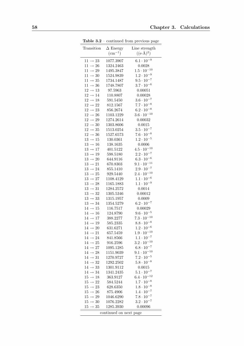
58 Chapter 3. Calculations
Table 3.2 – continued from previous page
Transition ∆ Energy Line strength(cm−1) ((e·A)2)
11 → 23 1077.3907 6.1 · 10−9
11 → 26 1324.2463 0.002811 → 29 1495.3847 1.5 · 10−10
11 → 30 1524.9839 1.2 · 10−9
11 → 35 1734.1487 9.5 · 10−7
11 → 36 1748.7807 3.7 · 10−6
12 → 13 97.5963 0.0005112 → 14 110.8807 0.0002812 → 18 591.5450 3.6 · 10−7
12 → 22 812.1567 7.7 · 10−8
12 → 23 856.2674 6.2 · 10−8
12 → 26 1103.1229 3.6 · 10−10
12 → 29 1274.2614 0.0003212 → 30 1303.8606 0.001512 → 35 1513.0254 3.5 · 10−7
12 → 36 1527.6573 7.6 · 10−8
13 → 15 130.0361 1.2 · 10−5
13 → 16 138.1635 0.000613 → 17 401.5122 4.5 · 10−10
13 → 19 598.5180 2.2 · 10−7
13 → 20 644.9116 6.3 · 10−6
13 → 21 670.8303 9.1 · 10−11
13 → 24 855.1410 2.9 · 10−7
13 → 25 929.5440 2.4 · 10−10
13 → 27 1108.4129 1.1 · 10−6
13 → 28 1165.1883 1.1 · 10−9
13 → 31 1284.2572 0.001413 → 32 1305.5346 0.0001213 → 33 1315.1957 0.000913 → 34 1354.5279 6.2 · 10−7
14 → 15 116.7517 0.0002914 → 16 124.8790 9.6 · 10−5
14 → 17 388.2277 7.3 · 10−10
14 → 19 585.2335 8.8 · 10−8
14 → 20 631.6271 1.2 · 10−6
14 → 21 657.5459 1.9 · 10−10
14 → 24 841.8566 1.1 · 10−7
14 → 25 916.2596 3.2 · 10−10
14 → 27 1095.1285 6.8 · 10−7
14 → 28 1151.9039 9.1 · 10−10
14 → 31 1270.9727 7.2 · 10−5
14 → 32 1292.2502 5.8 · 10−8
14 → 33 1301.9112 0.001514 → 34 1341.2435 5.1 · 10−7
15 → 18 363.9127 6.4 · 10−12
15 → 22 584.5244 1.7 · 10−8
15 → 23 628.6350 1.8 · 10−8
15 → 26 875.4906 1.4 · 10−7
15 → 29 1046.6290 7.8 · 10−7
15 → 30 1076.2282 3.2 · 10−7
15 → 35 1285.3930 0.00096
continued on next page
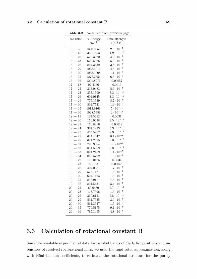
3.3. Calculation of rotational constant B 59
Table 3.2 – continued from previous page
Transition ∆ Energy Line strength(cm−1) ((e·A)2)
15 → 36 1300.0250 2.8 · 10−5
16 → 18 355.7853 1.2 · 10−10
16 → 22 576.3970 4.5 · 10−8
16 → 23 620.5076 5.3 · 10−8
16 → 26 867.3632 3.8 · 10−7
16 → 29 1038.5016 4.6 · 10−7
16 → 30 1068.1008 1.1 · 10−7
16 → 35 1277.2656 6.5 · 10−7
16 → 36 1291.8976 0.0005717 → 18 92.4366 0.001917 → 22 313.0483 5.6 · 10−9
17 → 23 357.1590 7.3 · 10−10
17 → 26 604.0145 1.3 · 10−12
17 → 29 775.1529 8.7 · 10−9
17 → 30 804.7521 1.3 · 10−7
17 → 35 1013.9169 5 · 10−11
17 → 36 1028.5489 2 · 10−12
18 → 19 104.5692 0.003118 → 20 150.9628 3.5 · 10−11
18 → 21 176.8816 0.0001218 → 24 361.1923 5.3 · 10−10
18 → 25 435.5952 8.9 · 10−11
18 → 27 614.4642 8.1 · 10−6
18 → 28 671.2395 5.8 · 10−13
18 → 31 790.3084 1.6 · 10−8
18 → 32 811.5859 5.8 · 10−11
18 → 33 821.2469 1.1 · 10−7
18 → 34 860.5792 1.6 · 10−8
19 → 22 116.0425 0.003419 → 23 160.1531 0.0004819 → 26 407.0087 1.7 · 10−9
19 → 29 578.1471 1.6 · 10−6
19 → 30 607.7463 1.5 · 10−5
19 → 35 816.9111 7.3 · 10−9
19 → 36 831.5431 5.4 · 10−9
20 → 22 69.6489 5.7 · 10−11
20 → 23 113.7596 1.6 · 10−9
20 → 26 360.6151 5.8 · 10−10
20 → 29 531.7535 3.9 · 10−8
20 → 30 561.3527 1.5 · 10−7
20 → 35 770.5175 9.1 · 10−9
20 → 36 785.1495 4.8 · 10−8
3.3 Calculation of rotational constant B
Since the available experimental data for parallel bands of C2H2 list positions and in-
tensities of resolved rovibrational lines, we used the rigid rotor approximation, along
with Honl–London coefficients, to estimate the rotational structure for the purely

60 Chapter 3. Calculations
vibrational parallel transitions we computed (see previous section). In this approxi-
mation, the energy difference between two rovibrational states is given by
∆E = ∆Evib + ∆Erot, (3.5)
where ∆Evib is tabulated in Table 3.2 and ∆Erot i given by
∆Erot = Bv′ [J ′ (J ′ + 1)]−Bv′′ [J ′′ (J ′′ + 1)] , (3.6)
which results from Eq. 2.6 neglecting centrifugal distortion constants and remembering
that l = 0 for all the vibrational states we consider here. In Eq. 3.6 Bv′ and Bv′′ are the
effective rotational constants in the upper and lower vibrational states involved in the
transition, and J ′ and J ′′ are the quantum numbers of the total angular momentum
in the upper and lower rovibrational states. Since we only have parallel transitions,
rovibrational selection rules dictate that we can only have J ′ = J ′′ + 1 (R branch) or
J ′ = J ′′− 1 (P branch). The effective Bv value for each vibrational state is estimated
as the expectation value of the rotational constant. Since the integrals involved, of
the form
Bv ≃ 〈V v|B|V v〉, (3.7)
are extremely similar to those in Eq. 3.3, the only difference being the integrated op-
erator (B versus µbf,t=z) it was relatively simple to adapt the Dipole code to compute
Bv for all the states. They are listed in the third column of Table 3.3, in wavenumber
units (cm−1).
Table 3.3: List of the computed vibrational states (l = 0 for all ofthem). Columns from left to right list: the number identifiyng thestate, its vibrational energy with respect to the ground state, theexpectation value of the rotational constant < B > in that state.
State ∆E < B >
(cm−1) (cm−1)
1 0.0000 1.21412 1203.5301 1.21823 1311.5770 1.21424 1448.6362 1.21325 1950.7096 1.20686 2419.0252 1.22127 2519.4822 1.21818 2632.0559 1.21459 2675.9469 1.217810 2772.0035 1.213411 2922.3308 1.211912 3143.4541 1.210713 3241.0504 1.2067
continued on next page

3.3. Calculation of rotational constant B 61
Table 3.3 – continued from previous page
State ∆E < B >
(cm−1) (cm−1)
14 3254.3348 1.206215 3371.0865 1.205416 3379.2138 1.205617 3642.5625 1.223818 3734.9991 1.221019 3839.5684 1.218020 3885.9619 1.199521 3911.8807 1.221222 3955.6108 1.214823 3999.7215 1.217824 4096.1914 1.213825 4170.5944 1.216926 4246.5770 1.212427 4349.4633 1.213428 4406.2387 1.210929 4417.7154 1.210430 4447.3147 1.210331 4525.3075 1.206632 4546.5850 1.209333 4556.2460 1.206534 4595.5783 1.210135 4656.4795 1.205536 4671.1114 1.205237 4691.0767 1.205538 4803.4661 1.204339 4834.1504 1.204340 4871.0003 1.226341 4954.9094 1.223742 5050.8188 1.221043 5067.1683 1.203144 5151.8718 1.224345 5158.1383 1.218246 5161.3607 1.199247 5200.0394 1.198948 5232.4308 1.221249 5276.9332 1.215450 5289.4019 1.198351 5312.3554 1.198152 5323.5664 1.218053 5416.1892 1.214454 5422.7541 1.220755 5493.5916 1.217256 5564.3075 1.215757 5565.1575 1.213158 5601.4740 1.213459 5654.0236 1.213060 5673.0780 1.216361 5701.6705 1.210462 5722.8625 1.211763 5733.4074 1.212564 5755.2825 1.2100
continued on next page

62 Chapter 3. Calculations
Table 3.3 – continued from previous page
State ∆E < B >
(cm−1) (cm−1)
65 5806.4457 1.191966 5815.0269 1.206967 5823.4057 1.213268 5841.0668 1.209069 5864.7617 1.209870 5867.5490 1.206771 5888.6633 1.210572 5908.9556 1.209873 5950.3214 1.205774 5969.2515 1.205375 6001.9846 1.208976 6004.2213 1.205777 6073.1629 1.208978 6100.4482 1.204579 6101.7787 1.228680 6123.0227 1.203881 6149.9998 1.204382 6176.5551 1.226283 6261.9368 1.202984 6263.1388 1.216185 6263.2558 1.213286 6303.6733 1.202987 6341.8096 1.202888 6361.1542 1.221289 6367.9932 1.202690 6393.1003 1.227291 6421.9534 1.198092 6442.5112 1.199193 6465.7725 1.224394 6470.1723 1.218695 6472.0369 1.201096 6476.5691 1.199797 6498.9653 1.202298 6500.0471 1.197099 6549.6350 1.2214100 6570.9212 1.1982101 6587.6399 1.1978102 6590.7456 1.2163103 6605.4110 1.1976104 6644.4411 1.2182105 6675.4471 1.2239106 6706.5705 1.1967107 6714.9810 1.1966108 6727.4496 1.2151109 6734.7135 1.1965110 6740.4044 1.2209111 6784.3837 1.2180112 6792.6368 1.2161113 6811.4575 1.2176114 6866.1414 1.2154115 6873.8255 1.2140
continued on next page

3.3. Calculation of rotational constant B 63
Table 3.3 – continued from previous page
State ∆E < B >
(cm−1) (cm−1)
116 6885.2008 1.2134117 6929.5947 1.2153118 6939.4803 1.2203119 6959.3073 1.2127120 6975.6818 1.1951121 6987.7753 1.2170122 6990.4473 1.2104123 7028.5278 1.2127124 7029.3018 1.2122125 7055.8602 1.2161126 7063.4611 1.2100127 7065.7359 1.1908128 7069.1160 1.2134129 7108.0911 1.2073130 7132.3399 1.1918131 7134.2313 1.2129132 7140.8641 1.2090133 7159.2152 1.2098134 7173.4888 1.2163135 7178.7993 1.2069136 7189.1066 1.1898137 7190.7518 1.2117138 7210.3746 1.2126139 7222.7642 1.2096140 7234.9684 1.1907141 7246.0505 1.2062142 7271.0853 1.2056143 7303.2393 1.2090144 7315.1060 1.2058145 7318.0570 1.2125146 7332.7162 1.2309147 7337.1234 1.2087148 7360.0813 1.2106149 7388.1128 1.2088150 7397.1783 1.2048151 7397.6303 1.2287152 7424.9047 1.2043153 7460.8017 1.2045154 7469.4980 1.2074155 7474.4165 1.2264156 7482.7162 1.2080157 7521.9754 1.2056158 7558.9345 1.2022159 7558.9612 1.2034160 7560.3553 1.2046161 7562.1200 1.2077162 7562.6083 1.2241163 7587.7545 1.2027164 7615.2063 1.2030165 7615.8704 1.2025166 7633.7724 1.2298
continued on next page

64 Chapter 3. Calculations
Table 3.3 – continued from previous page
State ∆E < B >
(cm−1) (cm−1)
167 7636.2173 1.2012168 7651.4728 1.2048169 7660.4458 1.2016170 7661.8081 1.2216171 7673.7415 1.1982172 7697.2380 1.2272173 7716.8645 1.1830174 7719.7958 1.2041175 7722.9462 1.1987176 7730.9489 1.2018177 7752.7590 1.2014178 7753.5731 1.1971179 7769.9658 1.1981180 7771.8173 1.2193181 7772.8206 1.2245182 7773.5859 1.2017183 7776.7576 1.2016184 7807.3558 1.2010185 7817.8998 1.1967186 7849.6554 1.2006187 7853.8329 1.1981188 7859.9954 1.2217189 7874.3761 1.1975190 7893.0605 1.2173191 7902.6464 1.1959192 7903.4204 1.1970193 7908.4063 1.2012194 7930.0334 1.2267195 7959.7643 1.2186196 7961.4073 1.1997197 7970.1372 1.1966198 7984.5176 1.2241199 7988.1005 1.2187200 7997.6822 1.1964201 8007.0031 1.2199202 8023.1153 1.1962203 8026.8548 1.2161204 8045.0308 1.1955205 8051.7729 1.2211206 8072.7044 1.2161207 8081.0193 1.2172208 8120.9396 1.1955209 8121.6274 1.2182210 8132.2879 1.2179211 8154.6630 1.1948212 8163.1240 1.1959213 8165.8759 1.2148214 8169.5851 1.2134215 8169.9110 1.2149216 8190.2211 1.1940217 8216.9159 1.2226
continued on next page

3.3. Calculation of rotational constant B 65
Table 3.3 – continued from previous page
State ∆E < B >
(cm−1) (cm−1)
218 8222.6629 1.2150219 8240.4611 1.1934220 8248.4194 1.2206221 8261.5833 1.2123222 8277.1764 1.2166223 8278.3288 1.2106224 8284.5672 1.1950225 8290.6449 1.2182226 8293.5781 1.2175227 8320.9139 1.2139228 8326.1399 1.2121229 8333.4671 1.1900230 8359.3942 1.2134231 8361.9628 1.2153232 8363.6414 1.1909233 8368.1191 1.2096234 8382.1241 1.1936235 8390.9209 1.1911236 8391.8869 1.1929237 8399.2373 1.2079238 8424.2523 1.2158239 8435.0991 1.1901240 8440.4066 1.2090241 8443.8365 1.2124242 8454.4804 1.2099243 8461.6832 1.1887244 8471.2093 1.2191245 8475.0277 1.2169246 8478.9920 1.2129247 8485.7720 1.2071248 8491.4124 1.1899249 8510.3421 1.2126250 8512.7486 1.1900251 8535.9785 1.2091252 8537.8377 1.2067253 8557.5840 1.2127254 8562.3774 1.2329255 8565.5071 1.2149256 8572.1805 1.2062257 8601.1504 1.1873258 8604.2358 1.2092259 8616.8933 1.2309260 8620.3297 1.2060261 8626.7398 1.1885262 8629.4972 1.2119263 8633.3317 1.2090264 8639.7158 1.1893265 8643.4953 1.2119266 8672.6561 1.2163267 8682.3879 1.2088268 8683.9504 1.2288
continued on next page

66 Chapter 3. Calculations
Table 3.3 – continued from previous page
State ∆E < B >
(cm−1) (cm−1)
269 8688.2886 1.2054270 8699.7302 1.2087271 8704.8295 1.2080272 8708.1011 1.2100273 8708.7740 1.2073274 8724.1369 1.2048275 8763.1168 1.2263276 8763.7277 1.2069277 8764.5936 1.2048278 8782.8997 1.2083279 8786.5700 1.2043280 8792.9251 1.2052281 8814.9091 1.2113282 8819.3859 1.2034283 8819.5033 1.2069284 8823.0017 1.2113285 8839.9502 1.2073286 8848.7144 1.2041287 8853.8080 1.2248288 8855.8898 1.2039289 8872.1696 1.2321290 8872.2930 1.2079291 8876.5578 1.1845292 8884.7033 1.2035293 8892.9473 1.2022294 8894.5359 1.2008295 8917.2988 1.2036296 8925.9448 1.2299297 8933.7717 1.2043298 8938.1304 1.1985299 8944.9821 1.2070300 8955.2933 1.2226301 8958.1750 1.2010302 8970.5485 1.1797303 8970.8984 1.2044304 8972.2470 1.2072305 8979.3851 1.2017306 8992.7250 1.2275307 9004.7066 1.1993308 9007.6136 1.2039309 9018.3656 1.2012310 9018.7895 1.1988311 9023.5095 1.2040312 9039.5700 1.2012313 9050.4366 1.1843314 9052.7562 1.2073315 9053.5058 1.2020316 9055.6414 1.2017317 9064.8797 1.2005318 9066.9870 1.2206319 9070.8909 1.1980
continued on next page

3.3. Calculation of rotational constant B 67
Table 3.3 – continued from previous page
State ∆E < B >
(cm−1) (cm−1)
320 9071.9853 1.2250321 9077.3674 1.2024322 9086.8738 1.1971323 9090.8441 1.1774324 9109.3735 1.2038325 9111.8127 1.2016326 9119.5380 1.2006327 9138.5178 1.1978328 9144.8729 1.1822329 9163.3322 1.2224330 9164.9145 1.1977331 9171.4380 1.1961332 9185.0640 1.2211333 9186.5062 1.2289334 9188.4131 1.2191335 9197.0736 1.2010336 9198.3086 1.2012337 9199.6149 1.2033338 9206.1269 1.1968339 9227.7182 1.2269340 9229.3068 1.2008341 9229.5962 1.2217342 9243.9453 1.1967343 9245.2741 1.1991344 9246.7764 1.1974345 9261.6048 1.2187346 9268.9973 1.2195347 9273.5915 1.1996348 9284.3578 1.1965349 9285.6115 1.2246350 9289.5716 1.2003351 9295.8488 1.2196352 9314.8418 1.1963353 9319.8781 1.2178354 9336.6085 1.1944355 9339.5401 1.2204356 9349.5776 1.2162357 9349.9068 1.1951358 9356.4222 1.2218359 9366.6361 1.1968360 9372.1283 1.1999361 9373.0042 1.2175362 9399.8182 1.1955363 9419.4446 1.2177364 9424.1754 1.2192365 9425.9099 1.1959366 9443.3491 1.1943367 9449.2759 1.2136368 9450.1926 1.1955369 9459.5038 1.2167370 9460.8561 1.2152
continued on next page

68 Chapter 3. Calculations
Table 3.3 – continued from previous page
State ∆E < B >
(cm−1) (cm−1)
371 9465.4143 1.1941372 9474.5453 1.1946373 9484.6172 1.1949374 9485.8336 1.2195375 9505.0231 1.1890376 9506.2027 1.1919377 9509.6214 1.2245378 9512.9551 1.2151379 9517.3467 1.2233380 9518.7494 1.1921381 9525.0173 1.2209382 9539.7186 1.1883383 9549.9007 1.2213384 9554.6735 1.1965385 9559.5061 1.2134386 9560.4629 1.1960387 9560.5575 1.2089388 9561.0098 1.2159389 9564.1238 1.1939390 9564.9227 1.1911391 9589.0115 1.2184392 9591.1221 1.2187393 9591.9165 1.1907394 9605.9989 1.2155395 9614.3565 1.1917396 9618.9280 1.2123397 9626.7218 1.1865398 9627.2177 1.1835399 9632.5487 1.1751400 9641.5693 1.2188401 9647.3796 1.2135402 9650.7693 1.1926403 9665.0230 1.2157404 9669.8832 1.2098405 9670.3470 1.1900406 9671.3298 1.1907407 9672.2515 1.1848408 9676.5737 1.1835409 9684.1831 1.2086410 9712.4104 1.1841411 9719.4605 1.2159412 9731.1562 1.1890413 9735.6542 1.2094414 9747.4080 1.2101415 9750.0536 1.1876416 9751.8776 1.2125417 9759.6956 1.2142418 9761.7994 1.1887419 9766.7711 1.1922420 9767.9962 1.2178421 9770.3863 1.1885
continued on next page
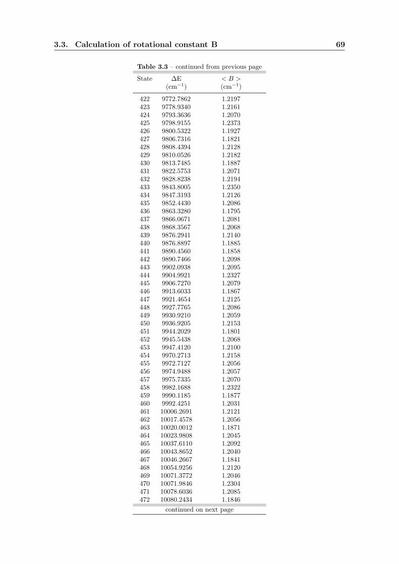
3.3. Calculation of rotational constant B 69
Table 3.3 – continued from previous page
State ∆E < B >
(cm−1) (cm−1)
422 9772.7862 1.2197423 9778.9340 1.2161424 9793.3636 1.2070425 9798.9155 1.2373426 9800.5322 1.1927427 9806.7316 1.1821428 9808.4394 1.2128429 9810.0526 1.2182430 9813.7485 1.1887431 9822.5753 1.2071432 9828.8238 1.2194433 9843.8005 1.2350434 9847.3193 1.2126435 9852.4430 1.2086436 9863.3280 1.1795437 9866.0671 1.2081438 9868.3567 1.2068439 9876.2941 1.2140440 9876.8897 1.1885441 9890.4560 1.1858442 9890.7466 1.2098443 9902.0938 1.2095444 9904.9921 1.2327445 9906.7270 1.2079446 9913.6033 1.1867447 9921.4654 1.2125448 9927.7765 1.2086449 9930.9210 1.2059450 9936.9205 1.2153451 9944.2029 1.1801452 9945.5438 1.2068453 9947.4120 1.2100454 9970.2713 1.2158455 9972.7127 1.2056456 9974.9488 1.2057457 9975.7335 1.2070458 9982.1688 1.2322459 9990.1185 1.1877460 9992.4251 1.2031461 10006.2691 1.2121462 10017.4578 1.2056463 10020.0012 1.1871464 10023.9808 1.2045465 10037.6110 1.2092466 10043.8652 1.2040467 10046.2667 1.1841468 10054.9256 1.2120469 10071.3772 1.2046470 10071.9846 1.2304471 10078.6036 1.2085472 10080.2434 1.1846
continued on next page

70 Chapter 3. Calculations
Table 3.3 – continued from previous page
State ∆E < B >
(cm−1) (cm−1)
473 10080.4546 1.1946474 10081.5109 1.2021475 10083.4576 1.2113476 10087.4261 1.2024477 10089.3484 1.1771478 10093.2798 1.2111479 10111.2938 1.2084480 10119.9721 1.2328481 10122.1549 1.2139482 10123.4516 1.2067483 10132.2864 1.2046484 10150.5783 1.2052485 10153.2769 1.2077486 10155.1749 1.1786487 10158.3880 1.2007488 10166.5719 1.2350489 10172.0205 1.2284490 10173.1315 1.2082491 10175.1907 1.2044492 10176.0083 1.2058493 10177.4527 1.2030494 10185.0740 1.2037495 10194.3271 1.1844496 10200.3852 1.2053497 10208.8866 1.1989498 10209.2643 1.2083499 10216.1544 1.2113500 10221.6912 1.2040501 10228.7317 1.2330502 10233.7655 1.2033503 10240.1449 1.2047504 10244.7087 1.1768505 10254.5248 1.2027506 10254.5492 1.2049507 10257.4536 1.2121508 10266.4156 1.2079509 10279.3845 1.2039510 10283.1969 1.1806511 10284.9475 1.2062512 10285.4194 1.2250513 10288.1577 1.1978514 10288.6558 1.1843515 10291.6030 1.2010516 10294.6493 1.1991517 10300.4721 1.2032518 10303.1808 1.2077519 10307.3964 1.1827520 10309.0234 1.2294521 10319.9521 1.1829522 10321.7718 1.2075523 10331.7741 1.2009
continued on next page

3.3. Calculation of rotational constant B 71
Table 3.3 – continued from previous page
State ∆E < B >
(cm−1) (cm−1)
524 10334.6112 1.2002525 10340.3819 1.2030526 10347.3591 1.2014527 10353.1628 1.1824528 10359.6235 1.1976529 10360.7534 1.2127530 10366.9644 1.2037531 10378.0680 1.1792532 10381.8097 1.2235533 10394.8876 1.2086534 10396.3847 1.2006535 10396.6678 1.1795536 10397.4996 1.2269537 10401.9408 1.2045538 10402.4410 1.2038539 10404.4179 1.2235540 10410.9142 1.1987541 10419.4402 1.1803542 10428.2152 1.2000543 10429.7873 1.1983544 10431.7451 1.2151545 10442.1777 1.1964546 10446.5731 1.2043547 10447.1326 1.2214548 10459.8184 1.1979549 10461.1056 1.2317550 10463.4243 1.2016551 10465.9454 1.2077552 10469.5721 1.2042553 10478.2367 1.2021554 10479.6281 1.2233555 10491.3044 1.2010556 10495.0265 1.2300557 10497.7449 1.2079558 10500.0079 1.2249559 10510.3349 1.1772560 10511.3739 1.2014561 10514.9101 1.1969562 10521.3229 1.2007563 10524.2425 1.2196564 10524.6620 1.1982565 10526.7544 1.1974566 10532.3269 1.2223567 10544.6786 1.1795568 10547.3872 1.2214569 10549.9200 1.1982570 10550.9004 1.2286571 10553.1513 1.1811572 10556.7293 1.2229573 10563.0823 1.2052574 10569.5476 1.2003
continued on next page

72 Chapter 3. Calculations
Table 3.3 – continued from previous page
State ∆E < B >
(cm−1) (cm−1)
575 10577.2758 1.1967576 10580.6820 1.2039577 10596.6373 1.2041578 10603.3846 1.1943579 10605.9074 1.2087580 10607.7363 1.1986581 10607.8014 1.1949582 10609.8736 1.1962583 10610.7730 1.2188584 10616.9124 1.2218585 10619.2076 1.1974586 10621.0125 1.2262587 10623.5563 1.2207588 10626.3895 1.2020589 10630.4291 1.2188590 10635.4153 1.2020591 10643.4577 1.1939592 10666.0499 1.2006593 10667.6136 1.2008594 10667.8137 1.2195595 10681.4226 1.1957596 10689.3851 1.1940597 10693.7923 1.2223598 10697.2943 1.1967599 10699.3138 1.1979600 10702.0830 1.1966601 10702.6614 1.1993602 10703.7552 1.2231603 10704.4761 1.2173604 10705.2165 1.2182605 10708.5064 1.2005606 10723.2720 1.1887607 10728.0786 1.2144608 10728.5651 1.1953609 10735.0860 1.1950610 10744.3611 1.1986611 10755.8849 1.1995612 10759.0202 1.1881613 10759.4028 1.2197614 10761.3524 1.2042615 10764.8195 1.2043616 10767.6335 1.1946617 10780.3330 1.2214618 10784.7431 1.1930619 10792.9417 1.2230620 10797.3985 1.1936621 10800.0660 1.2155622 10802.8830 1.1932623 10804.4585 1.1984624 10807.5421 1.2158625 10815.2624 1.2016
continued on next page

3.3. Calculation of rotational constant B 73
Table 3.3 – continued from previous page
State ∆E < B >
(cm−1) (cm−1)
626 10821.1590 1.2195627 10825.6586 1.2273628 10830.9733 1.2262629 10832.2120 1.1949630 10836.3360 1.1774631 10837.9343 1.2174632 10840.6224 1.2120633 10841.2800 1.1913634 10847.4870 1.1942635 10854.7194 1.1978636 10860.4706 1.2250637 10861.8313 1.2207638 10863.5586 1.1979639 10864.9399 1.1965640 10868.2803 1.1931641 10869.0741 1.2220642 10872.7089 1.1876643 10883.8777 1.1941644 10892.5656 1.2002645 10902.7662 1.1930646 10906.3060 1.2229647 10906.9778 1.1938648 10907.1001 1.2092649 10910.2535 1.1952650 10911.3823 1.1871651 10916.4233 1.1964652 10920.1290 1.1898653 10921.1809 1.2144654 10927.9315 1.2152655 10931.5171 1.1931656 10934.0452 1.1917657 10934.1019 1.2193658 10943.3193 1.2175659 10950.5239 1.1775660 10952.0186 1.1929661 10952.8976 1.2212662 10964.0447 1.2107663 10967.0621 1.1929664 10969.9245 1.1427665 10973.0466 1.1978666 10973.3192 1.2182667 10983.2659 1.1846668 10985.4297 1.1898669 10986.2511 1.1881670 10995.9445 1.2006671 10998.1361 1.1912672 11000.7269 1.1912673 11002.7484 1.2188674 11006.1483 1.1961675 11014.1129 1.2163676 11020.8080 1.1926
continued on next page
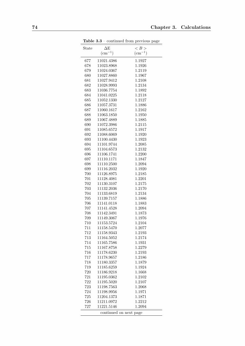
74 Chapter 3. Calculations
Table 3.3 – continued from previous page
State ∆E < B >
(cm−1) (cm−1)
677 11021.4386 1.1927678 11023.8968 1.1926679 11024.0367 1.2119680 11027.8860 1.1967681 11027.9412 1.2108682 11028.9993 1.2134683 11036.7754 1.1892684 11041.0225 1.2118685 11052.1330 1.2127686 11057.3731 1.1886687 11060.1617 1.2162688 11063.1850 1.1950689 11067.4889 1.1885690 11072.3986 1.2115691 11085.6572 1.1917692 11088.6069 1.1920693 11100.4430 1.1923694 11101.9744 1.2085695 11104.6573 1.2132696 11106.1741 1.2200697 11110.1171 1.1847698 11110.2500 1.2094699 11116.2032 1.1920700 11126.8975 1.2185701 11128.4081 1.2201702 11130.3107 1.2175703 11132.2036 1.2170704 11133.6819 1.2134705 11139.7157 1.1886706 11141.0118 1.1883707 11141.4528 1.2094708 11142.3491 1.1873709 11149.3067 1.1976710 11153.5724 1.2104711 11158.5470 1.2077712 11158.9343 1.2193713 11164.5052 1.2174714 11165.7586 1.1931715 11167.8758 1.2279716 11178.6230 1.2193717 11178.9657 1.2186718 11180.3357 1.1879719 11185.6259 1.1924720 11186.9218 1.1668721 11195.0362 1.2102722 11195.5020 1.2107723 11198.7563 1.2068724 11198.9956 1.1971725 11204.1373 1.1871726 11211.0972 1.2212727 11221.5146 1.2094
continued on next page

3.3. Calculation of rotational constant B 75
Table 3.3 – continued from previous page
State ∆E < B >
(cm−1) (cm−1)
728 11226.5381 1.1877729 11228.0119 1.1867730 11231.1812 1.1964731 11235.9993 1.2157732 11241.7879 1.2058733 11242.4107 1.2089734 11242.7482 1.2158735 11246.9097 1.2100736 11252.0956 1.2088737 11252.7926 1.2126738 11253.5462 1.2089739 11262.2441 1.1908740 11287.4277 1.2167741 11289.4605 1.1877742 11302.4351 1.2039743 11303.3514 1.2146744 11304.1441 1.2063745 11304.9588 1.2127746 11308.6422 1.2309747 11325.9381 1.2085748 11328.0225 1.1945749 11328.9614 1.2134750 11331.4541 1.2098751 11333.2994 1.2188752 11334.7618 1.1890753 11339.3917 1.2123754 11340.6455 1.1860755 11345.6972 1.2056756 11354.0974 1.2083757 11354.6399 1.2093758 11355.7255 1.2026759 11355.7862 1.2000760 11356.3300 1.1854761 11357.9204 1.2081762 11370.2169 1.2098763 11371.1783 1.2100764 11385.5911 1.1865765 11392.5215 1.1872766 11400.2504 1.2087767 11406.7313 1.2063768 11407.4927 1.2060769 11421.5410 1.2017770 11423.3222 1.2115771 11424.7068 1.2077772 11428.4022 1.2134773 11431.6091 1.2280774 11432.3607 1.2170775 11435.0928 1.2071776 11436.7532 1.1861777 11447.1470 1.2068778 11448.7053 1.1858
continued on next page

76 Chapter 3. Calculations
Table 3.3 – continued from previous page
State ∆E < B >
(cm−1) (cm−1)
779 11450.7602 1.2075780 11451.9463 1.1878781 11457.2691 1.2134782 11459.5726 1.2081783 11459.6528 1.2021784 11462.6426 1.2122785 11469.9668 1.1866786 11473.7403 1.2146787 11479.5618 1.1901788 11480.1826 1.2048789 11480.6669 1.1993790 11485.2519 1.2071791 11486.7654 1.1885792 11488.3126 1.2144793 11493.5189 1.1907794 11495.8428 1.1944795 11498.1472 1.2032796 11504.2304 1.2262797 11518.1914 1.2123798 11519.2277 1.1862799 11529.1386 1.2028800 11532.7408 1.2132801 11535.8176 1.2058802 11537.5839 1.2078803 11541.8966 1.2046804 11541.9393 1.2167805 11543.0656 1.1824806 11548.4794 1.2109807 11554.2842 1.2039808 11555.9826 1.1984809 11558.7833 1.2095810 11559.6790 1.2090811 11564.6912 1.2059812 11567.5626 1.1854813 11570.7377 1.2108814 11571.2690 1.1822815 11576.1738 1.2047816 11578.0942 1.2259817 11579.3151 1.1902818 11583.6757 1.1998819 11587.8541 1.2081820 11606.5262 1.2001821 11607.3313 1.2251822 11614.2091 1.2072823 11614.9564 1.2008824 11616.7873 1.2044825 11618.9051 1.2134826 11627.4748 1.1908827 11627.7948 1.2076828 11630.1600 1.2045829 11631.9781 1.1896
continued on next page

3.3. Calculation of rotational constant B 77
Table 3.3 – continued from previous page
State ∆E < B >
(cm−1) (cm−1)
830 11632.8327 1.2031831 11639.5201 1.2010832 11640.3980 1.2244833 11657.8349 1.2075834 11662.1079 1.2067835 11669.9432 1.1860836 11670.2504 1.2046837 11671.2638 1.1829838 11674.4528 1.2006839 11687.8280 1.1892840 11691.5539 1.2046841 11691.8382 1.1830842 11694.4434 1.2010843 11704.8783 1.2220844 11709.2435 1.1971845 11710.9389 1.1810846 11713.1295 1.1839847 11715.4912 1.1960848 11721.3740 1.2032849 11723.2841 1.1987850 11729.3021 1.2094851 11732.9440 1.2056852 11736.7275 1.2241853 11739.9378 1.2077854 11741.1390 1.1961855 11742.0535 1.2264856 11743.2335 1.2088857 11745.9985 1.2090858 11748.8698 1.2040859 11751.8127 1.1978860 11751.8867 1.2045861 11756.0282 1.2297862 11761.5038 1.2128863 11776.2487 1.2114864 11776.7510 1.1813865 11782.4627 1.1993866 11783.1681 1.1974867 11786.9394 1.2060868 11787.4250 1.2012869 11787.8057 1.2228870 11787.9512 1.2070871 11789.2074 1.2074872 11789.8008 1.2082873 11793.4513 1.2201874 11798.8034 1.1992875 11798.9966 1.1785876 11807.2122 1.2014877 11807.6728 1.2062878 11810.3228 1.2220879 11814.6294 1.2006880 11817.8360 1.1785
continued on next page

78 Chapter 3. Calculations
Table 3.3 – continued from previous page
State ∆E < B >
(cm−1) (cm−1)
881 11828.3645 1.1922882 11833.4097 1.2054883 11842.6614 1.2263884 11849.0551 1.1953885 11851.7662 1.2003886 11862.0150 1.1955887 11863.4308 1.2093888 11874.0762 1.1955889 11874.3586 1.1975890 11876.3258 1.1986891 11880.9712 1.1971892 11885.3018 1.2201893 11888.2385 1.2068894 11890.2766 1.1995895 11891.2423 1.2184896 11893.8867 1.2216897 11898.7970 1.2143898 11901.9401 1.2244899 11902.3613 1.1962900 11904.7940 1.1809901 11911.2949 1.2092902 11914.3659 1.2139903 11920.3498 1.1802904 11921.5146 1.2015905 11923.6045 1.2239906 11934.0366 1.2030907 11935.7240 1.2025908 11946.4684 1.1959909 11953.1440 1.1888910 11953.9811 1.1949911 11955.3518 1.2035912 11956.7101 1.2014913 11962.2032 1.2230914 11964.5053 1.1957915 11967.7005 1.2044916 11969.7995 1.2027917 11973.2810 1.1961918 11976.3319 1.2178919 11978.6303 1.1925920 11987.5547 1.1761921 11989.7317 1.1961922 11990.2348 1.1895923 11991.0944 1.1979924 11992.2093 1.2001925 11998.5416 1.1930926 12001.6416 1.2167927 12004.7537 1.2102928 12017.9079 1.1986929 12019.6173 1.2028930 12029.8282 1.1927931 12030.2485 1.2342
continued on next page

3.3. Calculation of rotational constant B 79
Table 3.3 – continued from previous page
State ∆E < B >
(cm−1) (cm−1)
932 12036.5443 1.2210933 12038.0633 1.2178934 12038.5302 1.1995935 12049.4107 1.1940936 12050.3329 1.2048937 12053.7376 1.2003938 12054.4056 1.1927939 12060.3518 1.2426940 12060.9734 1.1991941 12061.1991 1.1954942 12062.6860 1.2205943 12074.1722 1.2228944 12076.0963 1.1936945 12076.7792 1.1954946 12077.0252 1.1849947 12077.4636 1.2155948 12078.3157 1.2167949 12081.0148 1.1941950 12085.9765 1.2364951 12089.2097 1.1819952 12098.9861 1.1909953 12103.0030 1.2028954 12106.4335 1.1919955 12110.0936 1.1877956 12118.0576 1.2409957 12119.2135 1.1961958 12126.1514 1.1947959 12127.8266 1.2170960 12127.8541 1.2198961 12128.8095 1.1961962 12131.1179 1.2138963 12133.4889 1.1993964 12135.5799 1.2211965 12136.8564 1.1947966 12143.7876 1.1911967 12146.2387 1.1969968 12150.0378 1.1906969 12153.8988 1.2142970 12159.2023 1.1995971 12173.6298 1.1721972 12177.0489 1.1962973 12178.0253 1.1988974 12178.1772 1.1897975 12189.1826 1.2133976 12191.0567 1.2134977 12191.5869 1.2149978 12195.5903 1.1892979 12199.3370 1.1892980 12200.0346 1.1946981 12204.9700 1.1883982 12211.0831 1.2187
continued on next page

80 Chapter 3. Calculations
Table 3.3 – continued from previous page
State ∆E < B >
(cm−1) (cm−1)
983 12217.1785 1.1999984 12219.0050 1.1757985 12224.4598 1.1922986 12228.2099 1.1955987 12228.3452 1.2208988 12228.8635 1.1936989 12234.7834 1.1985990 12234.8872 1.1925991 12235.0303 1.1922992 12236.1589 1.1892993 12239.0338 1.2190994 12242.0850 1.2116995 12242.6888 1.1923996 12244.6995 1.2127997 12245.8929 1.1902998 12256.2369 1.2378999 12262.2706 1.21971000 12263.9389 1.21981001 12264.9655 1.17411002 12274.8665 1.19211003 12274.8734 1.17401004 12276.9358 1.18581005 12278.5987 1.21191006 12288.6126 1.19301007 12295.7560 1.21691008 12296.8204 1.21761009 12297.0977 1.21621010 12301.4035 1.19321011 12303.1355 1.19661012 12305.5599 1.16901013 12306.3054 1.22101014 12312.6147 1.18961015 12312.9618 1.21041016 12320.2063 1.21301017 12321.9617 1.18801018 12328.0470 1.18831019 12328.6557 1.21071020 12329.1941 1.21111021 12329.5929 1.19481022 12334.5205 1.19021023 12344.7612 1.21691024 12345.5800 1.19181025 12356.1307 1.22511026 12357.5365 1.18851027 12359.9813 1.19941028 12363.6613 1.20941029 12363.8803 1.19751030 12364.3996 1.18631031 12365.4152 1.20941032 12366.1805 1.19821033 12370.3585 1.2201
continued on next page

3.3. Calculation of rotational constant B 81
Table 3.3 – continued from previous page
State ∆E < B >
(cm−1) (cm−1)
1034 12372.1122 1.21591035 12374.0727 1.19701036 12382.2277 1.21331037 12384.8281 1.21391038 12394.5368 1.18771039 12397.2083 1.21341040 12398.3276 1.18851041 12399.7949 1.19391042 12402.3406 1.19281043 12403.6878 1.20941044 12410.1288 1.19111045 12411.0185 1.19131046 12414.9308 1.18961047 12416.3952 1.21861048 12422.7120 1.21401049 12424.6727 1.20861050 12434.8415 1.21151051 12443.5350 1.17541052 12446.9786 1.20841053 12454.4898 1.21921054 12455.0068 1.20791055 12458.5709 1.15801056 12458.8403 1.21811057 12460.5344 1.19281058 12461.1343 1.20861059 12467.3980 1.20981060 12477.3053 1.18801061 12484.3820 1.18671062 12485.1878 1.19131063 12489.0578 1.18661064 12489.7728 1.21141065 12502.0049 1.21151066 12502.8493 1.19531067 12506.1186 1.20621068 12507.1039 1.18851069 12510.9145 1.21001070 12515.3880 1.21741071 12517.5258 1.21001072 12522.5654 1.19141073 12524.3250 1.21631074 12525.6062 1.19151075 12525.8398 1.20671076 12534.3908 1.18581077 12535.2685 1.21021078 12541.6370 1.21231079 12557.3920 1.18541080 12558.5302 1.20521081 12559.6782 1.21131082 12568.2008 1.18661083 12569.4602 1.19081084 12570.9996 1.2077
continued on next page

82 Chapter 3. Calculations
Table 3.3 – continued from previous page
State ∆E < B >
(cm−1) (cm−1)
1085 12571.1407 1.18921086 12574.6612 1.21631087 12579.6309 1.21341088 12585.5482 1.18841089 12586.2703 1.21531090 12586.2951 1.21051091 12591.4308 1.21381092 12593.4582 1.20631093 12597.4764 1.19281094 12599.3026 1.15661095 12606.5205 1.18461096 12606.6555 1.18821097 12612.9732 1.19021098 12613.2604 1.18661099 12616.7203 1.20631100 12621.2333 1.20961101 12623.0791 1.20791102 12624.0594 1.20881103 12625.0798 1.21121104 12626.0303 1.21281105 12626.7252 1.18611106 12638.5917 1.20731107 12640.1944 1.18651108 12640.6361 1.21721109 12643.6123 1.20901110 12644.1932 1.18621111 12645.3628 1.18961112 12662.7357 1.21131113 12663.1160 1.18451114 12669.6751 1.20791115 12672.8859 1.18671116 12680.4640 1.20191117 12690.5313 1.20881118 12690.7206 1.20901119 12697.5280 1.20061120 12702.4492 1.18491121 12702.6809 1.20451122 12707.1761 1.20711123 12708.8341 1.17911124 12711.8213 1.17951125 12715.5427 1.18621126 12717.8041 1.20521127 12719.2208 1.18691128 12730.7722 1.21481129 12735.7587 1.18191130 12737.6626 1.20791131 12738.9025 1.21321132 12748.2582 1.20271133 12751.4335 1.20081134 12754.7838 1.21541135 12758.7310 1.1837
continued on next page

3.3. Calculation of rotational constant B 83
Table 3.3 – continued from previous page
State ∆E < B >
(cm−1) (cm−1)
1136 12760.2499 1.20551137 12764.8070 1.20431138 12766.6240 1.21421139 12771.1876 1.17651140 12776.5588 1.18491141 12778.5212 1.21061142 12779.8847 1.23111143 12793.3442 1.18681144 12803.3278 1.20291145 12804.4459 1.21221146 12806.4531 1.20791147 12809.2820 1.18791148 12809.9042 1.18251149 12813.8928 1.18461150 12814.0076 1.17731151 12817.3658 1.19951152 12819.8205 1.21001153 12821.6131 1.17581154 12822.9774 1.19971155 12823.4436 1.18521156 12827.4589 1.20381157 12833.0008 1.19811158 12838.3590 1.22431159 12838.8622 1.21151160 12848.6979 1.21111161 12849.7016 1.18231162 12853.3170 1.21061163 12854.8124 1.20921164 12857.4579 1.18431165 12858.5923 1.19741166 12859.4048 1.17531167 12859.7270 1.21061168 12864.3200 1.18641169 12868.2369 1.20681170 12868.2386 1.17391171 12872.1103 1.22161172 12876.3726 1.20101173 12876.7020 1.18991174 12878.9453 1.19991175 12880.3704 1.19761176 12880.6728 1.18431177 12885.7986 1.20751178 12892.2564 1.20431179 12895.0424 1.18431180 12900.5006 1.19891181 12905.7119 1.18311182 12908.8017 1.21091183 12909.8733 1.18941184 12913.6239 1.20111185 12914.6835 1.18101186 12916.2485 1.2264
continued on next page

84 Chapter 3. Calculations
Table 3.3 – continued from previous page
State ∆E < B >
(cm−1) (cm−1)
1187 12920.0905 1.20591188 12922.1423 1.18081189 12927.8508 1.20791190 12931.1131 1.16761191 12932.6341 1.19861192 12935.3171 1.20731193 12936.9393 1.20741194 12944.6862 1.20681195 12947.5692 1.20221196 12949.1039 1.20411197 12950.4855 1.20371198 12957.1859 1.18001199 12958.0650 1.19501200 12958.0727 1.21591201 12958.5883 1.17391202 12959.4442 1.19381203 12965.4604 1.20361204 12972.1162 1.20361205 12972.9324 1.19711206 12981.6001 1.17571207 12982.3236 1.23681208 12995.6300 1.20731209 12997.2324 1.20381210 13000.4042 1.20871211 13011.5886 1.22581212 13013.4391 1.19271213 13018.3363 1.19881214 13018.6214 1.17341215 13021.4709 1.17571216 13025.3036 1.17841217 13028.7093 1.20491218 13030.5419 1.20401219 13030.9267 1.20291220 13039.0309 1.20101221 13044.1455 1.20831222 13044.2431 1.23721223 13045.1536 1.20301224 13047.5173 1.20041225 13049.0444 1.18291226 13051.1961 1.19701227 13053.1072 1.18141228 13054.6063 1.19121229 13055.9776 1.20901230 13058.5626 1.21031231 13069.1020 1.20501232 13069.5609 1.20691233 13071.8304 1.19991234 13075.6464 1.19061235 13078.4613 1.20391236 13084.9743 1.19861237 13086.3042 1.2064
continued on next page
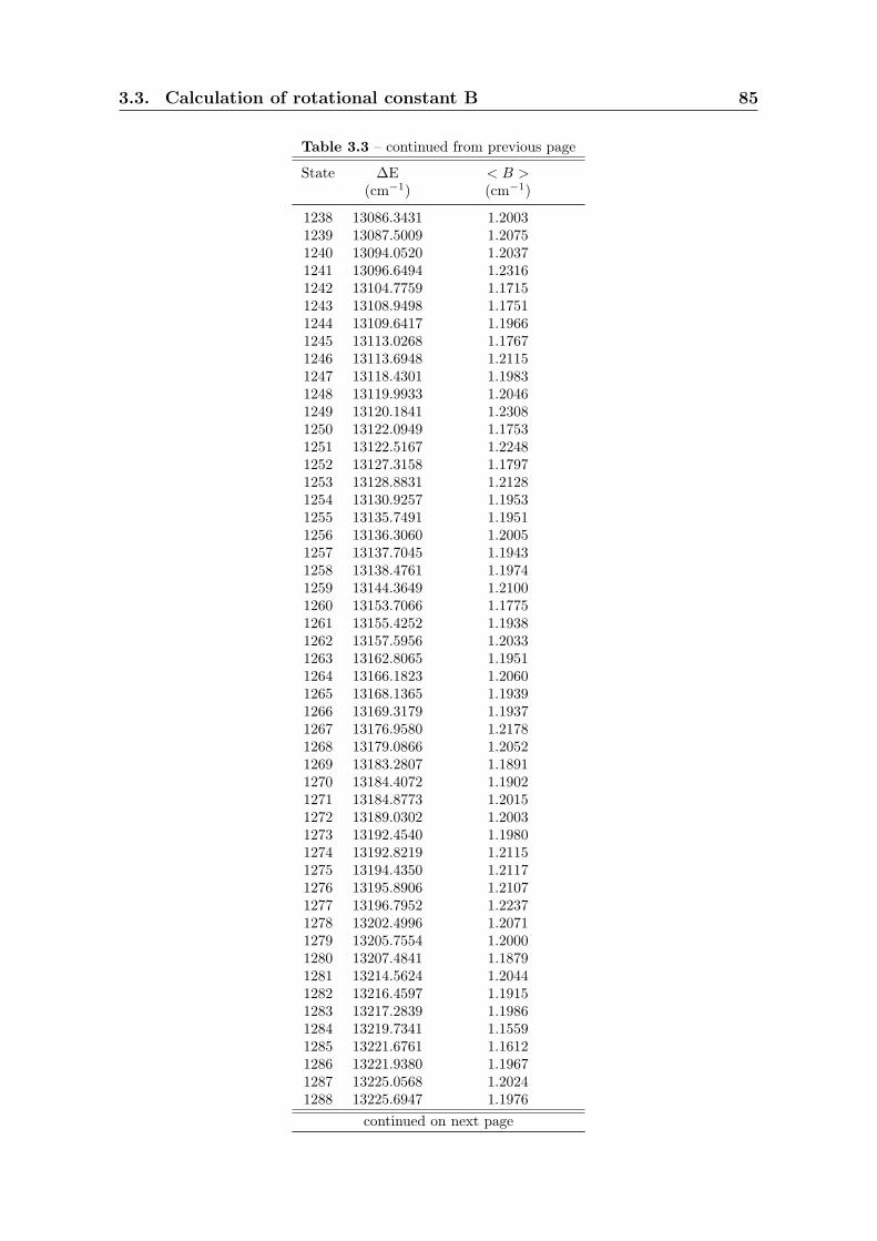
3.3. Calculation of rotational constant B 85
Table 3.3 – continued from previous page
State ∆E < B >
(cm−1) (cm−1)
1238 13086.3431 1.20031239 13087.5009 1.20751240 13094.0520 1.20371241 13096.6494 1.23161242 13104.7759 1.17151243 13108.9498 1.17511244 13109.6417 1.19661245 13113.0268 1.17671246 13113.6948 1.21151247 13118.4301 1.19831248 13119.9933 1.20461249 13120.1841 1.23081250 13122.0949 1.17531251 13122.5167 1.22481252 13127.3158 1.17971253 13128.8831 1.21281254 13130.9257 1.19531255 13135.7491 1.19511256 13136.3060 1.20051257 13137.7045 1.19431258 13138.4761 1.19741259 13144.3649 1.21001260 13153.7066 1.17751261 13155.4252 1.19381262 13157.5956 1.20331263 13162.8065 1.19511264 13166.1823 1.20601265 13168.1365 1.19391266 13169.3179 1.19371267 13176.9580 1.21781268 13179.0866 1.20521269 13183.2807 1.18911270 13184.4072 1.19021271 13184.8773 1.20151272 13189.0302 1.20031273 13192.4540 1.19801274 13192.8219 1.21151275 13194.4350 1.21171276 13195.8906 1.21071277 13196.7952 1.22371278 13202.4996 1.20711279 13205.7554 1.20001280 13207.4841 1.18791281 13214.5624 1.20441282 13216.4597 1.19151283 13217.2839 1.19861284 13219.7341 1.15591285 13221.6761 1.16121286 13221.9380 1.19671287 13225.0568 1.20241288 13225.6947 1.1976
continued on next page

86 Chapter 3. Calculations
Table 3.3 – continued from previous page
State ∆E < B >
(cm−1) (cm−1)
1289 13227.6468 1.20791290 13227.9985 1.17841291 13228.0377 1.20501292 13232.5718 1.19261293 13235.7619 1.21401294 13237.5575 1.22161295 13237.7902 1.15191296 13243.1940 1.19591297 13244.3890 1.19361298 13246.6484 1.20141299 13249.2075 1.20301300 13252.3595 1.16961301 13256.2997 1.17361302 13260.1265 1.20291303 13261.5159 1.19051304 13269.8665 1.21651305 13270.4622 1.20041306 13270.8496 1.19911307 13274.6229 1.21641308 13276.5043 1.17871309 13277.0190 1.19141310 13293.6806 1.19781311 13294.2980 1.19531312 13294.6831 1.19251313 13294.9291 1.18471314 13296.0245 1.19311315 13296.2922 1.20391316 13300.6927 1.17991317 13303.2618 1.15531318 13303.8855 1.19481319 13306.0457 1.19601320 13309.4916 1.18981321 13314.7822 1.17431322 13314.8795 1.19831323 13315.2182 1.19551324 13316.7576 1.20881325 13323.8489 1.19881326 13325.5944 1.19781327 13327.0021 1.19931328 13333.7571 1.19441329 13338.6532 1.19311330 13341.5945 1.20601331 13341.6616 1.19061332 13342.2170 1.19301333 13342.2835 1.19831334 13351.3153 1.19041335 13354.2550 1.21591336 13355.5330 1.19891337 13362.0911 1.17601338 13364.8315 1.19221339 13365.9262 1.1924
continued on next page

3.3. Calculation of rotational constant B 87
Table 3.3 – continued from previous page
State ∆E < B >
(cm−1) (cm−1)
1340 13366.5197 1.22011341 13367.6878 1.19671342 13369.9724 1.18091343 13370.2060 1.18491344 13370.3700 1.21861345 13370.5691 1.19321346 13372.4076 1.19721347 13382.3973 1.20311348 13388.2522 1.17781349 13393.6985 1.19611350 13393.9079 1.19421351 13395.9871 1.17511352 13403.4865 1.20861353 13406.0279 1.19621354 13406.3835 1.21261355 13406.4278 1.21351356 13406.6381 1.19741357 13412.1220 1.19321358 13417.9530 1.19531359 13423.0235 1.19061360 13424.6760 1.21721361 13425.3870 1.18951362 13427.1882 1.19701363 13427.8213 1.19001364 13432.3261 1.19591365 13441.5000 1.19061366 13442.5620 1.15331367 13446.1792 1.18871368 13449.7480 1.20261369 13450.7799 1.20001370 13453.6453 1.19291371 13454.9676 1.21431372 13456.7165 1.18901373 13464.2038 1.18981374 13464.9859 1.19021375 13467.5593 1.17811376 13467.9207 1.17691377 13470.0129 1.19111378 13472.9456 1.19851379 13473.7718 1.19831380 13477.4215 1.19511381 13482.2884 1.19571382 13482.5472 1.18471383 13483.8821 1.20611384 13483.9267 1.19361385 13483.9748 1.22151386 13486.4322 1.19331387 13489.8324 1.22621388 13504.0143 1.19611389 13505.5654 1.20771390 13507.2480 1.1576
continued on next page

88 Chapter 3. Calculations
Table 3.3 – continued from previous page
State ∆E < B >
(cm−1) (cm−1)
1391 13508.3412 1.19321392 13509.4567 1.20761393 13510.2786 1.21351394 13512.2228 1.17971395 13512.7661 1.18291396 13513.1500 1.21081397 13514.0818 1.19861398 13514.0945 1.19911399 13517.0740 1.18841400 13518.2886 1.1904

Chapter 4
Results vs HITRAN
4.1 Calculations of line intensities
In this chapter I will compare the results of our calculations with available experimen-
tal data, taken either from the HITRAN database (59) or from publications referred
to by HITRAN (63; 61). Such experimental data come in the form of lists of resolved
rovibrational lines, each with its position and integrated line strength. Since our
present variational calculations were restricted to rotationless (total angular momen-
tum J = 0) purely vibrational states, we estimated the rotational substructure, as
mentioned in the previous Chapter, in the rigid rotor approximation. The integrated
line strength of a given transition is given by (97)
S(T0) =
(
2π2
3hcǫ0
)[
g′′ν0
gVQ(T0)
]
SvibL(J, l) exp
(−E ′′
kT0
)[
1− exp
(−hcν0
kT0
)]
, (4.1)
where: g′′ is the statistical weight due to nuclear spin of the lower level (1 for para and
3 for ortho states); ν0 is the transition wavenumber; gV is a factor used to consider
bands with l-type doubling (gV is equal to 2 in such a case, otherwise, it is equal
to 1); Q(T0) (98) is the total partition function at temperature T0; L(J, l) is the
Honl-London factor, J being the rotational quantum number of the lower level of the
transition, and l its total vibrational quantum number (l = |l4 + l5|); E ′′ is the energy
of the lower level.
Eq. 4.1 is used in HITRAN to derive, in a multispectrum fit procedure (99), the
value of Svib. In that procedure, Svib is actually considered itself a (slowly variable)
function of J , and fitted with a second order polynomial in J with the so–called
Herman–Wallis coefficients (45). The apparent variability of Svib accounts for the
interaction between vibrational and angular motions, which is not explicitly considered
in Eq. 4.1. In a fully variational calculation (i. e. including states with J > 0) one does
not assume the line intensity to be factorised as S = SRot(J′′, J ′)SV ib(V
′′, V ′) (i. e.

90 Chapter 4. Results vs HITRAN
Eq. 2.20), with SRot(J′′, J ′) = L(J, l), but directly computes the accurate value of
S, treating vibration and rotation on the same footing and whus fully including their
interaction without empirical coefficients. However, we here restricted our calculations
to rotationless states, and are thus forced to use Eq. 4.1 to compare our results with
the lists of rovibrational transitions in HITRAN. Since our current calculation does
not enable us to obtain the Herman–Wallis coefficients, we expect our calculated
line intensities to be most accurate for low J values, for which separation between
rotational and vibrational motion is a better approximation.
Our calculations, having been restricted to states with J = 0 (and consequently
l = 0), necessarily yield an incomplete list of states, in which states with l 6= 0 are
missing. Consequently, we cannot include them in our calculation of the partition
function
Q(T0) =∑
i
di exp
(
− Ei
kT0
)
(4.2)
where di is the degeneracy of the i–th level and Ei is its rovibrational energy. We will
instead compute
Q(T0) =∑
i,l=0
di exp
(
− Ei
kT0
)
<∑
i
di exp
(
− Ei
kT0
)
= Q(T0) (4.3)
resulting in an underestimated partition function in our calculated spectra by a factor
of order of unity at room temperature (T = 296 Kelvin). This factor is expected to
be the same for all transitions calculated at the same temperature, and will translate
in a corresponding overestimation of our calculated line intensities.
Another consequence of the fact that we calculated only states with l = 0 is that
we can only obtain parallel bands, whose Honl-London factors, given by Eq. 2.25 and
2.27, become
L(J, l) = J (P-branch) (4.4)
L(J, l) = J + 1 (R-branch). (4.5)
In the following we show a detailed comparison for two parallel vibrational bands.
4.1.1 The (3ν4 + ν5)0 cold band
This cold (i. e. arising from the ground vibrational state) band has a calculated origin
at 2519.5 cm−1, versus a measured value of 2560.6 cm−1. Our calculated value of Svib
is 1.6 · 10−6 D2, versus an experimental value (derived from multispectrum fit) of
1.7 ·10−6 D2. The following Table 4.1 reports a line by line comparison with HITRAN
data.

4.1. Calculations of line intensities 91
4.1.2 The (ν3) fundamental hot band
This fundamental (i. e. arising from the ground vibrational state) hot band has
a calculated origin at 3241.1 cm−1, versus a measured value of 3316.9 cm−1. Our
calculated value of Svib is 5.1 · 10−3 D2, versus an experimental value (derived from
multispectrum fit) of 3.9 · 10−3 D2. The following Table 4.2 reports a line by line
comparison with HITRAN data.

92 Chapter 4. Results vs HITRAN
Table 4.1: Comparison between our calculated individual rovibrational line positionand intensities and the experimental ones in the HITRAN database, for the (3ν4+ν5)0
cold band (61). Columns, left to right, list: line type (branch and symmetry); Jquantum number in the lower state; calculated energy (cm−1); experimental energy(cm−1); calculated S (cm·molecule−1); experimental S (cm·molecule−1); ratio betweenthe calculated and experimental S.
Branch J Eth Eexp Sth Sexp Sth/Sexp
Pee 1 2517.1 2558.2 1.47·10−23 1.29·10−23 1.14Pee 2 2514.6 2555.9 9.55·10−24 8.38·10−24 1.14Pee 3 2512.2 2553.6 4.14·10−23 3.77·10−23 1.10Pee 4 2509.8 2551.3 1.76·10−23 1.59·10−23 1.11Pee 5 2507.4 2549.0 6.20·10−23 5.55·10−23 1.12Pee 6 2505.0 2546.7 2.31·10−23 2.13·10−23 1.08Pee 7 2502.7 2544.4 7.43·10−23 6.69·10−23 1.11Pee 8 2500.3 2542.2 2.57·10−23 2.32·10−23 1.11Pee 9 2497.9 2540.0 7.80·10−23 6.95·10−23 1.12Pee 10 2495.6 2537.8 2.57·10−23 2.20·10−23 1.17Pee 11 2493.2 2535.6 7.43·10−23 6.53·10−23 1.14Pee 12 2490.9 2533.4 2.34·10−23 2.04·10−23 1.15Pee 14 2486.2 2529.2 1.98·10−23 1.69·10−23 1.17Pee 16 2481.6 2525.2 1.57·10−23 1.25·10−23 1.26Pee 17 2479.3 2523.2 4.09·10−23 3.23·10−23 1.27Pee 18 2477.0 2521.2 1.17·10−23 8.99·10−24 1.30Pee 19 2474.7 2519.3 2.95·10−23 2.28·10−23 1.29Pee 20 2472.4 2517.3 8.16·10−24 6.25·10−24 1.30Pee 21 2470.1 2515.5 2.00·10−23 1.47·10−23 1.36
Ree 0 2521.9 2563.0 4.96·10−24 4.32·10−24 1.15Ree 1 2524.4 2565.3 2.95·10−23 2.60·10−23 1.14Ree 2 2526.8 2567.7 1.44·10−23 1.25·10−23 1.15Ree 3 2529.3 2570.1 5.56·10−23 4.96·10−23 1.12Ree 4 2531.7 2572.6 2.21·10−23 2.00·10−23 1.11Ree 5 2534.2 2575.0 7.52·10−23 6.64·10−23 1.13Ree 8 2541.7 2582.5 2.94·10−23 2.59·10−23 1.14Ree 10 2546.7 2587.6 2.88·10−23 2.41·10−23 1.20Ree 12 2551.8 2592.7 2.60·10−23 2.25·10−23 1.16Ree 14 2556.9 2598.1 2.19·10−23 1.79·10−23 1.22Ree 15 2559.4 2600.8 5.86·10−23 4.63·10−23 1.27Ree 16 2562.0 2603.5 1.72·10−23 1.31·10−23 1.31Ree 17 2564.5 2606.2 4.48·10−23 3.30·10−23 1.36Ree 18 2567.1 2609.0 1.28·10−23 9.09·10−24 1.41

4.1. Calculations of line intensities 93
Table 4.2: Comparison between our calculated individual rovibrational line positionand intensities and the experimental ones in the HITRAN database, for the (ν3)fundamental band (63). Columns, left to right, list: line type (branch and symmetry);J quantum number in the lower state; calculated energy (cm−1); experimental energy(cm−1); calculated S (cm·molecule−1); experimental S (cm·molecule−1); ratio betweenthe calculated and experimental S.
Branch J Eth Eexp Sth Sexp Sth/Sexp
Pe 2 3236.2 3290.1 3.89·10−20 2.61·10−20 1.49Pe 3 3233.7 3287.8 1.69·10−19 1.13·10−19 1.50Pe 6 3226.3 3280.6 9.40·10−20 6.30·10−20 1.49Pe 7 3223.7 3278.2 3.03·10−19 2.05·10−19 1.48Pe 8 3221.2 3275.8 1.05·10−19 7.02·10−20 1.50Pe 9 3218.7 3273.4 3.18·10−19 2.14·10−19 1.49Pe 10 3216.1 3270.9 1.05·10−19 7.17·10−20 1.46Pe 11 3213.5 3268.5 3.03·10−19 2.08·10−19 1.46Pe 12 3210.9 3266.0 9.55·10−20 6.50·10−20 1.47Pe 13 3208.3 3263.6 2.66·10−19 1.84·10−19 1.45Pe 14 3205.7 3261.1 8.09·10−20 5.55·10−20 1.46Pe 15 3203.1 3258.6 2.18·10−19 1.52·10−19 1.43Pe 16 3200.4 3256.1 6.40·10−20 4.39·10−20 1.46Pe 17 3197.7 3253.6 1.67·10−19 1.16·10−19 1.44Pe 18 3195.1 3251.1 4.76·10−20 3.28·10−20 1.45Pe 19 3192.4 3248.6 1.20·10−19 8.48·10−20 1.42Pe 20 3189.7 3246.0 3.33·10−20 2.31·10−20 1.44Pe 21 3186.9 3243.5 8.18·10−20 5.68·10−20 1.44Pe 22 3184.2 3240.9 2.29·10−20 1.56·10−20 1.47
Re 1 3245.9 3299.5 1.20·10−19 7.76·10−20 1.55Re 3 3250.6 3304.2 2.26·10−19 1.46·10−19 1.55Re 4 3253.0 3306.5 8.99·10−20 5.81·10−20 1.55Re 5 3255.3 3308.7 3.05·10−19 1.94·10−19 1.57Re 6 3257.6 3311.1 1.11·10−19 6.98·10−20 1.59Re 7 3259.9 3313.3 3.50·10−19 2.18·10−19 1.61Re 8 3262.2 3315.6 1.19·10−19 7.43·10−20 1.60Re 9 3264.5 3317.9 3.58·10−19 2.24·10−19 1.60Re 10 3266.8 3320.1 1.17·10−19 7.30·10−20 1.60Re 11 3269.0 3322.4 3.36·10−19 2.14·10−19 1.57Re 13 3273.5 3326.8 2.92·10−19 1.79·10−19 1.63Re 14 3275.7 3329.0 8.85·10−20 5.46·10−20 1.62Re 15 3277.9 3331.2 2.38·10−19 1.45·10−19 1.64Re 17 3282.2 3335.5 1.81·10−19 1.09·10−19 1.66

94 Chapter 4. Results vs HITRAN

Chapter 5
Conclusions and perspectives
We obtained, for the first time using variational methods and an ab initio P.E.S.,
calculated intensities of purely vibrational, parallel bands of C2H2 (in preparation,
100).
The results of the Dipole code have been compared with the HITRAN database,
under strict assumptions that sped up the test calculations by more than one or-
der of magnitude. This resulted in its successful validation, since calculated values
were compatible with experimental data, the discrepancies being accounted for by
the adopted simplifying assumptions. It is now sensible to relax such drastic sim-
plifications, moving the variational calculations one step further, fully including in
it the rotational degrees of freedom. This will enable us to obtain complete lists of
vibrational energy levels up to a given maximum excitation (i. e. including states
with nonzero vibrational angular momentum) and consequently of the electric dipole
transitions among them which are allowed (i. e. including perpendicular bands). The
completeness of the list of states will remove the main cause of discrepancy between
our test calculations and experimental data, enabling us to accurately estimate the
partition function at a given temperature. The completeness of the transitions will
enable us to reliably estimate the opacity of C2H2 at the temperatures prevailing in
the photospheres of cool stars (i. e. between 1000 and 2000 K). Such lists of states
and transitions will be suitable for straightforward integration in existing models of
stellar atmospheres (e.g. Kurucz models (101)), to estimate their effect on radiation
transport, their physical structure and the resulting spectra. One will also be able to
use the molecular data as they are, to directly estimate C2H2 absorption spectra at a
given temperature, for straight comparison with available observational data.

96 Chapter 5. Conclusions and perspectives
5.1 Example synthetic opacities
For example and testing purposes, we already implemented a simple calculation of
C2H2 opacities and applied it to the calculations we performed so far (despite their
limitations). The absorption coefficient or opacity function kν at wavenumber ν is
given by
kν =∑
i
Sifi(ν − ν0,i), (5.1)
where fi(ν − ν0,i) is the line profile and ν0,i is the line center of line i. The integrated
absorption, Si of line i is found from the absorption coefficient of the line, kν,i, by
Si =
∫ +∞
−∞
kν,idν. (5.2)
The integrated absorption for the complete spectrum is thus
S =∑
i
Si. (5.3)
In principle, therefore, to calculate kν one would need to know the line profiles fi(ν−ν0,i), and to sum over all transitions. However, when comparing with experimental
data, what one obtains from a spectrograph is a tabulated list of opacity values over
a grid of wavenumbers, each of them being an average over an interval corresponding
to the spectral sampling of the instrument. If the resolving power of the instrument is
so large to be considered, for all practical purposes, infinite, such average, tabulated
values of the opacity are coincident with the definition given in Eq. 5.1. Otherwise,
one should properly compare experimental data with
kν =1
∆ν
∫ ν+∆ν
ν
kνdν. (5.4)
However, in practice this is only strictly needed if one wants to compute the opac-
ity with a very high spectral resolution, namely high enough to resolve single line
profiles. This is usually not the case for astronomical instruments operating in the
infrared spectral range (i. e. where C2H2 lines are most conspicuous). Such instru-
ments, in most cases satellite–borne, usually have spectral resolving powers at most of
the order of a few thousand (e. g. R ≃ 1500 for the short–wavelength spectrometer
(SWS) on board the infrared space observatory (ISO), when used in its maximum res-
olution mode). In this case, the resolving power is not sufficient to resolve individual
rovibrational transitions, let alone resolving the detailed profile of each line. There-
fore, for each tabulated value of ν the interval ∆ν is much larger than the individual
linewidths. With the possible (unlikely) exception of a transition falling very precisely

5.2. Forthcoming work 97
in the middle between two such intervals, and therefore contributing to two neigh-
bouding average opacity values, each line will almost always fall either completely
inside or completely outside of any interval. This assumption leads to a much simpler
expression for kν : very simply, one just sums Si for all lines in the wavenumber inter-
val from ν to ν + ∆ν, and dividing by ∆ν. This frequency binning method has the
effect of producing computed, tabulated opacities corresponding to a resolving power
R ≃ ν∆ν
. Frequency–binned opacity data have been presented by Harris (102) in
his work on HCN and in other previous works (103; 104). We applied it to compute
some test absorption spectra from the results of our partial calculations, assuming
the resolving power of ISO–SWS spectrometer in its low–resolution (R ≃ 200) and
high-resolution (R ≃ 1500) modes. Aoki et al. (8) have observed C2H2 in carbon
(C) star spectra using the low–resolution mode of ISO–SWS. Figures 5.1 to 5.8 show
some synthetic absorption spectra, for illustrative properties only (see Sect. 4.1 for
the known limitations of the present calculations). For each plotted band, the opacity
was calculated at resolving powers R ≃ 200 (red line) and R ≃ 1500 (green line).
5.2 Forthcoming work
Since complete calculations including nonzero angular momenta involve a very large
computational cost, our first step, before embarking in this feat, will be to backport
the MPI parallelisation of the Dipole code to wavr4. Since a large fraction of the
time, in wavr4 runs, is spent in computing integrals over Gaussian grids, to obtain
the matrix elements of the various effective Hamiltonians, this section of the code
can be reused very nearle “as–is” from the MPI version of the Dipole code. We
will then investigate the possibility to use explicitly parallel linear algebra libraries
to solve the eigenvalue problems posed in each phase of a wavr4 run (e. g. using
scalapack routines). Finally, symmetries and conserved quantities (e. g. the total
angular momentum and its component over the z–axis of the space–fixed system)
spontaneously split the Hamiltonian in a number of block–diagonal submatrices, pro-
ducing separate eigenvalue subproblems which can be solved separately. At least the
simplest MPI parallelisation (backporting parallel calculation of matrix elements) will
be implemented in wavr4 before beginning to run full–fledged calculations. In par-
allel with this development work, we will test the performance of the semi–empirical
scaled P.E.S. by Xu et al. (77). While this P.E.S. was tuned to provide the best fit
with the first vibrational levels of C2H2 (see Table 3.1), the accuracy of the transition
intensities obtained with it are unknown so far. We plan to perform test calculations

98 Chapter 5. Conclusions and perspectives
Figure 5.1: Opacity estimated (see text for details) at resolving powers R ≃ 200 (redline) and R ≃ 1500 (green line), for the hot band (0, 0, 0, 11, 1−1)→ (0, 1, 0, 00, 00).
Figure 5.2: Opacity estimated (see text for details) at resolving powers R ≃ 200 (redline) and R ≃ 1500 (green line), for the cold band (0, 0, 0, 00, 00)→ (0, 0, 0, 11, 1−1).

5.2. Forthcoming work 99
Figure 5.3: Opacity estimated (see text for details) at resolving powers R ≃ 200 (redline) and R ≃ 1500 (green line), for the hot band (0, 0, 0, 20, 00)→ (0, 1, 0, 10, 1−1).
Figure 5.4: Opacity estimated (see text for details) at resolving powers R ≃ 200 (redline) and R ≃ 1500 (green line), for the cold band (0, 0, 0, 00, 00)→ (0, 0, 0, 31, 1−1).

100 Chapter 5. Conclusions and perspectives
Figure 5.5: Opacity estimated (see text for details) at resolving powers R ≃ 200 (redline) and R ≃ 1500 (green line), for the cold band (0, 0, 0, 00, 00)→ (0, 0, 0, 11, 3−1).
Figure 5.6: Opacity estimated (see text for details) at resolving powers R ≃ 200(red line) and R ≃ 1500 (green line), for the two cold bands (0, 0, 0, 00, 00) →(0, 0, 1, 00, 00) and (0, 0, 0, 00, 00)→ (0, 1, 0, 11, 1−1).

5.2. Forthcoming work 101
Figure 5.7: Opacity estimated (see text for details) at resolving powers R ≃ 200 (redline) and R ≃ 1500 (green line), for the cold band (0, 0, 0, 00, 00)→ (0, 0, 0, 51, 1−1).
Figure 5.8: Opacity estimated (see text for details) at resolving powers R ≃ 200 (redline) and R ≃ 1500 (green line), for the cold band (0, 0, 0, 00, 00)→ (0, 0, 0, 33, 3−3).

102 Chapter 5. Conclusions and perspectives
of transition intensities using this P.E.S., in a similar way to what we did in this work
for the ab initio potential of Zou and Bowman (74), to decide which P.E.S. is most
suitable for astrophysical modelling applications.

List of Tables
3.1 Calculated differencies of vibrational energy levels from ZPE (Eth1 and
Eth2 with (74) and (77) potential respectively) and comparison with
experimental data (Eexp) [(see references (57), (92) and (93))] . . . . . 51
3.2 A sample of the transitions among the first few tens of states having
nonzero intensity. Columns are, from left to right: identification of
the vibrational states involved, calculated vibrational energy difference,
and calculated SV ib(V′′, V ′). . . . . . . . . . . . . . . . . . . . . . . . . 55
3.3 List of the computed vibrational states (l = 0 for all of them). Columns
from left to right list: the number identifiyng the state, its vibrational
energy with respect to the ground state, the expectation value of the
rotational constant < B > in that state. . . . . . . . . . . . . . . . . . 60
4.1 Comparison between our calculated individual rovibrational line posi-
tion and intensities and the experimental ones in the HITRAN database,
for the (3ν4 + ν5)0 cold band (61). Columns, left to right, list: line
type (branch and symmetry); J quantum number in the lower state;
calculated energy (cm−1); experimental energy (cm−1); calculated S
(cm·molecule−1); experimental S (cm·molecule−1); ratio between the
calculated and experimental S. . . . . . . . . . . . . . . . . . . . . . . 92
4.2 Comparison between our calculated individual rovibrational line posi-
tion and intensities and the experimental ones in the HITRAN database,
for the (ν3) fundamental band (63). Columns, left to right, list: line
type (branch and symmetry); J quantum number in the lower state;
calculated energy (cm−1); experimental energy (cm−1); calculated S
(cm·molecule−1); experimental S (cm·molecule−1); ratio between the
calculated and experimental S. . . . . . . . . . . . . . . . . . . . . . . 93

104 List of Tables

List of Figures
1 Gaia satellite service module . . . . . . . . . . . . . . . . . . . . . . . . 6
2 Gaia satellite focal plane . . . . . . . . . . . . . . . . . . . . . . . . . . 7
3 ISO SWS spectra taken towards 12 YSO’s (young stellar objects). The
HCN and C2H2 bending mode are indicated. Figure taken from Lahuis
and van Dishoeck [(9)] . . . . . . . . . . . . . . . . . . . . . . . . . . . 8
1.1 Representation of the space–fixed and body–fixed reference frames, and
consequent definition of the Euler angles . . . . . . . . . . . . . . . . . 18
2.1 Normal vibration modes of acetylene C2H2. The harmonic frequen-
cies are from [(39)] (12C2H2); [(40)] (12C2D2); [(41)] (13C2H2); [(42)]
(12C2HD); and [(43)] (12C132 CH2). . . . . . . . . . . . . . . . . . . . . . 30
2.2 Representation of the clockwise and counterclockwise motion of the
nuclei in a linear molecule like acetylene . . . . . . . . . . . . . . . . . 31
2.3 HITRAN homepage . . . . . . . . . . . . . . . . . . . . . . . . . . . . . 39
2.4 Spectrum of C2H2 from the HITRAN 2004 database. Top panel shows
the overall spectrum, while the remaining four panels zoom in over
individual bands. Data are in cm/molecule vs. microns. . . . . . . . . . 40
3.1 Coordinate system supported by WAVR4. The position of the points
CM12, CM123, CM34, B and M are defined in Ref.(21) . . . . . . . . . 46
3.2 Atom position vectors ~r′1, ~r′2, ~r′3, ~r′4 in terms of the orthogonal inter-
nal vectors ~q1, ~q2, ~q3 for tetratomic molecules. Here mij = mi + mj,
m123 = m12 +m3 and M = m123 +m4. The constant α for the Radau
vectors is given by α = 1m123
(
1−√
Mm4
)
and the constant β for the
orthogonalized satellite vectors is given by β =√
MM34
− 1 . . . . . . . . 47

106 List of Figures
3.3 Running times for a large Dipole code run, MPI version, with varying
numbers of CPU cores. The blue line show the perfect linear scaling
extrapolated from the run using the smallest number of processors (27
CPU cores). The red line shows real running times for 27, 36, 54 and
108 CPU cores. . . . . . . . . . . . . . . . . . . . . . . . . . . . . . . . 54
5.1 Opacity estimated (see text for details) at resolving powers R ≃ 200
(red line) andR ≃ 1500 (green line), for the hot band (0, 0, 0, 11, 1−1)→(0, 1, 0, 00, 00). . . . . . . . . . . . . . . . . . . . . . . . . . . . . . . . . 98
5.2 Opacity estimated (see text for details) at resolving powers R ≃ 200
(red line) andR ≃ 1500 (green line), for the cold band (0, 0, 0, 00, 00)→(0, 0, 0, 11, 1−1). . . . . . . . . . . . . . . . . . . . . . . . . . . . . . . . 98
5.3 Opacity estimated (see text for details) at resolving powers R ≃ 200
(red line) and R ≃ 1500 (green line), for the hot band (0, 0, 0, 20, 00)→(0, 1, 0, 10, 1−1). . . . . . . . . . . . . . . . . . . . . . . . . . . . . . . . 99
5.4 Opacity estimated (see text for details) at resolving powers R ≃ 200
(red line) andR ≃ 1500 (green line), for the cold band (0, 0, 0, 00, 00)→(0, 0, 0, 31, 1−1). . . . . . . . . . . . . . . . . . . . . . . . . . . . . . . . 99
5.5 Opacity estimated (see text for details) at resolving powers R ≃ 200
(red line) andR ≃ 1500 (green line), for the cold band (0, 0, 0, 00, 00)→(0, 0, 0, 11, 3−1). . . . . . . . . . . . . . . . . . . . . . . . . . . . . . . . 100
5.6 Opacity estimated (see text for details) at resolving powers R ≃ 200
(red line) andR ≃ 1500 (green line), for the two cold bands (0, 0, 0, 00, 00)→(0, 0, 1, 00, 00) and (0, 0, 0, 00, 00)→ (0, 1, 0, 11, 1−1). . . . . . . . . . . . 100
5.7 Opacity estimated (see text for details) at resolving powers R ≃ 200
(red line) andR ≃ 1500 (green line), for the cold band (0, 0, 0, 00, 00)→(0, 0, 0, 51, 1−1). . . . . . . . . . . . . . . . . . . . . . . . . . . . . . . . 101
5.8 Opacity estimated (see text for details) at resolving powers R ≃ 200
(red line) andR ≃ 1500 (green line), for the cold band (0, 0, 0, 00, 00)→(0, 0, 0, 33, 3−3). . . . . . . . . . . . . . . . . . . . . . . . . . . . . . . . 101

Bibliography
[1] M. A. C. Perryman, K. S. de Boer, G. Gilmore, E. Høg, M. G. Lat-
tanzi, L. Lindegren, X. Luri, F. Mignard, O. Pace, and P. T. de
Zeeuw, A&A 369, 339 (2001).
[2] D. Katz, U. Munari, M. Cropper, T. Zwitter, F. Thevenin, M. David,
Y. Viala, F. Crifo, A. Gomboc, F. Royer, F. Arenou, P. Marrese,
R. Sordo, M. Wilkinson, A. Vallenari, C. Turon, A. Helmi, G. Bono,
M. Perryman, A. Gomez, L. Tomasella, F. Boschi, D. Morin, M. Hay-
wood, C. Soubiran, F. Castelli, A. Bijaoui, G. Bertelli, A. Prsa,
S. Mignot, A. Sellier, M.-O. Baylac, Y. Lebreton, U. Jauregi,
A. Siviero, R. Bingham, F. Chemla, J. Coker, T. Dibbens, B. Han-
cock, A. Holland, D. Horville, J.-M. Huet, P. Laporte, T. Melse,
F. Sayede, T.-J. Stevenson, P. Vola, D. Walton, and B. Winter,
MNRAS 354, 1223 (2004).
[3] T. Zwitter, A&A 386, 748 (2002).
[4] T. Zwitter, U. Munari, P. M. Marrese, A. Prsa, E. F. Milone,
F. Boschi, T. Tomov, and A. Siviero, A&A 404, 333 (2003).
[5] T. Zwitter, F. Castelli, and U. Munari, A&A 417, 1055 (2004).
[6] G. J. Harris, Y. V. Pavlenko, H. R. A. Jones, and J. Tennyson, MN-
RAS 344, 1107 (2003).
[7] R. Loidl, A. Lancon, and U. G. Jørgensen, A&A 371, 1065 (2001).
[8] W. Aoki, T. Tsuji, and K. Ohnaka, A&A 350, 945 (1999).
[9] F. Lahuis and E. F. van Dishoeck, A&A 355, 699 (2000).
[10] M. Born and R. Oppenheimer, Annalen der Physik 389, 457 (1927).
[11] P. Hohenberg and W. Kohn, Physical Review 136, 864 (1964).

108 Bibliography
[12] W. Kohn and L. J. Sham, Physical Review 140, 1133 (1965).
[13] Goldstein, H., Classical Mechanics, Reading, MA, Addison-Wesley, 1980.
[14] E. Bright Wilson and J. B. Howard, Chemical Physics 4, 260 (1936).
[15] B. Podolsky, Physical Review 32, 812 (1928).
[16] Papousek, D. and Aliev, M. R., Molecular vibrational-rotational spectra,
Elsevier scientific, New York, 1982.
[17] W. H. Shaffer and H. H. Nielsen, Physical Review 56, 188 (1939).
[18] Mills, I. M., Molecular Spectroscopy: Modern Research, Academic Press, New
York, 1972.
[19] Aliev, M. R. and Watson, J. K. G., Molecular Spectroscopy: Modern
Research, Vol.3, Academic Press, Orlando FL, 1985.
[20] G. D. Carney, L. L. Sprandel, and C. W. Kern, Advances in Chemical
Physics, Vol.37, Wiley, New York, 1978.
[21] M. Mladenovic, Journal of Chemical Physics 112, 1070 (2000).
[22] X. Chapuisat and C. Iung, Phisical Review A 45, 6217 (1992).
[23] F. Gatti, C. Iung, M. Menou, Y. Justum, A. Nauts, and X. Chapuisat,
Journal of Chemical Physics 108, 8804 (1998).
[24] M. Abramowitz and I. E. Stegun, Handbook of Mathematical Functions,
Natl. Bur. Stand. Appl. Mathematics Series 55 (U.S. GPO, Washington, DC),
1964.
[25] E. U. Condon and G. H. Shortley, The theory of Atomic Spectra, Cam-
bridge University Press, Cambridge, 1935.
[26] R. Zare, Angular Momentum, Wiley-Interscience, 1988.
[27] J. Tennyson and B. T. Sutcliffe, Journal of Chemical Physics 77, 4061
(1982).
[28] J. Tennyson and B. T. Sutcliffe, Journal of Molecular Spectroscopy 101,
71 (1983).

Bibliography 109
[29] J. Tennyson, J. R. Henderson, and N. G. Fulton, Computer Physics
Communications 86, 175 (1995).
[30] I. N. Kozin, M. M. Law, J. Tennyson, and J. M. Hutson, Computer
Physics Communications 163, 117 (2004).
[31] I. N. Kozin, M. M. Law, J. Tennyson, and J. M. Hutson, Journal of
Chemical Physics 122, 064309 (2005).
[32] I. N. Kozin, J. Tennyson, and M. M. Law, Computer Physics Communi-
cations 165, 10 (2005).
[33] D. Kincaid and W. Cheney, Numerical Analysis, Brooks/Cole Publishing
Company, 1991.
[34] S. D. Conte and C. de Boor, Elementary Numerical Analysis, McGraw-Hill,
1980.
[35] G. Evans, Practical Numerical Integration, John Wiley & Sons, 1993.
[36] A. H. Stroud and D. Secrest, Gaussian Quadrature Formulas, Prentice-
Hall, 1966.
[37] J. C. Light, I. P. Hamilton, and J. V. Lill, Journal of Chemical Physics
82, 1400 (1985).
[38] P. R. Bunker and P. Jensen, Molecular Symmetry and Spectroscopy, NRC
Research, Ottawa, 1998.
[39] M. I. El Idrissi, J. Lievin, A. Campargue, and M. Herman, Journal of
Chemical Physics 110, 2074 (1999).
[40] M. Herman, M. I. El Idrissi, A. Pisarchik, A. Campargue, A.-C. Gail-
lot, L. Biennier, G. di Lonardo, and L. Fusina, Journal of Chemical
Physics 108, 1377 (1998).
[41] G. di Lonardo, L. Fusina, E. Venuti, J. W. C. Johns, M. I. El Idrissi,
J. Lievin, and M. Herman, Journal of Chemical Physics 111, 1008 (1999).
[42] M. Herman, C. Depiesse, G. di Lonardo, A. Fayt, L. Fusina, D. Hurt-
mans, S. Kassi, M. Mollabashi, and J. Vander Auwera, Journal of
Molecular Spectroscopy 228, 499 (2004).

110 Bibliography
[43] A. Fayt, S. Robert, G. di Lonardo, L. Fusina, F. Tamassia, and
M. Herman, Journal of Chemical Physics 126, 114303 (2007).
[44] G. Herzberg, (1945).
[45] Bernath, P. F., Spectra of Atoms and Molecules, Oxford University Press
US, Academic Press, 2005.
[46] C. R. L. Sueur, S. Miller, J. Tennyson, and B. Sutcliffe, Molecular
Physics 76, 1147 (1992).
[47] C. Eckart, Physical Review 47, 552 (1935).
[48] E. B. Wilson, J. C. Decius, and P. C. Cross, Molecular Vibrations, Dover
Publications, 1980.
[49] H. Honl and F. London, Naturwissenschaften 13, 756 (1925).
[50] S. T. Ridgway, ApJ Letters 187, L41 (1974).
[51] M. Combes, T. Encrenaz, L. Vapillon, Y. Zeau, and C. Lesqueren,
A&A 34, 33 (1974).
[52] T. Encrenaz, H. Feuchtgruber, S. K. Atreya, B. Bezard, E. Lel-
louch, J. Bishop, S. Edgington, T. Degraauw, M. Griffin, and M. F.
Kessler, A&A 333, L43 (1998).
[53] A. Goldman, F. J. Murcray, R. D. Blatherwick, J. R. Gillis, F. S.
Bonomo, F. H. Murcray, D. G. Murcray, and R. J. Cicerone, Journal
of Geophysical Research 86, 12143 (1981).
[54] C. P. Rinsland, A. Baldacci, and K. N. Rao, ApJ Suppl. 49, 487 (1982).
[55] J. J. Hillman, D. E. Jennings, G. W. Halsey, S. Nadler, and W. E.
Blass, Journal of Molecular Spectroscopy 146, 389 (1991).
[56] J. Cernicharo, I. Yamamura, E. Gonzalez-Alfonso, T. de Jong,
A. Heras, R. Escribano, and J. Ortigoso, ApJ Letters 526, L41 (1999).
[57] M. Herman, J. Lievin, J. Vander Auwera, and A. Campargue,
Global and accurate vibration Hamiltonians from high-resolution molecular spec-
troscopy, Advances in Chemical Physics, Vol.108, Wiley, New York, 1999.

Bibliography 111
[58] B. I. Zhilinskiı, M. I. El Idrissi, and M. Herman, Journal of Chemical
Physics 113, 7885 (2000).
[59] The HITRAN database. http://www.cfa.harvard.edu/hitran//.
[60] L. S. Rothman, R. R. Gamache, A. Goldman, L. R. Brown, R. A.
Toth, H. M. Pickett, R. L. Poynter, J.-M. Flaud, C. Camy-Peyret,
A. Barbe, N. Husson, C. P. Rinsland, and M. A. H. Smith, Appl.Opt
26, 4058 (1987).
[61] D. Jacquemart, N. Lacome, J.-Y. Mandin, V. Dana, O. M. Lyulin,
and V. I. Perevalov, Journal of Quantitative Spectroscopy and Radiative
Transfer 103, 478 (2007).
[62] D. Jacquemart, J.-Y. Mandin, V. Dana, C. Claveau, J. Vander Auw-
era, M. Herman, L. S. Rothman, L. Regalia-Jarlot, and A. Barbe,
Journal of Quantitative Spectroscopy and Radiative Transfer 82, 363 (2003).
[63] J.-Y. Mandin, D. Jacquemart, V. Dana, L. Regalia-Jarlot, and
A. Barbe, Journal of Quantitative Spectroscopy and Radiative Transfer 92,
239 (2005).
[64] P. Varanasi, L. P. Giver, and F. P. J. Valero, Journal of Quantitative
Spectroscopy and Radiative Transfer 30, 497 (1983).
[65] V. M. Devi, D. C. Benner, C. P. Rinsland, M. A. H. Smith, and B. D.
Sidney, Journal of Molecular Spectroscopy 114, 49 (1985).
[66] P. Varanasi, L. P. Giver, and F. P. J. Valero, Journal of Quantitative
Spectroscopy and Radiative Transfer 30, 505 (1983).
[67] O. M. Lyulin, V. I. Perevalov, J.-Y. Mandin, V. Dana, F. Gueye,
X. Thomas, P. von der Heyden, D. Decatoire, L. Regalia-Jarlot,
D. Jacquemart, and N. Lacome, Journal of Quantitative Spectroscopy and
Radiative Transfer 103, 496 (2007).
[68] O. M. Lyulin, D. Jacquemart, N. Lacome, V. I. Perevalov, and J.-Y.
Mandin, Journal of Quantitative Spectroscopy and Radiative Transfer 109,
1856 (2008).
[69] S. Carter and I. M. Mills, Molecular Physics 41, 191 (1980).

112 Bibliography
[70] L. Halonen, M. S. Child, and S. Carter, Molecular Physics 47, 1097
(1982).
[71] C. E. Dykstra and H. F. Schaefer III, Journal of the American Chemical
Society 100, 1378 (1978).
[72] S. Zou, J. M. Bowman, and A. Brown, Journal of Chemical Physics 118,
10012 (2003).
[73] S. Zou and J. M. Bowman, Journal of Chemical Physics 117, 5507 (2002).
[74] S. Zou and J. M. Bowman, Chemical Physics Letters 368, 421 (2003).
[75] T. H. Dunning, Jr., Journal of Chemical Physics 90, 1007 (1989).
[76] Molpro2000.1, is a suite of ab initio programs written by H.J. Werner, P.J.
Knowles, with contributions from R.D. Amos et al. .
[77] D. Xu, H. Guo, S. Zou, and J. M. Bowman, Chemical Physics Letters 377,
582 (2003).
[78] A. D. Boese, N. L. Doltsinis, N. C. Handy, and M. Sprik, Journal of
Chemical Physics 112, 1670 (2000).
[79] M. J. Bramley and N. C. Handy, Journal of Chemical Physics 98, 1378
(1993).
[80] J. M. L. Martin, T. J. Lee, and P. R. Taylor, Journal of Chemical Physics
108, 676 (1998).
[81] S. Carter and N. C. Handy, Molecular Physics 100, 681 (2002).
[82] M. P. Jacobson and R. W. Field, Journal of Physical Chemistry 104, 3073
(2000).
[83] D. Xu, G. Li, D. Xie, and H. Guo, Chemical Physics Letters 365, 480 (2002).
[84] F. T. Smith, Physical Review Letters 45, 1157 (1980).
[85] M. J. Bramley and T. J. Carrington, Journal of Chemical Physics 99,
8519 (1993).
[86] J. . Hirschfelder, International Journal of Quantum Chemistry III S , 17
(1969).

Bibliography 113
[87] E. L. Sibert, III and R. C. Mayrhofer, Journal of Chemical Physics 99,
937 (1993).
[88] R. Wallace and C. Chu, Chemical Physics 161, 155 (1992).
[89] I. Kozin. Private communication (2008); Daresbury Laboratory, Warrington,
UK.
[90] H. Y. Mussa, J. Tennyson, C. J. Noble, and R. J. Allan, Computer
Physics Communications 108, 29 (1998).
[91] A Brief Introduction and Guide. http://www.cse.scitech.ac.uk/disco/cseem64t/.
[92] M. Herman, A. Campargue, M. I. El Idrissi, and J. Vander Auwera,
Journal of Physical and Chemical Reference Data 32, 921 (2003).
[93] M. P. Jacobson, R. J. Silbey, and R. W. Field, Journal of Chemical
Physics 110, 845 (1999).
[94] Energy states. http://astrochemistry.dsf.unica.it/∼aurru/Results/energies/.
[95] E. Matyus. Private communication (2008); Institute of Chemistry Eotvos Uni-
versity, Budapest, Hungary.
[96] Transition dipole moments. http://astrochemistry.dsf.unica.it/∼aurru/Results/dipole/.
[97] O. M. Lyulin, V. I. Perevalov, J.-Y. Mandin, V. Dana, D. Jacque-
mart, L. Regalia-Jarlot, and A. Barbe, Journal of Quantitative Spec-
troscopy and Radiative Transfer 97, 81 (2006).
[98] R. R. Gamache, S. Kennedy, R. L. Hawkins, and L. S. Rothman, Jour-
nal of Molecular Structure 517, 407 (2000).
[99] D. Jacquemart, J.-Y. Mandin, V. Dana, N. Picque, and
G. Guelachvili, European Physical Journal D 14, 55 (2001).
[100] A.Urru, I. Kozin, G.Mulas, B. Braams and J. Tennyson.
[101] Kurucz models. http://kurucz.harvard.edu.
[102] G. J. Harris, O. L. Polyansky, and J. Tennyson, ApJ 578, 657 (2002).
[103] J. H. Schryber, S. Miller, and J. Tennyson, Journal of Quantitative
Spectroscopy and Radiative Transfer 53, 373 (1995).

114 Bibliography
[104] L. Neale, S. Miller, and J. Tennyson, ApJ 464, 516 (1996).
[105] van Dishoeck, E. F., Molecules in Astrophysics: Probes and Processes,
Kluwer Academic, Dordrecht, IAU 1978.
[106] T. Tsuji, Annual Rev. A&A 24, 89 (1986).
[107] D. O. Harris, G. G. Engerholm, and W. D. Gwinn, Journal of Chemical
Physics 43, 1515 (1965).
[108] A. S. Dickinson and P. R. Certain, Journal of Chemical Physics 49, 4209
(1968).
[109] J. Lill, Chemical Physics Letters 89, 483 (1982).
[110] B. Shizgal and R. Blackmore, Journal of Computational Physics 55, 313
(1984).
[111] R. Blackmore and B. Shizgal, Phisical Review A 31, 1855 (1985).
[112] D. Baye and P.-H. Heenen, Journal of Physics A Mathematical General 19,
2041 (1986).
[113] Z. Bacic and J. C. Light, Annual Review of Physical Chemistry 40, 469
(1989).
[114] J. C. Light and T. C. Carrington Jr., Advances in Chemical Physics 113,
263 (2000).
[115] I. R. Levine, Quantum Chemistry, Prentice-Hall, 2000.
[116] A. Szabo and N. S. Ostlund, Modern Quantum Chemistry, Dover Publish-
ing, 1996, Originally published in 1989.
[117] W. J. Thompson, Angular momentum, John Wiley & Sons, 1994.
[118] B. T. Sutcliffe, Published as chapter 2 of (14) , 33 (1992).
[119] Brink, D. M and Satchler, G.R., Angular momentum, Oxford University
Press, 1994.
[120] C. F. Curtiss, J. O. Hirschfelder, and F. T. Adler, Journal of Chemical
Physics 18, 1638 (1950).

Acknowledgements
I would like to thank warmly my co-advisor, Dr. Giacomo Mulas, for his guidance,
patience, consideration, support and help provided costantly throughout the course
of this work. Thank you for providing me with the opportunity of working in a
stimulating research enviroment. I thank the AstroChemistry Group: Dr Giuliano
Malloci for his presence, always generous and so helpful for me, Dr Ignazio Porceddu
and Dr Silvia Casu. I thank Prof. Luciano Burderi for his continuous helpfulness.
I am grateful to Prof. Jonathan Tennyson, for giving me the opportunity to
collaborate with him and for conveying me his knowledge of molecular spectroscopy
with such enthusiasm. I thank him for allowing me to work at University College
London during this year and for letting me go back the next year. I wish to extend
my thanks to the TAMPA group and I particularly thank Dr Lorenzo Lodi for his
useful suggestions and help.
This thesis work was funded by Fondazione Banco di Sardegna.