Università degli Studi di Ferrara - EprintsUnifeeprints.unife.it/711/1/UardaGjoka_tesi...
147
Università degli Studi di Ferrara DOTTORATO DI RICERCA IN "FISICA" CICLO XXIV COORDINATORE Prof. Filippo Frontera Analysis of the precipitation characteristics on the Tibetan Plateau using Remote Sensing, Ground-Based Instruments and Cloud models Settore Scientifico Disciplinare Fis/06 Dottoranda: Tutor: Gjoka Uarda Dott. Porcù Federico Anni 2009/2011
Transcript of Università degli Studi di Ferrara - EprintsUnifeeprints.unife.it/711/1/UardaGjoka_tesi...

Università degli Studi di Ferrara
DOTTORATO DI RICERCA IN
"FISICA"
CICLO XXIV
COORDINATORE Prof. Filippo Frontera
Analysis of the precipitation characteristics on the
Tibetan Plateau using Remote Sensing, Ground-Based
Instruments and Cloud models
Settore Scientifico Disciplinare Fis/06
Dottoranda: Tutor:
Gjoka Uarda Dott. Porcù Federico
Anni 2009/2011

1
Contents
Acronyms list 5
Introduction 9
1 Precipitation over the Tibetan Plateau 11
1.1 Past and ongoing studies over the Plateau . . . . . . . . . . . . . . . . . . . . . . . . . 12
1.1.1 GAME-Tibet . . . . . . . . . . . . . . . . . . . . . . . . . . . . . . . . . . . . . . . . . . . . . 12
1.1.2 CAMP-Tibet . . . . . . . . . . . . . . . . . . . . . . . . . . . . . . . . . . . . . . . . . . . . . 15
1.1.3 CEOP-HE and Ev-K2-CNR . . . . . . . . . . . . . . . . . . . . . . . . . . . . . . . . 17
1.1.4 SHARE-paprika Himalaya . . . . . . . . . . . . . . . . . . . . . . . . . . . . . . . . . . . . 19
1.1.5 CEOP-AEGIS. . . . . . . . . . . . . . . . . . . . . . . . . . . . . . . . . . . . . . . . . . . . 20
1.1.6. Third Pole Environment (TPE Program) . . . . . . . . . . . . . . . . . . . . . .22
1.2 Precipitation over the Tibetan Plateau . . . . . . . . . . . . . . . . . . . . . . . . . . . . . 23
1.2.1 Satellite precipitation estimates. . . . . . . . . . . . . . . . . . . . . . . . . . . . . . . . 24
1.2.2 Characteristics of precipitation systems over the Tibetan Plateau . . . . . 29
2 Instruments for precipitation measure and estimate 35
2.1 Raingauge . . . . . . . . . . . . . . . . . . . . . . . . . . . . . . . . . . . . . . . . . . . . . . . . 35
2.2 Weather Radar . . . . . . . . . . . . . . . . . . . . . . . . . . .. . . . . . . . . . . . . . . . 37
2.2.1 Single target radar equation . . . . . . . . . . . . . .. . . . . . . . . . . . . . . . 39
2.2.2 Multiple target radar equation . . . . . . . . . . . .. . . . . . . . . . . . . . . . 41
2.2.3 The radar equation . . . . . . . . . . . . . . . . . . . . .. . . . . . . . . . . . . . . . 42
2.2.4 Observation radar system on the Tibetan Plateau . . . . . . . . . . . . . 44
2.2.4.1 Beam blocking and hybrid scan. . . . . . .. . . . . . . . . . . . . . . 45
2.2.4.2 Mosaic . . . . . . . . . . . . . . . . . . . . .. . . . . . . . . . . . . . . . . . . . . 47
2.2.4.3 Radar data quality control . . . . . .. . . . . . . . . . . . . . . . . . . . . 48
2.2.4.4. QPE . . . . . . . . . . . . . . . . . . . . .. . . . . . . . . . . . . . . . . . . . . . .50
2.3 Satellite systems for precipitation observations over the Tibetan Plateau 51

2
2.3.1 Resources for multisensor precipitation observation. . . . . . . . . . . . 52
2.3.2 Satellite instruments for precipitation estimation over the Tibetan
Plateau . . . . . . . . . . . . . . . . . . . . .. . . . . . . . . . . . . . . . . . . . . . . . . . . . . 54
2.3.2.1 Aqua and Terra satellite . . . . . . . . . . . . . . . . . . . . . . . . . . . . 54
2.3.2.2 DMSP satellite .. . . . . . . . . . . . . . . . . . . . . . . . . . . . . . . . . . . 60
2.3.2.3 TRMM satellite .. . . . . . . . . . . . . . . . . . . . . . . . . . . . . . . . . . 62
2.3.2.4 CLOUDSAT satellite . . . . . . . . . . . . . . . . . . . . . . . . . . . . . . 63
2.3.2.5 Meteosat 7 satellite . . . . . . . . . . . . . . . . . . . . . . . . . . . . . . . . 64
2.3.2.6 FengYung-2C satellite . . . . . . . . . . . . . . . . . . . . . . . . . . . . . 65
3 Data and Algorithms for precipitation retrieval over the Plateau
3.1 3-years raingauges and 3-D radar gridded data for case studies
and technique calibration . . . . . . . . . . . . . . . . . . . . . . . . . . . . . . . . . . . . . . . . . .67
3.1.1 Rain Gauges Data . . . . . . . . . . . . . . . . . . . . . . . . . . . . . . . . . . . . .68
3.1.2 3-D mosaic of quality controlled radar reflectivity . . . . . . . . . . 68
3.2 Data from Satellites sensors . . . . . . . . . . . . . . . . . . . . . . . . . . . . . . . . . . . .70
3.2.1 MODIS data . . . . . . . . . . . . . . . . . . . . . . . . . . . . . . . . . . . . . . . . . . .70
3.2.2 AMSR-E data . . . . . . . . . . . . . . . . . . . . . . . . . . . . . . . . . . . . . . . . . . .71
3.2.3 MVIRI data . . . . . . . . . . . . . . . . . . . . . . . . . . . . . . . . . . . . . . . . . . . .72
3.2.4 Cloudsat-CPR data . . . . . . . . . . . . . . . . . . . . . . . . . . . . . . . . . . . . . .73
3.2.5 2A25 TRMM PR . . . . . . . . . . . . . . . . . . . . . . . . . . . . . . . . . . . . . . .73
3.3 Precipitation retrieval algorithms . . . . . . . . . . . . . . . . . . . . . . . . . . . . . . . . 73
3.3.1 Cloudsat CPR Snow rate estimation technique . . . . . . . . . . . . . . . . . . .74
3.3.2 C-NAW Algorithm . . . . . . . . . . . . . . . . . . . . . . . . . . . . . . . . . . . . . . . 77
3.3.3 CDRD Algorithm . . . . . . . . . . . . . . . . . . . . . . . . . . . . . . . . . . . . . . . ..79
3.3.3.1 The forward and the inverse problem . . . . . . . . . . . . . . . . . . 80
3.3.3.2 The theoretical Bayesian method . . . . . . . . . . . . . . . . . . . . . 81
3.3.3.3 The retrieval system . . . . . . . . . . . . . . . . . . . . . . . . . . . . . . . . . . . . . . . .83
3.3.4 TANN Algorithm . . . . . . . . . . . . . . . . . . . . . . . . . . . . . . . . . . . . . . . . 85

3
3.3.4.1 Physical basis . . . . . . . . . . . . . . . . . . . . . . . . . . . . . . . . . . . . . ..85
3.3.4.2 Implementation over the Tibetan Plateau . . . . . . . . . . . . . . . . .87
3.3.5 GCD technique . . . . . . . . . . . . . . . . . . . . . . . . . . . . . . . . . . . . . . . .. . 89
3.4 Available global precipitation products . . . . . . . . . . . . . . . . . . . . . . . . . . . . 91
3.4.1 3B42-TRMM product . . . . . . . . . . . . . . . . . . . . . . . . . . . . . . . . . . . . . . 92
3.4.1.1 High Quality (HQ) microwave estimates . . . . . . . . . . . . . . . . 93
3.4.1.2 Variable Rain Rate (VAR) IR estimates . . . . . . . . . . . . . . . . 94
3.4.1.3 Combined HQ and VAR estimates . . . . . . . . . . . . . . . . . . . .. 94
3.4.1.4 Rescaling to monthly data . . . . . . . . . . . . . . . . . . . . . . . . . . . .95
3.4.2 CMORPH technique . . . . . . . . . . . . . . . . . . . . . . . . . . . . . . . . . . . . . . . 96
4 Satellite precipitation estimates over the Tibetan Plateau:
preliminary studies, applications and intercomparison 97
4.1. Data remapping process . . . . . . . . . . . . . . . . . . . . . . . . . . . . . . . . . . . . . . . 97
4.2 Sensitivity analysis for rain/no-rain discrimination . . . . . . . . . . . . . . . . . . 100
4.2.1 Sensitivity of MODIS channels . . . . . . . . . . . . . . . . . . . . . . . . . . . . 100
4.2.2 Sensitivity of AMSR-E channels . . . . . . . . . . . . . . . . . . . . . . . . . . . 104
4.2.3 Sensitivity of TRMM PR . . . . . . . . . . . . . . . . . . . . . . . . . . . . . . . .. .108
4.3 Implementation and/or application of retrieval algorithms . . . . . . . . . . .. 109
4.3.1 Implementation of the ―seasonal‖ algorithms . . . . . . . . . . . . . . . . . . 111
4.3.1.1 Snowrate retrieval from Clousat-CPR data (Kulie
and Bennartz, 2009) . . . . . . . . . . . . . . . . . . . . . . . . . . . . . 111
4.3.1.2 Output of the CDRD technique over the Tibetan Plateau . . 113
4.3.2 Implementation and applications of IR-based statistical
Retrieval techniques . . . . . . . . . . . . . . . . . . . . . . . . . . . . . . . . . . . . .115
4.3.2.1 Application of CNAW technique . . . . .. . . . . . . . . . . . . . . . 116
4.3.2.2 Application of TANN-R technique . . . . . . . . . . . . . . . . . . . 119
4.3.2.3 Application of TANN-S technique . . . . . . . . . . . . . . . . . .. .122
4.4 Algorithm intercomparison . . . . . . . . . . . . . . . . . . . . . . . . . . . . . . . . . . . . 124

4
4.4.1 Daily precipitation amount . . . . . . . . . . . . . . . . .. . . . . . . . . . . . . . . . 124
4.4.2 Case studies . . . . . . . . . . . . . . . . . . . . . . . . . . . . . . . . . . . . . . . . . . . . 128
4.4.3 Annual maps . . . . . . . . . . . . . . . . . . . . . . . . . . . . . . . . . . . . . . . . . . . .131
Conclusions 137
Bibliography 139
Acknowledgements 145

5
Acronyms list
AIRS Atmospheric Infra Red Sounder
ANN Artificial Neural Network
AMSR-E Advanced Microwave Scanning Radiometer for EOS (onboard
Aqua)
AMSU Advanced Microwave Sounding Unit
AP Anomalous Propagation
ASAR Advanced Synthetic Aperture Radar (onboard ENVISAT)
AVHRR Advanced Very High Resolution Radiometer
AWS Automatic Weather Stations
BTD Brightness Temperature Difference
CAMP CEOP Asia-Australia Monsoon Project
CAPPI Constant Altitude Plain Position Indicator
CAS Chinese Academy of Sciences
CDRD Cloud Dynamics & Radiation Database
CEOP Coordinated Enhanced Observing Period
CEOP-AEGIS Coordinated Asia-European long-term Observing system of
Qinghai – Tibet Plateau hydro-meteorological processes and the
Asian-monsoon systEm with Ground satellite Image data and
numerical Simulations
CEOP-HE CEOP-High Elevations
CERES Clouds and Earth‘s Radiant Energy System
CMA China Meteorological Administration
CMORPH CPC MORPHed precipitation
C-NAW Calibrated Negri Adler Wetzel technique
CNR Consiglio Nazionale delle Ricerche (National Council of Research
of Italy)
CPC Climate Prediction Center
CPR Cloud Profiling Radar (onboard CloudSat)
CRD Cloud Radiation Database
CRM Cloud Resolving Model
CS Convective System
CST Convective Stratiform Technique
DAAC NASA‘s Distributed Active Archive Center
DEM Digital Elevation Model
DMSP Defense Meteorological Satellites Program
DSD Drop Size Distribution
ECMWF European Center for Medium-range Weather Forecasting
ENVISAT European ENVIronment SATellite
EOS Earth Observing System
EPS European Polar Satellite
ESA European Space Agency
ESSP Earth Science System Pathfinder

6
ETS Equitable Threat Score
EUMETSAT European Organisation for the Exploitation of Meteorological
Satellites
FAR False Alarm Ratio
FSE Fractional Standard Error
GAME GEWEX Asian Monsoon Experiment
GCD Global Convective Diagnostic
GEO Geostationary Earth Orbit
GEWEX Global Energy and Water Cycle Experiment
GFS Global Forecast System Model
GMS Geostationary Meteorological Satellite (of Japan)
GOES Geosynchronous Operational Environmental Satellite
GPI GOES Precipitation Index
GPROF Goddard PROFiling algorithm
HSB Humidity Sounder for Brazil
HPNA High Precipitation NAW Area
IODC Indian Ocean Data Coverage
IFOV Instantaneous Field Of View
IOP Intense Observation Period
IR Infrared
ISAC Institute of Atmospheric Sciences and Climate (CNR)
ISCCP International Satellite Cloud Climatology Program
ISW Index for Soil Wetness
ITP Institute for Tibetan Plateau research
JAXA Japan Aerospace Exploration Agency
JEXAM China-Japan Cooperative Study on Asian Monsoon Mechanisms
LANDSAT Land Remote-Sensing Satellite
LEO Low Earth Orbit
LIS Lightning Imaging Sensor
LMCS Large Mesoscale Convective System
LST Local Standard Time
LT Local Time
MCS Mesoscale Convective System
MHS Microwave Humidity Sounder
MLP Multi-Layer Perceptron
MODIS Moderate Resolution Imaging Spectroradiometer
MSG Meteosat Second Generation
MVIRI Meteosat Visible and InfraRed Imager
MW Microwave
NASA National Aeronautics and Space Administration (USA)
NCEP National Centers for Environmental Prediction
NESDIS National Environmental Satellite, Data and Information System
NAW Negri Adler Wetzel technique
NIR Near infrared

7
NOAA National Oceanic and Atmospheric Administration (USA)
PAPRIKA CryosPheric responses to Anthropogenic PRessures in the HIndu
Kush-Himalaya
PBL Planetary Boundary Layer
PCT Polarization Corrected Temperature
PDF Probability Density Function
PI Polarization Index
PIP Precipitation Intercomparison Project
PMW Passive MicroWaves
POD Probability Of Detection
POP Pre-phase Observation Period
PoP Probability of Precipitation
PPI Plain Position Indicator
PR Precipitation Radar (onboard TRMM)
PRF Pulse Repetition Frequency
QC Quality Control
QPE Quantitative Precipitation Estimation
QPF Quantitative Precipitation Forecast
RASS Radio Acoustic Sounding System
RADAR RAdio Detection And Ranging
RMSE Root Mean Square Error
RMSD Root Mean Square Difference
RPM Round Per Minute
RPS Round Per Second
RR Rainrate
SAF Satellite Application Facility
SAR Syntetic Aperture Radar
SEVIRI Spinnig Enhanced Visible and Infrared Imager
SHARE Stations at High Altitude for Research on the Environment
SI Scattering Index
SMTMS Soil Moisture Temperature Measurement Systems
SPOT Système Pour L‘Observation de la Terre
SSM/I Special Sensor Microwave/Imager
SSMIS Special Sensor Microwave Imager/Sounder
SSP Sub Satellite Point
SWE Snow Water Equivalent
SWIR Short Wave Infrared
TANN-R Tibet Artificial Neural Network – trained with Radar data
TANN-S Tibet Artificial Neural Network – trained with Satellite data
TB Brightness Temperature
TBV Brightness Temperature (vertical polarization)
TBH Brightness Temperature (horizontal polarization)
TCI TRMM Combined Instrument
TIPEX Chinese national Tibetan Plateau Experiment

8
TIROS Television InfraRed Observing System
TMPA TRMM Multisensor Precipitation Analysis
TPE Third Pole Environment
TS Threat Score
TMI TRMM Microwave Imager
TRMM Tropical Rainfall Measuring Mission
UH Upper-tropospheric Height
UTC Coordinated Universal Time
UW–NMS University of Wisconsin – Non-hydrostatic Modeling System
VCP Volume Coverage Patterns
VIRS Visible InfraRed Scanner
VIS Visible
VLF/LF Very Low Frequency/Low Frequency
VWC Vegetation Water Content
WCRP World Climate Research Programme
WMO World Meteorological Organization
WRF Weather research and Forecasting model

9
Introduction
Tibetan Plateau represents an unique environment from many geophysical points
of view: with an average elevation higher than 4,000 m above sea level, it is
characterized by complex interactions of atmospheric, cryospheric, hydrological,
geological and environmental processes that have special significance for the
Earth‘s climate and water cycles. Moreover, these processes are critical for the life
of the 1.5 billion people living in the Plateau and surrounding regions in many
ways, e.g. in the onset of Asian Monsoon.
Despite the Plateau key role, there is a critical lack of knowledge, because the
current estimates of the Plateau water cycle are based on sparse and scarce
observations that can not provide the required accuracy, statistical significance
spatial and temporal resolution for quantitative studies and reliable monitoring,
especially on a climate change perspective. This is particularly true for
precipitation, probably the geophysical parameter with highest spatial and
temporal variability.
The constantly increasing availability of Earth system observation from space-
borne sensors makes the remote sensing an effective option for a wide range of
geophysical measurements and estimates, with different levels of accuracy. A
large number of precipitation estimation techniques have been proposed in the
literature, based on different methodological approaches and making use of data
in various spectral bands.
The aim of this work is to set up a multi-platform observational tool for the
precipitation monitoring over the Tibetan Plateau. Ground based observational
network data are used to calibrate and validate a set of satellite precipitation
estimation techniques purposely implemented to work on Tibetan Plateau. The
considered techniques make use of various approaches and attempt to exploit the
currently available spectrum of satellite measures.

10
This Thesis is structured as follows. In Chapter one the research in meteorology
carried out on the Tibetan Plateau is reviewed, with special emphasis on studies
on cloud structure and precipitation characteristics, and on the implementation of
satellite estimation techniques. The CEOP-AEGIS Project, which funded my PhD
work is also introduced.
In Chapter two the resources for precipitation studies over the Plateau are
presented. Raingauge network and ground weather radars, made available to this
study by the China Meteorological Administration, are introduced with a
description of the pre-processing algorithms. The space-borne sensors considered
in this work are also described.
Chapter three is devoted to the description of the data used and the algorithms
considered in this work. Some algorithms have been implemented from the
literature, others have been originally developed for the use over the Tibetan
Plateau. In other cases, algorithm outputs are analyzed.
In Chapter four the results are reported for the three year 2008-2010, and for
selected case studies, providing validation of the retrievals and intercomparison
among the different approaches. Finally, conclusions are drawn.

11
Chapter 1
Precipitation over the Tibetan Plateau
Human life and the entire ecosystem of South East Asia depend upon the Asian
monsoon system onset, strength, decay and predictability. More than 60% of the
earth's population lives in these regions, where droughts and floods due to the
variability of precipitation intensity and distribution frequently cause serious
damage to ecosystems in these regions and, more importantly, injury and loss of
human life.
The headwater areas of seven major rivers in South-East Asia, i.e. Yellow River,
Yangtze, Mekong, Salween, Irrawaddy, Brahmaputra and Ganges, are located in
the Tibetan Plateau (see Figure 1.1). Despite the relevance of accurate monitoring,
estimates of the Plateau water balance rely on sparse and scarce observations that
cannot provide the required accuracy, spatial density and temporal frequency.
Figure 1.1 Tibetan Plateau and the major rivers of south east Asia.

12
In this chapter the main studies carried out on the Tibetan Plateau meteorological
characteristics will be summarized, with particular emphasis on precipitation
analysis and remote sensing, deeply related to this Thesis work.
1.1 Past and ongoing studies over the Plateau
In this section the main international Projects dealing with the Tibetan Plateau and
surrounding regions are introduced, highlighting their areas of interest, the main
goals and the experimental campaigns carried on.
1.1.1 GAME-Tibet
To clarify the roles of the interactions between the land surface and the
atmosphere over the Tibetan Plateau in the Asian monsoon system, a series of
international efforts initiated in 1996 under the framework of the World Climate
Research Programme (WCRP) / Global Energy and Water Cycle Experiment
(GEWEX) Asian Monsoon Experiment (GAME) Tibet (GAME-Tibet) project.
The interdisciplinary GAME-Tibet project (1996-2001) has been an international,
land-atmosphere interaction field experiment implemented in the Tibetan Plateau
both at the Plateau scale and at meso-scale. The overall goal of GAME-Tibet was
to study the land surface and atmosphere processes and interactions over the
Tibetan Plateau. To achieve this goal, the scientific objectives of GAME-Tibet
were to improve the quantitative understanding of land-atmosphere interactions
over the Tibetan Plateau, to develop process models and methods for applying
them over large spatial scales, and to develop and validate satellite-based retrieval
methods.
GAME-Tibet started in 1996 with two experimental phases, the pre-phase
observation period (POP) in 1997 and the intensive observation period (IOP, May

13
to September) in 1998, contributed to international research activities in the
related science fields by providing the whole resulting dataset through the
GAME-Tibet Data Information System in year 2000, when started the most
rewarding part of project efforts for the analysis of results and the testing of new
theories, models and algorithms. In Figure 1.2 is reported the distribution of
experimental sites for IOP, including: towers for Planetary Boundary Layer (PBL)
measurements; Weather Doppler Radar; radiosonde and ballon stations;
Automatic Weather Stations; Sodar, Portable Automatic Mesonet for flux
measurements, Soil Moisture Temperature Measurement Systems, and
hydrological stations.
Figure 1.2. Observation area for the GAME-Tibet IOP in 1998.
The process-, modeling-, and satellite-based studies were carried out in
cooperation with the Chinese national Tibetan Plateau Experiment (TIPEX) and
the China-Japan Cooperative Study on Asian Monsoon Mechanisms (JEXAM)
under the framework of the Joint Coordination Committee. Taking into account
the importance of seasonal variations in key processes, the experiments were

14
carried out at two different scales, the Plateau-scale experiment and the meso-
scale experiment. To understand one-dimensional land surface-atmosphere
interaction processes with spatial and seasonal variations, and to develop and
validate sophisticated models, the Plateau-scale experiment was carried out
basically using the automatic weather station (AWS) and radiosounding networks.
The meso-scale experiment was implemented in the central Plateau, by using two-
and three-dimensional intensive observing systems.
GAME-Tibet covered the north to south transect observation of the Plateau-scale
experiment and the whole meso-scale one. The following measurements were
done during the IOP by the efforts of GAME-Tibet.
Land surface - atmosphere interaction:
Boundary Layer measurements by using the AWSs at the 14 stations, the
PBL Tower at Amdo, and the turbulent flux measurement at Amdo and BJ
site.
Intensive radio-sonde observation at Amdo on selected days to investigate
diurnal variations of the PBL in June, July and August.
Barometer network for local circulation measurement.
Precipitation and cloud studies:
3-D Doppler radar observation about 10 km south of Naqu from the end of
May to the middle of September.
Ground-based precipitation measurement using the rain gauge network in
the meso-scale area.
A snow particle measurement system and a microwave radiometer for
measurement of total water vapor and cloud liquid water content at Naqu.
A GPS receiver for water vapor measurement at Amdo.
Land surface monitoring by satellite RS:
Ground truth data collection of spectral reflectance, soil moisture, surface
temperature and surface roughness along the north-south transect and in
the west part of the Tibet.
Cold region hydrology including permafrost study:

15
Soil moisture and temperature measurements along the north-south and
east-west transects.
River discharge and evaporation measurements in the meso-scale area.
Isotope Study on Precipitation and Surface Water:
Isotope sampling for study on the origin of precipitation and its recycling
along the north-south and east-west transects.
Isotope sampling for understanding formation processes of stable isotopic
composition in the meso-scale experimental field.
The GAME-Tibet project was a major element of the Coordinated Enhanced
Observing Period (CEOP) Phase I initiative. CEOP was initiated as a major step
towards bringing together the research activities in GEWEX Hydrometeorology
Panel (GHP) /GEWEX and related projects in WCRP (CLIVAR; CLiC). CEOP
has now developed into an important element of WCRP. The Tibetan Plateau is
selected as the Key study area of the CEOP Phase II. The synergistic use of
ground and satellite data to study the global energy and water cycle is the core of
CEOP.
1.1.2 CAMP-Tibet
In the CEOP framework, a GAME-Tibet follow on project was focused on heath
and evapotranspiration fluxes between land and atmosphere. The CEOP Asia-
Australia Monsoon Project on the Tibetan Plateau (CAMP/Tibet) lasted from
2001 to 2005 (Ma et al., 2003). The objectives of CAMP/Tibet were: (1)
Quantitative understanding of an entire seasonal hydro-meteorological cycle
including winter processes by solving surface energy "imbalance" problems in the
Tibetan Plateau; (2) Observation of local circulation and evaluation of its impact
on Plateau scale water and energy cycle; and (3) establishment of quantitative
observational methods for entire water and energy cycle between land surface and
atmosphere by using satellites. To achieve the scientific objectives of

16
CAMP/Tibet, a meso-scale observational network (150250 km2, 91-92.50
oE,
30.7-33.30oN) were implemented and will be set up in the central Plateau, along
the Naqu river, as shown in Figure 1.3.
Figure 1.3. IOP area of CAMP/Tibet along the Naqu river with the indications of
instruments distribution. Gray solid line indicates the Dasa basin.
The area was equipped with the following instruments: Automatic Weather
Stations, sky radiometer, tower for PBL measure, wind profiler and Radar
Acoustic Sounding System (RASS), lidar, deep soil probes, radiosonde, Soil
Moisture Temperature Measurement Systems, and hydrological stations. The

17
main station, in BuJao (BJ in Figure 1.3), is located on the wide and plain
grassland, which belongs to the sub-frigid climate zone, with annual average
temperature between −0.9 °C and −3.3 °C. During the year, there is no absolute
frost-free period. The climate is arid, low temperature, very sandy from November
to March of every year, and it is warm and rainy with 80% of the precipitation
occurring from May to September, every year (Li et al., 2011).
1.2.3 CEOP-HE and Ev-K2-CNR
The Tibetan-Himalaya-Hindu Kush region is one of the areas of interest of
CEOP–HE (High Elevations): a working group implemented in early 2008 as a
new component of "regional focus" within CEOP Phase II ―project of projects‖.
CEOP-HE is a concerted, international and interdisciplinary effort aimed to
advance knowledge on physical and dynamical processes at high elevations while
contributing to global climate change and water cycle studies. CEOP-HE
addresses the current lack of harmonic, quality datasets in the majority of the
world‘s high elevation regions and the need for improved dialogue amongst
researchers concerned with this data. In this context, the term ―high elevations‖
should be understood to include obvious factors such as altitudes along and above
the timberline, high plateaus, rough relief, low atmospheric pressure and low
average temperature, although sites that directly create or influence regional
climate patterns (e.g., water supply) or allow for monitoring of boundary layer
dynamics are also taken into consideration.
Main peculiarity of CEOP-HE research is related to the extremes characteristics
of these sites, whose conditions of low pressure and temperature as well as the
inhomogeneous landscape roughness of the high altitude areas could affect data
quality and representativeness. It is furthermore important taking into account that
high elevation areas are often located in developing countries where the carrying
out of capacity buildings activities is very important for local populations.

18
The overall goal of CEOP-HE within the GEWEX/CEOP Projects is to study
multi-scale variability in hydro-meteorological and energy cycles in high
elevation environments, improving observation, modelling and data management.
In particular, to achieve the above goal, specific HE objectives are:
to improve the understanding of the energy cycle and climate change in
mountain regions, promoting long-term monitoring and establishing a
consolidated network of observatories located at high altitude, with the
perspective of coordinating a Global High Elevations Watch;
to study the water cycle in high elevation regions with particular attention
to climate change effects on glaciers, permafrost, hydrology and mountain
ecosystems;
to improve the understanding of aerosol influence on energy and water
cycles in high elevation areas;
to promote and develop research activities in case study areas located at
high elevations at the worldwide level.
The initiative was launched and is coordinated by the Ev-K2-CNR Committee, an
autonomous, non-profit association, which promotes scientific and technological
research in mountain areas, especially on the Hindu Kush – Karakorum –
Himalaya region, in Nepal, Pakistan, China (Tibetan Autonomous Region) and
India. Ev-K2-CNR is best represented by its Pyramid Laboratory/Observatory
located at 5,050 meters a.s.l. in Nepal at the base of Mount Everest. Ev-K2-CNR
research has traditionally focused on the fields of Earth Sciences, Environmental
Sciences, Medicine and Physiology, Anthropology, and development of new
technologies. Today, Ev-K2-CNR‘s work is mainly organized via broad-scale
integrated multi-disciplinary programs aimed at helping resolve urgent
environmental and development issues. Ev-K2-CNR works through a network of
national and international scientific collaborations, in particular with the Italian
National Research Council (CNR).

19
1.1.4 SHARE-PAPRIKA Himalaya
Ev-K2-CNR launched the SHARE project (Stations at High Altitude for Research
on the Environment) with the aim to promote continuous scientific observations in
key high-mountain regions of the world able to contribute to knowledge on
regional and global climate change. Through these activities, national and
international governments are supported in order to promote sustainable
development and adaptation policies against climate change effects in the
mountain regions. In particular, thanks to a direct cooperation with UNEP (United
Nations Environmental Program), extreme attention is devoted in addressing
priority issues and present themes.
Specific aims of SHARE are to improve scientific knowledge on climate
variability in mountain regions, by ensuring the availability of long term, high
quality data. To this aim, a global mountain observation network on atmospheric
composition, meteorology and glaciology, hydrology and water resources,
biodiversity and human health has been implemented and maintained. SHARE
activities also plan to include the design of mitigation and adaptation strategies to
oppose the effects of climate change.
Within SHARE, PAPRIKA project (CryosPheric responses to Anthropogenic
PRessures in the HIndu Kush-Himalaya regions: impacts on water resources and
society adaptation in Nepal) is a four year project (2010-2013) funded by French
National Research Agency - Planetary Environmental Changes. The PAPRIKA-
Himalaya Project focuses on current and future evolution of the cryosphere
system in response to global and regional environmental changes and their
consequences on water resources in four main landscape units within Nepal.
It addresses the driving physical and chemical processes acting on the evolution of
the cryosphere, their evolution in a changing climate and their impact on water
resource dynamics at regional scale. It also addresses perceptions and
representations of the water resource and of changes in water availability, on

20
subsequent adaptations already implemented, and on territorial and social
restructurings taking into account people's indigenous knowledge on the potential
changes in natural resources and environmental hazards.
PAPRIKA is divided in two interconnected elements: 1) Water Resources Input,
Climate and Anthropogenic Pressures on the Cryosphere, Climate, and Monsoon
System, and 2) Impact on the Water Resource System and Population.
The first one deals with a better understanding of physical processes driving the
dynamics of the glacier/ snow / precipitation system in Nepal. It includes the
development of new scientific knowledge in particular linked to the impact of
climate change on snow melting and delivers research results through the
acquisition of atmospheric and glaciological data as well as the development of a
modelling tool for the snow pack. Element 1 develops new scientific knowledge
and implements the modelling tools and the downscaling methods used later in the
projects.
The second element uses data and modelling outputs generated in Element 1 to
provide a state-of-the-art integrated tool for analyzing snow, glacier and water
production responses to large-scale Monsoon dynamics and atmospheric aerosol
loadings under different climate scenarios. It includes adaptation studies to
understand effective perception of change by local communities and adaptation
strategies.
1.1.5 CEOP-AEGIS
In 2008 the EU Commission financed the Coordinated Asia-European long-term
Observing system of Qinghai – Tibet Plateau hydro-meteorological processes and
the Asian-monsoon systEm with Ground satellite Image data and numerical
Simulations (CEOP-AEGIS) Project under the 7th
Framework Program (FP7). The
goal of this project, ending in 2012 is to:

21
1. construct out of existing ground measurements and current / future satellites an
observing system to determine and monitor the water yield of the Plateau, i.e. how
much water is finally going into the seven major rivers of SE Asia; this requires
estimating snowfall, rainfall, evapotranspiration and changes in soil moisture;
2. monitor the evolution of snow, vegetation cover, surface wetness and surface
fluxes and analyze the linkage with convective activity, (extreme) precipitation
events and the Asian Monsoon; this aims at using monitoring of snow, vegetation
and surface fluxes as a precursor of intense precipitation towards improving
forecasts of (extreme) precipitations in SE Asia.
The specific objective of the project is to establish a pilot observation system built
upon the elements listed below.
The Project is improving the spatial density and temporal frequency of
observations over the Tibetan Plateau at the ground, by means of specific field
campaigns aiming to measure radiative and turbulent fluxes, soil moisture,
precipitation and precipitation characteristics, glaciers and snow meltwater. Given
the scarcity of long-term, large-scale observation, are exploited satellite tools to
estimate: snow and vegetation cover, surface albedo and temperature, energy and
water fluxes, top soil moisture over the Plateau, glaciers and snow meltwater,
precipitation. Where possible, ground and satellite estimates are merged to
validate satellite products and to provide multiplatform retrieval algorithms. The
use of such unprecedented data set is contributing to advance understanding of
land-atmosphere interactions, monsoon system and precipitation, also linked to
numerical weather and climate prediction modelling system.
A prototype observing system is to be established for large area water
management by monitoring the water balance and water yield of the Plateau: its
benefits on the monitoring of floods and drought in China and India are
demonstrated.
Finally, CEOP-AEGIS is contributing to a GEO water theme and capacity
building infrastructure for South East Asia through dissemination and capacity
building activities and stakeholder panels.

22
1.1.6. Third Pole Environment (TPE Program)
The wide region centered on the Tibetan Plateau, stretching from the Pamir
Plateau and Hindu-Kush on the west to the Hengduan Mountains on the east, and
from the Kunlun and Qilian Mts on the north to the Himalayas on the south is
called the ―Third Pole‖ of the Earth, given its unique environment.
Figure 1.4. Extension of the Third Pole of the Earth.
The Third Pole region covers 5,000,000 km2 in total and with an average
elevation above 4000 m., it is home to thousands of glaciers in the tropical/sub-
tropical region that exert a direct influence on social and economic development
in the surrounding regions of China, India, Nepal, Tajikistan, Pakistan,
Afghanistan and Bhutan. It is subjected to influences from multiple climatic
systems, complicated geomorphologies and various internal and external
geological impacts. The result is a region with unique interactions among the
atmosphere, cryosphere, hydrosphere and biosphere. In particular, the special
atmospheric processes and active hydrological processes formed by glaciers,
permafrost and persistent snow are especially influential, as are the ecosystem
processes acting at multiple scales. These processes compose the fundamental

23
basis for the unique geographical unit of the Third Pole region. The area
demonstrates considerable feedbacks to global environmental changes, while
interacting with and affecting each other in response to global environmental
variations (Ma et al., 2011).
The TPE program (Yao and Greenwood, 2009), started in 2009, is designed to
gather international efforts aims and to attract relevant research institutions and
academic talents to focus on a theme of ‗water-ice-air-ecosystem-human‘
interaction in the TPE, to reveal environmental change processes and mechanisms
on the Third Pole and their influences and regional responses to global changes,
especially monsoon systems, and thus to serve for enhancement of human
adaptation to the changing environment and realization of human-nature harmony.
Moreover, aims to reveal and quantify, from the perspectives of earth system
sciences, the interactions among atmosphere, cryosphere, hydrosphere, biosphere
and anthroposphere on the Third Pole and their influences on the globe in order to
assess the likely future impacts of global change.
1.2 Precipitation over the Tibetan Plateau
The quantitative estimation of spatial distribution of precipitation in the Tibetan
Plateau is one of the important aspects for understanding the function of water
cycle processes and estimation of water resources. Unfortunately, precipitation is
one of the geophysical parameters with shorter decorrelation length (Rubel, 1996,
Kursinski and Mullen, 2008), and for this reason a raingauges network is
generally not able to fully describe all the features of precipitation fields. In case
of the Tibetan Plateau the raingauges are sparse and entire sub-regions, especially
in the north West part, are not monitored at all, as will be discussed in Chapter 2.
Few ground based weather radar are also present on the Plateau, operated by the
China Meteorological Administration (CMA), but their coverage is strongly

24
limited by a number of environmental factors, such as beam blocking due to
orography.
For these reason, the satellite point of view is a valuable option for precipitation
monitoring over the Plateau, and several studies have been carried out to highlight
precipitation characteristics.
1.2.1 Satellite precipitation estimates
One of the first studies available in literature is due to Ueno et al. (1994), who
used purposely calibrated raingauges to study precipitation patterns during the
1993 monsoon season in the Tanggula basin (see Figure 1.4). The analysis of 12h
cumulated precipitation showed that precipitation events are often associated to
meso-scale disturbances covering the whole basin simultaneously occurring, but
the amount is sporadically distributed in the basin due to the activity of convective
clouds, enhanced by surrounding orography. The need of satellite observations is
remarked in this work, and addressed by Ueno (1998), who implemented different
visible-infrared (VIS-IR) and passive microwave (PMW) algorithms to estimate
precipitation for the same 1993 monsoon season. The data of the Japanese
Geostationary Meteorological Satellite (GMS) infrared channel (centered at 11
m), re-sampled every 3 hours on a 0.250.25 degree resolution map, were
processed following the GOES Precipitation Index (GPI) technique (Arkin and
Meisner, 1987), after modification to take into account the climatological
properties of precipitation over the Plateau, and estimated 12 hours cumulated
precipitation by means of a regression function. The second approach for IR data
was the application of the Convective-Stratiform Technique (CST) due to Adler
and Negri (1988): also in this case, modifications were necessary, especially to
take into account the more coarse spatial resolution of the IR data over the Plateau.
Both the IR techniques are inadequate to properly address the variability in
precipitation distribution in relation to Plateau scale water cycle processes, due to

25
the coarse resolution of GMS data. As for passive microwave, the algorithm of
Ferraro and Marks, (1995) was applied to the Special Sensor Microwave Imager
(SSM/I) data at 19, 22 and 85 GHz (vertical polarization).
From this analysis the distribution of diurnal differences in precipitation show a
strong dependence on the major topography, as indicated by meso-scale
convective activity. Thus, local circulation with orographical precipitation may be
an important factor in the development of meso-scale convection. Moreover,
orographical precipitation also affects the regional water balance. Because
meteorological observatories are generally located in the bottom of valleys or low
level areas within the Plateau, the distribution of night-time precipitation has
possibly been emphasized too much as the overall feature in previous studies.
Another point is the stepwise onset observed in surface observations and estimates
of precipitation distribution. According to previous climatological studies, the
onset of rainy season in the southeastern Plateau is earlier than that over the
Indian continent. In addition, continuous heavy precipitation periods start in the
central Plateau after the onset of the Indian monsoon. One of the most urgent
problems highlighted by this study is the improvement of estimation algorithms.
To adjust the satellite data in experimental way, two important issues must be
addressed: the understanding of the structure for a unique precipitation cell in the
Plateau to emphasize the algorithm concept, and the measurement of accurate
aerial precipitation amounts to calibrate and validate the algorithms.
Both these issues have been addressed in 1998, during the above mentioned
GAME/Tibet project, when the study of precipitation by a 3-D Doppler Radar
system with a dense precipitation gauge network has been carried out, taking also
advantage of the observation of the Tropical Rainfall Measuring Mission
(TRMM) and Chinese Geostationary satellite FY/2.
A new algorithm for precipitation over land by deriving the optical thickness from
the brightness temperature of the TRMM Microwave Imager (TMI) was
developed by Fujii and Koike (2001). The effect of land surface controlled by soil
moisture emissivity on radiation transfer is taken into account in this algorithm.

26
This means that soil moisture can be estimated at the same time in addition to
precipitation. Based on a microwave radiative transfer equation, two indices,
Index of Soil Wetness (ISW) and Polarization Index (PI), which remove the effect
of land surface physical temperature, are introduced into the algorithm. Surface
roughness effects on land surface emissivity are included by using the polarization
mixing ratio and the surface roughness. As the results of the algorithm application
to the GAME-Tibet meso-scale experimental field, the estimated optical thickness
and soil moisture are in good agreement with the patterns of precipitation
observed by the 3D Doppler radar, and the observed soil moisture at 4 cm in depth,
respectively. A unique relationship between the optical thickness and the observed
precipitation by rain gauges can not be seen due to the emission from precipitation
layer, the temporal sampling of TMI observation, and the hydrometeor profiles. A
reasonable relationship between the estimated optical thickness, and observed
precipitation by rain gauges, is obtained after 10 days of longer temporal
averaging.
The TMI product has also been validated in this study: daily precipitation values
integrated over the Dasa Basin (see Figure 1.3), about 300 km2 wide, where 11
raingauge stations were present. Three major shortcomings for quantitative
precipitation estimation were outlined: 1) the assumption of only extinction with
no emission from atmosphere and rain at 85 GHz was too simplistic; 2) the
temporal sampling of TMI observations are inadequate to resolve the rapidly
varying precipitation patterns; 3) the relationship between optical thickness of
precipitation layer and actual rainrate depends upon the hydrometeor type, and it
is unknown.
Similar approach was pursued by Yao et al., (2001), that used TMI brightness
temperatures to estimate precipitation rate over the Tibetan Plateau. They used
four raingauges stations data during the TIPEX IOP (coincident with
GAME/Tibet IOP) to assess and calibrate the rainrate at the ground with two
parameters computed as linear combinations of brightness temperature (TB): the
Scattering Index (SI) and the Polarization Corrected Temperature (PCT). The SI,

27
firstly introduced by Grody (1991), is computed as a linear combination of TB at
different frequencies and estimates the contribution to scattered radiation due to
the ice crystals in atmosphere and it is expected to be positively correlated with
precipitation at the ground. Usually TBs at high-frequency channels are highly
affected by ice-crystal scattering, while the TBs at low-frequency channels are not.
If there is no effect from ice-crystal scattering in the atmosphere (rain-free
weather), the TB at a high-frequency channel (usually TB85V) can be simulated
well by the TBs at low-frequency channels (e.g., TB10V, TB19V, and TB21V).
When ice-crystal scattering exists (raining weather), the difference between the
simulated value of TB85V by the TBs at low-frequency channels and the actual
value of TB85V is used to determine the scattering intensity by ice crystals in the
atmosphere. Yao et al. (2001) derived for the Plateau the following formula for SI
over land:
SI = (- 65.487 - 0.1862 TB10V - 0.45456 TB19V + 1.86047 TB21V) – TB85V
where the part between brackets is the value of TB85V as estimated by lower
frequency TB.
The PCT at 85 GHz, proposed by Spencer et al. (1989), is defined as
PCT(85) = 1.818 TB85V – 0.818 TB85H
and it is expected to be negatively correlated with precipitation, since raindrops
tend to de-polarize the highly polarized radiation upwelling from the surface.
A detailed analysis carried on by Yao et al., (2001) shown that the TMI TB85V is
negatively correlated to the surface RR on the Tibetan Plateau, similar to what it
is in most other areas, but for given rainrate values, the TB85V over the Tibetan
Plateau is much lower than that in most other areas of the world. Despite
tremendous scattering at 85 GHz, the surface precipitation is not very intense on
the Tibetan Plateau. This result is mainly because of the dry atmosphere and
intense solar radiation in this area favours evaporation of the rain before it reaches
the ground.
To correctly calibrate the proposed algorithm a careful match of TMI data with
the surface observation data according to time and place was mandatory: the

28
effect of snow cover, highly variable on the Tibetan Plateau and deeply affecting
precipitation retrieval, was removed before the analysis of precipitation. Five
categories of surface types and rain areas on the Tibetan Plateau have been
identified: dry soil, wet soil, water area, stratiform rain area, and convective rain
area. The precipitation areas on the Tibetan Plateau were screened before the
precipitation retrieval. Two datasets of rain-free areas and precipitation areas were
formed after surface classification.
With SI, PCT(85), and their combinations as retrieval algorithms, three
precipitation retrieval formulas were brought forward as follows:
RR = 0.864 + 0.06933SI
RR = 39.090 - 0.13162PCT(85)
RR = 124.236 - 0.42906PCT(85) - 0.34318SI
where RR is the actual rainrate in mmh-1
.
These relationships were applied to precipitation retrieval on the Tibetan Plateau
during TIPEX/IOP 1998. It was shown that the retrieved values by means of
PCT(85) algorithm was larger than the one by the SI algorithm and smaller than
the one by the combined SI and PCT(85) algorithm. The comparison results
demonstrate that, on the Tibetan Plateau, the SI algorithm is most suitable for low
rainrates retrieval, while the PCT(85) algorithm is most suitable for moderate
rainrates, and the combined SI and PCT(85) algorithm is most suitable for
relatively large rain retrieval. By means of the two thresholds for TB85V, 265 and
245 K, the three rainrate retrieval formulas were applied comprehensively on the
Tibetan Plateau resulting in acceptable and encouraging surface RR retrieval. The
intercomparison among Yao at al. (2001) TMI algorithms and the SSM/I
algorithms from the 2nd
Precipitation Intercomparison Project (PIP-2) (Smith et al.,
1998) demonstrates that the use of the combined SI and PCT(85), tuned
exclusively for the Tibetan Plateau, is advantageous over a globally developed
technique. Also, the utilization of different relationships based on TB85V works
better than using a single method and is suitable for precipitation retrieval on the
Tibetan Plateau.

29
More recently, Yin et al. (2008) used different MW and MW-IR based algorithm
to infer precipitation over the Plateau at monthly scale. The aim of this work was
to look in the biases among the monsoon rain amounts form the different
algorithms, and to relate them to the orographic features. A total of 50 parameters
describing orography (height, slope, aspect, orientation, among others) computed
over a 11 km2 grid are used to try to ―correct‖ the original outputs of the
different techniques, through a principal component analysis. This analysis,
however, is strongly dependent on the cumulation time used for precipitation
evaluation (1 month) and can be only qualitatively referred to shorter time
intervals, as requested for hydrological purposes.
1.2.2 Characteristics of precipitation systems over the Tibetan
Plateau
The characteristics of convective clouds over the Plateau have been studied during
GAME/Tibet IOP (Uyeda et al., 2001) by means of a X-band, Doppler weather
radar installed in Naqu (see Figure 1.2). Doppler velocity and radar reflectivity 3D
volumes were analyzed for the 1998 monsoon pre-season and monsoon season
(from May 17 to September 19). First, a strong signal of diurnal cycle has been
detected by diurnal variation of echo top height and echo area: convective clouds
usually form in the daytime and decay at night. The maximum echo top height for
convective clouds (selected where reflectivity exceeds 10 dBZ) was found at 17
km a.s.l.. Doppler velocity field analysis showed the presence of vortices during
daytime cloud developments, often in correlation with the maximum radar
reflectivity, and the day maximum vorticity was larger after the monsoon onset
than the pre-monsoon period. Combined analysis with radiosounding data
highlighted the following processes: formation of a strong updraft by solar
heating; descending of westerly wind layer at lower altitude during daytime;

30
increase of vertical wind shear at lower levels; tilting of the vortex axis to the
vertical.
The meso-scale structure of stratified precipitation was the focus of a second
radar-based study during GAME/Tibet IOP, taking also advantage of the
observations of Precipitation Radar (PR) on board the TRMM satellite for two
case studies (Shimizu et al., 2001). Both case studies were stratiform events
occurring during evening and night: cloud clusters developed from east to west
across the radar site during the day, merged and broadened during the night and
dissipated in the morning. Common characteristics were: 1) presence of moist air
with relative humidity exceeding 80% below 9 km a.s.l.; 2) no winds variations
above 6 km a.s.l.; 3) strengthening of the meso-scale convergence below 6 km
a.s.l. related to precipitation enhancement. The passage of a cold front over the
radar site did not influenced at all precipitation patterns, mainly dependent on
meso-scale convergence lines and divergence aloft. As for precipitation, the
averaged rainrates were between 1 and 2 mm h-1
.
All Convective Systems (CS) originating from the Tibetan Plateau defined by the
International Satellite Cloud Climatology Program (ISCCP) deep convection
database (Machado and Rossow, 1993) along with associated TRMM
precipitation datasets for four summers (June–August 1998–2001) have been
analyzed by Li et al. (2008) to characterize their occurrence frequency, spatial
distribution, development, life cycle, track, and precipitation. Three types of
summer CS having their initiation over the Tibetan Plateau were identified. The
first one does not move out of the plateau and dominates the CS population with
53% of frequency. The second category (25% of the total CS) propagates
eastward out of the Tibetan Plateau and impacts primarily precipitation over the
upper-middle segment of the Yangtze River basin. The third type is CS moving
southward out of the region, which accounts for about 22% of all Tibetan CS. The
last type of CS produces heavy rainfall in the southwest of China, Thailand, and
even to the east of the Bay of Bengal.

31
The CS rainfall contribution to total precipitation is up to 76% over the central-
eastern area of the Tibetan Plateau, and 30%–40% over the east-southern adjacent
regions, showing important impacts of summer Tibetan CS on regional total
precipitation. The two maximum initiation centers of summer Tibetan CS are
located to the south of 33°N, one over the Yaluzangbu River valley to the west of
95°E and another over the Hengduan Mountain valley to the east of 95°E (see
Figure 1.4). The east center is much stronger, and moves slightly northward from
June to August because of the northward migration of the sun. The summer
Tibetan CS has a mean life span of about 36 h. Approximately 85% of the Tibetan
CS disappear within 60 h of their initiations. The southward-moving CS has the
longest life cycle, while those CS staying inside the Tibetan Plateau have the
shortest life cycle. The relatively stronger convection area is only about 22% of
the CS coverage. Embedded convective clusters clearly show the CS initiation–
decay processes and have an inhomogeneous distribution. Results also
demonstrate that the more intense a Tibetan CS is, the farther away the maximum
convective cluster is from its center, indicating an asymmetric development
process during the CS life cycle. In addition, CS staying inside the Tibetan
Plateau are generally smaller, have shorter life spans, and produce less rainfall
than those moving out of this region. The differences between these two types of
CSs suggest that the former is mainly forced by the surface heating while the
latter is due to interactions with the surrounding atmospheric circulations during
their life cycles.
Initiation of CS occur mainly in the afternoon with a maximum around 15:00 LST.
The maximum frequency in mid-afternoon is about 6 times the minimum
frequency at midnight, demonstrating that surface solar heating is the primary
force for initiation of the summer Tibetan CS. The CS development and
associated rainfall also have obvious diurnal cycles. It appears that stratiform
rainfall has a distinct late night peak and mid-afternoon maximum while
convective rainfall shows a major mid-afternoon peak, indicating possibly
multiple mechanisms controlling the diurnal cycle of rainfall over the Tibetan

32
Plateau. The afternoon rainfall peak corresponds to the convection forced by the
surface solar radiative heating, while the prominent peak of the CS precipitation
in late night also suggests a nighttime intensification process during the
development of the summer Tibetan CSs, indicating that the mechanism for the
CS development is different from its initiation.
Sugimoto and Ueno (2010) carried on a similar study focused on Large Mesoscale
Convective Systems (LMCS) characteristics over the Tibetan Plateau, their
initiation mechanisms and their role in modifying the circulation around the
eastern part of the Plateau, stretching to the east the upper tropospheric height
(UH) and its fluctuations. These authors used 9 years of Meteosat 5 and Meteosat
7 infrared data remapped onto a 0.3 by 0.3 degrees grid, MCS database, following
Evans and Shemo (1996) algorithm.
Results show that LMCS genesis is concentrated in the eastern and southern
Tibetan Plateau and is characterized by eastward magnification of an upper
tropospheric anticyclone with intensification of near-surface low pressure in the
western Plateau and enhancement of a low-level longitudinal convergence line in
the central Plateau. Diurnal changes of near-surface circulations were composed
by eastward propagation of a cyclonic low-pressure system and associated
development of low-level convergences that agreed with convective areas
detected on the satellite images.
Numerical simulations (Ueno et al, 2011), carried on with the Weather Research
and Forecasting model (WRF) before the day of the MCS genesis, show the role
of thermally induced low pressure over the western Plateau, corresponding with a
large sensible heat flux under the dry land-surface condition during daytime. The
low vortex moved eastward with the intensification of the westerlies, which were
induced by stronger geostrophic winds over the northern plateau under the
Tibetan High development centered over southern Plateau and the approach of the
synoptic trough. In the eastern plateau, low-level convergence between the
northerlies and southwesterlies was caused in the rear of the migrated low vortex,
and an MCS was formed, in correspondence with large convective instability over

33
wet surface conditions. The importance of soil moisture gradation from the
southeast to the northwest for MCS formation is also confirmed by numerical
sensitivity experiments: by cutting off the sensible heat flux over the western
Plateau simulated the weakening of a low vortex in the west, and no MCS in the
east was generated on the following day. The soil moisture gradation is primarily
determined by the occurrence of precipitation in the east produced by the
convective activity, including the MCSs themselves, and/or night-time orographic
precipitation in the central Plateau, which could lead to a northwestward
expansion of soil wetness the following morning. This points out the needs of
reliable, wide scale, surface fluxes estimates as can be obtained by satellite.
Xu and Zipser (2012) studied diurnal cycle of total rainfall, precipitation features,
MCS, deep convection, precipitation vertical structure, and lightning over the
eastern Tibetan Plateau and eastward through China using 11 years of TRMM
measurements. Results confirmed the propagation of diurnal cycles of
precipitating storms, total rainfall, convection, and lightning from the foothills of
the eastern Plateau downstream, which is most evident over the Sichuan basin
during the pre-Mei-yu and Mei-yu seasons, absent during midsummer. In the first
part of the summer the eastern Plateau foothills are dominated by nocturnal
rainfall, but the early morning peak of precipitation is only in phase with deep
convection, MCS, and lightning during pre-Mei-yu: most of the nocturnal
precipitation is in phase with MCS and possibly contributed to by long-lived
MCSs evolving from late afternoon or early night convection. Moreover, in all
three seasons considered by Xu and Zipser (2012), there is strong low-level
convergence in the Sichuan basin during night time with southerly winds flowing
into the basin, consistent with the nocturnal maximum of rainfall, while
divergence during the day is consistent with a marked rainfall minimum.
Finally, it has to be mentioned the first detailed disdrometric study of the fine
structure of precipitation over the Tibetan Plateau, undergoing in the frame of
CEOP-AEGIS project: three Pludix type disdrometers (Prodi et al., 2011) have
been installed on the Plateau to carry on an 11 months lasting field campaign.

34
Preliminary results (Caracciolo et al., 2011) show the occurrence of very high
precipitation peaks (around 500 mm h-1
for one minute), while most of the times
the precipitation rate does not exceeds 10 mm h-1
. High rainrates occurrence very
often is driven by the contribution of large drops with diameter between 2.5 and
3.0 mm: at such altitude (between 3000 and 3500 m a.s.l.) the reduced air density
makes the drop speed relatively higher than at the sea level, and this reduces the
breakup drop diameter to about 3.2 mm.

35
Chapter 2
Instruments for precipitation measure and estimate
Rainrate is a relevant parameter for geophysics and hydrology and has in general
very short decorrelation length (Kursinski and Mullen, 2008), due to the high
temporal and spatial variability. Different classes of instruments, based on
different physical principles, are used to measure or estimate precipitation at the
ground, each one with its own capabilities and drawbacks: active and passive
satellite-borne sensors (at different wavelengths), ground based radar and
raingauge networks.
The integrated use of weather satellite and ground observations is necessary to
support water resources management in SE Asia and to clarify the interactions
between land surface and the atmosphere over the Tibetan Plateau in the Asian
monsoon system.
In this Chapter will be presented a review of the instruments considered in this
study to estimate precipitation rate on the Tibetan Plateau.
2.1 Raingauge
The rain-gauge also called ‗pluviometer‘, is the only instrument used by
meteorologist and hydrologist able to measure precipitation at the ground. It
collects over a set of periods of time the precipitation elements in a funnel of few
square centimetres of section and measures the amount of water collected by the
system over a given sampling time.
Generally, the rain gauge measures the precipitation in millimetres and
precipitation amount is read in manual or automatic mode, with the reading

36
frequency depending on the user requirements. The instrument should be placed
in an adequate area, where there are no obstructions such as buildings or trees,
which could block the rain, as it is designed by World Meteorological
Organization indications (WMO, 2008).
Despite raingauge is the only instrument that measures the amount of water at the
ground, it has several drawbacks, and the measure is very often not representative,
especially in cases of coarse networks.
The raingauges data used in this study, provided by the CMA, are of the tipping
bucket type, which is the most common device used worldwide to have
continuous, point-like rainrate measurement. Nevertheless, several source of
uncertainty in the measurements are well known but difficult to mitigate. First,
very light rainrates (2 mm h-1
and less) can be incorrectly estimated due to the
long time it takes the rain to fill the bucket (Tokay et al., 2003). On the other side,
high rainrates (above 50 mm h-1
) are usually underestimated due to the loss of
water during the tips of the buckets (Duchon and Biddle, 2010). Drifting wind
can also greatly reduce the size of the effective catching area, if rain does not fall
vertically, resulting in a rainrate underestimation quantitatively assessed in about
15% for an average event (Duchon and Essenberg, 2001). Further errors occur in
case of solid precipitation (snow or hail), when frozen particles are collected by
the funnel but not measured by the buckets, resulting in a temporal shift of the
measurements since the melting (and the measure) can take place several hours
(or days, depending on the environmental conditions) after the precipitation event
(Leitinger et al, 2010, Sugiura et al, 2003). All these errors can be mitigated and
reduced, but in general not eliminated, by a careful maintenance of the instrument
(Vuerich et al., 2009, Lanza et al., 2010).
For the present work a total of 197 raingauges over Qinghai-Tibet and
surrounding regions are available from CMA (see Figure 2.1), with cumulation
time of 60 minutes. Among these 197 raingauges only about 40 are over the
Tibetan Plateau very irregularly distributed with very few stations in the northern
and western part of the Plateau.

37
Figure 2.1 Distribution of raingauges (hollow circles), and weather radar (black
squares) over the domain of this study (courtesy of CMA).
Rain-gauge measurements often are used as ―ground truth‖ for the quality control
of satellite precipitation estimates and have an important role into the calibration
procedure of weather radars. Given the scarcity of data available and the low
quality of the data we assessed during preliminary studies, we decided to limit the
use of raingauges data in this work.
2.2 Weather Radar
The term Radar is an acronym for Radio Detection And Ranging, and in general it
is widely used to remotely identify vehicles, moving objects, terrain and weather
conditions. Radar is an instrument that emits radiation by the transmitter
component, with a known wavelength and measures by the receiver component
the part of the same radiation backscattered by the target.

38
When the waves are sent and received by two different antennas the radar is called
bistatic. In the other cases when the waves are sent and received by the only one
antenna the radar is called monostatic. In this case is used the switch component
to connect alternatively the transmitter and the receiver to the antenna.
The first version of an anti-aircraft system for detection and localization (properly
called RADAR) was developed in 1938 and then during the Second World War
the radar technology was fully developed. The advancement in the radar
technology led in the following years to the wavelength reduction (e.g. developing
a progressive better directivity capability of the antenna) and increased the
possibility to detect smaller objects. With the quality enhancements of the
instruments, rain signature started to appear on radar signal: the first observation
of meteorological character was recorded in 1941, while the first quantitative
precipitation estimate became possible in the ‘60s. Then the radar Doppler
VHF/UHF use for wind and turbulence observations become available around
1970 and, finally, the last generation of radars gained polarimetic capabilities,
allowing the crucial feature to infer the shape of the precipitation elements and
improving the rainfall estimation (Doviak and Zrnic, 1993).
Most commonly, now are in use Doppler radars which can track the relative
velocity of the atmospheric targets in addition of the position and intensity.
The most widely used wavelength bands for weather radars are grouped as S-
band ( 7 15cm ) for long range precipitation in USA, C-band ( 4 7cm )
for all-seasons precipitation monitoring in Europe, X-band ( 2 4cm ) for
small scale basins/small rainrates monitoring. A further radar family are used in
clouds and precipitation studies (especially for research, rather than for
operational use) are cloud radars, allowing the detection of cloud droplets, but
affected by strong attenuation phenomenon) as the Ka-, W- band radar, with λ
around 8.5 mm and 3 mm, respectively.

39
2.2.1 Single target radar equation
The power flux density colliding with an isolated target ( , , )iS r , where r , ,
, are the distance and angles target with respect of the radar position, is defined
as:
2
2( , , ) | ( , ) | ( )
4
Ti M n
PS r g f l r
r
(2.1)
where TP is the transmitted power, Mg the maximum gain, 2| ( , ) |nf the
radiation pattern and ( )l r the atmospheric losses.
The power received by the i-th target iP , characterized by the backscattering cross
section B will be:
( , , ) ( , , )i i BP r S r (2.2)
By definition, B is the area intercepting an amount of incident power equal to
that which radiates isotropically and corresponds to the power effectively
backscattered to the radar.
2( , , ) ( , , ) 4i B rS r S r r (2.3)
where rS is the real backscattered power flux by the i-th target.
The backscattered power flux density returned by scatterer rS , can be written as:
2
( , , )( , , )
4
i Br
S rS r
r
(2.4)

40
Then rS will be:
2 2
2 2( , , ) | ( , ) | ( )
4 4
B Tr M n
PS r g f l r
r r
(2.5)
The backscattered power reached to the radar‘s antenna is defined as:
( , , ) ( , , ) ( , , )r e rP r A S r (2.6)
where eA is the antenna‘s effective aperture defined as:
2( , )
4e
gA
(2.7)
where g(,) is the antenna gain. Assembling into a constant 1C all radar fixed
parameters, the single scattering radar equation is given by:
2
1 4( , , ) ( ) B
r TP r P C l rr
(2.8)
and 1C is given by :
22 2
1 3| ( , ) |
(4 )
Mn
gC f
(2.9)

41
Since 2
B , for a given received power signal, the radar with smaller
measure a larger B , and it is more sensitive to small objects, for example cloud
droplet.
The size of radar antenna must be such as to obtain a narrow half power
beamwidth defined as :
1/ 2 70D
(2.10)
where D is the diameter of radar‘s antenna.
2.2.2 Multiple target radar equation
Each radar cell volume usually contains a variety of meteorological objects and
the radar instrument receives the backscattered signal from the objects contained
in a radar cell volume.
The received signal will be the contribution of all the received signals from the
targets in the cell volume V and the total received power is related with the total
backscatter cross section such as:
sin . argtotal g t et
V
P P (2.11)
total BtotalP (2.12)
where the total backscatter cross section is written as:
BBtotal B
V V
VV
(2.13)

42
The volume averaged backscattered cross section is called reflectivity and is
written as:
B
V V
(2.14)
From eq 2.13 and 2.14 Btotal can be written as:
Btotal V (2.15)
Assuming an uniform distribution targets and replacing fixed parameters with a
constant 2C we get the multiple target radar equation written as:
2
2 2( )r TP P C l r
r
(2.16)
According to the multiple target radar equation the signal received from multiple
scatterers decreases as r-2
, while the signal from a single scatter decreases as r-4
.
2.2.3 The radar equation
The energy received by the radar‘s antenna is characterized by the radar
reflectivity factor Z (mentioned as reflectivity) defined as:
6
i i
vol
Z n D (2.17)

43
where: in is the number of raindrops in a volume of the radar beam and iD is the
diameter of the in - raindrops in the volume of the radar beam.
For a range from D to D+dD the eq 2.17 becomes:
6
0
( , )Z N D r D dD
(2.18)
where N(D) is the Drop Size Distribution, so that N(D)dD is the number of
raindrops with diameter from D to D+dD per unit volume. Z-unit is 6 3[ ]mm m or
[dBZ]. Assembling all radar fixed parameter into a constant C the radar equation
2.16 becomes:
2
2( )r T
ZP P Cl r
r (2.19)
The relation between rainfall rates and reflected energy from the raindrops
establish the (R) rain intensity estimation. This Z-R relationship is generally
defined as:
bZ AR (2.20)
where R is rain intensity [mm/h], A and b are defined as empirically values
dependent on radar parameters, geographic position, rainfall type etc.
A wide variety of A and b valued can be found in the literature, for different
regions and rainfall characteristics. Among the first derived relationships we can
mention: for stratiform rain 1.6200Z R (Marshall and Palmer, 1948), for
orographic rain 1.7131Z R , for thunderstorm rain 1.37486Z R , and Z = 250R1.2
for tropical rain.

44
2.2.4 Observation radar system on the Tibetan Plateau
In Tibetan Plateau and in Qinghai Province, are installed six C band Doppler
radars, located in Lhasa, Naqu, Rikeze, Linzhi (Tibet Autonomous Region) and
Xining and Haibei (Qinghai Province) as shown in Figure 2.1. These radars form
two small networks, used by CMA for the summertime precipitation monitoring
of the two regions. Their usual operational mode performs volumetric scans every
6 minutes every day during the summer, while no operations are carried on
outside the monsoon season. All the pre-processing of the radar data have been
carried out at CMA, and we will just summarize the algorithms used.
The radar operates in C band with Doppler capabilities, with beam width of 0.95°,
gate depth of 250m and performs a volume scan with 14 or 9 elevation angles
(VCP-Volume Coverage Patterns on vertical height sampling). Figure 2.2 presents
VCP scans with 14 elevation angles.
VCP11
Number of scans 14 Beam width 0.95
0
4
8
12
16
20
0 50 100 150 200 250 300
Horizontal range(km)
Heig
ht a
bove
rad
ar(k
m)
Figure 2.2 Representation of the radar beams in case of 14 elevations scan.
Radar rain observation and quantitative estimates on the Tibetan Plateau reports
all the known radar errors classically recognized in any operational weather radar

45
with some addition and enhancements especially due to orography. The CMA
Group that provided the data within the CEOP-AEGIS Project used in this work
performed a variety of pre-processing to the raw data in order to minimize these
errors. A brief review of these methods is presented.
2.2.4.1 Beam blocking and hybrid scan
Weather radars operating in complex orographic areas usually suffer from partial
or total beam blockage caused by surrounding mountains. This shielding effect
may seriously restrict the use of the lowest antenna elevation angles which
provide the most useful information for rainfall rate estimation at ground level.
This problem is particularly severe over the Tibetan Plateau and Qinghai, where
steep orography is unavoidably present very close to radar sites.
-200 -100 0 100 200
x distance from radar(km)
-200
-100
0
100
200
y d
ista
nce
fro
m r
ad
ar(
km
)
0
0.3
0.6
0.9
1.2
1.5
1.8
2.1
2.4
2.7
3
3.3
3.6
3.9
4.2
4.5
4.8
5.1
5.4
5.7
6
西宁
Figure 2.3 The hybrid scan for C band radar in Xining, Qinghai Province. Colors
refer to the lowest elevation unaffected by blocking.

46
To minimize and manage this problem, hybrid scans are constructed starting from
the scanned volumes: high resolution Digital Elevation Model (DEM) data, radar
beam pattern (Gaussian beam approximation), and radar beam propagation path
(assuming radar beams propagate under standard atmospheric refraction
conditions) are used.
The hybrid scan is obtained collecting for each radar beam and gate the data of the
lowest elevation angle with no mountain blockage for echo azimuth. Figure 2.3
shows the hybrid scan for the Xining radar. We can see that the radar beam is
severely blocked by the mountains and for several azimuth the beam is blocked
for elevation lower than about 3.5 and higher.
In Figure 2.4 an example of hybrid scan processing applied to the Xining radar:
the elevations at 0.5°(2.4b), 1.4°(2.4c), 2.3° (2.4d), 3.4°(2.4e), 4.3°(2.4f)
are used to construct the hybrid scan image reported in Figure 2.4a.
Figure 2.4. Reflectivity at hybrid Scan (a) and original PPI scans at 0.5° (b), 1.4 °
(c), 2.3° (d), 3.4° (e), 4.3° (f) elevations for the Xining radar.

47
2.2.4.2 Mosaic
The mosaic approach is necessary, in case of radar networks, to calculate a final
reflectivity value for grid cells over sampled by more than one radar bins, and
thus to merge and mutually correct multiple radar observations. Three approaches
have been utilized by CMA for the Tibet-Qinghai radar preprocessing: Nearest-
neighbour reflectivity, maximum reflectivity and distance weighted means.
(a) Nearest-neighbour mosaic approach
In this approach, the closest radar is assigned to the grid cell. The nearest
neighbour method does not involve any smoothing when creating a mosaic from
multiple radars.
(b) Maximum reflectivity
This method uses the maximum reflectivity value among the multiple
observations that cover the same grid cell. This method does not involve
smoothing and it retains the highest reflectivity intensities in the data fields.
(c) Distance weighted means
The mosaic method considers a weighted mean. The weight is based on the
distance between an individual grid cell and the radar location. In this
implementations are considered Cressman and exponential weighting function.
Results have shown the distance- exponential-weighted mean scheme provided a
spatially consistent reflectivity mosaics while retaining the magnitude of the
observations from the close radar, and thus this approach has been used for
mosaic extraction.
In Figure 2.5 are shown the Constant Altitude Plan Parallel Indicator (CAPPI)
lowest plot of the Haibei (left), Xining (center) and the mosaic of the two (right).

48
Figure 2.5 CAPPI images for the radar in Haibei (left), in Xining (center), and the
mosaic of the two (right)
2.2.4.3 Radar data quality control
For the QC (Quality Control) of radar data is used a fuzzy logic algorithm, to
detect the anomalous propagation (AP) ground clutter. For the classification this
algorithm uses various derived fields, known as features, as input, scales them to a
common reference frame by use of a membership function, and then computes a
weighted sum of the resultant interest fields. After application of a threshold, the
final output product contain the location of the AP ground clutter. In the Figure
2.6 is shown the general scheme of AP clutter detection algorithm.
Figure 2.6 The general schematics of AP clutter detection algorithm.

49
The reflectivity, radial velocity and spectrum width in polar coordinate are input
into the feature generator for features calculation. The features used in the
algorithm includes: texture of the reflectivity (TdBZ), the vertical difference of
the reflectivity (GDBZ) between two elevation angles, the median radial velocity
(MVE) and spectrum width (MSW), the standard deviation of radial velocity
(SDEV), Percent of all of possible differences, that exceed the minimum
difference threshold (SPIN) and mean sign of reflectivity change along range
(SIGN).
The MDVE and MDSW are calculated by median filtering along the range for 7
gates. Three features from reflectivity, two features from velocity, one from
spectrum width and one from vertical structure of reflectivity are used to detect
AP clutter. The seven features calculated gate by gate are input to the
memberships to calculate the interests, respectively. The difference between this
algorithm and other methods proposed lies in the fact that the median velocity
and spectrum are used, instead of mean velocity and spectrum, considering the
velocity folding and noise of the data. All of memberships are given a equal
weight when calculating the interest field of AP clutter, and 0.5 is the threshold to
detect the AP clutter. In Figure 2.7 an example of application of the QC algorithm
to a radar operated by CMA.
a) b)
Figure 2.7 The lowest PPI original data a) and after QC b)

50
2.2.4.4. QPE
The QPE (Qualified Precipitation Estimation) Algorithm is based on 3D mosaic
pre-processed data. The CAPPI of 3D mosaic reflectivity between 2-5 km (MSL)
is chosen to calculate the precipitation. The altitude of CAPPI depends on the
domain for QPE, the blockage of radar beam, the precipitation system. The
horizontal and vertical resolution of 3D grid data are 2 km and 0.5 km,
respectively. Because of the mountain blockage radars beam, the composite
reflectivity is used. To filter the reflectivity data two thresholds are used. Isolated
sample bins are replaced with a valid reflectivity. Isolated bins are defined as
grids cells with reflectivity that exceed a certain threshold (15 dBZ) and for which
no more than one of the eight surrounding neighbors is also above that same
threshold.
A second maximum reflectivity threshold parameter (65 dBZ) is used to quality
control the extremely large outliers typically associated with residual ground
clutter or anomalous propagation that have not previously been removed. If a grid
cell has a reflectivity that exceeds this threshold, it is replaced with an average of
surrounding values threshold, or assigned a very small value (7 dBZ). However, is
occurred additionally quality control to remove all residual clutter or anomalous
propagation.
The standard Z–R power law relationship derived from the empirical relationship
in this study is defined as:
1.4300Z R (2.21)
The Z–R parameter settings are designed to be adjustable at each site.
The reflectivity stronger than 55 dBZ are considered as hail cores of
thunderstorms. The ―hail cap‖ threshold, an adaptable parameter representing the
maximum expected instantaneous, rain rate, has typical values ranging from about
75 mm h−1
to about 150 mm h−1
except in highly unusual events.

51
Real-time rain gauge data can be used to adjust the radar rainfall estimates in the
algorithm. Optimal Interpolation (OI) analysis is used in this QPE. The advantage
of OI is its simplicity of implementation and its relatively small cost if the right
assumptions can be made on the observation selection. High resolution (6 min)
raingauges data have been used to adjust QPE by correcting the Z-R relationship.
2.3 Satellite systems for precipitation observations over
the Tibetan Plateau
Weather Satellites have an important role in the rainfall estimation, for the
precipitation pattern monitoring, especially in mountain regions where the data
quality of the radars and some sparse rain gauges, is very poor. Satellite derived
precipitation estimates at high temporal and spatial resolution are used within
forecasting systems in meteo- and hydrological services.
After the first weather satellite, Television InfraRed Observing System (TIROS)
put in low earth orbit by U.S. Government in 1960 a series of satellites are
launched by U.S., Soviet Union, Japan, European Space Agency, India and China,
on different orbits and equipped with a variety of sensors.
There are two primary type weather satellite, depending on the orbit type:
a geostationary satellite is positioned at a distance from the earth surface
d=35,405 km, and located over the equator. It orbits around the earth at the
same speed as the earth rotates around its axis. The satellite remains
stationary above the same point on the earth, and is able to continuously
monitor the same large area.
a polar-orbiting satellite flies around the earth over both north and south
pole. This type of satellites is positioned at an altitude of approximately
800 km and it is often referred as Low Earth Orbit (LEO) satellite, moves

52
more rapidly and relay more detailed observation than a geostationary
satellite but the area monitoring is much smaller.
Other distinction among the satellite systems is about the sensors. If the sensor
only receives and measures radiation coming from the earth system is called
passive sensor, in case of the system emits radiation and measures the power
returned to the sensor after interaction with earth system (such as the radar), the
sensor is called active.
According to the satellite‘s sensor instrument, it is possible to receive data in a
wide range of frequencies of the electromagnetic spectrum, to have a variety of
data with different properties, and carrying different information on the Earth
system.
2.3.1 Resources for multisensor precipitation observation
A multi-sensor satellite approach to derive precipitation estimates is demonstrated
to be an effective tool in all the efforts to understand the variability of the
atmospheric moist processes over a large space and time scales and improving
climatological global water cycle studies (Kidd and Levizzani, 2011 for the most
recent development, Levizzani et al., 2007 for wider reference).
The use of VIS/IR part of spectrum offers the possibility of performing
precipitation monitoring with relatively high spatial resolution and, when the
sensor is on board a GEO platform, also on a global scale and with high temporal
resolution, which is the main advantage of VIS/IR systems. The disadvantage of
using VIS/IR sensors is that the radiation originates from the top cloud layers and
does not directly carry information from rain layers at the bottom of the cloud.
Looking from space in the VIS region, the cloud top layers (few hundreds of
meters) reflect most of the incident solar radiation, and no information from lower
parts of the cloud (where precipitation occurs) can reach the satellite. On the same

53
token, IR radiation emerging from the warm earth surface, is absorbed by the
lowest cloud layer, who emits radiation, following the Planck Law) at lower
temperature: the radiation travelling upward is absorbed and emitted by each
cloud layer, progressively cooling with height. The IR sensor, in case of cloudy
scene, receives the radiation emitted by the highest (and colder) cloud layer, while
the precipitation layers are hidden. Given these premises, the rainfall estimation in
the VIS-IR spectrum is necessarily of indirect nature.
In the microwave part of the spectrum the interaction between hydrometeors and
radiation is more detailed. For the longer wavelengths cm) the small cloud
particles (r < 1 mm) weakly scatter radiation, following Rayleigh approximation,
while raindrops or hailstones interact strongly with the incident radiation field.
For higher frequencies (e.g. 85 GHz) all cloud and rain particles are strong
scatterers. As for the absorption properties of water and ice, the imaginary part of
the refraction index of water is about 103 times larger than the one of ice,
indicating water drops as more effective absorbers as compared with ice particles.
The following properties can summarized: 1) ice essentially does not absorbs
microwave radiation, only scatters, 2) drops both absorb and scatter, but
absorption dominates and 3) scattering and absorption both increase with
frequency and rain rate, however scattering by ice increases much more rapidly
with frequency than scattering by liquid. In the first part of the microwave
spectrum (10 to 22 GHz) absorption is the primary mechanism affecting the
transfer of microwave radiation through a cloudy atmosphere; scattering does
occur but is negligible and the ice crystals and aggregates above the rain layer are
nearly transparent. Between 22 and 60 GHz both scattering and absorption are
important, while above 60 GHz scattering dominates: radiometer senses the ice
and not the rain below.
The use of active microwave sensors, such as the TRMM Precipitation Radar (PR,
launched in 1997 and still working) and the Cloudsat Cloud Profiling Radar (CPR,
launched in 2006) have in the last years greatly improved the knowledge of
precipitation systems over areas not covered by surface radars. Moreover, these

54
active sensors provided unprecedented tools for precipitation direct observations
from space. However, their direct use as space-borne precipitation estimation for
real time use is prevented by their poor coverage, given the LEO orbits of the two
spacecrafts and the narrow swaths (1 pixel for CPR).
For the present work it was of interest a full exploration of the satellite approach
and for the precipitation estimation over the Tibetan Plateau, and in the next
sections the space-borne instruments used in this study are presented.
2.3.2 Satellite instruments for precipitation estimation over the
Tibetan Plateau
In this Section is present a review of the operational satellites and their sensors for
the possible application for precipitation estimations over the Tibetan Plateau. It
has to be mentioned that the only mission specifically designed for precipitation is
the TRMM, carrying a Precipitation Radar (TRMM-PR), while other sensors
provide data that can indirectly be related to precipitation at the ground.
2.3.2.1 Aqua and Terra satellite
Terra satellite was launched by the Earth Observing System (EOS), in December
1999 and was followed by the ‗sister‘ Aqua satellite, launched on May 2002.
The Aqua satellite operate in near-polar and sun-synchronous orbit, at an altitude
of 705 km, with an inclination of 98.2°. Aqua orbits the Earth every 98.8 min,
moving north across the equator at 1:30 P.M. local time, and south across the
equator at 1:30 A.M. local time.
The TERRA satellite in contrast of AQUA Satellite, moves south across the
equator at 10:30A.M. local time and north across the equator at 10:30 P.M. local
time.

55
Formally, TERRA and AQUA satellites were named EOS-AM, and EOS-PM,
respectively. Approximately are 14 consecutive passes over the equator on a day.
In the Figure 2.8 is shown the schematic of the Aqua orbits, for nine consecutive
passes over the equator.
Figure 2.8. Schematic of the Aqua orbits, for nine consecutive passes over the
equator. (Schematic by J.Allen)
The Aqua satellite carries six distinct earth observing instruments: the
Atmospheric Infrared Sounder (AIRS), the Advanced Microwave Sounding Unit
(AMSU), the Humidity Sounder for Brazil (HSB), the Advanced Microwave
Scanning Radiometer for EOS (AMSR-E), the Moderate Resolution Imaging
Spectroradiometer (MODIS) and Cloud and the Earth‘s Radiant Energy System
(CERES) (Parkinson, 2003).
The three instruments AIRS, the AMSU and the HSB are cross-track scanners
obtaining information at multiple levels of the atmosphere.
AIRS is a high-spectral-resolution sounder, with 2378 channels measuring
infrared radiations in a spectrum range of 3.7-15.4 m and 4 channels measuring
visible and near-infrared radiation in the range of 0.4-0.94 m . Its primary

56
purpose is to obtain atmospheric temperature and humidity from surfaces upward
to an altitude of 40 km, and to provide substantial improvements especially in the
temperature measurements.
The primary purpose of the 4 channels VIS and NIR measurements is to provide
diagnostic support through higher spatial resolution, for the Infrared retrievals.
The secondary purpose is on the searching products for the surface solar radiation
flux and for the height of low-level clouds. Horizontally spatial resolution data
for the IR radiation measurements is 13.5 km at nadir, and for the visible and near
infrared measurement is 2.3 km at nadir. Vertically spatial resolution is 1 km
layers in the troposphere and 3-5 km layers in the stratosphere.
AMSU is a 15 channels sounders consisting in two physically separated units
called AMSU-A1 and AMSU-A2. Twelve channels measuring radiation in a
frequency range between 50 GHz and 60 GHz, are used for temperature sounding
and the other three channels measuring radiation at frequencies of 23.8 GHz, 31.4
GHz and 89 GHz, used predominantly for water vapour and precipitation
measurements. The AMSU horizontal spatial resolution varies from 16 to 40.5 km
at nadir, depending on the frequency.
HSB is a microwave humidity sounder, with a purpose to determine humidity,
cloud liquid water and precipitation. HSB has four channels, one measuring
radiation at 150GHz and the other three channels measuring radiation bands on
strong water vapor absorption line at 183.31 GHz. The horizontal spatial
resolution is 13.5 km at nadir.
CERES (Clouds and the Earth's Radiant Energy System) is a broadband scanning
radiometer with three channels, one in the wavelength band 0.3-0.5 m
measuring solar radiation reflected from the earth or atmosphere, one in the
wavelength band 8-12 m (atmospheric window) measuring top of the

57
atmosphere radiation emitted and one measuring top of the atmosphere total
reflected and emitted radiative energy, in a wavelength band from 0.3 m to
grater than 100 m . The CERES horizontal spatial resolution is 20 km at nadir.
MODIS (Moderate Resolution Imaging Spectroradiometer) is a cross-track
scanning radiometer operating on both the TERRA and AQUA satellite. The
instruments capture data in 36 spectral wavelength bands ranging from 0.4 m to
14.4 m .
MODIS instrument is designed to generate a wide variety of ocean, land and
atmosphere products, including photosynthetically active radiation, chlorophyll
fluorescence, organic matter concentrations, sea surface temperature and
emissivity, snow cover, cloud top properties, cloud optical thickness and
microphysical properties, aerosol size distribution, total ozone, total precipitable
water, temperature and water vapor profiles, and others.
Spatial resolution data is 250km for 2 bands, 500 m for 5 bands and 1 km for 29
bands, which is the finest spatial resolution data of the AQUA instruments.
In the Table 2.1 are shown the 36 channels wavelength range bands, spatial
resolution data and primary using of each channels data measurements.

58
Table 2.1 MODIS channels specifications
Band Wavelength (nm) Resolution (m) Primary Use
1 620–670 250 Land/Cloud/Aerosols
Boundaries 2 841–876 250
3 459–479 500
Land/Cloud/Aerosols
Properties
4 545–565 500
5 1230–1250 500
6 1628–1652 500
7 2105–2155 500
8 405–420 1000
OceanColor/
Phytoplankton/
Biogeochemistry
9 438–448 1000
10 483–493 1000
11 526–536 1000
12 546–556 1000
13 662–672 1000
14 673–683 1000
15 743–753 1000
16 862–877 1000
17 890–920 1000 Atmospheric
Water Vapor 18 931–941 1000
19 915–965 1000
Band Wavelength ( )m Resolution (m) Primary Use
20 3.660–3.840 1000
Surface/Cloud
Temperature
21 3.929–3.989 1000
22 3.929–3.989 1000
23 4.020–4.080 1000
24 4.433–4.498 1000 Atmospheric
Temperature 25 4.482–4.549 1000
26 1.360–1.390 1000 CirrusClouds
Water Vapor 27 6.535–6.895 1000
28 7.175–7.475 1000
29 8.400–8.700 1000 Cloud Properties
30 9.580–9.880 1000 Ozone
31 10.780–11.280 1000 Surface/Cloud
Temperature 32 11.770–12.270 1000
33 13.185–13.485 1000
Cloud Top
Altitude
34 13.485–13.785 1000
35 13.785–14.085 1000
36 14.085–14.385 1000

59
AMSR-E (Advanced Microwave Scanning Radiometer for EOS) is a twelve-
channel conically scanning passive microwave radiometer, with vertically and
horizontally polarized measurements at six-frequencies of 6.925, 10.65, 18.7 23.8,
36.5 and 89 GHz. The Earth-emitted microwave radiation is collected by a
parabolic reflector 1.6 meters in diameter that scans across the Earth along an
imaginary conical surface, maintaining a constant Earth incidence angle of 55°
and providing a swath width array of six feedhorns. The radiation collected by the
feedhorns is then amplified by 14 separate total-power radiometers. For the
89.Ghz channels are two feedhorns in order to achive 5 km along-track spacing.
The ASMR-E spatial resolution varies from approximately 5 km for the 89.GHz
channels to 56 km for the 6.9GHz channels. Observation will be produced at
spatial resolution of 10 km and 5 km, the highest resolution over the earlier
satellite passive microwave instruments.
Brightness temperature derived from the Level 2A stage of processing is a result
of a linear combination of actual observations, and will be defined as „constructed
observation‘ or an ‗effective observation‘. The data products from the AMSR-E
are rainfall areal measurements, total column water vapor and total column cloud
water, sea surface temperature/wind speed, sea ice temperature, snow depth on
land, surface soil moisture, etc.
The Satellite data products are being analyzed for their accuracy through
numerous validation efforts. In Figure 2.8 is shown a schematic wavelength and
frequency ranges of measurement from each AQUA observing instruments,
allowing scientists to monitor many earth and atmosphere variables.
The processed data from Aqua are available form NASA‘s Distributed Active
Archive Center (DAAC).

60
Figure 2.8 Schematic wavelength and frequency ranges of measurement from
each AQUA‘ observing instruments.
2.3.2.2 DMSP satellite
DMSP (Defence Meteorological Satellite Program) is a polar orbiting sun
synchronous satellites of the US Department of Defence with a numerous sensor
aboard. Can mention OLS (Operational Linescan System) a visible and infrared
sensor, which produce imagery in two different resolution: SMOOTH and FINE.
The DMSP satellite operate at an altitude of 833 km, with an inclination of 98.8°
causing missing the polar caps. DMSP orbits the Earth every 102 min,
approximately 14 orbits every day and pass over a given point on the earth at the
same local time each day. The DMSP satellites have three microwave sensors:
SSM/T or SSM/T-1, SSM/T-2 and SSM/I or SSMI. SSM/T-1 (Passive Microwave
Temperature Sounder) and SSM/T-2 (Passive Microwave Temperature Sounder-
Water Vapor) are primarily focused on the retrieval of temperatures in the upper
troposphere. SSM/I (Special Sensor Microwave/Imager) sensor is focused on the
retrieval of microwave energy emitted from the Earth‘s surface .

61
The passive microwave SSM/I sensor has a broadband, corrugated, parabolic
reflector scanning mechanism. The SSM/I instrument measures the Earth‘s
radiation at four frequencies 19.35 GHz, 22.235 GHz, 37.0 GHz and 85.5 GHz.
Except the 22 GHz frequency, at each frequency operate two separated channels
detecting vertically and horizontally polarized microwave energy.
Thus SSM/I has seven operational channels. Spatial resolution data is 50 km at 19
GHz and 22 GHz frequencies, 25 km at 37 GHz frequency and 13 km at 85 GHz
frequency. The SSM/I channels measure the brightness temperature directly
related with the real temperature by the equation BT eT , where e is the
emissivity of the Earth‘s surface, varying from 0 to 1. In Fig. 2.9 is shown the
profiling absorption of a atmosphere accomplished in water vapour and oxygen
absorption bands. At 22 GHz region, is one of the maximum absorption of
microwave energy, caused by water vapour in the atmosphere. Thus the 22 GHz
channel was chosen to provide water vapour estimations in the atmosphere.
Figure 2.9 profiling absorption of a atmosphere accomplished in water vapour and
oxygen absorption bands.

62
The emissions at 22 GHz coming from the atmospheric water vapour usually is
randomly polarized and does not have a preferred sense of polarization. For this
reason at 22 GHz operates only one vertical channel on the SSM/I. At 85 GHz
frequency channels radiation carries information that can be used for precipitation
estimates, since at the wavelength of 3.5 mm, the radiation is close to the size of
water droplet and ice particles, given the scattering properties of raindrops and ice
particles in the atmosphere. The 19 GHz channels are sensitive to the
characteristic of Earth‘s surface, such as land surface moisture, land type, ocean
surface roughness, etc. Surface winds can be derived from 19V GHz, 22V GHz,
and 37 GHz channels, studying the ocean surface roughness.
The SSMI/S (Special Sensor Microwave Imager/Sounder) sensor is a passive
conically scanning microwave radiometer that combines and extends the current
imaging and sounding capabilities of three previously separate DMSP microwave
sensors: the SSM/T-1 temperature sounder, the SSMI/T- 2 moisture sounder, and
the SSMI. The SSMIS instrument measures microwave energy at 24 discrete
frequencies from 19 to 183 GHz with a swath width of 1700 km.
2.3.2.3 TRMM satellite
The TRMM is the first mission dedicated to observing and understanding
tropical/subtropical rainfall and how this rainfall affect the global climate. TRMM
is a joint project between US and Japan ( Japan Aerospace Exploration Agency –
JAXA). TRMM operates in circular not sun-synchronous orbit, with and
inclination of 35° to equator at an altitude approximately of 402 km. The TRMM
is part of NASA‘s project, effort to study the Earth as a global environmental
system. The primary instruments aboard the TRMM for measuring precipitation
are the PR, the TMI and the Visible and Infrared Scanner (VIRS). Aboard the
TRMM are the Lighting Imaging Sensor (LIS) and the CERES.
In the Table 2.2 are shown the instrument specifications of TRMM Microwave
Imager (TMI), Visible and Infrared Scanner (VIRS) and PR.

63
The PR is the first space-borne rain radar instrument, designed to provide three
dimensional maps of the rain during a brief time. The horizontal resolution of
Precipitation Radar data is about 5 km with a swath width of 250 km.
The Precipitation Radar is able to detect light rain-rates down to 0.7 mmh-1
. The
most important features of PR is the ability to provide vertical profiles of the rain
and snow from surface up to a 20 km of altitude. Although, it has the ability to
separate out rain echoes fort vertical sample size of 250 m when looking straight
down. The measurement of rain over land, where passive microwave has
difficulty, is a unique features of PR. The Precipitation Radar is the most
innovative instrument aboard the TRMM satellite.
Table 2.2 TRMM instrument specifications
Instrument Frequencies Resolution Scanning Swath W
Microwave
Radiometer
10.7, 19.3, 21.3
37.0, 85.5 (GHZ)
Dual polarized
expect for 21.3
11 km X 8
km
field of view
at 37 GHz
Conically
scanning
880 km
Visible and
Infrared
Radiometer
0.63, 1.6, 3.75
10.8 12 ( m )
2.5 km Cross-track
scanning
830 km
Precipitation
Radar
13.8
(GHZ)
5 km footpri
Vertic 250 m
Cross-track
scanning
250 km
2.3.2.4 CLOUDSAT satellite
Cloudsat is a NASA Earth Science System Pathfinder (ESSP) mission and
operates in sun-synchronous orbit, at an altitude of 705 km. The Cloudsat satellite
mission is to provide the first global survey of the entire cloud vertical profiles

64
structure and physical characteristics. The 94 GHz nadir-looking radar instrument
(CPR) onboard the Cloudsat satellite, has a great sensitivity providing detailed
information of the water droplet and ice crystals inside the large cloud masses.
The CPR radar measures the power backscattered by clouds as a function of
distance from the radar.
The 94 GHz frequency offers the best compromise of performance within the
spacecraft instrument design. The footprint for a single profile is approximately
1.7 km along-track and 1.3 km across-track.
Cloudsat‘s radar sensitivity allows scientist to penetrate into the clouds with a
unprecedented level of detail, and provides the first time global vertical cross
section, showing how clouds form, evolve and affect weather and climate.
2.3.2.5 Meteosat 7 satellite
Meteosat 7 is a geostationary satellite, launched on September 1997. Meteosat 7 is
the last of Meteosat First Generation geostationary satellite series, that have
provided full Earth‘s images for 25 years continuously. On November 1995
Meteosat satellites passed under the control of EUMETSAT (European
Organization for the Exploitation of Meteorological Satellites). Meteosat 7 has
moved to 57.5° E, after Meteosat 8 reached the full operational stage in 2005, in
the frame of the Indian Ocean Data Coverage (IODC) Service, and the primary
mission is to provide high resolution images over the Indian Ocean and
surrounding areas.
Its main instrument is the Meteosat Visible and InfraRed Imager (MVIRI) which
operates in three spectral channels: visible, infrared, and water vapour regions of
electromagnetic spectrum, chosen in accordance of the primary Meteosat missions
of mapping clouds distribution and water vapour distribution.
Meteosat 7 provides data from MVIRI every 30 minutes, in the form of radiance
from the visible and infrared channels. The visible band (0.45- 1.0 m ), used for

65
daylight imaging, corresponds to peak solar irradiance (transparent atmospheric
gases), while the water vapour absorption band (5.7-7.1 m ) provide the amount
of water vapour in the upper trophosphere. The thermal infrared band is used for
day and night imaging, measuring the cloud tops temperature and the ocean‘s
surface temperature.
2.3.2.6 FengYung-2C satellite
FengYung-2c (FY-2C) is a geostationary satellite developed by Shanghai
Academy of Space Flight Technology and China Academy of Space Technology
and operated by CMA. The FY-2C is the first Chinese operational meteorological
satellite, launched on October 2004 and located above the equator at longitude
105°E.
The objective of the mission is to monitor the temperature and the clouds above
China and neighbouring areas and also to provide meteorological information for
the Asia-Pacific region. The upgraded Stretched-Visible and Infrared Spin-Scan
Radiometer (S-VISSR) is one of the major payloads onboard the FY-2C. This
optical imaging radiometer consists of one visible channel and four infrared
channels. It can acquire one full disc image covering the Earth surface from 60° N
to 60° S in latitude and from 45° E to 165° E in longitude per hour and 30 min per
acquisition for flood season.

66

67
Chapter 3
Data and Algorithms for precipitation retrieval
over the Plateau
In this Chapter will be described the data from raingauges, ground radars, remote
sensors and control data available for the set up of precipitation observation tools
over the Tibetan Plateau. The CEOP-AEGIS Project focused on three years, from
2008 to 2010, and all the data collected are within this period. Radar and
raingauge data have been delivered as case studies for selected rainfall episodes
occurred on the Plateau: these data have been used to study precipitation
characteristics and to calibrate and set up satellite algorithms. Satellite data used
to perform precipitation estimation have been collected for the whole three year
period.
The algorithms used for the precipitation estimates are also introduced and
described in this chapter.
3.1 3-years raingauges and 3-D radar gridded data for
case studies and technique calibration.
The datasets provided by CMA in the frame of CEOP-AEGIS project will be
described.
The datasets delivered are:
1) Hourly raingauges data over the Tibetan Plateau and surrounding areas
2) 3D mosaic of quality controlled radar reflectivity data for Qinghai region
3) 3D mosaic of quality controlled radar reflectivity data for Tibet region

68
4) Quantitative Precipitation Estimation from adjusted radar data for Qinghai
region
5) Quantitative Precipitation Estimation from adjusted radar data for Tibet region
3.1.1 Rain Gauges Data
In Table 3.1 the main characteristics of raingauge gridded data, delivered by CMA
are shown.
Table 3.1 Raingauge data characteristics.
day of the year
YYYYMMDD
grid size
Lines x
Columns
Latitude
min - max
Longitude
min - max
Grid step
(deg) in lat
lon
20080720 300x500 25.05 - 40.00 78.05 - 103.0 0.05
20090716 300x500 25.05 - 40.00 78.05 - 103.0 0.05
20090801 300x500 25.05 - 40.00 78.05 - 103.0 0.05
20090802 300x500 25.05 - 40.00 78.05 - 103.0 0.05
20090726 300x500 25.05 - 40.00 78.05 - 103.0 0.05
20090727 300x500 25.05 - 40.00 78.05 - 103.0 0.05
20090728 300x500 25.05 - 40.00 78.05 - 103.0 0.05
20090816 300x500 25.05 - 40.00 78.05 - 103.0 0.05
20090802 300x500 25.05 - 40.00 78.05 - 103.0 0.05
20100607 300x500 25.05 - 40.00 78.05 - 103.0 0.05
20100716 300x500 25.05 - 40.00 78.05 - 103.0 0.05
20100717 300x500 25.05 - 40.00 78.05 - 103.0 0.05
20100804 300x500 25.05 - 40.00 78.05 - 103.0 0.05
20100827 300x500 25.05 - 40.00 78.05 - 103.0 0.05
3.1.2 3-D mosaic of quality controlled radar reflectivity
The radar dataset consists in 3 dimensional volumes of reflectivity for the two
regions covered by the radar: Qinghai (2 radars) and Tibet (4 radars). The
volumes are recorded with time step of 5 minutes for 2008 and with time step of
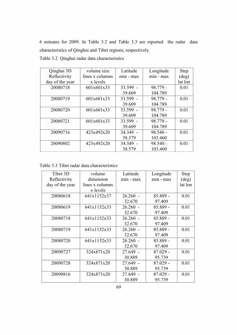
69
6 minutes for 2009. In Table 3.2 and Table 3.3 are reported the radar data
characteristics of Qinghai and Tibet regions, respectively.
Table 3.2 Qinghai radar data characteristics
Table 3.3 Tibet radar data characteristics
Qinghai 3D
Reflectivity
day of the year
volume size
lines x columns
x levels
Latitude
min - max
Longitude
min - max
Step
(deg)
lat lon
20080718 601x601x33 33.599 -
39.609
98.779 -
104.789
0.01
20080719 601x601x33 33.599 -
39.609
98.779 -
104.789
0.01
20080720 601x601x33 33.599 -
39.609
98.779 -
104.789
0.01
20080721 601x601x33 33.599 -
39.609
98.779 -
104.789
0.01
20090716 423x492x20 34.349 -
38.579
98.540 -
103.460
0.01
20090802 423x492x20 34.349 -
38.579
98.540 -
103.460
0.01
Tibet 3D
Reflectivity
day of the year
volume
dimension
lines x columns
x levels
Latitude
min - max
Longitude
min - max
Step
(deg)
lat lon
20080618 641x1152x37 26.260 -
32.670
85.889 -
97.409
0.01
20080619 641x1152x33 26.260 -
32.670
85.889 -
97.409
0.01
20080718 641x1152x33 26.260 -
32.670
85.889 -
97.409
0.01
20080719 641x1152x33 26.260 -
32.670
85.889 -
97.409
0.01
20080720 641x1152x33 26.260 -
32.670
85.889 -
97.409
0.01
20090727 324x871x20 27.649 -
30.889
87.029 -
95.739
0.01
20090728 324x871x20 27.649 -
30.889
87.029 -
95.739
0.01
20090816 324x871x20 27.649 -
30.889
87.029 -
95.739
0.01

70
The size of the grid and the number of vertical levels vary as indicated in the
tables. The data are stored as counts and have to be converted in reflectivity (dBz).
An example of 3D reflectivity data image is shown in figure 3.1, where the level
6 CAPPI for the Tibetan radars is reported for 2009 08 16 at 11:12 UTC.
Figure 3. 1. Screen dump of the visualization of a level of the reflectivity volume.
3.2 Data from Satellites sensors
Satellite sensor data will utilized first to evaluate the sensitivity of different
bands/channels to the precipitation on the ground, and then to develop and/or
apply precipitation retrieval algorithms over the Tibetan Plateau.
3.2.1 MODIS data
The data of MODIS sensor in HDF-EOS format are downloaded from :
http://laadsweb.nascom.nasa.gov

71
The granules dimension are 2030*1354 pixels, extracted by MOD021km-products
and the geolocation data from MOD03-products, with a spatial resolution of 1km.
The considered MODIS channels are shown in the Table 3.4 with their specific
primary use.
Table.3.4 MODIS sensor bands characteristics
3.2.2 AMSR-E data
The data product of AMSR-E/ Aqua L2A , contains brightness temperatures at
6.9GHz, 10.7GHz, 18.7GHz, 23.8GHz, 36.5GHz and 89GHz are downloaded
from :
http://nsidc.org/data/amsre/index.html
Band Wavelength (nm) Primary use
1 620–670 Land/Cloud/Aerosols
Boundaries 2 841–876
6 1628–1652 Land/Cloud/Aerosols
Properties
18 931–941 Atmospheric
Water Vapor 19 915–965
Band Wavelength ( )m Primary use
20 3.660–3.840 Surface/Cloud
Temperature 21 3.929–3.989
31 10.780–11.280 Surface/Cloud
Temperature 32 11.770–12.270

72
All channels have a mean spatial resolution of 56km for L2A (smoothed) of
AMSR-E, with a global coverage between 89.24°N and 89.24°S and granules
dimension are approximately of 2002*243 pixels.
Format data are in HDF-EOS format. The data scale, the offset values and the data
values in the specified units (Kelvin) are correlated by the relation:
Data_value_in_units= (stored_data_value*scale_factor)+ offset (3.1)
The scale_factor is 0.01 and the offset value is 327.68 then BT (K) is defined:
BT (K)= (stored_data_value*0.01)+ 327.68 (3.2)
3.2.3 MVIRI data
The data of MVIRI sensor (on board the Meteosat 7 spacecraft) are downloaded
from the EUMETSAT Earth Observation Portal, in EUMETSAT native format:
(http://www.eumetsat.int/Home/Main/DataProducts/ProductNavigator/index.htm?
l=en)
The full disc data called A-format, is 2500lines*2500column for the 11 m
thermal infrared and 6.7 m water vapor channels, utilized for the interval 2008-
2010, day and night every 30 minutes. Spatial resolution is 5x5 km2 at sub
satellite point (ssp) and approximately 7x10 km2 over the Tibetan Plateau.
The IR pixel value is to be converted into radiance by the relations:
R=(count –IRSPC)*IRCAL (3.3)
R=(IR –S)*c (3.4)
where, IR is the count in the infrared channel, S are the Space_Count, an c is the
Calibration Offset.
After the radiance has been computed, the corresponding temperature is picked up
from the instrument specific radiance-to-temperature look-up tables.

73
3.2.4 Cloudsat-CPR data
Cloudsat-CPR data have been downloaded in HDF format from the Cloudsat Data
Processing Center (http://www.cloudsat.cira.colostate.edu/index.php) for the cold
and dry months (JFMAM-OND) of the years 2008, 2009, 2010, for a total of 807
orbits.
Radar reflectivity vertical profiles and auxiliary data have been downloaded for
the satellite overpasses on the Tibetan Plateau. Auxiliary dataset includes the
height of the vertical profiles radar bins and the air temperature at the ground, as
estimated by the analysis of the European Center for Medium-range Weather
Forecasting (ECMWF).
3.2.5 2A25 TRMM PR
2A25 is a higher level of PR data processing. Data collected by the precipitation
radar (PR) onboard of TRMM satellite are processed from level 1 to 3. 2A25 is
part of the level 2 of product type processed based on level 1 processing. 2A25
processing is to calculate Z factor correcting rain attenuation( eZ ) for each beam
position using radar equation. The vertical product of rain rate (Rr) is produced on
accordance with Z-R relationship ( bR a Z ). The calculation accuracy of rain
rate is the output and each resolution pixel is 4kmx4kmx250m.
The 2A25 data product was downloaded from:
http://pmm.nasa.gov/TRMM/products-and-applications
3.3 Precipitation retrieval algorithms
In this section the retrieval algorithm considered for application over the Tibet
Plateau will be described. A number of these algorithm are adapted from the

74
literature to work on the Plateau, others are originally developed for this work,
and in cases of global products available from open archives (such as C-MORPH
and TMPA) we simply downloaded the data of interest.
3.3.1 Cloudsat CPR Snow rate estimation technique
The main technical characteristics of CPR are: sensitivity defined by a minimum
detectable reflectivity factor of -29 dBZ, cross-track and along-track resolution of
1.3 and 1.7 km, respectively, a dynamic range of 70 dB, 500 m vertical resolution
and calibration accuracy of 1.5 dB.
The CPR sends 94 GHz wave pulses of a width of 3.3 s with a repetition
frequency of 4.3 MHz and measures backscattered power along the beam. The
beam is sampled in 240 m deep bins and the measurement takes place in the lower
30 km of the atmosphere.
In figure 3.2 is shown the density of the CPR observation over the Plateau for the
2008, 2009 and 2010 for the cold season.
Figure 3.2. Number of CPR observations for the considered period.

75
The cold season is defined in this case for the months from January to May
(JFMA) and for the months from October to December (OND). Approximately
the satellite overpasses Tibetan Plateau twice a day.
The algorithm, originally developed for global scale application by Kulie and
Bennartz (2009) works as follows.
A threshold reflectivity value of -15 dBz is assumed to indicate the presence of a
cloud layer. The relationship between the radar equivalent reflectivity factor Ze
[mm6 m
-3] and the amount of snow in the scanned volume is defined by the
following equation (Kulie and Bennartz, 2009):
max
min
4
5 2( ) ( )
| |
D
e b
D
Z D N D dDK
(3.5)
where is the radar wavelength, K the refractive index of the atmospheric targets
(hydrometeors), D is their diameter, (D)b is the frequency-dependent backscatter
cross section for an individual frozen particle shape and size, and N(D) is the size
distribution of the hydrometeors in the scattering volume. The snow rate can be
obtained by an empirical relationship between snow particle size and mass and
fall speed, as follows:
max
min
1( ) ( ) ( )
D
w D
S D m D N D dD
(3.6)
where w is the water density and m(D) = aDb and v(D) = D
express the
relation between the diameter D and particle mass m and velocity v, respectively.
These relations are empirically determined, computing the a, b, coefficients
as best fit from the literature (Kulie and Bennartz, 2009).
The relation between Ze and S can be expressed in exponential form as Ze = aSb ,
where a and b coefficients have to be determined by scattering simulations and
strongly depends on particles shape.

76
In Table 3.5 are reported the values of these coefficients determined by the
particles shape (Kulie and Bennartz, 2009, Hiley et al., 2011).
Table 3.5. Values of the coefficients for the Ze-S relationship for different particles
size.
type a b
3 bullets rosette 13.16 1.4
aggregate 56.43 1.52
average 21.6 1.2
average + 1s 61.2 1.1
average - 1s 7.6 1.3
Over the Tibetan Plateau there are no observation available of particles size and
shapes, thus a sensitivity study for the different a and b values listed in Table 3.5
has been carried out and the results are illustrated in figure 3.3, where the
Probability Density Functions (PDF) for the snow rate over the Plateau are plotted.
The sensitivity is rather high, and the snow rate distributions vary especially for
the highest values, ranging from 1 to 5 mm h-1
.
Figure 3.3 Snow rate PDF for the 2008-2010 cold season over the Plateau for
different choices of a and b coefficients.

77
For the application to the Tibetan Plateau, the ―three bullet rosette‖ coefficients
are used, also compensating the different Diameter-Speed relation due to reduced
air density above 3600 m a.s.l..
The algorithm logical steps can be summarized as follows (Kulie and Bennartz,
2009):
1) ―near surface‖ reflectivity data are used. To avoid, or minimize, ground clutter
contamination, the 6th bin from the surface is considered, i.e. about 1.3 km above
the ground, as determined by the CPR DEM. This is especially needed over
complex orography as in the case of Tibetan Plateau area.
2) Since the inversion scheme is based on the backscattering properties of frozen
hydrometeors, a threshold in the 2 m temperature is applied. The retrieval is
performed only where the 2 m temperature (from the ECMWF data) is lower than
273 K, minimizing the case of wet snow.
3) A threshold in the reflectivity value is then applied in order to consider only
cloudy bins: the chosen value is –15 dBz. At the same time, a ―vertical continuity‖
test is applied to screen out too thin clouds and residual clutter. Only profiles with
at least 5 cloudy bins above the lowest considered are selected for retrieval: only
clouds thicker than 1 km are processed.
4) The ―three bullets rosette‖ reflectivity-snow rate relationship (Ze-S) is then
applied to the lowest cloudy bin and the value assigned to the given profile.
3.3.2 C-NAW Algorithm
The Calibrated Negri-Adler-Wetzel technique is an IR technique based on the
original NAW technique (Negri et. al, 1984), designed to estimate the
instantaneous precipitation rate for convective cloud systems. It has been used in
combination with ground radar precipitation data (Porcù et al, 1999) and with
PMW estimates (Porcù et al., 2000, Kotroni et al., 2005, Casella et al., 2012),

78
where the radar/PMW estimates were used to calibrate the rainrate values to be
assigned to the IR-defined rain areas. The cloud top temperature increases and the
cloud thickness decreases with the distance from the convective center, as well as
the capability to produce precipitation. The observation of Negri et al. (1984)
shown that for about the half cloud area (the warmer one) no precipitation is
registered, while stratified precipitation is expected below the 40% of the cloud
area between the coldest 10% and the warmest 50%.
As a consequence of these findings, the NAW technique was originally set up as
follows:
1) in the calibrated IR (11 m channel) temperature image, the areas colder than
253 K are isolated and labeled as cloud;
2) for each cloud the temperature structure of the cloud top is analyzed and three
areas are identified by means of two thresholds in temperature: coldest 10% (A10),
warmest 50% (A50), remaining 40% (A40). Note that the threshold values in K
vary from cloud to cloud;
3) nominal rainrates are then assigned to each cloud pixel according to its position
in one of the three areas:
RR(A50) = 0.0 mmh-1
RR(A40) = 2.0 mmh-1
RR(A10) = 8.0 mmh-1
This choice was able to maximize the matching with daily cumulated rain
measurement obtained with raingauges during the Florida Area Cumulus
Experiment (Negri et al., 1984).
Further development shown the possibility to provide an on-line calibration of the
technique, by using ground radar (Porcù et al, 1999) or PWM precipitation
estimates (Porcù et al., 2000) to compute the actual rainrate of each cloud detected
by the NAW technique.
To tailor the NAW technique to the Plateau, first we separated the Monsoon
season from the rest of the year. For the summer (June to September) we
considered as reference data for reliable precipitation the QPE products provided
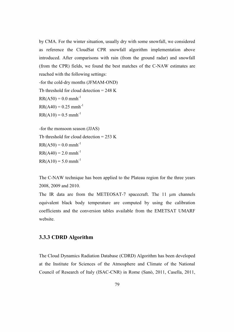
79
by CMA. For the winter situation, usually dry with some snowfall, we considered
as reference the CloudSat CPR snowfall algorithm implementation above
introduced. After comparisons with rain (from the ground radar) and snowfall
(from the CPR) fields, we found the best matches of the C-NAW estimates are
reached with the following settings:
-for the cold-dry months (JFMAM-OND)
Tb threshold for cloud detection = 248 K
RR(A50) = 0.0 mmh-1
RR(A40) = 0.25 mmh-1
RR(A10) = 0.5 mmh-1
-for the monsoon season (JJAS)
Tb threshold for cloud detection = 253 K
RR(A50) = 0.0 mmh-1
RR(A40) = 2.0 mmh-1
RR(A10) = 5.0 mmh-1
The C-NAW technique has been applied to the Plateau region for the three years
2008, 2009 and 2010.
The IR data are from the METEOSAT-7 spacecraft. The 11 m channels
equivalent black body temperature are computed by using the calibration
coefficients and the conversion tables available from the EMETSAT UMARF
website.
3.3.3 CDRD Algorithm
The Cloud Dynamics Radiation Database (CDRD) Algorithm has been developed
at the Institute for Sciences of the Atmosphere and Climate of the National
Council of Research of Italy (ISAC-CNR) in Rome (Sanò, 2011, Casella, 2011,

80
Sanò et al., 2012), and it has been applied to the Tibetan region for the monsoon
seasons 2008, 2009 and 2010.
3.3.3.1 The forward and the inverse problem
The CDRD algorithm is a cloud model-based statistical retrieval technique for
estimating surface precipitation and cloud profiles. The retrieval is based on the
Bayesian estimation theory. A schematic block diagram of CDRD is shown in
figure3.3. The two boxes refer to the two main blocks common to all physically
based retrieval approaches, referred as the ―forward problem‖ and the ―inverse
problem‖. The forward problem consists in the generation of a database (the
Cloud Radiation Database (CRD)), using a Cloud Resolving Model (CRM) and a
Radiative Transfer Model. At the base of the forward problem there is the fact
that precipitation on the ground can not be directly observed from space. It can be
derived from knowledge of cloud microphysical structure along the direction of
sight. Consequently, information relating cloud microphysics to observations
from satellite-borne microwave radiometers needs to be contributed from
external sources. Such microphysical information can be derived from a Cloud
Resolving Model. The model used is the CRM ―University of Wisconsin – Non-
hydrostatic Modeling System‖ (UW-NMS) (Tripoli 1992).
A shortcoming of this approach is that it is currently not possible to run these
models in-line with the flow of satellite data. It is therefore necessary to run the
CRM off-line for a number of well-documented events (generally, results of re-
analysis exercises) and collect the results in a database.
The collection of cloud and precipitation microphysical profiles for a series of
different CRM simulations and of the associated TBs at the instrument (for
instance SSM/I or SSMIS) channel frequencies constitutes the CRD. It is
important to use several cloud model simulations for different types of
precipitation systems, and to generate the corresponding cloud-radiation databases
in order to specialize the algorithm to different storm structures.

81
Figure 3.3. Block diagram of the Bayesian Algorithm for Microwave-Based
Precipitation Retrieval (CDRD).
The inverse problem consists in the retrieval of meteorological parameters, the
hydrometeor columnar content and the surface rain rates, using the experimental
data (the brightness temperatures) of a microwave radiometer, and a probabilistic
analysis (Bayesian) of the CRD.
3.3.3.2 The theoretical Bayesian method
The main resulting expressions of the theoretical Bayesian method utilized in the
―inversion problem‖ will be presented. In the case of CRD database, considering
the vector g related to a cloud profile and the multispectral vector mt related of
radiometer measurements, the optimal estimation of the minimum Mean Square
(MMS) Bayesian method is defined as:
ĝMMS = g p(g|tm) dg (3.7)

82
According to Bayes Theorem the probability density function p(g|tm), can be
expressed as:
p(g|tm) =
)(
)()(
)(
)()|(
mm
m
t
ggε
t
ggt
p
pp
p
pp t (3.8)
where p(tm) is the pdf of tm, p(g) is the apriori pdf of g, εt(g)=[ tm- t(g)] is the Tb
error with t(g) the simulated Tb vector related to g by means of the adopted
radiative transfer model. Assuming that the errors in the observation and the
simulated observations are Gaussian and uncorrelated, the approximate
expression of the i-th element ĝMMS(i) of the hydrometeor profile results as (the
dependence of εt from g is not considered)
)),(g()))(())((5,0exp()(g1
)(ˆ 1
1
jjtjt
T
tj
NP
j
jMMS ihik
ig gεtgtCεtgt mm
(3.9)
where jg is the j-th profile sample of the cloud radiation database with )(ig j the
i-th element, t(gj) is the corresponding Tb, Cεt is the error covariance matrix, and
h(gi,Δgi) is the histogram relative to the sample gi within a variable bin Δg. The
normalizing constant k is given by the expression
)),(g()))g(())g((5,0exp( 1
1
jjtjt
T
tj
NP
j
ihk gεttCεtt mm
(3.10)
The profiles (NP) utilized in the last expressions are selected from CRD database
on the basis of the ―Bayesian distance‖ d2tb(gi) among the measured brightness
temperatures ™ and the simulated t(gj) of the profile gi
D2tb(gi) = ( WtgtCtgt mm )))(())(( 1
it
T
i (3.11)

83
where W is the weight vector of the microwave channels. Profiles with a distance
grater than an a-priori fixed threshold are rejected.
3.3.3.3 The retrieval system
In Figure 3.4 details of the inversion scheme of the inversion are illustrated. The
scheme refers to the general case where, in addition to the use of brightness
temperatures (TB), also the use of dynamical variable (Tag) is considered.
The TBs measured by SSM/I or SSMIS microwave radiometer are firstly
processed (block ―Interpolation Procedure‖) in order to estimate the TB
measurements by all different channels at the same geographical position
(latitude and longitude). This is necessary because the low frequency channels
(19, 22, and 37 GHz) have larger footprints than the higher-frequency channels,
and therefore a lower number of TBs is measured for them during each swath.
Thus, an interpolation procedure is used for the low resolution channels. In
parallel (block ―Interpolation Procedure for Dynamical Variables‖) the values of
tags obtained from NOAA are interpolated to match those of CDRD, in terms of
time and geographical location (latitude, longitude).
Subsequently, all the TBs are analyzed with a ―screening procedure‖ in order to
reject areas (pixels) having incorrect TB values due to sensor errors (quality
control screening), or recognized as areas without rain or with a very low
probability of rain (geographic screening).
The PTC at 85 GHz is preferred in order to optimize the sensitivity to rainfall and
spatial resolution. The TBs of selected pixels, and the corresponding tags, are
then used for the inversion algorithm, using the data (TBs and tags of profiles) of
the CDRD. In the inversion procedure, for each pixel a set of profiles must be
selected from the database, basing on their proximity (in terms of TBs and tags
values) to the observed (pixel) values.

84
This selection of profiles is carried out using the ‖Bayesian distance‖ among the
measured vectors of brightness temperatures and tags, and the corresponding
simulated vectors of the previously selected set of profiles of the CDRD database.
Figure 3.4. Block diagram of the CDRD retrieval algorithm.
The profiles obtained after the selection are used, with their different Bayesian
weights depending on the proximity to the measured data, to compute the
expected value of the retrieved surface rain rate and the associated rain rate
Bayesian variance. For the application over the Tibetan Plateau, the collection of
synthetic cloud and precipitation microphysical profiles obtained by CRM, have
been integrated with three new simulations specifically carried out by UW-NMS
for case studies over the Tibetan Plateau.

85
3.3.4 TANN Algorithm
The Tibetan Plateau Artificial Neural Network technique (TANN) is derived from
a published algorithm (Capacci and Porcù, 2009): this technique has been
developed using data from for mid latitude and trained with radar and raingauges
data for different applications.
For this Project two TANN version have been implemented, with different
reference precipitation fields in the training supervised datasets for the monsoon
season. The first version, TANN-R, has been calibrated by using ground radar
network QPE data, while the second one (TANN-S) makes use of the CDRD
derived rainrate fields. For colder months the same training dataset have been
used, based on CPR snow rate retrieval.
3.3.4.1 Physical basis
The type of neural network used here is the ‗Multilayer Perceptron‘ or MLP
(Rosenblatt 1962), which consists of input nodes, hidden nodes and output nodes,
the nodes being called ‗perceptrons‘. The ANN configuration used is the single
hidden layer version employing a sigmoidal transfer function at the nodes, as
described by Pankiewicz et al. (2001). The input nodes are the numerical values
of the selected features (i. e. satellite brightness temperatures and features): the
appropriate set of features and therefore the number of input nodes has to be
established. The number of outputs depends on the number of classes and ANN
theory shows that each output is just the posterior class probability. Since the sum
of the posterior probabilities of all the classes is 1 it is possible to reduce the
number of outputs to the number of classes less 1. In the rain/no rain case,
therefore, only one output is required and with the value 1 corresponding to the
class ‗rain‘ (more strictly, precipitation) the output is the posterior probability of
the class precipitation or simply the Probability of Precipitation (PoP), to which a

86
threshold may be applied to delineate regions of precipitation. The output of each
node in one layer is connected to the inputs of all the nodes in the next layer. The
strengths of the connections are represented by continuously variable, signed
multipliers known as ‗weights‘. The process of training the ANN consists of
adjusting the values of these weights. To build the ANN there are two phases: the
training phase and the testing phase. For these phases there are two independent
data sets: the training data set and the testing data set. In the training phase the
correct output has to be known a priori. Considering a series of labeled samples (0
= no rain, 1 = rain) the ANN generates an output value from each set of feature-
values presented at its inputs. After each such presentation its internal weights are
adjusted, until the ANN‘s behavior is stable and its output matches the true values
to an acceptable accuracy. The ANN thus ‗learns‘ to recognize the correct output
from the input feature-values. The weights are adjusted using the well-known
backpropagation method using gradient-descent applied to a sum-of-squares error
function (see, for example, Bishop 1995: Chapter 4). In the testing phase, the
weights remain fixed at the values established in the training phase and the ANN
computes output values for a series of samples from an independent data set.
From the ANN output, values less than or equal to 0.5 are considered to
correspond to no rain, and those more than 0.5 to rain, in the original set up of the
technique.
Taking the independent rainrate measurements (such as radar, raingaugesas or
other satellite products) of precipitation ‗true‘ indications of rain or no rain we can
calculate statistical measures of ANN performance (Capacci and Conway, 2005).
The main parameter used here is the Equitable Threat Score (ETS), but also
Probability of Detection (POD) and False Alarm Rate (FAR) are used for
diagnostic: all these parameters are defined below (Nurmi, 2003):
Probability of detection: POD H
H M
(3.12)
False-alarm ratio: FARF
H F
(3.13)

87
Equitable threat score: ETSH G
H M F G
(3.14)
where ( )( )
G( )
H M H F
H M F Z
(3.15)
H (hits) = number of grid boxes correctly classified as rain,
M (misses) = number of grids boxes incorrectly classified as no rain,F (false alarm)
= number of grids boxes incorrectly classified as rain, and
Z (correct no rain) = number of grids boxes correctly classified as no rain.
3.3.4.2 Implementation over the Tibetan Plateau
The original algorithm has been modified in order to work on the Tibetan Plateau
area. First, three appropriated supervised dataset are created for the training phase
of the network. A monsoon season training set used as ―truth‖ data the
observations of the ground radars operated by CMA (for the TANN-R algorithm).
Also for the summer months training set used as ‗truth‘ rain-rate data estimated
by the CDRD algorithm, described in previous section (for the TANN-S
algorithm). For the winter months, when rare and solid precipitation occurs, the
training set was formed by using the CPR derived snowrate estimate, for both
algorithms.
A second relevant modification was about the inputs: the original technique works
on 9 channels of the SEVIRI on board Meteosat Second Generation, while for this
project the three-channels MVIRI sensor on board METEOSAT-7 is used. Only
two channels were continuously available night and day over the Plateau: WV and
IR. The contribution of the WV channel is expected in removing cold soil
contamination, since the WV weighting function is peaked in the upper
troposphere and the WV radiation does not carry surface contribution. Earlier
studies (Hsu et al., 1997, among others) shown that textural cloud top features can
be also weakly related to the cloud structure and, therefore, to precipitation at the
ground. Following this approach, two others input were added for each channel:

88
the local standard deviation and the average of the temperature in the IR and WV
channels as computed over a 3x3 pixel.
Finally, the original technique provides as output and index varying between 0
and 1, that indicates the probability of precipitation. We fitted an empirical
function that related the ANN output to the rainrate obtained by reference
measurements (i.e. ground radar and CDRD algorithm for the summer and CPR
for the winter), to convert the output in rainrate.
a)
b)
Figure 3.8. TANN-R (a) and radar (b) 3-hours averaged rainrate maps for the
24/08/2009 at 18:00 UTC

89
The TANN-R estimate is shown in figure 3.8 for the 24 August 2009 at 18:00
UTC in comparison of radar rain map at the same time, averaged over 3 hours.
It can be remarked that the calibration area (i.e. the area covered by the radar
network) it is very small with respect to the region of interest, and also the
calibration is carried on the same area, and thus the technique should not be able
to resolve high rainrates events, such as the ones typically occurring on the eastern
part of the Plateau (Ueno, 1998). The calibration carried on with CDRD satellite
derived products is expected to overcome these problems, even if the quality of
the satellite estimates is probably power than the one of radar QPE.
3.3.5 GCD technique
The original GCD (Global Convective Diagnostic) technique was developed
(Mosher 2001, Martin et al., 2008) to delineate deep-convection areas from GEO
observation. Further developments aim to assign precipitation rates to the deep-
convection areas, after calibration with a reliable reference rainrate measurement.
Precipitation based MW retrievals in conjunction with the GCD technique is a
new method to provide precipitation estimates from heavy convective storm at the
GEO time and space resolution (Casella et al., 2012), after a calibration with
satellite derived rainrate estimates.
The technique works as follows. For each GEO IR pixel the brightness
temperature difference BT between WV and IR channels, is interpreted as deep
convection signal when is higher that a given threshold (-1 K).
A strong correlation between BT and RR can be found in the limitation of a
single cloud and to a given time. A local empirical relation between two quantities
can be obtained by calibrate BT in term of corresponding RR values, obtained
from another reliable source.

90
In order to generate this relationship for each cloud and each corresponding
observations, the ( BT , RR) values that refer to all cloud pixels into 0.5K -
intervals centered at 0K, 0.5K, 1K, 1.5K are grouped, and so on, within
such intervals, the averaged RR values. These sets of ( BT , RR) values can be
fitted by exponential functions:
RR= BTe (3.16)
Where the best fit of and coefficient values, can vary considerably with
season, latitude, time of the day and cloud type.
Then the GCD formula applies to all pixels for all GEO images associating rain
rates values, for the selected cloud, until a new MW observation is available. An
incorporated simple cloud tracking algorithm, makes possible to follow the
evolution of the various precipitating clouds from a GEO observation to the next.
The GCD applied over the Tibetan Plateau uses radar derived QPE data to infer
robust and flexible a and b values to be used in (3.16) to retrieve rainrate. The
tests we carried on was really unsatisfactory, because the database we used for
calibration did not allow to extend the relationship toward high rainrates. As an
example, in Figure 3.9 is reported the TB-RR relationship we found for Tibet
cases (left) and the one assessed by Casella et al. (2012) for Mediterranean area
(right).
There are marked differences between the two datasets: over the Tibetan Plateau
the dynamics of TB is much higher, spanning between -15 K to 10 K, but the
rainrates are lower, while in the Mediterranean rainrates as high as 18 mm h-1 are
related with comparably lower TB, around 3-4 K.

91
a) b)
Figure 3.9 Relationship of rainrate and brightness temperature differences:
experimental data (black dots) and exponential fit (solid line). Plots refer to Tibet
dataset (a) and Mediterranean dataset (b), as found in Casella et al (2012).
For these basic reasons we decided to not use GCD output in the precipitation
analysis over the Plateau, considering also that, the ANN we introduced above is
certainly able to manage linear combinations of input channels.
3.4 Available global precipitation products
Global satellite precipitation products are freely available on the web, released by
scientific institutions and weather services, mainly for climatological purposes,
but also can be used for satellite reference during the implementation of new
algorithms, especially over ocean or region not covered by conventional
instruments.
Two the different approaches make use of satellite data in the MW spectrum,
usually to ensure a reliable quantitative rainrate estimates, while GEO IR is used
to increase the temporal sampling of the estimate.

92
3.4.1 3B42-TRMM product
The TRMM Multisatellite Precipitation Analysis (TMPA) provides a calibration-
based sequential scheme for combining precipitation estimates from multiple
satellites, as well as gauge analyses where feasible, at fine scales (Huffmann et al.,
2007). TMPA is available both after and in real time, based on calibration by the
TRMM Combined Instrument (TCI) and TRMM Microwave Imager (TMI)
precipitation products, respectively. Only the after-real-time product incorporates
gauge data at the present. The dataset covers the latitude band 50°N–S for the
period from 1998 to the delayed present on a grid 0.25x0.25 degrees.
Validation results show reasonable TMPA performance at monthly scales,
although it is shown to have precipitation rate–dependent low bias due to lack of
sensitivity to low precipitation rates over ocean. At finer scales the TMPA is
successful at approximately reproducing the surface observation–based histogram
of precipitation, as well as reasonably detecting large daily events. The TMPA,
however, has lower skill in correctly specifying moderate and light event amounts
on short time intervals, in common with other fine scale estimators.
The purpose of Algorithm 3B-42 is to produce Tropical Rainfall Measuring
Mission merged high quality (HQ)/infrared (IR) precipitation and root-mean-
square (RMS) precipitation-error estimates.
The 3B-42 estimates are produced in four stages; (1) the microwave estimates
precipitation are calibrated and combined, (2) infrared precipitation estimates are
created using the calibrated microwave precipitation, (3) the microwave and IR
estimates are combined, and (4) rescaling to monthly data is applied. Each
precipitation field is best interpreted as the precipitation rate effective at the
nominal observation time.

93
3.4.1.1 High Quality (HQ) microwave estimates
All of the available passive microwave data are converted to precipitation
estimates prior to use, then each data set is averaged to the 0.25° spatial grid over
the time range ±90 minutes from the nominal observation time. All of these
estimates are adjusted to a "best" estimate using probability matching of
precipitation rate histograms assembled from coincident data. The algorithm takes
the TCI as the calibrating data source. However, the coincidence of TCI with any
of the sensors other than TMI is highly sparse, so we establish a TCI—TMI
calibration, then apply that to TMI calibrations of the other sensors to estimate the
TCI-calibrated values. After extensive preliminary testing, the ocean calibration is
performed in regions of significant precipitation and applied everywhere. In all
cases the calibration is a simple match-up of histograms.
The calibration interval is chosen to be a month to ensure stability and
representativeness, except the TMI—AMSR-E calibration is computed with 2
months for stability.
Once the estimates are calibrated for each satellite the grid is populated by the
"best" data from all available overpasses, although the most likely number of
overpasses in the 3-hr window for a given grid box is either one or zero. When
there are multiple overpasses, data from TCI, TCI-adjusted TMI, TCI-adjusted
AMSR-E, and TCI-adjusted SSM/I are averaged together, and TCI-adjusted
AMSU-B estimates are used if none of the others are available for the grid box.
Tests show that the histogram of precipitation rate is somewhat sensitive to the
number of overpasses averaged together when that number is small. Accordingly,
in the future we expect to test a scheme taking the single "best" overpass in the 3-
hr period.

94
3.4.1.2 Variable Rain Rate (VAR) IR estimates
The 3B-42 algorithm, for the period from 7 February 2000 onwards, the CPC
merged IR is averaged to 0.25° resolution and combined into hourly files as ±30
minutes from the nominal time. The amount of imagery delivered to CPC varies
by satellite operator, but international agreements mandate that full coverage is
provided for the 3-hourly synoptic times from 00Z. Histograms of time-space
matched HQ precipitation rates and IR TBs, each represented on the same 3-
hourly 0.25° grid, are accumulated for a month, and then used to create spatially
varying calibration coefficients that convert IR TBs to precipitation rates. As in
the HQ, the calibration interval for the IR is a calendar month, and the resulting
adjustments are applied to data for the same calendar month. This choice is
intended to keep the dependent and independent data sets for the calibrations as
close as possible in time. In fact, the full month of data in the estimates includes
the dependent data. A second ambiguous screening is performed on the matched
microwave data after accumulation; compared to instantaneous screening, the
monthly screening provides better control of artifacts.
By design, there is no precipitation when the 0.25°x0.25°-average TB is greater
than the local threshold value that matches the frequency of precipitation in the IR
to that of the microwave. Increasingly colder TBs are assigned increasingly large
precipitation rates using histogram matching. Those grid boxes that lack
coincident data throughout the month, usually due to cold-land dropouts or
ambiguous editing, are given calibration coefficients by smooth-filling histograms
of coincident data from surrounding grid boxes. Once computed, the HQ-IR
calibration coefficients are applied to each 3-hourly IR data set during the month.
3.4.1.3 Combined HQ and VAR estimates
The ultimate goal of this algorithm is to provide the "best" estimate of
precipitation in each grid box at each observation time. It is frequently quite

95
challenging to combine different estimates of an intermittent field such as
precipitation. The process of combining passive microwave estimates is relatively
well-behaved because the sensors are quite similar and the Goddard Profiling
algorithm (GPROF) is used for most retrievals. This is not the case for the HQ and
VAR fields.
A simple approach for combining the HQ and VAR estimates is considered,
namely the physically-based HQ estimates are taken "as is" where available, and
the remaining grid boxes are filled with VAR estimates. This scheme provides the
"best" local estimate, at the expense of a time series that is built from data sets
displaying heterogeneous statistics.
3.4.1.4 Rescaling to monthly data
The final step in generating 3B-42 is the indirect use of rain gauge data. It is
highly advantageous to include rain gauge data in combination data sets. However,
experience shows that on any time scale shorter than a month the gauge data are
not reported with sufficient density nor reported with consistent observational
intervals to warrant direct inclusion in a global algorithm that provides sub-
monthly resolution. The authors solved this issue in the GPCP One-Degree Daily
combination data set by scaling the short-period estimates to sum to a monthly
estimate that includes monthly gauge data. Here, we take a similar approach with
the 3B-42 estimates. All available 3-hourly HQ+VAR estimates are summed over
a calendar month to create a monthly multi-satellite (MS) product. The MS and
gauge are combined to create a post-real-time monthly satellite-gauge
combination (SG), which is a TRMM product in its own right (3B43). Then the
field of SG/MS ratios is computed (with controls) and applied to scale each 3-
hourly field in the month.
The monthly multisatellite (Ms) product are combined with gauge to create a
post real monthly satellite-gauge combination (SG), which is 3B43 TRMM
product.

96
3.4.2 CMORPH technique
CMORPH (CPC MORPHed precipitation) is a high resolution, real-time global
precipitation estimates technique, developed at NOAA‘s Climate Prediction
Center (CPC). CMORPH method uses precipitation estimates derived from low
orbiter satellite microwave sensors, and whose patterns characteristic are
transported via spatial propagation information that is obtained entirely form
geostationary IR sensors (Joyce et al., 2004).
Half hourly IR from GEO satellites data are used as a means to transport the
microwave-derived precipitation features during the intervals between subsequent
PMW observations. Propagation vector-matrices are produced by computing
spatial lag correlations on successive IR images of geostationary satellite, which is
used to propagate the microwave derived precipitation estimates. The shape and
the intensity of the precipitation features are modified (morphed) during the time
between microwave sensor scans by performing a time-weighted linear
interpolation. The method is flexible that permit precipitation morphing from any
satellite source (AMSU, TMI, AMSR-E, SSM/I).
CMORPH shows substantial improvements over both averaging of the microwave
estimates and over techniques that blend microwave and infrared information but
that derive estimates of precipitation from infrared data when passive microwave
data is unavailable.
The CMORP products is downloadable from the NOAA-CPC ftp-site:
ftp.cpc.ncep.noaa.gov. Archived 3-hourly cumulated precipitation on a grid of
0.250.25 degrees are available from tear 2003 onwards, while last week
instantaneous rainrates can be obtained at 8x8 km resolution every 30 minutes.
Precipitation maps extend from 60S to 60N in latitude, given the extension of
GEO satellites observation domain.

97
Chapter 4
Satellite precipitation estimates over the Tibetan
Plateau: preliminary studies, applications and
intercomparison
In this chapter firstly will be described the remapping phase of all dataset obtained
from ground, satellite and algorithms retrieval. Secondly, will be presented a
study on the sensitivity of sensors channels to the presence of precipitation at the
ground, as measured by raingauges data as ―truth‖ values. Then will be shown the
result of all algorithms retrieval for the precipitation estimation over the Tibetan
Plateau and, finally, will be described the validation of the algorithm results and
intercomparison among the different algorithms.
4.1. Data remapping process
All the data processed in this work are received mapped on their own grid,
determined by the Institution in charge of data pre-processing (CMA in case of
raingauge and radar data), or by the data acquisition characteristics (e.g. geometry,
resolution, type of the orbit) in case of satellite data. In order to design
intercomparison studies and multisensor procedures, remapping procedures have
been defined to reduce different data to the same grid. Three reference grids are
defined onto which remap the data for different applications: the rain gauge grid,
the radars grid and MVIRI grid. In figure 4.1 the considered grid are plotted: grid
labelled as 1 is the raingauge grid, number 2 and 3 are the Tibetan and Qinghai
radar grids, respectively, and number 4 is the MVIRI grid. Each satellite pixel in

98
its native grid is positioned accordingly with longitude and latitude values
provided by the satellite navigation references.
Figure 4.1. Plot of the reference grids used in this study: 1 raingauge; 2 Tibetan
radar network; Qinghai radar network; 4 Meteosat MVIRI grid.
In the remapping process we calculate the pixel position with respect to the
reference grid by using the Nearest Neighbour approach, which consist to
associate at a given cell of the reference grid the satellite pixel closest to it, if it
exists. Then the relative size of the satellite pixel with respect to the reference grid
cell size is considered: if the reference grid cell is large enough to include more
than one satellite pixel, the associated values will to be the averaged values of all
satellite pixels contained in the grid cell.
In the table 4.1 is shown the remapping process for all data provided by the
instrument and algorithm described in Chapter 3 and the grid referee. The pixel
size of MVIRI (Meteosat 7) varies from the reference 55 km2 at the sub satellite
point (at coordinates 57E, 0N) due to the Earth curvature. On the Tibetan Plateau
the pixel size varies approximately from 5.55.5 km2, for the lowest latitude and
longitude, to around 1411 km2
for the highest (see figure 4.1). In figure 4.2 is
shown the distribution of MVIRI pixels area in the selected grid.

99
Table 4.1 Remapping data into the reference grid
Figure 4.2. Distribution of MVIRI pixel area in the grid sketched in figure 4.1.
REFERENCE
GRID
Size
Instruments data and algorithms retrieval data
G
A
U
G
E
R
A
D
A
R
M
O
D
I
S
A
M
S
R
E
P
R T
R
M
M
M
V
I
R
I
S
S
M
I
S
C
P
R
T
A
N
N
C
M
O
R
P
H
3
B
4
2
GAUGES
0.050.05
RADAR
0.010.01
MVIRI
79 km2
Legend
- coincident grids
- Nearest Neighbour only
- Nearest-Neighbour and pixel averaging

100
4.2 Sensitivity analysis for rain/no-rain discrimination
In this section will be investigated the sensitivity of the radiances at the
wavelengths available for this study to the rain/no-rain discrimination. As true
rainfall rate we used the raingauges measurements for selected case studies during
the 2008 and 2009 monsoon seasons. For each channel of the considered sensors
the measured radiance map is matched with the precipitation map obtained from
the raingauges network. Two curves are then computed as function of the radiance
value: one collects the number of satellite IFOV where gauges measured
precipitation rates higher than 0.2 mm h-1
(rain curve), the other collects the
number of IFOV without precipitation (no-rain curve). A wavelength is assumed
to be sensitive to precipitation as far as the two curves are well separated in the
plots, with moderate overlapping. On the contrary, the channel sensitivity is low if
the two curves are mostly overlapped.
In the following we will be describe the sensitivity analysis of rain and no-rain
discrimination of selected MODIS channels, all AMSR-E channels and the
TRMM-PR 14 GHz sensor.
4.2.1 Sensitivity of MODIS channels
The channels sensitivity of the precipitation is determined by the normalized
distribution of the radiance or reflectance of MODIS channels, for classes rain/no-
rain of the hourly raingauges ―truth‖ data. To make easier the comparison
between the different channels, also the radiance values are normalized.
In Figure 4.3 (a) and (b) are shown the normalized reflectance distributions for
precipitation classes rain/no-rain, of ch01 and ch02 (VIS wavelengths) which are
primarily used for Land/Cloud/Aerosol discrimination, and in Figure 4.3 (c) the
same for the channel ch06, in the short wave infrared at 1.6 m, used for cloud
particle size and phase estimate and for the detection of snow at the ground.

101
(a) (b)
(c)
Figure 4.3 Normalized reflectance distributions for precipitation classes rain and
non-rain. Channel considered: Ch01 (a), Ch02 (b) and Ch06 (c).
Results show very limited skill in rain detection of ch06, while ch01 is the most
effective in separating rain and no-rain pixel given the contrast between dark
background (in summer) and thick highly reflecting clouds. This behaviour is
quite similar to what is known in the literature of other parts of the word (Capacci
and Conway, 2005).
In Figure 4.4 (a) and (b) are shown the normalized radiance distribution for
precipitation classes rain/no-rain, of the Ch18 and Ch19 sensitive to WV
atmospheric content, showing good separation between curves.
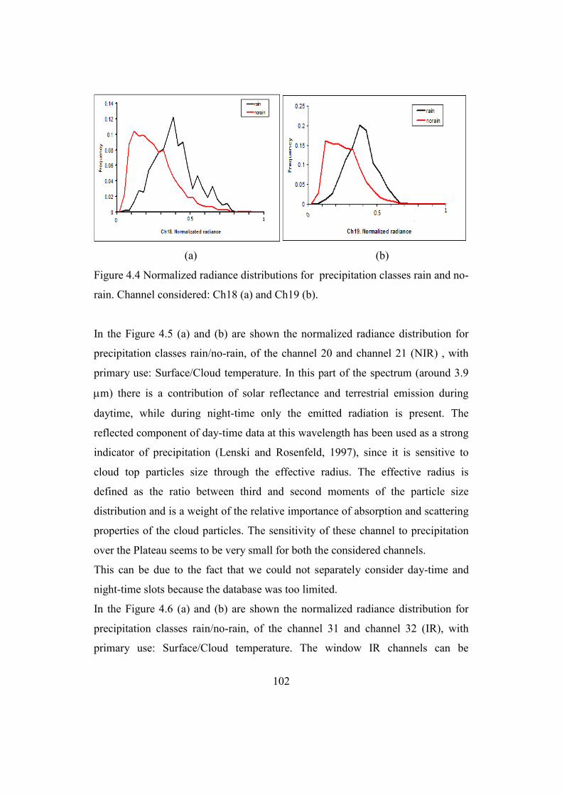
102
(a) (b)
Figure 4.4 Normalized radiance distributions for precipitation classes rain and no-
rain. Channel considered: Ch18 (a) and Ch19 (b).
In the Figure 4.5 (a) and (b) are shown the normalized radiance distribution for
precipitation classes rain/no-rain, of the channel 20 and channel 21 (NIR) , with
primary use: Surface/Cloud temperature. In this part of the spectrum (around 3.9
m) there is a contribution of solar reflectance and terrestrial emission during
daytime, while during night-time only the emitted radiation is present. The
reflected component of day-time data at this wavelength has been used as a strong
indicator of precipitation (Lenski and Rosenfeld, 1997), since it is sensitive to
cloud top particles size through the effective radius. The effective radius is
defined as the ratio between third and second moments of the particle size
distribution and is a weight of the relative importance of absorption and scattering
properties of the cloud particles. The sensitivity of these channel to precipitation
over the Plateau seems to be very small for both the considered channels.
This can be due to the fact that we could not separately consider day-time and
night-time slots because the database was too limited.
In the Figure 4.6 (a) and (b) are shown the normalized radiance distribution for
precipitation classes rain/no-rain, of the channel 31 and channel 32 (IR), with
primary use: Surface/Cloud temperature. The window IR channels can be
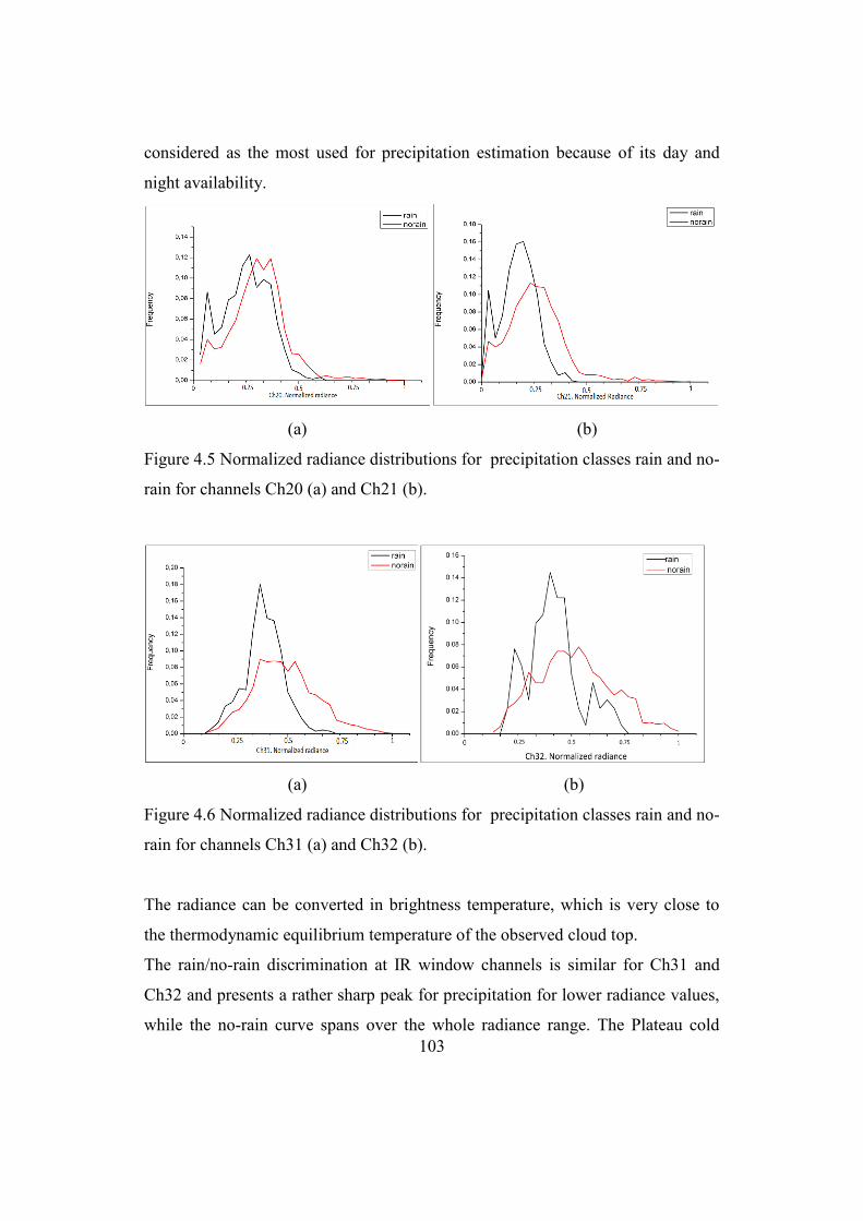
103
considered as the most used for precipitation estimation because of its day and
night availability.
(a) (b)
Figure 4.5 Normalized radiance distributions for precipitation classes rain and no-
rain for channels Ch20 (a) and Ch21 (b).
(a) (b)
Figure 4.6 Normalized radiance distributions for precipitation classes rain and no-
rain for channels Ch31 (a) and Ch32 (b).
The radiance can be converted in brightness temperature, which is very close to
the thermodynamic equilibrium temperature of the observed cloud top.
The rain/no-rain discrimination at IR window channels is similar for Ch31 and
Ch32 and presents a rather sharp peak for precipitation for lower radiance values,
while the no-rain curve spans over the whole radiance range. The Plateau cold

104
background during the night, also in summer, and the presence of relatively low
top precipitating clouds (Shimitzu et al., 2001) contribute to make the contrast
between precipitating cloud top and background less sharp with respect to other
parts of the Earth.
The near-infrared total-column precipitable water is very sensitive to boundary-
layer WV since it is derived from attenuation of reflected solar light from the
surface. Techniques employing ratios of WV-absorbing channels 17, 18, and 19
with the atmospheric window channels 2 and 5 are used. The column WV
amounts are derived from the transmittances based on theoretical radiative-
transfer calculations and using look-up-table procedures. Other, split-window,
methods also exist. This class of techniques uses the difference in WV absorption
that exists between channel 31 (10.78-11.28) µm and channel 32 (11.7-12.27) µm.
In this case of study the channel 31 and 32 is not sensitive for the rain/no-rain
discrimination.
4.2.2 Sensitivity of AMSR-E channels
To test the sensitivity to precipitation of the PMW channels we considered the
AMSR-E data because it has very similar frequencies as other widely used sensors,
such as TMI and SSM/I. As for the MODIS channels, the TB values are matched
with raingauges rainrates maps for the available case studies, and rain/no-rain
curves are plotted. In the Figure 4.7 are shown normalized brightness
temperatures distribution of 6.9 GHz, 10.7 GHz and 18.7 GHz horizontally and
vertically polarized channels.
The radiation measured at the lowest frequencies in the PMW spectrum mainly
carries information on the large water drops in the cloud rain layers: the relatively
long wavelength (between 4 and 1.6 cm) makes the interaction with small cloud
droplets and crystals negligible, so the radiation emitted by cloud drops (water is a
good emitter in the MW) can reach the satellite with little extinction (Ferraro et al.,
105
1998). The signal from precipitation layers, however, is often masked by the
strong signal coming from the surface (especially land). The emissivity of the
ground in PMW is usually highly polarized and rapidly varying in space and time,
due to the dependence of the soil emissivity on its condition: vegetation and its
conditions, moisture content, and snow cover modify the amount of radiation
reaching the sensor.
Thus it is often difficult to screen out the ground contribution from the total
measured radiation to isolate the rain signal and number of different approaches
have been pursued in the literature (Levizzani et al., 2007).
From the figures, it seems that the only channel with a marked separation between
rain and no-rain curves is the vertically polarized 6.9 GHz, which shows the rain
slightly colder than the no-rain peak. For other channels the sensitivity to
precipitation is very low.
Increasing the frequency, thus decreasing the wavelength, the interaction of the
radiation with smaller cloud particles and crystals becomes more effective, due to
scattering, and the radiation reaching the satellite carries information on the cloud
upper layer.
The signal at 89.9 GHz (corresponding to = 3.3 mm), as an example, is a
measure of the scattering due to ice particles on the upper cloud layers. Also at
these frequencies it is expected a strong surface signal, able to mask the
atmospheric contribution.

106
(a) (b)
(c) (d)
(e) (f)
Figure 4.7 Normalized distribution of TB6.9H (a) TB6.9V GHz (b), TB10.7H
GHz (c) TB10.7V GHz (d), TB18.7H GHz (e), and 18.7V GHz (f) in
correspondence to wet and dry raingauges.
In figure 4.8 are shown normalized brightness temperatures distribution at 23.8
GHz, 36.5 GHz and 89.0 GHz at horizontal and vertical polarization.

107
(a) (b)
(c) (d)
(e) (f)
Figure 4.8 Normalized distribution of TB23.8H GHz (a), TB23.8V GHz (b),
TB36.5H GHz (c), TB36.5V GHz (d), and TB89.0H GHz (e), and TB89.0V GHz
(f) in correspondence to wet and dry raingauges.
Also at these wavelengths the separation between rain and no-rain curves is often
negligible: the rain curve peak is always colder than the no-rain peak, but with
only few degrees of difference. The TB89.0 distribution at both polarizations,

108
however, shows a smaller, secondary peak rather colder for the rain curve,
probably related to heavy precipitation cloud with thick ice layer at the top.
The channels considered in this study are in window regions of the MW spectrum,
i. e. the radiation interacts very weakly with atmospheric gases. A valuable
approach to retrieve precipitation from absorption channels has been pursued
(Cheng and Staelin, 2003, Laviola and Levizzani, 2010). These techniques
retrieve precipitation as signal in the water vapour or oxygen emitted radiation.
The main advantage is that the contribution of the soil usually does not reach the
satellite, being absorbed by gas layers in the atmosphere. On the Tibetan Plateau,
however, the atmosphere is thinner (and generally dryer) than in other part of the
Earth, and the integral gas content is lower, so that also the signal in absorption
bands can be contaminated by surface contribution. For these reasons, we did not
consider the sensitivity to MW absorption channels. Moreover, for the PMW
retrieval of the Tibetan Plateau, we considered the output of the CDRD algorithm,
that fully exploit the physical contents of the MW channels.
4.2.3 Sensitivity of TRMM PR
The TRMM-PR sensitivity of the precipitation is determined in the same way as
dome for passive sensors, and results are shown in figure 4.9 for the 2008 and
2009 case studies. We considered the 2A25 TRMM-PR precipitation product
(Iguchi et al., 2000), and rain and no-rain curves are plotted as function of the
estimated rainrate.
The plots reported show very limited sensitivity, since rain and no-rain curves are
mostly overlapped, indicating the inability of TRMM-PR to correctly assign
precipitation, when it is well known in literature that TRMM-PR usually provides
the best rainrate estimate available from space borne sensors. Two reasons can
explain this behaviour: 1) the database is very limited and, given the narrow
TRMM-PR swath, the plots are constructed with very few points, 2) the rainfall
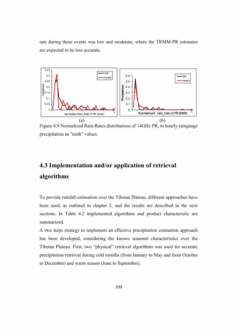
109
rate during these events was low and moderate, where the TRMM-PR estimates
are expected to be less accurate.
(a) (b)
Figure 4.9 Normalized Rain-Rates distributions of 14GHz PR, to hourly raingauge
precipitation as ―truth‖ values.
4.3 Implementation and/or application of retrieval
algorithms
To provide rainfall estimation over the Tibetan Plateau, different approaches have
been used, as outlined in chapter 2, and the results are described in the next
sections. In Table 4.2 implemented algorithms and product characteristic are
summarized.
A two steps strategy to implement an effective precipitation estimation approach
has been developed, considering the known seasonal characteristics over the
Tibetan Plateau. First, two ―physical‖ retrieval algorithms was used for accurate
precipitation retrieval during cold months (from January to May and from October
to December) and warm season (June to September).

110
Table 4.2 Algorithms implemented over the Tibetan Plateau.
In cold months it is expected mainly snowfall and light precipitation, thus an
algorithm based on Cloudsat-CPR data has been implemented, while during
monsoon season, when convective activity is expected to dominate, a PMW
algorithm has been used.
In the second stage, the outputs of the two algorithms have been used to
seasonally calibrate IR based retrieval techniques, based on statistical approach.
Algorithm Sensor Frequency/
wavelength
Time
resolution
Ground
resolution
KB CPR/CloudSat
Radar 94
GHz
twice a day
over HB 1.31.7 km
2
CDRD SSMI/S 19 to 190
GHz 6 hours 1515 km
2
TANN-R
TANN-S
MVIRI
6.7 m +
11 m
30 min
67 km
2
3B42
MVIRI +
TMI +
AMSR-E +
AMSU-B
11 m
6 to 190
GHz
3 hours 0.250.25
deg
C-MORPH
MVIRI +
TMI +
SSMIS +
AMSU-B
11 m
+
6 to 190
GHz
3 hours 0.250.25
deg
C-NAW MVIRI 11 m 30 min 67 km2
111
4.3.1 Implementation of the “seasonal” algorithms
In the next sections will be shown some results of the two satellite algorithms
used to calibrate statistical rainrate retrieval algorithms.
4.3.1.1 Snowrate retrieval from Clousat-CPR data (Kulie and Bennartz,
2009)
About 800 CloudSat overpasses have been processed to retrieve snow rate: given
the narrow (1.7 km) CPR swath, it is not possible to separately analyze the results
of each overpass, and only averaged products will be shown. In figure 4.10 maps
at the resolution of 50x50 km2 are shown for frequency of snowfall and mean
snow rate during the whole set of CPR retrievals.
The maximum snowfall frequency (around 50%) is registered in the Karakorum
region on the western part of the domain, where also the highest average snow
rate is estimated. The southern part of the Plateau seems to be dry even during the
winter, while relatively high frequency is also measured on the northern part and
high snow rate is found in south-eastern Plateau.
In figure 4.11 are reported three curves. The black one represents the number of
5050 km2 pixel of the domain as function of the percentage of overpasses with
snowfall with respect to the total satellite overpasses. The green line shows the
number of pixel as function of the percentage of cloud covered overpasses, while
the red line represents the number of pixels as function of the percentage of
snowfall observations with respect to cloudy observations.

112
a)
b)
Figure 4.10 Frequency of snowfall occurrence (a) and averaged mean snowfall
rate (b) for the years 2008, 2009 and 2010 (805 overpasses)
In most of the areas visited by CPR the frequency of snow occurrence is below
15% (90% of the areas has less than 15% of occurrence), with very few spots
between 40% and 50%. The sky is covered between 10% and 40% of the times,
while the fraction of producing snow clouds could also very high (above 50% for
the 15% of the pixels), but the distribution does not presents marked peaks.

113
Figure 4.11 Number of 5050 km2 pixel as function of cloud fraction (green line),
snow fraction (black line) and cloud fraction with snow (red line) for the
considered periods.
4.3.1.2 Output of the CDRD technique over the Tibetan Plateau
The CDRD rainfall maps have been provided by the ISAC-CNR in Rome, where
the algorithm is developing (Sanò et al, 2012). Four months of SSMI/S overpasses
for the years were processed: SSMI/S sensor is currently on board the DMSP
satellites F-16, F-17 and F-18, the latter launched in 2010 March. Given the
different number of available satellites, the number of overpasses varies across the
years: 1312 in 2008, 1314 in 2009 and 1939 in 2010.
As an example, in figure 4.12 the CDRD rainrate map for a case study in 2009 is
presented at its original resolution.

114
Figure 4.12 CDRD estimated precipitation map for 02/08/2009 at 11:35 UTC,
colorscale in mm h-1
.
a) b)
c) d)
Figure 4.13 SSMI/S TB91H (a), TB91V (b), TB150 (c), TB1837 (d) for the
02/08/2010 at 11:15UTC. Colorscale in K.

115
In Figure 4.13 are reported the SSMI/S TB maps more correlated to the estimated
precipitation field.
The channels at 91 and 150 GHz are in window with high atmospheric
transmittance, and also include strong contribution from the cloud-free surface.
The 183.37 GHz channels is on the strong WV absorption band, but its
weighting function is peaked in mid troposphere so a small surface contribution is
expected, given the relatively dry atmosphere and the altitude of the ground.
The rainrate PDF of the CDRD estimates in 2010 (when 3 satellites are
operational) is reported in Figure 4.14 for the larger MVIRI grid domain (see
Figure 4.1, grid n. 4): the CDRD is able to estimate rather high rainrates (more
than 60 mm h-1
for few IFOV). The 96% of the rainrates, however is below 20
mm h-1
.
Figure 4.14 Rainrate PDF of the CDRD estimates for the 2010 monsoon season
(JJAS)
4.3.2 Implementation and applications of IR-based statistical
retrieval techniques
Two approaches have been attempted to make a synergistic use of MW derived
precipitation fields and IR GEO satellites data. The first approach is of the type
―entity based‖: clouds are identified by a dynamic threshold in the IR images as

116
objects and a nominal rainrate is assigned to them on the basis of the outputs of
the MW based algorithms (CNAW technique). The second is fully statistic: an
ANN is trained using as true precipitation values the outputs of MW retrievals
(TANN technique).
4.3.2.1 Application of CNAW technique
The CNAW technique has been applied on the Tibetan Plateau after a off-line
calibration based on statistical matching of the HPNA with MW based retrieval
output, as described in Section 3.2.
As an example, the determination of the threshold to be used to delineate snowfall
in the IR has been made by looking at Figure 4.15, where POD, FAR and ETS are
reported as function of the IR threshold temperature. Here snowfall maps are
assumed to be the truth and precipitation areas on IR images are defined by
varying the threshold. The maximum value for ETS is reached for T = 239 K, and
this value has been selected to fix the threshold for precipitation in the cold
months.
Figure 4.15 Dependence of skill parameters on the threshold temperature used to
discriminate precipitation areas on IR images.
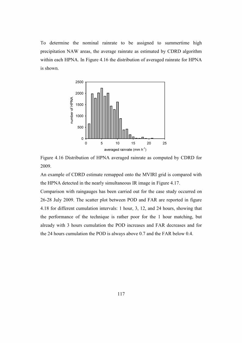
117
To determine the nominal rainrate to be assigned to summertime high
precipitation NAW areas, the average rainrate as estimated by CDRD algorithm
within each HPNA. In Figure 4.16 the distribution of averaged rainrate for HPNA
is shown.
Figure 4.16 Distribution of HPNA averaged rainrate as computed by CDRD for
2009.
An example of CDRD estimate remapped onto the MVIRI grid is compared with
the HPNA detected in the nearly simultaneous IR image in Figure 4.17.
Comparison with raingauges has been carried out for the case study occurred on
26-28 July 2009. The scatter plot between POD and FAR are reported in figure
4.18 for different cumulation intervals: 1 hour, 3, 12, and 24 hours, showing that
the performance of the technique is rather poor for the 1 hour matching, but
already with 3 hours cumulation the POD increases and FAR decreases and for
the 24 hours cumulation the POD is always above 0.7 and the FAR below 0.4.

118
a)
b)
Figure 4.16 HPNA as extracted by the IR MVIRI image (a), and CDRD estimates
remapped to match the MVIRI grid (b) for 18/06/2008 at 13:00 UTC

119
a) b)
c) d)
Figure 4.18 POD as function of FAR of raingauges validation of CNAW
technique at different cumulation times for the case study occurred on 26-
28/07/2009: 1hour (a), 3 hours (b), 12 hours (c) and 24 hours (d)
4.3.2.2 Application of TANN-R technique
As mentioned in section 3.3.4 two different implementation of TANN have been
pursued in this work: TANN-R (trained on ground radar data during the monsoon
season) and TANN-S (trained on CDRD estimates during the monsoon season).
Both techniques have been trained on Cloudsat-CPR data in cold months.
To perform the TANN-R training and testing, the available case studies have been
used for the Tibetan network, since in the Qinghai network area the MVIRI pixel
size is very large (see Figures 4.1 and 4.2). A total of about 4.6 106 pixels in the
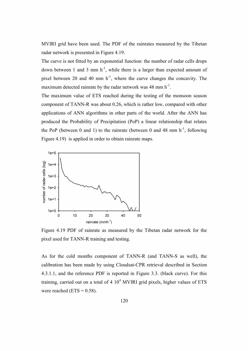
120
MVIRI grid have been used. The PDF of the rainrates measured by the Tibetan
radar network is presented in Figure 4.19.
The curve is not fitted by an exponential function: the number of radar cells drops
down between 1 and 3 mm h-1
, while there is a larger than expected amount of
pixel between 20 and 40 mm h-1
, where the curve changes the concavity. The
maximum detected rainrate by the radar network was 48 mm h-1
.
The maximum value of ETS reached during the testing of the monsoon season
component of TANN-R was about 0.26, which is rather low, compared with other
applications of ANN algorithms in other parts of the world. After the ANN has
produced the Probability of Precipitation (PoP) a linear relationship that relates
the PoP (between 0 and 1) to the rainrate (between 0 and 48 mm h-1
, following
Figure 4.19) is applied in order to obtain rainrate maps.
Figure 4.19 PDF of rainrate as measured by the Tibetan radar network for the
pixel used for TANN-R training and testing.
As for the cold months component of TANN-R (and TANN-S as well), the
calibration has been made by using Cloudsat-CPR retrieval described in Section
4.3.1.1, and the reference PDF is reported in Figure 3.3. (black curve). For this
training, carried out on a total of 4 104 MVIRI grid pixels, higher values of ETS
were reached (ETS = 0.58).

121
In Figure 4.20 are reported the instantaneous precipitation rate maps obtained
from the TANN for cold months (showing a snowfall episode), and a monsoon
season map (with convective cells).
a)
b)
Figure 4.20 Precipitation intensity maps derived from cold months TANN (a) for
a snowfall episode occurred on 23/01/2010, and from the TANN-R algorithms (b)
for a convective episode occurred on 16/07/2010.

122
The wintertime map shows wide very low precipitation rate area, with few spots
with rates around 1 mm h-1
.
The rainrate during monsoon season is much higher, the rain area is smaller and
precipitation is retrieved on pixel size spots, with very high spatial variability and
sometime isolated precipitation pixel are found, probably due to noise in the
original images.
4.3.2.3 Application of TANN-S technique
The cold months component of the TANN-S algorithm has the same ANN as
TANN-R, as described above. The monsoon season component has been trained
on CDRC estimates, whose PDF is reported on Figure 4.21 for the year 2010. If
compared to Figure 4.19, the CDRD is able to estimate higher values of
precipitation rate (few IFOV above 60 mm h-1
), and the shape of the distribution
is more likely to be fitted by a power low. A possible reason for differences
between radar and CDRD estimates PDF shapes cold be that the radar data are
obtained on a small portion of the Plateau, while the CDRD estimates view
extends over the whole area of interest, an in particular over the eastern part of the
Plateau, where more intense convective systems are expected (Sugimoto and
Ueno, 2010).
The training has been performed on 5.9 106 pixel on the MVIR grid, and the ETS
of the selected ANN was about 0.41, sensitively higher than the one find during
the TANN-S training.
In Figure 4.21 the TANN-S precipitation intensity map for the same episode as in
Figure 4.20b is shown. Differences between the two versions of the algorithm can
be noted (larger precipitation areas, higher rainrate peaks), and will be more
deeply discussed in the next Sections.

123
Figure 4.21 PDF of rainrate as estimated over the Plateau by the CDRD algorithm
pixel used for TANN-S training and testing.
Figure 4.22 Precipitation intensity maps derived from the TANN-S algorithms for
the same convective episode shown in Figure 4.19 occurred on 16/07/2010.

124
4.4 Algorithm intercomparison
Seven algorithms have been applied to the three year period over the Tibetan
Plateau (see Table 4.1). Two are for instantaneous precipitation rate and cannot be
used for operational monitoring, since they are onboard LEO satellites (Cloudsat
and DMSP). Two are global products that uses PMW and IR data: the products
can be downloaded at the resolution of 0.250.25 for the Tibetan area, as 3
hourly cumulated maps. Three algorithms are IR based techniques that are
calibrated following different approaches and using different data.
4.4.1 Daily precipitation amount
The first comparison is made by reducing all the products at the coarser grid
(0.250.25) and computing daily cumulated values. Thus 5 PDF are derived for
monsoon season and 4 for cold months, and are reported after normalization in
figure 4.23 (a) and (b), respectively.
The monsoon season PDF of the global products are very similar: the values
decreases exponentially after 10 mm, and more than 70 mm are recorded in a
significant number of pixels (10-4
of the total). The other IR-based techniques
behave rather differently. First, they have a large number of low rain amount pixel
(between 2 and 10 mm), then the curves descend rapidly to very low values
between 20 and 35 mm. Among the three IR-based techniques, the TANN-R
reaches the highest values around 35 mm with a fraction of 10-4
of the total
number of pixels, while TANN-S and CNAW have rather parallel shapes, with the
latter showing higher values.
For the cold months the behaviors show differences and similarities. The TMPA
product reaches large precipitation amounts as in the warmer months, while for
CMORPH the value of 35 mm of precipitation is present a fraction of 10-4
of the

125
total number of considered pixel. Also in this case the IR-based techniques are
decreasing more rapidly and the highest values at the 10-4
% fraction is 22 mm for
CNAW and 26 mm for TANN.
a)
b)
Figure 4.23 Normalized PDF of 24 h rain amount at the 0.250.25 resolution
for the year 2009, for cold months (JFMAM-OND) (a), and monsoon season
(JJAS).

126
Few preliminary conclusions can be drawn. The IR based techniques always
overestimate the area with lower precipitation amounts, below 10 mm for summer
and between 1 and 3 mm for clod months. On the other side, global techniques
overestimates larger rain amounts. During monsoon season, could be likely to
have an averaged rain amount over an 0.250.25 area exceeding 70 mm, but this
is very unlikely during cold months, when weak precipitation is expected.
During the monsoon season TANN-R is able to estimate larger rain amount than
TANN-S, this could be due to the finer resolution of radar rainfall maps, that are
able to estimate high rainrates, even if Figure 4.19 shows the ability of CDRD to
estimate few pixels above 50 mm h-1
, while Figure 4.21 shows that our database
of radar data is limited by lower rainrate values. Again it has to be mentioned the
Tibetan radar network is located in a region where heavy rainfall are rarely
observed.
Finally, the time series of Tibetan Plateau integrated daily mean rain amount is
shown in figure 4.24 for all the monitoring technique considered in this work,
keeping in mind that TANN-R and TANN-S coincide for cold months.
For the first two months the precipitation is very low: well below 0.5 mm for both
the global products, but 3B42 shows few peaks above 1 mm, while IR base
techniques have values between 1 and 2 mm on the average. A very large peak,
probably due to snow at the ground, is estimated by TANN-R, and by other
techniques but at markedly lower values, except CMORPH. Around day 80
CMORPH has a 10-day wide peak not sensed by other techniques, while between
day 100 and 150 the techniques agree with rather constant averaged value around
1 mm, with some isolated peaks observed by 3B42. Around day 150 there is the
onset of monsoon season TANN-R and TANN-S and the precipitation amount
increases for all the techniques: average values are now between 3 and 5 mm,
except for CMORPH, that keeps below the other curves.

127
Fig
ure
4.2
4 T
ime
seri
es o
f dai
ly p
reci
pit
atio
n a
mount
inte
gra
te o
ver
th
e T
ibet
an P
late
au f
or
the
tech
niq
ue
consi
der
ed i
n t
his
stu
dy

128
Sharp peaks, during 1 o 2 days, are seen during the monsoon season: sometimes
they are observed by more than one technique, but in general not with the same
values. Even TANN-R and TANN-S are far to be similar, with the latter generally
overestimating.
Around day 300, after the monsoon season has finished, the amount of rain
decreases with the agreement of all the techniques, except CMORPH, that in this
case tends to overestimate precipitation amount. TANN and CNAW are highly
correlated.
4.4.2 Case studies
On 24 August 2009 in the late morning (LT) a group of weak convective cells
developed on the southern and eastern part of the Plateau and have been observed
by both the Tibetan and Qinghai radar network. The data of all the estimation
techniques have been remapped onto the coarse grid 0.250.25 (except TANN-
R and TANN-S) and cumulated over three hours in order to make all the estimates
comparable. The derived maps are reported in Figure 4.25, where also the radar
map is shown, reduced a the same resolution of the other products.
Radar network shows a precipitation structure with low precipitation in the 3
hours, and one small peak with cumulated rain around 10 mm (a). CMORPH (b)
completely misses the precipitation structures, detecting only low rain
accumulation but slightly misplaced with respect to radar observations. CNAW
(c) detects several precipitating areas in the region, with rain amount comparable
with radar observations, but also a misplacement is noted. The 3B42 (d) estimates
is rather good in detecting rain areas, but the amount of rain is underestimated.
TANN-R (e) and TANN-S (f) show similar shapes in the precipitation patterns,
and the wet areas is the largest among the estimates. The higher resolution shows
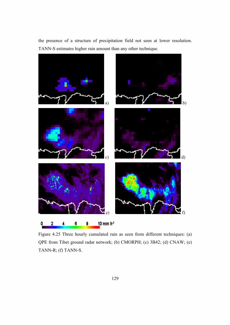
129
the presence of a structure of precipitation field not seen at lower resolution.
TANN-S estimates higher rain amount than any other technique.
a) b)
c) d)
e) f)
Figure 4.25 Three hourly cumulated rain as seen from different techniques: (a)
QPE from Tibet ground radar network; (b) CMORPH; (c) 3B42; (d) CNAW; (e)
TANN-R; (f) TANN-S.
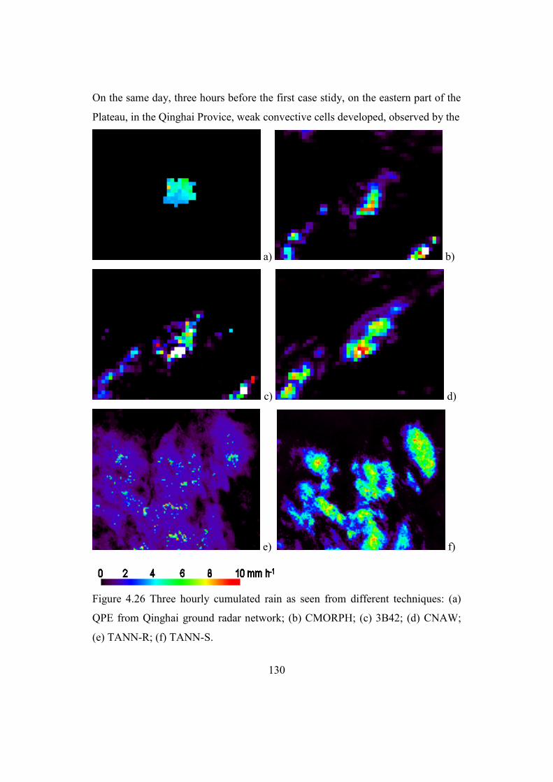
130
On the same day, three hours before the first case stidy, on the eastern part of the
Plateau, in the Qinghai Provice, weak convective cells developed, observed by the
a) b)
c) d)
e) f)
Figure 4.26 Three hourly cumulated rain as seen from different techniques: (a)
QPE from Qinghai ground radar network; (b) CMORPH; (c) 3B42; (d) CNAW;
(e) TANN-R; (f) TANN-S.

131
Qinghai radar network, and in Figure 4.26 are reported the radar 3 hours
cumualted precipitation (a), and the corresponding estimates: CMORPH (b), 3B42
(c), CNAW (d), TANN-R (e) and TANN-S (f).
In this case all the techniques detect reasonably well the rain areas, but the rain
amount is overestimated. Probably there is also a slight misplacement of the rain
area, due to parallax problem, that in the Qinghai region is rather sever, given the
high longitude with respect to the Meteosat 7 position (see figure 4.1).
Unfortunately, the available radar data were too few to make possible a systematic
validation with significant statistics, and only visual matching of the precipitation
patterns is possible.
However, the comparisons of the two case studies highlight the difficulties in
getting reliable precipitation estimation over the Plateau: satellite estimation
techniques based on different data and approaches give rain maps that markedly
differs on many points of view. Increasing the cumulation time the outputs of the
techniques converge to more similar description.
4.4.3 Annual maps
A final comparison can be considered by looking at the long term precipitation
cumulation: Tibet Plateau annual cumulated maps are considered in this section.
In Figure 4.27 the annual cumulated precipitation is reported for 3B42 (a),
CMORPH (b), CNAW (c), and TANN-R (d). All the estimates find the maximum
rain amount over the coast facing the Gulf of Bengal with other secondary peaks
along the south slopes of Himalayan chain. Global products show a very dry
Plateau: especially 3B42 estimates very low rain amount with relative abundance
on the eastern part of the Plateau. Some artifacts can also be detected in the 3B42
maps: square boxes with relatively high spatial precipitation gradient can be due
to the image segmentation used for the technique calibration.

132
The CMORPH map shows also a very dry Plateau, with less intense precipitation
peaks on the south Himalayan side, and some patchy pattern also on the northern
slopes. An artifact is probably present on the northern border of the Plateau,
where a narrow strip of relatively higher cumulated precipitation follows the
northern Plateau rim.
The CNAW map appears much different: higher precipitation amount (by a factor
slightly lower than 2), the precipitation peak on the southern Himalayan slopes is
missing, and relative high precipitation amount is found on the central and east
Plateau. Correctly, CNAW finds also relatively high cumulated values on the
eastern part of the domain, accordingly to other studies (Sugimoto and Ueno,
2010).
a)
0 200 400 600 mm y-1

133
b)
c)
0 200 400 600 mm y-1

134
d)
e)
Figure 4.27 Annual cumulated precipitation for year 2010 as computed from:
3B42 (a), CMORPH (b), CNAW (c), TANN-R (d) and TANN-S (e).

135
TANN-R shows lower cumulated values, weaker and less defined peaks on the
Gulf of Bengal, no peaks on the Himalayan south slope and relatively wet eastern
part of the Plateau.
The TANN-S maps estimates much higher precipitation amount, finds large peaks
on the Gulf of Bengal and along the south Himalayan slope. Also the eastern part
of the Plateau receives more precipitation than estimated by the other techniques.
As assessed for case studies and daily values, there are marked differences among
the outputs of the different techniques, especially between global products (3B42
and CMORPH) and the IR-based techniques calibrated over the Plateau (CNAW,
TANN-R and TANN-S). The basic difference is that global products are able to
estimates higher rainrates than other techniques, but underestimates the extent of
precipitation areas. Case studies show that global products can miss some area,
while IR techniques always find large, low rainrate, patterns. On the single images,
or daily means, this results in little differences, but if integrated on a whole year,
results in large discrepancies. The setup of blended IR-MW techniques is a trade-
off between the IR tendency to overestimate precipitation area size, and the MW
inability of detecting low-moderate rainrates.
Further studies are needed to resolve these ambiguities, and the forthcoming full
exploitation of the Global Precipitation Measurement mission will probably help
on this task.

136

137
Conclusions
In this Thesis work, carried out in the frame of CEOP-AEGIS, an EU FP7 funded
project, the problem of the precipitation monitoring over the Tibetan Plateau has
been addressed. Data from ground based instruments, made available by the
Chinese Meteorological Administration, are used for case studies and to feed
multiplatform satellite precipitation retrievals.
The main focus is the implementation and applications for three years of data
(2008, 2009 and 2010) of an array of satellite precipitation techniques. The work
has been broken down as follows.
First, a sensitivity study on the capability of the most used satellite sensors to
detect precipitation at the ground, assessed with respect to raingauges data for
selected case studies, has been carried out. Results show that the overall behaviour
of satellite sensor channels is quite different from the one well known at lower
elevation surfaces, probably due to the strong surface signal in the PMW and the
varying soil temperature across the day.
Then, two physically based techniques have been implemented for snow rate,
based on Cloudsat-CPR data (during cold months) and rainrate derived from
SSMI/S data (during monsoon season). These techniques, given the high
revisiting time, are not suitable for direct use as precipitation monitoring tool, but
are used as ―calibrator‖ of multisensor techniques based on geostationary IR data.
Two approaches are tested to merge MW retrieval to IR data: entity based and
fully statistical. The first approach requires the definition of precipitating area as
separated entities, and the assignment of rainrates as determined by coincident
MW estimates: at the beginning of this work, two techniques were selected
CNAW and GCD, but the latter was abandoned because of the poor sensitivity
over the Plateau.
The full statistical approach has been pursued by implementing an ANN
technique, trained on ground radar data (TANN-R) or PMW retrieval (TANN-S)
138
for the monsoon season, and on snowfall retrieval from Cloudsat-CPR during cold
months.
Finally, two well reputed global precipitation products have been considered for
reference and intercomparison: the CMORPH and the TMPA product 3B42. All
the techniques have been implemented for the 3 years and the results compared at
different spatial and temporal scales.
The analysis of daily rain amount has shown that in general CMORPH and TMPA
are able to estimate rain amount larger than the ones estimated by other
techniques during the monsoon season. In cold months global techniques
underestimate precipitation amount and areas, resulting in a dry bias with respect
to IR calibrated techniques. Case studies compared with ground radar QPE data
on convective episodes shown that global products tend to underestimate
precipitation areas, while IR calibrated techniques provides reliable rainrate
patterns, as compared with radar data. Unfortunately, the number of radar case
studies was not large enough to allow significant validation studies, and also non
data were available for cold months.
Annual precipitation cumulated maps show marked differences among the
techniques: IR calibrated techniques generally overestimate precipitation amount
by a factor of 2 with respect of global products.
Reasons for discrepancies are probably in the role the IR data have on the
techniques: when the rain area delineation is based on IR, overestimation is likely
to occur, while when the MW estimate is used, underestimation of low
precipitation areas is expected. Further studies are needed to resolve these
ambiguities, and the forthcoming full exploitation of the Global Precipitation
Measurement mission will surely help on this task, and probably give a clearer
picture of precipitation properties over the Tibetan Plateau.

139
Bibliography
Adler, R.F. and A.J. Negri, 1988, A satellite infrared technique to estimate tropical
convective and stratiform rainfall. J. Appl. Meteor., 27, 30-51.
Arkin, P.A. and B.N. Meisner, 1987, The relationship betweenl arge-scalec onvectivera
infall and cold cloud over the western hemisphere during 1982-84. Mon. Wea.
Rev., 115, 51-74.
Bishop, C. M., 1995, Neural Networks for Pattern Recognition. Clarendon Press -
Oxford, pp 546
Caracciolo, C., Porcù, F. and F. Prodi, 2011, Drop Size Distribution over the Tibetan
Plateau. Geophysical Research Abstracts, Vol. 13, EGU2011-12732, 2011, EGU
General Assembly 2011.
Capacci, D., and B. J. Conway, 2005, Delineation of precipitation areas from MODIS
visible and infrared imagery with artificial neural networks. Meteor. Appl., 12,
291–305
Capacci, D., and F. Porcù, 2009, Evaluation of a Satellite Multispectral VIS–IR Daytime
Statistical Rain-Rate Classifier and Comparison with Passive Microwave Rainfall
Estimates. J. Appl. Meteor. Climatol., 48, 284–300.
Casella, D., 2010, Analysis and Verification of the Cloud Dynamics and Radiation
Database (CDRD) Methodology for Bayesian Retrieval of Precipitation with
Passive Microwave Radiometer Instruments Onboard Satellites. PhD. Thesis,
Department of Science, Technical Information and Communication, University
of Rome ―La Sapienza‖, Rome, Italy, 121 pp.
Casella, D., S. Dietrich, F. Di Paola, M. Formenton, A. Mugnai, F. Porcù, and P. Sanò,
2012, PM-GCD – a combined IR–MW satellite technique for frequent retrieval of
heavy precipitation, Nat. Hazards Earth Syst. Sci., 12, 231-240
Chen F. W. and D. H. Staelin, 2003 AIRS/AMSU/HSB precipitation estimates. IEEE
Trans. Geosci. Remote Sens., 41, 410-417
Doviak, R., J., and D. Zrnic, 1994, Doppler radar and weather observations, Dover
Publications, 562 pp.
Duchon, C. E. and G. R. Essenberg, G. R., 2001, Comparative rainfall observations from
pit and aboveground gauges with and without wind shields, Water Resour. Res.,
37, 3253–3263.
Duchon, C.E. and C.J. Biddle, 2010, Undercatch of tipping-bucket gauges in high rain
rate events. Adv. Geosci., 25, 11–15.
Evans, L. J., and R. E. Shemo, 1996, A procedure for automated satellite-based
identification and climatology development of various classes of organized
convection. J. Appl. Meteor., 35, 638-652.
Ferraro, R.R. and G.F. Marks, 1995, The development of SSM/I rain rate retrieval
algorithms using ground based radar measurements. J. Atmos. Oceanic Technol.,
12, 755-770.
140
Ferraro, R. R., E. A. Smith, W. Berg, G. J. Huffman, 1998, A Screening Methodology for
Passive Microwave Precipitation Retrieval Algorithms. J. Atmos. Sci., 55, 1583–
1600.
Fujii, H. and T. Koike, 2001, Development of a TRMM/TMI Algorithm for Precipitation
in the Tibetan Plateau by Considering Effects of Land Surface Emissivity. J.
Meteor. Soc. Japan, 79, 475-483.
Fujinami, H., and T. Yasunari, 2004, Sub-monthly variability of convection and
circulation over and around the Tibetan Plateau during the boreal summer. J. Met.
Soc. Japan., 82, 1545-1564.
Grody, N. C., 1991: Classification of snow cover and precipitation using the Special
Sensor Microwave/Imager (SSM/I). J. Geophys. Res., 96, 7423–7435.
Hiley, M. J., M. S. Kulie, and R. Bennartz, 2011, Uncertainty Analysis for CloudSat
Snowfall Retrievals. J. Appl. Meteor. Climatol., 50, 399–418.
Hsu, K., X. Gao, S. Sorooshian, and H. V. Gupta, 1997: Precipitation estimation from
remotely sensed information using artificial neural networks. J. Appl. Meteor., 36,
1176–1190.
Huffman, G. J., D. T. Bolvin, E. J. Nelkin, D. B. Wolff, R. F. Adler, G. Gu, Y. Hong, K.
P. Bowman, and E. F. Stocker, 2007, The TRMM Multisatellite Precipitation
Analysis (TMPA): Quasi-Global, Multiyear, Combined-Sensor Precipitation
Estimates at Fine Scales. J. Hydrometeor, 8, 38–55
Iguchi, T., T. Kozu, R. Meneghini, J. Awaka, K. Okamoto, 2000, Rain-Profiling
Algorithm for the TRMM Precipitation Radar. J. Appl. Meteor., 39, 2038–2052.
Joyce, R. J., J. E. Janowiak, P. A. Arkin, and P. Xie, 2004, CMORPH: A method that
produces global precipitation estimates from passive microwave and infrared data
at high spatial and temporal resolution.. J. Hydromet., 5, 487-503.
Kidd, C. and Levizzani, V., 2011, Status of satellite precipitation retrievals, Hydrol. Earth
Syst. Sci., 15, 1109-1116.
Kotroni, V, Lagouvardos K Defer E, Dietrich S, Porcù F, Medaglia CM, Demirtas M,
2006: The Antalya 5 December 2002 storm: observations and model analysis. J.
Appl. Meteor., 45, 576-590.
Kulie, M. S., and R. Bennartz, 2009, Utilizing Spaceborne Radars to Retrieve Dry
Snowfall. J. Appl. Meteor. Climatol., 48, 2564–2580
Kursinski, A. L., S. L. Mullen, 2008, Spatiotemporal Variability of Hourly Precipitation
over the Eastern Contiguous United States from Stage IV Multisensor Analyses. J.
Hydrometeor, 9, 3–21.
Lanza, L. G., E. Vuerich, and I. Gnecco, 2010, Analysis of highly accurate rain intensity
measurements from a field test site. Adv. Geosci., 25, 37-44.
Laviola, S., and V. Levizzani, 2010, The 183-WSL fast rain rate retrieval algorithm: Part
I: Retrieval design, Atmos. Res., 99, 443-461.
Leitinger, G., N. Obojes and U. Tappeiner, 2010, Accuracy of winter precipitation
measurements in alpine areas: snow pillow versus heated tipping bucket rain
gauge versus accumulative rain gauge, EGU General Assembly 2010, held 2-7
May, 2010 in Vienna, Austria, p.5076.

141
Lensky, I. M. and D. Rosenfeld, 1996, Estimation of Precipitation Area and Rain
Intensity Based on the Microphysical Properties Retrieved from NOAA AVHRR
Data. J. Appl. Meteor., 36, 234-242
Levizzani, V., P. Bauer and J. F. Turk, (eds.), 2007, Measuring precipitation from space:
EURAINSAT & the future, Advances in global change research, Vol. 28,
Springer, 724 pp.
Li, M., Y. Ma, W. Ma, I., Hirohiko, F. Sun and S. Ogino, 2011, Different characteristics
of the structure of atmospheric boundary layer between dry and rainy periods over
the northern Tibetan Plateau. Sciences in Cold and Arid Regions, 3, 509–516
Li, Y. W. Yun, S. Yang, H. Liang, G. Shouting, and R. Fu, 2008, Characteristics of
summer convective systems initiated over the Tibetan Plateau. Part 1: Origin,
track, development, and precipitation. J. Appl. Meteor. Climatol., 47, 2679- 2695.
Ma, Y, H, Ishikawa, O. Tsukamoto, M. Menenti, Z. Su, T. Yao, T. Koike and T Yasunari,
2003, Regionalization of surface fluxes ove rheterogeneous landsacape of the
Tibetan Plateau by using satellite remote sensing. J. Meteor., Soc., Japan, 81,
277-293.
Ma, Y., M. Li, X. Chen, S. Wang, R. Wu, W. Ma, L. Zhong, B. Wang, C. ZHU, and T,
YAO, 2011, Third Pole Environment (TPE) program: a new base for the study of
atmosphere―land interaction over the heterogeneous landscape of the Tibetan
Plateau and surrounding areas, Proc. of IUGG2011, Melbourne, 343, 110-117.
Machado, L. A. T., and W. B. Rossow, 1993, Structural characteristics and radiative
properties of tropical cloud clusters. Mon. Wea. Rev., 121, 3234–3260.
Marshall, J. S. and W. McK. Palmer, 1948, The Distribution of Raindrops with Size. J.
Meteorol., 5, 165-166.
Martin, D.W., R. A. Kohrs, F. R. Mosher, C. M. Medaglia, and C. Adamo, 2008, Over-
Ocean Validation of the Global Convective Diagnostic, J. Appl. Meteor. Climatol.,
47, 525–543
Mosher, F.R., 2001, A satellite diagnostic of global convention, Preprints, 11th Conf on
Satellite Meteorology, Madison, WI. Amer. Meteor. Soc., 416-419
Negri, Andrew J., Robert F. Adler, Peter J. Wetzel, 1984, Rain Estimation from
Satellites: An Examination of the Griffith-Woodley Technique. J. Climate Appl.
Meteor., 23, 102–116.
Nurmi, P., 2003: Recommendations on the verification of local weather forecasts. 11
ECMWF Tech. Memo. N. 430, 19pp.2/29/2012
Pankiewicz, G. S., C. J. Johnson, and D. L. Harrison, 2001, Improving radar observations
of precipitation with a Meteosat neural network classifier. Meteor. Atmos. Phys.,
76, 9–22
Porcú F., M. Borga and F. Prodi, 1999: Rainfall estimation by combining radar and
infrared satellite data for nowcasting purposes. Meteorol. Appl., 6, 289-300.
Porcù F., Prodi F., Dietrich S., Mugnai A. and Bechini R., 2000, Multisensor estimation
of severe rainfall events, Proc. of the 2000 Eumetsat Meteorological Satellite
Data Users' Conference. EUM P 29, Eumetsat, Darmstadt, 371-378

142
Prodi, F. Caracciolo, C., D‘Adderio, L.P., Gnuffi, M., Lanzinger, E., 2011. Comparative
Investigation of Pludix disdrometer capability as Present Weather Sensor (PWS)
during the Wasserkuppe campaign. Atm.Res., 99, 162-173.
Rubel, F., 1996. Scale dependent statistical precipitation analysis. Proc. of the Int. Conf.
on Water Resour. & Environ. Res., 29-31 ottobre 1996, Kyoto, 317-324
Sanò, P., The Cloud Dynamics and Radiation Database (CDRD) Approach for
Precipitation Retrieval by Means of Satellite Based Microwave Radiometry. PhD
thesis, Department of Computer, Systems and Production Engineering, Tor
Vergata University of Rome "Tor Vergata", Rome, ITALY,, 2010.
Sanò, P., D.Casella, A.Mugnai, G.Schiavon, E.A.Smith, and G.J.Tripoli, 2012, Bayesian
Estimation of Precipitation from Satellite Passive Microwave Measurements using
CDRD Technique. Part 1: Algorithm Description and Applications over Italy.
IEEE Trans. Geo. Rem. Sens., submitted
Sevruk, M. Ondrás, B. Chvíla, 2009, The WMO precipitation measurement
intercomparisons, Atmos. Res., 92, 376-380.
Shimizu, S., K. Ueno, H. Fujii, H. Yamada, R. Shirooka, and L. Liu, 2001, Mesoscale
characteristics and structures of stratiform precipitation on the Tibetan Plateau. J.
Meteor. Soc. Japan, 79, 435-461.
Smith, E. A., and Coauthors, 1998, Results of WetNet PIP-2 project. J. Atmos. Sci., 55,
1483–1536.
Spencer, W., H. M. Goodman, and R. E. Hood, 1989, Precipitation retrieval over land and
ocean with the SSM/I: Identification and characteristics of the scattering signal. J.
Atmos. Oceanic Technol., 6, 254–273.
Sugiura, K., D. Yang, T. Ohata, 2003, Systematic error aspects of gauge-measured solid
precipitation in the Arctic, Barrow, Alaska. Geophysical Research Letters, 30, 1-5.
Sugimoto, S. and K. Ueno, 2010, Formation of mesoscale convective systems over the
eastern Tibetan Plateau affected by plateau scale heating contrasts, J. Geophys.
Res., 115, D16105
Tripoli, G. J., 1992: A Nonhydrostatic Mesoscale Model Designed to Simulate Scale
Interaction. Mon. Wea. Rev., 120, 1342–1359.
Tokay, A., D.B. Wolff, K.R. Wolff and P. Bashor, 2003, Rain Gauge and Disdrometer
Measurements during the Keys Area Microphysics Project (KAMP). J. Atmos.
Oceanic Technol., 20, 1460-1477.
Ueno, K., N. Endho, T. Ohta, H. Yabuki, T. Koike, M. Koike, T. Ohata and Y.
Zhang,1994, Characteristics of precipitation distribution in Tanggula, monsoon,
1993. Bull. of Glac. Res., 12, 39-47.
Ueno, K., 1998, Characteristics of Plateau-scale precipitation in Tibet estimated by
satellite data during 1993mosoon season. J. Meteor. Soc. Japan, 76, 533-548.
Ueno, K., S. Sugimoto, T. Koike, H. Tsutsui, and X. Xu, 2011, Generation processes of
mesoscale convective systems following mid-latitude troughs around the Sichuan
Basin. J. Geophys. Res., 115, D16105
Uyeda, H., H. Yamada, J. Horikomi, R. Shirooka, S. Shimizu, L. Liu, K. Ueno, H. Fujii
and T. Koike, 2001, Characteristics of Convective Clouds Observed by a Doppler

143
Radar at Naqu on Tibetan Plateau during the GAME-Tibet IOP. J. Meteor. Soc.
Japan, 79, 436-474.
Vuerich, E., Monesi, C., Lanza, L. G., Stag, L., & Lanzinger, E. (2009). WMO Field
intercomparison of rainfall intensity gauges. World Meteorological Organisation -
Instruments and Observing Methods Rep. No. 99, WMO/TD No. 1504 , 286.
World Meteorological Organization, 2008, Guide to meteorological instruments and
methods of observations, WMO-n 8, 7th
edition, Geneva, 681 pp.
Xu, W., and E. J. Zipser, 2011, Diurnal Variations of Precipitation, Deep Convection, and
Lightning over and East of the Eastern Tibetan Plateau. J. Climate, 24, 448–465.
Yao, T. and G. Greenwood, 2009, A New ―Polar‖ Program: Third Pole Environment
(TPE) Workshop; Beijing, China, 14–16 August 2009. Eos Trans. AGU, 90, 515.
Yao, Z., W. Li, Y. Zhu, B. Zhao, and Y. Chen, 2001, Remote Sensing of Precipitation on
the Tibetan Plateau Using the TRMM Microwave Imager. J. Appl. Meteor., 40,
1381-1392.
Yin, Z-Y, X. Zhang, X. Liu, M. Colella, and X. Chen, 2008, An Assessment of the Biases
of Satellite Rainfall Estimates over the Tibetan Plateau and Correction Methods
Based on Topographic Analysis. J. Hydrometeor, 9, 301–326.

144

145
Acknowledgements
The work described here has been supported by the European Commission (Call
FP7-ENV-2007-1 Grant nr. 212921) as part of the CEOP-AEGIS project
(www.ceop-aegis.org) coordinated by the Université de Strasbourg.
The availability of radar and raingauge data was granted by prof. Liping Liu of
the China Meteorological Administration, and the help of Wei Zhuang in data
managing is acknowledged.
The group headed by dr. Alberto Mugnai al the ISAC-CNR in Rome, provided the
CDRD estimates and the UW-NMS outputs, and particular thanks go to dr. Paolo
Sanò and dr. Daniele Casella.
Satellite data have been downloaded free as follows:
The MODIS product was downloaded from :
http://laadsweb.nascom.nasa.gov
The AMSR-E L2A product was downloaded from :
http://nsidc.org/data/amsre/index.html
The 3B24 product was downloaded from NASA-GESDIS server at:
http://mirador.gsfc.nasa.gov/, while CMORPH products have been downloaded
from the NOAA-CPC ftp site: ftp.cpc.ncep.noaa.gov/precip/global_CMORPH/.
The MVIRI product was downloaded from the EUMETSAT Earth Observation
Portal:
(http://www.eumetsat.int/Home/Main/DataProducts/ProductNavigator/index.htm?
l=en)
The 2A25 higher product level of TRMM PR was download from:
http://pmm.nasa.gov/TRMM/products-and-applications
I wish to express my sincere gratitude to my advisor Dr. Federico Porcù for his
guidance, important technical and scientific contributes to my thesis. I would like
to thanks my colleague Lisa Milani for her technical and moral support gave me.

146
A would like to thanks Dr. Pietro Domenico de Cosmo for his technical
contribute.
Outside the work environment I would like to thanks my parents and all my
friends gave me their best feelings refilled my heart of positive energy.