UNIVERSIDADE FEDERAL DO RIO DE JANEIRO

INSTITUTO DE FÍSICA

Quantum Speed Limits for General Physical Processes

Márcio Mendes Taddei

Ph.D. Thesis presented to the Graduate Program inPhysics of the Institute of Physics of the Federal Uni-versity of Rio de Janeiro - UFRJ, as part of the require-ments to the obtention of the title of Doctor in Sciences(Physics).

Advisor: Dr. Ruynet Lima de Matos Filho

Rio de Janeiro

February, 2014

arX

iv:1

407.

4343

v1 [

quan

t-ph

] 1

6 Ju

l 201

4

ii

T121 Taddei, Márcio MendesQuantum Speed Limits for General Physical Processes /

Márcio Mendes Taddei. - Rio de Janeiro, 2014.xviii, 115f. : il. ; 30 cm.

Tese (Doutorado em Física) - Programa de Pós-graduaçãoem Física, Instituto de Física , Universidade Federal do Rio de Janeiro.

Orientador: Dr. Ruynet Lima de Matos FilhoBibliografia: f. 90-98.

1. Física Quântica. 2. Limite Quântico de Velocidade. 3.Informação Quântica de Fisher. 4. Geometria de Estados Quânticos.I. Matos Filho, Ruynet Lima de. II. Universidade Federal do Rio deJaneiro. Instituto de Física. III. Quantum Speed Limits for GeneralPhysical Processes.

CDD 530.12

iv

Resumo

Limites Quânticos para a Velocidadede Processos Físicos Gerais

Márcio Mendes Taddei

Orientador: Ruynet Lima de Matos Filho

Resumo da Tese de Doutorado apresentada ao Programa de Pós-Graduaçãoem Física do Instituto de Física da Universidade Federal do Rio de Janeiro -UFRJ, como parte dos requisitos necessários à obtenção do título de Doutorem Ciências (Física).

Limites quânticos de velocidade são relações que fornecem limites inferiores ao tempo

de evolução de sistemas quânticos. Este tipo de resultado começou com Mandelstam e

Tamm, que associaram o tempo mínimo necessário para um estado ficar ortogonal com

a variância de energia de tal estado. Outro limite inferior, obtido mais tarde, foi o de

Margolus e Levitin, que relacionaram este tempo mínimo com a energia média do sistema

quântico. Tais limites são comumente usados para discutir o papel do emaranhamento na

velocidade de evolução de sistemas quânticos, e têm potencial de aplicação a sistemas de

evolução especialmente rápida, como os de computação (clássica ou quântica) ou mesmo

nos esquemas explicativos do surgimento do comportamento clássico a partir de um sub-

strato quântico, que dependem de uma descoerência extremamente veloz.

Tais resultados, especialmente o de Mandelstam-Tamm, já foram generalizados de al-

gumas formas, em particular a incluir evoluções a estados não-ortogonais. Entretanto,

havia uma lacuna na literatura da área, pois apenas evoluções unitárias – sistemas quân-

ticos fechados – eram consideradas. Nesta tese, esta limitação é superada: nosso principal

v

resultado é um limite para evoluções gerais, unitárias ou não, de sistemas quânticos, que

corretamente recupera os limites de Mandelstam-Tamm no caso unitário. Aplicações desse

limite para certos casos concretos interessantes são apresentadas. Esse limite também é

usado para estender para o caso não-unitário a discussão do papel do emaranhamento em

evoluções rápidas, fornecendo resultados não-triviais.

Para a dedução dos resultados, emprega-se uma abordagem geométrica que já havia

se mostrado extremamente útil quando desenvolvida no caso unitário por Anandan e

Aharonov, em especial por permitir uma clara interpretação dos limites e a discussão dos

critérios para sua saturação. Faz-se mister ressaltar que não se pressupõe neste trabalho

conhecimento prévio do leitor sobre geometria de estados quânticos. Nota-se ainda que

o problema de limites ao tempo de evolução é intimamente ligado à metrologia quântica,

em particular, ao problema de estimação quântica de parâmetros. Talvez o sinal mais

manifesto desta proximidade seja a utilização, em nosso limite geométrico, da informação

quântica de Fisher, grandeza de larga aplicação em metrologia quântica.

Por fim, apresentam-se resultados adicionais na direção de obter uma interpretação

geométrica de limites do tipo de Margolus-Levitin.

Palavras-chave: 1. Limite Quântico de Velocidade, 2. Informação Quântica de

Fisher, 3. Processos não-unitários, 4. Geometria de Estados Quânticos.

vi

Abstract

Quantum Speed Limits for General Physical Processes

Márcio Mendes Taddei

Advisor: Ruynet Lima de Matos Filho

Abstract of the Ph.D. Thesis presented to the Graduate Program in Physicsof the Institute of Physics of the Federal University of Rio de Janeiro - UFRJ,as part of the requirements to the obtention of the title of Doctor in Sciences(Physics).

Quantum speed limits are relations yielding lower bounds on the evolution time of

quantum systems. This kind of result was started by Mandelstam and Tamm, who asso-

ciated the minimal time needed for a state to turn orthogonal with the energy variance

of said state. Another lower bound, of much later obtention, was that of Margolus and

Levitin, who related this minimal time to the average energy of the quantum system.

These bounds are commonly used to discuss the role of entanglement in the evolution

speed of quantum systems, and have the potential to be applied to extremely fast-evolving

systems, such as those in both classical and quantum computation or in the explanatory

schemes for how classical behavior arises from a quantum substrate, which depend on an

exceedingly fast decoherence.

These results, especially that of Mandelstam and Tamm, have been generalized in some

ways, in particular by including evolutions to non-orthogonal states. However, there was

a gap in the literature on this area, for only unitary evolutions – closed quantum systems

– had been considered. On this thesis, such limitation is overcome: our main result is a

bound for quantum-system evolutions in general, whether unitary or not, and correctly

vii

recovers the Mandelstam-Tamm bounds in the unitary case. Applications of this bound to

several concrete cases of interest are herein presented. This bound is also used to extend to

the non-unitary case the discussion of the role of entanglement in fast evolutions, leading

to nontrivial results.

For the derivation of the results, a geometric approach has been employed, which had

already shown to be extremely useful for unitary evolutions when developed by Anan-

dan and Aharonov, especially for allowing a clear interpretation of the bounds and the

discussion of the criteria for their saturation. It should be noted that in this work no

previous knowledge of quantum-state geometry by the reader is assumed. An important

remark is that the problem of lower bounds on evolution time is closely related to quantum

metrology, in particular, to quantum parameter estimation. Perhaps the most manifest

sign of such proximity is the utilization, in our geometric bound, of the quantum Fisher

information, a quantity largely applied in quantum metrology.

Finally, additional results towards obtaining a geometric interpretation of Margolus-

Levitin bounds are presented.

Keywords: 1. Quantum Speed Limit, 2. Quantum Fisher Information, 3. Non-

unitary processes, 4. Quantum-state geometry.

viii

Acknowledgments

First and foremost, I acknowledge the contribution of my research group not only to

this thesis, but, more importantly, to science as practiced in Brazil. As part of the Quan-

tum Optics and Quantum Information Group, I am able to do science at an international

level and be a living witness — and even proof! — against the notion that quality science

can only be done in fully developed countries. There sure still are difficulties and limita-

tions, especially regarding funding, but research in Brazil has come a great way and my

group is part of that effort. It is particularly satisfying to watch conferences and talk to

colleagues from all over the world on an equal footing, be they from Toronto, Hannover,

Turku or Singapore.

I must thank my advisor, Prof. Ruynet L. de Matos Filho, who accepted me as

a student as I joined the group mid-Ph.D. During this time, Ruynet has always been

interested in working with me, proposing new ideas, listening to me when I had results

to show. A great part of the work on this thesis was done during the weekly meetings at

his office. He has a very well defined notion of the responsibilities of advisor and advisee,

and does not shirk his share of duties. He has always been understanding of my needs

during this time, and helped me professionally whenever necessary. I have always had a

good measure of freedom when working with him — with a matching demand in return!

He has also seen to it that I participate in conferences and meetings and had contact

with scientists of related areas from the whole world. I also thank my direct collaborators

Bruno M. Escher, who has often taken part in those meetings at Ruynet’s office, and

Prof. Luiz Davidovich, who has contributed in ways I could not have understood before

his participation. The work here presented couldn’t have come to fruition without them.

ix

I thank my former advisor, Prof. Carlos Farina, with whom I had my scientific initi-

ation in the Casimir Effect Group. The three formative years I spent working with the

group were decisive for the scientist and the person I have become. Farina is a human

being with a deep sense of the qualms of those around him, and an extremely rare ability

to put himself in the place of others. I have always felt the liberty to come to him with

my worries, including my wish to leave his group mid-Ph.D. I thank him for not only

being completely understanding of my move, but also helpful towards it (all the while

without giving up of me as a student until I had completely made up my mind). Even

though I have left the group, I still feel attached to the people in it, and it is with great

joy that I see their ongoing success. I also thank Tarciro Mendes who, along with Farina,

was my first scientific collaborator, and Marcus Venícius Cougo-Pinto, for teaching me a

more formal approach to mathematics — which has been directly helpful to this thesis —

as well as being an inspiration in terms of didactics, clarity and mathematical rigor.

I thank my parents, Jayme and Angela, for not only accepting my choices of studying

first Chemistry, then Physics, but encouraging me to pursue an academic career to the

point of believing that anything else would be nonsensical. I also thank my father for

the corrections to the English in this thesis. And I thank my elder brother, Paulo, with

whom I have had contact with interesting different perspectives on academic life.

I acknowledge the Physics Institute of the Federal University of Rio de Janeiro (IF-

UFRJ) for the very professional atmosphere that can be found here. The commitment to

doing science at a high level can be distinctly seen in many of the research groups I have

come in contact with. It is an environment with an abnormal affluence of bright people,

generation after generation. This professional environment is also reflected in the good

work of Casé, Pedro and the administrative staff of the graduate courses of IF-UFRJ as

a whole.

I thank the funding agencies that have directly supported me, CNPq (Brazilian Na-

tional Council for Scientific and Technological Development), Faperj (Foundation for Re-

x

search Support of the State of Rio de Janeiro) and INCT-IQ (Brazilian National Institute

for Science and Technology of Quantum Information), as well as sister agency CAPES,

which has also supported the group. E agradeço ao povo brasileiro, que financia as insti-

tuições de apoio à pesquisa e permite que elas existam1.

I must nevertheless play a down note. It is saddening that the academic career (world-

wide) is so structured that the work one puts the most effort into during their graduation

ends up being read by a small amount of people. In the writing of this thesis I have ardu-

ously striven to reach out to more people but, as with anything in life, all the dedication

one can summon in an endeavor can only change the world by the tiniest bit. If they get

to be so lucky.

I now take the liberty to write the remainder of the acknowledgments in Portuguese.

Agora em bom português, agradeço aos colegas do grupo de ótica e informação quân-

ticas. Ao Eduardo Paul e Alvaro Pimentel pelas conversas que iam do jogo da velha

quântico às utilizações da palavra “whose” em inglês, e pelas várias vezes que entrei na

sala de vocês para colocar alguma ideia no quadro (de física ou não). Ao Wellison Bastos,

logo na sala em frente, pela paciência de me ouvir em muitos de meus anseios. À Mariana

Barros, minha companheira de viagens. E ao grupo como um todo, mesmo quando vocês

comem todo o churrasco antes de eu chegar.

Agradeço aos amigos que fiz na Física desde a época da graduação. Ao compadre

Renato Aranha, ao Guilherme Bastos — nosso querido Quantum Boy, de quem fui colega

da graduação ao doutorado e em ambos os grupos de pesquisa —, ao Wilton Kort-Kamp,

Andreson Rego, Anderson Kendi, Rafael Bezerra, Gustavo Quintas de Medeiros, às pes-

soas do LAPE, de quem eu sempre estive próximo, Daniel Vieira, Oscar Augusto, Danielle

Tostes, Daniela Szilard, Vinícius Franco.

Agradeço aos amigos que tenho e tive ao longo do doutorado, com os quais eu chorei

1Translation: “And I thank the Brazilian people, which finances the research support institutions andallows them to exist.”

xi

e sorri, e sem os quais a trajetória seria muito mais penosa: Alexandre Sardinha, Edu-

ardo Ambrosio, Franco de Castro, Gabriella Cruz, Gustavo Rocha, Sarah Ozorio, Lidi-

ane Cavalcante, Thaís Alves, Tatiana Hessab, Wando Fortes, Warny Marçano, li

Samulenok. Isso sem falar, é claro, nos amigos da 23C, Alan Albuquerque, Anto-

nio Henrique Campello, Fabiane Almeida, Gustavo Coelho, Larissa Alves, Larissa Bar-

bosa, Leonardo Marques, Mariana Perfeito, Mario Gesteira, Ricardo Barboza, Rodrigo de

Oliveira, Tatiana Teitelroit, Ulysses Vilela (como é estranho não usar alguns dos apelidos).

Por fim, agradeço aos loucos companheiros do teatro, essa arte tão oposta à física em

tantos sentidos, e por isso mesmo tão estimulante de fazer: Nathalia Colón, Ana Beatriz

Machado, Beatriz Schuwartz, Daniel dos Anjos, Jailson Junior, João Pedro Marques, José

Henrique Calazans, Luis Zacharias, Michelle André, Rafael de Andrade, Bárbara Cruz,

Tayná Germano, Vinícius Ferreira, Wagner dos Santos. Sem vocês não seria fácil seguir

dia após dia.

xii

Contents

Contents xii

List of Figures xiv

List of Tables xviii

1 Introduction 1

2 Main concepts and existing literature 8

2.1 The Mandelstam-Tamm bound . . . . . . . . . . . . . . . . . . . . . . . . 9

2.2 The Margolus-Levitin bound . . . . . . . . . . . . . . . . . . . . . . . . . . 14

2.3 Main features of the bounds . . . . . . . . . . . . . . . . . . . . . . . . . . 16

2.4 Further results . . . . . . . . . . . . . . . . . . . . . . . . . . . . . . . . . 19

2.5 What had not been done . . . . . . . . . . . . . . . . . . . . . . . . . . . . 20

3 Quantum Speed Limits for General Physical Processes 23

3.1 Useful quantum information tools . . . . . . . . . . . . . . . . . . . . . . . 23

3.1.1 The Bures Fidelity . . . . . . . . . . . . . . . . . . . . . . . . . . . 24

3.1.2 Purifications . . . . . . . . . . . . . . . . . . . . . . . . . . . . . . . 24

3.1.3 POVMs . . . . . . . . . . . . . . . . . . . . . . . . . . . . . . . . . 26

3.2 Geometric Approach . . . . . . . . . . . . . . . . . . . . . . . . . . . . . . 28

3.2.1 A distance for pure quantum states . . . . . . . . . . . . . . . . . . 28

3.2.2 Mandelstam-Tamm bound obtained geometrically . . . . . . . . . . 37

xiii

3.3 Fisher information . . . . . . . . . . . . . . . . . . . . . . . . . . . . . . . 40

3.3.1 The quantum Fisher information . . . . . . . . . . . . . . . . . . . 45

3.4 The most general quantum speed limit . . . . . . . . . . . . . . . . . . . . 50

3.4.1 A distance for all quantum states . . . . . . . . . . . . . . . . . . . 51

3.4.2 The bound . . . . . . . . . . . . . . . . . . . . . . . . . . . . . . . . 52

3.5 Additional results . . . . . . . . . . . . . . . . . . . . . . . . . . . . . . . . 57

4 Applying the bounds 61

4.1 Calculating the quantum Fisher information . . . . . . . . . . . . . . . . . 61

4.1.1 A purification-based expression . . . . . . . . . . . . . . . . . . . . 61

4.2 Application to non-unitary channels . . . . . . . . . . . . . . . . . . . . . . 64

4.2.1 Amplitude-damping channel . . . . . . . . . . . . . . . . . . . . . . 66

4.2.2 Single-qubit dephasing . . . . . . . . . . . . . . . . . . . . . . . . . 69

4.2.3 Dephasing and entanglement . . . . . . . . . . . . . . . . . . . . . . 74

4.3 Application of the additional bound . . . . . . . . . . . . . . . . . . . . . . 84

5 Final comments and perspectives 87

Bibliography 90

A Integration of the Fubini-Study metric 99

B Minimization yielding the median 103

C Tightness of the bound on the quantum Fisher information 106

D Optimization of the bound for the dephasing channel 109

E Later results in the literature 112

xiv

List of Figures

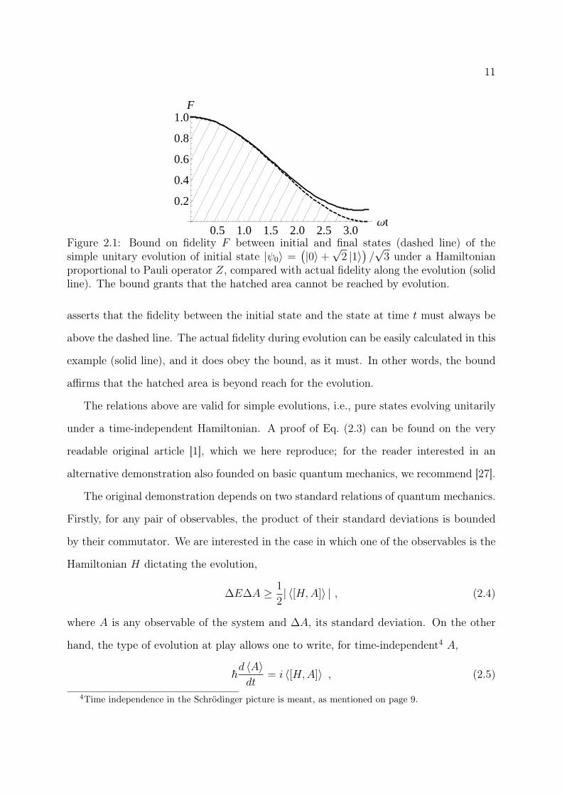
2.1 Bound on fidelity F between initial and final states (dashed line) of the

simple unitary evolution of initial state |ψ0〉 =(|0〉+

√2 |1〉

)/√

3 under

a Hamiltonian proportional to Pauli operator Z, compared with actual

fidelity along the evolution (solid line). The bound grants that the hatched

area cannot be reached by evolution. . . . . . . . . . . . . . . . . . . . . . 11

3.1 Depiction of a two-dimensional Hilbert space. Integration on the straight

line yields DBures, but is unsuited for our purposes, because the distance

thus obtained would necessarily distinguish collinear vectors. We note that

states inside the unit circle (dashed line), like |ψm〉, are pure, but not

normalized. . . . . . . . . . . . . . . . . . . . . . . . . . . . . . . . . . . . 36

3.2 Example of plot of ∆E(t)/~ over time t. The bound on the time for a

certain distance D1 to be reached is given by the value t = τ such that the

area under the graph equals D1. . . . . . . . . . . . . . . . . . . . . . . . . 38

3.3 Values of Pk(gtrue) for a measurement of g in Huascarán, in the Andes (blue

circles) and at the Arctic Sea (red squares). The distributions within each

image are different because so is gtrue. Measurement as made in a simple

laboratory (left) is compared to that by higher-precision satellites (right). . 43

xv

4.1 Depiction of the Bloch sphere showing the path followed by an initially ex-

cited state (|e〉) in the amplitude-damping channel. This path is a geodesic

between the orthogonal states |e〉 and |g〉, in addition to the great semi-

circles also shown. . . . . . . . . . . . . . . . . . . . . . . . . . . . . . . . . 67

4.2 Depiction of the Bloch sphere showing the effect of the dephasing channel

(thick line) on a superposition of |0〉 and |1〉. The rotation around z occurs

with (angular) frequency ω0, the radius shrinkage has characteristic time

1/γ. . . . . . . . . . . . . . . . . . . . . . . . . . . . . . . . . . . . . . . . 71

4.3 Single-qubit dephasing: bound on the distance D(0,∞) at time τ →∞ as

a function of parameter r = ω0/γ, Eq. (4.37). It is readily seen that, for

r < rcrit ≈ 2.60058, no initial state can become orthogonal in finite time. . 74

4.4 Plot of the relative discrepancy from the bound (Eq. 4.38) to exact calcula-

tions (Eq. 4.39) in the single-qubit dephasing as a function of dimensionless

time γτ , with r = 8. The various ∆Z (longitudinal axis) correspond to dif-

ferent initial states. . . . . . . . . . . . . . . . . . . . . . . . . . . . . . . . 74

4.5 Lower bound on time γτ for fully entangled GHZ state (∆Z = 1) to reach

D = 94% of the maximal distance (FB = 1%), calculated numerically from

(4.51), as a function of N , with r = 8, 40 and 400, respectively (error bars

smaller than symbols). The straight line, proportional to 1/N , obeys (4.57). 80

4.6 N -qubit dephasing: lower bound on the time necessary for separable,

symmetric state undergoing to reach D = 94% of the maximal distance

(FB = 1% relative to its initial state) as a function of the number of qubits

N , Eq. (4.59). Two different asymptotic behaviors can be seen, τ ∼ 1/√N

and τ ∼ 1/N , obeying Eqs. (4.62, 4.60). . . . . . . . . . . . . . . . . . . . . 81

xvi

4.7 N -qubit dephasing: comparison between lower bound (dashed line) and ex-

act calculation (solid line) for the time necessary for separable, symmetric

state to reach D = 94% of the maximal distance (FB = 1%) as a func-

tion of the number of qubits N , Eqs. (4.59, 4.64), resp. The asymptotes,

proportional to 1/√N , 1/N , are taken from Eq. (4.65). . . . . . . . . . . . 82

4.8 Plot of the first, weaker version of the median-based bound, dependent on

〈ψ0|∣∣H − Emed

∣∣|ψ0〉, applied to the three-level system for p2 = 0.25. The

thick (purple) line represents the bound as in Eq. (4.68), actual evolution

is given by the uppermost (blue) curve, the Mandelstam-Tamm bound,

plotted for comparison, is the intermediate (tan-colored) curve (Eq. 4.69).

The Margolus-Levitin bound on orthogonality time τML is shown as a red

mark on the ωτ axis. . . . . . . . . . . . . . . . . . . . . . . . . . . . . . . 85

4.9 Plot of the stronger version of the median-based bound, dependent on

|〈ψ0|H − Emed|ψ(t)〉|, applied to a three-level system for p2 = 0.1, 0.2 and

0.35, resp. — different p2 correspond to different initial states. The thick

(purple) line represents the bound as in Eq. (4.72), actual evolution is given

by the uppermost (blue) curve, the Mandelstam-Tamm bound, plotted for

comparison, is the remaining (tan-colored) curve (Eq. 4.69). The Margolus-

Levitin bound on orthogonality time τML is shown as a red mark on the

ωτ axis. . . . . . . . . . . . . . . . . . . . . . . . . . . . . . . . . . . . . . 86

A.1 The integration of the Fubini-Study metric is mapped onto the line integral

of a radial function on the complex plane (with usual Euclidean metric)

from the origin to the final point zf . The straight line is, in fact, the

minimizing path. . . . . . . . . . . . . . . . . . . . . . . . . . . . . . . . . 100

B.1 An example of the graph of the function we are minimizing as a function

of g. The slope changes whenever g = En for some n. . . . . . . . . . . . . 104

xvii

B.2 Graph of the function we are minimizing as a function of g with a zero-slope

region. . . . . . . . . . . . . . . . . . . . . . . . . . . . . . . . . . . . . . . 104

xviii

List of Tables

4.1 Notational correspondence between evolution operator and Hamiltonian.

The last column indicates the notation for the Hamiltonian corrected for

initial-state averaging, as defined by Eq. (4.11) for the first line and anal-

ogously for the rest of the table. . . . . . . . . . . . . . . . . . . . . . . . . 66

1

Chapter 1

Introduction

How fast can a quantum system evolve to an orthogonal state? This question serves

as a starting point in the search for the quantum speed limit, the maximal evolution

speed of a quantum system. The goal of this search is to obtain general bounds, valid

for any particular system one may wish to apply it to, limiting (from below) the time it

takes for a system to become distinguishable from its initial state. A paradigmatic first

answer to this problem, appearing in the seminal work of Mandelstam and Tamm [1], was

that, given an evolution dictated by a time-independent Hamiltonian H and a pure initial

state, the time τ necessary for the final state to be orthogonal to the given initial state is

bounded by1

τ ≥ π~2∆E

, (1.1)

where ∆E is the standard deviation of H and ~ is the reduced Planck constant. A key

feature of the above bound is the dependence on the inverse of the standard deviation of

the system energy.

Why study such bounds?

The motivation for working on the quantum speed limit is fourfold. The topic originally

arose from discussions on the structure of quantum mechanics, especially in attempts to

define a suitable time operator and derive an uncertainty relation for time and energy

1We shall later see in Section 2.1 that Mandelstam and Tamm’s result in [1] is more general than this.

2

analogous to that for position and momentum. The obtention of an uncertainty relation

would often guide and serve as basic test for posited definitions. We remark that there has,

in fact, been quite a lot of confusion regarding phrases such as “time-energy uncertainty

relation” and that we find the term “uncertainty relation” unsuitable to refer to quantum

speed limits such as the above (see page 4 below for details).

The advances of computer science in its incessant search for faster computation times

brought along a practical applicability for the quantum speed limit. While the evolution in

computer processing power — roughly exponential increase on clock rates observed since

the 1960s, although with restrictions [2] — has been dictated mostly by advances in mate-

rials science, electronics (in particular, integrated circuitry and the ubiquitous transistor)

and computer architecture, there are limits imposed solely by quantum mechanics [3],

irrespective of any technological hurdle. Such limits are relevant even for classical com-

putation if it relies on quantum systems for storage or transfer of information: in the

(oversimplified) case of a spin-based memory which only uses the pointer states up and

down of a single spin to represent bits 0 and 1 without implementing or taking advantage

of any superposition, computation times still depend on the time taken to flip a spin,

which is an evolution between orthogonal states of a quantum system. (Dominant tech-

nology for hard-disk drives uses memory blocks comprising many spins each as bits [4,5],

as well as promising candidates for novel random-access memories [5, 6]). Naturally, the

quantum-mechanically imposed limits are particularly important for quantum computing

and quantum communication, which count on explicit quantum properties (superposition,

entanglement).

A third problem related to exceedingly short-timed evolutions is that of the quantum-

classical transition, i.e., understanding how, from a quantum-mechanical substrate —

which is experimentally demonstrated to be a more general theory —, our human classical

experience emerges. In other words, the problem consists in finding out why our everyday

experience inhabits only a small fraction of quantum state space. The most promising

3

explanatory models [7, 8] focus on the inevitable interaction with the environment and

the consequent selection of few states and their classical mixture in exceedingly short

time (decoherence). Evolution times are therefore key to this explanation, as quantum

phenomena are not perceived on a macroscopic system due to the short-livedness of its

quantum properties.

Lastly, the control of the state and dynamics of a quantum system, which has for quite

some time received a great deal of interest for its practical usefulness in fields as diverse as

bond-selective chemistry and quantum computation [9–13], has always had as a concern

the search for fast evolutions. A subset of the quantum control program called quantum

brachistochrone problem, which consists [65] in finding the fastest evolution given initial

and final states and some restriction on the resources used and on the form of evolution

allowed, can be greatly aided by results on the quantum speed limit. We nonetheless

remark that the quantum speed limit and the brachistochrone, albeit interconnected,

are answers to different questions. The former inquires how long it must take for a

state in a given process to change by some amount; the latter seeks to tailor a process

(given some restrictions) so that the evolution between chosen states is as fast as possible.

Their relatedness is depicted by a simple example, though: if the only restriction to the

evolution of a closed system is on its energy, the brachistochrone (fastest path) is the one

that saturates the quantum speed limit.

Another relevant bound

Much work has taken the original bound further, but the most impacting later result

on the topic was the bound obtained by Margolus and Levitin [43],

τ ≥ π~2 〈E〉

, (1.2)

where the time τ necessary for a state to become orthogonal is bounded by the inverse of

〈E〉, the average energy with respect to the ground state of the system. When discussing

4

generalized forms of these bounds, it is useful to characterize them as Mandelstam-Tamm-

like bounds when they depend on the energy variance and/or reduce to Eq. (1.1) or as

Margolus-Levitin-like bounds, when they depend on average energies and/or reduce to

Eq. (1.2). We note that Mandelstam-Tamm-like bounds are founded on a more elaborate

framework, with a clear physical interpretation and with stances in which they are sat-

urated along the course of entire evolutions, whereas for Margolus-Levitin-bounds these

two features are absent (see Section 2.3 for more on the subject).

Distinguishing between bounds and uncertainty relations

There has been in fact much discussion on relations involving time and energy since

the dawn of quantum mechanics, and any informed reader would be readily reminded

by Eq.(1.1) of the “time-energy uncertainty relation”. We feel the need to clarify some

distinctions among these similar-looking equations to better precise the goal of our work.

Heisenberg’s uncertainty relation for canonical conjugate observables — best known

by the ubiquitous position-momentum case

∆X∆P ≥ ~/2 , (1.3)

but valid for any canonical pair — has had two main interpretations in the literature. The

first claims that the relation bounds the precision of sequential measurements of position

and momentum (or any canonical pair) on a given particle. This was the spirit of the

famous Gedankenexperiment consisting of “looking at an electron through a microscope”

mentioned in the original article of 1927 [14]. However, the most recurrent interpre-

tation states that a particle cannot have, at the same time, position- and momentum-

distributions whose standard deviations are below values allowed by the relation. In

terms of experiments, this view would translate into comparing the standard deviations

in position and momentum from measurements made on identical, but different, ensem-

bles. (As before, the argument goes for any canonical pair.) Kennard [15] and Weyl [16]

5

showed, shortly after, that which later became a standard passage on textbooks on quan-

tum mechanics (e.g. [17]): the commutation relation between canonical pairs implies the

uncertainty relation in the latter view.

If the topic seems controversial so far, it only turns worse when one attempts to write

time-energy relations such as

∆E∆t ≥ ~/2 . (1.4)

This happens for a few reasons, such as the lack of a satisfactory definition of a time

observable and the conceptual infeasibility of an independent subsequent time measure-

ment. One interpretation of this kind of relation, posited by Bohr [18] and Landau and

Peierls [19], was that an energy measurement made during a time ∆t would induce a

disturbance ∆E in the energy of the system according to Eq.(1.4). This disturbance

would be relevant for subsequent measurements of the energy, but not restrictive of the

precision of the original measurement. Fock and Krylov [20], on the other hand, viewed

Eq.(1.4) as a relation between the precision of an energy measurement ∆E and the time

∆t taken to perform it. These discrepant viewpoints triggered a long, heated discussion

in the literature, especially between, but not restricted to, Fock on one side and Aharonov

and Bohm on the other [20–24]. The latter defended that the relation did not hold in

this sense, i.e., precise energy measurements could be done arbitrarily fast, and further

concluded that not even the disturbance for later measuring the energy of the system

occurred by necessity: it was, in principle, possible to construct an energy measurement

on a system in which the only perturbations created were in the energy of the interact-

ing field/apparatus2. Aharonov and Bohm’s point of view eventually gained widespread

acceptance [25, 26, 35]; a review of this debate can be found in [25]. The present work

nevertheless does not undertake these issues of relating time duration of an energy mea-

surement to precision of and/or disturbance caused by said measurement.

There were, however, efforts to obtain a time-energy inequality without mention of2This basically amounts to stating the existence of quantum non-demolition (QND) measurements.

6

measurements and describable directly by the state of the system, akin to the more usual

interpretation of Eq.(1.3), by developing a definition of a time observable in some sense

canonically conjugate to the Hamiltonian. This search for a time observable was unfruitful

and eventually abandoned, but this was the spirit in which the seminal Mandelstam-Tamm

bound arose: Eq.(1.1) relates quantities of a given state in a given evolution, without

mention of any measurement.

Because the quantum speed limit, despite the notational resemblance, is to be in-

terpreted in ways radically different from the well-established canonical-conjugate uncer-

tainty relation (e.g. Eq. 1.3), given that neither is Eq. (1.1) a consequence of a com-

mutation relation (no accepted definition of time operator) nor does it refer directly to

measurements, we refrain from calling it “uncertainty relation” and favor terms such as

“bound on evolution time” or simply “quantum speed limit”.

Our contribution

Despite the interest in quantum speed limits for decades, very little had been done [70,

78–80] for open systems, described by non-unitary evolutions, and even so, always dealing

with particular cases, not seeking general expressions. Jones and Kok [48] had even argued

the case of impossibility of a general bound for time evolutions for the non-unitary case.

Many of the applications of the bounds would benefit from results for non-unitary evolu-

tions, though. They would allow one to assess noise effects on a system, which is crucial for

realistic descriptions of fast computation and communication channels; the decoherence

used to explain the quantum-classical transition is an intrinsically non-unitary process;

quantum control in general could be improved if more evolution forms were available to

choose from.

Our main original contribution to the topic comes in the form of a very general bound

for the time evolution of a state, valid for any physical process, be it unitary or not, appli-

cable for any time during the evolution. It is derived geometrically and has a straightfor-

7

ward geometrical interpretation; it is a Mandelstam-Tamm-like bound, saturated under

a simple and clear criterion. An additional result is a second bound, dependent on the

median of the energy distribution and applicable for unitary cases, which could lead to a

more general Margolus-Levitin-like bound in the future.

This thesis is structured as follows: in Chapter 2, we review previous results found in

the literature and define some of the notation. Chapter 3 is dedicated to present our main

bound, preceded by the concepts and definitions necessary to discuss it. We also show our

additional results. In Chapter 4 we apply the bound to some examples, including some

instances of the brachistochrone problem, and final remarks and perspectives are left to

Chapter 5.

In an effort to broaden the prospective readership of this thesis past examination, we

have striven to make it accessible to the reader not knowledgeable on Quantum Informa-

tion Theory, although Quantum Mechanics is a prerequisite. The aim at a larger reach is

also the motivation for choosing to compose the present work in English.

8

Chapter 2

Main concepts and existing literature

In this Chapter, we introduce the main concepts of the topic of bounds on quantum

state evolution by reviewing the preceding works in the literature. Although chronological

order is largely respected, we are ultimately guided by the presentation and development

of the conceptual framework necessary for our work, and by situating our work in the

literature1. More elaborate constructs, such as the geometry of quantum states and the

(quantum) Fisher information, are left for the following Chapter.

We note that the question of how long a system must evolve for so that initial and

final states are orthogonal (or distinguishable to some degree) must be undertaken in the

Schrödinger picture, in which evolution manifests itself fully in the state of the system.

The question as expressed above would be void — simply put, moot — in the Heisenberg

picture, since its evolution acts not on the state of the system, but on its observables.

The interaction picture is also unsuitable for this discussion, for in this case the effect of

evolution is partly imparted to the state and partly to the observables. Because we are

comparing states at different times, orthogonality (and, later on, fidelity) in each of these

pictures is not equivalent, and should be assessed in the Schrödinger picture in order for

all the changes caused by evolution to be reflected in the state. One could, in principle,

restate the problem in order to work in different frameworks — e.g., phrase it in terms

of the orthogonality of supports of observables in the Heisenberg picture —, but this will

1Comments on works subsequent to our own are left to Appendix E.

9

not concern us here. We work in the Schrödinger picture throughout this thesis.

2.1 The Mandelstam-Tamm bound

The first fundamental bound on evolution time was achieved by Mandelstam and

Tamm in their seminal work of 1945 [1]. In its most cited form, it states that for an

evolution governed by a time-independent Hamiltonian H to turn a state orthogonal, it

must take time τ obeying

τ ≥ π~2∆E

, (2.1)

where ∆E is the standard deviation of H. We remark that the numerical value of the

bound depends on the Hamiltonian at hand as well as on the initial state. This is a

general feature of the quantum speed limit: for each process (in this case defined by

H and the initial state), a different value of τ may be obtained. That this must be

the case can be seen by two extreme scenarios: firstly, if the system is initially in an

energy eigenstate (∆E = 0), it will never reach an orthogonal state, an aspect grasped

by Eq.(2.1) as it predicts τ ≥ ∞. On the other hand, with no constraint on the energy

spread of a system, its evolution can be arbitrarily fast. Such is the case of a spin-flip

under a field of arbitrarily high magnitude and, since the bound is still valid, it must

yield a correspondingly small time to reach an orthogonal state. Because ∆E in a spin-

flip is proportional to the magnitude of the field, Eq. (2.1) correctly indicates a vanishing

time. Hence, only a process-dependent bound can produce relevant results. We seize

the opportunity to note that ∆E in the bound must be the standard deviation of the

full Hamiltonian governing the evolution, which, in the case of a spin-flip, includes the

applied field as well as the spin Hamiltonian2.

Mandelstam and Tamm’s result, however, encompasses more than just Eq. (2.1), for

it assesses not only orthogonality, but also how distinguishable an evolved state can be

from its initial state on a gradual scale. The fidelity F is a function that indicates how2A common misconception is that the bound can do without the applied field.

10

much two states can be distinguished by measurements. F is a real-valued, symmetric

function of two states which is null when they are orthogonal (ideally distinguishable)

and maximal (unity) when they coincide. For two pure states, the fidelity F between

them is simply the modulus squared of their overlap, so that F (|ψ0〉 , |ψτ 〉) = | 〈ψ0|ψτ 〉 |2.

The Mandelstam-Tamm bound asserts that, given an evolution generated by a time-

independent Hamiltonian H and an initial state |ψ0〉, the fidelity between the latter and

the evolved state at time τ , |ψτ 〉, is bounded by (from3 Eq.(10) of [1])

F (|ψ0〉 , |ψτ 〉) = | 〈ψ0|ψτ 〉 |2 ≥ cos2 (∆Eτ/~) (2.2)

for 0 ≤ ∆Eτ/~ ≤ π/2. The reader should note that, because of the time independence of

the Hamiltonian, ∆E is constant and can be calculated on the initial or any other state

along the evolution. Relation (2.2) can be easily inverted to yield an explicit bound on

the time τ necessary for the system to reach some state |ψτ 〉 such that the fidelity relative

to the initial state goes below a given value F :

τ ≥ ~∆E

arccos√F , (2.3)

where arccos is defined to have [0, π] as image throughout this thesis. To illustrate the

improvement on the previous result (Eq. 2.1), we notice that, for an energy eigenstate

(∆E = 0), Eq. (2.3) not only grants that it fails to reach an orthogonal state, but exactly

predicts that the state does not evolve at all, since τ ≥ ∞ for any fidelity F 6= 1. The

term “Mandelstam-Tamm bound” nevertheless most commonly refers to the special case

of orthogonal states, Eq. (2.1), recovered by Eq. (2.3) with F = 0.

Perhaps the best way to interpret the fidelity-dependent bound is by plotting the

fidelity between initial and final states allowed by Eq. (2.3) against time. This is done

in Fig.2.1, where a simple application to a qubit (two-level system) is presented, with

a Hamiltonian proportional to the Pauli operator Z, H = ~ωZ/2, and an initial state

|ψ0〉 =(|0〉+

√2 |1〉

)/√

3 (|0〉 and |1〉 being the ±1 eigenstates of Z, resp.). The bound3In the original Russian version, it corresponds to Eq. (9).

11

0.5 1.0 1.5 2.0 2.5 3.0Ωt

0.2

0.4

0.6

0.8

1.0F

Figure 2.1: Bound on fidelity F between initial and final states (dashed line) of thesimple unitary evolution of initial state |ψ0〉 =

(|0〉+

√2 |1〉

)/√

3 under a Hamiltonianproportional to Pauli operator Z, compared with actual fidelity along the evolution (solidline). The bound grants that the hatched area cannot be reached by evolution.

asserts that the fidelity between the initial state and the state at time t must always be

above the dashed line. The actual fidelity during evolution can be easily calculated in this

example (solid line), and it does obey the bound, as it must. In other words, the bound

affirms that the hatched area is beyond reach for the evolution.

The relations above are valid for simple evolutions, i.e., pure states evolving unitarily

under a time-independent Hamiltonian. A proof of Eq. (2.3) can be found on the very

readable original article [1], which we here reproduce; for the reader interested in an

alternative demonstration also founded on basic quantum mechanics, we recommend [27].

The original demonstration depends on two standard relations of quantum mechanics.

Firstly, for any pair of observables, the product of their standard deviations is bounded

by their commutator. We are interested in the case in which one of the observables is the

Hamiltonian H dictating the evolution,

∆E∆A ≥ 1

2| 〈[H,A]〉 | , (2.4)

where A is any observable of the system and ∆A, its standard deviation. On the other

hand, the type of evolution at play allows one to write, for time-independent4 A,

~d 〈A〉dt

= i 〈[H,A]〉 , (2.5)

4Time independence in the Schrödinger picture is meant, as mentioned on page 9.

12

where the averages are taken in the state |ψt〉 at time t. By taking the modulus of the

latter and comparing with the former, one obtains

∆E∆A ≥ ~2

∣∣∣∣d 〈A〉dt

∣∣∣∣ . (2.6)

Let us now choose A to be the projection operator onto the initial state, A = P0 =

|ψ0〉 〈ψ0|, P 20 = P0. Then ∆P0 =

√〈P 2

0 〉 − 〈P0〉2 =√〈P0〉 − 〈P0〉2 ≥ 0 and from (2.6) one

finds

∆E ≥ ~2

∣∣∣∣∣∣ d 〈P0〉 /dt√〈P0〉 − 〈P0〉2

∣∣∣∣∣∣ . (2.7)

Upon integration with respect to time from 0 to τ , one uses the fact that∫ ba|f(t)|dt ≥∣∣∣∫ ba f(t)dt

∣∣∣ for any f(t) and that the whole expression depends on P0 only via 〈P0〉 to

arrive at

∆E · τ ≥ ~ arccos√〈P0〉τ , (2.8)

where 〈P0〉τ is the expectation value of the projector P0 at time τ , i.e., the modulus

squared of the overlap, or fidelity, 〈ψτ |ψ0〉 〈ψ0|ψτ 〉 = F (|ψ0〉 , |ψτ 〉) (it should be clear that

〈P0〉0 = 1). From this we recover (2.3).

Interestingly, Mandelstam and Tamm present two different bounds in [1]. The one

mentioned above, on a par with modern usages, is presented only after a relation based

on the possibility of inferring a change on some given observable of the system. The

authors define ∆T as the minimum time necessary for the average value of an observable

A to change by an amount equal to its standard deviation. Valid, as before, for a pure-

state evolution dictated by a time-independent Hamiltonian H, the bound (Eq.(5b) of [1])

reads

∆E∆T ≥ ~/2. (2.9)

Since this relation is valid for any observable A of the system, ∆T must be interpreted

as the time necessary for the state of the system to change, but this form does not lend

itself easily to a quantitative description of state evolution.

13

This relation can be demonstrated by integrating Eq. (2.6) over time from t to t+ ∆t

and applying again the relation∫ ba|f(t)|dt ≥

∣∣∣∫ ba f(t)dt∣∣∣ , yielding

∆E∆t ≥ ~2

(∣∣〈A〉t+∆t − 〈A〉t∣∣

∆A

), (2.10)

where ∆A := 1/∆t∫ t+∆t

t∆Adt is the time average of ∆A over the integration region.

By definition, ∆T is the first value of ∆t for which the term in parentheses in Eq.(2.10)

equals one (“shortest time during which the average value of a certain quantity is changed

by an amount equal to the standard [deviation] of this quantity”5). We thus have derived

Eq. (2.9).6

We note that the definition of time ∆T has also been taken as a definition of a time

operator [32, 36]

T :=A

|d 〈A〉 /dt|, ∆T =

∆A

|d 〈A〉 /dt|, (2.11)

since, when applied to Eq. (2.6), it clearly leads to Eq. (2.9).

After Mandelstam and Tamm’s original paper, Bhattacharyya [29] rederived and ap-

plied the bound of Eq. (2.1), whereas Fleming [30], Bauer and Mello [31], Gislason et

al [32], Uffink and Hilgevoord [33,34] recognized that usual decays, not being unitary evo-

lutions, do not obey Eq. (2.1) and attempted definitions of time (inverse energy widths,

average lifetime, etc.) to tackle such cases. Eberly and Singh [35] presented another time

definition, being followed by Leubner and Kiener [36]. All of these definitions, although

occasionally valid for more general cases than Eq. (2.1), had a strong heuristic character,

which undermined the relevance of their application: none has achieved usage by the

community.

More interesting are the results that take Eq. (2.1) further: Pfeifer and Fröhlich [37,38]

have generalized it for time-dependent Hamiltonians. In the presented framework, this5Quote from [1]6Gray and Vogt have, for some reason, recently shown formally which of the properties of the mathe-

matical structure of quantum mechanics are necessary and sufficient for this inequality to be valid [28].We remark that the standard assumption of observables H and A being defined over the whole Hilbertspace is sufficient.

14

can be done straightforwardly: Eqs.(2.4)-(2.7) carry over for time-dependent Hamiltonians

H(t) (with their standard deviation being ∆E(t)), and integration of Eq. (2.7) over time

from 0 to τ then yields ∫ τ

0

∆E(t)dt ≥ ~ arccos√F , (2.12)

an implicit bound on the time τ necessary for the fidelity | 〈ψ0|ψτ 〉 |2 between initial

and final states to reach an amount F . The bound is particularly easy to apply if the

Hamiltonian is self-commuting (i.e. [H(t), H(t′)] = 0 ∀ t, t′), because ∆E(t) can then be

calculated as an average on the initial state of the evolution (in fact, the result has been

generalized for non-self-commuting Hamiltonians only later, on geometrical grounds, by

Anandan and Aharonov [39] and then Uhlmann [41]; later still by Deffner and Lutz [42]).

2.2 The Margolus-Levitin bound

A different bound was obtained by Margolus and Levitin [43] fifty-three years after

Mandelstam and Tamm’s seminal paper. It is independent — in the sense that it does

not recover Eq. (2.1) in any way — and relates the minimal time τ to reach an orthogonal

state to 〈E〉, the average energy of the system relative to the ground state:

τ ≥ π~2 〈E〉

. (2.13)

This bound is valid for pure states evolving under a time-independent Hamiltonian H. To

demonstrate it, let us start by denoting by |ψ0〉 the initial state, which can be decomposed

in energy eigenstates |En〉 as |ψ0〉 =∑

n cn |En〉 (with H |En〉 = En |En〉), and assume,

without loss of generality, a zero-energy ground state, such that En ≥ 0. We are interested

in finding the first root of the overlap S(t),

S(t) = 〈ψ0|ψt〉 =∑n

|cn|2e−iEnt/~ , (2.14)

15

where the summations run through all energy eigenstates. By taking the real part of the

above,

Re S(t) =∑n

|cn|2 cosEnt

~. (2.15)

The derivation now makes use of a trigonometric inequality

cosx ≥ 1− 2

π(x+ sinx) ∀ x ≥ 0 , (2.16)

where equality only holds for x = 0 and x = π. This choice of inequality entails a certain

degree of arbitrariness that prevents a clear interpretation of the following result and is

ground for criticism, especially since no derivation so far has been able to do without such

an arbitrary choice. Substituting Eq. (2.16) with x = Ent/~ ≥ 0 in each term of (2.15),

one finds

Re S(t) ≥∑n

|cn|2[1− 2

π

(Ent

~+ sin

Ent

~

)],

= 1− 2 〈E〉π~

t+2

πIm S(t) .

(2.17)

If τ is a root of the overlap, or 〈ψ0|ψτ 〉 = 0, both real and imaginary parts of S(τ) are

null, leading to Eq. (2.13).

Unlike the Mandelstam-Tamm relations, the Margolus-Levitin bound in its closed, an-

alytic form only applies to orthogonal initial and final states, and is unable to describe the

system throughout its evolution. Giovannetti et al [44] seeked to overcome this limitation

and extend the Margolus-Levitin bound to any fidelity between initial and final states,

i.e., to find a bound valid along the system evolution akin to Eq. (2.3). They pursued a

relation of the form

τ ≥ π~2 〈E〉

α(F ) (2.18)

bounding the time τ needed to reach a fidelity F between initial and final states, where

α(F ), a function depending only on F , was to be found. The rather cumbersome following

formula for α(F ) was obtained

α(F ) = minθ

[maxq

([1−√F (cos θ − q sin θ)

] 2

πa

)], (2.19)

16

where q ∈ [0,∞) and θ ∈ [0, 2π] are parameters over which the expression has to be

optimized, and a is an implicit function of q defined by

a =y√y2(1 + q2) + q2

1 + y2,

sin y =a(1− qy) + q

1 + q2,

(2.20)

with y ∈ [π − arctan 1/q, π + arctan q]. The authors resorted to numerical calculation for

estimation of α(F ). Readers interested in the demonstration are referred to Appendix 1

of [44].

2.3 Main features of the bounds

A clear interpretation of the Mandelstam-Tamm bound has been enabled by Anandan

and Aharonov [39,40], who developed a geometric approach to the quantum speed limit,

i.e., they rederived the Mandelstam-Tamm bound on geometrical foundations. Succinctly

stated, they have shown that Eq. (2.12) can be interpreted as a comparison between the

path followed in state space in a certain evolution with the geodesic between the endpoints

of that evolution. Their approach will be discussed in greater detail in Section 3.2 due to

its importance to our main result, also derived geometrically.

An additional sign of the relevance of the geometric approach is that it presents a

straightforward criterion for saturating the speed limit (equality in Eq. 2.12), namely,

that the evolution be along a geodesic. Such finding paved the way for the first works,

by Horesh and Mann [45] and Pati [46], on finding the states that reach the limit. The

necessary and sufficient condition is that the states be of the form

|ψ0〉 =1√2

(|En〉+ eiφ |En′〉

), (2.21)

i.e., equiprobable, coherent superpositions of two energy eigenstates, with H |En〉 =

En |En〉. Saturation of the Mandelstam-Tamm bound is achieved along the entire evolu-

tion for these states. Since geometric arguments are to be developed only in Section 3.2,

17

we here present a simplified proof of the saturation, limited to orthogonal states and

constant Hamiltonians, due to Levitin and Toffoli [47].

This demonstration stems from a rederivation of the bound with the mentioned restric-

tions, bearing some resemblance to the derivation in Section 2.2. Being |ψ0〉 =∑

n cn |En〉

the decomposition of the initial state into energy eigenstates, the fidelity can be written

as

F (|ψ0〉 , |ψt〉) = | 〈ψ0|ψt〉 |2 =∑n,n′

|cn|2|cn′ |2e−i(En−En′ )t~ =

∑n,n′

|cn|2|cn′ |2 cos(En−En′

~ t),

(2.22)

where the fact that the fidelity is real was used and summations are over all energy

eigenstates. Once again a (quite arbitrary) trigonometric inequality is used,

cosx ≥ 1− 4

π2x sinx− 2

π2x2 , (2.23)

valid for any real x; equality occurs if and only if x = 0 or x = ±π. By substituting this

inequality in Eq. (2.22) for every term,

F (|ψ0〉 , |ψt〉) ≥∑n,n′

|cn|2|cn′ |2[1− 4

π2

(En−En′

~ t)

sin(En−En′

~ t)− 2

π2

(En−En′

~ t)2],

= 1 +4

π2

dF

dtt− 4

π2

(∆E)2t2

~2.

(2.24)

Because F is non-negative (and smooth), whenever F = 0, dF/dt = 0 as well, and

orthogonality is only reached for a time τ if

0 ≥ 1− 4

π2

(∆E)2τ 2

~2, (2.25)

which rederives the Mandelstam-Tamm bound. The condition for saturation at τ is

that of the trigonometric inequality for all n. This requires either (En − En′)τ = 0 or

(En −En′)τ = ±π~ for every pair (n, n′) with nonzero initial-state-expansion coefficients

(cn, cn′), which can only be accomplished if |ψ0〉 is a superposition of no more than two

eigenstates. Simple calculations show that the only two-eigenstate superpositions that

18

reach an orthogonal state are the equiprobable ones from Eq. (2.21), and it can be verified

that their orthogonality time is indeed τ = π~/2∆E. A more general demonstration based

on geometrical arguments will be found in Section 3.2.

No clear interpretation such as that provided by geometrical arguments has been

bestowed on the Margolus-Levitin bound. Attempts to derive it geometrically have been

made [48, 49], but they have been unable to recover Eq. (2.13) exactly. Furthermore,

its saturation has only been proven for reaching orthogonality (a single instant during

evolution) and occurs in evolutions along which the Mandelstam-Tamm bound saturates

at all times, with the same states given by Eq. (2.21). This has been proven for the

first time by Söderholm et al [50]; we here reproduce Levitin and Toffoli’s proof [47],

based on the derivation of the Margolus-Levitin bound presented above. For equality

to occur in Eq. (2.17) at time τ , each term of the sum must correspond to equality on

the trigonometric relation Eq. (2.16). This implies, for every n such that cn 6= 0, either

Enτ = 0 or Enτ = π~. The state that saturates the bound must then only be composed

of two energy eigenstates — one of them being the ground state —, and, as before, only

equiprobable superpositions become orthogonal. It is easily verified that these actually

saturate the Margolus-Levitin bound. We remark that, although the two demonstrations

parallel one another in many senses, this is the most comprehensive, definitive proof of

saturation for the Margolus-Levitin bound, whereas the above can be considered a quite

restricted proof of the Mandelstam-Tamm bound given the bulk of results on the subject.

As for Giovannetti et al’s α(F )-based bound from page 15, saturation of Eqs. (2.18)-

(2.20) has only been characterized numerically, happening at a single instant of time (at

most) for each evolution. Furthermore, no average-energy-based bound in the form of

Eq. (2.18) can be saturable along an evolution in the neighborhood of the initial time

(except for the trivial case of a non-evolving state). This is due to the fact, granted by

geometrical considerations (see Section 3.4 for details), that the Mandelstam-Tamm bound

is valid as an equality up to second order in time, i.e., always saturates for sufficiently

19

short times (as illustrated in Fig.2.1). For an average-energy-based bound to saturate

in such short times, it would have to equal the Mandelstam-Tamm bound. Since the

dependence of the two bounds Eqs. (2.3) and (2.18) on F is necessarily different (it is

straightforward to test arccos√F as α(F ) in Eq. (2.18) to verify it is unfit), they can

only be equal when ∆E and 〈E〉 equal zero, i.e., the trivial case.

2.4 Further results

The subject has amassed an impressive number of publications and the above is by

no means an exhaustive list of the previous works. A frequently approached issue is

how entanglement of a multipartite system affects the speed of evolution, and it has been

tackled with both bounds [51–57], with special interest on how evolution speed scales with

the amount N of subsystems. For pure states, it has been established that entanglement

is a resource that is able to speed up evolution: the time τ necessary for pure, separable

states to reach a given distinguishability scales no faster than τ ∼ 1/√N , whereas fully

entangled states can reach a τ ∼ 1/N scaling. This will be shown in detail in Section 4.2.3,

but we can advance the following argument: if a pure N -partite state begins and remains

separable throughout evolution, its Hamiltonian can (effectively) be written as a sum

of local Hamiltonians, H =∑

iHi, each Hi acting only on subsystem i. In this case,

the energy variance is additive, [∆E]2 =∑

i[∆Ei]2, which implies a scaling [∆E]2 ∼

N . Applying to the Mandelstam-Tamm result, τ is bounded by a ∼ 1/√N scaling for

separable states. On the other hand, a fully entangled initial state (|000...0〉+|111...1〉)/√

2

evolves under a specific choice of local Hamiltonian with the fidelity relative to the initial

state being a function of the product (Nτ), so that it reaches a τ ∼ 1/N scaling and breaks

the bound valid to separable states. The actual demonstration is found in Section 4.2.3.

The application of the bound to mixed states has received quite some attention [41,42,

44,51,54,56,57]. These works analyze how a mixed initial state evolves under a possibly

time-dependent Hamiltonian, tackling unitary evolutions, unable to reduce the purity of a

20

state in any way — i.e., evolutions describing closed systems. This approach can be useful

for systems with a given constant degree of mixture, but cannot describe processes actually

responsible for mixing a state. At first, the extension of the entanglement/speed-up

relation to mixed states were example-based approaches (chiefly on qubits) by Giovannetti

et al [52], Borrás et al [54], and Kupferman et al [56] that verified entanglement speeding

up evolution [52, 54], but not in every case [56]. It was Fröwis [57] who demonstrated

that entanglement is a necessary condition to the speed-up of the unitary evolution of

an N -qubit system: fully separable states are bounded by a τ ∼ 1/√N scaling, while

entangled states can be faster, possibly reaching τ ∼ 1/N . More details will be given in

Section 4.2.3 after discussing the quantum Fisher information, a quantity first brought to

the topic of quantum speed limits by Uhlmann [41] and instrumental to Fröwis’s result,

as well as ours.

Moreover, there have been different inequalities based on higher moments of the energy

distribution [58–63], as well as other definitions of energy dispersion [64]. We also mention

relevant works [65–74] on the related brachistochrone problem: given initial and final

states, what Hamiltonian drives the system the fastest? This is particularly problematic

on the so-called adiabatic paths, for which the usual route requires slow driving [75, 76].

The quantum speed limit has been applied under that restriction in [77].

2.5 What had not been done

All of the aforementioned papers have in common that they are applicable solely

to unitary evolutions. In spite of the comprehensive literature on the subject, very few

contributions treat the more realistic, and more general, non-unitary evolutions. As ex-

ceptions we mention Beretta [78], who derives a bound based on a nonequilibrium Massieu

function, the application of which to describe evolution is admittedly ad hoc; Obada et

al [79], who obtain a speed limit for the specific case of a Cooper-pair box interacting

with a cavity field; and Brody et al [80], who briefly discuss speed of evolution in the

21

context of a system with gain or loss. Carlini et al in 2008 [70] interestingly treat the

brachistochrone problem searching for paths among unitary and non-unitary evolutions.

The single publication in the literature preceding our work that does discuss a gen-

eral bound for non-unitary evolution is [48] by Jones and Kok, who state that “there is

no quantum speed limit for non-unitary evolution”. However, their proof, based on a

counterexample, is flawed and cannot be used to ascertain such a conclusion. The coun-

terexample consists of a qubit, initially in a pure state, on which an interaction is turned

on, driving an evolution through mixed states until another pure state, orthogonal to the

initial one, is attained, point at which the interaction is turned off. This is accomplished

by applying gates that entangle the initial, central qubit with N other, “satellite”, qubits.

Before and after the interaction, the energy of the central qubit is given by a Hamiltonian

proportional to a Pauli operator, such that initial and final states have the same energy

average 〈E〉0 and standard deviation ∆E0. Disregarding the fact that the evolution in

between is not governed by this Hamiltonian, the authors expect orthogonalization time

to obey τ ≥ π~/2∆E0 or τ ≥ π~/2 〈E〉0, which can clearly be violated if the interaction

energies — not accounted for in ∆E0 and 〈E〉0 — are high7. Although the evolution of

the central qubit is indeed non-unitary, the fallacy is reminiscent of a misconception men-

tioned in the beginning of this Chapter, page 9, when discussing unitary evolutions: even

when initial and final energies only depend on a simpler Hamiltonian, if during evolution

some field is applied, this field must be taken into account for the speed limit, since it

can, naturally, speed up evolution. The dependence on ∆E along evolution in Eq. (2.12)

is also due to that factor. The bound we present, valid for non-unitary evolutions, also

indirectly refutes their finding.

After our work had been developed, there have been other publications on bounds for

non-unitary evolutions. These are discussed in Appendix E.

7This is particularly blatant considering the authors of [48] disregard a coupling Hamiltonian, appliedto the central qubit N times, whose coupling constant g must be g ≥ 2∆E0 for there to be a violation.

22

In the next Chapter, we present our main bound (Section 3.4) preceded by impor-

tant notions leading to it: a short review of necessary quantum information results in

Section 3.1, the geometry of quantum state space in Section 3.2, the (quantum) Fisher

information in Section 3.3. Additional bounds obtained are introduced in Section 3.5.

Application of the bounds is left to Chapter 4.

23

Chapter 3

Quantum Speed Limits for GeneralPhysical Processes

This is the Chapter in which we present our main results. We begin by considera-

tions on relevant theoretical foundations: some aspects of quantum information theory

are shown in Section 3.1, the geometry of quantum state space in Section 3.2, and the

(quantum) Fisher information in Section 3.3. Our most important bound is presented in

Section 3.4, product of a work done in collaboration with B.M. Escher, L. Davidovich, and

R.L. de Matos Filho and has led to the publication [81]. Additional results are presented

in Section 3.5. Applications of the results are left to the next Chapter.

3.1 Useful quantum information tools

We begin by briefly reviewing some quantum-informational concepts that will be used

throughout this Chapter. We will present the Bures fidelity of mixed states; discuss

the purification, an important tool for dealing with open-system evolution; and make a

comment on POVMs and quantum measurement theory. The contents of this Section can

be found in most textbooks on quantum information theory, such as [88], and the reader

knowledgeable in quantum information may feel free to skip ahead to the next Section.

24

3.1.1 The Bures Fidelity

Evolutions of open systems are (in general) non-unitary, and the applicability of our

main result to non-unitary evolutions is instrumental to its relevance. Since non-unitary

evolutions turn pure states into mixtures, a first prerequisite is a definition of fidelity for

mixed states. In the previous Chapter, the fidelity was only defined for pure states by

their overlap, so that F (|ψ〉 , |φ〉) = | 〈ψ|φ〉 |2. For (possibly) mixed states, described by

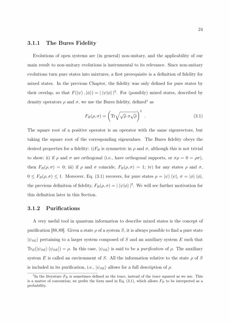
density operators ρ and σ, we use the Bures fidelity, defined1 as

FB(ρ, σ) =

(Tr√√

ρ σ√ρ

)2

. (3.1)

The square root of a positive operator is an operator with the same eigenvectors, but

taking the square root of the corresponding eigenvalues. The Bures fidelity obeys the

desired properties for a fidelity: i)FB is symmetric in ρ and σ, although this is not trivial

to show; ii) if ρ and σ are orthogonal (i.e., have orthogonal supports, or σρ = 0 = ρσ),

then FB(ρ, σ) = 0; iii) if ρ and σ coincide, FB(ρ, σ) = 1; iv) for any states ρ and σ,

0 ≤ FB(ρ, σ) ≤ 1. Moreover, Eq. (3.1) recovers, for pure states ρ = |ψ〉 〈ψ|, σ = |φ〉 〈φ|,

the previous definition of fidelity, FB(ρ, σ) = | 〈ψ|φ〉 |2. We will see further motivation for

this definition later in this Section.

3.1.2 Purifications

A very useful tool in quantum information to describe mixed states is the concept of

purification [88,89]. Given a state ρ of a system S, it is always possible to find a pure state

|ψSE〉 pertaining to a larger system composed of S and an auxiliary system E such that

TrE(|ψSE〉 〈ψSE|) = ρ. In this case, |ψSE〉 is said to be a purification of ρ. The auxiliary

system E is called an environment of S. All the information relative to the state ρ of S

is included in its purification, i.e., |ψSE〉 allows for a full description of ρ.

1In the literature FB is sometimes defined as the trace, instead of the trace squared as we use. Thisis a matter of convention; we prefer the form used in Eq. (3.1), which allows FB to be interpreted as aprobability.

25

Although inspired by physical environments, we emphasize that purifications are, first

and foremost, a theoretical construct. In other words, E is a fictitious system that need not

have any direct physical significance: we will not be interested in an accurate description

of a physical environment. For a given state ρ of S, there are infinitely many valid ways to

purify it, and our choice of purification is guided by how to describe the system S to the

best of our interest, disregarding the actual physical state of E (often favoring simplicity

and low dimensionality).

An important reason for the adoption of the Bures fidelity can be understood by

purifications. Given two states ρ and σ, the fidelity FB is the maximal fidelity between

their respective purifications |ψSE〉 and |φSE〉, where the maximum is taken over the

different purifications possible for each of the states. This result is comprised in Uhlmann’s

theorem [90], which further guarantees the existence of purifications reaching FB and also

that maximization only needs to be performed over the purifications of one of the states,

using a fixed arbitrary purification for the other. In mathematical form, Uhlmann’s

theorem reads

FB(ρ, σ) = max|φSE〉| 〈ψSE|φSE〉 |2 , (3.2)

where |ψSE〉 is an arbitrary purification of ρ, and the maximum is taken over purifications

|φSE〉 of σ. In fact, the maximization does not even need to be performed over all purifi-

cations of σ, but can be restricted to auxiliary systems E with the same dimension as S.

Besides in the original paper [90], demonstrations of this theorem can be found in [88,91].

Purifications can be used to describe non-unitary evolutions of quantum states. Given

a state ρ(t) of system S which evolves non-unitarily, there are purifications |ψSE(t)〉 for

every time t. The evolution of |ψSE(t)〉 is unitary (for the state is always pure), and can

be described by a unitary operator USE. Since a purification in S+E conveys a complete

description of the state of system S, the unitary operator USE fully characterizes the non-

unitary evolution of S. There are various other ways to describe non-unitary evolutions,

such as Kraus operators [89], Lindblad equations [88, 89] or master equations [92], but

26

because of the further importance of purification to our results, we explicitly make use

of such unitary operators. We note that this approach of a unitary evolution of a larger

system can be used to derive all three aforementioned non-unitary-evolution frameworks.

3.1.3 POVMs

Quantum theory not only entails the dynamics of a system, but also its measurement

possibilities. It is a standard postulate of the Copenhagen interpretation of quantum

mechanics (e.g. [17]) that, whereas physical observables are represented by operators O

on the Hilbert space, measurements on a quantum state ρ are represented by projection

operators Πm = |φm〉 〈φm|. This is to be understood in the sense that i) any measured

quantity will be one of the eigenvalues λm of the observable O with corresponding eigen-

state given by |φm〉, ii) the state is projected onto |φm〉 〈φm| by the measurement and

iii) the probability of finding this measurement outcome is given by Tr(ρΠm). Each such

measurement corresponds to a set Πm of projectors onto the eigenstates of O; the

Hermiticity of observable O implies that this set is composed of orthogonal projection

operators.

This type of measurement, called projective or von Neumann measurement, is never-

theless not the only possible kind. In quantum information, it is useful to deal with a

more general set, that of the so-called positive operator-valued measures (POVMs) [88].

A POVM is composed of elements Ek, each corresponding to a measurement outcome k

whose occurrence probability is given by Pk = Tr(ρEk). A POVM is a set Ek meeting

two defining properties: i) each Ek is a positive operator and ii) the set obeys a com-

pleteness relation of the form∑

k Ek = I. The simplest examples of POVMs are, in fact,

complete sets of orthogonal projectors, but the fact that the Ek need not be orthogonal

can be used to one’s advantage. Suppose [88] one is sent a system in one of two non-

orthogonal pure states |0〉 and (|0〉+ |1〉)/√

2 (with |0〉 orthogonal to |1〉) and has to find

out which of the two was received. No measurement can perfectly distinguish the two,

27

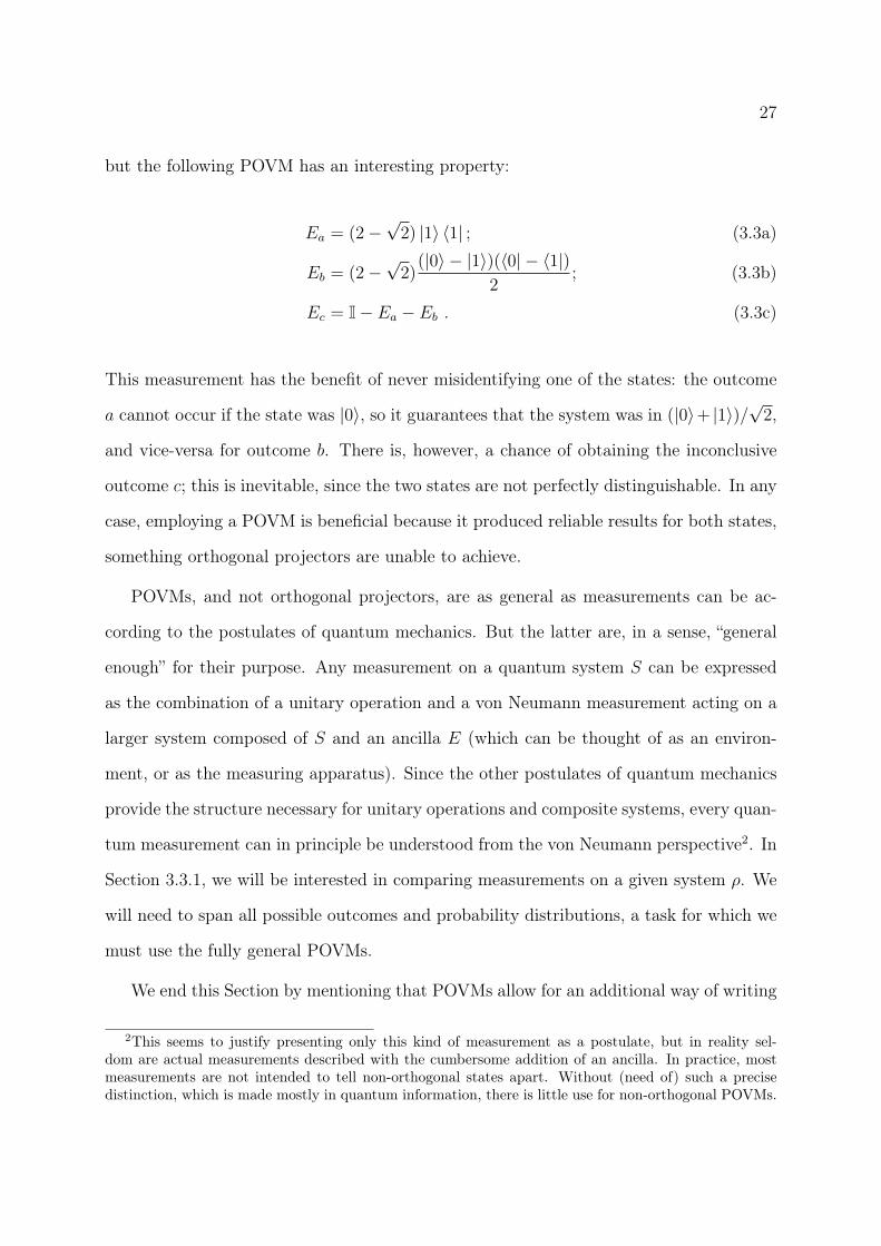
but the following POVM has an interesting property:

Ea = (2−√

2) |1〉 〈1| ; (3.3a)

Eb = (2−√

2)(|0〉 − |1〉)(〈0| − 〈1|)

2; (3.3b)

Ec = I− Ea − Eb . (3.3c)

This measurement has the benefit of never misidentifying one of the states: the outcome

a cannot occur if the state was |0〉, so it guarantees that the system was in (|0〉+ |1〉)/√

2,

and vice-versa for outcome b. There is, however, a chance of obtaining the inconclusive

outcome c; this is inevitable, since the two states are not perfectly distinguishable. In any

case, employing a POVM is beneficial because it produced reliable results for both states,

something orthogonal projectors are unable to achieve.

POVMs, and not orthogonal projectors, are as general as measurements can be ac-

cording to the postulates of quantum mechanics. But the latter are, in a sense, “general

enough” for their purpose. Any measurement on a quantum system S can be expressed

as the combination of a unitary operation and a von Neumann measurement acting on a

larger system composed of S and an ancilla E (which can be thought of as an environ-

ment, or as the measuring apparatus). Since the other postulates of quantum mechanics

provide the structure necessary for unitary operations and composite systems, every quan-

tum measurement can in principle be understood from the von Neumann perspective2. In

Section 3.3.1, we will be interested in comparing measurements on a given system ρ. We

will need to span all possible outcomes and probability distributions, a task for which we

must use the fully general POVMs.

We end this Section by mentioning that POVMs allow for an additional way of writing

2This seems to justify presenting only this kind of measurement as a postulate, but in reality sel-dom are actual measurements described with the cumbersome addition of an ancilla. In practice, mostmeasurements are not intended to tell non-orthogonal states apart. Without (need of) such a precisedistinction, which is made mostly in quantum information, there is little use for non-orthogonal POVMs.

28

the Bures fidelity, namely

FB(ρ, σ) = minEk

(∑k

√Tr(ρEk)Tr(σEk)

)2

= minEk

(∑k

√Pk(ρ)

√Pk(σ)

)2

, (3.4)

where the minimum is taken over all possible POVMs, and Pk(ρ) is the probability of out-

come k occurring with the system in state ρ (respectively for σ). This can be demonstrated

by obtaining a lower bound on FB using the polar decomposition of √ρ√σ [88, p.412].

3.2 Geometric Approach

Geometric approaches have greatly contributed to the quantum speed limit, especially

by providing a clear interpretation of the bound and a straightforward criterion for its

saturation. We first introduce and discuss key aspects of the geometry of Hilbert spaces.

This introduction is by no means exhaustive and is rather intended to show the reader

knowledgeable in quantum mechanics how a (useful) geometric structure can be built from

the space of quantum states. Although no mathematical rigor is lacking in the presented

results, demonstrations thereof expressible in familiar quantum-mechanical terms will be

favored over more mathematically rigorous versions, which will be referenced along the

way. We summarize the main results at the end of the Section.

3.2.1 A distance for pure quantum states

Any geometric structure of a set is related to the definition of a distance in this set.

A distance is a function of two elements of the set, say, x and y, and yields a real number

D(x, y). The three defining properties of a distance function are that, for any elements

x, y, z of the set,

i)D(x, y) ≥ 0 and D(x, y) = 0⇔ x = y ; (3.5a)

ii)D(x, y) = D(y, x) (symmetric) ; (3.5b)

iii)D(x, z) ≤ D(x, y) +D(y, z) (triangle inequality) . (3.5c)

29

The first, seemingly innocuous, property has an important consequence to applications

to quantum mechanics. Since two vectors of a Hilbert space which are proportional to

each other represent the exact same quantum state, we demand a physically meaningful

distance function to be null when comparing collinear states, say, |ψ〉 and 2eiφ |ψ〉. But

property i) above requires that any distance rigorously defined in the Hilbert vector space

distinguish 2eiφ |ψ〉 from |ψ〉.

The projective Hilbert space and its metric

The best way to circumvent that impediment is to work on the so-called projective

Hilbert space. A projective space is obtained from a vector space V by identifying vectors

which only differ by a nonzero prefactor. The definition of projective space also specifically

excludes the null vector. The projective space of three-dimensional flat space can be

thought of as the set of straight lines through the origin. Yet another depiction is a unit

sphere in which pairs of antipodal points are identified, since each such pair defines the

direction of a straight line through the origin. More formally, the projective space is

defined as the set of equivalent classes of V \0 by the relation ∼, where u ∼ v ⇔ u = λv

for vectors u, v ∈ V and λ 6= 0. We note that a projective space is typically not a vector

space.

When V is the Hilbert space of quantum states, the projective Hilbert space is ob-

tained. It is a set which does not distinguish 2eiφ |ψ〉 from |ψ〉 and does not include the

null vector in any form. It is also called the set of “rays” of the vector space (in analogy

with the straight-line depiction of the projective space), and the common statement that

quantum states are given by vectors on the unit sphere coincides with the aforementioned

unit-sphere image of the projective space.

Readers familiarized with the Bloch sphere should beware that there is limited analogy

between this unit-sphere image of state space and the Bloch sphere, since in the former

antipodal points represent the same state and orthogonal states are given by perpendic-

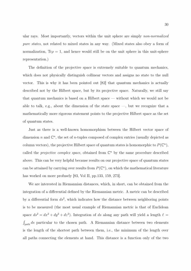
30

ular rays. Most importantly, vectors within the unit sphere are simply non-normalized

pure states, not related to mixed states in any way. (Mixed states also obey a form of

normalization, Trρ = 1, and hence would still be on the unit sphere in this unit-sphere

representation.)

The definition of the projective space is extremely suitable to quantum mechanics,

which does not physically distinguish collinear vectors and assigns no state to the null

vector. This is why it has been pointed out [82] that quantum mechanics is actually

described not by the Hilbert space, but by its projective space. Naturally, we still say

that quantum mechanics is based on a Hilbert space — without which we would not be

able to talk, e.g., about the dimension of the state space —, but we recognize that a

mathematically more rigorous statement points to the projective Hilbert space as the set

of quantum states.

Just as there is a well-known homomorphism between the Hilbert vector space of

dimension n and Cn, the set of n-tuples composed of complex entries (usually depicted as

column vectors), the projective Hilbert space of quantum states is homomorphic to P (Cn),

called the projective complex space, obtained from Cn by the same procedure described

above. This can be very helpful because results on our projective space of quantum states

can be attained by carrying over results from P (Cn), on which the mathematical literature

has worked on more profusely [83, Vol II, pp.133, 159, 273].

We are interested in Riemannian distances, which, in short, can be obtained from the

integration of a differential defined by the Riemannian metric. A metric can be described

by a differential form ds2, which indicates how the distance between neighboring points

is to be measured (the most usual example of Riemannian metric is that of Euclidean

space ds2 = dx2 + dy2 + dz2). Integration of ds along any path will yield a length ` =∫path

ds particular to the chosen path. A Riemannian distance between two elements

is the length of the shortest path between them, i.e., the minimum of the length over

all paths connecting the elements at hand. This distance is a function only of the two

31

endpoint elements, not of any path between them, and always obeys the properties given in

Eq. (3.5). We remark that this has been an oversimplified characterization and that there

are additional assumptions to the establishment of a Riemannian metric; the interested

reader is referred to [83, Chap IV] for a more complete introduction.

We then need to define a metric valid on the projective Hilbert space. More math-

ematical treatments achieve this [83, Vol II, p.159] directly on P (Cn) by way of general

theorems on complex manifolds; we prefer to start from the Hilbert vector space to build a

definition befitting the projective space (this is a deliberate choice, there are authors who

avoid the projective space almost completely, e.g. [84]). In the vector space, a differential

can be readily constructed with the usual norm. Let |dψ〉 be the infinitesimal variation of

state |ψ〉, that is, for some parameter θ on which the state depends, |dψ〉 = dθ(∂ |ψ〉 /∂θ).

A simple metric is then given by

ds20 = 〈dψ|dψ〉 . (3.6)

The integral∫ds0 along a path in the vector space defines a length, from which a distance

can be obtained. Nevertheless, ds20 is unsuitable for our purposes, since it would assign a

nonzero length to paths such as |ψ(θ)〉 = (1 + θ) |ψ0〉, θ ∈ [0, 1], and eventually a nonzero

distance between parallel states such as |ψ〉 and 2 |ψ〉. In other words, ds0 is a metric on

the vector space, not on the projective space.

We therefore need a differential form that does not distinguish collinear vectors. It

can be constructed by subtracting from |dψ〉 its projection on |ψ〉,

|dψ⊥〉 := |dψ〉 − |ψ〉 〈ψ|〈ψ|ψ〉

|dψ〉 , (3.7)

where the fraction above is a normalized projector on |ψ〉. Note that |ψ〉 is not assumed

to be normalized, we instead require that our distance does not distinguish between states

differing only by normalization (or phase). It is in fact straightforward to see that collinear

variations of |ψ〉, of the form |dψ〉 = dz |ψ〉 for complex dz, yield zero when applied above

32

to any |ψ〉. As notation suggests, |dψ⊥〉 is the component of |dψ〉 orthogonal to |ψ〉. The

“angular variation” of |dψ〉 is defined as

|dψproj〉 :=|dψ⊥〉√〈ψ|ψ〉

=1√〈ψ|ψ〉

|dψ〉 − 〈ψ|dψ〉〈ψ|ψ〉3/2

|ψ〉 , (3.8)

where an overall normalization factor has been included so that |dψproj〉 be a measure

of changes on the projective space. The form |dψ⊥〉, orthogonal to |ψ〉, can be seen

as a circle arc; the extra factor turns it into an angle, in line with the image of the

projective space as the set of straight lines (which can be fully characterized by angular

components). The need for that extra factor can also be seen by the following example

using orthogonal vectors |a〉 and |b〉. Let us perform the same variation on vectors 0.01 |a〉

and 100 |a〉, which only differ by a prefactor. Say the variation is to add |b〉. It is clear that

100 |a〉+ |b〉 is quite different from 0.01 |a〉+ |b〉, corresponding to different elements of the

projective space (equivalently, they correspond to different straight lines). The prefactor

added to (3.8) bears the fact that the greater the modulus of a vector, the smaller its

variation by an addition.

The differential form of the distance is given directly by the norm of |dψproj〉,

ds2FS = 〈dψproj|dψproj〉 =

〈dψ|dψ〉〈ψ|ψ〉

− | 〈ψ|dψ〉 |2

〈ψ|ψ〉2, (3.9)

where the subscript FS denotes that this is the Fubini-Study metric, developed indepen-

dently by Fubini [85] and Study [86]. It can already be seen that this metric is invariant

by any unitary U applied to both |ψ〉 and |ψ〉+ |dψ〉. We remark that, although written

in terms of vectors, ds2FS can only be a distance in the projective space, not on the vector

space itself.

Integrating dsFS

We now need to integrate dsFS to obtain the finite distance between two states. This

has been done for P (Cn) in [83]. Instead of simply carrying over the result, we feel it is

instructive to perform the integration and minimization here to explicitly show that, by

33

construction, we do not need to assume any normalization or phase. We do make use

of the fact that the geodesic calculated in [83, p.277] lies entirely in a two-dimensional

subspace of the vector space. This bidimensionality can be motivated by the analogy with

a unit sphere, whose geodesics — great circles — lie in a plane containing the origin [84].

Barring the trivial case where initial and final states are collinear, it should be clear that

the subspace in question is that spanned by initial and final states.

Let |ψ0〉, |ψf〉 denote the initial and final states, respectively, and let |ψ1〉 be a state

orthogonal to |ψ0〉 such that the final state is spanned by |ψ0〉 , |ψ1〉 (a Gram-Schmidt

procedure can always produce a suitable |ψ1〉). Since the integration path belongs to the

two-dimensional space spanned by |ψ0〉 , |ψf〉 or, equivalently, spanned by |ψ0〉 , |ψ1〉,

we can write the state of the system along evolution as

|ψ(t)〉 = f(t) |ψ0〉+ g(t) |ψ1〉 , (3.10)

where t is a real parameter (not necessarily time), f , g are complex functions of t, and

no normalization is required from |ψ(t)〉, |ψ0〉, |ψf〉 or |ψ1〉. We demand g(0) = 0 and

f(0) 6= 0, such that the initial state of the system be identified with |ψ0〉. (Since we only

require |ψ(0)〉 ∼ |ψ0〉, it is not even necessary that |f(0)| = 1.) The finite distance DFS

is obtained by inserting Eq. (3.10) into Eq. (3.9), integrating dsFS to obtain a length `FS

and then finding the path (i.e., f(t) and g(t)) that minimizes this length. These steps are

performed in Appendix A, and the result is that the distance between initial state |ψ0〉

and final state |ψf〉 measured by the Fubini-Study metric is [86]

DFS(|ψ0〉 , |ψf〉) = arccos

(| 〈ψ0|ψf〉 |√

〈ψ0|ψ0〉√〈ψf |ψf〉

). (3.11)

We note that DFS = π/2 if the states are orthogonal, in which case it is maximal. The

independence of this distance on the phase and normalization of either state is explicit in

the above formula. Wootters [87] has proposed that this distance also serves as a measure

of statistical fluctuations in a sequence of measurements of quantum states. Moreover,

34

DFS is the only Riemannian distance (up to rescaling) invariant by any unitary [86, 87].

The argument of the arc cosine above is the square root of the fidelity between the two

states, so we can also write

DFS(|ψ0〉 , |ψf〉) = arccos√F (|ψ0〉 , |ψf〉) . (3.12)

A consistency check left to the reader is to apply DFS to two neighboring states and

obtain3 dsFS.

Geodesics of the Fubini-Study metric

We can also find the geodesics linking any two given states. Since the geodesics

belong to a two-dimensional subspace, we can discuss them using the Bloch sphere4.

From Appendix A we know that states of the form Eq. (3.10) will travel along a geodesic

if and only ifg(t)

f(t)= ξ(t)

g(tf )

f(tf ), (3.13)

where ξ(t) is any monotonic real function null at t = 0 and equal to one at t = tf and

f(tf ), g(tf ) are such that the combination in Eq. (3.10) equals |ψf〉 at tf .

Let us begin by the geodesics linking non-orthogonal states, so that f(t) 6= 0 for all

times and singularities are avoided. Eq. (3.13) then guarantees that the ratio g(t)/f(t) is

well-behaved, and we can hence write

|ψ(t)〉 = f(t)

(|ψ0〉+

g(t)

f(t)|ψ1〉

). (3.14)

We can disregard the overall factor f(t) and substitute Eq. (3.13) in Eq. (3.14), obtaining

|ψ(t)〉 = |ψ0〉+ ξ(t)g(tf )

f(tf )|ψ1〉 , (3.15)

from which one sees that the relative phase between the components is fixed along the

path. This necessarily implies that geodesics lie along a great circle of the Bloch sphere.3The relation arccos

√1− x = x1/2 +O(x3/2) may be of help.

4For readers unfamiliar with the Bloch sphere, it is a standard vector representation of a qubit statevery similar to the expectation value 〈~S〉 of a spin-1/2 system, see [89, p.168].

35

These conclusions can be seen even more clearly if, without any loss of generality, the

phase of |ψf〉 is chosen such that g(tf )/f(tf ) ∈ R, making both coefficients of |ψ(t)〉 real.

Bloch vectors with all real components are confined to a plane and, given that these are

pure states, to a great circle. There are two paths between two non-orthogonal states

along a great circle of the Bloch sphere. It is intuitive that the geodesic is given by the

shorter of these paths. This is indeed confirmed by Eq. (3.15) in that |ψ(t)〉 is never

orthogonal to |ψ0〉.

For orthogonal states, one may use the divisibility of geodesic paths, i.e., the fact

that any (compact) section of a geodesic is also a geodesic. Let |ψf〉 be orthogonal to

|ψ0〉. Because every vector in the vicinity of |ψf〉 is linked to |ψ0〉 through a great-circle

geodesic, the (infinitely many) great circles linking |ψ0〉 to |ψf〉 are the only suitable

candidates for the geodesics. It can be easily seen that all such great circles are, in fact,

geodesics between the orthogonal states.

We observe that, although the geometry of pure quantum states shown so far is anal-

ogous to Euclidean geometry on the Bloch sphere, the analogies break down with the

inclusion of mixed states.

Comments on another distance

We now take a moment to mention another function present in the discussion of

distances in quantum state space, the Bures distance5

DBures(|ψ0〉 , |ψf〉) =√

2

√1−

√F (|ψ0〉 , |ψf〉) . (3.16)

This is a distance in the projective Hilbert space in the sense that it obeys the axioms of

Eq. (3.5), but it is not Riemannian, because it cannot be obtained as the shortest path

along elements of the projective space. It is possible, though, to obtain DBures as the5The nomenclature becomes quite cumbersome here: the Bures distance is different from the so-called

Bures angle (a.k.a. Bures arc or even Bures length, even though it is a distance, not a length, by geometricdefinitions), which is a generalization of the Fubini-Study distance; all of them can be written in termsof the Bures fidelity.

36

length of a path along the Hilbert vector space. The distinction matters because this

path must necessarily go through nonnormalized vectors and this length is only obtained

when distinguishing collinear vectors (differing only by normalization). This is shown

in Fig. 3.1, which represents the vector space as a plane: only through the straight-line

(solid) path is DBures attained. Were the path traveled on the unit circle (dashed line), it

would coincide with a special case of the Fubini-Study metric, and DFS would be found6.

This assertion can perhaps be seen best by the fact that the above form is only valid

ÈΨ0\

ÈΨ1\

ÈΨm\

Figure 3.1: Depiction of a two-dimensional Hilbert space. Integration on the straight lineyields DBures, but is unsuited for our purposes, because the distance thus obtained wouldnecessarily distinguish collinear vectors. We note that states inside the unit circle (dashedline), like |ψm〉, are pure, but not normalized.

for unit vectors. If we write this distance for vectors of different norm, such as |ψm〉 of

Fig. 3.1, we get

DBures(|ψ0〉 , |ψm〉) =√〈ψ0|ψ0〉+ 〈ψm|ψm〉 − 2| 〈ψ0|ψm〉 | . (3.17)

In other words, the Bures distance is only Riemannian if one distinguishes between

collinear vectors. If restricted to unit vectors, it is a valid distance on the projective

Hilbert space, but loses its Riemannian character7. Most importantly, it certainly cannot6We warn the reader familiarized with the Bloch sphere that, contrary to first intuition, intermediate

states like |ψm〉 in Fig. 3.1 are pure, nonnormalized states.7For the sake of completeness, we mention that DBures is the shortest length on the quotient space

obtained by identifying vectors which differ only by a phase, as can be seen by the phase-independence

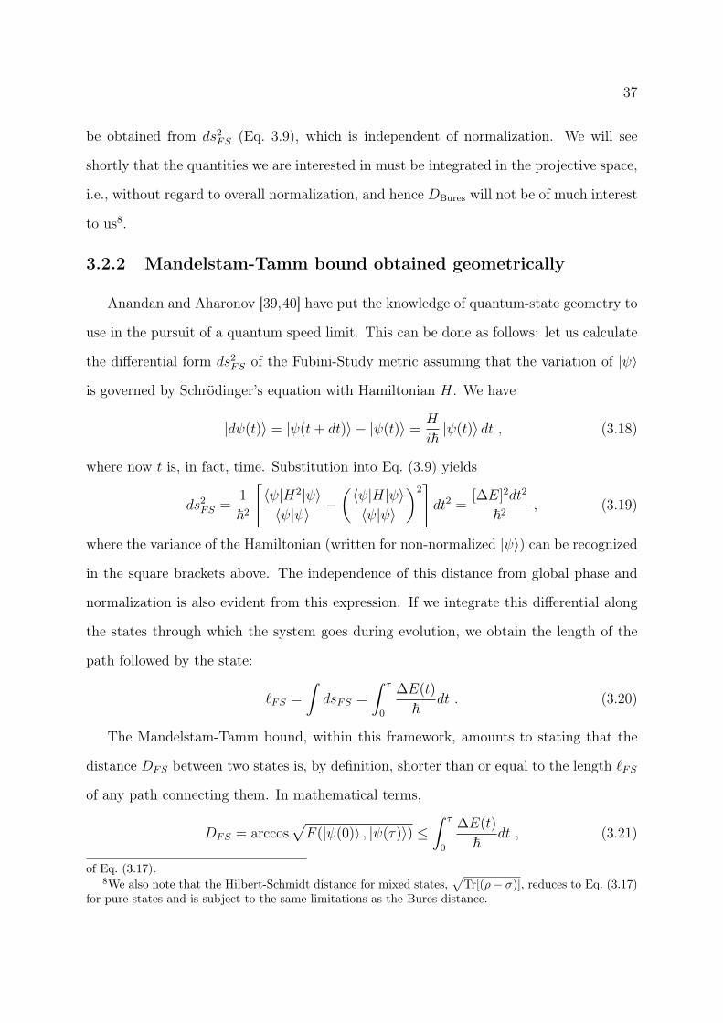
37

be obtained from ds2FS (Eq. 3.9), which is independent of normalization. We will see

shortly that the quantities we are interested in must be integrated in the projective space,

i.e., without regard to overall normalization, and hence DBures will not be of much interest

to us8.

3.2.2 Mandelstam-Tamm bound obtained geometrically

Anandan and Aharonov [39,40] have put the knowledge of quantum-state geometry to

use in the pursuit of a quantum speed limit. This can be done as follows: let us calculate

the differential form ds2FS of the Fubini-Study metric assuming that the variation of |ψ〉

is governed by Schrödinger’s equation with Hamiltonian H. We have

|dψ(t)〉 = |ψ(t+ dt)〉 − |ψ(t)〉 =H

i~|ψ(t)〉 dt , (3.18)

where now t is, in fact, time. Substitution into Eq. (3.9) yields

ds2FS =

1

~2

[〈ψ|H2|ψ〉〈ψ|ψ〉

−(〈ψ|H|ψ〉〈ψ|ψ〉

)2]dt2 =

[∆E]2dt2

~2, (3.19)

where the variance of the Hamiltonian (written for non-normalized |ψ〉) can be recognized

in the square brackets above. The independence of this distance from global phase and

normalization is also evident from this expression. If we integrate this differential along

the states through which the system goes during evolution, we obtain the length of the

path followed by the state:

`FS =

∫dsFS =

∫ τ

0

∆E(t)

~dt . (3.20)

The Mandelstam-Tamm bound, within this framework, amounts to stating that the

distance DFS between two states is, by definition, shorter than or equal to the length `FS

of any path connecting them. In mathematical terms,

DFS = arccos√F (|ψ(0)〉 , |ψ(τ)〉) ≤

∫ τ

0

∆E(t)

~dt , (3.21)

of Eq. (3.17).8We also note that the Hilbert-Schmidt distance for mixed states,

√Tr[(ρ− σ)], reduces to Eq. (3.17)

for pure states and is subject to the same limitations as the Bures distance.

38

recovering Eq. (2.3). We note that this demonstration is valid for pure states evolving

unitarily.

A slightly different interpretation of the above formula is more useful for the obtention

of bounds on evolution time. In a given evolution, the most a final state can be distant

from the initial one is the length of the path followed by the system. Accordingly, the

minimal time necessary for the distance to reach a chosen value (or, equivalently, for the

fidelity to reach a chosen value) is the time at which the path length reaches this value.

This can be seen with the help of the graph on Fig.3.2, where ∆E(t)/~ is plotted against

time. Given a certain value D1 of the distance, the minimal time τ needed to reach it is

that which makes the area under the curve ∆E(t)/~ equal D1.

t1

DE HtL

Ñ

t2t

Figure 3.2: Example of plot of ∆E(t)/~ over time t. The bound on the time for a certaindistance D1 to be reached is given by the value t = τ such that the area under the graphequals D1.

A breakthrough of the geometric interpretation of the bound was to enable a clear,

straightforward criterion for its saturation: it occurs when evolution follows a geodesic.

We have seen that geodesics are great circles of the Bloch sphere. On the other hand, any

Hamiltonian evolution of a qubit is locally a rotation around some axis of the Bloch sphere.

A state evolving along a geodesic must then perform a rotation around a fixed axis and,

furthermore, belong to a great circle, which must, then, be the equator relative to this

axis. The only pure states that obey these conditions and hence saturate the Mandelstam-

Tamm inequality for unitary evolutions are equiprobable on any pair of energy eigenstates

39

|Ei〉, |Ej〉, or

|ψ(t)〉 =1√2

(|Ei〉+ e−iφ(t) |Ej〉

), (3.22)

where the phase φ(t) has a monotonic dependence on t. Although H must be a rotation

around a fixed axis, there can be a time dependence of the form H(t) = ~ω(t)σ, where σ

is the Pauli operator relative to the direction of the axis, as long as ω(t) does not change

sign. The phase φ(t) is related to H(t) by φ(t) =∫ t

0ω(t′)dt′.

Summary

The main results of this Section are that Anandan and Aharonov recognized ∆E(t)dt/~

as the differential of a well established metric, the Fubini-Study metric. This allowed the

bound to be reinterpreted as stating that the length of any path is greater than or equal

to the distance between its endpoints. The (finite) distance measured by this metric is

DFS(|ψ0〉 , |ψf〉) = arccos√F (|ψ0〉 , |ψf〉), whereas the length is the integral of ∆E(t)dt/~,

and so the inequality is proved in geometric terms. Saturation occurs on geodesic paths,

where the length equals the distance between the endpoints.

We end this Section with a simple analogy. The quantity ∆E(t)/~ is the speed of

evolution. It is analogous to what is measured by the speedometer of a car, in that it

does not distinguish the direction of the path in any way. Given a traveled course, the

information given by the speedometer allows one to calculate the traveled length ` along

the path and, furthermore, the time τ it takes to travel such length. Since the actual

straight-line (geodesic) distance D between starting and finish points may not be greater

than the length (D ≤ `), τ is a lower bound on the time needed to become D apart from

the starting point. Only if the path is traveled in a straight line do length and distance

coincide.

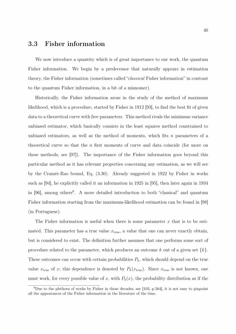
40

3.3 Fisher information

We now introduce a quantity which is of great importance to our work, the quantum

Fisher information. We begin by a predecessor that naturally appears in estimation

theory, the Fisher information (sometimes called “classical Fisher information” in contrast

to the quantum Fisher information, in a bit of a misnomer).

Historically, the Fisher information arose in the study of the method of maximum

likelihood, which is a procedure, started by Fisher in 1912 [93], to find the best fit of given

data to a theoretical curve with free parameters. This method rivals the minimum variance

unbiased estimator, which basically consists in the least squares method constrained to

unbiased estimators, as well as the method of moments, which fits n parameters of a

theoretical curve so that the n first moments of curve and data coincide (for more on

these methods, see [97]). The importance of the Fisher information goes beyond this

particular method as it has relevant properties concerning any estimation, as we will see

by the Cramér-Rao bound, Eq. (3.30). Already suggested in 1922 by Fisher in works

such as [94], he explicitly called it an information in 1925 in [95], then later again in 1934

in [96], among others9. A more detailed introduction to both “classical” and quantum

Fisher information starting from the maximum-likelihood estimation can be found in [98]

(in Portuguese).

The Fisher information is useful when there is some parameter x that is to be esti-

mated. This parameter has a true value xtrue, a value that one can never exactly obtain,

but is considered to exist. The definition further assumes that one performs some sort of

procedure related to the parameter, which produces an outcome k out of a given set k.

These outcomes can occur with certain probabilities Pk, which should depend on the true

value xtrue of x; this dependence is denoted by Pk(xtrue). Since xtrue is not known, one

must work, for every possible value of x, with Pk(x), the probability distribution as if the

9Due to the plethora of works by Fisher in those decades, see [103, p.564], it is not easy to pinpointall the appearances of the Fisher information in the literature of the time.

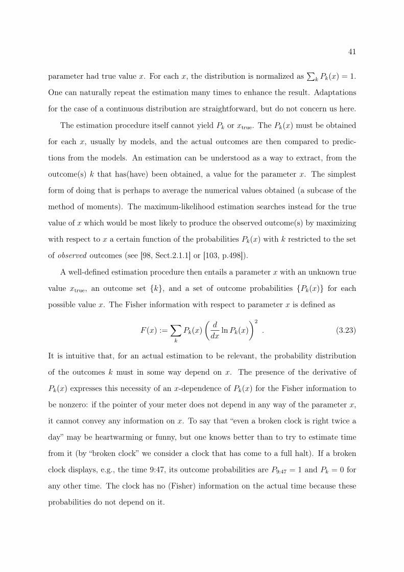
41

parameter had true value x. For each x, the distribution is normalized as∑

k Pk(x) = 1.

One can naturally repeat the estimation many times to enhance the result. Adaptations

for the case of a continuous distribution are straightforward, but do not concern us here.

The estimation procedure itself cannot yield Pk or xtrue. The Pk(x) must be obtained

for each x, usually by models, and the actual outcomes are then compared to predic-

tions from the models. An estimation can be understood as a way to extract, from the

outcome(s) k that has(have) been obtained, a value for the parameter x. The simplest

form of doing that is perhaps to average the numerical values obtained (a subcase of the

method of moments). The maximum-likelihood estimation searches instead for the true

value of x which would be most likely to produce the observed outcome(s) by maximizing

with respect to x a certain function of the probabilities Pk(x) with k restricted to the set

of observed outcomes (see [98, Sect.2.1.1] or [103, p.498]).

A well-defined estimation procedure then entails a parameter x with an unknown true

value xtrue, an outcome set k, and a set of outcome probabilities Pk(x) for each

possible value x. The Fisher information with respect to parameter x is defined as

F (x) :=∑k

Pk(x)

(d

dxlnPk(x)

)2

. (3.23)

It is intuitive that, for an actual estimation to be relevant, the probability distribution

of the outcomes k must in some way depend on x. The presence of the derivative of

Pk(x) expresses this necessity of an x-dependence of Pk(x) for the Fisher information to

be nonzero: if the pointer of your meter does not depend in any way of the parameter x,

it cannot convey any information on x. To say that “even a broken clock is right twice a

day” may be heartwarming or funny, but one knows better than to try to estimate time

from it (by “broken clock” we consider a clock that has come to a full halt). If a broken

clock displays, e.g., the time 9:47, its outcome probabilities are P9:47 = 1 and Pk = 0 for

any other time. The clock has no (Fisher) information on the actual time because these

probabilities do not depend on it.

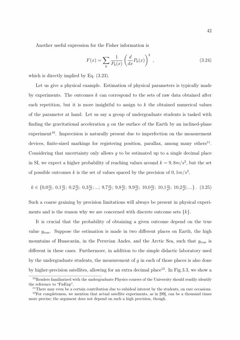
42

Another useful expression for the Fisher information is

F (x) =∑k

1

Pk(x)

(d

dxPk(x)

)2

, (3.24)

which is directly implied by Eq. (3.23).

Let us give a physical example. Estimation of physical parameters is typically made

by experiments. The outcomes k can correspond to the sets of raw data obtained after

each repetition, but it is more insightful to assign to k the obtained numerical values

of the parameter at hand. Let us say a group of undergraduate students is tasked with

finding the gravitational acceleration g on the surface of the Earth by an inclined-plane

experiment10. Imprecision is naturally present due to imperfection on the measurement

devices, finite-sized markings for registering position, parallax, among many others11.

Considering that uncertainty only allows g to be estimated up to a single decimal place

in SI, we expect a higher probability of reaching values around k = 9, 8m/s2, but the set

of possible outcomes k is the set of values spaced by the precision of 0, 1m/s2,

k ∈ 0,0ms2

; 0,1ms2

; 0,2ms2

; 0,3ms2

; ...; 9,7ms2

; 9,8ms2

; 9,9ms2

; 10,0ms2

; 10,1ms2

; 10,2ms2

; ... . (3.25)

Such a coarse graining by precision limitations will always be present in physical experi-

ments and is the reason why we are concerned with discrete outcome sets k.

It is crucial that the probability of obtaining a given outcome depend on the true

value gtrue. Suppose the estimation is made in two different places on Earth, the high

mountains of Huascarán, in the Peruvian Andes, and the Arctic Sea, such that gtrue is

different in these cases. Furthermore, in addition to the simple didactic laboratory used

by the undergraduate students, the measurement of g in each of those places is also done

by higher-precision satellites, allowing for an extra decimal place12. In Fig.3.3, we show a

10Readers familiarized with the undergraduate Physics courses of the University should readily identifythe reference to “FisExp”.

11There may even be a certain contribution due to subideal interest by the students, on rare occasions.12For completeness, we mention that actual satellite experiments, as in [99], can be a thousand times

more precise; the argument does not depend on such a high precision, though.

43

simulation of the distributions of Pk(gtrue) in the four cases, assuming gtrue = 9, 76392m/s2

(Huascarán, Andes) and gtrue = 9, 83366m/s2 (Arctic Sea); these two values are inspired

by measured data taken from [99]. The Pk or gtrue cannot be obtained by measurements;

instead, models (of measurement and dynamics) assign Pk for each possible g, and the

actual measurements are then compared to distributions from the models. The capability

æææææææææææ

æ

æ

æ

æ

æ

æææ

æ

æ

æ

æ

æ

æ

æææææææææææàààààààààà

àà

à

à

à

à

à

ààà

à

à

à

à

à

à

àààààààààà

8.5 9.5 10.5 11.5k Hms2L

0.02

0.06

0.1

PkHgtrueLUndergraduate students

ææææææææææ

æ

æ

æ

æ

æ

ææ

æ

æ

æ

æ

æ

ææææææææææææææààààààààààààààà

àà

à

à

à

à

à

àà

à

à

à

à

à

ààààààà

9.65 9.75 9.85 9.95k Hms2L

0.02

0.06

0.1

PkHgtrueLSatellite measurement

Figure 3.3: Values of Pk(gtrue) for a measurement of g in Huascarán, in the Andes (bluecircles) and at the Arctic Sea (red squares). The distributions within each image are dif-ferent because so is gtrue. Measurement as made in a simple laboratory (left) is comparedto that by higher-precision satellites (right).

of Pk(g) to discern a minute difference in the true value of g is essential for a precise

estimation. The higher precision of the satellite experiments is translated in the way it is

easier to distinguish the true values of g from the Pk of these measurements. The Fisher

information is a measure of this very property: how much does the outcome distribution

change by a change of the underlying true value of the parameter?

This interpretation is helped out by the definition of the Hellinger distance, a distance

between probability distributions Pk for a given set k of outcomes. If one assumes

that two probability distributions are different because they belong to two different values

x, x′ of the parameter, the Hellinger distance DH can be written as a function of these

values [100, p.33] (or [98, p.16])

DH(x, x′) =

√1

2

∑k

[√Pk(x′)−

√Pk(x)

]2

. (3.26)

We remark nonetheless that DH is a distance only on the set of probability distributions.

It obeys Eq. (3.5), and especially Eq. (3.5a), for the probability distributions Pk, P ′k,

44

not necessarily for parameter values x, x′. In other words, DH(x, x′) does not measure

variations of the parameter x, but instead how distinguishable the distribution Pk(x)

becomes if x is varied. If distinct parameter values correspond to the same distribution,

as in the broken clock, DH will be zero.

These aspects of the Hellinger distance are analogous to some of what has been said

about the Fisher information, and we now show how they are mathematically related.

The first step is to rewrite the Fisher information as

F (x) = 4∑k

(d

dx

√Pk(x)

)2

, (3.27)

and then to write DH for infinitesimally separated arguments x, x+ dx:

D2H(x, x+ dx) =

1

2

∑k

[√Pk(x+ dx)−

√Pk(x)

]2

=1

2

∑k

[d

dx

√Pk(x)

]2

dx2 . (3.28)

By comparing the two equations, it is easy to see that, to lowest order in dx,

D2H(x, x+ dx) = ds2

H =F (x)

8dx2 , (3.29)

i.e., the Fisher information is the core of the infinitesimal form of that distance, measuring

how probability distributions grow apart due to an infinitesimal variation of the parameter.

Another sign of the importance of the Fisher information is that it bounds the precision

of any parameter estimation. This connection is established by the Cramér-Rao bound,

shown independently by Rao [102] and Cramér [103, p.480], although some results had

been anticipated by Fisher, as recognized in [104]. The Cramér-Rao relation states that

the error δx of an estimation is bounded from below:

δx ≥ 1√F (x)

. (3.30)

Our interest will be to use the Fisher information not in estimation theory, but as (the

square of) a speed related to the geometry of quantum states, so the reader interested in

this result (and its proof) is referred to a more detailed discussion to be found in [101,

Sect.2] or in [98, Sect.2.1.2 onwards], which are works dedicated specifically to parameter

estimation.

45

3.3.1 The quantum Fisher information

The Fisher information can naturally be applied to the estimation of a parameter via

a physical measurement, be it on a classical or quantum system. Although no estimation,

in either case, can be exact, there is an important difference in the sources of imprecisions

in the classical and quantum scenarios. Classically, it is the imperfection of the measure-

ment/estimation process that introduces errors; classical states themselves would allow

for perfect estimations if probed by perfect, idealized apparatus. In quantum mechanics,

indeterminacy originates additionally from the probabilistic nature of quantum states.

Even with ideal measurements, one cannot in general obtain complete information about

a parameter on which a quantum state depends, because it is not possible, in general, to

distinguish between two non-orthogonal quantum states. The quantum Fisher informa-

tion aims to quantify how much about a certain parameter can be learned by a quantum

state that depends on it, assuming the best measurements possible. The classical coun-

terpart to this quantity would be trivially infinite — different classical states are always

perfectly distinguishable —; the goal here is to measure how imperfect the information

possessed by a quantum state is (alternatively, how finite it is).

An important difference between the original Fisher information and its quantum

version is that, whereas the former is defined for each specific estimation procedure, the

latter is a function solely of the quantum state and of its dependence on the parameter to

be estimated. This is possible because the Fisher information requires a set of outcomes

and its occurrence probabilities, while quantum measurement theory, by indicating what

the possible measurements are, supplies both of these. The quantum Fisher information

is, in fact, the Fisher information of the best measurement available on the quantum state.

Let us now give an introductory example, admittedly oversimplified. Consider that

one wishes to measure the coupling constant λ of an interaction between a field and a

two-level atom13. Atom and field will be left to interact for a certain time T , and the13The interaction in this example is given by the Jaynes-Cummings model on resonance.

46

experiment makes a measurement solely on the atom. The main idea is that the atom

starts in a state |a〉 and is driven to |b〉 by the field. The stronger the coupling constant

λ, the closer to |b〉 the final state will be. Let us assume for the sake of simplicity that

there is a maximal value to λ, which is λ = 1, and that the total interaction time T is so

chosen that the final state will be exactly |b〉 if λ = 1. Other values of λ will leave the

state after T in a mixture of |a〉 and |b〉,

ρT =

(λ 00 1− λ

), (3.31)

with the representation |a〉 =(

01

), |b〉 =

(10

).

By letting the system interact for a time T and measuring ρT in this basis, |a〉 , |b〉,

one can make a crude estimate of the value of λ. Since pa = 1− λ and pb = λ, the Fisher

information for this estimation is

Fa,b(λ) =1

pa

(∂pa∂λ

)2

+1

pb

(∂pb∂λ

)2

=(−1)2

1− λ+

12

λ=

1

λ(1− λ), (3.32)

where the subscript a, b indicates the measurement basis. One can see from this ex-

pression that the estimate is worst for values of λ close to 1/2, as expected14. Due to the

idealizations in this model, when λ equals 0 or 1, the measurement outcome is certain.

This is reflected by the behavior F (λ) → ∞ on these two values, which corresponds to

the possibility of making an error-free measurement. A more realistic description would

be to assume some degree of irremovable mixture on the initial and final states, which

would produce a well-behaved F (λ). We nevertheless keep treating this idealization in

order to present some of the important ideas.

As crude as this estimation may be, it is certainly better than to measure in the

“rotated” basis |+〉 , |−〉, with |±〉 := 1√2(|a〉 ± |b〉). The outcomes on this basis have

no dependence on λ (p = 1/2 for both measurements for every λ) and hence yield no

14A possibility to reduce error is, of course, to repeat the experiment multiple times. It has beenshown [98, p.17] that the Fisher information is additive, i.e., in ν independent runs of an estimation,Fν(x) = νF1(x).

47

information whatsoever on the parameter, F±(λ) = 0. It can be shown that the original

basis |a〉 , |b〉 is, in fact, the most capable of distinguishing values of λ. The quantum

Fisher information for the estimation of λ, denoted FQ(λ), of the state ρT from Eq. (3.31)

is precisely the Fisher information of the best measurement,

FQ(λ) = Fa,b(λ) =1

λ(1− λ). (3.33)

Now turning to a more formal discussion, we know from Section 3.1.3 that all possible

measurements on a quantum system are given by POVMs. In the above example, simple

orthogonal projectors were used, Ea = |a〉 〈a|, Eb = |b〉 〈b|, E+ = |+〉 〈+|, E− = |−〉 〈−|,

and the POVMs employed to obtain the Fisher information were Ea, Eb for Fa,b(λ)

and E+, E− for F±(λ). In general, the quantum Fisher information for estimation of

parameter x is defined as the maximum of the Fisher information over all POVMs, i.e.,

FQ(x) := maxEk

F (x)|Ek

= maxEk

∑k

1

Tr (ρ(x)Ek)

[d

dxTr (ρ(x)Ek)

]2

, (3.34)

where we have used that Pk(x) = Tr(ρ(x)Ek).

The Cramér-Rao bound is still valid for FQ(x), but it is now a bound not on the error

of a specific estimation procedure, but on the error of any estimation of x from state ρ(x).

The quantum Cramér-Rao bound reads

δx ≥ 1√FQ(x)

. (3.35)

We are interested, however, in viewing the quantum Fisher information in a different

light. We have seen that it is a quantity depending only on the state ρ and on its

dependence on the parameter x. The example given in Fig. 3.3 shows that the “classical”

Fisher information can measure how much probability distributions grow apart as the

parameter varies. Since the quantum version maximizes the Fisher information over all

possible measurements, FQ should be sensitive to any variation of ρ. In fact, we now show

an important result that substantiates this interpretation.

48

Suppose one is interested in distinguishing two neighboring states, characterized by

parameter values x and x′, using measurements indicated by the POVM Ek. The

Hellinger distance Eq.(3.26) between the two probability distributions is

D2H(x, x′) =

1

2

∑k

(√Pk(x)−

√Pk(x′)

)2

= 1−∑k

√Pk(x)

√Pk(x′) . (3.36)

Now let us assume that x and x′ are infinitesimally separated, x′ = x + dx. We know

from Eq. (3.29) that D2H(x, x+ dx) is related to the (“classical”) Fisher information F (x),

so that

1−∑k

√Pk(x)

√Pk(x+ dx) =

F (x)

8

∣∣∣∣Ek

dx2 . (3.37)

The subscript on the right-hand side serves as a reminder that this equation is valid for

any POVM. By choosing the POVM that maximizes this equation, both left- and right-

hand sides at the same time. By writing the above for such a POVM, we obtain, due to

the definition of the quantum Fisher information and to Eq. (3.4),

1−√FB[ρ(x), ρ(x+ dx)] =

FQ(x)

8dx2 , (3.38)

or, solving for FB,

FB[ρ(x), ρ(x+ dx)] = 1− FQ(x)

4dx2 +O(dx4) . (3.39)

This very important relation shows that, as we have mentioned less formally, the quantum

Fisher information is a measure of the rate at which a state becomes distinct following

the variation of a parameter. When the parameter in question is time,√FQ(t) can

be understood as a speed of the evolving state. This result will be relevant for our

geometrically-derived bound in the next Section.

Another important expression for the quantum Fisher information can be obtained by

the use of the symmetric logarithmic derivative L(x) [105, 106]. For a given parameter x

and a given state ρ(x), L(x) is the Hermitian operator implicitly defined by

d

dxρ(x) =

ρ(x)L(x) + L(x)ρ(x)

2. (3.40)

49

This is, in fact, a way to quantize the classical expression dp/dx = pd(ln p)/dx accounting

for the non-commutativity of ρ and dρ/dx. The existence of such an operator is guaranteed

by an application of the Riesz-Fréchet theorem to Hilbert spaces [106, p.257].

We reproduce the derivation in [98, p.37] of the relation linking FQ(x) to L(x). It

begins with a bound on FQ(x), obtained observing that[d

dxPk(x)

]2

=

[d

dxTr (ρ(x)Ek)

]2

=

[Tr

(dρ(x)

dxEk

)]2

(3.41a)

=

[Tr

(ρ(x)L(x) + L(x)ρ(x)

2Ek

)]2

(3.41b)

=

[Tr

(ρLEk + EkLρ

2

)]2

=[Re(Tr (ρLEk)

)]2 (3.41c)

≤ |Tr (ρLEk)|2 =

∣∣∣∣Tr

[(ρ1/2E

1/2k

)† (ρ1/2LE

1/2k

)]∣∣∣∣2 . (3.41d)

But the inner product (A,B) = Tr(A†B) obeys the Cauchy-Schwarz inequality, so[d

dxPk(x)

]2

≤ Tr

[(ρ1/2E

1/2k

)† (ρ1/2E

1/2k

)]Tr

[(ρ1/2LE

1/2k

)† (ρ1/2LE

1/2k

)](3.41e)

= Pk(x)Tr [ρ(x)L(x)EkL(x)] . (3.41f)

The quantum Fisher information is then bounded by

FQ(x) = maxEk

∑k

1

Pk(x)

[d

dxPk(x)

]2

(3.42a)

≤ maxEk

∑k

Tr [ρ(x)L(x)EkL(x)] (3.42b)

= Tr[ρ(x)L2(x)

]. (3.42c)

To demonstrate the equality, we must show that there is a POVM Ek such that

both inequalities in Eqs. (3.41) turn into equalities for all k. For Eq. (3.41d), equality

amounts to

Im(Tr (ρ(x)L(x)Ek)

)= 0 , (3.43)

while equality in the Cauchy-Schwarz relation of Eq. (3.41e) is equivalent to

ρ1/2(x)L(x)E1/2k = λk(x)ρ1/2(x)E

1/2k (3.44)

50

for some15 complex λk(x). We remark that if a POVM obeys Eq. (3.44) with real λk(x)

for all k, both conditions are met. But this last equation can be rewritten as

ρ1/2(x) (L(x)− λk(x)I)E1/2k = 0 . (3.45)

By taking projector POVMs, such that E2k = Ek = E

1/2k , we can assure that there

is at least one solution to the above for each k, because L(x) is Hermitian and hence

diagonalizable with real eigenvalues.

We have thus shown that the quantum Fisher information can be written as

FQ(x) = Tr(ρ(x)L2(x)

). (3.46)

This can be understood as an alternate definition of the quantum Fisher information,

somewhat analogous to Eq. (3.23). The concision of this expression does not incur in

an easier calculation of FQ(x), since the symmetric logarithmic derivative is often cum-

bersome to obtain. We show in Section 4.1 a more feasible method of calculating the

quantum Fisher information developed by our group [110,111].

We now turn to the Section where we present our main result.

3.4 The most general quantum speed limit

We are now ready to derive our main result, the bound on quantum evolutions be they

unitary or not. This is a bound that encompasses any kind of evolution a quantum system

can undergo. Because non-unitary evolutions can turn pure states into mixed ones, the

first step will be to define a distance valid for mixed as well as pure states. We make

extensive use of the purifications presented in Section 3.1.2.

15The case ρ1/2(x)E1/2k = 0 need not obey Eq. (3.44), but attains both equalities in Eqs. (3.41d, 3.41e)

trivially, since (ρ1/2(x)E1/2k )† = E

1/2k ρ1/2(x) = 0.

51

3.4.1 A distance for all quantum states

Along the lines of Section 3.2, we are interested in metrics that can be computed by

integrating a differential form. Let us define the differential form of the distance between

two neighboring states ρ and ρ + dρ as the minimal Fubini-Study differential of their

respective purifications |ψ〉 and |ψ〉+ |dψ〉,

ds2α

∣∣ρ,ρ+dρ

:= minpurif

ds2FS

∣∣∣∣|ψ〉,|ψ〉+|dψ〉

, (3.47)

where the minimum is taken over all purifications of ρ and ρ + dρ, but can equivalently

be taken over the purifications of only one of the states. The corresponding length is

`α :=

∫path

dsα =

∫path

minpurif

dsFS . (3.48)

We are interested in minimizing not the integrand, but the integrated length. The first

condition to do so is to have a non-negative integrand, which dsFS is by definition. A

second potential hindrance would be the fact that each state ρ along the path belongs

to two differentials on the integration, (ρ − dρ, ρ) and (ρ, ρ + dρ), except for the path

endpoints. The purification of ρ used to minimize the distance of the first pair could,

in principle, not be compatible with minimizing the latter pair. This is however not the

case, because we know dsFS can be expressed as a decreasing function of the fidelity F

(or overlap) of two pure states, and we have seen in Eq. (3.2) that the maximization of

the fidelity of two purifications can be performed varying the purification of only one of

the mixed states. We may then write

`α = minpurif

∫path

dsFS = minpurif

`FS , (3.49)

where minimization is now performed over all purifications of each state of the path.

A distance can, as before, be defined as the length of the shortest path between two

states,

D(ρ, σ) := minpath

`α = minpath

minpurif

`FS

, (3.50)

52

but the order of the minimizations may be inverted, so that

D(ρ, σ) = minpurif

minpath

`FS

= min

purifDFS(|ψ〉 , |φ〉) = min

purifarccos

√F (|ψ〉 , |φ〉) , (3.51)

with the minimization being performed over all purifications |ψ〉, |φ〉 of ρ, σ. Because

DFS is a decreasing function of the fidelity, we can write

D(ρ, σ) = arccos√

maxpurif

F (|ψ〉 , |φ〉) = arccos√FB(ρ, σ) , (3.52)

where we have used Uhlmann’s theorem, Eq. (3.2).

This distance is called Bures angle (among other names, see footnote on p. 35), and

is not only valid as a distance for mixed quantum states, but also possesses the most

important of the Riemannian features, that of being able to be obtained as an integral of

a differential ds. Just as with the Fubini-Study distance on p. 34, a consistency check left

to reader is to verify that D(ρ, σ) = ds for infinitesimally separated ρ, σ.

It is indeed quite intuitive to generalize the Fubini-Study distance to mixed states

by replacing the pure-state fidelity for the Bures fidelity, but there are two reasons for

carrying the derivation as above. Firstly, it explicitly shows the relation between the

finite Bures angle and its differential ds. Secondly, there are other functions of two mixed

states that recover the pure-state fidelity in the proper limit; this route reinforces the

importance of the Bures fidelity by naturally arriving at it via Uhlmann’s theorem.

3.4.2 The bound

We now have a proper distance also for mixed states, but what is its relation to the

dynamics of a quantum system? This is our main result, obtained in collaboration with

B.M. Escher, L. Davidovich, R.L. de Matos Filho and published in [81].

Let us consider a state ρ(t) which evolves in time from t = 0 to t = τ and travels a

given path. The length of this path is necessarily greater than (or equal to) the distance

between ρ(0) and ρ(τ). This statement, written in a shorthand notation in which D(0, τ)

53

is the distance between these two states (and analogously for any D(t1, t2) at other times),

reads

D(0, τ) ≤ `α =

∫path

dsα . (3.53)

But dsα can be written in terms of D by noting that

D(t, t+ t′) =∂D(t, t+ t′)

∂t′t′ +O(t′2) , (3.54)

so that, with η = t+ t′ and taking t′ to be infinitesimal,

dsα =∂D(t, η)

∂η

∣∣∣∣η→t

dt . (3.55)

The length is then written as

`α =

∫ τ

0

∂D(t, η)

∂η

∣∣∣∣η→t

dt . (3.56)

Since only through the Bures fidelity does the distance depend on the states, and hence

on the parameter η, the integrand can be calculated using the chain rule,

∂D(t, η)

∂η

∣∣∣∣η→t

=

[dD(FB)

dFB

∂FB(t, η)

∂η

]η→t

, (3.57)

where FB(t, η) = FB (ρ(t), ρ(η)) and D(FB) is a notation used to stress that the distance

D is a function of FB. We know from the relation between these two (Eq. 3.52) that

dD(FB)/dFB tends to infinity in the limit at hand, FB → 1. Furthermore, Eq. (3.39)

informs us that the first derivative of FB, ∂FB(t, η)/∂η vanishes for η → t. The indeter-

minacy can be removed with the aid of l’Hôpital’s rule,

∂D(t, η)

∂η

∣∣∣∣η→t

=

∂FB(t, η)

∂η1

dD(FB)/dFB

∣∣∣∣∣∣∣∣η→t

=

∂2FB(t, η)

∂η2

d

dFB

[1

dD(FB)/dFB

]∂FB(t, η)

∂η

∣∣∣∣∣∣∣∣η→t

. (3.58)

The numerator is, due to Eq. (3.39), proportional to the quantum Fisher information.

The denominator, when multiplied and divided by dD/dFB, yields(− 1

[dD(FB)/dFB]3d2D(FB)

dF 2B

)(dD(FB)

dFB

∂FB(t, η)

∂η

)∣∣∣∣η→t

. (3.59)

54

The first factor in parentheses can be calculated independently of t, η by replacing the

limit η → t by FB → 1 since the metric D only depends on t, η through FB(t, η). The

second factor in parentheses is simply a recurrence of ∂D(t, η)/∂η|η→t, the term we are

calculating. Substituting in (3.58) and rearranging the terms, one finds

[∂D(t, η)

∂η

]2

η→t=

[dD(FB)

dFB

]3

d2D(FB)

dF 2B

∣∣∣∣∣∣∣∣∣FB→1

FQ(t)

2. (3.60)

Multiplying and dividing by 2, the length is given by

`α =

√2 [dD(FB)/dFB]3

d2D(FB)/dF 2B

∣∣∣∣∣∣FB→1

∫ τ

0

√FQ(t)

4dt , (3.61)

and substitution in Eq. (3.53) leads to the general bound√d2D(FB)/dF 2

B

2 [dD(FB)/dFB]3

∣∣∣∣∣FB→1

D(0, τ) ≤∫ τ

0

√FQ(t)

4dt . (3.62)

Let us make three comments about the formula above. First, the integral of the

quantum Fisher information is to be interpreted as a path integral parametrized by time

t. FQ(t) is a local quantity, dependent on the state at t and its neighboring values, and

hence dependent on the chosen path. Another relevant remark is that the freedom to

regauge the distance by a constant k, D → kD, does not affect the bound, since the D-

dependent prefactor in the equation cancels such a constant. Lastly, because dD(FB)/dFB

diverges at FB → 1, the bound can be rewritten as√|d2D(FB)/dF 2

B|2 1 + [dD(FB)/dFB]23/2

∣∣∣∣∣FB→1

D(0, τ) ≤∫ τ

0

√FQ(t)

4dt, (3.63)

and this shows that this prefactor depends on the curvature of the graph of D(FB) as a

function of FB at FB → 1.

We can now replace D(FB) for D(FB) = arccos√FB:

arccos√FB [ρ(0), ρ(τ)] ≤

∫ τ

0

√FQ(t)/4 dt , (3.64)

55

where the prefactor tends to one. This is the main result of the present thesis. It can be

summarized as: the length of the traveled path in state space must be less than (or equal

to) the distance between initial and final states. For infinitesimal variations, the length

is in fact equal to the distance. This implies that the relation above is an equality in the

immediate vicinity of τ = 0. Eq. (3.39) applied to time serves as a suitable expansion to

show that the bound is saturated up to second order in time:

FB[ρ(0), ρ(dt)] = 1− FQ(0)

4dt2 +O(dt4) . (3.65)

Although originally defined in quantum metrology, the quantum Fisher information

for time estimation is closely related to the dynamics of the system. This is seen best by

remembering that FQ(t) = Tr[ρ(t)L2(t)] and seeing that

ρ =1

2[ρ(t)L(t) + L(t)ρ(t)] , (3.66)

where the dot over ρ represents the time derivative. In fact, there is a closed form for

L(t) for unitary evolutions which clearly reflects the dynamics of the system. Any unitary

evolution can be written as

ρ(t) = U(t)ρ(0)U †(t) , (3.67)

with U(t)U †(t) = I = U †(t)U(t), and equivalently as

ρ(t) =1

i~

[i~ U(t)U †(t), ρ(t)

]= [H(t), ρ(t)] , (3.68)

with H(t) = i~ U(t)U †(t) being the Hamiltonian governing the evolution, i~U = HU .

For a system always in pure states, the relation ρ2(t) = ρ(t) can be derived with

respect to time, so

ρρ+ ρρ = ρ (3.69)

ρLρ+ Lρρ+ ρLρ+ ρρL = ρL+ Lρ (3.70)

ρLρ = 0 , (3.71)

56

such that

ρρ =1

2[ρρL+ ρLρ] =

ρL

2; (3.72)

ρρ =1

2[ρLρ+ Lρρ] =

Lρ

2. (3.73)

The last two, together with ρ2(t) = ρ(t), allow us to write

FQ(t) = Tr(ρL2)

(3.74)

= Tr (ρLLρ) (3.75)

= 4Tr (ρρρρ) (3.76)

= 4Tr(ρρ2)

(3.77)

= − 4

~2Tr(ρ [H, ρ]2

)(3.78)

=4

~2[∆H]2 , (3.79)

where [∆H]2 is the variance of H(t). We thus see that, for unitary pure-state evolutions,

the quantum Fisher information for time estimation is simply the energy variance of the

system. Substituting this result in the general bound, Eq. (3.64), we exactly recover

the Mandelstam-Tamm bound for unitary evolutions, Eqs. (2.12), (3.21). The result of

Eq. (3.79) will be of utmost importance to the method we will present in Section 4.1 to

calculate the quantum Fisher information.

This geometric derivation provides, as before, a clear criterion for saturation. Equality

will prevail on Eq. (3.64) if, and only if, the state travels on a geodesic. We note that

pure-state geodesics are still geodesics on the space of density operators, but that there

are more geodesic paths, even for a qubit. In Chapter 4, we apply this bound to different

examples, and in some cases we will see saturation, i.e., evolution on geodesics.

A last comment is that related derivations are possible for parameter estimation, with

which the precision of estimates of parameter θ can be bound employing the quantum

Fisher information for estimation of θ, FQ(θ).

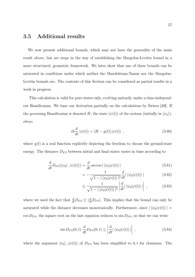
57

3.5 Additional results

We now present additional bounds, which may not have the generality of the main

result above, but are steps in the way of establishing the Margolus-Levitin bound in a

more structured, geometric framework. We later show that one of these bounds can be

saturated in conditions under which neither the Mandelstam-Tamm nor the Margolus-

Levitin bounds are. The contents of this Section can be considered as partial results in a

work in progress.

This calculation is valid for pure states only, evolving unitarily under a time-independ-

ent Hamiltonian. We base our derivation partially on the calculations by Zwierz [49]. If

the governing Hamiltonian is denoted H, the state |ψ(t)〉 of the system (initially in |ψ0〉),

obeys

i~d

dt|ψ(t)〉 = [H − g(t)] |ψ(t)〉 , (3.80)

where g(t) is a real function explicitly depicting the freedom to choose the ground-state

energy. The distance DFS between initial and final states varies in time according to

d

dtDFS(|ψ0〉 , |ψ(t)〉) =

d

dtarccos | 〈ψ0|ψ(t)〉 | (3.81)

= − 1√1− | 〈ψ0|ψ(t)〉 |2

d

dt| 〈ψ0|ψ(t)〉 | (3.82)

≤ 1√1− | 〈ψ0|ψ(t)〉 |2

∣∣∣∣ ddt | 〈ψ0|ψ(t)〉 |∣∣∣∣ , (3.83)

where we used the fact that ddtDFS ≤ | ddtDFS|. This implies that the bound can only be

saturated while the distance decreases monotonically. Furthermore, since | 〈ψ0|ψ(t)〉 | =

cosDFS, the square root on the last equation reduces to sinDFS, so that we can write

sinDFS(0, t)d

dtDFS(0, t) ≤

∣∣∣∣ ddt | 〈ψ0|ψ(t)〉 |∣∣∣∣ , (3.84)

where the argument |ψ0〉 , |ψ(t)〉 of DFS has been simplified to 0, t for cleanness. The

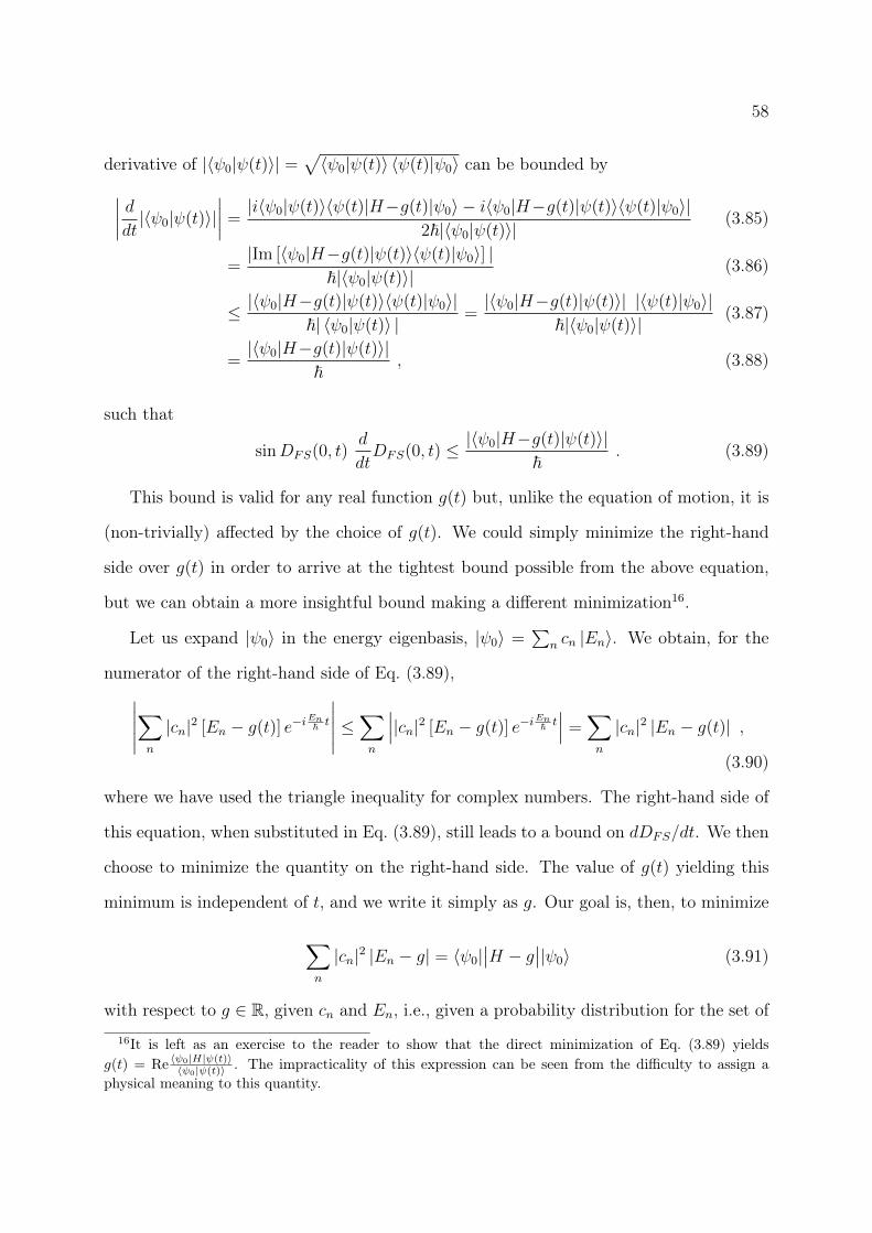
58

derivative of |〈ψ0|ψ(t)〉| =√〈ψ0|ψ(t)〉 〈ψ(t)|ψ0〉 can be bounded by∣∣∣∣ ddt |〈ψ0|ψ(t)〉|

∣∣∣∣ =|i〈ψ0|ψ(t)〉〈ψ(t)|H−g(t)|ψ0〉 − i〈ψ0|H−g(t)|ψ(t)〉〈ψ(t)|ψ0〉|

2~|〈ψ0|ψ(t)〉|(3.85)

=|Im [〈ψ0|H−g(t)|ψ(t)〉〈ψ(t)|ψ0〉] |

~|〈ψ0|ψ(t)〉|(3.86)

≤ |〈ψ0|H−g(t)|ψ(t)〉〈ψ(t)|ψ0〉|~| 〈ψ0|ψ(t)〉 |

=|〈ψ0|H−g(t)|ψ(t)〉| |〈ψ(t)|ψ0〉|

~|〈ψ0|ψ(t)〉|(3.87)

=|〈ψ0|H−g(t)|ψ(t)〉|

~, (3.88)

such that

sinDFS(0, t)d

dtDFS(0, t) ≤ |〈ψ0|H−g(t)|ψ(t)〉|

~. (3.89)

This bound is valid for any real function g(t) but, unlike the equation of motion, it is

(non-trivially) affected by the choice of g(t). We could simply minimize the right-hand

side over g(t) in order to arrive at the tightest bound possible from the above equation,

but we can obtain a more insightful bound making a different minimization16.

Let us expand |ψ0〉 in the energy eigenbasis, |ψ0〉 =∑

n cn |En〉. We obtain, for the

numerator of the right-hand side of Eq. (3.89),∣∣∣∣∣∑n

|cn|2 [En − g(t)] e−iEn~ t

∣∣∣∣∣ ≤∑n

∣∣∣|cn|2 [En − g(t)] e−iEn~ t∣∣∣ =

∑n

|cn|2 |En − g(t)| ,

(3.90)

where we have used the triangle inequality for complex numbers. The right-hand side of

this equation, when substituted in Eq. (3.89), still leads to a bound on dDFS/dt. We then

choose to minimize the quantity on the right-hand side. The value of g(t) yielding this

minimum is independent of t, and we write it simply as g. Our goal is, then, to minimize

∑n

|cn|2 |En − g| = 〈ψ0|∣∣H − g∣∣|ψ0〉 (3.91)

with respect to g ∈ R, given cn and En, i.e., given a probability distribution for the set of

16It is left as an exercise to the reader to show that the direct minimization of Eq. (3.89) yieldsg(t) = Re 〈ψ0|H|ψ(t)〉

〈ψ0|ψ(t)〉 . The impracticality of this expression can be seen from the difficulty to assign aphysical meaning to this quantity.

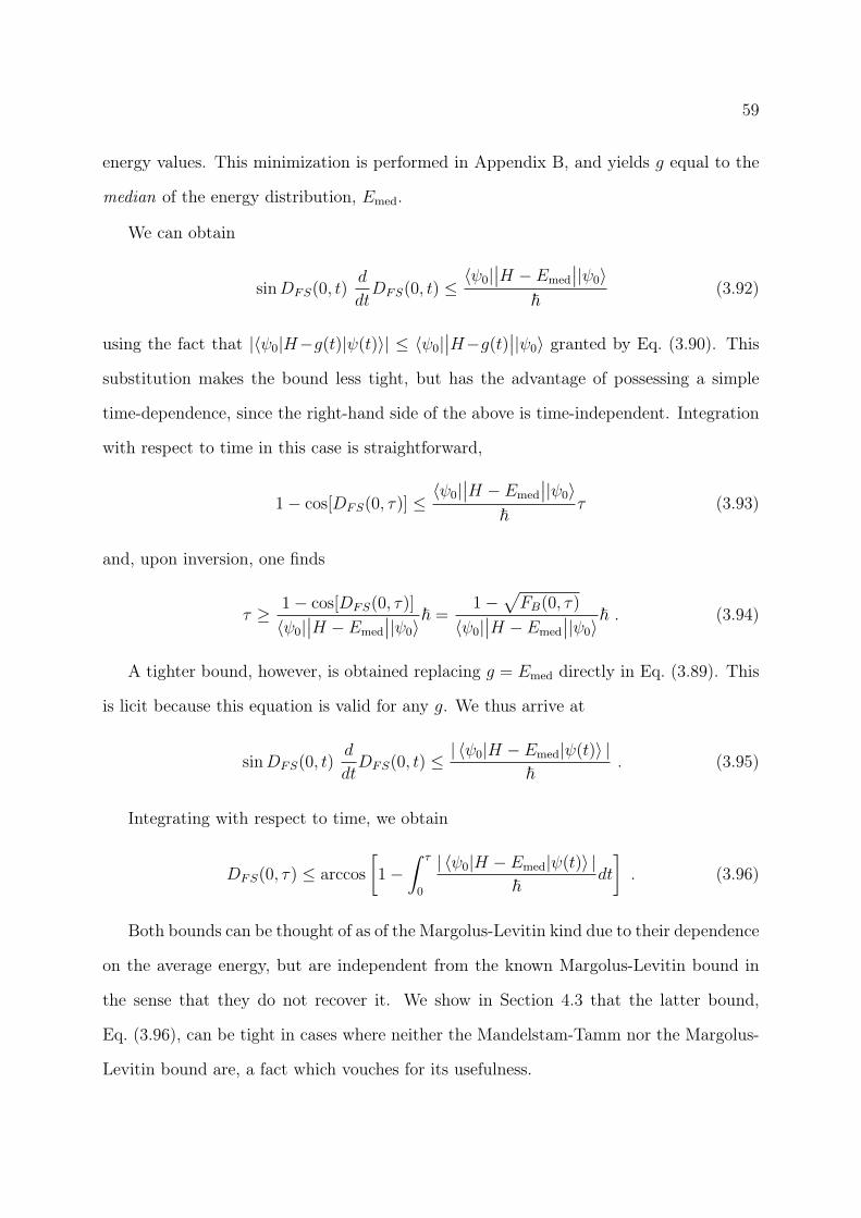
59

energy values. This minimization is performed in Appendix B, and yields g equal to the

median of the energy distribution, Emed.

We can obtain

sinDFS(0, t)d

dtDFS(0, t) ≤

〈ψ0|∣∣H − Emed

∣∣|ψ0〉~

(3.92)

using the fact that |〈ψ0|H−g(t)|ψ(t)〉| ≤ 〈ψ0|∣∣H−g(t)

∣∣|ψ0〉 granted by Eq. (3.90). This

substitution makes the bound less tight, but has the advantage of possessing a simple

time-dependence, since the right-hand side of the above is time-independent. Integration

with respect to time in this case is straightforward,

1− cos[DFS(0, τ)] ≤〈ψ0|

∣∣H − Emed

∣∣|ψ0〉~

τ (3.93)

and, upon inversion, one finds

τ ≥ 1− cos[DFS(0, τ)]

〈ψ0|∣∣H − Emed

∣∣|ψ0〉~ =

1−√FB(0, τ)

〈ψ0|∣∣H − Emed

∣∣|ψ0〉~ . (3.94)

A tighter bound, however, is obtained replacing g = Emed directly in Eq. (3.89). This

is licit because this equation is valid for any g. We thus arrive at

sinDFS(0, t)d

dtDFS(0, t) ≤ | 〈ψ0|H − Emed|ψ(t)〉 |

~. (3.95)

Integrating with respect to time, we obtain

DFS(0, τ) ≤ arccos

[1−

∫ τ

0

| 〈ψ0|H − Emed|ψ(t)〉 |~

dt

]. (3.96)

Both bounds can be thought of as of the Margolus-Levitin kind due to their dependence

on the average energy, but are independent from the known Margolus-Levitin bound in

the sense that they do not recover it. We show in Section 4.3 that the latter bound,

Eq. (3.96), can be tight in cases where neither the Mandelstam-Tamm nor the Margolus-

Levitin bound are, a fact which vouches for its usefulness.

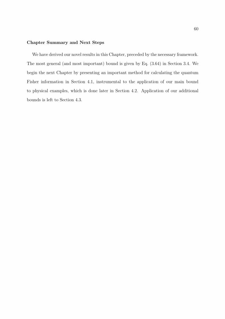
60

Chapter Summary and Next Steps

We have derived our novel results in this Chapter, preceded by the necessary framework.

The most general (and most important) bound is given by Eq. (3.64) in Section 3.4. We

begin the next Chapter by presenting an important method for calculating the quantum

Fisher information in Section 4.1, instrumental to the application of our main bound

to physical examples, which is done later in Section 4.2. Application of our additional

bounds is left to Section 4.3.

61

Chapter 4

Applying the bounds

After having presented our novel results in the last Chapter, we now devote ourselves

to the application of those bounds to physical evolutions. We start by introducing in

Section 4.1 an important technique, developed by collaborators B.M. Escher, N. Zagury,

R.L. de Matos Filho and L. Davidovich [110, 111], for obtaining the quantum Fisher

information, a quantity central to our main result of Eq. (3.64). In Section 4.2 we proceed

to the actual application of the bound to non-unitary evolutions. Section 4.3 is left to the

application of the additional bounds of Eqs. (3.94,3.96).

4.1 Calculating the quantum Fisher information

4.1.1 A purification-based expression

An apparent disadvantage of our bound of Eq. (3.64) is the difficulty to calculate the

quantum Fisher information. We here present a method which enables the calculation of

this quantity based on purifications.

The basic idea is that the non-unitary evolution of a given system can be described

by the unitary evolution of its purification. We have seen in Eq. (3.79) that the quantum

Fisher information of a unitary evolution is easy to evaluate. We will see how the quantum

Fisher information of the original system and that of its purification are related.

Let us consider, as in Section 3.1.2, a system S in state ρ(t) evolving non-unitarily.

62

A purification of ρ(t) requires an auxiliary system, denoted E (for “environment”), and is

given by a joint state |ψS,E(t)〉 such that

TrE(|ψS,E(t)〉 〈ψS,E(t)|

)= ρ(t) ∀ t . (4.1)

Let us consider |ψS,E(t)〉 to be an arbitrary purification of ρ(t) out of the infinitely many

possible. Because |ψS,E(t)〉 contains all information about ρ(t), it is physically reasonable

that the quantum Fisher information of the former is at least as great as that of the

latter. In fact, the quantum Fisher information of |ψS,E(t)〉, denoted CQ(t), acts as an

upper bound on the quantum Fisher information of ρ(t). This can be shown by using the

definition of quantum Fisher information, Eq. (3.34), as well as the fact that a POVM

element E(S)k acting only on S can be understood as E(S)

k ⊗ I(E), where I(E) is the identity

on E:

TrS(ρ(t)E(S)k ) = TrS,E(|ψS,E(t)〉 〈ψS,E(t)|E(S)

k ⊗ I(E)) . (4.2)

We can then write the quantum Fisher information of the state of S as

FQ(t) = maxE(S)

k ⊗I(E)

F (t)|E(S)

k ⊗I(E)

, (4.3)

whereas that of the purification reads

CQ(t) = maxE(S,E)

k

F (t)|E(S,E)

k

, (4.4)

where E(S,E)k is a POVM element acting on the joint system S +E. The quantum Fisher

information of the purification is then the result of a maximization over all POVMs on

S + E, a larger family than that of the original system, i.e., FQ(t) is maximized on a

subset of that used for CQ(t). Hence FQ(t) ≤ CQ(t).

The state |ψS,E(t)〉 remains pure along its evolution, which must then be describable by

a unitary operator US,E(t). The Hamiltonian governing the evolution can always be found

by HS,E(t) = i~US,E(t)U †S,E(t), and we know from Eq. (3.79) that the quantum Fisher

63

information of a unitary evolution is proportional to the variance of its Hamiltonian, so

that

CQ(t) =4

~2[∆HS,E(t)]2 . (4.5)

Bringing these results together, we can find a bound on evolution times written in terms

of ∆HS,E(t),

arccos√FB [ρ(0), ρ(τ)] ≤

∫ τ

0

√FQ(t)

4dt ≤

∫ τ

0

√CQ(t)

4dt =

1

~

∫ τ

0

∆HS,E(t) dt . (4.6)

Written in this form, in terms of any purification of ρ(t), the bound may or may not be

tight. The choice of purification in fact affects the saturation of the speed limit.

We show in Appendix C that for each evolution there is at least one purification whose

quantum Fisher information equals that of the original system, i.e., there is a purifica-

tion such that CQ(t) = FQ(t). It can be obtained by minimizing CQ(t), or equivalently

∆HS,E(t), over all purifications such that E has the same dimension as S. This means

that all saturation features of our main bound carry over to the above if one minimizes

over such purifications.

In some situations it may, however, be advantageous to forgo the exact obtention of

FQ(t) and minimize CQ(t) over a restricted family of purifications for the sake of prac-

ticality. We undertake both full and partial optimization in the examples in the next

Section.

Before we move on to the non-unitary channels, we mention that which is perhaps the

simplest application of this purification procedure: an initially mixed state of S evolving

unitarily. It is possible to purify it such that the Hamiltonian governing the evolution of

the purification |ψS,E(t)〉 is the original Hamiltonian acting on the mixed state. Applying

this to Eq. (4.6), one can generalize Eqs. (2.3,3.21) to

D(0, τ) = arccos√FB [ρ(0), ρ(τ)] ≤

∫ τ

0

∆E(t)

~dt , (4.7)

where the standard deviation ∆E(t) of the Hamiltonian is calculated in the pure or mixed

state of system S. This result for unitary evolutions has been shown by Uhlmann in [41]

64

also by geometric means. In this case, the purification yielding the minimum is in fact

the one governed by the original Hamiltonian, so that the bound above is tight under the

same conditions of the general bound.

4.2 Application to non-unitary channels

We now consider some examples of non-unitary evolutions, or channels, to which we

apply our bound. As mentioned previously, our description is made in terms of purifi-

cations. Given a state ρ(t) of system S that evolves non-unitarily, let |ψS,E(t)〉 be a

purification of it. The evolution of this pure state in time can always be described by a

suitable unitary operator, denoted US,E(t), so that |ψS,E(t)〉 = US,E(t) |ψS,E(0)〉.

We know from the previous Section that, in order to obtain the quantum Fisher

information (or a useful bound on it), we need the variance of the Hamiltonian HS,E(t)

respective to US,E(t),

HS,E(t) = i~US,E(t)U †S,E(t) . (4.8)

This variance is, in principle, to be evaluated at time t, i.e., in state |ψS,E(t)〉. There is

nevertheless a tactic to make this evaluation easier: the expectation value of an operator

in state |ψS,E(t)〉 can be cast as an expectation value in the initial state |ψS,E(0)〉 if the

evolution operators are “absorbed” by HS,E(t). For an operator that satisfies

HS,E(t) = U †S,E(t)HS,E(t)US,E(t) , (4.9)

its averaging obeys

〈ψS,E(0)|HS,E(t)|ψS,E(0)〉 = 〈ψS,E(t)|HS,E(t)|ψS,E(t)〉 (4.10)

and the same goes for any polynomial function ofHS,E. This definition presents a practical

advantage: the form of the state in which the expectation values are taken is simplified,

because there is no time dependence anymore, but the operator maintains a similar level

65

of complexity when expressed in terms of US,E,

HS,E(t) := i~U †S,E(t)US,E(t) (4.11)

(compare Eq. 4.8). This equation can, in fact, be taken as a definition of HS,E(t). This

tactic is not restricted to US,E, along this Chapter we define several analogous operators

based on different unitaries. The use of fraktur/gothic or other modified fonts always

denotes the employment of this tactic for initial-state averaging, see Table 4.1. We note

that, for self-commuting Hamiltonians, [H(t), H(t′)] = 0 ∀ t, t′, this tactic does not change

the operator, i.e., H(t) = H(t).

Another important point is that the purification |ψS,E(t)〉 of the process characterized

by ρ(t) is not unique. The freedom to choose different purifications can be expressed in the

following manner: given a first purification |ψS,E(t)〉 and its unitary evolution operator

US,E(t), every other purification of the process can be obtained through

uE(t)US,E(t) |ψS,E(0)〉 , (4.12)

by varying uE(t), a unitary operator acting only on system E (note that uEUS,E is also

unitary). When we need to minimize over all purifications, as required by Section 4.1, it

suffices to minimize over all unitary operators uE(t) acting on the environment E only.

Moreover, we are interested in minimizing the variance of the Hamiltonian correspond-

ing to the unitary operator uE(t)US,E(t). We once again use the tactic for initial-state

averaging, so that we are faced with the problem of minimizing the variance of

HS,E(t) := i~ [uE(t)US,E(t)]†d

dt[uE(t)US,E(t)] . (4.13)

It is straightforward to show that HS,E can be written as

HS,E(t) = HS,E(t) + U †S,E(t)hE(t)US,E(t) , (4.14)

where hE(t) := i~u†E(t)uE(t) is defined from hE(t) analogously to the way HS,E(t) was

from HS,E(t), see Table 4.1. The minimization over uE(t) then amounts to minimizing

over all possible Hermitian operators hE(t).

66

Evolution operator Hamiltonian Corrected HamiltonianUS,E(t) HS,E(t) HS,E(t)uE(t) hE(t) hE(t)

uE(t)US,E(t) HS,E(t)Table 4.1: Notational correspondence between evolution operator and Hamiltonian. Thelast column indicates the notation for the Hamiltonian corrected for initial-state averaging,as defined by Eq. (4.11) for the first line and analogously for the rest of the table.

Turning once more to the mixed state evolving unitarily, the suitable first purification

is that whose evolution is governed by the original Hamiltonian. It is then straightforward

to see that uE(t) = I, corresponding to hE(t) = 0, yields the minimal variance of HS,E(t)

from Eq. (4.14).

4.2.1 Amplitude-damping channel

The first example to which we apply our bound is the so-called amplitude-damping

channel. This channel is useful for describing energy loss: a qubit (system S) initially

in the excited state |e〉 that decays onto the ground state |g〉. We suppose there is a

probability P (t) of |e〉 not decaying to |g〉 in the interval [0, t] (conversely, a probability

1 − P (t) of a |e〉 → |g〉-decay up to time t; it should be clear that P (0) = 1). This

evolution of S is described by

ρ(0) =

(ρgg ρgeρ∗ge ρee

)→ ρ(t) =

(ρgg + [1− P (t)]ρee

√P (t)ρge√

P (t)ρ∗ge P (t)ρee

), (4.15)

with the representation |g〉 =(

10

), |e〉 =

(01

). The most prevalent case of the amplitude-

damping channel is when ρge = 0 = ρgg and the system is initially in the excited state

|e〉. In this scenario, the qubit evolves along mixtures of |e〉 and |g〉 with varying weights.

In the Bloch sphere, this corresponds to a path along the axis connecting |e〉 to |g〉, see

Fig. 4.1.

For the purposes of calculating the quantum Fisher information, we now need to write

the evolution of S in the form of a purification, which explicitly includes an auxiliary

system E. System E only needs to be a qubit, so whenever the initial state of S is pure

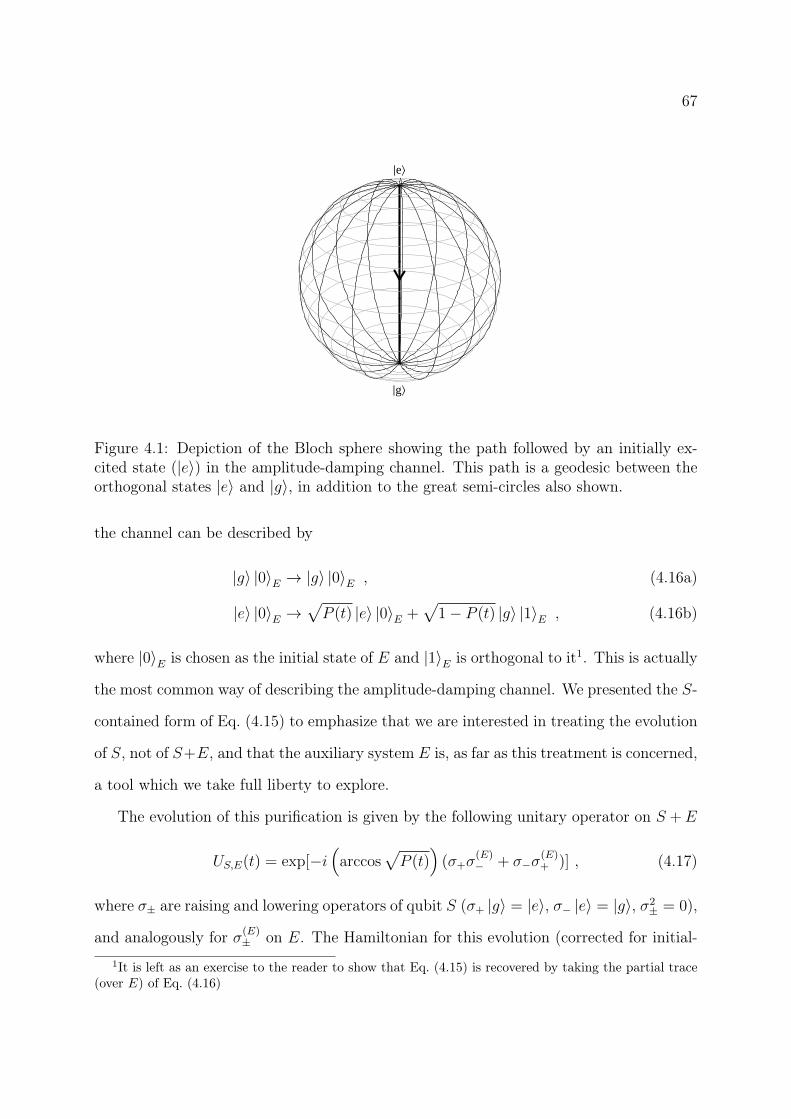
67

Èe\

Èg\

Figure 4.1: Depiction of the Bloch sphere showing the path followed by an initially ex-cited state (|e〉) in the amplitude-damping channel. This path is a geodesic between theorthogonal states |e〉 and |g〉, in addition to the great semi-circles also shown.

the channel can be described by

|g〉 |0〉E → |g〉 |0〉E , (4.16a)

|e〉 |0〉E →√P (t) |e〉 |0〉E +

√1− P (t) |g〉 |1〉E , (4.16b)

where |0〉E is chosen as the initial state of E and |1〉E is orthogonal to it1. This is actually

the most common way of describing the amplitude-damping channel. We presented the S-

contained form of Eq. (4.15) to emphasize that we are interested in treating the evolution

of S, not of S+E, and that the auxiliary system E is, as far as this treatment is concerned,

a tool which we take full liberty to explore.

The evolution of this purification is given by the following unitary operator on S +E

US,E(t) = exp[−i(

arccos√P (t)

)(σ+σ

(E)− + σ−σ

(E)+ )] , (4.17)

where σ± are raising and lowering operators of qubit S (σ+ |g〉 = |e〉, σ− |e〉 = |g〉, σ2± = 0),

and analogously for σ(E)± on E. The Hamiltonian for this evolution (corrected for initial-

1It is left as an exercise to the reader to show that Eq. (4.15) is recovered by taking the partial trace(over E) of Eq. (4.16)

68

state averaging) is

HS,E(t) := i~U †S,E(t)US,E(t) = ~d arccos

√P (t)

dt

(σ+σ

(E)− + σ−σ

(E)+

), (4.18)

from which we obtain the bound CQ(t) on the quantum Fisher information:

CQ(t)

4=

1

~2[∆HS,E(t)]2 = 〈σ+σ−〉

(d arccos

√P (t)

dt

)2

, (4.19)

where the variance is calculated in the initial state of S +E (hence the expectation value

〈σ+σ−〉 is to be calculated in the initial state of S). The corresponding bound on evolution

time is given by

D(0, τ) ≤√〈σ+σ−〉

∫ τ

0

∣∣∣∣∣d arccos√P (t)

dt

∣∣∣∣∣ dt . (4.20)

A first result is that if the initial state of S is |g〉, the bound shows exactly that the

distance D(0, τ) remains zero, as it must according to Eq. (4.16a). Furthermore, if P is a

monotonic (decreasing) function of t, integration can be performed at once and yields

D(0, τ) = arccos√FB(0, τ) ≤

√〈σ+σ−〉 arccos

√P (τ) . (4.21)

An example is the exponential damping P (t) = e−γt, for which

D(0, τ) ≤√〈σ+σ−〉 arccos e−γτ/2 , (4.22)

or

τ ≥ 2

γln

(sec

D√〈σ+σ−〉

). (4.23)

If system S is initially in state |e〉, the expectation value 〈σ+σ−〉 = 1 and the bound

is saturated, since for this case FB(0, τ) = P (τ), see Eq. (4.21). We can draw a couple of

conclusions from this fact. Firstly, saturation implies that CQ(t) above is the minimum

over different purifications for initial states |e〉 or |g〉, i.e. CQ(t) = FQ(t). This is, in fact,

an exception: we see in the next Subsections that the first, most intuitive purification

does not usually yield the minimum, and an optimization must be performed.

69

Secondly, saturation implies that the path from |e〉 to |g〉 through mixed states of

Fig. 4.1 is a geodesic. We have seen in Section 3.2 that great circles of the Bloch sphere

are the geodesics between two orthogonal states; the inclusion of mixed states adds this

path (among others) to the set. We should also note that the geometry of the Bures angle

is radically different from the usual, Euclidean geometry on the Bloch sphere, since both

a diameter and a great semi-circle have here the same length (as shown in Fig. 4.1).

Another feature of the result is that the bound saturates for any monotonic P (t).

This is a manifestation of the geometric nature of the bound, since varying P (t) among

monotonic functions can be understood as a rescaling of the time parameter, still on the

route of Fig. 4.1. A non-monotonic P (t) would imply going back and forth along the

path, which cannot constitute a geodesic, and the bound is no longer saturated.

A special case of this channel is a two-level atom interacting with an external field

modeled by the resonant Jaynes-Cummings Hamiltonian when there is only one quantum

of energy in the compound system. If we take the atom to be system S and the external

field as E, the interaction is given by HS,E(t) = ~g(σ+σ(E)− +σ−σ

(E)+ ) = HS,E(t), g being a

coupling constant. Eq. (4.16) is obeyed with P (t) = cos2 gt up to the first root of cos gt,

which is the relevant short-time regime for speed limits. The bound is then also saturated,

since it predicts

FB(0, τ) ≥ cos2 gt . (4.24)

4.2.2 Single-qubit dephasing

We now present an interaction typically used to describe the generation of decoherence,

the dephasing. In this Markov evolution, a qubit (system S) loses information on the

relative phase between its |0〉 and |1〉 components. This channel can arise physically when

a system interacts with many external degrees of freedom without energy loss. An example

is a particle scattering off of many different atoms in a medium, with each scattering being

elastic. Energy is a constant of motion, but the relative phase accumulated between the

70

energy eigenstates depends on the time during which scattering took place. This time is

usually not known (partly because it is a function of the precise path in physical space

traveled by the particle, which is also unknown), hence there is a gradual loss of phase

information.

The system Hamiltonian is ~ω0Z/2, with Z being the Pauli operator on S (Z |0〉 =

+ |0〉, Z |1〉 = − |1〉) and analogously for X, Y . The evolution can be written as

dρ

dt= −iω0

2[Z, ρ]− γ

2(ρ− ZρZ) , (4.25)

where, in addition to the Hamiltonian term (ω0), there is a term proportional to γ mod-

eling the loss of phase information. In terms of the Bloch sphere, the term in ω0 is

responsible for a rotation around the z-axis, whereas the term in γ reduces the x,y com-

ponents of the vector, or the distance from the vector to the z-axis. The trajectory is

contained in a plane perpendicular to the z-axis, and the expectation value 〈Z〉 is constant

throughout the motion, see Fig. 4.2. For sufficiently long times, the state is an incoherent

mixture of |0〉, |1〉. It is customary to treat the dephasing channel in the interaction

picture so that the Hamiltonian part of the evolution (rotation around the z-axis) does

not manifest itself in the state of the system, but it is not licit to do so in our problem

for the reasons pointed out on p. 9.

Let us now introduce a purification describing the dephasing channel. The auxiliary

system E once again only needs to be a qubit. With the initial state of S assumed pure,

S+E can be initially separable, and hence the initial state of E can be chosen to be |0〉E:

|0〉 |0〉E → e−iω0t/2(√

P (t) |0〉 |0〉E +√

1− P (t) |0〉 |1〉E), (4.26a)

|1〉 |0〉E → e+iω0t/2(√

P (t) |1〉 |0〉E −√

1− P (t) |1〉 |1〉E), (4.26b)

with2 P (t) := (1 + e−γt)/2. The purity of the initial state of S poses no restriction, since,2It is left once again as an exercise to the reader to show that Eq. (4.25) is recovered by taking the

partial trace (over E) of Eq. (4.26) and deriving the resulting ρ with respect to time.

71

È0\

È1\

Figure 4.2: Depiction of the Bloch sphere showing the effect of the dephasing channel(thick line) on a superposition of |0〉 and |1〉. The rotation around z occurs with (angular)frequency ω0, the radius shrinkage has characteristic time 1/γ.

in this channel, every evolution starting in a mixed state of S can be seen as part of a

longer evolution (starting earlier in time) from a pure state.

The matching evolution operator on S + E is

US,E(t) = e−iω0tZ/2e−i arccos√P (t) Z Y (E)

, (4.27)

where Y (E) is a Pauli operator acting on qubit E. The corresponding Hamiltonian cor-

rected for initial-state averaging is

HS,E(t) =~ω0

2Z +

~γ/2√e2γt − 1

ZY (E) . (4.28)

The bound CQ(t) on the quantum Fisher information obtained from this US,E(t) is

CQ(t)

4=

1

~2[∆HS,E(t)]2 = ω2

0

[∆Z]2

4+

γ2/4

e2γt − 1, (4.29)

where [∆Z]2 =(1− 〈Z〉2

)is the variance of Z, again to be evaluated in the initial state

of S. A quantum speed limit can already be obtained from it, but this is just one of

the many possible purifications of this channel; any additional unitary operator uE(t)

72

applied to the right-hand side of Eq. (4.26) maintains its partial trace unaltered. To

minimize CQ(t) over different purifications, we have to minimize the variance of HS,E(t)

from Eq. (4.14) over all possible operators hE(t). Since E is a qubit, we only need to

minimize over all Hermitian 2× 2 operators, which can in general be written in terms of

the Pauli operators and the identity. Furthermore, the addition of an identity does not

affect the variance of an operator, so that, for our purposes, the most general form of

hE(t) is

hE(t) = α(t)X(E) + β(t)Y (E) + δ(t)Z(E) , (4.30)

where α(t), β(t), δ(t) are real parameters to minimize over, and X(E), Y (E), Z(E) are

Pauli operators acting on qubit E. This minimization is performed in Appendix D, and

the result is

minCQ(t)

4=FQ(t)

4=

[∆Z]2

4

(ω2

0e−2γt +

γ2

e2γt − 1

), (4.31)

dependent on the initial-state variance [∆Z]2 of Z. This leads to the following implicit

bound on τ

D(0, τ) ≤ ∆Z

2

∫ τ

0

√ω2

0e−2γt +

γ2

e2γt − 1dt , (4.32)

where ∆Z =√

[∆Z]2 is the standard deviation of Z.

A first feature of the bound is that it correctly portrays the non-evolution of eigenstates

of Z. Moreover, in the two extreme cases γ → 0 or ω0 → 0, Eq. (4.32) reduces to simple

analytical expressions. For the former, the evolution becomes once again unitary, and the

Mandelstam-Tamm bound is recovered [compare Eq. (2.3)]

D(0, τ) ≤ ω0∆Z

2τ =

∆E

~τ . (4.33)

For the latter, the bound reduces to

D(0, τ) ≤ ∆Z

2arccos

(e−γτ

), (4.34)

from which one sees that the distance from initial to final states cannot exceed D = π/4.

73

Equivalently, we can write

τ ≥ 1

γln

(sec

2D

∆Z

). (4.35)

The bound can be saturated in this “pure-dephasing” (ω0 = 0) case: this happens when

the initial state of the system is on the equator of the Bloch sphere (∆Z = 1), for which

the bound yields

FB(0, τ) ≥ 1

2

(1 + e−γτ

)= P (τ) (4.36)

and the actual value of FB is indeed FB(0, τ) = P (τ).

We can also analyze the asymptotic behavior of the bound for τ → ∞. Integration

of Eq. (4.32) over the region (0,∞) arrives at the elliptic integral of the second kind3

E(y,m),

D(0,∞) ≤ ∆Z

2

√r2 + 1E

(π

2,

r2

r2 + 1

), (4.37)

with r := ω0/γ. Given the way the bound has been constructed, a bound for D(0,∞)

serves as bound for the distance at any other time τ . In Fig. 4.3 we have plotted the

bound for D(0,∞) for ∆Z = 1, an expression bounding the distance at any time and

for any initial state. From this graph, we see that, analogously to Eq. (4.34), the bound

guarantees that orthogonal states are not reachable in finite time for certain values of r,

namely r < rcrit ≈ 2.60058 (compare the amplitude-damping channel, where |e〉 evolves

to |g〉).

The integral in the general result on Eq. (4.32) is in fact solvable in terms of elliptic

integrals of the second kind E(y,m),

D(0, τ) ≤ ∆Z

2

√r2 + 1

[E

(π

2,

r2

r2 + 1

)− E

(arcsin e−γτ ,

r2

r2 + 1

)]. (4.38)

In Fig. 4.4, we plot the relative discrepancy between the bound and the distance as

calculated exactly from its evolution. The exact distance in the dephasing channel obeys

Dexact(0, τ) =1

2

[1 + 〈Z〉2 + [∆Z]2e−γτ cosω0τ

](4.39)

3We adopt the notation where the second argument m is the so-called parameter of the elliptic integralin all occurrences of E(y,m).

74

rcrit1 2 3 4r

Π

4

Π

2

DH0,¥LHboundL

Figure 4.3: Single-qubit dephasing: bound on the distance D(0,∞) at time τ →∞ as afunction of parameter r = ω0/γ, Eq. (4.37). It is readily seen that, for r < rcrit ≈ 2.60058,no initial state can become orthogonal in finite time.

and we see that the bound remains close to the exact result up to the first minimum of

the latter, which is the region of interest for quantum speed limits. This is a display of

the usefulness of the bound even when it is not strictly tight.

Figure 4.4: Plot of the relative discrepancy from the bound (Eq. 4.38) to exact calculations(Eq. 4.39) in the single-qubit dephasing as a function of dimensionless time γτ , with r = 8.The various ∆Z (longitudinal axis) correspond to different initial states.

4.2.3 Dephasing and entanglement

Another display of the usefulness of the bound lies in the discussion of the relation

between entanglement and quantum evolution time. This issue concerns quantum systems

composed of many (N) subsystems and consists in understanding the interplay between

75

correlations among the subsystems (especially entanglement) and the speed of evolution

of the system as a whole.

Established results for unitary evolutions

Several works [44, 51, 53–55, 57] have shown that in unitary evolutions entanglement

is a resource that allows for a speed-up of quantum evolution. Let us then compare the

speed of separable and entangled states. We assume that the subsystems do not interact

among themselves in order to guarantee that no entanglement is created in the initially

separable states.

We begin by applying the quantum speed limit to a separable pure state in a unitary

evolution, as done in [44]. Let us assume the bound saturates for some time τ for the

whole state,

τ =~

∆Earccos

√FB(0, τ) . (4.40)

Each subsystem j has fidelity FB,(j) compared to its initial state and energy spread ∆E(j),

with FB =∏

j FB,(j) and [∆E]2 =∑

j[∆E(j)]2. Now, the quantum speed limit can be

applied to each subsystem, such that

τ ≥ ~∆E(j)

arccos√FB,(j)(0, τ) (4.41)

and, inserting Eq. (4.40) into Eq. (4.41),

~∆E

arccos√FB(0, τ) ≥ ~

∆E(j)

arccos√FB,(j)(0, τ) . (4.42)

Moving ∆E(j) to the left-hand side, squaring and summing on j, one finds

arccos2

√∏j

FB,(j)(0, τ) ≥∑j

arccos2√FB,(j)(0, τ) , (4.43)

where FB =∏

j FB,(j) was also used. But a property of the function arccos2 is that it is

subadditive in the sense that the left-hand side of the above must be less than or equal

76

to the right-hand side4. The only solution for Eq. (4.43), then, is for equality to hold.

But the condition for equality is that all arguments FB,(j) = 1 except for a single j′,

for which FB,(j′) = FB. This means that a separable state cannot reach the quantum

speed limit unless only a single subsystem evolves and the remaining are stationary. For

mixed separable states, ρ =∑

n pn |φn〉 〈φn|, the same is true of each term |φn〉 of the

decomposition [44].

In contrast, anN -party Greenberger-Horne-Zeilinger (GHZ) state of the form (|000...〉+

|111...〉)/√

2 — an example of a fully entangled state — can reach the quantum speed

limit. Saturation occurs on an evolution under a Hamiltonian H =∑

j Hj with |0〉j and

|1〉j being the eigenstates of Hj. This can be seen by taking Hj = ~ω0Zj/2, where Zj

is the Z Pauli operator acting on qubit j. One obtains√FB(0, τ) = cos(Nω0τ/2), with

∆E = N~ω0/2.

A measure of the speed-up due to entanglement is obtained by comparing, for N 1,

the N -dependence of the evolution time of states symmetric on all subsystems. For our

purposes, we assume each subsystem has energy spread ∆Esub (unaffected by variation

of N) and the global Hamiltonian is of the form H =∑

j Hj. For separable states, the

bound on each subsystem is tighter than that for the state as a whole, so relation (4.40)

is eclipsed by the more relevant relation

τ ≥ ~∆Esub

arccos

√F

1/NB (0, τ) =

~∆Esub

√ln

[1

FB(0, τ)

]1√N

+O(

1

N3/2

), (4.44)

where it was used that the fidelity for each subsystem relative to its initial state equals

F1/NB (0, τ). We then say that there is a τ ∼ 1/

√N scaling of the time τ with the number

of subsystems N , where τ is the time necessary to reach a certain distance (or fidelity).

Every separable state is limited by this scaling, there are states that reach this bound,

4The relation arccos2(∏

j xj

)≤∑j arccos2(xj) for 0 ≤ xj ≤ 1 can be proven first for two variables

and then by induction. For two variables, one can use that, for any given value of x2, equality holdsfor x1 = 1 and that the derivative of the left-hand side is greater than that of the right-hand side for0 ≤ x1 < 1.

77

e.g., an initial state [|0〉 + |1〉]⊗N/√

2N

under Hj = ~ω0Zj/2. Note that the scaling does

not depend on the value of FB.

On the other hand, this scaling does not hold for entangled systems, the GHZ state

serves as a counterexample. It is symmetric in all subsystems and, assuming the same

evolution under Hj = ~ω0Zj/2, it obeys

τ =arccos

√FB(0, τ)

∆E=

1

N

arccos√FB(0, τ)

∆Esub

, (4.45)

with a clear τ ∼ 1/N scaling. The change in scaling from 1/√N to 1/N in going from

separable to entangled states expresses the evolution speed-up due to the presence of

entanglement.

It can then be said that separable states are “slow” as compared to the speed that

entangled ones can reach5. Fröwis [57] has shown this shift in behavior in a multi-qubit

system by showing that the quantum Fisher information of a unitary evolution of N

qubits is upper-bounded by N for separable states and by N2 in general6. Inserting those

upper bounds in our main quantum speed limit of Eq. (3.64) demonstrates the change in

scaling. This has also been discussed in [44,51], examples have been given in [53–55]. Let

us see how these scalings behave in a non-unitary evolution.

Non-unitary case: N-qubit dephasing

We study the dephasing of N qubits, each of them undergoing the dephasing channel

of Eq. (4.25) or Eq. (4.26). The auxiliary system is also a set of N qubits, and the only

interaction between S and E occurs between the j-th qubit of S and the j-th of E.

The unitary operator describing our first purification is

US,E(t) =N∏j=1

e−iω0tZj/2e−i arccos√P (t)ZjY

(E)j , (4.46)

5It should be noted that entangled states are not necessarily fast, as can be seen by the evolution ofa fully entangled initial state |010101...〉 + |101010...〉 under the same H =

∑j Hj as before. Assuming

an even number of subsystems, this state does not evolve at all.6The authors of [57] and references therein assume dimensionless time units to arrive at a dimensionless

quantum Fisher information. The employment of t with dimension of time does not affect the scaling inany way, though.

78

where Zj is a Pauli operator acting on the j-th qubit of S, and Y (E)j , on the j-th of E.

The corresponding corrected Hamiltonian is

HS,E(t) =∑j

~ω0

2Zj +

~γ/2√e2γt − 1

ZjY(E)j (4.47)

and we must minimize the variance of

HS,E(t) = HS,E(t) + U †S,E(t)hE(t)US,E(t) (4.48)

with respect to different hE(t). Minimizing over the complete set of hE(t), composed of all

Hermitian 2N × 2N matrices, is impractical. We optimize instead over a three-parameter

family of operators, the choice of which hinges on the symmetry of the system:

hE(t) = α(t)∑j

X(E)j + β(t)

∑j

Y(E)j + δ(t)

∑j

Z(E)j . (4.49)

This minimization is performed in Appendix D. The result is expressed in terms of

the variance [∆Z]2 and average 〈Z〉 of Z :=∑

j Zj/N . We also define a parameter

q := [∆Z]2/(1− 〈Z〉2

). The minimum is

CoptQ (t) = [∆Z]2

[ω2

0N2

Nq(e2γt − 1) + 1+

γ2N/q

e2γt − 1

], (4.50)

where expectation values are to be taken on initial states.

The parameter q is restricted to 0 ≤ q ≤ 1 and acts as an indicator of the degree of

the correlations among the qubits of S. A GHZ state (full correlation between qubits)

obeys q = 1; for any separable state, q ≤ 1/N , with equality occurring for symmetric

states. The value q = 0 can be attained by anticorrelated states of the form |010101...〉

or [|010101...〉+ |101010...〉]/√

2.

Let us then evaluate the τ × N behavior of the bound. We begin by taking q = 1,

which corresponds in general to an initial state of the form √p |000...〉+eiφ√

1− p |111...〉.

The bound then reads

2D(0, τ) ≤√N∆Z

∫ γτ

0

√r2

N

N(e2u − 1) + 1+

1

e2u − 1du , (4.51)

79

with r := ω0/γ. An equally general upper bound for D(0, τ) leads to an analytically

expressible bound on τ . It is found by considering N(e2γτ − 1) 1:

2D(0, τ) ≤√N∆Z

∫ γτ

0

√r2 + 1

e2u − 1du =

√N∆Z

√r2 + 1 arctan

√e2γτ − 1 . (4.52)

Notice that the bound maintains its generality by making this substitution, but becomes

less tight. Solving for τ , we find

τ ≥ 1

γln

[sec

2D√N∆Z

√r2 + 1

], (4.53)

which, for N 1, leads to

τ ≥ 1

N

4D2

γ(r2 + 1), (4.54)

where the τ ∼ 1/N behavior is explicit. There is an alternative estimate yielding a better

approximation of the integral in Eq. (4.51), obtained in the r 1 limit:

2D(0, τ) ≤√Nr∆Z

∫ γτ

0

1√e2u − (1− 1

N)du (4.55)

=√Nr∆Z

√N

N − 1

[arctan

√e2γτ − (1− 1

N)

1− 1N

− arctan1√

N − 1

]. (4.56)

Expanding for high values of N , one obtains

τ ≥ 1

N

2D

ω0∆Z

(1 +

D

r∆Z

), (4.57)

which not only shows the τ ∼ 1/N dependence, but also produces a very good fit of the

numerically calculated bound, see Fig. 4.5.

The τ ∼ 1/N behavior for q = 1 can also be corroborated by an exact calculation with

an initial GHZ state [|000...〉+ |111...〉]/√

2. This yields

cos2D = FB(0, τ) =1 + e−Nγτ cosNω0τ

2, (4.58)

where the τ ∼ 1/N scaling is clear from the joint dependence on the product (Nτ), even

if solving for τ is not trivial.

80

1 10 100 1000 104 105 106N

10-5

10-4

0.001

0.01

0.1

ΓΤ

1 10 100 1000 104 105 106N

10-6

10-5

10-4

0.001

0.01

0.1

ΓΤ

1 10 100 1000 104 105 106N

10-7

10-6

10-5

10-4

0.001

ΓΤ

Figure 4.5: Lower bound on time γτ for fully entangled GHZ state (∆Z = 1) to reachD = 94% of the maximal distance (FB = 1%), calculated numerically from (4.51), as afunction of N , with r = 8, 40 and 400, respectively (error bars smaller than symbols).The straight line, proportional to 1/N , obeys (4.57).

In summary, the fully entangled states found by setting q = 1 present, on this non-

unitary channel, a behavior analogous to that of unitary evolutions, namely, it is capable

of a “fast” evolution τ ∼ 1/N . Let us now turn to the evolution of separable states under

this same channel.

Any separable state has q ≤ 1/N , where equality occurs for separable states symmetric

on all qubits (more generally, for states such that 〈Zj〉 = 〈Z〉 for every j). We take

q = 1/N as our paradigm for separable states. The bound in this case reads

2D(0, τ) ≤√N

√1− 〈Z〉2

√r2 + 1

[E

(π

2,

r2

r2 + 1

)− E

(arcsin e−γτ ,

r2

r2 + 1

)]. (4.59)

Notice that we write the initial-state dependence as 1 − 〈Z〉2 (∈ [0, 1]) because ∆Z is

now bounded by 1/√N and we are interested in making the N -dependence explicit. The

result is quite similar to that of a single qubit, Eq. (4.38), except for a factor√N (notice

that for a single qubit ∆Z =√

1− 〈Z〉2).

We plot in Fig. 4.6 the bound on the time needed to arrive at a 1% fidelity relative

to the initial state (equivalently, D(0, τ) ≈ 94%π/2) as a function of N . We observe a

striking result: the τ ×N dependence is not the same for all values of N . By the change

of slope on the logarithmic graph, it is clear that there are two different power laws and

a transition between them.

We can find asymptotic expressions to better understand this behavior. The steeper

slope can be fitted by expanding Eq. (4.59) to lowest order in γτ and solving for τ

81

100 104 106 108N

10-5

0.001

0.1

ΓΤ

r=400

r=8

r=1

Figure 4.6: N -qubit dephasing: lower bound on the time necessary for separable, sym-metric state undergoing to reach D = 94% of the maximal distance (FB = 1% relativeto its initial state) as a function of the number of qubits N , Eq. (4.59). Two differentasymptotic behaviors can be seen, τ ∼ 1/

√N and τ ∼ 1/N , obeying Eqs. (4.62, 4.60).

(equivalent to the N 1 limit, since τ ×N is unequivocally decreasing),

τ ≥ 1

N

2D2

γ(1− 〈Z〉2), (4.60)

which shows the τ ∼ 1/N dependence for N 1. As in Fig. 4.6, the asymptotes are the

same for every r. To obtain the other asymptotic limit, one should notice that for a less

slanted region to appear r must be sufficiently high. Taking the r 1 limit in Eq. (4.59),

one finds

2D(0, τ) ≤√

1− 〈Z〉2√Nr(1− e−γτ ) . (4.61)

We can still use γτ < 1, which then yields

τ ≥ 1√N

2D

ω0

√1− 〈Z〉2

, (4.62)

exhibiting a τ ∼ 1/√N behavior. We can also estimate when the transition between

the two behaviors occurs as when the two expansions of Eqs. (4.60, 4.62) coincide. This

corresponds to

Ntr ' r2 D2

1− 〈Z〉2, (4.63)

which amounts to a Ntr ∼ r2 scaling. Eqs. (4.60, 4.62) are the asymptotes shown in

Fig. 4.6.

82

We have thus shown that for separable states the relation τ ×N given by the bound

presents two different behaviors. For γ2N ω20, the bound exhibits a “slow” τ ∼ 1/

√N

relation, but as N increases there is a transition to a “fast” τ ∼ 1/N dependence, achieved

when γ2N ω20. This is remarkably different from the unitary case, where no separable

state presents such a “fast” evolution. An important advantage of the bound is that it is

able to present such result in a more general manner, independent of initial state. Such

“fast” evolutions are of interest and could have potential applications in fields such as

computation. A non-unitary reset operation that is fast independently of initial-state

entanglement can be of great use in this area.

To corroborate even further the result, we have selected a specific initial state to

calculate exact results for D(0, τ) and compare to our bound, namely, the state (|0〉 +

|1〉)⊗N/√

2N. Fig. 4.7 displays the bound for separable states together with exact calcula-

tions. It shows that our bound is capable of depicting important features of the quantum

systems at hand even without being saturated. We note that the bound correctly predicts

not only the twofold behavior of τ × N , but the scaling of Ntr at which the transition

between the different slopes takes place.

100 104 106 108 N

10-5

0.001

0.1

ΓΤ

r=400

r=8

Figure 4.7: N -qubit dephasing: comparison between lower bound (dashed line) and exactcalculation (solid line) for the time necessary for separable, symmetric state to reachD = 94% of the maximal distance (FB = 1%) as a function of the number of qubitsN , Eqs. (4.59, 4.64), resp. The asymptotes, proportional to 1/

√N , 1/N , are taken from

Eq. (4.65).

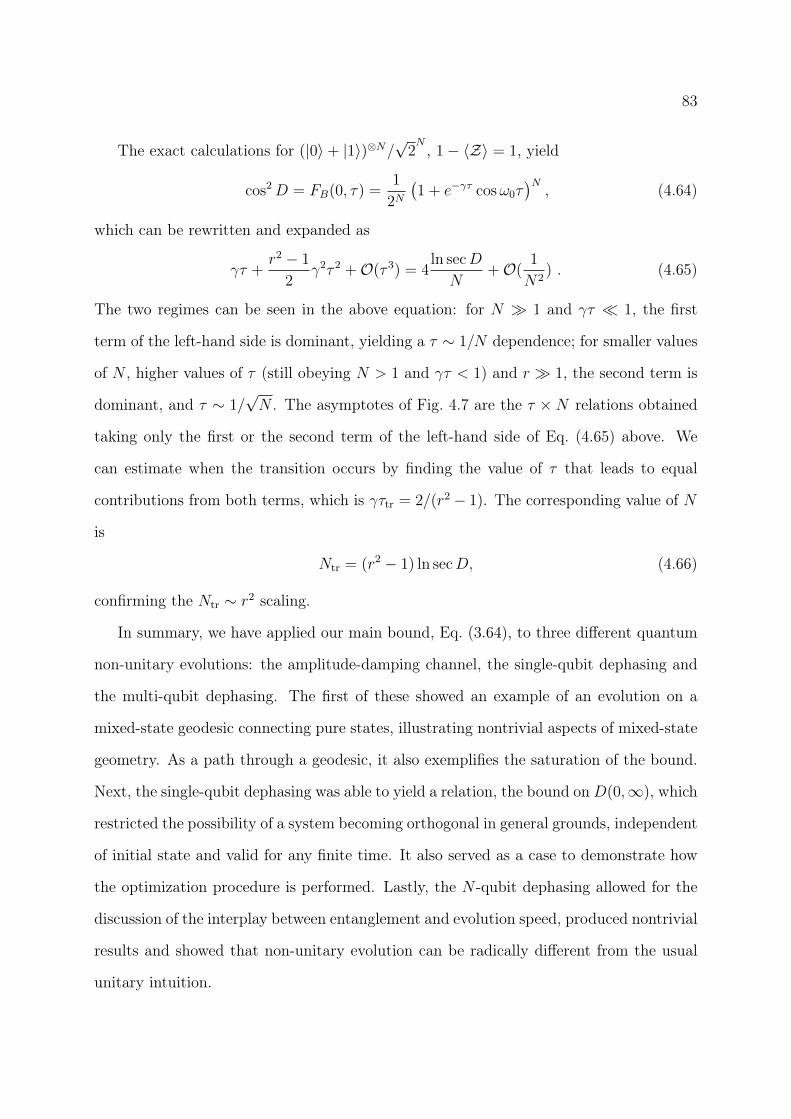
83

The exact calculations for (|0〉+ |1〉)⊗N/√

2N, 1− 〈Z〉 = 1, yield

cos2D = FB(0, τ) =1

2N(1 + e−γτ cosω0τ

)N, (4.64)

which can be rewritten and expanded as

γτ +r2 − 1

2γ2τ 2 +O(τ 3) = 4

ln secD

N+O(

1

N2) . (4.65)

The two regimes can be seen in the above equation: for N 1 and γτ 1, the first

term of the left-hand side is dominant, yielding a τ ∼ 1/N dependence; for smaller values

of N , higher values of τ (still obeying N > 1 and γτ < 1) and r 1, the second term is

dominant, and τ ∼ 1/√N . The asymptotes of Fig. 4.7 are the τ ×N relations obtained

taking only the first or the second term of the left-hand side of Eq. (4.65) above. We

can estimate when the transition occurs by finding the value of τ that leads to equal

contributions from both terms, which is γτtr = 2/(r2 − 1). The corresponding value of N

is

Ntr = (r2 − 1) ln secD, (4.66)

confirming the Ntr ∼ r2 scaling.

In summary, we have applied our main bound, Eq. (3.64), to three different quantum

non-unitary evolutions: the amplitude-damping channel, the single-qubit dephasing and

the multi-qubit dephasing. The first of these showed an example of an evolution on a

mixed-state geodesic connecting pure states, illustrating nontrivial aspects of mixed-state

geometry. As a path through a geodesic, it also exemplifies the saturation of the bound.

Next, the single-qubit dephasing was able to yield a relation, the bound onD(0,∞), which

restricted the possibility of a system becoming orthogonal in general grounds, independent

of initial state and valid for any finite time. It also served as a case to demonstrate how

the optimization procedure is performed. Lastly, the N -qubit dephasing allowed for the

discussion of the interplay between entanglement and evolution speed, produced nontrivial

results and showed that non-unitary evolution can be radically different from the usual

unitary intuition.

84

4.3 Application of the additional bound

We end this Chapter presenting an application of our additional, median-based bound

of Section 3.5, Eqs. (3.94, 3.96). This bound, valid for pure states evolving unitarily, is

applied to a three-level state, initially in

|ψ0〉 = c0 |0〉+ c1 |1〉+ c2 |2〉 , (4.67)

with the governing Hamiltonian H |n〉 = n~ω |n〉. If the median Emed = 0~ω, the result

reduces to a Margolus-Levitin bound, in the sense that it depends on the average energy

respective to the ground state. If Emed = 2~ω, the average energy is taken respective

to the highest energy level, but the resulting expression is still analogous to a Margolus-

Levitin bound. More interesting is the intermediate case Emed = 1~ω. We set |c1|2 = 1/2

in order to guarantee this value of the median. There is then only one relevant free

parameter, the value of p2 = |c2|2 (since |c0|2 = 1/2− p2).

Let us first examine the version of the bound dependent on 〈ψ0|∣∣H − Emed

∣∣|ψ0〉,

Eq. (3.93). In this case, 〈ψ0|∣∣H − Emed

∣∣|ψ0〉 = ~ω/2, and

cos[DFS(0, τ)] =√FB(0, τ) ≥ 1− ωτ

2. (4.68)

This bound is always surpassed by the Mandelstam-Tamm bound for the same evolution,

√FB(0, τ) ≥ cos

[√1

4+ 2|c2|2(1− 2|c2|2) ωτ

], (4.69)

but can often beat the Margolus-Levitin bound on the time to become orthogonal, τML ≥

π/[ω(1+4p2)]. The three are plotted in Fig. 4.8 for p2 = 1/4, which is the value for which

Eq. (4.68) presents the best results. Also plotted is the fidelity as by exact calculations,

which yield

cos[DFS(0, τ)] =√FB(0, τ) =

1 + cosωτ

2− 2p2(1− 2p2) sin2 ωτ . (4.70)

85

0.0 0.5 1.0 1.5 2.0 2.5 3.0ΩΤ

0.2

0.4

0.6

0.8

1.0

F H0, ΤL

Figure 4.8: Plot of the first, weaker version of the median-based bound, dependent on〈ψ0|

∣∣H − Emed

∣∣|ψ0〉, applied to the three-level system for p2 = 0.25. The thick (purple)line represents the bound as in Eq. (4.68), actual evolution is given by the uppermost(blue) curve, the Mandelstam-Tamm bound, plotted for comparison, is the intermediate(tan-colored) curve (Eq. 4.69). The Margolus-Levitin bound on orthogonality time τML

is shown as a red mark on the ωτ axis.

A tighter result is attained with the second version of the median-based bound, de-

pendent on |〈ψ0|H − Emed|ψ(t)〉|. We have, for this three-state evolution,

|〈ψ0|H − Emed|ψ(t)〉| = ~ω√

1

4− 2p2(1− 2p2) cos2 ωt , (4.71)

and the bound of Eq. (3.96), obtained by integration, is expressed in terms of elliptic

integrals of the second kind E(y,m):

cos[DFS(0, τ)] =√FB(0, τ) ≥ 1− 2

∣∣∣∣14 − p2

∣∣∣∣E (ωτ,−p2(12− p2)

(14− p2)2

). (4.72)

This version is actually competitive with both the Mandelstam-Tamm and Margolus-

Levitin bounds: for certain values of p2, it is the best of the three, as shown in Fig. 4.9.

This happens in the vicinity of p2 = 1/4, value at which the bound is saturated throughout

the evolution. We note that for p2 = 1/4 Eq. (4.72) is indefinite, but the bound is well-

defined and reads

cos[DFS(0, τ)] =√FB(0, τ) ≥ 1 + cosωτ

2. (4.73)

This application shows that the additional result of Section 3.5 has the potential to

lead to useful bounds on evolution times. Although still restricted to unitary evolutions,

it has been able to overcome the previously known bounds on certain occasions. The

86

0.0 0.5 1.0 1.5 2.0 2.5 3.0ΩΤ

0.2

0.4

0.6

0.8

1.0

F H0, ΤL

0.0 0.5 1.0 1.5 2.0 2.5 3.0ΩΤ

0.2

0.4

0.6

0.8

1.0

F H0, ΤL

0.0 0.5 1.0 1.5 2.0 2.5 3.0ΩΤ

0.2

0.4

0.6

0.8

1.0

F H0, ΤL

Figure 4.9: Plot of the stronger version of the median-based bound, dependent on|〈ψ0|H − Emed|ψ(t)〉|, applied to a three-level system for p2 = 0.1, 0.2 and 0.35, resp.— different p2 correspond to different initial states. The thick (purple) line representsthe bound as in Eq. (4.72), actual evolution is given by the uppermost (blue) curve, theMandelstam-Tamm bound, plotted for comparison, is the remaining (tan-colored) curve(Eq. 4.69). The Margolus-Levitin bound on orthogonality time τML is shown as a redmark on the ωτ axis.

analytically demonstrated saturation at p2 = 1/4 above for all times up to becoming

orthogonal is a feat that has not been achieved with Margolus-Levitin-like bounds. This

median-based results may be a path for a more structured derivation, possibly geometric,

of a general bound encompassing that of Margolus and Levitin.

87

Chapter 5

Final comments and perspectives

We have in this thesis developed different quantum speed limits, which are bounds on

how fast a quantum system can evolve.

In the Introduction, besides presenting motivations for this study, we took the time

to discern bounds on evolution time from energy-time uncertainty relations, which share

similar mathematical expressions, but relate to conceptually different assertions.

We performed in Chapter 2 a review of the literature on the subject prior to our con-

tributions. We presented the two paradigmatic quantum speed limits, the Mandelstam-

Tamm bound and and the Margolus-Levitin bound, the most easily noticeable difference

between them being that the former relies on the energy variance of the state and the lat-

ter, on the average energy. Another important distinction is that the former is established

in a more complete quantum-mechanical framework than the latter.

Chapter 3 is the central chapter of this work, in which we derived our novel results.

We first introduced some of the standard quantum-informational tools in Section 3.1.

In Section 3.2 we defined and developed a geometric structure for pure quantum states,

culminating in a distance measure for this set and in a reinterpretation of the Mandelstam-

Tamm bound on geometric foundations, with practical gains especially with regard to the

issue of saturation of the bound. Section 3.3 was dedicated to presenting the Fisher

information, both “classical” and quantum. The core of this thesis is found in Section 3.4,

where we derived the main result, the general bound on evolution times of Eq. (3.64),

88

valid for non-unitary as well as unitary evolutions. The greatest novelty of this finding

is to extend the Mandelstam-Tamm bound to non-unitary evolutions, a feat deemed

impossible on at least one occasion [48]. We were also able to preserve important features

such as clear conditions for saturation. Additional bounds, based on the median of the

energy distribution, were introduced in Section 3.5. They are still restricted to unitary

evolutions and can be considered as a work in progress, but are relevant candidates for

future developments.

Applications of the bounds to physical situations are the subject of Chapter 4. It

nevertheless starts with a development for calculating the quantum Fisher information

based on purifications, central to the application of our main bound. We saw examples

displaying saturation along with useful bounds even when not saturated. We were also able

to make use of the bound to discuss the interplay between entanglement of a multipartite

system and the speed of its evolution, achieving nontrivial results for non-unitary channels

fundamentally distinct from their unitary counterparts.

There have been other results on the quantum speed limit for non-unitary processes

after our work had been developed, but prior to the writing of this thesis. We discuss

their properties and shortcomings in Appendix E.

We mention two main perspectives for future work. We are of the opinion that the

Margolus-Levitin bound is founded, at this moment, on less than ideal grounds. To be

able to derive it as a consequence of a more structured framework, possibly entailing a

clearer interpretation of its meaning, would be a considerable achievement. We believe

that the median-based bound presented in Section 3.5 is a potential candidate for arriving

at such a derivation, since it reduces to the Margolus-Levitin bound in some scenarios

and stems from geometric considerations.

The other perspective is the quantum brachistochrone problem, which consists in

finding the fastest route from a quantum state to another given a set of allowed paths,

or equivalently, given a set of restrictions. This problem is of direct practical importance

89

and is closely related to quantum speed limits. One of the basic results of this topic is

that if restriction is placed only on the available energy, the solution saturates the bound

on evolution times [66]. We feel that the experience with the geometry of quantum states

and optimization procedures gained along the present Ph.D. course will be of great help

towards this goal.

90

Bibliography

[1] L. Mandelstam, I. Tamm, J. Phys. (Moscow) 9, 249 (1945). Original Russian version:

L. I. Mandel~xtam, I. E. Tamm, Izv. Akad. Nauk SSSR (ser. fiz.) 9, 122 (1945).

1, 9, 10, 11, 12, 13

[2] K. Asanovic, R. Bodik, J. Demmel, T. Keaveny, K. Keutzer, J. Kubiatowicz, N.

Morgan, D. Patterson, K. Sen, J. Wawrzynek, D. Wessel, and K. Yelick, Commun.

ACM 52, 10 (2009). 2

[3] S. Lloyd, Nature 406, 1047 (2000). 2

[4] G. A. Prinz, Science 282, 1660 (1998). 2

[5] S. A. Wolf, D. D. Awschalom, R. A. Buhrman, J. M. Daughton, S. von Molnár, M.

L. Roukes, A. Y. Chtchelkanova, and D. M. Treger, Science 294 1488 (2001). 2

[6] D. Apalkov, A. Khvalkovskiy, S. Watts, V. Nikitin, X. Tang, D. Lottis, K. Moon, X.

Luo, E. Chen, A. Ong, A. Driskill-Smith, M. Krounbi, ACM J. Emerg. Technol. 9,

13 (2013). 2

[7] W. H. Zurek, Rev. Mod. Phys. 75, 715 (2003). 3

[8] C. Gogolin, Phys. Rev. E 81, 051127 (2010). 3

[9] W. S. Warren, H. Rabitz, and M. Dahleh, Science 259, 1521 (1993). 3

[10] R. J. Gordon and S. A. Rice, Annu. Rev. Phys. Chem. 48, 601 (1997). 3

91

[11] H. Rabitz, R. de Vivie-Riedle, M. Motzkus, and K. Kompa, Science 288, 824 (2000).

3

[12] H. Rabitz, New J. Phys. 11, 105030 (2009). 3

[13] N. Khaneja, R. Brockett, and S. J. Glaser, Phys. Rev. A 63, 032308 (2001). 3

[14] W. Heisenberg, Z. Phys. 43, 172 (1927). English translation in J. A. Wheeler and

W. H. Zurek, Quantum Theory and Measurement (Princeton: Princeton Univ. Press,

1983), p. 62. 4

[15] E. H. Kennard, Z. Phys. 44, 326 (1927). 4

[16] H. Weyl, Gruppentheorie und Quantenmechanik (Hirzel, Leipzig, 1928). English

translation: H. Weyl, The Theory of Groups and Quantum Mechanics (Methuen,

London, 1931). 4

[17] C. Cohen-Tannoudji, B. Diu, F. Laloë, Mécanique Quantique, Tome I (Hermann,

Paris, 1977). 5, 26

[18] N. Bohr, Naturwiss. 16 245, 1928. English version: N. Bohr, Nature 121, 580 (1928),

also in J. A. Wheeler and W. H. Zurek, op.cit. 5

[19] L. Landau and R. Peierls, Z. Phys. 69, 56, (1931). English translation in D. ter Haar

(org.), Collected Papers of L. D. Landau (Pergamon, Oxford, 1965) p. 4, also in J.

A. Wheeler and W. H. Zurek, op.cit. 5

[20] V. A. Fock and N. S. Krylov, J. Phys. (Moscow) 11, 112 (1947). Original Russian

version: V. A. Fok, N. S. Krylov, TF 17, 93 (1947). 5

[21] Y. Aharonov and D. Bohm, Phys. Rev. 122, 1649 (1961). 5

[22] V. A. Fock, Sov. Phys. JETP 15, 784 (1962). Original Russian version: V. A. Fok,

TF 42, 1135 (1962). 5

92

[23] Y. Aharonov and D. Bohm, Phys. Rev. 134, B1417 (1964). 5

[24] V. A. Fock, Sov. Phys. Usp. 8, 628 (1966). Original Russian version: V. A. Fok, Usp.

Fiz. Nauk, 86, 363 (1965). 5

[25] Y. I. Vorontsov, Sov. Phys. Usp. 24, 150 (1981). Original Russian version: . I.

Voroncov, Usp. Fiz. Nauk, 133, 351 (1981). 5

[26] Y. Aharonov and J. L. Safko, Ann. Phys. (N.Y.), 91, 279 (1975). 5

[27] L. Vaidman, Am. J. Phys 60, 182 (1992). 11

[28] J. E. Gray and A. Vogt, J. Math. Phys. 46, 052108 (2005). 13

[29] K. Bhattacharyya, J. Phys. A: Math. Gen. 16, 2993 (1983). 13

[30] G. N. Fleming, Nuovo Cimento A 16, 263 (1973). 13

[31] M. Bauer and P. A. Mello, Proc. Nat. Acad. Sci. USA 73, 283 (1976); Ann. Phys

(N.Y.) 111, 38 (1978). 13

[32] E. A. Gislason, N. H. Sabelli and J. W. Wood, Phys. Rev. A 31, 2078 (1985). 13

[33] J. Uffink and J. Hilgevoord, Found. Phys. 15, 925 (1985). 13

[34] J. Uffink, Am. J. Phys. 61, 935 (1993). 13

[35] J. H. Eberly and L. P. S. Singh, Phys. Rev. D 7, 359 (1973). 5, 13

[36] C. Leubner and C. Kiener, Phys. Rev. A 31, 483 (1985). 13

[37] P. Pfeifer, Phys. Rev. Lett. 70, 3365 (1993). 13

[38] P. Pfeifer and J. Fröhlich, Rev. Mod. Phys. 67, 759 (1995). 13

[39] J. Anandan and Y. Aharonov, Phys. Rev. Lett. 65, 1697 (1990). 14, 16, 37

93

[40] J. Anandan, Found. Phys 21, 1265 (1991). 16, 37

[41] A. Uhlmann, Phys. Lett. A 161, 329 (1992). 14, 19, 20, 63

[42] S. Deffner and E. Lutz, arXiv:1104.5104 (2011). 14, 19

[43] N. Margolus and L. B. Levitin, Physica (Amsterdam) 120D, 188 (1998). 3, 14

[44] V. Giovannetti, S. Lloyd, and L. Maccone, Phys. Rev. A 67, 052109 (2003). 15, 16,

19, 75, 76, 77

[45] N. Horesh and A. Mann, J. Phys. A: Math. Gen. 31, L609 (1998). 16

[46] A. K. Pati, Phys. Lett. A 262, 296 (1999). 16

[47] L. B. Levitin and T. Toffoli, Phys. Rev. Lett. 103, 160502 (2009). 17, 18

[48] P. J. Jones and P. Kok, Phys. Rev. A 82, 022107 (2010). 6, 18, 21, 88, 93

[49] M. Zwierz, Phys. Rev. A 86 016101 (2012), comment on [48]. 18, 57

[50] J. Söderholm, G. Björk, T. Tsegaye, and A. Trifonov, Phys. Rev. A 59, 1788 (1999).

18

[51] V. Giovannetti, S. Lloyd, and L. Maccone, Europhys. Lett. 62, 615 (2003); 19, 75,

77

[52] V. Giovannetti, S. Lloyd, and L. Maccone, J. Opt. B 6, S807 (2004). 19, 20

[53] J. Batle, M. Casas, A. Plastino, and A.R. Plastino, Phys. Rev. A 72, 032337 (2005).

19, 75, 77

[54] A. Borras, M. Casas, A. R. Plastino, and A. Plastino, Phys. Rev. A 74, 022326

(2006). 19, 20, 75, 77

94

[55] C. Zander, A. R. Plastino, A. Plastino, and M. Casas, J. Phys. A: Math. Theor. 40,

2861 (2007). 19, 75, 77

[56] J. Kupferman and B. Reznik, Phys. Rev. A 78, 042305 (2008). 19, 20

[57] F. Fröwis, Phys. Rev. A 85, 052127 (2012). 19, 20, 75, 77

[58] S. Luo and Z. Zhang, Lett. Math. Phys. 71, 1 (2005). 20

[59] M. Andrews, Phys. Rev. A 75, 062112 (2007). 20

[60] B. Zielinski and M. Zych, Phys. Rev. A 74, 034301 (2006). 20

[61] U. Yurtsever, Phys. Scr. 82, 035008 (2010). 20

[62] S.-S. Fu, N. Li, and S. Luo, Commun. Theor. Phys. 54, 661 (2010). 20

[63] D. C. Brody, J. Phys. A: Math. Theor. 44 252002 (2011). 20

[64] H. F. Chau, Phys. Rev. A 81, 062133 (2010). 20

[65] S. Luo, Physica (Amsterdam) 189D, 1 (2004). 3, 20

[66] A. Carlini, A. Hosoya, T. Koike, and Y. Okudaira, Phys.Rev.Lett. 96 060503 (2006).

20, 89

[67] D.C. Brody and D.W. Hook, J. Phys. A: Math. Gen. 39 L167 (2006).

doi:10.1088/0305-4470/39/11/L02 20

[68] M.-H. Yung, Phys. Rev. A 74 030303(R) (2006) 20

[69] A. Carlini, A. Hosoya, T. Koike, and Y. Okudaira, Phys. Rev. A 75, 042308 (2007)

20

[70] A. Carlini, A. Hosoya, T. Koike, and Y. Okudaira, J. Phys. A: Math. Theor. 41,

045303 (2008). 6, 20, 21

95

[71] V.C.G. Oliveira, H.A.B. Santos, L.A.M. Torres, and A.M.C. Souza, Int. J. Quant.

Inf. 6 379 (2008) 20

[72] A. Borrás, A.R. Plastino, M. Casas, and A. Plastino, Phys. Rev. A 78 052104 (2008)

20

[73] A. Mostafazadeh, Phys. Rev. A 79 014101 (2009) 20

[74] B.-K. Zhao, F.-G. Deng, F.-S. Zhang, and H.-Y. Zhou, Phys. Rev. A 80 052106

(2009) 20

[75] M. Born and V. Fock, Z. Phys. 51, 165 (1928). 20

[76] B.H. Bransden and C.J. Joachain, Quantum mechanics, 2nd ed. (Pearson, Harlow,

2000) p. 447. 20

[77] M. Andrecut and M. K. Ali, J. Phys. A 37, L157 (2004). 20

[78] G. P. Beretta, arXiv:quant-ph/0511091 (2006). 6, 20

[79] A.-S. F. Obada, D. A. M. Abo-Kahla, N. Metwally, and M. Abdel-Aty, Physica E

43, 1792 (2011). 6, 20

[80] D. C. Brody and E.-M. Graefe, arXiv:1208.5297v1 (2012). 6, 20

[81] M. M. Taddei, B. M. Escher, L. Davidovich, and R. L. de Matos Filho, Phys. Rev.

Lett. 110, 050402 (2013). 23, 52

[82] I. Bengtsson, K. Życzowski, Geometry of Quantum States: An Introduction to Quan-

tum Entanglement (Cambridge University Press, 2006). 30

[83] S. Kobayashi and K. Nomizu, Foundations of Differential Geometry, vols I and II

(Wiley Interscience, New York, 1969). 30, 31, 32, 33

96

[84] A. Uhlmann and B. Crell, Lect. Notes Phys. 768, 1 (2009) in A. Buchleitner, C.

Viviescas, M Tiersch (eds.), Entanglement and Decoherence, Foundations and Mod-

ern Trends (Springer, Berlin Heidelberg, 2009). 31, 33

[85] G. Fubini, Atti Istit. Veneto, 63, 501 (1904). Reprinted in: G. Fubini, Opere Scelte,

Vol. 2. (Cremonese, Rome, 1958), p. 10. 32

[86] E. Study, Math. Ann. (Berlin) 60, 321 (1905). 32, 33, 34

[87] W. K. Wootters, Phys. Rev. D, 23, 357 (1981). 33, 34

[88] M. A. Nielsen and I. L. Chuang, Quantum Computation and Quantum Information

(Cambridge University Press, Cambridge, 2000). 23, 24, 25, 26, 28

[89] B. Schumacher and M.Westmoreland, Quantum Processes, Systems, and Information

(Cambridge University Press, Cambridge, 2010). 24, 25, 34

[90] A. Uhlmann, Rep. Math. Phys. 9, 273 (1976). 25

[91] R. Jozsa, J. Mod. Opt. 41, 2315 (1994). 25

[92] C. Cohen-Tannoudji, J. Dupont-Roc, and G. Grynberg, Processus d’interaction entre

photons et atomes (EDP Sciences, Les Ulis, 1988). English Version: Atom-Photon

Interactions: Basic Process and Applications (Wiley-VCH, Weinheim, 2004). 25

[93] R. A. Fisher, Messenger Math. 41, 155 (1912). 40

[94] R. A. Fisher, Phil. Trans. R. Soc. Lond. A 222, 309 (1922). 40

[95] R. A. Fisher, Math. Proc. Camb. Phil. Soc. 22, 700 (1925). 40

[96] R. A. Fisher, Proc. R. Soc. Lond. A 144, 285 (1934). 40

[97] S. M. Kay, Fundamentals of Statistical Signal Processing: Estimation Theory

(Prentice-Hall, New Jersey, 1993). 40

97

[98] B. M. Escher, Estimação de parâmetros em sistemas quânticos abertos, Ph.D. thesis

(2011), in Portuguese. 40, 41, 43, 44, 46, 49

[99] C. Hirt, S. Claessens, T. Fecher, M. Kuhn, R Pail, and M. Rexer, Geoph. Res. Lett.

40, 1 (2013). 42, 43

[100] L. Pardo, Statistical Inference Based on Divergence Measures (CRC Press, Boca

Raton, 2006). 43

[101] B. M. Escher, R. L. de Matos Filho, and L. Davidovich, Braz. J. Phys. 41, 229,

(2011). 44

[102] C. R. Rao, Bull. Calcutta Math. Soc. 37, 81 (1945). 44

[103] H Cramér, Mathematical Methods in Statistics (Princeton University Press, Prince-

ton, 1946). 40, 41, 44

[104] C. R. Rao, Math. Proc. Camb. Phil. Soc. 43, 280 (1947). 44

[105] C. W. Helstrom, Phys. Lett. 25A, 101 (1967); C. W. Helstrom, Quantum Detection

and Estimation Theory (New York, Academic, 1976). 48

[106] A. S. Holevo Probabilistic and statistical aspects of quantum theory (Amsterdam,

North-Holland, 1982). 48, 49

[107] S. L. Braunstein and C. M. Caves, Phys. Rev. Lett. 72, 3439 (1994).

[108] A. Uhlmann, “The Metric of Bures and the Geometric Phase”, in R. Gielerak, J.

Lukierski, Z. Popowicz (Eds.), Quantum Groups and Related Topics: Proceedings of

the First Max Born Symposium (Kluwer Academic, Dordrecht, 1992), p. 267.

[109] S. Boixo, S. T. Flammia, C. M. Caves, and J. M. Geremia, Phys. Rev. Lett. 98,

090401 (2007).

98

[110] B. M. Escher, L. Davidovich, N. Zagury, and R. L. de Matos Filho, Phys. Rev. Lett.

109, 190404 (2012). 50, 61

[111] B. M. Escher, R. L. de Matos Filho, and L. Davidovich, Nature Phys. 7, 406 (2011).

50, 61

[112] A. del Campo, I. L. Egusquiza, M. B. Plenio, and S. F. Huelga, Phys. Rev. Lett.

110, 050403 (2013). 112, 113, 114

[113] S. Deffner and E. Lutz, Phys. Rev. Lett 111, 010402 (2013). 114, 115

99

Appendix A

Integration of the Fubini-Study metric

We here perform the integration in two-dimensional Hilbert space of the differential

form of the Fubini-Study metric from Eq. (3.9),

ds2FS = 〈dψproj|dψproj〉 =

〈dψ|dψ〉 〈ψ|ψ〉 − | 〈ψ|dψ〉 |2

〈ψ|ψ〉2, (A.1)

to find the finite Fubini-Study distance between two states, as mentioned on p. 33. Just

as in Chapter 3, we denote by |ψ0〉 and |ψf〉 the initial and final states, respectively, and

|ψ1〉 will be a state orthogonal to |ψ0〉 so that |ψf〉 belongs to the span of |ψ0〉 , |ψ1〉.

Any evolution between these states can be parametrized as in Eq. (3.10) by

|ψ(t)〉 = f(t) |ψ0〉+ g(t) |ψ1〉 , (A.2)

where t ∈ [0, tf ] is a parameter and f and g are complex functions of it, with g(0) = 0.

None of the states mentioned need to be normalized, so there is no constraint on f(0)

other than f(0) 6= 0 (in other words, we only demand |ψ(0)〉 ∼ |ψ0〉, not equality).

The variation |dψ〉 is given by

|dψ〉 = |ψ(t+ dt)〉 − |ψ(t)〉 =(f(t) |ψ0〉+ g(t) |ψ1〉

)dt , (A.3)

while the product 〈ψ|dψ〉 is

〈ψ|dψ〉 = 〈ψ(t)|dψ〉 =(f ∗(t)f(t) 〈ψ0|ψ0〉+ g∗(t)g(t) 〈ψ1|ψ1〉

)dt , (A.4)

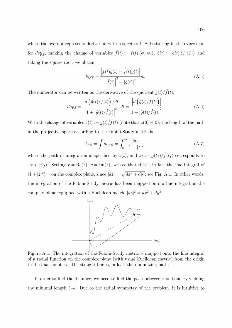
100

where the overdot represents derivation with respect to t. Substituting in the expression

for ds2FS, making the change of variables f(t) := f(t) 〈ψ0|ψ0〉, g(t) := g(t) 〈ψ1|ψ1〉 and

taking the square root, we obtain

dsFS =

∣∣∣f(t) ˙g(t)− ˙f(t)g(t)∣∣∣∣∣∣f(t)

∣∣∣2 + |g(t)|2dt . (A.5)

The numerator can be written as the derivative of the quotient g(t)/f(t),

dsFS =

∣∣∣d(g(t)/f(t))/dt∣∣∣

1 +∣∣∣g(t)/f(t)

∣∣∣2 dt =

∣∣∣d(g(t)/f(t))∣∣∣

1 +∣∣∣g(t)/f(t)

∣∣∣2 . (A.6)

With the change of variables z(t) := g(t)/f(t) (note that z(0) = 0), the length of the path

in the projective space according to the Fubini-Study metric is

`FS =

∫dsFS =

∫ zf

0

|dz|1 + |z|2

, (A.7)

where the path of integration is specified by z(t), and zf := g(tf )/f(tf ) corresponds to

state |ψf〉. Setting x = Re(z), y = Im(z), we see that this is in fact the line integral of

(1 + |z|2)−1 on the complex plane, since |dz| =√dx2 + dy2; see Fig. A.1. In other words,

the integration of the Fubini-Study metric has been mapped onto a line integral on the

complex plane equipped with a Euclidean metric |dz|2 = dx2 + dy2.

z f

ReHzL

ImHzL

Figure A.1: The integration of the Fubini-Study metric is mapped onto the line integralof a radial function on the complex plane (with usual Euclidean metric) from the originto the final point zf . The straight line is, in fact, the minimizing path.

In order to find the distance, we need to find the path between z = 0 and zf yielding

the minimal length `FS. Due to the radial symmetry of the problem, it is intuitive to

101

consider the straight line in the complex plane as yielding the minimum. This intuition

can be confirmed by the fact that the radial straight line is the shortest path between the

endpoints of the complex plane (in Euclidean metric!) and at the same time the path of

steepest descent of the integrand throughout – the second assertion is due to the radial

gradient thereof.

Alternatively, this minimization can be performed by standard calculus of variations.

Let (x(η), y(η)) be a parametrization of the path for some parameter η. The length we

wish to minimize is then written as

DFS = minpath

∫path

√x2 + y2

1 + x2(η) + y2(η)dη , (A.8)

for fixed initial and final points, where the overdot now represents derivation with respect

to η. The Euler equation for this minimization problem reads

xy − xyx2 + y2

+ 2xy − xy

1 + x2 + y2= 0 , (A.9)

and it is straightforward to see that the straight line through the origin, y(η) = Cx(η),

y = Cx and y = Cx, where C is a constant, is a solution to the above.

For the outward straight line we then have |dz| = d|z|, and

DFS(|ψ0〉 , |ψf〉) =

∫ |zf |0

d|z|1 + |z|2

= arctan |zf | = arctan

∣∣∣∣ g(tf ) 〈ψ1|ψ1〉f(tf ) 〈ψ0|ψ0〉

∣∣∣∣ , (A.10)

which can be rewritten as

DFS(|ψ0〉 , |ψf〉) = arccos

(|f(tf )

√〈ψ0|ψ0〉|√

|f(tf )|2 〈ψ0|ψ0〉+ |g(tf )|2 〈ψ1|ψ1〉

). (A.11)

But the (normalized) inner product between initial and final states reads

〈ψ0|ψf〉√〈ψ0|ψ0〉

√〈ψf |ψf〉

=f(tf )

√〈ψ0|ψ0〉√

|f(tf )|2 〈ψ0|ψ0〉+ |g(tf )|2 〈ψ1|ψ1〉(A.12)

and we conclude that

DFS(|ψ0〉 , |ψf〉) = arccos

(|〈ψ0|ψf〉|√

〈ψ0|ψ0〉√〈ψf |ψf〉

), (A.13)

102

as displayed in Eq. (3.11) of the main text.

Moreover, we now know that the geodesic is the straight line from the origin to zf .

Expressed in terms of z(t), it reads z(t) = ξ(t)zf , where ξ(t) is any nondecreasing real

function of t such that ξ(0) = 0 and ξ(tf ) = 1. Any condition imposed on z will ignore,

as it should, the overall phase and normalization of the state. When written in terms of

f , g, the condition for the geodesic is

g(t)

f(t)= ξ(t)

g(tf )

f(tf ), (A.14)

from which one sees that on the geodesic the relative phase between the components must

be constant and the ratio of their moduli must not decrease during evolution.

103

Appendix B

Minimization yielding the median

We have the task of minimizing the function of Eq. (3.91),

∑n

|cn|2 |En − g| = 〈ψ0|∣∣H − g∣∣|ψ0〉 , (B.1)

with respect to the real parameter g, given the set of energies En and the probability

distribution |cn|2.

The first step is to notice that this function tends to infinity if g → ±∞, but is

bounded from below because it is non-negative, so the minimum exists. This expression

is, as a function of g, sectionally linear. This can be seen best by taking the derivative

with respect to g, which gives

∑n

|cn|2 sign (g − En) =∑

n | En<g

|cn|2 −∑

n | En>g

|cn|2 . (B.2)

The derivative is ill-defined when g = En for some value of n. A graph of the function

is shown in Fig. B.1. It is linear in each section in which g is between two consecutive

values of En. Notice that the slope of the function always increases from one section to

the other, since the increase of g can only remove a term from the second summation in

Eq. (B.2) and add it to the first. The point where the slope goes from negative to positive

is where the minimum of this function is achieved. This corresponds to the energy En∗

such that the probability of all energies below En∗ is less than one half,∑

n<n∗ |cn|2 <12

and, at the same time, the probability of all energies above En∗ is also less than one half,

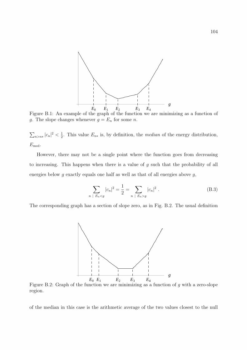
104

E0 E1 E2 E3 E4

g

Figure B.1: An example of the graph of the function we are minimizing as a function ofg. The slope changes whenever g = En for some n.

∑n>n∗ |cn|2 <

12. This value En∗ is, by definition, the median of the energy distribution,

Emed.

However, there may not be a single point where the function goes from decreasing

to increasing. This happens when there is a value of g such that the probability of all

energies below g exactly equals one half as well as that of all energies above g,

∑n | En<g

|cn|2 =1

2=

∑n | En>g

|cn|2 . (B.3)

The corresponding graph has a section of slope zero, as in Fig. B.2. The usual definition

E0 E1 E2 E3 E4

g

Figure B.2: Graph of the function we are minimizing as a function of g with a zero-sloperegion.

of the median in this case is the arithmetic average of the two values closest to the null

105

slope. Since our function is constant in this interval, this value is one of those which yield

the minimum of our function. The minimum is achieved by Emed also in this case.

We can then state with no loss of generality that the minimum of Eq. (3.91), or (B.1),

is found when g = Emed, and equals

∑n

|cn|2 |En − Emed| = 〈ψ0|∣∣H − Emed

∣∣|ψ0〉 . (B.4)

106

Appendix C

Tightness of the bound on the quantumFisher information

We have shown in Section 4.1 that there is an upper bound on the quantum Fisher

information FQ(t) of a system S in state ρ(t) based on the purification of this state

FQ(t) ≤ CQ(t) . (C.1)

In this Appendix, we show that this bound, CQ(t), can be saturated. CQ(t) is nothing more

than the quantum Fisher information of a purification |ψS,E(t)〉 of ρ(t) into a larger system

S + E. We must then show that there is a purification of ρ(t) such that CQ(t) = FQ(t).

We start by considering the Bures fidelity of two states ρ(t) and ρ(t′). We know from

Uhlmann’s theorem, Eq. (3.2), that for any purification |ψS,E(t)〉 of the former there is a

purification |φmaxS,E (t′)〉 of the latter such that

FB[ρ(t), ρ(t′)] =∣∣〈ψS,E(t)|φmax

S,E (t′)〉∣∣2 . (C.2)

Let us expand both sides of this equation on t′ around t′ = t. The left-hand side has been

expanded in Eq. (3.39) of the main text,

FB[ρ(t), ρ(t′)] = 1− FQ(t)

4dt2 +O(dt3) , (C.3)

with dt = t′ − t, while the expansion of the right-hand side yields

|〈ψ(t)|φmax(t′)〉|2 = I(0)(t′)∣∣t′=t

+ I(1)(t′)∣∣t′=t

dt+I(2)(t′)

2

∣∣∣∣t′=t

dt2 +O(dt3) , (C.4)

107

where we have omitted the subscript S,E for cleanness. The zero-order coefficient is simply

the inner product squared, I(0)(t) = |〈ψ(t)|φmax(t)〉|2, and it must equal one, since this is

the value of the Bures fidelity between state ρ(t) and itself. In fact, the unit value of FB

in this case allows us to write

|φmax(t)〉 〈φmax(t)| = |ψ(t)〉 〈ψ(t)| . (C.5)

The higher-order terms are

I(1)(t′)∣∣t′=t

=

[d 〈φmax(t′)|

dt′|ψ(t)〉〈ψ(t)|φmax(t′)〉+ 〈φmax(t′)|ψ(t)〉〈ψ(t)| d |φ

max(t′)〉dt′

]t′=t

,

(C.6)

I(2)(t′)∣∣t′=t

=

[d2 〈φmax(t′)|

dt′2|ψ(t)〉〈ψ(t)|φmax(t′)〉+ 〈φmax(t′)|ψ(t)〉〈ψ(t)| d

2 |φmax(t′)〉dt′2

+

+2d 〈φmax(t′)|

dt′|ψ(t)〉〈ψ(t)| d |φ

max(t′)〉dt′

]t′=t

,

(C.7)

and, by using Eq. (C.5), these simplify to

I(1)(t′)∣∣t′=t

=d

dt′(〈φmax(t′)|φmax(t′)〉)

∣∣∣∣t′=t

, (C.8)

I(2)(t′)∣∣t′=t

=d2

dt′2(〈φmax(t′)|φmax(t′)〉)

∣∣∣∣t′=t

+

− 2

[(d 〈φmax(t′)|

dt′

)(d |φmax(t′)〉

dt′

)−∣∣∣∣d 〈φmax(t′)|

dt′|φmax(t)〉

∣∣∣∣2]t′=t

.

(C.9)

The normalization of |φmax〉 implies that the first and second derivatives of 〈φmax|φmax〉

are zero, so that the first-order term of Eq. (C.8) is null and substitution of Eq. (C.9) into

Eq. (C.4) gives, up to second order,

|〈ψ(t)|φmax(t′)〉|2 = 1−

[(d 〈φmax(t′)|

dt′

)(d |φmax(t′)〉

dt′

)−∣∣∣∣d 〈φmax(t′)|

dt′|φmax(t)〉

∣∣∣∣2]t′=t

dt2 .

(C.10)

The evolution of |φmaxS,E (t′)〉 (reinserting the subscript!) is unitary, since this state is always

pure. Considering that its derivative can be written in terms of the Hamiltonian HS,E(t′)

108

as i~ ddt′|φmaxS,E (t′)〉 = HS,E(t′) |φmax

S,E (t′)〉, the expansion up to second order becomes

∣∣〈ψ(t)|φmaxS,E (t′)〉

∣∣2 = 1− [∆HS,E(t)]2

~2dt2 , (C.11)

where [∆HS,E(t)]2 is the variance of HS,E(t). From the comparison of the two expansions,

Eqs. (C.3, C.11), we can ascertain that

FQ(t) =4

~2[∆HS,E(t)]2

∣∣∣∣|φmax

S,E 〉= CQ(t)

∣∣∣∣∣|φmax

S,E 〉

, (C.12)

i.e., there is a purification |φmaxS,E (t)〉 of ρ(t) such that the quantum Fisher information of

the two (CQ(t) and FQ(t), respectively) coincide. Since the former is an upper bound to

the latter, FQ(t) is the minimum over purifications:

FQ(t) = minpurifCQ(t) = min

purif

4

~2[∆HS,E(t)]2 . (C.13)

Since the equality on Uhlmann’s theorem requires the auxiliary system to have the

same dimension as the original, that is the requirement for equality to hold for this

bound.

109

Appendix D

Optimization of the bound for thedephasing channel

In this Appendix, we minimize the bound CQ(t) for the dephasing channel. This is

done directly in the N -qubit case. The single-qubit case is recovered by taking N = 1, an

independent derivation thereof can also serve as an exercise to the reader.

We are tasked with minimizing the initial-state variance of

HS,E(t) = HS,E(t) + U †S,E(t)hE(t)US,E(t) (D.1)

over the three-parameter family of Eq. (4.49), where the quantities have been defined

along Chapter 4 in Eqs. (4.11,4.13,4.14), see also the table on p. 66. For N = 1, this

represents a minimization over all possible purifications. It is straightforward to show

that this variance can be cast in the form

[∆HS,E(t)]2 = [∆HS,E(t)]2 +[∆hE(t)]2 +2Re[〈HS,E(t)hE(t)〉 − 〈HS,E(t)〉 〈hE(t)〉

], (D.2)

with hE(t) := U †S,E(t)hE(t)US,E(t) (for any operator A, [∆A]2 denotes its variance).

Let |ψ0〉|0〉E be the initial state of S + E. From HS,E(t) of Eq. (4.47),

〈HS,E(t)〉 = N~ω0

2〈Z〉 , (D.3)

with Z :=∑

j Zj/N , and

[∆HS,E(t)]2 = N2~2ω20

4[∆Z]2 +N

~2γ2/4

e2γt − 1. (D.4)

110

From Eqs. (4.49,4.46), one obtains

〈hE(t)〉 = −α(t)N 〈Z〉 2√P (t)

√1− P (t) + δ(t)N [2P (t)− 1] , (D.5)

where P (t) := (1 + e−γt)/2, and

[∆hE(t)]2 =N[α2(t) + β2(t) + δ2(t)

]+ α2(t)

(N2[∆Z]2 −N

)4P (t)[1− P (t)]

−Nδ2(t)[2P (t)− 1]2 + 2α(t)δ(t)N 〈Z〉 2√P (t)

√1− P (t)[2P (t)− 1] .

(D.6)

From the previous equations,

2Re [〈HS,E(t) hE(t)〉 − 〈HS,E(t)〉 〈hE(t)〉]

=

= −2α(t)N2~ω0[∆Z]2√P (t)

√1− P (t) + β(t)

N~γ√e2γt − 1

〈Z〉 ,(D.7)

and [∆HS,E(t)]2, according to (D.2), is the sum of (D.4), (D.6), and (D.7),

[∆HS,E(t)]2 =N2~2ω20

4[∆Z]2 +N

~2γ2/4

e2γt − 1+N

[α2(t) + β2(t) + δ2(t)

]+ β(t)

N~γ√e2γt − 1

〈Z〉+

+ α2(t)(N2[∆Z]2 −N

)4P (t)[1− P (t)]−Nδ2(t)[2P (t)− 1]2+

+ 2α(t)N√P (t)

√1− P (t)

δ(t) 〈Z〉 2[2P (t)− 1]−N~ω0[∆Z]2

.

(D.8)

One now minimizes over α(t), β(t), δ(t) for each t. From ∂[∆HS,E(t)]2/∂β = 0, one

finds

β(t) = − ~γ2√e2γt − 1

〈Z〉. (D.9)

Conditions ∂[∆HS,E(t)]2/∂α = 0 and ∂[∆HS,E(t)]2/∂δ = 0 lead to a linear system of

equations, with solutions

α(t) = +~ω0

2

eγt√e2γt − 1Nq

1 + (e2γt − 1)Nq, (D.10)

δ(t) = − ~ω0

2

e2γtNq

1 + (e2γt − 1)Nq〈Z〉 , (D.11)

where q := [∆Z]2/(1− 〈Z〉2

). By replacing Eqs. (D.9,D.10,D.11) into Eq. (D.8), one

finds

CoptQ (t) =

4

~2[∆HS,E(t)]2 = [∆Z]2

[ω2

0N2

Nq(e2γt − 1) + 1+

γ2N/q

e2γt − 1

], (D.12)

111

as in Eq. (4.50). The single-qubit result of Eq. (4.31) is recovered by taking N = 1 (notice

that q = 1 in this case).

112

Appendix E

Later results in the literature

After the completion and submission to publication of our work, other authors have

also derived bounds on non-unitary evolution. We now comment on these results.

In [112], a work subsequent to ours both in publication as preprint and submission to a

refereed journal, del Campo and collaborators have also obtained bounds on non-unitary

evolutions. Their bounds, albeit technically correct, lack some of the interesting features

of our results.

Firstly, although they recognize that the well-established Bures fidelity FB would be

the natural choice [112, p.1], del Campo et alli base their comparison of initial and final

states — ρ0 and ρt, respectively — on a figure of merit

f(t) =Tr (ρ0ρt)

Tr(ρ20)

(E.1)

without justification other than its past employment on pure states and/or unitary evolu-

tions. We note that for pure states evolving unitarily both FB and f above — as well as

many other possible functions — recover the pure-state fidelity F (|ψ〉 , |φ〉) = | 〈ψ|φ〉 |2.

The figure of merit f above does yield f = 0 for orthogonal states and f = 1 for coinciding

ones, but a meaning for its intermediate values has not been offered1.

1It would seem particularly telling of the arbitrariness of this figure of merit that on a different sectionof the same paper [112, Eq. (10)], a different function f(t) = Tr (ρ0ρt) is used for the same purpose.Comparing the main text of [112] with its supplemental material, though, we are inclined to pardon thisdifferent version of f as a typo.

113

Another shortcoming of their result is that neither of their two bounds can be satu-

rated in a non-unitary evolution, because their derivation either makes use of Tr(ρ2t ) ≤ 1

or of a Cauchy-Schwarz inequality whose saturation occurs only if ρt ∝ ρ0, and saturation

of either bound at time τ would require either Tr(ρ2t ) = 1 or ρt ∝ ρ0 for all t ∈ (0, τ). Con-

sidering that the novelty of general bounds is their application to non-unitary processes,

such a limitation severely restricts the potential usefulness of the result in [112].

On the other hand, even when confined to unitary evolutions and pure states, the

bound does not fare much better. The authors agree that a bound should reduce to the

Mandelstam-Tamm bound in this case; their results fail to do so. Their bounds, applied

to a unitary evolution of pure states, yield orthogonalization2 times τ ≥ ~/(√

2∆E) and

τ ≥ ~/(2∆E), more than a factor of 2 worse than the tight Mandelstam-Tamm bound,

τ ≤ π~/(2∆E). In light of this reasoning, the claim of the authors of [112] of generalizing

the Mandelstam-Tamm bound seems inappropriate.

A last comment on this paper is that a confusing notation is used. Their bounds

are implicit on time τ , just as Eq. (2.12) or Eq. (3.64). Each of their results can be

schematically cast into the form∫ τ

0

(t, evolution

)dt ≥ function[f(τ)] , (E.2)

where the integrand is determined by the evolution and is time-dependent, and the right-

hand side is some function of the figure of merit f at final time τ . The bounds are implicit

because the integrand is time-dependent and integration can only be performed for each

specific evolution. The authors nevertheless choose to multiply by τ/τ in order to express

this in terms of a time average 1τ

∫ τ0

(t, evolution

)dt =

(t, evolution

):

τ ≥ function[f(τ)]

1τ

∫ τ0

(t, evolution

)dt

=function[f(τ)](t, evolution

) . (E.3)

This apparent explicitation of τ on the left-hand side and its omission on the denominator

on the right-hand side have proven to be quite confusing. It can lead to the interpretation2For non-orthogonal final states, the bounds in [112] fare even worse.

114

that the right-hand side be a bound on time τ , whereas it actually depends on τ . We

have come across researchers in the very field of Quantum Information who have been

mislead by this notation, and we believe that it should be avoided completely.

Another article published after our results was that of Deffner and Lutz in [113].

Although it has advantages over [112], it shares some of the criticism above. The authors

here make use of the actual fidelity between initial and final states, restricting themselves

to pure initial states. The alleged generalization of both Margolus-Levitin (ML) and

Mandelstam-Tamm (MT) bounds is not achieved. As for the ML bound, there is a

technical flaw in the relation that links the average energy to one of the obtained bounds.

Applying the general bound to a unitary evolution under Hamiltonian Ht, the relation

also depends on the state ρt at time t and reads

Tr|Htρt| = TrHtρt = 〈Ht〉 , (incorrect!) (E.4)

claimed to be valid for Ht having non-negative spectrum, see [113, Eq. (10)]. The mistake

is due to the fact that the product Htρt is assumed Hermitian, which need not be the

case. A simple counterexample of a qubit in state ρ = (I + X)/2 under a Hamiltonian

H = I+Z disproves the relation. As such, the results of [113] have not been related to the

average energy, and no relation to the ML bound have been shown. As for the claim of

recovering the MT bound, the corresponding result, when applied to a unitary evolution

under a constant Hamiltonian, reads∫ τ

0

∆E(t)dt ≥ ~√2

(1− F ) , (E.5)

where F is the fidelity between initial and final states. It recovers one of the two bounds

present in [112]. In spite of the functional similarity to Eq. (2.12), the different prefactor

and functional dependence of Eq. (E.5) on F imply a less tight bound, which cannot be

saturated in any case. The most central result of [113] is a bound that is expressible

in terms of the operator norm (even when applied to unitary evolutions, it is expressible

115

neither in terms of average energy nor of energy variance, hence is fundamentally different

from ML or MT bounds). A purported advantage of this result is that it would be sharper

than the MT bound [113, p.1], but the comparison is made not with the actual MT bound,

but with the weaker Eq. (E.5) and thus does not suffice to corroborate the relevance of

the result.

Saturation is observed numerically in some instances for this bound, but it is shown

to occur only for specific instants, not along an evolution. Clear criteria for saturation

are also lacking, as well as an interpretation of the bound.

Deffner and Lutz also make use of the confusing notation illustrated in Eq. (E.3); they

go so far as to use a specific value of τ to calculate the average on the right-hand side and

treat the resulting fraction as a bound on τ ! (See [113, Fig. 1], which is supposed to be a

plot of the bound on τ obtained by taking τ = 1.) This impedes a proper interpretation

of their results. Only saturation can be (cumbersomely) evaluated from their plots and it

is, as mentioned, only seen numerically for a specific value of τ . This serves as an example

of the damage done by the confusing choice of an apparently explicit τ as in Eq. (E.3).