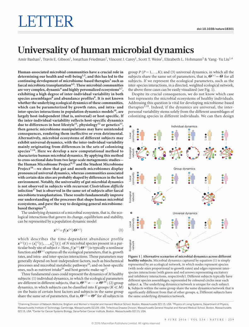
9 j u n e 2 0 1 6 | V O L 5 3 4 | n A T u R e | 2 5 9

LeTTeRdoi:10.1038/nature18301

Universality of human microbial dynamicsAmir Bashan1, Travis e. Gibson1, jonathan Friedman2, Vincent j. Carey1, Scott T. Weiss1, elizabeth L. Hohmann3 & Yang-Yu Liu1,4

Human-associated microbial communities have a crucial role in determining our health and well-being1,2, and this has led to the continuing development of microbiome-based therapies3 such as faecal microbiota transplantation4,5. These microbial communities are very complex, dynamic6 and highly personalized ecosystems3,7, exhibiting a high degree of inter-individual variability in both species assemblages8 and abundance profiles9. It is not known whether the underlying ecological dynamics of these communities, which can be parameterized by growth rates, and intra- and inter-species interactions in population dynamics models10, are largely host-independent (that is, universal) or host-specific. If the inter-individual variability reflects host-specific dynamics due to differences in host lifestyle11, physiology12 or genetics13, then generic microbiome manipulations may have unintended consequences, rendering them ineffective or even detrimental. Alternatively, microbial ecosystems of different subjects may exhibit universal dynamics, with the inter-individual variability mainly originating from differences in the sets of colonizing species7,14. Here we develop a new computational method to characterize human microbial dynamics. By applying this method to cross-sectional data from two large-scale metagenomic studies—the Human Microbiome Project9,15 and the Student Microbiome Project16—we show that gut and mouth microbiomes display pronounced universal dynamics, whereas communities associated with certain skin sites are probably shaped by differences in the host environment. Notably, the universality of gut microbial dynamics is not observed in subjects with recurrent Clostridium difficile infection17 but is observed in the same set of subjects after faecal microbiota transplantation. These results fundamentally improve our understanding of the processes that shape human microbial ecosystems, and pave the way to designing general microbiome-based therapies18.

The underlying dynamics of a microbial ecosystem, that is, the eco-logical interactions that govern its change, equilibrium and stability, can be represented by a population dynamic model

Θ= ( ) ( )ν ν ν( ) ( ) ( )�x f x ; 1

which describes the time-dependent abundance profile ( )= ( ( ) … ( ))ν ν ν( ) ( ) ( )x t x t x t, , N1 of N microbial species present in a par-

ticular body site of subject ν. Here, Θ( )ν ν( ) ( )xf ; is typically a nonlinear function and Θ ν( ) captures all the ecological parameters, that is, growth rates, and intra- and inter-species interactions. Those parameters may generally depend on host-independent factors, such as biochemical processes and microbial metabolic pathways19; and on host-specific ones, such as nutrient intake20 and host genetic make-up13.

Three fundamental cases could represent the dynamics of M healthy subjects: (1) individual dynamics, in which the ecological parameters are different in different subjects, that is, Θ Θ≠ ≠( ) ( )� M1 ; (2) group dynamics, in which subjects can be classified into K groups ( �K M) on the basis of certain host factors and subjects in the same group share the same set of parameters, that is, Θ Θ=ν( ) P for all subjects in

group P (P = 1, ..., K); and (3) universal dynamics, in which all the subjects share the same set of parameters, that is, Θ Θ=ν( ) for all subjects. If we represent the ecological parameters, such as the inter-species interactions, in a directed, weighted ecological network, the above three cases can be easily visualized (see Fig. 1).

Despite its crucial consequences, we do not know which case best represents the microbial ecosystems of healthy individuals. Addressing this question is vital for developing microbiome-based therapies3,18. Indeed, if the dynamics are universal, the inter- personal variability stems solely from the different assemblages of colonizing species in different individuals. We can then design

1Channing Division of Network Medicine, Brigham and Women’s Hospital and Harvard Medical School, Boston, Massachusetts 02115, USA. 2Physics of Living Systems, Department of Physics, Massachusetts Institute of Technology, Cambridge, Massachusetts 02139, USA. 3Infectious Disease Division, Massachusetts General Hospital and Harvard Medical School, Boston, Massachusetts 02115, USA. 4Center for Cancer Systems Biology, Dana-Farber Cancer Institute, Boston, Massachusetts 02115, USA.

a Individual dynamicsLo

cal

com

mun

ityE

colo

gica

lne

twor

k

b Group dynamics

Loca

lco

mm

unity

Eco

logi

cal

netw

ork

c Universal dynamics

Loca

lco

mm

unity

Eco

logi

cal

netw

ork

Figure 1 | Alternative scenarios of microbial dynamics across different healthy subjects. Microbial dynamics captured by equation (1) is simply represented by an ecological network, in which nodes represent species (with node sizes proportional to growth rates) and edges represent inter-species interactions (with green and red arrows representing excitatory and inhibitory interactions, respectively). Different subjects typically have different species assemblages, represented by coloured circles near each subject. a, The underlying dynamics/network is unique for each subject. b, Subjects within the same group share the same dynamics/network that is significantly different from that of other groups. c, Different subjects have the same underlying dynamics/network.

© 2016 Macmillan Publishers Limited. All rights reserved

LetterreSeArCH

2 6 0 | n A T u R e | V O L 5 3 4 | 9 j u n e 2 0 1 6

general interventions to control the microbial state (in terms of spe-cies assemblage and abundance profile) of different individuals. By contrast, if the dynamics are strongly host-specific, we must design truly personalized interventions, which need to consider not only the unique microbial state of an individual but also the unique dynam-ics of the underlying microbial ecosystem. In addition, host-specific dynamics, if they exist, raise a major safety concern for faecal micro-biota transplantation (FMT), because although the healthy microbiota are stable in the donor’s gut, they may be shifted to an undesired state in the recipient’s gut.

The ideal approach to addressing this fundamental question would be to infer the dynamic model captured by equation (1) for a large number of healthy individuals from temporal metagenomic data, and then compare the system parameters Θ ν( ) directly. However, empirical parameterization of the exact functional form of Θ( )ν ν( ) ( )f x ; is extremely difficult for complex ecological systems. Furthermore, infer-ring the system parameters typically requires high-quality time series data and well-designed experiments to ensure the system parameters are identifiable21. Such data sets are not currently available. A conven-tional correlation analysis of cross-sectional data cannot address this question either, because it only captures effective (or indirect) inter-actions and is subject to spurious correlations due to the composition-ality of relative abundances in genomic survey data22.

To overcome these issues, we developed a novel method to detect ‘fingerprints’ of universal microbial dynamics. This is achieved by restricting ourselves to answer the question of whether the dynamics are universal or not, rather than the broader and harder question of what the dynamics are. The key idea is that when comparing microbial communities (samples) from different subjects, we distinguish between two contributors to the inter-individual variability: the dif-ference in species assemblages and the difference in abundance pro-files. We quantify those two contributors by: ( )� �x yO , , the overlap of the species assemblages, calculated from the relative abundances of the shared species; and ˆ ˆ( )x yD , , the dissimilarity between the renormal-ized abundance profiles of the shared species (see Methods). Note that the two measures (overlap and dissimilarity) are not a priori depend-ent on each other. Indeed, ˆ ˆ( )x yD , is mathematically not constrained by any value of ( )>� �x yO , 0 (see Supplementary Information section 1.2.1 for details). Hence any constraints of ˆ ˆ( )x yD , by ( )� �x yO , observed from real data deserve our attention and may have ecological inter-pretations (see Fig. 2a, b).

To compare samples systematically from a given microbi-ome data set, we first calculate the overlap and dissimilarity of all the sample pairs and represent each sample pair as a point in the

dissimilarity–overlap plane. We then perform nonparametric regression and bootstrap sampling to calculate the dissimilarity– overlap curve (DOC) and its confidence interval (see Fig. 2b and Methods). In the case of (i) individual dynamics, or (ii) univer-sal dynamics but without inter-species interactions, a flat DOC is expected (see Supplementary Information section 1.2.3). By contrast, for systems with universal dynamics and inter-species interactions, we expect the corresponding DOC to display a characteristic feature: a negative slope in the high-overlap region; that is, abundance profiles of sample pairs become more similar as their overlap becomes higher (see Supplementary Information section 1.2 and Extended Data Fig. 1). A negative slope can also be seen in the DOC of microbial communities characterized by group dynamics. The existence of such group dynam-ics however can be easily detected by standard ordination techniques and clustering analysis23,24 and hence ruled out (see Extended Data Fig. 2). Note that the DOC analysis described above is not affected by the compositionality of the genomic survey data and requires neither time series data nor any a priori knowledge of the specific ecological dynamics. Instead, it only relies on a few reasonable assumptions (see Methods).

To verify our DOC analysis, we first applied it to synthetic data gen-erated from the canonical generalized Lotka–Volterra (GLV) model, which has been used for predictive modelling of the intestinal micro-biota25–27. Extended Data Figure 3 shows that in the case of universal dynamics with strong inter-species interactions, the DOC displays a clear negative slope in the high-overlap region. By contrast, in the case of individual dynamics or universal dynamics without inter-species interactions, a flat DOC is observed.

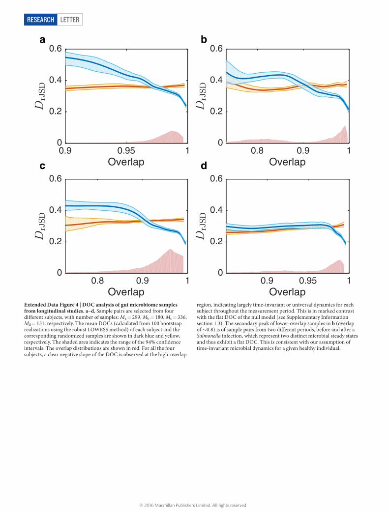
To verify the DOC analysis directly using real data, we analysed longitudinal gut microbial samples of four healthy individuals from two microbiome studies11,28. For each individual, we expect a highly universal microbial dynamics throughout the period of measurement; that is, the ecological parameters Θ ν( ) of the corresponding microbial community are largely time-invariant. We found that the DOCs of all four subjects show a clear negative slope in the high-overlap region (Extended Data Fig. 4), consistent with our expectation.

Next, we systematically analysed cross-sectional microbial samples of different body sites from two large-scale metagenomic studies, the Human Microbial Project (HMP)9,15 and the Student Microbiome Project (SMP)16. The results are shown in Fig. 3 and Extended Data Fig. 5. In Fig. 3, for each body site the DOCs calculated from real and randomized samples are shown in dark blue and red, respectively. The overlap distributions of the real between-subjects sample pairs are shown in pink. Note that the characteristic overlap in a particular body

0.5 0.6 0.7 0.8 0.9 1.0

0.1

0.2

0.3

0.4

0.5

Overlap0.5 0.6 0.7 0.8 0.9 1.0

Overlap

Dis

sim

ilarit

y

0.1

0.2

0.3

0.4

0.5

Dis

sim

ilarit

y

b

ii iii iv

Rel

ativ

e ab

und

ance

Ren

orm

aliz

ed a

bun

dan

ce

iii

iii

iv

c

i

a Real data Randomized data

Figure 2 | Higher overlap of microbial communities is associated with lower dissimilarity. a, Four gut microbial sample pairs (i–iv) represented by stacked bars at the genus level. For each sample pair, their shared genera are coloured while non-shared genera are shown in grey. b, DOC (in dark blue) of gut microbial sample pairs from the HMP study

(M = 190 samples). Grey dots represent all the 17,955 sample pairs. c, DOC (in dark red) of the randomized samples is flat. In b and c, and throughout the paper, shaded area indicates the range of the 94% confidence interval (see Methods).

© 2016 Macmillan Publishers Limited. All rights reserved

Letter reSeArCH

9 j u n e 2 0 1 6 | V O L 5 3 4 | n A T u R e | 2 6 1

site is different in the two studies. For example, the average overlap between HMP gut samples is about 0.4 and between SMP samples is about 0.75. To account for this fact and to compare the DOCs fairly across different body sites and studies, we used two different measures to quantify the universality (see Methods). Notably, although these two measures quantify different features of the DOC analysis, the body- sites stratification pattern is consistent across the two measures and

the two studied data sets (Extended Data Fig. 6). In particular, the neg-ative slope of DOC is most significantly observed in samples from the gut and mouth and least observed in samples from hand skin (palm and elbow). These findings strongly suggest the existence of universal dynamics characterized by inter-species interactions in the gut and mouth microbiomes.

An alternative explanation for the observed negative slope of the DOC for gut and mouth microbiomes of healthy subjects could be that some host factors not only select for the presence of certain microbes but also drive their relative abundances by enforcing certain optimally adapted compositions. To test this alternative explanation, we system-atically analysed microbial samples while controlling for the effect of several leading candidates for potential confounding factors, for exam-ple, body mass index, age, long-term dietary pattern and stool con-sistency. We found that as long as their values are in the normal range those factors cannot explain the observed DOC pattern (see Extended Data Figs 7 and 8). Hence, the alternative explanation for the negative slope in DOC is unlikely to be true. Of course, with currently available data sets we cannot possibly account for all other confounders, such as drugs, genetics, inflammation, or their combinations. More data sets will be needed to test this intriguing alternative explanation.

The above results of healthy subjects raise an interesting question: does the universality of microbial dynamics also exist in subjects with disrupted microbiomes? To address this question, we applied the DOC analysis to microbial samples of 17 subjects with recurrent Clostridium difficile infection (rCDI) and the same set of subjects after FMT17. Clostridium difficile is an opportunistic pathogen that causes disease worldwide and greatly increases morbidity and mortality in hospital-ized patients. Fortunately, FMT is very efficacious in treating patients with rCDI, with pronounced clinical improvement even after a single treatment29. We found that the dissimilarity between rCDI subjects is largely independent of their species overlap, rendering a flat DOC (Fig. 4a). By contrast, after FMT (median, 4 days) the DOC displays a pronounced negative slope in the high-overlap region (Fig. 4b), sug-gesting a universal gut microbial dynamics. FMT treatments show the flexibility of microbial communities and their adaptation to composi-tion changes. Our result suggests that this adaptive behaviour may be associated with the observed universal microbial dynamics after FMT.

Overlap

DrJ

SD

0.30 0.2 0.4 0.6 0.8 1.0

Overlap

0 0.2 0.4 0.6 0.8 1.0

0.4

0.5

0.6

0.7

0.8

0.9

DrJ

SD

0.3

0.4

0.5

0.6

0.7

0.8

0.9a

Pre-FMT

b

Post-FMT

Different donorsSame donor

Figure 4 | DOC analysis of human subjects with rCDI. a, Before FMT, the DOC (dark green line) of the rCDI subjects is nearly flat. b, After FMT, the DOC (dark blue line) displays a pronounced negative slope in the high-overlap region. We denoted a subject pair as a solid (or hollow) circle if the two subjects received FMT from the same donor (or two different donors). Notably, solid circles spread over a wide range of overlap values, suggesting that even if two subjects share the same donor, their post-FMT microbiomes may still display strong inter-individual variability.

Gastrointestinal

Skin Airways

UrogenitalOral

Overlap

DrJ

SD

a c1 c2b

SM

PH

MP

d e1 f1 f2

f3 f4e2 e3

e4 e5 g1

g3

g2

e6 e7 h

e8 e9

0.5

0.2

0.4

0.6

0.5

0.2

0.4

0.6

0 0.5

0.2

0.4

0.6

0 0.5

0.2

0.4

0.6

0.5

0.2

0.4

0.6

0.5

0.2

0.4

0.6

0.5

0.2

0.4

0.6

0.5

0.2

0.4

0.6

0 0.5

0.2

0.4

0.6

0 0.5

0.2

0.4

0.6

0.5

0.2

0.4

0.6

0.5

0.2

0.4

0.6

0.5

0.2

0.4

0.6

0.5

0.2

0.4

0.6

0 0.5

0.2

0.4

0.6

0 0.5

0.2

0.4

0.6

0.5

0.2

0.4

0.6

0.5

0.2

0.4

0.6

0.4 0.6 0.8 1.0

1.0 1.0 1.0 1.0

1.0 1.0 1.0 1.0

1.0 1.0 1.0 1.0

1.0 1.0

1.0 1.0

1.0 1.0

1.0 1.0 1.0

0.2

0.4

0.6

0.7 0.8 0.9

0.2

0.4

0.6

0.7 0.8 0.9

0.2

0.4

0.6

0.6 0.8

0.2

0.4

0.6

Figure 3 | Detecting universality of microbial dynamics in different body sites. a–h, We calculated DOCs for real (dark blue) and randomized (dark red) samples of two data sets: (1) SMP: gut (a), tongue (b), forehead skin (c1), palm skin (c2); (2) HMP: gut (d), tongue dorsam (e1), attached keratinized gingiva (e2), buccal mucosa (e3), hard palate (e4), palatine tonsils (e5), subgingival plaque (e6), supergingival plaque (e7), throat (e8), saliva (e9), left/right antecubital fossa (f1/f2), left/right retroauricular crease (f3/f4), vaginal introitus (g1), mid-vagina (g2), posterior fornix (g3), anterior nares (h). The overlap distributions of the real between-subjects sample pairs are shown in pink. The vertical green line represents the change point (see Methods).

© 2016 Macmillan Publishers Limited. All rights reserved

LetterreSeArCH

2 6 2 | n A T u R e | V O L 5 3 4 | 9 j u n e 2 0 1 6

Finally, we anticipate that applying our DOC analysis to subjects with other diseases (especially non-gastrointestinal diseases) or infants at different developmental stages will offer deeper insights into how dynamical processes shape human microbial ecosystems. The devel-oped DOC analysis can also be directly applied to other microbial ecosystems—for example, the microbiome of soil, ocean, lakes, phyllosphere/rhizosphere and fermenters—to detect the universality of the underlying ecological dynamics (see Extended Data Fig. 9). This sheds light on the design of more advanced methods to extract dynamical information from microbial data.

Online Content Methods, along with any additional Extended Data display items and Source Data, are available in the online version of the paper; references unique to these sections appear only in the online paper.

received 24 August 2015; accepted 9 May 2016.

1. Cho, I. & Blaser, M. J. The human microbiome: at the interface of health and disease. Nat. Rev. Genet. 13, 260–270 (2012).

2. Pflughoeft, K. J. & Versalovic, J. Human microbiome in health and disease. Annu. Rev. Pathol. 7, 99–122 (2012).

3. Lozupone, C. A., Stombaugh, J. I., Gordon, J. I., Jansson, J. K. & Knight, R. Diversity, stability and resilience of the human gut microbiota. Nature 489, 220–230 (2012).

4. Borody, T. J. & Khoruts, A. Fecal microbiota transplantation and emerging applications. Nat. Rev. Gastroenterol. Hepatol. 9, 88–96 (2011).

5. Aroniadis, O. C. & Brandt, L. J. Fecal microbiota transplantation: past, present and future. Curr. Opin. Gastroenterol. 29, 79–84 (2013).

6. Gerber, G. K. The dynamic microbiome. FEBS Lett. 588, 4131–4139 (2014).7. Costello, E. K., Stagaman, K., Dethlefsen, L., Bohannan, B. J. M. & Relman, D.

a. The application of ecological theory toward an understanding of the human microbiome. Science 336, 1255–1262 (2012).

8. Franzosa, E. A. et al. Identifying personal microbiomes using metagenomic codes. Proc. Natl Acad. Sci. USA 112, E2930–E2938 (2015).

9. The Human Microbiome Project Consortium. Structure, function and diversity of the healthy human microbiome. Nature 486, 207–214 (2012).

10. Bucci, V. & Xavier, J. B. Towards predictive models of the human gut microbiome. J. Mol. Biol. 426, 3907–3916 (2014).

11. David, L. A. et al. Host lifestyle affects human microbiota on daily timescales. Genome Biol. 15, R89 (2014).

12. Sommer, F. & Backhed, F. The gut microbiota—masters of host development and physiology. Nat. Rev. Microbiol. 11, 227–238 (2013).

13. Goodrich, J. K. et al. Human genetics shape the gut microbiome. Cell 159, 789–799 (2014).

14. Walter, J. & Ley, R. The human gut microbiome: ecology and recent evolutionary changes. Annu. Rev. Microbiol. 65, 411–429 (2011).

15. The Human Microbiome Project Consortium. A framework for human microbiome research. Nature 486, 215–221 (2012).

16. Flores, G. E. et al. Temporal variability is a personalized feature of the human microbiome. Genome Biol. 15, 531 (2014).

17. Youngster, I. et al. Fecal microbiota transplant for relapsing Clostridium difficile infection using a frozen inoculum from unrelated donors: a randomized, open-label, controlled pilot study. Clin. Infect. Dis. 58, 1515–1522 (2014).

18. Lemon, K. P., Armitage, G. C., Relman, D. a. & Fischbach, M. a. Microbiota-targeted therapies: an ecological perspective. Sci. Transl. Med. 4, 137rv135 (2012).

19. Levy, R. & Borenstein, E. Metabolic modeling of species interaction in the human microbiome elucidates community-level assembly rules. Proc. Natl Acad. Sci. USA 110, 12804–12809 (2013).

20. Jumpertz, R. et al. Energy-balance studies reveal associations between gut microbes, caloric load, and nutrient absorption in humans. Am. J. Clin. Nutr. 94, 58–65 (2011).

21. Faust, K. & Raes, J. Microbial interactions: from networks to models. Nat. Rev. Microbiol. 10, 538–550 (2012).

22. Friedman, J. & Alm, E. J. Inferring correlation networks from genomic survey data. PLoS Comput. Biol. 8, e1002687 (2012).

23. Koren, O. et al. A guide to enterotypes across the human body: meta-analysis of microbial community structures in human microbiome datasets. PLoS Comput. Biol. 9, e1002863 (2013).

24. Gibson, T. E., Bashan, A., Cao, H.-T., Weiss, S. T. & Liu, Y.-Y. On the origins and control of community types in the human microbiome. PLOS Comput. Biol. 12, e1004688 (2016).

25. Stein, R. R. et al. Ecological modeling from time-series inference: insight into dynamics and stability of intestinal microbiota. PLOS Comput. Biol. 9, e1003388 (2013).

26. Fisher, C. K. & Mehta, P. Identifying keystone species in the human gut microbiome from metagenomic timeseries using sparse linear regression. PLoS ONE 9, e102451 (2014).

27. Buffie, C. G. et al. Precision microbiome reconstitution restores bile acid mediated resistance to Clostridium difficile. Nature 517, 205–208 (2015).

28. Caporaso, J. G. et al. Moving pictures of the human microbiome. Genome Biol. 12, R50 (2011).

29. Kassam, Z., Lee, C. H., Yuan, Y. & Hunt, R. H. Fecal microbiota transplantation for Clostridium difficile infection: systematic review and meta-analysis. Am. J. Gastroenterol. 108, 500–508 (2013).

Supplementary Information is available in the online version of the paper.

Acknowledgements We thank E. K. Silverman, G. Weinstock, C. Huttenhower, R. Knight, G. Ackermann, D. Del Vecchio, D. Lauffenburger, G. Abu-Ali, J. Sordillo, M. McGeachie, and J. Gore for discussions. Special thanks to A.-L. Barabási and J. Loscalzo for careful reading of the manuscript. This work was partially supported by the John Templeton Foundation (award number 51977) and National Institutes of Health (R01 HL091528).

Author Contributions Y.-Y.L. conceived and designed the project. A.B. developed the DOC analysis, performed numerical simulations, and analysed all the real data. A.B. and Y.-Y.L. performed analytical calculations. A.B. and V.J.C. performed statistical tests. All authors analysed the results. A.B. and Y.-Y.L. wrote the manuscript. All authors edited the manuscript.

Author Information Reprints and permissions information is available at www.nature.com/reprints. The authors declare no competing financial interests. Readers are welcome to comment on the online version of the paper. Correspondence and requests for materials should be addressed to Y.-Y.L. (yyl@channing.harvard.edu).

reviewer Information Nature thanks F. He, P. Rohani and the other anonymous reviewer(s) for their contribution to the peer review of this work.

© 2016 Macmillan Publishers Limited. All rights reserved

Letter reSeArCH

MethOdSAll the data sets analysed in this work have been published (see Methods section ‘Human microbiome data sets analysed in this work’ for details). The original experiments and corresponding power analysis have been reported in previous publications.Overlap between species assemblages. Consider two microbial samples, represented by two abundance vectors R= ( … )∈x x x, , N

N1 and R= ( … )∈y y y, , N

N1 . For

genomic survey data of the human microbiome, only the relative abundances are known. Hence, we are dealing with the relative abundance profiles = ( … )� ��x x x, , N1 and = ( … )� ��y y y, , N1 , where ≡

∑ =�xi

x

xi

jN

j1 and ≡

∑ =�yi

y

yi

jN

j1. To quantify the similarity

of the species assemblages (sets) of the two samples, denoted as = | >X i x{ 0}i and

= | >Y i y{ 0}i , we defined the overlap measure ∑( )≡∈

+� �

� �x yO , ,i S

x y2

i i where

∩≡S X Y is the set of shared species present in both samples. In case S is empty, ( ) = .� �x yO , 0 If = …S N{1, , } , that is, all the species in X and Y are shared, then ( ) =� �x yO , 1, but the abundance profiles �x and �y can still be very different. In the

extreme case when the relative abundance is the same for all species in X and Y, the overlap measure can be written as a function of the classical Jaccard index. Yet, there are many advantages of using the overlap measure, instead of the Jaccard index, in our analysis (see Supplementary Information section 1.1.4).Dissimilarity between abundance profiles. To compare the abundance profiles of two samples, we first renormalize the relative abundances of only the shared species (in set S), yielding ˆ ˆ= ∈x x{ }i i S and ˆ ˆ= ∈y y{ }i i S . Here

ˆ ≡ = =∑

/∑

∑ /∑ ∑∈

∈

∈ ∈ ∈

��

xix

xx x

x xx

xi

j S j

i k X k

j S j k X k

i

j S j and yi is defined similarly. This way we

remove the spurious dependence between the relative abundances of the shared and the non-shared species. More importantly, this renormalization assures that the calculated dissimilarity measure is mathematically independent of the overlap measure (see Supplementary Information section 1.2.1). The dissimilarity is then evaluated via the root Jensen–Shannon divergence (rJSD) measure

ˆ ˆ ˆ ˆ ˆ ˆ( ) = ( )≡

( ) + ( )

x y x y x m y mD D D D, , , ,2rJSD

KL KL12

in which ˆ ˆ≡ +m x y

2 and ˆ ˆ ˆ ˆ

ˆ( ) ≡∑ ∈x yD x, logi S ixyKL

i

i is the Kullback–Leibler diver-

gence between x and y. The dissimilarity can also be evaluated via any other clas-sical dissimilarity measures in ecology and biology, for example, Bray–Curtis dissimilarity, Yue–Clayton dissimilarity, and the negative Spearman correlation (see Extended Data Fig. 5). In this work, we focused on rJSD because it is a distance metric that satisfies non-negativity, identity, symmetry and triangle inequality (see Supplementary Information section 1.1.1). Comparing sample pairs on the basis of phylogenetic information, for example, using weighted- and unweighted- UniFrac30 as quantitative and qualitative measures, respectively, has the potential to provide better insight on the communities’ dissimilarity–overlap behaviour. However, since the weighted- and unweighted-UniFrac are not mathematically independent, they cannot be trivially integrated into our DOC analysis.DOC. To compare sample pairs systematically with a wide range of overlap val-ues and analyse their dissimilarity–overlap relations, we calculate the overlap and dissimilarity of all the sample pairs from a given set of microbiome samples and represent each sample pair as a point in the dissimilarity–overlap plane. We then use the robust LOWESS (locally weighted scatterplot smoothing) method, a standard non-parametric regression method that is resistant to outliers, to calculate the DOC.

To get the confidence interval, we use the following bootstrap technique. (1) From a data set of M samples we calculate the overlap and dissimilarity of the M(M − 1)/2 sample pairs, represented as M(M − 1)/2 points in the overlap– dissimilarity plane. (2) In each bootstrap realization, we resample a new set = …K k k{ , , }M1 from the M original samples with replacement. Some of the orig-

inal samples might not be included and some could be sampled more than once. (3) We create a new cloud of points C: a point associated with sample pair (i, j) is included in C only if both ∈i j K, , while a point is chosen several times if the sam-ple i or j were resampled more than once in K. (4) A new DOC is calculated for C using the robust LOWESS method. We set the smoothing parameter (‘span’) to be 0.2. (5) We repeat steps (2)–(4) T times to create T DOCs. (6) The 3rd and 97th percentiles of the T curves represent the 94% confidence interval for the DOC. In this work, we chose T = 100.Assumptions of the DOC analysis. There are two reasonable assumptions under-lying the DOC analysis. First, the abundance profiles of the samples should repre-sent the steady states of the microbial ecosystem and hence the fixed points of the underlying dynamics that satisfy =�x 0. This assumption is fairly reasonable because human gut microbiota is a relatively resilient ecosystem3, and until the next large perturbation (for example, antibiotic administration or dramatic dietary

change) is introduced, the system remains stable for months and possibly even years11,28,31. Second, if two communities have the same species assemblages and the same abundance profile (steady state), then the two communities have the same microbial dynamics. Mathematically, this is not necessarily true, because different dynamical systems can give rise to an identical steady state or fixed point. Yet, given the large number of species and all the other levels of complexity in their interac-tions, the possibility of having different dynamics with the same fixed point is very unlikely. Indeed, universal dynamics is the most plausible explanation for the observed pattern, that is, the negative slope of DOC in the high-overlap region.Limitations of the DOC analysis. We point out that for overlap values close to zero, a positive slope may occur as the artefact of dissimilarity between relative abundance profiles with small number of species (see Fig. 3e4, f1–f4, g1–3, h, Extended Data Fig. 10, and Supplementary Information section 1.1.3).

We also emphasize that a flat DOC does not completely rule out the possibility of universal dynamics. For example, the DOC of the gut microbiome samples of rCDI patients is flat (Fig. 4a). There are two possibilities. First, the universality of microbial dynamics found in healthy subjects (Fig. 3a, d) is completely lost in the rCDI subjects, owing to the infection and/or the dysbiosis caused by the extensive inciting antibiotic treatment. Second, the possibly universal microbial dynamics of the rCDI subjects are just undetectable by the DOC analysis. This could be due to the extremely liquid stool samples of the rCDI subjects that suffer from diarrhoea, as stool consistency has been found to be strongly correlated with the gut microbiota compositions32,33. It is also possible that the abundance profiles of rCDI subjects are markedly varying over time and hence do not represent the steady states of the underlying microbial ecosystem (although a mouse infection model does not seem to support this hypothesis34).

If true multi-stability exists, that is, multiple stable states (abundance profiles) are associated with the same set of species present in the same environment, then our DOC analysis may not detect it. However, true multi-stability in human- associated microbial communities has not been demonstrated experimentally, partially because any subtle differences in the species assemblages can drive those microbial communities35.

In summary, our DOC analysis detects universal dynamics under certain condi-tions. More precisely, it provides a means of discriminating dynamics into universal or possibly universal.Universality measures and statistical test. Note that the DOCs of different data sets/studies must be compared with caution, especially if the microbial samples were preprocessed by different pipelines36, for example, with different operational taxonomic unit (OTU) clustering thresholds, or different OTU picking methods. As shown in Fig. 3, the characteristic overlap in a particular body site is different in different studies. For example, the average overlap between HMP gut samples is about 0.4 and between SMP samples is about 0.75. To account for this fact and to compare the DOCs fairly across different body sites and studies, we used two different measures to quantify the universality.

(1) fns. For each cohort we determined the fraction of data points for which the DOC displays a negative slope, denoted as fns. Specifically, for a given DOC calcu-lated from a cohort of M microbial samples, we first detected the ‘change point’ Oc such that ( )y O

Od

d< 0 for any >O Oc, in which y(O) is a smoothed curve of the DOC

(for example, using the default ‘smooth’ function of Matlab with moving average over 5 neighbours). Then, fns is defined as ≡ .>f O O

nsnumber of sample pairs with

total number of sample pairsc In

Fig. 3a–h, this is the area of the overlap distribution to the right of the green vertical line (the change point Oc). The results of fns for different body sites are shown in Extended Data Fig. 6a.

(2) P value. To estimate the slope of the DOC, we used a linear mixed-effects model, which explicitly takes into account the fact that those data points in the dissimilarity–overlap plane are not completely independent (because for a data set of M samples, each sample affects (M − 1) data points). To avoid any potential biases due to the detection of change point, we use data points with overlap larger than the median value, that is 50% of all the data points, for all the data sets (from all the body sites). We repeated this step for 200 bootstrap realizations. The distri-butions of the slopes for different body sites are shown in Extended Data Fig. 6b. The one-tailed P values are calculated as the fraction of bootstrap realizations with a non-negative slope, and adjusted for multiple comparisons by the procedure of Benjamini and Hochberg37.

We emphasize that those two measures are complementary. In the first measure (fns), we consider the existence of a negative slope and ask what is the fraction of data points that support it. In the second measure, we consider a fixed fraction of data points (50%) and asked whether a significant negative slope is observed.Population dynamics model. The GLV model represents the dynamics of N interacting species as a set of ordinary differential equations:

∑= + = … .=

r x a x x i N, 1, ,xt i i

j

N

ij i jdd

1

i Here, ri is the intrinsic growth rate of species

© 2016 Macmillan Publishers Limited. All rights reserved

LetterreSeArCH

i, aij is the interaction strength between species j and i, and a xii i2 (with <a 0ii )

represents the logistic growth term. We considered a microbial ‘sample’ as a steady state of a GLV model parameterized by the growth rate vector R= ∈r r{ }i N and the interaction matrix R= ( ) ∈ ×A aij

N N and we set N = 100 and aii = −1 in our simulations. We generated different ‘cohorts’, each consists of M = 100 ‘samples’. The GLV models differ from each other in their specific parameters (ri and aij). To achieve that, for each cohort, we first constructed a ‘base’ GLV model ( )� �r A, as follows: �ri is randomly chosen from the uniform distribution U( ).0, 1 �aij is randomly chosen from the normal distribution N σσ σ( ( ) )� �0, ,max

2 varies between 0 and 1, σmax is the maximal interaction strength allowed to ensure stability of the ecological system (here σ = .0 1max ). Then, different GLV models ν( = … )M1, , are generated as random variations of this base model with ϕ=ν ν �r ri i i and φ=ν ν �a aij ij ij where both ϕνi and φνij are randomly chosen from a uni-

form distribution U δ δ( − + )1 , 1 so that the expected values of the parameters of those models in the same cohort are the same as the base model, that is,

=ν �r rE[ ] and =ν �E A A[ ] . In other words, all the samples of the same cohort are generated from GLV models that share the same structure and sign pattern of the base interaction matrix �A . As δ→ 0 the model parameters become identical in all the GLV models of the same cohort. Thus, δ δ≡ −� 1 quantifies the ‘universal-ity’ of the dynamics of those models. Finally, for each cohort, the 100 samples (steady states) were generated by integrating the GLV differential equations with random initial conditions (both initial assemblage and abundance profile are randomly chosen).Human microbiome data sets analysed in this work. Longitudinal microbiome data sets. (1) Two time series of gut microbiome consist of 336 and 131 stool sam-ples, respectively. A 16S rRNA gene-based data set, variable region V4, analysed here at the OTU level. For detailed description of this data set see ref. 28. The data are available at http://qiita.ucsd.edu under study ID 550. (2) Two time series of gut microbiome consist of 299 and 180 stool samples, respectively. A 16S rRNA gene-based data set, variable region V4, analysed here at the OTU level. For detailed description of this data set see ref. 11. The data are available in the European Bioinformatics Institute (EBI) European Nucleotide Archive (ENA) under the nucleotide accession number ERP006059.Cross-sectional microbiome data sets. To compare quantitatively the universality of microbial dynamics in different body sites, we used two large-scale microbiome data sets. (1) Human Microbiome Project (HMP)9,15. A 16S rRNA gene-based data set, variable regions V3 to V5, of the human microbiome from 239 healthy subjects. The data are available at http://hmpdacc.org/ and are detailed in refs 9, 15. This data set covers 18 body sites in five areas: the oral cavity (nine sites: saliva (M = 262), tongue dorsum (M = 291), palatine tonsils (M = 285), keratinized gin-giva (M = 289), hard palate (M = 275), buccal mucosa (M = 287), throat (M = 283), and sub- and supragingival plaques (M = 283 and M = 289, respectively)), the gut (one site: stool (M = 297)), the vagina (three sites: introitus (M = 115), mid-vagina (M = 124), and posterior fornix (M = 124)), the nasal cavity (one site: anterior nares (M = 230)), and the skin (four sites: left and right antecubital fossae (M = 161 and M = 171, respectively) and retroauricular creases (M = 240 and M = 257, respec-tively)). Full protocols are available on the HMP DACC website (http://hmpdacc.org/HMMCP). We performed the DOC analysis at the OUT level. We used a single sample from each subject. In case more than one sample is available, we used the first visit. (2) Student Microbiome Project (SMP). A 16S rRNA gene-based data set, variable region V4 from 85 college-aged adults. The data set covers four body sites: gut (M = 72), tongue (M = 79), forehead skin (M = 78) and palm skin (M = 60). In case there are multiple samples measured for one subject, we used the sample

from the first visit. For detailed description of this data set see ref. 16. The data are available at https://github.com/gregcaporaso/student-microbiome-project/tree/master/otu-tables.

To rule out several leading candidates of confounding factors in our DOC analysis, we analysed two additional data sets. (3) A data set of healthy volun-teers (M = 98) from the Cross-sectional Study of Diet and Stool Microbiome Composition (COMBO). Diet information was collected using two questionnaires that queried recent diet (recall) and habitual long-term diet (food frequency ques-tionnaire, FFQ). Stool samples were collected, and DNA samples were analysed by 454/Roche pyrosequencing of the variable region V1–V2 of the 16S rDNA gene segments. We performed the DOC analysis at the OTU level. For detailed descrip-tion of this data set see ref. 38. (4) A data set of healthy women (M = 53), aged 20–55 years (median 42.5), as part of the Flemish Gut Flora Project (FGFP). Stool consistency levels using Bristol stool scale (BSS) scores were self-reported. The V4 region of the 16S rDNA gene was sequenced. We performed the DOC analysis at the OTU level. For detailed description of this data set see ref. 33.Clinical trial data set. Stool samples of patients with rCDI: before and after FMT. This clinical trial was approved by the Partners Human Research Committee as well as by the US Food and Drug Administration (FDA) (Investigational New Drug application number 15199) and registered at Clinical Trials.gov (NCT01704937). Informed consent was obtained from all participants. Microbial samples from 17 patients with rCDI were analysed in the groups of pre-FMT and post-FMT. Only subjects for whom both pre- and post-FMT samples are available were included. In cases where more than one post-FMT sample is available we included only the first one (median, 4 days after FMT). The V4 region of the 16S rRNA gene was sequenced using an Illumina MiSeq. We performed the DOC analysis at the OTU level. For detailed description of this data set see ref. 17.Code availability. The Matlab code for computing the DOC and the universality measures as well as an example data set (that is, the data set used to generate Fig. 2b) are freely available at the project webpage: http://scholar.harvard.edu/yyl/doc and have been added to the Supplementary Information.

30. Lozupone, C. A., Hamady, M., Kelley, S. T. & Knight, R. Quantitative and qualitative beta diversity measures lead to different insights into factors that structure microbial communities. Appl. Environ. Microbiol. 73, 1576–1585 (2007).

31. Faith, J. J. et al. The long-term stability of the human gut microbiota. Science 341, 1237439 (2013).

32. Gilbert, J. A. & Alverdy, J. Stool consistency as a major confounding factor affecting microbiota composition: an ignored variable? Gut 65, 1–2 (2016).

33. Vandeputte, D. et al. Stool consistency is strongly associated with gut microbiota richness and composition, enterotypes and bacterial growth rates. Gut 65, 57–62 (2016).

34. Lawley, T. D. et al. Targeted restoration of the intestinal microbiota with a simple, defined bacteriotherapy resolves relapsing Clostridium difficile disease in mice. PLoS Pathog. 8, e1002995 (2012).

35. Faust, K. & Raes, J. Microbial interactions: from networks to models. Nat. Rev. Microbiol. 10, 538–550 (2012).

36. Goodrich, J. K. et al. Conducting a microbiome study. Cell 158, 250–262 (2014).37. Benjamini, Y. & Hochberg, Y. Controlling the false discovery rate: a practical

and powerful approach to multiple testing. J. R. Statist. Soc. B 57, 289–300 (1995).

38. Wu, G. D. et al. Linking long-term dietary patterns with gut microbial enterotypes. Science 334, 105–108 (2011).

39. Bickel, S. L., Tang, K. W. & Grossart, H.-P. Ciliate epibionts associated with crustacean zooplankton in German lakes: distribution, motility and bacterivory. Front. Microbiol. 3, 243 (2012).

© 2016 Macmillan Publishers Limited. All rights reserved

Letter reSeArCH

Extended Data Figure 1 | Displacement of normalized N-dimensional random walks. a, Trajectory of a two-dimensional random-walk represents the absolute abundance of two species x x,1 2. The initial state is marked by a red circle and the first 100 steps are shown. The solid black line is the one-dimensional simplex upon which the locations are projected to obtain the relative abundances � �x x,1 2. The dotted lines starting at the origin represent the projection process: all the points in a dotted line have the same relative abundances and they are all projected to the intersection of the dotted line and the simplex (for example, the solid red and green circles are projected to the red and green open circles, respectively). We define a new coordinate ( )≡ ( )− ( )� � �z t x t x t2 1 for the location of normalized relative abundance on the simplex. The displacement of the normalized random walk after t steps is then ( )− ( )� �z t z 0 , where ( )�z 0 is the projected location of the initial state (see, as an example, the distance

between the green and the red open circles in a). b, Distributions of displacement of an ensemble of 1,000 random walks after t steps (t = 1, 5, 10, 100, 1,000). For small t, the displacement distributions depend on t, while for large t (t = 100, 1,000) the distributions are the same. c, Symbols represent the average displacement of 1,000 N-dimensional normalized random walks (here we set N = 50), measured as DrJSD, and the error bars represent the s.d. Each random walk is forced to stay on the positive orthant, that is, if <( )x 0i

t we set =( )x 0it . DrJSD was calculated using all N

coordinates, setting =( ) −x 10it 4 as a pseudo count for =( )x 0i

t . Where t is small, the distance grows with increasing t; however, the distance saturates for large t. The dashed red and green lines represent the average distance between two random locations (green) and between the final locations ( ( = )x t 1,000 ) of the random walks (red).

© 2016 Macmillan Publishers Limited. All rights reserved

LetterreSeArCH

Extended Data Figure 2 | Detection of group dynamics using an ordination technique. a–h, In each row, 500 synthetic samples were generated. Samples in the same group were taken from the steady states of the same GLV model of 100 species. The initial species assemblages were determined in two scenarios: at random (a–d) or on the basis of the group (e–h). In the latter scenario, in each group the species were first randomly ordered and then in each of the samples the first f species were selected and the other been removed (f is randomly chosen from a uniform distribution U( )20, 100 ). In columns a and e, a standard ordination technique, that is, principal coordinate analysis (PCoA), was applied. All 500 samples were shown in the plane of the first two principal coordinates (using rJSD as the distance metric) and coloured according to their group. In b and f, only the samples that have high overlap (>0.95) with at least one other sample were shown. Panels c and g show the

dissimilarity distributions P(rJSD) between the high-overlap sample pairs. Panels d and h show the DOCs. The ordination technique successfully detects the existence of group dynamics (especially when the number of groups is small). We anticipate that the group dynamics can also be detected by classical clustering analysis. In the scenario of random collections, the PCoA of high-overlap samples, that is, samples that have high overlap (>0.95) with at least one other sample, is doing better than the PCoA of all samples to detect group dynamics, especially for a small number (~2–10) of groups. Moreover, for a small number of groups, the dissimilarity distributions P(rJSD) can distinguish between the two scenarios of initial assemblage selection: random or group-based. The ordination technique cannot distinguish between the cases of 500 groups (individual dynamics) and single group (universal dynamics). Those cases can be distinguished by the DOC analysis.

© 2016 Macmillan Publishers Limited. All rights reserved

Letter reSeArCH

Extended Data Figure 3 | Detecting universality in population dynamics models. Synthetic microbial samples were calculated as steady states of GLV models (see Methods). The GLV models are generated as cohorts (100 models in each cohort) with different levels of (i) inter-species interaction strength; and (ii) universality, tuned by the parameters σ� and δ�, respectively (see Methods). In each of the 100 models, a random fraction f of the species ( U∼ ( . )f 0, 0 8 ) was initially removed, and the remaining species were initiated with random abundance ( U∼ ( )x 0, 1 ). The dissimilarity–overlap points of sample pairs in each cohort and of the corresponding randomized samples are shown in light blue and yellow, respectively. The solid curves represent the DOCs calculated using the

robust LOWESS method. The DOC of cohorts generated by GLV models without inter-species interactions (a1, a4, a7) is flat even in the high-overlap region. This is because, without inter-species interactions, for any sample pair the presence or absence of unique (that is, non-shared) species has no effect on the shared ones. A flat DOC is also observed in the case of individual dynamics (a7, a8, a9), where a higher overlap between sample pairs does not lead to more similar abundance profiles. However, in the case of universal dynamics with strong inter-species interactions (for example, a3), the DOC displays a clear negative slope in the high-overlap region.

© 2016 Macmillan Publishers Limited. All rights reserved

LetterreSeArCH

Extended Data Figure 4 | DOC analysis of gut microbiome samples from longitudinal studies. a–d, Sample pairs are selected from four different subjects, with number of samples: Ma = 299, Mb = 180, Mc = 336, Md = 131, respectively. The mean DOCs (calculated from 100 bootstrap realizations using the robust LOWESS method) of each subject and the corresponding randomized samples are shown in dark blue and yellow, respectively. The shaded area indicates the range of the 94% confidence intervals. The overlap distributions are shown in red. For all the four subjects, a clear negative slope of the DOC is observed at the high-overlap

region, indicating largely time-invariant or universal dynamics for each subject throughout the measurement period. This is in marked contrast with the flat DOC of the null model (see Supplementary Information section 1.3). The secondary peak of lower-overlap samples in b (overlap of ~0.8) is of sample pairs from two different periods, before and after a Salmonella infection, which represent two distinct microbial steady states and thus exhibit a flat DOC. This is consistent with our assumption of time-invariant microbial dynamics for a given healthy individual.

© 2016 Macmillan Publishers Limited. All rights reserved

Letter reSeArCH

Student Microbiome Project (SMP) Human Microbiome Project (HMP)

Extended Data Figure 5 | DOC analysis of gut microbiome samples is consistent across different studies and different dissimilarity measures. For two microbiome samples, the dissimilarity of their abundance profiles over shared species can be evaluated by different measures. Weighted measures, such as rJSD, Bray–Curtis (BC) dissimilarity and Yue–Clayton (YC) dissimilarity should be applied to the renormalized abundance profiles, to ensure mathematical independence between the overlap and the dissimilarity measures. Rank-based dissimilarity measures, for

example, negative Spearman correlation (nSC), can be directly applied without renormalization. We used the four dissimilarity measures (rJSD, BC, YC and nSC) to calculate the DOC (using robust LOWESS) of gut microbiome samples from two studies: HMP and SMP. In all cases, we observed a pronounced negative slope in the DOC (dark-blue curve) of real sample pairs (light-blue points) and a flat DOC (orange curve) for the pairs of randomized samples (yellow points).

© 2016 Macmillan Publishers Limited. All rights reserved

LetterreSeArCH

Extended Data Figure 6 | Quantifying the universality of human microbial dynamics in different body sites. a, The fraction (fns) of data for which a negative slope is observed in Fig. 3. Note that for overlap values close to zero (for example, Fig. 3d, f1–4, g1–3) a positive slope occurs as the artefact of dissimilarity between relative abundance profiles with small number of species (see Supplementary Information section 1.1.3). For gut and mouth, a negative slope of DOC is observed in the two data sets for a broad range of overlap, indicating a significant universality of microbial dynamics in those habitats. By contrast, the negative slope of DOC in the hand’s skin microbiome is observed only for a small part of the sample

pairs. b, Box plot of the slope of DOC calculated from 200 bootstrap realizations. The slope is calculated by fitting a linear mixed-effects model for data points with overlap larger than the median. We report one-tailed P values, calculated as the fraction of bootstrap realizations with a non-negative slope, adjusted for multiple comparisons by the procedure of Benjamini and Hochberg. The null hypothesis of non-negative slope is rejected for all body sites (P < 1 × 10−2) except four skin sites: forehead (P = 0.099), palm (P = 0.377) in the SMP study and left/right antecubital fossa in the HMP study (P = 0.099 and P = 0.495).

© 2016 Macmillan Publishers Limited. All rights reserved

Letter reSeArCH

BMI

Long

-ter

m d

iet

Age

Stoo

l con

sist

ency

Race

Extended Data Figure 7 | See next page for caption.

© 2016 Macmillan Publishers Limited. All rights reserved

LetterreSeArCH

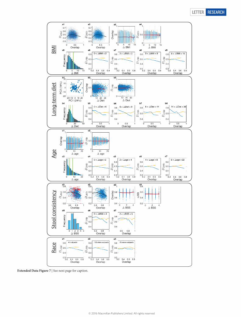
Extended Data Figure 7 | Effects of various host factors on the DOC analysis. a, The effect of body mass index (BMI) on the DOC analysis. a1, DOC analysis of all gut microbiome sample pairs among 190 subjects from the HMP study. Red points represent samples pairs associated with at least one obese subject (with BMI > 30). a2, Same as in a1, but 13 obese subjects with BMI > 30 were excluded. a3, Blue points represent the gut microbiome samples’ overlap and ΔBMI. The red curve is the average (error bars represent the s.e.m.). a4, Dissimilarity versus ΔBMI. a5, Distribution of ΔBMI values, divided into four groups of equal number of pairs. a6–a9, DOC analysis of the sample pairs in each group. b, The effect of diet on the DOC analysis. b1, Diet difference (Δdiet) between two subjects is defined as the Euclidean distance between their associated diet scores in the two leading principal components PC1 and PC2. In total there are M = 97 healthy subjects in the COMBO study38. b2, Overlap versus Δdiet. Blue points represent the overlap and Δdiet of all gut microbiome pairs among the 97 subjects from the COMBO study. The red curve is the average (error bars represent the s.e.m.). b3, Dissimilarity versus Δdiet. b4, Distribution of Δdiet values, divided into four groups of equal number of pairs. b5–b8, DOC analysis of the pairs in each group. c, The effect of age on the DOC analysis. c1, Overlap

versus Δdiet. Blue points represent the overlap and Δage of all gut microbiome samples pairs between the 190 subjects from the HMP study. The red curve is the average (error bars represent the s.e.m.). c2, Dissimilarity versus Δage. c3, Distribution of Δage values, divided into four groups of equal number of pairs. c4–c7, DOC analysis of the pairs in each group. d, The effect of stool consistency on the DOC analysis. d1, DOC analysis of all sample pairs. In this data set the subjects have BSS values between 1 and 6. The points (sample pairs) associated with subjects with BSS = 6 (at least one subject has BSS = 6) are coloured in red. The black line is the DOC. d2, DOC analysis of all subjects with BSS < 6. d3, d4, Among all subjects with 1 ≤ BSS ≤ 5, the overlap and the dissimilarity are independent of ΔBSS. d5, Distribution of ΔBSS values for the 46 subjects with 1 ≤ BSS ≤ 5. d6, d7, DOC analysis of the pairs with similar BSS values, 0 ≤ ΔBSS ≤ 1 (d6), and pairs with more different BSS values, 2 ≤ ΔBSS ≤ 4 (d7). In both cases, a clear negative slope of the DOC is observed. e, The effect of race on the DOC analysis. e1, All subjects (M = 190). e2, e3, White subjects (M = 153) (e2) and Asian subjects (M = 25) (e3). Note that in the HMP study, stool samples were collected from 153 white subjects, 10 black subjects, 25 Asian subjects, and 2 subjects from other races.

© 2016 Macmillan Publishers Limited. All rights reserved

Letter reSeArCH

Extended Data Figure 8 | DOC analysis under special conditions. a, The effect of strongly interacting species. A comparison of two GLV models of 100 species with random inter-species interactions. The system parameters were fixed for all the simulated samples (M = 100), representing maximal universality. In a1, all species have the same characteristic interaction strength, while in a2, the inter-species interactions of one species are markedly stronger than all other species, representing a strongly interacting species. The presence/absence of the strongly interacting species markedly affects (either directly or indirectly) the abundance profile of many other species, leading to a pronounced secondary cloud of points in the dissimilarity–overlap plane (a4). The effect is the most pronounced in the region of high-overlap (top 5%) pairs, and can be detected by looking at their dissimilarity distributions (a5, a6). b, DOC behaves the same for samples with uniform or skewed abundance distribution. b1, b2, Samples were generated from the steady states of the GLV model with largely uniform abundance distribution (determined mainly by the species growth rates). In the presence of inter-species interactions (b1), a negative slope of the DOC is observed. By contrast, in the absence of inter-species interactions (b2), a flat DOC is observed. b3, Real samples from the gut (from the HMP study, genus level) exhibit a high level of alpha-diversity and a very skewed abundance distribution. A negative slope of the DOC in the high-overlap region is observed. b4, The randomized samples preserve the abundance distribution of the real samples but the effect of inter-species interactions is removed, leading to a flat DOC. c, Effect of core species and non-interacting periphery species. c1, Samples were generated as steady states of the GLV model with N =100 species. The parameters of the GLV model were fixed for all the samples, representing maximal universality. The initial

species assemblages were chosen as follows: 30 species were present in all the samples, representing a set of ‘core species’, and the other 70 ‘peripheral’ species were present with lower probability (mean 0.18, min 0.12, and max 0.24). c2, Presence probability of real gut microbial samples, from the HMP at the genus level. Only one genus (Bacterioides) is present in all the samples. c3, Species presence probability in a GLV model where all species are present with average probability 0.6. c4, The effect of the interactions of the peripheral species. In the GLV model, the inter-species interactions among the core species (core–core) has a characteristic strength σcore = 0.15, and both the periphery–periphery and the periphery–core interactions have a characteristic strength σp. When σp = 0, that is, the peripheral species do not interact with the core species, the DOC is flat. When σp > 0, the DOC has a negative slope. c5, c6, In the case of real gut microbiome samples as well as the GLV model without core species, the DOC has a negative slope in the high-overlap region. d, The effect of sequencing depth on the DOC analysis. d1, Richness (number of present OTUs) versus sequencing depth of 190 HMP gut samples. 12 subjects with fewer than 1,300 reads per sample were excluded and the remaining 178 were assigned into two groups of n = 89 subjects, with average sequencing depth 3,019 and 8,640 reads per sample. d2, d3, The characteristic overlap between samples of group 1 is smaller than between samples of group 2. However, DOC analysis of each group shows a clear negative slope. d4–d6, Samples of each group were rarefied before analysis with minimal community size of 1,317 and 4,333 in group 1 and 2, respectively, as represented by the black dashed lines in d4. d7–d9, Samples of both groups were rarefied before analysis with the same minimal community size of 1,317, as represented by the black dashed line in d7.

© 2016 Macmillan Publishers Limited. All rights reserved

LetterreSeArCH

Extended Data Figure 9 | DOC analysis of longitudinal microbiome data from six lakes in Germany39. Data downloaded from http://qiita.microbio.me, study ID 945. a, Stechlin (M = 440). b, Haus (M = 26). c, Tiefwaren (M = 164). d, Melzer (M = 68). e, Breiter Luzin (M = 89). f, Fuchskuhle (M = 355). Blue points represent the dissimilarity–overlap values of sample pairs from the same lake. The DOCs of real samples from each lake and that from the corresponding randomized samples are calculated using robust LOWESS and shown in red and yellow,

respectively. For all the six lakes, a clear negative slope is observed for the DOCs of real samples, suggesting universal or time-invariant microbial dynamics for each lake. Differences in the DOC shapes (for example, the moderate DOC slope in b, c and d, in contrast with the steep DOC in a, e and f) deserve a systematic study of those microbial ecosystems. This example clear demonstrates the applicability of DOC analysis to general microbial ecosystems, for example, soil, ocean, rizosphere/phyllosphere and fermenters.

© 2016 Macmillan Publishers Limited. All rights reserved

Letter reSeArCH

Extended Data Figure 10 | Average dissimilarity between two normalized random vectors. Two independent vectors x, y of n elements randomly chosen from the uniform distribution U( )0, 1 were generated and then normalized ˆ ≡

∑ =xi

xx

i

jn

j1 and ˆ ≡

∑ =yi

yy

i

jn

j1. (Note that in practice all

n elements are always shared in x and y, since zeros are very unlikely.) The dissimilarity ˆ ˆ( )x yD , is then calculated using the five dissimilarity measures (DJSD, DrJSD, DBC, DYC and DnSC). Average dissimilarity and standard deviations of 1,000 pairs are shown in a1, b1, c1, d1 and e1,

for the different measures. The horizontal black dashed line represents the average dissimilarity for n = 100. For all the measures here, the dissimilarity displays no n-dependence for n > 15, while DnSC is n-independent for any n > 0. Similar analysis was performed for vectors whose elements were chosen from power-law distributions ( )∼ α−P x x with α = 3 (a2, b2, c2, d2 and e2) and ( )∼ α−P x x with α = 2

(a3, b3, c3, d3 and e3).

© 2016 Macmillan Publishers Limited. All rights reserved