Universal lossless data compression algorithms
214
Silesian University of Technology Faculty of Automatic Control, Electronics and Computer Science Institute of Computer Science Doctor of Philosophy Dissertation Universal lossless data compression algorithms Sebastian Deorowicz Supervisor: Prof. dr hab. in˙ z. Zbigniew J. Czech Gliwice, 2003
Transcript of Universal lossless data compression algorithms
Silesian University of TechnologyFaculty of Automatic Control, Electronics
and Computer ScienceInstitute of Computer Science
Doctor of Philosophy Dissertation
Universal losslessdata compression algorithms
Sebastian Deorowicz
Supervisor: Prof. dr hab. inz. Zbigniew J. Czech
Gliwice, 2003


To My Parents

Contents
Contents i
1 Preface 1
2 Introduction to data compression 72.1 Preliminaries . . . . . . . . . . . . . . . . . . . . . . . . . . . . . . . 72.2 What is data compression? . . . . . . . . . . . . . . . . . . . . . . . 82.3 Lossy and lossless compression . . . . . . . . . . . . . . . . . . . . 9
2.3.1 Lossy compression . . . . . . . . . . . . . . . . . . . . . . . 92.3.2 Lossless compression . . . . . . . . . . . . . . . . . . . . . . 10
2.4 Definitions . . . . . . . . . . . . . . . . . . . . . . . . . . . . . . . . 102.5 Modelling and coding . . . . . . . . . . . . . . . . . . . . . . . . . 11
2.5.1 Modern paradigm of data compression . . . . . . . . . . . 112.5.2 Modelling . . . . . . . . . . . . . . . . . . . . . . . . . . . . 112.5.3 Entropy coding . . . . . . . . . . . . . . . . . . . . . . . . . 12
2.6 Classes of sources . . . . . . . . . . . . . . . . . . . . . . . . . . . . 162.6.1 Types of data . . . . . . . . . . . . . . . . . . . . . . . . . . 162.6.2 Memoryless source . . . . . . . . . . . . . . . . . . . . . . . 162.6.3 Piecewise stationary memoryless source . . . . . . . . . . 172.6.4 Finite-state machine sources . . . . . . . . . . . . . . . . . . 172.6.5 Context tree sources . . . . . . . . . . . . . . . . . . . . . . 19
2.7 Families of universal algorithms for lossless data compression . . 202.7.1 Universal compression . . . . . . . . . . . . . . . . . . . . . 202.7.2 Ziv–Lempel algorithms . . . . . . . . . . . . . . . . . . . . 202.7.3 Prediction by partial matching algorithms . . . . . . . . . 232.7.4 Dynamic Markov coding algorithm . . . . . . . . . . . . . 262.7.5 Context tree weighting algorithm . . . . . . . . . . . . . . 272.7.6 Switching method . . . . . . . . . . . . . . . . . . . . . . . 28
2.8 Specialised compression algorithms . . . . . . . . . . . . . . . . . 29
i
ii CONTENTS
3 Algorithms based on the Burrows–Wheeler transform 313.1 Description of the algorithm . . . . . . . . . . . . . . . . . . . . . . 31
3.1.1 Compression algorithm . . . . . . . . . . . . . . . . . . . . 313.1.2 Decompression algorithm . . . . . . . . . . . . . . . . . . . 36
3.2 Discussion of the algorithm stages . . . . . . . . . . . . . . . . . . 383.2.1 Original algorithm . . . . . . . . . . . . . . . . . . . . . . . 383.2.2 Burrows–Wheeler transform . . . . . . . . . . . . . . . . . 383.2.3 Run length encoding . . . . . . . . . . . . . . . . . . . . . . 453.2.4 Second stage transforms . . . . . . . . . . . . . . . . . . . . 463.2.5 Entropy coding . . . . . . . . . . . . . . . . . . . . . . . . . 523.2.6 Preprocessing the input sequence . . . . . . . . . . . . . . 57
4 Improved compression algorithm based on the Burrows–Wheeler trans-form 614.1 Modifications of the basic version of the compression algorithm . 61
4.1.1 General structure of the algorithm . . . . . . . . . . . . . . 614.1.2 Computing the Burrows–Wheeler transform . . . . . . . . 624.1.3 Analysis of the output sequence of the Burrows–Wheeler
transform . . . . . . . . . . . . . . . . . . . . . . . . . . . . 644.1.4 Probability estimation for the piecewise stationary memo-
ryless source . . . . . . . . . . . . . . . . . . . . . . . . . . . 704.1.5 Weighted frequency count as the algorithm’s second stage 814.1.6 Efficient probability estimation in the last stage . . . . . . 84
4.2 How to compare data compression algorithms? . . . . . . . . . . . 924.2.1 Data sets . . . . . . . . . . . . . . . . . . . . . . . . . . . . . 924.2.2 Multi criteria optimisation in compression . . . . . . . . . 97
4.3 Experiments with the algorithm stages . . . . . . . . . . . . . . . . 984.3.1 Burrows–Wheeler transform computation . . . . . . . . . 984.3.2 Weight functions in the weighted frequency count transform1024.3.3 Approaches to the second stage . . . . . . . . . . . . . . . . 1044.3.4 Probability estimation . . . . . . . . . . . . . . . . . . . . . 106
4.4 Experimental comparison of the improved algorithm and the otheralgorithms . . . . . . . . . . . . . . . . . . . . . . . . . . . . . . . . 1064.4.1 Choosing the algorithms for comparison . . . . . . . . . . 1064.4.2 Examined algorithms . . . . . . . . . . . . . . . . . . . . . 1074.4.3 Comparison procedure . . . . . . . . . . . . . . . . . . . . . 1094.4.4 Experiments on the Calgary corpus . . . . . . . . . . . . . 1104.4.5 Experiments on the Silesia corpus . . . . . . . . . . . . . . 1204.4.6 Experiments on files of different sizes and similar contents 1284.4.7 Summary of comparison results . . . . . . . . . . . . . . . 136
5 Conclusions 141
iii
Acknowledgements 145
Bibliography 147
Appendices 161
A Silesia corpus 163
B Implementation details 167
C Detailed options of examined compression programs 173
D Illustration of the properties of the weight functions 177
E Detailed compression results for files of different sizes and similarcontents 185
List of Symbols and Abbreviations 191
List of Figures 195
List of Tables 196
Index 197

Chapter 1
Preface
I am now going to begin my story(said the old man), so please attend.
— ANDREW LANG
The Arabian Nights Entertainments (1898)
Contemporary computers process and store huge amounts of data. Some partsof these data are excessive. Data compression is a process that reduces the datasize, removing the excessive information. Why is a shorter data sequence of-ten more suitable? The answer is simple: it reduces the costs. A full-lengthmovie of high quality could occupy a vast part of a hard disk. The compressedmovie can be stored on a single CD-ROM. Large amounts of data are transmit-ted by telecommunication satellites. Without compression we would have tolaunch many more satellites that we do to transmit the same number of televi-sion programs. The capacity of Internet links is also limited and several meth-ods reduce the immense amount of transmitted data. Some of them, as mirroror proxy servers, are solutions that minimise a number of transmissions on longdistances. The other methods reduce the size of data by compressing them.Multimedia is a field in which data of vast sizes are processed. The sizes oftext documents and application files also grow rapidly. Another type of datafor which compression is useful are database tables. Nowadays, the amount ofinformation stored in databases grows fast, while their contents often exhibitmuch redundancy.
Data compression methods can be classified in several ways. One of themost important criteria of classification is whether the compression algorithm
1
2 CHAPTER 1. PREFACE
removes some parts of data which cannot be recovered during the decompres-sion. The algorithms removing irreversibly some parts of data are called lossy,while others are called lossless. The lossy algorithms are usually used whena perfect consistency with the original data is not necessary after the decom-pression. Such a situation occurs for example in compression of video or picturedata. If the recipient of the video is a human, then small changes of colors ofsome pixels introduced during the compression could be imperceptible. Thelossy compression methods typically yield much better compression ratios thanlossless algorithms, so if we can accept some distortions of data, these methodscan be used. There are, however, situations in which the lossy methods must notbe used to compress picture data. In many countries, the medical images can becompressed only by the lossless algorithms, because of the law regulations.
One of the main strategies in developing compression methods is to preparea specialised compression algorithm for the data we are going to transmit orstore. One of many examples where this way is useful comes from astronomy.The distance to a spacecraft which explores the universe is huge, what causesbig communication problems. A critical situation took place during the Jupitermission of Galileo spacecraft. After two years of flight, the Galileo’s high-gainantenna did not open. There was a way to get the collected data through a sup-porting antenna, but the data transmission speed through it was slow. The sup-porting antenna was designed to work with a speed of 16 bits per second atthe Jupiter distance. The Galileo team improved this speed to 120 bits per sec-ond, but the transmission time was still quite long. Another way to improve thetransmission speed was to apply highly efficient compression algorithm. Thecompression algorithm that works at Galileo spacecraft reduces the data sizeabout 10 times before sending. The data have been still transmitted since 1995.Let us imagine the situation without compression. To receive the same amountof data we would have to wait about 80 years.
The situation described above is of course specific, because we have heregood knowledge of what kind of information is transmitted, reducing the sizeof the data is crucial, and the cost of developing a compression method is oflower importance. In general, however, it is not possible to prepare a specialisedcompression method for each type of data. The main reasons are: it would resultin a vast number of algorithms and the cost of developing a new compressionmethod could surpass the gain obtained by the reduction of the data size. On theother hand, we can assume nothing about the data. If we do so, we have noway of finding the excessive information. Thus a compromise is needed. Thestandard approach in compression is to define the classes of sources producingdifferent types of data. We assume that the data are produced by a source ofsome class and apply a compression method designed for this particular class.The algorithms working well on the data that can be approximated as an output
3
of some general source class are called universal.
Before we turn to the families of universal lossless data compression algo-rithms, we have to mention the entropy coders. An entropy coder is a methodthat assigns to every symbol from the alphabet a code depending on the prob-ability of symbol occurrence. The symbols that are more probable to occur getshorter codes than the less probable ones. The codes are assigned to the symbolsin such a way that the expected length of the compressed sequence is minimal.The most popular entropy coders are Huffman coder and an arithmetic coder. Boththe methods are optimal, so one cannot assign codes for which the expectedcompressed sequence length would be shorter. The Huffman coder is optimalin the class of methods that assign codes of integer length, while the arithmeticcoder is free from this limitation. Therefore it usually leads to shorter expectedcode length.
A number of universal lossless data compression algorithms were proposed.Nowadays they are widely used. Historically the first ones were introduced byZiv and Lempel [202, 203] in 1977–78. The authors propose to search the datato compress for identical parts and to replace the repetitions with the informa-tion where the identical subsequences appeared before. This task can be accom-plished in several ways. Ziv and Lempel proposed two main variants of theirmethod: LZ77 [202], which encodes the information of repetitions directly, andLZ78 [203], which maintains a supporting dictionary of subsequences appearedso far, and stores the indexes from this dictionary in the output sequence. Themain advantages of these methods are: high speed and ease of implementation.Their compression ratio is, however, worse than the ratios obtained by othercontemporary methods.
A few years later, in 1984, Cleary and Witten introduced a prediction by partialmatching (PPM) algorithm [48]. It works in a different way from Ziv and Lempelmethods. This algorithm calculates the statistics of symbol occurrences in con-texts which appeared before. Then it uses them to assign codes to the symbolsfrom the alphabet that can occur at the next position in such a way that the ex-pected length of the sequence is minimised. It means that the symbols which aremore likely to occur have shorter codes than the less probably ones. The statis-tics of symbol occurrences are stored for separate contexts, so after processingone symbol, the codes assigned for symbols usually differ completely because ofthe context change. To assign codes for symbols an arithmetic coder is used. Themain disadvantages of the PPM algorithms are slow running and large memoryneeded to store the statistics of symbol occurrences. At present, these methodsobtain the best compression ratios in the group of universal lossless data com-pression algorithms. Their low speed of execution limits, however, their usagein practice.
Another statistical compression method, a dynamic Markov coder (DMC), was
4 CHAPTER 1. PREFACE
invented by Cormack and Horspool [52] in 1987. Their algorithm assumes thatthe data to compress are an output of some Markov source class, and during thecompression, it tries to discover this source by better and better estimating theprobability of occurrence of the next symbol. Using this probability, the codes forsymbols from the alphabet are assigned by making use of an arithmetic coder.This algorithm also needs a lot of memory to store the statistics of symbol occur-rences and runs rather slowly. After its formulation, the DMC algorithm seemedas an interesting alternative for the PPM methods, because it led to the compa-rable compression ratios with similar speed of running. In last years, there weresignificant improvements in the field of the PPM methods, while the researchon the DMC algorithms stagnated. Nowadays, the best DMC algorithms obtainsignificantly worse compression ratios than the PPM ones, and are slower.
In 1995, an interesting compression method, a context tree weighting (CTW) al-gorithm, was proposed by Willems et al. [189]. The authors introduced a conceptof a context tree source class. In their compression algorithm, it is assumed thatthe data are produced by some source of that class, and relating on this assump-tion the probability of symbol occurrence is estimated. Similarly to the PPM andthe DMC methods, an arithmetic coder is used to assign codes to the symbolsduring the compression. This method is newer than the before-mentioned anda relatively small number of works in this field have appeared so far. The mainadvantage of this algorithm is its high compression ratio, only slightly worsethan those obtained by the PPM algorithms. The main disadvantage is a lowspeed of execution.
Another compression method proposed recently is a block-sorting compressionalgorithm, called usually a Burrows–Wheeler compression algorithm (BWCA) [39].The authors invented this method in 1994. The main concept of their algo-rithm is to build a matrix, whose rows store all the one-character cyclic shiftsof the compressed sequence, to sort the rows lexicographically, and to use thelast column of this matrix for further processing. This process is known as theBurrows–Wheeler transform (BWT). The output of the transform is then handledby a move-to-front transform [26], and, in the last stage, compressed by an en-tropy coder, which can be a Huffman coder or an arithmetic coder. As the resultof the BWT, a sequence is obtained, in which all symbols appearing in similarcontexts are grouped. The important features of the BWT-based methods aretheir high speed of running and reasonable compression ratios, which are muchbetter than those for the LZ methods and only slightly worse than for the bestexisting PPM algorithms. The algorithms based on the transform by Burrowsand Wheeler seem to be an interesting alternative to fast, Ziv–Lempel methods,which give comparatively poor compression ratios, and the PPM algorithmswhich obtain the better compression ratios, but work slowly.
In this dissertation the attention is focused on the BWT-based compression
5
algorithms. We investigate the properties of this transform and propose an im-proved compression method based on it.
Dissertation thesis: An improved algorithm based on the Burrows–Wheelertransform we propose, achieves the best compression ratio among the BWT-based algorithms, while its speed of operation is comparable to the fastest algo-rithms of this family.
In the dissertation, we investigate all stages of the BWT-based algorithms,introducing new solutions at every phase. First, we analyse the structure of theBurrows–Wheeler transform output, proving some results, and showing thatthe output of the examined transform can be approximated by the output of thepiecewise stationary memoryless source. We investigate also methods for theBWT computation, demonstrating that a significant improvement to the Itoh–Tanaka’s method [90] is possible. The improved BWT computation method isfast and is used in further research. Using the investigation results of the BWToutput we introduce a weighted frequency count (WFC) transform. We examineseveral proposed weight functions, being the important part of the transform, onthe piecewise stationary memoryless source output, performing also numeri-cal analysis. The WFC transform is then proposed as the second stage of theimproved BWT-based algorithm (the replacement of the originally used MTFtransform). In the last stage of the compression method, the output sequenceof previous phases is compressed by the arithmetic coder. The most importantproblem at this stage is to estimate the probabilities of symbol occurrences whichare then used by the entropy coder. An original method, a weighted probability,is proposed for this task. Some of the results of this dissertation were publishedby the author in References [54, 55].
The properties of the proposed compression method are examined on thereal-world data. There are three well known data sets, used by researchers inthe field of compression: the Calgary corpus [20], the Canterbury corpus [12], andthe large Canterbury corpus [98]. The first one, proposed in 1989, is rather old,but it is still used by many researchers. The later corpora are more recent, butthey are not so popular and, as we discuss in the dissertation, they are not goodcandidates as the standard data sets. In the dissertation, we discuss also a needof examining the compression methods on files of sizes significantly larger thanthe existing ones in the three corpora. As the result, we propose a Silesia corpusto perform tests of the compression methods on files of sizes and contents whichare used nowadays.
The dissertation begins, in Chapter 2, with the formulation of the data com-pression problem. Then we define some terms needed to discuss compressionprecisely. In this chapter, a modern paradigm of data compression, modellingand coding, is described. Then, the entropy coding methods, such as Huffmanand arithmetic coding are presented. The families of universal lossless com-
6 CHAPTER 1. PREFACE
pression algorithms that are used nowadays: Ziv–Lempel algorithms, predic-tion by partial matching algorithms, dynamic Markov coder algorithms, andcontext tree weighting algorithms are also described in detail. Chapter 2 endswith a short review of some specialised compression methods. Such methodsare useful when we know something more about the data to compress. One ofthese methods was discussed by Ciura and the author of this dissertation in Ref-erence [47]. In Chapter 3, we focus our attention on the family of compressionalgorithms based on the Burrows–Wheeler transform. In the first part of thischapter, we describe the original BWCA in detail. Then, we present the resultsof the investigations on this algorithm, which were made by other researches.
Chapter 4, containing the main contribution of the dissertation, starts fromthe description of the proposed solutions. Then we discuss the methods of com-paring data compression algorithms. To this end, we describe three existing cor-pora for examining universal lossless data compression algorithms. The argu-ments for and against usage of the Calgary, the Canterbury, and the large Can-terbury corpora are presented. We also argue for a need of existence of a corpuscontaining larger and more representable files to the ones used contemporarily.Therefore, we introduce a Silesia corpus. Then, we discuss multi criteria optimisa-tion. This is done because the compression process cannot be treated as a simpleoptimisation problem in which only one criterion is optimised, say for examplethe compression ratio. Such criteria as compression and decompression speedsare also important. In the end of this chapter, we describe the experiments andcomment the obtained results.
Chapter 5 contains a discussion of obtained results and justification of thedissertation thesis. The dissertation ends with appendices, in which some de-tails are presented. Appendix A contains a more precise specification of files inthe Silesia corpus. Appendix B contains some technical information of the im-plementation. We briefly discuss here the contents of the source code files, em-ployed techniques, and the usage of the compression program implementing theproposed compression algorithm. The detailed information of the compressionprograms used for the comparison can be found in Appendix C. In Appendix D,some more detailed graphs obtained during the investigation of the probabilityestimation method in sequences produced by the piecewise stationary memo-ryless sources are presented. Appendix E contains the auxiliary results of theperformed experiments.
Chapter 2
Introduction todata compression
‘It needs compression,’I suggested, cautiously.
— RUDYARD KIPLING
The Phantom ’Rickshawand Other Ghost Stories (1899)
2.1 Preliminaries
Computers process miscellaneous data. Some data, as colours, tunes, smells,pictures, voices, are analogue. Contemporary computers do not work withinfinite-precise analogue values, so we have to convert such data to a digitalform. During the digitalisation process, the infinite number of values is reducedto a finite number of quantised values. Therefore some information is alwayslost, but the larger the target set of values, the less information is lost. Often theprecision of digitalisation is good enough to allow us neglecting the differencebetween digital version of data and their analogue original.
There are also discrete data, for example written texts or databases containdata composed of finite number of possible values. We do not need to digitisesuch types of data but only to represent them somehow by encoding the originalvalues. In this case, no information is lost.
7
8 CHAPTER 2. INTRODUCTION TO DATA COMPRESSION
Regardless of the way we gather data to computers, they usually are se-quences of elements. The elements come from a finite ordered set, called an al-phabet. The elements of the alphabet, representing all possible values, are calledsymbols or characters. One of the properties of a given alphabet is its number ofsymbols, and we call this number the size of the alphabet. The size of a sequence isthe number of symbols it is composed of.
The size of the alphabet can differ for various types of data. For a Booleansequence the alphabet consists of only two symbols: false and true, representableon 1 bit only. For typical English texts the alphabet contains less than 128 sym-bols and each symbol is represented on 7 bits using the ASCII code. The mostpopular code in contemporary computers is an 8-bit code; some texts are storedusing the 16-bit Unicode designed to represent all the alphabetic symbols usedworldwide. Sound data typically are sequences of symbols, which representtemporary values of the tone. The size of the alphabet to encode this data isusually 28, 216, or 224. Picture data typically contain symbols from the alphabetrepresenting the colours of image pixels. The colour of a pixel can be repre-sented using various coding schemes. We mention here only one of them, theRGB code that contains the brightness of the three components red, green, andblue. The brightness of each component can be represented, for example, using28 different values, so the size of the alphabet is 224 in this case.
A sequence of symbols can be stored in a file or transmitted over a network.The sizes of modern databases, application files, or multimedia files can be ex-tremely large. Reduction of the sequence size can save computing resources orreduce the transmission time. Sometimes we even would not be able to storethe sequence without compression. Therefore the investigation of possibilitiesof compressing the sequences is very important.
2.2 What is data compression?
A sequence over some alphabet usually exhibits some regularities, what is nec-essary to think of compression. For typical English texts we can spot that themost frequent letters are e, t, a, and the least frequent letters are q, z. We canalso find such words as the, of, to frequently. Often also longer fragments of thetext repeat, possibly even the whole sentences. We can use these properties insome way, and the following sections elaborate this topic.
A different strategy to compress the sequence of picture data is needed. Witha photo of night sky we can still expect that the most frequent colour of pixelsis black, or dark grey. But with a generic photo we usually have no informationwhat colour is the most frequent. In general, we have no a priori knowledge ofthe picture, but we can find regularities in it. For example, colours of successivepixels usually are similar, some parts of the picture are repeated.
2.3. LOSSY AND LOSSLESS COMPRESSION 9
Video data are typically composed of subsequences containing the data ofthe successive frames. We can simply treat the frames as pictures and com-press them separately, but more can be achieved with analysing the consecutiveframes. What can happen in a video during a small fraction of a second? Usuallynot much. We can assume that successive video frames are often similar.
We have noticed above that regularities and similarities often occur in thesequences we want to compress. Data compression bases on such observationsand attempts to utilise them to reduce the sequence size. For different types ofdata there are different types of regularities and similarities, and before we startto compress a sequence, we should know of what type it is. One more thingwe should mark here is that the compressed sequence is useful only for storingor transmitting, but not for a direct usage. Before we can work on our data weneed to expand them to the original form. Therefore the compression methodsmust be reversible. The decompression is closely related to the compression,but the latter is more interesting because we have to find the regularities in thesequence. Since during the decompression nothing new is introduced, it willnot be discussed here in detail.
A detailed description of the compression methods described in this chaptercan be found also in one of several good books on data compression by Bell etal. [22], Moffat and Turpin [116], Nelson and Gailly [118], Sayood [143], Skar-bek [157], or Witten et al. [198].
2.3 Lossy and lossless compression
2.3.1 Lossy compression
The assumed recipient of the compressed data influences the choice of a com-pression method. When we compress audio data some tones are not audibleto a human because our senses are imperfect. When a human will be the onlyrecipient, we can freely remove such unnecessary data. Note that after the de-compression we do not obtain the original audio data, but the data that soundidentically. Sometimes we can also accept some small distortions if it entails asignificant improvement to the compression ratio. It usually happens when wehave a dilemma: we can have a little distorted audio, or we can have no audioat all because of data storage restrictions. When we want to compress picture orvideo data, we have the same choice—we can sacrifice the perfect conformity tothe original data gaining a tighter compression. Such compression methods arecalled lossy, and the strictly bi-directional ones are called lossless.
The lossy compression methods can achieve much better compression ratiothan lossless ones. It is the most important reason for using them. The gap be-tween compression results for video and audio data is so big that lossless meth-ods are almost never employed for them. Lossy compression methods are also
10 CHAPTER 2. INTRODUCTION TO DATA COMPRESSION
employed to pictures. The gap for such data is also big but there are situationswhen we cannot use lossy methods. Sometimes we cannot use lossy methods tothe images because of the law regulations. This occurs for medical images as inmany countries they must not be compressed loosely.
Roughly, we can say that lossy compression methods may be used to datathat were digitised before compression. During the digitalisation process smalldistortions are introduced and during the compression we can only increasethem.
2.3.2 Lossless compression
When we need certainty that we achieve the same what we compressed afterdecompression, lossless compression methods are the only choice. They areof course necessary for binary data or texts (imagine an algorithm that couldchange same letters or words). It is also sometimes better to use lossless com-pression for images with a small number of different colours or for scanned text.
The rough answer to the question when to use lossless data compressionmethods is: We use them for digital data, or when we cannot apply lossy meth-ods for some reasons.
This dissertation deals with lossless data compression, and we will not con-cern lossy compression methods further. From time to time we can mentionthem but it will be strictly denoted. If not stated otherwise, further discussionconcerns lossless data compression only.
2.4 Definitions
For precise discussion, we introduce now some terms. Some of them were usedbefore but here we provide their precise definitions.
Let us assume that x = x1x2 . . . xn is a sequence. The sequence length or sizedenoted by n is a number of elements in x, and xi denotes the ith element of x.We also define the reverse sequence, x−1, as xnxn−1 . . . x1. Given a sequence x letus assume that x = uvw for some, possibly empty, subsequences u, v, w. Then uis called a prefix of x, v a component of x, and w a suffix of x. Each element of thesequence, xi, belongs to a finite ordered set A = {a0, a1, . . . , ak−1} that is calledan alphabet. The number of elements in A is the size of the alphabet and is denotedby k. The elements of the alphabet are called symbols or characters. We introducealso a special term for a non-empty component of x that consists of identicalsymbols that we call a run. To simplify the notation we denote the componentxixi+1 . . . xj by xi..j. Except the first one, all characters xi in a sequence x are pre-ceded by a nonempty prefix x(i−d)..(i−1). We name this prefix a context of order d ofthe xi. If the order of the context is unspecified we arrive at the longest possible
2.5. MODELLING AND CODING 11
context x1..(i−1) that we call simply a context of xi. It will be useful for clear pre-sentation to use also terms such as past, current, or future, related to time whenwe talk about the positions in a sequence relative to the current one.
2.5 Modelling and coding
2.5.1 Modern paradigm of data compression
The modern paradigm of compression splits it into two stages: modelling andcoding. First, we recognise the sequence, look for regularities and similarities.This is done in the modelling stage. The modelling method is specialised for thetype of data we compress. It is obvious that in video data we will be searchingfor different similarities than in text data. The modelling methods are oftendifferent for lossless and lossy methods. Choosing the proper modelling methodis important because the more regularities we find the more we can reduce thesequence length. In particular, we cannot reduce the sequence length at all if wedo not know what is redundant in it.
The second stage, coding, is based on the knowledge obtained in the mod-elling stage, and removes the redundant data. The coding methods are not sodiverse because the modelling process is the stage where the adaptation to thedata is made. Therefore we only have to encode the sequence efficiently remov-ing known redundancy.
Some older compression methods, such as Ziv–Lempel algorithms (see Sec-tion 2.7.2), cannot be precisely classified as representatives of modelling-codingparadigm. They are also still present in contemporary practical solutions, buttheir importance seems to be decreasing. We consider them to have a betterview of the background but we pay our attention to the modern algorithms.
2.5.2 Modelling
The modelling stage builds a model representing the sequence to compress, theinput sequence, and predicts the future symbols in the sequence. Here we esti-mate a probability distribution of occurrences of symbols.
The simplest way of modelling is to use a precalculated table of probabilitiesof symbol occurrences. The better is our knowledge of symbol occurrences inthe current sequence, the better we can predict the future characters. We canuse precalculated tables if we know exactly what we compress. If we knowthat the input sequence is an English text, we can use typical frequencies ofcharacter occurrences. If, however, we do not know the language of the text,and we use, e.g., the precalculated table for the English language to a Polishtext, we can achieve much worse results, because the difference between theinput frequencies and the precalculated ones is big. The more so, the Polish
12 CHAPTER 2. INTRODUCTION TO DATA COMPRESSION
language uses letters such as o, s that do not exist in English. Therefore thefrequencies table contains a frequency equal to zero for such symbols. It is a bigproblem and the compressor may not work when such extraordinary symbolsappear. Furthermore, the probability of symbol occurrences differs for texts ofvarious authors. Probably the most astonishing example of this discrepancy isa two hundred pages French novel La Disparition by Georges Perec [128] and itsEnglish translation A Void by Gilbert Adair [129], both not using the letter e atall!
Therefore a better way is not to assume too much about the input sequenceand build the model from the encoded part of the sequence. During the decom-pression process the decoder can build its own model in the same way. Such anapproach to the compression is called adaptive because the model is built onlyfrom past symbols and adapts to the contents of the sequence. We could not usethe future symbols because they are unknown to the decompressor. Other, static,methods build the model from the whole sequence before the compression andthen use it. The decompressor has no knowledge of the input sequence, and themodel has to be stored in the output sequence, too. The static approach wentalmost out of use because is can be proved that the adaptive way is equivalent,so we will not be considering it further.
2.5.3 Entropy coding
Entropy
The second part of the compression is typically the entropy coding. The methodsof entropy coding are based on a probability distribution of occurrences of thealphabet symbols, which is prepared by the modelling stage, and then compressthese characters. When we know the probability of occurrences of every symbolfrom the alphabet, but we do not know the current character, the best what wecan do is to assign to each character a code of length
log1pi
= − log pi (2.1)
where pi is the probability of occurrence of symbol ai [151]. (All logarithms inthe dissertation are to the base 2.) If we do so, the expected code length of thecurrent symbol is
E(.) = −k−1
∑i=0
pi · log pi. (2.2)
The difference between these codes and the ones used for representing the sym-bols in the input sequence is that here the codes have different length, while suchcodes as ASCII, Unicode, or RGB store all symbols using the identical numberof bits.
2.5. MODELLING AND CODING 13
0 1
0
1
0 1
0
1
5a 2b 2r 1c 1d
2
4
7
11
Huffman codes:
a:
b: 01
c: 0
d: 1
r: 10
Figure 2.1: Example of the Huffman tree for the sequence abracadabra
The expected code length of the current symbol is not greater than the codelength of this symbol. Replacing all characters from the input sequence withcodes of smaller expected length causes a reduction of the total sequence lengthand gives us compression. Note that if the modelling stage produces inadequateestimated probabilities, the sequence can expand during the compression. Herewe can also spot why a data compression algorithm will not be working on thePolish text with the English frequency table. Let us assume that we have tocompress the Polish letter s for which the expected probability is 0. Using therule of the best code length (Equation 2.1) the coder would generate an infinite-length code, what is impossible.
Huffman coding
Expression 2.1 means that we usually should assign codes of noninteger lengthto most symbols from the input sequence. It is possible, but let us first takea look on a method giving the best expected code length among the methodswhich use codes of integer length only. This coding procedure was introducedby Huffman [87] in 1952.
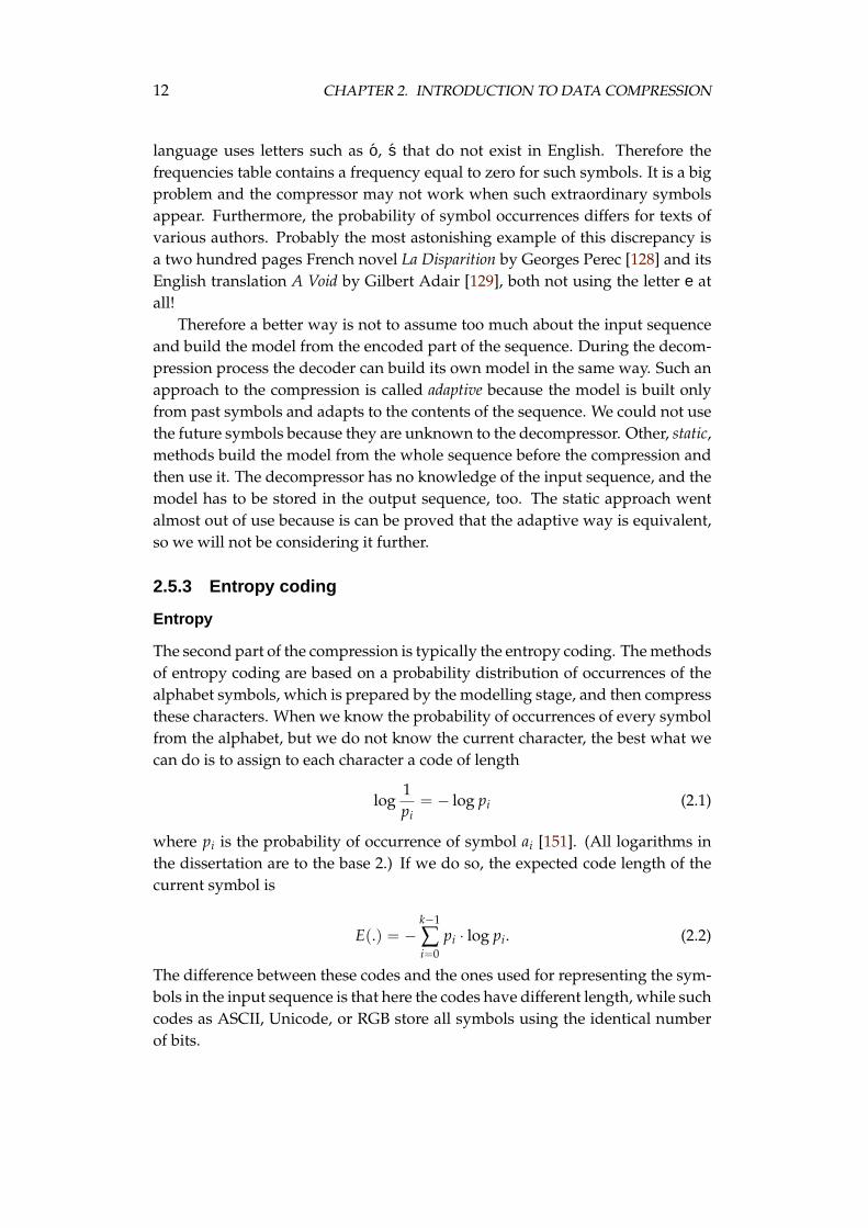
Let us assume that we have a table of frequencies of symbol occurrences inthe encoded part of the sequence (this is what the simple modelling method cando). Now we start building a tree by creating the leaves, one leaf for each symbolfrom the alphabet. Then we create a common parent for the two nodes withoutparents and with the smallest frequency. We assign to the new node a frequencybeing a sum of the frequencies of its sons. This process is repeated until thereis only one node without a parent. We call this node a root of the tree. Then wecreate the code for a given symbol, starting from the root and moving towardsthe leaf corresponding to the symbol. We start with an empty code, and when-
14 CHAPTER 2. INTRODUCTION TO DATA COMPRESSION
ever we go to a left son, we append 0 to it, whenever we go to a right son, weappend 1. When we arrive to the leaf, the code for the symbol is ready. This pro-cedure is repeated for all symbols. Figure 2.1 shows an example of the Huffmantree and the codes for symbols after processing a sequence abracadabra. Thereis more than one possible Huffman tree for our data, because if there are twonodes with the same frequency we can choose any of them.
The Huffman coding is simple, even though rebuilding the tree after pro-cessing each character is quite complicated. It was shown by Gallager [73] thatits maximum inefficiency, i.e., the maximum difference between the expectedcode length and the optimum (Equation 2.2) is bounded by
pm + log2 log e
e≈ pm + 0.086, (2.3)
where pm is the probability of occurrence of the most frequent symbol. Typicallythe loss is smaller and, owing to its simplicity and effectiveness, this algorithmis often used when compression speed is important.
The Huffman coding was intensively investigated during the years. Someof the interesting works were provided by Faller [62], Knuth [93], Cormack andHorspool [51], and Vitter [176, 177]. These works contain description of methodsof storing and maintaining the Huffman tree.
Arithmetic coding
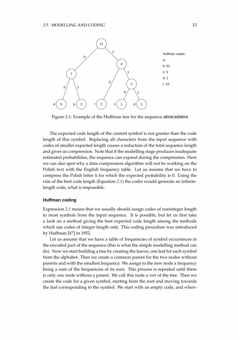
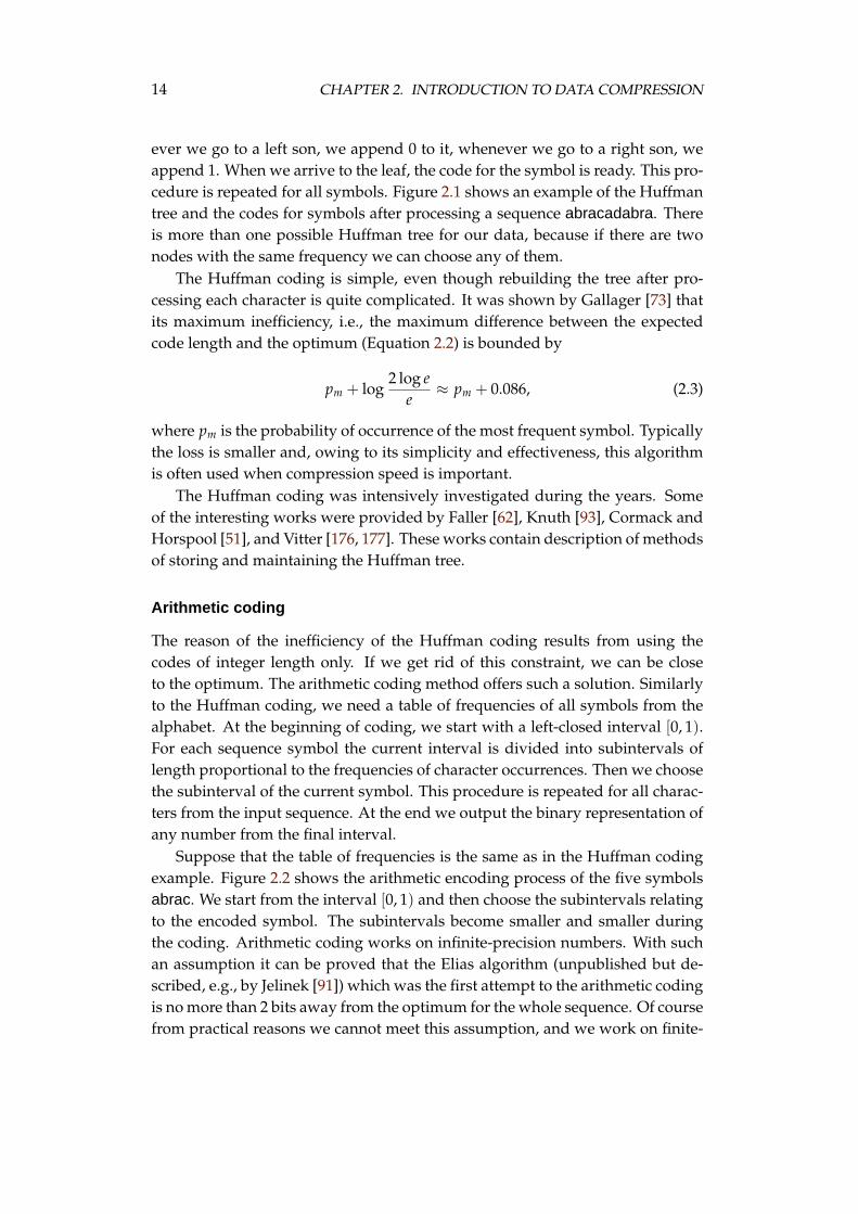
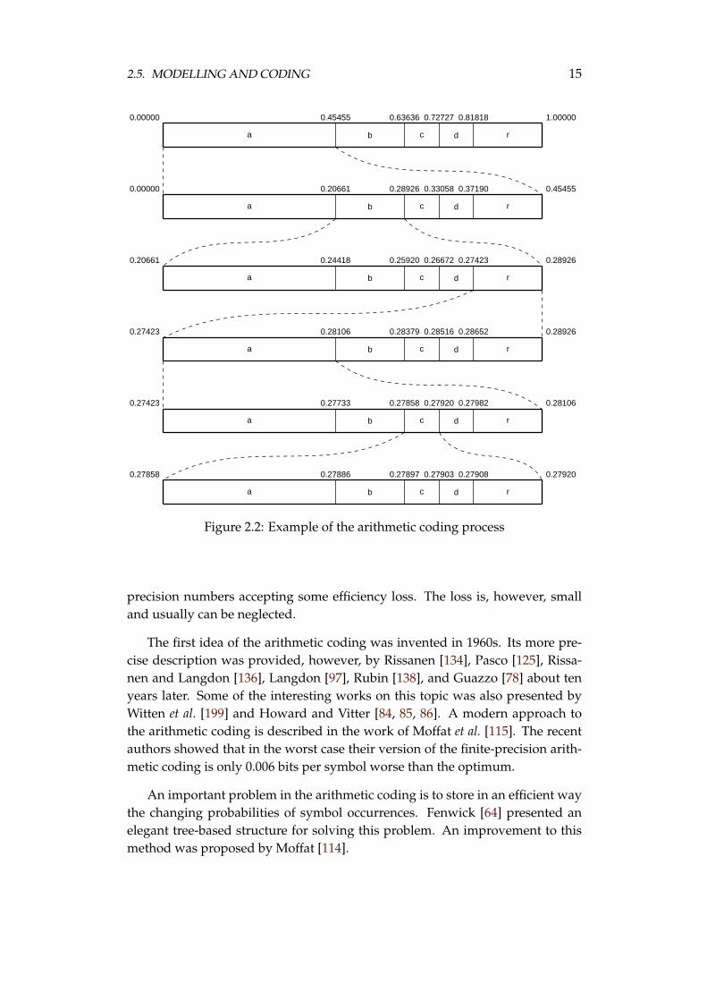
The reason of the inefficiency of the Huffman coding results from using thecodes of integer length only. If we get rid of this constraint, we can be closeto the optimum. The arithmetic coding method offers such a solution. Similarlyto the Huffman coding, we need a table of frequencies of all symbols from thealphabet. At the beginning of coding, we start with a left-closed interval [0, 1).For each sequence symbol the current interval is divided into subintervals oflength proportional to the frequencies of character occurrences. Then we choosethe subinterval of the current symbol. This procedure is repeated for all charac-ters from the input sequence. At the end we output the binary representation ofany number from the final interval.
Suppose that the table of frequencies is the same as in the Huffman codingexample. Figure 2.2 shows the arithmetic encoding process of the five symbolsabrac. We start from the interval [0, 1) and then choose the subintervals relatingto the encoded symbol. The subintervals become smaller and smaller duringthe coding. Arithmetic coding works on infinite-precision numbers. With suchan assumption it can be proved that the Elias algorithm (unpublished but de-scribed, e.g., by Jelinek [91]) which was the first attempt to the arithmetic codingis no more than 2 bits away from the optimum for the whole sequence. Of coursefrom practical reasons we cannot meet this assumption, and we work on finite-
2.5. MODELLING AND CODING 15
a b c d r
0.00000 0.45455 0.63636 0.72727 0.81818 1.00000
a b c d r
0.00000 0.20661 0.28926 0.33058 0.37190 0.45455
a b c d r
0.20661 0.24418 0.25920 0.26672 0.27423 0.28926
a b c d r
0.27423 0.28106 0.28379 0.28516 0.28652 0.28926
a b c d r
0.27423 0.27733 0.27858 0.27920 0.27982 0.28106
a b c d r
0.27858 0.27886 0.27897 0.27903 0.27908 0.27920
Figure 2.2: Example of the arithmetic coding process
precision numbers accepting some efficiency loss. The loss is, however, smalland usually can be neglected.
The first idea of the arithmetic coding was invented in 1960s. Its more pre-cise description was provided, however, by Rissanen [134], Pasco [125], Rissa-nen and Langdon [136], Langdon [97], Rubin [138], and Guazzo [78] about tenyears later. Some of the interesting works on this topic was also presented byWitten et al. [199] and Howard and Vitter [84, 85, 86]. A modern approach tothe arithmetic coding is described in the work of Moffat et al. [115]. The recentauthors showed that in the worst case their version of the finite-precision arith-metic coding is only 0.006 bits per symbol worse than the optimum.
An important problem in the arithmetic coding is to store in an efficient waythe changing probabilities of symbol occurrences. Fenwick [64] presented anelegant tree-based structure for solving this problem. An improvement to thismethod was proposed by Moffat [114].
16 CHAPTER 2. INTRODUCTION TO DATA COMPRESSION
2.6 Classes of sources
2.6.1 Types of data
Before choosing the right compression algorithm we must know the sequenceto be compressed. Ideally, we would know that in a particular case we have,e.g., a Dickens novel, a Picasso painting, or an article from a newspaper. In sucha case, we can choose the modelling method that fits such a sequence best. Ifour knowledge is even better and we know that the sequence is an article fromthe New York Times we can choose the more suitable model corresponding tothe newspaper style. Going further, if we know the author of the article, wecan make even better choice. Using this knowledge one may choose a modelwell adjusted to the characteristics of the current sequence. To apply such anapproach, providing different modelling methods for writers, painters, newspa-pers, and so on, is insufficient. It is also needed to provide different modellingmethods for all newspapers and all authors publishing there. The number ofmodelling methods would be incredibly large in this case. The more so, we donot know the future writers and painters and we cannot prepare models for theirworks.
On the other side, we cannot assume nothing about the sequence. If we doso, we have no way of finding similarities. The less we know about the sequence,the less we can utilise.
To make a compression possible we have to make a compromise. The stan-dard approach is to define the classes of sources producing sequences of differenttypes. We assume that the possible sequences can be treated as an output ofsome of the sources. The goal is to choose the source’s class which approxi-mates the sequence best. Then we apply a universal compression algorithm thatworks well on the sources from the chosen class. This strategy offers a possibilityof reduction the number of modelling methods to a reasonable level.
2.6.2 Memoryless source
Let us start the description of source types from the simplest one which is amemoryless source. We assume that Θ = {θ0, . . . , θk−1} is a set of probabilities ofoccurrence of all symbols from the alphabet. These parameters fully define thesource.
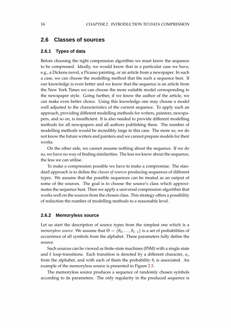
Such sources can be viewed as finite-state machines (FSM) with a single stateand k loop-transitions. Each transition is denoted by a different character, ai,from the alphabet, and with each of them the probability θi is associated. Anexample of the memoryless source is presented in Figure 2.3.
The memoryless source produces a sequence of randomly chosen symbolsaccording to its parameters. The only regularity in the produced sequence is
2.6. CLASSES OF SOURCES 17
a
r
dc
b
0.4
0.2
0.10.1
0.2
Figure 2.3: Example of the memoryless source
that the frequency of symbol occurrences is close to the probabilities being thesource parameters.
2.6.3 Piecewise stationary memoryless source
The parameters of the memoryless source do not depend on the number of sym-bols it generated so far. This means that the probability of occurrence of eachsymbol is independent from its position in the output sequence. Such sources,which do not vary their characteristics in time, are called stationary.
The piecewise stationary memoryless source is a memoryless source, where theset of probabilities Θ depends on the position in the output sequence. Thismeans that we assume a sequence 〈Θ1, . . . , Θm〉 of probabilities sets, and a re-lated sequence of positions, 〈t1, . . . , tm〉, after which every set Θi becomes actualto the source.
This source is nonstationary, because its characteristics varies in time. Typi-cally we assume that the sequence to be compressed is produced by a stationarysource. Therefore all other source classes considered in the dissertation are sta-tionary. The reason to distinguish the piecewise stationary memoryless sourcesis that they are closely related to one stage of the Burrows–Wheeler compressionalgorithm, what we will discuss in Section 4.1.3.
2.6.4 Finite-state machine sources
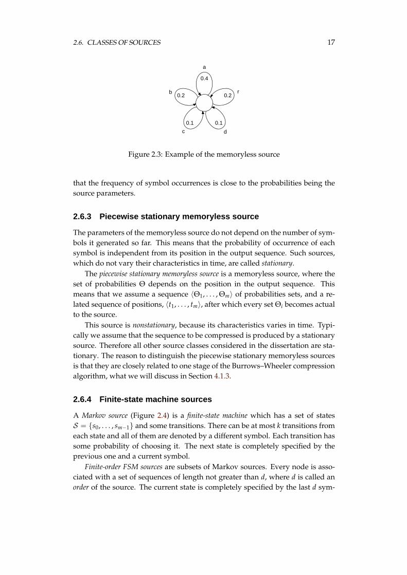
A Markov source (Figure 2.4) is a finite-state machine which has a set of statesS = {s0, . . . , sm−1} and some transitions. There can be at most k transitions fromeach state and all of them are denoted by a different symbol. Each transition hassome probability of choosing it. The next state is completely specified by theprevious one and a current symbol.
Finite-order FSM sources are subsets of Markov sources. Every node is asso-ciated with a set of sequences of length not greater than d, where d is called anorder of the source. The current state is completely specified by the last d sym-
18 CHAPTER 2. INTRODUCTION TO DATA COMPRESSION
a
b
d
a
b
a cb
r d
ar
0.5
0.5
0.5
0.3
0.2
0.4 0.5 0.1 0.4 0.3
0.9
0.1
Figure 2.4: Example of the Markov source
a1.0
b0.5
r0.4
a0.6
c0.3a0.2d
0.2
a0.8
d0.8
c0.2
abr
c d
Figure 2.5: Example of the finite-order FSM source
bols. The next state is specified by the current one and the current symbol. Anexample of a finite-order FSM source is shown in Figure 2.5.
The FSMX sources [135] are subsets of finite-order FSM sources. The reduc-tion is made by the additional assumption that sets denoting the nodes containexactly one element.
2.6. CLASSES OF SOURCES 19
0 1
0 1 0 1
0 1 0 1
0 1θ000
θ0010 θ0011
θ01
θ100 θ101
θ11
Figure 2.6: Example of the binary CT-source
2.6.5 Context tree sources
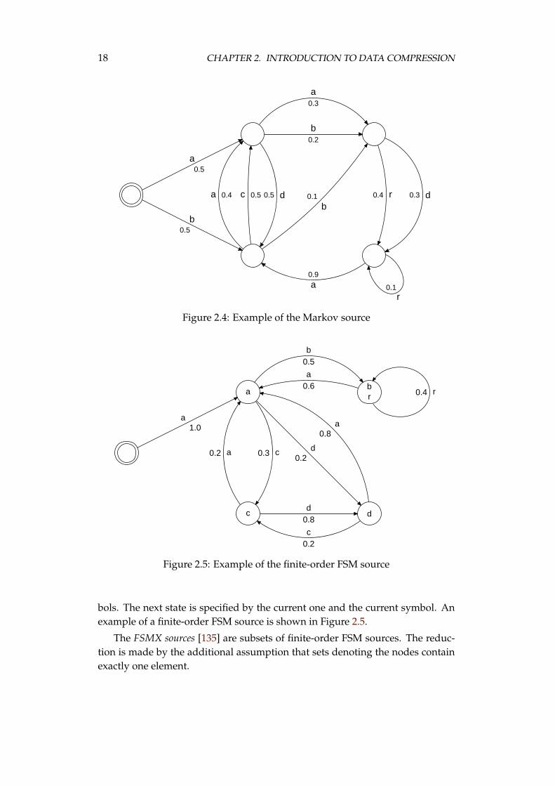
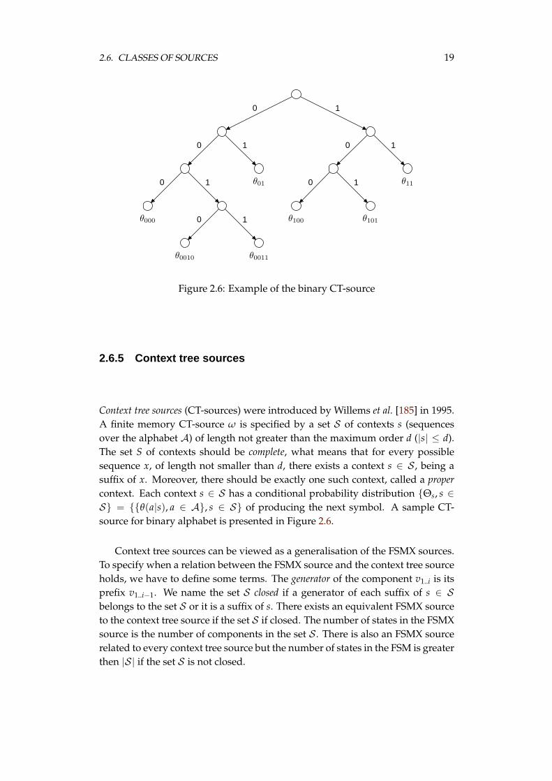
Context tree sources (CT-sources) were introduced by Willems et al. [185] in 1995.A finite memory CT-source ω is specified by a set S of contexts s (sequencesover the alphabet A) of length not greater than the maximum order d (|s| ≤ d).The set S of contexts should be complete, what means that for every possiblesequence x, of length not smaller than d, there exists a context s ∈ S , being asuffix of x. Moreover, there should be exactly one such context, called a propercontext. Each context s ∈ S has a conditional probability distribution {Θs, s ∈S} = {{θ(a|s), a ∈ A}, s ∈ S} of producing the next symbol. A sample CT-source for binary alphabet is presented in Figure 2.6.
Context tree sources can be viewed as a generalisation of the FSMX sources.To specify when a relation between the FSMX source and the context tree sourceholds, we have to define some terms. The generator of the component v1..i is itsprefix v1..i−1. We name the set S closed if a generator of each suffix of s ∈ Sbelongs to the set S or it is a suffix of s. There exists an equivalent FSMX sourceto the context tree source if the set S if closed. The number of states in the FSMXsource is the number of components in the set S . There is also an FSMX sourcerelated to every context tree source but the number of states in the FSM is greaterthen |S| if the set S is not closed.
20 CHAPTER 2. INTRODUCTION TO DATA COMPRESSION
2.7 Families of universal algorithmsfor lossless data compression
2.7.1 Universal compression
We noticed that it is impossible to design a single compression method for alltypes of data without some knowledge of the sequence. It is also impossible toprepare a different compression algorithm for every possible sequence. The rea-sonable choice is to invent a data compression algorithm for some general sourceclasses, and to use such an algorithm to the sequences which can be treated, witha high precision, as outputs of the assumed source.
Typical sequences appearing in real world contain texts, databases, pictures,binary data. Markov sources, finite-order FSM sources, FSMX sources, and con-text tree sources were invented to model such real sequences. Usually real se-quences can be successfully approximated as produced by these sources. There-fore it is justified to call algorithms designed to work well on sequences pro-duced by such sources universal.
Sometimes, before the compression process, it is useful to transpose the se-quence in some way to achieve a better fit to the assumption. For example, im-age data are often decomposed before the compression. This means that everycolour component (red, green, and blue) is compressed separately. We considerthe universal compression algorithms which in general do not include such pre-liminary transpositions.
We are now going to describe the most popular universal data compressionalgorithms. We start from the classic Ziv–Lempel algorithms then we presentthe more recent propositions.
2.7.2 Ziv–Lempel algorithms
Main idea
Probably the most popular data compression algorithms are Ziv–Lempel methods,first described in 1977. These algorithms are dictionary methods: during thecompression they build a dictionary from the components appeared in the pastand use it to reduce the sequence length if the same component appears in thefuture.
Let us suppose that the input sequence starts with characters abracadabra.We can notice that the first four symbols are abra and the same symbols appearin the sequence once more (from position 8). We can reduce the sequence lengthreplacing the second occurrence of abra by a special marker denoting a repe-tition of the previous component. Usually we can choose the subsequences tobe replaced by a special marker in various ways (take a look for example atthe sequence abracadabradab, where we can replace the second appearance of
2.7. FAMILIES OF UNIVERSAL ALGORITHMS FOR LOSSLESS . . . 21
component abra or adab, but not both of them). At a given moment, we cannotfind out which replacement will give better results in the future. Therefore theZiv–Lempel algorithm use heuristics for choosing the replacements.
The other problem is how to build the dictionary and how to denote thereplacements of components. There are two major versions of the Ziv–Lempelalgorithms: LZ77 [202] and LZ78 [203], and some minor modifications.
The main idea of the Ziv–Lempel methods is based on the assumption thatthere are repeated components in the input sequence, x. This means that theprobability of occurrence of the current symbol, xi, after a few previous charac-ters, a component xi−j..i−1, is not uniform. The FSM, FSMX, and CT-source withnonuniform probability distribution in states fulfil this assumption.
LZ77 algorithm
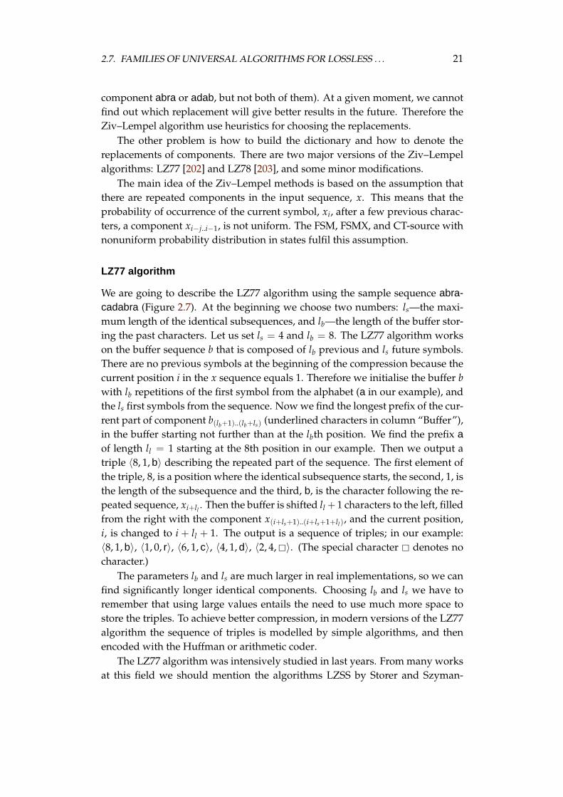
We are going to describe the LZ77 algorithm using the sample sequence abra-cadabra (Figure 2.7). At the beginning we choose two numbers: ls—the maxi-mum length of the identical subsequences, and lb—the length of the buffer stor-ing the past characters. Let us set ls = 4 and lb = 8. The LZ77 algorithm workson the buffer sequence b that is composed of lb previous and ls future symbols.There are no previous symbols at the beginning of the compression because thecurrent position i in the x sequence equals 1. Therefore we initialise the buffer bwith lb repetitions of the first symbol from the alphabet (a in our example), andthe ls first symbols from the sequence. Now we find the longest prefix of the cur-rent part of component b(lb+1)..(lb+ls) (underlined characters in column “Buffer”),in the buffer starting not further than at the lbth position. We find the prefix aof length ll = 1 starting at the 8th position in our example. Then we output atriple 〈8, 1, b〉 describing the repeated part of the sequence. The first element ofthe triple, 8, is a position where the identical subsequence starts, the second, 1, isthe length of the subsequence and the third, b, is the character following the re-peated sequence, xi+ll . Then the buffer is shifted ll + 1 characters to the left, filledfrom the right with the component x(i+ls+1)..(i+ls+1+ll), and the current position,i, is changed to i + ll + 1. The output is a sequence of triples; in our example:〈8, 1, b〉, 〈1, 0, r〉, 〈6, 1, c〉, 〈4, 1, d〉, 〈2, 4, �〉. (The special character � denotes nocharacter.)
The parameters lb and ls are much larger in real implementations, so we canfind significantly longer identical components. Choosing lb and ls we have toremember that using large values entails the need to use much more space tostore the triples. To achieve better compression, in modern versions of the LZ77algorithm the sequence of triples is modelled by simple algorithms, and thenencoded with the Huffman or arithmetic coder.
The LZ77 algorithm was intensively studied in last years. From many worksat this field we should mention the algorithms LZSS by Storer and Szyman-
22 CHAPTER 2. INTRODUCTION TO DATA COMPRESSION
Remaining sequence Buffer Longest prefix Code
abracadabra aaaaaaaaabra a 〈8, 1, b〉racadabra aaaaaaabraca 〈1, 0, r〉acadabra aaaaaabracad a 〈6, 1, c〉adabra aaaabracadab a 〈4, 1, d〉abra aabracadabra abra 〈2, 4, �〉
Figure 2.7: Example of the LZ77 algorithm processing the sequence abracadabra
Compressor
Remaining sequence Code
abracadabra 〈0, a〉bracadabra 〈0, b〉racadabra 〈0, r〉acadabra 〈1, c〉adabra 〈1, d〉abra 〈1, b〉ra 〈3, a〉
Dictionary
Index Sequence
1 a2 b3 r4 ac5 ad6 ab7 ra
Figure 2.8: Example of the LZ78 algorithm processing the sequence abracadabra
ski [159], LZFG by Fiala and Greene [70], and LZRW by Williams [193, 194].Further improvements were introduced also by Bell [21], Bell and Kulp [23],Bell and Witten [24], Gutmann and Bell [79], and Horspool [82].
LZ78 algorithm
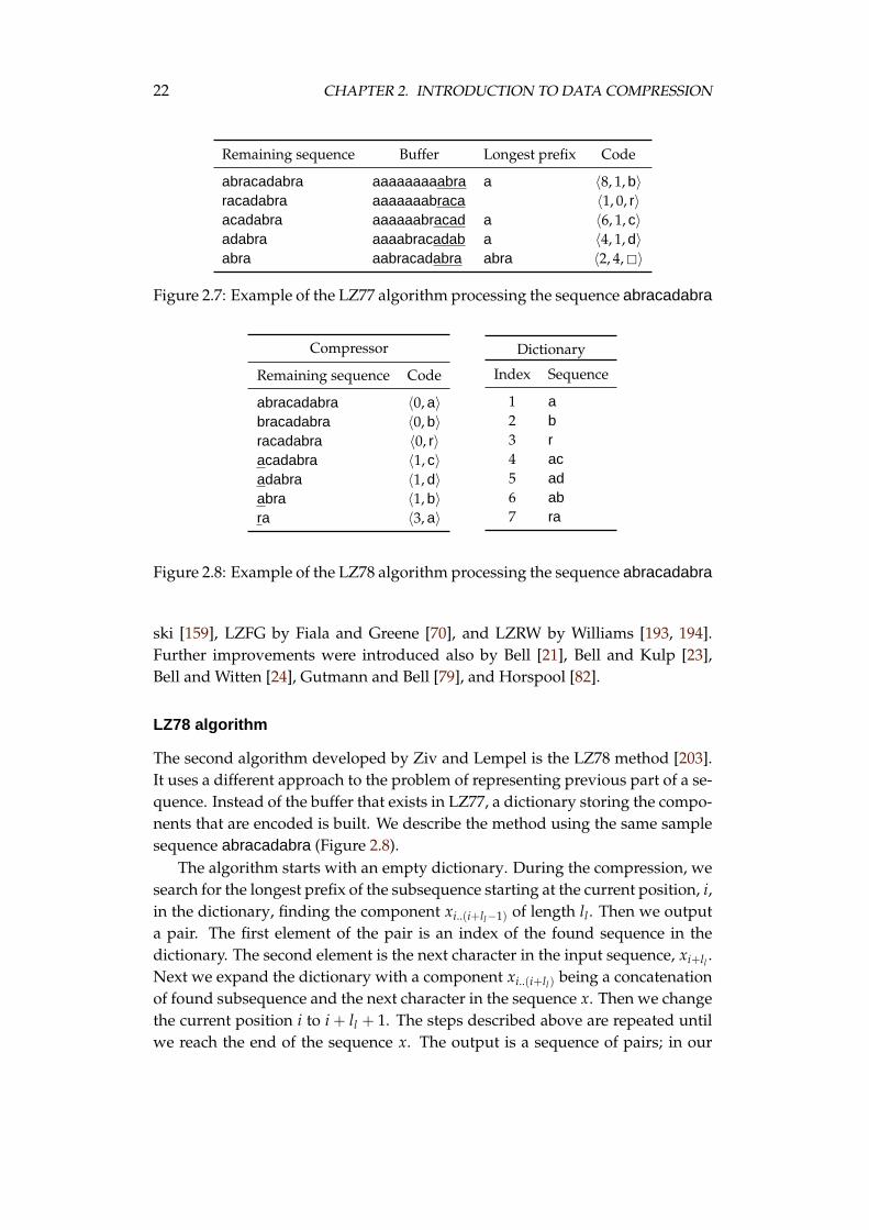
The second algorithm developed by Ziv and Lempel is the LZ78 method [203].It uses a different approach to the problem of representing previous part of a se-quence. Instead of the buffer that exists in LZ77, a dictionary storing the compo-nents that are encoded is built. We describe the method using the same samplesequence abracadabra (Figure 2.8).
The algorithm starts with an empty dictionary. During the compression, wesearch for the longest prefix of the subsequence starting at the current position, i,in the dictionary, finding the component xi..(i+ll−1) of length ll . Then we outputa pair. The first element of the pair is an index of the found sequence in thedictionary. The second element is the next character in the input sequence, xi+ll .Next we expand the dictionary with a component xi..(i+ll) being a concatenationof found subsequence and the next character in the sequence x. Then we changethe current position i to i + ll + 1. The steps described above are repeated untilwe reach the end of the sequence x. The output is a sequence of pairs; in our
2.7. FAMILIES OF UNIVERSAL ALGORITHMS FOR LOSSLESS . . . 23
example: 〈0, a〉, 〈0, b〉, 〈0, r〉, 〈1, c〉, 〈1, d〉, 〈1, b〉, 〈3, a〉.During the compression process the dictionary grows, so the indexes become
larger numbers and require more bits to be encoded. Sometimes it is unprof-itable to let the dictionary grow unrestrictedly and the dictionary is periodicallypurged. (Different versions of LZ78 use different strategies in this regard.)
From many works on LZ78-related algorithms the most interesting ones arethe propositions by Miller and Wegman [112], Hoang et al. [80], and the LZWalgorithm by Welch [187]. The LZW algorithm is used by a well-known UNIXcompress program.
2.7.3 Prediction by partial matching algorithms
The prediction by partial matching (PPM) data compression method was devel-oped by Cleary and Witten [48] in 1984. The main idea of this algorithm is togather the frequencies of symbol occurrences in all possible contexts in the pastand use them to predict probability of occurrence of the current symbol xi. Thisprobability is then used to encode the symbol xi with the arithmetic coder.
Many versions of PPM algorithm have been developed since the time of itsinvention. One of the main differences between them is the maximum orderof contexts they consider. There is also an algorithm, PPM* [49], that workswith an unbounded context length. The limitation of the context length in thefirst versions of the algorithm was motivated by the exponential growth of thenumber of possible contexts together to the order, what causes a proportionalgrowth of the space requirements. There are methods for reducing the spacerequirements and nowadays it is possible to work with long contexts (even upto 128 symbols). When we choose a too large order, we, however, often meet thesituation that a current context has not appeared in the past. Overcoming thisproblem entails some additional cost so we must decide to some compromise inchoosing the order.
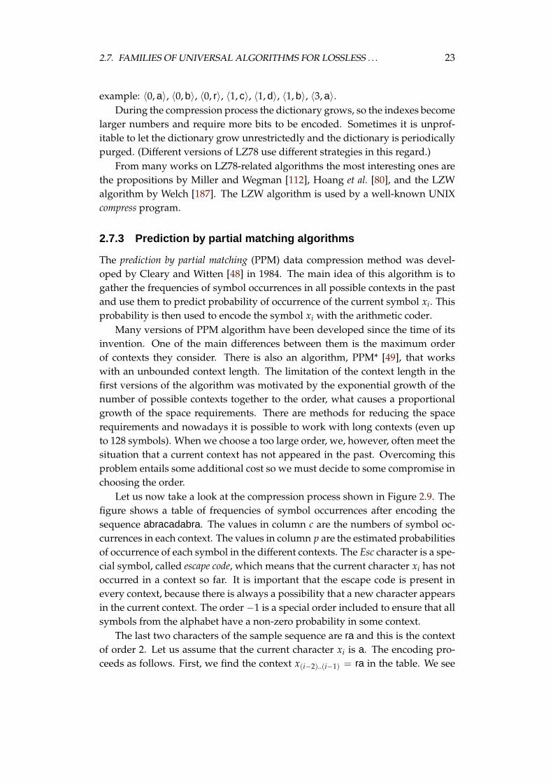
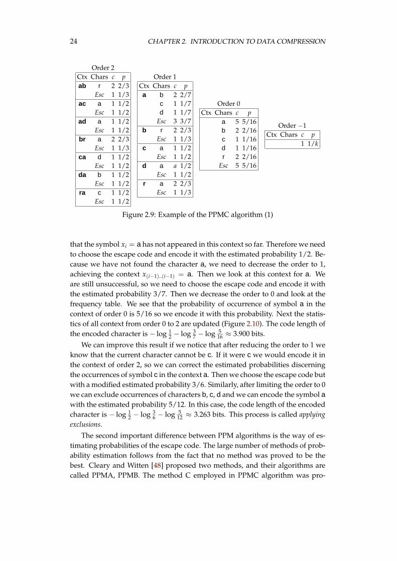
Let us now take a look at the compression process shown in Figure 2.9. Thefigure shows a table of frequencies of symbol occurrences after encoding thesequence abracadabra. The values in column c are the numbers of symbol oc-currences in each context. The values in column p are the estimated probabilitiesof occurrence of each symbol in the different contexts. The Esc character is a spe-cial symbol, called escape code, which means that the current character xi has notoccurred in a context so far. It is important that the escape code is present inevery context, because there is always a possibility that a new character appearsin the current context. The order −1 is a special order included to ensure that allsymbols from the alphabet have a non-zero probability in some context.
The last two characters of the sample sequence are ra and this is the contextof order 2. Let us assume that the current character xi is a. The encoding pro-ceeds as follows. First, we find the context x(i−2)..(i−1) = ra in the table. We see
24 CHAPTER 2. INTRODUCTION TO DATA COMPRESSION
Order 2Ctx Chars c pab r 2 2/3
Esc 1 1/3ac a 1 1/2
Esc 1 1/2ad a 1 1/2
Esc 1 1/2br a 2 2/3
Esc 1 1/3ca d 1 1/2
Esc 1 1/2da b 1 1/2
Esc 1 1/2ra c 1 1/2
Esc 1 1/2
Order 1Ctx Chars c pa b 2 2/7
c 1 1/7d 1 1/7
Esc 3 3/7b r 2 2/3
Esc 1 1/3c a 1 1/2
Esc 1 1/2d a a 1/2
Esc 1 1/2r a 2 2/3
Esc 1 1/3
Order 0Ctx Chars c p
a 5 5/16b 2 2/16c 1 1/16d 1 1/16r 2 2/16
Esc 5 5/16
Order −1Ctx Chars c p
1 1/k
Figure 2.9: Example of the PPMC algorithm (1)
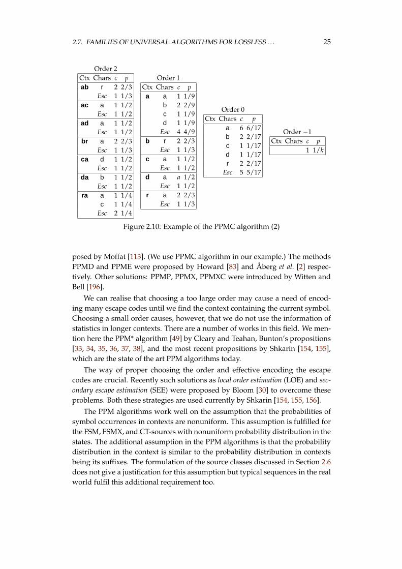
that the symbol xi = a has not appeared in this context so far. Therefore we needto choose the escape code and encode it with the estimated probability 1/2. Be-cause we have not found the character a, we need to decrease the order to 1,achieving the context x(i−1)..(i−1) = a. Then we look at this context for a. Weare still unsuccessful, so we need to choose the escape code and encode it withthe estimated probability 3/7. Then we decrease the order to 0 and look at thefrequency table. We see that the probability of occurrence of symbol a in thecontext of order 0 is 5/16 so we encode it with this probability. Next the statis-tics of all context from order 0 to 2 are updated (Figure 2.10). The code length ofthe encoded character is − log 1
2 − log 37 − log 5
16 ≈ 3.900 bits.
We can improve this result if we notice that after reducing the order to 1 weknow that the current character cannot be c. If it were c we would encode it inthe context of order 2, so we can correct the estimated probabilities discerningthe occurrences of symbol c in the context a. Then we choose the escape code butwith a modified estimated probability 3/6. Similarly, after limiting the order to 0we can exclude occurrences of characters b, c, d and we can encode the symbol awith the estimated probability 5/12. In this case, the code length of the encodedcharacter is − log 1
2 − log 36 − log 5
12 ≈ 3.263 bits. This process is called applyingexclusions.
The second important difference between PPM algorithms is the way of es-timating probabilities of the escape code. The large number of methods of prob-ability estimation follows from the fact that no method was proved to be thebest. Cleary and Witten [48] proposed two methods, and their algorithms arecalled PPMA, PPMB. The method C employed in PPMC algorithm was pro-
2.7. FAMILIES OF UNIVERSAL ALGORITHMS FOR LOSSLESS . . . 25
Order 2Ctx Chars c pab r 2 2/3
Esc 1 1/3ac a 1 1/2
Esc 1 1/2ad a 1 1/2
Esc 1 1/2br a 2 2/3
Esc 1 1/3ca d 1 1/2
Esc 1 1/2da b 1 1/2
Esc 1 1/2ra a 1 1/4
c 1 1/4Esc 2 1/4
Order 1Ctx Chars c pa a 1 1/9
b 2 2/9c 1 1/9d 1 1/9
Esc 4 4/9b r 2 2/3
Esc 1 1/3c a 1 1/2
Esc 1 1/2d a a 1/2
Esc 1 1/2r a 2 2/3
Esc 1 1/3
Order 0Ctx Chars c p
a 6 6/17b 2 2/17c 1 1/17d 1 1/17r 2 2/17
Esc 5 5/17
Order −1Ctx Chars c p
1 1/k
Figure 2.10: Example of the PPMC algorithm (2)
posed by Moffat [113]. (We use PPMC algorithm in our example.) The methodsPPMD and PPME were proposed by Howard [83] and Aberg et al. [2] respec-tively. Other solutions: PPMP, PPMX, PPMXC were introduced by Witten andBell [196].
We can realise that choosing a too large order may cause a need of encod-ing many escape codes until we find the context containing the current symbol.Choosing a small order causes, however, that we do not use the information ofstatistics in longer contexts. There are a number of works in this field. We men-tion here the PPM* algorithm [49] by Cleary and Teahan, Bunton’s propositions[33, 34, 35, 36, 37, 38], and the most recent propositions by Shkarin [154, 155],which are the state of the art PPM algorithms today.
The way of proper choosing the order and effective encoding the escapecodes are crucial. Recently such solutions as local order estimation (LOE) and sec-ondary escape estimation (SEE) were proposed by Bloom [30] to overcome theseproblems. Both these strategies are used currently by Shkarin [154, 155, 156].
The PPM algorithms work well on the assumption that the probabilities ofsymbol occurrences in contexts are nonuniform. This assumption is fulfilled forthe FSM, FSMX, and CT-sources with nonuniform probability distribution in thestates. The additional assumption in the PPM algorithms is that the probabilitydistribution in the context is similar to the probability distribution in contextsbeing its suffixes. The formulation of the source classes discussed in Section 2.6does not give a justification for this assumption but typical sequences in the realworld fulfil this additional requirement too.
26 CHAPTER 2. INTRODUCTION TO DATA COMPRESSION
01 (1)(1)
Figure 2.11: Initial situation in the DMC algorithm
At the end we notice that the PPM algorithms yield the best compressionrates today. Unfortunately their time and space complexities are relatively high,because they maintain a complicated model of data.
2.7.4 Dynamic Markov coding algorithm
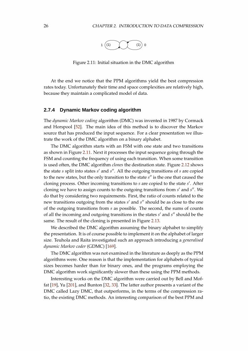
The dynamic Markov coding algorithm (DMC) was invented in 1987 by Cormackand Horspool [52]. The main idea of this method is to discover the Markovsource that has produced the input sequence. For a clear presentation we illus-trate the work of the DMC algorithm on a binary alphabet.
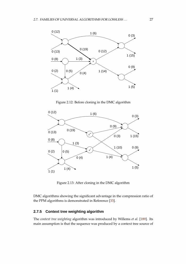
The DMC algorithm starts with an FSM with one state and two transitionsas shown in Figure 2.11. Next it processes the input sequence going through theFSM and counting the frequency of using each transition. When some transitionis used often, the DMC algorithm clones the destination state. Figure 2.12 showsthe state s split into states s′ and s′′. All the outgoing transitions of s are copiedto the new states, but the only transition to the state s′′ is the one that caused thecloning process. Other incoming transitions to s are copied to the state s′. Aftercloning we have to assign counts to the outgoing transitions from s′ and s′′. Wedo that by considering two requirements. First, the ratio of counts related to thenew transitions outgoing from the states s′ and s′′ should be as close to the oneof the outgoing transitions from s as possible. The second, the sums of countsof all the incoming and outgoing transitions in the states s′ and s′′ should be thesame. The result of the cloning is presented in Figure 2.13.
We described the DMC algorithm assuming the binary alphabet to simplifythe presentation. It is of course possible to implement it on the alphabet of largersize. Teuhola and Raita investigated such an approach introducing a generaliseddynamic Markov coder (GDMC) [169].
The DMC algorithm was not examined in the literature as deeply as the PPMalgorithms were. One reason is that the implementation for alphabets of typicalsizes becomes harder than for binary ones, and the programs employing theDMC algorithm work significantly slower than these using the PPM methods.
Interesting works on the DMC algorithm were carried out by Bell and Mof-fat [19], Yu [201], and Bunton [32, 33]. The latter author presents a variant of theDMC called Lazy DMC, that outperforms, in the terms of the compression ra-tio, the existing DMC methods. An interesting comparison of the best PPM and
2.7. FAMILIES OF UNIVERSAL ALGORITHMS FOR LOSSLESS . . . 27
1 (1)
0 (2)
0 (8)
0 (12)
0 (13)
0 (9)
1 (5)
0 (3)
1 (15)
0 (4)
1 (4)
1 (3)
0 (5)
0 (19)
1 (6)
0 (12)
1 (14)
s
Figure 2.12: Before cloning in the DMC algorithm
1 (1)
0 (2)
0 (8)
0 (12)
0 (13)
0 (9)
1 (5)
0 (3)
1 (15)
0 (4)
1 (4)
1 (3)
0 (5)
0 (19)
1 (6)
0 (3)
1 (4)
0 (9)
1 (10)s′
s′′
Figure 2.13: After cloning in the DMC algorithm
DMC algorithms showing the significant advantage in the compression ratio ofthe PPM algorithms is demonstrated in Reference [33].
2.7.5 Context tree weighting algorithm
The context tree weighting algorithm was introduced by Willems et al. [189]. Itsmain assumption is that the sequence was produced by a context tree source of
28 CHAPTER 2. INTRODUCTION TO DATA COMPRESSION
an unknown structure and parameters.For a clear presentation we follow the way that the authors used to present
their algorithm, rather than describing it in work, what could be confusing with-out introducing some notions. The authors start with a simple binary mem-oryless source and notice that using the Krichevsky–Trofimov estimator [95]to estimate the probability for the arithmetic coding, we can encode every se-quence produced by any such source with a small bounded inefficiency equals1/2 log n + 1. Next they assume that the source is a binary CT-source of knownstructure (the set of contexts) and unknown parameters (the probabilities ofproducing 0 or 1 in each context). The authors show how the maximum re-dundancy of the encoded sequence grows in such a case. The result is strictlybounded only by the size of the context set and the length of the sequence.The last step is to assume that we also do not know the structure of the con-text tree source. The only thing we know is the maximum length d of the con-text from the set S . The authors show how to employ an elegant weightingprocedure over all the possible context tree sources of the maximum depth d.They show that, in this case, a maximum redundancy is also strictly boundedfor their algorithm. The first idea of the CTW algorithm was extended in fur-ther works [171, 180, 181, 188, 190, 192], and the simple introduction to the basicconcepts of the CTW algorithm is presented by Willems et al. [191].
The significant disadvantage of the CTW algorithm is the fact that the con-text tree sources are binary. The formulation of the CTW algorithm for larger al-phabets is possible, but the mathematics and computations become much morecomplicated. Hence, to employ the CTW algorithm to the non-binary sequence,we have to decompose it into binary sequences first.
The results of Willems et al. are theoretical, and the authors do not supply ex-perimental tests. The compression for text sequences was investigated by Abergand Shtarkov [1], Tjalkens et al. [170], Sadakane et al. [140], Suzuki [161], andVolf [179]. Ekstrand [57, 58] as well as Arimura et al. [8] considered also thecompression of sequences of grey scale images with the CTW algorithm. (Theworks mentioned in this paragraph contain also experimental results.)
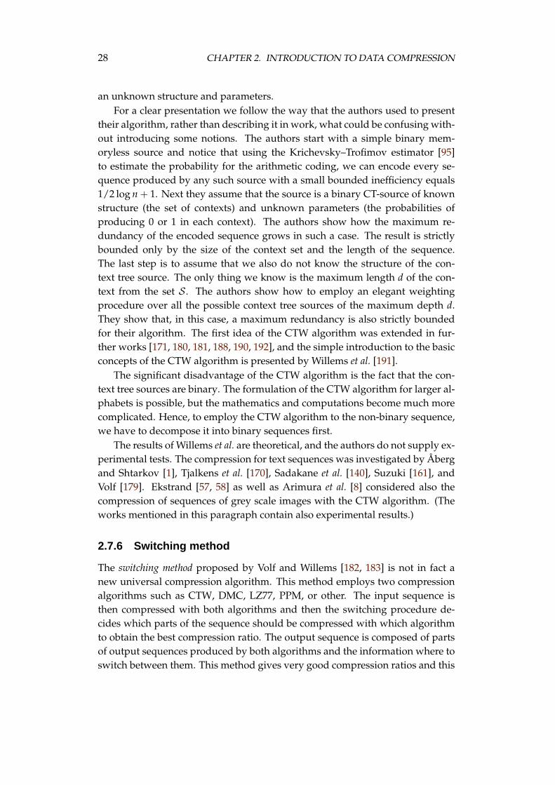
2.7.6 Switching method
The switching method proposed by Volf and Willems [182, 183] is not in fact anew universal compression algorithm. This method employs two compressionalgorithms such as CTW, DMC, LZ77, PPM, or other. The input sequence isthen compressed with both algorithms and then the switching procedure de-cides which parts of the sequence should be compressed with which algorithmto obtain the best compression ratio. The output sequence is composed of partsof output sequences produced by both algorithms and the information where toswitch between them. This method gives very good compression ratios and this
2.8. SPECIALISED COMPRESSION ALGORITHMS 29
is the reason we mention it here. We, however, do so only for the possibility ofcomparing the experimental results.
2.8 Specialised compression algorithms
Sometimes the input sequence is very specific and applying the universal datacompression algorithm does not give satisfactory results. Many specialised com-pression algorithms were proposed for such specific data. They work well on theassumed types of sequences but are useless for other types. We enumerate hereonly a few examples indicating the need of such algorithms. As we aim at uni-versal algorithms, we will not mention specialised ones in subsequent chapters.
The first algorithm we mention is Inglis [88] method for scanned texts com-pression. This problem is important in archiving texts that are not available inan electronic form. The algorithm exploits the knowledge of the picture andfinds consistent objects (usually letters) that are almost identical. This processis slightly relevant to the Optical Character Recognition (OCR), though the goalis not to recognise letters. The algorithm only looks for similarities. This ap-proach for scanned texts effects in a vast improvement of the compression ratiowith regard to standard lossless data compression algorithms usually appliedfor images.
The other interesting example is compressing DNA sequences. Loewensternand Yianilos investigated the entropy bound of such sequences [104]. Nevill–Manning and Witten concluded that the genome sequence is almost incompress-ible [119]. Chen et al. [45] show that applying sophisticated methods based onthe knowledge of the structure of DNA we can achieve some compression. Theother approach is shown by Apostolico and Lonardi [5].
The universal algorithms work well on sequences containing text, but wecan improve compression ratio for texts when we use more sophisticated algo-rithms. The first works on text compression was done by Shannon [152] in 1951.He investigated the properties of English text and bounded its entropy relatingon experiments with people. This kind of data is specific, because the text hascomplicated structure. At the first level it is composed of letters that are groupedinto words. The words form sentences, which are parts of paragraphs, and soon. The structure of sentences is specified by semantics. We can treat the textsas the output of a CT-source but we can go further and exploit more. The recentextensive discussion of how we can improve compression ratio for texts waspresented by Brown et al. [31] and Teahan et al. [163, 164, 165, 166, 167, 197].
The last specific compression problem we mention here is storing a sequencerepresenting a finite set of finite sequences (words), i.e., a lexicon. There are dif-ferent possible methods of compressing lexicons, and we notice here only oneof them by Daciuk et al. [53] and Ciura and Deorowicz [47], where the effective

30 CHAPTER 2. INTRODUCTION TO DATA COMPRESSION
compression goes hand in hand with efficient usage of the data. Namely, thecompressed sequence can be searched for given words faster than the uncom-pressed one.
Chapter 3
Algorithms based on theBurrows–Wheeler transform
If they don’t suit your purpose as they are,transform them into something more satisfactory.
— SAKI [HECTOR HUGH MUNRO]The Chronicles of Clovis (1912)
3.1 Description of the algorithm
3.1.1 Compression algorithm
Structure of the algorithm
In 1994, Burrows and Wheeler [39] presented a data compression algorithmbased on the Burrows–Wheeler transform (BWT). Its compression ratios werecomparable with the ones obtained using known best methods. This algorithmis in the focus of our interests, so we describe it more precisely.
At the beginning of the discussion of the Burrows–Wheeler compression al-gorithm let us provide an insight description of its stages (Figure 3.1). The pre-sentation is illustrated by a step-by-step example of working of the BWCA.
Burrows–Wheeler transform
The input datum of the BWCA is a sequence x of length n. First we computethe Burrows–Wheeler transform (BWT). To achieve this, n sequences are created
31
32 CHAPTER 3. ALGORITHMS BASED ON THE BURROWS–WHEELER . . .
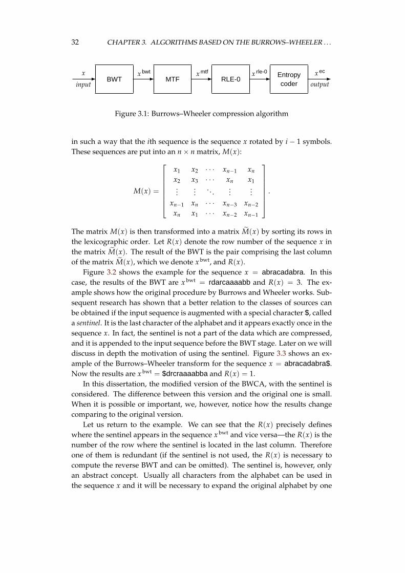
BWT MTF RLE-0Entropycoder
- - - - -x
input
x bwt x mtf x rle-0 x ec
output
Figure 3.1: Burrows–Wheeler compression algorithm
in such a way that the ith sequence is the sequence x rotated by i − 1 symbols.These sequences are put into an n × n matrix, M(x):
M(x) =
x1 x2 · · · xn−1 xn
x2 x3 · · · xn x1...
.... . .
......
xn−1 xn · · · xn−3 xn−2
xn x1 · · · xn−2 xn−1
.
The matrix M(x) is then transformed into a matrix M(x) by sorting its rows inthe lexicographic order. Let R(x) denote the row number of the sequence x inthe matrix M(x). The result of the BWT is the pair comprising the last columnof the matrix M(x), which we denote x bwt, and R(x).
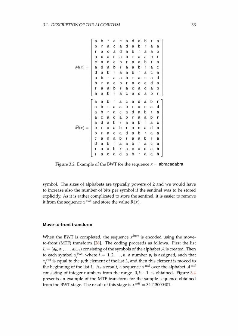
Figure 3.2 shows the example for the sequence x = abracadabra. In thiscase, the results of the BWT are x bwt = rdarcaaaabb and R(x) = 3. The ex-ample shows how the original procedure by Burrows and Wheeler works. Sub-sequent research has shown that a better relation to the classes of sources canbe obtained if the input sequence is augmented with a special character $, calleda sentinel. It is the last character of the alphabet and it appears exactly once in thesequence x. In fact, the sentinel is not a part of the data which are compressed,and it is appended to the input sequence before the BWT stage. Later on we willdiscuss in depth the motivation of using the sentinel. Figure 3.3 shows an ex-ample of the Burrows–Wheeler transform for the sequence x = abracadabra$.Now the results are x bwt = $drcraaaabba and R(x) = 1.
In this dissertation, the modified version of the BWCA, with the sentinel isconsidered. The difference between this version and the original one is small.When it is possible or important, we, however, notice how the results changecomparing to the original version.
Let us return to the example. We can see that the R(x) precisely defineswhere the sentinel appears in the sequence x bwt and vice versa—the R(x) is thenumber of the row where the sentinel is located in the last column. Thereforeone of them is redundant (if the sentinel is not used, the R(x) is necessary tocompute the reverse BWT and can be omitted). The sentinel is, however, onlyan abstract concept. Usually all characters from the alphabet can be used inthe sequence x and it will be necessary to expand the original alphabet by one
3.1. DESCRIPTION OF THE ALGORITHM 33
M(x) =
a b r a c a d a b r ab r a c a d a b r a ar a c a d a b r a a ba c a d a b r a a b rc a d a b r a a b r aa d a b r a a b r a cd a b r a a b r a c aa b r a a b r a c a db r a a b r a c a d ar a a b r a c a d a ba a b r a c a d a b r
M(x) =
a a b r a c a d a b ra b r a a b r a c a da b r a c a d a b r aa c a d a b r a a b ra d a b r a a b r a cb r a a b r a c a d ab r a c a d a b r a ac a d a b r a a b r ad a b r a a b r a c ar a a b r a c a d a br a c a d a b r a a b
Figure 3.2: Example of the BWT for the sequence x = abracadabra
symbol. The sizes of alphabets are typically powers of 2 and we would haveto increase also the number of bits per symbol if the sentinel was to be storedexplicitly. As it is rather complicated to store the sentinel, it is easier to removeit from the sequence x bwt and store the value R(x).
Move-to-front transform
When the BWT is completed, the sequence x bwt is encoded using the move-to-front (MTF) transform [26]. The coding proceeds as follows. First the listL = (a0, a1, . . . , ak−1) consisting of the symbols of the alphabet A is created. Thento each symbol x bwt
i , where i = 1, 2, . . . , n, a number pi is assigned, such thatx bwt
i is equal to the pith element of the list L, and then this element is moved tothe beginning of the list L. As a result, a sequence x mtf over the alphabet Amtf
consisting of integer numbers from the range [0, k − 1] is obtained. Figure 3.4presents an example of the MTF transform for the sample sequence obtainedfrom the BWT stage. The result of this stage is x mtf = 34413000401.
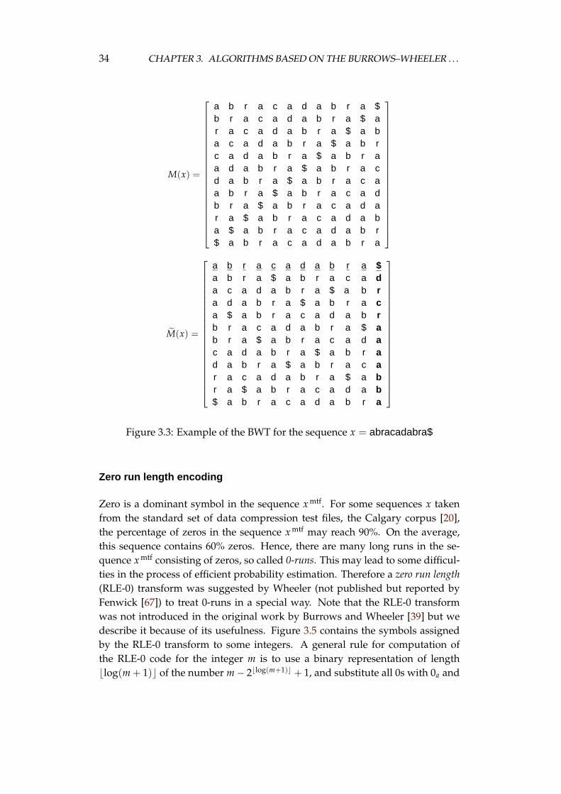
34 CHAPTER 3. ALGORITHMS BASED ON THE BURROWS–WHEELER . . .
M(x) =
a b r a c a d a b r a $b r a c a d a b r a $ ar a c a d a b r a $ a ba c a d a b r a $ a b rc a d a b r a $ a b r aa d a b r a $ a b r a cd a b r a $ a b r a c aa b r a $ a b r a c a db r a $ a b r a c a d ar a $ a b r a c a d a ba $ a b r a c a d a b r$ a b r a c a d a b r a
M(x) =
a b r a c a d a b r a $a b r a $ a b r a c a da c a d a b r a $ a b ra d a b r a $ a b r a ca $ a b r a c a d a b rb r a c a d a b r a $ ab r a $ a b r a c a d ac a d a b r a $ a b r ad a b r a $ a b r a c ar a c a d a b r a $ a br a $ a b r a c a d a b$ a b r a c a d a b r a
Figure 3.3: Example of the BWT for the sequence x = abracadabra$
Zero run length encoding
Zero is a dominant symbol in the sequence x mtf. For some sequences x takenfrom the standard set of data compression test files, the Calgary corpus [20],the percentage of zeros in the sequence x mtf may reach 90%. On the average,this sequence contains 60% zeros. Hence, there are many long runs in the se-quence x mtf consisting of zeros, so called 0-runs. This may lead to some difficul-ties in the process of efficient probability estimation. Therefore a zero run length(RLE-0) transform was suggested by Wheeler (not published but reported byFenwick [67]) to treat 0-runs in a special way. Note that the RLE-0 transformwas not introduced in the original work by Burrows and Wheeler [39] but wedescribe it because of its usefulness. Figure 3.5 contains the symbols assignedby the RLE-0 transform to some integers. A general rule for computation ofthe RLE-0 code for the integer m is to use a binary representation of lengthblog(m + 1)c of the number m− 2blog(m+1)c + 1, and substitute all 0s with 0a and
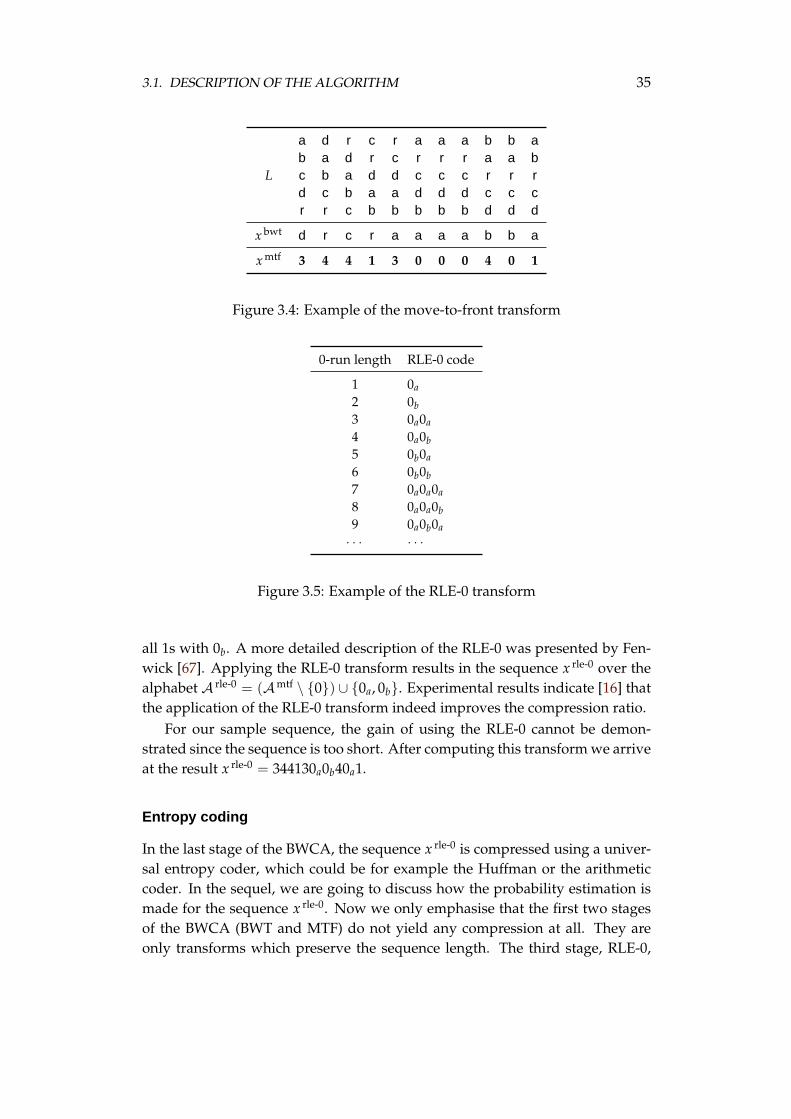
3.1. DESCRIPTION OF THE ALGORITHM 35
a d r c r a a a b b ab a d r c r r r a a b
L c b a d d c c c r r rd c b a a d d d c c cr r c b b b b b d d d
x bwt d r c r a a a a b b a
x mtf 3 4 4 1 3 0 0 0 4 0 1
Figure 3.4: Example of the move-to-front transform
0-run length RLE-0 code
1 0a2 0b3 0a0a4 0a0b5 0b0a6 0b0b7 0a0a0a8 0a0a0b9 0a0b0a· · · · · ·
Figure 3.5: Example of the RLE-0 transform
all 1s with 0b. A more detailed description of the RLE-0 was presented by Fen-wick [67]. Applying the RLE-0 transform results in the sequence x rle-0 over thealphabet A rle-0 = (Amtf \ {0}) ∪ {0a, 0b}. Experimental results indicate [16] thatthe application of the RLE-0 transform indeed improves the compression ratio.
For our sample sequence, the gain of using the RLE-0 cannot be demon-strated since the sequence is too short. After computing this transform we arriveat the result x rle-0 = 344130a0b40a1.
Entropy coding
In the last stage of the BWCA, the sequence x rle-0 is compressed using a univer-sal entropy coder, which could be for example the Huffman or the arithmeticcoder. In the sequel, we are going to discuss how the probability estimation ismade for the sequence x rle-0. Now we only emphasise that the first two stagesof the BWCA (BWT and MTF) do not yield any compression at all. They areonly transforms which preserve the sequence length. The third stage, RLE-0,
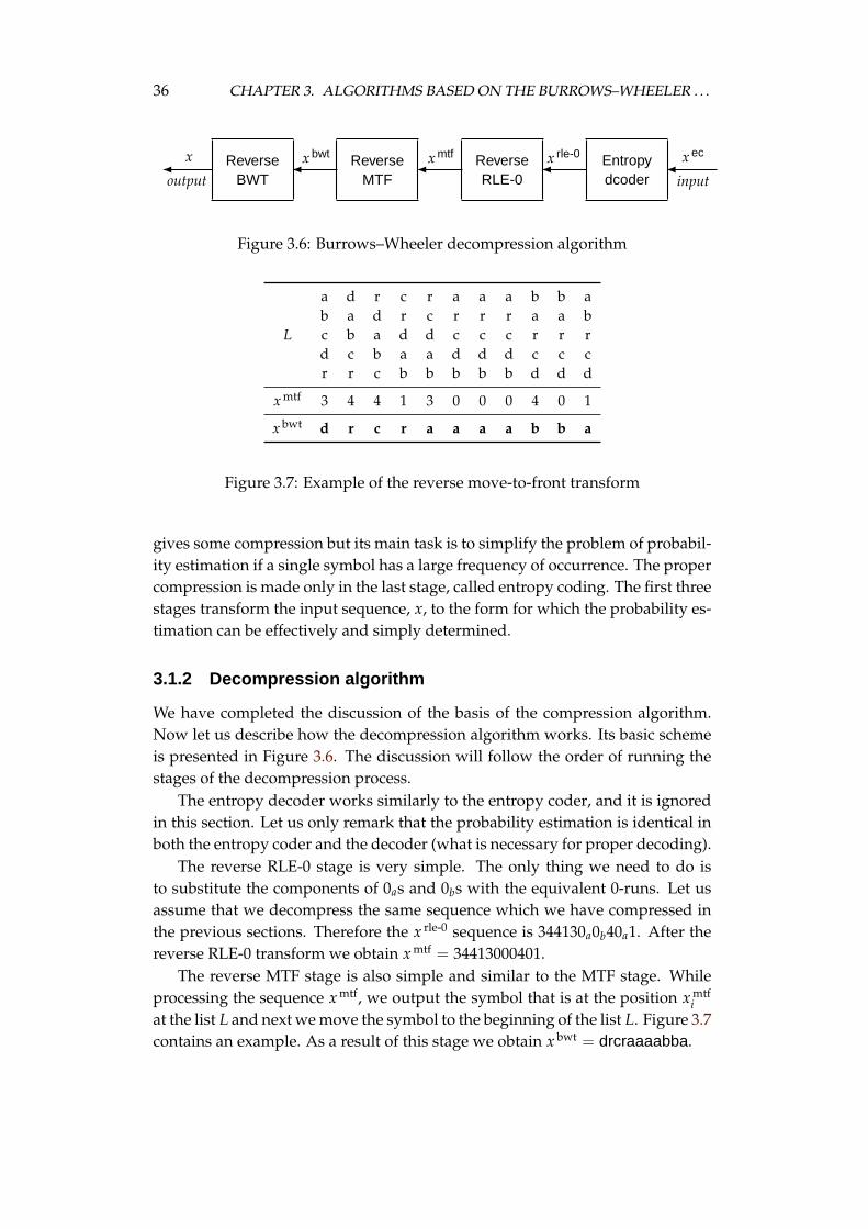
36 CHAPTER 3. ALGORITHMS BASED ON THE BURROWS–WHEELER . . .
ReverseBWT
ReverseMTF
ReverseRLE-0
Entropydcoder
� � � � �x
outputx bwt x mtf x rle-0 x ec
input
Figure 3.6: Burrows–Wheeler decompression algorithm
a d r c r a a a b b ab a d r c r r r a a b
L c b a d d c c c r r rd c b a a d d d c c cr r c b b b b b d d d
x mtf 3 4 4 1 3 0 0 0 4 0 1
x bwt d r c r a a a a b b a
Figure 3.7: Example of the reverse move-to-front transform
gives some compression but its main task is to simplify the problem of probabil-ity estimation if a single symbol has a large frequency of occurrence. The propercompression is made only in the last stage, called entropy coding. The first threestages transform the input sequence, x, to the form for which the probability es-timation can be effectively and simply determined.
3.1.2 Decompression algorithm
We have completed the discussion of the basis of the compression algorithm.Now let us describe how the decompression algorithm works. Its basic schemeis presented in Figure 3.6. The discussion will follow the order of running thestages of the decompression process.
The entropy decoder works similarly to the entropy coder, and it is ignoredin this section. Let us only remark that the probability estimation is identical inboth the entropy coder and the decoder (what is necessary for proper decoding).
The reverse RLE-0 stage is very simple. The only thing we need to do isto substitute the components of 0as and 0bs with the equivalent 0-runs. Let usassume that we decompress the same sequence which we have compressed inthe previous sections. Therefore the x rle-0 sequence is 344130a0b40a1. After thereverse RLE-0 transform we obtain x mtf = 34413000401.
The reverse MTF stage is also simple and similar to the MTF stage. Whileprocessing the sequence x mtf, we output the symbol that is at the position x mtf
iat the list L and next we move the symbol to the beginning of the list L. Figure 3.7contains an example. As a result of this stage we obtain x bwt = drcraaaabba.
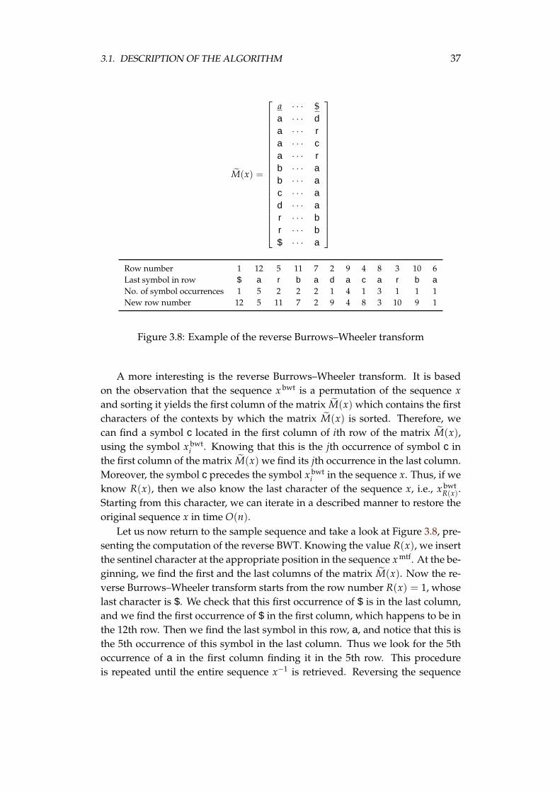
3.1. DESCRIPTION OF THE ALGORITHM 37
M(x) =
a · · · $a · · · da · · · ra · · · ca · · · rb · · · ab · · · ac · · · ad · · · ar · · · br · · · b$ · · · a
Row number 1 12 5 11 7 2 9 4 8 3 10 6Last symbol in row $ a r b a d a c a r b aNo. of symbol occurrences 1 5 2 2 2 1 4 1 3 1 1 1New row number 12 5 11 7 2 9 4 8 3 10 9 1
Figure 3.8: Example of the reverse Burrows–Wheeler transform
A more interesting is the reverse Burrows–Wheeler transform. It is basedon the observation that the sequence x bwt is a permutation of the sequence xand sorting it yields the first column of the matrix M(x) which contains the firstcharacters of the contexts by which the matrix M(x) is sorted. Therefore, wecan find a symbol c located in the first column of ith row of the matrix M(x),using the symbol x bwt
i . Knowing that this is the jth occurrence of symbol c inthe first column of the matrix M(x) we find its jth occurrence in the last column.Moreover, the symbol c precedes the symbol x bwt
i in the sequence x. Thus, if weknow R(x), then we also know the last character of the sequence x, i.e., x bwt
R(x).Starting from this character, we can iterate in a described manner to restore theoriginal sequence x in time O(n).
Let us now return to the sample sequence and take a look at Figure 3.8, pre-senting the computation of the reverse BWT. Knowing the value R(x), we insertthe sentinel character at the appropriate position in the sequence x mtf. At the be-ginning, we find the first and the last columns of the matrix M(x). Now the re-verse Burrows–Wheeler transform starts from the row number R(x) = 1, whoselast character is $. We check that this first occurrence of $ is in the last column,and we find the first occurrence of $ in the first column, which happens to be inthe 12th row. Then we find the last symbol in this row, a, and notice that this isthe 5th occurrence of this symbol in the last column. Thus we look for the 5thoccurrence of a in the first column finding it in the 5th row. This procedureis repeated until the entire sequence x−1 is retrieved. Reversing the sequence
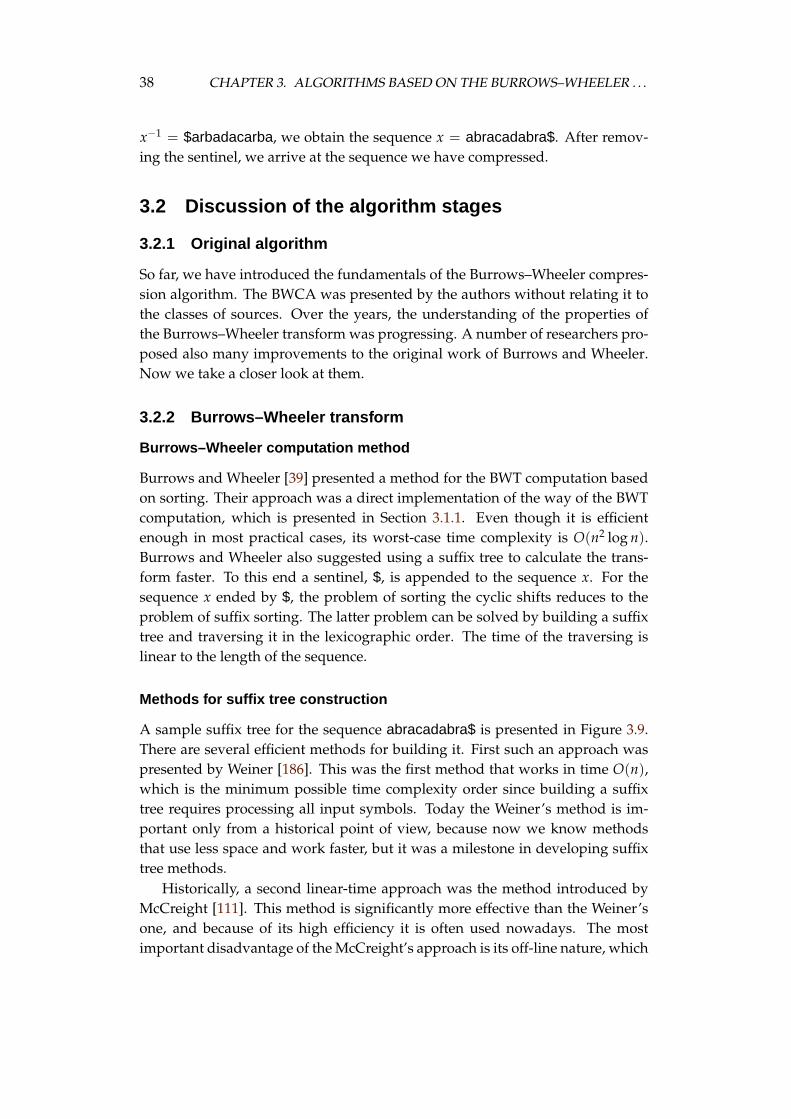
38 CHAPTER 3. ALGORITHMS BASED ON THE BURROWS–WHEELER . . .
x−1 = $arbadacarba, we obtain the sequence x = abracadabra$. After remov-ing the sentinel, we arrive at the sequence we have compressed.
3.2 Discussion of the algorithm stages
3.2.1 Original algorithm
So far, we have introduced the fundamentals of the Burrows–Wheeler compres-sion algorithm. The BWCA was presented by the authors without relating it tothe classes of sources. Over the years, the understanding of the properties ofthe Burrows–Wheeler transform was progressing. A number of researchers pro-posed also many improvements to the original work of Burrows and Wheeler.Now we take a closer look at them.
3.2.2 Burrows–Wheeler transform
Burrows–Wheeler computation method
Burrows and Wheeler [39] presented a method for the BWT computation basedon sorting. Their approach was a direct implementation of the way of the BWTcomputation, which is presented in Section 3.1.1. Even though it is efficientenough in most practical cases, its worst-case time complexity is O(n2 log n).Burrows and Wheeler also suggested using a suffix tree to calculate the trans-form faster. To this end a sentinel, $, is appended to the sequence x. For thesequence x ended by $, the problem of sorting the cyclic shifts reduces to theproblem of suffix sorting. The latter problem can be solved by building a suffixtree and traversing it in the lexicographic order. The time of the traversing islinear to the length of the sequence.
Methods for suffix tree construction
A sample suffix tree for the sequence abracadabra$ is presented in Figure 3.9.There are several efficient methods for building it. First such an approach waspresented by Weiner [186]. This was the first method that works in time O(n),which is the minimum possible time complexity order since building a suffixtree requires processing all input symbols. Today the Weiner’s method is im-portant only from a historical point of view, because now we know methodsthat use less space and work faster, but it was a milestone in developing suffixtree methods.
Historically, a second linear-time approach was the method introduced byMcCreight [111]. This method is significantly more effective than the Weiner’sone, and because of its high efficiency it is often used nowadays. The mostimportant disadvantage of the McCreight’s approach is its off-line nature, which
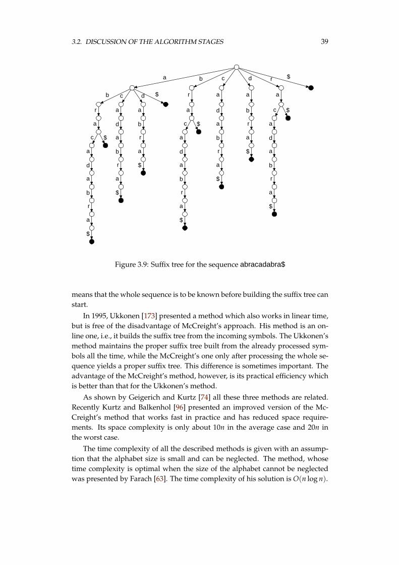
3.2. DISCUSSION OF THE ALGORITHM STAGES 39
a b c d r $
b c d $ r a a a
r
a
c $
a
d
a
b
r
a
$
a
d
a
b
r
a
$
a
b
r
a
$
a
c $
a
d
a
b
r
a
$
d
a
b
r
a
$
b
r
a
$
c $
a
d
a
b
r
a
$
Figure 3.9: Suffix tree for the sequence abracadabra$
means that the whole sequence is to be known before building the suffix tree canstart.
In 1995, Ukkonen [173] presented a method which also works in linear time,but is free of the disadvantage of McCreight’s approach. His method is an on-line one, i.e., it builds the suffix tree from the incoming symbols. The Ukkonen’smethod maintains the proper suffix tree built from the already processed sym-bols all the time, while the McCreight’s one only after processing the whole se-quence yields a proper suffix tree. This difference is sometimes important. Theadvantage of the McCreight’s method, however, is its practical efficiency whichis better than that for the Ukkonen’s method.
As shown by Geigerich and Kurtz [74] all these three methods are related.Recently Kurtz and Balkenhol [96] presented an improved version of the Mc-Creight’s method that works fast in practice and has reduced space require-ments. Its space complexity is only about 10n in the average case and 20n inthe worst case.
The time complexity of all the described methods is given with an assump-tion that the alphabet size is small and can be neglected. The method, whosetime complexity is optimal when the size of the alphabet cannot be neglectedwas presented by Farach [63]. The time complexity of his solution is O(n log n).
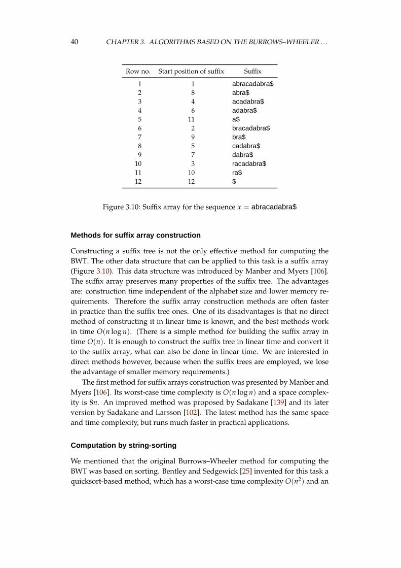
40 CHAPTER 3. ALGORITHMS BASED ON THE BURROWS–WHEELER . . .
Row no. Start position of suffix Suffix
1 1 abracadabra$2 8 abra$3 4 acadabra$4 6 adabra$5 11 a$6 2 bracadabra$7 9 bra$8 5 cadabra$9 7 dabra$
10 3 racadabra$11 10 ra$12 12 $
Figure 3.10: Suffix array for the sequence x = abracadabra$
Methods for suffix array construction
Constructing a suffix tree is not the only effective method for computing theBWT. The other data structure that can be applied to this task is a suffix array(Figure 3.10). This data structure was introduced by Manber and Myers [106].The suffix array preserves many properties of the suffix tree. The advantagesare: construction time independent of the alphabet size and lower memory re-quirements. Therefore the suffix array construction methods are often fasterin practice than the suffix tree ones. One of its disadvantages is that no directmethod of constructing it in linear time is known, and the best methods workin time O(n log n). (There is a simple method for building the suffix array intime O(n). It is enough to construct the suffix tree in linear time and convert itto the suffix array, what can also be done in linear time. We are interested indirect methods however, because when the suffix trees are employed, we losethe advantage of smaller memory requirements.)
The first method for suffix arrays construction was presented by Manber andMyers [106]. Its worst-case time complexity is O(n log n) and a space complex-ity is 8n. An improved method was proposed by Sadakane [139] and its laterversion by Sadakane and Larsson [102]. The latest method has the same spaceand time complexity, but runs much faster in practical applications.
Computation by string-sorting
We mentioned that the original Burrows–Wheeler method for computing theBWT was based on sorting. Bentley and Sedgewick [25] invented for this task aquicksort-based method, which has a worst-case time complexity O(n2) and an
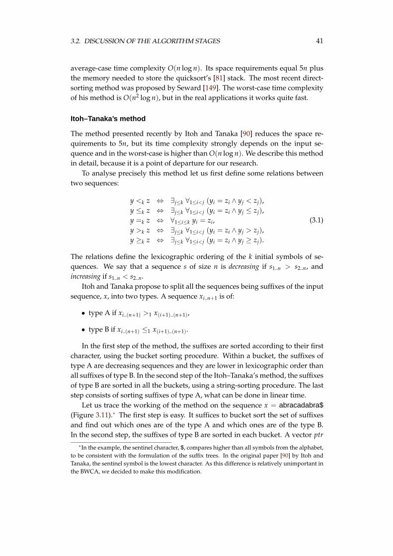
3.2. DISCUSSION OF THE ALGORITHM STAGES 41
average-case time complexity O(n log n). Its space requirements equal 5n plusthe memory needed to store the quicksort’s [81] stack. The most recent direct-sorting method was proposed by Seward [149]. The worst-case time complexityof his method is O(n2 log n), but in the real applications it works quite fast.
Itoh–Tanaka’s method
The method presented recently by Itoh and Tanaka [90] reduces the space re-quirements to 5n, but its time complexity strongly depends on the input se-quence and in the worst-case is higher than O(n log n). We describe this methodin detail, because it is a point of departure for our research.
To analyse precisely this method let us first define some relations betweentwo sequences:
y <k z ⇔ ∃j≤k ∀1≤i<j (yi = zi ∧ yj < zj),y ≤k z ⇔ ∃j≤k ∀1≤i<j (yi = zi ∧ yj ≤ zj),y =k z ⇔ ∀1≤i≤k yi = zi,y >k z ⇔ ∃j≤k ∀1≤i<j (yi = zi ∧ yj > zj),y ≥k z ⇔ ∃j≤k ∀1≤i<j (yi = zi ∧ yj ≥ zj).
(3.1)
The relations define the lexicographic ordering of the k initial symbols of se-quences. We say that a sequence s of size n is decreasing if s1..n > s2..n, andincreasing if s1..n < s2..n.
Itoh and Tanaka propose to split all the sequences being suffixes of the inputsequence, x, into two types. A sequence xi..n+1 is of:
• type A if xi..(n+1) >1 x(i+1)..(n+1),
• type B if xi..(n+1) ≤1 x(i+1)..(n+1).
In the first step of the method, the suffixes are sorted according to their firstcharacter, using the bucket sorting procedure. Within a bucket, the suffixes oftype A are decreasing sequences and they are lower in lexicographic order thanall suffixes of type B. In the second step of the Itoh–Tanaka’s method, the suffixesof type B are sorted in all the buckets, using a string-sorting procedure. The laststep consists of sorting suffixes of type A, what can be done in linear time.
Let us trace the working of the method on the sequence x = abracadabra$(Figure 3.11).∗ The first step is easy. It suffices to bucket sort the set of suffixesand find out which ones are of the type A and which ones are of the type B.In the second step, the suffixes of type B are sorted in each bucket. A vector ptr
∗In the example, the sentinel character, $, compares higher than all symbols from the alphabet,to be consistent with the formulation of the suffix trees. In the original paper [90] by Itoh andTanaka, the sentinel symbol is the lowest character. As this difference is relatively unimportant inthe BWCA, we decided to make this modification.
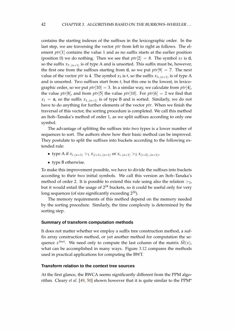
42 CHAPTER 3. ALGORITHMS BASED ON THE BURROWS–WHEELER . . .
contains the starting indexes of the suffixes in the lexicographic order. In thelast step, we are traversing the vector ptr from left to right as follows. The el-ement ptr[1] contains the value 1 and as no suffix starts at the earlier position(position 0) we do nothing. Then we see that ptr[2] = 8. The symbol x7 is d,so the suffix x7..(n+1) is of type A and is unsorted. This suffix must be, however,the first one from the suffixes starting from d, so we put ptr[9] = 7. The nextvalue of the vector ptr is 4. The symbol x3 is r, so the suffix x3..(n+1) is of type Aand is unsorted. Two suffixes start from r, but this one is the lowest, in lexico-graphic order, so we put ptr[10] = 3. In a similar way, we calculate from ptr[4],the value ptr[8], and from ptr[5] the value ptr[10]. For ptr[6] = 2 we find thatx1 = a, so the suffix x1..(n+1) is of type B and is sorted. Similarly, we do nothave to do anything for further elements of the vector ptr. When we finish thetraversal of this vector, the sorting procedure is completed. We call this methodan Itoh–Tanaka’s method of order 1, as we split suffixes according to only onesymbol.
The advantage of splitting the suffixes into two types is a lower number ofsequences to sort. The authors show how their basic method can be improved.They postulate to split the suffixes into buckets according to the following ex-tended rule:
• type A if xi..(n+1) >1 x(i+1)..(n+1) or xi..(n+1) >2 x(i+2)..(n+1),
• type B otherwise.
To make this improvement possible, we have to divide the suffixes into bucketsaccording to their two initial symbols. We call this version an Itoh–Tanaka’smethod of order 2. It is possible to extend this rule using also the relation >3,but it would entail the usage of 224 buckets, so it could be useful only for verylong sequences (of size significantly exceeding 224).
The memory requirements of this method depend on the memory neededby the sorting procedure. Similarly, the time complexity is determined by thesorting step.
Summary of transform computation methods
It does not matter whether we employ a suffix tree construction method, a suf-fix array construction method, or yet another method for computation the se-quence x bwt. We need only to compute the last column of the matrix M(x),what can be accomplished in many ways. Figure 3.12 compares the methodsused in practical applications for computing the BWT.
Transform relation to the context tree sources
At the first glance, the BWCA seems significantly different from the PPM algo-rithm. Cleary et al. [49, 50] shown however that it is quite similar to the PPM*
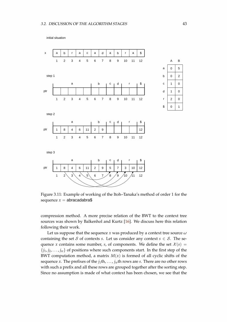
3.2. DISCUSSION OF THE ALGORITHM STAGES 43
initial situation
1 2 3 4 5 6 7 8 9 10 11 12
a b r a c a d a b r a $x
step 1
1 2 3 4 5 6 7 8 9 10 11 12
ptr
a b c d r $
a
b
c
d
r
$
A B
0
0
1
1
2
0
5
2
0
0
0
1
step 2
1 2 3 4 5 6 7 8 9 10 11 12
ptr
a b c d r $
1 8 4 6 11 2 9 12
step 3
1 2 3 4 5 6 7 8 9 10 11 12
ptr
a b c d r $
1 8 4 6 11 2 9 127 35 10
Figure 3.11: Example of working of the Itoh–Tanaka’s method of order 1 for thesequence x = abracadabra$
compression method. A more precise relation of the BWT to the context treesources was shown by Balkenhol and Kurtz [16]. We discuss here this relationfollowing their work.
Let us suppose that the sequence x was produced by a context tree source ω
containing the set S of contexts s. Let us consider any context s ∈ S . The se-quence x contains some number, s, of components. We define the set X (s) ={j1, j2, . . . , jw} of positions where such components start. In the first step of theBWT computation method, a matrix M(x) is formed of all cyclic shifts of thesequence x. The prefixes of the j1th, . . . , jwth rows are s. There are no other rowswith such a prefix and all these rows are grouped together after the sorting step.Since no assumption is made of what context has been chosen, we see that the
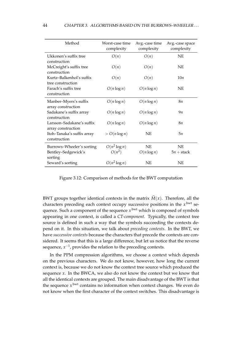
44 CHAPTER 3. ALGORITHMS BASED ON THE BURROWS–WHEELER . . .
Method Worst-case time Avg.-case time Avg.-case spacecomplexity complexity complexity
Ukkonen’s suffix treeconstruction
O(n) O(n) NE
McCreight’s suffix treeconstruction
O(n) O(n) NE
Kurtz–Balkenhol’s suffixtree construction
O(n) O(n) 10n
Farach’s suffix treeconstruction
O(n log n) O(n log n) NE
Manber–Myers’s suffixarray construction
O(n log n) O(n log n) 8n
Sadakane’s suffix arrayconstruction
O(n log n) O(n log n) 9n
Larsson–Sadakane’s suffixarray construction
O(n log n) O(n log n) 8n
Itoh–Tanaka’s suffix arrayconstruction
> O(n log n) NE 5n
Burrows–Wheeler’s sorting O(n2 log n) NE NEBentley–Sedgewick’ssorting
O(n2) O(n log n) 5n + stack
Seward’s sorting O(n2 log n) NE NE
Figure 3.12: Comparison of methods for the BWT computation
BWT groups together identical contexts in the matrix M(x). Therefore, all thecharacters preceding each context occupy successive positions in the x bwt se-quence. Such a component of the sequence x bwt which is composed of symbolsappearing in one context, is called a CT-component. Typically, the context treesource is defined in such a way that the symbols succeeding the contexts de-pend on it. In this situation, we talk about preceding contexts. In the BWT, wehave successive contexts because the characters that precede the contexts are con-sidered. It seems that this is a large difference, but let us notice that the reversesequence, x−1, provides the relation to the preceding contexts.
In the PPM compression algorithms, we choose a context which dependson the previous characters. We do not know, however, how long the currentcontext is, because we do not know the context tree source which produced thesequence x. In the BWCA, we also do not know the context but we know thatall the identical contexts are grouped. The main disadvantage of the BWT is thatthe sequence x bwt contains no information when context changes. We even donot know when the first character of the context switches. This disadvantage is
3.2. DISCUSSION OF THE ALGORITHM STAGES 45
important, since the probability distribution of symbol occurrence in one contextis determined by the parameters of the context tree source and does not change,but in the another context this probability differs significantly. Typically, theprobability distribution of similar context is also similar. There are no groundsfor such an assumption in the context tree source model, but this similarity isvery frequent in real sequences. The length of the common prefix of two con-texts is shorter, the difference of probability distribution is usually larger. ThePPM scheme can exploit this phenomenon, because it knows this length. In theBWCA, however, we do not have such a precise knowledge. We only knowthat the CT-components related to similar contexts appear in the sequence x bwt
closely to each other.There were a number of other theoretical analyses of the Burrows–Wheeler
transform and similar transforms. A transform closely related to the BWT, thelexical permutation sorting transform, was introduced by Arnavut and Magliv-eras [10, 11]. Other theoretical analysis of the BWT-based algorithms was pre-sented by Effros [56]. The author has shown the properties of the BWT outputassuming the FSMX source model. Manzini [107, 108, 109] also discussed theproperties of the BWT and has proven a bound of the compression ratio. Otherinteresting works on the properties of the BWT were presented by Arimura andYamamoto [6, 7].
3.2.3 Run length encoding
The run length encoding (RLE) [75] was absent in the original implementation ofthe BWCA. Some researchers postulate, however, its usage before the BWT, sowe describe here the RLE and present the arguments in favour of its inclusioninto a BWT-based compression algorithm.
The main idea of the RLE is simple—the runs of length longer or equal tosome fixed number, usually 3, are replaced by a pair: the current symbol andthe number of its repetitions. This transform rarely improves the compressionratio significantly, but this is not the only motivation of using the RLE. Sincethe sequence x may contain many long runs, the time of the successive stages(especially, the computation of the Burrows–Wheeler transform) can be quitelong. To overcome this problem various solutions were suggested. Burrows andWheeler [39] introduced a special sorting procedure for such sequences. Fen-wick [66, 68] used RLE, which eliminates long runs and decreases the length ofthe sequence x. The main advantage is reducing the time of computing the BWT.
Using the RLE destroys some contexts. In most cases, the RLE slightly wors-ens the compression ratio, by about 0.1%. If the sequence x contains many longruns, then it turns out that the sequence x mtf comprises 90% of 0s. In such acase, the RLE allows for reducing substantially the number of zeros in the se-quence x mtf and better estimating the probability of non-zero symbols, thus im-
46 CHAPTER 3. ALGORITHMS BASED ON THE BURROWS–WHEELER . . .
proving the overall compression ratio. Taking this observation into account,Balkenhol and Kurtz [16] suggested that the RLE should be used only when itmakes the length of the sequence x rle-0 to be less than 0.7n.
Note that if the method for the BWT computation based on constructing asuffix tree or a suffix array is used, then the occurrences of runs do not signifi-cantly influence its execution time. If the RLE-0 transform is employed, then theproblem of improper probability estimation in the entropy coder also becomesinsignificant. Therefore we conclude that the RLE should not be used.
3.2.4 Second stage transforms
Structure of the Burrows–Wheeler transform output sequence
As we mentioned, the sequence x bwt is a concatenation of components corre-sponding to the separate contexts. Unfortunately, there is no information onwhere exactly each such a CT-component starts in the sequence x bwt. By mon-itoring the probability distribution in the sequence x bwt, however, we can tryto uncover some of this information [18, 99, 101]. Surely the sequence x bwt isa permutation of the sequence x. In order to exploit the properties of the se-quence x bwt, we have to transform its local structure into a global structure insome way. Alternatively, we have to find a way to rapidly adapt to a chang-ing probability distribution in the sequence x bwt without information on wherethe CT-components start. Several approaches have been proposed to solve thisproblem. Some of them are based on the observation that the problem is similarto the list update problem.
List update problem
The formulation of the list update problem (LUP) [110] states that there is a list ofitems and a sequence of requests. A request can be an insertion, a deletion, or anaccess to an item in the list. The method solving the problem must serve theserequests. The cost of serving an access request to an item p on the ith positionfrom the front of the list equals i, which is the number of comparisons neededto find p. After processing a request, the list can be reorganised in order to min-imise the total cost of its maintenance. Once an item p is accessed, it may bemoved free of charge to any position closer to the front of the list (free transposi-tions). Other transpositions, of elements located closer than p to the end of thelist are called paid, and their cost equals 1. The methods solving the LUP shouldminimise the total cost of maintaining the list, i.e., the sum of all costs of servingthe sequence of requests.
There are two main classes of on-line methods solving the LUP: deterministicand randomised. Here we present the theoretical bounds of their performance.Before we can establish these bounds, we need to introduce a new term. We say
3.2. DISCUSSION OF THE ALGORITHM STAGES 47
that a deterministic method A is c-competitive if there is a constant α such that
A(σ)− c ·OPT(σ) ≤ α, (3.2)
for all possible sequences of requests σ. The A(·) denotes the total cost of main-tenance performed by the method A, and OPT(·) is the total cost of maintenancedone by the optimal off-line algorithm. Similarly we define the c-competitivenessfor the randomised method as
E(A(σ))− c ·OPT(σ) ≤ α, (3.3)
where E(·) is the expected value taken with respect to the random choices madeby the considered method.
The optimal off-line method knows the whole sequence of requests and canserve it with the minimal cost. The time complexity of such a method is expo-nential, what disqualifies it in practice. The best known optimal off-line method,proposed by Reingold and Westbrook [132], runs in time O(l2n(n− 1)!), where nis the number of requests and l is the number of elements on the list L.
There are bounds of the competitiveness of the deterministic as well as ran-domised methods. Raghavan and Karp (reported by Irani [89]) proved that thelower bound for deterministic methods is c = 2 − 2/(l + 1). The randomisedmethods can improve this bound, and the best known lower bound for them isc = 1.5 [168]. The best known randomised method achieves c = (1 +
√5)/2 ≈
1.62 [3].A recent review of many methods for the LUP was presented by Bachrach
and El-Yaniv [15]. The authors provide a brief description of over forty methodsgiving their proven competitiveness. They also compare these methods empiri-cally.
In the second stage of the BWCA, we do not want to minimise the total costof maintenance of the list L. When we apply the method solving the LUP tothe list L and the sequence of requests x bwt, we obtain the sequence x lup whichcontains the integers being the number of positions on which the symbols fromthe sequence x bwt appear in the list L. If we sum up the numbers from the se-quence x lup, we get the total cost of maintaining the list L (it is assumed here thatthe method for the LUP does not perform paid transpositions). The main goalof the second stage of the BWCA is not to minimise the total cost, even thoughtypically when this cost is smaller, the distribution of probabilities of symbol oc-currences in the sequence x lup is less uniform. In the last stage of the BWCA,we apply the entropy coder to the sequence x lup, and when the distribution ofthe symbols in this sequence is less uniform, then a better compression ratio isachieved. This observation is of course imprecise because the compression ra-tio depends on the probability distribution of symbols in the sequence x lup ina more complicated way. When we use the RLE-0 transform, we in fact encode
48 CHAPTER 3. ALGORITHMS BASED ON THE BURROWS–WHEELER . . .
the sequence x rle-0, whose probability distribution of symbols is slightly differ-ent. The overall compression ratio depends also on the probability estimation inthe last stage of the BWCA. Nevertheless, minimising the total cost of maintain-ing the list L typically yields a better compression ratio.
Let us notice that the additional cost of paid transpositions can be neglectedbecause the symbols in the sequence x lup correspond to the cost of finding thecurrent items, and there is no cost related to the reorganisation of the list L. Inparticular, we can say that in the BWCA the problem is similar to the modi-fied LUP, in which the paid transpositions cost 0. The sequence x bwt has alsoa specific structure, as it is composed of CT-components. In the LUP, we donot assume anything about the sequence of requests. Therefore, using the bestmethods specialised for the LUP does not always lead to the best compressionresults. Several modifications of these methods were proposed in order to ex-ploit the properties of the BWT in a better way.
Move-to-front transform and its modifications
In the work introducing the BWCA [39], Burrows and Wheeler suggested usingthe move-to-front transform [26] as the second stage of the compression algo-rithm. The MTF transform is a method solving the LUP (it meets the lowerbound for the deterministic methods), and maintains a character list L. Whena character x bwt
i appears, the list L is scanned and the position of the charac-ter x bwt
i in the list L is assigned to x mtfi . Then the character is moved to the
beginning of the list L. As a result we get the sequence x mtf over the alphabetAmtf = {0, 1, . . . , k − 1}. This is a very simple strategy, but its results are quitegood in practice. The usage of the MTF transform in the BWCA is motivated bythe observation that the most likely symbols to appear are the most recent ones.This is because the more recent the last occurrence of the character is, the morelikely it is in a different CT-component.
Burrows and Wheeler [39] suggested that it may be useful to refrain frommoving the current character to the very first position of the list. Fenwick [65,67, 68] and Schindler [144] explored such a possibility, but failed to obtain bettercompression results. Recently, Balkenhol et al. [17] proposed an improvement ofthe MTF called MTF-1, which improves the compression ratio. Its only modifi-cation of the MTF transform is that only the symbols from the second position inthe list L are moved to top of the list. The symbols from the higher positions aremoved to the second position. Balkenhol and Shtarkov [18] proposed a furthermodification of the MTF-1—the symbols from the second position are movedto the beginning of the list L only if the previous transformed symbol is at thefirst position (following the authors we call this version MTF-2). The illustrationand the comparison of the MTF, the MTF-1, and the MTF-2 transforms is shownin Figure 3.13.
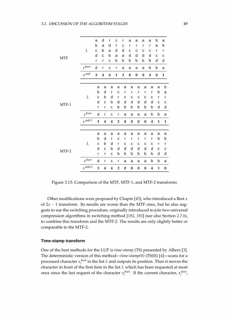
3.2. DISCUSSION OF THE ALGORITHM STAGES 49
MTF
a d r c r a a a a b ab a d r c r r r r a b
L c b a d d c c c c r rd c b a a d d d d c cr r c b b b b b b d d
x bwt d r c r a a a a b b a
x mtf 3 4 4 1 3 0 0 0 4 0 1
MTF-1
a a a a a a a a a a bb d r c r r r r r b a
L c b d r c c c c c r rd c b d d d d d d c cr r c b b b b b b d d
x bwt d r c r a a a a b b a
x mtf-1 3 4 4 2 0 0 0 0 4 1 1
MTF-2
a a a a a a a a a a ab d r c r r r r r b b
L c b d r c c c c c r rd c b d d d d d d c cr r c b b b b b b d d
x bwt d r c r a a a a b b a
x mtf-2 3 4 4 2 0 0 0 0 4 1 0
Figure 3.13: Comparison of the MTF, MTF-1, and MTF-2 transforms
Other modifications were proposed by Chapin [43], who introduced a Best xof 2x − 1 transform. Its results are worse than the MTF ones, but he also sug-gests to use the switching procedure, originally introduced to join two universalcompression algorithms in switching method [182, 183] (see also Section 2.7.6),to combine this transform and the MTF-2. The results are only slightly better orcomparable to the MTF-2.
Time-stamp transform
One of the best methods for the LUP is time-stamp (TS) presented by Albers [3].The deterministic version of this method—time-stamp(0) (TS(0)) [4]—scans for aprocessed character x bwt
i in the list L and outputs its position. Then it moves thecharacter in front of the first item in the list L which has been requested at mostonce since the last request of the character x bwt
i . If the current character, x bwti ,
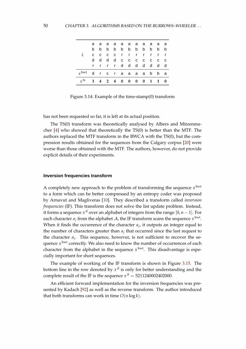
50 CHAPTER 3. ALGORITHMS BASED ON THE BURROWS–WHEELER . . .
a a a a a a a a a a ab b b b b b b b b b b
L c c c c r r r r r r rd d d d c c c c c c cr r r r d d d d d d d
x bwt d r c r a a a a b b a
x ts 3 4 2 4 0 0 0 0 1 1 0
Figure 3.14: Example of the time-stamp(0) transform
has not been requested so far, it is left at its actual position.
The TS(0) transform was theoretically analysed by Albers and Mitzenma-cher [4] who showed that theoretically the TS(0) is better than the MTF. Theauthors replaced the MTF transform in the BWCA with the TS(0), but the com-pression results obtained for the sequences from the Calgary corpus [20] wereworse than those obtained with the MTF. The authors, however, do not provideexplicit details of their experiments.
Inversion frequencies transform
A completely new approach to the problem of transforming the sequence x bwt
to a form which can be better compressed by an entropy coder was proposedby Arnavut and Magliveras [10]. They described a transform called inversionfrequencies (IF). This transform does not solve the list update problem. Instead,it forms a sequence x if over an alphabet of integers from the range [0, n− 1]. Foreach character aj from the alphabet A, the IF transform scans the sequence x bwt.When it finds the occurrence of the character aj, it outputs an integer equal tothe number of characters greater than aj that occurred since the last request tothe character aj. This sequence, however, is not sufficient to recover the se-quence x bwt correctly. We also need to know the number of occurrences of eachcharacter from the alphabet in the sequence x bwt. This disadvantage is espe-cially important for short sequences.
The example of working of the IF transform is shown in Figure 3.15. Thebottom line in the row denoted by x if is only for better understanding and thecomplete result of the IF is the sequence x if = 5211240002402000.
An efficient forward implementation for the inversion frequencies was pre-sented by Kadach [92] as well as the reverse transform. The author introducedthat both transforms can work in time O(n log k).
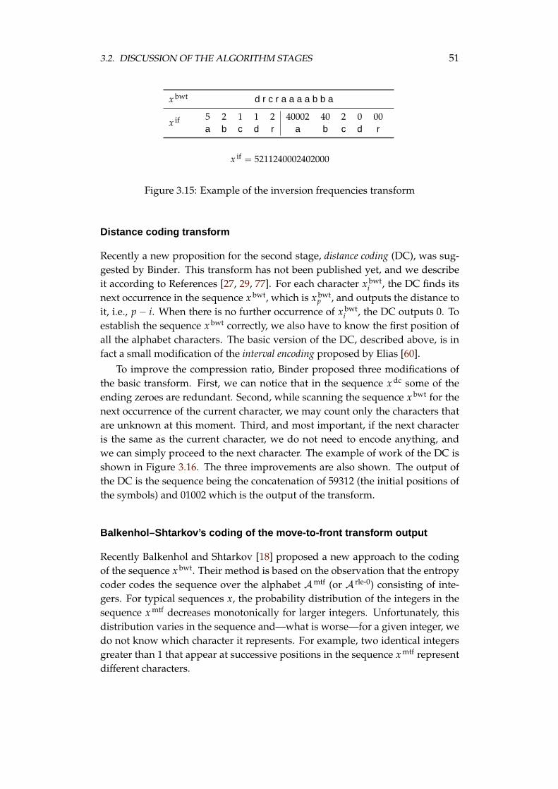
3.2. DISCUSSION OF THE ALGORITHM STAGES 51
x bwt d r c r a a a a b b a
x if 5 2 1 1 2 40002 40 2 0 00a b c d r a b c d r
x if = 5211240002402000
Figure 3.15: Example of the inversion frequencies transform
Distance coding transform
Recently a new proposition for the second stage, distance coding (DC), was sug-gested by Binder. This transform has not been published yet, and we describeit according to References [27, 29, 77]. For each character x bwt
i , the DC finds itsnext occurrence in the sequence x bwt, which is x bwt
p , and outputs the distance toit, i.e., p − i. When there is no further occurrence of x bwt
i , the DC outputs 0. Toestablish the sequence x bwt correctly, we also have to know the first position ofall the alphabet characters. The basic version of the DC, described above, is infact a small modification of the interval encoding proposed by Elias [60].
To improve the compression ratio, Binder proposed three modifications ofthe basic transform. First, we can notice that in the sequence x dc some of theending zeroes are redundant. Second, while scanning the sequence x bwt for thenext occurrence of the current character, we may count only the characters thatare unknown at this moment. Third, and most important, if the next characteris the same as the current character, we do not need to encode anything, andwe can simply proceed to the next character. The example of work of the DC isshown in Figure 3.16. The three improvements are also shown. The output ofthe DC is the sequence being the concatenation of 59312 (the initial positions ofthe symbols) and 01002 which is the output of the transform.
Balkenhol–Shtarkov’s coding of the move-to-front transform output
Recently Balkenhol and Shtarkov [18] proposed a new approach to the codingof the sequence x bwt. Their method is based on the observation that the entropycoder codes the sequence over the alphabet Amtf (or A rle-0) consisting of inte-gers. For typical sequences x, the probability distribution of the integers in thesequence x mtf decreases monotonically for larger integers. Unfortunately, thisdistribution varies in the sequence and—what is worse—for a given integer, wedo not know which character it represents. For example, two identical integersgreater than 1 that appear at successive positions in the sequence x mtf representdifferent characters.
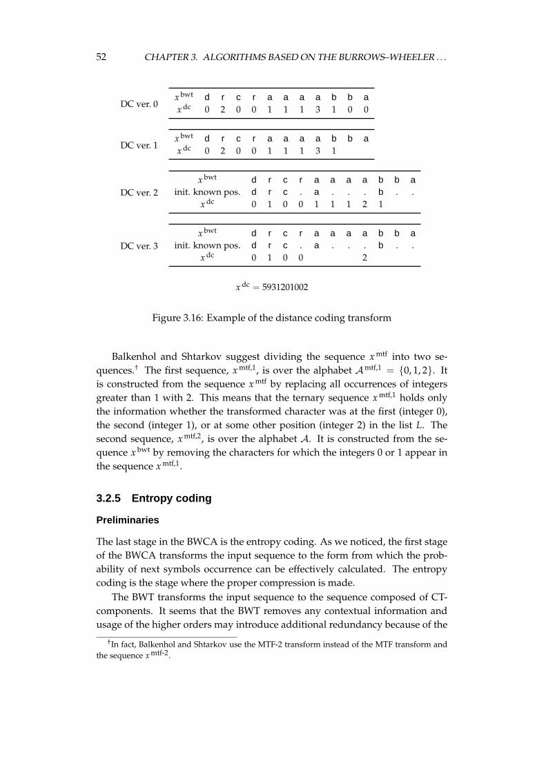
52 CHAPTER 3. ALGORITHMS BASED ON THE BURROWS–WHEELER . . .
DC ver. 0x bwt d r c r a a a a b b ax dc 0 2 0 0 1 1 1 3 1 0 0
DC ver. 1x bwt d r c r a a a a b b ax dc 0 2 0 0 1 1 1 3 1
DC ver. 2x bwt d r c r a a a a b b a
init. known pos. d r c . a . . . b . .x dc 0 1 0 0 1 1 1 2 1
DC ver. 3x bwt d r c r a a a a b b a
init. known pos. d r c . a . . . b . .x dc 0 1 0 0 2
x dc = 5931201002
Figure 3.16: Example of the distance coding transform
Balkenhol and Shtarkov suggest dividing the sequence x mtf into two se-quences.† The first sequence, x mtf,1, is over the alphabet Amtf,1 = {0, 1, 2}. Itis constructed from the sequence x mtf by replacing all occurrences of integersgreater than 1 with 2. This means that the ternary sequence x mtf,1 holds onlythe information whether the transformed character was at the first (integer 0),the second (integer 1), or at some other position (integer 2) in the list L. Thesecond sequence, x mtf,2, is over the alphabet A. It is constructed from the se-quence x bwt by removing the characters for which the integers 0 or 1 appear inthe sequence x mtf,1.
3.2.5 Entropy coding
Preliminaries
The last stage in the BWCA is the entropy coding. As we noticed, the first stageof the BWCA transforms the input sequence to the form from which the prob-ability of next symbols occurrence can be effectively calculated. The entropycoding is the stage where the proper compression is made.
The BWT transforms the input sequence to the sequence composed of CT-components. It seems that the BWT removes any contextual information andusage of the higher orders may introduce additional redundancy because of the
†In fact, Balkenhol and Shtarkov use the MTF-2 transform instead of the MTF transform andthe sequence x mtf-2.
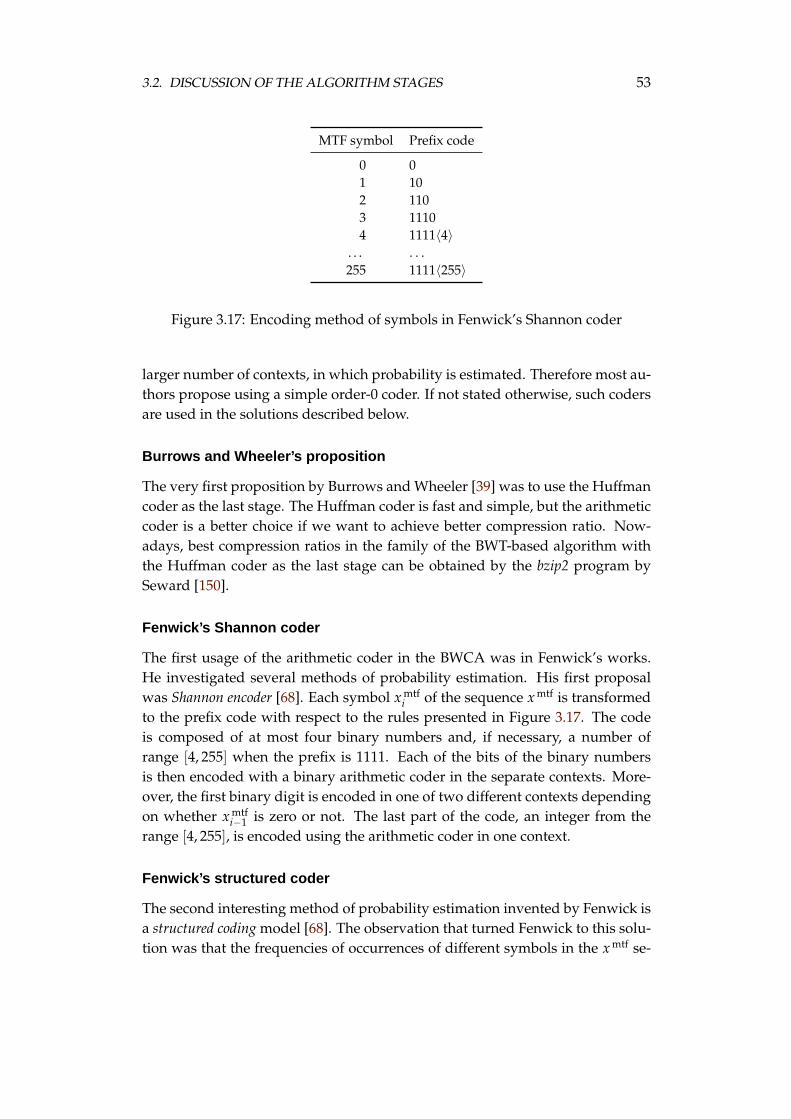
3.2. DISCUSSION OF THE ALGORITHM STAGES 53
MTF symbol Prefix code
0 01 102 1103 11104 1111〈4〉
. . . . . .255 1111〈255〉
Figure 3.17: Encoding method of symbols in Fenwick’s Shannon coder
larger number of contexts, in which probability is estimated. Therefore most au-thors propose using a simple order-0 coder. If not stated otherwise, such codersare used in the solutions described below.
Burrows and Wheeler’s proposition
The very first proposition by Burrows and Wheeler [39] was to use the Huffmancoder as the last stage. The Huffman coder is fast and simple, but the arithmeticcoder is a better choice if we want to achieve better compression ratio. Now-adays, best compression ratios in the family of the BWT-based algorithm withthe Huffman coder as the last stage can be obtained by the bzip2 program bySeward [150].
Fenwick’s Shannon coder
The first usage of the arithmetic coder in the BWCA was in Fenwick’s works.He investigated several methods of probability estimation. His first proposalwas Shannon encoder [68]. Each symbol x mtf
i of the sequence x mtf is transformedto the prefix code with respect to the rules presented in Figure 3.17. The codeis composed of at most four binary numbers and, if necessary, a number ofrange [4, 255] when the prefix is 1111. Each of the bits of the binary numbersis then encoded with a binary arithmetic coder in the separate contexts. More-over, the first binary digit is encoded in one of two different contexts dependingon whether x mtf
i−1 is zero or not. The last part of the code, an integer from therange [4, 255], is encoded using the arithmetic coder in one context.
Fenwick’s structured coder
The second interesting method of probability estimation invented by Fenwick isa structured coding model [68]. The observation that turned Fenwick to this solu-tion was that the frequencies of occurrences of different symbols in the x mtf se-
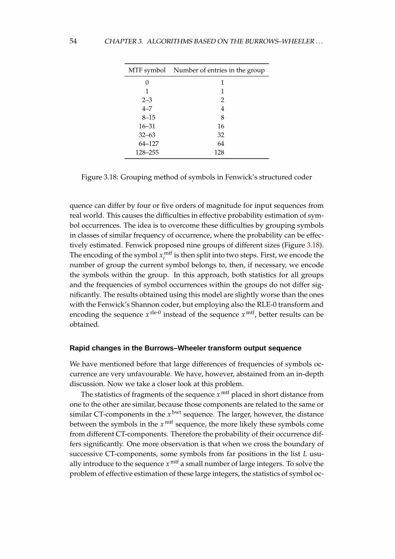
54 CHAPTER 3. ALGORITHMS BASED ON THE BURROWS–WHEELER . . .
MTF symbol Number of entries in the group
0 11 1
2–3 24–7 48–15 8
16–31 1632–63 3264–127 64
128–255 128
Figure 3.18: Grouping method of symbols in Fenwick’s structured coder
quence can differ by four or five orders of magnitude for input sequences fromreal world. This causes the difficulties in effective probability estimation of sym-bol occurrences. The idea is to overcome these difficulties by grouping symbolsin classes of similar frequency of occurrence, where the probability can be effec-tively estimated. Fenwick proposed nine groups of different sizes (Figure 3.18).The encoding of the symbol x mtf
i is then split into two steps. First, we encode thenumber of group the current symbol belongs to, then, if necessary, we encodethe symbols within the group. In this approach, both statistics for all groupsand the frequencies of symbol occurrences within the groups do not differ sig-nificantly. The results obtained using this model are slightly worse than the oneswith the Fenwick’s Shannon coder, but employing also the RLE-0 transform andencoding the sequence x rle-0 instead of the sequence x mtf, better results can beobtained.
Rapid changes in the Burrows–Wheeler transform output sequence
We have mentioned before that large differences of frequencies of symbols oc-currence are very unfavourable. We have, however, abstained from an in-depthdiscussion. Now we take a closer look at this problem.
The statistics of fragments of the sequence x mtf placed in short distance fromone to the other are similar, because those components are related to the same orsimilar CT-components in the x bwt sequence. The larger, however, the distancebetween the symbols in the x mtf sequence, the more likely these symbols comefrom different CT-components. Therefore the probability of their occurrence dif-fers significantly. One more observation is that when we cross the boundary ofsuccessive CT-components, some symbols from far positions in the list L usu-ally introduce to the sequence x mtf a small number of large integers. To solve theproblem of effective estimation of these large integers, the statistics of symbol oc-
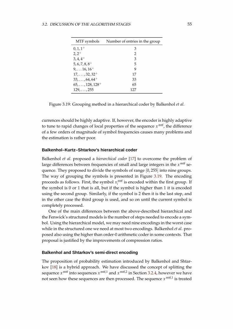
3.2. DISCUSSION OF THE ALGORITHM STAGES 55
MTF symbols Number of entries in the group
0, 1, 1+ 32, 2+ 23, 4, 4+ 35, 6, 7, 8, 8+ 59, . . . 16, 16+ 917, . . . , 32, 32+ 1733, . . . , 64, 64+ 3365, . . . , 128, 128+ 65129, . . . , 255 127
Figure 3.19: Grouping method in a hierarchical coder by Balkenhol et al.
currences should be highly adaptive. If, however, the encoder is highly adaptiveto tune to rapid changes of local properties of the sequence x mtf, the differenceof a few orders of magnitude of symbol frequencies causes many problems andthe estimation is rather poor.
Balkenhol–Kurtz–Shtarkov’s hierarchical coder
Balkenhol et al. proposed a hierarchical coder [17] to overcome the problem oflarge differences between frequencies of small and large integers in the x mtf se-quence. They proposed to divide the symbols of range [0, 255] into nine groups.The way of grouping the symbols is presented in Figure 3.19. The encodingproceeds as follows. First, the symbol x mtf
i is encoded within the first group. Ifthe symbol is 0 or 1 that is all, but if the symbol is higher than 1 it is encodedusing the second group. Similarly, if the symbol is 2 then it is the last step, andin the other case the third group is used, and so on until the current symbol iscompletely processed.
One of the main differences between the above-described hierarchical andthe Fenwick’s structured models is the number of steps needed to encode a sym-bol. Using the hierarchical model, we may need nine encodings in the worst casewhile in the structured one we need at most two encodings. Balkenhol et al. pro-posed also using the higher than order-0 arithmetic coder in some contexts. Thatproposal is justified by the improvements of compression ratios.
Balkenhol and Shtarkov’s semi-direct encoding
The proposition of probability estimation introduced by Balkenhol and Shtar-kov [18] is a hybrid approach. We have discussed the concept of splitting thesequence x mtf into sequences x mtf,1 and x mtf,2 in Section 3.2.4, however we havenot seen how these sequences are then processed. The sequence x mtf,1 is treated
56 CHAPTER 3. ALGORITHMS BASED ON THE BURROWS–WHEELER . . .
as a Markov chain and is encoded using the standard universal coding scheme.To encode the sequence x mtf,2, the alphabet is divided into four groups of chang-ing sizes and contents. The symbols from the sequence x mtf,2 are encoded withthe probability estimation from one of these groups. The groups are maintainedto work as sliding windows and contain statistics of symbol occurrences in thesewindows. Because the last symbols have similar probability distribution, suchan estimation helps in obtaining good compression results.
Direct coding of the Burrows–Wheeler transform output
Fenwick examined also one more solution which refrains from usage of the MTFtransform. He investigated what could be obtained if the arithmetic coder wereemployed to encode the x bwt sequence. The main problem in such a situationis that the symbols occurring in successive CT-components can be completelydifferent, and the statistics of symbol occurrences vary rapidly. When we usethe MTF, we transform the local structure of the x bwt sequence to the globalone, obtaining the sequence x mtf in which the distribution of symbol frequenciesdecreases roughly monotonically. The sequence x bwt is a permutation of thesequence x, so the distribution of symbol frequencies is much more uniform.These were the reasons why Fenwick [68] obtained significantly worse results.
The approach of refraining from usage of the MTF transform was continuedrecently by Wirth and Moffat [195]. They employed the idea of the hierarchi-cal coder by Balkenhol and Shtarkov and modified it to work without the MTFstage. Wirth and Moffat propose a probability estimation with exponential for-getting. The authors improve the basic approach using the concepts of exclusionand update exclusion. They also decide to use a higher than order-0 arithmeticcoder in some contexts. The obtained results are very good in the group of theBWT-based algorithms that do not use MTF transform or similar second stagemethods. The results, however, are still significantly worse than the best ones inthe Burrows–Wheeler transform-based algorithms family.
Encoding the distance coder and the inversion frequencies outputs
The MTF transform and related methods are not the only possibility of the sec-ond stage in the BWCA. In Section 3.2.4, we mentioned also the inversion fre-quencies and the distance coder. The sequences x if and x dc consist of integersfrom the range [0, n], so we need to apply a different approach to the entropycoder when these transforms are used.
Various solutions to encode such numbers may be considered. One of themis to use an exponential hierarchy and to group the integers into sets {0}, {1},{2, 3}, {4, . . . , 7}, . . . , {2blog nc, . . . , n}. In the first step, we encode the number ofthe group containing the current symbol, then we encode the symbol withinthis group. The other approach is to use a binary prefix code, encode the current
3.2. DISCUSSION OF THE ALGORITHM STAGES 57
symbol using it, and finally encode each bit separately using the binary arith-metic encoder. A good choice for this task can be an Elias γ code [59]. Thissolution, presented in Reference [55], was invented by the author of the disser-tation, and will be discussed also in Section 4.1.6. This approach is reported tobe the best one of those examined by Arnavut [9].
The distance coder transform was not published so far and unfortunately wedo not know the internals of the algorithms using it, so we could not describethe way of encoding the integers in the compression programs, like the dc pro-gram [28]. A solution similar to the one used for coding the output of the IF canbe, however, used for the output of the DC.
Variable-length integer codes
Recently, an alternative way as the last stage of the BWT-based compression al-gorithm was proposed by Fenwick [69]. He postulates to use a variable-lengthinteger codes instead of the Huffman or the arithmetic coder if the speed of com-pression is crucial. Fenwick investigates Elias γ codes [59] and Fraenkel–KleinFibonacci codes [71]. The gain in the compression speed is, however, occupiedby a significant lost in compression ratio.
3.2.6 Preprocessing the input sequence
Why to preprocess the input sequence?
We observed that the BWCA is similar to the PPM algorithms. We also pointedout a significant difference between them—in the BWCA the information wherethe context is changed is lost after the BWT stage. Here we want to point out thesecond important difference.
The compression ratio in most data compression algorithms, such as PPM,LZ77, LZ78, or DMC, does not depend on the order of the symbols in the al-phabet. We can permute the alphabet and the compression ratio will be onlyslightly different (theoretically it will be identical). The behaviour of the BWCAis different. In some algorithms, like PPM, we know where the context startsand we can exploit this knowledge. In the BWCA, we do not know this, andin the entropy coding stage, for the probability estimation, we also use symbolsfrom the CT-components close to the current one, what can be harmful.
Alphabet reordering
If we drastically change the ordering of the alphabet symbols, it may cause thecontexts grouped together with the current one have significantly different prob-ability distributions. Chapin and Tate [44] showed that if the alphabet orderingis changed randomly, the compression ratio decreases highly (even by 20%).
58 CHAPTER 3. ALGORITHMS BASED ON THE BURROWS–WHEELER . . .
(We have to stress here that in the whole dissertation we assume the defaultASCII ordering of the alphabet.) They suggested that we can try to employ thisdisadvantage to our benefit and reorganise the alphabet in such a way that thecompression ratio will improve.
Chapin and Tate suggested a few approaches—first, an ad hoc reordering ofthe alphabet, grouping vowels and consonants. The other approaches are morecomplicated. They create histograms of symbols appearing in all one-charactercontexts. Then they try to reorganise the alphabet in such a way that the totalcost of changing the context will be lower. The first problem is to choose whichway of finding the difference between two histograms is the best for this task.Chapin and Tate have presented some proposals in this regard. The secondproblem is how to find the best ordering. They used the algorithms solving theTravelling Salesman Problem (TSP) [103] to find the solution. The similarity tothe TSP may by not clear at the first glance. If we notice, however, that we dealwith k one-character contexts, the costs of changing to the all other one-charactercontexts, and we have to produce a permutation of the k contexts, the similaritycomes out more clear.
The experimental results obtained by Chapin and Tate are, however, ratherdisappointing. The gain is significant only when we try all the proposed meth-ods to improve the compression ratio and choose the best one for each singlefile. It is impractical to compress a file with a dozen or so versions of the trans-form, and choose the best result if the gain is less than 1%. Moreover, we haveto consider also the cost of solving the TSP.
The alphabet reordering was also discussed by Balkenhol and Shtarkov [18].They modified the ordering proposed by Chapin and Tate. The gain is verysmall, and the proposed order is adapted to the text files only, so we considerthat this artificial reorganisation is unjustified.
Reversing the input sequence
Balkenhol et al. [17] suggested that if the number of symbols used in the inputsequence is the maximum number of characters which can be represented withan assumed number of bits (typically 256 characters), it should be assumed thatthe sequence stores a binary file. For such sequences, the succeeding contextsare much better than the preceding ones. Therefore they propose to use in sucha case the reversed sequence, x−1. This heuristics gives gains for binary files sowe decided to use it in our research to provide a thorough comparison to thebest existing algorithms.
Preliminary filtering
Other preliminary improvements (before the BWT) were proposed by Grabow-ski [76]. His proposals are reversible filters that are used before the compression.
3.2. DISCUSSION OF THE ALGORITHM STAGES 59
Some of them are independent on the compression algorithm and can be usedalso with the different compression schemes, not only with the BWCA. All theimprovements are based on the assumption that text files are to be compressed.
The first proposition is to use a capital conversion what means that the wordsstarting with a capital letter (only the first letter should be a capital) are changedin such a way that the first letter is transformed to the lowercase and a specialflag denoting the change is inserted. (Till the end of the current section we willbe using the intuitive terms words and letters to emphasise that we consider onlythe sequences being texts.) The second improvement is motivated by the obser-vation that most text files contain the lines starting with a letter. This means thatthe previous character (the context) of this letter is the end-of-line (EOL) char-acter. It appears only because of formating rules and typically it has no othermeaning. Grabowski proposes to insert an additional space character after theEOL, so the context of the first letter of the word is the space symbol, what isa typical situation. The other proposition is a phrase substitution. This idea isnot new, also Teahan [163] proposed such a solution to improve the compres-sion ratios. The main idea is to replace the groups of letters with a new symbol.It can be simply done in the text files, because the standard ASCII code usesonly 128 first characters of the 256 possibilities. Grabowski provides a list ofsubstitutions which improve the compression ratio. This list was establishedexperimentally, because it is very hard to provide an exact rule which groupsof letters to replace in order to improve the compression ratio. Therefore it isclear that for a different set of files other list of substitutions can give better re-sults. We have mentioned only the most important propositions of Grabowskiwhich give significant improvements. These experiments show that by usinghis modifications we can achieve a gain in the compression ratio about 3% onthe text files from the Calgary corpus. This gain is significant and much greaterthan can be obtained with the alphabet reordering. We have to remember, how-ever, that these improvements are motivated by the assumption that text filesare compressed, and applying these modifications to binary files worsens thecompression ratio.
Yet another preprocessing method was proposed by Awan and Mukher-jee [13, 14]. The authors introduce a reversible length index preserving transform(LIPT), based on the dictionary prepared before the compression and the corpusof files, used to order the words in the dictionary. If we have the dictionary,where for each word a special code is prepared, we process the input sequenceand replace each known word (the word that belongs to the dictionary) witha related code. Applying the LIPT before the compression gives a gain in thecompression ratio of about 5% on the text files from the Calgary corpus. Themain disadvantages of the LIPT are: we have to know that we compress a textfile, what is the language of the file, and we need a pre-built dictionary with
60 CHAPTER 3. ALGORITHMS BASED ON THE BURROWS–WHEELER . . .
ready-made encodings.We have mentioned only preprocessors for the text files. There are also fil-
ters for different types of binary data. The number of types of binary data is,however, large, and we want only to notice that such filters exist.
Since this dissertation concerns the universal compression algorithms, wedo not make any assumptions regarding the type of the compressed sequence.As a consequence we discuss the above data-specific improvements only as anotification of works on the BWCA, but we do not use them in our research.
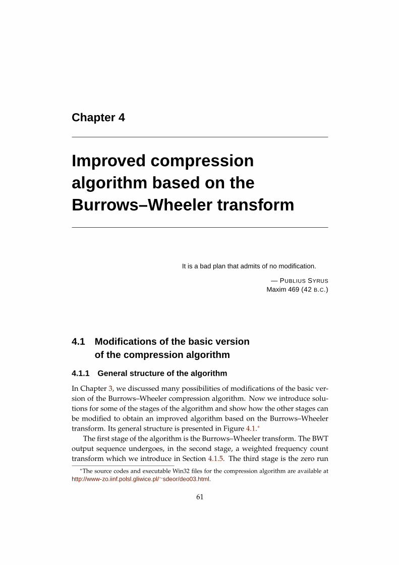
Chapter 4
Improved compressionalgorithm based on theBurrows–Wheeler transform
It is a bad plan that admits of no modification.
— PUBLIUS SYRUS
Maxim 469 (42 B.C.)
4.1 Modifications of the basic versionof the compression algorithm
4.1.1 General structure of the algorithm
In Chapter 3, we discussed many possibilities of modifications of the basic ver-sion of the Burrows–Wheeler compression algorithm. Now we introduce solu-tions for some of the stages of the algorithm and show how the other stages canbe modified to obtain an improved algorithm based on the Burrows–Wheelertransform. Its general structure is presented in Figure 4.1.∗
The first stage of the algorithm is the Burrows–Wheeler transform. The BWToutput sequence undergoes, in the second stage, a weighted frequency counttransform which we introduce in Section 4.1.5. The third stage is the zero run
∗The source codes and executable Win32 files for the compression algorithm are available athttp://www-zo.iinf.polsl.gliwice.pl/∼sdeor/deo03.html.
61
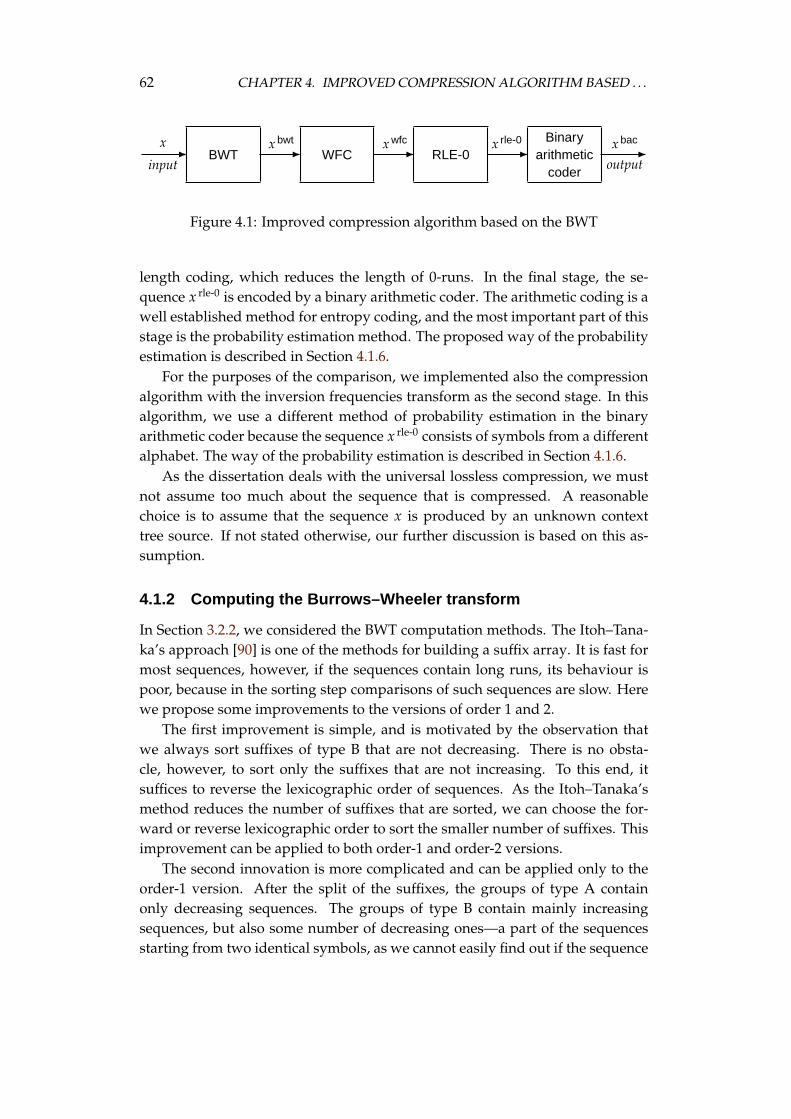
62 CHAPTER 4. IMPROVED COMPRESSION ALGORITHM BASED . . .
BWT WFC RLE-0Binary
arithmeticcoder
- - - - -x
input
x bwt x wfc x rle-0 x bac
output
Figure 4.1: Improved compression algorithm based on the BWT
length coding, which reduces the length of 0-runs. In the final stage, the se-quence x rle-0 is encoded by a binary arithmetic coder. The arithmetic coding is awell established method for entropy coding, and the most important part of thisstage is the probability estimation method. The proposed way of the probabilityestimation is described in Section 4.1.6.
For the purposes of the comparison, we implemented also the compressionalgorithm with the inversion frequencies transform as the second stage. In thisalgorithm, we use a different method of probability estimation in the binaryarithmetic coder because the sequence x rle-0 consists of symbols from a differentalphabet. The way of the probability estimation is described in Section 4.1.6.
As the dissertation deals with the universal lossless compression, we mustnot assume too much about the sequence that is compressed. A reasonablechoice is to assume that the sequence x is produced by an unknown contexttree source. If not stated otherwise, our further discussion is based on this as-sumption.
4.1.2 Computing the Burrows–Wheeler transform
In Section 3.2.2, we considered the BWT computation methods. The Itoh–Tana-ka’s approach [90] is one of the methods for building a suffix array. It is fast formost sequences, however, if the sequences contain long runs, its behaviour ispoor, because in the sorting step comparisons of such sequences are slow. Herewe propose some improvements to the versions of order 1 and 2.
The first improvement is simple, and is motivated by the observation thatwe always sort suffixes of type B that are not decreasing. There is no obsta-cle, however, to sort only the suffixes that are not increasing. To this end, itsuffices to reverse the lexicographic order of sequences. As the Itoh–Tanaka’smethod reduces the number of suffixes that are sorted, we can choose the for-ward or reverse lexicographic order to sort the smaller number of suffixes. Thisimprovement can be applied to both order-1 and order-2 versions.
The second innovation is more complicated and can be applied only to theorder-1 version. After the split of the suffixes, the groups of type A containonly decreasing sequences. The groups of type B contain mainly increasingsequences, but also some number of decreasing ones—a part of the sequencesstarting from two identical symbols, as we cannot easily find out if the sequence
4.1. MODIFICATIONS OF THE BASIC VERSION . . . 63
starting from the run is increasing or not, without analysing more than two sym-bols.
In the Itoh–Tanaka’s approach, we need only to sort the suffixes that are in-creasing. In their original work, some suffixes are sorted excessively. Moreover,the suffixes starting from a run of length 2 may not be sorted at all by a string-sorting procedure. We postulate to split the suffixes into three groups:
• type D, if xi..(n+1) >1 x(i+1)..(n+1),
• type E, if xi..(n+1) =1 x(i+1)..(n+1),
• type I, if xi..(n+1) <1 x(i+1)..(n+1).
The suffixes of type I have to be sorted by a string-sorting procedure, and theordering of the suffixes of type D can be easily discovered during a linear passover the vector ptr. What can we say about the suffixes of type E? Those that aredecreasing can be also handled in the traversal over the vector ptr, and thosethat are increasing can be sorted in a special way. Let us suppose that all thesuffixes of type I are sorted. Traversing each bucket (storing sequences startingfrom the same symbol) from right to left, we analyse the suffixes xi..(n+1). Foreach such a sequence we check if the symbol xi−1 is equal to xi. If it is equal,then the suffix x(i−1)..(n+1) is of type E, and moreover it is the last suffix, in thelexicographic order, in all the unsorted suffixes from this group. Therefore wecan put the right position of it to the vector ptr, and mark it as sorted. We con-tinue the passing till we analyse sorted suffixes. When this process is finished,all increasing suffixes from the bucket are sorted.
After the author of this dissertation improved the Itoh–Tanaka’s approach,he found the work by Tsai–Hsing [172], also presenting a way to improve thismethod. Tsai–Hsing postulates to split the suffixes into four groups. The mainidea is similar, as he also refrains from sorting the suffixes starting from a run oflength 2. He divides, before sorting, our group of type E into two groups: firstof the increasing sequences, and second of the decreasing sequences.
In our proposition, the preliminary split is unnecessary, as after sorting thesuffixes of type I, in a pass from right to left over the bucket, we simply placethe increasing suffixes from group of type E. The decreasing suffixes of type Eare sorted together with the suffixes of type D in the left-to-right pass over thevector ptr.
Owing to this improvements, we always have to sort at most a half of thesuffixes. What is more important in practice, the suffixes of type E, which previ-ously were hard to sort, are now easy to process.
64 CHAPTER 4. IMPROVED COMPRESSION ALGORITHM BASED . . .
4.1.3 Analysis of the output sequenceof the Burrows–Wheeler transform
Sequence anatomy
In Section 3.2.2, we mentioned that it is known that the sequence x bwt is com-posed of the CT-components. This means that the probability of symbol occur-rence inside a CT-component is specified by the parameter of the correspondingleaf in the context tree. We, however, did not investigate if something more canbe said about the CT-components. The analysis of the output sequence of theBWT we start from proving several lemmas.
Lemma 4.1. In the non-sentinel version of the BWT, the lowest character of the alphabetin the sequence x is the first character of the sequence x bwt if and only if the sequence isa single run consisting of this character.
Proof. Let us denote by c the lowest character of the alphabet that appears in thesequence x. The first character of the sequence x bwt is the last character of thefirst row of the matrix M(x). The rows of the matrix M(x) are ordered in thelexicographic order, so no other row precedes the first one in the lexicographicorder. What if the last character of the first row is c? The sequence being theone-character-to-right rotation of the first row will be not greater than the firstrow. The only case when it will not be also lower is when the rotated sequenceequals the initial one, which entails that the sequence x is a single run of thecharacter c.
Lemma 4.2. In the sentinel version of the BWT, the lowest character of the alphabet inthe sequence x cannot be the first character of the sequence x bwt.
Proof. At the beginning, let us consider what happens if the last character ofthe first row of the matrix M(x) is a character, c, which is the lowest characterappearing in the sequence x. It cannot happen because the one-character-to-right rotation of the first row will be not greater than this row. It cannot beequal to the first row, for, due to the sentinel, all rotations of the sequence x aredifferent. Therefore, the first character of the x bwt sequence can be the sentinelor some other character greater than c.
In the above discussion, we did not assume anything on the source that pro-duced the sequence x. Let us now assume that the sequence processed by theBWT is produced by a context tree source.
Lemma 4.3. The position of symbol occurrence in the CT-component influences theprobability of its occurrence.
4.1. MODIFICATIONS OF THE BASIC VERSION . . . 65
Proof. We only want to show that the probability of symbol occurrence is depen-dent on its position in the CT-component. Therefore, we will consider only onecase, for which the calculation is the simplest.
Let us consider the first CT-component of the sequence x bwt. Independentlyon the parameters of the related context tree leaf, the first character of this com-ponent can be the first character appearing in the x sequence, c, with a verysmall probability in the non-sentinel version of the BWT (confer Lemma 4.1) orwith zero probability in the sentinel version of the BWT (confer Lemma 4.2).The characters of the CT-component were produced by the context tree withpredefined parameters. These parameters also specify the frequency of symboloccurrences of the all characters in the CT-component. Therefore the probabilityof occurrence of the character c at some other positions at the CT-componentdiffers from the assumed parameter.
Corollary 4.4. At least one CT-component is not an output of a memoryless sourcewith the parameter of the related leaf in the context tree source.
Proof. From Lemma 4.3 we see that at least in some CT-components the proba-bility of character occurrence depends on its position. This fact contradicts theassumed stationarity of the memoryless source.
Number of different output sequences of the transform
Let us leave the assumption of the source that produced the input sequence, toinvestigate the properties of the BWT from an other side. At first, we will findthe total number of possible sequences x bwt. To this end we have to prove somelemmas.
Lemma 4.5. For any two sequences y1..n and z1..n, the equality y bwt = z bwt holds ifand only if there exists an integer i such that y1..n = z(1+i)..nz1..i.
Proof. For convenience we denote by M(·)j the sequence in the jth row of thematrix M(·). Let us assume that
∃i y1..n = z(1+i)..nz1..i. (4.1)
ThereforeM(y)1 = M(z)1+i (4.2)
since, from the formulation of the BWT computation, the (i + 1)th row of the ma-trix M(z) starts with the (i + 1)th character of the sequence z. The (j + 1)th row isproduced from the jth row in the matrix M(·) by cyclically shifting the sequenceone character to the left, so
∀1≤j≤n M(y)j = M(z)((i+j−1) mod n)+1, (4.3)
66 CHAPTER 4. IMPROVED COMPRESSION ALGORITHM BASED . . .
which means that the matrices M(y) and M(z) contain the same sets of rows. Inthe second step of the BWT, the rows from the matrix M(·) are sorted. From theabove we achieve
M(y) = M(z), (4.4)
andy bwt = z bwt. (4.5)
Let us now recall that if x = uvw for some, possible empty sequences u, v, w,then we call v a component of x. Similarly, we call a sequence v of length m (notgreater than n), a cyclic component of x of length m if, for some, possible empty,sequences u and w, holds uvw = x1..nx1..(m−1).
Let us now assume thaty bwt = z bwt. (4.6)
It means that the last columns of the matrices M(y) and M(z) are equal:
∀1≤j≤n M(y)jn = M(z)j
n. (4.7)
The first column of both matrices M(y) and M(z) contains all the cyclic com-ponents of length 1 of the sequences y bwt and z bwt, sorted lexicographically.From Equation 4.6 we conclude that their first columns are also identical:
∀1≤j≤n M(y)j1 = M(z)j
1. (4.8)
Let us now assume that the last one and m initial columns of the matri-ces M(y) and M(z) are equal:
∀1≤j≤n
(M(y)j
n = M(z)jn ∧ M(y)j
1..m = M(z)j1..m
), (4.9)
for some m ∈ [1, n − 1]. For each row number j, a concatenation of a charac-ter M(x)j
n and a cyclic component M(x)j1..m of length m forms a cyclic component
of length m + 1. Therefore M(x)jn M(x)j
1..m for all 1 ≤ j ≤ n is a set of all pos-sible cyclic components of length m + 1 of the sequence x. As the m initial andone last column of the matrices M(y) and M(z) are equal, then the sets of cycliccomponents of length m + 1 for the sequences y and z must also be equal. Allthese components appear in consecutive rows of the matrices M(y) and M(z)in the initial m + 1 columns. As the matrices are sorted lexicographically, theymust be identical on the first m + 1 columns. Therefore we can write:
∀1≤j≤n
(M(y)j
n = M(z)jn ∧ M(y)j
1..m = M(z)j1..m
)=⇒
∀1≤j≤n
(M(y)j
1..(m+1) = M(z)j1..(m+1)
), (4.10)
for m ∈ [1, n − 1]. From this we obtain
M(y) = M(z). (4.11)
4.1. MODIFICATIONS OF THE BASIC VERSION . . . 67
As y = M(y)R(y) and Equation 4.11 holds, then y = M(z)R(y). Therefore we canconclude that:
∃i y1..n = z(1+i)..nz1..i. (4.12)
It will be useful for our investigations to define a new term. We call two se-quences BWT-equivalent if and only if for these sequences we achieve the sameoutput sequence of the BWT. As we have proven, such sequences must be mu-tual cyclic shifts. Of course, for the BWT-equivalent sequences, the equalityR(y) = R(z) holds only when y = z. In this section, however, we consider onlythe output sequences, so the value of R(.) is neglected.
Corollary 4.6. The number of different sequences after the BWT is the number of non-BWT-equivalent sequences.
The total number of different sequences of length n over the alphabet of size kis clearly kn. It is not obvious, however, how many non-BWT-equivalent se-quences are there. Let us consider a sequence x such that
∀1≤i<n x 6= x(1+i)..nx1..i. (4.13)
For such a sequence there exist n different BWT-equivalent sequences. Each ofthem is a cyclic shift of the sequence x.
Let us now consider a sequence x, such that
∃1≤i<n x = x(1+i)..nx1..i, (4.14)
and i reaches the smallest possible value. Now there are only i different se-quences (including the sequence x) that are BWT-equivalent to the sequence x.We also notice that
∃1≤i<n x = x(1+i)..nx1..i =⇒ ∀1≤j≤n ∧ ij≤n x = x(1+ij)..nx1..(ij), (4.15)
and∃1≤i<n x = x(1+i)..nx1..i =⇒ i|n. (4.16)
From the above, we can conclude that if the sequence x is identical to someits cyclic shift, then it is composed of identical components:
∃1≤i<n x = x(1+i)..nx1..i =⇒ x = y1..iy1..i . . . y1..i︸ ︷︷ ︸n/i
. (4.17)
Now we are ready to find the total number of different non-BWT-equivalentsequences. Let us denote by U(n) the total number of sequences of length nthat are different from cyclic shifts of themselves, and by G(n) the number ofnon-BWT-equivalent sequences.
We also notice that the results to be proven depend on the version of theBWT considered. First we consider the classical BWT (without the sentinel).
68 CHAPTER 4. IMPROVED COMPRESSION ALGORITHM BASED . . .
Theorem 4.7. The number of non-BWT-equivalent sequences in the non-sentinel ver-sion of the BWT is
G(n) =kn
n+ O
(√n kn/2
). (4.18)
Proof. The total number of the sequences of length n that are not identical tocyclic shifts of themselves is
U(n) = kn − ∑1≤i<n
i|n
U(i). (4.19)
The total number of different non-BWT-equivalent sequences is
G(n) =U(n)
n+ ∑
1≤i<ni|n
U(i)i
=
=kn
n− ∑
1≤i<ni|n
U(i)n
+ ∑1≤i<n
i|n
U(i)i
=
=kn
n+ ∑
1≤i<ni|n
U(i)(
1i− 1
n
). (4.20)
The recursive Equations 4.19 and 4.20 contain a sum over the divisors of n.To the best of our knowledge, the sum G(n) defies reduction and we do notpresent its compact form also.
The asymptotical behaviour of G(n) can, however, be analysed. For this, letus first bound the second term of the sum of Equation 4.20. It is obvious that1 ≤ U(n) ≤ kn, so we can introduce the following bound:
0 < ∑1≤i<n
i|n
U(i)︸︷︷︸≤ki
(1i− 1
n
)︸ ︷︷ ︸
<1
< 2⌈√
n⌉
kn/2. (4.21)
Now the function G(n) can be bound:
kn
n≤ G(n) ≤ kn
n+ 2
⌈√n⌉
kn/2. (4.22)
ThusG(n) =
kn
n+ O
(√n kn/2
). (4.23)
We also can find some of the very first values of G(n), which are presentedin Figure 4.2.
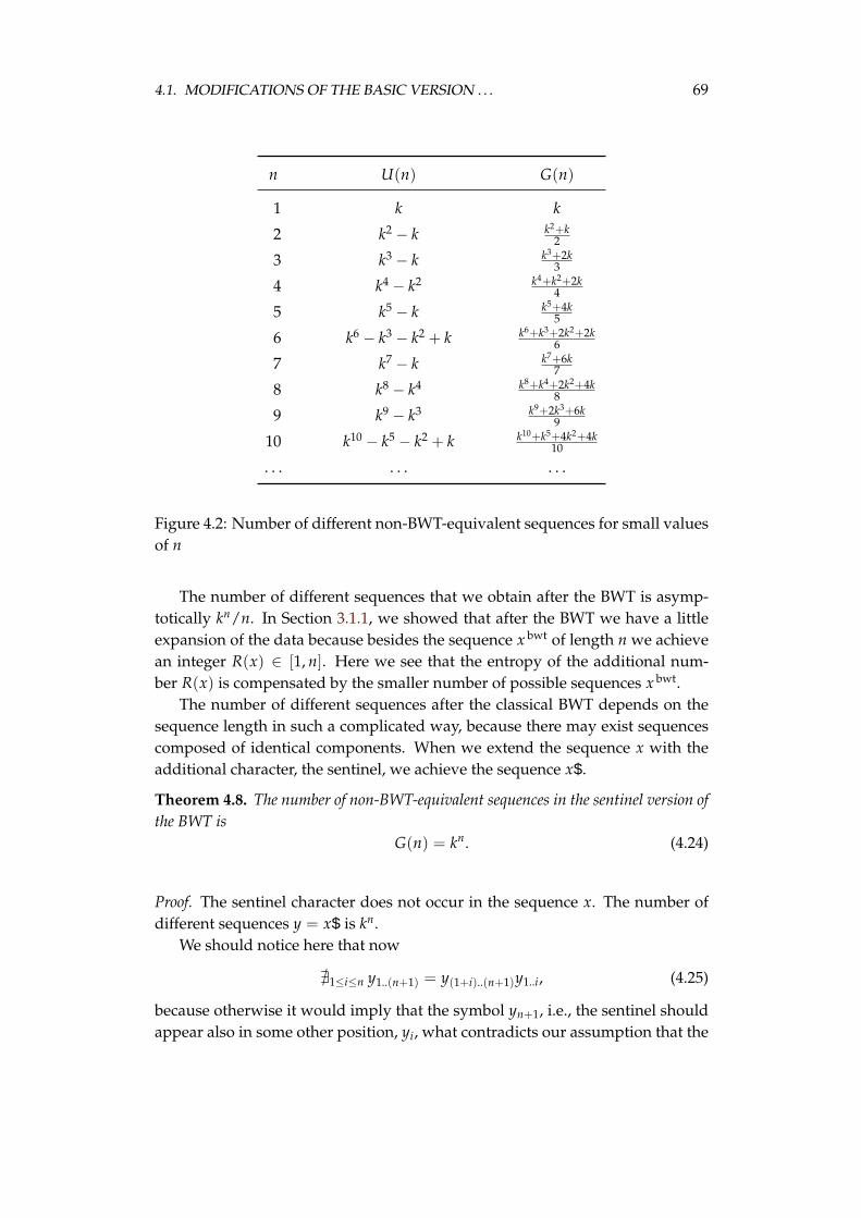
4.1. MODIFICATIONS OF THE BASIC VERSION . . . 69
n U(n) G(n)
1 k k
2 k2 − k k2+k2
3 k3 − k k3+2k3
4 k4 − k2 k4+k2+2k4
5 k5 − k k5+4k5
6 k6 − k3 − k2 + k k6+k3+2k2+2k6
7 k7 − k k7+6k7
8 k8 − k4 k8+k4+2k2+4k8
9 k9 − k3 k9+2k3+6k9
10 k10 − k5 − k2 + k k10+k5+4k2+4k10
. . . . . . . . .
Figure 4.2: Number of different non-BWT-equivalent sequences for small valuesof n
The number of different sequences that we obtain after the BWT is asymp-totically kn/n. In Section 3.1.1, we showed that after the BWT we have a littleexpansion of the data because besides the sequence x bwt of length n we achievean integer R(x) ∈ [1, n]. Here we see that the entropy of the additional num-ber R(x) is compensated by the smaller number of possible sequences x bwt.
The number of different sequences after the classical BWT depends on thesequence length in such a complicated way, because there may exist sequencescomposed of identical components. When we extend the sequence x with theadditional character, the sentinel, we achieve the sequence x$.
Theorem 4.8. The number of non-BWT-equivalent sequences in the sentinel version ofthe BWT is
G(n) = kn. (4.24)
Proof. The sentinel character does not occur in the sequence x. The number ofdifferent sequences y = x$ is kn.
We should notice here that now
@1≤i≤n y1..(n+1) = y(1+i)..(n+1)y1..i, (4.25)
because otherwise it would imply that the symbol yn+1, i.e., the sentinel shouldappear also in some other position, yi, what contradicts our assumption that the
70 CHAPTER 4. IMPROVED COMPRESSION ALGORITHM BASED . . .
sentinel does not appear in the sequence x. For this reason, no sequences areBWT-equivalent to the sequence x$. From Corollary 4.6 we conclude that thenumber of different sequences after the BWT is in this case
G(n) = kn. (4.26)
We obtained also a justification for the statement that the integer R(x) can beneglected in the sentinel version of the BWT. For every sequence x we achieve adifferent x bwt sequence.
Let us now again assume that the sequence x is produced by the contexttree source. We know that the sequence x bwt is a concatenation of the CT-components. If we assume that the CT-components are produced by a memory-less source of parameters from the context tree, we then treat the sequence x bwt
as the output of the piecewise stationary memoryless source. This assumptionis superfluous, because at least some CT-components cannot be strictly treatedas the output of the context tree source (see Corollary 4.4). A similar corollarycan be also concluded from the observation that the number of different x bwt se-quences is smaller than the total number of possible sequences of length equalto the length of the sequence x bwt (i.e., n in the non-sentinel version and n + 1in the sentinel version). These difference is, however, so small that can be ne-glected, and in practice we can assume that the sequence x bwt is the output ofthe piecewise stationary memoryless source.
The conclusion similar to the one that the sequence x bwt can be asymp-totically treated as an output of the piecewise stationary memoryless sourcewas derived independently in a different way by other authors, as reported byVisweswariah et al. [175].
4.1.4 Probability estimation for thepiecewise stationary memoryless source
Relation of the source to the Burrows–Wheeler transform
The sequence x bwt is a concatenation of the CT-components. After the BWT,the boundaries between successive CT-components in the sequence x bwt are,however, unknown. In this section, we examine various ways of probabilityestimation in such a case, what will be useful in our further investigations. Tomake the considerations possible, we have to make some simplifications. Theinvestigations for large alphabets are possible, but using the binary alphabetmakes calculations much easier. Therefore we assume that the elements of thesequence come from a binary alphabet.
4.1. MODIFICATIONS OF THE BASIC VERSION . . . 71
Simple estimation
Let us focus on some position in the sequence x bwt. We assume that the lengthof the current CT-component is m, and the parameter of it is θj, however wedo not know the position in this component. The parameter of the previousCT-component is θj−1.
During the compression, we have to estimate the probability of occurrenceof all possible characters as the next character in the sequence. To this end,we introduce an estimator Pe(a, b). The inputs of the estimator denote: a—thenumber of 0s, b—the number of 1s in the last a + b characters, while the itsoutput is an estimation of the probability that the next character be 1.
The probability that memoryless source with parameter θj produces one spe-cific sequence of a zeros and b ones (of fixed order) is
P0(j, a, b) = (1− θj)aθbj . (4.27)
When we consider all the possible sequences of a 0s and b 1s, then the probabilityis
P(j, a, b) = P0(j, a, b)(
a + bb
)= (1− θj)aθb
j
(a + b
b
). (4.28)
The entropy of a memoryless source of known parameter is
Hj = −θj log θj − (1− θj) log(1− θj). (4.29)
The entropy, Hj, is the lower bound of the expected code length that can beassigned to the symbol. For a given estimator Pe(a, b), the expected code lengthis
Le(a, b) = −θj log Pe(a, b)− (1− θj) log(1− Pe(a, b)). (4.30)
The estimators usually predict the future character better when they takemore previous characters into account. Here we assume that a + b = d where dis constant. Now we can find the expected redundancy of the estimation, i.e.,the difference between the actual code length and the entropy of the source. It is
R1(j, d) =d
∑a=0
(Le(a, d − a)− Hj) · P(j, a, b)
)=
=d
∑a=0
Le(a, d − a)P(j, a, d − a)− Hj. (4.31)
So far we have assumed that the estimator bases on the symbols from oneCT-component. Let us now investigate what happens, when we assume thatonly dj symbols come from the current CT-component, while the remainingdj−1 = d − dj symbols come from the previous CT-component. The expected
72 CHAPTER 4. IMPROVED COMPRESSION ALGORITHM BASED . . .
redundancy equals in this case
R2(j, dj−1, dj) =dj−1
∑aj−1=0
dj
∑aj=0
((Le(aj−1 + aj, dj−1 − aj−1 + dj − aj)− Hj)×
× P(j − 1, aj−1, dj−1 − aj−1)P(j, aj, dj − aj)) =
=dj−1
∑aj−1=0
dj
∑aj=0
Le(aj−1 + aj, dj−1 − aj−1 + dj − aj)×
× P(j − 1, aj−1, dj−1 − aj−1)P(j, aj, dj − aj)− Hj. (4.32)
We assumed nothing about the position of the current symbol within the currentCT-component, so to find the expected redundancy we need to weight it overthe all m possible positions. Considering this we arrive at
R(j, d) =1m
d−1
∑dj=0
R2(j, d − dj, dj) + (m − d)R1(j, d)
. (4.33)
Equation 4.33 holds only when d ≤ m, but it is obvious that when d > m, thenthe estimator uses superfluous symbols that come from another CT-component,and the prediction will not be better than in the case when d = m.
Better estimation
When we assume that the sequence is composed of components produced by amemoryless sources, and we try to estimate the probability of the current sym-bol, then we base on the previous symbols. So far we have neglected the in-tuitive observation that the longer the distance to the previous symbol is, themore likely it comes from the component produced by a source with differentparameter. If a symbol is from a different CT-component, then it introduces anadditional redundancy to the estimation. We claim that the importance of thesymbol in the probability estimation should depend on the distance betweenthem and the estimated one.
Now we are going to rewrite Equations 4.31, 4.32, and 4.33 introducing aweight function w(·), which specifies the “importance” of the symbol dependingon the distance. The redundancy in the case when all the symbols come from
4.1. MODIFICATIONS OF THE BASIC VERSION . . . 73
the same CT-component is
R∗1(j, d) = ∑
0≤i1,...,id≤1
(Le
(∑
1≤j≤dw(j)(1− ij), ∑
1≤j≤dw(j)ij
)− Hj
)×
× P0
(j, ∑
1≤j≤d(1− ij), ∑
1≤j≤dij
)=
= ∑0≤i1,...,id≤1
Le
(∑
1≤j≤dw(j)(1− ij), ∑
1≤j≤dw(j)ij
)×
× P0
(j, ∑
1≤j≤d(1− ij), ∑
1≤j≤dij
)− Hj. (4.34)
If symbols from the previous CT-component are also considered, then the re-dundancy is
R∗2(j, dj−1, dj) = ∑
0≤i1,...,idj−1+dj≤1
Le
dj−1+dj
∑j=1
w(j)(1− ij),dj−1+dj
∑j=1
w(j)ij
− Hj
×
× P0
j − 1, ∑1≤j≤dj−1
(1− ij), ∑1≤j≤dj−1
ij
×
× P0
j, ∑1≤j≤dj
(1− idj−1+j), ∑1≤j≤dj
idj−1+j
=
= ∑0≤i1,...,idj−1+dj
≤1Le
dj−1+dj
∑j=1
w(j)(1− ij),dj−1+dj
∑j=1
w(j)ij
×
× P0
j − 1, ∑1≤j≤dj−1
(1− ij), ∑1≤j≤dj−1
ij
×
× P0
j, ∑1≤j≤dj
(1− idj−1+j), ∑1≤j≤dj
idj−1+j
− Hj. (4.35)
Finally, as we do not know the position within the CT-component, we have toweight the redundancy over all possibilities. Fortunately for our calculationsevery position in the CT-component is equally probable, so the result is
R∗(j, d) =1m
d−1
∑dj=0
R∗2(j, d − dj, dj) + (m − d)R∗
1(j, d)
. (4.36)
So far we have assumed nothing about the weight function. If we put
w(t) = 1, for t > 0, (4.37)
74 CHAPTER 4. IMPROVED COMPRESSION ALGORITHM BASED . . .
then Equation 4.36 reduces to Equation 4.33.Equation 4.36 specifies the expected redundancy in the case when the se-
quence is composed of two adjacent components produced by different memo-ryless sources. The estimation is complex even in the situation when we assumethe simplest weight function (Equation 4.37). An exact analysis of the redun-dancy and finding the value d for which R∗(j, d) is minimal is a hard task. Weshould also remember that we have made no assumption of parameters of thesource, so the values θj and θj−1 are unknown. In general, we can weight theexpected redundancy, R∗(·), over these parameters, obtaining
R∗w(j, d) =
1∫0
1∫0
1m
d−1
∑dj=0
R∗2(j, d − dj, dj) + (m − d)R∗
1(j, d)
dθj−1 dθj. (4.38)
The expected redundancy is weighted, assuming a uniform distribution of theparameters θj−1 and θj. There is no justification for such an assumption, butthere are also no justifications for different distributions so we have chosen thesimplest one. Since solving Equation 4.38 is very hard, we analyse it numerically,comparing different weight functions.
Numerical analysis of the weight functions
Before we proceed with the numerical analysis, we have to specify the way ofprobability estimation, i.e., the function Pe. Simple estimators are usually de-fined as
Pe(1| a zeros and b ones) =b + α
a + b + 2α. (4.39)
The choice of α determines the estimator, e.g., the Laplace estimator [174] isobtained for α = 1 and the Krichevsky–Trofimov estimator (KT-estimator) [95]for α = 0.5. The KT-estimator is often used because the upper bound of its re-dundancy is known. Using it for the weight function specified by Equation 4.37is well justified, but the grounds are not so strong for other weight functions. Inthe following analysis, we decided to use the KT-estimator for all the examinedweight functions to make the comparison independent on the estimator. (In fact,choosing the value of α can be usually compensated by rescaling the w(·) val-ues.) The examined weight functions are presented in Figure 4.3.
First we have to assume the length of the CT-component. For now, we as-sume m = 20. Such a length is typical in real sequences. In the first experiment,we investigate the redundancy R(j, d) as expressed by Equation 4.36. The val-ues θj−1 and θj lie anywhere in the range [0, 1], but we assume here four typicalpairs: (θj−1 = 0.15, θj = 0.65), (θj−1 = 0.25, θj = 0.85), (θj−1 = 0.55, θj = 0.30),and (θj−1 = 0.90, θj = 0.60). The examined weight functions have one or two pa-rameters that determine the expected redundancy. At the beginning we examine
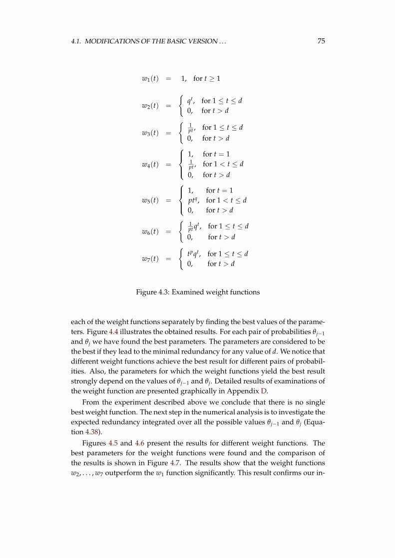
4.1. MODIFICATIONS OF THE BASIC VERSION . . . 75
w1(t) = 1, for t ≥ 1
w2(t) =
{qt, for 1 ≤ t ≤ d0, for t > d
w3(t) =
{1pt , for 1 ≤ t ≤ d0, for t > d
w4(t) =
1, for t = 11pt , for 1 < t ≤ d0, for t > d
w5(t) =
1, for t = 1ptq, for 1 < t ≤ d0, for t > d
w6(t) =
{1pt qt, for 1 ≤ t ≤ d0, for t > d
w7(t) =
{tpqt, for 1 ≤ t ≤ d0, for t > d
Figure 4.3: Examined weight functions
each of the weight functions separately by finding the best values of the parame-ters. Figure 4.4 illustrates the obtained results. For each pair of probabilities θj−1
and θj we have found the best parameters. The parameters are considered to bethe best if they lead to the minimal redundancy for any value of d. We notice thatdifferent weight functions achieve the best result for different pairs of probabil-ities. Also, the parameters for which the weight functions yield the best resultstrongly depend on the values of θj−1 and θj. Detailed results of examinations ofthe weight function are presented graphically in Appendix D.
From the experiment described above we conclude that there is no singlebest weight function. The next step in the numerical analysis is to investigate theexpected redundancy integrated over all the possible values θj−1 and θj (Equa-tion 4.38).
Figures 4.5 and 4.6 present the results for different weight functions. Thebest parameters for the weight functions were found and the comparison ofthe results is shown in Figure 4.7. The results show that the weight functionsw2, . . . , w7 outperform the w1 function significantly. This result confirms our in-
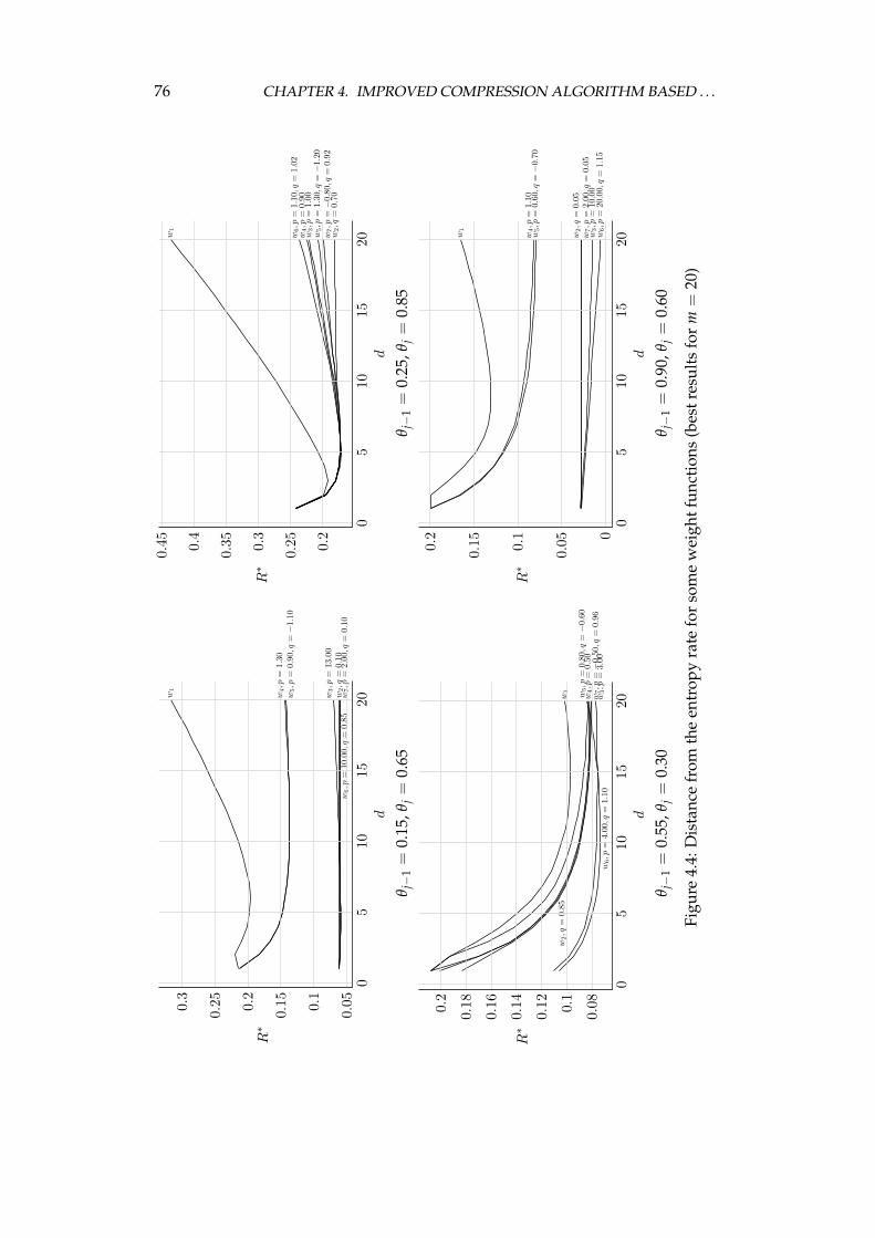
76 CHAPTER 4. IMPROVED COMPRESSION ALGORITHM BASED . . .
w1
w2,q
=0.
10w
3,p
=13
.00
w4,p
=1.
30w
5,p
=0.
90,q
=−
1.10
w6,p
=10
.00,
q=
0.85
w7,p
=2.
00,q
=0.
10
05
1015
200.
050.1
0.150.2
0.250.3
d
R∗
w1
w2,q
=0.
70
w3,p
=1.
00w
4,p
=0.
90
w5,p
=1.
30,q
=−
1.20
w6,p
=1.
10,q
=1.
02
w7,p
=−
0.80
,q=
0.92
05
1015
20
0.2
0.250.3
0.350.4
0.45
d
R∗
θ j−
1=
0.15
,θj=
0.65
θ j−
1=
0.25
,θj=
0.85
w1
w2,q
=0.
85
w3,p
=3.
00w
4,p
=0.
50w
5,p
=0.
80,q
=−
0.60
w6,p
=4.
00,q
=1.
10w
7,p
=−
0.50
,q=
0.96
05
1015
20
0.080.1
0.12
0.14
0.16
0.180.2
d
R∗
w1
w2,q
=0.
05
w3,p
=10
.00
w4,p
=1.
10w
5,p
=0.
60,q
=−
0.70
w6,p
=20
.00,
q=
1.15
w7,p
=2.
00,q
=0.
05
05
1015
200
0.050.1
0.150.2
d
R∗
θ j−
1=
0.55
,θj=
0.30
θ j−
1=
0.90
,θj=
0.60
Figu
re4.
4:D
ista
nce
from
the
entr
opy
rate
for
som
ew
eigh
tfun
ctio
ns(b
estr
esul
tsfo
rm
=20
)
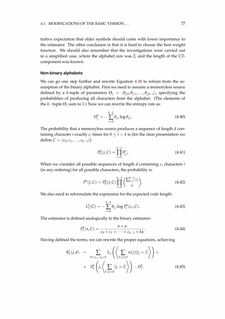
4.1. MODIFICATIONS OF THE BASIC VERSION . . . 77
tuitive expectation that older symbols should come with lower importance tothe estimator. The other conclusion is that it is hard to choose the best weightfunction. We should also remember that the investigations were carried outin a simplified case, where the alphabet size was 2, and the length of the CT-component was known.
Non-binary alphabets
We can go one step further and rewrite Equation 4.38 to refrain from the as-sumption of the binary alphabet. First we need to assume a memoryless sourcedefined by a k-tuple of parameters Θj = 〈θj,0, θj,1, . . . , θj,k−1〉, specifying theprobabilities of producing all characters from the alphabet. (The elements ofthe k−tuple Θj sum to 1.) Now we can rewrite the entropy rate as:
Hkj = −
k−1
∑i=0
θj,i log θj,i. (4.40)
The probability that a memoryless source produces a sequence of length d con-taining character i exactly ci times for 0 ≤ i < k is (for the clear presentation wedefine C = 〈c0, c1, . . . , ck−1〉):
Pk0 (j, C) =
k−1
∏i=0
θcij,i. (4.41)
When we consider all possible sequences of length d containing ci characters i(in any ordering) for all possible characters, the probability is:
Pk(j, C) = Pk0 (j, C)
k−1
∏i=0
(∑k−1
l=i cl
ci
). (4.42)
We also need to reformulate the expression for the expected code length:
Lke(C) = −
k−1
∑i=0
θj,i log Pke (ci, C). (4.43)
The estimator is defined analogically to the binary estimator:
Pke (a, C) =
a + α
c0 + c1 + · · ·+ ck−1 + kα. (4.44)
Having defined the terms, we can rewrite the proper equations, achieving
R∗1(j, d) = ∑
0≤i1,...,id<kLe
(⟨∑
1≤j≤dw(j)[ij = l]
⟩)×
× Pk0
(j,
⟨∑
1≤j≤d[ij = l]
⟩)− Hk
j . (4.45)
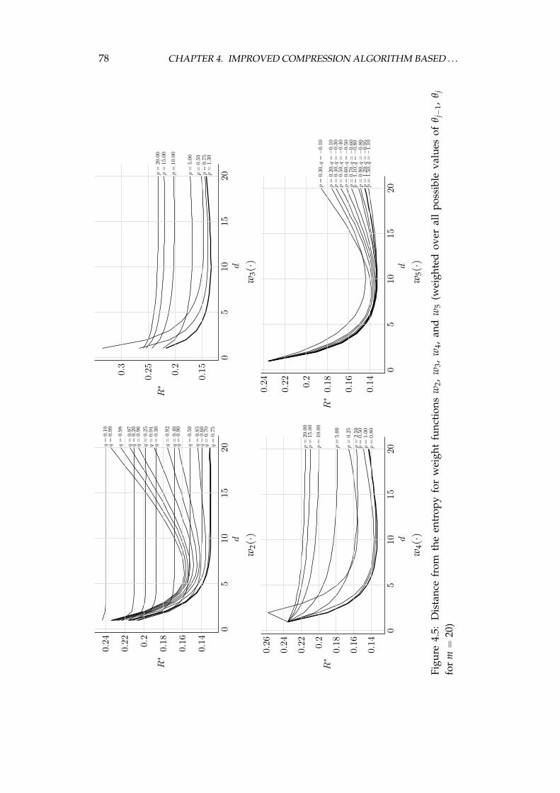
78 CHAPTER 4. IMPROVED COMPRESSION ALGORITHM BASED . . .
q=
0.10
q=
0.99
q=
0.98
q=
0.97
q=
0.20
q=
0.96
q=
0.25
q=
0.94
q=
0.30
q=
0.92
q=
0.40
q=
0.90
q=
0.50
q=
0.85
q=
0.60
q=
0.70
q=
0.75
05
1015
20
0.14
0.16
0.180.2
0.22
0.24
d
R∗
p=
20.0
0p
=15
.00
p=
10.0
0
p=
5.00
p=
0.50
p=
0.75
p=
1.30
05
1015
20
0.150.2
0.250.3
d
R∗
w2(·)
w3(·)
p=
20.0
0p
=15
.00
p=
10.0
0
p=
5.00
p=
0.25
p=
2.50
p=
0.50
p=
1.00
p=
0.80
05
1015
20
0.14
0.16
0.180.2
0.22
0.24
0.26
d
R∗
p=
0.30
,q=−
0.10
p=
0.20
,q=−
0.10
p=
0.40
,q=−
0.30
p=
0.50
,q=−
0.40
p=
0.60
,q=−
0.50
p=
0.70
,q=−
0.60
p=
1.10
,q=−
0.80
p=
0.90
,q=−
0.80
p=
1.20
,q=−
0.95
p=
1.50
,q=−
1.10
05
1015
20
0.14
0.16
0.180.2
0.22
0.24
d
R∗
w4(·)
w5(·)
Figu
re4.
5:D
ista
nce
from
the
entr
opy
for
wei
ght
func
tion
sw
2,w
3,w
4,an
dw
5(w
eigh
ted
over
all
poss
ible
valu
esof
θ j−
1,θ j
for
m=
20)
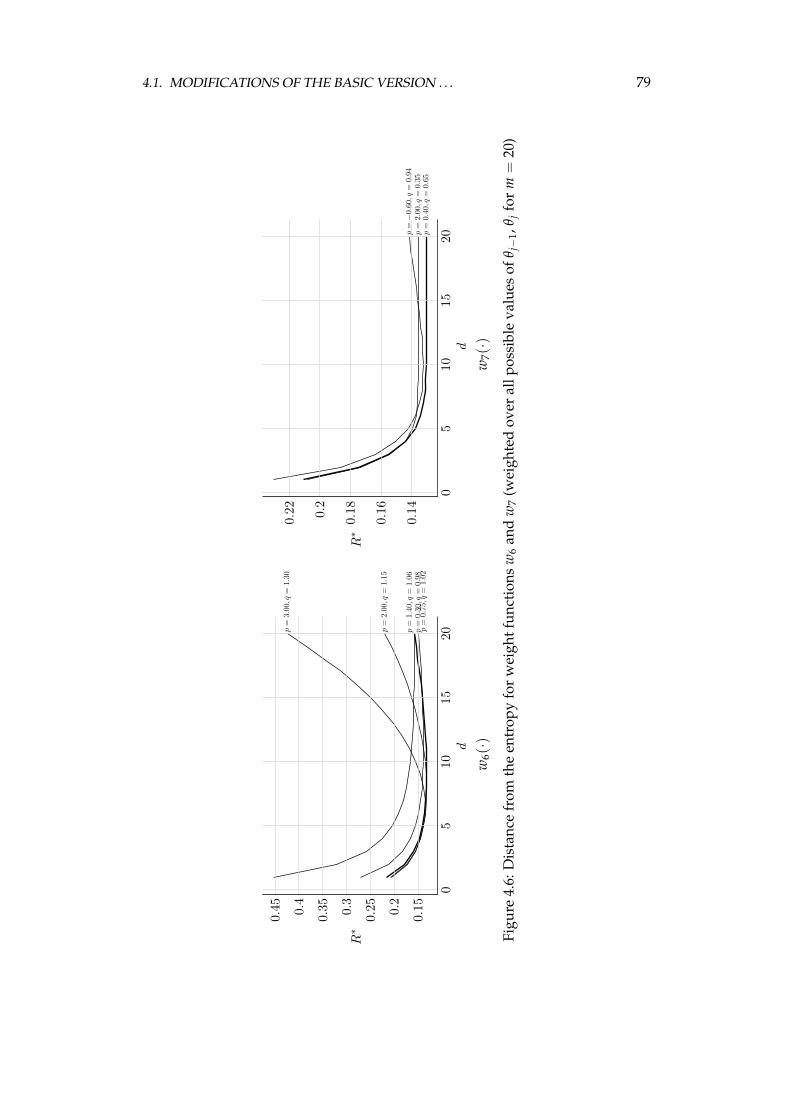
4.1. MODIFICATIONS OF THE BASIC VERSION . . . 79
p=
3.00
,q=
1.30
p=
2.00
,q=
1.15
p=
0.30
,q=
0.98
p=
1.40
,q=
1.06
p=
0.75
,q=
1.02
05
1015
20
0.150.2
0.250.3
0.350.4
0.45
d
R∗
p=−
0.60
,q=
0.94
p=
2.00
,q=
0.35
p=
0.40
,q=
0.65
05
1015
20
0.14
0.16
0.180.2
0.22
d
R∗
w6(·)
w7(·)
Figu
re4.
6:D
ista
nce
from
the
entr
opy
for
wei
ghtf
unct
ions
w6
and
w7
(wei
ghte
dov
eral
lpos
sibl
eva
lues
ofθ j−
1,θ j
for
m=
20)
80 CHAPTER 4. IMPROVED COMPRESSION ALGORITHM BASED . . .
w1
w2, q = 0.75w3, p = 1.30w4, p = 0.80w5, p = 1.20, q = −0.95
w6, p = 1.40, q = 1.06
w7, p = 0.40, q = 0.65
0 5 10 15 20
0.14
0.16
0.18
0.2
0.22
0.24
d
R∗
Figure 4.7: Comparison of the best results for different weight functions
R∗k2 (j, dj−1, dj) = ∑
0≤i1,...,idj−1+dj<k
Le
⟨dj−1+dj
∑j=1
w(j)[ij = l]
⟩×
× Pk0
j − 1,
⟨∑
1≤j≤dj−1
[ij = l]
⟩×
× Pk0
j,
⟨∑
1≤j≤dj
[ij+dj−1 = l]
⟩− Hkj . (4.46)
R∗k(j, d) =1m
d−1
∑dj=0
R∗k2 (j, d − dj, dj) + (m − d)R∗k
1 (j, d)
. (4.47)
R∗kw =
∫· · ·∫
Θj−1
∫· · ·∫
Θj
1m×
×
d−1
∑dj=0
R∗k2 (j, d − dj, dj) + (m − d)R∗k
1 (j, d)
×
× dθj−1,0 . . . dθj−1,k−1 dθj,0 . . . dθj,k−1. (4.48)
Equation 4.48 is quite complicated and very hard to solve numerically. Evenif we had solved it, the solutions would have not been valuable because in prac-tice we do not know the size of the alphabet—it is usually less than the typicallyassumed 28. The probability distribution of symbols is also usually distant fromthe assumed one. Because of the above, we will not try to solve this equationand we will base on the results obtained for the binary alphabet.
4.1. MODIFICATIONS OF THE BASIC VERSION . . . 81
4.1.5 Weighted frequency count as the algorithm’s second stage
Weighted frequency count
The sequence x bwt is a concatenation of the CT-components, and can be treatedas the output of a piecewise stationary memoryless source. In Section 4.1.4, wediscussed how to estimate the probability in such a case.
In typical implementations of the BWCA, the second stage is the MTF trans-form. This transform keeps the symbols that appeared recently in the front ofthe list L. This rule is strong—for every two symbols, the one that has appearedmore recently is at a lower position. The numbers of occurrences of charac-ters are not used in the MTF. Now we introduce a solution, a weighted frequencycount (WFC) transform, which can be considered as a generalisation of the wellknown frequency count transform (FC). (It was introduced first by the author inReference [55].) The WFC transform makes use of more information about theprevious symbols than the MTF.
We first formulate the FC transform in an alternative way. To each charac-ter aj appearing prior to the ith position in the sequence x bwt we assign a sum
Wi(aj) = ∑1≤p<iaj=xp
1, (4.49)
and sort the list L according to the decreasing values of counters Wi(aj).Next, we note that instead of summing 1s for all the characters, we can sum
the numbers depending on their relative position in the sequence x bwt. To thisend, we introduce a weight function w(·) and reformulate the sum as
Wi(aj) = ∑1≤p<iaj=xp
w(i − p). (4.50)
If some two characters have the same value of Wi(·), then we find their rela-tive order using the values Wi−1(·), Wi−2(·), and so on, until the counters aredifferent. For completeness we define W0(aj) = −j. The procedure outputtingthe position of processed characters in the list L and maintaining the list in thedescribed way is called the weighted frequency count transform.
The usage of the weight functions is motivated by the results of the investiga-tions in Section 4.1.4. We should notice that we examined the weight functionsfor the binary alphabet only. The equations for larger alphabets were elabo-rated, but they were unsolved because of their complexity. We also assumedsome arbitrarily chosen length of the CT-components. For real sequences, thelength of the successive CT-components can vary strongly. Finally, we exam-ined the expected redundancy estimating the probability of symbol occurrence,while now this estimation is used to give ranks to the symbols. The last differ-ence was motivated by the observation that the CT-components are rather short,
82 CHAPTER 4. IMPROVED COMPRESSION ALGORITHM BASED . . .
so they contain only a fraction of characters from the alphabet. This is a simi-lar problem to the zero frequency problem that exists in the PPM algorithms. Asmentioned in Sections 3.2.5 and 3.2.5, some researchers investigated methods fordirect entropy coding of the sequence x bwt without transforming them in orderto overcome these problems [67, 195]. Other used a semi-direct encoding andtransform some part of the sequence, but the other part is encoded directly [18].The compression results with a direct entropy encoding method are still signifi-cantly worse than the results with some second stage transform, so we decidedto introduce the WFC transform as the second stage in the improved BWCA.
Because of the described reasons, we treat previous investigations only assuggestions how the symbols in the second stage should be transformed. Un-fortunately, providing the more formal justification of the usage of the WFCtransform is a complex task.
From the formulation of the WFC, it is clear that if we set
w(t) = 1, for t > 0, (4.51)
then we obtain the FC transform, and if we set
w(t) =
{1, for t = 1,0, for t > 1,
(4.52)
then we obtain the MTF transform.The sort-by-time (SBT) method—proposed by Schulz [146]—is also a special
case of the WFC. We achieve it by setting
w(t) = qt, for t > 0. (4.53)
The theoretical properties of this method for different values of q have beenexamined by Schulz. He has shown that one obtains the MTF transform byestablishing 0 < q ≤ 0.5.
Relation to context tree sources
As mentioned before, the sequence x bwt is a concatenation of the CT-compo-nents. Therefore, a character that has occurred at the previous position is morelikely to be at the same context than the penultimate and so on. In general,the character that has appeared at recent positions is more likely described bythe same probability distribution as the current one, than by the distribution ofthe characters from more distant positions. Unfortunately, we do not know thecurrent position in the context tree, how long the CT-component of the currentleaf is, and where in that CT-component we are. We examined all these problemsin Section 4.1.4.
4.1. MODIFICATIONS OF THE BASIC VERSION . . . 83
There is also one more property to consider: similar context typically haveonly a slightly different probability distribution. (In fact, the similarity of proba-bility distributions of similar contexts is one of the bases of the PPM algorithms.)It may be useful to explore some of the information regarding the probabilitydistribution of the previous contexts. Because the formulation of the contexttree source does not give a way to represent this fact, it is impossible to incorpo-rate it in the theoretical analysis, when the context tree source is assumed. Allin all, the values w(i) of the weight function should decrease with increasing i.It is not clear, however, how fast it should decrease.
We theoretically examined some weight functions for the binary alphabet.Now, concerning the results of the theoretical analysis, we will examine how theweight functions work for real-world sequences. The experimental results showthat for different sequences from the Calgary corpus different functions w givethe best results. This is what one would expect. (We made the same observationin the theoretical analysis.) The CT-components of short sequences are typicallyshorter than those of longer sequences. Also, the sequences x are generated bydifferent sources with a different number of contexts.
Efficient implementation
Prior to the empirical comparison of the weight functions, let us discuss its im-plementation. The formulation of the WFC transform does not give us a wayfor computing the values of Wi(·) quickly. When we move to the next character,we have to recalculate the values of all counters Wi(·). To this end, we have torescan the encoded part of the sequence x bwt. This rescanning makes the timecomplexity of the transform O(n(n + k log k)).
We can improve the time complexity of the WFC transform by sacrificingits precision. One possibility is to quantise the values of the weight function tointeger powers of 2. This quantisation decreases the number of different val-ues of w to at most l = log w(1)/w(tmax + 1) (we assume that the weight func-tion is non-increasing), which is typically small. For such values of the weightfunction, we can obtain the values of Wi(·) from Wi−1(·) by updating only thecounters for the characters where the values w(·) are changing (for all such tthat w(t) 6= w(t − 1)). Using this approach, we obtain a method of the worst-case time complexity O(nlk), which is not much greater than O(nk) for trans-forms like the MTF. In practice, the characters on the list L move only by a fewpositions at a time. With a version of the insertion sort procedure the cost ofmaintaining the list is small (e.g., for the function w8q the average number ofswaps of characters in the list L per input character does not exceed 6 for almostall files from the Calgary corpus, except for binary files such us geo, where it islarger).
84 CHAPTER 4. IMPROVED COMPRESSION ALGORITHM BASED . . .
The disadvantage, in the compression ratio, of using the quantisation de-pends on the weight function w and properties of the sequence. One can doublethe number of different values of w if necessary by using also the powers of 2for half exponents. It is also possible to introduce even faster methods for someweight functions, e.g., for the function w2. We will not discuss, however, heresuch improvements, which are specific to weight functions.
We examined a number of weight functions. Here we present (Figure 4.8)only some of them (the best ones and those that we find interesting). Figure 4.9shows an example of working of the WFC transform and Section 4.3.2 containsthe experimental results we obtained for these weight functions on standarddata compression sets.
4.1.6 Efficient probability estimation in the last stage
Binary arithmetic coder
The last stage of the BWCA is the entropy coding of the sequence x rle-0. Dif-ferent solutions to this task were discussed in Section 3.2.5. In this section, weintroduce yet another method. The way of probability estimation described inthis section was introduced by the author of this dissertation in Reference [54]and partially (for the IF transform) in Reference [55].
As the motivation of this work is to improve the compression ratio, the arith-metic coder is chosen as the entropy coder. In contrast to other researchers, wechoose, however, a binary arithmetic coder. This coder is highly efficient, and nocomplicated model is needed to store the statistics of symbol occurrences. Manyexperiments with different methods for probability estimation of symbols fromthe sequence x rle-0 were carried out and the simplicity of the binary arithmeticcoder is its important asset.
Decomposing a sequence into binary codes
Since a binary arithmetic coder is chosen, the symbols from the sequence x rle-0
have to be decomposed to binary codes before the coding. The decompositionof the symbols from the alphabet A rle-0 proceeds as follows. In the first step, thesymbols are grouped into nine subsets: {0a}, {0b}, {1}, {2, . . . , 7}, {8, . . . , 15},. . . , {128, . . . , 255}. Then all the symbols are encoded using the binary prefixcode presented in Figure 4.10. The code for each symbol consists of two parts:a unique prefix that distinguishes the subsets from each other, and a suffix,which is a binary representation of the symbol (bi denotes the ith bit of the binaryrepresentation of the symbol). The second part of the code (not always present)contains these bits, which are indispensable to distinguish all the characters ina given subset. For example, for the subsets {8, . . . , 15}, . . . , {128, . . . , 255} it isunnecessary to encode the most significant bit of the symbol.
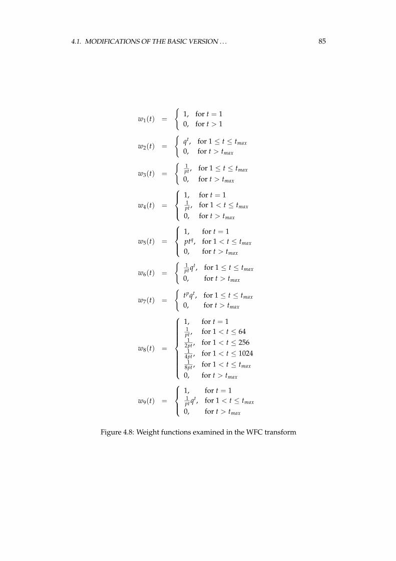
4.1. MODIFICATIONS OF THE BASIC VERSION . . . 85
w1(t) =
{1, for t = 10, for t > 1
w2(t) =
{qt, for 1 ≤ t ≤ tmax
0, for t > tmax
w3(t) =
{1pt , for 1 ≤ t ≤ tmax
0, for t > tmax
w4(t) =
1, for t = 11pt , for 1 < t ≤ tmax
0, for t > tmax
w5(t) =
1, for t = 1ptq, for 1 < t ≤ tmax
0, for t > tmax
w6(t) =
{1pt qt, for 1 ≤ t ≤ tmax
0, for t > tmax
w7(t) =
{tpqt, for 1 ≤ t ≤ tmax
0, for t > tmax
w8(t) =
1, for t = 11pt , for 1 < t ≤ 641
2pt , for 1 < t ≤ 2561
4pt , for 1 < t ≤ 10241
8pt , for 1 < t ≤ tmax
0, for t > tmax
w9(t) =
1, for t = 11pt qt, for 1 < t ≤ tmax
0, for t > tmax
Figure 4.8: Weight functions examined in the WFC transform
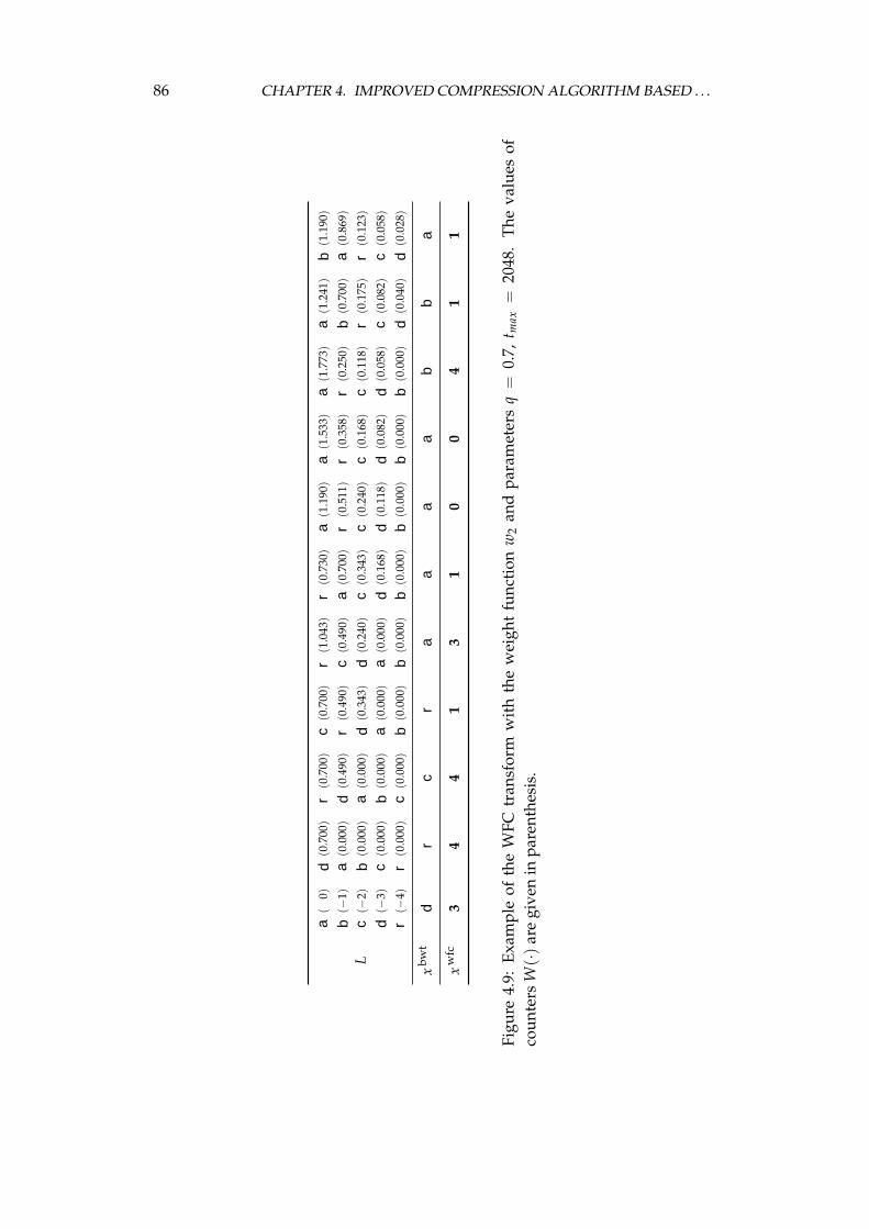
86 CHAPTER 4. IMPROVED COMPRESSION ALGORITHM BASED . . .
a(
0)d
(0.7
00)
r(0
.700
)c
(0.7
00)
r(1
.043
)r
(0.7
30)
a(1
.190
)a
(1.5
33)
a(1
.773
)a
(1.2
41)
b(1
.190
)
b(−
1)a
(0.0
00)
d(0
.490
)r
(0.4
90)
c(0
.490
)a
(0.7
00)
r(0
.511
)r
(0.3
58)
r(0
.250
)b
(0.7
00)
a(0
.869
)
Lc
(−2)
b(0
.000
)a
(0.0
00)
d(0
.343
)d
(0.2
40)
c(0
.343
)c
(0.2
40)
c(0
.168
)c
(0.1
18)
r(0
.175
)r
(0.1
23)
d(−
3)c
(0.0
00)
b(0
.000
)a
(0.0
00)
a(0
.000
)d
(0.1
68)
d(0
.118
)d
(0.0
82)
d(0
.058
)c
(0.0
82)
c(0
.058
)
r(−
4)r
(0.0
00)
c(0
.000
)b
(0.0
00)
b(0
.000
)b
(0.0
00)
b(0
.000
)b
(0.0
00)
b(0
.000
)d
(0.0
40)
d(0
.028
)
xbw
td
rc
ra
aa
ab
ba
xw
fc3
44
13
10
04
11
Figu
re4.
9:Ex
ampl
eof
the
WFC
tran
sfor
mw
ith
the
wei
ght
func
tion
w2
and
para
met
ers
q=
0.7,
t max
=20
48.
The
valu
esof
coun
ters
W(·
)ar
egi
ven
inpa
rent
hesi
s.
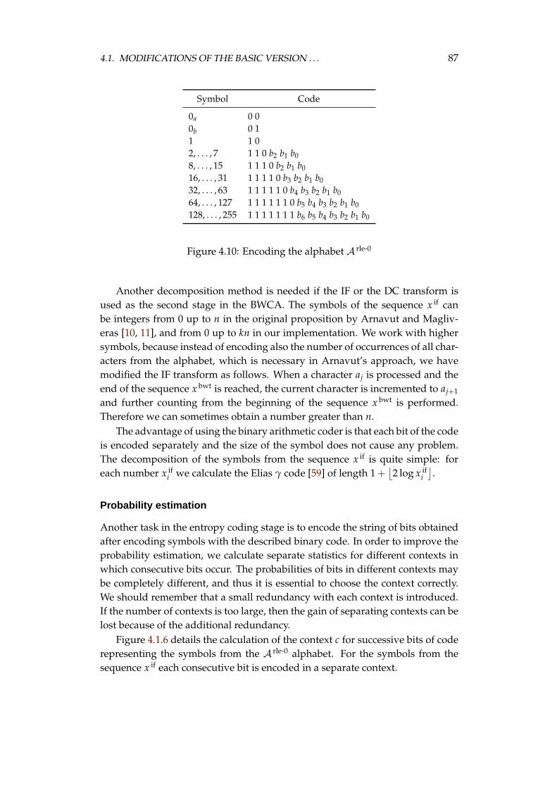
4.1. MODIFICATIONS OF THE BASIC VERSION . . . 87
Symbol Code
0a 0 00b 0 11 1 02, . . . , 7 1 1 0 b2 b1 b08, . . . , 15 1 1 1 0 b2 b1 b016, . . . , 31 1 1 1 1 0 b3 b2 b1 b032, . . . , 63 1 1 1 1 1 0 b4 b3 b2 b1 b064, . . . , 127 1 1 1 1 1 1 0 b5 b4 b3 b2 b1 b0128, . . . , 255 1 1 1 1 1 1 1 b6 b5 b4 b3 b2 b1 b0
Figure 4.10: Encoding the alphabet A rle-0
Another decomposition method is needed if the IF or the DC transform isused as the second stage in the BWCA. The symbols of the sequence x if canbe integers from 0 up to n in the original proposition by Arnavut and Magliv-eras [10, 11], and from 0 up to kn in our implementation. We work with highersymbols, because instead of encoding also the number of occurrences of all char-acters from the alphabet, which is necessary in Arnavut’s approach, we havemodified the IF transform as follows. When a character aj is processed and theend of the sequence x bwt is reached, the current character is incremented to aj+1
and further counting from the beginning of the sequence x bwt is performed.Therefore we can sometimes obtain a number greater than n.
The advantage of using the binary arithmetic coder is that each bit of the codeis encoded separately and the size of the symbol does not cause any problem.The decomposition of the symbols from the sequence x if is quite simple: foreach number x if
i we calculate the Elias γ code [59] of length 1 +⌊2 log x if
i⌋.
Probability estimation
Another task in the entropy coding stage is to encode the string of bits obtainedafter encoding symbols with the described binary code. In order to improve theprobability estimation, we calculate separate statistics for different contexts inwhich consecutive bits occur. The probabilities of bits in different contexts maybe completely different, and thus it is essential to choose the context correctly.We should remember that a small redundancy with each context is introduced.If the number of contexts is too large, then the gain of separating contexts can belost because of the additional redundancy.
Figure 4.1.6 details the calculation of the context c for successive bits of coderepresenting the symbols from the A rle-0 alphabet. For the symbols from thesequence x if each consecutive bit is encoded in a separate context.
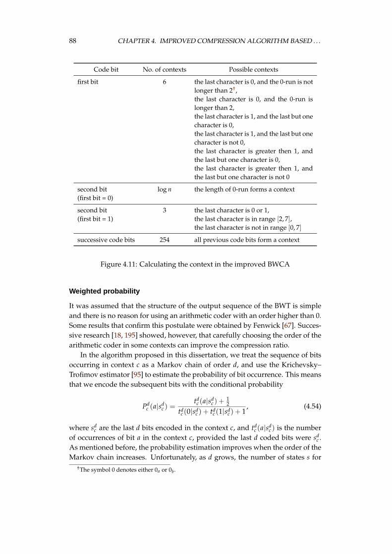
88 CHAPTER 4. IMPROVED COMPRESSION ALGORITHM BASED . . .
Code bit No. of contexts Possible contexts
first bit 6 the last character is 0, and the 0-run is notlonger than 2†,the last character is 0, and the 0-run islonger than 2,the last character is 1, and the last but onecharacter is 0,the last character is 1, and the last but onecharacter is not 0,the last character is greater then 1, andthe last but one character is 0,the last character is greater then 1, andthe last but one character is not 0
second bit log n the length of 0-run forms a context(first bit = 0)
second bit 3 the last character is 0 or 1,(first bit = 1) the last character is in range [2, 7],
the last character is not in range [0, 7]
successive code bits 254 all previous code bits form a context
Figure 4.11: Calculating the context in the improved BWCA
Weighted probability
It was assumed that the structure of the output sequence of the BWT is simpleand there is no reason for using an arithmetic coder with an order higher than 0.Some results that confirm this postulate were obtained by Fenwick [67]. Succes-sive research [18, 195] showed, however, that carefully choosing the order of thearithmetic coder in some contexts can improve the compression ratio.
In the algorithm proposed in this dissertation, we treat the sequence of bitsoccurring in context c as a Markov chain of order d, and use the Krichevsky–Trofimov estimator [95] to estimate the probability of bit occurrence. This meansthat we encode the subsequent bits with the conditional probability
Pdc (a|sd
c ) =tdc (a|sd
c ) + 12
tdc (0|sd
c ) + tdc (1|sd
c ) + 1, (4.54)
where sdc are the last d bits encoded in the context c, and td
c (a|sdc ) is the number
of occurrences of bit a in the context c, provided the last d coded bits were sdc .
As mentioned before, the probability estimation improves when the order of theMarkov chain increases. Unfortunately, as d grows, the number of states s for
†The symbol 0 denotes either 0a or 0b.
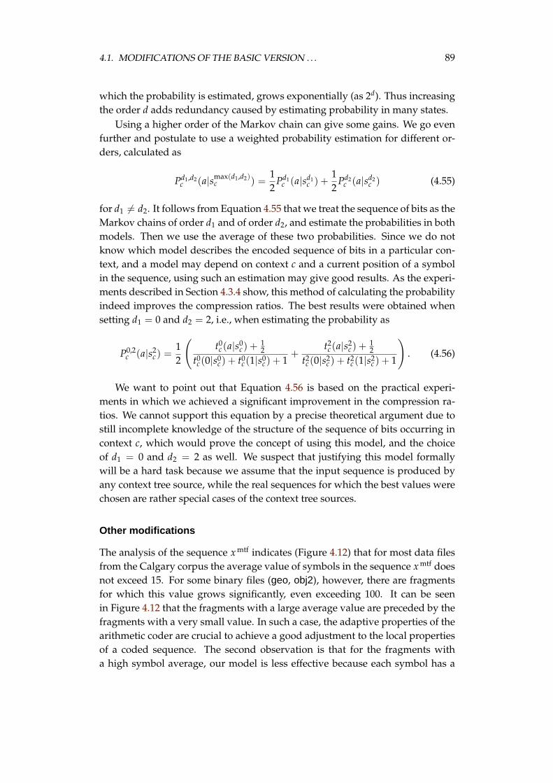
4.1. MODIFICATIONS OF THE BASIC VERSION . . . 89
which the probability is estimated, grows exponentially (as 2d). Thus increasingthe order d adds redundancy caused by estimating probability in many states.
Using a higher order of the Markov chain can give some gains. We go evenfurther and postulate to use a weighted probability estimation for different or-ders, calculated as
Pd1,d2c (a|smax(d1,d2)
c ) =12
Pd1c (a|sd1
c ) +12
Pd2c (a|sd2
c ) (4.55)
for d1 6= d2. It follows from Equation 4.55 that we treat the sequence of bits as theMarkov chains of order d1 and of order d2, and estimate the probabilities in bothmodels. Then we use the average of these two probabilities. Since we do notknow which model describes the encoded sequence of bits in a particular con-text, and a model may depend on context c and a current position of a symbolin the sequence, using such an estimation may give good results. As the experi-ments described in Section 4.3.4 show, this method of calculating the probabilityindeed improves the compression ratios. The best results were obtained whensetting d1 = 0 and d2 = 2, i.e., when estimating the probability as
P0,2c (a|s2
c ) =12
(t0c (a|s0
c ) + 12
t0c (0|s0
c ) + t0c (1|s0
c ) + 1+
t2c (a|s2
c ) + 12
t2c (0|s2
c ) + t2c (1|s2
c ) + 1
). (4.56)
We want to point out that Equation 4.56 is based on the practical experi-ments in which we achieved a significant improvement in the compression ra-tios. We cannot support this equation by a precise theoretical argument due tostill incomplete knowledge of the structure of the sequence of bits occurring incontext c, which would prove the concept of using this model, and the choiceof d1 = 0 and d2 = 2 as well. We suspect that justifying this model formallywill be a hard task because we assume that the input sequence is produced byany context tree source, while the real sequences for which the best values werechosen are rather special cases of the context tree sources.
Other modifications
The analysis of the sequence x mtf indicates (Figure 4.12) that for most data filesfrom the Calgary corpus the average value of symbols in the sequence x mtf doesnot exceed 15. For some binary files (geo, obj2), however, there are fragmentsfor which this value grows significantly, even exceeding 100. It can be seenin Figure 4.12 that the fragments with a large average value are preceded by thefragments with a very small value. In such a case, the adaptive properties of thearithmetic coder are crucial to achieve a good adjustment to the local propertiesof a coded sequence. The second observation is that for the fragments witha high symbol average, our model is less effective because each symbol has a
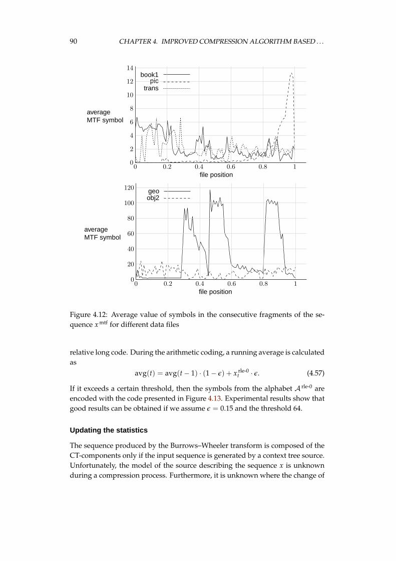
90 CHAPTER 4. IMPROVED COMPRESSION ALGORITHM BASED . . .
book1pic
trans
0 0.2 0.4 0.6 0.8 10
2
4
6
8
10
12
14
file position
averageMTF symbol
geoobj2
0 0.2 0.4 0.6 0.8 10
20
40
60
80
100
120
file position
averageMTF symbol
Figure 4.12: Average value of symbols in the consecutive fragments of the se-quence x mtf for different data files
relative long code. During the arithmetic coding, a running average is calculatedas
avg(t) = avg(t − 1) · (1− ε) + x rle-0t · ε. (4.57)
If it exceeds a certain threshold, then the symbols from the alphabet A rle-0 areencoded with the code presented in Figure 4.13. Experimental results show thatgood results can be obtained if we assume ε = 0.15 and the threshold 64.
Updating the statistics
The sequence produced by the Burrows–Wheeler transform is composed of theCT-components only if the input sequence is generated by a context tree source.Unfortunately, the model of the source describing the sequence x is unknownduring a compression process. Furthermore, it is unknown where the change of
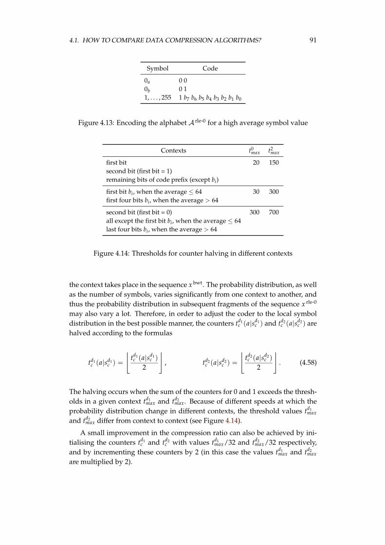
4.1. HOW TO COMPARE DATA COMPRESSION ALGORITHMS? 91
Symbol Code
0a 0 00b 0 11, . . . , 255 1 b7 b6 b5 b4 b3 b2 b1 b0
Figure 4.13: Encoding the alphabet A rle-0 for a high average symbol value
Contexts t0max t2
max
first bit 20 150second bit (first bit = 1)remaining bits of code prefix (except bi)
first bit bi, when the average ≤ 64 30 300first four bits bi, when the average > 64
second bit (first bit = 0) 300 700all except the first bit bi, when the average ≤ 64last four bits bi, when the average > 64
Figure 4.14: Thresholds for counter halving in different contexts
the context takes place in the sequence x bwt. The probability distribution, as wellas the number of symbols, varies significantly from one context to another, andthus the probability distribution in subsequent fragments of the sequence x rle-0
may also vary a lot. Therefore, in order to adjust the coder to the local symboldistribution in the best possible manner, the counters td1
c (a|sd1c ) and td2
c (a|sd2c ) are
halved according to the formulas
td1c (a|sd1
c ) =
⌊td1c (a|sd1
c )2
⌋, td2
c (a|sd2c ) =
⌊td2c (a|sd2
c )2
⌋. (4.58)
The halving occurs when the sum of the counters for 0 and 1 exceeds the thresh-olds in a given context td1
max and td2max. Because of different speeds at which the
probability distribution change in different contexts, the threshold values td1max
and td2max differ from context to context (see Figure 4.14).
A small improvement in the compression ratio can also be achieved by ini-tialising the counters td1
c and td2c with values td1
max/32 and td2max/32 respectively,
and by incrementing these counters by 2 (in this case the values td1max and td2
max
are multiplied by 2).
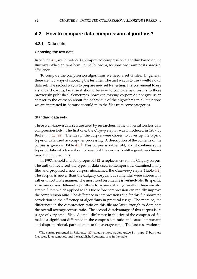
92 CHAPTER 4. IMPROVED COMPRESSION ALGORITHM BASED . . .
4.2 How to compare data compression algorithms?
4.2.1 Data sets
Choosing the test data
In Section 4.1, we introduced an improved compression algorithm based on theBurrows–Wheeler transform. In the following sections, we examine its practicalefficiency.
To compare the compression algorithms we need a set of files. In general,there are two ways of choosing the test files. The first way is to use a well-knowndata set. The second way is to prepare new set for testing. It is convenient to usea standard corpus, because it should be easy to compare new results to thosepreviously published. Sometimes, however, existing corpora do not give us ananswer to the question about the behaviour of the algorithms in all situationswe are interested in, because it could miss the files from some categories.
Standard data sets
Three well-known data sets are used by researchers in the universal lossless datacompression field. The first one, the Calgary corpus, was introduced in 1989 byBell et al. [20, 22]. The files in the corpus were chosen to cover up the typicaltypes of data used in computer processing. A description of the contents of thecorpus is given in Table 4.1.‡ This corpus is rather old, and it contains sometypes of data which went out of use, but the corpus is still a good benchmarkused by many authors.
In 1997, Arnold and Bell proposed [12] a replacement for the Calgary corpus.The authors reviewed the types of data used contemporarily, examined manyfiles and proposed a new corpus, nicknamed the Canterbury corpus (Table 4.2).The corpus is newer than the Calgary corpus, but some files were chosen in arather unfortunate manner. The most troublesome file is kennedy.xls. Its specificstructure causes different algorithms to achieve strange results. There are alsosimple filters which applied to this file before compression can rapidly improvethe compression ratio. The difference in compression ratio for this file shows nocorrelation to the efficiency of algorithms in practical usage. The more so, thedifferences in the compression ratio on this file are large enough to dominatethe overall average corpus ratio. The second disadvantage of this corpus is itsusage of very small files. A small difference in the size of the compressed filemakes a significant difference in the compression ratio and causes important,and disproportional, participation to the average ratio. The last reservation to
‡The corpus presented in Reference [22] contains more papers (paper3 . . . paper6) but thesefiles were later removed, and the established contents is as in the table.
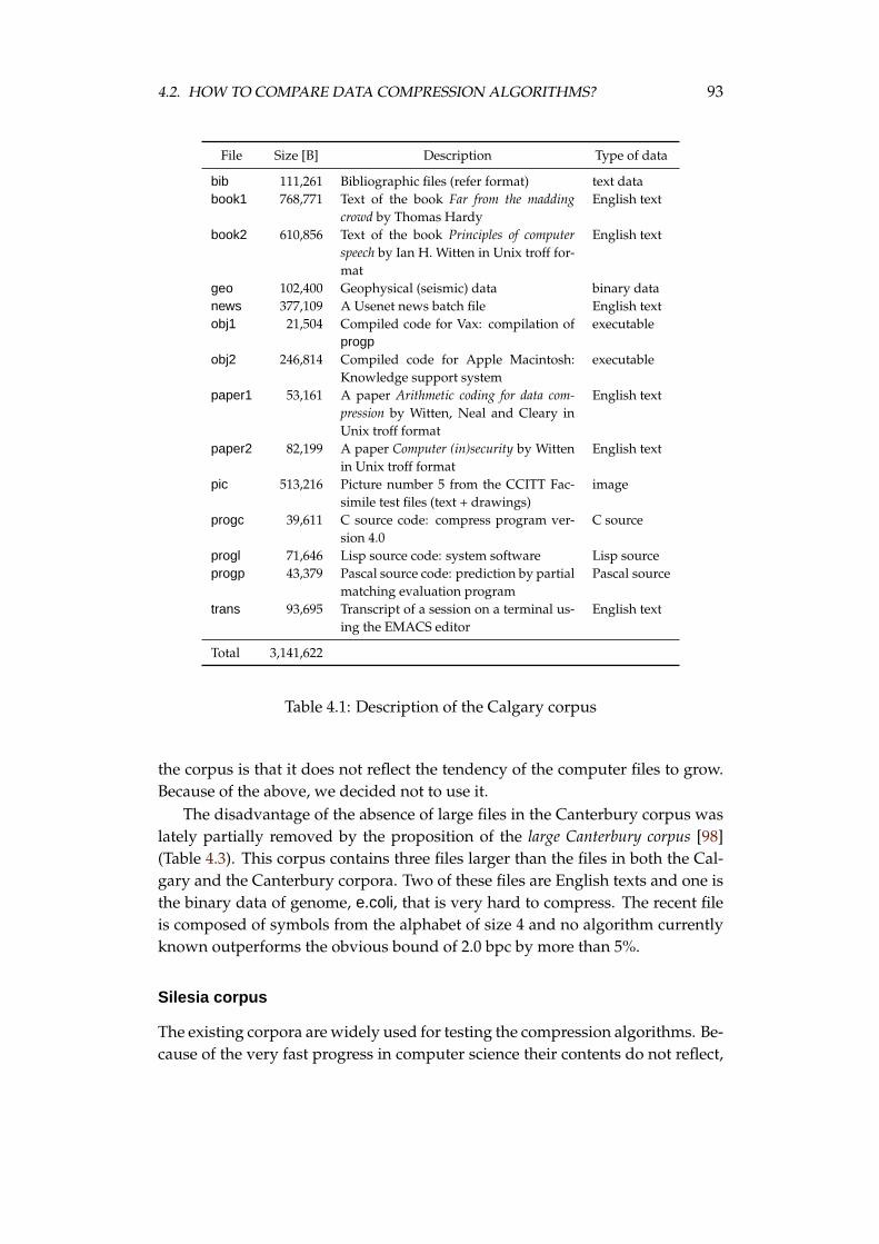
4.2. HOW TO COMPARE DATA COMPRESSION ALGORITHMS? 93
File Size [B] Description Type of data
bib 111,261 Bibliographic files (refer format) text databook1 768,771 Text of the book Far from the madding
crowd by Thomas HardyEnglish text
book2 610,856 Text of the book Principles of computerspeech by Ian H. Witten in Unix troff for-mat
English text
geo 102,400 Geophysical (seismic) data binary datanews 377,109 A Usenet news batch file English textobj1 21,504 Compiled code for Vax: compilation of
progpexecutable
obj2 246,814 Compiled code for Apple Macintosh:Knowledge support system
executable
paper1 53,161 A paper Arithmetic coding for data com-pression by Witten, Neal and Cleary inUnix troff format
English text
paper2 82,199 A paper Computer (in)security by Wittenin Unix troff format
English text
pic 513,216 Picture number 5 from the CCITT Fac-simile test files (text + drawings)
image
progc 39,611 C source code: compress program ver-sion 4.0
C source
progl 71,646 Lisp source code: system software Lisp sourceprogp 43,379 Pascal source code: prediction by partial
matching evaluation programPascal source
trans 93,695 Transcript of a session on a terminal us-ing the EMACS editor
English text
Total 3,141,622
Table 4.1: Description of the Calgary corpus
the corpus is that it does not reflect the tendency of the computer files to grow.Because of the above, we decided not to use it.
The disadvantage of the absence of large files in the Canterbury corpus waslately partially removed by the proposition of the large Canterbury corpus [98](Table 4.3). This corpus contains three files larger than the files in both the Cal-gary and the Canterbury corpora. Two of these files are English texts and one isthe binary data of genome, e.coli, that is very hard to compress. The recent fileis composed of symbols from the alphabet of size 4 and no algorithm currentlyknown outperforms the obvious bound of 2.0 bpc by more than 5%.
Silesia corpus
The existing corpora are widely used for testing the compression algorithms. Be-cause of the very fast progress in computer science their contents do not reflect,
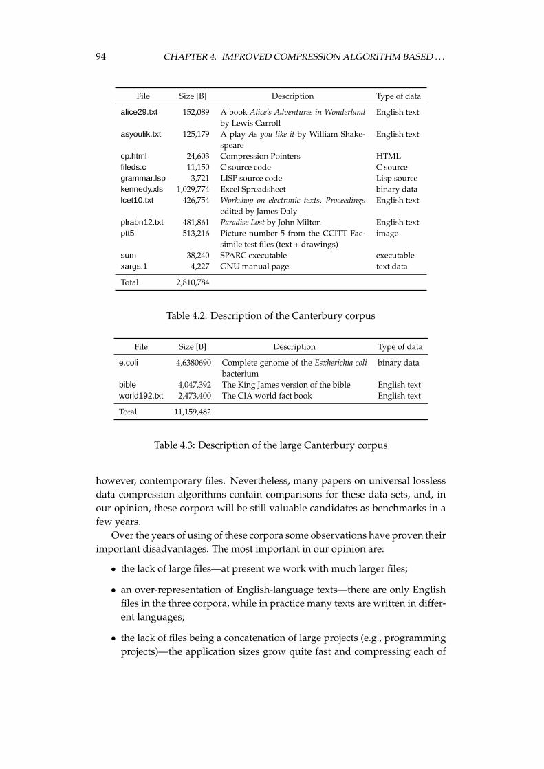
94 CHAPTER 4. IMPROVED COMPRESSION ALGORITHM BASED . . .
File Size [B] Description Type of data
alice29.txt 152,089 A book Alice’s Adventures in Wonderlandby Lewis Carroll
English text
asyoulik.txt 125,179 A play As you like it by William Shake-speare
English text
cp.html 24,603 Compression Pointers HTMLfileds.c 11,150 C source code C sourcegrammar.lsp 3,721 LISP source code Lisp sourcekennedy.xls 1,029,774 Excel Spreadsheet binary datalcet10.txt 426,754 Workshop on electronic texts, Proceedings
edited by James DalyEnglish text
plrabn12.txt 481,861 Paradise Lost by John Milton English textptt5 513,216 Picture number 5 from the CCITT Fac-
simile test files (text + drawings)image
sum 38,240 SPARC executable executablexargs.1 4,227 GNU manual page text data
Total 2,810,784
Table 4.2: Description of the Canterbury corpus
File Size [B] Description Type of data
e.coli 4,6380690 Complete genome of the Esxherichia colibacterium
binary data
bible 4,047,392 The King James version of the bible English textworld192.txt 2,473,400 The CIA world fact book English text
Total 11,159,482
Table 4.3: Description of the large Canterbury corpus
however, contemporary files. Nevertheless, many papers on universal losslessdata compression algorithms contain comparisons for these data sets, and, inour opinion, these corpora will be still valuable candidates as benchmarks in afew years.
Over the years of using of these corpora some observations have proven theirimportant disadvantages. The most important in our opinion are:
• the lack of large files—at present we work with much larger files;
• an over-representation of English-language texts—there are only Englishfiles in the three corpora, while in practice many texts are written in differ-ent languages;
• the lack of files being a concatenation of large projects (e.g., programmingprojects)—the application sizes grow quite fast and compressing each of
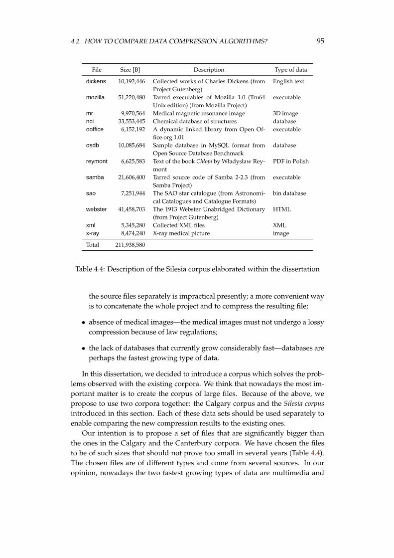
4.2. HOW TO COMPARE DATA COMPRESSION ALGORITHMS? 95
File Size [B] Description Type of data
dickens 10,192,446 Collected works of Charles Dickens (fromProject Gutenberg)
English text
mozilla 51,220,480 Tarred executables of Mozilla 1.0 (Tru64Unix edition) (from Mozilla Project)
executable
mr 9,970,564 Medical magnetic resonance image 3D imagenci 33,553,445 Chemical database of structures databaseooffice 6,152,192 A dynamic linked library from Open Of-
fice.org 1.01executable
osdb 10,085,684 Sample database in MySQL format fromOpen Source Database Benchmark
database
reymont 6,625,583 Text of the book Chłopi by Władysław Rey-mont
PDF in Polish
samba 21,606,400 Tarred source code of Samba 2-2.3 (fromSamba Project)
executable
sao 7,251,944 The SAO star catalogue (from Astronomi-cal Catalogues and Catalogue Formats)
bin database
webster 41,458,703 The 1913 Webster Unabridged Dictionary(from Project Gutenberg)
HTML
xml 5,345,280 Collected XML files XMLx-ray 8,474,240 X-ray medical picture image
Total 211,938,580
Table 4.4: Description of the Silesia corpus elaborated within the dissertation
the source files separately is impractical presently; a more convenient wayis to concatenate the whole project and to compress the resulting file;
• absence of medical images—the medical images must not undergo a lossycompression because of law regulations;
• the lack of databases that currently grow considerably fast—databases areperhaps the fastest growing type of data.
In this dissertation, we decided to introduce a corpus which solves the prob-lems observed with the existing corpora. We think that nowadays the most im-portant matter is to create the corpus of large files. Because of the above, wepropose to use two corpora together: the Calgary corpus and the Silesia corpusintroduced in this section. Each of these data sets should be used separately toenable comparing the new compression results to the existing ones.
Our intention is to propose a set of files that are significantly bigger thanthe ones in the Calgary and the Canterbury corpora. We have chosen the filesto be of such sizes that should not prove too small in several years (Table 4.4).The chosen files are of different types and come from several sources. In ouropinion, nowadays the two fastest growing types of data are multimedia and
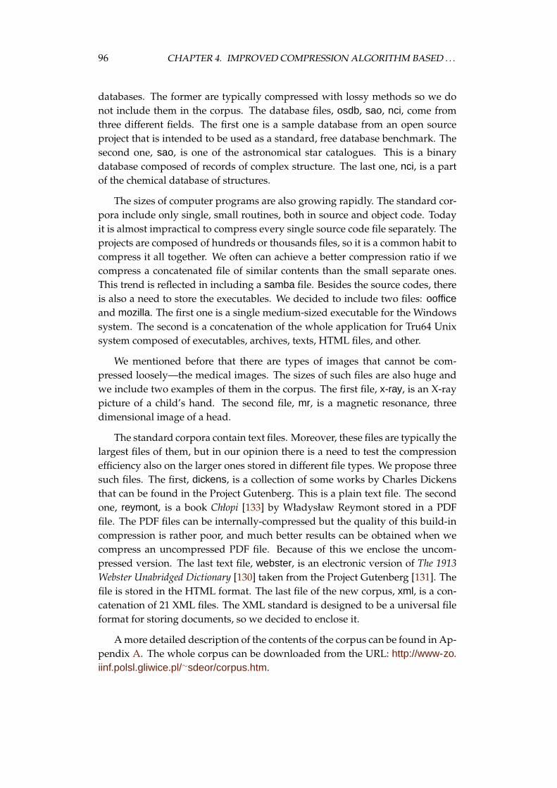
96 CHAPTER 4. IMPROVED COMPRESSION ALGORITHM BASED . . .
databases. The former are typically compressed with lossy methods so we donot include them in the corpus. The database files, osdb, sao, nci, come fromthree different fields. The first one is a sample database from an open sourceproject that is intended to be used as a standard, free database benchmark. Thesecond one, sao, is one of the astronomical star catalogues. This is a binarydatabase composed of records of complex structure. The last one, nci, is a partof the chemical database of structures.
The sizes of computer programs are also growing rapidly. The standard cor-pora include only single, small routines, both in source and object code. Todayit is almost impractical to compress every single source code file separately. Theprojects are composed of hundreds or thousands files, so it is a common habit tocompress it all together. We often can achieve a better compression ratio if wecompress a concatenated file of similar contents than the small separate ones.This trend is reflected in including a samba file. Besides the source codes, thereis also a need to store the executables. We decided to include two files: oofficeand mozilla. The first one is a single medium-sized executable for the Windowssystem. The second is a concatenation of the whole application for Tru64 Unixsystem composed of executables, archives, texts, HTML files, and other.
We mentioned before that there are types of images that cannot be com-pressed loosely—the medical images. The sizes of such files are also huge andwe include two examples of them in the corpus. The first file, x-ray, is an X-raypicture of a child’s hand. The second file, mr, is a magnetic resonance, threedimensional image of a head.
The standard corpora contain text files. Moreover, these files are typically thelargest files of them, but in our opinion there is a need to test the compressionefficiency also on the larger ones stored in different file types. We propose threesuch files. The first, dickens, is a collection of some works by Charles Dickensthat can be found in the Project Gutenberg. This is a plain text file. The secondone, reymont, is a book Chłopi [133] by Władysław Reymont stored in a PDFfile. The PDF files can be internally-compressed but the quality of this build-incompression is rather poor, and much better results can be obtained when wecompress an uncompressed PDF file. Because of this we enclose the uncom-pressed version. The last text file, webster, is an electronic version of The 1913Webster Unabridged Dictionary [130] taken from the Project Gutenberg [131]. Thefile is stored in the HTML format. The last file of the new corpus, xml, is a con-catenation of 21 XML files. The XML standard is designed to be a universal fileformat for storing documents, so we decided to enclose it.
A more detailed description of the contents of the corpus can be found in Ap-pendix A. The whole corpus can be downloaded from the URL: http://www-zo.iinf.polsl.gliwice.pl/∼sdeor/corpus.htm.
4.2. HOW TO COMPARE DATA COMPRESSION ALGORITHMS? 97
4.2.2 Multi criteria optimisation in compression
Compression is a process of reducing the size of a sequence of characters to savethe cost of transmission or storage. One could think that the better the com-pression ratio, the better the algorithm is. This is true if we neglect time, buttime also matters. Let us suppose that we can choose between two compressionmethods: one of them gives good compression ratio, but is slow; the other is fastbut offers a poorer compression ratio. If our goal is to transmit the sequence overa communication channel, then it is not obvious which method should be used.The slower one will produce a shorter compressed sequence, but the compres-sion process is slow, and maybe the compression time surpass the transmissiontime and we could not use the full communication speed available, because wewould have to wait for the data to transmit. The faster method will producea longer compressed sequence, but the communication could be done with fullspeed. Without knowledge of the speed of compression methods on particu-lar sequences, the sequence length, and the parameters of the communicationchannel, we cannot say, which method leads us to faster transmission.
We should not forget also the decompression process. The speed of the de-compression in many cases significantly differs from the compression speed. Wecan imagine a situation typical in the multimedia world. We usually have muchtime to compress a DVD film, and we often have powerful computers for thistask. The compression will be done, however, only once. The decompressionis done in every DVD player many times. The computation power of the DVDplayer is lower. The files distributed via Internet are also compressed only once,but they are downloaded and decompressed many times. Often the decompres-sion speed is more important than the compression speed.
We should not forget, however, the situation in the data transmission, whenthe data are compressed before the transmission, and decompressed after it. Insuch a case, the compression and decompression speed is usually of equal im-portance. An opposite situation takes place in backup utilities. The data arecompressed many times, in every backup, but almost never decompressed. Inthis case, the decompression speed is of low importance.
The situation described before is typical in the real world. We often havemany criteria, which can be exclusive, and we cannot optimise all of them. Wehave to opt for a compromise, and without a detailed knowledge of the caseat which the compression will be used, we cannot choose the best compressionmethod. In such situations, we talk about multi criteria optimisation. The first re-search in this field was conducted by Pareto [122, 123] in 1896–1897, who inves-tigated the problem of satisfying many exclusive criteria. In 1906, in his famousbook, Manuale di economia politica, conuna introduzione alla scienca Sociale [124],Pareto introduced a concept of the non-dominated solutions. Pareto formulatedsuch a solution in economical terms as a solution, where no individual could be
98 CHAPTER 4. IMPROVED COMPRESSION ALGORITHM BASED . . .
more satisfied without satisfying others less. Currently, we call such solutionsPareto-optimal. The solutions that are not non-dominated are called dominatedsolutions.
We formulate the problem of multi criteria optimisation in modern terms,following the works by von Neumann and Morgenstern [184]. There are somenumber of criteria Q1, Q2, . . . , Qm dependent on some variables:
Qi = Qi(q1, q2, . . . , qr), for i = 1, 2, . . . , m. (4.59)
A tuple of variables:q = 〈q1, q2, . . . , qr〉 (4.60)
is called a point in the optimisation. A point q is called Pareto-optimal if there isno other point p such that
∀1≤i≤m Qi(p) ≥ Qi(q). (4.61)
The goal of multi criteria optimisation is to find the set of all the Pareto-optimal points. The formulation of the Pareto-optimal set (Equation 4.61) is forthe case, in which all the criteria Qi are maximised. In general case, all or somecriteria can be minimised. Therefore, we should reformulate Equation 4.61 to:
∀1≤i≤m Qi(p) �i Qi(q), (4.62)
where �i is the ≤ relation if the criterion Qi is minimised and the ≥ relation if itis maximised.
There are at least three criteria of compression quality: the compression ra-tio, the compression speed, and the decompression speed. We measure the com-pression ratio by the mean number of output bits per input symbol (bpc), so thesmaller is the compression ratio, the better the compression is. Therefore weminimise this criterion. The speed of compression and decompression is mea-sured in kB/s, so these criteria are maximised.
4.3 Experiments with the algorithm stages
4.3.1 Burrows–Wheeler transform computation
The Burrows–Wheeler transform can be computed in many ways. A brief sum-mary of the possibilities is shown in Figure 3.12. In Section 4.1.2, we introducedan improvement to the Itoh–Tanaka’s computation method. Here we examinethe existing approaches in practice. Tables 4.5 and 4.6 contain the experimentalresults of several BWT computation methods on the files from the Calgary andthe Silesia corpora.
We compare the methods for which either the source code or the in-depth de-scription of the implementation are available. The columns of Tables 4.5 and 4.6

4.3. EXPERIMENTS WITH THE ALGORITHM STAGES 99
File
Size
[B]
%ru
nsSe
wiS
ewLS
MM
IT1S
IT2S
IT1i
SIT
2iS
iIT1
iIT
2C
IT
bib
111,
261
2.26
0.06
0.06
0.08
0.16
0.05
0.05
0.04
0.05
0.05
0.05
0.05
book
176
8,77
12.
170.
540.
521.
082.
250.
040.
360.
380.
340.
370.
340.
34bo
ok2
610,
856
2.17
0.40
0.38
0.80
1.71
0.29
0.28
0.27
0.25
0.28
0.25
0.25
geo
102,
400
4.11
0.06
0.06
0.08
0.11
0.05
0.06
0.05
0.05
0.05
0.06
0.05
new
s37
7,10
96.
200.
210.
200.
431.
050.
190.
180.
160.
160.
150.
160.
15ob
j121
,504
20.6
90.
030.
030.
010.
030.
150.
120.
080.
080.
030.
080.
03ob
j224
6,81
45.
420.
130.
130.
240.
550.
110.
110.
100.
110.
100.
100.
10pa
per1
53,1
612.
350.
030.
040.
030.
050.
030.
040.
030.
040.
030.
030.
03pa
per2
82,1
991.
850.
050.
050.
060.
100.
030.
040.
040.
040.
040.
040.
04pi
c51
3,21
685
.20
0.15
0.12
0.59
1.16
183.
9718
6.51
224.
5020
2.46
0.10
204.
240.
10pr
ogc
39,6
117.
650.
040.
030.
020.
040.
030.
030.
030.
030.
030.
030.
03pr
ogl
71,6
4615
.61
0.04
0.04
0.05
0.09
0.05
0.05
0.04
0.05
0.04
0.05
0.04
prog
p43
,379
15.4
80.
040.
040.
030.
060.
030.
040.
040.
040.
030.
070.
03tr
ans
93,6
958.
860.
060.
060.
070.
130.
050.
060.
050.
050.
040.
050.
04
Tabl
e4.
5:C
ompa
riso
nof
diff
eren
tBW
Tco
mpu
tati
onm
etho
dsfo
rth
eC
alga
ryco
rpus
.T
heco
mpu
tati
onti
mes
are
expr
esse
din
seco
nds.
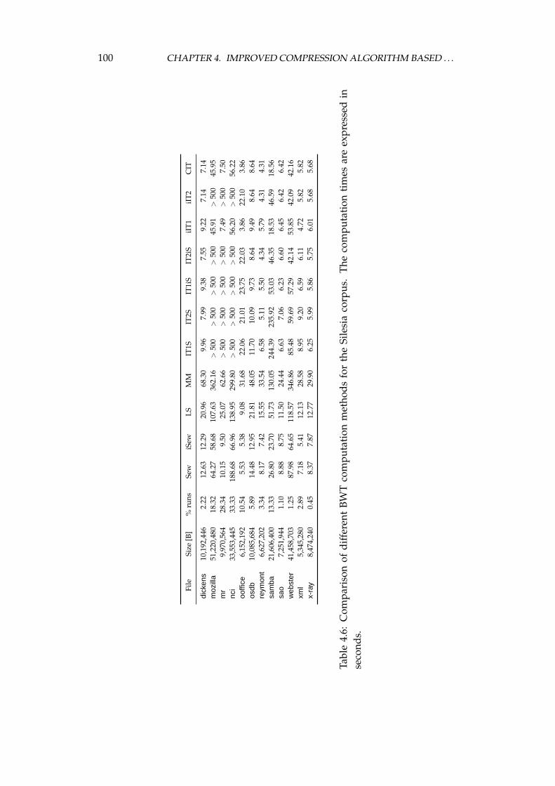
100 CHAPTER 4. IMPROVED COMPRESSION ALGORITHM BASED . . .
File
Size
[B]
%ru
nsSe
wiS
ewLS
MM
IT1S
IT2S
IT1i
SIT
2iS
iIT
1iI
T2
CIT
dick
ens
10,1
92,4
462.
2212
.63
12.2
920
.96
68.3
09.
967.
999.
387.
559.
227.
147.
14m
ozill
a51
,220
,480
18.3
264
.27
58.6
810
7.63
362.
16>
500
>50
0>
500
>50
045
.91
>50
045
.95
mr
9,97
0,56
428
.34
10.1
59.
5025
.07
62.6
6>
500
>50
0>
500
>50
07.
49>
500
7.50
nci
33,5
53,4
4533
.33
188.
6866
.96
138.
9529
9.80
>50
0>
500
>50
0>
500
56.2
0>
500
56.2
2oo
ffice
6,15
2,19
210
.54
5.53
5.38
9.08
31.6
822
.06
21.0
123
.75
22.0
33.
8622
.10
3.86
osdb
10,0
85,6
845.
8914
.48
12.9
521
.81
48.0
511
.70
10.0
99.
738.
649.
498.
648.
64re
ymon
t6,
627,
202
3.34
8.17
7.42
15.5
533
.54
6.58
5.11
5.50
4.34
5.79
4.31
4.31
sam
ba21
,606
,400
13.3
326
.80
23.7
051
.73
130.
0524
4.39
235.
9253
.03
46.3
518
.53
46.5
918
.56
sao
7,25
1,94
41.
108.
888.
7511
.50
24.4
46.
637.
066.
236.
606.
456.
426.
42w
ebst
er41
,458
,703
1.25
87.9
864
.65
118.
5734
6.86
85.4
859
.69
57.2
942
.14
53.8
542
.09
42.1
6xm
l5,
345,
280
2.89
7.18
5.41
12.1
328
.58
8.95
9.20
6.59
6.11
4.72
5.82
5.82
x-ra
y8,
474,
240
0.45
8.37
7.87
12.7
729
.90
6.25
5.99
5.86
5.75
6.01
5.68
5.68
Tabl
e4.
6:C
ompa
riso
nof
diff
eren
tBW
Tco
mpu
tati
onm
etho
dsfo
rth
eSi
lesi
aco
rpus
.T
heco
mpu
tati
onti
mes
are
expr
esse
din
seco
nds.
4.3. EXPERIMENTS WITH THE ALGORITHM STAGES 101
contain the time of the BWT computation expressed in seconds for the followingmethods:
• Sew—the copy method by Seward [149]; this method is implemented in thebzip2 program [150]; our implementation is based on the original one bySeward,
• iSew—the improved version of Seward’s method; the improvements weredone in implementation only (a brief description of the improvements canbe found in Appendix B),
• LS—the Larsson–Sadakane’s method [102],
• MM—the Manber–Myers’s method [106],
• IT1S—the basic Itoh–Tanaka’s method [90] of order 1 with Seward’s [149]sorting suffixes method,
• IT2S—the basic Itoh–Tanaka’s method [90] of order 2 with Seward’s [149]for sorting suffixes method,
• IT1iS—the basic Itoh–Tanaka’s method [90] of order 1 with improved Se-ward’s method for sorting suffixes,
• IT2iS—the basic Itoh–Tanaka’s method [90] of order 2 with improved Se-ward’s method for sorting suffixes,
• iIT1—the improved Itoh–Tanaka’s method (Section 4.1.2) of order 1 withimproved Seward’s method for sorting suffixes,
• iIT2—the improved Itoh–Tanaka’s method (Section 4.1.2) of order 2 withimproved Seward’s method for sorting suffixes,
• CIT—the combined method which chooses between the iIT1 and the iIT2method depending on contents of the sequence to process.
The computation times of the methods for the Calgary corpus are small. Thisis caused by the short test files. The most interesting observation for this corpusis the slowness of some methods processing the pic file. The main problem of allthe sorting-based methods (all of the examined except for LS and MM) is sort-ing strings with long identical prefixes. The simplest way to find such files is tocount the number of runs occurrence. This method is not perfect, however it iseasy to calculate and, as we can observe from the experiments, it is a good adhoc rule to choose files hard to process. The column denoted % runs contains thepercentage number of runs of length 2. As we can see, this ratio is over 85% forthe pic file. The other file for which this value is large is obj1. The computation
102 CHAPTER 4. IMPROVED COMPRESSION ALGORITHM BASED . . .
times for this file are small, because of its size, but we can notice that most IT-based methods work on it 5 times slower than the Sew method. When we focuson the methods for suffix arrays construction, whose good worst-case complexi-ties are known (LS and MM methods), we can see, that in practice these methodsare slower than the sorting-based ones.
The files in the Silesia corpus are larger. Therefore the differences betweenthe computation times for different methods are higher. As we can see, theLarsson–Sadakane’s and the Manber–Myers’s methods are significantly slowerthan the Seward’s method. There are three files, mozilla, mr, and nci, for whichsome IT-based methods work very slow. In fact, we stopped the experimentsafter 500 seconds, because we decided this time to be impractical, as there aremuch faster other methods. The Itoh–Tanaka-based methods employ the Se-ward’s method for sorting suffixes, but there is one important difference be-tween the employed method and the Seward’s method. Seward introduced ahighly efficient method for sorting runs. In the original Itoh–Tanaka’s method,we cannot use this improvement. Therefore, for the files with long runs (all thementioned files have the ratio of runs of length 2 over 15%) this method is slow.One of the improvements proposed in Section 4.1.2 is a special method for sort-ing runs. Unfortunately, this special treating of runs cannot be applied in theItoh–Tanaka’s method of order 2. As we can notice, the improvement of speedgained by this innovation is significant for all files, and for files hard to sort it ishuge. The improved Itoh–Tanaka’s method of order 2 works, however, faster forsequences with small number of runs. Therefore, we propose to use the order-2version if the ratio of runs of length 2 is lower than 7%. Such a combined method(column CIT), choosing between iIT1 and iIT2, is used in further experiments.
4.3.2 Weight functions in the weighted frequency count transform
In this experiment, we examine the weight functions w. The comparison of thesefunctions is made using the files from the Calgary corpus. The results are pre-sented in Table 4.7.§ For each of the examined weight functions, the best set ofparameters were found. We see that the weight functions w8 and w9 achieve thebest compression ratios. The usage of different parameters for different rangesin the weight function w8 is motivated by the observation that typically charac-ters in these ranges are from different, but similar, contexts. It is useful to exploitthe information on the probability distribution in such contexts, but it should notdominate the probability distribution of the current context. The parameter q forthe weight function w9 is the most complex. In this weight function, the numberof different contexts of length 4 that appear in the input sequence is used (theparameter C4) to exploit some information on the structure of the sequence x.
§The results in this dissertation are slightly different from the ones that were presented inReferences [54, 55] because a slightly modified probability estimation method was used.
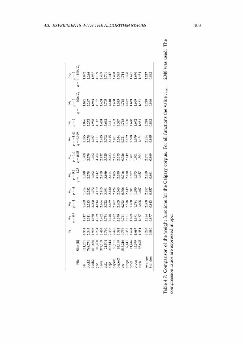
4.3. EXPERIMENTS WITH THE ALGORITHM STAGES 103
w1
w2
w3
w4
w5
w6
w7
w8
w9
w9q
q=
0.7
p=
4p
=4
p=
0.5
p=
1.0
p=−
1.40
p=
4p
=3
p=
3Fi
leSi
ze[B
]q
=−
1.25
q=
0.95
q=
0.99
9q
=1−
100/
C4
q=
1−
100/
C4
bib
111,
261
1.91
41.
917
1.96
91.
914
1.89
81.
908
1.89
51.
896
1.89
11.
892
book
176
8,77
12.
343
2.31
12.
283
2.28
22.
278
2.27
92.
278
2.27
22.
267
2.26
6bo
ok2
610,
856
1.99
81.
980
2.00
01.
972
1.96
21.
962
1.95
71.
958
1.95
41.
957
geo
102,
400
4.23
44.
229
4.11
44.
119
4.14
24.
204
4.17
14.
147
4.15
74.
139
new
s37
7,10
92.
463
2.46
22.
464
2.41
52.
410
2.43
72.
415
2.40
82.
408
2.40
9ob
j121
,504
3.76
03.
754
3.72
23.
691
3.69
03.
725
3.70
23.
692
3.70
53.
701
obj2
246,
814
2.43
62.
448
2.48
92.
430
2.41
42.
433
2.41
52.
411
2.41
02.
417
pape
r153
,161
2.42
02.
422
2.48
72.
424
2.40
52.
415
2.40
12.
403
2.40
02.
400
pape
r282
,199
2.38
12.
370
2.40
52.
363
2.35
02.
355
2.34
42.
347
2.34
32.
345
pic
513,
216
0.75
90.
741
0.70
30.
706
0.71
60.
726
0.72
10.
718
0.71
80.
714
prog
c39
,611
2.45
32.
461
2.51
82.
449
2.43
02.
449
2.42
92.
430
2.42
72.
428
prog
l71
,646
1.68
41.
699
1.76
81.
681
1.67
21.
701
1.67
81.
670
1.66
91.
671
prog
p43
,379
1.66
71.
691
1.78
41.
690
1.67
31.
701
1.67
91.
672
1.66
91.
670
tran
s93
,695
1.45
11.
487
1.60
81.
467
1.45
71.
504
1.47
41.
451
1.45
11.
454
Ave
rage
2.28
32.
284
2.30
82.
257
2.25
02.
271
2.25
42.
248
2.24
82.
247
Std.
dev.
0.88
00.
877
0.84
30.
857
0.86
10.
869
0.86
50.
862
0.86
60.
862
Tabl
e4.
7:C
ompa
riso
nof
the
wei
ght
func
tion
sfo
rth
eC
alga
ryco
rpus
.Fo
ral
lfu
ncti
ons
the
valu
et m
ax=
2048
was
used
.Th
eco
mpr
essi
onra
tios
are
expr
esse
din
bpc.
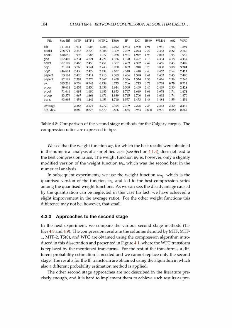
104 CHAPTER 4. IMPROVED COMPRESSION ALGORITHM BASED . . .
File Size [B] MTF MTF-1 MTF-2 TS(0) IF DC BS99 WM01 A02 WFC
bib 111,261 1.914 1.906 1.906 2.012 1.963 1.930 1.91 1.951 1.96 1.892book1 768,771 2.343 2.320 2.306 2.309 2.239 2.224 2.27 2.363 2.22 2.266book2 610,856 1.998 1.985 1.977 2.028 1.964 1.927 1.96 2.013 1.95 1.957geo 102,400 4.234 4.221 4.221 4.186 4.190 4.497 4.16 4.354 4.18 4.139news 377,109 2.463 2.453 2.451 2.587 2.459 2.392 2.42 2.465 2.45 2.409obj1 21,504 3.760 3.741 3.743 3.900 3.889 3.948 3.73 3.800 3.88 3.701obj2 246,814 2.436 2.429 2.431 2.637 2.548 2.448 2.45 2.462 2.54 2.417paper1 53,161 2.420 2.414 2.413 2.589 2.454 2.398 2.41 2.453 2.45 2.400paper2 82,199 2.381 2.373 2.367 2.458 2.366 2.334 2.36 2.416 2.36 2.345pic 513,216 0.759 0.742 0.738 0.733 0.706 0.713 0.72 0.768 0.70 0.714progc 39,611 2.453 2.450 2.453 2.644 2.500 2.469 2.45 2.469 2.50 2.428progl 71,646 1.684 1.680 1.683 1.853 1.747 1.689 1.68 1.678 1.74 1.671progp 43,379 1.667 1.666 1.671 1.889 1.745 1.700 1.68 1.692 1.74 1.670trans 93,695 1.451 1.449 1.453 1.710 1.557 1.473 1.46 1.484 1.55 1.454
Average 2.283 2.274 2.272 2.395 2.309 2.296 2.26 2.312 2.30 2.247Std. dev. 0.880 0.878 0.879 0.866 0.885 0.954 0.868 0.901 0.885 0.862
Table 4.8: Comparison of the second stage methods for the Calgary corpus. Thecompression ratios are expressed in bpc.
We see that the weight function w7, for which the best results were obtainedin the numerical analysis of a simplified case (see Section 4.1.4), does not lead tothe best compression ratios. The weight function w9 is, however, only a slightlymodified version of the weight function w6, which was the second best in thenumerical analysis.
In subsequent experiments, we use the weight function w9q, which is thequantised version of the function w9, and led to the best compression ratiosamong the quantised weight functions. As we can see, the disadvantage causedby the quantisation can be neglected in this case (in fact, we have achieved aslight improvement in the average ratio). For the other weight functions thisdifference may not be, however, that small.
4.3.3 Approaches to the second stage
In the next experiment, we compare the various second stage methods (Ta-bles 4.8 and 4.9). The compression results in the columns denoted by MTF, MTF-1, MTF-2, TS(0), and WFC are obtained using the compression algorithm intro-duced in this dissertation and presented in Figure 4.1, where the WFC transformis replaced by the mentioned transforms. For the rest of the transforms, a dif-ferent probability estimation is needed and we cannot replace only the secondstage. The results for the IF transform are obtained using the algorithm in whichalso a different probability estimation method is applied.
The other second stage approaches are not described in the literature pre-cisely enough, and it is hard to implement them to achieve such results as pre-
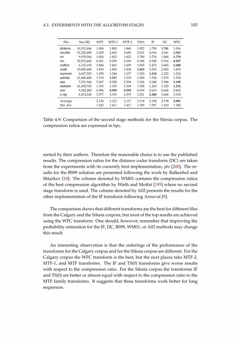
4.3. EXPERIMENTS WITH THE ALGORITHM STAGES 105
File Size [B] MTF MTF-1 MTF-2 TS(0) IF DC WFC
dickens 10,192,446 1.904 1.883 1.868 1.852 1.794 1.781 1.816mozilla 51,220,480 2.629 2.603 2.600 2.631 2.616 2.641 2.543mr 9,970,564 1.826 1.823 1.822 1.780 1.776 1.806 1.770nci 33,553,445 0.301 0.299 0.299 0.306 0.298 0.316 0.297ooffice 6,152,192 3.484 3.461 3.459 3.505 3.473 3.465 3.380osdb 10,085,684 1.839 1.830 1.828 1.815 1.933 2.002 1.835reymont 6,627,202 1.258 1.246 1.237 1.243 1.218 1.222 1.224samba 21,606,400 1.518 1.517 1.518 1.594 1.554 1.574 1.518sao 7,251,944 5.367 5.298 5.294 5.226 5.248 5.306 5.195webster 41,458,703 1.332 1.319 1.309 1.308 1.263 1.325 1.276xml 5,345,280 0.596 0.595 0.595 0.639 0.619 0.606 0.602x-ray 8,474,240 3.577 3.576 3.575 3.521 3.500 3.606 3.518
Average 2.136 2.121 2.117 2.118 2.108 2.138 2.081Std. dev. 1.425 1.411 1.411 1.390 1.397 1.410 1.380
Table 4.9: Comparison of the second stage methods for the Silesia corpus. Thecompression ratios are expressed in bpc.
sented by their authors. Therefore the reasonable choice is to use the publishedresults. The compression ratios for the distance coder transform (DC) are takenfrom the experiments with its currently best implementation, ybs [200]. The re-sults for the BS99 solution are presented following the work by Balkenhol andShtarkov [18]. The column denoted by WM01 contains the compression ratiosof the best compression algorithm by Wirth and Moffat [195] where no secondstage transform is used. The column denoted by A02 presents the results for theother implementation of the IF transform following Arnavut [9].
The comparison shows that different transforms are the best for different filesfrom the Calgary and the Silesia corpora, but most of the top results are achievedusing the WFC transform. One should, however, remember that improving theprobability estimation for the IF, DC, BS99, WM01, or A02 methods may changethis result.
An interesting observation is that the orderings of the performance of thetransforms for the Calgary corpus and for the Silesia corpus are different. For theCalgary corpus the WFC transform is the best, but the next places take MTF-2,MTF-1, and MTF transforms. The IF and TS(0) transforms give worse resultswith respect to the compression ratio. For the Silesia corpus the transforms IFand TS(0) are better or almost equal with respect to the compression ratio to theMTF family transforms. It suggests that these transforms work better for longsequences.
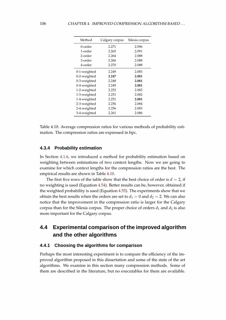
106 CHAPTER 4. IMPROVED COMPRESSION ALGORITHM BASED . . .
Method Calgary corpus Silesia corpus
0-order 2.271 2.0961-order 2.265 2.0912-order 2.264 2.0883-order 2.266 2.0884-order 2.270 2.088
0-1-weighted 2.249 2.0830-2-weighted 2.247 2.0810-3-weighted 2.248 2.0810-4-weighted 2.249 2.0811-2-weighted 2.252 2.0831-3-weighted 2.251 2.0821-4-weighted 2.251 2.0812-3-weighted 2.256 2.0842-4-weighted 2.256 2.0833-4-weighted 2.261 2.086
Table 4.10: Average compression ratios for various methods of probability esti-mation. The compression ratios are expressed in bpc.
4.3.4 Probability estimation
In Section 4.1.6, we introduced a method for probability estimation based onweighting between estimations of two context lengths. Now we are going toexamine for which context lengths for the compression ratios are the best. Theempirical results are shown in Table 4.10.
The first five rows of the table show that the best choice of order is d = 2, ifno weighting is used (Equation 4.54). Better results can be, however, obtained ifthe weighted probability is used (Equation 4.55). The experiments show that weobtain the best results when the orders are set to d1 = 0 and d2 = 2. We can alsonotice that the improvement in the compression ratio is larger for the Calgarycorpus than for the Silesia corpus. The proper choice of orders d1 and d2 is alsomore important for the Calgary corpus.
4.4 Experimental comparison of the improved algorithmand the other algorithms
4.4.1 Choosing the algorithms for comparison
Perhaps the most interesting experiment is to compare the efficiency of the im-proved algorithm proposed in this dissertation and some of the state of the artalgorithms. We examine in this section many compression methods. Some ofthem are described in the literature, but no executables for them are available.
4.4. EXPERIMENTAL COMPARISON OF THE IMPROVED ALGORITHM . . . 107
For these algorithms we cannot provide the experimental compression resultsfor the Silesia corpus. The other ones are available for downloading so we canexamine them on both corpora.
The dissertation concerns universal compression, so we have to exclude fromthe comparison the compression programs that are highly tuned to files from theCalgary corpus. Some of such compressors use a different compression methoddepending on what they recognise as a file to process. For example, the picand geo files can be better compressed if they undergo a special transformationbefore the compression. There exist compressors that monitor the size of the fileand if it is exactly the same as the size of files from the Calgary corpus, they makesuch a transformation. Other programs monitor the contents of the file and ifthey recognise that the file is an English text, they run some preliminary filters,which are similar to those described in Section 3.2.6. Many files of the Calgarycorpus are English texts, so such a heuristics gives an advantage for this corpus.There are also methods for improving the compression ratio for executable files,and some compression programs also use a heuristic to recognise such files.
When it was possible, such data-specific preliminary filtering methods wereturned off in the programs. Unfortunately, in some compressors there is no wayto abandon filters and we have to resign from including them in the experi-ments.
4.4.2 Examined algorithms
Before we go to the comparison of the compression algorithms, we expand theabbreviations of the examined methods:
• A02—the BWT-based algorithm with the inversion frequencies transformas the second stage; the results are from the work by Arnavut [9];
• acb—the Associative Coder by Buyanovsky [40]; the compression resultsare from experiments with the acb 2.00c program [41];
• B97—the best version of the PPM algorithms proposed by Bunton [37];
• boa—the boa 0.58b compression program by Sutton [160], which is an im-plementation of the PPM algorithm;
• BS99—the BWT-based algorithm invented by Balkenhol and Shtarkov [18];
• BW94—the original Burrows–Wheeler compression algorithm [39];
• bzip—the bzip 0.21 compression program by Seward [148]; this programachieves the same compression ratios as Fenwick’s method [68];
• CTW—context tree weighting method proposed by Willems et al. [189]; theresults are from Reference [17];
108 CHAPTER 4. IMPROVED COMPRESSION ALGORITHM BASED . . .
• DM—the improved BWT-based algorithm proposed in this dissertationwith the move-to-front transform as the second stage;
• DW—the improved BWT-based algorithm proposed in this dissertationwith the weighted frequency count transform as the second stage;
• F96—the BWT-based algorithm proposed by Fenwick [68]; the same com-pression ratios are achieved by the bzip 0.21 program [148], which is usedfor experiments on the Silesia corpus;
• gzip—standard gzip program[72]; this is an implementation of the wellknown LZ77 algorithm [202];
• LDMC—currently the best dynamic Markov coding algorithm, originallyintroduced by Cormack and Horspool [52]; this is an improved version,LazyDMC, by Bunton [33];
• lgha—the speed-optimised ha compression program; this implementationis provided by Lyapko [105];
• LZMA—the Ziv–Lempel algorithm presented by Pavlov [127]; the resultsare from experiments with the 7-zip program;
• LZW—standard UNIX compress program; this is an implementation of theLZW algorithm [187];
• MH—the cPPMII algorithm proposed by Shkarin [154, 155]; the results arefrom experiments with the PPMonstr var. H program;
• MI4—the cPPMII algorithm by Shkarin [156]; the result are from experi-ments with the PPMonstr var. I program with order 4;
• MI64—the cPPMII algorithm by Shkarin [156]; the result are from experi-ments with the PPMonstr var. I program with order 64;
• PPMdH—the PPMII algorithm proposed by Shkarin [154, 155]; the resultsare from experiments with the PPMd var. H program;
• PPMN—the PPMN algorithm by Smirnov [158]; the results are from ex-periments with the ppmnb1+ program;
• rar—the rar 2.90 compression program [137];
• szip—the BWT-based algorithm presented by Schindler [144]; the resultsare from experiments with the szip program [145];
• T98—the PPMD+ algorithm proposed by Teahan [163]; the results are fromexperiments with the ppmd+ program [162];
4.4. EXPERIMENTAL COMPARISON OF THE IMPROVED ALGORITHM . . . 109
• ufa—the binary PPM algorithm by Pavlov [126]; the results are from ex-periments with the ufa 0.04 Beta 1 program;
• VW98—the switching method, algorithm presented by Volf and Willems[182, 183];
• WM01—the best BWT-based algorithm with no second stage; the resultsare from the work by Wirth and Moffat [195];
• ybs—the BWT-based compression program with the distance coder (DC)transform as the second stage; this is an implementation by Yoockin [200].
4.4.3 Comparison procedure
All the mentioned compression algorithms were compared on two corpora—the Calgary corpus and the Silesia corpus. For each file of the corpora, all thecompression programs were run and the size of the compressed file, the com-pression time, and the decompression time were measured. The experimentswere performed on a computer equipped with the AMD Athlon 1.4 GHz pro-cessor, 512 MB DDRAM, and Microsoft Windows 2000 Professional operatingsystem. The times of program execution were measured by using the programutility ntimer. The presented times are user times, as we want to know only thetime of compression not the I/O operations times.
For comparison, we calculated two compression ratios. The first one is thestandard compression ratio expressed in output bits per input character (bpc).The second one is a normalised compression ratio. We calculated it by dividingthe standard compression ratio by the best standard compression ratio of all theexamined compression methods. The goal of using also normalised compres-sion ratio is that each file can be compressed to the smallest possible numberof bits, namely its entropy. We do not know, however, the entropy. The bestwhat we can do is to approximate it by the length of the shortest compressedsequence. Therefore, the normalised compression ratio says how far each com-pression algorithm is from the best one. To compare the algorithms in terms ofmulti criteria optimisation, we calculated also the compression and decompres-sion speed. For each file these speeds were found and then the average werecalculated.
We mentioned about large differences between the three main families of al-gorithms in modern compression: the Ziv–Lempel methods, the prediction bypartial matching methods, and the Burrows–Wheeler transform-based methods.For a clear distinction we denote these algorithms by different marks at the fig-ures. The LZ methods are denoted by ◦, the PPM methods are denoted by ?,and the BWT-based methods by •.
110 CHAPTER 4. IMPROVED COMPRESSION ALGORITHM BASED . . .
The compression programs were examined with many combinations of pa-rameters. For some of them, however, the number of available sets of param-eters is vast, and it is impossible to examine all possibilities. The compressionresults presented in the literature are in most cases optimised for the compres-sion ratio. Therefore, for possibility of comparison to the published methods,for which there are no executables available, we decided to choose such a set ofparameters that leads us to the best compression ratio. If, however, there can befound an interesting set of parameters, for example such a set for which a givenalgorithm dominates some other algorithms that it does not dominate for thechosen set, we also included these combination of parameters in comparison.This situation took place for Shkarin’s PPM algorithms, for which we examinedfour set of parameters.
The data-specific compression options, like English text filters, were turnedoff. The maximum size of memory available for the compression was chosento provide an honest comparison of algorithms. The memory limit equal to10 times the size of the file to compress (but not less than 16 MB) was decidedto be a good choice. This is a natural memory requirement for the BWT-basedcompression algorithms and the PPM methods significantly differ in the mem-ory consumption from each other (with the growth of the context length thememory needed to store the model grows fast and is not naturally bounded).A more detailed description of the options of the programs used in the experi-ments is presented in Appendix C.
4.4.4 Experiments on the Calgary corpus
The Calgary corpus is a standard corpus for examining the compression algo-rithms. There are a number of compression methods for which the compressionratios can be found in the literature. Therefore, we can compare the best com-pression methods proposed so far.
Table 4.11 contains the standard compression ratios for files from the Calgarycorpus, and Table 4.12 contains the normalised compression ratios. The bestPPM algorithms achieve on this corpus significantly better compression ratiosthan the LZ and the BWT-based methods. If, however, we look at Tables 4.13and 4.14, we see that this high efficiency is occupied by the low speed of thesealgorithms.
Better comparison can be done if we look at Figures 4.15, 4.16, 4.17, and 4.18.(The figures do not contain data for some algorithms presented in Table 4.11 asthere are no executables for them, and we could not measure their compressionand decompression speed.)
We can see that in general, the PPM algorithms achieve the best compres-sion ratio, but they are slow (Figures 4.15 and 4.16). The fastest compressionalgorithms are the LZ methods, but their compression ratio is poor. The BWT-
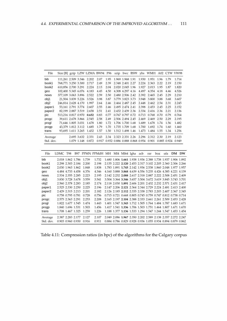
4.4. EXPERIMENTAL COMPARISON OF THE IMPROVED ALGORITHM . . . 111
File Size [B] gzip LZW LZMA BW94 F96 szip bwc BS99 ybs WM01 A02 CTW VW98
bib 111,261 2.509 3.346 2.202 2.07 1.95 1.969 1.968 1.91 1.930 1.951 1.96 1.79 1.714book1 768,771 3.250 3.300 2.717 2.49 2.39 2.348 2.401 2.27 2.224 2.363 2.22 2.19 2.150book2 610,856 2.700 3.291 2.224 2.13 2.04 2.020 2.045 1.96 1.927 2.013 1.95 1.87 1.820geo 102,400 5.345 6.076 4.183 4.45 4.50 4.308 4.297 4.16 4.497 4.354 4.18 4.46 4.526news 377,109 3.063 3.896 2.522 2.59 2.50 2.480 2.506 2.42 2.392 2.465 2.45 2.29 2.210obj1 21,504 3.839 5.226 3.526 3.98 3.87 3.779 3.823 3.73 3.948 3.800 3.88 3.68 3.607obj2 246,814 2.628 4.170 1.997 2.64 2.46 2.464 2.487 2.45 2.448 2.462 2.54 2.31 2.245paper1 53,161 2.791 3.774 2.607 2.55 2.46 2.495 2.474 2.41 2.398 2.453 2.45 2.25 2.152paper2 82,199 2.887 3.519 2.658 2.51 2.41 2.432 2.439 2.36 2.334 2.416 2.36 2.21 2.136pic 513,216 0.817 0.970 0.652 0.83 0.77 0.767 0.797 0.72 0.713 0.768 0.70 0.79 0.764progc 39,611 2.678 3.866 2.545 2.58 2.49 2.506 2.494 2.45 2.469 2.469 2.50 2.29 2.195progl 71,646 1.805 3.031 1.678 1.80 1.72 1.706 1.700 1.68 1.689 1.678 1.74 1.56 1.482progp 43,379 1.812 3.112 1.685 1.79 1.70 1.735 1.709 1.68 1.700 1.692 1.74 1.60 1.460trans 93,695 1.611 3.265 1.432 1.57 1.50 1.512 1.498 1.46 1.473 1.484 1.55 1.34 1.256
Average 2.695 3.632 2.331 2.43 2.34 2.323 2.331 2.26 2.296 2.312 2.30 2.19 2.123Std. dev. 1.079 1.148 0.872 0.917 0.932 0.886 0.888 0.868 0.954 0.901 0.885 0.924 0.949
File LDMC T98 B97 PPMN PPMdH MH MI4 MI64 lgha acb rar boa ufa DM DW
bib 2.018 1.862 1.786 1.739 1.732 1.680 1.806 1.661 1.938 1.936 2.388 1.738 1.937 1.906 1.892book1 2.298 2.303 2.184 2.200 2.198 2.135 2.222 2.120 2.453 2.317 3.102 2.205 2.360 2.306 2.266book2 2.030 1.963 1.862 1.848 1.838 1.783 1.891 1.745 2.142 1.936 2.538 1.860 2.048 1.977 1.957geo 4.484 4.733 4.458 4.376 4.346 4.160 3.888 3.868 4.639 4.556 5.235 4.426 4.385 4.221 4.139news 2.534 2.355 2.285 2.223 2.195 2.142 2.232 2.088 2.617 2.318 2.887 2.222 2.508 2.451 2.409obj1 3.830 3.728 3.678 3.559 3.541 3.504 3.364 3.346 3.657 3.504 3.672 3.619 3.845 3.743 3.701obj2 2.560 2.378 2.283 2.185 2.174 2.118 2.030 1.891 2.606 2.201 2.432 2.232 2.571 2.431 2.417paper1 2.525 2.330 2.250 2.225 2.196 2.147 2.206 2.121 2.364 2.344 2.729 2.224 2.481 2.413 2.400paper2 2.429 2.315 2.213 2.201 2.182 2.126 2.185 2.112 2.335 2.338 2.783 2.203 2.407 2.367 2.345pic 0.758 0.795 0.781 0.728 0.756 0.715 0.721 0.668 0.805 0.745 0.759 0.747 0.812 0.738 0.714progc 2.575 2.363 2.291 2.253 2.208 2.165 2.197 2.104 2.388 2.333 2.661 2.261 2.509 2.453 2.428progl 1.822 1.677 1.545 1.474 1.443 1.401 1.547 1.343 1.712 1.505 1.764 1.484 1.787 1.683 1.671progp 1.840 1.696 1.531 1.503 1.456 1.417 1.541 1.336 1.706 1.503 1.751 1.464 1.807 1.671 1.670trans 1.708 1.467 1.325 1.259 1.226 1.188 1.377 1.136 1.533 1.294 1.547 1.244 1.547 1.453 1.454
Average 2.387 2.283 2.177 2.127 2.107 2.049 2.086 1.967 2.350 2.202 2.589 2.138 2.357 2.272 2.247Std. dev. 0.903 0.960 0.930 0.916 0.911 0.884 0.786 0.829 0.928 0.936 1.055 0.934 0.894 0.879 0.862
Table 4.11: Compression ratios (in bpc) of the algorithms for the Calgary corpus
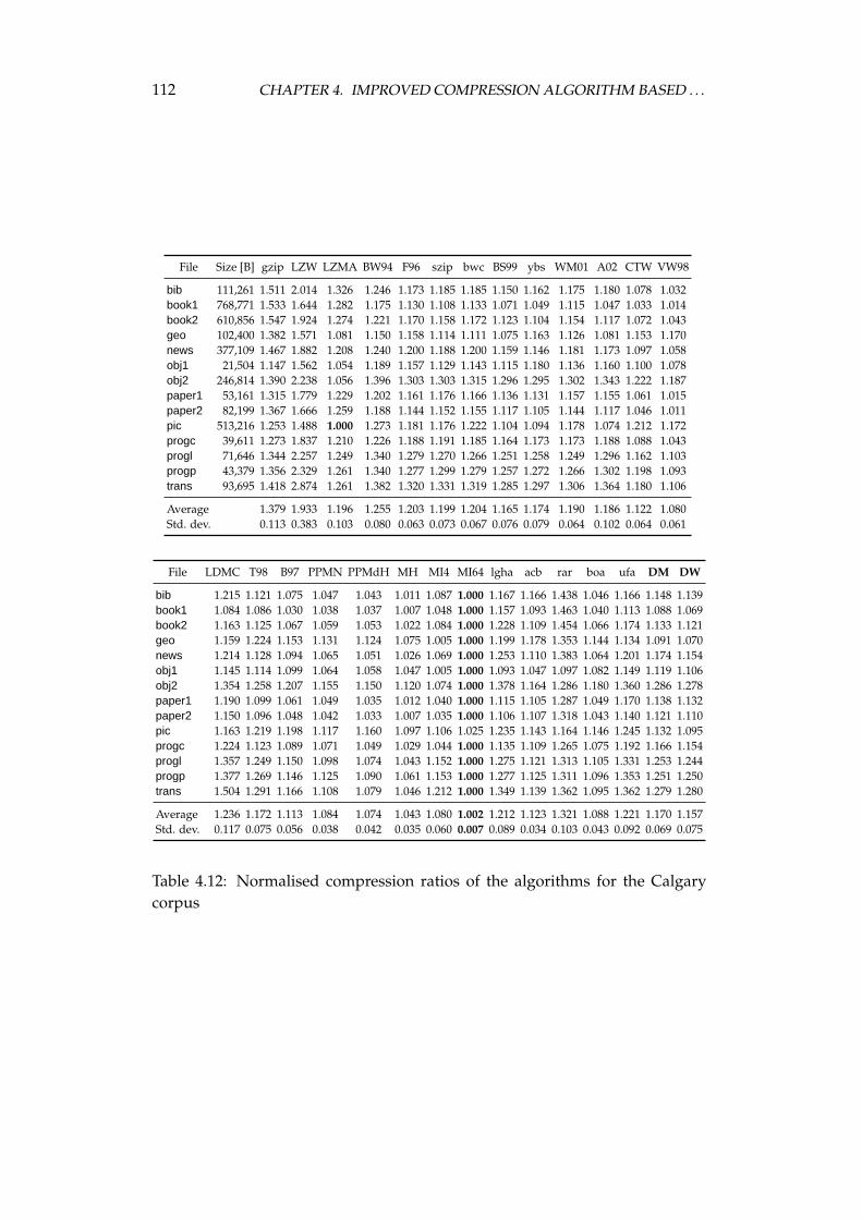
112 CHAPTER 4. IMPROVED COMPRESSION ALGORITHM BASED . . .
File Size [B] gzip LZW LZMA BW94 F96 szip bwc BS99 ybs WM01 A02 CTW VW98
bib 111,261 1.511 2.014 1.326 1.246 1.173 1.185 1.185 1.150 1.162 1.175 1.180 1.078 1.032book1 768,771 1.533 1.644 1.282 1.175 1.130 1.108 1.133 1.071 1.049 1.115 1.047 1.033 1.014book2 610,856 1.547 1.924 1.274 1.221 1.170 1.158 1.172 1.123 1.104 1.154 1.117 1.072 1.043geo 102,400 1.382 1.571 1.081 1.150 1.158 1.114 1.111 1.075 1.163 1.126 1.081 1.153 1.170news 377,109 1.467 1.882 1.208 1.240 1.200 1.188 1.200 1.159 1.146 1.181 1.173 1.097 1.058obj1 21,504 1.147 1.562 1.054 1.189 1.157 1.129 1.143 1.115 1.180 1.136 1.160 1.100 1.078obj2 246,814 1.390 2.238 1.056 1.396 1.303 1.303 1.315 1.296 1.295 1.302 1.343 1.222 1.187paper1 53,161 1.315 1.779 1.229 1.202 1.161 1.176 1.166 1.136 1.131 1.157 1.155 1.061 1.015paper2 82,199 1.367 1.666 1.259 1.188 1.144 1.152 1.155 1.117 1.105 1.144 1.117 1.046 1.011pic 513,216 1.253 1.488 1.000 1.273 1.181 1.176 1.222 1.104 1.094 1.178 1.074 1.212 1.172progc 39,611 1.273 1.837 1.210 1.226 1.188 1.191 1.185 1.164 1.173 1.173 1.188 1.088 1.043progl 71,646 1.344 2.257 1.249 1.340 1.279 1.270 1.266 1.251 1.258 1.249 1.296 1.162 1.103progp 43,379 1.356 2.329 1.261 1.340 1.277 1.299 1.279 1.257 1.272 1.266 1.302 1.198 1.093trans 93,695 1.418 2.874 1.261 1.382 1.320 1.331 1.319 1.285 1.297 1.306 1.364 1.180 1.106
Average 1.379 1.933 1.196 1.255 1.203 1.199 1.204 1.165 1.174 1.190 1.186 1.122 1.080Std. dev. 0.113 0.383 0.103 0.080 0.063 0.073 0.067 0.076 0.079 0.064 0.102 0.064 0.061
File LDMC T98 B97 PPMN PPMdH MH MI4 MI64 lgha acb rar boa ufa DM DW
bib 1.215 1.121 1.075 1.047 1.043 1.011 1.087 1.000 1.167 1.166 1.438 1.046 1.166 1.148 1.139book1 1.084 1.086 1.030 1.038 1.037 1.007 1.048 1.000 1.157 1.093 1.463 1.040 1.113 1.088 1.069book2 1.163 1.125 1.067 1.059 1.053 1.022 1.084 1.000 1.228 1.109 1.454 1.066 1.174 1.133 1.121geo 1.159 1.224 1.153 1.131 1.124 1.075 1.005 1.000 1.199 1.178 1.353 1.144 1.134 1.091 1.070news 1.214 1.128 1.094 1.065 1.051 1.026 1.069 1.000 1.253 1.110 1.383 1.064 1.201 1.174 1.154obj1 1.145 1.114 1.099 1.064 1.058 1.047 1.005 1.000 1.093 1.047 1.097 1.082 1.149 1.119 1.106obj2 1.354 1.258 1.207 1.155 1.150 1.120 1.074 1.000 1.378 1.164 1.286 1.180 1.360 1.286 1.278paper1 1.190 1.099 1.061 1.049 1.035 1.012 1.040 1.000 1.115 1.105 1.287 1.049 1.170 1.138 1.132paper2 1.150 1.096 1.048 1.042 1.033 1.007 1.035 1.000 1.106 1.107 1.318 1.043 1.140 1.121 1.110pic 1.163 1.219 1.198 1.117 1.160 1.097 1.106 1.025 1.235 1.143 1.164 1.146 1.245 1.132 1.095progc 1.224 1.123 1.089 1.071 1.049 1.029 1.044 1.000 1.135 1.109 1.265 1.075 1.192 1.166 1.154progl 1.357 1.249 1.150 1.098 1.074 1.043 1.152 1.000 1.275 1.121 1.313 1.105 1.331 1.253 1.244progp 1.377 1.269 1.146 1.125 1.090 1.061 1.153 1.000 1.277 1.125 1.311 1.096 1.353 1.251 1.250trans 1.504 1.291 1.166 1.108 1.079 1.046 1.212 1.000 1.349 1.139 1.362 1.095 1.362 1.279 1.280
Average 1.236 1.172 1.113 1.084 1.074 1.043 1.080 1.002 1.212 1.123 1.321 1.088 1.221 1.170 1.157Std. dev. 0.117 0.075 0.056 0.038 0.042 0.035 0.060 0.007 0.089 0.034 0.103 0.043 0.092 0.069 0.075
Table 4.12: Normalised compression ratios of the algorithms for the Calgarycorpus
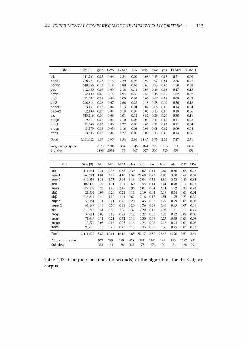
4.4. EXPERIMENTAL COMPARISON OF THE IMPROVED ALGORITHM . . . 113
File Size [B] gzip LZW LZMA F96 szip bwc ybs PPMN PPMdH
bib 111,261 0.03 0.06 0.34 0.09 0.08 0.15 0.08 0.21 0.09book1 768,771 0.23 0.16 2.29 0.97 0.92 0.97 0.84 2.56 0.95book2 610,856 0.13 0.14 1.80 0.66 0.65 0.73 0.60 1.50 0.58geo 102,400 0.06 0.05 0.18 0.11 0.07 0.16 0.08 0.47 0.13news 377,109 0.08 0.11 0.94 0.36 0.36 0.46 0.30 1.07 0.37obj1 21,504 0.01 0.03 0.05 0.03 0.02 0.07 0.02 0.08 0.03obj2 246,814 0.08 0.07 0.66 0.22 0.18 0.28 0.19 0.50 0.18paper1 53,161 0.02 0.04 0.13 0.04 0.04 0.08 0.03 0.14 0.04paper2 82,199 0.03 0.04 0.19 0.07 0.06 0.13 0.05 0.19 0.06pic 513,216 0.30 0.06 1.01 0.12 8.82 0.29 0.20 0.30 0.11progc 39,611 0.02 0.04 0.10 0.02 0.03 0.11 0.03 0.11 0.03progl 71,646 0.03 0.06 0.22 0.06 0.06 0.11 0.02 0.11 0.04progp 43,379 0.03 0.03 0.16 0.04 0.06 0.08 0.02 0.09 0.04trans 93,695 0.02 0.04 0.27 0.07 0.08 0.13 0.06 0.14 0.06
Total 3,141,622 1.07 0.93 8.34 2.86 11.43 3.75 2.52 7.47 2.71
Avg. comp. speed 2875 2710 384 1346 1074 728 1615 511 1414Std. dev. 1108 2034 73 867 357 330 723 359 951
File Size [B] MH MI4 MI64 lgha acb rar boa ufa DM DW
bib 111,261 0.21 0.38 0.53 0.39 1.07 0.11 0.69 0.56 0.08 0.13book1 768,771 1.81 2.27 4.10 1.54 22.60 0.73 8.00 3.60 0.67 0.89book2 610,856 1.31 1.73 3.44 1.16 12.04 0.51 4.80 2.72 0.49 0.64geo 102,400 0.29 1.01 1.01 0.60 1.55 0.14 1.44 0.78 0.14 0.18news 377,109 0.76 1.45 2.48 0.96 6.01 0.34 3.14 1.92 0.33 0.43obj1 21,504 0.06 0.20 0.21 0.11 0.19 0.04 0.19 0.14 0.04 0.04obj2 246,814 0.44 1.10 1.41 0.62 2.16 0.17 1.54 1.25 0.23 0.30paper1 53,161 0.11 0.21 0.28 0.20 0.45 0.05 0.29 0.29 0.06 0.08paper2 82,199 0.16 0.30 0.41 0.20 0.76 0.08 0.46 0.43 0.07 0.11pic 513,216 0.31 0.63 1.06 0.32 2.20 0.15 0.93 1.81 0.19 0.29progc 39,611 0.08 0.18 0.21 0.12 0.27 0.05 0.20 0.22 0.04 0.06progl 71,646 0.11 0.21 0.32 0.14 0.30 0.06 0.27 0.35 0.06 0.08progp 43,379 0.08 0.16 0.25 0.14 0.24 0.03 0.18 0.24 0.04 0.07trans 93,695 0.16 0.28 0.45 0.15 0.33 0.06 0.30 0.45 0.06 0.11
Total 3,141,622 5.89 10.11 16.16 6.65 50.17 2.52 22.43 14.76 2.50 3.41
Avg. comp. speed 572 295 195 458 131 1241 196 193 1187 821Std. dev. 313 164 88 343 75 674 120 34 488 292
Table 4.13: Compression times (in seconds) of the algorithms for the Calgarycorpus
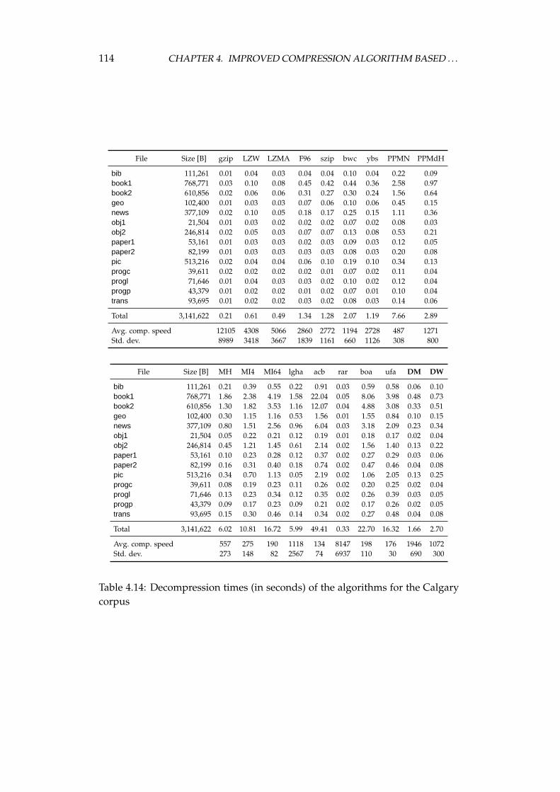
114 CHAPTER 4. IMPROVED COMPRESSION ALGORITHM BASED . . .
File Size [B] gzip LZW LZMA F96 szip bwc ybs PPMN PPMdH
bib 111,261 0.01 0.04 0.03 0.04 0.04 0.10 0.04 0.22 0.09book1 768,771 0.03 0.10 0.08 0.45 0.42 0.44 0.36 2.58 0.97book2 610,856 0.02 0.06 0.06 0.31 0.27 0.30 0.24 1.56 0.64geo 102,400 0.01 0.03 0.03 0.07 0.06 0.10 0.06 0.45 0.15news 377,109 0.02 0.10 0.05 0.18 0.17 0.25 0.15 1.11 0.36obj1 21,504 0.01 0.03 0.02 0.02 0.02 0.07 0.02 0.08 0.03obj2 246,814 0.02 0.05 0.03 0.07 0.07 0.13 0.08 0.53 0.21paper1 53,161 0.01 0.03 0.03 0.02 0.03 0.09 0.03 0.12 0.05paper2 82,199 0.01 0.03 0.03 0.03 0.03 0.08 0.03 0.20 0.08pic 513,216 0.02 0.04 0.04 0.06 0.10 0.19 0.10 0.34 0.13progc 39,611 0.02 0.02 0.02 0.02 0.01 0.07 0.02 0.11 0.04progl 71,646 0.01 0.04 0.03 0.03 0.02 0.10 0.02 0.12 0.04progp 43,379 0.01 0.02 0.02 0.01 0.02 0.07 0.01 0.10 0.04trans 93,695 0.01 0.02 0.02 0.03 0.02 0.08 0.03 0.14 0.06
Total 3,141,622 0.21 0.61 0.49 1.34 1.28 2.07 1.19 7.66 2.89
Avg. comp. speed 12105 4308 5066 2860 2772 1194 2728 487 1271Std. dev. 8989 3418 3667 1839 1161 660 1126 308 800
File Size [B] MH MI4 MI64 lgha acb rar boa ufa DM DW
bib 111,261 0.21 0.39 0.55 0.22 0.91 0.03 0.59 0.58 0.06 0.10book1 768,771 1.86 2.38 4.19 1.58 22.04 0.05 8.06 3.98 0.48 0.73book2 610,856 1.30 1.82 3.53 1.16 12.07 0.04 4.88 3.08 0.33 0.51geo 102,400 0.30 1.15 1.16 0.53 1.56 0.01 1.55 0.84 0.10 0.15news 377,109 0.80 1.51 2.56 0.96 6.04 0.03 3.18 2.09 0.23 0.34obj1 21,504 0.05 0.22 0.21 0.12 0.19 0.01 0.18 0.17 0.02 0.04obj2 246,814 0.45 1.21 1.45 0.61 2.14 0.02 1.56 1.40 0.13 0.22paper1 53,161 0.10 0.23 0.28 0.12 0.37 0.02 0.27 0.29 0.03 0.06paper2 82,199 0.16 0.31 0.40 0.18 0.74 0.02 0.47 0.46 0.04 0.08pic 513,216 0.34 0.70 1.13 0.05 2.19 0.02 1.06 2.05 0.13 0.25progc 39,611 0.08 0.19 0.23 0.11 0.26 0.02 0.20 0.25 0.02 0.04progl 71,646 0.13 0.23 0.34 0.12 0.35 0.02 0.26 0.39 0.03 0.05progp 43,379 0.09 0.17 0.23 0.09 0.21 0.02 0.17 0.26 0.02 0.05trans 93,695 0.15 0.30 0.46 0.14 0.34 0.02 0.27 0.48 0.04 0.08
Total 3,141,622 6.02 10.81 16.72 5.99 49.41 0.33 22.70 16.32 1.66 2.70
Avg. comp. speed 557 275 190 1118 134 8147 198 176 1946 1072Std. dev. 273 148 82 2567 74 6937 110 30 690 300
Table 4.14: Decompression times (in seconds) of the algorithms for the Calgarycorpus
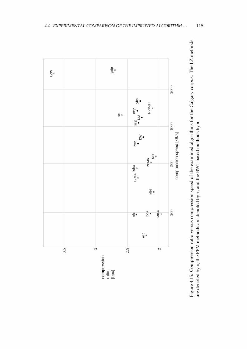
4.4. EXPERIMENTAL COMPARISON OF THE IMPROVED ALGORITHM . . . 115
••
◦
??
••
◦
◦
?
??
??
?
◦
•?
•D
WD
MLZ
MA
acb
boa
bwc
bzip
LZW gz
ip
lgha P
PM
NP
PM
dHM
HM
I4
MI6
4
rar
szip
ufa
ybs
200
500
1000
2000
2
2.53
3.5
com
pres
sion
spee
d[k
B/s
]
com
pres
sion
ratio
[bpc
]
Figu
re4.
15:
Com
pres
sion
rati
ove
rsus
com
pres
sion
spee
dof
the
exam
ined
algo
rith
ms
for
the
Cal
gary
corp
us.
The
LZm
etho
dsar
ede
note
dby
◦,th
ePP
Mm
etho
dsar
ede
note
dby
?,a
ndth
eBW
T-ba
sed
met
hods
by•.
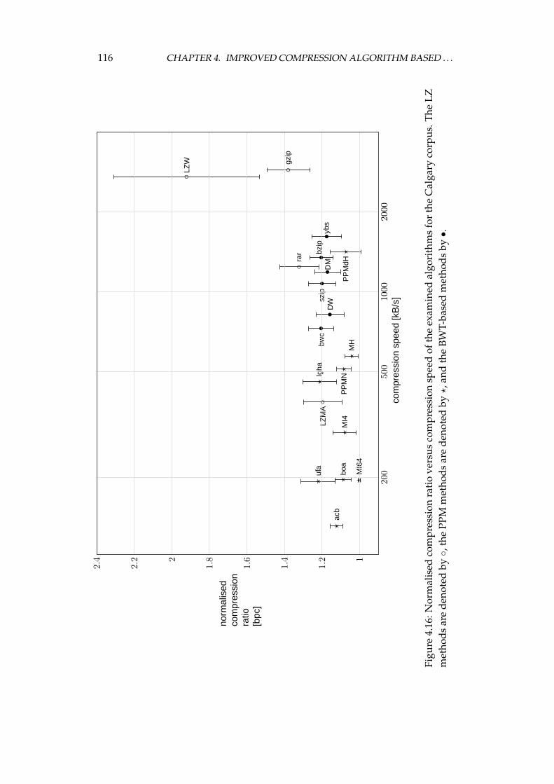
116 CHAPTER 4. IMPROVED COMPRESSION ALGORITHM BASED . . .
••
◦?
?
••
◦
◦
?
??
??
?
◦
•?
•D
WD
MLZ
MA
acb
boa
bwc
bzip
LZW gz
ip
lgha
PP
MN
PP
MdH
MH
MI4
MI6
4
rar
szip
ufa
ybs
200
500
1000
2000
1
1.2
1.4
1.6
1.82
2.2
2.4
com
pres
sion
spee
d[k
B/s
]
norm
alis
edco
mpr
essi
onra
tio[b
pc]
Figu
re4.
16:N
orm
alis
edco
mpr
essi
onra
tio
vers
usco
mpr
essi
onsp
eed
ofth
eex
amin
edal
gori
thm
sfo
rth
eC
alga
ryco
rpus
.The
LZm
etho
dsar
ede
note
dby
◦,th
ePP
Mm
etho
dsar
ede
note
dby
?,a
ndth
eBW
T-ba
sed
met
hods
by•.
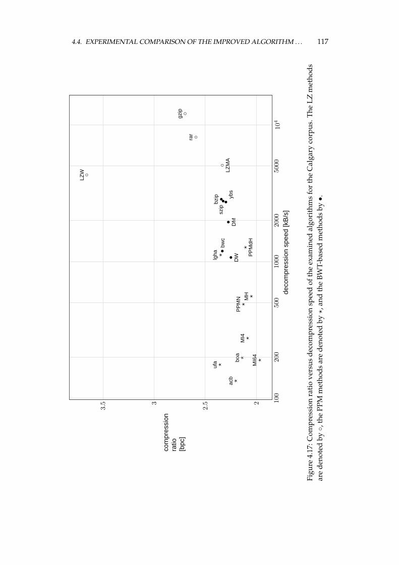
4.4. EXPERIMENTAL COMPARISON OF THE IMPROVED ALGORITHM . . . 117
••
◦
??
••
◦
◦
?
??
??
?
◦
•?
•D
WD
MLZ
MA
acb
boa
bwc
bzip
LZW
gzip
lgha
PP
MN
PP
MdH
MH
MI4
MI6
4
rar
szip
ufa
ybs
100
200
500
1000
2000
5000
104
2
2.53
3.5
deco
mpr
essi
onsp
eed
[kB
/s]
com
pres
sion
ratio
[bpc
]
Figu
re4.
17:C
ompr
essi
onra
tio
vers
usde
com
pres
sion
spee
dof
the
exam
ined
algo
rith
ms
for
the
Cal
gary
corp
us.T
heLZ
met
hods
are
deno
ted
by◦,
the
PPM
met
hods
are
deno
ted
by?
,and
the
BWT-
base
dm
etho
dsby
•.
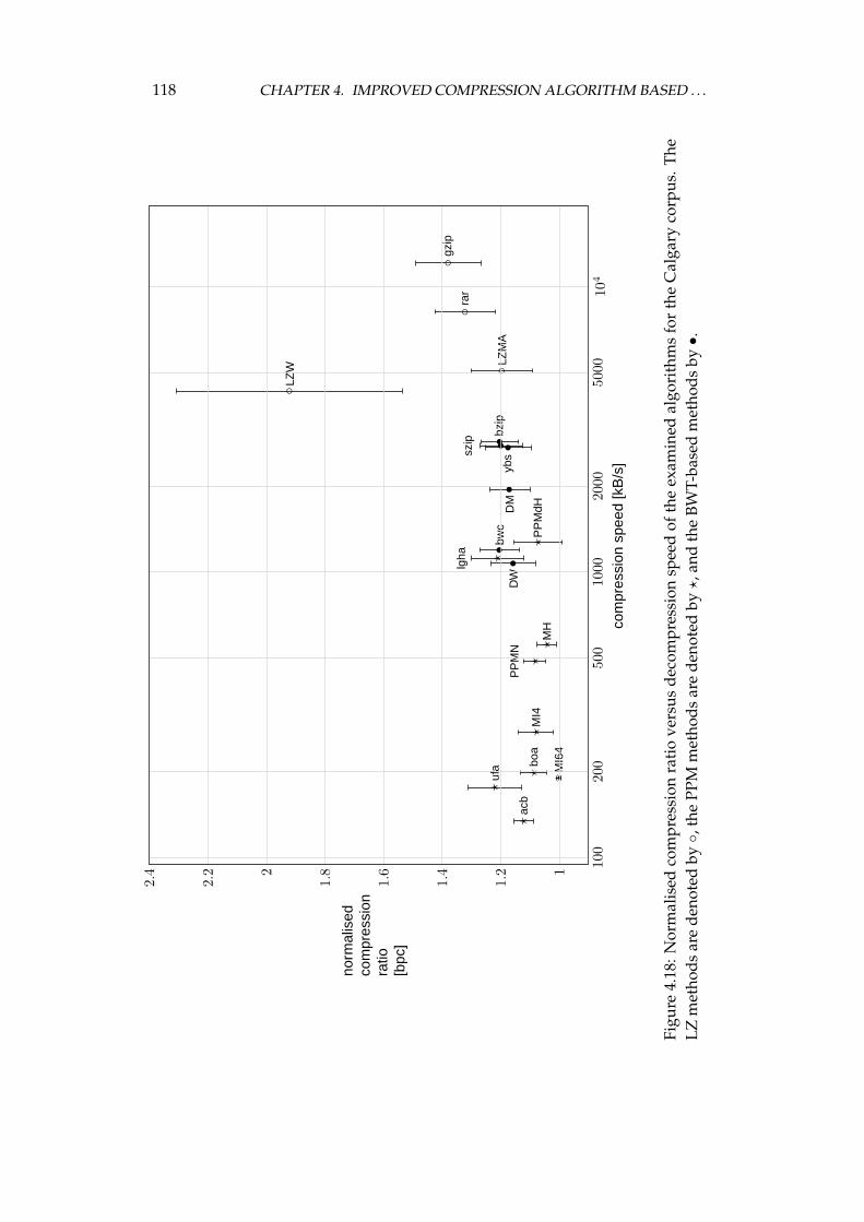
118 CHAPTER 4. IMPROVED COMPRESSION ALGORITHM BASED . . .
••
◦?
?
••
◦
◦
?
??
??
?
◦
•?
•D
WD
MLZ
MA
acb
boa
bwc
bzip
LZW
gzip
lgha
PP
MN
PP
MdH
MH
MI4
MI6
4
rar
szip
ufa
ybs
100
200
500
1000
2000
5000
104
1
1.2
1.4
1.6
1.82
2.2
2.4
com
pres
sion
spee
d[k
B/s
]
norm
alis
edco
mpr
essi
onra
tio[b
pc]
Figu
re4.
18:N
orm
alis
edco
mpr
essi
onra
tio
vers
usde
com
pres
sion
spee
dof
the
exam
ined
algo
rith
ms
for
the
Cal
gary
corp
us.T
heLZ
met
hods
are
deno
ted
by◦,
the
PPM
met
hods
are
deno
ted
by?
,and
the
BWT-
base
dm
etho
dsby
•.
4.4. EXPERIMENTAL COMPARISON OF THE IMPROVED ALGORITHM . . . 119
based compression methods obtain compression ratios comparable to the PPMmethods, but work significantly faster. The only exception is the recent PPMdHalgorithm by Shkarin [155] published in 2002. It obtains very good compressionratios and compresses relatively fast. We see that this algorithm dominates themost of the BWT-based algorithms, however standard deviation of compressionratio and especially compression speed is much higher than for the BWT-basedmethods. We can see that also both the BWT-based algorithms proposed in thisdissertation, the DW (BWT-based algorithm with the WFC as the second stage)and the DM (BWT-based algorithm with the MTF-2 as the second stage), ob-tain better compression ratios than other BWT-based algorithms and all the LZmethods.
Let us take a look at Figures 4.17 and 4.18, in which the speeds of decompres-sion are compared to the compression ratios. We can observe that, the decom-pression speed of the PPM algorithms is almost identical to their compressionspeed. The LZ algorithms decompress much faster than compress. The differ-ence between decompression and compression speed for the BWT-based algo-rithms is significant but lower than for the LZ algorithms. Now, the PPMdHalgorithm dominates only two BWT-based methods, however standard devia-tions of their average decompression speed is much higher than for those al-gorithms. The DM algorithm is Pareto-optimal, while the DW algorithm leadsto the best compression ratios in the family of the BWT-based methods. An in-teresting algorithm is the LZMA method, which achieves the best compressionratios among the LZ methods. The compression speed of this algorithm is low, itis over two times slower than the slowest BWT-based method, but with regardsto the decompression speed it outperforms all the BWT-based algorithms, andalso the LZW method.
As we can see, the results are almost identical if we analyse the standardcompression ratio and the normalised compression ratio. The advantage of thenormalised ratios is that the standard deviation of compression ratios are muchlower. It is caused by the definition of this ratio, which entails that the best com-pression ratio can be 1.000. If we calculate the standard deviation of standardcompression ratios, we should remember, that we compress files of differenttypes, so the possible compression ratio can differ by a large factor. For example,no algorithm achieves better compression ratio than 3.800 bpc for geo file, whileall the examined compression methods have no problem to break the 1.000 bpcratio for pic file. The advantage of the standard compression ratio is that it doesnot change when new compression methods are introduced. The normalisedcompression ratio changes every time an algorithm that gives the best compres-sion ratio for any file from the corpus is introduced. Many papers also containcompression results calculated as the standard compression ratio, so it is easy touse them for a brief comparison.
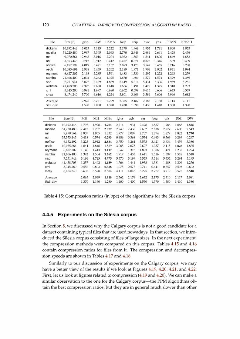
120 CHAPTER 4. IMPROVED COMPRESSION ALGORITHM BASED . . .
File Size [B] gzip LZW LZMA bzip szip bwc ybs PPMN PPMdH
dickens 10,192,446 3.023 3.145 2.222 2.178 1.968 1.952 1.781 1.800 1.853mozilla 51,220,480 2.967 5.305 2.093 2.770 2.649 2.684 2.641 2.428 2.476mr 9,970,564 2.948 3.016 2.204 1.932 1.869 1.841 1.806 1.849 1.883nci 33,553,445 0.712 0.912 0.412 0.427 0.371 0.328 0.316 0.539 0.439ooffice 6,152,192 4.019 5.471 3.157 3.693 3.473 3.547 3.465 3.216 3.288osdb 10,085,684 2.948 3.459 2.262 2.189 1.971 1.908 2.002 1.941 1.894reymont 6,627,202 2.198 2.265 1.591 1.483 1.330 1.292 1.222 1.293 1.279samba 21,606,400 2.002 3.262 1.395 1.670 1.600 1.579 1.574 1.429 1.389sao 7,251,944 5.877 7.429 4.889 5.449 5.314 5.431 5.306 4.959 5.281webster 41,458,703 2.327 2.680 1.618 1.656 1.491 1.429 1.325 1.310 1.293xml 5,345,280 0.991 1.697 0.680 0.652 0.599 0.616 0.606 0.643 0.569x-ray 8,474,240 5.700 6.616 4.224 3.801 3.609 3.584 3.606 3.946 3.682
Average 2.976 3.771 2.229 2.325 2.187 2.183 2.138 2.113 2.111Std. dev. 1.590 2.000 1.320 1.420 1.390 1.430 1.410 1.330 1.390
File Size [B] MH MI4 MI64 lgha acb rar boa ufa DM DW
dickens 10,192,446 1.797 1.928 1.704 2.214 1.931 2.498 1.837 1.986 1.868 1.816mozilla 51,220,480 2.417 2.237 2.077 2.949 2.436 2.602 2.638 2.777 2.600 2.543mr 9,970,564 1.857 1.835 1.832 1.977 2.007 2.707 1.874 1.879 1.822 1.770nci 33,553,445 0.418 0.574 0.293 0.686 0.368 0.534 0.463 0.569 0.299 0.297ooffice 6,152,192 3.225 2.942 2.834 3.750 3.264 3.573 3.421 3.634 3.459 3.380osdb 10,085,684 1.844 1.848 1.839 3.085 2.075 2.627 1.957 2.115 1.828 1.835reymont 6,627,202 1.140 1.413 1.117 1.547 1.313 1.893 1.386 1.471 1.237 1.224samba 21,606,400 1.342 1.504 1.262 1.917 1.453 1.641 1.516 1.697 1.518 1.518sao 7,251,944 5.186 4.763 4.775 5.370 5.199 5.555 5.214 5.332 5.294 5.195webster 41,458,703 1.257 1.402 1.159 1.766 1.441 1.938 1.381 1.488 1.309 1.276xml 5,345,280 0.556 0.803 0.538 1.075 0.577 0.741 0.641 0.857 0.595 0.602x-ray 8,474,240 3.637 3.578 3.584 4.411 4.043 5.275 3.772 3.919 3.575 3.518
Average 2.065 2.069 1.918 2.562 2.176 2.632 2.175 2.310 2.117 2.081Std. dev. 1.370 1.190 1.280 1.400 1.400 1.550 1.370 1.380 1.410 1.380
Table 4.15: Compression ratios (in bpc) of the algorithms for the Silesia corpus
4.4.5 Experiments on the Silesia corpus
In Section 5, we discussed why the Calgary corpus is not a good candidate for adataset containing typical files that are used nowadays. In that section, we intro-duced the Silesia corpus consisting of files of large sizes. In the next experiment,the compression methods were compared on this corpus. Tables 4.15 and 4.16contain compression ratios for files from it. The compression and decompres-sion speeds are shown in Tables 4.17 and 4.18.
Similarly to our discussion of experiments on the Calgary corpus, we mayhave a better view of the results if we look at Figures 4.19, 4.20, 4.21, and 4.22.First, let us look at figures related to compression (4.19 and 4.20). We can make asimilar observation to the one for the Calgary corpus—the PPM algorithms ob-tain the best compression ratios, but they are in general much slower than other
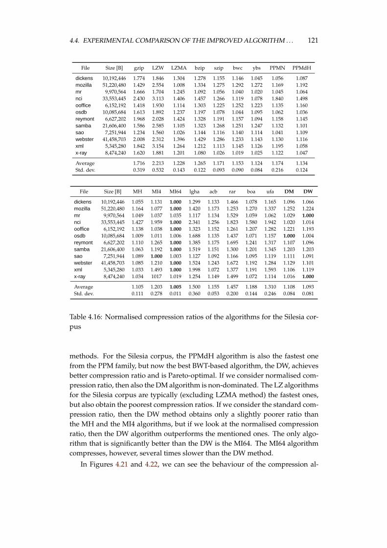
4.4. EXPERIMENTAL COMPARISON OF THE IMPROVED ALGORITHM . . . 121
File Size [B] gzip LZW LZMA bzip szip bwc ybs PPMN PPMdH
dickens 10,192,446 1.774 1.846 1.304 1.278 1.155 1.146 1.045 1.056 1.087mozilla 51,220,480 1.429 2.554 1.008 1.334 1.275 1.292 1.272 1.169 1.192mr 9,970,564 1.666 1.704 1.245 1.092 1.056 1.040 1.020 1.045 1.064nci 33,553,445 2.430 3.113 1.406 1.457 1.266 1.119 1.078 1.840 1.498ooffice 6,152,192 1.418 1.930 1.114 1.303 1.225 1.252 1.223 1.135 1.160osdb 10,085,684 1.613 1.892 1.237 1.197 1.078 1.044 1.095 1.062 1.036reymont 6,627,202 1.968 2.028 1.424 1.328 1.191 1.157 1.094 1.158 1.145samba 21,606,400 1.586 2.585 1.105 1.323 1.268 1.251 1.247 1.132 1.101sao 7,251,944 1.234 1.560 1.026 1.144 1.116 1.140 1.114 1.041 1.109webster 41,458,703 2.008 2.312 1.396 1.429 1.286 1.233 1.143 1.130 1.116xml 5,345,280 1.842 3.154 1.264 1.212 1.113 1.145 1.126 1.195 1.058x-ray 8,474,240 1.620 1.881 1.201 1.080 1.026 1.019 1.025 1.122 1.047
Average 1.716 2.213 1.228 1.265 1.171 1.153 1.124 1.174 1.134Std. dev. 0.319 0.532 0.143 0.122 0.093 0.090 0.084 0.216 0.124
File Size [B] MH MI4 MI64 lgha acb rar boa ufa DM DW
dickens 10,192,446 1.055 1.131 1.000 1.299 1.133 1.466 1.078 1.165 1.096 1.066mozilla 51,220,480 1.164 1.077 1.000 1.420 1.173 1.253 1.270 1.337 1.252 1.224mr 9,970,564 1.049 1.037 1.035 1.117 1.134 1.529 1.059 1.062 1.029 1.000nci 33,553,445 1.427 1.959 1.000 2.341 1.256 1.823 1.580 1.942 1.020 1.014ooffice 6,152,192 1.138 1.038 1.000 1.323 1.152 1.261 1.207 1.282 1.221 1.193osdb 10,085,684 1.009 1.011 1.006 1.688 1.135 1.437 1.071 1.157 1.000 1.004reymont 6,627,202 1.110 1.265 1.000 1.385 1.175 1.695 1.241 1.317 1.107 1.096samba 21,606,400 1.063 1.192 1.000 1.519 1.151 1.300 1.201 1.345 1.203 1.203sao 7,251,944 1.089 1.000 1.003 1.127 1.092 1.166 1.095 1.119 1.111 1.091webster 41,458,703 1.085 1.210 1.000 1.524 1.243 1.672 1.192 1.284 1.129 1.101xml 5,345,280 1.033 1.493 1.000 1.998 1.072 1.377 1.191 1.593 1.106 1.119x-ray 8,474,240 1.034 1017 1.019 1.254 1.149 1.499 1.072 1.114 1.016 1.000
Average 1.105 1.203 1.005 1.500 1.155 1.457 1.188 1.310 1.108 1.093Std. dev. 0.111 0.278 0.011 0.360 0.053 0.200 0.144 0.246 0.084 0.081
Table 4.16: Normalised compression ratios of the algorithms for the Silesia cor-pus
methods. For the Silesia corpus, the PPMdH algorithm is also the fastest onefrom the PPM family, but now the best BWT-based algorithm, the DW, achievesbetter compression ratio and is Pareto-optimal. If we consider normalised com-pression ratio, then also the DM algorithm is non-dominated. The LZ algorithmsfor the Silesia corpus are typically (excluding LZMA method) the fastest ones,but also obtain the poorest compression ratios. If we consider the standard com-pression ratio, then the DW method obtains only a slightly poorer ratio thanthe MH and the MI4 algorithms, but if we look at the normalised compressionratio, then the DW algorithm outperforms the mentioned ones. The only algo-rithm that is significantly better than the DW is the MI64. The MI64 algorithmcompresses, however, several times slower than the DW method.
In Figures 4.21 and 4.22, we can see the behaviour of the compression al-
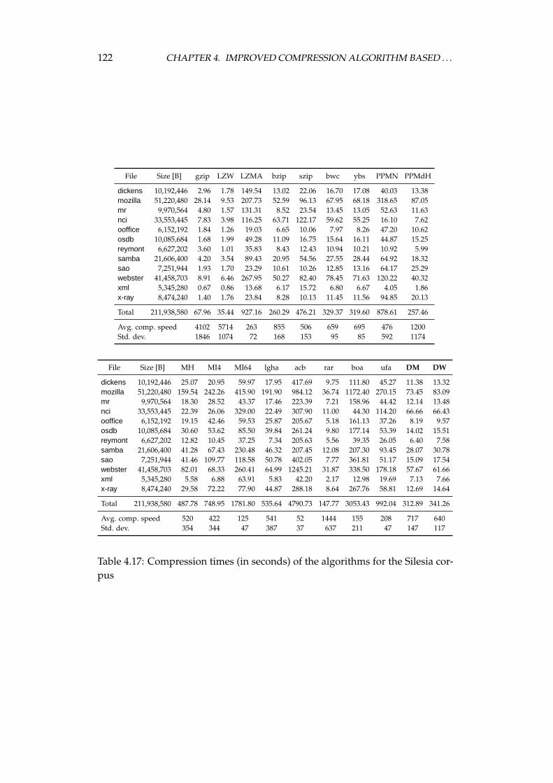
122 CHAPTER 4. IMPROVED COMPRESSION ALGORITHM BASED . . .
File Size [B] gzip LZW LZMA bzip szip bwc ybs PPMN PPMdH
dickens 10,192,446 2.96 1.78 149.54 13.02 22.06 16.70 17.08 40.03 13.38mozilla 51,220,480 28.14 9.53 207.73 52.59 96.13 67.95 68.18 318.65 87.05mr 9,970,564 4.80 1.57 131.31 8.52 23.54 13.45 13.05 52.63 11.63nci 33,553,445 7.83 3.98 116.25 63.71 122.17 59.62 55.25 16.10 7.62ooffice 6,152,192 1.84 1.26 19.03 6.65 10.06 7.97 8.26 47.20 10.62osdb 10,085,684 1.68 1.99 49.28 11.09 16.75 15.64 16.11 44.87 15.25reymont 6,627,202 3.60 1.01 35.83 8.43 12.43 10.94 10.21 10.92 5.99samba 21,606,400 4.20 3.54 89.43 20.95 54.56 27.55 28.44 64.92 18.32sao 7,251,944 1.93 1.70 23.29 10.61 10.26 12.85 13.16 64.17 25.29webster 41,458,703 8.91 6.46 267.95 50.27 82.40 78.45 71.63 120.22 40.32xml 5,345,280 0.67 0.86 13.68 6.17 15.72 6.80 6.67 4.05 1.86x-ray 8,474,240 1.40 1.76 23.84 8.28 10.13 11.45 11.56 94.85 20.13
Total 211,938,580 67.96 35.44 927.16 260.29 476.21 329.37 319.60 878.61 257.46
Avg. comp. speed 4102 5714 263 855 506 659 695 476 1200Std. dev. 1846 1074 72 168 153 95 85 592 1174
File Size [B] MH MI4 MI64 lgha acb rar boa ufa DM DW
dickens 10,192,446 25.07 20.95 59.97 17.95 417.69 9.75 111.80 45.27 11.38 13.32mozilla 51,220,480 159.54 242.26 415.90 191.90 984.12 36.74 1172.40 270.15 73.45 83.09mr 9,970,564 18.30 28.52 43.37 17.46 223.39 7.21 158.96 44.42 12.14 13.48nci 33,553,445 22.39 26.06 329.00 22.49 307.90 11.00 44.30 114.20 66.66 66.43ooffice 6,152,192 19.15 42.46 59.53 25.87 205.67 5.18 161.13 37.26 8.19 9.57osdb 10,085,684 30.60 53.62 85.50 39.84 261.24 9.80 177.14 53.39 14.02 15.51reymont 6,627,202 12.82 10.45 37.25 7.34 205.63 5.56 39.35 26.05 6.40 7.58samba 21,606,400 41.28 67.43 230.48 46.32 207.45 12.08 207.30 93.45 28.07 30.78sao 7,251,944 41.46 109.77 118.58 50.78 402.05 7.77 361.81 51.17 15.09 17.54webster 41,458,703 82.01 68.33 260.41 64.99 1245.21 31.87 338.50 178.18 57.67 61.66xml 5,345,280 5.58 6.88 63.91 5.83 42.20 2.17 12.98 19.69 7.13 7.66x-ray 8,474,240 29.58 72.22 77.90 44.87 288.18 8.64 267.76 58.81 12.69 14.64
Total 211,938,580 487.78 748.95 1781.80 535.64 4790.73 147.77 3053.43 992.04 312.89 341.26
Avg. comp. speed 520 422 125 541 52 1444 155 208 717 640Std. dev. 354 344 47 387 37 637 211 47 147 117
Table 4.17: Compression times (in seconds) of the algorithms for the Silesia cor-pus
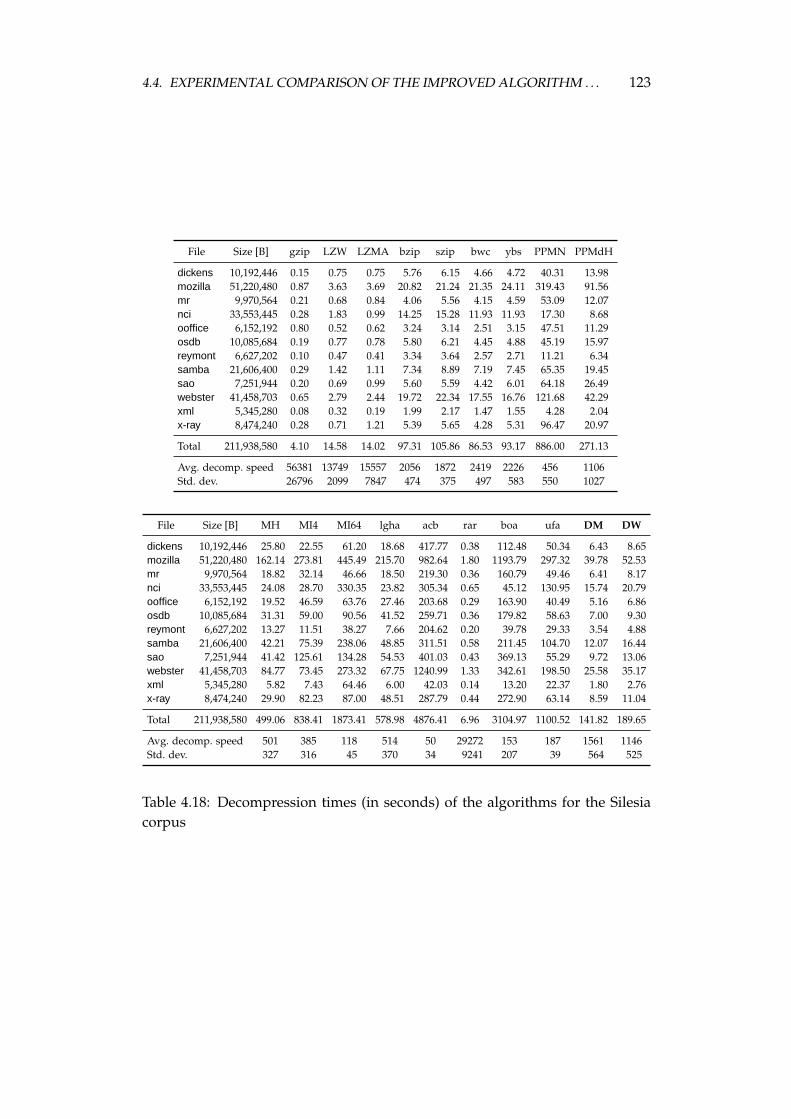
4.4. EXPERIMENTAL COMPARISON OF THE IMPROVED ALGORITHM . . . 123
File Size [B] gzip LZW LZMA bzip szip bwc ybs PPMN PPMdH
dickens 10,192,446 0.15 0.75 0.75 5.76 6.15 4.66 4.72 40.31 13.98mozilla 51,220,480 0.87 3.63 3.69 20.82 21.24 21.35 24.11 319.43 91.56mr 9,970,564 0.21 0.68 0.84 4.06 5.56 4.15 4.59 53.09 12.07nci 33,553,445 0.28 1.83 0.99 14.25 15.28 11.93 11.93 17.30 8.68ooffice 6,152,192 0.80 0.52 0.62 3.24 3.14 2.51 3.15 47.51 11.29osdb 10,085,684 0.19 0.77 0.78 5.80 6.21 4.45 4.88 45.19 15.97reymont 6,627,202 0.10 0.47 0.41 3.34 3.64 2.57 2.71 11.21 6.34samba 21,606,400 0.29 1.42 1.11 7.34 8.89 7.19 7.45 65.35 19.45sao 7,251,944 0.20 0.69 0.99 5.60 5.59 4.42 6.01 64.18 26.49webster 41,458,703 0.65 2.79 2.44 19.72 22.34 17.55 16.76 121.68 42.29xml 5,345,280 0.08 0.32 0.19 1.99 2.17 1.47 1.55 4.28 2.04x-ray 8,474,240 0.28 0.71 1.21 5.39 5.65 4.28 5.31 96.47 20.97
Total 211,938,580 4.10 14.58 14.02 97.31 105.86 86.53 93.17 886.00 271.13
Avg. decomp. speed 56381 13749 15557 2056 1872 2419 2226 456 1106Std. dev. 26796 2099 7847 474 375 497 583 550 1027
File Size [B] MH MI4 MI64 lgha acb rar boa ufa DM DW
dickens 10,192,446 25.80 22.55 61.20 18.68 417.77 0.38 112.48 50.34 6.43 8.65mozilla 51,220,480 162.14 273.81 445.49 215.70 982.64 1.80 1193.79 297.32 39.78 52.53mr 9,970,564 18.82 32.14 46.66 18.50 219.30 0.36 160.79 49.46 6.41 8.17nci 33,553,445 24.08 28.70 330.35 23.82 305.34 0.65 45.12 130.95 15.74 20.79ooffice 6,152,192 19.52 46.59 63.76 27.46 203.68 0.29 163.90 40.49 5.16 6.86osdb 10,085,684 31.31 59.00 90.56 41.52 259.71 0.36 179.82 58.63 7.00 9.30reymont 6,627,202 13.27 11.51 38.27 7.66 204.62 0.20 39.78 29.33 3.54 4.88samba 21,606,400 42.21 75.39 238.06 48.85 311.51 0.58 211.45 104.70 12.07 16.44sao 7,251,944 41.42 125.61 134.28 54.53 401.03 0.43 369.13 55.29 9.72 13.06webster 41,458,703 84.77 73.45 273.32 67.75 1240.99 1.33 342.61 198.50 25.58 35.17xml 5,345,280 5.82 7.43 64.46 6.00 42.03 0.14 13.20 22.37 1.80 2.76x-ray 8,474,240 29.90 82.23 87.00 48.51 287.79 0.44 272.90 63.14 8.59 11.04
Total 211,938,580 499.06 838.41 1873.41 578.98 4876.41 6.96 3104.97 1100.52 141.82 189.65
Avg. decomp. speed 501 385 118 514 50 29272 153 187 1561 1146Std. dev. 327 316 45 370 34 9241 207 39 564 525
Table 4.18: Decompression times (in seconds) of the algorithms for the Silesiacorpus
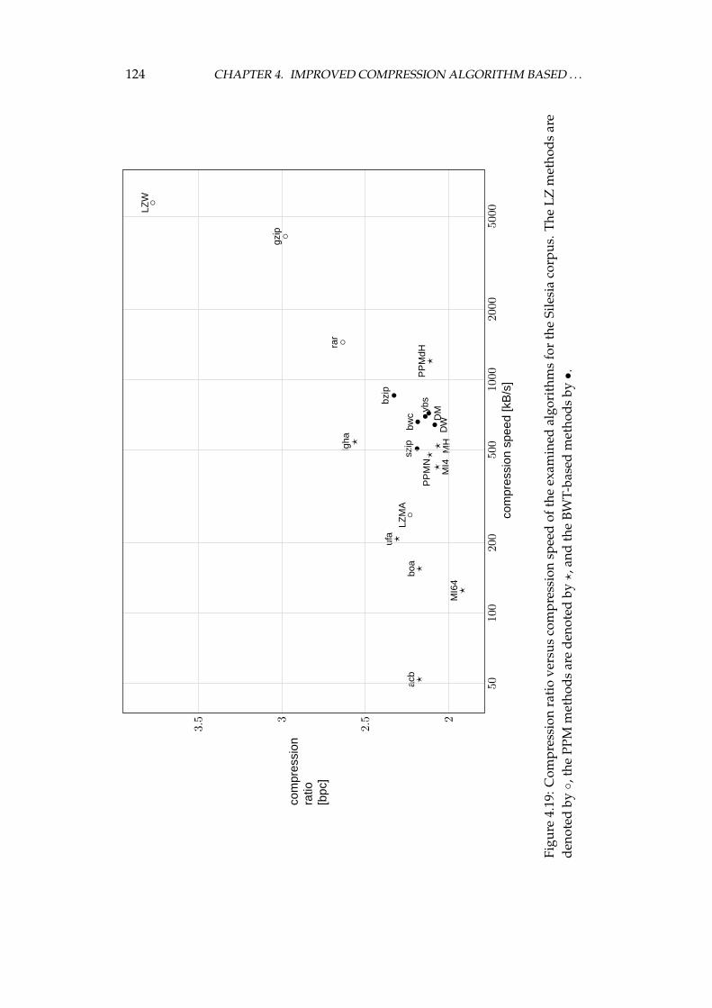
124 CHAPTER 4. IMPROVED COMPRESSION ALGORITHM BASED . . .
••
◦?
?•
•
◦
◦
?
??
??
?
◦
•
?
•D
WD
M
LZM
Aac
bbo
abw
c
bzip
LZW
gzip
lgha
PP
MN
PP
MdH
MH
MI4
MI6
4
rar
szip
ufa
ybs
5010
020
050
010
0020
0050
00
2
2.53
3.5
com
pres
sion
spee
d[k
B/s
]
com
pres
sion
ratio
[bpc
]
Figu
re4.
19:C
ompr
essi
onra
tio
vers
usco
mpr
essi
onsp
eed
ofth
eex
amin
edal
gori
thm
sfo
rth
eSi
lesi
aco
rpus
.The
LZm
etho
dsar
ede
note
dby
◦,th
ePP
Mm
etho
dsar
ede
note
dby
?,a
ndth
eBW
T-ba
sed
met
hods
by•.
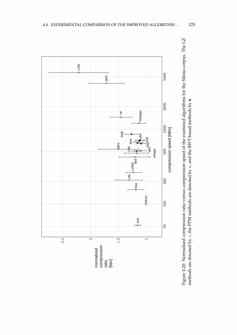
4.4. EXPERIMENTAL COMPARISON OF THE IMPROVED ALGORITHM . . . 125
••
◦?
?•
•
◦
◦
?
??
?
?
?
◦
•
?
•
DW
DM
LZM
A
acb
boa
bwc
bzip
LZW
gzip
lgha
PP
MN
PP
MdH
MH
MI4
MI6
4
rar
szip
ufa
ybs
5010
020
050
010
0020
0050
00
1
1.52
2.5
com
pres
sion
spee
d[k
B/s
]
norm
alis
edco
mpr
essi
onra
tio[b
pc]
Figu
re4.
20:
Nor
mal
ised
com
pres
sion
rati
ove
rsus
com
pres
sion
spee
dof
the
exam
ined
algo
rith
ms
for
the
Sile
sia
corp
us.
The
LZm
etho
dsar
ede
note
dby
◦,th
ePP
Mm
etho
dsar
ede
note
dby
?,a
ndth
eBW
T-ba
sed
met
hods
by•.
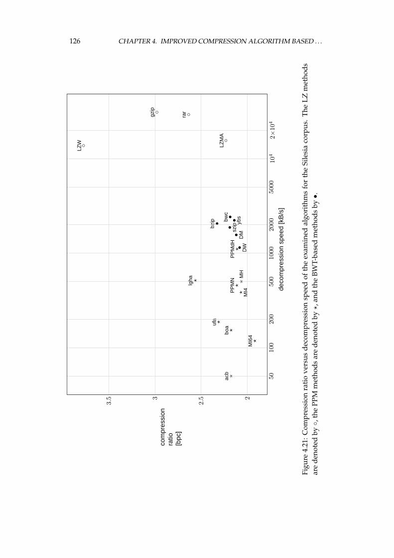
126 CHAPTER 4. IMPROVED COMPRESSION ALGORITHM BASED . . .
••
◦?
?•
•
◦
◦
?
??
??
?
◦
•
?
•D
WD
M
LZM
Aac
bbo
abw
c
bzip
LZW
gzip
lgha
PP
MN
PP
MdH
MH
MI4
MI6
4
rar
szip
ufa
ybs
5010
020
050
010
0020
0050
0010
42×
104
2
2.53
3.5
deco
mpr
essi
onsp
eed
[kB
/s]
com
pres
sion
ratio
[bpc
]
Figu
re4.
21:
Com
pres
sion
rati
ove
rsus
deco
mpr
essi
onsp
eed
ofth
eex
amin
edal
gori
thm
sfo
rth
eSi
lesi
aco
rpus
.T
heLZ
met
hods
are
deno
ted
by◦,
the
PPM
met
hods
are
deno
ted
by?
,and
the
BWT-
base
dm
etho
dsby
•.
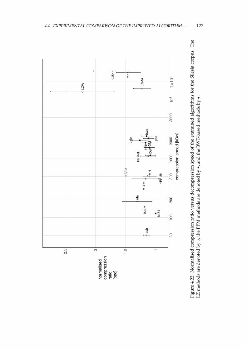
4.4. EXPERIMENTAL COMPARISON OF THE IMPROVED ALGORITHM . . . 127
••
◦?
?•
•
◦
◦
?
??
?
?
?
◦
•
?
•D
WD
M
LZM
Aac
bbo
abw
c
bzip
LZW
gzip
lgha
PP
MN
PP
MdH
MH
MI4
MI6
4
rar
szip
ufa
ybs
5010
020
050
010
0020
0050
0010
42×
104
1
1.52
2.5
com
pres
sion
spee
d[k
B/s
]
norm
alis
edco
mpr
essi
onra
tio[b
pc]
Figu
re4.
22:
Nor
mal
ised
com
pres
sion
rati
ove
rsus
deco
mpr
essi
onsp
eed
ofth
eex
amin
edal
gori
thm
sfo
rth
eSi
lesi
aco
rpus
.Th
eLZ
met
hods
are
deno
ted
by◦,
the
PPM
met
hods
are
deno
ted
by?
,and
the
BWT-
base
dm
etho
dsby
•.
128 CHAPTER 4. IMPROVED COMPRESSION ALGORITHM BASED . . .
gorithms in the decompress process for the Silesia corpus. The observation isalso similar to that made for the Calgary corpus. The decompression speed ofthe LZ methods is significantly higher than their compression speed. The PPMalgorithms compress and decompress with almost identical speed. All the ex-amined BWT-based methods decompress faster than PPM algorithms, but thedifference between the PPMdH and DW is small.
The standard deviation of the compression and decompression speed is sig-nificantly lower for the BWT-based algorithms than for the PPM methods. Alsothe standard deviation of the normalised compression ratio for the majority ofthe BWT-based algorithms is smaller than for the PPM methods (except for MI64and acb).
Until now, we have analysed the average compression ratio. Let us now takea look at the specific files from the Silesia corpus. The dominance, in terms of thecompression ratio, of the MI64 algorithm is almost total for the Calgary corpus.In the experiments for the Silesia corpus, we see that this method achieves thebest compression ratios only for 8 out of 12 files. For one file, sao, the bestcompression ratio obtains the MI4 algorithm, while for the other three, the bestare the methods introduced in this dissertation—DW and DM. For two medicalfiles, mr and x-ray, the DW method achieves significantly better compressionratio than the MI64 algorithm. For the last file, osdb, the DW algorithm alsooutperforms the MI64 method, but the DM algorithm is even better.
4.4.6 Experiments on files of different sizes and similar contents
In the last experiment, we compare the compression algorithms on files of sim-ilar contents and different sizes. For this purpose, four files from the Silesiacorpus were chosen. Each file is of different type: dickens is a plain text file,osdb is a binary database file, samba consists of concatenated source code filesof a programming project, and x-ray is a representation of a medical image.
From each file the pieces of sizes 8 kB, 16 kB, 32 kB, 64 kB, . . . , 8192 kB,and in one case also 16384 kB, were taken starting always from the beginningof the file. Several compression methods were run on the obtained files. Ta-bles E.1–E.8 contain the results of these experiments. The results are also plottedin Figures 4.23–4.30 to show how the properties of the compression methodsdepend on the file size.
Figures 4.23 and 4.24 illustrate the experiments with parts of the dickens file.The compression ratio decreases almost monotonically while the file size grows.It is what one would expect, as the contents of the dickens file is an English textand on larger files the probability of symbol occurrence can be estimated better.The only compression algorithm, for which there is no progress in the compres-sion ratio for large files is bzip. It happens because if the size of the file to becompressed is bigger than 900 kB, the bzip program splits the file into pieces of
4.4. EXPERIMENTAL COMPARISON OF THE IMPROVED ALGORITHM . . . 129
size 900 kB, and compresses them separately. More interesting observations canbe made for this file if we look at the dependence of the compression speed onthe file size. For small files, the compression speed grows for all the algorithmsif the file size grows. If the file to be compressed breaks the limit of several tens–several hundred kB, the compression speed decreases. For the PPM algorithmsit is caused by the need of storing and searching a model of vast size. For theBWT-based algorithms, the decrease of speed is caused by the sorting procedurein the BWT, which is super-linear. The speed of the bzip method is steady forlarge files, as this program compresses separately pieces of size of 900 kB. Thespeed-improved BWT computation algorithm used in the DW method allowsthe compressor decrease the speed of compression slowly.
The results of the experiments for a binary database file, osdb, are presentedin Figures 4.25 and 4.26. Looking at the first figure, we see also a monotonicimprovement of the compression ratio for all the compression methods withgrowing file size. We notice also how the compression ratio of the BWT-basedmethods, ybs and DW, improves, closing to the one obtained by the MI64 al-gorithm. For the largest file, the compression ratios of the DW and the MI64algorithms are almost equal. The situation shown in Figure 4.26 is similar tothe one discussed for the dickens file. Here the decrease of speed for the DWalgorithm is also slow.
The samba file is a tarred source code of a programming project. The projectcontains files which are: C and Perl sources, documentation in HTML, PDF andtext files, text configuration files, and others. What is important, the files arerather small and of very different contents. Therefore, the contents of the sambafile is changing from part to part of this file. Figure 4.27 shows how hard aredifferent parts of the file to compress. All the compression algorithms behavesimilarly and as we can see, the PPM, and the LZ algorithms achieve the bestcompression ratios. Analysing Figure 4.28 we notice how the compression speedvaries. The general tendency of decreasing the speed with file size growing can-not be observed. We can, however, notice that the speeds of the bzip, PPMdH,and DW algorithms are similar for files of different sizes (larger than 50 kB).
The last file in this experiment, x-ray, stores an X-ray image. The compres-sion ratios, shown in Figure 4.29, decrease with growing file size, however forthe largest files, the ratio slightly deteriorates. For pieces of small size the bestresults are obtained by the MI64 and the LZMA algorithms. With the growth ofthe file size, the compression ratio improves for them much slower than for theBWT-based algorithms. When the file size exceeds 100 kB, the DW algorithmyields the best compression ratio. The DW method outperforms significantly,with regard to the compression ratio, other methods for this sequence. Weshould notice also a very good result of the BWT-based compression method,ybs, which obtains ratios almost identical to the best PPM algorithm. Similar
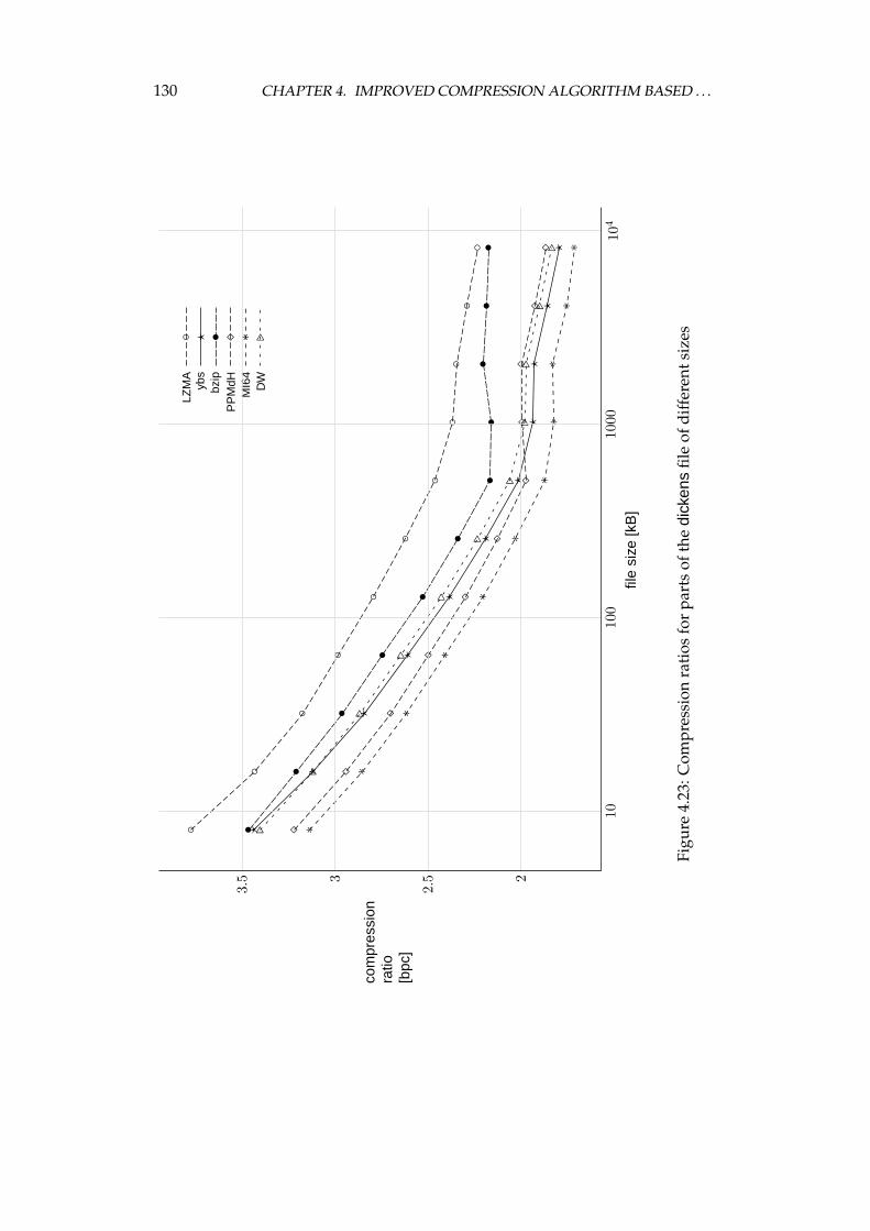
130 CHAPTER 4. IMPROVED COMPRESSION ALGORITHM BASED . . .
◦
◦
◦
◦
◦
◦
◦◦
◦◦
◦
?
?
?
?
?
?
??
??
?
•
•
•
•
•
•
••
••
•
�
�
�
�
�
�
��
��
�
∗
∗
∗
∗
∗
∗
∗∗
∗∗
∗
.
.
.
.
.
.
..
..
.
LZM
A◦
ybs
?bz
ip•
PP
MdH
�M
I64
∗D
W.
1010
010
0010
4
2
2.53
3.5
file
size
[kB
]
com
pres
sion
ratio
[bpc
]
Figu
re4.
23:C
ompr
essi
onra
tios
for
part
sof
the
dick
ens
file
ofdi
ffer
ents
izes
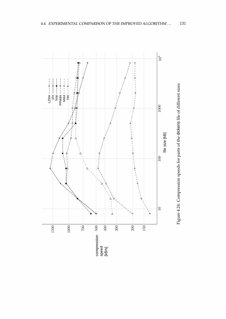
4.4. EXPERIMENTAL COMPARISON OF THE IMPROVED ALGORITHM . . . 131
◦
◦
◦
◦◦
◦◦
◦◦
◦◦
?
?
?
??
?
?
??
??
•
•
••
••
••
••
•
�
�
��
��
��
��
�
∗
∗∗
∗∗
∗∗
∗∗
∗∗
..
.
.
..
..
..
.
LZM
A◦
ybs
?bz
ip•
PP
MdH
�M
I64
∗D
W.
1010
010
0010
4
150
200
300
400
500
700
1000
1500
file
size
[kB
]
com
pres
sion
spee
d[k
B/s
]
Figu
re4.
24:C
ompr
essi
onsp
eeds
for
part
sof
the
dick
ens
file
ofdi
ffer
ents
izes
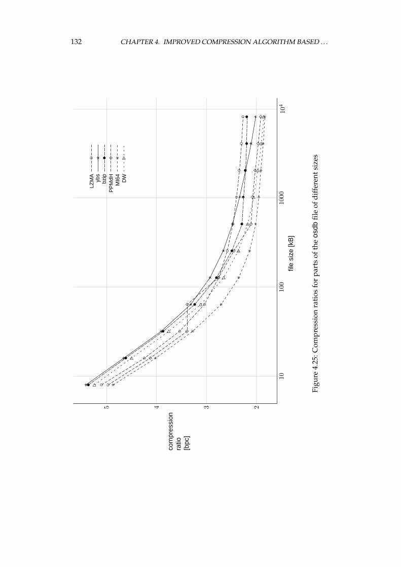
132 CHAPTER 4. IMPROVED COMPRESSION ALGORITHM BASED . . .
◦
◦
◦
◦
◦◦
◦◦
◦◦
◦
?
?
?
?
?
?
??
??
?
•
•
•
•
•
••
••
••
�
�
��
�
�
��
��
�
∗
∗
∗
∗
∗∗
∗∗
∗∗
∗
.
.
.
.
.
.
..
..
.
LZM
A◦
ybs
?bz
ip•
PP
MdH
�M
I64
∗D
W.
1010
010
0010
4
2345
file
size
[kB
]
com
pres
sion
ratio
[bpc
]
Figu
re4.
25:C
ompr
essi
onra
tios
for
part
sof
the
osdb
file
ofdi
ffer
ents
izes
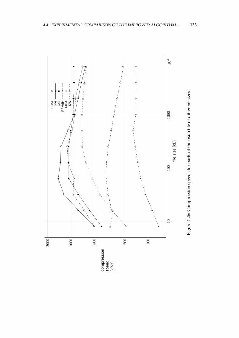
4.4. EXPERIMENTAL COMPARISON OF THE IMPROVED ALGORITHM . . . 133
◦
◦◦
◦◦
◦◦
◦◦
◦◦
?
?
?
??
?
?
??
??
•
•
•
••
••
••
••
�
�
��
��
��
��
�
∗∗
∗∗
∗∗
∗∗
∗∗
∗
..
.
.
..
..
..
.
LZM
A◦
ybs
?bz
ip•
PP
MdH
�M
I64
∗D
W.
1010
010
0010
4
100
200
500
1000
2000
file
size
[kB
]
com
pres
sion
spee
d[k
B/s
]
Figu
re4.
26:C
ompr
essi
onsp
eeds
for
part
sof
the
osdb
file
ofdi
ffer
ents
izes
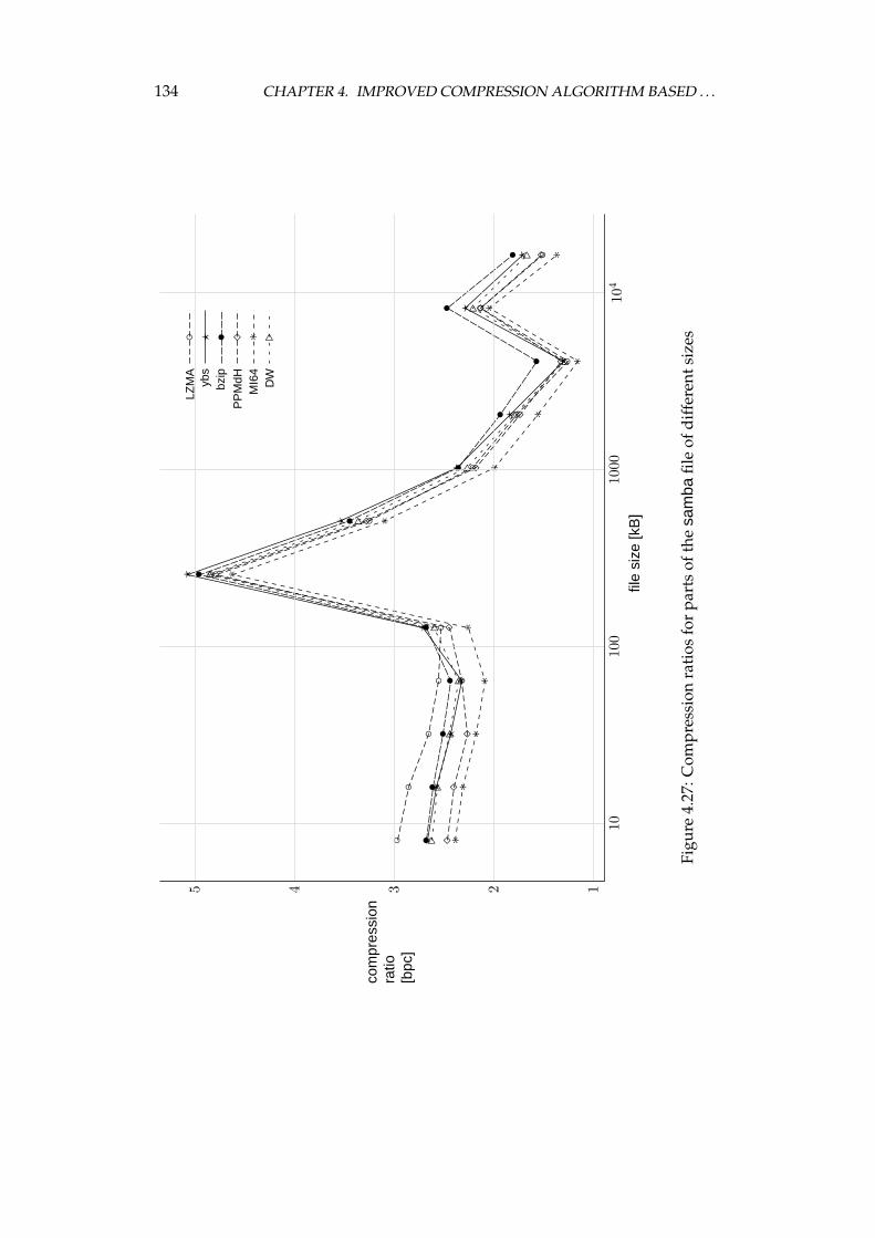
134 CHAPTER 4. IMPROVED COMPRESSION ALGORITHM BASED . . .
◦◦
◦◦
◦
◦
◦
◦
◦
◦
◦
◦
??
??
?
?
?
?
?
?
?
?
••
••
•
•
•
•
•
•
•
•
��
��
�
�
�
�
�
�
�
�
∗∗
∗∗
∗
∗
∗
∗
∗
∗
∗
∗
..
..
.
.
.
.
.
.
.
.
LZM
A◦
ybs
?bz
ip•
PP
MdH
�M
I64
∗D
W.
1010
010
0010
4
12345
file
size
[kB
]
com
pres
sion
ratio
[bpc
]
Figu
re4.
27:C
ompr
essi
onra
tios
for
part
sof
the
sam
bafil
eof
diff
eren
tsiz
es
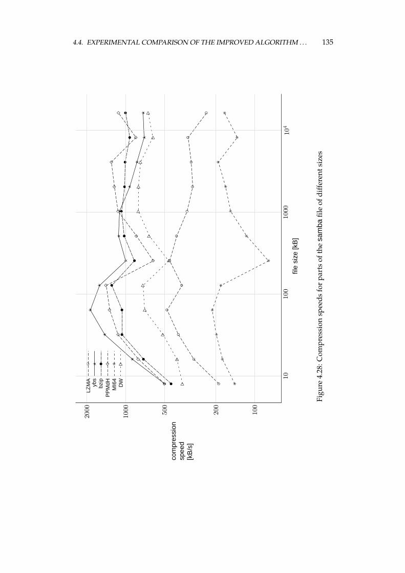
4.4. EXPERIMENTAL COMPARISON OF THE IMPROVED ALGORITHM . . . 135
◦
◦
◦◦
◦
◦◦
◦◦
◦◦
◦
?
?
?
?
?
??
?
??
??
•
•
••
•
••
••
••
•
�
�
��
�
�
�
��
�
�
�
∗
∗∗
∗∗
∗
∗
∗∗
∗
∗
∗
..
.
..
.
.
..
.
..
LZM
A◦
ybs
?bz
ip•
PP
MdH
�M
I64
∗D
W.
1010
010
0010
4
100
200
500
1000
2000
file
size
[kB
]
com
pres
sion
spee
d[k
B/s
]
Figu
re4.
28:C
ompr
essi
onsp
eeds
for
part
sof
the
sam
bafil
eof
diff
eren
tsiz
es
136 CHAPTER 4. IMPROVED COMPRESSION ALGORITHM BASED . . .
results for file sizes from 128 kB to 512 kB gives the bzip method. The improve-ment of the compression ratio for it is stopped by the maximal size of a piecewhich can be compressed by this algorithm. The results of the compressionspeed for this file (Figure 4.30) are similar to the ones for the other discussedfiles. The ybs and bzip are the fastest algorithms, but the speed of the DWmethod deteriorates only slightly and is also high.
4.4.7 Summary of comparison results
The results show that for both corpora the best compression ratios are obtainedby Shkarin’s cPPMII compression algorithm [155, 156]. The advantage in termsof the compression ratio of this algorithm over other compression methods issignificant. Its main disadvantages are low speed of running and high memoryconsumption.
From the LZ algorithms the most interesting one is the LZMA. The compres-sion ratios obtained by this method are significantly better than those achievedby other algorithms from this family. Unfortunately, the compression speed islow, comparable to the PPM methods. This disadvantage is partially compen-sated by fast decompression. In the situations, in which the compression will bemade rarely, the LZMA is an interesting candidate to employ.
The PPM methods significantly outperform other compression algorithms interms of the compression ratio for the files from the Calgary corpus. The maindisadvantage of all the PPM algorithms, as also of the DMC and the CTW (whichunfortunately we could not examine because of the unavailability of their imple-mentations), is their low speed of compression and decompression.
The BWT-based algorithms yield worse compression ratios for small files(from the Calgary corpus) than the PPM algorithms. For large files, however, thedistance between these two families of algorithms becomes smaller. The com-pression speed of the BWT-based algorithms is also higher. In these methods,the decompression speed is about two or three times higher than the compres-sion speed, what can be important in some cases.
Analysing the experimental results for different algorithms from the point ofview of multi criteria optimisation, we can roughly split the methods into threegroups. The first group contains the PPM algorithms (also the CTW and theDMC ones), which achieve the best compression ratios, but work slow. The sec-ond group contains the LZ algorithms, which work fast, but provide poor com-pression ratios. The third group contains the BWT-based algorithms, which runfaster than the PPM algorithms, and offer the compression ratios much betterthan those obtained with the LZ methods. Many of these algorithms, ybs, szip,bzip, DW, DM, are non-dominated by other algorithms in some experiments.
The algorithm that leads to the best compression ratios among the BWT-based family is the improved algorithm introduced in this dissertation—DW.
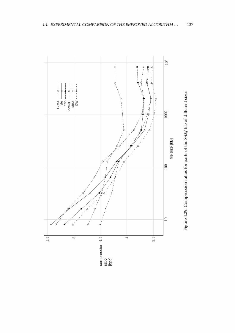
4.4. EXPERIMENTAL COMPARISON OF THE IMPROVED ALGORITHM . . . 137
◦
◦
◦◦
◦
◦◦
◦◦
◦◦
?
?
?
?
?
?
??
??
?
•
•
•
•
•
•
••
••
•
�
�
�
�
�
�
�
��
��
∗∗
∗∗
∗
∗
∗∗
∗∗
∗
.
.
.
.
.
.
..
..
.
LZM
A◦
ybs
?bz
ip•
PP
MdH
�M
I64
∗D
W.
1010
010
0010
4
3.54
4.55
5.5
file
size
[kB
]
com
pres
sion
ratio
[bpc
]
Figu
re4.
29:C
ompr
essi
onra
tios
for
part
sof
the
x-ra
yfil
eof
diff
eren
tsiz
es
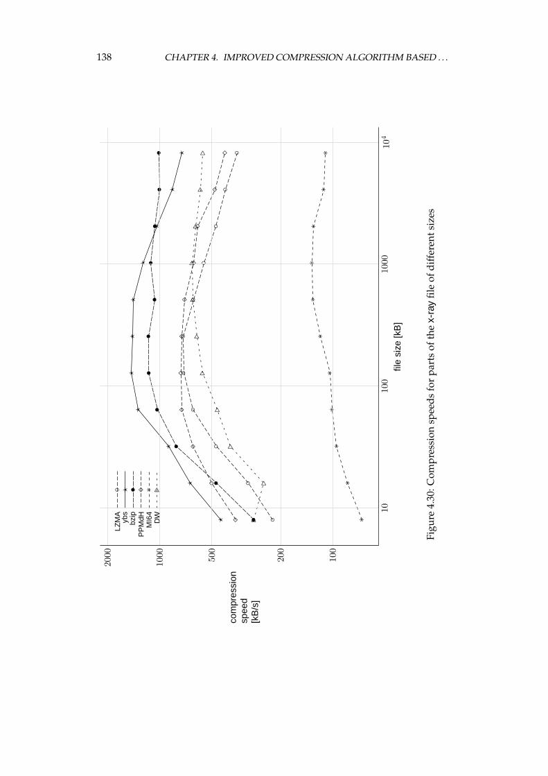
138 CHAPTER 4. IMPROVED COMPRESSION ALGORITHM BASED . . .
◦
◦
◦
◦◦
◦◦
◦◦
◦◦
?
?
?
??
??
?
?
??
•
•
•
••
••
••
••
�
�
��
��
��
�
��
∗∗
∗∗
∗∗
∗∗
∗∗
∗
..
.
.
..
..
..
.
LZM
A◦
ybs
?bz
ip•
PP
MdH
�M
I64
∗D
W.
1010
010
0010
4
100
200
500
1000
2000
file
size
[kB
]
com
pres
sion
spee
d[k
B/s
]
Figu
re4.
30:C
ompr
essi
onsp
eeds
for
part
sof
the
x-ra
yfil
eof
diff
eren
tsiz
es
4.4. EXPERIMENTAL COMPARISON OF THE IMPROVED ALGORITHM . . . 139
The speed of the DW method is comparable to the other BWT-based algorithms.The tests on files of different sizes show, however, that the speed of compres-sion and decompression is much more steady for the DW method than for otherBWT-based algorithm which use blocks of large sizes.

Chapter 5
Conclusions
What will be the conclusion of all this?
— ROBERT BOLTON
Instructions for a Right ComfortingAfflicted Consciences (1635)
The subject of the dissertation are universal lossless data compression algo-rithms. The background of this field of research was presented in Chapter 2.There we talked about a need of compression, and situations in which univer-sal lossless methods are useful. The algorithms used contemporarily were de-scribed in detail. A special, in-depth description of the Burrows–Wheeler trans-form-based algorithms, was provided (Chapter 3) as the thesis of the disserta-tion concerns this family of compression methods.
The stages of the BWCA [39] were examined in detail. The first stage is thetransform, introduced by Burrows and Wheeler. The transform is well estab-lished and the research concentrates on the efficient methods for its computa-tion. Several approaches to this task were discussed. We proposed a signifi-cant improvement to the Itoh–Tanaka’s method [90], and some small improve-ments to the Seward’s method [149] which combined together offer a highlyefficient BWT computation method (Section 4.1.2). A practical performance ofthe proposed solution was compared, in Section 4.3.1, with other approaches,for which the implementation, or detailed description that allows us to imple-ment it efficiently, was available. The results showed that the combined methodof the improved Itoh–Tanaka’s methods of orders 1 and 2 is significantly fasterthan the other examined approaches. Its memory requirement is 8n, where nis the length of the input sequence. The main disadvantage of this approach
141
142 CHAPTER 5. CONCLUSIONS
is its unknown average-case time complexity and poor worst-case complex-ity, O(n2 log n). The poor time complexity is caused by the sorting procedureused—the Seward’s method. It is possible to use different sorting procedures,but in practice they are less efficient. Since the worst-case time complexity of theimproved Itoh–Tanaka’s method is its significant disadvantage, we proposed,similarly to Seward [150], a fallback procedure, which is used if the executionof the main method takes too long. To this end, the maximal time of execu-tion of the method of time complexity O(n log n) is estimated, and if the im-proved Itoh–Tanaka’s method exceeds this limit it is stopped to run the fallbackprocedure. The fallback can be for example the Manber–Myers’s method [106],as Seward proposed [150], of the worst-case time complexity O(n(log n)2), or theLarsson–Sadakane’s method [102] of the worst-case time complexity O(n log n).The combined solution guarantees the worst-case time complexity O(n log n)and offers a fast work due to the proposed improved method, which is highlyefficient for typical sequences.
The research on the second stage transform was started from the analysisof the structure of the Burrows–Wheeler transform output. In Section 4.1.3, weproved some results regarding the structure of this sequence, concluding that itcan be approximated with high precision as an output of a piecewise stationarymemoryless source. Then, the methods of probability estimation of symbol oc-currence in such sequences were investigated (Section 4.1.4). We postulated toweight the symbol importance in the estimation process. We also derived thebounds on the expected redundancy introduced by this method. The equationsobtained are very hard to solve, so we decided to analyse them numericallyfor some weight functions. As the result of these investigations, a transform,weighted frequency count (WFC), as the second stage of the BWCA was intro-duced. We showed that the WFC is a generalisation of the well known methods:move-to-front, frequency count, and sort-by-time. Some of these methods wereformerly used in the versions of the BWCA. We also discussed the time com-plexity of the WFC, showing a way in which it can be implemented with theworst-case time complexity O(nkl), where k is the alphabet size, and l is a smallnumber, lower than 32 on typical computers. The experiments performed in Sec-tions 4.3.2 and 4.3.3 showed that the WFC transform leads to the best compres-sion ratios among the second stage methods.
The last stage of the BWCA is an entropy coding. The arithmetic coding is anoptimal solution for this task, in terms of the compression ratio. The most im-portant part of this stage is a probability estimation of symbol occurrence, whichis then used to assign codes to symbols from the alphabet. For this task we in-troduced a weighted probability estimation (Section 4.1.6). The experimentalresults (Section 4.3.4) confirmed the validity of usage of this method. Becausethe sequences are only assumed to be an output of the context tree source of un-
143
known parameters and structure, and the understanding of the BWCA workingis incomplete, we were unable to provide a thorough justification for the usageof this method of probability estimation in the BWCA.
The improved algorithm was compared to the state of the art methods pub-lished in the literature. The first task in this comparison was to choose a set oftest data. There are three widely used standard corpora: the Calgary corpus,the Canterbury corpus, and the large Canterbury corpus. The first corpus is themost popular and many compression methods were examined on it. As we dis-cussed in Section 4.2.1, the two Canterbury corpora are not good candidates tobe contemporarily the standard data sets. The main disadvantage of the threecorpora is their lack of files of sizes and contents that are used nowadays. There-fore, to provide a comparison of the compression methods on modern files, weintroduced the Silesia corpus.
As we discussed in Section 4.2.2, compression methods should be comparedin terms of multi criteria optimisation, as three criteria are important: compres-sion ratio, compression speed, and decompression speed. Therefore we con-sidered two processes separately: compression, in which the compression ra-tio and the compression speed are important, and decompression, in which thecompression ratio and the decompression speed matter.
The comparison showed that the proposed algorithm, denoted by DW inthe tables and figures, yields the best compression ratios for the both corporain the family of the BWT-based algorithms. It gives also the best compressionratios for most component files of the corpora. Its compression speed is compa-rable to other such algorithms. For the Silesia corpus, the DW algorithm com-presses about 26% faster than the slowest examined BWT-based method, szip,and about 34% slower than the fastest such an algorithm, bzip. Typically, thecompression speeds of the BWT-based algorithms differ by about 10%. The de-compression speed of the DW algorithm is about two times higher than its com-pression speed. In the decompression, the fastest BWT-based algorithm, bwc, ishowever about two times faster than the DW method. From figures shown inChapter 4 we can determine also the set of the BWT-based algorithms, which arenon-dominated by other methods from this family. One of the non-dominatedalgorithms is the DW method.
We proposed also a variant of this method, the DM algorithm, which obtainsthe second best compression ratios from the examined BWT-based algorithmsfor the Silesia corpus. Its compression speed is lower only from the bzip al-gorithm. In the decompression, the DM method is about 35% slower than thefastest, bwc, algorithm. The DM algorithm is also non-dominated for both thecompression and decompression processes for the both corpora.
The above-described observations of the behaviour of the improved algo-rithm confirm the thesis of this dissertation.
144 CHAPTER 5. CONCLUSIONS
A comparison of the DW algorithm to the other universal lossless data com-pression algorithms showed that some PPM algorithms lead to better compres-sion ratios. They are typically much slower than the BWT-based algorithms, butone of the recent methods by Shkarin [155], PPMdH, dominates the DW in thecompression of the Calgary corpus. In the decompression, a variant of the DWalgorithm, DM, is non-dominated, though. We should also notice that the stan-dard deviation of the speeds of the Shkarin’s algorithm is over 3 times largerthan the standard deviation of the speeds of the proposed method. The advan-tage of the PPMdH algorithm comes from the compression of small files. As wecan see in the experiments described in Section 4.4.6, the BWT-based algorithmswork relatively slow for small files, because of the properties of the BWT com-putation methods, and they speed up when the file size grows. The experimentson the Silesia corpus showed that the proposed algorithm is non-dominated inboth processes, and significantly outperforms the best PPM algorithms in thecompression and decompression speed. It also yields the best compression ra-tios for 3 out of 12 files from the Silesia corpus.
The results in this work can surely be a point of departure for further re-search. The proposed method for the BWT computation is highly efficient inpractice, but the analysis of its average-case time complexity is missed. Theexperiments suggest that it is low, but calculating it is a difficult, open problem.The theoretical research on the probability estimation for the output of the piece-wise stationary memoryless source were at some point discontinued, because ofthe high complexity of the equations. It could be interesting to provide somemore in-depth theoretical analysis. There is probably also a possibility to pro-pose weight functions that yield better compression ratios. Finally, it would benice if more convincing theoretical grounds for the weighted probability havebeen found.
Acknowledgements
If we meet someone who owes us thanks,we right away remember that.But how often do we meet someone to whomwe owe thanks without remembering that?
— JOHANN WOLFGANG VON GOETHE
Ottilie’s Diary (1809)
I cannot imagine that this dissertation could be completed without help frommany people. Here, I want to thank all of them.
First, I would like to thank my supervisor, Zbigniew J. Czech, who encour-aged me to work in the field of theoretical computer science, and motivated meall the time during the last four years. I am most grateful for his support, stim-ulating discussions, and constructive remarks on my work. I also thank himfor a vast number of improvements, that he suggested to incorporate into thedissertation.
Marcin Ciura, Roman Starosolski, and Szymon Grabowski proofread thewhole dissertation or its major parts. Thank them all for their patience in read-ing the early versions of the dissertation and for suggesting many ways in whichthe text can be improved. Thank you Marcin for your enormous persistence inshowing me how I can be more clear and precise in writing. Thank you alsofor collaboration on a paper we wrote together. I would like to thank you, Ro-man, for discussions on the compression algorithms. As Szymon shares my in-terests in universal lossless data compression, and especially Burrows–Wheelertransform-based compression, he was a very good discussion partner. Thankyou Szymon for our stimulating discussions, for your relevant remarks, and forpointing me the papers that I did not know.
Some parts of the compression program accompanying the dissertation arebased on existing source codes. An implementation of one of the BWT com-
145

146 ACKNOWLEDGEMENTS
putation methods is based on the routines by N. Jesper Larsson and KunihikoSadakane. An implementation of some other methods for computing the BWT isbased on source code by Julian Seward. The arithmetic coding routines, used byme, are modified source codes by John Carpinelli, Alistair Moffat, Radford Neal,Wayne Salamonsen, Lang Stuiver, Andrew Turpin, and Ian Witten. Thank youall for publishing the source codes. The contents of the Silesia corpus introducedin this dissertation was changing, and I want to thank Szymon Grabowski, UweHerklotz, Sami J. Makinen, Maxim Smirnov, and Vadim Yoockin, who sharedwith me their opinion and suggested improvements. I would like also to thankEwa Piętka for her suggestion of including medical data in the experiments, andfor providing me such files. I am grateful to my friend, Adam Skorczynski forthe possibility of developing together the LATEX Editor, which was used to writethe whole dissertation.
During my Ph.D. study I was employed in the Software Department of theSilesian University of Technology. I am thankful for the possibility to work inthis team. Many thanks go to the manager Przemysław Szmal. I am not ableto enumerate all the staff, so I would like to give special thanks to my closestfriends and colleagues: Marcin Ciura, Agnieszka Debudaj–Grabysz, Aleksan-dra Łazarczyk, Adam Skorczynski, Roman Starosolski, Bozena Wieczorek, andMirosław Wieczorek.
Finally, an exceptional ‘Thank you!’ I would like to say to my mother andfather who are present in my life for the longest time, and who gave me the bestpossible upbringing.
Tarnowskie GoryFebruary, 2003
Bibliography
[1] J. Aberg and Yu. M. Shtarkov. Text compression by context tree weighting. InJ. A. Storer and M. Cohn, editors, Proceedings of the IEEE Data Compression Conference(DCC’97), pages 377–386, March 25–27, 1997. IEEE Computer Society Press, LosAlamitos, California. [cited at p. 28]
[2] J. Aberg, Yu. M. Shtarkov, and B. J. M. Smeets. Towards understanding and im-proving escape probabilities in PPM. In J. A. Storer and M. Cohn, editors, Proceedingsof the IEEE Data Compression Conference (DCC’97), pages 22–31, March 25–27, 1997.IEEE Computer Society Press, Los Alamitos, California. [cited at p. 25]
[3] S. Albers. Improved randomized on-line algorithms for the list update prob-lem. In Proceedings of the 6th Annual ACM-SIAM Symposium on Discrete Algorithms,pages 412–419, 1995. [cited at p. 47, 49]
[4] S. Albers and M. Mitzenmacher. Average case analyses of list update algorithms,with applications to data compression. Algorithmica, 21(3):312–329, July 1998.[cited at p. 49, 50, 168, 170]
[5] A. Apostolico and S. Lonardi. Compression of biological sequences by greedyoff-line textual substitution. In J. A. Storer and M. Cohn, editors, Proceedings of theIEEE Data Compression Conference (DCC’2000), pages 143–152, March 28–30, 2000.IEEE Computer Society Press, Los Alamitos, California. [cited at p. 29]
[6] M. Arimura and H. Yamamoto. Almost sure convergence coding theorem forblock sorting data compression algorithm. In Proceedings of International Sym-posium on Information Theory and Its Applications (ISITA98), Mexico City, Mexico,October 14–16, 1998. [cited at p. 45]
[7] M. Arimura and H. Yamamoto. Asymptotic optimality of the block sorting datacompression algorithm. IEICE Transactions on Fundamentals of Electronics Commu-nications & Computer Sciences, E81-A(10):2117–2122, October 1998. [cited at p. 45]
[8] M. Arimura, H. Yamamoto, and S. Arimoto. A bitplane tree weighting method forlossless compression of gray scale images. IEICE Transactions on Fundamentals ofElectronics Communications & Computer Sciences, E80-A(11):2268–2271, November1997. [cited at p. 28]
147
148 BIBLIOGRAPHY
[9] Z. Arnavut. Generalization of the BWT transformation and inversion ranks. InJ. A. Storer and M. Cohn, editors, Proceedings of the IEEE Data Compression Confer-ence (DCC’2002), page 447, April 2–4, 2002. IEEE Computer Society Press, LosAlamitos, California. [cited at p. 57, 105, 107]
[10] Z. Arnavut and S. S. Magliveras. Block sorting and compression. In J. A. Storerand M. Cohn, editors, Proceedings of the IEEE Data Compression Conference (DCC’97),pages 181–190, March 25–27, 1997. IEEE Computer Society Press, Los Alamitos,California. [cited at p. 45, 50, 87]
[11] Z. Arnavut and S. S. Magliveras. Lexical permutation sorting algorithm. TheComputer Journal, 40(5):292–295, 1997. [cited at p. 45, 87]
[12] R. Arnold and T. C. Bell. A corpus for the evaluation of lossless compression algo-rithms. In J. A. Storer and M. Cohn, editors, Proceedings of the IEEE Data CompressionConference (DCC’97), pages 201–210, March 25–27, 1997. IEEE Computer SocietyPress, Los Alamitos, California. [cited at p. 5, 92]
[13] F. D. Awan, N. Zhang, N. Motgi, R. T. Iqbal, and A. Mukherjee. LIPT: A reversiblelossless text transform to improve compression performance. In J. A. Storer andM. Cohn, editors, Proceedings of the IEEE Data Compression Conference (DCC’2001),page 481, March 27–29, 2001. [cited at p. 59]
[14] F. S. Awan and A. Mukherjee. LIPT: A lossless text transform to improve com-pression. In Proceedings of International Conference on Information and Theory: Cod-ing and Computing, IEEE Computer Society, Las Vegas, Nevada, pages 452–460, April2–4 2001. [cited at p. 59]
[15] R. Bachrach and R. El-Yaniv. Online list accessing algorithms and their applica-tions: Recent empirical evidence. In Proceedings of the ACM-SIAM Symposium onDiscrete Algorithms, pages 53–62, 1997. [cited at p. 47]
[16] B. Balkenhol and S. Kurtz. Universal data compression based on the Burrows–Wheeler transformation: Theory and practice. IEEE Transactions on Computers,49(10):1043–1053, October 2000. [cited at p. 35, 43, 46]
[17] B. Balkenhol, S. Kurtz, and Yu. M. Shtarkov. Modifications of the Burrows andWheeler data compression algorithm. In J. A. Storer and M. Cohn, editors, Pro-ceedings of the IEEE Data Compression Conference (DCC’99), pages 188–197, March29–31, 1999. IEEE Computer Society Press, Los Alamitos, California. [cited at p. 48,
55, 58, 107]
[18] B. Balkenhol and Yu. M. Shtarkov. One attempt of a compression algorithm usingthe BWT. Preprint 99-133, SFB343, Discrete Structures in Mathematics, Facultyof Mathematics, University of Bielefeld, Postfach 100131 33501, Bielefeld, Ger-many, 1999. http://www.mathematik.uni-bielefeld.de/sfb343/preprints/pr99133.ps.gz. [cited at p. 46, 48, 51, 55, 58, 82, 88, 105, 107]
[19] T. Bell and A. Moffat. A note on the DMC data compression scheme. The ComputerJournal, 32(1):16–20, February 1989. [cited at p. 26]
[20] T. Bell, I. H. Witten, and J. G. Cleary. Modelling for text compression. ACMComputing Surveys, 21(4):557–591, 1989. [cited at p. 5, 34, 50, 92]
149
[21] T. C. Bell. Better OPM/L test compression. IEEE Transactions on Communications,COM-34(12):1176–1182, December 1986. [cited at p. 22]
[22] T. C. Bell, J. G. Cleary, and I. H. Witten. Text Compression. Prentice Hall, EnglewoodCliffs, NJ, 1990. [cited at p. 9, 92]
[23] T. C. Bell and D. Kulp. Longest-match string searching for Ziv–Lempel compres-sion. Software–Practice and Experience, 23(7):757–772, July 1993. [cited at p. 22]
[24] T. C. Bell and I. H. Witten. The relationship between greedy parsing and symbol-wise text compression. Journal of the ACM, 41(4):708–724, 1994. [cited at p. 22]
[25] J. L. Bentley and R. Sedgewick. Fast algorithms for sorting and searching strings.In Proceedings of the ACM-SIAM Symposium on Discrete Algorithms, pages 360–369,1997. [cited at p. 40, 169]
[26] J. L. Bentley, D. D. Sleator, R. E. Tarjan, and V. K. Wei. A locally adaptive data com-pression scheme. Communications of ACM, 29(4):320–330, April 1986. [cited at p. 4,
33, 48, 168, 170]
[27] E. Binder. Distance coder. Usenet group: comp.compression, 2000. [cited at p. 51]
[28] E. Binder. The dc program. ftp://ftp.elf.stuba.sk/pub/pc/pack/dc124.zip, 2000.[cited at p. 57]
[29] E. Binder. Private communication, 2001. [cited at p. 51]
[30] Ch. Bloom. Solving the problem of context modeling. http://www.cbloom.com/papers/ppmz.zip, March 1998. [cited at p. 25]
[31] P. F. Brown, S. A. Della Pietra, V. J. Della Pietra, J. C. Lai, and R. L. Mercer. Anestimate of an upper bound for the entropy of English. Computational Linguistics,18(1):31–40, 1992. [cited at p. 29]
[32] S. Bunton. The structure of DMC. In J. A. Storer and M. Cohn, editors, Proceedings ofthe IEEE Data Compression Conference (DCC’95), pages 72–81, March 28–30, 1995.IEEE Computer Society Press, Los Alamitos, California. [cited at p. 26]
[33] S. Bunton. On-line stochastic processes in data compression. Ph.D. Thesis, Universityof Washington, 1996. [cited at p. 25, 26, 27, 108]
[34] S. Bunton. An executable taxonomy of on-line modeling algorithms. In J. A. Storerand M. Cohn, editors, Proceedings of the IEEE Data Compression Conference (DCC’97),pages 42–51, March 25–27, 1997. IEEE Computer Society Press, Los Alamitos,California. [cited at p. 25]
[35] S. Bunton. A generalization and improvement to PPM’s blending. UW-CSETechnical Report UW-CSE-97-01-10, The University of Washington, January 1997.ftp://ftp.cs.washington.edu/tr/1997/01/UW-CSE-97-01-10.PS.Z (also Proceedingsof DCC’97 p. 426). [cited at p. 25]
[36] S. Bunton. A percolating state selector for suffix-tree context models. In J. A. Storerand M. Cohn, editors, Proceedings of the IEEE Data Compression Conference (DCC’97),pages 32–41, March 25–27, 1997. IEEE Computer Society Press, Los Alamitos,California. [cited at p. 25]
150 BIBLIOGRAPHY
[37] S. Bunton. Semantically motivated improvements for PPM variants. The ComputerJournal, 40(2-3):76–93, 1997. [cited at p. 25, 107]
[38] S. Bunton. Bayesian state combining for context models (extended abstract). InJ. A. Storer and M. Cohn, editors, Proceedings of the IEEE Data Compression Conference(DCC’98), pages 329–338, March 30–April 1, 1998. IEEE Computer Society Press,Los Alamitos, California. [cited at p. 25]
[39] M. Burrows and D. J. Wheeler. A block-sorting lossless data compression al-gorithm. SRC Research Report 124, Digital Equipment Corporation, Palo Alto,California, May 10, 1994. ftp://ftp.digital.com/pub/DEC/SRC/research-reports/SRC-124.ps.zip. [cited at p. 4, 31, 34, 38, 45, 48, 53, 107, 141]
[40] G. Buyanovsky. Associative coding. The Monitor, 8:10–22, 1994. In Russian.[cited at p. 107]
[41] G. Buyanovsky. The acb 2.00c program. ftp://ftp.elf.stuba.sk/pub/pc/pack/acb200c.zip, 1997. [cited at p. 107]
[42] J. Carpinelli, A. Moffat, R. Neal, W. Salamonsen, L. Stuiver, A. Turpin, andI. H. Witten. The source codes for word, character, integer, and bit based com-pression using arithmetic coding. http://www.cs.mu.oz.au/∼alistair/arith coder/arith coder-3.tar.gz, February 1999. [cited at p. 170]
[43] B. Chapin. Switching between two on-line list update algorithms for higher com-pression of Burrows–Wheeler transformed data. In J. A. Storer and M. Cohn, ed-itors, Proceedings of the IEEE Data Compression Conference (DCC’2000), pages 183–192, March 28–30, 2000. IEEE Computer Society Press, Los Alamitos, California.[cited at p. 49]
[44] B. Chapin and S. R. Tate. Higher compression from the Burrows–Wheeler trans-form by modified sorting. In J. A. Storer and M. Cohn, editors, Proceedings of theIEEE Data Compression Conference (DCC’98), page 532, March 30–April 1, 1998.IEEE Computer Society Press, Los Alamitos, California. [cited at p. 57]
[45] X. Chen, S. Kwong, and M. Li. A compression algorithm for DNA sequencesand its applications in genome comparison. Genome Informatics, 10:51–61, 1999.[cited at p. 29]
[46] J. Cheney. Compressing XML with multiplexed hierarchical PPM models. InJ. A. Storer and M. Cohn, editors, Proceedings of the IEEE Data Compression Conference(DCC’2001), pages 163–172, March 27–29, 2001. IEEE Computer Society Press, LosAlamitos, California. [cited at p. 165]
[47] M. G. Ciura and S. Deorowicz. How to squeeze a lexicon. Software–Practice andExperience, 31(11):1077–1090, 2001. [cited at p. 6, 29]
[48] J. Cleary and I. Witten. Data compression using adaptive coding and partialstring matching. IEEE Transactions on Communications, COM-32:396–402, 1984.[cited at p. 3, 23, 24]
[49] J. G. Cleary and W. J. Teahan. Unbounded length context for PPM. The ComputerJournal, 40(2/3):67–75, 1997. [cited at p. 23, 25, 42]
151
[50] J. G. Cleary, W. J. Teahan, and I. H. Witten. Unbounded length context for PPM. InJ. A. Storer and M. Cohn, editors, Proceedings of the IEEE Data Compression Conference(DCC’95), pages 52–61, March 28–30, 1995. IEEE Computer Society Press, LosAlamitos, California. [cited at p. 42]
[51] G. V. Cormack and R. N. Horspool. Algorithms for adaptive Huffman codes.Information Processing Letters, 18(3):159–165, 1984. [cited at p. 14]
[52] G. V. Cormack and R. N. Horspool. Data compression using dynamic Markovmodeling. The Computer Journal, 30(6):541–550, December 1987. [cited at p. 4, 26, 108]
[53] J. Daciuk, S. Mihov, B. W. Watson, and R. E. Watson. Incremental construction ofminimal acyclic finite-state automata. Computational Linguistics, 26(1):3–16, 2000.[cited at p. 29]
[54] S. Deorowicz. Improvements to Burrows–Wheeler compression algorithm.Software–Practice and Experience, 30(13):1465–1483, 10 November 2000. [cited at p. 5,
84, 102]
[55] S. Deorowicz. Second step algorithms in the Burrows–Wheeler compression al-gorithm. Software–Practice and Experience, 32(2):99–111, 2002. [cited at p. 5, 57, 81, 84,
102]
[56] M. Effros. Universal lossless source coding with the Burrows Wheeler transform.In J. A. Storer and M. Cohn, editors, Proceedings of the IEEE Data Compression Confer-ence (DCC’99), pages 178–187, March 29–31, 1999. IEEE Computer Society Press,Los Alamitos, California. [cited at p. 45]
[57] N. Ekstrand. Lossless compression of grayscale images via context tree weighting.In J. A. Storer and M. Cohn, editors, Proceedings of the IEEE Data Compression Confer-ence (DCC’96), pages 132–139, April 1–3, 1996. IEEE Computer Society Press, LosAlamitos, California. [cited at p. 28]
[58] N. Ekstrand. Universal Lossless Source Coding Techniques for Images and Short DataSequences. Ph.D. Thesis, Lund Institute of Technology, Lund University, 2001.[cited at p. 28]
[59] P. Elias. Universal codeword sets and representations of the integers. IEEE Trans-actions on Information Theory, IT-21:194–203, 1975. [cited at p. 57, 87]
[60] P. Elias. Interval and recency rank source coding: Two on-line adaptive variablelength schemes. IEEE Transactions on Information Theory, IT-33:3–10, January 1987.[cited at p. 51]
[61] Erlangen/bethesda data and online services. http://cactus.nci.nih.gov/, 2002.[cited at p. 164]
[62] N. Faller. An adaptive system for data compression. In Record of the 7th AsilomarConference on Circuits, Systems, and Computers, pages 593–597, 1973. [cited at p. 14]
[63] M. Farach. Optimal suffix construction with large alphabets. In Proceedings of the38th Annual IEEE Symposium on Foundations of Computer Science, pages 137–143,October 1997. [cited at p. 39]
152 BIBLIOGRAPHY
[64] P. Fenwick. A new data structure for cumulative frequency tables. Software–Practice and Experience, 24(3):327–336, March 1994. (Errata published in 24(7):677,July 1994.). [cited at p. 15]
[65] P. Fenwick. Experiments with a block sorting text compression algorithm. Tech-nical Report 111, The University of Auckland, Department of Computer Science,May 1995. ftp://ftp.cs.auckland.ac.nz/pub/peter-f/TechRep111.ps. [cited at p. 48]
[66] P. Fenwick. Improvements to the block sorting text compression algorithm. Tech-nical Report 120, The University of Auckland, Department of Computer Science,August 1995. ftp://ftp.cs.auckland.ac.nz/pub/peter-f/TechRep120.ps. [cited at p. 45]
[67] P. Fenwick. Block sorting text compression—final report. Technical Report 130,The University of Auckland, Department of Computer Science, April 1996. ftp://ftp.cs.auckland.ac.nz/pub/peter-f/TechRep130.ps. [cited at p. 34, 35, 48, 82, 88]
[68] P. Fenwick. The Burrows–Wheeler transform for block sorting text compres-sion: Principles and improvements. The Computer Journal, 39(9):731–740, 1996.[cited at p. 45, 48, 53, 56, 107, 108]
[69] P. Fenwick. Burrows–Wheeler compression with variable length integer codes.Software–Practice and Experience, 32(13):1307–1316, 2002. [cited at p. 57]
[70] E. R. Fiala and D. H. Greene. Data compression with finite windows. Communi-cations of ACM, 32(4):490–505, 1989. [cited at p. 22]
[71] A. S. Fraenkel and S. T. Klein. Robust universal complete codes for transmissionand compression. Discrete Applied Mathematics, 64:31–55, 1996. [cited at p. 57]
[72] J. L. Gailly. The gzip program. http://www.gzip.org/, 1993. [cited at p. 108]
[73] R. G. Gallager. Variations on a theme by Huffman. IEEE Transactions on InformationTheory, 24(6):668–674, 1978. [cited at p. 14]
[74] R. Giegerich and S. Kurtz. From Ukkonen to McCreight and Weiner: A unify-ing view of linear-time suffix tree construction. Algorithmica, 19:331–353, 1997.[cited at p. 39]
[75] S. Golomb. Runlength encodings. IEEE Transactions on Information Theory, IT-12(3):399–401, July 1966. [cited at p. 45]
[76] Sz. Grabowski. Text preprocessing for Burrows–Wheeler block sorting compres-sion. In VII Konferencja Sieci i Systemy Informatyczne Łodz’1999, Materiały konferen-cyjne, pages 229–239, 1999. [cited at p. 58]
[77] Sz. Grabowski. Private communication, November 2000. [cited at p. 51]
[78] M. Guazzo. A general minimum-redundancy source-coding algorithm. IEEETransactions on Information Theory, IT-26(1):15–25, January 1980. [cited at p. 15]
[79] P. C. Gutmann and T. C. Bell. A hybrid approach to text compression. In J. A. Storerand M. Cohn, editors, Proceedings of the IEEE Data Compression Conference (DCC’94),pages 225–233, March 29–31, 1994. [cited at p. 22]
[80] D. T. Hoang, P. M. Long, and J. S. Vitter. Dictionary selection using partial match-ing. Information Sciences, 119(1-2):57–72, 1999. [cited at p. 23]
153
[81] C. A. R. Hoare. Quicksort. The Computer Journal, 4:10–15, 1962. [cited at p. 41]
[82] R. N. Horspool. The effect of non-greedy parsing in Ziv-Lempel compressionmethods. In J. A. Storer and M. Cohn, editors, Proceedings of the IEEE Data Compres-sion Conference (DCC’95), pages 302–311, March 28–30, 1995. [cited at p. 22]
[83] P. G. Howard. The design and analysis of efficient lossless data compression sys-tems. Technical Report CS-93-28, Department of Computer Science, Brown Uni-versity, Providence, Rhode Island, 1993. http://www.cs.brown.edu/publications/techreports/reports/CS-93-28.html. [cited at p. 25]
[84] P. G. Howard and J. S. Vitter. Analysis of arithmetic coding for data compression.Information Processing and Management, 28(6):749–763, 1992. [cited at p. 15]
[85] P. G. Howard and J. S. Vitter. Practical implementations of arithmetic cod-ing. Image and text compression. Kluwer Academic Publishers, pages 85–112, 1992.[cited at p. 15]
[86] P. G. Howard and J. S. Vitter. Arithmetic coding for data compression. Proceedingsof the IEEE, 82(6):857–865, June 1994. [cited at p. 15]
[87] D. A. Huffman. A method for the construction of minimum-redundancy codes.In Proceedings of the Institute of Radio Engineers, pages 1098–1101, September 1952.[cited at p. 13]
[88] S. J. Inglis. Lossless Document Image Compression. Ph.D. Thesis, The University ofWaikato, March 1999. [cited at p. 29]
[89] S. Irani. Two results on the list update problem. Information Processing Letters,38(6):301–306, 1991. [cited at p. 47]
[90] H. Itoh and H. Tanaka. An efficient method for in memory construction of suffixarrays. In Proceedings of the IEEE String Processing and Information Retrieval Sym-posium & International Workshop on Groupware, pages 81–88, 1999. [cited at p. 5, 41, 62,
101, 141]
[91] F. Jelinek. Probabilistic Information Theory. New York: McGraw-Hill, 1968.[cited at p. 14]
[92] A. Kadach. Effective algorithms for lossless compression of textual data. Ph.D.Thesis, Russian Science Society, Novosibirsk, Russia, 1997. In Russian, http://www.compression.graphicon.ru/download/articles/lz/kadach cndd 1997 ps.rar.[cited at p. 50]
[93] D. E. Knuth. Dynamic Huffman coding. Journal of Algorithms, 6:163–180, 1985.[cited at p. 14]
[94] D. E. Knuth. The Art of Computer Programming. Sorting and Searching, volume 3.Addison-Wesley, Reading, MA, second edition, 1998. [cited at p. 169]
[95] R. E. Krichevsky and V. K. Trofimov. The performance of universal encoding.IEEE Transactions on Information Theory, 27:199–207, 1981. [cited at p. 28, 74, 88]
[96] S. Kurtz and B. Balkenhol. Space efficient linear time computation of the Bur-rows and Wheeler transformation. Numbers, Information and Complexity, KluwerAcademic Publishers, pages 375–383, 2000. [cited at p. 39]
154 BIBLIOGRAPHY
[97] G. G. Langdon. An introduction to arithmetic coding. IBM Journal of Research andDevelopment, 28(2):135–149, March 1984. [cited at p. 15]
[98] Large Canterbury corpus. http://corpus.canterbury.ac.nz/descriptions/, 1997.[cited at p. 5, 93]
[99] N. J. Larsson. The context trees of block sorting compression. In J. A. Storerand M. Cohn, editors, Proceedings of the IEEE Data Compression Conference (DCC’98),pages 189–198, March 30–April 1, 1998. IEEE Computer Society Press, Los Alami-tos, California. [cited at p. 46]
[100] N. J. Larsson. The source code for the Larsson–Sadakane suffix array computationalgorithm. http://www.dna.lth.se/∼jesper/research.html, 1999. [cited at p. 169]
[101] N. J. Larsson. Structures of String Matching and Data Compression. Ph.D. Thesis, De-partment of Computer Science, Lund University, Box 118, S-22100 Lund, Sweden,September 1999. [cited at p. 46]
[102] N. J. Larsson and K. Sadakane. Faster suffix sorting. Technical Report LU-CS-TR:99-214, Department of Computer Science, Lund University, Box 118, S-22100Lund, Sweden, May 1999. http://www.cs.lth.se/∼jesper/ssrev-tr.pdf. [cited at p. 40,
101, 142, 167, 169]
[103] E. L. Lawler, J. K. Lenstra, A. H. G. Rinnooy-Kan, and D. B. Shmoys, editors.The Traveling Salesman Problem: A Guided Tour of Combinatorial Optimization. JohnWiley and Sons, Chichester, West Sussex, New York, 1985. [cited at p. 58]
[104] D. Loewenstern and P. N. Yianilos. Significantly lower entropy estimates for natu-ral DNA sequences. In J. A. Storer and M. Cohn, editors, Proceedings of the IEEE DataCompression Conference (DCC’97), pages 151–160, March 25–27, 1997. [cited at p. 29]
[105] G. Lyapko. The lgha program. http://www.geocities.com/SiliconValley/Lab/6606/lgha.htm, 1999. [cited at p. 108]
[106] U. Manber and E. W. Myers. Suffix arrays: A new method for on-line stringsearches. SIAM Journal on Computing, 22(5):935–948, 1993. [cited at p. 40, 101, 142, 167,
169]
[107] G. Manzini. An analysis of the Burrows–Wheeler transform (extended abstract).In Proceedings of the tenth annual ACM-SIAM symposium on discrete algorithms(SODA’99), pages 669–677, 1999. [cited at p. 45]
[108] G. Manzini. The Burrows–Wheeler transform: Theory and practice. Lecture Notesin Computer Science, Springer Verlag, 1672:34–47, 1999. [cited at p. 45]
[109] G. Manzini. An analysis of the Burrows–Wheeler transform. Journal of the ACM,48(3):407–430, 2001. [cited at p. 45]
[110] J. McCabe. On serial files with relocatable records. Operations Research, 13:609–618, 1965. [cited at p. 46]
[111] E. M. McCreight. A space-economical suffix tree construction algorithm. Journalof the ACM, 23(2):262–272, 1976. [cited at p. 38]
155
[112] V. Miller and M. Wegman. Variations on a theme be Ziv and Lempel. In A. Apos-tolico and Z. Galil, editors, Combinatorial Algorithms on Words, Volume 12, pages 131–140, 1985. NATO ASI Series F. [cited at p. 23]
[113] A. Moffat. Implementing the PPM data compression scheme. IEEE Transactionson Communications, 28(11):1917–1921, November 1990. [cited at p. 25]
[114] A. Moffat. An improved data structure for cumulative probability tables.Software–Practice and Experience, 29(7):647–659, 1999. [cited at p. 15]
[115] A. Moffat, R. M. Neal, and I. H. Witten. Arithmetic coding revisited. ACM Trans-actions on Information Systems, 16(3):256–294, 1998. [cited at p. 15, 170]
[116] A. Moffat and A. Turpin. Compression and Coding Algorithms. Kluwer AcademicPublishers, Norwell, Massachusetts, 2002. [cited at p. 9]
[117] Mozilla Project. http://www.mozilla.org/, 1998–2002. [cited at p. 163]
[118] M. Nelson and J. L. Gailly. The Data Compression Book. M&T Books, New York,NY, second edition, 1995. [cited at p. 9]
[119] C. G. Nevill-Manning and I. H. Witten. Protein is incompressible. In J. A. Storerand M. Cohn, editors, Proceedings of the IEEE Data Compression Conference (DCC’99),pages 257–266, March 29–31, 1999. IEEE Computer Society Press, Los Alamitos,California. [cited at p. 29]
[120] Open source database benchmark. http://sourceforge.net/projects/osdb, 2002.[cited at p. 164]
[121] Openoffice.org source project. http://www.openoffice.org, 2002. [cited at p. 164]
[122] V. Pareto. Cours d’economie politique, professe a l’Universite de Lausanne, tome I. Lau-sanne: Rouge, 1896. [cited at p. 97]
[123] V. Pareto. Cours d’economie politique, professe a l’Universite de Lausanne, tome II.Lausanne: Rouge, 1897. [cited at p. 97]
[124] V. Pareto. Manuale di economia politica, conuna introduzione alla scienca Sociale, vol-ume in-8. Milano, 1906. [cited at p. 97]
[125] R. Pasco. Source coding algorithms for fast data compression. Ph.D. Thesis, Depart-ment of Electrical Engineering, Stanford University, Stanford, 1976. [cited at p. 15]
[126] I. Pavlov. The ufa 0.04 beta 1 program. ftp://ftp.elf.stuba.sk/pub/pc/pack/ufa004b1.zip, 1998. [cited at p. 109]
[127] I. Pavlov. The 7-zip 2.30 beta 17 program. http://www.7-zip.org, 2002. [cited at p. 108]
[128] G. Perec. La Disparition. Denoel, 1969. In French. [cited at p. 12]
[129] G. Perec. A Void. Harvill, 1994. (English translation by A. Gilbert). [cited at p. 12]
[130] N. Porter, editor. Webster’s Revised Unabridged Dictionary. C. & G. Merriam Co.,Springfield, Massachusetts, 1913. [cited at p. 96, 165]
[131] Project Gutenberg. http://www.promo.net/pg/, 1971–2002. [cited at p. 96, 163, 165]
[132] N. Reingold and J. Westbrook. Off-line algorithms for the list update problem.Information Processing Letters, 60:75–80, 1996. [cited at p. 47]
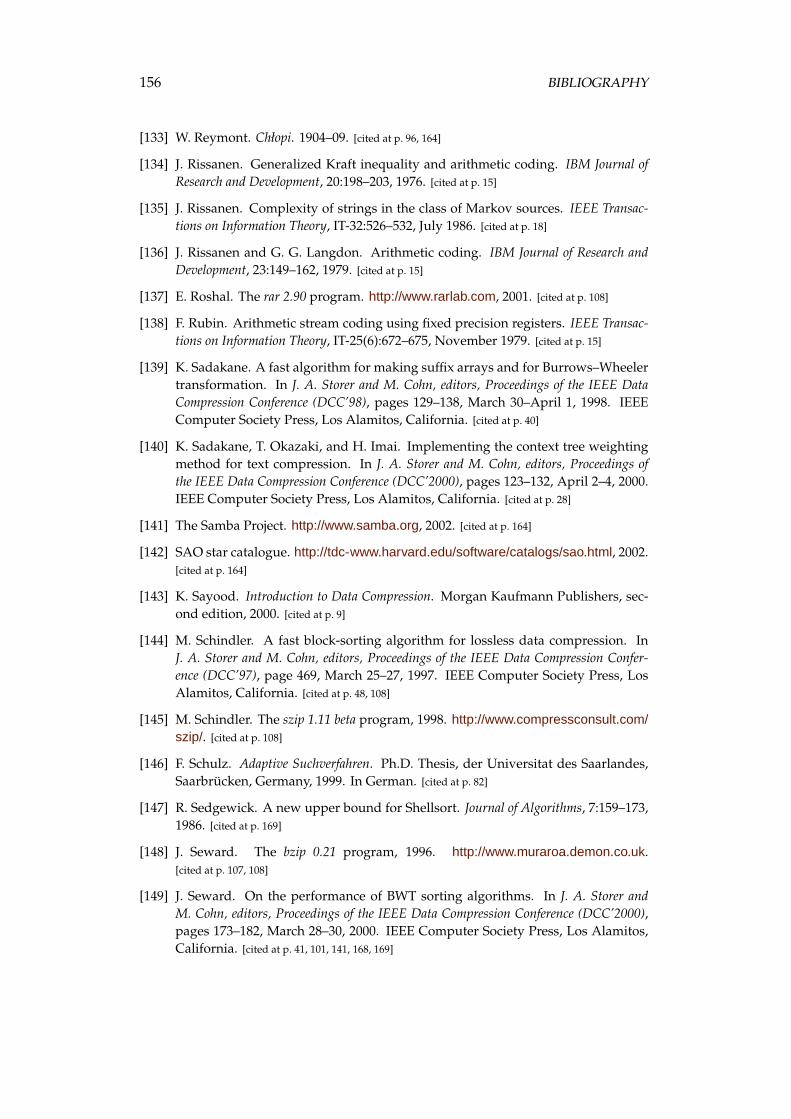
156 BIBLIOGRAPHY
[133] W. Reymont. Chłopi. 1904–09. [cited at p. 96, 164]
[134] J. Rissanen. Generalized Kraft inequality and arithmetic coding. IBM Journal ofResearch and Development, 20:198–203, 1976. [cited at p. 15]
[135] J. Rissanen. Complexity of strings in the class of Markov sources. IEEE Transac-tions on Information Theory, IT-32:526–532, July 1986. [cited at p. 18]
[136] J. Rissanen and G. G. Langdon. Arithmetic coding. IBM Journal of Research andDevelopment, 23:149–162, 1979. [cited at p. 15]
[137] E. Roshal. The rar 2.90 program. http://www.rarlab.com, 2001. [cited at p. 108]
[138] F. Rubin. Arithmetic stream coding using fixed precision registers. IEEE Transac-tions on Information Theory, IT-25(6):672–675, November 1979. [cited at p. 15]
[139] K. Sadakane. A fast algorithm for making suffix arrays and for Burrows–Wheelertransformation. In J. A. Storer and M. Cohn, editors, Proceedings of the IEEE DataCompression Conference (DCC’98), pages 129–138, March 30–April 1, 1998. IEEEComputer Society Press, Los Alamitos, California. [cited at p. 40]
[140] K. Sadakane, T. Okazaki, and H. Imai. Implementing the context tree weightingmethod for text compression. In J. A. Storer and M. Cohn, editors, Proceedings ofthe IEEE Data Compression Conference (DCC’2000), pages 123–132, April 2–4, 2000.IEEE Computer Society Press, Los Alamitos, California. [cited at p. 28]
[141] The Samba Project. http://www.samba.org, 2002. [cited at p. 164]
[142] SAO star catalogue. http://tdc-www.harvard.edu/software/catalogs/sao.html, 2002.[cited at p. 164]
[143] K. Sayood. Introduction to Data Compression. Morgan Kaufmann Publishers, sec-ond edition, 2000. [cited at p. 9]
[144] M. Schindler. A fast block-sorting algorithm for lossless data compression. InJ. A. Storer and M. Cohn, editors, Proceedings of the IEEE Data Compression Confer-ence (DCC’97), page 469, March 25–27, 1997. IEEE Computer Society Press, LosAlamitos, California. [cited at p. 48, 108]
[145] M. Schindler. The szip 1.11 beta program, 1998. http://www.compressconsult.com/szip/. [cited at p. 108]
[146] F. Schulz. Adaptive Suchverfahren. Ph.D. Thesis, der Universitat des Saarlandes,Saarbrucken, Germany, 1999. In German. [cited at p. 82]
[147] R. Sedgewick. A new upper bound for Shellsort. Journal of Algorithms, 7:159–173,1986. [cited at p. 169]
[148] J. Seward. The bzip 0.21 program, 1996. http://www.muraroa.demon.co.uk.[cited at p. 107, 108]
[149] J. Seward. On the performance of BWT sorting algorithms. In J. A. Storer andM. Cohn, editors, Proceedings of the IEEE Data Compression Conference (DCC’2000),pages 173–182, March 28–30, 2000. IEEE Computer Society Press, Los Alamitos,California. [cited at p. 41, 101, 141, 168, 169]
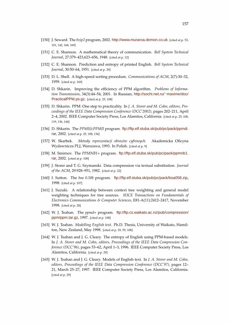
157
[150] J. Seward. The bzip2 program, 2002. http://www.muraroa.demon.co.uk. [cited at p. 53,
101, 142, 168, 169]
[151] C. E. Shannon. A mathematical theory of communication. Bell System TechnicalJournal, 27:379–423,623–656, 1948. [cited at p. 12]
[152] C. E. Shannon. Prediction and entropy of printed English. Bell System TechnicalJournal, 30:50–64, 1951. [cited at p. 29]
[153] D. L. Shell. A high-speed sorting procedure. Communications of ACM, 2(7):30–32,1959. [cited at p. 169]
[154] D. Shkarin. Improving the efficiency of PPM algorithm. Problems of Informa-tion Transmission, 34(3):44–54, 2001. In Russian, http://sochi.net.ru/∼maxime/doc/PracticalPPM.ps.gz. [cited at p. 25, 108]
[155] D. Shkarin. PPM: One step to practicality. In J. A. Storer and M. Cohn, editors, Pro-ceedings of the IEEE Data Compression Conference (DCC’2002), pages 202–211, April2–4, 2002. IEEE Computer Society Press, Los Alamitos, California. [cited at p. 25, 108,
119, 136, 144]
[156] D. Shkarin. The PPMII/cPPMII program. ftp://ftp.elf.stuba.sk/pub/pc/pack/ppmdi.rar, 2002. [cited at p. 25, 108, 136]
[157] W. Skarbek. Metody reprezentacji obrazow cyfrowych. Akademicka OficynaWydawnicza PLJ, Warszawa, 1993. In Polish. [cited at p. 9]
[158] M. Smirnov. The PPMNB1+ program. ftp://ftp.elf.stuba.sk/pub/pc/pack/ppmnb1.rar, 2002. [cited at p. 108]
[159] J. Storer and T. G. Szymanski. Data compression via textual substitution. Journalof the ACM, 29:928–951, 1982. [cited at p. 22]
[160] I. Sutton. The boa 0.58b program. ftp://ftp.elf.stuba.sk/pub/pc/pack/boa058.zip,1998. [cited at p. 107]
[161] J. Suzuki. A relationship between context tree weighting and general modelweighting techniques for tree sources. IEICE Transactions on Fundamentals ofElectronics Communications & Computer Sciences, E81-A(11):2412–2417, November1998. [cited at p. 28]
[162] W. J. Teahan. The ppmd+ program. ftp://ftp.cs.waikato.ac.nz/pub/compression/ppm/ppm.tar.gz, 1997. [cited at p. 108]
[163] W. J. Teahan. Modelling English text. Ph.D. Thesis, University of Waikato, Hamil-ton, New Zealand, May 1998. [cited at p. 29, 59, 108]
[164] W. J. Teahan and J. G. Cleary. The entropy of English using PPM-based models.In J. A. Storer and M. Cohn, editors, Proceedings of the IEEE Data Compression Con-ference (DCC’96), pages 53–62, April 1–3, 1996. IEEE Computer Society Press, LosAlamitos, California. [cited at p. 29]
[165] W. J. Teahan and J. G. Cleary. Models of English text. In J. A. Storer and M. Cohn,editors, Proceedings of the IEEE Data Compression Conference (DCC’97), pages 12–21, March 25–27, 1997. IEEE Computer Society Press, Los Alamitos, California.[cited at p. 29]
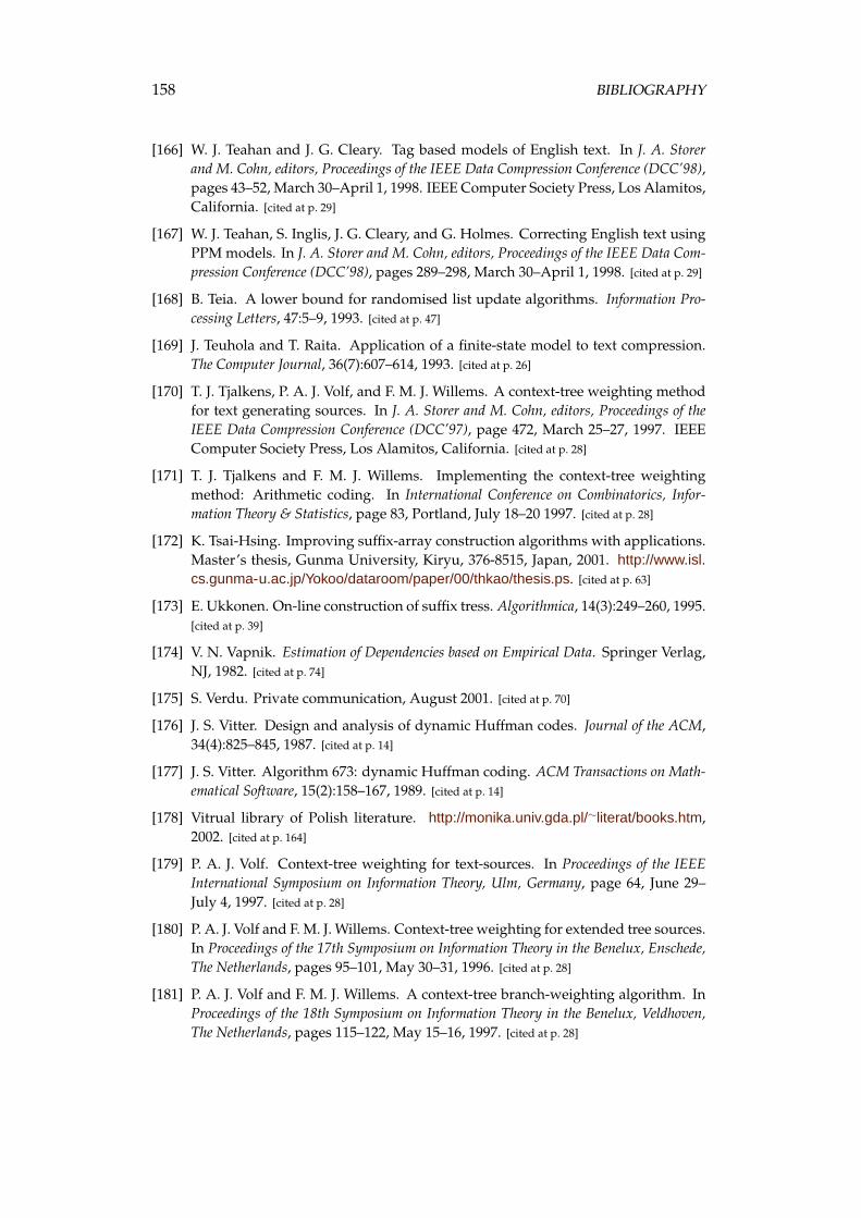
158 BIBLIOGRAPHY
[166] W. J. Teahan and J. G. Cleary. Tag based models of English text. In J. A. Storerand M. Cohn, editors, Proceedings of the IEEE Data Compression Conference (DCC’98),pages 43–52, March 30–April 1, 1998. IEEE Computer Society Press, Los Alamitos,California. [cited at p. 29]
[167] W. J. Teahan, S. Inglis, J. G. Cleary, and G. Holmes. Correcting English text usingPPM models. In J. A. Storer and M. Cohn, editors, Proceedings of the IEEE Data Com-pression Conference (DCC’98), pages 289–298, March 30–April 1, 1998. [cited at p. 29]
[168] B. Teia. A lower bound for randomised list update algorithms. Information Pro-cessing Letters, 47:5–9, 1993. [cited at p. 47]
[169] J. Teuhola and T. Raita. Application of a finite-state model to text compression.The Computer Journal, 36(7):607–614, 1993. [cited at p. 26]
[170] T. J. Tjalkens, P. A. J. Volf, and F. M. J. Willems. A context-tree weighting methodfor text generating sources. In J. A. Storer and M. Cohn, editors, Proceedings of theIEEE Data Compression Conference (DCC’97), page 472, March 25–27, 1997. IEEEComputer Society Press, Los Alamitos, California. [cited at p. 28]
[171] T. J. Tjalkens and F. M. J. Willems. Implementing the context-tree weightingmethod: Arithmetic coding. In International Conference on Combinatorics, Infor-mation Theory & Statistics, page 83, Portland, July 18–20 1997. [cited at p. 28]
[172] K. Tsai-Hsing. Improving suffix-array construction algorithms with applications.Master’s thesis, Gunma University, Kiryu, 376-8515, Japan, 2001. http://www.isl.cs.gunma-u.ac.jp/Yokoo/dataroom/paper/00/thkao/thesis.ps. [cited at p. 63]
[173] E. Ukkonen. On-line construction of suffix tress. Algorithmica, 14(3):249–260, 1995.[cited at p. 39]
[174] V. N. Vapnik. Estimation of Dependencies based on Empirical Data. Springer Verlag,NJ, 1982. [cited at p. 74]
[175] S. Verdu. Private communication, August 2001. [cited at p. 70]
[176] J. S. Vitter. Design and analysis of dynamic Huffman codes. Journal of the ACM,34(4):825–845, 1987. [cited at p. 14]
[177] J. S. Vitter. Algorithm 673: dynamic Huffman coding. ACM Transactions on Math-ematical Software, 15(2):158–167, 1989. [cited at p. 14]
[178] Vitrual library of Polish literature. http://monika.univ.gda.pl/∼literat/books.htm,2002. [cited at p. 164]
[179] P. A. J. Volf. Context-tree weighting for text-sources. In Proceedings of the IEEEInternational Symposium on Information Theory, Ulm, Germany, page 64, June 29–July 4, 1997. [cited at p. 28]
[180] P. A. J. Volf and F. M. J. Willems. Context-tree weighting for extended tree sources.In Proceedings of the 17th Symposium on Information Theory in the Benelux, Enschede,The Netherlands, pages 95–101, May 30–31, 1996. [cited at p. 28]
[181] P. A. J. Volf and F. M. J. Willems. A context-tree branch-weighting algorithm. InProceedings of the 18th Symposium on Information Theory in the Benelux, Veldhoven,The Netherlands, pages 115–122, May 15–16, 1997. [cited at p. 28]
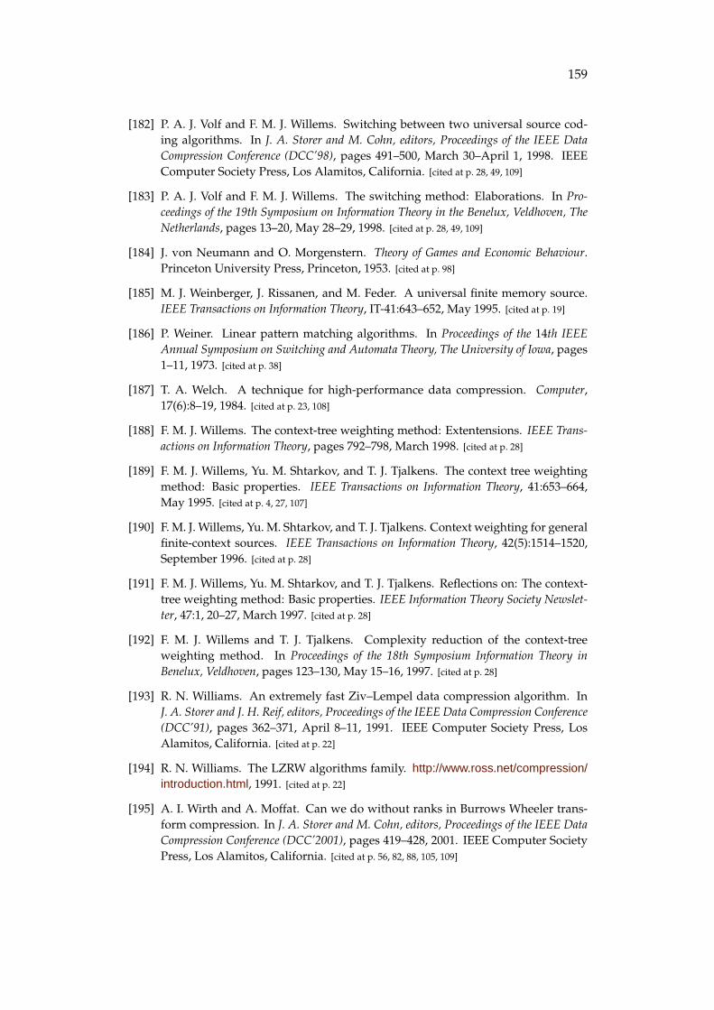
159
[182] P. A. J. Volf and F. M. J. Willems. Switching between two universal source cod-ing algorithms. In J. A. Storer and M. Cohn, editors, Proceedings of the IEEE DataCompression Conference (DCC’98), pages 491–500, March 30–April 1, 1998. IEEEComputer Society Press, Los Alamitos, California. [cited at p. 28, 49, 109]
[183] P. A. J. Volf and F. M. J. Willems. The switching method: Elaborations. In Pro-ceedings of the 19th Symposium on Information Theory in the Benelux, Veldhoven, TheNetherlands, pages 13–20, May 28–29, 1998. [cited at p. 28, 49, 109]
[184] J. von Neumann and O. Morgenstern. Theory of Games and Economic Behaviour.Princeton University Press, Princeton, 1953. [cited at p. 98]
[185] M. J. Weinberger, J. Rissanen, and M. Feder. A universal finite memory source.IEEE Transactions on Information Theory, IT-41:643–652, May 1995. [cited at p. 19]
[186] P. Weiner. Linear pattern matching algorithms. In Proceedings of the 14th IEEEAnnual Symposium on Switching and Automata Theory, The University of Iowa, pages1–11, 1973. [cited at p. 38]
[187] T. A. Welch. A technique for high-performance data compression. Computer,17(6):8–19, 1984. [cited at p. 23, 108]
[188] F. M. J. Willems. The context-tree weighting method: Extentensions. IEEE Trans-actions on Information Theory, pages 792–798, March 1998. [cited at p. 28]
[189] F. M. J. Willems, Yu. M. Shtarkov, and T. J. Tjalkens. The context tree weightingmethod: Basic properties. IEEE Transactions on Information Theory, 41:653–664,May 1995. [cited at p. 4, 27, 107]
[190] F. M. J. Willems, Yu. M. Shtarkov, and T. J. Tjalkens. Context weighting for generalfinite-context sources. IEEE Transactions on Information Theory, 42(5):1514–1520,September 1996. [cited at p. 28]
[191] F. M. J. Willems, Yu. M. Shtarkov, and T. J. Tjalkens. Reflections on: The context-tree weighting method: Basic properties. IEEE Information Theory Society Newslet-ter, 47:1, 20–27, March 1997. [cited at p. 28]
[192] F. M. J. Willems and T. J. Tjalkens. Complexity reduction of the context-treeweighting method. In Proceedings of the 18th Symposium Information Theory inBenelux, Veldhoven, pages 123–130, May 15–16, 1997. [cited at p. 28]
[193] R. N. Williams. An extremely fast Ziv–Lempel data compression algorithm. InJ. A. Storer and J. H. Reif, editors, Proceedings of the IEEE Data Compression Conference(DCC’91), pages 362–371, April 8–11, 1991. IEEE Computer Society Press, LosAlamitos, California. [cited at p. 22]
[194] R. N. Williams. The LZRW algorithms family. http://www.ross.net/compression/introduction.html, 1991. [cited at p. 22]
[195] A. I. Wirth and A. Moffat. Can we do without ranks in Burrows Wheeler trans-form compression. In J. A. Storer and M. Cohn, editors, Proceedings of the IEEE DataCompression Conference (DCC’2001), pages 419–428, 2001. IEEE Computer SocietyPress, Los Alamitos, California. [cited at p. 56, 82, 88, 105, 109]
160 BIBLIOGRAPHY
[196] I. H. Witten and T. C. Bell. The zero-frequency problem: estimating the probabili-ties of novel events in adaptive text compression. IEEE Transactions on InformationTheory, 37(3):1085–1094, 1991. [cited at p. 25]
[197] I. H. Witten, Z. Bray, M. Mahoui, and B. Teahan. Text mining: A new frontierfor lossless compression. In J. A. Storer and M. Cohn, editors, Proceedings of the IEEEData Compression Conference (DCC’99), March 29–31, 1999. IEEE Computer SocietyPress, Los Alamitos, California. [cited at p. 29]
[198] I. H. Witten, A. Moffat, and T. C. Bell. Managing Gigabytes: Compressing and Index-ing Documents and Images. Morgan Kaufmann Publishers, San Francisco, secondedition, 1999. [cited at p. 9]
[199] I. H. Witten, R. M. Neal, and J. F. Cleary. Arithmetic coding for data compression.Communications of the ACM, 30(6):520–540, 1987. [cited at p. 15]
[200] V. Yoockin. The ybs 0.03 program. ftp://ftp.elf.stuba.sk/pub/pc/pack/ybs003ew.zip,2002. [cited at p. 105, 109]
[201] T. L. Yu. Dynamic Markov compression. Dr. Dobb’s Journal, (243):30–33, 96–100,January 1996. [cited at p. 26]
[202] J. Ziv and A. Lempel. A universal algorithm for sequential data compression.IEEE Transactions on Information Theory, IT-23:337–343, 1977. [cited at p. 3, 21, 108]
[203] J. Ziv and A. Lempel. Compression of individual sequences via variable-rate cod-ing. IEEE Transactions on Information Theory, IT-24:530–536, 1978. [cited at p. 3, 21,
22]

Appendices
161

Appendix A
Silesia corpus
In this appendix, a more detailed description of the files in the Silesia corpus ispresented.
dickens
Charles Dickens wrote many novels. The file is a concatenation of fourteen ofhis works that can be found in the Project Gutenberg [131]. This is a simple textfile. The included novels are: A Child’s History Of England, All The Year Round:Contributions, American Notes, The Battle Of Life, Bleak House, A Christmas Carol,David Copperfield, Dombey And Son, Doctor Marigold, Going Into Society, GeorgeSilverman’s Explanation, Barnaby Rudge: a tale of the Riots of ’eighty, The Chimes,The Cricket On The Hearth.
mozilla
A Mozilla 1.0 [117] open source web browser was installed on the Tru64 UNIXoperating system and then the contents of the Mozilla.org directory were tarred.There are 525 files of types such as: executables, jar archives, HTML, XML, text,and others.
mr
A magnetic resonance medical picture of a head. This file is stored in a DICOMformat and contains 19 planes.
nci
The chemical databases of structures contain information of structures, theircomponents, 2D or 3D coordinates, properties, etc. The file is a part of the Au-
163
164 APPENDIX A. SILESIA CORPUS
gust 2000 2D file stored in an SDF format which is a common file format devel-oped to handle a list of molecular structures associated with properties [61]. Theoriginal database is of size 982 MB so it is necessary to truncate it to be suitablefor a part of the corpus. The 32 MB piece (rounded down to the nearest end ofthe record) is taken from about the middle of the original file (starting at the firstrecord after leaving 400 MB of data).
ooffice
An OpenOffice.org [121] is an open source project, which is composed of theword processor, spreadsheet program, presentation maker, and graphical pro-gram. The file is a dynamic linked library from version 1.01 for Windows oper-ating system.
osdb
An Open Source Database Benchmark [120] is a project created to provide a freetest for database systems. Some of the parts of the project are sample databases.The 40 MB benchmark was run on a MySQL 3.23 server. The file is one of theMySQL database files, hundred.med.
reymont
A book Chłopi [133] by Władysław Reymont was honoured the Nobel Pricein 1924. The text of the book was taken from the Virtual Library of Polish Litera-ture [178]. Then it was converted to the LATEX files from which the uncompressedPDF file was produced. The file is uncompressed, because the build-in compres-sion in the PDF format is rather poor, and much better results can be obtainedwhen we compress the uncompressed PDF files.
samba
Samba [141] is an open source project that is intended to be a free alternative tothe SMB/CIFS clients. The file contains tarred source code (also documentationand graphics) of the Samba 2.2-3 version.
sao
There are many star catalogues containing the data of sky objects. The chosenone, SAO catalogue [142], is suitable especially for the amateur astronomers. Itcontains the description of 258,996 stars, and is composed of binary records.

165
webster
The 1913 Webster Unabridged Dictionary [130] is an English dictionary storedin a rather simple HTML. The file is a concatenation of files that can be obtainedfrom Project Gutenberg [131].
xml
A concatenation of 21 XML files used by Cheney [46]. The chosen files are highly,mixed, and little structured and tagged.
x-ray
An X-ray medical picture of child’s hand. This is a 12-bit grayscale image.

Appendix B
Implementation details
The compression program introduced in the thesis is implemented in C++. Herewe provide a brief description of its usage and the contents of source code files.
B.1 Program usage
The compression program sdc can be executed with several command line pa-rameters to choose the compression method. The syntax of the execution is:
sdc 〈e|d|i〉 [switches] 〈input file name〉 〈output file name〉The options are:
• e—encoding,
• d—decoding; if this option is chosen, then switches are ignored,
• i—show info of the compressed file; if this option is chosen, then switchesare ignored.
The available switches are:
• –b〈size〉—sets the block size. The proper values are expressed in MB andmust lie in the range [1, 128]. It should be remembered that the memoryused by program is about 9 times greater than the block size. The specialvalue 0 sets the block size equal to the size of the file to be compressed butnot greater than 128 MB. The default value is 0.
• –f{L|S|I|C}—chooses the BWT computation method. The available op-tions are:
– M—the Manber–Myers’s method [106],
– L—the Larsson–Sadakane’s method [102],
167
168 APPENDIX B. IMPLEMENTATION DETAILS
– S—the improved Seward’s copy method [149] implemented in thebzip2 program [150], with the Manber–Myers’s method as a fallback,
– IT1—the improved Itoh–Tanaka-based method (Section 4.1.2) of or-der 1, with the Manber–Myers’s method as a fallback,
– IT2—the improved Itoh–Tanaka-based method of order 2, with theManber–Myers’s method as a fallback,
– IT—the improved Itoh–Tanaka-based method of order chosen relat-ing on the contents of the file, with the Manber–Myers’s method as afallback,
– C—the combined method; depending on the contents of the file, theprogram chooses between all the available methods.
The choice of the method affects the compression speed only. Usually thefastest method is C, but the best worst-case time complexity gives the Lmethod. The default value is C.
• –s{W|M|T}—chooses the second stage transform. The available optionsare:
– M—the move-to-front transform [26],
– T—the time-stamp(0) transform [4],
– W—the weighted frequency count transform (Section 4.1.5).
The default value is W.
• –w〈wf〉—chooses the weight function if the WFC transform is used. (Al-ways the quantised versions of the weight functions are used.) The propervalues for wf are from the range [1, 9]. The weight functions are shownin Figure 4.8. The default value is 9.
• –t〈dist〉—chooses the maximum distance in the WFC weight functions.The proper values are from the range [1, 15]. The distance is set accord-ing to the rule tmax = 2 dist. The default value is 11.
• –m{0|1|2}—chooses the version of the move-to-front transform. The avail-able options are:
– 0—the original MTF transform,
– 1—the MTF-1 transform,
– 2—the MTF-2 transform.
The default value is 2.
B.2. SOURCE CODE 169
B.2 Source code
Burrows–Wheeler transform
Several BWT computation methods are implemented in the compression pro-gram. The Larsson–Sadakane’s method [102], implemented in a class CLSBWT,is located in the files lsbwt.cpp and lsbwt.h. This source code is based on theoriginal implementation by Larsson and Sadakane [100].
The other BWT computation methods are implemented in a class CSITBWT,located in the source code files sitbwt.cpp and sitbwt.h. The main sorting proce-dure is based on the Seward’s method [149]. It executes as follows:
1. Sort the suffixes with the bucket sort procedure according to one (largebuckets) and two (small buckets) initial symbols.
2. Sort the large buckets with the Shell sort [153] procedure according to theirsize.
3. Sort the suffixes in the buckets with a ternary quick sort procedure [25].As the pivot in the quick sort procedure a median of three is used. If thenumber of suffixes to be sorted is less than some threshold then the Shellsort procedure is used.
4. If a level of recursive calls of the quick sort procedure is higher than anassumed number, the Shell sort procedure for sorting the remaining partis executed.
5. If the sorting takes too long (longer than the assumed complexity) thequick sort procedure is stopped and the fallback procedure is used, whichis the Manber–Myers’s method [106].
We introduced several improvements to the implementation based on thebzip2 program [150]. The most important are:
• The increments in the Shell sort procedure [153] are replaced from Knuthproposal [94] to Sedgewick proposal [147]. The experiments show that thischange accelerates the sorting process.
• If the number of suffixes to be sorted with the quick sort procedure is largerthan some threshold, a pseudo-median of nine is used to choose the pivot.
• If the number of suffixes is small (lest than 8) an insertion sort procedureis employed.
• A number of the recursive levels of the quick sort procedure is increasedfrom 12 to 256.

170 APPENDIX B. IMPLEMENTATION DETAILS
• A speed up for sorting strings with a long common prefix is used. Suchstrings are compared in a special way without the recursive calls of thequick sort procedure.
The class CSITBWT includes also an implementation of the improved Itoh–Tanaka’s method (Section 4.1.2). The working of the Itoh–Tanaka’s method is asfollows:
1. Sort the suffixes with the bucket sort procedure according to one (largebuckets) and two (small buckets) initial symbols, splitting meanwhile thebuckets into types D, E, and I.
2. Calculate what is the number of buckets of type E. If it is higher than 0.07n,then use the improved Itoh–Tanaka’s method of order 1. In the other case,use the improved Itoh–Tanaka’s method of order 2.
3. Calculate the total number of suffixes of types D and I. Choose the smallernumber and use according to it a forward or a reverse lexicographic orderto sort with the string-sorting procedure the smaller number of suffixes.
4. Execute the improved Seward’s method for sorting strings. If the im-proved Itoh–Tanaka’s method of order 1 is used, the special processingof the suffixes of type E is cared during sorting.
5. Sort the remaining unsorted suffixes.
Other stages
A weighted frequency count transform (Section 4.1.5) is implemented in a classCWFC, stored in the files wfc.cpp and wfc.h. The implementation is highly op-timised for speed to minimise the cost of maintaining the list L. The worst-casetime complexity of this implementation is O(nlk).
A move-to-front transform [26] is implemented in a class CMTF located inthe files mtf.cpp and mtf.h. This is an optimised implementation of the worst-case time complexity O(nk).
A time-stamp(0) transform [4] is implemented in a class CTS located in thefiles ts.cpp and ts.h. This is an implementation of the worst-case time complex-ity O(nk).
A zero run length encoding is implemented in a class CRLE0 located inthe files rle0.cpp and rle0.h. The worst-case time complexity of this transformis O(n).
The arithmetic coding class CBAC is an implementation based on the sourcecode by Moffat et al. [42] presented, in 1998, with the paper revisiting the arith-metic coding [115]. This class implements the weighted probability estimationmethod introduced in this thesis, as well as the coding of symbols being the
B.2. SOURCE CODE 171
output of the RLE-0 stage into a binary code. This class is located in the filesaac.cpp and aac.h.
Auxiliary program components
A class CCompress is a class gathering all the stages of the proposed compres-sion algorithm. It is located in the files compress.cpp and compress.h.
All the classes implementing the stages of the compression algorithm inher-its from the class CStage. An implementation of this abstract class is located inthe files stage.cpp and stage.h. As all the stages of the compression algorithmare implemented in the separate classes, the memory buffers are necessary tostore the intermediate results. To this end, a class CMemBuf is implemented.It is located in the files membuf.cpp and membuf.h. For easy processing of pa-rameters of the compression algorithm, e.g., the version of the move-to-fronttransform, the chosen weight function, etc. a class CParameters is designed. Itis located in the files pars.cpp and pars.h.
The main class of the compression program, CSDC, implements the fullfunctionality of the utility sdc. It is located in the files sdc.cpp and sdc.h.

Appendix C
Detailed options of examinedcompression programs
This appendix contains a more detailed description of the options chosen for theexamined programs.
7-zip
The method LZMA is chosen with the option –m0=LZMA. The memory for thedictionary is set to be 10 times larger (but not less than 16 MB) than the size ofthe file to compress. The option –mx is used to get the maximum compression.
acb 2.00c
The maximum compression method, u, is used.
boa 0.58b
The program is executed with a compression method –m15.
bzip 0.21
The block size is set, with the option –9, to the maximal possible value, 900 kB.
compress
The maximum size of the dictionary is used.
DW, DM
The size of the block is chosen to be the size of the file to compress.
173
174 APPENDIX C. DETAILED OPTIONS OF EXAMINED . . .
gzip
The option –9 is used for maximum compression.
lgha
The default options are used.
PPMd var. H
The PPM order is set to 16 with the option –o16. The memory limit is set, withthe option –m, to be 10 times the size of the file to compress, but not less than16 MB.
ppmnb1+
The order of the PPM is set to a pseudo order 9 with the option –O9. The mem-ory limit is set, with the option –M:50, to maximum possible value, which is50 MB. Also options –DA, –ICd, –E8d are used to disable data-specific filters.
PPMonstr var. H
The PPM order is set to 16 with the option –o16. The memory limit is set, withthe option –m, to be 10 times the size of the file to compress, but not less than16 MB.
PPMonstr var. I
The PPM order is set to 4 and 64, with the options –o4 and –o64 respectively, aswe examine two sets of parameters for this program. The memory limit is set,with the option –m, to be 10 times the size of the file to compress, but not lessthan 16 MB. The special memory limit of 256 MB was set for file mozilla, becausewith larger memory limit for this file the program crushed.
rar 2.90
The program is used with a compression method –m3. The maximum size ofthe dictionary is chosen with the option –md4096. The multimedia filters areturned off using –mm–.
szip
The order of the BWT is set to unlimited (as in the classical BWT) with the option–o0. The size of the block is set to 4.1 MB (maximal possible value) with theoption –b41.
175
ufa 0.04 Beta 1
The program is executed with the option –m5, which chooses the binary PPMalgorithm.
ybs
The block size is set to 16 MB, which is the maximum possible value, with theoption –m16m.


Appendix D
Illustration of the propertiesof the weight functions
This appendix contains additional figures presenting the results of the experi-ments with probability estimation methods for the output of the piecewise sta-tionary memoryless source.
177
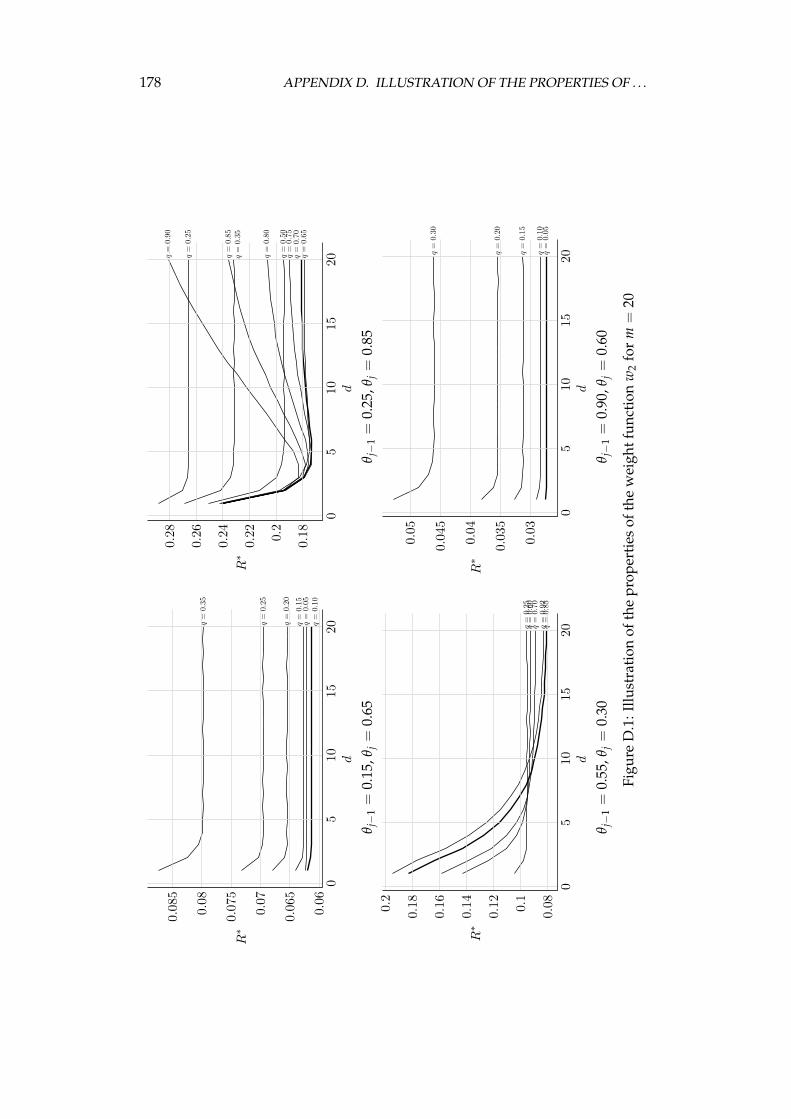
178 APPENDIX D. ILLUSTRATION OF THE PROPERTIES OF . . .
q=
0.35
q=
0.25
q=
0.20
q=
0.15
q=
0.05
q=
0.10
05
1015
200.
06
0.06
5
0.07
0.07
5
0.08
0.08
5
d
R∗
q=
0.90
q=
0.25
q=
0.85
q=
0.35
q=
0.80
q=
0.50
q=
0.75
q=
0.70
q=
0.65
05
1015
20
0.180.2
0.22
0.24
0.26
0.28
d
R∗
θ j−
1=
0.15
,θj=
0.65
θ j−
1=
0.25
,θj=
0.85
q=
0.25
q=
0.60
q=
0.70
q=
0.92
q=
0.85
05
1015
200.
080.1
0.12
0.14
0.16
0.180.2
d
R∗
q=
0.30
q=
0.20
q=
0.15
q=
0.10
q=
0.05
05
1015
20
0.03
0.03
5
0.04
0.04
5
0.05
d
R∗
θ j−
1=
0.55
,θj=
0.30
θ j−
1=
0.90
,θj=
0.60
Figu
reD
.1:I
llust
rati
onof
the
prop
erti
esof
the
wei
ghtf
unct
ion
w2
for
m=
20
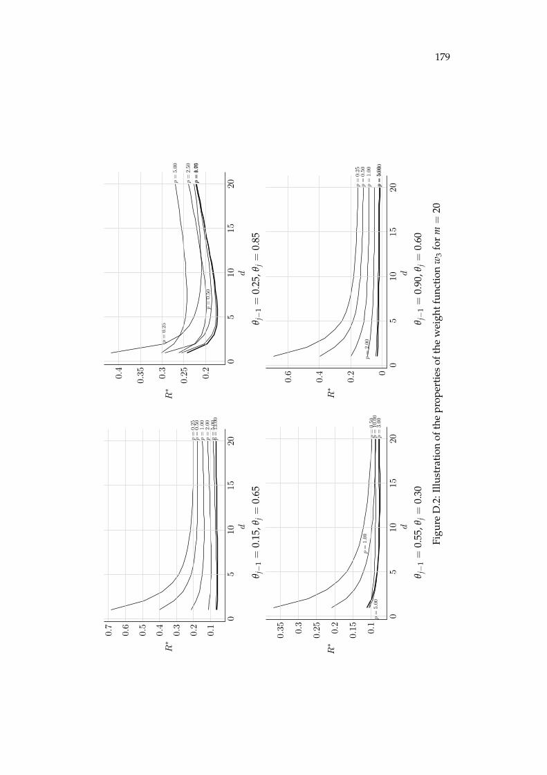
179
p=
0.25
p=
0.50
p=
1.00
p=
2.00
p=
5.00
p=
13.0
0
05
1015
20
0.1
0.2
0.3
0.4
0.5
0.6
0.7
d
R∗
p=
0.25
p=
5.00
p=
2.50
p=
1.00
p=
0.75
p=
0.50
05
1015
20
0.2
0.250.3
0.350.4
d
R∗
θ j−
1=
0.15
,θj=
0.65
θ j−
1=
0.25
,θj=
0.85
p=
0.50
p=
10.0
0p
=3.
00
p=
1.00
p=
5.00
05
1015
20
0.1
0.150.2
0.250.3
0.35
d
R∗
p=
0.25
p=
0.50
p=
1.00
p=
5.00
p=
2.00
p=
10.0
0
05
1015
200
0.2
0.4
0.6
d
R∗
θ j−
1=
0.55
,θj=
0.30
θ j−
1=
0.90
,θj=
0.60
Figu
reD
.2:I
llust
rati
onof
the
prop
erti
esof
the
wei
ghtf
unct
ion
w3
for
m=
20
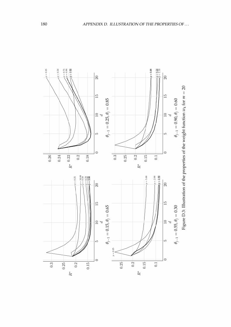
180 APPENDIX D. ILLUSTRATION OF THE PROPERTIES OF . . .
p=
0.25
p=
10.0
0p
=0.
50p
=0.
70p
=0.
90p
=2.
00p
=1.
30
05
1015
20
0.150.2
0.250.3
d
R∗
p=
0.25
p=
0.50
p=
0.75
p=
0.90
p=
5.00
p=
1.50
05
1015
20
0.180.2
0.22
0.24
0.26
d
R∗
θ j−
1=
0.15
,θj=
0.65
θ j−
1=
0.25
,θj=
0.85
p=
0.25
p=
5.00
p=
2.00
p=
1.00
p=
0.50
05
1015
20
0.1
0.150.2
0.25
d
R∗
p=
5.00
p=
0.25
p=
0.50
p=
2.00
p=
1.10
05
1015
20
0.1
0.150.2
0.250.3
d
R∗
θ j−
1=
0.55
,θj=
0.30
θ j−
1=
0.90
,θj=
0.60
Figu
reD
.3:I
llust
rati
onof
the
prop
erti
esof
the
wei
ghtf
unct
ion
w4
for
m=
20
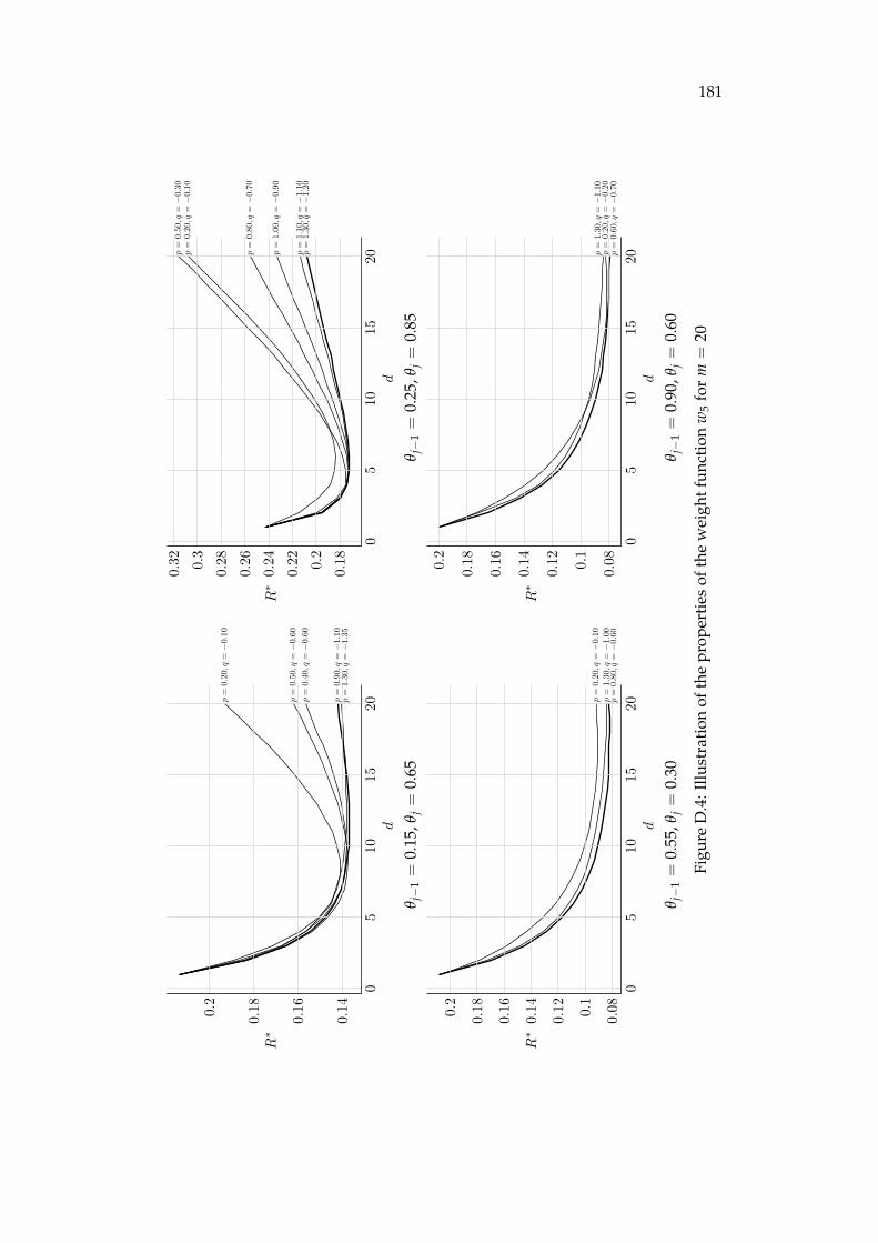
181
p=
0.20
,q=−
0.10
p=
0.40
,q=−
0.60
p=
0.50
,q=−
0.60
p=
0.90
,q=−
1.10
p=
1.30
,q=−
1.35
05
1015
20
0.14
0.16
0.180.2
d
R∗
p=
0.20
,q=−
0.10
p=
0.50
,q=−
0.30
p=
0.80
,q=−
0.70
p=
1.00
,q=−
0.90
p=
1.10
,q=−
1.10
p=
1.30
,q=−
1.20
05
1015
20
0.180.2
0.22
0.24
0.26
0.280.3
0.32
d
R∗
θ j−
1=
0.15
,θj=
0.65
θ j−
1=
0.25
,θj=
0.85
p=
0.20
,q=−
0.10
p=
0.80
,q=−
0.60
p=
1.30
,q=−
1.00
05
1015
200.
080.1
0.12
0.14
0.16
0.180.2
d
R∗
p=
0.20
,q=−
0.20
p=
0.60
,q=−
0.70
p=
1.30
,q=−
1.10
05
1015
200.
080.1
0.12
0.14
0.16
0.180.2
d
R∗
θ j−
1=
0.55
,θj=
0.30
θ j−
1=
0.90
,θj=
0.60
Figu
reD
.4:I
llust
rati
onof
the
prop
erti
esof
the
wei
ghtf
unct
ion
w5
for
m=
20
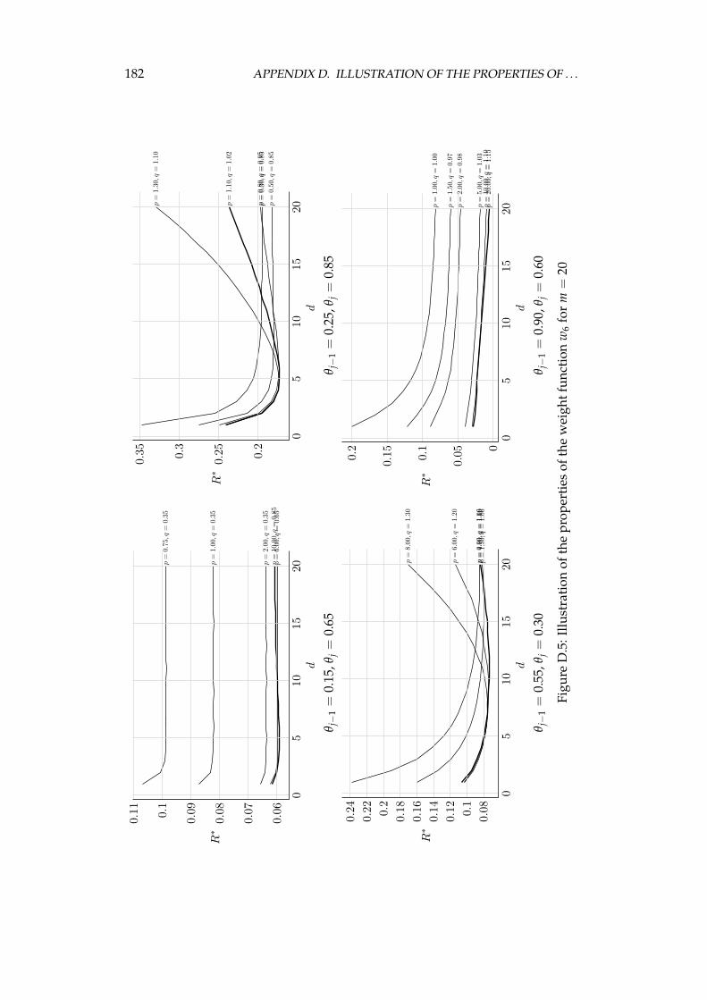
182 APPENDIX D. ILLUSTRATION OF THE PROPERTIES OF . . .
p=
0.75
,q=
0.35
p=
1.00
,q=
0.35
p=
2.00
,q=
0.35
p=
10.0
0,q
=0.
85p
=6.
00,q
=0.
65
05
1015
20
0.06
0.07
0.08
0.090.1
0.11
d
R∗
p=
1.30
,q=
1.10
p=
1.10
,q=
1.02
p=
0.80
,q=
0.95
p=
0.30
,q=
0.85
p=
0.50
,q=
0.85
05
1015
20
0.2
0.250.3
0.35
d
R∗
θ j−
1=
0.15
,θj=
0.65
θ j−
1=
0.25
,θj=
0.85
p=
8.00
,q=
1.30
p=
6.00
,q=
1.20
p=
0.90
,q=
1.06
p=
4.00
,q=
1.10
p=
1.50
,q=
1.06
05
1015
20
0.080.1
0.12
0.14
0.16
0.180.2
0.22
0.24
d
R∗
p=
1.00
,q=
1.00
p=
1.50
,q=
0.97
p=
2.00
,q=
0.98
p=
5.00
,q=
1.03
p=
10.0
0,q
=1.
10p
=20
.00,
q=
1.15
05
1015
200
0.050.1
0.150.2
d
R∗
θ j−
1=
0.55
,θj=
0.30
θ j−
1=
0.90
,θj=
0.60
Figu
reD
.5:I
llust
rati
onof
the
prop
erti
esof
the
wei
ghtf
unct
ion
w6
for
m=
20
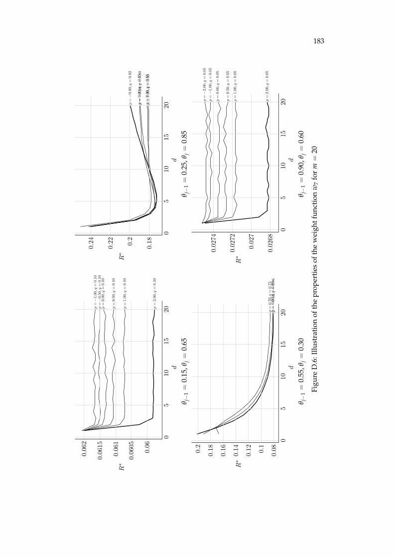
183
p=−
1.00
,q=
0.10
p=−
0.50
,q=
0.10
p=
0.00
,q=
0.10
p=
0.50
,q=
0.10
p=
1.00
,q=
0.10
p=
2.00
,q=
0.10
05
1015
20
0.06
0.06
05
0.06
1
0.06
15
0.06
2
d
R∗
p=−
0.80
,q=
0.92
p=
0.00
,q=
0.75
p=−
0.30
,q=
0.80
p=
0.30
,q=
0.65
p=
1.00
,q=
0.50
05
1015
20
0.180.2
0.22
0.24
d
R∗
θ j−
1=
0.15
,θj=
0.65
θ j−
1=
0.25
,θj=
0.85
p=
0.70
,q=
0.75
p=
0.00
,q=
0.90
p=−
0.50
,q=
0.96
05
1015
200.
080.1
0.12
0.14
0.16
0.180.2
d
R∗
p=−
2.00
,q=
0.05
p=−
1.00
,q=
0.05
p=
0.00
,q=
0.05
p=
0.50
,q=
0.05
p=
1.00
,q=
0.05
p=
2.00
,q=
0.05
05
1015
20
0.02
68
0.02
7
0.02
72
0.02
74
d
R∗
θ j−
1=
0.55
,θj=
0.30
θ j−
1=
0.90
,θj=
0.60
Figu
reD
.6:I
llust
rati
onof
the
prop
erti
esof
the
wei
ghtf
unct
ion
w7
for
m=
20

Appendix E
Detailed compression resultsfor files of different sizesand similar contents
This appendix contains detailed results of compression ratios and speeds forparts of different sizes of standard data files.
185
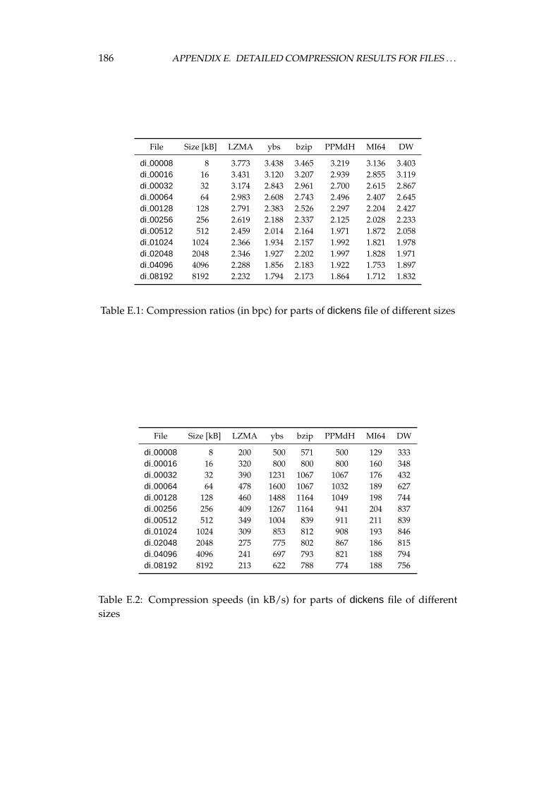
186 APPENDIX E. DETAILED COMPRESSION RESULTS FOR FILES . . .
File Size [kB] LZMA ybs bzip PPMdH MI64 DW
di 00008 8 3.773 3.438 3.465 3.219 3.136 3.403di 00016 16 3.431 3.120 3.207 2.939 2.855 3.119di 00032 32 3.174 2.843 2.961 2.700 2.615 2.867di 00064 64 2.983 2.608 2.743 2.496 2.407 2.645di 00128 128 2.791 2.383 2.526 2.297 2.204 2.427di 00256 256 2.619 2.188 2.337 2.125 2.028 2.233di 00512 512 2.459 2.014 2.164 1.971 1.872 2.058di 01024 1024 2.366 1.934 2.157 1.992 1.821 1.978di 02048 2048 2.346 1.927 2.202 1.997 1.828 1.971di 04096 4096 2.288 1.856 2.183 1.922 1.753 1.897di 08192 8192 2.232 1.794 2.173 1.864 1.712 1.832
Table E.1: Compression ratios (in bpc) for parts of dickens file of different sizes
File Size [kB] LZMA ybs bzip PPMdH MI64 DW
di 00008 8 200 500 571 500 129 333di 00016 16 320 800 800 800 160 348di 00032 32 390 1231 1067 1067 176 432di 00064 64 478 1600 1067 1032 189 627di 00128 128 460 1488 1164 1049 198 744di 00256 256 409 1267 1164 941 204 837di 00512 512 349 1004 839 911 211 839di 01024 1024 309 853 812 908 193 846di 02048 2048 275 775 802 867 186 815di 04096 4096 241 697 793 821 188 794di 08192 8192 213 622 788 774 188 756
Table E.2: Compression speeds (in kB/s) for parts of dickens file of differentsizes
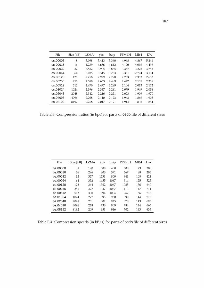
187
File Size [kB] LZMA ybs bzip PPMdH MI64 DW
os 00008 8 5.098 5.413 5.360 4.968 4.867 5.241os 00016 16 4.239 4.656 4.612 4.120 4.016 4.496os 00032 32 3.532 3.905 3.865 3.387 3.275 3.752os 00064 64 3.035 3.315 3.233 3.381 2.704 3.114os 00128 128 2.758 2.929 2.798 2.753 2.353 2.653os 00256 256 2.580 2.663 2.489 2.447 2.135 2.358os 00512 512 2.470 2.477 2.289 2.104 2.013 2.172os 01024 1024 2.396 2.337 2.261 2.079 1.949 2.056os 02048 2048 2.342 2.216 2.221 2.023 1.909 1.970os 04096 4096 2.298 2.110 2.193 1.963 1.866 1.905os 08192 8192 2.268 2.017 2.191 1.914 1.835 1.854
Table E.3: Compression ratios (in bpc) for parts of osdb file of different sizes
File Size [kB] LZMA ybs bzip PPMdH MI64 DW
os 00008 8 190 500 400 500 73 308os 00016 16 296 800 571 667 88 286os 00032 32 327 1231 800 941 108 421os 00064 64 352 1455 1067 914 125 525os 00128 128 344 1362 1067 1085 136 640os 00256 256 327 1347 1067 1113 147 711os 00512 512 300 1094 1004 962 156 716os 01024 1024 277 895 930 890 144 715os 02048 2048 251 802 925 870 143 696os 04096 4096 228 730 909 784 144 666os 08192 8192 209 651 916 702 143 635
Table E.4: Compression speeds (in kB/s) for parts of osdb file of different sizes
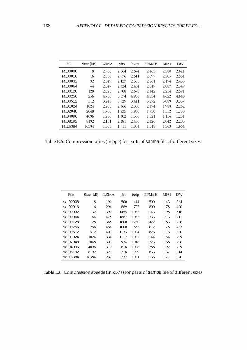
188 APPENDIX E. DETAILED COMPRESSION RESULTS FOR FILES . . .
File Size [kB] LZMA ybs bzip PPMdH MI64 DW
sa 00008 8 2.966 2.664 2.674 2.463 2.380 2.621sa 00016 16 2.850 2.576 2.611 2.397 2.305 2.561sa 00032 32 2.649 2.427 2.505 2.261 2.174 2.438sa 00064 64 2.547 2.324 2.434 2.317 2.087 2.349sa 00128 128 2.525 2.708 2.673 2.442 2.254 2.591sa 00256 256 4.786 5.074 4.956 4.834 4.622 4.846sa 00512 512 3.243 3.529 3.441 3.272 3.089 3.357sa 01024 1024 2.205 2.366 2.350 2.174 1.988 2.262sa 02048 2048 1.766 1.835 1.930 1.730 1.552 1.788sa 04096 4096 1.256 1.302 1.566 1.321 1.156 1.281sa 08192 8192 2.131 2.281 2.466 2.126 2.042 2.205sa 16384 16384 1.503 1.711 1.804 1.518 1.363 1.664
Table E.5: Compression ratios (in bpc) for parts of samba file of different sizes
File Size [kB] LZMA ybs bzip PPMdH MI64 DW
sa 00008 8 190 500 444 500 143 364sa 00016 16 296 889 727 800 178 400sa 00032 32 390 1455 1067 1143 198 516sa 00064 64 478 1882 1067 1333 213 711sa 00128 128 368 1600 1280 1422 183 736sa 00256 256 456 1000 853 612 78 463sa 00512 512 403 1133 1024 826 116 660sa 01024 1024 334 1112 1077 1144 154 799sa 02048 2048 303 934 1018 1223 168 796sa 04096 4096 310 818 1008 1288 192 769sa 08192 8192 329 718 929 833 137 614sa 16384 16384 237 732 1001 1136 171 670
Table E.6: Compression speeds (in kB/s) for parts of samba file of different sizes
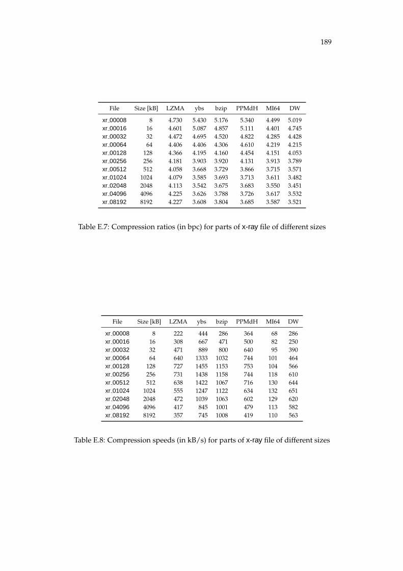
189
File Size [kB] LZMA ybs bzip PPMdH MI64 DW
xr 00008 8 4.730 5.430 5.176 5.340 4.499 5.019xr 00016 16 4.601 5.087 4.857 5.111 4.401 4.745xr 00032 32 4.472 4.695 4.520 4.822 4.285 4.428xr 00064 64 4.406 4.406 4.306 4.610 4.219 4.215xr 00128 128 4.366 4.195 4.160 4.454 4.151 4.053xr 00256 256 4.181 3.903 3.920 4.131 3.913 3.789xr 00512 512 4.058 3.668 3.729 3.866 3.715 3.571xr 01024 1024 4.079 3.585 3.693 3.713 3.611 3.482xr 02048 2048 4.113 3.542 3.675 3.683 3.550 3.451xr 04096 4096 4.225 3.626 3.788 3.726 3.617 3.532xr 08192 8192 4.227 3.608 3.804 3.685 3.587 3.521
Table E.7: Compression ratios (in bpc) for parts of x-ray file of different sizes
File Size [kB] LZMA ybs bzip PPMdH MI64 DW
xr 00008 8 222 444 286 364 68 286xr 00016 16 308 667 471 500 82 250xr 00032 32 471 889 800 640 95 390xr 00064 64 640 1333 1032 744 101 464xr 00128 128 727 1455 1153 753 104 566xr 00256 256 731 1438 1158 744 118 610xr 00512 512 638 1422 1067 716 130 644xr 01024 1024 555 1247 1122 634 132 651xr 02048 2048 472 1039 1063 602 129 620xr 04096 4096 417 845 1001 479 113 582xr 08192 8192 357 745 1008 419 110 563
Table E.8: Compression speeds (in kB/s) for parts of x-ray file of different sizes

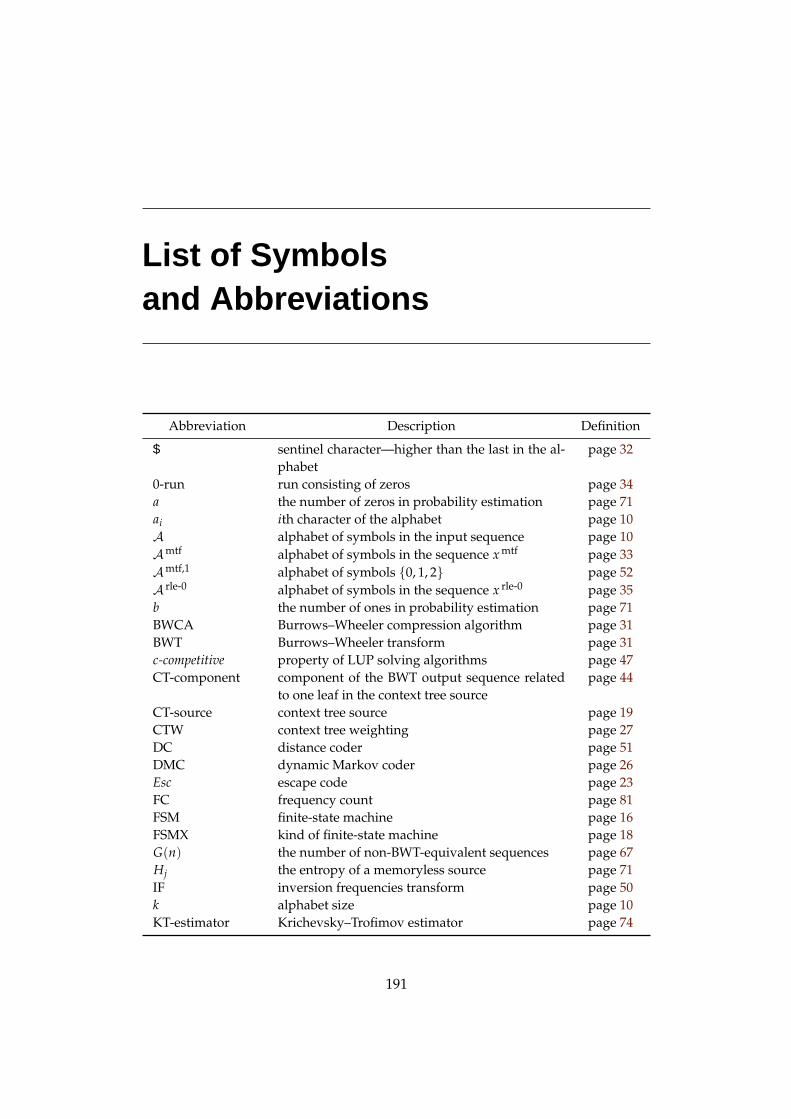
List of Symbolsand Abbreviations
Abbreviation Description Definition
$ sentinel character—higher than the last in the al-phabet
page 32
0-run run consisting of zeros page 34a the number of zeros in probability estimation page 71ai ith character of the alphabet page 10A alphabet of symbols in the input sequence page 10Amtf alphabet of symbols in the sequence x mtf page 33Amtf,1 alphabet of symbols {0, 1, 2} page 52A rle-0 alphabet of symbols in the sequence x rle-0 page 35b the number of ones in probability estimation page 71BWCA Burrows–Wheeler compression algorithm page 31BWT Burrows–Wheeler transform page 31c-competitive property of LUP solving algorithms page 47CT-component component of the BWT output sequence related
to one leaf in the context tree sourcepage 44
CT-source context tree source page 19CTW context tree weighting page 27DC distance coder page 51DMC dynamic Markov coder page 26Esc escape code page 23FC frequency count page 81FSM finite-state machine page 16FSMX kind of finite-state machine page 18G(n) the number of non-BWT-equivalent sequences page 67Hj the entropy of a memoryless source page 71IF inversion frequencies transform page 50k alphabet size page 10KT-estimator Krichevsky–Trofimov estimator page 74
191
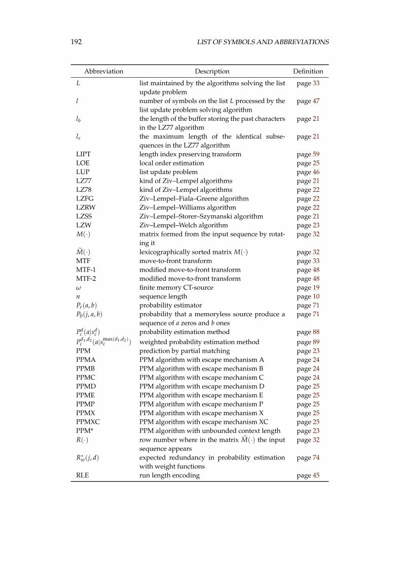
192 LIST OF SYMBOLS AND ABBREVIATIONS
Abbreviation Description Definition
L list maintained by the algorithms solving the listupdate problem
page 33
l number of symbols on the list L processed by thelist update problem solving algorithm
page 47
lb the length of the buffer storing the past charactersin the LZ77 algorithm
page 21
ls the maximum length of the identical subse-quences in the LZ77 algorithm
page 21
LIPT length index preserving transform page 59LOE local order estimation page 25LUP list update problem page 46LZ77 kind of Ziv–Lempel algorithms page 21LZ78 kind of Ziv–Lempel algorithms page 22LZFG Ziv–Lempel–Fiala–Greene algorithm page 22LZRW Ziv–Lempel–Williams algorithm page 22LZSS Ziv–Lempel–Storer–Szymanski algorithm page 21LZW Ziv–Lempel–Welch algorithm page 23M(·) matrix formed from the input sequence by rotat-
ing itpage 32
M(·) lexicographically sorted matrix M(·) page 32MTF move-to-front transform page 33MTF-1 modified move-to-front transform page 48MTF-2 modified move-to-front transform page 48ω finite memory CT-source page 19n sequence length page 10Pe(a, b) probability estimator page 71P0(j, a, b) probability that a memoryless source produce a
sequence of a zeros and b onespage 71
Pdc (a|sd
c ) probability estimation method page 88Pd1,d2
c (a|smax(d1,d2)c ) weighted probability estimation method page 89
PPM prediction by partial matching page 23PPMA PPM algorithm with escape mechanism A page 24PPMB PPM algorithm with escape mechanism B page 24PPMC PPM algorithm with escape mechanism C page 24PPMD PPM algorithm with escape mechanism D page 25PPME PPM algorithm with escape mechanism E page 25PPMP PPM algorithm with escape mechanism P page 25PPMX PPM algorithm with escape mechanism X page 25PPMXC PPM algorithm with escape mechanism XC page 25PPM* PPM algorithm with unbounded context length page 23R(·) row number where in the matrix M(·) the input
sequence appearspage 32
R∗w(j, d) expected redundancy in probability estimation
with weight functionspage 74
RLE run length encoding page 45
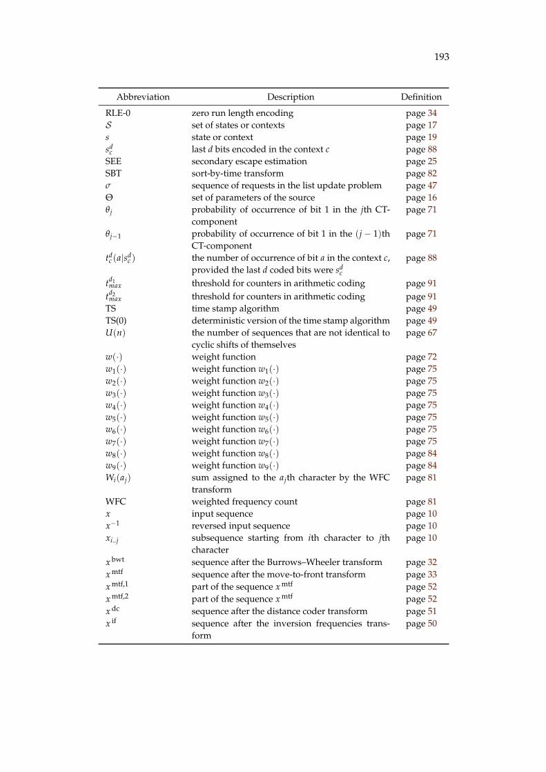
193
Abbreviation Description Definition
RLE-0 zero run length encoding page 34S set of states or contexts page 17s state or context page 19sd
c last d bits encoded in the context c page 88SEE secondary escape estimation page 25SBT sort-by-time transform page 82σ sequence of requests in the list update problem page 47Θ set of parameters of the source page 16θj probability of occurrence of bit 1 in the jth CT-
componentpage 71
θj−1 probability of occurrence of bit 1 in the (j − 1)thCT-component
page 71
tdc (a|sd
c ) the number of occurrence of bit a in the context c,provided the last d coded bits were sd
c
page 88
td1max threshold for counters in arithmetic coding page 91
td2max threshold for counters in arithmetic coding page 91
TS time stamp algorithm page 49TS(0) deterministic version of the time stamp algorithm page 49U(n) the number of sequences that are not identical to
cyclic shifts of themselvespage 67
w(·) weight function page 72w1(·) weight function w1(·) page 75w2(·) weight function w2(·) page 75w3(·) weight function w3(·) page 75w4(·) weight function w4(·) page 75w5(·) weight function w5(·) page 75w6(·) weight function w6(·) page 75w7(·) weight function w7(·) page 75w8(·) weight function w8(·) page 84w9(·) weight function w9(·) page 84Wi(aj) sum assigned to the ajth character by the WFC
transformpage 81
WFC weighted frequency count page 81x input sequence page 10x−1 reversed input sequence page 10xi..j subsequence starting from ith character to jth
characterpage 10
x bwt sequence after the Burrows–Wheeler transform page 32x mtf sequence after the move-to-front transform page 33x mtf,1 part of the sequence x mtf page 52x mtf,2 part of the sequence x mtf page 52x dc sequence after the distance coder transform page 51x if sequence after the inversion frequencies trans-
formpage 50

194 LIST OF SYMBOLS AND ABBREVIATIONS
Abbreviation Description Definition
x lup sequence after the algorithm solving the list up-date problem
page 47
x rle-0 sequence after the zero run length encoding page 35X (s) set of positions where CT-components starts in
the x bwt sequencepage 43
ZL Ziv–Lempel algorithms page 20
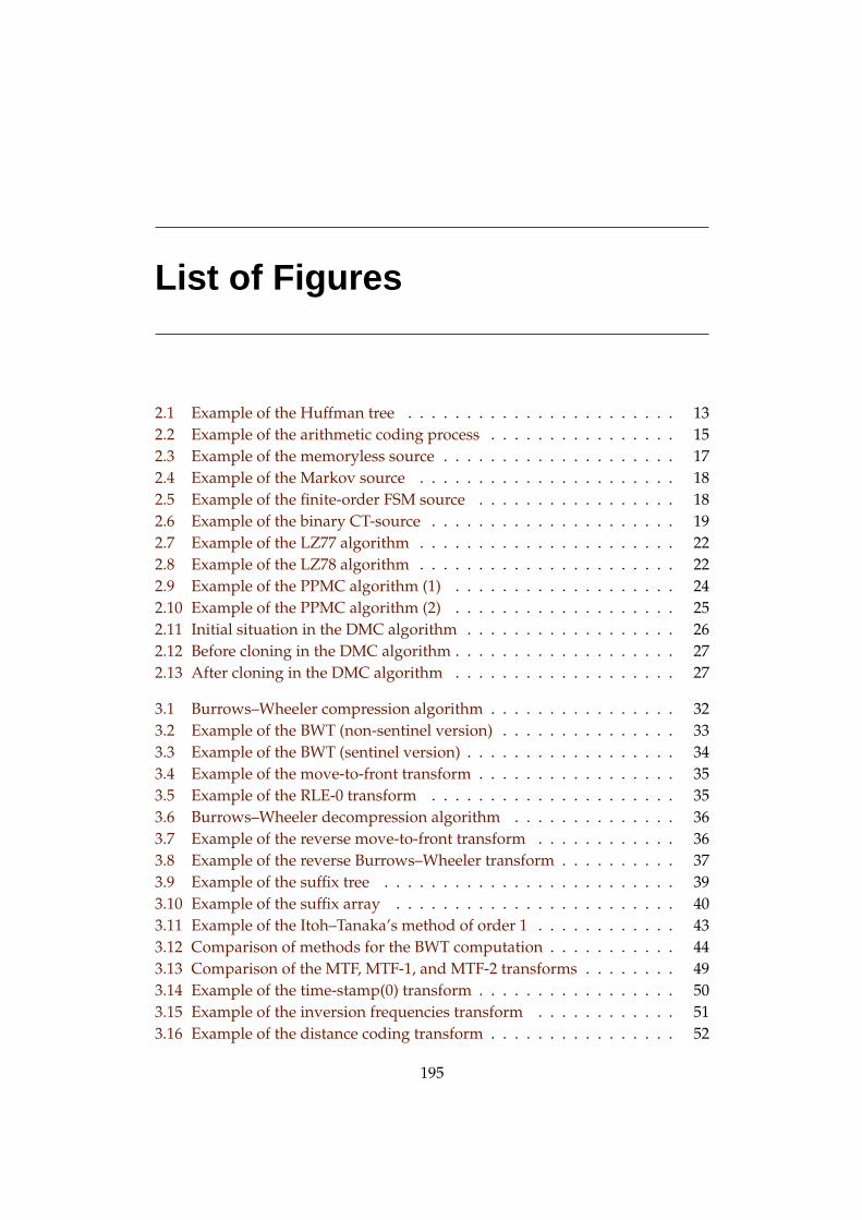
List of Figures
2.1 Example of the Huffman tree . . . . . . . . . . . . . . . . . . . . . . . 132.2 Example of the arithmetic coding process . . . . . . . . . . . . . . . . 152.3 Example of the memoryless source . . . . . . . . . . . . . . . . . . . . 172.4 Example of the Markov source . . . . . . . . . . . . . . . . . . . . . . 182.5 Example of the finite-order FSM source . . . . . . . . . . . . . . . . . 182.6 Example of the binary CT-source . . . . . . . . . . . . . . . . . . . . . 192.7 Example of the LZ77 algorithm . . . . . . . . . . . . . . . . . . . . . . 222.8 Example of the LZ78 algorithm . . . . . . . . . . . . . . . . . . . . . . 222.9 Example of the PPMC algorithm (1) . . . . . . . . . . . . . . . . . . . 242.10 Example of the PPMC algorithm (2) . . . . . . . . . . . . . . . . . . . 252.11 Initial situation in the DMC algorithm . . . . . . . . . . . . . . . . . . 262.12 Before cloning in the DMC algorithm . . . . . . . . . . . . . . . . . . . 272.13 After cloning in the DMC algorithm . . . . . . . . . . . . . . . . . . . 27
3.1 Burrows–Wheeler compression algorithm . . . . . . . . . . . . . . . . 323.2 Example of the BWT (non-sentinel version) . . . . . . . . . . . . . . . 333.3 Example of the BWT (sentinel version) . . . . . . . . . . . . . . . . . . 343.4 Example of the move-to-front transform . . . . . . . . . . . . . . . . . 353.5 Example of the RLE-0 transform . . . . . . . . . . . . . . . . . . . . . 353.6 Burrows–Wheeler decompression algorithm . . . . . . . . . . . . . . 363.7 Example of the reverse move-to-front transform . . . . . . . . . . . . 363.8 Example of the reverse Burrows–Wheeler transform . . . . . . . . . . 373.9 Example of the suffix tree . . . . . . . . . . . . . . . . . . . . . . . . . 393.10 Example of the suffix array . . . . . . . . . . . . . . . . . . . . . . . . 403.11 Example of the Itoh–Tanaka’s method of order 1 . . . . . . . . . . . . 433.12 Comparison of methods for the BWT computation . . . . . . . . . . . 443.13 Comparison of the MTF, MTF-1, and MTF-2 transforms . . . . . . . . 493.14 Example of the time-stamp(0) transform . . . . . . . . . . . . . . . . . 503.15 Example of the inversion frequencies transform . . . . . . . . . . . . 513.16 Example of the distance coding transform . . . . . . . . . . . . . . . . 52
195
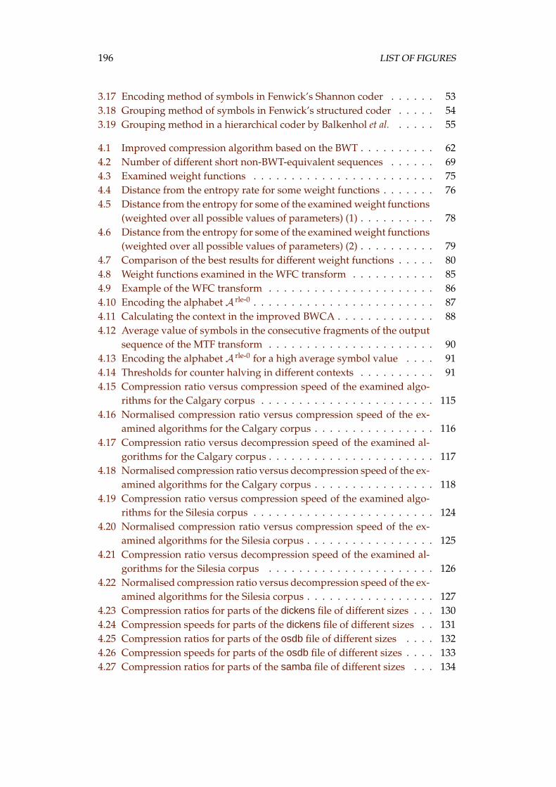
196 LIST OF FIGURES
3.17 Encoding method of symbols in Fenwick’s Shannon coder . . . . . . 533.18 Grouping method of symbols in Fenwick’s structured coder . . . . . 543.19 Grouping method in a hierarchical coder by Balkenhol et al. . . . . . 55
4.1 Improved compression algorithm based on the BWT . . . . . . . . . . 624.2 Number of different short non-BWT-equivalent sequences . . . . . . 694.3 Examined weight functions . . . . . . . . . . . . . . . . . . . . . . . . 754.4 Distance from the entropy rate for some weight functions . . . . . . . 764.5 Distance from the entropy for some of the examined weight functions
(weighted over all possible values of parameters) (1) . . . . . . . . . . 784.6 Distance from the entropy for some of the examined weight functions
(weighted over all possible values of parameters) (2) . . . . . . . . . . 794.7 Comparison of the best results for different weight functions . . . . . 804.8 Weight functions examined in the WFC transform . . . . . . . . . . . 854.9 Example of the WFC transform . . . . . . . . . . . . . . . . . . . . . . 864.10 Encoding the alphabet A rle-0 . . . . . . . . . . . . . . . . . . . . . . . . 874.11 Calculating the context in the improved BWCA . . . . . . . . . . . . . 884.12 Average value of symbols in the consecutive fragments of the output
sequence of the MTF transform . . . . . . . . . . . . . . . . . . . . . . 904.13 Encoding the alphabet A rle-0 for a high average symbol value . . . . 914.14 Thresholds for counter halving in different contexts . . . . . . . . . . 914.15 Compression ratio versus compression speed of the examined algo-
rithms for the Calgary corpus . . . . . . . . . . . . . . . . . . . . . . . 1154.16 Normalised compression ratio versus compression speed of the ex-
amined algorithms for the Calgary corpus . . . . . . . . . . . . . . . . 1164.17 Compression ratio versus decompression speed of the examined al-
gorithms for the Calgary corpus . . . . . . . . . . . . . . . . . . . . . . 1174.18 Normalised compression ratio versus decompression speed of the ex-
amined algorithms for the Calgary corpus . . . . . . . . . . . . . . . . 1184.19 Compression ratio versus compression speed of the examined algo-
rithms for the Silesia corpus . . . . . . . . . . . . . . . . . . . . . . . . 1244.20 Normalised compression ratio versus compression speed of the ex-
amined algorithms for the Silesia corpus . . . . . . . . . . . . . . . . . 1254.21 Compression ratio versus decompression speed of the examined al-
gorithms for the Silesia corpus . . . . . . . . . . . . . . . . . . . . . . 1264.22 Normalised compression ratio versus decompression speed of the ex-
amined algorithms for the Silesia corpus . . . . . . . . . . . . . . . . . 1274.23 Compression ratios for parts of the dickens file of different sizes . . . 1304.24 Compression speeds for parts of the dickens file of different sizes . . 1314.25 Compression ratios for parts of the osdb file of different sizes . . . . 1324.26 Compression speeds for parts of the osdb file of different sizes . . . . 1334.27 Compression ratios for parts of the samba file of different sizes . . . 134
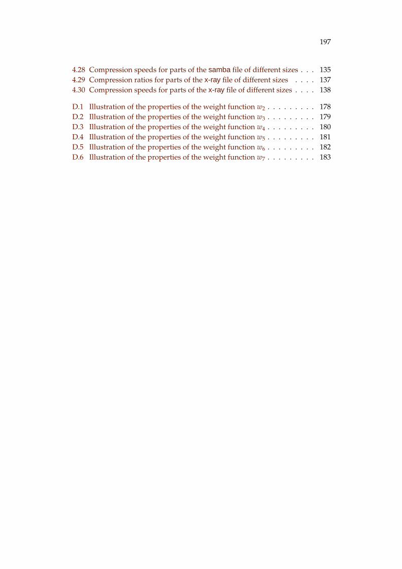
197
4.28 Compression speeds for parts of the samba file of different sizes . . . 1354.29 Compression ratios for parts of the x-ray file of different sizes . . . . 1374.30 Compression speeds for parts of the x-ray file of different sizes . . . . 138
D.1 Illustration of the properties of the weight function w2 . . . . . . . . . 178D.2 Illustration of the properties of the weight function w3 . . . . . . . . . 179D.3 Illustration of the properties of the weight function w4 . . . . . . . . . 180D.4 Illustration of the properties of the weight function w5 . . . . . . . . . 181D.5 Illustration of the properties of the weight function w6 . . . . . . . . . 182D.6 Illustration of the properties of the weight function w7 . . . . . . . . . 183
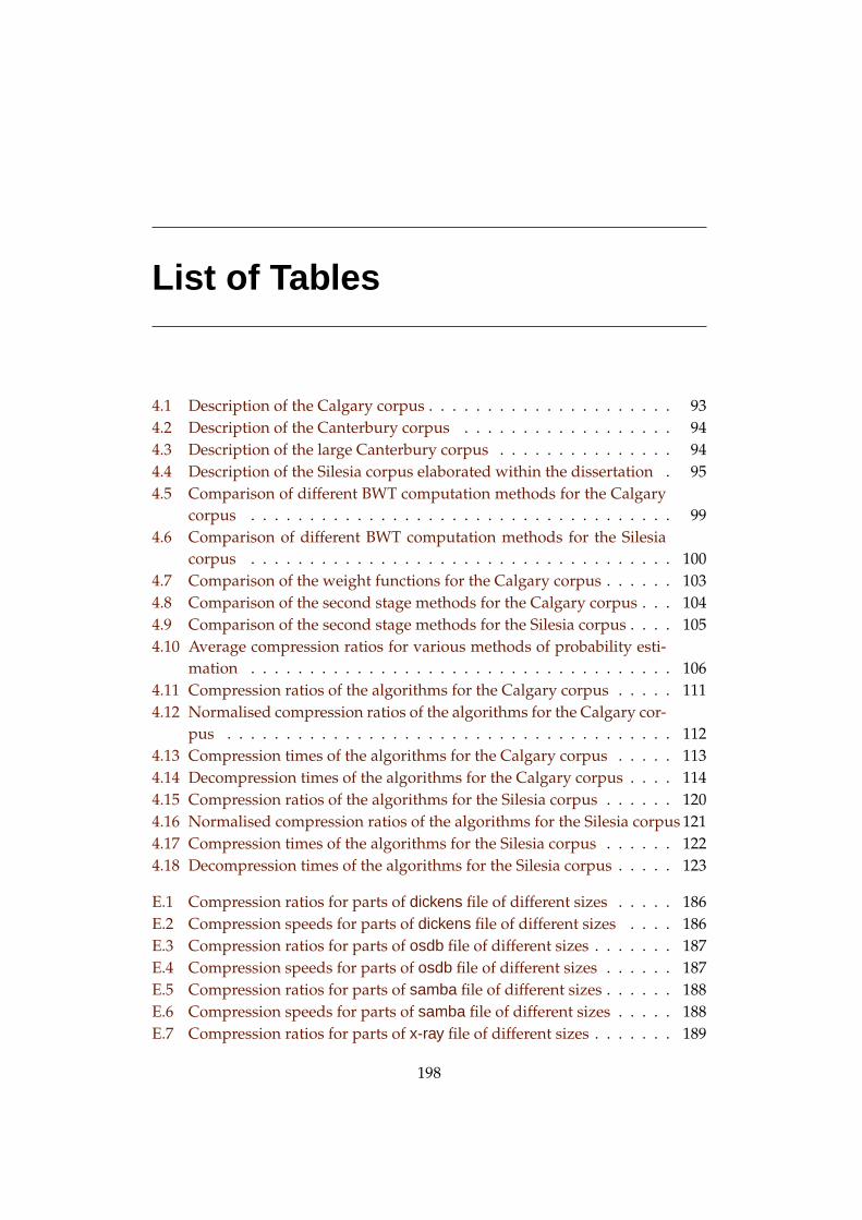
List of Tables
4.1 Description of the Calgary corpus . . . . . . . . . . . . . . . . . . . . . 934.2 Description of the Canterbury corpus . . . . . . . . . . . . . . . . . . 944.3 Description of the large Canterbury corpus . . . . . . . . . . . . . . . 944.4 Description of the Silesia corpus elaborated within the dissertation . 954.5 Comparison of different BWT computation methods for the Calgary
corpus . . . . . . . . . . . . . . . . . . . . . . . . . . . . . . . . . . . . 994.6 Comparison of different BWT computation methods for the Silesia
corpus . . . . . . . . . . . . . . . . . . . . . . . . . . . . . . . . . . . . 1004.7 Comparison of the weight functions for the Calgary corpus . . . . . . 1034.8 Comparison of the second stage methods for the Calgary corpus . . . 1044.9 Comparison of the second stage methods for the Silesia corpus . . . . 1054.10 Average compression ratios for various methods of probability esti-
mation . . . . . . . . . . . . . . . . . . . . . . . . . . . . . . . . . . . . 1064.11 Compression ratios of the algorithms for the Calgary corpus . . . . . 1114.12 Normalised compression ratios of the algorithms for the Calgary cor-
pus . . . . . . . . . . . . . . . . . . . . . . . . . . . . . . . . . . . . . . 1124.13 Compression times of the algorithms for the Calgary corpus . . . . . 1134.14 Decompression times of the algorithms for the Calgary corpus . . . . 1144.15 Compression ratios of the algorithms for the Silesia corpus . . . . . . 1204.16 Normalised compression ratios of the algorithms for the Silesia corpus 1214.17 Compression times of the algorithms for the Silesia corpus . . . . . . 1224.18 Decompression times of the algorithms for the Silesia corpus . . . . . 123
E.1 Compression ratios for parts of dickens file of different sizes . . . . . 186E.2 Compression speeds for parts of dickens file of different sizes . . . . 186E.3 Compression ratios for parts of osdb file of different sizes . . . . . . . 187E.4 Compression speeds for parts of osdb file of different sizes . . . . . . 187E.5 Compression ratios for parts of samba file of different sizes . . . . . . 188E.6 Compression speeds for parts of samba file of different sizes . . . . . 188E.7 Compression ratios for parts of x-ray file of different sizes . . . . . . . 189
198
199
E.8 Compression speeds for parts of x-ray file of different sizes . . . . . . 189
Index
0-run, 34, 627-zip program, 108, 173
Aberg, Jan, 25, 28acb 2.00c program, 107, 173Adair, Gilbert, 12adaptive compression, 12Albers, Susanne, 49, 50alice29.txt test file, 94alphabet, 8, 10, 16, 19, 33, 50, 64, 87
binary, 26, 28, 70, 77, 80, 81, 83decomposition, 28non-binary, 26, 28, 70, 77reordering, 57, 58size, 8, 10, 67, 142
analogue data, 7Apostolico, Alberto, 29Arimura, Mitsuharu, 28, 45arithmetic coding, 3–5, 14, 15, 21, 23, 35, 53, 56,
62, 84, 142binary, 53, 62, 84Elias algorithm, 14Fenwick’s tree, 15finite precision, 15interval, 14probability estimation, 62
Arnavut, Ziya, 45, 50, 57, 87, 105, 107Arnold, Ross, 92ASCII code, 8, 12, 58, 59asyoulik.txt test file, 94Awan, Fauzia Salim, 59
Bachrach, Ran, 47backup utilities, 97Balkenhol, Bernhard, 39, 43, 46, 48, 51, 52, 55,
56, 58, 105, 107Bell, Timothy C., 9, 22, 25, 26, 92Bentley, Jon Louis, 40bib test file, 93, 99, 103, 104, 111–114
bible test file, 94Binder, Edgar, 51Bloom, Charles, 25boa 0.58b program, 107, 173Bolton, Robert, 141book1 test file, 93, 99, 103, 104, 111–114book2 test file, 93, 99, 103, 104, 111–114Brown, Peter F., 29bucket sort procedure, 41, 169, 170Bunton, Suzanne, 25, 26, 107, 108Burrows, Michael, 4, 31, 32, 34, 38, 45, 48, 53,
141Burrows–Wheeler transform, 4, 6, 31–33, 35, 38,
40, 43–45, 48, 52, 56, 57, 61, 64, 65, 67,69, 70, 88, 90, 92, 98, 129, 141, 142, 174
computation, 5, 38, 40, 42, 44, 46, 62, 65,98, 141, 144, 146, 167, 169
Bentley–Sedgewick’s sorting method, 40Burrows–Wheeler’s sorting method, 38fallback method, 142Seward’s sorting method, 41, 141, 142,
168–170suffix array-based methods, see suffix ar-
raysuffix tree-based methods, see suffix tree
CT-component, 44–46, 48, 52, 54, 56, 57, 64,65, 70–74, 77, 81–83, 90
last column, 32matrix M, 32, 64–66
sorted, 32, 42–44, 64output, 5output sequence, 45, 142reverse, 37sentinel, 32, 33, 38, 67
Burrows–Wheeler transform-based compressionalgorithms, 4–6, 17, 31, 32, 35, 38, 41,42, 44, 45, 47, 48, 50, 57, 59–61, 81,
200
201
107–110, 119, 121, 128, 129, 136, 139,141–144
alphabet reordering, 57–59arithmetic coding, 53, 55–57, 88, 90
binary, 57, 87counters, 91decomposition, 84
block size, 139, 167decompression, 36direct encoding BWT output, 56, 82entropy coding, 35, 36, 57, 142entropy decoding, 36first stage, 52Huffman coding, 53, 57last stage, 47, 48, 52, 53, 57, 84preliminary filters, 58, 107
binary data, 60capital conversion, 59phrase substitution, 59text data, 60
probability estimation, 36, 87, 143Balkenhol’s et al. hierarchical coder, 55Balkenhol–Shtarkov’s hybrid approach,
55, 56exponential forgetting, 56Fenwick’s Shannon coder, 53, 54Fenwick’s structured coder, 54, 55
reversing input sequence, 44, 58run length encoding, 45second stage, 47, 48, 56, 62, 81, 82, 87, 104,
107–109, 119, 142Buyanovsky, George, 107BWCA, see Burrows–Wheeler transform-based
compression algorithmsBWT, see Burrows–Wheeler transformBWT-equivalent sequences, 67–70bzip 0.21 program, 107, 108, 173bzip program, 128bzip2 program, 53, 101, 168, 169
C programming language, 93, 94, 129C++ programming language, 167Calgary corpus, see corpusCanterbury corpus, see corpusCarpinelli, John, 146Carroll, Lewis, 94CD-ROM, 1Chapin, Brenton, 49, 57, 58character, 8, 10, 16Chen, Xin, 29Cheney, James, 165
Ciura, Marcin G., 6, 29, 145, 146Cleary, John G., 3, 23–25, 42, 93coding, 11
methods, 11communication satellites, 1compress program, 23, 108, 173compression ratio, 97, 98compression speed, 6, 97, 98context, 11
order d, 10preceding, 44, 58succeeding, 58successive, 44
context tree weighting algorithm, 4, 6, 27, 28,107, 136
arithmetic coding, 28binary alphabet, 28context tree source, 28non-binary alphabet, 28
Cormack, Gordon V., 4, 14, 26, 108corpus
Calgary, 5, 6, 34, 50, 59, 83, 89, 92, 93, 95,98, 99, 101–107, 109–118, 120, 128, 136,143, 144
Canterbury, 5, 6, 92–95, 143large Canterbury, 5, 6, 93, 94, 143Silesia, 5, 6, 95, 98, 100, 102, 105–109, 120–
128, 143, 144, 146, 163cp.html test file, 94CT-component, see Burrows–Wheeler transformCTW, see context tree weighting algorithmCzech, Zbigniew Janusz, 145
Daciuk, Jan, 29Daly, James, 94data expansion, 13data type
application files, 1, 8, 164audio, 9binary, 20databases, 1, 7, 8, 20, 95, 96, 163, 164English text, 11, 107HTML, 94–96, 129, 163, 165medical images, 2, 10, 95, 96, 163, 165
magnetic resonance, 95, 96movie, 1, 2multimedia, 1, 8, 95, 97PDF, 95, 96, 129, 164picture, 2, 8, 10, 20Polish text, 11, 13programming source code, 129
202 INDEX
text, 1, 7, 11, 20, 96, 129, 163video, 9, 11
frame, 9XML, 95, 96, 163, 165
dc program, 57Debudaj–Grabysz, Agnieszka, 146decompression speed, 6, 97, 98Deorowicz, Sebastian, 29dickens test file, 95, 96, 100, 105, 120–123, 128–
131, 163, 186Dickens, Charles, 95, 96, 163DICOM, 163dictionary compression methods, 20digital data, 7discrete data, 7distance coder, 51, 52, 56, 57, 87, 105, 109
basic version, 51improved version, 51
DMC, see dynamic Markov coderdominated solution, 98DVD, 97
player, 97dynamic Markov coder, 3, 4, 6, 26–28, 57, 108,
136binary alphabet, 26cloning, 26, 27FSM, 26generalised, 26Lazy DMC, 26, 108non-binary alphabet, 26states, 26transitions, 26
e.coli test file, 93, 94Effros, Michelle, 45Ekstrand, Nicklas, 28El-Yaniv, Ran, 47Elias γ code, 57, 87Elias, Peter, 51EMACS editor, 93entropy coding, 3–5, 12, 36, 46, 47, 50–52, 56, 62,
84, 87EOL character, 59Esxherichia coli genome, 94expected code length, 13
fallback method, 142, 168, 169Faller, Newton, 14Farach, Martin, 39Fenwick, Peter, 15, 34, 35, 45, 48, 53, 54, 56, 57,
88, 108Fiala, Edward R., 22
fileds.c test file, 94finite-precision numbers, 14, 15finite-state machine, 16, 17, 19Fraenkel, Aviezri S., 57Fraenkel–Klein Fibonacci codes, 57frequencies of symbol occurrences, 23frequency count transform, see list update prob-
lemfrequency table, 12, 13
Gailly, Jean-loup, 9Geigerich, Robert, 39geo test file, 83, 89, 93, 99, 103, 104, 107, 111–
114, 119Goethe, Johann Wolfgang von, 145Grabowski, Szymon, 58, 59, 145, 146grammar.lsp test file, 94Greene, Daniel H., 22Guazzo, Mauro, 15Gutmann, Peter C., 22gzip program, 108, 174
Hardy, Thomas, 93Herklotz, Uwe, 146Hoang, Dzung T., 23Horspool, R. Nigel, 4, 14, 22, 26, 108Howard, Paul Glor, 15, 25HTML, see data typeHuffman coding, 3–5, 13, 14, 21, 35, 53
code, 13, 14tree, 13, 14
leaf, 13, 14rebuilding, 14root, 13
Huffman, David Albert, 13
Inglis, Stuart J., 29insertion sort procedure, 83, 169interval encoding, 51inversion frequencies transform, 50, 51, 56, 57,
62, 84, 87, 104, 105, 107forward, 50reverse, 50
Irani, Sandra S., 47Itoh, Hideo, 41, 101Itoh–Tanaka’s method, see suffix array
Jelinek, Frederick, 14Jupiter, 2
Kadach, Andriej Viktorovich, 50Karp, Richard Manning, 47
203
kennedy.xls test file, 92, 94Kipling, Rudyard, 7Klein, Shmuel Tomi, 57Knuth, Donald Ervin, 14, 169Krichevsky, Raphail E., 28Krichevsky–Trofimov estimator, 28, 74, 88Kulp, David, 22Kurtz, Stefan, 39, 43, 46
Lang, Andrew, 1Langdon, Glen G., Jr., 15large Canterbury corpus, see corpusLarsson, N. Jesper, 40, 101, 146, 169LATEX, 164LATEX Editor, 146lcet10.txt test file, 94Lempel, Abraham, 3, 20, 22length index preserving transform, 59lexical permutation sorting transform, 45lexicographic order, 4, 32, 38, 41, 42, 63, 64
forward, 62reverse, 62, 170
lgha program, 108, 174Lisp programming language, 93, 94list update problem, 46–50
c-competitiveness, 47algorithm
Best x of 2x − 1, 49deterministic, 46–48frequency count, 81, 142move-to-front, see move-to-front trans-
formoptimal off-line, 47randomised, 46, 47sort-by-time, 82, 142time-stamp, 49time-stamp(0), 49, 50, 104, 105, 168, 170weighted frequency count, see weighted
frequency count transformfree transpositions, 46frequency count, 82paid transpositions, 46–48randomised algorithms, 47requests, 46
access, 46deletion, 46insertion, 46
Loewenstern, David, 29Lonardi, Stefano, 29lossless compression algorithms, 2, 9–11lossy compression algorithms, 2, 9–11
LUP, see list update problemLyapko, George, 108LZ algorithms, see Ziv–Lempel algorithmsLZ77, see Ziv–Lempel algorithmsLZ78, see Ziv–Lempel algorithmsLZFG, see Ziv–Lempel algorithmsLZMA, see Ziv–Lempel algorithmsLZSS, see Ziv–Lempel algorithmsLZW, see Ziv–Lempel algorithmsŁazarczyk, Aleksandra, 146
Magliveras, Spyros S., 45, 50, 87Makinen, Sami J., 146Manber, Udi, 40, 101Manzini, Giovanni, 45Markov chain, 56, 88, 89Markov, Andrei Andreevich, 17, 20, 26McCreight, Edward Meyers, 38Miller, Victor S., 23Milton, John, 94mirror server, 1Mitzenmacher, Michael, 50modelling, 11–13modelling and coding, 5, 11modelling methods, 11, 16Moffat, Alistair, 9, 15, 25, 26, 56, 105, 109, 146,
170Morgenstern, Oskar, 98move-to-front transform, 4, 5, 33, 35, 36, 48–52,
56, 81–83, 104, 105, 108, 142, 168, 170,171
MTF-1, 48, 49, 104, 105, 168MTF-2, 48, 49, 52, 104, 105, 119, 168reverse, 36
Mozilla project, 95mozilla test file, 95, 96, 100, 102, 105, 120–123,
163, 174mr test file, 95, 96, 100, 102, 105, 120–123, 128,
163MTF, see move-to-front transformMTF-1, see move-to-front transformMTF-2, see move-to-front transformMukherjee, Amar, 59multi criteria optimisation, 6, 97, 143multimedia, see data typeMunro, Hector Hugh, 31Myers, Gene, 40, 101MySQL
database, 95, 164server, 164
nci test file, 95, 96, 100, 102, 105, 120–123, 163
204 INDEX
Neal, Radford M., 93, 146Nelson, Mark, 9Nevill–Manning, Craig G., 29news test file, 93, 99, 103, 104, 111–114non-dominated optimal solution, 97
obj1 test file, 93, 99, 101, 103, 104, 111–114obj2 test file, 89, 93, 99, 103, 104, 111–114ooffice test file, 95, 96, 100, 105, 120–123, 164Open Office.org project, 95Open Source Database Benchmark, 95Optical Character Recognition, 29osdb test file, 95, 96, 100, 105, 120–123, 128, 129,
132, 133, 164, 187
paper1 test file, 93, 99, 103, 104, 111–114paper2 test file, 93, 99, 103, 104, 111–114paper3 test file, 92paper6 test file, 92Pareto, Vilfredo Frederico Damaso, 97Pareto-optimal solution, 98, 121Pascal programming language, 93Pasco, Richard C., 15Pavlov, Igor, 108, 109PDF, see data typePerec, Georges, 12Perl programming language, 129pic test file, 93, 99, 101, 103, 104, 107, 111–114,
119Piętka, Ewa, 146plrabn12.txt test file, 94PPM, see prediction by partial matching algo-
rithmsPPMd var. H program, 108, 174ppmd+ program, 108ppmnb1+ program, 108, 174PPMonstr var. H program, 108, 174PPMonstr var. I program, 108, 174prediction by partial matching algorithms, 3, 4,
6, 23–28, 42, 44, 45, 57, 82, 83, 107, 109,110, 115–121, 124–129, 136, 144
applying exclusions, 24binary, 109, 175context, 3cPPMII, 108, 136escape code, 23, 24frequencies of symbol occurrence, 23frequency table, 24limited context length, 23local order estimation, 25order, 23, 174PPM*, 23, 25, 42
PPMA, 24PPMB, 24PPMC, 24, 25PPMD, 25PPMD+, 108PPMdH, 119, 121, 128, 129, 144PPME, 25PPMII, 108PPMN, 108PPMP, 25PPMX, 25PPMXC, 25secondary escape estimation, 25space complexity, 26space requirements, 23statistics of symbol occurrences, 3time complexity, 26unbounded context length, 23zero frequency problem, 82
probability estimation, 74progc test file, 93, 99, 103, 104, 111–114progl test file, 93, 99, 103, 104, 111–114progp test file, 93, 99, 103, 104, 111–114Project Gutenberg, 95, 96, 163, 165proxy server, 1ptt5 test file, 94
quick sort procedure, 169, 170median of three, 169pseudo-median of nine, 169stack, 41
Raghavan, Prabhakar, 47Raita, Timo, 26rar 2.90 program, 108, 174redundancy, 1, 11, 73, 74Reingold, Nick, 47reymont test file, 95, 96, 100, 105, 120–123, 164Reymont, Władysław, 95, 96, 164RGB code, 8, 12Rissanen, Jorma, 15RLE, see run length encodingRLE-0, see zero run length encodingRubin, Frank, 15run, 10, 62, 64run length encoding, 45, 46
Sadakane, Kunihiko, 28, 40, 101, 146, 169Salamonsen, Wayne, 146Samba project, 95samba test file, 95, 96, 100, 105, 120–123, 128,
129, 134, 135, 164, 188
205
SAO star catalogue, 95, 164sao test file, 95, 96, 100, 105, 120–123, 128, 164Sayood, Khaild, 9Schindler, Michael, 48, 108Schulz, Frank, 82sdc program, 167, 171Sedgewick, Robert, 40, 169sentinel, 69, 70sequence, 10
component, 10cyclic component, 66decreasing, 41, 62, 63increasing, 41, 62, 63input, 11length, 10prefix, 10reverse, 10, 44, 58size, 8, 10suffix, 10
Seward, Julian, 41, 53, 101, 107, 142, 146Shakespeare, William, 94Shannon, Cluade Elwood, 29Shell sort procedure, 169
increments, 169Shell, Donald Lewis, 169Shkarin, Dmitry, 25, 108, 136, 144Shtarkov, Yuri M., 28, 48, 51, 52, 55, 56, 58, 105,
107Silesia corpus, see corpusSkarbek, Władysław, 9Skorczynski, Adam, 146Smirnov, Maxim, 108, 146sort by time transform, see list update problemsource
classes, 2, 3, 16, 20, 25, 32, 38context tree, 4, 19–21, 25, 27–29, 43–45, 62,
64, 65, 70, 83, 89, 90, 142complete contexts set, 19order, 19proper context, 19
finite memory CT-source, 19finite-order FSM, 20finite-state machine
loop-transition, 16FSM, 17, 21, 25, 26
finite order, 17, 18FSMX, 18–21, 25, 45Markov, 4, 17, 18, 20, 26
states, 17transitions, 17
memoryless, 16, 17, 28, 65, 70–72, 74, 77
parameters, 16, 17nonstationary, 17piecewise stationary memoryless, 5, 6, 17,
70, 81, 142, 144parameters, 17
stationary, 17, 65spacecraft, 2
Galileo, 2SPARC executable, 94specialised compression algorithms, 2, 6, 29
DNA compression, 29lexicon compression, 29scanned text compression, 29text compression, 29
Starosolski, Roman, 145, 146static compression, 12Storer, James Andrew, 21Stuiver, Lang, 146suffix array, 40, 62, 101
construction, 40, 42, 46, 102improved Itoh–Tanaka’s construction method,
142, 168, 170order 1, 62, 101, 141, 168, 170order 2, 62, 101, 141, 168, 170suffixes of type D, 63, 170suffixes of type E, 63, 170suffixes of type I, 63, 170
Itoh–Tanaka’s construction method, 5, 41,62, 63, 101, 102, 141
memory complexity, 41, 42order 1, 42, 43, 62order 2, 42, 62sorting procedure, 42suffixes of type A, 41, 42, 62suffixes of type B, 41, 42, 62time complexity, 41, 42
Larsson–Sadakane’s construction method,40, 101, 102, 142, 167, 169
Manber–Myers’s construction method, 40,101, 102, 142, 167–169
Sadakane’s construction method, 40Seward’s construction method, 101
suffix sorting, 38suffix tree, 38–41
construction, 38, 39, 42, 46Farach’s construction method, 39McCreight’s construction method, 38, 39Ukkonen’s construction method, 39Weiner’s construction method, 38
sum test file, 94Sutton, Ian, 107
206 INDEX
Suzuki, Joe, 28switching compression method, 28, 109symbol, 8, 10Syrus, Publius, 61szip program, 108, 174Szmal, Przemysław, 146Szymanski, Thomas G., 22
Tanaka, Hozumi, 41, 101Tate, Stephen R., 57, 58Teahan, William John, 25, 29, 59, 108Teuhola, Jukka, 26time-stamp transform, see list update problemTjalkens, Tjalling J., 28trans test file, 93, 99, 103, 104, 111–114Travelling Salesman Problem, 58Trofimov, Victor K., 28Tsai–Hsing, Kao, 63Turpin, Andrew, 9, 146
ufa 0.04 Beta 1 program, 109, 175Ukkonen, Esko, 39Unicode, 8, 12universal compression algorithms, 3, 6, 16, 20,
62, 141Unix operating system, 93
Tru64, 95, 96, 163
Visweswariah, Karthik, 70Vitter, Jeffrey Scott, 14, 15Volf, Paul A. J., 28, 109von Neumann, John, 98
webster test file, 95, 96, 100, 105, 120–123, 165Wegman, Mark N., 23weight function, 72–81, 83, 84, 142weighted frequency count transform, 5, 61, 81–
84, 104, 105, 108, 119, 142, 168, 170efficient implementation, 83time complexity, 83, 142weight function, 5, 81, 83–86, 102–104, 144,
168, 171quantised, 83, 104
weighted probability estimation, 5, 89, 106, 142,144, 170
Weiner, Peter, 38Welch, Terry, 23Westbrook, Jeffery, 47WFC, see weighted frequency count transformWheeler, David John, 4, 31, 32, 34, 38, 45, 48, 53,
141Wieczorek, Bozena, 146
Wieczorek, Mirosław, 146Willems, Frans M. J., 4, 19, 27, 28, 107, 109Williams, Ross N., 22Wirth, Anthony Ian, 56, 105, 109Witten, Ian H., 3, 9, 15, 22–25, 29, 93, 146world192.txt test file, 94
x-ray test file, 95, 96, 100, 105, 120–123, 128, 129,137, 138, 165, 189
xargs.1 test file, 94XML, see data typexml test file, 95, 96, 100, 105, 120–123, 165
Yamamoto, Hirosuke, 45ybs program, 105, 109, 175Yianilos, Peter N., 29Yoockin, Vadim, 109, 146Yu, Tong Lai, 26
zero run length encoding, 34, 35, 46, 47, 54, 62,170, 171
reverse, 36Ziv, Jacob, 3, 20, 22Ziv–Lempel algorithms, 3, 4, 6, 11, 20, 21, 109,
110, 119, 121, 128, 129, 136dictionary, 20LZ77, 3, 21, 22, 28, 57, 108
buffer, 21, 22dictionary, 21
LZ78, 3, 21–23, 57dictionary, 3, 22purging dictionary, 23sequence index, 22
LZFG, 22LZMA, 108, 119, 121, 129, 136, 173LZRW, 22LZSS, 21LZW, 23, 108, 119