UNIVERSAL, COMPUTER FACILITATED, STEADY STATE OSCILLATOR,

CLOSED LOOP ANALYSIS THEORY A N D SOME APPLICATIONS TO PRECISION

OSCILLATORS

Benjamin Parzen consulting engineer

3634 Seventh Avenue San Diego, CA 92103

Abstract

The theory of oscillator analysis in the immittance domain was. presented in Ref I which shoulcl he read in conjunction with the additional theory in this paper. The combined theory enables the computer simuhtion of the steady state osciUator. The simulcltion makes practical the cakulution of the oscilhtor total steady state performance, including noke at all oscillutor locations. Some specific preckion oscilla- tors are analyzed.

PART 1 THEORY 1. INTRODUCTION The thcory cor~sists of all the rna,teria,l in R,ef 1 plus the I-na.tcria1 of Sections 3.12 through 3.14 preser~ted in tliis paper.

3. THE REAL OSCILLATOR 3.12 The circuit noise transformation function, CsyTh'rn (J), in the ZN configuration of Fig 2 of Reference 1

Eq 20, repeated herr for convenience,

ma,y be considered a special ca,sc of general Fq 25

In Eq 25, term 0 is the oscillator phase ~ioise at location 171, where, in Eq 20, m = Tx. Term 1 is called thc rcsidrlal phase noise [6] of the active or other device. Tern1 2 is called the c,ircuit

1 tra.nsforrna,tion of res id l~d noise f~i~ic t ion at location m.

The importance of the residual noise lies in the fact that it can be mcasurcd indcpcnrlcntly of the oscillator. Then, one needs only to conlpute the applicable C T R m ( f ) and thcn, using Eq 25, I

determine the oscillator noise, at any and every location.

Since it is stipulated that the noise is due to Vn, then

= C v n ( f ) [Vs(0)/V;n(0)]2, (27) where V,,, is the carrier input voltagc at which the residual phase noise is measured and V, is defined in Fig 2 (in Ref 1) and t~sed i n Eq 21.

3.12.1 The computation of Cl112m(f)

From Eq 23;

c,, = PS,,(./-)IPS"?L(O)

Fror-n Eq 12a;

P S r r L ( f ) = C ' F m , v m , ( f ) m P S v l z ( f ) = c F , , ~ . ~ ~ ( f ) c ~ n ( . f ) [K(0)12

From E q 2 1 = C & v n ( f ) C K ( S ) m ( ~ , n ) ~

From Eq 27

Let

= ~sm(o) l (K7L>2 ROT,, = p s ( o ) l p s v v n ( o )

The11 P,S7,(fl) = ( v , , ) ~ ROm Corrlbi~ling Kqs 28, 31 and 32b, we obtain;

& ( f ) = L K ( S ) l CF7,v,( f) lR0,

Comparing Eq 33 with Eq 25, we sec that:

CFTnV, is calculated as in Sect. 3.9.

3.12.2 The calculation of RO, with the BPT program.

(Note that RO,, is independent of V71 and d R )

a. Enter the applicable Z N corlfiguratiorl of the oscillator.

b. Set F = f, and dR = 1E - 9 ohtn.

c,. Make V n a VW compone~lt (whitc noise voltage source) of corlvenicnt magnitude.

d. Execute Option C and note the rna.gnitudes Vm, a.t locations 712 a.nd V,.rl.

Then RUM = (V7,,/1/;:1L)2

or in dB using the DB option,

E ) m ( d B ) = T/n, referred to V;,,

3.12.3 Notes for Sect 3.12

a. Validity of this s c c t i o ~ ~ - Thc rea,der is reminded that, for fiicker noisc, this section is valid only for Fourier frequencies, f , at which X t ( f ) >> R f ( f ) as stipulated i n Sect 3.1 1

b. Figure of merit - C7'R,,(f) is a vcry useful figure of merit, of the traiisforrnstion of device rcsidual noisc: into oscillatot. noise at a,ll locations.

c. If it is desired to ascertain t h ~ magniti~dss of the voltages and currents at all locations at f = 0, thcrl

1. Make dR a value such as that of Step 3.12.2.b.

2. Set the Ma,gnitude of V n i11 step 3.12.2.c so that K,,(o.sc) becomes equal to l471, (residual ~neasurcrnent input V) by means of' Option E.

3. Execute Option C: a.nc1 record the data.

3.13 The oscillator &,,,,( f )

QOp, the oscillator operating Q, is generally clcfined by

It is seen that Q,,, applies only to low f

I t is proposcd that Eq 36 be extended to he

Wopin(f) = (dx/df) So/2RT (which inclr~des Q,,) as it will yield Inore information.

I t c,ati be shown that

Both Q,,,, and CTR,, will become rnorc: important with the expanded use of oscillators, wi th lriorc complicated resonators, for which Leesoti's noise trlodel [1],[5] may not apply.

3.14 Oscillator circuit configs.

'l'hus tar the % and N configorations have been desc.ribcd. There are additional useful configura.tions whic,h are considered in detail in R,eC 9. Some of' these are

3.14.1 N co~lfig This is th r raw co~riplctc oscillatot. circuit It is assigned nod^ numbers and then entcrrd into the rompui,er.

3.14.1.1 Z N config - This is the N config set up by means of the Z config. The N config of Fig 2 of R.el 1 is a Z N config.

3.14.2 Er config -This is the Y dual of the Z config ant\ has d G , GV, and BV instead of dR, K.V, and X V .

3.14.3 Y N conlig -'l'his is tho. N conlig. set up by means of the Y config. In addition, i t has a jumper to enable % measut.cruents.

3.14.4 %Y N config -This is the Z N co~lfiguration which has also been provided with B V , C V , and dG.

Y and Y N configurations have the important a.dvarltage of having fewer nodes.

The Z configuration is preferred over the Y configuration becarise of its rnuch greater frequency capture range.

Therc are also marly more possible Y , YN, arid Z Y N co~ifiguratio~ls since tuning elements can be corlriectcd between any 2 nodes. norles. Choosing the optiruurn node pair is difficult.

PART 2 SOME APPLICATIONS T O PRECISION OSCILLA- TORS

7. INTRODUCTION This part describrs some applications to the precision oscillators likely to bc founci i n PTTI systems.

The data was obtaintd with program B P T as directrd by the user guided by the above theory. 'l'he circuit is entered into the computer as a NETLIST via a file or thr keyboard. The computer trarisla.tcs the nctlist into a PARTS LIST whirh is readily understood by any user. The user then interartively directs the co~r~putcr to generate the desircd data.

The program is hasically an elaborate la,boratory simulator with extensive stockroom, fabric,ation, instrulrlent room, measureme~lt, housekeeping, and recordkeeping facilities, unmatchablc in any real laboratory. At present;, the program is available for the TBM PC, AT ctc. and compatible c,omputers. The user proceeds, controls and opcrates the program as if he or she were construct- ing, testing, arlcl then modifying the "simulated breadboard circuit", as directed by the user and the program, in exactly the same manner as in a real laboratory, but muc;li more expeditiously, accnrately, thoronghly. and with much greater understanding. The iniportarit difference is that the simulatcrl breadboard includes only the i~lformation as dirccted by the user but the real bread- board also includes intrinsic inforxnation, llnknow~l to the user, such as parasitic components and frequencies. This diffwence signilies that only about 90% of the r e d laboratory testing can be elilriinated by the cotnputer simulation.

Frorn this program description, is seer1 that the gencra.1 a.nalysis and design rnodifica,tion procedures consists of the following 5 steps d l perforrncd withjii the prograrn environment.

1 . Construc,tion of t l ~ e oscillator.

2. Trirrlrning this oscillator to thc desired operating lreyue11c:y.

3. Atlalyxing and evaluating the oscillator perfor~nancc with the aid of the exterlsive measure- ment Facilities within the program.

I . Modifying the osc,illator to improve the perfc)rlnance.

5. Repeating steps 3 and 4 until the clesired perf~rma~ncc is obtained.

6. The arldysis is then c.onfirrned by constrl~cting and tcsting the red oscillator to check the covcct cntraaice of the parts a ~ ~ d layout data into the co~uputer and to be alerted of important omissions in the data.

I t will be noted that above steps 1 to 5 are exactly those Sollowed in the real laboratory but s1iglltl.y modificd for use with the above described theory. The effort and time required to perform these steps will be a small fraction of those for step 6.

The main difference between the this method of analysis ancl the c,ustomary present methods are

1. The circuit of the device being analyzed is that of thc full rcal oscilla,tor. and not a, possibly poor approximation i~lc,apable oP producirig all the important a.nd correct da.ta.

2. Thc type of data, obtained closely reserrlbles tl-iat for thc rcal oscilla.tor and, i n a.ddition, types, practically, uriobtainable in the rca.1 laboratory.

The difference is primarily d i ~ e to t,he crlosed loop analysis and the noisc source, aanplilier and filter oscillator rnodel, rnade possible by the computer and the al~ove theory, as contrastccl with the customary open loop analysis . Ii, sl-~ould be remembered that the real oscillator operates c,loscd, and not open, loop.

The applications are:

1. A 10 MHz 1 resonator oscillator.

2. A 10 MHz 2 resonator oscillator.

Application 1 has bccn and is being manufacti~red i11 very largc quantities and it is difficult to appreciate the value of a detailed ar~alysis at this stage in its design llistory. However, the analysis is still useful, a t this time, in the lollowing respects:

1. It providcs a greater understanding of the oscillator operamtion.

2. It clea,rly deruonstrates the validity of the complete design basis including the optimu~n noise performa,nce.

3. It serves as a production control tool for quickly determining the effect of changes in part characteristics upon the total oscillator perforrna~lce and thus providing inforrnatio~l as to the permissibility of substituting parts with these changes. Such changes are very often found

I necessary during prodnction.

Application 2 is an exarnple of the use of the theory and program as a research and development tool. This oscillator has never becn built and i t is advisable to conduct a preliminary computer study to explore its behavior and desirability prior to more intensive computer studies and expensive experimental efforts.

The data for these applications are presented in the forrri of simplified schematics, a typical nctlist, a, typical parts list, and plots of the more important, and infrcqilently or not previously published, operating characteristics. Comrncnts on the data are also included.

The oscillator plots are for 2 quantities versus the Fourier frequency, f .

The circxit transformation of residual noise at location m, CYIR,(f). The magnitude of the closed loop impedance, Z;,( f ) , a t the input terminals of the active device.

The CTR, frlnction is dcscribcrl in Sect 3.12

If the noise pcrformancc of thr oscillator, C,(f), has bcen expclrirnentally determined and C?'R,(f) has been calculated, then the residual noise can then be calculated from Ey 25.

The Zin quantity dctcrmincs the contribution of the active device input noise current, In, to the oscillator noise as it produccs a noise voltage, E,, = I,, a Z,,,, across the active device input tcnninals. It is therefore very important, when measuring the device residual noise, that the device be terminated to simulate the irrlpeda~lces present in the closed loop oscillator.

In this co~~~lec t iou , the noisc corrents may be determined by rneasuri~lg the residual noises a t the calculated terminations and then calculating the correspond ing noise currents (see Sect 3.12.3~).

8. 10 MHz 1 RESONATOR OSCILLATOR Fig 4 is the schclnatic diagram ol t.his oscillator, called OSC1.

It is the familiar Colpitts type with an SC cut 3rd overtone crystal resonator, XL, having It1 = 70 Ohms, C1 = 2.1E-16 Farad and Qx = 1.08336,

There are 5 additional components which arc critical and therefore rrlust be carefully controlled; (:A, LA, CN, TAN, and C'L. (:A and LA snake 11p the resonator mode selector network, X l (see Ref 3). C N and LN makc up the resonator overtone selcctor network, X2. I t is possihlc to combine the overto~le and mode selector functions into 1 three element network, either in X1 or X2. However, in production, the control of the elements becomes very difficult.

C'L is the tuning elcrnent of the resonator. I t may be a capacitance, inductance, or a network including a tuning diode.

The use of elements consuming RF powcr has been rninimizetl so that the calculateti oscillator Q,,, 1.080E6, is very close to Q,. This is true only when RL is 1 Megohm. For R L = 10 Kilohms, Q,, becorries 9.605E.5 and for RL = 1 Kilohm, Q,, = 4.88535 and quickly decreases with further rcd~lctions in RL.

Fig 4 shows both V,, and V, (see Sect 3.12) defined as if RE were an integral part of the transistor

Q1. This is done to ensure that the measurement of the residual noise, L R ( f ) , i11 Q1 includes the, well known, marked reduction in Ilicker noise due to RE. . Fig 5 sl-lows CTR,,, and Z;,, plotted VerSllS j .

C T R data is presented for '2 locations, Rl, and I,. RL is the norrnal output loc,ation. However, the curves indicate that the I:,, noise performanc,e is superior past f = 10 Hz and much superior a t liigl~ values o f f . Therefore consideration slionld be givcn to extracting the outpnt from I,. One mctkod of doing this without significant de,terioration in a,, and the low frequency noise pcrforruancc is described in Ref 8.

The curves include data for botl-1 tl-ie upper arid lower sidebands, + f and - f , of the spectrum since they may not be symmetrical. symmetrical. The asymmetry is ca,used by the fact that thc signal, a.t the loca,tion being obscrvcd, is the surri of a t least 2 s i g ~ a ~ l s a,rrivirlg via dilrerent paths. If there is only 1 tna.jor 1la.tor m i s t so111.(:~ the11 the sig11;ils are correlated alid must he col-ribined as phasors.

The relative phase varies with the frequency J , and at f = fa the signals will be i n phase i t ) one sideba~ld and out of phase in the other sideband. The out of phase signals causes dips i n the Cs7TR function i n thc region of f a . The va,lue of f,, has a strong dependence upon Q,,, being c,loscr to f, the grratcr the Q,,, bccause the phase shifts more rapidly.

The ~riagnilude of Ihe dip is a f i~nct io~l of the equality of the magnitudes of tlie 2 signals. Cnrvc B of Fig 5 shows a dip of about 20 tlb at about 20 Hz below the carrier. Thcrc is no conspicuous dip in the resonator current, I,, noise because of the rcsotlatos filtering action. This effec,t may be of grea,t importance in syste~ns whicl-1 require an usually low noise signal in a relatively narrow f region close to the carrier.

A strong dip also exists in curve Ci , the curve for. Zi,, - f, at a, somewhat higher tna.gnitudt3 fa.

Thc Z;,, plots sl-low an increase of over X 100 a,s f va,ries Srom 100 to .I Hz.

9. 10 MHz 2 RESONATOR OSCILLATOR The following reports on the result of a prclirx~inary colllputer study to determine whether it merits a.dtlitiona1 col-nputer and expcri mental studies.

Fig 6 is the working but unoptimizcd scherriatic diagram of thr a.c circuits of this oscilla.tor, cdled OSC2.

I t is a ~rlodilied I'ierce type with 2 resonators, X L l and XL2, identical to X L I of Fig 4, capacitivrly coupled by Cc.

'I'he oscillator parts list i t i shown i11 Fig 7 and the letl list is that i n Fig 8.

For simplicity, the nlode selector and overtone selector networks are not i~lcluded but they can be similar to those of OSC1. It is interesting to observe that their omissio~i is tolerable i ~ i the computer oscillator but may be disastrous in the real oscilla,tor.

C'L1 and C'L2 are the tuning adjustrne~lts for their respective resonators. These adjnstme~lts also serve to set the oscillator frequency, f,, aad to shape the oscillator phase noise curve a t low Fourier frequencies.

A +1 Hz shift in the effective f , ol XLl corrcspo~ids to +.43 117, shift in the oscilla.tor j,.

A +l Hz shift in thc effective f, of X I 2 corresponds to +.55 Hz shift i n the oscillator f,. This data

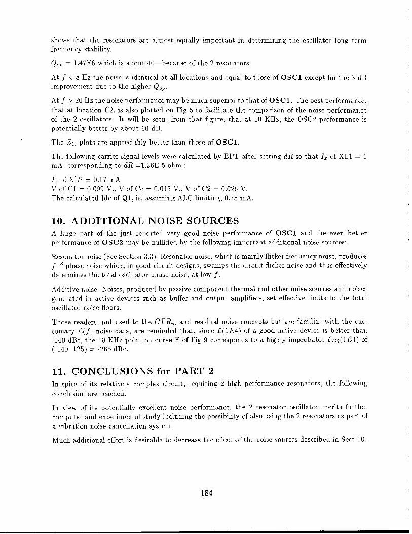
shows t,ha,t the resonators aae almost equally il-riporta~~t in determining the oscillator long tcrm freq~~cncy stability.

Q,, = I.47EG which is about 40-because of the 2 rcsonators.

At j < 8 Hz the noisc is idcntical at d l locatiorls and equd to thosc of OSCl exc,ept for the 3 dB improvement due to the higher Q,,.

At f > 20 Hz the noise performance may be mudl superior to that of OSC1. The best performance, that at 1ocatio11 C2, is also plotted on Fig 5 to h i l i t a t e the comparison of the noise performance of the 2 oscillators. It will be seen, from that figure, that a t 10 KHz, the OSC2 prrformance is pottntidly better by about 60 dU.

The Xi,,, plots are appreciably bcttcr than those of OSCl

The following carrier signal levels were calculated by B P T after setting dR so that IT of XL1 = 1 mA, corresponding to dh! =1.36E-5 ohm :

IT of X1,2 = 0.17 I ~ A V o f C l = 0.099 V., V o f Cc = 0.015 V . , V o f C:2 = 0.026 V. The calculated Idc of Q1, is, assuming AJ,C limiting, 0.75 mA.

10. ADDITIONAL NOISE SOURCES A large part of the just reportcd very good ~ioise performance of OSCl and the even better performance of OSC2 may be nullified by the followi~lg i11iporta.nt additional noise sollrces:

Resonator ~ioiscl (See Section 3.3)- Resonator noise, which is mainly ilicker frequenc,y noise, produces f-"jkasc noise which, in good circuit designs, swamps the circuit flic,ker noise and thus effectively deterl-11i1ies thc total oscillator phase noise, a t low f .

Adrlitive noise- Noises, produced by passive component therrrld and other noise sources and noises gerieratetl in active devirts such as buffrr and output amplifiers, set effective limits to the total oscillator 11oise floors.

Those readers, not used to the CTR, and residual noise concepts but are familiar with the cus- tornary L ( j ) noisc: data, are bem minded that, since L ( l E 4 ) of a good active devicc is better than -140 dRc, the 10 KHz point on curve E of Fig 9 corresponds to a highly improbable Ccz(l E4) of (-140 -125) = -265 dnc.

11. CONCLUSIONS for PART 2 In spite of its relatively coniplex circuit, requiring 2 high performance resonators, the following conclusion are reached:

In view of its potentially excellent noise performance, the 2 resonator oscillator merits further corrlputer and experimental study including the possibility of also using the 2 resonators as part of a vibration noise cancellation system.

Much additional effort is desirable to decrease the effect of the noise sources described in Sect 10.

12. REFERENCES

[I] B.Parzen, '(Steady State Oscillator. Artn.lysis i n the I~nmit tar~ce llomain", Proc. 21st Annua,l Precise Tirrle and 'l'imc Tnterval Applications and Planning Meeting, p p 161-168, Nov. Nov. 1989

[2] D.B. Leeson, " A Simple Model of Feedback Oscillntor Noise ,Sjlcctr..nrrr", Proc,. 1.E.E.E) vol 51, pp. 329-330, Feh. 1966.

[3] B. Parzen, Design of Crystd and Othcr tiartnonic Oscillators. Oscillators. New York:Wilcy, 1983.

[4] W.P. Robins, Phase Noise in Signa.1 Sources. London:Peter Pcrcgrinus Ltd, 1982.

[5] B. Parzen, "Universal, Cyornputer. ki~~cilitnted, Steady State Oscillrztor Aizalysis T1~eor.y n~zd ,5'o;'onxe U H F and Micr.owave A1~1icntiorzs", Proc. 45th Annua,l k'rcqnenc,y Corltrol Sy~npnsi~l r - n , 1111. 368-383. May 1991.

[6] 13. Pa,rzcn, "Clari,ficut~ioi~ and a Cenerulized Reslaleir~ei~t of Leesoiz's Oscillator. Noise Model", Proc. 42nd Annual Frequency C:ontrbol Syrnposium, pp. 348-351, June 11388.

[7] C;. Montrose et ad., "Residual Noise Mca.sur.eine~zt.s of Vllt;', (JHF, and Mil:r.otoaz)e ( h ~ n p o - nc~zts" , Proc. 43rd Anllud Freque~lcy Control Syrnposiurn, pp. 349-359, May 1989.

[8] R. nnrgoon and H. 1. Wilson, "L~esigiz /Ispert.$ 01 url Oscillator. using the S'C C7712 @yslulff Proc. g r d Annual E'rey~lcncy Control Symposium, pp. 41 1-416, 1979.

[9] H . Pa.r*zcn, Oscillator arld Stability Analysis i n thc Tnimi thrice Doraain. In prcpa.ra.tion.

P1 .........................................

To convert to Z config. set Un = 6 Replace J with 12

F I G 4 1 8 M H z 1 XTeL. OSCILLF lTOR ZN CONFIG

'DIOZN osc C T R m ( f ) & IZinl ( f ) \

m = RL, lx Qop = 1.08E6 CTR dB IZinldB 1 ohm I

C 2 2RESN OSCL

Zin - f Zin + f CTRlx - f CTRlx + f

CTRRL - f

CTRRL t f

J

WRZEN FIG 5 D l OZN

................................. J t . . A.

, - - I / . .

: OSCI . . .... ..... . . ...................I,,IIItIII,,,,,,, iiiiiiiiiiiiiiiiii:i;i~,9iii;iiiiiiiii WrOJl IS REST OF CIRCUIT

- ........................................ A J ..................................... C'Ll 131

C't2 ................. .... .........: 2 X T A L Z N

To conwrt t o Z config, set Vn = 0 Replace J with IZ

FIG 6 1 8 M H z 2 X T A L OSCILLATOR ZN CONFIQ

1 2XTALZN OSC CTRm ( f ) & IZinl ( f )

\

m = C1 , Cc, C2 Qop = I .47E6 f o = 10,000,003t Hz

'. I PhRZEN FIG 9 2XTPLZN

11-18-1991 09: 48:26 # OF COHPONENTS = 20 HIGHEST NODE I = 13 # OF VOLTAGE SOURCES = 1 2XTALDRZ FREQUENCY= 10000003.14865001 CIRCUIT NOTE : 10 mhz 2xtal osc z confiq COMPNT. CONNECTED TO NODE

1 SYB N1- tN2 TYPE VALUE PHASE ANGLE 1 cl 1 - 0 CAPACITOR 1B-010 2 I J I 1 - 10 J W E R , R = 9.999999999999999E-021 3 IdRl 10 - 11 RESISTOR 1.363-005 4 {RV} 11 - 12 RESISTOR -3.917113507084587E-002 5 IXVI 12 - 13 XI REACTANCE -1.876242564109969E-007 6 (R1)XLl 13 - 2 RESISTOR 70 PO XL 7 (Cl) 2 - 3 XTAL RSN'TOR C1= 2.1E-016 fs= 10000000 8 ( C o ) 1 - 3 CAPACITOR 1E-050 PO XL 9 C'L1 3 - 4 INDUCTOR 5.386228087475492E-007 10 CC 4 - 0 CAPACITOR 1E-009 11 (RlIXL2 4 - 5 RESISTOR 70 PO XL 12 (Cl) 5 - 6 XTAL RSN'TOR C1= 2E-016 fs= 10000000 13 (CO) 4 - 6 CAPACITOR 1E-050 PO XL 14 C'L2 6 - 7 INDUCTOR 1E-006 15 C2 7 - 0 CAPACITOR 1E-010 16 mm B = 9 E = O C = 1 N, NPN BIP TRANSISTOR

gmo= 2.859460045734375E-002 BETA= 100 FT (MHz)= 1000 17 (rbe) 0 - 7 RESISTOR 3497.163744224225 PO BIP 18 (Cbed) 0 - 7 CAPACITOR 4.550972008524029E-012 PO BIP 19 Vn 7 - 9 VW, WH NS V 3E-009 PO BIP 20 Vins 0 - 7 TESTPOINT SET, R = 1Et020

FIG7 PARTS LKT 2 ~ r n R ~ R

10 mhz 2xtal osc z config, 1 cl,C, 1 , 0 , 1E-010 , 0 , 0 , 0 I12),1, 1 , 1 0 , 1 , 0 , 0 , 0 (dR],R, 10 , 11 , 1.363-005 , 0 , O , O {RV},R, 11 , 12 ,-3.917113507084587E-002 , 0 , 1 , 0 (XV} ,X , 12 , 13 ,-1.876242564109969E-007 , 0 , 0 , 0 (Rl)XLl,R, 13 , 2 , 70 , 0 , 9 , 0 (Cl),C, 2 , 3 , 2.1E-016 , 0 , 9 , 10000000 (Col,C, 1 , 3 , 1E-050, 0 , 9 , 0 CtL1,L, 3 , 4 , 5.386228087475492E-007 , 0 , 1 , 0 Cc,C, 4 , 0 , 13-009 , 0 , 0 , 0 (R1)XL2,RI 4 , 5 , 70 , 0 , 9 , 0 (Cl),C, 5 , 6 , 2E-016 , 0 , 9 , 10000000 (Co),C, 4 , 6 , 1E-050 , 0 , 9 , 0 C1L2,L, 6 , 7 , 1E-006 , 0 , 1 , 0 C2,C, 7 , O , 1E-010 , 0 , O , O mm,N, 9 , 0 , 1 , 2.859460045734375E-002 , 100 , 1000 (rbe),R, 0 , 7 , 3497.163744224224 , 0 , 7 , 0 (Cbed),C, 0 , 7 , 4.550972008524029E-012 , 0 , 7 , 0 V n , V W , 7 , 9 , O , O I O , O FIGS NE)[UIST

Vins,TP, 0 , 7 , 1Et020 , 0 , 0 , 0 2 m R C S C E U T O R