United States Environmental Protection Agency · PDF fileApplication of Selected Mathematical...

Estimation of InfiltrationRate in the Vadose Zone:Application of SelectedMathematical Models

Volume II

United StatesEnvironmental ProtectionAgency

National Risk ManagementResearch LaboratoryAda, OK 74820

EPA/600/R-97/128bFebruary 1998

EPA/600/R-97/128bFebruary 1998

ESTIMATION OF INFILTRATION RATE IN VADOSE ZONE:APPLICATION OF SELECTED MATHEMATICAL MODELS

Volume II

by

Joseph R. WilliamsU.S. EPA

andYing Ouyang

ManTech Environmental Technologies, Inc. (METI)and

Jin-Song ChenVaradhan Ravi

Dynamac Corporation

ALM (METI) Contract No. 68-W5-0011 DO 022Dynamac Corp. 68-C4-0031

Project Officer Delivery Order Project OfficerDavid S. Burden David G. JewettSubsurface Protection and Remediation DivisionNational Risk Management Research Laboratory

Ada, Oklahoma 74820

In cooperation with:CENTER FOR REMEDIATION TECHNOLOGY AND TOOLS

OFFICE OF RADIATION AND INDOOR AIROFFICE OF AIR AND RADIATION

WASHINGTON, DC 20460

NATIONAL RISK MANAGEMENT RESEARCH LABORATORYOFFICE OF RESEARCH AND DEVELOPMENT

U.S. ENVIRONMENTAL PROTECTION AGENCYCINCINNATI, OH 45268

ii

NOTICE

The U.S. Environmental Protection Agency through its Office of Research andDevelopment partially funded and collaborated in the research described here as indicated throughthe authors’ affiliations. Additional support for this project was provided by the Office ofRadiation and Indoor Air (ORIA) of the Office of Air and Radiation in collaboration with theOffice of Emergency and Remedial Response (OERR) of the Office of Solid Waste andEmergency Response and the U.S. Department of Energy (EM-40). ManTech EnvironmentalTechnologies, Inc. (METI) is an in-house support contractor to NRMRL/SPRD under 68-W5-0011, Delivery Order 022 (Dr. David Jewett, Delivery Order Project Officer). Dynamac is anoff-site support contractor to NRMRL/SPRD under 68-C4-0031 (Dr. David S. Burden, ProjectOfficer). Ron Wilhelm and Robin Anderson (ORIA) provided valuable technical review andadministrative support to this project. The assistance of Sierra Howry, a student in theEnvironmental Research Apprenticeship Program through East Central University in Ada,Oklahoma, in the completion of this project is greatly appreciated. This report has been subjectedto the Agency’s peer and administrative review and has been approved for publication as an EPAdocument.

Mention of trade names or commercial products does not constitute endorsement orrecommendation for use.

All research projects making conclusions or recommendations based on environmentallyrelated measurements and funded by the U.S. Environmental Protection Agency are required toparticipate in the Agency Quality Assurance Program. This project did not involve environmentalrelated measurements and did not require a Quality Assurance Plan.

iii

FOREWORD

The U.S. Environmental Protection Agency is charged by Congress with protecting the Nation’sland, air, and water resources. Under a mandate of national environmental laws, the Agencystrives to formulate and implement actions leading to a compatible balance between humanactivities and the ability of natural systems to support and nurture life. To meet these mandates,EPA’s research program is providing data and technical support for solving environmentalproblems today and building a science knowledge base necessary to manage our ecologicalresources wisely, understand how pollutants affect our health, and prevent or reduceenvironmental risks in the future.

The National Risk Management Research Laboratory is the Agency’s center for investigation oftechnological and management approaches for reducing risks from threats to human health andthe environment. The focus of the laboratory’s research program is on methods for the preventionand control of pollution to air, land, water, and subsurface resources; protection of water qualityin public water systems; remediation of contaminated sites and ground water, and prevention andcontrol of indoor air pollution. The goal of this research effort is to catalyze development andimplementation of innovative, cost-effective environmental technologies; develop scientific andengineering information needed by EPA to support regulatory and policy decisions; and providetechnical support and information transfer to ensure effective implementation of environmentalregulations and strategies.

Numerous infiltration estimation methods have been developed, and have become an integral partof the assessment of contaminant transport and fate. This document selects six (6) methodshaving utility under varying conceptualizations. The methods are described in detail and areprovided in electronic format for actual application.

Clinton W. Hall, DirectorSubsurface Protection and Remediation DivisionNational Risk Management Research Laboratory

iv

ABSTRACT

Movement of water into and through the vadose zone is of great importance to theassessment of contaminant fate and transport, agricultural management, and natural resourceprotection. The process of water movement is very dynamic, changing dramatically over time andspace. Infiltration is defined as the initial process of water movement into the vadose zonethrough the soil surface. Knowledge of the infiltration process is prerequisite for managing soilwater flux, and thus the transport of contaminants in the vadose zone.

Although a considerable amount of research has been devoted to the investigation ofwater infiltration in unsaturated soils, the investigations have primarily focused on scientificresearch aspects. An overall evaluation of infiltration models in terms of their application tovarious climatic characteristics, soil physical and hydraulic properties, and geological conditionshas not been done. Specifically, documentation of these models has been limited and, to someextent, non existent for the purpose of demonstrating appropriate site-specific application. Thisdocument attempts to address this issue by providing a set of water infiltration models which havethe flexibility of handling a wide variety of hydrogeologic, soil, and climate scenarios. Morespecifically, the purposes of this document are to: (1) categorize infiltration models presentedbased on their intended use; (2) provide a conceptualized scenario for each infiltration model thatincludes assumptions, limitations, boundary conditions, and application; (3) provide guidance formodel selection for site-specific scenarios; (4) provide a discussion of input parameter estimation;(5) present example application scenarios for each model; and, (6) provide a demonstration ofsensitivity analysis for selected input parameters.

Six example scenarios were chosen as illustrations for applications of the infiltrationmodels with one scenario for each model. The intention of these scenarios is to provideapplications guidance to users for these models to various field conditions. Each modelapplication scenario includes the problem setup, conceptual model, input parameters, and resultsand discussion.

v

CONTENTS

NOTICE . . . . . . . . . . . . . . . . . . . . . . . . . . . . . . . . . . . . . . . . . . . . . . . . . . . . . . . . . . . . . . . . . iiABSTRACT . . . . . . . . . . . . . . . . . . . . . . . . . . . . . . . . . . . . . . . . . . . . . . . . . . . . . . . . . . . . . . ivLIST OF FIGURES . . . . . . . . . . . . . . . . . . . . . . . . . . . . . . . . . . . . . . . . . . . . . . . . . . . . . . . . . viiLIST OF TABLES . . . . . . . . . . . . . . . . . . . . . . . . . . . . . . . . . . . . . . . . . . . . . . . . . . . . . . . . . ix

CHAPTER 1. INTRODUCTION . . . . . . . . . . . . . . . . . . . . . . . . . . . . . . . . . . . . . . . . . . . . . . 1

1.1 Phenomena of Water Infiltration in the Unsaturated Zone . . . . . . . . . . . . . . . . . . . . . 11.2 Intended Use of this Document . . . . . . . . . . . . . . . . . . . . . . . . . . . . . . . . . . . . . . . . 3

CHAPTER 2. DESCRIPTIONS OF INFILTRATION MODELS . . . . . . . . . . . . . . . . . . . . . . 5

2.1 Classification of Infiltration Models Chosen in the Document . . . . . . . . . . . . . . . . . 52.1.1 Semi-Empirical Model . . . . . . . . . . . . . . . . . . . . . . . . . . . . . . . . . . . . . . . 52.1.2 Homogeneous Model . . . . . . . . . . . . . . . . . . . . . . . . . . . . . . . . . . . . . . . . . 5

2.1.3 Non-Homogeneous Model . . . . . . . . . . . . . . . . . . . . . . . . . . . . . . . . . . . . . 62.1.4 Infiltration Model for Ponding Conditions . . . . . . . . . . . . . . . . . . . . . . . . . 62.1.5 Infiltration Model for Non-Ponding Conditions . . . . . . . . . . . . . . . . . . . . . 62.1.6 Infiltration/Exfiltration Model . . . . . . . . . . . . . . . . . . . . . . . . . . . . . . . . . . 6

2.2 Infiltration Model Conceptualization . . . . . . . . . . . . . . . . . . . . . . . . . . . . . . . . . . . . 62.3 Selected Models . . . . . . . . . . . . . . . . . . . . . . . . . . . . . . . . . . . . . . . . . . . . . . . . . . . 9

2.3.1 SCS Model . . . . . . . . . . . . . . . . . . . . . . . . . . . . . . . . . . . . . . . . . . . . . . . 92.3.2 Philip’s Two-Term Model . . . . . . . . . . . . . . . . . . . . . . . . . . . . . . . . . . . . 92.3.3 Green-Ampt Model for Layered Systems . . . . . . . . . . . . . . . . . . . . . . . . . 102.3.4 Explicit Green-Ampt Model . . . . . . . . . . . . . . . . . . . . . . . . . . . . . . . . . . . 12

2.3.5 Constant Flux Green-Ampt Model . . . . . . . . . . . . . . . . . . . . . . . . . . . . . . 132.3.6 Infiltation / Exfiltration Model . . . . . . . . . . . . . . . . . . . . . . . . . . . . . . . . . 14

CHAPTER 3. METHOD FOR SELECTION OF INFILTRATION MODEL . . . . . . . . . . . . . 163.1 Model Selection Criteria . . . . . . . . . . . . . . . . . . . . . . . . . . . . . . . . . . . . . . . 163.2 Example for Selecting the Water Infiltration Model . . . . . . . . . . . . . . . . . . . 17

CHAPTER 4. INPUT PARAMETER ESTIMATIONS . . . . . . . . . . . . . . . . . . . . . . . . . . . . . 194.1 General Description of Parameters . . . . . . . . . . . . . . . . . . . . . . . . . . . . . . . . . . . . . 194.2 Estimation of the F in SCS Model . . . . . . . . . . . . . . . . . . . . . . . . . . . . . . . . . . . . . 23w

4.3 Estimation of Green-Ampt Model Parameters . . . . . . . . . . . . . . . . . . . . . . . . . . . . 244.4 Estimation of Philip’s Two-Term Model Parameters . . . . . . . . . . . . . . . . . . . . . . . . 29

CHAPTER 5. EXAMPLE APPLICATION SCENARIOS . . . . . . . . . . . . . . . . . . . . . . . . . . . 305.1 Semi-Empirical Model (SCS) . . . . . . . . . . . . . . . . . . . . . . . . . . . . . . . . . . . . . . . . . 305.2 Infiltration Model for Homogeneous Conditions (PHILIP2T) . . . . . . . . . . . . . . . . . 32

vi

5.3 Infiltration Model for Non-homogeneous Conditions (GALAYER) . . . . . . . . . . . . 345.4 Infiltration Model for Ponding Conditions (GAEXP) . . . . . . . . . . . . . . . . . . . . . . . 365.5 Infiltration Model for Non-ponding Conditions (GACONST) . . . . . . . . . . . . . . . . . 385.6 Infiltration and Exfiltration (INFEXF) . . . . . . . . . . . . . . . . . . . . . . . . . . . . . . . . . . 40

REFERENCES . . . . . . . . . . . . . . . . . . . . . . . . . . . . . . . . . . . . . . . . . . . . . . . . . . . . . . . . . . . . 42

APPENDIXESAppendix A. User’s Instructions for Mathcad Worksheets . . . . . . . . . . . . . . . . . . . . A-1

Appendix B. Mathematical Models in Mathcad . . . . . . . . . . . . . . . . . . . . . . . . . . . . B-11. SCS Model . . . . . . . . . . . . . . . . . . . . . . . . . . . . . . . . . . . . . . . . . . . . . . . B1-12. Philip’s Two-Term Model . . . . . . . . . . . . . . . . . . . . . . . . . . . . . . . . . . . . B2-13. Green-Ampt Model for layered systems . . . . . . . . . . . . . . . . . . . . . . . . . . B3-14. Green-Ampt Model, Explicit Model . . . . . . . . . . . . . . . . . . . . . . . . . . . . B4-15. Constant Flux Green-Ampt Model . . . . . . . . . . . . . . . . . . . . . . . . . . . . . . B5-16. Infiltration/Exfiltration Model . . . . . . . . . . . . . . . . . . . . . . . . . . . . . . . . . B6-1

Appendix C. Sensitivity Analysis Discussion and Demonstration . . . . . . . . . . . . . . . C-1

vii

LIST OF FIGURES

Number Page

1. Zones of the infiltration process for the water content profile under pondedconditions (Adapted from Hillel, 1982) . . . . . . . . . . . . . . . . . . . . . . . . . . . . . . . . . . . . . 2

2. Infiltration rate will generally be high in the first stages, and will decrease with time(Adapted from Hillel, 1982) . . . . . . . . . . . . . . . . . . . . . . . . . . . . . . . . . . . . . . . . . . . . . . 3

3. Conceptual model for simulating water infiltration using the SCS model . . . . . . . . . . . . 31

4. Surface infiltration rate as a function of daily rainfall rate . . . . . . . . . . . . . . . . . . . . . . . 31

5. Surface runoff rate as a function of daily rainfall rate . . . . . . . . . . . . . . . . . . . . . . . . . . 31

6. Conceptual model for simulating water infiltration using the Philip’s Two TermModel . . . . . . . . . . . . . . . . . . . . . . . . . . . . . . . . . . . . . . . . . . . . . . . . . . . . . . . . . . . . . 33

7. Water infiltration as a function of time . . . . . . . . . . . . . . . . . . . . . . . . . . . . . . . . . . . . . 33

8. Cumulative infiltration as a function of time . . . . . . . . . . . . . . . . . . . . . . . . . . . . . . . . . 33

9. Conceptual model for simulating water infiltration into a layered soil . . . . . . . . . . . . . . 35

10. Comparison of water infiltration between Scenarios 1 (solid line) and 2 (dash line) . . . . 35

11. Conceptual model for simulating water infiltration using the Explicit Green-Amptmodel . . . . . . . . . . . . . . . . . . . . . . . . . . . . . . . . . . . . . . . . . . . . . . . . . . . . . . . . . . . . . . 37



14. Conceptual model for simulating water infiltration using the constant flux Green-Ampt model . . . . . . . . . . . . . . . . . . . . . . . . . . . . . . . . . . . . . . . . . . . . . . . . . . . . . . . . . 39



17. Conceptual model for simulating water infiltration and exfiltration . . . . . . . . . . . . . . . . 41

viii


19. Water exfiltration as a function of time . . . . . . . . . . . . . . . . . . . . . . . . . . . . . . . . . . . . 41

ix

LIST OF TABLES

Number Page1. Infiltration model classification . . . . . . . . . . . . . . . . . . . . . . . . . . . . . . . . . . . . . . . . . . . . 5

2. Summary of assumptions, limitations, and mathematical boundary conditions foreach model selected, where 2 is the volumetric water content. In this table,features are identified as being present for the particular model (Y for YES), or notconsidered (N for NO). The model names are defined in next section.. . . . . . . . . . . . . . . 8

3. Summary of common site conditions and the selected models capabilities ofsimulating those conditions. Y indicates the model is designed for the specific sitecondition and N indicates that it is not.. . . . . . . . . . . . . . . . . . . . . . . . . . . . . . . . . . . . . 18

4. Listing of input parameters for running the infiltration models. . . . . . . . . . . . . . . . . . . . 19

5. Curve numbers for hydrologic soil-cover complex for the average antecedent moisturecondition and I = 0.2F . I is initial water abstraction (USDA-SCS, 1972). . . . . . . 23a w a

6. Description of hydrologic soil groups. . . . . . . . . . . . . . . . . . . . . . . . . . . . . . . . . . . . . . 24

7. Typical values of saturated volumetric water content (2 ). . . . . . . . . . . . . . . . . . . . . . . 25s

8. Typical values of residual volumetric water content (2 ). . . . . . . . . . . . . . . . . . . . . . . . 26r

9. Typical values of air-entry head (h ).. . . . . . . . . . . . . . . . . . . . . . . . . . . . . . . . . . . . . . . 26b

10. Typical values of pore size index (8). . . . . . . . . . . . . . . . . . . . . . . . . . . . . . . . . . . . . . . 27

11. Typical values for soil hydraulic property parameters (Rawls et al., 1992).. . . . . . . . . . 28

12. Input parameter values for simulations with a sandy soil using the SCS model.. . . . . . . 30

13. Input parameter values for the simulations in a sandy soil using PHILIP2Tmodel. . . . . 32

14. Input parameter values for the simulations using GALAYER model.. . . . . . . . . . . . . . . 34

15. Input parameters for the simulations in a clay soil using GAEXP.. . . . . . . . . . . . . . . . . 36

16. Input parameters for the simulations with r >K in a clay soil using GACONST.. . . . . . 38s

17. Input parameters for the simulations using the INFEXF model. . . . . . . . . . . . . . . . . . . 40

1

CHAPTER 1. INTRODUCTION

1.1 Phenomena of Water Infiltration in the Unsaturated ZoneWater applied to the soil surface through rainfall and irrigation events subsequently enters the

soil through the process of infiltration. If the supply rate of water to the soil surface is greaterthan the soil’s ability to allow the water to enter, excess water will either accumulate on the soilsurface or become runoff. The process by which water enter the soil and thus the vadose zonethrough the soil-atmosphere interface is known as infiltration. Infiltrability is a term generallyused in the disciplines of soil physics and hydrology to define the maximum rate at which rain orirrigation water can be absorbed by a soil under a given condition. Indirectly, infiltrabilitydetermines how much of the water will flow over the ground surface into streams or rivers, andhow much will enter the soil, and thus assists in providing an estimate of water available fordownward percolation through drainage, or return to the atmosphere by the process ofevapotranspiration.

Understanding water movement into and through the unsaturated zone is of great importanceto both policy and engineering decision-makers for the assessment of contaminant fate andtransport, the management of agricultural lands, and natural resource protection. The process ofwater movement is very dynamic, changing dramatically over time and space. Knowledge of theinfiltration process is a prerequisite for managing soil water flux, and thus the transport ofcontaminants in the vadose zone.

The distribution of water during the infiltration process under ponded conditions is illustrated inFigure 1. In this idealized profile for soil water distribution for a homogeneous soil, five zonesare illustrated for the infiltration process.

1) Saturated zone: The pore space in the saturated zone is filled with water, or saturated. Depending on the length of time elapsed from the initial application of the water, this zonewill generally extend only to a depth of a few millimeters.

2) Transition zone: This zone is characterized by a rapid decrease in water content with depth,and will extend approximately a few centimeters.

3) Transmission zone: The transmission zone is characterized by a small change in watercontent with depth. In general, the transmission zone is a lengthening unsaturated zonewith a uniform higher water content. The hydraulic gradient in this zone is primarilydriven by gravitational forces.

4) Wetting zone: In this zone, the water content sharply decreases with depth from the watercontent of the transmission zone to near the initial water content of the soil.

5) Wetting front: This zone is characterized by a steep hydraulic gradient and forms a sharpboundary between the wet and dry soil. The hydraulic gradient is driven primarily bymatric potentials.

Beyond the wetting front, there is no visible penetration of water. Comprehensive reviews of theprinciples governing the infiltration process have been published by Philip (1969) and Hillel(1982).

2

Figure 1. Zones of the infiltration process for the water content profile under ponded conditions (Adapted from Hillel, 1982).

Soil water infiltration is controlled by the rate and duration of water application, soil physicalproperties, slope, vegetation, and surface roughness. Generally, whenever water is ponded overthe soil surface, the rate of water application exceeds the soil infiltrability. On the other hand, ifwater is applied slowly, the application rate may be smaller than the soil infiltrability. In otherwords, water can infiltrate into the soil as quickly as it is applied, and the supply rate determinesthe infiltration rate. This type infiltration process has been termed as supply controlled (Hillel,1982). However, once the infiltration rate exceeds the soil infiltrability, it is the latter whichdetermines the actual infiltration rate, and thus the process becomes profile controlled. Generally, soil water infiltration has a high rate in the beginning, decreasing rapidly, and thenslowly decreasing until it approaches a constant rate. As shown in Figure 2, the infiltration ratewill eventually become steady and approach the value of the saturated hydraulic conductivity(K ).s

The initial soil water content and saturated hydraulic conductivity of the soil media are theprimary factors affecting the soil water infiltration process. The wetter the soil initially, thelower will be the initial infiltrability (due to a smaller suction gradient), and a constantinfiltration rate will be attained more quickly. In general, the higher the saturated hydraulicconductivity of the soil, the higher the infiltrability.

Naturally formed soil profiles are rarely homogeneous with depth, rather they will containdistinct layers, or horizons with specific hydraulic and physical characteristics. The presence ofthese layers in the soil profile will generally retard water movement during infiltration. Claylayers impede flow due to their lower saturated hydraulic conductivity; however, when theselayers are near the surface and initially very dry, the initial infiltration rate may be much higherand then drop off rapidly. Sand layers will have a tendency to also retard the movement of the

The process of water movement through layers can be investigated through an interactive1

software package entitled SUMATRA-1 developed by M. Th. van Genuchten (1978), USDA/ARS, US Salinity Laboratory, Riverside, CA 92521.

3

Figure 2. Infiltration rate will generally be highin the first stages, and will decrease with time(Adapted from Hillel, 1982).

wetting front due to larger pore size and thus ahigher hydraulic gradient would be required forflow into the layers. The surface crust will1

also act as a hydraulic barrier to infiltration dueto the lower hydraulic conductivity near thesurface, reducing both the initial infiltrabilityand the eventually attained steady infiltrability.

As might be expected, the slope of the landcan also indirectly impact the infiltration rate. Steep slopes will result in runoff, which willimpact the amount of time the water will beavailable for infiltration. In contrast, gentleslopes will have less of an impact on theinfiltration process due to decreased runoff. When compared to the bare soil surface,vegetation cover tends to increase infiltration by retarding surface flow, allowing time for waterinfiltration. Plant roots may also increase infiltration by increasing the hydraulic conductivity ofthe soil surface. Due to these effects, infiltration may vary widely under different types ofvegetation.

A number of mathematical models have been developed for water infiltration in unsaturatedzone (Philip, 1957; Bouwer, 1969; Fok 1970; Moore 1981; Ahuja and Ross, 1983; Parlange etal., 1985; Haverkamp et al., 1990; Haverkamp et al., 1991). A thorough review of waterinfiltration models used in the fields of soil physics and hydrology has been presented in aprevious volume prepared in conjunction with the current project (Ravi and Williams, 1998).

1.2 Intended Use of this DocumentSoil water infiltration has been determined from experimental measurements (Parlange, et al.,

1985) and mathematical modeling (Philip, 1957; Bouwer, 1969; Fok 1970; Moore 1981; Ahujaand Ross, 1983; Parlange et al., 1985; Haverkamp et al., 1990; Haverkamp et al., 19941). Although a considerable amount of research has been devoted to the investigation of waterinfiltration in unsaturated soils, these investigations have primarily focused on scientific researchaspects. An overall evaluation of infiltration models in terms of their application to variousclimatic characteristics, and soil physical and geological conditions has not been done. Specifically, documentation of these type models has been limited and, to some extent, non-existent for the purpose of demonstrating appropriate site-specific application. This documentattempts to address this issue by providing a set of water infiltration models which have beenapplied to a variety of hydrogeologic, soil, and climate scenarios. More specifically, the

4

purposes of this document are to: (1) categorize infiltration models presented based on theirintended use; (2) provide a conceptualized scenario for each infiltration model that includesassumptions, limitations, mathematical boundary conditions, and application; (3) provideguidance for model selection for site-specific scenarios; (4) provide a discussion of inputparameter estimation; (5) present example application scenarios for each model; and, (6)provide a demonstration of sensitivity analysis for selected input parameters. This document doesnot provide an in-depth sensitivity analysis for each model presented; however, a detaileddiscussion of the process is provided in Appendix C.

5

CHAPTER 2. DESCRIPTIONS OF INFILTRATION MODELS

2.1 Classification of Infiltration ModelsSix infiltration models (Table 1) were chosen for inclusion in this document based on several

considerations: (1) relatively simple approach, easy to use, and realistic in applications; (2) abilityto handle various field conditions including surface ponding, non-ponding, various rainfall rates,surface runoff, and wetting and drying; and (3) application to both homogeneous ornonhomogeneous soil profiles. The categories presented are not considered to be all-inclusive,but do provide a wide range of model applications.

Infiltration models can be divided into various categories, depending on the purpose of themodel, boundary conditions, and the nature of subsurface systems. In this study, six categorieswere identified for which the models chosen could be associated. The categories were chosen forrepresentativeness to site-specific conditions, which is discussed in the following.

Table 1. Infiltration model classification.

Category Model Selected Reference

Semi-Empirical SCS model USDA-SCS, 1972

Homogeneous Philip’s two-term model Philip, 1957

Nonhomogeneous Green-Ampt model for layered systems Flerchinger et al., 1988

Ponding Green-Ampt explicit model Salvucci and Entekhabi, 1994

Non-ponding Constant Flux Green-Ampt model Swartzendruber, 1974

Wetting and Drying Infiltration/Exfiltration model Eagleson, 1978

2.1.1 Semi-Empirical Model: As indicated by the term empirical, these type infiltrationmodels are developed entirely from field data and have little or no physical basis. The empiricalapproach to developing a field infiltration equation consists of first finding a mathematicalfunction whose shape, as a function of time, matches the observed features of the infiltration rate,and then attempting a physical explanation of the process (Jury et al., 1991). Most physicalprocesses in semi-empirical models are represented by commonly accepted and simplisticconceptual methods, rather than by equations derived from fundamental physical principles. Thecommonly used semi-empirical infiltration models in the field of soil physics and hydrology areKostiakov’s model, Horton’s model, and the SCS (Soil Conservation Service) model (USDA-SCS, 1972; Hillel, 1982).

2.1.2 Homogeneous Model: Most infiltration models have been developed for application inhomogeneous porous media. These models are commonly derived from mathematical solutionsbased on well-defined, physically based theories of infiltration (e.g., Richards equation). Sincethis mechanistic infiltration model is derived from the water flow equation, considerable insight isgiven to the physical and hydraulic processes governing infiltration. Infiltration models commonly

6

used for homogeneous soil profiles include the Green-Ampt infiltration model, the Philipinfiltration model, the Burger infiltration model, and the Parlange infiltration model. Descriptionsof these models are provided in documentation by Hillel (1982), Ghildal and Tripathi (1987), andJury et al. (1991).

2.1.3 Non-Homogeneous Model: Naturally developed soil profiles are seldom uniform withdepth, nor is the water content distribution uniform at the initiation of infiltration. Because of thenonuniform soil profile, field infiltration measurement data frequently show differentcharacteristics than the models based on theoretical calculations for the uniform soil profile. Formost field observations of infiltration rates, the field observations would be less than what wouldbe predicted by models designed for homogeneous systems. In conceptualization of a non-homogeneous soil profile, it is usually more convenient to divide the profile into layers orhorizons, each of which is assumed to be homogeneous (Childs and Bybordi, 1969; Hillel andGardner, 1970). The application of the Green-Ampt equation to calculate cumulative infiltrationinto nonuniform soils has been studied by Bouwer (1969), Childs and Bybordi, (1969), Fok(1970), Moore (1981), and Flerchinger et al. (1988).

2.1.4 Infiltration Model for Ponding Conditions: When the application rate of water to thesoil surface exceeds the rate of infiltration, free water (i.e., surface water excess) tends toaccumulate over the soil surface. This water collects in depressions, thus ponding on the soilsurface. Depending on the geometric irregularities of the surface and on the overall slope of theland, some of the ponded water may become runoff, if the surface storage becomes filled. Underponded conditions, the cumulative infiltration is a function of soil properties, initial conditions,and the ponding depth on the soil surface. Several infiltration models for ponding conditions havebeen developed, including those by Parlange et al. (1985), Haverkamp et al. (1990, 1994), andSalvucci and Entekhabi (1994).

2.1.5 Infiltration Model for Non-ponding Conditions: When the rate of water supply to thesoil surface does not exceed the soil infiltrability, all water can percolate into the soil and nosurface ponding of water occurs. This process depends on the rate of water supply, initial soilwater content, and the saturated hydraulic conductivity. Infiltration models for non-pondingconditions have been developed by several researchers (Philip, 1957; Childs and Bybordi, 1969;Hillel and Gardner, 1970). Probably the most common approach is an implementation of theGreen-Ampt model in an explicit approach.

2.1.6 Wetting and Drying Model: Alternate infiltration and exfiltration of water at the soilsurface will result in an unsteady diffusion of water into the soil. The presence of transpiringvegetation adds another mechanism for moisture extraction distributed over a depth which isrelated to root structure. Infiltration models for such conditions have been developed byEagleson (1978) and Corradini et al. (1994).

2.2 Infiltration Model ConceptualizationWater infiltration into unsaturated porous media for various climatic conditions, soil physical

and hydraulic properties, and geological conditions is very complex, resulting in a challenge tomathematically simulate observed conditions. An understanding of the principles governing

7

infiltration and factors affecting infiltration processes must be attained. Since a universalmathematical model is not available to address water infiltration for all field conditions,assumptions are commonly made, and limitations are identified during the model development andapplication process. Assumptions used in developing water infiltration models commonly includethe following:

(1) Initial soil water content profile: Most infiltration models assume a constant and uniforminitial soil water content profile. However, under field conditions, the soil water contentprofile is seldom constant and uniformly distributed.

(2) Soil profile: There are two types of soil profiles which exist under field conditions: (a)homogeneous and (b) heterogeneous. Infiltration models developed for the homogeneoussoil profile cannot be used for heterogeneous soil profile without simplifying assumptionsconcerning the heterogeneity.

(3) Constant and near saturated soil water content at the soil surface: This is a commonassumption for most infiltration models, which will allow for the ignoring of the initiallyhigh hydraulic gradient across the soil’s surface. The length of time the surface is not nearsaturation is very small when compared to the length of time associated with theinfiltration event.

(4) Duration of infiltration process: Some infiltration models are only valid for a short termperiod of infiltration, which can limit their usefulness to field applications where infiltrationmay last for longer time periods. A short term period might be representative of a rainfallor irrigation event.

(5) Surface crust and sealing: None of the selected models can be used for the surface crustingboundary condition. This boundary condition is complex and dynamic.

(6) Flat and smooth surface: These surface boundary conditions can be easily incorporatedinto mathematical models, whereas an irregular surface or sloping surface can result in anadded dimension to the mathematical modeling.

Boundary conditions are those conditions defined in the modeling scenario to account forobserved conditions at the boundaries of the model domain. These conditions must be definedmathematically, the most common of which are given as follows:

(1) Constant or specified flux at the surface: The rate of water applied to the soil surface canbe constant or time-varying. Because of its simplicity as compared to other boundaryconditions, a constant flux condition has been used in most infiltration models.

(2) Surface ponding condition. The surface ponding or non-ponding conditions are dependenton the rate of water application as well as soil infiltrability. Whenever the rate of waterapplication to the soil exceeds the soil infiltrability, the surface ponding occurs. Theopposite case will result in surface non-ponding conditions.

(3) Finite column length at the lower boundary. Some infiltration models are limited to a finitecolumn length and others may allow for an infinite column length. Infiltration modelswith the finite column length condition may limit their applications for deeper waterinfiltration.

(4) Based on Richards equation. Several infiltration models (e.g., Philip’s model andEagleson’s model) were developed based on Richards equation. These models commonlyhave well-defined physically based theories and give considerable insight into theprocesses governing infiltration. These would require information related to the waterretention characteristics of the soil media.

8

A summary of assumptions, limitations, and boundary conditions for each model chosen in thisdocument is given in Table 2. Detailed descriptions of the models are provided below.

Table 2. Summary of assumptions, limitations, and mathematical boundary conditions for eachmodel selected, where 2 is the volumetric water content. In this table, features areidentified as being present for the particular model (Y for YES), or not considered (Nfor NO). The model names are defined in next section.

Modelname

Model Features

Assumptions and Limitations Boundary Conditions

Con

stan

t and

uni

form

initi

al 2

Hom

ogen

eous

soi

l pro

file

Val

id f

or o

nly

sho

rt te

rm in

filtr

atio

n

Surf

ace

crus

t and

sea

ling

Con

stan

t wat

er c

onte

nt a

t top

bou

ndar

y

Con

stan

t flu

x at

the

top

boun

dary

Surf

ace

pond

ing

cond

ition

Fini

te c

olum

n le

ngth

Bas

ed o

n R

icha

rds

equa

tion

Bas

ed o

n em

piri

cal e

quat

ion

SCS N N N N N N N N N Y

Philip’s twoterm Y Y Y N Y N N N Y N

Green-Amptmodel for

layered systemsY Y N N Y N Y Y N N

Green-Amptexplicit Y Y N N Y N Y Y N N

Constant fluxGreen-Ampt Y Y N N Y Y N Y N N

Infiltration/Exfiltration Y Y N N Y N N N Y N

R'

(P&0.2Fw)2

P% 0.8Fw

P> 0.2Fw

0, otherwise: P<_ 0.2 Fw

q ' P & R

The Mathcad worksheets provided in Appendix B are referenced in parentheses. These2

are also used as the filenames.

9

(1)

(2)

2.3 Selected Models

2.3.1 SCS ModelDescription: The empirical approach of developing a water infiltration equation consists of

first identifying a mathematical function whose shape, as a function of time, matches the observedfeatures of the infiltration rate, followed by an attempt at providing a physical explanation of theprocess (Jury et al., 1991). For semi-empirical models, most physical processes are representedby commonly accepted, and simplistic conceptual methods rather than by equations derived fromfundamental physical principles. The Soil Conservation Service (SCS) model is a commonly2

used semi-empirical infiltration model in the field of soil physics and hydrology (USDA, 1972).

Equations: Mathematical functions for the SCS model are given as:

and

where R is amount of runoff (inches), P is the daily rainfall amount (inches), F is a statisticallyw

derived parameter (also called the retention parameter) with the units of inches, and q is the dailyinfiltration amount (inches). Justification for the use of this model is based on a consideration thatthe model is simple, it requires few input parameters, and has been widely used and understood inthe fields of soil physics and hydrology.

Assumptions and Limitations: A major limitation for applying the SCS model lies in that thecoefficients in Equation 1 must be evaluated with field data for each specific site. Since the modelis not derived from fundamental physical principles, it can only be used as a screening tool forinitial approximations.

2.3.2 Philip's Two-Term ModelDescription: The Philip's two-term model (PHILIP2T) is a truncated form of the Taylor

power series solution presented by Philip (1957). During the initial stages of infiltration (i.e.,when t is very small), the first term of Equation 3 dominates. In this stage, the vertical infiltrationproceeds at almost the same rate as absorption or horizontal infiltration due to the gravity

q(t)'12

St &½%A

I(t)'St ½%At

10

(3)

(4)

component, represented by the second term, being negligible. As infiltration continues,the second term becomes progressively more important until it dominates the infiltration process. Philips (1957) suggested the use of the two-term model in applied hydrology when t is not toolarge.

Equations: The Philip’s two-term model is represented by the following equations,

and

where q is infiltration rate (cm/h), t is time for infiltration (h), S is the sorptivity (cm/h ) and is a1/2

function of the boundary, initial, and saturated water contents, A is a constant (cm/h) thatdepends on soil properties and initial and saturated water contents, and I(t) is the cumulativeinfiltration (cm) at any time, t.

Assumptions and Limitations: The three primary assumptions for this model are: (1)homogeneous soil conditions and properties; (2) antecedent (i.e., conditions prior to infiltration)water content distribution is uniform and constant (i.e., single-valued); and (3) water content atthe surface remains constant and near saturation. There are basically four limitations for thismodel, which are as follows: (1) field soils are seldom homogeneous, and this model is notdesigned for layered systems; (2) initial moisture content is seldom uniformly distributedthroughout the profile; (3) in most situations of rainfall or irrigation, the soil surface is rarely at aconstant water content; and (4) the approach is not valid for large times. Regarding the thirdlimitation identified above, if the rainfall or irrigation rate is smaller than the saturated hydraulicconductivity, the soil may never be saturated at the surface, and no ponding will occur. Underthese conditions, the infiltration rate will be equal to the rainfall or irrigation rate. Even when therate is greater than saturated hydraulic conductivity, there will be some time lag between thebeginning of infiltration and the time of surface saturation and subsequent ponding. Under thesecircumstances the constant flux Green-Ampt model presented by Swartzendruber (1974) may beused.

2.3.3. Green-Ampt Model for Layered SystemsDescription: The Green-Ampt Model has been modified to calculate water infiltration into

nonuniform soils by several researchers (Bouwer, 1969; Childs and Bybordi, 1969; Fok, 1970;Moore, 1981). Flerchinger et al. (1988) developed a model, based on the Green-Ampt model, forcalculating infiltration over time in vertically heterogeneous soils. This model is referred to as theGreen-Ampt model for layered systems (GALAYER).

Equations: Mathematical formulations for this model are given below:

f ' f (Kn

f ( 'F ( % 1

F ( % z (

F ( '12

[t ( & 2z ( % (t ( & 2z ()2% 8t ( ]

t ( 'Kn t

)2(Hn % jn&1

i'1zi)

z ( 'Kn

(Hn % jn&1

i'1

zi)jn&1

i'1

zi

Ki

11

(5)

(6)

(7)

(8)

(9)

where f is infiltration rate (cm/h), f* is dimensionless infiltration, K is hydraulic conductivityn

(cm/h) of the layer n containing wetting front, F* is the dimensionless accumulated infiltration inlayer n, z* is dimensionless depth accounting for thickness and conductivity of layers behind thewetting front, t is time (h), )2 is change in volumetric water content (cm /cm ) as the wetting3 3

front passes layer n, H is potential head while the wetting front passes through layer n, z isn i

thickness (cm) of layer i, and K is hydraulic conductivity of layer i. As can be seen, accounting fori

layers significantly increases the complexity of this model.

Assumptions and Limitations: There are basically two assumptions for this model. Thefirst assumption is nearly saturated plug flow. An example of when this assumption may beviolated is if a coarse-textured soil with a high hydraulic conductivity is underlying a fine-texturedsoil with a low hydraulic conductivity. In general, any time the infiltration rate becomes less thanthe hydraulic conductivity at the wetting front, complete wetting will not occur beyond thewetting front, and the assumption of nearly saturated flow is no longer valid. The secondassumption is that the water content is uniform within each layer behind the wetting front,although it is nonuniform between layers. The limitation for this model is that this equation isvalid for layered soils only if the dimensionless depth (z*) is less than or equal to 1. Crusted soilsand surface seals are typical conditions when this criterion is not met.

IKs

'(1&2

3)t%

23

Pt%t 2%(2&13

)P[ln(t%P)&lnP]

%2

3P[ln(t%

P2% Pt%t 2)&ln(P/2)]

qKs

'2

2J&1/2%

23&

26J1/2%

1& 23

J

P'(hs&hf)(2s&20)

Ks

J' tt%P

12

(10)

(11)

(12)

(13)

2.3.4 Explicit Green-Ampt Model Description: The Green-Ampt model is the first physically-based equation describing theinfiltration of water into a soil. It has been the subject of considerable development in soil physicsand hydrology owing to its simplicity and satisfactory performance for a wide variety of waterinfiltration problems. This model yields cumulative infiltration and infiltration rates as implicitfunctions of time (i.e., given a value of time, t, q and I cannot be obtained by direct substitution). The equations have to be solved in an iterative manner to obtain these quantities. Therefore, therequired functions are q(t) and I(t) instead of t(q) and t(I). The explicit Green-Ampt model(GAEXP) for q(t) and I(t), developed by Salvucci and Entekhabi (1994), facilitated astraightforward and accurate estimation of infiltration for any given time. This model supposedlyyields less than 2% error at all times when compared to the exact values from the implicit Green-Ampt model.

Equations: Mathematical formulations for this model are as follows:

with

and

where q is infiltration rate (cm/h), K is saturated hydraulic conductivity (cm/h), t is time (h), h iss s

q ' r

I 'rt

q ' r

I 'rt

13

(14)

(15)

(16)

(17)

ponding depth or capillary pressure head at the surface (cm), h is capillary pressure head at thef

wetting front (cm), 2 is saturated volumetric water content (cm /cm ) and 2 is initial volumetrics 03 3

water content (cm /cm ).3 3

Assumptions and Limitations: The assumptions of the model are: (1) the water contentprofile is of a piston-type with a well-defined wetting front; (2) antecedent (i.e., prior toinfiltration) water content distribution is uniform and constant; (3) water content drops abruptlyto its antecedent value at the front; (4) soil-water pressure head (negative) at wetting front is h ;f

(5) soil-water pressure head at the surface, h , is equal to the depth of the ponded water; and, (6)s

soil in the wetted region has constant properties. The limitations of the model are: (1)homogeneous soil conditions and properties; (2) constant, non-zero surface ponding depth; and,(3) in most situations of rainfall or irrigation, the surface is not at a constant water content.

2.3.5 Constant Flux Green-Ampt Model Description: The constant flux Green-Ampt model (GACONST) can be used to simulate thewater infiltration for non-ponding conditions, where the water flux application rate is representedby r (cm/h). Two cases are presented, that where the application rate is less than the saturatedhydraulic conductivity r < K ), and where the application rate is greater than the saturateds

hydraulic conductivity r > K ). When r < K , the infiltration rate (q) is always equal to the surfaces s

application rate (r) and the surface is never saturated; when r > K , surface saturation first occurss

at time t .o

Equations: Mathematical formulations for this model are given below:

For r K and t > 0, we have:s

For r > K , we have the following cases:s

(i) t < to

q'Ks[1&(2s&20)hf

I]

I0'rt0

Ks(t&t0 )'I&I0%hf (2s&20 ) ln[I&(2s&20 )hf

I0&(2s&20)hf

]

t0'&Kshf (2s&20 )

r (r&Ks )

14

(18)

(19)

(20)

(21)

(ii) t > to

with

where q is the surface infiltration rate (cm/h), r is the constant water application rate at the surface(cm/h), t is time (h), K is saturated hydraulic conductivity (cm/h), 2 is saturated volumetrics s

water content (cm /cm ), and 2 is initial volumetric water content (cm /cm ), and h is capillary3 3 3 30 f

pressure head (< 0) at the wetting front (cm). In the case of r >K , before surface saturations

occurs, the infiltration rate is simply equal to r.

Assumptions and Limitations: The assumptions and limitations are the same as thoseidentified for the other Green-Ampt models.

2.3.6 Infiltration/Exfiltration ModelDescription: The vertical movement of soil water between the surface and the water

table can be divided into two processes according to the predominant forces involved: (1)infiltration and (2) exfiltration (evapotranspiration). An infiltration/exfiltration model (INFEXF)developed by Eagleson (1978) was selected to estimate the water infiltration during a wettingseason and exfiltration during a drying season. Philip’s equation, which can be used to simulateboth infiltration and exfiltration, assumes the medium to be effectively semi-infinite and theinternal soil water content at the beginning of each storm and inter-storm period to be uniform atthe long term space-time average. The exfiltration equation is modified for presence of naturalvegetation through the approximate introduction of a distributed sink representing the moistureextraction by plant roots.

fi '12

Si t &½%12

(K1%K0)

fe '12

Se t &½&12

(K1%K0) & MEv

15

(22)

(23)

Equations: Mathematical formulations for this model are given as:

for water infiltration, and

for water exfiltration, where f is the infiltration rate (cm/h), S is the infiltration, sorptivityi i

(cm/h ), t is the time (h), K is the hydraulic conductivity (cm/h)’s of soil at soil surface with1/21

water content 2, K is the initial hydraulic conductivity (cm/h), f is the exfiltration rate (cm/h), S0 e e

is the exfiltration sorptivity (cm/h ), M is the vegetated fraction of land surface, and E is the1/2v

transpiration rate (cm/h). During the wetting season (Infiltration), K and 2 might represent the1 1

saturated hydraulic conductivity (K ) and the saturated water content (2 ) repectively for thes s

conditions at the soil surface. During the dry season (exfiltration), K might represent the1

hydraulic conductivity for the dry soil surface with the water content approaches to zero.

Assumptions and Limitations: Assumptions and limitations for the model are: (1) thewater table depth is much greater than the larger of the penetration depth and the root depth; (2) soil water content throughout the surface boundary layer is spatially uniform at the start of eachstorm period and at the start of each inter-storm period at the value s = s , where s is degree ofo

saturation and s is initial degree of saturation in surface boundary layer; (3) vegetation iso

distributed uniformly and roots extend through the entire volume of soil; and (4) homogeneoussoil system.

16

CHAPTER 3. METHOD FOR SELECTION OF INFILTRATION MODEL

Mathematical modeling has become an important methodology in support of the planningand decision-making process. Soil infiltration models provide an analytical framework forobtaining an understanding of the mechanisms and controls of the vadose zone and ground-waterflow. Results from soil water infiltration models can be used to simulate the fate and transport ofcontaminants by other models. For managers of water resources, infiltration models may providean essential support for planning and screening of alternative policies, regulations, and engineeringdesigns affecting ground-water flow and contaminant transport. A successful application of soilwater infiltration models requires a combined knowledge of scientific principles, mathematicalmethods, and site characterization. In general, application of mathematical models involves thefollowing processes (US EPA, 1994a): (1) model application objectives; (2) projectmanagement; (3) conceptual model development; (4) model selection; (5) model setup and inputparameter estimation; (6) simulation scenarios; (7) post simulation analysis; and (8) overalleffectiveness. In this chapter, the focus will be on methods for selecting appropriate soilinfiltration models. A detailed discussion of model selection is reported by U.S.EPA (1994a &1994b, 1996) and van der Heijde and Elnawawy (1992).

3.1 Model Selection CriteriaIn the model application process, mathematical model selection is a critical step to ensure

an optimal trade-off between project effort and result. It is the process of choosing theappropriate software, algorithm, or other analysis techniques capable of simulating thecharacteristics of the physical, chemical, and biological processes, as identified in the conceptualmodel, as well as meeting the overall objectives for the model application. In general, the majorcriteria in selecting a model are: (1) suitability of the model for the intended use, (2) reliability ofthe model, and (3) efficiency of the model application.

A major criterion in selecting a mathematical model is its suitability for the identified task. A selected mathematical model must meet the needs identified in the conceptual model. These include initial and boundary conditions (e.g., surface ponding), hydrogeological properties (e.g.,layered soil), biological properties (e.g., root water uptake), and availability of input parameters. Before a final selection is made, users should develop an understanding of the details incorporatedinto the mathematical model. Also, the user should be aware that each model has its strengthsand weaknesses, often related to terms included in the governing equations and in the boundaryconditions. It should be realized that a perfect match rarely exists between desired characteristicsand the characteristics presented in the mathematical models.

Another criterion in selecting a mathematical model is model credibility. The credibility ofthe model, and that of the theoretical framework represented, is based on the model’s provenreliability, and on its acceptance by users. Model credibility is a major concern in model use. Therefore, special attention should be given in the selection process to ensure the use of qualifiedsimulation models which have undergone adequate review and testing.

The applicability of a model is referred to as how the model can be used for givenconditions. The infiltration models chosen in this document are simple and easy to use, and yetcover a variety of field conditions, including (1) rainfall and irrigation, (2) surface runoff, (3)

17

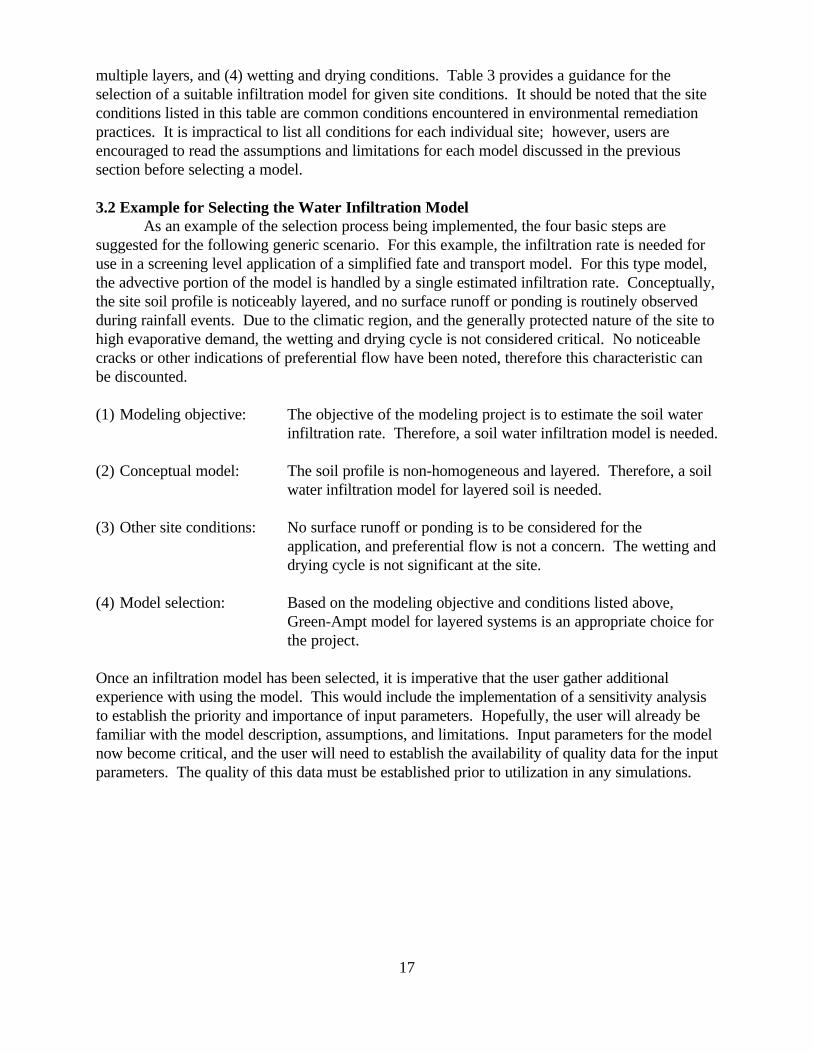
multiple layers, and (4) wetting and drying conditions. Table 3 provides a guidance for theselection of a suitable infiltration model for given site conditions. It should be noted that the siteconditions listed in this table are common conditions encountered in environmental remediationpractices. It is impractical to list all conditions for each individual site; however, users areencouraged to read the assumptions and limitations for each model discussed in the previoussection before selecting a model.

3.2 Example for Selecting the Water Infiltration ModelAs an example of the selection process being implemented, the four basic steps are

suggested for the following generic scenario. For this example, the infiltration rate is needed foruse in a screening level application of a simplified fate and transport model. For this type model,the advective portion of the model is handled by a single estimated infiltration rate. Conceptually,the site soil profile is noticeably layered, and no surface runoff or ponding is routinely observedduring rainfall events. Due to the climatic region, and the generally protected nature of the site tohigh evaporative demand, the wetting and drying cycle is not considered critical. No noticeablecracks or other indications of preferential flow have been noted, therefore this characteristic canbe discounted.

(1) Modeling objective: The objective of the modeling project is to estimate the soil waterinfiltration rate. Therefore, a soil water infiltration model is needed.

(2) Conceptual model: The soil profile is non-homogeneous and layered. Therefore, a soilwater infiltration model for layered soil is needed.

(3) Other site conditions: No surface runoff or ponding is to be considered for theapplication, and preferential flow is not a concern. The wetting anddrying cycle is not significant at the site.

(4) Model selection: Based on the modeling objective and conditions listed above,Green-Ampt model for layered systems is an appropriate choice forthe project.

Once an infiltration model has been selected, it is imperative that the user gather additionalexperience with using the model. This would include the implementation of a sensitivity analysisto establish the priority and importance of input parameters. Hopefully, the user will already befamiliar with the model description, assumptions, and limitations. Input parameters for the modelnow become critical, and the user will need to establish the availability of quality data for the inputparameters. The quality of this data must be established prior to utilization in any simulations.

18

Table 3. Summary of common site conditions and the selected model’s capabilities of simulatingthose conditions. Y indicates the model is suitable for the specific site condition and Nindicates that it is not.

SiteConditions

Model Name

SCS Green- Flux Green-Philip Explicit Infiltration/

2-Term Green-Ampt Exfiltration

Layered Constant

Ampt Ampt

SurfacePonding

N N Y Y N N

SurfaceRunoff

Y N N N N N

Rainfall &Irrigation

Y N N N Y Y

MultipleLayers

N N Y N N N

Wetting &Evaporation

N N N N N Y

HomogeneousSoil Profile

Y Y Y Y Y Y

VegetationCover

N N N N N Y

19

CHAPTER 4. INPUT PARAMETER ESTIMATIONS

4.1 General Description of ParametersAn important step in a model project is input parameter estimation. Because of

improvements in computer software and hardware, the usefulness of numerical models hingesincreasingly on the availability of accurate input parameters. Approaches for obtaining inputparameters in numerical modeling include field observations and measurements, experimentalmeasurements, curve-fitting, and theoretical calculations. Table 4 provides a list of inputparameters required for the use of models discussed in this document. A majority of parametervalues required for these models can be found in the literature (Hillel, 1982; Carsel and Parrish,1988; van Genuchten et al., 1989; Breckenridge et al., 1991; Leij et al., 1996). Typicalparameter values are provided in this table for common soil conditions; however, it is always agood practice to obtain site-specific values.

Table 4. Listing of input parameters for running the infiltration models.

Parameter Symbol Data SourceTypical Value or Required ModelMethod Name

Statistically derivedparameter F 0.1 to 90 inches SCS USDA-SCS, 1972w

Daily rainfall P 0.1 to 10 inches SCS Weather Stations

Duration of All models exceptinfiltration for SCSt Site-Specific

Sorptivity S Philip’s two term0.1 to 1 cm/h Philip, 1969; Jury et al,½

or Calculated 1991

Empirical Constant A Calculated Philip, 1969; Hillel, 1982Philip’s two term

Saturated Hydraulic 1x10 to 60 cm/h All models except Carsel and Parrish, 1988;Conductivity or Measured for SCS Hillel, 1982; Li et al.,Ks

-5Breckenridge et al., 1991;

1976

Unsaturated Breckenridge et al., 1991;Hydraulic Site-Specific Carsel and Parrish, 1988;Conductivity of or Measured Hillel, 1982; Li et al.,Layer n 1976

K model for layeredn

Green Ampt

systems

Hydraulic Green AmptConductivity of K model for layeredLayer i systems

iSite-Specific Carsel and Parrish, 1988;or Measured Hillel, 1982; Li et al.,

Breckenridge et al., 1991;

1976

Thickness ofLayer i Z Measured model for layeredi

Green Ampt

systems

Parameter Symbol Data SourceTypical Value or Required ModelMethod Name

20

Potential Head Breckenridge et al., 1991;While Wetting Site-Specific Carsel and Parrish, 1988;Front Passes or Measured Hillel, 1982; Li et al.,Through Layer n 1976

H model for layeredn

Green-Ampt

systems

Change in Breckenridge et al., 1991;Volumetric Water Site-Specific Carsel and Parrish, 1988;Content Within or Measured Hillel, 1982; Li et al.,Layer n 1976

)2 model for layeredGreen-Ampt

systems

Saturated Site-SpecificVolumetric Water 2 0.3 to 0.5 cm /cmContent (or Table 7)

s3 3

Green-Ampt Breckenridge et al., 1991;explicit & Carsel and Parrish, 1988;

Constant flux Hillel, 1982; Li et al.,Green-Ampt 1976

Initial Volumetric Site-Specific explicit & Carsel and Parrish, 1988;Water Content or Measured Constant flux Hillel, 1982; Li et al.,2o

Green-Ampt Breckenridge et al., 1991;

Green-Ampt 1976

Ponding Depth hsSite-Specific Green-Amptor Measured explicit

Capillary Pressureat the Wetting h CalculatedFront

fGreen-Ampt Hillel, 1982; Jury et al.,

explicit 1991

Constant Constant fluxApplication Rate Green-Amptr Measured

Vegetated Fraction M Site-Specific Eagleson, 1978Infiltration/Exfiltr-ation

Transpiration Rate E Measured Eagleson, 1978vInfiltration/Exfilt

-ration

Infiltration Infiltration/ExfiltSorptivity -rationS Eagleson’s Report Eagleson, 1978i

Exfiltration Infiltration/ExfiltSorptivity -rationS Eagleson’s Report Eagleson, 1978e

A brief description of each parameter listed in Table 4 is provided as follows. Thesedescriptions are not intended to be fully explanatory, and the reader is referred to cited referencesfor more detail.

1. Statistically derived parameter with some resemblance to the initial water content(F ): This parameter can be estimated according to USDA-SCS (1972). Detailedw

estimation of F is provided in Section 4.2. This parameter is required in the SCS model.w

2. Daily rainfall rate (P): The daily rainfall rate for a specific site can be obtained fromlocal weather station or atmospheric research institutes. This parameter is required in theSCS model.

21

3. Duration of infiltration (t): The duration of infiltration is site specific, and depends onrainfall rate, surface application rate, and soil infiltrability. This is also the simulationtime.

4. Sorptivity (S): The sorptivity is a function of initial and saturated water contents, andcan be obtained simply by determining the slope of I/t versus t in Equation 4. This-1/2

parameter is required in Philip’s two-term model.

5. Empirical constant (A): This parameter is required in Philip’s two-term model. Whenthe infiltration time is very large, the constant A is similar to hydraulic conductivity, andcan be obtained simply by determining the intercept of I/t versus t in Equation 4.-1/2

6. Saturated hydraulic conductivity (K ): This parameter measures the ability of the soilsto conduct water when saturated. The value of the saturated hydraulic conductivitydepends on soil types and is site-specific. This parameter can be obtained fromexperimental measurements and literature, and is required in Philip’s two-term model,Green-Ampt model for layered systems, the Green-Ampt explicit model, and the Constantflux Green-Ampt model.

7. Hydraulic conductivity of layer n (K ): This parameter measures the ability of the soiln to conduct water in layer n when the soil is unsaturated. The value of the unsaturatedhydraulic conductivity depends on soil types and soil water content, and is site-specific. This parameter can be obtained from experimental measurements or literature, and isrequired in the Green-Ampt model for layered systems.

8. Hydraulic conductivity of layer i (K ): This parameter measures the ability of the soili

to conduct water in layer i when the soil is unsaturated. The value of unsaturatedconductivity depends on soil types and soil water content, and is site-specific. Thisparameter can be obtained from experimental measurements and literature, and is requiredin the Green-Ampt model for layered systems.

9. Thickness of layer i (Z ): This parameter defines the thickness of layer i when the soil isi

heterogeneous. The value of each layer’s thickness is site-specific, and is required in theGreen-Ampt model for layered systems.

10. Potential head while wetting front passes through layer n (H ): The potential head isnthe difference between the energy state of soil water and that of pure free water. The soilwater potential head is a function of soil water content, and can be determined from thesoil water retention curve. Users may need to know basic concepts of the soil waterretention curves in order to estimate this parameter. This parameter is required in theGreen-Ampt model for layered system.

11. Change in volumetric water content within layer i ()2): The volumetric watercontent is expressed as a decimal fraction of the volume of the total soil sample. Thechange in volumetric water content within layer i is the difference between the maximumand minimum water content in the i layer at a given time frame. This parameter isth

required in the Green-Ampt model for layered system.

12. Saturated volumetric water content (2 ): The saturated volumetric water content is thes

percentage of the volume of the soil sample when all soil pore spaces are filled with water(i.e., saturated). The value of the saturated volumetric water content is dependent on soil

22

type and is site-specific. This parameter can be obtained from experimental measurementsand the literature, and is required in the Green-Ampt explicit model.

13. Initial volumetric water content (2 ): This parameter defines the volumetric waterocontent at start of the simulation. The value of the initial volumetric water content isdependent on soil type and is site-specific, and is required in the Green-Ampt explicitmodel.

14. Ponding depth (h ): This parameter defines the thickness of water accumulated at thes

soil surface during water infiltration. The extent of ponding depth depends on soil typesand is thus site-specific. This parameter is required in the Green-Ampt explicit model.

15. Capillary pressure at the wetting front (h ): The capillary pressure is the suction off

water in the pore space due to surface tension or capillary force. This parameter is afunction of soil water content, and can be determined from experimental measurements(Hillel, 1982) or from the following equation h = 2(/ r, where ( is the surface tension off

water and r is the radius of capillary. The parameter is required in the Green-Amptexplicit model, and is discussed in the section on the estimation of the Green-Amptparameters.

16. Constant application rate (r): This is the rate of water application to the soil surface,and is site-specific. This parameter is required in the constant flux Green-Ampt model.

17. Vegetated fraction (M): This parameter defines the density of plant canopy coverage atthe soil surface. This parameter is site-specific, and is required in theinfiltration/exfiltration model.

18. Transpiration rate (E ): This parameter defines the plant water transpiration rate. Itv

depends on type of plant and soil water availability to roots. This parameter can beobtained from experimental measurements, and is required in the infiltration/exfiltrationmodel.

19. Infiltration sorptivity (S ): The infiltration sorptivity is a function of initial and saturatedi

water contents. It can be obtained from Eagleson’s report (1978). This parameter isrequired in the INFEXF model.

20. Exfiltration sorptivity (S ). The exfiltration sorptivity is a function of initial andesaturated water contents and surface evaporation rate. This parameter can be obtainedfrom Eagleson (1978), and is required in the infiltration/exfiltration model.

In summary, the saturated water content at the application surface (2 ), antecedent waters

content (2 ), and respective hydraulic conductivities (K and K ) are required for most infiltrationo s o

models. However, the pore size index (8) and air entry head (h ) are also required by some of theb

models for the estimation of other input parameters (e.g., head at the wetting front (h )). Thesef

values are listed in Tables 9 and 10. In addition to the tabulations indicated, the electronicdatabase known as UNSODA (Leij et al., 1996) provides information on the soil hydraulicparameters related to water retention and hydraulic conductivity. Estimates of infiltration basedon tabulated parameter values should be considered only for preliminary, and order-of-magnitudetype analyses. For a more reliable estimation of infiltration at a given site, it is recommended thatthe values of 2 , 2 , K , K , and the retention parameters be measured. Johnson and Ravi (1993)s o s o

call for caution in the use of literature values for a specific application and discuss the resulting

Fw '1000CNI

& 10

23

(24)

uncertainty.

4.2 Estimation of F in SCS ModelwThe statistically derived parameter F utilized in the SCS model can be estimated based onw

the following equation:

where CN is the soil moisture condition I curve number or hydrologic soil-cover complexI

number. CN is related to the soil moisture condition II curve number, CN , with the polynomial:I II

CN = -16.91 + 1.348 CN - 0.01379(CN ) + 0.0001177(CN ) . F can be considered anI II II II w2 3

estimate of the maximum potential difference between rainfall and runoff (Schwab et al., 1981). The CN is based on an antecedent moisture condition (AMC) II determined by the total rainfallII

in the 5-day period preceding a storm (USDA-SCS, 1972). Three levels of AMC are used: (1)lower limit of moisture content, (2) average moisture content, and (3) upper limit of moisturecontent. Table 5 lists values for CN at the average AMC. The description of hydrologic groupsII

used in Table 5 is provided in Table 6.

Table 5. Curve numbers CN for hydrologic soil-cover complex for the antecedent moistureII

condition II and I = 0.2F . I is initial water abstraction (USDA-SCS, 1972). a w a

Land Use or HydrologicCrop ConditionTreatment or Practice

Hydrologic Soil GroupA B C D

Fallow Straight Row --- 77 86 91 94

Row Crops Straight Row Poor 72 81 88 91Straight Row Good 67 78 85 89

Contoured Poor 70 79 84 88Contoured Good 65 75 82 86Terraced Poor 66 74 80 82Terraced Good 62 71 78 81

Small Grain Straight Row Poor 65 76 84 88Straight Row Good 63 75 83 87

Contoured Poor 63 74 82 85Contoured Good 61 73 81 84Terraced Poor 61 72 79 82Terraced Good 59 70 78 81

Close-seededLegumes orRotationMeadow

Straight Row Poor 66 77 85 89Straight Row Good 58 72 81 85

Contoured Poor 64 75 83 85

24

Contoured Good 55 69 78 83Terraced Poor 63 73 80 83Terraced Good 51 67 76 80

Pasture or Range Poor 68 79 86 89Fair 49 69 79 84

Good 39 61 74 80Contoured Poor 47 67 81 88Contoured Fair 25 59 75 83Contoured Good 6 35 70 79

Meadow Good 30 58 71 78

Woods Poor 45 66 77 83Fair 36 60 73 79

Good 25 55 70 77

Farmsteads --- 59 74 82 86

Roads andRight-of-Way --- 74 84 90 92(Hard Surface

Table 6. Description of hydrologic soil groups.

Group Description of Hydrologic Group

A Lowest runoff potential. Includes deep sands with very little silt and clay, alsodeep, rapidly permeable loess.

B loess less deep or less aggregated than group A, but the group as a whole hasModerately low runoff potential. Mostly sandy soils less deep than Group A, and

above average infiltration after thorough wetting.

C considerable clay and colloids, though less than those of group D. The group hasModerately high runoff potential. Comprises shallow soils and soils containing

below-average infiltration after presaturation.

D group also includes some shallow soils with nearly impermeable subhorizons nearHighest runoff potential. Includes mostly clays of high swelling percent, but the

the surface.

An example on how to determine the CN from Table 5 is given as follows. For pasture landII

with good hydrologic conditions, under moderately high runoff potential (Group C), the CN isII

74 and CN is 55, and thus F is about 8.2 inches.I w

4.3 Estimation of Green-Ampt Model ParametersThe discussion presented here is relevant to the three models which utilize the Green-Ampt

parameters: (1) the explicit Green-Ampt (Salvucci and Entekhabi, 1994), (2) the constant fluxGreen-Ampt model (Swartzendruber, 1974), and (3) the layered Green-Ampt model (Flerchinger

25

et al., 1988). The parameters 2 , 2 , K , and K are required in most models. If no measurementss o s o

are available, then 2 can be approximated based on soil texture (Table 7), and the residual ors

irreducible water content, 2 , can be used in place of 2 (Table 8), even though this would tend tor o

overestimate infiltration. K and K correspond to the hydraulic conductivities at the respectives o

water contents (i.e., K(2 ) and K(2 )). K may be estimated based on Table 11. However,s o s

Bouwer (1966) recommended that K be taken as one half of K , and K may be assumed to bes sat o

zero. If the water content at the soil surface and the initial water content are quite different fromthat of the saturated and residual water contents, respectively, then K and K may be estimateds o

from either the Brooks-Corey or the van Genuchten model for K(2) (van Genuchten et al., 1991). Typical values of 2 , and 2 for different textures are provided in Tables 7 and 8. Similarly,s o

typical values of h and 8, respectively, for different textures are provided in Tables 9 and 10. b

Only the magnitude of h is provided in Table 9 (i.e., the negative sign is omitted). Table 11b

provides a summary of soil hydraulic parameters commonly used in the unsaturated zone models(Rawls et al., 1992).

Table 7. Typical values of saturated volumetric water content (2 ).s

Texture Brakensiek et al., 1981 Panian, 1987 Carsel and Parrish, 1988

Sand 0.35 0.38 0.43

Loamy Sand 0.41 0.43 0.41

Sandy Loam 0.42 0.44 0.41

Loam 0.45 0.44 0.43

Silty Loam 0.48 0.49 0.45

Sandy Clay Loam 0.41 0.48 0.39

Clay Loam 0.48 0.47 0.41

Silty Clay Loam 0.47 0.48 0.43

Silty Clay 0.48 0.49 0.36

Clay 0.48 0.49 0.38

26

Table 8. Typical values of residual volumetric water content (2 ).r


Sand 0.054 0.020 0.045

Loamy Sand 0.060 0.032 0.057

Sandy Loam 0.118 0.045 0.065

Loam 0.078 0.057 0.078

Silty Loam 0.038 0.026 0.067

Sandy Clay Loam 0.188 0.093 0.100

Clay Loam 0.185 0.107 0.095

Silty Clay Loam 0.155 0.089 0.089

Silty Clay 0.182 0.102 0.070

Clay 0.226 0.178 0.068

Table 9. Typical values of air-entry head (h )(cm).b


Sand 35.30 3.58 6.90

Loamy Sand 15.85 1.32 8.06

Sandy Loam 29.21 9.01 13.33

Loam 50.94 19.61 27.78

Silty Loam 69.55 31.25 50.00


Clay Loam 42.28 31.25 52.63

Silty Clay Loam 57.78 30.30 100.00

Silty Clay 41.72 15.87 200.00

Clay 63.96 10.00 125.00

27

Table 10. Typical values of pore size index (8).


Sand 0.57 0.40 1.68

Loamy Sand 0.46 0.47 1.28

Sandy Loam 0.40 0.52 0.89

Loam 0.26 0.40 0.56

Silty Loam 0.22 0.42 0.41


Clay Loam 0.28 0.40 0.31

Silty Clay Loam 0.18 0.36 0.23

Silty Clay 0.21 0.38 0.09

Clay 0.21 0.41 0.09

28

Table 11. Typical values for soil hydraulic property parameters (Rawls et al., 1992).

Texture Class SampleSize

Total Residual HydraulicPorosity (N) Water Content Conductivity

Effective Water WaterPorosity Bubbling Pressure (h ) Pore Size Distribution (8) Retained at Retained at

(N ) -33 kPa -1500 kPae

b

Saturated

(K )s

cm /cm cm /cm cm /cm cm /cm cm /cm cm/hr3 3 3 3 3 3 Arithmetic Geometric Arithmetic Geometriccm cm

** **3 3 3 3

Sand 762 21.000.437 0.020 0.417 15.98 7.26 0.694 0.592 0.091 0.033*

(.374-.500) (.001-.039) (.354-.480) (.24-31.72) (1.36-38.74) (.298-1.090) (.334-1.051) (.018-.164) (.007-.059)

Loamy Sand 338 6.110.437 0.035 0.401 20.58 8.69 0.553 0.474 0.125 0.055(.368-.506) (.003-.067) (.329-.473) (-4.04-45.20) (1.80-41.85) (.234-.872) (.271-.827) (.060-.190) (.019-.091)

Sandy Loam 666 2.590.453 0.041 0.412 30.20 14.66 0.378 0.322 0.207 0.095(.351-.555) (.024-.106) (.283-.541) (-3.61-64.01) ( 3.45-62.24) (.140-.616) (.186-.558) (.126-.288) (.031-.159)

Loam 383 1.320.463 0.027 0.434 40.12 11.15 0.252 0.220 0.270 0.117(.375-.551) (.020-.074) (.334-.534) (-20.07-100.3) (1.63-76.40) (.086-.418) (.137-.355) (.195-.345) (.069-.165)

Silt Loam 1206 0.680.501 0.015 0.486 50.87 20.76 0.234 0.211 0.330 0.133(.420-.582) (.028-.058) (.394-.578) (-7.68-109.4) (3.58-120.4) (.105-.363) (.136-.326) (.258-.402) (.078-.188)

Sandy Clay Loam 498 4.30.398 0.068 0.330 59.41 28.08 0.319 0.250 0.255 0.148(.332-.464) (.001-.137) (.235-.425) (-4.62-123.4) (5.57-141.5) (.079-.889) (.125-.502) (.186-.324) (.085-.211)

Clay Loam 366 .230.464 0.075 0.390 56.43 25.89 0.242 0.194 0.318 0.197(.409-.519) (.024-.174) (.279-.501) (-11.44-124.3) (5.80-115.7) (.070-.414) (.100-.377) (.250-.386) (.115-.279)

Silty Clay Loam 689 .150.471 0.040 0.432 70.33 32.56 0.177 0.151 0.366 0.208(.418-.524) (.038-.118) (.347-.517) (-3.26-143.9) (6.68-158.7) (.039-.315) (.090-.253) (.304-.428) (.138-.278)

Sandy Clay 45 .120.430 0.109 0.321 79.48 29.17 0.223 0.168 0.339 0.239(.370-.490) (.013-.205) (.201-.435) (-20.15-179.1) (4.96-171.6) (.048-.398) (.078-.364) (.245-.433) (.162-.316)

Silty Clay 127 .090.479 0.56 0.423 76.54 34.19 0.150 0.127 0.387 0.250(.425-.533) (.024-.136) (.334-.512) (-6.47-159.6) (7.04-166.2) (.040-.260) (.074-.219) (.332-.442) (.193-.307)

Clay 291 .060.475 0.090 0.385 85.60 37.30 0.165 0.131 0.396 0.272(.427-.523) (.015-.195) (.269-.501) (-4.92-176.1) (7.43-187.2) (0.31-.293) (.068-.253) (.326-.466) (.208-.336)

*First line is the mean value, and second is one standard deviation about the mean.**Antilog of the log mean.

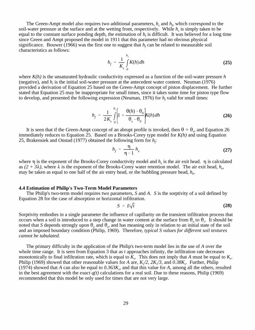
hf '1Ks

mh i

0

K(h) dh

hf '1

2Ksmh i

0

1 %2(h)&20

2s&20

K(h)dh

hf '0

0&1he

S ' I/ t

29

(25)

(26)

(27)

(28)

The Green-Ampt model also requires two additional parameters, h and h , which correspond to thes f

soil-water pressure at the surface and at the wetting front, respectively. While h is simply taken to bes

equal to the constant surface ponding depth, the estimation of h is difficult. It was believed for a long timef

since Green and Ampt proposed the model in 1911 that this parameter had no obvious physicalsignificance. Bouwer (1966) was the first one to suggest that h can be related to measurable soilf

characteristics as follows:

where K(h) is the unsaturated hydraulic conductivity expressed as a function of the soil-water pressure h(negative), and h is the initial soil-water pressure at the antecedent water content. Neuman (1976)i

provided a derivation of Equation 25 based on the Green-Ampt concept of piston displacement. He furtherstated that Equation 25 may be inappropriate for small times, since it takes some time for piston type flowto develop, and presented the following expression (Neuman, 1976) for h valid for small times:f

It is seen that if the Green-Ampt concept of an abrupt profile is invoked, then 2 = 2 , and Equation 26s

immediately reduces to Equation 25. Based on a Brooks-Corey type model for K(h) and using Equation25, Brakensiek and Onstad (1977) obtained the following form for h :f

where 0 is the exponent of the Brooks-Corey conductivity model and h is the air exit head. 0 is calculatede

as (2 + 38), where 8 is the exponent of the Brooks-Corey water retention model. The air exit head, h ,e

may be taken as equal to one half of the air entry head, or the bubbling pressure head, h . b

4.4 Estimation of Philip's Two-Term Model ParametersThe Philip's two-term model requires two parameters, S and A. S is the sorptivity of a soil defined by

Equation 28 for the case of absorption or horizontal infiltration.

Sorptivity embodies in a single parameter the influence of capillarity on the transient infiltration process thatoccurs when a soil is introduced to a step change in water content at the surface from 2 to 2 . It should beo s

noted that S depends strongly upon 2 and 2 , and has meaning only in relation to an initial state of the soilo s

and an imposed boundary condition (Philip, 1969). Therefore, typical S values for different soil texturescannot be tabulated.

The primary difficulty in the application of the Philip's two-term model lies in the use of A over thewhole time range. It is seen from Equation 3 that as t approaches infinity, the infiltration rate decreasesmonotonically to final infiltration rate, which is equal to K . This does not imply that A must be equal to K . s s

Philip (1969) showed that other reasonable values for A are, K /2, 2K /3, and 0.38K . Further, Philips s s

(1974) showed that A can also be equal to 0.363K , and that this value for A, among all the others, resulteds

in the best agreement with the exact q(t) calculations for a real soil. Due to these reasons, Philip (1969)recommended that this model be only used for times that are not very large.

30

CHAPTER 5. EXAMPLE APPLICATION SCENARIOS

Six example application scenarios were chosen, and are illustrated in the following discussion. Anapplication scenario is presented for each model. The intention of these scenarios is to provide guidancefor users to apply infiltration models for various field conditions.

5.1 Semi-Empirical Model (SCS)Statement of the Problem: This scenario was chosen to simulate water infiltration through a loamy

sand soil for conditions with rainfall and surface runoff. A hypothetical site has been contaminated withhazardous waste materials and an estimate of the contaminant transport through the vadose zone is desired. Since the soil water infiltrating flux is an important factor controlling contaminant migration in the vadosezone, it must be first estimated before performing the contaminant transport modeling.

Conceptual model: Figure 3 is a schematic diagram of the hypothetical site showing the conceptualmodel for this scenario. The sandy material is bounded above by the soil surface and below by the ground-water table. Factors that affect the rate of water infiltration into the soil include initial soil moisturecontent, rainfall rate and duration, and surface runoff.

In this scenario, the purpose is to calculate the daily infiltration amount into the soil profile verticallyduring a process of rainfall and surface runoff. Since little is known concerning the mathematical boundaryconditions for the site and little soil physical data available, the semi-empirical model known as the SCSmodel is chosen for the simulations.

Input Parameters: Input parameters for running the simulations are obtained from several sources. Attempts are made to obtain realistic values for the input parameters. Table 12 lists the input parametervalues used for this scenario. In this model, only two input parameters are required (refer to Equations 1and 2). For detailed estimation of F under different soil conditions, readers are encouraged to read thew

USDA report cited in the table. The daily rainfall amount can be obtained from a local weather station orclimatic research institutes.

Table 12. Input parameter values for simulations with a sandy soil using the SCS model.

Parameter Symbol Value Units Reference

Statistically USDA-SCS,Derived 1972F 8.2 inchesw

Daily RainfallAmount P 0.1 to 10.0 inches Assumed

Simulation Results: Figure 4 shows the daily infiltration amount as a function of the daily rainfallamount while Figure 5 shows the surface runoff as a function of the daily rainfall amount. Each point onthe curves of Figures 4 and 5 could represent one rainfall event. In Figure 5, the runoff does not occur inthe event where the daily rainfall amount is smaller than 1.64 inches (0.2F =1.64 inches). Before runoff w

occurs, the daily infiltration amount equals the daily rainfall amount. After that, the daily infiltrationamount increases as the daily rainfall amount increases but the rate of the increase of the daily infiltrationdecreases (Fig. 4). Note that the SCS model is applicable to the situation in which the daily amounts of rainfall, runoff and infiltration are of interest.

31

Figure 5. Daily runoff amount as afunction of daily rainfall amount.

Figure 4. Daily infiltration amount as afunction of daily rainfall amount.

Figure 3. Conceptual model for simulating water infiltration using the SCS model.

32

5.2 Infiltration Model for Homogeneous Conditions (PHILIP2T)Statement of the Problem: This scenario was chosen to simulate the vertical infiltration of water into

a sandy soil with a homogeneous soil profile. A hypothetical site has been contaminated with hazardouswaste materials. In order to estimate the transport of the contaminants in the vadose zone, the infiltrationrate (water flux) must be known before performing transport modeling. Initial soil water constant at thesite is approximately uniformly distributed and constant. Soil water content at the inflow end (at thesurface) is held constant and near saturation. Other soil physical properties such as saturated water contentand saturated hydraulic conductivity values are available.

Conceptual model: Figure 6 is a schematic diagram of the hypothetical site showing the conceptualmodel for this scenario. This site is bounded above by the soil surface and below by the ground-water table.The water depth is much greater than the water penetration depth. The free water is available in excess atthe surface and a constant water content at the surface is maintained through the infiltration period. In thisscenario, the Philip’s two-term model was selected for the simulations.

Input Parameters: Input parameters for running the simulations are obtained from several sources. Attempts are made to obtain realistic values for the input parameters. Table 13 lists the input parametervalues used in the simulations. The sorptivity (S) and the constant (A) can be obtained simply bydetermining the slope and intercept of I/t versus t in Equation 4, respectively. -1/2

Table 13. Input parameter values for the simulations in a sandy soil using PHILIP2T model.


Duration of t 1 to 24 h AssumedInfiltration

Sorptivity S 1 cm/h Philip, 1969½

Constant A 7.6 (=0.363 k ) cm/h Jury et al., 1991s

Saturated Hydraulic K 21 cm/h Carsel and Parrish,Conductivity 1988

s

Simulation Results: Figure 7 shows a typical soil infiltration pattern, with an infiltration raterelatively high at the onset of the infiltration, then decreasing, and eventually approaching a constant rate att > 20 h. Figure 8 illustrates a linear relationship between the cumulative infiltration and time. By knowingthe soil water infiltration rate, the movement of contaminants in the soil could be evaluated using othertransport models.

33

Figure 7. Surface water infiltration rateas a function of time.

Figure 8. Cumulative infiltration as afunction of time.

Figure 6. Conceptual model for simulating water infiltration using Philip’s Two-TermModel.

34

5.3. Infiltration Model for Nonhomogeneous Conditions (GALAYER)Statement of the Problem: Since the soil profiles are differentiated into layers, the water distribution

during infiltration is not uniform. Two scenarios were selected to calculate water infiltration into layeredsoils. In Scenario 1, the soil consists of two layers with a sand layer underlain by a loam. In Scenario 2,the soil consists of three layers with a sand layer underlain by a loam, and the loam underlain by a claylayer. Under such conditions, the infiltration rate is initially controlled by the sand layer, and with time theinfiltration rate will become controlled by the lower fine-textured layer with the low hydraulic conductivity. Simulation results from these scenarios would provide information concerning water infiltrating into nonhomogeneous soil profiles.

Conceptual model: Figures 9a and 9b are the schematic diagrams of the layered soils showing the conceptual model for the Scenario 1 and the Scenario 2, respectively. In Scenario 1, the soil profileconsists of sand and loam. The thickness of the sand layer is 10 cm. The loam layer extends from thebottom of the first layer to the bottom of the soil profile. Scenario 1 is to estimate water infiltration intothe sand layer and continuing through the loam layer. Scenario 2 is to estimate water infiltration into threelayers (with sand, loam and clay in sequence). The thickness of the upper layers (sand and loam) is 10 cm.The lowest layers (loam or clay) extend to the rest of the soil profile. In these scenarios, the GALAYER(Flerchinger et al., 1988) model for layered soils was selected for the simulations. The comparison of thetwo scenarios for water infiltration was also provided.

Input Parameters: Input parameters for running the simulations are obtained from several sources. Attempts are made to obtain realistic values for the input parameters. Table 14 listed the input parametervalues used in the simulations.

Table 14. Input parameter values for the simulations using the GALAYER (Flerchinger et al., 1988) model.


Duration of Infiltration t 1 to 24 h Assumed

Saturated HydraulicConductivity (Layer 1) K 1 cm/h Hillel, 19821

Saturated HydraulicConductivity (Layer 2) K 0.5 cm/h Hillel, 19822

Saturated HydraulicConductivity (Layer 3) K 0.1 cm/h Hillel, 19823

Change in VolumetricWater Content in Layer 2 )2 0.2 cm /cm Assumed

for Scenario 1.2

3 3

Change in VolumetricWater Content in Layer 3 )2 0.1 cm /cm Assumed

for Scenario 2.3

3 3

Suction Head of Layer 2for Scenario 1. H 3000 cm Hillel, 19822

Suction Head of Layer 3for Scenario 2. H 7000 cm Hillel, 19823

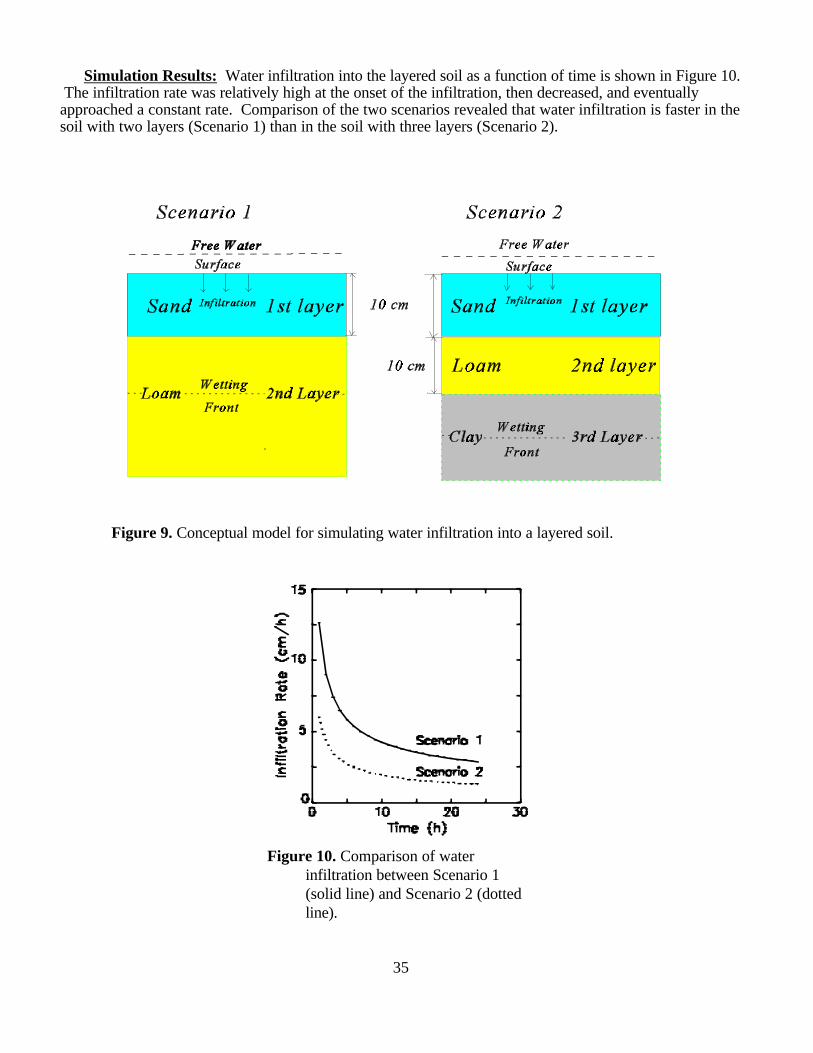
35

Figure 9. Conceptual model for simulating water infiltration into a layered soil.

Figure 10. Comparison of waterinfiltration between Scenario 1(solid line) and Scenario 2 (dottedline).

Simulation Results: Water infiltration into the layered soil as a function of time is shown in Figure 10. The infiltration rate was relatively high at the onset of the infiltration, then decreased, and eventuallyapproached a constant rate. Comparison of the two scenarios revealed that water infiltration is faster in thesoil with two layers (Scenario 1) than in the soil with three layers (Scenario 2).

36

5.4 Infiltration Model for Ponding Conditions (GAEXP)Statement of the Problem: This scenario was chosen to simulate water infiltration into a sandy soil

under surface ponding conditions. A water depth of 1 cm was applied at the soil surface. The initial soilwater content of 0.05 cm /cm is uniformly distributed in the soil profile. Under such continuous ponding3 3

conditions, the infiltration rate (equal to the infiltrability) can be expected to settle down to a steady-induced rate which is practically equal to the saturated conductivity.

Conceptual model: Figure 11 is a schematic diagram of a sandy soil profile showing the conceptualmodel for this scenario. This soil profile is bounded above by the soil surface which is under the waterponding condition and below by a groundwater table. In this scenario, the Explicit Green-Ampt modelwas selected for the simulations.

Input Parameters: Input parameters for running the simulations are obtained from several sources. Attempts are made to obtain realistic values for the input parameters. Table 15 lists the input parametervalues used in the simulations.

Table 15. Input parameters for the simulations in a clay soil using GAEXP Model.


Saturated Hydraulic K 21 cm/h Carsel and Parrish,Conductivity 1988

s

Ponding Depth h 1 cm Assumeds

Saturated Volumetric 2 0.43 cm /cm Hillel, 1982Water Content

s3 3

Initial Volumetric 2 0.05 cm /cm AssumedWater Content

o3 3

Simulation Results: Figures 12 and 13 show the surface infiltration and cumulative infiltration as afunction of time, respectively. A typical soil infiltration pattern, with an infiltration rate relatively high atthe onset of the infiltration, then decreasing, and eventually approaching a constant rate was obtained forthis sandy soil (Figure 12).

Groundwater Table

Soil surface

Vadose zone

Ponding water

(Sand)

Infiltration

1 cm

37

Figure 11. Conceptual model for simulating water infiltration using the Explicit Green-Ampt model.

Figure 13. Cumulative infiltration as afunction of time.Figure 12. Water infiltration as a function

of time.

38

5.5 Infiltration Model for Non-ponding Conditions (GACONST)Statement of the Problem: This scenario was chosen to simulate water infiltration into a sandy

loam soil under non-ponding conditions. The initial soil water content of 0.05 cm /cm is uniformly3 3

distributed in the soil profile. Under this non-ponding condition, water from rainfall or surface irrigation either enters the soil or flows over the surface as runoff.

Conceptual model: Figure 14 is a schematic diagram of a sandy loam soil profile showing theconceptual model for this scenario. This soil profile is bounded above by the soil surface which is under thenon-ponding conditions and below by the groundwater table. No ponding occurs after the soil is saturatedand the excess water is discharged as surface run-off. Several infiltration models for non-pondingconditions have been developed (Philip, 1957; Swartzendruber, 1974). In this scenario, the Constant FluxGreen-Ampt Model was chosen for the simulations.

Input Parameters: Input parameters for running the simulations are obtained from Carsel and Parrish (1988). Attempts are made to obtain realistic values for the input parameters. Table 16 listed the inputparameter values used in the simulations.

Table 16. Input parameters for the simulations with r >K in a sandy loam soil using the GACONSTs

model.


Saturated Hydraulic K 2.59 cm/h Carsel and Parrish,Conductivity 1988

s

Constant Application r 3.5 cm/h AssumedRate

Saturated Volumetric 2 0.41 cm /cm Carsel and Parrish,Water Content 1988

s3 3

Initial Volumetric 2 0.05 cm /cm AssumedWater Content

o3 3

Air Exit Head h -13.33 cm Carsel and Parrish,e

1988

Pore Size Index 8 0.89 - Carsel and Parrish,1988

Simulation Results: Figure 15 shows a constant-flux infiltration pattern when r>K . Before thes

surface saturation first occurs at time t ( 5 hours), infiltration rate is constant and equals to r, after that, 0

infiltration rate decreases with time. Figure 16 illustrates a linear relationship between the cumulativeinfiltration and time.

39

Figure 14. Conceptual model for simulating water infiltration using the constant fluxGreen-Ampt model.

Figure 15. Water infiltration as a functionof time. Figure 16. Cumulative infiltration as a

function of time.

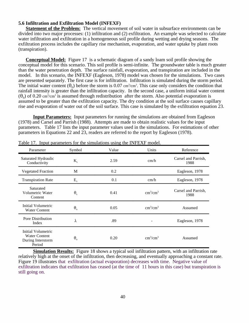
40

5.6 Infiltration and Exfiltration Model (INFEXF)Statement of the Problem: The vertical movement of soil water in subsurface environments can be

divided into two major processes: (1) infiltration and (2) exfiltration. An example was selected to calculatewater infiltration and exfiltration in a homogeneous soil profile during wetting and drying seasons. Theexfiltration process includes the capillary rise mechanism, evaporation, and water uptake by plant roots(transpiration).

Conceptual Model: Figure 17 is a schematic diagram of a sandy loam soil profile showing theconceptual model for this scenario. This soil profile is semi-infinite. The groundwater table is much greaterthan the water penetration depth. The surface rainfall, evaporation, and transpiration are included in themodel. In this scenario, the INFEXF (Eagleson, 1978) model was chosen for the simulations. Two casesare presented separately. The first case is for infiltration. Infiltration is simulated during the storm period.The initial water content (2 ) before the storm is 0.07 cm /cm . This case only considers the condition that0

3 3

rainfall intensity is greater than the infiltration capacity. In the second case, a uniform initial water content(2 ) of 0.20 cm /cm is assumed through redistribution after the storm. Also potential evaporation is0

3 3

assumed to be greater than the exfiltration capacity. The dry condition at the soil surface causes capillaryrise and evaporation of water out of the soil surface. This case is simulated by the exfiltration equation 23.

Input Parameters: Input parameters for running the simulations are obtained from Eagleson(1978) and Carsel and Parrish (1988). Attempts are made to obtain realistic values for the inputparameters. Table 17 lists the input parameter values used in the simulations. For estimations of otherparameters in Equations 22 and 23, readers are referred to the report by Eagleson (1978).

Table 17. Input parameters for the simulations using the INFEXF model.


Saturated Hydraulic Carsel and Parrish,Conductivity 1988K 2.59 cm/hs

Vegetated Fraction M 0.2 Eagleson, 1978

Transpiration Rate E 0.1 cm/h Eagleson, 1978v

SaturatedVolumetric Water 2 0.41 cm /cm

Contents

3 3 Carsel and Parrish,1988

Initial VolumetricWater Content 2 0.05 cm /cm Assumedo

3 3

Pore DistributionIndex 8 .89 - Eagleson, 1978

Initial VolumetricWater Content

During InterstormPeriod

2 0.20 cm /cm Assumedo3 3

Simulation Results: Figure 18 shows a typical soil infiltration pattern, with an infiltration raterelatively high at the onset of the infiltration, then decreasing, and eventually approaching a constant rate. Figure 19 illustrates that exfiltration (actual evaporation) decreases with time. Negative value of exfiltration indicates that exfiltration has ceased (at the time of 11 hours in this case) but transpiration isstill going on.

41

Figure 18. Water infiltration as a functionof time.

Figure 17. Conceptual model for simulating water infiltration and exfiltration.

Figure 19. Water exfiltration as afunction of time.

42

REFERENCES

Ahuja, L.R. and J.D. Ross. 1983. A new Green-Ampt type model for infiltration through a surface sealpermitting transient parameters below the seal. In: Advance infiltration (Proc. Nat. Conf. On Advancesin Infiltration), ASAE. 147-162.

Bouwer, H. 1966. Rapid field measurement of air entry value and hydraulic conductivity of soil assignificant parameters in flow system analysis. Water Resour. Res., 2:729-738.

Bouwer, H. 1969. Infiltration of water into nonuniform soil. J. Irrigation and Drainage Division of ASCE95:451-462.

Brakensiek, D. L., R. L. Engelman, and W. J. Rawls. Variation within texture classes of soil waterparameters, Transaction of the ASAE 24:335-339, 1981.

Brakensiek, D.L., and C.A. Onstad, Parameter estimation of the Green and Ampt infiltration equation.Water Resour. Res., 13:1009-1012, 1977.

Breckenridge, R.P., J.R. Williams, and J.F. Keck. 1991. Characterizing soil for hazardous waste siteassessments. EPA Ground-Water Issue Paper. EPA/540/4-91/003.

Carsel, R.F., and R.S. Parrish. 1988. Developing joint probability distributions of soil water retentioncharacteristics. Water Resour. Res., 24:755-769.

Childs, E.C., and M. Bybordi. 1969. The vertical movement of water in stratified porous materials. I.Infiltration. Water Resour. Res., 5:446-459.

Corradini, C., F. Melone, and R.E. Smith. 1994. Modeling infiltration during complex rainfall sequences. Water Resour. Res., 30:2777-2784.

Eagleson, P. 1978. Climate, soil, and vegetation. 3. A simplified model of soil moisture movement in theliquid phase. Water Resour. Res., 14:722-730.

Flerchinger, G.N., F.J. Waltts, and G.L. Bloomsburg. 1988. Explicit solution to Green-Ampt equation for

nonuniform soils. J. Irrig. and Drain. Div., ASCE, 114:561-565.

Fok, Y. -S. 1970. One-dimensional infiltration into layered soils. J. Irrig. and Drain. Div., ASCE, 90:121-129.

Ghildal, B.P., and R.P. Tripathi. 1987. Soil Physics. John Wiley & Sons. New York.

Haverkamp, R, J.Y. Parlange, J.L. Starr, Schmitz, and C. Fuentes. 1990. Infiltration under pondedconditions: 3. A predictive equation based on physical parameters. Soil Sci., 149:292-300.

Haverkamp, R., P.J. Ross, and J.Y. Parlange. 1994. Three-dimensional analysis of infiltration from thedisc infiltrometer, 2. Physically based infiltration equation. Water Resour. Res. 30:2931-2935.

Hillel, D. 1982. Introduction to Soil Physics. Academic Press. New York.

Hillel, D., and W.R. Gardner. 1970. Measurement of unsaturated conductivity diffusivity by infiltration

43

through an impeding layer. Soil Sci., 109:149.

Johnson, J. A., and V. Ravi. 1993. Uncertainty in the use of literature soil hydraulic parameter data inground-water modeling of the vadose zone, Robert S. Kerr Environmental Research Laboratory, Ada,Oklahoma (unpublished).

Jury, W.A., W.R. Gardner, and W.H. Gardner. 1991. Soil Physics. John Wiley & Sons. New York.

Leij, F.J., W.J. Alves, Martinus Th. van Genuchten, and J.R. Williams. 1996. The UNSODA unsaturatedsoil hydraulic database, User’s Manual Version 1.0. National Risk Management Research Laboratory,Office of Research and Development, U.S. EPA, Cincinnati, Ohio 45268. EPA/600/R-96/095.

Li, E. A., V.O. Shanholtz, and E. W. Carson. 1976. Estimating saturated hydraulic conductivity and capillary potential at the wetting front. Department of Agricultural Engineers, Virginia PolytechnicInstitute and State University, Blacksburg.

Moore, I.D. 1981. Infiltration equation modified for subsurf`ce effects. J. Irrigation and DrainageDivision, ASCE( 107:71-86.

Neuman, S.P. 1976. Wetting front pressure head in the infiltration model of Green and Ampt. WaterResour. Res., 12:564-566.

Pajian, T. F. 1987. Unsaturated flow properties data catalog, Volume II, Publication #45061, WaterResources Canter, Desert Research Institute, DOE/NV/10384-20.

Parlange, J. Y., R. Haverkamp, and J. Touma. 1985. Infiltration under ponded conditions. 1. Optimalanalytical solution and comparison with experimental observations. Soil Sci., 139: 305-311.

Philip, J.R. 1957. The theory of infiltration* 4. Sorptivity and algebraic infiltration equations. Soil Sci.,84:257-264.

Philip, J.R. 1969. Theory of infiltration. Advances in Hydroscience. 5:215-296. Academic Press, NewYork, NY.

Philip, J.R. 1974. Recent progress in the solution of nonlinear diffusion equations. Soil Sci,, 117: 257-264,

Ravi, V and J.R Williams. 1998. Estimation of infiltration rate in the vadose zone: Compilation of simplemathematical models. Volume I. U.S. Environmental Protection Agency, Subsurface Protection andRemediation Division, National Risk Management Research Laboratory, Ada, Oklahoma, 74820.EPA/600/R-97/128a.

Rawls, W.J., L. R. Ahuja, and D. L. Brakensiek. 0992. Estimatinf soil hydraulic properties from soils data. In: van Genuchten, M. Th, F. J. Leij, and L. J. Lund (ed.). Indirect Methods for Estimating theHydraulic Properties of Unsaturated Soils. Proceedings of the international workshop on indirectmethods for estimating the hydraulic properties of unsaturated soils. Riverside, California, October 11-13, 1989. University of California, Riverside, CA 92521, USA.

Salvucci, G.D., and D. Entekhabi. 1994. Explicit expressions for Green-Ampt (Delta function diffusivity)infiltration rate and cumulative storage. Water Resour. Res., 30:2661-2663.

Schwab, G. O., R. F. Frevert, T. W. Edminster, and K. K. Barnes. 1981. Soil and Water Conservation

44

Engineering. 3 Edition. John Wiley and Sons, New York.rd

Swartzendruber, D. 1974. Infiltration of constant-flux rainfall into soil as analyzed by the approach ofGreen and Ampt. Soil Sci., 117: 272-281.

van der Heijde, P.K.M., and O.A. Elnawawy. 1992. Quality assurance and quality control in thedevelopment and application of ground-water models. Robert S. Kerr Environmental ResearchLaboratory, U.S. Environmental Protection Agency, Ada, OK 74820. EPA/600/R-93/011.

van Genuchten, M. Th., F.J. Leij, and L.J. Lund. 1989. Indirect methods for estimating the hydraulicproperties of unsaturated soils. Proceedings of the international workshop on indirect methods forestimating the hydraulic properties of unsaturated soils. Riverside, California, October 11-13, 1989. University of California, Riverside, CA 92521, USA.

van Genuchten, M. Th., F.J. Leij, and S. R. Yates. 1991. The RETC code for quantifying the HydraulicFunctions of unsaturated soils. Robert S. Kerr Environmental Research Laboratory, U.S.Environmental Protection agency, Ada, OK 74820. EPA/600/2-91/065.

USDA-SCS. 1972. National Engineering Handbook, Hydrology Section 4. USDA, Washington,DC.

US EPA, 1994a. Assessment framework for ground-water model applications. OSWER Directive#9029.00. EPA/500/B-94/003.

US EPA, 1994b. A technical guide to ground-water model selection at sites contaminated with radioactivesubstances. EPA/402/R-94/012.

US EPA, 1996. Documenting ground-water modeling at sites contaminated with radioactive substances.EPA/540/R-96/003, PB96-963302, January 1996.

APPENDICES

APPENDIX A

User’s Instructions for MathCad Worksheets

MathCad Plus 6.0 is a registered trademark of Mathsoft, Inc., of Cambridge,3

Massachusetts. Mention and use of this package, or any other commercial product does notconstitute endorsement or recommendation for use.

A - 2

Appendix A

User Instructions for Mathcad Worksheets

Infiltration models presented in this report have been incorporated into MathCad Plus 6.0 worksheets®

to facilitate their ease of use. These worksheets are provided in both hardcopy and electronic formats, and3

are also available through the U.S.EPA/NRMRL/SPRD’s Center for Subsurface Modeling Support(CSMoS). They have been developed on systems running Windows 3.x and Windows 95. The electronicformats from CSMoS can be obtained via diskette exchange or through the Center’s website athttp://www.epa.gov/ada/kerrlab.html. Each model is presented with a brief description, definition ofvariables, equations, results, discussion, and an example sensitivity analysis.

Before using these worksheets, make a backup copy of the files for retrieval of the initially distributedworksheets including equations and variable quantities. For greater accessibility to the worksheets, copythem to a subdirectory of the hard disk, preferably under a Mathcad associated directory. For example, ifthe main Mathcad subdirectory has the name winmcad, create a subdirectory under this directory with thename infiltra by entering the following from a DOS prompt.

C:\>cd winmcadC:\winmcad>md infiltraC:\winmcad>cd infiltraC:\winmcad\infiltra>copy a:*.mcd (Assuming that the distribution diskette is in drive A:.)

MathCad can now be executed from Windows, and the files of interest loaded from the winmcad\infiltradirectory. There are a total of six (6) files distributed including: SCS.mcd, philip2t.mcd, galayer.mcd,gaexp.mcd, gaconst.mcd, stochmac.mcd, and infexf.mcd. Values for the various parameters can be easilychanged, and the resulting output can quickly be observed to evaluate any changes resulting in the output. By utilizing the tiling features within Windows, the same worksheet can be loaded several times to allowside-by-side evaluation of results. As a word of caution, these files are not protected in any way fromchanges that can be made by the user. Therefore, any changes made and saved back to the same file namewill result in the original information being lost.

B - 1

Appendix B

MathCad Worksheets for Infiltration Models

Note that all references cited in the individual worksheets are listedin the references section of this document.

B1. SCS Model

A. Description

The empirical approach to develop water infiltration equation consists of first finding a mathematical function whose shape as a function of time matches the observed features of the infiltration rate and then attempting a physical explanation of the process (Jury et al., 1991). In semi-empirical models, most physical processes are represented by commonly accepted and simplistic conceptual methods rather than by equations derived from fundamentally physical principles. The commonly used semi-empirical infiltration model in the fields of soil physics and hydrology is Soil Conservation Service (SCS) model. A scenario was chosen to simulate water infiltration into a soil for conditions with rainfall and surface run off by using the SCS model. Input parameters and simulation results are discussed below.

B. Definition of Variables

P ..,0.0 0.4 10.0 Daily rainfall amount (inches)

F w 8.2 Statistically derived parameter (Water retention parameter), (inches)

C. Equations

R( )P ifP .0.2 F w

2

P .0.8 F w>P .0.2 F w

otherwise0

Daily surface runoff (inches) (1)

q( )P P R( )P (2)Daily infiltration amount (inches)

D. Results

P

00.40.81.21.62

2.42.83.23.64

4.4

R( )P

000000.0150.0640.1440.2490.3780.5270.695

q( )P

00.40.81.21.61.9852.3362.6562.9513.2223.4733.705

B1 - 1

4.85.25.66

6.46.87.27.68

8.48.89.29.610

0.8791.0781.291.5141.7481.9932.2472.5092.7783.0553.3383.6263.9214.22

3.9214.1224.314.4864.6524.8074.9535.0915.2225.3455.4625.5745.6795.78

0 5 10 150

5

10

Daily rainfall amount (inches)

Da

ily in

filtr

atio

n a

mo

un

t (i

nch

es)

q( )P

P

0 5 100

3

6

Daily rainfall amount (inches)

Dai

ly s

urfa

ce r

unof

f (in

ches

)

R( )P

P

Figure B1-1. Daily infiltration amount as a function of daily rainfall amount.

Figure B1-2. Daily runoff amount as a function of daily rainfall amount.

E. Discussion

Figure B1-1 shows the daily infiltration amount as a function of the daily rainfall amount while Figure B1-2 shows the surface runoff as a function of the daily rainfall amount. Each point on the curves of Figs. B1-1 and B1-2 could represent one rainfall event. In figure B1-2, the runoff does not occur in the event where the daily rainfall amount is smaller than 1.64 inches (0.2Fw =1.64 inches). Before runoff occurs, the infiltration amount equals the rainfall amount. After that, the daily infiltration amount increases as the daily rainfall amount increases but the rate of the increase of the daily infiltration decreases (Fig. B1-1). Note that the SCS model is applicable to the situation in which the daily amounts of rainfall, runoff and infiltration are of interest.

B1 - 2

B2. Philip's Two-Term Model (PHILIP2T)

A. Description

The Philip's two-term model (PHILIP2T) is a truncated form of the power series solution of Philip (1957). During the initial stages of infiltration, i.e., when t is very small, the first term of Equation 1 below dominates. In this stage the vertical infiltration proceeds at almost the same rate as absorption or horizontal infiltration, because the gravity component, represented by the second terms of Equation 1, is negligible. As infiltration continues, the second term becomes progressively more important until it dominates the infiltration process. Philips (1957) suggested the use of the two-term model in applied hydrology when t is not too large. A scenario was chosen to simulate the water infiltration into a sandy soil by using the PHILIP2T model. Input parameters and simulation results were given below.


t ..1 24 Duration of infiltration (h)

S 1.0 The sorptivity of a soil defined by S = I/(t)1/2 (cm/h1/2) for the horizontal infiltration and is a function of the boundary and initial water contents Θ0 and saturated water content Θs (Philip, 1969)

K s 21 Saturated hydraulic conductivity (cm/h)

A .0.363K s A constant in Equation 3 (cm/h)

C. Equations

q( )t ..1

2S t

12 A Infiltration rate (1)

I( )t .S t

12 .A t Cumulative infiltration (2)

0 10 20 307.6

7.8

8

8.2

Time (h)

Su

rfa

ce in

filtr

atio

n r

ate

(cm

/h)

q( )t

t

D. Results

t

12345678910111213

q( )t

8.1237.9777.9127.8737.8477.8277.8127.8

7.797.7817.7747.7677 762

I( )t

8.62316.6624.60132.49240.35148.18756.00763.81271.60779.39287.1794.94102 705

Figure B2-1. Surface infiltration as a function of time.

B2 - 1

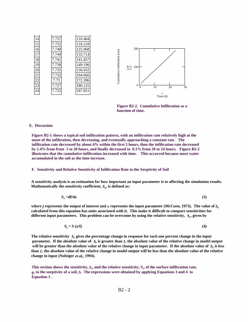
1415161718192021222324

7.7577.7527.7487.7447.7417.7387.7357.7327.737.7277.725

110.464118.218125.968133.714141.457149.196156.932164.666172.396180.125187.851

0 10 20 300

100

200

Time (h)

Cu

mu

lativ

e in

filtr

atio

n (

cm)

I( )t

t

Figure B2-2. Cumulative Infiltration as a function of time.

E. Discussion

Figure B2-1 shows a typical soil infiltration pattern, with an infiltration rate relatively high at the onset of the infiltration, then decreasing, and eventually approaching a constant rate. The infiltration rate decreased by about 4% within the first 5 hours, then the infiltration rate decreased by 1.4% from from 5 to 20 hours, and finally decreased to 0.1% from 20 to 24 hours. Figure B2-2 illustrates that the cumulative infiltration increased with time. This occurred because more water accumulated in the soil as the time increase.

F. Sensitivity and Relative Sensitivity of Infiltration Rate to the Sorptivity of Soil

A sensitivity analysis is an estimation for how important an input parameter is to affecting the simulation results. Mathematically the sensitivity coefficient, Ss, is defined as:

Ss =df/dx (3) where f represents the output of interest and x represents the input parameter (McCuen, 1973). The value of Ss calculated from this equation has units associated with it. This make it difficult to compare sensitivities for different input parameters. This problem can be overcome by using the relative sensitivity, Sr, given by

Sr = S (x/f) (4)

The relative sensitivity Sr gives the percentage change in response for each one percent change in the input parameter. If the absolute value of Sr is greater than 1, the absolute value of the relative change in model output will be greater than the absolute value of the relative change in input parameter. If the absolute value of Sr is less than 1, the absolute value of the relative change in model output will be less than the absolute value of the relative change in input (Nofziger et al., 1994).

This section shows the sensitivity, Ss, and the relative sensitivity, Sr, of the surface infiltration rate, q, to the sorptivity of a soil, S. The expressions were obtained by applying Equations 3 and 4 to Equation 1 .

B2 - 2

F.1. Input Data

t 5 S ..,0 0.1 2

F.2. Sensitivity

Ss( )S .1

2t

12 (5)

F.3. Relative Sensitivity

(6)Sr( )S

.S t

12

.S t

12 .2 A

0 1 2 30.2232

0.2234

0.2236

0.2238

0.224

Sorptivity

Sen

sitiv

ity o

f inf

iltra

tion

rate

S s( )S

S

F.4. Results

S

00.10.20.30.40.50.60.70.80.91

1.11.21.31.41.51.61.71.81.92

Ss( )S

0.2240.2240.2240.2240.2240.2240.2240.2240.2240.2240.2240.2240.2240.2240.2240.2240.2240.2240.2240.2240.224

Sr( )S

0.2.92510 3

.5.83210 3

.8.72310 3

0.0120.0140.0170.020.0230.0260.0280.0310.0340.0370.0390.0420.0450.0470.050.0530.055

Figure B2-3. Sensitivity of infiltration rate for different values of sorptivity of the soil at t = 5 h.

0 1 2 30

0.05

0.1

Soprtivity

Rel

ativ

e se

nsiti

vity

of i

nfilt

r. r

ate

S r( )S

S

Figure B2-4. Relative sensitivity of infiltration rate for different values of sorptivity of the soil at t = 5 h.

B2 - 3

F.5. Discussion

Figure B2-3 shows a sensitivity of the infiltration rate for different values of sorptivity of a soil, which has a constant value of 0.224 for all sorptivities of the soil at t = 5 h. This implies that a 10-fold increase in sorptivity will have a 2.24-fold increase in infiltration rate. Figure B2-4 shows the relative sensitivity of infiltration rate for different values of sorptivity of the soil. The relative sensitivity increased as the sorptivity of the soil increased.

B2 - 4

B3. Green-Ampt Model for Layered Systems (GALAYER )A. Description

The Green-Ampt Model has been modified to calculate water infiltration into nonuniform soils by several researchers (Bouwer, 1969; Fok, 1970; Moore, 1981; Ahuja and Ross, 1983). In this section, the Green-Ampt model for layering systems (GALAYER) developed by Flerchinger et al. (1989) was selected to calculate water infiltration over time in vertically heterogeneous soils. Two simulation scenarios were selected in the application. The first scenario was to estimate water infiltration into a soil with two layers (sand and loam), while the second scenario was to estimate the water infiltration into a soil with three layers (with sand, loam, and clay in sequence). Comparison of the two scenarios for water infiltration was also provided.


K1

1 Hydraulic conductivity (cm/h) for layer 1 (Top layer)

K2

0.5 Hydraulic conductivity (cm/h) for layer 2 (Middle layer)

K3

0.1 Hydraulic conductivity (cm/h) for layer 3 (Bottom layer)

t ..1 24 Time for infiltration (h)

∆θ n1 0.2 Change in volumetric water content as wetting front passes in last layer for Scenario 1 (cm3/cm3)

K n1 K2

Hydraulic conductivity for last layer in Scenario 1 (cm/h)

H n1 3000 Potential head (cm) as the wetting front passes last layer for Scenario 1.

n 2 Number of soil layers

Z1

10 Depth of layer 1 (cm)

Z2

10 Depth of layer 2 (cm)

∆θ n2 0.1 Change in volumetric water content as wetting front passes in last layer for Scenario 2 (cm3/cm3)

K n2 K3

Hydraulic conductivity for last layer in Scenario 2 (cm/h)

H n2 7000 Potential head (cm) as the wetting front passes last layer for Scenario 2.

Z3

10 Depth of layer 3 (cm) for scenario 2 with n=3

C. Equations and Results

a. Scenario 1

n 2

n1 n

B3 - 1

td( )t.K n1 t

.∆θ n1 H n1= 1

n 1

i

Zi

Dimensionless time since wetting front penetration. (1)

Dimensionless depth accounting for the thickness and conductivity of layers behind wetting front.

zd .K n1

H n1= 1

n 1

i

Zi

= 1

n 1

i

Zi

Ki

(2)

Dimensionless accumulated infiltration. (3)

Fd( )t .1

2td( )t .2 zd ( )td( )t .2 zd

2 .8 td( )t

fd( )tFd( )t 1

Fd( )t zd Dimensionless infiltration rate.(4)

f1( )t .fd( )t K n1 Infiltration rate. (5)

t

1

2

3

4

5

6

7

8

9

10

11

12

13

14

15

16

17

18

19

20

21

22

23

f1( )t

12.618

9.036

7.448

6.501

5.855

5.378

5.007

4.708

4.461

4.251

4.071

3.914

3.775

3.652

3.541

3.441

3.349

3.266

3.189

3.118

3.052

2.99

2.933

0 10 20 300

5

10

15

Time (h)

Infil

trat

ion

Rat

e (c

m/h

)

f1( )t

t

Figure B3-1. Water infiltration as a function of time through the layered soil profile in Scenario 1.

B3 - 2

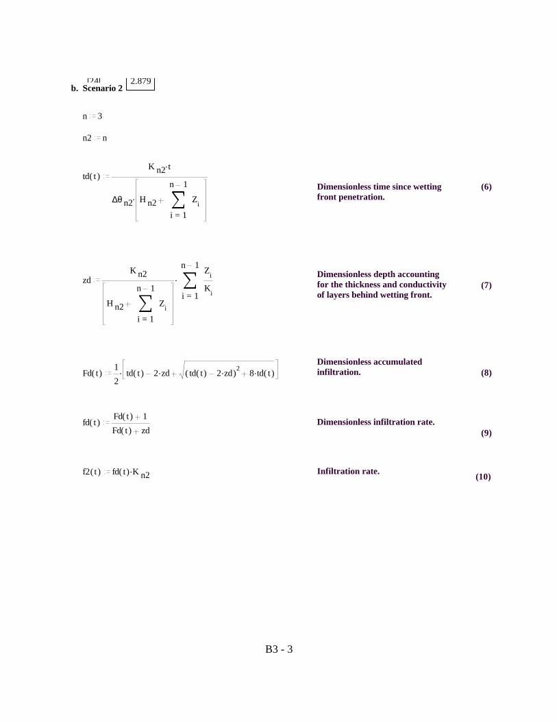
24 2.879b. Scenario 2

n 3

n2 n

td( )t.K n2 t

.∆θ n2 H n2= 1

n 1

i

Zi

Dimensionless time since wetting front penetration.

(6)


zd .K n2

H n2= 1

n 1

i

Zi

= 1

n 1

i

Zi

Ki

(7)

Dimensionless accumulated infiltration.Fd( )t .1

2td( )t .2 zd ( )td( )t .2 zd

2 .8 td( )t (8)

fd( )tFd( )t 1

Fd( )t zdDimensionless infiltration rate.

(9)

f2( )t .fd( )t K n2 Infiltration rate.(10)

B3 - 3

t

1

2

3

4

5

6

7

8

9

10

11

12

13

14

15

16

17

18

19

20

21

22

23

24

f2( )t

5.996

4.262

3.494

3.036

2.724

2.493

2.314

2.169

2.049

1.948

1.861

1.785

1.718

1.658

1.604

1.556

1.512

1.471

1.434

1.4

1.368

1.338

1.31

1.284

0 10 20 300

2

4

6

Time (h)In

filtr

atio

n R

ate

(cm

/h)

f2( )t

t

Figure B3-2. Water infiltration as a function of time through the layered soil profile in Scenario 2.

0 10 20 300

5

10

15

Time (h)

Infil

trat

ion

Rat

e (c

m/h

)

f1( )t

f2( )t

t

Figure B3-3. Comparison of water infiltration between Scenarios 1[solid line] and 2 [dash line].

E. Discussion

Water Infiltration into a two-layer soil (Scenario 1) and a three-layer soil (Scenario 2) as a function of time is given in Figures B3-1 and B3-2, respectively. These figures show that the infiltration rate is relatively high at the onset of the infiltration, then decreasing, and eventually approaching a constant rate at t > 20 h. Comparison of the two scenarios revealed that water infiltration is faster in the two-layer soil than in the three-layer soil.

B3 - 4

F. Sensitivity of Infiltration Rate to ∆Θ∆Θ

This section shows the sensitivity coefficient (Ss) and the relative sensitivity (Sr) of the surface infiltration rate to the change in volumetric water content. The expressions were obtained by applying Equations 3 and 4 in Section B2 (PHILIP2T model) to Equation 5 in this section. The input parameters were the same as in Scenario 2 except for ∆Θ ∆Θ and t as shown below.

F.1. Input Data

n 3

n2 n

∆θ n ..,0.1 0.11 0.2 t 5

F.2. Sensitivity Calculation Equations

td ∆θ n

.K n2 t

.∆θ n H n2= 1

n 1

i

Zi

Dimensionless time since wetting front penetration.

(11)


(12)zd ∆θ n

.K n2

H n2= 1

n 1

i

Zi

= 1

n 1

i

Zi

Ki

(13)Fd ∆θ n

.1

2td ∆θ n

.2 zd ∆θ n td ∆θ n.2 zd ∆θ n

2 .8 td ∆θ n

fd ∆θ n

Fd ∆θ n 1

Fd ∆θ n zd ∆θ n

(14)

f ∆θ n.fd ∆θ n K n2 (15)

B3 - 5

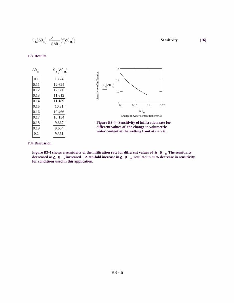
Ss ∆θ nd

d∆θ nf ∆θ n Sensitivity (16)

F.3. Results

0.1 0.15 0.2 0.258

10

12

14

Change in water content (cm3/cm3)

Sen

sitiv

ity o

f inf

iltra

tion

S s ∆θ n

∆θ n

∆θ n

0.1

0.11

0.12

0.13

0.14

0.15

0.16

0.17

0.18

0.19

0.2

Ss ∆θ n

13.24

12.624

12.086

11.612

11.189

10.81

10.466

10.154

9.867

9.604

9.361

Figure B3-4. Sensitivity of infiltration rate for different values of the change in volumetric water content at the wetting front at t = 5 h.

F.4. Discussion

Figure B3-4 shows a sensitivity of the infiltration rate for different values of ∆∆ θθ n. The sensitivity decreased as ∆∆ θθ n increased. A ten-fold increase in ∆∆ θθ n resulted in 30% decrease in sensitivity for conditions used in this application.

B3 - 6

B4. Green-Ampt Explicit Model (GAEXP) A. Description

The Green-Ampt model is the first physically-based equation describing the infiltration of water into a soil. It has been the subject of considerable developments in soil physics and hydrology owing to its simplicity and satisfactory performance for a great variety of water infiltration problems. This model yields cumulative infiltration and infiltration rate as implicit functions of time, i.e., given a value of time, t, q and I cannot be obtained by direct substitution. The equations have to be solved in an iterative manner to obtain these quantities. Therefore, the required functions are q(t) and I(t) instead of t(q) and t(I). The Green Ampt explicit model (GAEXP) for q(t) and I(t) , developed by Salvucci and Entekhabi (1994), facilitated a straight forward and accurate estimation of infiltration for any given time. This model supposedly yield less than 2% error at all times when compared to the exact values from the implicit Green-Ampt model. A scenario was chosen to simulate the water infiltration into a sandy soil under ponding conditions by using the GAEXP model. A ponding depth of 1 cm was applied at the soil surface. Input parameters and simulation results were given below.


h e 6.9 Air exit head and is equal to one half of the bubbling pressure head (cm)

λ 1.68 The exponent of the Brooks-Corey water retention model

θ s 0.43 Saturated volumetric water content (cm3/cm3)

θ 0 0.05 Initial volumetric water content (cm3/cm3)

K s 21 Saturated hydraulic conductivity (cm/h)

h s 1 Ponding depth or capillary pressure head at the surface (cm)

t ..1 24 Duration of infiltration (h)

Values given above were obtained from Carsel and Parrish (1988) for a sandy soil.

C. Equations

(1)η ( )2 .3 λ

h f.η

( )η 1h e Capillary pressure head at the wetting front (2)

χ.h s h f θ s θ 0

K s(3)

τ( )tt

( )t χ(4)

Infiltration rateq( )t ..2

2τ( )t

1

2 2

3.2

6τ( )t

1

2 .1 2

3τ( )t K s (5)

B4 - 1

I( )t ..12

3t .2

3.χ t t2 ..2 1

3χ ( )ln( )t χ ln( )χ ..2

3χ ln t

χ2

.χ t t2 lnχ2

K s (6)

Cumulative infiltration

D. Results

0 10 20 3021

22

23

Time (h)

Infil

trat

ion

rate

(cm

/h)

q( )t

t

t

123456789101112131415161718192021222324

q( )t

22.9422.0121.6821.5121.4121.3421.321.2621.2321.2121.1921.1721.1621.1521.1421.1321.1221.1221.1121.121.121.0921.0921.09

I( )t

28.0150.3872.293.79

.1.15102

.1.37102

.1.58102

.1.79102

.2 102

.2.22102

.2.43102

.2.64102

.2.85102

.3.06102

.3.28102

.3.49102

.3.7 102

.3.91102

.4.12102

.4.33102

.4.54102

.4.75102

.4.96102

.5.18102

Figure B4-1. Soil infiltration as a function of time.

0 10 20 300

200

400

600

Time (h)

Cu

mu

lativ

e in

filtr

atio

n (

cm)

I( )t

t

Figure B4-2. Cumulative Infiltration as a function of time.

E. Discussion

Figures B4-1 and B4-2 show the soil water infiltration rate and cumulative infiltration as a function of time, respectively. A rapid decrease in water infiltration rate was observed within the first 5 hours. From 5 to 24 hours, the water infiltration rate decreased gradually and finally approached a constant rate at t > 20 hours.

B4 - 2

F. Sensitivity Analysis of Infiltration Rate to Saturated hydraulic Conductivity

This section shows the sensitivity coefficient (Ss) and the relative sensitivity (Sr) of the surface infiltration rate, q, to the saturated hydraulic conductivity (Ks) at the time of 5 hours. The expressions were obtained by applying Equations 3 and 4 in Section B2 (PHILIP2T model) to Equation 5 in this section.

F.1. Input Data

K s ..,20.5 20.6 21.5 t 5

F.2. Sensitivity Calculation Equations

χ K s

.h s h f θ s θ 0

K s(7)

τ K st

t χ K s(8)

(9)q K s

..2

2τ K s

1

2 2

3.2

6τ K s

1

2 .1 2

3τ K s K s

(10)Ss K s

d

dK sq K s Sensitivity

(11)Relative Sensitivity

Sr K s.d

dK sq K s

K s

q K s

F.3.Results

20.5 21 21.5 221.0003

1.00032

1.00034

Saturated hydrualic conductivity (cm/h)

Sen

sitiv

ity o

f inf

iltra

tion

rate

S s K s

K s

K s20.520.620.720.820.921

21.121.221.321.421.5

q K s20.9121.0121.1121.2121.3121.4121.5121.6121.7121.8121.91

Ss K s1.00033541.00033221.00032911.0003261.0003231.000321.0003171.00031411.00031131.00030841.0003057

Sr K s0.980.980.980.980.980.980.980.980.980.980.98

Figure B4-3. Sensitivity of infiltration rate for different values of saturated hydraulic conductivity at t = 5 hours.

B4 - 3

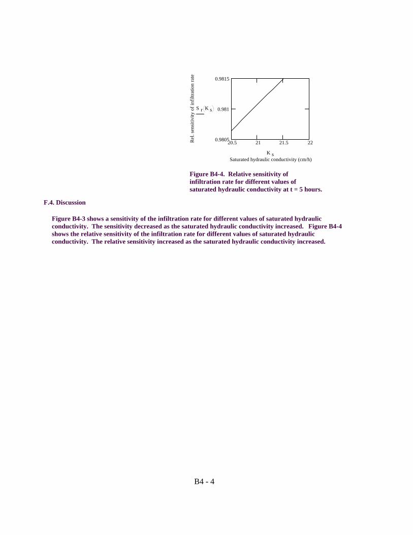
20.5 21 21.5 220.9805

0.981

0.9815

Saturated hydraulic conductivity (cm/h)

Rel

. sen

sitiv

ity o

f inf

iltra

tion

rate

S r K s

K s

Figure B4-4. Relative sensitivity of infiltration rate for different values of saturated hydraulic conductivity at t = 5 hours.

F.4. Discussion

Figure B4-3 shows a sensitivity of the infiltration rate for different values of saturated hydraulic conductivity. The sensitivity decreased as the saturated hydraulic conductivity increased. Figure B4-4 shows the relative sensitivity of the infiltration rate for different values of saturated hydraulic conductivity. The relative sensitivity increased as the saturated hydraulic conductivity increased.

B4 - 4

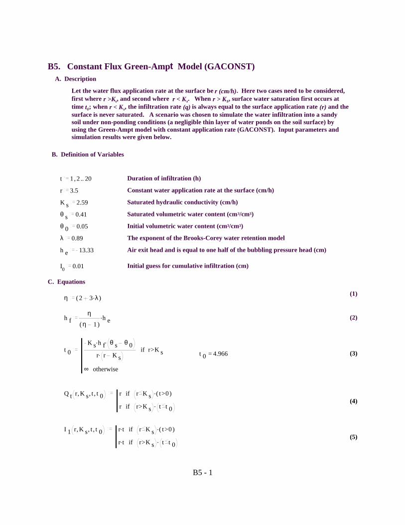
B5. Constant Flux Green-Ampt Model (GACONST) A. Description

Let the water flux application rate at the surface be r (cm/h). Here two cases need to be considered, first where r >Ks, and second where r < Ks. When r > Ks, surface water saturation first occurs at time t0; when r < Ks, the infiltration rate (q) is always equal to the surface application rate (r) and the surface is never saturated. A scenario was chosen to simulate the water infiltration into a sandy soil under non-ponding conditions (a negligible thin layer of water ponds on the soil surface) by using the Green-Ampt model with constant application rate (GACONST). Input parameters and simulation results were given below.


t ..,1 2 20 Duration of infiltration (h)

r 3.5 Constant water application rate at the surface (cm/h)

K s 2.59 Saturated hydraulic conductivity (cm/h)

θ s 0.41 Saturated volumetric water content (cm3/cm3)


λ 0.89 The exponent of the Brooks-Corey water retention model

h e 13.33 Air exit head and is equal to one half of the bubbling pressure head (cm)

I0 0.01 Initial guess for cumulative infiltration (cm)

C. Equations

(1)η ( )2 .3 λ

h f.η

( )η 1h e (2)

t 0 if..K s h f θ s θ 0

.r r K s>r K s

otherwise∞

=t 0 4.966 (3)

Q t ,,,r K s t t 0 ifr .r K s ( )>t 0

ifr .>r K s t t 0(4)

I 1 ,,,r K s t t 0 if.r t .r K s ( )>t 0

if.r t .>r K s t t 0(5)

B5 - 1

I 0 if.r t 0 >r K s

otherwise∞(6)

f 1 ,,,,K s t t 0 I I 0 I I 0..h f θ s θ 0 ln

I .θ s θ 0 h f

I 0.θ s θ 0 h f

.K s t t 0 (7)

f( ),t I root ,f 1 ,,,,K s t t 0 I I 0 I(8)

f( ),t I ifroot ,f 1 ,,,,K s t t 0 I I 0 I .>r K s t t 0

otherwiseI 1 ,,,r K s t t 0 (9)

It iff ,t It.>r K s t t 0

otherwiseI 1 ,,,r K s t t 0(10)

qt if.K s 1 .θ s θ 0

h f

f ,t It

.>r K s t t 0

otherwiseQ t ,,,r K s t t 0

(11)

0 10 202.5

3

3.5

Time (h)

Su

rfa

ce in

filtr

atio

n r

ate

(cm

/h)

qt

t

D. Results

t

1234567891011121314151617181920

qt

3.53.53.53.53.4943.3463.2433.1673.1083.063.0212.9892.9612.9372.9162.8982.8812.8672.8532.841

It3.57

10.514

17.520.91524.20727.4130.54633.62936.6739.67442.64945.59748.52451.4354.31957.19360.05362.9

Figure B5-1. Surface infiltration rate as a function of time.

0 10 200

50

100

It

t

Figure B5-2. Cumulative Infiltration as function of time.

B5 - 2

r 2.5

t 0 if..K s h f θ s θ 0

.r r K s>r K s

otherwise∞

=t 0 1 10307 (12)

Q t ,,,r K s t t 0 ifr .r K s ( )>t 0

ifr .>r K s t t 0(13)

I 1 ,,,r K s t t 0 if.r t .r K s ( )>t 0

if.r t .>r K s t t 0(14)

I 0 if.r t 0 >r K s

otherwise∞ (15)

f 1 ,,,,K s t t 0 I I 0 I I 0..h f θ s θ 0 ln

I .θ s θ 0 h f

I 0.θ s θ 0 h f

.K s t t 0 (16)

f( ),t I ifroot ,f 1 ,,,,K s t t 0 I I 0 I .>r K s t t 0

otherwiseI 1 ,,,r K s t t 0

(17)

It iff ,t It.>r K s t t 0

otherwiseI 1 ,,,r K s t t 0(18)

qt if.K s 1 .θ s θ 0h f

f ,t It

.>r K s t t 0

otherwiseQ t ,,,r K s t t 0(19)

B5 - 3

0 10 202.496

2.498

2.5

2.502

2.504

Time (h)

Su

rfa

ce in

filtr

atio

n r

ate

(cm

/h)

qt

t

t

1234567891011121314151617181920

qt

2.52.52.52.52.52.52.52.52.52.52.52.52.52.52.52.52.52.52.52.5

It2.55

7.51012.515

17.520

22.525

27.530

32.535

37.540

42.545

47.550

Figure B5-3. Surface infiltration rate as a function of time.

0 10 200

20

40

60

It

t

Figure B5-4. Cumulative Infiltration as function of time.

E. Discussion

Figure B5-1 shows a constant-flux infiltration pattern when r>Ks. Before the surface saturation first occurs at time t0 ( 5 hours), infiltration rate is constant (=r) , after that, infiltration rate decreases with time. Figure B5-3 illustrates a soil infiltration with a constant rate equal to r. Figures B5-2 and B5-4 deplict a nearly linear relationship between the cumulative infiltration and time during the infiltration period.

B5 - 4

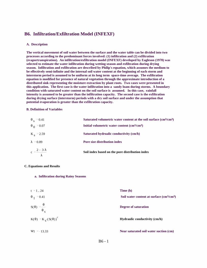
B6. Infiltration/Exfiltration Model ( INFEXF)

A. Description

The vertical movement of soil water between the surface and the water table can be divided into two processes according to the predominant forces involved: (1) infiltration and (2) exfiltration (evaportranspiration). An infiltration/exfiltration model (INFEXF) developed by Eagleson (1978) was selected to estimate the water infiltration during wetting season and exfiltration during drying season. Infiltration and exfiltration are described by Philip's equation, which assumes the medium to be effectively semi-infinite and the internal soil water content at the beginning of each storm and interstorm period is assumed to be uniform at its long term space-time average. The exfiltration equation is modified for presence of natural vegetation through the approximate introduction of a distributed sink representing the moisture extraction by plant roots. Two cases were presented in this application. The first case is the water infiltration into a sandy loam during storms. A boundary condition with saturated water content on the soil surface is assumed. In this case, rainfall intensity is assumed to be greater than the infiltration capacity. The second case is the exfiltration during drying surface (interstorm) periods with a dry soil surface and under the assumption that potential evaporation is greater than the exfiltration capacity.


θ s 0.41 Saturated volumetric water content at the soil surface (cm3/cm3)


K s 2.59 Saturated hydrualic conductivity (cm/h)

λ 0.89 Pore size distribution index

c2 .3 λ

λSoil index based on the pore distribution index

C. Equations and Results

a. Infiltration during Rainy Seasons

t ..1 24 Time (h)

θ 1 0.41 Soil water content at surface (cm3/cm3)

S( )θθ

θ s

Degree of saturation

K( )θ .K s ( )S( )θ cHydraulic conductivity (cm/h)

Ψ1 13.33 Near saturated soil water suction (cm)

B6 - 1

Soil water suction (cm) (1)Ψ( )θ .Ψ1 S( )θ

1

λ

D( )θ .K( )θ d

dθ( )Ψ( )θ Soil water diffusivity (cm2/h) (2)

Di ..5

3θ 1 θ 0

53

d

θ 0

θ 1

θ.θ θ 0

23

D( )θ Diffusivity over range θ1-θ0, (cm/h1/2) (3)

=Di 38.218

Si..2 θ 1 θ 0

Di

π

1

2Sorptivity (cm/h1/2)

(4)

fi t..1

2Si t

1

2 .1

2K θ 1 K θ 0 Infiltration rate (cm/h) (5)

=K θ 1 2.59 =K θ 0 2.427104

t

123456789101112131415161718192021222324

fi t2.4812.1341.981.8881.8251.7791.7431.7141.691.671.6531.6371.6241.6121.6011.5921.5831.5751.5671.561.5541.5481.5421.537

0 10 20 301.5

2

2.5

Time (h)

Infil

trat

ion

Rat

e (c

m/h

)

fi t

t

Figure B6-1. Water infiltration as a function of time during rainy season.

B6 - 2

b. Exfiltration During Drying Season

t ..1 24 Time (h)

θ 1 0.0001 Soil water content at dry surface (cm3/cm3)

θ 0 0.15 Initial soil water content (cm3/cm3)

Ψ1 13.33 Near saturated soil water suction (cm)

Ev 0.05 Transpiration rate (cm/h)

M 0.2 Vegetated fraction of land surface

Ψ( )θ .Ψ1 S( )θ

1

λSoil water suction (cm) (6)

D( )θ .K( )θ d

dθ( )Ψ( )θ Soil water diffusivity (cm2/h) (7)

De ..( )1.85 θ 0 θ 1( )1.85

d

θ 1

θ 0

θ.θ 0 θ 0.85D( )θ Desorption diffusivity (cm2/h) (8)

=De 0.439

Se ..2 θ 0 θ 1De

π

12

Exfiltration sorptivity (cm/h 1/2) (9)

=Se 0.112

fet..1

2Set

12 .1

2K θ 1 K θ 0

.M Ev Exfiltration rate (cm/h) (10)

t

123456789101112

fet

0.0390.0230.0160.011

.8.42710 3

.6.24510 3

.4.54910 3

.3.18210 3

.2.04910 3

.1.09110 3

B6 - 3

12131415161718192021222324

.2.66910 4

.4.5210 4

.1.08610 3

.1.65110 3

.2.15910 3

.2.61810 3

.3.03610 3

.3.41910 3

.3.77110 3

.4.09610 3

.4.39810 3

.4.67910 3

.4.94210 3

.5.18810 3

0 10 20 300.02

0

0.02

0.04

Time (h)

Exf

iltra

tion

ra

te (

cm/h

)

fet

t

Figure B6-2. Water exfiltration as a function of time during drying season.

D. Discussion

Water Infiltration into and exfiltration out of soil surface as a function of time is shown in Figures B6-1 and B6-2, respectively. Figure B6-1 shows a typical soil infiltration pattern, with an infiltration rate relatively high at the onset of the infiltration, then decreasing, and eventually approaching a constant rate. Figure B6-2 (Case 2) illustrates that exfiltration (actual evaporation) decreases with time. Nagative value of exfiltration indicates that exfiltration has ceased (at the time of 11 hours in this case) but transpiration is still going on.

B6 - 4

C - 1

APPENDIX C

Sensitivity Analysis Discussion and Demonstration

Si, j 0yi

0xj

C - 2

(C1)

Sensitivity Analysis Discussion and Demonstration

1. IntroductionSensitivity analysis should be considered an essential step to all mathematical-based

model applications. To the users of these models, the sensitivity analysis can provide a basis forgreater understanding of the processes identified in a site conceptualization. This appendix isprovided to model users as (1) an explanation of the purpose of the sensitivity analysis, (2) aworking definition of sensitivity coefficients, (3) an explanation of approaches to the sensitivityanalysis, (4) an explanation of the role of sensitivity in an parameter uncertainty analysis, and (5)a set of tools, or procedures for conducting a sensitivity analysis. As an example, a sensitivityanalysis is given for the Philip’s two-term model using a published dataset from an infiltrationexperiment. Uncertainty estimation of model outputs due to uncertain input parameters is alsoanalyzed using another set of reported field experimental data. Implications of the case studies of sensitivity analysis using these two sets of experimental data for Philip’s two-term model are alsodiscussed.

2. Purpose of Sensitivity AnalysisThe purpose of conducting a sensitivity analysis is two-fold. That is, first to evaluate

model’s response to changes in input parameters, and secondly, to quantify the likely uncertaintyof the calibrated model resulting from uncertainties associated with the input parameters,stresses, and boundary conditions (Anderson and Woessner, 1992; Zheng and Bennett, 1995). The sensitivity analysis can be used to estimate model parameters, design experiments, andanalyze ground-water management problems (Skaggs and Barry, 1996). In field sampling,sensitivity analysis can assist with the identification of parameters requiring more accuratemeasurements. This will be driven by the need to reduce overall uncertainty in the model results,as well as to identify parameters requiring less precision and thereby saving time, money andeffort in the data collection process. In the model development process, sensitivity analysis canbe utilized to determine the need for specific parameters in the final model. This would bedependent on the significance of the parameter to the model output (Hamby, 1994).

3. Sensitivity CoefficientsSensitivity (S) is a measure of the impact of change in one input parameter on an output

result. The sensitivity (S ) of the j model dependent variable (y ) to the i model inputi,j jth th

parameter (x ) is the partial derivative of the dependent variable with respect to the inputi

parameter, and is expressed as

where i is the index for i model dependent variable (i.e., model output), j is the index for jth th

S ri, j

0yi

0xj

xj

yi

Si, j 0yi

0xj

��yi

�xj

C - 3

(C2)

(C3)

model input parameter. For a model with n output variables and m input parameters, the numberof sensitivity coefficients that could be generated is given by nm. The units for S are the unitsi,j

of y over the units of x . For convenience of comparing the sensitivity coefficients of varyingi i

parameters and dependent variables, as well as comparing different models, a normalized formof the sensitivity coefficient defined in Equation C1 is utilized. The normalized form is given byEquation C2.

The normalized sensitivity, S , is referred to as the relative sensitivity of dependent variable yi,j ir

with respect to independent input parameter x . The normalized sensitivity coefficient S isj i,jr

dimensionless.

4. Approaches to Computing Sensitivity CoefficientsThree approaches for computing sensitivity coefficients are commonly recognized and

used. They are the direct, the perturbation, and the adjoint methods (Skaggs and Barry, 1996). The direct method computes the sensitivity coefficients analytically through the solving of thecoefficients’ governing equations. These equations are obtained by differentiating the governingequation and associated boundary and initial conditions with respect to model input parametersof interest. Sensitivity coefficients are calculated from the sensitivity equations using a base setof model parameters. The perturbation method, also known as the divided difference method,computes a numerical approximation to the sensitivity coefficients for the model inputparameters. The perturbation method is the simplest of the sensitivity methods and is widelyused. The adjoint method also makes use of sensitivity equations, but rather than solving themdirectly, the sensitivities are obtained by solving the adjoint problem. In the adjoint method, thefunctionals (e.g., concentration in solute transport problem), that dependent on state variables(e.g., velocity and head) and model parameters, are formulated, and the sensitivity of functionalsare computed without evaluating the sensitivities of the state variables. As a result, it can lead tocomputational savings. The details of this method can be seen in Skaggs and Barry (1996).

Complex models, for which analytical sensitivity equations are not easily derived,generally result in the need for using the perturbation method. The sensitivity coefficients arecalculated using the approximation forms (i.e., the difference equations) of Equations C1 and C2.The difference forms for these equations are given by

S ri, j

0yi

0xj

xj

yi

��yi

�xj

xj

yi

�f f(x) f(xo)(xxo)

1!fx(xo)�

(xxo)sup2

2!fxx(xo)� ...�

(xxo)n

n!f(n)(xo)�Rn(xo)

y f(x)

C - 4

(C4)

(C5)

(C6)

and

where �y is the change of y due to an infinitesimal change (�x ) in x .i i j j

In addition to these three methods of calculating sensitivity coefficients, other approachesare also used based on differing needs and objectives. Furthermore, the reader must be awarethat slightly different definitions of “sensitivity coefficients” could be defined in literature. Inthis regard, Hamby (1994, 1995) has provided a detailed review and evaluation of more than tensensitivity methods.

5. Role of Sensitivity in Uncertainty AnalysisTo examine the deviation of model output (�f) due to the deviation (x-x ) of inputo

parameters, the Taylor’s formula can be used

where f(x ) is the function value in the neighborhood of a point x=x ; f (x ), f (x ), f (x ), are theo o x o xx o (n) o

first, second, and n derivatives of f(x) with respect to x at x=x , and R (x ) is the remainder.tho n o

Here f (x ) is the sensitivity coefficient as defined in Equation C1 and evaluated at x=x . Whenx o o

high-order terms are ignored, �f is approximated by the first term, (x-x )·f, in Equation C5. Ino x

other words, the deviation of the model output (�f) can be approximated by the product ofdeviation of input parameter (x-x ) and sensitivity (f =S )o x i,j

Equation C5 is useful for the analysis of a single set of input parameters (i.e., only onerealization). The common way to quantify uncertainty is to treat the input parameters as randomvariables. For examining model uncertainty (in terms of variance or covariance) due to uncertaininput parameters, the First-Order Second-Moment (FOSM) technique can be used. It provides amethod of calculating the mean, variance, and covariance of model outputs from means,variances, covariance and sensitivity coefficients for the model inputs. The following equationsare used to determine these quantities (Dettinger and Wilson, 1981).

my f(mx) �

120

2f

0x 2var(x)

cov(y) Si,j cov(x)[Si,j]T

C - 5

(C7)

(C8)

where the variables are defined as follows:

n is the number of model outputs,k is the number of model input parameters,y is a (n x 1) vector of model outputs,f(x) is the (n x 1) vector of model outputs with inputs of x, x is a (k x 1) vector of modelparameters,m is a (n x 1) vector of mean model outputs,y

f(m ) is a (n x 1) vector of model outputs where the model is evaluated at m ,x x

m is a (k x 1) vector of mean parameter values,x

0 f/0x is a (n x k) matrix of 2 partial derivatives of f(m ),2 2 ndx

cov(x) is a (k x k) covariance matrix of the input parameters,cov(y) is a (n x n) covariance matrix of model outputs,var(x) is a (k x 1) vector of variances of parameters, andS is a (n x k) matrix of sensitivity coefficients of model outputs to input parameters. Thei,j

First-Order Second-Moment analysis is most appropriate when the model is not too nonlinearwith respect to its input parameters, and the coefficients of variation for the parameters are small. When the model is highly nonlinear, or the model is so complex that sensitivity coefficients arenot easily obtained, a Monte Carlo method could be used. The methodology of conductinguncertainty analysis using the Monte Carlo method for transport models can be seen in Nofzigeret al., (1993). Using Equations C6 through C8, uncertainty of model outputs, cov(y), can beobtained when uncertainty of input parameters, cov(x), and sensitivity coefficients of modeloutputs to input parameters, S , are known. i,j

6. Procedures for Sensitivity AnalysisAn optimal set of input parameters for the problem of interest should be identified before

the sensitivity analysis is conducted. This set of input parameters is referred to as the base set. The basic procedures for the sensitivity analysis are outlined as follows:

1. Gathering of input parameters: When site-specific input parameters are not available,the base set of parameters could be obtained either from indirect estimation usingother data at the site (e.g., to estimate conductivity using soil texture data) or from the

C - 6

“best justified” mean values of published data which are “appropriate” for the siteconditions. When experimental data are available, calibration of the model to obtainan optimal set of input parameters (i.e., base set) should be performed first beforesensitivity analysis.

2. After an optimal set of parameters has been identified, sensitivity analysis isperformed to quantify the sensitivity of the model results with respect to modelparameters. It is typically performed by changing one parameter at a time whilekeeping the rest constant. By changing the parameter over a range (e.g., above andbelow a certain percent or standard deviation of the base set value), the responses ofmodel output to input parameters can be examined. The results are usually presentedby a) presenting the model outputs for several values of input parameters; b) plotting(absolute or relative) sensitivity coefficients versus input parameters; and c) providingthe ranking descriptors, such as high, medium, and low.

If the sensitivity results show that the model results are highly sensitive to a particularparameter, the uncertainty associated with that parameter will significantly affect the ability ofthe model to make meaningful interpretations and predictions. This is specifically true when thatparameter exhibits great spatial variability in the field, and/or great uncertainty due toexperimental measurement/estimation of parameters. On the other hand, if the model results arenot sensitive to a given parameter, the uncertainty in that parameter will have little impact on themodel’s interpretative or predictive capabilities and that parameter might be eliminated.

7. Case StudiesIn this section, two sets of infiltration experimental data are used for performing

sensitivity analysis with the Philip’s two-term infiltration model. The model outputs arecumulative infiltration (I) and infiltration rate (q). The model input parameters are sorptivity (s)and a constant, A, that depends on the soil properties, saturated water content and initial watercontent.

Data Set 1: The experimental data for infiltration into the Grenoble sand of Barry et al., (1995) isused for illustration of model calibration and performing sensitivity analysis. The infiltrationexperiment was conducted on a vertical, ponding column (93.5 cm in length and 6 cm indiameter) filled with air-dried, graded Grenoble sand. The reported cumulative infiltration (I) isshown in Figure C1a. From cumulative infiltration data, infiltration rates are calculated from theinfiltration data (Figure C1a) and presented in Figure C1b. The experimental conditions andhydraulic properties of the Grennoble sand is given in Table C1.

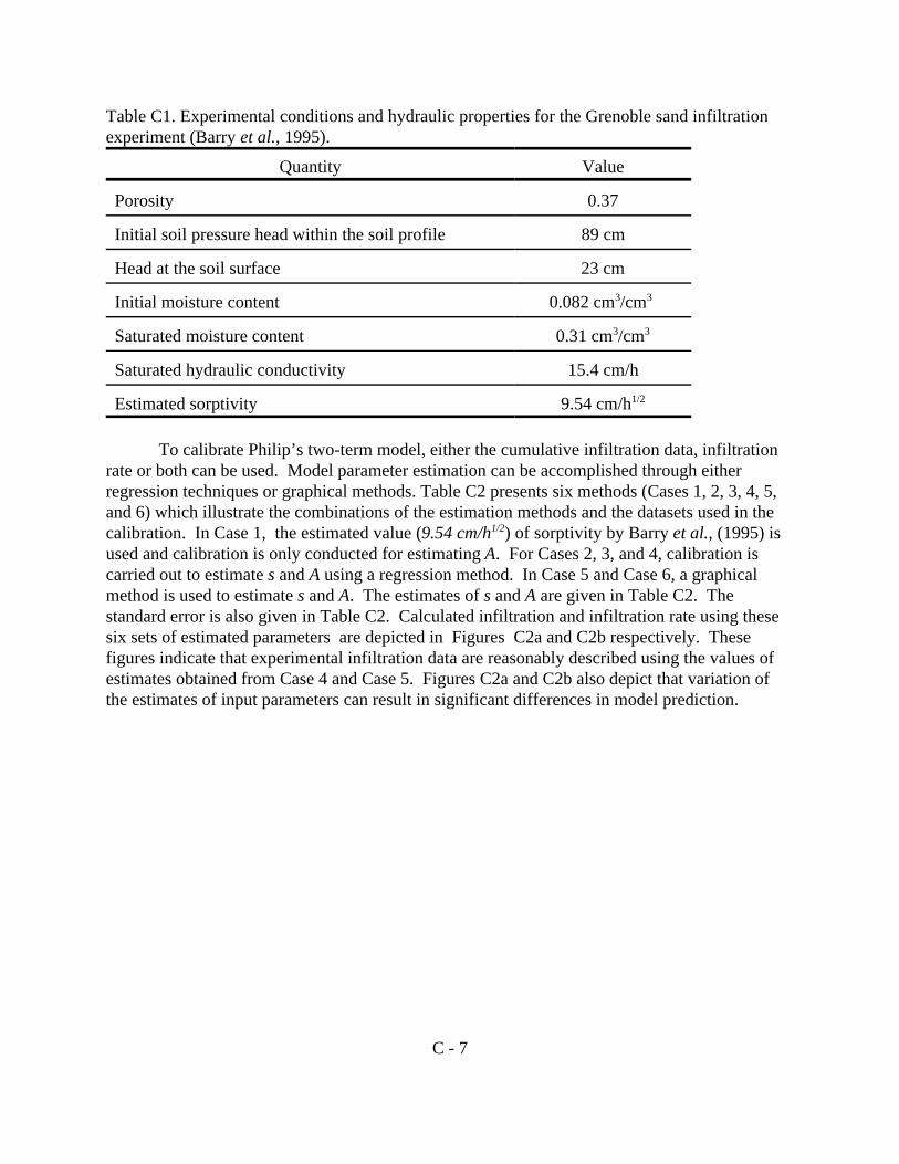
C - 7

Table C1. Experimental conditions and hydraulic properties for the Grenoble sand infiltrationexperiment (Barry et al., 1995).

Quantity Value

Porosity 0.37

Initial soil pressure head within the soil profile 89 cm

Head at the soil surface 23 cm

Initial moisture content 0.082 cm /cm 3 3

Saturated moisture content 0.31 cm /cm3 3

Saturated hydraulic conductivity 15.4 cm/h

Estimated sorptivity 9.54 cm/h1/2

To calibrate Philip’s two-term model, either the cumulative infiltration data, infiltrationrate or both can be used. Model parameter estimation can be accomplished through eitherregression techniques or graphical methods. Table C2 presents six methods (Cases 1, 2, 3, 4, 5,and 6) which illustrate the combinations of the estimation methods and the datasets used in thecalibration. In Case 1, the estimated value (9.54 cm/h ) of sorptivity by Barry et al., (1995) is1/2

used and calibration is only conducted for estimating A. For Cases 2, 3, and 4, calibration iscarried out to estimate s and A using a regression method. In Case 5 and Case 6, a graphicalmethod is used to estimate s and A. The estimates of s and A are given in Table C2. Thestandard error is also given in Table C2. Calculated infiltration and infiltration rate using thesesix sets of estimated parameters are depicted in Figures C2a and C2b respectively. Thesefigures indicate that experimental infiltration data are reasonably described using the values ofestimates obtained from Case 4 and Case 5. Figures C2a and C2b also depict that variation ofthe estimates of input parameters can result in significant differences in model prediction.

C - 8

Table C2. Calibration of Philip’s two-term model parameters using the experimental infiltrationdata of Barry et al., (1995).

Case s, (cm/h ) A, (cm/h )1/2 2

Case 1: Reported sorptivity of 9.54 cm/h1/2

(Barry et al., 1995) is used. Calibration isperformed on A only using cumulativeinfiltration data.

[9.54] 10.62±0.08†

Case 2: Calibration is performed on both s andA using cumulative infiltration data.

8.92±0.19 11.78±0.36 † †

Case 3: Calibration is performed on both s andA using infiltration rate data.

12.65±1.19 7.35±2.13† †

Case 4: Calibration is performed on both s andA using both cumulative infiltration and 11.17±0.99 8.13±1.74 infiltration rate data.

† †

Case 5: Graphical estimation of s and A fromthe plot of I(t)/t versus t .-½ 11.0±0.46 9.00±0.15† †

Case 6: Graphical estimation of s from the plotof q(t) versus t .-½ 8.0±0.41 --†

†.. Estimated value ±Standard error

Figures C2a and C2b also indicate that using the estimates of s and A of Case 4 and Case5 provides better fits of both the observed cumulative infiltration and infiltration rate data thanusing those estimates from Case 1, 2, 3, and 6. From this evaluation, the estimates of either Case4 or Case 5 can be chosen as the optimal set. However, the estimates of s and A obtained fromCase 4 is arbitrarily selected as an optimal set (i.e., the base set).

To compute sensitivity and relative sensitivity, the direct method is selected for thisexample due to its simplicity. The sensitivity and relative sensitivities equations are given inTable C3. Table C3 gives the analytically derived sensitivities for infiltration rate, q(t), andcumulative infiltration, I(t), with respect to sorptivity (s) and the constant term (A). Note that thesensitivities of I(t) with respect to s (or A) and q(t) with respect to s (or A) are independent with s(or A). In other words, the sensitivities are constant at given particular time over the whole rangeof s (or A). However, sensitivities vary with time for Philip’s two-term model.

q(t)

12

st

12�A

I(t) st12�At

12

t

12

s

s�2A t

2A t

st�2A t

t12

s t

s t�At

A t

s t�At

C - 9

Table C3. Sensitivity and relative sensitivity of infiltration rate, q(t), and cumulation infiltration,I(t) with respect to sorptivity, s and soil-dependent constant, A, of Philip’s two-term model.

Model Output Sensitivity Output withInput Sensitivity

Parameter Si,j

Relative Derivatives of

S respect to inputi,jr

Second

Parameter

s 0

A 1 0

s 0

A t 0

Using the identified base set of estimates, sensitivity analysis is conducted and presentedin the following four areas.

1. Examining the time changes of infiltration by changing one parameter while keeping the rest of parameters fixed (Figures C3a and C3b);

2. Examining sensitivity changes of infiltration with respect to s or A over a range ofinput parameter at different time periods, t. The range of input parameter is presentedin terms of relative ratios of that parameter to the base value (Figures C4a and C4b);

3. Examining time changes of sensitivities of infiltration with respect to s or A over timeusing 60%, 100%, and 140% of base values of input parameters (Figures C4c andC4d); and

4. Examining the changes of relative sensitivities over a range of one particularparameter at different time periods (Figures C5a and C5b).

The results indicate:1. sensitivities of infiltration with respect to s (or A) are constant over a range of 60% to

140 % of s (or A) at any given time (Figures C4a and C4b);2. sensitivities of infiltration with respect to s (or A) vary with time but they are

independent of s (or A) (Figures C4c and C4d);3. Relative sensitivities of infiltration with respect to sorptivity, s, are greater than those

with respect to constant A (Figures C5a and C5b).

�I I(s,A) I(so,Ao)(sso)

1!Is(so,Ao)�

(sso)2

2!Iss(so)� (sso)(AAo)IsA(so,Ao)

�

(AAo)

1!IA(so,Ao)�

(AAo)2

2!IAA(so,Ao)�R3(so,Ao)

�I I(s,A) I(so,Ao) Is(so,Ao)(sso)� IA(so,Ao)(AAo)

C - 10

(C9)

(C10)

4. Similar results (not shown) are obtained for sensitivities of infiltration rate withrespect to s and A.

The results of sensitivities shown in Figures C4a, C4b, C5a, and C5b, indicate that s isthe most sensitive parameter in Philip’s two-term model for the range of input parametersexamined. Similar results are also observed for infiltration rates (not shown).

To examine the impact of deviation of the estimates of input parameters, s and A from thevalues of the base set on the deviation of infiltration, Taylor’s formula (Equation C5) is appliedto Philip’s two-term infiltration model. Taking up to second-order terms, deviation (difference)of infiltration (�I) is expressed as

where• I (s ,A ), I (s ,A ) are the first, and second derivatives of I(s,A) with respect to s at s=ss o o ss o o o

and A=A respectively; o

• I (s ,A ), I (s ,A ) are the first, and second derivatives of I(s,A) with respect to A atA o o AA o o

s=s and A=A respectively;o o

• I (s ,A ) is the partial derivative of I(s,A) with respect to s and A; andsA o o

• R (s ,A ) is the remainder for the terms in the order of 3 and up. 3 o o

Here, I (s ,A ) and I (s ,A ) are the sensitivity coefficients of I(t) with respect to s, and As o o A o o

respectively. It is worth noting that analytical values of I , I and I and higher-orderss AA sA

derivatives are zeros (Table C3). Accordingly, the deviation (�I) of I(s,A) from I(s ,A ), (I(s,A)-o o

I(s ,A )) is given byo o

Equation C10 states that deviation of I(s,A) from I(s ,A ) can be estimated from the sum of theo o

products of sensitivity and deviation of a parameter value from its base value.

Assuming s and A are the optimal values (Case 4 in Table C2) for s and A in Philip’so o

two-term model, there is interest in how the sensitivities of I with respect to s and A will impactthe prediction of infiltration. Taking Case 5 (e.g., using the graphical method to estimate s and Afrom infiltration data) as an example, deviation (difference) of predicted infiltration, due toestimated s and A, from using the optimal data set is shown in Figure C6. The differencesbetween predicted infiltration are approximately equal to the sum of the products of sensitivity

C - 11

and the difference between estimated and optimal values. Figure C6 indicates that: (a)contribution of deviation of infiltration due to deviation of the constant A term (i.e., the secondterm on the right-hand-side of Equation C10, I #(A-A )) is greater than contribution of deviationA o

of infiltration due to deviation of sorptivity (i.e., the first term on the right-hand-side of equation,I #(s-s )) and (b) the difference of predicted infiltration (maximum value is around 0.1 cm) iss o

negligible compared to the magnitudes of infiltration during the first 0.4 hours (Figures C6 andFigure C2a). It is worth noting that the difference of predicted infiltration is dependent onsensitivities as well as the deviation of input parameters from base set values.

8. Uncertainty Analysis using Sensitivity ResultsAfter obtaining sensitivity coefficients of input parameters, uncertainty of model outputs

due to uncertainty of input parameters can be quantified using Equation C8. Here uncertainty isexpressed in terms of variance (or covariance) which is the expected value of the square of thedifference between a random variable and its mean (e.g., Variance of sorptivity is E((s- *s) ). Here 2

*s is the mean of sorptivity.). To demonstrate quantifying uncertainty of predicted infiltration dueto uncertainty of input parameters (s and A), another set of reported experimental data is used.

Data Set #2: A set of field measurement data for sorptivity (s) and conductivity at the surface(K ) in a field study using disk permeameters had been reported by Lien (1989). Fieldo

measurements of infiltration were conducted at four locations in a field of about 35 hectares. Thedominant soils in the field are Casa Grande - Trix fine loamy soils. The Cassel ring and the discpermeameters at a 2 cm positive head, and the 10 cm and the 5 cm tension disc permeameterswere used. For this case study, values of K were used to estimate constant A (A=0.363 K)o o

(Philip, 1974). The reported values and their statistics of sorptivity (s) and the calculated valuesof A are given in Table C4. Note that this data set includes uncertainty due to spatial variabilityas well as differences among the measurement methods.

C - 12

Table C4. Statistics of parameters used in FOSM uncertainty analysis for Casa Grande/Trix fine-loamy soils .

Sorptivity, s Constant, A

Mean 4.03 2.38

Coefficient of Variance 0.93 1.16

log Mean 1.08 0.44†

log Coefficient of Variance 0.73 2.11†

Correlation Matrix

log (s) log (A)

log (s) 1.00

log (A) 0.69 1.00

Natural logarithm; The sample size is 16.†

The infiltration phenomena is examined during the first hour infiltration period. Themeans of sorptivity and the constant A (Table C4), second derivatives (all zeros for the two-termmodel, Table C3), and variances are used to calculate the means of infiltration (*I) and infiltrationrates (*q) (Equation C7). The sensitivity coefficients and covariances for s and A (Table C4) areused to calculate covariances (cov(I) and cov(q)) of infiltration (I) and infiltration rates (q) usingEquation C8. The means of infiltration, 97.5% confidence values are given in Figures C7a andC7b. Here, 97.5% confidence values for infiltration are obtained as (*I±�#) ) and (*q ±�#) )I q

respectively. Here �’s are confidence coefficient (±1.96) at 97.5% confidence percentiles. ) andi

) are standard deviations (square root of variance) for infiltration (I) and infiltration rate (q)q

respectively. Since sorptivity, the constant A, the predicted infiltration and infiltration ratesfollow log-normal distributions, calculation is performed using the log-transformed values for s,A, I and q. The First-Order Second-Moment (FOSM) technique used is simple and straightforward. For comparison, the Monte Carlo technique is also used to quantify uncertainty ofinfiltration. The results are shown in Figures C7a and C7b. It indicates that great variability ofinfiltration exists due to the uncertainty of parameter measurement and their spatial variabilitiesin the field. Figures C7a and C7b also show that both FOSM and Monte Carlo approaches givevery close results for uncertainty estimation.

var(I) I 2s var(s)� I 2

A var(A)� IsAcov(s,A)

C - 13

(C11)

Table C5. Statistics of parameters used in FOSM uncertainty analysis for Grenoble sand.

Sorptivity, s Constant, A

Mean 10.2 9.38

Coefficient of Variance 0.169 0.167

Correlation Matrix

s A

s 1.00

A 1.00-0.69

Remark: The sample size is 6.

To examine the impact of uncertainty of estimates using different methods on predictedinfiltration, the same procedures are repeated for Grenoble sand except normal distributions areused for the input parameters, s and A, and output parameters, I and q. The estimates of s and Aobtained from different parameterization methods (Cases 1, 2, 3, 4, 5 and 6 in Table C2) arefound to be better described by the normal distribution. The statistics of these estimates aregiven in Table C5. As a result, predicted values of I and q form normal distributions. Uncertainty results for Grenoble sand are shown in Figures C8a and C8b. It indicates that

a) The predicted infiltration and infiltration rates satisfactorily described the observeddata using estimates of s and A. Although differences exist due to different parametermethods, prediction of infiltration using any set of estimates in Table C2 arereasonably good and the predicted values are fallen within the 95% confidenceintervals (Figures C2a, C2b, C8a, and C8b).

b) Uncertainty of predicted infiltration using data set #2 is much greater than using dataset #1 since data set #2 possess greater uncertainty in measured values of s and A.

Furthermore, sensitivity results are also used to examine predicted uncertainty ofinfiltration due to uncertainty of estimates of input parameters. Contribution of uncertainty ofpredicted infiltration is quantified by using Equation C8. Expanding Equation C8 for infiltration(I), we can describe uncertainty of I as follows

where var(s) and var(A) are variances of s and A respectively, and cov(s,A) are covariances of sand A. The term, var(I), in the left-hand side of Equation C11 represents uncertainty of predictedinfiltration due to uncertainty of s and A. The term I #var(s) represents the contribution resultings

2

C - 14

from s. The term I #var(A) represents the amount of contribution resulted from A. The term IA sA2

#cov(s,A) represents the amount of contribution resulted from both s and A. The case study isgiven for the Casa Grande - Trix fine-loamy soils using data set #2. The results are shown inFigure C9a. It indicates that contribution of uncertainty of predicted infiltration due to sorptivityis much greater than that due to the constant A. The similar results are also found for infiltrationrate particularly in the earlier infiltration time period (t < 0.4h, Figure C9b). In this case, infiltration is more sensitive to s than to A and variability of s is greater than variability of A. As

the result, the model parameter s is more important than the constant A.

9. ImplicationsIn Philip’s two term model, the first term (Equation C3) represents the contribution of the

influence of the matric suction, and the second term. represents the contribution of the influenceof gravity (Philip, 1969). The analysis has illustrated that

a) Infiltration rate dramatically decreases with time and gradually reaches a constantvalue. In other words, matric suction (sorptivity) will mostly contribute to infiltrationat the early stage. On the other hand, gravity (the constant A) increasingly contributesmore to infiltration at later stage. This phenomena is clearly observed from the resultsof the sensitivity/uncertainty analysis.

b) For Grenoble sand, uncertainty of infiltration due to uncertainty of sorptivity is abouttwo thirds or greater of overall total uncertainty of predicted infiltration during thefirst hour of infiltration (Figure C9). Therefore, more effort to accurately measuresorptivity is needed to reduce uncertainty of the predicted infiltration.

c) The estimates of input parameters using different estimation methods (Table C2) canbe used to provide reasonable prediction on infiltration. Using the mean values of theestimates would be appropriate for uncertainty analysis since these estimates obtainedfrom different parameterization methods follow normal distributions (Figures C8a,and C8b).

10. SummaryThe procedures of conducting sensitivity analysis are illustrated using two sets of reported

experimental data for Philip’s two-term model. Sensitivity results are used to quantifyuncertainty of model prediction due to uncertainty of input parameters. The results indicate thatsorptivity is the most sensitive and important input parameter to predicted infiltration andinfiltration rate; and uncertainty of sorptivity contributes significantly to uncertainty of predictedinfiltration at the early stage of infiltration.

C - 15

ReferencesAnderson, M.P., and W.W. Woessner. 1992. Applied groundwater modeling -- Simulation of

flow and advective transport. Academic Press Inc., New York.

Barry, D.A., J.-Y. Parlange, R. Haverkamp, and P.J. Ross. 1995. Infiltration under pondedconditions: 4. An explicit predictive infiltration formula. Soil Sci. 160:8-17.

Dettinger, M.D., and J.L. Wilson. 1981. First order analysis of uncertainty in numerical modelsof groundwater. Part 1. Mathematical development. Water Resour. Res. 17:149-161.

Hamby, D.M. 1994. A review of techniques for parameter sensitivity analysis of environmentalmodels. Environmental Monitoring and Assessment. 31:135-154.

Hamby, D.M. 1995. A numerical comparison of sensitivity analysis techniques. Health Phys.68:195-204.

Lien, B.K. 1989. Field measurement of soil sorptivity and hydraulic conductivity, M.S. thesis,Univ. of Ariz., Tucson.

Nofziger, D.L., J.-S. Chen, and C.T. Haan. 1993. Evaluation of unsaturated/vadose zone modelsfor superfund sites. EPA/600/R-93/184. Robert S. Kerr Environmental ResearchLaboratory, Ada, OK.

Philip, J.R. 1974. Recent progress in the solution of nonlinear diffusion equations. Soil. Sci.116:257-264.

Philip, J.R. 1969. Theory of infiltration. Adv. Hydrosci. 5:215-290.

Skaggs, T.H., and D.A. Barry. 1996. Sensitivity methods for time-continuous, spatially discretegroundwater contaminant transport models. Water Resourc. Res. 32:2409-2420.

Zheng, C., and G.D. Bennett. 1995. Applied contaminant transport modeling: theory andpractice. Van Nostrand Reinhold, New York.

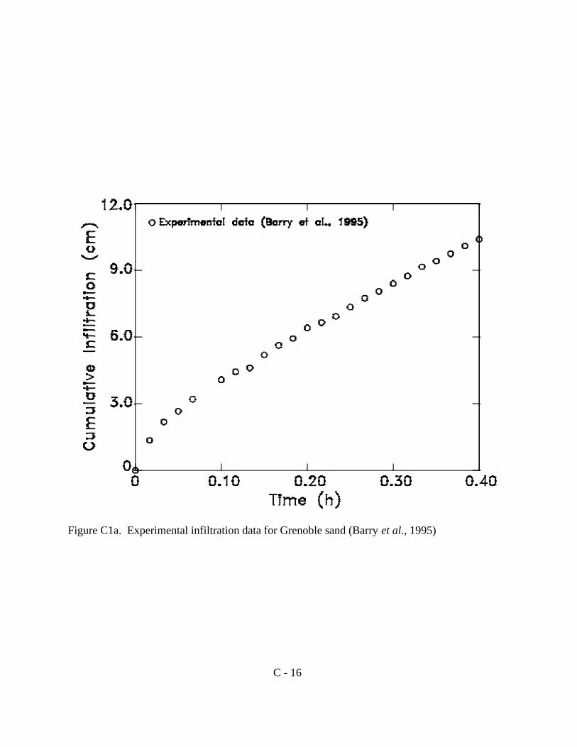
C - 16

Figure C1a. Experimental infiltration data for Grenoble sand (Barry et al., 1995)

C - 17

Figure C1b. Calculated infiltration rates from the experimental infiltration data for Grenoblesand (Barry et al., 1995).

C - 18

Figure C2a. Prediction of infiltration in Grenoble sand using the calibrated input parameters inPhilip’s two-term model.

C - 19

Figure C2b. Prediction of infiltration rates in Grenoble sand using the calibrated inputparameters in Philip’s two-term model.

C - 20

Figure C3a. Sensitivity of infiltration with respect to sorptivity (s) in Grenoble sand for Philip’stwo-term model.

C - 21

Figure C3b. Sensitivity of infiltration with respect to the constant A in Grenoble sand forPhilip’s two-term model.

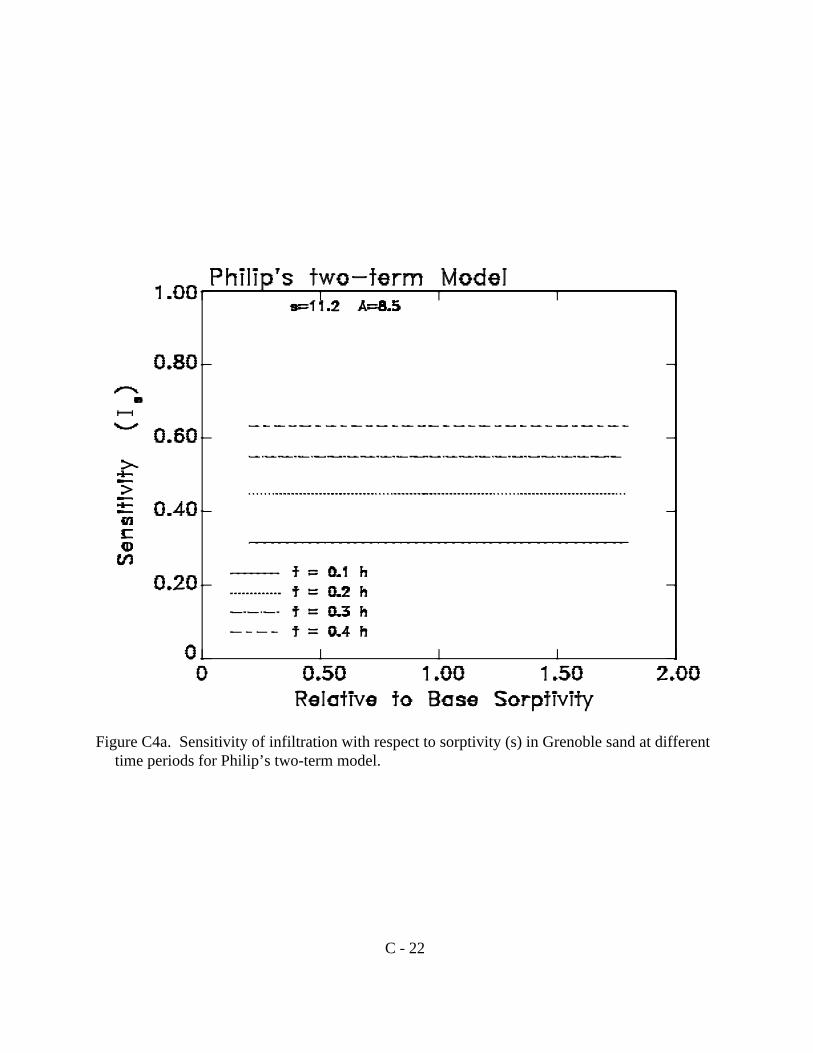
C - 22

Figure C4a. Sensitivity of infiltration with respect to sorptivity (s) in Grenoble sand at differenttime periods for Philip’s two-term model.

C - 23

Figure C4b. Sensitivity of infiltration with respect to constant A in Grenoble sand at differenttime periods for Philip’s two-term model.

C - 24

Figure C4c. Sensitivities of infiltration with respect to sorptivity (s) vary with time for 60%,100%, and 140% of base values of s in Grenoble sand. Note that time curves (solid and dashlines) are coincident each other.

C - 25

Figure C4d. Sensitivity of infiltration with respect to constant A vary with time for 60%, 100%,and 140% of base values of A in Grenoble sand. Note that time curves (solid and dash lines)are coincident each other.

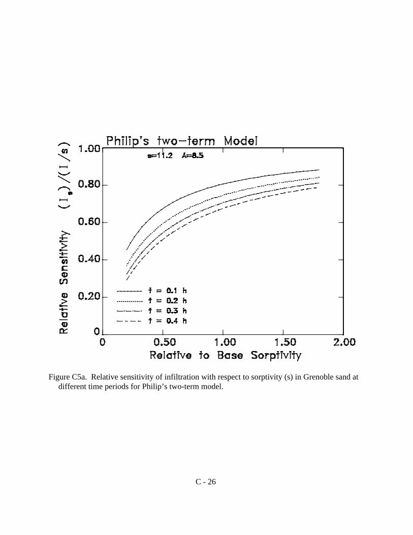
C - 26

Figure C5a. Relative sensitivity of infiltration with respect to sorptivity (s) in Grenoble sand atdifferent time periods for Philip’s two-term model.

C - 27

Figure C5b. Relative sensitivity of infiltration with respect to constant A in Grenoble sand atdifferent time periods for Philip’s two-term model.

C - 28

Figure C6. Deviation (difference) of predicted infiltration as the results of contribution fromdeviation of the values of input parameters from base values.

C - 29

Figure C7a. Uncertainty of infiltration due to uncertainty of input parameters in Casa Grande-Trix fine-loamy soils. The mean predicted infiltration (solid line) as well as 95% confidencelimits are shown.

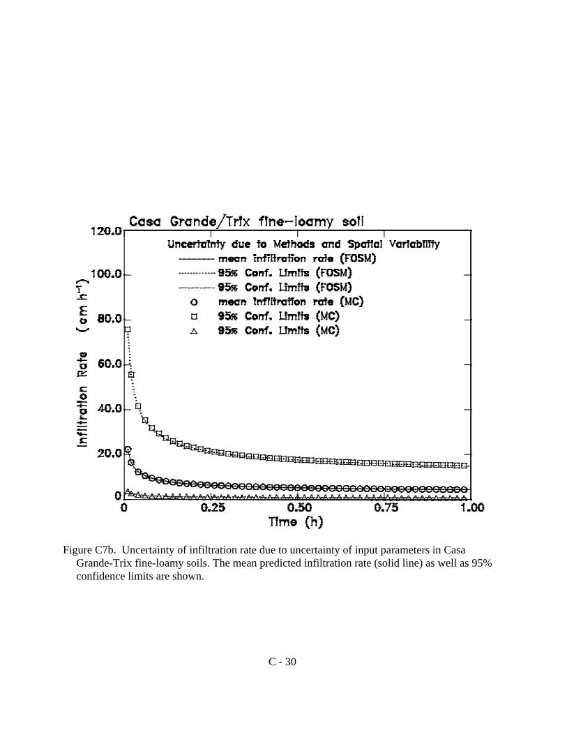
C - 30

Figure C7b. Uncertainty of infiltration rate due to uncertainty of input parameters in CasaGrande-Trix fine-loamy soils. The mean predicted infiltration rate (solid line) as well as 95%confidence limits are shown.

C - 31

Figure C8a. Uncertainty of infiltration due to uncertainty of input parameters in Grenoble sand.The mean predicted infiltration (solid line) as well as 95% confidence limits are shown.

C - 32

Figure C8b. Uncertainty of infiltration rate due to uncertainty of input parameters in Grenoblesand. The mean predicted infiltration rate (solid line) as well as 95% of confidence limits areshown.

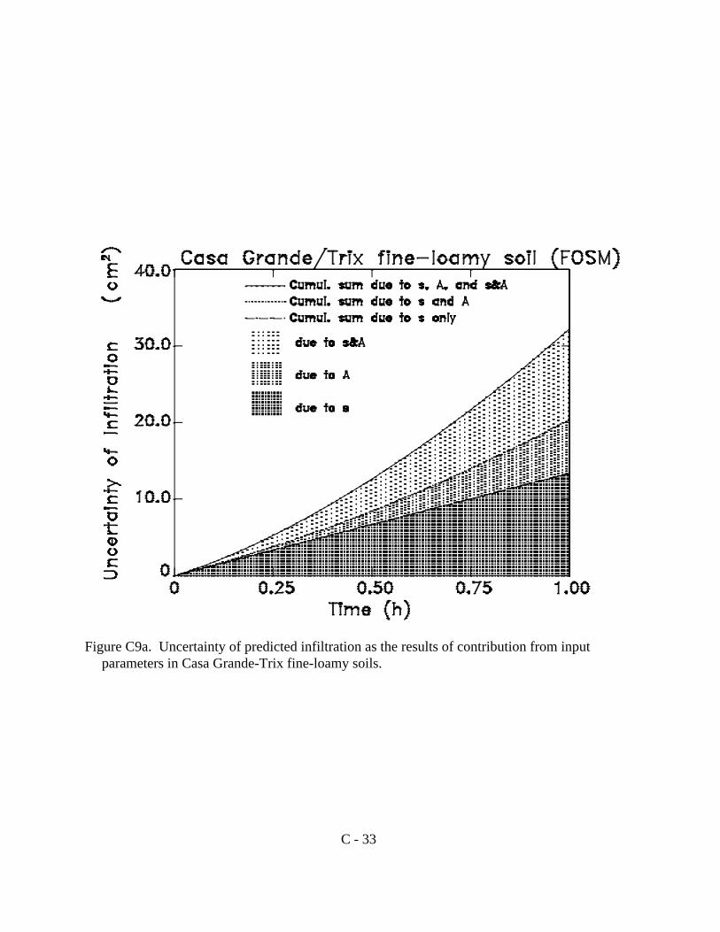
C - 33

Figure C9a. Uncertainty of predicted infiltration as the results of contribution from inputparameters in Casa Grande-Trix fine-loamy soils.

C - 34

Figure C9b. Uncertainty of predicted infiltration rate as the results of contribution from inputparameters in Casa Grande-Trix fine-loamy soils.

United States Environmental Protection Agency · PDF fileApplication of Selected Mathematical...

Documents

Transcript of United States Environmental Protection Agency · PDF fileApplication of Selected Mathematical...