Unit-V DSP
56
Unit-V DSP APPLICATIONS
-
Upload
shanmugachitra -
Category
Documents
-
view
278 -
download
4
description
DSP applications
Transcript of Unit-V DSP

Unit-V
DSP APPLICATIONS
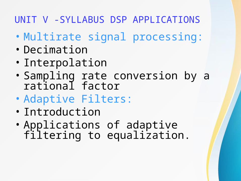
UNIT V -SYLLABUS DSP APPLICATIONS
• Multirate signal processing: • Decimation• Interpolation• Sampling rate conversion by a rational
factor • Adaptive Filters: • Introduction• Applications of adaptive filtering to
equalization.
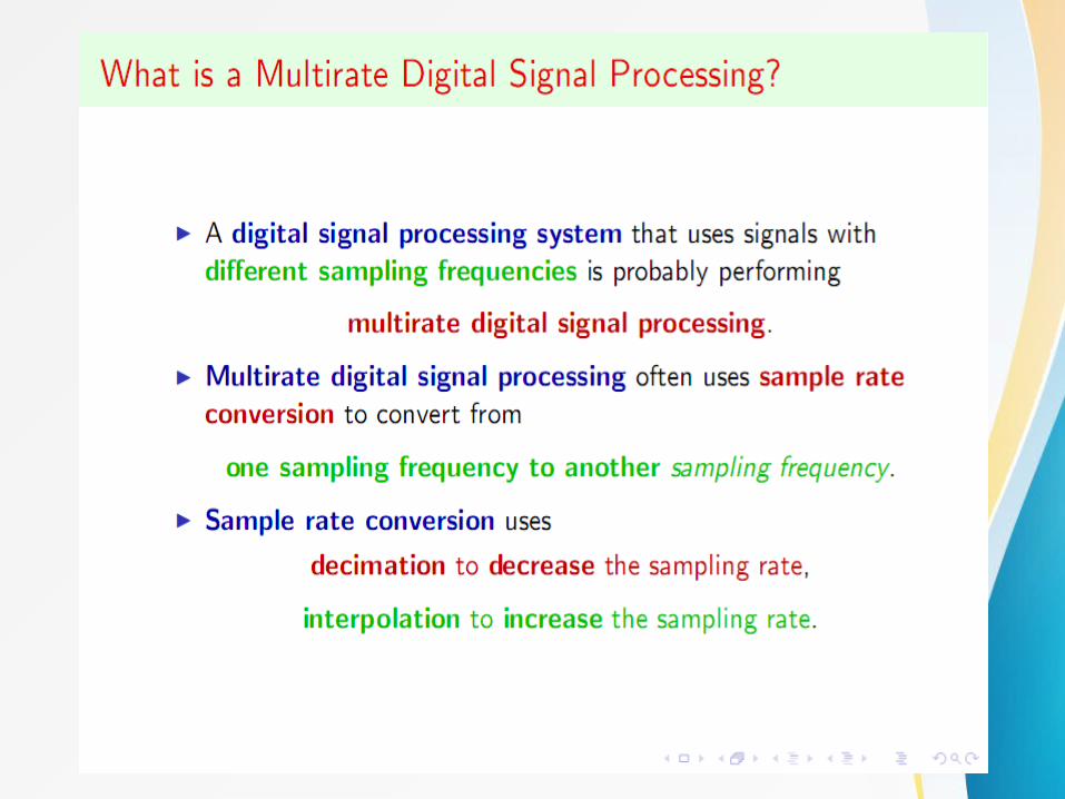
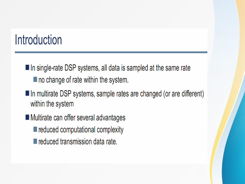


Multirate Digital Signal ProcessingMultirate Digital Signal Processing
Basic Sampling Rate Alteration DevicesBasic Sampling Rate Alteration Devices
• Up-samplerUp-sampler - Used to increase the sampling rate by an integer factor
• Down-samplerDown-sampler - Used to decrease the sampling rate by an integer factor


DECIMATION

DECIMATION
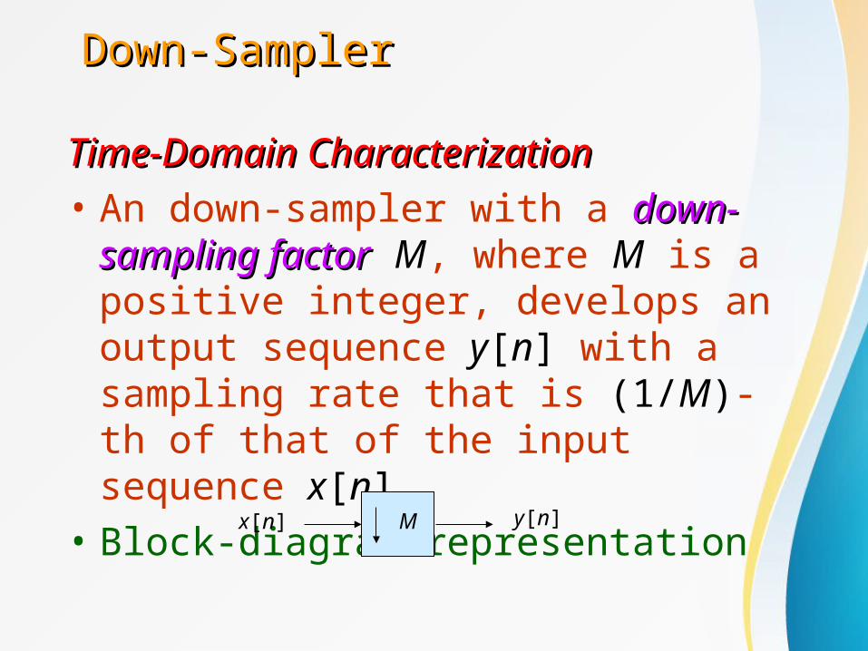
Down-SamplerDown-Sampler
Time-Domain CharacterizationTime-Domain Characterization
• An down-sampler with a down-sampling down-sampling factorfactor M, where M is a positive integer, develops an output sequence y[n] with a sampling rate that is (1/M)-th of that of the input sequence x[n]
• Block-diagram representation
Mx[n] y[n]
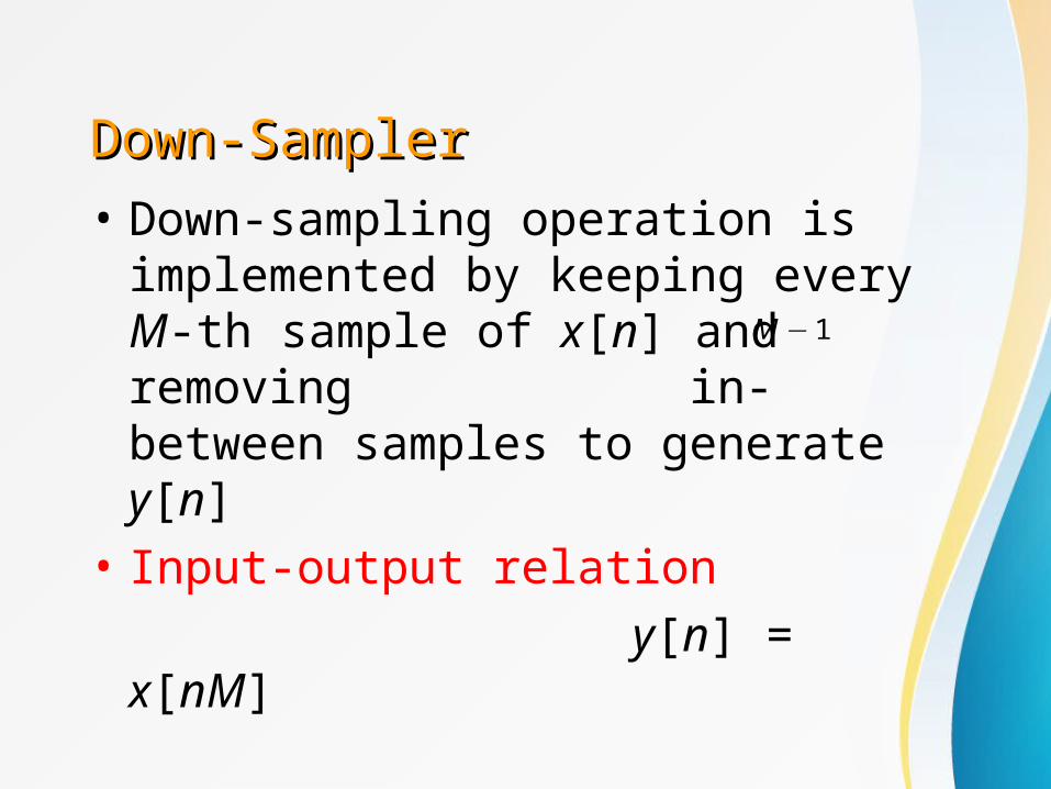
Down-SamplerDown-Sampler
• Down-sampling operation is implemented by keeping every M-th sample of x[n] and removing in-between samples to generate y[n]
• Input-output relation
y[n] = x[nM]
M −1

Down-SamplerDown-Sampler
• Figure below shows the down-sampling by a factor of 3 of a sinusoidal sequence of frequency 0.042 Hz obtained using Program 10_2
0 10 20 30 40 50-1
-0.5
0
0.5
1Input Sequence
Time index n
Am
plitu
de
0 10 20 30 40 50-1
-0.5
0
0.5
1Output sequence down-sampled by 3
Am
plitu
de
Time index n
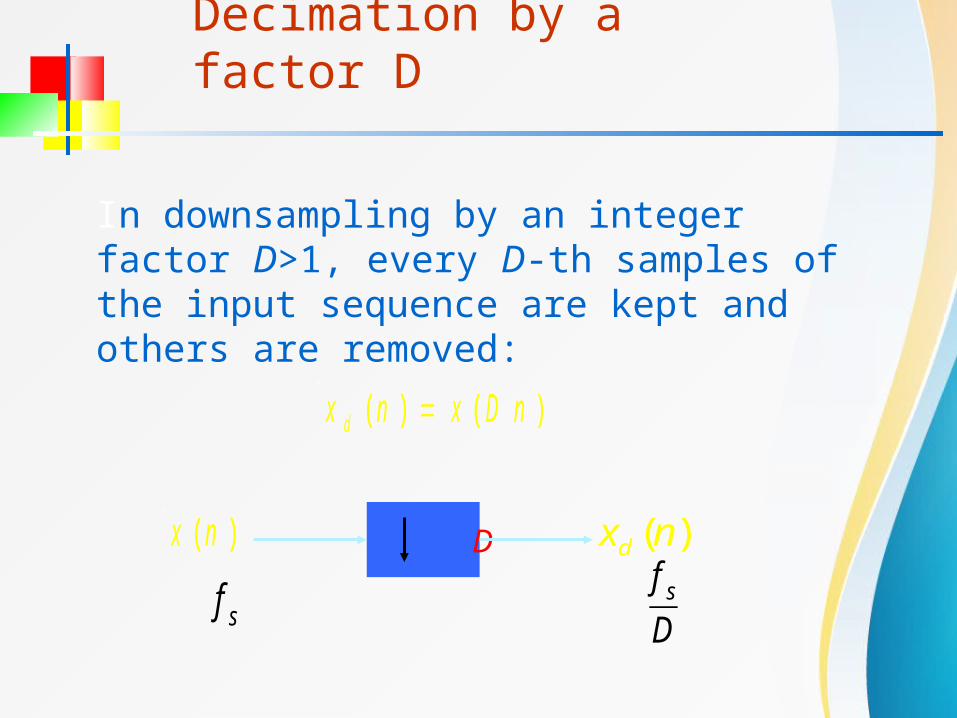
In downsampling by an integer factor D>1, every D-th samples of the input sequence are kept and others are removed:
)()( Dnxnxd
D)(nx )(nxd
Decimation by a factor D
f sf sD

Relationship in time domain
x p ( n )= x ( n ) p ( n )
x(n) Input sequence
p(n )= ∑k=−∞
∞δ (n−kD ) Periodic train of impulses
x d ( n )= x p( Dn )= x ( Dn ) Output sequence
Decimation by a factor D

C
Relationship in frequency domain
X p(ejω)=
12π∫0
2πP (e jθ)X (e j (ω−θ ))dθ
p(n )=1D
∑k=0
D−1
P(k )ej2πD
kn
, P(k )= ∑n=0
D−1
p(n )e− j
2πD
kn
P ( k )=∑n=0
D−1
[ ∑i=−∞
∞
δ (n− iD )]e− j2πD
kn
=∑n=0
D−1
δ (n ) e− j
2πD
kn
=1
Decimation by a factor D

C
X p(ejω )= 1
D∑k=0
D−1
X ( ej (ω−kω s))
X d (ejω)= ∑
m=−∞
∞xd (m )e− jω m= ∑
m=−∞
∞x p(mD )e− jω m
¿ ∑n=mD
x p (n)e− jω
nD = ∑
n=−∞
∞
x p( n)e− jω
nD = X p (e
jωD )
ωs=2πD
P(e jω )= ∑n=−∞
∞p( n)e− jωn= ∑
n=−∞
∞ [1D ∑k=0
D−1
P(k )ej2πD
kn]e− jωn
¿1D ∑
k=0
D−1
∑n=−∞
∞ej2πD
kne− jωn=2π
D ∑k=0
D−1
δ (ω−2πD
k )
le t n=mD

h(n)x(n) x d ( n ) D
x ' (n )
H (e jω)={1, 0≤∣ω∣≤ πD
0, otherwise
Using a digital low-pass filter to prevent aliasing
Decimation by a factor D

INTERPOLATION
INTERPOLATION

Up-SamplerUp-Sampler
Time-Domain CharacterizationTime-Domain Characterization
• An up-sampler with an up-sampling up-sampling factorfactor L, where L is a positive integer, develops an output sequence with a sampling rate that is L times larger than that of the input sequence x[n]
• Block-diagram representation
x u [n ]
Lx[n] x u [ n]
Up-SamplerUp-Sampler
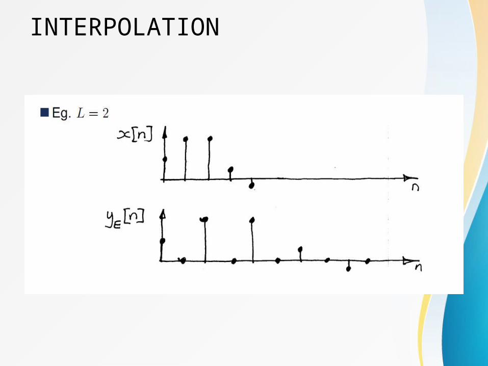
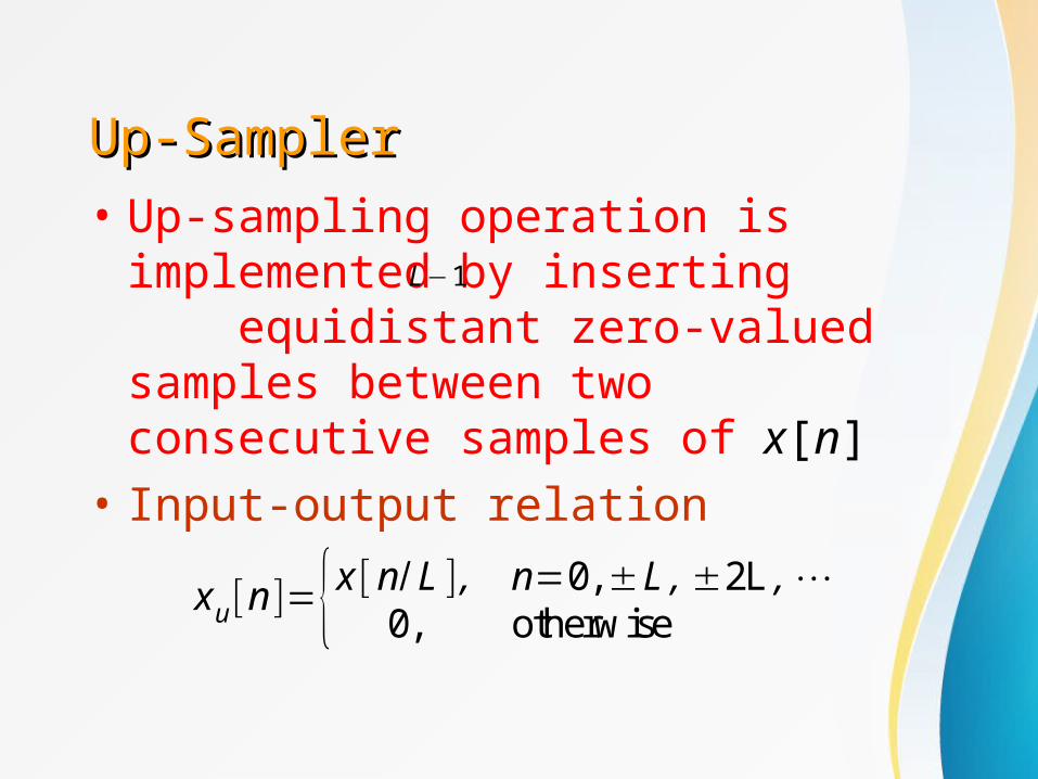
• Up-sampling operation is implemented by inserting equidistant zero-valued samples between two consecutive samples of x[n]
• Input-output relation
L−1
xu [n ]={x [ n/ L ] , n=0, ±L , ±2L , ⋯0, otherwise

Up-SamplerUp-Sampler
• Figure below shows the up-sampling by a factor of 3 of a sinusoidal sequence with a frequency of 0.12 Hz obtained using Program 10_1
0 10 20 30 40 50-1
-0.5
0
0.5
1Input Sequence
Time index n
Am
plitu
de
0 10 20 30 40 50-1
-0.5
0
0.5
1Output sequence up-sampled by 3
Time index n
Am
plitu
de

Up-SamplerUp-Sampler
• In practice, the zero-valued samples inserted by the up-sampler are replaced with appropriate nonzero values using some type of filtering process
• Process is called interpolationinterpolation and will be discussed later

In up-sampling by an integer factor I >1, I -1 equidistant zeros-valued samples are inserted between each two consecutive samples of the input sequence. Then a digital low-pass filter is applied.
x p (n)={x ( nI ) , n=0, ±I , ±2I⋯
0, otherwise
Ix(n) x I ( n )h(n)x p (n )
Interpolation by a factor I
f s If s
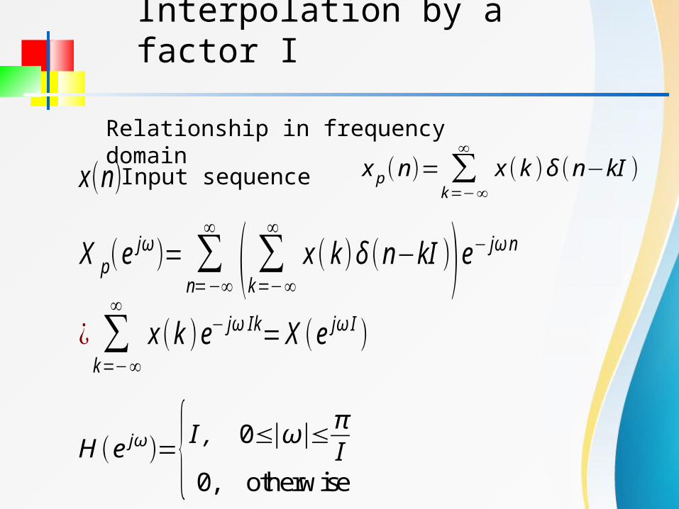
Relationship in frequency domain
x p (n)= ∑k=−∞
∞x (k )δ (n−kI )x(n) Input sequence
X p(ejω )= ∑
n=−∞
∞
( ∑k=−∞
∞x ( k )δ (n−kI ))e− jω n
¿ ∑k=−∞
∞
x (k )e− jω Ik= X (e jω I )
H (e jω)={I , 0≤∣ω∣≤πI
0, otherwise
Interpolation by a factor I

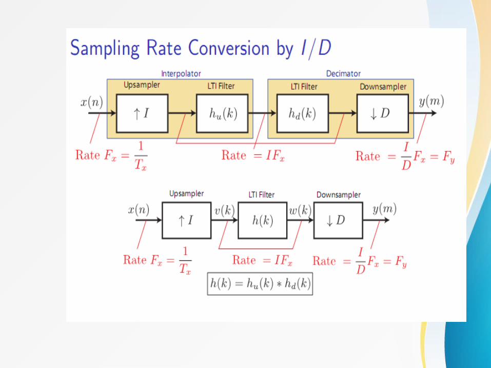
If is a rational numberR=ID
h1(n)
h2(n)
I Dx(n)
interpolation decimationf s
x I ( n )
If s
x Id ( n )
IDf s
Sampling rate conversion by a rational factor I/D
Sampling period
TTI
TI
TI
DTI

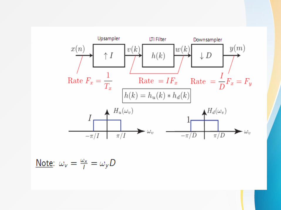
h (n) I Dx(n) x Id ( n )
H (e jω)={I , 0≤∣ω∣≤min ( πI,πD
)
0, otherwise
Sampling Rate Conversion

-15 -10 -5 0 5 10 150
2
n
-15 -10 -5 0 5 10 150
0.5
1
n
-15 -10 -5 0 5 10 150
2
n
-15 -10 -5 0 5 10 150
2
n
x(n)
p(n )
x p (n )
x d ( n )
D = 4

ω h−ω h ω
∣X ( e jω)∣
0 π 2π−2π −π
ω
∣P ( e jω )∣
0 π 2π−2π −π ωs−ω s 3ωs−3ω s
2πD
ω0 π 2π−2π −π ω h−ω h
1D
ωs−ω s 3ωs−3ω s
∣X p (ejω )∣
ω0 π 2π−2π −π Dωh−Dωh
1D
∣Xd (ejω )∣
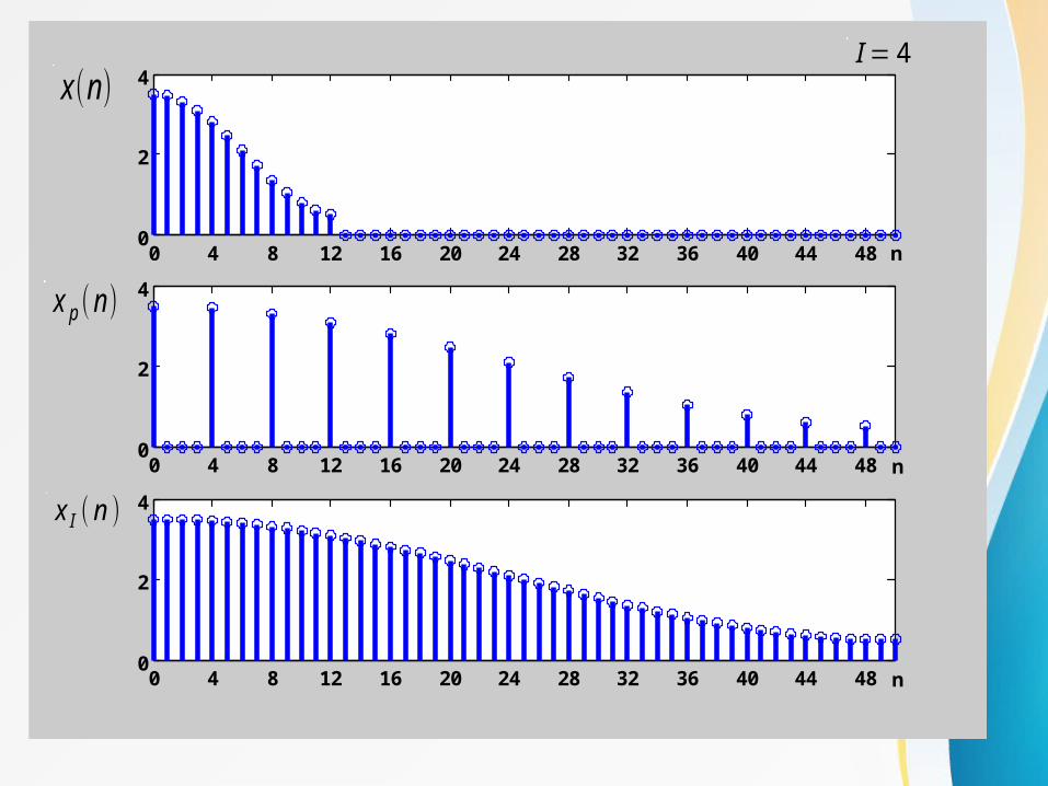
0 4 8 12 16 20 24 28 32 36 40 44 480
2
4
n
0 4 8 12 16 20 24 28 32 36 40 44 480
2
4
n
0 4 8 12 16 20 24 28 32 36 40 44 480
2
4
n
x(n)
x p (n )
x I ( n )
I= 4

ω0 π 2π−2π −π ω h−ω h
∣X ( e jω)∣
ω0 π 2π−2π −π ωh
I−ωh
I
∣X I (ejω )∣
ω0 π 2π−2π −π ωh
I2πI
6πI
∣X p (ejω )∣
−ωh
I


INTRODUCTION TO ADAPTIVE FILTER

Adaptive filter
• the signal and/or noise characteristics are often nonstationary and the statistical parameters vary with time
• An adaptive filter has an adaptation algorithm, that is meant to monitor the environment and vary the filter transfer function accordingly
• based in the actual signals received, attempts to find the optimum filter design

ADAPTIVE FILTER
• The basic operation now involves two processes :1. a filtering process, which produces an output signal
in response to a given input signal.2. an adaptation process, which aims to adjust the filter
parameters (filter transfer function) to the (possibly time-varying) environment
Often, the (average) square value of the error signal is used as the optimization criterion
Adaptive filter
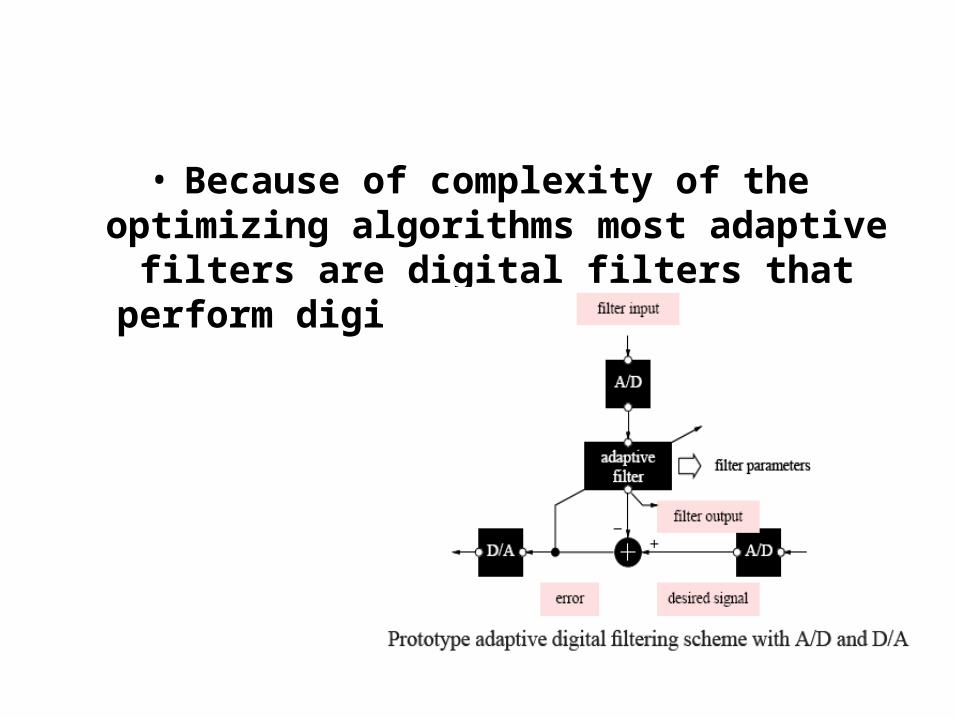
• Because of complexity of the optimizing algorithms most adaptive filters are digital
filters that perform digital signal processing
When processing
analog signals,
the adaptive filter
is then preceded
by A/D and D/A
convertors.

• Adaptive filters differ from other filters such as FIR and IIR in the sense that:
– The coefficients are not determined by a set of desired specifications.
– The coefficients are not fixed.
• With adaptive filters the specifications are not known and change with time.
• Applications include: process control, medical instrumentation, speech processing, echo and noise calculation and channel equalisation.
Introduction
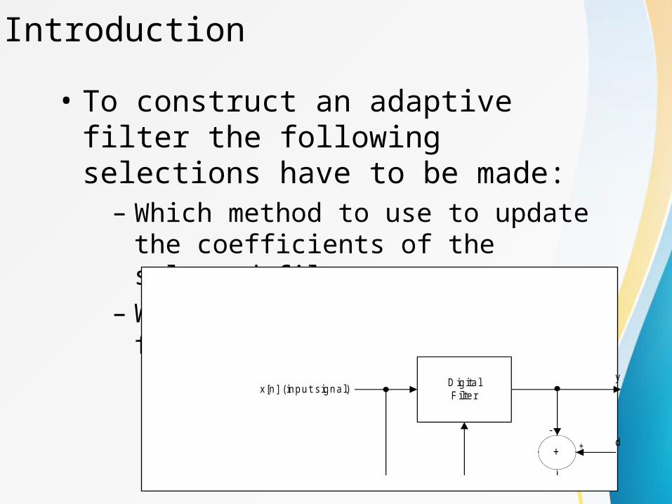
• To construct an adaptive filter the following selections have to be made:
– Which method to use to update the coefficients of the selected filter.
– Whether to use an FIR or IIR filter.
DigitalF ilter
AdaptiveAlgorithm
-
+
e[n] (error signal)
d[n] (desired signal)
y[n] (output signal)x[n] (input signal)
+
44
Adaptive filter
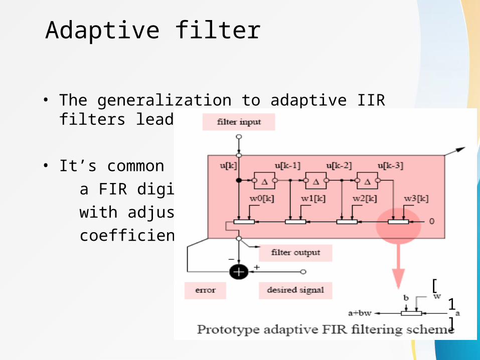
• The generalization to adaptive IIR filters leads to stability problems
• It’s common to use
a FIR digital filter
with adjustable
coefficients.
[1]
45
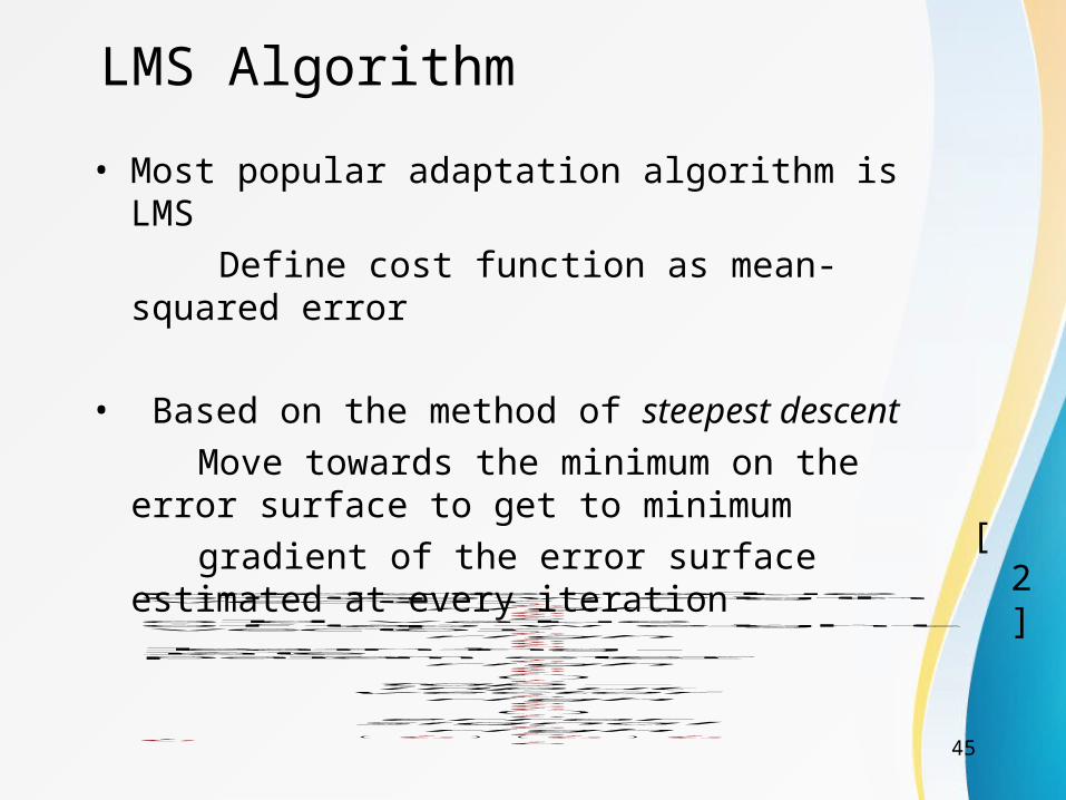
LMS Algorithm
• Most popular adaptation algorithm is LMS
Define cost function as mean-squared error
• Based on the method of steepest descent
Move towards the minimum on the error surface to get to minimum
gradient of the error surface estimated at every iteration
update valueof tap-weigthvector
¿righ¿¿¿
old valueof tap-weightvector
¿righ¿¿¿
learning-rateparameter
¿righ¿¿¿()¿
tap−inputvector
¿righ¿¿¿()¿
errorsignal
¿righ¿
( ¿ ) (¿ ) ¿¿
¿
[2]

46
LMS Algorithm
[2]
W (n )=[w0 ,w1 , .. . ,wN ] , X ( n)=[ x (n ) , x ( n−1 ) ,. .. , x (n−N ) ]e (n )=d (n )− y ( n)ξ̂=e2(n )W (n+1)=W (n )−μ∇ e2(n ) , μ=StepSize∂ e2(n )∂W i
=2 e (n)∂ e (n )∂W i
e⃗(n )=d (n )− y (n )=−2 e (n )∂ y (n )∂W i
y=∑i=0
N−1
W (n) x (n−i)⇒∂e2 (n )∂W i
=−2e (n ) x (n− i)
∇ e2( n)=−2 e( n)X (n )⇒W (n+1)=W (n )+2μe( n)X (n)

47
Stability of LMS
• The LMS algorithm is convergent in the mean square if and only if the step-size parameter satisfy
• Here max is the largest eigenvalue of the correlation matrix of the input data
• More practical test for stability is
• Larger values for step size– Increases adaptation rate (faster adaptation)– Increases residual mean-squared error
0< μ <2
λmax
0<μ<2
input signal power
[2]
48
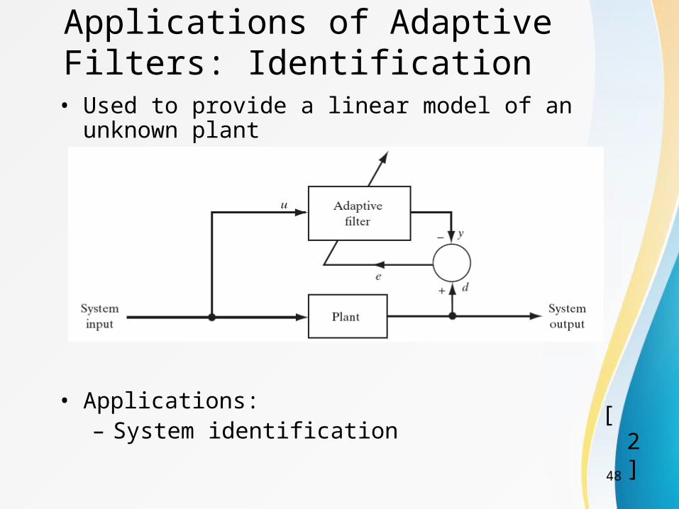
Applications of Adaptive Filters: Identification• Used to provide a linear model of an unknown plant
• Applications: – System identification [2]
49
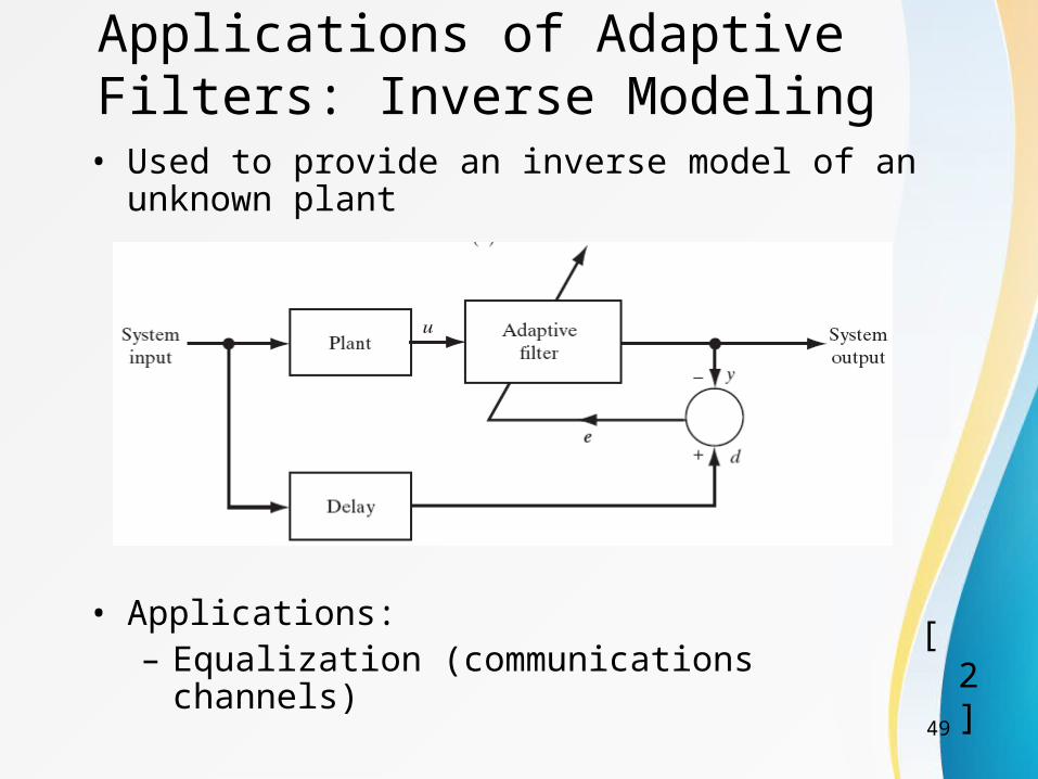
Applications of Adaptive Filters: Inverse Modeling• Used to provide an inverse model of an unknown
plant
• Applications: – Equalization (communications channels)
[2]

50
Applications of Adaptive Filters: Prediction• Used to provide a prediction of the present value of a
random signal
• Applications: – Linear predictive coding
[2]

51
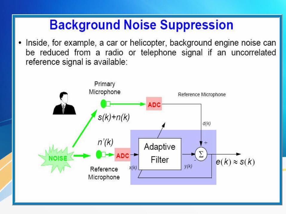
Applications of Adaptive Filters: Interference Cancellation• Used to cancel unknown interference from a primary
signal
• Applications: – Echo / Noise cancellation
hands-free carphone, aircraft headphones etc [2]
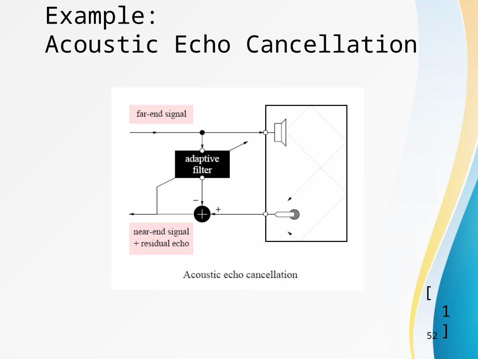
Example:Acoustic Echo Cancellation
52
[1]