Unit Quaternions and Rotations in SO(3)
242
March 25, 2021 15:30 ws-book9x6 Linear Algebra for Computer Vision, Robotics, and Machine Learning ws-book-I-9x6 page 567 Chapter 15 Unit Quaternions and Rotations in SO(3) This chapter is devoted to the representation of rotations in SO(3) in terms of unit quaternions. Since we already defined the unitary groups SU(n), the quickest way to introduce the unit quaternions is to define them as the elements of the group SU(2). The skew field H of quaternions and the group SU(2) of unit quater- nions are discussed in Section 15.1. In Section 15.2, we define a homo- morphism r : SU(2) ! SO(3) and prove that its kernel is {-I,I }. We compute the rotation matrix R q associated with the rotation r q induced by a unit quaternion q in Section 15.3. In Section 15.4, we prove that the homomorphism r : SU(2) ! SO(3) is surjective by providing an algorithm to construct a quaternion from a rotation matrix. In Section 15.5 we define the exponential map exp : su(2) ! SU(2) where su(2) is the real vector space of skew-Hermitian 2 ⇥ 2 matrices with zero trace. We prove that exponential map exp : su(2) ! SU(2) is surjective and give an algorithm for finding a logarithm. We discuss quaternion interpolation and prove the famous slerp interpolation formula due to Ken Shoemake in Section 15.6. This formula is used in robotics and computer graphics to deal with inter- polation problems. In Section 15.7, we prove that there is no “nice” section s : SO(3) ! SU(2) of the homomorphism r : SU(2) ! SO(3), in the sense that any section of r is neither a homomorphism nor continuous. 567
Transcript of Unit Quaternions and Rotations in SO(3)

March 25, 2021 15:30 ws-book9x6 Linear Algebra for Computer Vision, Robotics, and Machine Learning ws-book-I-9x6
page 567
Chapter 15
Unit Quaternions and Rotations inSO(3)
This chapter is devoted to the representation of rotations in SO(3) in termsof unit quaternions. Since we already defined the unitary groups SU(n),the quickest way to introduce the unit quaternions is to define them as theelements of the group SU(2).
The skew field H of quaternions and the group SU(2) of unit quater-nions are discussed in Section 15.1. In Section 15.2, we define a homo-morphism r : SU(2) ! SO(3) and prove that its kernel is {�I, I}. Wecompute the rotation matrix Rq associated with the rotation rq inducedby a unit quaternion q in Section 15.3. In Section 15.4, we prove that thehomomorphism r : SU(2) ! SO(3) is surjective by providing an algorithmto construct a quaternion from a rotation matrix. In Section 15.5 we definethe exponential map exp: su(2) ! SU(2) where su(2) is the real vectorspace of skew-Hermitian 2 ⇥ 2 matrices with zero trace. We prove thatexponential map exp: su(2) ! SU(2) is surjective and give an algorithmfor finding a logarithm. We discuss quaternion interpolation and prove thefamous slerp interpolation formula due to Ken Shoemake in Section 15.6.This formula is used in robotics and computer graphics to deal with inter-polation problems. In Section 15.7, we prove that there is no “nice” sections : SO(3) ! SU(2) of the homomorphism r : SU(2) ! SO(3), in the sensethat any section of r is neither a homomorphism nor continuous.
567
March 25, 2021 15:30 ws-book9x6 Linear Algebra for Computer Vision, Robotics, and Machine Learning ws-book-I-9x6
page 568
568 Unit Quaternions and Rotations in SO(3)
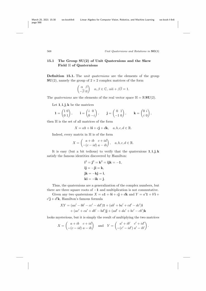
15.1 The Group SU(2) of Unit Quaternions and the SkewField H of Quaternions
Definition 15.1. The unit quaternions are the elements of the groupSU(2), namely the group of 2 ⇥ 2 complex matrices of the form
✓↵ �
�� ↵
◆↵,� 2 C, ↵↵+ �� = 1.
The quaternions are the elements of the real vector space H = RSU(2).
Let 1, i, j,k be the matrices
1 =
✓1 00 1
◆, i =
✓i 00 �i
◆, j =
✓0 1
�1 0
◆, k =
✓0 ii 0
◆,
then H is the set of all matrices of the form
X = a1+ bi+ cj+ dk, a, b, c, d 2 R.
Indeed, every matrix in H is of the form
X =
✓a+ ib c+ id
�(c � id) a � ib
◆, a, b, c, d 2 R.
It is easy (but a bit tedious) to verify that the quaternions 1, i, j,ksatisfy the famous identities discovered by Hamilton:
i2 = j2 = k2 = ijk = �1,
ij = �ji = k,
jk = �kj = i,
ki = �ik = j.
Thus, the quaternions are a generalization of the complex numbers, butthere are three square roots of �1 and multiplication is not commutative.
Given any two quaternions X = a1+ bi+ cj+ dk and Y = a01+ b0i+c0j+ d0k, Hamilton’s famous formula
XY = (aa0 � bb0 � cc0 � dd0)1+ (ab0 + ba0 + cd0 � dc0)i
+ (ac0 + ca0 + db0 � bd0)j+ (ad0 + da0 + bc0 � cb0)k
looks mysterious, but it is simply the result of multiplying the two matrices
X =
✓a+ ib c+ id
�(c � id) a � ib
◆and Y =
✓a0 + ib0 c0 + id0
�(c0 � id0) a0 � ib0
◆.

March 25, 2021 15:30 ws-book9x6 Linear Algebra for Computer Vision, Robotics, and Machine Learning ws-book-I-9x6
page 569
15.2. Representation of Rotation in SO(3) By Quaternions in SU(2) 569
It is worth noting that this formula was discovered independently byOlinde Rodrigues in 1840, a few years before Hamilton (Veblen and Young[Veblen and Young (1946)]). However, Rodrigues was working with a dif-ferent formalism, homogeneous transformations, and he did not discoverthe quaternions.
If
X =
✓a+ ib c+ id
�(c � id) a � ib
◆, a, b, c, d 2 R,
it is immediately verified that
XX⇤ = X⇤X = (a2 + b2 + c2 + d2)1.
Also observe that
X⇤ =
✓a � ib �(c+ id)c � id a+ ib
◆= a1 � bi � cj � dk.
This implies that if X 6= 0, then X is invertible and its inverse is givenby
X�1 = (a2 + b2 + c2 + d2)�1X⇤.
As a consequence, it can be verified that H is a skew field (a noncom-mutative field). It is also a real vector space of dimension 4 with basis(1, i, j,k); thus as a vector space, H is isomorphic to R4.
Definition 15.2. A concise notation for the quaternion X defined by ↵ =a+ ib and � = c+ id is
X = [a, (b, c, d)].
We call a the scalar part of X and (b, c, d) the vector part of X. With thisnotation, X⇤ = [a,�(b, c, d)], which is often denoted by X. The quaternionX is called the conjugate of X. If q is a unit quaternion, then q is themultiplicative inverse of q.
15.2 Representation of Rotations in SO(3) by Quaternionsin SU(2)
The key to representation of rotations in SO(3) by unit quaternions is acertain group homomorphism called the adjoint representation of SU(2).To define this mapping, first we define the real vector space su(2) of skewHermitian matrices.
Definition 15.3. The (real) vector space su(2) of 2 ⇥ 2 skew Hermitianmatrices with zero trace is given by
su(2) =
⇢✓ix y + iz
�y + iz �ix
◆ ���� (x, y, z) 2 R3
�.

March 25, 2021 15:30 ws-book9x6 Linear Algebra for Computer Vision, Robotics, and Machine Learning ws-book-I-9x6
page 570
570 Unit Quaternions and Rotations in SO(3)
Observe that for every matrix A 2 su(2), we have A⇤ = �A, that is, Ais skew Hermitian, and that tr(A) = 0.
Definition 15.4. The adjoint representation of the group SU(2) is thegroup homomorphismAd: SU(2) ! GL(su(2)) defined such that for every q 2 SU(2), with
q =
✓↵ �
�� ↵
◆2 SU(2),
we have
Adq(A) = qAq⇤, A 2 su(2),
where q⇤ is the inverse of q (since SU(2) is a unitary group) and is givenby
q⇤ =
✓↵ ��� ↵
◆.
One needs to verify that the map Adq is an invertible linear map fromsu(2) to itself, and that Ad is a group homomorphism, which is easy to do.
In order to associate a rotation ⇢q (in SO(3)) to q, we need to embedR3 into H as the pure quaternions, by
(x, y, z) =
✓ix y + iz
�y + iz �ix
◆, (x, y, z) 2 R3.
Then q defines the map ⇢q (on R3) given by
⇢q(x, y, z) = �1(q (x, y, z)q⇤).
Therefore, modulo the isomorphism , the linear map ⇢q is the linearisomorphism Adq. In fact, it turns out that ⇢q is a rotation (and so is Adq),which we will prove shortly. So, the representation of rotations in SO(3)by unit quaternions is just the adjoint representation of SU(2); its imageis a subgroup of GL(su(2)) isomorphic to SO(3).
Technically, it is a bit simpler to embed R3 in the (real) vector spacesof Hermitian matrices with zero trace,
⇢✓x z � iy
z + iy �x
◆ ���� x, y, z 2 R�.
Since the matrix (x, y, z) is skew-Hermitian, the matrix �i (x, y, z) isHermitian, and we have
�i (x, y, z) =
✓x z � iy
z + iy �x
◆= x�
3
+ y�2
+ z�1
,

March 25, 2021 15:30 ws-book9x6 Linear Algebra for Computer Vision, Robotics, and Machine Learning ws-book-I-9x6
page 571
15.2. Representation of Rotation in SO(3) By Quaternions in SU(2) 571
where �1
,�2
,�3
are the Pauli spin matrices
�1
=
✓0 11 0
◆, �
2
=
✓0 �ii 0
◆, �
3
=
✓1 00 �1
◆.
Matrices of the form x�3
+ y�2
+ z�1
are Hermitian matrices with zerotrace.
It is easy to see that every 2⇥ 2 Hermitian matrix with zero trace mustbe of this form. (observe that (i�
1
, i�2
, i�3
) forms a basis of su(2). Also,i = i�
3
, j = i�2
, k = i�1
.)Now, if A = x�
3
+y�2
+z�1
is a Hermitian 2⇥2 matrix with zero trace,we have
(qAq⇤)⇤ = qA⇤q⇤ = qAq⇤,
so qAq⇤ is also Hermitian, and
tr(qAq⇤) = tr(Aq⇤q) = tr(A),
and qAq⇤ also has zero trace. Therefore, the map A 7! qAq⇤ preserves theHermitian matrices with zero trace. We also have
det(x�3
+ y�2
+ z�1
) = det
✓x z � iy
z + iy �x
◆= �(x2 + y2 + z2),
and
det(qAq⇤) = det(q) det(A) det(q⇤) = det(A) = �(x2 + y2 + z2).
We can embed R3 into the space of Hermitian matrices with zero traceby
'(x, y, z) = x�3
+ y�2
+ z�1
.
Note that
' = �i and '�1 = i �1.
Definition 15.5. The unit quaternion q 2 SU(2) induces a map rq on R3
by
rq(x, y, z) = '�1(q'(x, y, z)q⇤) = '�1(q(x�3
+ y�2
+ z�1
)q⇤).
The map rq is clearly linear since ' is linear.
Proposition 15.1. For every unit quaternion q 2 SU(2), the linear maprq is orthogonal, that is, rq 2 O(3).

March 25, 2021 15:30 ws-book9x6 Linear Algebra for Computer Vision, Robotics, and Machine Learning ws-book-I-9x6
page 572
572 Unit Quaternions and Rotations in SO(3)
Proof. Since
� k(x, y, z)k2 = �(x2 + y2 + z2) = det(x�3 + y�2 + z�1
) = det('(x, y, z)),
we have
� krq(x, y, z)k2 = det('(rq(x, y, z))) = det(q(x�3
+ y�2
+ z�1
)q⇤)
= det(x�3
+ y�2
+ z�1
) = ���(x, y, z)2
�� ,
and we deduce that rq is an isometry. Thus, rq 2 O(3).
In fact, rq is a rotation, and we can show this by finding the fixed pointsof rq. Let q be a unit quaternion of the form
q =
✓↵ �
�� ↵
◆
with ↵ = a+ ib, � = c+ id, and a2 + b2 + c2 + d2 = 1 (a, b, c, d 2 R).If b = c = d = 0, then q = I and rq is the identity so we may assume
that (b, c, d) 6= (0, 0, 0).
Proposition 15.2. If (b, c, d) 6= (0, 0, 0), then the fixed points of rq aresolutions (x, y, z) of the linear system
�dy + cz = 0
cx � by = 0
dx � bz = 0.
This linear system has the nontrivial solution (b, c, d) and has rank 2.Therefore, rq has the eigenvalue 1 with multiplicity 1, and rq is a rota-tion whose axis is determined by (b, c, d).
Proof. We have rq(x, y, z) = (x, y, z) i↵
'�1(q(x�3
+ y�2
+ z�1
)q⇤) = (x, y, z)
i↵
q(x�3
+ y�2
+ z�1
)q⇤ = '(x, y, z),
and since
'(x, y, z) = x�3
+ y�2
+ z�1
= A
with
A =
✓x z � iy
z + iy �x
◆,

March 25, 2021 15:30 ws-book9x6 Linear Algebra for Computer Vision, Robotics, and Machine Learning ws-book-I-9x6
page 573
15.2. Representation of Rotation in SO(3) By Quaternions in SU(2) 573
we see that rq(x, y, z) = (x, y, z) i↵
qAq⇤ = A i↵ qA = Aq.
We have
qA =
✓↵ �
�� ↵
◆✓x z � iy
z + iy �x
◆=
✓↵x+ �z + i�y ↵z � i↵y � �x
��x+ ↵z + i↵y ��z + i�y � ↵x
◆
and
Aq =
✓x z � iy
z + iy �x
◆✓↵ �
�� ↵
◆=
✓↵x � �z + i�y �x+ ↵z � i↵y↵z + i↵y + �x �z + i�y � ↵x
◆.
By equating qA and Aq, we get
i(� � �)y + (� + �)z = 0
2�x+ i(↵� ↵)y + (↵� ↵)z = 0
2�x+ i(↵� ↵)y + (↵� ↵)z = 0
i(� � �)y + (� + �)z = 0.
The first and the fourth equation are identical and the third equation isobtained by conjugating the second, so the above system reduces to
i(� � �)y + (� + �)z = 0
2�x+ i(↵� ↵)y + (↵� ↵)z = 0.
Replacing ↵ by a+ ib and � by c+ id, we get
�dy + cz = 0
cx � by + i(dx � bz) = 0,
which yields the equations
�dy + cz = 0
cx � by = 0
dx � bz = 0.
This linear system has the nontrivial solution (b, c, d) and the matrix of thissystem is 0
@0 �d cc �b 0d 0 �b
1
A .
Since (b, c, d) 6= (0, 0, 0), this matrix always has a 2 ⇥ 2 submatrix whichis nonsingular, so it has rank 2, and consequently its kernel is the one-dimensional space spanned by (b, c, d). Therefore, rq has the eigenvalue1 with multiplicity 1. If we had det(rq) = �1, then the eigenvalues ofrq would be either (�1, 1, 1) or (�1, ei✓, e�i✓) with ✓ 6= k2⇡ (with k 2 Z),contradicting the fact that 1 is an eigenvalue with multiplicity 1. Therefore,rq is a rotation; in fact, its axis is determined by (b, c, d).

March 25, 2021 15:30 ws-book9x6 Linear Algebra for Computer Vision, Robotics, and Machine Learning ws-book-I-9x6
page 574
574 Unit Quaternions and Rotations in SO(3)
In summary, q 7! rq is a map r from SU(2) to SO(3).
Theorem 15.1. The map r : SU(2) ! SO(3) is a homomorphism whosekernel is {I,�I}.
Proof. This map is a homomorphism, because if q1
, q2
2 SU(2), then
rq2(rq1(x, y, z)) = '�1(q2
'(rq1(x, y, z))q⇤2
)
= '�1(q2
'('�1(q1
'(x, y, z)q⇤1
))q⇤2
)
= '�1((q2
q1
)'(x, y, z)(q2
q1
)⇤)
= rq2q1(x, y, z).
The computation that showed that if (b, c, d) 6= (0, 0, 0), then rq has theeigenvalue 1 with multiplicity 1 implies the following: if rq = I
3
, namelyrq has the eigenvalue 1 with multiplicity 3, then (b, c, d) = (0, 0, 0). Butthen a = ±1, and so q = ±I
2
. Therefore, the kernel of the homomorphismr : SU(2) ! SO(3) is {I,�I}.
Remark: Perhaps the quickest way to show that r maps SU(2) into SO(3)is to observe that the map r is continuous. Then, since it is known thatSU(2) is connected, its image by r lies in the connected component of I,namely SO(3).
The map r is surjective, but this is not obvious. We will return to thispoint after finding the matrix representing rq explicitly.
15.3 Matrix Representation of the Rotation rq
Given a unit quaternion q of the form
q =
✓↵ �
�� ↵
◆
with ↵ = a + ib, � = c + id, and a2 + b2 + c2 + d2 = 1 (a, b, c, d 2 R), tofind the matrix representing the rotation rq we need to compute
q(x�3
+ y�2
+ z�1
)q⇤ =
✓↵ �
�� ↵
◆✓x z � iy
z + iy �x
◆✓↵ ��� ↵
◆.
First we have✓
x z � iyz + iy �x
◆✓↵ ��� ↵
◆=
✓x↵+ z� � iy� �x� + z↵� iy↵z↵+ iy↵� x� �z� � iy� � x↵
◆.

March 25, 2021 15:30 ws-book9x6 Linear Algebra for Computer Vision, Robotics, and Machine Learning ws-book-I-9x6
page 575
15.3. Matrix Representation of the Rotation rq 575
Next, we have✓↵ �
�� ↵
◆✓x↵+ z� � iy� �x� + z↵� iy↵z↵+ iy↵� x� �z� � iy� � x↵
◆=
✓A
1
A2
A3
A4
◆,
with
A1
= (↵↵� ��)x+ i(↵� � ↵�)y + (↵� + ↵�)z
A2
= �2↵�x � i(↵2 + �2)y + (↵2 � �2)z
A3
= �2↵�x+ i(↵2 + �2
)y + (↵2 � �2
)z
A4
= �(↵↵� ��)x � i(↵� � ↵�)y � (↵� + ↵�)z.
Since ↵ = a+ ib and � = c+ id, with a, b, c, d 2 R, we have
↵↵� �� = a2 + b2 � c2 � d2
i(↵� � ↵�) = 2(bc � ad)
↵� + ↵� = 2(ac+ bd)
�↵� = �ac+ bd � i(ad+ bc)
�i(↵2 + �2) = 2(ab+ cd) � i(a2 � b2 + c2 � d2)
↵2 � �2 = a2 � b2 � c2 + d2 + i2(ab � cd).
Using the above, we get
(↵↵� ��)x+ i(↵� � ↵�)y + (↵� + ↵�)z
= (a2 + b2 � c2 � d2)x+ 2(bc � ad)y + 2(ac+ bd)z,
and
� 2↵�x � i(↵2 + �2)y + (↵2 � �2)z
= 2(�ac+ bd)x+ 2(ab+ cd)y + (a2 � b2 � c2 + d2)z
� i[2(ad+ bc)x+ (a2 � b2 + c2 � d2)y + 2(�ab+ cd)z].
If we write
q(x�3
+ y�2
+ z�1
)q⇤ =
✓x0 z0 � iy0
z0 + iy0 �x0
◆,
we obtain
x0 = (a2 + b2 � c2 � d2)x+ 2(bc � ad)y + 2(ac+ bd)z
y0 = 2(ad+ bc)x+ (a2 � b2 + c2 � d2)y + 2(�ab+ cd)z
z0 = 2(�ac+ bd)x+ 2(ab+ cd)y + (a2 � b2 � c2 + d2)z.

March 25, 2021 15:30 ws-book9x6 Linear Algebra for Computer Vision, Robotics, and Machine Learning ws-book-I-9x6
page 576
576 Unit Quaternions and Rotations in SO(3)
In summary, we proved the following result.
Proposition 15.3. The matrix representing rq is
Rq =
0
@a2 + b2 � c2 � d2 2bc � 2ad 2ac+ 2bd
2bc+ 2ad a2 � b2 + c2 � d2 �2ab+ 2cd�2ac+ 2bd 2ab+ 2cd a2 � b2 � c2 + d2
1
A .
Since a2 + b2 + c2 + d2 = 1, this matrix can also be written as
Rq =
0
@2a2 + 2b2 � 1 2bc � 2ad 2ac+ 2bd2bc+ 2ad 2a2 + 2c2 � 1 �2ab+ 2cd
�2ac+ 2bd 2ab+ 2cd 2a2 + 2d2 � 1
1
A .
The above is the rotation matrix in Euler form induced by the quater-nion q, which is the matrix corresponding to ⇢q. This is because
' = �i , '�1 = i �1,
so
rq(x, y, z) = '�1(q'(x, y, z)q⇤) = i �1(q(�i (x, y, z))q⇤)
= �1(q (x, y, z)q⇤) = ⇢q(x, y, z),
and so rq = ⇢q.We showed that every unit quaternion q 2 SU(2) induces a rotation
rq 2 SO(3), but it is not obvious that every rotation can be represented bya quaternion. This can shown in various ways.
One way to is use the fact that every rotation in SO(3) is the composi-tion of two reflections, and that every reflection � of R3 can be representedby a quaternion q, in the sense that
�(x, y, z) = �'�1(q'(x, y, z)q⇤).
Note the presence of the negative sign. This is the method used in Gallier[Gallier (2011b)] (Chapter 9).
15.4 An Algorithm to Find a Quaternion Representing aRotation
Theorem 15.2. The homomorphism r : SU(2) ! SO(3) is surjective.

March 25, 2021 15:30 ws-book9x6 Linear Algebra for Computer Vision, Robotics, and Machine Learning ws-book-I-9x6
page 577
15.4. An Algorithm to Find a Quaternion Representing a Rotation 577
Here is an algorithmic method to find a unit quaternion q representinga rotation matrix R, which provides a proof of Theorem 15.2.
Let
q =
✓a+ ib c+ id
�(c � id) a � ib
◆, a2 + b2 + c2 + d2 = 1, a, b, c, d 2 R.
First observe that the trace of Rq is given by
tr(Rq) = 3a2 � b2 � c2 � d2,
but since a2 + b2 + c2 + d2 = 1, we get tr(Rq) = 4a2 � 1, so
a2 =tr(Rq) + 1
4.
If R 2 SO(3) is any rotation matrix and if we write
R =
0
@r11
r12
r13
r21
r22
r23
r31
r32
r33
,
1
A
we are looking for a unit quaternion q 2 SU(2) such that Rq = R. There-fore, we must have
a2 =tr(R) + 1
4.
We also know that
tr(R) = 1 + 2 cos ✓,
where ✓ 2 [0,⇡] is the angle of the rotation R, so we get
a2 =cos ✓ + 1
2= cos2
✓✓
2
◆,
which implies that
|a| = cos
✓✓
2
◆(0 ✓ ⇡).
Note that we may assume that ✓ 2 [0,⇡], because if ⇡ ✓ 2⇡, then✓� 2⇡ 2 [�⇡, 0], and then the rotation of angle ✓� 2⇡ and axis determinedby the vector (b, c, d) is the same as the rotation of angle 2⇡ � ✓ 2 [0,⇡]and axis determined by the vector �(b, c, d). There are two cases.
Case 1 . tr(R) 6= �1, or equivalently ✓ 6= ⇡. In this case a 6= 0. Pick
a =
ptr(R) + 1
2.

March 25, 2021 15:30 ws-book9x6 Linear Algebra for Computer Vision, Robotics, and Machine Learning ws-book-I-9x6
page 578
578 Unit Quaternions and Rotations in SO(3)
Then by equating R � R> and Rq � R>q , we get
4ab = r32
� r23
4ac = r13
� r31
4ad = r21
� r12
,
which yields
b =r32
� r23
4a, c =
r13
� r31
4a, d =
r21
� r12
4a.
Case 2 . tr(R) = �1, or equivalently ✓ = ⇡. In this case a = 0. Byequating R+R> and Rq +R>
q , we get
4bc = r21
+ r12
4bd = r13
+ r31
4cd = r32
+ r23
.
By equating the diagonal terms of R and Rq, we also get
b2 =1 + r
11
2
c2 =1 + r
22
2
d2 =1 + r
33
2.
Since q 6= 0 and a = 0, at least one of b, c, d is nonzero.If b 6= 0, let
b =
p1 + r
11p2
,
and determine c, d using
4bc = r21
+ r12
4bd = r13
+ r31
.
If c 6= 0, let
c =
p1 + r
22p2
,
and determine b, d using
4bc = r21
+ r12
4cd = r32
+ r23
.
March 25, 2021 15:30 ws-book9x6 Linear Algebra for Computer Vision, Robotics, and Machine Learning ws-book-I-9x6
page 579
15.4. An Algorithm to Find a Quaternion Representing a Rotation 579
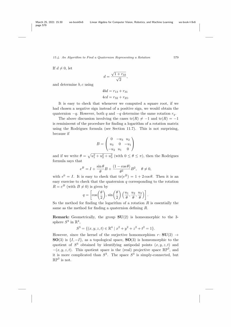
If d 6= 0, let
d =
p1 + r
33p2
,
and determine b, c using
4bd = r13
+ r31
4cd = r32
+ r23
.
It is easy to check that whenever we computed a square root, if wehad chosen a negative sign instead of a positive sign, we would obtain thequaternion �q. However, both q and �q determine the same rotation rq.
The above discussion involving the cases tr(R) 6= �1 and tr(R) = �1is reminiscent of the procedure for finding a logarithm of a rotation matrixusing the Rodrigues formula (see Section 11.7). This is not surprising,because if
B =
0
@0 �u
3
u2
u3
0 �u1
�u2
u1
0
1
A
and if we write ✓ =pu2
1
+ u2
2
+ u2
3
(with 0 ✓ ⇡), then the Rodriguesformula says that
eB = I +sin ✓
✓B +
(1 � cos ✓)
✓2B2, ✓ 6= 0,
with e0 = I. It is easy to check that tr(eB) = 1 + 2 cos ✓. Then it is aneasy exercise to check that the quaternion q corresponding to the rotationR = eB (with B 6= 0) is given by
q =
cos
✓✓
2
◆, sin
✓✓
2
◆⇣u1
✓,u2
✓,u3
✓
⌘�.
So the method for finding the logarithm of a rotation R is essentially thesame as the method for finding a quaternion defining R.
Remark: Geometrically, the group SU(2) is homeomorphic to the 3-sphere S3 in R4,
S3 = {(x, y, z, t) 2 R4 | x2 + y2 + z2 + t2 = 1}.However, since the kernel of the surjective homomorphism r : SU(2) !SO(3) is {I,�I}, as a topological space, SO(3) is homeomorphic to thequotient of S3 obtained by identifying antipodal points (x, y, z, t) and�(x, y, z, t). This quotient space is the (real) projective space RP3, andit is more complicated than S3. The space S3 is simply-connected, butRP3 is not.

March 25, 2021 15:30 ws-book9x6 Linear Algebra for Computer Vision, Robotics, and Machine Learning ws-book-I-9x6
page 580
580 Unit Quaternions and Rotations in SO(3)
15.5 The Exponential Map exp: su(2) ! SU(2)
Given any matrix A 2 su(2), with
A =
✓iu
1
u2
+ iu3
�u2
+ iu3
�iu1
◆,
it is easy to check that
A2 = �✓2✓1 00 1
◆,
with ✓ =pu2
1
+ u2
2
+ u2
3
. Then we have the following formula whose proofis very similar to the proof of the formula given in Proposition 8.17.
Proposition 15.4. For every matrix A 2 su(2), with
A =
✓iu
1
u2
+ iu3
�u2
+ iu3
�iu1
◆,
if we write ✓ =pu2
1
+ u2
2
+ u2
3
, then
eA = cos ✓I +sin ✓
✓A, ✓ 6= 0,
and e0 = I.
Therefore, by the discussion at the end of the previous section, eA is aunit quaternion representing the rotation of angle 2✓ and axis (u
1
, u2
, u3
)(or I when ✓ = k⇡, k 2 Z). The above formula shows that we may assumethat 0 ✓ ⇡. Proposition 15.4 shows that the exponential yields a mapexp: su(2) ! SU(2). It is an analog of the exponential map exp: so(3) !SO(3).
Remark: Because so(3) and su(2) are real vector spaces of dimension 3,they are isomorphic, and it is easy to construct an isomorphism. In fact,so(3) and su(2) are isomorphic as Lie algebras, which means that thereis a linear isomorphism preserving the the Lie bracket [A,B] = AB �BA. However, as observed earlier, the groups SU(2) and SO(3) are notisomorphic.
An equivalent, but often more convenient, formula is obtained by as-suming that u = (u
1
, u2
, u3
) is a unit vector, equivalently det(A) = 1, inwhich case A2 = �I, so we have
e✓A = cos ✓I + sin ✓A.
March 25, 2021 15:30 ws-book9x6 Linear Algebra for Computer Vision, Robotics, and Machine Learning ws-book-I-9x6
page 581
15.5. The Exponential Map exp: su(2) ! SU(2) 581
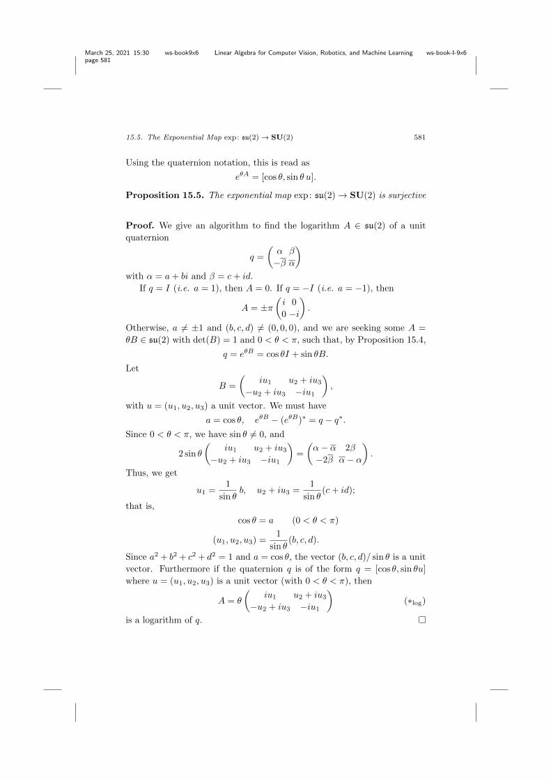
Using the quaternion notation, this is read as
e✓A = [cos ✓, sin ✓ u].
Proposition 15.5. The exponential map exp: su(2) ! SU(2) is surjective
Proof. We give an algorithm to find the logarithm A 2 su(2) of a unitquaternion
q =
✓↵ �
�� ↵
◆
with ↵ = a+ bi and � = c+ id.If q = I (i.e. a = 1), then A = 0. If q = �I (i.e. a = �1), then
A = ±⇡✓i 00 �i
◆.
Otherwise, a 6= ±1 and (b, c, d) 6= (0, 0, 0), and we are seeking some A =✓B 2 su(2) with det(B) = 1 and 0 < ✓ < ⇡, such that, by Proposition 15.4,
q = e✓B = cos ✓I + sin ✓B.
Let
B =
✓iu
1
u2
+ iu3
�u2
+ iu3
�iu1
◆,
with u = (u1
, u2
, u3
) a unit vector. We must have
a = cos ✓, e✓B � (e✓B)⇤ = q � q⇤.
Since 0 < ✓ < ⇡, we have sin ✓ 6= 0, and
2 sin ✓
✓iu
1
u2
+ iu3
�u2
+ iu3
�iu1
◆=
✓↵� ↵ 2��2� ↵� ↵
◆.
Thus, we get
u1
=1
sin ✓b, u
2
+ iu3
=1
sin ✓(c+ id);
that is,
cos ✓ = a (0 < ✓ < ⇡)
(u1
, u2
, u3
) =1
sin ✓(b, c, d).
Since a2 + b2 + c2 + d2 = 1 and a = cos ✓, the vector (b, c, d)/ sin ✓ is a unitvector. Furthermore if the quaternion q is of the form q = [cos ✓, sin ✓u]where u = (u
1
, u2
, u3
) is a unit vector (with 0 < ✓ < ⇡), then
A = ✓
✓iu
1
u2
+ iu3
�u2
+ iu3
�iu1
◆(⇤
log
)
is a logarithm of q.

March 25, 2021 15:30 ws-book9x6 Linear Algebra for Computer Vision, Robotics, and Machine Learning ws-book-I-9x6
page 582
582 Unit Quaternions and Rotations in SO(3)
Observe that not only is the exponential map exp: su(2) ! SU(2)surjective, but the above proof shows that it is injective on the open ball
{✓B 2 su(2) | det(B) = 1, 0 ✓ < ⇡}.Also, unlike the situation where in computing the logarithm of a rotation
matrix R 2 SO(3) we needed to treat the case where tr(R) = �1 (theangle of the rotation is ⇡) in a special way, computing the logarithm of aquaternion (other than ±I) does not require any case analysis; no specialcase is needed when the angle of rotation is ⇡.
15.6 Quaternion Interpolation ~
We are now going to derive a formula for interpolating between two quater-nions. This formula is due to Ken Shoemake, once a Penn student andmy TA! Since rotations in SO(3) can be defined by quaternions, this hasapplications to computer graphics, robotics, and computer vision.
First we observe that multiplication of quaternions can be expressedin terms of the inner product and the cross-product in R3. Indeed, ifq1
= [a, u1
] and q2
= [a2
, u2
], it can be verified that
q1
q2
= [a1
, u1
][a2
, u2
] = [a1
a2
� u1
· u2
, a1
u2
+ a2
u1
+ u1
⇥ u2
]. (⇤mult
)
We will also need the identity
u ⇥ (u ⇥ v) = (u · v)u � (u · u)v.Given a quaternion q expressed as q = [cos ✓, sin ✓ u], where u is a unitvector, we can interpolate between I and q by finding the logs of I and q,interpolating in su(2), and then exponentiating. We have
A = log(I) =
✓0 00 0
◆, B = log(q) = ✓
✓iu
1
u2
+ iu3
�u2
+ iu3
�iu1
◆,
and so q = eB . Since SU(2) is a compact Lie group and since the innerproduct on su(2) given by
hX,Y i = tr(X>Y )
is Ad(SU(2))-invariant, it induces a biinvariant Riemannian metric onSU(2), and the curve
� 7! e�B , � 2 [0, 1]
is a geodesic from I to q in SU(2). We write q� = e�B . Given twoquaternions q
1
and q2
, because the metric is left invariant, the curve
� 7! Z(�) = q1
(q�1
1
q2
)�, � 2 [0, 1]
March 25, 2021 15:30 ws-book9x6 Linear Algebra for Computer Vision, Robotics, and Machine Learning ws-book-I-9x6
page 583
15.6. Quaternion Interpolation ~ 583
is a geodesic from q1
to q2
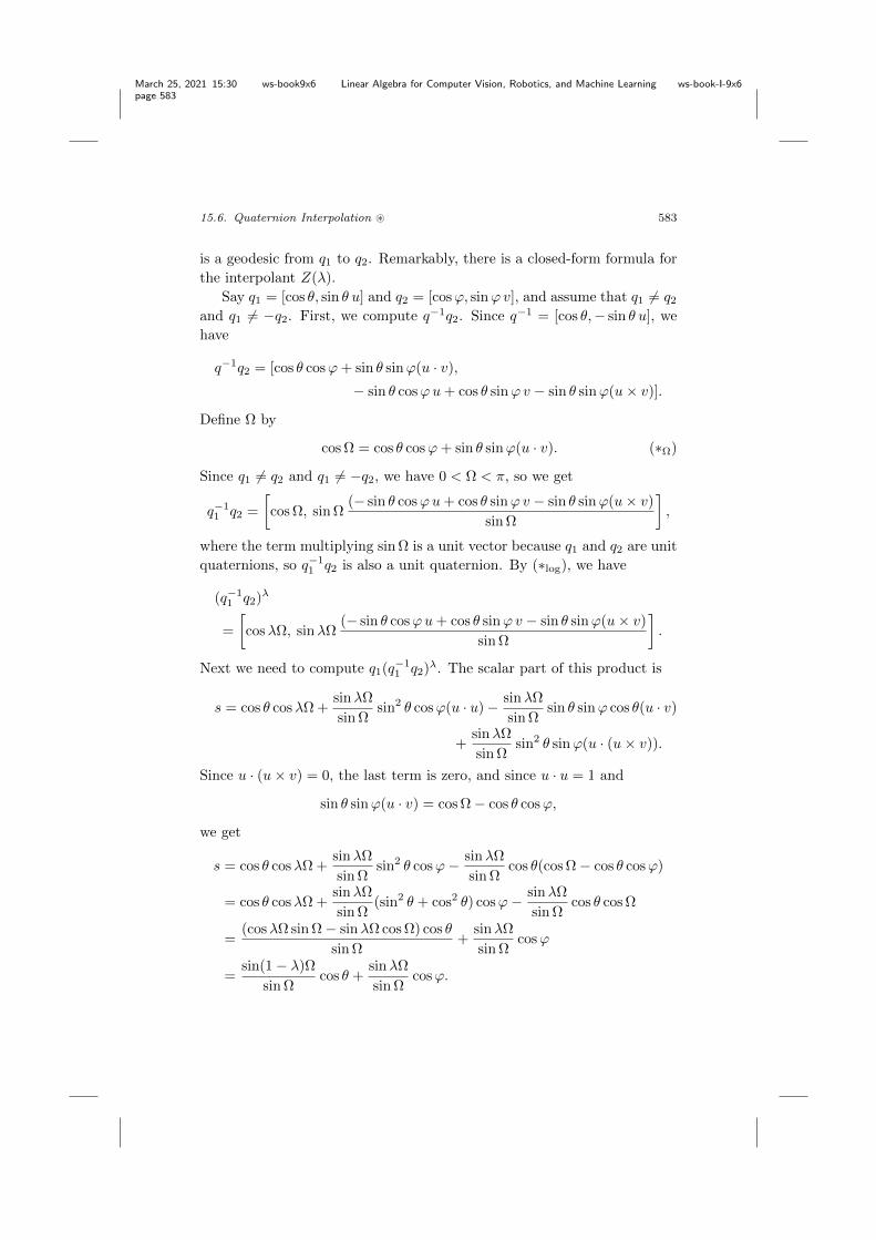
. Remarkably, there is a closed-form formula forthe interpolant Z(�).
Say q1
= [cos ✓, sin ✓ u] and q2
= [cos', sin' v], and assume that q1
6= q2
and q1
6= �q2
. First, we compute q�1q2
. Since q�1 = [cos ✓,� sin ✓ u], wehave
q�1q2
= [cos ✓ cos'+ sin ✓ sin'(u · v),� sin ✓ cos'u+ cos ✓ sin' v � sin ✓ sin'(u ⇥ v)].
Define ⌦ by
cos⌦ = cos ✓ cos'+ sin ✓ sin'(u · v). (⇤⌦
)
Since q1
6= q2
and q1
6= �q2
, we have 0 < ⌦ < ⇡, so we get
q�1
1
q2
=
cos⌦, sin⌦
(� sin ✓ cos'u+ cos ✓ sin' v � sin ✓ sin'(u ⇥ v)
sin⌦
�,
where the term multiplying sin⌦ is a unit vector because q1
and q2
are unitquaternions, so q�1
1
q2
is also a unit quaternion. By (⇤log
), we have
(q�1
1
q2
)�
=
cos�⌦, sin�⌦
(� sin ✓ cos'u+ cos ✓ sin' v � sin ✓ sin'(u ⇥ v)
sin⌦
�.
Next we need to compute q1
(q�1
1
q2
)�. The scalar part of this product is
s = cos ✓ cos�⌦+sin�⌦
sin⌦sin2 ✓ cos'(u · u) � sin�⌦
sin⌦sin ✓ sin' cos ✓(u · v)
+sin�⌦
sin⌦sin2 ✓ sin'(u · (u ⇥ v)).
Since u · (u ⇥ v) = 0, the last term is zero, and since u · u = 1 and
sin ✓ sin'(u · v) = cos⌦ � cos ✓ cos',
we get
s = cos ✓ cos�⌦+sin�⌦
sin⌦sin2 ✓ cos'� sin�⌦
sin⌦cos ✓(cos⌦ � cos ✓ cos')
= cos ✓ cos�⌦+sin�⌦
sin⌦(sin2 ✓ + cos2 ✓) cos'� sin�⌦
sin⌦cos ✓ cos⌦
=(cos�⌦ sin⌦ � sin�⌦ cos⌦) cos ✓
sin⌦+
sin�⌦
sin⌦cos'
=sin(1 � �)⌦
sin⌦cos ✓ +
sin�⌦
sin⌦cos'.

March 25, 2021 15:30 ws-book9x6 Linear Algebra for Computer Vision, Robotics, and Machine Learning ws-book-I-9x6
page 584
584 Unit Quaternions and Rotations in SO(3)
The vector part of the product q1
(q�1
1
q2
)� is given by
⌫ = � sin�⌦
sin⌦cos ✓ sin ✓ cos'u+
sin�⌦
sin⌦cos2 ✓ sin' v
� sin�⌦
sin⌦cos ✓ sin ✓ sin'(u ⇥ v) + cos�⌦ sin ✓ u
� sin�⌦
sin⌦sin2 ✓ cos'(u ⇥ u) +
sin�⌦
sin⌦cos ✓ sin ✓ sin'(u ⇥ v)
� sin�⌦
sin⌦sin2 ✓ sin'(u ⇥ (u ⇥ v)).
We have u ⇥ u = 0, the two terms involving u ⇥ v cancel out,
u ⇥ (u ⇥ v) = (u · v)u � (u · u)v,and u · u = 1, so we get
⌫ = � sin�⌦
sin⌦cos ✓ sin ✓ cos'u+ cos�⌦ sin ✓ u+
sin�⌦
sin⌦cos2 ✓ sin' v
+sin�⌦
sin⌦sin2 ✓ sin' v � sin�⌦
sin⌦sin2 ✓ sin'(u · v)u.
Using
sin ✓ sin'(u · v) = cos⌦ � cos ✓ cos',
we get
⌫ = � sin�⌦
sin⌦cos ✓ sin ✓ cos'u+ cos�⌦ sin ✓ u+
sin�⌦
sin⌦sin' v
� sin�⌦
sin⌦sin ✓(cos⌦ � cos ✓ cos')u
= cos�⌦ sin ✓ u+sin�⌦
sin⌦sin' v � sin�⌦
sin⌦sin ✓ cos⌦u
=(cos�⌦ sin⌦ � sin�⌦ cos⌦)
sin⌦sin ✓ u+
sin�⌦
sin⌦sin' v
=sin(1 � �)⌦
sin⌦sin ✓ u+
sin�⌦
sin⌦sin' v.
Putting the scalar part and the vector part together, we obtain
q1
(q�1
1
q2
)� =
sin(1 � �)⌦
sin⌦cos ✓ +
sin�⌦
sin⌦cos',
sin(1 � �)⌦
sin⌦sin ✓ u+
sin�⌦
sin⌦sin' v
�,
=sin(1 � �)⌦
sin⌦[cos ✓, sin ✓ u] +
sin�⌦
sin⌦[cos', sin' v].
This yields the celebrated slerp interpolation formula
Z(�) = q1
(q�1
1
q2
)� =sin(1 � �)⌦
sin⌦q1
+sin�⌦
sin⌦q2
,
with
cos⌦ = cos ✓ cos'+ sin ✓ sin'(u · v).

March 25, 2021 15:30 ws-book9x6 Linear Algebra for Computer Vision, Robotics, and Machine Learning ws-book-I-9x6
page 585
15.7. Nonexistence of a “Nice” Section from SO(3) to SU(2) 585
15.7 Nonexistence of a “Nice” Section from SO(3) to SU(2)
We conclude by discussing the problem of a consistent choice of sign forthe quaternion q representing a rotation R = ⇢q 2 SO(3). We are lookingfor a “nice” section s : SO(3) ! SU(2), that is, a function s satisfying thecondition
⇢ � s = id,
where ⇢ is the surjective homomorphism ⇢ : SU(2) ! SO(3).
Proposition 15.6. Any section s : SO(3) ! SU(2) of ⇢ is neither a ho-momorphism nor continuous.
Intuitively, this means that there is no “nice and simple ” way to pickthe sign of the quaternion representing a rotation.
The following proof is due to Marcel Berger.
Proof. Let � be the subgroup of SU(2) consisting of all quaternions of theform q = [a, (b, 0, 0)]. Then, using the formula for the rotation matrix Rq
corresponding to q (and the fact that a2 + b2 = 1), we get
Rq =
0
@1 0 00 2a2 � 1 �2ab0 2ab 2a2 � 1
1
A .
Since a2 + b2 = 1, we may write a = cos ✓, b = sin ✓, and we see that
Rq =
0
@1 0 00 cos 2✓ � sin 2✓0 sin 2✓ cos 2✓
1
A ,
a rotation of angle 2✓ around the x-axis. Thus, both � and its image areisomorphic to SO(2), which is also isomorphic toU(1) = {w 2 C | |w| = 1}.By identifying i and i, and identifying � and its image to U(1), if we writew = cos ✓ + i sin ✓ 2 �, the restriction of the map ⇢ to � is given by⇢(w) = w2.
We claim that any section s of ⇢ is not a homomorphism. Considerthe restriction of s to U(1). Then since ⇢ � s = id and ⇢(w) = w2, for�1 2 ⇢(�) ⇡ U(1), we have
�1 = ⇢(s(�1)) = (s(�1))2.
On the other hand, if s is a homomorphism, then
(s(�1))2 = s((�1)2) = s(1) = 1,

March 25, 2021 15:30 ws-book9x6 Linear Algebra for Computer Vision, Robotics, and Machine Learning ws-book-I-9x6
page 586
586 Unit Quaternions and Rotations in SO(3)
contradicting (s(�1))2 = �1.We also claim that s is not continuous. Assume that s(1) = 1, the case
where s(1) = �1 being analogous. Then s is a bijection inverting ⇢ on �whose restriction to U(1) must be given by
s(cos ✓ + i sin ✓) = cos(✓/2) + i sin(✓/2), �⇡ ✓ < ⇡.
If ✓ tends to ⇡, that is z = cos ✓ + i sin ✓ tends to �1 in the upper-halfplane, then s(z) tends to i, but if ✓ tends to �⇡, that is z tends to �1in the lower-half plane, then s(z) tends to �i, which shows that s is notcontinuous.
Another way (due to Jean Dieudonne) to prove that a section s of ⇢ isnot a homomorphism is to prove that any unit quaternion is the productof two unit pure quaternions. Indeed, if q = [a, u] is a unit quaternion, ifwe let q
1
= [0, u1
], where u1
is any unit vector orthogonal to u, then
q1
q = [�u1
· u, au1
+ u1
⇥ u] = [0, au1
+ u1
⇥ u] = q2
is a nonzero unit pure quaternion. This is because if a 6= 0 then au1
+u1
⇥u 6= 0 (since u
1
⇥ u is orthogonal to au1
6= 0), and if a = 0 then u 6= 0, sou1
⇥ u 6= 0 (since u1
is orthogonal to u). But then, q�1
1
= [0,�u1
] is a unitpure quaternion and we have
q = q�1
1
q2
,
a product of two pure unit quaternions.We also observe that for any two pure quaternions q
1
, q2
, there is someunit quaternion q such that
q2
= qq1
q�1.
This is just a restatement of the fact that the group SO(3) is transi-tive. Since the kernel of ⇢ : SU(2) ! SO(3) is {I,�I}, the subgroups(SO(3)) would be a normal subgroup of index 2 in SU(2). Then wewould have a surjective homomorphism ⌘ from SU(2) onto the quotientgroup SU(2)/s(SO(3)), which is isomorphic to {1,�1}. Now, since anytwo pure quaternions are conjugate of each other, ⌘ would have a constantvalue on the unit pure quaternions. Since k = ij, we would have
⌘(k) = ⌘(ij) = (⌘(i))2 = 1.
Consequently, ⌘ would map all pure unit quaternions to 1. But since everyunit quaternion is the product of two pure quaternions, ⌘ would map everyunit quaternion to 1, contradicting the fact that it is surjective onto {�1, 1}.

March 25, 2021 15:30 ws-book9x6 Linear Algebra for Computer Vision, Robotics, and Machine Learning ws-book-I-9x6
page 587
15.8. Summary 587
15.8 Summary
The main concepts and results of this chapter are listed below:
• The group SU(2) of unit quaternions.• The skew field H of quaternions.• Hamilton’s identities.• The (real) vector space su(2) of 2 ⇥ 2 skew Hermitian matrices withzero trace.
• The adjoint representation of SU(2).• The (real) vector space su(2) of 2 ⇥ 2 Hermitian matrices with zerotrace.
• The group homomorphism r : SU(2) ! SO(3); Ker (r) = {+I,�I}.• The matrix representation Rq of the rotation rq induced by a unitquaternion q.
• Surjectivity of the homomorphism r : SU(2) ! SO(3).• The exponential map exp: su(2) ! SU(2).• Surjectivity of the exponential map exp: su(2) ! SU(2).• Finding a logarithm of a quaternion.• Quaternion interpolation.• Shoemake’s slerp interpolation formula.• Sections s : SO(3) ! SU(2) of r : SU(2) ! SO(3).
15.9 Problems
Problem 15.1. Verify the quaternion identities
i2 = j2 = k2 = ijk = �1,
ij = �ji = k,
jk = �kj = i,
ki = �ik = j.
Problem 15.2. Check that for every quaternion X = a1+ bi+ cj+dk, wehave
XX⇤ = X⇤X = (a2 + b2 + c2 + d2)1.
Conclude that if X 6= 0, then X is invertible and its inverse is given by
X�1 = (a2 + b2 + c2 + d2)�1X⇤.

March 25, 2021 15:30 ws-book9x6 Linear Algebra for Computer Vision, Robotics, and Machine Learning ws-book-I-9x6
page 588
588 Unit Quaternions and Rotations in SO(3)
Problem 15.3. Given any two quaternions X = a1 + bi + cj + dk andY = a01+ b0i+ c0j+ d0k, prove that
XY = (aa0 � bb0 � cc0 � dd0)1+ (ab0 + ba0 + cd0 � dc0)i
+ (ac0 + ca0 + db0 � bd0)j+ (ad0 + da0 + bc0 � cb0)k.
Also prove that if X = [a, U ] and Y = [a0, U 0], the quaternion productXY can be expressed as
XY = [aa0 � U · U 0, aU 0 + a0U + U ⇥ U 0].
Problem 15.4. Let Ad: SU(2) ! GL(su(2)) be the map defined suchthat for every q 2 SU(2),
Adq(A) = qAq⇤, A 2 su(2),
where q⇤ is the inverse of q (since SU(2) is a unitary group) Prove that themap Adq is an invertible linear map from su(2) to itself and that Ad is agroup homomorphism.
Problem 15.5. Prove that every Hermitian matrix with zero trace is ofthe form x�
3
+ y�2
+ z�1
, with
�1
=
✓0 11 0
◆, �
2
=
✓0 �ii 0
◆, �
3
=
✓1 00 �1
◆.
Check that i = i�3
, j = i�2
, and that k = i�1
.
Problem 15.6. If
B =
0
@0 �u
3
u2
u3
0 �u1
�u2
u1
0
1
A ,
and if we write ✓ =pu2
1
+ u2
2
+ u2
3
(with 0 ✓ ⇡), then the Rodriguesformula says that
eB = I +sin ✓
✓B +
(1 � cos ✓)
✓2B2, ✓ 6= 0,
with e0 = I. Check that tr(eB) = 1 + 2 cos ✓. Prove that the quaternion qcorresponding to the rotation R = eB (with B 6= 0) is given by
q =
cos
✓✓
2
◆, sin
✓✓
2
◆⇣u1
✓,u2
✓,u3
✓
⌘�.

March 25, 2021 15:30 ws-book9x6 Linear Algebra for Computer Vision, Robotics, and Machine Learning ws-book-I-9x6
page 589
15.9. Problems 589
Problem 15.7. For every matrix A 2 su(2), with
A =
✓iu
1
u2
+ iu3
�u2
+ iu3
�iu1
◆,
prove that if we write ✓ =pu2
1
+ u2
2
+ u2
3
, then
eA = cos ✓I +sin ✓
✓A, ✓ 6= 0,
and e0 = I. Conclude that eA is a unit quaternion representing the rotationof angle 2✓ and axis (u
1
, u2
, u3
) (or I when ✓ = k⇡, k 2 Z).
Problem 15.8. Write a Matlab program implementing the method of Sec-tion 15.4 for finding a unit quaternion corresponding to a rotation matrix.
Problem 15.9. Show that there is a very simple method for producingan orthonormal frame in R4 whose first vector is any given nonnull vector(a, b, c, d).
Problem 15.10. Let i, j, and k, be the unit vectors of coordinates (1, 0, 0),(0, 1, 0), and (0, 0, 1) in R3.
(1) Describe geometrically the rotations defined by the following quater-nions:
p = (0, i), q = (0, j).
Prove that the interpolant Z(�) = p(p�1q)� is given by
Z(�) = (0, cos(�⇡/2)i+ sin(�⇡/2)j) .
Describe geometrically what this rotation is.(2) Repeat Question (1) with the rotations defined by the quaternions
p =
1
2,
p3
2i
!, q = (0, j).
Prove that the interpolant Z(�) is given by
Z(�) =
1
2cos(�⇡/2),
p3
2cos(�⇡/2)i+ sin(�⇡/2)j
!.
Describe geometrically what this rotation is.(3) Repeat Question (1) with the rotations defined by the quaternions
p =
✓1p2,1p2i
◆, q =
✓0,
1p2(i+ j)
◆.
Prove that the interpolant Z(�) is given by
Z(�) =
✓1p2cos(�⇡/3) � 1p
6sin(�⇡/3),
(1/p2 cos(�⇡/3) + 1/
p6 sin(�⇡/3))i+
2p6sin(�⇡/3)j
◆.

March 25, 2021 15:30 ws-book9x6 Linear Algebra for Computer Vision, Robotics, and Machine Learning ws-book-I-9x6
page 590
590 Unit Quaternions and Rotations in SO(3)
Problem 15.11. Prove that
w ⇥ (u ⇥ v) = (w · v)u � (u · w)v.
Conclude that
u ⇥ (u ⇥ v) = (u · v)u � (u · u)v.

March 25, 2021 15:30 ws-book9x6 Linear Algebra for Computer Vision, Robotics, and Machine Learning ws-book-I-9x6
page 591
Chapter 16
Spectral Theorems in Euclidean andHermitian Spaces
16.1 Introduction
The goal of this chapter is to show that there are nice normal forms forsymmetric matrices, skew-symmetric matrices, orthogonal matrices, andnormal matrices. The spectral theorem for symmetric matrices states thatsymmetric matrices have real eigenvalues and that they can be diagonalizedover an orthonormal basis. The spectral theorem for Hermitian matricesstates that Hermitian matrices also have real eigenvalues and that they canbe diagonalized over a complex orthonormal basis. Normal real matricescan be block diagonalized over an orthonormal basis with blocks havingsize at most two and there are refinements of this normal form for skew-symmetric and orthogonal matrices.
The spectral result for real symmetric matrices can be used to prove twocharacterizations of the eigenvalues of a symmetric matrix in terms of theRayleigh ratio. The first characterization is the Rayleigh–Ritz theorem andthe second one is the Courant–Fischer theorem. Both results are used inoptimization theory and to obtain results about perturbing the eigenvaluesof a symmetric matrix.
In this chapter all vector spaces are finite-dimensional real or complexvector spaces.
16.2 Normal Linear Maps: Eigenvalues and Eigenvectors
We begin by studying normal maps, to understand the structure of theireigenvalues and eigenvectors. This section and the next three were in-spired by Lang [Lang (1993)], Artin [Artin (1991)], Mac Lane and Birkho↵[Mac Lane and Birkho↵ (1967)], Berger [Berger (1990a)], and Bertin [Bertin
591

March 25, 2021 15:30 ws-book9x6 Linear Algebra for Computer Vision, Robotics, and Machine Learning ws-book-I-9x6
page 592
592 Spectral Theorems
(1981)].
Definition 16.1. Given a Euclidean or Hermitian space E, a linear mapf : E ! E is normal if
f � f⇤ = f⇤ � f.
A linear map f : E ! E is self-adjoint if f = f⇤, skew-self-adjoint iff = �f⇤, and orthogonal if f � f⇤ = f⇤ � f = id.
Obviously, a self-adjoint, skew-self-adjoint, or orthogonal linear map isa normal linear map. Our first goal is to show that for every normal linearmap f : E ! E, there is an orthonormal basis (w.r.t. h�,�i) such that thematrix of f over this basis has an especially nice form: it is a block diagonalmatrix in which the blocks are either one-dimensional matrices (i.e., singleentries) or two-dimensional matrices of the form
✓� µ
�µ �
◆.
This normal form can be further refined if f is self-adjoint, skew-self-adjoint, or orthogonal. As a first step we show that f and f⇤ have the samekernel when f is normal.
Proposition 16.1. Given a Euclidean space E, if f : E ! E is a normallinear map, then Ker f = Ker f⇤.
Proof. First let us prove that
hf(u), f(v)i = hf⇤(u), f⇤(v)ifor all u, v 2 E. Since f⇤ is the adjoint of f and f � f⇤ = f⇤ � f , we have
hf(u), f(u)i = hu, (f⇤ � f)(u)i,= hu, (f � f⇤)(u)i,= hf⇤(u), f⇤(u)i.
Since h�,�i is positive definite,
hf(u), f(u)i = 0 i↵ f(u) = 0,
hf⇤(u), f⇤(u)i = 0 i↵ f⇤(u) = 0,
and since
hf(u), f(u)i = hf⇤(u), f⇤(u)i,we have
f(u) = 0 i↵ f⇤(u) = 0.
Consequently, Ker f = Ker f⇤.

March 25, 2021 15:30 ws-book9x6 Linear Algebra for Computer Vision, Robotics, and Machine Learning ws-book-I-9x6
page 593
16.2. Normal Linear Maps: Eigenvalues and Eigenvectors 593
Assuming again that E is a Hermitian space, observe that Proposition16.1 also holds. We deduce the following corollary.
Proposition 16.2. Given a Hermitian space E, for any normal linear mapf : E ! E, we have Ker (f) \ Im(f) = (0).
Proof. Assume v 2 Ker (f) \ Im(f), which means that v = f(u) for someu 2 E, and f(v) = 0. By Proposition 16.1, Ker (f) = Ker (f⇤), so f(v) = 0implies that f⇤(v) = 0. Consequently,
0 = hf⇤(v), ui= hv, f(u)i= hv, vi,
and thus, v = 0.
We also have the following crucial proposition relating the eigenvaluesof f and f⇤.
Proposition 16.3. Given a Hermitian space E, for any normal linear mapf : E ! E, a vector u is an eigenvector of f for the eigenvalue � (in C) i↵u is an eigenvector of f⇤ for the eigenvalue �.
Proof. First it is immediately verified that the adjoint of f�� id is f⇤�� id.Furthermore, f � � id is normal. Indeed,
(f � � id) � (f � � id)⇤ = (f � � id) � (f⇤ � � id),
= f � f⇤ � �f � �f⇤ + �� id,
= f⇤ � f � �f⇤ � �f + �� id,
= (f⇤ � � id) � (f � � id),
= (f � � id)⇤ � (f � � id).
Applying Proposition 16.1 to f � � id, for every nonnull vector u, we seethat
(f � � id)(u) = 0 i↵ (f⇤ � � id)(u) = 0,
which is exactly the statement of the proposition.
The next proposition shows a very important property of normal linearmaps: eigenvectors corresponding to distinct eigenvalues are orthogonal.
Proposition 16.4. Given a Hermitian space E, for any normal linear mapf : E ! E, if u and v are eigenvectors of f associated with the eigenvalues� and µ (in C) where � 6= µ, then hu, vi = 0.

March 25, 2021 15:30 ws-book9x6 Linear Algebra for Computer Vision, Robotics, and Machine Learning ws-book-I-9x6
page 594
594 Spectral Theorems
Proof. Let us compute hf(u), vi in two di↵erent ways. Since v is an eigen-vector of f for µ, by Proposition 16.3, v is also an eigenvector of f⇤ for µ,and we have
hf(u), vi = h�u, vi = �hu, vi,and
hf(u), vi = hu, f⇤(v)i = hu, µvi = µhu, vi,where the last identity holds because of the semilinearity in the secondargument. Thus
�hu, vi = µhu, vi,that is,
(�� µ)hu, vi = 0,
which implies that hu, vi = 0, since � 6= µ.
We can show easily that the eigenvalues of a self-adjoint linear map arereal.
Proposition 16.5. Given a Hermitian space E, all the eigenvalues of anyself-adjoint linear map f : E ! E are real.
Proof. Let z (in C) be an eigenvalue of f and let u be an eigenvector forz. We compute hf(u), ui in two di↵erent ways. We have
hf(u), ui = hzu, ui = zhu, ui,and since f = f⇤, we also have
hf(u), ui = hu, f⇤(u)i = hu, f(u)i = hu, zui = zhu, ui.Thus,
zhu, ui = zhu, ui,which implies that z = z, since u 6= 0, and z is indeed real.
There is also a version of Proposition 16.5 for a (real) Euclidean spaceE and a self-adjoint map f : E ! E since every real vector space E can beembedded into a complex vector space EC, and every linear map f : E ! Ecan be extended to a linear map fC : EC ! EC.
Definition 16.2. Given a real vector space E, let EC be the structureE ⇥ E under the addition operation
(u1
, u2
) + (v1
, v2
) = (u1
+ v1
, u2
+ v2
),
and let multiplication by a complex scalar z = x+ iy be defined such that
(x+ iy) · (u, v) = (xu � yv, yu+ xv).
The space EC is called the complexification of E.
March 25, 2021 15:30 ws-book9x6 Linear Algebra for Computer Vision, Robotics, and Machine Learning ws-book-I-9x6
page 595
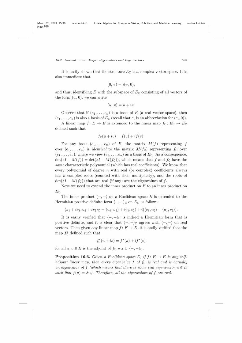
16.2. Normal Linear Maps: Eigenvalues and Eigenvectors 595
It is easily shown that the structure EC is a complex vector space. It isalso immediate that
(0, v) = i(v, 0),
and thus, identifying E with the subspace of EC consisting of all vectors ofthe form (u, 0), we can write
(u, v) = u+ iv.
Observe that if (e1
, . . . , en) is a basis of E (a real vector space), then(e
1
, . . . , en) is also a basis of EC (recall that ei is an abbreviation for (ei, 0)).A linear map f : E ! E is extended to the linear map fC : EC ! EC
defined such that
fC(u+ iv) = f(u) + if(v).
For any basis (e1
, . . . , en) of E, the matrix M(f) representing fover (e
1
, . . . , en) is identical to the matrix M(fC) representing fC over(e
1
, . . . , en), where we view (e1
, . . . , en) as a basis of EC. As a consequence,det(zI � M(f)) = det(zI � M(fC)), which means that f and fC have thesame characteristic polynomial (which has real coe�cients). We know thatevery polynomial of degree n with real (or complex) coe�cients alwayshas n complex roots (counted with their multiplicity), and the roots ofdet(zI � M(fC)) that are real (if any) are the eigenvalues of f .
Next we need to extend the inner product on E to an inner product onEC.
The inner product h�,�i on a Euclidean space E is extended to theHermitian positive definite form h�,�iC on EC as follows:
hu1
+ iv1
, u2
+ iv2
iC = hu1
, u2
i + hv1
, v2
i + i(hv1
, u2
i � hu1
, v2
i).
It is easily verified that h�,�iC is indeed a Hermitian form that ispositive definite, and it is clear that h�,�iC agrees with h�,�i on realvectors. Then given any linear map f : E ! E, it is easily verified that themap f⇤
C defined such that
f⇤C(u+ iv) = f⇤(u) + if⇤(v)
for all u, v 2 E is the adjoint of fC w.r.t. h�,�iC.
Proposition 16.6. Given a Euclidean space E, if f : E ! E is any self-adjoint linear map, then every eigenvalue � of fC is real and is actuallyan eigenvalue of f (which means that there is some real eigenvector u 2 Esuch that f(u) = �u). Therefore, all the eigenvalues of f are real.
March 25, 2021 15:30 ws-book9x6 Linear Algebra for Computer Vision, Robotics, and Machine Learning ws-book-I-9x6
page 596
596 Spectral Theorems
Proof. Let EC be the complexification of E, h�,�iC the complexificationof the inner product h�,�i on E, and fC : EC ! EC the complexificationof f : E ! E. By definition of fC and h�,�iC, if f is self-adjoint, we have
hfC(u1
+ iv1
), u2
+ iv2
iC = hf(u1
) + if(v1
), u2
+ iv2
iC= hf(u
1
), u2
i + hf(v1
), v2
i+ i(hu
2
, f(v1
)i � hf(u1
), v2
i)= hu
1
, f(u2
)i + hv1
, f(v2
)i+ i(hf(u
2
), v1
i � hu1
, f(v2
)i)= hu
1
+ iv1
, f(u2
) + if(v2
)iC= hu
1
+ iv1
, fC(u2
+ iv2
)iC,which shows that fC is also self-adjoint with respect to h�,�iC.
As we pointed out earlier, f and fC have the same characteristic polyno-mial det(zI�fC) = det(zI�f), which is a polynomial with real coe�cients.Proposition 16.5 shows that the zeros of det(zI � fC) = det(zI � f) are allreal, and for each real zero � of det(zI � f), the linear map �id � f is sin-gular, which means that there is some nonzero u 2 E such that f(u) = �u.Therefore, all the eigenvalues of f are real.
Proposition 16.7. Given a Hermitian space E, for any linear mapf : E ! E, if f is skew-self-adjoint, then f has eigenvalues that are pureimaginary or zero, and if f is unitary, then f has eigenvalues of absolutevalue 1.
Proof. If f is skew-self-adjoint, f⇤ = �f , and then by the definition of theadjoint map, for any eigenvalue � and any eigenvector u associated with �,we have
�hu, ui = h�u, ui = hf(u), ui = hu, f⇤(u)i = hu,�f(u)i= �hu,�ui = ��hu, ui,
and since u 6= 0 and h�,�i is positive definite, hu, ui 6= 0, so
� = ��,which shows that � = ir for some r 2 R.
If f is unitary, then f is an isometry, so for any eigenvalue � and anyeigenvector u associated with �, we have
|�|2hu, ui = ��hu, ui = h�u,�ui = hf(u), f(u)i = hu, ui,and since u 6= 0, we obtain |�|2 = 1, which implies
|�| = 1.

March 25, 2021 15:30 ws-book9x6 Linear Algebra for Computer Vision, Robotics, and Machine Learning ws-book-I-9x6
page 597
16.3. Spectral Theorem for Normal Linear Maps 597
16.3 Spectral Theorem for Normal Linear Maps
Given a Euclidean space E, our next step is to show that for every linearmap f : E ! E there is some subspace W of dimension 1 or 2 such thatf(W ) ✓ W . When dim(W ) = 1, the subspace W is actually an eigenspacefor some real eigenvalue of f . Furthermore, when f is normal, there is asubspace W of dimension 1 or 2 such that f(W ) ✓ W and f⇤(W ) ✓ W .The di�culty is that the eigenvalues of f are not necessarily real. One wayto get around this problem is to complexify both the vector space E andthe inner product h�,�i as we did in Section 16.2.
Given any subspaceW of a Euclidean space E, recall that the orthogonalcomplement W? of W is the subspace defined such that
W? = {u 2 E | hu,wi = 0, for all w 2 W}.Recall from Proposition 11.9 that E = W �W? (this can be easily shown,for example, by constructing an orthonormal basis of E using the Gram–Schmidt orthonormalization procedure). The same result also holds forHermitian spaces; see Proposition 13.12.
As a warm up for the proof of Theorem 16.2, let us prove that everyself-adjoint map on a Euclidean space can be diagonalized with respect toan orthonormal basis of eigenvectors.
Theorem 16.1. (Spectral theorem for self-adjoint linear maps on a Eu-clidean space) Given a Euclidean space E of dimension n, for every self-adjoint linear map f : E ! E, there is an orthonormal basis (e
1
, . . . , en) ofeigenvectors of f such that the matrix of f w.r.t. this basis is a diagonalmatrix
0
BBB@
�1
. . .�2
. . ....
.... . .
.... . . �n
1
CCCA,
with �i 2 R.
Proof. We proceed by induction on the dimension n of E as follows. Ifn = 1, the result is trivial. Assume now that n � 2. From Proposition16.6, all the eigenvalues of f are real, so pick some eigenvalue � 2 R, andlet w be some eigenvector for �. By dividing w by its norm, we may assumethat w is a unit vector. Let W be the subspace of dimension 1 spanned byw. Clearly, f(W ) ✓ W . We claim that f(W?) ✓ W?, where W? is theorthogonal complement of W .

March 25, 2021 15:30 ws-book9x6 Linear Algebra for Computer Vision, Robotics, and Machine Learning ws-book-I-9x6
page 598
598 Spectral Theorems
Indeed, for any v 2 W?, that is, if hv, wi = 0, because f is self-adjointand f(w) = �w, we have
hf(v), wi = hv, f(w)i= hv,�wi= �hv, wi = 0
since hv, wi = 0. Therefore,
f(W?) ✓ W?.
Clearly, the restriction of f to W? is self-adjoint, and we conclude byapplying the induction hypothesis to W? (whose dimension is n � 1).
We now come back to normal linear maps. One of the key points in theproof of Theorem 16.1 is that we found a subspace W with the propertythat f(W ) ✓ W implies that f(W?) ✓ W?. In general, this does nothappen, but normal maps satisfy a stronger property which ensures thatsuch a subspace exists.
The following proposition provides a condition that will allow us toshow that a normal linear map can be diagonalized. It actually holds forany linear map. We found the inspiration for this proposition in Berger[Berger (1990a)].
Proposition 16.8. Given a Hermitian space E, for any linear mapf : E ! E and any subspace W of E, if f(W ) ✓ W , then f⇤�W?� ✓ W?.Consequently, if f(W ) ✓ W and f⇤(W ) ✓ W , then f
�W?� ✓ W? and
f⇤�W?� ✓ W?.
Proof. If u 2 W?, then
hw, ui = 0 for all w 2 W.
However,
hf(w), ui = hw, f⇤(u)i,and f(W ) ✓ W implies that f(w) 2 W . Since u 2 W?, we get
0 = hf(w), ui = hw, f⇤(u)i,which shows that hw, f⇤(u)i = 0 for all w 2 W , that is, f⇤(u) 2 W?.Therefore, we have f⇤(W?) ✓ W?.
We just proved that if f(W ) ✓ W , then f⇤�W?� ✓ W?. If we also havef⇤(W ) ✓ W , then by applying the above fact to f⇤, we get f⇤⇤(W?) ✓ W?,and since f⇤⇤ = f , this is just f(W?) ✓ W?, which proves the secondstatement of the proposition.

March 25, 2021 15:30 ws-book9x6 Linear Algebra for Computer Vision, Robotics, and Machine Learning ws-book-I-9x6
page 599
16.3. Spectral Theorem for Normal Linear Maps 599
It is clear that the above proposition also holds for Euclidean spaces.Although we are ready to prove that for every normal linear map f
(over a Hermitian space) there is an orthonormal basis of eigenvectors (seeTheorem 16.3 below), we now return to real Euclidean spaces.
Proposition 16.9. If f : E ! E is a linear map and w = u + iv is aneigenvector of fC : EC ! EC for the eigenvalue z = �+ iµ, where u, v 2 Eand �, µ 2 R, then
f(u) = �u � µv and f(v) = µu+ �v. (⇤)
As a consequence,
fC(u � iv) = f(u) � if(v) = (�� iµ)(u � iv),
which shows that w = u � iv is an eigenvector of fC for z = �� iµ.
Proof. Since
fC(u+ iv) = f(u) + if(v)
and
fC(u+ iv) = (�+ iµ)(u+ iv) = �u � µv + i(µu+ �v),
we have
f(u) = �u � µv and f(v) = µu+ �v.
Using this fact, we can prove the following proposition.
Proposition 16.10. Given a Euclidean space E, for any normal linearmap f : E ! E, if w = u + iv is an eigenvector of fC associated with theeigenvalue z = � + iµ (where u, v 2 E and �, µ 2 R), if µ 6= 0 (i.e., z isnot real) then hu, vi = 0 and hu, ui = hv, vi, which implies that u and v arelinearly independent, and if W is the subspace spanned by u and v, thenf(W ) = W and f⇤(W ) = W . Furthermore, with respect to the (orthogonal)basis (u, v), the restriction of f to W has the matrix
✓� µ
�µ �
◆.
If µ = 0, then � is a real eigenvalue of f , and either u or v is an eigenvectorof f for �. If W is the subspace spanned by u if u 6= 0, or spanned by v 6= 0if u = 0, then f(W ) ✓ W and f⇤(W ) ✓ W .

March 25, 2021 15:30 ws-book9x6 Linear Algebra for Computer Vision, Robotics, and Machine Learning ws-book-I-9x6
page 600
600 Spectral Theorems
Proof. Since w = u+ iv is an eigenvector of fC, by definition it is nonnull,and either u 6= 0 or v 6= 0. Proposition 16.9 implies that u � iv is aneigenvector of fC for �� iµ. It is easy to check that fC is normal. However,if µ 6= 0, then �+ iµ 6= �� iµ, and from Proposition 16.4, the vectors u+ ivand u � iv are orthogonal w.r.t. h�,�iC, that is,
hu+ iv, u � iviC = hu, ui � hv, vi + 2ihu, vi = 0.
Thus we get hu, vi = 0 and hu, ui = hv, vi, and since u 6= 0 or v 6= 0, u andv are linearly independent. Since
f(u) = �u � µv and f(v) = µu+ �v
and since by Proposition 16.3 u+ iv is an eigenvector of f⇤C for �� iµ, we
have
f⇤(u) = �u+ µv and f⇤(v) = �µu+ �v,
and thus f(W ) = W and f⇤(W ) = W , where W is the subspace spannedby u and v.
When µ = 0, we have
f(u) = �u and f(v) = �v,
and since u 6= 0 or v 6= 0, either u or v is an eigenvector of f for �. If W isthe subspace spanned by u if u 6= 0, or spanned by v if u = 0, it is obviousthat f(W ) ✓ W and f⇤(W ) ✓ W . Note that � = 0 is possible, and this iswhy ✓ cannot be replaced by =.
The beginning of the proof of Proposition 16.10 actually shows that forevery linear map f : E ! E there is some subspaceW such that f(W ) ✓ W ,where W has dimension 1 or 2. In general, it doesn’t seem possible to provethat W? is invariant under f . However, this happens when f is normal .
We can finally prove our first main theorem.
Theorem 16.2. (Main spectral theorem) Given a Euclidean space E ofdimension n, for every normal linear map f : E ! E, there is an orthonor-mal basis (e
1
, . . . , en) such that the matrix of f w.r.t. this basis is a blockdiagonal matrix of the form
0
BBB@
A1
. . .A
2
. . ....
.... . .
.... . . Ap
1
CCCA

March 25, 2021 15:30 ws-book9x6 Linear Algebra for Computer Vision, Robotics, and Machine Learning ws-book-I-9x6
page 601
16.3. Spectral Theorem for Normal Linear Maps 601
such that each block Aj is either a one-dimensional matrix (i.e., a realscalar) or a two-dimensional matrix of the form
Aj =
✓�j �µj
µj �j
◆,
where �j , µj 2 R, with µj > 0.
Proof. We proceed by induction on the dimension n of E as follows. Ifn = 1, the result is trivial. Assume now that n � 2. First, since C isalgebraically closed (i.e., every polynomial has a root in C), the linear mapfC : EC ! EC has some eigenvalue z = � + iµ (where �, µ 2 R). Letw = u+ iv be some eigenvector of fC for �+ iµ (where u, v 2 E). We cannow apply Proposition 16.10.
If µ = 0, then either u or v is an eigenvector of f for � 2 R. Let Wbe the subspace of dimension 1 spanned by e
1
= u/kuk if u 6= 0, or bye1
= v/kvk otherwise. It is obvious that f(W ) ✓ W and f⇤(W ) ✓ W . Theorthogonal W? of W has dimension n � 1, and by Proposition 16.8, wehave f
�W?� ✓ W?. But the restriction of f to W? is also normal, and
we conclude by applying the induction hypothesis to W?.If µ 6= 0, then hu, vi = 0 and hu, ui = hv, vi, and if W is the subspace
spanned by u/kuk and v/kvk, then f(W ) = W and f⇤(W ) = W . We alsoknow that the restriction of f to W has the matrix
✓� µ
�µ �
◆
with respect to the basis (u/kuk, v/kvk). If µ < 0, we let �1
= �, µ1
= �µ,e1
= u/kuk, and e2
= v/kvk. If µ > 0, we let �1
= �, µ1
= µ, e1
= v/kvk,and e
2
= u/kuk. In all cases, it is easily verified that the matrix of therestriction of f to W w.r.t. the orthonormal basis (e
1
, e2
) is
A1
=
✓�1
�µ1
µ1
�1
◆,
where �1
, µ1
2 R, with µ1
> 0. However, W? has dimension n� 2, and byProposition 16.8, f
�W?� ✓ W?. Since the restriction of f to W? is also
normal, we conclude by applying the induction hypothesis to W?.
After this relatively hard work, we can easily obtain some nice normalforms for the matrices of self-adjoint, skew-self-adjoint, and orthogonal lin-ear maps. However, for the sake of completeness (and since we have all thetools to so do), we go back to the case of a Hermitian space and show that

March 25, 2021 15:30 ws-book9x6 Linear Algebra for Computer Vision, Robotics, and Machine Learning ws-book-I-9x6
page 602
602 Spectral Theorems
normal linear maps can be diagonalized with respect to an orthonormalbasis. The proof is a slight generalization of the proof of Theorem 16.6.
Theorem 16.3. (Spectral theorem for normal linear maps on a Hermitianspace) Given a Hermitian space E of dimension n, for every normal linearmap f : E ! E there is an orthonormal basis (e
1
, . . . , en) of eigenvectorsof f such that the matrix of f w.r.t. this basis is a diagonal matrix
0
BBB@
�1
. . .�2
. . ....
.... . .
.... . . �n
1
CCCA,
where �j 2 C.
Proof. We proceed by induction on the dimension n of E as follows. Ifn = 1, the result is trivial. Assume now that n � 2. Since C is algebraicallyclosed (i.e., every polynomial has a root in C), the linear map f : E ! Ehas some eigenvalue � 2 C, and let w be some unit eigenvector for �. LetW be the subspace of dimension 1 spanned by w. Clearly, f(W ) ✓ W . ByProposition 16.3, w is an eigenvector of f⇤ for �, and thus f⇤(W ) ✓ W .By Proposition 16.8, we also have f(W?) ✓ W?. The restriction of f toW? is still normal, and we conclude by applying the induction hypothesisto W? (whose dimension is n � 1).
Theorem 16.3 implies that (complex) self-adjoint, skew-self-adjoint, andorthogonal linear maps can be diagonalized with respect to an orthonormalbasis of eigenvectors. In this latter case, though, an orthogonal map iscalled a unitary map. Proposition 16.5 also shows that the eigenvaluesof a self-adjoint linear map are real, and Proposition 16.7 shows that theeigenvalues of a skew self-adjoint map are pure imaginary or zero, and thatthe eigenvalues of a unitary map have absolute value 1.
Remark: There is a converse to Theorem 16.3, namely, if there is an or-thonormal basis (e
1
, . . . , en) of eigenvectors of f , then f is normal. Weleave the easy proof as an exercise.
In the next section we specialize Theorem 16.2 to self-adjoint, skew-self-adjoint, and orthogonal linear maps. Due to the additional structure, weobtain more precise normal forms.

March 25, 2021 15:30 ws-book9x6 Linear Algebra for Computer Vision, Robotics, and Machine Learning ws-book-I-9x6
page 603
16.4. Self-Adjoint and Other Special Linear Maps 603
16.4 Self-Adjoint, Skew-Self-Adjoint, and OrthogonalLinear Maps
We begin with self-adjoint maps.
Theorem 16.4. Given a Euclidean space E of dimension n, for every self-adjoint linear map f : E ! E, there is an orthonormal basis (e
1
, . . . , en) ofeigenvectors of f such that the matrix of f w.r.t. this basis is a diagonalmatrix
0
BBB@
�1
. . .�2
. . ....
.... . .
.... . . �n
1
CCCA,
where �i 2 R.
Proof. We already proved this; see Theorem 16.1. However, it is instruc-tive to give a more direct method not involving the complexification ofh�,�i and Proposition 16.5.
Since C is algebraically closed, fC has some eigenvalue � + iµ, and letu + iv be some eigenvector of fC for � + iµ, where �, µ 2 R and u, v 2 E.We saw in the proof of Proposition 16.9 that
f(u) = �u � µv and f(v) = µu+ �v.
Since f = f⇤,
hf(u), vi = hu, f(v)i
for all u, v 2 E. Applying this to
f(u) = �u � µv and f(v) = µu+ �v,
we get
hf(u), vi = h�u � µv, vi = �hu, vi � µhv, vi
and
hu, f(v)i = hu, µu+ �vi = µhu, ui + �hu, vi,
and thus we get
�hu, vi � µhv, vi = µhu, ui + �hu, vi,
that is,
µ(hu, ui + hv, vi) = 0,

March 25, 2021 15:30 ws-book9x6 Linear Algebra for Computer Vision, Robotics, and Machine Learning ws-book-I-9x6
page 604
604 Spectral Theorems
which implies µ = 0, since either u 6= 0 or v 6= 0. Therefore, � is a realeigenvalue of f .
Now going back to the proof of Theorem 16.2, only the case where µ = 0applies, and the induction shows that all the blocks are one-dimensional.
Theorem 16.4 implies that if �1
, . . . ,�p are the distinct real eigenvaluesof f , and Ei is the eigenspace associated with �i, then
E = E1
� · · · � Ep,
where Ei and Ej are orthogonal for all i 6= j.
Remark: Another way to prove that a self-adjoint map has a real eigen-value is to use a little bit of calculus. We learned such a proof from HermanGluck. The idea is to consider the real-valued function � : E ! R definedsuch that
�(u) = hf(u), ui
for every u 2 E. This function is C1, and if we represent f by a matrix Aover some orthonormal basis, it is easy to compute the gradient vector
r�(X) =
✓@�
@x1
(X), . . . ,@�
@xn(X)
◆
of � at X. Indeed, we find that
r�(X) = (A+A>)X,
where X is a column vector of size n. But since f is self-adjoint, A = A>,and thus
r�(X) = 2AX.
The next step is to find the maximum of the function � on the sphere
Sn�1 = {(x1
, . . . , xn) 2 Rn | x2
1
+ · · · + x2
n = 1}.
Since Sn�1 is compact and � is continuous, and in fact C1, � takes amaximum at some X on Sn�1. But then it is well known that at anextremum X of � we must have
d�X(Y ) = hr�(X), Y i = 0
for all tangent vectors Y to Sn�1 at X, and so r�(X) is orthogonal to thetangent plane at X, which means that
r�(X) = �X
March 25, 2021 15:30 ws-book9x6 Linear Algebra for Computer Vision, Robotics, and Machine Learning ws-book-I-9x6
page 605
16.4. Self-Adjoint and Other Special Linear Maps 605
for some � 2 R. Since r�(X) = 2AX, we get
2AX = �X,
and thus �/2 is a real eigenvalue of A (i.e., of f).
Next we consider skew-self-adjoint maps.
Theorem 16.5. Given a Euclidean space E of dimension n, for every skew-self-adjoint linear map f : E ! E there is an orthonormal basis (e
1
, . . . , en)such that the matrix of f w.r.t. this basis is a block diagonal matrix of theform
0
BBB@
A1
. . .A
2
. . ....
.... . .
.... . . Ap
1
CCCA
such that each block Aj is either 0 or a two-dimensional matrix of the form
Aj =
✓0 �µj
µj 0
◆,
where µj 2 R, with µj > 0. In particular, the eigenvalues of fC are pureimaginary of the form ±iµj or 0.
Proof. The case where n = 1 is trivial. As in the proof of Theorem 16.2,fC has some eigenvalue z = � + iµ, where �, µ 2 R. We claim that � = 0.First we show that
hf(w), wi = 0
for all w 2 E. Indeed, since f = �f⇤, we get
hf(w), wi = hw, f⇤(w)i = hw,�f(w)i = �hw, f(w)i = �hf(w), wi,
since h�,�i is symmetric. This implies that
hf(w), wi = 0.
Applying this to u and v and using the fact that
f(u) = �u � µv and f(v) = µu+ �v,
we get
0 = hf(u), ui = h�u � µv, ui = �hu, ui � µhu, vi

March 25, 2021 15:30 ws-book9x6 Linear Algebra for Computer Vision, Robotics, and Machine Learning ws-book-I-9x6
page 606
606 Spectral Theorems
and
0 = hf(v), vi = hµu+ �v, vi = µhu, vi + �hv, vi,from which, by addition, we get
�(hv, vi + hv, vi) = 0.
Since u 6= 0 or v 6= 0, we have � = 0.Then going back to the proof of Theorem 16.2, unless µ = 0, the case
where u and v are orthogonal and span a subspace of dimension 2 applies,and the induction shows that all the blocks are two-dimensional or reducedto 0.
Remark: One will note that if f is skew-self-adjoint, then ifC is self-adjointw.r.t. h�,�iC. By Proposition 16.5, the map ifC has real eigenvalues,which implies that the eigenvalues of fC are pure imaginary or 0.
Finally we consider orthogonal linear maps.
Theorem 16.6. Given a Euclidean space E of dimension n, for everyorthogonal linear map f : E ! E there is an orthonormal basis (e
1
, . . . , en)such that the matrix of f w.r.t. this basis is a block diagonal matrix of theform
0
BBB@
A1
. . .A
2
. . ....
.... . .
.... . . Ap
1
CCCA
such that each block Aj is either 1, �1, or a two-dimensional matrix of theform
Aj =
✓cos ✓j � sin ✓jsin ✓j cos ✓j
◆
where 0 < ✓j < ⇡. In particular, the eigenvalues of fC are of the formcos ✓j ± i sin ✓j, 1, or �1.
Proof. The case where n = 1 is trivial. It is immediately verified thatf � f⇤ = f⇤ � f = id implies that fC � f⇤
C = f⇤C � fC = id, so the map fC is
unitary. By Proposition 16.7, the eigenvalues of fC have absolute value 1.As a consequence, the eigenvalues of fC are of the form cos ✓± i sin ✓, 1, or�1. The theorem then follows immediately from Theorem 16.2, where thecondition µ > 0 implies that sin ✓j > 0, and thus, 0 < ✓j < ⇡.

March 25, 2021 15:30 ws-book9x6 Linear Algebra for Computer Vision, Robotics, and Machine Learning ws-book-I-9x6
page 607
16.4. Self-Adjoint and Other Special Linear Maps 607
It is obvious that we can reorder the orthonormal basis of eigenvectorsgiven by Theorem 16.6, so that the matrix of f w.r.t. this basis is a blockdiagonal matrix of the form
0
BBBBB@
A1
. . ....
. . ....
.... . . Ar
�Iq. . . Ip
1
CCCCCA
where each block Aj is a two-dimensional rotation matrix Aj 6= ±I2
of theform
Aj =
✓cos ✓j � sin ✓jsin ✓j cos ✓j
◆
with 0 < ✓j < ⇡.The linear map f has an eigenspace E(1, f) = Ker (f � id) of dimen-
sion p for the eigenvalue 1, and an eigenspace E(�1, f) = Ker (f + id) ofdimension q for the eigenvalue �1. If det(f) = +1 (f is a rotation), thedimension q of E(�1, f) must be even, and the entries in �Iq can be pairedto form two-dimensional blocks, if we wish. In this case, every rotation inSO(n) has a matrix of the form
0
BBB@
A1
. . ....
. . ....
. . . Am
. . . In�2m
1
CCCA
where the first m blocks Aj are of the form
Aj =
✓cos ✓j � sin ✓jsin ✓j cos ✓j
◆
with 0 < ✓j ⇡.Theorem 16.6 can be used to prove a version of the Cartan–Dieudonne
theorem.
Theorem 16.7. Let E be a Euclidean space of dimension n � 2. For everyisometry f 2 O(E), if p = dim(E(1, f)) = dim(Ker (f � id)), then f is thecomposition of n � p reflections, and n � p is minimal.
Proof. From Theorem 16.6 there are r subspaces F1
, . . . , Fr, each of di-mension 2, such that
E = E(1, f) � E(�1, f) � F1
� · · · � Fr,

March 25, 2021 15:30 ws-book9x6 Linear Algebra for Computer Vision, Robotics, and Machine Learning ws-book-I-9x6
page 608
608 Spectral Theorems
and all the summands are pairwise orthogonal. Furthermore, the restrictionri of f to each Fi is a rotation ri 6= ±id. Each 2D rotation ri can be writtenas the composition ri = s0i � si of two reflections si and s0i about lines in Fi
(forming an angle ✓i/2). We can extend si and s0i to hyperplane reflectionsin E by making them the identity on F?
i . Then
s0r � sr � · · · � s01
� s1
agrees with f on F1
� · · · � Fr and is the identity on E(1, f) � E(�1, f).If E(�1, f) has an orthonormal basis of eigenvectors (v
1
, . . . , vq), letting s00jbe the reflection about the hyperplane (vj)?, it is clear that
s00q � · · · � s001
agrees with f on E(�1, f) and is the identity on E(1, f) � F1
� · · · � Fr.But then
f = s00q � · · · � s001
� s0r � sr � · · · � s01
� s1
,
the composition of 2r + q = n � p reflections.If
f = st � · · · � s1
,
for t reflections si, it is clear that
F =t\
i=1
E(1, si) ✓ E(1, f),
where E(1, si) is the hyperplane defining the reflection si. By the Grass-mann relation, if we intersect t n hyperplanes, the dimension of theirintersection is at least n � t. Thus, n � t p, that is, t � n � p, and n � pis the smallest number of reflections composing f .
As a corollary of Theorem 16.7, we obtain the following fact: If thedimension n of the Euclidean space E is odd, then every rotation f 2SO(E) admits 1 as an eigenvalue.
Proof. The characteristic polynomial det(XI � f) of f has odd degreen and has real coe�cients, so it must have some real root �. Since fis an isometry, its n eigenvalues are of the form, +1,�1, and e±i✓, with0 < ✓ < ⇡, so � = ±1. Now the eigenvalues e±i✓ appear in conjugatepairs, and since n is odd, the number of real eigenvalues of f is odd. Thisimplies that +1 is an eigenvalue of f , since otherwise �1 would be theonly real eigenvalue of f , and since its multiplicity is odd, we would havedet(f) = �1, contradicting the fact that f is a rotation.

March 25, 2021 15:30 ws-book9x6 Linear Algebra for Computer Vision, Robotics, and Machine Learning ws-book-I-9x6
page 609
16.5. Normal and Other Special Matrices 609
When n = 3, we obtain the result due to Euler which says that every3D rotation R has an invariant axis D, and that restricted to the planeorthogonal to D, it is a 2D rotation. Furthermore, if (a, b, c) is a unitvector defining the axis D of the rotation R and if the angle of the rotationis ✓, if B is the skew-symmetric matrix
B =
0
@0 �c bc 0 �a
�b a 0
1
A ,
then the Rodigues formula (Proposition 11.13) states that
R = I + sin ✓B + (1 � cos ✓)B2.
The theorems of this section and of the previous section can be immedi-ately translated in terms of matrices. The matrix versions of these theoremsis often used in applications so we briefly present them in the section.
16.5 Normal and Other Special Matrices
First we consider real matrices. Recall the following definitions.
Definition 16.3. Given a real m ⇥ n matrix A, the transpose A> of A isthe n ⇥ m matrix A> = (a>i j) defined such that
a>i j = aj i
for all i, j, 1 i m, 1 j n. A real n ⇥ n matrix A is
• normal if
AA> = A>A,
• symmetric if
A> = A,
• skew-symmetric if
A> = �A,
• orthogonal if
AA> = A>A = In.

March 25, 2021 15:30 ws-book9x6 Linear Algebra for Computer Vision, Robotics, and Machine Learning ws-book-I-9x6
page 610
610 Spectral Theorems
Recall from Proposition 11.12 that when E is a Euclidean space and(e
1
, . . ., en) is an orthonormal basis for E, if A is the matrix of a linearmap f : E ! E w.r.t. the basis (e
1
, . . . , en), then A> is the matrix of theadjoint f⇤ of f . Consequently, a normal linear map has a normal matrix,a self-adjoint linear map has a symmetric matrix, a skew-self-adjoint linearmap has a skew-symmetric matrix, and an orthogonal linear map has anorthogonal matrix.
Furthermore, if (u1
, . . . , un) is another orthonormal basis for E and Pis the change of basis matrix whose columns are the components of the ui
w.r.t. the basis (e1
, . . . , en), then P is orthogonal, and for any linear mapf : E ! E, if A is the matrix of f w.r.t (e
1
, . . . , en) and B is the matrix off w.r.t. (u
1
, . . . , un), then
B = P>AP.
As a consequence, Theorems 16.2 and 16.4–16.6 can be restated as fol-lows.
Theorem 16.8. For every normal matrix A there is an orthogonal matrixP and a block diagonal matrix D such that A = PDP>, where D is of theform
D =
0
BBB@
D1
. . .D
2
. . ....
.... . .
.... . . Dp
1
CCCA
such that each block Dj is either a one-dimensional matrix (i.e., a realscalar) or a two-dimensional matrix of the form
Dj =
✓�j �µj
µj �j
◆,
where �j , µj 2 R, with µj > 0.
Theorem 16.9. For every symmetric matrix A there is an orthogonal ma-trix P and a diagonal matrix D such that A = PDP>, where D is of theform
D =
0
BBB@
�1
. . .�2
. . ....
.... . .
.... . . �n
1
CCCA,
where �i 2 R.

March 25, 2021 15:30 ws-book9x6 Linear Algebra for Computer Vision, Robotics, and Machine Learning ws-book-I-9x6
page 611
16.5. Normal and Other Special Matrices 611
Theorem 16.10. For every skew-symmetric matrix A there is an orthogo-nal matrix P and a block diagonal matrix D such that A = PDP>, whereD is of the form
D =
0
BBB@
D1
. . .D
2
. . ....
.... . .
.... . . Dp
1
CCCA
such that each block Dj is either 0 or a two-dimensional matrix of the form
Dj =
✓0 �µj
µj 0
◆,
where µj 2 R, with µj > 0. In particular, the eigenvalues of A are pureimaginary of the form ±iµj, or 0.
Theorem 16.11. For every orthogonal matrix A there is an orthogonalmatrix P and a block diagonal matrix D such that A = PDP>, where Dis of the form
D =
0
BBB@
D1
. . .D
2
. . ....
.... . .
.... . . Dp
1
CCCA
such that each block Dj is either 1, �1, or a two-dimensional matrix of theform
Dj =
✓cos ✓j � sin ✓jsin ✓j cos ✓j
◆
where 0 < ✓j < ⇡. In particular, the eigenvalues of A are of the formcos ✓j ± i sin ✓j, 1, or �1.
Theorem 16.11 can be used to show that the exponential mapexp: so(n) ! SO(n) is surjective; see Gallier [Gallier (2011b)].
We now consider complex matrices.
Definition 16.4. Given a complex m ⇥ n matrix A, the transpose A> ofA is the n ⇥ m matrix A> =
�a>i j
�defined such that
a>i j = aj i
for all i, j, 1 i m, 1 j n. The conjugate A of A is the m⇥n matrixA = (bi j) defined such that
bi j = ai j

March 25, 2021 15:30 ws-book9x6 Linear Algebra for Computer Vision, Robotics, and Machine Learning ws-book-I-9x6
page 612
612 Spectral Theorems
for all i, j, 1 i m, 1 j n. Given an m ⇥ n complex matrix A, theadjoint A⇤ of A is the matrix defined such that
A⇤ = (A>) = (A)>.
A complex n ⇥ n matrix A is
• normal if
AA⇤ = A⇤A,
• Hermitian if
A⇤ = A,
• skew-Hermitian if
A⇤ = �A,
• unitary if
AA⇤ = A⇤A = In.
Recall from Proposition 13.14 that when E is a Hermitian space and(e
1
, . . ., en) is an orthonormal basis for E, if A is the matrix of a linearmap f : E ! E w.r.t. the basis (e
1
, . . . , en), then A⇤ is the matrix of theadjoint f⇤ of f . Consequently, a normal linear map has a normal matrix,a self-adjoint linear map has a Hermitian matrix, a skew-self-adjoint linearmap has a skew-Hermitian matrix, and a unitary linear map has a unitarymatrix.
Furthermore, if (u1
, . . . , un) is another orthonormal basis for E and Pis the change of basis matrix whose columns are the components of theui w.r.t. the basis (e
1
, . . . , en), then P is unitary, and for any linear mapf : E ! E, if A is the matrix of f w.r.t (e
1
, . . . , en) and B is the matrix off w.r.t. (u
1
, . . . , un), then
B = P ⇤AP.
Theorem 16.3 and Proposition 16.7 can be restated in terms of matricesas follows.
Theorem 16.12. For every complex normal matrix A there is a unitarymatrix U and a diagonal matrix D such that A = UDU⇤. Furthermore,if A is Hermitian, then D is a real matrix; if A is skew-Hermitian, thenthe entries in D are pure imaginary or zero; and if A is unitary, then theentries in D have absolute value 1.

March 25, 2021 15:30 ws-book9x6 Linear Algebra for Computer Vision, Robotics, and Machine Learning ws-book-I-9x6
page 613
16.6. Rayleigh–Ritz Theorems and Eigenvalue Interlacing 613
16.6 Rayleigh–Ritz Theorems and Eigenvalue Interlacing
A fact that is used frequently in optimization problems is that the eigen-values of a symmetric matrix are characterized in terms of what is knownas the Rayleigh ratio, defined by
R(A)(x) =x>Ax
x>x, x 2 Rn, x 6= 0.
The following proposition is often used to prove the correctness of vari-ous optimization or approximation problems (for example PCA; see Section21.4). It is also used to prove Proposition 16.13, which is used to justifythe correctness of a method for graph-drawing (see Chapter 19).
Proposition 16.11. (Rayleigh–Ritz) If A is a symmetric n ⇥ n matrixwith eigenvalues �
1
�2
· · · �n and if (u1
, . . . , un) is any orthonormalbasis of eigenvectors of A, where ui is a unit eigenvector associated with �i,then
maxx 6=0
x>Ax
x>x= �n
(with the maximum attained for x = un), and
maxx 6=0,x2{un�k+1,...,un}?
x>Ax
x>x= �n�k
(with the maximum attained for x = un�k), where 1 k n � 1. Equiva-lently, if Vk is the subspace spanned by (u
1
, . . . , uk), then
�k = maxx 6=0,x2Vk
x>Ax
x>x, k = 1, . . . , n.
Proof. First observe that
maxx 6=0
x>Ax
x>x= max
x{x>Ax | x>x = 1},
and similarly,
maxx 6=0,x2{un�k+1,...,un}?
x>Ax
x>x
= maxx
�x>Ax | (x 2 {un�k+1
, . . . , un}?) ^ (x>x = 1) .
Since A is a symmetric matrix, its eigenvalues are real and it can be di-agonalized with respect to an orthonormal basis of eigenvectors, so let(u
1
, . . . , un) be such a basis. If we write
x =nX
i=1
xiui,
March 25, 2021 15:30 ws-book9x6 Linear Algebra for Computer Vision, Robotics, and Machine Learning ws-book-I-9x6
page 614
614 Spectral Theorems
a simple computation shows that
x>Ax =nX
i=1
�ix2
i .
If x>x = 1, thenPn
i=1
x2
i = 1, and since we assumed that �1
�2
· · · �n, we get
x>Ax =nX
i=1
�ix2
i �n
✓ nX
i=1
x2
i
◆= �n.
Thus,
maxx
�x>Ax | x>x = 1
�n,
and since this maximum is achieved for en = (0, 0, . . . , 1), we conclude that
maxx
�x>Ax | x>x = 1
= �n.
Next observe that x 2 {un�k+1
, . . . , un}? and x>x = 1 i↵ xn�k+1
= · · · =xn = 0 and
Pn�ki=1
x2
i = 1. Consequently, for such an x, we have
x>Ax =n�kX
i=1
�ix2
i �n�k
✓n�kX
i=1
x2
i
◆= �n�k.
Thus,
maxx
�x>Ax | (x 2 {un�k+1
, . . . , un}?) ^ (x>x = 1)
�n�k,
and since this maximum is achieved for en�k = (0, . . . , 0, 1, 0, . . . , 0) with a1 in position n � k, we conclude that
maxx
�x>Ax | (x 2 {un�k+1
, . . . , un}?) ^ (x>x = 1) = �n�k,
as claimed.
For our purposes we need the version of Proposition 16.11 applying tomin instead of max, whose proof is obtained by a trivial modification of theproof of Proposition 16.11.
Proposition 16.12. (Rayleigh–Ritz) If A is a symmetric n ⇥ n matrixwith eigenvalues �
1
�2
· · · �n and if (u1
, . . . , un) is any orthonormalbasis of eigenvectors of A, where ui is a unit eigenvector associated with �i,then
minx 6=0
x>Ax
x>x= �
1

March 25, 2021 15:30 ws-book9x6 Linear Algebra for Computer Vision, Robotics, and Machine Learning ws-book-I-9x6
page 615
16.6. Rayleigh–Ritz Theorems and Eigenvalue Interlacing 615
(with the minimum attained for x = u1
), and
minx 6=0,x2{u1,...,ui�1}?
x>Ax
x>x= �i
(with the minimum attained for x = ui), where 2 i n. Equivalently, ifWk = V ?
k�1
denotes the subspace spanned by (uk, . . . , un) (with V0
= (0)),then
�k = minx 6=0,x2Wk
x>Ax
x>x= min
x 6=0,x2V ?k�1
x>Ax
x>x, k = 1, . . . , n.
Propositions 16.11 and 16.12 together are known the Rayleigh–Ritz the-orem.
As an application of Propositions 16.11 and 16.12, we prove a proposi-tion which allows us to compare the eigenvalues of two symmetric matricesA and B = R>AR, where R is a rectangular matrix satisfying the equationR>R = I.
First we need a definition.
Definition 16.5. Given an n ⇥ n symmetric matrix A and an m ⇥ msymmetric B, with m n, if �
1
�2
· · · �n are the eigenvalues of Aand µ
1
µ2
· · · µm are the eigenvalues of B, then we say that theeigenvalues of B interlace the eigenvalues of A if
�i µi �n�m+i, i = 1, . . . ,m.
For example, if n = 5 and m = 3, we have
�1
µ1
�3
�2
µ2
�4
�3
µ3
�5
.
Proposition 16.13. Let A be an n⇥ n symmetric matrix, R be an n⇥mmatrix such that R>R = I (with m n), and let B = R>AR (an m ⇥ mmatrix). The following properties hold:
(a) The eigenvalues of B interlace the eigenvalues of A.(b) If �
1
�2
· · · �n are the eigenvalues of A and µ1
µ2
· · · µm
are the eigenvalues of B, and if �i = µi, then there is an eigenvectorv of B with eigenvalue µi such that Rv is an eigenvector of A witheigenvalue �i.

March 25, 2021 15:30 ws-book9x6 Linear Algebra for Computer Vision, Robotics, and Machine Learning ws-book-I-9x6
page 616
616 Spectral Theorems
Proof. (a) Let (u1
, . . . , un) be an orthonormal basis of eigenvectors for A,and let (v
1
, . . . , vm) be an orthonormal basis of eigenvectors for B. LetUj be the subspace spanned by (u
1
, . . . , uj) and let Vj be the subspacespanned by (v
1
, . . . , vj). For any i, the subspace Vi has dimension i and thesubspace R>Ui�1
has dimension at most i � 1. Therefore, there is somenonzero vector v 2 Vi \ (R>Ui�1
)?, and since
v>R>uj = (Rv)>uj = 0, j = 1, . . . , i � 1,
we have Rv 2 (Ui�1
)?. By Proposition 16.12 and using the fact thatR>R = I, we have
�i (Rv)>ARv
(Rv)>Rv=
v>Bv
v>v.
On the other hand, by Proposition 16.11,
µi = maxx 6=0,x2{vi+1,...,vn}?
x>Bx
x>x= max
x 6=0,x2{v1,...,vi}
x>Bx
x>x,
so
w>Bw
w>w µi for all w 2 Vi,
and since v 2 Vi, we have
�i v>Bv
v>v µi, i = 1, . . . ,m.
We can apply the same argument to the symmetric matrices �A and �B,to conclude that
��n�m+i �µi,
that is,
µi �n�m+i, i = 1, . . . ,m.
Therefore,
�i µi �n�m+i, i = 1, . . . ,m,
as desired.(b) If �i = µi, then
�i =(Rv)>ARv
(Rv)>Rv=
v>Bv
v>v= µi,
so v must be an eigenvector for B and Rv must be an eigenvector for A,both for the eigenvalue �i = µi.

March 25, 2021 15:30 ws-book9x6 Linear Algebra for Computer Vision, Robotics, and Machine Learning ws-book-I-9x6
page 617
16.7. The Courant–Fischer Theorem; Perturbation Results 617
Proposition 16.13 immediately implies the Poincare separation theorem.It can be used in situations, such as in quantum mechanics, where one hasinformation about the inner products u>
i Auj .
Proposition 16.14. (Poincare separation theorem) Let A be a n⇥n sym-metric (or Hermitian) matrix, let r be some integer with 1 r n, and let(u
1
, . . . , ur) be r orthonormal vectors. Let B = (u>i Auj) (an r⇥ r matrix),
let �1
(A) . . . �n(A) be the eigenvalues of A and �1
(B) . . . �r(B)be the eigenvalues of B; then we have
�k(A) �k(B) �k+n�r(A), k = 1, . . . , r.
Observe that Proposition 16.13 implies that
�1
+ · · · + �m tr(R>AR) �n�m+1
+ · · · + �n.
If P1
is the the n ⇥ (n � 1) matrix obtained from the identity matrix bydropping its last column, we have P>
1
P1
= I, and the matrix B = P>1
AP1
is the matrix obtained from A by deleting its last row and its last column.In this case the interlacing result is
�1
µ1
�2
µ2
· · · µn�2
�n�1
µn�1
�n,
a genuine interlacing. We obtain similar results with the matrix Pn�r ob-tained by dropping the last n�r columns of the identity matrix and settingB = P>
n�rAPn�r (B is the r ⇥ r matrix obtained from A by deleting itslast n� r rows and columns). In this case we have the following interlacinginequalities known as Cauchy interlacing theorem:
�k µk �k+n�r, k = 1, . . . , r. (⇤)
16.7 The Courant–Fischer Theorem; Perturbation Results
Another useful tool to prove eigenvalue equalities is the Courant–Fischercharacterization of the eigenvalues of a symmetric matrix, also known asthe Min-max (and Max-min) theorem.
Theorem 16.13. (Courant–Fischer) Let A be a symmetric n ⇥ n matrixwith eigenvalues �
1
�2
· · · �n. If Vk denotes the set of subspaces ofRn of dimension k, then
�k = maxW2Vn�k+1
minx2W,x 6=0
x>Ax
x>x
�k = minW2Vk
maxx2W,x 6=0
x>Ax
x>x.

March 25, 2021 15:30 ws-book9x6 Linear Algebra for Computer Vision, Robotics, and Machine Learning ws-book-I-9x6
page 618
618 Spectral Theorems
Proof. Let us consider the second equality, the proof of the first equalitybeing similar. Let (u
1
, . . . , un) be any orthonormal basis of eigenvectors ofA, where ui is a unit eigenvector associated with �i. Observe that the spaceVk spanned by (u
1
, . . . , uk) has dimension k, and by Proposition 16.11, wehave
�k = maxx 6=0,x2Vk
x>Ax
x>x� min
W2Vk
maxx2W,x 6=0
x>Ax
x>x.
Therefore, we need to prove the reverse inequality; that is, we have to showthat
�k maxx 6=0,x2W
x>Ax
x>x, for all W 2 Vk.
Now for any W 2 Vk, if we can prove that W \ V ?k�1
6= (0), then for anynonzero v 2 W \ V ?
k�1
, by Proposition 16.12 , we have
�k = minx 6=0,x2V ?
k�1
x>Ax
x>x v>Av
v>v max
x2W,x 6=0
x>Ax
x>x.
It remains to prove that dim(W\V ?k�1
) � 1. However, dim(Vk�1
) = k�1, sodim(V ?
k�1
) = n�k+1, and by hypothesis dim(W ) = k. By the Grassmannrelation,
dim(W ) + dim(V ?k�1
) = dim(W \ V ?k�1
) + dim(W + V ?k�1
),
and since dim(W + V ?k�1
) dim(Rn) = n, we get
k + n � k + 1 dim(W \ V ?k�1
) + n;
that is, 1 dim(W \ V ?k�1
), as claimed.
The Courant–Fischer theorem yields the following useful result aboutperturbing the eigenvalues of a symmetric matrix due to Hermann Weyl.
Proposition 16.15. Given two n⇥n symmetric matrices A and B = A+�A, if ↵
1
↵2
· · · ↵n are the eigenvalues of A and �1
�2
· · · �nare the eigenvalues of B, then
|↵k � �k| ⇢(�A) k�Ak2
, k = 1, . . . , n.
Proof. Let Vk be defined as in the Courant–Fischer theorem and let Vk bethe subspace spanned by the k eigenvectors associated with �
1
, . . . ,�k. By

March 25, 2021 15:30 ws-book9x6 Linear Algebra for Computer Vision, Robotics, and Machine Learning ws-book-I-9x6
page 619
16.7. The Courant–Fischer Theorem; Perturbation Results 619
the Courant–Fischer theorem applied to B, we have
�k = minW2Vk
maxx2W,x 6=0
x>Bx
x>x
maxx2Vk
x>Bx
x>x
= maxx2Vk
✓x>Ax
x>x+
x>�Ax
x>x
◆
maxx2Vk
x>Ax
x>x+ max
x2Vk
x>�Ax
x>x.
By Proposition 16.11, we have
↵k = maxx2Vk
x>Ax
x>x,
so we obtain
�k maxx2Vk
x>Ax
x>x+ max
x2Vk
x>�Ax
x>x
= ↵k + maxx2Vk
x>�Ax
x>x
↵k + maxx2Rn
x>�Ax
x>x.
Now by Proposition 16.11 and Proposition 8.6, we have
maxx2Rn
x>�Ax
x>x= max
i�i(�A) ⇢(�A) k�Ak
2
,
where �i(�A) denotes the ith eigenvalue of �A, which implies that
�k ↵k + ⇢(�A) ↵k + k�Ak2
.
By exchanging the roles of A and B, we also have
↵k �k + ⇢(�A) �k + k�Ak2
,
and thus,
|↵k � �k| ⇢(�A) k�Ak2
, k = 1, . . . , n,
as claimed.
Proposition 16.15 also holds for Hermitian matrices.A pretty result of Wielandt and Ho↵man asserts that
nX
k=1
(↵k � �k)2 k�Ak2F ,

March 25, 2021 15:30 ws-book9x6 Linear Algebra for Computer Vision, Robotics, and Machine Learning ws-book-I-9x6
page 620
620 Spectral Theorems
where k kF is the Frobenius norm. However, the proof is significantly harderthan the above proof; see Lax [Lax (2007)].
The Courant–Fischer theorem can also be used to prove some famousinequalities due to Hermann Weyl. These can also be viewed as perturba-tion results. Given two symmetric (or Hermitian) matrices A and B, let�i(A),�i(B), and �i(A+B) denote the ith eigenvalue of A,B, and A+B,respectively, arranged in nondecreasing order.
Proposition 16.16. (Weyl) Given two symmetric (or Hermitian) n ⇥ nmatrices A and B, the following inequalities hold: For all i, j, k with 1 i, j, k n:
(1) If i+ j = k + 1, then
�i(A) + �j(B) �k(A+B).
(2) If i+ j = k + n, then
�k(A+B) �i(A) + �j(B).
Proof. Observe that the first set of inequalities is obtained from the secondset by replacing A by �A and B by �B, so it is enough to prove the secondset of inequalities. By the Courant–Fischer theorem, there is a subspace Hof dimension n � k + 1 such that
�k(A+B) = minx2H,x 6=0
x>(A+B)x
x>x.
Similarly, there exists a subspace F of dimension i and a subspace G ofdimension j such that
�i(A) = maxx2F,x 6=0
x>Ax
x>x, �j(B) = max
x2G,x 6=0
x>Bx
x>x.
We claim that F \ G \ H 6= (0). To prove this, we use the Grassmannrelation twice. First,
dim(F \ G \ H) = dim(F ) + dim(G \ H) � dim(F + (G \ H))
� dim(F ) + dim(G \ H) � n,
and second,
dim(G \ H) = dim(G) + dim(H) � dim(G+H) � dim(G) + dim(H) � n,
so
dim(F \ G \ H) � dim(F ) + dim(G) + dim(H) � 2n.

March 25, 2021 15:30 ws-book9x6 Linear Algebra for Computer Vision, Robotics, and Machine Learning ws-book-I-9x6
page 621
16.7. The Courant–Fischer Theorem; Perturbation Results 621
However,
dim(F ) + dim(G) + dim(H) = i+ j + n � k + 1
and i+ j = k + n, so we have
dim(F \ G \ H) � i+ j + n � k + 1 � 2n = k + n+ n � k + 1 � 2n = 1,
which shows that F \G\H 6= (0). Then for any unit vector z 2 F \G\H6= (0), we have
�k(A+B) z>(A+B)z, �i(A) � z>Az, �j(B) � z>Bz,
establishing the desired inequality �k(A+B) �i(A) + �j(B).
In the special case i = j = k, we obtain
�1
(A) + �1
(B) �1
(A+B), �n(A+B) �n(A) + �n(B).
It follows that �1
(as a function) is concave, while �n (as a function) isconvex.
If i = 1 and j = k, we obtain
�1
(A) + �k(B) �k(A+B),
and if i = k and j = n, we obtain
�k(A+B) �k(A) + �n(B),
and combining them, we get
�1
(A) + �k(B) �k(A+B) �k(A) + �n(B).
In particular, if B is positive semidefinite, since its eigenvalues are non-negative, we obtain the following inequality known as the monotonicitytheorem for symmetric (or Hermitian) matrices: if A and B are symmetric(or Hermitian) and B is positive semidefinite, then
�k(A) �k(A+B) k = 1, . . . , n.
The reader is referred to Horn and Johnson [Horn and Johnson (1990)](Chapters 4 and 7) for a very complete treatment of matrix inequalities andinterlacing results, and also to Lax [Lax (2007)] and Serre [Serre (2010)].

March 25, 2021 15:30 ws-book9x6 Linear Algebra for Computer Vision, Robotics, and Machine Learning ws-book-I-9x6
page 622
622 Spectral Theorems
16.8 Summary
The main concepts and results of this chapter are listed below:
• Normal linear maps, self-adjoint linear maps, skew-self-adjoint linearmaps, and orthogonal linear maps.
• Properties of the eigenvalues and eigenvectors of a normal linear map.• The complexification of a real vector space, of a linear map, and of aEuclidean inner product.
• The eigenvalues of a self-adjoint map in a Hermitian space are real .• The eigenvalues of a self-adjoint map in a Euclidean space are real .• Every self-adjoint linear map on a Euclidean space has an orthonormalbasis of eigenvectors.
• Every normal linear map on a Euclidean space can be block diagonal-ized (blocks of size at most 2⇥2) with respect to an orthonormal basisof eigenvectors.
• Every normal linear map on a Hermitian space can be diagonalizedwith respect to an orthonormal basis of eigenvectors.
• The spectral theorems for self-adjoint, skew-self-adjoint, and orthogo-nal linear maps (on a Euclidean space).
• The spectral theorems for normal, symmetric, skew-symmetric, andorthogonal (real) matrices.
• The spectral theorems for normal, Hermitian, skew-Hermitian, and uni-tary (complex) matrices.
• The Rayleigh ratio and the Rayleigh–Ritz theorem.• Interlacing inequalities and the Cauchy interlacing theorem.• The Poincare separation theorem.• The Courant–Fischer theorem.• Inequalities involving perturbations of the eigenvalues of a symmetricmatrix.
• The Weyl inequalities .
16.9 Problems
Problem 16.1. Prove that the structure EC introduced in Definition 16.2is indeed a complex vector space.
Problem 16.2. Prove that the formula
hu1
+ iv1
, u2
+ iv2
iC = hu1
, u2
i + hv1
, v2
i + i(hv1
, u2
i � hu1
, v2
i)

March 25, 2021 15:30 ws-book9x6 Linear Algebra for Computer Vision, Robotics, and Machine Learning ws-book-I-9x6
page 623
16.9. Problems 623
defines a Hermitian form on EC that is positive definite and that h�,�iCagrees with h�,�i on real vectors.
Problem 16.3. Given any linear map f : E ! E, prove the map f⇤C defined
such that
f⇤C(u+ iv) = f⇤(u) + if⇤(v)
for all u, v 2 E is the adjoint of fC w.r.t. h�,�iC.
Problem 16.4. Let A be a real symmetric n⇥n matrix whose eigenvaluesare nonnegative. Prove that for every p > 0, there is a real symmetricmatrix S whose eigenvalues are nonnegative such that Sp = A.
Problem 16.5. Let A be a real symmetric n⇥n matrix whose eigenvaluesare positive.
(1) Prove that there is a real symmetric matrix S such that A = eS .(2) Let S be a real symmetric n⇥n matrix. Prove that A = eS is a real
symmetric n ⇥ n matrix whose eigenvalues are positive.
Problem 16.6. Let A be a complex matrix. Prove that if A can be diag-onalized with respect to an orthonormal basis, then A is normal.
Problem 16.7. Let f : Cn ! Cn be a linear map.(1) Prove that if f is diagonalizable and if �
1
, . . . ,�n are the eigenvaluesof f , then �2
1
, . . . ,�2n are the eigenvalues of f2, and if �2i = �2j implies that�i = �j , then f and f2 have the same eigenspaces.
(2) Let f and g be two real self-adjoint linear maps f, g : Rn ! Rn.Prove that if f and g have nonnegative eigenvalues (f and g are positvesemidefinite) and if f2 = g2, then f = g.
Problem 16.8. (1) Let so(3) be the space of 3⇥3 skew symmetric matrices
so(3) =
8<
:
0
@0 �c bc 0 �a
�b a 0
1
A���� a, b, c 2 R
9=
; .
For any matrix
A =
0
@0 �c bc 0 �a
�b a 0
1
A 2 so(3),
if we let ✓ =pa2 + b2 + c2, recall from Section 11.7 (the Rodrigues formula)
that the exponential map exp: so(3) ! SO(3) is given by
eA = I3
+sin ✓
✓A+
(1 � cos ✓)
✓2A2, if ✓ 6= 0,

March 25, 2021 15:30 ws-book9x6 Linear Algebra for Computer Vision, Robotics, and Machine Learning ws-book-I-9x6
page 624
624 Spectral Theorems
with exp(03
) = I3
.(2) Prove that eA is an orthogonal matrix of determinant +1, i.e., a
rotation matrix.(3) Prove that the exponential map exp: so(3) ! SO(3) is surjective.
For this proceed as follows: Pick any rotation matrix R 2 SO(3);
(1) The case R = I is trivial.(2) If R 6= I and tr(R) 6= �1, then
exp�1(R) =
⇢✓
2 sin ✓(R � RT )
���� 1 + 2 cos ✓ = tr(R)
�.
(Recall that tr(R) = r1 1
+ r2 2
+ r3 3
, the trace of the matrix R).Show that there is a unique skew-symmetric B with corresponding ✓satisfying 0 < ✓ < ⇡ such that eB = R.
(3) If R 6= I and tr(R) = �1, then prove that the eigenvalues of R are1,�1,�1, that R = R>, and that R2 = I. Prove that the matrix
S =1
2(R � I)
is a symmetric matrix whose eigenvalues are �1,�1, 0. Thus S can bediagonalized with respect to an orthogonal matrix Q as
S = Q
0
@�1 0 00 �1 00 0 0
1
AQ>.
Prove that there exists a skew symmetric matrix
U =
0
@0 �d cd 0 �b
�c b 0
1
A
so that
U2 = S =1
2(R � I).
Observe that
U2 =
0
@�(c2 + d2) bc bd
bc �(b2 + d2) cdbd cd �(b2 + c2)
1
A ,
and use this to conclude that if U2 = S, then b2 + c2 + d2 = 1. Thenshow that
exp�1(R) =
8<
:(2k + 1)⇡
0
@0 �d cd 0 �b
�c b 0
1
A , k 2 Z
9=
; ,
where (b, c, d) is any unit vector such that for the corresponding skewsymmetric matrix U , we have U2 = S.
March 25, 2021 15:30 ws-book9x6 Linear Algebra for Computer Vision, Robotics, and Machine Learning ws-book-I-9x6
page 625
16.9. Problems 625
(4) To find a skew symmetric matrix U so that U2 = S = 1
2
(R � I) asin (3), we can solve the system
0
@b2 � 1 bc bdbc c2 � 1 cdbd cd d2 � 1
1
A = S.
We immediately get b2, c2, d2, and then, since one of b, c, d is nonzero, sayb, if we choose the positive square root of b2, we can determine c and dfrom bc and bd.
Implement a computer program in Matlab to solve the above system.
Problem 16.9. It was shown in Proposition 14.10 that the exponentialmap is a map exp: so(n) ! SO(n), where so(n) is the vector space of realn⇥n skew-symmetric matrices. Use the spectral theorem to prove that themap exp: so(n) ! SO(n) is surjective.
Problem 16.10. Let u(n) be the space of (complex) n⇥n skew-Hermitianmatrices (B⇤ = �B) and let su(n) be its subspace consisting of skew-Hermitian matrice with zero trace (tr(B) = 0).
(1) Prove that if B 2 u(n), then eB 2 U(n), and if if B 2 su(n), theneB 2 SU(n). Thus we have well-defined maps exp: u(n) ! U(n) andexp: su(n) ! SU(n).
(2) Prove that the map exp: u(n) ! U(n) is surjective.(3) Prove that the map exp: su(n) ! SU(n) is surjective.
Problem 16.11. Recall that a matrix B 2 Mn(R) is skew-symmetric ifB> = �B. Check that the set so(n) of skew-symmetric matrices is avector space of dimension n(n� 1)/2, and thus is isomorphic to Rn(n�1)/2.
(1) Given a rotation matrix
R =
✓cos ✓ � sin ✓sin ✓ cos ✓
◆,
where 0 < ✓ < ⇡, prove that there is a skew symmetric matrix B such that
R = (I � B)(I +B)�1.
(2) Prove that the eigenvalues of a skew-symmetric matrix are either 0or pure imaginary (that is, of the form iµ for µ 2 R.).
Let C : so(n) ! Mn(R) be the function (called the Cayley transform ofB) given by
C(B) = (I � B)(I +B)�1.
March 25, 2021 15:30 ws-book9x6 Linear Algebra for Computer Vision, Robotics, and Machine Learning ws-book-I-9x6
page 626
626 Spectral Theorems
Prove that if B is skew-symmetric, then I � B and I + B are invertible,and so C is well-defined. Prove that
(I +B)(I � B) = (I � B)(I +B),
and that
(I +B)(I � B)�1 = (I � B)�1(I +B).
Prove that
(C(B))>C(B) = I
and that
detC(B) = +1,
so that C(B) is a rotation matrix. Furthermore, show that C(B) does notadmit �1 as an eigenvalue.
(3) Let SO(n) be the group of n ⇥ n rotation matrices. Prove that themap
C : so(n) ! SO(n)
is bijective onto the subset of rotation matrices that do not admit �1 asan eigenvalue. Show that the inverse of this map is given by
B = (I +R)�1(I � R) = (I � R)(I +R)�1,
where R 2 SO(n) does not admit �1 as an eigenvalue.
Problem 16.12. Please refer back to Problem 3.6. Let �1
, . . . ,�n be theeigenvalues of A (not necessarily distinct). Using Schur’s theorem, A issimilar to an upper triangular matrix B, that is, A = PBP�1 with Bupper triangular, and we may assume that the diagonal entries of B indescending order are �
1
, . . . ,�n.(1) If the Eij are listed according to total order given by
(i, j) < (h, k) i↵
⇢i = h and j > kor i < h.
prove that RB is an upper triangular matrix whose diagonal entries are
(�n, . . . ,�1, . . . ,�n, . . . ,�1| {z }n2
),
and that LB is an upper triangular matrix whose diagonal entries are
(�1
, . . . ,�1| {z }
n
. . . ,�n, . . . ,�n| {z }n
).
Hint . Figure out what are RB(Eij) = EijB and LB(Eij) = BEij .(2) Use the fact that
LA = LP � LB � L�1
P , RA = R�1
P � RB � RP ,
to express adA = LA � RA in terms of LB � RB , and conclude that theeigenvalues of adA are �i � �j , for i = 1, . . . , n, and for j = n, . . . , 1.

March 25, 2021 15:30 ws-book9x6 Linear Algebra for Computer Vision, Robotics, and Machine Learning ws-book-I-9x6
page 627
Chapter 17
Computing Eigenvalues andEigenvectors
After the problem of solving a linear system, the problem of computingthe eigenvalues and the eigenvectors of a real or complex matrix is oneof most important problems of numerical linear algebra. Several methodsexist, among which we mention Jacobi, Givens–Householder, divide-and-conquer, QR iteration, and Rayleigh–Ritz; see Demmel [Demmel (1997)],Trefethen and Bau [Trefethen and Bau III (1997)], Meyer [Meyer (2000)],Serre [Serre (2010)], Golub and Van Loan [Golub and Van Loan (1996)],and Ciarlet [Ciarlet (1989)]. Typically, better performing methods exist forspecial kinds of matrices, such as symmetric matrices.
In theory, given an n ⇥ n complex matrix A, if we could compute aSchur form A = UTU⇤, where T is upper triangular and U is unitary, wewould obtain the eigenvalues of A, since they are the diagonal entries in T .However, this would require finding the roots of a polynomial, but methodsfor doing this are known to be numerically very unstable, so this is not apractical method.
A common paradigm is to construct a sequence (Pk) of matrices suchthat Ak = P�1
k APk converges, in some sense, to a matrix whose eigenvaluesare easily determined. For example, Ak = P�1
k APk could become uppertriangular in the limit. Furthermore, Pk is typically a product of “nice”matrices, for example, orthogonal matrices.
For general matrices, that is, matrices that are not symmetric, theQR iteration algorithm, due to Rutishauser, Francis, and Kublanovskayain the early 1960s, is one of the most e�cient algorithms for computingeigenvalues. A fascinating account of the history of the QR algorithm isgiven in Golub and Uhlig [Golub and Uhlig (2009)]. The QR algorithmconstructs a sequence of matrices (Ak), where Ak+1
is obtained from Ak
by performing a QR-decomposition Ak = QkRk of Ak and then setting
627

March 25, 2021 15:30 ws-book9x6 Linear Algebra for Computer Vision, Robotics, and Machine Learning ws-book-I-9x6
page 628
628 Computing Eigenvalues and Eigenvectors
Ak+1
= RkQk, the result of swapping Qk and Rk. It is immediately ver-ified that Ak+1
= Q⇤kAkQk, so Ak and Ak+1
have the same eigenvalues,which are the eigenvalues of A.
The basic version of this algorithm runs into di�culties with matricesthat have several eigenvalues with the same modulus (it may loop or not“converge” to an upper triangular matrix). There are ways of dealing withsome of these problems, but for ease of exposition, we first present a sim-plified version of the QR algorithm which we call basic QR algorithm. Weprove a convergence theorem for the basic QR algorithm, under the ratherrestrictive hypothesis that the input matrix A is diagonalizable and thatits eigenvalues are nonzero and have distinct moduli. The proof shows thatthe part of Ak strictly below the diagonal converges to zero and that thediagonal entries of Ak converge to the eigenvalues of A.
Since the convergence of the QR method depends crucially only on thefact that the part of Ak below the diagonal goes to zero, it would be highlydesirable if we could replace A by a similar matrix U⇤AU easily computablefrom A and having lots of zero strictly below the diagonal. It turns out thatthere is a way to construct a matrix H = U⇤AU which is almost triangular,except that it may have an extra nonzero diagonal below the main diagonal.Such matrices called, Hessenberg matrices, are discussed in Section 17.2.An n ⇥ n diagonalizable Hessenberg matrix H having the property thathi+1i 6= 0 for i = 1, . . . , n � 1 (such a matrix is called unreduced) has thenice property that its eigenvalues are all distinct. Since every Hessenbergmatrix is a block diagonal matrix of unreduced Hessenberg blocks, it su�cesto compute the eigenvalues of unreduced Hessenberg matrices. There isa special case of particular interest: symmetric (or Hermitian) positivedefinite tridiagonal matrices. Such matrices must have real positive distincteigenvalues, so the QR algorithm converges to a diagonal matrix.
In Section 17.3, we consider techniques for making the basic QR methodpractical and more e�cient. The first step is to convert the original inputmatrix A to a similar matrix H in Hessenberg form, and to apply the QRalgorithm to H (actually, to the unreduced blocks of H). The second andcrucial ingredient to speed up convergence is to add shifts.
A shift is the following step: pick some �k, hopefully close to someeigenvalue of A (in general, �n), QR-factor Ak � �kI as
Ak � �kI = QkRk,
and then form
Ak+1
= RkQk + �kI.

March 25, 2021 15:30 ws-book9x6 Linear Algebra for Computer Vision, Robotics, and Machine Learning ws-book-I-9x6
page 629
17.1. The Basic QR Algorithm 629
It is easy to see that we still have Ak+1
= Q⇤kAkQk. A judicious choice
of �k can speed up convergence considerably. If H is real and has pairs ofcomplex conjugate eigenvalues, we can perform a double shift, and it canbe arranged that we work in real arithmetic.
The last step for improving e�ciency is to compute Ak+1
= Q⇤kAkQk
without even performing a QR-factorization of Ak ��kI. This can be donewhen Ak is unreduced Hessenberg. Such a method is called QR iterationwith implicit shifts. There is also a version of QR iteration with implicitdouble shifts.
If the dimension of the matrix A is very large, we can find approxima-tions of some of the eigenvalues of A by using a truncated version of thereduction to Hessenberg form due to Arnoldi in general and to Lanczosin the symmetric (or Hermitian) tridiagonal case. Arnoldi iteration is dis-cussed in Section 17.4. If A is an m⇥m matrix, for n ⌧ m (n much smallerthan m) the idea is to generate the n⇥ n Hessenberg submatrix Hn of thefull Hessenberg matrix H (such that A = UHU⇤) consisting of its first nrows and n columns; the matrix Un consisting of the first n columns ofU is also produced. The Rayleigh–Ritz method consists in computing theeigenvalues of Hn using the QR- method with shifts. These eigenvalues,called Ritz values , are approximations of the eigenvalues of A. Typically,extreme eigenvalues are found first.
Arnoldi iteration can also be viewed as a way of computing an orthonor-mal basis of a Krylov subspace, namely the subspace Kn(A, b) spanned by(b, Ab, . . . , Anb). We can also use Arnoldi iteration to find an approximatesolution of a linear equation Ax = b by minimizing kb � Axnk
2
for all xn
is the Krylov space Kn(A, b). This method named GMRES is discussed inSection 17.5.
The special case where H is a symmetric (or Hermitian) tridiagonal ma-trix is discussed in Section 17.6. In this case, Arnoldi’s algorithm becomesLanczos’ algorithm. It is much more e�cient than Arnoldi iteration.
We close this chapter by discussing two classical methods for computinga single eigenvector and a single eigenvalue: power iteration and inverse(power) iteration; see Section 17.7.
17.1 The Basic QR Algorithm
Let A be an n⇥n matrix which is assumed to be diagonalizable and invert-ible. The basic QR algorithm makes use of two very simple steps. Startingwith A
1
= A, we construct sequences of matrices (Ak), (Qk) (Rk) and (Pk)
March 25, 2021 15:30 ws-book9x6 Linear Algebra for Computer Vision, Robotics, and Machine Learning ws-book-I-9x6
page 630
630 Computing Eigenvalues and Eigenvectors
as follows:
Factor A1
= Q1
R1
Set A2
= R1
Q1
Factor A2
= Q2
R2
Set A3
= R2
Q2
...
Factor Ak = QkRk
Set Ak+1
= RkQk
...
Thus, Ak+1
is obtained from a QR-factorization Ak = QkRk of Ak byswapping Qk and Rk. Define Pk by
Pk = Q1
Q2
· · ·Qk.
Since Ak = QkRk, we have Rk = Q⇤kAk, and since Ak+1
= RkQk, weobtain
Ak+1
= Q⇤kAkQk. (⇤
1
)
An obvious induction shows that
Ak+1
= Q⇤k · · ·Q⇤
1
A1
Q1
· · ·Qk = P ⇤kAPk,
that is
Ak+1
= P ⇤kAPk. (⇤
2
)
Therefore, Ak+1
and A are similar, so they have the same eigenvalues.The basic QR iteration method consists in computing the sequence of
matrices Ak, and in the ideal situation, to expect that Ak “converges” to anupper triangular matrix, more precisely that the part of Ak below the maindiagonal goes to zero, and the diagonal entries converge to the eigenvaluesof A.
This ideal situation is only achieved in rather special cases. For onething, if A is unitary (or orthogonal in the real case), since in the QRdecomposition we have R = I, we get A
2
= IQ = Q = A1
, so the methoddoes not make any progress. Also, if A is a real matrix, since the Ak
are also real, if A has complex eigenvalues, then the part of Ak below themain diagonal can’t go to zero. Generally, the method runs into troubleswhenever A has distinct eigenvalues with the same modulus.

March 25, 2021 15:30 ws-book9x6 Linear Algebra for Computer Vision, Robotics, and Machine Learning ws-book-I-9x6
page 631
17.1. The Basic QR Algorithm 631
The convergence of the sequence (Ak) is only known under some fairlyrestrictive hypotheses. Even under such hypotheses, this is not really gen-uine convergence. Indeed, it can be shown that the part of Ak below themain diagonal goes to zero, and the diagonal entries converge to the eigen-values of A, but the part of Ak above the diagonal may not converge.However, for the purpose of finding the eigenvalues of A, this does notmatter.
The following convergence result is proven in Ciarlet [Ciarlet (1989)](Chapter 6, Theorem 6.3.10 and Serre [Serre (2010)] (Chapter 13, The-orem 13.2). It is rarely applicable in practice, except for symmetric (orHermitian) positive definite matrices, as we will see shortly.
Theorem 17.1. Suppose the (complex) n ⇥ n matrix A is invertible, di-agonalizable, and that its eigenvalues �
1
, . . . ,�n have di↵erent moduli, sothat
|�1
| > |�2
| > · · · > |�n| > 0.
If A = P⇤P�1, where ⇤ = diag(�1
, . . . ,�n), and if P�1 has an LU-factorization, then the strictly lower-triangular part of Ak converges to zero,and the diagonal of Ak converges to ⇤.
Proof. We reproduce the proof in Ciarlet [Ciarlet (1989)] (Chapter 6, The-orem 6.3.10). The strategy is to study the asymptotic behavior of the ma-trices Pk = Q
1
Q2
· · ·Qk. For this, it turns out that we need to consider thepowers Ak.
Step 1 . Let Rk = Rk · · ·R2
R1
. We claim that
Ak = (Q1
Q2
· · ·Qk)(Rk · · ·R2
R1
) = PkRk. (⇤3
)
We proceed by induction. The base case k = 1 is trivial. For theinduction step, from (⇤
2
), we have
PkAk+1
= APk.
Since Ak+1
= RkQk = Qk+1
Rk+1
, we have
Pk+1
Rk+1
= PkQk+1
Rk+1
Rk = PkAk+1
Rk = APkRk = AAk = Ak+1
establishing the induction step.Step 2 . We will express the matrix Pk as Pk = Q eQkDk, in terms of a
diagonal matrix Dk with unit entries, with Q and eQk unitary.Let P = QR, a QR-factorization of P (with R an upper triangular
matrix with positive diagonal entries), and P�1 = LU , an LU -factorizationof P�1. Since A = P⇤P�1, we have
Ak = P⇤kP�1 = QR⇤kLU = QR(⇤kL⇤�k)⇤kU. (⇤4
)

March 25, 2021 15:30 ws-book9x6 Linear Algebra for Computer Vision, Robotics, and Machine Learning ws-book-I-9x6
page 632
632 Computing Eigenvalues and Eigenvectors
Here, ⇤�k is the diagonal matrix with entries ��ki . The reason for introduc-
ing the matrix ⇤kL⇤�k is that its asymptotic behavior is easy to determine.Indeed, we have
(⇤kL⇤�k)ij =
8>>><
>>>:
0 if i < j
1 if i = j✓�i�j
◆k
Lij if i > j.
The hypothesis that |�1
| > |�2
| > · · · > |�n| > 0 implies that
limk 7!1
⇤kL⇤�k = I. (†)
Note that it is to obtain this limit that we made the hypothesis on themoduli of the eigenvalues. We can write
⇤kL⇤�k = I + Fk, with limk 7!1
Fk = 0,
and consequently, since R(⇤kL⇤�k) = R(I + Fk) = R + RFkR�1R =(I +RFkR�1)R, we have
R(⇤kL⇤�k) = (I +RFkR�1)R. (⇤
5
)
By Proposition 8.8(1), since limk 7!1 Fk = 0, and thus limk 7!1 RFkR�1 =0, the matrices I+RFkR�1 are invertible for k large enough. Consequentlyfor k large enough, we have a QR-factorization
I +RFkR�1 = eQk
eRk, (⇤6
)
with ( eRk)ii > 0 for i = 1, . . . , n. Since the matrices eQk are unitary, we
have��� eQk
���2
= 1, so the sequence ( eQk) is bounded. It follows that it has
a convergent subsequence ( eQ`) that converges to some matrix eQ, which isalso unitary. Since
eR` = ( eQ`)⇤(I +RF`R
�1),
we deduce that the subsequence ( eR`) also converges to some matrix eR,which is also upper triangular with positive diagonal entries. By passing tothe limit (using the subsequences), we get eR = ( eQ)⇤, that is,
I = eQ eR.
By the uniqueness of a QR-decomposition (when the diagonal entries of Rare positive), we get
eQ = eR = I.

March 25, 2021 15:30 ws-book9x6 Linear Algebra for Computer Vision, Robotics, and Machine Learning ws-book-I-9x6
page 633
17.1. The Basic QR Algorithm 633
Since the above reasoning applies to any subsequences of ( eQk) and ( eRk),by the uniqueness of limits, we conclude that the “full” sequences ( eQk) and( eRk) converge:
limk 7!1
eQk = I, limk 7!1
eRk = I.
Since by (⇤4
),
Ak = QR(⇤kL⇤�k)⇤kU,
by (⇤5
),
R(⇤kL⇤�k) = (I +RFkR�1)R,
and by (⇤6
)
I +RFkR�1 = eQk
eRk,
we proved that
Ak = (Q eQk)( eRkR⇤kU). (⇤7
)
Observe that Q eQk is a unitary matrix, and eRkR⇤kU is an upper triangularmatrix, as a product of upper triangular matrices. However, some entriesin ⇤ may be negative, so we can’t claim that eRkR⇤kU has positive diagonalentries. Nevertheless, we have another QR-decomposition of Ak,
Ak = (Q eQk)( eRkR⇤kU) = PkRk.
It is easy to prove that there is diagonal matrix Dk with |(Dk)ii| = 1 fori = 1, . . . , n, such that
Pk = Q eQkDk. (⇤8
)
The existence of Dk is consequence of the following fact: If an invertiblematrix B has two QR factorizations B = Q
1
R1
= Q2
R2
, then there is adiagonal matrix D with unit entries such that Q
2
= DQ1
.The expression for Pk in (⇤
8
) is that which we were seeking.Step 3 . Asymptotic behavior of the matrices Ak+1
= P ⇤kAPk.
Since A = P⇤P�1 = QR⇤R�1Q�1 and by (⇤8
), Pk = Q eQkDk, we get
Ak+1
= D⇤k( eQk)
⇤Q⇤QR⇤R�1Q�1Q eQkDk = D⇤k( eQk)
⇤R⇤R�1 eQkDk. (⇤9
)
Since limk 7!1 eQk = I, we deduce that
limk 7!1
( eQk)⇤R⇤R�1 eQk = R⇤R�1 =
0
BBB@
�1
⇤ · · · ⇤0 �
2
· · · ⇤...
. . ....
0 0 · · · �n
1
CCCA,

March 25, 2021 15:30 ws-book9x6 Linear Algebra for Computer Vision, Robotics, and Machine Learning ws-book-I-9x6
page 634
634 Computing Eigenvalues and Eigenvectors
an upper triangular matrix with the eigenvalues of A on the diagonal. SinceR is upper triangular, the order of the eigenvalues is preserved. If we let
Dk = ( eQk)⇤R⇤R�1 eQk, (⇤
10
)
then by (⇤9
) we have Ak+1
= D⇤kDkDk, and since the matrices Dk are
diagonal matrices, we have
(Ak+1
)jj = (D⇤kDkDk)ij = (Dk)ii(Dk)jj(Dk)ij ,
which implies that
(Ak+1
)ii = (Dk)ii, i = 1, . . . , n, (⇤11
)
since |(Dk)ii| = 1 for i = 1, . . . , n. Since limk 7!1 Dk = R⇤R�1, we concludethat the strictly lower-triangular part of Ak+1
converges to zero, and thediagonal of Ak+1
converges to ⇤.
Observe that if the matrix A is real, then the hypothesis that the eigen-values have distinct moduli implies that the eigenvalues are all real andsimple.
The following Matlab program implements the basic QR-method usingthe function qrv4 from Section 11.8.
function T = qreigen(A,m)
T = A;
for k = 1:m
[Q R] = qrv4(T);
T = R*Q;
end
end
Example 17.1. If we run the function qreigen with 100 iterations on the8 ⇥ 8 symmetric matrix
A =
0
BBBBBBBBBBB@
4 1 0 0 0 0 0 01 4 1 0 0 0 0 00 1 4 1 0 0 0 00 0 1 4 1 0 0 00 0 0 1 4 1 0 00 0 0 0 1 4 1 00 0 0 0 0 1 4 10 0 0 0 0 0 1 4
1
CCCCCCCCCCCA
,

March 25, 2021 15:30 ws-book9x6 Linear Algebra for Computer Vision, Robotics, and Machine Learning ws-book-I-9x6
page 635
17.1. The Basic QR Algorithm 635
we find the matrix
T =
0
BBBBBBBBBBB@
5.8794 0.0015 0.0000 �0.0000 0.0000 �0.0000 0.0000 �0.00000.0015 5.5321 0.0001 0.0000 �0.0000 0.0000 0.0000 0.0000
0 0.0001 5.0000 0.0000 �0.0000 0.0000 0.0000 0.00000 0 0.0000 4.3473 0.0000 0.0000 0.0000 0.00000 0 0 0.0000 3.6527 0.0000 0.0000 �0.00000 0 0 0 0.0000 3.0000 0.0000 �0.00000 0 0 0 0 0.0000 2.4679 0.00000 0 0 0 0 0 0.0000 2.1.206
1
CCCCCCCCCCCA
.
The diagonal entries match the eigenvalues found by running the Matlab
function eig(A).
If several eigenvalues have the same modulus, then the proof breaksdown, we can no longer claim (†), namely that
limk 7!1
⇤kL⇤�k = I.
If we assume that P�1 has a suitable “block LU -factorization,” it can beshown that the matrices Ak+1
converge to a block upper-triangular matrix,where each block corresponds to eigenvalues having the same modulus. Forexample, if A is a 9 ⇥ 9 matrix with eigenvalues �i such that |�
1
| = |�2
| =|�
3
| > |�4
| > |�5
| = |�6
| = |�7
| = |�8
| = |�9
|, then Ak converges to a blockdiagonal matrix (with three blocks, a 3⇥ 3 block, a 1⇥ 1 block, and a 5⇥ 5block) of the form
0
BBBBBBBBBBBBB@
? ? ? ⇤ ⇤ ⇤ ⇤ ⇤ ⇤? ? ? ⇤ ⇤ ⇤ ⇤ ⇤ ⇤? ? ? ⇤ ⇤ ⇤ ⇤ ⇤ ⇤0 0 0 ? ⇤ ⇤ ⇤ ⇤ ⇤0 0 0 0 ? ? ? ? ?0 0 0 0 ? ? ? ? ?0 0 0 0 ? ? ? ? ?0 0 0 0 ? ? ? ? ?0 0 0 0 ? ? ? ? ?
1
CCCCCCCCCCCCCA
.
See Ciarlet [Ciarlet (1989)] (Chapter 6 Section 6.3) for more details.Under the conditions of Theorem 17.1, in particular, if A is a symmetric
(or Hermitian) positive definite matrix, the eigenvectors of A can be ap-proximated. However, when A is not a symmetric matrix, since the uppertriangular part of Ak does not necessarily converge, one has to be cautiousthat a rigorous justification is lacking.

March 25, 2021 15:30 ws-book9x6 Linear Algebra for Computer Vision, Robotics, and Machine Learning ws-book-I-9x6
page 636
636 Computing Eigenvalues and Eigenvectors
Suppose we apply the QR algorithm to a matrix A satisfying the hy-potheses of Theorem Theorem 17.1. For k large enough, Ak+1
= P ⇤kAPk
is nearly upper triangular and the diagonal entries of Ak+1
are all distinct,so we can consider that they are the eigenvalues of Ak+1
, and thus of A.To avoid too many subscripts, write T for the upper triangular matrix ob-tained by settting the entries of the part of Ak+1
below the diagonal to0. Then we can find the corresponding eigenvectors by solving the linearsystem
Tv = tiiv,
and since T is upper triangular, this can be done by bottom-up elimi-nation. We leave it as an exercise to show that the following vectorsvi = (vi
1
, . . . , vin) are eigenvectors:
v1 = e1
,
and if i = 2, . . . , n, then
vij =
8>>><
>>>:
0 if i+ 1 j n
1 if j = i
�tjj+1
vij+1
+ · · · + tjiviitjj � tii
if i � 1 � j � 1.
Then the vectors (Pkv1, . . . , Pkvn) are a basis of (approximate) eigenvectorsfor A. In the special case where T is a diagonal matrix, then vi = ei for i =1, . . . , n and the columns of Pk are an orthonormal basis of (approximate)eigenvectors for A.
If A is a real matrix whose eigenvalues are not all real, then there is somecomplex pair of eigenvalues � + iµ (with µ 6= 0), and the QR-algorithmcannot converge to a matrix whose strictly lower-triangular part is zero.There is a way to deal with this situation using upper Hessenberg matriceswhich will be discussed in the next section.
Since the convergence of the QR method depends crucially only onthe fact that the part of Ak below the diagonal goes to zero, it would behighly desirable if we could replace A by a similar matrix U⇤AU easilycomputable from A having lots of zero strictly below the diagonal. Wecan’t expect U⇤AU to be a diagonal matrix (since this would mean that Awas easily diagonalized), but it turns out that there is a way to constructa matrix H = U⇤AU which is almost triangular, except that it may havean extra nonzero diagonal below the main diagonal. Such matrices calledHessenberg matrices are discussed in the next section.

March 25, 2021 15:30 ws-book9x6 Linear Algebra for Computer Vision, Robotics, and Machine Learning ws-book-I-9x6
page 637
17.2. Hessenberg Matrices 637
17.2 Hessenberg Matrices
Definition 17.1. An n⇥ n matrix (real or complex) H is an (upper) Hes-senberg matrix if it is almost triangular, except that it may have an extranonzero diagonal below the main diagonal. Technically, hjk = 0 for all(j, k) such that j � k � 2.
The 5 ⇥ 5 matrix below is an example of a Hessenberg matrix.
H =
0
BBBB@
⇤ ⇤ ⇤ ⇤ ⇤h21
⇤ ⇤ ⇤ ⇤0 h
32
⇤ ⇤ ⇤0 0 h
43
⇤ ⇤0 0 0 h
54
⇤
1
CCCCA.
The following result can be shown.
Theorem 17.2. Every n ⇥ n complex or real matrix A is similar to anupper Hessenberg matrix H, that is, A = UHU⇤ for some unitary matrixU . Furthermore, H can be constructed as a product of Householder matrices(the definition is the same as in Section 12.1, except that W is a complexvector, and that the inner product is the Hermitian inner product on Cn).If A is a real matrix, then H is an orthogonal matrix (and H is a realmatrix).
Theorem 17.2 and algorithms for converting a matrix to Hessenbergform are discussed in Trefethen and Bau [Trefethen and Bau III (1997)](Lecture 26), Demmel [Demmel (1997)] (Section 4.4.6, in the real case),Serre [Serre (2010)] (Theorem 13.1), and Meyer [Meyer (2000)] (Example5.7.4, in the real case). The proof of correctness is not di�cult and will bethe object of a homework problem.
The following functions written in Matlab implement a function to com-pute a Hessenberg form of a matrix.
The function house constructs the normalized vector u defining theHouseholder reflection that zeros all but the first entries in a vector x.
function [uu, u] = house(x)
tol = 2*10^(-15); % tolerance
uu = x;
p = size(x,1);
% computes l^1-norm of x(2:p,1)

March 25, 2021 15:30 ws-book9x6 Linear Algebra for Computer Vision, Robotics, and Machine Learning ws-book-I-9x6
page 638
638 Computing Eigenvalues and Eigenvectors
n1 = sum(abs(x(2:p,1)));
if n1 <= tol
u = zeros(p,1); uu = u;
else
l = sqrt(x’*x); % l^2 norm of x
uu(1) = x(1) + signe(x(1))*l;
u = uu/sqrt(uu’*uu);
end
end
The function signe(z) returms �1 if z < 0, else +1.The function buildhouse builds a Householder reflection from a vector
uu.
function P = buildhouse(v,i)
% This function builds a Householder reflection
% [I 0 ]
% [0 PP]
% from a Householder reflection
% PP = I - 2uu*uu’
% where uu = v(i:n)
% If uu = 0 then P - I
%
n = size(v,1);
if v(i:n) == zeros(n - i + 1,1)
P = eye(n);
else
PP = eye(n - i + 1) - 2*v(i:n)*v(i:n)’;
P = [eye(i-1) zeros(i-1, n - i + 1);
zeros(n - i + 1, i - 1) PP];
end
end
The function Hessenberg1 computes an upper Hessenberg matrix Hand an orthogonal matrix Q such that A = Q>HQ.
function [H, Q] = Hessenberg1(A)
%
% This function constructs an upper Hessenberg

March 25, 2021 15:30 ws-book9x6 Linear Algebra for Computer Vision, Robotics, and Machine Learning ws-book-I-9x6
page 639
17.2. Hessenberg Matrices 639
% matrix H and an orthogonal matrix Q such that
% A = Q’ H Q
n = size(A,1);
H = A;
Q = eye(n);
for i = 1:n-2
% H(i+1:n,i)
[~,u] = house(H(i+1:n,i));
% u
P = buildhouse(u,1);
Q(i+1:n,i:n) = P*Q(i+1:n,i:n);
H(i+1:n,i:n) = H(i+1:n,i:n) - 2*u*(u’)*H(i+1:n,i:n);
H(1:n,i+1:n) = H(1:n,i+1:n) - 2*H(1:n,i+1:n)*u*(u’);
end
end
Example 17.2. If
A =
0
BB@
1 2 3 42 3 4 53 4 5 64 5 6 7
1
CCA ,
running Hessenberg1 we find
H =
0
BB@
1.0000 �5.3852 0 0�5.3852 15.2069 �1.6893 �0.0000�0.0000 �1.6893 �0.2069 �0.0000
0 �0.0000 0.0000 0.0000
1
CCA
Q =
0
BB@
1.0000 0 0 00 �0.3714 �0.5571 �0.74280 0.8339 0.1516 �0.53070 0.4082 �0.8165 0.4082
1
CCA .
An important property of (upper) Hessenberg matrices is that if somesubdiagonal entry Hp+1p = 0, then H is of the form
H =
✓H
11
H12
0 H22
◆,
where both H11
and H22
are upper Hessenberg matrices (with H11
a p⇥ pmatrix and H
22
a (n � p) ⇥ (n � p) matrix), and the eigenvalues of H are

March 25, 2021 15:30 ws-book9x6 Linear Algebra for Computer Vision, Robotics, and Machine Learning ws-book-I-9x6
page 640
640 Computing Eigenvalues and Eigenvectors
the eigenvalues of H11
and H22
. For example, in the matrix
H =
0
BBBB@
⇤ ⇤ ⇤ ⇤ ⇤h21
⇤ ⇤ ⇤ ⇤0 h
32
⇤ ⇤ ⇤0 0 h
43
⇤ ⇤0 0 0 h
54
⇤
1
CCCCA,
if h43
= 0, then we have the block matrix
H =
0
BBBB@
⇤ ⇤ ⇤ ⇤ ⇤h21
⇤ ⇤ ⇤ ⇤0 h
32
⇤ ⇤ ⇤0 0 0 ⇤ ⇤0 0 0 h
54
⇤
1
CCCCA.
Then the list of eigenvalues of H is the concatenation of the list of eigen-values of H
11
and the list of the eigenvalues of H22
. This is easily seen byinduction on the dimension of the block H
11
.More generally, every upper Hessenberg matrix can be written in such
a way that it has diagonal blocks that are Hessenberg blocks whose subdi-agonal is not zero.
Definition 17.2. An upper Hessenberg n ⇥ n matrix H is unreduced ifhi+1i 6= 0 for i = 1, . . . , n�1. A Hessenberg matrix which is not unreducedis said to be reduced .
The following is an example of an 8⇥ 8 matrix consisting of three diag-onal unreduced Hessenberg blocks:
H =
0
BBBBBBBBBBB@
? ? ? ⇤ ⇤ ⇤ ⇤ ⇤h21 ? ? ⇤ ⇤ ⇤ ⇤ ⇤0 h32 ? ⇤ ⇤ ⇤ ⇤ ⇤0 0 0 ? ? ? ⇤ ⇤0 0 0 h54 ? ? ⇤ ⇤0 0 0 0 h65 ? ⇤ ⇤0 0 0 0 0 0 ? ?0 0 0 0 0 0 h87 ?
1
CCCCCCCCCCCA
.
An interesting and important property of unreduced Hessenberg matri-ces is the following.
Proposition 17.1. Let H be an n ⇥ n complex or real unreduced Hessen-berg matrix. Then every eigenvalue of H is geometrically simple, that is,

March 25, 2021 15:30 ws-book9x6 Linear Algebra for Computer Vision, Robotics, and Machine Learning ws-book-I-9x6
page 641
17.2. Hessenberg Matrices 641
dim(E�) = 1 for every eigenvalue �, where E� is the eigenspace associ-ated with �. Furthermore, if H is diagonalizable, then every eigenvalue issimple, that is, H has n distinct eigenvalues.
Proof. We follow Serre’s proof [Serre (2010)] (Proposition 3.26). Let � beany eigenvalue of H, let M = �In � H, and let N be the (n � 1) ⇥ (n � 1)matrix obtained from M by deleting its first row and its last column. SinceH is upper Hessenberg, N is a diagonal matrix with entries �hi+1i 6=0, i = 1, . . . , n � 1. Thus N is invertible and has rank n � 1. But amatrix has rank greater than or equal to the rank of any of its submatrices,so rank(M) = n � 1, since M is singular. By the rank-nullity theorem,rank(KerN) = 1, that is, dim(E�) = 1, as claimed.
If H is diagonalizable, then the sum of the dimensions of the eigenspacesis equal to n, which implies that the eigenvalues of H are distinct.
As we said earlier, a case where Theorem 17.1 applies is the case whereA is a symmetric (or Hermitian) positive definite matrix. This follows fromtwo facts.
The first fact is that if A is Hermitian (or symmetric in the real case),then it is easy to show that the Hessenberg matrix similar to A is a Hermi-tian (or symmetric in real case) tridiagonal matrix . The conversion methodis also more e�cient. Here is an example of a symmetric tridiagonal matrixconsisting of three unreduced blocks:
H =
0
BBBBBBBBBBB@
↵1 �1 0 0 0 0 0 0�1 ↵2 �2 0 0 0 0 00 �2 ↵3 0 0 0 0 00 0 0 ↵4 �4 0 0 00 0 0 �4 ↵5 �5 0 00 0 0 0 �5 ↵6 0 00 0 0 0 0 0 ↵7 �70 0 0 0 0 0 �7 ↵8
1
CCCCCCCCCCCA
.
Thus the problem of finding the eigenvalues of a symmetric (or Hermi-tian) matrix reduces to the problem of finding the eigenvalues of a symmet-ric (resp. Hermitian) tridiagonal matrix, and this can be done much moree�ciently.
The second fact is that if H is an upper Hessenberg matrix and if it isdiagonalizable, then there is an invertible matrix P such that H = P⇤P�1
with ⇤ a diagonal matrix consisting of the eigenvalues of H, such that P�1
has an LU -decomposition; see Serre [Serre (2010)] (Theorem 13.3).

March 25, 2021 15:30 ws-book9x6 Linear Algebra for Computer Vision, Robotics, and Machine Learning ws-book-I-9x6
page 642
642 Computing Eigenvalues and Eigenvectors
As a consequence, since any symmetric (or Hermitian) tridiagonal ma-trix is a block diagonal matrix of unreduced symmetric (resp. Hermitian)tridiagonal matrices, by Proposition 17.1, we see that the QR algorithmapplied to a tridiagonal matrix which is symmetric (or Hermitian) positivedefinite converges to a diagonal matrix consisting of its eigenvalues. Let usrecord this important fact.
Theorem 17.3. Let H be a symmetric (or Hermitian) positive definitetridiagonal matrix. If H is unreduced, then the QR algorithm converges toa diagonal matrix consisting of the eigenvalues of H.
Since every symmetric (or Hermitian) positive definite matrix is sim-ilar to tridiagonal symmetric (resp. Hermitian) positive definite matrix,we deduce that we have a method for finding the eigenvalues of a sym-metric (resp. Hermitian) positive definite matrix (more accurately, to findapproximations as good as we want for these eigenvalues).
If A is a symmetric (or Hermitian) matrix, since its eigenvalues are real,for some µ > 0 large enough (pick µ > ⇢(A)), A + µI is symmetric (resp.Hermitan) positive definite, so we can apply the QR algorithm to an upperHessenberg matrix similar to A + µI to find its eigenvalues, and then theeigenvalues of A are obtained by subtracting µ.
The problem of finding the eigenvalues of a symmetric matrix is dis-cussed extensively in Parlett [Parlett (1997)], one of the best references onthis topic.
The upper Hessenberg form also yields a way to handle singular matri-ces. First, checking the proof of Proposition 13.20 that an n ⇥ n complexmatrix A (possibly singular) can be factored as A = QR where Q is a uni-tary matrix which is a product of Householder reflections and R is uppertriangular, it is easy to see that if A is upper Hessenberg, then Q is alsoupper Hessenberg. If H is an unreduced upper Hessenberg matrix, sinceQ is upper Hessenberg and R is upper triangular, we have hi+1i = qi+1iriifor i = 1 . . . , n � 1, and since H is unreduced, rii 6= 0 for i = 1, . . . , n � 1.Consequently H is singular i↵ rnn = 0. Then the matrix RQ is a matrixwhose last row consists of zero’s thus we can deflate the problem by con-sidering the (n � 1) ⇥ (n � 1) unreduced Hessenberg matrix obtained bydeleting the last row and the last column. After finitely many steps (notlarger that the multiplicity of the eigenvalue 0), there remains an invertibleunreduced Hessenberg matrix. As an alternative, see Serre [Serre (2010)](Chapter 13, Section 13.3.2).
As is, the QR algorithm, although very simple, is quite ine�cient for

March 25, 2021 15:30 ws-book9x6 Linear Algebra for Computer Vision, Robotics, and Machine Learning ws-book-I-9x6
page 643
17.3. Making the QR Method More E�cient Using Shifts 643
several reasons. In the next section, we indicate how to make the methodmore e�cient. This involves a lot of work and we only discuss the mainideas at a high level.
17.3 Making the QR Method More E�cientUsing Shifts
To improve e�ciency and cope with pairs of complex conjugate eigenvaluesin the case of real matrices, the following steps are taken:
(1) Initially reduce the matrix A to upper Hessenberg form, as A = UHU⇤.Then apply the QR-algorithm to H (actually, to its unreduced Hessen-berg blocks). It is easy to see that the matrices Hk produced by theQR algorithm remain upper Hessenberg.
(2) To accelerate convergence, use shifts, and to deal with pairs of complexconjugate eigenvalues, use double shifts.
(3) Instead of computing a QR-factorization explicitly while doing a shift,perform an implicit shift which computes Ak+1
= Q⇤kAkQk without
having to compute a QR-factorization (of Ak � �kI), and similarly inthe case of a double shift. This is the most intricate modification ofthe basic QR algorithm and we will not discuss it here. This methodis usually referred as bulge chasing . Details about this technique forreal matrices can be found in Demmel [Demmel (1997)] (Section 4.4.8)and Golub and Van Loan [Golub and Van Loan (1996)] (Section 7.5).Watkins discusses the QR algorithm with shifts as a bulge chasingmethod in the more general case of complex matrices [Watkins (1982,2008)].
Let us repeat an important remark made in the previous section. If westart with a matrix H in upper Hessenberg form, if at any stage of the QRalgorithm we find that some subdiagonal entry (Hk)p+1p = 0 or is verysmall , then Hk is of the form
Hk =
✓H
11
H12
0 H22
◆,
where both H11
and H22
are upper Hessenberg matrices (with H11
a p⇥ pmatrix and H
22
a (n� p)⇥ (n� p) matrix), and the eigenvalues of Hk are

March 25, 2021 15:30 ws-book9x6 Linear Algebra for Computer Vision, Robotics, and Machine Learning ws-book-I-9x6
page 644
644 Computing Eigenvalues and Eigenvectors
the eigenvalues of H11
and H22
. For example, in the matrix
H =
0
BBBB@
⇤ ⇤ ⇤ ⇤ ⇤h21
⇤ ⇤ ⇤ ⇤0 h
32
⇤ ⇤ ⇤0 0 h
43
⇤ ⇤0 0 0 h
54
⇤
1
CCCCA,
if h43
= 0, then we have the block matrix
H =
0
BBBB@
⇤ ⇤ ⇤ ⇤ ⇤h21
⇤ ⇤ ⇤ ⇤0 h
32
⇤ ⇤ ⇤0 0 0 ⇤ ⇤0 0 0 h
54
⇤
1
CCCCA.
Then we can recursively apply the QR algorithm to H11
and H22
.In particular, if (Hk)nn�1
= 0 or is very small, then (Hk)nn is a goodapproximation of an eigenvalue, so we can delete the last row and the lastcolumn of Hk and apply the QR algorithm to this submatrix. This processis called deflation. If (Hk)n�1n�2
= 0 or is very small, then the 2 ⇥ 2“corner block”
✓(Hk)n�1n�1
(Hk)n�1n
(Hk)nn�1
(Hk)nn
◆
appears, and its eigenvalues can be computed immediately by solving aquadratic equation. Then we deflate Hk by deleting its last two rows andits last two columns and apply the QR algorithm to this submatrix.
Thus it would seem desirable to modify the basic QR algorithm sothat the above situations arises, and this is what shifts are designed for.More precisely, under the hypotheses of Theorem 17.1, it can be shown(see Ciarlet [Ciarlet (1989)], Section 6.3) that the entry (Ak)ij with i > jconverges to 0 as |�i/�j |k converges to 0. Also, if we let ri be defined by
r1
=
�����2
�1
���� , ri = max
⇢�����i�i�1
���� ,�����i+1
�i
����
�, 2 i n � 1, rn =
�����n�n�1
���� ,
then there is a constant C (independent of k) such that
|(Ak)ii � �i| Crki , 1 i n.
In particular, if H is upper Hessenberg, then the entry (Hk)i+1i con-verges to 0 as |�i+1
/�i|k converges to 0. Thus if we pick �k close to �i,we expect that (Hk � �kI)i+1i converges to 0 as |(�i+1
� �k)/(�i � �k)|kconverges to 0, and this ratio is much smaller than 1 as �k is closer to �i.

March 25, 2021 15:30 ws-book9x6 Linear Algebra for Computer Vision, Robotics, and Machine Learning ws-book-I-9x6
page 645
17.3. Making the QR Method More E�cient Using Shifts 645
Typically, we apply a shift to accelerate convergence to �n (so i = n � 1).In this case, both (Hk � �kI)nn�1
and |(Hk � �kI)nn � �n| converge to 0as |(�n � �k)/(�n�1
� �k)|k converges to 0.A shift is the following modified QR-steps (switching back to an arbi-
trary matrix A, since the shift technique applies in general). Pick some�k, hopefully close to some eigenvalue of A (in general, �n), and QR-factorAk � �kI as
Ak � �kI = QkRk,
and then form
Ak+1
= RkQk + �kI.
Since
Ak+1
= RkQk + �kI
= Q⇤kQkRkQk +Q⇤
kQk�k
= Q⇤k(QkRk + �kI)Qk
= Q⇤kAkQk,
Ak+1
is similar to Ak, as before. If Ak is upper Hessenberg, then it is easyto see that Ak+1
is also upper Hessenberg.If A is upper Hessenberg and if �i is exactly equal to an eigenvalue, then
Ak � �kI is singular, and forming the QR-factorization will detect that Rk
has some diagonal entry equal to 0. Assuming that the QR-algorithmreturns (Rk)nn = 0 (if not, the argument is easily adapted), then the lastrow of RkQk is 0, so the last row of Ak+1
= RkQk + �kI ends with �k (allother entries being zero), so we are in the case where we can deflate Ak
(and �k is indeed an eigenvalue).The question remains, what is a good choice for the shift �k?Assuming again that H is in upper Hessenberg form, it turns out that
when (Hk)nn�1
is small enough, then a good choice for �k is (Hk)nn. In fact,the rate of convergence is quadratic, which means roughly that the numberof correct digits doubles at every iteration. The reason is that shifts arerelated to another method known as inverse iteration, and such a methodconverges very fast. For further explanations about this connection, seeDemmel [Demmel (1997)] (Section 4.4.4) and Trefethen and Bau [Trefethenand Bau III (1997)] (Lecture 29).
One should still be cautious that the QR method with shifts does notnecessarily converge, and that our convergence proof no longer applies,because instead of having the identity Ak = PkRk, we have
(A � �kI) · · · (A � �2
I)(A � �1
I) = PkRk.

March 25, 2021 15:30 ws-book9x6 Linear Algebra for Computer Vision, Robotics, and Machine Learning ws-book-I-9x6
page 646
646 Computing Eigenvalues and Eigenvectors
Of course, the QR algorithm loops immediately when applied to an or-thogonal matrix A. This is also the case when A is symmetric but notpositive definite. For example, both the QR algorithm and the QR algo-rithm with shifts loop on the matrix
A =
✓0 11 0
◆.
In the case of symmetric matrices, Wilkinson invented a shift whichhelps the QR algorithm with shifts to make progress. Again, looking at thelower corner of Ak, say
B =
✓an�1
bn�1
bn�1
an
◆,
the Wilkinson shift picks the eigenvalue of B closer to an. If we let
� =an�1
� an2
,
it is easy to see that the eigenvalues of B are given by
� =an + an�1
2±q�2 + b2n�1
.
It follows that
�� an = � ±q�2 + b2n�1
,
and from this it is easy to see that the eigenvalue closer to an is given by
µ = an �sign(�)b2n�1
(|�| +q�2 + b2n�1
).
If � = 0, then we pick arbitrarily one of the two eigenvalues. Observe thatthe Wilkinson shift applied to the matrix
A =
✓0 11 0
◆
is either +1 or �1, and in one step, deflation occurs and the algorithmterminates successfully.
We now discuss double shifts, which are intended to deal with pairs ofcomplex conjugate eigenvalues.
Let us assume that A is a real matrix. For any complex number �k withnonzero imaginary part, a double shift consists of the following steps:
Ak � �kI = QkRk
Ak+1
= RkQk + �kI
Ak+1
� �kI = Qk+1
Rk+1
Ak+2
= Rk+1
Qk+1
+ �kI.

March 25, 2021 15:30 ws-book9x6 Linear Algebra for Computer Vision, Robotics, and Machine Learning ws-book-I-9x6
page 647
17.3. Making the QR Method More E�cient Using Shifts 647
From the computation made for a single shift, we have Ak+1
= Q⇤kAkQk
and Ak+2
= Q⇤k+1
Ak+1
Qk+1
, so we obtain
Ak+2
= Q⇤k+1
Q⇤kAkQkQk+1
.
The matrices Qk are complex, so we would expect that the Ak are alsocomplex, but remarkably we can keep the products QkQk+1
real, and so theAk also real. This is highly desirable to avoid complex arithmetic, which ismore expensive.
Observe that since
Qk+1
Rk+1
= Ak+1
� �kI = RkQk + (�k � �k)I,
we have
QkQk+1
Rk+1
Rk = Qk(RkQk + (�k � �k)I)Rk
= QkRkQkRk + (�k � �k)QkRk
= (Ak � �kI)2 + (�k � �k)(Ak � �kI)
= A2
k � 2(<�k)Ak + |�k|2I.
If we assume by induction that matrix Ak is real (with k = 2`+1, ` � 0),then the matrix S = A2
k �2(<�k)Ak+ |�k|2I is also real, and since QkQk+1
is unitary and Rk+1
Rk is upper triangular, we see that
S = QkQk+1
Rk+1
Rk
is a QR-factorization of the real matrix S, thus QkQk+1
and Rk+1
Rk canbe chosen to be real matrices, in which case (QkQk+1
)⇤ is also real, andthus
Ak+2
= Q⇤k+1
Q⇤kAkQkQk+1
= (QkQk+1
)⇤AkQkQk+1
is real. Consequently, if A1
= A is real, then A2`+1
is real for all ` � 0.The strategy that consists in picking �k and �k as the complex conjugate
eigenvalues of the corner block✓(Hk)n�1n�1
(Hk)n�1n
(Hk)nn�1
(Hk)nn
◆
is called the Francis shift (here we are assuming that A has be reduced toupper Hessenberg form).
It should be noted that there are matrices for which neither a shift by(Hk)nn nor the Francis shift works. For instance, the permutation matrix
A =
0
@0 0 11 0 00 1 0
1
A

March 25, 2021 15:30 ws-book9x6 Linear Algebra for Computer Vision, Robotics, and Machine Learning ws-book-I-9x6
page 648
648 Computing Eigenvalues and Eigenvectors
has eigenvalues ei2⇡/3, ei4⇡/3,+1, and neither of the above shifts apply tothe matrix
✓0 01 0
◆.
However, a shift by 1 does work. There are other kinds of matrices forwhich the QR algorithm does not converge. Demmel gives the example ofmatrices of the form
0
BB@
0 1 0 01 0 h 00 �h 0 10 0 1 0
1
CCA
where h is small.Algorithms implementing the QR algorithm with shifts and double
shifts perform “exceptional” shifts every 10 shifts. Despite the fact thatthe QR algorithm has been perfected since the 1960’s, it is still an openproblem to find a shift strategy that ensures convergence of all matrices.
Implicit shifting is based on a result known as the implicit Q theo-rem. This theorem says that if A is reduced to upper Hessenberg formas A = UHU⇤ and if H is unreduced (hi+1i 6= 0 for i = 1, . . . , n � 1),then the columns of index 2, . . . , n of U are determined by the first col-umn of U up to sign; see Demmel [Demmel (1997)] (Theorem 4.9) andGolub and Van Loan [Golub and Van Loan (1996)] (Theorem 7.4.2) for theproof in the case of real matrices. Actually, the proof is not di�cult andwill be the object of a homework exercise. In the case of a single shift,an implicit shift generates Ak+1
= Q⇤kAkQk without having to compute a
QR-factorization of Ak � �kI. For real matrices, this is done by applyinga sequence of Givens rotations which perform a bulge chasing process (aGivens rotation is an orthogonal block diagonal matrix consisting of a sin-gle block which is a 2D rotation, the other diagonal entries being equal to1). Similarly, in the case of a double shift, Ak+2
= (QkQk+1
)⇤AkQkQk+1
is generated without having to compute the QR-factorizations of Ak � �kIand Ak+1
� �kI. Again, (QkQk+1
)⇤AkQkQk+1
is generated by applyingsome simple orthogonal matrices which perform a bulge chasing process.See Demmel [Demmel (1997)] (Section 4.4.8) and Golub and Van Loan[Golub and Van Loan (1996)] (Section 7.5) for further explanations regard-ing implicit shifting involving bulge chasing in the case of real matrices.Watkins [Watkins (1982, 2008)] discusses bulge chasing in the more generalcase of complex matrices.

March 25, 2021 15:30 ws-book9x6 Linear Algebra for Computer Vision, Robotics, and Machine Learning ws-book-I-9x6
page 649
17.4. Krylov Subspaces; Arnoldi Iteration 649
The Matlab function for finding the eigenvalues and the eigenvectorsof a matrix A is eig and is called as [U, D] = eig(A). It is implementedusing an optimized version of the QR-algorithm with implicit shifts.
If the dimension of the matrix A is very large, we can find approxima-tions of some of the eigenvalues of A by using a truncated version of thereduction to Hessenberg form due to Arnoldi in general and to Lanczos inthe symmetric (or Hermitian) tridiagonal case.
17.4 Krylov Subspaces; Arnoldi Iteration
In this section, we denote the dimension of the square real or complexmatrix A by m rather than n, to make it easier for the reader to followTrefethen and Bau exposition [Trefethen and Bau III (1997)], which isparticularly lucid.
Suppose that the m ⇥ m matrix A has been reduced to the upper Hes-senberg form H, as A = UHU⇤. For any n m (typically much smallerthan m), consider the (n+ 1) ⇥ n upper left block
eHn =
0
BBBBBBBB@
h11
h12
h13
· · · h1n
h21
h22
h23
· · · h2n
0 h32
h33
· · · h3n
.... . .
. . .. . .
...0 · · · 0 hnn�1
hnn
0 · · · 0 0 hn+1n
1
CCCCCCCCA
of H, and the n⇥ n upper Hessenberg matrix Hn obtained by deleting thelast row of eHn,
Hn =
0
BBBBB@
h11
h12
h13
· · · h1n
h21
h22
h23
· · · h2n
0 h32
h33
· · · h3n
.... . .
. . .. . .
...0 · · · 0 hnn�1
hnn
1
CCCCCA.
If we denote by Un the m ⇥ n matrix consisting of the first n columns ofU , denoted u
1
, . . . , un, then matrix consisting of the first n columns of thematrix UH = AU can be expressed as
AUn = Un+1
eHn. (⇤1
)
It follows that the nth column of this matrix can be expressed as
Aun = h1nu1
+ · · · + hnnun + hn+1nun+1
. (⇤2
)

March 25, 2021 15:30 ws-book9x6 Linear Algebra for Computer Vision, Robotics, and Machine Learning ws-book-I-9x6
page 650
650 Computing Eigenvalues and Eigenvectors
Since (u1
, . . . , un) form an orthonormal basis, we deduce from (⇤2
) that
huj , Auni = u⇤jAun = hjn, j = 1, . . . , n. (⇤
3
)
Equations (⇤2
) and (⇤3
) show that Un+1
and eHn can be computed it-eratively using the following algorithm due to Arnoldi, known as Arnoldiiteration:
Given an arbitrary nonzero vector b 2 Cm, let u1
= b/ kbk;for n = 1, 2, 3, . . . do
z := Aun;
for j = 1 to n do
hjn := u⇤jz;
z := z � hjnuj
endfor
hn+1n := kzk;if hn+1n = 0 quit
un+1
= z/hn+1n
When hn+1n = 0, we say that we have a breakdown of the Arnoldiiteration.
Arnoldi iteration is an algorithm for producing the n ⇥ n Hessenbergsubmatrix Hn of the full Hessenberg matrix H consisting of its first n rowsand n columns (the first n columns of U are also produced), not usingHouseholder matrices.
As long as hj+1j 6= 0 for j = 1, . . . , n, Equation (⇤2
) shows by an easyinduction that un+1
belong to the span of (b, Ab, . . . , Anb), and obviouslyAun belongs to the span of (u
1
, . . . , un+1
), and thus the following spacesare identical:
Span(b, Ab, . . . , Anb) = Span(u1
, . . . , un+1
).
The space Kn(A, b) = Span(b, Ab, . . . , An�1b) is called a Krylov sub-space. We can view Arnoldi’s algorithm as the construction of an orthonor-mal basis for Kn(A, b). It is a sort of Gram–Schmidt procedure.
Equation (⇤2
) shows that if Kn is the m⇥ n matrix whose columns arethe vectors (b, Ab, . . . , An�1b), then there is a n⇥n upper triangular matrixRn such that
Kn = UnRn. (⇤4
)
The above is called a reduced QR factorization of Kn.

March 25, 2021 15:30 ws-book9x6 Linear Algebra for Computer Vision, Robotics, and Machine Learning ws-book-I-9x6
page 651
17.4. Krylov Subspaces; Arnoldi Iteration 651
Since (u1
, . . . , un) is an orthonormal system, the matrix U⇤nUn+1
is then⇥ (n+1) matrix consisting of the identity matrix In plus an extra columnof 0’s, so U⇤
nUn+1
eHn = U⇤nAUn is obtained by deleting the last row of eHn,
namely Hn, and so
U⇤nAUn = Hn. (⇤
5
)
We summarize the above facts in the following proposition.
Proposition 17.2. If Arnoldi iteration run on an m⇥m matrix A startingwith a nonzero vector b 2 Cm does not have a breakdown at stage n m,then the following properties hold:
(1) If Kn is the m ⇥ n Krylov matrix associated with the vectors(b, Ab, . . . , An�1b) and if Un is the m ⇥ n matrix of orthogonal vec-tors produced by Arnoldi iteration, then there is a QR-factorization
Kn = UnRn,
for some n ⇥ n upper triangular matrix Rn.(2) The m⇥n upper Hessenberg matrices Hn produced by Arnoldi iteration
are the projection of A onto the Krylov space Kn(A, b), that is,
Hn = U⇤nAUn.
(3) The successive iterates are related by the formula
AUn = Un+1
eHn.
Remark: If Arnoldi iteration has a breakdown at stage n, that is, hn+1
=0, then we found the first unreduced block of the Hessenberg matrix H.It can be shown that the eigenvalues of Hn are eigenvalues of A. So abreakdown is actually a good thing. In this case, we can pick some newnonzero vector un+1
orthogonal to the vectors (u1
, . . . , un) as a new startingvector and run Arnoldi iteration again. Such a vector exists since the(n + 1)th column of U works. So repeated application of Arnoldi yields afull Hessenberg reduction of A. However, this is not what we are after, sincem is very large an we are only interested in a “small” number of eigenvaluesof A.
There is another aspect of Arnoldi iteration, which is that it solves anoptimization problem involving polynomials of degree n. Let Pn denotethe set of (complex) monic polynomials of degree n, that is, polynomials ofthe form
p(z) = zn + cn�1
zn�1 + · · · + c1
z + c0
(ci 2 C).

March 25, 2021 15:30 ws-book9x6 Linear Algebra for Computer Vision, Robotics, and Machine Learning ws-book-I-9x6
page 652
652 Computing Eigenvalues and Eigenvectors
For any m ⇥ m matrix A, we write
p(A) = An + cn�1
An�1 + · · · + c1
A+ c0
I.
The following result is proven in Trefethen and Bau [Trefethen and Bau III(1997)] (Lecture 34, Theorem 34.1).
Theorem 17.4. If Arnoldi iteration run on an m ⇥ m matrix A start-ing with a nonzero vector b does not have a breakdown at stage n m,then there is a unique polynomial p 2 Pn such that kp(A)bk
2
is minimum,namely the characteristic polynomial det(zI � Hn) of Hn.
Theorem 17.4 can be viewed as the “justification” for a method to findsome of the eigenvalues of A (say n ⌧ m of them). Intuitively, the closerthe roots of the characteristic polynomials of Hn are to the eigenvalues ofA, the smaller kp(A)bk
2
should be, and conversely. In the extreme casewhere m = n, by the Cayley–Hamilton theorem, p(A) = 0 (where p isthe characteristic polynomial of A), so this idea is plausible, but this is farfrom constituting a proof (also, b should have nonzero coordinates in alldirections associated with the eigenvalues).
The method known as the Rayleigh–Ritz method is to run Arnoldi iter-ation on A and some b 6= 0 chosen at random for n ⌧ m steps before oruntil a breakdown occurs. Then run the QR algorithm with shifts on Hn.The eigenvalues of the Hessenberg matrix Hn may then be considered asapproximations of the eigenvalues of A. The eigenvalues of Hn are calledArnoldi estimates or Ritz values . One has to be cautious because Hn is atruncated version of the full Hessenberg matrix H, so not all of the Ritzvalues are necessary close to eigenvalues of A. It has been observed that theeigenvalues that are found first are the extreme eigenvalues of A, namelythose close to the boundary of the spectrum of A plotted in C. So if Ahas real eigenvalues, the largest and the smallest eigenvalues appear first asRitz values. In many problems where eigenvalues occur, the extreme eigen-values are the one that need to be computed. Similarly, the eigenvectors ofHn may be considered as approximations of eigenvectors of A.
The Matlab function eigs is based on the computation of Ritz values.It computes the six eigenvalues of largest magnitude of a matrix A, and thecall is [V, D] = eigs(A). More generally, to get the top k eigenvalues, use[V, D] = eigs(A, k).
In the absence of rigorous theorems about error estimates, it is hard tomake the above statements more precise; see Trefethen and Bau [Trefethenand Bau III (1997)] (Lecture 34) for more on this subject.
March 25, 2021 15:30 ws-book9x6 Linear Algebra for Computer Vision, Robotics, and Machine Learning ws-book-I-9x6
page 653
17.5. GMRES 653
However, if A is a symmetric (or Hermitian) matrix, then Hn is a sym-metric (resp. Hermitian) tridiagonal matrix and more precise results canbe shown; see Demmel [Demmel (1997)] (Chapter 7, especially Section 7.2).We will consider the symmetric (and Hermitan) case in the next section,but first we show how Arnoldi iteration can be used to find approximationsfor the solution of a linear system Ax = b where A is invertible but of verylarge dimension m.
17.5 GMRES
Suppose A is an invertiblem⇥mmatrix and let b be a nonzero vector in Cm.Let x
0
= A�1b, the unique solution of Ax = b. It is not hard to show thatx0
2 Kn(A, b) for some n m. In fact, there is a unique monic polynomialp(z) of minimal degree s m such that p(A)b = 0, so x
0
2 Ks(A, b).Thus it makes sense to search for a solution of Ax = b in Krylov spaces ofdimension m s. The idea is to find an approximation xn 2 Kn(A, b) ofx0
such that rn = b � Axn is minimized, that is, krnk2
= kb � Axnk2
isminimized over xn 2 Kn(A, b). This minimization problem can be statedas
minimize krnk2
= kAxn � bk2
, xn 2 Kn(A, b).
This is a least-squares problem, and we know how to solve it (see Section21.1). The quantity rn is known as the residual and the method whichconsists in minimizing krnk
2
is known as GMRES, for generalized minimalresiduals.
Now since (u1
, . . . , un) is a basis of Kn(A, b) (since n s, no breakdownoccurs, except for n = s), we may write xn = Uny, so our minimizationproblem is
minimize kAUny � bk2
, y 2 Cn.
Since by (⇤1
) of Section 17.4, we have AUn = Un+1
eHn, minimiz-ing kAUny � bk
2
is equivalent to minimizing kUn+1
eHny � bk2
over Cm.Since Un+1
eHny and b belong to the column space of Un+1
, minimizingkUn+1
eHny� bk2
is equivalent to minimizing k eHny�U⇤n+1
bk2
. However, byconstruction,
U⇤n+1
b = kbk2
e1
2 Cn+1,
so our minimization problem can be stated as
minimize k eHny � kbk2
e1
k2
, y 2 Cn.

March 25, 2021 15:30 ws-book9x6 Linear Algebra for Computer Vision, Robotics, and Machine Learning ws-book-I-9x6
page 654
654 Computing Eigenvalues and Eigenvectors
The approximate solution of Ax = b is then
xn = Uny.
Starting with u1
= b/ kbk2
and with n = 1, the GMRES method runsn s Arnoldi iterations to find Un and eHn, and then runs a method tosolve the least squares problem
minimize k eHny � kbk2
e1
k2
, y 2 Cn.
When krnk2
= k eHny � kbk2
e1
k2
is considered small enough, we stopand the approximate solution of Ax = b is then
xn = Uny.
There are ways of improving e�ciency of the “naive” version of GM-RES that we just presented; see Trefethen and Bau [Trefethen and Bau III(1997)] (Lecture 35). We now consider the case where A is a Hermitian (orsymmetric) matrix.
17.6 The Hermitian Case; Lanczos Iteration
If A is an m ⇥ m symmetric or Hermitian matrix, then Arnoldi’s methodis simpler and much more e�cient. Indeed, in this case, it is easy to seethat the upper Hessenberg matrices Hn are also symmetric (Hermitianrespectively), and thus tridiagonal. Also, the eigenvalues of A and Hn arereal. It is convenient to write
Hn =
0
BBBBBB@
↵1
�1
�1
↵2
�2
�2
↵3
. . .. . .
. . . �n�1
�n�1
↵n
1
CCCCCCA.
The recurrence (⇤2
) of Section 17.4 becomes the three-term recurrence
Aun = �n�1
un�1
+ ↵nun + �nun+1
. (⇤6
)
We also have ↵n = u⇤nAUn, so Arnoldi’s algorithm become the following
algorithm known as Lanczos’ algorithm (or Lanczos iteration). The in-ner loop on j from 1 to n has been eliminated and replaced by a singleassignment.
Given an arbitrary nonzero vector b 2 Cm, let u1
= b/ kbk;for n = 1, 2, 3, . . . do

March 25, 2021 15:30 ws-book9x6 Linear Algebra for Computer Vision, Robotics, and Machine Learning ws-book-I-9x6
page 655
17.7. Power Methods 655
z := Aun;
↵n := u⇤nz;
z := z � �n�1
un�1
� ↵nun
�n := kzk;if �n = 0 quit
un+1
= z/�nWhen �n = 0, we say that we have a breakdown of the Lanczos iteration.Versions of Proposition 17.2 and Theorem 17.4 apply to Lanczos itera-
tion.Besides being much more e�cient than Arnoldi iteration, Lanczos it-
eration has the advantage that the Rayleigh–Ritz method for finding someof the eigenvalues of A as the eigenvalues of the symmetric (respectivelyHermitian) tridiagonal matrix Hn applies, but there are more methods forfinding the eigenvalues of symmetric (respectively Hermitian) tridiagonalmatrices. Also theorems about error estimates exist. The version of Lanc-zos iteration given above may run into problems in floating point arithmetic.What happens is that the vectors uj may lose the property of being orthog-onal, so it may be necessary to reorthogonalize them. For more on all this,see Demmel [Demmel (1997)] (Chapter 7, in particular Section 7.2-7.4).The version of GMRES using Lanczos iteration is called MINRES.
We close our brief survey of methods for computing the eigenvalues andthe eigenvectors of a matrix with a quick discussion of two methods knownas power methods.
17.7 Power Methods
Let A be an m⇥m complex or real matrix. There are two power methods,both of which yield one eigenvalue and one eigenvector associated with thisvector:
(1) Power iteration.(2) Inverse (power) iteration.
Power iteration only works if the matrix A has an eigenvalue � of largestmodulus, which means that if �
1
, . . . ,�m are the eigenvalues of A, then
|�1
| > |�2
| � · · · � |�m| � 0.
In particular, if A is a real matrix, then �1
must be real (since otherwisethere are two complex conjugate eigenvalues of the same largest modulus).

March 25, 2021 15:30 ws-book9x6 Linear Algebra for Computer Vision, Robotics, and Machine Learning ws-book-I-9x6
page 656
656 Computing Eigenvalues and Eigenvectors
If the above condition is satisfied, then power iteration yields �1
and someeigenvector associated with it. The method is simple enough:
Pick some initial unit vector x0 and compute the following sequence(xk), where
xk+1 =Axk
kAxkk , k � 0.
We would expect that (xk) converges to an eigenvector associated with�1
, but this is not quite correct. The following results are proven in Serre[Serre (2010)] (Section 13.5.1). First assume that �
1
6= 0.We have
limk 7!1
��Axk�� = |�
1
|.
If A is a complex matrix which has a unique complex eigenvalue �1
oflargest modulus, then
v = limk 7!1
✓�1
|�1
|
◆k
xk
is a unit eigenvector of A associated with �1
. If �1
is real, then
v = limk 7!1
xk
is a unit eigenvector of A associated with �1
. Actually some conditionon x0 is needed: x0 must have a nonzero component in the eigenspace Eassociated with �
1
(in any direct sum of Cm in which E is a summand).The eigenvalue �
1
is found as follows. If �1
is complex, and if vj 6= 0 isany nonzero coordinate of v, then
�1
= limk 7!1
(Axk)jxkj
.
If �1
is real, then we can define the sequence (�(k)) by
�(k+1) = (xk+1)⇤Axk+1, k � 0,
and we have
�1
= limk 7!1
�(k).
Indeed, in this case, since v = limk 7!1 xk and v is a unit eigenvector for�1
, we have
limk 7!1
�(k) = limk 7!1
(xk+1)⇤Axk+1 = v⇤Av = �1
v⇤v = �1
.
Note that since xk+1 is a unit vector, (xk+1)⇤Axk+1 is a Rayleigh ratio.

March 25, 2021 15:30 ws-book9x6 Linear Algebra for Computer Vision, Robotics, and Machine Learning ws-book-I-9x6
page 657
17.7. Power Methods 657
If A is a Hermitian matrix, then the eigenvalues are real and we can saymore about the rate of convergence, which is not great (only linear). Fordetails, see Trefethen and Bau [Trefethen and Bau III (1997)] (Lecture 27).
If �1
= 0, then there is some power ` < m such that Ax` = 0.The inverse iteration method is designed to find an eigenvector associ-
ated with an eigenvalue � of A for which we know a good approximationµ.
Pick some initial unit vector x0 and compute the following sequences(wk) and (xk), where wk+1 is the solution of the system
(A � µI)wk+1 = xk equivalently wk+1 = (A � µI)�1xk, k � 0,
and
xk+1 =wk+1
kwk+1k , k � 0.
The following result is proven in Ciarlet [Ciarlet (1989)] (Theorem6.4.1).
Proposition 17.3. Let A be an m⇥m diagonalizable (complex or real) ma-trix with eigenvalues �
1
, . . . ,�m, and let � = �` be an arbitrary eigenvalueof A (not necessary simple). For any µ such that
µ 6= � and |µ � �| < |µ � �j | for all j 6= `,
if x0 does not belong to the subspace spanned by the eigenvectors associatedwith the eigenvalues �j with j 6= `, then
limk 7!1
✓(�� µ)k
|�� µ|k
◆xk = v,
where v is an eigenvector associated with �. Furthermore, if both � and µare real, we have
limk 7!1
xk = v if µ < �,
limk 7!1
(�1)kxk = v if µ > �.
Also, if we define the sequence (�(k)) by
�(k+1) = (xk+1)⇤Axk+1,
then
limk 7!1
�(k+1) = �.

March 25, 2021 15:30 ws-book9x6 Linear Algebra for Computer Vision, Robotics, and Machine Learning ws-book-I-9x6
page 658
658 Computing Eigenvalues and Eigenvectors
The condition of x0 may seem quite stringent, but in practice, a vectorx0 chosen at random usually satisfies it.
If A is a Hermitian matrix, then we can say more. In particular, theinverse iteration algorithm can be modified to make use of the newly com-puted �(k+1) instead of µ, and an even faster convergence is achieved. Sucha method is called the Rayleigh quotient iteration. When it converges(which is for almost all x0), this method eventually achieves cubic con-vergence, which is remarkable. Essentially, this means that the number ofcorrect digits is tripled at every iteration. For more details, see Trefethenand Bau [Trefethen and Bau III (1997)] (Lecture 27) and Demmel [Demmel(1997)] (Section 5.3.2).
17.8 Summary
The main concepts and results of this chapter are listed below:
• QR iteration, QR algorithm.• Upper Hessenberg matrices.• Householder matrix.• Unreduced and reduced Hessenberg matrices.• Deflation.• Shift.• Wilkinson shift.• Double shift.• Francis shift.• Implicit shifting.• Implicit Q-theorem.• Arnoldi iteration.• Breakdown of Arnoldi iteration.• Krylov subspace.• Rayleigh–Ritz method.• Ritz values, Arnoldi estimates.• Residual.• GMRES• Lanczos iteration.• Power iteration.• Inverse power iteration.• Rayleigh ratio.

March 25, 2021 15:30 ws-book9x6 Linear Algebra for Computer Vision, Robotics, and Machine Learning ws-book-I-9x6
page 659
17.9. Problems 659
17.9 Problems
Problem 17.1. Prove Theorem 17.2; see Problem 12.7.
Problem 17.2. Prove that if a matrix A is Hermitian (or real symmetric),then any Hessenberg matrix H similar to A is Hermitian tridiagonal (realsymmetric tridiagonal).
Problem 17.3. For any matrix (real or complex) A, if A = QR is a QR-decomposition of A using Householder reflections, prove that if A is upperHessenberg then so is Q.
Problem 17.4. Prove that if A is upper Hessenberg, then the matrices Ak
obtained by applying the QR-algorithm are also upper Hessenberg.
Problem 17.5. Prove the implicit Q theorem. This theorem says that if Ais reduced to upper Hessenberg form as A = UHU⇤ and if H is unreduced(hi+1i 6= 0 for i = 1, . . . , n� 1), then the columns of index 2, . . . , n of U aredetermined by the first column of U up to sign;
Problem 17.6. Read Section 7.5 of Golub and Van Loan [Golub andVan Loan (1996)] and implement their version of the QR-algorithm withshifts.
Problem 17.7. If an Arnoldi iteration has a breakdown at stage n, thatis, hn+1
= 0, then we found the first unreduced block of the Hessenbergmatrix H. Prove that the eigenvalues of Hn are eigenvalues of A.
Problem 17.8. Prove Theorem 17.4.
Problem 17.9. Implement GRMES and test it on some linear systems.
Problem 17.10. State and prove versions of Proposition 17.2 and Theorem17.4 for the Lanczos iteration.
Problem 17.11. Prove the results about the power iteration methodstated in Section 17.7.
Problem 17.12. Prove the results about the inverse power iterationmethod stated in Section 17.7.
Problem 17.13. Implement and test the power iteration method and theinverse power iteration method.

March 25, 2021 15:30 ws-book9x6 Linear Algebra for Computer Vision, Robotics, and Machine Learning ws-book-I-9x6
page 660
660 Computing Eigenvalues and Eigenvectors
Problem 17.14. Read Lecture 27 in Trefethen and Bau [Trefethen andBau III (1997)] and implement and test the Rayleigh quotient iterationmethod.
March 25, 2021 15:30 ws-book9x6 Linear Algebra for Computer Vision, Robotics, and Machine Learning ws-book-I-9x6
page 661
Chapter 18
Graphs and Graph Laplacians; BasicFacts
In this chapter and the next we present some applications of linear algebrato graph theory. Graphs (undirected and directed) can be defined in termsof various matrices (incidence and adjacency matrices), and various con-nectivity properties of graphs are captured by properties of these matrices.Another very important matrix is associated with a (undirected) graph:the graph Laplacian. The graph Laplacian is symmetric positive definite,and its eigenvalues capture some of the properties of the underlying graph.This is a key fact that is exploited in graph clustering methods, the mostpowerful being the method of normalized cuts due to Shi and Malik [Shiand Malik (2000)]. This chapter and the next constitute an introductionto algebraic and spectral graph theory. We do not discuss normalized cuts,but we discuss graph drawings. Thorough presentations of algebraic graphtheory can be found in Godsil and Royle [Godsil and Royle (2001)] andChung [Chung (1997)].
We begin with a review of basic notions of graph theory. Even thoughthe graph Laplacian is fundamentally associated with an undirected graph,we review the definition of both directed and undirected graphs. For bothdirected and undirected graphs, we define the degree matrix D, the inci-dence matrix B, and the adjacency matrix A. Then we define a weightedgraph. This is a pair (V,W ), where V is a finite set of nodes and W is am⇥m symmetric matrix with nonnegative entries and zero diagonal entries(where m = |V |).
For every node vi 2 V , the degree d(vi) (or di) of vi is the sum of theweights of the edges adjacent to vi:
di = d(vi) =mX
j=1
wi j .
661
March 25, 2021 15:30 ws-book9x6 Linear Algebra for Computer Vision, Robotics, and Machine Learning ws-book-I-9x6
page 662
662 Graphs and Graph Laplacians; Basic Facts
The degree matrix is the diagonal matrix
D = diag(d1
, . . . , dm).
The notion of degree is illustrated in Figure 18.1. Then we introduce the
18
Degree of a node:di = ¦j Wi,j
Degree matrix:Dii = ¦j Wi,j
Fig. 18.1 Degree of a node.
(unnormalized) graph Laplacian L of a directed graph G in an “old-fashion”way, by showing that for any orientation of a graph G,
BB> = D � A = L
is an invariant. We also define the (unnormalized) graph Laplacian L ofa weighted graph G = (V,W ) as L = D � W . We show that the notionof incidence matrix can be generalized to weighted graphs in a simple way.For any graph G� obtained by orienting the underlying graph of a weightedgraph G = (V,W ), there is an incidence matrix B� such that
B�(B�)> = D � W = L.
We also prove that
x>Lx =1
2
mX
i,j=1
wi j(xi � xj)2 for all x 2 Rm.
Consequently, x>Lx does not depend on the diagonal entries in W , and ifwi j � 0 for all i, j 2 {1, . . . ,m}, then L is positive semidefinite. Then if Wconsists of nonnegative entries, the eigenvalues 0 = �
1
�2
. . . �m of Lare real and nonnegative, and there is an orthonormal basis of eigenvectorsof L. We show that the number of connected components of the graph

March 25, 2021 15:30 ws-book9x6 Linear Algebra for Computer Vision, Robotics, and Machine Learning ws-book-I-9x6
page 663
663
G = (V,W ) is equal to the dimension of the kernel of L, which is also equalto the dimension of the kernel of the transpose (B�)> of any incidencematrix B� obtained by orienting the underlying graph of G.
We also define the normalized graph Laplacians Lsym
and Lrw
, given by
Lsym
= D�1/2LD�1/2 = I � D�1/2WD�1/2
Lrw
= D�1L = I � D�1W,
and prove some simple properties relating the eigenvalues and the eigen-vectors of L, L
sym
and Lrw
. These normalized graph Laplacians show upwhen dealing with normalized cuts.
Next, we turn to graph drawings (Chapter 19). Graph drawing is a veryattractive application of so-called spectral techniques, which is a fancy wayof saying that that eigenvalues and eigenvectors of the graph Laplacian areused. Furthermore, it turns out that graph clustering using normalized cutscan be cast as a certain type of graph drawing.
Given an undirected graph G = (V,E), with |V | = m, we would liketo draw G in Rn for n (much) smaller than m. The idea is to assign apoint ⇢(vi) in Rn to the vertex vi 2 V , for every vi 2 V , and to draw aline segment between the points ⇢(vi) and ⇢(vj). Thus, a graph drawing isa function ⇢ : V ! Rn.
We define the matrix of a graph drawing ⇢ (in Rn) as a m⇥n matrix Rwhose ith row consists of the row vector ⇢(vi) corresponding to the pointrepresenting vi in Rn. Typically, we want n < m; in fact n should be muchsmaller than m.
Since there are infinitely many graph drawings, it is desirable to havesome criterion to decide which graph is better than another. Inspired bya physical model in which the edges are springs, it is natural to considera representation to be better if it requires the springs to be less extended.We can formalize this by defining the energy of a drawing R by
E(R) =X
{vi,vj}2E
k⇢(vi) � ⇢(vj)k2 ,
where ⇢(vi) is the ith row of R and k⇢(vi) � ⇢(vj)k2 is the square of theEuclidean length of the line segment joining ⇢(vi) and ⇢(vj).
Then “good drawings” are drawings that minimize the energy functionE . Of course, the trivial representation corresponding to the zero matrixis optimum, so we need to impose extra constraints to rule out the trivialsolution.
March 25, 2021 15:30 ws-book9x6 Linear Algebra for Computer Vision, Robotics, and Machine Learning ws-book-I-9x6
page 664
664 Graphs and Graph Laplacians; Basic Facts
We can consider the more general situation where the springs are notnecessarily identical. This can be modeled by a symmetric weight (or sti↵-ness) matrix W = (wij), with wij � 0. In this case, our energy functionbecomes
E(R) =X
{vi,vj}2E
wij k⇢(vi) � ⇢(vj)k2 .
Following Godsil and Royle [Godsil and Royle (2001)], we prove that
E(R) = tr(R>LR),
where
L = D � W,
is the familiar unnormalized Laplacian matrix associated with W , andwhere D is the degree matrix associated with W .
It can be shown that there is no loss in generality in assuming that thecolumns of R are pairwise orthogonal and that they have unit length. Sucha matrix satisfies the equation R>R = I and the corresponding drawing iscalled an orthogonal drawing . This condition also rules out trivial drawings.
Then we prove the main theorem about graph drawings (Theorem 19.1),which essentially says that the matrix R of the desired graph drawing isconstituted by the n eigenvectors of L associated with the smallest nonzeron eigenvalues of L. We give a number examples of graph drawings, manyof which are borrowed or adapted from Spielman [Spielman (2012)].
18.1 Directed Graphs, Undirected Graphs, Incidence Ma-trices, Adjacency Matrices, Weighted Graphs
Definition 18.1. A directed graph is a pair G = (V,E), where V ={v
1
, . . . , vm} is a set of nodes or vertices, and E ✓ V ⇥ V is a set ofordered pairs of distinct nodes (that is, pairs (u, v) 2 V ⇥ V with u 6= v),called edges. Given any edge e = (u, v), we let s(e) = u be the source of eand t(e) = v be the target of e.
Remark: Since an edge is a pair (u, v) with u 6= v, self-loops are notallowed. Also, there is at most one edge from a node u to a node v. Suchgraphs are sometimes called simple graphs.
An example of a directed graph is shown in Figure 18.2.
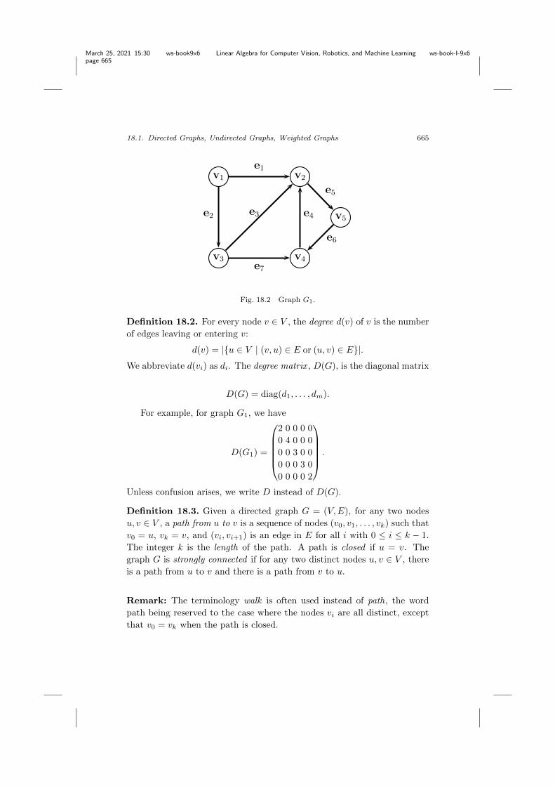
March 25, 2021 15:30 ws-book9x6 Linear Algebra for Computer Vision, Robotics, and Machine Learning ws-book-I-9x6
page 665
18.1. Directed Graphs, Undirected Graphs, Weighted Graphs 665
1
v4
v5
v1 v2
v3
e1
e7
e2 e3 e4
e5
e6
Fig. 18.2 Graph G1.
Definition 18.2. For every node v 2 V , the degree d(v) of v is the numberof edges leaving or entering v:
d(v) = |{u 2 V | (v, u) 2 E or (u, v) 2 E}|.
We abbreviate d(vi) as di. The degree matrix , D(G), is the diagonal matrix
D(G) = diag(d1
, . . . , dm).
For example, for graph G1
, we have
D(G1
) =
0
BBBB@
2 0 0 0 00 4 0 0 00 0 3 0 00 0 0 3 00 0 0 0 2
1
CCCCA.
Unless confusion arises, we write D instead of D(G).
Definition 18.3. Given a directed graph G = (V,E), for any two nodesu, v 2 V , a path from u to v is a sequence of nodes (v
0
, v1
, . . . , vk) such thatv0
= u, vk = v, and (vi, vi+1
) is an edge in E for all i with 0 i k � 1.The integer k is the length of the path. A path is closed if u = v. Thegraph G is strongly connected if for any two distinct nodes u, v 2 V , thereis a path from u to v and there is a path from v to u.
Remark: The terminology walk is often used instead of path, the wordpath being reserved to the case where the nodes vi are all distinct, exceptthat v
0
= vk when the path is closed.
March 25, 2021 15:30 ws-book9x6 Linear Algebra for Computer Vision, Robotics, and Machine Learning ws-book-I-9x6
page 666
666 Graphs and Graph Laplacians; Basic Facts
The binary relation on V ⇥V defined so that u and v are related i↵ thereis a path from u to v and there is a path from v to u is an equivalence relationwhose equivalence classes are called the strongly connected components ofG.
Definition 18.4. Given a directed graph G = (V,E), with V ={v
1
, . . . , vm}, if E = {e1
, . . . , en}, then the incidence matrix B(G) of Gis the m ⇥ n matrix whose entries bi j are given by
bi j =
8>><
>>:
+1 if s(ej) = vi
�1 if t(ej) = vi
0 otherwise.
Here is the incidence matrix of the graph G1
:
B =
0
BBBB@
1 1 0 0 0 0 0�1 0 �1 �1 1 0 00 �1 1 0 0 0 10 0 0 1 0 �1 �10 0 0 0 �1 1 0
1
CCCCA.
Observe that every column of an incidence matrix contains exactly twononzero entries, +1 and �1. Again, unless confusion arises, we write Binstead of B(G).
When a directed graph has m nodes v1
, . . . , vm and n edges e1
, . . . , en,a vector x 2 Rm can be viewed as a function x : V ! R assigning the valuexi to the node vi. Under this interpretation, Rm is viewed as RV . Similarly,a vector y 2 Rn can be viewed as a function in RE . This point of view isoften useful. For example, the incidence matrix B can be interpreted as alinear map from RE to RV , the boundary map, and B> can be interpretedas a linear map from RV to RE , the coboundary map.
Remark: Some authors adopt the opposite convention of sign in definingthe incidence matrix, which means that their incidence matrix is �B.
Undirected graphs are obtained from directed graphs by forgetting theorientation of the edges.
Definition 18.5. A graph (or undirected graph) is a pair G = (V,E), whereV = {v
1
, . . . , vm} is a set of nodes or vertices, and E is a set of two-elementsubsets of V (that is, subsets {u, v}, with u, v 2 V and u 6= v), called edges.

March 25, 2021 15:30 ws-book9x6 Linear Algebra for Computer Vision, Robotics, and Machine Learning ws-book-I-9x6
page 667
18.1. Directed Graphs, Undirected Graphs, Weighted Graphs 667
Remark: Since an edge is a set {u, v}, we have u 6= v, so self-loops are notallowed. Also, for every set of nodes {u, v}, there is at most one edge be-tween u and v. As in the case of directed graphs, such graphs are sometimescalled simple graphs.
An example of a graph is shown in Figure 18.3.
1
v4
v5
v1 v2
v3
a
g
b c d
e
f
Fig. 18.3 The undirected graph G2.
Definition 18.6. For every node v 2 V , the degree d(v) of v is the numberof edges incident to v:
d(v) = |{u 2 V | {u, v} 2 E}|.
The degree matrix D(G) (or simply, D) is defined as in Definition 18.2.
Definition 18.7. Given a (undirected) graph G = (V,E), for any twonodes u, v 2 V , a path from u to v is a sequence of nodes (v
0
, v1
, . . . , vk)such that v
0
= u, vk = v, and {vi, vi+1
} is an edge in E for all i with0 i k � 1. The integer k is the length of the path. A path is closedif u = v. The graph G is connected if for any two distinct nodes u, v 2 V ,there is a path from u to v.
Remark: The terminology walk or chain is often used instead of path, theword path being reserved to the case where the nodes vi are all distinct,except that v
0
= vk when the path is closed.The binary relation on V ⇥ V defined so that u and v are related i↵
there is a path from u to v is an equivalence relation whose equivalenceclasses are called the connected components of G.

March 25, 2021 15:30 ws-book9x6 Linear Algebra for Computer Vision, Robotics, and Machine Learning ws-book-I-9x6
page 668
668 Graphs and Graph Laplacians; Basic Facts
The notion of incidence matrix for an undirected graph is not as usefulas in the case of directed graphs
Definition 18.8. Given a graph G = (V,E), with V = {v1
, . . . , vm}, ifE = {e
1
, . . . , en}, then the incidence matrix B(G) of G is the m⇥n matrixwhose entries bi j are given by
bi j =
(+1 if ej = {vi, vk} for some k
0 otherwise.
Unlike the case of directed graphs, the entries in the incidence matrix ofa graph (undirected) are nonnegative. We usually write B instead of B(G).
Definition 18.9. If G = (V,E) is a directed or an undirected graph, givena node u 2 V , any node v 2 V such that there is an edge (u, v) in thedirected case or {u, v} in the undirected case is called adjacent to u, andwe often use the notation
u ⇠ v.
Observe that the binary relation ⇠ is symmetric whenG is an undirectedgraph, but in general it is not symmetric when G is a directed graph.
The notion of adjacency matrix is basically the same for directed orundirected graphs.
Definition 18.10. Given a directed or undirected graph G = (V,E), withV = {v
1
, . . . , vm}, the adjacency matrix A(G) of G is the symmetric m⇥mmatrix (ai j) such that
(1) If G is directed, then
ai j =
(1 if there is some edge (vi, vj) 2 E or some edge (vj , vi) 2 E
0 otherwise.
(2) Else if G is undirected, then
ai j =
(1 if there is some edge {vi, vj} 2 E
0 otherwise.
As usual, unless confusion arises, we write A instead of A(G). Here isthe adjacency matrix of both graphs G
1
and G2
:
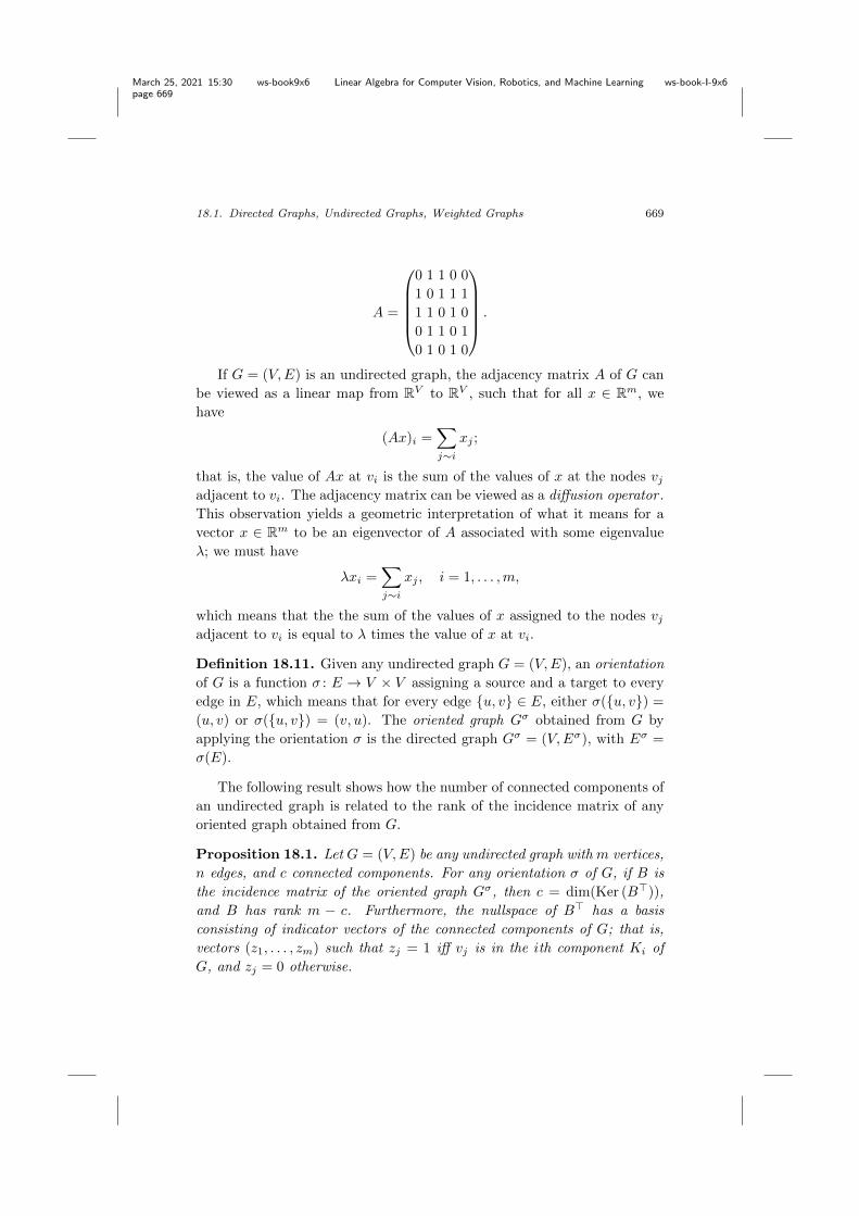
March 25, 2021 15:30 ws-book9x6 Linear Algebra for Computer Vision, Robotics, and Machine Learning ws-book-I-9x6
page 669
18.1. Directed Graphs, Undirected Graphs, Weighted Graphs 669
A =
0
BBBB@
0 1 1 0 01 0 1 1 11 1 0 1 00 1 1 0 10 1 0 1 0
1
CCCCA.
If G = (V,E) is an undirected graph, the adjacency matrix A of G canbe viewed as a linear map from RV to RV , such that for all x 2 Rm, wehave
(Ax)i =X
j⇠i
xj ;
that is, the value of Ax at vi is the sum of the values of x at the nodes vjadjacent to vi. The adjacency matrix can be viewed as a di↵usion operator .This observation yields a geometric interpretation of what it means for avector x 2 Rm to be an eigenvector of A associated with some eigenvalue�; we must have
�xi =X
j⇠i
xj , i = 1, . . . ,m,
which means that the the sum of the values of x assigned to the nodes vjadjacent to vi is equal to � times the value of x at vi.
Definition 18.11. Given any undirected graph G = (V,E), an orientationof G is a function � : E ! V ⇥ V assigning a source and a target to everyedge in E, which means that for every edge {u, v} 2 E, either �({u, v}) =(u, v) or �({u, v}) = (v, u). The oriented graph G� obtained from G byapplying the orientation � is the directed graph G� = (V,E�), with E� =�(E).
The following result shows how the number of connected components ofan undirected graph is related to the rank of the incidence matrix of anyoriented graph obtained from G.
Proposition 18.1. Let G = (V,E) be any undirected graph with m vertices,n edges, and c connected components. For any orientation � of G, if B isthe incidence matrix of the oriented graph G�, then c = dim(Ker (B>)),and B has rank m � c. Furthermore, the nullspace of B> has a basisconsisting of indicator vectors of the connected components of G; that is,vectors (z
1
, . . . , zm) such that zj = 1 i↵ vj is in the ith component Ki ofG, and zj = 0 otherwise.

March 25, 2021 15:30 ws-book9x6 Linear Algebra for Computer Vision, Robotics, and Machine Learning ws-book-I-9x6
page 670
670 Graphs and Graph Laplacians; Basic Facts
Proof. (After Godsil and Royle [Godsil and Royle (2001)], Section 8.3).The fact that rank(B) = m � c will be proved last.
Let us prove that the kernel of B> has dimension c. A vector z 2 Rm
belongs to the kernel of B> i↵ B>z = 0 i↵ z>B = 0. In view of thedefinition of B, for every edge {vi, vj} of G, the column of B correspondingto the oriented edge �({vi, vj}) has zero entries except for a +1 and a �1in position i and position j or vice-versa, so we have
zi = zj .
An easy induction on the length of the path shows that if there is a pathfrom vi to vj in G (unoriented), then zi = zj . Therefore, z has a constantvalue on any connected component of G. It follows that every vector z 2Ker (B>) can be written uniquely as a linear combination
z = �1
z1 + · · · + �czc,
where the vector zi corresponds to the ith connected component Ki of Gand is defined such that
zij =
(1 i↵ vj 2 Ki
0 otherwise.
This shows that dim(Ker (B>)) = c, and that Ker (B>) has a basis con-sisting of indicator vectors.
Since B> is a n ⇥ m matrix, we have
m = dim(Ker (B>)) + rank(B>),
and since we just proved that dim(Ker (B>)) = c, we obtain rank(B>) =m� c. Since B and B> have the same rank, rank(B) = m� c, as claimed.
Definition 18.12. Following common practice, we denote by 1 the (col-umn) vector (of dimension m) whose components are all equal to 1.
Since every column of B contains a single +1 and a single �1, the rowsof B> sum to zero, which can be expressed as
B>1 = 0.
According to Proposition 18.1, the graph G is connected i↵ B has rankm � 1 i↵ the nullspace of B> is the one-dimensional space spanned by 1.
In many applications, the notion of graph needs to be generalized tocapture the intuitive idea that two nodes u and v are linked with a degree

March 25, 2021 15:30 ws-book9x6 Linear Algebra for Computer Vision, Robotics, and Machine Learning ws-book-I-9x6
page 671
18.1. Directed Graphs, Undirected Graphs, Weighted Graphs 671
of certainty (or strength). Thus, we assign a nonnegative weight wi j toan edge {vi, vj}; the smaller wi j is, the weaker is the link (or similarity)between vi and vj , and the greater wi j is, the stronger is the link (orsimilarity) between vi and vj .
Definition 18.13. A weighted graph is a pair G = (V,W ), where V ={v
1
, . . . , vm} is a set of nodes or vertices, and W is a symmetric matrixcalled the weight matrix , such that wi j � 0 for all i, j 2 {1, . . . ,m}, andwi i = 0 for i = 1, . . . ,m. We say that a set {vi, vj} is an edge i↵ wi j > 0.The corresponding (undirected) graph (V,E) with E = {{vi, vj} | wi j > 0},is called the underlying graph of G.
Remark: Since wi i = 0, these graphs have no self-loops. We can think ofthe matrix W as a generalized adjacency matrix. The case where wi j 2{0, 1} is equivalent to the notion of a graph as in Definition 18.5.
We can think of the weight wi j of an edge {vi, vj} as a degree of sim-ilarity (or a�nity) in an image, or a cost in a network. An example of aweighted graph is shown in Figure 18.4. The thickness of an edge corre-sponds to the magnitude of its weight.
15
Encode Pairwise Relationships as a Weighted Graph
Fig. 18.4 A weighted graph.
Definition 18.14. Given a weighted graph G = (V,W ), for every node
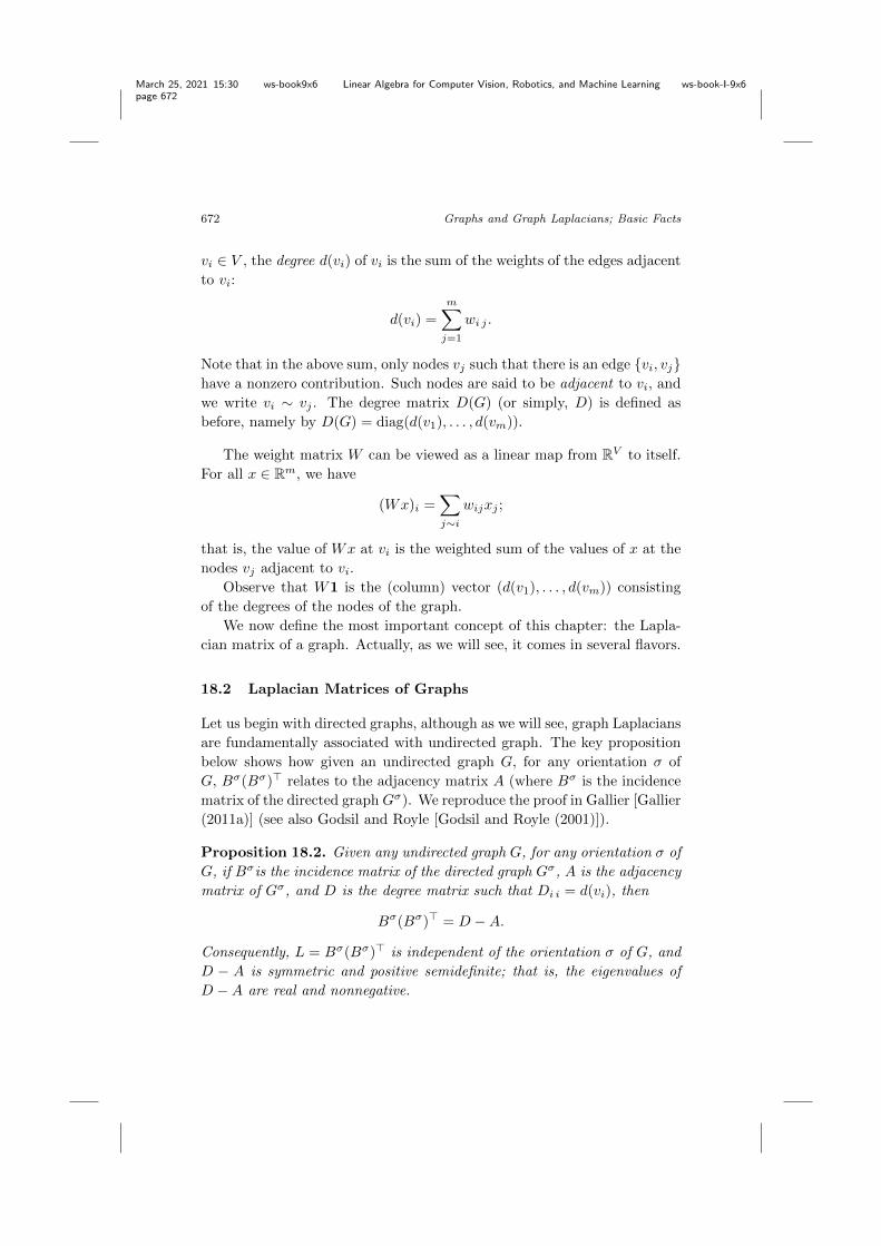
March 25, 2021 15:30 ws-book9x6 Linear Algebra for Computer Vision, Robotics, and Machine Learning ws-book-I-9x6
page 672
672 Graphs and Graph Laplacians; Basic Facts
vi 2 V , the degree d(vi) of vi is the sum of the weights of the edges adjacentto vi:
d(vi) =mX
j=1
wi j .
Note that in the above sum, only nodes vj such that there is an edge {vi, vj}have a nonzero contribution. Such nodes are said to be adjacent to vi, andwe write vi ⇠ vj . The degree matrix D(G) (or simply, D) is defined asbefore, namely by D(G) = diag(d(v
1
), . . . , d(vm)).
The weight matrix W can be viewed as a linear map from RV to itself.For all x 2 Rm, we have
(Wx)i =X
j⇠i
wijxj ;
that is, the value of Wx at vi is the weighted sum of the values of x at thenodes vj adjacent to vi.
Observe that W1 is the (column) vector (d(v1
), . . . , d(vm)) consistingof the degrees of the nodes of the graph.
We now define the most important concept of this chapter: the Lapla-cian matrix of a graph. Actually, as we will see, it comes in several flavors.
18.2 Laplacian Matrices of Graphs
Let us begin with directed graphs, although as we will see, graph Laplaciansare fundamentally associated with undirected graph. The key propositionbelow shows how given an undirected graph G, for any orientation � ofG, B�(B�)> relates to the adjacency matrix A (where B� is the incidencematrix of the directed graph G�). We reproduce the proof in Gallier [Gallier(2011a)] (see also Godsil and Royle [Godsil and Royle (2001)]).
Proposition 18.2. Given any undirected graph G, for any orientation � ofG, if B�is the incidence matrix of the directed graph G�, A is the adjacencymatrix of G�, and D is the degree matrix such that Di i = d(vi), then
B�(B�)> = D � A.
Consequently, L = B�(B�)> is independent of the orientation � of G, andD � A is symmetric and positive semidefinite; that is, the eigenvalues ofD � A are real and nonnegative.
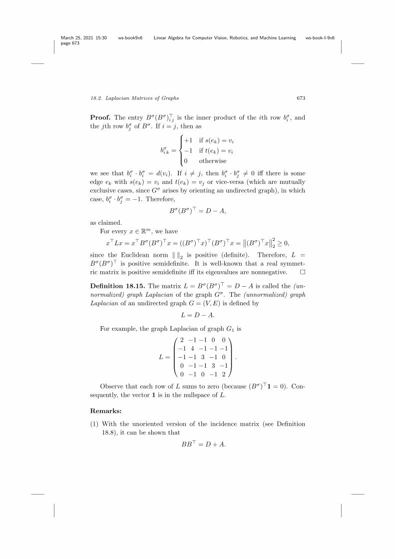
March 25, 2021 15:30 ws-book9x6 Linear Algebra for Computer Vision, Robotics, and Machine Learning ws-book-I-9x6
page 673
18.2. Laplacian Matrices of Graphs 673
Proof. The entry B�(B�)>i j is the inner product of the ith row b�i , andthe jth row b�j of B�. If i = j, then as
b�i k =
8>><
>>:
+1 if s(ek) = vi
�1 if t(ek) = vi
0 otherwise
we see that b�i · b�i = d(vi). If i 6= j, then b�i · b�j 6= 0 i↵ there is someedge ek with s(ek) = vi and t(ek) = vj or vice-versa (which are mutuallyexclusive cases, since G� arises by orienting an undirected graph), in whichcase, b�i · b�j = �1. Therefore,
B�(B�)> = D � A,
as claimed.For every x 2 Rm, we have
x>Lx = x>B�(B�)>x = ((B�)>x)>(B�)>x =��(B�)>x
��22
� 0,
since the Euclidean norm k k2
is positive (definite). Therefore, L =B�(B�)> is positive semidefinite. It is well-known that a real symmet-ric matrix is positive semidefinite i↵ its eigenvalues are nonnegative.
Definition 18.15. The matrix L = B�(B�)> = D � A is called the (un-normalized) graph Laplacian of the graph G�. The (unnormalized) graphLaplacian of an undirected graph G = (V,E) is defined by
L = D � A.
For example, the graph Laplacian of graph G1
is
L =
0
BBBB@
2 �1 �1 0 0�1 4 �1 �1 �1�1 �1 3 �1 00 �1 �1 3 �10 �1 0 �1 2
1
CCCCA.
Observe that each row of L sums to zero (because (B�)>1 = 0). Con-sequently, the vector 1 is in the nullspace of L.
Remarks:
(1) With the unoriented version of the incidence matrix (see Definition18.8), it can be shown that
BB> = D +A.

March 25, 2021 15:30 ws-book9x6 Linear Algebra for Computer Vision, Robotics, and Machine Learning ws-book-I-9x6
page 674
674 Graphs and Graph Laplacians; Basic Facts
(2) As pointed out by Evangelos Chatzipantazis, Proposition 18.2 in whichthe incidence matrix B� is replaced by the incidence matrix B of anyarbitrary directed graph G does not hold. The problem is that suchgraphs may have both edges (vi, vj) and (vj , vi) between two distinctnodes vi and vj , and as a consequence, the inner product bi · bj = �2instead of �1. A simple counterexample is given by the directed graphwith three vertices and four edges whose incidence matrix is given by
B =
0
@1 �1 0 �1
�1 1 �1 00 0 1 1
1
A .
We have
BB> =
0
@3 �2 �1
�2 3 �1�1 �1 2
1
A 6=
0
@3 0 00 3 00 0 2
1
A�
0
@0 1 11 0 11 1 0
1
A = D � A.
The natural generalization of the notion of graph Laplacian to weightedgraphs is this:
Definition 18.16. Given any weighted graph G = (V,W ) with V ={v
1
, . . . , vm}, the (unnormalized) graph Laplacian L(G) of G is defined by
L(G) = D(G) � W,
where D(G) = diag(d1
, . . . , dm) is the degree matrix of G (a diagonal ma-trix), with
di =mX
j=1
wi j .
As usual, unless confusion arises, we write D instead of D(G) and L insteadof L(G).
The graph Laplacian can be interpreted as a linear map from RV toitself. For all x 2 RV , we have
(Lx)i =X
j⇠i
wij(xi � xj).
It is clear from the equation L = D �W that each row of L sums to 0,so the vector 1 is the nullspace of L, but it is less obvious that L is positivesemidefinite. One way to prove it is to generalize slightly the notion ofincidence matrix.
Definition 18.17. Given a weighted graph G = (V,W ), with V ={v
1
, . . . , vm}, if {e1
, . . ., en} are the edges of the underlying graph of G
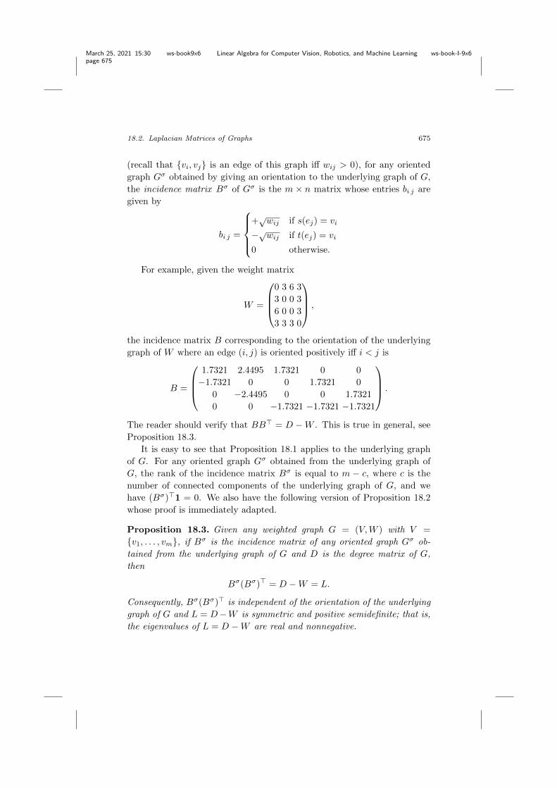
March 25, 2021 15:30 ws-book9x6 Linear Algebra for Computer Vision, Robotics, and Machine Learning ws-book-I-9x6
page 675
18.2. Laplacian Matrices of Graphs 675
(recall that {vi, vj} is an edge of this graph i↵ wij > 0), for any orientedgraph G� obtained by giving an orientation to the underlying graph of G,the incidence matrix B� of G� is the m ⇥ n matrix whose entries bi j aregiven by
bi j =
8>><
>>:
+pwij if s(ej) = vi
�pwij if t(ej) = vi
0 otherwise.
For example, given the weight matrix
W =
0
BB@
0 3 6 33 0 0 36 0 0 33 3 3 0
1
CCA ,
the incidence matrix B corresponding to the orientation of the underlyinggraph of W where an edge (i, j) is oriented positively i↵ i < j is
B =
0
BB@
1.7321 2.4495 1.7321 0 0�1.7321 0 0 1.7321 0
0 �2.4495 0 0 1.73210 0 �1.7321 �1.7321 �1.7321
1
CCA .
The reader should verify that BB> = D � W . This is true in general, seeProposition 18.3.
It is easy to see that Proposition 18.1 applies to the underlying graphof G. For any oriented graph G� obtained from the underlying graph ofG, the rank of the incidence matrix B� is equal to m � c, where c is thenumber of connected components of the underlying graph of G, and wehave (B�)>1 = 0. We also have the following version of Proposition 18.2whose proof is immediately adapted.
Proposition 18.3. Given any weighted graph G = (V,W ) with V ={v
1
, . . . , vm}, if B� is the incidence matrix of any oriented graph G� ob-tained from the underlying graph of G and D is the degree matrix of G,then
B�(B�)> = D � W = L.
Consequently, B�(B�)> is independent of the orientation of the underlyinggraph of G and L = D�W is symmetric and positive semidefinite; that is,the eigenvalues of L = D � W are real and nonnegative.

March 25, 2021 15:30 ws-book9x6 Linear Algebra for Computer Vision, Robotics, and Machine Learning ws-book-I-9x6
page 676
676 Graphs and Graph Laplacians; Basic Facts
Another way to prove that L is positive semidefinite is to evaluate thequadratic form x>Lx.
Proposition 18.4. For any m ⇥ m symmetric matrix W = (wij), if welet L = D � W where D is the degree matrix associated with W (that is,di =
Pmj=1
wij), then we have
x>Lx =1
2
mX
i,j=1
wi j(xi � xj)2 for all x 2 Rm.
Consequently, x>Lx does not depend on the diagonal entries in W , and ifwi j � 0 for all i, j 2 {1, . . . ,m}, then L is positive semidefinite.
Proof. We have
x>Lx = x>Dx � x>Wx
=mX
i=1
dix2
i �mX
i,j=1
wi jxixj
=1
2
0
@mX
i=1
dix2
i � 2mX
i,j=1
wi jxixj +mX
i=1
dix2
i
1
A
=1
2
mX
i,j=1
wi j(xi � xj)2.
Obviously, the quantity on the right-hand side does not depend on thediagonal entries in W , and if wi j � 0 for all i, j, then this quantity isnonnegative.
Proposition 18.4 immediately implies the following facts: For anyweighted graph G = (V,W ),
(1) The eigenvalues 0 = �1
�2
. . . �m of L are real and nonnegative,and there is an orthonormal basis of eigenvectors of L.
(2) The smallest eigenvalue �1
of L is equal to 0, and 1 is a correspondingeigenvector.
It turns out that the dimension of the nullspace of L (the eigenspace of0) is equal to the number of connected components of the underlying graphof G.
Proposition 18.5. Let G = (V,W ) be a weighted graph. The number cof connected components K
1
, . . . ,Kc of the underlying graph of G is equal

March 25, 2021 15:30 ws-book9x6 Linear Algebra for Computer Vision, Robotics, and Machine Learning ws-book-I-9x6
page 677
18.3. Normalized Laplacian Matrices of Graphs 677
to the dimension of the nullspace of L, which is equal to the multiplicityof the eigenvalue 0. Furthermore, the nullspace of L has a basis consist-ing of indicator vectors of the connected components of G, that is, vectors(f
1
, . . . , fm) such that fj = 1 i↵ vj 2 Ki and fj = 0 otherwise.
Proof. Since L = BB> for the incidence matrix B associated with any ori-ented graph obtained from G, and since L and B> have the same nullspace,by Proposition 18.1, the dimension of the nullspace of L is equal to thenumber c of connected components of G and the indicator vectors of theconnected components of G form a basis of Ker (L).
Proposition 18.5 implies that if the underlying graph of G is connected,then the second eigenvalue �
2
of L is strictly positive.Remarkably, the eigenvalue �
2
contains a lot of information about thegraph G (assuming that G = (V,E) is an undirected graph). This was firstdiscovered by Fiedler in 1973, and for this reason, �
2
is often referred toas the Fiedler number . For more on the properties of the Fiedler number,see Godsil and Royle [Godsil and Royle (2001)] (Chapter 13) and Chung[Chung (1997)]. More generally, the spectrum (0,�
2
, . . . ,�m) of L containsa lot of information about the combinatorial structure of the graph G.Leverage of this information is the object of spectral graph theory .
18.3 Normalized Laplacian Matrices of Graphs
It turns out that normalized variants of the graph Laplacian are needed,especially in applications to graph clustering. These variants make senseonly if G has no isolated vertices.
Definition 18.18. Given a weighted graph G = (V,W ), a vertex u 2 V isisolated if it is not incident to any other vertex. This means that every rowof W contains some strictly positive entry.
If G has no isolated vertices, then the degree matrix D contains positiveentries, so it is invertible and D�1/2 makes sense; namely
D�1/2 = diag(d�1/21
, . . . , d�1/2m ),
and similarly for any real exponent ↵.
Definition 18.19. Given any weighted directed graph G = (V,W ) with noisolated vertex and with V = {v
1
, . . . , vm}, the (normalized) graph Lapla-

March 25, 2021 15:30 ws-book9x6 Linear Algebra for Computer Vision, Robotics, and Machine Learning ws-book-I-9x6
page 678
678 Graphs and Graph Laplacians; Basic Facts
cians Lsym
and Lrw
of G are defined by
Lsym
= D�1/2LD�1/2 = I � D�1/2WD�1/2
Lrw
= D�1L = I � D�1W.
Observe that the Laplacian Lsym
= D�1/2LD�1/2 is a symmetric matrix(because L and D�1/2 are symmetric) and that
Lrw
= D�1/2Lsym
D1/2.
The reason for the notation Lrw
is that this matrix is closely related to arandom walk on the graph G.
Example 18.1. As an example, the matrices Lsym
and Lrw
associated withthe graph G
1
are
Lsym
=
0
BBBB@
1.0000 �0.3536 �0.4082 0 0�0.3536 1.0000 �0.2887 �0.2887 �0.3536�0.4082 �0.2887 1.0000 �0.3333 0
0 �0.2887 �0.3333 1.0000 �0.40820 �0.3536 0 �0.4082 1.0000
1
CCCCA
and
Lrw
=
0
BBBB@
1.0000 �0.5000 �0.5000 0 0�0.2500 1.0000 �0.2500 �0.2500 �0.2500�0.3333 �0.3333 1.0000 �0.3333 0
0 �0.3333 �0.3333 1.0000 �0.33330 �0.5000 0 �0.5000 1.0000
1
CCCCA.
Since the unnormalized Laplacian L can be written as L = BB>, whereB is the incidence matrix of any oriented graph obtained from the under-lying graph of G = (V,W ), if we let
Bsym
= D�1/2B,
we get
Lsym
= Bsym
B>sym
.
In particular, for any singular decomposition Bsym
= U⌃V > of Bsym
(withU an m ⇥ m orthogonal matrix, ⌃ a “diagonal” m ⇥ n matrix of singularvalues, and V an n ⇥ n orthogonal matrix), the eigenvalues of L
sym
arethe squares of the top m singular values of B
sym
, and the vectors in Uare orthonormal eigenvectors of L
sym
with respect to these eigenvalues (thesquares of the top m diagonal entries of ⌃). Computing the SVD of B
sym

March 25, 2021 15:30 ws-book9x6 Linear Algebra for Computer Vision, Robotics, and Machine Learning ws-book-I-9x6
page 679
18.3. Normalized Laplacian Matrices of Graphs 679
generally yields more accurate results than diagonalizing Lsym
, especiallywhen L
sym
has eigenvalues with high multiplicity.There are simple relationships between the eigenvalues and the eigen-
vectors of Lsym
, and Lrw
. There is also a simple relationship with thegeneralized eigenvalue problem Lx = �Dx.
Proposition 18.6. Let G = (V,W ) be a weighted graph without isolatedvertices. The graph Laplacians, L,L
sym
, and Lrw
satisfy the following prop-erties:
(1) The matrix Lsym
is symmetric and positive semidefinite. In fact,
x>Lsym
x =1
2
mX
i,j=1
wi j
xipdi
� xjpdj
!2
for all x 2 Rm.
(2) The normalized graph Laplacians Lsym
and Lrw
have the same spectrum(0 = ⌫
1
⌫2
. . . ⌫m), and a vector u 6= 0 is an eigenvector of Lrw
for � i↵ D1/2u is an eigenvector of Lsym
for �.(3) The graph Laplacians L and L
sym
are symmetric and positive semidef-inite.
(4) A vector u 6= 0 is a solution of the generalized eigenvalue problemLu = �Du i↵ D1/2u is an eigenvector of L
sym
for the eigenvalue � i↵u is an eigenvector of L
rw
for the eigenvalue �.(5) The graph Laplacians, L and L
rw
have the same nullspace. For anyvector u, we have u 2 Ker (L) i↵ D1/2u 2 Ker (L
sym
).(6) The vector 1 is in the nullspace of L
rw
, and D1/21 is in the nullspaceof L
sym
.(7) For every eigenvalue ⌫i of the normalized graph Laplacian L
sym
, wehave 0 ⌫i 2. Furthermore, ⌫m = 2 i↵ the underlying graph of Gcontains a nontrivial connected bipartite component.
(8) If m � 2 and if the underlying graph of G is not a complete graph,1
then ⌫2
1. Furthermore the underlying graph of G is a completegraph i↵ ⌫
2
= mm�1
.(9) If m � 2 and if the underlying graph of G is connected, then ⌫
2
> 0.(10) If m � 2 and if the underlying graph of G has no isolated vertices, then
⌫m � mm�1
.
Proof. (1) We have Lsym
= D�1/2LD�1/2, and D�1/2 is a symmet-ric invertible matrix (since it is an invertible diagonal matrix). It is a1Recall that an undirected graph is complete if for any two distinct nodes u, v, there is
an edge {u, v}.

March 25, 2021 15:30 ws-book9x6 Linear Algebra for Computer Vision, Robotics, and Machine Learning ws-book-I-9x6
page 680
680 Graphs and Graph Laplacians; Basic Facts
well-known fact of linear algebra that if B is an invertible matrix, thena matrix S is symmetric, positive semidefinite i↵ BSB> is symmetric,positive semidefinite. Since L is symmetric, positive semidefinite, so isLsym
= D�1/2LD�1/2. The formula
x>Lsym
x =1
2
mX
i,j=1
wi j
xipdi
� xjpdj
!2
for all x 2 Rm
follows immediately from Proposition 18.4 by replacing x by D�1/2x, andalso shows that L
sym
is positive semidefinite.(2) Since
Lrw
= D�1/2Lsym
D1/2,
the matrices Lsym
and Lrw
are similar, which implies that they have thesame spectrum. In fact, since D1/2 is invertible,
Lrw
u = D�1Lu = �u
i↵
D�1/2Lu = �D1/2u
i↵
D�1/2LD�1/2D1/2u = Lsym
D1/2u = �D1/2u,
which shows that a vector u 6= 0 is an eigenvector of Lrw
for � i↵ D1/2u isan eigenvector of L
sym
for �.(3) We already know that L and L
sym
are positive semidefinite.(4) Since D�1/2 is invertible, we have
Lu = �Du
i↵
D�1/2Lu = �D1/2u
i↵
D�1/2LD�1/2D1/2u = Lsym
D1/2u = �D1/2u,
which shows that a vector u 6= 0 is a solution of the generalized eigenvalueproblem Lu = �Du i↵ D1/2u is an eigenvector of L
sym
for the eigenvalue�. The second part of the statement follows from (2).
(5) SinceD�1 is invertible, we have Lu = 0 i↵D�1Lu = Lrw
u = 0. Sim-ilarly, since D�1/2 is invertible, we have Lu = 0 i↵ D�1/2LD�1/2D1/2u = 0i↵ D1/2u 2 Ker (L
sym
).(6) Since L1 = 0, we get L
rw
1 = D�1L1 = 0. That D1/21 is in thenullspace of L
sym
follows from (2). Properties (7)–(10) are proven in Chung[Chung (1997)] (Chapter 1).

March 25, 2021 15:30 ws-book9x6 Linear Algebra for Computer Vision, Robotics, and Machine Learning ws-book-I-9x6
page 681
18.4. Graph Clustering Using Normalized Cuts 681
The eigenvalues the matrices Lsym
and Lrw
from Example 18.1 are
0, 7257, 1.1667, 1.5, 1.6076.
On the other hand, the eigenvalues of the unnormalized Laplacian for G1
are
0, 1.5858, 3, 4.4142, 5.
Remark: Observe that although the matrices Lsym
and Lrw
have the samespectrum, the matrix L
rw
is generally not symmetric, whereas Lsym
is sym-metric.
A version of Proposition 18.5 also holds for the graph Laplacians Lsym
and Lrw
. This follows easily from the fact that Proposition 18.1 applies tothe underlying graph of a weighted graph. The proof is left as an exercise.
Proposition 18.7. Let G = (V,W ) be a weighted graph. The number c ofconnected components K
1
, . . . ,Kc of the underlying graph of G is equal tothe dimension of the nullspace of both L
sym
and Lrw
, which is equal to themultiplicity of the eigenvalue 0. Furthermore, the nullspace of L
rw
has abasis consisting of indicator vectors of the connected components of G, thatis, vectors (f
1
, . . . , fm) such that fj = 1 i↵ vj 2 Ki and fj = 0 otherwise.For L
sym
, a basis of the nullpace is obtained by multiplying the above basisof the nullspace of L
rw
by D1/2.
A particularly interesting application of graph Laplacians is graph clus-tering.
18.4 Graph Clustering Using Normalized Cuts
In order to explain this problem we need some definitions.
Definition 18.20. Given any subset of nodes A ✓ V , we define the volumevol(A) of A as the sum of the weights of all edges adjacent to nodes in A:
vol(A) =X
vi2A
mX
j=1
wi j .
Given any two subsets A,B ✓ V (not necessarily distinct), we definelinks(A,B) by
links(A,B) =X
vi2A,vj2B
wi j .

March 25, 2021 15:30 ws-book9x6 Linear Algebra for Computer Vision, Robotics, and Machine Learning ws-book-I-9x6
page 682
682 Graphs and Graph Laplacians; Basic Facts
The quantity links(A,A) = links(A,A) (where A = V � A denotes thecomplement of A in V ) measures how many links escape from A (and A).We define the cut of A as
cut(A) = links(A,A).
The notion of volume is illustrated in Figure 18.5 and the notions of cutis illustrated in Figure 18.6.
Fig. 18.5 Volume of a set of nodes.
Fig. 18.6 A cut involving the set of nodes in the center and the nodes on the perimeter.
The above concepts play a crucial role in the theory of normalized cuts.

March 25, 2021 15:30 ws-book9x6 Linear Algebra for Computer Vision, Robotics, and Machine Learning ws-book-I-9x6
page 683
18.4. Graph Clustering Using Normalized Cuts 683
This beautiful and deeply original method first published in Shi and Ma-lik [Shi and Malik (2000)], has now come to be a “textbook chapter” ofcomputer vision and machine learning. It was invented by Jianbo Shi andJitendra Malik and was the main topic of Shi’s dissertation. This methodwas extended to K � 3 clusters by Stella Yu in her dissertation [Yu (2003)]and is also the subject of Yu and Shi [Yu and Shi (2003)].
Given a set of data, the goal of clustering is to partition the data intodi↵erent groups according to their similarities. When the data is given interms of a similarity graph G, where the weight wi j between two nodes viand vj is a measure of similarity of vi and vj , the problem can be stated asfollows: Find a partition (A
1
, . . . , AK) of the set of nodes V into di↵erentgroups such that the edges between di↵erent groups have very low weight(which indicates that the points in di↵erent clusters are dissimilar), and theedges within a group have high weight (which indicates that points withinthe same cluster are similar).
The above graph clustering problem can be formalized as an optimiza-tion problem, using the notion of cut mentioned earlier. If we want to par-tition V into K clusters, we can do so by finding a partition (A
1
, . . . , AK)that minimizes the quantity
cut(A1
, . . . , AK) =1
2
KX
i=1
cut(Ai) =1
2
KX
i=1
links(Ai, Ai).
For K = 2, the mincut problem is a classical problem that can be solvede�ciently, but in practice, it does not yield satisfactory partitions. Indeed,in many cases, the mincut solution separates one vertex from the rest ofthe graph. What we need is to design our cost function in such a way thatit keeps the subsets Ai “reasonably large” (reasonably balanced).
An example of a weighted graph and a partition of its nodes into twoclusters is shown in Figure 18.7.
A way to get around this problem is to normalize the cuts by dividingby some measure of each subset Ai. A solution using the volume vol(Ai)of Ai (for K = 2) was proposed and investigated in a seminal paper of Shiand Malik [Shi and Malik (2000)]. Subsequently, Yu (in her dissertation[Yu (2003)]) and Yu and Shi [Yu and Shi (2003)] extended the method toK > 2 clusters. The idea is to minimize the cost function
Ncut(A1
, . . . , AK) =KX
i=1
links(Ai, Ai)
vol(Ai)=
KX
i=1
cut(Ai)
vol(Ai).
The next step is to express our optimization problem in matrix form, andthis can be done in terms of Rayleigh ratios involving the graph Laplacian
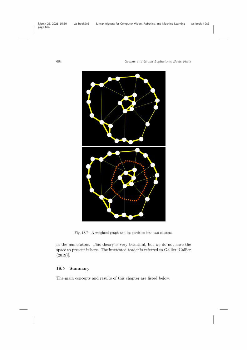
March 25, 2021 15:30 ws-book9x6 Linear Algebra for Computer Vision, Robotics, and Machine Learning ws-book-I-9x6
page 684
684 Graphs and Graph Laplacians; Basic Facts
15
Encode Pairwise Relationships as a Weighted Graph
16
Cut the graph into two pieces
Fig. 18.7 A weighted graph and its partition into two clusters.
in the numerators. This theory is very beautiful, but we do not have thespace to present it here. The interested reader is referred to Gallier [Gallier(2019)].
18.5 Summary
The main concepts and results of this chapter are listed below:

March 25, 2021 15:30 ws-book9x6 Linear Algebra for Computer Vision, Robotics, and Machine Learning ws-book-I-9x6
page 685
18.6. Problems 685
• Directed graphs, undirected graphs.• Incidence matrices, adjacency matrices.• Weighted graphs.• Degree matrix.• Graph Laplacian (unnormalized).• Normalized graph Laplacian.• Spectral graph theory.• Graph clustering using normalized cuts.
18.6 Problems
Problem 18.1. Find the unnormalized Laplacian of the graph representinga triangle and of the graph representing a square.
Problem 18.2. Consider the complete graph Km on m � 2 nodes.(1) Prove that the normalized Laplacian L
sym
of K is
Lsym
=
0
BBBBB@
1 �1/(m � 1) . . . �1/(m � 1) �1/(m � 1)�1/(m � 1) 1 . . . �1/(m � 1) �1/(m � 1)
.... . .
. . .. . .
...�1/(m � 1) �1/(m � 1) . . . 1 �1/(m � 1)�1/(m � 1) �1/(m � 1) . . . �1/(m � 1) 1
1
CCCCCA.
(2) Prove that the characteristic polynomial of Lsym
is�����������
�� 1 1/(m � 1) . . . 1/(m � 1) 1/(m � 1)1/(m � 1) �� 1 . . . 1/(m � 1) 1/(m � 1)
.... . .
. . .. . .
...1/(m � 1) 1/(m � 1) . . . �� 1 1/(m � 1)1/(m � 1) 1/(m � 1) . . . 1/(m � 1) �� 1
�����������
= �
✓�� m
m � 1
◆m�1
.
Hint . First subtract the second column from the first, factor ��m/(m�1),and then add the first row to the second. Repeat this process. You willend up with the determinant
������ 1/(m � 1) 11/(m � 1) �� 1
���� .
Problem 18.3. Consider the complete bipartite graph Km,n on m+n � 3nodes, with edges between each of the first m � 1 nodes to each of the lastn � 1 nodes. Prove that the eigenvalues of the normalized Laplacian L
sym
of Km,n are 0, 1 with multiplicity m+ n � 2, and 2.

March 25, 2021 15:30 ws-book9x6 Linear Algebra for Computer Vision, Robotics, and Machine Learning ws-book-I-9x6
page 686
686 Graphs and Graph Laplacians; Basic Facts
Problem 18.4. Let G be a graph with a set of nodes V with m � 2elements, without isolated nodes, and let L
sym
= D�1/2LD�1/2 be itsnormalized Laplacian (with L its unnormalized Laplacian).
(1) For any y 2 RV , consider the Rayleigh ratio
R =y>L
sym
y
y>y.
Prove that if x = D�1/2y, then
R =x>Lx
(D1/2x)>D1/2x=
X
u⇠v
(x(u) � x(v))2
X
v
dvx(v)2
.
(2) Prove that the second eigenvalue ⌫2
of Lsym
is given by
⌫2
= min1>Dx=0,x 6=0
X
u⇠v
(x(u) � x(v))2
X
v
dvx(v)2
.
(3) Prove that the largest eigenvalue ⌫m of Lsym
is given by
⌫m = maxx 6=0
X
u⇠v
(x(u) � x(v))2
X
v
dvx(v)2
.
Problem 18.5. Let G be a graph with a set of nodes V with m � 2elements, without isolated nodes. If 0 = ⌫
1
⌫1
. . . ⌫m are theeigenvalues of L
sym
, prove the following properties:
(1) We have ⌫1
+ ⌫2
+ · · · + ⌫m = m.(2) We have ⌫
2
m/(m � 1), with equality holding i↵ G = Km, thecomplete graph on m nodes.
(3) We have ⌫m � m/(m � 1).(4) If G is not a complete graph, then ⌫
2
1Hint . If a and b are nonadjacent nodes, consider the function x givenby
x(v) =
8>><
>>:
db if v = a
�da if v = b
0 if v 6= a, b,
and use Problem 18.4(2).

March 25, 2021 15:30 ws-book9x6 Linear Algebra for Computer Vision, Robotics, and Machine Learning ws-book-I-9x6
page 687
18.6. Problems 687
(5) Prove that ⌫m 2. Prove that ⌫m = 2 i↵ the underlying graph of Gcontains a nontrivial connected bipartite component.Hint . Use Problem 18.4(3).
(6) Prove that if G is connected, then ⌫2
> 0.
Problem 18.6. Let G be a graph with a set of nodes V with m � 2elements, without isolated nodes. Let vol(G) =
Pv2V dv and let
x =
Pv dvx(v)
vol(G).
Prove that
⌫2
= minx 6=0
X
u⇠v
(x(u) � x(v))2
X
v
dv(x(v) � x)2.
Problem 18.7. Let G be a connected bipartite graph. Prove that if ⌫ isan eigenvalue of L
sym
, then 2 � ⌫ is also an eigenvalue of Lsym
.
Problem 18.8. Prove Proposition 18.7.

March 25, 2021 15:30 ws-book9x6 Linear Algebra for Computer Vision, Robotics, and Machine Learning ws-book-I-9x6
page 688

March 25, 2021 15:30 ws-book9x6 Linear Algebra for Computer Vision, Robotics, and Machine Learning ws-book-I-9x6
page 689
Chapter 19
Spectral Graph Drawing
19.1 Graph Drawing and Energy Minimization
Let G = (V,E) be some undirected graph. It is often desirable to drawa graph, usually in the plane but possibly in 3D, and it turns out thatthe graph Laplacian can be used to design surprisingly good methods. Say|V | = m. The idea is to assign a point ⇢(vi) in Rn to the vertex vi 2 V ,for every vi 2 V , and to draw a line segment between the points ⇢(vi) and⇢(vj) i↵ there is an edge {vi, vj}.
Definition 19.1. Let G = (V,E) be some undirected graph with mvertices. A graph drawing is a function ⇢ : V ! Rn, for some n � 1. Thematrix of a graph drawing ⇢ (in Rn) is a m ⇥ n matrix R whose ith rowconsists of the row vector ⇢(vi) corresponding to the point representing viin Rn.
For a graph drawing to be useful we want n m; in fact n should bemuch smaller than m, typically n = 2 or n = 3.
Definition 19.2. A graph drawing is balanced i↵ the sum of the entries ofevery column of the matrix of the graph drawing is zero, that is,
1>R = 0.
If a graph drawing is not balanced, it can be made balanced by a suitabletranslation. We may also assume that the columns of R are linearly inde-pendent, since any basis of the column space also determines the drawing.Thus, from now on, we may assume that n m.
Remark: A graph drawing ⇢ : V ! Rn is not required to be injective,which may result in degenerate drawings where distinct vertices are drawn
689

March 25, 2021 15:30 ws-book9x6 Linear Algebra for Computer Vision, Robotics, and Machine Learning ws-book-I-9x6
page 690
690 Spectral Graph Drawing
as the same point. For this reason, we prefer not to use the terminologygraph embedding , which is often used in the literature. This is because indi↵erential geometry, an embedding always refers to an injective map. Theterm graph immersion would be more appropriate.
As explained in Godsil and Royle [Godsil and Royle (2001)], we canimagine building a physical model of G by connecting adjacent vertices (inRn) by identical springs. Then it is natural to consider a representation tobe better if it requires the springs to be less extended. We can formalizethis by defining the energy of a drawing R by
E(R) =X
{vi,vj}2E
k⇢(vi) � ⇢(vj)k2 ,
where ⇢(vi) is the ith row of R and k⇢(vi) � ⇢(vj)k2 is the square of theEuclidean length of the line segment joining ⇢(vi) and ⇢(vj).
Then, “good drawings” are drawings that minimize the energy functionE . Of course, the trivial representation corresponding to the zero matrixis optimum, so we need to impose extra constraints to rule out the trivialsolution.
We can consider the more general situation where the springs are notnecessarily identical. This can be modeled by a symmetric weight (or sti↵-ness) matrix W = (wij), with wij � 0. Then our energy function becomes
E(R) =X
{vi,vj}2E
wij k⇢(vi) � ⇢(vj)k2 .
It turns out that this function can be expressed in terms of the LaplacianL = D�W . The following proposition is shown in Godsil and Royle [Godsiland Royle (2001)]. We give a slightly more direct proof.
Proposition 19.1. Let G = (V,W ) be a weighted graph, with |V | = mand W an m ⇥ m symmetric matrix, and let R be the matrix of a graphdrawing ⇢ of G in Rn (a m⇥n matrix). If L = D�W is the unnormalizedLaplacian matrix associated with W , then
E(R) = tr(R>LR).
Proof. Since ⇢(vi) is the ith row of R (and ⇢(vj) is the jth row of R), if

March 25, 2021 15:30 ws-book9x6 Linear Algebra for Computer Vision, Robotics, and Machine Learning ws-book-I-9x6
page 691
19.1. Graph Drawing and Energy Minimization 691
we denote the kth column of R by Rk, using Proposition 18.4, we have
E(R) =X
{vi,vj}2E
wij k⇢(vi) � ⇢(vj)k2
=nX
k=1
X
{vi,vj}2E
wij(Rik � Rjk)2
=nX
k=1
1
2
mX
i,j=1
wij(Rik � Rjk)2
=nX
k=1
(Rk)>LRk = tr(R>LR),
as claimed.
Since the matrix R>LR is symmetric, it has real eigenvalues. Actually,since L is positive semidefinite, so is R>LR. Then the trace of R>LR isequal to the sum of its positive eigenvalues, and this is the energy E(R) ofthe graph drawing.
If R is the matrix of a graph drawing in Rn, then for any n⇥n invertiblematrix M , the map that assigns ⇢(vi)M to vi is another graph drawing ofG, and these two drawings convey the same amount of information. Fromthis point of view, a graph drawing is determined by the column space of R.Therefore, it is reasonable to assume that the columns of R are pairwiseorthogonal and that they have unit length. Such a matrix satisfies theequation R>R = I.
Definition 19.3. If the matrix R of a graph drawing satisfies the equationR>R = I, then the corresponding drawing is called an orthogonal graphdrawing .
This above condition also rules out trivial drawings. The following resulttells us how to find minimum energy orthogonal balanced graph drawings,provided the graph is connected. Recall that
L1 = 0,
as we already observed.
Theorem 19.1. Let G = (V,W ) be a weighted graph with |V | = m. IfL = D � W is the (unnormalized) Laplacian of G, and if the eigenvaluesof L are 0 = �
1
< �2
�3
. . . �m, then the minimal energy of anybalanced orthogonal graph drawing of G in Rn is equal to �
2
+ · · · + �n+1

March 25, 2021 15:30 ws-book9x6 Linear Algebra for Computer Vision, Robotics, and Machine Learning ws-book-I-9x6
page 692
692 Spectral Graph Drawing
(in particular, this implies that n < m). The m ⇥ n matrix R consistingof any unit eigenvectors u
2
, . . . , un+1
associated with �2
. . . �n+1
yields a balanced orthogonal graph drawing of minimal energy; it satisfiesthe condition R>R = I.
Proof. We present the proof given in Godsil and Royle [Godsil and Royle(2001)] (Section 13.4, Theorem 13.4.1). The key point is that the sum ofthe n smallest eigenvalues of L is a lower bound for tr(R>LR). This can beshown using a Rayleigh ratio argument; see Proposition 16.13 (the Poincareseparation theorem). Then any n eigenvectors (u
1
, . . . , un) associated with�1
, . . . ,�n achieve this bound. Because the first eigenvalue of L is �1
= 0and because we are assuming that �
2
> 0, we have u1
= 1/pm. Since the
uj are pairwise orthogonal for i = 2, . . . , n and since ui is orthogonal tou1
= 1/pm, the entries in ui add up to 0. Consequently, for any ` with
2 ` n, by deleting u1
and using (u2
, . . . , u`), we obtain a balancedorthogonal graph drawing in R`�1 with the same energy as the orthogonalgraph drawing in R` using (u
1
, u2
, . . . , u`). Conversely, from any balancedorthogonal drawing in R`�1 using (u
2
, . . . , u`), we obtain an orthogonalgraph drawing in R` using (u
1
, u2
, . . . , u`) with the same energy. Therefore,the minimum energy of a balanced orthogonal graph drawing in Rn is equalto the minimum energy of an orthogonal graph drawing in Rn+1, and thisminimum is �
2
+ · · · + �n+1
.
Since 1 spans the nullspace of L, using u1
(which belongs to KerL) asone of the vectors in R would have the e↵ect that all points representingvertices of G would have the same first coordinate. This would mean thatthe drawing lives in a hyperplane in Rn, which is undesirable, especiallywhen n = 2, where all vertices would be collinear. This is why we omit thefirst eigenvector u
1
.Observe that for any orthogonal n ⇥ n matrix Q, since
tr(R>LR) = tr(Q>R>LRQ),
the matrix RQ also yields a minimum orthogonal graph drawing. Thisamounts to applying the rigid motion Q> to the rows of R.
In summary, if �2
> 0, an automatic method for drawing a graph in R2
is this:
(1) Compute the two smallest nonzero eigenvalues �2
�3
of the graphLaplacian L (it is possible that �
3
= �2
if �2
is a multiple eigenvalue);(2) Compute two unit eigenvectors u
2
, u3
associated with �2
and �3
, andlet R = [u
2
u3
] be the m ⇥ 2 matrix having u2
and u3
as columns.

March 25, 2021 15:30 ws-book9x6 Linear Algebra for Computer Vision, Robotics, and Machine Learning ws-book-I-9x6
page 693
19.2. Examples of Graph Drawings 693
(3) Place vertex vi at the point whose coordinates is the ith row of R, thatis, (Ri1, Ri2).
This method generally gives pleasing results, but beware that there isno guarantee that distinct nodes are assigned distinct images since R canhave identical rows. This does not seem to happen often in practice.
19.2 Examples of Graph Drawings
We now give a number of examples using Matlab. Some of these are bor-rowed or adapted from Spielman [Spielman (2012)].
Example 1. Consider the graph with four nodes whose adjacency matrixis
A =
0
BB@
0 1 1 01 0 0 11 0 0 10 1 1 0
1
CCA .
We use the following program to compute u2
and u3
:
A = [0 1 1 0; 1 0 0 1; 1 0 0 1; 0 1 1 0];
D = diag(sum(A));
L = D - A;
[v, e] = eigs(L);
gplot(A, v(:,[3 2]))
hold on;
gplot(A, v(:,[3 2]),’o’)
The graph of Example 1 is shown in Figure 19.1. The function eigs(L)
computes the six largest eigenvalues of L in decreasing order, and corre-sponding eigenvectors. It turns out that �
2
= �3
= 2 is a double eigenvalue.Example 2. Consider the graph G
2
shown in Figure 18.3 given by theadjacency matrix
A =
0
BBBB@
0 1 1 0 01 0 1 1 11 1 0 1 00 1 1 0 10 1 0 1 0
1
CCCCA.
We use the following program to compute u2
and u3
:

March 25, 2021 15:30 ws-book9x6 Linear Algebra for Computer Vision, Robotics, and Machine Learning ws-book-I-9x6
page 694
694 Spectral Graph Drawing
−0.8 −0.6 −0.4 −0.2 0 0.2 0.4 0.6 0.8−0.8
−0.6
−0.4
−0.2
0
0.2
0.4
0.6
0.8
Fig. 19.1 Drawing of the graph from Example 1.
A = [0 1 1 0 0; 1 0 1 1 1; 1 1 0 1 0; 0 1 1 0 1; 0 1 0 1 0];
D = diag(sum(A));
L = D - A;
[v, e] = eig(L);
gplot(A, v(:, [2 3]))
hold on
gplot(A, v(:, [2 3]),’o’)
The function eig(L) (with no s at the end) computes the eigenvalues ofL in increasing order. The result of drawing the graph is shown in Figure19.2. Note that node v
2
is assigned to the point (0, 0), so the di↵erencebetween this drawing and the drawing in Figure 18.3 is that the drawingof Figure 19.2 is not convex.
Example 3. Consider the ring graph defined by the adjacency matrix Agiven in the Matlab program shown below:
A = diag(ones(1, 11),1);
A = A + A’;
A(1, 12) = 1; A(12, 1) = 1;
D = diag(sum(A));
L = D - A;
[v, e] = eig(L);
gplot(A, v(:, [2 3]))
hold on

March 25, 2021 15:30 ws-book9x6 Linear Algebra for Computer Vision, Robotics, and Machine Learning ws-book-I-9x6
page 695
19.2. Examples of Graph Drawings 695
−0.8 −0.6 −0.4 −0.2 0 0.2 0.4 0.6 0.8−0.8
−0.6
−0.4
−0.2
0
0.2
0.4
0.6
Fig. 19.2 Drawing of the graph from Example 2.
gplot(A, v(:, [2 3]),’o’)
−0.5 −0.4 −0.3 −0.2 −0.1 0 0.1 0.2 0.3 0.4 0.5−0.5
−0.4
−0.3
−0.2
−0.1
0
0.1
0.2
0.3
0.4
0.5
Fig. 19.3 Drawing of the graph from Example 3.
Observe that we get a very nice ring; see Figure 19.3. Again �2
= 0.2679is a double eigenvalue (and so are the next pairs of eigenvalues, except thelast, �
12
= 4).Example 4. In this example adapted from Spielman, we generate 20
randomly chosen points in the unit square, compute their Delaunay trian-

March 25, 2021 15:30 ws-book9x6 Linear Algebra for Computer Vision, Robotics, and Machine Learning ws-book-I-9x6
page 696
696 Spectral Graph Drawing
gulation, then the adjacency matrix of the corresponding graph, and finallydraw the graph using the second and third eigenvalues of the Laplacian.
A = zeros(20,20);
xy = rand(20, 2);
trigs = delaunay(xy(:,1), xy(:,2));
elemtrig = ones(3) - eye(3);
for i = 1:length(trigs),
A(trigs(i,:),trigs(i,:)) = elemtrig;
end
A = double(A >0);
gplot(A,xy)
D = diag(sum(A));
L = D - A;
[v, e] = eigs(L, 3, ’sm’);
figure(2)
gplot(A, v(:, [2 1]))
hold on
gplot(A, v(:, [2 1]),’o’)
The Delaunay triangulation of the set of 20 points and the drawing ofthe corresponding graph are shown in Figure 19.4. The graph drawing onthe right looks nicer than the graph on the left but is is no longer planar.
Example 5. Our last example, also borrowed from Spielman [Spielman(2012)], corresponds to the skeleton of the “Buckyball,” a geodesic domeinvented by the architect Richard Buckminster Fuller (1895–1983). TheMontreal Biosphere is an example of a geodesic dome designed by Buck-minster Fuller.
A = full(bucky);
D = diag(sum(A));
L = D - A;
[v, e] = eig(L);
gplot(A, v(:, [2 3]))
hold on;
gplot(A,v(:, [2 3]), ’o’)
Figure 19.5 shows a graph drawing of the Buckyball. This picture seemsa bit squashed for two reasons. First, it is really a 3-dimensional graph;second, �
2
= 0.2434 is a triple eigenvalue. (Actually, the Laplacian of L

March 25, 2021 15:30 ws-book9x6 Linear Algebra for Computer Vision, Robotics, and Machine Learning ws-book-I-9x6
page 697
19.2. Examples of Graph Drawings 697
0 0.1 0.2 0.3 0.4 0.5 0.6 0.7 0.8 0.9 10
0.1
0.2
0.3
0.4
0.5
0.6
0.7
0.8
0.9
−0.4 −0.3 −0.2 −0.1 0 0.1 0.2 0.3 0.4−0.4
−0.3
−0.2
−0.1
0
0.1
0.2
0.3
0.4
0.5
Fig. 19.4 Delaunay triangulation (left) and drawing of the graph from Example 4(right).
has many multiple eigenvalues.) What we should really do is to plot thisgraph in R3 using three orthonormal eigenvectors associated with �
2
.A 3D picture of the graph of the Buckyball is produced by the following
Matlab program, and its image is shown in Figure 19.6. It looks better!
[x, y] = gplot(A, v(:, [2 3]));
[x, z] = gplot(A, v(:, [2 4]));
plot3(x,y,z)

March 25, 2021 15:30 ws-book9x6 Linear Algebra for Computer Vision, Robotics, and Machine Learning ws-book-I-9x6
page 698
698 Spectral Graph Drawing
−0.25 −0.2 −0.15 −0.1 −0.05 0 0.05 0.1 0.15 0.2 0.25−0.25
−0.2
−0.15
−0.1
−0.05
0
0.05
0.1
0.15
0.2
0.25
Fig. 19.5 Drawing of the graph of the Buckyball.
−0.4 −0.3 −0.2 −0.1 0 0.1 0.2 0.3
−0.4
−0.2
0
0.2
0.4−0.25
−0.2
−0.15
−0.1
−0.05
0
0.05
0.1
0.15
0.2
0.25
Fig. 19.6 Drawing of the graph of the Buckyball in R3.
19.3 Summary
The main concepts and results of this chapter are listed below:
• Graph drawing.• Matrix of a graph drawing.

March 25, 2021 15:30 ws-book9x6 Linear Algebra for Computer Vision, Robotics, and Machine Learning ws-book-I-9x6
page 699
19.3. Summary 699
• Balanced graph drawing.• Energy E(R) of a graph drawing.• Orthogonal graph drawing.• Delaunay triangulation.• Buckyball.

March 25, 2021 15:30 ws-book9x6 Linear Algebra for Computer Vision, Robotics, and Machine Learning ws-book-I-9x6
page 700

March 25, 2021 15:30 ws-book9x6 Linear Algebra for Computer Vision, Robotics, and Machine Learning ws-book-I-9x6
page 701
Chapter 20
Singular Value Decomposition andPolar Form
20.1 Properties of f⇤ � f
In this section we assume that we are dealing with real Euclidean spaces.Let f : E ! E be any linear map. In general, it may not be possible todiagonalize f . We show that every linear map can be diagonalized if weare willing to use two orthonormal bases. This is the celebrated singularvalue decomposition (SVD). A close cousin of the SVD is the polar form ofa linear map, which shows how a linear map can be decomposed into itspurely rotational component (perhaps with a flip) and its purely stretchingpart.
The key observation is that f⇤ � f is self-adjoint since
h(f⇤ � f)(u), vi = hf(u), f(v)i = hu, (f⇤ � f)(v)i.Similarly, f � f⇤ is self-adjoint.
The fact that f⇤�f and f �f⇤ are self-adjoint is very important, becauseby Theorem 16.1, it implies that f⇤�f and f�f⇤ can be diagonalized and thatthey have real eigenvalues. In fact, these eigenvalues are all nonnegative asshown in the following proposition.
Proposition 20.1. The eigenvalues of f⇤ � f and f � f⇤ are nonnegative.
Proof. If u is an eigenvector of f⇤ � f for the eigenvalue �, then
h(f⇤ � f)(u), ui = hf(u), f(u)iand
h(f⇤ � f)(u), ui = �hu, ui,and thus
�hu, ui = hf(u), f(u)i,which implies that � � 0, since h�,�i is positive definite. A similar proofapplies to f � f⇤.
701

March 25, 2021 15:30 ws-book9x6 Linear Algebra for Computer Vision, Robotics, and Machine Learning ws-book-I-9x6
page 702
702 Singular Value Decomposition and Polar Form
Thus, the eigenvalues of f⇤ � f are of the form �2
1
, . . . ,�2
r or 0, where�i > 0, and similarly for f � f⇤.
The above considerations also apply to any linear map f : E ! F be-tween two Euclidean spaces (E, h�,�i
1
) and (F, h�,�i2
). Recall that theadjoint f⇤ : F ! E of f is the unique linear map f⇤ such that
hf(u), vi2
= hu, f⇤(v)i1
, for all u 2 E and all v 2 F .
Then f⇤ � f and f � f⇤ are self-adjoint (the proof is the same as in theprevious case), and the eigenvalues of f⇤ � f and f � f⇤ are nonnegative.
Proof. If � is an eigenvalue of f⇤ � f and u ( 6= 0) is a correspondingeigenvector, we have
h(f⇤ � f)(u), ui1
= hf(u), f(u)i2
,
and also
h(f⇤ � f)(u), ui1
= �hu, ui1
,
so
�hu, ui1
,= hf(u), f(u)i2
,
which implies that � � 0. A similar proof applies to f � f⇤.
The situation is even better, since we will show shortly that f⇤ � f andf � f⇤ have the same nonzero eigenvalues.
Remark: Given any two linear maps f : E ! F and g : F ! E, wheredim(E) = n and dim(F ) = m, it can be shown that
�m det(� In � g � f) = �n det(� Im � f � g),
and thus g � f and f � g always have the same nonzero eigenvalues; seeProblem 14.14.
Definition 20.1. Given any linear map f : E ! F , the square roots �i > 0of the positive eigenvalues of f⇤�f (and f �f⇤) are called the singular valuesof f .
Definition 20.2. A self-adjoint linear map f : E ! E whose eigenvaluesare nonnegative is called positive semidefinite (or positive), and if f isalso invertible, f is said to be positive definite. In the latter case, everyeigenvalue of f is strictly positive.

March 25, 2021 15:30 ws-book9x6 Linear Algebra for Computer Vision, Robotics, and Machine Learning ws-book-I-9x6
page 703
20.1. Properties of f⇤ � f 703
If f : E ! F is any linear map, we just showed that f⇤ �f and f �f⇤ arepositive semidefinite self-adjoint linear maps. This fact has the remarkableconsequence that every linear map has two important decompositions:
(1) The polar form.(2) The singular value decomposition (SVD).
The wonderful thing about the singular value decomposition is thatthere exist two orthonormal bases (u
1
, . . . , un) and (v1
, . . . , vm) such that,with respect to these bases, f is a diagonal matrix consisting of the singularvalues of f or 0. Thus, in some sense, f can always be diagonalized withrespect to two orthonormal bases. The SVD is also a useful tool for solv-ing overdetermined linear systems in the least squares sense and for dataanalysis, as we show later on.
First we show some useful relationships between the kernels and theimages of f , f⇤, f⇤ � f , and f � f⇤. Recall that if f : E ! F is a linearmap, the image Im f of f is the subspace f(E) of F , and the rank of f isthe dimension dim(Im f) of its image. Also recall that (Theorem 5.1)
dim (Ker f) + dim (Im f) = dim (E),
and that (Propositions 11.9 and 13.12) for every subspace W of E,
dim (W ) + dim (W?) = dim (E).
Proposition 20.2. Given any two Euclidean spaces E and F , where E hasdimension n and F has dimension m, for any linear map f : E ! F , wehave
Ker f = Ker (f⇤ � f),
Ker f⇤ = Ker (f � f⇤),
Ker f = (Im f⇤)?,
Ker f⇤ = (Im f)?,
dim(Im f) = dim(Im f⇤),
and f , f⇤, f⇤ � f , and f � f⇤ have the same rank.
Proof. To simplify the notation, we will denote the inner products on Eand F by the same symbol h�,�i (to avoid subscripts). If f(u) = 0, then(f⇤ � f)(u) = f⇤(f(u)) = f⇤(0) = 0, and so Ker f ✓ Ker (f⇤ � f). Bydefinition of f⇤, we have
hf(u), f(u)i = h(f⇤ � f)(u), ui
March 25, 2021 15:30 ws-book9x6 Linear Algebra for Computer Vision, Robotics, and Machine Learning ws-book-I-9x6
page 704
704 Singular Value Decomposition and Polar Form
for all u 2 E. If (f⇤ � f)(u) = 0, since h�,�i is positive definite, we musthave f(u) = 0, and so Ker (f⇤ � f) ✓ Ker f . Therefore,
Ker f = Ker (f⇤ � f).
The proof that Ker f⇤ = Ker (f � f⇤) is similar.By definition of f⇤, we have
hf(u), vi = hu, f⇤(v)i for all u 2 E and all v 2 F . (⇤)This immediately implies that
Ker f = (Im f⇤)? and Ker f⇤ = (Im f)?.
Let us explain why Ker f = (Im f⇤)?, the proof of the other equation beingsimilar.
Because the inner product is positive definite, for every u 2 E, we have
• u 2 Ker f• i↵ f(u) = 0• i↵ hf(u), vi = 0 for all v,• by (⇤) i↵ hu, f⇤(v)i = 0 for all v,• i↵ u 2 (Im f⇤)?.
Since
dim(Im f) = n � dim(Ker f)
and
dim(Im f⇤) = n � dim((Im f⇤)?),
from
Ker f = (Im f⇤)?
we also have
dim(Ker f) = dim((Im f⇤)?),
from which we obtain
dim(Im f) = dim(Im f⇤).
Since
dim(Ker (f⇤ � f)) + dim(Im (f⇤ � f)) = dim(E),
Ker (f⇤ � f) = Ker f and Ker f = (Im f⇤)?, we get
dim((Im f⇤)?) + dim(Im (f⇤ � f)) = dim(E).
Since
dim((Im f⇤)?) + dim(Im f⇤) = dim(E),
we deduce that
dim(Im f⇤) = dim(Im (f⇤ � f)).
A similar proof shows that
dim(Im f) = dim(Im (f � f⇤)).
Consequently, f , f⇤, f⇤ � f , and f � f⇤ have the same rank.

March 25, 2021 15:30 ws-book9x6 Linear Algebra for Computer Vision, Robotics, and Machine Learning ws-book-I-9x6
page 705
20.2. Singular Value Decomposition for Square Matrices 705
20.2 Singular Value Decomposition forSquare Matrices
We will now prove that every square matrix has an SVD. Stronger resultscan be obtained if we first consider the polar form and then derive the SVDfrom it (there are uniqueness properties of the polar decomposition). Forour purposes, uniqueness results are not as important so we content our-selves with existence results, whose proofs are simpler. Readers interestedin a more general treatment are referred to Gallier [Gallier (2011b)].
The early history of the singular value decomposition is described in afascinating paper by Stewart [Stewart (1993)]. The SVD is due to Beltramiand Camille Jordan independently (1873, 1874). Gauss is the grandfatherof all this, for his work on least squares (1809, 1823) (but Legendre alsopublished a paper on least squares!). Then come Sylvester, Schmidt, andHermann Weyl. Sylvester’s work was apparently “opaque.” He gave a com-putational method to find an SVD. Schmidt’s work really has to do withintegral equations and symmetric and asymmetric kernels (1907). Weyl’swork has to do with perturbation theory (1912). Autonne came up withthe polar decomposition (1902, 1915). Eckart and Young extended SVD torectangular matrices (1936, 1939).
Theorem 20.1. (Singular value decomposition) For every real n⇥n matrixA there are two orthogonal matrices U and V and a diagonal matrix D suchthat A = V DU>, where D is of the form
D =
0
BBB@
�1
. . .�2
. . ....
.... . .
.... . . �n
1
CCCA,
where �1
, . . . ,�r are the singular values of f , i.e., the (positive) square rootsof the nonzero eigenvalues of A>A and AA>, and �r+1
= · · · = �n = 0.The columns of U are eigenvectors of A>A, and the columns of V areeigenvectors of AA>.
Proof. Since A>A is a symmetric matrix, in fact, a positive semidefinitematrix, there exists an orthogonal matrix U such that
A>A = UD2U>,
with D = diag(�1
, . . . ,�r, 0, . . . , 0), where �2
1
, . . . ,�2
r are the nonzero eigen-values of A>A, and where r is the rank of A; that is, �
1
, . . . ,�r are the
March 25, 2021 15:30 ws-book9x6 Linear Algebra for Computer Vision, Robotics, and Machine Learning ws-book-I-9x6
page 706
706 Singular Value Decomposition and Polar Form
singular values of A. It follows that
U>A>AU = (AU)>AU = D2,
and if we let fj be the jth column of AU for j = 1, . . . , n, then we have
hfi, fji = �2
i �ij , 1 i, j r
and
fj = 0, r + 1 j n.
If we define (v1
, . . . , vr) by
vj = ��1
j fj , 1 j r,
then we have
hvi, vji = �ij , 1 i, j r,
so complete (v1
, . . . , vr) into an orthonormal basis (v1
, . . . , vr, vr+1
, . . . , vn)(for example, using Gram–Schmidt). Now since fj = �jvj for j = 1 . . . , r,we have
hvi, fji = �jhvi, vji = �j�i,j , 1 i n, 1 j r
and since fj = 0 for j = r + 1, . . . , n,
hvi, fji = 0 1 i n, r + 1 j n.
If V is the matrix whose columns are v1
, . . . , vn, then V is orthogonal andthe above equations prove that
V >AU = D,
which yields A = V DU>, as required.The equation A = V DU> implies that
A>A = UD2U>, AA> = V D2V >,
which shows that A>A and AA> have the same eigenvalues, that thecolumns of U are eigenvectors of A>A, and that the columns of V areeigenvectors of AA>.
Example 20.1. Here is a simple example of how to use the proof of The-
orem 20.1 to obtain an SVD decomposition. Let A =
✓1 10 0
◆. Then
A> =
✓1 01 0
◆, A>A =
✓1 11 1
◆, and AA> =
✓2 00 0
◆. A simple calculation
shows that the eigenvalues of A>A are 2 and 0, and for the eigenvalue 2,

March 25, 2021 15:30 ws-book9x6 Linear Algebra for Computer Vision, Robotics, and Machine Learning ws-book-I-9x6
page 707
20.2. Singular Value Decomposition for Square Matrices 707
a unit eigenvector is
✓1/
p2
1/p2
◆, while a unit eigenvector for the eigenvalue
0 is
✓1/
p2
�1/p2
◆. Observe that the singular values are �
1
=p2 and �
2
= 0.
Furthermore, U =
✓1/
p2 1/
p2
1/p2 �1/
p2
◆= U>. To determine V , the proof of
Theorem 20.1 tells us to first calculate
AU =
✓p2 00 0
◆,
and then set
v1
= (1/p2)
✓p20
◆=
✓10
◆.
Once v1
is determined, since �2
= 0, we have the freedom to choose v2
such that (v1
, v2
) forms an orthonormal basis for R2. Naturally, we chose
v2
=
✓01
◆and set V =
✓1 00 1
◆. The columns of V are unit eigenvectors
of AA>, but finding V by computing unit eigenvectors of AA> does notguarantee that these vectors are consistent with U so that A = V ⌃U>.Thus one has to use AU instead. We leave it to the reader to check that
A = V
✓p2 00 0
◆U>.
Theorem 20.1 suggests the following definition.
Definition 20.3. A triple (U,D, V ) such that A = V DU>, where U and Vare orthogonal and D is a diagonal matrix whose entries are nonnegative (itis positive semidefinite) is called a singular value decomposition (SVD) of A.If D = diag(�
1
, . . . ,�n), it is customary to assume that �1
� �2
� · · · � �n.
The Matlab command for computing an SVD A = V DU> of a matrixA is [V, D, U] = svd(A).
The proof of Theorem 20.1 shows that there are two orthonormal bases(u
1
, . . . , un) and (v1
, . . . , vn), where (u1
, . . . , un) are eigenvectors of A>Aand (v
1
, . . . , vn) are eigenvectors of AA>. Furthermore, (u1
, . . . , ur) isan orthonormal basis of ImA>, (ur+1
, . . . , un) is an orthonormal basis ofKerA, (v
1
, . . . , vr) is an orthonormal basis of ImA, and (vr+1
, . . . , vn) isan orthonormal basis of KerA>.
Using a remark made in Chapter 3, if we denote the columns of U byu1
, . . . , un and the columns of V by v1
, . . . , vn, then we can write
A = V DU> = �1
v1
u>1
+ · · · + �rvru>r ,

March 25, 2021 15:30 ws-book9x6 Linear Algebra for Computer Vision, Robotics, and Machine Learning ws-book-I-9x6
page 708
708 Singular Value Decomposition and Polar Form
with �1
� �2
� · · · � �r. As a consequence, if r is a lot smaller thann (we write r ⌧ n), we see that A can be reconstructed from U and Vusing a much smaller number of elements. This idea will be used to provide“low-rank” approximations of a matrix. The idea is to keep only the ktop singular values for some suitable k ⌧ r for which �k+1
, . . .�r are verysmall.
Remarks:
(1) In Strang [Strang (1988)] the matrices U, V,D are denoted by U = Q2
,V = Q
1
, and D = ⌃, and an SVD is written as A = Q1
⌃Q>2
. This hasthe advantage that Q
1
comes before Q2
in A = Q1
⌃Q>2
. This has thedisadvantage that A maps the columns of Q
2
(eigenvectors of A>A) tomultiples of the columns of Q
1
(eigenvectors of AA>).(2) Algorithms for actually computing the SVD of a matrix are presented in
Golub and Van Loan [Golub and Van Loan (1996)], Demmel [Demmel(1997)], and Trefethen and Bau [Trefethen and Bau III (1997)], wherethe SVD and its applications are also discussed quite extensively.
(3) If A is a symmetric matrix, then in general, there is no SVD V ⌃U>
of A with V = U . However, if A is positive semidefinite, then theeigenvalues of A are nonnegative, and so the nonzero eigenvalues of Aare equal to the singular values of A and SVDs of A are of the form
A = V ⌃V >.
(4) The SVD also applies to complex matrices. In this case, for everycomplex n ⇥ n matrix A, there are two unitary matrices U and V anda diagonal matrix D such that
A = V DU⇤,
whereD is a diagonal matrix consisting of real entries �1
, . . . ,�n, where�1
� · · · � �r are the singular values of A, i.e., the positive square rootsof the nonzero eigenvalues of A⇤A and AA⇤, and �r+1
= . . . = �n = 0.
20.3 Polar Form for Square Matrices
A notion closely related to the SVD is the polar form of a matrix.
Definition 20.4. A pair (R,S) such that A = RS with R orthogonal andS symmetric positive semidefinite is called a polar decomposition of A.

March 25, 2021 15:30 ws-book9x6 Linear Algebra for Computer Vision, Robotics, and Machine Learning ws-book-I-9x6
page 709
20.3. Polar Form for Square Matrices 709
Theorem 20.1 implies that for every real n ⇥ n matrix A, there is someorthogonal matrix R and some positive semidefinite symmetric matrix Ssuch that
A = RS.
This is easy to show and we will prove it below. Furthermore, R,S areunique if A is invertible, but this is harder to prove; see Problem 20.9.
For example, the matrix
A =1
2
0
BB@
1 1 1 11 1 �1 �11 �1 1 �11 �1 �1 1
1
CCA
is both orthogonal and symmetric, and A = RS with R = A and S = I,which implies that some of the eigenvalues of A are negative.
Remark: In the complex case, the polar decomposition states that forevery complex n ⇥ n matrix A, there is some unitary matrix U and somepositive semidefinite Hermitian matrix H such that
A = UH.
It is easy to go from the polar form to the SVD, and conversely.Given an SVD decomposition A = V DU>, let R = V U> and S =
UDU>. It is clear that R is orthogonal and that S is positive semidefinitesymmetric, and
RS = V U>UDU> = V DU> = A.
Example 20.2. Recall from Example 20.1 that A = V DU> where V = I2
and
A =
✓1 10 0
◆, U =
1p2
1p2
1p2
� 1p2
!, D =
✓p2 00 0
◆.
Set R = V U> = U and
S = UDU> =
1p2
1p2
1p2
1p2
!.
Since S = 1p2
A>A, S has eigenvaluesp2 and 0. We leave it to the reader
to check that A = RS.

March 25, 2021 15:30 ws-book9x6 Linear Algebra for Computer Vision, Robotics, and Machine Learning ws-book-I-9x6
page 710
710 Singular Value Decomposition and Polar Form
Going the other way, given a polar decomposition A = R1
S, where R1
isorthogonal and S is positive semidefinite symmetric, there is an orthogonalmatrix R
2
and a positive semidefinite diagonal matrix D such that S =R
2
DR>2
, and thus
A = R1
R2
DR>2
= V DU>,
where V = R1
R2
and U = R2
are orthogonal.
Example 20.3. Let A =
✓1 10 0
◆and A = R
1
S, where R1
=✓1/
p2 1/
p2
1/p2 �1/
p2
◆and S =
✓1/
p2 1/
p2
1/p2 1/
p2
◆. This is the polar decomposi-
tion of Example 20.2. Observe that
S =
1p2
1p2
1p2
� 1p2
!✓p2 00 0
◆ 1p2
1p2
1p2
� 1p2
!= R
2
DR>2
.
Set U = R2
and V = R1
R2
=
✓1 00 1
◆to obtain the SVD decomposition of
Example 20.1.
The eigenvalues and the singular values of a matrix are typically notrelated in any obvious way. For example, the n ⇥ n matrix
A =
0
BBBBBBBBBB@
1 2 0 0 . . . 0 00 1 2 0 . . . 0 00 0 1 2 . . . 0 0....... . .
. . .. . .
......
0 0 . . . 0 1 2 00 0 . . . 0 0 1 20 0 . . . 0 0 0 1
1
CCCCCCCCCCA
has the eigenvalue 1 with multiplicity n, but its singular values, �1
� · · · ��n, which are the positive square roots of the eigenvalues of the matrixB = A>A with
B =
0
BBBBBBBBBB@
1 2 0 0 . . . 0 02 5 2 0 . . . 0 00 2 5 2 . . . 0 0....... . .
. . .. . .
......
0 0 . . . 2 5 2 00 0 . . . 0 2 5 20 0 . . . 0 0 2 5
1
CCCCCCCCCCA
March 25, 2021 15:30 ws-book9x6 Linear Algebra for Computer Vision, Robotics, and Machine Learning ws-book-I-9x6
page 711
20.4. Singular Value Decomposition for Rectangular Matrices 711
have a wide spread, since�1
�n= cond
2
(A) � 2n�1.
If A is a complex n ⇥ n matrix, the eigenvalues �1
, . . . ,�n and thesingular values�1
� �2
� · · · � �n of A are not unrelated, since
�2
1
· · ·�2
n = det(A⇤A) = | det(A)|2
and
|�1
| · · · |�n| = | det(A)|,
so we have
|�1
| · · · |�n| = �1
· · ·�n.
More generally, Hermann Weyl proved the following remarkable theo-rem:
Theorem 20.2. (Weyl’s inequalities, 1949) For any complex n⇥n matrix,A, if �
1
, . . . ,�n 2 C are the eigenvalues of A and �1
, . . . ,�n 2 R+
are thesingular values of A, listed so that |�
1
| � · · · � |�n| and �1
� · · · � �n � 0,then
|�1
| · · · |�n| = �1
· · ·�n and
|�1
| · · · |�k| �1
· · ·�k, for k = 1, . . . , n � 1.
A proof of Theorem 20.2 can be found in Horn and Johnson [Horn andJohnson (1994)], Chapter 3, Section 3.3, where more inequalities relatingthe eigenvalues and the singular values of a matrix are given.
Theorem 20.1 can be easily extended to rectangular m ⇥ n matrices,as we show in the next section. For various versions of the SVD for rect-angular matrices, see Strang [Strang (1988)] Golub and Van Loan [Goluband Van Loan (1996)], Demmel [Demmel (1997)], and Trefethen and Bau[Trefethen and Bau III (1997)].
20.4 Singular Value Decomposition forRectangular Matrices
Here is the generalization of Theorem 20.1 to rectangular matrices.
Theorem 20.3. (Singular value decomposition) For every real m⇥n matrixA, there are two orthogonal matrices U (n ⇥ n) and V (m ⇥ m) and a
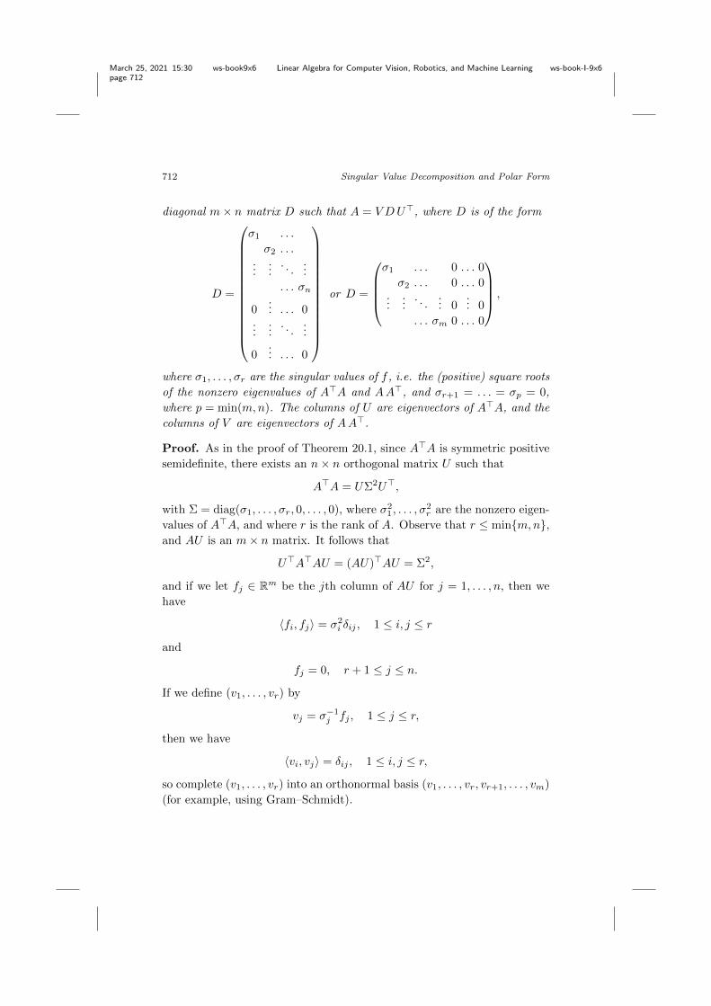
March 25, 2021 15:30 ws-book9x6 Linear Algebra for Computer Vision, Robotics, and Machine Learning ws-book-I-9x6
page 712
712 Singular Value Decomposition and Polar Form
diagonal m ⇥ n matrix D such that A = V DU>, where D is of the form
D =
0
BBBBBBBBBBBBB@
�1
. . .�2
. . ....
.... . .
.... . . �n
0... . . . 0
......
. . ....
0... . . . 0
1
CCCCCCCCCCCCCA
or D =
0
BBB@
�1
. . . 0 . . . 0�2
. . . 0 . . . 0...
.... . .
... 0... 0
. . . �m 0 . . . 0
1
CCCA,
where �1
, . . . ,�r are the singular values of f , i.e. the (positive) square rootsof the nonzero eigenvalues of A>A and AA>, and �r+1
= . . . = �p = 0,where p = min(m,n). The columns of U are eigenvectors of A>A, and thecolumns of V are eigenvectors of AA>.
Proof. As in the proof of Theorem 20.1, since A>A is symmetric positivesemidefinite, there exists an n ⇥ n orthogonal matrix U such that
A>A = U⌃2U>,
with ⌃ = diag(�1
, . . . ,�r, 0, . . . , 0), where �2
1
, . . . ,�2
r are the nonzero eigen-values of A>A, and where r is the rank of A. Observe that r min{m,n},and AU is an m ⇥ n matrix. It follows that
U>A>AU = (AU)>AU = ⌃2,
and if we let fj 2 Rm be the jth column of AU for j = 1, . . . , n, then wehave
hfi, fji = �2
i �ij , 1 i, j r
and
fj = 0, r + 1 j n.
If we define (v1
, . . . , vr) by
vj = ��1
j fj , 1 j r,
then we have
hvi, vji = �ij , 1 i, j r,
so complete (v1
, . . . , vr) into an orthonormal basis (v1
, . . . , vr, vr+1
, . . . , vm)(for example, using Gram–Schmidt).

March 25, 2021 15:30 ws-book9x6 Linear Algebra for Computer Vision, Robotics, and Machine Learning ws-book-I-9x6
page 713
20.4. Singular Value Decomposition for Rectangular Matrices 713
Now since fj = �jvj for j = 1 . . . , r, we have
hvi, fji = �jhvi, vji = �j�i,j , 1 i m, 1 j r
and since fj = 0 for j = r + 1, . . . , n, we have
hvi, fji = 0 1 i m, r + 1 j n.
If V is the matrix whose columns are v1
, . . . , vm, then V is an m ⇥ morthogonal matrix and if m � n, we let
D =
✓⌃
0m�n
◆=
0
BBBBBBBBBBBBB@
�1
. . .�2
. . ....
.... . .
.... . . �n
0... . . . 0
......
. . ....
0... . . . 0
1
CCCCCCCCCCCCCA
,
else if n � m, then we let
D =
0
BBB@
�1
. . . 0 . . . 0�2
. . . 0 . . . 0...
.... . .
... 0... 0
. . . �m 0 . . . 0
1
CCCA.
In either case, the above equations prove that
V >AU = D,
which yields A = V DU>, as required.The equation A = V DU> implies that
A>A = UD>DU> = Udiag(�2
1
, . . . ,�2
r , 0, . . . , 0| {z }n�r
)U>
and
AA> = V DD>V > = V diag(�2
1
, . . . ,�2
r , 0, . . . , 0| {z }m�r
)V >,
which shows that A>A and AA> have the same nonzero eigenvalues, thatthe columns of U are eigenvectors of A>A, and that the columns of V areeigenvectors of AA>.

March 25, 2021 15:30 ws-book9x6 Linear Algebra for Computer Vision, Robotics, and Machine Learning ws-book-I-9x6
page 714
714 Singular Value Decomposition and Polar Form
A triple (U,D, V ) such that A = V DU> is called a singular valuedecomposition (SVD) of A. If D = diag(�
1
, . . . ,�p) (with p = min(m,n)),it is customary to assume that �
1
� �2
� · · · � �p.
Example 20.4. Let A =
0
@1 10 00 0
1
A. Then A> =
✓1 0 01 0 0
◆A>A =
✓1 11 1
◆,
and AA> =
0
@2 0 00 0 00 0 0
1
A. The reader should verify that A>A = U⌃2U> where
⌃2 =
✓2 00 0
◆and U = U> =
✓1/
p2 1/
p2
1/p2 �1/
p2
◆. Since AU =
0
@
p2 00 00 0
1
A , set
v1
= 1p2
0
@
p200
1
A =
0
@100
1
A , and complete an orthonormal basis for R3 by
assigning v2
=
0
@010
1
A, and v3
=
0
@001
1
A. Thus V = I3
, and the reader should
verify that A = V DU>, where D =
0
@
p2 00 00 0
1
A.
Even though the matrix D is an m ⇥ n rectangular matrix, since itsonly nonzero entries are on the descending diagonal, we still say that D isa diagonal matrix.
The Matlab command for computing an SVD A = V DU> of a matrixA is also [V, D, U] = svd(A).
If we view A as the representation of a linear map f : E ! F , wheredim(E) = n and dim(F ) = m, the proof of Theorem 20.3 shows thatthere are two orthonormal bases (u
1
, . . ., un) and (v1
, . . . , vm) for E and F ,respectively, where (u
1
, . . . , un) are eigenvectors of f⇤ � f and (v1
, . . . , vm)are eigenvectors of f �f⇤. Furthermore, (u
1
, . . . , ur) is an orthonormal basisof Im f⇤, (ur+1
, . . . , un) is an orthonormal basis of Ker f , (v1
, . . . , vr) is anorthonormal basis of Im f , and (vr+1
, . . . , vm) is an orthonormal basis ofKer f⇤.
The SVD of matrices can be used to define the pseudo-inverse of arectangular matrix; we will do so in Chapter 21. The reader may alsoconsult Strang [Strang (1988)], Demmel [Demmel (1997)], Trefethen and

March 25, 2021 15:30 ws-book9x6 Linear Algebra for Computer Vision, Robotics, and Machine Learning ws-book-I-9x6
page 715
20.4. Singular Value Decomposition for Rectangular Matrices 715
Bau [Trefethen and Bau III (1997)], and Golub and Van Loan [Golub andVan Loan (1996)].
One of the spectral theorems states that a symmetric matrix can be di-agonalized by an orthogonal matrix. There are several numerical methodsto compute the eigenvalues of a symmetric matrix A. One method consistsin tridiagonalizing A, which means that there exists some orthogonal matrixP and some symmetric tridiagonal matrix T such that A = PTP>. In fact,this can be done using Householder transformations; see Theorem 17.2. Itis then possible to compute the eigenvalues of T using a bisection methodbased on Sturm sequences. One can also use Jacobi’s method. For details,see Golub and Van Loan [Golub and Van Loan (1996)], Chapter 8, Dem-mel [Demmel (1997)], Trefethen and Bau [Trefethen and Bau III (1997)],Lecture 26, Ciarlet [Ciarlet (1989)], and Chapter 17. Computing the SVDof a matrix A is more involved. Most methods begin by finding orthogonalmatrices U and V and a bidiagonal matrix B such that A = V BU>; seeProblem 12.8 and Problem 20.3. This can also be done using Householdertransformations. Observe that B>B is symmetric tridiagonal. Thus, inprinciple, the previous method to diagonalize a symmetric tridiagonal ma-trix can be applied. However, it is unwise to compute B>B explicitly, andmore subtle methods are used for this last step; the matrix of Problem 20.1can be used, and see Problem 20.3. Again, see Golub and Van Loan [Goluband Van Loan (1996)], Chapter 8, Demmel [Demmel (1997)], and Trefethenand Bau [Trefethen and Bau III (1997)], Lecture 31.
The polar form has applications in continuum mechanics. Indeed, in anydeformation it is important to separate stretching from rotation. This isexactly what QS achieves. The orthogonal part Q corresponds to rotation(perhaps with an additional reflection), and the symmetric matrix S tostretching (or compression). The real eigenvalues �
1
, . . . ,�r of S are thestretch factors (or compression factors) (see Marsden and Hughes [Marsdenand Hughes (1994)]). The fact that S can be diagonalized by an orthogonalmatrix corresponds to a natural choice of axes, the principal axes.
The SVD has applications to data compression, for instance in imageprocessing. The idea is to retain only singular values whose magnitudesare significant enough. The SVD can also be used to determine the rank ofa matrix when other methods such as Gaussian elimination produce verysmall pivots. One of the main applications of the SVD is the computationof the pseudo-inverse. Pseudo-inverses are the key to the solution of variousoptimization problems, in particular the method of least squares. This topicis discussed in the next chapter (Chapter 21). Applications of the material
March 25, 2021 15:30 ws-book9x6 Linear Algebra for Computer Vision, Robotics, and Machine Learning ws-book-I-9x6
page 716
716 Singular Value Decomposition and Polar Form
of this chapter can be found in Strang [Strang (1988, 1986)]; Ciarlet [Ciarlet(1989)]; Golub and Van Loan [Golub and Van Loan (1996)], which containsmany other references; Demmel [Demmel (1997)]; and Trefethen and Bau[Trefethen and Bau III (1997)].
20.5 Ky Fan Norms and Schatten Norms
The singular values of a matrix can be used to define various norms on ma-trices which have found recent applications in quantum information theoryand in spectral graph theory. Following Horn and Johnson [Horn and John-son (1994)] (Section 3.4) we can make the following definitions:
Definition 20.5. For any matrix A 2 Mm,n(C), let q = min{m,n}, and if�1
� · · · � �q are the singular values of A, for any k with 1 k q, let
Nk(A) = �1
+ · · · + �k,
called the Ky Fan k-norm of A.More generally, for any p � 1 and any k with 1 k q, let
Nk;p(A) = (�p1
+ · · · + �pk)
1/p,
called the Ky Fan p-k-norm of A. When k = q, Nq;p is also called theSchatten p-norm.
Observe that when k = 1, N1
(A) = �1
, and the Ky Fan norm N1
issimply the spectral norm from Chapter 8, which is the subordinate matrixnorm associated with the Euclidean norm. When k = q, the Ky Fan normNq is given by
Nq(A) = �1
+ · · · + �q = tr((A⇤A)1/2)
and is called the trace norm or nuclear norm. When p = 2 and k = q, theKy Fan Nq;2 norm is given by
Nk;2(A) = (�2
1
+ · · · + �2
q )1/2 =
ptr(A⇤A) = kAkF ,
which is the Frobenius norm of A.It can be shown that Nk and Nk;p are unitarily invariant norms, and
that when m = n, they are matrix norms; see Horn and Johnson [Horn andJohnson (1994)] (Section 3.4, Corollary 3.4.4 and Problem 3).

March 25, 2021 15:30 ws-book9x6 Linear Algebra for Computer Vision, Robotics, and Machine Learning ws-book-I-9x6
page 717
20.6. Summary 717
20.6 Summary
The main concepts and results of this chapter are listed below:
• For any linear map f : E ! E on a Euclidean space E, the maps f⇤ �fand f � f⇤ are self-adjoint and positive semidefinite.
• The singular values of a linear map.• Positive semidefinite and positive definite self-adjoint maps.• Relationships between Im f , Ker f , Im f⇤, and Ker f⇤.• The singular value decomposition theorem for square matrices (Theo-rem 20.1).
• The SVD of matrix.• The polar decomposition of a matrix.• The Weyl inequalities .• The singular value decomposition theorem for m⇥n matrices (Theorem20.3).
• Ky Fan k-norms, Ky Fan p-k-norms, Schatten p-norms.
20.7 Problems
Problem 20.1. (1) Let A be a real n⇥nmatrix and consider the (2n)⇥(2n)real symmetric matrix
S =
✓0 AA> 0
◆.
Suppose that A has rank r. If A = V ⌃U> is an SVD for A, with⌃ = diag(�
1
, . . . ,�n) and �1
� · · · � �r > 0, denoting the columns ofU by uk and the columns of V by vk, prove that �k is an eigenvalue of S
with corresponding eigenvector
✓vkuk
◆for k = 1, . . . , n, and that ��k is an
eigenvalue of S with corresponding eigenvector
✓vk
�uk
◆for k = 1, . . . , n.
Hint . We have Auk = �kvk for k = 1, . . . , n. Show that A>vk = �kuk
for k = 1, . . . , r, and that A>vk = 0 for k = r + 1, . . . , n. Recall thatKer (A>) = Ker (AA>).
(2) Prove that the 2n eigenvectors of S in (1) are pairwise orthogonal.Check that if A has rank r, then S has rank 2r.
(3) Now assume that A is a real m ⇥ n matrix and consider the (m +

March 25, 2021 15:30 ws-book9x6 Linear Algebra for Computer Vision, Robotics, and Machine Learning ws-book-I-9x6
page 718
718 Singular Value Decomposition and Polar Form
n) ⇥ (m+ n) real symmetric matrix
S =
✓0 AA> 0
◆.
Suppose that A has rank r. If A = V ⌃U> is an SVD for A, prove that �k
is an eigenvalue of S with corresponding eigenvector
✓vkuk
◆for k = 1, . . . , r,
and that ��k is an eigenvalue of S with corresponding eigenvector
✓vk
�uk
◆
for k = 1, . . . , r.Find the remaining m + n � 2r eigenvectors of S associated with the
eigenvalue 0.(4) Prove that these m+ n eigenvectors of S are pairwise orthogonal.
Problem 20.2. Let A be a real m ⇥ n matrix of rank r and let q =min(m,n).
(1) Consider the (m+ n) ⇥ (m+ n) real symmetric matrix
S =
✓0 AA> 0
◆
and prove that✓Im z�1A0 In
◆✓zIm �A�A> zIn
◆=
✓zIm � z�1AA> 0
�A> zIn
◆.
Use the above equation to prove that
det(zIm+n � S) = tn�m det(t2Im � AA>).
(2) Prove that the eigenvalues of S are ±�1
, . . . ,±�q, with |m � n|additional zeros.
Problem 20.3. Let B be a real bidiagonal matrix of the form
B =
0
BBBBBB@
a1
b1
0 · · · 0
0 a2
b2
. . . 0...
. . .. . .
. . ....
0 · · · 0 an�1
bn�1
0 0 · · · 0 an
1
CCCCCCA.
Let A be the (2n) ⇥ (2n) symmetric matrix
A =
✓0 B>
B 0
◆,

March 25, 2021 15:30 ws-book9x6 Linear Algebra for Computer Vision, Robotics, and Machine Learning ws-book-I-9x6
page 719
20.7. Problems 719
and let P be the permutation matrix given by P = [e1
, en+1
, e2
, en+2
,· · · , en, e2n].
(1) Prove that T = P>AP is a symmetric tridiagonal (2n)⇥(2n) matrixwith zero main diagonal of the form
T =
0
BBBBBBBBBBBB@
0 a1
0 0 0 0 · · · 0a1
0 b1
0 0 0 · · · 00 b
1
0 a2
0 0 · · · 00 0 a
2
0 b2
0 · · · 0...
......
. . .. . .
. . .. . .
...0 0 0 · · · an�1
0 bn�1
00 0 0 · · · 0 bn�1
0 an0 0 0 · · · 0 0 an 0
1
CCCCCCCCCCCCA
.
(2) Prove that if xi is a unit eigenvector for an eigenvalue �i of T , then�i = ±�i where �i is a singular value of B, and that
Pxi =1p2
✓ui
±vi
◆,
where the ui are unit eigenvectors of B>B and the vi are unit eigenvectorsof BB>.
Problem 20.4. Find the SVD of the matrix
A =
0
@0 2 00 0 30 0 0
1
A .
Problem 20.5. Let u, v 2 Rn be two nonzero vectors, and let A = uv> bethe corresponding rank 1 matrix. Prove that the nonzero singular value ofA is kuk
2
kvk2
.
Problem 20.6. Let A be a n⇥ n real matrix. Prove that if �1
, . . . ,�n arethe singular values of A, then �3
1
, . . . ,�3
n are the singular values of AA>A.
Problem 20.7. Let A be a real n ⇥ n matrix.(1) Prove that the largest singular value �
1
of A is given by
�1
= supx 6=0
kAxk2
kxk2
,
and that this supremum is achieved at x = u1
, the first column in U in anSVD A = V ⌃U>.
(2) Extend the above result to real m ⇥ n matrices.
March 25, 2021 15:30 ws-book9x6 Linear Algebra for Computer Vision, Robotics, and Machine Learning ws-book-I-9x6
page 720
720 Singular Value Decomposition and Polar Form
Problem 20.8. Let A be a real m ⇥ n matrix. Prove that if B is anysubmatrix of A (by keeping M m rows and N n columns of A), then(�
1
)B (�1
)A (where (�1
)A is the largest singular value of A and similarlyfor (�
1
)B).
Problem 20.9. Let A be a real n ⇥ n matrix.(1) Assume A is invertible. Prove that if A = Q
1
S1
= Q2
S2
are twopolar decompositions of A, then Q
1
= Q2
and S1
= S2
.Hint . A>A = S2
1
= S2
2
, with S1
and S2
symmetric positive definite. Thenuse Problem 16.7.
(2) Now assume that A is singular. Prove that if A = Q1
S1
= Q2
S2
aretwo polar decompositions of A, then S
1
= S2
, but Q1
may not be equal toQ
2
.
Problem 20.10. (1) Let A be any invertible (real) n ⇥ n matrix. Provethat for every SVD, A = V DU> of A, the product V U> is the same (i.e.,if V
1
DU>1
= V2
DU>2
, then V1
U>1
= V2
U>2
). What does V U> have to dowith the polar form of A?
(2) Given any invertible (real) n ⇥ n matrix, A, prove that there isa unique orthogonal matrix, Q 2 O(n), such that kA � QkF is minimal(under the Frobenius norm). In fact, prove that Q = V U>, where A =V DU> is an SVD of A. Moreover, if det(A) > 0, show that Q 2 SO(n).
What can you say if A is singular (i.e., non-invertible)?
Problem 20.11. (1) Prove that for any n⇥n matrix A and any orthogonalmatrix Q, we have
max{tr(QA) | Q 2 O(n)} = �1
+ · · · + �n,
where �1
� · · · � �n are the singular values of A. Furthermore, thismaximum is achieved by Q = UV >, where A = V ⌃U> is any SVD for A.
(2) By applying the above result with A = Z>X and Q = R>, deducethe following result : For any two fixed n ⇥ k matrices X and Z, theminimum of the set
{kX � ZRkF | R 2 O(k)}is achieved by R = V U> for any SVD decomposition V ⌃U> = Z>X ofZ>X.
Remark: The problem of finding an orthogonal matrix R such that ZRcomes as close as possible to X is called the orthogonal Procrustes problem;see Strang [Strang (2019)] (Section IV.9) for the history of this problem.

March 25, 2021 15:30 ws-book9x6 Linear Algebra for Computer Vision, Robotics, and Machine Learning ws-book-I-9x6
page 721
Chapter 21
Applications of SVD andPseudo-Inverses
De tous les principes qu’on peut proposer pour cet objet, je pensequ’il n’en est pas de plus general, de plus exact, ni d’une applicationplus facile, que celui dont nous avons fait usage dans les recherchesprecedentes, et qui consiste a rendre minimum la somme des carres deserreurs. Par ce moyen il s’etablit entre les erreurs une sorte d’equilibrequi, empechant les extremes de prevaloir, est tres propre as faire con-naitre l’etat du systeme le plus proche de la verite.
—Legendre, 1805, Nouvelles Methodes pour la determination des Or-bites desCometes
21.1 Least Squares Problems and the Pseudo-Inverse
This chapter presents several applications of SVD. The first one is thepseudo-inverse, which plays a crucial role in solving linear systems by themethod of least squares. The second application is data compression. Thethird application is principal component analysis (PCA), whose purpose isto identify patterns in data and understand the variance–covariance struc-ture of the data. The fourth application is the best a�ne approximation ofa set of data, a problem closely related to PCA.
The method of least squares is a way of “solving” an overdeterminedsystem of linear equations
Ax = b,
i.e., a system in which A is a rectangular m⇥n matrix with more equationsthan unknowns (whenm > n). Historically, the method of least squares wasused by Gauss and Legendre to solve problems in astronomy and geodesy.The method was first published by Legendre in 1805 in a paper on methods
721

March 25, 2021 15:30 ws-book9x6 Linear Algebra for Computer Vision, Robotics, and Machine Learning ws-book-I-9x6
page 722
722 Applications of SVD and Pseudo-Inverses
for determining the orbits of comets. However, Gauss had already usedthe method of least squares as early as 1801 to determine the orbit of theasteroid Ceres, and he published a paper about it in 1810 after the discoveryof the asteroid Pallas. Incidentally, it is in that same paper that Gaussianelimination using pivots is introduced.
The reason why more equations than unknowns arise in such problemsis that repeated measurements are taken to minimize errors. This producesan overdetermined and often inconsistent system of linear equations. Forexample, Gauss solved a system of eleven equations in six unknowns todetermine the orbit of the asteroid Pallas.
Example 21.1. As a concrete illustration, suppose that we observe themotion of a small object, assimilated to a point, in the plane. From ourobservations, we suspect that this point moves along a straight line, say ofequation y = cx + d. Suppose that we observed the moving point at threedi↵erent locations (x
1
, y1
), (x2
, y2
), and (x3
, y3
). Then we should have
d+ cx1
= y1
,
d+ cx2
= y2
,
d+ cx3
= y3
.
If there were no errors in our measurements, these equations would becompatible, and c and d would be determined by only two of the equations.However, in the presence of errors, the system may be inconsistent. Yet wewould like to find c and d!
The idea of the method of least squares is to determine (c, d) such thatit minimizes the sum of the squares of the errors, namely,
(d+ cx1
� y1
)2 + (d+ cx2
� y2
)2 + (d+ cx3
� y3
)2.
See Figure 21.1.In general, for an overdetermined m ⇥ n system Ax = b, what Gauss
and Legendre discovered is that there are solutions x minimizing
kAx � bk22
(where kuk22
= u2
1
+ · · ·+u2
n, the square of the Euclidean norm of the vectoru = (u
1
, . . . , un)), and that these solutions are given by the square n ⇥ nsystem
A>Ax = A>b,
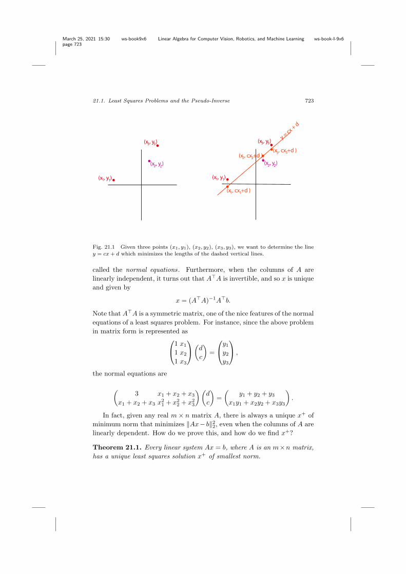
March 25, 2021 15:30 ws-book9x6 Linear Algebra for Computer Vision, Robotics, and Machine Learning ws-book-I-9x6
page 723
21.1. Least Squares Problems and the Pseudo-Inverse 723
y = cx + d
(x , y )1 1
(x , y )2 2
(x , y )3 3
1(x , cx +d )1
(x , cx +d )(x , cx +d )2 2
3 3
(x , y )1 1
(x , y )2 2
(x , y )3 3
Fig. 21.1 Given three points (x1, y1), (x2, y2), (x3, y3), we want to determine the liney = cx + d which minimizes the lengths of the dashed vertical lines.
called the normal equations . Furthermore, when the columns of A arelinearly independent, it turns out that A>A is invertible, and so x is uniqueand given by
x = (A>A)�1A>b.
Note that A>A is a symmetric matrix, one of the nice features of the normalequations of a least squares problem. For instance, since the above problemin matrix form is represented as
0
@1 x
1
1 x2
1 x3
1
A✓dc
◆=
0
@y1
y2
y3
1
A ,
the normal equations are
✓3 x
1
+ x2
+ x3
x1
+ x2
+ x3
x2
1
+ x2
2
+ x2
3
◆✓dc
◆=
✓y1
+ y2
+ y3
x1
y1
+ x2
y2
+ x3
y3
◆.
In fact, given any real m ⇥ n matrix A, there is always a unique x+ ofminimum norm that minimizes kAx� bk2
2
, even when the columns of A arelinearly dependent. How do we prove this, and how do we find x+?
Theorem 21.1. Every linear system Ax = b, where A is an m⇥n matrix,has a unique least squares solution x+ of smallest norm.

March 25, 2021 15:30 ws-book9x6 Linear Algebra for Computer Vision, Robotics, and Machine Learning ws-book-I-9x6
page 724
724 Applications of SVD and Pseudo-Inverses
Proof. Geometry o↵ers a nice proof of the existence and uniqueness ofx+. Indeed, we can interpret b as a point in the Euclidean (a�ne) spaceRm, and the image subspace of A (also called the column space of A) as asubspace U of Rm (passing through the origin). Then it is clear that
infx2Rn
kAx � bk22
= infy2U
ky � bk22
,
with U = ImA, and we claim that x minimizes kAx�bk22
i↵ Ax = p, wherep the orthogonal projection of b onto the subspace U .
Recall from Section 12.1 that the orthogonal projection pU : U �U? !U is the linear map given by
pU (u+ v) = u,
with u 2 U and v 2 U?. If we let p = pU (b) 2 U , then for any point y 2 U ,
the vectors �!py = y � p 2 U and�!bp = p � b 2 U? are orthogonal, which
implies that
k�!byk2
2
= k�!bpk2
2
+ k�!pyk22
,
where�!by = y � b. Thus, p is indeed the unique point in U that minimizes
the distance from b to any point in U . See Figure 21.2.
Im A = U
b
p
Im A = U
b
p
y
Fig. 21.2 Given a 3 ⇥ 2 matrix A, U = ImA is the peach plane in R3 and p is theorthogonal projection of b onto U . Furthermore, given y 2 U , the points b, y, and p arethe vertices of a right triangle.
Thus the problem has been reduced to proving that there is a unique x+
of minimum norm such that Ax+ = p, with p = pU (b) 2 U , the orthogonal
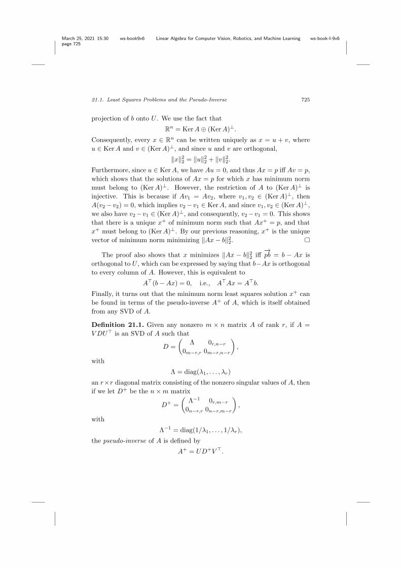
March 25, 2021 15:30 ws-book9x6 Linear Algebra for Computer Vision, Robotics, and Machine Learning ws-book-I-9x6
page 725
21.1. Least Squares Problems and the Pseudo-Inverse 725
projection of b onto U . We use the fact that
Rn = KerA � (KerA)?.
Consequently, every x 2 Rn can be written uniquely as x = u + v, whereu 2 KerA and v 2 (KerA)?, and since u and v are orthogonal,
kxk22
= kuk22
+ kvk22
.
Furthermore, since u 2 KerA, we have Au = 0, and thus Ax = p i↵ Av = p,which shows that the solutions of Ax = p for which x has minimum normmust belong to (KerA)?. However, the restriction of A to (KerA)? isinjective. This is because if Av
1
= Av2
, where v1
, v2
2 (KerA)?, thenA(v
2
� v2
) = 0, which implies v2
� v1
2 KerA, and since v1
, v2
2 (KerA)?,we also have v
2
�v1
2 (KerA)?, and consequently, v2
�v1
= 0. This showsthat there is a unique x+ of minimum norm such that Ax+ = p, and thatx+ must belong to (KerA)?. By our previous reasoning, x+ is the uniquevector of minimum norm minimizing kAx � bk2
2
.
The proof also shows that x minimizes kAx � bk22
i↵�!pb = b � Ax is
orthogonal to U , which can be expressed by saying that b�Ax is orthogonalto every column of A. However, this is equivalent to
A>(b � Ax) = 0, i.e., A>Ax = A>b.
Finally, it turns out that the minimum norm least squares solution x+ canbe found in terms of the pseudo-inverse A+ of A, which is itself obtainedfrom any SVD of A.
Definition 21.1. Given any nonzero m ⇥ n matrix A of rank r, if A =V DU> is an SVD of A such that
D =
✓⇤ 0r,n�r
0m�r,r 0m�r,n�r
◆,
with
⇤ = diag(�1
, . . . ,�r)
an r⇥r diagonal matrix consisting of the nonzero singular values of A, thenif we let D+ be the n ⇥ m matrix
D+ =
✓⇤�1 0r,m�r
0n�r,r 0n�r,m�r
◆,
with
⇤�1 = diag(1/�1
, . . . , 1/�r),
the pseudo-inverse of A is defined by
A+ = UD+V >.

March 25, 2021 15:30 ws-book9x6 Linear Algebra for Computer Vision, Robotics, and Machine Learning ws-book-I-9x6
page 726
726 Applications of SVD and Pseudo-Inverses
If A = 0m,n is the zero matrix, we set A+ = 0n,m. Observe that D+ isobtained from D by inverting the nonzero diagonal entries of D, leaving allzeros in place, and then transposing the matrix. For example, given thematrix
D =
0
BB@
1 0 0 0 00 2 0 0 00 0 3 0 00 0 0 0 0
1
CCA ,
its pseudo-inverse is
D+ =
0
BBBB@
1 0 0 00 1
2
0 00 0 1
3
00 0 0 00 0 0 0
1
CCCCA.
The pseudo-inverse of a matrix is also known as the Moore–Penrose pseudo-inverse.
Actually, it seems that A+ depends on the specific choice of U and Vin an SVD (U,D, V ) for A, but the next theorem shows that this is not so.
Theorem 21.2. The least squares solution of smallest norm of the linearsystem Ax = b, where A is an m ⇥ n matrix, is given by
x+ = A+b = UD+V >b.
Proof. First assume that A is a (rectangular) diagonal matrix D, as above.Then since x minimizes kDx � bk2
2
i↵ Dx is the projection of b onto theimage subspace F of D, it is fairly obvious that x+ = D+b. Otherwise, wecan write
A = V DU>,
where U and V are orthogonal. However, since V is an isometry,
kAx � bk2
= kV DU>x � bk2
= kDU>x � V >bk2
.
Letting y = U>x, we have kxk2
= kyk2
, since U is an isometry, and sinceU is surjective, kAx� bk
2
is minimized i↵ kDy � V >bk2
is minimized, andwe have shown that the least solution is
y+ = D+V >b.
Since y = U>x, with kxk2
= kyk2
, we get
x+ = UD+V >b = A+b.
Thus, the pseudo-inverse provides the optimal solution to the least squaresproblem.
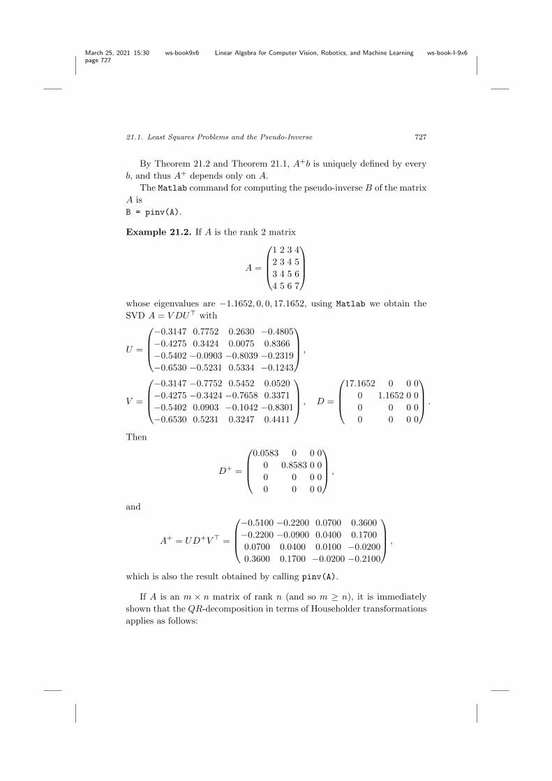
March 25, 2021 15:30 ws-book9x6 Linear Algebra for Computer Vision, Robotics, and Machine Learning ws-book-I-9x6
page 727
21.1. Least Squares Problems and the Pseudo-Inverse 727
By Theorem 21.2 and Theorem 21.1, A+b is uniquely defined by everyb, and thus A+ depends only on A.
The Matlab command for computing the pseudo-inverse B of the matrixA isB = pinv(A).
Example 21.2. If A is the rank 2 matrix
A =
0
BB@
1 2 3 42 3 4 53 4 5 64 5 6 7
1
CCA
whose eigenvalues are �1.1652, 0, 0, 17.1652, using Matlab we obtain theSVD A = V DU> with
U =
0
BB@
�0.3147 0.7752 0.2630 �0.4805�0.4275 0.3424 0.0075 0.8366�0.5402 �0.0903 �0.8039 �0.2319�0.6530 �0.5231 0.5334 �0.1243
1
CCA ,
V =
0
BB@
�0.3147 �0.7752 0.5452 0.0520�0.4275 �0.3424 �0.7658 0.3371�0.5402 0.0903 �0.1042 �0.8301�0.6530 0.5231 0.3247 0.4411
1
CCA , D =
0
BB@
17.1652 0 0 00 1.1652 0 00 0 0 00 0 0 0
1
CCA .
Then
D+ =
0
BB@
0.0583 0 0 00 0.8583 0 00 0 0 00 0 0 0
1
CCA ,
and
A+ = UD+V > =
0
BB@
�0.5100 �0.2200 0.0700 0.3600�0.2200 �0.0900 0.0400 0.17000.0700 0.0400 0.0100 �0.02000.3600 0.1700 �0.0200 �0.2100
1
CCA ,
which is also the result obtained by calling pinv(A).
If A is an m ⇥ n matrix of rank n (and so m � n), it is immediatelyshown that the QR-decomposition in terms of Householder transformationsapplies as follows:

March 25, 2021 15:30 ws-book9x6 Linear Algebra for Computer Vision, Robotics, and Machine Learning ws-book-I-9x6
page 728
728 Applications of SVD and Pseudo-Inverses
There are n m ⇥ m matrices H1
, . . . , Hn, Householder matrices or theidentity, and an upper triangular m ⇥ n matrix R of rank n such that
A = H1
· · ·HnR.
Then because each Hi is an isometry,
kAx � bk2
= kRx � Hn · · ·H1
bk2
,
and the least squares problem Ax = b is equivalent to the system
Rx = Hn · · ·H1
b.
Now the system
Rx = Hn · · ·H1
b
is of the form ✓R
1
0m�n
◆x =
✓cd
◆,
where R1
is an invertible n ⇥ n matrix (since A has rank n), c 2 Rn, andd 2 Rm�n, and the least squares solution of smallest norm is
x+ = R�1
1
c.
Since R1
is a triangular matrix, it is very easy to invert R1
.The method of least squares is one of the most e↵ective tools of the
mathematical sciences. There are entire books devoted to it. Readers areadvised to consult Strang [Strang (1988)], Golub and Van Loan [Goluband Van Loan (1996)], Demmel [Demmel (1997)], and Trefethen and Bau[Trefethen and Bau III (1997)], where extensions and applications of leastsquares (such as weighted least squares and recursive least squares) aredescribed. Golub and Van Loan [Golub and Van Loan (1996)] also containsa very extensive bibliography, including a list of books on least squares.
21.2 Properties of the Pseudo-Inverse
We begin this section with a proposition which provides a way to calculatethe pseudo-inverse of an m⇥n matrix A without first determining an SVDfactorization.
Proposition 21.1. When A has full rank, the pseudo-inverse A+ can beexpressed as A+ = (A>A)�1A> when m � n, and as A+ = A>(AA>)�1
when n � m. In the first case (m � n), observe that A+A = I, so A+ is aleft inverse of A; in the second case (n � m), we have AA+ = I, so A+ isa right inverse of A.

March 25, 2021 15:30 ws-book9x6 Linear Algebra for Computer Vision, Robotics, and Machine Learning ws-book-I-9x6
page 729
21.2. Properties of the Pseudo-Inverse 729
Proof. If m � n and A has full rank n, we have
A = V
✓⇤
0m�n,n
◆U>
with ⇤ an n ⇥ n diagonal invertible matrix (with positive entries), so
A+ = U�⇤�1 0n,m�n
�V >.
We find that
A>A = U�⇤ 0n,m�n
�V >V
✓⇤
0m�n,n
◆U> = U⇤2U>,
which yields
(A>A)�1A> = U⇤�2U>U�⇤ 0n,m�n
�V > = U
�⇤�1 0n,m�n
�V > = A+.
Therefore, if m � n and A has full rank n, then
A+ = (A>A)�1A>.
If n � m and A has full rank m, then
A = V�⇤ 0m,n�m
�U>
with ⇤ an m ⇥ m diagonal invertible matrix (with positive entries), so
A+ = U
✓⇤�1
0n�m,m
◆V >.
We find that
AA> = V�⇤ 0m,n�m
�U>U
✓⇤
0n�m,m
◆V > = V ⇤2V >,
which yields
A>(AA>)�1 = U
✓⇤
0n�m,m
◆V >V ⇤�2V > = U
✓⇤�1
0n�m,m
◆V > = A+.
Therefore, if n � m and A has full rank m, then A+ = A>(AA>)�1.
For example, if A =
0
@1 22 30 1
1
A, then A has rank 2 and since m � n,
A+ = (A>A)�1A> where
A+ =
✓5 88 14
◆�1
A> =
✓7/3 �4/34/3 5/6
◆✓1 2 02 3 1
◆=
✓�1/3 2/3 �4/31/3 �1/6 5/6
◆.

March 25, 2021 15:30 ws-book9x6 Linear Algebra for Computer Vision, Robotics, and Machine Learning ws-book-I-9x6
page 730
730 Applications of SVD and Pseudo-Inverses
If A =
✓1 2 3 00 1 1 �1
◆, since A has rank 2 and n � m, then A+ = A>(AA>)�1
where
A+ = A>✓14 55 3
◆�1
=
0
BB@
1 02 13 10 �1
1
CCA
✓3/17 �5/17
�5/17 14/17
◆=
0
BB@
3/17 �5/171/17 4/174/17 �1/175/17 �14/17
1
CCA .
Let A = V ⌃U> be an SVD for any m⇥n matrix A. It is easy to checkthat both AA+ and A+A are symmetric matrices. In fact,
AA+ = V ⌃U>U⌃+V > = V ⌃⌃+V > = V
✓Ir 00 0m�r
◆V >
and
A+A = U⌃+V >V ⌃U> = U⌃+⌃U> = U
✓Ir 00 0n�r
◆U>.
From the above expressions we immediately deduce that
AA+A = A,
A+AA+ = A+,
and that
(AA+)2 = AA+,
(A+A)2 = A+A,
so both AA+ and A+A are orthogonal projections (since they are bothsymmetric).
Proposition 21.2. The matrix AA+ is the orthogonal projection onto therange of A and A+A is the orthogonal projection onto Ker(A)? = Im(A>),the range of A>.
Proof. Obviously, we have range(AA+) ✓ range(A), and for any y = Ax 2range(A), since AA+A = A, we have
AA+y = AA+Ax = Ax = y,
so the image of AA+ is indeed the range of A. It is also clear that Ker(A) ✓Ker(A+A), and since AA+A = A, we also have Ker(A+A) ✓ Ker(A), andso
Ker(A+A) = Ker(A).
Since A+A is symmetric, range(A+A) = range((A+A)>) = Ker(A+A)? =Ker(A)?, as claimed.

March 25, 2021 15:30 ws-book9x6 Linear Algebra for Computer Vision, Robotics, and Machine Learning ws-book-I-9x6
page 731
21.2. Properties of the Pseudo-Inverse 731
Proposition 21.3. The set range(A) = range(AA+) consists of all vectorsy 2 Rm such that
V >y =
✓z0
◆,
with z 2 Rr.
Proof. Indeed, if y = Ax, then
V >y = V >Ax = V >V ⌃U>x = ⌃U>x =
✓⌃r 00 0m�r
◆U>x =
✓z0
◆,
where ⌃r is the r⇥r diagonal matrix diag(�1
, . . . ,�r). Conversely, if V >y =( z0
), then y = V ( z0
), and
AA+y = V
✓Ir 00 0m�r
◆V >y
= V
✓Ir 00 0m�r
◆V >V
✓z0
◆
= V
✓Ir 00 0m�r
◆✓z0
◆
= V
✓z0
◆= y,
which shows that y belongs to the range of A.
Similarly, we have the following result.
Proposition 21.4. The set range(A+A) = Ker(A)? consists of all vectorsy 2 Rn such that
U>y =
✓z0
◆,
with z 2 Rr.
Proof. If y = A+Au, then
y = A+Au = U
✓Ir 00 0n�r
◆U>u = U
✓z0
◆,
for some z 2 Rr. Conversely, if U>y = ( z0
), then y = U ( z0
), and so
A+AU
✓z0
◆= U
✓Ir 00 0n�r
◆U>U
✓z0
◆
= U
✓Ir 00 0n�r
◆✓z0
◆
= U
✓z0
◆= y,
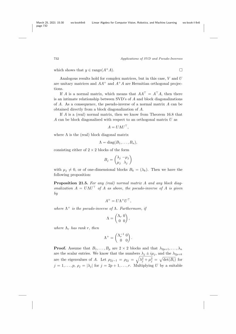
March 25, 2021 15:30 ws-book9x6 Linear Algebra for Computer Vision, Robotics, and Machine Learning ws-book-I-9x6
page 732
732 Applications of SVD and Pseudo-Inverses
which shows that y 2 range(A+A).
Analogous results hold for complex matrices, but in this case, V and Uare unitary matrices and AA+ and A+A are Hermitian orthogonal projec-tions.
If A is a normal matrix, which means that AA> = A>A, then thereis an intimate relationship between SVD’s of A and block diagonalizationsof A. As a consequence, the pseudo-inverse of a normal matrix A can beobtained directly from a block diagonalization of A.
If A is a (real) normal matrix, then we know from Theorem 16.8 thatA can be block diagonalized with respect to an orthogonal matrix U as
A = U⇤U>,
where ⇤ is the (real) block diagonal matrix
⇤ = diag(B1
, . . . , Bn),
consisting either of 2 ⇥ 2 blocks of the form
Bj =
✓�j �µj
µj �j
◆
with µj 6= 0, or of one-dimensional blocks Bk = (�k). Then we have thefollowing proposition:
Proposition 21.5. For any (real) normal matrix A and any block diag-onalization A = U⇤U> of A as above, the pseudo-inverse of A is givenby
A+ = U⇤+U>,
where ⇤+ is the pseudo-inverse of ⇤. Furthermore, if
⇤ =
✓⇤r 00 0
◆,
where ⇤r has rank r, then
⇤+ =
✓⇤�1
r 00 0
◆.
Proof. Assume that B1
, . . . , Bp are 2 ⇥ 2 blocks and that �2p+1
, . . . ,�nare the scalar entries. We know that the numbers �j ± iµj , and the �
2p+k
are the eigenvalues of A. Let ⇢2j�1
= ⇢2j =
q�2j + µ2
j =pdet(Bi) for
j = 1, . . . , p, ⇢j = |�j | for j = 2p + 1, . . . , r. Multiplying U by a suitable

March 25, 2021 15:30 ws-book9x6 Linear Algebra for Computer Vision, Robotics, and Machine Learning ws-book-I-9x6
page 733
21.2. Properties of the Pseudo-Inverse 733
permutation matrix, we may assume that the blocks of ⇤ are ordered sothat ⇢
1
� ⇢2
� · · · � ⇢r > 0. Then it is easy to see that
AA> = A>A = U⇤U>U⇤>U> = U⇤⇤>U>,
with
⇤⇤> = diag(⇢21
, . . . , ⇢2r, 0, . . . , 0),
so ⇢1
� ⇢2
� · · · � ⇢r > 0 are the singular values �1
� �2
� · · · � �r > 0of A. Define the diagonal matrix
⌃ = diag(�1
, . . . ,�r, 0, . . . , 0),
where r = rank(A), �1
� · · · � �r > 0 and the block diagonal matrix ⇥defined such that the block Bi in ⇤ is replaced by the block ��1Bi where� =
pdet(Bi), the nonzero scalar �j is replaced �j/|�j |, and a diagonal
zero is replaced by 1. Observe that ⇥ is an orthogonal matrix and
⇤ = ⇥⌃.
But then we can write
A = U⇤U> = U⇥⌃U>,
and we if let V = U⇥, since U is orthogonal and ⇥ is also orthogonal, V isalso orthogonal and A = V ⌃U> is an SVD for A. Now we get
A+ = U⌃+V > = U⌃+⇥>U>.
However, since ⇥ is an orthogonal matrix, ⇥> = ⇥�1, and a simple calcu-lation shows that
⌃+⇥> = ⌃+⇥�1 = ⇤+,
which yields the formula
A+ = U⇤+U>.
Also observe that ⇤r is invertible and
⇤+ =
✓⇤�1
r 00 0
◆.
Therefore, the pseudo-inverse of a normal matrix can be computed directlyfrom any block diagonalization of A, as claimed.

March 25, 2021 15:30 ws-book9x6 Linear Algebra for Computer Vision, Robotics, and Machine Learning ws-book-I-9x6
page 734
734 Applications of SVD and Pseudo-Inverses
Example 21.3. Consider the following real diagonal form of the normalmatrix
A =
0
BB@
�2.7500 2.1651 �0.8660 0.50002.1651 �0.2500 �1.5000 0.86600.8660 1.5000 0.7500 �0.4330
�0.5000 �0.8660 �0.4330 0.2500
1
CCA = U⇤U>,
with
U =
0
BB@
cos(⇡/3) 0 sin(⇡/3) 0sin(⇡/3) 0 � cos(⇡/3) 0
0 cos(⇡/6) 0 sin(⇡/6)0 � cos(⇡/6) 0 sin(⇡/6)
1
CCA , ⇤ =
0
BB@
1 �2 0 02 1 0 00 0 �4 00 0 0 0
1
CCA .
We obtain
⇤+ =
0
BB@
1/5 2/5 0 0�2/5 1/5 0 00 0 �1/4 00 0 0 0
1
CCA ,
and the pseudo-inverse of A is
A+ = U⇤+U> =
0
BB@
�0.1375 0.1949 0.1732 �0.10000.1949 0.0875 0.3000 �0.1732
�0.1732 �0.3000 0.1500 �0.08660.1000 0.1732 �0.0866 0.0500
1
CCA ,
which agrees with pinv(A).
The following properties, due to Penrose, characterize the pseudo-inverse of a matrix. We have already proved that the pseudo-inverse satis-fies these equations. For a proof of the converse, see Kincaid and Cheney[Kincaid and Cheney (1996)].
Proposition 21.6. Given any m ⇥ n matrix A (real or complex), thepseudo-inverse A+ of A is the unique n⇥m matrix satisfying the followingproperties:
AA+A = A,
A+AA+ = A+,
(AA+)> = AA+,
(A+A)> = A+A.

March 25, 2021 15:30 ws-book9x6 Linear Algebra for Computer Vision, Robotics, and Machine Learning ws-book-I-9x6
page 735
21.3. Data Compression and SVD 735
21.3 Data Compression and SVD
Among the many applications of SVD, a very useful one is data compres-sion, notably for images. In order to make precise the notion of closenessof matrices, we use the notion of matrix norm. This concept is defined inChapter 8, and the reader may want to review it before reading any further.
Given an m ⇥ n matrix of rank r, we would like to find a best approx-imation of A by a matrix B of rank k r (actually, k < r) such thatkA � Bk
2
(or kA � BkF ) is minimized. The following proposition is knownas the Eckart–Young theorem.
Proposition 21.7. Let A be an m⇥n matrix of rank r and let V DU> = Abe an SVD for A. Write ui for the columns of U , vi for the columns of V ,and �
1
� �2
� · · · � �p for the singular values of A (p = min(m,n)). Thena matrix of rank k < r closest to A (in the k k
2
norm) is given by
Ak =kX
i=1
�iviu>i = V diag(�
1
, . . . ,�k, 0, . . . , 0)U>
and kA � Akk2
= �k+1
.
Proof. By construction, Ak has rank k, and we have
kA � Akk2
=���
pX
i=k+1
�iviu>i
���2
=��V diag(0, . . . , 0,�k+1
, . . . ,�p)U>��
2
= �k+1
.
It remains to show that kA � Bk2
� �k+1
for all rank k matrices B. LetB be any rank k matrix, so its kernel has dimension n � k. The subspaceUk+1
spanned by (u1
, . . . , uk+1
) has dimension k+1, and because the sumof the dimensions of the kernel of B and of Uk+1
is (n� k)+ k+1 = n+1,these two subspaces must intersect in a subspace of dimension at least 1.Pick any unit vector h in Ker(B) \ Uk+1
. Then since Bh = 0, and since Uand V are isometries, we have
kA � Bk22
� k(A � B)hk22
= kAhk22
=��V DU>h
��22
=��DU>h
��22
� �2
k+1
��U>h��22
= �2
k+1
,
which proves our claim.

March 25, 2021 15:30 ws-book9x6 Linear Algebra for Computer Vision, Robotics, and Machine Learning ws-book-I-9x6
page 736
736 Applications of SVD and Pseudo-Inverses
Note that Ak can be stored using (m + n)k entries, as opposed to mnentries. When k ⌧ m, this is a substantial gain.
Example 21.4. Consider the badly conditioned symmetric matrix
A =
0
BB@
10 7 8 77 5 6 58 6 10 97 5 9 10
1
CCA
from Section 8.5. Since A is SPD, we have the SVD
A = UDU>,
with
U =
0
BB@
�0.5286 �0.6149 0.3017 �0.5016�0.3803 �0.3963 �0.0933 0.8304�0.5520 0.2716 �0.7603 �0.2086�0.5209 0.6254 0.5676 0.1237
1
CCA ,
D =
0
BB@
30.2887 0 0 00 3.8581 0 00 0 0.8431 00 0 0 0.0102
1
CCA .
If we set �3
= �4
= 0, we obtain the best rank 2 approximation
A2
= U(:, 1 : 2) ⇤D(:, 1 : 2) ⇤U(:, 1 : 2)0 =
0
BB@
9.9207 7.0280 8.1923 6.85637.0280 4.9857 5.9419 5.04368.1923 5.9419 9.5122 9.36416.8563 5.0436 9.3641 9.7282
1
CCA .
A nice example of the use of Proposition 21.7 in image compression isgiven in Demmel [Demmel (1997)], Chapter 3, Section 3.2.3, pages 113–115;see the Matlab demo.
Proposition 21.7 also holds for the Frobenius norm; see Problem 21.4.An interesting topic that we have not addressed is the actual computa-
tion of an SVD. This is a very interesting but tricky subject. Most methodsreduce the computation of an SVD to the diagonalization of a well-chosensymmetric matrix which is not A>A; see Problem 20.1 and Problem 20.3.Interested readers should read Section 5.4 of Demmel’s excellent book [Dem-mel (1997)], which contains an overview of most known methods and anextensive list of references.

March 25, 2021 15:30 ws-book9x6 Linear Algebra for Computer Vision, Robotics, and Machine Learning ws-book-I-9x6
page 737
21.4. Principal Components Analysis (PCA) 737
21.4 Principal Components Analysis (PCA)
Suppose we have a set of data consisting of n points X1
, . . . , Xn, with eachXi 2 Rd viewed as a row vector . Think of the Xi’s as persons, and ifXi = (xi 1, . . . , xi d), each xi j is the value of some feature (or attribute) ofthat person.
Example 21.5. For example, the Xi’s could be mathematicians, d = 2,and the first component, xi 1, of Xi could be the year that Xi was born, andthe second component, xi 2, the length of the beard of Xi in centimeters.Here is a small data set.
Name year length
Carl Friedrich Gauss 1777 0
Camille Jordan 1838 12
Adrien-Marie Legendre 1752 0
Bernhard Riemann 1826 15
David Hilbert 1862 2
Henri Poincare 1854 5
Emmy Noether 1882 0
Karl Weierstrass 1815 0
Eugenio Beltrami 1835 2
Hermann Schwarz 1843 20
We usually form the n⇥d matrix X whose ith row is Xi, with 1 i n.Then the jth column is denoted by Cj (1 j d). It is sometimes called afeature vector , but this terminology is far from being universally accepted.In fact, many people in computer vision call the data points Xi featurevectors!
The purpose of principal components analysis, for short PCA, is toidentify patterns in data and understand the variance–covariance structureof the data. This is useful for the following tasks:
(1) Data reduction: Often much of the variability of the data can be ac-counted for by a smaller number of principal components .
(2) Interpretation: PCA can show relationships that were not previouslysuspected.
Given a vector (a sample of measurements) x = (x1
, . . . , xn) 2 Rn,

March 25, 2021 15:30 ws-book9x6 Linear Algebra for Computer Vision, Robotics, and Machine Learning ws-book-I-9x6
page 738
738 Applications of SVD and Pseudo-Inverses
recall that the mean (or average) x of x is given by
x =
Pni=1
xi
n.
We let x � x denote the centered data point
x � x = (x1
� x, . . . , xn � x).
In order to measure the spread of the xi’s around the mean, we definethe sample variance (for short, variance) var(x) (or s2) of the sample x by
var(x) =
Pni=1
(xi � x)2
n � 1.
Example 21.6. If x = (1, 3,�1), x = 1+3�1
3
= 1, x � x = (0, 2,�2), and
var(x) = 0
2+2
2+(�2)
2
2
= 4. If y = (1, 2, 3), y = 1+2+3
3
= 2, y�y = (�1, 0, 1),
and var(y) = (�1)
2+0
2+1
2
2
= 2.
There is a reason for using n�1 instead of n. The above definition makesvar(x) an unbiased estimator of the variance of the random variable beingsampled. However, we don’t need to worry about this. Curious readers willfind an explanation of these peculiar definitions in Epstein [Epstein (2007)](Chapter 14, Section 14.5) or in any decent statistics book.
Given two vectors x = (x1
, . . . , xn) and y = (y1
, . . . , yn), the samplecovariance (for short, covariance) of x and y is given by
cov(x, y) =
Pni=1
(xi � x)(yi � y)
n � 1.
Example 21.7. If we take x = (1, 3,�1) and y = (0, 2,�2), we knowfrom Example 21.6 that x � x = (0, 2,�2) and y � y = (�1, 0, 1). Thus,cov(x, y) = 0(�1)+2(0)+(�2)(1)
2
= �1.
The covariance of x and y measures how x and y vary from the meanwith respect to each other . Obviously, cov(x, y) = cov(y, x) and cov(x, x) =var(x).
Note that
cov(x, y) =(x � x)>(y � y)
n � 1.
We say that x and y are uncorrelated i↵ cov(x, y) = 0.

March 25, 2021 15:30 ws-book9x6 Linear Algebra for Computer Vision, Robotics, and Machine Learning ws-book-I-9x6
page 739
21.4. Principal Components Analysis (PCA) 739
Finally, given an n ⇥ d matrix X of n points Xi, for PCA to be mean-ingful, it will be necessary to translate the origin to the centroid (or centerof gravity) µ of the Xi’s, defined by
µ =1
n(X
1
+ · · · +Xn).
Observe that if µ = (µ1
, . . . , µd), then µj is the mean of the vector Cj (thejth column of X).
We let X � µ denote the matrix whose ith row is the centered datapoint Xi � µ (1 i n). Then the sample covariance matrix (for short,covariance matrix ) of X is the d ⇥ d symmetric matrix
⌃ =1
n � 1(X � µ)>(X � µ) = (cov(Ci, Cj)).
Example 21.8. Let X =
0
@1 13 2
�1 3
1
A, the 3 ⇥ 2 matrix whose columns are
the vector x and y of Example 21.6. Then
µ =1
3[(1, 1) + (3, 2) + (�1, 3)] = (1, 2),
X � µ =
0
@0 �12 0
�2 1
1
A ,
and
⌃ =1
2
✓0 2 �2
�1 0 1
◆0
@0 �12 0
�2 1
1
A =
✓4 �1
�1 1
◆.
Remark: The factor 1
n�1
is irrelevant for our purposes and can be ignored.
Example 21.9. Here is the matrix X �µ in the case of our bearded math-ematicians: since
µ1
= 1828.4, µ2
= 5.6,
we get the following centered data set.

March 25, 2021 15:30 ws-book9x6 Linear Algebra for Computer Vision, Robotics, and Machine Learning ws-book-I-9x6
page 740
740 Applications of SVD and Pseudo-Inverses
Name year length
Carl Friedrich Gauss �51.4 �5.6
Camille Jordan 9.6 6.4
Adrien-Marie Legendre �76.4 �5.6
Bernhard Riemann �2.4 9.4
David Hilbert 33.6 �3.6
Henri Poincare 25.6 �0.6
Emmy Noether 53.6 �5.6
Karl Weierstrass 13.4 �5.6
Eugenio Beltrami 6.6 �3.6
Hermann Schwarz 14.6 14.4
See Figure 21.3.
Gauss
Jordan
Legendre
Riemann
Hilbert
Poincare
Noether
Weierstrass
Beltrami
Schwarz
Fig. 21.3 The centered data points of Example 21.9.
We can think of the vector Cj as representing the features of X in the di-rection ej (the jth canonical basis vector in Rd, namely ej = (0, . . . , 1, . . . 0),with a 1 in the jth position).

March 25, 2021 15:30 ws-book9x6 Linear Algebra for Computer Vision, Robotics, and Machine Learning ws-book-I-9x6
page 741
21.4. Principal Components Analysis (PCA) 741
If v 2 Rd is a unit vector, we wish to consider the projection of thedata points X
1
, . . . , Xn onto the line spanned by v. Recall from Euclideangeometry that if x 2 Rd is any vector and v 2 Rd is a unit vector, theprojection of x onto the line spanned by v is
hx, viv.
Thus, with respect to the basis v, the projection of x has coordinate hx, vi.If x is represented by a row vector and v by a column vector, then
hx, vi = xv.
Therefore, the vector Y 2 Rn consisting of the coordinates of the projec-tions of X
1
, . . . , Xn onto the line spanned by v is given by Y = Xv, andthis is the linear combination
Xv = v1
C1
+ · · · + vdCd
of the columns of X (with v = (v1
, . . . , vd)).Observe that because µj is the mean of the vector Cj (the jth column
of X), we get
Y = Xv = v1
µ1
+ · · · + vdµd,
and so the centered point Y � Y is given by
Y � Y = v1
(C1
� µ1
) + · · · + vd(Cd � µd) = (X � µ)v.
Furthermore, if Y = Xv and Z = Xw, then
cov(Y, Z) =((X � µ)v)>(X � µ)w
n � 1
= v>1
n � 1(X � µ)>(X � µ)w
= v>⌃w,
where ⌃ is the covariance matrix of X. Since Y � Y has zero mean, wehave
var(Y ) = var(Y � Y ) = v>1
n � 1(X � µ)>(X � µ)v.
The above suggests that we should move the origin to the centroid µ of theXi’s and consider the matrix X � µ of the centered data points Xi � µ.
From now on beware that we denote the columns of X�µ by C1
, . . . , Cd
and that Y denotes the centered point Y = (X � µ)v =Pd
j=1
vjCj , wherev is a unit vector.

March 25, 2021 15:30 ws-book9x6 Linear Algebra for Computer Vision, Robotics, and Machine Learning ws-book-I-9x6
page 742
742 Applications of SVD and Pseudo-Inverses
Basic idea of PCA: The principal components of X are uncorrelatedprojections Y of the data points X
1
, . . ., Xn onto some directions v (wherethe v’s are unit vectors) such that var(Y ) is maximal. This suggests thefollowing definition:
Definition 21.2. Given an n ⇥ d matrix X of data points X1
, . . . , Xn, ifµ is the centroid of the Xi’s, then a first principal component of X (firstPC) is a centered point Y
1
= (X � µ)v1
, the projection of X1
, . . . , Xn ontoa direction v
1
such that var(Y1
) is maximized, where v1
is a unit vector(recall that Y
1
= (X�µ)v1
is a linear combination of the Cj ’s, the columnsof X � µ).
More generally, if Y1
, . . . , Yk are k principal components ofX along someunit vectors v
1
, . . . , vk, where 1 k < d, a (k+1)th principal component ofX ((k + 1)th PC) is a centered point Yk+1
= (X � µ)vk+1
, the projectionof X
1
, . . . , Xn onto some direction vk+1
such that var(Yk+1
) is maximized,subject to cov(Yh, Yk+1
) = 0 for all h with 1 h k, and where vk+1
is aunit vector (recall that Yh = (X�µ)vh is a linear combination of the Cj ’s).The vh are called principal directions .
The following proposition is the key to the main result about PCA. Thisresult was already proven in Proposition 16.11 except that the eigenvalueswere listed in increasing order. For the reader’s convenience we prove itagain.
Proposition 21.8. If A is a symmetric d⇥d matrix with eigenvalues �1
��2
� · · · � �d and if (u1
, . . . , ud) is any orthonormal basis of eigenvectorsof A, where ui is a unit eigenvector associated with �i, then
maxx 6=0
x>Ax
x>x= �
1
(with the maximum attained for x = u1
) and
maxx 6=0,x2{u1,...,uk}?
x>Ax
x>x= �k+1
(with the maximum attained for x = uk+1
), where 1 k d � 1.
Proof. First observe that
maxx 6=0
x>Ax
x>x= max
x{x>Ax | x>x = 1},
and similarly,
maxx 6=0,x2{u1,...,uk}?
x>Ax
x>x= max
x
�x>Ax | (x 2 {u
1
, . . . , uk}?) ^ (x>x = 1) .

March 25, 2021 15:30 ws-book9x6 Linear Algebra for Computer Vision, Robotics, and Machine Learning ws-book-I-9x6
page 743
21.4. Principal Components Analysis (PCA) 743
Since A is a symmetric matrix, its eigenvalues are real and it can be di-agonalized with respect to an orthonormal basis of eigenvectors, so let(u
1
, . . . , ud) be such a basis. If we write
x =dX
i=1
xiui,
a simple computation shows that
x>Ax =dX
i=1
�ix2
i .
If x>x = 1, thenPd
i=1
x2
i = 1, and since we assumed that �1
� �2
� · · · ��d, we get
x>Ax =dX
i=1
�ix2
i �1
✓ dX
i=1
x2
i
◆= �
1
.
Thus,
maxx
�x>Ax | x>x = 1
�
1
,
and since this maximum is achieved for e1
= (1, 0, . . . , 0), we conclude that
maxx
�x>Ax | x>x = 1
= �
1
.
Next observe that x 2 {u1
, . . . , uk}? and x>x = 1 i↵ x1
= · · · = xk = 0and
Pdi=1
xi = 1. Consequently, for such an x, we have
x>Ax =dX
i=k+1
�ix2
i �k+1
✓ dX
i=k+1
x2
i
◆= �k+1
.
Thus,
maxx
�x>Ax | (x 2 {u
1
, . . . , uk}?) ^ (x>x = 1)
�k+1
,
and since this maximum is achieved for ek+1
= (0, . . . , 0, 1, 0, . . . , 0) with a1 in position k + 1, we conclude that
maxx
�x>Ax | (x 2 {u
1
, . . . , uk}?) ^ (x>x = 1) = �k+1
,
as claimed.

March 25, 2021 15:30 ws-book9x6 Linear Algebra for Computer Vision, Robotics, and Machine Learning ws-book-I-9x6
page 744
744 Applications of SVD and Pseudo-Inverses
The quantity
x>Ax
x>x
is known as the Rayleigh ratio or Rayleigh–Ritz ratio (see Section 16.6 )and Proposition 21.8 is often known as part of the Rayleigh–Ritz theorem.
Proposition 21.8 also holds if A is a Hermitian matrix and if we re-place x>Ax by x⇤Ax and x>x by x⇤x. The proof is unchanged, since aHermitian matrix has real eigenvalues and is diagonalized with respect toan orthonormal basis of eigenvectors (with respect to the Hermitian innerproduct).
We then have the following fundamental result showing how the SVDof X yields the PCs :
Theorem 21.3. (SVD yields PCA) Let X be an n⇥d matrix of data pointsX
1
, . . . , Xn, and let µ be the centroid of the Xi’s. If X � µ = V DU> isan SVD decomposition of X � µ and if the main diagonal of D consists ofthe singular values �
1
� �2
� · · · � �d, then the centered points Y1
, . . . , Yd,where
Yk = (X � µ)uk = kth column of V D
and uk is the kth column of U , are d principal components of X. Further-more,
var(Yk) =�2
k
n � 1
and cov(Yh, Yk) = 0, whenever h 6= k and 1 k, h d.
Proof. Recall that for any unit vector v, the centered projection of thepoints X
1
, . . . , Xn onto the line of direction v is Y = (X �µ)v and that thevariance of Y is given by
var(Y ) = v>1
n � 1(X � µ)>(X � µ)v.
Since X � µ = V DU>, we get
var(Y ) = v>1
(n � 1)(X � µ)>(X � µ)v
= v>1
(n � 1)UDV >V DU>v
= v>U1
(n � 1)D2U>v.

March 25, 2021 15:30 ws-book9x6 Linear Algebra for Computer Vision, Robotics, and Machine Learning ws-book-I-9x6
page 745
21.4. Principal Components Analysis (PCA) 745
Similarly, if Y = (X � µ)v and Z = (X � µ)w, then the covariance of Yand Z is given by
cov(Y, Z) = v>U1
(n � 1)D2U>w.
Obviously, U 1
(n�1)
D2U> is a symmetric matrix whose eigenvalues are�21
n�1
� · · · � �2d
n�1
, and the columns of U form an orthonormal basis ofunit eigenvectors.
We proceed by induction on k. For the base case, k = 1, maximizingvar(Y ) is equivalent to maximizing
v>U1
(n � 1)D2U>v,
where v is a unit vector. By Proposition 21.8, the maximum of the above
quantity is the largest eigenvalue of U 1
(n�1)
D2U>, namely �21
n�1
, and it isachieved for u
1
, the first columnn of U . Now we get
Y1
= (X � µ)u1
= V DU>u1
,
and since the columns of U form an orthonormal basis, U>u1
= e1
=(1, 0, . . . , 0), and so Y
1
is indeed the first column of V D.By the induction hypothesis, the centered points Y
1
, . . . , Yk, where Yh =(X � µ)uh and u
1
, . . . , uk are the first k columns of U , are k principalcomponents of X. Because
cov(Y, Z) = v>U1
(n � 1)D2U>w,
where Y = (X � µ)v and Z = (X � µ)w, the condition cov(Yh, Z) = 0 forh = 1, . . . , k is equivalent to the fact that w belongs to the orthogonal com-plement of the subspace spanned by {u
1
, . . . , uk}, and maximizing var(Z)subject to cov(Yh, Z) = 0 for h = 1, . . . , k is equivalent to maximizing
w>U1
(n � 1)D2U>w,
where w is a unit vector orthogonal to the subspace spanned by{u
1
, . . . , uk}. By Proposition 21.8, the maximum of the above quantity
is the (k+1)th eigenvalue of U 1
(n�1)
D2U>, namely�2k+1
n�1
, and it is achievedfor uk+1
, the (k + 1)th columnn of U . Now we get
Yk+1
= (X � µ)uk+1
= V DU>uk+1
,
and since the columns of U form an orthonormal basis, U>uk+1
= ek+1
,and Yk+1
is indeed the (k+1)th column of V D, which completes the proofof the induction step.

March 25, 2021 15:30 ws-book9x6 Linear Algebra for Computer Vision, Robotics, and Machine Learning ws-book-I-9x6
page 746
746 Applications of SVD and Pseudo-Inverses
The d columns u1
, . . . , ud of U are usually called the principal directionsof X � µ (and X). We note that not only do we have cov(Yh, Yk) = 0whenever h 6= k, but the directions u
1
, . . . , ud along which the data areprojected are mutually orthogonal.
Example 21.10. For the centered data set of our bearded mathematicians(Example 21.9) we have X�µ = V ⌃U>, where ⌃ has two nonzero singularvalues, �
1
= 116.9803,�2
= 21.7812, and with
U =
✓0.9995 0.03250.0325 �0.9995
◆,
so the principal directions are u1
= (0.9995, 0.0325) and u2
=(0.0325,�0.9995). Observe that u
1
is almost the direction of the x-axis,and u
2
is almost the opposite direction of the y-axis. We also find that theprojections Y
1
and Y2
along the principal directions are
V D =
0
BBBBBBBBBBBBBBB@
�51.5550 3.92499.8031 �6.0843
�76.5417 3.1116�2.0929 �9.473133.4651 4.691225.5669 1.432553.3894 7.340813.2107 6.03306.4794 3.812815.0607 �13.9174
1
CCCCCCCCCCCCCCCA
, with X � µ =
0
BBBBBBBBBBBBBBB@
�51.4000 �5.60009.6000 6.4000
�76.4000 �5.6000�2.4000 9.400033.6000 �3.600025.6000 �0.600053.6000 �5.600013.4000 �5.60006.6000 �3.600014.6000 14.4000
1
CCCCCCCCCCCCCCCA
.
See Figures 21.4, 21.5, and 21.6.
We know from our study of SVD that �2
1
, . . . ,�2
d are the eigenvaluesof the symmetric positive semidefinite matrix (X � µ)>(X � µ) and thatu1
, . . . , ud are corresponding eigenvectors. Numerically, it is preferable touse SVD on X � µ rather than to compute explicitly (X � µ)>(X � µ)and then diagonalize it. Indeed, the explicit computation of A>A froma matrix A can be numerically quite unstable, and good SVD algorithmsavoid computing A>A explicitly.
In general, since an SVD of X is not unique, the principal directionsu1
, . . . , ud are not unique. This can happen when a data set has somerotational symmetries, and in such a case, PCA is not a very good methodfor analyzing the data set.

March 25, 2021 15:30 ws-book9x6 Linear Algebra for Computer Vision, Robotics, and Machine Learning ws-book-I-9x6
page 747
21.5. Best A�ne Approximation 747
u1
u2
GaussLegendre
Riemann
Jordan
Schwarz
NoetherWeierstrass
Hilbert
Poincaire
Beltrami
Fig. 21.4 The centered data points of Example 21.9 and the two principal directions ofExample 21.10.
21.5 Best A�ne Approximation
A problem very close to PCA (and based on least squares) is to best approx-imate a data set of n points X
1
, . . . , Xn, with Xi 2 Rd, by a p-dimensionala�ne subspace A of Rd, with 1 p d � 1 (the terminology rank d � p isalso used).
First consider p = d � 1. Then A = A1
is an a�ne hyperplane (in Rd),and it is given by an equation of the form
a1
x1
+ · · · + adxd + c = 0.
By best approximation, we mean that (a1
, . . . , ad, c) solves the homogeneouslinear system
0
B@x1 1
· · · x1 d 1
......
......
xn 1
· · · xn d 1
1
CA
0
BBB@
a1
...adc
1
CCCA=
0
BBB@
0...00
1
CCCA
in the least squares sense, subject to the condition that a = (a1
, . . . , ad) isa unit vector , that is, a>a = 1, where Xi = (xi 1, · · · , xi d).

March 25, 2021 15:30 ws-book9x6 Linear Algebra for Computer Vision, Robotics, and Machine Learning ws-book-I-9x6
page 748
748 Applications of SVD and Pseudo-Inverses
Gauss
Jordan
Schwarz
Poincaire
Legendre
Beltrami
Riemann
Hilbert
Noether
Weierstrass
u1
Fig. 21.5 The first principal components of Example 21.10, i.e. the projection of thecentered data points onto the u1 line.
If we form the symmetric matrix0
B@x1 1
· · · x1 d 1
......
......
xn 1
· · · xn d 1
1
CA
>0
B@x1 1
· · · x1 d 1
......
......
xn 1
· · · xn d 1
1
CA
involved in the normal equations, we see that the bottom row (and lastcolumn) of that matrix is
nµ1
· · · nµd n,
where nµj =Pn
i=1
xi j is n times the mean of the column Cj of X.Therefore, if (a
1
, . . . , ad, c) is a least squares solution, that is, a solutionof the normal equations, we must have
nµ1
a1
+ · · · + nµdad + nc = 0,
that is,
a1
µ1
+ · · · + adµd + c = 0,
which means that the hyperplane A1
must pass through the centroid µ ofthe data points X
1
, . . . , Xn. Then we can rewrite the original system with

March 25, 2021 15:30 ws-book9x6 Linear Algebra for Computer Vision, Robotics, and Machine Learning ws-book-I-9x6
page 749
21.5. Best A�ne Approximation 749
Legendre Gauss
Riemann
Jordan
Schwarz
Beltrami
Weierstrass
Poincare
Hilbert
Noether
u2
Fig. 21.6 The second principal components of Example 21.10, i.e. the projection of thecentered data points onto the u2 line.
respect to the centered data Xi � µ, find that the variable c drops out, getthe system
(X � µ)a = 0,
where a = (a1
, . . . , ad).Thus, we are looking for a unit vector a solving (X � µ)a = 0 in the
least squares sense, that is, some a such that a>a = 1 minimizing
a>(X � µ)>(X � µ)a.
Compute some SVD V DU> of X � µ, where the main diagonal of Dconsists of the singular values �
1
� �2
� · · · � �d of X � µ arranged indescending order. Then
a>(X � µ)>(X � µ)a = a>UD2U>a,
where D2 = diag(�2
1
, . . . ,�2
d) is a diagonal matrix, so pick a to be the lastcolumn in U (corresponding to the smallest eigenvalue �2
d of (X �µ)>(X �µ)). This is a solution to our best fit problem.
Therefore, if Ud�1
is the linear hyperplane defined by a, that is,
Ud�1
= {u 2 Rd | hu, ai = 0},

March 25, 2021 15:30 ws-book9x6 Linear Algebra for Computer Vision, Robotics, and Machine Learning ws-book-I-9x6
page 750
750 Applications of SVD and Pseudo-Inverses
where a is the last column in U for some SVD V DU> of X � µ, we haveshown that the a�ne hyperplane A
1
= µ + Ud�1
is a best approximationof the data set X
1
, . . . , Xn in the least squares sense.It is easy to show that this hyperplane A
1
= µ + Ud�1
minimizes thesum of the square distances of each Xi to its orthogonal projection ontoA
1
. Also, since Ud�1
is the orthogonal complement of a, the last columnof U , we see that Ud�1
is spanned by the first d � 1 columns of U , that is,the first d � 1 principal directions of X � µ.
All this can be generalized to a best (d� k)-dimensional a�ne subspaceAk approximating X
1
, . . . , Xn in the least squares sense (1 k d � 1).Such an a�ne subspace Ak is cut out by k independent hyperplanes Hi
(with 1 i k), each given by some equation
ai 1x1
+ · · · + ai dxd + ci = 0.
If we write ai = (ai 1, · · · , ai d), to say that the Hi are independent meansthat a
1
, . . . , ak are linearly independent. In fact, we may assume thata1
, . . . , ak form an orthonormal system.Then finding a best (d� k)-dimensional a�ne subspace Ak amounts to
solving the homogeneous linear system
0
B@X 1 0 · · · 0 0 0...
....... . .
......
...0 0 0 · · · 0 X 1
1
CA
0
BBBBB@
a1
c1
...akck
1
CCCCCA=
0
1
CA ,
in the least squares sense, subject to the conditions a>i aj = �i j , for all i, jwith 1 i, j k, where the matrix of the system is a block diagonal matrixconsisting of k diagonal blocks (X,1), where 1 denotes the column vector(1, . . . , 1) 2 Rn.
Again it is easy to see that each hyperplane Hi must pass through thecentroid µ of X
1
, . . . , Xn, and by switching to the centered data Xi �µ weget the system
0
B@X � µ 0 · · · 0
....... . .
...0 0 · · · X � µ
1
CA
0
B@a1
...ak
1
CA =
0
1
CA ,
with a>i aj = �i j for all i, j with 1 i, j k.If V DU> = X � µ is an SVD decomposition, it is easy to see that
a least squares solution of this system is given by the last k columns of

March 25, 2021 15:30 ws-book9x6 Linear Algebra for Computer Vision, Robotics, and Machine Learning ws-book-I-9x6
page 751
21.5. Best A�ne Approximation 751
U , assuming that the main diagonal of D consists of the singular values�1
� �2
� · · · � �d of X � µ arranged in descending order. But now the(d � k)-dimensional subspace Ud�k cut out by the hyperplanes defined bya1
, . . . , ak is simply the orthogonal complement of (a1
, . . . , ak), which is thesubspace spanned by the first d � k columns of U .
So the best (d � k)-dimensional a�ne subpsace Ak approximatingX
1
, . . . , Xn in the least squares sense is Ak = µ + Ud�k, where Ud�k isthe linear subspace spanned by the first d�k principal directions of X �µ,that is, the first d � k columns of U . Consequently, we get the followinginteresting interpretation of PCA (actually, principal directions):
Theorem 21.4. Let X be an n⇥d matrix of data points X1
, . . . , Xn, and letµ be the centroid of the Xi’s. If X � µ = V DU> is an SVD decompositionof X � µ and if the main diagonal of D consists of the singular values�1
� �2
� · · · � �d, then a best (d � k)-dimensional a�ne approximationAk of X
1
, . . . , Xn in the least squares sense is given by
Ak = µ+ Ud�k,
where Ud�k is the linear subspace spanned by the first d � k columns of U ,the first d � k principal directions of X � µ (1 k d � 1).
Example 21.11. Going back to Example 21.10, a best 1-dimensional a�neapproximation A
1
is the a�ne line passing through (µ1
, µ2
) = (1824.4, 5.6)of direction u
1
= (0.9995, 0.0325).
Example 21.12. Suppose in the data set of Example 21.5 that we addthe month of birth of every mathematician as a feature. We obtain thefollowing data set.
Name month year length
Carl Friedrich Gauss 4 1777 0
Camille Jordan 1 1838 12
Adrien-Marie Legendre 9 1752 0
Bernhard Riemann 9 1826 15
David Hilbert 1 1862 2
Henri Poincare 4 1854 5
Emmy Noether 3 1882 0
Karl Weierstrass 10 1815 0
Eugenio Beltrami 10 1835 2
Hermann Schwarz 1 1843 20

March 25, 2021 15:30 ws-book9x6 Linear Algebra for Computer Vision, Robotics, and Machine Learning ws-book-I-9x6
page 752
752 Applications of SVD and Pseudo-Inverses
The mean of the first column is 5.2, and the centered data set is givenbelow.
Name month year length
Carl Friedrich Gauss �1.2 �51.4 �5.6
Camille Jordan �4.2 9.6 6.4
Adrien-Marie Legendre 3.8 �76.4 �5.6
Bernhard Riemann 3.8 �2.4 9.4
David Hilbert �4.2 33.6 �3.6
Henri Poincare �1.2 25.6 �0.6
Emmy Noether �2.2 53.6 �5.6
Karl Weierstrass 4.8 13.4 �5.6
Eugenio Beltrami 4.8 6.6 �3.6
Hermann Schwarz �4.2 14.6 14.4
Running SVD on this data set we get
U =
0
@0.0394 0.1717 0.9844
�0.9987 0.0390 0.0332�0.0327 �0.9844 0.1730
1
A , D =
0
BBBBBBBBBBBBBBB@
117.0706 0 00 22.0390 00 0 10.15710 0 00 0 00 0 00 0 00 0 00 0 00 0 0
1
CCCCCCCCCCCCCCCA
,
and
V D =
0
BBBBBBBBBBBBBBB@
51.4683 3.3013 �3.8569�9.9623 �6.6467 �2.708276.6327 3.1845 0.23482.2393 �8.6943 5.2872
�33.6038 4.1334 �3.6415�25.5941 1.3833 �0.4350�53.4333 7.2258 �1.3547�13.0100 6.8594 4.2010�6.2843 4.6254 4.3212�15.2173 �14.3266 �1.1581
1
CCCCCCCCCCCCCCCA
,

March 25, 2021 15:30 ws-book9x6 Linear Algebra for Computer Vision, Robotics, and Machine Learning ws-book-I-9x6
page 753
21.5. Best A�ne Approximation 753
X � µ =
0
BBBBBBBBBBBBBBB@
�1.2000 �51.4000 �5.6000�4.2000 9.6000 6.40003.8000 �76.4000 �5.60003.8000 �2.4000 9.4000
�4.2000 33.6000 �3.6000�1.2000 25.6000 �0.6000�2.2000 53.6000 �5.60004.8000 13.4000 �5.60004.8000 6.6000 �3.6000
�4.2000 14.6000 14.4000
1
CCCCCCCCCCCCCCCA
.
The first principal direction u1
= (0.0394,�0.9987,�0.0327) is basicallythe opposite of the y-axis, and the most significant feature is the year ofbirth. The second principal direction u
2
= (0.1717, 0.0390,�0.9844) is closeto the opposite of the z-axis, and the second most significant feature is thelenght of beards. A best a�ne plane is spanned by the vectors u
1
and u2
.
There are many applications of PCA to data compression, dimensionreduction, and pattern analysis. The basic idea is that in many cases, givena data set X
1
, . . . , Xn, with Xi 2 Rd, only a “small” subset of m < d ofthe features is needed to describe the data set accurately.
If u1
, . . . , ud are the principal directions of X � µ, then the first mprojections of the data (the first m principal components, i.e., the first mcolumns of V D) onto the first m principal directions represent the datawithout much loss of information. Thus, instead of using the original datapoints X
1
, . . . , Xn, with Xi 2 Rd, we can use their projections onto the firstm principal directions Y
1
, . . . , Ym, where Yi 2 Rm and m < d, obtaining acompressed version of the original data set.
For example, PCA is used in computer vision for face recognition.Sirovitch and Kirby (1987) seem to be the first to have had the idea ofusing PCA to compress facial images. They introduced the term eigen-picture to refer to the principal directions, ui. However, an explicit facerecognition algorithm was given only later by Turk and Pentland (1991).They renamed eigenpictures as eigenfaces.
For details on the topic of eigenfaces, see Forsyth and Ponce [Forsythand Ponce (2002)] (Chapter 22, Section 22.3.2), where you will also findexact references to Turk and Pentland’s papers.
Another interesting application of PCA is to the recognition of hand-written digits. Such an application is described in Hastie, Tibshirani, andFriedman, [Hastie et al. (2009)] (Chapter 14, Section 14.5.1).
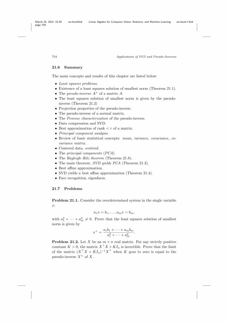
March 25, 2021 15:30 ws-book9x6 Linear Algebra for Computer Vision, Robotics, and Machine Learning ws-book-I-9x6
page 754
754 Applications of SVD and Pseudo-Inverses
21.6 Summary
The main concepts and results of this chapter are listed below:
• Least squares problems.• Existence of a least squares solution of smallest norm (Theorem 21.1).• The pseudo-inverse A+ of a matrix A.• The least squares solution of smallest norm is given by the pseudo-inverse (Theorem 21.2)
• Projection properties of the pseudo-inverse.• The pseudo-inverse of a normal matrix.• The Penrose characterization of the pseudo-inverse.• Data compression and SVD.• Best approximation of rank < r of a matrix.• Principal component analysis .• Review of basic statistical concepts: mean, variance, covariance, co-variance matrix .
• Centered data, centroid .• The principal components (PCA).• The Rayleigh–Ritz theorem (Theorem 21.8).• The main theorem: SVD yields PCA (Theorem 21.3).• Best a�ne approximation.• SVD yields a best a�ne approximation (Theorem 21.4).• Face recognition, eigenfaces.
21.7 Problems
Problem 21.1. Consider the overdetermined system in the single variablex:
a1
x = b1
, . . . , amx = bm,
with a21
+ · · · + a2m 6= 0. Prove that the least squares solution of smallestnorm is given by
x+ =a1
b1
+ · · · + ambma21
+ · · · + a2m.
Problem 21.2. Let X be an m ⇥ n real matrix. For any strictly positiveconstant K > 0, the matrix X>X +KIn is invertible. Prove that the limitof the matrix (X>X + KIn)�1X> when K goes to zero is equal to thepseudo-inverse X+ of X.

March 25, 2021 15:30 ws-book9x6 Linear Algebra for Computer Vision, Robotics, and Machine Learning ws-book-I-9x6
page 755
21.7. Problems 755
Problem 21.3. Use Matlab to find the pseudo-inverse of the 8⇥ 6 matrix
A =
0
BBBBBBBBBBB@
64 2 3 61 60 69 55 54 12 13 5117 47 46 20 21 4340 26 27 37 36 3032 34 35 29 28 3841 23 22 44 45 1949 15 14 52 53 118 58 59 5 4 62
1
CCCCCCCCCCCA
.
Observe that the sums of the columns are all equal to to 256. Let b bethe vector of dimension 8 whose coordinates are all equal to 256. Find thesolution x+ of the system Ax = b.
Problem 21.4. The purpose of this problem is to show that Proposition21.7 (the Eckart–Young theorem) also holds for the Frobenius norm. Thisproblem is adapted from Strang [Strang (2019)], Section I.9.
Suppose the m ⇥ n matrix B of rank at most k minimizes kA � BkF .Start with an SVD of B,
B = V
✓D 00 0
◆U>,
where D is a diagonal k ⇥ k matrix. We can write
A = V
✓L+ E +R F
G H
◆U>,
where L is strictly lower triangular in the first k rows, E is diagonal, andR is strictly upper triangular, and let
C = V
✓L+D +R F
0 0
◆U>,
which clearly has rank k.(1) Prove that
kA � Bk2F = kA � Ck2F + kLk2F + kRk2F + kFk2F .
Since kA � BkF is minimal, show that L = R = F = 0.Similarly, show that G = 0.(2) We have
V >AU =
✓E 00 H
◆, V >BU =
✓D 00 0
◆,
where E is diagonal, so deduce that
March 25, 2021 15:30 ws-book9x6 Linear Algebra for Computer Vision, Robotics, and Machine Learning ws-book-I-9x6
page 756
756 Applications of SVD and Pseudo-Inverses
(1) D = diag(�1
, . . . ,�k).(2) The singular values of H must be the smallest n� k singular values of
A.(3) The minimum of kA � BkF must be kHkF = (�2
k+1
+ · · · + �2
r)1/2.
Problem 21.5. Prove that the closest rank 1 approximation (in k k2
) ofthe matrix
A =
✓3 04 5
◆
is
A1
=3
2
✓1 13 3
◆.
Show that the Eckart–Young theorem fails for the operator norm k k1by finding a rank 1 matrix B such that kA � Bk1 < kA � A
1
k1.
Problem 21.6. Find a closest rank 1 approximation (in k k2
) for the ma-trices
A =
0
@3 0 00 2 00 0 1
1
A , A =
✓0 32 0
◆, A =
✓2 11 2
◆.
Problem 21.7. Find a closest rank 1 approximation (in k k2
) for the matrix
A =
✓cos ✓ � sin ✓sin ✓ cos ✓
◆.
Problem 21.8. Let S be a real symmetric positive definite matrix and letS = U⌃U> be a diagonalization of S. Prove that the closest rank 1 matrix(in the L2-norm) to S is u
1
�1
u>1
, where u1
is the first column of U .

March 25, 2021 15:30 ws-book9x6 Linear Algebra for Computer Vision, Robotics, and Machine Learning ws-book-I-9x6
page 757
Chapter 22
Annihilating Polynomials and thePrimary Decomposition
In this chapter all vector spaces are defined over an arbitrary field K.In Section 6.7 we explained that if f : E ! E is a linear map on a K-
vector space E, then for any polynomial p(X) = a0
Xd + a1
Xd�1 + · · ·+ adwith coe�cients in the field K, we can define the linear map p(f) : E ! Eby
p(f) = a0
fd + a1
fd�1 + · · · + adid,
where fk = f � · · · � f , the k-fold composition of f with itself. Note that
p(f)(u) = a0
fd(u) + a1
fd�1(u) + · · · + adu,
for every vector u 2 E. Then we showed that if E is finite-dimensionaland if �f (X) = det(XI � f) is the characteristic polynomial of f , by theCayley–Hamilton theorem, we have
�f (f) = 0.
This fact suggests looking at the set of all polynomials p(X) such that
p(f) = 0.
Such polynomials are called annihilating polynomials of f , the set of allthese polynomials, denoted Ann(f), is called the annihilator of f , and theCayley-Hamilton theorem shows that it is nontrivial since it contains apolynomial of positive degree. It turns out that Ann(f) contains a poly-nomial mf of smallest degree that generates Ann(f), and this polynomialdivides the characteristic polynomial. Furthermore, the polynomial mf en-capsulates a lot of information about f , in particular whether f can bediagonalized. One of the main reasons for this is that a scalar � 2 K is azero of the minimal polynomial mf if and only if � is an eigenvalue of f .
757

March 25, 2021 15:30 ws-book9x6 Linear Algebra for Computer Vision, Robotics, and Machine Learning ws-book-I-9x6
page 758
758 Annihilating Polynomials; Primary Decomposition
The first main result is Theorem 22.2 which states that if f : E ! E isa linear map on a finite-dimensional space E, then f is diagonalizable i↵its minimal polynomial m is of the form
m = (X � �1
) · · · (X � �k),
where �1
, . . . ,�k are distinct elements of K.One of the technical tools used to prove this result is the notion of f -
conductor ; see Definition 22.7. As a corollary of Theorem 22.2 we obtainresults about finite commuting families of diagonalizable or triangulablelinear maps.
If f : E ! E is a linear map and � 2 K is an eigenvalue of f , recall thatthe eigenspace E� associated with � is the kernel of the linear map �id�f .If all the eigenvalues �
1
. . . ,�k of f are in K and if f is diagonalizable, then
E = E�1 � · · · � E�k ,
but in general there are not enough eigenvectors to span E. A remedy is togeneralize the notion of eigenvector and look for (nonzero) vectors u (calledgeneralized eigenvectors) such that
(�id � f)r(u) = 0, for some r � 1.
Then it turns out that if the minimal polynomial of f is of the form
m = (X � �1
)r1 · · · (X � �k)rk ,
then r = ri does the job for �i; that is, if we let
Wi = Ker (�iid � f)ri ,
then
E = W1
� · · · � Wk.
The above facts are parts of the primary decomposition theorem (Theorem22.4). It is a special case of a more general result involving the factorizationof the minimal polynomialm into its irreducible monic factors; see Theorem22.3.
Theorem 22.4 implies that every linear map f that has all its eigenval-ues in K can be written as f = D+N , where D is diagonalizable and N isnilpotent (which means that Nr = 0 for some positive integer r). Further-more D and N commute and are unique. This is the Jordan decomposition,Theorem 22.5.

March 25, 2021 15:30 ws-book9x6 Linear Algebra for Computer Vision, Robotics, and Machine Learning ws-book-I-9x6
page 759
22.1. Basic Properties of Polynomials; Ideals, GCD’s 759
The Jordan decomposition suggests taking a closer look at nilpotentmaps. We prove that for any nilpotent linear map f : E ! E on a finite-dimensional vector space E of dimension n over a field K, there is a basisof E such that the matrix N of f is of the form
N =
0
BBBBB@
0 ⌫1
0 · · · 0 00 0 ⌫
2
· · · 0 0...
......
......
...0 0 0 · · · 0 ⌫n0 0 0 · · · 0 0
1
CCCCCA,
where ⌫i = 1 or ⌫i = 0; see Theorem 22.6. As a corollary we obtain theJordan form; which involves matrices of the form
Jr(�) =
0
BBBBBB@
� 1 0 · · · 00 � 1 · · · 0....... . .
. . ....
0 0 0. . . 1
0 0 0 · · · �
1
CCCCCCA,
called Jordan blocks; see Theorem 22.7.
22.1 Basic Properties of Polynomials; Ideals, GCD’s
In order to understand the structure of Ann(f), we need to review threebasic properties of polynomials. We refer the reader to Ho↵man and Kunze,[Ho↵man and Kunze (1971)], Artin [Artin (1991)], Dummit and Foote[Dummit and Foote (1999)], and Godement [Godement (1963)] for com-prehensive discussions of polynomials and their properties.
We begin by recalling some basic nomenclature. Given a field K, anynonzero polynomial p(X) 2 K[X] has some monomial of highest degreea0
Xn with a0
6= 0, and the integer n = deg(p) � 0 is called the degree of p.It is convenient to set the degree of the zero polynomial (denoted by 0) tobe
deg(0) = �1.
A polynomial p(X) such that the coe�cient a0
of its monomial of highestdegree is 1 is called a monic polynomial. For example, let K = R. Thepolynomial p(X) = 4X7 + 2X5 is of degree 7 but is not monic since a
0
=4. On the other hand, the polynomial p(X) = X3 � 3X + 1 is a monicpolynomial of degree 3.
We now discuss three key concepts of polynomial algebra:

March 25, 2021 15:30 ws-book9x6 Linear Algebra for Computer Vision, Robotics, and Machine Learning ws-book-I-9x6
page 760
760 Annihilating Polynomials; Primary Decomposition
(1) Ideals(2) Greatest common divisors and the Bezout identity.(3) Irreducible polynomials and prime factorization.
Recall the definition a of ring (see Definition 2.2).
Definition 22.1. A ring is a set A equipped with two operations +: A ⇥A ! A (called addition) and ⇤ : A ⇥ A ! A (called multiplication) havingthe following properties:
(R1) A is an abelian group w.r.t. +;(R2) ⇤ is associative and has an identity element 1 2 A;(R3) ⇤ is distributive w.r.t. +.
The identity element for addition is denoted 0, and the additive inverseof a 2 A is denoted by �a. More explicitly, the axioms of a ring are thefollowing equations which hold for all a, b, c 2 A:
a+ (b+ c) = (a+ b) + c (associativity of +) (22.1)
a+ b = b+ a (commutativity of +) (22.2)
a+ 0 = 0 + a = a (zero) (22.3)
a+ (�a) = (�a) + a = 0 (additive inverse) (22.4)
a ⇤ (b ⇤ c) = (a ⇤ b) ⇤ c (associativity of ⇤) (22.5)
a ⇤ 1 = 1 ⇤ a = a (identity for ⇤) (22.6)
(a+ b) ⇤ c = (a ⇤ c) + (b ⇤ c) (distributivity) (22.7)
a ⇤ (b+ c) = (a ⇤ b) + (a ⇤ c) (distributivity) (22.8)
The ring A is commutative if
a ⇤ b = b ⇤ a for all a, b 2 A.
From (22.7) and (22.8), we easily obtain
a ⇤ 0 = 0 ⇤ a = 0 (22.9)
a ⇤ (�b) = (�a) ⇤ b = �(a ⇤ b). (22.10)
The first crucial notion is that of an ideal.
Definition 22.2. Given a commutative ring A with unit 1, an ideal of Ais a nonempty subset I of A satisfying the following properties:
(ID1) If a, b 2 I, then b � a 2 I.(ID2) If a 2 I, then ax 2 I for all x 2 A.

March 25, 2021 15:30 ws-book9x6 Linear Algebra for Computer Vision, Robotics, and Machine Learning ws-book-I-9x6
page 761
22.1. Basic Properties of Polynomials; Ideals, GCD’s 761
An ideal I is a principal ideal if there is some a 2 I, called a generator ,such that
I = {ax | x 2 A}.In this case we usually write I = aA or I = (a). The ideal I = (0) = {0}is called the null ideal (or zero ideal).
The following proposition is a fundamental result about polynomialsover a field.
Proposition 22.1. If K is a field, then every polynomial ideal I ✓ K[X]is a principal ideal. As a consequence, if I is not the zero ideal, then thereis a unique monic polynomial
p(X) = Xn + a1
Xn�1 + · · · + an�1
X + an
in I such that I = (p).
Proof. This result is not hard to prove if we recall that polynomials candivided. Given any two nonzero polynomials f, g 2 K[X], there are uniquepolynomials q, r such that
f = qg + r, and deg(r) < deg(g). (*)
If I is not the zero ideal, there is some polynomial of smallest degree in I,and since K is a field, by suitable multiplication by a scalar, we can makesure that this polynomial is monic. Thus, let f be a monic polynomial ofsmallest degree in I. By (ID2), it is clear that (f) ✓ I. Now let g 2 I.Using (⇤), there exist unique q, r 2 K[X] such that
g = qf + r and deg(r) < deg(f).
If r 6= 0, there is some � 6= 0 in K such that �r is a monic polynomial, andsince �r = �g � �qf , with f, g 2 I, by (ID1) and (ID2), we have �r 2 I,where deg(�r) < deg(f) and �r is a monic polynomial, contradicting theminimality of the degree of f . Thus, r = 0, and g 2 (f). The uniquenessof the monic polynomial f is left as an exercise.
We will also need to know that the greatest common divisor of polyno-mials exist. Given any two nonzero polynomials f, g 2 K[X], recall that fdivides g if g = qf for some q 2 K[X].
Definition 22.3. Given any two nonzero polynomials f, g 2 K[X], a poly-nomial d 2 K[X] is a greatest common divisor of f and g (for short, a gcdof f and g) if d divides f and g and whenever h 2 K[X] divides f and g,then h divides d. We say that f and g are relatively prime if 1 is a gcd off and g.
March 25, 2021 15:30 ws-book9x6 Linear Algebra for Computer Vision, Robotics, and Machine Learning ws-book-I-9x6
page 762
762 Annihilating Polynomials; Primary Decomposition
Note that f and g are relatively prime i↵ all of their gcd’s are constants(scalars in K), or equivalently, if f, g have no common divisor q of degreedeg(q) � 1. For example, over R, gcd(X2 � 1, X3 +X2 � X � 1) = (X �1)(X+1) sinceX3+X2�X�1 = (X�1)(X+1)2, while gcd(X3+1, X�1) =1.
We can characterize gcd’s of polynomials as follows.
Proposition 22.2. Let K be a field and let f, g 2 K[X] be any two nonzeropolynomials. For every polynomial d 2 K[X], the following properties areequivalent:
(1) The polynomial d is a gcd of f and g.(2) The polynomial d divides f and g and there exist u, v 2 K[X] such that
d = uf + vg.
(3) The ideals (f), (g), and (d) satisfy the equation
(d) = (f) + (g).
In addition, d 6= 0, and d is unique up to multiplication by a nonzeroscalar in K.
As a consequence of Proposition 22.2, two nonzero polynomials f, g 2K[X] are relatively prime i↵ there exist u, v 2 K[X] such that
uf + vg = 1.
The identity
d = uf + vg
of Part (2) of Proposition 22.2 is often called the Bezout identity . For anexample of Bezout’s identity, take K = R. Since X3 + 1 and X � 1 arerelatively prime, we have1 = 1/2(X3 + 1) � 1/2(X2 +X + 1)(X � 1).
An important consequence of the Bezout identity is the following result.
Proposition 22.3. (Euclid’s proposition) Let K be a field and let f, g, h 2K[X] be any nonzero polynomials. If f divides gh and f is relatively primeto g, then f divides h.
Proposition 22.3 can be generalized to any number of polynomials.
Proposition 22.4. Let K be a field and let f, g1
, . . . , gm 2 K[X] be somenonzero polynomials. If f and gi are relatively prime for all i, 1 i m,then f and g
1
· · · gm are relatively prime.

March 25, 2021 15:30 ws-book9x6 Linear Algebra for Computer Vision, Robotics, and Machine Learning ws-book-I-9x6
page 763
22.1. Basic Properties of Polynomials; Ideals, GCD’s 763
Definition 22.3 is generalized to any finite number of polynomials asfollows.
Definition 22.4. Given any nonzero polynomials f1
, . . . , fn 2 K[X], wheren � 2, a polynomial d 2 K[X] is a greatest common divisor of f
1
, . . . , fn(for short, a gcd of f
1
, . . . , fn) if d divides each fi and whenever h 2 K[X]divides each fi, then h divides d. We say that f
1
, . . . , fn are relatively primeif 1 is a gcd of f
1
, . . . , fn.
It is easily shown that Proposition 22.2 can be generalized to any finitenumber of polynomials.
Proposition 22.5. Let K be a field and let f1
, . . . , fn 2 K[X] be anyn � 2 nonzero polynomials. For every polynomial d 2 K[X], the followingproperties are equivalent:
(1) The polynomial d is a gcd of f1
, . . . , fn.(2) The polynomial d divides each fi and there exist u
1
, . . . , un 2 K[X]such that
d = u1
f1
+ · · · + unfn.
(3) The ideals (fi), and (d) satisfy the equation
(d) = (f1
) + · · · + (fn).
In addition, d 6= 0, and d is unique up to multiplication by a nonzeroscalar in K.
As a consequence of Proposition 22.5, any n � 2 nonzero polynomialsf1
, . . . , fn 2 K[X] are relatively prime i↵ there exist u1
, . . . , un 2 K[X]such that
u1
f1
+ · · · + unfn = 1,
the Bezout identity .We will also need to know that every nonzero polynomial (over a field)
can be factored into irreducible polynomials, which is the generalization ofthe prime numbers to polynomials.
Definition 22.5. Given a field K, a polynomial p 2 K[X] is irreducibleor indecomposable or prime if deg(p) � 1 and if p is not divisible by anypolynomial q 2 K[X] such that 1 deg(q) < deg(p). Equivalently, p isirreducible if deg(p) � 1 and if p = q
1
q2
, then either q1
2 K or q2
2 K (andof course, q
1
6= 0, q2
6= 0).

March 25, 2021 15:30 ws-book9x6 Linear Algebra for Computer Vision, Robotics, and Machine Learning ws-book-I-9x6
page 764
764 Annihilating Polynomials; Primary Decomposition
Every polynomial aX + b of degree 1 is irreducible. Over the field R,the polynomial X2 +1 is irreducible (why?), but X3 +1 is not irreducible,since
X3 + 1 = (X + 1)(X2 � X + 1).
The polynomial X2 � X + 1 is irreducible over R (why?). It would seemthat X4 + 1 is irreducible over R, but in fact,
X4 + 1 = (X2 �p2X + 1)(X2 +
p2X + 1).
However, in view of the above factorization, X4 + 1 is irreducible over Q.It can be shown that the irreducible polynomials over R are the polyno-
mials of degree 1 or the polynomials of degree 2 of the form aX2 + bX + c,for which b2 � 4ac < 0 (i.e., those having no real roots). This is not easyto prove! Over the complex numbers C, the only irreducible polynomialsare those of degree 1. This is a version of a fact often referred to as the“Fundamental Theorem of Algebra.”
Observe that the definition of irreducibilty implies that any finite num-ber of distinct irreducible polynomials are relatively prime.
The following fundamental result can be shown
Theorem 22.1. Given any field K, for every nonzero polynomial
f = adXd + ad�1
Xd�1 + · · · + a0
of degree d = deg(f) � 1 in K[X], there exists a unique set {hp1
, k1
i,. . . , hpm, kmi} such that
f = adpk11
· · · pkmm ,
where the pi 2 K[X] are distinct irreducible monic polynomials, the ki are(not necessarily distinct) integers, and with m � 1, ki � 1.
We can now return to minimal polynomials.
22.2 Annihilating Polynomials and the Minimal Polynomial
Given a linear map f : E ! E, it is easy to check that the set Ann(f) ofpolynomials that annihilate f is an ideal. Furthermore, when E is finite-dimensional, the Cayley–Hamilton theorem implies that Ann(f) is not thezero ideal. Therefore, by Proposition 22.1, there is a unique monic polyno-mial mf that generates Ann(f).
Definition 22.6. If f : E ! E is a linear map on a finite-dimensionalvector space E, the unique monic polynomial mf (X) that generates theideal Ann(f) of polynomials which annihilate f (the annihilator of f) iscalled the minimal polynomial of f .
March 25, 2021 15:30 ws-book9x6 Linear Algebra for Computer Vision, Robotics, and Machine Learning ws-book-I-9x6
page 765
22.2. Annihilating Polynomials and the Minimal Polynomial 765
The minimal polynomial mf of f is the monic polynomial of smallestdegree that annihilates f . Thus, the minimal polynomial divides the char-acteristic polynomial �f , and deg(mf ) � 1. For simplicity of notation, weoften write m instead of mf .
If A is any n⇥n matrix, the set Ann(A) of polynomials that annihilateA is the set of polynomials
p(X) = a0
Xd + a1
Xd�1 + · · · + ad�1
X + ad
such that
a0
Ad + a1
Ad�1 + · · · + ad�1
A+ adI = 0.
It is clear that Ann(A) is a nonzero ideal and its unique monic generator iscalled the minimal polynomial of A. We check immediately that if Q is aninvertible matrix, then A and Q�1AQ have the same minimal polynomial.Also, if A is the matrix of f with respect to some basis, then f and A havethe same minimal polynomial.
The zeros (in K) of the minimal polynomial of f and the eigenvalues off (in K) are intimately related.
Proposition 22.6. Let f : E ! E be a linear map on some finite-dimensional vector space E. Then � 2 K is a zero of the minimal poly-nomial mf (X) of f i↵ � is an eigenvalue of f i↵ � is a zero of �f (X).Therefore, the minimal and the characteristic polynomials have the samezeros (in K), except for multiplicities.
Proof. First assume that m(�) = 0 (with � 2 K, and writing m insteadof mf ). If so, using polynomial division, m can be factored as
m = (X � �)q,
with deg(q) < deg(m). Since m is the minimal polynomial, q(f) 6= 0, sothere is some nonzero vector v 2 E such that u = q(f)(v) 6= 0. But then,because m is the minimal polynomial,
0 = m(f)(v)
= (f � �id)(q(f)(v))
= (f � �id)(u),
which shows that � is an eigenvalue of f .Conversely, assume that � 2 K is an eigenvalue of f . This means that
for some u 6= 0, we have f(u) = �u. Now it is easy to show that
m(f)(u) = m(�)u,
and since m is the minimal polynomial of f , we have m(f)(u) = 0, som(�)u = 0, and since u 6= 0, we must have m(�) = 0.

March 25, 2021 15:30 ws-book9x6 Linear Algebra for Computer Vision, Robotics, and Machine Learning ws-book-I-9x6
page 766
766 Annihilating Polynomials; Primary Decomposition
Proposition 22.7. Let f : E ! E be a linear map on some finite-dimensional vector space E. If f diagonalizable, then its minimal poly-nomial is a product of distinct factors of degree 1.
Proof. If we assume that f is diagonalizable, then its eigenvalues are all inK, and if �
1
, . . . ,�k are the distinct eigenvalues of f , and then by Proposi-tion 22.6, the minimal polynomial m of f must be a product of powers ofthe polynomials (X � �i). Actually, we claim that
m = (X � �1
) · · · (X � �k).
For this we just have to show that m annihilates f . However, for anyeigenvector u of f , one of the linear maps f � �iid sends u to 0, so
m(f)(u) = (f � �1
id) � · · · � (f � �kid)(u) = 0.
Since E is spanned by the eigenvectors of f , we conclude that
m(f) = 0.
It turns out that the converse of Proposition 22.7 is true, but this will takea little work to establish it.
22.3 Minimal Polynomials of DiagonalizableLinear Maps
In this section we prove that if the minimal polynomial mf of a linear mapf is of the form
mf = (X � �1
) · · · (X � �k)
for distinct scalars �1
, . . . ,�k 2 K, then f is diagonalizable. This is apowerful result that has a number of implications. But first we need of fewproperties of invariant subspaces.
Given a linear map f : E ! E, recall that a subspaceW of E is invariantunder f if f(u) 2 W for all u 2 W . For example, if f : R2 ! R2 isf(x, y) = (�x, y), the y-axis is invariant under f .
Proposition 22.8. Let W be a subspace of E invariant under the linearmap f : E ! E (where E is finite-dimensional). Then the minimal poly-nomial of the restriction f | W of f to W divides the minimal polynomialof f , and the characteristic polynomial of f | W divides the characteristicpolynomial of f .

March 25, 2021 15:30 ws-book9x6 Linear Algebra for Computer Vision, Robotics, and Machine Learning ws-book-I-9x6
page 767
22.3. Minimal Polynomials of Diagonalizable Linear Maps 767
Sketch of proof. The key ingredient is that we can pick a basis(e
1
, . . . , en) of E in which (e1
, . . . , ek) is a basis of W . The matrix of fover this basis is a block matrix of the form
A =
✓B C0 D
◆,
where B is a k ⇥ k matrix, D is an (n � k) ⇥ (n � k) matrix, and C is ak ⇥ (n � k) matrix. Then
det(XI � A) = det(XI � B) det(XI � D),
which implies the statement about the characteristic polynomials. Further-more,
Ai =
✓Bi Ci
0 Di
◆,
for some k ⇥ (n � k) matrix Ci. It follows that any polynomial whichannihilates A also annihilates B and D. So the minimal polynomial of Bdivides the minimal polynomial of A.
For the next step, there are at least two ways to proceed. We can use anold-fashion argument using Lagrange interpolants, or we can use a slightgeneralization of the notion of annihilator. We pick the second methodbecause it illustrates nicely the power of principal ideals.
What we need is the notion of conductor (also called transporter).
Definition 22.7. Let f : E ! E be a linear map on a finite-dimensionalvector space E, let W be an invariant subspace of f , and let u be any vectorin E. The set Sf (u,W ) consisting of all polynomials q 2 K[X] such thatq(f)(u) 2 W is called the f -conductor of u into W .
Observe that the minimal polynomial mf of f always belongs toSf (u,W ), so this is a nontrivial set. Also, if W = (0), then Sf (u, (0))is just the annihilator of f . The crucial property of Sf (u,W ) is that it isan ideal.
Proposition 22.9. If W is an invariant subspace for f , then for eachu 2 E, the f -conductor Sf (u,W ) is an ideal in K[X].
We leave the proof as a simple exercise, using the fact that ifW invariantunder f , then W is invariant under every polynomial q(f) in Sf (u,W ).

March 25, 2021 15:30 ws-book9x6 Linear Algebra for Computer Vision, Robotics, and Machine Learning ws-book-I-9x6
page 768
768 Annihilating Polynomials; Primary Decomposition
Since Sf (u,W ) is an ideal, it is generated by a unique monic polynomialq of smallest degree, and because the minimal polynomial mf of f is inSf (u,W ), the polynomial q divides m.
Definition 22.8. The unique monic polynomial which generates Sf (u,W )is called the conductor of u into W .
Example 22.1. For example, suppose f : R2 ! R2 where f(x, y) = (x, 0).Observe that W = {(x, 0) 2 R2} is invariant under f . By representing f
as
✓1 00 0
◆, we see that mf (X) = �f (X) = X2 � X. Let u = (0, y). Then
Sf (u,W ) = (X), and we say X is the conductor of u into W .
Proposition 22.10. Let f : E ! E be a linear map on a finite-dimensionalspace E and assume that the minimal polynomial m of f is of the form
m = (X � �1
)r1 · · · (X � �k)rk ,
where the eigenvalues �1
, . . . ,�k of f belong to K. If W is a proper subspaceof E which is invariant under f , then there is a vector u 2 E with thefollowing properties:
(a) u /2 W ;(b) (f � �id)(u) 2 W , for some eigenvalue � of f .
Proof. Observe that (a) and (b) together assert that the conductor of uinto W is a polynomial of the form X � �i. Pick any vector v 2 E notin W , and let g be the conductor of v into W , i.e. g(f)(v) 2 W . Since gdivides m and v /2 W , the polynomial g is not a constant, and thus it is ofthe form
g = (X � �1
)s1 · · · (X � �k)sk ,
with at least some si > 0. Choose some index j such that sj > 0. ThenX � �j is a factor of g, so we can write
g = (X � �j)q. (*)
By definition of g, the vector u = q(f)(v) cannot be in W , since otherwiseg would not be of minimal degree. However, (⇤) implies that
(f � �j id)(u) = (f � �j id)(q(f)(v))
= g(f)(v)
is in W , which concludes the proof.

March 25, 2021 15:30 ws-book9x6 Linear Algebra for Computer Vision, Robotics, and Machine Learning ws-book-I-9x6
page 769
22.3. Minimal Polynomials of Diagonalizable Linear Maps 769
We can now prove the main result of this section.
Theorem 22.2. Let f : E ! E be a linear map on a finite-dimensionalspace E. Then f is diagonalizable i↵ its minimal polynomial m is of theform
m = (X � �1
) · · · (X � �k),
where �1
, . . . ,�k are distinct elements of K.
Proof. We already showed in Proposition 22.7 that if f is diagonalizable,then its minimal polynomial is of the above form (where �
1
, . . . ,�k are thedistinct eigenvalues of f).
For the converse, let W be the subspace spanned by all the eigenvectorsof f . If W 6= E, since W is invariant under f , by Proposition 22.10, thereis some vector u /2 W such that for some �j , we have
(f � �j id)(u) 2 W.
Let v = (f � �j id)(u) 2 W . Since v 2 W , we can write
v = w1
+ · · · + wk
where f(wi) = �iwi (either wi = 0 or wi is an eigenvector for �i), and sofor every polynomial h, we have
h(f)(v) = h(�1
)w1
+ · · · + h(�k)wk,
which shows that h(f)(v) 2 W for every polynomial h. We can write
m = (X � �j)q
for some polynomial q, and also
q � q(�j) = p(X � �j)
for some polynomial p. We know that p(f)(v) 2 W , and since m is theminimal polynomial of f , we have
0 = m(f)(u) = (f � �j id)(q(f)(u)),
which implies that q(f)(u) 2 W (either q(f)(u) = 0, or it is an eigenvectorassociated with �j). However,
q(f)(u) � q(�j)u = p(f)((f � �j id)(u)) = p(f)(v),
and since p(f)(v) 2 W and q(f)(u) 2 W , we conclude that q(�j)u 2 W .But, u /2 W , which implies that q(�j) = 0, so �j is a double root of m, acontradiction. Therefore, we must have W = E.
Remark: Proposition 22.10 can be used to give a quick proof of Theorem14.1.

March 25, 2021 15:30 ws-book9x6 Linear Algebra for Computer Vision, Robotics, and Machine Learning ws-book-I-9x6
page 770
770 Annihilating Polynomials; Primary Decomposition
22.4 Commuting Families of Diagonalizable and Triangula-ble Maps
Using Theorem 22.2, we can give a short proof about commuting diagonal-izable linear maps.
Definition 22.9. If F is a family of linear maps on a vector space E, wesay that F is a commuting family i↵ f � g = g � f for all f, g 2 F .
Proposition 22.11. Let F be a commuting family of diagonalizable linearmaps on a vector space E. There exists a basis of E such that every linearmap in F is represented in that basis by a diagonal matrix.
Proof. We proceed by induction on n = dim(E). If n = 1, there is nothingto prove. If n > 1, there are two cases. If all linear maps in F are of theform �id for some � 2 K, then the proposition holds trivially. In the secondcase, let f 2 F be some linear map in F which is not a scalar multiple ofthe identity. In this case, f has at least two distinct eigenvalues �
1
, . . . ,�k,and because f is diagonalizable, E is the direct sum of the correspondingeigenspaces E�1 , . . . , E�k . For every index i, the eigenspace E�i is invariantunder f and under every other linear map g in F , since for any g 2 F andany u 2 E�i , because f and g commute, we have
f(g(u)) = g(f(u)) = g(�iu) = �ig(u)
so g(u) 2 E�i . Let Fi be the family obtained by restricting each f 2 Fto E�i . By Proposition 22.8, the minimal polynomial of every linear mapf | E�i in Fi divides the minimal polynomial mf of f , and since f isdiagonalizable, mf is a product of distinct linear factors, so the minimalpolynomial of f | E�i is also a product of distinct linear factors. By The-orem 22.2, the linear map f | E�i is diagonalizable. Since k > 1, we havedim(E�i) < dim(E) for i = 1, . . . , k, and by the induction hypothesis, foreach i there is a basis of E�i over which f | E�i is represented by a diagonalmatrix. Since the above argument holds for all i, by combining the basesof the E�i , we obtain a basis of E such that the matrix of every linear mapf 2 F is represented by a diagonal matrix.
There is also an analogous result for commuting families of linear mapsrepresented by upper triangular matrices. To prove this we need the fol-lowing proposition.
Proposition 22.12. Let F be a nonempty commuting family of triangula-ble linear maps on a finite-dimensional vector space E. Let W be a proper

March 25, 2021 15:30 ws-book9x6 Linear Algebra for Computer Vision, Robotics, and Machine Learning ws-book-I-9x6
page 771
22.4. Commuting Families of Linear Maps 771
subspace of E which is invariant under F . Then there exists a vector u 2 Esuch that:
(1) u /2 W .(2) For every f 2 F , the vector f(u) belongs to the subspace W � Ku
spanned by W and u.
Proof. By renaming the elements of F if necessary, we may assume that(f
1
, . . . , fr) is a basis of the subspace of End(E) spanned by F . We proveby induction on r that there exists some vector u 2 E such that
(1) u /2 W .(2) (fi � ↵iid)(u) 2 W for i = 1, . . . , r, for some scalars ↵i 2 K.
Consider the base case r = 1. Since f1
is triangulable, its eigenvaluesall belong to K since they are the diagonal entries of the triangular matrixassociated with f
1
(this is the easy direction of Theorem 14.1), so theminimal polynomial of f
1
is of the form
m = (X � �1
)r1 · · · (X � �k)rk ,
where the eigenvalues �1
, . . . ,�k of f1
belong to K. We conclude by apply-ing Proposition 22.10.
Next assume that r � 2 and that the induction hypothesis holds forf1
, . . . , fr�1
. Thus, there is a vector ur�1
2 E such that
(1) ur�1
/2 W .(2) (fi � ↵iid)(ur�1
) 2 W for i = 1, . . . , r � 1, for some scalars ↵i 2 K.
Let
Vr�1
= {w 2 E | (fi � ↵iid)(w) 2 W, i = 1, . . . , r � 1}.
Clearly, W ✓ Vr�1
and ur�1
2 Vr�1
. We claim that Vr�1
is invariantunder F . This is because, for any v 2 Vr�1
and any f 2 F , since f and ficommute, we have
(fi � ↵iid)(f(v)) = f((fi � ↵iid)(v)), 1 i r � 1.
Now (fi � ↵iid)(v) 2 W because v 2 Vr�1
, and W is invariant under F , sof(fi � ↵iid)(v)) 2 W , that is, (fi � ↵iid)(f(v)) 2 W .
Consider the restriction gr of fr to Vr�1
. The minimal polynomial ofgr divides the minimal polynomial of fr, and since fr is triangulable, justas we saw for f
1
, the minimal polynomial of fr is of the form
m = (X � �1
)r1 · · · (X � �k)rk ,
March 25, 2021 15:30 ws-book9x6 Linear Algebra for Computer Vision, Robotics, and Machine Learning ws-book-I-9x6
page 772
772 Annihilating Polynomials; Primary Decomposition
where the eigenvalues �1
, . . . ,�k of fr belong to K, so the minimal polyno-mial of gr is of the same form. By Proposition 22.10, there is some vectorur 2 Vr�1
such that
(1) ur /2 W .(2) (gr � ↵rid)(ur) 2 W for some scalars ↵r 2 K.
Now since ur 2 Vr�1
, we have (fi � ↵iid)(ur) 2 W for i = 1, . . . , r � 1, so(fi �↵iid)(ur) 2 W for i = 1, . . . , r (since gr is the restriction of fr), whichconcludes the proof of the induction step. Finally, since every f 2 F isthe linear combination of (f
1
, . . . , fr), Condition (2) of the inductive claimimplies Condition (2) of the proposition.
We can now prove the following result.
Proposition 22.13. Let F be a nonempty commuting family of triangu-lable linear maps on a finite-dimensional vector space E. There exists abasis of E such that every linear map in F is represented in that basis byan upper triangular matrix.
Proof. Let n = dim(E). We construct inductively a basis (u1
, . . . , un) ofE such that if Wi is the subspace spanned by (u
1
. . . , ui), then for everyf 2 F ,
f(ui) = af1iu1
+ · · · + afiiui,
for some afij 2 K; that is, f(ui) belongs to the subspace Wi.We begin by applying Proposition 22.12 to the subspace W
0
= (0) toget u
1
so that for all f 2 F ,
f(u1
) = ↵f1
u1
.
For the induction step, since Wi invariant under F , we apply Proposition22.12 to the subspace Wi, to get ui+1
2 E such that
(1) ui+1
/2 Wi.(2) For every f 2 F , the vector f(ui+1
) belong to the subspace spannedby Wi and ui+1
.
Condition (1) implies that (u1
, . . . , ui, ui+1
) is linearly independent, andCondition (2) means that for every f 2 F ,
f(ui+1
) = af1i+1
u1
+ · · · + afi+1i+1
ui+1
,
for some afi+1j 2 K, establishing the induction step. After n steps, eachf 2 F is represented by an upper triangular matrix.
March 25, 2021 15:30 ws-book9x6 Linear Algebra for Computer Vision, Robotics, and Machine Learning ws-book-I-9x6
page 773
22.5. The Primary Decomposition Theorem 773
Observe that if F consists of a single linear map f and if the minimalpolynomial of f is of the form
m = (X � �1
)r1 · · · (X � �k)rk ,
with all �i 2 K, using Proposition 22.10 instead of Proposition 22.12, theproof of Proposition 22.13 yields another proof of Theorem 14.1.
22.5 The Primary Decomposition Theorem
If f : E ! E is a linear map and � 2 K is an eigenvalue of f , recall thatthe eigenspace E� associated with � is the kernel of the linear map �id�f .If all the eigenvalues �
1
. . . ,�k of f are in K, it may happen that
E = E�1 � · · · � E�k ,
but in general there are not enough eigenvectors to span E. What if wegeneralize the notion of eigenvector and look for (nonzero) vectors u suchthat
(�id � f)r(u) = 0, for some r � 1?
It turns out that if the minimal polynomial of f is of the form
m = (X � �1
)r1 · · · (X � �k)rk ,
then r = ri does the job for �i; that is, if we let
Wi = Ker (�iid � f)ri ,
then
E = W1
� · · · � Wk.
This result is very nice but seems to require that the eigenvalues of f allbelong to K. Actually, it is a special case of a more general result involvingthe factorization of the minimal polynomial m into its irreducible monicfactors (see Theorem 22.1),
m = pr11
· · · prkk ,
where the pi are distinct irreducible monic polynomials over K.
Theorem 22.3. (Primary Decomposition Theorem) Let f : E ! E be alinear map on the finite-dimensional vector space E over the field K. Writethe minimal polynomial m of f as
m = pr11
· · · prkk ,
where the pi are distinct irreducible monic polynomials over K, and the riare positive integers. Let
Wi = Ker (prii (f)), i = 1, . . . , k.
Then

March 25, 2021 15:30 ws-book9x6 Linear Algebra for Computer Vision, Robotics, and Machine Learning ws-book-I-9x6
page 774
774 Annihilating Polynomials; Primary Decomposition
(a) E = W1
� · · · � Wk.(b) Each Wi is invariant under f .(c) The minimal polynomial of the restriction f | Wi of f to Wi is prii .
Proof. The trick is to construct projections ⇡i using the polynomials prjj
so that the range of ⇡i is equal to Wi. Let
gi = m/prii =Y
j 6=i
prjj .
Note that
prii gi = m.
Since p1
, . . . , pk are irreducible and distinct, they are relatively prime. Thenusing Proposition 22.4, it is easy to show that g
1
, . . . , gk are relatively prime.Otherwise, some irreducible polynomial p would divide all of g
1
, . . . , gk, soby Proposition 22.4 it would be equal to one of the irreducible factors pi.But that pi is missing from gi, a contradiction. Therefore, by Proposition22.5, there exist some polynomials h
1
, . . . , hk such that
g1
h1
+ · · · + gkhk = 1.
Let qi = gihi and let ⇡i = qi(f) = gi(f)hi(f). We have
q1
+ · · · + qk = 1,
and since m divides qiqj for i 6= j, we get
⇡1
+ · · · + ⇡k = id
⇡i⇡j = 0, i 6= j.
(We implicitly used the fact that if p, q are two polynomials, the linear mapsp(f)�q(f) and q(f)�p(f) are the same since p(f) and q(f) are polynomialsin the powers of f , which commute.) Composing the first equation with ⇡iand using the second equation, we get
⇡2
i = ⇡i.
Therefore, the ⇡i are projections, and E is the direct sum of the images ofthe ⇡i. Indeed, every u 2 E can be expressed as
u = ⇡1
(u) + · · · + ⇡k(u).
Also, if
⇡1
(u) + · · · + ⇡k(u) = 0,

March 25, 2021 15:30 ws-book9x6 Linear Algebra for Computer Vision, Robotics, and Machine Learning ws-book-I-9x6
page 775
22.5. The Primary Decomposition Theorem 775
then by applying ⇡i we get
0 = ⇡2
i (u) = ⇡i(u), i = 1, . . . k.
To finish proving (a), we need to show that
Wi = Ker (prii (f)) = ⇡i(E).
If v 2 ⇡i(E), then v = ⇡i(u) for some u 2 E, so
prii (f)(v) = prii (f)(⇡i(u))
= prii (f)gi(f)hi(f)(u)
= hi(f)prii (f)gi(f)(u)
= hi(f)m(f)(u) = 0,
because m is the minimal polynomial of f . Therefore, v 2 Wi.Conversely, assume that v 2 Wi = Ker (prii (f)). If j 6= i, then gjhj is
divisible by prii , so
gj(f)hj(f)(v) = ⇡j(v) = 0, j 6= i.
Then since ⇡1
+ · · · + ⇡k = id, we have v = ⇡iv, which shows that v is inthe range of ⇡i. Therefore, Wi = Im(⇡i), and this finishes the proof of (a).
If prii (f)(u) = 0, then prii (f)(f(u)) = f(prii (f)(u)) = 0, so (b) holds.If we write fi = f | Wi, then prii (fi) = 0, because prii (f) = 0 on Wi (its
kernel). Therefore, the minimal polynomial of fi divides prii . Conversely,let q be any polynomial such that q(fi) = 0 (on Wi). Since m = prii gi, thefact that m(f)(u) = 0 for all u 2 E shows that
prii (f)(gi(f)(u)) = 0, u 2 E,
and thus Im(gi(f)) ✓ Ker (prii (f)) = Wi. Consequently, since q(f) is zeroon Wi,
q(f)gi(f) = 0 for all u 2 E.
But then qgi is divisible by the minimal polynomial m = prii gi of f , andsince prii and gi are relatively prime, by Euclid’s proposition, prii must divideq. This finishes the proof that the minimal polynomial of fi is prii , whichis (c).
To best understand the projection constructions of Theorem 22.3, weprovide the following two explicit examples of the primary decompositiontheorem.

March 25, 2021 15:30 ws-book9x6 Linear Algebra for Computer Vision, Robotics, and Machine Learning ws-book-I-9x6
page 776
776 Annihilating Polynomials; Primary Decomposition
Example 22.2. First let f : R3 ! R3 be defined as f(x, y, z) = (y,�x, z).In terms of the standard basis f is represented by the 3 ⇥ 3 matrix
Xf :=
0
@0 �1 01 0 00 0 1
1
A .
Then a simple calculation shows that mf (x) = �f (x) = (x2 + 1)(x � 1).Using the notation of the preceding proof set
m = p1
p2
, p1
= x2 + 1, p2
= x � 1.
Then
g1
=m
p1
= x � 1, g2
=m
p2
= x2 + 1.
We must find h1
, h2
2 R[x] such that g1
h1
+ g2
h2
= 1. In general this isthe hard part of the projection construction. But since we are only workingwith two relatively prime polynomials g
1
, g2
, we may apply the Euclideanalgorithm to discover that
�x+ 1
2(x � 1) +
1
2(x2 + 1) = 1,
where h1
= �x+1
2
while h2
= 1
2
. By definition
⇡1
= g1
(f)h1
(f) = �1
2(Xf � id)(Xf + id) = �1
2(X2
f � id) =
0
@1 0 00 1 00 0 0
1
A ,
and
⇡2
= g2
(f)h2
(f) =1
2(X2
f + id) =
0
@0 0 00 0 00 0 1
1
A .
Then R3 = W1
� W2
, where
W1
= ⇡1
(R3) = Ker (p1
(Xf )) = Ker (X2
f + id)
= Ker
0
@0 0 00 0 00 0 1
1
A = {(x, y, 0) 2 R3},
W2
= ⇡2
(R3) = Ker (p2
(Xf )) = Ker (Xf � id)
= Ker
0
@�1 �1 01 �1 00 0 0
1
A = {(0, 0, z) 2 R3}.
March 25, 2021 15:30 ws-book9x6 Linear Algebra for Computer Vision, Robotics, and Machine Learning ws-book-I-9x6
page 777
22.5. The Primary Decomposition Theorem 777
Example 22.3. For our second example of the primary decompositiontheorem let f : R3 ! R3 be defined as f(x, y, z) = (y,�x + z,�y), with
standard matrix representation Xf =
0
@0 �1 01 0 �10 1 0
1
A. A simple calculation
shows that mf (x) = �f (x) = x(x2 + 2). Set
p1
= x2 + 2, p2
= x, g1
=mf
p1
= x, g2
=mf
p2
= x2 + 2.
Since gcd(g1
, g2
) = 1, we use the Euclidean algorithm to find
h1
= �1
2x, h
2
=1
2,
such that g1
h1
+ g2
h2
= 1. Then
⇡1
= g1
(f)h1
(f) = �1
2X2
f =
0
@1
2
0 � 1
2
0 1 0� 1
2
0 1
2
1
A ,
while
⇡2
= g2
(f)h2
(f) =1
2(X2
f + 2id) =
0
@1
2
0 1
2
0 0 01
2
0 1
2
1
A .
Although it is not entirely obvious, ⇡1
and ⇡2
are indeed projections since
⇡2
1
=
0
@1
2
0 � 1
2
0 1 0� 1
2
0 1
2
1
A
0
@1
2
0 � 1
2
0 1 0� 1
2
0 1
2
1
A =
0
@1
2
0 � 1
2
0 1 0� 1
2
0 1
2
1
A = ⇡1
,
and
⇡2
2
=
0
@1
2
0 1
2
0 0 01
2
0 1
2
1
A
0
@1
2
0 1
2
0 0 01
2
0 1
2
1
A =
0
@1
2
0 1
2
0 0 01
2
0 1
2
1
A = ⇡2
.
Furthermore observe that ⇡1
+ ⇡2
= id. The primary decomposition theo-rem implies that R3 = W
1
� W2
where
W1
= ⇡1
(R3) = Ker (p1
(f)) = Ker (X2 + 2)
= Ker
0
@1 0 10 0 01 0 1
1
A = span{(0, 1, 0), (1, 0,�1)},
W2
= ⇡2
(R3) = Ker (p2
(f)) = Ker (X) = span{(1, 0, 1)}.
See Figure 22.1.

March 25, 2021 15:30 ws-book9x6 Linear Algebra for Computer Vision, Robotics, and Machine Learning ws-book-I-9x6
page 778
778 Annihilating Polynomials; Primary Decomposition
Fig. 22.1 The direct sum decomposition of R3 = W1 � W2 where W1 is the planex + z = 0 and W2 is line t(1, 0, 1). The spanning vectors of W1 are in blue.
If all the eigenvalues of f belong to the field K, we obtain the followingresult.
Theorem 22.4. (Primary Decomposition Theorem, Version 2) Letf : E ! E be a linear map on the finite-dimensional vector space E overthe field K. If all the eigenvalues �
1
, . . . ,�k of f belong to K, write
m = (X � �1
)r1 · · · (X � �k)rk
for the minimal polynomial of f ,
�f = (X � �1
)n1 · · · (X � �k)nk
for the characteristic polynomial of f , with 1 ri ni, and let
Wi = Ker (�iid � f)ri , i = 1, . . . , k.
Then
(a) E = W1
� · · · � Wk.(b) Each Wi is invariant under f .(c) dim(Wi) = ni.

March 25, 2021 15:30 ws-book9x6 Linear Algebra for Computer Vision, Robotics, and Machine Learning ws-book-I-9x6
page 779
22.6. Jordan Decomposition 779
(d) The minimal polynomial of the restriction f | Wi of f to Wi is (X ��i)ri .
Proof. Parts (a), (b) and (d) have already been proven in Theorem 22.3,so it remains to prove (c). Since Wi is invariant under f , let fi be therestriction of f to Wi. The characteristic polynomial �fi of fi divides �(f),and since �(f) has all its roots in K, so does �i(f). By Theorem 14.1, thereis a basis of Wi in which fi is represented by an upper triangular matrix,and since (�iid � f)ri = 0, the diagonal entries of this matrix are equal to�i. Consequently,
�fi = (X � �i)dim(Wi),
and since �fi divides �(f), we conclude hat
dim(Wi) ni, i = 1, . . . , k.
Because E is the direct sum of the Wi, we have dim(W1
)+ · · ·+dim(Wk) =n, and since n
1
+ · · · + nk = n, we must have
dim(Wi) = ni, i = 1, . . . , k,
proving (c).
Definition 22.10. If � 2 K is an eigenvalue of f , we define a generalizedeigenvector of f as a nonzero vector u 2 E such that
(�id � f)r(u) = 0, for some r � 1.
The index of � is defined as the smallest r � 1 such that
Ker (�id � f)r = Ker (�id � f)r+1.
It is clear that Ker (�id � f)i ✓ Ker (�id � f)i+1 for all i � 1. ByTheorem 22.4(d), if � = �i, the index of �i is equal to ri.
22.6 Jordan Decomposition
Recall that a linear map g : E ! E is said to be nilpotent if there is somepositive integer r such that gr = 0. Another important consequence ofTheorem 22.4 is that f can be written as the sum of a diagonalizable anda nilpotent linear map (which commute). For example f : R2 ! R2 bethe R-linear map f(x, y) = (x, x+ y) with standard matrix representation
Xf =
✓1 10 1
◆. A basic calculation shows that mf (x) = �f (x) = (x � 1)2.
By Theorem 22.2 we know that f is not diagonalizable over R. But since

March 25, 2021 15:30 ws-book9x6 Linear Algebra for Computer Vision, Robotics, and Machine Learning ws-book-I-9x6
page 780
780 Annihilating Polynomials; Primary Decomposition
the eigenvalue �1
= 1 of f does belong to R, we may use the projectionconstruction inherent within Theorem 22.4 to write f = D +N , where Dis a diagonalizable linear map and N is a nilpotent linear map. The proofof Theorem 22.3 implies that
pr11
= (x � 1)2, g1
= 1 = h1
, ⇡1
= g1
(f)h1
(f) = id.
Then
D = �1
⇡1
= id,
N = f � D = f(x, y) � id(x, y) = (x, x+ y) � (x, y) = (0, y),
which is equivalent to the matrix decomposition
Xf =
✓1 10 1
◆=
✓1 00 1
◆+
✓0 10 0
◆.
This example suggests that the diagonal summand of f is related to theprojection constructions associated with the proof of the primary decom-position theorem. If we write
D = �1
⇡1
+ · · · + �k⇡k,
where ⇡i is the projection from E onto the subspace Wi defined in the proofof Theorem 22.3, since
⇡1
+ · · · + ⇡k = id,
we have
f = f⇡1
+ · · · + f⇡k,
and so we get
N = f � D = (f � �1
id)⇡1
+ · · · + (f � �kid)⇡k.
We claim that N = f � D is a nilpotent operator. Since by constructionthe ⇡i are polynomials in f , they commute with f , using the properties ofthe ⇡i, we get
Nr = (f � �1
id)r⇡1
+ · · · + (f � �kid)r⇡k.
Therefore, if r = max{ri}, we have (f � �kid)r = 0 for i = 1, . . . , k, whichimplies that
Nr = 0.
It remains to show that D is diagonalizable. Since N is a polynomial inf , it commutes with f , and thus with D. From
D = �1
⇡1
+ · · · + �k⇡k,

March 25, 2021 15:30 ws-book9x6 Linear Algebra for Computer Vision, Robotics, and Machine Learning ws-book-I-9x6
page 781
22.6. Jordan Decomposition 781
and
⇡1
+ · · · + ⇡k = id,
we see that
D � �iid = �1
⇡1
+ · · · + �k⇡k � �i(⇡1 + · · · + ⇡k)
= (�1
� �i)⇡1 + · · · + (�i�1
� �i)⇡i�1
+ (�i+1
� �i)⇡i+1
+ · · · + (�k � �i)⇡k.
Since the projections ⇡j with j 6= i vanish onWi, the above equation impliesthat D��iid vanishes on Wi and that (D��j id)(Wi) ✓ Wi, and thus thatthe minimal polynomial of D is
(X � �1
) · · · (X � �k).
Since the �i are distinct, by Theorem 22.2, the linear map D is diagonaliz-able.
In summary we have shown that when all the eigenvalues of f belongto K, there exist a diagonalizable linear map D and a nilpotent linear mapN such that
f = D +N
DN = ND,
and N and D are polynomials in f .
Definition 22.11. A decomposition of f as f = D+N as above is calleda Jordan decomposition.
In fact, we can prove more: the maps D and N are uniquely determinedby f .
Theorem 22.5. (Jordan Decomposition) Let f : E ! E be a linear mapon the finite-dimensional vector space E over the field K. If all the eigen-values �
1
, . . . ,�k of f belong to K, then there exist a diagonalizable linearmap D and a nilpotent linear map N such that
f = D +N
DN = ND.
Furthermore, D and N are uniquely determined by the above equations andthey are polynomials in f .

March 25, 2021 15:30 ws-book9x6 Linear Algebra for Computer Vision, Robotics, and Machine Learning ws-book-I-9x6
page 782
782 Annihilating Polynomials; Primary Decomposition
Proof. We already proved the existence part. Suppose we also have f =D0 + N 0, with D0N 0 = N 0D0, where D0 is diagonalizable, N 0 is nilpotent,and both are polynomials in f . We need to prove that D = D0 and N = N 0.
Since D0 and N 0 commute with one another and f = D0 + N 0, we seethat D0 and N 0 commute with f . Then D0 and N 0 commute with anypolynomial in f ; hence they commute with D and N . From
D +N = D0 +N 0,
we get
D � D0 = N 0 � N,
and D,D0, N,N 0 commute with one another. Since D and D0 are bothdiagonalizable and commute, by Proposition 22.11, they are simultaneousydiagonalizable, so D � D0 is diagonalizable. Since N and N 0 commute, bythe binomial formula, for any r � 1,
(N 0 � N)r =rX
j=0
(�1)j✓r
j
◆(N 0)r�jN j .
Since both N and N 0 are nilpotent, we have Nr1 = 0 and (N 0)r2 = 0,for some r
1
, r2
> 0, so for r � r1
+ r2
, the right-hand side of the aboveexpression is zero, which shows that N 0 � N is nilpotent. (In fact, it iseasy that r
1
= r2
= n works). It follows that D � D0 = N 0 � N isboth diagonalizable and nilpotent. Clearly, the minimal polynomial of anilpotent linear map is of the form Xr for some r > 0 (and r dim(E)).But D � D0 is diagonalizable, so its minimal polynomial has simple roots,which means that r = 1. Therefore, the minimal polynomial of D � D0 isX, which says that D � D0 = 0, and then N = N 0.
If K is an algebraically closed field, then Theorem 22.5 holds. This isthe case when K = C. This theorem reduces the study of linear maps (fromE to itself) to the study of nilpotent operators. There is a special normalform for such operators which is discussed in the next section.
22.7 Nilpotent Linear Maps and Jordan Form
This section is devoted to a normal form for nilpotent maps. We followGodement’s exposition [Godement (1963)]. Let f : E ! E be a nilpotentlinear map on a finite-dimensional vector space over a field K, and assumethat f is not the zero map. There is a smallest positive integer r � 1such fr 6= 0 and fr+1 = 0. Clearly, the polynomial Xr+1 annihilates

March 25, 2021 15:30 ws-book9x6 Linear Algebra for Computer Vision, Robotics, and Machine Learning ws-book-I-9x6
page 783
22.7. Nilpotent Linear Maps and Jordan Form 783
f , and it is the minimal polynomial of f since fr 6= 0. It follows thatr + 1 n = dim(E). Let us define the subspaces Ni by
Ni = Ker (f i), i � 0.
Note that N0
= (0), N1
= Ker (f), and Nr+1
= E. Also, it is obvious that
Ni ✓ Ni+1
, i � 0.
Proposition 22.14. Given a nilpotent linear map f with fr 6= 0 andfr+1 = 0 as above, the inclusions in the following sequence are strict:
(0) = N0
⇢ N1
⇢ · · · ⇢ Nr ⇢ Nr+1
= E.
Proof. We proceed by contradiction. Assume that Ni = Ni+1
for some iwith 0 i r. Since fr+1 = 0, for every u 2 E, we have
0 = fr+1(u) = f i+1(fr�i(u)),
which shows that fr�i(u) 2 Ni+1
. Since Ni = Ni+1
, we get fr�i(u) 2 Ni,and thus fr(u) = 0. Since this holds for all u 2 E, we see that fr = 0, acontradiction.
Proposition 22.15. Given a nilpotent linear map f with fr 6= 0 andfr+1 = 0, for any integer i with 1 i r, for any subspace U of E,if U \ Ni = (0), then f(U) \ Ni�1
= (0), and the restriction of f to U isan isomorphism onto f(U).
Proof. Pick v 2 f(U) \ Ni�1
. We have v = f(u) for some u 2 U andf i�1(v) = 0, which means that f i(u) = 0. Then u 2 U \ Ni, so u = 0since U \ Ni = (0), and v = f(u) = 0. Therefore, f(U) \ Ni�1
= (0). Therestriction of f to U is obviously surjective on f(U). Suppose that f(u) = 0for some u 2 U . Then u 2 U \ N
1
✓ U \ Ni = (0) (since i � 1), so u = 0,which proves that f is also injective on U .
Proposition 22.16. Given a nilpotent linear map f with fr 6= 0 andfr+1 = 0, there exists a sequence of subspace U
1
, . . . , Ur+1
of E with thefollowing properties:
(1) Ni = Ni�1
� Ui, for i = 1, . . . , r + 1.(2) We have f(Ui) ✓ Ui�1
, and the restriction of f to Ui is an injection,for i = 2, . . . , r + 1.
See Figure 22.2.

March 25, 2021 15:30 ws-book9x6 Linear Algebra for Computer Vision, Robotics, and Machine Learning ws-book-I-9x6
page 784
784 Annihilating Polynomials; Primary Decomposition
N r U r+1
f( U r+1 )
f
0
E =
4
4N r U r+1
Nr-1 Ur
f(U )r+1f(U )r
f
0
Nr-1=N r Ur
f(U )r
Nr-2 Ur-1
Nr-1 Ur-1Nr-2= 4Ur-1f( )
f
0
Fig. 22.2 A schematic illustration of Ni = Ni�1 � Ui with f(Ui) ✓ Ui�1 for i =r + 1, r, r � 1.
Proof. We proceed inductively, by defining the sequence Ur+1
, Ur, . . . , U1
.We pick Ur+1
to be any supplement of Nr in Nr+1
= E, so that
E = Nr+1
= Nr � Ur+1
.
Since fr+1 = 0 and Nr = Ker (fr), we have f(Ur+1
) ✓ Nr, and by Proposi-tion 22.15, as Ur+1
\Nr = (0), we have f(Ur+1
)\Nr�1
= (0). As a conse-quence, we can pick a supplement Ur of Nr�1
in Nr so that f(Ur+1
) ✓ Ur.

March 25, 2021 15:30 ws-book9x6 Linear Algebra for Computer Vision, Robotics, and Machine Learning ws-book-I-9x6
page 785
22.7. Nilpotent Linear Maps and Jordan Form 785
We have
Nr = Nr�1
� Ur and f(Ur+1
) ✓ Ur.
By Proposition 22.15, f is an injection from Ur+1
to Ur. Assume inductivelythat Ur+1
, . . . , Ui have been defined for i � 2 and that they satisfy (1) and(2). Since
Ni = Ni�1
� Ui,
we have Ui ✓ Ni, so f i�1(f(Ui)) = f i(Ui) = (0), which implies thatf(Ui) ✓ Ni�1
. Also, since Ui \ Ni�1
= (0), by Proposition 22.15, wehave f(Ui)\Ni�2
= (0). It follows that there is a supplement Ui�1
of Ni�2
in Ni�1
that contains f(Ui). We have
Ni�1
= Ni�2
� Ui�1
and f(Ui) ✓ Ui�1
.
The fact that f is an injection from Ui into Ui�1
follows from Proposition22.15. Therefore, the induction step is proven. The construction stopswhen i = 1.
Because N0
= (0) and Nr+1
= E, we see that E is the direct sum of theUi:
E = U1
� · · · � Ur+1
,
with f(Ui) ✓ Ui�1
, and f an injection from Ui to Ui�1
, for i = r+1, . . . , 2.By a clever choice of bases in the Ui, we obtain the following nice theorem.
Theorem 22.6. For any nilpotent linear map f : E ! E on a finite-dimensional vector space E of dimension n over a field K, there is a basisof E such that the matrix N of f is of the form
N =
0
BBBBB@
0 ⌫1
0 · · · 0 00 0 ⌫
2
· · · 0 0...
......
......
...0 0 0 · · · 0 ⌫n0 0 0 · · · 0 0
1
CCCCCA,
where ⌫i = 1 or ⌫i = 0.
Proof. First apply Proposition 22.16 to obtain a direct sum E =Lr+1
i=1
Ui.Then we define a basis of E inductively as follows. First we choose a basis
er+1
1
, . . . , er+1
nr+1
March 25, 2021 15:30 ws-book9x6 Linear Algebra for Computer Vision, Robotics, and Machine Learning ws-book-I-9x6
page 786
786 Annihilating Polynomials; Primary Decomposition
of Ur+1
. Next, for i = r + 1, . . . , 2, given the basis
ei1
, . . . , eini
of Ui, since f is injective on Ui and f(Ui) ✓ Ui�1
, the vectorsf(ei
1
), . . . , f(eini) are linearly independent, so we define a basis of Ui�1
bycompleting f(ei
1
), . . . , f(eini) to a basis in Ui�1
:
ei�1
1
, . . . , ei�1
ni, ei�1
ni+1
, . . . , ei�1
ni�1
with
ei�1
j = f(eij), j = 1 . . . , ni.
Since U1
= N1
= Ker (f), we have
f(e1j ) = 0, j = 1, . . . , n1
.
These basis vectors can be arranged as the rows of the following matrix:
0
BBBBBBBBBBBBBBB@
er+1
1
· · · er+1
nr+1
......
er1
· · · ernr+1ernr+1+1
· · · ernr
......
......
er�1
1
· · · er�1
nr+1er�1
nr+1+1
· · · er�1
nrer�1
nr+1
· · · er�1
nr�1
......
......
......
......
......
......
e11
· · · e1nr+1e1nr+1+1
· · · e1nre1nr+1
· · · e1nr�1· · · · · · e1n1
1
CCCCCCCCCCCCCCCA
Finally, we define the basis (e1
, . . . , en) by listing each column of theabove matrix from the bottom-up, starting with column one, then columntwo, etc. This means that we list the vectors eij in the following order:
For j = 1, . . . , nr+1
, list e1j , . . . , er+1
j ;In general, for i = r, . . . , 1,
for j = ni+1
+ 1, . . . , ni, list e1j , . . . , eij .
Then because f(e1j ) = 0 and ei�1
j = f(eij) for i � 2, either
f(ei) = 0 or f(ei) = ei�1
,
which proves the theorem.

March 25, 2021 15:30 ws-book9x6 Linear Algebra for Computer Vision, Robotics, and Machine Learning ws-book-I-9x6
page 787
22.7. Nilpotent Linear Maps and Jordan Form 787
As an application of Theorem 22.6, we obtain the Jordan form of alinear map.
Definition 22.12. A Jordan block is an r ⇥ r matrix Jr(�), of the form
Jr(�) =
0
BBBBBB@
� 1 0 · · · 00 � 1 · · · 0....... . .
. . ....
0 0 0. . . 1
0 0 0 · · · �
1
CCCCCCA,
where � 2 K, with J1
(�) = (�) if r = 1. A Jordan matrix , J , is an n ⇥ nblock diagonal matrix of the form
J =
0
B@Jr1(�1) · · · 0
.... . .
...0 · · · Jrm(�m)
1
CA ,
where each Jrk(�k) is a Jordan block associated with some �k 2 K, andwith r
1
+ · · · + rm = n.
To simplify notation, we often write J(�) for Jr(�). Here is an exampleof a Jordan matrix with four blocks:
J =
0
BBBBBBBBBBB@
� 1 0 0 0 0 0 00 � 1 0 0 0 0 00 0 � 0 0 0 0 00 0 0 � 1 0 0 00 0 0 0 � 0 0 00 0 0 0 0 � 0 00 0 0 0 0 0 µ 10 0 0 0 0 0 0 µ
1
CCCCCCCCCCCA
.
Theorem 22.7. (Jordan form) Let E be a vector space of dimension nover a field K and let f : E ! E be a linear map. The following propertiesare equivalent:
(1) The eigenvalues of f all belong to K (i.e. the roots of the characteristicpolynomial �f all belong to K).
(2) There is a basis of E in which the matrix of f is a Jordan matrix.
Proof. Assume (1). First we apply Theorem 22.4, and we get a directsum E =
Lkj=1
Wk, such that the restriction of gi = f � �j id to Wi is

March 25, 2021 15:30 ws-book9x6 Linear Algebra for Computer Vision, Robotics, and Machine Learning ws-book-I-9x6
page 788
788 Annihilating Polynomials; Primary Decomposition
nilpotent. By Theorem 22.6, there is a basis of Wi such that the matrix ofthe restriction of gi is of the form
Gi =
0
BBBBB@
0 ⌫1
0 · · · 0 00 0 ⌫
2
· · · 0 0...
......
......
...0 0 0 · · · 0 ⌫ni
0 0 0 · · · 0 0
1
CCCCCA,
where ⌫i = 1 or ⌫i = 0. Furthermore, over any basis, �iid is represented bythe diagonal matrix Di with �i on the diagonal. Then it is clear that wecan split Di + Gi into Jordan blocks by forming a Jordan block for everyuninterrupted chain of 1s. By putting the bases of the Wi together, weobtain a matrix in Jordan form for f .
Now assume (2). If f can be represented by a Jordan matrix, it isobvious that the diagonal entries are the eigenvalues of f , so they all belongto K.
Observe that Theorem 22.7 applies if K = C. It turns out that there areuniqueness properties of the Jordan blocks but more machinery is neededto prove this result.
If a complex n⇥ n matrix A is expressed in terms of its Jordan decom-position as A = D+N , since D and N commute, by Proposition 8.16, theexponential of A is given by
eA = eDeN ,
and since N is an n ⇥ n nilpotent matrix, Nn�1 = 0, so we obtain
eA = eD✓I +
N
1!+
N2
2!+ · · · + Nn�1
(n � 1)!
◆.
In particular, the above applies if A is a Jordan matrix. This fact canbe used to solve (at least in theory) systems of first-order linear di↵erentialequations. Such systems are of the form
dX
dt= AX, (⇤)
where A is an n ⇥ n matrix and X is an n-dimensional vector of functionsof the parameter t.
It can be shown that the columns of the matrix etA form a basis of thevector space of solutions of the system of linear di↵erential equations (⇤);see Artin [Artin (1991)] (Chapter 4). Furthermore, for any matrix B and

March 25, 2021 15:30 ws-book9x6 Linear Algebra for Computer Vision, Robotics, and Machine Learning ws-book-I-9x6
page 789
22.7. Nilpotent Linear Maps and Jordan Form 789
any invertible matrix P , if A = PBP�1, then the system (⇤) is equivalentto
P�1
dX
dt= BP�1X,
so if we make the change of variable Y = P�1X, we obtain the system
dY
dt= BY. (⇤⇤)
Consequently, if B is such that the exponential etB can be easily computed,we obtain an explicit solution Y of (⇤⇤) , andX = PY is an explicit solutionof (⇤). This is the case when B is a Jordan form of A. In this case, it su�cesto consider the Jordan blocks of B. Then we have
Jr(�) = �Ir +
0
BBBBBB@
0 1 0 · · · 00 0 1 · · · 0....... . .
. . ....
0 0 0. . . 1
0 0 0 · · · 0
1
CCCCCCA= �Ir +N,
and the powers Nk are easily computed.For example, if
B =
0
@3 1 00 3 10 0 3
1
A = 3I3
+
0
@0 1 00 0 10 0 0
1
A
we obtain
tB = t
0
@3 1 00 3 10 0 3
1
A = 3tI3
+
0
@0 t 00 0 t0 0 0
1
A
and so
etB =
0
@e3t 0 00 e3t 00 0 e3t
1
A
0
@1 t (1/2)t2
0 1 t0 0 1
1
A =
0
@e3t te3t (1/2)t2e3t
0 e3t te3t
0 0 e3t
1
A .
The columns of etB form a basis of the space of solutions of the system oflinear di↵erential equations
dY1
dt= 3Y
1
+ Y2
dY2
dt= 3Y
2
+ Y3
dY3
dt= 3Y
3
,

March 25, 2021 15:30 ws-book9x6 Linear Algebra for Computer Vision, Robotics, and Machine Learning ws-book-I-9x6
page 790
790 Annihilating Polynomials; Primary Decomposition
in matrix form,
0
BB@
dY1dt
dY2dt
dY3dt
1
CCA =
0
@3 1 00 3 10 0 3
1
A
0
@Y1
Y2
Y3
1
A .
Explicitly, the general solution of the above system is
0
@Y1
Y2
Y3
1
A = c1
0
@e3t
00
1
A+ c2
0
@te3t
e3t
0
1
A+ c3
0
@(1/2)t2e3t
te3t
e3t
1
A ,
with c1
, c2
, c3
2 R.Solving systems of first-order linear di↵erential equations is discussed in
Artin [Artin (1991)] and more extensively in Hirsh and Smale [Hirsh andSmale (1974)].
22.8 Summary
The main concepts and results of this chapter are listed below:
• Ideals, principal ideals, greatest common divisors.• Monic polynomial, irreducible polynomial, relatively prime polynomi-als.
• Annihilator of a linear map.• Minimal polynomial of a linear map.• Invariant subspace.• f -conductor of u into W ; conductor of u into W .• Diagonalizable linear maps.• Commuting families of linear maps.• Primary decomposition.• Generalized eigenvectors.• Nilpotent linear map.• Normal form of a nilpotent linear map.• Jordan decomposition.• Jordan block.• Jordan matrix.• Jordan normal form.• Systems of first-order linear di↵erential equations.

March 25, 2021 15:30 ws-book9x6 Linear Algebra for Computer Vision, Robotics, and Machine Learning ws-book-I-9x6
page 791
22.9. Problems 791
22.9 Problems
Problem 22.1. Prove that the minimal monic polynomial of Proposition22.1 is unique.
Problem 22.2. Given a linear map f : E ! E, prove that the set Ann(f)of polynomials that annihilate f is an ideal.
Problem 22.3. Provide the details of Proposition 22.8.
Problem 22.4. Prove that the f -conductor Sf (u,W ) is an ideal in K[X](Proposition 22.9).
Problem 22.5. Prove that the polynomials g1
, . . . , gk used in the proof ofTheorem 22.3 are relatively prime.
Problem 22.6. Find the minimal polynomial of the matrix
A =
0
@6 �3 �24 �1 �210 �5 �3
1
A .
Problem 22.7. Find the Jordan decomposition of the matrix
A =
0
@3 1 �12 2 �12 2 0
1
A .
Problem 22.8. Let f : E ! E be a linear map on a finite-dimensionalvector space. Prove that if f has rank 1, then either f is diagonalizable orf is nilpotent but not both.
Problem 22.9. Find the Jordan form of the matrix
A =
0
BB@
0 1 0 00 0 2 00 0 0 30 0 0 0
1
CCA .
Problem 22.10. Let N be a 3 ⇥ 3 nilpotent matrix over C. Prove thatthe matrixA = I + (1/2)N � (1/8)N2 satisfies the equation
A2 = I +N.
In other words, A is a square root of I +N .Generalize the above fact to any n⇥n nilpotent matrix N over C using
the binomial series for (1 + t)1/2.

March 25, 2021 15:30 ws-book9x6 Linear Algebra for Computer Vision, Robotics, and Machine Learning ws-book-I-9x6
page 792
792 Annihilating Polynomials; Primary Decomposition
Problem 22.11. Let K be an algebraically closed field (for example, K =C). Prove that every 4 ⇥ 4 matrix is similar to a Jordan matrix of thefollowing form:
0
BB@
�1
0 0 00 �
2
0 00 0 �
3
00 0 0 �
4
1
CCA ,
0
BB@
� 1 0 00 � 0 00 0 �
3
00 0 0 �
4
1
CCA ,
0
BB@
� 1 0 00 � 1 00 0 � 00 0 0 �
4
1
CCA ,
0
BB@
� 1 0 00 � 0 00 0 µ 10 0 0 µ
1
CCA ,
0
BB@
� 1 0 00 � 1 00 0 � 10 0 0 �
1
CCA .
Problem 22.12. In this problem the fieldK is of characteristic 0. Consideran (r ⇥ r) Jordan block
Jr(�) =
0
BBBBBB@
� 1 0 · · · 00 � 1 · · · 0....... . .
. . ....
0 0 0. . . 1
0 0 0 · · · �
1
CCCCCCA.
Prove that for any polynomial f(X), we have
f(Jr(�)) =
0
BBBBBB@
f(�) f1
(�) f2
(�) · · · fr�1
(�)0 f(�) f
1
(�) · · · fr�2
(�)...
.... . .
. . ....
0 0 0. . . f
1
(�)0 0 0 · · · f(�)
1
CCCCCCA,
where
fk(X) =f (k)(X)
k!,
and f (k)(X) is the kth derivative of f(X).

March 25, 2021 15:30 ws-book9x6 Linear Algebra for Computer Vision, Robotics, and Machine Learning ws-book-I-9x6
page 793
Bibliography
Andrews, G. E., Askey, R., and Roy, R. (2000). Special Functions, 1st edn. (Cam-bridge University Press).
Artin, E. (1957). Geometric Algebra, 1st edn. (Wiley Interscience).Artin, M. (1991). Algebra, 1st edn. (Prentice Hall).Axler, S. (2004). Linear Algebra Done Right, 2nd edn., Undergraduate Texts in
Mathematics (Springer Verlag).Berger, M. (1990a). Geometrie 1 (Nathan), english edition: Geometry 1, Univer-
sitext, Springer Verlag.Berger, M. (1990b). Geometrie 2 (Nathan), english edition: Geometry 2, Univer-
sitext, Springer Verlag.Bertin, J. (1981). Algebre lineaire et geometrie classique, 1st edn. (Masson).Bourbaki, N. (1970). Algebre, Chapitres 1-3, Elements de Mathematiques (Her-
mann).Bourbaki, N. (1981a). Algebre, Chapitres 4-7, Elements de Mathematiques (Mas-
son).Bourbaki, N. (1981b). Espaces Vectoriels Topologiques, Elements de
Mathematiques (Masson).Boyd, S. and Vandenberghe, L. (2004). Convex Optimization, 1st edn. (Cambridge
University Press).Cagnac, G., Ramis, E., and Commeau, J. (1965). Mathematiques Speciales, Vol.
3, Geometrie (Masson).Chung, F. R. K. (1997). Spectral Graph Theory, Regional Conference Series in
Mathematics, Vol. 92, 1st edn. (AMS).Ciarlet, P. (1989). Introduction to Numerical Matrix Analysis and Optimization,
1st edn. (Cambridge University Press), french edition: Masson, 1994.Coxeter, H. (1989). Introduction to Geometry, 2nd edn. (Wiley).Demmel, J. W. (1997). Applied Numerical Linear Algebra, 1st edn. (SIAM Pub-
lications).Dieudonne, J. (1965). Algebre Lineaire et Geometrie Elementaire, 2nd edn. (Her-
mann).Dixmier, J. (1984). General Topology, 1st edn., UTM (Springer Verlag).Dummit, D. S. and Foote, R. M. (1999). Abstract Algebra, 2nd edn. (Wiley).
793

March 25, 2021 15:30 ws-book9x6 Linear Algebra for Computer Vision, Robotics, and Machine Learning ws-book-I-9x6
page 794
794 Bibliography
Epstein, C. L. (2007). Introduction to the Mathematics of Medical Imaging, 2ndedn. (SIAM).
Forsyth, D. A. and Ponce, J. (2002). Computer Vision: A Modern Approach, 1stedn. (Prentice Hall).
Fresnel, J. (1998). Methodes Modernes En Geometrie, 1st edn. (Hermann).Gallier, J. H. (2011a). Discrete Mathematics, 1st edn., Universitext (Springer
Verlag).Gallier, J. H. (2011b). Geometric Methods and Applications, For Computer Sci-
ence and Engineering, 2nd edn., TAM, Vol. 38 (Springer).Gallier, J. H. (2019). Spectral Graph Theory of Unsigned and Signed Graphs.
Applications to Graph Clustering: A survey, Tech. rep., University of Penn-sylvania, http://www.cis.upenn.edu/ jean/spectral-graph-notes.pdf.
Godement, R. (1963). Cours d’Algebre, 1st edn. (Hermann).Godsil, C. and Royle, G. (2001). Algebraic Graph Theory, 1st edn., GTM No. 207
(Springer Verlag).Golub, G. H. and Uhlig, F. (2009). The QR algorithm: 50 years later its genesis
by john francis and vera kublanovskaya and subsequent developments, IMAJournal of Numerical Analysis 29, pp. 467–485.
Golub, G. H. and Van Loan, C. F. (1996). Matrix Computations, 3rd edn. (TheJohns Hopkins University Press).
Hadamard, J. (1947). Lecons de Geometrie Elementaire. I Geometrie Plane, thir-teenth edn. (Armand Colin).
Hadamard, J. (1949). Lecons de Geometrie Elementaire. II Geometrie dansl’Espace, eighth edn. (Armand Colin).
Halko, N., Martinsson, P., and Tropp, J. A. (2011). Finding structure with ran-domness: Probabilistic algorithms for constructing approximate matrix de-compositions, SIAM Review 53(2), pp. 217–288.
Hastie, T., Tibshirani, R., and Friedman, J. (2009). The Elements of StatisticalLearning: Data Mining, Inference, and Prediction, 2nd edn. (Springer).
Hirsh, M. W. and Smale, S. (1974). Di↵erential Equations, Dynamical Systemsand Linear Algebra, 1st edn. (Academic Press).
Ho↵man, K. and Kunze, R. (1971). Linear Algebra, 2nd edn. (Prentice Hall).Horn, R. A. and Johnson, C. R. (1990). Matrix Analysis, 1st edn. (Cambridge
University Press).Horn, R. A. and Johnson, C. R. (1994). Topics in Matrix Analysis, 1st edn.
(Cambridge University Press).Kincaid, D. and Cheney, W. (1996). Numerical Analysis, 2nd edn. (Brooks/Cole
Publishing).Kumpel, P. G. and Thorpe, J. A. (1983). Linear Algebra, 1st edn. (W. B. Saun-
ders).Lang, S. (1993). Algebra, 3rd edn. (Addison Wesley).Lang, S. (1996). Real and Functional Analysis, 3rd edn., GTM 142 (Springer
Verlag).Lang, S. (1997). Undergraduate Analysis, 2nd edn., UTM (Springer Verlag).Lax, P. (2007). Linear Algebra and Its Applications, 2nd edn. (Wiley).Lebedev, N. N. (1972). Special Functions and Their Applications, 1st edn.

March 25, 2021 15:30 ws-book9x6 Linear Algebra for Computer Vision, Robotics, and Machine Learning ws-book-I-9x6
page 795
Bibliography 795
(Dover).Mac Lane, S. and Birkho↵, G. (1967). Algebra, 1st edn. (Macmillan).Marsden, J. E. and Hughes, T. J. (1994). Mathematical Foundations of Elasticity,
1st edn. (Dover).Meyer, C. D. (2000). Matrix Analysis and Applied Linear Algebra, 1st edn.
(SIAM).O’Rourke, J. (1998). Computational Geometry in C, 2nd edn. (Cambridge Uni-
versity Press).Parlett, B. N. (1997). The Symmetric Eigenvalue Problem, 1st edn. (SIAM Pub-
lications).Pedoe, D. (1988). Geometry, A comprehensive Course, 1st edn. (Dover).Rouche, E. and de Comberousse, C. (1900). Traite de Geometrie, seventh edn.
(Gauthier-Villars).Sansone, G. (1991). Orthogonal Functions, 1st edn. (Dover).Schwartz, L. (1991). Analyse I. Theorie des Ensembles et Topologie, Collection
Enseignement des Sciences (Hermann).Schwartz, L. (1992). Analyse II. Calcul Di↵erentiel et Equations Di↵erentielles,
Collection Enseignement des Sciences (Hermann).Seberry, J., Wysocki, B. J., and Wysocki, T. A. (2005). On some applications of
Hadamard matrices, Metrika 62, pp. 221–239.Serre, D. (2010). Matrices, Theory and Applications, 2nd edn., GTM No. 216
(Springer Verlag).Shi, J. and Malik, J. (2000). Normalized cuts and image segmentation, Transac-
tions on Pattern Analysis and Machine Intelligence 22(8), pp. 888–905.Snapper, E. and Troyer, R. J. (1989). Metric A�ne Geometry, 1st edn. (Dover).Spielman, D. (2012). Spectral graph theory, in U. Naumannn and O. Schenk
(eds.), Combinatorial Scientific Computing (CRC Press).Stewart, G. (1993). On the early history of the singular value decomposition,
SIAM review 35(4), pp. 551–566.Stollnitz, E. J., DeRose, T. D., and Salesin, D. H. (1996). Wavelets for Computer
Graphics Theory and Applications, 1st edn. (Morgan Kaufmann).Strang, G. (1986). Introduction to Applied Mathematics, 1st edn. (Wellesley-
Cambridge Press).Strang, G. (1988). Linear Algebra and its Applications, 3rd edn. (Saunders HBJ).Strang, G. (2019). Linear Algebra and Learning from Data, 1st edn. (Wellesley-
Cambridge Press).Strang, G. and Truong, N. (1997). Wavelets and Filter Banks, 2nd edn.
(Wellesley-Cambridge Press).Tisseron, C. (1994).Geometries a�nes, projectives, et euclidiennes, 1st edn. (Her-
mann).Trefethen, L. and Bau III, D. (1997). Numerical Linear Algebra, 1st edn. (SIAM
Publications).Tropp, J. A. (2011). Improved analysis of the subsampled Hadamard transform,
Advances in Adaptive Data Analysis 3, pp. 115–126.Van Der Waerden, B. (1973). Algebra, Vol. 1, seventh edn. (Ungar).van Lint, J. and Wilson, R. (2001). A Course in Combinatorics, 2nd edn. (Cam-

March 25, 2021 15:30 ws-book9x6 Linear Algebra for Computer Vision, Robotics, and Machine Learning ws-book-I-9x6
page 796
796 Bibliography
bridge University Press).Veblen, O. and Young, J. W. (1946). Projective Geometry, Vol. 2, 1st edn. (Ginn).Watkins, D. S. (1982). Understanding the QR algorithm, SIAM Review 24(4),
pp. 447–440.Watkins, D. S. (2008). The QR algorithm revisited, SIAM Review 50(1), pp.
133–145.Yu, S. X. (2003). Computational Models of Perceptual Organization, Ph.D. thesis,
Carnegie Mellon University, Pittsburgh, PA 15213, USA, dissertation.Yu, S. X. and Shi, J. (2003). Multiclass spectral clustering, in 9th International
Conference on Computer Vision, Nice, France, October 13-16 (IEEE).

March 25, 2021 15:30 ws-book9x6 Linear Algebra for Computer Vision, Robotics, and Machine Learning ws-book-I-9x6
page 797
Index
(k + 1)th principal componentof X, 742
3-sphere S
3, 579C
0-continuity, 203C
2-continuity, 203I-indexed family, 28
I-sequence, 29I-sequence, 29K-vector space, 26LDU -factorization, 217LU -factorization, 214, 216QR algorithm, 629
deflation, 644double shift, 643, 646Francis shift, 647implicit Q theorem, 648implicit shift, 643
bulge chasing, 643shift, 643, 645Wilkinson shift, 646
QR-decomposition, 443, 510Hom(E,F ), 62SO(2), 585SU(2), 568
adjoint representation, 569, 570U(1), 585so(n), 441su(2), 569
inner product, 582f -conductor of u into W , 767k-plane, 48
kth elementary symmetricpolynomial, 537
n-linear form, see multilinear formn-linear map, see multilinear map(real) projective space RP3, 579(upper) Hessenberg matrix, 637
reduced, 640unreduced, 640
“musical map”, 422
`
2-norm, 12I-indexed family
subfamily, 35Gauss-Jordan factorization, 214permanent
Van der Waerden conjecture, 193
abelian group, 21adjacency matrix, 661, 668
di↵usion operator, 669adjoint map, 424, 502adjoint of f , 424, 426, 503adjoint of a matrix, 508adjugate, 179a�ne combination, 145a�ne frame, 151a�ne map, 148, 437
unique linear map, 148a�ne space, 149
free vectors, 149points, 149
797

March 25, 2021 15:30 ws-book9x6 Linear Algebra for Computer Vision, Robotics, and Machine Learning ws-book-I-9x6
page 798
798 Index
translations, 149algebraic varieties, 381algebraically closed field, 545alternating multilinear map, 167annihilating polynomials, 757annihilator
linear map, 764of a polynomial, 757
applicationsof Euclidean geometry, 449
Arnoldi iteration, 650breakdown, 650Rayleigh–Ritz method, 652
Arnoldi estimates, 652Ritz values, 652
attribute, 737automorphism, 63average, 737
Bezier curve, 201control points, 201
Bezier spline, 203back-substitution, 206Banach space, 328barycentric combination, see a�ne
combinationbasis, 41
dimension, 44, 48Beltrami, 705Bernstein polynomials, 42, 91, 201best (d� k)-dimensional a�ne
approximation, 750, 751best a�ne approximation, 747best approximation, 747Bezout’s identity, 762, 763bidual, 63, 371bijection between E and its dual E⇤,
421bilinear form, see bilinear mapbilinear map, 167, 377
canonical pairing, 377definite, 408positive, 408symmetric, 167
block diagonalizationof a normal linear map, 600
of a normal matrix, 610of a skew-self-adjoint linear map,
605of a skew-symmetric matrix, 611of an orthogonal linear map, 606of an orthogonal matrix, 611
canonicalisomorphism, 421
canonical pairing, 377evaluation at v, 377
Cartan–Dieudonne theorem, 607sharper version, 607
Cauchy determinant, 324Cauchy sequence
normed vector space, 328Cauchy–Schwarz inequality, 296, 297,
411, 496Cayley–Hamilton theorem, 186, 189center of gravity, 739centered data point, 738centroid, 739, 748, 750chain, see graph pathchange of basis matrix, 89, 90characteristic polynomial, 185, 303,
536characteristic value, see eigenvaluecharacteristic vector, see eigenvectorChebyshev polynomials, 433Cholesky factorization, 242, 243cofactor, 172column vector, 8, 50, 375commutative group, see abelian groupcommuting family
linear maps, 770complete normed vector space, see
Banach spacecomplex number
conjugate, 489imaginary part, 489modulus, 489real part, 489
complex vector space, 26complexification
of a vector space, 594of an inner product, 595

March 25, 2021 15:30 ws-book9x6 Linear Algebra for Computer Vision, Robotics, and Machine Learning ws-book-I-9x6
page 799
Index 799
complexification of vector space, 594computational geometry, 449condition number, 318, 477conductor, 768conjugate
of a complex number, 489of a matrix, 508
continuousfunction, 313linear map, 313
contravariant, 90Courant–Fishcer theorem, 617covariance, 738covariance matrix, 739covariant, 375covector, see linear form, see linear
formCramer’s rules, 184cross-product, 423curve interpolation, 201, 203
de Boor control points, 203
data compression, 19, 715, 735low-rank decomposition, 19
de Boor control points, 203QR-decomposition, 430, 443, 449,
465, 471, 476, 505, 510QR-decomposition, in terms of
Householder matrices, 471degree matrix, 661, 662, 665, 667, 672degree of a vertex, 662Delaunay triangulation, 449, 695Demmel, 736determinant, 170, 172
Laplace expansion, 172linear map, 185
determinant of a linear map, 440determining orbits of asteroids, 722diagonal matrix, 533diagonalizable, 541diagonalizable matrix, 533diagonalization, 93
of a normal linear map, 602of a normal matrix, 612of a self-adjoint linear map, 603of a symmetric matrix, 610
diagonalize a matrix, 449di↵erential equations
system of first order, 788dilation of hyperplane, 270
direction, 270scale factor, 270
direct graphstrongly connected components,
666direct product
inclusion map, 132projection map, 131vector spaces, 131
direct suminclusion map, 135projection map, 136vector space, 132
directed graph, 664closed, 665path, 665
length, 665simply connected, 665source, 664target, 664
discriminant, 163dual basis, 66dual norm, 519, 520dual space, 63, 371, 519
annihilator, 378canonical pairing, 377coordinate form, 65, 371dual basis, 66, 371, 382, 383Duality theorem, 382linear form, 63, 371orthogonal, 377
dualityin Euclidean spaces, 421
Duality theorem, 382
edge of a graph, 664, 666eigenfaces, 754eigenspace, 302, 535eigenvalue, 93, 302, 303, 534, 593
algebraic multiplicity, 539Arnoldi iteration, 651basic QR algorithm, 629

March 25, 2021 15:30 ws-book9x6 Linear Algebra for Computer Vision, Robotics, and Machine Learning ws-book-I-9x6
page 800
800 Index
conditioning number, 553extreme, 652geometric multiplicity, 539interlace, 615spectrum, 303
eigenvector, 93, 302, 535, 593generalized, 758
elementary matrix, 211, 213endomorphism, 63Euclid’s proposition, 762Euclidean geometry, 407Euclidean norm, 12, 290
induced by an inner product, 414Euclidean space, 599
definition, 408Euclidean structure, 408evaluation at v, 377
face recognition, 754family, see I-indexed familyfeature, 737
vector, 737Fiedler number, 677field, 25finding eigenvalues
inverse iteration method, 657power iteration, 655Rayleigh quotient iteration, 658Rayleigh–Ritz method, 652, 655
finite support, 420first principal component
of X, 742flip
transformations, 440, 509flip about F
definition, 466forward-substitution, 207Fourier analysis, 409Fourier matrix, 510free module, 53free variables, 256Frobenius norm, 305, 410, 494from polar form to SVD, 709from SVD to polar form, 709
Gauss, 450, 721
Gauss–Jordan factorization, 258Gaussian elimination, 207, 208, 213
complete pivoting, 236partial pivoting, 235pivot, 209pivoting, 209
gcd, see greatest common divisor, seegreatest common divisor
general linear group, 22vector space, 63
generalized eigenvector, 758, 779index, 779
geodesic dome, 696Gershgorin disc, 547Gershgorin domain, 547Gershgorin–Hadamard theorem, 549Givens rotation, 648gradient, 423Gram–Schmidt
orthonormalization, 442, 505orthonormalization procedure, 428
graphbipartite, 192connected, 667connected component, 667cut, 681degree of a vertex, 667directed, 664edge, 666edges, 664isolated vertex, 677links between vertex subsets, 681matching, 192orientation, 669
relationship to directed graph,669
oriented, 669path, 667
closed, 667length, 667
perfect matching, 192simple, 664, 667vertex, 666vertex degree, 665vertices, 664volume of set of vertices, 681

March 25, 2021 15:30 ws-book9x6 Linear Algebra for Computer Vision, Robotics, and Machine Learning ws-book-I-9x6
page 801
Index 801
weighted, 671graph clustering, 683graph clustering method, 661
normalized cut, 661graph drawing, 663, 689
balanced, 689energy, 663, 690function, 689matrix, 663, 689orthogonal drawing, 664, 691relationship to graph clustering,
663weighted energy function, 690
graph embedding, see graph drawinggraph Laplacian, 662Grassmann’s relation, 140greatest common divisor
polynomial, 761, 763relatively prime, 761, 763
group, 20abelian, 21identity element, 21
Holder’s inequality, 296, 297Haar basis, 42, 103, 106, 107Haar matrix, 107Haar wavelets, 103, 108Hadamard, 408Hadamard matrix, 124
Sylvester–Hadamard, 125Hahn–Banach theorem, 525Hermite polynomials, 434Hermitian form
definition, 490positive, 492positive definite, 492
Hermitian geometry, 489Hermitian norm, 498Hermitian reflection, 511Hermitian space, 489
definition, 492Hermitian product, 492
Hilbert matrix, 324Hilbert space, 422, 501Hilbert’s Nullstellensatz, 381
Hilbert-Schmidt norm, see Frobeniusnorm
homogenous system, 256nontrivial solution, 256
Householder matrices, 444, 465definition, 469
Householder matrix, 512hyperplane, 48, 422, 501hyperplane symmetry
definition, 466
ideal, 381, 760null, 761principal, 761radical, 381zero, 761
idempotent function, 137identity matrix, 13, 52image
linear map, 56image Im f of f , 703image compression, 736implicit Q theorem, 648, 659improper
isometry, 440, 509orthogonal transformation, 440unitary transformation, 509
incidence matrix, 661, 666, 668boundary map, 666coboundary map, 666weighted graph, 675
inner product, 12, 56, 407definition, 408Euclidean, 297Gram matrix, 411Hermitian, 296weight function, 434
invariant subspace, 766inverse map, 61inverse matrix, 52isometry, 426isomorphism, 61isotropic
vector, 422
Jacobi polynomials, 434

March 25, 2021 15:30 ws-book9x6 Linear Algebra for Computer Vision, Robotics, and Machine Learning ws-book-I-9x6
page 802
802 Index
Jacobian matrix, 423Jordan, 705Jordan block, 787Jordan blocks, 759Jordan decomposition, 781Jordan form, 759, 787Jordan matrix, 787
Kernellinear map, 56
Kronecker product, 112Kronecker symbol, 65Krylov subspace, 650Ky Fan k-norm, 716Ky Fan p-k-norm, 716
Laguerre polynomials, 434Lanczos iteration, 654
Rayleigh–Ritz method, 655Laplacian
connection to energy function, 690Fiedler number, 677normalized Lrw, 678normalized Lsym, 678unnormalized, 673unnormalized weighted graph, 674
lasso, 15least squares, 715, 721
method, 450problems, 447recursive, 728weighted, 728
least squares solution x
+, 723least-squares
error, 326least-squares problem
generalized minimal residuals, 653GMRES method, 653, 654residual, 653
Legen¿dre, 450Legendre, 721
polynomials, 432length of a line segment, 407Lie algebra, 580Lie bracket, 580line, 48
linear combination, 8, 35linear equation, 64linear form, 63, 371linear isometry, 407, 426, 435, 506
definition, 435linear map, 55
automorphism, 63bounded, 307, 313continuous, 313determinant, 185endomorphism, 63idempotent, 516identity map, 55image, 56invariant subspace, 134inverse, 61involution, 516isomorphism, 61Jordan form, 787matrix representation, 80nilpotent, 758, 779nullity, 140projection, 516rank, 57retraction, 143section, 143transpose, 391
linear subspace, 38linear system
condition, 318ill-conditioned, 318
linear transformation, 11linearly dependent, 10, 35linearly independent, 8, 35liner map
Kernel, 56Lorentz form, 422
magic square, 267magic sum, 267normal, 267
matrix, 9, 50adjoint, 301, 612analysis, 449bidiagonal, 715block diagonal, 135, 600

March 25, 2021 15:30 ws-book9x6 Linear Algebra for Computer Vision, Robotics, and Machine Learning ws-book-I-9x6
page 803
Index 803
change of basis, 89conjugate, 301, 611determinant, 170, 172diagonal, 533Hermitian, 301, 612identity, 13, 52inverse, 14, 52invertible, 14Jordan, 787minor, 171, 179nonsingular, 14, 53normal, 301, 612orthogonal, 14, 302, 609permanent, 191product, 51pseudo-inverse, 15rank, 144rank normal form, 269reduced row echelon, 250, 253similar, 93singular, 14, 53skew-Hermitian, 612skew-symmetric, 609square, 50strictly column diagonally
dominant, 235strictly row diagonally dominant,
236sum, 50symmetric, 135, 301, 609trace, 65, 536transpose, 301tridiagonal, 236, 715unit lower-triangular, 214unitary, 302, 612upper triangular, 443, 534, 542
matrix addition, 50matrix completion, 524
Netflix competition, 524matrix exponential, 331
eigenvalue, 554eigenvector, 554skew symmetric matrix, 333, 555surjectivity exp: su(2) ! SU(2),
581
surjectivity exp: so(3) ! SO(3),442
matrix multiplication, 51matrix norm, 301, 735
Frobenius, 305spectral, 312submultiplicativity, 301
matrix norms, 19matrix of the iterative method, 344
error vector, 344Gauss–Seidel method, 351
Gauss–Seidel matrix, 351Jacobi’s method, 348
Jacobi’s matrix, 348relaxation method, 352
matrix of relaxation, 352Ostrowski-Reich theorem, 356parameter of relaxation, 353successive overrelaxation, 353
maximal linearly independent family,43
mean, 737metric map, 435metric notions, 407minimal generating family, 43minimal polynomial, 757, 764minimizing kAx� bk2, 723Minkowski inequality, 412, 496Minkowski’s inequality, 297Minkowski’s lemma, 525minor, 171, 179
cofactor, 172modified Gram–Schmidt method, 430module, 53
free, 53modulus
complex number, 289monoid, 21Moore–Penrose pseudo-inverse, 726motion
planning, 449mulitset, 29multilinear form, 167multilinear map, 166, 167
symmetric, 167multiresolution signal analysis, 113

March 25, 2021 15:30 ws-book9x6 Linear Algebra for Computer Vision, Robotics, and Machine Learning ws-book-I-9x6
page 804
804 Index
nilpotent, 758linear map, 779
nodes, see vertexnondegenerate
symmetric bilinear form, 422norm, 289, 409, 411, 414, 432, 498
1-norm, 290`
2-norm, 12`
p-norm, 290dual, 519, 520equivalent, 299Euclidean, 12, 290Frobenius, 410matrix, 301nuclear, 523parallelogram law, 414quadratic norm, 300subordinate, 307, 308sup-norm, 290triangle inequality, 289
normalmatrix, 732
normal equations, 450, 723definition, 723
normal linear map, 426, 591, 599, 602definition, 592
normal matrix, 301normalized cuts, 682normalized Haar coe�cients, 117normalized Haar transform matrix,
117normed vector space, 289, 498
1-norm, 290`
p-norm, 290complete, 328Euclidean norm, 290norm, 289sup-norm, 290triangle inequality, 289
nuclear norm, 523matrix completion, 524
nullity, 140nullspace, see Kernel
operator norm, see subordinate normL(E;F ), 313
seesubordinate norm, 307optimization problems, 721orthogonal, 725
basis, 440complement, 417, 597family, 417linear map, 592, 606reflection, 466spaces, 434symmetry, 466transformation
definition, 435vectors, 417, 499
orthogonal group, 438definition, 440
orthogonal matrix, 14, 302, 440definition, 439
orthogonal projection, 730orthogonal vectors, 12orthogonal versus orthonormal, 440orthogonality, 407, 417
and linear independence, 418orthonormal
basis, 438, 504family, 417
orthonormal basisexistence, 427existence, second proof, 428
overdetermined linear system, 721
pairingbilinear, 388nondegenerate, 388
parallelepiped, 175parallelogram, 175parallelogram law, 414, 499parallelotope, 175partial sums, 420Pauli spin matrices, 571PCA, 737, 742, 744permanent, 191permutation, 21permutation matrix, 286permutation metrix, 220permutation on n elements, 161
Cauchy two-line notation, 162

March 25, 2021 15:30 ws-book9x6 Linear Algebra for Computer Vision, Robotics, and Machine Learning ws-book-I-9x6
page 805
Index 805
inversion, 165one-line notation, 162sign, 165signature, 165symmetric group, 162transposition, 162
basic, 163perpendicular
vectors, 417piecewise linear function, 107plane, 48Poincare separation theorem, 617polar decomposition, 449
of A, 708polar form, 701
definition, 708of a quadratic form, 410
polynomialdegree, 759greatest common divisor, 761, 763indecomposable, 763irreducible, 763monic, 759prime, 763relatively prime, 761, 763
positiveself-adjoint linear map, 702
positive definitebilinear form, 408self-adjoint linear map, 702
positive definite matrix, 239positive semidefinite
self-adjoint linear map, 702pre-Hilbert space, 492
Hermitian product, 492pre-norm, 521Primary Decomposition Theorem,
773, 778principal axes, 715principal components, 737principal components analysis, 737principal directions, 20, 742, 746principal ideal, 761
generator, 761projection
linear, 465
projection map, 131, 465proper
isometry, 440orthogonal transformations, 440unitary transformations, 509
proper subspace, see eigenspaceproper value, see eigenvalueproper vector, see eigenvectorpseudo-inverse, 15, 450, 715
definition, 725Penrose properties, 734
quadratic form, 491associated with ', 408
quaternions, 568conjugate, 569Hamilton’s identities, 568interpolation formula, 584multiplication of, 568pure quaternions, 570scalar part, 569unit, 510vector part, 569
ranklinear map, 57matrix, 144, 396of a linear map, 703
rank normal form, 269Rank-nullity theorem, 138ratio, 407Rayleigh ratio, 613Rayleigh–Ritz
ratio, 744theorem, 744
Rayleigh–Ritz theorem, 613, 614real eigenvalues, 425, 449real vector space, 25reduced QR factorization, 650reduced row echelon form, see rrefreduced row echelon matrix, 250, 253reflection, 407
with respect to F and parallel toG, 465
reflection about Fdefinition, 466

March 25, 2021 15:30 ws-book9x6 Linear Algebra for Computer Vision, Robotics, and Machine Learning ws-book-I-9x6
page 806
806 Index
replacement lemma, 44, 46ridge regression, 15Riesz representation theorem, 422rigid motion, 407, 435ring, 24Rodrigues, 569Rodrigues’ formula, 441, 579rotation, 407
definition, 440row vector, 8, 50, 375rref, see reduced row echelon matrix
augmented matrix, 251pivot, 253
sample, 737covariance, 738covariance matrix, 739mean, 737variance, 738
scalar productdefinition, 408
Schatten p-norm, 716Schmidt, 705Schur complement, 243Schur norm, see Frobenius normSchur’s lemma, 544SDR, see system of distinct
representativesself-adjoint linear map, 592, 603, 605
definition, 425semilinear map, 490seminorm, 290, 499sequence, 28
normed vector space, 328convergent, 328, 341
seriesabsolutely convergent
rearrangement property, 330normed vector space, 329
absolutely convergent, 329convergent, 329rearrangement, 330
sesquilinear formdefinition, 490
signal compression, 103compressed signal, 104
reconstruction, 104signed volume, 175similar matrix, 93simple graph, 664, 667singular decomposition, 15
pseudo-inverse, 15singular value decomposition, 321,
449, 701, 714case of a rectangular matrix, 712definition, 707singular value, 321square matrices, 708square matrix, 705
singular values, 15Weyl’s inequalities, 711
singular values of f , 702skew field, 569skew-self-adjoint linear map, 592skew-symmetric matrix, 135SOR, see successive overrelaxationspanning set, 41special linear group, 22, 185, 440special orthogonal group, 22
definition, 440special unitary group
definition, 509spectral graph theory, 677spectral norm, 312
dual, 523spectral radius, 303spectral theorem, 597spectrum, 303
spectral radius, 303spline
Bezier spline, 203spline curves, 42splines, 201square matrix, 50SRHT, see subsampled randomized
Hadamard transformsubordinate matrix norm, 307, 308subordinate norm, 519subsampled randomized Hadamard
transform, 126subspace, see linear subspace
k-plane, 48

March 25, 2021 15:30 ws-book9x6 Linear Algebra for Computer Vision, Robotics, and Machine Learning ws-book-I-9x6
page 807
Index 807
finitely generated, 41generators, 41hyperplane, 48invariant, 766line, 48plane, 48spanning set, 41
sum of vector spaces, 132SVD, see singular decomposition, see
singular value decomposition, 449,705, 714, 744, 750
Sylvester, 705Sylvester’s criterion, 242, 247Sylvester–Hadamard matrix, 125
Walsh function, 126symmetric bilinear form, 408symmetric group, 162symmetric matrix, 135, 425, 449
positive definite, 239symmetric multilinear map, 167symmetry
with respect to F and parallel toG, 465
with respect to the origin, 467system of distinct representatives, 193
tensor product of matrices, seeKronecker product
total derivative, 64, 422Jacobian matrix, 423
trace, 65, 302, 536trace norm, see nuclear normtranslation, 145
translation vector, 145transporter, see conductortranspose map, 391transpose of a matrix, 14, 52, 438,
507, 609, 611transposition, 162
basic, 163transposition matrix, 211transvection of hyperplane, 272
direction, 272triangle inequality, 289, 414
Minkowski’s inequality, 297triangularized matrix, 534
tridiagonal matrix, 236
uncorrelated, 738undirected graph, 666unit quaternions, 568unitary
group, 507map, 602matrix, 507
unitary groupdefinition, 509
unitary matrix, 302definition, 509
unitary spacedefinition, 492
unitary transformation, 506definition, 506
unreduced Hessenberg matrix, 640upper triangular matrix, 534
Vandermonde determinant, 177variance, 738vector space
basis, 41component, 49coordinate, 49
complex, 26complexification, 594dimension, 44, 48direct product, 131direct sum, 132field of scalars, 26infinite dimension, 48norm, 289real, 25scalar multiplication, 25sum, 132vector addition, 25vectors, 25
vertexadjacent, 668
vertex of a graph, 664, 666degree, 665
Voronoi diagram, 449
walk, see directed graph path, see

March 25, 2021 15:30 ws-book9x6 Linear Algebra for Computer Vision, Robotics, and Machine Learning ws-book-I-9x6
page 808
808 Index
graph pathWalsh function, 126wavelets
Haar, 103weight matrix
isolated vertex, 677weighted graph, 661, 671
adjacent vertex, 672
degree of vertex, 672edge, 671underlying graph, 671weight matrix, 671
Weyl, 705Weyl’s inequalities, 711
zero vector, 8