UNIT-II THREADS R13 PROCESS SYNCHRONIZATION...UNIT-II THREADS R13 PROCESS SYNCHRONIZATION CPU...

UNIT-II

THREADS R13 PROCESS SYNCHRONIZATION

CPU SCHEDULING

jkmaterials.yolasite.com jkdirectory.yolasite.com

THREADS:

OVERVIEW:

A thread is a basic unit of CPU utilization; it comprises a thread ID, a program counter, a

register set, and a stack. It shares with other threads belonging to the same process its code

section, data section, and other operating-system resources, such as open files and signals.A

traditional (or heavyweight) process has a single thread of control. If a process has multiple

threads of control, it can perform more than one task at a time. Figure 2.1 illustrates the

difference between a traditional single-threaded process and a multithreaded process.

FIGURE 2.1: SINGLE-THREADED AND MULTITHREADED PROCESSES

Motivation:

Most software applications that run on modern computers are multithreaded. An

application typically is implemented as a separate process with several threads of control. A

web browser might have one thread display images or text while another thread retrieves data

from the network, for example.

A word processor may have a thread for displaying graphics, another thread for

responding to keystrokes from the user, and a third thread for performing spelling and

grammar checking in the background.

In certain situations, a single application may be required to perform several similar

tasks. For example, a web server accepts client requests for web pages, images, sound, and so

forth.

UNIT-II


CPU SCHEDULING


A busy web server may have several (perhaps thousands of) clients concurrently

accessing it. If the web server ran as a traditional single-threaded process, it would be able to

service only one client at a time, and a client might have to wait a very long time for its request

to be serviced.

One solution is to have the server run as a single process that accepts requests. When

the server receives a request, it creates a separate process to service that request. In fact, this

process-creation method was in common use before threads became popular. Process creation

is time consuming and resource intensive, however.

It is generally more efficient to use one process that contains multiple threads. If the

web-server process is multithreaded, the server will create a separate thread that listens for

client requests. When a request is made, rather than creating another process, the server

creates a new thread to service the request and resume listening for additional requests. This is

illustrated in Figure 2.2. Threads also play a vital role in remote procedure call (RPC) systems.

FIGURE 2.2: MULTITHREADED SERVER ARCHITECTURE

Typically, RPC servers are multithreaded. When a server receives a message, it services

the message using a separate thread. This allows the server to service several concurrent

requests. Finally, most operating-system kernels are now multithreaded. Several threads

operate in the kernel, and each thread performs a specific task, such as managing devices,

managing memory, or interrupt handling.

BENEFITS:

The benefits of multithreaded programming can be broken down into four major

categories: 1) Responsiveness 2) Resource sharing 3) Economy and 4) Scalability

UNIT-II


CPU SCHEDULING


1. Responsiveness. Multithreading an interactive application may allow a program to continue

running even if part of it is blocked or is performing a lengthy operation, thereby increasing

responsiveness to the user. This quality is especially useful in designing user interfaces.

2. Resource sharing. Processes can only share resources through techniques such as shared

memory and message passing. Such techniques must be explicitly arranged by the

programmer. However, threads share the memory and the resources of the process to

which they belong by default. The benefit of sharing code and data is that it allows an

application to have several different threads of activity within the same address space.

3. Economy. Allocating memory and resources for process creation is costly. Because threads

share the resources of the process to which they belong, it is more economical to create

and context-switch threads. Empirically gauging the difference in overhead can be difficult,

but in general it is significantly more time consuming to create and manage processes than

threads. In Solaris, for example, creating a process is about thirty times slower than is

creating a thread, and context switching is about five times slower.

4. Scalability. The benefits of multithreading can be even greater in a multiprocessor

architecture, where threads may be running in parallel on different processing cores. A

single-threaded process can run on only one processor, regardless how many are available.

MULTICORE PROGRAMMING:

Earlier in the history of computer design, in response to the need for more computing

performance, single-CPU systems evolved into multi-CPU systems. A more recent, similar trend

in system design is to place multiple computing cores on a single chip. Each core appears as a

separate processor to the operating system.

Whether the cores appear across CPU chips or within CPU chips, we call these systems

multicore or multiprocessor systems. Multithreaded programming provides a mechanism for

more efficient use of these multiple computing cores and improved concurrency.

Consider an application with four threads. On a system with a single computing core,

concurrency merely means that the execution of the threads will be interleaved over time

(Figure 2.3), because the processing core is capable of executing only one thread at a time. On a

system with multiple cores, however, concurrency means that the threads can run in parallel,

because the system can assign a separate thread to each core (Figure 2.4).

UNIT-II


CPU SCHEDULING


FIGURE 2.3: CONCURRENT EXECUTION ON A SINGLE-CORE SYSTEM

FIGURE 2.4: PARALLEL EXECUTION ON A MULTICORE SYSTEM

There is a distinction between parallelism and concurrency. A system is parallel if it can

perform more than one task simultaneously. In contrast, a concurrent system supports more

than one task by allowing all the tasks to make progress. Thus, it is possible to have

concurrency without parallelism.

CPU schedulers were designed to provide the illusion of parallelism by rapidly switching

between processes in the system, thereby allowing each process to make progress. Such

processes were running concurrently, but not in parallel.

PROGRAMMING CHALLENGES:

The trend towards multicore systems continues to place pressure on system designers

and application programmers to make better use of the multiple computing cores. Designers of

operating systems must write scheduling algorithms that use multiple processing cores to allow

the parallel execution shown in Figure 2.4.

For application programmers, the challenge is to modify existing programs as well as

design new programs that are multithreaded. In general, five areas present challenges in

programming for multicore systems:

1. Identifying tasks. This involves examining applications to find areas that can be

divided into separate, concurrent tasks. Ideally, tasks are independent of one

another and thus can run in parallel on individual cores.

2. Balance. While identifying tasks that can run in parallel, programmers must also

ensure that the tasks perform equal work of equal value. In some instances, a

UNIT-II


CPU SCHEDULING


certain task may not contribute as much value to the overall process as other tasks.

Using a separate execution core to run that task may not be worth the cost.

3. Data splitting. Just as applications are divided into separate tasks, the data accessed

and manipulated by the tasks must be divided to run on separate cores.

4. Data dependency. The data accessed by the tasks must be examined for

dependencies between two or more tasks. When one task depends on data from

another, programmers must ensure that the execution of the tasks is synchronized

to accommodate the data dependency.

5. Testing and debugging. When a program is running in parallel on multiple cores,

many different execution paths are possible. Testing and debugging such concurrent

programs is inherently more difficult than testing and debugging single-threaded

applications.

Because of these challenges, many software developers argue that the advent of

multicore systems will require an entirely new approach to designing software systems in the

future.

TYPES OF PARALLELISM:

In general, there are two types of parallelism: data parallelism and task parallelism. Data

parallelism focuses on distributing subsets of the same data across multiple computing cores

and performing the same operation on each core. Consider, for example, summing the contents

of an array of size N.

On a single-core system, one thread would simply sum the elements [0] . . . [N − 1]. On a

dual-core system, however, thread A, running on core 0, could sum the elements [0] . . . [N/2 −

1] while thread B, running on core 1, could sum the elements [N/2] . . . [N − 1]. The two threads

would be running in parallel on separate computing cores.

Task parallelism involves distributing not data but tasks (threads) across multiple

computing cores. Each thread is performing a unique operation. Different threads may be

operating on the same data, or they may be operating on different data. Consider again our

example above. In contrast to that situation, an example of task parallelism might involve two

threads, each performing a unique statistical operation on the array of elements. The threads

again are operating in parallel on separate computing cores, but each is performing a unique

operation.

UNIT-II


CPU SCHEDULING


MULTITHREADING MODELS:

Support for threads may be provided either at the user level, for user threads, or by the

kernel, for kernel threads. User threads are supported above the kernel and are managed

without kernel support, whereas kernel threads are supported and managed directly by the

operating system. Virtually all contemporary operating systems—including Windows, Linux,

Mac OS X, and Solaris— support kernel threads. Ultimately, a relationship must exist between

user threads and kernel threads.

There are three common ways of establishing such a relationship: the many-to-one

model, the one-to-one model, and the many-tomany model.

Many-to-One Model:

The many-to-one model (Figure 2.5) maps many user-level threads to one kernel thread.

Thread management is done by the thread library in user space, so it is efficient. However, the

entire process will block if a thread makes a blocking system call.

FIGURE 2.5: MANY-TO-ONE MODEL

Also, because only one thread can access the kernel at a time,multiple threads are

unable to run in parallel on multicore systems. Green threads—a thread library available for

Solaris systems and adopted in early versions of Java—used the many-to-one model.

UNIT-II


CPU SCHEDULING


One-to-One Model:

The one-to-one model (Figure 2.6) maps each user thread to a kernel thread. It provides

more concurrency than the many-to-one model by allowing another thread to run when a

thread makes a blocking system call. It also allows multiple threads to run in parallel on

multiprocessors.

FIGURE 2.6: ONE-TO-ONE MODEL

The only drawback to this model is that creating a user thread requires creating the

corresponding kernel thread. Because the overhead of creating kernel threads can burden the

performance of an application, most implementations of this model restrict the number of

threads supported by the system. Linux, along with the family of Windows operating systems,

implement the one-to-one model.

Many-to-Many Model:

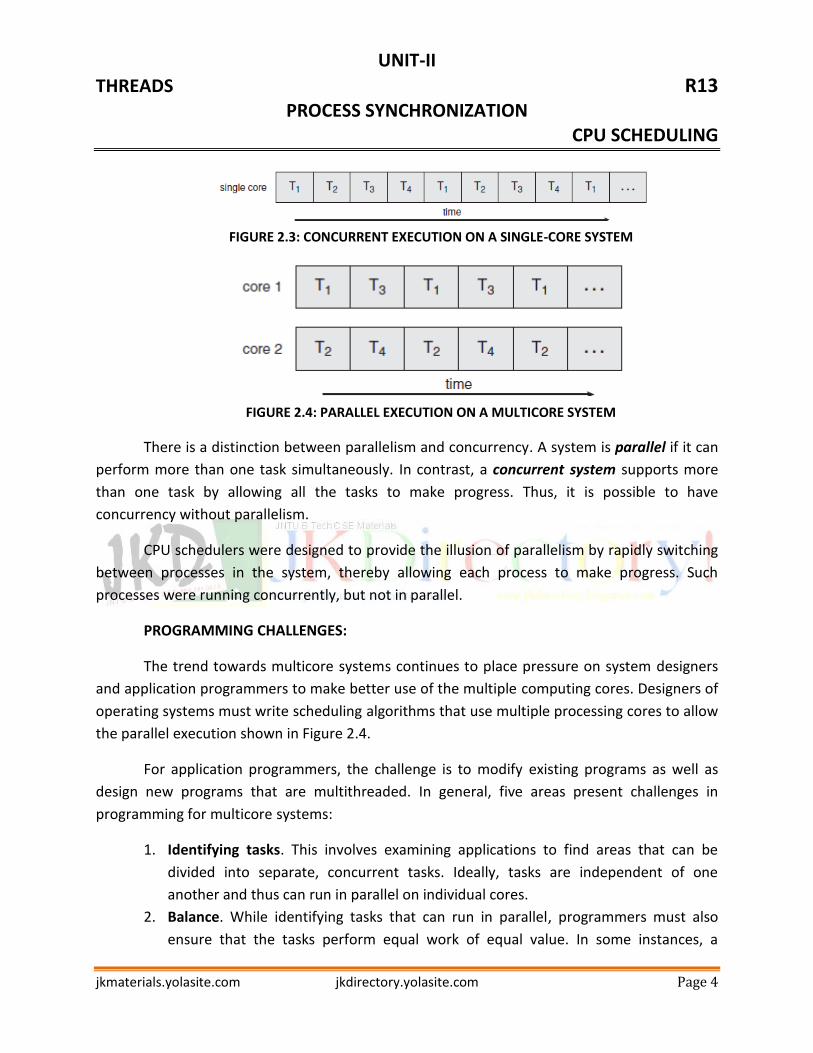
The many-to-many model (Figure 2.7) multiplexes many user-level threads to a smaller

or equal number of kernel threads. The number of kernel threads may be specific to either a

particular application or a particular machine (an application may be allocated more kernel

threads on a multiprocessor than on a single processor).

Let’s consider the effect of this design on concurrency. Whereas the many-to-one model

allows the developer to create as many user threads as she wishes, it does not result in true

concurrency, because the kernel can schedule only one thread at a time. The one-to-one model

allows greater concurrency, but the developer has to be careful not to create too many threads

within an application.

The many-to-many model suffers from neither of these shortcomings: developers can

create as many user threads as necessary, and the corresponding kernel threads can run in

parallel on a multiprocessor. Also, when a thread performs a blocking system call, the kernel

can schedule another thread for execution.

UNIT-II


CPU SCHEDULING


FIGURE 2.7: MANY-TO-MANY MODEL

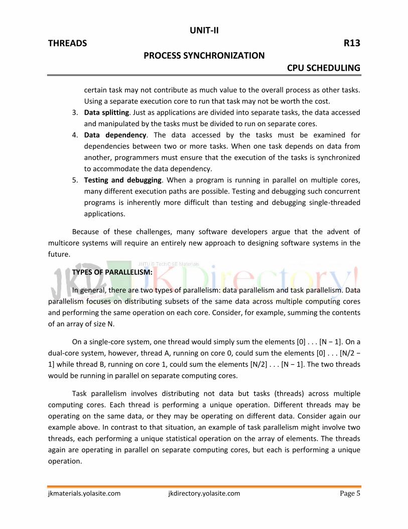
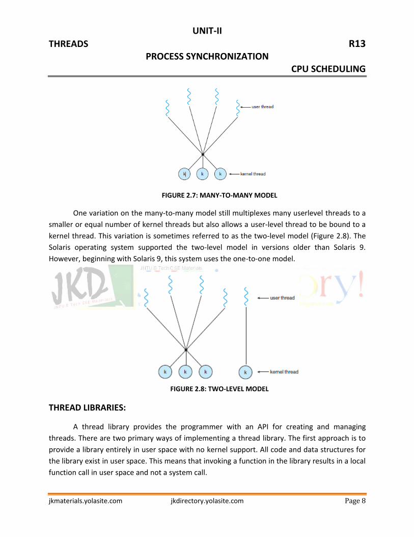
One variation on the many-to-many model still multiplexes many userlevel threads to a

smaller or equal number of kernel threads but also allows a user-level thread to be bound to a

kernel thread. This variation is sometimes referred to as the two-level model (Figure 2.8). The

Solaris operating system supported the two-level model in versions older than Solaris 9.

However, beginning with Solaris 9, this system uses the one-to-one model.

FIGURE 2.8: TWO-LEVEL MODEL

THREAD LIBRARIES:

A thread library provides the programmer with an API for creating and managing

threads. There are two primary ways of implementing a thread library. The first approach is to

provide a library entirely in user space with no kernel support. All code and data structures for

the library exist in user space. This means that invoking a function in the library results in a local

function call in user space and not a system call.

UNIT-II


CPU SCHEDULING


The second approach is to implement a kernel-level library supported directly by the

operating system. In this case, code and data structures for the library exist in kernel space.

Invoking a function in the API for the library typically results in a system call to the kernel.

Three main thread libraries are in use today: POSIX Pthreads,Windows, and Java.

Pthreads, the threads extension of the POSIX standard, may be provided as

either a user-level or a kernel-level library.

The Windows thread library is a kernel-level library available on Windows

systems.

The Java thread API allows threads to be created and managed directly in Java

programs.

However, because in most instances the JVM is running on top of a host operating

system, the Java thread API is generally implemented using a thread library available on the

host system. This means that on Windows systems, Java threads are typically implemented

using theWindows API; UNIX and Linux systems often use Pthreads.

For POSIX and Windows threading, any data declared globally—that is, declared outside

of any function—are shared among all threads belonging to the same process. Because Java has

no notion of global data, access to shared data must be explicitly arranged between threads.

Data declared local to a function are typically stored on the stack. Since each thread has its own

stack, each thread has its own copy of local data.

IMPLICIT THREADING:

With the continued growth of multicore processing, applications containing hundreds—

or even thousands—of threads are looming on the horizon. Designing such applications is not a

trivial undertaking: programmers must address not only the challenges but additional

difficulties as well.

One way to address these difficulties and better support the design of multithreaded

applications is to transfer the creation and management of threading from application

developers to compilers and run-time libraries. This strategy, termed implicit threading, is a

popular trend today. There are three alternative approaches for designing multithreaded

programs that can take advantage of multicore processors through implicit threading.

UNIT-II


CPU SCHEDULING


THREAD POOLS:

Whenever the server receives a request, it creates a separate thread to service the

request. Whereas creating a separate thread is certainly superior to creating a separate

process, amultithreaded server nonetheless has potential problems.

The first issue concerns the amount of time required to create the thread,

together with the fact that the thread will be discarded once it has completed its

work.

The second issue is more troublesome.

If we allow all concurrent requests to be serviced in a new thread, we have not placed a

bound on the number of threads concurrently active in the system. Unlimited threads could

exhaust system resources, such as CPU time or memory. One solution to this problem is to use

a thread pool.

The general idea behind a thread pool is to create a number of threads at process

startup and place them into a pool, where they sit and wait for work. When a server receives a

request, it awakens a thread from this pool—if one is available—and passes it the request for

service. Once the thread completes its service, it returns to the pool and awaits more work. If

the pool contains no available thread, the server waits until one becomes free.

Thread pools offer these benefits:

1. Servicing a request with an existing thread is faster than waiting to create a

thread.

2. A thread pool limits the number of threads that exist at any one point. This is

particularly important on systems that cannot support a large number of

concurrent threads.

3. Separating the task to be performed from the mechanics of creating the task

allows us to use different strategies for running the task. For example, the task

could be scheduled to execute after a time delay or to execute periodically.

The number of threads in the pool can be set heuristically based on factors such as the

number of CPUs in the system, the amount of physical memory, and the expected number of

concurrent client requests.

UNIT-II


CPU SCHEDULING


More sophisticated thread-pool architectures can dynamically adjust the number of

threads in the pool according to usage patterns. Such architectures provide the further benefit

of having a smaller pool—thereby consuming less memory—when the load on the system is

low.

OpenMP:

OpenMP is a set of compiler directives as well as an API for programs written in C, C++,

or FORTRAN that provides support for parallel programming in shared-memory environments.

OpenMP identifies parallel regions as blocks of code that may run in parallel. Application

developers insert compiler directives into their code at parallel regions, and these directives

instruct the OpenMP run-time library to execute the region in parallel.

The following C program illustrates a compiler directive above the parallel region

containing the printf() statement:

#include <omp.h>

#include <stdio.h>

int main(int argc, char *argv[])

{

/* sequential code */

#pragma omp parallel

{

printf("I am a parallel region.");

}

/* sequential code */

return 0;

}

When OpenMP encounters the directive #pragma omp parallel it creates as many

threads are there are processing cores in the system. Thus, for a dual-core system, two threads

are created, for a quad-core system, four are created; and so forth. All the threads then

simultaneously execute the parallel region. As each thread exits the parallel region, it is

terminated.

OpenMP provides several additional directives for running code regions in parallel,

including parallelizing loops.

UNIT-II


CPU SCHEDULING


GRAND CENTRAL DISPATCH:

Grand Central Dispatch (GCD)—a technology for Apple’s Mac OS X and iOS operating

systems—is a combination of extensions to the C language, an API, and a run-time library that

allows application developers to identify sections of code to run in parallel. Like OpenMP, GCD

manages most of the details of threading.

GCD identifies extensions to the C and C++ languages known as blocks. A block is simply

a self-contained unit of work. It is specified by a caret ˆ inserted in front of a pair of braces { }. A

simple example of a block is: ˆ{ printf("I am a block"); } GCD schedules blocks for run-time

execution by placing them on a dispatch queue. When it removes a block from a queue, it

assigns the block to an available thread from the thread pool it manages. GCD identifies two

types of dispatch queues: serial and concurrent.

Blocks placed on a serial queue are removed in FIFO order. Once a block has been

removed from the queue, it must complete execution before another block is removed. Each

process has its own serial queue (known as its main queue). Developers can create additional

serial queues that are local to particular processes. Serial queues are useful for ensuring the

sequential execution of several tasks.

Blocks placed on a concurrent queue are also removed in FIFO order, but several blocks

may be removed at a time, thus allowing multiple blocks to execute in parallel. There are three

system-wide concurrent dispatch queues, and they are distinguished according to priority: low,

default, and high. Priorities represent an approximation of the relative importance of blocks.

Quite simply, blocks with a higher priority should be placed on the highpriority dispatch queue.

THREADING ISSUES:

The fork() and exec() System Calls

The fork() system call is used to create a separate, duplicate process. The semantics of

the fork() and exec() system calls change in a multithreaded program.

If one thread in a program calls fork(), does the new process duplicate all threads, or is

the new process single-threaded? Some UNIX systems have chosen to have two versions of

fork(), one that duplicates all threads and another that duplicates only the thread that invoked

the fork() system call.

UNIT-II


CPU SCHEDULING


The exec() system call loads a binary file into memory (destroying the memory image of

the program containing the exec() system call) and starts its execution. That is, if a thread

invokes the exec() system call, the program specified in the parameter to exec() will replace the

entire process—including all threads.

SIGNAL HANDLING:

A signal is used in UNIX systems to notify a process that a particular event has occurred.

A signal may be received either synchronously or asynchronously, depending on the source of

and the reason for the event being signaled. All signals, whether synchronous or asynchronous,

follow the same pattern:

1. A signal is generated by the occurrence of a particular event.

2. The signal is delivered to a process.

3. Once delivered, the signal must be handled.

Examples of synchronous signal include illegal memory access and division by 0. If a

running program performs either of these actions, a signal is generated. Synchronous signals

are delivered to the same process that performed the operation that caused the signal.

When a signal is generated by an event external to a running process, that process

receives the signal asynchronously. Examples of such signals include terminating a process with

specific keystrokes (such as <control><C>) and having a timer expire. Typically, an asynchronous

signal is sent to another process.

A signal may be handled by one of two possible handlers:

1. A default signal handler

2. A user-defined signal handler

Every signal has a default signal handler that the kernel runs when handling that signal.

This default action can be overridden by a user-defined signal handler that is called to handle

the signal.

Signals are handled in different ways. Some signals (such as changing the size of a

window) are simply ignored; others (such as an illegal memory access) are handled by

terminating the program.

UNIT-II


CPU SCHEDULING


Handling signals in single-threaded programs is straightforward: signals are always

delivered to a process. However, delivering signals is more complicated in multithreaded

programs, where a process may have several threads. Where, then, should a signal be

delivered? In general, the following options exist:

1. Deliver the signal to the thread to which the signal applies.

2. Deliver the signal to every thread in the process.

3. Deliver the signal to certain threads in the process.

4. Assign a specific thread to receive all signals for the process.

The method for delivering a signal depends on the type of signal generated. For

example, synchronous signals need to be delivered to the thread causing the signal and not to

other threads in the process. However, the situation with asynchronous signals is not as clear.

Some asynchronous signals—such as a signal that terminates a process (<control><C>, for

example)—should be sent to all threads.

The standard UNIX function for delivering a signal is kill(pid t pid, int signal)

This function specifies the process (pid) towhich a particular signal (signal) is to be

delivered. Most multithreaded versions of UNIX allow a thread to specify which signals it will

accept and which it will block. Therefore, in some cases, an asynchronous signal may be

delivered only to those threads that are not blocking it. However, because signals need to be

handled only once, a signal is typically delivered only to the first thread found that is not

blocking it.

Although Windows does not explicitly provide support for signals, it allows us to

emulate them using asynchronous procedure calls (APCs). The APC facility enables a user

thread to specify a function that is to be called when the user thread receives notification of a

particular event.

As indicated by its name, an APC is roughly equivalent to an asynchronous signal in

UNIX. However, whereas UNIX must contend with how to deal with signals in a multithreaded

environment, the APC facility is more straightforward, since an APC is delivered to a particular

thread rather than a process.

UNIT-II


CPU SCHEDULING


THREAD CANCELLATION:

Thread cancellation involves terminating a thread before it has completed. For example,

if multiple threads are concurrently searching through a database and one thread returns the

result, the remaining threads might be canceled.

A thread that is to be canceled is often referred to as the target thread. Cancellation of a

target thread may occur in two different scenarios:

1. Asynchronous cancellation. One thread immediately terminates the target

thread.

2. Deferred cancellation. The target thread periodically checks whether it should

terminate, allowing it an opportunity to terminate itself in an orderly fashion.

The difficulty with cancellation occurs in situations where resources have been allocated

to a canceled thread or where a thread is canceled while in the middle of updating data it is

sharing with other threads.

This becomes especially troublesome with asynchronous cancellation. Often, the

operating system will reclaim system resources from a canceled thread but will not reclaim all

resources. Therefore, canceling a thread asynchronously may not free a necessary system-wide

resource. With deferred cancellation, in contrast, one thread indicates that a target thread is to

be canceled, but cancellation occurs only after the target thread has checked a flag to

determine whether or not it should be canceled. The thread can perform this check at a point

at which it can be canceled safely.

THREAD-LOCAL STORAGE:

Threads belonging to a process share the data of the process. Indeed, this data sharing

provides one of the benefits of multithreaded programming. However, in some circumstances,

each thread might need its own copy of certain data.We will call such data thread-local storage

(or TLS).

SCHEDULER ACTIVATIONS:

A final issue to be considered with multithreaded programs concerns communication

between the kernel and the thread library, which may be required by the many-to-many and

two-level models.

UNIT-II


CPU SCHEDULING


Such coordination allows the number of kernel threads to be dynamically adjusted to

help ensure the best performance. Many systems implementing either the many-to-many or

the two-level model place an intermediate data structure between the user and kernel threads.

This data structure—typically known as a lightweight process, or LWP—is shown in Figure 2.9.

To the user-thread library, the LWP appears to be a virtual processor on which the application

can schedule a user thread to run.

FIGURE 2.9: LIGHT WEIGHT PROCESS (LWP)

Each LWP is attached to a kernel thread, and it is kernel threads that the operating

system schedules to run on physical processors. If a kernel thread blocks (such as while waiting

for an I/O operation to complete), the LWP blocks as well. Up the chain, the user-level thread

attached to the LWP also blocks.

Anapplication may require any number of LWPs to run efficiently.Consider a CPU-bound

application running on a single processor. In this scenario, only one thread can run at at a time,

so one LWP is sufficient. An application that is I/O-intensive may require multiple LWPs to

execute, however. Typically, an LWP is required for each concurrent blocking system call.

One scheme for communication between the user-thread library and the kernel is

known as scheduler activation. It works as follows: The kernel provides an application with a set

of virtual processors (LWPs), and the application can schedule user threads onto an available

virtual processor. Furthermore, the kernel must inform an application about certain events.

This procedure is known as an upcall. Upcalls are handled by the thread library with an upcall

handler, and upcall handlers must run on a virtual processor.

UNIT-II


CPU SCHEDULING


One event that triggers an upcall occurs when an application thread is about to block. In

this scenario, the kernel makes an upcall to the application informing it that a thread is about to

block and identifying the specific thread.

The kernel then allocates a new virtual processor to the application. The application

runs an upcall handler on this new virtual processor, which saves the state of the blocking

thread and relinquishes the virtual processor on which the blocking thread is running.

The upcall handler then schedules another thread that is eligible to run on the new

virtual processor. When the event that the blocking thread was waiting for occurs, the kernel

makes another upcall to the thread library informing it that the previously blocked thread is

now eligible to run.

The upcall handler for this event also requires a virtual processor, and the kernel may

allocate a new virtual processor or preempt one of the user threads and run the upcall handler

on its virtual processor. After marking the unblocked thread as eligible to run, the application

schedules an eligible thread to run on an available virtual processor.

PROCESS SYNCHRONIZATION

A cooperating process is one that can affect or be affected by other processes executing

in the system. Cooperating processes can either directly share a logical address space (that is,

both code and data) or be allowed to share data only through files or messages. The former

case is achieved through the use of threads. Concurrent access to shared data may result in

data inconsistency, however.

THE CRITICAL-SECTION PROBLEM:

We begin our consideration of process synchronization by discussing the so called

critical-section problem. Consider a system consisting of n processes {P0, P1, ..., Pn−1}. Each

process has a segment of code, called a critical section, in which the process may be changing

common variables, updating a table, writing a file, and so on.

The important feature of the system is that, when one process is executing in its critical

section, no other process is allowed to execute in its critical section. That is, no two processes

are executing in their critical sections at the same time. The critical-section problem is to design

a protocol that the processes can use to cooperate.

UNIT-II


CPU SCHEDULING


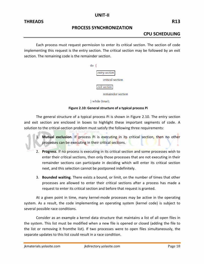
Each process must request permission to enter its critical section. The section of code

implementing this request is the entry section. The critical section may be followed by an exit

section. The remaining code is the remainder section.

Figure 2.10: General structure of a typical process Pi

The general structure of a typical process Pi is shown in Figure 2.10. The entry section

and exit section are enclosed in boxes to highlight these important segments of code. A

solution to the critical-section problem must satisfy the following three requirements:

1. Mutual exclusion. If process Pi is executing in its critical section, then no other

processes can be executing in their critical sections.

2. Progress. If no process is executing in its critical section and some processes wish to

enter their critical sections, then only those processes that are not executing in their

remainder sections can participate in deciding which will enter its critical section

next, and this selection cannot be postponed indefinitely.

3. Bounded waiting. There exists a bound, or limit, on the number of times that other

processes are allowed to enter their critical sections after a process has made a

request to enter its critical section and before that request is granted.

At a given point in time, many kernel-mode processes may be active in the operating

system. As a result, the code implementing an operating system (kernel code) is subject to

several possible race conditions.

Consider as an example a kernel data structure that maintains a list of all open files in

the system. This list must be modified when a new file is opened or closed (adding the file to

the list or removing it fromthe list). If two processes were to open files simultaneously, the

separate updates to this list could result in a race condition.

UNIT-II


CPU SCHEDULING


Two general approaches are used to handle critical sections in operating systems:

preemptive kernels and nonpreemptive kernels. A preemptive kernel allows a process to be

preempted while it is running in kernel mode.

A nonpreemptive kernel does not allow a process running in kernel mode to be

preempted; a kernel-mode process will run until it exits kernel mode, blocks, or voluntarily

yields control of the CPU. Obviously, a nonpreemptive kernel is essentially free from race

conditions on kernel data structures, as only one process is active in the kernel at a time.

We cannot say the same about preemptive kernels, so they must be carefully designed

to ensure that shared kernel data are free from race conditions. Preemptive kernels are

especially difficult to design for SMP architectures, since in these environments it is possible for

two kernel-mode processes to run simultaneously on different processors.

PETERSON’S SOLUTION

A classic software-based solution to the critical-section problem known as Peterson’s

solution. Because of the way modern computer architectures perform basic machine-language

instructions, such as load and store, there are no guarantees that Peterson’s solution will work

correctly on such architectures.

However,we present the solution because it provides a good algorithmic description of

solving the critical-section problem and illustrates some of the complexities involved in

designing software that addresses the requirements of mutual exclusion, progress, and

bounded waiting.

Peterson’s solution is restricted to two processes that alternate execution between their

critical sections and remainder sections. The processes are numbered P0 and P1. For

convenience, when presenting Pi, we use Pj to denote the other process; that is, j equals 1 − i.

Peterson’s solution requires the two processes to share two data items:

int turn;

boolean flag[2];

The variable turn indicates whose turn it is to enter its critical section. That is, if turn ==

i, then process Pi is allowed to execute in its critical section. The flag array is used to indicate if a

process is ready to enter its critical section.

UNIT-II


CPU SCHEDULING


For example, if flag[i] is true, this value indicates that Pi is ready to enter its critical

section. With an explanation of these data structures complete, we are now ready to describe

the algorithm shown in Figure 2.11.

To enter the critical section, process Pi first sets flag[i] to be true and then sets turn to

the value j, thereby asserting that if the other process wishes to enter the critical section, it can

do so. If both processes try to enter at the same time, turn will be set to both i and j at roughly

the same time. Only one of these assignments will last; the other will occur but will be

overwritten immediately. The eventual value of turn determines which of the two processes is

allowed to enter its critical section first.

FIGURE 2.11: THE STRUCTURE OF PROCESS pi IN PETERSON’S SOLUTION

SYNCHRONIZATION HARDWARE:

We have one software-based solution to the critical-section problem such as Peterson’s

solution, are not guaranteed to work on modern computer architectures.

we explore several more solutions to the critical-section problem using techniques

ranging from hardware to software-based APIs available to both kernel developers and

application programmers. All these solutions are based on the premise of locking —that is,

protecting critical regions through the use of locks.

We start by presenting some simple hardware instructions that are available on many

systems and showing how they can be used effectively in solving the critical-section problem.

Hardware features can make any programming task easier and improve system efficiency.

UNIT-II


CPU SCHEDULING


The critical-section problem could be solved simply in a single-processor environment if

we could prevent interrupts from occurring while a shared variable was being modified. In this

way, we could be sure that the current sequence of instructions would be allowed to execute in

order without preemption.

No other instructions would be run, so no unexpected modifications could be made to

the shared variable. This is often the approach taken by nonpreemptive kernels. Unfortunately,

this solution is not as feasible in a multiprocessor environment.

Disabling interrupts on a multiprocessor can be time consuming, since the message is

passed to all the processors. This message passing delays entry into each critical section, and

system efficiency decreases. Also consider the effect on a system’s clock if the clock is kept

updated by interrupts.

Many modern computer systems therefore provide special hardware instructions that

allow us either to test and modify the content of a word or to swap the contents of two words

atomically—that is, as one uninterruptible unit. We can use these special instructions to solve

the critical-section problem in a relatively simple manner.

Rather than discussing one specific instruction for one specific machine, we abstract the

main concepts behind these types of instructions by describing the test_and_set() and

compare_and_swap() instructions. The test_and_set() instruction can be defined as shown in

Figure 2.12:

boolean test and set(boolean *target) {

boolean rv = *target;

*target = true;

return rv;

}

FIGURE 2.12: THE DEFINITION OF THE test_and_set() INSTRUCTION

The important characteristic of this instruction is that it is executed atomically. Thus, if

two test and set() instructions are executed simultaneously (each on a different CPU), they will

be executed sequentially in some arbitrary order.

UNIT-II


CPU SCHEDULING


If the machine supports the test and set() instruction, thenwe can implement mutual

exclusion by declaring a boolean variable lock, initialized to false. The structure of process Pi is

shown in Figure 2.13.

do {

while (test_and_set(&lock))

; /* do nothing */

/* critical section */

lock = false;

/* remainder section */

} while (true);

FIGURE 2.13: MUTUAL-EXCLUSION IMPLEMENTATION WITH test_and_set()

The compare_and_swap() instruction operates on three operands; it is defined in Figure

2.14. Regardless, compare and swap() always returns the original value of the variable value.

The operand value is set to new_value only if the expression (*value == exected) is true.

int compare and swap(int *value, int expected, int new value) {

int temp = *value;

if (*value == expected)

*value = new value;

return temp;

}

FIGURE 2.14: THE DEFINITION OF THE compare_and_swap() INSTRUCTION

Like the test_and_set() instruction, compare_and_swap() is executed atomically.

Mutual exclusion can be provided as follows: a global variable (lock) is declared and is initialized

to 0. The first process that invokes compare_and_swap() will set lock to 1. It will then enter its

critical section, because the original value of lock was equal to the expected value of 0.

UNIT-II


CPU SCHEDULING


Subsequent calls to compare_and_swap() will not succeed, because lock now is not

equal to the expected value of 0. When a process exits its critical section, it sets lock back to 0,

which allows another process to enter its critical section. The structure of process Pi is shown in

Figure 2.15. Although these algorithms satisfy the mutual-exclusion requirement, they do not

satisfy the bounded-waiting requirement.

do {

while (compare and swap(&lock, 0, 1) != 0)

; /* do nothing */


lock = 0;


} while (true);

FIGURE 2.15: MUTUAL-EXCLUSION IMPLEMENTATION WITH THE compare_and_swap()

INSTRUCTION

In Figure 2.16, we present another algorithm using the test and set() instruction that

satisfies all the critical-section requirements.

do {

waiting[i] = true;

key = true;

while (waiting[i] && key)

key = test and set(&lock);

waiting[i] = false;


j = (i + 1) % n;

while ((j != i) && !waiting[j])

j = (j + 1) % n;

if (j == i)

lock = false;

else

waiting[j] = false;


} while (true);

FIGURE 2.16: BOUNDED-WAITING MUTUAL EXCLUSION WITH test_and_set()

UNIT-II


CPU SCHEDULING


The common data structures are

boolean waiting[n];

boolean lock;

These data structures are initialized to false.

MUTEX LOCKS:

The hardware-based solutions to the critical-section problem presented using

synchronization hardware are complicated as well as generally inaccessible to application

programmers. Instead, operating-systems designers build software tools to solve the critical-

section problem. The simplest of these tools is the mutex lock. (In fact, the term mutex is short

for mutual exclusion.)

We use the mutex lock to protect critical regions and thus prevent race conditions. That

is, a process must acquire the lock before entering a critical section; it releases the lock when it

exits the critical section. The acquire()function acquires the lock, and the release() function

releases the lock, as illustrated in Figure 2.17.

do {

acquire lock

critical section

release lock

remainder section

} while (true);

FIGURE 2.17: SOLUTION TO THE CRITICAL-SECTION PROBLEM USING MUTEX LOCKS

A mutex lock has a boolean variable available whose value indicates if the lock is

available or not. If the lock is available, a call to acquire() succeeds, and the lock is then

considered unavailable. A process that attempts to acquire an unavailable lock is blocked until

the lock is released. The definition of acquire() is as follows:

acquire() {

while (!available)

; /* busy wait */

available = false;; }

UNIT-II


CPU SCHEDULING


The definition of release() is as follows:

release() {

available = true;

}

Calls to either acquire() or release() must be performed atomically. The main

disadvantage of the implementation given here is that it requires busy waiting. While a process

is in its critical section, any other process that tries to enter its critical section must loop

continuously in the call to acquire(). In fact, this type of mutex lock is also called a spinlock

because the process “spins” while waiting for the lock to become available.

Spinlocks do have an advantage, however, in that no context switch is required when a

process must wait on a lock, and a context switch may take considerable time.

SEMAPHORES:

Mutex locks, are generally considered the simplest of synchronization tools. Now we

examine a more robust tool that can behave similarly to a mutex lock but can also provide more

sophisticated ways for processes to synchronize their activities.

A semaphore S is an integer variable that, apart from initialization, is accessed only

through two standard atomic operations: wait() and signal(). The wait() operation was originally

termed P (from the Dutch proberen, “to test”); signal() was originally called V (from verhogen,

“to increment”). The definition of wait() is as follows:

wait(S) {

while (S <= 0)

; // busy wait

S--;

}

The definition of signal() is as follows:

signal(S) {

S++; }

UNIT-II


CPU SCHEDULING


All modifications to the integer value of the semaphore in the wait() and signal()

operations must be executed indivisibly. That is, when one process modifies the semaphore

value, no other process can simultaneously modify that same semaphore value.

Semaphore Usage:

Operating systems often distinguish between counting and binary semaphores. The

value of a counting semaphore can range over an unrestricted domain. The value of a binary

semaphore can range only between 0 and 1. Thus, binary semaphores behave similarly to

mutex locks. In fact, on systems that do not provide mutex locks, binary semaphores can be

used instead for providing mutual exclusion.

Counting semaphores can be used to control access to a given resource consisting of a

finite number of instances. The semaphore is initialized to the number of resources available.

Each process that wishes to use a resource performs a wait() operation on the semaphore

(thereby decrementing the count). When a process releases a resource, it performs a signal()

operation (incrementing the count). When the count for the semaphore goes to 0, all resources

are being used. After that, processes that wish to use a resource will block until the count

becomes greater than 0. We can also use semaphores to solve various synchronization

problems.

Semaphore Implementation:

The implementation of mutex locks suffers from busy waiting. The definitions of the

wait() and signal() semaphore operations present the same problem. To overcome the need for

busy waiting, we can modify the definition of the wait() and signal() operations as follows:

When a process executes the wait() operation and finds that the semaphore value is not

positive, it must wait.

However, rather than engaging in busy waiting, the process can block itself. The block

operation places a process into a waiting queue associated with the semaphore, and the state

of the process is switched to the waiting state. Then control is transferred to the CPU scheduler,

which selects another process to execute.

A process that is blocked, waiting on a semaphore S, should be restarted when some

other process executes a signal() operation. The process is restarted by a wakeup() operation,

which changes the process from the waiting state to the ready state.

UNIT-II


CPU SCHEDULING


The process is then placed in the ready queue. (The CPU may or may not be switched

from the running process to the newly ready process, depending on the CPU-scheduling

algorithm.)

To implement semaphores under this definition, we define a semaphore as follows:

typedef struct {

int value;

struct process *list;

} semaphore;

Each semaphore has an integer value and a list of processes list. When a process must

wait on a semaphore, it is added to the list of processes. A signal() operation removes one

process from the list of waiting processes and awakens that process.

Now, the wait() semaphore operation can be defined as

wait(semaphore *S) {

S->value--;

if (S->value < 0) {

add this process to S->list;

block();

}

}

and the signal() semaphore operation can be defined as

signal(semaphore *S) {

S->value++;

if (S->value <= 0) {

remove a process P from S->list;

wakeup(P);

}

}

The block() operation suspends the process that invokes it. The wakeup(P) operation

resumes the execution of a blocked process P. These two operations are provided by the

operating system as basic system calls.

UNIT-II


CPU SCHEDULING


Note that in this implementation, semaphore values may be negative, whereas

semaphore values are never negative under the classical definition of semaphores with busy

waiting.

Deadlocks and Starvation:

The implementation of a semaphore with a waiting queue may result in a situation

where two or more processes are waiting indefinitely for an event that can be caused only by

one of the waiting processes. The event in question is the execution of a signal() operation.

When such a state is reached, these processes are said to be deadlocked.

To illustrate this, consider a system consisting of two processes, P0 and P1, each

accessing two semaphores, S and Q, set to the value 1:

P0 P1

wait(S); wait(Q);

wait(Q); wait(S);

. .

. .

. .

signal(S); signal(Q);

signal(Q); signal(S);

Suppose that P0 executes wait(S) and then P1 executes wait(Q).When P0 executes

wait(Q), it must wait until P1 executes signal(Q). Similarly, when P1 executes wait(S), it must

wait until P0 executes signal(S). Since these signal() operations cannot be executed, P0 and P1

are deadlocked.

Priority Inversion:

A scheduling challenge arises when a higher-priority process needs to read or modify

kernel data that are currently being accessed by a lower-priority process—or a chain of lower-

priority processes.

Since kernel data are typically protected with a lock, the higher-priority process will

have to wait for a lower-priority one to finish with the resource. The situation becomes more

complicated if the lower-priority process is preempted in favor of another process with a higher

priority.

UNIT-II


CPU SCHEDULING


CLASSIC PROBLEMS OF SYNCHRONIZATION:

We present a number of synchronization problems as examples of a large class of

concurrency-control problems. These problems are used for testing nearly every newly

proposed synchronization scheme.

In our solutions to the problems, we use semaphores for synchronization, since that is

the traditional way to present such solutions. However, actual implementations of these

solutions could use mutex locks in place of binary semaphores.

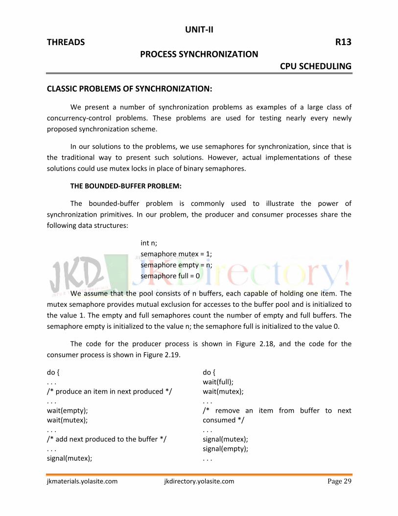
THE BOUNDED-BUFFER PROBLEM:

The bounded-buffer problem is commonly used to illustrate the power of

synchronization primitives. In our problem, the producer and consumer processes share the

following data structures:

int n;

semaphore mutex = 1;

semaphore empty = n;

semaphore full = 0

We assume that the pool consists of n buffers, each capable of holding one item. The

mutex semaphore provides mutual exclusion for accesses to the buffer pool and is initialized to

the value 1. The empty and full semaphores count the number of empty and full buffers. The

semaphore empty is initialized to the value n; the semaphore full is initialized to the value 0.

The code for the producer process is shown in Figure 2.18, and the code for the

consumer process is shown in Figure 2.19.

do { . . . /* produce an item in next produced */ . . . wait(empty); wait(mutex); . . . /* add next produced to the buffer */ . . . signal(mutex);

do { wait(full); wait(mutex); . . . /* remove an item from buffer to next consumed */ . . . signal(mutex); signal(empty); . . .

UNIT-II


CPU SCHEDULING


signal(full); } while (true);

/* consume the item in next consumed */ . . . } while (true);

Figure 2.18The structure of the producer process Figure 2.19 The structure of the consumer process

THE READERS–WRITERS PROBLEM:

Suppose that a database is to be shared among several concurrent processes. Some of

these processes may want only to read the database, whereas others may want to update (that

is, to read and write) the database.

Obviously, if two readers access the shared data simultaneously, no adverse effects will

result. However, if a writer and some other process (either a reader or a writer) access the

database simultaneously, chaos may ensue.

To ensure that these difficulties do not arise, we require that the writers have exclusive

access to the shared database while writing to the database. This synchronization problem is

referred to as the readers–writers problem.

The readers–writers problem has several variations, all involving priorities. The simplest

one, referred to as the first readers–writers problem, requires that no reader be kept waiting

unless a writer has already obtained permission to use the shared object. In other words, no

reader should wait for other readers to finish simply because a writer is waiting.

The second readers –writers problem requires that, once a writer is ready, that writer

perform its write as soon as possible. In other words, if a writer is waiting to access the object,

no new readers may start reading.

A solution to either problem may result in starvation. In the first case, writers may

starve; in the second case, readers may starve. For this reason, other variants of the problem

have been proposed.

In the solution to the first readers–writers problem, the reader processes share the

following data structures:

semaphore rw mutex = 1;

semaphore mutex = 1;

int read count = 0;

UNIT-II


CPU SCHEDULING


The semaphores mutex and rw mutex are initialized to 1; read count is initialized to 0.

The semaphore rw mutex is common to both reader and writer processes. The mutex

semaphore is used to ensure mutual exclusion when the variable read count is updated.

The read count variable keeps track of how many processes are currently reading the

object. The semaphore rw mutex functions as a mutual exclusion semaphore for the writers. It

is also used by the first or last reader that enters or exits the critical section. It is not used by

readers who enter or exit while other readers are in their critical sections.

The code for a writer process is shown in Figure 2.20; the code for a reader process is


do { wait(rw mutex); . . . /* writing is performed */ . . . signal(rw mutex); } while (true);

do { wait(mutex); read count++; if (read count == 1) wait(rw mutex); signal(mutex); . . . /* reading is performed */ . . . wait(mutex); read count--; if (read count == 0) signal(rw mutex); signal(mutex); } while (true);

Figure 2.20 The structure of the writer process Figure 2.21 The structure of the reader process

The readers–writers problem and its solutions have been generalized to provide reader–

writer locks on some systems. Acquiring a reader–writer lock requires specifying the mode of

the lock: either read or write access. When a process wishes only to read shared data, it

requests the reader–writer lock in read mode.

A process wishing to modify the shared data must request the lock in write mode.

Multiple processes are permitted to concurrently acquire a reader–writer lock in read mode,

but only one process may acquire the lock for writing, as exclusive access is required for writers.

Reader–writer locks are most useful in the following situations:

UNIT-II


CPU SCHEDULING


FIGURE 2.22: THE SITUATION OF THE DINING PHILOSOPHERS

• In applications where it is easy to identify which processes only read shared data and

which processes only write shared data.

• In applications that have more readers than writers. This is because reader–writer

locks generally requiremore overhead to establish than semaphores or mutual-exclusion locks.

The increased concurrency of allowing multiple readers compensates for the overhead involved

in setting up the reader–writer lock.

THE DINING-PHILOSOPHERS PROBLEM

Consider five philosophers who spend their lives thinking and eating. The philosophers

share a circular table surrounded by five chairs, each belonging to one philosopher. In the

center of the table is a bowl of rice, and the table is laid with five single chopsticks (Figure 2.22).

When a philosopher thinks, she does not interact with her colleagues. From time to

time, a philosopher gets hungry and tries to pick up the two chopsticks that are closest to her

(the chopsticks that are between her and her left and right neighbors).

A philosopher may pick up only one chopstick at a time. Obviously, she cannot pick up a

chopstick that is already in the hand of a neighbor. When a hungry philosopher has both her

chopsticks at the same time, she eats without releasing the chopsticks. When she is finished

eating, she puts down both chopsticks and starts thinking again.

The dining-philosophers problem is considered a classic synchronization problem

neither because of its practical importance nor because computer scientists dislike

philosophers but because it is an example of a large class of concurrency-control problems.

UNIT-II


CPU SCHEDULING


It is a simple representation of the need to allocate several resources among several

processes in a deadlock-free and starvation-free manner.

One simple solution is to represent each chopstick with a semaphore. A philosopher

tries to grab a chopstick by executing a wait() operation on that semaphore. She releases her

chopsticks by executing the signal() operation on the appropriate semaphores. Thus, the shared

data are semaphore chopstick[5]; where all the elements of chopstick are initialized to 1. The

structure of philosopher i is shown in Figure 2.23.

do {

wait(chopstick[i]);

wait(chopstick[(i+1) % 5]);

. . .

/* eat for awhile */

. . .

signal(chopstick[i]);

signal(chopstick[(i+1) % 5]);

. . .

/* think for awhile */

. . .

} while (true);

FIGURE 2.23: THE STRUCTURE OF PHILOSOPHER i.

Although this solution guarantees that no two neighbors are eating simultaneously, it

nevertheless must be rejected because it could create a deadlock. Suppose that all five

philosophers become hungry at the same time and each grabs her left chopstick. All the

elements of chopstick will now be equal to 0. When each philosopher tries to grab her right

chopstick, she will be delayed forever.

Several possible remedies to the deadlock problem are replaced by:

Allow at most four philosophers to be sitting simultaneously at the table.

Allow a philosopher to pick up her chopsticks only if both chopsticks are available (to

do this, she must pick them up in a critical section).

UNIT-II


CPU SCHEDULING


Use an asymmetric solution—that is, an odd-numbered philosopher picks up first

her left chopstick and then her right chopstick, whereas an even numbered

philosopher picks up her right chopstick and then her left chopstick.

MONITORS:

Although semaphores provide a convenient and effective mechanism for process

synchronization, using them incorrectly can result in timing errors that are difficult to detect.

Unfortunately, such timing errors can still occur when semaphores are used. To illustrate

how,we review the semaphore solution to the critical-section problem. All processes share a

semaphore variable mutex, which is initialized to 1.

Each process must execute wait(mutex) before entering the critical section and

signal(mutex) afterward. If this sequence is not observed, two processes may be in their critical

sections simultaneously. Next, we examine the various difficulties that may result. Note that

these difficulties will arise even if a single process is not well behaved.

Suppose that a process interchanges the order in which the wait() and signal()

operations on the semaphore mutex are executed, resulting in the following execution:

signal(mutex);

...

critical section

...

wait(mutex);

In this situation, several processes may be executing in their critical sections

simultaneously, violating the mutual-exclusion requirement. This error may be

discovered only if several processes are simultaneously active in their critical

sections.

Suppose that a process replaces signal(mutex) with wait(mutex). That is, it executes

wait(mutex);

...

critical section

...

wait(mutex);

UNIT-II


CPU SCHEDULING


In this case, a deadlock will occur.

Suppose that a process omits the wait(mutex), or the signal(mutex), or both. In this

case, either mutual exclusion is violated or a deadlock will occur.

These examples illustrate that various types of errors can be generated easily when

programmers use semaphores incorrectly to solve the critical-section problem. To deal with

such errors, researchers have developed high-level language constructs. One fundamental high-

level synchronization construct—the monitor type.

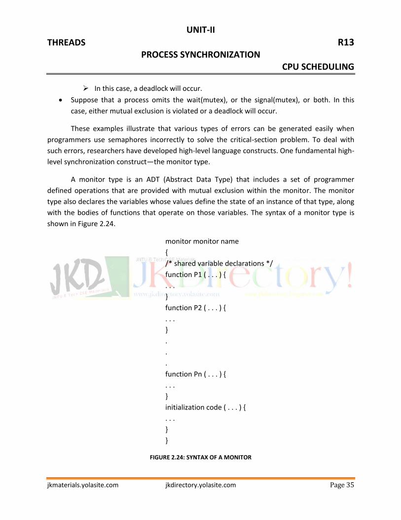
A monitor type is an ADT (Abstract Data Type) that includes a set of programmer

defined operations that are provided with mutual exclusion within the monitor. The monitor

type also declares the variables whose values define the state of an instance of that type, along

with the bodies of functions that operate on those variables. The syntax of a monitor type is


monitor monitor name

{

/* shared variable declarations */

function P1 ( . . . ) {

. . .

}

function P2 ( . . . ) {

. . .

}

.

.

.

function Pn ( . . . ) {

. . .

}

initialization code ( . . . ) {

. . .

}

}

FIGURE 2.24: SYNTAX OF A MONITOR

UNIT-II


CPU SCHEDULING


The representation of a monitor type cannot be used directly by the various processes.

Thus, a function defined within a monitor can access only those variables declared locally within

the monitor and its formal parameters.

Similarly, the local variables of a monitor can be accessed by only the local functions.

The monitor construct ensures that only one process at a time is active within the monitor.

Consequently, the programmer does not need to code this synchronization constraint explicitly

(Figure 2.25).

FIGURE 2.25: SCHEMATIC VIEW OF A MONITOR

However, the monitor construct, as defined so far, is not sufficiently powerful for

modeling some synchronization schemes. For this purpose, we need to define additional

synchronization mechanisms.

These mechanisms are provided by the condition construct. A programmer who needs

to write a tailor-made synchronization scheme can define one or more variables of type

condition: condition x, y;

The only operations that can be invoked on a condition variable are wait() and signal().

The operation x.wait(); means that the process invoking this operation is suspended until

another process invokes x.signal();

UNIT-II


CPU SCHEDULING


The x.signal() operation resumes exactly one suspended process. If no process is

suspended, then the signal() operation has no effect; that is, the state of x is the same as if the

operation had never been executed.

Now suppose that, when the x.signal() operation is invoked by a process P, there exists a

suspended processQassociated with condition x. Clearly, if the suspended process Q is allowed

to resume its execution, the signaling process P must wait. Otherwise, both P and Q would be

active simultaneously within the monitor.

Two possibilities exist:

1. Signal and wait. P either waits until Q leaves the monitor or waits for another

condition.

2. Signal and continue. Q either waits until P leaves the monitor or waits for another

condition.

There are reasonable arguments in favor of adopting either option. On the one hand,

since P was already executing in the monitor, the signal-andcontinue method seems more

reasonable. On the other, if we allow thread P to continue, then by the time Q is resumed, the

logical condition for which Q was waiting may no longer hold.

DINING-PHILOSOPHERS SOLUTION USING MONITORS

We illustrate monitor concepts by presenting a deadlock-free solution to the dining-

philosophers problem. This solution imposes the restriction that a philosopher may pick up her

chopsticks only if both of them are available.

To code this solution, we need to distinguish among three states in which we may find a

philosopher. For this purpose, we introduce the following data structure:

enum {THINKING, HUNGRY, EATING} state[5];

Philosopher i can set the variable state[i] = EATING only if her two neighbors are not

eating: (state[(i+4) % 5] != EATING) and(state[(i+1) % 5] != EATING). We also need to declare

condition self[5];

This allows philosopher i to delay herself when she is hungry but is unable to obtain the

chopsticks she needs. We are now in a position to describe our solution to the dining-

philosophers problem.

UNIT-II


CPU SCHEDULING


The distribution of the chopsticks is controlled by the monitor DiningPhilosophers,

whose definition is shown in Figure 2.26. Each philosopher, before starting to eat, must invoke

the operation pickup().

monitor DiningPhilosophers

{

enum {THINKING, HUNGRY, EATING} state[5];

condition self[5];

void pickup(int i) {

state[i] = HUNGRY;

test(i);

if (state[i] != EATING)

self[i].wait();

}

void putdown(int i) {

state[i] = THINKING;

test((i + 4) % 5);

test((i + 1) % 5);

}

void test(int i) {

if ((state[(i + 4) % 5] != EATING) &&

(state[i] == HUNGRY) &&

(state[(i + 1) % 5] != EATING)) {

state[i] = EATING;

self[i].signal();

}

}

initialization code() {

for (int i = 0; i < 5; i++)

state[i] = THINKING;

}

}

FIGURE 2.26: A MONITOR SOLUTION TO THE DINING-PHILOSOPHER PROBLEM

UNIT-II


CPU SCHEDULING


This act may result in the suspension of the philosopher process. After the successful

completion of the operation, the philosopher may eat.

Following this, the philosopher invokes the putdown() operation. Thus, philosopher i

must invoke the operations pickup() and putdown() in the following sequence:

DiningPhilosophers.pickup(i);

...

eat

...

DiningPhilosophers.putdown(i);

Implementing a Monitor Using Semaphores:

We now consider a possible implementation of the monitor mechanism using

semaphores. For each monitor, a semaphore mutex (initialized to 1) is provided. A process must

execute wait(mutex) before entering the monitor and must execute signal(mutex) after leaving

the monitor.

Resuming Processes within a Monitor:

We turn now to the subject of process-resumption order within a monitor. If several

processes are suspended on condition x, and an x.signal() operation is executed by some

process, then how do we determine which of the suspended processes should be resumed

next? One simple solution is to use a first-come, first-served (FCFS) ordering, so that the

process that has been waiting the longest is resumed first. In many circumstances, however,

such a simple scheduling scheme is not adequate. For this purpose, the conditional-wait

construct can be used. This construct has the form x.wait(c);

where c is an integer expression that is evaluated when the wait() operation is executed.

The value of c, which is called a priority number, is then stored with the name of the process

that is suspended.When x.signal() is executed, the process with the smallest priority number is

resumed next.

To illustrate this new mechanism, consider the ResourceAllocator monitor shown in

Figure 2.27, which controls the allocation of a single resource among competing processes.

monitor ResourceAllocator

UNIT-II


CPU SCHEDULING


{

boolean busy;

condition x;

void acquire(int time) {

if (busy)

x.wait(time);

busy = true;

}

void release() {

busy = false;

x.signal();

}

initialization code() {

busy = false;

}

}

FIGURE 2.27: A MONITOR TO ALLOCATE A SINGLE RESOURCE

SYNCHRONIZATION EXAMPLES:

Synchronization in Windows:

TheWindows operating system is a multithreaded kernel that provides support for real-

time applications and multiple processors. When theWindows kernel accesses a global resource

on a single-processor system, it temporarily masks interrupts for all interrupt handlers that may

also access the global resource.

On a multiprocessor system, Windows protects access to global resources using

spinlocks, although the kernel uses spinlocks only to protect short code segments. Furthermore,

for reasons of efficiency, the kernel ensures that a thread will never be preempted while

holding a spinlock.

For thread synchronization outside the kernel, Windows provides dispatcher objects.

Using a dispatcher object, threads synchronize according to several different mechanisms,

includingmutex locks, semaphores, events, and timers.

UNIT-II


CPU SCHEDULING


The system protects shared data by requiring a thread to gain ownership of a mutex to

access the data and to release ownership when it is finished.

Dispatcher objects may be in either a signaled state or a nonsignaled state. An object in

a signaled state is available, and a thread will not block when acquiring the object. An object in

a nonsignaled state is not available, and a thread will block when attempting to acquire the

object.

Synchronization in Linux:

Prior to Version 2.6, Linux was a nonpreemptive kernel, meaning that a process running

in kernel mode could not be preempted—even if a higher-priority process became available to

run. Now, however, the Linux kernel is fully preemptive, so a task can be preempted when it is

running in the kernel.

Linux provides several different mechanisms for synchronization in the kernel. As most

computer architectures provide instructions for atomic versions of simple math operations, the

simplest synchronization technique within the Linux kernel is an atomic integer, which is

represented using the opaque data type atomic_t. As the name implies, all math operations

using atomic integers are performed without interruption.

The following code illustrates declaring an atomic integer counter and then performing

various atomic operations:

atomic_t counter;

int value;

atomic_set(&counter,5); /* counter = 5 */

atomic_add(10, &counter); /* counter = counter + 10 */

atomic_sub(4, &counter); /* counter = counter - 4 */

atomic_inc(&counter); /* counter = counter + 1 */

value = atomic_read(&counter); /* value = 12 */

Atomic integers are particularly efficient in situations where an integer variable —such

as a counter—needs to be updated, since atomic operations do not require the overhead of

locking mechanisms. However, their usage is limited to these sorts of scenarios.

Linux also provides spinlocks and semaphores (as well as reader–writer versions of

these two locks) for locking in the kernel.

UNIT-II


CPU SCHEDULING


Linux uses an interesting approach to disable and enable kernel preemption. It provides

two simple system calls—preempt disable() and preempt enable()—for disabling and enabling

kernel preemption.

Synchronization in Solaris:

To control access to critical sections, Solaris provides adaptive mutex locks, condition

variables, semaphores, reader–writer locks, and turnstiles. Solaris implements semaphores and

condition variables.

An adaptive mutex protects access to every critical data item. On a multiprocessor

system, an adaptive mutex starts as a standard semaphore implemented as a spinlock. Solaris

uses the adaptive-mutex method to protect only data that are accessed by short code

segments.

Reader–writer locks are used to protect data that are accessed frequently but are

usually accessed in a read-only manner. In these circumstances, reader–writer locks are more

efficient than semaphores, because multiple threads can read data concurrently,whereas

semaphores always serialize access to the data. Reader–writer locks are relatively expensive to

implement, so again they are used only on long sections of code.

Solaris uses turnstiles to order the list of threads waiting to acquire either an adaptive

mutex or a reader–writer lock. A turnstile is a queue structure containing threads blocked on a

lock.

ALTERNATIVE APPROACHES:

With the emergence of multicore systems has come increased pressure to develop

multithreaded applications that take advantage of multiple processing cores. However,

multithreaded applications present an increased risk of race conditions and deadlocks.

Traditionally, techniques such as mutex locks, semaphores, and monitors have been

used to address these issues, but as the number of processing cores increases, it becomes

increasingly difficult to design multithreaded applications that are free from race conditions

and deadlocks.

Transactional Memory: The concept of transactional memory originated in database

theory, for example, yet it provides a strategy for process synchronization.

UNIT-II


CPU SCHEDULING


A memory transaction is a sequence of memory read–writeoperations that are atomic.

If all operations in a transaction are completed, the memory transaction is committed.

Otherwise, the operations must be aborted and rolled back.

Transactional memory can be implemented in either software or hardware. Software

transactional memory (STM), as the name suggests, implements transactional memory

exclusively in software—no special hardware is needed.

Hardware transactional memory (HTM) uses hardware cache hierarchies and cache

coherency protocols to manage and resolve conflicts involving shared data residing in separate

processors’ caches. HTM requires no special code instrumentation and thus has less overhead

than STM.

OpenMP: OpenMP includes a set of compiler directives and an API. Any code following

the compiler directive #pragma omp parallel is identified as a parallel region and is performed

by a number of threads equal to the number of processing cores in the system. The advantage

of OpenMP (and similar tools) is that thread creation and management are handled by the

OpenMP library and are not the responsibility of application developers.

CPU SCHEDULING:

CPU scheduling is the basis of multiprogrammed operating systems. By switching the

CPU among processes, the operating system can make the computer more productive.

Basic Concepts:

In a single-processor system, only one process can run at a time. Others must wait until

the CPU is free and can be rescheduled. The objective of multiprogramming is to have some

process running at all times, to maximize CPU utilization. The idea is relatively simple.

A process is executed until it must wait, typically for the completion of some I/O

request. In a simple computer system, the CPU then just sits idle. All this waiting time is wasted;

no useful work is accomplished. With multiprogramming, we try to use this time productively.

Several processes are kept in memory at one time.

When one process has to wait, the operating system takes the CPU away from that

process and gives the CPU to another process. This pattern continues. Every time one process

has to wait, another process can take over use of the CPU.

UNIT-II


CPU SCHEDULING


Scheduling of this kind is a fundamental operating-system function. Almost all computer

resources are scheduled before use. The CPU is, of course, one of the primary computer

resources. Thus, its scheduling is central to operating-system design.

CPU – I/O Burst Cycle:

The success of CPU scheduling depends on an observed property of processes: process

execution consists of a cycle of CPU execution and I/O wait. Processes alternate between these

two states. Process execution begins with a CPU burst. That is followed by an I/O burst, which is

followed by another CPU burst, then another I/O burst, and so on. Eventually, the final CPU

burst ends with a system request to terminate execution (Figure 2.28).

FIGURE 2.28: ALTERNATING SEQUENCE OF CPU AND I/O BURSTS

The durations of CPU bursts have been measured extensively. Although they vary

greatly from process to process and from computer to computer. An I/O-bound program

typically has many short CPU bursts. A CPU-bound program might have a few long CPU bursts.

This distribution can be important in the selection of an appropriate CPU-scheduling algorithm.

UNIT-II


CPU SCHEDULING


CPU Scheduler:

Whenever the CPU becomes idle, the operating system must select one of the processes

in the ready queue to be executed. The selection process is carried out by the short-term

scheduler, or CPU scheduler. The scheduler selects a process from the processes in memory

that are ready to execute and allocates the CPU to that process.

Preemptive Scheduling:

CPU-scheduling decisions may take place under the following four circumstances:

1. When a process switches from the running state to the waiting state

2. When a process switches from the running state to the ready state

3. When a process switches from the waiting state to the ready state

4. When a process terminates

For situations 1 and 4, there is no choice in terms of scheduling. A new process (if one

exists in the ready queue) must be selected for execution. There is a choice, however, for

situations 2 and 3.

When scheduling takes place only under circumstances 1 and 4, we say that the

scheduling scheme is nonpreemptive or cooperative. Otherwise, it is preemptive.

Under nonpreemptive scheduling, once the CPU has been allocated to a process, the

process keeps the CPU until it releases the CPU either by terminating or by switching to the

waiting state. This scheduling method was used by Microsoft Windows 3.x.

Windows 95 introduced preemptive scheduling, and all subsequent versions of

Windows operating systems have used preemptive scheduling.

TheMac OS X operating system for the Macintosh also uses preemptive scheduling;

previous versions of the Macintosh operating system relied on cooperative scheduling.

Cooperative scheduling is the only method that can be used on certain hardware

platforms, because it does not require the special hardware (for example, a timer) needed for

preemptive scheduling. Unfortunately, preemptive scheduling can result in race conditions

when data are shared among several processes.

UNIT-II


CPU SCHEDULING


Dispatcher:

Another component involved in the CPU-scheduling function is the dispatcher. The

dispatcher is the module that gives control of the CPUto the process selected by the short-term

scheduler. This function involves the following:

Switching context

Switching to user mode

Jumping to the proper location in the user program to restart that program

The dispatcher should be as fast as possible, since it is invoked during every process

switch. The time it takes for the dispatcher to stop one process and start another running is

known as the dispatch latency.

SCHEDULING CRITERIA:

In choosing which algorithm to use in a particular situation, we must consider the

properties of the various algorithms. Many criteria have been suggested for comparing CPU-

scheduling algorithms.

The criteria include the following:

CPU utilization. We want to keep the CPU as busy as possible. Conceptually, CPU

utilization can range from 0 to 100 percent. In a real system, it should range from

40 percent (for a lightly loaded system) to 90 percent (for a heavily loaded

system).

Throughput. If the CPU is busy executing processes, then work is being done.

One measure of work is the number of processes that are completed per time

unit, called throughput. For long processes, this rate may be one process per

hour; for short transactions, it may be ten processes per second.

Turnaround time. The interval from the time of submission of a process to the

time of completion is the turnaround time. Turnaround time is the sum of the

periods spent waiting to get into memory, waiting in the ready queue, executing

on the CPU, and doing I/O.

UNIT-II


CPU SCHEDULING


Waiting time. The CPU-scheduling algorithm does not affect the amount of time

during which a process executes or does I/O. It affects only the amount of time

that a process spends waiting in the ready queue. Waiting time is the sum of the

periods spent waiting in the ready queue.

Response time. In an interactive system, turnaround time may not be the best

criterion. Thus, another measure is the time from the submission of a request

until the first response is produced. This measure, called response time, is the

time it takes to start responding, not the time it takes to output the response.

The turnaround time is generally limited by the speed of the output device.

It is desirable to maximize CPU utilization and throughput and to minimize turnaround

time, waiting time, and response time.

SCHEDULING ALGORITHMS:

CPU scheduling deals with the problem of deciding which of the processes in the ready

queue is to be allocated the CPU.There are many different CPU-scheduling algorithms.

First-Come, First-Served Scheduling:

The simplest CPU-scheduling algorithm is the first-come, first-served (FCFS) scheduling

algorithm. With this scheme, the process that requests the CPU first is allocated the CPU first.

The implementation of the FCFS policy is easily managed with a FIFO queue. When a process

enters the ready queue, its PCB is linked onto the tail of the queue. When the CPU is free, it is

allocated to the process at the head of the queue. The running process is then removed from

the queue. The code for FCFS scheduling is simple to write and understand.

On the negative side, the average waiting time under the FCFS policy is often quite long.

Consider the following set of processes that arrive at time 0, with the length of the CPU burst

given in milliseconds:

Process Burst Time

P1 24

P2 3

P3 3

UNIT-II


CPU SCHEDULING


If the processes arrive in the order P1, P2, P3, and are served in FCFS order, we get the

result shown in the following Gantt chart, which is a bar chart that illustrates a particular

schedule, including the start and finish times of each of the participating processes:

The waiting time is 0 milliseconds for process P1, 24 milliseconds for process P2, and 27

milliseconds for process P3. Thus, the average waiting time is (0 + 24 + 27)/3 = 17 milliseconds.

If the processes arrive in the order P2, P3, P1, however, the results will be as shown in the

following Gantt chart:

The average waiting time is now (6 + 0 + 3)/3 = 3 milliseconds. This reduction is

substantial. Thus, the average waiting time under an FCFS policy is generally not minimal and

may vary substantially if the processes’ CPU burst times vary greatly.

Shortest-Job-First Scheduling:

A different approach to CPU scheduling is the shortest-job-first (SJF) scheduling

algorithm. This algorithm associates with each process the length of the process’s next CPU

burst. When the CPU is available, it is assigned to the process that has the smallest next CPU

burst.

Note that a more appropriate term for this scheduling method would be the shortest-

next-CPU-burst algorithm, because scheduling depends on the length of the next CPU burst of a

process, rather than its total length. As an example of SJF scheduling, consider the following set

of processes, with the length of the CPU burst given in milliseconds:

Process Burst Time

P1 6

P2 8

P3 7

P4 3

UNIT-II


CPU SCHEDULING


Using SJF scheduling, we would schedule these processes according to the following

Gantt chart:

The waiting time is 3 milliseconds for process P1, 16 milliseconds for process P2, 9

milliseconds for process P3, and 0 milliseconds for process P4. Thus, the average waiting time is

(3 + 16 + 9 + 0)/4 = 7 milliseconds. By comparison, if we were using the FCFS scheduling

scheme, the average waiting time would be 10.25 milliseconds.

The SJF scheduling algorithm is provably optimal, in that it gives the minimum average

waiting time for a given set of processes. Moving a short process before a long one decreases

the waiting time of the short process more than it increases the waiting time of the long

process. Consequently, the average waiting time decreases. The real difficulty with the SJF

algorithm is knowing the length of the next CPU request.

Priority Scheduling:

The SJF algorithm is a special case of the general priority-scheduling algorithm. A priority

is associated with each process, and the CPU is allocated to the process with the highest

priority. Equal-priority processes are scheduled in FCFS order. An SJF algorithm is simply a

priority algorithm where the priority (p) is the inverse of the (predicted) next CPU burst. The

larger the CPU burst, the lower the priority, and vice versa.

Some systems use low numbers to represent low priority; others use low numbers for

high priority. We assume that low numbers represent high priority. As an example, consider the

following set of processes, assumed to have arrived at time 0 in the order P1, P2, · · ·, P5, with

the length of the CPU burst given in milliseconds:

Process Burst Time Priority

P1 10 3

P2 1 1

P3 2 4

P4 1 5

P5 5 2

UNIT-II


CPU SCHEDULING


Using priority scheduling, we would schedule these processes according to the following

Gantt chart:

The average waiting time is 8.2 milliseconds.

Priorities can be defined either internally or externally.

Internally defined priorities use some measurable quantity or quantities to compute the

priority of a process. For example, time limits, memory requirements, the number of open files,

and the ratio of average I/O burst to average CPU burst have been used in computing priorities.

External priorities are set by criteria outside the operating system, such as the

importance of the process, the type and amount of funds being paid for computer use, the

department sponsoring the work, and other, often political, factors.

Priority scheduling can be either preemptive or nonpreemptive. When a process arrives

at the ready queue, its priority is compared with the priority of the currently running process. A

preemptive priority scheduling algorithm will preempt the CPU if the priority of the newly

arrived process is higher than the priority of the currently running process. A nonpreemptive

priority scheduling algorithm will simply put the new process at the head of the ready queue.

A major problem with priority scheduling algorithms is indefinite blocking, or starvation.

A process that is ready to run but waiting for the CPU can be considered blocked. A priority

scheduling algorithm can leave some lowpriority processes waiting indefinitely.

Round-Robin Scheduling:

The round-robin (RR) scheduling algorithm is designed especially for time sharing

systems. It is similar to FCFS scheduling, but preemption is added to enable the system to

switch between processes. A small unit of time, called a time quantum or time slice, is defined.

A time quantum is generally from 10 to 100 milliseconds in length.

The ready queue is treated as a circular queue. The CPU scheduler goes around the

ready queue, allocating the CPU to each process for a time interval of up to 1 time quantum. To

implement RR scheduling, we again treat the ready queue as a FIFO queue of processes.

UNIT-II


CPU SCHEDULING


New processes are added to the tail of the ready queue. The CPU scheduler picks the

first process from the ready queue, sets a timer to interrupt after 1 time quantum, and

dispatches the process.

One of two things will then happen. The process may have a CPU burst of less than 1

time quantum. In this case, the process itself will release the CPU voluntarily. The scheduler will

then proceed to the next process in the ready queue.

If the CPU burst of the currently running process is longer than 1 time quantum, the

timer will go off and will cause an interrupt to the operating system. A context switch will be

executed, and the process will be put at the tail of the ready queue. The CPU scheduler will

then select the next process in the ready queue.

The average waiting time under the RR policy is often long. Consider the following set of

processes that arrive at time 0, with the length of the CPU burst given in milliseconds:

Process Burst Time

P1 24

P2 3

P3 3

If we use a time quantum of 4 milliseconds, then process P1 gets the first 4 milliseconds.

Since it requires another 20 milliseconds, it is preempted after the first time quantum, and the

CPU is given to the next process in the queue, process P2. Process P2 does not need 4

milliseconds, so it quits before its time quantum expires. The CPU is then given to the next

process, process P3. Once each process has received 1 time quantum, the CPU is returned to

process P1 for an additional time quantum. The resulting RR schedule is as follows:

Let’s calculate the average waiting time for this schedule. P1 waits for 6 milliseconds (10

- 4), P2 waits for 4 milliseconds, and P3 waits for 7 milliseconds. Thus, the average waiting time

is 17/3 = 5.66 milliseconds.

In the RR scheduling algorithm, no process is allocated the CPU for more than 1 time

quantum in a row (unless it is the only runnable process).

UNIT-II


CPU SCHEDULING


If a process’s CPU burst exceeds 1 time quantum, that process is preempted and is put

back in the ready queue. The RR scheduling algorithm is thus preemptive. The performance of

the RR algorithm depends heavily on the size of the time quantum. At one extreme, if the time

quantum is extremely large, the RR policy is the same as the FCFS policy.

Multilevel Queue Scheduling:

Another class of scheduling algorithms has been created for situations in which

processes are easily classified into different groups. For example, a common division is made

between foreground (interactive) processes and background (batch) processes.

These two types of processes have different response-time requirements and so may

have different scheduling needs. In addition, foreground processes may have priority

(externally defined) over background processes.

A multilevel queue scheduling algorithm partitions the ready queue into several

separate queues (Figure 2.29).

Figure 2.29: Multilevel queue scheduling

The processes are permanently assigned to one queue, generally based on some

property of the process, such as memory size, process priority, or process type. Each queue has

its own scheduling algorithm. For example, separate queues might be used for foreground and

background processes. The foreground queue might be scheduled by an RR algorithm, while

the background queue is scheduled by an FCFS algorithm.

UNIT-II


CPU SCHEDULING


Multilevel Feedback Queue Scheduling:

Normally, when the multilevel queue scheduling algorithm is used, processes are

permanently assigned to a queue when they enter the system. If there are separate queues for

foreground and background processes, for example, processes do not move from one queue to

the other, since processes do not change their foreground or background nature. This setup has

the advantage of low scheduling overhead, but it is inflexible.

The multilevel feedback queue scheduling algorithm, in contrast, allows a process to

move between queues. The idea is to separate processes according to the characteristics of

their CPU bursts. If a process uses too much CPU time, it will be moved to a lower-priority

queue. This scheme leaves I/O-bound and interactive processes in the higher-priority queues. In

addition, a process that waits too long in a lower-priority queue may be moved to a higher-

priority queue. This form of aging prevents starvation.

For example, consider a multilevel feedback queue scheduler with three queues,

numbered from 0 to 2 (Figure 2.30). The scheduler first executes all processes in queue 0. Only

when queue 0 is empty will it execute processes in queue 1. Similarly, processes in queue 2 will

be executed only if queues 0 and 1 are empty. A process that arrives for queue 1 will preempt a

process in queue 2. A process in queue 1 will in turn be preempted by a process arriving for

queue 0.

FIGURE 2.30: MULTILEVEL FEEDBACK QUEUES

A process entering the ready queue is put in queue 0. A process in queue 0 is given a

time quantum of 8 milliseconds. If it does not finish within this time, it is moved to the tail of

queue 1. If queue 0 is empty, the process at the head of queue 1 is given a quantum of 16

milliseconds. If it does not complete, it is preempted and is put into queue 2. Processes in

queue 2 are run on an FCFS basis but are run only when queues 0 and 1 are empty.

UNIT-II


CPU SCHEDULING


This scheduling algorithm gives highest priority to any process with a CPU burst of 8

milliseconds or less. Such a process will quickly get the CPU, finish its CPU burst, and go off to

its next I/O burst. Processes that need more than 8 but less than 24 milliseconds are also served

quickly, although with lower priority than shorter processes. Long processes automatically sink

to queue 2 and are served in FCFS order with any CPU cycles left over from queues 0 and 1.

In general, a multilevel feedback queue scheduler is defined by the following

parameters:

The number of queues

The scheduling algorithm for each queue

The method used to determine when to upgrade a process to a higherpriority

queue

The method used to determine when to demote a process to a lowerpriority

queue

Themethod used to determine which queue a process will enter when that

process needs service

The definition of a multilevel feedback queue scheduler makes it the most general CPU-

scheduling algorithm. Unfortunately, it is also the most complex algorithm.

THREAD SCHEDULING:

We introduced threads to the process model, distinguishing between user-level and

kernel-level threads. On operating systems that support them, it is kernel-level threads—not

processes—that are being scheduled by the operating system. User-level threads are managed

by a thread library, and the kernel is unaware of them.

To run on a CPU, user-level threads must ultimately be mapped to an associated kernel-

level thread, although this mapping may be indirect and may use a lightweight process (LWP).

We explore scheduling issues involving user-level and kernel-level threads and offer specific

examples of scheduling for Pthreads.

UNIT-II


CPU SCHEDULING


Contention Scope:

One distinction between user-level and kernel-level threads lies in how they are

scheduled. On systems implementing the many-to-one and many-to-many models, the thread

library schedules user-level threads to run on an available LWP.

This scheme is known as process contention scope (PCS), since competition for the CPU

takes place among threads belonging to the same process.

To decide which kernel-level thread to schedule onto a CPU, the kernel uses system-

contention scope (SCS). Competition for the CPU with SCS scheduling takes place among all

threads in the system. Systems using the one-to-one model, such as Windows, Linux, and

Solaris, schedule threads using only SCS.

Typically, PCS is done according to priority—the scheduler selects the runnable thread

with the highest priority to run. User-level thread priorities are set by the programmer and are

not adjusted by the thread library, although some thread libraries may allow the programmer

to change the priority of a thread. It is important to note that PCS will typically preempt the

thread currently running in favor of a higher-priority thread; however, there is no guarantee of

time slicing among threads of equal priority.

Pthread Scheduling:

POSIX Pthread API allows specifying PCS or SCS during thread creation. Pthreads

identifies the following contention scope values:

PTHREAD SCOPE PROCESS schedules threads using PCS scheduling.

PTHREAD SCOPE SYSTEM schedules threads using SCS scheduling.

On systems implementing the many-to-many model, the PTHREAD SCOPE PROCESS

policy schedules user-level threads onto available LWPs. The number of LWPs is maintained by

the thread library, perhaps using scheduler activations.

The PTHREAD SCOPE SYSTEM scheduling policy will create and bind an LWP for each

user-level thread on many-to-many systems, effectively mapping threads using the one-to-one

policy. The Pthread IPC provides two functions for getting—and setting—the contention scope

policy:

UNIT-II


CPU SCHEDULING


pthread attr setscope(pthread attr t *attr, int scope)

pthread attr getscope(pthread attr t *attr, int *scope)

MULTIPLE-PROCESSOR SCHEDULING:

If multiple CPUs are available, load sharing becomes possible—but scheduling problems

become correspondingly more complex. Many possibilities have been tried; and as we saw with

singleprocessor CPU scheduling, there is no one best solution.

Here, we discuss several concerns in multiprocessor scheduling. We concentrate on

systems in which the processors are identical—homogeneous —in terms of their functionality.

We can then use any available processor to run any process in the queue. Note, however, that

even with homogeneous multiprocessors, there are sometimes limitations on scheduling.

Consider a system with an I/O device attached to a private bus of one processor. Processes that

wish to use that device must be scheduled to run on that processor.

Approaches to Multiple-Processor Scheduling:

One approach to CPU scheduling in a multiprocessor system has all scheduling decisions,

I/O processing, and other system activities handled by a single processor—the master server.

The other processors execute only user code. This asymmetric multiprocessing is simple

because only one processor accesses the system data structures, reducing the need for data

sharing.

A second approach uses symmetric multiprocessing (SMP), where each processor is

self-scheduling. All processes may be in a common ready queue, or each processor may have its

own private queue of ready processes. Regardless, scheduling proceeds by having the scheduler

for each processor examine the ready queue and select a process to execute.

Processor Affinity:

Consider what happens to cache memory when a process has been running on a specific

processor. The data most recently accessed by the process populate the cache for the

processor. As a result, successive memory accesses by the process are often satisfied in cache

memory.

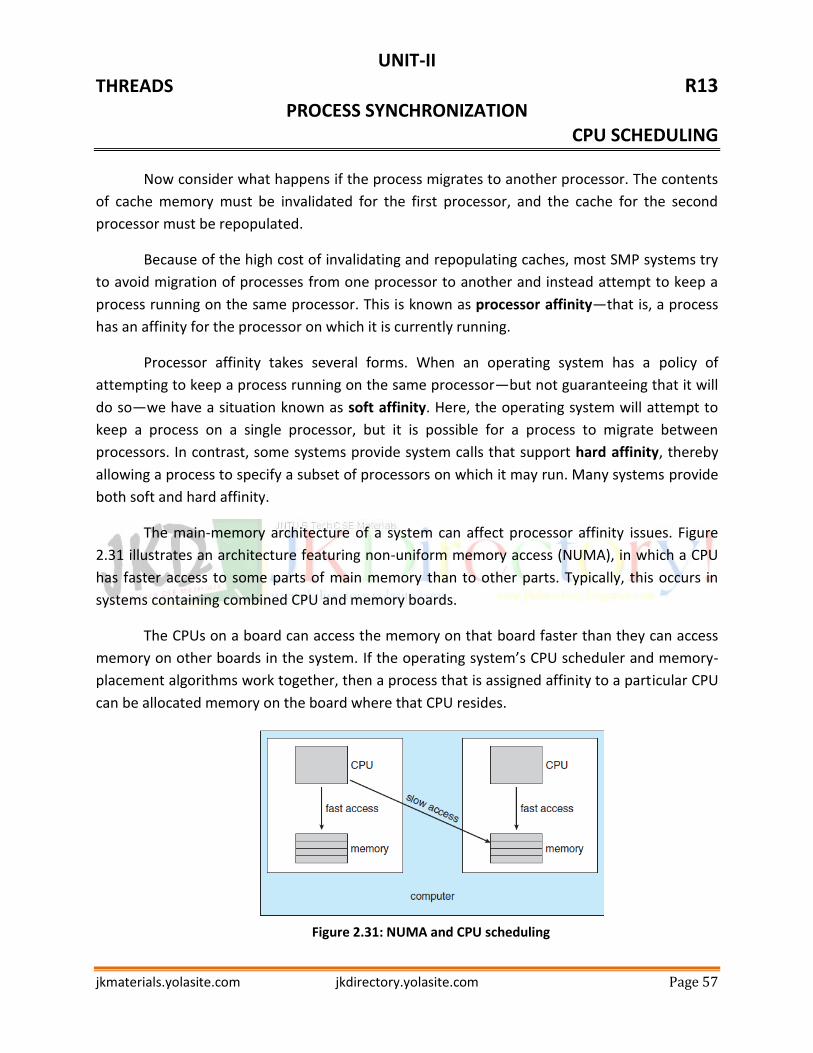
UNIT-II


CPU SCHEDULING


Now consider what happens if the process migrates to another processor. The contents

of cache memory must be invalidated for the first processor, and the cache for the second

processor must be repopulated.

Because of the high cost of invalidating and repopulating caches, most SMP systems try

to avoid migration of processes from one processor to another and instead attempt to keep a

process running on the same processor. This is known as processor affinity—that is, a process

has an affinity for the processor on which it is currently running.

Processor affinity takes several forms. When an operating system has a policy of

attempting to keep a process running on the same processor—but not guaranteeing that it will

do so—we have a situation known as soft affinity. Here, the operating system will attempt to

keep a process on a single processor, but it is possible for a process to migrate between

processors. In contrast, some systems provide system calls that support hard affinity, thereby

allowing a process to specify a subset of processors on which it may run. Many systems provide

both soft and hard affinity.

The main-memory architecture of a system can affect processor affinity issues. Figure

2.31 illustrates an architecture featuring non-uniform memory access (NUMA), in which a CPU

has faster access to some parts of main memory than to other parts. Typically, this occurs in

systems containing combined CPU and memory boards.

The CPUs on a board can access the memory on that board faster than they can access

memory on other boards in the system. If the operating system’s CPU scheduler and memory-

placement algorithms work together, then a process that is assigned affinity to a particular CPU

can be allocated memory on the board where that CPU resides.

Figure 2.31: NUMA and CPU scheduling

UNIT-II


CPU SCHEDULING


Load Balancing:

On SMP systems, it is important to keep the workload balanced among all processors to

fully utilize the benefits of having more than one processor. Otherwise, one or more processors

may sit idle while other processors have high workloads, along with lists of processes awaiting

the CPU.

Load balancing attempts to keep the workload evenly distributed across all processors

in an SMP system. It is important to note that load balancing is typically necessary only on

systems where each processor has its own private queue of eligible processes to execute.

On systems with a common run queue, load balancing is often unnecessary, because

once a processor becomes idle, it immediately extracts a runnable process from the common

run queue. It is also important to note, however, that in most contemporary operating systems

supporting SMP, each processor does have a private queue of eligible processes.

There are two general approaches to load balancing: push migration and pull migration.

With push migration, a specific task periodically checks the load on each processor and—if it

finds an imbalance—evenly distributes the load by moving (or pushing) processes from

overloaded to idle or less-busy processors. Pull migration occurs when an idle processor pulls a

waiting task from a busy processor. Push and pull migration need not be mutually exclusive and

are in fact often implemented in parallel on load-balancing systems.

Multicore Processors:

Traditionally, SMP systems have allowed several threads to run concurrently by

providingmultiple physical processors. However, a recent practice in computer hardware has

been to place multiple processor cores on the same physical chip,

resulting in a multicore processor. Each core maintains its architectural state and thus

appears to the operating system to be a separate physical processor. SMP systems that use

multicore processors are faster and consume less power than systems in which each processor

has its own physical chip.

Multicore processors may complicate scheduling issues. Let’s consider how this can

happen. Researchers have discovered that when a processor accesses memory, it spends a

significant amount of time waiting for the data to become available. This situation, known as a

UNIT-II


CPU SCHEDULING


memory stall, may occur for various reasons, such as a cache miss (accessing data that are not

in cache memory). Figure 2.32 illustrates a memory stall.

Figure 2.32: Memory Stall

In this scenario, the processor can spend up to 50 percent of its time waiting for data to

become available from memory. To remedy this situation, many recent hardware designs have

implemented multithreaded processor cores in which two (or more) hardware threads are

assigned to each core. That way, if one thread stalls while waiting for memory, the core can

switch to another thread.

Figure 2.33 illustrates a dual-threaded processor core on which the execution of thread

0 and the execution of thread 1 are interleaved. From an operating-system perspective, each

hardware thread appears as a logical processor that is available to run a software thread. Thus,

on a dual-threaded, dual-core system, four logical processors are presented to the operating

system.

Figure 2.33: Multithreaded multicore system

In general, there are two ways to multithread a processing core: coarse-grained and

fine-grained multithreading.With coarse-grained multithreading, a thread executes on a

processor until a long-latency event such as a memory stall occurs. Because of the delay caused

by the long-latency event, the processor must switch to another thread to begin execution.

However, the cost of switching between threads is high, since the instruction pipeline

must be flushed before the other thread can begin execution on the processor core. Once this

new thread begins execution, it begins filling the pipeline with its instructions.

UNIT-II


CPU SCHEDULING


Fine-grained (or interleaved) multithreading switches between threads at a much finer

level of granularity—typically at the boundary of an instruction cycle. However, the

architectural design of fine-grained systems includes logic for thread switching. As a result, the

cost of switching between threads is small.

REAL-TIME CPU SCHEDULING:

CPU scheduling for real-time operating systems involves special issues. In general, we

can distinguish between soft real-time systems and hard real-time systems. Soft real-time

systems provide no guarantee as to when a critical real-time process will be scheduled. They

guarantee only that the process will be given preference over noncritical processes. Hard real-

time systems have stricter requirements. A task must be serviced by its deadline; service after

the deadline has expired is the same as no service at all.

Minimizing Latency:

Consider the event-driven nature of a real-time system. The system is typically waiting

for an event in real time to occur. Events may arise either in software —as when a timer

expires—or in hardware—as when a remote-controlled vehicle detects that it is approaching an

obstruction.When an event occurs, the system must respond to and service it as quickly as

possible.We refer to event latency as the amount of time that elapses from when an event

occurs to when it is serviced (Figure 2.34).

Figure 2.34: Event latency

Two types of latencies affect the performance of real-time systems:

1. Interrupt latency

2. Dispatch latency

UNIT-II


CPU SCHEDULING


Interrupt latency refers to the period of time fromthe arrival of an interrupt at the CPU

to the start of the routine that services the interrupt. When an interrupt occurs, the operating

system must first complete the instruction it is executing and determine the type of interrupt

that occurred. It must then save the state of the current process before servicing the interrupt

using the specific interrupt service routine (ISR). The total time required to perform these tasks

is the interrupt latency (Figure 2.35).

Figure 2.35: Interrupt latency

Obviously, it is crucial for real-time operating systems to minimize interrupt latency to

ensure that real-time tasks receive immediate attention. Indeed, for hard real-time systems,

interrupt latency must not simply be minimized, it must be bounded to meet the strict

requirements of these systems.

The amount of time required for the scheduling dispatcher to stop one process and start

another is known as dispatch latency. Providing real-time tasks with immediate access to the

CPU mandates that real-time operating systems minimize this latency as well. The most

effective technique for keeping dispatch latency low is to provide preemptive kernels.

In Figure 2.36, we diagram the makeup of dispatch latency. The conflict phase of

dispatch latency has two components:

1. Preemption of any process running in the kernel

2. Release by low-priority processes of resources needed by a high-priority process

UNIT-II


CPU SCHEDULING


Priority-Based Scheduling:

The most important feature of a real-time operating system is to respond immediately

to a real-time process as soon as that process requires the CPU.

As a result, the scheduler for a real-time operating system must support a priority-based

algorithm with preemption. Recall that priority-based scheduling algorithms assign each

process a priority based on its importance; more important tasks are assigned higher priorities

than those deemed less important. If the scheduler also supports preemption, a process

currently running on the CPU will be preempted if a higher-priority process becomes available

to run.

Rate-Monotonic Scheduling:

The rate-monotonic scheduling algorithm schedules periodic tasks using a static priority

policy with preemption. If a lower-priority process is running and a higher-priority process

becomes available to run, it will preempt the lower-priority process.Uponentering the system,

each periodic task is assigned a priority inversely based on its period.

The shorter the period, the higher the priority; the longer the period, the lower the

priority. The rationale behind this policy is to assign a higher priority to tasks that require the

CPU more often. Furthermore, rate-monotonic scheduling assumes that the processing time of

a periodic process is the same for each CPU burst. That is, every time a process acquires the

CPU, the duration of its CPU burst is the same.

Earliest-Deadline-First Scheduling:

Earliest-deadline-first (EDF) scheduling dynamically assigns priorities according to

deadline. The earlier the deadline, the higher the priority; the later the deadline, the lower the

priority. Under the EDF policy, when a process becomes runnable, it must announce its

deadline requirements to the system. Priorities may have to be adjusted to reflect the deadline

of the newly runnable process. Note how this differs from rate-monotonic scheduling, where

priorities are fixed.

Proportional Share Scheduling: Proportional share schedulers operate by allocating T

shares among all applications. An application can receive N shares of time, thus ensuring that

the application will have N/T of the total processor time.

UNIT-II


CPU SCHEDULING


Proportional share schedulers must work in conjunction with an admission-control

policy to guarantee that an application receives its allocated shares of time. An admission-

control policy will admit a client requesting a particular number of shares only if sufficient

shares are available.

ALGORITHM EVALUATION:

As there are many scheduling algorithms, each with its own parameters. As a result,

selecting an algorithm can be difficult. The first problem is defining the criteria to be used in

selecting an algorithm.

To select an algorithm, we must first define the relative importance of these elements.

Our criteria may include several measures, such as these:

Maximizing CPU utilization under the constraint that the maximum response time is

1 second

Maximizing throughput such that turnaround time is (on average) linearly

proportional to total execution time

Once the selection criteria have been defined, we want to evaluate the algorithms

under consideration.

Deterministic Modeling:

One major class of evaluation methods is analytic evaluation. Analytic evaluation uses

the given algorithm and the system workload to produce a formula or number to evaluate the

performance of the algorithm for that workload.

Deterministic modeling is one type of analytic evaluation. This method takes a

particular predetermined workload and defines the performance of each algorithm for that

workload. For example, assume that we have the workload shown below. All five processes

arrive at time 0, in the order given, with the length of the CPU burst given in milliseconds:

Process Burst Time

P1 10

P2 29

P3 3

P4 7

P5 12

UNIT-II


CPU SCHEDULING


Consider the FCFS, SJF, and RR (quantum = 10 milliseconds) scheduling algorithms for

this set of processes. Which algorithm would give the minimum average waiting time? For the

FCFS algorithm, we would execute the processes as


milliseconds for process P3, 42 milliseconds for process P4, and 49 milliseconds for process P5.

Thus, the average waiting time is (0 + 10 + 39 + 42 + 49)/5 = 28 milliseconds. With

nonpreemptive SJF scheduling, we execute the processes as



Thus, the average waiting time is (10 + 32 + 0 + 3 + 20)/5 = 13 milliseconds. With the RR

algorithm, we execute the processes as



Thus, the average waiting time is (0 + 32 + 20 + 23 + 40)/5 = 23 milliseconds.

We can see that, in this case, the average waiting time obtained with the SJF policy is

less than half that obtained with FCFS scheduling; the RR algorithm gives us an intermediate

value.

Deterministic modeling is simple and fast. It gives us exact numbers, allowing us to

compare the algorithms. However, it requires exact numbers for input, and its answers apply

only to those cases.

UNIT-II


CPU SCHEDULING


Queueing Models:

On many systems, the processes that are run vary from day to day, so there is no static

set of processes (or times) to use for deterministic modeling. What can be determined,

however, is the distribution of CPU and I/O bursts. These distributions can be measured and

then approximated or simply estimated.

The result is a mathematical formula describing the probability of a particular CPU burst.

Commonly, this distribution is exponential and is described by its mean. Similarly, we can

describe the distribution of times when processes arrive in the system (the arrival-time

distribution). From these two distributions, it is possible to compute the average throughput,

utilization, waiting time, and so on for most algorithms.

The computer system is described as a network of servers. Each server has a queue of

waiting processes. The CPU is a server with its ready queue, as is the I/O system with its device

queues. Knowing arrival rates and service rates, we can compute utilization, average queue

length, average wait time, and so on. This area of study is called queueing-network analysis.

Simulations:

To get a more accurate evaluation of scheduling algorithms, we can use simulations.

Running simulations involves programming a model of the computer system. Software data

structures represent the major components of the system.

The simulator has a variable representing a clock. As this variable’s value is increased,

the simulator modifies the system state to reflect the activities of the devices, the processes,

and the scheduler. As the simulation executes, statistics that indicate algorithm performance

are gathered and printed.

The data to drive the simulation can be generated in several ways. The

mostcommonmethod uses a random-number generator that is programmed to generate

processes, CPU burst times, arrivals, departures, and so on, according to probability

distributions.

The distributions can be defined mathematically (uniform, exponential, Poisson) or

empirically. If a distribution is to be defined empirically, measurements of the actual system

under study are taken. The results define the distribution of events in the real system; this

distribution can then be used to drive the simulation.

UNIT-II


CPU SCHEDULING


Implementation:

Even a simulation is of limited accuracy. The only completely accurate way to evaluate a

scheduling algorithm is to code it up, put it in the operating system, and see how it works. This

approach puts the actual algorithm in the real system for evaluation under real operating

conditions.

The major difficulty with this approach is the high cost. The expense is incurred not only

in coding the algorithm and modifying the operating system to support it (along with its

required data structures) but also in the reaction of the users to a constantly changing

operating system.

Most users are not interested in building a better operating system; they merely want to

get their processes executed and use their results. A constantly changing operating system does

not help the users to get their work done. Another difficulty is that the environment in which

the algorithm is used will change.

UNIT-II THREADS R13 PROCESS SYNCHRONIZATION...UNIT-II THREADS R13 PROCESS SYNCHRONIZATION CPU...

Documents

Transcript of UNIT-II THREADS R13 PROCESS SYNCHRONIZATION...UNIT-II THREADS R13 PROCESS SYNCHRONIZATION CPU...