UNIT-I ARTIFICIAL NEURAL NETWORKS Artificial Neural ... · According to Haykin, Neural Networks: A...
80
Neural Networks and Fuzzy Logic (15A02605) Lecture Notes Dept. of ECE, CREC Page 1 UNIT-I ARTIFICIAL NEURAL NETWORKS Artificial Neural Networks and their Biological Motivation Artificial Neural Network (ANN) There is no universally accepted definition of an NN. But perhaps most people in the field would agree that an NN is a network of many simple processors (“units”), each possibly having a small amount of local memory. The units are connected by communication channels (“connections”) which usually carry numeric (as opposed to symbolic) data, encoded by any of various means. The units operate only on their local data and on the inputs they receive via the connections. The restriction to local operations is often relaxed during training. Some NNs are models of biological neural networks and some are not, but historically, much of the inspiration for the field of NNs came from the desire to produce artificial systems capable of sophisticated, perhaps “intelligent”, computations similar to those that the human brain routinely performs, and thereby possibly to enhance our understanding of the human brain. Most NNs have some sort of “training” rule whereby the weights of connections are adjusted on the basis of data. In other words, NNs “learn” from examples (as children learn to recognize dogs from examples of dogs) and exhibit some capability for generalization beyond the training data. NNs normally have great potential for parallelism, since the computations of the components are largely independent of each other. Some people regard massive parallelism and high connectivity to be defining characteristics of NNs, but such requirements rule out various simple models, such as simple linear regression (a minimal feed forward net with only two units plus bias), which are usefully regarded as special cases of NNs. According to Haykin, Neural Networks: A Comprehensive Foundation: A neural network is a massively parallel distributed processor that has a natural propensity for storing experimental knowledge and making it available for use. It resembles the brain in two respects: 1. Knowledge is acquired by the network through a learning process. 2. Interneuron connection strengths known as synaptic weights are used to store the knowledge. We can also say that: Neural networks are parameterised computational nonlinear algorithms for (numerical) data/signal/image processing. These algorithms are either implemented on a general-purpose computer or are built into a dedicated hardware. Basic characteristics of biological neurons • Biological neurons, the basic building blocks of the brain, are slower than silicon logic gates. The neurons operate in millisecond which is about six orders of magnitude slower that the silicon gates operating in the nanosecond range. • The brain makes up for the slow rate of operation with two factors: – a huge number of nerve cells (neurons) and interconnections between them. The number of neurons is estimated to be in the range of 1010 with 60 · 1012 synapses (interconnections). – A function of a biological neuron seems to be much more complex than that of a logic gate.
Transcript of UNIT-I ARTIFICIAL NEURAL NETWORKS Artificial Neural ... · According to Haykin, Neural Networks: A...
Neural Networks and Fuzzy Logic (15A02605) Lecture Notes
Dept. of ECE, CREC Page 1
UNIT-I ARTIFICIAL NEURAL NETWORKS
Artificial Neural Networks and their Biological Motivation Artificial Neural Network (ANN)
There is no universally accepted definition of an NN. But perhaps most people in the field would agree that an NN is a network of many simple processors (“units”), each possibly having a small amount of local memory. The units are connected by communication channels (“connections”) which usually carry numeric (as opposed to symbolic) data, encoded by any of various means. The units operate only on their local data and on the inputs they receive via the connections. The restriction to local operations is often relaxed during training.
Some NNs are models of biological neural networks and some are not, but historically, much of the inspiration for the field of NNs came from the desire to produce artificial systems capable of sophisticated, perhaps “intelligent”, computations similar to those that the human brain routinely performs, and thereby possibly to enhance our understanding of the human brain.
Most NNs have some sort of “training” rule whereby the weights of connections are adjusted on the basis of data. In other words, NNs “learn” from examples (as children learn to recognize dogs from examples of dogs) and exhibit some capability for generalization beyond the training data.
NNs normally have great potential for parallelism, since the computations of the components are largely independent of each other. Some people regard massive parallelism and high connectivity to be defining characteristics of NNs, but such requirements rule out various simple models, such as simple linear regression (a minimal feed forward net with only two units plus bias), which are usefully regarded as special cases of NNs. According to Haykin, Neural Networks: A Comprehensive Foundation:
A neural network is a massively parallel distributed processor that has a natural propensity for storing experimental knowledge and making it available for use. It resembles the brain in two respects: 1. Knowledge is acquired by the network through a learning process. 2. Interneuron connection strengths known as synaptic weights are used to store the knowledge. We can also say that: Neural networks are parameterised computational nonlinear algorithms for (numerical) data/signal/image processing. These algorithms are either implemented on a general-purpose computer or are built into a dedicated hardware. Basic characteristics of biological neurons • Biological neurons, the basic building blocks of the brain, are slower than silicon logic gates. The neurons operate in millisecond which is about six orders of magnitude slower that the silicon gates operating in the nanosecond range. • The brain makes up for the slow rate of operation with two factors: – a huge number of nerve cells (neurons) and interconnections between them. The number of neurons is estimated to be in the range of 1010 with 60 · 1012 synapses (interconnections). – A function of a biological neuron seems to be much more complex than that of a logic gate.
Neural Networks and Fuzzy Logic (15A02605) Lecture Notes
Dept. of ECE, CREC Page 2
• The brain is very energy efficient. It consumes only about 10−16 joules per operation per second, comparing with 10−6 J/oper·sec for a digital computer.
The brain is a highly complex, non-linear, parallel information processing system. It performs tasks like pattern recognition, perception, motor control, many times faster than the fastest digital computers. • Consider an efficiency of the visual system which provides a representation of the environment which enables us to interact with the environment. For example, a complex task of perceptual recognition, e.g. recognition of a familiar face embedded in an unfamiliar scene can be accomplished in 100-200 ms, whereas tasks of much lesser complexity can take hours if not days on conventional computers. • As another example consider an efficiency of the sonar system of a bat. Sonar is an active echo-location system. A bat sonar provides information about the distance from a target, its relative velocity and size, the size of various features of the target, and its azimuth and elevation.
The complex neural computations needed to extract all this information from the target echo occur within a brain which has the size of a plum.
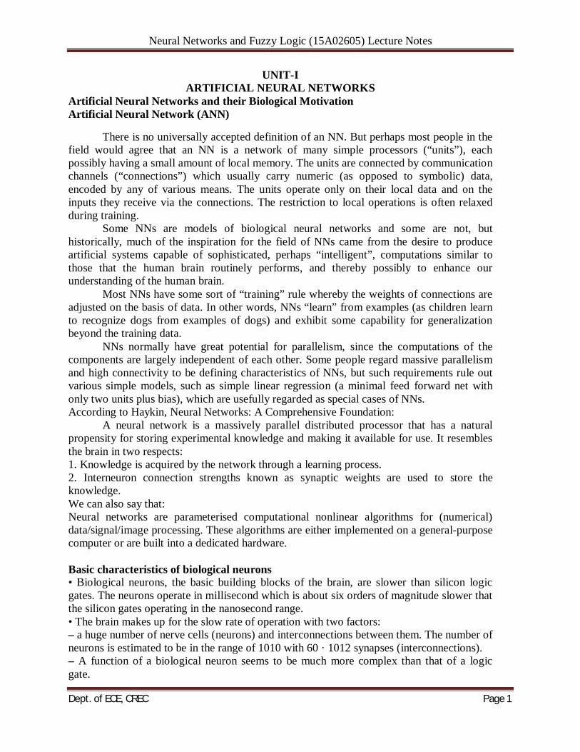
The precision and success rate of the target location is rather impossible to match by radar or sonar engineers. A (naive) structure of biological neurons A biological neuron, or a nerve cell, consists of
Fig: The pyramidal cell— a “prototype” of an artificial neuron.

Neural Networks and Fuzzy Logic (15A02605) Lecture Notes
Dept. of ECE, CREC Page 3
synapses, dendrites, the cell body (or hillock), the axon. Simplified functions of this very complex in their nature “building blocks” are as follow: • The synapses are elementary signal processing devices. – A synapse is a biochemical device which converts a Pre-synaptic electrical signal into a chemical signal and then back into a post-synaptic electrical signal. – The input pulse train has its amplitude modified by parameters stored in the synapse. The nature of this modification depends on the type of the synapse, which can be either inhibitory or excitatory. • The postsynaptic signals are aggregated and transferred along the dendrites to the nerve cell body. • The cell body generates the output neuronal signal, a spike, which is transferred along the axon to the synaptic terminals of other neurons.
The frequency of firing of a neuron is proportional to the total synaptic activities and is controlled by the synaptic parameters (weights). • The pyramidal cell can receive 104 synaptic inputs and it can fan-out the output signal to thousands of target cells — the connectivity difficult to achieve in the artificial neural networks. Taxonomy of neural networks
From the point of view of their active or decoding phase, artificial neural networks can be classified into feed forward (static) and feedback (dynamic, recurrent) systems.
From the point of view of their learning or encoding phase, artificial neural networks can be classified into supervised and unsupervised systems. Feed forward supervised networks
This network is typically used for function approximation tasks. Specific examples include: • Linear recursive least-mean-square (LMS) networks • Back propagation networks • Radial Basis networks Feed forward unsupervised networks
These networks are used to extract important properties of the input data and to map input data into a “representation” domain. Two basic groups of methods belong to this category • Hebbian networks performing the Principal Component Analysis of the input data, also known as the Karhunen-Loeve Transform. • Competitive networks used to performed Learning Vector Quantization, or tessellation of the input data set. Self-Organizing Kohonen Feature Maps also belong to this group. Feedback networks
These networks are used to learn or process the temporal features of the input data and their internal state evolves with time. Specific examples include: • Recurrent Back propagation networks • Associative Memories • Adaptive Resonance networks
Neural Networks and Fuzzy Logic (15A02605) Lecture Notes
Dept. of ECE, CREC Page 4
Models of artificial neurons Artificial neural networks are nonlinear information (signal) processing devices
which are built from interconnected elementary processing devices called neurons. An artificial neuron is a p-input single-output signal processing element which can be
thought of as a simple model of a non-branching biological neuron. Graphically, an artificial neuron is represented in one of the following forms:
From a dendritic representation of a single neuron we can identify p synapses arranged along a linear dendrite which aggregates the synaptic activities, and a neuron body or axon-hillock generating an output signal.
The pre-synaptic activities are represented by a p-element column vector of input signals
x = [x1 . . . xp]T In other words the space of input patterns is p-dimensional.
Synapses are characterized by adjustable parameters called weights or synaptic strength parameters. The weights are arranged in a p-element row vector:
w = [w1 . . . wp] In a signal flow representation of a neuron p synapses are arranged in a layer of input
nodes. A dendrite is replaced by a single summing node. Weights are now attributed to branches (connections) between input nodes and the summing node.
Passing through synapses and a dendrite (or a summing node), input signals are aggregated (combined) into the activation potential, which describes the total post-synaptic activity. The activation potential is formed as a linear combination of input signals and synaptic strength parameters, that is, as an inner product of the weight and input vectors:
Subsequently, the activation potential (the total post-synaptic activity) is passed through an activation function, '(·), which generates the output signal: y = '(v) (2.2)
The activation function is typically a saturating function which normalizes the total post-synaptic activity to the standard values of output (axonal) signal.
The block-diagram representation encapsulates basic operations of an artificial neuron, namely, aggregation of pre-synaptic activities, eqn (2.1), and generation of the output signal, eqn (2.2)
A single synapse in a dendritic representation of a neuron can be represented by the following block-diagram:
In the synapse model of Figure 2–3 we can identify: a storage for the synaptic weight, augmentation (multiplication) of the pre-synaptic signal with the weight parameter, and the dendritic aggregation of the post-synaptic activities. Types of activation functions Typically, the activation function generates either unipolar or bipolar signals.A linear function: y = v. Such linear processing elements, sometimes called ADALINEs, are studied in the theory of linear systems, for example, in the “traditional” signal processing and statistical regression analysis. A step function Unipolar:
Neural Networks and Fuzzy Logic (15A02605) Lecture Notes
Dept. of ECE, CREC Page 5
Such a processing element is traditionally called perceptron, and it works as a threshold element with a binary output. A step function with bias The bias (threshold) can be added to both, unipolar and bipolar step function. We then say that a neuron is “fired”, when the synaptic activity exceeds the threshold level, _. For a unipolar case, A piecewise-linear function • For small activation potential, v, the neuron works as a linear combiner (an ADALINE) with the gain (slope) _. • For large activation potential, v, the neuron saturates and generates the output signal either) or 1. • For large gains _! 1, the piecewise-linear function is reduced to a step function. Sigmoidal functions
The hyperbolic tangent (bipolar sigmoidal) function is perhaps the most popular choice of the activation function specifically in problems related to function mapping and approximation. Radial-Basis Functions
Radial-basis functions arise as optimal solutions to problems of interpolation, approximation and regularization of functions. The optimal solutions to the above problems are specified by some integro-differential equations which are satisfied by a wide range of nonlinear differentiable functions Typically, Radial-Basis Functions '(x; ti) form a family of functions of a p-dimensional vector, x, each function being centered at point ti.
A popular simple example of a Radial-Basis Function is a symmetrical multivariate Gaussian function which depends only on the distance between the current point, x, and the center point,
where ||x − ti|| is the norm of the distance vector between the current vector x and the centre, ti, of the symmetrical multidimensional Gaussian surface. Two concluding remarks: • In general, the smooth activation functions, like sigmoidal, or Gaussian, for which a continuous derivative exists, are typically used in networks performing a function approximation task, whereas the step functions are used as parts of pattern classification networks. • Many learning algorithms require calculation of the derivative of the activation function see the relevant assignments/practical. Multi-layer feed forward neural networks
Connecting in a serial way layers of neurons presented in Figure 2–5 we can build multi-layer feed forward neural networks.
The most popular neural network seems to be the one consisting of two layers of neurons as presented in Figure 2–6. In order to avoid a problem of counting an input layer, the architecture of Figure 2–6 is referred to as a single hidden layer neural network.
There are L neurons in the hidden layer (hidden neurons), and m neurons in the output layer (output neurons). Input signals, x, are passed through synapses of the hidden layer with connection strengths described by the hidden weight matrix, Wh, and the L hidden activation signals, ˆh, are generated.
Neural Networks and Fuzzy Logic (15A02605) Lecture Notes
Dept. of ECE, CREC Page 6
The hidden activation signals are then normalized by the functions into the L hidden signals, h. Introduction to learning
In the previous sections we concentrated on the decoding part of a neural network assuming that the weight matrix, W, is given. If the weight matrix is satisfactory, during the decoding process the network performs some useful task it has been design to do.
In simple or specialized cases the weight matrix can be pre-computed, but more commonly it is obtained through the learning process. Learning is a dynamic process which modifies the weights of the network in some desirable way. As any dynamic process learning can be described either in the continuous-time or in the discrete-time framework.
The learning can be described either by differential equations (continuous-time) ˙W(t) = L(W(t), x(t), y(t), d(t) ) (2.8) or by the difference equations (discrete-time) W(n + 1) = L(W(n), x(n), y(n), d(n) ) (2.9)
Where d is an external teaching/supervising signal used in supervised learning. This signal in not present in networks employing unsupervised learning. Perceptron
The perceptron was introduced by McCulloch and Pitts in 1943 as an artificial neuron with a hard-limiting activation function. Recently the term multilayer perceptron has often been used as a synonym for the term multilayer feedforward neural network. In this section we will be referring to the former meaning.
Input signals, xi, are assumed to have real values. The activation function is a unipolar step function (sometimes called the Heaviside function), therefore, the output signal is binary, y 2 {0, 1}. One input signal is constant (xp = 1), and the related weight is interpreted as the bias, or threshold.
The input signals and weights are arranged in the following column and row vectors, respectively: Aggregation of the “proper” input signals results in the activation potential, v, which can be expressed as the inner product of “proper” input signals and related weights:
Hence, a perceptron works as a threshold element, the output being “active” if the activation potential exceeds the threshold. A Perceptron as a Pattern Classifier
A single perceptron classifies input patterns, x, into two classes. A linear combination of signals and weights for which the augmented activation potential is zero, ˆv = 0, describes a decision surface which partitions the input space into two regions.
The input patterns that can be classified by a single perceptron into two distinct classes are called linearly separable patterns. A Perceptron as a Pattern Classifier
A single perceptron classifies input patterns, x, into two classes. A linear combination of signals and weights for which the augmented activation potential is zero, ˆv = 0, describes a decision surface which partitions the input space into two regions. The decision surface is a hyperplane specified.
The input patterns that can be classified by a single perceptron into two distinct classes are called linearly separable patterns. The Perceptron learning law
Neural Networks and Fuzzy Logic (15A02605) Lecture Notes
Dept. of ECE, CREC Page 7
Learning is a recursive procedure of modifying weights from a given set of input-output patterns. For a single perceptron, the objective of the learning (encoding) procedure is to find the decision plane, (that is, the related weight vector), which separates two classes of given input-output training vectors.
Once the learning is finalised, every input vector will be classified into an appropriate class. A single perceptron can classify only the linearly separable patterns. The perceptron learning procedure is an example of a supervised error-correcting learning law.
Obtain the correct decision plane specified by the weight vector w. The training patterns are arrange in a training set which consists of a p × N input matrix, X, and an N-element output vector.
We can identify a current weight vector, w(n), the next weight vector, w(n + 1), and the correct weight vector, w_. Related decision planes are orthogonal to these vectors and are depicted as straight lines. During the learning process the current weight vector w(n) is modified in the direction of the current input vector x(n), if the input pattern is misclassified, that is, if the error is non-zero. Presenting the perceptron with enough training vectors, the weight vector w(n) will tend to the correct value w. Rosenblatt proved that if input patterns are linearly separable, then the perceptron learning law converges, and the hyperplane separating two classes of input patterns can be determined. ADALINE — The Adaptive Linear Element
The Adaline can be thought of as the smallest, linear building block of the artificial neural networks. This element has been extensively used in science, statistics (in the linear regression analysis), engineering (the adaptive signal processing, control systems), and so on. In general, the Adaline is used to perform linear approximation of a “small” segment of a nonlinear hyper-surface, which is generated by a p–variable function, y = f(x). In this case, the bias is usually needed, hence, wp = 1. linear filtering and prediction of data (signals) pattern association, that is, generation of m–element output vectors associated with respective p–element input vectors.
We will discuss two first items in greater detail. Specific calculations are identical in all cases, only the interpretation varies. The LMS (Widrow-Hoff) Learning Law
The Least-Mean-Square (LMS) algorithm also known as the Widrow-Hoff Learning Law, or the Delta Rule is based on the instantaneous update of the correlation matrices, that is, on the instantaneous update of the gradient of the mean-squared error.
To derive the instantaneous update of the gradient vector we will first express the current values of the correlation matrices in terms of their previous values (at the step n − 1) and the updates at the step n.
First observe that the current input vector x(n) and the desired output signal d(n) are appended to the matrices d(n − 1) and X(n − 1) as follows:
d(n) = [d(n − 1) d(n)] , and X(n) = [X(n − 1) x(n)] Some general comments on the learning process:
• Computationally, the learning process goes through all training examples (an epoch) number of times, until a stopping criterion is reached.
Neural Networks and Fuzzy Logic (15A02605) Lecture Notes
Dept. of ECE, CREC Page 8
• The convergence process can be monitored with the plot of the mean-squared error function J(W(n)). Feedforward Multilayer Neural Networks
Feedforward multilayer neural networks were introduced in sec. 2. Such neural networks with supervised error correcting learning are used to approximate (synthesise) a non-linear input-output mapping from a set of training patterns. Consider a mapping f(X) from a p-dimensional domain X into an m-dimensional output space D. Multilayer perceptrons
Multilayer perceptrons are commonly used to approximate complex nonlinear mappings. In general, it is possible to show that two layers are sufficient to approximate any nonlinear function. Therefore, we restrict our considerations to such two-layer networks.
The structure of each layer has been depicted in Figure. Nonlinear functions used in the hidden layer and in the output layer can be different. There are two weight matrices: an L × p matrix Wh in the hidden layer, and an m × L matrix Wy in the output layer.
Typically, sigmoidal functions (hyperbolic tangents) are used, but other choices are also possible. The important condition from the point of view of the learning law is for the function to be differentiable. Note that • Derivatives of the sigmoidal functions are always non-negative. • Derivatives can be calculated directly from output signals using simple arithmetic operations. • In saturation, for big values of the activation potential, v, derivatives are close to zero. • Derivatives of used in the error-correction learning law.
Neural Networks and Fuzzy Logic (15A02605) Lecture Notes
Dept. of ECE, CREC Page 9
UNIT II Single Layer Perception classifier:
Classification model, Features and Decision regions:
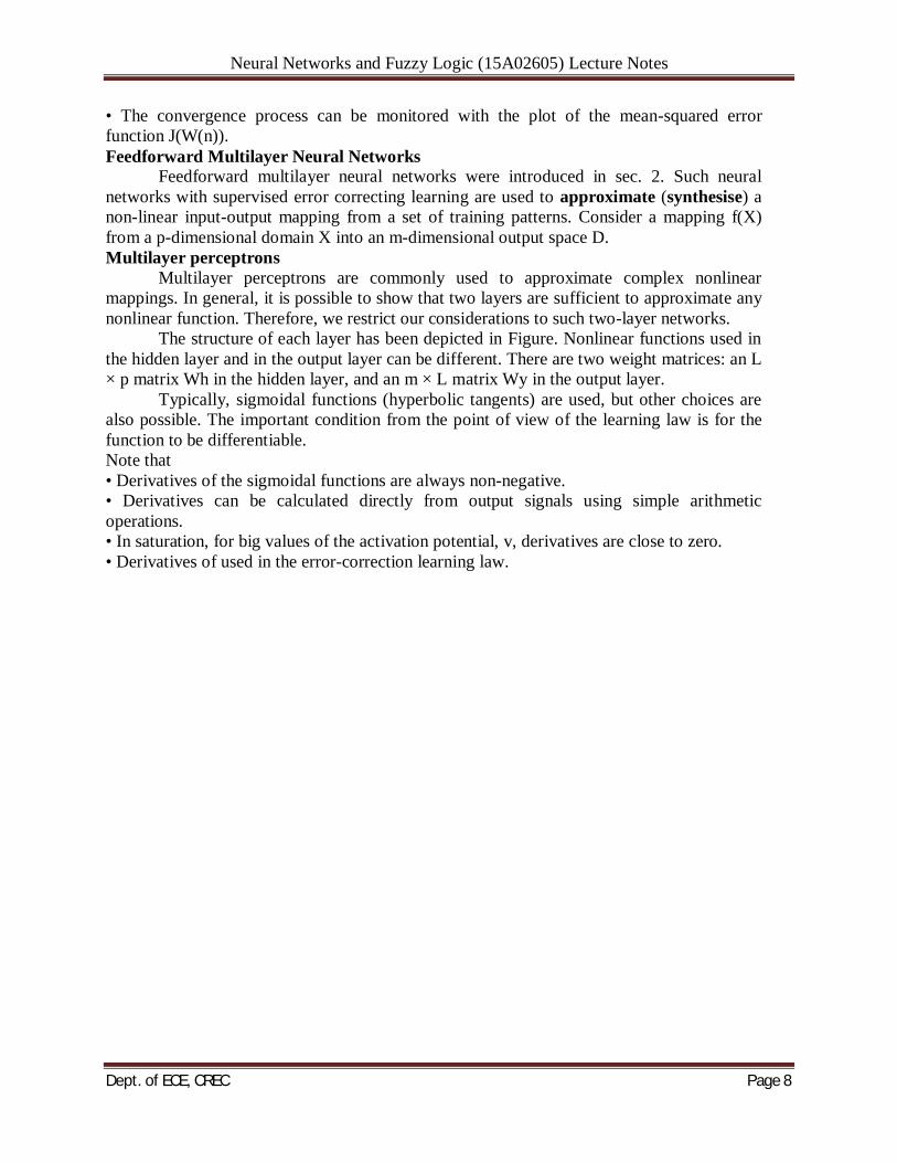
A pattern is the quantitative description of an object, event or phenomenon. The important function of neural networks is pattern classification
The classification may involve spatial and temporal patterns. Examples of patterns are pictures, video images of ships, weather maps, finger prints and characters. Examples of temporal patterns include speech signals, signals vs time produced by sensors, electrocardiograms, and seismograms. Temporal patterns usually involve ordered sequences of data appearing in time. The goal of pattern classification is to assign a physical object, event or phenomenon to one of the prescribed classes (categories)
The classifying system consists of an input transducer providing the input pattern data to the feature extractor. Typically, inputs to the feature extractor are sets of data vectors that belong to a certain category. Assume that each such set member consists of real numbers corresponding to measurement results for a given physical situation. Usually, the converted data at the output of the transducer can be compressed while still maintaining the same level of machine performance. The compressed data are called features
Neural Networks and Fuzzy Logic (15A02605) Lecture Notes
Dept. of ECE, CREC Page 10
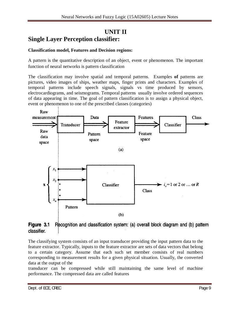
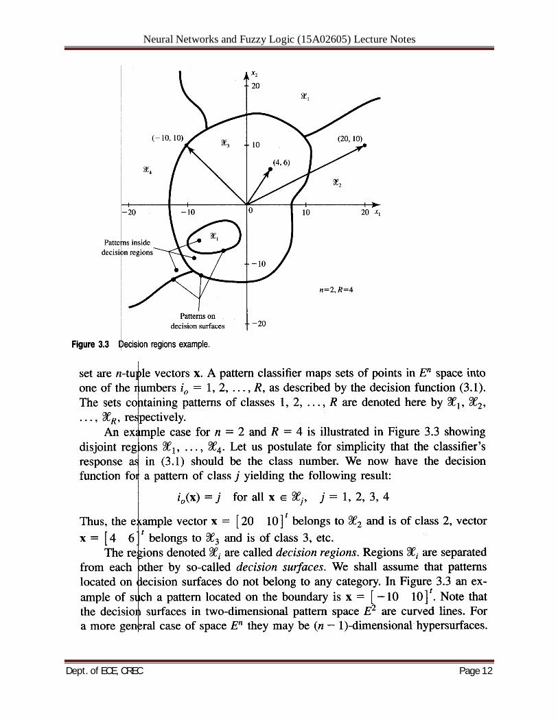
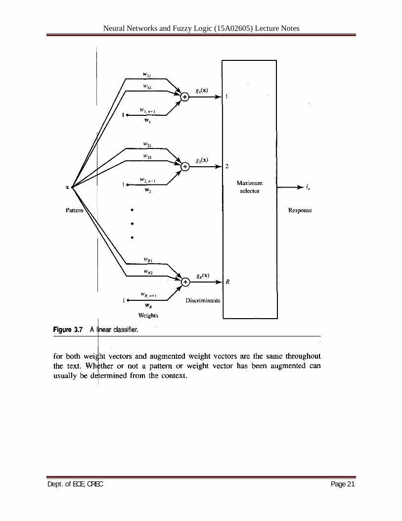
The feature extractor at the input of the classifier in Figure 3.l(a) performs the reduction of dimensionality. The feature space dimensionality is postulated to be much smaller than the dimensionality of the pattern space. The feature vectors retain the minimum number of data dimensions while maintaining the probability of correct classification, thus making handling data easier. An example of possible feature extraction is available in the analysis of speech vowel sounds. A 16-channel filter bank can provide a set of 16-component spectral vectors. The vowel spectral content can be transformed into perceptual quality space consisting of two dimensions only. They are related to tongue height and retraction Another example of dimensionality reduction is the projection of planar data on a single line, reducing the feature vector size to a single dimension. Although the projection of data will often produce a useless mixture, by moving and/or rotating the line it might be possible to find its orientation for which the projected data are well separated the n-tuple vectors may be input pattern data, in that classifier’s function is to perform not only the classification itself but also to internally extract input patterns. We will represent the classifier input components as a vector x. The classification at the system's output is obtained by the classifier implementing the decision function i,(x). The discrete values of the response i, are 1 or 2 or . . . or R. The responses represent the categories into which the patterns should be placed. The classification (decision) function is provided by the transformation, or mapping, of the n-component vector x into one of the category numbers i,
Neural Networks and Fuzzy Logic (15A02605) Lecture Notes
Dept. of ECE, CREC Page 11
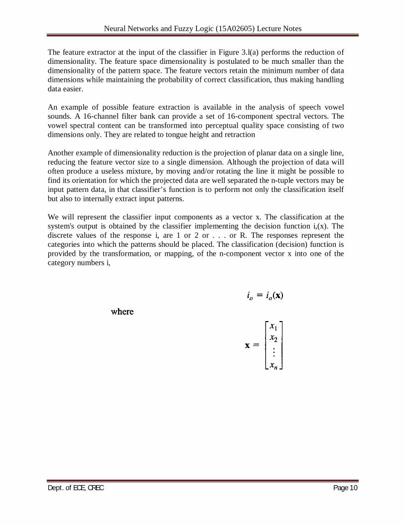
Two simple ways to generate the pattern vector for cases of spatial and temporal objects to be classified. In the case shown in Figure 3.2(a), each component xi of the vector x = [xl x2 . . . xn]t is assigned the value 1 if the i'th cell contains a portion of a spatial object; otherwise, the value 0 (or - 1) is assigned. In the case of a temporal object being a continuous function of time t, the pattern vector may be formed at discrete time instants ti by letting xi = f (ti), for i = 1, 2, . . . , n. Classification can often be conveniently described in geometric terms. Any pattern can be represented by a point in n-dimensional Euclidean space En called the pattern space. Points in that space corresponding to members of the pattern
Neural Networks and Fuzzy Logic (15A02605) Lecture Notes
Dept. of ECE, CREC Page 12
Neural Networks and Fuzzy Logic (15A02605) Lecture Notes
Dept. of ECE, CREC Page 13
Discriminant Functions:
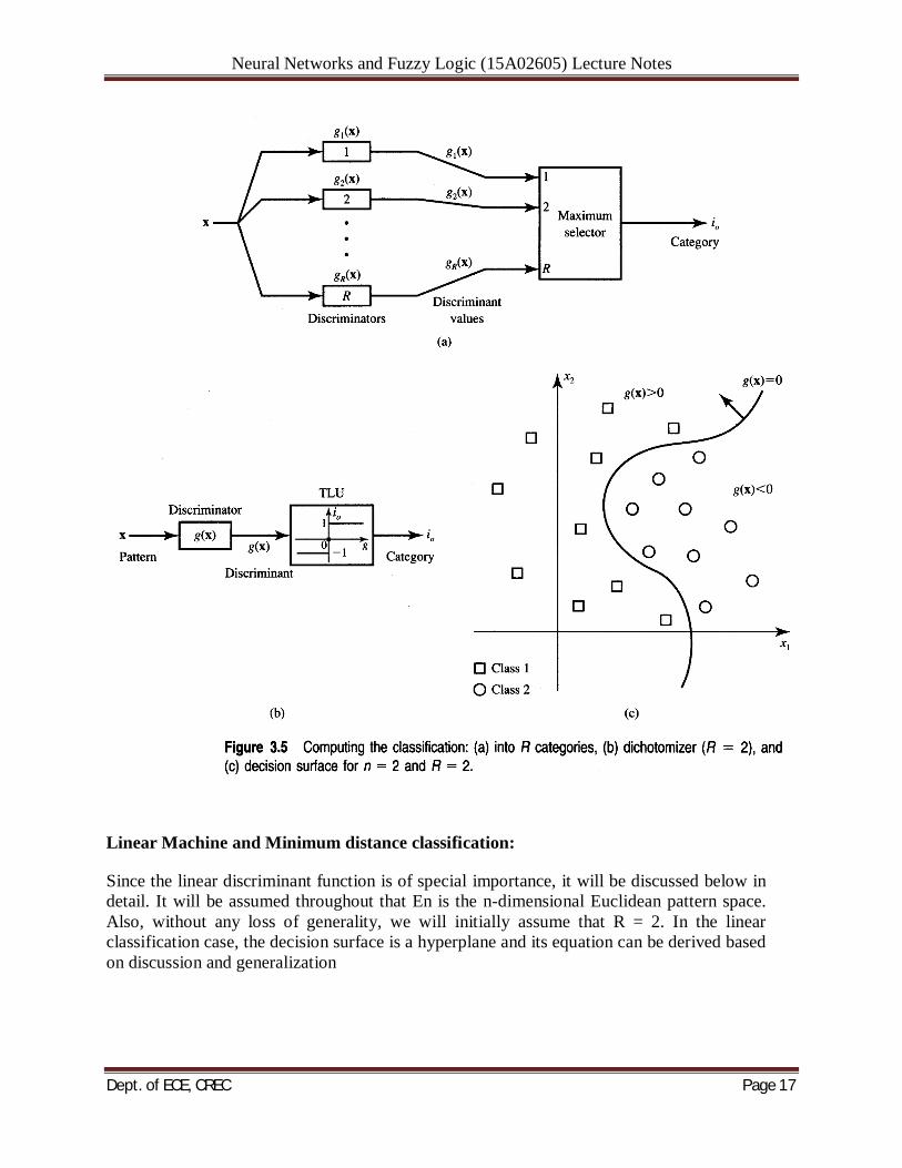
Let us assume momentarily, and for the purpose of this presentation, that the classifier has already been designed so that it can correctly perform the classification tasks. During the classification step, the membership in a category needs to be determined by the classifier based on the comparison of R discrirninant functions gl(x), g2(x), . . . , gR(x); computed for the input pattern under consideration. It is convenient to assume that the discriminant functions gi(x) are scalar values and that the pattern x belongs to the i'th category if and only if
Thus, within the region Zi, the id discriminant function will have the largest value. This maximum property of the discriminant function gi(x) for the pattern of class i is fundamental, and it will be subsequently used to choose, or assume, specific forms of the gi(x) functions. The discriminant functions' gi(x) and gj(x) for contiguous decision regions Zi and Zj 'define the decision surface between patterns of classes i and j in En space. Since the decision surface itself obviously contains patterns x without membership in any category, it is characterized by gi(x) equal to gj(x) Thus, the decision surface equation is
Neural Networks and Fuzzy Logic (15A02605) Lecture Notes
Dept. of ECE, CREC Page 14
Neural Networks and Fuzzy Logic (15A02605) Lecture Notes
Dept. of ECE, CREC Page 15
Neural Networks and Fuzzy Logic (15A02605) Lecture Notes
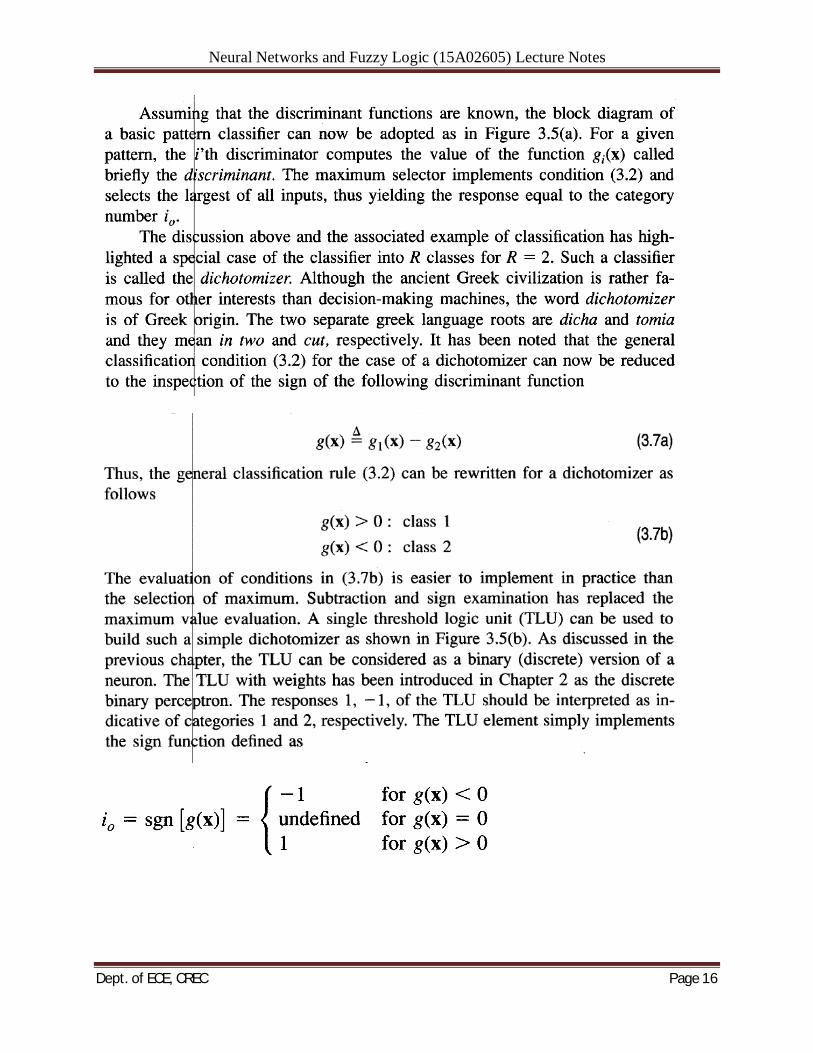
Dept. of ECE, CREC Page 16
Neural Networks and Fuzzy Logic (15A02605) Lecture Notes
Dept. of ECE, CREC Page 17
Linear Machine and Minimum distance classification:
Since the linear discriminant function is of special importance, it will be discussed below in detail. It will be assumed throughout that En is the n-dimensional Euclidean pattern space. Also, without any loss of generality, we will initially assume that R = 2. In the linear classification case, the decision surface is a hyperplane and its equation can be derived based on discussion and generalization
Neural Networks and Fuzzy Logic (15A02605) Lecture Notes
Dept. of ECE, CREC Page 18
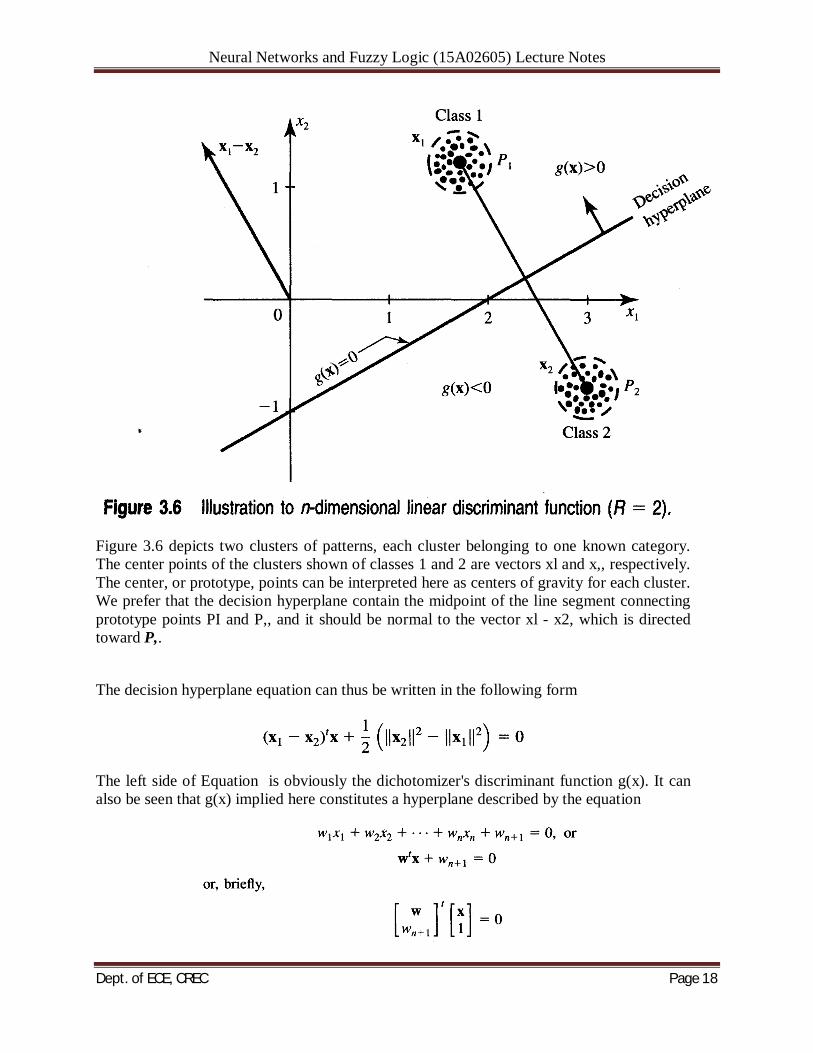
Figure 3.6 depicts two clusters of patterns, each cluster belonging to one known category. The center points of the clusters shown of classes 1 and 2 are vectors xl and x,, respectively. The center, or prototype, points can be interpreted here as centers of gravity for each cluster. We prefer that the decision hyperplane contain the midpoint of the line segment connecting prototype points PI and P,, and it should be normal to the vector xl - x2, which is directed toward P,.
The decision hyperplane equation can thus be written in the following form
The left side of Equation is obviously the dichotomizer's discriminant function g(x). It can also be seen that g(x) implied here constitutes a hyperplane described by the equation

Neural Networks and Fuzzy Logic (15A02605) Lecture Notes
Dept. of ECE, CREC Page 19
Neural Networks and Fuzzy Logic (15A02605) Lecture Notes
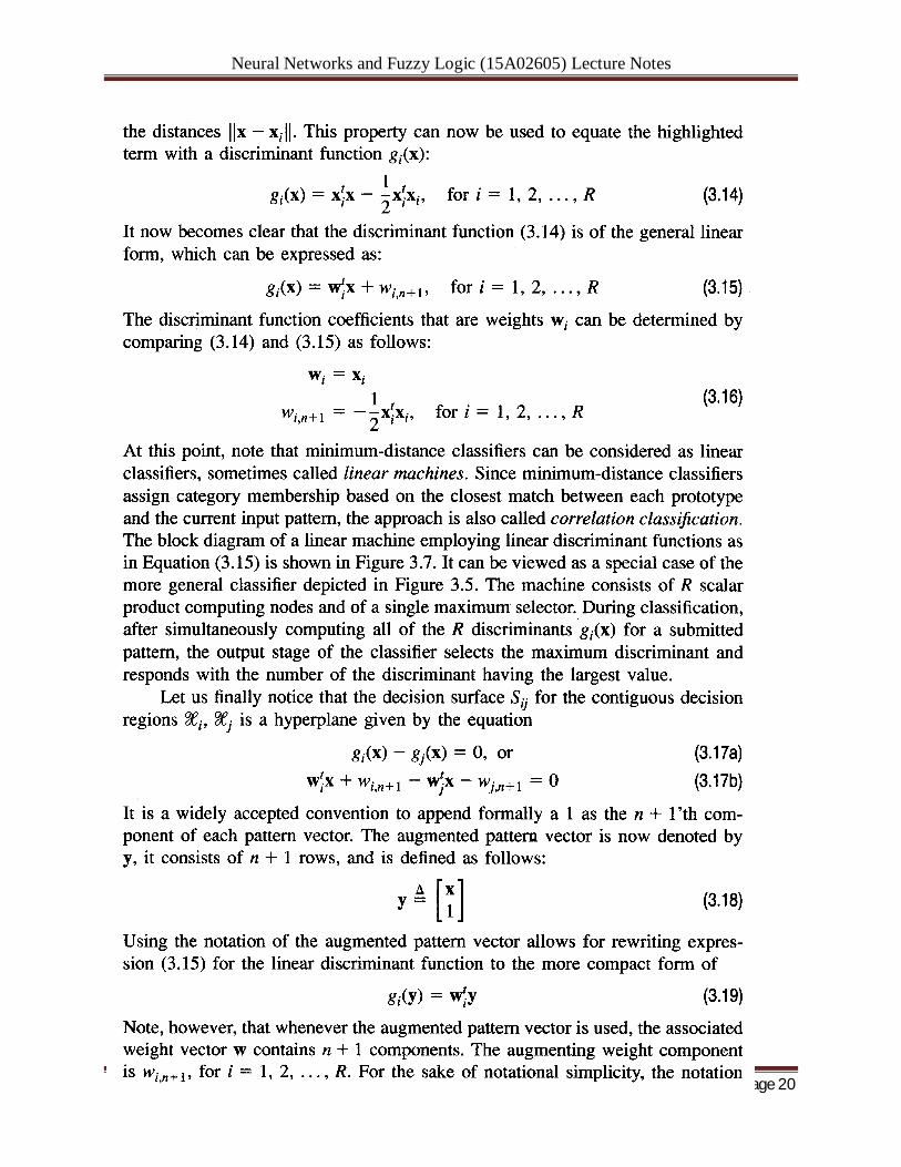
Dept. of ECE, CREC Page 20
Neural Networks and Fuzzy Logic (15A02605) Lecture Notes
Dept. of ECE, CREC Page 21
Neural Networks and Fuzzy Logic (15A02605) Lecture Notes
Dept. of ECE, CREC Page 22
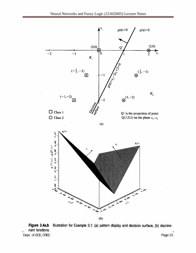
Multi layer Feed forward network:
Assume the two training sets 9, and 9J2 of augmented patterns are available for training. If no weight vector w exists such that then the pattern sets 9, and 9J2 are linearly nonseparable.
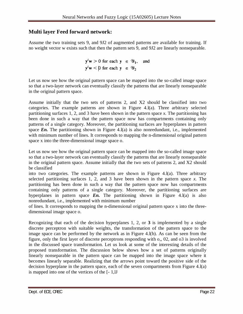
Let us now see how the original pattern space can be mapped into the so-called image space so that a two-layer network can eventually classify the patterns that are linearly nonseparable in the original pattern space. Assume initially that the two sets of patterns 2, and X2 should be classified into two categories. The example patterns are shown in Figure 4.l(a). Three arbitrary selected partitioning surfaces 1, 2, and 3 have been shown in the pattern space x. The partitioning has been done in such a way that the pattern space now has compartments containing only patterns of a single category. Moreover, the partitioning surfaces are hyperplanes in pattern space En. The partitioning shown in Figure 4.l(a) is also nonredundant, i.e., implemented with minimum number of lines. It corresponds to mapping the n-dimensional original pattern space x into the three-dimensional image space o. Let us now see how the original pattern space can be mapped into the so-called image space so that a two-layer network can eventually classify the patterns that are linearly nonseparable in the original pattern space. Assume initially that the two sets of patterns 2, and X2 should be classified into two categories. The example patterns are shown in Figure 4.l(a). Three arbitrary selected partitioning surfaces 1, 2, and 3 have been shown in the pattern space x. The partitioning has been done in such a way that the pattern space now has compartments containing only patterns of a single category. Moreover, the partitioning surfaces are hyperplanes in pattern space En. The partitioning shown in Figure 4.l(a) is also nonredundant, i.e., implemented with minimum number of lines. It corresponds to mapping the n-dimensional original pattern space x into the three-dimensional image space o. Recognizing that each of the decision hyperplanes 1, 2, or 3 is implemented by a single discrete perceptron with suitable weights, the transformation of the pattern space to the image space can be performed by the network as in Figure 4.l(b). As can be seen from the figure, only the first layer of discrete perceptrons responding with o,, 02, and o3 is involved in the discussed space transformation. Let us look at some of the interesting details of the proposed transformation. The discussion below shows how a set of patterns originally linearly nonseparable in the pattern space can be mapped into the image space where it becomes linearly separable. Realizing that the arrows point toward the positive side of the decision hyperplane in the pattern space, each of the seven compartments from Figure 4.l(a) is mapped into one of the vertices of the [- 1,lJ
Neural Networks and Fuzzy Logic (15A02605) Lecture Notes
Dept. of ECE, CREC Page 23
Neural Networks and Fuzzy Logic (15A02605) Lecture Notes
Dept. of ECE, CREC Page 24
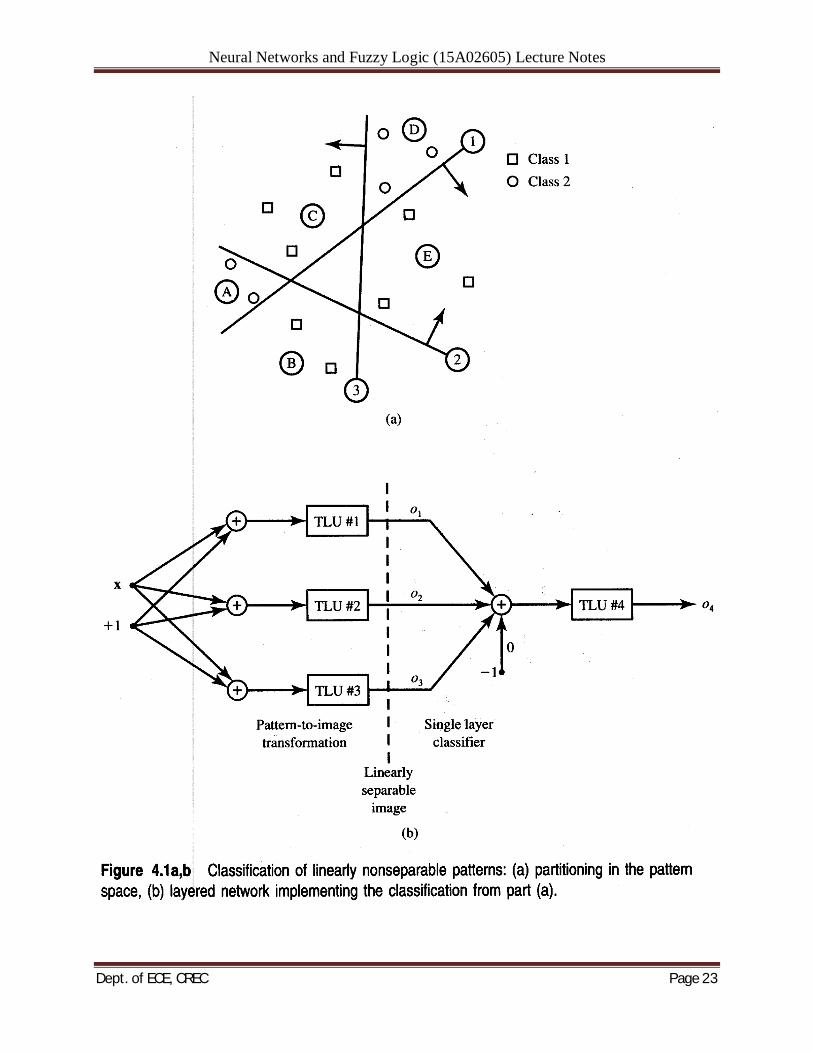
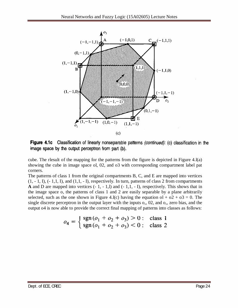
cube. The rlesult of the mapping for the patterns from the figure is depicted in Figure 4.l(a) showing the cube in image space ol, 02, and o3 with corresponding compartment label pat corners. The patterns of class 1 from the original compartments B, C, and E are mapped into vertices (1, - 1, I), (- 1,1, I), and (1,1, - I), respectively. In turn, patterns of class 2 from compartments A and D are mapped into vertices (- 1, - 1,l) and (- 1,1, - I), respectively. This shows that in the image space o, the patterns of class 1 and 2 are easily separable by a plane arbitrarily selected, such as the one shown in Figure 4.l(c) having the equation ol + o2 + o3 = 0. The single discrete perceptron in the output layer with the inputs o,, 02, and o,, zero bias, and the output o4 is now able to provide the correct final mapping of patterns into classes as follows:
Neural Networks and Fuzzy Logic (15A02605) Lecture Notes
Dept. of ECE, CREC Page 25
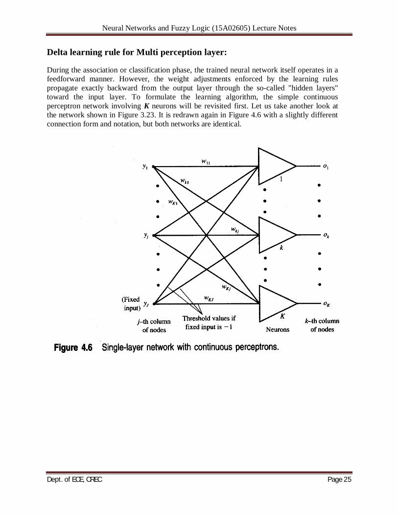
Delta learning rule for Multi perception layer:
During the association or classification phase, the trained neural network itself operates in a feedforward manner. However, the weight adjustments enforced by the learning rules propagate exactly backward from the output layer through the so-called "hidden layers" toward the input layer. To formulate the learning algorithm, the simple continuous perceptron network involving K neurons will be revisited first. Let us take another look at the network shown in Figure 3.23. It is redrawn again in Figure 4.6 with a slightly different connection form and notation, but both networks are identical.
Neural Networks and Fuzzy Logic (15A02605) Lecture Notes
Dept. of ECE, CREC Page 26
Neural Networks and Fuzzy Logic (15A02605) Lecture Notes
Dept. of ECE, CREC Page 27
Neural Networks and Fuzzy Logic (15A02605) Lecture Notes
Dept. of ECE, CREC Page 28
Neural Networks and Fuzzy Logic (15A02605) Lecture Notes
Dept. of ECE, CREC Page 29

Neural Networks and Fuzzy Logic (15A02605) Lecture Notes
Dept. of ECE, CREC Page 30
Neural Networks and Fuzzy Logic (15A02605) Lecture Notes
Dept. of ECE, CREC Page 31
UNIT-III ASSOCIATIVE MEMORIES
ASSOCIATIVE MEMORIES: An efficient associative memory can store a large set of patterns as memories. During recall, the memory is excited with a key pattern (also called the search argument) containing a portion of information about a particular member of a stored pattern set. This particular stored prototype can be recalled through association of the key pattern and the information memorized. A number of architectures and approaches have been devised in the literature to solve effectively the problem of both memory recording and retrieval of its content. Associative memories belong to a class of neural networks that learns according to a certain recording algorithm. They usually acquire information a priori, and their connectivity (weight) matrices most often need to be formed in advance. Associative memory usually enables a parallel search within a stored data file. The purpose of the search is to output either one or all stored items that match the given search argument, and to retrieve it either entirely or partially. It is also believed that biological memory operates according to associative memory principles. No memory locations have addresses; storage is distributed over a large, densely interconnected, ensemble of neurons. BASIC CONCEPTS: Figure shows a general block diagram of an associative memory performing an associative mapping of an input vector x into an output vector v. The system shown maps vectors x to vectors v, in the pattern space Rn and output space Rm, respectively, by performing the transformation
The operator M denotes a general nonlinear matrix-type operator, and it has different meaning for each of the memory models. Its form, in fact, defines a specific model that will need to be carefully outlined for each type of memory. The structure of M reflects a specific neural memory paradigm. For dynamic memories, M also involves time variable. Thus, v is available at memory output at a later time than the input has been applied. For a given memory model, the form of the operator M is usually expressed in terms of given prototype vectors that must be stored. The algorithm allowing the computation of M is called the recording or storage algorithm. The operator also involves the nonlinear mapping performed by the ensemble of neurons. Usually, the ensemble of neurons is arranged in one or two layers, sometime intertwined with each other. The mapping as in Equation (6.1) performed on a key vector x is called a retrieval. Retrieval may or may not provide a desired solution prototype, or an undesired prototype, but it may not even provide a stored prototype at all. In such an extreme case, erroneously recalled output does not belong to the set of prototypes. In the following sections we will attempt to define mechanisms and conditions for efficient retrieval of prototype vectors. Prototype vectors that are stored in memory are denoted with a superscript in parenthesis throughout this chapter. As we will see below, the storage algorithm can be formulated using one or two sets of prototype vectors. The storage algorithm depends on whether an autoassociative or a heteroassociative type of memory is designed. Let us assume that the memory has certain
Neural Networks and Fuzzy Logic (15A02605) Lecture Notes
Dept. of ECE, CREC Page 32
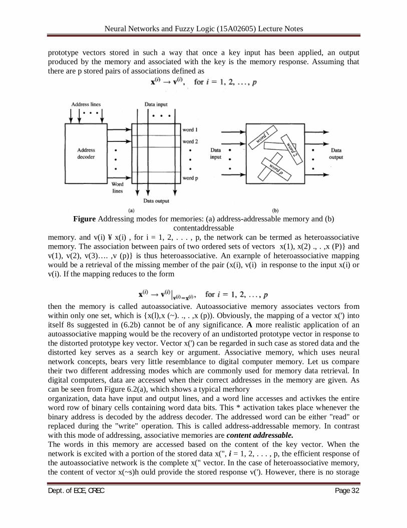
prototype vectors stored in such a way that once a key input has been applied, an output produced by the memory and associated with the key is the memory response. Assuming that there are p stored pairs of associations defined as
Figure Addressing modes for memories: (a) address-addressable memory and (b)
contentaddressable memory. and v(i) ¥ x(i) , for i = 1, 2, . . . , p, the network can be termed as heteroassociative memory. The association between pairs of two ordered sets of vectors x(1), x(2) ., . ,x (P)} and v(1), v(2), v(3)…. ,v (p)} is thus heteroassociative. An exarnple of heteroassociative mapping would be a retrieval of the missing member of the pair (x(i), v(i) in response to the input x(i) or v(i). If the mapping reduces to the form
then the memory is called autoassociative. Autoassociative memory associates vectors from within only one set, which is {x(l),x (~). ., . ,x (p)). Obviously, the mapping of a vector x(') into itself 8s suggested in (6.2b) cannot be of any significance. A more realistic application of an autoassociative mapping would be the recovery of an undistorted prototype vector in response to the distorted prototype key vector. Vector x(') can be regarded in such case as stored data and the distorted key serves as a search key or argument. Associative memory, which uses neural network concepts, bears very little resemblance to digital computer memory. Let us compare their two different addressing modes which are commonly used for memory data retrieval. In digital computers, data are accessed when their correct addresses in the memory are given. As can be seen from Figure 6.2(a), which shows a typical merhory organization, data have input and output lines, and a word line accesses and activkes the entire word row of binary cells containing word data bits. This * activation takes place whenever the binary address is decoded by the address decoder. The addressed word can be either "read" or replaced during the "write" operation. This is called address-addressable memory. In contrast with this mode of addressing, associative memories are content addressable. The words in this memory are accessed based on the content of the key vector. When the network is excited with a portion of the stored data x(", i = 1, 2, . . . , p, the efficient response of the autoassociative network is the complete x(" vector. In the case of heteroassociative memory, the content of vector x(~s)h ould provide the stored response v('). However, there is no storage
Neural Networks and Fuzzy Logic (15A02605) Lecture Notes
Dept. of ECE, CREC Page 33
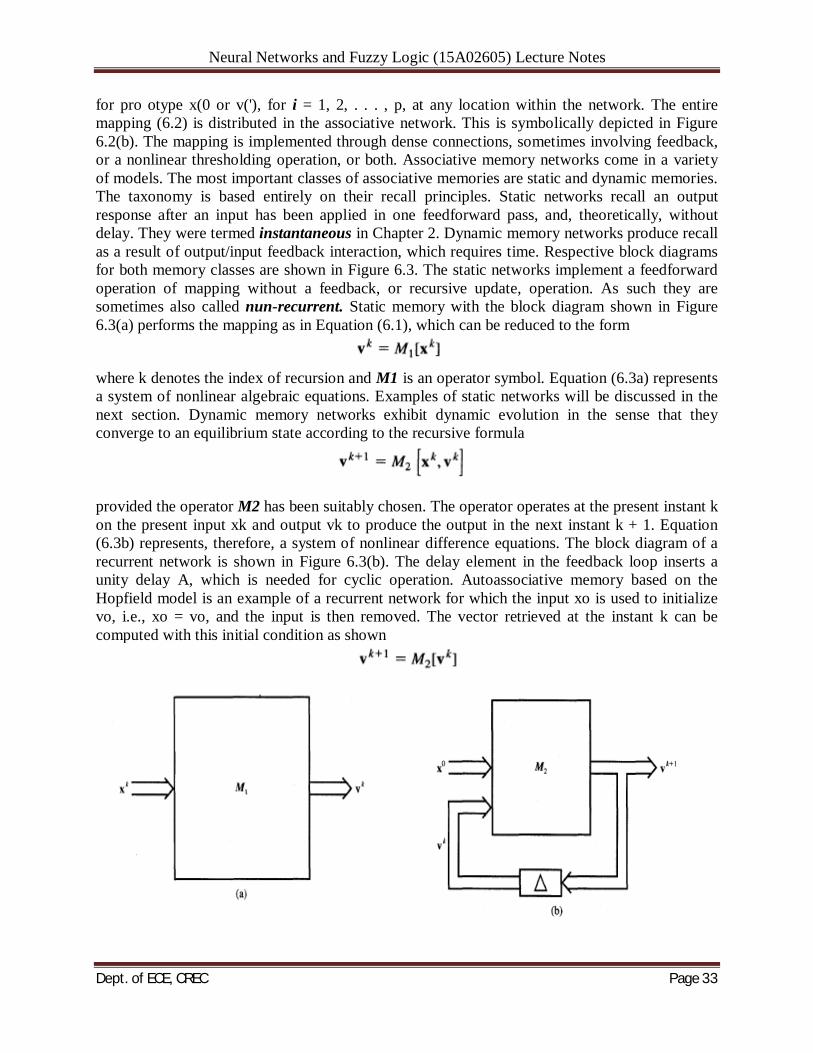
for pro otype x(0 or v('), for i = 1, 2, . . . , p, at any location within the network. The entire mapping (6.2) is distributed in the associative network. This is symbolically depicted in Figure 6.2(b). The mapping is implemented through dense connections, sometimes involving feedback, or a nonlinear thresholding operation, or both. Associative memory networks come in a variety of models. The most important classes of associative memories are static and dynamic memories. The taxonomy is based entirely on their recall principles. Static networks recall an output response after an input has been applied in one feedforward pass, and, theoretically, without delay. They were termed instantaneous in Chapter 2. Dynamic memory networks produce recall as a result of output/input feedback interaction, which requires time. Respective block diagrams for both memory classes are shown in Figure 6.3. The static networks implement a feedforward operation of mapping without a feedback, or recursive update, operation. As such they are sometimes also called nun-recurrent. Static memory with the block diagram shown in Figure 6.3(a) performs the mapping as in Equation (6.1), which can be reduced to the form
where k denotes the index of recursion and M1 is an operator symbol. Equation (6.3a) represents a system of nonlinear algebraic equations. Examples of static networks will be discussed in the next section. Dynamic memory networks exhibit dynamic evolution in the sense that they converge to an equilibrium state according to the recursive formula
provided the operator M2 has been suitably chosen. The operator operates at the present instant k on the present input xk and output vk to produce the output in the next instant k + 1. Equation (6.3b) represents, therefore, a system of nonlinear difference equations. The block diagram of a recurrent network is shown in Figure 6.3(b). The delay element in the feedback loop inserts a unity delay A, which is needed for cyclic operation. Autoassociative memory based on the Hopfield model is an example of a recurrent network for which the input xo is used to initialize vo, i.e., xo = vo, and the input is then removed. The vector retrieved at the instant k can be computed with this initial condition as shown
Neural Networks and Fuzzy Logic (15A02605) Lecture Notes
Dept. of ECE, CREC Page 34
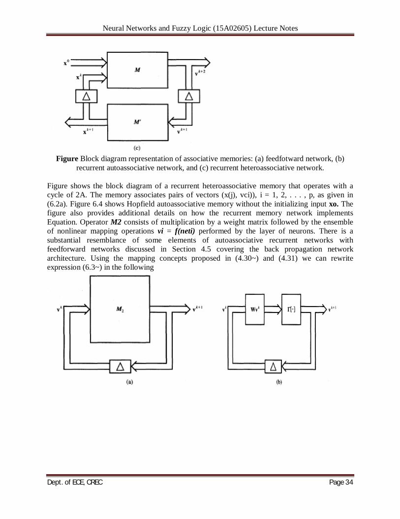
Figure Block diagram representation of associative memories: (a) feedfotward network, (b)
recurrent autoassociative network, and (c) recurrent heteroassociative network.
Figure shows the block diagram of a recurrent heteroassociative memory that operates with a cycle of 2A. The memory associates pairs of vectors (x(j), vci)), i = 1, 2, . . . , p, as given in (6.2a). Figure 6.4 shows Hopfield autoassociative memory without the initializing input xo. The figure also provides additional details on how the recurrent memory network implements Equation. Operator M2 consists of multiplication by a weight matrix followed by the ensemble of nonlinear mapping operations vi = f(neti) performed by the layer of neurons. There is a substantial resemblance of some elements of autoassociative recurrent networks with feedforward networks discussed in Section 4.5 covering the back propagation network architecture. Using the mapping concepts proposed in (4.30~) and (4.31) we can rewrite expression (6.3~) in the following
Neural Networks and Fuzzy Logic (15A02605) Lecture Notes
Dept. of ECE, CREC Page 35
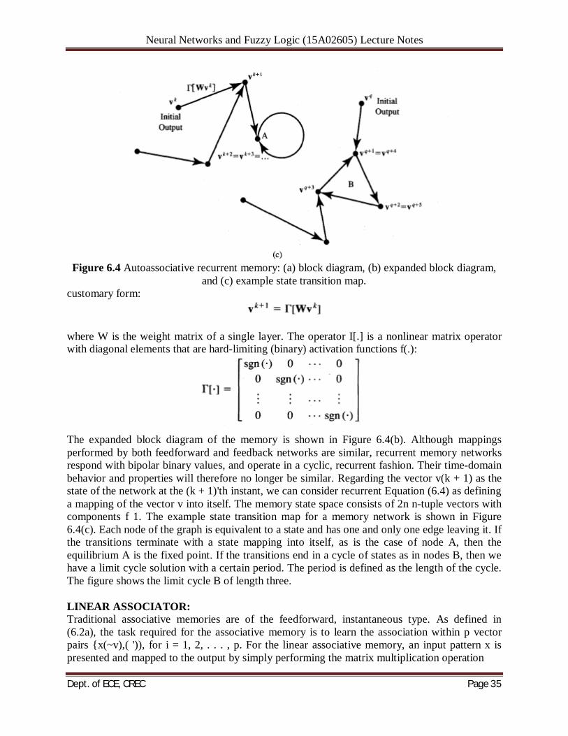
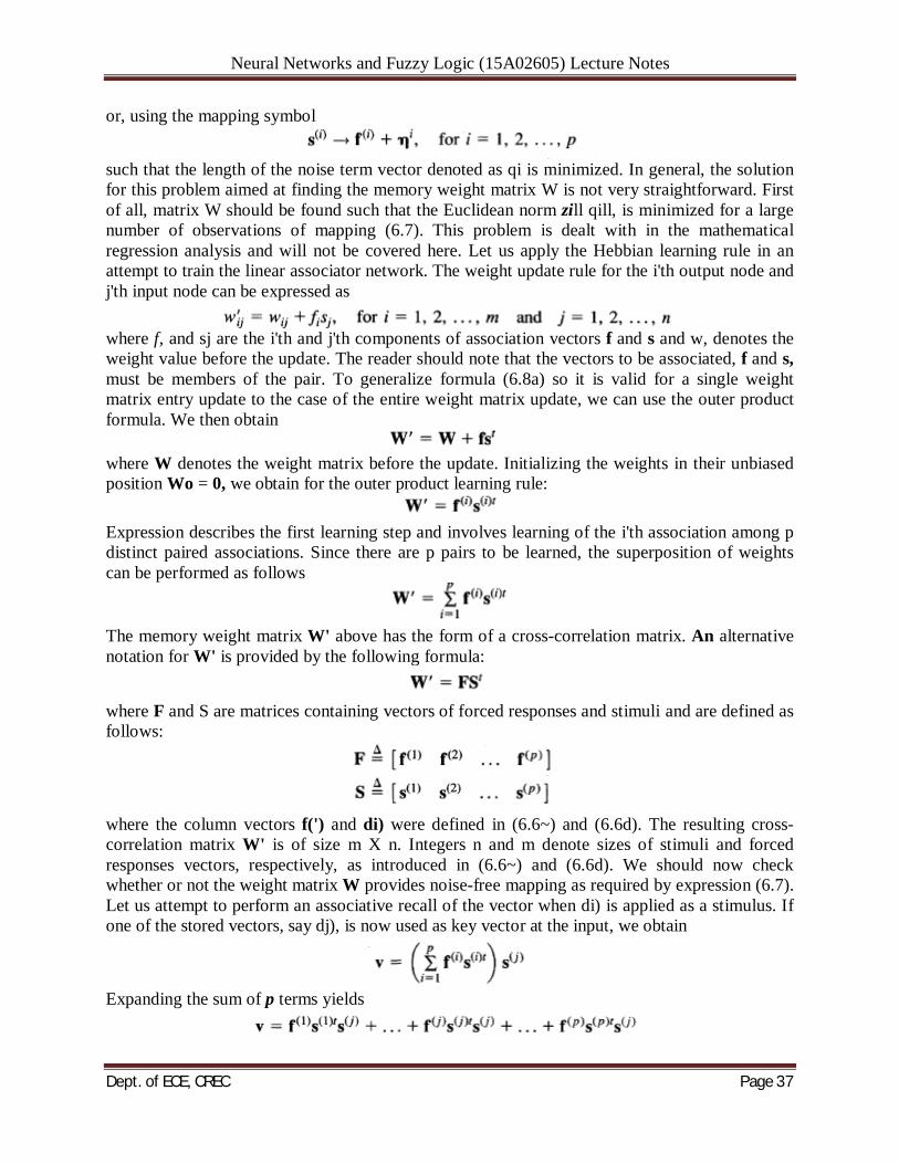
Figure 6.4 Autoassociative recurrent memory: (a) block diagram, (b) expanded block diagram,
and (c) example state transition map. customary form:
where W is the weight matrix of a single layer. The operator I[.] is a nonlinear matrix operator with diagonal elements that are hard-limiting (binary) activation functions f(.):
The expanded block diagram of the memory is shown in Figure 6.4(b). Although mappings performed by both feedforward and feedback networks are similar, recurrent memory networks respond with bipolar binary values, and operate in a cyclic, recurrent fashion. Their time-domain behavior and properties will therefore no longer be similar. Regarding the vector v(k + 1) as the state of the network at the (k + 1)'th instant, we can consider recurrent Equation (6.4) as defining a mapping of the vector v into itself. The memory state space consists of 2n n-tuple vectors with components f 1. The example state transition map for a memory network is shown in Figure 6.4(c). Each node of the graph is equivalent to a state and has one and only one edge leaving it. If the transitions terminate with a state mapping into itself, as is the case of node A, then the equilibrium A is the fixed point. If the transitions end in a cycle of states as in nodes B, then we have a limit cycle solution with a certain period. The period is defined as the length of the cycle. The figure shows the limit cycle B of length three. LINEAR ASSOCIATOR: Traditional associative memories are of the feedforward, instantaneous type. As defined in (6.2a), the task required for the associative memory is to learn the association within p vector pairs {x(~v),( ')), for i = 1, 2, . . . , p. For the linear associative memory, an input pattern x is presented and mapped to the output by simply performing the matrix multiplication operation
Neural Networks and Fuzzy Logic (15A02605) Lecture Notes
Dept. of ECE, CREC Page 36
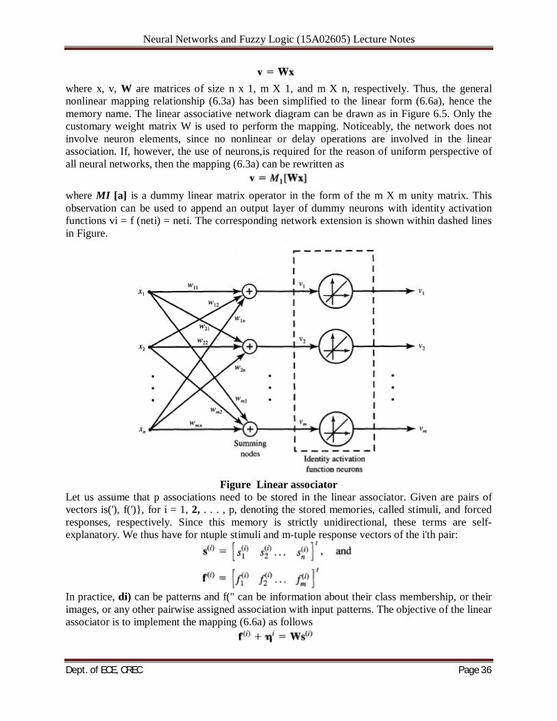
where x, v, W are matrices of size n x 1, m X 1, and m X n, respectively. Thus, the general nonlinear mapping relationship (6.3a) has been simplified to the linear form (6.6a), hence the memory name. The linear associative network diagram can be drawn as in Figure 6.5. Only the customary weight matrix W is used to perform the mapping. Noticeably, the network does not involve neuron elements, since no nonlinear or delay operations are involved in the linear association. If, however, the use of neurons,is required for the reason of uniform perspective of all neural networks, then the mapping (6.3a) can be rewritten as
where MI [a] is a dummy linear matrix operator in the form of the m X m unity matrix. This observation can be used to append an output layer of dummy neurons with identity activation functions vi = f (neti) = neti. The corresponding network extension is shown within dashed lines in Figure.
Figure Linear associator
Let us assume that p associations need to be stored in the linear associator. Given are pairs of vectors is('), f(')}, for i = 1, 2, . . . , p, denoting the stored memories, called stimuli, and forced responses, respectively. Since this memory is strictly unidirectional, these terms are self-explanatory. We thus have for ntuple stimuli and m-tuple response vectors of the i'th pair:
In practice, di) can be patterns and f(" can be information about their class membership, or their images, or any other pairwise assigned association with input patterns. The objective of the linear associator is to implement the mapping (6.6a) as follows
Neural Networks and Fuzzy Logic (15A02605) Lecture Notes
Dept. of ECE, CREC Page 37
or, using the mapping symbol
such that the length of the noise term vector denoted as qi is minimized. In general, the solution for this problem aimed at finding the memory weight matrix W is not very straightforward. First of all, matrix W should be found such that the Euclidean norm zill qill, is minimized for a large number of observations of mapping (6.7). This problem is dealt with in the mathematical regression analysis and will not be covered here. Let us apply the Hebbian learning rule in an attempt to train the linear associator network. The weight update rule for the i'th output node and j'th input node can be expressed as
where f, and sj are the i'th and j'th components of association vectors f and s and w, denotes the weight value before the update. The reader should note that the vectors to be associated, f and s, must be members of the pair. To generalize formula (6.8a) so it is valid for a single weight matrix entry update to the case of the entire weight matrix update, we can use the outer product formula. We then obtain
where W denotes the weight matrix before the update. Initializing the weights in their unbiased position Wo = 0, we obtain for the outer product learning rule:
Expression describes the first learning step and involves learning of the i'th association among p distinct paired associations. Since there are p pairs to be learned, the superposition of weights can be performed as follows
The memory weight matrix W' above has the form of a cross-correlation matrix. An alternative notation for W' is provided by the following formula:
where F and S are matrices containing vectors of forced responses and stimuli and are defined as follows:
where the column vectors f(') and di) were defined in (6.6~) and (6.6d). The resulting cross-correlation matrix W' is of size m X n. Integers n and m denote sizes of stimuli and forced responses vectors, respectively, as introduced in (6.6~) and (6.6d). We should now check whether or not the weight matrix W provides noise-free mapping as required by expression (6.7). Let us attempt to perform an associative recall of the vector when di) is applied as a stimulus. If one of the stored vectors, say dj), is now used as key vector at the input, we obtain
Expanding the sum of p terms yields
Neural Networks and Fuzzy Logic (15A02605) Lecture Notes
Dept. of ECE, CREC Page 38
According to the mapping criterion (6.7), the ideal mapping S(J) + f(j) such that no noise term is present would require
By inspecting (6.10b) and (6.10~)it can be seen that the ideal mapping can be achieved in the case for which
Thus, the orthonormal set of p input stimuli vectors {dl), d2), . . . , s(P)) ensures perfect mapping (6.10~). Orthonormality is the condition on the inputs if they are to be ideally associated. However, the condition is rather strict and may not always hold for the set of stimuli vectors. Let us evaluate the retrieval of associations evoked by stimuli that are not originally encoded. Consider the consequences of a distortion of pattern s(j) submitted at the memory input as dj)' so that
where the distortion term A(J) can be assumed to be statistically independent of s(J), and thus it can be considered as orthogonal to it. Substituting (6.12) into formula (6.10a), we obtain for orthonormal vectors originally encoded in the memory
Due to the orthonormality condition this further reduces to
It can be seen that the memory response contains the desired association f(j) and an additive component, which is due to the distortion term A(j). The second term in the expression above has the meaning of cross-talk noise and is caused by the distortion of the input pattern and is present due to the vector A(j). The term contains, in parentheses, almost all elements of the memory cross-correlation matrix weighted by a distortion term A(j). Therefore, even in the case of stored orthonormal patterns, the cross-talk noise term from all other patterns remains additive at the memory output to the originally stored association. We thus see that the linear associator provides no means for suppression of the cross-talk noise term is of limited use for accurate retrieval of the originally stored association. Finally, let us notice an interesting property of the linear associator for the case of its autoassociative operation with p distinct n-dimensional prototype patterns di). In such a case the network can be called an autocorrelator. Plugging f") = di) in (6.9b) results in the autocorrelation matrix W':
This result can also be expressed using the S matrix from (6.9~)a s follows
The autocorrelation matrix of an autoassociator is of size n X n. Note that thismatrix can also be obtained directly from the Hebbian learning rule. Let use xamine the attempted regeneration of a stored pattern in response to a distorted pattern d~)su'b mitted at the input of the linear
Neural Networks and Fuzzy Logic (15A02605) Lecture Notes
Dept. of ECE, CREC Page 39
autocorrelator. Assume again that input is expressed by (6.12). The output can be expressed using (6.10b), and it simplifies for orthonormal patterns s(J), for j = 1, 2, . . . , p, to the form
This becomes equal
As we can see, the cross-talk noise term again has not been eliminated even for stored orthogonal patterns. The retrieved output is the stored pattern plus the distortion term amplified p - 1 times. Therefore, linear associative memories perform rather poorly when retrieving associations due to distorted stimuli vectors. Linear associator and autoassociator networks can also be used when linearly independent vectors dl), d2), . . . , s(p), are to be stored. The assumption of linear independence is weaker than the assumption of orthogonality and it allows for consideration of a larger class of vectors to be stored. As discussed by Kohonen (1977) and Kohonen et al. (1981), the weight matrix W can be expressed for such a case as follows:
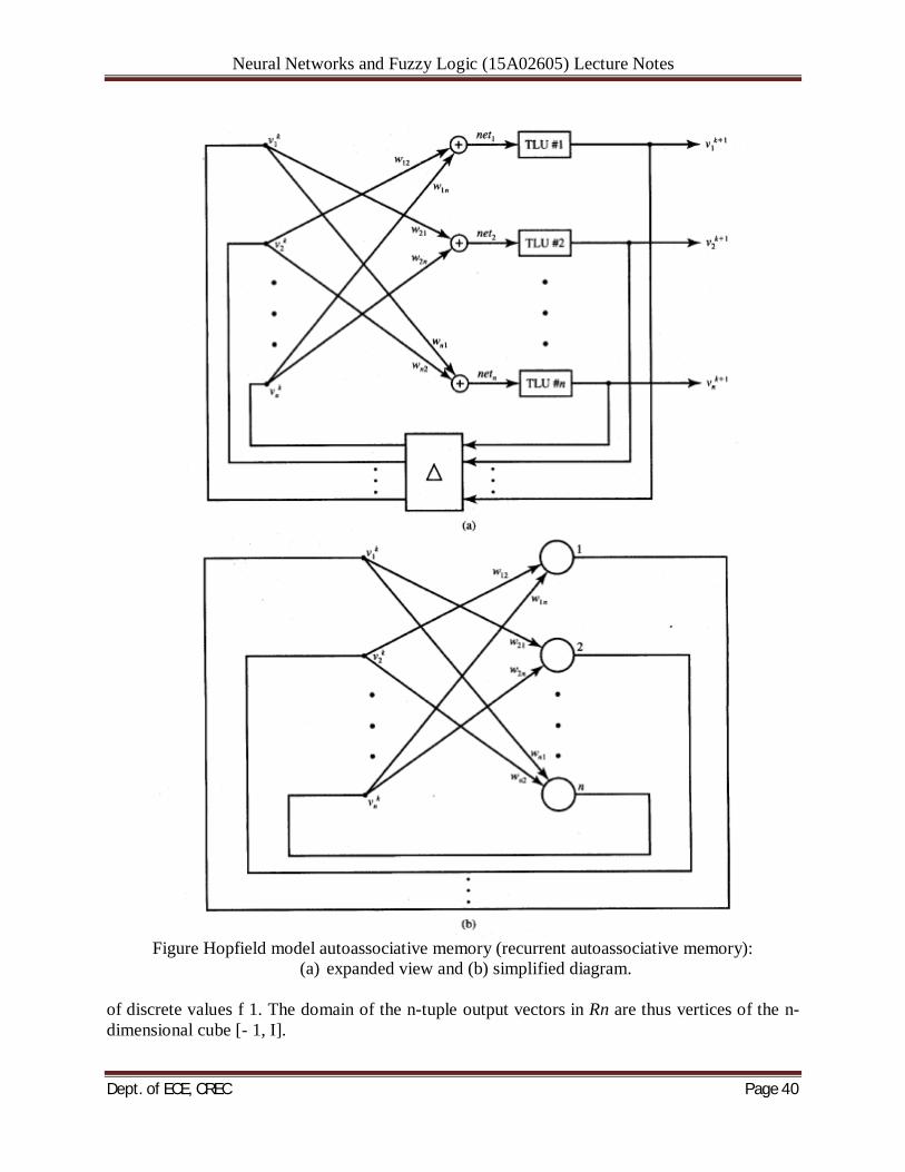
The weight matrix found from Equation (6.16) minimizes the squared output error between f(j) and v(j) in the case of linearly independent vectors S(J) (see Appendix). Because vectors to be used as stored memories are generally neither orthonormal nor linearly independent, the linear associator and autoassociator may not be efficient memories for many practical tasks. BASIC CONCEPTS OF RECURRENT AUTOASSOCIATIVE MEMORY: An expanded view of the Hopfield model network from Figure 6.4 is shownin Figure 6.6. Figure 6.6(a) depicts Hopfield's autoassociative memory. Under the asynchronous update mode, only one neuron is allowed to compute, or change state, at a time, and then all outputs are delayed by a time A produced by the unity delay element in the feedback loop. This symbolic delay allows for the time-stepping of the retrieval algorithm embedded in the update rule of (5.3) or (5.4). Figure 6.6(b) shows a simplified diagram of the network in the form that is often found in the technical literature. Note that the time step and the neurons' thresholding function have been suppressed on the figure. The computingneurons represented in the figure as circular nodes need to. perform summation and bipolar thresholding and also need to introduce a unity delay. Note that the recurrent autoassociative memories studied in this chapter provide node responses
Neural Networks and Fuzzy Logic (15A02605) Lecture Notes
Dept. of ECE, CREC Page 40
Figure Hopfield model autoassociative memory (recurrent autoassociative memory):
(a) expanded view and (b) simplified diagram. of discrete values f 1. The domain of the n-tuple output vectors in Rn are thus vertices of the n-dimensional cube [- 1, I].
Neural Networks and Fuzzy Logic (15A02605) Lecture Notes
Dept. of ECE, CREC Page 41
Retrieval Algorithm Based on the discussion in Section 5.2 the output update rule for Hopfield autoassociative memory can be expressed in the form
where k is the index of recursion and i is the number of the neuron currently undergoing an update. The update rule (6.17) has been obtained from (5.4a) under the simplifying assumption that both the external bias ii and threshold values Ti are zero for i = 1, 2, . . . , n. These assumptions will remain valid for the remainder of this chapter. In addition, the asynchronous update sequence considered here is random. Thus, assuming that recursion starts at vo, and a random sequence of updating neurons m, p, q, . . . is chosen, the output vectors obtained are as follows
Considerable insight into the Hopfield autoassociative memory performance can be gained by evaluating its respective energy function. The energy function (5.5) for the discussed memory network simplifies to
We consider the memory network to evolve in a discrete-time mode, for k = 1, 2, . . . , and its outputs are one of the 2n bipolar binary n-tuple vectors, each representing a vertex of the n-dimensional [- 1, + 11 cube. We also discussed in Section 5.2 the fact that the asynchronous recurrent update never increases energy (6.19a) computed for v = vk, and that the network settles in one of the local energy minima located at cube vertices. We can now easily observe that the complement of a stored memory is also a stored memory. For the bipolar binary notation the complement vector of v is equal to -v. It is easy to see from (6.19a) that
and thus both energies E(v) and E(-v) are identical. Therefore, a minimum of E(v) is of the same value as a minimum of E(-v). This provides us with an important conclusion that the memory transitions may terminate as easily at v as at -v. The crucial factor determining the convergence is the "similarity" between the initializing output vector, and v and -v. Storage Algorithm Let us formulate the information storage algorithm for the recurrent autoassociative memory. Assume that the bipolar binary prototype vectors that need to be stored are dm), for m = 1, 2, . . . , p. The storage algorithm for calculating the weight matrix is
Neural Networks and Fuzzy Logic (15A02605) Lecture Notes
Dept. of ECE, CREC Page 42
OR
where, as before, 6, denotes the usual Kronecker function 6, = 1 if i = j, and 6, = 0 if i + j. The weight matrix W is very similar to the autocorrelation matrix obtained using Hebb's learning rule for the linear associator introduced in (6.14). The difference is that now wii = 0. Note that the system does not remember the individual vectors dm) but only the weights w,, which basically represent correlation terms among the vector entries. Also, the original Hebb's learning rule does not involve the presence of negative synaptic weight values, which can appear as a result of learning as in (6.20). This is a direct consequence of the condition that only bipolar binary vectors dm) are allowed for building the autocorrelation matrix in (6.20). Interestingly, additional autoassociations can be added at any time to the existing memory by superimposing new, incremental weight matrices. Autoassociations an also be removed by respective weight matrix subtraction. The storage rule (6.20) is also invariant with respect to the sequence of storing patterns. The information storage algorithm for unipolar binary vectors dm), for m = 1, 2, . . . , p, needs to be modified so that a - 1 component of the vectors simply replaces the 0 element in the original unipolar vector. This can be formally done by replacing the entries of the original unipolar vector dm) with the entries 2sy) - 1, i = 1, 2, . . . , n. The memory storage algorithm (6.20b) for the unipolar binary vectors thus involves scaling and shifting and takes the form
Notice that the information storage rule is invariant under the binary complement operation. Indeed, storing complementary patterns s'(~i)n stead of original patterns dm) results in the weights as follows:
The reader can easily verify that substituting
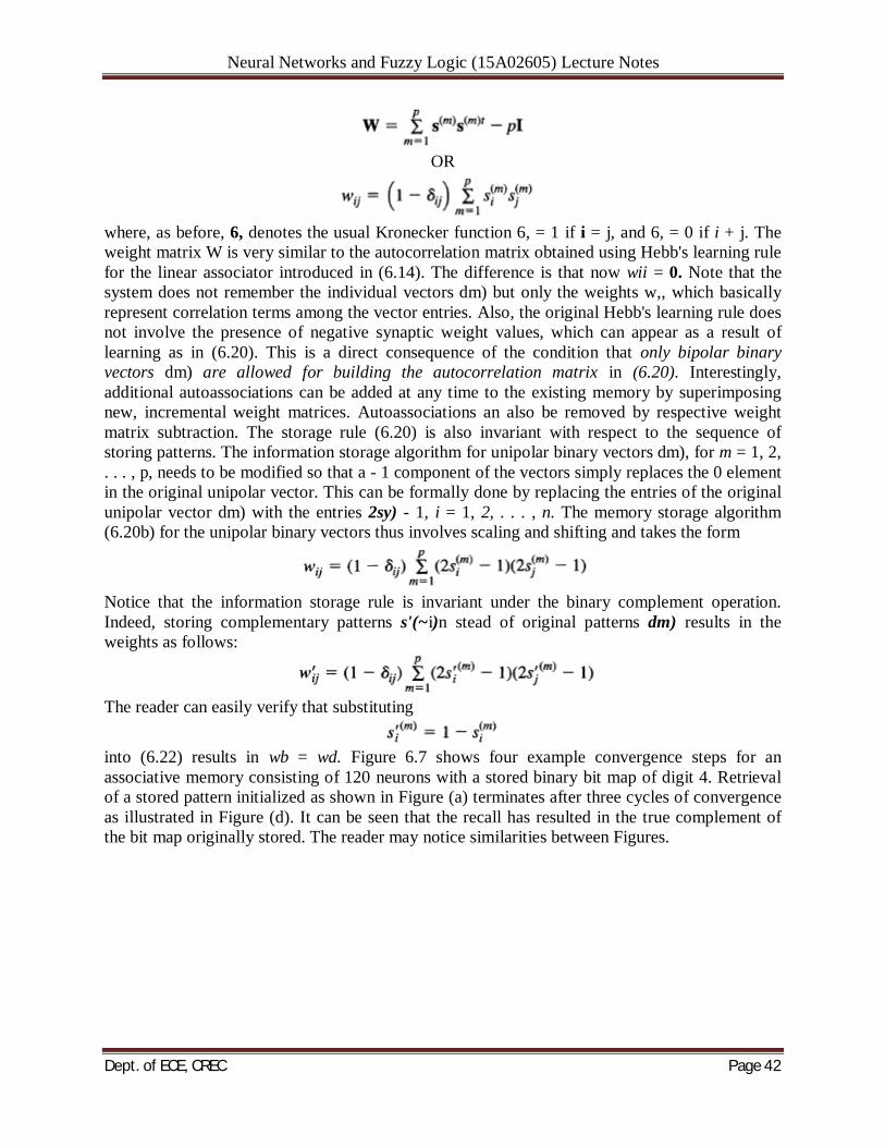
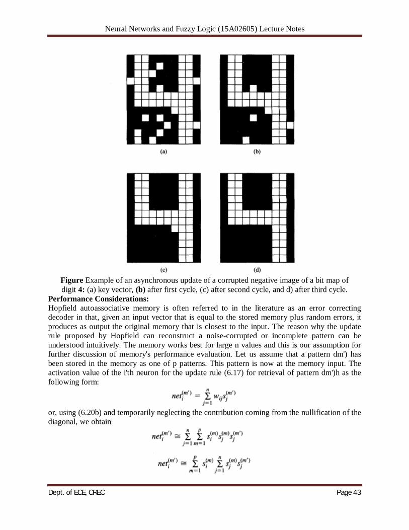
into (6.22) results in wb = wd. Figure 6.7 shows four example convergence steps for an associative memory consisting of 120 neurons with a stored binary bit map of digit 4. Retrieval of a stored pattern initialized as shown in Figure (a) terminates after three cycles of convergence as illustrated in Figure (d). It can be seen that the recall has resulted in the true complement of the bit map originally stored. The reader may notice similarities between Figures.
Neural Networks and Fuzzy Logic (15A02605) Lecture Notes
Dept. of ECE, CREC Page 43
Figure Example of an asynchronous update of a corrupted negative image of a bit map of digit 4: (a) key vector, (b) after first cycle, (c) after second cycle, and d) after third cycle.
Performance Considerations: Hopfield autoassociative memory is often referred to in the literature as an error correcting decoder in that, given an input vector that is equal to the stored memory plus random errors, it produces as output the original memory that is closest to the input. The reason why the update rule proposed by Hopfield can reconstruct a noise-corrupted or incomplete pattern can be understood intuitively. The memory works best for large n values and this is our assumption for further discussion of memory's performance evaluation. Let us assume that a pattern dm') has been stored in the memory as one of p patterns. This pattern is now at the memory input. The activation value of the i'th neuron for the update rule (6.17) for retrieval of pattern dm')h as the following form:
or, using (6.20b) and temporarily neglecting the contribution coming from the nullification of the diagonal, we obtain
Neural Networks and Fuzzy Logic (15A02605) Lecture Notes
Dept. of ECE, CREC Page 44
If terms sy) and strn')f,o r j = 1, 2, . . . , n, were totally statistically independent or J unrelated for m = 1, 2, . . . , p, then the average value of the second sum resulted in zero. Note that the second sum is the scalar product of two n-tuple vectors and if the two vectors are statistically independent (also when orthogonal) their product vanishes. If, however, any of the stored patterns dm), for m = 1, 2, . . . , p, and vector dm') are somewhat overlapping, then the value of the second sum becomes positive. Note that in the limit case the second sum would reach n for both vectors being identical, understandably so since we have here the scalar product of two identical n-tuple vectors with entries of value &1. Thus for the major overlap case, the sign of entry sjm" is expected to be the same as that of netj"'), and we can write
This indicates that the vector dm')d oes not produce any updates and is therefore stable. Assume now that the input vector is a distorted version of the prototype vector dm'), which has been stored in the memory. The distortion is such that only a small percentage of bits differs between the stored memory dm') and the initializing input vector. The discussion that formerly led to the simplification of (6.27~)to (6.27d) still remains valid for this present case with the additional qualification that the multiplier originally equal to n in (6.27d) may take a somewhat reduced value. The multiplier becomes equal to the number of overlapping bits of and of the input vector. It thus follows that the impending update of node i will be in the same direction as the entry sy'). Negative and positive bits of vector dm') are likely to cause negative and positive transitions, respectively, in the upcoming recurrences. We may say that the majority of memory initializing bits is assumed to be correct and allowed to take a vote for the minority of bits. The minority bits do not prevail, so they are flipped, one by one and thus asynchronously, according to the will of the majority. This shows vividly how bits of the input vector can be updated in the right direction toward the closest prototype stored. The above discussion has assumed large n values, so it has been more relevant for real-life application networks. A very interesting case can be observed for the stored orthogonal patterns dm)T. he activation vector net can be computed as
The orthogonality condition, which is di)'s(j) = 0, for i # j, and sci)*s(j=) n, for i = j, makes it possible to simplify (6.28a) to the following form
Assuming that under normal operating conditions the inequality n > p holds, the network will be in equilibrium at state dm? Indeed, computing the value of the energy function (6.19) for the storage rule (6.20b) we obtain
For every stored vector dm') which is orthogonal to all other vectors the energy value (6.29a) reduces to
and further to
Neural Networks and Fuzzy Logic (15A02605) Lecture Notes
Dept. of ECE, CREC Page 45
The memory network is thus in an equilibrium state at every stored prototype vector dm'), and the energy assumes its minimum value expressed in (6.29~). Considering the simplest autoassociative memory with two neurons and a single stored vector (n = 2, p = l), Equation (6.29~)y ields the energy minimum of value - 1. Indeed, the energy function (6.26) for the memory network of Example 6.1 has been evaluated and found to have minima of that value. For the more general case, however, when stored patterns dl), d2), . . . , S(P) are not mutually orthogonal, the energy function (6.29b) does not necessarily assume a minimum at dm'), nor is the vector dm') always an equilibrium for the memory. To gain better insight into memory performance let us calculate the activation vector net in a more general case using expression (6.28a) without an assumption of orthogonality:
This resulting activation vector can be viewed as consisting of an equilibrium state term (n -p)dm') similar to (6.28b). In this case discussed before, either full statistical independence or orthogonality of the stored vectors was assumed. If none of these assumptions is valid, then the sum term in (6.30a) is also present in addition to the equilibrium term. The sum term can be viewed as a "noise" term vector q which is computed as follows
Expression (6.30b) allows for comparison of the noise terms relative to the equilibrium term at the input to each neuron. When the magnitude of the i'th component of the noise vector is larger than (n - p)sYr) and the term has the opposite sign, then sim') will not be the network's equilibrium. The noise term obviously increases for an increased number of stored patterns, and also becomes relatively significant when the factor (n - p) decreases. As we can see from the preliminary study, the analysis of stable states of memory can become involved. In addition, firm conclusions are hard to derive unless statistical methods of memory evaluation are employed. PERFORMANCE ANALYSIS OF RECURRENT AUTOASSOCIATIVE MEMORY: In this section relationships will be presented that relate the size of the memory n to the number of distinct patterns that can be efficiently recovered. These also depend on the degree of similarity that the initializing key vector has to the closest stored vector and on the similarity between the stored patterns. We will look at example performance and capacity, as well as the fixed points of associative memories. Associative memories retail patterns that display a degree of "similarity" to the search argument. To measure this "similarity" precisely, the quantity called the Hamming distance (HD) is often used. Strictly speaking, the Hamming distance is proportional to the dissimilarity of vectors. It is defined as an integer equal to the number of bit positions differing between two binary vectors of the same length. For two n-tuple bipolar binary vectors x and y, the Hamming distance is equal:
Obviously, the maximum HD value between any vectors is n and is the distance between a vector and its complement. Let us also notice that the asynchronous update allows for updating of the output vector by HD = 1 at a time. The following example depicts some of the typical occurrences within the autoassociative memory and focuses on memory state transitions. Energy Function Reduction
Neural Networks and Fuzzy Logic (15A02605) Lecture Notes
Dept. of ECE, CREC Page 46
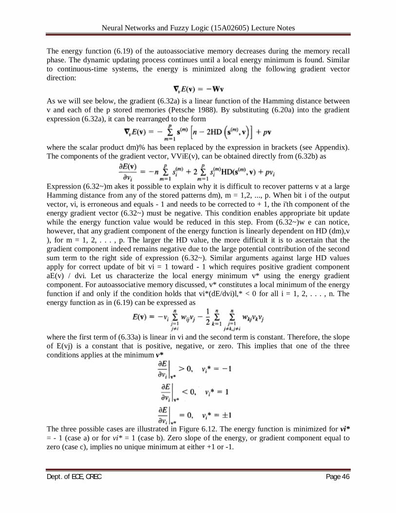
The energy function (6.19) of the autoassociative memory decreases during the memory recall phase. The dynamic updating process continues until a local energy minimum is found. Similar to continuous-time systems, the energy is minimized along the following gradient vector direction:
As we will see below, the gradient (6.32a) is a linear function of the Hamming distance between v and each of the p stored memories (Petsche 1988). By substituting (6.20a) into the gradient expression (6.32a), it can be rearranged to the form
where the scalar product dm)% has been replaced by the expression in brackets (see Appendix). The components of the gradient vector, VViE(v), can be obtained directly from (6.32b) as
Expression (6.32~)m akes it possible to explain why it is difficult to recover patterns v at a large Hamming distance from any of the stored patterns dm), m = 1,2, ..., p. When bit i of the output vector, vi, is erroneous and equals - 1 and needs to be corrected to + 1, the i'th component of the energy gradient vector (6.32~) must be negative. This condition enables appropriate bit update while the energy function value would be reduced in this step. From (6.32~)w e can notice, however, that any gradient component of the energy function is linearly dependent on HD (dm),v ), for m = 1, 2, . . . , p. The larger the HD value, the more difficult it is to ascertain that the gradient component indeed remains negative due to the large potential contribution of the second sum term to the right side of expression (6.32~). Similar arguments against large HD values apply for correct update of bit vi = 1 toward - 1 which requires positive gradient component aE(v) / dvi. Let us characterize the local energy minimum v* using the energy gradient component. For autoassociative memory discussed, v* constitutes a local minimum of the energy function if and only if the condition holds that vi*(dE/dvi)l,* < 0 for all i = 1, 2, . . . , n. The energy function as in (6.19) can be expressed as
where the first term of (6.33a) is linear in vi and the second term is constant. Therefore, the slope of E(vj) is a constant that is positive, negative, or zero. This implies that one of the three conditions applies at the minimum v*
The three possible cases are illustrated in Figure 6.12. The energy function is minimized for vi* = - 1 (case a) or for vi* = 1 (case b). Zero slope of the energy, or gradient component equal to zero (case c), implies no unique minimum at either +1 or -1.
Neural Networks and Fuzzy Logic (15A02605) Lecture Notes
Dept. of ECE, CREC Page 47
Capacity of Auto-associative Recurrent Memory: One of the most important performance parameters of an associative memory is its capacity. Detailed studies of memory capacity have been reported inby McEliece et al. (1987) and Komlos and Paturi (1988). A state vector of the memory is considered to be stable if vkC1 = T[wvk] provided that vk+l = vk. Note that the definition of stability is not affected by synchronous versus asynchronous transition mode; rather, the stability concept is independent from the transition mode. A useful measure for memory capacity evaluation is the radius of attraction p, which is defined in terms of the distance pn from a stable state v such that every vector within the distance pn eventually reaches the stable state v. It is understood that the distance pn is convenient if measured as a Hamming distance and therefore is of integer value. For the reasons explained earlier in the chapter the radius of attraction for an autoassociative memory is somewhere between 1 / n and 1 / 2, which corresponds to the distance of attraction between 1 and n / 2. For the system to function as a memory, we require that every stored memory dm) be stable. Somewhat less restrictive is the assumption that there is at least a stable state at a small distance en from the stored memory where E is positive number. In such a case it is then still reasonable to expect that the memory has an error correction capability. For example, when recovering the input key vector at a distance pn from stored memory, the stable state will be found at a distance en from it. Note that this may still be an acceptable output in situations when the system has learned too many vectors and the memory of each single vector is faded. Obviously, when E = 0, the stored memory is stable within a radius of p. The discussion above indicates that the error correction capability of an autoassociative memory can only be evaluated if stored vectors are not too close to each other. Therefore, each of the p distinct stored vectors used for a capacity study are usually selected at random. The asymptotic capacity of an autoassociative memory consisting of n neurons has been estimated in by McEliece et al. (1987) as
When the number of stored patterns p is below the capacity c expressed as in (6.34a), then all of the stored memories, with probability near 1, will be stable. The formula determines the number of key vectors at a radius p from the stored memory that are correctly recallable to one of the stable, stored memories. The simple stability of the stored memories, with probability near 1, is ensured by the upper bound on the number p given as
For any radius between 0 and 112 of key vectors to the stored memory, almost all of the c stored memories are attractive when c is bounded as in (6.34b). If a small fraction of the stored memories can be tolerated as unrecoverable, and not stable, then the capacity boundary c can be considered twice as large compared to c computed from (6.34b). In summary, it is appropriate to state that regardless of the radius of attraction 0 < p < 112 the capacity of the Hopfield memory is bounded as follows
To offer a numerical example, the boundary values for a 100-neuron network computed from (6.34~)a re about 5.4, with 10.8 memory vectors. Assume that the number of stored patterns p is kept at the level an, for 0 < a! < 1, and n is large. It has been shown that the memory still
Neural Networks and Fuzzy Logic (15A02605) Lecture Notes
Dept. of ECE, CREC Page 48
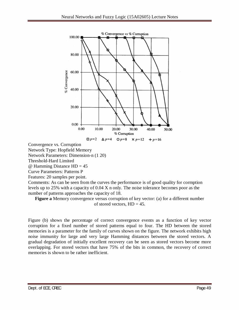
functions efficiently at capacity levels exceeding those stated in (6.34~) (Amit, Gutfreund, and Sompolinsky 1985). When a 0.14, stable states are found that are very close to the stored memories at a distance 0.03n. As a decreases to zero, this distance decreases as exp (-(I 12)~~H)e.n ce, the memory retrieval is mostly accurate for p 5 0.14n. A small percentage of error must be tolerated though if the memory operates at these upper capacity levels. The study by McEliece et al. (1987) also reveals the presence of spurious fixed points, which are not stored memories. They tend to have rather small basins of attraction compared to the stored memories. Therefore, updates terminate in them if they start in their vicinity. Although the number of distinct pattern vectors that can be stored and perfectlyrecalled in Hopfield's memory is not large, the network has found a number of practical applications. However, it is somewhat peculiar that the network can recover only c memories out of the total of 2n states available in the network as the cube comers of n-dimensional hypercube. Memory Convergence versus Corruption: To supplement the study of the original Hopfield autoassociative memory, it is worthwhile to look at the actual performance of an example memory. Of particular interest are the convergence rates versus memory parameters discussed earlier. Let us inspect the memory performance analysis curves shown in Figure 6.13 (Desai 1990). The memory performance on this figure has been evaluated for a network with n = 120 neurons. As pointed out earlier in this section, the total number of stored patterns, their mutual Hamming distance and their Hamming distance to the key vector determine the success of recovery. Figure (a) shows the percentage of correct convergence as a function of key vector corruption compared to the stored memories. Computation shown is for a fixed HD between the vectors stored of value 45. It can be seen that the correct convergence rate drops about linearly with the amount of corruption of the key vector. The correct convergence rate also reduces as the number of stored patterns increases for a fixed distortion value of input key vectors. The network performs very well at p = 2 patterns stored but recovers rather poorly distorted vectors at p = 16 patterns stored.
Neural Networks and Fuzzy Logic (15A02605) Lecture Notes
Dept. of ECE, CREC Page 49
Convergence vs. Corruption Network Type: Hopfield Memory Network Parameters: Dimension-n (1 20) Threshold-Hard Limited @ Hamming Distance HD = 45 Curve Parameters: Patterns P Features: 20 samples per point. Comments: As can be seen from the curves the performance is of good quality for cormption levels up to 25% with a capacity of 0.04 X n only. The noise tolerance becomes poor as the number of patterns approaches the capacity of 18.
Figure a Memory convergence versus corruption of key vector: (a) for a different number of stored vectors, HD = 45.
Figure (b) shows the percentage of correct convergence events as a function of key vector corruption for a fixed number of stored patterns equal to four. The HD between the stored memories is a parameter for the family of curves shown on the figure. The network exhibits high noise immunity for large and very large Hamming distances between the stored vectors. A gradual degradation of initially excellent recovery can be seen as stored vectors become more overlapping. For stored vectors that have 75% of the bits in common, the recovery of correct memories is shown to be rather inefficient.
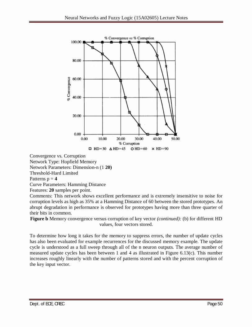
Neural Networks and Fuzzy Logic (15A02605) Lecture Notes
Dept. of ECE, CREC Page 50
Convergence vs. Corruption Network Type: Hopfield Memory Network Parameters: Dimension-n (1 20) Threshold-Hard Limited Patterns p = 4 Curve Parameters: Hamming Distance Features: 20 samples per point. Comments: This network shows excellent performance and is extremely insensitive to noise for corruption levels as high as 35% at a Hamming Distance of 60 between the stored prototypes. An abrupt degradation in performance is observed for prototypes having more than three quarter of their bits in common. Figure b Memory convergence versus corruption of key vector (continued): (b) for different HD
values, four vectors stored. To determine how long it takes for the memory to suppress errors, the number of update cycles has also been evaluated for example recurrences for the discussed memory example. The update cycle is understood as a full sweep through all of the n neuron outputs. The average number of measured update cycles has been between 1 and 4 as illustrated in Figure 6.13(c). This number increases roughly linearly with the number of patterns stored and with the percent corruption of the key input vector.
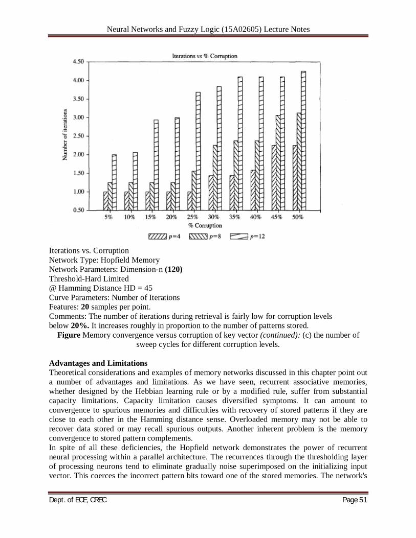
Neural Networks and Fuzzy Logic (15A02605) Lecture Notes
Dept. of ECE, CREC Page 51
Iterations vs. Corruption Network Type: Hopfield Memory Network Parameters: Dimension-n (120) Threshold-Hard Limited @ Hamming Distance HD = 45 Curve Parameters: Number of Iterations Features: 20 samples per point. Comments: The number of iterations during retrieval is fairly low for corruption levels below 20%. It increases roughly in proportion to the number of patterns stored.
Figure Memory convergence versus corruption of key vector (continued): (c) the number of sweep cycles for different corruption levels.
Advantages and Limitations Theoretical considerations and examples of memory networks discussed in this chapter point out a number of advantages and limitations. As we have seen, recurrent associative memories, whether designed by the Hebbian learning rule or by a modified rule, suffer from substantial capacity limitations. Capacity limitation causes diversified symptoms. It can amount to convergence to spurious memories and difficulties with recovery of stored patterns if they are close to each other in the Hamming distance sense. Overloaded memory may not be able to recover data stored or may recall spurious outputs. Another inherent problem is the memory convergence to stored pattern complements. In spite of all these deficiencies, the Hopfield network demonstrates the power of recurrent neural processing within a parallel architecture. The recurrences through the thresholding layer of processing neurons tend to eliminate gradually noise superimposed on the initializing input vector. This coerces the incorrect pattern bits toward one of the stored memories. The network's
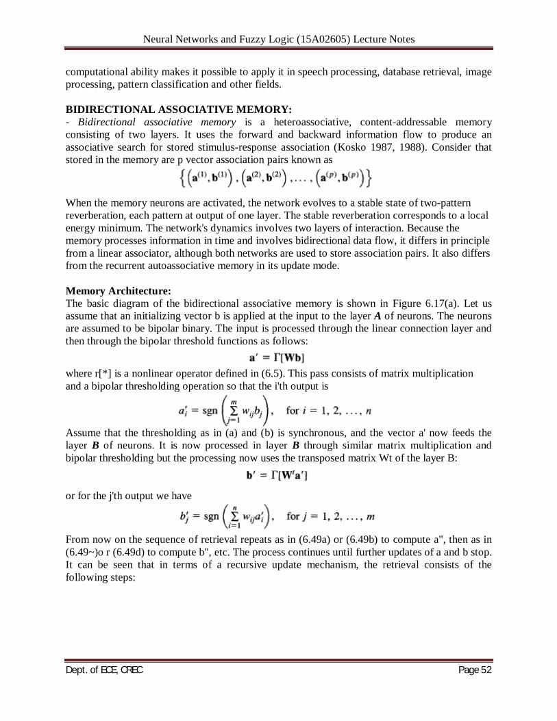
Neural Networks and Fuzzy Logic (15A02605) Lecture Notes
Dept. of ECE, CREC Page 52
computational ability makes it possible to apply it in speech processing, database retrieval, image processing, pattern classification and other fields. BIDIRECTIONAL ASSOCIATIVE MEMORY: - Bidirectional associative memory is a heteroassociative, content-addressable memory consisting of two layers. It uses the forward and backward information flow to produce an associative search for stored stimulus-response association (Kosko 1987, 1988). Consider that stored in the memory are p vector association pairs known as
When the memory neurons are activated, the network evolves to a stable state of two-pattern reverberation, each pattern at output of one layer. The stable reverberation corresponds to a local energy minimum. The network's dynamics involves two layers of interaction. Because the memory processes information in time and involves bidirectional data flow, it differs in principle from a linear associator, although both networks are used to store association pairs. It also differs from the recurrent autoassociative memory in its update mode. Memory Architecture: The basic diagram of the bidirectional associative memory is shown in Figure 6.17(a). Let us assume that an initializing vector b is applied at the input to the layer A of neurons. The neurons are assumed to be bipolar binary. The input is processed through the linear connection layer and then through the bipolar threshold functions as follows:
where r[*] is a nonlinear operator defined in (6.5). This pass consists of matrix multiplication and a bipolar thresholding operation so that the i'th output is
Assume that the thresholding as in (a) and (b) is synchronous, and the vector a' now feeds the layer B of neurons. It is now processed in layer B through similar matrix multiplication and bipolar thresholding but the processing now uses the transposed matrix Wt of the layer B:
or for the j'th output we have
From now on the sequence of retrieval repeats as in (6.49a) or (6.49b) to compute a", then as in (6.49~)o r (6.49d) to compute b", etc. The process continues until further updates of a and b stop. It can be seen that in terms of a recursive update mechanism, the retrieval consists of the following steps:
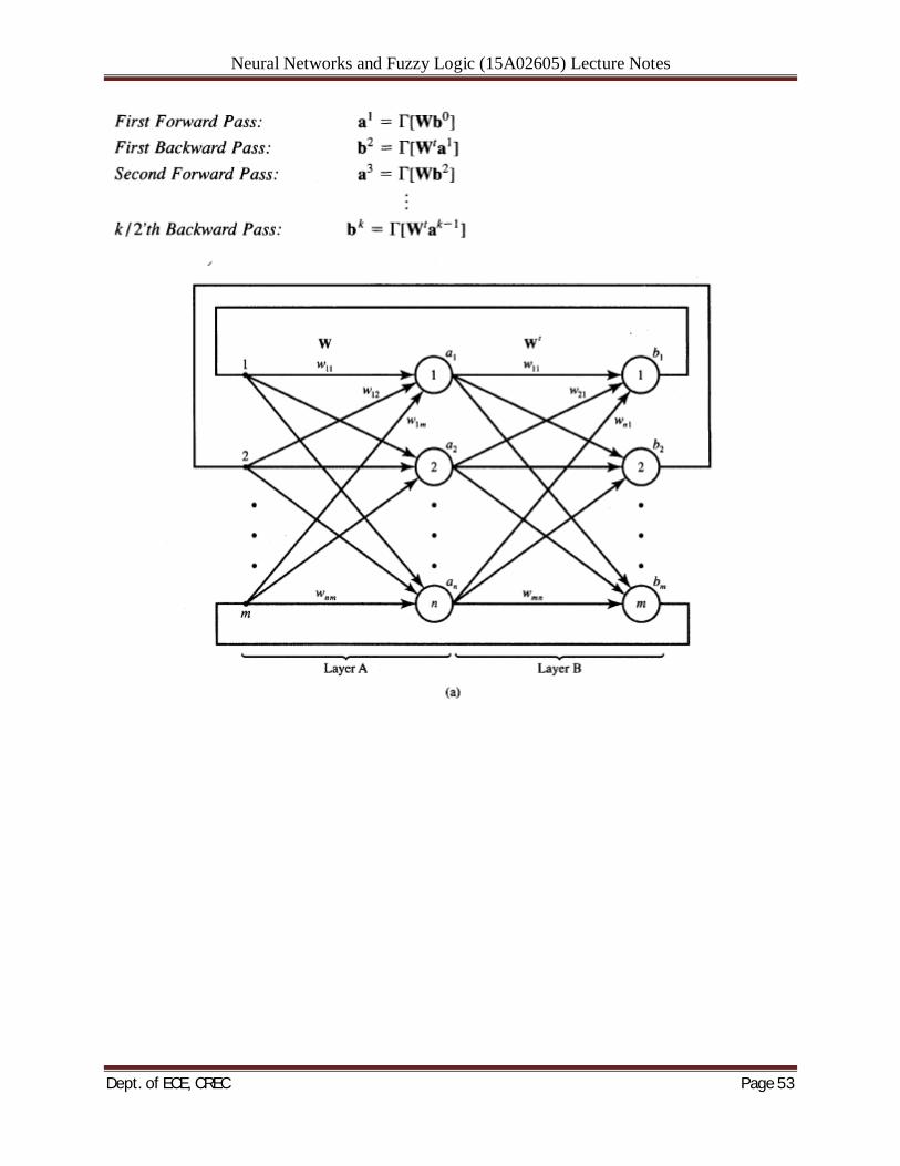
Neural Networks and Fuzzy Logic (15A02605) Lecture Notes
Dept. of ECE, CREC Page 53
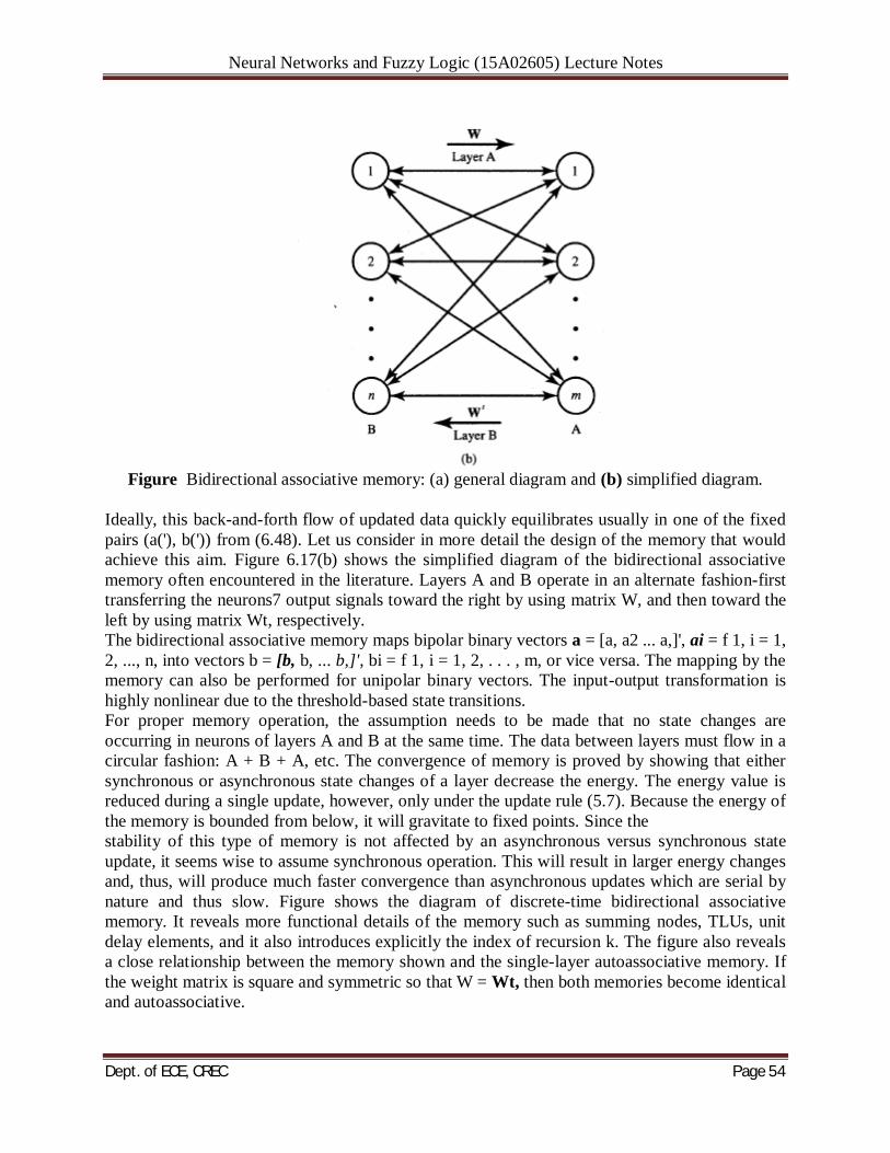
Neural Networks and Fuzzy Logic (15A02605) Lecture Notes
Dept. of ECE, CREC Page 54
Figure Bidirectional associative memory: (a) general diagram and (b) simplified diagram.
Ideally, this back-and-forth flow of updated data quickly equilibrates usually in one of the fixed pairs (a('), b(')) from (6.48). Let us consider in more detail the design of the memory that would achieve this aim. Figure 6.17(b) shows the simplified diagram of the bidirectional associative memory often encountered in the literature. Layers A and B operate in an alternate fashion-first transferring the neurons7 output signals toward the right by using matrix W, and then toward the left by using matrix Wt, respectively. The bidirectional associative memory maps bipolar binary vectors a = [a, a2 ... a,]', ai = f 1, i = 1, 2, ..., n, into vectors b = [b, b, ... b,]', bi = f 1, i = 1, 2, . . . , m, or vice versa. The mapping by the memory can also be performed for unipolar binary vectors. The input-output transformation is highly nonlinear due to the threshold-based state transitions. For proper memory operation, the assumption needs to be made that no state changes are occurring in neurons of layers A and B at the same time. The data between layers must flow in a circular fashion: A + B + A, etc. The convergence of memory is proved by showing that either synchronous or asynchronous state changes of a layer decrease the energy. The energy value is reduced during a single update, however, only under the update rule (5.7). Because the energy of the memory is bounded from below, it will gravitate to fixed points. Since the stability of this type of memory is not affected by an asynchronous versus synchronous state update, it seems wise to assume synchronous operation. This will result in larger energy changes and, thus, will produce much faster convergence than asynchronous updates which are serial by nature and thus slow. Figure shows the diagram of discrete-time bidirectional associative memory. It reveals more functional details of the memory such as summing nodes, TLUs, unit delay elements, and it also introduces explicitly the index of recursion k. The figure also reveals a close relationship between the memory shown and the single-layer autoassociative memory. If the weight matrix is square and symmetric so that W = Wt, then both memories become identical and autoassociative.
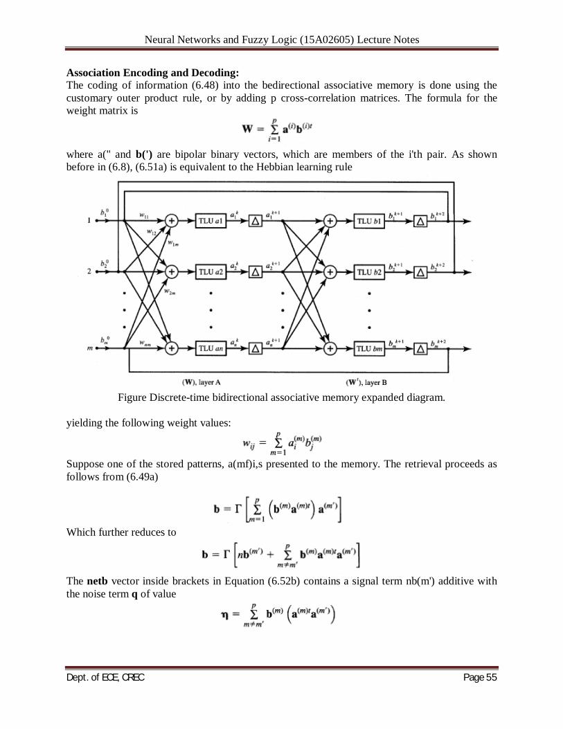
Neural Networks and Fuzzy Logic (15A02605) Lecture Notes
Dept. of ECE, CREC Page 55
Association Encoding and Decoding: The coding of information (6.48) into the bedirectional associative memory is done using the customary outer product rule, or by adding p cross-correlation matrices. The formula for the weight matrix is
where a(" and b(') are bipolar binary vectors, which are members of the i'th pair. As shown before in (6.8), (6.51a) is equivalent to the Hebbian learning rule
Figure Discrete-time bidirectional associative memory expanded diagram.
yielding the following weight values:
Suppose one of the stored patterns, a(mf)i,s presented to the memory. The retrieval proceeds as follows from (6.49a)
Which further reduces to
The netb vector inside brackets in Equation (6.52b) contains a signal term nb(m') additive with the noise term q of value
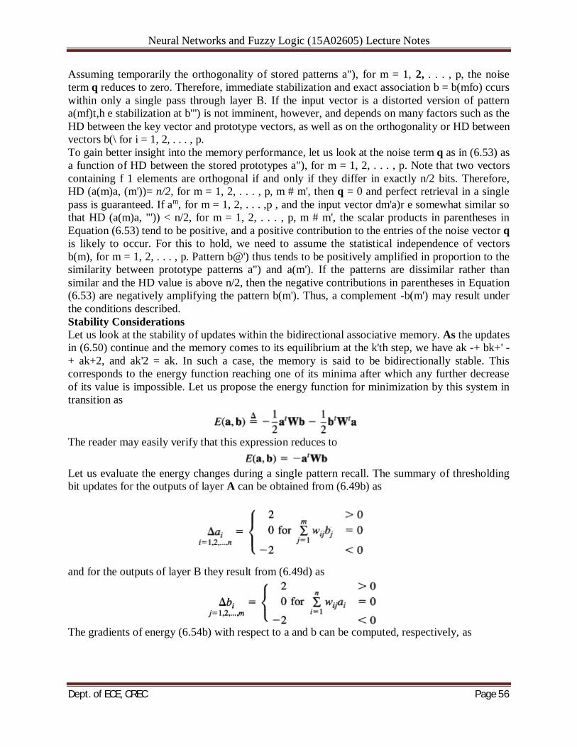
Neural Networks and Fuzzy Logic (15A02605) Lecture Notes
Dept. of ECE, CREC Page 56
Assuming temporarily the orthogonality of stored patterns a"), for m = 1, 2, . . . , p, the noise term q reduces to zero. Therefore, immediate stabilization and exact association b = b(mfo) ccurs within only a single pass through layer B. If the input vector is a distorted version of pattern a(mf)t,h e stabilization at b"') is not imminent, however, and depends on many factors such as the HD between the key vector and prototype vectors, as well as on the orthogonality or HD between vectors b(\ for i = 1, 2, . . . , p. To gain better insight into the memory performance, let us look at the noise term q as in (6.53) as a function of HD between the stored prototypes a"), for m = 1, 2, . . . , p. Note that two vectors containing f 1 elements are orthogonal if and only if they differ in exactly n/2 bits. Therefore, HD (a(m)a, (m'))= n/2, for m = 1, 2, . . . , p, m # m', then q = 0 and perfect retrieval in a single pass is guaranteed. If am, for m = 1, 2, . . . ,p , and the input vector dm'a)r e somewhat similar so that HD (a(m)a, "')) < n/2, for m = 1, 2, . . . , p, m # m', the scalar products in parentheses in Equation (6.53) tend to be positive, and a positive contribution to the entries of the noise vector q is likely to occur. For this to hold, we need to assume the statistical independence of vectors b(m), for m = 1, 2, . . . , p. Pattern b@') thus tends to be positively amplified in proportion to the similarity between prototype patterns a") and a(m'). If the patterns are dissimilar rather than similar and the HD value is above n/2, then the negative contributions in parentheses in Equation (6.53) are negatively amplifying the pattern b(m'). Thus, a complement -b(m') may result under the conditions described. Stability Considerations Let us look at the stability of updates within the bidirectional associative memory. As the updates in (6.50) continue and the memory comes to its equilibrium at the k'th step, we have ak -+ bk+' -+ ak+2, and ak'2 = ak. In such a case, the memory is said to be bidirectionally stable. This corresponds to the energy function reaching one of its minima after which any further decrease of its value is impossible. Let us propose the energy function for minimization by this system in transition as
The reader may easily verify that this expression reduces to
Let us evaluate the energy changes during a single pattern recall. The summary of thresholding bit updates for the outputs of layer A can be obtained from (6.49b) as
and for the outputs of layer B they result from (6.49d) as
The gradients of energy (6.54b) with respect to a and b can be computed, respectively, as
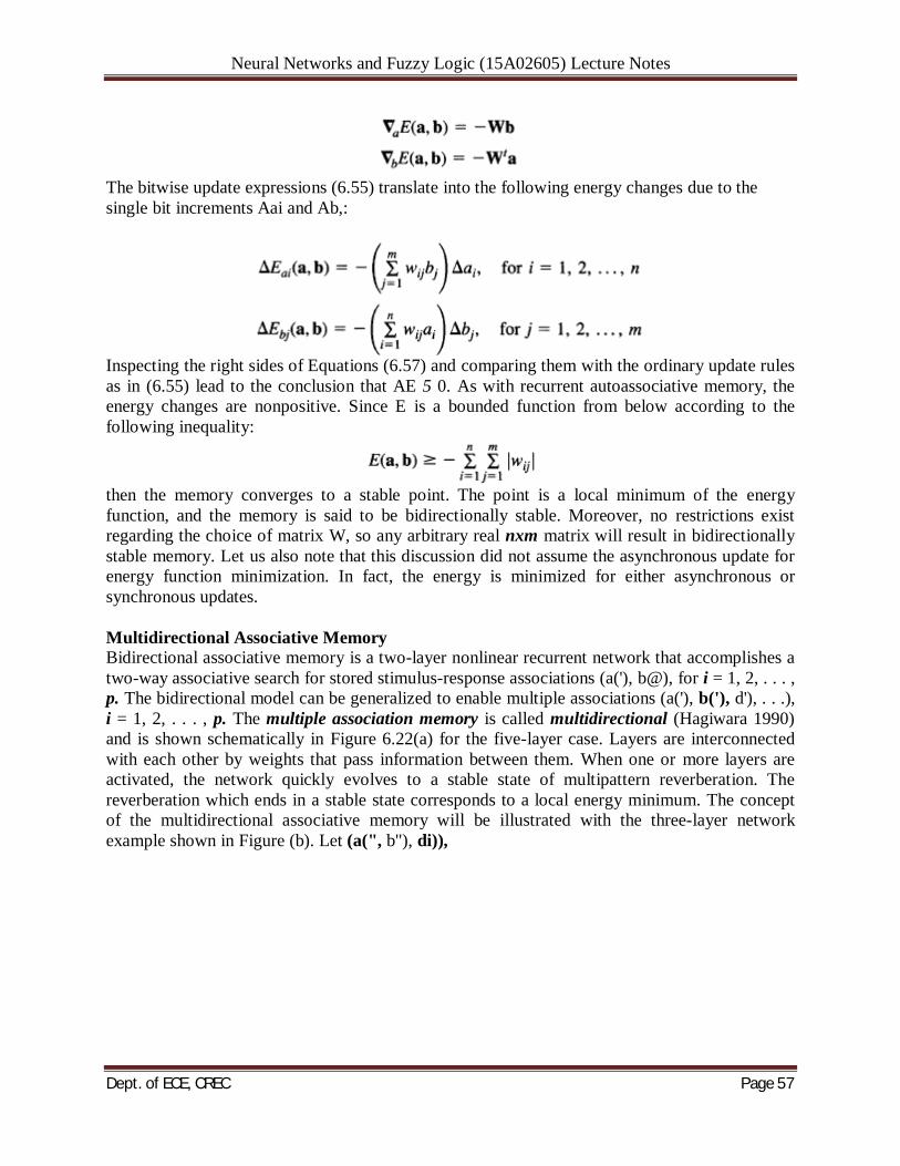
Neural Networks and Fuzzy Logic (15A02605) Lecture Notes
Dept. of ECE, CREC Page 57
The bitwise update expressions (6.55) translate into the following energy changes due to the single bit increments Aai and Ab,:
Inspecting the right sides of Equations (6.57) and comparing them with the ordinary update rules as in (6.55) lead to the conclusion that AE 5 0. As with recurrent autoassociative memory, the energy changes are nonpositive. Since E is a bounded function from below according to the following inequality:
then the memory converges to a stable point. The point is a local minimum of the energy function, and the memory is said to be bidirectionally stable. Moreover, no restrictions exist regarding the choice of matrix W, so any arbitrary real nxm matrix will result in bidirectionally stable memory. Let us also note that this discussion did not assume the asynchronous update for energy function minimization. In fact, the energy is minimized for either asynchronous or synchronous updates. Multidirectional Associative Memory Bidirectional associative memory is a two-layer nonlinear recurrent network that accomplishes a two-way associative search for stored stimulus-response associations (a('), b@), for i = 1, 2, . . . , p. The bidirectional model can be generalized to enable multiple associations (a('), b('), d'), . . .), i = 1, 2, . . . , p. The multiple association memory is called multidirectional (Hagiwara 1990) and is shown schematically in Figure 6.22(a) for the five-layer case. Layers are interconnected with each other by weights that pass information between them. When one or more layers are activated, the network quickly evolves to a stable state of multipattern reverberation. The reverberation which ends in a stable state corresponds to a local energy minimum. The concept of the multidirectional associative memory will be illustrated with the three-layer network example shown in Figure (b). Let (a(", b"), di)),
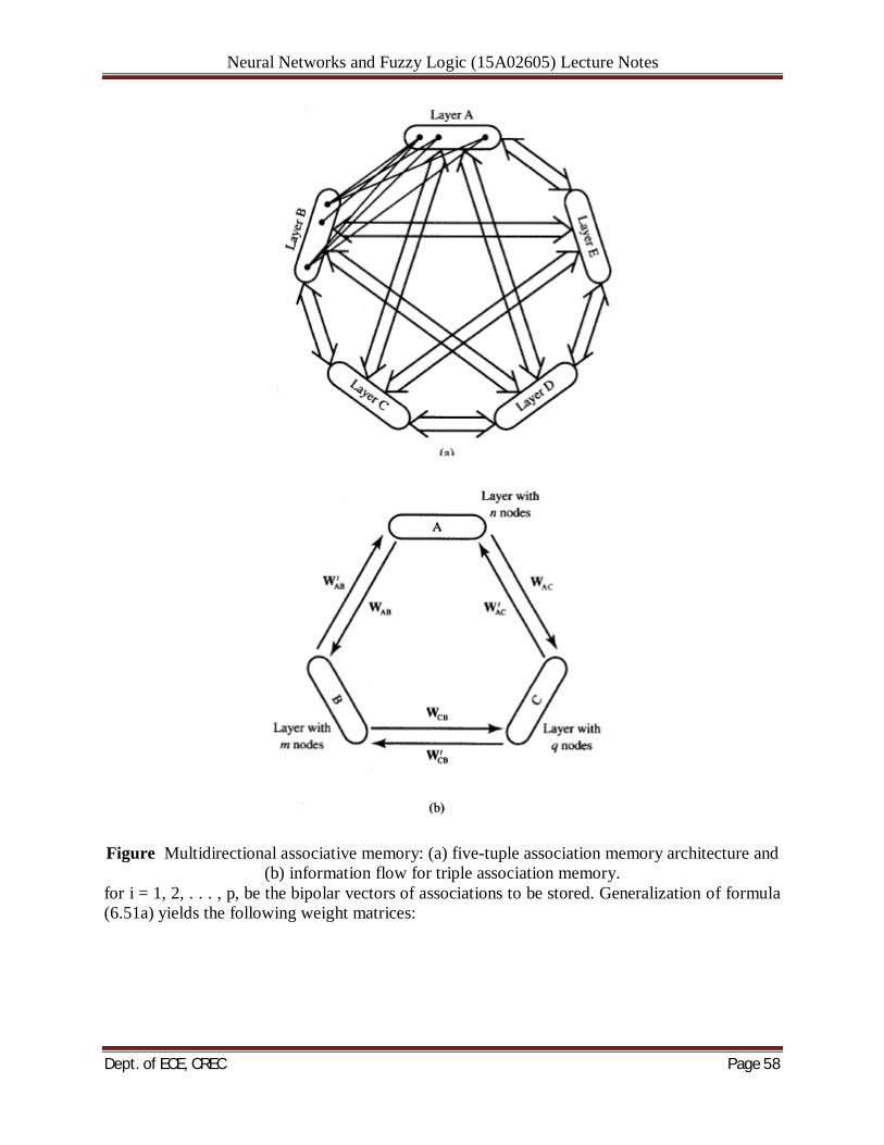
Neural Networks and Fuzzy Logic (15A02605) Lecture Notes
Dept. of ECE, CREC Page 58
Figure Multidirectional associative memory: (a) five-tuple association memory architecture and
(b) information flow for triple association memory. for i = 1, 2, . . . , p, be the bipolar vectors of associations to be stored. Generalization of formula (6.51a) yields the following weight matrices:
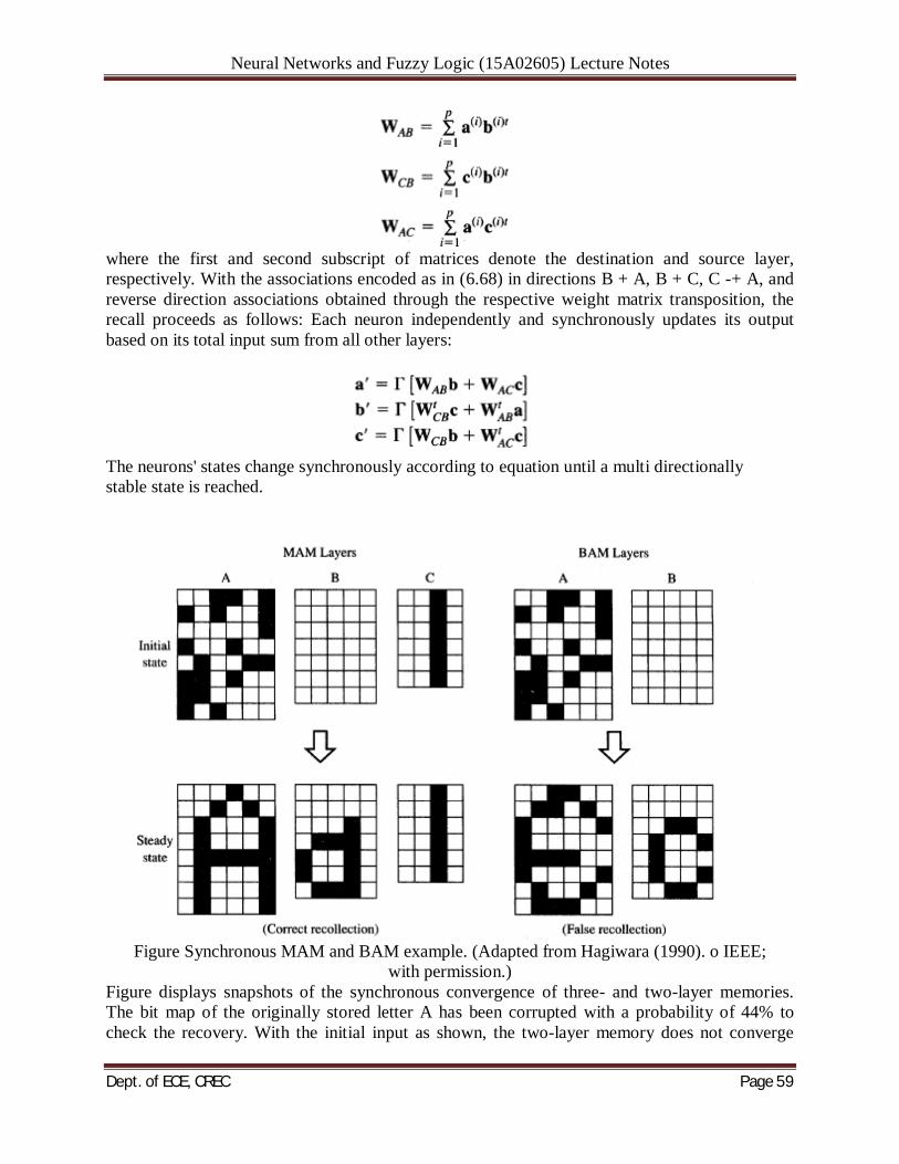
Neural Networks and Fuzzy Logic (15A02605) Lecture Notes
Dept. of ECE, CREC Page 59
where the first and second subscript of matrices denote the destination and source layer, respectively. With the associations encoded as in (6.68) in directions B + A, B + C, C -+ A, and reverse direction associations obtained through the respective weight matrix transposition, the recall proceeds as follows: Each neuron independently and synchronously updates its output based on its total input sum from all other layers:
The neurons' states change synchronously according to equation until a multi directionally stable state is reached.
Figure Synchronous MAM and BAM example. (Adapted from Hagiwara (1990). o IEEE;
with permission.) Figure displays snapshots of the synchronous convergence of three- and two-layer memories. The bit map of the originally stored letter A has been corrupted with a probability of 44% to check the recovery. With the initial input as shown, the two-layer memory does not converge
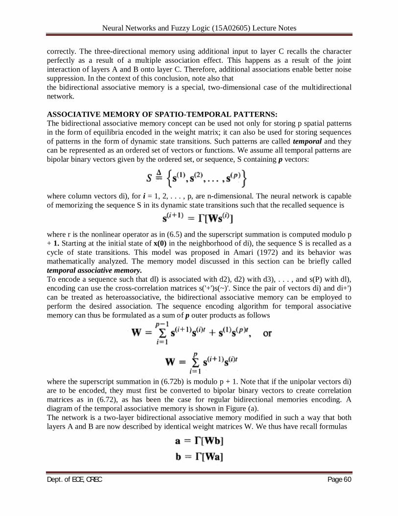
Neural Networks and Fuzzy Logic (15A02605) Lecture Notes
Dept. of ECE, CREC Page 60
correctly. The three-directional memory using additional input to layer C recalls the character perfectly as a result of a multiple association effect. This happens as a result of the joint interaction of layers A and B onto layer C. Therefore, additional associations enable better noise suppression. In the context of this conclusion, note also that the bidirectional associative memory is a special, two-dimensional case of the multidirectional network. ASSOCIATIVE MEMORY OF SPATIO-TEMPORAL PATTERNS: The bidirectional associative memory concept can be used not only for storing p spatial patterns in the form of equilibria encoded in the weight matrix; it can also be used for storing sequences of patterns in the form of dynamic state transitions. Such patterns are called temporal and they can be represented as an ordered set of vectors or functions. We assume all temporal patterns are bipolar binary vectors given by the ordered set, or sequence, S containing p vectors:
where column vectors di), for i = 1, 2, . . . , p, are n-dimensional. The neural network is capable of memorizing the sequence S in its dynamic state transitions such that the recalled sequence is
where r is the nonlinear operator as in (6.5) and the superscript summation is computed modulo p + 1. Starting at the initial state of x(0) in the neighborhood of di), the sequence S is recalled as a cycle of state transitions. This model was proposed in Amari (1972) and its behavior was mathematically analyzed. The memory model discussed in this section can be briefly called temporal associative memory. To encode a sequence such that dl) is associated with d2), d2) with d3), . . . , and s(P) with dl), encoding can use the cross-correlation matrices s('+')s(~)'. Since the pair of vectors di) and di+') can be treated as heteroassociative, the bidirectional associative memory can be employed to perform the desired association. The sequence encoding algorithm for temporal associative memory can thus be formulated as a sum of p outer products as follows
where the superscript summation in (6.72b) is modulo p + 1. Note that if the unipolar vectors di) are to be encoded, they must first be converted to bipolar binary vectors to create correlation matrices as in (6.72), as has been the case for regular bidirectional memories encoding. A diagram of the temporal associative memory is shown in Figure (a). The network is a two-layer bidirectional associative memory modified in such a way that both layers A and B are now described by identical weight matrices W. We thus have recall formulas
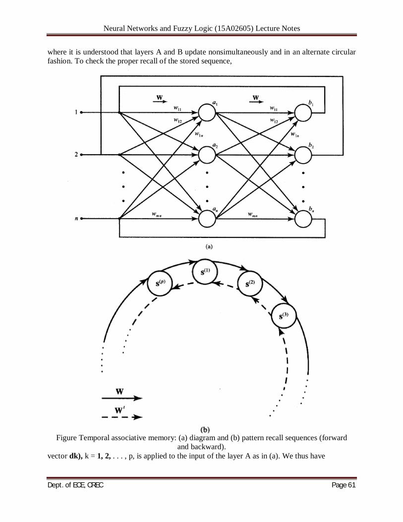
Neural Networks and Fuzzy Logic (15A02605) Lecture Notes
Dept. of ECE, CREC Page 61
where it is understood that layers A and B update nonsimultaneously and in an alternate circular fashion. To check the proper recall of the stored sequence,
Figure Temporal associative memory: (a) diagram and (b) pattern recall sequences (forward
and backward). vector dk), k = 1, 2, . . . , p, is applied to the input of the layer A as in (a). We thus have
Neural Networks and Fuzzy Logic (15A02605) Lecture Notes
Dept. of ECE, CREC Page 62
The vector net, in brackets of Equation (6.74) contains a signal term ndk+') and the remainder, which is the noise term q
where the superscript summation is modulo p + 1. Assuming the orthogonality of the vectors within the sequence S, the noise term is exactly zero and <he thresholding operation on vector ndk+') results in dkf') being the retrieved vector. Therefore, immediate stabilization and exact association of the appropriate member vector of the sequence occurs within a single pass within layer A. Similarly, vector s('+') at the input to layer B will result in recall of dk+*) The reader may verify this using (6.73b) and (6.72). Thus, input of any member of the sequence set S, say dk), results in the desired circular recalls as follows: dk+l) + s(~++~ .) . . + S(P) --+ dl) -+ . . . . This is illustrated in Figure 6.24(b), which shows the forward recall sequence. The reader may easily notice that reverse order recall can be implemented using the transposed weight matrices in both layers A and B. Indeed, transposing (6.72b) yields
When the signal term due to the input dk) is ndk-'), the recall of dk-l) will follow. Obviously, if the vectors of sequence S are not mutually orthogonal, the noise term q may not vanish, even after thresholding. Still, for vectors stored at a distance HD << n, the thresholding operation in layer A or B should be expected to result in recall of the correct sequence. This type of memory will undergo the same limitations and capacity bounds as the bidirectional associative memory. The storage capacity of the temporal associative memory can be estimated using expression (6.61a). Thus, we have the maximum length sequence to be bounded according to the condition p < n. More generally, the memory can be used to store k sequences of length pl, p2, . . . , pk. Together they include:
patterns. In such cases, the total number of patterns as in (6.77) should below the n value. The temporal associative memory operates in a synchronous serial be kept fashion similar to a single synchronous update step of a bidirectional associative memory. The stability of the memory can be proven by generalizing the theory of stability of the bidirectional associative memory. The temporal memory energy function is defined as
Calculation of the energy increment due to changes of s(') produces the following equation:
Neural Networks and Fuzzy Logic (15A02605) Lecture Notes
Dept. of ECE, CREC Page 63
The gradient of energy with respect to sk becomes
Considering bitwise updates due to increments AS?) we obtain
Each of the two sums in parentheses in Equation (6.81) agree in sign with AS!" under the sgn (neti) update rule. The second sum corresponds to neti due to the input dk-'), which retrieves s" in the forward direction. The first sum corresponds to neti due to the input dk+'), which again retrieves dk) in the reverse direction. Thus, the energy increments are negative during the temporal sequence retrieval -+ d2) -+ . . . -+ s(P). AS shown by Kosko (1988), the energy increases stepwise, however, at the transition s(p) -+ dl), and then it continues to decrease within the complete sequence of p - 1 retrievals to follow.
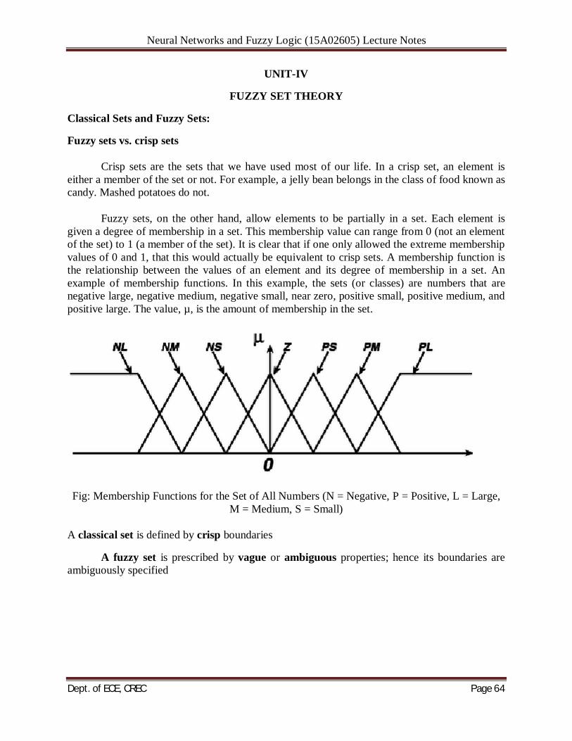
Neural Networks and Fuzzy Logic (15A02605) Lecture Notes
Dept. of ECE, CREC Page 64
UNIT-IV
FUZZY SET THEORY
Classical Sets and Fuzzy Sets:
Fuzzy sets vs. crisp sets
Crisp sets are the sets that we have used most of our life. In a crisp set, an element is either a member of the set or not. For example, a jelly bean belongs in the class of food known as candy. Mashed potatoes do not.
Fuzzy sets, on the other hand, allow elements to be partially in a set. Each element is given a degree of membership in a set. This membership value can range from 0 (not an element of the set) to 1 (a member of the set). It is clear that if one only allowed the extreme membership values of 0 and 1, that this would actually be equivalent to crisp sets. A membership function is the relationship between the values of an element and its degree of membership in a set. An example of membership functions. In this example, the sets (or classes) are numbers that are negative large, negative medium, negative small, near zero, positive small, positive medium, and positive large. The value, µ, is the amount of membership in the set.
Fig: Membership Functions for the Set of All Numbers (N = Negative, P = Positive, L = Large, M = Medium, S = Small)
A classical set is defined by crisp boundaries
A fuzzy set is prescribed by vague or ambiguous properties; hence its boundaries are ambiguously specified
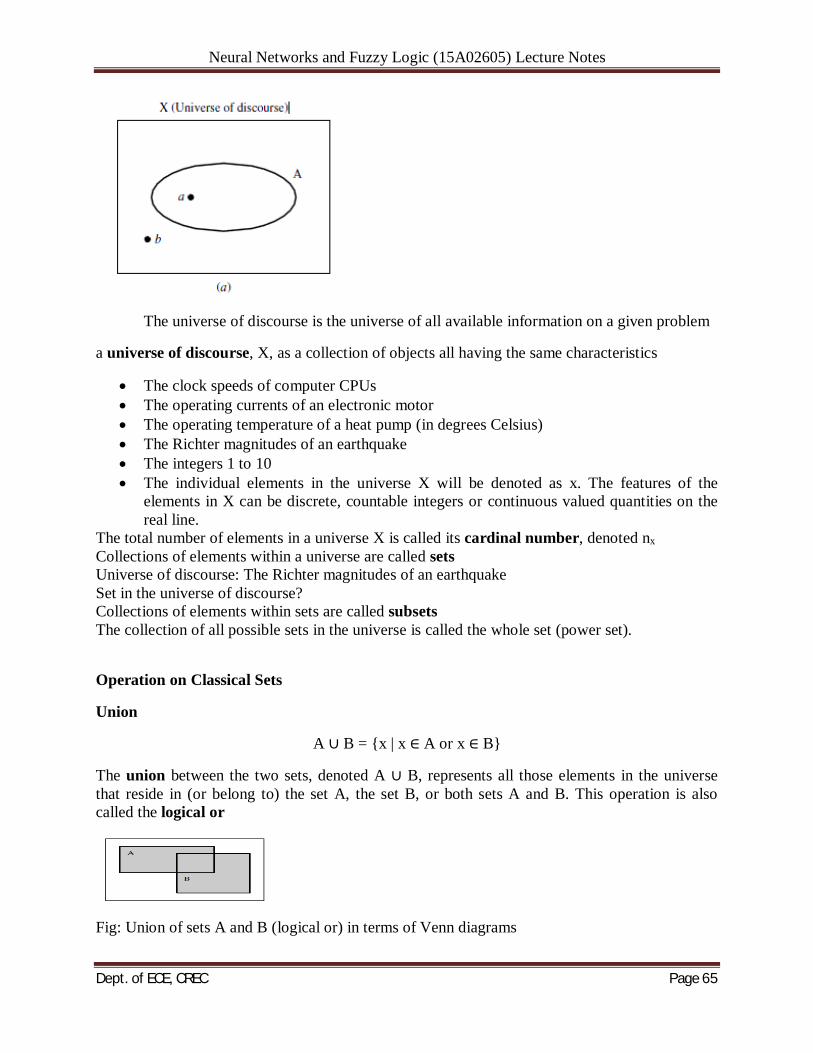
Neural Networks and Fuzzy Logic (15A02605) Lecture Notes
Dept. of ECE, CREC Page 65
The universe of discourse is the universe of all available information on a given problem
a universe of discourse, X, as a collection of objects all having the same characteristics
The clock speeds of computer CPUs The operating currents of an electronic motor The operating temperature of a heat pump (in degrees Celsius) The Richter magnitudes of an earthquake The integers 1 to 10 The individual elements in the universe X will be denoted as x. The features of the
elements in X can be discrete, countable integers or continuous valued quantities on the real line.
The total number of elements in a universe X is called its cardinal number, denoted nx Collections of elements within a universe are called sets Universe of discourse: The Richter magnitudes of an earthquake Set in the universe of discourse? Collections of elements within sets are called subsets The collection of all possible sets in the universe is called the whole set (power set).
Operation on Classical Sets
Union
A ∪ B = {x | x ∈ A or x ∈ B}
The union between the two sets, denoted A ∪ B, represents all those elements in the universe that reside in (or belong to) the set A, the set B, or both sets A and B. This operation is also called the logical or
Fig: Union of sets A and B (logical or) in terms of Venn diagrams
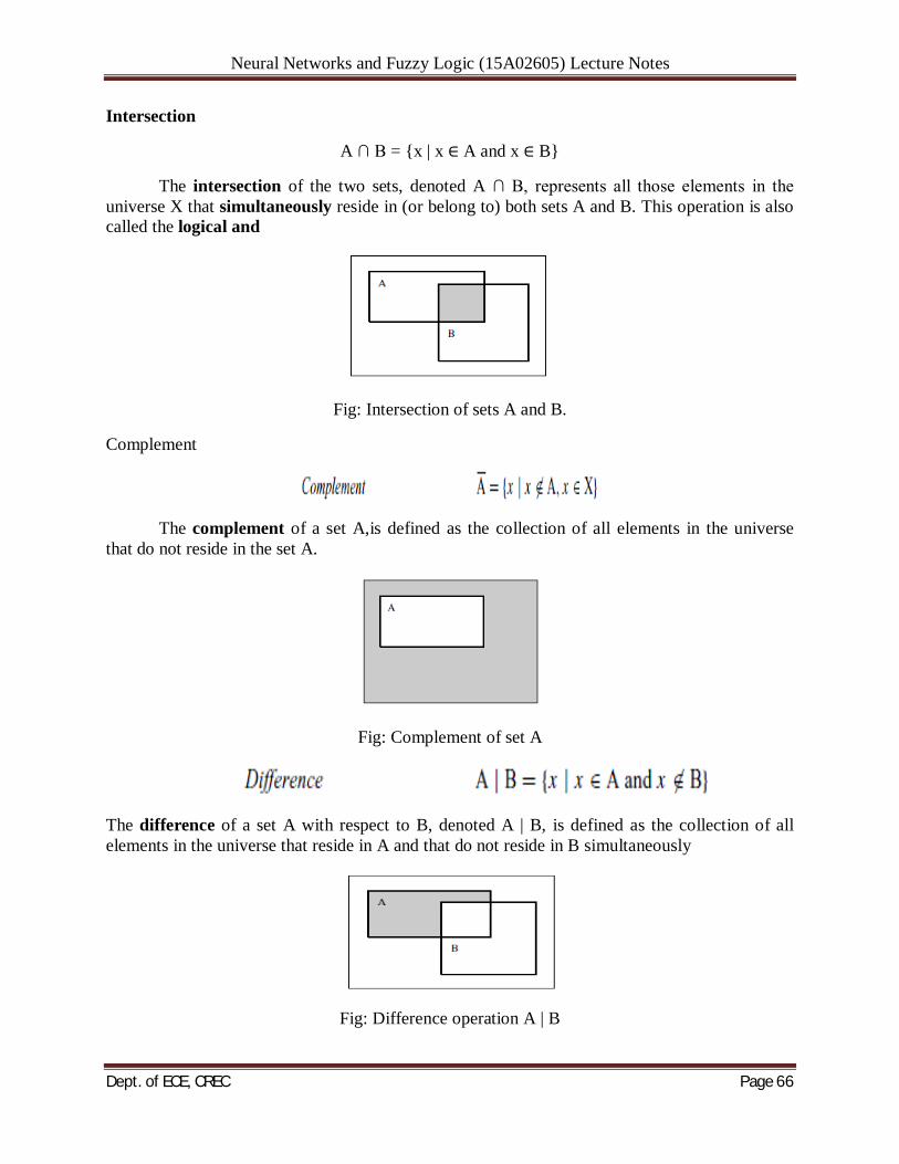
Neural Networks and Fuzzy Logic (15A02605) Lecture Notes
Dept. of ECE, CREC Page 66
Intersection
A ∩ B = {x | x ∈ A and x ∈ B}
The intersection of the two sets, denoted A ∩ B, represents all those elements in the universe X that simultaneously reside in (or belong to) both sets A and B. This operation is also called the logical and
Fig: Intersection of sets A and B.
Complement
The complement of a set A,is defined as the collection of all elements in the universe that do not reside in the set A.
Fig: Complement of set A
The difference of a set A with respect to B, denoted A | B, is defined as the collection of all elements in the universe that reside in A and that do not reside in B simultaneously
Fig: Difference operation A | B
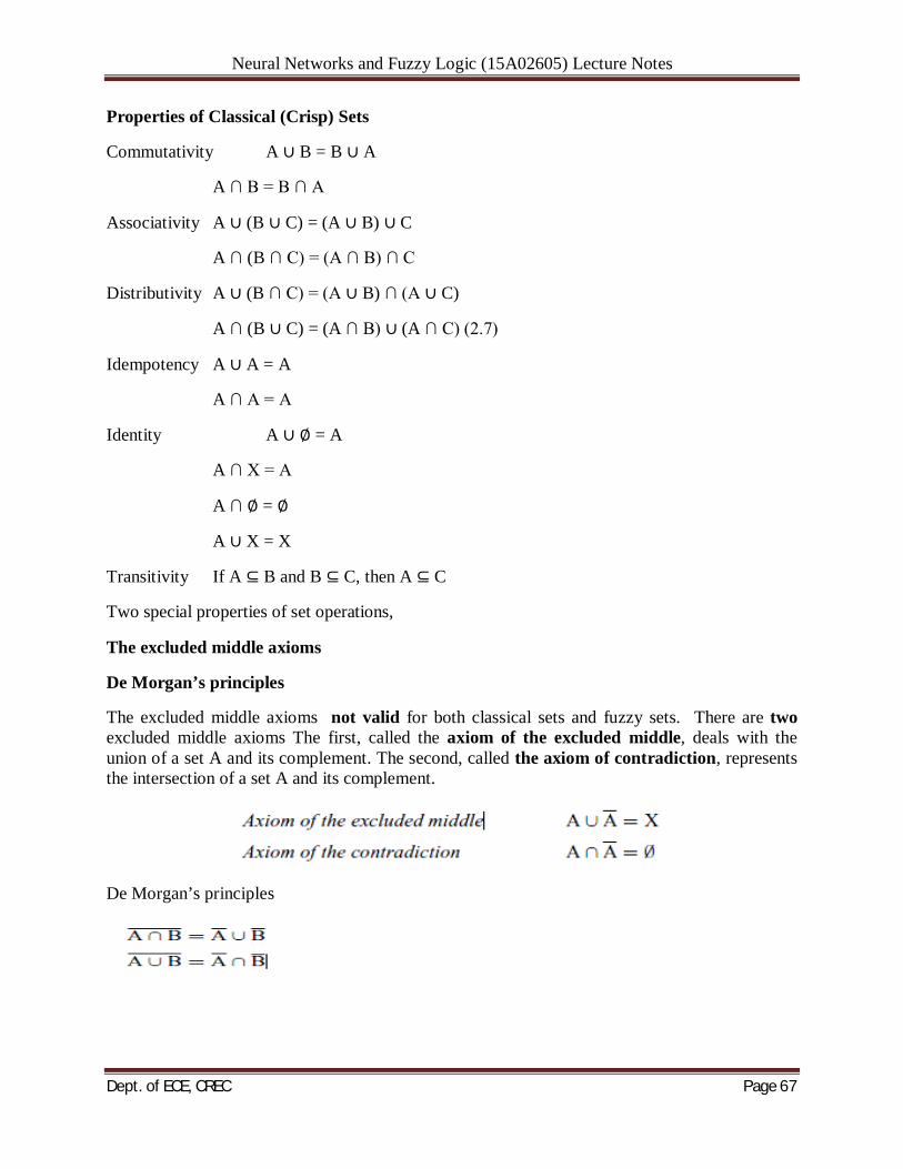
Neural Networks and Fuzzy Logic (15A02605) Lecture Notes
Dept. of ECE, CREC Page 67
Properties of Classical (Crisp) Sets
Commutativity A ∪ B = B ∪ A
A ∩ B = B ∩ A
Associativity A ∪ (B ∪ C) = (A ∪ B) ∪ C
A ∩ (B ∩ C) = (A ∩ B) ∩ C
Distributivity A ∪ (B ∩ C) = (A ∪ B) ∩ (A ∪ C)
A ∩ (B ∪ C) = (A ∩ B) ∪ (A ∩ C) (2.7)
Idempotency A ∪ A = A
A ∩ A = A
Identity A ∪ ∅ = A
A ∩ X = A
A ∩ ∅ = ∅
A ∪ X = X
Transitivity If A ⊆ B and B ⊆ C, then A ⊆ C
Two special properties of set operations,
The excluded middle axioms
De Morgan’s principles
The excluded middle axioms not valid for both classical sets and fuzzy sets. There are two excluded middle axioms The first, called the axiom of the excluded middle, deals with the union of a set A and its complement. The second, called the axiom of contradiction, represents the intersection of a set A and its complement.
De Morgan’s principles
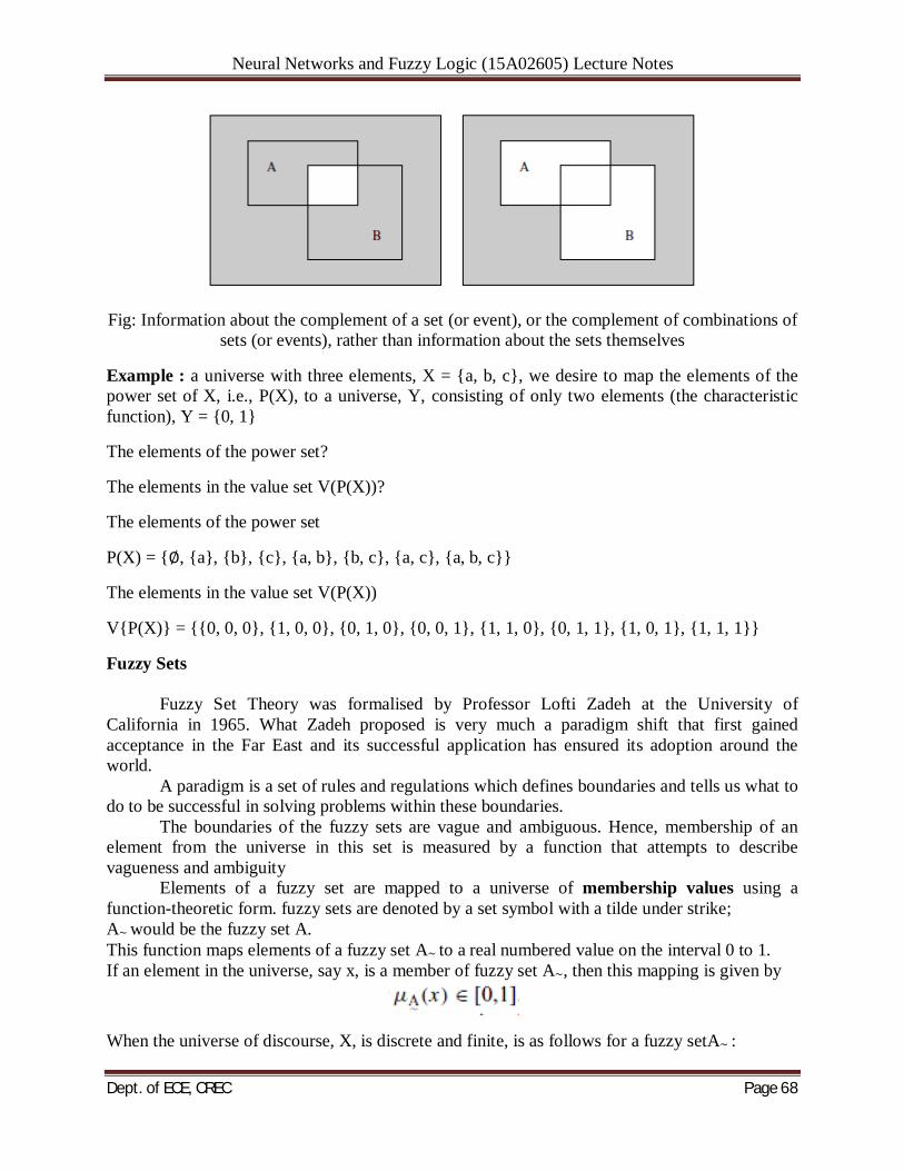
Neural Networks and Fuzzy Logic (15A02605) Lecture Notes
Dept. of ECE, CREC Page 68
Fig: Information about the complement of a set (or event), or the complement of combinations of sets (or events), rather than information about the sets themselves
Example : a universe with three elements, X = {a, b, c}, we desire to map the elements of the power set of X, i.e., P(X), to a universe, Y, consisting of only two elements (the characteristic function), Y = {0, 1}
The elements of the power set?
The elements in the value set V(P(X))?
The elements of the power set
P(X) = {∅, {a}, {b}, {c}, {a, b}, {b, c}, {a, c}, {a, b, c}}
The elements in the value set V(P(X))
V{P(X)} = {{0, 0, 0}, {1, 0, 0}, {0, 1, 0}, {0, 0, 1}, {1, 1, 0}, {0, 1, 1}, {1, 0, 1}, {1, 1, 1}}
Fuzzy Sets
Fuzzy Set Theory was formalised by Professor Lofti Zadeh at the University of California in 1965. What Zadeh proposed is very much a paradigm shift that first gained acceptance in the Far East and its successful application has ensured its adoption around the world.
A paradigm is a set of rules and regulations which defines boundaries and tells us what to do to be successful in solving problems within these boundaries.
The boundaries of the fuzzy sets are vague and ambiguous. Hence, membership of an element from the universe in this set is measured by a function that attempts to describe vagueness and ambiguity
Elements of a fuzzy set are mapped to a universe of membership values using a function-theoretic form. fuzzy sets are denoted by a set symbol with a tilde under strike; A∼ would be the fuzzy set A. This function maps elements of a fuzzy set A∼ to a real numbered value on the interval 0 to 1. If an element in the universe, say x, is a member of fuzzy set A∼, then this mapping is given by
When the universe of discourse, X, is discrete and finite, is as follows for a fuzzy setA∼ :
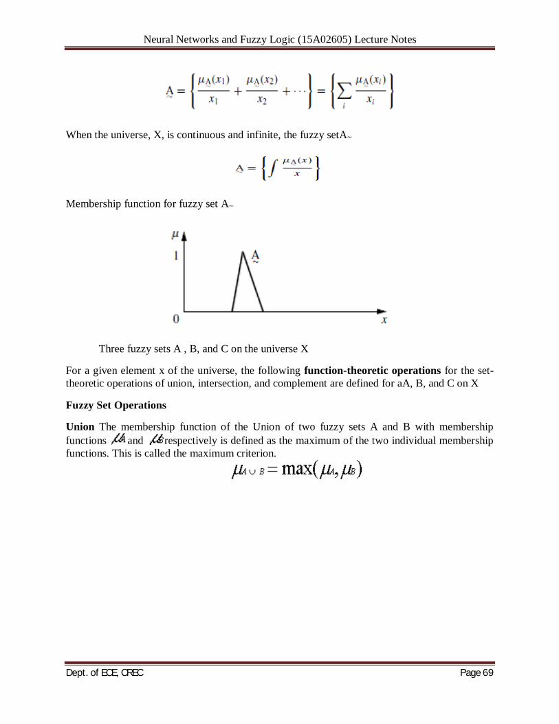
Neural Networks and Fuzzy Logic (15A02605) Lecture Notes
Dept. of ECE, CREC Page 69
When the universe, X, is continuous and infinite, the fuzzy setA∼
Membership function for fuzzy set A∼
Three fuzzy sets A , B, and C on the universe X
For a given element x of the universe, the following function-theoretic operations for the set-theoretic operations of union, intersection, and complement are defined for aA, B, and C on X
Fuzzy Set Operations
Union The membership function of the Union of two fuzzy sets A and B with membership functions and respectively is defined as the maximum of the two individual membership functions. This is called the maximum criterion.
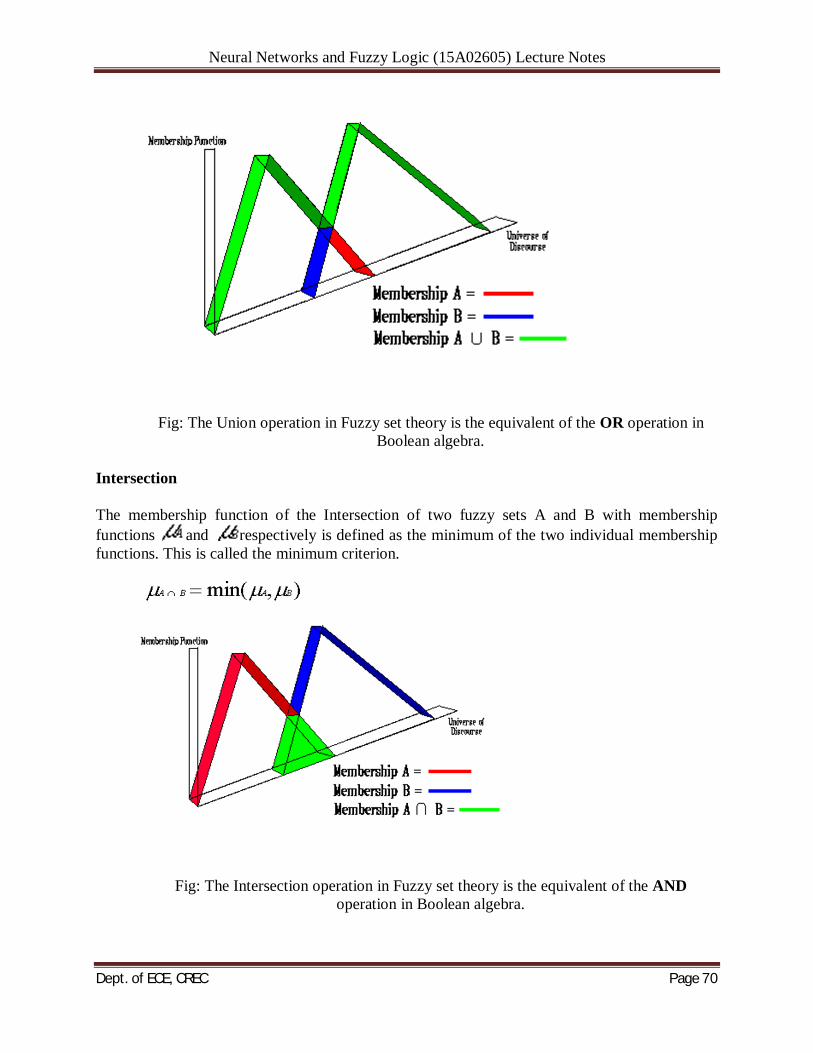
Neural Networks and Fuzzy Logic (15A02605) Lecture Notes
Dept. of ECE, CREC Page 70
Fig: The Union operation in Fuzzy set theory is the equivalent of the OR operation in Boolean algebra.
Intersection
The membership function of the Intersection of two fuzzy sets A and B with membership functions and respectively is defined as the minimum of the two individual membership functions. This is called the minimum criterion.
Fig: The Intersection operation in Fuzzy set theory is the equivalent of the AND operation in Boolean algebra.
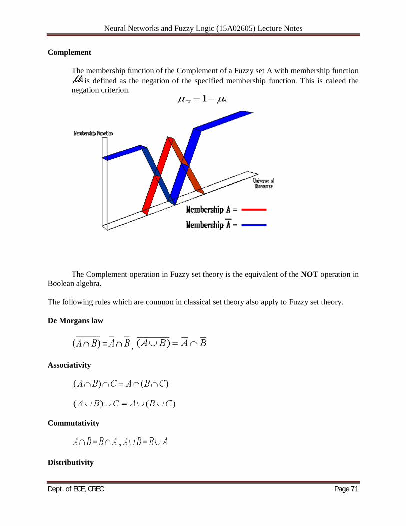
Neural Networks and Fuzzy Logic (15A02605) Lecture Notes
Dept. of ECE, CREC Page 71
Complement
The membership function of the Complement of a Fuzzy set A with membership function is defined as the negation of the specified membership function. This is caleed the
negation criterion.
The Complement operation in Fuzzy set theory is the equivalent of the NOT operation in Boolean algebra.
The following rules which are common in classical set theory also apply to Fuzzy set theory.
De Morgans law
,
Associativity
Commutativity
Distributivity
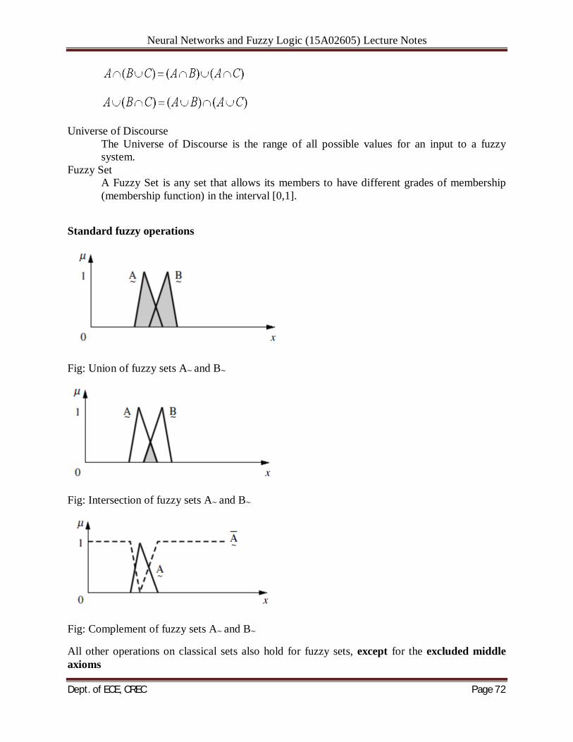
Neural Networks and Fuzzy Logic (15A02605) Lecture Notes
Dept. of ECE, CREC Page 72
Universe of Discourse The Universe of Discourse is the range of all possible values for an input to a fuzzy system.
Fuzzy Set A Fuzzy Set is any set that allows its members to have different grades of membership (membership function) in the interval [0,1].
Standard fuzzy operations
Fig: Union of fuzzy sets A∼ and B∼
Fig: Intersection of fuzzy sets A∼ and B∼
Fig: Complement of fuzzy sets A∼ and B∼
All other operations on classical sets also hold for fuzzy sets, except for the excluded middle axioms
Neural Networks and Fuzzy Logic (15A02605) Lecture Notes
Dept. of ECE, CREC Page 73
RELATIONS
Relations represent mappings between sets and connectives in logic. A classical binary relation represents the presence or absence of a connection or interaction or association between the elements of two sets. Fuzzy binary relations are a generalization of crisp binary relations, and they allow various degrees of relationship (association) between elements.
Fuzzy Relations
Crisp and Fuzzy Relations
A crisp relation represents the presence or absence of association, interaction, or interconnectedness between the elements of two or more sets. This concept can be generalized to allow for various degrees or strengths of relation or interaction between elements. Degrees of association can be represented by membership grades in a fuzzy relation in the same way as degrees of set membership are represented in the fuzzy set. In fact, just as the crisp set can be viewed as a restricted case of the more general fuzzy set concept, the crisp relation can be considered to be a restricted case of the fuzzy relations. Cartesian product The Cartesian product of two crisp sets X and Y, denoted by , is the crisp set of all ordered pairs such that the first element in each pair is a member of X and the second element is a member of Y. Formally,
The Cartesian product can be generalized for a family of crisp sets and denoted
either by . Elements of the Cartesian product of n crisp sets are n-
tuples Thus,
It is possible for all sets to be equal, that is, to be a single set X. In this case, the Cartesian
product of a set X with itself n times is usually denoted by .
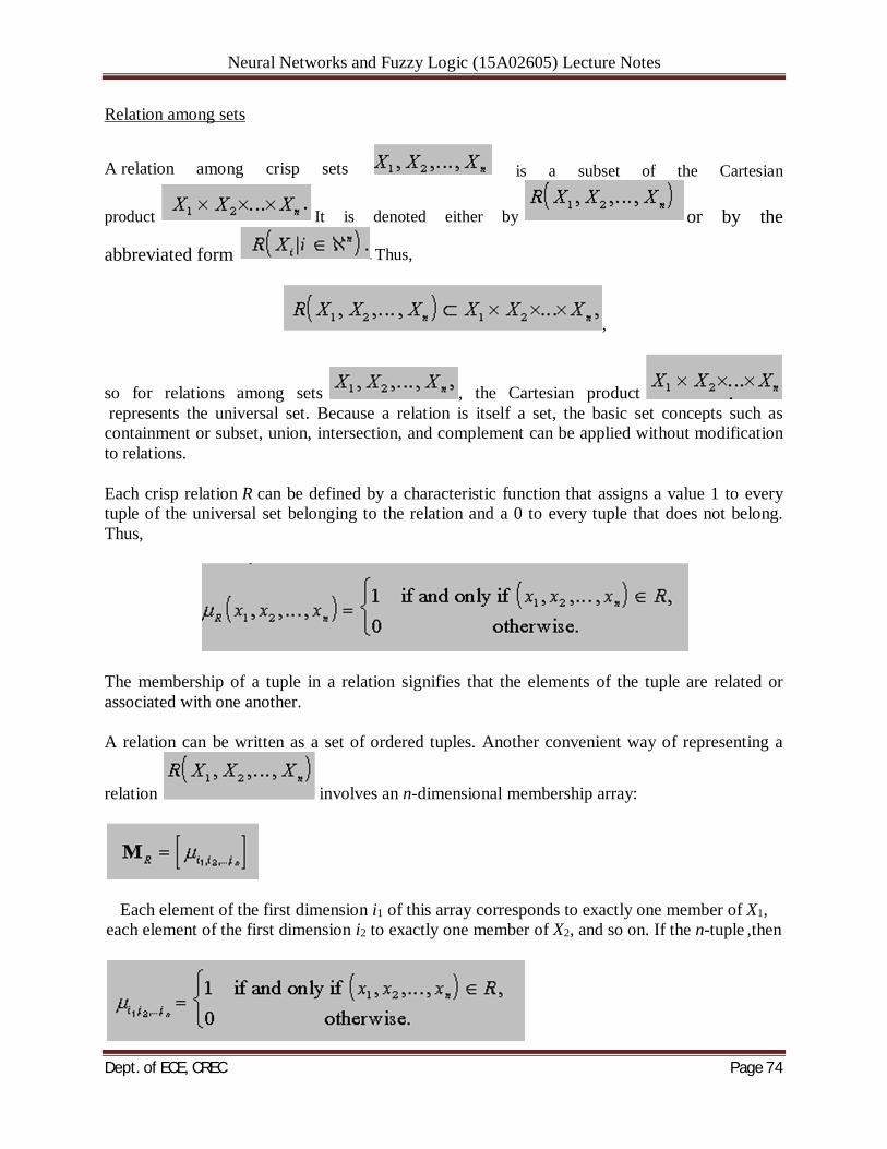
Neural Networks and Fuzzy Logic (15A02605) Lecture Notes
Dept. of ECE, CREC Page 74
Relation among sets
A relation among crisp sets is a subset of the Cartesian
product It is denoted either by or by the
abbreviated form . Thus,
,
so for relations among sets , the Cartesian product represents the universal set. Because a relation is itself a set, the basic set concepts such as containment or subset, union, intersection, and complement can be applied without modification to relations.
Each crisp relation R can be defined by a characteristic function that assigns a value 1 to every tuple of the universal set belonging to the relation and a 0 to every tuple that does not belong. Thus,
The membership of a tuple in a relation signifies that the elements of the tuple are related or associated with one another.
A relation can be written as a set of ordered tuples. Another convenient way of representing a
relation involves an n-dimensional membership array:
Each element of the first dimension i1 of this array corresponds to exactly one member of X1, each element of the first dimension i2 to exactly one member of X2, and so on. If the n-tuple ,then
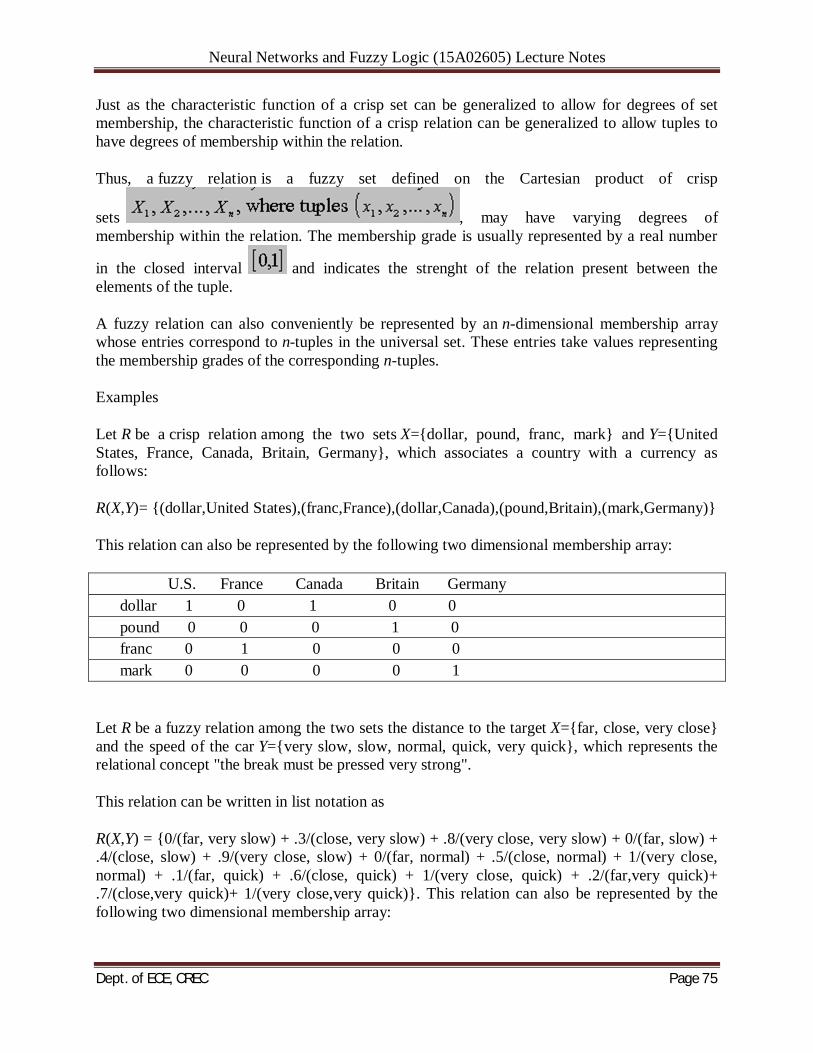
Neural Networks and Fuzzy Logic (15A02605) Lecture Notes
Dept. of ECE, CREC Page 75
Just as the characteristic function of a crisp set can be generalized to allow for degrees of set membership, the characteristic function of a crisp relation can be generalized to allow tuples to have degrees of membership within the relation.
Thus, a fuzzy relation is a fuzzy set defined on the Cartesian product of crisp
sets , may have varying degrees of membership within the relation. The membership grade is usually represented by a real number
in the closed interval and indicates the strenght of the relation present between the elements of the tuple.
A fuzzy relation can also conveniently be represented by an n-dimensional membership array whose entries correspond to n-tuples in the universal set. These entries take values representing the membership grades of the corresponding n-tuples.
Examples
Let R be a crisp relation among the two sets X={dollar, pound, franc, mark} and Y={United States, France, Canada, Britain, Germany}, which associates a country with a currency as follows:
R(X,Y)= {(dollar,United States),(franc,France),(dollar,Canada),(pound,Britain),(mark,Germany)}
This relation can also be represented by the following two dimensional membership array:
U.S. France Canada Britain Germany dollar 1 0 1 0 0 pound 0 0 0 1 0 franc 0 1 0 0 0 mark 0 0 0 0 1
Let R be a fuzzy relation among the two sets the distance to the target X={far, close, very close} and the speed of the car Y={very slow, slow, normal, quick, very quick}, which represents the relational concept "the break must be pressed very strong".
This relation can be written in list notation as
R(X,Y) = {0/(far, very slow) + .3/(close, very slow) + .8/(very close, very slow) + 0/(far, slow) + .4/(close, slow) + .9/(very close, slow) + 0/(far, normal) + .5/(close, normal) + 1/(very close, normal) + .1/(far, quick) + .6/(close, quick) + 1/(very close, quick) + .2/(far,very quick)+ .7/(close,very quick)+ 1/(very close,very quick)}. This relation can also be represented by the following two dimensional membership array:

Neural Networks and Fuzzy Logic (15A02605) Lecture Notes
Dept. of ECE, CREC Page 76
very slow slow normal quick very quick far 0 0 0 .1 .2 close .3 .4 .5 .6 .7 very close .8 .9 1 1 1
Neural Networks and Fuzzy Logic (15A02605) Lecture Notes
Dept. of ECE, CREC Page 77
UNIT-V
FUZZY SYSTEMS
Propositional Logic A proposition or statement is a sentence which is either true or false. If a proposition is
true, then we say its truth value is true, and if a proposition is false, we say its truth value is false. A propositional variable represents an arbitrary proposition. We represent propositional variables with uppercase letters.
Sam wrote a C program containing the if-statement if (a < b || (a >= b && c == d)) .Sally points out that the conditional expression in the if-statement could have been written more simply as if (a < b || c == d). Suppose a < b. Then the first of the two OR’ed conditions is true in both statements, so the then-branch is taken in either of the if-statements. Now suppose a < b is false. In this case, we can only take the then-branch if the second of the two conditions is true. For statement (12.1), we are asking whether a >= b && c == d is true. Now a >= b is surely true, since we assume a < b is false. Thus we take the then-branch in exactly when c == d is true. For statement, we clearly take the then-branch exactly when c == d. Thus no matter what the values of a, b, c, and d are, either both or neither of the if-statements cause the then-branch to be followed.
We conclude that Sally is right, and the simplified conditional expression can be substituted for the first with no change in what the program does. Propositional logic is a mathematical model that allows us to reason about the truth or falsehood of logical expressions. We shall define logical expressions formally in the next section, but for the time being we can think of a logical expression as a simplification of a conditional expression such as lines or above that abstracts away the order of evaluation contraints of the logical operators in C. Propositions and Truth Values Notice that our reasoning about the two if-statements above did not depend on what a < b or similar conditions “mean.” All we needed to know was that the conditions a < b and a >= b are complementary, that is, when one is true the other is false and vice versa. We may therefore replace the statement a < b by a single symbol p, replace a >= b by the expression NOT p, and replace c == d by the symbol q. The symbols p and q are called propositional variables, since they can stand for any “proposition,” that is, any statement that can have one of the truth values, true or false. Logical expressions can contain logical operators such as AND, OR, and NOT. When the values of the operands of the logical operators in a logical expression are known, the value of the expression can be determined using rules such as 1. The expression p AND q is true only when both p and q are true; it is false otherwise. 2. The expression p OR q is true if either p or q, or both are true; it is false otherwise. 3. The expression NOT p is true if p is false, and false if p is true. The operator NOT has the same meaning as the C operator !. The operators AND and OR are like the C operators && and ||, respectively, but with a technical difference. The C operators are defined to evaluate the second operand only when the first operand does not resolve the matter — that is, when the first operation of && is true or the first operand of || is false. However, this detail is only important when the C expression has side effects. Since there are no “side effects” in the evaluation of logical expressions, we can take AND to be synonymous with the C operator && and take OR to be synonymous with ||.
For example, the condition in Equation (12.1) can be written as the logical expression p OR (NOT p) AND q and Equation (12.2) can be written as p OR q. Our reasoning about the two if statements showed the general proposition that p OR (NOT p) AND q ≡ (p OR q) where ≡
Neural Networks and Fuzzy Logic (15A02605) Lecture Notes
Dept. of ECE, CREC Page 78
means “is equivalent to” or “has the same Boolean value as.” That is, no matter what truth values are assigned to the propositional variables p and q, the left-hand side and right-hand side of ≡ are either both true or both false. We discovered that for the equivalence above, both are true when p is true or when q is true, and both are false if p and q are both false. Thus, we have a valid equivalence. As p and q can be any propositions we like, we can use equivalence (12.3) to simplify many different expressions. For example, we could let p be a == b+1 && c < d while q is a == c || b == c. In that case, the left-hand side of (12.3) is (a == b+1 && c < d) || (12.4) ( !(a == b+1 && c < d) && (a == c || b == c)) Note that we placed parentheses around the values of p and q to make sure the resulting expression is grouped properly. Equivalence (12.3) tells us that (12.4) can be simplified to the right-hand side of (12.3), which is (a == b+1 && c < d) || (a == c || b == c). Logical Connectives Use logical connectives to build complex propositions from simpler ones. The First Three Logical Connectives • ¬ denotes not. ¬P is the negation of P. • ∨ denotes or. P ∨ Q is the disjunction of P and Q. • ∧ denotes and. P ∧ Q is the conjunction of P and Q. Order of Operations • ¬ first • ∧/∨ second • implication and biconditionals last (more on these later) • parentheses can be used to change the order Examples with Identities 1. P ≡ P ∧ P - idempotence of ∧ “Anna is wretched” is equivalent to “Anna is wretched and Anna is wretched”. 2. P ≡ P ∨ P - idempotence of ∨ “Anna is wretched” is equivalent to “Anna is wretched or wretched”. 3. P ∨ Q ≡ Q ∨ P - commutativity “Sam is rich or happy” is equivalent to “Sam is happy or rich”. 4. P ∧ Q ≡ Q ∧ P “Sam is rich and Sam is happy” is equivalent to “Sam is happy and Sam is rich”. 5.¬(P ∨ Q) ≡ ¬P ∧ ¬Q - DeMorgan’s law “It is not the case that Sam is rich or happy” is equivalent to “Sam is not rich and he is not happy”. 4. ¬(P ∧ Q) ≡ ¬P ∨ ¬Q “It is not true that Abby is quick and strong” is equivalent to “Abby is not quick or Abby is not strong”. 5. P ∧ (Q ∨ R) ≡ (P ∧ Q) ∨ (P ∧ R) - distributivity “Abby is strong, and Abby is happy or nervous” is equivalent to “Abby is strong and happy, or Abby is strong and nervous”. 5. P ∨ (Q ∧ R) ≡ (P ∨ Q) ∧ (P ∨ R) “Sam is tired, or Sam is happy and rested” is equivalent to “Sam is tired or happy, and Sam is tired or rested”. 6. P ∨ ¬P ≡ T - negation law “Ted is healthy or Ted is not healthy” is true. 6. P ∧ ¬P ≡ F “Kate won the lottery and Kate didn’t win the lottery” is false. 7.¬(¬P) ≡ P - double negation “It is not the case that Tom is not rich” is equivalent to “Tom is rich”. 8. P ∨ (P ∧ Q) ≡ P - absorption “Kate is happy, or Kate is happy and healthy” is true if and only if “Kate is happy” is true. 8 ′ . P ∧ (P ∨ Q) ≡ P “Kate is sick, and Kate is sick or angry” is true if and only if “Kate is sick” is true.
Neural Networks and Fuzzy Logic (15A02605) Lecture Notes
Dept. of ECE, CREC Page 79
9. P → Q ≡ ¬P ∨ Q - implication “If I win tne lottery, then I will give you half the money” is true exactly when I either don’t win the lottery, or I give you half the money. 10. P → Q ≡ ¬Q → ¬P - contrapositive “If Anna is healthy, then she is happy” is equivalent to “If Anna is not happy, then she is not healthy”. 11. P ↔ Q ≡ (P → Q) ∧ (Q → P) equivalence “Anna is healthy if and only if she is happy” is equivalent to “If Anna is healthy, then she is happy, and if Anna is happy, then she is healthy”. 12. (P ∧ Q) → R ≡ P → (Q → R) - exportation “Anna is famous implies that if she is rich, then she is happy” is equivalent to “If Anna is famous and rich, then she is happy”. Fuzzy Logic Controller: Fuzzification Establishes the fact base of the fuzzy system. It identifies the input and output of the
system, defines appropriate IF THEN rules, and uses raw data to derive a membership function.
Consider an air conditioning system that determine the best circulation level by sampling temperature and moisture levels. The inputs are the current temperature and moisture level. The fuzzy system outputs the best air circulation level: “none”, “low”, or “high”. The following fuzzy rules are used:
1. If the room is hot, circulate the air a lot. 2. If the room is cool, do not circulate the air. 3. If the room is cool and moist, circulate the air slightly. A knowledge engineer determines membership functions that map temperatures to fuzzy values and map moisture measurements to fuzzy values. Inference Evaluates all rules and determines their truth values. If an input does not precisely
correspond to an IF THEN rule, partial matching of the input data is used to interpolate an answer.
Continuing the example, suppose that the system has measured temperature and moisture levels and mapped them to the fuzzy values of .7 and .1 respectively. The system now infers the truth of each fuzzy rule. To do this a simple method called MAX-MIN is used. This method sets the fuzzy value of the THEN clause to the fuzzy value of the IF clause. Thus, the method infers fuzzy values of 0.7, 0.1, and 0.1 for rules 1, 2, and 3 respectively.
Composition Combines all fuzzy conclusions obtained by inference into a single conclusion. Since
different fuzzy rules might have different conclusions, consider all rules. Continuing the example, each inference suggests a different action
rule 1 suggests a "high" circulation level rule 2 suggests turning off air circulation rule 3 suggests a "low" circulation level.
A simple MAX-MIN method of selection is used where the maximum fuzzy value of the inferences is used as the final conclusion. So, composition selects a fuzzy value of 0.7 since this was the highest fuzzy value associated with the inference conclusions.
Defuzzification Convert the fuzzy value obtained from composition into a “crisp” value. This process is
often complex since the fuzzy set might not translate directly into a crisp

Neural Networks and Fuzzy Logic (15A02605) Lecture Notes
Dept. of ECE, CREC Page 80
value.Defuzzification is necessary, since controllers of physical systems require discrete signals.
Continuing the example, composition outputs a fuzzy value of 0.7. This imprecise value is not directly useful since the air circulation levels are “none”, “low”, and “high”. The defuzzification process converts the fuzzy output of 0.7 into one of the air circulation levels. In this case it is clear that a fuzzy output of 0.7 indicates that the circulation should be set to “high”.
There are many defuzzification methods. Two of the more common techniques are the centroid and maximum methods.
In the centroid method, the crisp value of the output variable is computed by finding the variable value of the center of gravity of the membership function for the fuzzy value.
In the maximum method, one of the variable values at which the fuzzy subset has its maximum truth value is chosen as the crisp value for the output variable.