Unit DT Decision T rees and Recursiondb.ucsd.edu/static/CSE21F01/text/DT.pdfand v o w els; e.g., CCV...
52
-
Upload
phungquynh -
Category
Documents
-
view
212 -
download
0
Transcript of Unit DT Decision T rees and Recursiondb.ucsd.edu/static/CSE21F01/text/DT.pdfand v o w els; e.g., CCV...

Unit DT
Decision Trees and Recursion
In many situations one needs to make a series of decisions. This leads naturally toa structure called a \decision tree." Decision trees provide a geometrical framework fororganizing the decisions. The important aspect is the decisions that are made. Everythingwe do in this unit could be rewritten to avoid the use of trees; however, trees
� give us a powerful intuitive basis for viewing the problems of this chapter,
� provide a language for discussing the material,
� allow us to view the collection of all decisions in an organized manner.
We'll begin with elementary examples of decision trees. Next we'll relate decision trees toinduction and recursive equations. We then show how decision trees can be used to studyrecursive algorithms. Finally, we shall look at decision trees and \Baysian methods" inprobability theory.
Section 1: Basic Concepts of Decision Trees
One area of application for decision trees is systematically listing a variety of functions.The simplest general class of functions to list is the entire set nk. We can create a typicalelement in the list by choosing an element of n and writing it down, choosing anotherelement (possibly the same as before) of n and writing it down next, and so on until wehave made k decisions. This generates a function in one line form sequentially: First f(1)is chosen, then f(2) is chosen and so on. We can represent all possible decisions pictoriallyby writing down the decisions made so far and then some downward \edges" indicating thepossible choices for the next decision.
We begin this section by discussing the picture of a decision tree, illustrating this witha variety of examples. Then we study how a tree is traversed, which is a way computersdeal with the trees.
What is a Decision Tree?
Example 1 (Decision tree for 23) Here is an example of a decision tree for thefunctions 23. We've omitted the commas; for example, 121 stands for the function 1,2,1 inone-line form.
c Edward A. Bender & S. Gill Williamson 2001. All rights reserved.

Decision Trees and Recursion
1
1
1 1
1
2
2
2
2
2
21 22
211 212 221 222
1 1
1
2 2
2
11 12
111 112 121 122
R
The setV = fR; 1; 2; 11; 12; 21; 22; 111; 112; 121; 122; 211; 212; 221; 222g
is called the set of vertices of the decision tree. The vertex set for a decision tree can beany set, but must be speci�ed in describing the tree. You can see from the picture of thedecision tree that the places where the straight line segments (called edges) of the tree endis where the vertices appear in the picture. Each vertex should appear exactly once in thepicture. The symbol R stands for the root of the decision tree. Various choices other thanR can be used as the symbol for the root.
The edges of a decision tree such as this one are speci�ed by giving the pair of verticesat the two ends of the edge, top vertex �rst, as follows: (R; 1), (21; 212), etc. The vertices atthe ends of an edge are said to be \incident" on that edge. The complete set of edges of thisdecision tree is the set E = f (R,1), (R,2), (1,11), (1,12), (2,21),(2,22), (11,111), (11,112),(12,121), (12,122), (21,211), (21,212), (22,221), (22,222)g : In addition to the edges, thereare \labels," either a \1" or a \2," shown on the line segments representing the edges in thepicture. This labeling of the edges can be thought of as a function from the set of edges,E, to the set f1; 2g.
If e = (v; w) is an edge, the vertex w, is called a child of v, and v is the parent or w.The children of 22 are 221 and 222. The parent of 22 is 2.
The degree of a vertex v is the number of edges incident on that vertex. The down
degree of v is the number of edges e = (v; w) incident on that vertex (and below it);in other words, it is the number of children of v. The degree of 22 is 3 (counting edges(2; 22); (22; 221); (22; 222)). The down degree of 22 is 2 (counting edges (22; 221); (22; 222)).Vertices with down degree 0 are called leaves. All other vertices are called internal vertices.
For any vertex v in a decision tree there is a unique list of edges (x1; x2); (x2; x3); : : : ;(xk; xk+1) from the root x1 to v = xk+1. This sequence is called the path to a vertex in thedecision tree. The number of edges, k, is the length of this path and is called the height ordistance of vertex v to from the root. The path to 22 is (R; 2); (2; 22). The height of 22 is2.
The decision tree of previous example illustrates the various ways of generating afunction in 23 sequentially. It's called a decision tree for generating the functions in 23.
DT-2

Section 1: Basic Concepts of Decision Trees
Each edge in the decision tree is labeled with the choice of function value to which itcorresponds. Note that the labeling does not completely describe the corresponding decision| we should have used something like \Choose 1 for the value of f(2)" instead of simply\1" on the line from 1 to 11.
In this terminology, a vertex v represents the partial function constructed so far, whenthe vertex v has been reached by starting at the root, following the edges to v, and makingthe decisions that label the edges on that unique path from the root to v. The edgesleading out of a vertex are labeled with all possible decisions that can be made next, giventhe partial function at the vertex. We labeled the edges so that the labels on edges out ofeach vertex are in order, 1,2, when read left to right. The leaves are the �nished functions.Notice that the leaves are in lexicographic order. In general, if we agree to label the edgesfrom each vertex in order, then any set of functions generated sequentially by specifyingf(i) at the ith step will be in lex order.
To create a single function we start at the root and choose downward edges (i.e., makedecisions) until we reach a leaf. This creates a path from the root to a leaf. We maydescribe a path in any of the following ways:
� the sequence of vertices v0; v1; : : : ; vm on the path from the root v0 to the leaf vm;
� the sequence of edges e1; e2; : : : ; em, where ei = (vi�1; vi), i = 1; : : : ;m;
� the sequence of decisions D1;D1; : : : ;Dm, where ei is labeled with decision Di.
We illustrate with three descriptions of the path from the root R to the leaf 212 in Exam-ple 1:
� the vertex sequence is R, 2, 21, 212;
� the edge sequence is (R; 2); (2; 21); (21; 212);
� the decision sequence is 2, 1, 2.
Decision trees are a part of a more general subject in discrete mathematics called\graph theory," which is studied in another unit.
It is now time to look at some more challenging examples so that we can put decisiontrees to work for us. The next example involves counting words where the decisions arebased on patterns of consonants and vowels.
Example 2 (Counting words) Using the 26 letters of the alphabet and considering theletters AEIOUY to be vowels how many �ve letter \words" (i.e. �ve long lists of letters)are there, subject to the following rules?
(a) No vowels are ever adjacent.
(b) There are never three consonants adjacent.
(c) Adjacent consonants are always di�erent.
To start with, it would be useful to have a list of all the possible patterns of consonantsand vowels; e.g., CCVCV (with C for consonant and V for vowel) is possible but CVVCVand CCCVC violate conditions (a) and (b) respectively and so are not possible. We'll usea decision tree to generate these patterns in lex order. Of course, a pattern CVCCV canbe thought of as a function f where f(1) = C, f(2) = V, : : :, f(5) = V.
DT-3

Decision Trees and Recursion
We could simply try to list the patterns (functions) directly without using a deci-sion tree. The decision tree approach is preferable because we are less likely to overlooksomething. The resulting tree can be pictured as follows:
C V
CC CV
CCV CVC
CCVC CVCC CVCV
CCVCC CVCCVCCVCV CVCVC
VC
VCC VCV
VCCV
VCCVC
VCVC
VCVCC VCVCV
_
At each vertex there are potentially two choices, but at some vertices only one is possiblebecause of rules (a) and (b) above. Thus there are one or two decisions at each vertex. Youshould verify that this tree lists all possibilities systematically.
We have used the dash \{" as the symbol for the root. This stands for the empty wordon the letters C and V. The set of labels for the vertices of this decision tree T is a setof words of length 0 through 5. The vertex set is determined by the rules (or \syntax")associated with the problem (rules (a), (b), and (c) above).
Using the rules of construction, (a), (b), and (c), we can now easily count the numberof words assoicated with each leaf. The total number of words is the sum of these individualcounts. For CCVCC we obtain (20�19)2�6; for CCVCV, CVCCV, VCCVC, and VCVCCwe obtain (20 � 19) � 20 � 62; for CVCVC we obtain 203 � 62; for V CV CV we obtain202 � 63.
Example 3 (Permutations in lexicographic order) Recall that we can think of apermutation on 3 as a bijection f : 3! 3. Its one-line form is f(1); f(2); f(3). Here is anexample of a decision trees for this situation (omitting commas):
1
1 1
1 1
1
2
2 2
22
2
3
33
33
3
12 13 21 23 31 32
123 132 213 231 312 321
_
Because we �rst chose f(1), listing its values in increasing order, then did the same withf(2) and �nally with f(3), the leaves are listed lexicographically, that is, in \alphabetical"order like a dictionary only with numbers instead of letters.
DT-4

Section 1: Basic Concepts of Decision Trees
We could have abbreviated this decision tree a bit by shrinking the edges coming fromvertices with only one decision and omitting labels on nonleaf vertices. As you can see,there is no \correct" way to label a decision tree. The intermediate labels are simply atool to help you correctly list the desired objects (functions in this case) at the leaves.Sometimes one may even omit the function at the leaf and simply read it o� the tree bylooking at the labels on the edges or vertices associated with the decisions that lead fromthe root to the leaf. In this tree, the labels on an edge going down from vertex v tell us whatvalues to add to the end of v to get a \partial permutation" that is one longer than v.
De�nition 1 (Rank of an element of a list) The rank of an element in a list is the
number of elements that appear before it in the list. The rank of a leaf of a decision tree is
the number of leaves that are to the left of it in the picture of the tree. The rank is denoted
by the function RANK.
In the previous example, RANK(213) = 2 and RANK(321) = 5. What is RANK(3241) inthe lex list of permutations on 4?
Rank can be used to store data in a computer. For example, suppose we want to storeinformation for each of the 10! � 3:6� 106 permutations of 10. The naive way to do thisis to have a 10 � 10 � � � � � 10 array and store information about the permutation f inlocation f(1); : : : ; f(10). This requires storage of size 1010. If we store information aboutpermutations in a one dimensional array with information about f stored at RANK(f), weonly need 10! storage locations, which is much less. The inverse of the rank function is alsouseful. Suppose we want to generate permutations of n uniformly at random. We can use arandom number generator to generate an integer k uniformly at random where 0 � k < n!.We then construct the permutation that has rank k. There are better ways to generaterandom permutations, but this idea applies to situations where there are no better ways.
Example 4 (Permutations in direct insertion order) Another way to create a per-mutation is by direct insertion. (Often this is simply called \insertion.") Suppose that wehave an ordered list of k items into which we want to insert a new item. It can be placedin any of k + 1 places; namely, at the end of the list or immediately before the ith itemwhere 1 � i � k. By starting out with 1, choosing one of the two places to insert 2 in thislist, choosing one of the three places to insert 3 in the new list and, �nally, choosing one ofthe four places to insert 4 in the newest list, we will have produced a permutation of 4. Todo this, we need to have some convention as to how the places for insertion are numberedwhen the list is written from left to right. The obvious choice is from left to right; however,right to left is often preferred. We'll use right to left. One reason for this choice is that theleftmost leaf is 12 : : : n as it is for lex order.
If there are k + 1 possible positions to insert something, we number the positions0; 1; : : : ; k, starting with the rightmost position as number 0. We'll use the notation ( )i tostand for position i so that we can keep track of the positions when we write a list intowhich something is to be inserted.
Here's the derivation of the permutation of 4 associated with the insertions 1, 1 and 2.
� Start with ( )11( )0.
DT-5

Decision Trees and Recursion
� Choose the insertion of the symbol 2 into position 1 (designated by ( )1) to get21. With positions of possible insertions indicated, this is ( )22( )11( )0.
� Now insert symbol 3 into position 1 (designated by ( )1) to get 231 or, with possibleinsertions indicated ( )32( )23( )11( )0.
� Finally, insert symbol 4 into position 2 to get 2431.
Here is the decision tree for permutations of 4 in direct insertion order. We've turnedthe vertices sideways so that rightmost becomes topmost in the insertion positions.
1234
1423
4123
1243
1324
1432
4132
1342
3124
3412
4312
3142
2134
2413
4213
2143
2314
2431
4231
2341
3214
3421
4321
3241
00
0
0 1 2 3 0 1 2 3 0 1 2 3 0 1 2 3 0 1 2 3 0 1 2 3
123
132
312
213
231
321
12 21
11
11 22
The labels on the vertices are, of course, the partial permutations, with the full permuta-tions appearing on the leaves. The decision labels on the edges are the positions in whichto insert the next number. Notice that the labels on the leaves are no longer in lex orderbecause we constructed the permutations di�erently. Had we labeled the vertices with thepositions used for insertion, the leaves would then be labeled in lex order. If you don't seewhy this is so, label the vertices of the decision tree with the insertion positions instead ofwith the symbols being inserted.
Like the method of lex order generation, the method of direct insertion generationcan be used for other things besides permutations. However, direct insertion cannot beapplied as widely as lex order. Lex order generation works with anything that can bethought of as an (ordered) list, but direct insertion requires more structure. Note thatthe RANK(3412) = 10 and RANK(4321) = 23. What would RANK(35412) be for thepermutations on 5 in direct insertion order?
DT-6

Section 1: Basic Concepts of Decision Trees
Traversing Decision Trees
We conclude this section with an important class of search algorithms called back-
tracking algorithms. In many computer algorithms it is necessary either to systematicallyinspect all the vertices of a decision tree or to �nd the leaves of the tree. An algorithm thatsystematically inspects all the vertices (and so also �nds the leaves) is called a traversal of
the tree. How can we create such an algorithm? To understand how to do this, we �rstlook at how a tree can be \traversed."
Example 5 (Traversals of a decision tree) Here is a sample decision tree T withedges labeled A through J and vertices labeled 1 through 11.
E
A
C
1
FD
B
2 3
4 5 6 7
G H
8 9
I J
10 11
The arrows are not part of the decision tree, but will be helpful to us in describingcertain ideas about linear orderings of vertices and edges that are commonly associatedwith decision trees. Imagine going around (\traversing") the decision tree following arrows.Start at the root, 1, go down edge A to vertex 2, etc. Here is the sequence of vertices asencountered in this process: 1, 2, 4, 2, 5, 2, 1, 3, 6, 8, 6, 9, 6, 10, 6, 11, 6, 3, 7, 3, 1. Thissequence of vertices is called the depth �rst vertex sequence, DFV(T ), of the decision treeT . The number of times each vertex appears in DFV(T ) is one plus the down degree ofthat vertex. For edges, the corresponding sequence is A, C, C, D, D, A, B, E, G, G, H,H, I, I, J, J, E, F, F, B. This sequence is the depth �rst edge sequence, DFE(T ), of thetree. Every edge appears exactly twice in DFE(T ). If the vertices of the tree are read leftto right, top to bottom, we obtain the sequence 1, 2, 3, 4, 5, 6, 7, 8, 9, 10, 11. This iscalled the breadth �rst vertex sequence, BFV(T ). Similarly, the breadth �rst edge sequence,BFE(T ), is A, B, C, D, E, F, G, H, I, J.
The sequences BFV(T ) and BFE(T ) are linear orderings of the vertices and edges ofthe tree T (i.e., each vertex or edge appears exactly once in the sequence). We also associatetwo linear orderings with DFV(T ):
DT-7

Decision Trees and Recursion
� PREV(T ), called the preorder sequence of vertices of T , is the sequence of �rst occur-rences of the vertices of T in DFV(T ).
� POSV(T ), called the postorder sequence of vertices of T , is the sequence of last occur-rences of the vertices of T in DFV(T ).
For the present tree
PREV(T ) = 1; 2; 4; 5; 3; 6; 8; 9; 10; 11; 7 and POSV(T ) = 4; 5; 2; 8; 9; 10; 11; 6; 7; 3; 1:
With a little practice, you can quickly construct PREV(T ) and POSV(T ) directly fromthe picture of the tree. For PREV(T ), follow the arrows and list each vertex the �rst timeyou encounter it (and only then). For POSV(T ), follow the arrows and list each vertex thelast time you encounter it (and only then). Notice that the order in which the leaves of Tappear, 4, 5, 8, 9, 10, 11, is the same in both PREV(T ) and POSV(T ).
We now return to the problem of creating a traversal algorithm. One way to imaginedoing this is to generate the depth �rst sequence of vertices and/or edges of the tree asdone in the preceding example. We can describe our traversal more precisely by giving analgorithm. Here is one which traverses a tree whose leaves are associated with functionsand lists the functions in the order of PREV(T ).
Theorem 1 (Systematic Traversal Algorithm) The following procedure systemati-
cally visits the vertices of a tree T in depth-�rst order, DFV(T ), listing the leaves as they
occur in the list DFV(T ).
1. Start: Mark all edges as unused and position yourself at the root.
2. Leaf: If you are at a leaf, list the function.
3. Decide case: If there are no unused edges leading out from the vertex, go to
Step 4; otherwise, go to Step 5.
4. Backtrack: If you are at the root, STOP; otherwise, return to the vertex just
above this one and go to Step 3.
5. Decision: Select the leftmost unused edge out of this vertex, mark it used, follow
it to a new vertex and go to Step 2.
Step 4 is labeled Backtrack. What does this mean? If you follow the arrows in the treepictured in Example 5, backtracking corresponds to going toward the root on an edge thathas already been traversed in the opposite direction. In other words, backtracking refersto the process of moving along an edge back toward the root of the tree. Thinking interms of the decision sequence, backtracking corresponds to undoing (i.e., backtracking on)a decision previously made. Notice that the algorithm only needs to keep track of thedecisions from the root to the present vertex | when it backtracks, it can \forget" thedecision it is backtracking from. You should take the time now to apply the algorithm toExample 1, noting which decisions you need to remember at each time.
So far in our use of decision trees, it has always been clear what decisions are reasonable;i.e., are on a path to a solution. (In this case every leaf is a solution.) This is because we'velooked only at simple problems such as listing all permutations of n or listing all functionsin nk. We now look at a situation where that is not the case.
DT-8

Section 1: Basic Concepts of Decision Trees
Example 6 (Restricted permutations) Consider the following problem.
List all permutations f of n such that
jf(i)� f(i+ 1)j � 3 for 1 � i < n .
It's not at all obvious what decisions are reasonable in this case. For instance, when n = 9,the partially speci�ed one line function 124586 cannot be completed to a permutation.
There is a simple cure for this problem: We will allow ourselves to make decisionswhich lead to \dead ends," situations where we cannot continue on to a solution. With thisexpanded notion of a decision tree, there are often many possible decision trees that appearreasonable for doing something. Suppose that we're generating things in lex order and we'vereached the vertex 12458. What do we do now? We'll simply continue to generate more ofthe permutation, making sure that jf(i)� f(i+ 1)j � 3 is satis�ed for that portion of thepermutation we have generated so far. The resulting portion of the tree that starts withthe partial permutation 12458 is represented by the following decision tree. Because thenames the of the vertices are so long, we've omitted all of the name except for the functionvalue just added for all but the root. Thus the rightmost circled vertex is 124589763.
6
6 6
6
7
7
7 7
7
9
99
99 3 3
3{7, 9}
{3}{3} {3}{3} {9} {7}
3
6
3
12458
Each vertex is labeled with an additional symbol of the permutation after the symbols12458. The circled leaves represent solutions. Each solution is obtained by starting with12458 and adding all symbols on vertices of the path from the root, 12458, to the circledleaf. Thus the two solutions are 124587963 and 124589763. The leaves that are not circledare places where there is no way to extend the partial permutation corresponding to thatleaf such that jf(i)� f(i+ 1)j � 3 is satis�ed. Below each leaf that is not a solution, youcan see the set of values available for completing the partial permutation at that leaf. It isclear in those cases that no completion satisfying jf(i)� f(i+ 1)j � 3 is possible.
Had we been smarter, we might have come up with a simple test that would have toldus that 124586 could not be extended to a solution. This would have lead to a di�erentdecision tree in which the vertex corresponding to the partial permutation 124586 wouldhave been a leaf.
You should note here that the numbers 3, 6, 7, 9 are labels on the vertices of thistree. A vertex of this tree is the partial permutation gotten by adding the labels on thepath from the root to that vertex to the permutaton 12458. Thus, 124586 is a vertex withlabel 6. The path from the root to that vertex is 12458, 124586 (corresponding to the edge
DT-9

Decision Trees and Recursion
(12458; 124586)). The vertices are not explicitly shown, but can be �gured out from therules just mentioned. The labels on the vertices correspond to the decisions to be made(how to extend the partial permutation created thus far).
Our tree traversal algorithm, Theorem 1, requires a slight modi�cation to cover thistype of extended decision tree concept where a leaf need not be a solution: Change Step 2to
20. Leaf: If you are at a leaf, take appropriate action.
For the tree rooted at 12458 in this example, seven of the leaves are not solutions and twoare. For the two that are, the \appropriate action" is to print them out, jump and shout,or, in some way, proclaim success. For the leaves that are not solutions, the appropriateaction is to note failure in some way (or just remain silent) and Backtrack (Step (4)of Theorem 1). This backtracking on leaves that are not solutions is where this type ofalgorithm gets its name: \backtracking algorithm."
How can there be more than one decision tree for generating solutions in a speci�edorder? Suppose someone who was not very clever wanted to generate all permutations of nin lex order. He might program a computer to generate all functions in nn in lex order andto then discard those functions which are not permutations. This leads to a much biggertree because nn is much bigger than n!, even when n is as small as 3. A somewhat clevererfriend might suggest that he have the program check to see that f(k) 6= f(k � 1) for eachk > 1. This won't slow down the program very much and will lead to only n(n � 1)n�1
functions. Thus the program should run faster. Someone else might suggest that theprogrammer check at each step to see that the function produced so far is an injection. Ifthis is done, nothing but permutations will be produced, but the program may be muchslower.
The lesson to be learned from the previous paragraph is that there is often a tradeo� between the size of the decision tree and the time that must be spent at each vertexdetermining what decisions to allow. Because of this, di�erent people may develop di�erentdecision trees for the same problem. The di�erences between computer run times fordi�erent decision trees can be truly enormous. By carefully de�ning the criteria that allowone to decide that a vertex is a leaf, people have changed problems that were too long torun on a supercomputer into problems that could be easily run on a personal computer.We'll conclude this section with two examples of backtracking of the type just discussed.
Example 7 (Domino coverings) We are going to consider the problem of covering a mby n board (for example, m = n = 8 gives a chess board) with 1 by 2 rectangles (called\dominoes"). A domino can be placed either horizontally or vertically so that it covers twosquares and does not overlap another domino. Here is a picture of the situation for m = 3,n = 4. (The sequences of h's and v's under eleven covered boards will be explained below.)
DT-10

Section 1: Basic Concepts of Decision Trees
h = horizontal domino v = vertical domino
vhvhhh
hhvvvvhhvvhhhhvhvhhhhvvhhhhhhh
hvvvvhhvvhhh
3 x 4 board
vvhhhh vvhvvh vvvvhh
If the squares of the board are numbered systematically, left to right, top to bottom,from 1 to 12, we can describe any placement of dominoes by a sequence of 6 h's and v's:Each of the domino placements in the above picture has such a description just below it.Take as an example, hhvhvh (the third domino covering in the picture). We begin with nodominoes on the board. None of the squares, numbered 1 to 12 are covered. The list of\unoccupied squares"is as follows:
1 2 3 45 6 7 89 10 11 12
Thus, the smallest unoccupied square is 1. The �rst symbol in hhvhvh is the h. Thatmeans that we take a horizontal domino and cover the square 1 with it. That forces us tocover square 2 also. The list of unoccupied squares is as follows:
3 45 6 7 89 10 11 12
Now the smallest unoccupied square is 3. The second symbol in hhvhhv is also an h. Coversquare 3 with a horizontal domino, forcing us to cover square 4 also. The list of unoccupiedsquares is as follows:
5 6 7 89 10 11 12
At this point, the �rst row of the board is covered with two horizontal dominoes (checkthe picture). Now the smallest unoccupied square is 5 (the �rst square in the second row).The third symbol in hhvhvh is v. Thus we cover square 5 with a vertical domino, forcingus to cover square 9 also. The list of unoccupied squares is as follows:
6 7 810 11 12
We leave it to you to continue this process to the bitter end and obtain the domino coveringshown in the picture.
DT-11

Decision Trees and Recursion
Here is the general description of the process. Place dominoes sequentially as follows.If the �rst unused element in the sequence is h, place a horizontal domino on the �rstunoccupied square and the square to its right. If the �rst unused element in the sequence isv, place a vertical domino on the �rst unoccupied square and the square just below it. Notall sequences correspond to legal placements of dominoes (try hhhhhv). For a 2� 2 board,the only legal sequences are hh and vv For a 2� 3 board, the legal sequences are hvh, vhhand vvv. For a 3� 4 board, there are eleven legal sequences as shown in the picture at thestart of this example.
To �nd these sequences in lex order we used a decision tree for generating sequencesof h's and v's in lex order. Each decision is required to lead to a domino that lies entirelyon the board and does not overlap another domino. Here is our decision tree:
vv
v
v v
v
v
v
v
v
v v v v v
v v v
v
v
v h
h
h
h h
h
h
h
h
h
h
h h
h
h
h
h
h
h
h
h
h
h hh
Note that in this tree, the decision (label) that led to a vertex is placed at the vertex ratherthan on the edge. The actual vertices, not explicitly labeled, are the sequences of choicesfrom the root to that vertex (e.g., the vertex hvv has label v). The leaf vhvvv associatedwith the path v;h; v; v; v does not correspond to a covering. It has been abandoned (i.e.,declared a leaf but not a solution) because there is no way to place a domino on the lowerleft square of the board, which is the �rst free square. Draw a picture of the board to seewhat is happening. Our criterion for deciding if a vertex is a leaf is to check if that vertexcorresponds to a solution or to a placement that does not permit another domino to beplaced on the board. It is not hard to come up with a criterion that produces a smallerdecision tree. For example, vhvv leaves the lower left corner of the board isolated. Thatmeans that vhvv cannot be extended to a solution, even though more dominoes can beplaced on the board. But, checking this more restrictive criterion is more time consuming.
Exercises for Section 1
1.1. List the nonroot vertices of the decision tree in Example 2 in PREV, POSV andBFV orders.
DT-12

Section 2: Inductive Proofs and Recursive Equations
1.2. Let RANKL denote the rank in lex order and let RANKI denote the rank in inser-tion order on permutation of n. Answer the following questions and give reasonsfor your answers:
(a) For n = 3 and n = 4 which permutations � have RANKL(�) = RANKI(�)?
(b) What is RANKL(2314)? RANKL(45321)?
(c) What is RANKI(2314)? RANKI(45321)?
(d) What permutation � of 4 has RANKL(�) = 15?
(e) What permutation � of 4 has RANKI(�) = 15?
(f) What permutation � of 5 has RANKL(�) = 15?
1.3. Draw a decision tree to list all sequences of length six of A's and B's that satisfythe following condiditons:
� There are no two adjacent A's
� There are never three B's adjacent.
1.4. Draw a decision tree for D(65), the strictly decreasing functions from 5 to 6. Youshould choose a decision tree so that the leaves are in lex order when read from leftto right
(a) What is the rank of 5431? of 6531?
(b) What function has rank 0? rank 7?
(c) Your decision tree should contain the decision tree for D(54). Indicate it anduse it to list those functions in lex order.
(d) Indicate how all of the parts of this exercise can be interpreted in terms ofsubsets of a set.
1.5. Modify Theorem 1 to list all vertices in PREV order. Do the same for POSV order.
1.6. The president of Hardy Hibachi Corporation decided to design a series of di�er-ent grills for his square-topped hibachis. They were to be collectibles. He hopedhis customers would want one of each di�erent design (and spend big bucks toget them). Having studied combinatorics in college, his undergrad summer internsuggested that these grills be modeled after the patterns associated with dominoarrangements on 4 � 4 boards. Their favorite grill was in the design which hasthe code vvhvvhhh. The student, looking at some old class notes, suggested sevenother designs: vvhhvhvh, hhvvhvvh, vhvhhvvh, hvvhvhvh, hvvvvhhh, vhvhvvhh,hhhvvvh. These eight grills were fabricated out of sturdy steel rods, put in box, andshipped to the boss. When he opened up the box, much to his disgust, he foundthat all of the grills were the same. What went wrong? How should the collectionof di�erent grills be designed? (This is called an isomorph rejection problem.)
The favorite grill: vvhvvhhh =
DT-13

Decision Trees and Recursion
Section 2: Inductive Proofs and Recursive Equations
We'll begin by reviewing proof by induction. Then we'll look at recursions. The two subjectsare related since induction proofs use smaller cases to prove larger cases and recursions useprevious values in a sequence to compute later values. A \solution" to a recursion is aformula that tells us how to compute any term in the sequence without �rst computing theprevious terms. We will �nd that it is usually easy to verify a solution to a recursion ifsomeone gives it to us; however, it can be quite diÆcult to �nd the solution on our own |in fact there may not even be a simple solution even when the solution looks simple.
Induction
Suppose A(n) is an assertion that depends on n. We use induction to prove that A(n) istrue when we show that
� it's true for the smallest value of n and
� if it's true for everything less than n, then it's true for n.
Closely related to proof by induction is the notion of a recursion. A recursion describes howto calculate a value from previously calculated values. For example, n! can be calculatedby using n! = 1 if n = 0, n! = n(n� 1)! if n > 0.
Notice the similarity between the two ideas: There is something to get us startedand then each new thing depends on similar previous things. Because of this similarity,recursions often appear in inductively proved theorems. We'll study inductive proofs andrecursive equations in this section.
Inductive proofs and recursive equations are special cases of the general concept of arecursive approach to a problem. Thinking recursively is often fairly easy when one hasmastered it. Unfortunately, people are sometimes defeated before reaching this level. InSection 3 we look at some concepts related to recursive thinking and recursive algorithms.
We recall the theorem on induction and some related de�nitions:
Theorem 2 (Induction) Let A(m) be an assertion, the nature of which is dependent
on the integer m. Suppose that n0 � n1. If we have proved the two statements
(a) \A(n) is true for n0 � n � n1" and
(b) \If n > n1 and A(k) is true for all k such that n0 � k < n, then A(n) is true."Then A(m) is true for all m � n0.
Let's look at a common special case: n0 = n1 and, in proving (b) we use onlyA(n� 1). Then the theorem becomes
DT-14

Section 2: Inductive Proofs and Recursive Equations
Let A(m) be an assertion, the nature of which is dependent on the integer m. If
we have proved the two statements
(a) \A(n0) is true" and
(b) \If n > n0 and A(n� 1) is true, then A(n) is true."Then A(m) is true for all m � n0.
Some people use terms like \weak induction", \simple induction" and \strong induction"to distinguish the various types of induction.
De�nition 2 (Induction hypothesis) The statement \A(k) is true for all k such that
n0 � k < n" is called the induction assumption or induction hypothesis and proving that
this implies A(n) is called the inductive step. A(n0); : : : ;A(n1) are called the base cases or
simplest cases.
Proof: We now prove the theorem. Suppose that A(n) is false for some n � n0. Letm be the least such n. We cannot have m � n1 because (a) says that A(n) is true forn0 � n � n1. Thus m > n1.
Since m is as small as possible, A(k) is true for n0 � k < m. By (b), the inductivestep, A(m) is also true. This contradicts our assumption that A(n) is false for some n � n0.Hence the assumption is false; in other words, A(n) is never false for n � n0. This completesthe proof.
Example 8 (Every integer is a product of primes) A positive integer n > 1 is calleda prime if its only divisors are 1 and n. The �rst few primes are 2, 3, 5, 7, 11, 13, 17, 19,23. If a number is not a prime, such as 12, it can be written as a product of primes (prime
factorization: 12 = 2�2�3). We adopt the terminology that a single prime p is a productof one prime, itself. We shall prove A(n) that \every integer n � 2 is a product of primes."Our proof will be by induction. We start with n0 = n1 = 2, which is a prime and hence aproduct of primes. The induction hypothesis is the following:
\Suppose that for some n > 2, A(k) is true for all k such that 2 � k < n."
Assume the induction hypothesis and consider n. If n is a prime, then it is a product ofprimes (itself). Otherwise, n = st where 1 < s < n and 1 < t < n. By the inductionhypothesis, s and t are each a product of primes, hence n = st is a product of primes.
In the example just given, we needed the induction hypothesis \for all k such that2 � k < n." In the next example we have the more common situation where we only needto assume \for k = n � 1." We can still make the stronger assumption and the proof isvalid, but the stronger assumption is not used; in fact, we are using the simpler form ofinduction described after the theorem.
DT-15

Decision Trees and Recursion
Example 9 (Sum of �rst n integers) We would like a formula for the sum of the �rst nintegers. Let us write S(n) = 1+2+ : : :+n for the value of the sum. By a little calculation,
S(1) = 1; S(2) = 3; S(3) = 6; S(4) = 10; S(5) = 15; S(6) = 21:
What is the general pattern? It turns out that S(n) = n(n+1)
2is correct for 1 � n � 6. Is
it true in general? This is a perfect candidate for an induction proof with
n0 = n1 = 1 and A(n) : \S(n) = n(n+1)
2:"
Let's prove it. We have shown that A(1) is true. In this case we need only the restrictedinduction hypothesis; that is, we will prove the formula for S(n) by assuming the formulafor k = n� 1. Thus, we assume only A(n� 1) is true. Here it is (the inductive step):
S(n) = 1 + 2 + � � � + n by the de�nition of S(n)
=�1 + 2 + � � � + (n� 1)
�+ n
= S(n� 1) + n by de�nition of S(n� 1),
=(n� 1)
�(n� 1) + 1
�2
+ n by A(n� 1),
=n(n+ 1)
2by algebra.
This completes the proof.
Recursions
The equation S(n) = S(n� 1) + n (for n > 1) that arose in the inductive proof in the pre-ceding example is called a recurrence relation, recursion, or recursive equation. A recursionis not complete unless there is information on how to get started. In this case the infor-mation was S(1) = 1. This information is called the initial condition or, if there is morethan one, initial conditions. Many examples of such recurrence relations occur in computerscience and mathematics. We discussed recurrence relations in Section 3 of Unit CL (BasicCounting and Listing) for binomial coeÆcients C(n; k) and Stirling numbers S(n; k).
In the preceding example, we found that S(n) = n(n+ 1)=2. This is a solution to therecursion because it tells us how to compute S(n) without having to compute S(k) for anyother values of k. If we had used the recursion S(n) = S(n� 1)+ n, we would have had tocompute S(n� 1), which requires S(n� 2), and so on all the way back to S(1).
A recursion tells us how to compute values in a sequence an from earlier values. In-duction proofs deduce the truth of A(n) from earlier statements. Thus it seems natural touse induction to prove that a formula for the solution to a recursion is correct as we didin the previous example. That's correct; however, the use of induction is the same in allthese cases so we can extract the method and state it as a theorem so that we do not need
DT-16

Section 2: Inductive Proofs and Recursive Equations
to give an induction proof for such problems. The following theorem does that. (The anand f(n) of the theorem are Sn and n(n+1)
2in the previous example.)
Theorem 3 (Verifying the solution of a recursion) Suppose we have initial con-
ditions that give an for n0 � n � n1 and a recursion that allows us to compute an when
n > n1. To verify that an = f(n), it suÆces to do two things:
Step 1. Verify that f satis�es the initial conditions.
Step 2. Verify that f satis�es the recursion.
Proof: The goal of this theorem is to take care of the inductive part of proving that aformula is the solution to a recursion. Thus we will have to prove it by induction. We mustverify (a) and (b) in Theorem 2. Let A(n) be the assertion \an = f(n)." By Step 1, A(n) istrue for n0 � n � n1, which proves (a). Suppose the recursion is an = G(n; an�1; an�2; : : :)for some formula G. We have
f(n) = G�n; f(n� 1); f(n� 2); : : :
�by Step 2,
= G(n; an�1; an�2; : : :) by A(k) for k < n,
= an by the recursion for an.
This proves (b) and so completes the proof.
Example 10 (Proving a formula for the solution of a recursion) Let S(n) bethe sum of the �rst n integers. The initial condition S(1) = 1 and the recursion S(n) =
n + S(n � 1) allow us to compute S(n) for all n � 1. It is claimed that f(n) = n(n+1)
2
equals S(n). Since f(1) = 1, so f satis�es the initial condition. (This is Step 1.) For n > 1we have
n+ f(n� 1) = n+n(n� 1)
2=n(n+ 1)
2= f(n)
and so f satis�es the recursion. (This is Step 2.)
We now consider a di�erent problem Suppose we are given that
a0 = 2; a1 = 7; and an = 3an�1 � 2an�2 when n > 1
and we are asked to prove that an = 5�2n�3 for n � 0. You should be able to verify thatthe formula is correct for n = 0 and n = 1 (the initial conditions | Step 1 in our theorem).Now for Step 2, the recursion. Let f(x) = 5� 2x � 3 and assume that n > 1. We have
3f(n� 1)� 2f(n� 2) = 3(5� 2n�1 � 3)� 2(5� 2n�2 � 3)
= (3� 5� 2� 2� 5)2n�2 � 3
= 5� 2n � 3 = f(n):
This completes the proof.
DT-17

Decision Trees and Recursion
In the second part of the previous example, we were asked to prove that 5� 2n � 3 isthe solution to the recursion
a0 = 2; a1 = 7; and an = 3an�1 � 2an�2 when n > 1:
How did we �nd the solution? It is sometimes possible to look at the �rst few valuesa0; a1; a2 : : : and guess. That doesn't always work because the answer is too complicated.The following theorem gives us the solution for some recursions.
Theorem 4 (Second Order Linear Constant CoeÆcient Recursions) Suppose
there are constants b and c such that an = ban�1 + can�2 for n � 2. Let r1 and r2 be the
roots of the polynomial x2 � bx� c.
� If r1 6= r2, then an = K1rn1 +K2r
n2 for n � 0, where K1 and K2 are solutions to the
equations
K1 +K2 = a0 and r1K1 + r2K2 = a1:
� If r1 = r2, then an = K1rn1 +K2nr
n1 for n � 0, where K1 and K2 are solutions to the
equations
K1 = a0 and r1K1 + r2K2 = a1:
The recursion an = ban�1 + can�2 is \second order" because computing an requires onlythe two previous values. It is \linear" because the a's only appear to the �rst power addedtogether. It is \constant coeÆcient" because the coeÆcients b and c do not depend onn. The equation x2 � bx � c = 0 for r1 and r2 is called the characteristic equation of therecursion.
Before proving the theorem, we give some examples. In all cases, the roots of x2�bx�ccan be found either by factoring it or by using the quadratic formula
r1; r2 =b�pb2 + 4c
2:
Example 11 (Applying Theorem 4) Let's redo the recursion
a0 = 2; a1 = 7; and an = 3an�1 � 2an�2 when n > 1:
We have b = 3 and c = �2. Since the roots of x2 � 3x+ 2 are r1 = 2 and r2 = 1, we haveto solve
K1 +K2 = 2 and 2K1 +K2 = 7:
The solution is K1 = 5 and K2 = �3 and so an = 5� 2n � 3� 1n = 5� 2n � 3.
Consider the recursion
F0 = F1 = 1 and Fk = Fk�1 + Fk�2 when k � 2:
This is called the Fibonacci recursion. We want to �nd an explicit formula for Fk.
DT-18

Section 2: Inductive Proofs and Recursive Equations
The characterstic equation is x2 � x � 1 = 0 with roots r1 = 1+p5
2and r2 = 1�
p5
2.
Thus, we need to solve the equations
K1 + K2 = 1r1K1 + r2K2 = 1
High school math gives
K1 =1� r2
r1 � r2=
1 +p5
2p5
=r1p5
K2 =1� r1
r2 � r1=
1�p5
�2p5= � r2p
5:
Thus
Fn =1p5
1 +p5
2
!n+1
� 1p5
1�p5
2
!n+1
:
It would be diÆcult to guess this solution from a few values of Fn!
Let's solve the recursion a1 = 0, a2 = 1, and an = 4an�1 � 4an�2 for n � 3. Thisdoesn't quite �t the theorem since it starts with a1 instead of a0. What can we do? Thereare four possibilities:
� Forget the theorem. This would work since it's easy to guess the solution. If wecouldn't guess it, this would be a bad approach. We'll look for something that willwork in general.
� Understand the theorem better so we can adjust it to start elsewhere than at a0. Thisis a good approach and you should be able to do it after reading the proof of thetheorem.
� Find a0 so that a2 = 4a1�4a0 and then use the theorem. You should try this approach.� Change the subscripts by 1. That's what we'll do.
Let An = an+1. Then A0 = 0, A1 = 1, and An = 4An�1 � 4An�2 for n � 2. Applyingthe theorem, r1 = r2 = 2 and so An = K12
n +K2n2n where K1 = 0 and 2K1 + 2K2 = 1.
Thus K1 = 0, K2 = 1=2, and An = (1=2)n2n = n2n�1. Finally, since An = an+1, we havean = An�1 = (n� 1)2n�2.
Proof: (of Theorem 4) We apply Theorem 3 with n0 = 0 and n1 = 1.
We �rst assume that r1 6= r2 and we set f(n) = K1rn1 +K2r
n2 where K1 and K2 are
as given by the theorem. Step 1 is simple because the equations for K1 and K2 are simplythe equations f(0) = a0 and f(1) = a1. Here's Step 2
bf(n� 1) + cf(n� 2) = b(K1rn�11 +K2r
n�12 ) + c(K1r
n�21 +K2r
n�22 )
= K1rn�21 (br1 + c) +K2r
n�22 (br2 + c)
= K1rn�21 r21 +K2r
n�22 r22
= f(n):
Wait! Something must be wrong | the theorem says r1 6= r2 and we never use thatfact! What happened? We assumed that the equations could be solved for K1 and K2.
DT-19

Decision Trees and Recursion
How do we know that they have a solution One way is to actually solve them using highschool algebra. We �nd that
K1 =a0r2 � a1
r2 � r1and K2 =
a0r1 � a1r1 � r2
:
Now we can see where r1 6= r2 is needed: The denominators in these formulas must benonzero.
We now consider the case r1 = r2. Here it's clear that we can solve the equations forK1 and K2. Step 1 in Theorem 3 is checked as it was for the r1 6= r2 case. Step 2 requiresalgebra similar to that needed for r1 6= r2. The only di�erence is that we end up needingto show that
K2rn�22 ((n� 1)br2 + (n� 2)c) = K2nr
n2 :
You should be able to see that this is the same as showing �br2 � 2c = 0. This followsfrom the fact that the only way we can have r1 = r2 is to have
pb2 + 4c = 0. In this case
r2 = b=2. We leave it to you to �ll in the details of the proof.
If we have a recursion for an, how can we use that to �nd a simple formula for an?Theorem 4 provides the answer in some cases, but how can we �nd the formula in othersituations? That is a bad question because it contains a hidden assumption: There may beno simple formula for an and we may have to settle for a table. How can we tell? Here'san example that illustrates why it is probably impossible to come up with a general rulefor deciding if there is a nice simple formula.
Example 12 (A recursion for derangements) A derangement of n is a permutationf of n with no �xed points; that is, f(x) = x has no solutions. Let Dn denote the numberof derangements of n. If f is written in cycle form, f is a derangement if and only if it hasno cycles of length one. Thus, for n = 8, (1)(2; 4; 6; 8)(3; 5; 7) is not a derangement, but(1; 3)(2; 4; 6; 8)(5; 7) is a derangement, as is (1; 8)(2; 4; 6; 3)(5; 7).
There is no short, simple formula for Dn, but we will derive the following recursion forit.
D1 = 0; D2 = 1; and Dn = (n� 1)(Dn�1 +Dn�2) for n > 2:
You should verify that n!, which has a nice simple formula, satis�es the recursion
F1 = 1; F2 = 2; and Fn = (n� 1)(Fn�1 + Fn�2) for n > 2:
This is exactly the same as the recursion for Dn except that the initial conditions aredi�erent. That's not much of a change, but the recursion for Fn has the simple solution n!while the recursion for Dn does not have such a simple formula.1
We now derive the recursion. For this purpose, a type A derangement f on n isone where removing n from its cycle leaves a derangement in cycle form on n� 1. The
1 We lied a little bit here. It turns out that Dn is the closest integer to n!=e wheree = 2:71828 : : : is the number you learned about when studying natural logarithms. Sincethe formula requires knowing the value of e very accurately to compute something likeD(100) exactly, it's not a practical formula.
DT-20

Section 2: Inductive Proofs and Recursive Equations
derangement (1; 3)(2; 4; 6; 8)(5; 7) is a type A derangement on 8 as removing 8 from itscycle gives the derangement (1; 3)(2; 4; 6)(5; 7) on 7. A type B derangement is one whereremoving n from its cycle leaves a permutation on n� 1 with exactly one �xed point. Thederangment (1; 8)(2; 4; 6; 3)(5; 7) is a type B derangement on 8 as removing 8 from its cyclegives the permutation (1)(2; 4; 6; 3)(5; 7) on 7 with exactly one �xed point x = 1. Everyderangement is either type A or type B.
If you are told that (1; 3)(2; 4; 6)(5; 7) on 7 has been gotten by removing 8 from itscycle (thus removing 8 from a type A derangement), where was the 8 before it was removed?There are exactly 7 possibilities: (1 ; 3 )(2 ; 4 ; 6 )(5 ; 7 ), indicated by the underscores.Thus, in general, there are (n � 1)Dn�1 derangements of type A on n. To construct aderangement of type B on n, �rst form a cycle of length two, (x; n), and then form aderangement on n � fx; ng. There are just n � 1 choices for the value of x. Thus, ingeneral, there are (n � 1)Dn�2 derangements of type B on n. We have shown that thequantity Dn satis�es the recursion Dn = (n� 1)Dn�1 + (n� 1)Dn�2 for n > 2. We easilycompute D1 = 0 and D2 = 1 to get the initial conditions. The �rst few values of Dn are 0,1, 2, 9, 44, 265.
We could have done the preceding work with n = 0 the smallest value of n. What doesD0 mean? Look at the process for building D2. In the type B case, we want to add thecycle (1,2) to a derangement of nothing and we should obtain the permutation (1,2). ThusD0 = 1.
We already said there was no simple formula for Dn. Is there any formula? Yes,
Dn = n!
nXk=0
(�1)kk!
:
There is also another simple recursion: Dn = nDn�1 + (�1)n for n > 1. This is similar tothe recursion Fn = nFn�1 for n!.
The process we used for obtaining a recursion for derangements can be used as a\recursive" method for constructing derangements. Such techniques are discussed in thenext section. Since we have split the problem (Dn) into smaller problems (Dn�1 andDn�2),this recursive approach is often called divide and conquer.
We've seen that there are some recursions (Theorem 4) which can be solved easily andothers (derangements) which don't have a simple solution. If we're faced with a recursionthat doesn't �t one of our theorems, what can we do? The only tool we have is guessing.Let's look at some examples.
Example 13 (Guessing solutions to recurrence relations)
(1) Let rk = �rk�1=k for k � 1, with r0 = 1. Writing out the �rst few terms gives1;�1; 1=2;�1=6; 1=24; : : :. Guessing, it looks like rk = (�1)k=k! is a solution.
(2) Let tk = 2tk�1 + 1 for k > 0, t0 = 0. Of course, we now know how to solve this,but let's pretend we don't. Writing out some terms gives 0; 1; 3; 7; 15; : : :. It looks liketk = 2k � 1, for k � 0.
DT-21

Decision Trees and Recursion
(3) Let dn = (n � 1)dn�1 + (n � 1)dn�2 for n � 2, with d0 = 1 and d1 = 0. Pretendyou never read Example 12. Here are the �rst few terms: 1; 0; 1; 2; 9; 44; 265; : : :. Youmight have to stare at this for awhile and fool around with various guesses. It mighthelp to use two-line notation for this sequence
0 1 2 3 4 5 6 : : :
1 0 1 2 9 44 265 : : :
Note that ndn�1 is, in each case, very close to dn. To compare them, we write ndn�1,n > 0, on the top and dn on the bottom.
1 0 3 8 45 264 : : :
1 0 1 2 9 44 265 : : :
Note that the numbers in the top row are alternately bigger by one or smaller by onethan the corresponding number on the bottom row. This means that dn = ndn�1 +(�1)n. Pretty tricky!
(4) Let bn = b1bn�1 + b2bn�2 + � � � + bn�1b1 for n � 2, with b1 = 1. Here are the �rst fewterms: 1; 1; 2; 5; 14; 42; 132; 429; 1430; 4862; : : :. Each term is around 3 or 4 times thepreceding one. Let's compute the ratio exactly
n 2 3 4 5 6 7 8 9 10bn=bn�1 1 2 5=2 14=5 3 22=7 13=4 10=3 17=5
These ratios have surprisingly small numerators and denominators. Can we �nd apattern? The large primes 13 and 17 in the numerators for n = 8 and 10 suggest thatmaybe we should look for 2n�3 in the numerator.2 Let's adjust our ratios accordingly:
n 2 3 4 5 6 7 8 9 10bn=(2n� 3)bn�1 1 2=3 1=2 2=5 1=3 2=7 1=4 2=9 1=5
Aha! These numbers are just 2=n. Our table leads us to guess bn = 2(2n� 3)bn�1=n,a much simpler recursion than the one we started with.
This recursion is so simple we can \unroll" it:
bn =2(2n� 3)
nbn�1 =
2(2n� 3)
n
2(2n� 5)
n� 1bn�2 = � � � =
2n�1(2n� 3)(2n� 5) � � � 1n!
:
This is a fairly simple formula. Of course, it is still only a conjecture and it is not easyto prove that it is the solution to the original recursion.
2 \Why look at large primes?" you ask. Because they are less likely to have come froma larger number that has lost a factor due to reduction of the fraction.
DT-22
Section 3: Recursive Algorithms
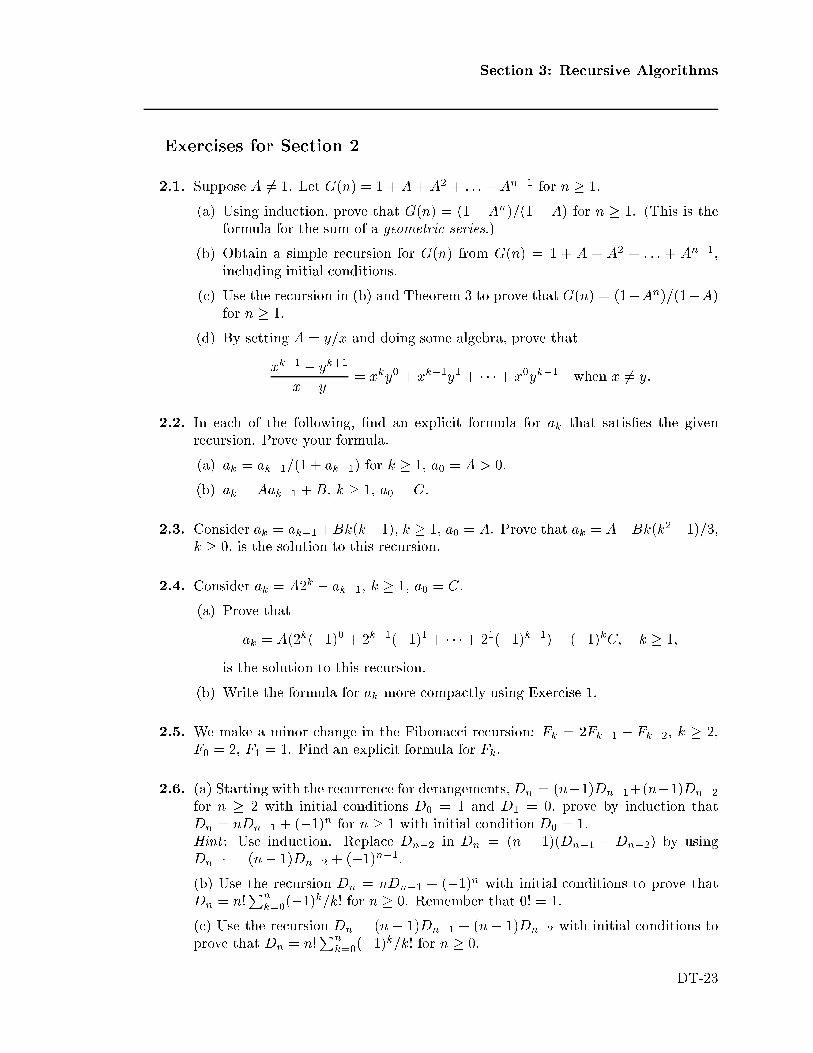
Exercises for Section 2
2.1. Suppose A 6= 1. Let G(n) = 1 +A+A2 + : : : +An�1 for n � 1.
(a) Using induction, prove that G(n) = (1� An)=(1� A) for n � 1. (This is theformula for the sum of a geometric series.)
(b) Obtain a simple recursion for G(n) from G(n) = 1 + A + A2 + : : : + An�1,including initial conditions.
(c) Use the recursion in (b) and Theorem 3 to prove that G(n) = (1�An)=(1�A)for n � 1.
(d) By setting A = y=x and doing some algebra, prove that
xk+1 � yk+1
x� y= xky0 + xk�1y1 + � � � + x0yk�1 when x 6= y.
2.2. In each of the following, �nd an explicit formula for ak that satis�es the givenrecursion. Prove your formula.
(a) ak = ak�1=(1 + ak�1) for k � 1, a0 = A > 0.
(b) ak = Aak�1 +B, k � 1, a0 = C.
2.3. Consider ak = ak�1+Bk(k�1), k � 1, a0 = A. Prove that ak = A+Bk(k2�1)=3,k � 0, is the solution to this recursion.
2.4. Consider ak = A2k � ak�1, k � 1, a0 = C.
(a) Prove that
ak = A(2k(�1)0 + 2k�1(�1)1 + � � � + 21(�1)k�1) + (�1)kC; k � 1;
is the solution to this recursion.
(b) Write the formula for ak more compactly using Exercise 1.
2.5. We make a minor change in the Fibonacci recursion: Fk = 2Fk�1 � Fk�2, k � 2,F0 = 2, F1 = 1. Find an explicit formula for Fk.
2.6. (a) Starting with the recurrence for derangements,Dn = (n�1)Dn�1+(n�1)Dn�2for n � 2 with initial conditions D0 = 1 and D1 = 0, prove by induction thatDn = nDn�1 + (�1)n for n � 1 with initial condition D0 = 1.Hint : Use induction. Replace Dn�2 in Dn = (n � 1)(Dn�1 + Dn�2) by usingDn�1 = (n� 1)Dn�2 + (�1)n�1.(b) Use the recursion Dn = nDn�1 + (�1)n with initial conditions to prove thatDn = n!
Pn
k=0(�1)k=k! for n � 0. Remember that 0! = 1.
(c) Use the recursion Dn = (n � 1)Dn�1 + (n� 1)Dn�2 with initial conditions toprove that Dn = n!
Pn
k=0(�1)k=k! for n � 0.
DT-23

Decision Trees and Recursion
Section 3: Recursive Algorithms
A recursive algorithm is an algorithm that refers to itself when it is executing. As with anyrecursive situation, when an algorithm refers to itself, it must be with \simpler" parame-ters so that it eventually reaches one of the \simplest" cases, which is then done withoutrecursion. Let's look at a couple of examples before we try to formalize this idea.
Example 14 (A recursive algorithm for 0-1 sequences) Suppose you are interestedin listing all sequences of length eight, consisting of four zeroes and four ones. Supposethat you have a friend who does this sort of thing, but will only make such lists if thelength of the sequence is seven or less. \Nope," he says, \I can't do it | the sequence istoo long." There is a way to trick your friend into doing it. First give him the problem oflisting all sequences of length seven with three ones. He doesn't mind, and gives you thelist 1110000, 1011000, 0101100, etc. that he has made. You thank him politely, sneak o�,and put a \1" in front of every sequence in the list he has given you to obtain 11110000,11011000, 10101100, etc. Now, you return to him with the problem of listing all strings oflength seven with four ones. He returns with the list 1111000, 0110110, 0011101, etc. Nowyou thank him and sneak o� and put a \0" in front of every sequence in the list he hasgiven you to obtain 01111000, 00110110, 00011101, etc. Putting these two lists together,you have obtained the list you originally wanted.
How did your friend produce these lists that he gave you? Perhaps he had a friendthat would only do lists of length 6 or less, and he tricked this friend in the same way youtricked him! Perhaps the \6 or less" friend had a \5 or less friend" that he tricked, etc. Ifyou are sure that your friend gave you a correct list, it doesn't really matter how he gotit.
Next we consider an example from sorting theory. We imagine we are given a setof objects which have a linear order described on them (perhaps, but not necessarily,lexicographic order of some sort). As a concrete example, we could imagine that we aregiven a set of integers S, perhaps a large number of them. They are not in order as presentedto us, be we want to list them in order, smallest to largest. That problem of putting theset S in order is called sorting S. On the other hand, if we are given two ordered lists,like (25; 235; 2333; 4321) and (21; 222; 2378; 3421; 5432), and want to put the combined listin order, in this case (21; 25; 222; 235; 2333; 2378; 3421; 4321; 5432), this process is calledmerging the two lists. Our next example considers the relationship between sorting andmerging.
Example 15 (Sorting by recursive merging) Sorting by recursive merging, calledmerge sorting, can be described as follows.
� The lists containing just one item are the simplest and they are already sorted.
� Given a list of n > 1 items, choose k with 1 � k < n, sort the �rst k items, sort thelast n� k items and merge the two sorted lists.
DT-24

Section 3: Recursive Algorithms
This algorithm builds up a way to sort an n-list out of procedures for sorting shorter lists.Note that we have not speci�ed how the �rst k or last n � k items are to be sorted, wesimply assume that it has been done. Of course, an obvious way to do this is to simplyapply our merge sorting algorithm to each of these sublists.
Let's implement the algorithm using people rather than a computer. Imagine traininga large number of obedient people to carry out two tasks: (a) splitting a list for otherpeople to sort and (b) merging two lists. We give one person the unsorted list and tell himto sort it using the algorithm and return the result to us. What happens?
� Anyone who has a list with only one item returns it unchanged to the person he receivedit from.
� Anyone with a list having more than one item splits it and gives each piece to a personwho has not received a list, telling each person to sort it and return the result. Whenthe results have been returned, this person merges the two lists and returns the resultto whoever gave him the list.
If there are enough obedient people around, we'll eventually get our answer back.
Notice that no one needs to pay any attention to what anyone else is doing to a list.This is makes a local description possible; that is, we tell each person what to do and theydo not need to concern themselves with what other people are doing. This can also be seenin the pseudocode for merge sorting a list L:
Sort(L)If length is 1, return LElse
Split L into two lists L1 and L2S1 = Sort(L1)S2 = Sort(L2)S = Merge(L1, L2)Return S
End ifEnd
The procedure is not concerned with what goes on when it calls itself recursively. Thisis very much like proof by induction. To see that, let's prove that the algorithm sortscorrectly. We assume that splitting and merging have been shown to be correct | that'sa separate problem. We induct on the length n of the list. The base case, n = 1 is handledcorrectly by the program since it returns the list unchanged. Now for induction. SplittingL results in shorter lists and so, by the induction hypothesis, S1 and S2 are sorted. Sincemerging is done correctly, S is also sorted.
This algorithm is another case of divide and conquer since it splits the sorting probleminto two smaller sorting problems whose answers are combined (merged) to obtain thesolution to the original sorting problem.
Let's summarize some of the above observations with two de�nitions.
De�nition 3 (Recursive approach) A recursive approach to a problem consists of two
parts:
DT-25

Decision Trees and Recursion
1. The problem is reduced to one or more problems of the same kind which are simpler
in some sense.
2. There is a set of simplest problems to which all others are reduced after one or more
steps. Solutions to these simplest problems are given.
The preceding de�nition focuses on tearing down (reduction to simpler cases). Sometimesit may be easier or better to think in terms of building up (construction of bigger cases):
De�nition 4 (Recursive solution) We have a recursive solution to the problem (proof,
algorithm, data structure, etc.) if the following two conditions hold.
1. The set of simplest problems can be dealt with (proved, calculated, sorted, etc.).
2. The solution to any other problem can be built from solutions to simpler problems,
and this process eventually leads back to the original problem.
The recursion C(n; k) = C(n� 1; k � 1) +C(n; k) for computing binomial coeÆcientscan be viewed as a recursive algorithm, as can any of the examples in Section 2. Suchalgorithms for computing can be turned into algorithms for constructing. Let's do this forderangements.
Example 16 (Constructing derangements) You should review the derivation of therecursion Dn = (n� 1)Dn�1 + (n� 1)Dn�2 in Example 12. The derivation told us how toconstruct derangements of an n-set from derangements of smaller sets. Here is the algorithmit gives. Given a set S, D(S) should provide a list of the derangements of S in cycle form.
D(S)If jSj = 1, return the empty list.If jSj = 2, return the list containing the single derangement (x; y).If jSj > 2
(a) Choose x 2 S and let T = S n fxg.(b) Construct a list using D(T ).
For each derangement in the list from D(T ), generate jT jderangements by inserting x in all possible positions in cycle form.
(c) For all y 2 T :Construct a list using D(T n fyg).To each derangement in the list, add the cycle (x; y).
(d) Return the list of all derangements produced in (b) and (c).Endif
End
Suppose we call D(f1; 2; 3; 4g). Since jf1; 2; 3; 4gj = 4 > 2, we choose, in (a), an x, sayx = 2. We now call D(f1; 3; 4g) in (b). Assuming everything is working correctly, that willreturn the list containing the two derangements
(1; 3; 4) (1; 4; 3)
The insertions in (b) give us the list
(1; 2; 3; 4) (1; 3; 2; 4) (1; 3; 4; 2) (1; 2; 4; 3) (1; 4; 2; 3) (1; 4; 3; 2):
DT-26

Section 3: Recursive Algorithms
In (c) we consider all y 2 f1; 3; 4g. We'll just look at one, say y = 3. ThenD(T nf3g) returnsthe list containing the single derangement (1,4). We add to this the cycle (x; y) = (2; 3),obtaining (1,4)(2,3). For y = 1 we obtain (3,4)(1,2). For y = 4 we obtain (1,3)(2,4). Thus,we've obtained all 9 derangements of f1; 2; 3; 4g.
The discussion at the end of the last example can be a bit confusing. We need a moresystematic way to think about recursive algorithms. In the next example we introduce atree to represent the local description of a recursive algorithm.
Example 17 (Permutations in lex order) The following �gure represents the local
description of a decision tree for listing the permutation of an ordered set
S = fs1; s2; : : : ; sng :The vertices of this decision tree are of the form L(X) where X is some set. The simplestcase, shown below, is where the tree has one edge. The labels on the edges are of the form(t), where t is an element of the X associated with the uppermost vertex L(X) incident onthat edge.
L({s})
(s)
L(S)
S = { }s1 sns2, , ,. . .
. . .
s1( ) s2( ) sn( )
S { }s2L( )S { }s1L( ) S L( ){ }sn
One way to think of the local description is to regard it as a rule for recursivelyconstructing and entire decision tree, once the set S is speci�ed. Here this construction hasbeen carried out for S = f1; 2; 3; 4g.
(1)
(1)(1)(1)
(2)
(2)(2)(2)
(3)
(3)(3)(3)
(3)
(4)
(4)(4)(4)
(4) (2) (4) (2) (4)(2) (3) (2) (3)(3) (4) (1) (4) (1) (4) (1) (3)(1) (2) (1) (2)(1) (3)
L(1,2,3,4)
L(2,3,4)
L(3,4)L(3,4) L(2,4)L(2,4) L(2,3)L(2,3)
L(1,3,4)
L(1,3)L(1,3) L(1,4)L(1,4)
L(1,2,4) L(1,2,3)
L(1,2)L(1,2)
L(1)L(1)L(1)L(1)L(1)L(1) L(2)L(2)L(2)L(2)L(2)L(2)L(3) L(3)L(3)L(3)L(3)L(3) L(4)L(4)L(4)L(4)L(4)L(4)
To obtain a permutation of 4, read the labels (t) on the edges from the root to a particularleaf. For example the if this is done for the preorder �rst leaf, one obtains (1)(2)(3)L(4).
DT-27

Decision Trees and Recursion
L(4) is a \simplest case" and has the label (4), giving the permutation 1234 in one linenotation. Repeating this process for the leaves from left to right (in preorder on the leaves)gives the list of permutations of 4 in lex order.
We'll use induction to prove that this is the correct tree. When n = 1, it is clear.Suppose it is true for all S with cardinality less than n. The permutations of S in lexorder are those beginning with s1 followed by those beginning with s2 and so on. If sk isremoved from those permutations of S beginning with sk, what remains is the permutationsof S�fskg in lex order. By the induction hypothesis, these are given by L(S�fskg). Notethat the validity of our proof does not depend on how they are given by L(S � fskg).
No discussion of recursion would be complete without the entertaining example of theTowers of Hanoi puzzle. We shall explore additional aspects of this problem in the exercises.Our approach will be the same as the previous example. We shall give a local descriptionof the recursion. Having done so, we construct the trees for some examples and try to gaininsight into the sequence of moves associated with the general Towers of Hanoi problem.
Example 18 (Towers of Hanoi) The Towers of Hanoi puzzle consists of n di�erentsized washers (i.e., discs with holes in their centers) and three poles. Initially the washersare stacked on one pole as shown below.
S E G
S E G
S E G
(a)
(b)
(c)
The object is to switch all of the washers from the pole S to G using pole E as a placefor temporary placement of discs. A legal move consists of taking the top washer from apole and placing on top of the pile on another pole, provided it is not placed on a smallerwasher. Con�guration (a), above, is the starting con�guration, (b) is an intermediate stage,and (c) is illegal.
Here is a recursive description of how to solve the Towers of Hanoi. To move thelargest washer, we must move the other n� 1 to the spare peg. After moving the largest,we can then move the other n� 1 on top of it. Let the washers be numbered 1 to n fromsmallest to largest. When we are moving any of the washers 1 through k, we can ignorethe presence of all larger washers beneath them. Thus, moving washers 1 through n � 1from one peg to another when washer n is present uses the same moves as moving themwhen washer n is not present. Since the problem of moving washers 1 through n � 1 issimpler, we practically have a recursive description of a solution. All that's missing is the
DT-28

Section 3: Recursive Algorithms
observation that the simplest case, n = 1, is trivial. The following diagram gives the localdescription of a decision tree that represents this recursive algorithm.
H(n, S, E, G)
H(n-1, E, S, G) H(n-1, S, G, E)
H(1, S, E, G)
S G1
S Gn
The \simplest case," n equal 1 is shown on the left. The case for general n is designatedby H(n, S, E, G). You can think of the symbol H(n, S, E, G) as designating a vertex of adecision tree. The local description tells you how to construct the rest of the decision tree,down to and including the simplest cases. All leaves of the decision tree are designated by
symbols of the form \Xk! Y ." This symbol has the interpretation \move washer number
k from pole X to pole Y ." These leaves in preorder (left to right order in the tree) give thesequence of moves needed to solve the Towers of Hanoi puzzle. The local description tellsus that, in order to list the leaves of H(n, S, E, G), we
� list the leaves of H(n-1, S, G, E), moving the top n-1 washers from S to E using G
� move the largest washer from S to G
� list the leaves of H(n-1, E, S, G), moving the top n-1 washers from E to G using S
For example, the leaves of the tree with root H(2,S,E,G) are, in order,
S1! E; S
2! G; E1! G:
The leaves of H(3,S,E,G) are gotten by concatenating (piecing together) the leaves of
the subtree rooted at H(2,S,G,E) with S3! G and the leaves of the subtree rooted at
H(2,E,S,G). This gives
S1! G, S
2! E, G1! E, S
3! G, E1! S, E
2! G, S1! G.
How many moves does the algorithm take? In other words, how many leaves does thetree have? The local description immediately gives us a recursion! Let hn be the numberof moves. Simply replace H(n,� � �) with hn and leaves with 1. The local tree for H(1,S,E,G)gives us h1 = 1. The local tree for H(n,S,E,G) gives us hn = hn�1 + 1+ hn�1. You shoulduse this to prove that hn = 2n � 1.
Example 19 (The Towers of Hanoi decision tree for n = 4) Starting with the localdescription of the general decision tree for the Towers of Hanoi and applying the rules ofconstruction speci�ed by it, we obtain the decision tree for the Towers of Hanoi puzzle withn = 4.
DT-29
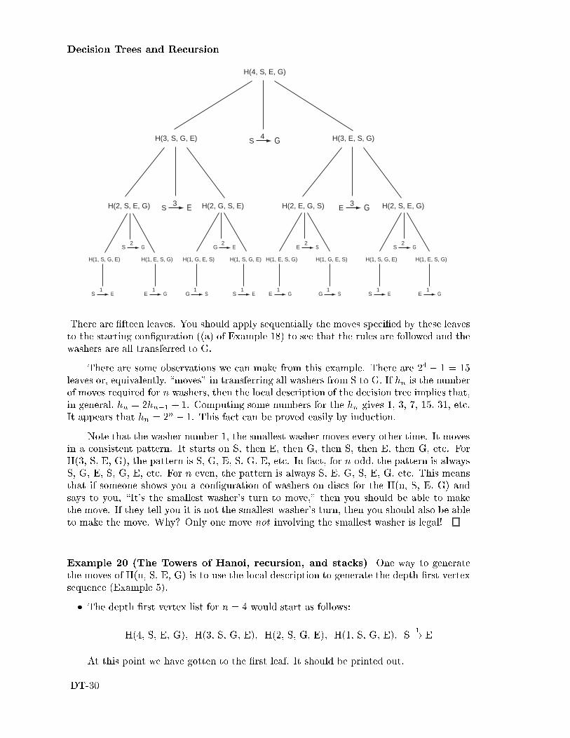
Decision Trees and Recursion
H(4, S, E, G)
H(3, E, S, G) H(3, S, G, E) S G4
H(2, G, S, E) H(2, S, E, G) S E3 H(2, S, E, G) H(2, E, G, S) E G3
H(1, E, S, G)
E G1
H(1, G, E, S)
G S1
H(1, S, G, E)
S E1
H(1, E, S, G)
E G1
S G2
G E2
E S2
S G2
H(1, S, G, E)
S E1
H(1, G, E, S)
G S1
H(1, E, S, G)
E G1
H(1, S, G, E)
S E1
There are �fteen leaves. You should apply sequentially the moves speci�ed by these leavesto the starting con�guration ((a) of Example 18) to see that the rules are followed and thewashers are all transferred to G.
There are some observations we can make from this example. There are 24 � 1 = 15leaves or, equivalently, \moves" in transferring all washers from S to G. If hn is the numberof moves required for n washers, then the local description of the decision tree implies that,in general, hn = 2hn�1 + 1. Computing some numbers for the hn gives 1, 3, 7, 15, 31, etc.It appears that hn = 2n � 1. This fact can be proved easily by induction.
Note that the washer number 1, the smallest washer moves every other time. It movesin a consistent pattern. It starts on S, then E, then G, then S, then E, then G, etc. ForH(3, S, E, G), the pattern is S, G, E, S, G, E, etc. In fact, for n odd, the pattern is alwaysS, G, E, S, G, E, etc. For n even, the pattern is always S, E, G, S, E, G, etc. This meansthat if someone shows you a con�guration of washers on discs for the H(n, S, E, G) andsays to you, \It's the smallest washer's turn to move," then you should be able to makethe move. If they tell you it is not the smallest washer's turn, then you should also be ableto make the move. Why? Only one move not involving the smallest washer is legal!
Example 20 (The Towers of Hanoi, recursion, and stacks) One way to generatethe moves of H(n, S, E, G) is to use the local description to generate the depth �rst vertexsequence (Example 5).
� The depth �rst vertex list for n = 4 would start as follows:
H(4, S, E, G), H(3, S, G, E), H(2, S, G, E), H(1, S, G, E), S1! E
At this point we have gotten to the �rst leaf. It should be printed out.
DT-30

Section 3: Recursive Algorithms
� The next vertex in the depth �rst vertex sequence is H(1, S, G, E) again. We represent
this by removing S1! E to get
H(4, S, E, G), H(3, S, G, E), H(2, S, G, E), H(1, S, G, E).
� Next we remove H(1, S, G E) to get
H(4, S, E, G), H(3, S, G, E), H(2, S, G, E).
� The next vertex in depth �rst order is S2! G. We add this to our list to get
H(4, S, E, G), H(3, S, G, E), H(2, S, G, E), S2! G.
Continuing in this manner we generate, for each vertex in the decision tree, the path fromthe root to that vertex. The vertices occur in depth �rst order. Computer scientists referto the path from the root to a vertex v as the stack of v. Adding a vertex to the stackis called pushing the vertex on the stack. Removing a vertex is popping the vertex fromthe stack. Stack operations of this sort re ect how most computers carry out recursion.This \one dimensional" view of recursion is computer friendly, but the geometric pictureprovided by the local tree is more people friendly.
Example 21 (The Towers of Hanoi con�guration analysis) In the �gure below, weshow the starting con�guration for H(6, S, E, G) and a path,
H(6, S, E, G), 6H(5, E, S, G), H(4, E, G, S), H(3, G, E, S), G3! S.
This path goes from the root H(6, S, E, G) to the leaf G3! S. Given this path, we want to
construct the con�guration of washers corresponding to that path, assuming that the move
G3! S has just been carried out. This is also shown in the �gure and we now explain how
we obtained it.
H(6, S, E, G)
H(5,E, S, G)
H(4, E, G, S)
H(3, G, E, S)
G S35
34 6
12
S E G
56
34
12
4 5 6
S E G
31
2
6
S E G5
34
12
6
S E G5
34
12
S E G
MOVE JUST MADE
STARTING CONFIGURATION
ENDING CONFIGURATION
1 Leaf
1 Leaf5h Leaves
RANK 43NUMBER 44
3h Leaves
2h Leaves
DT-31

Decision Trees and Recursion
The �rst part of the path shows what happens when we use the local tree for H(6,S,E,G).Since we are going to H(5,E,S,G), the �rst edge of the path \slopes down to the right."At this point, the left edge, which led to H(5,S,G,E) moved washers 1 to 5 to pole E using
h5 = 25 � 1 = 31 moves and move S6! G has moved washer 6. This is all shown in the
�gure and it has taken 31 + 1 = 32 moves.
Next, one replaces H(5,E,S,G) with the local tree (being careful with the S, E, Glabels!). This time the path \slopes to the left". Continuing in this manner we completethe entire path and have the con�guration that is reached.
We can compute the rank of this con�guration by noticing how many moves were
made to reach it. Each move, except our �nal one G3! S, is a leaf to the left of the leaf
corresponding to the move G3! S at the end of the path. We can see from the �gure that
there were(h5 + 1) + 0 + (h3 + 1) + h2 = (31 + 1) + (7 + 1) + 3 = 43
such moves and so the rank of this con�guration is 43.
You should study this example carefully. It represents a very basic way of studyingrecursions. In particular,
� you should be able to do the same analysis for a di�erent path,
� you should be able to start with an ending con�guration and reconstruct the path,and
� you should be able to start with a con�guration and, by attempting to reconstructthe path (and failing), be able to show that the con�guration is illegal (can neverarise).
We conclude this section with another \canonical" example of recursive algorithm anddecision trees. We want to look at all subsets of n. It will be more convenient to workwith the representation of subsets by functions with domain n and range f0; 1g. In oneline notation, these functions become n-strings of zeroes and ones: The string s1 : : : sncorresponds to the subset S where i 2 S if and only if si = 1. Thus the all zeroes stringcorresponds to the empty set and the all ones string to n. This correspondence is calledthe characteristic function interpretation of subsets of n.
Our goal is to make a list of all subsets of n such that subsets adjacent to each other inthe list are \close" to each other. Before we can begin to look for such a Gray code, we mustsay what it means for two subsets (or, equivalently, two strings) to be close. Two stringswill be considered close if they di�er in exactly one position. In set terms, this means oneof the sets can be obtained from the other by removing or adding a single element. Withthis notion of closeness, a Gray code for all subsets when n = 1 is 0; 1. A Gray code forall subsets when n = 2 is 00; 01; 11; 10.
How can we produce a Gray code for all subsets for arbitrary n? There is a simplerecursive procedure. The following construction of the Gray code for n = 3 illustrates it.
0 00 1 100 01 1 110 11 1 010 10 1 00
DT-32

Section 3: Recursive Algorithms
You should read down the �rst column and then down the second. Notice that the sequencesin the �rst column begin with 0 and those in the second with 1. The rest of the �rst columnis simply the Gray code for n = 2 while the second column is the Gray code for n = 2, readfrom the last sequence to the �rst.
We now prove that this two column procedure for building a Gray code for subsets ofan n-set from the Gray code for subsets of an (n� 1)-set always works. Our proof will beby induction. For n = 1, we have already exhibited a Gray code. Suppose that n > 1 andthat we have a Gray code for n� 1. (This is the induction assumption.)
� Between the bottom of the �rst column and the top of the second, the only changeis in the �rst position since the remaining n � 1 positions are the last element of ourGray code for n� 1.
� Within a column, there is never any change in the �rst position and there is only asingle change from line to line in the remaining positions because they are a Gray codeby the induction assumption.
This completes the proof.
As an extra bene�t, we note that the last element of our Gray code di�ers in only oneposition from the �rst element (Prove it!), so we can cycle around from the last element tothe �rst by a single change.
Example 22 (Decision tree for the subset Gray code) Here is another notation for
describing our subset Gray code. Let����!GRAY(1) = 0; 1, and let
����GRAY(1) = 1; 0. As the
arrows indicate,����!GRAY(1) is the Gray code for n = 1 listed from �rst to last element, while ����
GRAY(1) is this Gray code in reverse order. In general, if����!GRAY(n) is the Gray code for
n-bit words, then ����GRAY(n) is de�ned to be that list in reverse order.
We de�ne����!GRAY(2) = 0
����!GRAY(1); 1
����GRAY(1):
The meaning of 0����!GRAY(1) is that 0 is put at the front of every string in
����!GRAY(1).
Juxtaposing the two lists (or \concatenation") means just listing the second list after the
�rst. Thus, 0����!GRAY(1) = 00; 01, and 1
����GRAY(1) = 11; 10. Hence,
����!GRAY(2) = 0
����!GRAY(1); 1
����GRAY(1) = 00; 01; 10; 11 :
If we read����!GRAY(2) in reverse order, we obtain
����GRAY(2). You should verify the following
equality. ����GRAY(2) = 1
����!GRAY(1); 0
����GRAY(1):
What we did for n = 2 works in general: The following diagram gives the local de-scription of a decision tree for constructing subset Gray codes:
DT-33
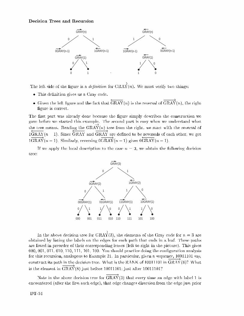
Decision Trees and Recursion
GRAY(n)
0GRAY(n-1) 1GRAY(n-1)
10
0
GRAY(1)
1 0
0
GRAY(1)
1
1 1
0
1GRAY(n-1)
GRAY(n)
0GRAY(n-1)
1 0
The left side of the �gure is a de�nition for����!GRAY(n). We must verify two things:
� This de�nition gives us a Gray code.
� Given the left �gure and the fact that ����GRAY(n) is the reversal of
����!GRAY(n), the right
�gure is correct.
The �rst part was already done because the �gure simply describes the construction wegave before we started this example. The second part is easy when we understand what
the tree means. Reading the����!GRAY(n) tree from the right, we start with the reversal of
1 ����GRAY(n� 1). Since
����GRAY and
����!GRAY are de�ned to be reversals of each other, we get
1����!GRAY(n� 1). Similarly, reversing 0
����!GRAY(n� 1) gives 0
����GRAY(n� 1).
If we apply the local description to the case n = 3, we obtain the following decisiontree:
00GRAY(1) 01GRAY(1)
10
11GRAY(1) 10GRAY(1)
1 0
GRAY(3)
0GRAY(2) 1GRAY(2)
10
10 1 0 10 1 0
000 001 011 010 110 111 101 100
In the above decision tree for����!GRAY(3), the elements of the Gray code for n = 3 are
obtained by listing the labels on the edges for each path that ends in a leaf. These pathsare listed in preorder of their corresponding leaves (left to right in the picture). This gives000, 001, 011, 010, 110, 111, 101, 100. You should practice doing the con�guration analysisfor this recursion, analogous to Example 21. In particular, given a sequence, 10011101 say,
construct its path in the decision tree. What is the RANK of 10011101 in����!GRAY(8)? What
is the element in����!GRAY(8) just before 10011101; just after 10011101?
Note in the above decision tree for����!GRAY(3) that every time an edge with label 1 is
encountered (after the �rst such edge), that edge changes direction from the edge just prior
DT-34

Section 3: Recursive Algorithms
to it in the path. By \changing direction," we mean that if an edge is sloping downwardto the right (downward to the left) and the previous edge in the path sloped downwardto the left (downward to the right), then a change of direction has occurred. Conversly,every time an edge with label 0 is encountered (after the �rst such edge), that edge doesnot change direction from the edge just prior to it in the path. This is a general rule thatcan be proved by induction.
Exercises for Section 3
3.1. Suppose the permutations on 8 are listed in lexicographic order.
(a) What is the RANK in the list of all such permutations of 87612345?
(b) What permutation has RANK 20,160?
3.2. Consider the Towers of Hanoi puzzle, H(8, S, E, G). Suppose that pole S has washers6, 5, 2, 1; pole E has no washers; pole G has washers 8, 7, 4, 3. Call this the basiccon�guration.
(a) What is the path in the decision tree that corresponds to the basic con�gura-tion?
(b) What was the move that produced the basic con�guration and what was thecon�guration from which that move was made?
(c) What was the move just prior to the one that produced the basic con�gurationand what was the con�guration from which that move was made?
(d) What will be the move just after the one that produced the basic con�guration?
(e) What is the RANK, in the list of all moves of H(8, S, E, G), of the move thatproduced the basic con�guration?
3.3. Consider����!GRAY(9).
(a) What is the element just before and just after 110010000?
(b) What is the �rst element of the second half of the list?
(c) What is the RANK of 111111111?
(d) What is the element of RANK 372?
3.4. Consider the Towers of Hanoi puzzle with four poles and n washers. The rulesare the same, except that there are two \extra" poles E and F. The problem is totransfer all of the n washers from S to G using the extra poles E and F as temporarystorage. Let h0n denote the optimal number of moves needed to solve the three poleproblem. Let fn denote the optimal number of moves needed to solve the four poleproblem with n washers.
DT-35

Decision Trees and Recursion
(a) Recall that hn = 2n � 1 is the number of moves in the recursive algorithmH(n, S, E, G). Prove by induction that h0n = hn.
(b) Compute fn for n = 1; 2; 3, describing, in the process, optimal sequences ofmoves.
Let's adopt a speci�c strategy for doing four poles and n washers. Choose integersp � 0 and q > 0 so that p+ q = n. We now describe strategy G(p, q, S, E, F, G).To execute G(p, q, S, E, F, G), proceed as follows:
(i) If p = 0, then q = n. Use H(n, S, E, G) to move washers 1; : : : ; n to G.
(ii) If p > 0, choose integers i � 0 and j > 0 such that i + j = p. UseG(i, j, S, E, G, F) to move washers 1; 2; : : : ; p to pole F (the washers are num-bered in order of size). Next, use H(q, S, E, G) to move washers q; : : : ;n to G.Finally, use G(i, j, F, S, E, G) to move 1; 2; : : : ; p to pole G, completing thetransfer. For all possible choices of i and j, choose the one that minimizes thenumber of moves.
Finally, to move the n washers, choose that G(p, q, S, E, F, G) with n = p + q
which has the minimum number of moves. Call this number sn.
(c) What are the simplest cases in this recursive algorithm? How can you computethe values of i and j to minimize the number of moves? Use your method tosolve the problem for n � 6.
(d) What is the recursion for sn?
(e) Prove that fn � 2min(fn�q + hq), where the minimum is over q > 0 andf0 = 0. recursion.
Section 4: Decision Trees and Conditional Probability
We conclude our discussion of decision trees by giving examples of the use of decision treesin elementary probability theory. In particular, we focus on what are called conditional
probabilities and Bayesian methods in probability.
De�nition 5 (Conditional probability) Let U be a sample space with probability
function P . If A � U and B � U are events (subsets) of U then the conditional probabililty
of B given A, denoted by P (BjA), is
P (BjA) =�P (A \B)=P (A); if P (A) 6= 0,unde�ned; if P (A) = 0.
How should we interpret P (BjA)? If an experiment is performed n times and b of thosetimes B occurs, then b=n is nearly P (B). Furthermore, as n increases, the ratio b=n almostsurely approaches P (B) as a limit. For example, we might toss fair coin 100 times andobtain 55 heads, so a=n; = 55=100 is nearly 1=2 = P (head). With 10,000 tosses, we mightobtain 4,930 heads and 4,930/10,000 is even closer to 1/2 than 55/100. (This is the sort of
DT-36

Section 4: Decision Trees and Conditional Probability
accuracy one might realistically expect.) Now suppose an experiment is performed n timesbut we are only interested in those times when A occurs. Furthermore, suppose we wouldlike to know the chances that B occurs, given that A has occurred. Let the count for Abe a and that for A \ B be c. Since we are interested only in the cases when A occurs,only a of the experiments matter. In these a experiments, B occurred c times. Hence theprobability that B occurs given that A has occurred is approximately c=a = (c=n)=(a=n),which is approximately P (A\B)=P (A), which is the de�nition of P (BjA). As n increases,the approximations almost surely approach P (BjA). Hence
P (BjA) should be thought of as the probability thatB occurred,given that we know A occurred.
The following theorem contains some simple but important properties of conditional prob-ability.
Theorem 5 (Properties of conditional probability) Let (U;P ) be a probability
space. All events in the following statements are subsets of U and the conditional proba-
bilities are assumed to be de�ned. (Recall that P (CjD) is unde�ned when P (D) = 0.)
(a) P (BjU) = P (B) and P (BjA) = P (A \B j A).(b) A and B are independent events if and only if P (BjA) = P (B).
(c) (Bayes' Theorem) P (AjB) = P (BjA)P (A)=P (B).(d) P (A1 \ � � � \An) = P (A1)P (A2 j A1)P (A3 j A1 \A2) � � �P (An j A1 \ � � � \An�1).
You can think of (b) as a justi�cation for the terminology \independent" since P (BjA) =P (B) says that the probability of B having occurred is unchanged even if we know that Aoccurred; in other words, A does not in uence B's chances. We will encounter other formsof Bayes' Theorem. All of them involve reversing the order in conditional probabilities.(Here, AjB and BjA.)
Proof: All the proofs are simple applications of the de�nition of conditional probability,so we prove just (b) and (d) and leave (a) and (c) as exercises.
We prove (b). Suppose A and B are independent. By the de�nition of independence,this means that P (A \ B) = P (A)P (B). Dividing both sides by P (A) and using thede�nition of conditional probability, we obtain P (BjA) = P (B). For the converse, supposeP (BjA) = P (B). Using the de�nition of conditional probability and multiplying by P (A),we obtain P (A \B) = P (A)P (B), which is the de�nition of independence.
We prove (d) simply by using the de�nition of conditional probability and doing a lotof cancellation of adjacent numerators and denominators:
P (A1)P (A2 j A1)P (A3 j A1 \A2) � � �P (An j A1 \ � � � \An�1)
= P (A1)P (A2 \A1)
P (A1)
P (A1 \A2 \A3)
P (A1 \A2)� � � P (A1 \ � � � \ An)
P (A1 \ � � � \An�1)= P (A1 \ � � � \An):
This completes the proof.
DT-37
Decision Trees and Recursion
An alternative proof of (d) can be given by induction on n. For n = 1, (d) becomesP (A1) = P (A1), which is obviously true. For n > 1 we have
P (A1)P (A2 j A1) � � �P (An�1 j A1 \ � � � \An�2)P (An j A1 \ � � � \An�1)
=�P (A1)P (A2 j A1) � � �P (An�1 j A1 \ � � � \An�2)
�P (An j A1 \ � � � \An�1)
= P (A1 \ � � � \An�1)P (An j A1 \ � � � \ An�1) by induction
= P (A1 \ � � � \An) De�nition 5.
This completes the proof.
Example 23 (Diagnosis and Bayes' Theorem) Suppose we are developing a test tosee if a person has a disease, say the dreaded wur es. It's known that 1 person in about500 has the wur es. To measure the e�ectiveness of the test, we tried it on a lot of people.Of the 87 people with wur es, the test always detected it, so we decide it is 100% e�ectiveat detection. We also tried the test on a large number of people who do not have wur esand found that the test incorrectly told us that they have wur es 3% of the time. (Theseare called \false positives.")
If the test is released for general use, what is the probability that a person who testspositive actually has wur es?
Let's represent our information mathematically. Our probability space will be thegeneral population with the uniform distribution. The event W will correspond to havingwur es and the event T will correspond to the test being positive. Our information can bewritten
P (W ) = 1=500 = 0:002 P (T jW ) = 1 P (T jW c) = 0:03;
and we are asked to �nd P (W jT ). Bayes' formula (Theorem 5(c)) tells us
P (W jT ) = P (T jW )P (W )
P (T ):
Everything on the right is known except P (T ). How can we compute it? The idea is topartition T using W and then convert to known conditional probabilities:
P (T ) = P (T \W ) + P (T \W c) partition T
= P (T jW )P (W ) + P (T jW c)P (W c) convert to conditional
= 1� 0:002 + 0:03� (1� 0:002) � 0:032;
where we have rounded o�. Thus P (W jT ) � 1� 0:002=0:032 � 6%: In other words, even ifthe test is positive, you only have a 6% chance of having wur es. This shows how misleadinga rather accurate test can be when it is used to detect a rare condition.
DT-38
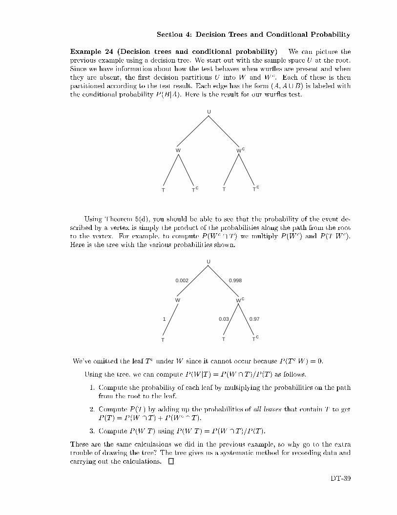
Section 4: Decision Trees and Conditional Probability
Example 24 (Decision trees and conditional probability) We can picture theprevious example using a decision tree. We start out with the sample space U at the root.Since we have information about how the test behaves when wur es are present and whenthey are absent, the �rst decision partitions U into W and W c. Each of these is thenpartitioned according to the test result. Each edge has the form (A;A[B) is labeled withthe conditional probability P (BjA). Here is the result for our wur es test.
U
W
TT
Wc
TcTc
Using Theorem 5(d), you should be able to see that the probability of the event de-scribed by a vertex is simply the product of the probabilities along the path from the rootto the vertex. For example, to compute P (W c \ T ) we multiply P (W c) and P (T jW c).Here is the tree with the various probabilities shown.
U
W
TT
Wc
Tc
0.002 0.998
0.03 0.971
We've omitted the leaf T c under W since it cannot occur because P (T cjW ) = 0.
Using the tree, we can compute P (W jT ) = P (W \ T )=P (T ) as follows.1. Compute the probability of each leaf by multiplying the probabilities on the path
from the root to the leaf.
2. Compute P (T ) by adding up the probabilities of all leaves that contain T to getP (T ) = P (W \ T ) + P (W c \ T ).
3. Compute P (W jT ) using P (W jT ) = P (W \ T )=P (T ).These are the same calculations we did in the previous example, so why go to the extratrouble of drawing the tree? The tree gives us a systematic method for recording data andcarrying out the calculations.
DT-39

Decision Trees and Recursion
In the previous example, each vertex was speci�cally labeled with the event, such asW \ T c, associated with it. In the next example, we simply keep track of the informationwe need to compute our answer.
Example 25 (Another decision tree with probabilities) We are given an urn withone red ball and one white ball. A fair die is thrown. If the number is 1, then 1 red balland 2 white balls are added to the urn. If the number is 2 or 3, then 2 red balls and 3white balls are added to the urn. If the number is 4, 5, or 6, then 3 red balls and 4 whiteballs are added to the urn. A ball is then selected uniformly at random from the urn. Werepresent the situation in the following decision tree.
[1R, 1W]
[2R, 3W]
[3R, 3W] [3R, 5W] [4R, 4W][2R, 4W][2R, 2W][1R, 3W]
[3R, 4W] [4R, 5W]
RRR WWW
1/6 1/3 1/2
2/5
1/15 1/10 1/7 4/21 5/182/9
3/5 3/7 4/7 4/9 5/9
{1} {2,3} {4,5,6}
The root is represented by the initial composition of the urn. The children of the root[1R; 1W] are [2R; 3W], [3R; 4W], and [4R; 5W]. Beside each of these children of the rootis the outcome set of the roll of the die that produces that urn composition: f1g, f2; 3g,f4; 5; 6g. The probabilities on the edges incident on the root are the probabilities of theoutcome sets of the die. The probabilities on the edges incident on the leaves are theconditional probabilites as discussed in Example 24. Thus, 3=7 is the conditional probabilitythat the �nal outcome is R, given that the outcome of the die was in the set f2; 3g.
Here is a typical sort of question asked about this type of probabilistic decision tree:\Given that the ball drawn was red, what is the probability that the outcome of the die wasin the set f2; 3g." We could write this mathematically as P (f2; 3g j R), where f2; 3g repre-sents the result of rolling the die and R represents the result of the draw. Note in this processthat the basic data given are conditional probabilities of the form P (drawing is R j die in S).We are computing conditional probabilities of the form P (die roll in S j drawing is R). Thisis exactly the same situation as in Example 24. Thus our question is answered by carryingout the three steps in Example 24:
1. Compute the probabilities of the leaves. The results are shown in the picture ofthe decision tree.
2. Add up the probabilities of all leaves resulting from the drawing of a red ball toobtain P (R) = 1=15 + 1=7 + 2=9 = 136=315.
3. Compute the conditional probability P (f2; 3g j R) by dividing P (f2; 3g \ R) =1=7 by P (R). Divide this into the answer from part (1). In this case, we get(1=7)=(136=315) = 0:331.
If you wish, you can think of this problem in terms of a new sample space. Theelements of the sample space are the leaves. Step 1 (multiplying probabilities along paths)
DT-40

Section 4: Decision Trees and Conditional Probability
computes the probability function for this sample space. Since an event is a subset of thesample space, an event is a set of leaves and its probability is the sum of the probabilitiesof the leaves it contains. Can we interpret the nonleaf vertices? Yes. Each such vertexrepresents an event that consists of the set of leaves below it. Many people prefer thisalternative way of thinking about the decision tree.
The procedure we used to compute conditional probabilities in Steps 1 to 3 of twoprevious examples can be stated as a formula, which is another form of Bayes' Theorem:
Theorem 6 (Bayes' Theorem) Let (U;P ) be a probability space, let
fAi : i = 1; 2; : : : ; ng be a partition of U , and let B � U . Then
P (AijB) =P (Ai)P (BjAi)Pn
t=1 P (At)P (BjAt):
Most students �nd decision trees much easier to work with than trying to apply the formalstatement of Bayes' theorem.
Proof: We can draw a decision tree like the ones in the previous examples, but now thereare n edges of the decision tree coming down from the root and 2 edges coming down fromeach child of the root. Here is a decision tree for this generalization:
A1 A2 A i A n
A iP( ) A nP( )A2P( )A1P( )
U
A iP(B| ) A iP(~B| )
i BAP( ) P( ) iA ~B
B1A 1A ~B 2A B 2A ~B nA B nA ~BBiA iA ~B
Following the three step process of Example 24:
1. For 1 � t � n, compute the products of the probabilities along the path passingthrough the vertex At and leading to the leaves At \ B and At\ � B.
2. Add up the probabilities of all leaves contained in B, i.e., add up P (At)P (BjAt)over 1 � t � n.
3. Compute the quotient.
This process gives the formula in the theorem.
All of our probabilistic decision trees discussed thus far have had height two. However,probabilistic decision trees can have leaves at any distance from the root and di�erentleaves may be at di�erent distances. The three step procedure in Example 24 containsno assumptions about the height of leaves and, in fact, will work for all trees. The nextexample illustrates this.
DT-41

Decision Trees and Recursion
Example 26 (Tossing coins) Suppose you have two coins. One has heads on both sidesand the other is a normal coin. You select a coin randomly and toss it. If the result isheads, you switch coins; otherwise you keep the coin you just tossed. Now toss the coinyou're holding. What is the probability that the result of the toss is heads? Here is thedecision tree.
hh
H:ht
H T
ht
H:hh T:ht
H H T
1
1
1/2 1/2
1/2 1/2
1/21/2 1/2 1/2
1/4 1/4 1/4 1/8 1/8
The labels hh and ht indicate which coin you're holding | two headed or normal. Thelabels H and T indicate the result of the toss. A label like H:ht means the toss was H andso I am now holding the ht coin. The conditional probabilities are on the edges and the leafprobabilities were computed by multiplying the probabilities along the paths, as requiredby Step 1. Adding up, we �nd that the probability of heads is 1=4 + 1=4 + 1=8 = 5=8.
Given that the �nal toss is heads, what is the probability that you're holding thedouble-headed coin? The leaf where you're holding the double headed coin and tossed ahead is the middle leaf, which has probability 1/4, so the answer is (1=4)=(5=8) = 2=5.
Given that the �nal toss is heads, what is the probability that the coin you picked upat the start was not double headed? This is a bit di�erent than what we've done beforebecause there are two leaves associated with this event. Since the formula for conditionalprobability is
P ((chose ht) \ (second toss was H))
P (second toss was H);
we simply add up the probability of those two leaves to get the numerator and so ouranswer is (1=4 + 1=8)=(5=8) = 3=5.
In the last paragraph we introduced a generalization of our three step procedure: Ifan event corresponds to more than one leaf, we add up the probability of those leaves.
Generating Objects at Random
To test complicated algorithms, we may want to run the algorithm on a lot of randomproblems. Even if we know the algorithm works, we may want to do this to study the speedof the algorithm. Computer languages include routines for generating random numbers.What can we do if we want something more complicated?
DT-42

Section 4: Decision Trees and Conditional Probability
In Section 4 of Unit Fn, we gave an algorithm for generating random permutations.Here we show how to generate random objects using a decision tree.
Let (U;P ) be a probability space. Suppose we want to choose elements of U at randomaccording to the probability function P . In other words, u 2 U will have a probability P (u)of being chosen each time we choose an element. This is easy to do if we have a decision treewhose leaves correspond to the elements of U . The process is best understood by lookingat an example
Example 27 (Generating random words) In Example 2 we looked at the problem ofcounting certain types of \words." Go back and review that example before continuing.
� � �
We want to generate those words at random.
We'll use a two step approach. First, we'll select a CV-pattern corresponding to oneof the leaves it the tree from Example 2. (We've reproduced the �gure below. For thepresent, ignore the numbers in the �gure.) Second, we'll generate a word at random that�ts the pattern.
C V
CC CV
CCV CVC
CCVC CVCC CVCV
CCVCC CVCCVCCVCV CVCVC
VC
VCC VCV
VCCV
VCCVC
VCVC
VCVCC VCVCV
_1.00
0.73
0.27
0.24
0.49 0.15
0.3710 0.1172 0.1172 0.1233 0.1172 0.1172 0.0370
Generating a random word to �t the pattern is simple. To illustrate, suppose thepattern is CCVCV. Since there are 20 choices for the �rst C, use the computer software togenerate a random number between 1 and 21 to decide what consonant to choose for C.The second C has 19 choices since adjacent consonants must be di�erent and so on. Here'sthe result of some random choices
position number random letter& type of choices number chosen comments
1 C 20 5 G 5th among consonants (BCDFG: : :)2 C 19 11 P 11th among consonants except G3 V 6 2 E 2nd among vowels (AEIOUY)4 C 20 11 N 11th among consonants (BCDFG: : :)5 V 6 3 I 3rd among vowels (AEIOUY)
DT-43

Decision Trees and Recursion
How should we choose a pattern? We discovered in Example 2 that some patterns �tmore words than other patterns �t. Each pattern should be chosen in proportion to thenumber of words it �ts so that each word will have an equal chance. Using the counts inExample 2, we computed the probabilities of the leaves in the preceding �gure. Thus
P (leaf) =number of words with leaf pattern
total number of words
You should compute those values yourself. We have constructed a probability space whereU is the set of leaves in the tree and P has the values shown at the leaves. Each vertex inthe tree corresponds to an event, namely the set of leaves that are below it in the tree. Thuswe can compute the probability of each vertex in the tree by adding up the probabilities ofthe leaves below that vertex. Many of those probabilities are shown in the previous �gure.
How do we generate a leaf at random using the probabilities we've computed? We startat the root of the tree and choose a path randomly as follows. If we are at a vertex v that hasedges (v; w), (v; x) and (v; y), we simply choose among w, x and y by using the conditionalprobabilities P (wjv) = P (w)=P (v), P (xjv) = P (x)=P (v) and P (yjv) = P (y)=P (v). Inother words, choose w with probability P (wjv) and so on. (This can be done using randomnumber generators on computers.)
Someone might say:
All that work with the tree is not necessary since we can use the following\direct" method: Using the leaf probabilities, generate a random pattern.
That approach is not always feasible. For example, suppose we wanted to generate arandom strictly decreasing function from 200 to 100. We learned in Section 3 of Unit Fnthat there are
�200100
�of these functions. This number is about 3 � 1058. Many random
number generators cannot reliably generate random integers between 1 and a number thislarge. Thus we need a di�erent method. One way is to use a decision tree that lists thefunctions. It's a much bigger tree than we've looked at, but we don't need to construct thetree. All we need to know is how to compute the conditional probabilities so that each leafwill have probability 1=
�200100
�. It turns out that this can be done rather easily. In summary,
the tree method can be used when the \direct" method is not practical.
The First Moment Method and the SAT Problem
We now review brie y the concept of conjunctive normal form. Suppose p; q; r; : : : areBoolean variables (that is, variables that can be 0 or 1). The operations �, _, and ^ standfor \negation", \or", and \and", respectively. A disjunctive clause is a list of Boolean vari-ables and negations of Boolean variables joined by _. Here are four examples of disjunctiveclauses:
q _ r; p _ (� q) _ r; (� p) _ (� q) _ (� r); (� r) _ q:Conjunctive normal form is a statement form consisting of disjunctive clauses joined by ^;for example
(q _ r) ^ (p _ (� q) _ (� r)) ^ ((� p) _ (� q) _ r) ^ ((� r) _ q):
DT-44
Section 4: Decision Trees and Conditional Probability
(Disjunctive normal form is the same as conjunctive normal form except that ^ and _are switched.) The satis�ability problem is the following. Given a statement in conjunc-tive normal form, is there some choice of values for the Boolean variables that make thestatement equal to 1? One may also want to know what choice of variables does this. Thesatis�ability problem is also called the SAT problem. The SAT problem is known to behard in general. (The technical term is \NP-complete".)
Given a statement in conjunctive normal form, how might we try to solve the satis-�ability problem? One way is with the following backtracking algorithm for a statementinvolving p1; p2; : : : ; pn
Step 1. Set k = 1.
Step 2. Set pk = 0.
Step 3. (Test) Check to see if any of the clauses that contain only p1; : : : ; pk are 0. If so,go to Step 40; if not, go to Step 41.
Step 40. (Failure) If pk = 0, set pk = 1 and go to Step 3. If pk = 1, replace k with k � 1and go to Step 40.
Step 41. (Partial success) If k = n, stop because the current values of the variables makethe statement 1. If k < n, replace k with k + 1 and go to Step 2.
You should use the algorithm on the conjunctive normal form statement given earlier.
The following example shows that we can sometimes guarantee that the algorithmwill succeed if there are not too many clauses. However, it does not give us values of thevariables that will make the statement 1. In the example after that, we will see how to usethe idea from the next example to �nd those values without backtracking.
Example 28 (SAT with just a few clauses) Suppose we have a conjunctive normalform statement S = C1 ^ C2 ^ � � � ^ Ck, where the Ci are clauses in the Boolean variablesp1; : : : ; pn. Make the set �nf0; 1g, the possible values for p1; : : : ; pn into a probability spaceby letting each n-tuple have probability 1=2n.
Let Xi be a random variable whose value is 1 if Ci has the value 0, and let Xi = 0 ifCi has the value 1. (Be careful: note the reversal | Xi is the opposite of Ci.) The numberof clauses which are 0 is X = X1 + � � � +Xk. If we can show that P (X = 0) = 0, we willhave shown that there is some choice of p1; : : : ; pn for which all clauses are 1 and so S willbe 1 as well. How can we do this? Here is one tool:
Theorem 7 (First Moment Method) Suppose that X is an integer-valued random
variable and E(X) < m+ 1, then P (X � m) is greater than 0.
This is easy to prove:
m+ 1 > E(X) =Xk
kP (X = k) �X
k�m+1
(m+ 1)P (X = k) = (m+ 1)P (X � m+ 1):
Thus P (X � m+ 1) < 1 and so P (X � m) = 1� P (X � m+ 1) > 0.
DT-45
Decision Trees and Recursion
To apply this, we need to compute E(X) = E(X1)+ � � �+E(Xk). Let vi be the numberof variables and their negations appearing in Ci. We claim that E(Xi) = 2�vi . Why isthis? Note that E(Xi) equals the probability that Ci has the value 0. To make Ci havethe value 0, each variable in Ci must be chosen correctly: 0 if it appears without beingnegated and 1 if it appears negated. The variables not appearing in Ci can have any valueswhatsoever.
We have shown that E(X) = 2�v1 + � � �+2�vk . By the First Moment Method, we aredone if this is less than 1. We have proved:
Theorem 8 (SAT for few clauses) Suppose we have a conjunctive normal form
statement S = C1 ^ C2 ^ � � � ^ Ck, where the Ci are clauses in the Boolean variables
p1; : : : ; pn. Let vi be the number of variables (and negations of variables) that appear in
Ci. If 2�v1 + � � � + 2�vk < 1, then there is a choice of values for p1; : : : ; pn which gives S
the value 1.
Let's apply the theorem to
S = (q _ r) ^ (p _ (� q) _ (� r)) ^ ((� p) _ (� q) _ r) ^ ((� r) _ q):
We have v1 = 2, v2 = 3, v3 = 3, and v4 = 2. Thus
E(X) = 2�2 + 2�3 + 2�3 + 2�2 = 3=4 < 1:
Thus there is a choice of variables that give S the value 1. If you carried out the backtrackingalgorithm as you were asked to earlier, you found such an assignment. Of course, you may�nd the assignment rather easily without backtracking. However, the theorem tells us a lotmore: It doesn't look at the structure of the clauses, so you could change p to � p and soon in any of the clauses you wish and the statement would still be satis�able.
Example 29 (Satis�ability without backtracking) Suppose the situation in the pre-ceding example holds; that is, E(X) < 1. We want to �nd values for p1; : : : ; pn that satisfyS (give it the value 1). We have
E(X) = P (pn = 0)E(X j pn = 0) + P (pn = 1)E(X j pn = 1)
= 12E(X j pn = 0) + 1
2E(X j pn = 1):
Since E(X) < 1 at least one of E(X j pn = 0) and E(X j pn = 1) must be less than 1.Suppose that E(X j pn = 0) < 1. Set pn = 0 and simplify S to get a new statement S0 inp1; : : : ; pn�1. To get this new statement S0 from S when pn = 0:
� any clause not containing pn or � pn is unchanged;
� any clause containing � pn will have the value 1 regardless of the remaining variablesand so is dropped;
� any clause containing pn depends on the remaining variables for its value and so iskept, with pn removed.
DT-46

Section 4: Decision Trees and Conditional Probability
When pn = 1, the last two cases are reversed to produce S0. This method will be illustratedsoon.
Let X 0 be for S0 what X is for S. You should show that
E(X 0) = E(X j pn = 0) < 1:
We can now repeat the above procedure for S0, which will give us a value for pn�1. Con-tinuing in this way, we �nd values for pn; pn�1; : : : ; p1.
Let's apply this to
S = (q _ r) ^ (p _ (� q) _ (� r)) ^ ((� p) _ (� q) _ r) ^ ((� r) _ q):
When p = 0, this reduces to
(q _ r) ^ ((� q) _ (� r)) ^ ((� r) _ q);
and so E(X j p = 0) = 2�2 + 2�2 + 2�2 < 1. Thus we can take the previous statement tobe S0. Suppose we try q = 0. Then
(q _ r) ^ ((� q) _ (� r)) ^ ((� r) _ q)
reduces to r^(� r) because the middle clause disappears. The expectation is 2�1+2�1 = 1,so this is a bad choice. (Of course this is obviously a bad choice, but we're applying themethod blindly like a computer program would.) Thus we must choose q = 1. Thestatement reduces to � r, and we choose r = 0.
Exercises for Section 4
4.1. A box contains 3 white and 4 green balls.
(a) Two balls are sampled with replacement, what is the probability that thesecond is white if the �rst is green? If the �rst is white?
(b) Two balls are sampled without replacement, what is the probability that thesecond is white if the �rst is green? If the �rst is white?
4.2. Two dice are rolled and the total is six.
(a) What is the probability that at least one die is three?
(b) What is the probability that at least one die is four?
(c) What is the probability that at least one die is odd?
4.3. In a certain college, 10 percent of the students are physical science majors, 40percent are engineering majors, 20 percent are biology majors and 30 percent are
DT-47

Decision Trees and Recursion
humanities majors. Of the physical science majors, 10 percent have read Hamlet,of the engineering majors, 50 percent have read Hamlet, of the biology majors,30 percent have read Hamlet, and of the humanities majors, 20 percent have readHamlet.
(a) Given that a student selected at random has read Hamlet, what is the proba-bility that that student is a humanities major?
(b) Given that a student selected at random has not read Hamlet, what is theprobability that that student is an engineering or physical science major?
4.4. We are given an urn that has one red ball and one white ball. A fair die is thrown.If the number is a 1 or 2, one red ball is added to the urn. Otherwise three redballs are added to the urn. A ball is then drawn at random from the urn.
(a) Given that a red ball was drawn, what is the probability that a 1 or 2 appearedwhen the die was thrown?
(b) Given that the �nal composition of the urn contained more than one red ball,what is the probability that a 1 or 2 appeared when the die was thrown?
4.5. A man starts with one dollar in a pot. A \play" consists of ipping a fair coin and,if heads occurs, a dollar is added to the pot, if tails occurs, a dollar is removed fromthe pot. The game ends if the man has zero dollars or if he has played four times.Let X denote the random variable which, for each outcome of the game, speci�esthe maximum amount of money that was ever in the pot, from (and including) thestart of the game to (and including) that �nal outcome. What is the expected valueE(X)?
4.6. The probability of team A winning any game is 1/3, of B winning 2=3 (no ties ingame play). Team A plays team B in a tournament. If either team wins two gamesin a row, that team is declared the winner. At most four games are played in thetournament and, if no team has won the tournament at the end of four games,the tournament is declared a draw. What is the expected number of games in thetournament?
4.7. A gambler has t � 0 dollars to start with. He bets one dollar each time a fair coinis tossed. If he wins Q, Q � t, dollars, he quits, a happy man. If he loses all hismoney he quits, a sad man. What is the probabililty qt that he wins Q dollarsinstead of losing all his money and quits a happy man? What is the probabilitypt that he loses all his money and quits a sad man (i.e., ruined)? This problem iscalled the Gambler's Ruin problem.
DT-48

Review Questions
Multiple Choice Questions for Review
1. In each case, two permutations on 6 are listed. In which case is the �rst permutationless than the second in direct insertion order?
(a) 2; 3; 1; 4; 5; 6 1; 3; 2; 4; 5; 6
(b) 2; 3; 1; 4; 5; 6 2; 1; 3; 4; 5; 6
(c) 2; 3; 1; 4; 5; 6 4; 5; 6; 1; 3; 2
(d) 6; 1; 2; 3; 4; 5 2; 1; 3; 4; 5; 6
(e) 6; 2; 3; 1; 4; 5 2; 3; 1; 4; 5; 6
2. What is the rank, in direct insertion order, of the permutation 5; 4; 6; 3; 2; 1?
(a) 3 (b) 4 (c) 715 (d) 716 (e) 717
3. What is the rank, in lex order, of the permutation 6; 1; 2; 3; 4; 5?
(a) 20 (b) 30 (c) 480 (d) 600 (e) 619
4. Consider the list of all sequences of length six of A's and B's that satisfy the followingcondiditons:
(i) There are no two adjacent A's.
(ii) There are never three B's adjacent.
What is the next sequence after ABBABB in lex order?
(a) ABABAB
(b) ABBABA
(c) BABABA
(d) BABBAB
(e) BBABBA
5. Which of the following 4� 4 domino covers represent two distinct hibachi grills?
(a) hhhhhvvh and hvvhhhhh
(b) hvvhvvhh and vvhhvvhh
(c) vhvvvhvh and hhvhvhvv
(d) vvhhvvhh and hhhhvvvv
(e) vvvvvvvv and hhhhhhhh
6. Given that ak = ak�1=(1 + ak�1) for k � 1, a0 = 1. Which of the following gives anexplicit formula for ak?
(a) 1=3k, k = 0; 1; 2; 3; : : :
(b) 1=2k, k = 0; 1; 2; 3; : : :
(c) 1=(3k+1 � 2), k = 0; 1; 2; 3; : : :
DT-49

Decision Trees and Recursion
(d) 1=(k + 1), k = 0; 1; 2; 3; : : :
(e) 2=(k + 2), k = 0; 1; 2; 3; : : :
7. Consider the recurrence relation ak = �8ak�1 � 15ak�2 with initial conditions a0 = 0and a1 = 2. Which of the following is an explicit solution to this recurrence relation?
(a) ak = (�3)k � (�5)k
(b) ak = k(�3)k � k(�5)k
(c) ak = k(�3)k � (�5)k
(d) ak = (�5)k � (�3)k
(e) ak = k(�5)k � k(�3)k
8. In the Towers of Hanoi puzzle H(8, S, E, G), the con�guration is
Pole S: 6, 5; Pole E: 1; Pole G: 8,7,4,3,2.
What move was just made to create this con�guration?
(a) washer 1 from S to E
(b) washer 1 from G to E
(c) washer 2 from S to G
(d) washer 2 from E to G
(e) washer 5 from G to S
9. In the Towers of Hanoi puzzle H(8, S, E, G), the con�guration is
Pole S: 6, 5; Pole E: empty; Pole G: 8, 7, 4 ,3 ,2, 1 .
What are the next two moves?
(a) washer 1 from G to E followed by washer 2 from G to S
(b) washer 1 from G to S followed by washer 2 from G to E
(c) washer 5 from S to E followed by washer 1 from G to E
(d) washer 5 from S to E followed by washer 1 from G to S
(e) washer 5 from S to E followed by washer 2 from G to S
10. In the Towers of Hanoi puzzle H(8, S, E, G), the con�guration is
Pole S: 6, 5, 2; Pole E: 1; Pole G: 8, 7, 4 ,3.
The next move is washer 2 from S to G. What is the RANK of this move in the list ofall moves for H(8, S, E, G)?
(a) 205 (b) 206 (c) 214 (d) 215 (e) 216
11. In the subset Gray code for n = 6, what is the next element after 111000?
(a) 000111
DT-50

Review Questions
(b) 101000
(c) 111001
(d) 111100
(e) 101100
12. In the subset Gray code for n = 6, what is the element just before 110000?
(a) 010000
(b) 100000
(c) 110001
(d) 110100
(e) 111000
13. In the subset Gray code for n = 6, what is the RANK of 110000?
(a) 8 (b) 16 (c) 32 (d) 48 (e) 63
14. In the subset Gray code for n = 6, what is the element of RANK 52?
(a) 101011
(b) 101110
(c) 101101
(d) 110000
(e) 111000
15. The probability of team A winning any game is 1/3. Team A plays team B in a tour-nament. If either team wins two games in a row, that team is declared the winner.At most three games are played in the tournament and, if no team has won the tour-nament at the end of three games, the tournament is declared a draw. What is theexpected number of games in the tournament?
(a) 3 (b) 19=9 (c) 22=9 (d) 25=9 (e) 61=27
16. The probability of team A winning any game is 1/2. Team A plays team B in a tour-nament. If either team wins two games in a row, that team is declared the winner. Atmost four games are played in the tournament and, if no team has won the tournamentat the end of four games, the tournament is declared a draw. What is the expectednumber of games in the tournament?
(a) 4 (b) 11=4 (c) 13=4 (d) 19=4 (e) 21=8
17. A man starts with one dollar in a pot. A \play" consists of ipping a fair coin and,
� if heads occurs, doubling the amount in the pot,
� if tails occurs, losing one dollar from the pot. The game ends if the man has zerodollars or if he has played three times. Let Y denote the random variable which,for each outcome of the game, speci�es the amount of money in the pot. What isthe value of Var(Y )?
(a) 9=8 (b) 10=8 (c) 12=8 (d) 14=8 (e) 447=64
DT-51
Decision Trees and Recursion
18. We are given an urn that has one red ball and one white ball. A fair die is thrown. Ifthe number is a 1 or 2, one red ball is added to the urn. Otherwise two red balls areadded to the urn. A ball is then drawn at random from the urn. Given that a red ballwas drawn, what is the probability that a 1 or 2 appeared when the die was thrown?
(a) 4/13 (b) 5/13 (c) 6/13 (d) 7/13 (e) 8/13
19. In a certain college,
� 10 percent of the students are science majors.
� 10 percent are engineering majors.
� 80 percent are humanities majors.
� Of the science majors, 20 percent have read Newsweek.
� Of the engineering majors, 10 percent have read Newsweek.
� Of the humanities majors, 20 percent have read Newsweek.
Given that a student selected at random has read Newsweek, what is the probabilitythat that student is an engineering major?
(a) 1/19 (b) 2/19 (c) 5/19 (d) 9/19 (e) 10/19
Answers: 1 (d), 2 (e), 3 (d), 4 (c), 5 (b), 6 (d), 7 (a), 8 (c), 9 (d), 10 (a), 11 (b),12 (a), 13 (c), 14 (b), 15 (c), 16 (b), 17 (e), 18 (a), 19 (a).
DT-52