Unit 7 - Lecture 15 - Linear optics -...

US Particle Accelerator School

Unit 7- Lecture 15

Linear optics & beam transport

William A. Barletta

Director, United States Particle Accelerator School

Dept. of Physics, MIT


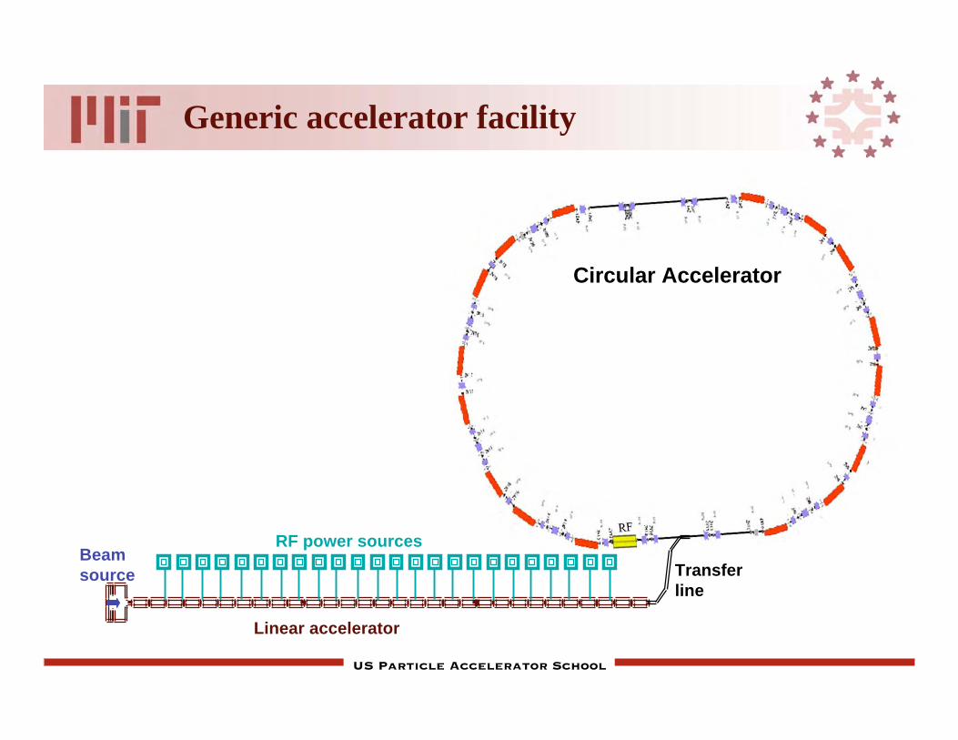
Generic accelerator facility

Beam

source

Linear accelerator

Transfer

line

RF power sources

Circular Accelerator


These components can be seen in an earlystorage ring light source


Optics are essential to guide the beamthrough the accelerator

• Optics (lattice): distribution of magnets that direct & focus beam

• Lattice design depends upon the goal & type of accelerator– Linac or synchrotron– High brightness: small spot size & small divergence– Physical constraints (building or tunnel)

The lattice must transport a real beam not just an ideal beam


Motion of each charged particle is determined byE & B forces that it encounters as it orbits the ring:

Lorentz Force

Lattice design problems:1. Given an existing lattice, determine the beam properties

2. For a desired set of beam properties, design the lattice.

Problem 2 requires some art

Particle trajectories (orbits)

F = ma = e (E + v B )


Types of magnets & their fields:dipoles

Dipoles:Used for steering

Bx = 0By = Bo


Types of magnets & their fields:

quadrupoles

Quadrupoles: Used for focusing

Bx = KyBy = Kx


Types of magnets & their fields:sextupoles

Sextupoles:Used for chromatic correctionBx = 2SxyBy = S(x2 – y2)


Average dipole strength drives

ring size & cost

In a ring for particles with energy E with N dipoles of length l, bend angle is

=2

N

The bending radius is =l

The integrated dipole strength will be Bl =2

N

E

e

The on-energy particle defines the central orbit: y = 0


The field B is generated by a current I in coils surrounding the polls

The ferromagnetic return yoke provides a return path for the flux

Integrate around the path

Characteristics of a dipole magnet

Bμr

=4

cJ

2GB +Bμriron

o ds =4

cItotal

B

0

Itotal (Amp turns) =1

0.4B (Gauss)G(cm)


Horizontal aperture of a dipole

Horizontal aperture must contain the saggita, S, of the beam

sin 2 =l

2=

lB

2(B )

S

S = ± (1 cos 2) ±82

8

l

8


To analyze particle motionwe will use local Cartesian coordinates

Change dependent variable from time, t, to longitudinal position, s

The origin of the local coordinates is a point on the design trajectory inthe bend plane

The bend plane is generally called the horizontal plane

The vertical is y in American literature & often z in European literature


Charged particle motion ina uniform (dipole) magnetic field

Let

Write the Lorentz force equation in two components, z and

==> py is a constant of the motion

Since B does no work on the particle, p is also constant

The total momentum & total energy are constant

For py,o 0, the orbit is a helix

B = Boˆ y

dpydt

= 0 and dpdt

= q v B( ) =qBo

mo

p ˆ y ( )


Write the equations for the velocities

dvxdt

=qBo

mo

vx and dvydt

=qBo

mo

vy

d2vxdt 2 =

qBo

mo

d

dtvx and

d2vydt 2 =

qBo

mo

d

dtvy

Differentiate

d2vxdt 2 = c

2vx and d2vydt 2 = c

2vy where c

qBo

mo

Differentiate

Relativistic cyclotron frequencyHarmonic motion


Integrating we obtain

and

Hence, the particle moves in a circle of radius R = vo/ c centered at (xo,yo)

and drifting at constant velocity in z.

Balancing the radial and centripetal force implies

Or in practical units

p (MeV /c) = 299.8 Bo(T) R(m)

mv 2

R= qv Bo or p = qBoR

x = Rcos( ct + ) + xo and y = Rsin( ct + ) + y0

vx = vo sin( ct + ) and vy = vo cos( ct + )


Returning to the circular accelerator:Orbit stability

The orbit of the ideal particle (design orbit) must be closed

==> Our analysis strictly applies for pz= 0

For other particles motion can be

Stable (orbits near the design orbit remain near the design orbit)

Unstable (orbit is unbounded)

For a pure uniform dipole B out of plane, motion is unbounded

For particle deflections in the plane,

the orbit is perturbed as shown

For off-energy particles, the orbit

size changes


Orbit stability & weak focusing

Early cyclotron builders found that they could not preventthe beam from hitting the upper & lower pole pieces with auniform field

They added vertical focusing of the circulating particles bysloping magnetic fields, from inwards to outwards radii

At any given moment, the average vertical B field sensedduring one particle revolution is larger for smaller radii ofcurvature than for larger ones


Orbit stability & weak focusing

Focusing in the vertical plane is provided at the expense of weakening

horizontal focusing

Suppose along the mid-plane varies as

By = Bo/rn

For n = 0, we have a uniform field with no vertical focusing

For n > 1, By cannot provide enough centripital force to keep the

particles in a circular orbit.

For stability of the particle orbits we want 0 < n < 1


Weak focusing equations of motion

In terms of derivatives measured along the equilibrium orbit

Particles oscillate about the design trajectory with the number of

oscillations in one turn being

The number of oscillations in one turn is termed the tune of the ring

Stability requires that 0<n<1

For stable oscillations the tune is less than one in both planes.

( )

orbitdesign therespect to with derivative a is ' where

0'' ,01

''2

0

2

0

=+=+R

nyy

R

xnx

ly vertical n

radially n-1


Disadvantages of weak focusing

Tune is small (less than 1)

As the design energy increased so does the circumference of the

orbit

As the energy increases the required magnetic aperture increases

for a given angular deflection

Because the focusing is weak the maximum radial displacement

is proportional to the radius of the machine


What’s wrong with this approach

The magnetic components of a high energy synchrotron

become unreasonably large & costly

As the beam energy increases, the aperture becomes big

enough to fit whole physicists!!

Cosmotron dipole


The solution is strong focusing

One would like the restoring force on a particle displaced

from the design trajectory to be as strong as possible

A strong focusing lattice has a sequence of elements that

are either strongly focusing or defocusing

The overall lattice is “stable”

In a strong focusing lattice the displacement of the

trajectory does not scale with energy of the machine

The tune is a measure of the amount of net focusing.


For a thin lens the particles position doesnot change its displacement in the lens

Along the particle path in the lens B is constant

For paraxial beams x' = dx/ds

The change in x' due to the lens is

Therefore we have a standard situation from ray optics

By =By

xx B x = constant

x =s

= seBy

p=

e B y x

ps


Focusing the beam forits trip through the accelerator

For a lens with focal length f, the deflection angle, = -x/f

Then,

For a Quadrupole with length l & with gradient B’ ==> By = B' x

x Focal point

f

k

For Z = 1

=l

f=

q

EByl =

q

E B xl

k m 2[ ] = 0.2998 B T /m[ ]

E GeV[ ]


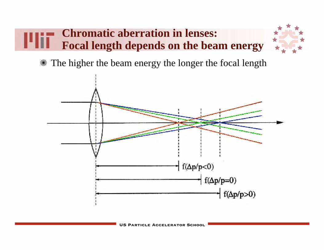
Chromatic aberration in lenses:Focal length depends on the beam energy

The higher the beam energy the longer the focal length


In the absence of J,

For small displacements from the

design trajectory

Terms in circles are linear restoring forces

One is focusing, the other is defocusing

The other terms = 0 with correct alignment of quadrupole

Quadrupole magnets

B = 0 By

x=

Bx

y

B = Bxˆ x + By

ˆ y

= Bx (0,0) +Bx

yy +

Bx

xx

x + By (0,0) +

By

xx +

By

yy

y

y

x

s

Force in y direction Force in -x direction


Generally one wants to avoid coupling the motion in x & y

Requires precise alignment of the quadrupole with the bend plane

Skew Quadrupole magnets

y

x

z

Skew quadrupole


The quadrupole magnet & its field

Exercise: Show that

B T

m

= 2.51

NI [A - turns]

R [mm2]


It is useful to write the action of thequadrupole in matrix form

A lens transforms a ray as

For a concave lens f < 0

For a drift space of length d

Note: both matrices are unimodular (required by Liouville’s theorem)

x

x

out

=1 01

f 1

x

x

in

x

x

out

=1 d

0 1

x

x

in


If the motion in x and y are uncoupled

The transport matrix is in block diagonal form

We can work the transport in both planes separately in 2x2 matrices

x

x

y

y

out

=

1 0 0 01

fx1 0 0

0 0 1 0

0 0 1fy

1

x

x

y

y

in


Now combine a concave + convex lensseparated by a drift space

x

x

out

=1 01

f 1

1 d

0 1

1 01

f 1

x

x

in

=

1+ df d

df 2 1 d

f

x

x

in

-f f

d

For 0 < d << f, the net effect is focusing with fnet f 2/d > 0

The same is true if we put the convex lens first


From optics we know that a combination of two lenses, with focal lengths f1

and f2 separated by a distance d, has

If f1 = - f2, the net effect is focusing!

A quadrupole doublet is focusing in both planes!

=> Strong focusing by sets of quadrupole doublets with alternating gradient

More generally…

1

f=1

f1+1

f2

d

f1 f2

N.B. This is only valid in thin lens approximation


What happens in phase space?

D FO O

These examples shows a slight focusing

DF O O


Is such a transport stable?

In storage rings particles may make 1010 passes through the lattice

We can analyze stability of lattice for an infinite number of passes

Say there are n sets of lens & the ith set of lenses has a matrix Mi

Then, the total transport has a matrix

M = Mn … M3 M2 M1

After m passes through the lattice

For stability Mmx must remain finite as m

x

x

m

=Mm x

x

in


Example of waist-to-waist transportwith magnification

If we did this n times eventually the beam would be lost into the walls


Mathematical diversion - Eigenvectors

We say that v is an eigenvector of the matrix M if

M v = v where is called the eigenvalue

A n x n matrix will have n eigenvectors

Any n x 1 vector can written as the sum of n eigenvectors

Mv v = M I( )v = 0 Det (M I) = Det

m11 m12 ... m1n

m21 m22 m2n

...

mn1 mn2 mnn

= 0


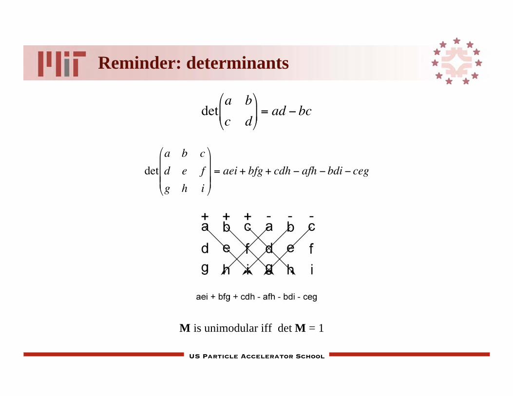
Reminder: determinants

deta b

c d

= ad bc

det

a b c

d e f

g h i

= aei + bfg + cdh afh bdi ceg

M is unimodular iff det M = 1


Write the stability conditionin terms of the eigenvectors

For our transport

So,

Therefore, 1m and 2

m must remain finite as m

Notes:

Since each Mi is unimodular ==> Det M = 1 and 2 = 1/ 1

If we write 1 = eiμ, then 2 = e-iμ

For to remain finite, μ must be real

x

x

= av1 + bv2

x

x

m

=Mm x

x

in

= a 1mv1 + b 2

mv2


Say that ; the eigenvalue equation is

So we have (a- )(d- ) - bc = 2 - (a + d) + (ad - bc) = 0

Since M is unimodular, (ad - bc) = 1

Therefore 2 - (a + d) + 1 = 0 or + -1 = (a + d) = Trace M

Recalling that = eiμ, we have

eiμ + e-iμ =2 cos = Trace M for real

Thus the stability condition is

-1 1/2 Trace M 1

has an important physical interpretation to be discussed later

Solving the eigenvalue equation…

M =a b

c d

Det

a b

c d

= 0


This would seem to make the job of latticedesign extremely difficult for large rings

But…. there are tricks

Remember the trivial result that

Suppose the ring is made of a number, m,

of identical modules consisting of a small

number of elements

Now design the modules such that

Ma = M1M2..Mfew= I

Then the Mam

= Im = I

The whole ring transport would seem to be stable

…BUT…

We can’t sit on a resonance; still the idea of modular design is valuable

In =1 0

0 1

n

=1 0

0 1

= I

MaMa

Ma

Ma

MaMa

Ma

Ma


Equations of motion

for

particles in synchrotrons & storage rings


The nominal energy, Eo, defines the “design orbit”

Closed orbit of the ideal particle with zero betatron amplitude

Static guide (dipole) field ==> trajectory is determined

Size of machine is approximately set

Final size will depend on fraction of the ring that is dipoles

Assume that the guide field is symmetric about the plane

of motion

Key quantities are B(s) & dB(s)/dy (field gradient)

Usually (but not always) followed in practice

Design orbit of a storage ring


If all magnetic fields scale ~ Ebeam, orbit doesn’t change

This is exactly the concept of the synchrotron

==> We can describe the performance in terms of an energy

independent guide field

Define cyclic functions of s to describe the action of

dipoles and quadrupoles

Motion of particles in a storage ring

G(s) =ecBo(s)

Eo

= 1curve (s)

=G(s+ L)

K(s) =ec

Eo

dB

dy= K(s+ L)


Magnetic field properties

For simplicity

Consider ideal “isomagnetic” guide fields

G(s) = Go in the dipoles

G(s) = 0 elsewhere

Assume that we have a “separated function” lattice:

Dipoles have no gradient

Quadrupoles have no dipole component

G(s) K(s) = 0

Nonetheless dipoles provide focusing in the bend plane

explain


Guide functions in a real bend magnet

a real field cannot be isomagnetic because B must be continuous


By inspection we can write equations of

motion of particles in a storage ring

Harmonic oscillator with time dependent frequency

k = 2 / = 1/ (s)

The term 1/ 2 corresponds to the dipole weak focusing

The term p/(p ) is present for off-momentum particles

Tune = # of oscillations in one trip around the ring

x k(s)1

(s)2

x =

1

(s)

p

p

y + k(s)y = 0

Hill’s equations


Deriving the equation of motion

Consider motion in the horizontal plane along the s direction

Recall that for a particle passing through a B field with

gradient B' the slope of the trajectory changes by

or

Taking the limit as s 0,

This missed the effects of dipole focusing

x =s

= seBy

p= s

e B y x

p= s

B y x

(B )

x

s=

B y(B )

x

x + B y

(B )x = 0


Let’s do this more carefully, step-by-step

R = rˆ x + yˆ y where r + x

v B = vsByˆ x + vsBx

ˆ y + (vxBy vyBx )ˆ s ( )

The equation of motion is

Assume Bs = 0; then

dpdt

=d( mv)dt

= e v B

The magnetic field cannot change

dpdt

= m˙ R = e v B

where


Express R in orbit coordinates

˙ R = rˆ x + yˆ y = ˙ r x + rˆ ˙ x + ˙ y y

With ˆ ˙ x = ˙ ˆ s where ˙ =vsr

˙ R = ˙ r x + (2˙ r + r ˙ )ˆ s + r ˙ ˙ s + ˙ y y

Since ˆ ˙ s = ˙ x

˙ R = (˙ r r ˙ 2) ˆ x + (2˙ r ˙ + r ˙ )ˆ s + ˙ y y

Recall that v B = vsByˆ x + vsBx

ˆ y + (vxBy vyBx )ˆ s ( )

dpdt

x

= m ˙ R ( )x

= e v B( )x (˙ r r ˙ 2) =vsBy

m=

vs2By

mvs


In paraxial beams vs>>vx>>vy

(˙ r r ˙ 2) =vsBy

m=

vs2By

mvs

vs2By

pd

dt=ds

dt

d

ds

ds = d = vsdt r

Change the independent variable to s

Assuming that d2s

dt 2 = 0

d2

dt 2 =ds

dt

2d2

ds2 = vs r

2d2

ds2

Note that r = + x

d2x

ds2+ x2 =

By

(B )1+

x

2


This general equation is non-linear

Simplify by restricting analysis to fields that are linear in x

and y

Perfect dipoles & perfect quadrupoles

Recall the description of quadrupoles

Curl B = 0 ==> the mixed partial derivatives are equal ==>

B = Bxˆ x + By

ˆ y = Bx (0,0) +Bx

yy +

Bx

xx

x + By (0,0) +

By

xx +

By

yy

y

0 0 00

d2x

ds2+12

+1

(B )

By(s)

x

x = 0


The linearized equation matches the Hill’s

equation that we wrote by inspection

A similar analysis can be done for motion in the vertical

plane

The centripital terms will be absent as unless there are

(unusual) bends in the vertical plane

We will look at two methods of solution

Piecewise linear solutions

Closed form solutions

x k(s)1

(s)2

x =

1

(s)

p

p

y + k(s)y = 0

Unit 7 - Lecture 15 - Linear optics -...

Documents

Transcript of Unit 7 - Lecture 15 - Linear optics -...