UNIT 3: ONE-DIMENSIONAL MOTION I A Graphical Description · UNIT 3: ONE-DIMENSIONAL MOTION I A...

Name _________________________ Date (YY/MM/DD) ______/_________/_______ St.No. __ __ __ __ __-__ __ __ __ Section__________

INSTRUCTOR VERSION

UNIT 3: ONE-DIMENSIONAL MOTION IA Graphical Description

Approximate Classroom Time: Three 110 minute sessions

A picture is worth a thousand words!

OBJECTIVES 1. To learn about three ways that physicists can describe motion in one dimension — words, pictures and graphs.

2. To acquire an intuitive understanding of speed, velocity, and acceleration in one dimension.

3. To learn to recognize the pattern of position vs. time, ve-locity vs. time, and acceleration vs. time for the motion of objects which speed up and/or slow down at a constant rate and to recognize this type of motion as constantly acceler-ated motion.

© 1992-93 Dickinson College, U. of Oregon, Tufts U. Supported by FIPSE, U.S. Dept. of EducationModified for SFU by N. Alberding.

OVERVIEW 5 min

In Unit 4 you will turn your attention to a more formal mathematical description of one dimensional motion.

We are interested in learning how to describe one-dimensional motion both graphically and mathematically. The study of how to describe motion using mathematical and graphical representations is known as kinematics.

Describing the motion of real objects is not always easy. An odd shaped cloud scooting along in the sky could be chang-ing its size and shape as it moves. Physicists often start investigations by using simplifying assumptions and ide-alizations. Thus, we begin with the study of objects that are small compared to the distances they move so we can treat them as mathematical points.

We will begin the study of motion by studying motion along a line. Such motion is said to be one dimensional. The key to the description of observed motions in one di-mension is the ability to measure the distance of an object from a reference point and the time at which it is at each distance. Physicists define distance from a reference point as position. Position and time are indeed the fundamental measurements in the study of motion. You will begin your motion studies using an ultrasonic mo-tion detector attached to a computer, to study the motion of your own body as well as that of a cart that increases and decreases its velocity at a steady rate. Since the actual rules for calculating velocity and acceleration from dis-tance and time measurements are programmed into the motion software, you have a unique opportunity to "dis-cover" intuitively what velocity and acceleration mean and how they are represented graphically.

The motion detector investigations used in this unit are based on activities developed initially by Dr. Ronald Thornton of Tufts University and Dr. David Sokoloff of the University of Oregon.

Page 3-2 Workshop Physics Activity Guide SFU 1067

© 1992-93 Dickinson College, U. of Oregon, Tufts U. Supported by FIPSE, U.S. Dept. of EducationModified for SFU by N. Alberding, 2005

The focus in this session on kinematics is to be able to de-scribe your position and velocity over time using words and graphs. You will use a motion detector attached to a com-puter in the laboratory to learn to describe one-dimensional motion.

For the investigations in this unit you will need:

• a computer • an laboratory interface • an ultrasonic motion detector • LoggerPro software • OPTIONAL: a number line on the floor

Workshop Physics: Unit 3-One Dimensional Motion -3Authors: Priscilla Laws, Ronald Thornton, & David Sokoloff

© 1992-93 Dickinson College, U. of Oregon, Tufts U. Supported by FIPSE, U.S. Dept. of EducationModified for SFU by N. Alberding, 2005.

The Ultrasonic Motion Detector

The ultrasonic motion detector acts like a stupid bat when hooked up with a computer system. It sends out a series of sound pulses that are too high frequency to hear. These pulses reflect from objects in the vicinity of the motion detector and some of the sound energy re-turns to the detector. The computer is able to record the time it takes for reflected sound waves to return to the detector and then, by knowing the speed of sound in air, figure out how far away the reflecting object is. There are several things to watch out for when using a motion detector.

When Using a Motion Detector

1. Do not get closer that 0.2 metres from the detector because it cannot record reflected pulses which come back too soon.

2. The ultrasonic waves come out in a cone of about 15o. It will see the closest object. Be sure there is a clear path between the object whose motion you want to track and the motion detector.

3. The motion detector is very sensitive and will detect slight motions. You can try to glide smoothly along the floor, but don't be surprised to see small bumps in velocity graphs and larger ones in acceleration graphs.

4. Some objects like bulky sweaters are good sound absorbers and may not be "seen" well by a motion detector. You may want to hold a book in front of you if you have loose clothing on.

30 min



SESSION ONE: DESCRIBING MOTION WITH WORDS AND GRAPHS 10 min

Session one will be skipped. This material is typically covered in BC grade 12 physics or SFU Physics 100 and will not be done in Physics 140. You find this section to review on the WebCT page. Note especially the discus-sion of vectors.

Comments about Velocity Graphs: (1) Velocity implies both speed and direction. How fast you move is your speed, the rate of change of position with re-spect to time. As you have seen, for motion along a line (e.g., the positive x-axis) the sign (+ or –) of the velocity in-dicates the direction. If you move away from the detector (origin), your velocity is positive, and if you move toward the detector, your velocity is negative.

(2) The faster you move away from the origin, the larger positive number your velocity is. The faster you move to-ward the origin, the "larger" negative number your velocity is. That is –4 m/s is twice as fast as –2 m/s and both mo-tions are toward the origin.

Velocity Vectors:These two ideas of speed and direction can be combined and represented by vectors.

A velocity vector is represented by an arrow pointing in the direction of motion. The length of the arrow is drawn pro-portional to the speed; the longer the arrow, the larger the speed. If you are moving toward the right, your velocity vector can be represented by the arrow shown below.

If you were moving twice as fast toward the right, the ar-row representing your velocity vector would look like:

while moving twice as fast toward the left would be repre-sented by the following arrow:

What is the relationship between a one-dimensional veloc-ity vector and the sign of velocity? This depends on the way you choose to set the positive x-axis.

Workshop Physics: Unit 3-One Dimensional Motion Page 3-5Authors: Priscilla Laws, Ronald Thornton, & David Sokoloff


0 +

Positive velocity

Negative velocity0+

Positive velocity

Negative velocity

In both diagrams the top vectors represent velocity toward the right. In the left diagram, the x-axis has been drawn so that the positive x-direction is toward the right. Thus the top arrow represents positive velocity. However, in the right diagram, the positive x-direction is toward the left. Thus the top arrow represents negative velocity. Likewise, in both diagrams the bottom arrows represent velocity to-ward the left. In the left diagram this is negative velocity, and in the right diagram it is positive velocity.



SESSION TWO: CHANGING MOTION 30 min

Discussion of the Motion HomeworkYou should share your observations on motion and conclu-sions you drew from them with your classmates.

50 minVelocity and Acceleration GraphsBody motions can be very jerky and irregular. We are in-terested in having you learn to describe some simple mo-tions in which the velocity of an object is changing. In or-der to learn to describe motion in more detail for some simple situations, you will be asked to observe and de-scribe the motion of a cart on a flat track. Although, graphs and words are still important representations of these mo-tions, you will also be asked to draw velocity vectors, which are arrows that indicate both the direction and speed of a moving object. Thus, you will also learn how to represent simple motions with velocity diagrams .

Describing Motion With Pictures . . .

t = 0s t = 1s t = 2s

Ave

rage

Joe

Sch

moe

Phys

ics

Stud

ent

1.1 m 1.4 m2.1 m

Your goal in this session is to learn how to describe vari-ous kinds of motion with precision. It is not enough when studying motion in physics to simply say that "the object is moving toward the right" or "it is standing still."



You probably realize that a velocity vs. time graph is better than a position vs. time graph when you want to know how fast and in what direction you are moving at each instant in time. When the velocity of an object is changing, it is also important to know how it is changing. The rate of change of velocity is known as the acceleration.

In order to get a feeling for acceleration, it is helpful to create and learn to interpret velocity vs. time and accelera-tion vs. time graphs for some relatively simple motions of a cart on a track. You will be observing the cart with the mo-tion detector as it moves at a constant velocity and as it changes its velocity at a constant rate. For the activities in this session you will need:

•a computer •a laboratory interface (LabPro) • an ultrasonic motion detector • motion software (Logger Pro) • a cart or toy car with very little friction • a smooth, level track (Force and Motion Track) • a battery-operated fan cart • 4 fresh AA cells and 2 aluminum dummy cells

IMPORTANT NOTE ON SAVING YOUR FILES: You may be asked to use the data collected using the motion software in some of the Activities for mathematical analysis in future ses-sions. For each activity please save the graph sets and associated data on the SFU fileserver, or on your own USB drive, as in-structed in Appendix A. We recommend that you identify your files by the lab number and activity number for later reference along with your group initials. Thus, if Stern, Ricci, and Pers-inger work together on the LAB 2 activities, the file names might be, for example, L2A1-1(SRP), L2A1-2 (SRP), etc.

Graphing a Constant Velocity Cart MotionLet's start by giving a frictionless cart a push along a smooth track and graphing its motion.

0.3 m

To do this you should:

1. Set up the motion detector at the end of a level track, If the cart has a friction pad, move it out of contact with the track so that the cart can move freely.



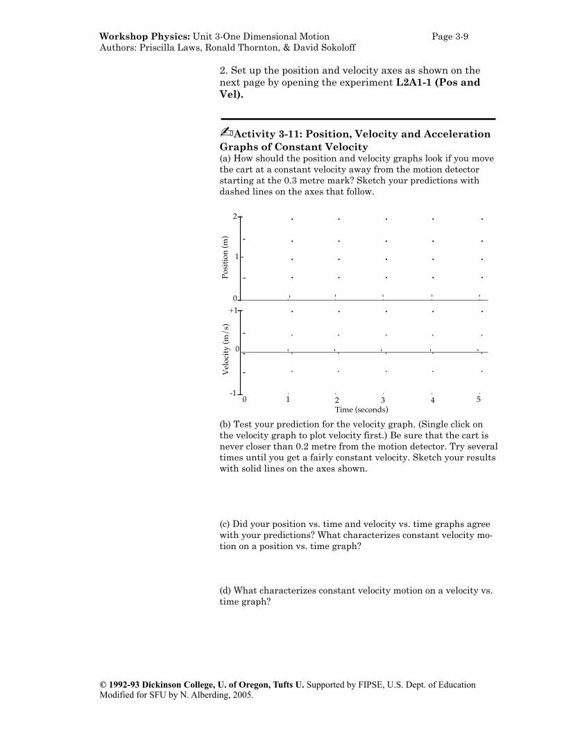
2. Set up the position and velocity axes as shown on the next page by opening the experiment L2A1-1 (Pos and Vel).

✍Activity 3-11: Position, Velocity and Acceleration Graphs of Constant Velocity(a) How should the position and velocity graphs look if you move the cart at a constant velocity away from the motion detector starting at the 0.3 metre mark? Sketch your predictions with dashed lines on the axes that follow.

-1

+1

0

. . . . .

. . . . .

. . . . .

-

-

-

- - - - -

0

. . . . .

. . . . .

. . . . .

. . . . .

-

1 -

-

- - - --

2

. . . . .

Posi

tion

(m)

Vel

ocity

(m/s

)

1 2 3 4 50Time (seconds)

(b) Test your prediction for the velocity graph. (Single click on the velocity graph to plot velocity first.) Be sure that the cart is never closer than 0.2 metre from the motion detector. Try several times until you get a fairly constant velocity. Sketch your results with solid lines on the axes shown.

(c) Did your position vs. time and velocity vs. time graphs agree with your predictions? What characterizes constant velocity mo-tion on a position vs. time graph?

(d) What characterizes constant velocity motion on a velocity vs. time graph?



(e) Acceleration is defined as the time rate of change of velocity. Sketch your prediction of the cart acceleration (for the motion you just observed) on the axes that follow using a dashed line.

-2

+2

0

. . . . .

. . . . .

. . . . .

-

-

-

- - - - -

. . . . .


Acc

eler

atio

n (m

/s/s

)

(f) Display and the acceleration graph of the cart and use a solid line to sketch it using the axes above. Note: To display an accel-eration graph in the motion software the mouse button down on the Position label on your graph and selecting Acceleration. You may wish to change the minimum on the Acceleration axis by clicking on 0.0 and changing it to -2.0.

Finding Accelerations To find the average acceleration of the cart during some time interval (the average time rate of change of its veloc-ity), you must measure its velocity at two different times, calculate the difference between the final value and the initial value and divide by the time interval.

To find the acceleration vector from two velocity vectors, you must first find the vector representing the change in velocity by subtracting the initial velocity vector from the final one. Then you divide this vector by the time interval.

✍Activity 3-12: Representing Acceleration(a) Does the acceleration vs. time graph you observed agree with this method of calculating acceleration? Explain. Does it agree with your prediction?

(b) The next diagram shows the positions of the cart at equal time intervals. (This is like taking snapshots of the cart at equal time intervals.) At each indicated time, sketch a vector above the cart which might represent the velocity of the cart at that time while it is moving at a constant velocity away from the motion detector.



(c) Explain how you would find the vector representing the change in velocity between the times 1.0 s and 2.0 s in the dia-gram above. From this vector, what value would you calculate for the acceleration? Explain. Is this value in agreement with the acceleration graph you obtained in Activity 3-11?

Speeding Up at a Moderate RateIn the next activity you will look at velocity and accelera-tion graphs of the motion of a cart when its velocity is changing. You will be able to see how these two represen-tations of the motion are related to each other when the cart is speeding up.

In order to get your cart speeding up smoothly you can use a propeller driven by an electric motor to accelerate the cart. Your task in the next activity is to create nice smooth graphs of position and velocity vs. time of a fan cart with a moderate thrust that shows the cart starting from rest.

You should set up the cart, track, fan attachment and mo-tion detector as shown in the following diagrams.

0.3 m

end stop



• Use two batteries and two dummy cells in the fan assembly so that the cart does not speed up too fast.)

• Always catch the fan at the end of a run before it crashes!

• To keep the motion detector from collecting bad data from the rotation of the propeller, be sure that the fan blade does not ex-tend beyond the front end of the cart.

• Use the motion software experiment file L2A1-2 (Speeding Up) to display Position from 0 to 2.0 m and Velocity from -1.0 to 1.0 m/sec for a total time of 3.0 sec.

• Scale the graphs so that the traces fill the screen

• Practise several times before completing the tasks described below.

✍Activity 3-13: Graphs Depicting Speeding Up(a) Create position vs. time and velocity vs. time graphs of your fan cart as it moves away from the detector and speeds up. Sketch the graphs neatly on the following axes.

(c ). Keep your data for analysis in the next activity by selecting Store Latest Run . . . on the Experiment Menu. Then Save the file with the name SPEEDUP1.XXX, where XXX are your initials.

(d) How does your position graph differ from the position graphs for steady (constant velocity) motion?



(e) What feature of your velocity graph signifies that the motion was away from the detector?

(f) What feature of your velocity graph signifies that the cart was speeding up? How would a graph of motion with a constant veloc-ity differ?

(g) Sketch the acceleration graph on the axes that follow. (Adjust the axes if necessary).

SPEEDING UP MODERATELY

(h) During the time that the cart is speeding up, is the accelera-tion positive or negative? How does speeding up while moving away from the detector result in this sign of acceleration? Hint: Remember that acceleration is the rate of change of velocity. Look at how the velocity is changing.

(i) How does the velocity vary in time as the cart speeds up? Does it increase at a steady rate or in some other way?

(j) How does the acceleration vary in time as the cart speeds up? Is this what you expect based on the velocity graph? Explain.

Using Vectors to Describe the Acceleration



Let's return to the Vector Diagram representation and use it to describe the acceleration.

✍Activity 3-14: Acceleration Vectors (a) The diagram that follows shows the positions of the cart at equal time intervals. At each indicated time, sketch a vector above the cart which might represent the velocity of the cart at that time while it is moving away from the motion detector and speeding up.

(b) Show below how you would find the approximate length and direction of the vector representing the change in velocity be-tween the times 1.0 s and 2.0 s using the diagram above. No quantitative calculations are needed. Based on the direction of this vector and the direction of the positive x-axis, what is the sign of the acceleration? Does this agree with your answer to Ac-tivity 3-13 (h)?

30 minMeasuring Acceleration In this investigation you will analyse the motion of your accelerated cart quantitatively. This analysis will be quan-titative in the sense that your results will consist of num-bers. You will determine the cart's acceleration from the slope your velocity vs. time graph and compare it to the average acceleration read from the acceleration vs. time graph. You can display actual values for your acceleration and velocity data using the motion software.

At any rate, to do this next activity you will need the Log-ger Pro software and your experiment file, Speedup1.xxx, from Activity 3-13.



✍Activity 3-15: Calculating Accelerations (a) Re sketch the velocity and acceleration graphs you found in Activity 3-13 using the axes that follow. Correct the scales if nec-essary.

-1

+1

0

. . . . .

. . . . .

. . . . .

-

-

-

- - - - -

-1

+1

0

. . . . .

. . . . .

. . . . .

-

-

-

- - - - -

.6 1.2 1.8 2.4 3.00

. . . . .

. . . . .

Acc

eler

atio

n (m

/s/s)

Vel

ocity

(m/s)

Time (seconds)

(b) List 10 of the typical recorded accelerations of the cart. To find these values select Examine from the Analyze Menu. Scroll along with the mouse to display the values at different times. (Only use values from the portion of the graph after the cart was released and before you stopped it.)

Accel. Accel.1 62 73 84 95 10

Select Examine again to turn off the display of values.

(c) Calculate the average value of the ten accelerations.

Average accelerations: _________m/s2

(d) The average acceleration during a particular time period is defined as the change in velocity divided by the change in time. This is the average rate of change of velocity. By definition, the rate of change of a quantity graphed with respect to time is also



the slope of the curve. Thus the (average) slope of an object's ve-locity vs. time graph is the (average) acceleration of the object.

Find the data needs to calculate the approximate slope of your velocity graph. Use Examine to read the velocity and time co-ordinates for two typical points on the velocity graph. For a more accurate answer, use two points as far apart in time as possible but still during the time the cart was speeding up.

Velocity (m/s) Time (s)Point 1Point 2

(e) Calculate the change in velocity between points 1 and 2. Also calculate the corresponding change in time (time interval). Di-vide the change in velocity by the change in time. This is the av-erage acceleration. Show and then summarize your calculations below.

Speeding Up

Change in Velocity (m/s)

Time Interval (s)

Avg. Acceleration (m/s2)

(f) Is the acceleration positive or negative? Is this what you ex-pected?

(g) Does the average acceleration you just calculated agree with the average of the accelerations you averaged from the accelera-tion graph? Do you expect them to agree? How would you ac-count for any differences?



Speeding Up at a Faster RateSuppose that you accelerate your cart at a faster rate by putting four batteries instead of two in it? How would your velocity and acceleration graphs change?

✍Activity 3-16: Calculating Accelerations (a) Re sketch the velocity and acceleration graphs you found in Activity 3-13 once more using the axes that follow.

-1

+1

0

. . . . .

. . . . .

. . . . .

-

-

-

- - - - -

-1

+1

0

. . . . .

. . . . .

. . . . .

-

-

-

- - - - -

.6 1.2 1.8 2.4 3.00

. . . . .

. . . . .

Acc

eler

atio

n (m

/s/s)

Vel

ocity

(m/s)

Time (seconds)

(b) In the previous set of axes, use a dashed line or another col-our to sketch your predictions for the general graphs that depict a fan cart running under more power (i.e., the four batteries). Exact predictions are not expected. We just want to know how you think the general shapes of the graphs will change.

(c) Test your predictions by accelerating the cart with four AA cells in the fan assembly battery compartment. Repeat if neces-sary to get nice graphs and then sketch the results in the axes that follow. Use the same scale as you did for the sketch of the two battery graph.



-1

+1

0

. . . . .

. . . . .

. . . . .

-

-

-

- - - - -

-1

+1

0

. . . . .

. . . . .

. . . . .

-

-

-

- - - - -

.6 1.2 1.8 2.4 3.00

. . . . .

. . . . .

Acc

eler

atio

n (m

/s/s)

Vel

ocity

(m/s)

Time (seconds) EXPERIMENTAL RESULTS OF SPEEDING UP RAPIDLY

(d) Did the general shapes of your velocity and acceleration graphs agree with your predictions? How is the greater magni-tude (size) of acceleration represented on a velocity vs. time graph?

(e) How is the greater magnitude (size) of acceleration repre-sented on an acceleration vs. time graph?



SESSION THREE: SLOWING DOWN, SPEEDING UP, AND TURNING30 min

Discussion of the Changing Motion HomeworkYou should share your observations on motion and conclu-sions you drew from them with your classmates.

5 minAbout Slowing Down, Speeding Up and TurningIn the previous sessions in this unit, you explored the characteristics of position vs. time, velocity vs. time and acceleration vs. time graphs of the motion of a cart. In the cases examined, the cart was always moving away from a motion detector, either at a constant velocity or with a con-stant acceleration. Under these conditions, the velocity and acceleration are both positive. You also learned how to find the magnitude of the accel-eration from velocity vs. time and acceleration vs. time graphs, and how to represent the velocity and acceleration using vectors.

In the motions you studied in the last sessions the velocity and acceleration vectors representing the motion of the cart both pointed in the same direction.In order to get a better feeling for acceleration, it will be helpful to examine velocity vs. time and acceleration vs. time graphs for some slightly more complicated motions of a cart on a track. Again you will use the motion detector to observe the cart as it changes its velocity at a constant rate. Only this time the motion may be toward the detec-tor, and the cart may be speeding up or slowing down.

In order to complete the activities in this session you will need the same apparatus you used last time. This includes:

• a computer • a Lab Pro interface • an ultrasonic motion detector • Logger Pro software • a cart or toy car with very little friction • a smooth, level track • a battery-operated fan cart

45 min Slowing down and Speeding UpIn this activity you will look at a cart (or toy car) moving along a track and slowing down. A car being brought to rest by the steady action of brakes is a good example of this type of motion. Later you will examine the motion of the cart toward the motion detector and speeding up. In both cases, we are interested in the shapes of the velocity vs.



time and acceleration vs. time graphs, as well as the vec-tors representing velocity and acceleration. Let's start with the creation of velocity and acceleration graphs of when it is moving away from the motion detector and slowing down. To do this activity, you should set up the cart, track, and motion detector as shown below. If the cart has a friction pad, move it out of contact with the track so that the cart can move freely. Use the same two AA cells and two dummy cells as you used for the Speeding Up 1 activity in the last session.

Direction of hand push

Direction of fan thrust

0.3 m

The fan in the picture is exerting a thrust on the cart to-wards the motion detector.. Your hand will give the cart an initial velocity away from the motion detector. In this ac-tivity you will examine the velocity and acceleration of this motion.

✍Activity 3-17: Graphs Depicting Slowing Down(a) If you give the cart a push away from the motion detector and release it, will the acceleration be positive, negative or zero (after it is released)? Sketch your predictions for the velocity vs. time and acceleration vs. time graphs on the axes below.

-

- - - - -

Vel

ocity

(m/s)

- - - - -

Acc

eler

atio

n (m

/s/s)

Time (seconds)

+

0

-+

0

-

(b) To test your predictions open the experiment L3A1-1 (Slow-ing Down) to display the velocity vs. time and acceleration vs. time. Then locate the cart 0.5 m from the detector, turn on its fan, and push the cart away from the motion detector once starts clicking. Graph velocity first. Catch the cart before it turns around.



Draw the results on the axes that follow. You may have to try a few times to get a good run. Don't forget to change the scales if this will make your graphs clearer before making the sketch so change the scale on the axes shown, if needed.

-2

+2

0

. . . . .

-

-

. . . . .

Acc

eler

atio

n (m

/s/s

) -1

+1

0

. . . . .-

-

. . . . .

Vel

ocity

(m/s

)


. . . . .

. . . . .

. . . . .

. . . . .

. . . . .

. . . . .

SLOWING DOWN MOVING AWAY (c) Keep your graphs for later comparison, by selecting Store Latest Run from the Experiment menu, and then label your graphs with— "A" at the spot where you started pushing. "B" at the spot where you stopped pushing. "C" at the spot where the cart stopped moving.Also sketch on the same axes the velocity and acceleration graphs for Speeding Up from Activity 3-13. Use the same scale for the two sketches.

(d) Did the shapes of your velocity and acceleration graphs agree with your predictions? How is the sign of the acceleration repre-sented on a velocity vs. time graph?

(e) How is the sign of the acceleration represented on an accel-eration vs. time graph?



(f) Is the sign of the acceleration what you predicted? How does slowing down while moving away from the detector result in this sign of acceleration? Hint: Remember that acceleration is the rate of change of velocity. Look at how the velocity is changing.

Constructing Acceleration Vectors for Slowing DownLet's consider a diagrammatic representation of a cart which is slowing down and use vector techniques to figure out the direction of the acceleration.

✍Activity 3-18: Vector Diagrams for Slowing Down(a) The diagram that follows shows the positions of the cart at equal time intervals. (This is like taking snapshots of the cart at equal time intervals.) At each indicated time, sketch a vector above the cart which might represent the velocity of the cart at that time while it is moving away from the motion detector and slowing down.

(b) Show below how you would find the vector representing the change in velocity between the times 1s and 2 s in the diagram above. Based on the direction of this vector and the direction of the positive x-axis, what is the sign of the acceleration? Does this agree with your answer to Question (f) in Activity 3-17?

(c) Based on your observations in this activity and in the last session, state a general rule to predict the sign and direction of the acceleration if you know the sign of the velocity (i.e. the di-rection of motion) and whether the object is speeding up or slow-ing down.



Speeding Up Toward the Motion DetectorLet's investigate another common situation. Suppose the cart is allowed to speed up when travelling toward the mo-tion detector. What will the direction of the acceleration be? Positive or negative?

✍Activity 3-19: Graphs Depicting Speeding Up(a) Use the general rule that you stated in Activity 3-18 to pre-dict the shapes of the velocity and acceleration graphs. Sketch your predictions using the axes that follow.



-

- - - - -

Vel

ocity

(m/s)

- - - - -

Acc

eler

atio

n (m

/s/s)

Time (seconds)

+

0

-+

0

-

(b) Test your predictions by turning on the fan and releasing the cart from rest at the end of the track after the motion detector starts clicking. Catch the cart before it gets too close to the detec-tor.

Draw the results on the axes that follow. You may have to try a few times to get a good run. Don't forget to change the scales if this will make your graphs clearer before making the sketch so change the scale on the axes shown, if needed.

-2

+2

0

. . . . .

-

-

. . . . .

Acc

eler

atio

n (m

/s/s

)

-1

+1

0

. . . . .-

-

. . . . .

Vel

ocity

(m/s

)


. . . . .

. . . . .

. . . . .

. . . . .

. . . . .

. . . . .

SPEEDING UP MOVING TOWARD



(c) How does your velocity graph show that the cart was moving toward the detector?

(d) During the time that the cart was speeding up, is the accel-eration positive or negative? Does this agree with your predic-tion? Explain how speeding up while moving toward the detector results in this sign of acceleration. Hint: Think about how the velocity is changing.

Constructing Acceleration Vectors for Speeding UpLet's consider a diagrammatic representation of a cart which is speeding up and use vector techniques to figure out the direction of the acceleration.

✍Activity 3-20: Vector Diagrams for Slowing Down(a) The diagram that follows shows the positions of the cart at equal time intervals. (This is like taking snapshots of the cart at equal time intervals.) At each indicated time, sketch a vector above the cart which might represent the velocity of the cart at that time while it is moving toward the motion detector and speeding up.

(b) Show below how you would find the vector representing the change in velocity between the times 1s and 2 s in the diagram above. Based on the direction of this vector and the direction of the positive x-axis, what is the sign of the acceleration? Does this agree with your answer to Question (d) in Activity 3-19?



(c) Was the general rule you developed in Activity 3-18 (c) cor-rect? If not, modify it and restate it here.

Moving Toward the Detector and Slowing DownThere is one more possible combination of velocity and ac-celeration for the cart, that of moving toward the detector while slowing down.

✍Activity 3-21: Slowing Down Toward the Detector(a) Use your general rule to predict the direction and sign of the acceleration when the cart is slowing down as it moves toward the detector. Explain why the acceleration should have this di-rection and this sign in terms of the velocity and how the velocity is changing.

(b) The diagram below shows the positions of the cart at equal time intervals for slowing down while moving toward the detec-tor. At each indicated time, sketch a vector above the cart which might represent the velocity of the cart at that time while it is moving toward the motion detector and slowing down.



(c) Show below how you would find the vector representing the change in velocity between the times 1s and 2 s in the diagram above. Based on the direction of this vector and the direction of the positive x-axis, what is the sign of the acceleration? Does this agree with the prediction you made in part (a)?

40 minAcceleration and Turning AroundIn Session 2 of this unit and in the first activity in this ses-sion, you looked at velocity vs. time and acceleration vs. time graphs for a cart moving in one direction with a changing velocity. In this investigation you will look at what happens when the cart slows down, turns around and then speeds up. How is its velocity changing? What is its acceleration?

The set-up you can use shown below--the same as for the first activity you did in this session. Once again fan cart should have two AA cells and two dummy cells.

Direction of hand push

0.3 m

Direction of fan thrust

To practice this motion you should start the fan, and give the cart a push away from the motion detector. It moves toward the end of the track, slows down, reverses direction and then moves back toward the detector. Try it without activating the motion detector! Be sure to stop the cart be-fore it hits the motion detector.

✍ Activity 3-22: Reversing Direction(a) For each part of the motion — away from the detector, at the turning point, and toward the detector, predict in the table that follows whether the velocity will be positive, zero or negative.



Also indicate whether the acceleration is positive, zero or nega-tive.

Moving Away Turning Around Moving Toward

Velocity

Acceleration

(b) Sketch the predicted shapes of the velocity vs. time and accel-eration vs. time graphs of this entire motion on the axes that fol-low.

-

- - - - -

Vel

ocity

(m/s)

- - - - -

Acc

eler

atio

n (m

/s/s)

Time (seconds)

+

0

-+

0

-

(c) To test your predictions set up the velocity and acceleration axes as shown below. (Open the experiment L3A1-1 (Slowing Down) if it is not already opened.) . Use procedures that are similar to the ones you used in the slowing down and speeding up activities. You may have to try a few times to get a good run. Don't forget to change the scales if this will make your graphs clearer. When you get a good run, sketch both graphs on the axes.



-2

+2

0

. . . . .

-

-

. . . . .

Acc

eler

atio

n (m

/s/s

)

-1

+1

0

. . . . .-

-

. . . . .

Vel

ocity

(m/s

)


. . . . .

. . . . .

. . . . .

. . . . .

. . . . .

. . . . .

(d) Label both graphs withA. where the cart started being pushed.B. where the push ended (where your hand left the cart).C. where the cart reached the end of the track (and is

about to reverse direction).D. where you stopped the cart.

(e) Did the cart have a zero velocity? (Hint: Look at the velocity graph. What was the velocity of the cart at the end of the track?) Does this agree with your prediction? How much time did it spend at zero velocity before it started back toward the detector? Explain.

(f) According to your acceleration graph, what is the acceleration at the instant the cart comes to rest? Is it positive, negative or zero? Does this agree with your prediction?

(g) Explain the observed sign of the acceleration at the end of the track. (Hint: Remember that acceleration is the rate of change of velocity. When the cart is at rest at the end of the track, what will its velocity be in the next instant? Will it be positive or nega-tive?)



Tossing a BallSuppose you throw a ball up into the air. It moves up-ward, reaches its highest point and then moves back down toward your hand. What can you say about the directions of its velocity and acceleration at various points?

✍ Activity 3-23: The Rise and Fall of a BallConsider the ball toss carefully. Assume that upward is the posi-tive direction. Indicate in the table that follows whether the ve-locity is positive, zero or negative during each of the three parts of the motion. Also indicate if the acceleration is positive, zero or negative. Hint: Remember that to find the acceleration, you must look at the change in velocity.

Moving UpAfter Release

At HighestPoint

Moving Down

Velocity

Acceleration

(b) In what ways is the motion of the ball similar to the motion of the cart which you just observed?



UNIT 3: ONE-DIMENSIONAL MOTION I A Graphical Description · UNIT 3: ONE-DIMENSIONAL MOTION I A...

Documents

Transcript of UNIT 3: ONE-DIMENSIONAL MOTION I A Graphical Description · UNIT 3: ONE-DIMENSIONAL MOTION I A...