UNIT 2 : THEORY OF COST - CA-FOUNDATION.in...THEORY OF PRODUCTION AND COST 3.121 In the previous...

3.121THEORY OF PRODUCTION AND COST

In the previous unit, we have discussed the relationship between inputs and output in physical quantities. However, as we are aware, business decisions are generally based on cost of production i.e. the money value of inputs and output is considered. Cost analysis refers to the study of behaviour of cost in relation to one or more production criteria, namely, size of output, scale of operations, prices of factors of production and other relevant economic variables. In other words, cost analysis is concerned with the �nancial aspects of production relations as against physical aspects which were considered in production analysis. In order to have a clear understanding of the cost function, it is important for a businessman to understand various concepts of costs.

2.0 COST CONCEPTSAccounting Costs and Economic costs: An entrepreneur has to pay price for the factors of production which he employs for production. He thus pays wages to workers employed, prices for the raw materials, fuel and power used, rent for the building he hires and interest on the money borrowed for doing business. All these are included in his cost of production and are termed as accounting costs. Accounting costs relate to those costs which involve cash payments by the entrepreneur of the �rm. Thus, accounting costs are explicit costs and includes all the payments and charges made by the entrepreneur to the suppliers of various productive factors. Accounting costs are expenses already incurred by the �rm. Accountants record these in the �nancial statements of the �rm.

However, it generally happens that an entrepreneur invests a certain amount of capital in his business. If the capital invested by the entrepreneur in his business had been invested elsewhere, it would have earned a certain amount of interest or dividend. Moreover, an entrepreneur may devote his time to his own work of production and contributes his entrepreneurial and managerial ability to do business. Had he not set up his own business, he would have sold his services to others for some positive amount of money. Accounting costs do not include these costs. These costs form part of economic cost. Thus, economic costs include: (1) the normal return on money capital invested by the entrepreneur himself in his own business; (2) the wages or salary not paid to the entrepreneur, but could have been earned if the services had been sold somewhere else. Likewise, the monetary rewards for all factors owned by the entrepreneur himself and employed by him in his own business are also considered a part of economic costs. Economic costs take into account these accounting costs; in addition, they also take into account the amount of money the entrepreneur could have earned if he had invested his money and sold his own services and other factors in the next best alternative uses. Accounting costs are also called explicit costs whereas the cost of factors owned by the entrepreneur himself and employed in his own business is called implicit costs. Thus, economic costs include both accounting costs and implicit costs. Therefore, economic costs are useful for businessmen while making decisions.

At the end of this Unit, you should be able to:

w Explain the meaning and di�erent types of Costs.

w De�ne Cost Function and explain the di�erence between a Short-run and Long-run Cost Function.

w Explain the linkages between the production function and the cost function.

w Explain Economies and Diseconomies of Scale and reasons for their existence.

UNIT 2 : THEORY OF COST

LEARNING OUTCOMES

© The Institute of Chartered Accountants of India

3.122 BUSINESS ECONOMICS

The concept of economic cost is important because an entrepreneur must cover his economic cost if he wants to earn normal pro�ts. Normal pro�t is part of implicit costs. If the total revenue received by an entrepreneur just covers both implicit and explicit costs, then he has zero economic pro�ts. Super normal pro�ts or positive economic pro�ts (abnormal pro�ts) are over and above these normal pro�ts. In other words, an entrepreneur is said to be earning positive economic pro�ts (abnormal pro�ts) only when his revenues are greater than the sum of his explicit costs and implicit costs.

Outlay costs and Opportunity costs: Outlay costs involve actual expenditure of funds on, say, wages, materials, rent, interest, etc. Opportunity cost, on the other hand, is concerned with the cost of the next best alternative opportunity which was foregone in order to pursue a certain action. It is the cost of the missed opportunity and involves a comparison between the policy that was chosen and the policy that was rejected. For example, the opportunity cost of using capital is the interest that it can earn in the next best use with equal risk.

A distinction between outlay costs and opportunity costs can be drawn on the basis of the nature of the sacri�ce. Outlay costs involve �nancial expenditure at some point of time and hence are recorded in the books of account. Opportunity cost is the amount or subjective value that is foregone in choosing one activity over the next best alternative. It relates to sacri�ced alternatives; it is, in general not recorded in the books of account.

The opportunity cost concept is generally very useful for business managers and therefore it has to be considered whenever resources are scarce and a decision involving choice of one option over other(s) is involved. e.g., in a cloth mill which spins its own yarn, the opportunity cost of yarn to the weaving department is the price at which the yarn could be sold. This has to be considered while measuring pro�tability of the weaving operations.

In long-term cost calculations also opportunity cost is a useful concept e.g., while calculating the cost of higher education, it is not the tuition fee and cost of books alone that are relevant. One should also take into account the earnings foregone, other foregone uses of money which is paid as tuition fees and the value of missed activities etc. as the cost of attending classes.

Direct or Traceable costs and Indirect or Non-Traceable costs: Direct costs are those which have direct relationship with a component of operation like manufacturing a product, organizing a process or an activity etc. Since such costs are directly related to a product, process or machine, they may vary according to the changes occurring in these. Direct costs are costs that are readily identi�ed and are traceable to a particular product, operation or plant. Even overhead costs can be direct as to a department; manufacturing costs can be direct to a product line, sales territory, customer class etc. We must know the purpose of cost calculation before considering whether a cost is direct or indirect.

Indirect costs are those which are not easily and de�nitely identi�able in relation to a plant, product, process or department. Therefore, such costs are not visibly traceable to speci�c goods, services, operations, etc.; but are nevertheless charged to di�erent jobs or products in standard accounting practice. The economic importance of these costs is that these, even though not directly traceable to a product, may bear some functional relationship to production and may vary with output in some de�nite way. Examples of such costs are electric power and common costs incurred for general operation of business bene�ting all products jointly.

Incremental costs and Sunk costs: Theoretically, incremental costs are related to the concept of marginal cost. Incremental cost refers to the additional cost incurred by a �rm as result of a business decision. For example, incremental costs will have to be incurred by a �rm when it makes a decision to change its product line, replace worn out machinery, buy a new production facility or acquire a new set of clients. Sunk costs refer to those costs which are already incurred once and for all and cannot be recovered. They are based on past commitments and cannot be revised or reversed if the �rm wishes to do so. Examples of sunk costs



are expenses incurred on advertising, R& D, specialised equipments and �xed facilities such as railway lines. Sunk costs act as an important barrier to entry of �rms into business.

Historical costs and Replacement costs: Historical cost refers to the cost incurred in the past on the acquisition of a productive asset such as machinery, building etc. Replacement cost is the money expenditure that has to be incurred for replacing an old asset. Instability in prices make these two costs di�er. Other things remaining the same, an increase in price will make replacement costs higher than historical cost.

Private costs and Social costs: Private costs are costs actually incurred or provided for by �rms and are either explicit or implicit. They normally �gure in business decisions as they form part of total cost and are internalised by the �rm. Social cost, on the other hand, refers to the total cost borne by the society on account of a business activity and includes private cost and external cost. It includes the cost of resources for which the �rm is not required to pay price such as atmosphere, rivers, roadways etc. and the cost in terms of dis-utility created such as air, water and environment pollution.

Fixed and Variable costs: Fixed or constant costs are not a function of output; they do not vary with output upto a certain level of activity. These costs require a �xed expenditure of funds irrespective of the level of output, e.g., rent, property taxes, interest on loans and depreciation when taken as a function of time and not of output. However, these costs vary with the size of the plant and are a function of capacity. Therefore, �xed costs do not vary with the volume of output within a capacity level.

Fixed costs cannot be avoided. These costs are �xed so long as operations are going on. They can be avoided only when the operations are completely closed down. These are, by their very nature, inescapable or uncontrollable costs. But, there are some costs which will continue even after the operations are suspended, as for example, for storing of old machines which cannot be sold in the market. These are called shut down costs. Some of the �xed costs such as costs of advertising, etc. are programmed �xed costs or discretionary expenses, because they depend upon the discretion of management whether to spend on these services or not.

Variable costs are costs that are a function of output in the production period. For example, wages of casual labourers and cost of raw materials and cost of all other inputs that vary with output are variable costs. Variable costs vary directly and sometimes proportionately with output. Over certain ranges of production, they may vary less or more than proportionately depending on the utilization of �xed facilities and resources during the production process.

2.1 COST FUNCTIONCost function refers to the mathematical relation between cost of a product and the various determinants of costs. In a cost function, the dependent variable is unit cost or total cost and the independent variables are the price of a factor, the size of the output or any other relevant phenomenon which has a bearing on cost, such as technology, level of capacity utilization, e�ciency and time period under consideration. Cost function is a function which is obtained from production function and the market supply of inputs. It expresses the relationship between costs and output. Cost functions are derived from actual cost data of the �rms and are presented through cost curves. The shape of the cost curves depends upon the cost function. Cost functions are of two kinds: They are short-run cost functions and long-run cost functions.

2.2 SHORT RUN TOTAL COSTSTotal, �xed and variable costs: There are some factors which can be easily adjusted with changes in the level of output. A �rm can readily employ more workers if it has to increase output. Similarly, it can purchase more raw materials if it has to expand production. Such factors which can be easily varied with a change in the



level of output are called variable factors. On the other hand, there are some factors such as building, capital equipment, or top management team which cannot be so easily varied. It requires comparatively longer time to make changes in them. It takes time to install new machinery. Similarly, it takes time to build a new factory. Such factors which cannot be readily varied and require a longer period to adjust are called �xed factors.

Corresponding to the distinction between variable and �xed factors, we distinguish between short run and long run periods of time. Short run is a period of time in which output can be increased or decreased by changing only the amount of variable factors such as, labour, raw materials, etc. In the short run, quantities of �xed factors cannot be varied in accordance with changes in output. If the �rm wants to increase output in the short run, it can do so only by increasing the variable factors, i.e., by using more labour and/or by buying more raw materials. Thus, short run is a period of time in which only variable factors can be varied, while the quantities of �xed factors remain unaltered. On the other hand, long run is a period of time in which the quantities of all factors may be varied. In other words, all factors become variable in the long run.

Fig. 5 : Completely Fixed Cost

Fig. 6 : Completely Variable Cost

Thus, we �nd that �xed costs are those costs which are independent of output, i.e., they do not change with changes in output. These costs are a “�xed amount” which are incurred by a �rm in the short run, whether the output is small or large. Even if the �rm closes down for some time in the short run but remains in business, these costs have to be borne by it. Fixed costs include such charges as contractual rent, insurance fee, maintenance cost, property taxes, interest on capital employed, managers’ salary, watchman’s wages etc. The �xed cost curve is presented in �gure 5.



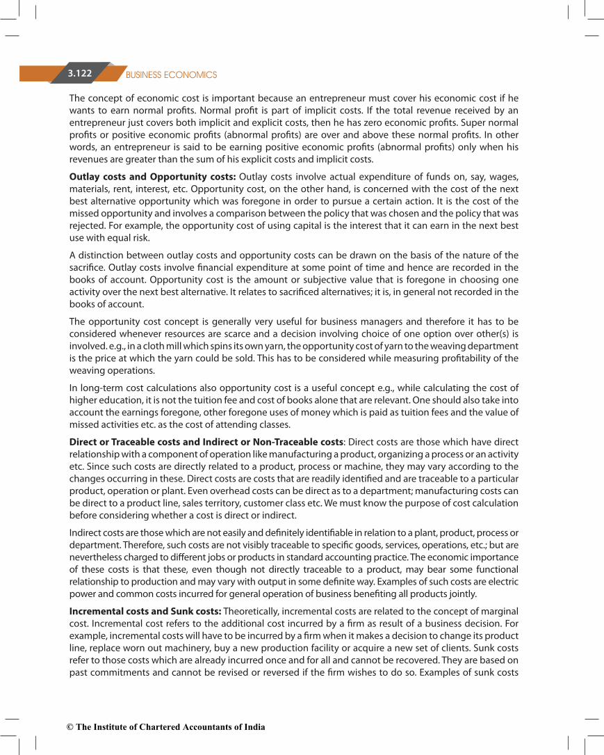
Variable costs, on the other hand are those costs which change with changes in output. These costs include payments such as wages of casual labour employed, prices of raw material, fuel and power used, transportation cost etc. If a �rm shuts down for a short period, it may not use the variable factors of production and therefore, will not therefore incur any variable cost. Figure 6 above presents completely variable cost curve drawn under the assumption that variable costs change linearly with changes in output.

Fig. 7 : Semi Variable Cost

There are some costs which are neither perfectly variable, nor absolutely �xed in relation to the changes in the size of output. They are known as semi-variable costs. Example: Electricity charges include both a �xed charge and a charge based on consumption.

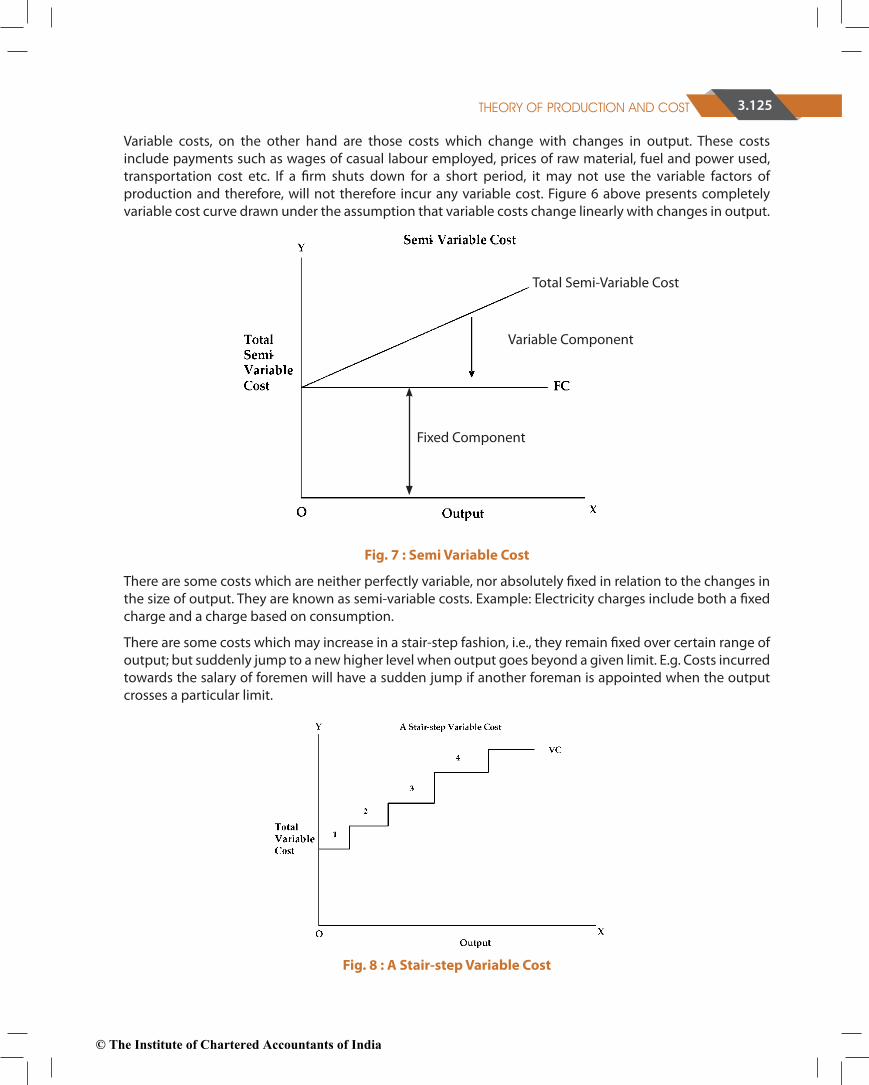
There are some costs which may increase in a stair-step fashion, i.e., they remain �xed over certain range of output; but suddenly jump to a new higher level when output goes beyond a given limit. E.g. Costs incurred towards the salary of foremen will have a sudden jump if another foreman is appointed when the output crosses a particular limit.

Fig. 8 : A Stair-step Variable Cost

Total Semi-Variable Cost

Variable Component

Fixed Component



Fig. 9 : Short run Total Cost Curves

The total cost of a business is de�ned as the actual cost that must be incurred for producing a given quantity of output. The short run total cost is composed of two major elements namely, total �xed cost and total variable cost. Symbolically TC = TFC + TVC. We may represent total cost, total variable cost and �xed cost diagrammatically.

In the diagram above, the total �xed cost curve (TFC) is a horizontal straight line parallel to X-axis as TFC remains �xed for the whole range of output. This curve starts from a point on the Y-axis meaning thereby that �xed costs will be incurred even if the output is zero. On the other hand, the total variable cost curve rises upward indicating that as output increases, total variable cost increases. The total variable cost curve starts from the origin because variable costs are zero when the output is zero. It should be noted that the total variable cost initially increases at a decreasing rate and then at an increasing rate with increases in output. This pattern of change in the TVC occurs due to the operation of the law of increasing and diminishing returns to the variable inputs. Due to the operation of diminishing returns, as output increases, larger quantities of variable inputs are required to produce the same quantity of output. Consequently, variable cost curve is steeper at higher levels of output. The total cost curve has been obtained by adding vertically the total �xed cost curve and the total variable cost curve. The slopes of TC and TVC are the same at every level of output and at each point the two curves have vertical distance equal to total �xed cost. Its position re�ects the amount of �xed costs and its slope re�ects variable costs.

Short run average costs

Average �xed cost (AFC) : AFC is obtained by dividing the total �xed cost by the number of units of output

produced. i.e. TFCAFCQ

= where Q is the number of units produced. Thus, average �xed cost is the �xed cost

per unit of output. For example, if a �rm is producing with a total �xed cost of ` 2,000/-. When output is 100 units, the average �xed cost will be ̀ 20. And now, if the output increases to 200 units, average �xed cost will be ` 10. Since total �xed cost is a constant amount, average �xed cost will steadily fall as output increases. Therefore, if we draw an average �xed cost curve, it will slope downwards throughout its length but will not touch the X-axis as AFC cannot be zero. (Fig. 10)

Average variable cost (AVC) : Average variable cost is found out by dividing the total variable cost by

the number of units of output produced, i.e. TVCAVCQ

= where Q is the number of units produced. Thus,

average variable cost is the variable cost per unit of output. Average variable cost normally falls as output increases from zero to normal capacity output due to occurrence of increasing returns to variable factors.



But beyond the normal capacity output, average variable cost will rise steeply because of the operation of diminishing returns (the concepts of increasing returns and diminishing returns have already been discussed earlier). If we draw an average variable cost curve, it will �rst fall, then reach a minimum and then rise. (Fig. 10)

Fig. 10: Short run Average and Marginal Cost Curves

Average total cost (ATC): Average total cost is the sum of average variable cost and average �xed cost. i.e., ATC = AFC + AVC. It is the total cost divided by the number of units produced, i.e. ATC = TC/Q.The behaviour of average total cost curve depends upon the behaviour of the average variable cost curve and the average �xed cost curve. In the beginning, both AVC and AFC curves fall, therefore, the ATC curve will also fall sharply. When AVC curve begins to rise, but AFC curve still falls steeply, ATC curve continues to fall. This is because, during this stage, the fall in AFC curve is greater than the rise in the AVC curve, but as output increases further, there is a sharp rise in AVC which more than o�sets the fall in AFC. Therefore, ATC curve �rst falls, reaches its minimum and then rises. Thus, the average total cost curve is a “U” shaped curve. (Fig. 10)

Marginal cost: Marginal cost is the addition made to the total cost by the production of an additional unit of output. In other words, it is the total cost of producing t units instead of t-1 units, where t is any given number. For example, if we are producing 5 units at a cost of ` 200 and now suppose the 6th unit is produced and the total cost is ` 250, then the marginal cost is ` 250 - 200 i.e., ` 50. And marginal cost will be ` 24, if 10 units are produced at a total cost of ` 320 [(320-200) / (10-5)]. It is to be noted that marginal cost is independent of �xed cost. This is because �xed costs do not change with output. It is only the variable costs which change with a change in the level of output in the short run. Therefore, marginal cost is in fact due to the changes in variable costs. Symbolically marginal cost may be written as:

MC = TCQ

∆∆

DTC = Change in Total cost

DQ = Change in Output

or

MCn = TC

n – TC

n-1

Marginal cost curve falls as output increases in the beginning. It starts rising after a certain level of output. This happens because of the in�uence of the law of variable proportions. The MC curve becomes minimum



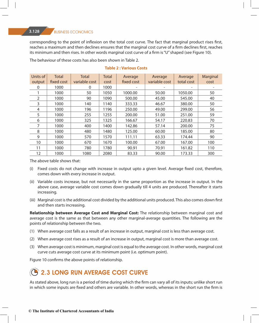
corresponding to the point of in�exion on the total cost curve. The fact that marginal product rises �rst, reaches a maximum and then declines ensures that the marginal cost curve of a �rm declines �rst, reaches its minimum and then rises. In other words marginal cost curve of a �rm is “U” shaped (see Figure 10).

The behaviour of these costs has also been shown in Table 2.

Table 2 : Various Costs

Units of output

Total �xed cost

Total variable cost

Total cost

Average �xed cost

Average variable cost

Average total cost

Marginal cost

0 1000 0 1000 - - - -1 1000 50 1050 1000.00 50.00 1050.00 502 1000 90 1090 500.00 45.00 545.00 403 1000 140 1140 333.33 46.67 380.00 504 1000 196 1196 250.00 49.00 299.00 565 1000 255 1255 200.00 51.00 251.00 596 1000 325 1325 166.67 54.17 220.83 707 1000 400 1400 142.86 57.14 200.00 758 1000 480 1480 125.00 60.00 185.00 809 1000 570 1570 111.11 63.33 174.44 90

10 1000 670 1670 100.00 67.00 167.00 10011 1000 780 1780 90.91 70.91 161.82 11012 1000 1080 2080 83.33 90.00 173.33 300

The above table shows that:

(i) Fixed costs do not change with increase in output upto a given level. Average �xed cost, therefore, comes down with every increase in output.

(ii) Variable costs increase, but not necessarily in the same proportion as the increase in output. In the above case, average variable cost comes down gradually till 4 units are produced. Thereafter it starts increasing.

(iii) Marginal cost is the additional cost divided by the additional units produced. This also comes down �rst and then starts increasing.

Relationship between Average Cost and Marginal Cost: The relationship between marginal cost and average cost is the same as that between any other marginal-average quantities. The following are the points of relationship between the two.

(1) When average cost falls as a result of an increase in output, marginal cost is less than average cost.

(2) When average cost rises as a result of an increase in output, marginal cost is more than average cost.

(3) When average cost is minimum, marginal cost is equal to the average cost. In other words, marginal cost curve cuts average cost curve at its minimum point (i.e. optimum point).

Figure 10 con�rms the above points of relationship.

2.3 LONG RUN AVERAGE COST CURVEAs stated above, long run is a period of time during which the �rm can vary all of its inputs; unlike short run in which some inputs are �xed and others are variable. In other words, whereas in the short run the �rm is



tied with a given plant, in the long run the �rm can build any size or scale of plant and therefore, can move from one plant to another; it can acquire a big plant if it wants to increase its output and a small plant if it wants to reduce its output. The long run being a planning horizon, the �rm plans ahead to build the most appropriate scale of plant to produce the future level of output. It should be kept in mind that once the �rm has built a particular scale of plant, its production takes place in the short run. Brie�y put, the �rm actually operates in the short run and plans for the long run. Long run cost of production is the least possible cost of producing any given level of output when all individual factors are variable. A long run cost curve depicts the functional relationship between output and the long run cost of production.

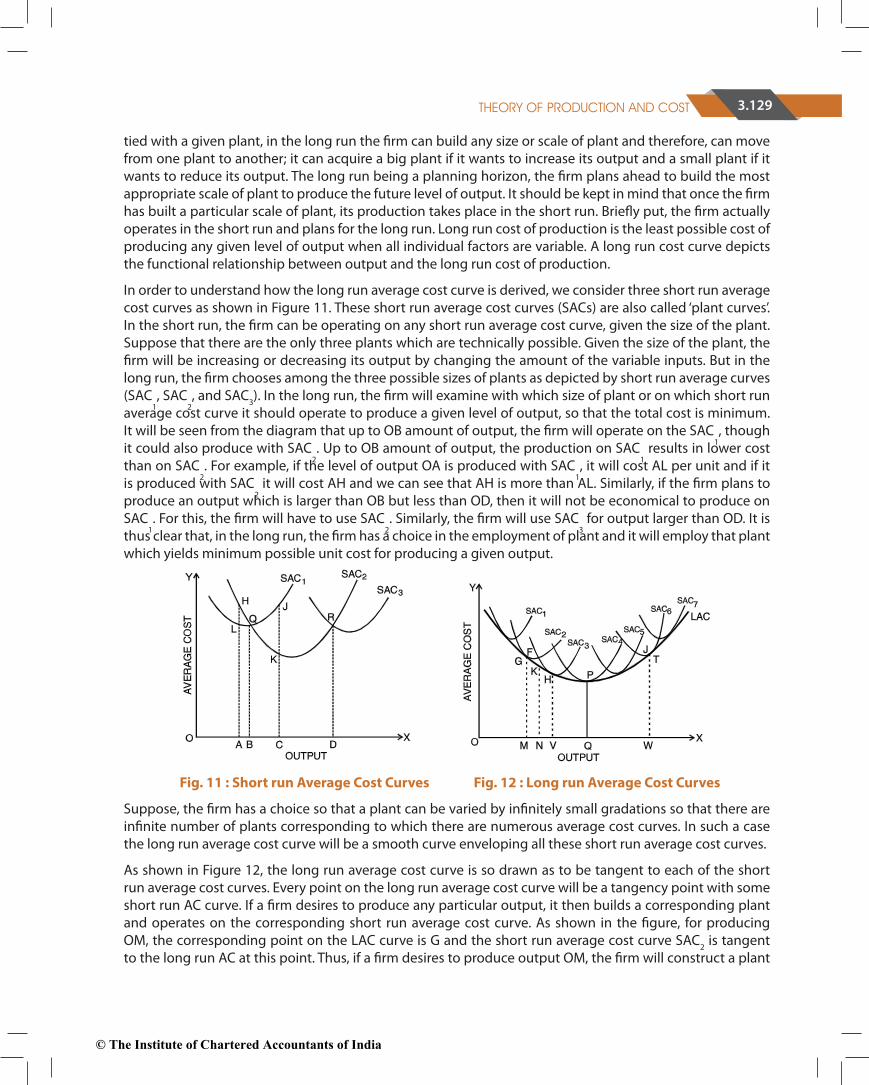
In order to understand how the long run average cost curve is derived, we consider three short run average cost curves as shown in Figure 11. These short run average cost curves (SACs) are also called ‘plant curves’. In the short run, the �rm can be operating on any short run average cost curve, given the size of the plant. Suppose that there are the only three plants which are technically possible. Given the size of the plant, the �rm will be increasing or decreasing its output by changing the amount of the variable inputs. But in the long run, the �rm chooses among the three possible sizes of plants as depicted by short run average curves (SAC

1, SAC

2, and SAC3). In the long run, the �rm will examine with which size of plant or on which short run

average cost curve it should operate to produce a given level of output, so that the total cost is minimum. It will be seen from the diagram that up to OB amount of output, the �rm will operate on the SAC

1, though

it could also produce with SAC2. Up to OB amount of output, the production on SAC

1 results in lower cost

than on SAC2. For example, if the level of output OA is produced with SAC

1, it will cost AL per unit and if it

is produced with SAC2 it will cost AH and we can see that AH is more than AL. Similarly, if the �rm plans to

produce an output which is larger than OB but less than OD, then it will not be economical to produce on SAC

1. For this, the �rm will have to use SAC

2. Similarly, the �rm will use SAC

3 for output larger than OD. It is

thus clear that, in the long run, the �rm has a choice in the employment of plant and it will employ that plant which yields minimum possible unit cost for producing a given output.

Fig. 11 : Short run Average Cost Curves Fig. 12 : Long run Average Cost Curves

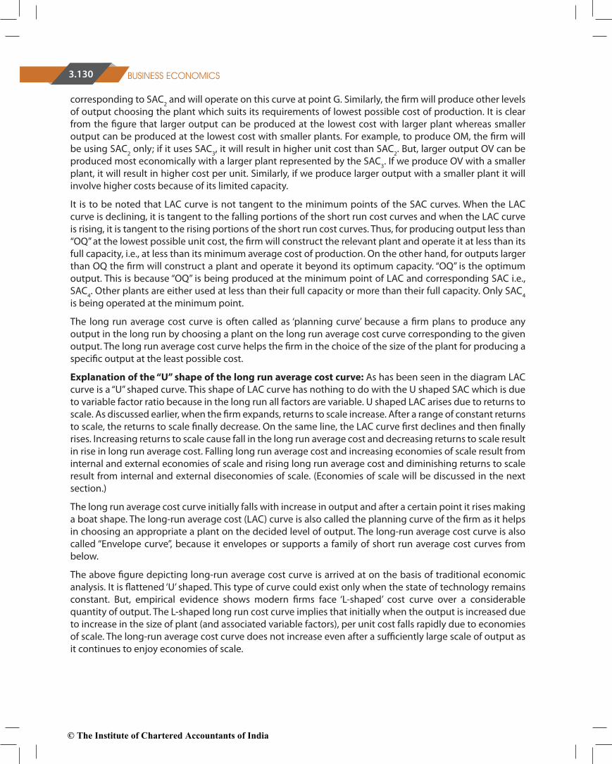
Suppose, the �rm has a choice so that a plant can be varied by in�nitely small gradations so that there are in�nite number of plants corresponding to which there are numerous average cost curves. In such a case the long run average cost curve will be a smooth curve enveloping all these short run average cost curves.

As shown in Figure 12, the long run average cost curve is so drawn as to be tangent to each of the short run average cost curves. Every point on the long run average cost curve will be a tangency point with some short run AC curve. If a �rm desires to produce any particular output, it then builds a corresponding plant and operates on the corresponding short run average cost curve. As shown in the �gure, for producing OM, the corresponding point on the LAC curve is G and the short run average cost curve SAC2 is tangent to the long run AC at this point. Thus, if a �rm desires to produce output OM, the �rm will construct a plant



corresponding to SAC2 and will operate on this curve at point G. Similarly, the �rm will produce other levels of output choosing the plant which suits its requirements of lowest possible cost of production. It is clear from the �gure that larger output can be produced at the lowest cost with larger plant whereas smaller output can be produced at the lowest cost with smaller plants. For example, to produce OM, the �rm will be using SAC2 only; if it uses SAC3, it will result in higher unit cost than SAC2. But, larger output OV can be produced most economically with a larger plant represented by the SAC3. If we produce OV with a smaller plant, it will result in higher cost per unit. Similarly, if we produce larger output with a smaller plant it will involve higher costs because of its limited capacity.

It is to be noted that LAC curve is not tangent to the minimum points of the SAC curves. When the LAC curve is declining, it is tangent to the falling portions of the short run cost curves and when the LAC curve is rising, it is tangent to the rising portions of the short run cost curves. Thus, for producing output less than “OQ” at the lowest possible unit cost, the �rm will construct the relevant plant and operate it at less than its full capacity, i.e., at less than its minimum average cost of production. On the other hand, for outputs larger than OQ the �rm will construct a plant and operate it beyond its optimum capacity. “OQ” is the optimum output. This is because “OQ” is being produced at the minimum point of LAC and corresponding SAC i.e., SAC4. Other plants are either used at less than their full capacity or more than their full capacity. Only SAC4is being operated at the minimum point.

The long run average cost curve is often called as ‘planning curve’ because a �rm plans to produce any output in the long run by choosing a plant on the long run average cost curve corresponding to the given output. The long run average cost curve helps the �rm in the choice of the size of the plant for producing a speci�c output at the least possible cost.

Explanation of the “U” shape of the long run average cost curve: As has been seen in the diagram LAC curve is a “U” shaped curve. This shape of LAC curve has nothing to do with the U shaped SAC which is due to variable factor ratio because in the long run all factors are variable. U shaped LAC arises due to returns to scale. As discussed earlier, when the �rm expands, returns to scale increase. After a range of constant returns to scale, the returns to scale �nally decrease. On the same line, the LAC curve �rst declines and then �nally rises. Increasing returns to scale cause fall in the long run average cost and decreasing returns to scale result in rise in long run average cost. Falling long run average cost and increasing economies of scale result from internal and external economies of scale and rising long run average cost and diminishing returns to scale result from internal and external diseconomies of scale. (Economies of scale will be discussed in the next section.)

The long run average cost curve initially falls with increase in output and after a certain point it rises making a boat shape. The long-run average cost (LAC) curve is also called the planning curve of the �rm as it helps in choosing an appropriate a plant on the decided level of output. The long-run average cost curve is also called “Envelope curve”, because it envelopes or supports a family of short run average cost curves from below.

The above �gure depicting long-run average cost curve is arrived at on the basis of traditional economic analysis. It is �attened ‘U’ shaped. This type of curve could exist only when the state of technology remains constant. But, empirical evidence shows modern �rms face ‘L-shaped’ cost curve over a considerable quantity of output. The L-shaped long run cost curve implies that initially when the output is increased due to increase in the size of plant (and associated variable factors), per unit cost falls rapidly due to economies of scale. The long-run average cost curve does not increase even after a su�ciently large scale of output as it continues to enjoy economies of scale.



2.4 ECONOMIES AND DISECONOMIES OF SCALE The Scale of Production

Production on a large scale is a very important feature of modern industrial society. As a consequence, the size of business undertakings has greatly increased. Large-scale production o�ers certain advantages which help in reducing the cost of production. Economies arising out of large-scale production can be grouped into two categories; viz., internal economies and external economies. Internal economies are those economies of production which accrue to the �rm when it expands its output, so that the cost of production would come down considerably and place the �rm in a better position to compete in the market e�ectively. Internal economies arise purely due to endogenous factors relating to e�ciency of the entrepreneur or his managerial talents or the type of machinery used or the marketing strategy adopted. These economies arise within the �rm and are available exclusively to the expanding �rm. On the other hand, external economies are the bene�ts accruing to each member �rm of the industry as a result of expansion of the industry.

Internal Economies and Diseconomies: We saw that returns to scale increase in the initial stages and after remaining constant for a while, they decrease. The question arises as to why we get increasing returns to scale due to which cost falls and why after a certain point we get decreasing returns to scale due to which cost rises. The answer is that initially a �rm enjoys internal economies of scale and beyond a certain limit it su�ers from internal diseconomies of scale. Internal economies and diseconomies are of the following main kinds:

(i) Technical economies and diseconomies: Large-scale production is associated with economies of superior techniques. As the �rm increases its scale of operations, it becomes possible to use more specialised and e�cient form of all factors, specially capital equipment and machinery. For producing higher levels of output, there is generally available a more e�cient machinery which when employed to produce a large output yields a lower cost per unit of output. The �rm is able to take advantage of composite technology whereby the whole process of production of a commodity is done as one composite unit. Secondly, when the scale of production is increased and the amount of labour and other factors become larger, introduction of greater degree of division of labour and specialisation becomes possible and as a result cost per unit declines. There are some advantages available to a large �rm on account of performance of a number of linked processes. The �rm can reduce the inconvenience and costs associated with the dependence on other �rms by undertaking various processes from the input supply stage to the �nal output stage.

However, beyond a certain point, a �rm experiences net diseconomies of scale. This happens because when the �rm has reached a size large enough to allow utilisation of almost all the possibilities of division of labour and employment of more e�cient machinery, further increase in the size of the plant will bring about high long-run cost because of di�culties of management. When the scale of operations becomes too large, it becomes di�cult for the management to exercise control and to bring about proper coordination.

(ii) Managerial economies and diseconomies: Managerial economies refer to reduction in managerial costs. When output increases, specialisation and division of labour can be applied to management. It becomes possible to divide its management into specialised departments under specialised personnel, such as production manager, sales manager, �nance manager etc. If the scale of production increases further, each department can be further sub-divided; for e.g. sales can be split into separate sections such as for advertising, exports and customer service. Since individual activities come under the supervision of specialists, management’s e�ciency and productivity will greatly improve. Decentralisation of decision making and mechanisation of managerial functions further enhance the e�ciency and productivity of



managers. Thus, specialisation of management enables large �rms to achieve reduction in managerial costs.

However, as the scale of production increases beyond a certain limit, managerial diseconomies set in. Communication at di�erent levels such as between the managers and labourers and among the managers become di�cult resulting in delays in decision making and implementation of decisions already made. Management �nds it di�cult to exercise control and to bring in coordination among its various departments. The managerial structure becomes more complex and is a�ected by greater bureaucracy, red tapism, lengthening of communication lines and so on. All these a�ect the e�ciency and productivity of management and that of the �rm itself.

(iii) Commercial economies and diseconomies: Production of large volumes of goods requires large amount of materials and components. A large �rm is able to place bulk orders for materials and components and enjoy lower prices for them. Economies can also be achieved in marketing of the product. If the sales sta� is not being worked to full capacity, additional output can be sold at little or no extra cost. Moreover, large �rms can bene�t from economies of advertising. As the scale of production increases, advertising costs per unit of output fall. In addition, a large �rm may also be able to sell its by-products or process it pro�tably; something which might be unpro�table for a small �rm. There are also economies associated with transport and storage.

These economies become diseconomies after an optimum scale. For example, advertisement expenditure and other marketing overheads will increase more than proportionately after the optimum scale.

(iv) Financial economies and diseconomies: A large �rm has advantages over small �rms in matters related to procurement of �nance for its business activities. It can, for instance, o�er better security to bankers and avail of advances with greater ease. On account of the goodwill enjoyed by large �rms, investors have greater con�dence in them and therefore would prefer their shares which can be readily sold on the stock exchange. A large �rm can thus raise capital at lower cost.

However, these costs of raising �nance will rise more than proportionately after the optimum scale of production. This may happen because of relatively greater dependence on external �nances.

(v) Risk bearing economies and diseconomies: It is said that a large business with diverse and multi-production capability is in a better position to withstand economic ups and downs, and therefore, enjoys economies of risk bearing. However, risk may increase if diversi�cation, instead of giving a cover to economic disturbances, increases these.

External Economies and Diseconomies: Internal economies are economies enjoyed by a �rm on account of use of greater degree of division of labour and specialised machinery at higher levels of output. They are internal in the sense that they accrue to the �rm due to its own e�orts. Besides internal economies, there are external economies which are very important for a �rm. External economies and diseconomies are those economies and diseconomies which accrue to �rms as a result of expansion in the output of the whole industry and they are not dependent on the output level of individual �rms. They are external in the sense that they accrue to �rms not out of their internal situation but from outside i.e. due to expansion of the industry. These are available to one or more of the �rms in the form of:

1. Cheaper raw materials and capital equipment: The expansion of an industry may result in exploration of new and cheaper sources of raw material, machinery and other types of capital equipments. Expansion of an industry results in greater demand for various kinds of materials and capital equipments required by it. The �rm can procure these on a large scale at competitive prices from other industries. This reduces their cost of production and consequently the prices of their output.



2. Technological external economies: When the whole industry expands, it may result in the discovery of new technical knowledge and in accordance with that, the use of improved and better machinery and processes than before. This will change the technical co-e�cient of production and enhance productivity of �rms in the industry and reduce their cost of production.

3. Development of skilled labour: When an industry expands in an area, the labourers in that area are well accustomed with the di�erent productive processes and tend to learn a good deal from experience. As a result, with the growth of an industry in an area, a pool of trained labour is developed which has a favourable e�ect on the level of productivity and cost of the �rms in that industry.

4. Growth of ancillary industries: Expansion of industry encourages the growth of a number of ancillary industries which specialise in the production and supply of raw materials, tools, machinery, components, repair services etc. Input prices go down in a competitive market and the bene�ts of it accrue to all �rms in the form of reduction in cost of production. Likewise, new units may come up for processing or recycling of the waste products of the industry. This will tend to reduce the cost of production in general.

5. Better transportation and marketing facilities: The expansion of an industry resulting from entry of new �rms may make possible the development of an e�cient transportation and marketing network. These will greatly reduce the cost of production of the �rms by avoiding the need for establishing and running these services by themselves. Similarly, communication systems may get modernised resulting in better and speedy information dissemination.

6. Economies of Information: Necessary information regarding technology, labour, prices and products may be easily and cheaply made available to the �rms on account of publication of information booklets and bulletins by industry associations or by governments in public interest.

However, external economies may cease if there are certain disadvantages which may neutralise the advantages of expansion of an industry. We call them external diseconomies. External diseconomies are disadvantages that originate outside the �rm, especially in the input markets. An example of external diseconomies is rise in various factor prices. When an industry expands the requirement of various factors of production, such as raw materials, capital goods, skilled labour etc increases. Increasing demand for inputs puts pressure on the input markets. This may result in an increase in the prices of factors of production, especially when they are short in supply. Moreover, too many �rms in an industry at one place may also result in higher transportation cost, marketing cost and high pollution control cost. The government may also, through its location policy, prohibit or restrict the expansion of an industry at a particular place.



SUMMARY

Ø Cost analysis refers to the study of behaviour of cost in relation to one or more production criteria. It is concerned with the �nancial aspects of production.

w Accounting costs are explicit costs and includes all the payments and charges made by the entrepreneur to the suppliers of various productive factors.

w Economic costs take into account explicit costs as well as implicit costs. A �rm has to cover its economic cost if it wants to earn normal pro�ts.

w Outlay costs involve actual expenditure of funds.

w Opportunity cost is concerned with the cost of the next best alternative opportunity which was foregone in order to pursue a certain action.

w Direct costs are those which have direct relationship with a component of operation. They are readily identi�ed and are traceable to a particular product, operation or plant.

w Indirect costs are those which cannot be easily and de�nitely identi�able in relation to a plant, product, process or department. They not visibly traceable to any speci�c goods, services, processes, departments or operations.

w Incremental cost refers to the additional cost incurred by a �rm as a result of a business decision.

w Sunk costs are already incurred once and for all, and cannot be recovered.

w Historical cost refers to the cost incurred in the past on the acquisition of a productive asset.

w Replacement cost is the money expenditure that has to be incurred for replacing an old asset.

w Private costs are costs actually incurred or provided for by �rms and are either explicit or implicit.

w Social cost, on the other hand, refers to the total cost borne by the society on account of a business activity and includes private cost and external cost.

Ø The cost function refers to the mathematical relation between cost and the various determinants of cost. It expresses the relationship between cost and output.

Ø Economists are generally interested in two types of cost functions; the short run cost function and the long run cost function.

Ø Short-run cost functions are

w Fixed or constant costs which are not a function of output. These are inescapable or uncontrollable.

w Variable costs are a function of output in the production period.

w Short run is a period of time in which output can be increased or decreased by changing only the amount of variable factors such as, labour, raw material, etc. ,

w Long run is a period of time in which the quantities of all factors may be varied. In other words, all factors become variable in the long run.

w Semi-variable costs are neither perfectly variable, nor absolutely �xed in relation to the changes in the size of output.



w Stair-step costs remain �xed over certain range of output; but suddenly jump to a new higher level when output goes beyond a given limit.

w Total cost of a business is de�ned as the actual cost that must be incurred for producing a given quantity of output.

w AFC is obtained by dividing the total �xed cost by the number of units of output produced.

w Average variable cost is found out by dividing the total variable cost by the number of units of output produced.

w Average total cost is the sum of average �xed cost and average variable cost.

w Marginal cost is the addition made to the total cost by the production of an additional unit of output.

Ø Long run cost of production is the least possible cost of producing any given level of output when all individual factors are variable.

w A long run cost curve depicts the functional relationship between output and the long run cost of production.

w The long run average cost curve, often called a planning curve, is so drawn as to be tangent to each of the short run average cost curves.

w LAC curve is not tangent to the minimum points of the SAC curves.

w Empirical evidence shows that the state of technology changes in the long-run. Therefore, modern �rms face ‘L-shaped’ cost curve over a considerable quantity of output.

Ø Economies of scale are of two kinds - external economies of scale and internal economies of scale.

w External economies of scale accrue to a �rm due to factors which are external to a �rm.

w Internal economies of scale accrue to a �rm when it engages in large scale production.

w Increase in scale, beyond the optimum level, results in diseconomies of scale.

MULTIPLE CHOICE QUESTIONS1. Which of the following is considered production in Economics?

(a) Tilling of soil.

(b) Singing a song before friends.

(c) Preventing a child from falling into a manhole on the road.

(d) Painting a picture for pleasure.

2. Identify the correct statement:

(a) The average product is at its maximum when marginal product is equal to average product.

(b) The law of increasing returns to scale relates to the e�ect of changes in factor proportions.

(c) Economies of scale arise only because of indivisibilities of factor proportions.

(d) Internal economies of scale can accrue when industry expands beyond optimum.



3. Which of the following is not a characteristic of land?

(a) Its supply for the economy is limited.

(b) It is immobile.

(c) Its usefulness depends on human e�orts.

(d) It is produced by our forefathers.

4. Which of the following statements is true?

(a) Accumulation of capital depends solely on income of individuals.

(b) Savings can be in�uenced by government policies.

(c) External economies go with size and internal economies with location.

(d) The supply curve of labour is an upward slopping curve.

5. In the production of wheat, all of the following are variable factors that are used by the farmer except:

(a) the seed and fertilizer used when the crop is planted.

(b) the �eld that has been cleared of trees and in which the crop is planted.

(c) the tractor used by the farmer in planting and cultivating not only wheat but also corn and barley.

(d) the number of hours that the farmer spends in cultivating the wheat �elds.

6. The marginal product of a variable input is best described as:

(a) total product divided by the number of units of variable input.

(b) the additional output resulting from a one unit increase in the variable input.

(c) the additional output resulting from a one unit increase in both the variable and �xed inputs.

(d) the ratio of the amount of the variable input that is being used to the amount of the �xed input that is being used.

7. Diminishing marginal returns implies:

(a) decreasing average variable costs.

(b) decreasing marginal costs.

(c) increasing marginal costs.

(d) decreasing average �xed costs.

8. The short run, as economists use the phrase, is characterized by:

(a) at least one �xed factor of production and �rms neither leaving nor entering the industry.

(b) generally a period which is shorter than one year.

(c) all factors of production are �xed and no variable inputs.

(d) all inputs are variable and production is done in less than one year.



9. The marginal, average, and total product curves encountered by the �rm producing in the short run exhibit all of the following relationships except:

(a) when total product is rising, average and marginal product may be either rising or falling.

(b) when marginal product is negative, total product and average product are falling.

(c) when average product is at a maximum, marginal product equals average product, and total product is rising.

(d) when marginal product is at a maximum, average product equals marginal product, and total product is rising.

10. To economists, the main di�erence between the short run and the long run is that:

(a) In the short run all inputs are �xed, while in the long run all inputs are variable.

(b) In the short run the �rm varies all of its inputs to �nd the least-cost combination of inputs.

(c) In the short run, at least one of the �rm’s input levels is �xed.

(d) In the long run, the �rm is making a constrained decision about how to use existing plant and equipment e�ciently.

11. Which of the following is the best de�nition of “production function”?

(a) The relationship between market price and quantity supplied.

(b) The relationship between the �rm’s total revenue and the cost of production.

(c) The relationship between the quantities of inputs needed to produce a given level of output.

(d) The relationship between the quantity of inputs and the �rm’s marginal cost of production.

12. The “law of diminishing returns” applies to:

(a) the short run, but not the long run.

(b) the long run, but not the short run.

(c) both the short run and the long run.

(d) neither the short run nor the long run.

13. Diminishing returns occur:

(a) when units of a variable input are added to a �xed input and total product falls.

(b) when units of a variable input are added to a �xed input and marginal product falls.

(c) when the size of the plant is increased in the long run.

(d) when the quantity of the �xed input is increased and returns to the variable input falls.



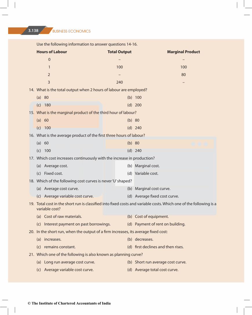
Use the following information to answer questions 14-16.

Hours of Labour Total Output Marginal Product

0 – –

1 100 100

2 – 80

3 240 –

14. What is the total output when 2 hours of labour are employed?

(a) 80 (b) 100

(c) 180 (d) 200

15. What is the marginal product of the third hour of labour?

(a) 60 (b) 80

(c) 100 (d) 240

16. What is the average product of the �rst three hours of labour?

(a) 60 (b) 80

(c) 100 (d) 240

17. Which cost increases continuously with the increase in production?

(a) Average cost. (b) Marginal cost.

(c) Fixed cost. (d) Variable cost.

18. Which of the following cost curves is never ‘U’ shaped?

(a) Average cost curve. (b) Marginal cost curve.

(c) Average variable cost curve. (d) Average �xed cost curve.

19. Total cost in the short run is classi�ed into �xed costs and variable costs. Which one of the following is a variable cost?

(a) Cost of raw materials. (b) Cost of equipment.

(c) Interest payment on past borrowings. (d) Payment of rent on building.

20. In the short run, when the output of a �rm increases, its average �xed cost:

(a) increases. (b) decreases.

(c) remains constant. (d) �rst declines and then rises.

21. Which one of the following is also known as planning curve?

(a) Long run average cost curve. (b) Short run average cost curve.

(c) Average variable cost curve. (d) Average total cost curve.



22. If a �rm moves from one point on a production isoquant to another, which of the following will not happen.

(a) A change in the ratio in which the inputs are combined to produce output.

(b) A change in the ratio of marginal products of the inputs.

(c) A change in the marginal rate of technical substitution.

(d) A change in the level of output.

23. With which of the following is the concept of marginal cost closely related?

(a) Variable cost. (b) Fixed cost.

(c) Opportunity cost. (d) Economic cost.

24. Which of the following statements is correct?

(a) When the average cost is rising, the marginal cost must also be rising.

(b) When the average cost is rising, the marginal cost must be falling.

(c) When the average cost is rising, the marginal cost is above the average cost.

(d) When the average cost is falling, the marginal cost must be rising.

25. Which of the following is an example of “explicit cost”?

(a) The wages a proprietor could have made by working as an employee of a large �rm.

(b) The income that could have been earned in alternative uses by the resources owned by the �rm.

(c) The payment of wages by the �rm.

(d) The normal pro�t earned by a �rm.

26. Which of the following is an example of an “implicit cost”?

(a) Interest that could have been earned on retained earnings used by the �rm to �nance expansion.

(b) The payment of rent by the �rm for the building in which it is housed.

(c) The interest payment made by the �rm for funds borrowed from a bank.

(d) The payment of wages by the �rm.

Use the following data to answer questions 27-29.

Output (O) 0 1 2 3 4 5 6Total Cost (TC) ` 240 ` 330 ` 410 ` 480 ` 540 ` 610 ` 690

27. The average �xed cost of 2 units of output is :

(a) ` 80 (b) ` 85

(c) ` 120 (d) ` 205

28. The marginal cost of the sixth unit of output is :

(a) ` 133 (b) ` 75

(c) ` 80 (d) ` 450



29. Diminishing marginal returns start to occur between units:

(a) 2 and 3. (b) 3 and 4.

(c) 4 and 5. (d) 5 and 6.

30. Marginal cost is de�ned as:

(a) the change in total cost due to a one unit change in output.

(b) total cost divided by output.

(c) the change in output due to a one unit change in an input.

(d) total product divided by the quantity of input.

31. Which of the following is true of the relationship between the marginal cost function and the average cost function?

(a) If MC is greater than ATC, then ATC is falling.

(b) The ATC curve intersects the MC curve at minimum MC.

(c) The MC curve intersects the ATC curve at minimum ATC.

(d) If MC is less than ATC, then ATC is increasing.

32. Which of the following statements is true of the relationship among the average cost functions?

(a) ATC = AFC – AVC. (b) AVC = AFC + ATC.

(c) AFC = ATC + AVC. (d) AFC = ATC – AVC.

33. Which of the following is not a determinant of the �rm’s cost function?

(a) The production function. (b) The price of labour.

(c) Taxes. (d) The price of the �rm’s output.

34. Which of the following statements is correct concerning the relationships among the �rm’s cost functions?

(a) TC = TFC – TVC. (b) TVC = TFC – TC.

(c) TFC = TC – TVC. (d) TC = TVC – TFC.

35. Suppose output increases in the short run. Total cost will:

(a) increase due to an increase in �xed costs only.

(b) increase due to an increase in variable costs only.

(c) increase due to an increase in both �xed and variable costs.

(d) decrease if the �rm is in the region of diminishing returns.

36. Which of the following statements concerning the long-run average cost curve is false?

(a) It represents the least-cost input combination for producing each level of output.

(b) It is derived from a series of short-run average cost curves.



(c) The short-run cost curve at the minimum point of the long-run average cost curve represents the least–cost plant size for all levels of output.

(d) As output increases, the amount of capital employed by the �rm increases along the curve.

37. The negatively-sloped (i.e. falling) part of the long-run average total cost curve is due to which of the following?

(a) Diseconomies of scale. (b) Diminishing returns.

(c) The di�culties encountered in coordinating the many activities of a large �rm.

(d) The increase in productivity that results from specialization.

38. The positively sloped (i.e. rising) part of the long run average total cost curve is due to which of the following?

(a) Diseconomies of scale. (b) Increasing returns.

(c) The �rm being able to take advantage of large-scale production techniques as it expands its output.

(d) The increase in productivity that results from specialization.

39. A �rm’s average total cost is ` 300 at 5 units of output and ` 320 at 6 units of output. The marginal cost of producing the 6th unit is :

(a) ` 20 (b) ` 120

(c) ` 320 (d) ` 420

40. A �rm producing 7 units of output has an average total cost of ` 150 and has to pay ` 350 to its �xed factors of production whether it produces or not. How much of the average total cost is made up of variable costs?

(a) ` 200 (b) ` 50

(c) ` 300 (d) ` 100

41. A �rm has a variable cost of ` 1000 at 5 units of output. If �xed costs are ` 400, what will be the average total cost at 5 units of output?

(a) ` 280 (b) ` 60

(c) ` 120 (d) ` 1400

42. A �rm’s average �xed cost is ` 20 at 6 units of output. What will it be at 4 units of output?

(a) ` 60 (b) ` 30

(c) ` 40 (d) ` 20


(a) The services of a doctor are considered production.

(b) Man can create matter.

(c) The services of a housewife are considered production.

(d) When a man creates a table, he creates matter.



44. Which of the following is a function of an entrepreneur?

(a) Initiating a business enterprise. (b) Risk bearing.

(c) Innovating. (d) All of the above.

45. In describing a given production technology, the short run is best described as lasting:

(a) up to six months from now. (b) up to �ve years from now.

(c) as long as all inputs are �xed. (d) as long as at least one input is �xed.

46. If decreasing returns to scale are present, then if all inputs are increased by 10% then:

(a) output will also decrease by 10%. (b) output will increase by 10%.

(c) output will increase by less than 10%. (d) output will increase by more than 10%.

47. The production function is a relationship between a given combination of inputs and:

(a) another combination that yields the same output.

(b) the highest resulting output.

(c) the increase in output generated by one-unit increase in one output.

(d) all levels of output that can be generated by those inputs.

48. If the marginal product of labour is below the average product of labour, it must be true that:

(a) the marginal product of labour is negative.

(b) the marginal product of labour is zero.

(c) the average product of labour is falling.

(d) the average product of labour is negative.

49. The average product of labour is maximized when marginal product of labour:

(a) equals the average product of labour. (b) equals zero.

(c) is maximized. (d) none of the above.

50. The law of variable proportions is drawn under all of the assumptions mentioned below except the assumption that:

(a) the technology is changing.

(b) there must be some inputs whose quantity is kept �xed.

(c) we consider only physical inputs and not economically pro�tability in monetary terms.

(d) the technology is given and stable.

51. What is a production function?

(a) Technical relationship between physical inputs and physical output.

(b) Relationship between �xed factors of production and variable factors of production.

(c) Relationship between a factor of production and the utility created by it.

(d) Relationship between quantity of output produced and time taken to produce the output.



52. Laws of production does not include ……

(a) returns to scale. (b) law of diminishing returns to a factor.

(c) law of variable proportions. (d) least cost combination of factors.

53. An iso quant shows

(a) All the alternative combinations of two inputs that can be produced by using a given set of output fully and in the best possible way.

(b) All the alternative combinations of two products among which a producer is indi�erent because they yield the same pro�t.

(c) All the alternative combinations of two inputs that yield the same total product.

(d) Both (b) and (c).

54. Economies of scale exist because as a �rm increases its size in the long run:

(a) Labour and management can specialize in their activities more.

(b) As a larger input buyer, the �rm can get �nance at lower cost and purchase inputs at a lower per unit cost.

(c) The �rm can a�ord to employ more sophisticated technology in production.

(d) All of these.

55. The production function:

(a) Is the relationship between the quantity of inputs used and the resulting quantity of product.

(b) Tells us the maximum attainable output from a given combination of inputs.

(c) Expresses the technological relationship between inputs and output of a product.

(d) All the above.

56. The production process described below exhibits.

Number of Workers Output0 01 232 403 50

(a) constant marginal product of labour.

(b) diminishing marginal product of labour.

(c) increasing return to scale.

(d) increasing marginal product of labour.

57. Which of the following is a variable cost in the short run?

(a) rent of the factory.

(b) wages paid to the factory labour.

(c) interest payments on borrowed �nancial capital.

(d) payment on the lease for factory equipment.



58. The e�cient scale of production is the quantity of output that minimizes

(a) average �xed cost. (b) average total cost.

(c) average variable cost. (d) marginal cost.

59. In the short run, the �rm's product curves show that

(a) Total product begins to decrease when average product begins to decrease but continues to increase at a decreasing rate.

(b) When marginal product is equal to average product, average product is decreasing but at its highest.

(c) When the marginal product curve cuts the average product curve from below, the average product is equal to marginal product.

(d) In stage two, total product increases at a diminishing rate and reaches maximum at the end of this stage.

60. A �xed input is de�ned as

(a) That input whose quantity can be quickly changed in the short run, in response to the desire of the company to change its production.

(b) That input whose quantity cannot be quickly changed in the short run, in response to the desire of the company to change its production.

(c) That input whose quantities can be easily changed in response to the desire to increase or reduce the level of production.

(d) That input whose demand can be easily changed in response to the desire to increase or reduce the level of production.

61. Average product is de�ned as

(a) total product divided by the total cost.

(b) total product divided by marginal product.

(c) total product divided by the number of units of variable input.

(d) marginal product divided by the number of units of variable input.


(a) After the in�ection point of the production function, a greater use of the variable input induces a reduction in the marginal product.

(b) Before reaching the inevitable point of decreasing marginal returns, the quantity of output obtained can increase at an increasing rate.

(c) The �rst stage corresponds to the range in which the AP is increasing as a result of utilizing increasing quantities of variable inputs.

(d) All the above.



63. Marginal product, mathematically, is the slope of the

(a) total product curve. (b) average product curve.

(c) marginal product curve. (d) implicit product curve.

64. Suppose the �rst four units of a variable input generate corresponding total outputs of 200, 350, 450, 500. The marginal product of the third unit of input is:

(a) 50 (b) 100

(c) 150 (d) 200

65. Which of the following statements is false in respect of �xed cost of a �rm?

(a) As the �xed inputs for a �rm cannot be changed in the short run, the TFC are constant, except when the prices of the �xed inputs change.

(b) TFC continue to exist even when production is stopped in the short run, but they exist in the long run even when production is not stopped.

(c) Total Fixed Costs (TFC) can be de�ned as the total sum of the costs of all the �xed inputs associated with production in the short run.

(d) In the short run, a �rm’s �xed cost cannot be escaped even when production is stopped.

66. Diminishing marginal returns for the �rst four units of a variable input is exhibited by the total product sequence:

(a) 50, 50, 50, 50 (b) 50, 110, 180, 260

(c) 50, 100, 150, 200 (d) 50, 90, 120, 140

67. Use the following diagram to answer the question given below it



The marginal physical product of the third unit of labour is _____, the MP of the _____ labour is Negative

(a) Six; fourth (b) Six; third

(c) Six ; �fth (d) Six; sixth

68. In the third of the three stages of production:

(a) the marginal product curve has a positive slope.

(b) the marginal product curve lies completely below the average product curve.

(c) total product increases.

(d) marginal product is positive.

69. When marginal costs are below average total costs,

(a) average �xed costs are rising. (b) average total costs are falling.

(c) average total costs are rising. (d) average total costs are minimized.

70. A �rm’s long-run average total cost curve is

(a) Identical to its long-run marginal-cost curve.

(b) Also its long-run supply curve because it explains the relationship between price and quantity supplied.

(c) In fact the average total cost curve of the optimal plant in the short run as it tries to produce at least cost.

(d) Tangent to all the curves of short-run average total cost.

71. In the long run, if a very small factory were to expand its scale of operations, it is likely that it would initially experience

(a) an increase in pollution level. (b) diseconomies of scale.

(c) economies of scale. (d) constant returns to scale.

72. A �rm’s long-run average total cost curve is.

(a) Identical to its long-run marginal-cost curve as all factors are variable.

(b) Also its long-run total cost curve because it explains the relationship cost and quantity supplied in the long run.

(c) In fact the average total cost curve of the optimal plant in the short run as it tries to produce at least cost.

(d) Tangent to all short-run average total cost the curves and represents the lowest average total cost for producing each level of output.

73. Which of the following statements describes increasing returns to scale?

(a) Doubling of all inputs used leads to doubling of the output.

(b) Increasing the inputs by 50% leads to a 25% increase in output.

(c) Increasing inputs by 1/4 leads to an increase in output of 1/3.

(d) None of the above.



74. The marginal cost for a �rm of producing the 9th unit of output is ` 20. Average cost at the same level of output is ` 15. Which of the following must be true?

(a) marginal cost and average cost are both falling

(b) marginal cost and average cost are both rising

(c) marginal cost is rising and average cost is falling

(d) it is impossible to tell if either of the curves are rising or falling

75. Implicit cost can be de�ned as

(a) Money payments made to the non-owners of the �rm for the self-owned factors employed in the business and therefore not entered into books of accounts.

(b) Money not paid out to the owners of the �rm for the self owned factors employed in a business and therefore not entered into books of accounts.

(c) Money payments which the self owned and employed resources could have earned in their next best alternative employment and therefore entered into books of accounts.

(d) Money payments which the self owned and employed resources earn in their best use and therefore entered into book of accounts.

76. The most important function of an entrepreneur is to ____________.

(a) Innovate

(b) Bear the sense of responsibility

(c) Finance

(d) Earn pro�t

77. Economic costs of production di�er from accounting costs of production because

(a) Economic costs include expenditures for hired resources while accounting costs do not.

(b) Accounting costs include opportunity costs which are deducted later to �nd paid out costs.

(c) Accounting costs include expenditures for hired resources while economic costs do not.

(d) Economic costs add the opportunity cost of a �rm which uses its own resources.



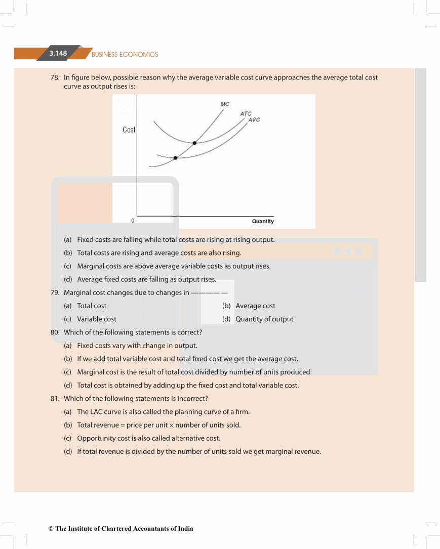
78. In �gure below, possible reason why the average variable cost curve approaches the average total cost curve as output rises is:

(a) Fixed costs are falling while total costs are rising at rising output.

(b) Total costs are rising and average costs are also rising.

(c) Marginal costs are above average variable costs as output rises.

(d) Average �xed costs are falling as output rises.

79. Marginal cost changes due to changes in —————

(a) Total cost (b) Average cost

(c) Variable cost (d) Quantity of output

80. Which of the following statements is correct?

(a) Fixed costs vary with change in output.

(b) If we add total variable cost and total �xed cost we get the average cost.

(c) Marginal cost is the result of total cost divided by number of units produced.

(d) Total cost is obtained by adding up the �xed cost and total variable cost.

81. Which of the following statements is incorrect?

(a) The LAC curve is also called the planning curve of a �rm.

(b) Total revenue = price per unit × number of units sold.

(c) Opportunity cost is also called alternative cost.

(d) If total revenue is divided by the number of units sold we get marginal revenue.



ANSWERS

1. a 2. a 3. d 4. b 5. b 6. b

7. c 8. a 9. d 10. c 11. c 12. a

13. b 14. c 15. a 16. b 17. d 18. d

19. a 20. b 21. a 22. d 23. a 24. c

25. c 26. a 27. c 28. c 29. c 30. a

31. c 32. d 33. d 34. c 35. b 36. c

37. d 38. a 39. d 40. d 41. a 42. b

43. a 44. d 45. d 46. c 47. b 48. c

49. a 50. a 51. a 52. d 53. c 54. d

55. d 56. b 57. b 58. b 59. d 60. b

61. c 62. d 63. a 64. b 65. b 66. d

67. d 68. b 69. b 70. d 71. c 72. d

73. c 74. b 75. b 76. a 77. d 78. d

79. c 80. d 81. d


UNIT 2 : THEORY OF COST - CA-FOUNDATION.in...THEORY OF PRODUCTION AND COST 3.121 In the previous...

Documents

Transcript of UNIT 2 : THEORY OF COST - CA-FOUNDATION.in...THEORY OF PRODUCTION AND COST 3.121 In the previous...