Unit 2 –Measures of Risk and Return

The purpose of this unit is for the student to understand, be able to compute, and interpret basic statistical measures of risk and return for financial

analysis

We will learn about three standard measures of return on investment:

• Holding period return

• Arithmetic mean return

• Geometric mean return

Holding Period Return

• The holding period return is a single period measure

• It is comprised of two potential components – change in asset price, and income.

• It does not take into account the time value of money, and should only be used to gauge performance for a single period, such as a quarter or a year

A Demonstration of Holding Period Return Calculation

Suppose a stock is worth 20 euros at the beginning of the year. The firm pays an annual dividend of .50 euros, and the end of year price is 24 euros.

Calculate the holding period return on investment. 

HPR = ((24 –20) + .50) / 20 = (4.5) / 20 = 22.5%. 

Here, the holding period is one year, and the investor earns  

4/20 = 20% from price appreciation, and .5 / 20 = 2.5 % from income (dividend), for a total annual return of 22.5%.

Arithmetic Mean Return

• The arithmetic mean return is a multi-period measure of return

• It is a simple arithmetic average, computed by summing the individual holding period returns from multiple periods, and dividing by the number of periods

• It provides an unbiased estimate of the expected return in the coming period

A Demonstration of the Calculation of Arithmetic Mean Return

Suppose a stock investment returned 22.5% in 1999, 7.75% in 2000, and –12% in 2001. What was the average annual return over the three year holding period?

 Am = (22.5% + 7.75% – 12%) / 3 = 6.08%

 So, during the 1999-2001 three year period, the average annual return was 6.08%.

Based on these three years performance, 6.08% would be the expectedholding period return for 2002 for this stock.

 

Some notes on the arithmetic mean return measure

• This measure does not consider compounding

• It overstates the actual rate of growth of an investment

• It does provide an average performance measure over multiple holding periods

• The name of the Excel statistical function to compute an arithmetic mean is Average

Geometric Mean Return

• The geometric mean return is a multi-period measure that incorporates the time value associated with compounding

• To compute a geometric mean, you must add 1 to each holding period return, creating what is known as a “return relative”, then take the nth root of the product of the return relatives.

• By creating return relatives, you eliminate negative numbers from the calculation

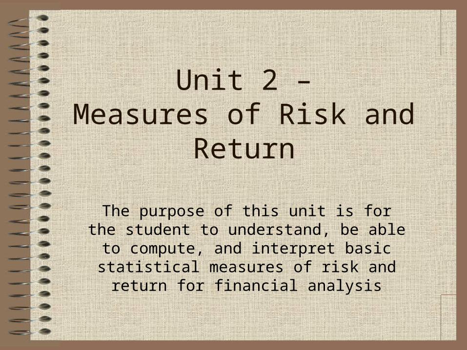
Example of Calculating a Geometric Mean Return

Using our same example of annual returns of 22.5%, 7.75%, and –12%, the return relatives would be 1.225, 1.0775, and .88. Then, the geometric

mean is given by 

Gm = [(1.225)(1.0775)(.88)] 1/3 - 1Gm = [1.1615] 1/3 –1

Gm = 5.12%

Some notes on the geometric mean return

• This is a compound average measure of periodic return

• It represents the periodic growth rate over the multiple holding periods. Here, the investment grew at an average annual rate of 5.12% for the three years

• This is the most appropriate measure of return for gauging historical performance, and comparative performance among different investments

Some additional thoughts on arithmetic and geometric mean returns

• Note that the arithmetic mean return will always be greater than the geometric mean return – here, 6.08% > 5.12%. This is because the geometric is a multiplicative measure that considers how each holding period return affects the others

• The greater the volatility in the holding period returns, the greater the difference in the arithmetic and geometric mean returns

• The importance of the last statement is that higher variability in holding period returns results in lower growth rates over time

• The Excel statistical function that computes the geometric mean from a set of return relatives is Geomean

Measures of Risk

• We now turn to quantitative measures of risk• For definitional purposes, we define risk as

uncertainty associated with the expected return on investment

• Note that uncertainty means the actual return earned may be higher or lower than the expected return (defined as the arithmetic mean return)

Standard Deviation

• Standard deviation is a statistical measure of dispersion around a most likely, or expected, outcome for a random variable

• Standard deviation gives a probability range of outcomes, assuming the returns follow an approximate normal distribution

• Recall that a normal distribution is the well known bell curve

Calculating Standard Deviation for a Forecasted Range of Returns

• Standard deviation may be used to measure risk for either projected returns based on forecasts or to analyze the risk associated with historical data

• To compute standard deviation for a forecast, subjective probabilities must be assigned to each possible outcome

• To compute standard deviation for historical data, the assumption is each period (year) is assigned equal probability

An Example of Calculating Standard Deviation for Forecast Data

Possible Outcomes Probability of Outcome Rate of ReturnPessimistic 25% 7%Most Likely 50% 15%Optimistic 25% 23%

 Compute the expected return and standard deviation of returns

associated with this investment. 

The expected return is Er = PiRi

Where Er = the expected return on investment Pi = the probability of outcome iRi = the return earned for outcome i

= summation for all possible outcomes i 

Er = .25(.07) + .50(.15) + .25(.23)Er = .15 = 15%

The standard deviation is given by = [ (Ri – Er)2 x Pi] ½

 

Where is the standard deviation associated with the possible returns.

  = [(.07 - .15)2 (.25) + (.15 - .15)2(.50) + (.23 - .15)2(.25)] ½

= [(.0032)] ½

= .0566 = 5.66%

Some notes on interpreting standard deviation

• Well know properties of a bell curve, or normal distribution, are the areas under the curve covered by standard deviations

• 68% of the area under the curve falls within plus or minus one standard deviation around the expected return, and 95% falls within plus or minus two standard deviations

• For our example, there is a 68% probability the actual return on this investment will be 15% plus or minus 5.66%, or between 9.34% and 20.66%

• There is a 95% probability the actual return will be between 3.68% and 26.32%

• For most finance applications, the 68% probability range makes the most economic sense

Some additional thoughts

• If using historical data, is given by • [((Ri – Er)2) / n – 1] ½

• n = number of periods, normally years• See any statistics text for further information• Excel has statistical functions built in for

computing standard deviations of sample data, STD DEV, and population data, STD DEVP.

The Coefficient of Variation

• Suppose you are comparing two investments of greatly different risk

• Standard deviation gives a measure of total risk in absolute terms, so naturally the investment with more risk is the one with higher standard deviation

• The coefficient of variation allows for relative risk comparisions

An Example of Coefficient of Variation – a relative measure of risk

Suppose you are comparing two investments; investment A has an expected return of 15% and a standard deviation of 36%, while

investment B has an expected return of 8% and a standard deviation of 24%.  

CV = coefficient of variationCV = / Er

 CV A = .36 / .15 = 2.4CV B = .24 / .08 =3.0 

We conclude that even though investment A has more absolute risk, investment B has greater risk per unit of return. This is a way of determining

if the extra risk is being compensated for by the extra return. In this example, investment A has 2.4 units of risk per unit of expected return,

while investment B has 3 units of total risk for each unit of expected return. While A has higher absolute risk, B has higher relative risk,

and a less favorable risk-reward trade-off.A manager can use this information to decide if they

believe the higher expected return offered by investment A is worth the extra risk exposure.

Risk Reduction Through Diversification

• Total risk, which we are measuring by standard deviation, can be decomposed into market risk and firm (or project) specific risk

• Market risk cannot be diversified away; examples of market risk include war, inflation, changes in legal or tax policy, etc.

• Firm specific risk can be diversified away; examples include a labor strike, new product technology, the emergence of new competition, etc.

• Managers can reduce total risk exposure by diversifying across industries or product lines to minimize or eliminate firm specific risk