Unit 17: Triple integrals - Harvard...

MULTIVARIABLE CALCULUS

MATH S-21A

Unit 17: Triple integrals

Lecture

17.1. Integrating over higher dimensional regions is done in the same way than in twodimensions. Three dimensional regions are referred to as solids.

Definition: If f(x, y, z) is continuous and E is a bounded solid in R3, then∫∫Ef(x, y, z) dxdydz is defined as the n→∞ limit of the Riemann sum

1

n3

∑( in, jn, kn)∈E

f(i

n,j

n,k

n) .

Triple integrals can be evaluated by iterated single integrals:

17.2. If E is the box {x ∈ [1, 2], y ∈ [0, 1], z ∈ [0, 1]} and f(x, y, z) = 24x2y3z.∫ 1

0

∫ 1

0

∫ 1

024x2y3z dz dy dx .

To evaluate the integral, start from the inside∫ 1

024x2y3z dz = 12x3y3, then then

integrate the middle layer,∫ 1

012x3y3 dy = 3x2 and finally and finally handle the most

outer layer:∫ 2

13x2dx =7.

For the inner integral, x = x0 and y = y0 are fixed. The middle integral now computesthe contribution over a slice z = z0 intersected with R. The outer integral sums up allthese slice contributions.

17.3. There are two reductions possible to compute triple integrals:

The burger method slices the solid a line

and computes∫ ba

∫∫R(z)

f(x, y, z) dA dz,

where g(z) is a double integral giv-ing the values when integrating overcheese, meet or tomato. The friesmethod eats up fries going from g(x, y)to h(x, y) over a region R. We have∫∫

R[∫ h(x,y)g(x,y)

f(x, y, z) dz] dA.

Multivariable Calculus

17.4. A special case is the signed volume∫ ∫R

∫ f(x,y)

0

1 dzdxdy .

below the graph of a function f(x, y) and above a region R, considered part of thexy-plane. It is the integral

∫ ∫Rf(x, y) dA. The triple integral which is more natural

when considering physical units as volume is measured in cubic meters for example.The triple integral also allows for flexibility: we can replace 1 with a function f(x, y, z).If interpreted as a charge density, then the integral is the total charge.

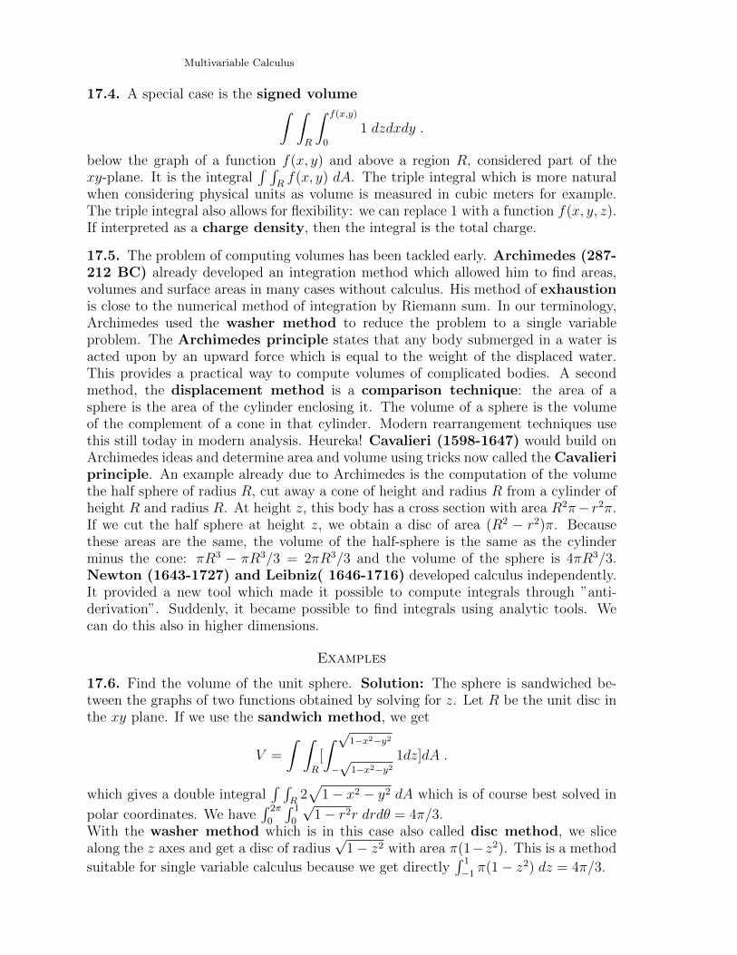
17.5. The problem of computing volumes has been tackled early. Archimedes (287-212 BC) already developed an integration method which allowed him to find areas,volumes and surface areas in many cases without calculus. His method of exhaustionis close to the numerical method of integration by Riemann sum. In our terminology,Archimedes used the washer method to reduce the problem to a single variableproblem. The Archimedes principle states that any body submerged in a water isacted upon by an upward force which is equal to the weight of the displaced water.This provides a practical way to compute volumes of complicated bodies. A secondmethod, the displacement method is a comparison technique: the area of asphere is the area of the cylinder enclosing it. The volume of a sphere is the volumeof the complement of a cone in that cylinder. Modern rearrangement techniques usethis still today in modern analysis. Heureka! Cavalieri (1598-1647) would build onArchimedes ideas and determine area and volume using tricks now called the Cavalieriprinciple. An example already due to Archimedes is the computation of the volumethe half sphere of radius R, cut away a cone of height and radius R from a cylinder ofheight R and radius R. At height z, this body has a cross section with area R2π− r2π.If we cut the half sphere at height z, we obtain a disc of area (R2 − r2)π. Becausethese areas are the same, the volume of the half-sphere is the same as the cylinderminus the cone: πR3 − πR3/3 = 2πR3/3 and the volume of the sphere is 4πR3/3.Newton (1643-1727) and Leibniz( 1646-1716) developed calculus independently.It provided a new tool which made it possible to compute integrals through ”anti-derivation”. Suddenly, it became possible to find integrals using analytic tools. Wecan do this also in higher dimensions.

Examples

17.6. Find the volume of the unit sphere. Solution: The sphere is sandwiched be-tween the graphs of two functions obtained by solving for z. Let R be the unit disc inthe xy plane. If we use the sandwich method, we get

V =

∫ ∫R

[

∫ √1−x2−y2

−√

1−x2−y21dz]dA .

which gives a double integral∫ ∫

R2√

1− x2 − y2 dA which is of course best solved in

polar coordinates. We have∫ 2π

0

∫ 1

0

√1− r2r drdθ = 4π/3.

With the washer method which is in this case also called disc method, we slicealong the z axes and get a disc of radius

√1− z2 with area π(1−z2). This is a method

suitable for single variable calculus because we get directly∫ 1

−1 π(1− z2) dz = 4π/3.

17.7. The mass of a body with mass density ρ(x, y, z) is defined as∫ ∫ ∫

Rρ(x, y, z) dV .

For bodies with constant density ρ, the mass is ρV , where V is the volume. Computethe mass of a body which is bounded by the parabolic cylinder z = 4 − x2, and theplanes x = 0, y = 0, y = 6, z = 0 if the density of the body is z. Solution:∫ 2

0

∫ 6

0

∫ 4−x2

0

z dz dy dx =

∫ 2

0

∫ 6

0

(4− x2)2/2 dydx

= 6

∫ 2

0

(4− x2)2/2 dx = 6(x5

5− 8x3

3+ 16x)|20 = 2 · 512/5

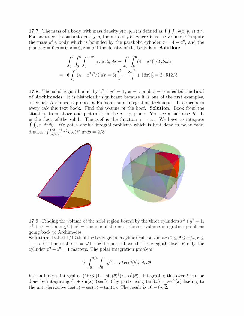
17.8. The solid region bound by x2 + y2 = 1, x = z and z = 0 is called the hoofof Archimedes. It is historically significant because it is one of the first examples,on which Archimedes probed a Riemann sum integration technique. It appears inevery calculus text book. Find the volume of the hoof. Solution. Look from thesituation from above and picture it in the x − y plane. You see a half disc R. Itis the floor of the solid. The roof is the function z = x. We have to integrate∫ ∫

Rx dxdy. We got a double integral problems which is best done in polar coor-

dinates;∫ π/2−π/2

∫ 1

0r2 cos(θ) drdθ = 2/3.

17.9. Finding the volume of the solid region bound by the three cylinders x2 + y2 = 1,x2 + z2 = 1 and y2 + z2 = 1 is one of the most famous volume integration problemsgoing back to Archimedes.Solution: look at 1/16’th of the body given in cylindrical coordinates 0 ≤ θ ≤ π/4, r ≤1, z > 0. The roof is z =

√1− x2 because above the ”one eighth disc” R only the

cylinder x2 + z2 = 1 matters. The polar integration problem

16

∫ π/4

0

∫ 1

0

√1− r2 cos2(θ)r drdθ

has an inner r-integral of (16/3)(1 − sin(θ)3)/ cos2(θ). Integrating this over θ can bedone by integrating (1 + sin(x)3) sec2(x) by parts using tan′(x) = sec2(x) leading tothe anti derivative cos(x) + sec(x) + tan(x). The result is 16− 8

√2.


Homework

This homework is due on Tuesday, 7/30/2019.

Problem 17.1: Evaluate the triple integral∫ 3

0

∫ z

0

∫ 4y

0

7e−y2

z dxdydz .

Problem 17.2: Find the volume of the solid bounded by the paraboloidsz = x2 + y2 and z = 36− (x2 + y2) and satisfying x ≥ 0, y ≥ 0.

Problem 17.3: Find the moment of inertia∫ ∫ ∫

E(x2 + y2) dV of a

coneE = {x2 + y2 ≤ z2 0 ≤ z ≤ 15 } ,

which has the z-axis as its center of symmetry.

Problem 17.4: Integrate f(x, y, z) = x2 + y2 − z over the tetrahedronwith vertices(0, 0, 0), (4, 4, 0), (0, 4, 0), (0, 0, 12).

Problem 17.5: This is a classic problem of Archimedes: What is thevolume of the body obtained by intersecting the solid cylinders x2+z2 ≤ 9and y2 + z2 ≤ 9?

Oliver Knill, [email protected], Math S-21a, Harvard Summer School, 2019


MATH S-21A

Unit 18: Spherical integrals

Lecture

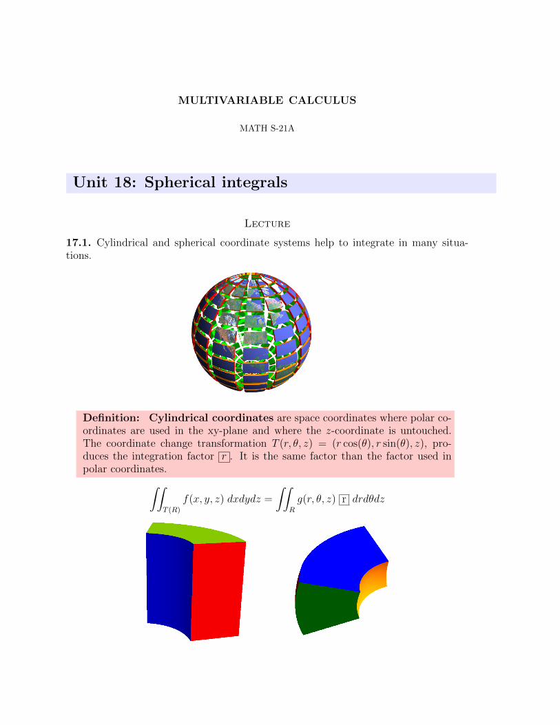
17.1. Cylindrical and spherical coordinate systems help to integrate in many situa-tions.

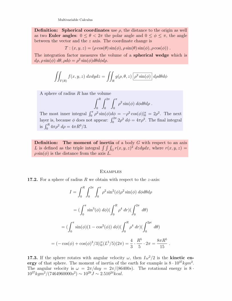
Definition: Cylindrical coordinates are space coordinates where polar co-ordinates are used in the xy-plane and where the z-coordinate is untouched.The coordinate change transformation T (r, θ, z) = (r cos(θ), r sin(θ), z), pro-duces the integration factor r . It is the same factor than the factor used inpolar coordinates.∫∫

T (R)

f(x, y, z) dxdydz =

∫∫R

g(r, θ, z) r drdθdz


Definition: Spherical coordinates use ρ, the distance to the origin as wellas two Euler angles: 0 ≤ θ < 2π the polar angle and 0 ≤ φ ≤ π, the anglebetween the vector and the z axis. The coordinate change is

T : (x, y, z) = (ρ cos(θ) sin(φ), ρ sin(θ) sin(φ), ρ cos(φ)) .

The integration factor measures the volume of a spherical wedge which isdρ, ρ sin(φ) dθ, ρdφ = ρ2 sin(φ)dθdφdρ.

∫∫T (R)

f(x, y, z) dxdydz =

∫∫R

g(ρ, θ, z) ρ2 sin(φ) dρdθdφ

A sphere of radius R has the volume∫ R

0

∫ 2π

0

∫ π

0

ρ2 sin(φ) dφdθdρ .

The most inner integral∫ π0ρ2 sin(φ)dφ = −ρ2 cos(φ)|π0 = 2ρ2. The next

layer is, because φ does not appear:∫ 2π

02ρ2 dφ = 4πρ2. The final integral

is∫ R0

4πρ2 dρ = 4πR3/3.

Definition: The moment of inertia of a body G with respect to an axisL is defined as the triple integral

∫ ∫ ∫Gr(x, y, z)2 dzdydx, where r(x, y, z) =

ρ sin(φ) is the distance from the axis L.

Examples

17.2. For a sphere of radius R we obtain with respect to the z-axis:

I =

∫ R

0

∫ 2π

0

∫ π

0

ρ2 sin2(φ)ρ2 sin(φ) dφdθdρ

= (

∫ π

0

sin3(φ) dφ)(

∫ R

0

ρ4 dr)(

∫ 2π

0

dθ)

= (

∫ π

0

sin(φ)(1− cos2(φ)) dφ)(

∫ R

0

ρ4 dr)(

∫ 2pi

0

dθ)

= (− cos(φ) + cos(φ)3/3)|π0 (L5/5)(2π) =4

3· R

5

5· 2π =

8πR5

15.

17.3. If the sphere rotates with angular velocity ω, then Iω2/2 is the kinetic en-ergy of that sphere. The moment of inertia of the earth for example is 8 · 1037kgm2.The angular velocity is ω = 2π/day = 2π/(86400s). The rotational energy is 8 ·1037kgm2/(7464960000s2) ∼ 1029J ∼ 2.51024kcal.

17.4. Find the volume and the center of mass of a diamond, the intersection of theunit sphere with the cone given in cylindrical coordinates as z =

√3r.

Solution: we use spherical coordinates to find the center of mass

x =

∫ 1

0

∫ 2π

0

∫ π/6

0

ρ3 sin2(φ) cos(θ) dφdθdρ1

V= 0

y =

∫ 1

0

∫ 2π

0

∫ π/6

0

ρ3 sin2(φ) sin(θ) dφdθdρ1

V= 0

z =

∫ 1

0

∫ 2π

0

∫ π/6

0

ρ3 cos(φ) sin(φ) dφdθdρ1

V=

2π

32V

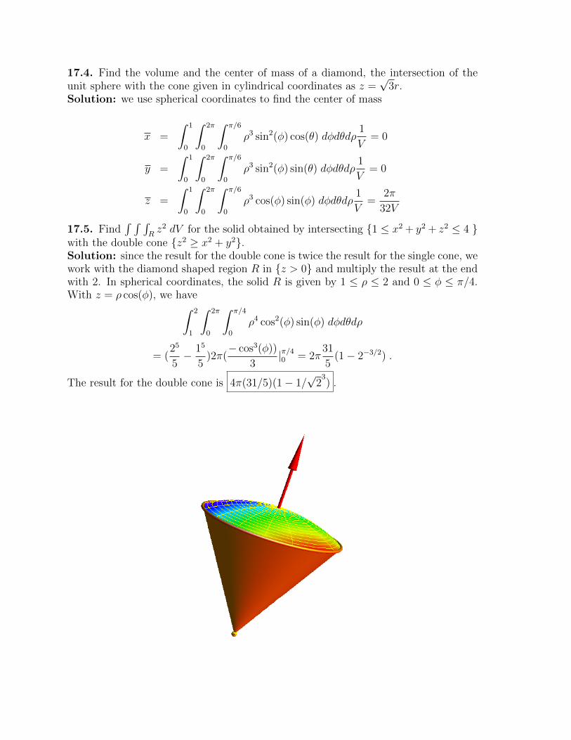
17.5. Find∫ ∫ ∫

Rz2 dV for the solid obtained by intersecting {1 ≤ x2 + y2 + z2 ≤ 4 }

with the double cone {z2 ≥ x2 + y2}.Solution: since the result for the double cone is twice the result for the single cone, wework with the diamond shaped region R in {z > 0} and multiply the result at the endwith 2. In spherical coordinates, the solid R is given by 1 ≤ ρ ≤ 2 and 0 ≤ φ ≤ π/4.With z = ρ cos(φ), we have∫ 2

1

∫ 2π

0

∫ π/4

0

ρ4 cos2(φ) sin(φ) dφdθdρ

= (25

5− 15

5)2π(− cos3(φ))

3|π/40 = 2π

31

5(1− 2−3/2) .

The result for the double cone is 4π(31/5)(1− 1/√

23) .


HomeworkThis homework is due on Tuesday, 7/30/2019.

Problem 18.1: Assume the density of a solid E = x2 + y2 − z2 <1,−1 < z < 1 is given by the 10’s power of the distance to the z-axes:σ(x, y, z) = r10 = (x2 + y2)5. Find its mass

M =

∫ ∫ ∫E

(x2 + y2)5 dxdydz .

Problem 18.2: Find the moment of inertia∫ ∫ ∫

E(x2 + y2) dV of the

body E whose volume is given by the integral

Vol(E) =

∫ π/4

0

∫ π/2

0

∫ 3

0

ρ2 sin(φ) dρdθdφ .

Problem 18.3: A solid is described in spherical coordinates by theinequality ρ ≤ 2 sin(φ). Find its volume.

Problem 18.4: Integrate the function

f(x, y, z) = e(x2+y2+z2)3/2

over the solid which lies between the spheres x2 + y2 + z2 = 1 and x2 +y2 + z2 = 4, which is in the first octant and which is above the conex2 + y2 = z2.

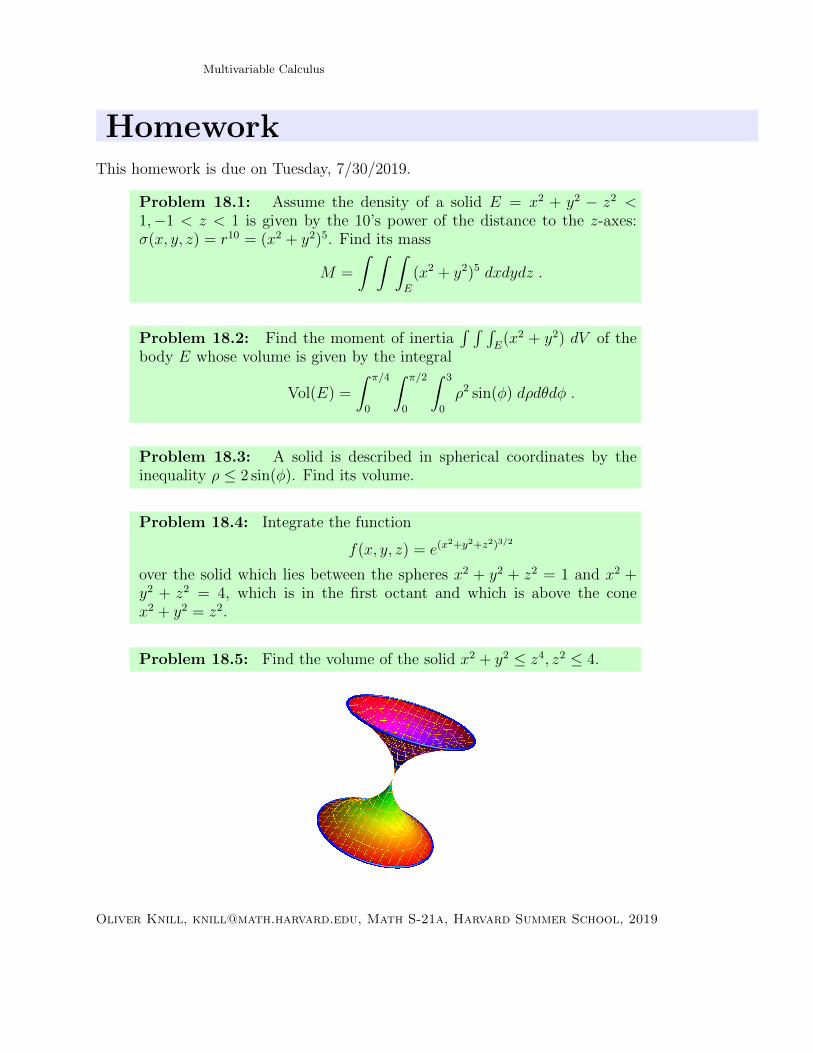
Problem 18.5: Find the volume of the solid x2 + y2 ≤ z4, z2 ≤ 4.



MATH S-21A

Unit 19: Vector fields

Lecture

17.1. We have already seen geometries like curves, surfaces or solids. Then we haveseen functions, which we consider to be scalar fields fields. If the function becomesvector valued we have vector field.

Definition: A planar vector field is a map F which assigns to a point(x, y) ∈ R2 a vector ~F (x, y) = [P (x, y), Q(x, y)]T . A vector field in space

is a map, which assigns to each point (x, y, z) ∈ R3 a vector ~F (x, y, z) =[P (x, y, z), Q(x, y, z), R(x, y, z)]T .

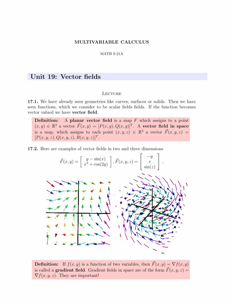
17.2. Here are examples of vector fields in two and three dimensions

~F (x, y) =

[y − sin(x)x3 + cos(2y)

], ~F (x, y, z) =

−yx

sin(z)

.

Definition: If f(x, y) is a function of two variables, then ~F (x, y) = ∇f(x, y)

is called a gradient field. Gradient fields in space are of the form ~F (x, y, z) =∇f(x, y, z). They are important!


17.3. When is a vector field a gradient field? ~F (x, y) = [P (x, y), Q(x, y)]T = ∇f(x, y)

implies Qx(x, y) = Py(x, y). If this does not hold at some point, ~F is no gradient field.

Clairaut test: If Qx(x, y) − Py(x, y) is not zero at some point, then ~F (x, y) =[P (x, y), Q(x, y)]T is not a gradient field.

17.4. We will see next week that curl(~F ) = Qx−Py = 0 is also sufficient for ~F to be a

gradient field if ~F is defined everywhere. How do we get f the function with ~F = ∇f?We will look at examples in class.

Examples

17.5. Is the vector field ~F (x, y) = [P,Q]T = [3x2y + y + 2, x3 + x − 1]T a gradientfield? Solution: the Clairaut test shows Qx − Py = 0. We integrate the equationfx = P = 3x2y + y + 2 and get f(x, y) = 2x+xy +x3y + c(y). Now take the derivativeof this with respect to y to get x + x3 + c′(y) and compare with x3 + x − 1. We see

c′(y) = −1 and so c(y) = −y + c. We see the solution x3y + xy − y + 2x .

17.6. Is the vector field ~F (x, y) = [xy, 2xy2]T a gradient field? Solution: No: Qx −Py = 2y2 − x is not zero.Vector fields appear naturally when studing differential equations. Here is an examplein population dynamics:

17.7. If x(t) is the population of a “prey species” like tuna fish and y(t) is the popu-lation size of a “predator” like sharks. We have x′(t) = ax(t) + bx(t)y(t) with positivea, b because both more predators and more prey species will lead to prey consump-tion. The rate of change of y(t) is y′(t) = −cy(t) + dxy, where c, d are positive. This

can be written using a vector field ~r′ = ~F (~r(t)). We have a negative sign in the firstpart because predators would die out without food. The second term is explained be-cause both more predators as well as more prey leads to a growth of predators throughreproduction. A concrete example is the Volterra-Lodka system

x = 0.4x− 0.4xy

y = −0.1y + 0.2xy ,

where ~F (x, y) = [0.4x− 0.4xy−0.1y+0.2xy]T . Volterra explained with such systems the oscillation of fish populationsin the Mediterranean sea. At any specific point ~r(x, y) = [x(t), y(t)]T , there is a curve= ~r(t) = [x(t), y(t)]T through that point for which the tangent ~r ′(t) = (x′(t), y′(t) isthe vector field.

17.8. In mechanics the class of Hamiltonian fields plays an important role: if H(x, y)is a function of two variables, then [Hy(x, y),−Hx(x, y)]T is called a Hamiltonianvector field. An example is the harmonic oscillator H(x, y) = (x2 + y2)/2. Its vectorfield (Hy(x, y),−Hx(x, y)) = (y,−x). The flow lines of a Hamiltonian vector fields arelocated on the level curves of H.

17.9. Here is a famous example. It is the Lorenz vector field

~F (x, y, z) =

10y − 10x−xz + 28x− y

xy − 83z

.

It features a so called strange attractor.


Homework


Problem 19.1:a) Draw the gradient vector field of f(x, y) = sin(x2 − y2).b) Draw the gradient vector field of f(x, y) = (x− 1)2 + (y − 2)2.In both cases, draw a contour map of f and use gradients to draw thevector field F (x, y) = ∇f .

Problem 19.2: The vector field

~F (x, y) =

[x

(x2+y2)(3/2)y

(x2+y2)(3/2)

]appears in electrostatics. Find a function f(x, y) such that ~F = ∇f .

Problem 19.3:

a) Is the vector field ~F (x, y) =

[xyx2

]a gradient field?

b) Is the vector field ~F (x, y) =

[sin(x) + ycos(y) + x

]a gradient field?

In both cases, find f(x, y) satisfying ∇f(x, y) = ~F (x, y) or give a reason,why it does not exist.

Problem 19.4: Find conditions such that a vector field ~F (x, y, z) is agradient field. Then check it in the following cases. If there is a gradientfield, find f such that ~F = ∇f .a) ~F (x, y, z) = [x11, y9, z]T .

b) ~F (x, y, z) = [y, x, z3]T .

c) ~F (x, y, z) = [10y + 10x, 10x + 10y, x]T .

d) ~F (x, y) = [y, z, x]T .

Problem 19.5: Find the potential f to

~F (x, y, z) = [5x4y + z4 + y cos(xy), x5 + x cos(xy), 4xz3]T .



MATH S-21A

Unit 20: Line integral theorem

Lecture

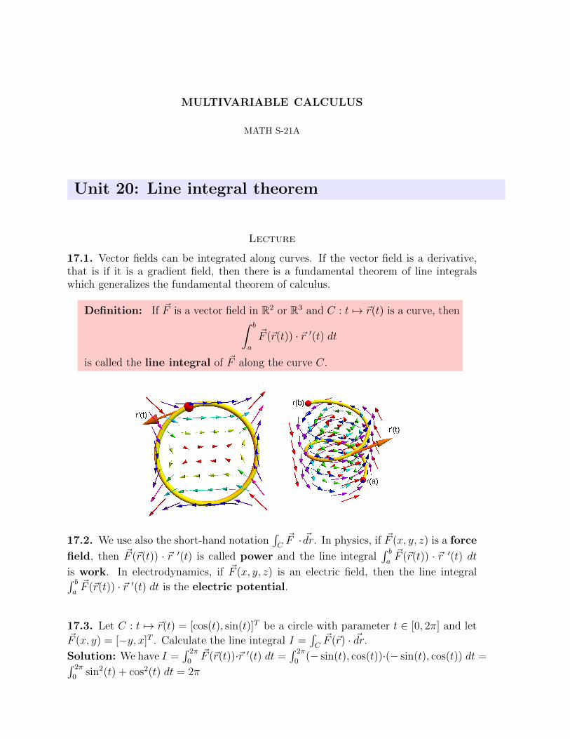
17.1. Vector fields can be integrated along curves. If the vector field is a derivative,that is if it is a gradient field, then there is a fundamental theorem of line integralswhich generalizes the fundamental theorem of calculus.

Definition: If ~F is a vector field in R2 or R3 and C : t 7→ ~r(t) is a curve, then∫ b

a

~F (~r(t)) · ~r ′(t) dt

is called the line integral of ~F along the curve C.

17.2. We use also the short-hand notation∫C~F · ~dr. In physics, if ~F (x, y, z) is a force

field, then ~F (~r(t)) · ~r ′(t) is called power and the line integral∫ ba~F (~r(t)) · ~r ′(t) dt

is work. In electrodynamics, if ~F (x, y, z) is an electric field, then the line integral∫ ba~F (~r(t)) · ~r ′(t) dt is the electric potential.

17.3. Let C : t 7→ ~r(t) = [cos(t), sin(t)]T be a circle with parameter t ∈ [0, 2π] and let~F (x, y) = [−y, x]T . Calculate the line integral I =

∫C~F (~r) · ~dr.

Solution: We have I =∫ 2π

0~F (~r(t))·~r ′(t) dt =

∫ 2π

0(− sin(t), cos(t))·(− sin(t), cos(t)) dt =∫ 2π

0sin2(t) + cos2(t) dt = 2π


17.4. Let ~r(t) be a curve given in polar coordinates as ~r(t) = cos(t), φ(t) = t defined on

[0, π]. Let ~F be the vector field ~F (x, y) = (−xy, 0). Calculate the line integral∫C~F · ~dr.

Solution: In Cartesian coordinates, the curve is r(t) = (cos2(t), cos(t) sin(t)). Thevelocity vector is then ~r ′(t) = [−2 sin(t) cos(t),− sin2(t) + cos2(t)) = (x(t), y(t)]T . Theline integral is∫ π

0

~F (~r(t)) · ~r ′(t) dt =

∫ π

0

(cos3(t) sin(t), 0) · (−2 sin(t) cos(t),− sin2(t) + cos2(t)) dt

= −2

∫ π

0

sin2(t) cos4(t) dt = −2(t/16 + sin(2t)/64− sin(4t)/64− sin(6t)/192)|π0 = −π/8 .

17.5. The first generalization of the fundamental theorem of calculus to higher dimen-sions is the fundamental theorem of line integrals.

Theorem: Fundamental theorem of line integrals: If ~F = ∇f ,then ∫ b

a

~F (~r(t)) · ~r ′(t) dt = f(~r(b))− f(~r(a)) .

17.6. In other words, the line integral is the potential difference between the end points~r(b) and ~r(a), if ~F is a gradient field.

Examples

17.7. Let f(x, y, z) be the temperature distribution in a room and let ~r(t) the pathof a fly in the room, then f(~r(t)) is the temperature, the fly experiences at the point~r(t) at time t. The change of temperature for the fly is d

dtf(~r(t)). The line-integral of

the temperature gradient ∇f along the path of the fly coincides with the temperaturedifference between the end point and initial point.

17.8. Here are some special cases: If ~r(t) is parallel to the level curve of f , thend/dtf(~r(t)) = 0 and ~r ′(t) orthogonal to ∇f(~r(t)). If ~r(t) is orthogonal to the levelcurve, then |d/dtf(~r(t))| = |∇f ||~r ′(t)| and ~r ′(t) is parallel to ∇f(~r(t)).

17.9. The proof of the fundamental theorem uses the chain rule in the second equalityand the fundamental theorem of calculus in the third equality of the following identities:∫ b

a

~F (~r(t)) · ~r′(t) dt =

∫ b

a

∇f(~r(t)) · ~r′(t) dt =

∫ b

a

d

dtf(~r(t)) dt = f(~r(b))− f(~r(a)) .

Theorem: For a gradient field, the line-integral along any closed curveis zero.

17.10. When is a vector field a gradient field? ~F (x, y) = ∇f(x, y) implies Py(x, y) =

Qx(x, y). If this does not hold at some point, ~F = [P,Q]T is no gradient field. Thisis called the component test or Clairaut test. We will see later that the conditioncurl(~F ) = Qx − Py = 0 implies that the field is conservative, if the region satisfies acertain property.

17.11. Let ~F (x, y) = [2xy2 + 3x2, 2yx2]T . Find a potential f of ~F = [P,Q]T .Solution: The potential function f(x, y) satisfies fx(x, y) = 2xy2 + 3x2 and fy(x, y) =2yx2. Integrating the second equation gives f(x, y) = x2y2 + h(x). Partial differentia-tion with respect to x gives fx(x, y) = 2xy2 +h′(x) which should be 2xy2 + 3x2 so thatwe can take h(x) = x3. The potential function is f(x, y) = x2y2 + x3. Find g, h fromf(x, y) =

∫ x0P (x, y) dx+ h(y) and fy(x, y) = g(x, y).

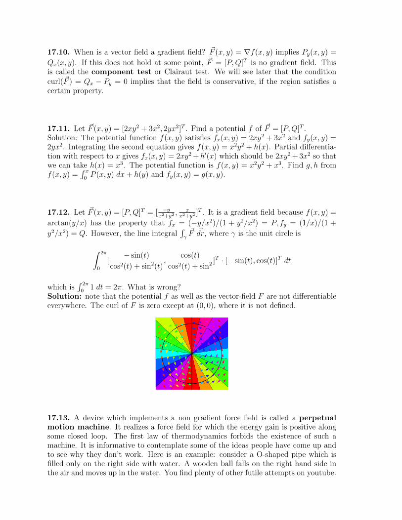
17.12. Let ~F (x, y) = [P,Q]T = [ −yx2+y2

, xx2+y2

]T . It is a gradient field because f(x, y) =

arctan(y/x) has the property that fx = (−y/x2)/(1 + y2/x2) = P, fy = (1/x)/(1 +

y2/x2) = Q. However, the line integral∫γ~F ~dr, where γ is the unit circle is

∫ 2π

0

[− sin(t)

cos2(t) + sin2(t),

cos(t)

cos2(t) + sin2 ]T · [− sin(t), cos(t)]T dt

which is∫ 2π

01 dt = 2π. What is wrong?

Solution: note that the potential f as well as the vector-field F are not differentiableeverywhere. The curl of F is zero except at (0, 0), where it is not defined.

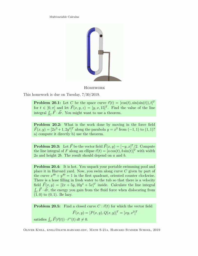
17.13. A device which implements a non gradient force field is called a perpetualmotion machine. It realizes a force field for which the energy gain is positive alongsome closed loop. The first law of thermodynamics forbids the existence of such amachine. It is informative to contemplate some of the ideas people have come up andto see why they don’t work. Here is an example: consider a O-shaped pipe which isfilled only on the right side with water. A wooden ball falls on the right hand side inthe air and moves up in the water. You find plenty of other futile attempts on youtube.


Homework


Problem 20.1: Let C be the space curve ~r(t) = [cos(t), sin(sin(t)), t]T

for t ∈ [0, π] and let ~F (x, y, z) = [y, x, 15]T . Find the value of the line

integral∫C~F · ~dr. You might want to use a theorem.

Problem 20.2: What is the work done by moving in the force field~F (x, y) = [2x3 + 1, 2y4]T along the parabola y = x2 from (−1, 1) to (1, 1)?a) compute it directly b) use the theorem.

Problem 20.3: Let ~F be the vector field ~F (x, y) = [−y, x]T/2. Computethe line integral of F along an ellipse ~r(t) = [a cos(t), b sin(t)]T with width2a and height 2b. The result should depend on a and b.

Problem 20.4: It is hot. You unpack your portable swimming pool andplace it in Harvard yard. Now, you swim along curve C given by part ofthe curve x40 + y40 = 1 in the first quadrant, oriented counter clockwise.There is a hose filling in fresh water to the tub so that there is a velocityfield ~F (x, y) = [2x + 5y, 10y4 + 5x]T inside. Calculate the line integral∫C~F · ~dr, the energy you gain from the fluid force when dislocating from

(1, 0) to (0, 1). Be lazy.

Problem 20.5: Find a closed curve C : ~r(t) for which the vector field

~F (x, y) = [P (x, y), Q(x, y)]T = [xy, x2]T

satisfies∫C~F (~r(t)) · ~r ′(t) dt 6= 0.


Unit 17: Triple integrals - Harvard...

Documents

Transcript of Unit 17: Triple integrals - Harvard...