Unit 10/Slide 1 Unit 10: Road Map (VERBAL) Nationally Representative Sample of 7,800 8 th Graders...
95
Unit 10/Slide 1 Unit 10: Road Map (VERBAL) Nationally Representative Sample of 7,800 8 th Graders Surveyed in 1988 (NELS 88). Outcome Variable (aka Dependent Variable): READING, a continuous variable, test score, mean = 47 and standard deviation = 9 Predictor Variables (aka Independent Variables): FREELUNCH, a dichotomous variable, 1 = Eligible for Free/Reduced Lunch and 0 = Not RACE, a polychotomous variable, 1 = Asian, 2 = Latino, 3 = Black and 4 = White Unit 1: In our sample, is there a relationship between reading achievement and free lunch? Unit 2: In our sample, what does reading achievement look like (from an outlier resistant perspective)? Unit 3: In our sample, what does reading achievement look like (from an outlier sensitive perspective)? Unit 4: In our sample, how strong is the relationship between reading achievement and free lunch? Unit 5: In our sample, free lunch predicts what proportion of variation in reading achievement? Unit 6: In the population, is there a relationship between reading achievement and free lunch? Unit 7: In the population, what is the magnitude of the relationship between reading and free lunch? Unit 8: What assumptions underlie our inference from the sample to the population? Parker istics.Org
-
Upload
zoe-thornton -
Category
Documents
-
view
214 -
download
1
Transcript of Unit 10/Slide 1 Unit 10: Road Map (VERBAL) Nationally Representative Sample of 7,800 8 th Graders...

Unit 10/Slide 1
Unit 10: Road Map (VERBAL)
Nationally Representative Sample of 7,800 8th Graders Surveyed in 1988 (NELS 88). Outcome Variable (aka Dependent Variable):
READING, a continuous variable, test score, mean = 47 and standard deviation = 9 Predictor Variables (aka Independent Variables):
FREELUNCH, a dichotomous variable, 1 = Eligible for Free/Reduced Lunch and 0 = NotRACE, a polychotomous variable, 1 = Asian, 2 = Latino, 3 = Black and 4 = White
Unit 1: In our sample, is there a relationship between reading achievement and free lunch?
Unit 2: In our sample, what does reading achievement look like (from an outlier resistant perspective)?
Unit 3: In our sample, what does reading achievement look like (from an outlier sensitive perspective)?
Unit 4: In our sample, how strong is the relationship between reading achievement and free lunch?
Unit 5: In our sample, free lunch predicts what proportion of variation in reading achievement?
Unit 6: In the population, is there a relationship between reading achievement and free lunch?
Unit 7: In the population, what is the magnitude of the relationship between reading and free lunch?
Unit 8: What assumptions underlie our inference from the sample to the population?
Unit 9: In the population, is there a relationship between reading and race?
Unit 10: In the population, is there a relationship between reading and race controlling for free lunch?
Appendix A: In the population, is there a relationship between race and free lunch?
© Sean Parker EdStatistics.Org
Unit 10/Slide 2© Sean Parker EdStatistics.Org
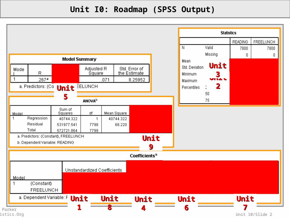
Unit I0: Roadmap (SPSS Output)
Unit Unit 11
Unit Unit 22
Unit Unit 33
Unit Unit 44
Unit Unit 55
Unit Unit 66
Unit Unit 77
Unit Unit 88
Unit Unit 99

Unit 10/Slide 3© Sean Parker EdStatistics.Org
Unit I0: Roadmap (SPSS Output)
Unit Unit 99

Unit 10/Slide 4© Sean Parker EdStatistics.Org
Unit I0: Roadmap (SPSS Output)
Unit Unit 10 10
Multiple Multiple RegressiRegressi
onon

Unit 10/Slide 5© Sean Parker EdStatistics.Org
Unit I0: Roadmap (SPSS Output)
Appendix Appendix AA
Unit Unit 10 10
ANOVAANOVA

Unit 10/Slide 6
Unit 10: Road Map (Schematic)
© Sean Parker EdStatistics.Org
Single PredictorContinuous
Polychotomous
Dichotomous
Continuous Regression
RegressionANOVA
RegressionANOVAT-tests
Polychotomous
Logistic Regression
Chi Squares Chi Squares
Dichotomous Chi Squares Chi Squares
Ou
tcom
e
Multiple PredictorsContinuous
Polychotomous
Dichotomous
Continuous Multiple Regression
RegressionANOVA
RegressionANOVA
Polychotomous
Logistic Regression
Chi Squares Chi Squares
Dichotomous Chi Squares Chi Squares
Ou
tcom
e
Units 6-8: Inferring From a Sample to a Population

Unit 10/Slide 7
Epistemological Minute
If we could look around, we would see the source of the shadows—models bonfire backlit. Plato believes that, with enough philosophical training, some of us will someday be able to look around. I doubt it.
Outside of the cave is the real world in which the sun illuminates all the real objects of which the models are mere representations.
We were born We were born prisoners in prisoners in Plato’s cave, and Plato’s cave, and to this day we to this day we remain. We only remain. We only ever perceive ever perceive flittering flittering shadows, but to shadows, but to us they are us they are everything.everything.

Unit 10/Slide 8
UALITYNxTEACHERQxMOTIVATIOLATINOxSES
ERQUALITYTIONxTEACHSESxMOTIVATYACHERQUALIIVATIONxTELATINOxMOT
ALITYxTEACHERQULATINOxSESNxMOTIVATIOLATINOxSES
ALITYxTEACHERQUMOTIVATION
RQUALITYSESxTEACHETIONSESxMOTIVA
YCHERQUALITLATINOxTEAIVATIONLATINOxMOTLATINOxSES
LITYTEACHERQUAMOTIVATIONSESLATINOREAD
2.1
3.22.0
1.28.8
7.4
9.22.0
1.62.67.3
4.83.94.17.64.3
Epistemological Minute
Platonic Myth Statistical Myth
The Shadows of a Model Horse
Sample Data From the Population
The Model Horse Population Model
The Horse Itself The Population Itself
We never get to see the population model. When we propose a theoretical model, we attempt to answer the question, “What population model gave rise to our sample data?” In our theoretical model, we recognize that the population parameters are unknown, so we use betas (e.g., β0, β1, β3 etc.) as stand-ins. However, we often fail to recognize that our model is probably too simple. Our theoretical models should probably include more variables and more interactions, but often the best we can do is:
sample data
Students with a capital S
LATINOxSESSESLATINOREAD 3210
Note that we never get to see the population model. For illustrative purposes, I include a population model, but there should be a million decimal places for each parameter, and there should be more variables with more interactions.
Unit 10/Slide 9© Sean Parker EdStatistics.Org
Unit 10: Introduction to Multiple Regression, 2-Way ANOVA and Statistical Interaction
Unit 10 Post Hole:
Interpret a two-way analysis of variance using F-tests and graphs.
Unit 10 Technical Memo and School Board Memo:
Conduct a two-way analysis of variance, produce an appropriate table and graph, fit the equivalent regression model, and discuss your results.
Unit 10 (and Unit 9) Reading:
http://onlinestatbook.com/ Chapter 8, ANOVA

Unit 10/Slide 10© Sean Parker EdStatistics.Org
Unit 10: Technical Memo and School Board Memo
Conduct one analysis (but from two perspectives) using the Sport.sav data set.
Answer the following research question:* Given that boys’ self-perceptions of athletic ability tend
to be greater than girls’ self-perceptions in the population of U.S. students, does the boy/girl difference vary from the third grade to the sixth grade to the ninth grade?
Conduct the analysis from a regression perspective.Conduct the analysis from an ANOVA perspective.

Unit 10/Slide 11© Sean Parker EdStatistics.Org
Unit 10: Technical Memo and School Board Memo
Work Products (Part I of II):
I. Technical Memo: Have one section per biviariate analysis. For each section, follow this outline. (2 Sections)
A. Introduction
i. State a theory (or perhaps hunch) for the relationship—think causally, be creative. (1 Sentence)
ii. State a research question for each theory (or hunch)—think correlationally, be formal. Now that you know the statistical machinery that justifies an inference from a sample to a population, begin each research question, “In the population,…” (1 Sentence)
iii. List the two variables, and label them “outcome” and “predictor,” respectively.
iv. Include your theoretical model.
B. Univariate Statistics. Describe your variables, using descriptive statistics. What do they represent or measure?
i. Describe the data set. (1 Sentence)
ii. Describe your variables. (1 Short Paragraph Each)
a. Define the variable (parenthetically noting the mean and s.d. as descriptive statistics).
b. Interpret the mean and standard deviation in such a way that your audience begins to form a picture of the way the world is. Never lose sight of the substantive meaning of the numbers.
c. Polish off the interpretation by discussing whether the mean and standard deviation can be misleading, referencing the median, outliers and/or skew as appropriate.
C. Correlations. Provide an overview of the relationships between your variables using descriptive statistics.
i. Interpret all the correlations with your outcome variable. Compare and contrast the correlations in order to ground your analysis in substance. (1 Paragraph)
ii. Interpret the correlations among your predictors. Discuss the implications for your theory. As much as possible, tell a coherent story. (1 Paragraph)
iii. As you narrate, note any concerns regarding assumptions (e.g., outliers or non-linearity), and, if a correlation is uninterpretable because of an assumption violation, then do not interpret it.

Unit 10/Slide 12© Sean Parker EdStatistics.Org
Unit 10: Technical Memo and School Board Memo
Work Products (Part II of II):
I. Technical Memo (continued)
D. Regression Analysis. Answer your research question using inferential statistics. (1 Paragraph)
i. Include your fitted model.
ii. Use the R2 statistic to convey the goodness of fit for the model (i.e., strength).
iii. To determine statistical significance, test the null hypothesis that the magnitude in the population is zero, reject (or not) the null hypothesis, and draw a conclusion (or not) from the sample to the population.
iv. Describe the direction and magnitude of the relationship in your sample, preferably with illustrative examples. Draw out the substance of your findings through your narrative.
v. Use confidence intervals to describe the precision of your magnitude estimates so that you can discuss the magnitude in the population.
vi. If simple linear regression is inappropriate, then say so, briefly explain why, and forego any misleading analysis.
X. Exploratory Data Analysis. Explore your data using outlier resistant statistics.
i. For each variable, use a coherent narrative to convey the results of your exploratory univariate analysis of the data. Don’t lose sight of the substantive meaning of the numbers. (1 Paragraph Each)
ii. For each relationship between your outcome and predictor, use a coherent narrative to convey the results of your exploratory bivariate analysis of the data. (1 Paragraph Each)
II. School Board Memo: Concisely, precisely and plainly convey your key findings to a lay audience. Note that, whereas you are building on the technical memo for most of the semester, your school board memo is fresh each week. (Max 200 Words)
III. Memo Metacognitive
Unit 10/Slide 13© Sean Parker EdStatistics.Org
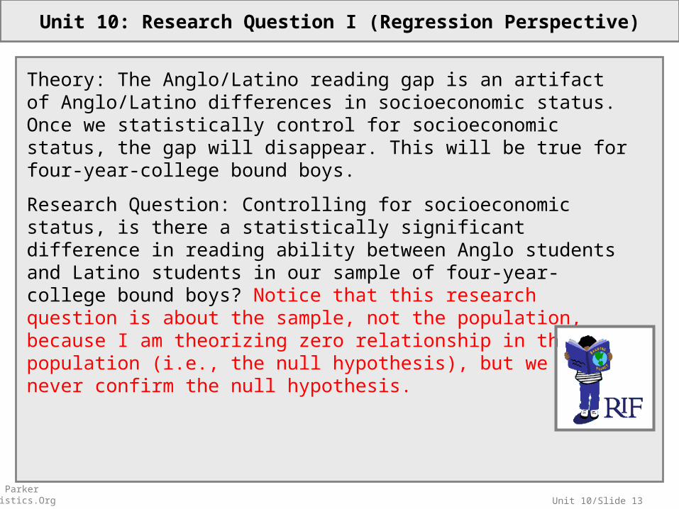
Unit 10: Research Question I (Regression Perspective)
Theory: The Anglo/Latino reading gap is an artifact of Anglo/Latino differences in socioeconomic status. Once we statistically control for socioeconomic status, the gap will disappear. This will be true for four-year-college bound boys.
Research Question: Controlling for socioeconomic status, is there a statistically significant difference in reading ability between Anglo students and Latino students in our sample of four-year-college bound boys? Notice that this research question is about the sample, not the population, because I am theorizing zero relationship in the population (i.e., the null hypothesis), but we can never confirm the null hypothesis.

Unit 10/Slide 14© Sean Parker EdStatistics.Org
Unit 10: Research Question I
Data Set: NELSBoys.sav National Education Longitudinal Survey (1988), a subsample of 1820 four-year-college bound boys, of whom 182 are Latino and the rest are Anglo.
Variables: Outcome—Reading Achievement Score (READ) Predictors—Latino = 1, Anglo = 0 (LATINO) —Low SES=1, Mid SES=2, High SES=3 (SocioeconomicStatus)
Model: TINOHighSESxLAINOLowSESxLATHighSESLowSESLATINOREAD 543210
54
32
10
TINOHighSESxLAINOLowSESxLAT
HighSESLowSES
LATINOREAD

Unit 10/Slide 15
Multiple Regression with Dummies and Interactions
There is a statistically significant relationship between our outcome and our predictors, F(5,1814)=24.492, p < 0.05. Ethnicity and socioeconomic status (and their interaction) predict about 6% of the variation in reading scores.

Unit 10/Slide 16
Interpreting The Mess: Plug and Play (Part I of II)
TINOHighSESxLAINOLowSESxLATHighSESLowSESLATINOREAD 543210
)*(6.3)*(3.5)(0.3)(0.1)(8.05.54ˆ LATINOHighSESLATINOLowSESHighSESLowSESLATINOADER
Let’s first look at our predictions for Anglo students (LATINO = 0):
)0*(6.3)0*(3.5)(0.3)(0.1)0(8.05.54ˆ HighSESLowSESHighSESLowSESADER
)(0.3)(0.15.54ˆ HighSESLowSESADER
Let’s then look at our predictions for Latino students (LATINO = 1):
)1*(6.3)1*(3.5)(0.3)(0.1)1(8.05.54ˆ HighSESLowSESHighSESLowSESADER
)(6.0)(3.67.53ˆ HighSESLowSESADER

Unit 10/Slide 17
Interpreting The Mess: Plug and Play (Part II of II)
Anglo students (LATINO = 0):
)(0.3)(0.15.54ˆ HighSESLowSESADER
Latino students (LATINO = 1):
)(6.0)(3.67.53ˆ HighSESLowSESADER
Low SES students (SocioEconomicStatus=1: LowSES = 1 and HighSES = 0 ):
5.53)0(0.3)1(0.15.54ˆ ADER 4.47)0(6.0)1(3.67.53ˆ ADER
Mid SES students (SocioEconomicStatus=2: LowSES = 0 and HighSES = 0 ):
5.54)0(0.3)0(0.15.54ˆ ADER 7.53)0(6.0)0(3.67.53ˆ ADER
High SES students (SocioEconomicStatus=3: LowSES = 0 and HighSES = 1 ):
5.57)1(0.3)0(0.15.54ˆ ADER 1.53)1(6.0)0(3.67.53ˆ ADER
This is our graph from Unit 9 that shows a relationship between socioeconomic status and reading scores. We’ll add to it in light of our new information.
The Anglo/Latino reading gap differs by socioeconomic status. There appears to be little or no gap for four-year-college bound boys of middle SES. However, there are large gaps of 6.1 and 4.4 points for students of low and high SES, respectively. (Note, we can also write about how the SES/Reading relationship differs for Anglo students and Latino students.)

Unit 10/Slide 18
Interpreting the Parameter Estimates
© Sean Parker EdStatistics.Org
1.Write out your fitted model.2.Create the first branches of your tree.
-Choose a factor (e.g., ethnicity).-For each level (e.g., Anglo or Latino) create a branch.-Each branch is a fitted model, partially instantiated.
3.Create the next branches of your tree.-For each level of the other factor (e.g., high, mid, low SES) create
a branch.-Each branch is a fitted model, fully instantiated.
4.Graph it.-Each point is a mean for a subgroup.-Connect the points with colored dotted lines.
5.Make sense of the graph in real-world terms. -Consider which mean differences might be statistically significant.-Consider which interactions (non-parallelisms) might be
statistically significant.
This probably should be a post hole, but it’s not!
Note, some people find it easier to collapse steps 2 and 3. Determine your subgroups (e.g., low SES Anglo students etc.) and solve for each subgroup (LowSES = 1, HighSES = 0, and Latino = 0).

Unit 10/Slide 19
Filling in the Gaps
• What is statistical interaction?– Abstractly: Sometimes the relationship between your outcome and one predictor
differs by the level of another predictor.– Geometrically: Sometimes your trend lines are not parallel.– Practically: Sometimes the effectiveness of your intervention or program differs
by gender, SES, age, proficiency etc. Or, sometimes the effectiveness of a drug is helped or hindered by another drug.
• What is statistical control?– A short introduction: Sometimes we include a predictor in our model not because
we are interested in the relationship between that predictor and the outcome, but rather because we are uninterested. Everybody knows SES is correlated with academic achievement, who cares? If you are interested in the Anglo/Latino achievement gap, you want to include SES in your model exactly because you do not care about SES. By including SES in your model, you get to compare Anglo students and Latino students of equal SES—you are statistically controlling for SES.
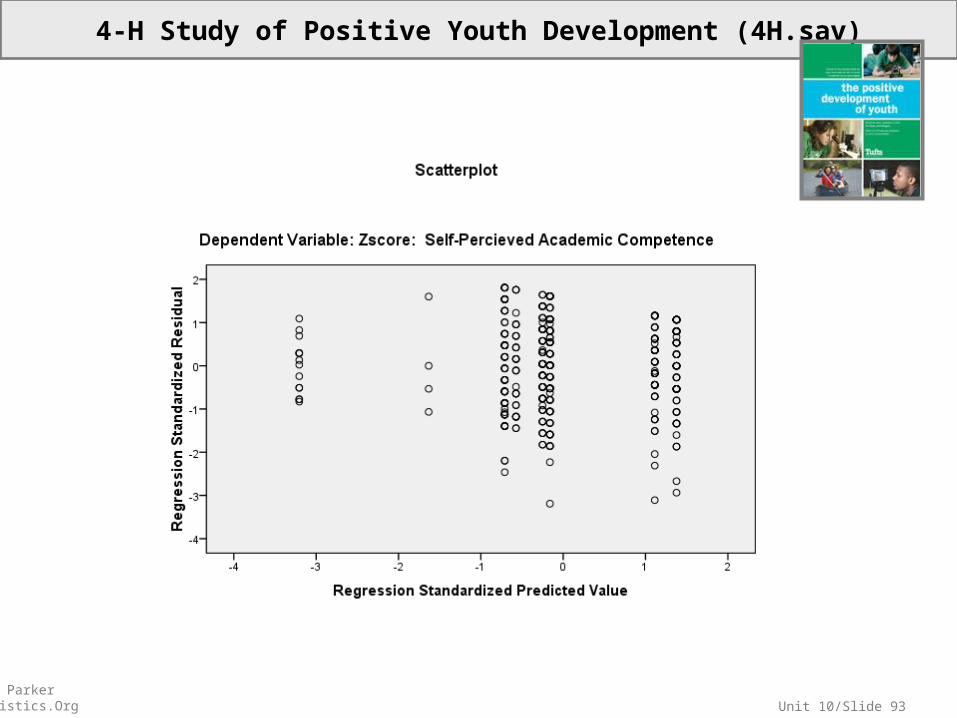
• How do you check assumptions when you have multiple predictors?– Create a residual vs. fitted scatterplot.– Residual values identify how wrong your prediction is.– Fitted values identify your prediction.– A residuals vs. fitted plot tells us how wrong our prediction is for each prediction.– You can use a residual vs. fitted plot to search HI-N-LO.

Unit 10/Slide 20© Sean Parker EdStatistics.Org
Conceptually Distinct: Interactions and Correlations
Interaction
Correlated Uncorrelated
No Interactio
n
Experimental DesignRed Pills (Uppers)Blue Pills (Downers)Outcome: Mood
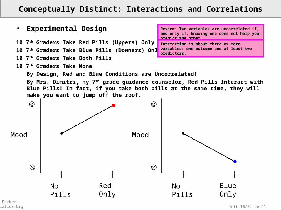
Unit 10/Slide 21© Sean Parker EdStatistics.Org
Conceptually Distinct: Interactions and Correlations
• Experimental Design
10 7th Graders Take Red Pills (Uppers) Only10 7th Graders Take Blue Pills (Downers) Only10 7th Graders Take Both Pills10 7th Graders Take None
By Design, Red and Blue Conditions are Uncorrelated!By Mrs. Dimitri, my 7th grade guidance counselor, Red Pills Interact with Blue Pills! In fact, if you take both pills at the same time, they will make you want to jump off the roof.
Red OnlyNo Pills
Mood
Blue OnlyNo Pills
Mood
Review: Two variables are uncorrelated if, and only if, knowing one does not help you predict the other.
Interaction is about three or more variables: one outcome and at least two predictors.

Unit 10/Slide 22© Sean Parker EdStatistics.Org
Conceptually Distinct: Interactions and Correlations
These Students DID Take the Red Pill
These Students Did NOT Take
the Red Pill
No Blue
Mood
Blue
When the lines are parallel, there is no interaction.
When the lines are non-parallel there is an interaction.
When the non-parallel lines do not cross, the interaction is ordinal.
When the non-parallel lines cross, the interaction is disordinal.
These Students Did
NOT Take the Red Pill
These Students DID Take the Red Pill
Mood
No Blue Blue
These Students Did
NOT Take the Red Pill
These Students DID Take the Red Pill
Mood
No Blue Blue

Unit 10/Slide 23
Including Interaction Terms in Your Regression Model
A main effects model has no interaction terms. The trend lines are constrained to be parallel.

Unit 10/Slide 24
Including Interaction Terms in Your Regression Model
Metaphorically, the crossproduct terms (i.e., interaction terms) allow the predictors to talk to one another.

Unit 10/Slide 25
Filling in the Gaps
• What is statistical interaction?– Abstractly: Sometimes the relationship between your outcome and one predictor
differs by the level of another predictor.– Geometrically: Sometimes your trend lines are not parallel.– Practically: Sometimes the effectiveness of your intervention or program differs
by gender, SES, age, proficiency etc. Or, sometimes the effectiveness of a drug is helped or hindered by another drug.
• What is statistical control?– A short introduction: Sometimes we include a predictor in our model not because
we are interested in the relationship between that predictor and the outcome, but rather because we are uninterested. Everybody knows SES is correlated with academic achievement, who cares? If you are interested in the Anglo/Latino achievement gap, you want to include SES in your model exactly because you do not care about SES. By including SES in your model, you get to compare Anglo students and Latino students of equal SES—you are statistically controlling for SES.
• How do you check assumptions when you have multiple predictors?– Create a residual vs. fitted scatterplot.– Residual values identify how wrong your prediction is.– Fitted values identify your prediction.– A residuals vs. fitted plot tells us how wrong our prediction is for each prediction.– You can use a residual vs. fitted plot to search HI-N-LO.

Unit 10/Slide 26
Introduction to Statistical Control
Zagat Ratings vs. PriceFor Restaurants Near Tufts (n = 47)
If money is no object, you go to the best restaurant regardless of the price. You know that the best restaurant will be expensive, but you don’t care.
If you are budget conscious, however, then you want to maximize the value of your dining dollar. You want to patronize restaurants that are good for the price. You want to compare cheap eats to cheap eats and determine the best. And, you want to compare fine dining to fine dining and determine the best. In statistics, we compare apple to apples and oranges to oranges by including a control predictor in our model and analyzing the residuals.
Look at the scatterplot. Look for good deals. I bet you naturally conduct a residual analysis.
Unit 10/Slide 27
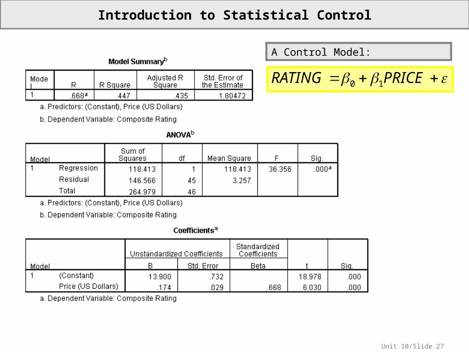
Introduction to Statistical Control
PRICERATING 10
A Control Model:

Unit 10/Slide 28
Zagat Ratings vs. PriceFor Restaurants Near Tufts (n = 47)
Zagat Ratings vs. PriceFor Restaurants Near Tufts (n = 47)
Introduction to Statistical Control
Once we fit the model, we produce residuals. Every observation has an associated residual. You can think of a residual as a controlled observation. In other words, the residuals are a measure of your outcome with the statistical effect of price removed.
By including price in our model and examining the residuals, we statistically remove the relationship between rating and price. Restaurants with a large positive residuals are good values! We are statistically controlling for price. Now, if we include another variable in our model, say a dichotomous variable indicating town, Somerville or Medford, we will have controlled for price, and the controlled relationship between rating and town will tell us which town has the better dining values on average. If we wanted to know which town has the best restaurants, we would simply regress rating on town. But, we want to level the playing field in terms of price, so we regress rating on town and price simultaneously.Likewise, if we want to consider the Latino/Anglo achievement gap, we may want to statistically level the SES playing field. We level the playing field by including in our model SES as a predictor along with ethnicity. Thus, we compare students of low SES to low SES, mid to mid, and high to high.

Unit 10/Slide 29
Residual vs. Fitted Plot from a Regression of Rating on Price
For Restaurants Near Tufts (n = 47)
Introduction to Statistical Control
KEEP IN MIND CONTEXT: The residuals and predictions are from a regression of Rating on Price.

Unit 10/Slide 30
Filling in the Gaps
• What is statistical interaction?– Abstractly: Sometimes the relationship between your outcome and one predictor
differs by the level of another predictor.– Geometrically: Sometimes your trend lines are not parallel.– Practically: Sometimes the effectiveness of your intervention or program differs
by gender, SES, age, proficiency etc. Or, sometimes the effectiveness of a drug is helped or hindered by another drug.
• What is statistical control?– A short introduction: Sometimes we include a predictor in our model not because
we are interested in the relationship between that predictor and the outcome, but rather because we are uninterested. Everybody knows SES is correlated with academic achievement, who cares? If you are interested in the Anglo/Latino achievement gap, you want to include SES in your model exactly because you do not care about SES. By including SES in your model, you get to compare Anglo students and Latino students of equal SES—you are statistically controlling for SES.
• How do you check assumptions when you have multiple predictors?– Create a residual vs. fitted scatterplot.– Residual values identify how wrong your prediction is.– Fitted values identify your prediction.– A residuals vs. fitted plot tells us how wrong our prediction is for each prediction.– You can use a residual vs. fitted plot to search HI-N-LO.

Unit 10/Slide 31
Checking Our Regressions Assumptions: Searching HI-N-LO
We are predicting nearly perfectly for these students.
We are underpredicting badly for these students.
We are overpredicting badly for these students.
Homoscedasticity: The variances are roughly equal for each prediction.
Independence: We cannot tell if the students are clustered in, for example, schools.
Normality: For our lowest prediction, the conditional distribution is positively skewed. For our highest predictions, the conditional distributions are negatively skewed. This is related, at least in part, to the ceiling effect of the test.
Linearity: No horseshoe, no problem.
Outliers: No outliers appear to be driving the conclusion.
Residual vs. Fitted Plot

Unit 10/Slide 32© Sean Parker EdStatistics.Org
Answering our Roadmap Question (Regression Perspective)
Unit 10: In the population, is there a relationship between reading and race controlling for free lunch?
In our nationally representative sample of 7,800 8th graders, there is a statistically significant relationship between reading achievement and our multiple predictors: race, SES and their interactions, F (7, 7792) = 121.8, p < .001. In our sample, among students who are eligible for free lunch, minority groups on average score lower than their White counterparts. Among students ineligible for free lunch, however, only Black and Latino students score lower on average than their White counterparts, and Asian students score higher on average. Our model predicts 10% of the variation in reading scores.
BlackFreeLatinoFreeAsianFreeBlackLatinoAsianFreeLunchReading *** 76543210
BlackFreeLatinoFreeAsianFreeBlackLatinoAsianFreeLunchReading *5.0*4.0*5.24.33.35.19.34.49
Unit 10/Slide 33© Sean Parker EdStatistics.Org
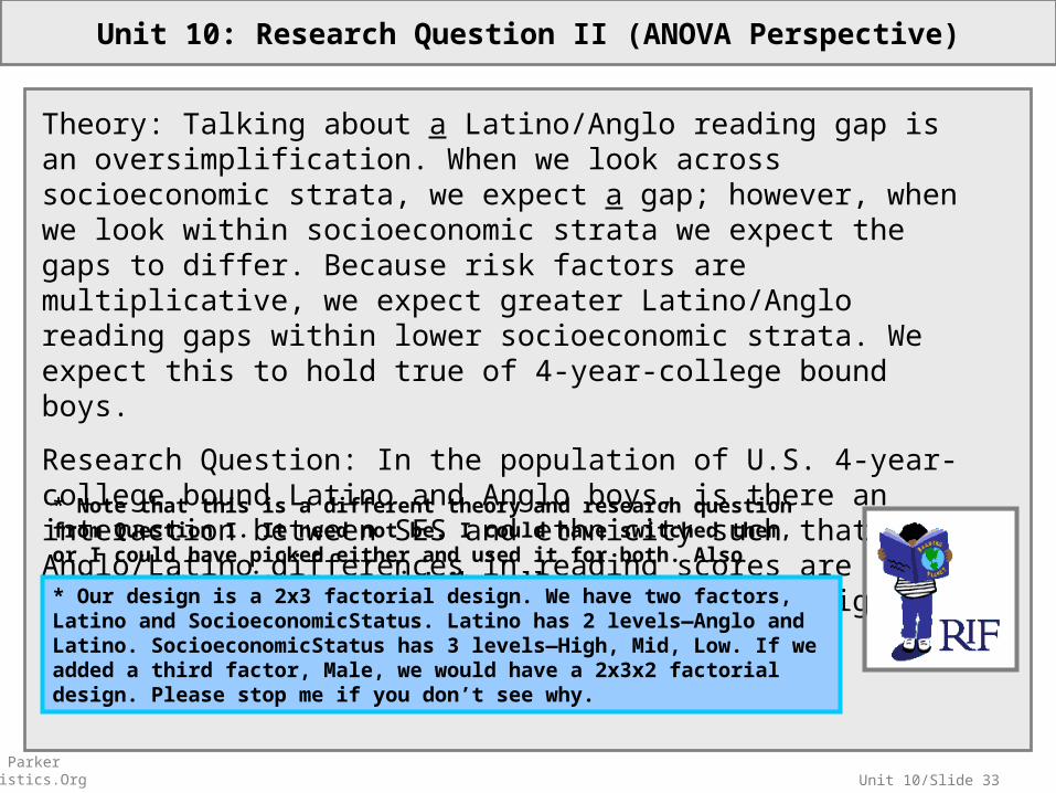
Unit 10: Research Question II (ANOVA Perspective)
Theory: Talking about a Latino/Anglo reading gap is an oversimplification. When we look across socioeconomic strata, we expect a gap; however, when we look within socioeconomic strata we expect the gaps to differ. Because risk factors are multiplicative, we expect greater Latino/Anglo reading gaps within lower socioeconomic strata. We expect this to hold true of 4-year-college bound boys.
Research Question: In the population of U.S. 4-year-college bound Latino and Anglo boys, is there an interaction between SES and ethnicity such that Anglo/Latino differences in reading scores are greatest for low SES students and least for high SES students? * Note that this is a different theory and research question from Question I. It need not be. I could have switched them, or I could have picked either and used it for both. Also note, my theory is wrong again! Ah, well.* Our design is a 2x3 factorial design. We have two factors, Latino and SocioeconomicStatus. Latino has 2 levels—Anglo and Latino. SocioeconomicStatus has 3 levels—High, Mid, Low. If we added a third factor, Male, we would have a 2x3x2 factorial design. Please stop me if you don’t see why.

Unit 10/Slide 34© Sean Parker EdStatistics.Org
Unit 10: Research Question II (ANOVA Perspective)
Data Set: NELSBoys.sav National Education Longitudinal Survey (1988), a subsample of 1820 four-year-college bound boys, of whom 182 are Latino and the rest are Anglo.
Variables: Outcome—Reading Achievement Score (READ) Predictors—Latino = 1, Anglo = 0 (LATINO) —Low SES=1, Mid SES=2, High SES=3 (SocioeconomicStatus)
ANOVA Model:jREAD Latino SocioeconomicStatus (Latino*SocioeconomicStatus)ijk i ij ijk
READijk = The reading score of the kth student within the ijth groupμ = The grand mean.Latinoi = The main effect of the “Latino” factor with two levels (i = 0,1)SocioeconomicStatusj = The main effect of the SocioeconomicStatus
factor with three levels (j = 1,2,3)(Latino*SocioeconomicStatus)ij = The interaction effect.εijk = The error associated with the kth student within the ijth group.

Unit 10/Slide 35
NELSBoys.sav After Creating Dummies and Crossproducts
Note that for ANOVA, we do not need to create dummies or crossproducts. Yippy skippy!

Unit 10/Slide 36
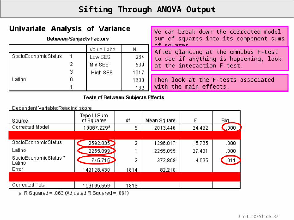
Sifting Through ANOVA Output
Ignore the lines for intercept and total. Everybody else does.
We covered Corrected Model, Error and Corrected Total (by other names) in Unit 5 and Unit 9.
? 159195.659
10067.229 is What :Trivia
Unit 10/Slide 37
Sifting Through ANOVA Output
We can break down the corrected model sum of squares into its component sums of squares.After glancing at the omnibus F-test to see if anything is happening, look at the interaction F-test.
Then look at the F-tests associated with the main effects.

Unit 10/Slide 38
Sifting Through ANOVA Output
A stat sig interaction tells us that the effect of one factor varies by the levels of another factor (enough to warrant an inference from the sample to the population).
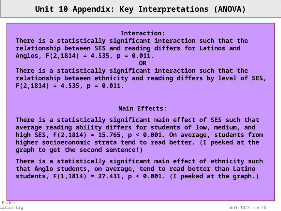
There is a statistically significant interaction such that the relationship between SES and reading differs for Latinos and Anglos, F(2,1814) = 4.535, p = 0.011.
OR
There is a statistically significant interaction such that the relationship between ethnicity and reading differs by level of SES, F(2,1814) = 4.535, p = 0.011.
Always interpret the interaction first! If it’s stat sig, the main effects are less important.
Alert! “Effect” here has nothing to do with cause and effect.

Unit 10/Slide 39
Sifting Through ANOVA Output
A stat sig main effect tells us that the averages within levels of the factor differ from the mean (enough to warrant an inference from the sample to the population).
There is a statistically significant main effect of SES such that average reading ability differs for students of low, medium, and high SES, F(2,1814) = 15.765, p < 0.001. On average, students from higher socioeconomic strata tend to read better. (I peeked at the graph to get the second sentence!)
We need graphs, planned contrasts and/or post hoc comparisons to explore the relationships more deeply.
There is a statistically significant main effect of ethnicity such that Anglo students, on average, tend to read better than Latino students, F(1,1814) = 27.431, p < 0.001. (I peeked at the graph!)

Unit 10/Slide 40
Two Snapshots of the Same Thing
Anglo
Latino
Read
ing
S
core
s
Mid SESLow SES
High SES
See the interaction. The lines are not parallel.
Trick question: Is the interaction ordinal or disordinal?
See the main effects. The average Anglo student performs differently from the average Latino student. The average High SES student differs from the average Mid SES student who, in turn, differs from the average Low SES student. (You only need one difference to make a main effect stat sig, so you must consult graphs, planned contrasts and/or post hoc comparisons to find where the action is.)

Unit 10/Slide 41
Interpreting Two-Way ANOVAS
© Sean Parker EdStatistics.Org
Interpret your omnibus F-test.Interpret your interaction F-test.Interpret your main effects F-tests.
Make sense of the graph in real-world terms. -Consider which mean differences might be statistically
significant.-Consider which interactions (non-parallelisms) might be
statistically significant.
In the future, use planned contrasts and/or post hoc comparisons to dig deeper.
This is the key to Post Hole 10. Practice is in back.h
ttp
://w
ww
.psm
.up
m.e
du
.my/5
95
0/S
tati
stic
sNote
s/PA
%2
07
65
%2
0A
NO
VA
.htm
* Conduct your analysis in this order, although you may want to report in a different order.

Unit 10/Slide 42
Calculating a Two-Way ANOVA by Hand
http://onlinestatbook.com/stat_sim/two_way/index.html
Lo SES
Mid SES
Hi SES
Anglo
Latino
Lo SES
Mid SES
Hi SES
Anglo
Latino
Six groups of 25 each.
Each group has an average reading score.
Each group has variation around its average reading score, which can be measured by taking the mean square error. This is “bad” variation.
Notice the means in the margins; these are “marginal means.”
Notice the grand mean.
With the above information, we can calculate by hand the ANOVA table…

Unit 10/Slide 43
Calculating a Two-Way ANOVA by Hand
Before we begin, let’s think backwards. It will help to root for statistically significant results.
We want a small p-value, therefore we want a big F-value.
The F-value is the mean square (for the main effect or interaction) divided by the mean square error.* You can think of the F-value as the ratio of good mean squares to bad mean squares. Some people think of it as the ratio of signal to noise.
Mean squares are sums of squares divided by degrees of freedom (df).
*This is true for fixed effects models. Random effects models are different, but we are not going to go there. Just kind of have in the back of your head that there’s a funky sort of ANOVA called “random effects ANOVA” that you have not studied.
WantSmall
WantBig
Noise
Signal
Bad
Good
MS
MSF
Error
LatinoLatino

Unit 10/Slide 44
Calculating a Two-Way ANOVA by Hand
Now, let’s think forwards.
We can calculate the sum of squares for each main effect. We will continue looking at the main effect of ethnicity.
Each of the 75 Anglo students has a “good” square: (55.17-53.28)2.
Each of the 75 Latino students has a “good” square: (51.40-53.28)2.
We add up all 150 squares to get SSLatino=532.04.
To get the SSerror we would calculate the squared deviation from the group mean (there are six groups) for each student. These squared deviations are “bad” squares. We would add the squared errors to get the SSerror, but we need the observed scores to do the math, and this little applet does not provide that information.
The SSSocioEconomicStatus is basically the same. Each of the 50 low SES students has a good square: (55.17-53.28)2…

Unit 10/Slide 45
Calculating a Two-Way ANOVA by Hand
We can calculate the sum of squares for the interaction. The key to an interaction is that it is what’s not predicted by the main effects. We have six predictions (i.e., group means). A main effect is a deviation between the marginal mean and the grand mean. We will subtract out the main effects from the group mean before we square the group mean deviation from the grand mean. We will use mid SES Latino students as an example
For the 25 mid SES Latino students:
Main effect of being Latino = (51.40-53.28).
Main effect of being mid SES = (54.10-53.28).
Each of the 25 mid SES Latino has a “good” square equal to 2.19: (53.7-(51.40-53.28)-(54.10-53.28)-53.28)2.
183.08 is the sum of the 150 “good” squares.
Note: When the main effects (i.e., marginal means) alone perfectly predict the group means, there is no interaction. Here, however, we find an interaction.

Unit 10/Slide 46
Calculating a Two-Way ANOVA by Hand
In order to get our mean squares, we divide by the degrees of freedom.
We want to divide our “bad” sum of squares (SSerror) by a big number. We get our wish when we have a large sample, because we divide by (basically) the sample size (really the degrees of freedom or “df” for short).
We want to divide a “good” sum of squares (e.g., SSLatino) by a small number. We divide by (basically) the number of levels of our factor, so we want to keep the levels as few as possible by excluding non-predictive variables from our model. I think of this step as a penalty for crappy variables.

Unit 10/Slide 47
Calculating a Two-Way ANOVA by Hand
As you may note, we are coming full circle.
The F-value is the mean square (for the main effect or interaction) divided by the mean square error.* You can think of the F-value as the ratio of good mean squares to bad mean squares. Some people think of it as the ratio of signal to noise.
Once we have our F-statistic, we consult an F-distribution. An F-distribution is a theoretical sampling distribution derived from the Central Limit Theorem, closely related to the t-distribution. If our F-statistic is far enough away from zero, we reject the null hypothesis that there is no relationship in the population.
Based on our p value of less than 0.05, we reject the null hypothesis and conclude there is a main effect of ethnicity in the population. If there were no relationship in the population, it is very unlikely we would randomly draw a sample with an F-statistic as extreme or more extreme than 21.28.
WantSmall
WantBig
Noise
Signal
Bad
Good
MS
MSF
Error
LatinoLatino

Unit 10/Slide 48
The F-Distribution
http://www.uvm.edu/~dhowell/SeeingStatisticsApplets/FProb.html
http://serc.carleton.edu/sp/cause/interactive/examples/17734.html
The F-distribution is a sampling distribution derived from the Central Limit Theorem. It takes different shapes depending on the degrees of freedom in the numerator and denominator. This is why we report the degrees of freedom whenever we report the F-statistic, F(1,144)=21.28, p < 0.001. The t-distribution also takes different shapes depending on degrees of freedom, but it never drastically diverges from normal, so it is not so important to report the degrees of freedom.

Unit 10/Slide 49
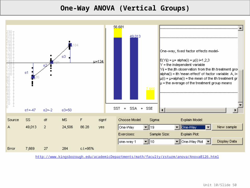
One-Way ANOVA (Horizontal Groups)
http://www.rossmanchance.com/applets/Anova/Anova.html
Unit 10/Slide 50
One-Way ANOVA (Vertical Groups)
http://www.kingsborough.edu/academicDepartments/math/faculty/rsturm/anova/Anova0126.html

Unit 10/Slide 51
Two-Way ANOVA (Vertical Groups)
http://www.kingsborough.edu/academicDepartments/math/faculty/rsturm/anova/Anova0126.html

Unit 10/Slide 52© Sean Parker EdStatistics.Org
Answering our Roadmap Question (ANOVA Perspective)
Unit 10: In the population, is there a relationship between reading and race controlling for free lunch?
In our nationally representative sample of 7,800 8th graders, there is a statistically significant relationship between reading achievement and our multiple predictors: race, SES and their interactions, F (7, 7792) = 121.8, p < .001. There is a statistically significant interaction such that the relationship between reading achievement and race differs by level of SES, F(3, 7792) = 2.8, p = 0.038. There are also statistically significant main effects of race and SES, F(3, 7792) = 74.0, p < 0.001 and F(1, 7792) = 243.6, p < 0.001, respectively. On average, students eligible for free lunch score lower than ineligible students, and Black and Latino students score lower than Asian and White students. There is a disordinal interaction between race and SES for White and Asian students such that among students eligible for free lunch, Asian students score lower on average than White students, whereas the opposite is true for ineligible students.
See the interaction in the graph. Not all the lines are parallel. It looks like the action is a disordinal interaction among White students and Asian students of varying SES.See the main effect of race. The lines differ vertically with Black and Latino students scoring lower on average (disregarding SES) than White and Asian students.See the main effect of SES. The lines are sloping downward indicating that students eligible for free lunch score lower on average (disregarding race) than their ineligible counterparts.

Unit 10/Slide 53© Sean Parker EdStatistics.Org
Unit 10 Appendix: Key Concepts
Review: Two variables are uncorrelated if, and only if, knowing one does not help you predict the other.
Interaction is about three or more variables: one outcome and at least two predictors.

Unit 10/Slide 54© Sean Parker EdStatistics.Org
Unit 10 Appendix: Key Concepts
When we talk about “effect sizes,” “main effects” and “effects,” we are not implying cause and effect. It’s really just unfortunate statistical nomenclature.
Predictions are more informative the more they differ from the mean. I call it “added value.”
A two-way ANOVA breaks down the corrected model sum of squares into its component sums of squares.
Attacking a Two-Way ANOVA table:
(1) After glancing at the omnibus F-test to see if anything is going on, look at the interaction F-test.
(2) Then look at the F-tests associated with the main effects.
Always interpret the interaction first! If it’s stat sig, the main effects are less important.We need graphs, planned contrasts and/or post hoc comparisons to explore the relationships more deeply.
The F-distribution is a sampling distribution derived from the Central Limit Theorem. It takes different shapes depending on the degrees of freedom in the numerator and denominator. This is why we report the degrees of freedom whenever we report the F-statistic, F(1,144)=21.28, p < 0.001. The t-distribution also takes different shapes depending on degrees of freedom but it never drastically diverges from normal, so it is not so important to report the degrees of freedom.

Unit 10/Slide 55© Sean Parker EdStatistics.Org
Unit 10 Appendix: Key Interpretations (Regression)
The Anglo/Latino reading gap differs by socioeconomic status. There appears to be little or no gap for four-year-college bound boys of middle SES. However, there are large gaps of 6.1 and 4.4 points for students of low and high SES, respectively. (Note, we can also write about how the SES/Reading relationship differs for Anglo students and Latino students.)
There is a statistically significant relationship between our outcome and our predictors, F(5,1814)=24.492, p < 0.05. Ethnicity and socioeconomic status (and their interaction) predict about 6% of the variation in reading scores.
Homoscedasticity: The variances are roughly equal for each prediction.Independence: We cannot tell if the students are clustered in, for example, schools.Normality: For our lowest prediction, the conditional distribution is positively skewed. For our highest predictions, the conditional distributions are negatively skewed. This is related, at least in part, to the ceiling effect of the test.Linearity: No horseshoe, no problem.Outliers: No outliers appear to be driving the conclusion.
Unit 10/Slide 56© Sean Parker EdStatistics.Org
Unit 10 Appendix: Key Interpretations (ANOVA)
Interaction:There is a statistically significant interaction such that the relationship between SES and reading differs for Latinos and Anglos, F(2,1814) = 4.535, p = 0.011.
ORThere is a statistically significant interaction such that the relationship between ethnicity and reading differs by level of SES, F(2,1814) = 4.535, p = 0.011.
Main Effects:
There is a statistically significant main effect of SES such that average reading ability differs for students of low, medium, and high SES, F(2,1814) = 15.765, p < 0.001. On average, students from higher socioeconomic strata tend to read better. (I peeked at the graph to get the second sentence!)
There is a statistically significant main effect of ethnicity such that Anglo students, on average, tend to read better than Latino students, F(1,1814) = 27.431, p < 0.001. (I peeked at the graph.)

Unit 10/Slide 57© Sean Parker EdStatistics.Org
Unit 10 Appendix: Key Terminology (Regression)
See Slide 19 for:
Statistical Interaction
Statistical Control
Residual vs. Fitted Scatterplot
Interactions appear in plots:• When the lines are parallel, there is no interaction.• When the lines are non-parallel there is an interaction.• When the non-parallel lines do not cross, the interaction is
ordinal.• When the non-parallel lines cross, the interaction is
disordinal.
A main effects model has no interaction terms. The trend lines are constrained to be parallel.

Unit 10/Slide 58© Sean Parker EdStatistics.Org
Unit 10 Appendix: Key Terminology (ANOVA)
Our design is a 2x3 factorial design. We have two factors, Latino and SocioeconomicStatus. Latino has 2 levels—Anglo and Latino. SocioeconomicStatus has 3 levels—High, Mid, Low. If we added a third factor, Male, we would have a 2x3x2 factorial design. See the pattern?
A stat sig interaction tells us that the effect of one factor varies by the levels of another factor (enough to warrant an inference from the sample to the population).
A stat sig main effect tells us that the averages within levels of the factor differ from the mean (enough to warrant an inference from the sample to the population).

Unit 10/Slide 59© Sean Parker EdStatistics.Org
Unit 10 Appendix: SPSS Syntax (Regression)
*******************************************.*Create interaction terms (or crossproduct terms).*******************************************.
COMPUTE LowSESXLatino=(LowSES*Latino).COMPUTE HighSESXLatino=(HighSES*Latino).Execute.
*******************************************.*Regress Read on Ethnicity and Socioeconomic Status (with interaction).*******************************************.
REGRESSION /MISSING LISTWISE /STATISTICS COEFF OUTS CI R ANOVA /CRITERIA=PIN(.05) POUT(.10) /NOORIGIN /DEPENDENT Read /METHOD=ENTER Latino LowSES HighSES LowSESXLatino HighSESXLatino /SCATTERPLOT=(*ZRESID ,*ZPRED) /SAVE SDRESID.
Unit 10/Slide 60© Sean Parker EdStatistics.Org
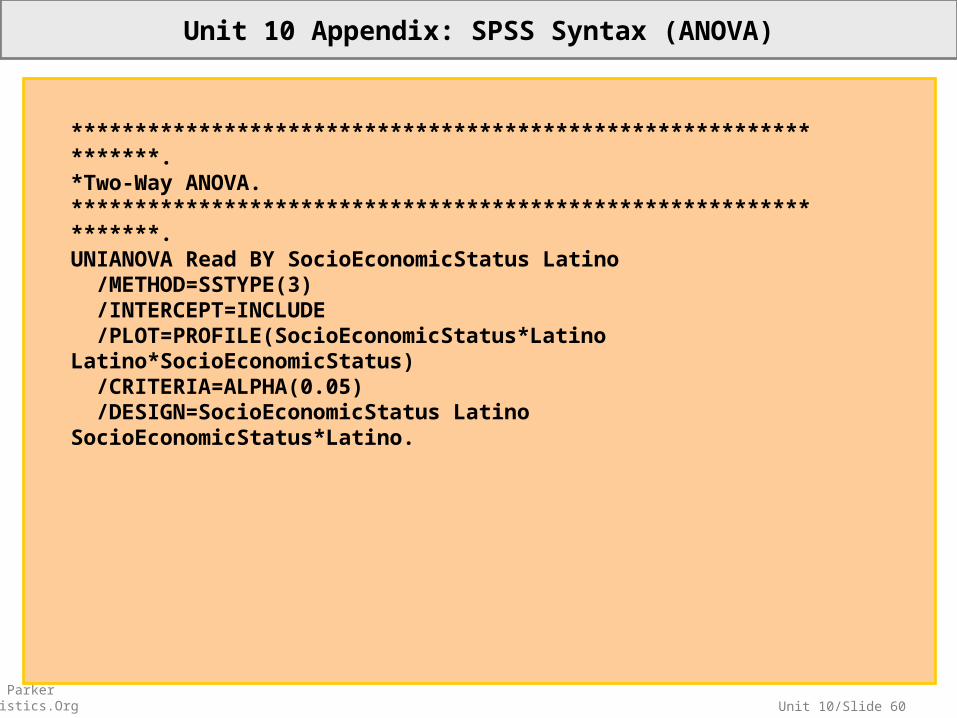
Unit 10 Appendix: SPSS Syntax (ANOVA)
*****************************************************************.*Two-Way ANOVA.*****************************************************************.UNIANOVA Read BY SocioEconomicStatus Latino /METHOD=SSTYPE(3) /INTERCEPT=INCLUDE /PLOT=PROFILE(SocioEconomicStatus*Latino Latino*SocioEconomicStatus) /CRITERIA=ALPHA(0.05) /DESIGN=SocioEconomicStatus Latino SocioEconomicStatus*Latino.

Unit 10/Slide 61
SPSS Menu Navigation
COMPUTE LowSESXLatino=(LowSES*Latino).COMPUTE HighSESXLatino=(HighSES*Latino).Execute.
In addition to the dummies from Unit 9, you need to create interaction terms (i.e., crossproducts). You can do this easily through code or dropdown menus.
Code:
Menus:
Go to Transform > Compute Variable…
With “Target Variable” you choose any name you want. I use the letter “x” to connect the two multipliers.
The asterisk is the multiplication sign.
Unit 10/Slide 62
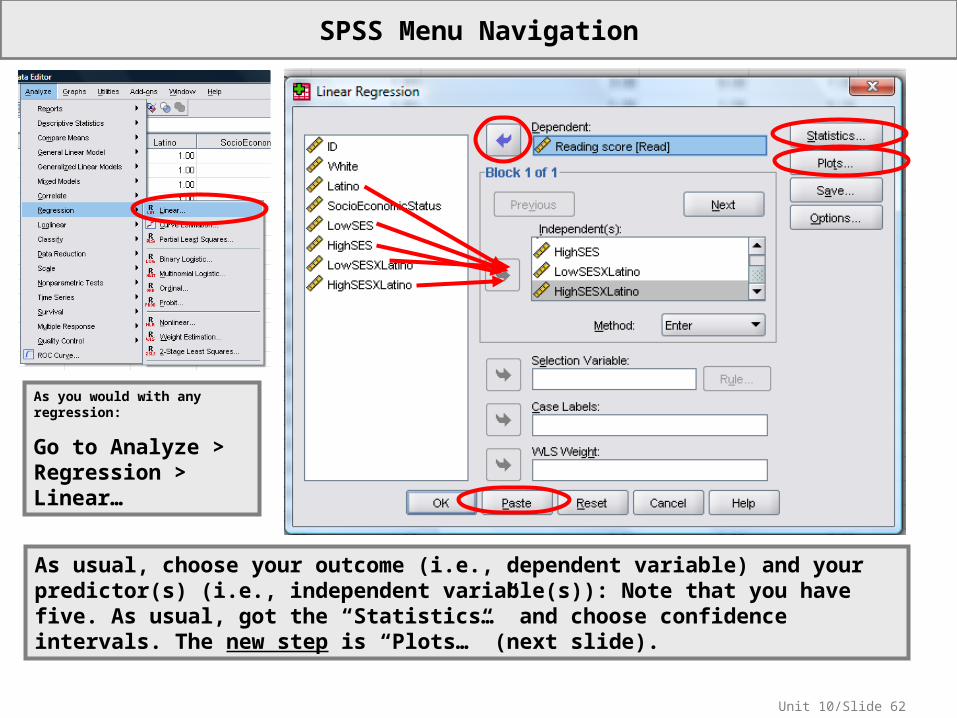
SPSS Menu Navigation
As you would with any regression:
Go to Analyze > Regression > Linear…
As usual, choose your outcome (i.e., dependent variable) and your predictor(s) (i.e., independent variable(s)): Note that you have five. As usual, got the “Statistics…” and choose confidence intervals. The new step is “Plots…” (next slide).

Unit 10/Slide 63
SPSS Menu Navigation
Create a residual vs. fitted plot (ZRESID vs. ZPRED plot).
FYI:
“Fitted” and “predicted” are synonymous.
FYI:
When we talk about scatterplots, we talk about plotting Y vs. X (not X vs. Y). When we talk about regression, we talk about regressing Y on X. It helps me to think of reading the plots and models from left to
right.
Unit 10/Slide 64© Sean Parker EdStatistics.Org
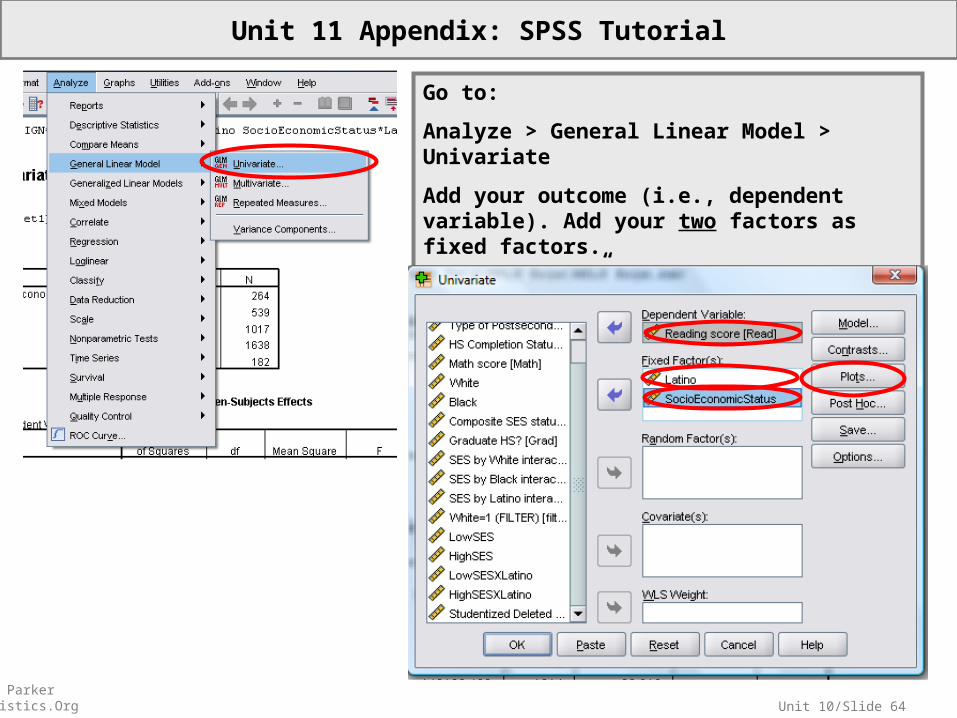
Unit 11 Appendix: SPSS Tutorial
Go to:
Analyze > General Linear Model > Univariate
Add your outcome (i.e., dependent variable). Add your two factors as fixed factors.
Go to “Plots…”

Unit 10/Slide 65© Sean Parker EdStatistics.Org
Unit 11 Appendix: SPSS Tutorial
Feel free to create a variety of graphs. Make sure you add each combination. When you’ve added a plot, you will see it appear below. In my example, I have added the two plots that appear in these slides.
Unit 10/Slide 66© Sean Parker EdStatistics.Org
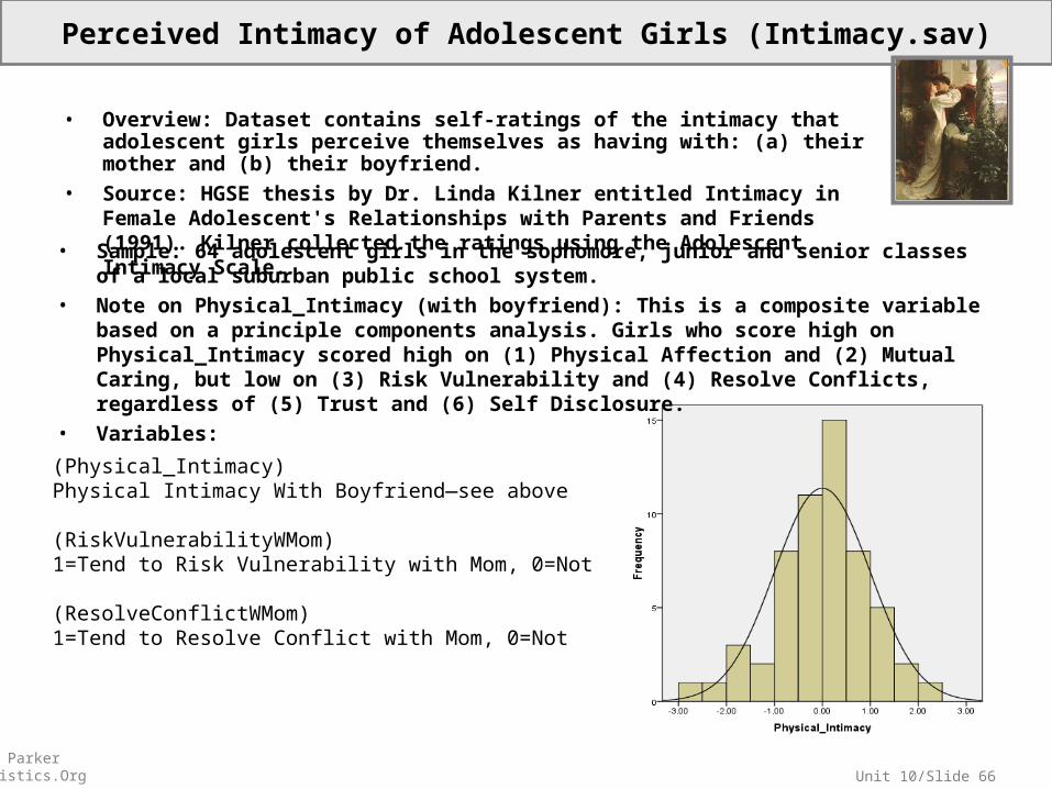
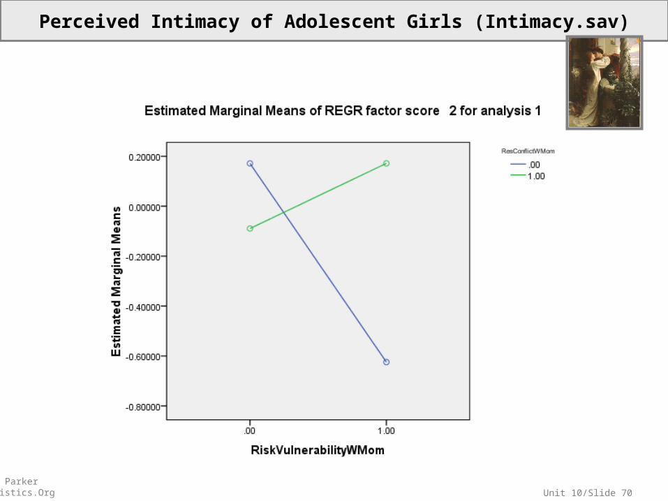
Perceived Intimacy of Adolescent Girls (Intimacy.sav)
• Sample: 64 adolescent girls in the sophomore, junior and senior classes of a local suburban public school system.
• Note on Physical_Intimacy (with boyfriend): This is a composite variable based on a principle components analysis. Girls who score high on Physical_Intimacy scored high on (1) Physical Affection and (2) Mutual Caring, but low on (3) Risk Vulnerability and (4) Resolve Conflicts, regardless of (5) Trust and (6) Self Disclosure.
• Variables:
• Overview: Dataset contains self-ratings of the intimacy that adolescent girls perceive themselves as having with: (a) their mother and (b) their boyfriend.
• Source: HGSE thesis by Dr. Linda Kilner entitled Intimacy in Female Adolescent's Relationships with Parents and Friends (1991). Kilner collected the ratings using the Adolescent Intimacy Scale.
(Physical_Intimacy) Physical Intimacy With Boyfriend—see above
(RiskVulnerabilityWMom) 1=Tend to Risk Vulnerability with Mom, 0=Not
(ResolveConflictWMom) 1=Tend to Resolve Conflict with Mom, 0=Not
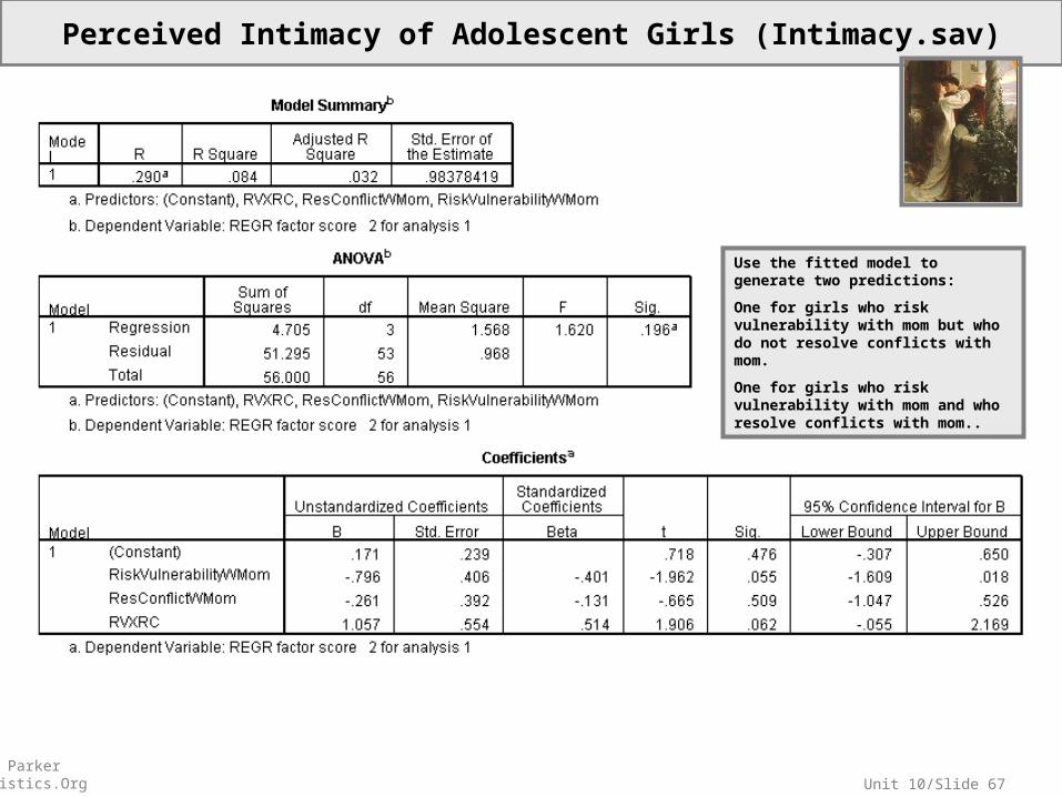
Unit 10/Slide 67© Sean Parker EdStatistics.Org
Perceived Intimacy of Adolescent Girls (Intimacy.sav)
Use the fitted model to generate two predictions:
One for girls who risk vulnerability with mom but who do not resolve conflicts with mom.
One for girls who risk vulnerability with mom and who resolve conflicts with mom..

Unit 10/Slide 68© Sean Parker EdStatistics.Org
Perceived Intimacy of Adolescent Girls (Intimacy.sav)
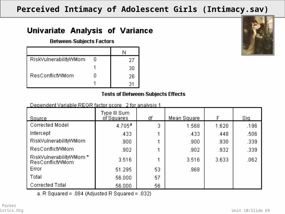
Unit 10/Slide 69© Sean Parker EdStatistics.Org
Perceived Intimacy of Adolescent Girls (Intimacy.sav)
Unit 10/Slide 70© Sean Parker EdStatistics.Org
Perceived Intimacy of Adolescent Girls (Intimacy.sav)

Unit 10/Slide 71© Sean Parker EdStatistics.Org
High School and Beyond (HSB.sav)
• Source: Subset of data graciously provided by Valerie Lee, University of Michigan.
• Sample: This subsample has 1044 students in 205 schools. Missing data on the outcome test score and family SES were eliminated. In addition, schools with fewer than 3 students included in this subset of data were excluded.
• Variables:
• Overview: High School & Beyond – Subset of data focused on selected student and school characteristics as predictors of academic achievement.
(ZBYTest) Standardized Base Year Composite Test Score(Sex) 1=Female, 0=Male(RaceEthnicity) Students Self-Identified Race/Ethnicity
1=White/Asian/Other, 2=Black, 3=Latino/a
Dummy Variables for RaceEthnicity:(Black) 1=Black, 0=Else(Latin) 1=Latino/a, 0=Else*Note that we will use RaceEthnicity=1, White/Asian/Other, as our reference category.

Unit 10/Slide 72© Sean Parker EdStatistics.Org
High School and Beyond (HSB.sav)
Use the fitted model to generate two predictions:
One for Latinas.
One for Latinos.
(Note that “SexXLatin” would be better named “FemalexLatin”)

Unit 10/Slide 73© Sean Parker EdStatistics.Org
High School and Beyond (HSB.sav)

Unit 10/Slide 74© Sean Parker EdStatistics.Org
High School and Beyond (HSB.sav)

Unit 10/Slide 75© Sean Parker EdStatistics.Org
High School and Beyond (HSB.sav)

Unit 10/Slide 76© Sean Parker EdStatistics.Org
Understanding Causes of Illness (ILLCAUSE.sav)
• Source: Perrin E.C., Sayer A.G., and Willett J.B. (1991). Sticks And Stones May Break My Bones: Reasoning About Illness Causality And Body Functioning In Children Who Have A Chronic Illness, Pediatrics, 88(3), 608-19.
• Sample: 301 children, including a sub-sample of 205 who were described as asthmatic, diabetic,or healthy. After further reductions due to the list-wise deletion of cases with missing data on one or more variables, the analytic sub-sample used in class ends up containing: 33 diabetic children, 68 asthmatic children and 93 healthy children.
• Variables:
• Overview: Data for investigating differences in children’s understanding of the causes of illness, by their health status.
(IllCause) A Measure of Understanding of Illness Causality(SocioEconomicStatus) 1=Low SES, 2=Lower Middle, 3=Upper Middle 4 = High SES (HealthStatus) 1=Healthy, 2=Asthmatic 3=Diabetic
Dummy Variables for SocioEconomicStatus:(LowSES) 1=Low SES, 0=Else(LowerMiddleSES) 1=Lower MiddleSES, 0=Else(HighSES) 1=High SES, 0=Else*Note that we will use SocioEconomicStatus=3, Upper Middle SES, as our reference category.
Dummy Variables for HealthStatus:(Asthmatic) 1=Asthmatic, 0=Else(Diabetic) 1=Diabetic, 0=Else*Note that we will use HealthStatus=1, Healthy, as our reference category.
Unit 10/Slide 77© Sean Parker EdStatistics.Org
Understanding Causes of Illness (ILLCAUSE.sav)
Use the fitted model to generate two predictions:
One for low SES asthmatic children.
One for lowmiddle SES asthmatic children.

Unit 10/Slide 78© Sean Parker EdStatistics.Org
Understanding Causes of Illness (ILLCAUSE.sav)

Unit 10/Slide 79© Sean Parker EdStatistics.Org
Understanding Causes of Illness (ILLCAUSE.sav)

Unit 10/Slide 80© Sean Parker EdStatistics.Org
Understanding Causes of Illness (ILLCAUSE.sav)

Unit 10/Slide 81© Sean Parker EdStatistics.Org
Children of Immigrants (ChildrenOfImmigrants.sav)
• Source: Portes, Alejandro, & Ruben G. Rumbaut (2001). Legacies: The Story of the Immigrant SecondGeneration. Berkeley CA: University of California Press.
• Sample: Random sample of 880 participants obtained through the website.• Variables:
• Overview: “CILS is a longitudinal study designed to study the adaptation process of the immigrant second generation which is defined broadly as U.S.-born children with at least one foreign-born parent or children born abroad but brought at an early age to the United States. The original survey was conducted with large samples of second-generation children attending the 8th and 9th grades in public and private schools in the metropolitan areas of Miami/Ft. Lauderdale in Florida and San Diego, California” (from the website description of the data set).
(Reading) Stanford Reading Achievement Scores(Depressed) 1=The Student is Depressed, 0=Not Depressed(SESCat) A Relative Measure Of Socio-Economic Status
1=Low SES, 2=Mid SES, 3=High SES
Dummy Variables for SESCat:(LowSES) 1=Low SES, 0=Else(MidSES) 1=Mid SES, 0=Else(HighSES) 1=High SES, 0=Else

Unit 10/Slide 82© Sean Parker EdStatistics.Org
Children of Immigrants (ChildrenOfImmigrants.sav)
Use the fitted model to generate two predictions:
One for high SES depressed students.
One for low SES depressed students.

Unit 10/Slide 83© Sean Parker EdStatistics.Org
Children of Immigrants (ChildrenOfImmigrants.sav)

Unit 10/Slide 84© Sean Parker EdStatistics.Org
Children of Immigrants (ChildrenOfImmigrants.sav)

Unit 10/Slide 85© Sean Parker EdStatistics.Org
Children of Immigrants (ChildrenOfImmigrants.sav)
Unit 10/Slide 86© Sean Parker EdStatistics.Org
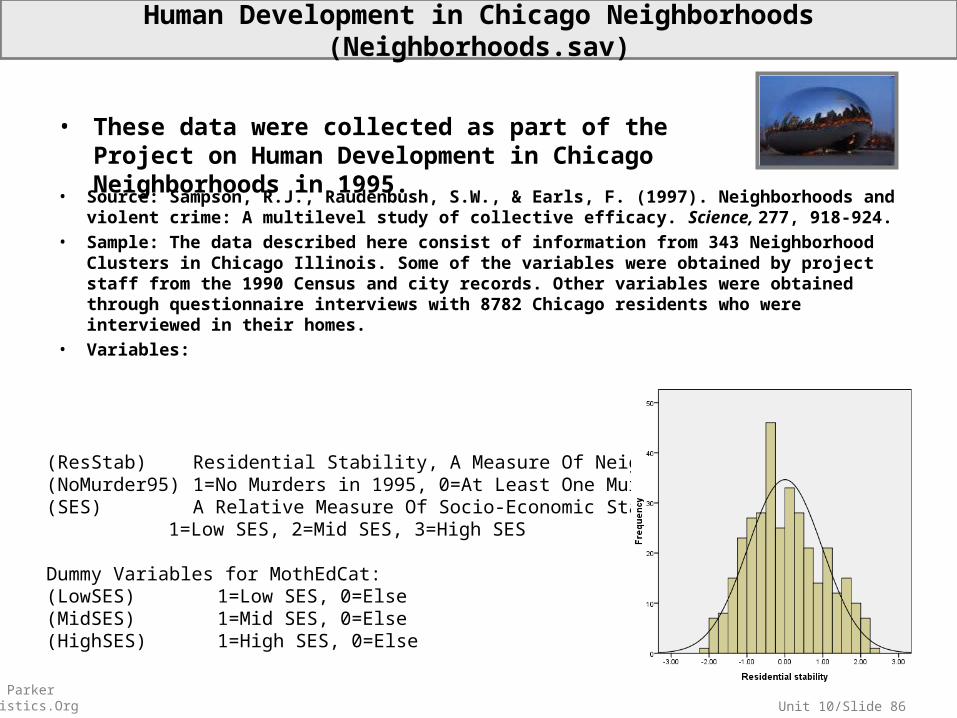
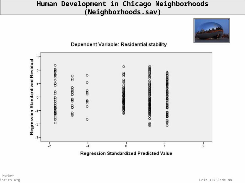
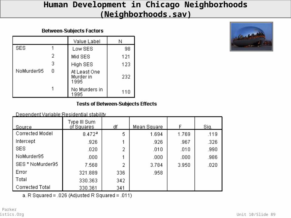
Human Development in Chicago Neighborhoods (Neighborhoods.sav)
• Source: Sampson, R.J., Raudenbush, S.W., & Earls, F. (1997). Neighborhoods and violent crime: A multilevel study of collective efficacy. Science, 277, 918-924.
• Sample: The data described here consist of information from 343 Neighborhood Clusters in Chicago Illinois. Some of the variables were obtained by project staff from the 1990 Census and city records. Other variables were obtained through questionnaire interviews with 8782 Chicago residents who were interviewed in their homes.
• Variables:
• These data were collected as part of the Project on Human Development in Chicago Neighborhoods in 1995.
(ResStab) Residential Stability, A Measure Of Neighborhood Flux(NoMurder95) 1=No Murders in 1995, 0=At Least One Murder in 1995(SES) A Relative Measure Of Socio-Economic Status
1=Low SES, 2=Mid SES, 3=High SES
Dummy Variables for MothEdCat:(LowSES) 1=Low SES, 0=Else(MidSES) 1=Mid SES, 0=Else(HighSES) 1=High SES, 0=Else

Unit 10/Slide 87© Sean Parker EdStatistics.Org
Human Development in Chicago Neighborhoods (Neighborhoods.sav)
Use the fitted model to generate two predictions:
One for high SES murderless neighborhoods.
One for low SES murderless neighborhoods.
Unit 10/Slide 88© Sean Parker EdStatistics.Org
Human Development in Chicago Neighborhoods (Neighborhoods.sav)
Unit 10/Slide 89© Sean Parker EdStatistics.Org
Human Development in Chicago Neighborhoods (Neighborhoods.sav)

Unit 10/Slide 90© Sean Parker EdStatistics.Org
Human Development in Chicago Neighborhoods (Neighborhoods.sav)
Unit 10/Slide 91© Sean Parker EdStatistics.Org
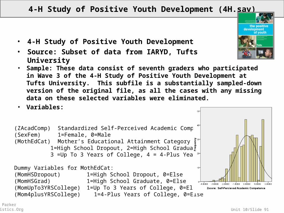
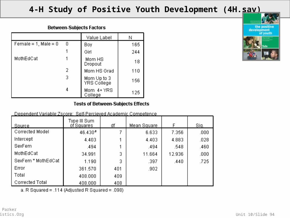
4-H Study of Positive Youth Development (4H.sav)
• Sample: These data consist of seventh graders who participated in Wave 3 of the 4-H Study of Positive Youth Development at Tufts University. This subfile is a substantially sampled-down version of the original file, as all the cases with any missing data on these selected variables were eliminated.
• Variables:
(ZAcadComp) Standardized Self-Perceived Academic Competence(SexFem) 1=Female, 0=Male(MothEdCat) Mother’s Educational Attainment Category
1=High School Dropout, 2=High School Graduate, 3 =Up To 3 Years of College, 4 = 4-Plus Years of College
Dummy Variables for MothEdCat:(MomHSDropout) 1=High School Dropout, 0=Else(MomHSGrad) 1=High School Graduate, 0=Else(MomUpTo3YRSCollege) 1=Up To 3 Years of College, 0=Else(Mom4plusYRSCollege) 1=4-Plus Years of College, 0=Else
• 4-H Study of Positive Youth Development• Source: Subset of data from IARYD, Tufts
University

Unit 10/Slide 92© Sean Parker EdStatistics.Org
4-H Study of Positive Youth Development (4H.sav)
Use the fitted model to generate two predictions:
One for girls whose moms dropped out from HS.
One for boys whose moms dropped out from HS.
Unit 10/Slide 93© Sean Parker EdStatistics.Org
4-H Study of Positive Youth Development (4H.sav)
Unit 10/Slide 94© Sean Parker EdStatistics.Org
4-H Study of Positive Youth Development (4H.sav)

Unit 10/Slide 95© Sean Parker EdStatistics.Org
4-H Study of Positive Youth Development (4H.sav)