UNIT 1: Theory of Metal Cutting: 7 Hrs Geometry of single...

Manufacturing Process II 06 ME45

M.K.Ravishankar - Assistant Professor, Department of Automobile Engineering

1

UNIT 1:

Theory of Metal Cutting: Single point cutting tool nomenclature, geometry, Merchants circle diagram and analysis, Ernst Merchant’s solution, shear angle relationship, problems of Merchant’s analysis, tool wear and tool failure, tool life, effects of cutting parameters on tool life, tool failure criteria, Taylor’s tool life equation, problems on tool life evaluation.

7 Hrs

Geometry of single point turning tools:

Instructional objectives:

At the end of this lesson, the student should be able to :

(a) Conceive rake angle and clearance angle of cutting tools

(b) Classify systems of description of tool geometry

(c) Demonstrate tool geometry and define tool angles in :

• Machine Reference System

• Orthogonal Rake System and

• Normal Rake System

(d) Designate cutting tool geometry in ASA, ORS and NRS

Geometry of single point turning tools:

Both material and geometry of the cutting tools play very important roles on their performances in achieving

Effectiveness,

Efficiency and

Overall economy of machining.

Cutting tools may be classified according to the number of major cutting edges (points) involved as follows:

1. Single point: e.g., turning tools, shaping, planning and slotting tools and boring tools

2. Double (two) point: e.g., drills

3. Multipoint (more than two): e.g., milling cutters, broaching tools, hobs, gear shaping cutters etc.



2

(i) Concept of rake and clearance angles of cutting tools.

The word tool geometry is basically referred to some specific angles or slope of the salient faces

and edges of the tools at their cutting point.

Rake angle and clearance angle are the most significant for all the cutting tools.

The concept of rake angle and clearance angle will be clear from some simple operations shown in Fig. 1.1

Fig. 1.1 Rake and clearance angles of cutting tools.

Definition:

• Rake angle (γ): Angle of inclination of rake surface from reference plane.

• Clearance angle (α): Angle of inclination of clearance or flank surface from the finished surface

Rake angle: is provided for ease of chip flow and overall machining. Rake angle may be positive, or negative

or even zero as shown in Fig. 1.2.

(a) positive rake (b) zero rake (c) negative rake

Fig. 1.2 Three possible types of rake angles



3

Relative advantages of such rake angles are:

• Positive rake – helps reduce cutting force and thus cutting power requirement.

• Negative rake – to increase edge-strength and life of the tool

• Zero rake – to simplify design and manufacture of the form tools.

Clearance angle: is essentially provided to avoid rubbing of the tool (flank) with the machined surface which

causes loss of energy and damages of both the tool and the job surface. Hence, clearance angle is a must

and must be positive (3o

~ 15o

depending upon tool-work materials and type of the machining operations like

turning, drilling, boring etc.)

(ii) Systems of description of tool geometry

• Tool-in-Hand System – where only the salient features of the cutting tool point are identified or visualized as

shown in Fig. 1.3. There is no quantitative information, i.e., value of the angles.

Fig. 1.3 Basic features of single point tool (turning) in Tool-in-hand system

• Machine Reference System – ASA system



4

• Tool Reference Systems

o Orthogonal Rake System – ORS

o Normal Rake System – NRS

• Work Reference System – WRS

(iii) Demonstration (expression) of tool geometry in :

Machine Reference System:

This system is also called ASA system; ASA stands for American Standards Association. Geometry of a

cutting tool refers mainly to its several angles or slope of its salient working surfaces and cutting edges.

Those angles are expressed w.r.t. some planes of reference.

In Machine Reference System (ASA), the three planes of reference and the coordinates are chosen based on

the configuration and axes of the machine tool concerned.

The planes and axes used for expressing tool geometry in ASA system for turning operation are shown in

Fig. 1.4.

Fig. 1.4 Planes and axes of reference in ASA system feed

The planes of reference and the coordinates used in ASA system for tool geometry are :



5

πR

- πX

- πY

and Xm

– Ym

- Zm

Where,

πR

= Reference plane; plane perpendicular to the velocity vector (shown in Fig. 1.4)

πX

= Machine longitudinal plane; plane perpendicular to πR

and taken in the direction of assumed

longitudinal feed

πY

= Machine Transverse plane; plane perpendicular to both πR

and πX

[This plane is taken in the direction

of assumed cross feed]

The axes Xm, Y

m and Z

m are in the direction of longitudinal feed, cross feed and cutting velocity (vector)

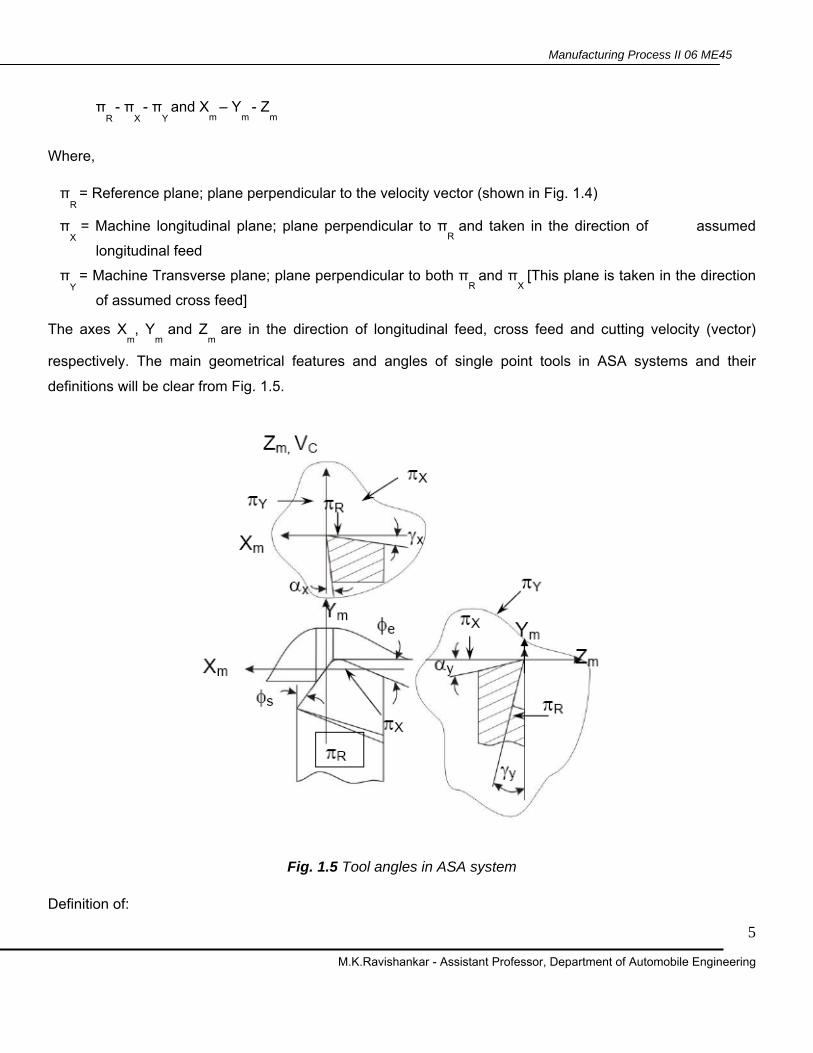
respectively. The main geometrical features and angles of single point tools in ASA systems and their

definitions will be clear from Fig. 1.5.

Fig. 1.5 Tool angles in ASA system

Definition of:



6

Rake angles: [Fig. 1.5] in ASA system:

γx

= side (axial rake: angle of inclination of the rake surface from the reference plane (πR) and easured on

Machine Ref. Plane, πX.

γy

= back rake: angle of inclination of the rake surface from the reference plane and measured on Machine

Transverse plane, πY.

Clearance angles: [Fig. 1.5]:

αx = side clearance: angle of inclination of the principal flank from the machined surface (or CV) and measured

on πX

plane.

αy = back clearance: same as α

x but measured on π

Y plane.

Cutting angles: [Fig. 1.5]:

φs

= approach angle: angle between the principal cutting edge (its projection on πR) and π

Y and measured on

πR

φe

= end cutting edge angle: angle between the end cutting edge (its projection on πR) from π

X and measured

on πR

Nose radius, r (in inch):

r = nose radius : curvature of the tool tip. It provides strengthening of the tool nose and better surface finish.

Tool Reference Systems

Orthogonal Rake System – ORS:

This system is also known as ISO – old.

The planes of reference and the co-ordinate axes used for expressing the tool angles in ORS are:

πR

- πC

- πO

and Xo - Y

o - Z

o

which are taken in respect of the tool configuration as indicated in Fig. 1.6



7

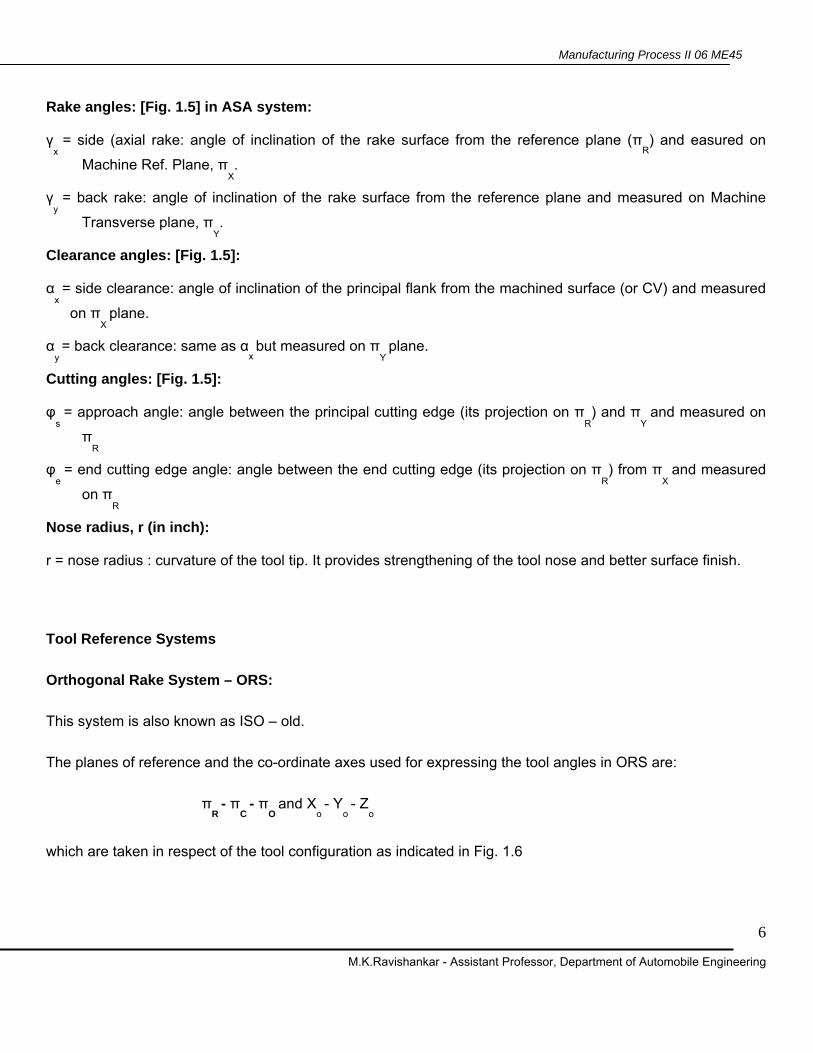
Fig. 1.6 Planes and axes of reference in OR

Where,

πR

= Reference plane perpendicular to the cutting velocity vector, CV

πC

= cutting plane; plane perpendicular to πR

and taken along the principal cutting edge

πO

= Orthogonal plane; plane perpendicular to both πR

and πC

and the axes;

Xo = along the line of intersection of π

R and π

O

Yo = along the line of intersection of π

R and π

C

Zo = along the velocity vector, i.e., normal to both X

o and Y

o axes.

The main geometrical angles used to express tool geometry in Orthogonal Rake System (ORS) and their

definitions will be clear from Fig. 1.7.



8

Fig. 1.7 Tool angles in ORS system

Definition of –

Rake angles [Fig. 1.7] in ORS:

γo

= orthogonal rake: angle of inclination of the rake surface from Reference plane, πR

and measured on the orthogonal plane, π

o

λ = inclination angle; angle between πC

from the direction of assumed longitudinal feed [πX] and measured

on πC

Clearance angles [Fig. 1.7]:

αo

= orthogonal clearance of the principal flank: angle of inclination of the principal flank from πC

and measured on π

o

αo’ = auxiliary orthogonal clearance: angle of inclination of the auxiliary flank from auxiliary cutting plane,

πC’ and measured on auxiliary orthogonal plane, π

o’ as indicated in Fig. 1.8.



9

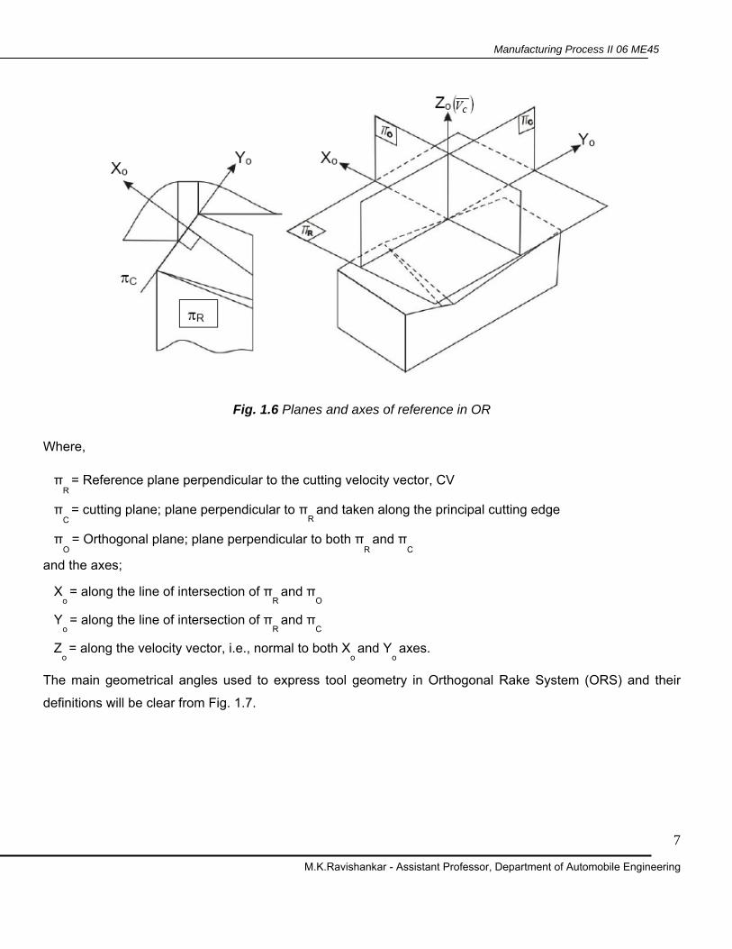
Cutting angles [Fig. 1.7]:

φ = principal cutting edge angle: angle between πC

and the direction of assumed longitudinal feed or πX

and measured on πR

φ1 = auxiliary cutting angle: angle between π

C’ and π

X and measured on π

R

Nose radius, r (mm): r = radius of curvature of tool tip

Fig. 1.8 Auxiliary orthogonal clearance angle

Normal Rake System – NRS: This system is also known as ISO – new.

ASA system has limited advantage and use like convenience of inspection. But ORS is advantageously used

for analysis and research in machining and tool performance. But ORS does not reveal the true picture of the

tool geometry when the cutting edges are inclined from the reference plane, i.e., λ≠0. Besides, sharpening or

resharpening, if necessary, of the tool by grinding in ORS requires some additional calculations for correction

of angles.



10

These two limitations of ORS are overcome by using NRS for description and use of tool geometry.

The basic difference between ORS and NRS is the fact that in ORS, rake and clearance angles are visualized

in the orthogonal plane, πo, whereas in NRS those angles are visualized in another plane called Normal plane,

πN. The orthogonal plane, π

o is simply normal to π

R and π

C irrespective of the inclination of the cutting edges,

i.e., λ, but πN

(and πN’ for auxiliary cutting edge) is always normal to the cutting edge. The differences between

ORS and NRS have been depicted in Fig. 1.9.

The planes of reference and the coordinates used in NRS are:

πRN

- πC

- πN

and Xn – Y

n – Z

n

where,

πRN

= normal reference plane

πN

= Normal plane: plane normal to the cutting edge

and

Xn = X

o

Yn = cutting edge

Zn = normal to X

n and Y

n

It is to be noted that when λ = 0, NRS and ORS become same, i.e. πo≅ π

N, Y

N ≅ Y

o and Z

n≅ Z

o.

Definition (in NRS) of

Rake angles:

γn

= normal rake: angle of inclination angle of the rake surface from πR

and measured on normal plane, π

N

αn = normal clearance: angle of inclination of the principal flank from π

C and measured on π

N

αn’= auxiliary clearance angle: normal clearance of the auxiliary flank (measured on π

N’ – plane normal to

the auxiliary cutting edge.

The cutting angles, φ and φ1 and nose radius, r (mm) are same in ORS and NRS.



11

Fig. 1.9 Differences of NRS from ORS w.r.t. cutting tool geometry.

(b) Designation of tool geometry

The geometry of a single point tool is designated or specified by a series of values of the salient angles and

nose radius arranged in a definite sequence as follows:

Designation (signature) of tool geometry in

• ASA System – γy, γ

x, α

y, α

x, φ

e, φ

s, r (inch)

• ORS System – λ, γo, α

o, α

o’, φ

1, φ, r (mm)

• NRS System – λ, γn, α

n, α

n’, φ

1, φ, r (mm)



12

Quiz Test:

Select the correct answer from the given four options :

1. Back rake of a turning tool is measured on its

(a) machine longitudinal plane (b) machine transverse plane (c) orthogonal plane (d) normal plane

2. Normal rake and orthogonal rake of a turning tool will be same when its

(a) φ = 0 (b) φ1 = 0 (c) λ = 0 (d) φ

1 = 90

o

3. Normal plane of a turning tool is always perpendicular to its

(a) πX

plane (b) πY

plane (c) πC

plane (d) none of them

4. Principal cutting edge angle of any turning tool is measured on its

(a) πR

(b) πY

(c) πX

(d) πo

5. A cutting tool can never have its

(a) rake angle – positive (b) rake angle – negative (c) clearance angle – positive

(d) clearance angle – negative

6. Orthogonal clearance and side clearance of a turning tool will be same if its perpendicular cutting edge angle is

(a) φ = 30o (b) φ = 45

o (c) φ = 60

o (d) φ = 90

o

7. Inclination angle of a turning tool is measured on its

(a) reference plane (b) cutting plane (c) orthogonal plane (d) normal plane

8. Normal rake and side rake of a turning tool will be same if its

(a) φ = 0o and λ = 0

o (b) φ = 90

o and λ = 0

o (c) φ = 90

o and λ = 90

o (d) φ = 0

o and λ = 90

o

Answer of the objective questions

1 – (b) 2 – (c) 3 – (c) 4 – (a) 5 – (d) 6 – (d) 7 – (b) 8 – (b)



13

Failure of cutting tools and tool life:

Instructional objectives:

At the end of this lesson, you will be able to

i) State how the cutting tools fail

ii) Illustrate the mechanisms and pattern of tool wear

iii) Ascertain the essential properties of cutting tool materials

iv) Define and assess tool life

v) Develop and use tool life equation.

(i) Failure of cutting tools:

Smooth, safe and economic machining necessitate

• Prevention of premature and catastrophic failure of the cutting tools

• Reduction of rate of wear of tool to prolong its life

To accomplish the aforesaid objectives one should first know why and how the cutting tools fail.

Cutting tools generally fail by:

i) Mechanical breakage due to excessive forces and shocks. Such kind of tool failure is random and

catastrophic in nature and hence are extremely detrimental.

ii) Quick dulling by plastic deformation due to intensive stresses and temperature. This type of failure

also occurs rapidly and are quite detrimental and unwanted.

iii) Gradual wear of the cutting tool at its flanks and rake surface.

The first two modes of tool failure are very harmful not only for the tool but also for the job and the

machine tool. Hence these kinds of tool failure need to be prevented by using suitable tool materials and

geometry depending upon the work material and cutting condition.

But failure by gradual wear, which is inevitable, cannot be prevented but can be slowed down only to

enhance the service life of the tool.



14

The cutting tool is withdrawn immediately after it fails or, if possible, just before it totally fails. For that one

must understand that the tool has failed or is going to fail shortly.

It is understood or considered that the tool has failed or about to fail by one or more of the following

conditions :

(a) In R&D laboratories

• Total breakage of the tool or tool tip(s)

• Massive fracture at the cutting edge(s)

• Excessive increase in cutting forces and/or vibration

• Average wear (flank or crater) reaches its specified limit(s)

(b) In machining industries

• Excessive (beyond limit) current or power consumption

• Excessive vibration and/or abnormal sound (chatter)

• Total breakage of the tool

• Dimensional deviation beyond tolerance

• Rapid worsening of surface finish

• Adverse chip formation.

(ii) Mechanisms and pattern (geometry) of cutting tool wear:

For the purpose of controlling tool wear one must understand the various mechanisms of wear, that the

cutting tool undergoes under different conditions.

The common mechanisms of cutting tool wear are :

i) Mechanical wear

• Thermally insensitive type; like abrasion, chipping and delamination

• Thermally sensitive type; like adhesion, fracturing, flaking etc.

ii) Thermochemical wear

• Macro-diffusion by mass dissolution



15

• Micro-diffusion by atomic migration

iii) Chemical wear

iv) Galvanic wear

In diffusion wear the material from the tool at its rubbing surfaces, particularly at the rake surface gradually

diffuses into the flowing chips either in bulk or atom by atom when the tool material has chemical affinity or

solid solubility towards the work material. The rate of such tool wear increases with the increase in

temperature at the cutting zone.

Diffusion wear becomes predominant when the cutting temperature becomes very high due to high cutting

velocity and high strength of the work material.

Chemical wear, leading to damages like grooving wear may occur if the tool material is not enough

chemically stable against the work material and/or the atmospheric gases.

Galvanic wear, based on electrochemical dissolution, seldom occurs when both the work tool materials are

electrically conductive, cutting zone temperature is high and the cutting fluid acts as an electrolyte.

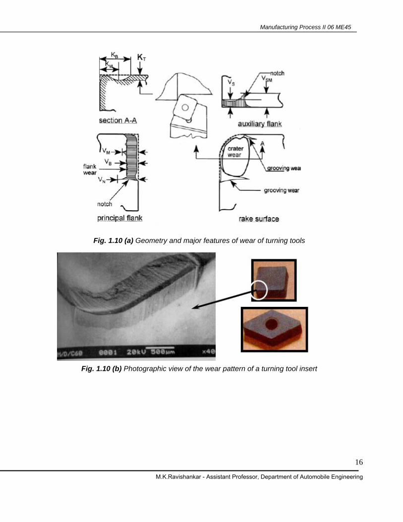
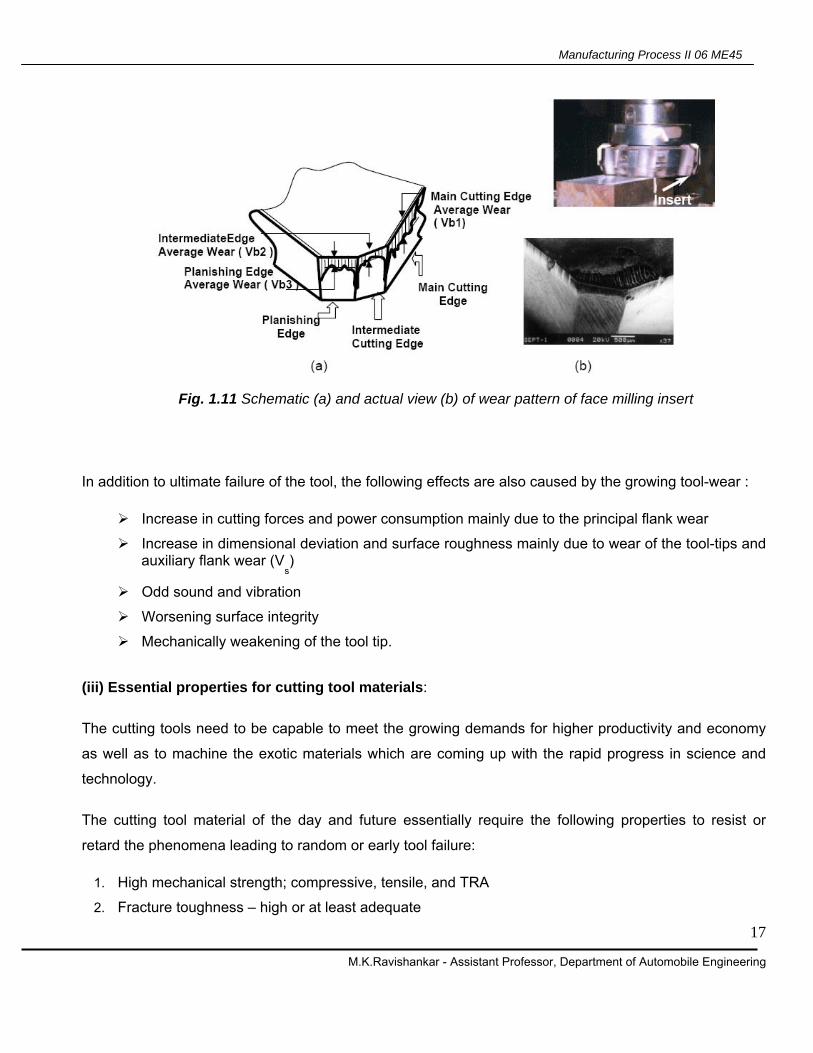
The usual pattern or geometry of wear of turning and face milling inserts are typically shown in Fig. 1.10 (a

and b) and Fig. 1.11 respectively.



16

Fig. 1.10 (a) Geometry and major features of wear of turning tools

Fig. 1.10 (b) Photographic view of the wear pattern of a turning tool insert



17

Fig. 1.11 Schematic (a) and actual view (b) of wear pattern of face milling insert

In addition to ultimate failure of the tool, the following effects are also caused by the growing tool-wear :

Increase in cutting forces and power consumption mainly due to the principal flank wear

Increase in dimensional deviation and surface roughness mainly due to wear of the tool-tips and auxiliary flank wear (V

s)

Odd sound and vibration

Worsening surface integrity

Mechanically weakening of the tool tip.

(iii) Essential properties for cutting tool materials:

The cutting tools need to be capable to meet the growing demands for higher productivity and economy

as well as to machine the exotic materials which are coming up with the rapid progress in science and

technology.

The cutting tool material of the day and future essentially require the following properties to resist or

retard the phenomena leading to random or early tool failure:

1. High mechanical strength; compressive, tensile, and TRA

2. Fracture toughness – high or at least adequate



18

3. High hardness for abrasion resistance

4. High hot hardness to resist plastic deformation and reduce wear rate at elevated temperature

5. Chemical stability or inertness against work material, atmospheric gases and cutting fluids

6. Resistance to adhesion and diffusion

7. Thermal conductivity – low at the surface to resist incoming of heat and high at the core to quickly dissipate the heat entered

8. High heat resistance and stiffness

9. Manufacturability, availability and low cost.

Tool Life:

Definition – Tool life generally indicates, the amount of satisfactory performance or service rendered by a

fresh tool or a cutting point till it is declared failed.

Tool life is defined in two ways :

(a) In R & D :

Actual machining time (period) by which a fresh cutting tool (or point) satisfactorily works after which it needs replacement or reconditioning.

The modern tools hardly fail prematurely or abruptly by mechanical breakage or rapid plastic deformation.

Those fail mostly by wearing process which systematically grows slowly with machining time.

In that case, tool life means the span of actual machining time by which a fresh tool can work before attaining the specified limit of tool wear.

Mostly tool life is decided by the machining time till flank wear, VB

reaches 0.3 mm or crater wear, K

T reaches 0.15 mm.

(b) In industries or shop floor :

The length of time of satisfactory service or amount of acceptable output provided by a fresh tool prior to it is required to replace or recondition.

Assessment of tool life

For R & D purposes, tool life is always assessed or expressed by span of machining time in

minutes,



19

Whereas, in industries besides machining time in minutes some other means are also used to

assess tool life, depending upon the situation, such as

No. of pieces of work machined

Total volume of material removed

Total length of cut.

Measurement of tool wear

The various methods are :

1. By loss of tool material in volume or weight, in one life time – this method is crude and is generally

applicable for critical tools like grinding wheels.

2. By grooving and indentation method – in this approximate method wear depth is measured indirectly

by the difference in length of the groove or the indentation outside and inside the worn area

3. Using optical microscope fitted with micrometer – very common and effective method

4. Using scanning electron microscope (SEM) – used generally, for detailed study; both qualitative and

quantitative

5. Talysurf, specially for shallow crater wear.

Taylor’s tool life equation:

Wear and hence tool life of any tool for any work material is governed mainly by the level of the machining parameters i.e., cutting velocity, (V

C), feed, (s

o) and depth of cut (t).

Cutting velocity affects maximum and depth of cut minimum.

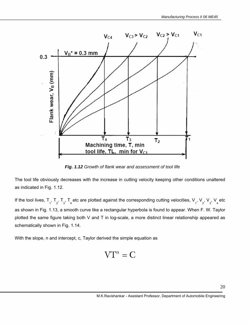
The usual pattern of growth of cutting tool wear (mainly VB), principle of assessing tool life and its

dependence on cutting velocity are schematically shown in Fig.1.12.

B



20

Fig. 1.12 Growth of flank wear and assessment of tool life

The tool life obviously decreases with the increase in cutting velocity keeping other conditions unaltered

as indicated in Fig. 1.12.

If the tool lives, T1, T

2, T

3, T

4 etc are plotted against the corresponding cutting velocities, V

1, V

2, V

3, V

4 etc

as shown in Fig. 1.13, a smooth curve like a rectangular hyperbola is found to appear. When F. W. Taylor

plotted the same figure taking both V and T in log-scale, a more distinct linear relationship appeared as

schematically shown in Fig. 1.14.

With the slope, n and intercept, c, Taylor derived the simple equation as

nVT C=



21

where, n is called, Taylor’s tool life exponent. The values of both ‘n’ and ‘c’ depend mainly upon the tool-

work materials and the cutting environment (cutting fluid application). The value of C depends also on the

limiting value of VB

undertaken ( i.e., 0.3 mm, 0.4 mm, 0.6 mm etc.)

Fig. 1.13 Cutting velocity – tool life relationship

Fig. 1.14 Cutting velocity vs tool life on a log-log scale



22

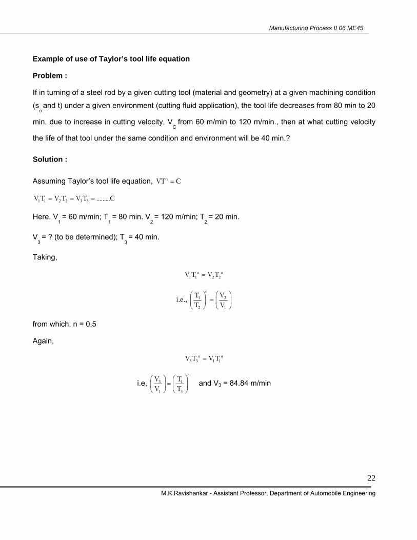
Example of use of Taylor’s tool life equation

Problem :

If in turning of a steel rod by a given cutting tool (material and geometry) at a given machining condition

(so and t) under a given environment (cutting fluid application), the tool life decreases from 80 min to 20

min. due to increase in cutting velocity, VC

from 60 m/min to 120 m/min., then at what cutting velocity

the life of that tool under the same condition and environment will be 40 min.?

Solution :

Assuming Taylor’s tool life equation, nVT C=

1 1 2 2 3 3V T V T V T .........C= = =

Here, V1 = 60 m/min; T

1 = 80 min. V

2 = 120 m/min; T

2 = 20 min.

V3 = ? (to be determined); T

3 = 40 min.

Taking,

n n1 1 2 2V T V T=

i.e., n

21

2 1

VTT V

⎛ ⎞ ⎛ ⎞=⎜ ⎟ ⎜ ⎟⎝ ⎠⎝ ⎠

from which, n = 0.5

Again,

n n3 3 1 1V T V T=

i.e, n

3 1

1 3

V TV T

⎛ ⎞⎛ ⎞= ⎜ ⎟⎜ ⎟

⎝ ⎠ ⎝ ⎠ and V3 = 84.84 m/min



23

Modified Taylor’s Tool Life equation

In Taylor’s tool life equation, only the effect of variation of cutting velocity, VC

on tool life has been

considered. But practically, the variation in feed (so) and depth of cut (t) also play role on tool life to

some extent.

Taking into account the effects of all those parameters, the Taylor’s tool life equation has been

modified as,

0

= Tx y z

c

CTL

V S t

where, TL = tool life in min

CT

= A constant depending mainly upon the tool – work materials and the limiting value of VB undertaken.

x, y and z - exponents so called tool life exponents depending upon the tool – work materials and the machining environment.

Generally, x > y > z as VC

affects tool life maximum and t minimum.

The values of the constants, CT, x, y and z are available in Machining Data Handbooks or can be

evaluated by machining tests.



24

Quiz Test

Identify the correct answer from the given four options.

1. In high speed machining of steels the teeth of milling cutters may fail by

(a) mechanical breakage (b) plastic deformation (c) wear (d) all of the above

2. Tool life in turning will decrease by maximum extent if we double the

(a) depth of cut (b) feed (c) cutting velocity (d) tool rake angle

3. In cutting tools, crater wear develops at

(a) the rake surface (b) the principal flank (c) the auxiliary flank (d) the tool nose

4. To prevent plastic deformation at the cutting edge, the tool material should possess

(a) high fracture toughness (b) high hot hardness (c) chemical stability (d) adhesion resistance

Problems

Problem – 1

During turning a metallic rod at a given condition, the tool life was found to increase from 25 min to 50 min. when V

C was reduced from 100 m/min to 80 m/min. How much will be the life of that tool if

machinedat 90 m/min ?

Problem – 2

While drilling holes in steel plate by a 20 mm diameter HSS drill at a given feed, the tool life decreased from 40 min. to 24 min. when speed was raised from 250 rpm to 320 rpm. At what speed (rpm) the life of that drill under the same condition would be 30 min.?

Answers of the questions of

Quiz Test

Q. 1 : (d) Q. 2 : (c) Q. 3 : (a) Q. 4 : (b)

Solution to Problem 1.

Ans. 34.6 min

Solution to Problem 2

Ans. 287 rpm.

UNIT 1: Theory of Metal Cutting: 7 Hrs Geometry of single...

Documents

Transcript of UNIT 1: Theory of Metal Cutting: 7 Hrs Geometry of single...