SCHOOL OF LAW

UNIT 1 – MICRO ECONOMICS – SBA1103

1  

SYLLABUS - UNIT – I INTRODUCTION

Meaning-Definitions of Economics - Nature & Scope of Economics – Subject Matter of

Economics – Branches of Economics – Importance and Uses and Relevance of Economics in

Law.

INTRODUCTION - ECONOMICS

Economics was formerly called political economy. The term Political economy means the

management of the wealth of the state. “Adam Smith, the father of modem Economics, in his

book entitled 'An Enquiry into the Nature and Causes of the Wealth of Nations’ (Published in

1776) defined Economics as a study of wealth. Smith considered the acquisition of wealth as

the main objective of human activity. According to him the subject matter of Economics is

the study of how wealth is produced and consumed.

Smith's definition is known as wealth definition.

This definition was too materialistic. It gave more importance to wealth than to man for

whose use wealth is produced. The emphasis on wealth was severely criticized by many

others. Cailyle, Ruskin and other philosophers called it the Gospel of Mammon. They even

called it a dismal science as it was supposed to teach selfishness. Later economists held that

apart from man the said study of wealth has no meaning Economics is concerned not only

with the production and use of wealth but also with man. It deals with wealth as serving the

purpose of man. Wealth is only a means to the end of human welfare. We cannot consider the

desire to acquire wealth as the inspiring factor behind every human endeavor. Nor can it be

expected to be the sole cause of human happiness. The emphasis has now shifted from wealth

to man. Man occupies the primary place and wealth only a secondary place.

2  

DEFINITIONSOF ECONOMICS:

Several definitions of Economics have been given. For the sake of convenience let us classify

the various definitions into four groups:

1. Science of wealth

2. Science of material well-being

3. Science of choice making and

4. Science of dynamic growth and development

We shall examine each one of these briefly.

WEALTH DEFINITION – Adam Smith

Economics as “an enquiry into the nature and causes of wealth”

MAIN FEATURES OF WEALTH DEFINITION

• Economics is concerned with the study of wealth only

• The term wealth denotes only material goods. Non-material goods like services and free

goods are excluded

• Economics studies the causes of wealth changes which means economic development

CRITICISM OF THE DEFINITION

1. Too much emphasis on wealth: Adam smith treated economics as political economy and

therefore emphasised the importance of wealth from a national angle. If wealth is looked

upon as money alone, it will give wrong pictures.

2. Restricted Meaning of Wealth: He defined wealth is material goods only, like table,

radio, sweets etc. Non-material services of teacher, doctors are not taken as wealth.

3. Concept of Economic Man: Wealth definition was based mainly on an economic man

who was supposed to give attention to economic activities only. But in reality, human

3  

behavior cannot be properly understood and analysed unless the other motives such as

love, affection, sympathy are also given due weightage.

4. No Mention of Man’s Welfare: Wealth definition explains the wealth-getting and wealth-

spending activities of man alone. It pays to attention to the importance of the welfare of

the society.

5. Economic Problem: He considered the basic economic problems of meeting unlimited

wants with scare means. But the central problem of economics is not at all touched by his

definition.

WELFARE DEFINITION – ALFRED MARSHALL

Economics is a study of mankind in the ordinary business of life. It examines that part of

individual and social action which is most closely connected with the attainment and with the

use of the material requisites of well being”.

Economics is on the one side a study of wealth and the other important side is a part of the

study of man.

FEATURES OF WELFARE DEFINITION

1. A study of mankind: Economics is study of mankind in the ordinary business of life that

means man’s activities in the market as a producer and as a consumer of wealth.

2. A study of social actions: According to him, economics is a social science which covers

the activities of an ordinary man.

3. Study of Material Welfare: He gave the primary place to man and secondary place to

wealth. Moreover it does not study the whole of human welfare, but only a part of its

economic or material welfare.

4. Normative Science: Welfare definition is the study of the causes affecting the material

welfare. Moreover it studies the related activities concerned with wealth. Therefore he

made economics as a normative study.

4  

CRITICISM OF WELFARE DEFINITION

1. Material and Non-Material Welfare: Marshall has given more attention to the study of

material welfare alone. The services of teacher, lawyers, singers etc, do promote welfare

and such welfare may be termer as non-material welfare.

2. Objection to welfare: According to Robbins, there are certain material activities which do

not promote welfare. The manufacture of wine and opium are certainly economic

activities, but they are not conductive to human welfare.

3. Classificatory Definition: According to Robbins, the materialist definition is

classificatory rather than analytical. Marshall definition classifies human activities into

‘economic’ and ‘non-economic’, ‘productive’ and ‘unproductive’, ‘material welfare’ and

‘non-material welfare’. And they considered only those human activities which are

undertaken to promote material welfare.

4. Welfare cannot be measured: Marshall’s idea of welfare is based on cardinal utility. But

utility is a psychological entity which cannot be measured.

SCARCITY DEFINITION – LIONEL ROBBINS

“Economics is the science which studies human behavior as a relationship between ends and

scarce which have alternative uses”.

FUNDAMENTAL CHARACTERISTICS OF SCARCITY DEFINITION

1. Human wants are unlimited: “Ends” refers to human wants which are unlimited but the

resources available to satisfy these wants are limited.

2. Scarcity: The scarcities of means resources (time or money) at the disposal of a person to

satisfy his wants are limited.

3. Alternative use of scare means: Economic resources are not only scare but are also put to

alternative uses that means various choice. We may use land for raising crops or for

building houses.

5  

4. The economic problem: According to him, resources are limited and it have alternative

use. The choosing of one is at the cost of another.

CRITICISM OF SCARCITY DEFINITION

1. It is too narrow and too wide: It is too narrow because it excludes such topics as defects

of economic organization which lead to idle resources. It is to wide to admit with

allocation of scarce means which have alternative uses.

2. It study only positive science: Robbins study explain only about positive science which

means what is it but not about what should be.

3. It confines micro analysis: It is concerned with how as individual faces unlimited ends

with scare means. But economic problems are mostly social in character rater than

individual.

4. Ignores growth Economics: Economics of growth and development is integral part of

economics. But he does not pay any attention to these aspects of economics.

5. Not applicable to under developed countries: A peculiar feature of many under

developed countries is that the resources are not scarce, but they are either underutilized

or unutilized or misutilized.

GROWTH DEFINITION – SAMUELSON

Economics is a social science mainly concerned with the way how society employs its limited

resources which have alternative uses, to produce goods and services for present and future

consumption of various people or groups.

MAIN FEATURES OF GROWTH DEFINITION:

1. It is applicable even in a batter economy where money measurement is not possible.

2. The inclusion of time element makes the scope of economics dynamics

3. This definition possesses universality in its applications.

Note: Growth definition is similar to scarcity definition and it is an improvement over the

scarcity definition.

6  

DIVISION OF ECONOMICS

i. Consumption

ii. Production

iii. Exchange

iv. Distribution

v. Public Finance

CONSUMPTION

Consumption deals with the satisfaction of human wants. There is economic activity in the

world because there are wants. When a want is satisfied, the process is known as

consumption. Generally, in plain language, when we use the term “consumption”, what we

mean is usage. But in economics, it has a special meaning. We can speak of the consumption

of the services of a lawyer, just as we speak of the consumption of food.

In this section, we study about the nature of wants, the classification of wants and some of the

laws dealing with consumption such as the law of diminishing marginal utility, Engel’s law

of family expenditure and the law of demand.

PRODUCTION

Production refers to the creation of wealth. Strictly speaking, it refers to the creation of

utilities. And utility refers to the ability of a good to satisfy a want. There are three kinds of

utility. They are form utility, place utility and time utility. Production refers to all activities

which are undertaken to produce goods which satisfy human wants. Land, labour, capital and

organization are the four factors of production. In the sub- division dealing with production,

we study about the laws which govern the factors of production. They include Malthusian

Theory of population and the laws of returns. We also study about the localization of

industries and industrial organization.

EXCHANGE

7  

In modern times, no one person or country can be self-sufficient. This gives rise to exchange.

In exchange, we give one thing and take another. Goods maybe exchanged for goods or for

money. If goods are exchanged for goods, we call it barter. Modern economy is a money

economy. As goods are exchanged for money, we study in economics about the functions of

money, the role of banks and we also study how prices are determined. We also discuss

various aspects of international trade.

DISTRIBUTION

Wealth is produced by the combination of land, labour, capital and organization. And it is

distributed in the form rent, wages, interest and profits. In economics, we are not much

interested in personal distribution. That is, we do not analyse how it is distributed among

different persons in the society. But we are interested in functional distribution. As the four

factors or agents of production perform different functions in production, we have to reward

them.

PUBLIC FINANCE

Public finance deals with the economics of government. It studies mainly about the income

and expenditure of government. So we have to study about different aspects relating to

taxation, public expenditure, public debt and so on.

NATURE OF ECONOMICS

The nature of economics deals with the question that whether economics falls into the

category of science or arts. Various economists have given their arguments in favour of

science while others have their reservations for arts.

ECONOMICS AS A SCIENCE

Science is a systematized body of knowledge which trades the relationship between cause

and effect. Robbins considered economics as a science and he explains that the last three

words of econom’ics’ indicate a clear proof that it is a science like Physics, Mathematics and

Dynamics.

ARGUMENT IN FAVOUR OF ECONOMICS AS A SCIENCE

The following arguments are advanced to consider economics as a science

1. Systematized study: The scientific method of study consists of three important steps

8  

a) Observation

b) Reasoning, and

c) Verification

Likewise in economics also theories have been formulated after the relevant matters are

systematically collected, classified and studied. Economics systematically divided into

consumption, Production, Exchange, Distribution and Public Finance

2. Scientific Law: A science is not a mere collection of facts, but establishes a relationship

between causes and effect. Like wise, in economics, the law of demand states that other

things being equal, a fall in price of a commodity leads to an increase in demand and vice

versa.

3. Experiments: In physical sciences, experiments can be conducted in laboratories, in

economics, laboratory is the economy/society in which several laws and theories can be

tested.

4. Measuring Rod of Money: According to Marshall, the measuring rod of money has

conferred a special status to economics like other physical sciences. Just as the chemist’s

fine balance has made chemistry more exact than most of other physical sciences; so

economics balance (money) rough and imperfect as it is, has made economics more exact

than any other branch of social science’.

5. Universal: The last requirement for a science is that its laws should be universal. In

economics also, the law of demand, law of diminishing returns etc. are universal in

nature.

ECONOMICS AS AN ART

Science is quantitative but the basis of art is qualitative. Science is descriptive while

art is suggestive. Scientific study is impersonal and objective while art is deeply

personal and subjective.

According to J.N. Keyne’s “An art is a system of rules for the attainment of given

end’.

A science teaches us to know, an art teaches us to do – Luigi Cossa.

The systematic application of scientific principles is an art.

9  

In this view, economics is an art. Economics provides solutions to many of the

problems. Example: the law of equi-marginal utility helps a consumer to solve his

problem of getting maximum satisfaction with limited means. The consumer surplus

analysis helps a finance minister in the field of taxation. Keyne’s Theory of

employment provides a solution to unemployment.

Science requires art; art requires science, each being complementary to the other.

Thus economics is both a science and an art.

POSITIVE AND NORMATIVE APPROACHES

POSITIVE SCIENCE

A positive science is concerned with ‘what is’. It explains what it is, how it works and what

its effects are. According to Milton Friedman, positive economics deals as to how an

economic problem is solved. Robbins, Senior and Friedman are the main champions of

positivism. It simply explained cause and effect relationship.

ARGUMENTS IN FAVOUR OF POSITIVE SCIENCE

1. It is based on logic: Logical enquiry is a rational enquiry with help of logic, the

relationship between cause and effect can be ascertained.

2. It is based on the principles of specialization of labour: The modern economy is based

on division of labour. Each work is entrusted to a specialization group of workers.

3. More uniformity: According to Robbins, the study of what ought to be will cause

perpetual disagreement and controversy in the subject. This may hamper the progress of

the science.

4. More Neutrality: It is said that a man cannot serve for two masters. If an economist deals

with the questions, what is, and what ought to be, he cannot be neutral.

NORMATIVE SCIENCE

Marshall, Fraser, wolf and Paul streeten are the main advocates of Normative science.

Normative science concerned with “what should be” or “What ought to be” Normative

science evaluates. According to Milton Friedman, normative science deals with how

economic problem should be solved. Normative economics depends on value judgment.

10  

ARGUMENTS IN FAVOUR OF NORMATIVE SCIENCE

1. Man is not only logical but also sentimental.

2. Wrong argument of equilibrium is equilibrium: According to Fraser ‘Economics is

something more than a value theory or equilibrium.

3. Necessity of value judgment: Economic policies in the real world affect some people

favorably and others unfavorably. In modern times planning is inevitable for developing

countries. For planning, economists use value judgment on the desirability of various

projects.

4. A means of social betterment: Various economists have developed policy measures to

develop the economy. For example, Adam smith stressed the necessity of Laissez faire.

Malthus warned the excess of over population.

ECONOMICS IS BOTH A POSITIVE AND A NORMATIVE SCIENCE

The modern economists accept that economics is both a positive science and a normative

science. They argue that optimum utilization of the resources would not be the only aim but

also the achievement of some desirable objective such as more and just distribution of

economic power and opportunities.

SCOPE OF ECONOMICS

Economists use different economic theories to solve various economic problems in society.

Its applicability is very vast. From a small organization to a multinational firm, economic

laws come into play. The scope of economics can be understood under two subheads:

Microeconomics and Macroeconomics.

11  

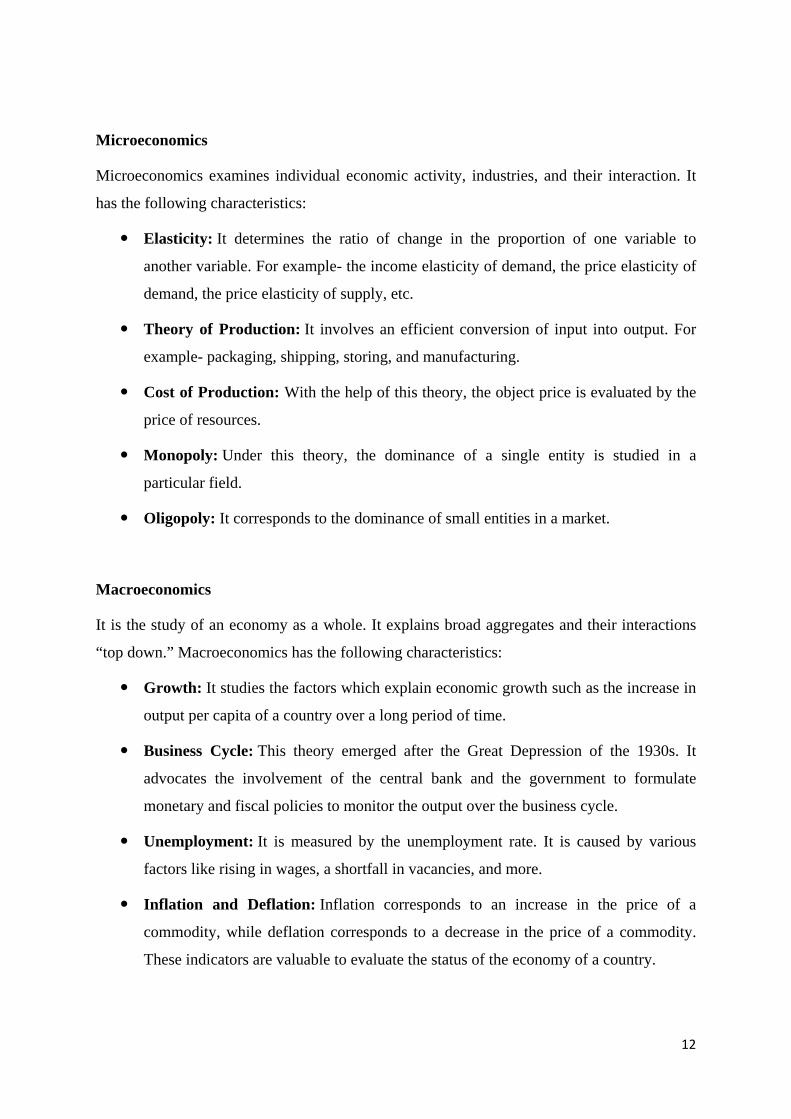
Microeconomics

Microeconomics examines individual economic activity, industries, and their interaction. It

has the following characteristics:

Elasticity: It determines the ratio of change in the proportion of one variable to

another variable. For example- the income elasticity of demand, the price elasticity of

demand, the price elasticity of supply, etc.

Theory of Production: It involves an efficient conversion of input into output. For

example- packaging, shipping, storing, and manufacturing.

Cost of Production: With the help of this theory, the object price is evaluated by the

price of resources.

Monopoly: Under this theory, the dominance of a single entity is studied in a

particular field.

Oligopoly: It corresponds to the dominance of small entities in a market.

Macroeconomics

It is the study of an economy as a whole. It explains broad aggregates and their interactions

“top down.” Macroeconomics has the following characteristics:

Growth: It studies the factors which explain economic growth such as the increase in

output per capita of a country over a long period of time.

Business Cycle: This theory emerged after the Great Depression of the 1930s. It

advocates the involvement of the central bank and the government to formulate

monetary and fiscal policies to monitor the output over the business cycle.

Unemployment: It is measured by the unemployment rate. It is caused by various

factors like rising in wages, a shortfall in vacancies, and more.

Inflation and Deflation: Inflation corresponds to an increase in the price of a

commodity, while deflation corresponds to a decrease in the price of a commodity.

These indicators are valuable to evaluate the status of the economy of a country.

12  

BRANCHES OF ECONOMICS

Microeconomics – concerned with individual markets and small aspects of the economy.

Macroeconomics – concerned with the whole aggregate economy. Issues such as inflation,

economic growth and trade.

I MICRO ECONOMICS

1. Neo-classical economics: Key people: Leon Walrus, William Jevons, John Hicks, George

Stigler and Alfred Marshall.

Neo-classical economics built on the foundations of free-market based classical economics. It

included new ideas such as Utility maximization, Rational choice theory, Marginal analysis.

Neo-classical economics is often considered to be orthodox economics. It is the economics

taught in most text-books as the starting point for economics teaching. The tools of neo-

classical economics (supply and demand, rational choice, utility maximisation) can be used in

new fields and also for critiques.

2. Development economics: Key people: Simon Kuznets and W. Arthur Lewis, Amartya Sen

and Muhammad Yunus.

Concerned with issues of poverty and under-development in poorer countries of the world.

Development economics is concerned with both micro and macro aspects of economic

development. Issues include Trade vs aid, Increasing capital investment, Best ways to

promote economic development, Third World debt

3. Environmental economics/welfare economics: Key people: Garrett Hardin, E.F.

Schumacher, Arthur Pigou.

This places greater emphasis on the environment. This can include: Neo-classical analysis of

external costs and external benefits. From this perspective, it is rational for man to reduce

pollution, Market failures – tragedy of the commons, Public goods, external costs, external

benefits, Environmental economics can take a more radical approach – questioning whether

economic growth is actually desirable.

4. Behavioural economics: Key people: Gary Becker, Amos Tversky, Daniel Kahneman,

Richard Thaler, Robert J. Shiller,

13  

Behavioural economics examines the psychology behind economic decision making and

economic activity. Behavioural economics examines the limitation of the assumption

individuals are perfectly rational. It includes Bounded rationality – people make choices by

rules of thumb, Irrational exuberance – People get carried away by asset bubbles,

Nudges/Choice architecture – how the framing of decisions affects the outcome

5. Econometrics: Key people: Jan Tinbergen

Use of data to find simple relationships. Econometrics uses statistical methods, regression

models and data to predict the outcome of economic policies. For example, Okun’s law

suggests a relationship between economic growth and unemployment.

6. Labour economics: Key people: Knut Wicksell

Concentration on wages, labour employment and labour markets. Labour economics starts

from neo-classical premise of labour supply and marginal revenue product of labour.

Recent developments in labour economics have placed greater emphasis on non-monetary

factors, such as motivation, enjoyment and labour market imperfections.

II MACRO ECONOMICS

1. Classical economics: Classical economics is often considered the foundation of modern

economics. It was developed by Adam Smith, David Ricardo, Jean-Baptiste Say. Classical

economics is based on

• Operation of free markets. How the invisible hand and market mechanism can enable

an efficient allocation of resources.

• Classical economics suggests that generally, economies work most efficiently when

government intervention is minimal and concerned with the protection of private

property, promotion of free trade and limited government spending.

• Classical economics does recognise that a government is needed for providing public

goods, such as defence, law and order and education.

2. Keynesian economics: Key people: John Maynard Keynes, Paul Samuelson.

Keynesian economics was developed in the 1930s against a backdrop of the Great

Depression. The existing economic orthodoxy was at a loss to explain the persistent

economic depression and mass unemployment. Keynes suggested that markets failed to clear

14  

for many reasons (e.g. paradox of thrift, negative multiplier, low confidence). Therefore,

Keynes advocated government intervention to kick-start the economy.

3. Marxist economics: Key people: Karl Marx

Emphasises unequal and unstable nature of capitalism. Seeks a radically different approach to

basic economic questions. Rather than relying on free-market advocate state intervention in

ownership, planning and distribution of resources.

4. Austrian economics : Key people: Ludwig Von Mises, Carl Menger

This is another school of economics that was critical of state intervention, price controls. It is

broadly free-market. However, it criticised elements of classical school – placing greater

emphasis on the individual value and actions of an individual. For example, Austrian

economists argue the value of a good reflects the marginal utility of the good – rather than the

labour inputs.

5. Mercantilism: Early model of economics emphasising tariff barriers and accumulation of

gold reserves. Mercantilism

6. Monetarist economics: Key people: Milton Friedman, Anna Schwartz.

Monetarism was partly a reaction to the dominance of Keynesian economics in the post-war

period. Monetarists, led by Milton Friedman argued that Keynesian fiscal policy was much

less effective than Keynesians suggested. Monetarists promoted previous classical ideals,

such as belief in the efficiency of markets. They also placed emphasis on the control of the

money supply as a way to control inflation. Monetarist economics became influential in the

1970s and 1980s, in a period of high inflation – which appeared to illustrate the breakdown of

the post-war consensus.

NATURE OF ECONOMIC LAWS

Every science uses terms such as hypothesis, theory and law. A hypothesis attempts to

explain some facts. If the hypothesis can explain new facts and is not contradicted by new

discoveries, it is promoted to the rank of a theory.

Like all sciences, economics has its own laws. A law is a statement of casual relationship

between two sets of phenomena, one is a cause and the other is an effect.

15  

FEATURES OF ECONOMIC LAWS

1. Economic laws are conditional: Economic laws are conditional or hypothetical and their

validity depends upon the fulfillment of certain conditions. That is why all economic laws

are qualified by the statement, “other things being equal”.

2. Economic laws are relative:

a) Universal laws: The statements like “saving is a function of income”, human want are

unlimited. These are universal to all countries and at all time.

b) Relative laws: Some laws are relative and specific to certain country and time. Example,

the laws which are applicable to a free enterprise economy cannot be applied to a

communist economy. Laws which are applicable to developed countries cannot be

applied to developing countries.

3. Economics laws are less exact: The law of physical and natural sciences are exact and

definite. But, Economic laws are not precise. This is because the economists laboratory is

the economy/society where he has to rely in a great measure on logic or perception which

are subject to variations from economist to economist.

Causes for the inexactness of Economic law, are;

a) Non-availability of laboratory method

b) Men are not similar in their tastes or purchasing power

c) Differences in bias and ideologies exist among persons

4. Economic laws are similar to biological law: Economics is more allied to biology than to

physics. This is mainly because both economics and biology deal with life and not with

matter.

5. Economic laws are more exact than laws of social sciences: Samuelson considered

economics as the queen of social sciences. Economics laws are more exact than the laws

of other social sciences like ethics, sociology, politics etc,. This is because, in economics,

economic activities can be measured with measuring rod of money.

16  

6. Economic laws are statements of tendencies: According to Prof. Marshall, economic

laws are statement of tendencies. They state that under certain conditions, certain things

will take place. Economic laws do not give any certainty that they ‘must’ happen.

Economic laws are only probabilities and not certain.

7. Economic laws and government laws: The laws of government must be obeyed. The

government laws are enacted by the legislature and enforced by the executives. If the

citizens violate these laws, they are punished. Economic laws are not commands.

Economic laws are indicative and not imperative.

ROLE AND IMPORTANCE OF ECONOMICS IN LAW

1. Economics helps in understanding tax laws: Economics helps in understanding various

concepts of tax laws. As we know Economics deal with the issues of the economy alike

law is concerned with the issues related to the society.

2. Economic help in understanding the company law: Company Law or we can say

business law which includes various terms and definitions which early man can’t

understand without understanding the concept of Economics. Therefore we can say that

company law can be understood to the people having a piece of basic knowledge

regarding economics.

3. Economics helps in understanding consumer protection law: Economic directly or

indirectly helping the understanding of consumer protection that is covered under the

Consumer Protection Act which is enacted for the protection of consumers and

encroachment of their rights as a consumer of the goods and services.

4. Laws related to the limited resources can only be understood by having a basic

knowledge of Economics: As we know India is a diverse country having very limited

resources for example water, petroleum and many others. For that purpose, to conserve

these resources proper rules and regulations are to be introduced in various legislation to

sustainable development.

5. Concept of uncertainty and expectations taught by economics in law: As we know

economics to deal with unlimited wants and limited resources thus comprises greater

expectations. And for the accomplishment of these expectations wants, normally people

17  

used to do unfair means to attain it. For that purpose, proper legislation is to be made in

the law itself which reflects the significance of economics in lawmaking.

6. Economics act as a critical examination of lawmaking: There is no doubt that

economics deals with each and every sector of the economy. Therefore, for the enactment

of necessary legislation, we have to consider the parameters of economics. Economics

exam board critical examination for the present situation of the economy which helps in

enactment of various promulgations related to the economy.

METHODS OF ECONOMIC LAW

1. Deductive Method

2. Inductive Method

DEDUCTIVE METHOD:

‘General to particular’

Example 1:

All dolphins are mammals; All mammals have kidneys.

Using deductive reasoning, you can conclude that all dolphins have kidneys.

Example 2:

"All men are mortal. Harold is a man. Therefore, Harold is mortal.“

Example 3:

“A is equal to B. B is also equal to C. Therefore, A is equal to C”

i. It is analytical, abstract or a priori method

ii. Step involves starting with few assumption, hypothesis or postulates are made

iii. Methods of deductive reasoning are mathematical and non-mathematical

iv. Law of demand and law of diminishing marginal utilities are derived from deductive

method.

18  

MERITS OF DEDUCTIVE METHOD

1. Simple: Deductive method is very simple in nature. It avoids the collection of statistical

data and information for proving economic laws. It helps us to draw conclusions from the

accepted generalizations.

2. Analytical: This method is useful for analyzing complex economic phenomena. It divides

a particular economic problem into several components.

3. Universal validity: The inferences adopted and the conclusions made under this method

have universal validity. The reason is that the inferences are based on certain general

principles.

4. Indispensable: This method is regarded as an indispensable method in Economics. As

Gide and Rist pointed out “In a science like Political Economy experiment is practically

impossible. Abstraction and analysis afford the only means of escape from those other

influences which complicate the problem so much”.

5. Exactness and clarity: Deductive method is based on logical reasoning. It helps us to

arrive at exact conclusions because its assumptions are definite, clear and true.

6.Reveals inconsistencies : This method provides scope for adopting mathematical approach

for arriving conclusions. So it reveals the inconsistencies in the economic phenomena.

7. Powerful method : This method is considered as a powerful method for analyzing the

economic phenomena. It is used for deducing conclusions from certain facts.

DEMERITS OF DEDUCTIVE METHOD

1. Based on wrong assumptions: Deductive method is based on certain assumptions. But the

assumptions may not be real at all times. So the conclusions based on these assumptions may

not be real

2. Universal applicability – a myth : The statement that deductive method has universal

applicability is not real. Because the causes and conclusions of economic problems differ

from country to country and from time to time.

3. Inadequate, data: The followers of this method adopted it on the basis of inadequate data.

So the conditions arrived from the assumption, were full of inconsistencies.

19  

4. Generalizations – full of faults: The proposers of this wrongly assumed that their

abstractions always correspond with the facts. So any research scholar commits the same

mistake if he tries to deduce faulty generalizations.

5. Excessively abstract: This method assumes that Economists possess special skill and

knowledge. for drawing inference from various assumptions. This makes them proud and

negligent in their research job.

6. Makes economics dogmatic: This method makes Economics dogmatic as it refuses to

admit that there can be some defects on the assumptions.

7. Difficulty in testing the conclusions : This method make difficult to test the validity of

conclusions. The conclusions drawn under this method are neither feasible nor practicable.

INDUCTIVE METHOD OF ECONOMIC LAW

‘Particular to general’

Example 1:

The first lipstick I pulled from my bag is red. The second lipstick I pulled from my

bag is red. Therefore, all the lipsticks in my bag are red.

Example 2:

Jennifer always leaves for school at 7:00 a.m. Jennifer is always on time. Therefore, if

she leaves at 7:00 a.m. for school today, she will be on time.

Example 3:

The chair in the living room is red. The chair in the dining room is red. The chair in

the bedroom is red. Therefore, All the chairs in the house are red.

i. It is historical, empirical or a posteriori method

ii. Step involves observation, formation of hypotheses, generalization and verification

iii. Methods of inductive reasoning are experimental method are statistical method

iv. The engel’s law of family expenditure, Malthusian theory of population are derived

from inductive statistical method.

20  

MERITS OF INDUCTIVE METHOD

1. Helps in future inquiries: Inductive method acts as -a guide for future inquiries. It helps

in future investigation through discovery and evidence of general principles.

2. More realistic: This method is more realistic as it is based on facts. It explains the facts

without any distortion.

3. Concrete and synthetic: This method is more concrete and synthetic since it deals with

the subject as a whole without dividing it into various components.

4. Related to time and place : This method helps us to draw generalizations on the basis of a

particular historical situation. So the generalization relate to a particular time and place.

Therefore there arises no practical difficulty in applying the conclusions for solving certain

economic problems.

5. More accurate: This method provides scope for the adoption of statistical methods.

Statistical methods are useful for studying matters relating to national income, inflation,

savings and investment. The conclusions drawn from such methods are more accurate.

6. Valuable to Government: This method is of great value to the ,Government . The

government by adopting this method, can solve complex economic problems.

7. Dynamic method: This method involves observation) and analysis of facts from historical

origin. As economic phenomena vary according to time, their nature, causes and effects can

be effectively studied under this method. Hence this method is described as dynamic one.

8. Complimentary: This method is considered as a complimentary to the deductive analysis

of economic phenomena. The conclusions drawn by deductive method can be verified by this

method. This helps us to get accurate and definite information regarding economic

phenomena.

21  

22  

DEMERITS OF INDUCTIVE METHOD

1. Misuse and this —interpretation: Inductive method depends to a great extent on

statistical data for analyzing the economic phenomena. This may lead to the misuse and

misinterpretation of statistical data,

2. Lacks concreteness: The definitions, sources and methods (used in the statistical approach

of this method) differ from investigator to investigator regarding a particular economic

phenomenon. For instance different techniques are used by the investigators for calculating

the national income of a country.

3. Not certain : The conclusions drawn from this method are not certain. As Bouldings

pointed out that statistical information can only give us .propositions whose truth is more or

less probable. It never gives us certainty.

4. Delay and costly affair: This method involves a detailed process of collection,

classification, analysis and interpretation of data. It also requires the services of expert

statistical investigators and analysts. Therefore, this method causes delay. It requires huge

expenditure.

5. Limited applicability: Observation and experimentation are employed in this method. But

as Economics is concerned with human behavior, it is not completely possible to predict the

behavior of individuals at all times. So the conclusions drawn by this method have limited

applicability.

6. Investigator’s talents doubtful: The success of this method for finding conclusions on

economic phenomena depends to a great extent on the talents, capacity and intelligence of the

investigators. If the investigators lack initiative and statistical knowledge, then this method is

of no use.

**********

SCHOOL OF LAW

UNIT 2 – MICRO ECONOMICS – SBA1103

1  

SYLLABUS - UNIT – II CONSUMER BEHAVIOUR

Theory of Demand and Supply – Law of Demand & Supply – Determinants of Demand &

Supply – Concept of Utility: Cardinal Utility Theory – Marginal Utility and Total Utility –

consumer’s Equilibrium – Marginal Valuation – Equi-Marginal Utility, Consumer’s Demand

Curve – consumer’s Surplus – Paradox of Value – Ordinal Utility Theory – Indifference

Curve Approach – Consumer’s Preferences – Indifference Curve – Budget Line –

Consumer’s Equilibrium – Income and Substitution – Effects – Price Consumption Curve and

the Derivation of Demand Curve for a commodity – Income Consumption Path – Engel’s

Law.

DEMAND

In general, Demand means desire by human. In economics, Demand refers to the desire

backed by ability to pay and willingness to buy it. A beggar may desire to have a car, but his

desire is not going to affect its market price as he is not having the necessary purchasing

power to buy a car. Thus, desire backed by purchasing power is called demand.

KINDS OF DEMAND

I. Direct Demand: It refers to demand for a commodity that is directly consumed to satisfy

human wants, for example demand for bread, butter and fruits.

a) Price Demand: it refers to the demand for a commodity at a particular price

b) Income Demand: It refers to the demand for a commodity at a various levels of

consumer’s income

c) Cross Demand: It refers to quantity demanded of a commodity due to change in the

price of other commodity

II. Indirect Demand or Derived Demand:

Demand for factors of production is indirect because they help in the production of a

commodity which is directly demanded by the consumer in the market.

III. Complementary Demand/ Joint Demand:

It refers to the demand for those goods for a commodity which are always demanded jointly.

Example: car and petrol.

2  

IV. Composite Demand:

It refers to the total demand for a commodity which can be used for various purposes.

LAW OF DEMAND – ALFRED MARSHALL

Definition: The law of demand states that , other things remaining equal, the quantity

demanded for a commodity increases when its price falls and decreases when the price rises.

There is a inverse relationship between the price of the good and the quantity demanded of

that good.

FACTOR AFFECTING THE DEMAND

1. Price of the Given Commodity: It is the most important factor affecting demand for the

given commodity. Generally, there exists an inverse relationship between price and quantity

demanded.

2. Price of substitutes/related goods: Some goods can be substituted for other goods. For

example, tea and coffee are substitutes. If the price of coffee increases while the price of tea

remains the same, there will be increase in the demand for tea and decrease in the demand for

coffee.

3. Income of the consumer: When the income of the consumer increases, more will be

demanded. Comforts and luxuries belong to this category

4. Tastes and preferences of the consumer: Demand for a commodity may change due to a

change in tastes, preferences and fashion.

5. Expectation of future price change: If the consumer believes that the price of a

commodity will rise in the future, he may buy a larger quantity in the present. Suppose he

expects the price to fall, he may defer some of his purchases to a future date.

ASSUMPTIONS OF THE LAW OF DEMAND

1. The price of the related goods remains the same

2. The income of the consumers remain unchanged

3. Tastes and preferences of the consumer remain the same

3  

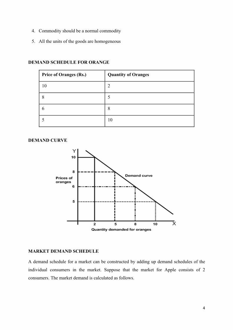
4. Commodity should be a normal commodity

5. All the units of the goods are homogeneous

DEMAND SCHEDULE FOR ORANGE

Price of Oranges (Rs.) Quantity of Oranges

10 2

8 5

6 8

5 10

DEMAND CURVE

MARKET DEMAND SCHEDULE

A demand schedule for a market can be constructed by adding up demand schedules of the

individual consumers in the market. Suppose that the market for Apple consists of 2

consumers. The market demand is calculated as follows.

4  

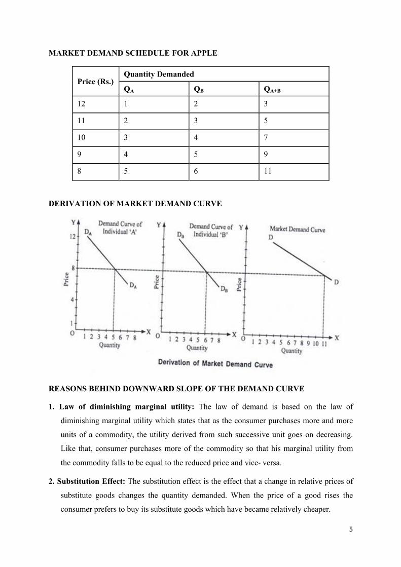
MARKET DEMAND SCHEDULE FOR APPLE

Price (Rs.) Quantity Demanded

QA QB QA+B

12 1 2 3

11 2 3 5

10 3 4 7

9 4 5 9

8 5 6 11

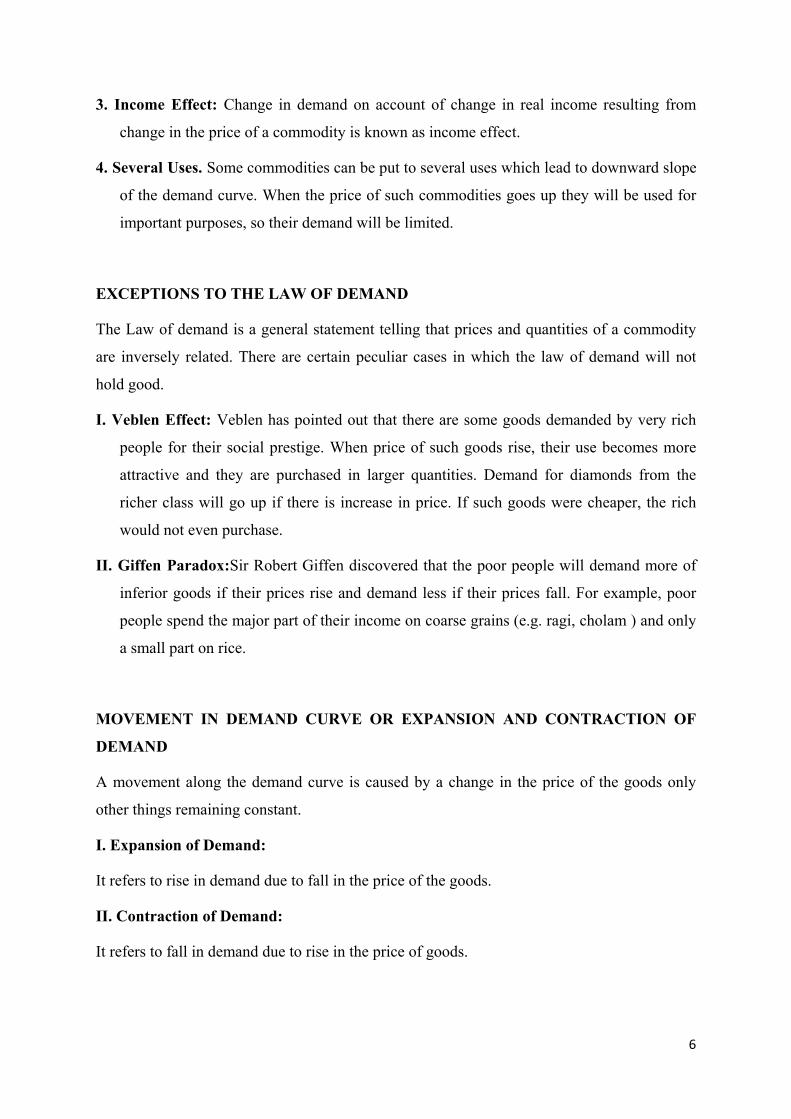
DERIVATION OF MARKET DEMAND CURVE

REASONS BEHIND DOWNWARD SLOPE OF THE DEMAND CURVE

1. Law of diminishing marginal utility: The law of demand is based on the law of

diminishing marginal utility which states that as the consumer purchases more and more

units of a commodity, the utility derived from such successive unit goes on decreasing.

Like that, consumer purchases more of the commodity so that his marginal utility from

the commodity falls to be equal to the reduced price and vice‐ versa.

2. Substitution Effect: The substitution effect is the effect that a change in relative prices of

substitute goods changes the quantity demanded. When the price of a good rises the

consumer prefers to buy its substitute goods which have became relatively cheaper.

5  

3. Income Effect: Change in demand on account of change in real income resulting from

change in the price of a commodity is known as income effect.

4. Several Uses. Some commodities can be put to several uses which lead to downward slope

of the demand curve. When the price of such commodities goes up they will be used for

important purposes, so their demand will be limited.

EXCEPTIONS TO THE LAW OF DEMAND

The Law of demand is a general statement telling that prices and quantities of a commodity

are inversely related. There are certain peculiar cases in which the law of demand will not

hold good.

I. Veblen Effect: Veblen has pointed out that there are some goods demanded by very rich

people for their social prestige. When price of such goods rise, their use becomes more

attractive and they are purchased in larger quantities. Demand for diamonds from the

richer class will go up if there is increase in price. If such goods were cheaper, the rich

would not even purchase.

II. Giffen Paradox:Sir Robert Giffen discovered that the poor people will demand more of

inferior goods if their prices rise and demand less if their prices fall. For example, poor

people spend the major part of their income on coarse grains (e.g. ragi, cholam ) and only

a small part on rice.

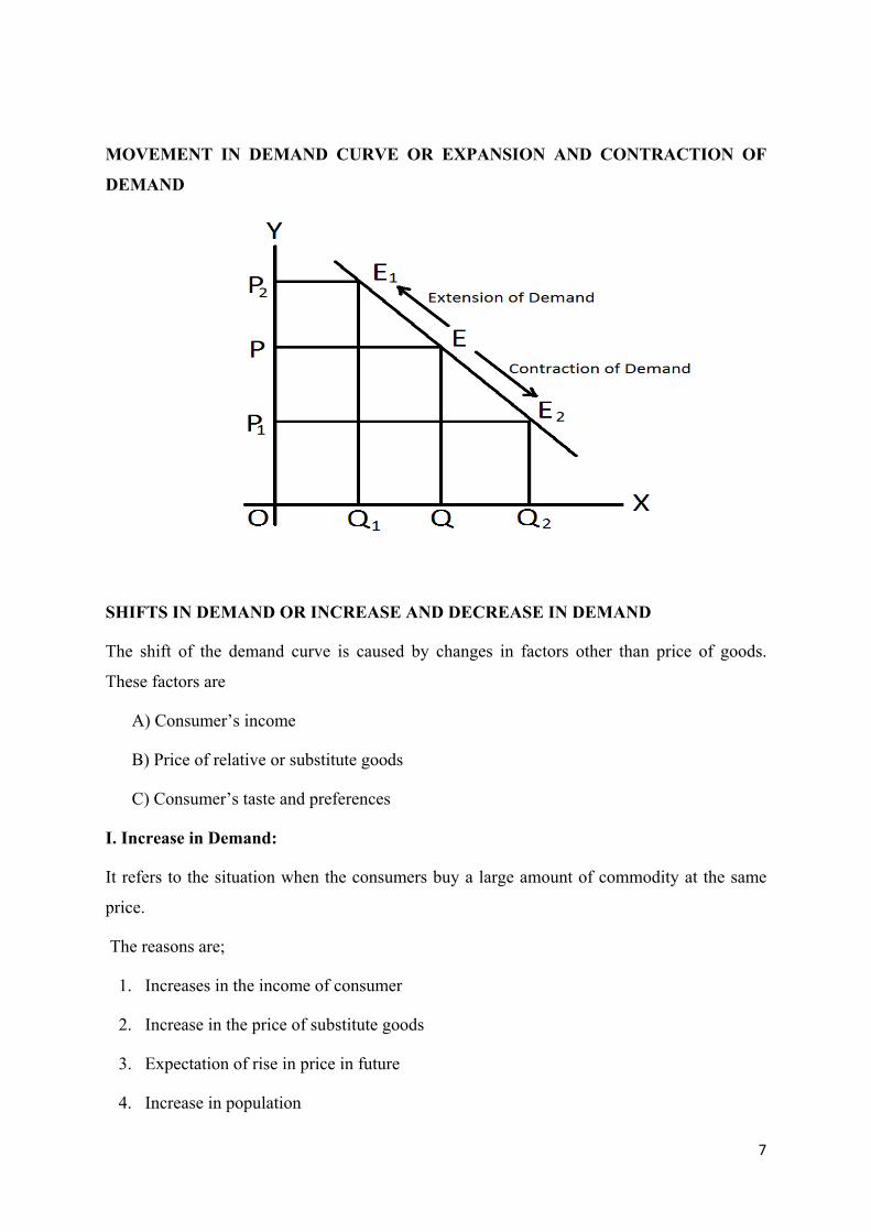
MOVEMENT IN DEMAND CURVE OR EXPANSION AND CONTRACTION OF

DEMAND

A movement along the demand curve is caused by a change in the price of the goods only

other things remaining constant.

I. Expansion of Demand:

It refers to rise in demand due to fall in the price of the goods.

II. Contraction of Demand:

It refers to fall in demand due to rise in the price of goods.

6  

MOVEMENT IN DEMAND CURVE OR EXPANSION AND CONTRACTION OF

DEMAND

SHIFTS IN DEMAND OR INCREASE AND DECREASE IN DEMAND

The shift of the demand curve is caused by changes in factors other than price of goods.

These factors are

A) Consumer’s income

B) Price of relative or substitute goods

C) Consumer’s taste and preferences

I. Increase in Demand:

It refers to the situation when the consumers buy a large amount of commodity at the same

price.

The reasons are;

1. Increases in the income of consumer

2. Increase in the price of substitute goods

3. Expectation of rise in price in future

4. Increase in population

7  

II. Decrrease in Deemand:

It refers

same pr

s to a situat

rice.

tion when tthe consummers buy a ssmaller quaantity of thee commoditty at the

The reaasons are;

1. Faall in the inccome of thee consumerss

2. Faall in the priice of the suubstitute gooods

3. Exxpectation oof fall in priice

4. Decrease in PPopulation

5. Coonsumers’ ttaste becomming unfavorrable towarrds the goodds

SHIFTTS IN DEMMAND OR IINCREASEE AND DECREASE IIN DEMANND

ELASSTICITY OF DEMMAND - AALFRED MMARSHAALL

The law

commo

The con

w of deman

odity. But it

ncept of ela

nd explains

t does not e

sticity of de

that deman

explain the

emand meas

nd will cha

rate at whi

sures the rat

ange due to

ch demand

te of change

o a change

changes to

e in demand

in the pric

o a change i

d.

e of the

in price.

8  

DEFINITION OF ELASTICITY OF DEMAND:

According to him “the elasticity (or responsiveness) of demand in a market is great or small

according as the amount demanded increases much or little for a given fall in price, and

diminishes much or little for a given rise in price”.

FACTORS DETERMINING THE PRICE ELASTICITY OF DEMAND

1. Availability of Substitute: Goods having close substitutes will have an elastic demand

and goods with no close substitutes will have an inelastic demand. Commodities such as

Pen, Pepsi, Maruti car have close substitutes and hence have an elastic demand.

2. Income of the consumers: If the income level of consumers is high, the elasticity of

demand will be less. It is because change in the price will not affect the quantity

demanded by greater proportion

3. Luxuries versus Necessities: The price elasticity of demand is likely to be low for

necessities and high for luxuries

4. Number of uses of the commodity: The more the number of uses of a commodity has

more elastic demand. If a commodity has few uses it has an inelastic demand.

5. Cost relative to total income: higher the cost of the goods relative to total income of

consumer more will be the price elasticity demand.

6. Level of price: if the price of the commodity is high the price elasticity of demand is more

and if it is low, its price elasticity of demand is less.

TYPES OF ELASTICITY OF DEMAND

1. Price Elasticity of Demand

2. Income Elasticity of Demand

3. Cross Elasticity of Demand

4. Advertising elasticity of Demand

5. Elasticity of Price Expectations

9  

1. PRICE ELASTICITY OF DEMAND

“The degree of responsiveness of quantity demanded to a change in price is called price

elasticity of demand”

DIFFERENT TYPES OF PRICE ELASTICITY OF DEMAND

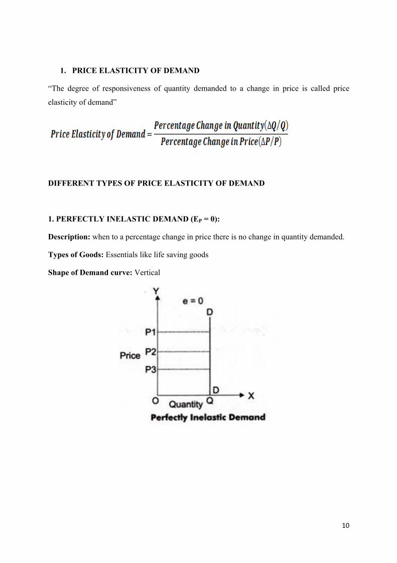
1. PERFECTLY INELASTIC DEMAND (EP = 0):

Description: when to a percentage change in price there is no change in quantity demanded.

Types of Goods: Essentials like life saving goods

Shape of Demand curve: Vertical

10  

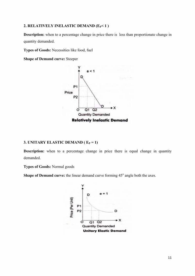
2. RELATIVELY INELASTIC DEMAND (EP< 1 )

Description: when to a percentage change in price there is less than proportionate change in

quantity demanded.

Types of Goods: Necessities like food, fuel

Shape of Demand curve: Steeper

3. UNITARY ELASTIC DEMAND ( EP = 1)

Description: when to a percentage change in price there is equal change in quantity

demanded.

Types of Goods: Normal goods

Shape of Demand curve: the linear demand curve forming 45o angle both the axes.

11  

4. RELATIVELY ELASTIC DEMAND (EP> 1)

Description: when to a percentage change in price there is more than proportionate change

in quantity demanded.

Types of Goods: Luxuries

Shape of Demand curve: Flatter

5. PERFECTLY ELASTIC DEMAND (EP = ∞)

Description: when there is infinite change in quantity situation demanded without any

changes in price

Types of Goods: Imaginary

Shape of Demand curve: Horizontal

12  

METHODS OF CALCULATING PRICE ELASTICITY OF DEMAND

1. The Percentage Method:

The price elasticity of demand is measured by its coefficient (Ep). This coefficient (Ep)

measures the percentage change in the quantity of a commodity demanded resulting from a

given percentage change in its price.

Thus,

Where q refers to quantity demanded, p to price and Δ to change. If EP>1, demand is elastic.

If EP< 1, demand is inelastic, and Ep= 1, demand is unitary elastic.

2. The Point Method or Geometrical or graphical method:

The point method of measuring elasticity of demand was developed by Alfred Marshall.

Elasticity measures at a point on a demand curve is known as point elasticity of demand.

Let RS be a straight line demand curve in Figure. If the price falls from PB ( = OA) to MD (

= OC), the quantity demanded increases from OB to OD.

13  

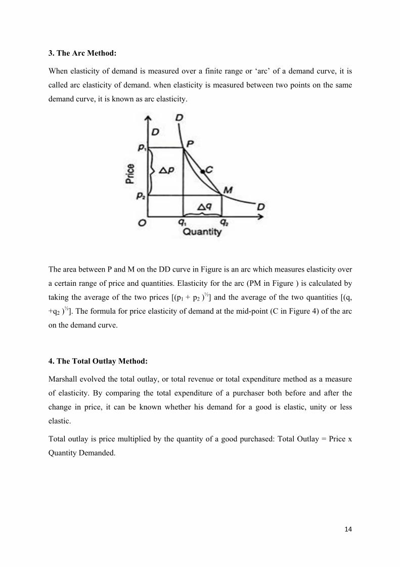
3. The Arc Method:

When elasticity of demand is measured over a finite range or ‘arc’ of a demand curve, it is

called arc elasticity of demand. when elasticity is measured between two points on the same

demand curve, it is known as arc elasticity.

The area between P and M on the DD curve in Figure is an arc which measures elasticity over

a certain range of price and quantities. Elasticity for the arc (PM in Figure ) is calculated by

taking the average of the two prices [(p1 + p2 )½] and the average of the two quantities [(q,

+q2 )½]. The formula for price elasticity of demand at the mid-point (C in Figure 4) of the arc

on the demand curve.

4. The Total Outlay Method:

Marshall evolved the total outlay, or total revenue or total expenditure method as a measure

of elasticity. By comparing the total expenditure of a purchaser both before and after the

change in price, it can be known whether his demand for a good is elastic, unity or less

elastic.

Total outlay is price multiplied by the quantity of a good purchased: Total Outlay = Price x

Quantity Demanded.

14  

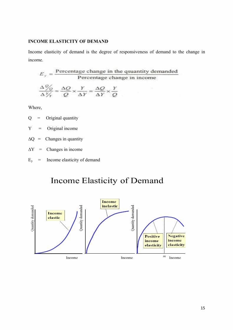
INCOME ELASTICITY OF DEMAND

Income elasticity of demand is the degree of responsiveness of demand to the change in

income.

Where,

Q = Original quantity

Y = Original income

∆Q = Changes in quantity

∆Y = Changes in income

Ey = Income elasticity of demand

15  

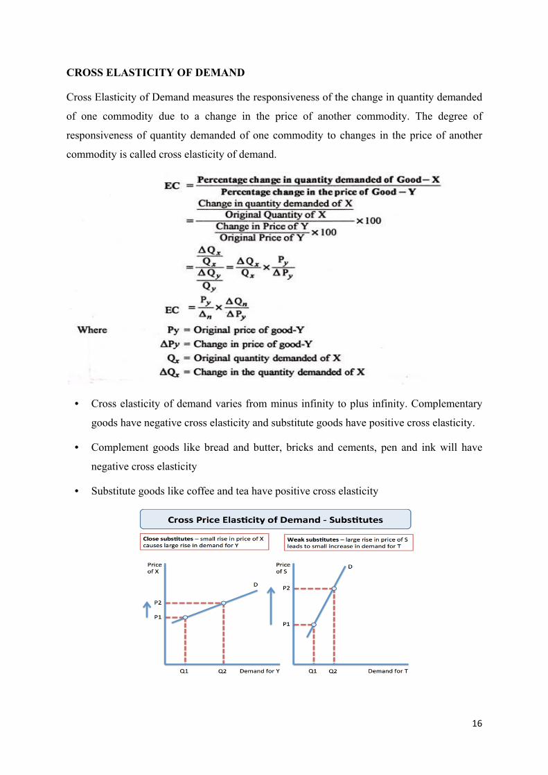
CROSSS ELASTICCITY OF DDEMAND

Cross E

of one

respons

commo

Elasticity of

commodity

siveness of

odity is calle

f Demand m

y due to a

quantity de

ed cross elas

measures the

a change in

emanded of

sticity of de

e responsive

n the price

f one comm

emand.

eness of the

of anothe

modity to ch

e change in

er commodi

hanges in th

quantity de

ity. The de

he price of

emanded

egree of

f another

• Cr

go

• Co

ne

• Su

ross elastic

oods have n

omplement

egative cros

ubstitute go

ity of dema

negative cro

goods like

ss elasticity

oods like cof

and varies f

ss elasticity

e bread and

ffee and tea

from minus

y and substit

d butter, bri

a have positi

s infinity to

tute goods h

icks and ce

ive cross el

plus infinit

have positiv

ements, pen

asticity

ty. Comple

ve cross ela

n and ink w

ementary

sticity.

will have

16  

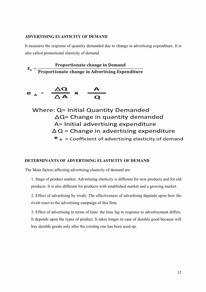
ADVERTISING ELASTICITY OF DEMAND

It measures the response of quantity demanded due to change in advertising expenditure. It is

also called promotional elasticity of demand.

DETERMINANTS OF ADVERTISING ELASTICITY OF DEMAND

The Main factors affecting advertising elasticity of demand are:

1. Stage of product market: Advertising elasticity is different for new products and for old

products. It is also different for products with established market and a growing market.

2. Effect of advertising by rivals: The effectiveness of advertising depends upon how the

rivals react to the advertising campaign of this firm.

3. Effect of advertising in terms of time: the time lag in response to advertisement differs.

It depends upon the types of product. It takes longer in case of durable good because will

buy durable goods only after the existing one has been used up.

17  

ELASTICITY OF PRICE EXPECTATIONS

• The concept of elasticity of price expectations was developed by J.R.Hicks.

• Elasticity of price expectations is defined as the ratio of the relative change in expected

future prices to the relative change in current price.

• It is symbolically

LAW OF SUPPLY

The relationship between price and quantity supplied is usually a positive relationship. A rise

in price is associated with a rise in quantity supplied.

Definitions

— In the words of Dooley. "The law of supply states that other things being equal the higher

the price, the greater the quantity supplied or the lower the price, the smaller the quantity

supplied.“

— According to Lipsey, "The law of supply states that other things being equal, the quantity

of any commodity that firms will produce and offer for sale is positively related to the

commodity's own price, rising when price rises and falling when price falls.“

As the price of good increases, suppliers will attempt to maximize profits by increasing the

quantity of the product sold.

18  

SUPPLLY SCHEDDULE

SUPPL

DETER

Innume

produce

1. Cost

Cost of

• pr

• re

• co

• pa

• tra

If cost o

LY CURVE

RMINANT

erable facto

e and sell a

of factor o

f production

rice of raw m

ents and inte

ost of machi

ayments to h

ansportation

of productio

E

TS OF SUP

ors and cir

good. Some

of productio

n depends on

materials

erest on cap

inery

human reso

n charges

on is high n

PPLY

rcumstances

e of the mor

on

n the factors

pital

ources (wag

ormally sup

s could aff

re common

s like

es and salar

pply will be

fect a selle

factors are

ries)

e low

er’s willing

:

gness or abbility to

19  

2. Statte of technoology

Use of

capacity

f latest tech

y which inc

hnology de

creases supp

ecreases the

ply of goods

e cost of p

s.

production and increases the prooduction

3. Factoors outsidee the econommic spheree

Supply

affect th

depends up

he supply d

pon the belo

irectly or in

ow said fact

ndirectly.

tors. These factors shouuld not arise if they ariise; they

• WWhether condditions

• Flloods

• WWars

• Eppidemics (uunexpected ssituations)

4. Tax and subsiddy

If tax su

that is

decreas

ubsidy (cha

not there p

se in supply

arge less tax

production

.

x) is given

cost raises.

by the gove

. Finally th

ernment the

he productio

e production

on will be

n cost decre

low and ef

eased. If

ffects to

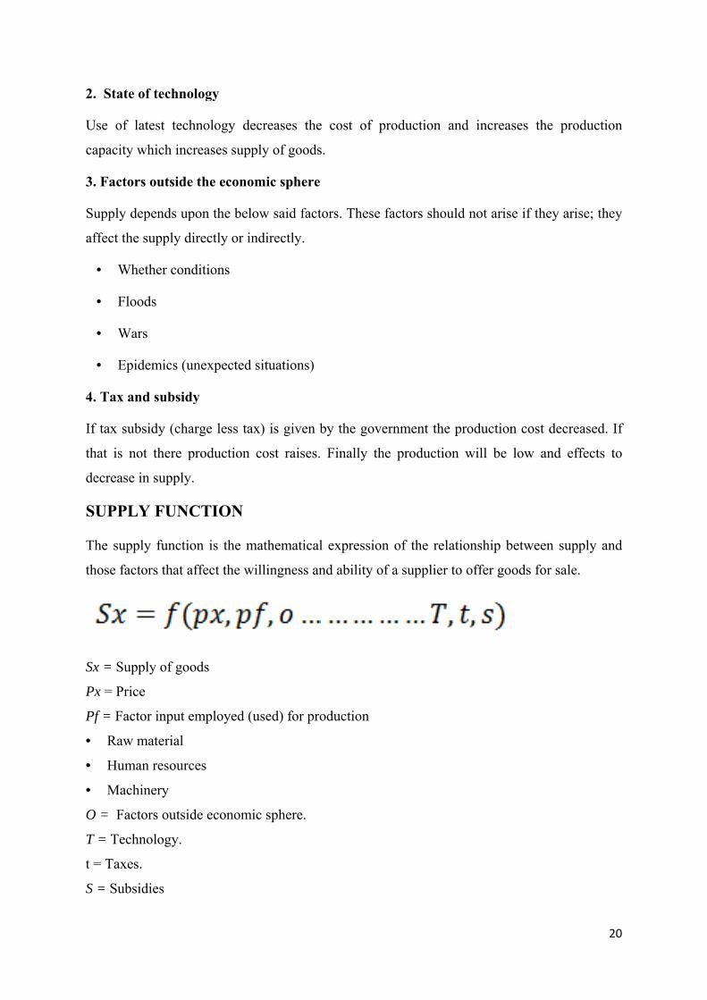
SUPPLLY FUNCCTION

The sup

those fa

pply functio

actors that a

on is the m

affect the wi

mathematical

illingness an

l expression

nd ability o

n of the rel

f a supplier

lationship b

r to offer go

between sup

ods for sale

pply and

e.

Sx = Suupply of gooods

Px = Prrice

Pf = Faactor input eemployed (uused) for production

• Raww material

• Humman resourcces

• Macchinery

O = Faactors outsidde economic sphere.

T = Tecchnology.

t = Taxees.

S = Subbsidies

20  

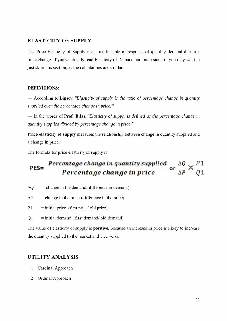
ELASSTICITY OF SUPPPLY

The Pri

price ch

just skim

ice Elasticit

hange. If yo

m this secti

ty of Suppl

ou've already

on, as the c

ly measures

y read Elast

alculations

s the rate o

ticity of De

are similar.

of response

emand and u

.

of quantity

understand i

y demand d

it, you may

due to a

y want to

DEFINNITIONS:

— Acc

supplied

ording to L

d over the p

Lipsey, "Ela

percentage c

asticity of s

change in p

supply is the

price.“

e ratio of ppercentage change in quantity

— In th

quantity

Price e

a chang

The for

∆Q

∆P

P1

Q1

The val

the quan

UTILI

1. Ca

2. O

he words of

y supplied d

f Prof. Bila

divided by p

as, "Elastici

percentage c

ity of supply

change in p

ly is defined

price."

d as the perrcentage chhange in

lasticity of

ge in price.

f supply meeasures the rrelationshipp between chhange in quuantity suppplied and

rmula for prrice elasticitty of supplyy is:

= change in the demannd.(differennce in demaand)

= change inn the price.((difference iin the price))

= initial priice. (first prrice/ old pricce)

= initial demmand. (firstt demand/ oold demand))

lue of elasti

ntity suppli

ITY ANA

ardinal App

rdinal Appr

icity of supp

ed to the m

ply is posit

arket and vi

ive, becaus

ice versa.

e an increasse in price iis likely to increase

ALYSIS

proach

roach

21  

CONCEPT OF UTILITY

UTILITY: Generally, Utility means “Usefulness”. In Economics, Utility is defined as the

power of a commodity or a service to satisfy the human wants.

TOTAL UTILITY: It refers to the sum of utilities of all units of a commodity consumed.

For example, if a person consumes ten apple, then the total utility is the sum of satisfaction of

consuming all the ten apple.

MARGINAL UTILITY: Marginal Utility is addition made to the total utility by consuming

one more unit of a commodity. Example: if a person consuming 10 apples, the marginal

utility is the utility derived from the 10th unit (or) last unit.

MUn=TUn-TUn-1

LAW OF DIMINISHING MARGINAL UTILITY

The law of diminishing marginal utility explains an ordinary experience of a consumer. “If a

consumer takes more and more units of a same commodity, the additional utility he derives

from an extra unit of the commodity goes on falling”.

H.H.Gossen contributed initially and Alfred Marshall refined these idea as a law. This is also

called as Gossen’s First Law

ASSUMPTIONS OF THE LAW

a) The law holds good only when the process of consumption continues without anytime

gap.

b) The consumer’s taste, habit or preference must remain the same during the process of

consumption.

c) The income of the consumer remains constant.

d) The prices of the commodity consumed and its substitutes are constant.

e) The consumer is assumed to be a rational economic man. As a rational consumer, he

wants to maximise the total utility.

f) Utility is measurable.

g) All the units of the commodity must be identical in all aspects like taste, quality,

colour and size.

22  

h) The units of consumption must be in standard units e.g., a cup of tea, a bottle of cool

drink etc.

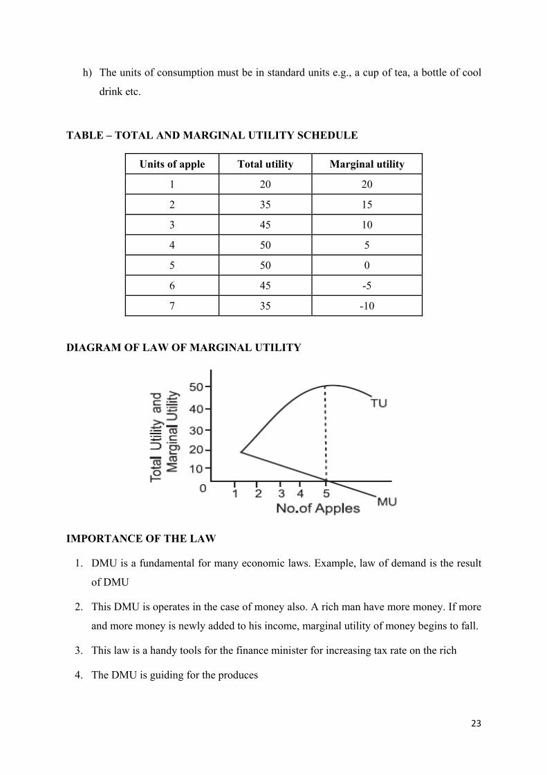
TABLE – TOTAL AND MARGINAL UTILITY SCHEDULE

Units of apple Total utility Marginal utility

1 20 20

2 35 15

3 45 10

4 50 5

5 50 0

6 45 -5

7 35 -10

DIAGRAM OF LAW OF MARGINAL UTILITY

IMPORTANCE OF THE LAW

1. U is a fundamental for many economic laws. Example, law of demand is the result

of DMU

DM

Th

ls for the finance minister for increasing tax rate on the rich

Th

2. is DMU is operates in the case of money also. A rich man have more money. If more

and more money is newly added to his income, marginal utility of money begins to fall.

3. This law is a handy too

4. e DMU is guiding for the produces

23  

LIM TION OF DMU ITA

1. Utility is a psychological experience and it cannot be measured

le commodity consumption mode

ut in real life it is not

itself is capable of varying from person to person.

he idea of equi-marginal principles was first mentioned by H.H. Gossen. Hence it is called

as law. The law of equi-marginal utility

explains the behavior of a consumer when he consumes more than one commodity. It

uses in such a way that it has the same marginal utility in all”.

a) The consumer is rational so he wants to get maximum satisfaction.

le.

g marginal utility.

2. This law based on sing

3. According to the law, a consumer should consume continuously. B

so.

4. The law assumes constancy of the marginal utility of money

5. A utility

LAW OF EQUI-MARGINAL UTILITY

T

as Gossen’s Second Law. Alfred Marshall made it

explains how the consumer spends his limited income on various commodities to get

maximum satisfaction. The law also called “law of substitution or law of maximum

satisfaction.

DEFINITION: “If a person has a thing which can be put to several uses, he will distribute it

among these

ASSUMPTIONS

b) The utility of each commodity is measurab

c) The marginal utility of money remains constant.

d) The income of the consumer is given.

e) The prices of the commodities are given.

f) The law is based on the law of diminishin

24  

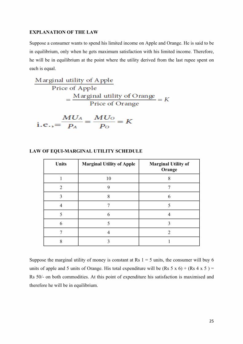
EXPLANATION OF THE LAW

uppose a consumer wants to spend his limited income on Apple and Orange. He is said to be

aximum satisfaction with his limited income. Therefore,

he will be in equilibrium at the point where the utility derived from the last rupee spent on

LAW OF EQUI-MARGINAL UTILITY SCHEDUL

Units Marginal Utility of Apple Marginal Utility of Orange

S

in equilibrium, only when he gets m

each is equal.

E

1 10 8

2 9 7

3 8 6

4 7 5

5 6 4

6 5 3

7 4 2

8 3 1

Suppose the ma tility of money is constant at Rs 1 = 5 units, th er will buy 6

nits of apple and 5 units of Orange. His total expenditure will be (Rs 5 x 6) + (Rs 4 x 5 ) =

Rs 50/- on both commodities. At this point of expenditure his satisfaction is maximised and

rginal u e consum

u

therefore he will be in equilibrium.

25  

LAW OF EQUI-MARGINAL UTILITY DIAGRAM

Taking the income of a consumer as given, let his marginal utility of money be constant at

M utils in this Fig. is equal to OM (the marginal utility of money) when OH

apple and OK of orange.

OF THE LAW

• Indivisibility of Goods: The theory is weakened by the fact that many commodities

divisible. In the case of indivisible goods, the law is not

applicable.

that the marginal utility of money is constant. But that is not really so.

O

amount of good apple is purchased; is equal to OM when OK quantity of good

orange is purchased. Therefore, the consumer will be in equilibrium when he buys OH of

LIMITATIONS

like a car, a house etc. are in

• The Marginal Utility of Money is Not Constant: The theory is based on the

assumption

• The Measurement of Utility is not Possible: Utility is a subjective concept, which

cannot be measured, in quantitative terms.

26  

CONSUMER’S SURPLUS

• The concept of consumer surplus was originally introduced by classical economists and

Jule Dupuit,

Marginal Utility.

pay a thing rather

an go without the thing, over that which he actually does pay is the economic measure of

this surplus satisfaction. This may be called consumer’s surplus”.

1. The utility can be measured.

l utilities of money of the consumer remain constant.

commodity.

n the other commodities.

other determinants of

consumer wants to buy an apple. He is willing to pay 4, but the actual price

2. Hence the consumer’s surplus is 2(4-2).

TU = Total Utility, P = Price and

tity of the commodity

later modified by Jevons and

• Refined form of the concept of consumer surplus was given by Alfred Marshall.

• This concept is based on the Law of Diminishing

DEFINITION: “the excess of price which a person would be willing to

th

ASSUMPTION

2. The margina

3. There are no substitutes for the

4. The taste, income and character of the consumer do not change.

5. Utility of one commodity does not depend upo

6. Demand for a commodity depends on its price alone; it excludes

demand

EXPLANATION

• Suppose a

of the apple is

• Therefore, Consumer’s surplus = Potential price – Actual price

Where,

Q= Quan

27  

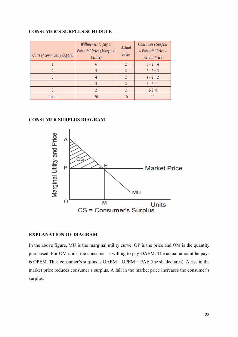
CONSUMER’S SURPLUS SCHEDULE

CONSUMER SURPLUS DIAGRAM

EXPLANATION OF DIAGRAM

the above figure, MU is the marginal utility curve. OP is the price and OM is the quantity

er is willing to pay OAEM. The actual amount he pays

is OPEM. Thus consumer’s surplus is OAEM – OPEM = PAE (the shaded area). A rise in the

In

purchased. For OM units, the consum

market price reduces consumer’s surplus. A fall in the market price increases the consumer’s

surplus.

28  

CRITICISM

1. Utility cannot be measured, because utility is subjective.

money does not remain constant.

er himself.

• English economists Prof. J.R. Hicks and Prof. R.G.D.Allen provided a refined version

rence very easily and say which is better than the other.

combinations of two

ncept of scale of preference has been explained by indifference curve. An

• His income remains constant

ain unchanged.

the concept “Diminishing Marginal Rate

ranked or compared or ordered by

2. Marginal utility of

3. Potential price is internal, it might be known to the consum

INDIFFERENCE CURVE ANALYSIS

of indifference curve approach.

• Utility cannot be measured. It can only be ranked or ordered.

• The consumer can rank his prefe

• Definition: “An indifference curve is the locus of different

commodities giving the same level of satisfaction”.

• The co

indifference curve shows different combinations of two commodities, which give the

consumer an equal satisfaction.

ASSUMPTIONS

• He purchases two goods only.

• His tastes, Preference , habits rem

• The Indifference Curve Approach is based on

of Substitution”.

• Utility cannot be cardinally measured, but can be

ordinal number such as I, II, III and so on.

29  

INDIFFFERENCEE CURVE SSCHEDULL

Let us

indiffer

INDIFF

assume tha

rence schedu

Com

A

B

C

D

E

FERENCE

at the consu

ule will be:

mbination

E MAP

umer buys

E

two commmodities - baananas and biscuits. TThen the

Biscu

1

2

3

4

5

uits Banana

12

8

5

3

2

a

30  

1. Indifference curves slope downwards to the right

2. Indifference curves are convex to the origin

3. No two indifference curves can ever cut each other.

CONSUMER EQUILIBRIUM

A consumer is in equilibrium when he obtains maximum satisfaction from his expenditure on

the commodities he wants to purchase. The main theme on the theory of consumer behavior

built is that a consumer attempts to allocate a limited money income among various

vailable goods and services so as to maximise his satisfaction or utility.

end on the two goods. It is assumed

that he will spend the amount on both the goods and not save any part of it.

n in the market and are assumed to be constant.

c) The consumer is assumed to act rationally and maximise his satisfaction.

e.

R BUDGET LINE

is

a

ASSUMPTION

a) The consumer has a fixed amount of money to sp

b) The prices of these goods are give

d) The consumer has before him an indifference map for a pair of goods say, tea and

biscuits. This map represents the preferences of the consumer for the two goods. It is

assumed that his scales of preferences remain constant at a given tim

PRICE LINE O

Suppose that the consumer has Rs.20 to spend on tea and biscuits, which cost 50 paise and 40

paise respectively. The consumer has three alternative possibilities before him.

He may decide to buy tea only, in which case he can buy 40 cups of tea.

He may decide to buy biscuits only, in which case he can buy 50 biscuits.

He may decide to buy some quantity of both the goods, say 20 cups of tea (Rs.10) and

25 biscuits (Rs.10) or 12 cups of tea (Rs.6) and 35 biscuits (Rs.14), and so on. (Total

amount = Rs.20).

31  

PRICEE LINE/BUUDGET LIN

DIAGR

Explan

The con

the indi

OY1 am

lesser s

income

RAM OF C

nation

nsumer gets

ifference cu

mount of bi

satisfaction

of the cons

CONSUME

s the maxim

urve I3. At

iscuits. Any

or will not

sumer.

NE

ER EQUILI

mum possib

this point,

y other poss

t be unobta

IBRIUM

ble satisfact

he buys a

sible combi

ainable at p

tion from hiis given inccome at poiint C on

combinatioon of OX1 amount off tea and

ination of thhe two gooods will eithher yield

present pricces, with thhe given ammount of

32  

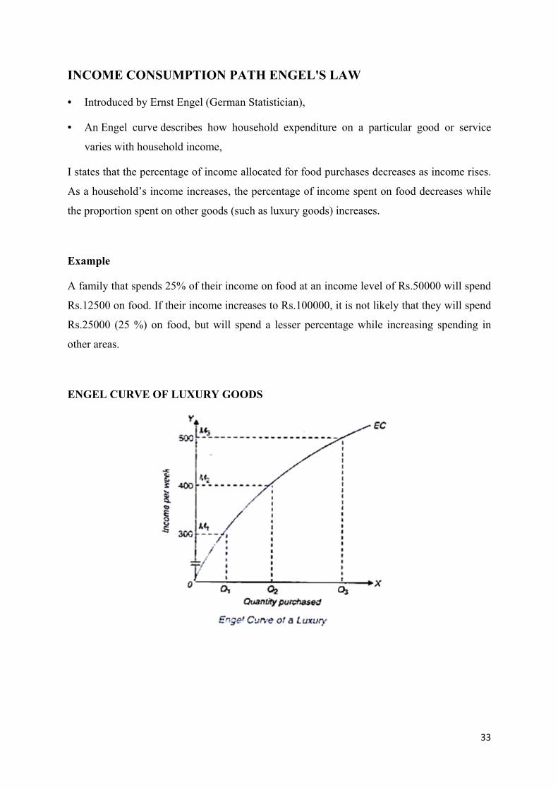
INCOME CONSUMPTION PATH ENGEL'S LAW

• Introduced by Ernst Engel (German Statistician),

• An Engel curve describes how household expenditure on a particular good or service

varies with household income,

I states that the percentage of income allocated for food purchases decreases as income rises.

As a household’s income increases, the percentage of income spent on food decreases while

the proportion spent on other goods (such as luxury goods) increases.

ENGEL CURVE OF LUXURY GOODS

Example

A family that spends 25% of their income on food at an income level of Rs.50000 will spend

Rs.12500 on food. If their income increases to Rs.100000, it is not likely that they will spend

Rs.25000 (25 %) on food, but will spend a lesser percentage while increasing spending in

other areas.

33  

34  

D

******

ENGEL CURVE OF AN INFERIOR GOO

1

SCHOOL OF LAW

UNIT 3 - MICRO ECONOMICS– SBA1103

2

SYLLABUS – UNIT - III

THEORY OF PRODUCTION, COST AND REVENUE

Production: Firm as an Agent of Production – Concept of Production Function – Law of Variable

Proportions – Isoquants – Returns to Scale – Economies & Diseconomies of Scale – cost &

Revenue: costs in the short Run – costs in the long run – Profit Maximization and cost

minimization – Equilibrium of the Firm – Technological Change – concept of Revenue: Total,

Average and Marginal Revenue.

PRODUCTION

Production in Economics refers to the creation of those goods and services which have exchange

value. It means the creation of utilities. These utilities are in the nature of form utility, time

utility and place utility. Creation of such utilities results in the overall increase in the production

and redistribution of goods and services in the economy. Utility of a commodity may increase

due to several reasons.

FACTORS OF PRODUCTION

Human activity can be broken down into two components, production and consumption. When

there is production, a process of transformation takes place. Inputs are converted into an output.

The inputs are classified and referred to as land, labour, and capital. Collectively the inputs are

called factors of production.

1. Land

Land as a factor of production refers to all those natural resources or gifts of nature which are

provided free to man. It includes within itself several things such as land surface, air, water,

minerals, forests, rivers, lakes, seas, mountains, climate and weather. Thus, ‘Land’ includes all

things that are not made by man.

3

Characteristics or Peculiarities of land

(i) Land is a free gift of nature

(ii) Land is fixed (inelastic) in supply.

(iii) Land is imperishable

(iv) Land is immobile

(v) Land differs in fertility and situation

(vi) Land is a passive factor of production

As a gift of nature, the initial supply price of land is zero. However, when used in production, it

becomes scarce. Therefore, it fetches a price, accordingly.

2. Labour

Labour is the human input into the production process. Alferd Marshall defines labour as ‘the use

or exertion of body or mind, partly or wholly, with a view to secure an income apart from the

pleasure derived from the work’.

Characteristics or Peculiarities of labour

(i) Labour is perishable.

(ii) Labour is an active factor of production. Neither land nor capital can yield much without

labour.

(iii) Labour is not homogeneous. Skill and dexterity vary from person to person.

(iv) Labour cannot be separated from the labourer.

(v) Labour is mobile. Man moves from one place to another from a low paid occupation to a

high paid occupation.

(vi) Individual labour has only limited bargaining power. He cannot fight with his employer for

a rise in wages or improvement in work- place conditions. However, when workers combine

to form trade unions, the bargaining power of labour increases.

4

3. Capital

Capital is the man made physical goods used to produce other goods and services. In the

ordinary language, capital means money. In Economics, capital refers to that part of man-made

wealth which is used for the further production of wealth. According to Marshall, “Capital

consists of those kinds of wealth other than free gifts of nature, which yield income”.

Forms of Capital/Livelihood Capitals

A. Physical Capital or Material Resources

B. Financial Capital or Monetary Resources, and

C. Human Capital or Human Resources

D. Natural Capital

E. Social Capital

4. Organization or Enterprise

An entrepreneur is a person who combines the different factors of production (land, labour and

capital), in the right proportion and initiates the process of production and also bears the risk

involved in it. The entrepreneur is also called ‘organiser’. Entrepreneurship is risk taking,

managerial, and organizational skills needed to produce goods and services in order to gain a

profit. In modern times, an entrepreneur is called ‘the changing agent of the society’. He is not

only responsible for producing the socially desirable output but also to increase the social

welfare.

Functions of an Entrepreneur

1. Identifying Profitable Investible Opportunities: Conceiving a new and most promising

and profitable idea or capturing a new idea available in the market is the foremost

function of an entrepreneur. This is known as identifying profitable investible

opportunities.

2. Deciding the size of unit of production: An entrepreneur has to decide the size of the unit

– whether big or small depending upon the nature of the product and the level of

competition in the market.

5

3. Deciding the location of the production unit: A rational entrepreneur will always locate

his unit of production nearer to both factor market and the end-use market. This is to be

done in order to bring down the delay in production and distribution of products and to

reduce the storage and transportation cost.

4. Identifying the optimum combination of factors of production: The entrepreneur, after

having decided to start a new venture, takes up the task of hiring factors of production.

Further, he decides in what combinations he should combine these factors so that

maximum output is produced at minimum cost.

5. Making innovations: According to Schumpeter, basically an entrepreneur is an innovator

of new markets and new techniques of production. A new market increases the sales

volume whereas a new cost cutting production technique will make the product cheaper.

This will in turn increase the volume of sales and the profit.

6. Deciding the reward payment: The factors used in production have to be rewarded on

the basis of their productivity. Measuring the productivity of the factors and the payment

of reward is the crucial function of an entrepreneur.

7. Taking Risks and facing uncertainties: According to Hawley, a business is nothing but a

bundle of risks. Products are produced for future demand. The future is uncertain. The

investments are made in the present. This is the serious risk in production. One who is

ready to accept the risk becomes a successful entrepreneur. A prudent entrepreneur

forecasts the future risks scientifically and take appropriate decision in the present to

overcome such risks. According to Knight one of the important functions of entrepreneur

is uncertainty bearing.

PRODUCTION FUNCTION

The functional relationship between inputs and outputs is known as production function. Inputs

refer to the factor services which are used in production i.e. land, labour, capital and enterprise.

Output refers to the volume of goods produced.

Q = f (x1, x2, x 3….xn ) in which

6

Q is the quantity produced during a given period of time and x1, x2, x3 ….xn are the quantities

of different factors used in production i.e. Land, Labour, Capital, raw material etc...,

RELATIONSHIP BETWEEN MARGINAL PRODUCT AND TOTAL PRODUCT

(i) When marginal product is positive, the total product increases

a. When marginal product increases, the total product will be increasing at an increasing rate

b. When marginal product remains constant, the total product will be increasing at a constant

rate

c. When marginal product decreases but is positive, the total product will be increasing at a

decreasing rate

(ii) When marginal product is zero, the total product reaches the maximum and remains constant

(iii) When marginal product is negative, the total product decreases.

Types of Production function

Production function may be classified into two:

1. Short-run production function: It refers to production in the short-run where there are some

fixed factors and variable factors. In the short-run, production will increase when more units of

variable factors are used with the fixed factor. Law of variable proportion comes under Short-

run production.

2. Long-run production function: It refers to production in the long-run where all factors

become variable. In the long-run, production can be increased by increasing units of all the

factors simultaneously and in the same proportion. Laws of returns to scale comes under long-

run production function.

7

LAW OF VARIABLE PROPORTION

The law of variable proportions states that as the quantity of one factor is increased, keeping the

other factors fixed, after a point, first the marginal and then the average product of that factor

will diminish. This law is also known as the “law of non-proportional returns” or “law of the

diminishing marginal returns”.

Assumptions of the law

1. Only one factor is variable and other factors are fixed

2. The variable factor units are homogenous

3. Input prices remain unchanged

4. The technology remains the same at a given point of time.

5. The entire operation is only for short-run

Stages of Law

Stage I: Stage of increasing returns

End of Stage I where the average product reaches its maximum point. During this stage, the

total product, the average product and the marginal product are increasing. It is notable that

the marginal product in this stage increases but in a later part it starts declining. Though

marginal product starts declining, it is greater than the average product so that the average

product continues to rise.

Stage II: Stage of decreasing returns

Stage II ends at the point where the marginal product is zero. In the second stage, the total

product continues to increase but at a diminishing rate. The marginal product and the average

product are declining but are positive. At the end of the second stage, the total product is

maximum and the marginal product is zero.

Stage III: Stage of negative returns

In this stage the marginal product becomes negative. The total product and the average

product are declining.

8

Table - Stages of Law of Variable Proportion

Fixed factor

Machine

Variable

factor labour

Total

product

in units

Average

product in

units

Marginal

product in

units

Stages

1+ 1 10 10 10

Increasing Return

1+ 2 22 11 12

1+ 3 36 12 14

1+ 4 52 13 16

1+ 5 66 13.2 14

1+ 6 76 12.6 10

Decreasing Return 1+ 7 80 11.4 4

1+ 8 82 10.2 2

1+ 9 82 9.1 0

1+ 10 78 7.8 -4 Negative Return

Diagram of Law of Variable Proportion

9

The stage of Operation

In stage I the fixed factor is too much in relation to the variable factor. Therefore in stage I,

marginal product of the fixed factor is negative. On the other hand, in stage III the marginal

product of the variable factor is negative. Therefore a rational producer will not choose to

produce in stages I and III. He will choose only the second stage to produce where the marginal

product of both the fixed factor and variable factor are positive. At this stage the total product is

maximum. The particular point at which the producer will decide to produce in this stage

depends upon the prices of factors. The stage II represents the range of rational production

decisions.

LAWS OF RETURNS TO SCALE

The term ‘returns to scale’ refers to the response of total output to changes in all inputs by the

same proportion. The laws of ‘returns to scale’ refers to the effects of scale relationship. The law

of returns to scale states that when all factors of production are increased in the same proportion,

the output will increase but the increase may be at increasing rate or constant rate or decreasing

rate. The ratio of the proportionate change in output to a proportionate change in all inputs is

called the function coefficient.

Assumption of the law

1. All the factors of production (such as land, labour and capital) are variable but

organization is fixed

2. There is no change in technology

3. There is perfect competition in the market

4. Outputs or returns are measured in physical quantities

5. The entire operation is only for long-run

10

Three phases of Returns to Scale

Phase I: Increasing returns to scale:

It occurs when the increase in output is more than proportional to increase in inputs. The first

stage starts from the point of origin and continues till the average product is maximum.

For example, if all the inputs are increased by 5%, the output increases by more than 5% i.e. by

10%. In this case the marginal product will be rising.

Phase II: Constant returns to scale:

It occurs when the increase in output is proportional to increase in inputs. If we increase all the

factors (i.e. scale) in a given proportion, the output will increase in the same proportion i.e. a 5%

increase in all the factors will result in an equal proportion of 5% increase in the output. Here the

marginal product is constant.

Phase III: Decreasing returns to scale:

It occurs when the increase in output is less than proportional to the increase in inputs.

For example: if all the factors are increased by 5%, the output will increase by less than 5% i.e.

by 3%. In this phase marginal product will be decreasing.

Three Stages of Returns to Scale

Scale of inputs Total

Product

Marginal

Product

Stages

1 Labour + 1 Capital 4 4

Stage I : Increasing Returns 2 Labour + 2 Capital 10 6

3 Labour + 3 Capital 18 8

4 Labour + 4 Capital 28 10

5 Labour + 5 Capital 38 10 Stage II : Constant Returns

6 Labour + 6 Capital 48 10

7 Labour + 7 Capital 56 8 Stage III : Decreasing Returns

8 Labour + 8 Capital 62 6

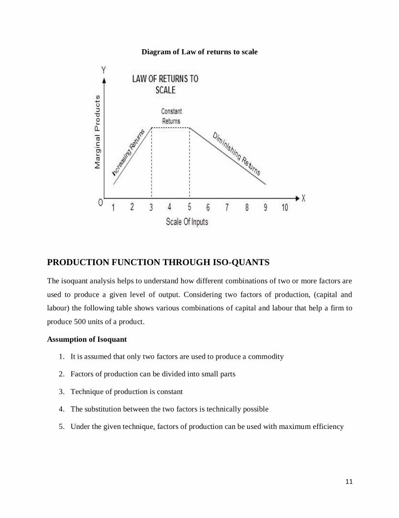
11

Diagram of Law of returns to scale

PRODUCTION FUNCTION THROUGH ISO-QUANTS

The isoquant analysis helps to understand how different combinations of two or more factors are

used to produce a given level of output. Considering two factors of production, (capital and

labour) the following table shows various combinations of capital and labour that help a firm to

produce 500 units of a product.

Assumption of Isoquant

1. It is assumed that only two factors are used to produce a commodity

2. Factors of production can be divided into small parts

3. Technique of production is constant

4. The substitution between the two factors is technically possible

5. Under the given technique, factors of production can be used with maximum efficiency

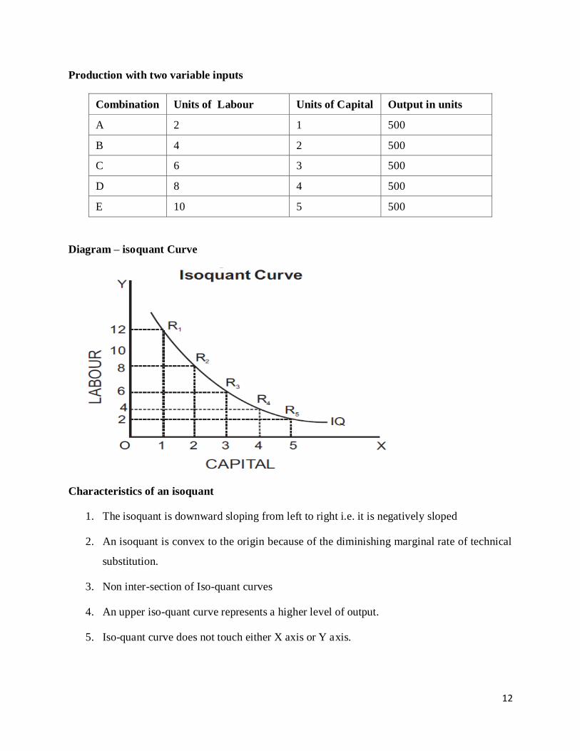
12

Production with two variable inputs

Combination Units of Labour Units of Capital Output in units

A 2 1 500

B 4 2 500

C 6 3 500

D 8 4 500

E 10 5 500

Diagram – isoquant Curve

Characteristics of an isoquant

1. The isoquant is downward sloping from left to right i.e. it is negatively sloped

2. An isoquant is convex to the origin because of the diminishing marginal rate of technical

substitution.

3. Non inter-section of Iso-quant curves

4. An upper iso-quant curve represents a higher level of output.

5. Iso-quant curve does not touch either X axis or Y axis.

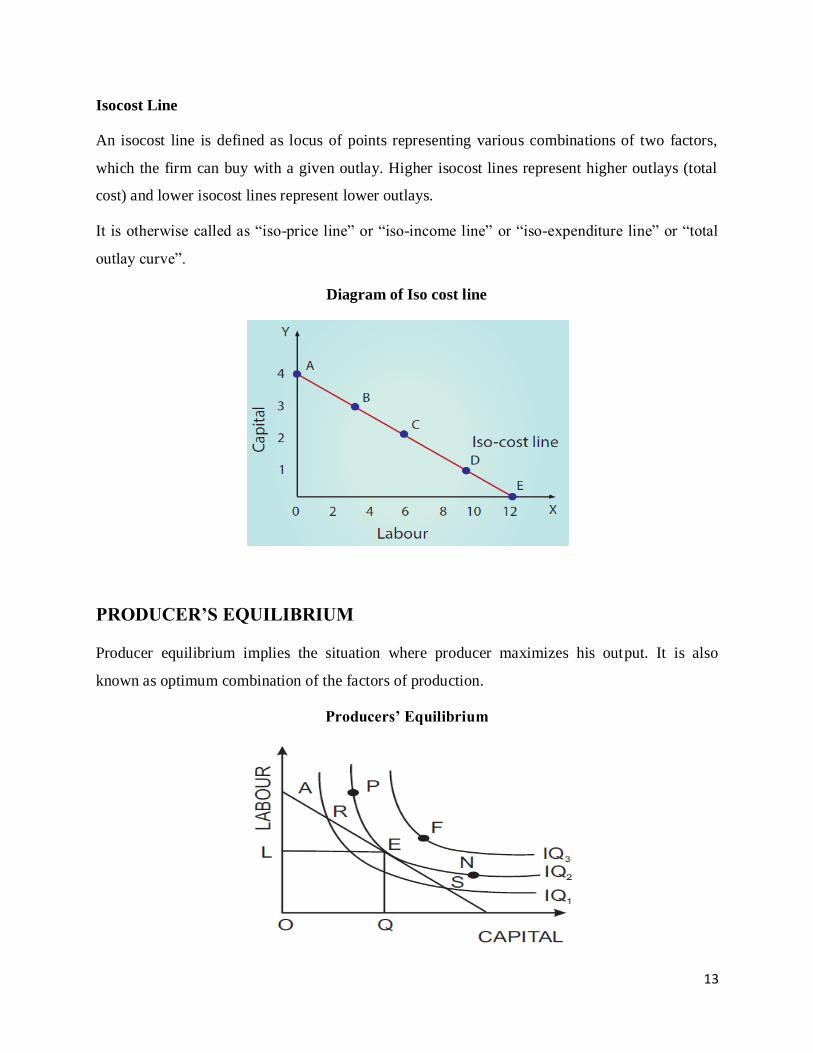
13

Isocost Line

An isocost line is defined as locus of points representing various combinations of two factors,

which the firm can buy with a given outlay. Higher isocost lines represent higher outlays (total

cost) and lower isocost lines represent lower outlays.

It is otherwise called as “iso-price line” or “iso-income line” or “iso-expenditure line” or “total

outlay curve”.

Diagram of Iso cost line

PRODUCER’S EQUILIBRIUM

Producer equilibrium implies the situation where producer maximizes his output. It is also

known as optimum combination of the factors of production.

Producers’ Equilibrium

14

In the above figure, E is the point of equilibrium, where isoquant IQ2 is tangential to isocost line

at AB. Given budget line AB, points ‘P’, ‘N’ and ‘F’ are beyond the reach of the producer and

points ‘R’ and ‘S’ on isoquant IQ1 give less output than the output at the point of equilibrium ‘E’

which is on IQ2 . The amount spent on combinations R, E, S is the same as all the three points lie

on the same isocost line. But the output produced at point E is higher as E lies on a higher

isoquant.

COBB-DOUGLAS PRODUCTION FUNCTION

The simplest and the most widely used production function in economics is the Cobb-Douglas

production function. It is a statistical production function given by professors C.W. Cobb and

P.H. Douglas.

The Cobb-Douglas production function can be stated as follows

Q = bL a C 1-a in which

Q = Actual output

L = Labour

C = Capital

b = number of units of Labour

a = Exponent∗ of labour

1-a = Exponent∗ of Capital

According to this production function, if both factors of production (labour and capital) are

increased by one percent, the output (total product) will increase by the sum of the exponents of

labour and capital i.e. by (a+1-a). Since a+1-a =1, according to the equation, when the inputs are

increased by one percent, the output also increases by one percent. Thus the Cobb Douglas

production function explains only constant returns to scale. In this production function, the sum

of the exponents shows the degree of “returns to scale” in production function.

a + b >1 : Increasing returns to scale

a + b =1 : Constant returns to scale

a + b <1 : Decreasing returns to scale

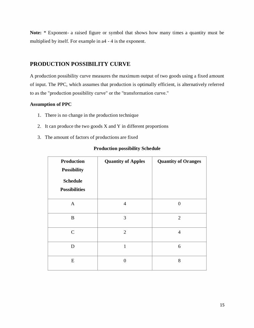
15

Note: * Exponent- a raised figure or symbol that shows how many times a quantity must be

multiplied by itself. For example in a4 - 4 is the exponent.

PRODUCTION POSSIBILITY CURVE

A production possibility curve measures the maximum output of two goods using a fixed amount

of input. The PPC, which assumes that production is optimally efficient, is alternatively referred

to as the "production possibility curve" or the "transformation curve."

Assumption of PPC

1. There is no change in the production technique

2. It can produce the two goods X and Y in different proportions

3. The amount of factors of productions are fixed

Production possibility Schedule

Production

Possibility

Schedule

Possibilities

Quantity of Apples Quantity of Oranges

A 4 0

B 3 2

C 2 4

D 1 6

E 0 8

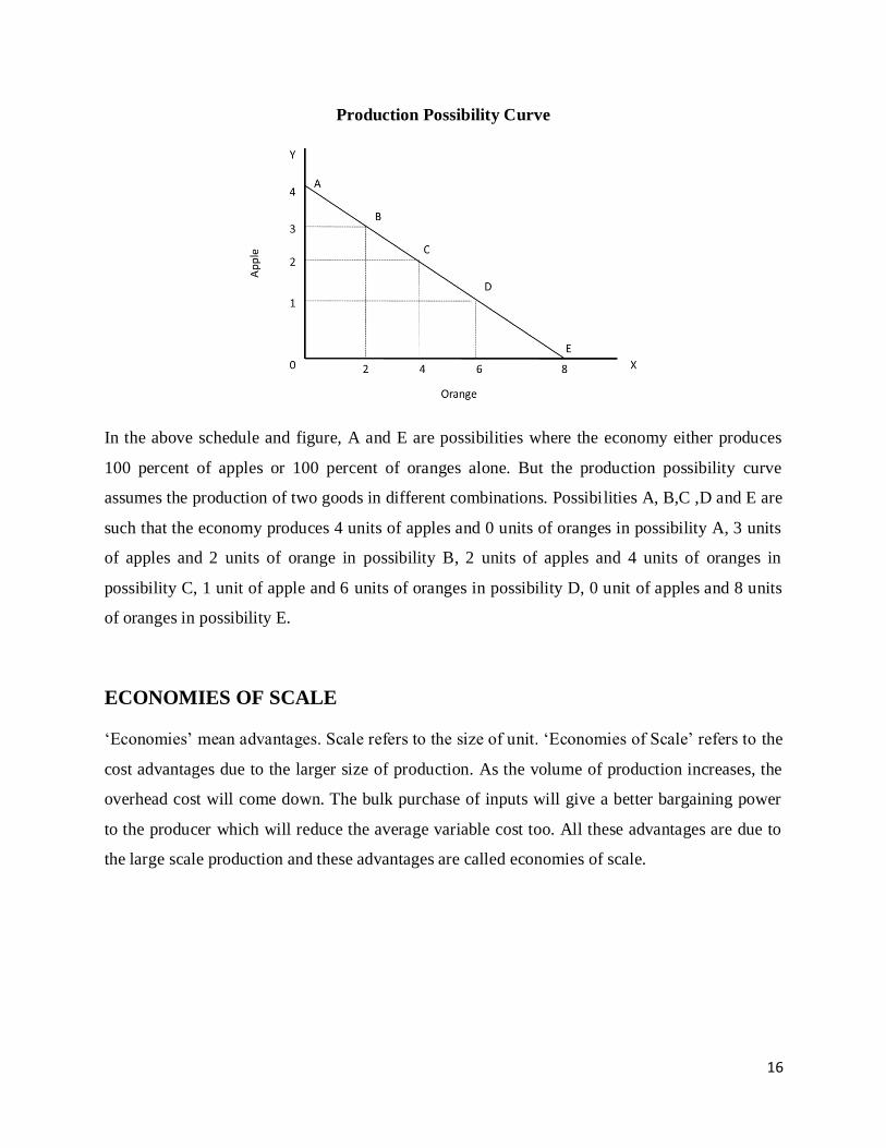
16

Production Possibility Curve

In the above schedule and figure, A and E are possibilities where the economy either produces

100 percent of apples or 100 percent of oranges alone. But the production possibility curve

assumes the production of two goods in different combinations. Possibilities A, B,C ,D and E are

such that the economy produces 4 units of apples and 0 units of oranges in possibility A, 3 units

of apples and 2 units of orange in possibility B, 2 units of apples and 4 units of oranges in

possibility C, 1 unit of apple and 6 units of oranges in possibility D, 0 unit of apples and 8 units

of oranges in possibility E.

ECONOMIES OF SCALE

‘Economies’ mean advantages. Scale refers to the size of unit. ‘Economies of Scale’ refers to the

cost advantages due to the larger size of production. As the volume of production increases, the

overhead cost will come down. The bulk purchase of inputs will give a better bargaining power

to the producer which will reduce the average variable cost too. All these advantages are due to

the large scale production and these advantages are called economies of scale.

17

TYPES OF ECONOMIES OF SCALE

1. Internal Economies of Scale:

‘Internal economies of scale’ are the advantages enjoyed within the production unit. These

economies are enjoyed by a single firm independently of the action of the other firms. For

instance, one firm may enjoy the advantage of good management; another may have the

advantage of more up-to-date machinery.

Kinds of internal economies

1. Technical Economies: As the size of the firm is large, the availability of capital is

more. Due to this, a firm can introduce up- to-date technologies; thereby the increase in

the productivity becomes possible. It is also possible to conduct research and development

which will help to increase the quality of the product.

2. Financial Economies: It is possible for big firms to float shares in the market for

capital formation. Small firms have to borrow capital whereas large firms can buy capital.

3. Managerial Economies: Division of labour is the result of large scale production. Right

person can be employed in the right department only if there is division of labour. This

will help a manager to fix responsibility to each department and thereby the productivity

can be increased and the total production can be maximized.

4. Labour Economies: Large Scale production paves the way for division of labour. This

is also known as specialization of labour. The specialization will increase the quality and

ability of the labour. As a result, the productivity of the firm increases.

5. Marketing Economies: In production, the first buyer is the producer who buys the raw

materials. As the size is large, the quantity bought is larger. This gives the producer a

better bargaining power. Also he can enjoy credit facilities. All these are possible because

of large scale production. Buying is the first function in marketing.

6. Economies of survival: A large firm can have many products. Even if one product fails

in the market, the loss incurred in that product can be managed by the profit earned from

the other products.

18

2. External economies of scale:

When many firms expand in a particular area – i.e., when the industry grows – they enjoy a

number of advantages which are known as external economies of scale. This is not the advantage

enjoyed by a single firm but by all the firms in the industry due to the structural growth. They are

a) Increased transport facilities

b) Banking facilities

c) Development of townships

d) Information and communication development

All these facilities are available to all firms in an industrial region.

DISECONOMIES OF SCALE

The diseconomies of the scale are a disadvantage to a firm or an industry or an organization. This

necessarily increases the cost of production of a commodity or service. Further it delays the

speed of the supply of the product to the market.

These diseconomies are of two types:

a) Internal Diseconomies of Scale: and

b) External Diseconomies of Scale

a. Internal Diseconomies of Scale: If a firm continues to grow and expand beyond the optimum

capacity, the economies of scale disappear and diseconomies will start operating. For instance, if

the size of a firm increases, after a point the difficulty of management arises to that particular

firm which will increase the average cost of production of that firm. This is known as internal

diseconomies of scale.

b. External Diseconomies of Scale: The term “External diseconomies of scale” refers to the

threat or disturbance to a firm or an industry from factor lying outside it. For example a bus

strike prevents the easy and correct entry of the workers into a firm. Similarly the rent of a firm

increases very much if new economic units are established in the locality.

19

COST ANALYSIS

Cost refers to the total expenses incurred in the production of a commodity. The functional

relationship between cost and output is expressed as ‘Cost Function’.

A Cost Function may be written as

C = f (Q)

where, C=Cost and Q=Quantity of output.

The determinants of cost of production are: the size of plant, the level of production, the nature

of technology used, the quantity of inputs used, managerial and labour efficiency.

Cost Concepts and Classification

1. Money Cost

2. Real Cost

3. Explicit Cost

4. Implicit Cost

5. Economic Cost

6. Social Cost

7. Opportunity Cost

8. Sunk Cost

9. Floating Cost

10. Prime Cost

11. Fixed Cost

12. Variable Cost

20

1. Money Cost : Money cost or nominal cost is the total money expenses incurred by a firm in

producing a commodity. It includes: cost of raw materials, payment of wages and salaries,

payment of rent, interest on capital, expenses on fuel and power, expenses on transportation

and so on.

2. Real Cost : Real cost is a subjective concept. Real cost refers to the payment made to

compensate the efforts and sacrifices of all factor owners for their services in production. It

includes the efforts and sacrifices of landlords in the use of land, capitalists to save and invest,

and workers in foregoing leisure.

3. Explicit Cost : Explicit costs are the payments made by the entrepreneur to the suppliers of

various productive factors. Explicit cost includes, wages, payment for raw material, rent for

the building, interest for capital invested, expenditure on transport and advertisement, other

expenses like license fee, depreciation and insurance charges, etc. It is also called Accounting

Cost or Out of Pocket Cost or Money Cost.

4. Implicit Cost : The money rewards for the own services of the entrepreneur and the factors

owned by himself and employed in production are known as implicit costs or imputed Costs.

5. Economic Cost: It refers to all payments made to the resources owned and purchased or hired

by the firm in order to ensure their regular supply to the process of production.

Economic Cost = Implicit Cost + Explicit Cost

6. Social Cost: It refers to the total cost borne by the society due to the production of a

commodity. Social Cost is the cost that is not borne by the firm, but incurred by others in the

society. For example, large business firms cause air pollution, water pollution and other

damages in a particular area which involve cost to the society. It is also called as External

Cost.

7. Opportunity Cost : It refers to the cost of next best alternative use. In other words, it is the

value of the next best alternative foregone. For example, a farmer can cultivate both paddy

and sugarcane in a farm land. If he cultivates paddy, the opportunity cost of paddy output is

the amount of sugarcane output given up. Opportunity Cost is also called as ‘Alternative Cost’

or ‘Transfer Cost’.

21

8. Sunk Cost : A cost incurred in the past and cannot be recovered in future is called as Sunk

Cost. Sunk cost are unalterable, unrecoverable, and if once invested it should be treated as

drowned. For example, if a firm purchases a specialized equipment designed for a special

plant, the expenditure on this equipment is a sunk cost, because it has no alternative use Sunk

cost is also called as ‘Retrospective Cost’.

9. Floating Cost: It refers to all expenses that are directly associated with business activities but

not with asset creation. It does not include the purchase of raw material as it is part of current

assets. It includes payments like wages to workers, transportation charges, fee for power and

administration. Floating cost is necessary to run the day-to-day business of a firm.

10. Prime Cost: All costs that vary with output, together with the cost of administration are

known as Prime Cost. In short, Prime cost = Variable costs + Costs of Administration.

11. Fixed Cost : Fixed Cost does not change with the change in the quantity of output. In other

words, expenses on fixed factors are called as fixed cost. For example, rent of the factory,

watchman’s wages, permanent worker’s salary, payments for minimum equipments and

machines insurance premium, deposit for power, license fee, etc fixed cost is also called as

‘Supplementary Cost’ or ‘Overhead Cost’.

12. Variable Cost : These costs vary with the level of output. In other words, the costs incurred

on variable factors are called variable costs. Examples of variable costs are: wages of

temporary workers, cost of raw materials, fuel cost, electricity charges, etc. Variable cost is

also called as Prime Cost, Special Cost, or Direct Cost.

SHORT-RUN AND LONG-RUN COST CURVES

Short-run is defined as that period of time in which the firm can expand or contract its output

only by varying the amounts of variables factors such as labour and raw materials. In the short

period the size of the plant cannot be altered. More production is possible only by over working

the existing plant or by hiring more workers and by purchasing and using more raw materials.

22

Long-run is defined as that period of time in which both fixed and variable factors are variable

and both the factors can be adjusted. Over a long period of time, the firm can expand its output

by enlarging the size of the existing plant or by building a new plant of a greater productive

capacity.

TOTAL COST

Total cost is the sum of total fixed cost and total variable cost.

TC = TFC + TVC

where

TC = Total cost

TFC = Total Fixed cost

TVC = Total variable cost

The relationship between total fixed cost, total variable cost and total cost will be clear from

following the Figure;

23

Average Fixed Cost (AFC)

The average fixed cost is the fixed cost per unit of output. It is obtained by dividing the total

fixed cost by the number of units of the commodity produced.

AFC = TFC / Q

Where AFC = Average fixed Cost

TFC = Total Fixed cost

Q = number of units of output produced

Example:

Suppose for a firm the total fixed cost is Rs 5000 when output is 100 units, AFC will be Rs

5000/100 = Rs 50

Average Variable cost (AVC):

Average variable cost is the variable cost per unit of output. It is the total variable cost divided

by the number of units of output produced.

AVC = TVC / Q

Where AVC = Average Variable Cost

TVC = Total Variable Cost

Q = number of units of output produced

Diagrammatially, the AVC is ‘U’ shaped. The law of variable proportions provides the

fundamental explanation for the shape of this curve. It means that the AVC curve first falls,

reaches a minimum and then begins to increase.

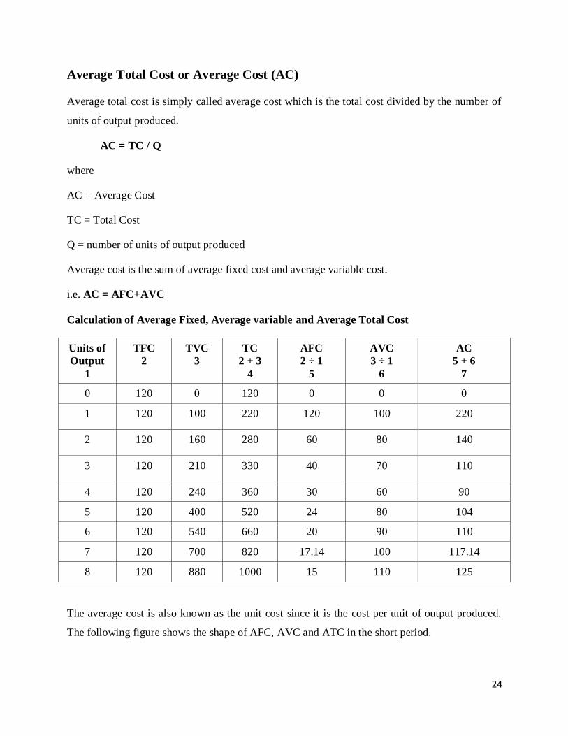
24

Average Total Cost or Average Cost (AC)

Average total cost is simply called average cost which is the total cost divided by the number of

units of output produced.

AC = TC / Q

where

AC = Average Cost

TC = Total Cost

Q = number of units of output produced

Average cost is the sum of average fixed cost and average variable cost.

i.e. AC = AFC+AVC

Calculation of Average Fixed, Average variable and Average Total Cost

Units of

Output

1

TFC

2

TVC

3

TC

2 + 3

4

AFC

2 ÷ 1

5

AVC

3 ÷ 1

6

AC

5 + 6

7

0 120 0 120 0 0 0

1 120 100 220 120 100 220

2 120 160 280 60 80 140

3 120 210 330 40 70 110

4 120 240 360 30 60 90

5 120 400 520 24 80 104

6 120 540 660 20 90 110

7 120 700 820 17.14 100 117.14

8 120 880 1000 15 110 125

The average cost is also known as the unit cost since it is the cost per unit of output produced.

The following figure shows the shape of AFC, AVC and ATC in the short period.

25

From the above figure, it can be understood that the behavior of the average total cost curve

depends on the behaviour of AFC and AVC curves. In the beginning, both AFC and AVC fall.

So ATC curve falls. When AVC curve begins rising, AFC curve falls steeply i.e, fall in AFC is

more than the rise in AVC. So ATC curve continues to fall. But as output increases further, there

is a sharp increase in AVC, which is more than the fall in AFC. Hence ATC curve rises after a

point. The ATC curve like AVC curve falls first, reaches the minimum value and then rises.

Hence it has taken a U shape.

Marginal cost (MC)

It is the cost of the last single unit produced. It is defined as the change in total costs resulting

from producing one extra unit of output. In other words, it is the addition made to the total cost

by producing one extra unit of output. Marginal cost is important for deciding whether any

additional output can be produced or not.

MC = ΔTC / ΔQ

where

MC = Marginal Cost,

ΔTC = change in total cost and

ΔQ = change in total quantity.

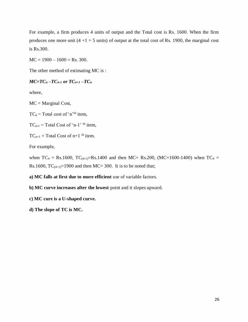
26

For example, a firm produces 4 units of output and the Total cost is Rs. 1600. When the firm

produces one more unit (4 +1 = 5 units) of output at the total cost of Rs. 1900, the marginal cost

is Rs.300.

MC = 1900 – 1600 = Rs. 300.

The other method of estimating MC is :

MC=TCn –TCn-1 or TCn+1 –TCn

where,

MC = Marginal Cost,

TCn = Total cost of ‘n’th item,

TCn-1 = Total Cost of ‘n-1’ th item,

TCn+1 = Total Cost of n+1 th item.

For example,

when TC4 = Rs.1600, TC(4-1)=Rs.1400 and then MC= Rs.200, (MC=1600-1400) when TC4 =

Rs.1600, TC(4+1)=1900 and then MC= 300. It is to be noted that;

a) MC falls at first due to more efficient use of variable factors.

b) MC curve increases after the lowest point and it slopes upward.

c) MC cure is a U-shaped curve.

d) The slope of TC is MC.

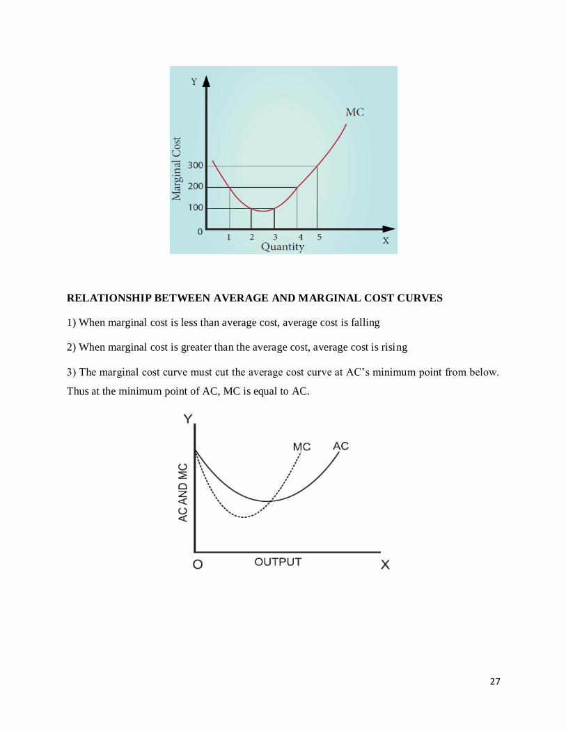
27

RELATIONSHIP BETWEEN AVERAGE AND MARGINAL COST CURVES

1) When marginal cost is less than average cost, average cost is falling

2) When marginal cost is greater than the average cost, average cost is rising

3) The marginal cost curve must cut the average cost curve at AC’s minimum point from below.

Thus at the minimum point of AC, MC is equal to AC.

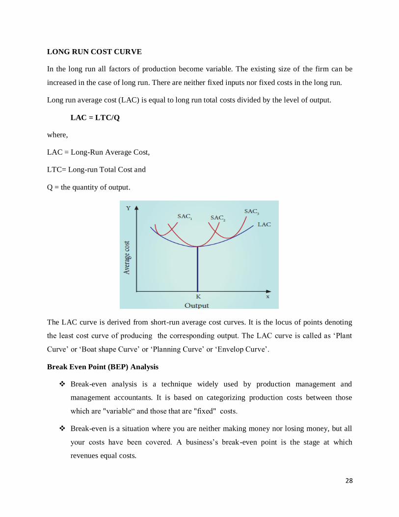
28

LONG RUN COST CURVE

In the long run all factors of production become variable. The existing size of the firm can be

increased in the case of long run. There are neither fixed inputs nor fixed costs in the long run.

Long run average cost (LAC) is equal to long run total costs divided by the level of output.

LAC = LTC/Q

where,

LAC = Long-Run Average Cost,

LTC= Long-run Total Cost and

Q = the quantity of output.

The LAC curve is derived from short-run average cost curves. It is the locus of points denoting

the least cost curve of producing the corresponding output. The LAC curve is called as ‘Plant

Curve’ or ‘Boat shape Curve’ or ‘Planning Curve’ or ‘Envelop Curve’.

Break Even Point (BEP) Analysis

Break-even analysis is a technique widely used by production management and

management accountants. It is based on categorizing production costs between those

which are "variable“ and those that are "fixed" costs.

Break-even is a situation where you are neither making money nor losing money, but all

your costs have been covered. A business’s break-even point is the stage at which

revenues equal costs.

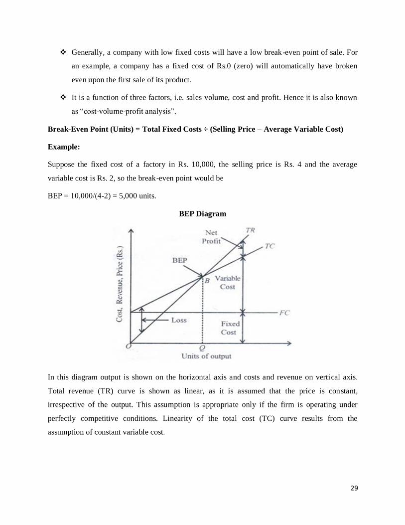
29

Generally, a company with low fixed costs will have a low break-even point of sale. For

an example, a company has a fixed cost of Rs.0 (zero) will automatically have broken

even upon the first sale of its product.

It is a function of three factors, i.e. sales volume, cost and profit. Hence it is also known

as “cost-volume-profit analysis”.

Break-Even Point (Units) = Total Fixed Costs ÷ (Selling Price – Average Variable Cost)

Example:

Suppose the fixed cost of a factory in Rs. 10,000, the selling price is Rs. 4 and the average

variable cost is Rs. 2, so the break-even point would be

ВЕР = 10,000/(4-2) = 5,000 units.

BEP Diagram

In this diagram output is shown on the horizontal axis and costs and revenue on vertical axis.

Total revenue (TR) curve is shown as linear, as it is assumed that the price is constant,

irrespective of the output. This assumption is appropriate only if the firm is operating under

perfectly competitive conditions. Linearity of the total cost (TC) curve results from the

assumption of constant variable cost.

30

CONCEPT OF REVENUE

Cost and revenue are just like two different faces of the same coin. The costs and revenues of a

firm determine its nature and the levels of profit. Cost refers to the expenses incurred by a

producer for the production of a commodity. Revenue denotes the amount of income which a

firm receives by the sale of its output. The revenue concepts commonly used in economics are

total revenue, average revenue and marginal revenue.

Total Revenue (TR)

Total revenue is the amount of income received by the firm from the sale of its products. It is

obtained by multiplying the price of the commodity by the number of units sold.

Symbolically, TR=P × Q

where,

TR = Total Revenue,

P = Price and

Q = Quantity sold

For example,

A cell-phone company sold 100 cell-phones at the price of Rs. 500 each. TR is Rs. 50,000.

(TR= 500 × 100 = 50,000).

Average Revenue (AR)

Average revenue is the revenue per unit of the commodity sold. It is calculated by dividing the

Total Revenue(TR) by the number of units sold (Q).

Symbolically; AR = TR /Q

Where,

AR = Average Revenue,

TR = Total Revenue and

Q = Quantity of unit sold.

31

For example,

If the Total Revenue from the sale of 5 units is Rs 30, the Average Revenue is Rs.6. (AR= 30/5

=6) It is to be noted that AR is equal to Price.

Marginal Revenue (MR)

Marginal revenue is the addition to total revenue by selling one more unit of the commodity. MR

can be found out by dividing change in total revenue by the change in quantity sold out.

Symbolically, MR = ΔTR /ΔQ

Where,

MR = Marginal Revenue,

ΔTR = change in Total Revenue and

ΔQ = change in total quantity.

The other method of estimating MR is:

MR=TRn –TRn-1 (or) TRn+1 – TRn

where, MR denotes Marginal Revenue,

TRn denotes total revenue of nth item, TRn-1

denotes Total Revenue of n-1th item and

TRn+1 denotes Total Revenue of n+1th item.

Example: Suppose 5 units of a product are sold at a revenue of Rs.50 and 6 units are sold at a

total revenue of Rs. 60. The marginal revenue will be Rs.60 – Rs. 50 = Rs. 10. it implies that the

6th unit ears an additional income of Rs. 10.

32

Relationship between AR and MR Curves

1. If a firm is able to sell additional units at the same price then AR and MR will be constant

and equal.

2. If the firm is able to sell additional units only by reducing the price, then both AR and

MR will fall and be different.

3. When price remains constant or fixed, the MR will be also constant and will coincide

with AR.

4. Under perfect competition as the price is uniform and fixed, AR is equal to MR and their

shape will be a straight line horizontal to X axis.

5. When a firm sells large quantities at lower prices both AR and MR will fall but the fall in

MR will be more steeper than the fall in the AR.

6. When marginal revenue is positive, total revenue rises, when MR is zero the total revenue

becomes maximum.

7. When price elasticity of demand is greater than one, MR is positive and TR is increasing.

8. When price elasticity of demand is less than one, MR is negative and TR is decreasing.

9. When price elasticity of demand is equal to one, MR is equal to zero and TR is maximum

and constant.

Significance of the concept of revenue

1. In determining the nature of profit: The concept of MR and AR both together

constitute a powerful analytical tool in economic analysis.

2. Helpful in Decision-making: the concept is also vital in determining the equilibrium of a

firm. The aim of every firm is to firm is to obtain maximum profits. The rule for profit

maximization is MC = MR.

3. Concept of Excess Capacity: This concept is helpful to indicate to the entrepreneur

whether the firm possesses excess capacity or not. Under perfect competition, production

will be carried on up to the minimum point of the LAC. Therefore excess capacity is not

possible.

33

4. Factor-Pricing: In fixing the prices of factors in the factor markets AR and MR concepts

are very useful. In factor pricing the average revenue curve becomes the average revenue

productivity curve and marginal revenue curve becomes the marginal revenue

productivity curve, ARP and MRP are inverted ‘U’ shaped curves.

***********

SCHOOL OF LAW

UNIT 4 – MICRO ECONOMICS – SBA1103

1  

SYLLABUS - UNIT - IV

PRICE AND OUTPUT DETERMINATION IN DIFFERENT MARKETS

Perfect competition – Short run and Long run – Equilibrium of the Firm and Industry – Price and

Output Determination – Supply Curve – Monopoly – Short run and Long run equilibrium – Price

Discrimination- Monopolistic competition - General and Chamberlin Approaches to Equilibrium

– Equilibrium of the Firm and Croup with Product Differentiation and selling Costs – Excess

Capacity under Monopolistic and Imperfect competition – Criticism of Monopolistic competition

– Oligopoly – Non-Collusive (Cournot, Bertrand, Edgeworth, Chamberlin, Kinked Demand

Curve and Stackelberg’s Solution) and collusive (Cartels and Mergers – Price Leadership and

Basic Point Price System).

MARKET

Generally the term market as come to signify a place or a geographical area in which goods and

services are bought and sold. In Economics, market refers to a group of buyers and sellers who

involve in the transaction of commodities and services.

According to Prof. Cournout, the term market is “not any particular market place in which things

are bought and sold, but the whole of any region in which buyers and sellers are in such free

intercourse with one another that the price of the same goods tend to equality easily and

quickly”.

According to Prof. F. Benham, Market is ‘any area over which buyers and sellers are in such

close touch with one another, either directly or through dealers, that the prices obtainable in one

part of the market affect the prices paid in other parts’.

2  

CHARACTERISTICS OF A MARKET

1. Existence of buyers and sellers of the commodity.

2. The establishment of contact between the buyers and sellers. Distance is of no

consideration if buyers and sellers could contact each other through the available

communication system like telephone, agents, letter correspondence and Internet.

3. Buyers and sellers deal with the same commodity or variety. Since the market in

economics is identified on the basis of the commodity, similarity of the product is very

essential.

4. There should be a price for the commodity bought and sold in the market.

CLASSIFICATION OF MARKET

1. Markets on the basis of Area: Based on the extent of the market for any product, markets

can be classified into local regional, national and international markets.

a) Local Market: It arises when products or services are sold and bought in the place of their

production. In such markets, the products exchanged are mostly perishable and semi-durable

in nature: For example, Vegetable, fruits etc.

b) Regional Market: It arises when products or services are sold and bought in a restricted

circle. For example, Regional newspaper.

c) National Market: It arises when products and services are sold and bought throughout a

country. For example, Nation-wide market for tea, coffee, cement, electrical goods, some

printed books etc.

d) international Market: It arises when products and services are sold and bought at the

world level. For example, petrol, gold etc.

2. Market on the basis of Time: Alfred Marshall classifies market on the basis of time.

a) Very short period market or Market Period: It refers to that type of market in which

the commodities are perishable and supply of commodities cannot be changed at all. So in a

very short period, the market supply is perfectly inelastic. The price of the commodity

3  

depends on the demand for the product alone. The perishable commodities like flowers are

the best example.

b) Short period: It refers to that period in which supply can be adjusted to a limited extent

by varying the variable factors alone. The short period supply curve is relatively elastic. The

short period price is determined by the interaction of the short-run supply and demand

curves.

c) Long Period: Long period is the time period during which the supply conditions are fully

able to meet the new demand conditions. In the long run, all (both fixed as well as variable)

factors are variable. the market supply is perfectly elastic.

d) Very long Period or Secular Period: The very long run is a situation where technology

and factors beyond the control of a firm can change significantly.

3. Market on the basis f ‘Nature of Transactions’: It refers that the market are classified into

a) Spot Market: It refers to those markets where goods are physically transacted on the spot.

b) Future Markets: it is related to those transactions which involve contracts of the future

date.

4. Markets on the basis of ‘Regulation’: on the basis of regulation, markets are classified into

a) Regulated market: In the former type of markets transactions are statutorily regulated so

as to put an end t unfair practices. Such markets may be established for specific products or a

group of products. Produce and stock exchanges are suitable examples of the regulated

markets.

b) Unregulated Markets: Unregulated or free markets are those where there are no

restrictions in the transactions.

5. Markets on the basis of ‘Volume of Business’: Based on the volume of business transacted,

markets are classified into;

a) Wholesale market: The wholesale market comes into existence when the commodities

are bought and sold in bulk or large quantities. The dealers in this market are knows as the

wholesalers. The wholesaler acts as an intermediary between the producer and the retailer.

4  

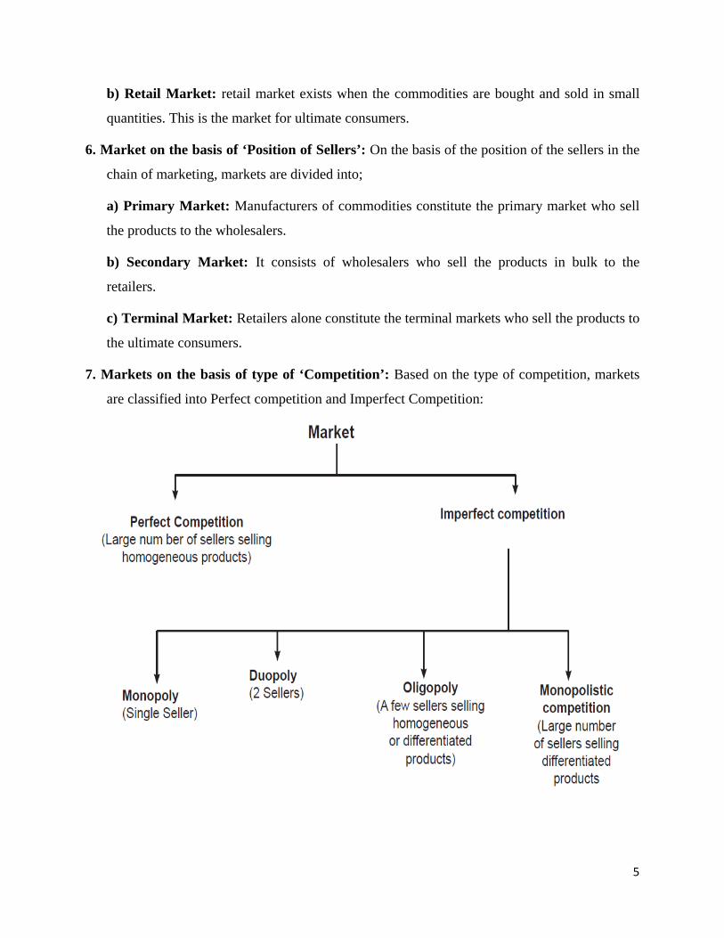
b) Retail Market: retail market exists when the commodities are bought and sold in small

quantities. This is the market for ultimate consumers.

6. Market on the basis of ‘Position of Sellers’: On the basis of the position of the sellers in the

chain of marketing, markets are divided into;

a) Primary Market: Manufacturers of commodities constitute the primary market who sell

the products to the wholesalers.

b) Secondary Market: It consists of wholesalers who sell the products in bulk to the

retailers.

c) Terminal Market: Retailers alone constitute the terminal markets who sell the products to

the ultimate consumers.

7. Markets on the basis of type of ‘Competition’: Based on the type of competition, markets

are classified into Perfect competition and Imperfect Competition:

5  

PERFECT COMPETITION

Perfect competition is a market situation where there are infinite number of sellers that no one is

big enough to have any appreciable influence over market price.

According to Joan Robinson, “Perfect competition prevails when the demand for the output of

each producer is perfectly elastic”.

For perfect competition, two conditions are necessary,. There should be a large number of

sellers, and buyers should be aware of the various price offers and their perfect conditions, so

that they have no reason to prefer one seller to another.

FEATURES OF PERFECT COMPETITION MARKET

1. Large Number of Buyers and Sellers: In the perfectly competitive market, There are a large

number of buyers and sellers in a perfect competitive market that neither a single buyer nor a

single seller can influence the price. The price is determined by market forces namely the

demand for and the supply of the product. There will be uniform price in the market. Sellers

accept this price and adjust the quantity produced to maximize their profit. Thus the sellers in

the perfect competitive market are price- takers and quantity adjusters.

2. Homogeneous Product and Uniform Price: The product sold and bought is homogeneous in

nature, in the sense that the units of the product are perfectly substitutable. All the units of

the product are identical (ie) of the same size, shape, colour, quality etc. Therefore, a uniform

price prevails in the market.

3. Perfect knowledge about market conditions : Both buyers and sellers are fully aware of the

current price in the market. Therefore the buyer will not offer high price and the sellers will

not accept a price less than the one prevailing in the market.

4. Free entry and Free exit : There must be complete freedom for the entry of new firms or the

exit of the existing firms from the industry. When the existing firms are earning super-normal

profits, new firms enter into the market. When there is loss in the industry, some firms leave

6  

the industry. The free entry and free exit are possible only in the long run. That is because the

size of the plant cannot be changed in the short run.

5. Perfect mobility of factors of production: The factors of productions should be free to move

from one use to another or from one industry to another easily to get better remuneration.

The assumption of perfect mobility of factors is essential to fulfil the first condition namely

large number of producers in the market.

6. Absence of transport cost: In a perfectly competitive market, it is assumed that there are no

transport costs. Under perfect competition, a commodity is sold at uniform price throughout

the market. If transport cost is incurred, the firms nearer to the market will charge a low price

than the firms far away. Hence it is assumed that there is no transport cost.

7. Absence of Government intervention: There are no government controls or restrictions on

supply, pricing etc. There is also no collusion among buyers or sellers. The price in the

perfectly competitive market is free to change in response to changes in demand and supply

conditions.

SHORT RUN EQUILIBRIUM PRICE AND OUTPUT DETERMINATION UNDER

PERFECT COMPETITION

1. Since a firm in the perfectly competitive market is a price-taker, it has to adjust its level of

output to maximize its profit. The aim of any producer is to maximize his profit.

2. The short run is a period in which the number and plant size of the firms are fixed. In this

period, the firm can produce more only by increasing the variable inputs.

3. As the entry of new firms or exits of the existing firms are not possible in the short-run, the

firm in the perfectly competitive market can either earn supernormal profit or normal profit

or incur loss in the short period.

7  

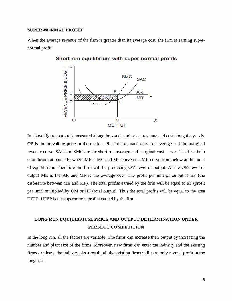
SUPER-NORMAL PROFIT

When the average revenue of the firm is greater than its average cost, the firm is earning super-

normal profit.

In above figure, output is measured along the x-axis and price, revenue and cost along the y-axis.

OP is the prevailing price in the market. PL is the demand curve or average and the marginal

revenue curve. SAC and SMC are the short run average and marginal cost curves. The firm is in

equilibrium at point ‘E’ where MR = MC and MC curve cuts MR curve from below at the point

of equilibrium. Therefore the firm will be producing OM level of output. At the OM level of

output ME is the AR and MF is the average cost. The profit per unit of output is EF (the

difference between ME and MF). The total profits earned by the firm will be equal to EF (profit

per unit) multiplied by OM or HF (total output). Thus the total profits will be equal to the area

HFEP. HFEP is the supernormal profits earned by the firm.

LONG RUN EQUILIBRIUM, PRICE AND OUTPUT DETERMINATION UNDER

PERFECT COMPETITION

In the long run, all the factors are variable. The firms can increase their output by increasing the

number and plant size of the firms. Moreover, new firms can enter the industry and the existing

firms can leave the industry. As a result, all the existing firms will earn only normal profit in the

long run.

8  

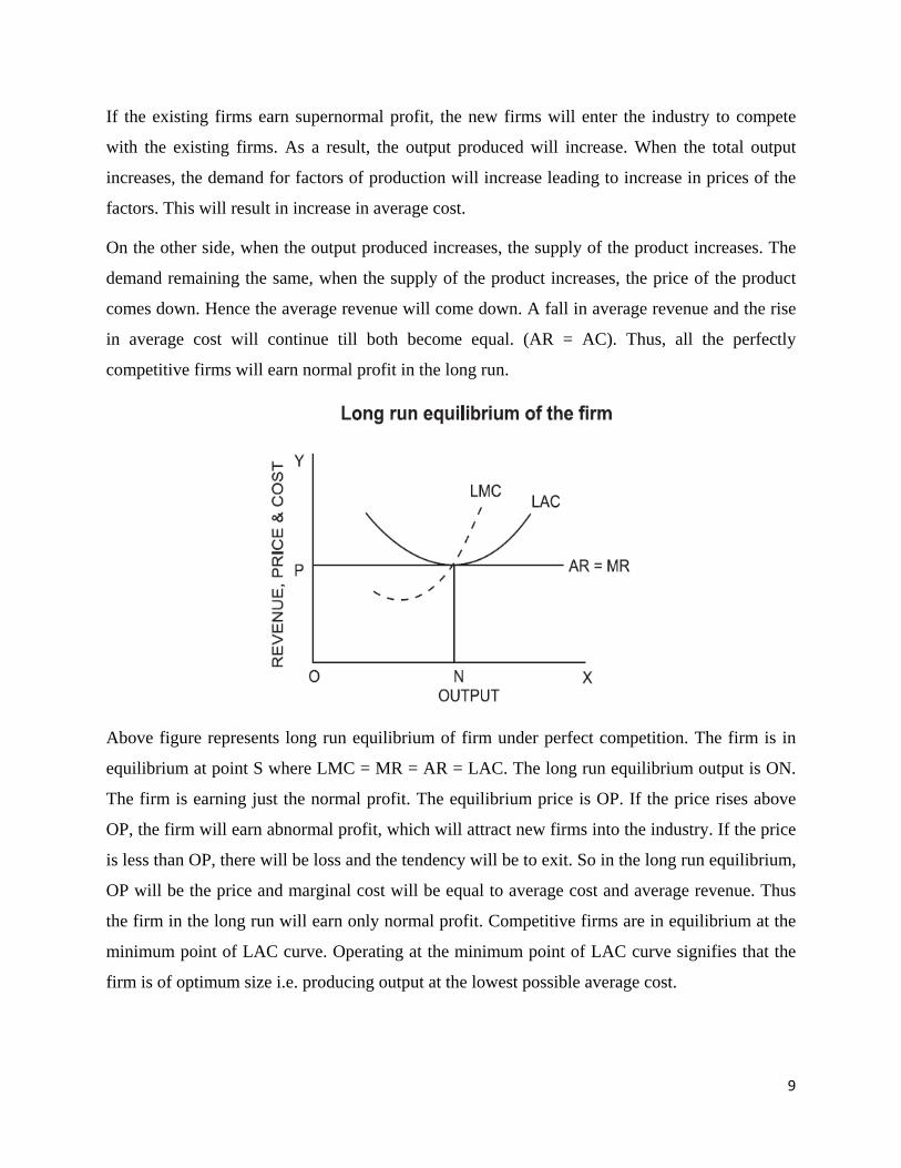
If the existing firms earn supernormal profit, the new firms will enter the industry to compete

with the existing firms. As a result, the output produced will increase. When the total output

increases, the demand for factors of production will increase leading to increase in prices of the

factors. This will result in increase in average cost.

On the other side, when the output produced increases, the supply of the product increases. The

demand remaining the same, when the supply of the product increases, the price of the product

comes down. Hence the average revenue will come down. A fall in average revenue and the rise

in average cost will continue till both become equal. (AR = AC). Thus, all the perfectly

competitive firms will earn normal profit in the long run.

Above figure represents long run equilibrium of firm under perfect competition. The firm is in

equilibrium at point S where LMC = MR = AR = LAC. The long run equilibrium output is ON.

The firm is earning just the normal profit. The equilibrium price is OP. If the price rises above

OP, the firm will earn abnormal profit, which will attract new firms into the industry. If the price

is less than OP, there will be loss and the tendency will be to exit. So in the long run equilibrium,

OP will be the price and marginal cost will be equal to average cost and average revenue. Thus

the firm in the long run will earn only normal profit. Competitive firms are in equilibrium at the

minimum point of LAC curve. Operating at the minimum point of LAC curve signifies that the

firm is of optimum size i.e. producing output at the lowest possible average cost.

9  

Advantages of perfect competition

1. There is consumer sovereignty in a perfect competitive market. The consumer is rational and

he has perfect knowledge about the market conditions. Therefore, he will not purchase the

products at a higher price.

2. In the perfectly competitive market, the price is equal to the minimum average cost. It is

beneficial to the consumer.

3. The perfectly competitive firms are price-takers and the products are homogeneous. Therefore

it is not necessary for the producers to incur expenditure on advertisement to promote sales.

This reduces the wastage of resources.

4. In the long run, the perfectly competitive firm is functioning at the optimum level. This means

that maximum economic efficiency in production is achieved. As the actual output produced

by the firm is equal to the optimum output, there is no idle or unused or excess capacity.

MONOPOLY

The word monopoly has been derived from the combination of two words i.e., ‘Mono’ and

‘Poly’. Mono refers to a single and “poly” to seller.

Monopoly is a market structure characterized by a single seller, selling the unique product with

the restriction for a new firm to enter the market.

It is situation where there exists single control over the market producing a commodity having no

substitutes and no possibilities for anyone to enter the industry and compete. Single control may

mean a single producer or a joint stock organization or governmental or quasi-governmental.

FEATURES OF MONOPOLY MARKET

1. Single Seller: There is only one seller; he can control either price or supply of his product. But

he cannot control demand for the product, as there are many buyers.

2. N o close Substitutes: There are no close substitutes for the product. The buyers have no

alternatives or choice. Either they have to buy the product or go without it.

10  

3. Price: The monopolist has control over the supply so as to increase the price. Sometimes he

may adopt price discrimination. He may fix different prices for different sets of consumers. A

monopolist can either fix the price or quantity of output; but he cannot do both, at the same

time.

4. N o Entry: There is no freedom to other producers to enter the market as the monopolist is

enjoying monopoly power. There are strong barriers for new firms to enter. There are legal,

technological, economic and natural obstacles, which may block the entry of new producers.

5. Firm and Industry: Under monopoly, there is no difference between a firm and an industry.

As there is only one firm, that single firm constitutes the whole industry.

Sources of Monopoly Power

1. Natural Monopoly: A monopoly may arise on account of some natural causes. Some

minerals are available only in certain regions. For example, South Africa has the monopoly

of diamonds; nickel in the world is mostly available in Canada and oil in Middle East. This is

natural monopoly.

2. Technical Monopoly : Monopoly power may be enjoyed due to technical reasons. A firm

may have control over raw materials, technical knowledge, special know-how, scientific

secrets and formula that enable a monopolist to produce a commodity. e.g., Coco Cola.

3. Legal Monopoly : Monopoly power is achieved through patent rights, copyright and trade

marks by the producers. This is called legal monopoly.

4. Monopoly by Large Amount of Capital: The manufacture of some goods requires a large

amount of capital or lumpiness of capital. All firms cannot enter the field because they

cannot afford to invest such a large amount of capital. This may give rise to monopoly. For

example, iron and steel industry, railways, etc.

5. State Monopoly : Government will have the sole right of producing and selling some goods.

They are State monopolies. For example, we have public utilities like electricity and

railways. These public utilities are undertaken by the State.

11  

PRICE & OUTPUT DETERMINATION UNDER MONOPOLY

A monopolist like a perfectly competitive firm tries to maximize his profits. A monopoly firm

faces a downward sloping demand curve, that is, its average revenue curve. The downward

sloping demand curve implies that larger output can be sold only by reducing the price. Its

marginal revenue curve will be below the average revenue curve. The average cost curve is ‘U’

shaped. The monopolist will be in equilibrium when MC = MR and the MC curve cuts the MR

curve from below.

Price & Output Determination under Monopoly

In the above figure, AR is the Average Revenue Curve and MR is the Marginal revenue curve.

AR curve is falling and MR curve lies below AR. The monopolist is in equilibrium at E where

MR = MC. He produces OM units of output and fixes price at OP. At OM output, the average

revenue is MS and average cost MT. Therefore the profit per unit is MS-MT = TS. Total profit is

average profit (TS) multiplied by output (OM), which is equal to HTSP. The monopolist is in

equilibrium at point E and produces OM output at which he is earning maximum profit. The

monopoly price is higher than the marginal revenue and marginal cost.

12  

Advantages of Monopoly Market

1. Monopoly firms have large-scale production possibilities and also can enjoy both internal

and external economies. This will result in the reduction of costs of production. Output can

be sold at low prices. This is beneficial to the consumers.

2. Monopoly firms have vast financial resources which could be used for research and

development. This will enable the firms to innovate quickly.

3. There are a number of weak firms in an industry. These firms can combine together in the

form of monopoly to meet competition. In such a case, market can be expanded.

Disadvantages of Monopoly Market

1. A monopolist always charges a high price, which is higher than the competitive price. Thus a

monopolist exploits the consumers.

2. A monopolist is interested in getting maximum profit. He may restrict the output and raise

prices. Thus, he creates artificial scarcity for his product.

3. A monopolist often charges different prices for the same product from different

consumers. He extracts maximum price according to the ability to pay of different

consumers.

4. A monopolist uses large-scale production and huge resources to promote his own selfish

interest. He may adopt wrong practices to establish absolute monopoly power.

5. In a country dominated by monopolies, wealth is concentrated in the hands of a few. It will

lead to inequality of incomes. This is against the principle of the socialistic pattern of society.

Methods of Controlling Monopoly

1. Legislative Method: Government can control monopolies by legal actions. Anti-monopoly

legislation has been enacted to check the growth of monopoly. In India, the Monopolies and

Restrictive Trade Practices Act was passed in 1969. The objective of this Act is to prevent

13  

the unwanted growth of private monopolies and concentration of economic power in the

hands of a small number of individuals and families.

2. Controlling Price and Output: This method can be applied in the case of natural

monopolies. Government would fix either price or output or both.

3. Taxation: Taxation is another method by which the monopolistic power can be prevented or

restricted. Government can impose a lump-sum tax on a monopoly firm, irrespective of its

level of output. Consequently, its total profit will fall.

4. Nationalization: Nationalizing big companies is one of the solutions. Government may take

over such monopolistic companies, which are exploiting the consumers.

5. Consumer’s Association: The growth of monopoly power can also be controlled by

encouraging the formation of consumers associations to improve the bargaining power of

consumers.

PRICE DISCRIMINATION UNDER MONOPOLY

This is called price discrimination practiced by the monopolist. Under this, the monopolist will

charge different prices from different class of customers. The idea is to get from each customer

whatever profits could be squeezed out of him depending on his purse and intensity of demand.

Types of Price Discrimination

1. Personal Discrimination: The monopolist will charge different prices from different

customers on the basis of their ability to pay. Rich customers will be asked to pay more and

poor customers to pay less. This is possible in specialized services of doctors and lawyers.

2. Place Discrimination: It is adopted by the monopolist having markets in different places for

the same commodity. The locality in which the market is situated will be the criterion in

fixing up the price.

3. Trade discrimination: It can also be called use discrimination. By this, the monopolist will

charge different prices for different types of uses of the same commodity. For example,

electricity will be sold at a cheaper rate for industrial establishment, while it will be charged

at a higher rate for domestic consumption.

14  

MONOPOLISTIC COMPETITION

Monopolistic competition refers to the market situation in which a large number of sellers are

offering similar but not identical products. As Chamberlin pointed out, it’s a blend of

competition and monopoly. The essential features of monopolistic competition are product

differentiation and existence of many sellers.

The following are some examples of monopolistic competition in the Indian context;

1. Shampoo – sunsilk, Clinic plus, ponds, chick.

2. Tea – Three roses, AVT, brooke bond

3. Tooth paste – Colgate, Close-up, Dabar, Himalaya

4. Soap – Doe, Hamam, Cinthol, Medimix

Characteristics of Monopolistic Competition

1. Large Number of firms/Sellers : Under monopolistic competition, the number of firms

producing a commodity will be very large. Each firm will act independently on the basis of

product differentiation and each firm determines its price-output policies. Any action of the

individual firm in increasing or decreasing the output will have little or no effect on other

firms.

2. Product differentiation: Product differentiation is the essence of monopolistic competition.

Product differentiation is attempted through (a) physical difference; (b) quality difference; (c)

imaginary difference and (d) purchase benefit difference. Product differentiation through

effective advertisement is another method. This is known as sales promotion.

3. Selling Costs: From the discussion of ‘product differentiation’, we can infer that the producer

under monopolistic competition has to incur expenses to popularise his brand. This

expenditure involved in selling the product is called selling cost. According to Prof.

Chamberlin, selling cost is “the cost incurred in order to alter the position or shape of the

demand curve for a product”. Most important form of selling cost is advertisement. Sales

promotion by advertisement is called non-price competition.

15  

4. Freedom of entry and exit of firms: Another important feature is the freedom of any firm to

enter into the field and produce the commodity under its own brand name and any firm can

go out of the field if so chosen. There are no barriers as in the case of monopoly.

DETERMINATION OF EQUILIBRIUM PRICE AND OUTPUT UNDER

MONOPOLISTIC COMPETITION

The firm under monopolistic competition achieves its equilibrium when it’s MC = MR, and

when its MC curve cuts its MR curve from below. If MC is less than MR, the sellers will find it

profitable to expand their output. Each firm will choose that price and output where it will be

maximising its profit.

MC and AC are the short period marginal cost and average cost curves. The sloping down

average revenue and marginal revenue curves are shown as AR and MR. The equilibrium point

is E where MR = MC. The equilibrium output is OM and the price of the product is fixed at OP.

The difference between average cost and average revenue is SQ. The output is OM. So, the

supernormal profit for the firm is shown by the rectangle PQ The different firms in monopolistic

competition may be making either abnormal.

16  

Profits or losses in the short period depending on their costs and revenue curves.SR. The firm by

producing OM units of its commodity and selling it at a price of OP per unit realizes the

maximum profit in the short run.

In the long run, if the existing firms earn super normal profit, the entry of new firms will reduce

its share in the market. The average revenue of the product will come down. The demand for

factors of production will increase the cost of production. Hence, the size of the profit will be

reduced. If the existing firms incur losses in the long-run, some of the firms will leave the

industry increasing the share of the existing firms in the market. As the demand for factors

becomes less, the price of factors will come down. This will reduce the cost of production, which

will increase the profit earned by the existing firm. Thus under monopolistic competition, all the

existing firms will earn normal profit in the long run.

WASTAGES OF MONOPOLISTIC COMPETITION

1. Unemployment: Under monopolistic competition, the firms produce less than optimum

output. As a result, the productive capacity is not used to the fullest extent. This will lead to

unemployment of resources.

2. Excess capacity: Excess capacity is the difference between the optimum output that can be

produced and the actual output produced by the firm. In the long run, a monopolistic firm

produces an output which is less than the optimum output that is the output corresponding to

the minimum average cost.

3. Advertisement: There is a lot of waste in competitive advertisements under monopolistic

competition. The wasteful and competitive advertisements lead to high cost to consumers.

4. Too Many Varieties of Goods: Introducing too many varieties of a good is another waste of

monopolistic competition. The goods differ in size, shape, style and colour. A reasonable

number of varieties would be desirable. Cost per unit can be reduced if only a few are

produced.

5. Inefficient Firms: Under monopolistic competition, inefficient firms charge prices higher

than their marginal cost. Such type of inefficient firms should be kept out of the industry.

17  

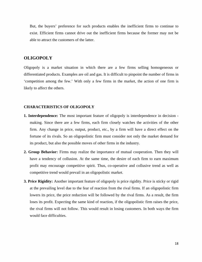
But, the buyers’ preference for such products enables the inefficient firms to continue to

exist. Efficient firms cannot drive out the inefficient firms because the former may not be

able to attract the customers of the latter.

OLIGOPOLY

Oligopoly is a market situation in which there are a few firms selling homogeneous or

differentiated products. Examples are oil and gas. It is difficult to pinpoint the number of firms in

‘competition among the few.’ With only a few firms in the market, the action of one firm is

likely to affect the others.

CHARACTERISTICS OF OLIGOPOLY

1. Interdependence: The most important feature of oligopoly is interdependence in decision -

making. Since there are a few firms, each firm closely watches the activities of the other

firm. Any change in price, output, product, etc., by a firm will have a direct effect on the

fortune of its rivals. So an oligopolistic firm must consider not only the market demand for

its product, but also the possible moves of other firms in the industry.

2. Group Behavior: Firms may realize the importance of mutual cooperation. Then they will

have a tendency of collusion. At the same time, the desire of each firm to earn maximum

profit may encourage competitive spirit. Thus, co-operative and collusive trend as well as

competitive trend would prevail in an oligopolistic market.

3. Price Rigidity: Another important feature of oligopoly is price rigidity. Price is sticky or rigid

at the prevailing level due to the fear of reaction from the rival firms. If an oligopolistic firm

lowers its price, the price reduction will be followed by the rival firms. As a result, the firm

loses its profit. Expecting the same kind of reaction, if the oligopolistic firm raises the price,

the rival firms will not follow. This would result in losing customers. In both ways the firm

would face difficulties.

18  

KINKED DEMAND CURVE

American economist Sweezy came up with the kinked demand curve hypothesis to explain the

reason behind this price rigidity under oligopoly.

In an oligopolistic market, firms cannot have a fixed demand curve since it keeps changing as

competitors change the prices/quantity of output. Since an oligopolist is not aware of the demand

curve, economists have designed various price-output models based on the behavior pattern of

other firms in the industry.

In many oligopolist markets, it has been observed that prices tend to remain inflexible for a very

long time. Even in the face of declining costs, they tend to change infrequently. According to the

kinked demand curve hypothesis, the demand curve facing an oligopolist has a kink at the level

of the prevailing price. This kink exists because of two reasons:

1. The segment above the prevailing price level is highly elastic.

2. The segment below the prevailing price level is inelastic.

Assumption of Kinked Demand curve

a. If a firm lowers the price below the prevailing level, then the competitors will follow

him.

b. If a firm increases the price above the prevailing level, then the competitors will not

follow him.

Diagram of Kinked Demand Curve

19  

From the figure, we know that The prevailing price level = P. The firm produces and sells output

= OM. Also, the upper segment (dP) of the demand curve (dD) is elastic. The lower segment

(PD) of the demand curve (dD) is relatively inelastic.

When an oligopolist lowers the price of his product, the competitors feel that if they don’t follow

the price cut, then their customers will leave them and buy from the firm who is offering a lower

price.

Therefore, they lower their prices too in order to maintain their customers. Hence, the lower

portion of the curve is inelastic. It implies that if an oligopolist lowers the price, he can obtain

very little sales.

On the other hand, when a firm increases the price of its product, it experiences a substantial

reduction in sales. The reason is simple – consumers will buy the same/similar product from its

competitors.

DUOPOLY

Duopoly is a special case of the theory of oligopoly in which there are only two sellers. Both the

sellers are completely independent and no agreement exists between them. Even though they are

independent, a change in the price and output of one will affect the other, and may set a chain of

reactions. A seller may, however, assume that his rival is unaffected by what he does, in that case

he takes only his own direct influence on the price.

Characteristics of Duopoly

1. Each seller is fully aware of his rival’s motive and actions.

2. Both sellers may collude (they agree on all matters regarding the sale of the commodity).

3. They may enter into cut-throat competition.

4. There is no product differentiation.

5. They fix the price for their product with a view to maximizing their profit.

20  

OLIGOPOLY MODELS

1. Augustin Cournot’s Model

2. Bertrand’s Model

3. Edgeworth’s Model

4. Stackelberg’s Model

5. Chamberlin’s Model

AUGUSTIN COURNOT’S MODEL

Oligopoly was made by the French Economist Augustin Cournot in 1839. He considered only

two firms and they are owing Mineral well. Each firm act on the assumption that its competition

will not change its output and decides its own output so as to maximise his profit.

Assumptions

This model rests upon the following main assumptions;

1. There are two firms in the market, A and B

2. Each firm owns the spring of mineral water which is identical

3. The cost of production is zero

4. Each firm is faced with a linear, negatively sloping market demand curve.

5. The productive capacity of each firm is unlimited

6. Each firm considers itself to be independent in determining its price or output

7. Each firm assumes that the supply of rival firm will remain unchanged

Given the Set of assumptions, when ultimately long run equilibrium determined, each firm will

share the market equally. Price will be zero because of zero cost of production and the long run

equilibrium under perfect competition.

21  

Price and Output under Duopoly

Initially, firm A is the only seller of mineral water in the market. By assuming cost of production

is zero, A charges 0P2 price and supply 0Q quantity. When MC=MR1, (MC is zero). Here he

charges monopoly price and Total Revenue is 0P2PQ. When firm B entered into the market, He

got half of the market share for his product. Firm B assumes that firm A will not change his price

and output, then market available for B is PM of demand curve. Here firm B supplies his product

to the half of his market control (when MR2-MC(MC is zero)). Firm B’s Price is 0P1 and output

is QN and Total Revenue is QRP’N.

Criticism

• The model does not say how long the adjustment period will be.

• The costless production is unrealistic.

• This is closed model because it does not allow entry of firms.

• This is a no-learning by doing model .

• He assumed the supply of rival is fixed but here supply is repeatedly changing.

22  

BERTRAND’S OLIGOPOLY MODEL

The oligopoly (duopoly) model developed by Joseph Bertram in 1883 was a modification upon

Cournot’s duopoly solution.

oligopoly model in which each firm chooses its price simultaneously, assuming that rivals will

continue charging their current prices.

Assumptions:

1. There are Two firms in the market, A and B

2. Each Firm owns the spring of mineral water which is identical.

3. The cost of production is zero

4. Each firm have unlimited production capacity.

5. Each firm considers itself to be independent in making the price – output decision. In other

words, the mutual interdependence is ignored by them.

6. The most significant assumption in this model, on account of which it departs from

Cournot’s solution is that each fierm belives that the price of rival firm remains constant.

Diagram of Bertrand’s oligopoly Model

23  

The result of the model creates a paradox, known as Bertrand’s paradox: in a case of imperfect

competition (here, a duopoly), where there is a strong incentive to collude, we end up with the

same outcome as in perfect competition. The equilibrium does not hold with asymmetric cost

functions since the firm with the lowest marginal cost would seize the entire market and become

a monopoly.

Criticism Of The Model

Bertrand’s model has been criticized on the same grounds of cournot’s model. Bertrand’s imficit

behavioral assumption that firms never learn from their past experience seems to be unrealistic.

If cost is assumed to be zero price will fluctuate between zero and upper limit of the price,

instead of stabilizing at a point.

EDGEWORTH’S DUOPOLY MODEL

Edgeworth developed his model of duopoly in 1897. Edgeworth’s model follows Bertrand’s

assumption that each seller assumes his rival’s price, instead of his output, to remain costant.

“There will be an indeterminate tract through which the index of value will oscillate, or, rather

will vibrate irregularly for an indefinite length of time.”

Assumptions of the model

Each seller continues to assume that his rival will never change his price even through they are

proved repeatedly wrong. But according to Hotelling , Edgeworth’s model is definitely an

improvement upon cournot’s model in that it assumes price, rather than output, to be the relevant

decision variable for the sellers.

24  

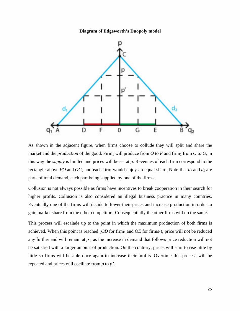
Diagram of Edgeworth’s Duopoly model

As shown in the adjacent figure, when firms choose to collude they will split and share the

market and the production of the good. Firm1 will produce from O to F and firm2 from O to G, in

this way the supply is limited and prices will be set at p. Revenues of each firm correspond to the

rectangle above FO and OG, and each firm would enjoy an equal share. Note that d1 and d2 are

parts of total demand, each part being supplied by one of the firms.

Collusion is not always possible as firms have incentives to break cooperation in their search for

higher profits. Collusion is also considered an illegal business practice in many countries.

Eventually one of the firms will decide to lower their prices and increase production in order to

gain market share from the other competitor. Consequentially the other firms will do the same.

This process will escalade up to the point in which the maximum production of both firms is

achieved. When this point is reached (OD for firm1 and OE for firms2), price will not be reduced

any further and will remain at p’, as the increase in demand that follows price reduction will not

be satisfied with a larger amount of production. On the contrary, prices will start to rise little by

little so firms will be able once again to increase their profits. Overtime this process will be

repeated and prices will oscillate from p to p’.

25  

STACKELBERG’S DUOPOLY MODEL

Stackelberg duopoly, also called Stackelberg competition, is a model of imperfect

competition based on a non-cooperative game. It was developed in 1934 by Heinrich

Stackelbelrg in his “Market Structure and Equilibrium” and represented a breaking point in the

study of market structure, particularly the analysis of duopolies, since it was a model based on

different starting assumptions and gave different conclusions to those of

the Cournot’s and Bertrand’s duopoly models.

There are two firms, which sell homogenous Products. It is a sequential game not simultaneous.

In game theory, a Stackelberg duopoly is a sequential game (not simultaneous as in Cournot’s

model). There are two firms, which sell homogeneous products, and are subject to the same

demand and cost functions. One firm, the leader, is perhaps better known or has greater brand

equity, and is therefore better placed to decide first which quantity q1 to sell, and the other firm,

the follower, observes this and decides on its production quantity q2. To find the Nash

equilibrium of the game we need to use backward induction, as in any sequential game. That is,

start analyzing the decision of the follower.

Diagram of Stackelberg’s Duopoly Model

26  

The perfect equilibrium of the game is the Stackelberg equilibrium. In this game, the leader has

decided not to behave as in the Cournot’s model, however, we cannot ensure that the leader is

going to produce more and make more profits than the follower (production will be larger for the

firm with lower marginal costs). Total production will be greater and prices lower, but player

one will be better off than player two, which serves to highlight two things: the importance of

accurate market information when defining a strategy, and the interdependence of each player’s

strategies, especially when there is a market leader (with the benefit of moving first) and a

follower.

When it comes to economic efficiency, the result is similar to Cournot’s duopoly model. The

Nash equilibrium is not Pareto efficient (isoprofit curves, green curves, are not tangent to each

other) and therefore, there is a loss in economic efficiency. Nevertheless, the loss is lower in the

Stackelberg duopoly than in Cournot’s. Stackelberg and Cournot equilibria are stable in a static

model of just one period. In a dynamic context (repeated games), the models need to be

reconsidered.

CHAMBERLIN’S OLIGOPOLY MODEL

Chamberlin opined that the oligopolists are intelligent enough to recognize their interdependence

and they therefore jointly produce monopoly output and charge monopoly price. Thus, in

Chamberlin’s model the stable equilibrium and maximization of joint profit by the oligopolist is

accomplished. It is interesting to note that the oligopoly firms behave in a non-collusive manner.

As compared to the classical Oligopoly models of Cournot, Bertrand, and Edgeworth the

Chamberlin’s oligopoly model is comparatively more advanced and superior. Chamberlin’s

model is based on the assumption that the oligopolistic firms understand and recognize the

mutual interdependence and behave accordingly.

27  

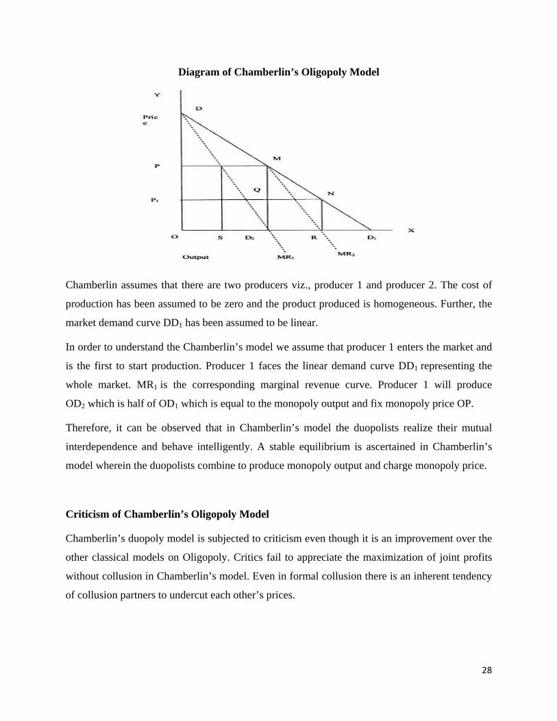
Diagram of Chamberlin’s Oligopoly Model

Chamberlin assumes that there are two producers viz., producer 1 and producer 2. The cost of

production has been assumed to be zero and the product produced is homogeneous. Further, the

market demand curve DD1 has been assumed to be linear.

In order to understand the Chamberlin’s model we assume that producer 1 enters the market and

is the first to start production. Producer 1 faces the linear demand curve DD1 representing the

whole market. MR1 is the corresponding marginal revenue curve. Producer 1 will produce

OD2 which is half of OD1 which is equal to the monopoly output and fix monopoly price OP.

Therefore, it can be observed that in Chamberlin’s model the duopolists realize their mutual

interdependence and behave intelligently. A stable equilibrium is ascertained in Chamberlin’s

model wherein the duopolists combine to produce monopoly output and charge monopoly price.

Criticism of Chamberlin’s Oligopoly Model

Chamberlin’s duopoly model is subjected to criticism even though it is an improvement over the

other classical models on Oligopoly. Critics fail to appreciate the maximization of joint profits

without collusion in Chamberlin’s model. Even in formal collusion there is an inherent tendency

of collusion partners to undercut each other’s prices.

28  

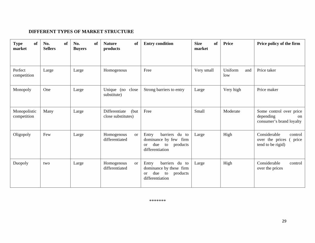
DIFFERENT TYPES OF MARKET STRUCTURE

Type of market

No. of Sellers

No. of Buyers

Nature of products

Entry condition Size of market

Price Price policy of the firm

Perfect competition

Large Large Homogenous Free Very small Uniform and low

Price taker

Monopoly One Large Unique (no close substitute)

Strong barriers to entry Large Very high Price maker

Monopolistic competition

Many Large Differentiate (but close substitutes)

Free Small Moderate Some control over price depending on consumer’s brand loyalty

Oligopoly Few Large Homogenous or differentiated

Entry barriers du to dominance by few firm or due to products differentiation

Large High Considerable control over the prices ( price tend to be rigid)

Duopoly two Large Homogenous or differentiated

Entry barriers du to dominance by these firm or due to products differentiation

Large High Considerable control over the prices

*******

29  

SCHOOL OF LAW

UNIT 5 – MICRO ECONOMICS – SBA1103

1  

SYLLABUS - UNIT IV – THEORY OF DISTRIBUTION

The Theory of Rent, Interest and Profits – Labour Supply and Wage Determination –

Exploitation of Labour – Role of Trade Unions and Collective Bargaining in Wage

Determination – Minimum Wage Legislation.

MARGINAL PRODUCTIVITY THEORY OF DISTRIBUTION

The marginal productivity theory of distribution was developed by J. B. Clark.

The marginal productivity theory of distribution is the general theory of distribution. The theory

explains how prices of various factors of production are determined under conditions of perfect

competition. It emphasizes that any variable factor must obtain a reward equal to its marginal

product.

Thus, rent is equal to the value of the marginal product (VMP) of land; wages are equal to the

VMP of labour and so on. A firm will go on employing more and more units of a factor until the

price of that factor is equal to the value of the marginal product. In other words, each factor will

be rewarded according to its marginal productivity.

The marginal productivity is equal to the value of the additional product which an employer gets

when he employs an additional unit of that factor. We assume that the supply of all other factors

remain constant. We shall give a simple illustration of the marginal productivity theory of

distribution by making use of labour.

The aim of a firm is maximization of profit. It will hire a factor as long as it adds more to total

revenue than to total cost. Thus a firm will hire a factor upto the point at which the marginal unit

contributes as much to total cost as to total revenue because total profit cannot be further

increased.

2  

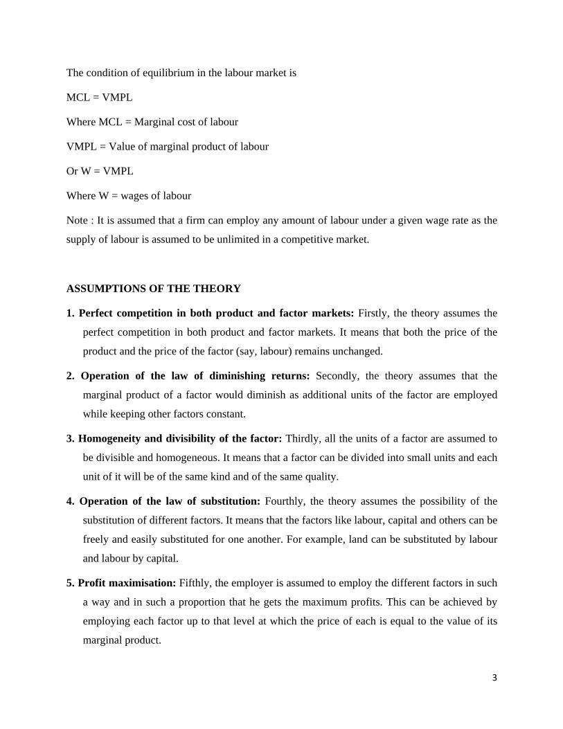
The condition of equilibrium in the labour market is

MCL = VMPL

Where MCL = Marginal cost of labour

VMPL = Value of marginal product of labour

Or W = VMPL

Where W = wages of labour

Note : It is assumed that a firm can employ any amount of labour under a given wage rate as the

supply of labour is assumed to be unlimited in a competitive market.

ASSUMPTIONS OF THE THEORY

1. Perfect competition in both product and factor markets: Firstly, the theory assumes the

perfect competition in both product and factor markets. It means that both the price of the

product and the price of the factor (say, labour) remains unchanged.

2. Operation of the law of diminishing returns: Secondly, the theory assumes that the

marginal product of a factor would diminish as additional units of the factor are employed

while keeping other factors constant.

3. Homogeneity and divisibility of the factor: Thirdly, all the units of a factor are assumed to

be divisible and homogeneous. It means that a factor can be divided into small units and each

unit of it will be of the same kind and of the same quality.

4. Operation of the law of substitution: Fourthly, the theory assumes the possibility of the

substitution of different factors. It means that the factors like labour, capital and others can be

freely and easily substituted for one another. For example, land can be substituted by labour

and labour by capital.

5. Profit maximisation: Fifthly, the employer is assumed to employ the different factors in such

a way and in such a proportion that he gets the maximum profits. This can be achieved by

employing each factor up to that level at which the price of each is equal to the value of its

marginal product.

3  

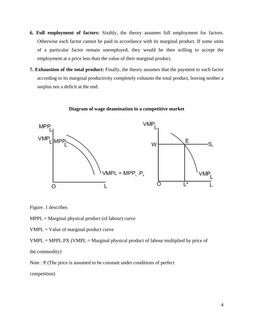
6. Full employment of factors: Sixthly, the theory assumes full employment for factors.

Otherwise each factor cannot be paid in accordance with its marginal product. If some units

of a particular factor remain unemployed, they would be then willing to accept the

employment at a price less than the value of their marginal product.

7. Exhaustion of the total product: Finally, the theory assumes that the payment to each factor

according to its marginal productivity completely exhausts the total product, leaving neither a

surplus nor a deficit at the end.

Diagram of wage deamination in a competitive market

Figure. 1 describes

MPPL = Marginal physical product (of labour) curve

VMPL = Value of marginal product curve

VMPL = MPPL.PX (VMPL = Marginal physical product of labour multiplied by price of

the commodity)

Note : P (The price is assumed to be constant under conditions of perfect

competition)

4  

In fig. 2, the equilibrium of the firm is shown by E. This is so because to the left of L*, each unit

of labour costs less than the value of its product (VMPL > W). Hence the firm will make more

profit by hiring more workers. To the right of VMPL<W. Hence, the profits of the firm will be

reduced. So profits will be maximum when VMPL = W.

It follows from the above discussion that the demand curve of a firm for a single variable factor

(e.g. labour) is its value of marginal product curve.

Thus the productivity of the marginal unit of a factor determines the rate that is to be paid to all

units of the factor. The employer adopts the principle of substitution and combines land, labour

and capital in such a way that the cost of production is minimum. Then the reward for each

factor is determined by its marginal productivity. The marginal productivity theory of

distribution has been used to explain the determination of rent, wages, interest and profits. That

is why, it is called general theory of distribution.

CRITICISMS OF THE THEORY

1. In determination of marginal product: Firstly, main product is a joint product— produced

by all the factors jointly. Hence the marginal product of any particular factor (say, land or

labour) cannot be separately determined. As William Petty pointed out as early in 1662:

Labour is the father and active principle of wealth, as lands are the mother.

2. Unrealistic: It is also shown that the employment of one additional unit of a factor may cause

an improvement in the whole of organisation in which case the MPP of the variable factors

may increase. In such circumstances, if the factor is paid in accordance with the VMP, the

total product will get exhausted before the distribution is completed. This is absurd. We

cannot think of such a situation in reality.

3. Market imperfection: The theory assumes the existence of perfect competition, which is

rarely found in the real world. But E. Chamberlin has shown that the theory can also be

applied in the case of monopoly and imperfect competition, where the marginal price of a

factor would be equal to its MRP (not to its VMP).

4. Full employment: Again, the assumption of full employment is also unrealistic. Full

employment is also a myth, not a reflection of reality.

5  

5. Difficulties of factor substitution: W. W. Leontief, the Nobel economist, denies the

possibility of free substitution of the factors always owing to the technical conditions of

production. In some products process, one factor cannot be substituted by another. Moreover

organisation or entrepreneurship is a specific factor which cannot be substituted by any other

factor.

6. Emphasis on the demand side only: The theory is one-sided as it ignores the supply side of a

factor; it has emphasised only the demand side i.e., the employer’s side, hi the opinion of

Samuelson, the marginal productivity theory is simply a theory of one aspect of the demand

for productive services by the firm.

7. Inhuman theory: Finally, the theory is often described as ‘inhuman’ as it treats human and

non-human factors in the same way for the determination of factor prices.

RENT

In ordinary language, “rent” refers to any periodic payment made for the use of a good. For

example, when we live in someone’s house, we pay rent. This rent is contract payment. The

contract rent includes besides the payment made for the use of land, interest on the capital

invested in the house, wages and profit. But classical economists like Ricardo referred by “rent”

to the payment made for the use of agricultural land. Rent arises because of the peculiar

characteristics of land. The supply of land is inelastic and it differs in fertility. Rent arises

because of differences in fertility. Those lands which are more fertile than others get rent.

THE RICARDIAN THEORY OF RENT

David Ricardo, an English classical economist, first developed a theory in 1817 to explain the

origin and nature of economic rent.

According to Ricardo, “rent is that portion of the produce of the earth which is paid to the

landlord for the use of the original and indestructible powers of the soil”.

6  

So rent is payment made for the use of land for its original powers. Ricardo believed that rent

arose on account of differences in the fertility of land. Only superior lands get rent. Rent is a

differential surplus.

Ricardo explained his theory by taking the example of colonization. If some people go and settle

down in a place, first they will cultivate the best lands. If more people go and settle down, the

demand for land will increase and they will cultivate the second-grade lands. The cost of

production will go up. So the price of grain in the market must cover the cost of cultivation. In

this case, the first grade land will get rent. After some time, if there is increase in population,

even third grade lands will be cultivated. Now, even second grade lands will get rent and first

grade lands will get more rent but the third grade land will not get rent. It is known as no - rent

land.

ASSUMPTIONS OF THE THEORY

1. Rent of land arises due to the differences in the fertility or situation of the different plots of

land. It arises owing to the original and indestructible powers of the soil.

2. Ricardo assumes the operation of the law of diminishing marginal returns in the case of

cultivation of land. As the different plots of land differ in fertility, the produce from the

inferior plots of land diminishes though the total cost of production in each plot of land is the

same.

3. Ricardo looks at the supply of land from the standpoint of the society as a whole.

4. In the Ricardian theory it is assumed that land, being a gift of nature, has no supply price and

no cost of production. So rent is not a part of cost, and being so it does not and cannot enter

into cost and price. This means that from society’s point of view the entire return from land is

a surplus earning.

7  

Diagram of Ricardian theory of Rent

In the above figure, grades of land are shown along the X axis and the output up the y – axis. The

shaded area in the diagram indicates rent. In this case, grade I and grade II lands get rent. The

grade III land will not get rent.

CRITICISM OF THE RICARDIAN THEORY OF RENT

1. According to Ricardo, land has “original and indestructible powers”. But the fertility of

land may decline after some time because of continuous cultivation.

2. Ricardo believed that rent is peculiar to land alone. But many modern economists argue

that the rent aspect can be seen in other factors like labour and capital. Rent arises

whenever the supply of a factor is inelastic in relation to the demand for it.

3. Ricardo is of the view that rent does not enter the price of the commodity produced in it.

But rent enters the price from the point of view of a single firm.

4. Ricardian theory does not take note of scarcity rent.

5. It is based on perfect competition. Only under perfect competition, there will be one price for

a good. But in the real world, we have imperfect competition.

8  

QUASI-RENT

The concept of quasi-rent was given by Alfred Marshall. He defined quasi rent as surplus

earnings generated by the factors of production, except land.

According to Marshall, ‘Quasi-rent is the income derived from machines and other appliances

for production by man”.

There are some machines and other man-made appliances (e.g. boats) whose supply may be

inelastic in the short run in relation to the demand for them. For example, when there is large

increase in demand for fish during a season, the demand for boats will increase. But you cannot

increase their supply over night. So they will earn some extra income over and above the normal

income they receive. This, Marshall calls Quasi-rent. Quasi-rent will disappear, when once the

supply of boats increases. So, It is used for a short-period of time.

Diagram of Quasi-Rent

In the above figure, SS represents the inelastic supply curve. The demand (DD) and supply (SS)

curve intersects at point E. At point E, the price is equal to OP and quantity of equipment is OS.

In the short run, the increased demand (D’D’) reaches to the price level of OP’ with the constant

supply of OS.

9  

As the number of equipment is constant in short-run, therefore, the transfer earnings are zero and

quasi-rent is equal to total earnings from the equipment. However, in long-run, the supply of

equipment (PL) is perfectly elastic. Therefore, any number of equipment can be supplied at OP.

Now, the supply reaches to OM and prices fall to E”M. The quasi- rent would disappear because

the price gets equal to the transfer earning (OP).

WAGES

Wages are a payment for the services of labour, whether intellectual or physical. Wage may be

paid daily, weekly, fortnightly, monthly or yearly and partly at the end of the year in the form of

bonus.

Wage is the price paid to the labourer for the services rendered. According to Benham, wage is

“A sum of money paid under contract by an employer to a worker for the services rendered”.

KINDS OF WAGES

1. Nominal Wages or Money Wages: Nominal wages are referred to the wages paid in terms of

money.

2. Real Wages: Real wages are the wages paid in terms of goods and services. Hence, real

wages are the purchasing power of money wages.

3. Piece Wages: Wages that are paid on the basis of quantum of work done.

4. Time Wages: Wages that are paid on the basis of the amount of time that the worker

works.rms of money.

10  

THEORIES OF WAGES

Traditional Theories of wages:

1. The Subsistence Theory of wages

2. The Standard of Living Theory

3. The Wages Fund Theory

4. The Residual Claimant Theory

Some of the important recent theories of wages:

1. The Marginal productivity theory of wages

2. The Market theory of wages and

3. The Bargaining theory of wages

THE SUBSISTENCE THEORY OF WAGES

Subsistence theory is one of the oldest theories of wages. It was first explained by Physiocrats, a

group of French economists and restated by Ricardo.

According to this theory, wage must be equal to the subsistence level of the labourer and his

family. Subsistence means the minimum amount of food, clothing and shelter which workers and

their family require for existence.

If workers are paid higher wages than the subsistence level, the workers would be better off and

they will have large families. Hence, the population would increase. When the population

increases, the supply of labourer would increase and therefore, wages will come down.

On the other hand, if wages are lower than the subsistence level, there would be a reduction in

population and thereby the supply of labour falls and wages increase to the subsistence level. So

this theory is closely associated with Malthusian Theory of Population.

11  

CRITICISMS OF SUBSISTENCE THEORY OF WAGES

1. Role of trade unions in collective bargainings was not found.

2. It does not explain the differences in wages in different occupations.

3. The assumption that population would increase with a rise in wage rate is not correct. Poor

families (and countries) have more Children than rich families (countries). Wage rate alone

does not-determine birth-rate Actually, as increases, people can afford to downsize their

family size for adopting costly family planning procedures; while poor people cannot do so.

STANDARD OF LIVING THEORY OF WAGES

The Standard of Living Theory of Wages developed by Torrance is an improved and refined

version of the Subsistence Theory of Wage.

According to this theory, wage is equal to the standard of living of the workers. If standard of

living is high, wages will be high and vice versa.

Standard of living wage means the amount necessary to maintain the labourer in the standard of

life to which he is accustomed.

CRITICISM OF STANDARD OF LIVING THEORY OF WAGES

1. According to this theory, the standard of living determines wages. But in actual practice,

wages determine the standard of living.

2. There is no doubt that the standard of living theory is an improvement on the subsistence

theory. It is true that there is relationship between standard of living and wages. But it is

rather difficult to say which is the cause and which is the result.

12  

THE WAGE FUND THEORY OF WAGES

This theory was first propounded by Adam Smith. But the credit goes to J.S.Mill who perfected

this theory.

According to Wages Fund Theory, “wages depend upon the proportion between population and

capital”. The term “capital” in the context refers to the fund set apart for payment of wages. And

the word ‘population’ refers to workers. If the supply of workers increases, wages will fall and

vice versa.

CRITICISMS WAGE FUND THEORY OF WAGES

1. It does not explain the difference in wages in different occupations.

2. It ignores the role of trade unions.

3. Actually the capitalists will take away a large sum before making payment of wages.

THE RESIDUAL CLAIMANT THEORY OF WAGE

This theory was propounded by the American economist F.A.Walkar in 1875, in his book

Political Economy.

According to this theory, wages “equal the whole product minus rent, interest and profits”

(Walker). In other words, the theory tells that wages are paid out of the residue that is left over

after making payment for rent, interest and profits.

CRITICISMS OF RESIDUAL CLAIMANT THEORY OF WAGE

1. This theory does not explain the role of trade unions can secure higher wage for workers.

2. Demand side of labour in the determination of wages needs to be considered.

3. It considers wages as residual payment. But wages are in the nature of advance payment

and they have to be paid first. Normally, profits are taken at the end.

13  

MARGINAL PRODUCTIVITY THEORY OF WAGE

The application of general theory of distribution to wage fixation is the marginal productivity

theory of wages.

According to the theory wages are determined by the marginal productivity of labour and equal

to it at the point of equilibrium.

Under perfect competition wage is paid equal to marginal product of labour (wage = MPL) But

in real world where there is imperfect competition, there is exploitation of labour and wage is

less than MPL.

ASSUMPTIONS

1. There is perfect competition in factor market and in product market.

2. Labour is homogeneous.

3. The law of diminishing returns operates in production.

4. There is free entry and exit of the firms.

5. There is perfect knowledge about the market conditions.

6. All factors of production can be substituted for each other.

7. There is free mobility of factors of production.

8. Factors of production are divisible.

CRITICISM

1. Every product is produced by the joint effort of all factors of production. It is rather

difficult to measure the productivity of each factor in terms of the product produced. The

difficulty is more in measuring the marginal productivity of those who render services (eg.

doctors, actors and lawyers)

2. it is based on the assumption of perfect competition. But in the real world, we have only

imperfect competition ;

14  

3) under monopoly, wages will be lower than the marginal product of labour because there is

exploitation of labour ;

4) wages are in the nature of advance payment. So an employer will deduct some amount to

cover the interest on capital and pay the workers wages which are lower than their marginal

product. So wages are the discounted marginal product of labour

5). The theory should not be used to justify the low wages in an economy and the

inequalitites of incomes. Wages might be low because of exploitation of labour. In spite of

the above criticism, “the doctrine throws into clear light the action of one of the causes that

govern wages”. (Marshall).

THE BARGAINING THEORY OF WAGES

The bargaining theory of wages takes note of the influence of trade unions on wages through

collective bargaining. According to the theory, the level of wages in an industry depends on the

bargaining strength of the trade union concerned. The strength of a trade union depends upon

many things like the size of its membership, the size of its “fighting fund”, and its ability to

cause dislocation in the industry and the economy through strike.

During periods of full employment and good trade, trade unions will be in a strong position and

during depression marked by bad trade and mass unemployment, trade unions will be in a weak

position.

A trade union may increase wages by restricting the supply of labour. For example, it may insist

that only members of a trade union should be employed. This is known as closed shop policy. It

may threaten that it will go on strike if a minimum wage is not paid.

THE MARKET THEORY OF WAGES

The market theory looks at wages as the price of labour. Like all other prices, wages are

determined by the market forces of supply and demand.

The supply of labour generally refers to the total number of people available for employment.

Some types of labour require long periods of training. During that long period, workers have to

15  

sacrifice their earnings. We have to take note of the foregone earnings while estimating the cost

of labour which determines its supply.

The demand for labour:

Demand for labour is a derived demand. Modern production is carried on largely on the basis of

anticipation of demand for goods. During good trade, demand for labour will be more. Again, if

capital is cheap, the employer will try to substitute capital for labour. When there is increase in

investment, there will be increase in demand for labour.

In a competitive labour market, equilibrium will be established at the wage that equates the

demand for labour with the supply of labour.

Diagram of determination of wages in a market

In the above figure, DL curve represents demand for labour and SL curve represents supply of

labour. Demand for and supply of labour are presented along the X axis and wages are

represented up the Y axis. Wages are determined (OW) at that point (E) where the demand for

labour is equal to the supply of labour (ON)

If demand for labour is high relative to its supply, wages will be high and vice versa. On the

supply side, there are many imperfections. There is geographical immobility of labour. There

may be shortage in the supply of certain categories of labour (eg. doctors, engineers). In some

industries, the supply of labour is controlled by trade unions.

16  

INTEREST

Generally speaking, interest is a payment made by a borrower to the lender for the money

borrowed.

Interest is the reward paid by the borrower to the lender for the use of capital.

According to Alfred Marshall “Interest is the price paid for the use of capital in any market”.

KINDS OF INTEREST

1. Gross Interest: Gross interest is the total interest amount received by creditors from

debtors.

Gross Interest = (Net Interest) + (reward for inconvenience) + (insurance against risk of non-

repayment) + (payment for service of debt management)

2. Net Interest: Net Interest is only a part of the gross interest. It is the payment for use of

capital only. A good example for net interest is the interest payable for Government

Securities.

THEORIES OF INTEREST

1. The Abstinence or Waiting Theory of Interest

2. The Agio Theory and Time Preference Theory

3. Saving and Investment Theory (The classical theory)

4. Loanable Funds Theory and

5. The Liquidity Preference Theory

17  

ABSTINENCE THEORY OR WAITING THEORY OF INTEREST

This theory was expounded in 18th century by an eminent economist N. W. Senior. According to

him, “Capital is the result of Saving”. He was the first economist to point-out that saving,

which was later on embodied in capital goods, involved a sacrifice, an ‘abstinence’ as he called

it.

According to the Abstinence theory, interest is the reward for abstaining from the immediate

consumption of wealth,. When people save, they abstain from present consumption. That

involves some sacrifice. To make them save, interest is offered as a reward.

Marshall accepted the Abstinence Theory of interest. But he used the word ‘waiting’ instead of

“abstinence”. Saving implies waiting. According to him, interest is the reward for waiting.

CRITICISMS

i. This theory takes no consideration of the productivity of capital: In fact, here the borrower

uses and pays for the capital because it is productive.

ii. In this sacrifice cannot be measured: In this theory the feeling of sacrifice or real cost of

saving cannot be measured so it is difficult to see how a given rate of Interest can be arrived

at by this theory. This theory is subjective and not amenable in practice.

iii. In this rich hardly experience any inconvenience as they have enough money: As we

have experienced that a large part of capital comes from rich, wealthy lenders who have a

surplus of income so that they hardly experience any inconvenience or sacrifice of

consumption and they save because they do not know what to do with their fabulous

income.

v. This theory has been called one-sided: Because it emphasises only the supply side, ignoring

the factors leading to the demand for saving or capital. Thus, Interest can be paid as a

reward to abstain from consumption and save resources for capital formation. Perhaps, this

is also true for certain backward modern economies.

18  

AGIO THEORY OF INTEREST/ THE PSYCHOLOGICAL THEORY OF

INTEREST/TIME PREFERENCE THEORY

This theory was propounded by John Rae in 1834. But credit goes to Bohm Bawerk an Austrian

School economist who has given final shape to the theory. The American economist Irving

Fisher modified and gave a new theory viz Time Preference theory.

According to this theory, the present carries a premium (agio) over the future, and as people

prefer present consumption to future consumption, we have to pay a price for them by way of

compensation. And that is interest. The time preference theory of Irving Fisher is more or less

the same as Agio theory of interest. The marginal productivity theory of distribution is nothing

but the application of the marginal productivity theory of distribution. It tells that interest tends

to equal the marginal productivity of capital.

ASSUMPTION:

1. the purchasing power of money is assumed to be constant

2. The taste , preferences and attitudes of the capital owners remain the same

CRITICISMS:

1. Agio theory fails if the above said assumptions are invalid. For example, if money is

expected to buy more in the future, than it does at present, or if the lender expects to lead

relatively a simpler life in future, the assumptions are violated and the Agio theory becomes

inapplicable.

2. It ignores completely the demand side.

19  

SAVING AND INVESTMENT THEORY (THE CLASSICAL THEORY)

According to the classical theory of interest, the rate of interest is determined by the demand for

capital (Investment) and the supply of capital (saving). So, this theory is also known as

investment – saving theory of interest.

The theory is based on the assumption that there is a direct relationship between the rate of

interest, savings and direct relationship between interest and investment.

The classical theory is a real theory because it seeks to explain the determination of the rate of

interest by real factors like productivity and thrift.

The classical economists believed that savings would increase when the interest rates were high,

and investment would increase with a fall in interest rate. And the equilibrium between saving

and investment was brought about by the rate of interest.

LOANABLE FUNDS THEORY/ THE NEO CLASSICAL THEORY

The Loanable Funds Theory, also known as the “Neo–Classical Theory”, was developed by

Swedish economist like Knut Wicksell, Bertil Ohlin, Viner and Gunnar Myrdal.

According to this theory, interest is the price paid for the use of loanable funds. The rate of

interest is determined by the equilibrium between demand for and supply of loanable funds in the

credit market.

The loanable funds theory is wider in its scope than the classical theory of interest. The term

“loanable funds” includes not only saving out of current income but also bank credit, dishoarding

and disinvestments. But by saving, the classical economists referred only to saving out of current

income. We know now that bank credit is an important source of funds for investment.

In the classical theory, saving was demanded only for investment. But according to loanable

funds theory, the demand for funds arose, not only for investment but also for hoarding wealth.

The classical theory regarded interest as a function of saving and investment, (r = f (S.I.) But,

according to loanable funds theory, the rate of interest is a function of four variables, i.e r = f (I

S M.L.) where r is the rate of interest, I = investment, S = saving, M = bank credit and L = desire

to hoard or the desire for liquidity.

20  

DEMAND FOR LOANABLE FUNDS

The demand for loanable funds depends upon the following:

1. Demand for Investment (I) : The most important factor responsible for the loanable

funds is the demand for investment. Bulk of the demand for loanable funds comes from

business firms which borrow money for purchasing capital goods.

2. Demand for Consumption (C) : The demand for loanable funds comes from individuals

who borrow money for consumption purposes also.

3. Demand for Hoarding (H) : The next demand for loanable funds comes from hoarders.

Demand for hoarding money arises because of people’s preference for liquidity, idle cash

balances and so on. The demand for C, I and H varies inversely with interest rate.

SUPPLY OF LOANABLE FUNDS

The supply of loanable funds depends upon the following four sources:

1. Savings (S) : Loanable funds come from savings. According to this theory, savings may

be of two types, namely,

a. Savings planned by individuals are called “ex-ante savings”. E.g. LIC premium, EMI

payment etc.

b. The unplanned savings are called, “ex-post savings”. Savings is left out after

spending are ex post saving.

2. Bank Credit (BC) : The bank credit is another source of loanable funds. Commercial

banks create credit and supply loanable funds to the investors.

3. Dishoarding (DH) : Dishoarding means bringing out the hoarded money into use and thus

it constitutes a source of supply of loanable funds. In India, after 1991,Public sector

undertakings are being sold to private people to mobilize more funds. This is also called

disinvestment.

21  

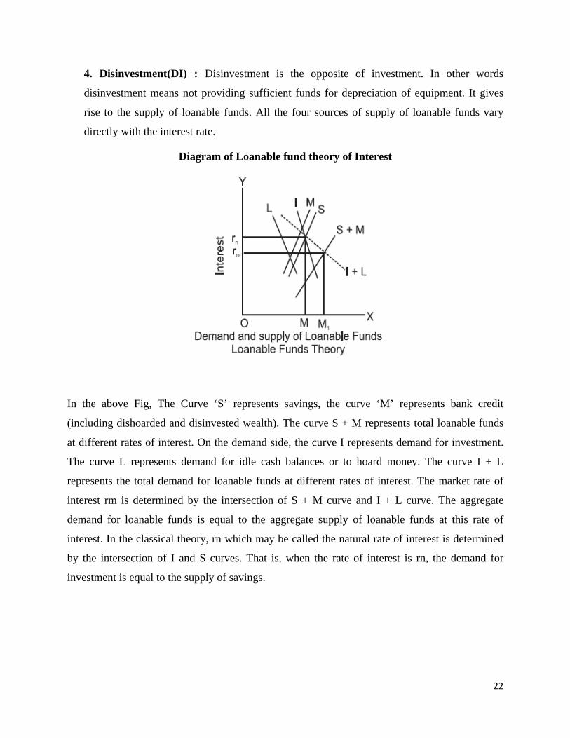
4. Disinvestment(DI) : Disinvestment is the opposite of investment. In other words

disinvestment means not providing sufficient funds for depreciation of equipment. It gives

rise to the supply of loanable funds. All the four sources of supply of loanable funds vary

directly with the interest rate.

Diagram of Loanable fund theory of Interest

In the above Fig, The Curve ‘S’ represents savings, the curve ‘M’ represents bank credit

(including dishoarded and disinvested wealth). The curve S + M represents total loanable funds

at different rates of interest. On the demand side, the curve I represents demand for investment.

The curve L represents demand for idle cash balances or to hoard money. The curve I + L

represents the total demand for loanable funds at different rates of interest. The market rate of

interest rm is determined by the intersection of S + M curve and I + L curve. The aggregate

demand for loanable funds is equal to the aggregate supply of loanable funds at this rate of

interest. In the classical theory, rn which may be called the natural rate of interest is determined

by the intersection of I and S curves. That is, when the rate of interest is rn, the demand for

investment is equal to the supply of savings.

22  

CRITICISMS OF LOANABLE FUND THEORY OF INTEREST

1. Many factors have been included in this theory.Still ther are many more factors.Two

such factors are 1)Asymmetric Information and 2) Moral Hazard.In practice larger firms, due

to their political powers, are able to get huge bank credit at lower interest rates.But due to

NPAs, (Non-Performing Assets)small firms and depositors lose their interest income. The

loanable funds theory is “indeterminate”’ unless the income level is already known. (This can

be studied in 12th standard Economics)

2. It is very difficult to combine real factors like savings and investment with monetary

factors like bank credit and liquidity preference.

KEYNES’ LIQUIDITY PREFERENCE THEORY OF INTEREST OR THE

MONETARY THEORY OF INTEREST

Keynes propounded the Liquidity Preference Theory of Interest in his famous book, “The

General Theory of Employment, Interest and Money” in 1936.

According to Keynes, interest is purely a monetary phenomenon because the rate of interest is

calculated in terms of money. To him, “interest is the reward for parting with liquidity for a

specifi ed period of time”.

According to Keynes, interest is purely a monetary phenomenon because the rate of interest is

calculated in terms of money. To him, “interest is the reward for parting with liquidity for a

specifi ed period of time”.

MOTIVES OF DEMAND FOR MONEY

According to Keynes, people have liquidity preference for three motives. They are;

1. Transaction motive

2. Precautionary motive; and

3. Speculative motive.

23  

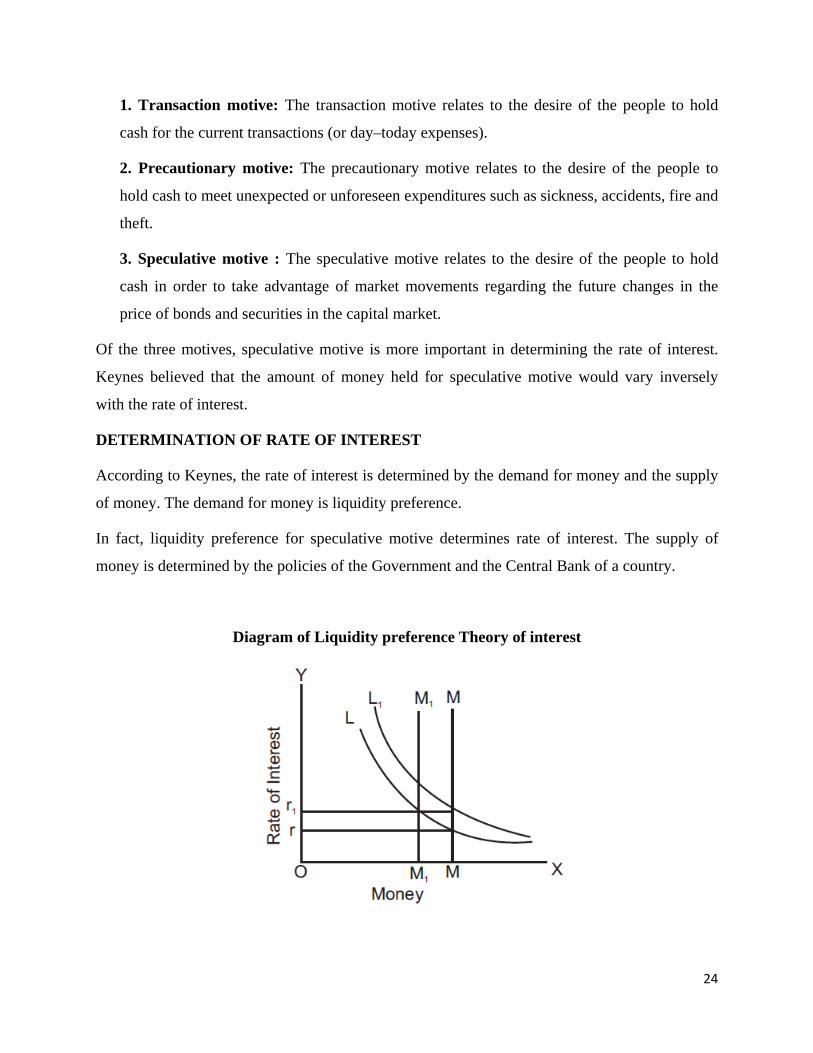
1. Transaction motive: The transaction motive relates to the desire of the people to hold

cash for the current transactions (or day–today expenses).

2. Precautionary motive: The precautionary motive relates to the desire of the people to

hold cash to meet unexpected or unforeseen expenditures such as sickness, accidents, fire and

theft.

3. Speculative motive : The speculative motive relates to the desire of the people to hold

cash in order to take advantage of market movements regarding the future changes in the

price of bonds and securities in the capital market.

Of the three motives, speculative motive is more important in determining the rate of interest.

Keynes believed that the amount of money held for speculative motive would vary inversely

with the rate of interest.

DETERMINATION OF RATE OF INTEREST

According to Keynes, the rate of interest is determined by the demand for money and the supply

of money. The demand for money is liquidity preference.

In fact, liquidity preference for speculative motive determines rate of interest. The supply of

money is determined by the policies of the Government and the Central Bank of a country.

Diagram of Liquidity preference Theory of interest

24  

In the above figure, Liquidity preference is shown by L and the supply of money is represented

by M and the rate of interest is indicated by r. Rate of interest is determined by the intersection of

L and M curves. There will be increase in the rate of interest to r1 ,when there is increase in

demand for money to L1 or by a decrease in the supply of money to M1 .

CRITICISMS

1. This theory does not explain the existence of different interest rates prevailing in the

market at the same time.

2. It explains interest rate only in the short-run.

PROFIT

Profits are the reward for organization or entrepreneurship. Risk- taking and uncertainty-bearing

are the main functions of an entrepreneur. So we may consider profit as the reward for the above

functions.

Profit is a return to the entrepreneur for the use of his entrepreneurial ability. It is the net income

of the organizer. In other words, profit is the amount left with the entrepreneur after he has

payments made for all the other factors (land, labour and capital) used by him in the production

process.

CONCEPT OF PROFIT

a. Gross Profit: Gross Profit is the surplus which accrues to a firm when it subtracts its Total

Expenditure from its Total Revenue.

Gross Profit = Total Revenue - Total cost

b. Net Profit: Net or pure or economic or true profit is the residual left with entrepreneur after

deducting from Gross profit the remuneration for the self-owned factors of production, which are

called implicit cost.

Net Profit = Gross Profit - Implicit costs

25  

c. Normal Profit: It refers to the minimum expected return to stay in business.

d. Super Normal Profit: Super normal profits are over and above the normal profit.

Super Normal Profit = Actual profit - Normal profit

THEORIES OF PROFIT

1. The rent theory of profits

2. The marginal productivity theory of profits

3. The wages theory of profits

4. The dynamic theory of profits

5. The innovation theory of profits

6. The risk theory of profits, and

7. The uncertainty – bearing theory of profits.

RENT THEORY OF PROFIT

This theory is associated with Francis Walker.

In his view, profits are the “rent of ability” and they are similar to rent. Rent arises because of

differences in fertility of land. Similarly profits arise because of differences in ability. That is

why it is called the “rent of ability”.

CRITICISMS:

1. The theory provides no explanation to the share of profits of the shareholders of joint-stock

companies

2. there cannot be a perfect similarity between rent and profit. Rents can never be negative

while profits can be negative when the entrepreneur suffers losses.

3. Walker has explained surplus profit. He has nothing to say about other types of profits and

the size of the profit.

26  

WAGE THEORY OF PROFIT

This theory was advanced by the American economist Prof. Taussig.

According to Prof. Taussig, profits are not different from wages. Profits are the wages of the

entrepreneur for his special ability. Profits are the wages of management.

CRITICISMS:

The theory has been criticized on the following points;

1. There are basic differences between wages and profits. Wages are fixed and are a

stipulated income, while profits are uncertain and are residual incomes

2. It is the entrepreneur who undertakes risks in any production process while the wage

earner is free from undertaking any such risks.

3. The theory fails to explain the reason as to why the shareholders of a company receive

profits while they do not put in any labour.

MARGINAL PRODUCTIVITY THEORY OF PROFIT

The chief exponents of the theory are Edgeworth, Chapman, Stigler and Stonier.

The theory is an application of the general theory of distribution. According to this theory, under

perfect competition, profits will be equal to the value of the marginal product of

entrepreneur/organizer.

27  

THE DYNAMIC THEORY OF PROFITS

This theory was propounded by the American economist J.B.Clark.

According to him, profit is the difference between price and cost of production of the

commodity. Hence, profit is the reward for dynamic changes in society. Further he points out

that, profit cannot arise in a static society. At present several changes are taking place in a

dynamic society. Changes are permanent.

According to Clark, the following five main changes are taking place in a dynamic society.

1. Population is increasing

2. Volume of Capital is increasing.

3. Methods of production are improving.

4. Forms of industrial organization are changing.

5. The wants of consumer are multiplying.

INNOVATION THEORY OF PROFITS

Innovation theory of profit was propounded by Josephs. A.Schumpeter.

According to him, an entrepreneur is not only an undertaker of a business, but also an innovator

in the process of production. To him, profit is the reward for “innovation”. Innovation means

invention put into commercial practice.

An innovation may consist of the following:

1. Introduction of a new product.

2. Introduction of a new method of production.

3. Opening up of a new market.

4. Discovery of new raw materials

5. Reorganization of an industry / firm.

28  

29  

THE RISK - BEARING THEORY OF PROFITS

Risk bearing theory of profit was propounded by the American economist F.B.Hawley.

According to him, profit is the reward for “risk taking” in business. Risk taking is an essential

function of the entrepreneur and is the basis of profit. It is a well known fact that every business

involves some risks.

Every entrepreneur produces goods in anticipation of demand. If his anticipation of demand is

correct, then there will be profit and if it is incorrect, there will be loss. It is the profit that

induces the entrepreneurs to undertake such risks.

THE UNCERTAINITY-BEARING THEORY OF PROFITS

Uncertainty theory was propounded by the American economist Frank H.Knight.

He distinguishes between “insurable” and “non-insurable” risks.

Insurable Risks (Known Risk): Certain risks are measurable or calculable. Some of the

examples of these risks are the risk of fire, theft and natural disasters. Hence, they are insurable.

Such risks are compensated by the Insurance Companies.

Non-Insurable Risks (Unknown Risk): There are some risks which are immeasurable or

incalculable. The probability of their occurrence cannot be anticipated because of the presence of

uncertainty in them. Some of the examples of these risks are competition, market condition,

technology change and public policy. No Insurance Company can undertake these risks. Hence,

they are non insurable.

When an entrepreneur takes himself the burden of facing an uncertain event, he secures

remuneration. That remuneration is “profit”.

*******