UNIT 1 FLUID PROPERTIES AND FLUID STATICS …CE8302 FLUID MECHANICS II year / III Sem Civil...
59
CE8302 FLUID MECHANICS II year / III Sem Civil Engineering 1 UNIT 1 FLUID PROPERTIES AND FLUID STATICS PART – A (2 MARKS) 1. Define fluids. Fluid may be defined as a substance which is capable of flowing. It has no definite shape of its own, but confirms to the shape of the containing vessel. 2. What are the properties of ideal fluid? Ideal fluids have following properties i) It is incompressible ii) It has zero viscosity iii) Shear force is zero 3. What are the properties of real fluid? Real fluids have following properties i) It is compressible ii) They are viscous in nature iii) Shear force exists always in such fluids. 4. Define density and specific weight. Density is defined as mass per unit volume (kg/m 3 ) Specific weight is defined as weight possessed per unit volume (N/m 3 ) 5. Define Specific volume and Specific Gravity. Specific volume is defined as volume of fluid occupied by unit mass (m 3 /kg) Specific gravity is defined as the ratio of specific weight of fluid to the specific weight of standard fluid. 6. Define Surface tension and Capillarity. Surface tension is due to the force of cohesion between the liquid particles at the free surface. Capillary is a phenomenon of rise or fall of liquid surface relative to the adjacent general level of liquid. 7. Define Viscosity. It is defined as the property of a liquid due to which it offers resistance to the movement of one layer of liquid over another adjacent layer. 8. Define kinematic viscosity. It is defined as the ratio of dynamic viscosity to mass density. (m²/sec) 9. Define Relative or Specific viscosity. It is the ratio of dynamic viscosity of fluid to dynamic viscosity of water at 20°C. 10. Define Compressibility. It is the property by virtue of which fluids undergoes a change in volume under the action of external pressure. 11. Define Newtonian law of Viscosity. According to Newton’s law of viscosity the shear force F acting between two layers of fluid is proportional to the difference in their velocities du
Transcript of UNIT 1 FLUID PROPERTIES AND FLUID STATICS …CE8302 FLUID MECHANICS II year / III Sem Civil...
CE8302 FLUID MECHANICS II year / III Sem Civil Engineering
1
UNIT 1
FLUID PROPERTIES AND FLUID STATICS
PART – A (2 MARKS)
1. Define fluids.
Fluid may be defined as a substance which is capable of flowing. It has
no definite shape of its own, but confirms to the shape of the containing
vessel.
2. What are the properties of ideal fluid?
Ideal fluids have following
properties
i) It is incompressible
ii) It has zero viscosity
iii) Shear force is zero
3. What are the properties of real fluid?
Real fluids have following
properties
i) It is compressible
ii) They are viscous in nature
iii) Shear force exists always in such fluids.
4. Define density and specific weight.
Density is defined as mass per unit volume (kg/m3
)
Specific weight is defined as weight possessed per unit volume (N/m3)
5. Define Specific volume and Specific Gravity.
Specific volume is defined as volume of fluid occupied by unit mass
(m3/kg) Specific gravity is defined as the ratio of specific weight of
fluid to the specific weight of standard fluid.
6. Define Surface tension and Capillarity.
Surface tension is due to the force of cohesion between the liquid particles
at the free surface.
Capillary is a phenomenon of rise or fall of liquid surface relative to
the adjacent general level of liquid.
7. Define Viscosity.
It is defined as the property of a liquid due to which it offers resistance to
the movement of one layer of liquid over another adjacent layer.
8. Define kinematic viscosity.
It is defined as the ratio of dynamic viscosity to mass density. (m²/sec)
9. Define Relative or Specific viscosity. It is the ratio of dynamic viscosity of fluid to dynamic viscosity of water
at 20°C.
10. Define Compressibility.
It is the property by virtue of which fluids undergoes a change in volume
under the action of external pressure.
11. Define Newtonian law of Viscosity.
According to Newton’s law of viscosity the shear force F acting between
two layers of fluid is proportional to the difference in their velocities du
CE8302 FLUID MECHANICS II year / III Sem Civil Engineering
2015 - 2016
and area A of the plate and inversely proportional to the distance between
them.
12. What is cohesion and adhesion in fluids?
Cohesion is due to the force of attraction between the molecules of the
same liquid.
Adhesion is due to the force of attraction between the molecules of two
different liquids or between the molecules of the liquid and molecules of
the solid boundary surface.
13. State momentum of momentum equation?
It states that the resulting torque acting on a rotating fluid is equal to
the rate of change of moment of momentum
14. What is momentum equation
It is based on the law of conservation of momentum or on the momentum
principle It states that,the net force acting on a fluid mass is equal to the
change in momentum of flow per unit time in that direction.
PART – B(16 MARKS)
1. What are the gauge pressure and absolute pressure at a point 3 m below the free
surface of a liquid having a density of 1.53x10³ kg/m3 if the atmospheric pressure is
equivalent to 750 mm of mercury? The specific gravity of mercury is 13.6 and
density of water is 1000 kg/m3.
Solution
Depth of liquid, Z1 = 3 m Density of liquid, ρ1 = 1.53x10³ kg/m3
Atmospheric pressure head, Z0 = 750 mm of Hg
= 0.75 m of Hg
Atmospheric pressure, Patm = ρ0 x g x Z0
= (13.6 x 1000) x 9.81 x 0.75
= 100062 N/m2
Pressure at a point at a depth of 3 m from the free surface of a liquid
P = ρ1 x g x Z1
= (1.53 x 1000) x 9.81 x 3
= 45028 N/m2
Gauge pressure, P = 45028 N/m2
Absolute pressure, = Gauge pressure + Atmospheric pressure
= 45028 + 100062
= 145090 N/m2
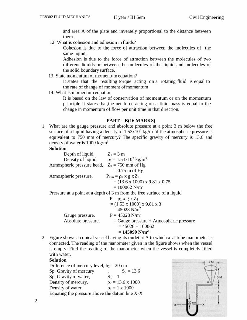
2. Figure shows a conical vessel having its outlet at A to which a U-tube manometer is
connected. The reading of the manometer given in the figure shows when the vessel
is empty. Find the reading of the manometer when the vessel is completely filled
with water.
Solution
Difference of mercury level, h2 = 20 cm Sp. Gravity of mercury , S2 = 13.6
Sp. Gravity of water, S1 = 1
Density of mercury, ρ2 = 13.6 x 1000
Density of water, ρ1 = 1 x 1000
Equating the pressure above the datum line X-X
2
CE8302 FLUID MECHANICS II year / III Sem Civil Engineering
m. The opening is 2 m
Ρ2 x g x h2 = ρ1 x g x h1
(13.6 x 1000) x 9.81 x 0.2 = 1000 x 9.81 x h1
h1 = 2.72 m of water
Pressure in left limb = Pressure in right limb
13.6 x 1000 x 9.81 x (0.2 + 2y/100) = 1000 x 9.81 x (3 + h1 + y/100)
(27.2y – y)/100 = 3.0
y = 11.45 cm
The difference of mercury level in two limbs,
= (20 + 2y) cm of mercury level
= 20 + (2 x 11.45)
= 42.90 cm of mercury
Reading of manometer = 42.90 cm
3. Determine the total pressure on a circular plate of diameter 1.5 m which is placed
vertically in water in such a way that the center of the plate is 3 m below the free
surface of water. Find the position of centre of pressure also.
Solution
Diameter of plate, d = 1.5 m
Area, A = (Π/4) x 1.52 = 1.767 m2
h = 3.0 m
Total pressure,F = ρ x g x A x h
= 1000 x 9.81 x 1.767 x 3
= 52002.81 N
Position of centre of pressure, h* = (IG/Ah) + h
IG = (Π x d4)/64
= 0.2485 m4
h* = (0.2485/(1.767 x 3)) + 3
Position of centre of pressure = 3.0468 m
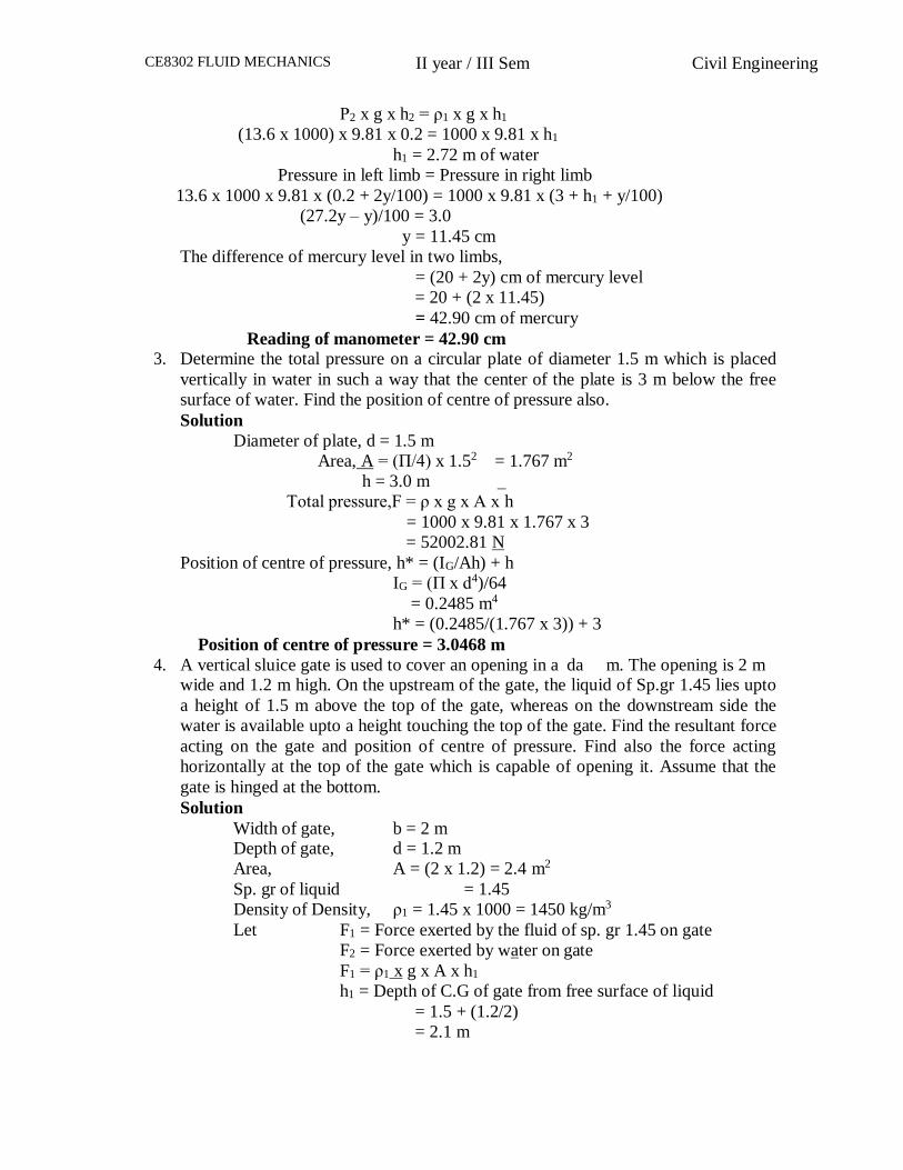
4. A vertical sluice gate is used to cover an opening in a da wide and 1.2 m high. On the upstream of the gate, the liquid of Sp.gr 1.45 lies upto
a height of 1.5 m above the top of the gate, whereas on the downstream side the
water is available upto a height touching the top of the gate. Find the resultant force
acting on the gate and position of centre of pressure. Find also the force acting
horizontally at the top of the gate which is capable of opening it. Assume that the
gate is hinged at the bottom.
Solution
Width of gate, b = 2 m Depth of gate, d = 1.2 m
Area, A = (2 x 1.2) = 2.4 m2
Sp. gr of liquid = 1.45
Density of Density, ρ1 = 1.45 x 1000 = 1450 kg/m3
Let F1 = Force exerted by the fluid of sp. gr 1.45 on gate
F2 = Force exerted by water on gate
F1 = ρ1 x g x A x h1
h1 = Depth of C.G of gate from free surface of liquid
= 1.5 + (1.2/2)
= 2.1 m
CE8302 FLUID MECHANICS II year / III Sem Civil Engineering
F1 = 1450 x 9.81 x 2.4 x 2.1 = 71691 N F2 = ρ2 x g x A x h2
Ρ2 = 1 x 1000 kg/m3
h2 = 1.2/2 = 0.6 m
F2 = 1000 x 9.81 x 2.4 x 0.6 = 71691 N
(i) Resultant force on the gate = F1 - F2= 71691 – 14126 = 57565 N
(ii) Position of centre of pressure of resultant force
The force F1 will be acting at a depth of h1* from free surface
of liquid, given by the relation,
h1* = (IG/A h1) + h1
IG = bd3/12 = 2 x 1.23/12 = 0.288 m4
h1* = 0.288 / (2.4 x 2.1) + 2.1 = 2.1571 m
Distance of F1 from hinge,
= (1.5 + 1.2) - h1* = 2.7 – 2.1571 = 0.5429 m
h2* = (IG/A h2) + h2
= (0.288/2.4 x 0.6) + 0.6 = 0.8 m
Distance of F2 from hinge = 1.2 – 0.8 = 0.4 m
The resultant force 57565 N will be acting at a distance given by
= ((71691 x 0.5429) – (14126 0.4))/57565
= 0.578 m above the hinge
(iii) Force at the top of gate which is capable of opening the gate
F x 1.2 + F2 x 0.4 = F1 x 0.5429 F = ((71691 x 0.5429)- (14126 x 0.4))/1.2
F = 27725.5 N
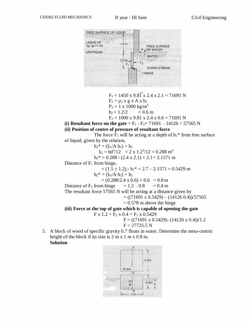
5. A block of wood of specific gravity 0.7 floats in water. Determine the meta-centric
height of the block if its size is 2 m x 1 m x 0.8 m.
Solution
CE8302 FLUID MECHANICS II year / III Sem Civil Engineering
Dimension of block = 2 x 1 x 0.8
Depth of immersion = h m
Sp. gr of wood = 0.7
Weight of wooden piece = Weight density of wood x Volume
= 0.7 x 1000 x 9.81 x 2 x 1 x 0.8
Weight of water displaced = Weight density of water x Volume of the wood
submerged in water
= 1000 x 9.81 x 2 x 1 x h
Weight of wooden piece = Weight of water displaced
0.7 x 1000 x 9.81 x 2 x 1 x 0.8 = 1000 x 9.81 x 2 x 1 x h
h = 0.56 m
Distance of centre of buoyancy from bottom,
AB = (h/2) = 0.56/2 = 0.28 m
AG = 0.8/2.0 = 0.4 m
BG = AG – AB = 0.4 – 0.28 = 0.12 m
The meta-centric height, GM = (I/A) – BG
= (2 x 13 / 12)/ (2 x 1 x 0.56)
= 0.0288 m
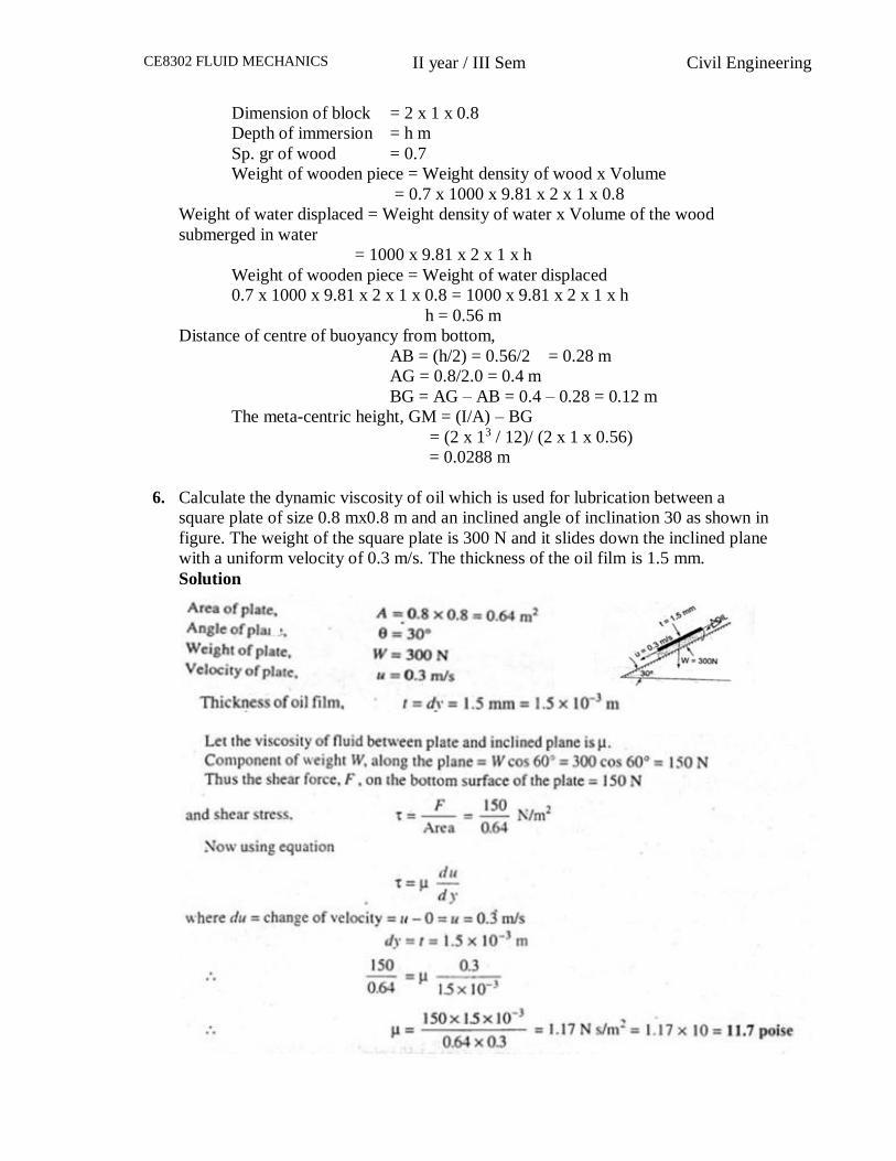
6. Calculate the dynamic viscosity of oil which is used for lubrication between a
square plate of size 0.8 mx0.8 m and an inclined angle of inclination 30 as shown in
figure. The weight of the square plate is 300 N and it slides down the inclined plane
with a uniform velocity of 0.3 m/s. The thickness of the oil film is 1.5 mm.
Solution
CE8302 FLUID MECHANICS II year / III Sem Civil Engineering
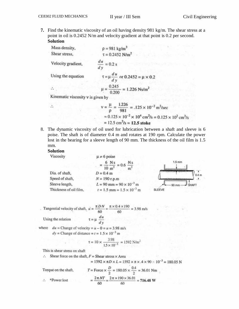
7. Find the kinematic viscosity of an oil having density 981 kg/m. The shear stress at a
point in oil is 0.2452 N/m and velocity gradient at that point is 0.2 per second.
Solution
8. The dynamic viscosity of oil used for lubrication between a shaft and sleeve is 6
poise. The shaft is of diameter 0.4 m and rotates at 190 rpm. Calculate the power
lost in the bearing for a sleeve length of 90 mm. The thickness of the oil film is 1.5
mm.
Solution
CE8302 FLUID MECHANICS II year / III Sem Civil Engineering
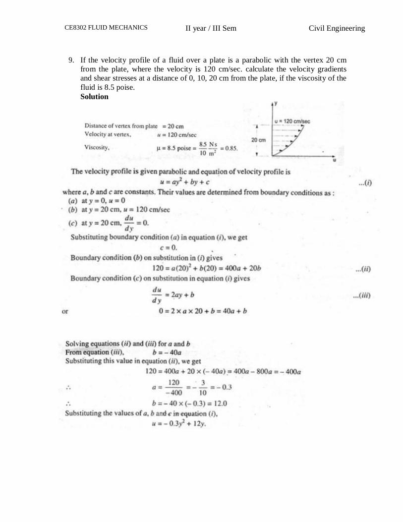
9. If the velocity profile of a fluid over a plate is a parabolic with the vertex 20 cm
from the plate, where the velocity is 120 cm/sec. calculate the velocity gradients
and shear stresses at a distance of 0, 10, 20 cm from the plate, if the viscosity of the
fluid is 8.5 poise.
Solution
CE8302 FLUID MECHANICS II year / III Sem Civil Engineering
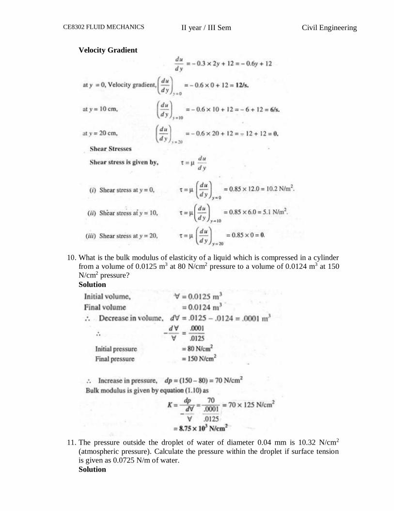
Velocity Gradient
10. What is the bulk modulus of elasticity of a liquid which is compressed in a cylinder
from a volume of 0.0125 m3 at 80 N/cm2 pressure to a volume of 0.0124 m3 at 150
N/cm2 pressure?
Solution
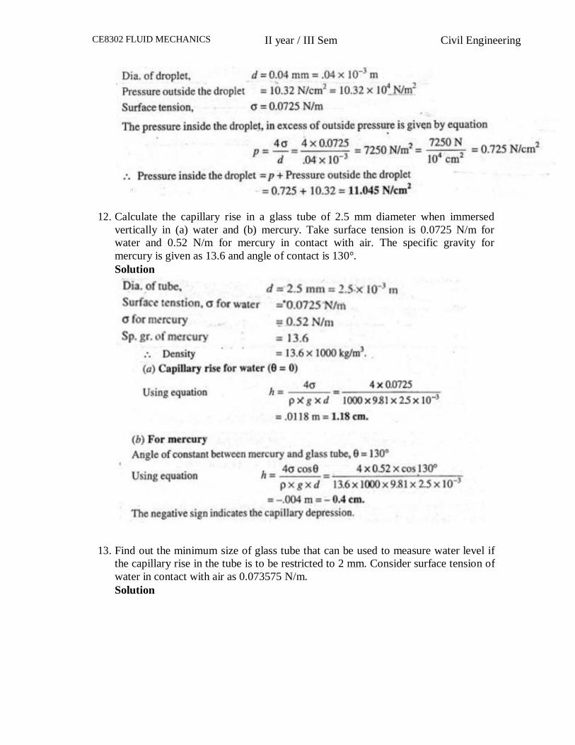
11. The pressure outside the droplet of water of diameter 0.04 mm is 10.32 N/cm2
(atmospheric pressure). Calculate the pressure within the droplet if surface tension
is given as 0.0725 N/m of water.
Solution
CE8302 FLUID MECHANICS II year / III Sem Civil Engineering
12. Calculate the capillary rise in a glass tube of 2.5 mm diameter when immersed
vertically in (a) water and (b) mercury. Take surface tension is 0.0725 N/m for
water and 0.52 N/m for mercury in contact with air. The specific gravity for
mercury is given as 13.6 and angle of contact is 130°.
Solution
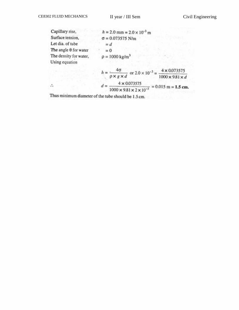
13. Find out the minimum size of glass tube that can be used to measure water level if
the capillary rise in the tube is to be restricted to 2 mm. Consider surface tension of
water in contact with air as 0.073575 N/m.
Solution
CE8302 FLUID MECHANICS II year / III Sem Civil Engineering
CE8302 FLUID MECHANICS II year / III Sem Civil Engineering
UNIT 2
FLUID KINEMATICS AND DYNAMICS
PART – A (2 MARKS)
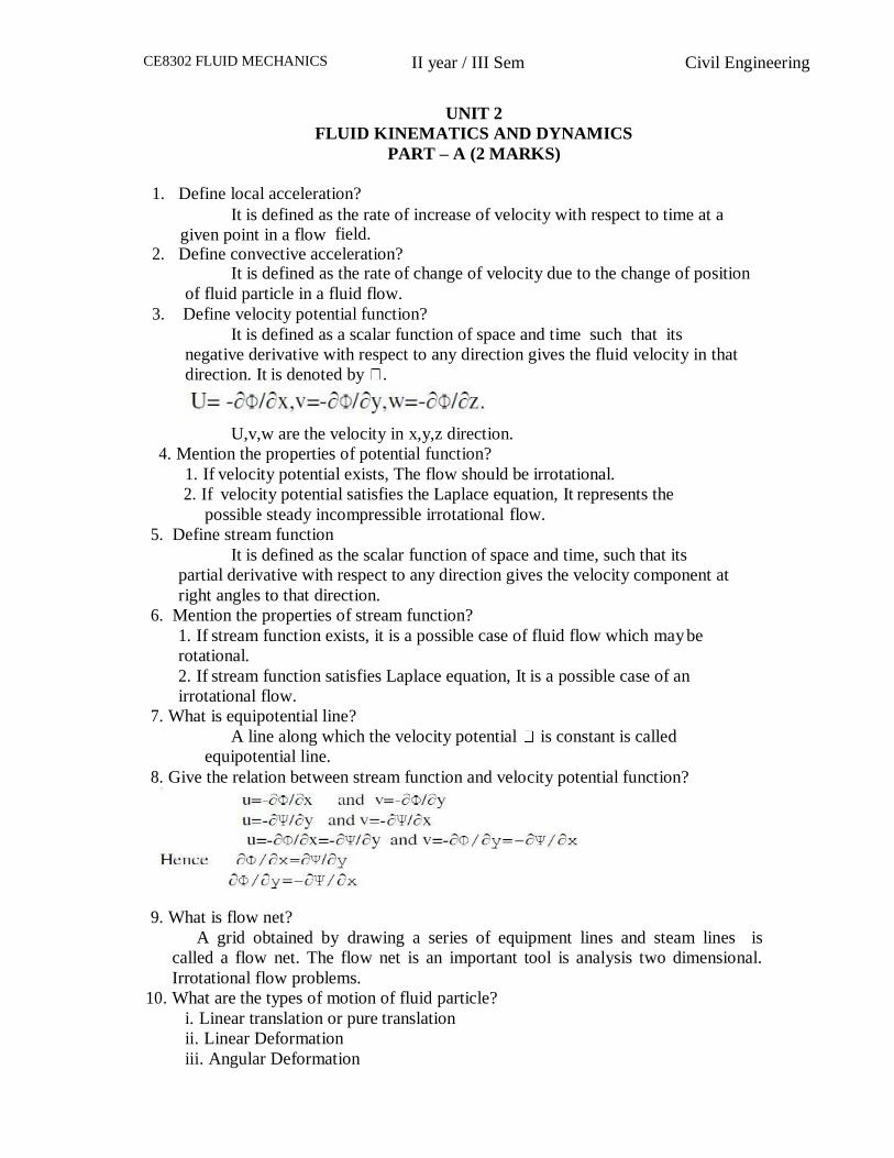
1. Define local acceleration?
It is defined as the rate of increase of velocity with respect to time at a
given point in a flow field. 2. Define convective acceleration?
It is defined as the rate of change of velocity due to the change of position
of fluid particle in a fluid flow.
3. Define velocity potential function?
It is defined as a scalar function of space and time such that its
negative derivative with respect to any direction gives the fluid velocity in that
direction. It is denoted by .
U,v,w are the velocity in x,y,z direction.
4. Mention the properties of potential function?
1. If velocity potential exists, The flow should be irrotational.
2. If velocity potential satisfies the Laplace equation, It represents the
possible steady incompressible irrotational flow.
5. Define stream function
It is defined as the scalar function of space and time, such that its
partial derivative with respect to any direction gives the velocity component at
right angles to that direction.
6. Mention the properties of stream function?
1. If stream function exists, it is a possible case of fluid flow which may be
rotational.
2. If stream function satisfies Laplace equation, It is a possible case of an
irrotational flow.
7. What is equipotential line?
A line along which the velocity potential is constant is called
equipotential line.
8. Give the relation between stream function and velocity potential function?
9. What is flow net?
A grid obtained by drawing a series of equipment lines and steam lines is
called a flow net. The flow net is an important tool is analysis two dimensional.
Irrotational flow problems.
10. What are the types of motion of fluid particle?
i. Linear translation or pure translation
ii. Linear Deformation
iii. Angular Deformation
CE8302 FLUID MECHANICS II year / III Sem Civil Engineering
iv. Rotation.
11. What is linear translation?
It is defined as the movement of a fluid element in such a way that it
moves bodily from one position to represents in new position by a’b’&c’d’ are
parallel.
12. What is linear deformation?
It is defined as the deformation of a fluid element in linear direction when
the element moves the axes of the element in the deformation position and un
deformation position are parallel but their lengths changes.
13. Define rotation of fluid element? It is defined as the movement of a fluid element in such a way
that both of Rotate in same direction. It is equal to1/2( v/ x-
u/ y) for a two-dimensional element x, y plane. x=1/2( w/ y- v/ z)
y=1/2( u/ z- w/ x)
z=1/2( u/ x- u/ y)
14. Define vortex flow mention its types? Vortex flow is defined as the flow of a fluid along a curved path or the
flow of a rotating mass of fluid is known as vortex flow.
i. Forced vortex flow.
ii. Free vortex flow.
15. Define free vortex flow?
When no external torque is required to rotate the fluid mass that type of flow
Is called free vortex flow.
16. Define forced vortex flow?
Forced vortex flow is defined as that type of vortex flow in which some
external Torque is required to rotate the fluid mass. The fluid mass in the type
of flow rotates at constant Angular velocity ‘w’.The tangential velocity of any
fluid particle is given by v=cosr.
PART – B(16 MARKS)
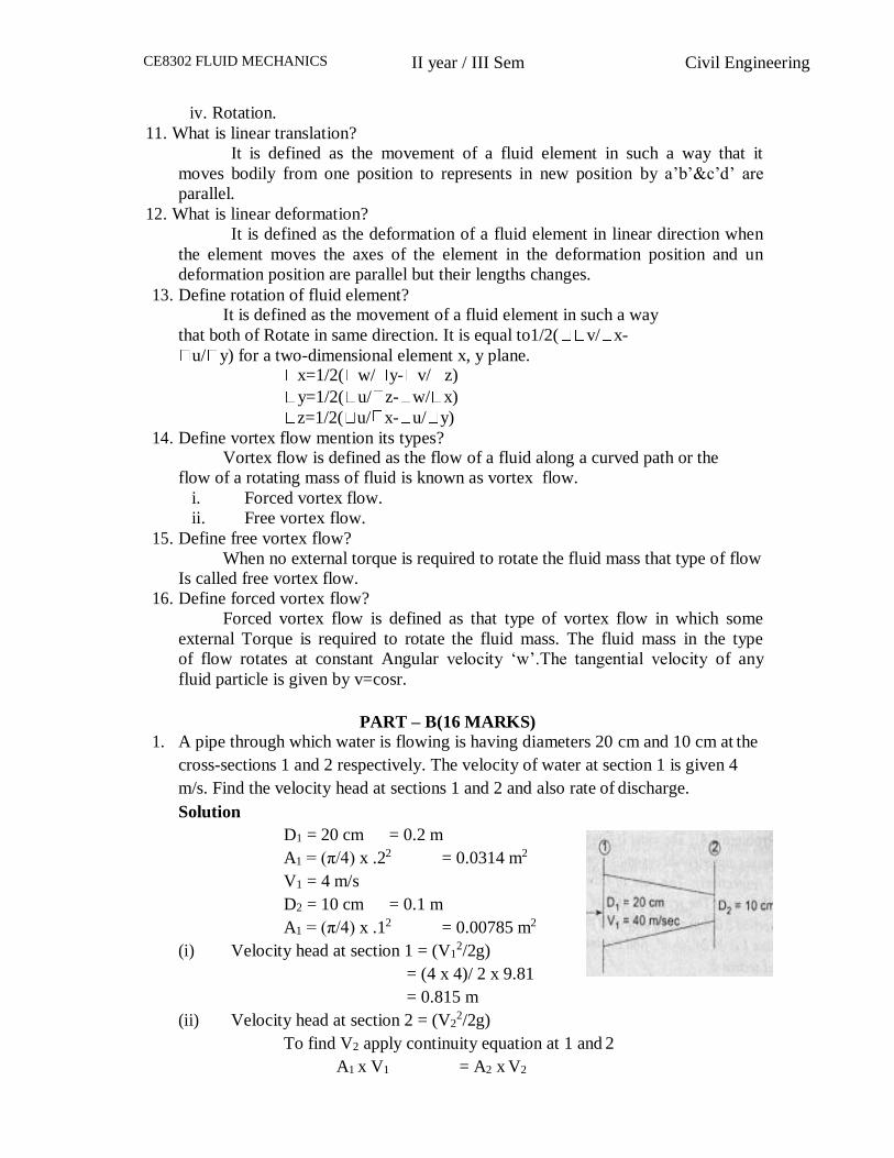
1. A pipe through which water is flowing is having diameters 20 cm and 10 cm at the
cross-sections 1 and 2 respectively. The velocity of water at section 1 is given 4
m/s. Find the velocity head at sections 1 and 2 and also rate of discharge.
Solution
D1 = 20 cm = 0.2 m
A1 = (π/4) x .22 = 0.0314 m2
V1 = 4 m/s
D2 = 10 cm = 0.1 m
A1 = (π/4) x .12 = 0.00785 m2
(i) Velocity head at section 1 = (V12/2g)
= (4 x 4)/ 2 x 9.81
= 0.815 m
(ii) Velocity head at section 2 = (V22/2g)
To find V2 apply continuity equation at 1 and 2
A1 x V1 = A2 x V2
CE8302 FLUID MECHANICS II year / III Sem Civil Engineering
3
V2 = (A1 x V1)/ A2
= (0.0314 x 4)/0.00785
= 16 m/s
Velocity head at section 2 = (V22/2g) = (16 x 16)/2 x 9.81
= 83.047 m
(iii) Rate of discharge = A1 x V1 (or) A2 x V2
= (0.0314 x 4)
= 125.6 litres
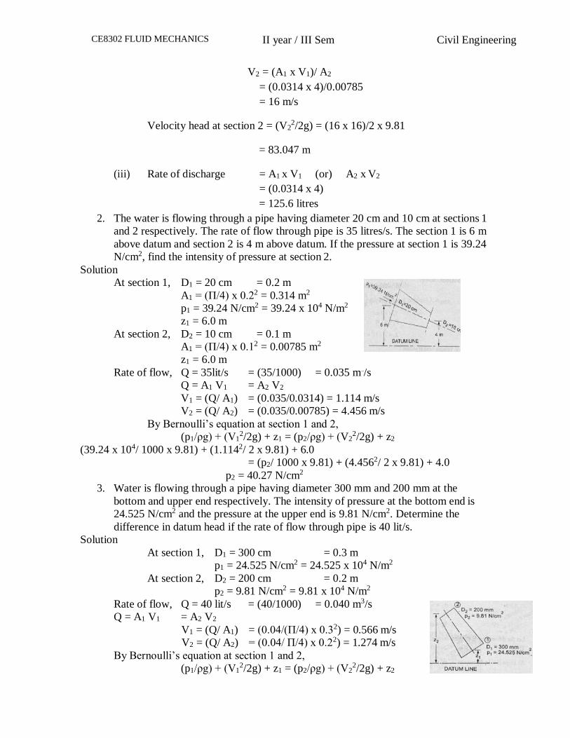
2. The water is flowing through a pipe having diameter 20 cm and 10 cm at sections 1
and 2 respectively. The rate of flow through pipe is 35 litres/s. The section 1 is 6 m
above datum and section 2 is 4 m above datum. If the pressure at section 1 is 39.24
N/cm2, find the intensity of pressure at section 2.
Solution
At section 1, D1 = 20 cm = 0.2 m
A1 = (Π/4) x 0.22 = 0.314 m2
p1 = 39.24 N/cm2 = 39.24 x 10⁴ N/m2
z1 = 6.0 m
At section 2, D2 = 10 cm = 0.1 m
A1 = (Π/4) x 0.12 = 0.00785 m2
z1 = 6.0 m
Rate of flow, Q = 35lit/s = (35/1000) = 0.035 m /s
Q = A1 V1 = A2 V2
V1 = (Q/ A1) = (0.035/0.0314) = 1.114 m/s
V2 = (Q/ A2) = (0.035/0.00785) = 4.456 m/s
By Bernoulli’s equation at section 1 and 2,
(p1/ρg) + (V12/2g) + z1 = (p2/ρg) + (V2
2/2g) + z2
(39.24 x 10⁴/ 1000 x 9.81) + (1.1142/ 2 x 9.81) + 6.0
= (p2/ 1000 x 9.81) + (4.4562/ 2 x 9.81) + 4.0
p2 = 40.27 N/cm2
3. Water is flowing through a pipe having diameter 300 mm and 200 mm at the
bottom and upper end respectively. The intensity of pressure at the bottom end is
24.525 N/cm2 and the pressure at the upper end is 9.81 N/cm2. Determine the
difference in datum head if the rate of flow through pipe is 40 lit/s.
Solution
At section 1, D1 = 300 cm = 0.3 m
p1 = 24.525 N/cm2 = 24.525 x 10⁴ N/m2
At section 2, D2 = 200 cm = 0.2 m
p2 = 9.81 N/cm2 = 9.81 x 10⁴ N/m2
Rate of flow, Q = 40 lit/s = (40/1000) = 0.040 m3/s
Q = A1 V1 = A2 V2
V1 = (Q/ A1) = (0.04/(Π/4) x 0.32) = 0.566 m/s
V2 = (Q/ A2) = (0.04/ Π/4) x 0.22) = 1.274 m/s
By Bernoulli’s equation at section 1 and 2,
(p1/ρg) + (V12/2g) + z1 = (p2/ρg) + (V2
2/2g) + z2
CE8302 FLUID MECHANICS II year / III Sem Civil Engineering
(24.525 x 10⁴/ 1000 x 9.81) + (0.5662/ 2 x 9.81) + z1 =
(9.81 x 10⁴/ 1000 x 9.81) + (1.2742/ 2 x 9.81) + z2
z2 - z1 = 25.32 – 11.623 = 13.70 m
Difference in datum head = 13.70 m
4. In a two dimensional incompressible flow the fluid velocity components
are given by u = x – 4y and v = -y – 4x, Where u and v are x and y
components of flow velocity. Show that the flow satisfies the continuity
equation and obtain the expression for stream function. If the flow is
potential, obtain also the expression for the velocity potential.
Solution:
u = x – 4y and v = -y – 4x
(∂ u /∂ x) = 1and(∂ v /∂ y) = -1
(∂ u /∂ x)+ (∂ v /∂ y) = 1-1 = 0.
Hence it satisfies continuity equation and the flow is continuous
and velocity potential exists.
Let φ be the velocity potential.
(∂φ/∂x) = -u = - (x – 4y) = -x + 4y (1)
(∂ φ /∂ y) = -v = - (-y – 4x) = y + 4x (2)
Integrating Eq. 1, we get
φ = (-x2
/2) + 4xy + C (3)
Differentiating Eq. 3 w.r.t. y, we get
(∂ φ /∂ y) = 0 + 4x + (∂ C /∂ y) ⇒ y + 4x Hence, we get (∂ C /∂ y) = y
Integrating the above expression, we get C = y2
/2
Substituting the value of C in Eq. 3, we get the general expression as
φ = (-x2 /2) + 4xy + y2 /2
Stream Function
Let ψ be the velocity potential.
(∂ ψ /∂ x) = v = (-y – 4x) = -y - 4x (4)
(∂ ψ /∂ y) = u = -(x – 4y) = -x + 4y (5)
Integrating Eq. 4, we get
ψ = - y x - 4 (x2/2) + K (6)
Differentiating Eq. 6 w.r.t. y, we get
(∂ ψ /∂ y) = - x – 0 + (∂ K /∂ y) ⇒ -x + 4 y Hence, we get (∂ K /∂ y) = 4 y
Integrating the above expression, we get C = 4 y2
/2 = 2 y2
Substituting the value of K in Eq. 6, we get the general expression as
ψ = - y x - 2 x2 + 2 y2
5. The stream function and velocity potential for a flow are given by ψ = 2xy
and φ = x2
– y2. Show that the conditions for continuity and irrotational flow
are satisfied.
Solution: From the properties of Stream function, the existence of stream function
CE8302 FLUID MECHANICS II year / III Sem Civil Engineering
shows the possible case of flow and if it satisfies Laplace equation, then
the flow is irrotational.
(i) ψ = 2xy
(∂ ψ /∂ x) = 2 y and (∂ ψ /∂ y) = 2 x
(∂ 2
ψ /∂ x2
) = 0 and
(∂ 2
ψ /∂ y2
) = 0
(∂ 2
ψ /∂ x ∂ y) = 2 and
(∂ 2
ψ /∂ y ∂ x) = 2
(∂ 2
ψ /∂ x ∂ y) = (∂ 2
ψ /∂ y ∂ x)
Hence the flow is Continuous.
(∂ 2 ψ /∂ x2) + (∂ 2ψ /∂ y2 ) = 0
As it satisfies the Laplace equation, the flow is irrotational. From the
properties of Velocity potential, the existence of Velocity potential shows the
flow is irrotational and if it satisfies Laplace equation, then it is a possible case
of flow
(ii) φ = x2
– y2
(∂ φ /∂ x) = 2 x and (∂ φ /∂ y) = -2 y
(∂ 2
φ /∂ x2
) = 2 and (∂ 2
φ /∂ y2
) = -2
(∂ 2
φ /∂ x ∂ y) = 0 and (∂ 2
φ/∂ y ∂ x) = 0
(∂ 2 φ /∂ x ∂ y) = (∂ 2 φ /∂ y ∂ x)
Hence the flow is irrotational
(∂ 2
φ /∂ x2) + (∂
2 φ /∂ y
2) = 0
As it satisfies the Laplace equation, the flow is Continuous.
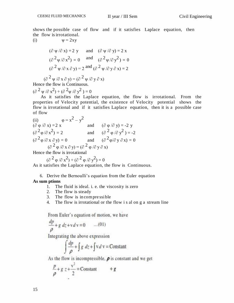
6. Derive the Bernoulli’s equation from the Euler equation
As sum ptions
1. The fluid is ideal. i. e. the viscosity is zero 2. The flow is steady
3. The flow is in com pre ssi ble
4. The flow is irrotational or the flow i s al on g a stream line
15
CE8302 FLUID MECHANICS II year / III Sem Civil Engineering
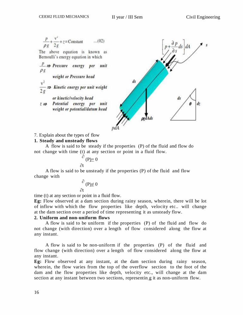
7. Explain about the types of flow
1. Steady and unsteady flows
A flow is said to be steady if the properties (P) of the fluid and flow do
not change with time (t) at any section or point in a fluid flow. ∂
(P)= 0
∂t A flow is said to be unsteady if the properties (P) of the fluid and flow
change with ∂
(P)≠ 0
∂t time (t) at any section or point in a fluid flow.
Eg: Flow observed at a dam section during rainy season, wherein, there will be lot
of inflow with which the flow properties like depth, velocity etc.. will change
at the dam section over a period of time representing it as unsteady flow.
2. Uniform and non-uniform flows
A flow is said to be uniform if the properties (P) of the fluid and flow do
not change (with direction) over a length of flow considered along the flow at
any instant.
A flow is said to be non-uniform if the properties (P) of the fluid and
flow change (with direction) over a length of flow considered along the flow at
any instant.
Eg: Flow observed at any instant, at the dam section during rainy season,
wherein, the flow varies from the top of the overflow section to the foot of the
dam and the flow properties like depth, velocity etc., will change at the dam
section at any instant between two sections, representin g it as non-uniform flow.
16
II year / III Sem CE6303 Mechanics of Fluids Civil Engineering
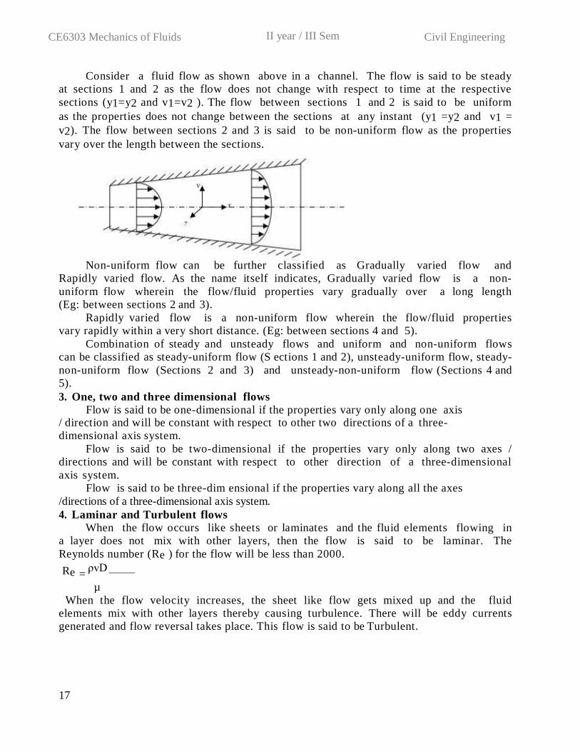
Consider a fluid flow as shown above in a channel. The flow is said to be steady
at sections 1 and 2 as the flow does not change with respect to time at the respective
sections (y1=y2 and v1=v2 ). The flow between sections 1 and 2 is said to be uniform
as the properties does not change between the sections at any instant (y1 =y2 and v1 =
v2). The flow between sections 2 and 3 is said to be non-uniform flow as the properties
vary over the length between the sections.
Non-uniform flow can be further classified as Gradually varied flow and
Rapidly varied flow. As the name itself indicates, Gradually varied flow is a non-
uniform flow wherein the flow/fluid properties vary gradually over a long length
(Eg: between sections 2 and 3).
Rapidly varied flow is a non-uniform flow wherein the flow/fluid properties
vary rapidly within a very short distance. (Eg: between sections 4 and 5).
Combination of steady and unsteady flows and uniform and non-uniform flows
can be classified as steady-uniform flow (S ections 1 and 2), unsteady-uniform flow, steady-
non-uniform flow (Sections 2 and 3) and unsteady-non-uniform flow (Sections 4 and
5).
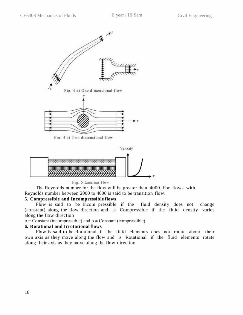
3. One, two and three dimensional flows
Flow is said to be one-dimensional if the properties vary only along one axis / direction and will be constant with respect to other two directions of a three-
dimensional axis system.
Flow is said to be two-dimensional if the properties vary only along two axes /
directions and will be constant with respect to other direction of a three-dimensional
axis system.
Flow is said to be three-dim ensional if the properties vary along all the axes
/directions of a three-dimensional axis system.
4. Laminar and Turbulent flows
When the flow occurs like sheets or laminates and the fluid elements flowing in
a layer does not mix with other layers, then the flow is said to be laminar. The
Reynolds number (Re ) for the flow will be less than 2000.
Re = ρvD
µ
When the flow velocity increases, the sheet like flow gets mixed up and the fluid
elements mix with other layers thereby causing turbulence. There will be eddy currents
generated and flow reversal takes place. This flow is said to be Turbulent.
17
II year / III Sem CE6303 Mechanics of Fluids Civil Engineering
The Reynolds number for the flow will be greater than 4000. For flows with
Reynolds number between 2000 to 4000 is said to be transition flow.
5. Compressible and Incompressible flows
Flow is said to be Incom pressible if the fluid density does not change
(constant) along the flow direction and is Compressible if the fluid density varies
along the flow direction
ρ = Constant (incompressible) and ρ ≠ Constant (compressible)
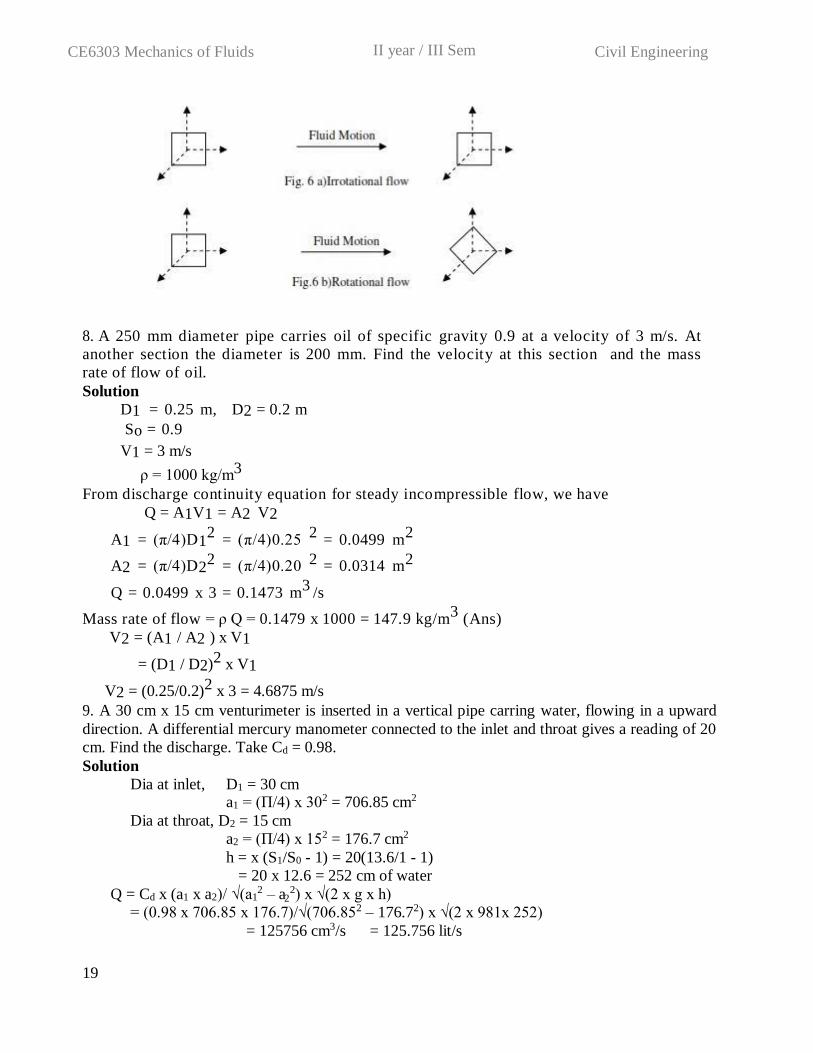
6. Rotational and Irrotational flows
Flow is said to be Rotational if the fluid elements does not rotate about their
own axis as they move along the flow and is Rotational if the fluid elements rotate
along their axis as they move along the flow direction
18
II year / III Sem CE6303 Mechanics of Fluids Civil Engineering
2
8. A 250 mm diameter pipe carries oil of specific gravity 0.9 at a velocity of 3 m/s. At
another section the diameter is 200 mm. Find the velocity at this section and the mass
rate of flow of oil.
Solution
D1 = 0.25 m, D2 = 0.2 m
So = 0.9
V1 = 3 m/s
ρ = 1000 kg/m3
From discharge continuity equation for steady incompressible flow, we have
Q = A1V1 = A2 V2
A1 = (π/4)D12
= (π/4)0.25 2
= 0.0499 m2
A2 = (π/4)D22 = (π/4)0.20 2 = 0.0314 m2
Q = 0.0499 x 3 = 0.1473 m3
/s
Mass rate of flow = ρ Q = 0.1479 x 1000 = 147.9 kg/m3
(Ans)
V2 = (A1 / A2 ) x V1
= (D1 / D2)2 x V1
V2 = (0.25/0.2)2 x 3 = 4.6875 m/s
9. A 30 cm x 15 cm venturimeter is inserted in a vertical pipe carring water, flowing in a upward
direction. A differential mercury manometer connected to the inlet and throat gives a reading of 20
cm. Find the discharge. Take Cd = 0.98.
Solution
Dia at inlet, D1 = 30 cm a1 = (Π/4) x 302 = 706.85 cm2
Dia at throat, D2 = 15 cm
a2 = (Π/4) x 152 = 176.7 cm2
h = x (S1/S0 - 1) = 20(13.6/1 - 1)
= 20 x 12.6 = 252 cm of water
Q = Cd x (a1 x a2)/ √(a12 – a 2) x √(2 x g x h)
= (0.98 x 706.85 x 176.7)/√(706.852 – 176.72) x √(2 x 981x 252)
= 125756 cm3/s = 125.756 lit/s
19
II year / III Sem CE6303 Mechanics of Fluids Civil Engineering
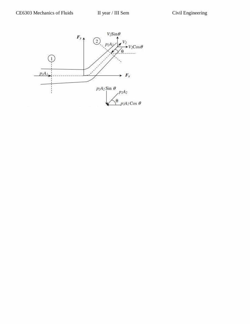
10. State the momentum equation. How will you apply momentum equation for determining the
force exerted by a flowing fluid on a pipe bend.
It is base d on the law of c onser vation of mome ntum or on mome ntu m princ ip
le, which st ates that the net f orce acting on a fluid mass is eq ual to the rate of cha
nge of momentum of flow in that direc ti on. If the f orce ac ting on a mass of fl uid
m is Fx along x direction, the net force along t he direction is give n b y N ewt on’s
second law of moti on as Fx = m ax
Where ax is the a ccelera tion produced d ue to th e f orc e Fx al ong the
sa me direction.
The abo ve equation is called moment um pri nciple. The sa me equa ti on can
also be written as
Fx dt = d (mu )whic h i s know n as im puls e m om entum principle an d can be state d as
“The impulse of a f orce acting on a f luid of ma ss m in a s hor t i nte r val of ti me dt
alon g a n y d irecti on is gi ven b y the rate of cha nge of mome ntu m d(m u) along the sa
me dire ction.
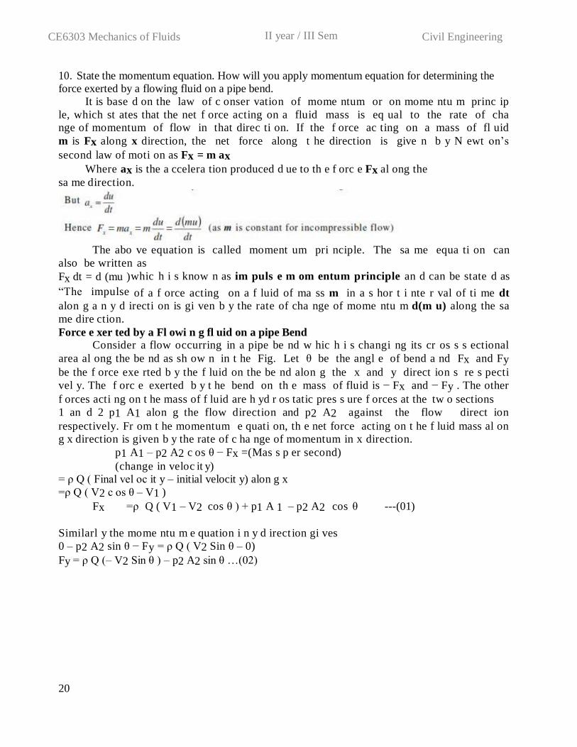
Force e xer ted by a Fl owi n g fl uid on a pipe Bend
Consider a flow occurring in a pipe be nd w hic h i s changi ng its cr os s s ectional
area al ong the be nd as sh ow n in t he Fig. Let θ be the angl e of bend a nd Fx and Fy
be the f orce exe rted b y the f luid on the be nd alon g the x and y direct ion s re s pecti
vel y. The f orc e exerted b y t he bend on th e mass of fluid is − Fx and − Fy . The other
f orces acti ng on t he mass of f luid are h yd r os tatic pres s ure f orces at the tw o sections
1 an d 2 p1 A1 alon g the flow direction and p2 A2 against the flow direct ion
respectively. Fr om t he momentum e quati on, th e net force acting on t he f luid mass al on
g x direction is given b y the rate of c ha nge of momentum in x direction.
p1 A1 – p2 A2 c os θ − Fx =(Mas s p er second)
(change in veloc it y)
= ρ Q ( Final vel oc it y – initial velocit y) alon g x
=ρ Q ( V2 c os θ – V1 )
Fx =ρ Q ( V1 – V2 cos θ ) + p1 A 1 – p2 A2 cos θ ---(01)
Similarl y the mome ntu m e quation i n y d irect ion gi ves
0 – p2 A2 sin θ − Fy = ρ Q ( V2 Sin θ – 0)
Fy = ρ Q (– V2 Sin θ ) – p2 A2 sin θ …(02)
20
II year / III Sem CE6303 Mechanics of Fluids Civil Engineering
II year / III Sem CE6303 Mechanics of Fluids Civil Engineering
UNIT III DIMENSIONAL ANALYSIS AND MODEL STUDIES
DIMENSIONAL ANALYSIS AND MODEL STUDIES
PART – A(2 MARKS)
1. Define dimensional analysis.
Dimensional analysis is a mathematical technique which makes use of the study of
dimensions as an aid to solution of several engineering problems. It plays an important role in
research work.
2. Write the uses of dimension analysis?
• It helps in testing the dimensional homogeneity of any equation of fluid
motion.
• It helps in deriving equations expressed in terms of non-dimensional parameters.
• It helps in planning model tests and presenting experimental results in a systematic manner.
3. Define dimensional homogeneity.
An equation is said to be dimensionally homogeneous if the dimensions of the terms on its LHS are same as the dimensions of the terms on its RHS.
4. Mention the methods available for dimensional analysis.
Rayleigh method,
Buckinghum π method
5. State Buckingham’s π theorem.
It states that “if there are ‘n’ variables (both independent & dependent variables) in a physical
phenomenon and if these variables contain ‘m’ functional dimensions and are related by a
dimensionally homogeneous equation, then the variables are arranged into n-m dimensionless
terms. Each term is called π term”.
6. List the repeating variables used in Buckingham π theorem.
Geometrical Properties – l, d, H, h, etc,
Flow Properties – v, a, g, ω, Q, etc,
Fluid Properties – ρ, μ, γ, etc.
7. Define model and prototype.
The small scale replica of an actual structure or the machine is known as its Model, while the
actual structure or machine is called as its Prototype. Mostly models are much smaller than the
corresponding prototype.
8. Write the advantages of model analysis.
• Model test are quite economical and convenient.
• Alterations can be continued until most suitable design is obtained.
• Modification of prototype based on the model results.
• The information about the performance of prototype can be obtained well in advance.
9. List the types of similarities or similitude used in model anlaysis.
Geometric similarities, Kinematic similarities, Dynamic similarities
10. Define geometric similarities
It exists between the model and prototype if the ratio of corresponding lengths, dimensions
in the model and the prototype are equal. Such a ratio is known as “Scale Ratio”.
11. Define kinematic similarities
It exists between the model and prototype if the paths of the homogeneous moving particles
are geometrically similar and if the ratio of the flow properties is equal.
12. Define dynamic similarities
48
II year / III Sem CE6303 Mechanics of Fluids Civil Engineering
50
It exits between model and the prototype which are geometrically and kinematic similar and if
the ratio of all forces acting on the model and prototype are equal.
13. Mention the various forces considered in fluid flow.
Inertia force,
Viscous force,
Gravity force,
Pressure force, Surface Tension force,
Elasticity force
14. Define model law or similarity law.
The condition for existence of completely dynamic similarity between a model and its prototype are
denoted by equation obtained from dimensionless numbers. The laws on which the models are designed
for dynamic similarity are called Model laws or Laws of Similarity.
15. List the various model laws applied in model analysis. Reynold’s Model Law,
Froude’s Model Law,
Euler’s Model Law,
Weber Model Law,
Mach Model Law
16. State Euler’s model law
In a fluid system where supplied pressures are the controlling forces in addition to inertia forces and
other forces are either entirely absent or in-significant the Euler’s number for both the model and
prototype which known as Euler Model Law.
17. State Weber’s model law
When surface tension effect predominates in addition to inertia force then the dynamic similarity is
obtained by equating the Weber’s number for both model and its prototype, which is called as Weber
Model Law.
18. State Mach’s model law
If in any phenomenon only the forces resulting from elastic compression are significant in addition
to inertia forces and all other forces may be neglected, then the dynamic similarity between model and
its prototype may be achieved by equating the Mach’s number for both the systems. This is known
Mach Model Law.
19. Classify the hydraulic models.
The hydraulic models are classified as: Undistorted model & Distorted model 20. Define undistorted model
An undistorted model is that which is geometrically similar to its prototype, i.e. the scale ratio for
corresponding linear dimensions of the model and its prototype are same.
21. Define distorted model
Distorted models are those in which one or more terms of the model are not identical with their
counterparts in the prototype.
22. Define Scale effect
An effect in fluid flow that results from changing the scale, but not the shape, of a body around
which the flow passes.
PART B
II year / III Sem CE6303 Mechanics of Fluids Civil Engineering
51
L
/ T 2 2 a
model
m 2
A prototype p L2 L
All corresponding angles are the same.
(ii) Kinematic similarity
Kinematic similarity is the similarity of time as well as geometry. It exists between model and
prototype
i. If the paths of moving particles are geometrically similar
ii. If the rations of the velocities of particles are similar
Some useful ratios are:
Velocity V L / T
V L / T m
m m L
u
p p p T
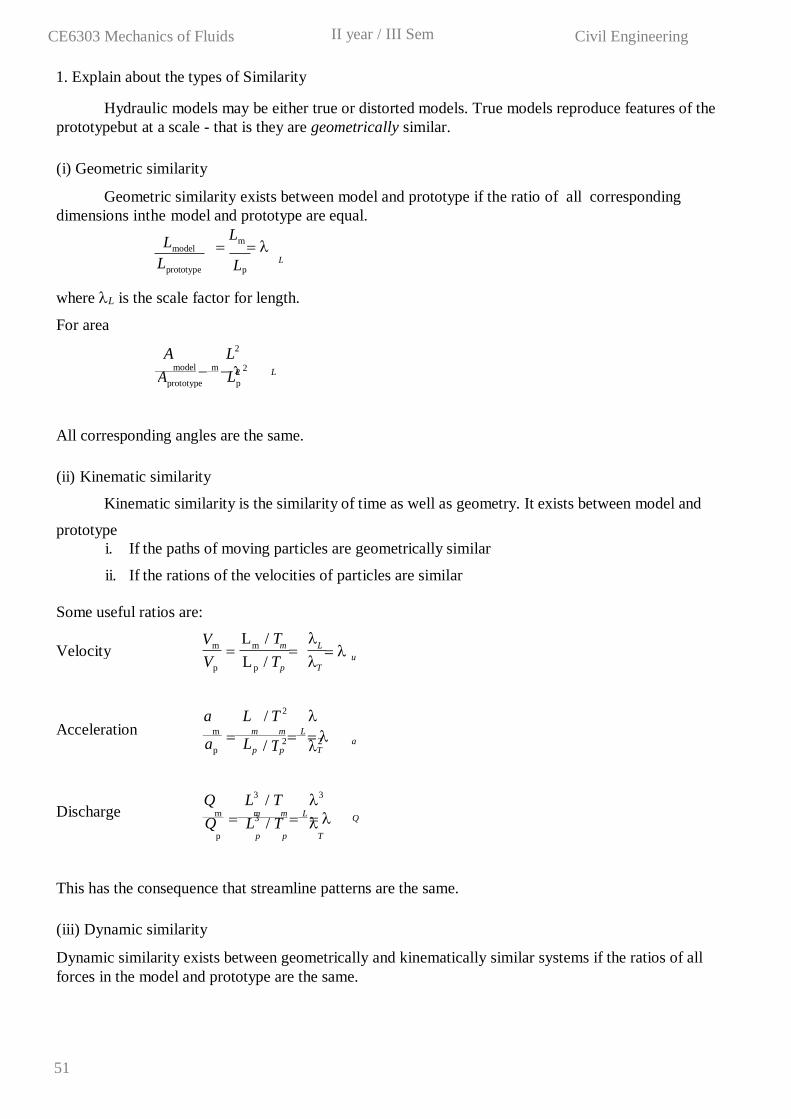
1. Explain about the types of Similarity
Hydraulic models may be either true or distorted models. True models reproduce features of the
prototypebut at a scale - that is they are geometrically similar.
(i) Geometric similarity
Geometric similarity exists between model and prototype if the ratio of all corresponding
dimensions inthe model and prototype are equal.
Lmodel Lm
Lprototype p
where L is the scale factor for length.
For area
A L2
a L / T 2
Acceleration m
m m
L
ap Lp p T
Q L3
/ T 3
Discharge m
m m
L Q L
3 / T Q
p p p T
This has the consequence that streamline patterns are the same.
(iii) Dynamic similarity
Dynamic similarity exists between geometrically and kinematically similar systems if the ratios of all
forces in the model and prototype are the same.
L
II year / III Sem CE6303 Mechanics of Fluids Civil Engineering
52
L T 3 2
F M a L3 2
Force ratio m m m
m m
L
2 L 2 2
Fp M p a p p p T
L
L u
This occurs when the controlling dimensionless group on the right hand side of the defining
equation isthe same for model and prototype.
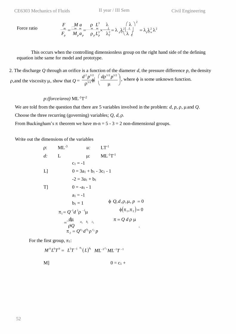
2. The discharge Q through an orifice is a function of the diameter d, the pressure difference p, the density
d 2 p1/2 d1/2 p1/2
,and the viscosity , show that Q 1/2
, where is some unknown function.
Write out the dimensions of the variables
ML-3 u: LT-1
d: L ML-1T-1
c1 = -1
L] 0 = 3a1 + b1 - 3c1 - 1
-2 = 3a1 + b1
T] 0 = -a1 - 1
a1 = -1
b1 = 1
1 Q1
d 1 1
d
Q
p:(force/area) ML-1T-2
We are told from the question that there are 5 variables involved in the problem: d, p, , and Q.
Choose the three recurring (governing) variables; Q, d,
From Buckingham’s theorem we have m-n = 5 - 3 = 2 non-dimensional groups.
Q, d , , , p 0
1 ,2 0
Q d a 1 b c 1 1
1 1
Qa2 d
b2 c2 p 2
For the first group, 1:
M 0 L
0T
0 L
3T
1 a1 Lb1 ML3 c1
ML1T 1
M] 0 = c1 + 1
II year / III Sem CE6303 Mechanics of Fluids Civil Engineering
53
2
And the second group 2 :
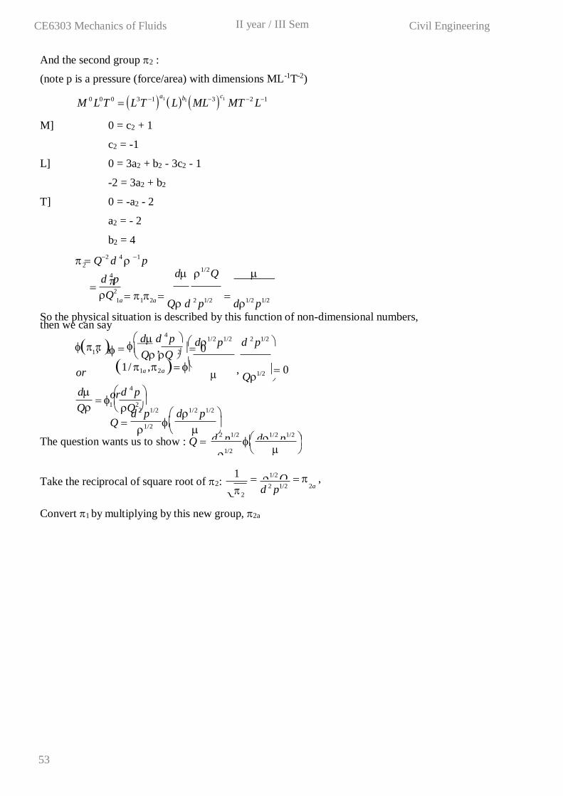
(note p is a pressure (force/area) with dimensions ML-1T-2)
M 0 L
0T
0 L3
T 1
a1 Lb1 ML3
c1
MT 2
L1
M] 0 = c2 + 1
c2 = -1
L] 0 = 3a2 + b2 - 3c2 - 1
-2 = 3a2 + b2
T] 0 = -a2 - 2
a2 = - 2
b2 = 4
Q2
d 4 1
p
d 1/2
Q
1a 12a Q d 2 p1/2
then we can say
d1/2 p1/2
d1/2 p1/2 d 2 p1/2
1 / 1a ,2a ,
Q1/2 0
or
d 2 p1/2 d1/2 p1/2
Q 1/2
Q
2
d 4 p
So the physical situation is described by this function of non-dimensional numbers,
1 , , 2 0 2
d d
4 p
Q Q
or
d d 4 p
Q Q 1 2
The question wants us to show : Q d 2 p1/2 d1/2 p1/2
1/2
Take the reciprocal of square root of 2: 1 1/2 Q
2
, d 2 p1/2 2a
Convert 1 by multiplying by this new group, 2a
II year / III Sem CE6303 Mechanics of Fluids Civil Engineering
53
d
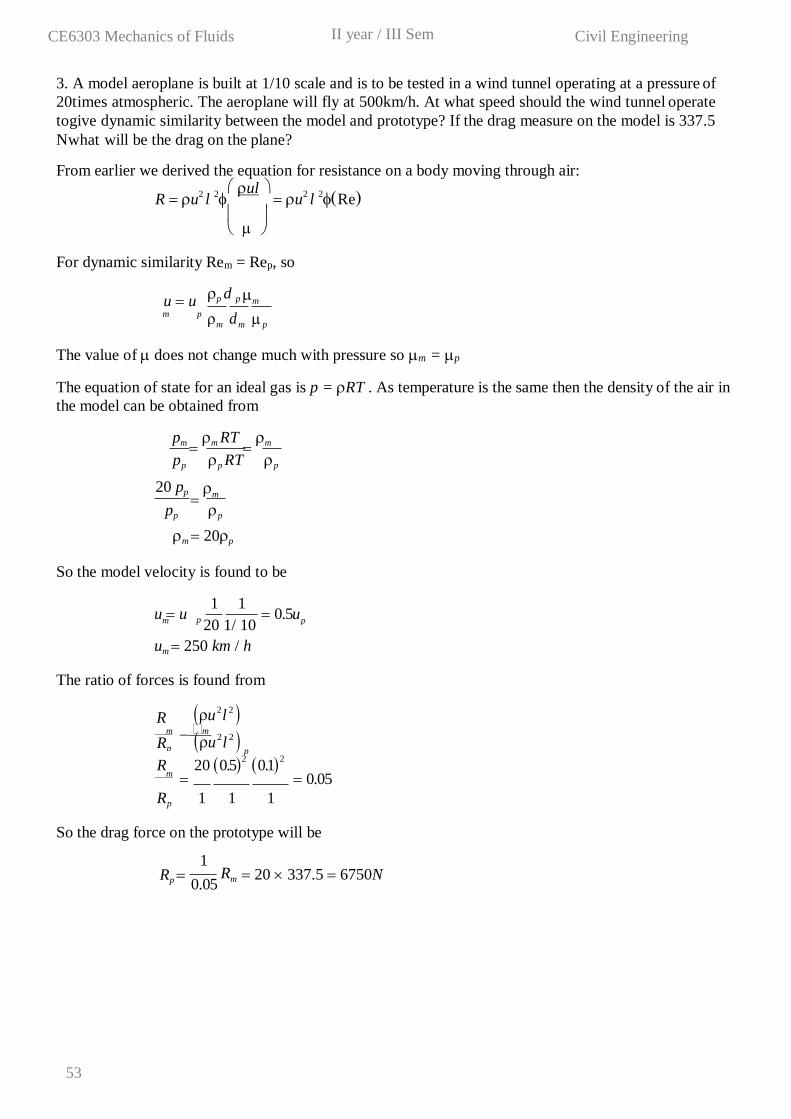
3. A model aeroplane is built at 1/10 scale and is to be tested in a wind tunnel operating at a pressure of
20times atmospheric. The aeroplane will fly at 500km/h. At what speed should the wind tunnel operate
togive dynamic similarity between the model and prototype? If the drag measure on the model is 337.5
Nwhat will be the drag on the plane?
From earlier we derived the equation for resistance on a body moving through air:
R u2 l
2 ul
u2 l
2Re
For dynamic similarity Rem = Rep, so
u u
p d p m
m p
m m p
The value of does not change much with pressure so m = p
R 20 0.52 0.12
m 0.05
Rp 1 1 1
So the drag force on the prototype will be
Rp
1
0.05 Rm
20 337.5 6750N
The equation of state for an ideal gas is p = RT . As temperature is the same then the density of the air in
the model can be obtained from
pm m RT
m
pp p RT p
pp p
m 20p
So the model velocity is found to be
20 pp m
u u 1 1
m p 20 1/ 10
0.5u p
um 250 km / h
The ratio of forces is found from
m m
R u2 l
2 Rp u
2 l
2 p
CE6303 Mechanics of Fluids II year / III Sem Civil Engineering
54
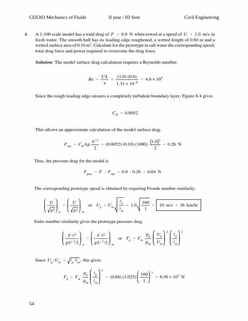
4.
CE6303 Mechanics of Fluids II year / III Sem Civil Engineering
55
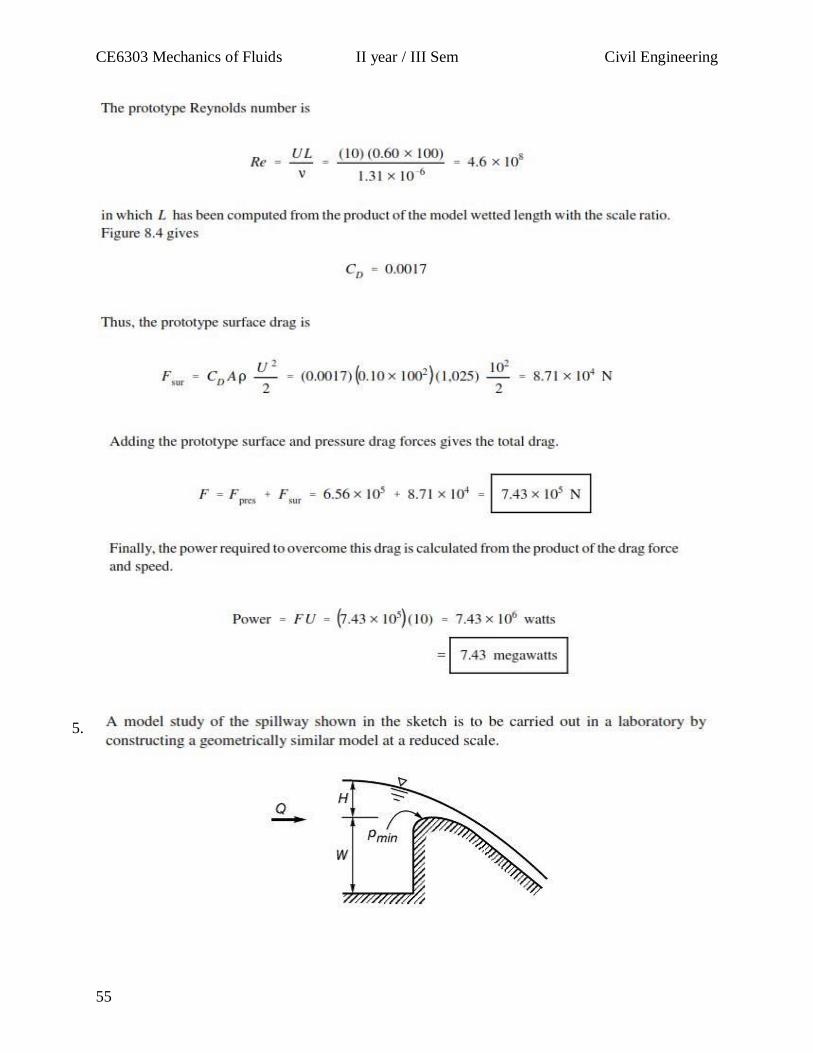
5.
CE6303 Mechanics of Fluids II year / III Sem Civil Engineering
56
CE6303 Mechanics of Fluids II year / III Sem Civil Engineering
57
CE6303 Mechanics of Fluids II year / III Sem Civil Engineering
58
6.
Solution
CE6303 Mechanics of Fluids II year / III Sem Civil Engineering
59
p
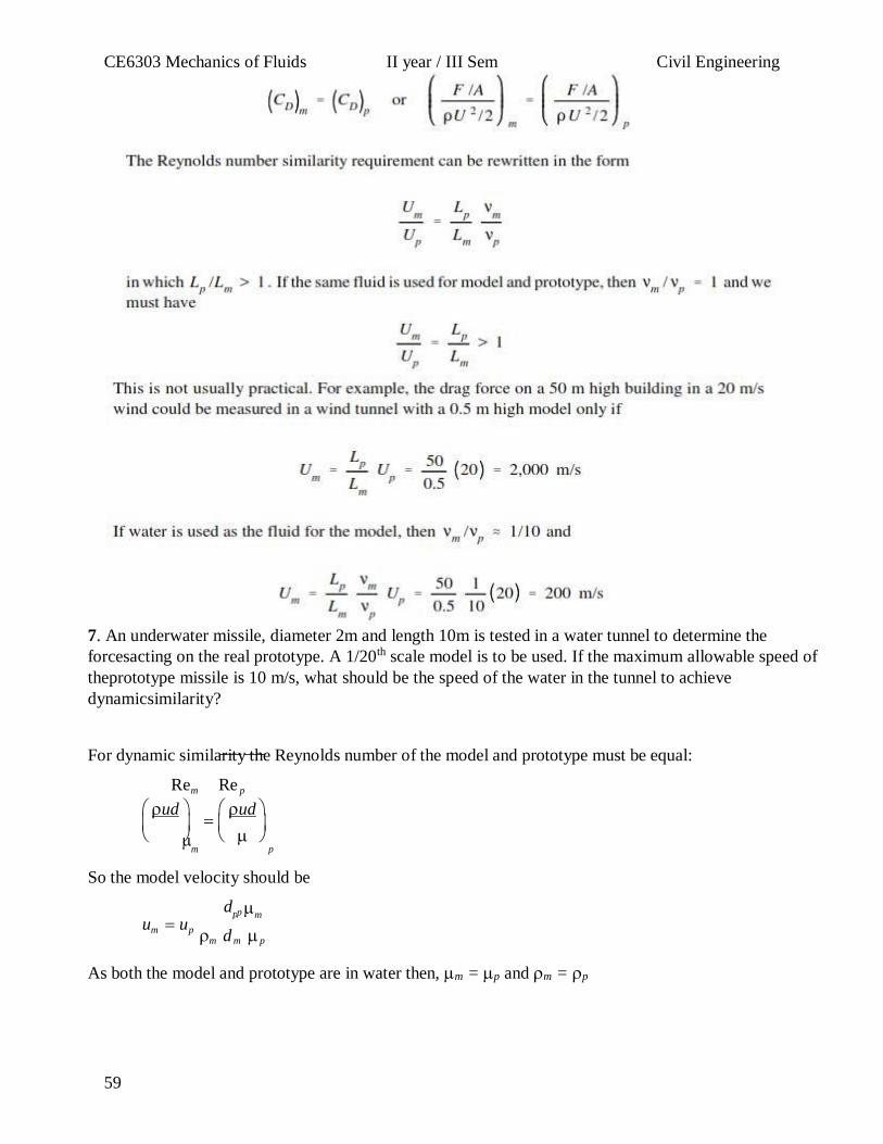
7. An underwater missile, diameter 2m and length 10m is tested in a water tunnel to determine the
forcesacting on the real prototype. A 1/20th scale model is to be used. If the maximum allowable speed of
theprototype missile is 10 m/s, what should be the speed of the water in the tunnel to achieve
dynamicsimilarity?
For dynamic similarity the Reynolds number of the model and prototype must be equal:
Rem Re p
ud ud
m p
So the model velocity should be
d p m
um up d
m m p
As both the model and prototype are in water then, m = p and m = p
CE6303 Mechanics of Fluids II year / III Sem Civil Engineering
60
f
UNIT IV FLOW THROUGH PIPES
PART – A(2 MARKS)
1. What is meant by energy loss in a pipe? When the fluid flows through a pipe, it loses some energy or head due to frictional
resistance and other reasons. It is called energy loss. The losses are classified as; Major
losses and Minor losses
2. Explain the major losses in a pipe.
The major energy losses in a pipe is mainly due to the frictional resistance caused by
the shear force between the fluid particles and boundary walls of the pipe and also due to
viscosity of the fluid.
3. Explain minor losses in a pipe. The loss of energy or head due to change of velocity of the flowing fluid in
magnitude or direction is called minor losses. It includes: sudden expansion of the pipe,
sudden contraction of the pipe, bend in a pipe, pipe fittings and obstruction in the pipe, etc. 4. State Darcy-Weisbach equation OR What is the expression for head loss due to friction?
h = 4flv2 / 2gd
where, h f = Head loss due to friction (m), L = Length of the pipe (m),
d = Diameter of the pipe (m), V = Velocity of flow (m/sec) f = Coefficient of friction where V varies from 1.5 to 2.0.
5. What are the factors influencing the frictional loss in pipe flow? Frictional resistance for the
turbulent flow is, n
i. Proportional to v ii. Proportional to the density of fluid.
iiiProportional to the area of surface in contact. iv. Independent of pressure.
v. Depend on the nature of the surface in contact.
6. What is compound pipe or pipes in series?
When the pipes of different length and different diameters are connected end to end,
then the pipes are called as compound pipes or pipes in series.
7. What is mean by parallel pipe and write the governing equations.
When the pipe divides into two or more branches and again join together downstream
to form a single pipe then it is called as pipes in parallel. The governing equations are:
Q1 = Q
2 + Q
3 h
f1 = h
f2
8. Define equivalent pipe and write the equation to obtain equivalent pipe diameter. The single pipe replacing the compound pipe with same diameter without change in
discharge and head loss is known as equivalent pipe.
9. What is meant by Moody’s chart and what are the uses of Moody’s chart?
The basic chart plotted against Darcy-Weisbach friction factor against Reynold’s
Number (Re) for the variety of relative roughness and flow regimes. The relative roughness
is the ratio of the mean height of roughness of the pipe and its diameter (ε/D).
Moody’s diagram is accurate to about 15% for design calculations and used for a
22
CE6303 Mechanics of Fluids II year / III Sem Civil Engineering
61
large number of applications. It can be used for non-circular conduits and also for open
channels.
10. Define the terms a) Hydraulic gradient line [HGL] b) Total Energy line [TEL]
Hydraulic gradient line: It is defined as the line which gives the sum of pressure head
and datum head of a flowing fluid in a pipe with respect the reference line.
HGL = Sum of Pressure Head and Datum head Total energy line: Total energy line is defined as the line which gives the sum of
pressure head, datum head and kinetic head of a flowing fluid in a pipe with respect to some
reference line.
TEL = Sum of Pressure Head, Datum head and Velocity head
11. What do you understand by the terms a) major energy losses , b) minor energy losses
Major energy losses : -
This loss due to friction and it is calculated by Darcy weis bach formula and
chezy’s formula .
Minor energy losses :- This is due to
i. Sudden expansion in pipe .
ii. Sudden contraction in pipe .
iii. Bend in pipe .
iv. Due to obstruction in pipe .
12. . Give an expression for loss of head due to sudden enlargement of the pipe :- he
= (V1-V2)2 /2g Where he = Loss of head due to sudden enlargement of pipe .
V1 = Velocity of flow at section 1-1
V2 = Velocity of flow at section 2-2
13. Give an expression for loss of head due to sudden contraction : -
hc =0.5 V2/2g
Where hc = Loss of head due to sudden contraction .
V = Velocity at outlet of pipe.
14. Give an expression for loss of head at the entrance of the pipe : -
hi =0.5V2/2g
where hi = Loss of head at entrance of pipe .
15. What are the basic educations to solve the problems in flow through branched pipes?
i. Continuity equation .
ii. Bernoulli’s formula .
iii. Darcy weisbach equation .
16. Mention the general characteristics of laminar flow.
• There is a shear stress between fluid layers
• ‘No slip’ at the boundary
• The flow is rotational
• There is a continuous dissipation of energy due to viscous shear
23
CE6303 Mechanics of Fluids II year / III Sem Civil Engineering
62
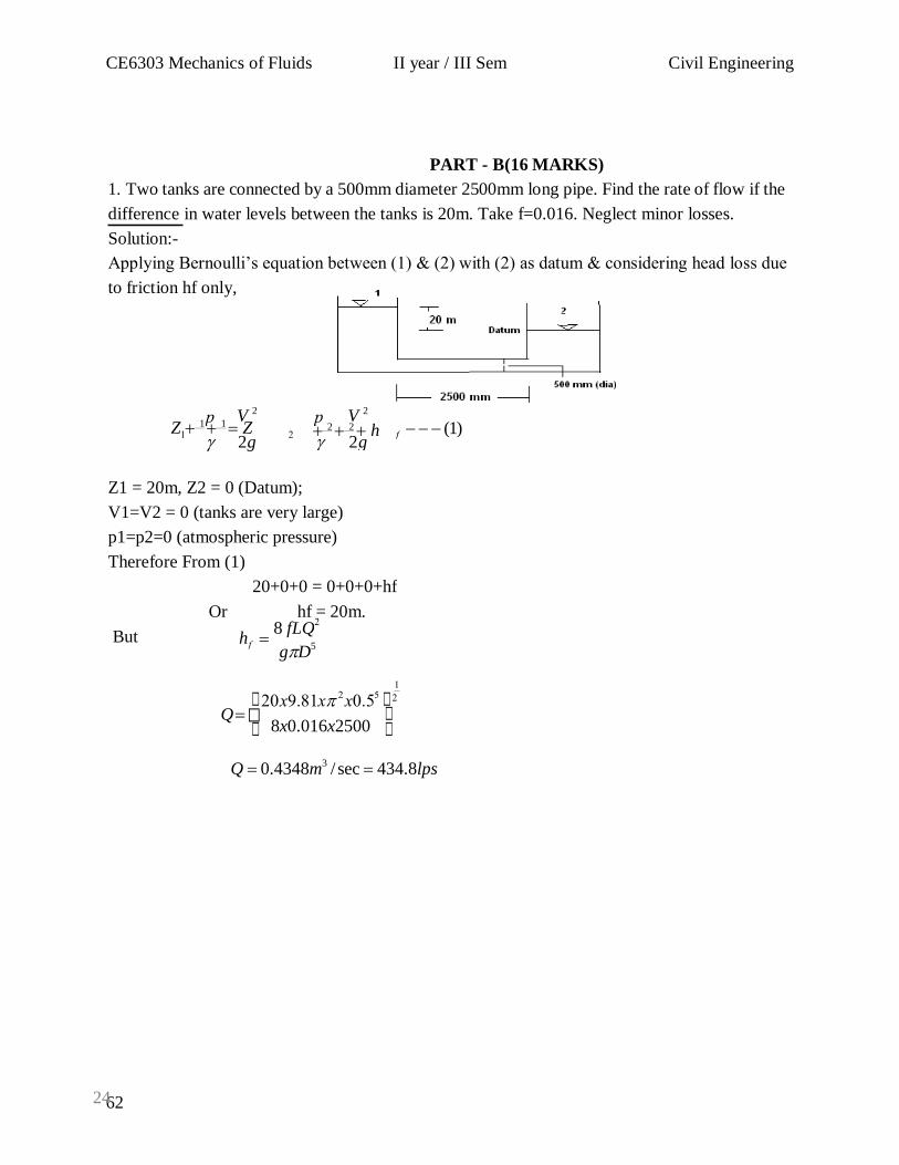
Z 1 1 Z V 2
V 2
2g
2 2 h 2g
(1)
Z1 = 20m, Z2 = 0 (Datum);
V1=V2 = 0 (tanks are very large)
p1=p2=0 (atmospheric pressure)
Therefore From (1)
20+0+0 = 0+0+0+hf
Or hf = 20m.
But h 8 fLQ
gD5
Q
8x0.016x2500
Q 0.4348m3 / sec 434.8lps
PART - B(16 MARKS)
1. Two tanks are connected by a 500mm diameter 2500mm long pipe. Find the rate of flow if the
difference in water levels between the tanks is 20m. Take f=0.016. Neglect minor losses.
Solution:-
Applying Bernoulli’s equation between (1) & (2) with (2) as datum & considering head loss due
to friction hf only,
24
CE6303 Mechanics of Fluids II year / III Sem Civil Engineering
63
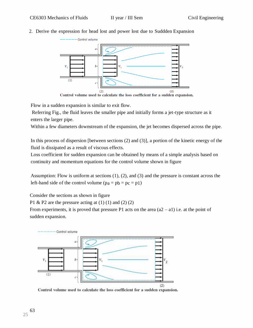
2. Derive the expression for head lost and power lost due to Suddden Expansion
Flow in a sudden expansion is similar to exit flow.
Referring Fig., the fluid leaves the smaller pipe and initially forms a jet-type structure as it
enters the larger pipe.
Within a few diameters downstream of the expansion, the jet becomes dispersed across the pipe.
In this process of dispersion [between sections (2) and (3)], a portion of the kinetic energy of the
fluid is dissipated as a result of viscous effects.
Loss coefficient for sudden expansion can be obtained by means of a simple analysis based on
continuity and momentum equations for the control volume shown in figure
Assumption: Flow is uniform at sections (1), (2), and (3) and the pressure is constant across the
left-hand side of the control volume (pa = pb = pc = p1)
Consider the sections as shown in figure
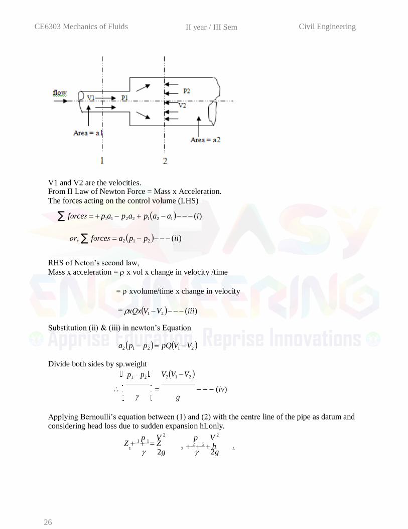
P1 & P2 are the pressure acting at (1) (1) and (2) (2)
From experiments, it is proved that pressure P1 acts on the area (a2 – a1) i.e. at the point of
sudden expansion.
25
II year / III Sem CE6303 Mechanics of Fluids Civil Engineering
Divide both sides by sp.weight
p1 p2
V2 V1 V2
(iv) g
Applying Bernoulli’s equation between (1) and (2) with the centre line of the pipe as datum and
considering head loss due to sudden expansion hLonly.
p V 2
p V 2
Z 1 1 Z 2 2 h 1
2g 2
2g L
26
V1 and V2 are the velocities. From II Law of Newton Force = Mass x Acceleration.
The forces acting on the control volume (LHS)
f ce p1a1 p2a2 p1 a2 a1 (i)
, f ce a2 p1 p2 (ii)
RHS of Neton’s second law,
Mass x acceleration = x vol x change in velocity /time
= xvolume/time x change in velocity
x x V1 V2 (iii)
Substitution (ii) & (iii) in newton’s Equation
a2 p1 p2 pQ V1 V2
II year / III Sem CE6303 Mechanics of Fluids Civil Engineering
2g
Z1 = Z2 because pipe is horizontal
p p V 2 V
2 1 2 ( 1 2 ) h
L
----------- v
Repalcing (p1-p2)/ɤ by Eq. (iv) in Eq. (v)
2V V V V 2 V
2 h 2 1 2 1 2
L 2g
2V V 2V 2 V
2 V
2
h 1 2 2 1 2 L
2g
Force = Mass x accn. But acceleration = 0, as there is no change in velocity, the reason that pipe
diameter is uniform or same throughout.
27
2 1 2 1 2
2g
2V 2 2V V V
2 V
2
2 1 1 2
2g
V 2 V
2 2V V
h V V 2
1 2
2g …..vi
The Equation (vi) represents the loss due to sudden expansion.
Loss of Power
The loss of power in overcoming the head loss in the transmission of fluid is given by
P Qhf (vi)
II year / III Sem CE6303 Mechanics of Fluids Civil Engineering
Applying Bernoulli’s equation between (1) & (2) with the centre line of the pipe as datum &
considering head loss due to friction hf,.
p V 2
p V 2
Z 1 1 Z 2 2 hf
1 2g 2 2g
Z1 Z2 Q
V1 V2 Q
P1 P2 h
Pipe is horizontal
Pipe diameter is same throughout
f (2)
V 4Q
From Continuity equation, Q= AxVD, V2
= Q/A
hf
8 fLQ2
(6) gh2 D
5
Substituting for V in Eq. 5,
Equations (5) & (6) are known as DARCY – WEISBACH Equation
28
Substituting eq (2) in eq.(1)
From Experiments, Darcy Found that
f V
2 (4)
f=Darcy’s friction factor (property of the pipe materials Mass density of the liquid.
V = average velocity
Substituting eq (4) in eq.(3)
V hf D
4L or
4LfV 2
hf 8D
But
g
hf
II year / III Sem CE6303 Mechanics of Fluids Civil Engineering
29
,
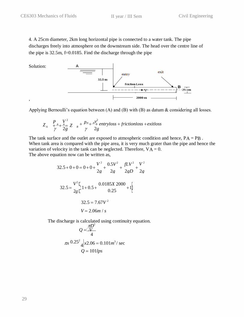
Applying Bernoulli’s equation between (A) and (B) with (B) as datum & considering all losses.
Z A A A Z 2g
P V 2
B B B entryloss frictionloss exitloss 2g
p v2
The tank surface and the outlet are exposed to atmospheric condition and hence, PA = PB .
When tank area is compared with the pipe area, it is very much grater than the pipe and hence the
variation of velocity in the tank can be neglected. Therefore, VA = 0.
The above equation now can be written as,
32.5 0 0 0 0 V 2
0.5V 2
fLV 2 V 2
2g 2g 2gD 2g
32.5 1 0.5 V 2
2g
0.0185X 2000
0.25 1
4. A 25cm diameter, 2km long horizontal pipe is connected to a water tank. The pipe
discharges freely into atmosphere on the downstream side. The head over the centre line of
the pipe is 32.5m, f=0.0185. Find the discharge through the pipe
Solution:
32.5 7.67V 2
V 2.06m / s
The discharge is calculated using continuity equation. D
2
Q V 4
x 0.252
4 x2.06 0.101m
3 / sec
Q 101lps
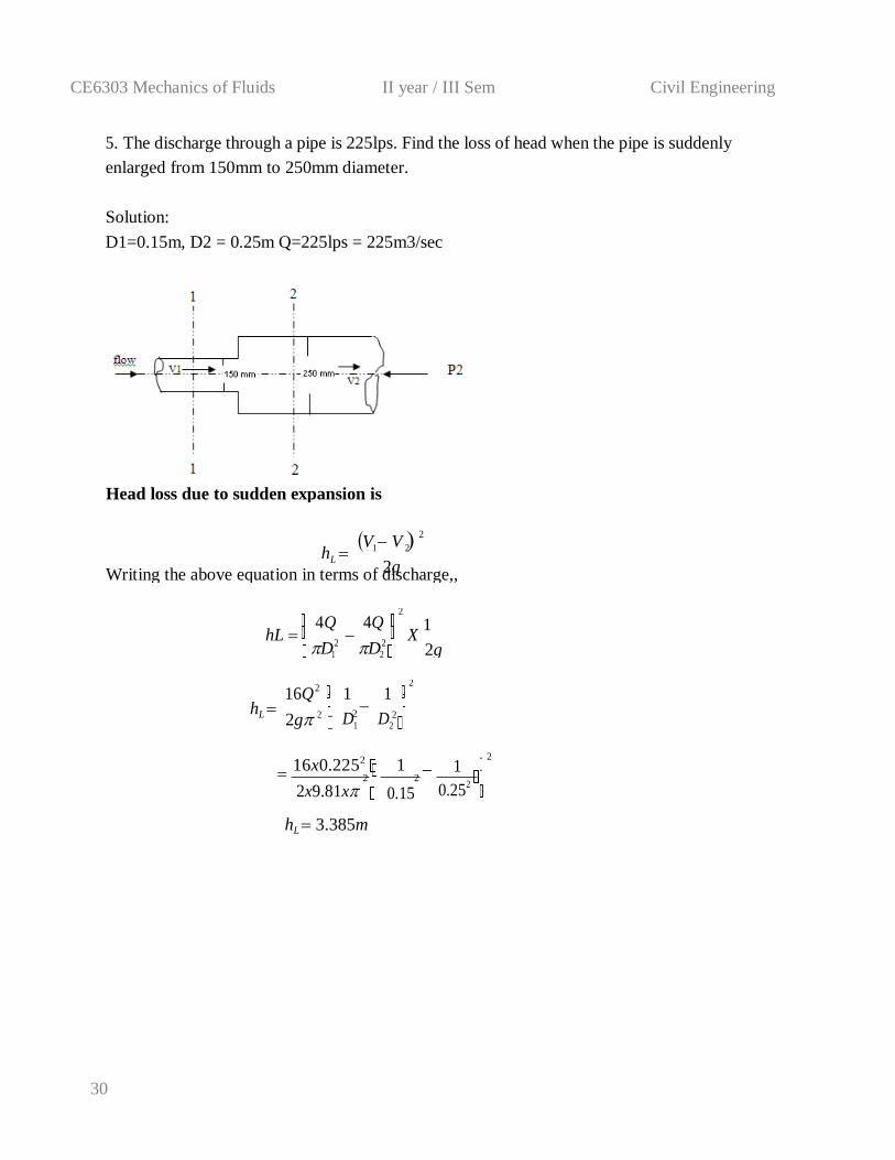
Head loss due to sudden expansion is
h V V 2
1 2
L
Writing the above equation in terms of discharge,, 2g
hL 4Q 4Q
2
1 D D 2
2 2
X 1
2g
hL 16Q
2 1 1 2
2g
2 D1 D2
2
2
16x0.2252 1 1
2
CE6303 Mechanics of Fluids II year / III Sem Civil Engineering
5. The discharge through a pipe is 225lps. Find the loss of head when the pipe is suddenly
enlarged from 150mm to 250mm diameter.
Solution:
D1=0.15m, D2 = 0.25m Q=225lps = 225m3/sec
2x9.81x
2 2
0.15 0.252
hL 3.385m
30
31
2
2
0
CE6303 Mechanics of Fluids II year / III Sem Civil Engineering
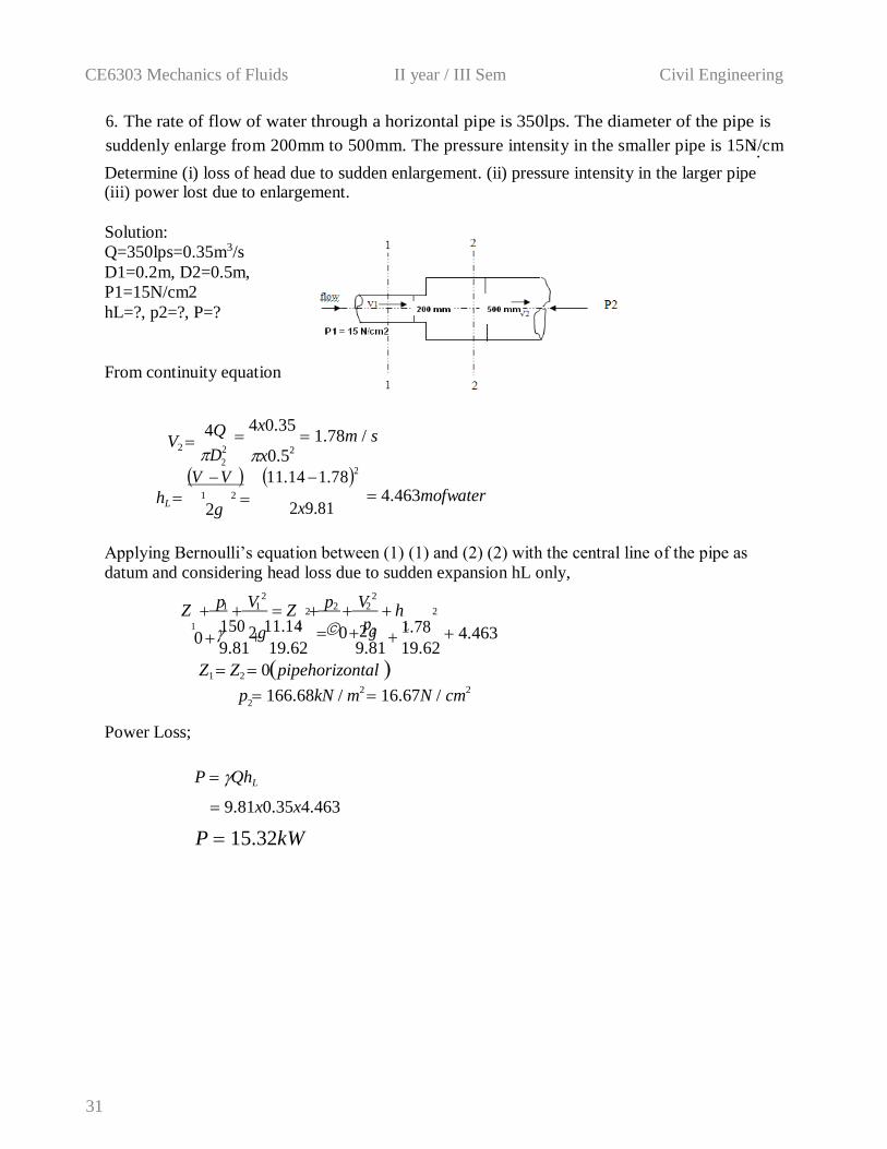
6. The rate of flow of water through a horizontal pipe is 350lps. The diameter of the pipe is
suddenly enlarge from 200mm to 500mm. The pressure intensity in the smaller pipe is 15N2./cm
Determine (i) loss of head due to sudden enlargement. (ii) pressure intensity in the larger pipe (iii) power lost due to enlargement.
Solution:
Q=350lps=0.35m3/s
D1=0.2m, D2=0.5m,
P1=15N/cm2
hL=?, p2=?, P=?
From continuity equation
V2 4Q
D2
4x0.35
1.78m / s
x0.52
V V 11.14 1.782
hL 1 2 2g 2x9.81
4.463mofwater
Applying Bernoulli’s equation between (1) (1) and (2) (2) with the central line of the pipe as
datum and considering head loss due to sudden expansion hL only,
p V 2
p V 2
Z 1 1 Z 2 2 2 h 2
1 150 2g
11.142 0 2pg2 1L.78 4.463
9.81 19.62 9.81 19.62
Power Loss;
Z1 Z2 0pipehorizontal p 166.68kN / m
2 16.67N / cm
2
P QhL
9.81x0.35x4.463
P 15.32kW
32
2
CE6303 Mechanics of Fluids II year / III Sem Civil Engineering
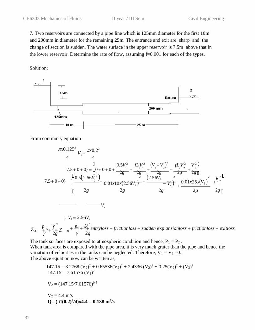
7. Two reservoirs are connected by a pipe line which is 125mm diameter for the first 10m
and 200mm in diameter for the remaining 25m. The entrance and exit are sharp and the
change of section is sudden. The water surface in the upper reservoir is 7.5m above that in
the lower reservoir. Determine the rate of flow, assuming f=0.001 for each of the types.
Solution;
0.5V 2 fLV 2 V V 2 fL V 2 V 2
7.5 0 0} 0 0 0 1 1 1 1 2 2 2 2
2g 2g 2g 2g 2g
7.5 0 0} 0.52.56V
2 0.01x10x2.56V2
2.56V2
V2 0.01x25xV2
V 2
2
2g 2g 2g 2g 2g
147.15 = 3.2768 (V2)2 + 0.65536(V2)
2 + 2.4336 (V2)2 + 0.25(V2)
2 + (V2)2
147.15 = 7.61576 (V2)2
V2 = (147.15/7.61576)0.5
V2 = 4.4 m/s
Q= ( π(0.2)2/4)x4.4 = 0.138 m3/s
From continuity equation
x0.1252
V1 4
x0.22
4
V2
V1 2.56V2
Z V 2 V 2
A A A Z 2g
p B B B entryloss frictionloss sudden exp ansionloss frictionloss exitloss 2g
p
The tank surfaces are exposed to atmospheric condition and hence, P1 = P2 . When tank area is compared with the pipe area, it is very much grater than the pipe and hence the
variation of velocities in the tanks can be neglected. Therefore, V1 = V2 =0.
The above equation now can be written as,
2 2 2
II year / III Sem CE6303 Mechanics of Fluids Civil Engineering
1
1 2 3 4
8. Derive the expression for pipes in series and parallel connection
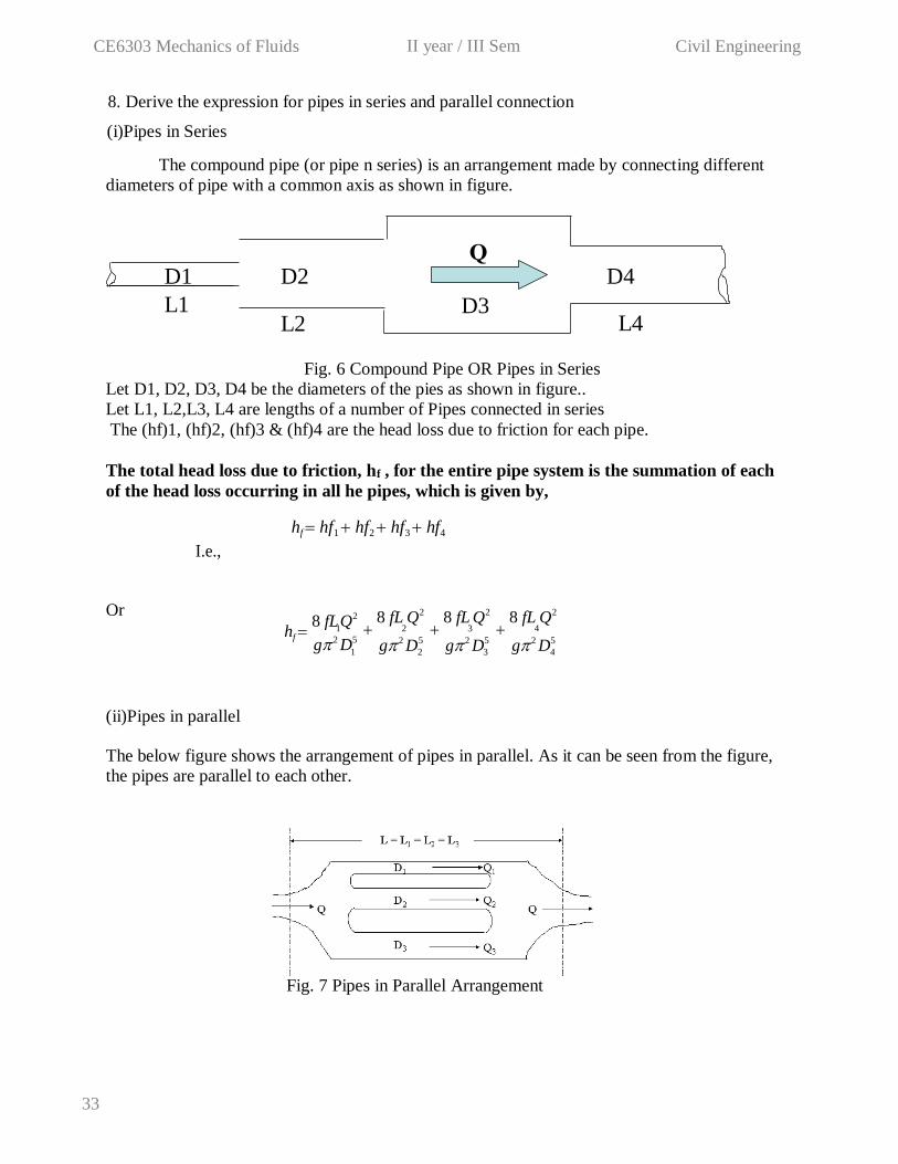
(i)Pipes in Series
The compound pipe (or pipe n series) is an arrangement made by connecting different
diameters of pipe with a common axis as shown in figure.
Fig. 6 Compound Pipe OR Pipes in Series
Let D1, D2, D3, D4 be the diameters of the pies as shown in figure..
Let L1, L2,L3, L4 are lengths of a number of Pipes connected in series
The (hf)1, (hf)2, (hf)3 & (hf)4 are the head loss due to friction for each pipe.
The total head loss due to friction, hf , for the entire pipe system is the summation of each
of the head loss occurring in all he pipes, which is given by,
I.e.,
hf hf1 hf2 hf3 hf4
Or
hf 8 fL Q2
g 2 D5
8 fL Q2
g 2 D5
8 fL Q2
g 2 D5
8 fL Q2
g 2 D5
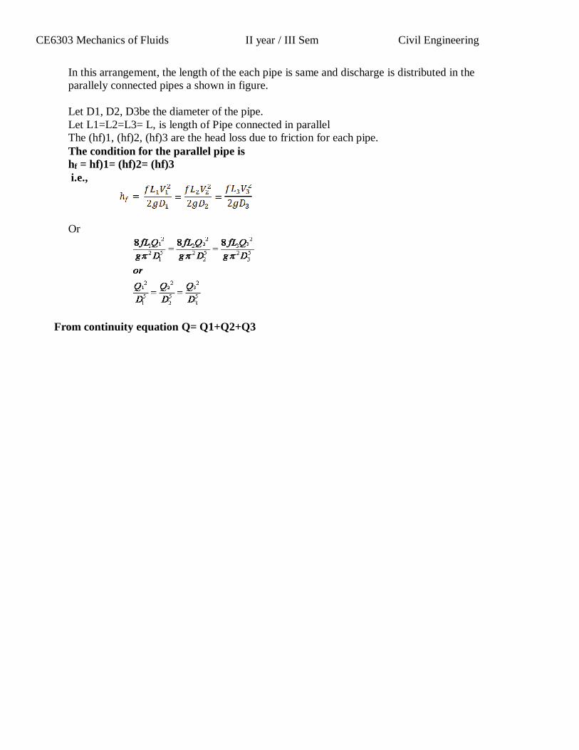
(ii)Pipes in parallel
The below figure shows the arrangement of pipes in parallel. As it can be seen from the figure,
the pipes are parallel to each other.
Fig. 7 Pipes in Parallel Arrangement
33
D1
L1
D2 D4
L2 D3
L4
2 3 4
CE6303 Mechanics of Fluids II year / III Sem Civil Engineering
In this arrangement, the length of the each pipe is same and discharge is distributed in the
parallely connected pipes a shown in figure.
Let D1, D2, D3be the diameter of the pipe.
Let L1=L2=L3= L, is length of Pipe connected in parallel
The (hf)1, (hf)2, (hf)3 are the head loss due to friction for each pipe.
The condition for the parallel pipe is
hf = hf)1= (hf)2= (hf)3
i.e.,
Or
From continuity equation Q= Q1+Q2+Q3
CE6303 Mechanics of Fluids II year / III Sem Civil Engineering
UNIT V BOUNDRY LAYER
PART – A (2 MARKS)
1. Mention the range of Reynold’s number for laminar and turbulent flow in a pipe. If the Reynolds number is less than 2000, the flow is laminar. But if the Reynold’s
number is greater than 4000, the flow is turbulent flow.
2. What does Haigen-Poiseulle equation refer to?
The equation refers to the value of loss of head in a pipe of length ‘L’ due to viscosity
in a laminar flow. 3. What are the factors to be determined when viscous fluid flows through the circular pipe?
The factors to be determined are:
i. Velocity distribution across the section.
ii. Ratio of maximum velocity to the average velocity. iii. Shear stress distribution.
iv. Drop of pressure for a given length
4. Define kinetic energy correction factor?
Kinetic energy factor is defined as the ratio of the kinetic energy of the flow per sec based on
actual velocity across a section to the kinetic energy of the flow per sec based on average
velocity across the same section. It is denoted by (α).
K. E factor (α) = K.E per sec based on actual velocity / K.E per sec based on
Average velocity
5. Define momentum correction factor (β): It is defined as the ratio of momentum of the flow per sec based on actual velocity to the
momentum of the flow per sec based on average velocity across the section.
β= Momentum per sec based on actual velocity/Momentum Per sec based on average
velocity
6. Define Boundary layer.
When a real fluid flow passed a solid boundary, fluid layer is adhered to the solid
boundary. Due to adhesion fluid undergoes retardation thereby developing a small region in the
immediate vicinity of the boundary. This region is known as boundary layer.
7. What is mean by boundary layer growth? At subsequent points downstream of the leading edge, the boundary layer region
increases because the retarded fluid is further retarded. This is referred as growth of boundary
layer.
8. Classification of boundary layer.
(i) Laminar boundary layer,
(ii) Transition zone,
(iii)Turbulent boundary layer.
9. Define Laminar boundary layer.
Near the leading edge of the surface of the plate the thickness of boundary layer is small
and flow is laminar. This layer of fluid is said to be laminar boundary layer.
The length of the plate from the leading edge, upto which laminar boundary layer exists
is called as laminar zone. In this zone the velocity profile is parabolic.
10. Define transition zone.
After laminar zone, the laminar boundary layer becomes unstable and the fluid motion
transformed to turbulent boundary layer. This short length over which the changes taking place
35
CE6303 Mechanics of Fluids II year / III Sem Civil Engineering
is called as transition zone.
11. Define Turbulent boundary.
Further downstream of transition zone, the boundary layer is turbulent and continuous to
grow in thickness. This layer of boundary is called turbulent boundary layer.
12. Define Laminar sub Layer
In the turbulent boundary layer zone, adjacent to the solid surface of the plate the
velocity variation is influenced by viscous effects. Due to very small thickness, the velocity
distribution is almost linear. This region is known as laminar sub layer.
13. Define Boundary layer Thickness. It is defined as the distance from the solid boundary measured in y-direction to the
point, where the velocity of fluid is approximately equal to 0.99 times the free stream velocity
(U) of the fluid. It is denoted by δ.
14. List the various types of boundary layer thickness.
Displacement thickness(δ*),
Momentum thickness(θ),
Energy thickness(δ**)
15. Define displacement thickness. The displacement thickness (δ) is defined as the distance by which the boundary
should be displaced to compensate for the reduction in flow rate on account of boundary
layer formation.
δ* = ∫ [ 1 – (u/U) ] dy
16. Define momentum thickness. The momentum thickness (θ) is defined as the distance by which the boundary
should be displaced to compensate for the reduction in momentum of the flowing fluid on
account of boundary layer formation.
17. Define energy thickness
2
θ = ∫ [ (u/U) – (u/U) ] dy
The energy thickness (δ**) is defined as the distance by which the boundary should be
displaced to compensate for the reduction in kinetic energy of the flowing fluid on account of
boundary layer formation.
36
105 37
CE6303 Mechanics of Fluids
II year / III Sem Civil Engineering
PART - B(16 MARKS)
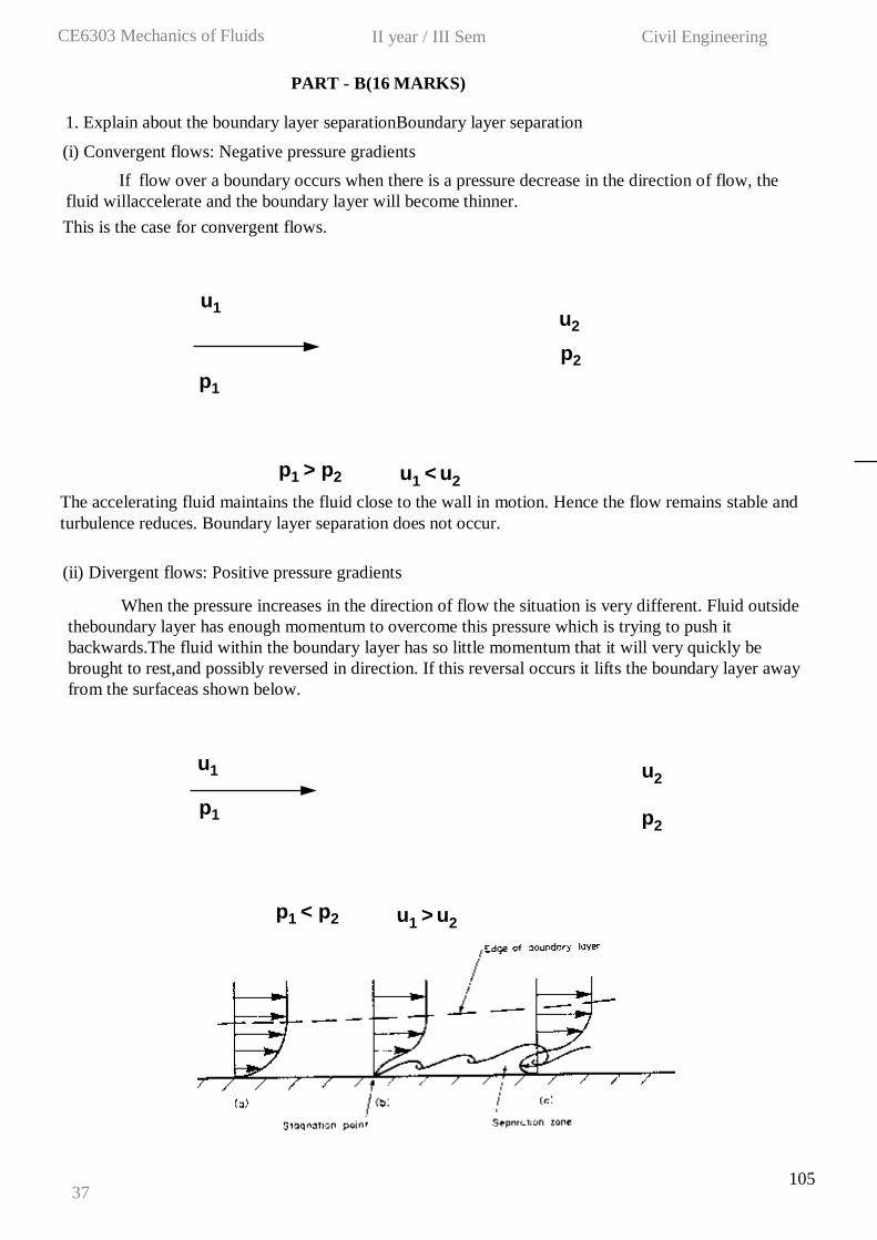
1. Explain about the boundary layer separationBoundary layer separation
(i) Convergent flows: Negative pressure gradients
If flow over a boundary occurs when there is a pressure decrease in the direction of flow, the
fluid willaccelerate and the boundary layer will become thinner.
This is the case for convergent flows.
u1
u2
p2
p1
p1 > p2 u1 < u2
The accelerating fluid maintains the fluid close to the wall in motion. Hence the flow remains stable and
turbulence reduces. Boundary layer separation does not occur.
(ii) Divergent flows: Positive pressure gradients
When the pressure increases in the direction of flow the situation is very different. Fluid outside
theboundary layer has enough momentum to overcome this pressure which is trying to push it
backwards.The fluid within the boundary layer has so little momentum that it will very quickly be
brought to rest,and possibly reversed in direction. If this reversal occurs it lifts the boundary layer away
from the surfaceas shown below.
u1 u2
p1 p2
p1 < p2 u1 > u2
II year / III Sem CE6303 Mechanics of Fluids Civil Engineering
106 38
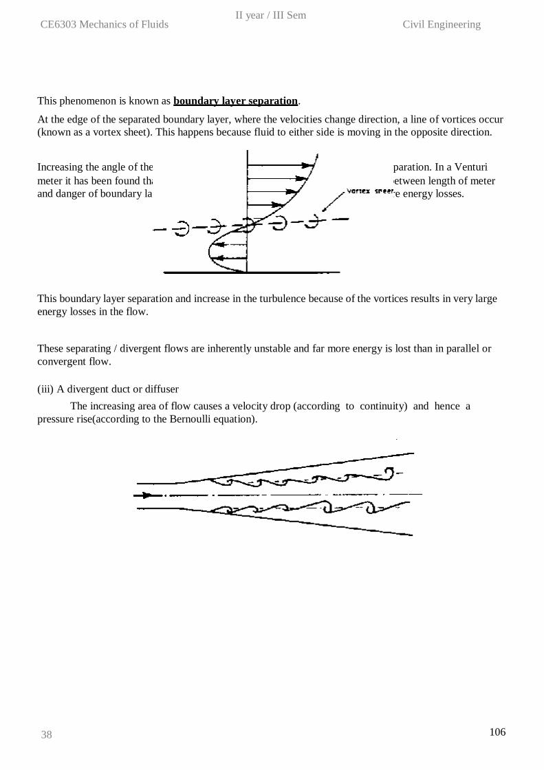
This phenomenon is known as boundary layer separation.
At the edge of the separated boundary layer, where the velocities change direction, a line of vortices occur
(known as a vortex sheet). This happens because fluid to either side is moving in the opposite direction.
Increasing the angle of the diffuser increases the probability of boundary layer separation. In a Venturi
meter it has been found that an angle of about 6 provides the optimum balance between length of meter
and danger of boundary layer separation which would cause unacceptable pressure energy losses.
This boundary layer separation and increase in the turbulence because of the vortices results in very large
energy losses in the flow.
These separating / divergent flows are inherently unstable and far more energy is lost than in parallel or
convergent flow.
(iii) A divergent duct or diffuser
The increasing area of flow causes a velocity drop (according to continuity) and hence a
pressure rise(according to the Bernoulli equation).
II year / III Sem CE6303 Mechanics of Fluids Civil Engineering
39
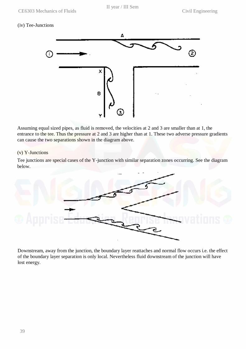
(iv) Tee-Junctions
Downstream, away from the junction, the boundary layer reattaches and normal flow occurs i.e. the effect
of the boundary layer separation is only local. Nevertheless fluid downstream of the junction will have
lost energy.
Assuming equal sized pipes, as fluid is removed, the velocities at 2 and 3 are smaller than at 1, the
entrance to the tee. Thus the pressure at 2 and 3 are higher than at 1. These two adverse pressure gradients
can cause the two separations shown in the diagram above.
(v) Y-Junctions
Tee junctions are special cases of the Y-junction with similar separation zones occurring. See the diagram
below.
II year / III Sem CE6303 Mechanics of Fluids Civil Engineering
40
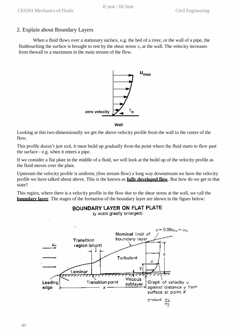
2. Explain about Boundary Layers
When a fluid flows over a stationary surface, e.g. the bed of a river, or the wall of a pipe, the
fluidtouching the surface is brought to rest by the shear stress o at the wall. The velocity increases
from thewall to a maximum in the main stream of the flow.
umax
zero velocity o
Wall
Looking at this two-dimensionally we get the above velocity profile from the wall to the centre of the
flow.
This profile doesn’t just exit, it must build up gradually from the point where the fluid starts to flow past
the surface - e.g. when it enters a pipe.
If we consider a flat plate in the middle of a fluid, we will look at the build up of the velocity profile as
the fluid moves over the plate.
Upstream the velocity profile is uniform, (free stream flow) a long way downstream we have the velocity
profile we have talked about above. This is the known as fully developed flow. But how do we get to that
state?
This region, where there is a velocity profile in the flow due to the shear stress at the wall, we call the
boundary layer. The stages of the formation of the boundary layer are shown in the figure below:
II year / III Sem CE6303 Mechanics of Fluids Civil Engineering
41
Above we noted that the boundary layer grows from zero when a fluid starts to flow over a solid
surface. As is passes over a greater length more fluid is slowed by friction between the fluid layers
close to the boundary. Hence the thickness of the slower layer increases.
The fluid near the top of the boundary layer is dragging the fluid nearer to the solid surface along. The
mechanism for this dragging may be one of two types:
The first type occurs when the normal viscous forces (the forces which hold the fluid together) are
large enough to exert drag effects on the slower moving fluid close to the solid boundary. If the
boundary layer is thin then the velocity gradient normal to the surface, (du/dy), is large so by
Newton’s law of viscosity the shear stress, = (du/dy), is also large. The corresponding force may
then be large enough to exert drag on the fluid close to the surface.
As the boundary layer thickness becomes greater, so the velocity gradient become smaller and the
shear stress decreases until it is no longer enough to drag the slow fluid near the surface along. If
this viscous force was the only action then the fluid would come to a rest.
It, of course, does not come to rest but the second mechanism comes into play. Up to this point the
flow has been laminar and Newton’s law of viscosity has applied. This part of the boundary layer is
own as the laminar boundary layer
We define the thickness of this boundary layer as the distance from the wall to the point where the
velocity is 99% of the “free stream” velocity, the velocity in the middle of the pipe or river.
boundary layer thickness, = distance from wall to point where u = 0.99 umainstream
The value of will increase with distance from the point where the fluid first starts to pass over the
boundary - the flat plate in our example. It increases to a maximum in fully developed flow.
Correspondingly, the drag force D on the fluid due to shear stress o at the wall increases from zero at the
start of the plate to a maximum in the fully developed flow region where it remains constant. We can
calculate the magnitude of the drag force by using the momentum equation. But this complex and not
necessary for this course.
Our interest in the boundary layer is that its presence greatly affects the flow through or round an object.
So here we will examine some of the phenomena associated with the boundary layer and discuss why
these occur.
3. Explain the effects of Formation of the boundary layer
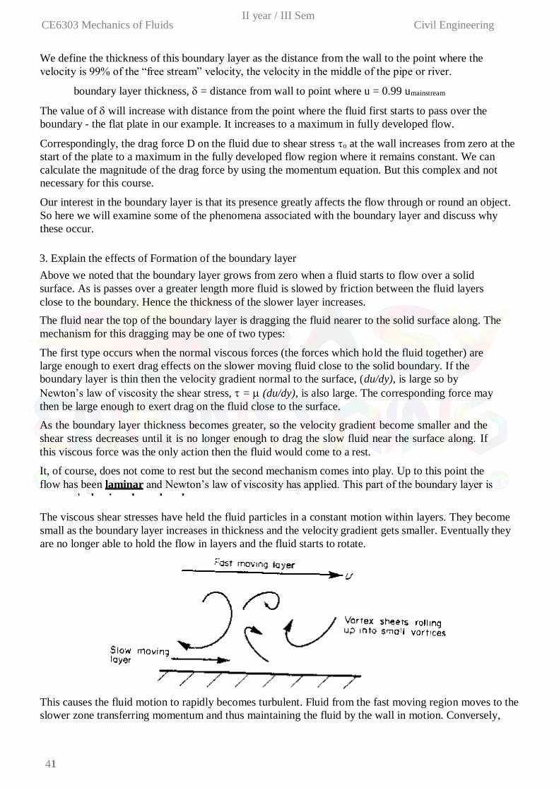
The viscous shear stresses have held the fluid particles in a constant motion within layers. They become
small as the boundary layer increases in thickness and the velocity gradient gets smaller. Eventually they
are no longer able to hold the flow in layers and the fluid starts to rotate.
This causes the fluid motion to rapidly becomes turbulent. Fluid from the fast moving region moves to the
slower zone transferring momentum and thus maintaining the fluid by the wall in motion. Conversely,
II year / III Sem CE6303 Mechanics of Fluids Civil Engineering
42
Boundary layers in pipes
As flow enters a pipe the boundary layer will initially be of the laminar form. This will change depending
on the ration of inertial and viscous forces; i.e. whether we have laminar (viscous forces high) or turbulent
flow (inertial forces high).
From earlier we saw how we could calculate whether a particular flow in a pipe is laminar or turbulent
using the Reynolds number.
Re ud
= density u = velocity = viscosity d = pipe diameter)
Laminar flow:
Transitional flow:
Turbulent flow:
Re < 2000
2000 < Re < 4000
Re > 4000
slow moving fluid moves to the faster moving region slowing it down. The net effect is an increase in
momentum in the boundary layer. We call the part of the boundary layer the turbulent boundary layer.
At points very close to the boundary the velocity gradients become very large and the velocity gradients
become very large with the viscous shear forces again becoming large enough to maintain the fluid in
laminar motion. This region is known as the laminar sub-layer. This layer occurs within the turbulent
zone and is next to the wall and very thin – a few hundredths of a mm.
Surface roughness effect
Despite its thinness, the laminar sub-layer can play a vital role in the friction characteristics of the surface.
This is particularly relevant when defining pipe friction - as will be seen in more detail in the level 2
module. In turbulent flow if the height of the roughness of a pipe is greater than the thickness of the
laminar sub-layer then this increases the amount of turbulence and energy losses in the flow. If the height
of roughness is less than the thickness of the laminar sub-layer the pipe is said to be smooth and it has
little effect on the boundary layer.
In laminar flow the height of roughness has very little effect
II year / III Sem CE6303 Mechanics of Fluids Civil Engineering
43
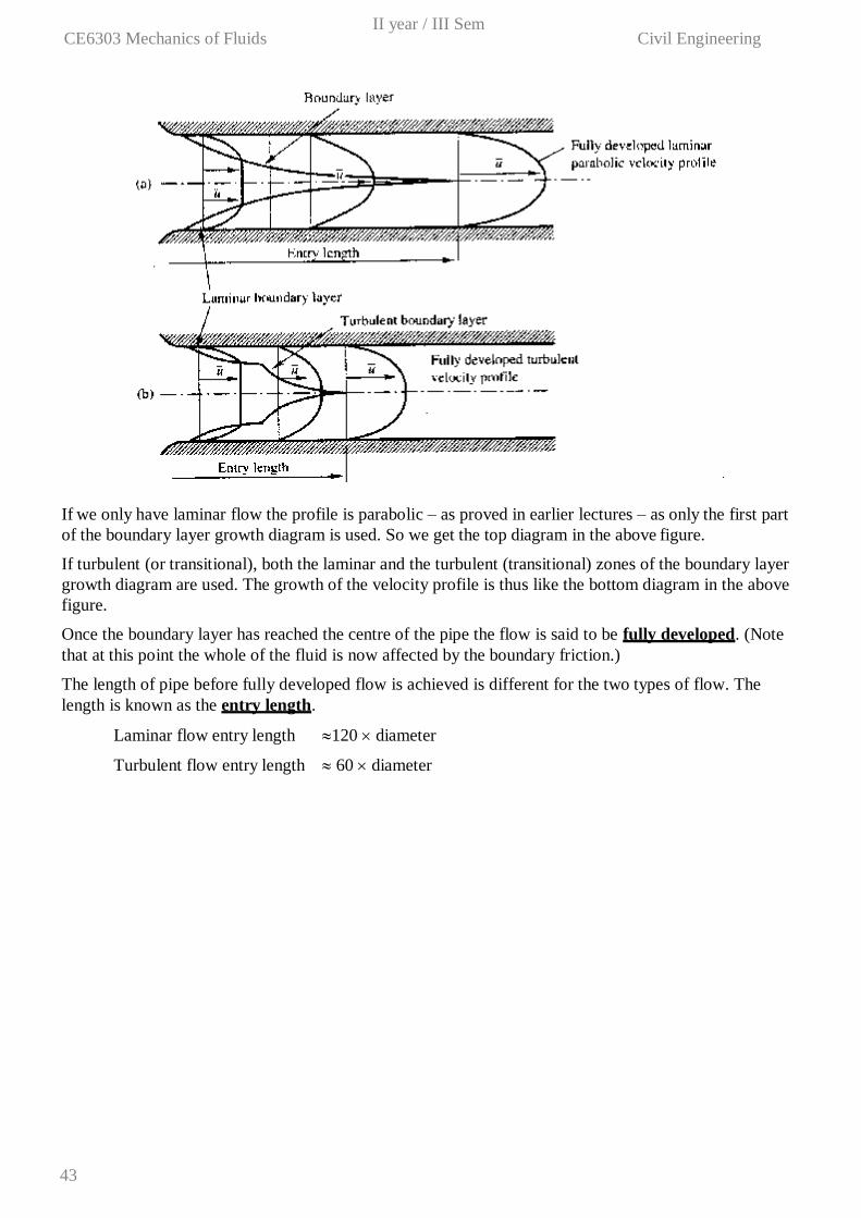
If we only have laminar flow the profile is parabolic – as proved in earlier lectures – as only the first part
of the boundary layer growth diagram is used. So we get the top diagram in the above figure.
If turbulent (or transitional), both the laminar and the turbulent (transitional) zones of the boundary layer
growth diagram are used. The growth of the velocity profile is thus like the bottom diagram in the above
figure.
Once the boundary layer has reached the centre of the pipe the flow is said to be fully developed. (Note
that at this point the whole of the fluid is now affected by the boundary friction.)
The length of pipe before fully developed flow is achieved is different for the two types of flow. The
length is known as the entry length.
Laminar flow entry length 120 diameter
Turbulent flow entry length 60 diameter
CE6303 Mechanics of Fluids II year / III Sem Civil Engineering
44
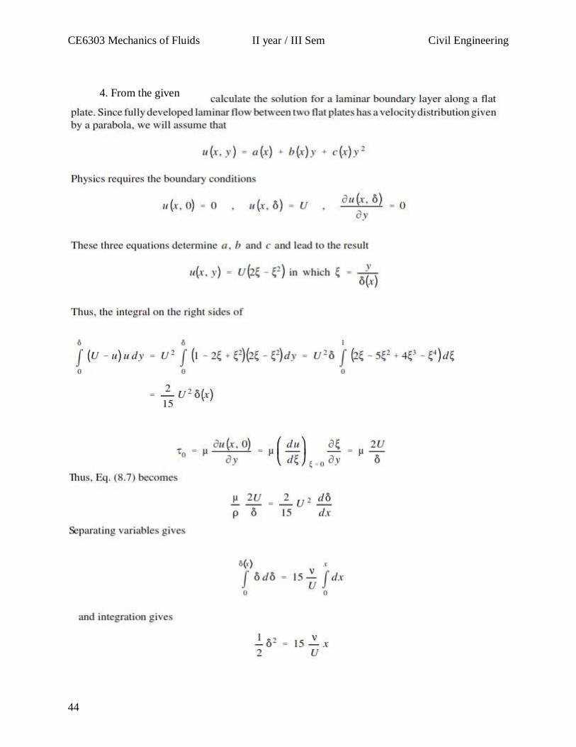
4. From the given
CE6303 Mechanics of Fluids II year / III Sem Civil Engineering
45
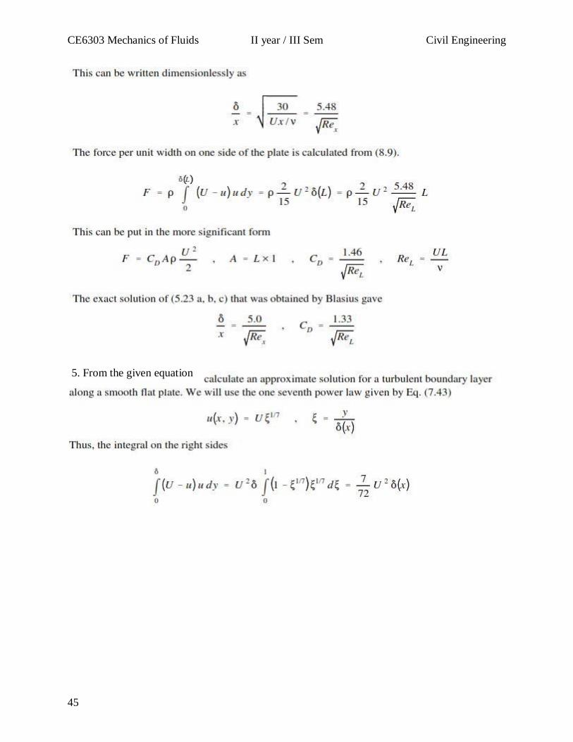
5. From the given equation
CE6303 Mechanics of Fluids II year / III Sem Civil Engineering
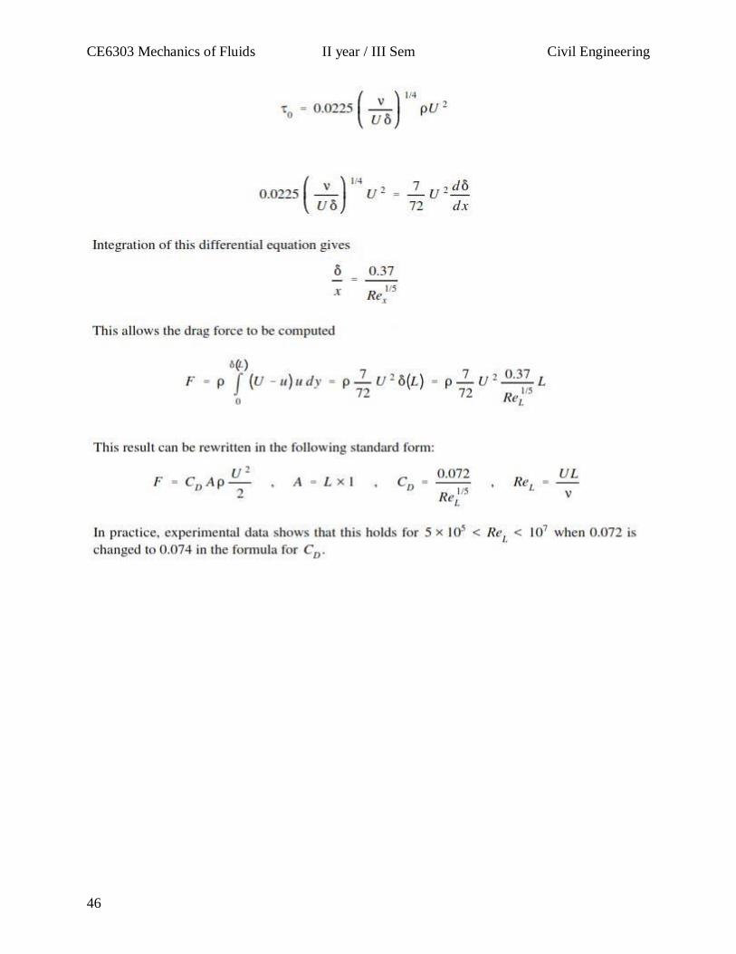
46
CE6303 Mechanics of Fluids II year / III Sem Civil Engineering
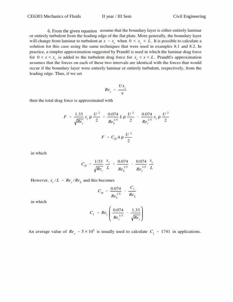
6. From the given equation