Unions, Wages and Labour Productivity:

Evidence from Indian Cotton Mills

No 753

WARWICK ECONOMIC RESEARCH PAPERS

DEPARTMENT OF ECONOMICS

1

Unions, Wages and Labour Productivity:

Evidence from Indian Cotton Mills

Bishnupriya Gupta1 Department of Economics

University of Warwick

July 2006

(Word Count: 7724)

1 This paper is dedicated to the memory of Raj Chandavarkar, who died suddenly. To Raj I owe many discussions and encouragement to revisit the history of cotton mills in India. I thank V. Bhaskar, Steve Broadberry, Greg Clark, Nick Crafts, Santhi Hejeebu, Morris D. Morris, Peter Lindert, Gavin Wright and the participants at the Business History Conference in Lowell, World Congress in Cliometrics at Venice and seminars at the LSE, Iowa, Davis and Warwick for comments. I am grateful to the staff at the Bombay Millowners Association and the Cotton Mills Federation in Bombay for giving me access to their archives and to the ESRC grant R.ECAA 0039 for financial support. The errors are mine alone.

2

Abstract

This paper uses firm level data from all the textile producing regions in India to

examine the relation between wages, unionization and labour productivity. We find

that fewer workers were employed per machine in the unionized mills in Bombay and

Ahmedabad, as compared to non-unionized regions implying that low labour

productivity was not due to union resistance to increased work intensity. Our findings

suggest that while low wages in India encouraged overmanning, higher wages,

prompted by unionization, had productivity enhancing effects. We explore alternative

explanations for low labour productivity, arising from the managerial and institutional

structure of Indian cotton mills.

3

1. Introduction

The effect of unionization on labour productivity has been debated in the

context of industrialized economies. Freeman and Medoff (1984) argue that unions

can increase labour productivity by reducing labour turnover and improving

managerial practices. Recent work suggests that presence of unions can increase

productivity by making mangers more keen to reduce organizational slack. (Metcalf

2003) The empirical evidence is mixed. Research using data from American

industries show that unions had a positive effect on labour productivity (Brown and

Medoff 1978, Clark 1980, Allen 1986) The evidence from the UK provides less clear

cut answers. (Machin 1991). Recent work suggests that multi-unionism has had a

negative effect on productivity in the UK (Bean and Crafts 1996), while in Germany

cooperative practice through work councils tend to have a more positive effect on

productivity. (Metcalf 2003)

The empirical evidence for less developed countries is scarce. Indian cotton

mills in early 20th century provide an interesting case of unionization. Labour strife

was common in Bombay from the late 19th century, although not always organized by

unions. Bombay was one of the two major cotton textiles producing regions and saw

early unionization. Wolcott and Clark (1998) attribute the divergent trajectory of

wages and productivity between Japan and India after 1910, to the failure to increase

labour productivity in Bombay cotton mills. Japanese workers increased their work

effort over time and consequently earned higher wages. The presence of a non-

unionized female workforce is seen by Wolcott (1992) an important factor in Japanese

success. Analyzing firm-level data from Bombay, Wolcott and Clark (1998) attribute

the persistence of low productivity to worker resistance to higher effort. Prescott and

4

Parente (1999) use the Bombay textile mills as an example of inefficient work

practice following unionization.

This paper re-examines the effect of unionization on labour productivity using

a data set of cotton mills from all the textile producing regions in India in early 20th

century. This is the first time such a data set is being analyzed. Labour unions were

important in the main two textile producing regions, Bombay and Ahmedabad.

Labour strife in these regions provides an interesting contrast with other textile

regions, where unions were less important. We do not have evidence on union

membership or strikes at the level of the firm. However, as union presence differed

from region to region, the regional effect allows us to test if labour productivity was

lower in the regions with union activity.

I analyze firm-level data to compare Bombay with the rest of India. My

measure of labour productivity is labour- use per machine. This captures total factor

productivity if machines are the same in cotton mills across all regions.2 My empirical

finding suggests that labour productivity was higher in regions where labour unions

were important and wages were high. This questions the Clark and Wolcott view that

low labour productivity in Bombay cotton mills was a result of worker militancy and

is in line with the empirical literature in developed countries that unionization may

reduce organizational inefficiency.

The cities of Bombay and Ahmedabad had the largest concentrations of cotton

mills in 1910. Both regions were located within the provincial boundary of the

Bombay Presidency in Western India. The daily employment figures show that until

the mid 1920s, Bombay had three times as many workers as Ahmedabad. By 1930 it

the difference had narrowed significantly. (Textile Labour Enquiry Committee, 1937-

2 Firms all over India imported their equipment from a few British firms. Clark 1987 also finds this to be the case at the international level in 1910.

5

38) Both cities saw large wage increases during the First World War, but the two

cities had very different experiences of labour movement. In Ahmedabad industrial

arbitration and peaceful settlements were the norm after 1922. The Bombay cotton

mills saw organized resistance to wage cuts in the 1920s.

If worker resistance prevented an increase in productivity, then the mills of

Bombay would have higher labour use per machine in comparison to other textile

producing regions, where union activity was lower. An interesting comparison would

be with Ahmedabad, where workers and management cooperated to set wages in the

1920s following Gandhi’s leadership. The statistical exercise in this paper suggests

that Bombay had a lower level of labour use compared to other regions over the

period 1910 to 1933, which was statistically significant. Ahmedabad also had a lower

labour use per machine, but this was significantly higher than the levels in Bombay in

1929 and 1933. The differences are observed at the end of a decade long conflict

between the worker and the management in Bombay cotton mills. Surprisingly the

two regions were not very different before the World War, but both had lower labour

use per machine compared to other regions. What was common between Bombay and

Ahmedabad was relatively higher wages. Thus the empirical finding suggests that

higher wages encouraged lower labour use per machine or higher labour productivity.

Comparisons of money wages in Bombay, Ahmedabad and Calcutta find that money

wages rose sharply in the first two cities after 1914. Although the wages rate was

comparable in the three cities before that, by the 1920s money wages diverged with

Bombay and Ahmedabad pulling ahead. This trend is also reflected in the real wages

although real wage in Calcutta was higher before the war. (See Figure 1) This

increase in part reflects the increased demand for cotton textiles as imports fell during

the war and the shortage of labour.

6

Labour militancy is not the only cause of higher wages. Wages can rise in the

economy due to other factors. The effect on labour efficiency would be similar. The

above argument may explain the productivity differential between India and Japan.

Japan saw rapid economic growth after 1870. Rising incomes and wages in Japan

compelled managers to raise labour productivity to stay competitive in the

international market for textiles. Both comparisons indicate that high wages and

worker efficiency are correlated. In this paper, I will argue that causality flows from

wages to productivity.

The organization of the paper is as follows: Section 2 discusses the

organization of the industry and the factors that may explain high labour use per

machinery. Section 3 presents an empirical analysis of firm-level data to quantify

labour use in different regions. Section 4 presents a simple model of wage- effort

trade off. Section 5 explores the role of institutions in causing organizational slack

and inefficient labour use. Section 6 analyzes the link between wages and labour

productivity using comparisons with Japan. Section 7 concludes.

2. Organization in cotton mills:

2.1 Background

The cotton textile industry was mainly an import substituting activity,

competing with imports from Lancashire. The first cotton mills were set up in

Bombay. Initially the main output was yarn for the domestic handloom industry and

for export to the Chinese market. Over time, spinning mills bought their own looms

and began producing cloth. The advantages the industry enjoyed were cheap labour

and local supplies of raw material. The industry had a unique management structure.

A managing agent was responsible for organizing production. This agent raised

7

capital and managed the financial side of the business for a commission. Production

was left in the hands of technical supervisors and labour supervisors known as the

jobbers, who were locally recruited. The agents mostly came from the merchant class

and had little technical training. The majority of the agency directors were Indians,

who had made money in the cotton and opium trade and moved into industry as

profits in trade began to decline. (Vicziany, 1975) Table 1 shows the background of

the directors and of technical staff in Bombay. The managing agents relied initially on

the men from Lancashire for the technical side of production. Over the years, Indian

technicians filled this important gap. However these technicians knew little about the

labour market, which was left to the jobber or the labour recruiting agent.

The process of hiring workers was complicated. India had abundant labour,

but mainly concentrated in agricultural activity. The industry had to draw its labour

from the rural hinterland. The task was assigned to the jobbers, who typically came

from the same social background as the labourers and used their rural connections to

recruit workers for the textile mills. The demand for labour fluctuated due to

fluctuations in demand in the product market. About one-fifth of the labour in

Bombay cotton mills was employed on a daily basis. (Chandavarkar, 1994: 82) The

jobbers were given the responsibility of maintaining adequate labour supply to suit the

level of demand. The production managers often did not have a common language of

communication with the mill workers. It was the jobber who was assigned the task of

worker management and supervision and to implement factory discipline.

The system encouraged high labour turnover as the jobber exercised control

over a readily available group of casual workers. (Morris, 1965, Chandavarkar 1994)

However, it also allowed quick reductions in employment if the need arose.

8

2.2 Choice of technology and labour productivity

The production process reflected the abundance and cheapness of labour.

Although the ring was also more suited to unskilled labour, the Indian cotton mill

industry adopted the mule. Saxonhouse and Wright (1984) find that the persistence of

the mule in India and Russia was due to the use of short staple cotton, which was the

variety produced in India. Japan and Brazil used long staple cotton and adopted the

ring much earlier. An alternative view emphasized the lack of technical knowledge of

the managing agents and the presence of British technical personnel as the cause of

India’s failure to switch to ring spinning. (Kiyokawa, 1983) Other research in this

field suggests that the Indian entrepreneurs made a rational choice in adopting the

mule given the factor endowments. Capital was expensive and the mule was relatively

cheaper, at least until 1890. The cost of setting up a cotton mill was 35% higher in

India compared to a Britain. Once a mill was set up, the machinery was operated as

long as possible and replacement was deferred, with repairs and replacement of parts.

The lower rate of scrapping and replacement of machinery delayed the rate of

adoption of rings, since rings could be adopted only as mules were scrapped.

Consequently mules persisted in Bombay longer than elsewhere.

High labour use was a response to factor prices. Tasks became more labour

intensive per unit of capital. Each mill produced a variety of yarn depending on

demand. The mule allowed greater flexibility in operation. Short staple cotton broke

more frequently. The machines were often operated at a speed higher than the

recommended level without introducing the appropriate quality cotton. (BMOA

Report 1928) These increased the need to have more men per machine. It was

estimated that a ringsider in India had to deal with nine times as many breakages per

9

100 spindles as his American counterpart. (Chandavarkar, 1994: 284) One survey

estimated that in the 1930s, for every worker employed in a month, two casual

workers were available. (Chandavarkar, 1994: 296)

The Tariff Board in 1927 saw high labour use per machine as an

organizational problem. (BMOA Report 1928):

“We cannot too strongly emphasize that no increase in outturn per operative can be reasonably expected unless they are provided with proper raw material. There undoubtedly exists a tendency in India to spin higher counts of yarn from cotton than the quality of cotton warrant. This reduces production, is injurious to quality and increases the work of the operative in both spinning and weaving by the large number of breakages.”

2.3: The labour movement

The labour movement in Bombay and Ahmedabad were mainly concerned

about wages. Spontaneous protests by textile workers in Bombay had been a part of

the industry from the beginning. The early protests started in one mill and spread to

others. The wave of strikes in 1900-01 came in response to wage cuts in twenty mills

when 20, 0000 workers went on strike for ten days. (Morris, 1965) Wages rose

dramatically during the war. Two factors contributed to this: The rise in demand for

labour and the rise in the cost of living. The mills paid a war bonus of 10% from 1917

to be followed by a “dear food allowance” of 15% from 1918. (Kooiman, 1989: 51-

52) As the war-time boom gave way to a recession, firms attempted wage cuts that led

to strike action. 150,000 workers struck work for 12 days in 1919 followed by a

general strike in 1920 that lasted for a month. (Morris, 1965: 178-79)

This period coincided with economic nationalism in the anti-imperialist

struggle. While workers in Bombay adopted a militant approach, with Gandhi’s

involvement workers in Ahmedabad sought consensual solutions through industrial

arbitration. Workers in Ahmedabad struck work in 1923 against an attempt to reduce

10

wages. Nevertheless, the industry implemented a wage cut of 15% and for the rest of

the decade, wages were negotiated through dialogue.( Patel, p32) In 1925 in Bombay,

strikes began as the Bombay Millowner’s Association (BMOA hereafter) announced

wage cuts.( Bombay Labour Office, 1926) The city witnessed a general strike that

lasted several weeks. By this time the trade unions had establishes a strong presence

in Bombay cotton mills and coordinated worker resistance. The strikes were

coordinated with the involvement of the jobbers. As several cotton mills in Bombay

sought to introduce a higher work load, the Communist union organized industrial

action in 1928 that lasted for over six months. (Morris, 1965:181-83)

The average wage in Bombay was 20% higher than the average wage in

Ahmedabad on the eve of the First World War. Between 1914 and 1921, wages rose

by 87% in Bombay city and by 122% in Ahmedabad. (Bombay Labour Office, 1923)

The rise in earnings in Bombay city was below the average for Bombay Presidency.

The rise in the cost of living in Bombay and Ahmedabad were similar. The fast

increase in the average wage in Ahmedabad reflected the increase in demand from the

domestic market as supply of British goods was disrupted. At the same time, the

workers ready to leave the city due to a plague epidemic when and were paid bonuses

to stay on.

Table 2 shows a comparison of wages in the two cities and the rest of India in

1929. Clearly the difference in wages between Bombay and Ahmedabad was

marginal, but these figures were higher than what was paid to workers in other textile

producing regions.

11

3. Empirical Analysis:

Did resistance from labour unions prevent an increase in labour productivity?

One way to analyze the role of unions in preventing organizational change would be

to compare the labour- capital ratio across different regions in India. If organized

labour resistance was important in influencing work norms, Bombay should have had

a higher use of labour per machine compared to other regions. On the other hand, if

union activity mainly increased wages and higher wages forced employers to initiate

productivity increases, one should find that Bombay had higher labour productivity

and fewer workers per machine. A comparison with Ahmedabad would be of interest

as the two regions had different experiences of labour resistance. Did militancy hinder

organizational change in Bombay as has been suggested by Wolcott and Clark? Did

cooperation rather than conflict lead to efficiency gains?

3.1. The data

My data covers all the textile producing regions in India. The data is at the

level of the firm and provide information on the number of workers employed daily in

each firm and the machinery in use. The latter is available by category, i.e. mules,

rings and looms. The data is for the years 1889, 1910, 1917, 1929 and 1933. Firm-

level information for 1889 is being used for the first time and allows us to go back to

the period when worker resistance had yet to make an impact on the industry. 1929

and 1933 are of particular interest as these follow a decade of labour strife.

Table 3 shows the use of capital and labour in cotton mills in different

regions. My focus is on Bombay relative to Ahmedabad and the rest of India. Bombay

had the highest concentration of cotton mills in 1889, while Ahmedabad was still

marginal. By 1910 both cities had roughly the same number of mills. Ahmedabad had

12

a large share of rings as newer were more likely to adopt the ring, while older firms in

Bombay with an existing capacity of mules were slow in switching to rings.

Ahmedabad also had more looms. These firms produced finer quality yarn and cloth

and competed with British imports. Bombay on the other hand produced more of

lower count yarn and exported to the Chinese market.

The average size of mills in Bombay was larger. By 1917, the changes in

Bombay are noticeable. The switch to rings and looms was well underway. There was

also an increase in the average size of the mill. The change that affected Bombay was

the loss of the Chinese market and the change in competition after the war. These

mills faced increased pressure to reorganize with the changes in the product market.

Several mills went out of business by 1929 and more disappeared by 1933. For

Ahmedabad, on other the other hand, there is evidence of increase in size as well as

new entry and these firms benefited from the changes in the product market.

3.2: The Analysis

From the data we can estimate coefficients of labour use by type of the

machine over time. The dependent variable, labour use per day, is regressed on the

number of mules, rings and looms within a firm. To allow for the possibility that

labour in a particular region, Bombay or Ahmedabad, is systematically less (or more)

efficient, a dummy variable for the region is interacted with each of the machinery

variables. That is, our regression takes the form:

Nit = βm (1 + γBDi + µADi )Muleit + βr (1 + γBDi+ µADi )Ringit

+ βl (1 + γ BDi + µADi)Loomit + εit,

where Nit is employment in firm i in year t, Muleit is the number of mules used by the

firm in this year, etc., and BDi is a dummy variable that takes value 1 of the firm is in

13

the Bombay region and ADi is a dummy variable that takes value 1 of the firm is in

the Ahmedabad region We estimate this equation for each year separately, that is we

allow the coefficients β, γ and µ to vary across years. As this equation is non-linear in

the parameters, the estimation is by non-linear least squares. Our interest is in the

values of γ, that is, the extent to which labour requirements in Bombay differ from

other regions.

Table 4 reports the estimated coefficients from the regression. We see that γ

is estimated to be negative in every single year. Although this is not statistically

significant in 1889, the coefficient is significant in subsequent years. Indeed, in 1929,

labour in Bombay is 48 per cent more efficient than labour in the other regions of

India. Labour in Ahmedabad is also more efficient than in other regions, but less

efficient than in Bombay. A t-test shows that the coefficient for labour use in Bombay

is significantly different from the coefficient for labour use in Ahmedabad for the

years 1929 and 1933, but not in the 1889, 1910 and 1917.

This result is striking. The 1920s strikes took place in response to reduction in

employment as the industry struggled to maintain profits after the war. In 1929 after a

decade of organized labour resistance, the productivity of Bombay textile workers in

relation to their Ahmedabad counterparts was high. The difference between the two

cities had narrowed by 1933. Clearly in other regions of India where the workers were

less militant, the labour- use ratio was higher.

These findings question the Wolcott –Clark view that workers’ resistance to

increases in labour productivity in Bombay was the main cause of over manning. The

results suggest that the relatively higher wages in Bombay and Ahmedabad required

higher labour efficiency (See table 2 to compare wages). This encouraged firms to

economize on wage costs so as to remain competitive in the product market. Higher

14

wages forced the Bombay entrepreneurs to increase work intensity in cotton mills and

reduce labour use per machine. Several inefficient firms went bankrupt as shown by

the decline in the number of firms in the region. This finding though contrary to the

work by Wolcott –Clark, is in line with the empirical literature on industrialized

countries that suggests that unions can remove managerial slack and increase

efficiency.

Although the money wage difference between Bombay and Ahmedabad was

marginal, the productivity difference in 1929 was large. This is puzzling. However, a

closer examination suggests that the product and factor markets in the two cities were

very different. Consequently, the pressure on entrepreneurs in Bombay to reduce

inefficiency was greater. Mills in Bombay relied on the export markets in yarn and

were hit hard as they lost overseas markets after the war. Ahmedabad on the other

hand produced higher quality yarn and cloth and benefited more as Britain lost market

share in India. Simple calculations of profits of the firms in the two cities show that

profits fell faster in Bombay.(Patel, 1987: 34) Bombay mills had a high turnover of

the workforce and a large proportion were casual workers estimated to be about 28%

of the workforce.(Chandavarkar, 1994: 296) This made it relatively easier to reduce

employment. Evidence from the wage census shows that absenteeism among male

and female time and piece-rate workers declined in Bombay between 1923 and 1926,

but stayed roughly the same for male workers in Ahmedabad and declined for both

categories of female workers. (Bombay Labour Office, 1923, 1929)

There is ample evidence in representations of firms in Bombay to the Tariff

Board that increased workload was seen as an alternative to wage cuts. One of the

industry leaders, the firm of Sassoon, presented estimated of savings in total wage

cost with increased workload even when wages increased. (Bombay Labour Office

15

1934) Estimates based on my data set show that Bombay saved in total wage cost as

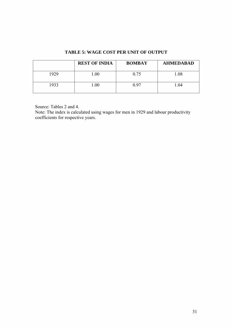
number of workers per machine declined. Wage cost per unit of output in Bombay in

1929 was 25% lower than that for the rest of India and 3% lower in 1933, while in

Ahmedabad it was roughly 8% and 4% higher. (See table 5) These figures suggest

that efficiency gains made by Bombay mills in the 1920s. The figure for 1929 for

Bombay is not out of line with estimated savings projected for spinners by Sassoon

between 46% and 62% depending on yarn count. Falling profits, older machinery and

changes in the product market created additional pressure on firms in Bombay to

bring about organizational change. To understand why firms had operated at sub-

optimal level and what prompted them to become more efficient, a simple model of

wage effort trade off is useful.

4. Wage- Effort Trade off:

Let e denote effort, and let us measure effort so that one unit of effort results

in one unit of output. Let p denote the price of output, let k denote the capital

requirement per worker, and r the interest rate. Let w denote the wage per unit of

effort, so that the profits of the firm per worker can be written as

π= ep-w-rk ……(1).

Turning to the representative worker, let us assume that the utility of the

worker, U, increases with the wage, but decreases with the disutility of effort, and can

be written as

U(w,e) = w – d(e) …….(2),

where the disutility of effort, d(e), is increasing and convex, so that the marginal

disutility rises at higher levels of effort.

16

Fig. 2A graphs the typical indifference curve of the worker IC, corresponding

to a given utility level. Let us now consider what effort choice would be a Pareto

efficient arrangement, given the preferences of the worker and the production

technology. To do this, we can graph the iso-profit curves of the firm. These are

straight lines with slope p. An efficient arrangement corresponds to a point of

tangency between the worker’s indifference curve and the iso-profit curve IP. Thus

e* is the efficient choice of effort in this context.

There are of course many Pareto efficient arrangements, which can be ordered

in terms of the extent to which they favour one party, say the worker. Thus some

Pareto efficient arrangements give the worker higher wages and higher utility and the

firm lower profits than the others. However, given our assumption of quasi linear

utility, in all Pareto-efficient arrangements the effort level is the same and equals e*,

and variations in worker utility are achieved entirely through the wage. Thus, even if

the worker has some bargaining power, and gets a higher utility level than in a

competitive labour market, an efficient bargain would imply that this increased utility

is achieved not via reduced effort but solely through a higher wage.

Let us now suppose that existing effort arrangements are inefficiently low, and

are at a level e’ that is less than e*. This is indicated in Fig. 2B. Since this is Pareto

inefficient, there is a way to make both the worker and the firm better off. This

involves an increase in worker effort towards e*, where the worker is compensated for

this by an increase in the wage.

There are two possible explanations for the low effort levels of the worker in

the Indian cotton mills. The first explanation, advanced by Wolcott and Clark (1998),

is that low effort reflected worker preferences, so that arrangements were Pareto

efficient. That is the, actual effort choices were in fact close to e*, so that it did not

17

make economic sense to increase effort. Similar views had been voiced by

managerial staff in the industry, policy makers and foreign observers from early days

of the industry. The increase in effort level of cotton mill workers in Bombay with

higher wages question such an interpretation.

An alternative explanation is that actual arrangements were Pareto-inefficient;

so that both workers and firms could be made better off by wage-productivity

agreements, where the worker agreed to raise work effort in exchange for higher

wages. For this latter explanation to hold, there must be a reason why the two parties

failed to make a Pareto-improving trade. This failure is could be a failure of initiative,

possibly based on a lack of information. For the two parties to make such an

improvement, one of them must recognize the potential for mutual gain, and has to

initiate the improvement. The specific institutional structure of management may

have created inefficiencies in the system. Unions in this context may play an

important role in moving to a more efficient arrangement.

5: An Institutional Failure?

Hall and Jones (1999) show that institutional differences explain difference in

labour productivity across countries. In the Indian context, it may be argued that the

managerial structure in cotton mills made for certain inefficiencies. The three tiers of

management created self contained spheres of function and resulted in information

gaps. Madholkar documents the friction between the men from Lancashire and the

managing agents and sees the presence of the jobber as the crucial factor in reducing

the managing agent’s reliance on the technicians. The agents’ distrust of the

technicians removed them from the sphere of decision making. The agent made

decisions regarding the purchase of inputs and the technician was asked to produce a

18

certain output per machine. (Madholkar, 1969, ch 3) An additional reason might have

been the incentives of the managing agents, who held overall responsibility for the

organization. Right up to the turn of the 20th century, the managing agents’ returns

depended upon the output of the firm rather than profits and provided relatively weak

incentives to engage in cost reductions. Even when firms switched to commission on

profits, the relevant category was total profits and not profits net of depreciation.

The managerial structure and the factor prices also had implications for

factory discipline, which is an important aspect of labour productivity. Thompson

(1967) documents how new working habits were formed in Britain after the industrial

revolution. Clark (1994) finds that greater discipline increased effort by 33% in

Britain in the course the 19th Century. The change in length of a working day and

increased effort at workplace was a result of a stringent system of penalties.

Discipline was also a crucial aspect in the Japanese cotton mills. Hunter (2003) argues

that dormitories were crucial in the evolution of factory discipline. The control of the

management extended not just during working hours, but for the whole day. Workers

were paid by piece rate and remuneration depended on quality and quantity.

The Indian cotton mills did little to develop mechanisms for higher discipline

on the shop floor to increase work intensity. A survey conducted by the Bombay

Labour Office in 1926 documented the penalties imposed on workers for the first ten

months. Information on dismissals is not available, but we do know how many

workers were penalized. The table 6 is based on information collected from 45 mills.

An overwhelming proportion of the fines for men and women were for negligence in

work. This referred to spoilt or damaged material- their value was deducted from the

workers wage. Weavers in particular were subjected to large penalties. (Pearse, 1930:

89-90) Late arrival at work or taking time off during working hours were less serious

19

offences compared to failing to produce the right quality product. It has been

suggested that this was a way to reduce the earnings of highly paid weavers. (Tariff

Board 1927) Interestingly, the survey showed that in factories other than textiles, 49%

of the fines were for breach of discipline. (BMOA Report, 1927) Morris documents

the evidence presented to the Factory Commissions and argues that in the textile

industry, although the formal system of rules was severe, regulation of work

discipline was surprisingly lax. Workers drifted in at the start of work and gradually

drifted away as the light began to fade. (Morris, 1965:111-112). Either supervisors

were not concerned about work intensity or chose to ignore breaches of it. The latter

could arise from the social relation between the worker and the jobber.

The evidence from cotton mills in India suggests that the managers had less

concern about factory discipline. Equipment costs were relatively high and the

managers chose to economize on capital cost by running the machines as long as

possible. The employers responded to worker absences by employing reserve labour

to step in when needed. The low wages provided a reason for over manning rather

than imposing greater discipline.

The Indian entrepreneurs were slow to introduce an organizational change that

was a feature of the Japanese industry. Unlike in Indian mills, where there was a

separation between technical and managerial activity, Japanese firms had a more

integrated approach. (Pearse, 1930) The Japanese entrepreneurs increased labour use

per unit of capital through a system of double shift. The Indian mills persisted with of

long hours of a single shift system. Arno Pearse, who studied cotton mills in different

parts of the world, showed that mills working two shifts would reduce costs by 12%-

13% on average. (Pearse, 1930) Longer hours also reduced efficiency.

20

As early as 1905, the BMOA discussed reduction of the working day to 12

hours. Firms, such as Wadia, Sassoon and Petit, who were the industry leaders in

introducing changes in work practices, argued that long hours reduced worker

efficiency. (BMOA 1905) In 1919 Wadia moved to introduce two shifts of eight

hours. However, BMOA voted against the introduction of double shifts. One of the

arguments was that the city infrastructure would not be able to cope with an additional

100,000-150,000 men required for the second shift. (BMOA reports, 1919-21) The

reluctance to work double shifts could have been associated with greater costs of

supervision and the high salaries paid to European technical staff. (Morris, 1965: 56-

7) Several millowners argued that mills on a double shift would bid up the wages and

cause labour disputes in mills on single shift. (Chandavarkar, 1994: 353-354) The

BMOA passed a resolution in 1920 prohibiting implementation double-shifts. Two

firms that introduced a double shift were expelled in 1921. (BMOA, Report 1921) In

his statement to the Industrial Disputes Committee, Wadia claimed that the

introduction of double shifts had reduced absenteeism. (Indian Textile Journal,

January 1922) However double shift did not become the norm until the 1930s. In fact

the BMOA rescinded the resolution of 1920 to allow firms to do so. (BMOA, Report

1928)

The agency problems associated with the separation of financial and technical

jobs in the cotton mills may explain the absence of organizational change.

Consequently, rising wages were instrumental in increasing efficiency if firms were to

remain competitive.

21

6. Wages & Labour Productivity: Cause & Effect?

The correlation between wages and labour productivity can be found in the

context of the divergence in productivity levels between India and Japan. Wolcott and

Clark (1998) see low labour productivity as a determinant of low wages. However,

this view is inconsistent with a competitive labour market, where textile workers were

only a small fraction of the total workforce. For example, in India, the entire

industrial workforce was less than 10% of the total labour force and cotton textiles

had an even smaller share. Thus the wages of cotton textile workers would not have

been determined by the level of productivity in cotton textiles, but mainly by the

general level of wages in the economy. If textile workers were substantially

productive, this would mainly be reflected in higher profits, with only a small effects

on wages. Alternatively, rising wages would require rising labour productivity if the

firm was a price taker.

GDP per capita in Japan rose faster than in India. In 1870, GDP per capita in

Japan was just over 35 per cent more than India’s per capita GDP, by 1913 Japan had

twice the per capita income of India and by 1950, three times as much Per capita

GDP grew by 0.54% per year in India during 1870-1913, almost one-third of Japan’s

growth rate of 1.48% per year. The corresponding growth rates in India and Japan

during 1913-1950 were -0.22% and 0.89% respectively. (Maddison, 200: 264-5,

Shivasubramoniam, 2000: 33) Money wages in Japanese cotton mills increased four

times between 1903-07 and 1918-22. In Indian cotton mills, wages doubled during the

same period. (See table 7)

As wages increased in Japan, sectors producing tradable goods, such as cotton

textiles, were compelled to increase labour productivity to stay competitive. On the

other hand, the Indian economy stagnated and wages did not rise much until the First

22

World War. The cotton mill entrepreneur faced little pressure for change and

productivity increase. Table 6 shows the differences in wages and capital costs in

India and Japan. In India, the relative price of capital goods increased, whereas in

Japan the relative price of capital goods declined continuously, creating the

momentum for technological change. Wage driven labour productivity growth was

not a factor in India until the 1920s. An Indian worker produced 0.75 pounds of yarn

per hour in 1890-94, and this remained static at 0.73 in 1915-1919. In Japan, yarn per

worker more than doubled, from 0.80 to 1.91 in the same years. (Wolcott & Clark,

1998)

Did India and Japan have similar levels of labour productivity before the

divergence in wage trends? Clark (1987) finds that labour productivity in cotton mills

in India and Japan was not very different in 1910. I use firm-level data from India and

Japan to test the differences in labour use per machine around 1890. Data from 104

Indian cotton mills in 1889 is combined with similar data from Japan, on 32 firms, for

the year 1892 to assess how employment norms differed between the two countries

very early in the process of industrialization.

To analyze employment norms, we need to take into account the difference in

shift work between the two countries. Japanese firms introduced double shifts in the

mid 1880s. By the early 1890s, most Japanese firms had adopted double shifts, while

Indian firms had only one shift. I therefore divide employment in each Japanese firm

by two in order to get the number of workers per shift in each country. I estimate the

following regression, which is similar to the one estimated in section 3:

Ni = βs (1 + γ IDi) Spindlesi + βl (1 + γ IDi) Loomi + εi,

where Ni is employment in firm i, Spindlesi is the number of spindles used by the

firm, and Loomi is the number of looms used by the firm. IDi is a dummy variable

23

that takes value 1 if the firm is located in India. This equation is estimated by non-

linear least squares. Our interest is in the parameter γ, which measures the extent to

which firms use more labour in India as compared to Japan.

Table 8 reports the regression results. Indian firms used about 9% more labour

than Japanese firms, but this effect is not statistically significant. This analysis is

subject to a few caveats. We have relatively few Japanese firms in our sample. We

have also assumed that all Japanese firms have switched to double shift – if there

were some exceptions, this would imply that we have underestimated employment

norms in Japan and thus the difference between the two countries would be less than

the estimated 9%. We have assumed that spindles are homogeneous between the two

countries although the Japanese firms had a larger share of rings. Subject to these

caveats, our analysis indicates that there was at most a small difference in labour

productivity between the two countries around 1890, and the divergence came later.

By 1910, Japanese productivity levels were higher than the Indian levels, but lower

than that in Britain. (Clark 1987) The divergence in productivity levels increased as

wages rose in Japan.

7. Conclusion

This paper has argued that unionization and worker resistance cannot be an

explanation for low labour productivity in the Indian cotton mills. On the contrary, the

militancy of textile workers in Bombay made the cotton mills in this region relatively

more efficient by increasing wages relative to other regions. Cotton mills in the cities

of Bombay and Ahmedabad used less labour per machine. Both cities had higher

wages in 1929 relative to other regions. While Bombay had seen several strikes over

the decade, wages were set by arbitration in Ahmedabad cotton mills.

24

REFERENCES:

Allen, S.G. , 1986, “Unionization and productivity in office building and school

construction”, Industrial and Labour Relations Review, 39:2, pp187-201.

Bagchi, A.K., 1972, Private Investment in India, Cambridge: Cambridge University

Press.

Bemmels, B. , 1987, “How unions affect productivity in manufacturing plants”,

Industrial and Labour Relations Review, 40:2, pp241-53.

Bombay Labour Office, Report on enquiry into wages and hours of labour in the

cotton mill industry, 1921, 1923, 1926.

Bombay Labour Office, Wages and Employment, 1934.

Bombay Millowners Association, Annual Reports.

Brown, C. and J.L.Medoff, 1978, “Trade unions in production process”, Journal of

Political Economy, 86: , pp355-78.

Buchanan, D. , 1966, The Development of Capitalist Enterprise in India, London:

Frank Cass.

Chandavarkar, R, 1994, Origins of Industrial Capitalism in India, Cambridge:

Cambridge University Press.

Clark, G., 1987, “Why isn’t the whole world developed? Lessons from the cotton

mills, Journal of Economic History, 49:3, pp107-14.

Clark, G., 1994, “Factory Discipline”, Journal of Economic History, 54:1, pp128-63

Clark, K.B., 1980, “Unionization and productivity: Micro-econometric evidence”,

Quarterly Journal of Economics, 95:4, pp613-39.

Freeman, R.B. and J.L, Medoff, 1984, What do Unions Do ? London: Basic Books..

Indian Textile Journal, various years.

25

Hall, R. E. and C.I. Jones, 1999, “Why to some countries produce so much more

output per worker than others”, Quarterly Journal of Economics, 114:1, pp 83-116

Kiyokawa, Y., 1983, “Technical Adaptations and Managerial Resources in India: A

study of the experience of the cotton textile industry from a comparative viewpoint”,

Journal of Developing Economies, 21:2.

Kooiman, D., 1989, Bombay Textile Labour: Managers, Trade Unionists and

Officials 1918-1939, Delhi: Manohar.

Machin, S.J., 1991, “The productivity effects of unionization and firm-size in British

engineering firms”, Economica, 58:232, pp479-490.

Maddison, A., 200, The World Economy: A Millennial Perspective, OECD.

Madholkar, G. V, 1967, The Entrepreneurial and Technical Cadres of Bombay

Cotton Textile Industry between 1854 and 1914: A Study in the International

Transmission and diffusion of Techniques, PhD thesis, University of North Carolina.

Metcalf, D., 2003, “Unions and Productivity, Financial Performance and Investment:

International Evidence” in Addison, J.; Schnabel, C. (ed), International Handbook of

Trade Unions, Edward Elgar, Chapter 5.

Morris, M.D., 1965, The Emergence of an Early Indian Labour Force in India,

Berkley.

Otsuka, K., G. Ranis & G. Saxonhouse, 1988, Comparative Technology-Choice in

Development: The Indian and Japanese Cotton Textile Industries, London.

Patel, S., 1987, The Making of Industrial Relations: The Ahmedabad Textile Industry,

1918-3, Oxford University Press, Delhi.

Pearse, A., 1930, The Cotton Industry India, Manchester.

Parente S.L. & Prescott, E.C, 1999, “Monopoly rights: A barrier to riches”, American

Economic Review, 89: 1216-1233.

26

Rutnagur, S.M., 1927, Bombay Industries: The Cotton Mills, Indian Textile Journal,

Bombay.

Report of the Indian Tariff Board, 1927.

Saxonhouse, G, 1977, “Productivity change and labour absorption in Japanese cotton

spinning, 1891-1935,” Quarterly Journal of Economics, 91:2, pp195-219.

Saxonhouse, G. & G. Wright, 1984, “New evidence on the English mule and cotton

industry”, Economic History Review, 37: 4, pp507-19.

Shivasubranomian, S., 2000, The National Income of India, Oxford University Press,

Delhi.

Thompson, E.P., 1967 “Time, work discipline and industrial capitalism”, Past and

Present, 38:2..

Vicziany, M., 1975, The Cotton Trade and Commercial Development of Bombay,

1855-1875, Ph.D thesis, London University.

Wolcott, S., 1994, “Perils of lifetime employment systems: Productivity advance in

the Indian and Japanese textile industries, 1920-1938”, Journal of Economic History,

54:2, pp302-24.

Wolcott, S. &, G. Clark, 1998, “Why nations fail: Managerial decisions and

performance in Indian cotton textile, 1890-1938”, Journal of Economic History,59:2:

397-423

27

TABLE 1: SOCIAL ORIGINS OF MANAGERS IN BOMBAY COTTON

MILLS

TECHNICAL

PERSONNEL

DIRECTORS

1925

1895 1925 MERCHANTS TECHNICAL LAWYER

PARSI 112 201 30 9 10

HINDU 21 67 74 0 3

MUSLIM 5 6 19 0 0

JEWISH 3 11 6 0 0

EUROPEAN 104 113 20 2 2

Source: Rutnagur, 1927, pp 251-253.

28

TABLE 2: WAGE DIFFERENTIAL IN BOMBAY PRESIDENCY 1929

(DAILY AVERAGE EARNING IN RUPEES)

BOMBAY AHMEDABAD SHOLAPUR BARODA OTHERS

MEN 1.45 1.39 1.00 1.03 1.00

WOMEN 0.78 0.80 0.40 0.57 0.54

ALL

WORKERS

1.26 1.24 0.80 0.95 0.87

Source: Pearse, 1930, p109.

29

TABLE 3: CAPITAL AND LABOUR USE IN COTTON MILLS

BOMBAY AHMEDABAD REST OF INDIA 1889

SPINDLES 29725 22423 26005 LOOMS 252 212 20

HANDS DAILY 996 779 884 NO. OF FIRMS 53 7 104

1910 MULES 11133 1494 7888 RINGS 23720 18648 20453 LOOM 296 305 291

HANDS DAILY 955 833 1101 NO. OF FIRMS 79 72 208

1917 MULES 7591 781 5280 RINGS 29433 20236 22873 LOOM 724 391 480

HANDS DAILY 1562 817 1175 NO. OF FIRMS 77 82 231

1929 MULES 4637 494 2940 RINGS 39812 21007 26670 LOOM 994 464 584

HANDS DAILY 1423 968 1213 NO. OF FIRMS 75 111 286

1933 MULES 3636 177 2200 RINGS 41930 24071 28642 LOOM 1014 526 608

HANDS DAILY 1863 1041 1367 NO. OF FIRMS 67 128 298

Source: BMOA Annual Reports for various years

30

TABLE 4: LABOUR USE: BOMBAY COMPARED TO OTHER REGIONS

1889 1910 1917 1929 1933

NO OF FIRMS 99 208 231 286 298

LABOUR USE

PER MULE

0.03

(21.5)

0.02

(4.4)**

0.01

(4.8)**

0.02

(4.5)**

0.02

(5.2)**

LABOUR USE

PER RING

0.04

(9.8)**

0.04

(19.2)**

0.03

(24.1)**

0.03

((31.0)**

LABOUR USE

PER LOOM

0.82

(8.4)

0.7

(4.1)**

1.2

(13.2)**

1.2

(14.8)**

1.2

(15.4)**

DIFFERENCE IN

LABOUR USE

BOMBAY

-0.41

(0.9)

-0.24

(3.3)*

-0.26

(8.5)**

-0.48

(23.0)**

-0.33

(12.2)**

DIFFERENCE IN

LABOUR USE

AHMEDABADa

-0.21

(2.3)**

-.30

(8.4)**

-0.22

(7.08)**

-0.25

(7.7)**

DIFFERENCE

BETWEEN

BOMBAY &

AHMEDABAD

-0.03

(0.3)

0.04

(1.3)

0.26

(.8.9)**

0.8

(2.5)**

R2 0.96 0.73 0.93 0.94 0.93

Note: *Total spindles. Source: Reports of Bombay Millowners Association. ** Statistically significant at 95 per cent. T- Statistic in parentheses. a The coefficient for Ahmedabad is not reported for 1889 as the number of firms is small. Source: BMOA Annual Reports for various years

31

TABLE 5: WAGE COST PER UNIT OF OUTPUT

REST OF INDIA BOMBAY AHMEDABAD

1929 1.00 0.75 1.08

1933 1.00 0.97 1.04

Source: Tables 2 and 4. Note: The index is calculated using wages for men in 1929 and labour productivity coefficients for respective years.

32

TABLE 6: FINES FOR INDISCIPLINE OR INCOMPETENCE JAN-OCT 1926

CAUSES FOR FINES NO. OF INSTANCES % SHARE BREACH OF DISCIPLINE

21158 6

BAD OR NEGLIGENT WORK

300296 87

DAMAGE TO EMPLOYER’S PROPERTY

12881 4

OTHERS

9771 3

TOTAL 344106 100 Source: Pearse 1930, p89.

33

TABLE 7: CHANGES IN WAGES AND COST OF CAPITAL:

JAPAN & INDIA YEARS JAPAN INDIA CAPITAL

GOODS PRICE INDEX

MONEY WAGE INDEX FOR COTTON SPINNERS

RELATIVEPRICE OF CAPITAL- LABOUR

TEXTILE MACHINERYPRICE INDEX

MONEY WAGE INDEX IN COTTON MILLS

RELATIVEPRICE OF CAPITAL- LABOUR

1903-07

100.0 100.0 1.00 100.0 100.0 1.00

1908-12

103.7 125.6 0.83 106.2 112.5 0.94

1913-17

131.8 148.8 0.89 196.3 130.7 1.50

1918-22

258.74 429.8 0.60 336.6 219.5 1.53

1923-27

232.0 525.1 0.44 242.1 252.3 0.94

1928-32

174.8 465.1 0.38 204.9 265.19 0.77

Source: For Japan- Otsuka et al. Technology-Choice in Development, table 5.1, p68 For India- Bagchi, Private Investment in India, p122

34

TABLE 8: LABOUR USE PER SPINDLE IN INDIA (1889) AND JAPAN (1892) No of firms: 104 (India) and 32 (Japan). WORKERS PER SPINDLE PERCENTAGE MORE LABOUR USE IN

INDIA

0.025

(12.4)

9.4

(1.0)

Notes: R2 = 0.96, T- statistic in parentheses. Source: Reports of Bombay Millowners Association for India and Cotton Spinners Federation, Japan.

35

Figure 1 A

Money Wage in the Cotton Textiles Industry

0.00

5.00

10.00

15.00

20.00

25.00

30.00

35.00

40.00

1900

1903

1906

1909

1912

1915

1918

1921

1924

1927

1930

1933

1936

1939

Years

Wag

es

BombayAhmedabadJute in Calcutta

Figure 1 B

Real Wages in Cotton Textiles Industry

0

20

40

60

80

100

120

140

1900

1903

1906

1909

1912

1915

1918

1921

1924

1927

1930

1933

1936

1939

Years

Wag

e

BombayAhmedabadJute in Calcutta

36

IC

IC

WAGE-EFFORT TRADE OFF

Figure 2 A

Figure 2 B

e e*

w

IP

e e*

w

e′

IP