Union-Oligopoly Bargaining and Vertical Differentiation ....… · Union-Oligopoly Bargaining and...
69
Union-Oligopoly Bargaining and Vertical Differentiation: Do Unions Affect Quality? Minas Vlassis †* Maria Varvataki ‡ † Department of Economics, University of Crete, Gallos University Campus, Rethymnon 74100, Greece ‡ Department of Economics, University of Crete, Gallos University Campus, Rethymnon 74100, Greece Abstract This paper investigates unionized oligopolistic markets with differentiated products and quality improvement-R&D investments. In endogenous union structures, we investigate the conditions under which firm-level unions may strategically collude, or not, and the impact of their decisions upon the firms’ incentives to individually spend on R&D investments. We show that, separate firm-level unions are sustained in the equilibrium, where product quality and the level of R&D investments are relatively high. Moreover, we consider two instances of policy maker’s intervention. In the first case, we assume that a benevolent policy maker proceeds to quality improvement- R&D, as a common public good, by undertaking the costs of those investments and providing for free the know-how to the industry. In the second case he finances a percentage of the cost of firm-specific R&D investments. In both cases he finances those costs by indirect taxation on market products. We conclude that all market participant surpluses are higher (and consequently so is Social Welfare), when the R&D – quality improvement is a public good, even if this leads to indirect taxation on market products. JEL Classification: D43; J51; L13; O31 Keywords: Oligopoly; Unions; Collusion; R&D Investments * Corresponding Author: Tel.: ++2831077396, Fax: ++2831077404, E-mail address: [email protected]
Transcript of Union-Oligopoly Bargaining and Vertical Differentiation ....… · Union-Oligopoly Bargaining and...

Union-Oligopoly Bargaining and Vertical Differentiation:
Do Unions Affect Quality?
Minas Vlassis †*
Maria Varvataki ‡
† Department of Economics, University of Crete, Gallos University Campus,
Rethymnon 74100, Greece
‡ Department of Economics, University of Crete, Gallos University Campus,
Rethymnon 74100, Greece
Abstract
This paper investigates unionized oligopolistic markets with differentiated products
and quality improvement-R&D investments. In endogenous union structures, we
investigate the conditions under which firm-level unions may strategically collude, or
not, and the impact of their decisions upon the firms’ incentives to individually spend
on R&D investments. We show that, separate firm-level unions are sustained in the
equilibrium, where product quality and the level of R&D investments are relatively
high. Moreover, we consider two instances of policy maker’s intervention. In the first
case, we assume that a benevolent policy maker proceeds to quality improvement-
R&D, as a common public good, by undertaking the costs of those investments and
providing for free the know-how to the industry. In the second case he finances a
percentage of the cost of firm-specific R&D investments. In both cases he finances
those costs by indirect taxation on market products. We conclude that all market
participant surpluses are higher (and consequently so is Social Welfare), when the
R&D – quality improvement is a public good, even if this leads to indirect taxation on
market products.
JEL Classification: D43; J51; L13; O31
Keywords: Oligopoly; Unions; Collusion; R&D Investments
* Corresponding Author: Tel.: ++2831077396, Fax: ++2831077404, E-mail address: [email protected]

[2]
1. Introduction
An approach of labor market analysis, regarding the perfect competitive rule, is the
existence of unions as a means to ensure higher wages for its members. The
institution of unions is not surprising, given the predominance of them in most
advanced industrial economies (especially in northern Europe). There are several
papers, theoretical and empirical, that are aimed to interpret the unions’ effects on
labor and product markets. The analysis focuses mainly on union structures
(centralized / decentralized), their objective function (wages or/and employment) and
their strategic environment (monopoly unions, efficient bargain, Nash equilibrium),
within a closed or open economy with various institutional arrangements.
The institution of the unions was introduced relatively recently on the agenda of
orthodox economics. The present paper focuses on unionized oligopolistic markets
with differentiated products and quality improvement-R&D investments. The entire
analysis explores the impact of unions’ decisions on their structure i.e. decentralized
and centralized wage-setting regimes on market outcomes, chiefly product quality
improvement. Notice that both union structures and R&D investments, hence product’
quality, are endogenously determined by market participants.
An approach to incorporate R&D into unionized oligopolies was realized by
Emmanuelle Bacchiega (2007). Assuming that product quality depends on highly-
skilled workers employed and firms entering into negotiations only with those
workers, he concludes that if the bargaining power of those workers is relatively high
(low), then firms prefer to produce low (high) quality products and the Social Welfare
decreases with the bargaining power of highly-skilled workers. While, Symeonidis
(2003) investigates duopolistic markets with differentiated products and R&D
[3]
investments – quality improvement, and focuses on the comparative analysis of firms’
mode of competition, Bertrand and Cournot.
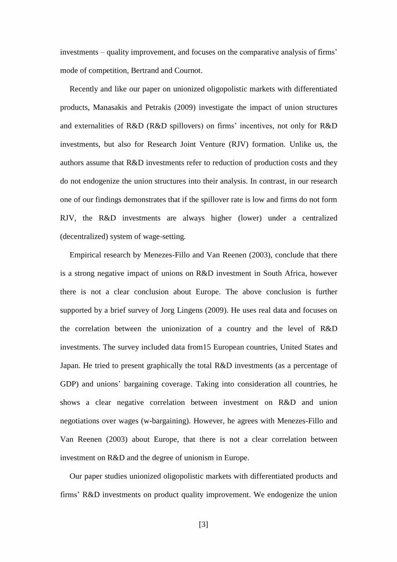
Recently and like our paper on unionized oligopolistic markets with differentiated
products, Manasakis and Petrakis (2009) investigate the impact of union structures
and externalities of R&D (R&D spillovers) on firms’ incentives, not only for R&D
investments, but also for Research Joint Venture (RJV) formation. Unlike us, the
authors assume that R&D investments refer to reduction of production costs and they
do not endogenize the union structures into their analysis. In contrast, in our research
one of our findings demonstrates that if the spillover rate is low and firms do not form
RJV, the R&D investments are always higher (lower) under a centralized
(decentralized) system of wage-setting.
Empirical research by Menezes-Fillo and Van Reenen (2003), conclude that there
is a strong negative impact of unions on R&D investment in South Africa, however
there is not a clear conclusion about Europe. The above conclusion is further
supported by a brief survey of Jorg Lingens (2009). He uses real data and focuses on
the correlation between the unionization of a country and the level of R&D
investments. The survey included data from15 European countries, United States and
Japan. He tried to present graphically the total R&D investments (as a percentage of
GDP) and unions’ bargaining coverage. Taking into consideration all countries, he
shows a clear negative correlation between investment on R&D and union
negotiations over wages (w-bargaining). However, he agrees with Menezes-Fillo and
Van Reenen (2003) about Europe, that there is not a clear correlation between
investment on R&D and the degree of unionism in Europe.
Our paper studies unionized oligopolistic markets with differentiated products and
firms’ R&D investments on product quality improvement. We endogenize the union

[4]
structures, i.e. the decentralized and the centralized wage-setting regimes, and
investigate the impact of their decision on market outcomes/participant surpluses. We
extend our research by developing two alternative market policies, where the role of
the social planner is inserted and endogenize the selection of market structure in our
model. In the first case, we assume that a benevolent policy maker proceeds to quality
improvement-R&D, as a common public good, by undertaking the costs of those
investments and providing for free the know-how to the industry. In the second case
he finances a percentage of the expenditures of firm-specific R&D investments. In
both cases he finances those costs by indirect taxation on market products. We
conclude that union collusive play decreases product quality and output level under
each of the proposed market structures (including where the social planner is absent).
Additionally, our findings show the market structure in where the R&D – quality
improvement is a public good, not only emerges in equilibrium, but also promotes
important industry elements s, such as output level, wages and product quality, and all
market participant surpluses (and consequently Social Welfare), even if this policy
leads to indirect taxation on market products.
The rest of the paper is structured as follows. In Section 2 we present our
unionized oligopoly model. In Section 3 - 5, we analyze separately the cases of
market structure in where the social planner is inactive/absent, proceeds to R&D
investments and partially funds the firms’ R&D investments, respectively.
Subsequently in Section 6, our model endogenizes the choice of market structure and
demonstrates the one which emerges in equilibrium, while in Section 7 we proceed to
the comparative analysis of each market structure outcomes/participant surpluses. Our
findings are summarized in Section 8.

[5]
2. The Model
Consider a unionized product market where two technologically identical firms,
denoted by , produce differentiated goods and investigate in R&D –
quality improvement. Each firm faces an inverse linear demand function, which is
derived by consumer utility from consumption under the restriction of their income.
Following Häckner (2000), the represented consumer utility function1 is the
following:
(1)
Where , and respectively are the quantities of good , good and the
competitive numeraire sector, consumed by the represented consumer and
denotes the degree of substitutability among the goods As the
firms’ products become more close substitutes. Moreover, denotes the quality of
products which arises from firms’ expenditures on R&D, and is the
consumer evaluation of the product quality: As the consumers become
completely indifferent about product quality.
Taking into consideration the represented consumer’s utility function [given in (1)]
and its income limitation, we get the inverse linear demand function that firms’ face,
which is:
(2)
Where, , respectively are the price and output of the firm .
For simplicity, we assume that the production technology exhibits constant returns
to scale, and requires only labor input to produce the good2. Labor productivity equals
1 For simplicity, we assumed that both and are equal to one.
2 This is equivalent to a two-factor Leontief technology in which the amount of capital is fixed in the
short run and it is large enough not to induce zero marginal product of labor.
[6]
one, for both firms, namely one unit of labor is needed to produce one unit of product,
that is:
(3)
Where and respectively represent employment and quantity of the firm
.3
The firm’s unit transformation cost of labor into product equals the wage rate, denoted
by . Hence, the profit function of firm is defined by:
(4)
Where the denotes the firm ’s expenditures on R&D in order to improve its
own product quality.
The labor market is unionized: Workers are organized into two separate firm-
specific unions. Hence, each firm enters into negotiations over (only) wages,
exclusively with its own union (decentralized Right-to-Manage bargaining4).
Moreover, we assume that unions are identical, endowed with monopoly bargaining
power during the negotiations with their own firms and may compete or collude by
independently adjusting their own wages. Hence, each union effectively acts as a
firm-specific monopoly union, setting the wage, with the firm in turn choosing firm
specific-employment. The union ’s objective is to maximize the sum of its members’
rents, given by the following equation:
(5)
3 We are aware of the limitations of our analysis in assuming specific functional forms and constant
returns to scale. However, the use of more general forms would jeopardize the clarity of our findings,
without significantly changing their qualitative character. 4 Right-to-manage literature was initially developed by the British school during the 1980s (Nickell). It
implies that the union-firm negotiations agenda includes only the wage rate, which is determined
according to a typical Nash Bargaining Maximization.

[7]
Where, is firm ’s wage rate, provided that union membership is fixed and all
members are (or the union leadership treats them as being) identical [see, e.g. Oswald
(1982), Pencavel (1991), Booth, (1995)].
In addition, we insert the role of a benevolent policy maker in our model, who aims
to maximize Social Welfare by endogenously deciding whether to intervene (and
how) or not in the market structure. We consider two instances of policy maker’s
intervention. In the first case, we assume that the policy maker proceeds to quality
improvement-R&D, as a common public good, by undertaking the costs of those
investments and providing the know-how to the industry for free. Thus, his cost
function is defined by the following equation:
(6)
Where denotes the expenditures on R&D in order to improve the industry’s
product quality.
In the second case he finances a percentage of the cost of firm-specific R&D
investments and his cost function is defined by:
(7)
Where the and denote the firm ’s expenditures on R&D and the presentence
of its financial participation in these expenditures, respectively. Consequently, the
factor presents the presentence of policy maker’s financing on firms’
expenditures on R&D.
In both cases the policy maker finances these costs by indirect taxation on market
products. In particular, we assume that he finances the investment on R&D
exclusively by indirect consumption taxation on the final product [ (Balance
[8]
Budget5)]. Accordingly, his revenue function is defined by the following equation and
applies to both cases:
(8)
Where and denote the collected tax per unit of product and the sum of the firms’
output level, respectively.
From the perspective of consumers, the consumption tax is an additional cost on
the purchase price of industry’s products, as it is presented in the following equation:
(9)
Where denotes consumer price of products, which is the sum of the product price
received by producers (denoted by factor ) and the consumption tax collected by the
Social Planner (denoted by factor ).
Taking into consideration (9), we get the new inverse linear demand function that
firms’ face, which is:
(10)
In the above context, we propose three games, one for each potential action of the
social planner, as follows:
1. Under the hypothesis that the social planner decides not to intervene in the
market structure, our envisaged four-stage game unfolds as follows:
At the 1st stage, both unions simultaneously and independently decide whether
to collude or to compete in the stage of w-negotiations with their firms.
At the 2nd
stage, firms simultaneously and independently determine the
optimal level of their R&D investments, by evaluating on the one hand the
5 A government balance budget refers to a budget in which total revenues are equal or greater to
total expenditures (no budget deficit). In our case, the balance budget has to do exclusively with our
oligopoly industry.

[9]
increase of their revenues, through increasing their product demand because of
their product quality improvement, and on the other hand the cost of these
investments.
At the 3rd
stage, if (at the first stage) one or both unions have independently
decided to play collusively, they simultaneously and independently set their
wages for their own firms so that each maximizes the joint member rents or
maximizes its own member rents. If, however, both unions have (at the first
stage) independently decided to play competitively they both set their own
wages in order for each one to maximize its own member rents.
At the 4th
stage, each firm simultaneously and independently compete with its
rival by adjusting its own quantities, in order to maximize their own profits.
2. Assuming that the social planner decides to intervene in the market structure by
proceeding to quality improvement-R&D and providing the know-how to the
industry for free, our envisaged four-stage game unfolds as follows:
At the 1st stage, the social planner determines the optimal level in terms of
Social Welfare of R&D investments and indirect taxation on industry
products.
At the 2nd
stage, both unions simultaneously and independently decide whether
to collude or to compete in the stage of w-negotiations with their firms.
The 3rd
stage and the 4th
stage of the present game remain the same with the
previously proposed one.
3. Now suppose that the social planner decides to intervene in the market structure
by financing a percentage of the cost of firm-specific R&D investments, thus our
envisaged five-stage game unfolds as follows:

[10]
At the 1st stage, the social planner determines the optimal level in terms of
Social Welfare of financing a percentage of the cost of firm-specific R&D
investments and the indirect taxation on industry products.
The 2nd
, 3rd
, 4th
and 5th
stages of the present game are nothing more or less
than an image of the first proposed game.
3. 1st case: Absence of policy maker in market structure
Like in standard game-theoretic analysis, using backwards induction, we propose a
candidate equilibrium and subsequently validate (or reject) it, by checking for all
possible unilateral deviations on the part of the agent(s) who consider such a
deviation. Due to symmetry, in our model three candidate equilibria arise, at the first
stage of the game: In Subsection 3.1 the candidate equilibrium is the one where union
collusive play takes place in w-negotiations with their firms (e.g., unions
independently set the wages that maximize the joint rents) and the possible deviation,
on the part of any union, is to adjust its own wages in order to maximize its own rents
given that the other union sticks to collusive play. In Subsection 3.2, the candidate
equilibrium is union competition and the possible deviation, on the part of any union,
is to set its own wages in order to maximize the joint rents, given that the other union
still behaves as a competitor. In Subsection 3.3, the candidate equilibrium is the one
where one union acts collusively, while its rival union acts competitively, and the
possible deviations arise by unilaterally switching each union’s strategy to its rival’s
one.

[11]
3.1. Competitive Play (m)
Assume that at the first stage of the game each union aims to maximize its own
rents by independently setting its wages at the stage of negotiations with their specific
firm (hence, its employment level).
At the last stage of the game, both firms independently choose their own quantities
(thus their own employment levels) in order to maximize their own profits. Hence,
according to (2) and (4), the firm’s ’s objective is:
(11)
The first order condition (f.o.c.) of (11) provides the reaction function of firm :
(12)
Notice that each firms’ output level decreases further with its rivals output level, the
higher the substitutability of the products is.
Taking the reaction functions of both firms and solving the system of equations, we
get the optimal output/employment rules in the candidate equilibrium:
(13)
It is easily observable that firm ’s output level is negatively affected by union ’s
wage rate and rival firm’s R&D investment but it is positively affected by union ’s
wage rates and its R&D investment.
At the third stage, each union chooses the firm-specific wage in order to
maximize its own rents [given in (5)], taking as given the outcomes of the production
game [given in (33)].
(14)

[12]
From the f.o.cs of that maximization we may then derive the unions’ ,
wage reaction functions which are as follows:
(15)
Observe that wages are strategic complements for the unions,
since:
Solving system (15) we get the wage outcome (s) in the candidate equilibrium:
(16)
Note that, , which means firm by
increasing its R&D investments (its product quality) and therefore its product and
labor demand, creates an extra union cost – in terms of a higher wage set by its union
of workers. The increment in union ’s wages would be higher, the higher the
consumer evaluation of the product quality from R&D is
. Moreover, even if wages are
strategic complements for the unions, if firm increases its R&D investment and
creates an increment in union ’s wages, the wages of union will be decreased.
. The explanation is that an
increment of firm ’s R&D investments, hence product ’s quality, cases two opposite
effects on union ’s wages: A positive one, due to higher union ’s wages and wages’
complementarity, and a negative one which is dominated, due to shrinkage of union
’s labor demand by increasing the product ’s output level.
At the second stage firms simultaneously and independently determine the optimal
level of their R&D investment in order to maximize their profits, given the optimal
output/employment rules and the equilibrium wages in (13) and (16) respectively. The
firms’ maximization objective is derived by substituting (4) for (13) and (16):

[13]
(17)
The f.o.cs of (27) provides the reaction function of firm to the investments in R&D:
(18)
From the above firms’ reaction function, we get that R&D investments are
strategic substitutes.
Solving the system of f.o.cs of that maximization, we get the (candidate)
equilibrium R&D investments:
(19)
The firms’ output/employment levels in the candidate equilibrium are then derived by
substituting (19) and (16) for (13):
(20)
Moreover, we get that the firms’ profits in the candidate equilibrium:
22242 8820644 shss
(21)
From Equations (16) and (5), we get the candidate equilibrium union wages and rents,
respectively, as follows:
(22)
(23)
[14]
3.2. Collusive Play (c)
Assume next that, at the first stage of the game, both unions independently choose
to behave collusively at the third stage, where they enter into negotiations over their
wages with their own firms, in order to maximize the joint rents.
Thus, at the last stage of the game, we get the firms’ reaction functions, and
consequently the optimal output/employment rules in the candidate equilibrium in
Equations (12) and (13).
Taking in to consideration (13) at the third stage, union chooses so as to
maximize the sum of rents of its members and the competitor firm’s union members:
(24)
From the f.o.cs of (24) we subsequently derive the union ’s wage reaction function:
(25)
As in the previous section, note that , hence,
wages are strategic complements on the part of unions. Solving the system (25) we
get the (candidate) equilibrium wages:
(26)
Observe that , i.e. the higher the quality of products, the higher
is the wage set by the union. The magnitude of this wage increment is higher, when
the consumer evaluation of the product quality from R&D is higher
.
At the second stage, firms simultaneously and independently determine the optimal
level of their R&D investment in order to maximize their profits [given by
substituting (4) for (13) and (26)]:

[15]
(27)
The f.o.cs of (27) provides the reaction function of firm to investments on R&D:
(28)
Solving the system of (28) we get the (candidate) equilibrium R&D investments:
(29)
The firms’ output/employment levels in the candidate equilibrium are then derived by
substituting (26) and (29) for (13):
(30)
Moreover, we get the firms’ profits in the candidate equilibrium:
(31)
From Equations (26) and (5), we get the candidate equilibrium union wages and rents,
respectively, as follows:
(32)
(33)
3.3. Mix of Strategies ( )
The candidate equilibrium here is the one where one union (e.g. union ) adjusts
its own wage competitively, while its rival’s (e.g. union i’s) strategy is to adjust its
own wages in order to maximize joint rents.

[16]
Thus, at the last stage of the game where firms compete by adjusting
simultaneously and independently their quantity in order to maximize their profits, we
get the optimal output/employment rules in the candidate equilibrium in (13).
According to this Mix of Strategies configuration, at the third stage we must
consider the f.o.cs of the pair (24) and (15) separately. Thus, respectively considering
the union reaction functions (25) and (16), and solving that system, we get the
following optimal wages in the candidate equilibrium:
(34)
(35)
Now at the second stage where firms simultaneously and independently determine the
optimal level of their R&D investment, we get the (candidate) equilibrium R&D
investments by solving the system of f.o.cs of maximization of their profits [given by
substituting (4) for (13), (34) and (35)]:
(36)
(37)
Substituting in turn (34), (35), (36) and (37) for (13) for each firm, respectively, we
obtain the following firm-specific output/employment levels in the candidate
equilibrium:
(38)
(39)
Moreover, we get that the firms’ profits in the candidate equilibrium:

[17]
(40)
(41)
From Equations (34), (35) and (5), we get the candidate equilibrium union wages and
rents, respectively, as follows:
(42)
(43)
(44)
(45)
3.4. Equilibrium Analysis: Endogenous Selection of Union Structures
We now turn to the first stage of the game and investigate the unions’ incentive to
play collusively in our static framework by setting wages at the stage of w-
negotiations that maximize the joint rents. Given our findings in 3.1.− 3.3., at the first
stage the unions deal with the following matrix game, in which the payoffs of each
union when both unions simultaneously and independently decide to collude or to
compete at the stage of w-negotiations (3rd
stage) with their specific firm is presented:
Union
Collusion Competition
Union
Collusion
Competition
Table 1: The Matrix Game that unions deal with at the first stage of the game.

[18]
Due to symmetry,
is applied and thus the number of
candidate equilibria is reduced to three.
Collusive play is an equilibrium institution only if no union has incentive to
unilaterally deviate in order to maximize its own revenue by adjusting independently
its own wages. In particular, each union has incentives to deviate and earn higher
revenue by decreasing its demanded wages at the stage of w-bargaining, enough to
achieve the optimal firm’s labor demand. To grasp it, let union deviate from
collusive play in order to maximize its own revenue by reducing its wages, assuming
that union sticks to collusion. The reduction of its wages causes two positive effects
on its employment due to firm ’s reaction to the lower labor cost; firstly, from the
increment of the firm’s demanded employment level and, secondly, from the release
of the firm’s economic resources to be invested in R&D investments that increase its
product’s quality and therefore the consumers’ demanded quantity, hence
employment level. Notice that, union ’s deviation leads indirectly to reduction of
union ’s revenue, because of complimentary wage and product substitution.
Consequently, it is deduced that union collusive play is not in Nash Equilibrium
because there is lack of stability. For the same reasons, neither the mix of strategies
emerge in equilibrium. The union that remains in collusion has incentive to switch its
strategy to competition, like its rival, by reducing its wages too. So according to the
above, union competition eventually emerges in equilibrium. Our relevant findings
are summarized in Proposition 1.
Proposition 1: Under the assumption of the absence of a policy maker in market
structure, union competitive play eventually emerges in Nash equilibrium.
[Proof: See Appendix (A.1)]

[19]
3.5. Consumer Evaluation of R&D’s Quality and Product Substitutability:
Unions Effects (utility)
In this section, we proceed to the analysis of the effects of our critical structural
parameters, namely and , on unions’ utility (wages and labor).
It is generally accepted that union collusion achieves Pareto improving
equilibrium, as it internalizes the negative externalities that are created from union
competition and gives unions the opportunity to further increase their wages, hence
their revenue. Thus, it could be a reasonable conclusion that Nash equilibrium
achieved at the first stage is not Pareto optimal, as a transition from Nash equilibrium
to a secure collusion increases the utility of both unions. However, in our model the
above conclusion is not universal and does not apply for each case.
In particular, if consumer evaluation of product quality is high enough ( and
the firms’ products tends to be independent ( , then the transition of the unions
from collusion to competition is not only in Nash Equilibrium but also Pareto
improving.
To grasp it, assume first the standard/ad-hoc – collusive versus competitive –
hypotheses in both of which R&D is absent ( , i.e. consumer evaluation of the
product quality equals to zero ( ). As the products are independent ( , the
two firms’ products are targeted at completely different markets and thus each firm
produces the quantity of a monopolist [ . While, as the products tend to be
close substitutes ( , the two firms’ products are targeted at exactly the same
market and consequently their total quantity is lower than that of two monopolists
[ . From the perspective of unions, the aforementioned product quantities are
translated into units of labor demand. Therefore, and in accordance with the above, as
the unions (no matter collusively or competitively) enjoy the maximum point

[20]
of their revenue , while as their revenue is reduced. Union
collusion in turn means more inflexible labor supply; so as , union revenues
under collusive play is reduced less than under competitive play, i.e.
and
.
We will now investigate the impact of consumer evaluation of product quality ( )
on union utility. According to (1), it is easy to check that consumer demand is
increasing with factor h. The increase in demand is even higher the higher the level of
investments on R&D is. Therefore, an increase in factor strengthens the firms’
incentives for R&D investments, which in turn increases consumer demand, hence
labor demand. Thus, as factor , the union utility increases , especially under
collusive play (more inelastic labor supply) than under competitive play, i.e.
and
.
0,08
0,10
0,12
0 0,2 0,4 0,6 0,8 1
Unio
n i
's U
tili
ty (
ui)
Degree of product substitutability (γ)
Figure 1: The utility of union under collusion and competition, given that .

[21]
In conclusion, it is proved that a high level of consumer evaluation of the products
( and a low level of product substitutability ( affects negatively the
differential. In contrast to conventional wisdom, those effects may be
such that the unions’ utility differential among competition and collusion can be
reversed, i.e. . The following Proposition summarizes the above results.
Proposition 2:
If , then Union Rents under Competition are always higher
than under Collusion, i.e.
. Thus, a transfer from collusive to
competitive play not only emerges in Nash Equilibrium, but is also Pareto
improving for unions.
Otherwise, the well-known in equation of
, where unions deal with
the well-known paradox of Prisoners’ dilemma applies.
[Proof: See Appendix (A.2)]
0,07
0,10
0,13
0,16
0 0,2 0,4 0,6 0,8 1
Unio
n i
's U
tility
(ui)
Degree of product substitutability (γ)
Figure 2: The upper and lower bound of the and
values.
[22]
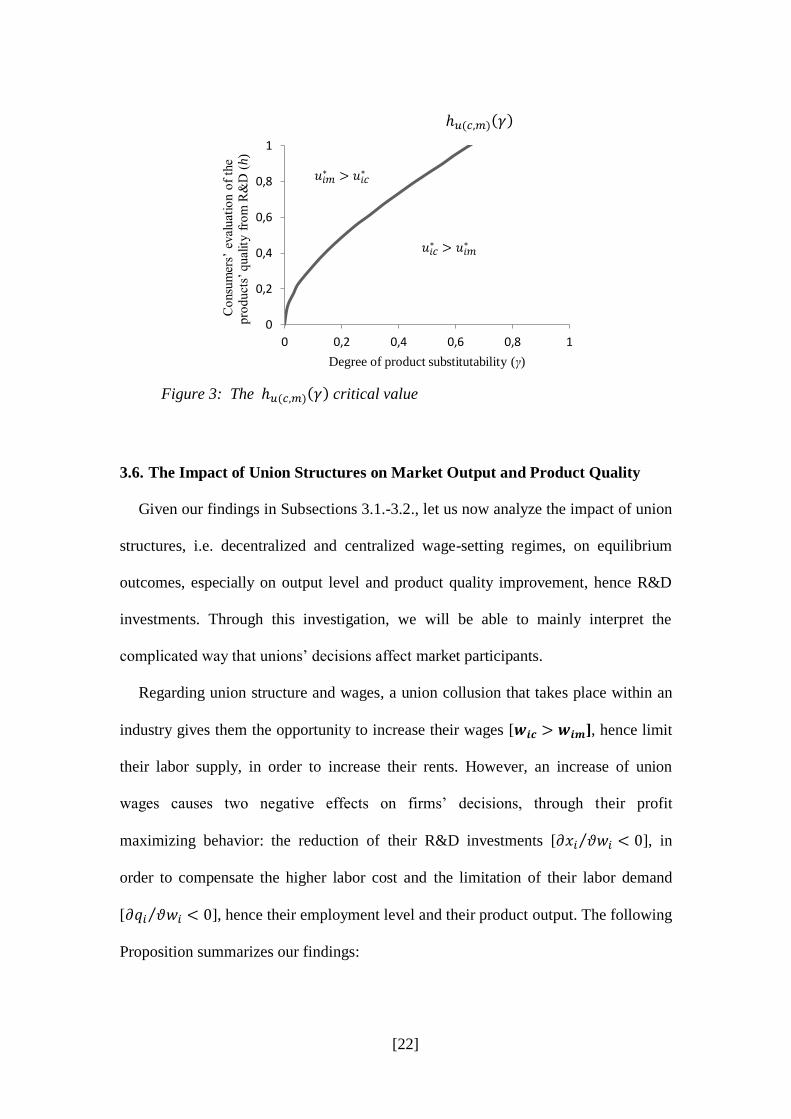
3.6. The Impact of Union Structures on Market Output and Product Quality
Given our findings in Subsections 3.1.-3.2., let us now analyze the impact of union
structures, i.e. decentralized and centralized wage-setting regimes, on equilibrium
outcomes, especially on output level and product quality improvement, hence R&D
investments. Through this investigation, we will be able to mainly interpret the
complicated way that unions’ decisions affect market participants.
Regarding union structure and wages, a union collusion that takes place within an
industry gives them the opportunity to increase their wages [ ], hence limit
their labor supply, in order to increase their rents. However, an increase of union
wages causes two negative effects on firms’ decisions, through their profit
maximizing behavior: the reduction of their R&D investments [ ], in
order to compensate the higher labor cost and the limitation of their labor demand
[ ], hence their employment level and their product output. The following
Proposition summarizes our findings:
0
0,2
0,4
0,6
0,8
1
0 0,2 0,4 0,6 0,8 1
Co
nsu
mer
s’ e
val
uat
ion o
f th
e
pro
duct
s’ q
ual
ity f
rom
R&
D (
h)
Degree of product substitutability (γ)
Figure 3: The critical value

[23]
Proposition 3: The output level (union employment) and R&D investments (product
quality) are always higher under a decentralized wage-setting regime than under a
centralized one, i.e. and . The opposite applies for union wages,
i.e. .
[Proof: See Appendix (A.4)
Proposition 4: The elasticity of output level on union wages is negative and defined
by
and union wages are obviously positive but lower
than , i.e. .
[Proof: See Appendix (A.5)]
Diagrammatically, the elasticity of output level on union wages is presented in the
following figure:
This implies that an increase in union wages of one unit decreases the equilibrium
output level at less than one unit. In other words, an increase in wage level leads to a
comparatively lower decrease in output level.
-1
-0,8
-0,6
-0,4
-0,2
0
0 0,1 0,2 0,3 0,4 0,5
Ela
stic
ity o
f o
utp
ut o
n’
wag
es (
eqw)
Union wages (w)
Figure 4: The elasticity of output level on union wages.

[24]
3.7. Welfare Analysis
The present section refers to the comparative analysis of the emerging equilibria
( and ) in terms of social welfare. Social Welfare is defined to be the sum of
Consumer Surplus (CS), Producer Surplus (PS) and Union Rents (UR), as follows:
; (46)
Where , and respectively denote collusive, competitive, and mix of strategies,
equilibria. The elements of the above equation are defined by:
(47)
(48)
(49)
The total Consumer and Producer Surplus under collusion and competition proves to
be [Proof: See Appendix (A.3)]:
(50)
(51)
Our findings from the comparative evaluation of (46), (47), (48) and (49), across ,
are summarized in Proposition 5, Proposition 6 and Proposition 7.
Proposition 5: Consumer and Producer Surpluses under Competition are always
higher than those under a Mix of Strategies configuration, the latter being always
higher than those under Collusion, i.e. and .
[Proof: See Appendix (A.4)]

[25]
Proposition 6:
a) If , then Union Rents under Competition are higher than
under a Mix of Strategies configuration, the latter being higher under
Collusion, i.e. .
b) If , then Union Rents under Mix of
Strategies are always higher than under Collusion and Competition
configuration, i.e. .
In particular, if , then. ,
while if , then.
c) If , then Unio Rents under Collusion is always higher than
under Competition, while under a Mix of Strategies it lays in-between, i.e.
.
Where,
[Proof: See Appendix (A.5)]
0
0,2
0,4
0,6
0,8
1
0 0,2 0,4 0,6 0,8 1
Co
nsu
mer
s’ e
val
uat
ion o
f th
e
pro
duct
s’ q
ual
ity f
rom
R&
D (
h)
Degree of product substitutability (γ)
Figure 5: The (γ) critical values for − c, m, mos, – Union Rents comparisons
[26]
Proposition 7: Social Welfare under Competition is always higher than under
Collusion, while under a Mix of Strategies it lies in-between, i.e.
.
[Proof: See Appendix (A.6)]
4. 2nd
case: Policy maker proceeds to R&D investments
In this section, we assume that the social planner decides to intervene in the market
structure by proceeding to quality improvement-R&D exclusively, as a public good,
and thereafter providing the know-how to the industry for free, i.e. the firms do not
invest in R&D and their profit function is defined by:
(52)
Moreover, we consider that the social planner finances the investment in R&D by
setting indirect taxation on market products, under the industry’s condition of a
balanced budget.
Taking the same path with the previous section, in the following Subsections 4.1.-
4.3., we propose all the candidate equilibria and then check their validation (or
rejection) by analyzing all possible unilateral deviations on the part of the agent(s).
4.1 Competitive Play (m)
Let unions adopt competitive play at the second stage of the game, i.e. set
independently their wages at the stage of w-bargaining with their firms.
At the last stage of the game, both firms independently determine their optimal
output level. According to (10) and (52), their new objective is:
(53)
Where denotes the quality of products which come from the policy maker’s
expenditures on R&D.

[27]
We get the reaction function of firm from the first order condition (f.o.c.) of (53):
(54)
Solving the system of both firms’ reaction functions in (54), we get the optimal
output/employment rules in the candidate equilibrium:
(55)
Notice that the industry’s output level increases with product quality improvement
and decreases with the level of per product unit tax.
At the third stage, unions independently determine the wage that maximizes
its rents. Taking as given the outcomes of the production game [given in (55)] and
getting the f.o.cs of their revenues’ objective [given in (14)], we find the wage reaction
functions which are as follows:
(56)
Solving now the system in (56), we get the wage outcome (s) in the candidate
equilibrium:
(57)
Note that , if and only if . Consequently, under the present
proposed market case, the oligopoly market exists, only if the following condition is
satisfied:
(58)
Taking into consideration the equations (5) and (57), we get the union ’s rent in the
candidate equilibrium:
(59)

[28]
Substituting now (57) for (55), we get the optimal output/employment:
(60)
4.2 Collusive Play (c)
Suppose next that unions decides to play collusively at the second stage, and thus
at the third stage set the wages as to maximize the sum of rents of its members and the
competitor firm’s union members.
At the last stage of the game, where firms’ Cournot competition is taking place, we
get firms’ reaction functions and optimal output level, hence employment, in the
candidate equilibrium by Equations (54) and (55), respectively.
At the third stage, we derive the union ’s wage reaction function, by substituting
union ’s objective function [given in (24)] for the optimal output rules in (55) and
taking the f.o.cs, as follows:
(61)
Solving now the system in (61) we get the candidate equilibrium wages:
(62)
Taking into consideration equations (5) and (62), we get the union ’s rent in the
candidate equilibrium:
(63)
Substituting now (62) for (55), we get the optimal output/employment:
(64)
[29]
4.3 Mix of Strategies ( )
Under the assumption of union mix of strategies candidate equilibrium, we let
union to be the one which plays competitively and union to be the one which plays
collusively. Thus, at the last stage of the game, where firms’ Cournot completion
takes place, we get the optimal output/employment in (55).
Consequently, at the third stage we get the optimal wages in the candidate
equilibrium by solving the system of union reaction function in (61) and (56),
respectively, as follows:
(65)
(66)
Taking into consideration equations (5), (65) and (66), we get the union rents in the
candidate equilibrium:
(67)
(68)
Substituting now (65) and (66) for (55), respectively, we get the optimal firm
output/employment:
(69)
(70)
[30]
4.4 Second Stage: Endogenous Selection of Union Structures
Turn now to the second stage of the game, where unions are asked to decide
simultaneously and independently their strategy, collusive or competitive play, at the
stage of w-negotiations (3rd
stage) with their specific firm. The unions deal with the
matrix game presented in Subsection 3.4., except that payoffs of each union are given
by Subsections 4.1-4.3.
Like in the previous market structure case, the union collusion and mix of
strategies do not emerge in Nash equilibrium, whereas even a union has incentive to
deviate. Union competition is the only candidate equilibrium where no union has
incentive to switch its strategy to collusive play, thus it is the only one emerging in
Nash equilibrium. The intuition behind this is that the collusive play is weak /
unstable, as a deviation from it gives the deviated union the advantage of wage
reduction and consequently the increment of its labor demand that maximize its own
rents, given that the rival union sticks to collusion. The mix of strategies is also an
unstable candidate equilibrium, as the union, which plays collusively, has incentive to
switch its strategy to competition in order to increase its rents by reducing its wage
too.
Proposition 8: Under the presence of a policy maker that proceeds to R&D
investments, union competitive play eventually emerges in Nash equilibrium, even if
union collusive play is Pareto improving candidate equilibrium. The unions deal with
the well-known paradox of Prisoners’ dilemma.
[Proof: See Appendix (A.7)]

[31]
4.5 First Stage: R&D investments and product taxation
Given our findings in Subsections 4.1-4.4, at this stage the social planner aims to
determine the optimal level of R&D investments for product quality improvement and
indirect taxation on market products that maximize Social Welfare. Therefore, the
social planner’s objective is:
(71)
We assumed that he finances the R&D investments exclusively by indirect
consumption taxation on the final product (Balance Budget):
(72)
So, the simplified formula of the social planner’s objective is:
(73)
Where Consumer Surplus ( ) is the sum of consumer utility minus the cost of
products purchased at the equilibrium price [given the (1) and (9)]:
(74)
Under the assumption that firms do not proceed to R&D investments in this case
i.e. , Producer Surplus is the sum of firms’ profits [given the (4)]:
(75)
The mathematical expression of Union Rents is defined by:
(76)
As mentioned, the social planner sets indirect taxes on final products in order to
finance the investments to improve product quality in the industry. Taking into
consideration that indirect taxes lead to distortions in the market, the determination of
the optimal tax is complicated. The R&D investment, hence taxes, should be such that

[32]
the increase of social welfare by improving the quality of products exceeds the
reduction by imposing indirect taxes on the market. Thus, given the impact of
taxation, the social welfare maximization problem of the policy maker gives us the
optimal combination of taxes and R&D investment, as it is presented in Proposition 9.
Proposition 9: Under union competition, the optimal levels of Policy Maker’s R&D
investments and taxation policy are
and
, respectively.
[Proof: See Appendix (A.8)]
According to Proposition 7, we get the optimal solution of
, which is:
(77)
(78)
Under the optimal solution of
, the Social Welfare in equilibrium is defined
by:
(79)
Substituting now the optimal levels of
for (57) and (60), we get the optimal
union ’s wages and firm ’s output level, respectively, in the equilibrium:
(80)
[33]
(81)
We can get now Consumer Surplus (CS), Producer Surplus (PS) and Union Rents
(UR), from Equations (74), (75) and (76), respectively, by taking into consideration
the optimal levels of
, (80) and (81):
(82)
(83)
(84)
5. 3rd
case: Policy maker funds partially firms’ R&D investments
In this section, we investigate the case of a market structure where the policy
maker intervenes by financing a percentage of the expenditures of firm-specific R&D
investments, i.e. firms proceed to investments in R&D, whose costs is partially
financed by the social planner. Thus firm ’s profit function is defined by:
(85)
Where denotes the presentence of its financial participation on this
expenditures.
As in the previous section, under the industry’s condition of a balanced budget, the
social planner imposes indirect taxation on market products, in order to finances
firms’ investment on R&D.
[34]
In the following Subsections 5.1.-5.3., we proceed to the validation (or rejection)
check of all candidate equilibria by analyzing all possible unilateral deviations on the
part of the agent(s).
5.1 Competitive Play (m)
Assume that both unions decide to play competitively at the second stage of the
game by setting independently their wages in the negotiations with their specific firm.
Thus, at the last stage of the game, where firms’ Cournot competition takes place,
firms’ aim to maximize their profits by deciding the optimal output level. Thus, firms’
objective is the following [given (10) and (85)]:
(86)
From the f.o.c.’s of (86), we get the reaction function of firm :
(87)
Solving now the system of both firms’ reaction functions from (87), we get the
optimal output level in the candidate equilibrium:
(88)
At the fourth stage of the game, each union decides its firm-specific wage rate. Taking
under consideration the unions’ objective in (14) and deriving the union wage reaction
functions [by taking the f.o.c.’s of (14), given t (88)], we get that:
(89)
Solving now the system of both union wage reaction functions from (89), we get the
optimal wage rate in the candidate equilibrium, as follows:
[35]
(90)
Now at the third stage, firms simultaneously and independently determine the optimal
level of their R&D investment in order to maximize their profits. Thus, their objective
is:
(91)
Solving the system of f.o.cs of that maximization for both firms, we get the
(candidate) equilibrium R&D investments:
(92)
Notice that:
(93)
Consequently, under the present proposed market case, the oligopoly market exists,
only if condition (93) is satisfied.
According to (5), (90) and (92), union ’s rent in the candidate equilibrium is the
following:
(94)
5.2 Collusive Play (c)
Take now as given that unions decide to play collusively at the second stage and
consequently at the fourth stage they set those wages to maximize their joint rents.

[36]
Taking the optimal output rule, hence employment, at the last stage of the game in
(88), at the fourth stage we derive the union ’s wage reaction function by taking the
f.o.cs of union ’s objective function by (24) [given in (88)], as follows:
(95)
Solving now the system in (95) we get the candidate equilibrium wages:
(96)
Getting in at the third stage, where firms simultaneously and independently
determine the optimal level of their R&D investment, by solving the system of f.o.cs
of their profit maximization [given by substituting i (91) for (88) and (96)]:
(97)
Notice that:
(98)
Consequently, under the present proposed market case, the oligopoly market exists,
only if condition (100) is satisfied.
We get the union ’s rent in the candidate equilibrium by equations (5), (88) and
(96):
(99)
5.3 Mix of Strategies ( )
Under the assumption of the union mix of strategies candidate equilibrium, we let
union to be the one which plays competitively and union to be the one which plays

[37]
collusively. Thus, at the last stage of the game, where firms’ Cournot completion
takes place, we get the optimal output/employment by (88).
At the fourth stage we get the optimal wages in the candidate equilibrium by
solving the system of union reaction function in (95) and (89), respectively, as
follows:
(100)
(101)
At the third stage, firms choose the optimal level of their R&D investment, which
is derived by solving the system of f.o.cs of their profit maximization [given by
substituting (91) for (88) and (100) for firm and (88) and (101) for firm ,
respectively]:
(102)
(103)
Notice that:
(104)
(105)
Consequently, under the present proposed market case, the oligopoly market exists,
only if conditions (104) and (105) are satisfied.
Taking into consideration equations (5), (100) and (101), we get the union rents in
the candidate equilibrium:

[38]
(106)
(107)
5.4 Second Stage: Endogenous Selection of Union Structures
At the second stage of the game, unions decide simultaneously and independently
to play collusively or competitively at the 4th
stage of w-negotiations. The unions deal
with the matrix game presented in Subsection 3.4., except that the payoffs of each
union are given in Subsections 5.1-5.3.
Like in Subsections 3.4 and 4.4, the union competition is the only one which
emerges in Nash Equilibrium, as no union has incentives to deviate by switching its
strategy to collusive play.
Proposition 10: Under the presence of a policy maker that funds partially firms’
R&D investments, union competitive play eventually emerges in Nash equilibrium,
even if union collusive play is Pareto improving candidate equilibrium. The unions
deal with the well-known paradox of Prisoners’ dilemma.
[Proof: See Appendix (A.9)]
5.5 First Stage: R&D investments and product taxation
Taking into considerations our findings in Subsections 5.1-5.4, at this stage the
social planner aims to determine the optimal level of funding rate of firms’ R&D
investments and indirect taxation on market products that maximize
Social Welfare. Thus, the social planner’s objective is:
(108)
Where and
are given by (8) and (7), respectively.

[39]
Like in the previous case of market structure, we suppose that the Social Planner
funds the firms’ R&D investments exclusively by indirect consumption taxation on
the final product (Balance Budget):
(109)
So, the simplified formula of the social planner’s objective is:
(110)
Where Consumer Surplus ( ) and Union Rents are given by (74) and (76),
respectively, while Producer Surplus is defined by the following equation:
(111)
Where denotes the total expenditures on R&D, while
presents the actual
firm ’s participation on those investments [the rest of the participation belongs to the
Social Planner through its findings, i.e.
].
Taking into consideration the indirect taxes’ market distortions, the Social planner
aims to determine the optimal combination of product taxes and funding rate of firms’
R&D investments in order to maximize Social Welfare. The optimal solution of the
social planner’s maximizing problem is presented in Proposition 11.
Proposition 11: Under union competition, the optimal levels of Policy Maker’s
funding rate in firms’ R&D investments and taxation policy are
and , respectively. Where:
(112)
6 (113)
[Proof: See Appendix (A.10)]
6 The mathematical expression of is left out because of its wide extent. It is available by the authors
upon request.

[40]
The 3D plots of the optimal Policy Maker’s funding rate in firms’ R&D
investments and taxation policy, respectively, are presented below:
Under the optimal solution of
, the Social Welfare in equilibrium is defined by:
Where:
(114)
Its 3D plot is presented below:
In addition, accordingly to the optimal solution of
, (88), (90), (91) and (92)
the output/employment levels and wages in Nash equilibrium are the following:
(115)
(116)

[41]
Where:
(117)
Furthermore, by means of the optimal solution of
, (116), (117), (121) and
market participant surplus configurations from (74), (76) and (111), we obtain:
(118)
(119)
Where:
(120)
6. Endogenous Selection of Market Structures
In this Section, we insert an additional dimension to the social planner’s role by
endogenously deciding whether to intervene (and how) or not in the market structure. In
fact, we insert an extra stage at the beginning of the game where the social planner
decides which of the three economic policies will be adopted, as analyzed in Sections 3-5:
Section 3: 1st case: Absence of policy maker in market structure.
No intervention of policy maker in market’s structure
Section 4: 2nd
case: Policy maker proceeds to R&D investments.
Policy maker proceeds to quality improvement-R&D, as a
common public good, by undertaking the costs of those
investments and providing the know-how to the industry for free.
Section 5: 3rd
case: Policy maker funds partially firms’ R&D investments
Financing a percentage of the cost of firm-specific R&D
investments

[42]
For convenience, we denote the above economic policies with indexes (a), (b) and (c),
respectively in the order referred.
The selection depends on which one is the optimum in terms of Social Welfare;
therefore, the social planner’s maximization problem is the following:
(121)
Social welfare is higher when the social planner undertakes R&D [economic policy
(b)], although this implies taxes that create distortions in the industry.
The interpretation is simple and is based on the following observations:
in economic policy (a) and (c), each firm independently, invest in R&D to
improve exclusively the quality of its own product,
while in economic policy (b), the social planner invests in R&D on behalf of
both firms by aiming to improve the quality of both products at once.
In conclusion, in economic policy (b) the market succeeds to save economic
resources by investing in R&D, because those investments aim to improve the quality
of both products of the present market. The following Proposition summarizes the
above findings.
Proposition 12: Social Welfare is higher when the social planner proceeds to R&D
investment, than when it finances part of firms’ ones. The market case, where the
social planner is absent, gives comparatively the lowest Social Welfare, i.e.

[43]
7. Comparative Results
In the present section, we proceed to the comparative analysis of the three
proposed markets structures / economic policies of the previous sections and
investigate the potential superiority of the one which emerges eventually in
equilibrium.
Our analysis targets to determine which of the three proposed markets structures
gives comparatively higher outcomes for the main industry. Our findings, regarding
the comparative evaluation of the main industry’s outcomes, are summarized in the
following Propositions.
Proposition 13: Important industry elements, such as output level, wages and product
quality improving, are always higher under the market structure where the social
planner proceeds to R&D investment. The market case, where the social planner is
absent, gives comparatively the lowest, i.e.
, and .
[Proof: See Appendix (A.12)]
Proposition 14: Consumer Surplus and Union Rents are always higher when the
social planner proceeds to R&D investment, than when it finances part of firms’ ones,
the latter being always higher than when it is absent, i.e. and
.
[Proof: See Appendix (A.13)]

[44]
Proposition 15: The Producer Surplus is at its highest when the social planner
proceeds to R&D investment, and at its lowest when it finances part of firms’ ones.
The market case, where the social planner is absent, lies in-between, i.e.
[Proof: See Appendix (A.14)]
Summarizing the above findings of the comparative analysis of the three proposed
markets structures / economic policies, we show the superiority of the one which
emerges eventually in equilibrium, by proving that under this market structure the
social planner proceeds to R&D investment where:
Social Welfare and its elements, Consumer Surplus, Producer Surplus, and
Union rents, are comparatively higher and
Important industry elements, such as output level, wages and product quality
improving are also comparatively higher.
The main reason is that the specific market formation succeeds to save comparative
economic resources by letting the social planner invests in R&D and thus improving
the quality of both products at once.
8. Concluding Remarks
The present paper focuses mainly on unionized oligopolistic markets with
differentiated products and R&D investments on product quality improvement. Its
contribution in the “R&D investments in unionized oligopolies” literature is manifold,
by not only investigating the correlation between quality improvement and union
incentives for collusive play, but also by developing alternative market policies in the
field of R&D, in order to promote Social Welfare. Additionally, we endogenize the

[45]
selection of the policy which will be adopted for the present market by the Social
Planner. The selection depends on which one is the optimum in terms of Social
Welfare.
In particular, we develop two additional instances of policy maker’s intervention.
Firstly, we assume that a benevolent policy maker proceeds to quality improvement-
R&D, as a common public good, by undertaking the costs of those investments and
providing for free the know-how to the industry. Secondly, he finances a percentage
of the cost of firm-specific R&D investments. The common assumption of both cases
is that the policy maker finances the investments on R&D by indirect consumption
taxation on final products, under the industry’s condition of a balanced budget
[ ].
In the one-shot game, our analysis demonstrates that union collusion is weak /
unstable and each union’s dominant strategy is to act independently (competitively)
under each social planner’s policy (including the case where he is absent). The union
competitive play increases the Social Welfare of the industry. Our remarkable
findings arise from the endogenous selection of one of the three social planner’s
policies. Specifically, it suggests that the market structure in which the social planner
proceeds to quality improvement-R&D, as a common public good, not only emerges
in equilibrium by maximizing Social Welfare, but also promotes important industry
elements, such as output level, wages and product quality improving, and all market
participant surpluses, i.e. consumer, producer and union. The main reason is that the
market, through that policy, succeeds to save economic resources by proceeding to
R&D, as a common good, which improves the quality of both products at once.

[46]
Appendix
A.1 Proof of Proposition 1
At the first stage of the game, both unions simultaneously and independently
decide whether to collude or to compete at the stage of w-negotiations (3rd
stage) with
their specific firms. The unions deal with the following matrix game, in which the
payoffs of each union in combination with the possible decisions of the unions are
presented:
Union
Collusion Competition
Union
Collusion (E1)
(E2)
Competition (E2)
(E3)
Due to symmetry,
is applied and thus the number of
candidate equilibria is reduced to three.
We demonstrate the Nash equilibrium by analyzing the candidate equilibria and
their deviations. The possible deviation on the part of each union is to unilaterally
switch its own strategy, given that its rival does not.
The first proposed candidate equilibrium (E1) is the one where union collusion is
formed and the possible deviation, on the part of any union, is to adjust its own wages
in order to maximize its own rents given that the other union sticks to collusive play.
From equations (33) and (45) it is derived that:
(A1)
Each union has incentive to deviate and consequently union collusive play is not in
Nash equilibrium. The 3D plot of factor is presented below.
Table 2: The Matrix Game that unions deal with at the first stage of the game.

[47]
The candidate equilibrium (E2) is the one where one union acts collusively (let it
be union ), while the other acts competitively (let it be union ), and the possible
deviations arise by unilaterally switching each union’s strategy to its rival’s one. Even
if union has no incentive to deviate [see (A1)], it is inferred that (E2) is also not in
Nash equilibrium because union has incentive to deviate by acting competitively.
From equations (23) and (44) it is derived that:
(A2)
The 3D plot of factor is presented below.
The last candidate equilibrium (E3) is the one where unions act competitively and
the possible deviation, on the part of any union, is to adjust its own wages in order to
maximize the collusive revenues. It is easy to check by (A1) and (A2) that this one is
in Nash equilibrium, as no union has incentive to deviate.

[48]
A.2 Proof of Proposition 2
By means of (23) and (33), we obtain:
(A3)
Where, 7 its 3D plot is the following:
Moreover, – with value field
and it is depicted in Figure 5 of the main text.
According to our findings, we conclude that:
(A4)
or (A5)
A.3 Proof of Equations (56) and (57)
(i) Proof of Equation (56):
By definition, the Consumer Surplus is the sum of consumer utility minus the cost of
products purchased at the equilibrium price, hence in our model the mathematical
expression of Consumer Surplus is the following [given in(1)]:
(A6)
Assuming the absolute symmetry of firms and their strategies, we get that:
7 The mathematical expressions of and are left out, because it was complicated to be
shaped as closed forms.

[49]
(A7)
(A8)
(A9)
(A10)
Moreover, substituting (A7), (A8), (A9) and (A10) for the demand function [given in
(2)] and firms’ reaction functions [given in (12)], we get that:
(A11)
(A12)
It is easy to check that taking (A11) and (A12) and substituting them for (A6), the
Consumer Surplus is defined by:
(A13)
Where is the sum of the firms’ output level.
(ii) Proof of Equation (57):
By definition the Producer Surplus is the sum of firms’ profits, hence in our model the
mathematical expression of Producer Surplus is the following [given in (4)]:
(A14)
Assuming the absolute symmetry of firms and their strategies, the Producer Surplus is
also defined by [taking (A11) and (A12) and substituting them for (A14)]:
(A15)
Where is the sum of the firms’ output level.

[50]
A.4 Proof of Proposition 3
We now proceed to the comparative analysis of equilibrium outcomes, i.e. wages,
output level and product quality improvement under each union structure, i.e.
decentralized and centralized wage-setting regimes:
Assuming the absolute symmetry of unions and their strategies, we get that:
(A16)
(A17)
(A18)
Where
Regarding wages, by means of (A16), (22) and (32), we obtain:
(A19)
Where, 8 and its 3D plot is respectively the below:
Summarizing the above results, we conclude that:
(A20)
8 The mathematical expression of and are left out because of their wide extent. They are
available by the authors upon request.
[51]
To easily grasp the effects of wages on R&D investments and market output level,
we get firms’ reaction functions to R&D investments by taking the f.o.cs of firm’s
profit maximization objective with respect to R&D investments in (17) given only the
optimal output rule in equilibrium in (13), as follows:
(A21)
By substituting (A16) for (A21) we obtain that the new formation of firms’
reaction functions to R&D investments is the following:
(A22)
From the f.o.c.s of (A22) we get the optimal R&D investment which is presented in
the following equation:
(A23)
It is easily observable that R&D investment decreases with the labor unit cost:
(A24)
Combining our findings presented by equations (A20) and (A24) we conclude that:
(A25)
By substituting now the optimal R&D investments in (A23) for the optimal output
rule in equilibrium in (13), we get:
(A26)
Notice that the market output level decreases with the union wages:
(A27)
According to equations (A20) and (A27), we conclude that:

[52]
(A28)
A.4. Proof of Proposition 4
Supposing the absolute symmetry of unions and their strategies, i.e. decentralized
and centralized wage-setting regimes, we get that:
(A29)
By definition, the unions set those wages that gives them positive utility:
(A30)
Thus, by substituting the optimal output rule [given in (A26)] into the union utility
function [given in (5)], we get that:
(A31)
Notice that the above in equation is satisfied if and only if the following applies:
(A32)
The elasticity of product on union wages is the following:
(A33)
Substituting now the optimal output rule in (A26) for the formula of elasticity of
product on union wages in the game in (A33), we get:
(A34)
Combining our findings presented by equations (A32) and (A34), we conclude that:
(A35)
(A36)

[53]
A.4. Proof of Proposition 5
Recall that total Consumer Surplus under collusion and competition proves to be:
(A37)
Furthermore, by means of (47), in the case of a Mix of Strategies configuration total
Consumer Surplus proves to be:
(A38)
Where, 9 and its 3D plot is presented below.
Using (A37) and (A38), it is then straightforward that, by virtue of Proposition 5:
(A39)
(A40)
Where, 10 and their 3D plot are presented below.
9 The mathematical expression of is left out because of its wide extent. It is available by the authors
upon request. 10
The mathematical expressions of and are left out because of their wide extent. They are
available by the authors upon request.

[54]
Turning now to total Producer Surplus and recalling its simplified expression under
collusion and competition, we get:
(A41)
Furthermore, by means of (54), in the case of a Mix of Strategies configuration, total
Producer Surplus proves to be:
(A42)
Where, 11 and its 3D plot is presented below.
Using (A41) and (A42), it is straightforward then that, by virtue of Proposition 5:
(A43)
(A44)
Where, 12 and their 3D plot are presented below.
11
The mathematical expression of is left out because of its wide extent. It is available by the authors
upon request. 12
The mathematical expressions of and are left out because of their wide extent. They are
available by the authors upon request.

[55]
A.5. Proof of Proposition 6
Total Union Rents in the m, c, and mos equilibria are defined as:
, where (A45)
By means of (23), (33), (44) and (45) Union Rents under collusion, competition, and
mix of strategies, is respectively given by:
(A46)
(A47)
(A48)
Where, 13 and its 3D plot is presented below.
It then proves that:
(A49)
(A50)
(A51)
13
The mathematical expression of is left out because of its wide extent. It is available by the
authors upon request.

[56]
Regarding the validity of (A49), (A50) and (A51), it holds that
, and
14
Hence, as shown in Figure 5 (see main text) depicting the ,
and critical schedules,
, with
Summarizing the above results, we conclude that:
or (A52)
(A53)
(A54)
(A55)
A.6. Proof of Proposition 7
Social Welfare, in the c, m, and mos equilibria, is defined as follows:
, where (A56)
Thus, respectively substituting the elements for (A52), by virtue of
(A37), (A38), (A41), (A42), (A46), (A47) and (A48), we get that:
(A57)
(A58)
Where, 15 and their 3D plots are respectively the
following:
14
The mathematical expressions of , and are left out because of
their wide extent. They are available by the authors upon request. 15
The mathematical expression of and are left out because of their wide extent. They are
available by the authors upon request.

[57]
A.7. Proof of Proposition 8
At the second stage of the game, both unions simultaneously and independently
decide the strategy that will follow in 3rd
stage. The unions deal with the matrix game
presented in Appendix A.1, except that payoffs of each union are given by equations
(59), (63), (67) and (68) in Subsections 4.1-4.3.
As proof of Proposition 1, we demonstrate the Nash equilibrium by proposing the
candidate equilibria and checking their deviations, with the possible deviation on the
part of each union being to switch its own strategy, given that its rival sticks to the
first decision.
The first proposed candidate equilibrium (E1) is not in Nash equilibrium, as both
unions have incentive to turn their strategy to competition. From equations (63) and
(68) it is derived that:
(A59)
Where
.
The candidate equilibrium (E2) does also not emerge in Nash equilibrium, as the
union plays collusively and has incentive to deviate by acting competitively. From
equations (59) and (67), it is derived that:
(A60)

[58]
Where
.
The last candidate equilibrium (E3) is in Nash equilibrium, as no union has
incentive to deviate and it is proved by equations (A59) and (A60).
Notice that although union collusive play is not in Nash equilibrium, it is Pareto
improving for the unions, as it is presented by the following in equation:
(A61)
Where
.
A.8. Proof of Proposition 9
The social planner aims to determine the optimal level of R&D investments for
product quality improvement and indirect taxation on market products that maximize
Social Welfare.
Under the assumption of a Balanced Budget policy by the social planner in the
industry, we substitute the equations (6) and (8) for (72) and get that:
(A62)
Where is the sum of the firms’ output level.
Given that union competitive play emerges in equilibrium, we get the optimal
industry output level by the equations (55) and (57):
(A63)
Taking now the optimal firms’ output level [given in (A62)] and substituting it on
the condition of a Balanced Budget [given in (A63)], we get the optimal combinations
of R&D investments and product taxation:
(A64)

[59]
(A65)
Therefore, the maximization problem of the social planner is to define the optimal
R&D investments under the one of the two proposed taxation forms satisfying the
Balanced Budget condition:
s.t.
(A66)
The above maximization problem gives the following solutions:
(A67)
(A68)
The solution
is rejected, because it does not satisfy the condition of
oligopoly existence in (58). Thence, it arises that the accepted solution is
and
the Social Welfare in equilibrium is defined by:
(A69)
A.9. Proof of Proposition 10
At the second stage of the game, both unions simultaneously and independently
decide the strategy which will follow in 4th
stage. The unions deal with the matrix
game presented in Appendix A.1, except that payoffs of each union are given by
equations (94), (99), (106) and (107) in Subsections 5.1-5.3.

[60]
We will demonstrate the Nash equilibrium by proposing the candidate equilibria
and checking for all possible deviations, taking into consideration the limitations of
minimum presentence of policy maker’s financial participation in firms’ R&D
expenditures. Those limitations are derived from Equations (93), (98), (104) and
(105), respectively, and they are presented below:
(A70)
(A71)
(A72)
(A73)
Consequently, the proposed market structure gives positive R&D investments
under all possible union strategic decisions when the following condition is satisfied:
(A74)
It then proves that:
(A75)
Taking into consideration the above condition, the first proposed candidate
equilibrium (E1) is not in Nash equilibrium, because both unions have incentive to
deviate from it, as it is derived from equations (99) and (107):
(A76)
Where , and
.
The candidate equilibrium (E2) does not also emerge in Nash equilibrium, as the
union which plays collusively has incentive to deviate by acting competitively. From
equations (94) and (106), it applies that:

[61]
(A77)
Where , and
.
The last candidate equilibrium (E3) is in Nash equilibrium, as no union has
incentive to deviate and it is proved by equations (A76) and (A77).
Notice that although union collusive play is not in Nash equilibrium, it is Pareto
improving for the unions, as presented by the following in equation:
(A78)
Where , and
16.
A.10. Proof of Proposition 11
The social planner’s maximization problem is to determine the optimal level of
funding rate of firms’ R&D investments and indirect taxation on market products that
maximize Social Welfare.
Accordingly to a Balanced Budget policy of the social planner in the industry, we
substitute equations (7) and (8) for (72) and get that:
(A79)
Where is the sum of the firms’ output level.
Getting the optimal industry output level and wage rate in Nash Equilibrium, i.e.
union competitive institution [given in (88) and (90), respectively], we get the optimal
industry output level as follows:
16
The mathematical expressions of , and are left out because of their wide extent. They are
available by the authors upon request. Their plot are not presentable as are depended by three variables,
, and . Their negative sign was found by using the Bolzano Theorem, i.e. (a) we found the
s that , (b) prove that and (c) get a random value of and observe
that .

[62]
(A80)
Substituting (A80) for (A79), we can get the level of product taxation that satisfies
the Balance Budget condition of the industry:
(A81)
(A82)
Therefore, the maximization problem of the social planner is to define the optimal
R&D investments under one of two taxation forms:
s.t.
(A83)
The above maximization problem gives the following solutions:
17
(A84)
(A85)
The solutions and
are rejected, as they do not satisfy the condition
presented in (A75). In addition, the solution is rejected, because it leads to null
Social Welfare. Thence, it arises that the accepted solution is
18 and the Social
Welfare in equilibrium is defined by:
Where:
(A86)
17
The mathematical expressions of and are left out because of their wide extent. They are
available by the authors upon request. 18
For simplicity, hereafter the factor is called
.

[63]
A.11. Proof of Proposition 12
The social planner’s maximization problem is to determine which of the three
economic policies, as analyzed in Sections 3 – 5, maximize Social Welfare:
Absence of policy maker
Policy maker proceeds to R&D investments
Policy maker funds partially firms’ R&D investments
The above economic policies give the followings outcomes in terms of Social
Welfare, respectively:
(A87)
(A88)
Where:
(A89)
It then proves that:
(A90)
(A91)
Where, 19 and their 3D plots are respectively the
following:
19
The mathematical expression of and are left out because of their wide extent. They are
available by the authors upon request.

[64]
Summarizing the above results, we conclude that:
(A92)
A.12. Proof of Proposition 13
We now proceed to the comparative analysis of important industry elements, such
as output level, wages and product quality improving under each of the three proposed
market structures in the present paper.
Regarding market output level, by means of (20), (81) and (115), we obtain:
(A93)
(A94)
Where, 20 and their 3D plots are respectively the
following:
20 The mathematical expression of and are left out because of their wide extent. They are
available by the authors upon request.

[65]
Summarizing the above results, we conclude that:
(A95)
Regarding union wages, by means of (22), (80) and (116), we obtain:
(A96)
(A97)
Where, 21 and their 3D plots are respectively the
following:
Summarizing the above results, we conclude that:
(A98)
Regarding product quality improving from R&D, by means of (19), (77) and (117),
we obtain:
(A99)
(A100)
Where, 22 and their 3D plots are respectively the
following:
21
The mathematical expression of and are left out because of their wide extent. They are
available by the authors upon request.

[66]
Summarizing the above results, we conclude that:
(A101)
A.13. Proof of Proposition 14
Let us now proceed to the comparative analysis of Consumer Surplus (CS) and
Union Rents (UR) under each of the three proposed market structures in the present
paper.
Regarding Consumer Surplus, by means of (50), (82) and (118), we obtain:
(A102)
(A103)
Where, 23 and their 3D plots are respectively the
following:
22
The mathematical expression of and are left out because of their wide extent. They are
available by the authors upon request. 23
The mathematical expression of and are left out because of their wide extent. They are
available by the authors upon request.
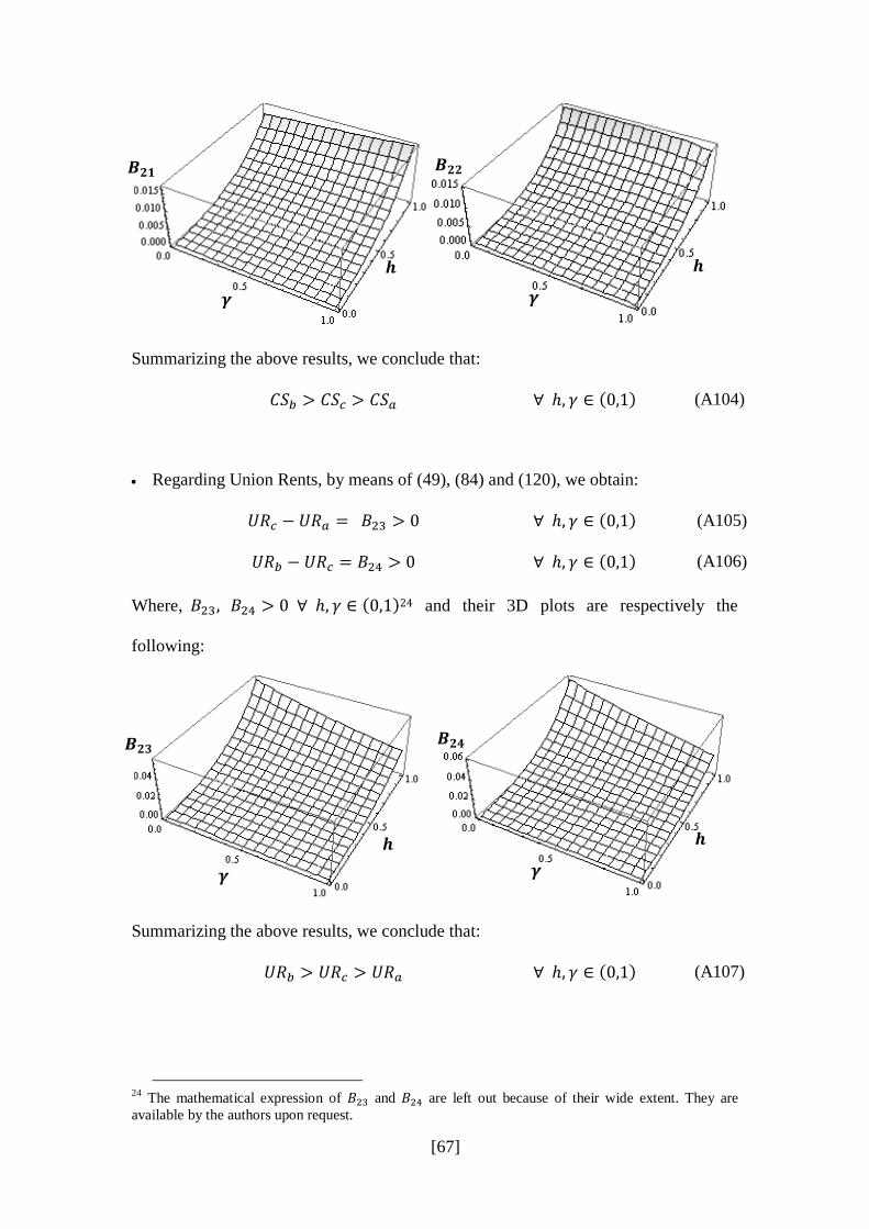
[67]
Summarizing the above results, we conclude that:
(A104)
Regarding Union Rents, by means of (49), (84) and (120), we obtain:
(A105)
(A106)
Where, 24 and their 3D plots are respectively the
following:
Summarizing the above results, we conclude that:
(A107)
24
The mathematical expression of and are left out because of their wide extent. They are
available by the authors upon request.
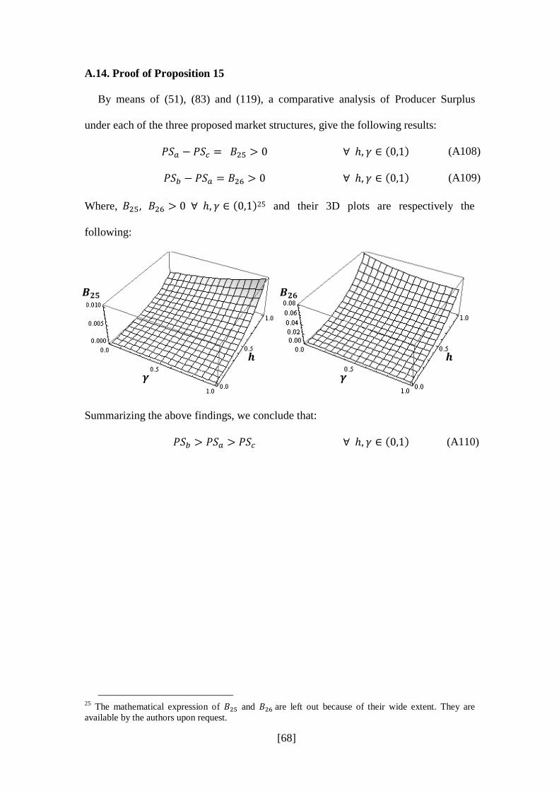
[68]
A.14. Proof of Proposition 15
By means of (51), (83) and (119), a comparative analysis of Producer Surplus
under each of the three proposed market structures, give the following results:
(A108)
(A109)
Where, 25 and their 3D plots are respectively the
following:
Summarizing the above findings, we conclude that:
(A110)
25
The mathematical expression of and are left out because of their wide extent. They are
available by the authors upon request.
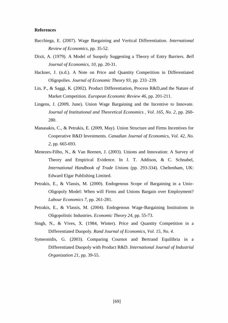
[69]
References
Bacchiega, E. (2007). Wage Bargaining and Vertical Differentiation. International
Review of Economics, pp. 35-52.
Dixit, A. (1979). A Model of Suopoly Suggesting a Theory of Entry Barriers. Bell
Journal of Economics, 10, pp. 20-31.
Hackner, J. (n.d.). A Note on Price and Quantity Competition in Differentiated
Oligopolies. Journal of Economic Theory 93, pp. 233–239.
Lin, P., & Saggi, K. (2002). Product Differentiation, Process R&D,and the Nature of
Market Competition. European Economic Review 46, pp. 201-211.
Lingens, J. (2009, June). Union Wage Bargaining and the Incentive to Innovate.
Journal of Institutional and Theoretical Economics , Vol. 165, No. 2, pp. 260-
280.
Manasakis, C., & Petrakis, E. (2009, May). Union Structure and Firms Incentives for
Cooperative R&D Investments. Canadian Journal of Economics, Vol. 42, No.
2, pp. 665-693.
Menezes-Filho, N., & Van Reenen, J. (2003). Unions and Innovation: A Survey of
Theory and Empirical Evidence. In J. T. Addison, & C. Schnabel,
International Handbook of Trade Unions (pp. 293-334). Cheltenham, UK:
Edward Elgar Publishing Limited.
Petrakis, E., & Vlassis, M. (2000). Endogenous Scope of Bargaining in a Unio-
Oligopoly Model: When will Firms and Unions Bargain over Employment?
Labour Economics 7, pp. 261-281.
Petrakis, E., & Vlassis, M. (2004). Endogenous Wage-Bargaining Institutions in
Oligopolistic Industries. Economic Theory 24, pp. 55-73.
Singh, N., & Vives, X. (1984, Winter). Price and Quantity Competition in a
Differentiated Duopoly. Rand Journal of Economics, Vol. 15, No. 4.
Symeonidis, G. (2003). Comparing Cournot and Bertrand Equilibria in a
Differentiated Duopoly with Product R&D. International Journal of Industrial
Organization 21, pp. 39-55.