UnifyingArraysandStreams ARTJOMSŠINKAROVS, SVEN … · UnifyingArraysandStreams ARTJOMSŠINKAROVS,...

arX

iv:1

710.

0383

2v1

[cs

.PL

] 1

0 O

ct 2

017

1

A Lambda Calculus for Transfinite ArraysUnifying Arrays and Streams

ARTJOMS ŠINKAROVS, Heriot-Watt University

SVEN-BODO SCHOLZ, Heriot-Watt University

Array programming languages allow for concise and generic formulations of numerical algorithms, therebyproviding a huge potential for program optimisation such as fusion, parallelisation, etc. One of the restric-tions that these languages typically have is that the number of elements in every array has to be finite. Thismeans that implementing streaming algorithms in such languages requires new types of data structures, withoperations that are not immediately compatible with existing array operations or compiler optimisations.

In this paper, we propose a design for a functional language that natively supports infinite arrays. We useordinal numbers to introduce the notion of infinity in shapes and indices. By doing so, we obtain a calculusthat naturally extends existing array calculi and, at the same time, allows for recursive specifications as theyare found in stream- and list-based settings. Furthermore, the main language construct that can be thoughtof as an n-fold cons operator gives rise to expressing transfinite recursion in data, something that lists orstreams usually do not support. This makes it possible to treat the proposed calculus as a unifying theory ofarrays, lists and streams. We give an operational semantics of the proposed language, discuss design choicesthat we have made, and demonstrate its expressibility with several examples. We also demonstrate that theproposed formalism preserves a number of well-known universal equalities from array/list/stream theories,and discuss implementation-related challenges.

CCS Concepts: • Theory of computation→ Operational semantics;

Additional Key Words and Phrases: ordinals, arrays, semantics, functional languages

ACM Reference format:

Artjoms Šinkarovs and Sven-Bodo Scholz. 2017. A Lambda Calculus for Transfinite Arrays. Proc. ACM Pro-

gram. Lang. 1, 1, Article 1 (January 2017), 28 pages.https://doi.org/10.1145/nnnnnnn.nnnnnnn

1 INTRODUCTION

Array-based computation offers many appealing properties when dealing with large amounts ofhomogeneous data. All data can be accessed inO(1) time, storage is compact, and array programstypically lend themselves to data-parallel execution. Another benefit arises from the fact that manyapplications naturally deal with data that is structured along several independent axes of linearlyordered elements.Besides these immediate benefits, the structuring facilities of arrays offer significant opportun-

ities for developing elaborate array calculi, such as Mullin’s ψ -calculus [47, 48], Nial [21] and themany APL-inspired array languages [8, 12, 30]. These calculi benefit programmers in several ways.Firstly, they improve programmer productivity. Array calculi provide the grounds for a rich set

of generic operators. Having these readily available, programmers can compose programs morequickly; the resulting algorithms are typically more versatile than implementations that manipu-late arrays directly on an element-by-element basis.Secondly, array calculi help improving program correctness. The operators that build the found-

ation of any given array calculus come with a wealth of properties that manifest in equalities thathold for all arrays. With these properties available, programming becomes less error-prone, e.g.

2017. 2475-1421/2017/1-ART1 $15.00https://doi.org/10.1145/nnnnnnn.nnnnnnn

Proc. ACM Program. Lang., Vol. 1, No. 1, Article 1. Publication date: January 2017.

http://arxiv.org/abs/1710.03832v1

https://doi.org/10.1145/nnnnnnn.nnnnnnn

https://doi.org/10.1145/nnnnnnn.nnnnnnn

1:2 Artjoms Šinkarovs and Sven-Bodo Scholz

avoidance of out-of-bound accesses through the use of array-oriented operators. It also becomeseasier to reason formally about programs and their behaviour.Finally, array calculi help compilers to optimise and parallelise programs. The aforementioned

equalities can also be leveraged when it comes to high-performance parallel executions. Theyallow compilers to restructure both algorithms and data structures, enabling improvements suchas better data locality [11, 22], better vectorisation [3, 53, 57], and streaming through acceleratordevices [2, 24].These advantages have inspired many languages and their attendant tool chains including vari-

ousAPL implementations [8, 17, 30, 31], parallel arrays inHaskell [38], push-pull arrays inHaskell [51],and arrays in SaC [23] and Futhark [28].Despite generic specification and the ability to stream finite arrays, array languages typically

cannot deal with infinite streams. If an existing application for finite arrays needs to be extended todeal with infinite streams, a complete code rewrite is often required, even if the algorithmic patternapplied to the array elements is unchanged. Retrofitting such streaming often obfuscates the corealgorithm, and adds overhead when the algorithm is applied to finite streams. If the overhead isnon-negligible, both code versions need to be maintained and, if the finiteness of the data is notknown a priori, a dynamic switch between them is required.Streaming style leads to a completely different way of thinking about data. Very similar to pro-

gramming on lists, traditional streaming deals with individual recursive acts of creation or con-sumption. This is appealing, as elegant recursive data definitions become possible and elementinsertion and deletion can be implemented efficiently, which is difficult to achieve in a traditionalarray setting. Another aspect of streams is the inevitable temporal existence of parts of streams orlists, which quite well matches the lazy regime prevalent in list-based languages, but is usually atodds with obtaining high-performance parallel array processing.In this paper, we try to tackle this limitation of array languages when it comes to infinite struc-

tures. Specifically, we look at extending array languages in a consistent way, to support streamingthrough infinite dimensions. Our aim is to avoid switching to a traditional streaming approach,and to stay within the array paradigm, thereby making it possible to use the same algorithm spe-cification for both finite and infinite inputs, possibly maintaining the benefits of a given underlyingarray calculus. We also hope that excellent parallel performance can be maintained for the finitecases, and that typical array-based optimisations can be applied to both the finite and infinite cases.We start from an applied λ-calculus supporting finite n-dimensional arrays, and investigate ex-

tensions to support infinite arrays. The design of this calculus aims to provide a solid basis forseveral array calculi, and to facilitate compilation to high-performance parallel code.In extending the calculus to deal with infinities, we pay particular attention to the algebraic

properties that are present in the finite case, and how they translate into the infinite scenario. Thekey insight here is that when ordinals are used to describe shapes and indices of arrays, many use-ful properties can be preserved. Borrowing from the nomenclature of ordinals, we refer to theseordinal-indexed infinite arrays as transfinite arrays. We identify and minimize requisite semanticextensions andmodifications.We also look into the relationship between the resulting array-basedλ-calculus and classical streaming. Finally, we look at several examples, and discuss implementa-tion issues.The individual contributions of this paper are as follows:

(1) We define an applied λ-calculus on finite arrays, and its operational semantics. The calculusis a rather generic core language that implicitly supports several array calculi as well ascompilation to highly efficient parallel code.


Transfinite Arrays 1:3

(2) We expand the λ-calculus to support infinite arrays and show that the use of ordinals as in-dices and shapes creates a wide range of universal equalities that apply to finite and transfin-ite arrays alike.

(3) We show that the proposed calculus also maintains many streaming properties even in thecontext of transfinite streaming.

(4) We show that the proposed calculus inherently supports transfinite recursion. Several ex-amples are contrasted to traditional list-based solutions.

(5) We describe a prototypical implementation1, and briefly discuss the opportunities and chal-lenges involved.

We start with a description of the finite array calculus and naive extensions for infinite arrays inSection 2, before presenting the ordinal-based approach and its potential in Sections 3–5. Section 6presents our prototypical implementation. Related work is discussed in Section 7; we conclude inSection 8.

2 EXTENDING ARRAYS TO INFINITY

We define an idealised, data-parallel array language, based on an applied λ-calculus that we callλα . The key aspect of λα is built-in support for shape- and rank-polymorphic array operations,similar to what is available in APL [32], J [35], or SaC [23].In the array programming community, it is well-known [19, 34] that basic design choicesmade in

a language have an impact on the array algebras to which the language adheres. While we believethat our proposed approach is applicable within various array algebras, we chose one concretesetting for the context of this paper.We follow the design decisions of the functional array languageSaC, which are compatible with many array languages, and which were taken directly from K.E.Iverson’s design of APL.

DD 1 All expressions in λα are arrays. Each array has a shape which defines how componentswithin arrays can be selected.

DD 2 Scalar expressions, such as constants or functions, are 0-dimensional objects with empty

shape. Note that this maintains the property that all arrays consist of as many elementsas the product of their shape, since the product of an empty shape is defined through theneutral element of multiplication, i.e. the number 1.

DD 3 Arrays are rectangular — the index space of every array forms a hyper-rectangle. Thisallows the shape of an array to be defined by a single vector containing the element countfor each axis of the given array.

DD 4 Nested arrays that cater for inhomogeneous nesting are not supported. Homogeneously nes-

ted array expressions are considered isomorphic with non-nested higher-dimensional arrays.

Inhomogeneous nesting, in principle, can be supported by adding dual constructs for en-closing and disclosing an entire array into a singleton, and vice versa. DD 2 implies thatfunctions and function application can be used for this purpose.

DD 5 λα supports infinitely many distinct empty arrays that differ only in their shapes. In thedefinition of array calculi, the choice whether there is only one empty array or several hasconsequences on the universal equalities that hold.While a single empty array benefits value-focussed equalities, structural equalities require knowledge of array shapes, evenwhen thosearrays are empty. In this work, we assume an infinite number of empty arrays; any arraywith at least one shape element being 0 is empty. Empty arrays with different shape areconsidered distinct. For example, the empty arrays of shape [3, 0] and [0] are different arrays.

1 The implementation is freely available at https://github.com/ashinkarov/heh.


https://github.com/ashinkarov/heh


2.1 Syntax Definition and Informal Semantics of λα

c ::= 0, 1, . . . , (numbers)| true, false (booleans)

e ::= c (constants)| x (variables)| λx .e (abstractions)| e e (applications)| if e then e else e (conditionals)| letrec x = e in e (recursive let)| e + e, . . . (built-in binary)| [e, . . . , e] (array constructor)| e .e (selections)| |e | (shape operation)∼

∼| reduce e e e (reduction)

| imap s

д1 : e1,

. . .

дn : en

(index map)

s ::= e (scalar imap)| e |e (generic imap)

д ::= (e <= x < e) (index set)| _(x) (full index set)

Fig. 1. The syntax of λα

We define the syntax of λα in Fig. 1. Its core is an untyped, applied λ-calculus. Besides scalarconstants, variables, abstractions and applications, we introduce conditionals, a recursive let oper-ator and some basic functions on the constants, including arithmetic operations such as +, -, *, /,a remainder operation denoted as %, and comparisons <, <=, =, etc. The actual support for arraysas envisioned by the aforementioned design principles is provided through five further constructs:array construction, selection, shape operation, reduce and imap combinators.All arrays in λα are immutable. Arrays can be constructed by using potentially nested sequences

of scalars in square brackets. For example, [1, 2, 3, 4]denotes a four-element vector, while [[1, 2], [3, 4]]denotes a two-by-two-element matrix. We require any such nesting to be homogeneous, for ad-herence to DD 4. For example, the term [[1, 2], [3]] is irreducible, so does not constitute a value.The dual of array construction is a built-in operation for element selection, denoted by a dot

symbol, used as an infix binary operator between an array to select from, and a valid index intothat array. A valid index is a vector containing as many elements as the array has dimensions;otherwise it is undefined.

[1, 2, 3, 4].[0] = 1 [[1, 2], [3, 4]].[1, 1] = 4 [[1, 2], [3, 4]].[1] = ⊥

The third array-specific addition to λα is the primitive shape operation, denoted by enclosingvertical bars. It is applicable to arbitrary expressions, as demanded byDD 1, and it returns the shapeof its argument as a vector, leveraging DD 3. For our running examples, we obtain:

��[1, 2, 3, 4]��=

[4] and��[[1, 2], [3, 4]]

�� = [2, 2]. DD 5 and DD 2 imply that we have:��[]�� = [0]

��[[]]�� = [1, 0]

��true�� = []

��42�� = []

��λx .x�� = []

λα includes a reduce combinator which in essence, it is a variant of foldl, extended to allow formulti-dimensional arrays instead of lists. reduce takes three arguments: the binary function, theneutral element and the array to reduce. For example, we have:

reduce (+) 0 [[1, 2], [3, 4]] = ((((0 + 1) + 2) + 3) + 4)

assuming row-major traversal order. This allows for shape-polymorphic reductions such as:



sum ≡ λa . reduce (λx . λy . x+y ) 0 a ; a l s o works f o r s c a l a r s and empty a r r a y s

The final, and most elaborate, language construct is the imap (index map) construct. It bearssome similarity to the classical map operation, but instead of mapping a function over the ele-ments of an array, it constructs an array by mapping a function over all legal indices into theindex space denoted by a given shape expression2 . Added flexibility is obtained by supporting apiecewise definition of the function to be mapped. Syntactically, the imap-construct starts out withthe keyword imap, followed by a description of the result shape (rule s in Fig. 1). The shape de-scription is followed by a curly bracket that precedes the definition of the mapping function. Thisfunction can be defined piecewise by providing a set of index-range expression pairs. We demandthat the set of index ranges constitutes a partitioning of the overall index space defined throughthe result shape expression, i.e. their union covers the entire index space and the index ranges aremutually disjoint. We refer to such index ranges as generators (rule д in Fig. 1), and we call a pairof a generator and its subsequent expression a partition. Each generator defines an index set anda variable (denoted by x in rule д in Fig. 1) which serves as the formal parameter of the functionto be mapped over the index set. Generators can be defined in two ways: by means of two expres-sions which must evaluate to vectors of the same shape, constituting the lower and upper boundsof the index set, or by using the underscore notation which is syntactic sugar for the followingexpansion rule:

( imap s { _ ( i v ) . . . ) ≡ ( imap s { [ 0, . . ., 0︸︷︷︸

n

] <= i v < s : . . . )

assuming that��s�� = [n]. The variable name of a generator can be referred to in the expression of

the corresponding partition.The <= and < operators in the generators can be seen as element-by-element array counterparts

of the corresponding scalar operators which, jointly, specify sets of constraints on the indicesdescribed by the generators. As the index-bounds are vectors, we have:

v1 <= v2 =⇒��v1

��.[0] =��v2

��.[0] ∧ ∀0 <= i <��v1

��.[0] : v1.[i] <= v2.[i]

In the rest of the paper, we use the same element-wise extensions for scalar operators, denotingthe non-scalar versions with dot on top: c = a Û+b =⇒ c .i = a.i + b .i . This often helps to simplifythe notation3.As an example of an imap, consider an element-wise increment of an array a of shape [n]. While

a classical map-based definition can be expressed as map (λx .x + 1) a, using imap, the same oper-ation can be defined as:

imap [ n ] { [ 0 ] <= i v < [n ] : a . i v + 1

Having mapping functions from indices to values rather than values to values adds to the flex-ibility of the construct. Arrays can be constructed from shape expressions without requiring anarray of the same shape available:

imap [ 3 , 3 ] { [ 0 , 0 ] <= i v < [ 3 , 3 ] : i v . [ 0 ] ∗ 3 + i v . [ 1 ]

defines a 2-dimensional array [[0, 1, 2], [3, 4, 5], [6, 7, 8]]. Structural manipulations can be definedconveniently as well. Consider a reverse function, defined as follows:

r e v e r s e ≡ λa . imap | a | { [ 0 ] <= i v < | a | : a . ( | a | Û− i v Û− [ 1 ] )

2 For readers familiar with Haskell: the imap defined here derives the index space from a shape expression. It does notrequire an argument array of that shape.3A formal definition of the extended operator is: ( Û⊕) ≡ λa .λb .imap |a | {_(iv) : a .iv ⊕ b .iv where ⊕ ∈ {+, −, · · · }.



In order to express this with map, one needs to construct an intermediate array, where indicesof a appear as values. Note also that the explicit shape of the imap construct makes it possible todefine shape-polymorphic functions in a way similar to our definition of reverse . An element-wiseincrement for arbitrarily shaped arrays can be defined as:

increment ≡ λa . imap | a | { _ ( i v ) : a . i v + 1 ; a l s o works f o r s c a l a r s & empty a r r a y s

DD 4 allows imap to be used for expressing operations in terms of n-dimensional sub-structures.All that is required for this is that the expressions on the right hand side of all partitions evaluate tonon-scalar values. For example, matrices can be constructed from vectors. Consider the followingexpression:

imap [ n ] { [ 0 ] <= i v < [n ] : [ 1 , 2 , 3 , 4 ] ; non− s c a l a r p a r t i t i o n s ( i n c o r r e c t a t t emp t )

Its shape is [n, 4]; however, this shape no longer can be computed without knowing the shape ofat least one element. If the overall result array is empty, its shape determination is a non-trivialproblem. To avoid this situation, we require the programmer to specify the result shape by meansof two shape expressions separated by a vertical bar: see the rule (generic imap) in Fig. 1. Werefer to these two shape expressions as the frame shape which specifies the overall index rangeof the imap construct as well as the cell shape which defines the shape of all expressions at anygiven index. The concatenation of those two shapes is the overall shape of the resulting array. Formore discussions related to the concepts of frame and cell shapes, see [6, 7, 9]. The above imap

expression therefore needs to be written as:

imap [ n ] | [ 4 ] { [ 0 ] <= i v < [ n ] : [ 1 , 2 , 3 , 4 ] ; non− s c a l a r p a r t i t i o n s ( c o r r e c t )

to be a legitimate expression of λα . The (scalar imap) case in Fig. 1, which we use predominantlyin the paper, can be seen as syntactic sugar for the generic version, with the second expressionbeing an empty vector.

2.2 Formal Semantics of λα

In this section, we offer a brief overview of the semantics. A complete semantics can be foundin [58].In λα , evaluated arrays are pairs of shape and element tuples. A shape tuple consists of numbers,

and an element tuple consists of numbers, booleans or functions closures. We denote pairs andtuples, as well as element selection and concatenation on them, using the following notation:

®a = 〈a1, . . . ,an〉 =⇒ ®ai = ai 〈a1, . . . ,an〉 ++ 〈b1, . . . ,bm〉 = 〈a1, . . . ,an ,b1, . . . ,bm〉

To denote the product of a tuple of numbers, we use the following notation:

®s = 〈s1, . . . , sn〉 =⇒ ⊗®s = sn · · · · s1 · 1

When a tuple is empty, its product is one. An array is rectangular, so its shape vector specifiesthe extent of each axis. The number of elements of each array is finite. Element vectors containall the elements in a linearised form. While the reader can assume row-major order, formally, itsuffices that a fixed linearisation function F®s exists which, given a shape vector ®s = 〈s1, . . . , sn〉, isa bijection between indices {〈0, . . . , 0〉, . . . , 〈s1 − 1, . . . , sn − 1〉} and offsets of the element vector:{1, . . . , ⊗®s}. Consider, as an example, the array [[1, 2], [3, 4]], with F being row-major order. Thisarray is evaluated into the shape-tuple element-tuple pair 〈〈2, 2〉, 〈1, 2, 3, 4〉〉. Scalar constants arearrays with empty shapes. We have 5 evaluating to 〈〈〉, 〈5〉〉. The same holds for booleans andfunction closures: true evaluates to 〈〈〉, 〈true〉〉 and λx .e evaluates to 〈〈〉, 〈Jλx .e, ρK〉〉.F is an invariant to the presented semantics. In finite cases, the usual choices of F are row-major

order or column-major order. In infinite cases, this might be not the best option, and one couldconsider space-filling curves instead. F is only relevant for two operations; the creation of array



values and the selection of elements from it. Selections relate the indices of the index vectors to theaxes of the arrays following the order of nesting and starting with the index 0 on each level. Wehave: [[1, 2], [3, 4]] [1, 0] = 3, Assuming F is row-major, F 〈2,2〉(〈1, 0〉) equals 2 which, when used asindex into 〈〈2, 2〉, 〈1, 2, 3, 4〉〉 returns the intended result 3.The inverse of F is denoted as F−1

®sand for every legal offset {1, . . . , ⊗®s} it returns an index

vector for that offset.

Deduction rules. To define the operational semantics of λα , we use a natural semantics, similarto the one described in [36]. To make sharing more visible, instead of a single environment ρ thatmaps names to values, we introduce a concept of storage; environments map names to pointersand storage maps pointers to values. Environments are denoted by ρ and are ordered lists of name-pointer pairs. Storage is denoted by S and consists of an ordered list of pointer-value pairs.Formally, we construct storage and environments as lists of pointer-value and variable-pointer

bindings, respectively, using comma to denote extensions:

S ::= ∅ | S,p 7→ v ρ ::= ∅ | ρ, x 7→ p

A look-up of a storage or an environment is performed right to left and is denoted as S(p) and ρ(x),respectively. Extensions are denoted with comma. Semantic judgements can take two forms:

S ; ρ ⊢ e ⇓ S ′; p S ; ρ ⊢ e ⇓ S ′; p ⇒ v

where S and ρ are initial storage and environment and e is a λα expression to be evaluated. Theresult of this evaluation ends up in the storage S ′ and the pointer p points to it. The latter form ofa judgement is a shortcut for: S ; ρ ⊢ e ⇓ S ′; p ∧ S ′(p) = v .

Values. The values in this semantics are constants (including arrays) and λ-closures which con-tain the λ term and the environment where this term shall be evaluated:

〈〈. . . 〉, 〈. . . 〉〉〈〈〉, 〈Jλx .e, ρK〉〉

Meta-operators. Further in this section we use the following meta-operators:

E(v) Lift the internal representation of a vector or a number into a valid λα expression. Forexample: E(5) = 5, E(〈1, 2, 3〉) = [1, 2, 3], etc.

〈®s, _〉 We use underscore to omit the part of a data structure, when binding names. For example:S ; p ⇒ 〈®s, _〉 refers to binding the variable ®s to the shape of S(p) which must be a constant.

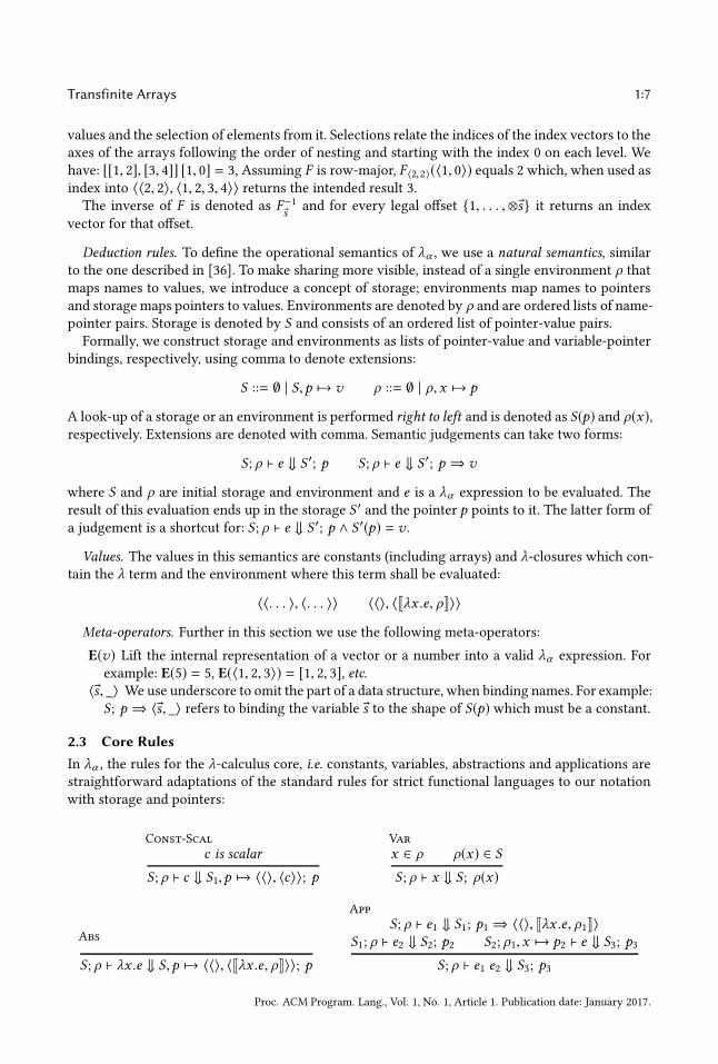
2.3 Core Rules

In λα , the rules for the λ-calculus core, i.e. constants, variables, abstractions and applications arestraightforward adaptations of the standard rules for strict functional languages to our notationwith storage and pointers:

Const-Scal

c is scalar

S ; ρ ⊢ c ⇓ S1,p 7→ 〈〈〉, 〈c〉〉; p

Var

x ∈ ρ ρ(x) ∈ S

S ; ρ ⊢ x ⇓ S ; ρ(x)

Abs

S ; ρ ⊢ λx .e ⇓ S,p 7→ 〈〈〉, 〈Jλx .e, ρK〉〉; p

App

S ; ρ ⊢ e1 ⇓ S1; p1 ⇒ 〈〈〉, Jλx .e, ρ1K〉S1; ρ ⊢ e2 ⇓ S2; p2 S2; ρ1, x 7→ p2 ⊢ e ⇓ S3; p3

S ; ρ ⊢ e1 e2 ⇓ S3; p3



As an illustration, consider the evaluation of (λx .x) 42:

∅; ∅ (λx .x) 42 Abs

S1 = p1 7→ 〈〈〉, Jλx .x , ∅K〉; ∅ p1 42 Const-Scal

S2 = S1,p2 7→ 〈〈〉, 〈42〉〉; ∅ p1 p2 App

S2; x 7→ p2 x Var

S2; ∅ p2 �

We start with an empty storage and an empty environment. The outer application demands thattheApp-rule be used. It enforces three computations: the evaluation of the function, the evaluationof the argument and the evaluation of the function body with an appropriately expanded environ-ment. The function is evaluated by the Abs-rule which adds a closure p1 7→ 〈〈〉, Jλx .x , ∅K〉 to thestorage and returns the pointer p1 to it. The argument is evaluated by the Const-Scal-rule whichadds p2 7→ 〈〈〉, 〈42〉〉 to the storage and returns p2. Finally, the App-rule demands the evaluationof the body of the function with an environment ρ1 = x 7→ p2. The body being just the variable x ,the Var-rule gives us S2; p2 as final result.The rules for array constructors and array selections are rather straightforward as well. Both

these constructs are strict:

Imm-Array

n ≥ 1n∀i=1

Si ; ρ ⊢ ci ⇓ Si+1; pi

P = 〈p1, . . . ,pn〉 AllSameShape(Sn+1, P) S ′ = Sn+1,po 7→ 〈〈1〉, 〈n〉〉,pi 7→ Sn+1(p1)S ′, ρ ⊢ imap1 po |pi {〈i−1〉 7→ pi | i ∈ {1, . . . ,n}} ⇓ S ′′; p

S1; ρ ⊢ [c1, . . . , cn] ⇓ S′′; p

Imm-Array-empty

S ; ρ ⊢ [] ⇓ S,p 7→ 〈〈0〉, 〈〉〉; p

Sel-strict

S ; ρ ⊢ i ⇓ S1; pi ⇒ 〈〈d〉,®ı〉 S1; ρ ⊢ a ⇓ S2; pa ⇒ 〈®s, ®a〉 k = F®s (®ı)

S ; ρ ⊢ a.i ⇓ S3,p 7→ 〈〈〉, 〈®ak 〉〉; p

Empty arrays are put into the storage with shape [0] (Imm-Array-empty-rule). Non-empty ar-rays (Imm-Array-rule) evaluate all the components and ensure that they are all of the same finiteshape. Subsequently, we assemble evaluated components into the resulting array value ensuringthat the flattening adheres to F . This is achieved by using an auxiliary term imap1. It takes theform imap1 po |pi {®ı

1 7→ p®ı 1 , . . . ,®ın 7→ p®ı n } where po and pi are pointers to frame and cell shapes,

and the set {®ı 1 7→ p®ı 1 , . . . ,®ın 7→ p®ı n } contains pairs of frame-shape indices and value pointers

for all legal indices into the frame shape. The formal definition of the deduction rule for imap1 isprovided in [58, Sec 2.1.1].The rule for selection (Sel-strict-rule) first evaluates the array we are selecting from, and the

index vector specifying the array index we wish to select. Then, we compute the offset into thedata vector by applying F to the index vector. Finally, we get the scalar value at the correspondingindex. When applying F , we implicitly check that:

• the index is within bounds 1 ≤ k ≤ ⊗®s , as F®s is undefined outside the index space boundedby ®s; and

• the index vector and the shape vector are of the same length, which means that selectionsevaluate scalars and not array sub-regions.



IMap. In order to keep the imap rule reasonably concise, we introduce two separate rules, a ruleGen for evaluating the generator bounds, and the main rule for imap, the Imap-Strict-Rule:

IMap-Strict

S ; ρ ⊢ eout ⇓ S1; pout ⇒ 〈〈do〉, ®sout〉 S1; ρ ⊢ ein ⇓ S2; pin ⇒ 〈〈di 〉, ®sin〉

S1 = S2n∀i=1

Si ; ρ ⊢ дi ⇓ Si+1; pдi ⇒ дi FormsPartition( ®sout, {д1, . . . , дn})

S1 = Sn+1 ∀(i,®ı) ∈ Enumerate( ®sout)∃k :

��

®ı ∈ дk ∧ дk = Gen(xk , _, _)Si ,p 7→ 〈〈do〉,®ı 〉; ρ, xk 7→ p ⊢ ek ⇓ S ′i ; p®ıS ′i ; ρ, x 7→ p®ı ⊢ |x | ⇓ Si+1; p

′®ı⇒ 〈〈di 〉, ®sin〉

S⊗ ®sout+1, ρ ⊢ imap1 pout |pin{®ı 7→ p®ı | (_,®ı) ∈ Enumerate( ®sout)

}⇓ S ′; p

S ; ρ ⊢ imap eout |ein

д1 : e1,

. . .

дn : en

⇓ S ′; p

Gen

S ; ρ ⊢ e1 ⇓ S1; p1 ⇒ 〈〈n〉, ®l 〉 S1; ρ ⊢ e2 ⇓ S2; p2 ⇒ 〈〈n〉, ®u〉

S ; ρ ⊢ (e1 ≤ x < e2) ⇓ S,p 7→ Gen(x , ®l, ®u); p

The Gen-rule introduces auxiliary values Gen(x , ®l, ®u) which are triplets that keep a variable name,lower bound and upper bound of a generator together. These auxiliary values are references onlyby the rule for imap.Evaluation of an imap happens in three steps. First, we compute shapes and generators, making

sure that generators form a partition of ®sout (FormsPartition is responsible for this). Secondly, forevery valid index defined by the frame shape (Enumerate generates a set of offset-index-vectorpairs), we find a generator that includes the given index (denoted®ı ∈ дk ).We evaluate the generatorexpression ek , binding the generator variable xk to the corresponding index value and check thatthe result has the same shape as pin. Finally, we combine evaluated expressions for every index ofthe frame shape into imap1 for further extraction of scalar values.All missing rules, including built-in operations, conditionals and recursion through the letrec-

construct are straightforward adaptations of the standard rules. They can be found in [58]. Formaldefinitions of helper functions, such as AllSameShape, will also be found there.

2.4 Infinite Arrays

In order to support infinite arrays, we introduce the notion of infinity in λα , and we allow infinitiesto appear in shape components. Syntactically, this can be achieved by adding a symbol for infinity,as shown in Fig. 2. For disambiguation, we refer to the extended version of λα as λ∞α . Adding ∞

λα with cardinal infinity. extends λα

c ::= · · ·| ∞ (infinity constant)

Fig. 2. The syntax of λ∞α

has several implications. First of all, our built-in arithmetic needs to be extended. We treat infinityin the usual way, applying the model commonly known as a Riemann sphere. That is:

z +∞ = ∞ z ×∞ = ∞z

∞= 0

z

0= ∞



The following operations are undefined:

∞ +∞ ∞ −∞ ∞× 00

0

∞

∞

While these additions to the semantics are trivial, allowing infinity to appear in shapes has amore profound impact on our semantics. Our rule for imap-constructs (Imap-Strict) forces theevaluation of all elements. If our result shape contains infinity, this can no longer be done. Aswe want to maintain a strict evaluation regime for function applications in general, we turn ourimap-construct into a lazy data-structure which does not immediately compute its elements, butonly does so when individual elements are being inspected. For this purpose, we extend our set ofallowed values of our semantics with an imap-closure:

uwvimap pout |pin

д1 : e1,

. . .

дn : en

, ρ

}�~

The imap closure contains pointers to frame and element shapes (pout and pin correspondingly),the list of partitions, where generators have been evaluated and the environment in which theimap shall be evaluated. The overall idea is to update, in place, this closure whenever individualelements are computed. With this extension, we can now replace our strict imap-rule by a lazyvariant:

IMap-Lazy

S ; ρ ⊢ eout ⇓ S1; pout ⇒ 〈〈_〉, ®sout〉 S1; ρ ⊢ ein ⇓ S2; pin ⇒ 〈〈_〉, _〉

S1 = S2n∀i=1

Si ; ρ ⊢ дi ⇓ Si+1; pдi ⇒ дi FormsPartition( ®sout, {д1, . . . , дn}, )

S ; ρ ⊢ imap eout |ein

д1 : e1,

. . .

дn : en

⇓ Sn+1,p 7→

uwvimap pout |pin

д1 : e1,

. . .

дn : en

; ρ

}�~ ; p

We can see that the new rule for imap-constructs, in essence, performs a subset of what the strictrule from the previous section does. It still forces the result shapes, it still computes the boundariesof the generators, and it checks the validity of the overall generator set. Once these computationshave been done, further element computation is delayed and an imap-closure is created instead.The actual computation of elements is triggered upon element selection. Consequently, we need

a second selection rule which can deal with imap closures in the array argument position:

Sel-lazy-imap

S ; ρ ⊢ i ⇓ S1; pi ⇒ 〈〈_〉, ®v 〉 S1; ρ ⊢ a ⇓ S2; pa ⇒

uwvimap pout |pin

д1 e1

. . .

дn en

, ρ ′

}�~

S2(pout) = 〈〈m〉, _〉 (®ı, ®) = Split(m, ®v )∃k : ®ı ∈ дk дk = Gen(xk , _, _) S2,p 7→ E(®ı); ρ ′, xk 7→ p ⊢ ek ⇓ S3; p®ı

S3; ρ′, x 7→ p®ı ⊢ x .E(®) ⇓ S4; p S5 = UpdateIMap(S4,pa,®ı,p®ı )

S ; ρ ⊢ a.i ⇓ S5; p

Selections into imap-closures happen at indices that are of the same length as the concatenation ofthe imap frame and cell shapes. This means that the index the imap-closure is being selected fromhas to be split into frame and cell sub-indices: ®ı and ® correspondingly. Given that дk contains ®ı, weevaluate ek with xk being bound to ®ı. As this value may be non-scalar, we evaluate a selection into



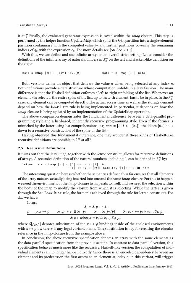
it at ® . Finally, the evaluated generator expression is saved within the imap closure. This step isperformed by the helper function UpdateIMap, which splits thek-th partition into a single-elementpartition containing ®ı with the computed value p®ı , and further partitions covering the remainingindices of дk with the expression ek . For more details see [58, Sec. 2.1.1].With this, we can define and use infinite arrays in an overall strict setting. Let us consider the

definitions of the infinite array of natural numbers in λ∞α on the left and Haskell-like definition onthe right:

na t s ≡ imap [∞ ] { _ ( i v ) : i v . [ 0 ] na t s = 0 : map ( + 1 ) na t s

Both versions define an object that delivers the value n when being selected at any index n.Both definitions provide a data structure whose computation unfolds in a lazy fashion. The maindifference is that the Haskell definition enforces a left-to-right unfolding of the list. Whenever anelementn is selected, the entire spine of the list, up to then-th element, has to be in place. In the λ∞αcase, any element can be computed directly. The actual access time as well as the storage demanddepend on how the Imap-Lazy-rule is being implemented. In particular, it depends on how theimap-closure is being updated by an implementation of the UpdateIMap operation.The above comparison demonstrates the fundamental difference between a data-parallel pro-

gramming style and a list-based, inherently recursive programming style. Even if the former ismimicked by the latter using list comprehensions, e.g. nats = [i | i <− [0..]], the idiom [0..] boilsdown to a recursive construction of the spine of the list.Having observed this fundamental difference, one may wonder if these kinds of Haskell-like

recursive definitions are possible in λ∞α at all?

2.5 Recursive Definitions

It turns out that the lazy imap, together with the letrec construct, allows for recursive definitionsof arrays. A recursive definition of the natural numbers, including 0, can be defined in λ∞α by:

l e t r e c na t s = imap [∞ ] { [ 0 ] <= i v < [ 1 ] : 0 ,[ 1 ] <= i v < [∞ ] : n a t s . ( i v Û− [ 1 ] ) + 1 in na t s

The interesting question here is whether the semantics defined thus far ensures that all elementsof the array nats are actually being inserted into one and the same imap-closure. For this to happen,we need the environment of the imap-closure tomap nats to itself, andwe need the selectionwithinthe body of the imap to modify the closure from which it is selecting. While the latter is giventhrough the Sel-Lazy-Imap-rule, the former is achieved through the rule for letrec-constructs. Forλα , we have:

Letrec

S1 = S,p 7→ ⊥ρ1 = ρ, x 7→ p S1; ρ1 ⊢ e1 ⇓ S2; p2 S3 = S2[p2/p] S3; ρ, x 7→ p2 ⊢ e2 ⇓ S4; pr

S ; ρ ⊢ letrec x = e1 in e2 ⇓ S4; pr

where S[p2/p] denotes substitution of the x 7→ p bindings inside of the enclosed environmentswith x 7→ p2, where x is any legal variable name. This substitution is key for creating the circularreference in the imap-closure from the example above.In conclusion, the above recursive specification denotes an array with the same elements as

the data-parallel specification from the previous section. In contrast to data-parallel version, thisspecification behaves much more like the recursive, Haskell-like version; the computation of indi-vidual elements can no longer happen directly. Since there is an encoded dependency between anelement and its predecessor, the first access to an element at index n, in this variant, will trigger



the computation of all elements from 0 up to n. The implementation of the UpdateIMap operationon imap-closures determines how these numbers are stored in memory and, consequently, howefficiently they can be accessed.The availability of direct indexes makes it possible to encode an arbitrary order for the recursion.

Consider the following example:

l e t r e c a = imap [ 1 0 ] { [ 9 ] <= i v < [ 1 0 ] : 9 ,[ 0 ] <= i v < [ 9 ] : a . ( i v Û+ [ 1 ] ) −1 in a

Selection of the 9th element can be evaluated in one step. In case of lists, the selection request al-ways starts at the beginning of the list. Hence, to obtain the same performance, some optimisationof the list case is required.

2.6 List Primitives in the Array Se�ing

We have enabled two features that are inherent with lists, but that are usually not supported inan array setting: recursively defined data-structures and infinite arrays. All that is required toachieve this is a recursion-aware, lazy semantics of the imap-construct and the inclusion of anexplicit notion of infinity. With these extensions, the key primitives for lists, head , tail , and conscan be defined as

head ≡ λa . a . [ 0 ]t a i l ≡ λa . imap | a | Û− [ 1 ] { _ ( i v ) : a . ( [ 1 ] Û+ i v )cons ≡ λa . λb . imap [ 1 ] Û+ | b | { [ 0 ] <= i v < [ 1 ] : a ,

[ 1 ] <= i v < [ 1 ] Û+ | b | : b . ( i v Û− [ 1 ] )

More complex list-like functions can be defined on top of these. An example is concatenation:

l e t r e c ( ++ ) = λa . λb . i f | a | . [ 0 ] = 0 then be l se cons ( head a ) ( ( t a i l a ) ++ b ) in ( ++ )

In casea is infinite, however, the above definition of concatenation is unsatisfying. The strict natureof λα will force tail a forever as

��a��.[0] = 0 never yields true. The way to avoid this is to shift the

case distinction into the lazy imap construct:

( ++ ) ≡ λa . λb . imap | a | Û+ | b | { [ 0 ] <= i v < | a | : a . iv ,| a | <= i v < | a | Û+ | b | : b . ( i v Û− | a | )

As we have seen earlier, λα enables the typical constructions of recursive definitions of infin-ite vectors well-known from the realm of lists such as list of ones, natural numbers or fibonaccisequence.Having a unified interface for arrays and lists enables programmers to switch the algorithmic

definitions of individual arrays from recursive to data-parallel styles without modifying any of thecode that operates on them.However, such a unification comes at a price: we have to support a lazy version of the imap-

construct. As a consequence, we conceptually lose the advantage of O(1) access. Despite λα of-fering many opportunities for compiler optimisations like pre-allocating arrays and potentiallyenforcing strictness on finite, non-recursive imaps, one may wonder at this point how much λαdiffers from a lazy array interface in a lazy, list-based language such as Haskell?

3 TRANSFINITE ARRAYS

We now investigate to what extent λ∞α adheres to the key properties of array programming— arrayalgebras and array equalities.



3.1 Algebraic Properties

Array-based operations offer a number of beneficial algebraic properties. Typically, these prop-erties manifest themselves as universally valid equalities which, once established, improve ourthinking about algorithms and their implementations, and give rise to high-level program trans-formations. We define equality between two non-scalar arrays a and b as

a == b ⇐⇒ |a | = |b | ∧ ∀ iv < |a | : a.iv = b .iv

that is, we demand equality of the shapes and equality of all elements. The demand for equality ofshapes recursively implies equality in dimensionality and the extensional character of this defin-ition through the use of array selections ensures that we can reason about equality on infinitearrays as well.Arrays give rise to many algebras such as Theory of Arrays [46], Mathematics of Arrays [48],

and Array Algebras [21]. Most of the developed algebras differ only slightly, and the set of equal-ities that are ultimately valid depends on some fundamental choices, such as the ones we made inthe beginning of the previous section. At the core of these equalities is the ability to change theshape of arrays in a systematic way without losing any of their data.An equality from [19] that plays a key role in consistent shape manipulations is:

reshape |a | (flatten a) == a (1)

where flatten maps an array recursively into a vector by concatenating its sub-arrays in a row-major fashion and reshape performs the dual operation of bringing a row-major linearisation backinto multi-dimensional form. These operations can be defined in λ∞α as

f l a t t e n ≡ λa . imap [ count a ] { _ ( i v ) : a . ( o2 i i v . [ 0 ] | a | )r e sh ape ≡ λ shp . λa . imap shp { _ ( i v ) : ( f l a t t e n a ) . [ i 2 o i v shp ]

where count returns the product of all shape components and o2i and i2o translate offsets into in-dices and vice versa, respectively. These operations effectively implement conversions frommixed-radix systems into natural numbers using multiplications and additions and back using divisionand remainder operations.The above equality states that any array a can be brought into flattened form and, subsequently

be brought back to its original shape. For arrays of finite shape s , this follows directly from thefact that o2i (i2o iv s) s = iv for all legitimate index vectors iv into the shape s .If we want Eq. 1 to hold for all arrays in λ∞α , we need to show that the above equality also holds

for arrays with infinite axes. Consider an array of shape s = [2,∞]. For any legal index vector[1,n] into the shape s , we obtain:

o2i (i2o [1,n] [2,∞]) [2,∞]) = o2i (∞ · 1 + n) [2,∞]

= o2i ∞ [2,∞]

= [∞ / ∞, ∞ % ∞]

which is not defined. We can also observe that all indices [1,n] are effectively mapped into thesame offset:∞ which is not a legitimate index into any array in λ∞α . This reflects the intuition thatthe concatenation of two infinite vectors effectively looses access to the second vector.The inability to concatenate infinite arrays also makes the following equality fail:

drop |a | (a ++ b) == b (2)

where a and b are vectors and drop s x removes first s elements from the left. The reason is exactlythe same: given that |a | = [∞] and b is of finite shape [n], the shape of the concatenation is[∞ + n] = [∞], and drop of |a | results in an empty vector.



Clearly, λ∞α as presented so far is not strong enough tomaintain universal equalities such as Eq. 1or 2. Instead, we have to find a way that enables us to represent sequences of infinite sequencesthat can be distinguished from each other.

3.2 Ordinals

When numbers are treated in terms of cardinality, they describe the number of elements in a set.Addition of two cardinal numbers a and b is defined as a size of a union of sets of a and b elements.This notion also makes it possible to operate with infinite numbers, where the number of elementsin an infinite set is defined via bijections. As a result, differently constructed infinite sets may endup having the same number of elements. For example, if there exists a bijection from N × N intoN, the cardinality of both sets is the same.When studying arrays, treating their shapes and indices using cardinal numbers is an oversim-

plification, because arrays have richer structure. Arrays are collections of ordered elements, wherethe order is established by the indices. Ordinal numbers, as introduced by G. Cantor in 1883, serveexactly this purpose — to “label” positions of objects within an ordered collection. When collec-tions are finite, cardinals and ordinals can be used interchangeably, as we can always count thelabels. Infinite collections are quite different in that regard: despite being of the same size, therecan be many non-isomorphic well-orderings of an infinite collection. For example, consider twoinfinite arrays of shapes [∞, 2] and [2,∞]. Both of these have infinitely many elements, but theydiffer in their structure. From a row major perspective, the former is an infinite sequence of pairs,whereas the latter are two infinite sequences of scalars. Ordinals give a formal way of describingsuch different well-orderings.First let us try to develop an intuition for the concept of ordinal numbers and then we give a

formal definition. Consider an ordered sequence of natural numbers: 0 < 1 < 2 < · · · . Theseare the first ordinals. Then, we introduce a number called ω that represents the limit of the abovesequence: 0 < 1 < 2 < · · · < ω. Further, we can construct numbers beyond ω by putting a “copy”of natural numbers “beyond” ω:

0 < 1 < 2 < · · ·ω < ω + 1 < ω + 2 < · · · < ω + ω

For the time being, we treat operations such as ω + n symbolically. The number ω + ω which canbe also denoted as ω · 2 is the second limit ordinal that limits any number of the form ω +n,n ∈ N.Such a procedure of constructing limit ordinals out of already constructed smaller ordinals can beapplied recursively. Consider a sequence of ω · n numbers and its limit:

0 < ω < ω · 2 < ω · 3 < · · · < (ω · ω = ω2)

and we can carry on further to ωn , ωω , etc. Note though that in the interval fromω2 to ω3 we haveinfinitely many limit ordinals of the form:

ω2< ω2

+ ω < ω2+ ω · 2 < · · · < ω3

and between any two of these we have a “copy” of the natural numbers:

ω2+ ω < ω2

+ ω + 1 < · · · < ω2+ ω · 2

3.2.1 Formal definitions. A totally ordered set 〈A, <〉 is said to be well ordered (or have a well-founded order) if and only if every nonempty subset of A has a least element [16]. Given a well-

ordered set 〈X , <〉 and a ∈ X , Xadef= {x ∈ X |x < a}. An ordinal is a well-ordered set 〈X , <〉, such

that: ∀a ∈ X : a = Xa . As a consequence, if 〈X , <〉 is an ordinal then < is equivalent to ∈. Given awell-ordered set A = 〈X , <〉 we define an ordinal that this set is isomorphic to asOrd(A, <). Given



an ordinal α , its successor is defined to be α ∪{α}. The minimal ordinal is ∅ which is denoted with0. The next few ordinals are:

1 = {0} = {∅}2 = {0, 1} = {∅, {∅}}3 = {0, 1, 2} = {∅, {∅}, {∅, {∅}}}

· · ·

A limit ordinal is an ordinal that is greater than zero that is not a successor. The set of naturalnumbers {0, 1, 2, 3, . . . } is the smallest limit ordinal that is denoted ω. We use islim x to denotethat x is a limit ordinal.

3.2.2 Arithmetic on Ordinals.

Addition. Ordinal addition is defined as α + β = Ord(A, <A), where A = {0} × α ∪ {1} × β

and <A is the lexicographic ordering on A. Ordinal addition is associative but not commutative.As an example consider expressions 2 + ω and ω + 2. The former can be seen as follows: 0 <1 < 0′ < 1′ < · · ·, which after relabeling is isomorphic to ω. However, the latter can be seenas: 0 < 1 < · · · < 0′ < 1′, which has the largest element 1′, whereas ω does not. Therefore2 + ω = ω < ω + 2. We have used 0′, 1′ to indicate the right hand side argument of the addition.

Subtraction. Ordinal subtraction can be defined in two ways, as partial inverse of the additionon the left and on the right. For left subtraction, which will be used by default throughout thispaper unless otherwise specified, α − β is defined when β ≤ α , as: ∃ξ : β + ξ = α . As ordinaladdition is left-cancelative (α + β = α + γ =⇒ β = γ ), left subtraction always exists and it isunique.Right subtraction is a bit harder to define as:

• it is not unique: 1 + ω = 2 + ω but 1 , 2; therefore ω −R ω can be any number that is lessthan ω: {0, 1, 2, . . . }.

• even if β < α , the difference α − β might not exist. For example: 42 < ω; however, ω −R 42does not exist as �ξ : ξ + 42 = ω.

Despite those difficulties, right subtraction can be useful at times and can be defined for α −R β :

min{ξ : ξ + β = α}

Multiplication. Ordinal multiplication α · β = Ord(A, <A) where A = α × β and <A is the lexico-graphic ordering on A. Multiplication is associative and left-distributive to addition:

α · (β + γ ) = (α · β) + (α · γ )

However, multiplication is not commutative and is not distributive on the right: 2 · ω = ω < ω · 2and (ω + 1) · ω = ω · ω < ω · ω + ω.

Exponentiation. Exponentiation can be defined using transfinite recursion: α0= 1,α β+1 = α β ·α

and for limit ordinals λ: αλ =⋃

0<ξ <λα ξ .

ϵ-ordinals. Using ordinal operationswe can construct the following hierarchy of ordinals: 0, 1, . . . ,ω,ω+1, . . . ,ω · 2,ω · 2 + 1, . . . ,ω2

, . . . ,ω3, . . .ωω

, . . . . The smallest ordinal for which α = ωα is calledϵ0. It can also be seen as a limit of the following ωω

,ωωω

, . . . ,ωω . . .

.

3.2.3 Cantor Normal Form. For every ordinal α < ϵ0 there are unique n,p < ω,α1 > α2 > · · · >αn and x1, . . . , xn ∈ ω \ {0} such that α > α1 and α = ωα1 · x1 + · · · +ω

αn · xn + p. Cantor NormalForm makes provides a standardized way of writing ordinals. It uniquely represents each ordinal



as a finite sum of ordinal powers, and can be seen as an ω based polynomial. This can be used asa basis for an efficient implementation of ordinals and their operations.

3.3 λω : Adding Ordinals to λα

The key contribution of this paper is the introduction of λω , a variant of λα , which use ordinalsas shapes and indices of arrays and which reestablishes global equalities in the context of infinitearrays.Before revisiting the equalities, we look at the changes to λα that are required to support transfin-

ite arrays. Syntactically, to introduce ordinals in the language, we make two minor additions to λα .Firstly, we add ordinals4 as scalar constants. Secondly, we add a built-in operation, islim, whichtakes one argument and returns true if the argument is a limit ordinal and false otherwise. Forexample: islim ω reduces to true and islim (ω + 21) reduces to false.

λα with ordinals extends λα

e ::= · · ·| islim (limit ordinal predicate)

c ::= · · ·| ω,ω + 1, . . . (ordinals)

Fig. 3. The syntax of λω .

Semantically, it turns out that all core rules can be kept unmodified apart from the aspect thatall helper functions, arithmetic, and relational operations now need to be able to deal with ordinalsinstead of natural numbers. In particular, the semantic for lazy imaps as developed for λ∞α can beused unaltered, provided that all helper functions involved such as for splitting generators etc. areexpanded to cope with ordinals.

3.4 Array Equalities Revisited

With the support of Ordinals in λω , we can now revisit our equalities Eq. 1 and 2. Let us first lookat the counter example for Eq. 1: from Section 3.1: With an array shape s = [2,ω] and a legal indexvector into s [1,n], we now obtain:

o2i (i2o [1,n] [2,ω]) [2,ω]) = o2i (ω + n) [2,ω]

= [(ω + n) / ω, (ω + n) % ω]

= [1, n]

The crucial difference to the situation from λ∞α in Section 3.1 here is the ability to divide (ω + n)by ω and to obtain a remainder, denoted by %, of that division as well. By means of induction overthe length of the shape and index vectors this equality can be proven to hold for arbitrary shapesin λω , and, based on this proof, Eq. 1 can be shown as well.In the same way as the arithmetic on ordinals is key to the proof of Eq. 1, it also enables the

proof of Eq. 2 for arbitrary ordinal-shaped vectors5 a and b, with the definition of ++ from theprevious section and drop being defined as:

drop ≡ λ s . λa . imap | a | Û−s { [ 0 ] <= i v < | a | Û−s : a . ( s Û+ i v )

4 Technically, we support ordinal values only up to ωω , as ordinals are constructed using the constant ω and +, −, ∗, / and% operations (no built-in ordinal exponentiation).5 Eq. 2 can be generalised and shown to hold in the multi-dimensional case, provided that ++ and drop operate over thesame axis.



After inlining ++ and drop, the left hand side of Eq. 2 can be rewritten as:

l e t r e c ab = imap | a | Û+ | b | { [ 0 ] <= j v < | a | : a . jv ,| a | <= j v < | a | Û+ | b | : b . ( j v Û− | a | ) in

imap | ab | Û− | a | { [ 0 ] <= i v < | ab | Û− | a | : ab . ( | a | Û+ i v )

Consider the shape of the goal expression of the letrec. According to the semantics of theshape of an imap, we get: |ab| Û−|a |. The shape of ab is |a | Û+|b |. According to ordinal arithmetic:(|a | Û+|b |) Û−|a | is |b |. Therefore the shapes of right-hand and left-hand sides of the goal expressionsare the same.Let us rewrite the last imap as:

imap | b | { [ 0 ] <= i v < | b | : ab . ( | a | Û+ i v )

Consider now selections into ab. All the selections into abwill happen at indices that are greaterthan a. This is because all the legal iv in the imap are from the range [0] to |b |.According to the semantics of selections into imaps, ab.(|a | Û+iv) will select from the second

partition of the imap that defines ab, and will evaluate to: b .((|a | Û+iv) Û−|a |). According to ordinalarithmetic, (|a | Û+iv) Û−|a | is identical to iv, therefore we can rewrite the previous imap as:

imap | b | { [ 0 ] <= i v < | b | : b . i v

As it can be seen, this is an identity imap, which is extensionally equivalent to b.

4 EXAMPLES

Transfinite tail. As explained in Section 3.3, the shift from natural numbers to ordinals as indicesin λω implies corresponding extensions of the built-in arithmetic operations. As these operationslose key properties, such as commutativity, once arguments exceed the range of natural numbers,we need to ensure that function definitions for finite arrays extend correctly to the transfinite case.

As an example, consider the definition of tail from the previous section:

t a i l ≡ λa . imap | a | Û− [ 1 ] { _ ( i v ) : a . ( [ 1 ] Û+ i v )

For the case of finite vectors, we can see that a vector shortened by one element is returned, wherethe first element is missing and all elements have been shifted to the left by one element.Let us assume we apply tail to an array a with |a | = [ω]. The arithmetic on ordinals gives us

a return shape of [ω] Û−[1] = [ω]. That is, the tail of an infinite array is the same size as the arrayitself, which matches our common intuition when applying tail to infinite lists. The elements ofthat infinite list are those of a, shifted by one element to the right, which, again, matches ourexpected interpretation for lists.Now, assume we have |a | = [ω + 42], which means that (tail a).[ω] should be a valid expression.

For the result shape of tail a, we obtain [ω + 42] Û−[1] = [ω + 42]. A selection (tail a).[ω] evaluatesto a.([1] Û+[ω]) = a.[ω]. This means that the above definition of the tail shifts all the elements atindices smaller than [ω] one left, and leaves all the other unmodified.While this may seem counter-intuitive at first, it actually only means that tail can be applied infinitely often but will never beable to reach “beyond” the first limit.Finally, observe that the body of the imap-construct in the definition of tail uses [1] Û+iv is an

index expression, not iv Û+[1]. In the latter case, the tail function would behave differently beyond[ω]: it would attempt to shift elements to the left. However, this would make the overall definitionfaulty. Consider again the case when |a | = [ω + 42]: the shape of the result would be |a |, whichwould mean that it would be possible to index at position [ω+41], triggering evaluation of a.([ω+41] Û+[1]) and consequently, producing an index error, or out-of-bounds access into a.



Zip. Let us now define zip of two vectors that produces a vector of tuples. Consider a Haskelldefinition of zip function first:

zip ( a : as ) ( b : bs ) = ( a , b ) : zip as bszip _ _ = [ ]

The result is computed lazily, and the length of the resulting list is a minimum of the lengths ofthe arguments. Like concatenation, a literal translation into λω is possible, but it has the samedrawbacks, i.e. it is restricted to arrays whose shape has no components bigger than ω.A better version of zip that can be applied to arbitrary transfinite arrays looks as follows:

z i p ≡ λa . λb . imap ( min | a | | b | ) | [ 2 ] { _ ( i v ) : [ a . iv , b . i v ]

Here, we use a constant array in the body of the imap. This forces evaluation of both arguments,even if only one of them is selected. This can be changed by replacing the constant array with animap:

z i p ≡ λa . λb . imap ( min | a | | b | ) | [ 2 ] { _ ( i v ) : imap [ 2 ] { [ 0 ] <= j v < [ 1 ] a . iv ,[ 1 ] <= j v < [ 2 ] b . i v

which can be fused in a single imap as follows:

z i p ≡ λa . λb . l e t r e c s = ( min | a | | b | ) . [ 0 ] inimap [ s , 2 ] { [ 0 , 0 ] <= i v < [ s , 1 ] : a . [ i v . [ 0 ] ] ,

[ 0 , 1 ] <= i v < [ s , 2 ] : b . [ i v . [ 0 ] ]

Data Layout and Transpose. A typical transformations in stream programming is changing thegranularity of a stream and joiningmultiple streams. In λω , these transformations can be expressedby manipulating the shape of an infinite array. Consider changing the granularity of a stream a ofshape [ω] into a stream of pairs:

imap ( | a | Û/ [ 2 ] ) | [ 2 ] { _ ( i v ) : [ a . [ 2 ∗ i v . [ 0 ] ] , a . [ 2 ∗ i v . [ 0 ] + 1 ] ]

or we can express the same code in a more generic fashion:

( λn . r e sh ape ( ( | a | Û/ [ n ] ) + + [n ] ) a ) 2

This code can operate on the streams of transfinite length, as well. If we envision compiling sucha program into machine code, the infinite dimension of an array can be seen as a time-loop, andthe operations at the inner dimension seen as a stream-transforming function. Such granularitychanges are often essential for making good use of (parallel) hardware resources, e.g. FPGAs.Transposing a stream makes it possible to introduce synchronisation. Consider transforming a

stream a of shape [2,ω] into a stream of pairs (shape [ω, 2]):

imap [ω ] | [ 2 ] { _ ( i v ) : [ a . [ i v . [ 0 ] , 0 ] , a . [ i v . [ 0 ] , 1 ] ]

Conceptually, an array of shape [2,ω] represents two infinite streams that reside in the same datastructure. An operation on such a data structure can progress independently on each stream, unlesssome dependencies on the outer index are introduced. A transpose, as above, makes it possible tointroduce such a dependency, ensuring that the operations on both streams are synchronized. Akey to achieving this is the ability to re-enumerate infinite structures, and ordinal-based infinitearrays make this possible.



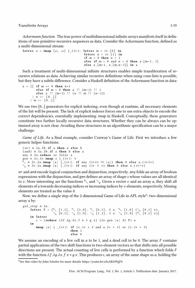
Ackermann function. The true power ofmultidimensional infinite arraysmanifests itself in defin-itions of non-primitive-recursive sequences as data. Consider the Ackermann function, defined asa multi-dimensional stream:

l e t r e c a = imap [ω , ω ] { _ ( i v ) : l e t r e c m = i v . [ 0 ] inl e t r e c n = i v . [ 1 ] ini f m = 0 then n + 1e l se i f m > 0 and n = 0 then a . [m−1 , 1 ]e l se a . [m−1 , a . [m, n−1] ] in a

Such a treatment of multi-dimensional infinite structures enables simple transliteration of re-cursive relations as data. Achieving similar recursive definitions when using cons-lists is possible,but they have a subtle difference. Consider a Haskell definition of the Ackermann function in data:

a = [ [ i f m == 0 then n+1e l se i f m > 0 then a ! ! (m−1) ! ! 1e l se a ! ! (m−1) ! ! ( a ! ! m ! ! ( n−1 ) )

| n <− [ 0 . . ] ]| m <− [ 0 . . ] ]

We use two [0..] generators for explicit indexing, even though at runtime, all necessary elementsof the list will be present. The lack of explicit indexes forces one to use extra objects to encode thecorrect dependencies, essentially implementing imap in Haskell. Conceptually, these generatorsconstitute two further locally recursive data structures. Whether they can be always can be op-timised away is not clear. Avoiding these structures in an algorithmic specification can be a majorchallenge.

Game of Life. As a final example, consider Conway’s Game of Life. First we introduce a fewgeneric helper functions:

( or ) ≡ λa . λb . i f a then a e l se b( and ) ≡ λa . λb . i f a then b e l se aany ≡ λa . reduce or f a l s e agen ≡ λ s . λv . imap s { _ ( i v ) : vտ ≡ λv . λa . imap | a | { _ ( i v ) : i f any ( i v Û+v Û>= | a | ) then 0 e l se a . ( i v Û+v )ց ≡ λv . λa . imap | a | { _ ( i v ) : i f any ( i v Û< v ) then 0 e l se a . ( i v Û−v )

or and and encode logical conjunction and disjunction, respectively. any folds an array of booleanexpressions with the disjunction, and gen defines an array of shape s whose values are all identicalto v . More interesting are the functions տ and ց. Given a vector v and an array a, they shift allelements of a towards decreasing indices or increasing indices byv elements, respectively. Missingelements are treated as the value 0.Now, we define a single step of the 2-dimensional Game of Life in APL style6: two-dimensional

array a by:

go l _ s t e p ≡ λa .l e t r e c F = [տ [ 1 , 1 ] , տ [ 1 , 0 ] , տ [ 0 , 1 ] , λ x . տ [ 1 , 0 ] (ց [ 0 , 1 ] x ) ,

ց [ 0 , 1 ] , ց [ 1 , 0 ] , ց [ 1 , 1 ] , λ x . ց [ 1 , 0 ] (տ [ 0 , 1 ] x ) ]in l e t r e c

c = ( reduce ( λ f . λg . λx . f x Û+ g x ) ( λx . gen | a | 0 ) F ) ain

imap | a | { _ ( i v ) : i f ( c . i v = 2 and a . i v = 1 ) or ( c . i v = 3 )then 1e l se 0

We assume an encoding of a live cell in a to be 1, and a dead cell to be 0. The array F containspartial applications of the two shift functions to two-element vectors so that shifts into all possibledirections are present. The actual counting of live cells is performed by a function which folds Fwith the function λf .λд.λx . f x +д x . This produces c , an array of the same shape as a, holding the

6See this video by John Scholes for more details: https://youtu.be/a9xAKttWgP4


https://youtu.be/a9xAKttWgP4


numbers of live cells surrounding each position. Defining the shift operationsտ andց to insert0 ensures that all cells beyond the shape of a are assumed to be dead.The definition of the result array is, therefore, a straightforward imap, implementing the rules

of birth, survival and death of the Game of Life.The most interesting aspect of this algorithm is the fact that there is no restriction on the shape

of a. In our transfinite setting, we can provide an array of shape [ω,ω]. With no changes to sourcecode, we can deal with an infinitely large plane. An infinite a requires a lazy implementation asdemanded by our semantics of λω , but a finite case offers a strict implementation as a possiblealternative.

5 TRANSFINITE ARRAYS VS. STREAMS

Streams have attracted a lot of attention due to the many algebraic properties they expose. [29]provides a nice collection of examples, many of which are based on the observation that streamsform an applicative functor. Transfinite arrays are applicative functors as well, not only for arraysof shape [ω], but also for any given shape shp. With definitions:

pure ≡ λx . imap shp { _ ( i v ) : x( ⋄ ) ≡ λa . λb . imap shp { _ ( i v ) : a . i v b . i v

we obtain for arbitrary arrays u, v ,w , and x of shape shp:

(pure λx .x) ⋄u == u (pure (λf .λд.λx . f (д x))) ⋄u ⋄v ⋄w == u ⋄ (v ⋄w)

(pure f ) ⋄ (pure x) == pure (f x) u ⋄ (pure x) == (pure (λf . f x)) ⋄u

This shows that arbitrarily shaped arrays of finite size have this property, as also shown by [20],and that these properties can be expanded into ordinal-shaped arrays. Classical streams are a spe-cial instance of these, i.e. arrays of shape [ω].For stream operations that insert or delete elements, it is less obvious whether these can be

easily extended into ordinal-shaped arrays other than shape [ω]. As an example, let us considerthe function filter , which takes a predicate p and a vectorv and returns a vector that contains onlythose elements x of v that satisfy (p x). A direct definition of filter can be given as:

f i l t e r ≡ λp . λv . i f ( p v . [ 0 ] ) then v . [ 0 ] ++ f i l t e r p ( t a i l v )e l se f i l t e r p ( t a i l v )

This definition, in principle, is applicable to arrays of any ordinal shape, but the use of tail in therecursive calls inhibits application beyond ω. Furthermore, the strict semantics of λω inhibits aterminating application to any infinite array, including arrays of shape [ω]. For the same reason,a definition of filter through the built-in reduce is restricted to finite arrays.To achieve possible termination of the above definition of filter for transfinite arrays, we would

need to change to a lazy regime for all function applications in λω and we would need to changethe semantics of imap into a variant where the shape computation can be delayed as well. Even ifthat would be done, we would still end up with an unsatisfying solution. The filtering effect wouldalways be restricted to the elements before the first limit ordinal ω. This limitation breaks severalfundamental properties, like those defined in [10], that hold in the finite and stream cases. As anexample, consider distributivity of filter over concatenation:

filter p (a ++ b) == (filter p a) ++ (filter p b) (3)

This property holds for finite arrays, but fails with the above definition of filter in case a is infinite.To regain this property for transfinite arrays, we need to apply filter to all elements of the

argument array, not only those before the first limit ordinal ω. When doing this in the context ofλω , the necessity to have a strict shape for every object forces us to “guess” the shape of the filtered



result in advance. The way we “guess” has an impact on the filter-based equalities that will holduniversally.In this paper we propose a scheme that respects the above equality. For finite arrays filter works

as usual, and for the infinite ones, we postulate that the result of filtering will be of an infinite-shape:

∀p∀a : |a | ≥ ω =⇒ |filter p a | ≥ ω

This is further applied to all infinite sequences contained within the given shape as follows:

∀i < |a | : (∃islim α : i < α ≤ |a |) =⇒ (∃k ∈ N : p (a.(i + k)) = true)

We assume that each infinite sequence contains infinitely many elements for which the predicateholds. Consequently, any limit ordinal component of the shape of the argument is carried over tothe result shape and only any potential finite rest undergoes potential shortening. Consider a filteroperation, applied to a vector of shape [ω ·2]. Following the above rationale, the shape of the resultwill be [ω · 2] as well. This means that the result of applying filter to such an expression shouldallow indexing from {0, 1, . . . } as well as from {ω,ω + 1, . . . } delivering meaningful results.This decision can lead to non-termination when there are only finitely many elements in the

filtered result. For example:

f i l t e r ( λx . x > 0 ) ( imap [ω +2] { _ ( i v ) : 0 )

reduces to an array of shape [ω], which effectively is empty. Any selection into it will lead to anon-terminating recursion.The overall scheme may be counter-intuitive, but it states that for every index position of the

output, the computation of the corresponding value is well-defined.Assuming the aforementioned behaviour of filter , Eq. 3 holds for all transfinite arrays. Another

universal equation that holds for all transfinite vectors concerns the interplay of filter and map:

filter p (map f a) == map f (filter (p · f ) a)

The proposed approach does not only respect the above equalities, but it also behaves similarlyto filtering of streams that can be found in languages such as Haskell: filter applied to an infinitestream cannot return a finite result.In principle, the chosen filtering scheme can be defined in λω by using the islim predicate within

an imap. However, the resulting definition is neither concise, nor likely to be runtime efficient.Given the importance of filter, we propose an extension of λω . Fig. 4 shows the syntactical exten-sion of λω .

λω with filters extends λω

e ::= · · ·| filter e e (filter operation)

Fig. 4. The syntax of λω with filters.

As filter conceptually is an alternative means of constructing arrays, its semantics is similar tothat of imap. In particular, it constitutes a lazy array constructor, whose elements are being eval-uated upon demand created through selections. Technically, this means that we have to introducea new value to keep filter-closures, a rule that builds such a closure from filter expression, and weneed to define the selection operation that forces evaluation within the filter closure.



We introduce as new value for filter-closures:

uwvfilter pf pe

α1 v1r v

1i

. . .

αn vnr vni

}�~

which contains the pointer to the filtering function pf , the shape of the argument we are filteringover (pe ) and the list of partitions that consist of a limit ordinal, and a pair of partial result andnatural number: vr and vi correspondingly.On every selection at index [ξ +n], where ξ is a limit ordinal or zero, and n is a natural number,

we find a ξ partition within the filter closure or add a new one if it is not there. Every partitionkeeps a vector with a partial result of filtering (vr ), and the index (vi ) with the following property:the element in the array we are filtering over at position ξ + (vi − 1) is the last element in the vr ,given thatvr > 0. This means that if n is withinvr , we returnvr .[n]. Otherwise, we extendvr untilits length becomes n + 1 using the following procedure: inspect the element in pe at the positionξ + vi — if the predicate function evaluates to true, append this element to vr and increase vi byone, otherwise, increase vi by one.A formal description of this procedure can be found in [58, Sec. 2.1.4].

6 TOWARDS AN IMPLEMENTATION

We used the semantics of λω as a blueprint for the implementation of an interpreter, called Hehavailable at https://github.com/ashinkarov/heh). The interpreter, which serves as a proof of concept,performs a literal translation of the semantic rules provided in the paper into Ocaml code. All ex-amples provided in the paper can be found in that repository, and run, correctly, in the interpreter.The implementation parses the program, evaluates it and prints the result. We represent the

storage S from our semantics by a hash table of pointer-value bindings. Environments ρ are im-plemented as lists of variable-pointer pairs. Pointers and variables are strings and values are ofan algebraic data type. In the proof-of-concept interpreter, we never actively discard pointers orvariables; however we do share pointers and we update imap/filter closures in place, in the sameway as it is done in the formal semantics.

We represent ordinals in Cantor Normal Form. The algorithms for implementing operations onordinals are based on [42]. In the same paper, we also find an in-depth study of the complexitiesof ordinal operations: comparisons, additions and subtractions have complexities O(n), where nis the minimum of the lengths of both arguments; multiplications have the complexity O(n ·m),wherem and n are the lengths of the two argument representations.

The interpreter makes it possible to run all the examples described in this paper. Additionally,the interpreter provides means for experimentation through the incorporation of variants in thesemantics of imap: two interpreter flags enable users to (i) avoid thememoization of array elementscompletely, and (ii) to apply the strict imap-semantics instead of the lazy one whenever arrays areof finite shape. The implementation comes with about 100 unit tests.

6.1 Performance considerations

Having an interpreter for λω available allows experimentation with ordinal indexing and transfin-ite definitions. However, one of our initial aims, to enable efficient runtime execution on parallelsystems, is not demonstrated by Heh. In the remainder of this section, we discuss several perform-ance considerations that show how we envision efficient parallel executions of λω to be possible.


https://github.com/ashinkarov/heh


Strictness. As mentioned in Section 2, the design of λα closely matches that of SaC whichhas been shown to deliver high-performance execution on a variety of parallel machine archi-tectures [56, 59]. Since λω is largely an extension of λα to support infinite arrays, we expect thatprograms that refrain from using infinite arrays can be mapped in SaC programs and, thus, benefitfrom the compiler tool chain7 for getting high-performance parallel execution. A prerequisite forthis is that switching from the lazy variant of the imap-construct as defined for λω , to the strictversion of imap from λα , is valid, i.e. the switch does not change the semantics of a program underconsideration. A comparison of the corresponding two semantic definitions in Section 2 showsthat this is legitimate, if and only if (i) the shape of the array that is constructed is finite, (ii) thearray is not recursively defined, and (iii) all elements of the array are being accessed. Criterion (i)is trivial to decide. Criterion (ii), while being undecidable in general, in practice, can be approxim-ated in most cases straightforwardly. The third criterion is more difficult to approximate by meansof analyses. We identify two possible alternatives to conservative approximation:

• programmers could be allowed to explicitly annotate strictness of imap-constructs or justindividual partitions of them. While this seems very effective, in principle, it comes withsome drawbacks as well: if a programmer annotates too little strictness, there might be anoticeable performance penalty and any wrong annotations could lead to non-termination.

• some form of dynamic switch between strict and lazy modes of imap evaluation could beimplemented, speculatively evaluating some arguments to some extent.

The ability to have mixed strict and lazy imap semantics in Heh facilitates experimentation in thisregard.

Strict Recursion. Even if criterion (ii) from the previous paragraph is not given, as long as theother two criteria hold, a strict evaluation is possible but it can no longer be performed in a data-parallel style because of dependencies between the elements. Given that it is known in advancethat the entire subspace of the imap needs to be evaluated, the order of traversal of the elementscan dramatically impact performance of such an evaluation. If all the dependencies between theelements in a recursive imap are linear with respect to index, then such a recursive imap canbe presented in the polyhedral model as a loop-nest. This would give a rise to very powerfuloptimisations that are well understood within polyhedral compilation frameworks. The questionwhether infinite specifications can be handled by the polyhedral model as efficiently as finite onesremains open, offering perspective for future work.

Data structures. The current semantics prescribe that, when evaluating selections into a lazyimap, the partition that contains the index is split into a single-element partition and the remainder.This means that, as the number of selections into the imap increases, the structure that storespartitions of the imap will have to deal with a large number of single-element arrays. Partitionscan be stored in a tree, providing O(logn) look-up; however triggering a memory allocation perevery scalar can be very inefficient. An alternate approachwould be to allocate larger chunks, eachof which would store a subregion of the index space of an imap. When doing so, we would needto establish a policy on the size of chunks and chose a mechanism on how to indicate evaluatedelements in a chunk. Another possibility would be to combine the chunking with some strictnessspeculation, as explained in the previous paragraph. We could trigger the evaluation of the entirechunk whenever any element of the chunk is selected.

Memory management. An efficient memory management model is not obvious. In case of strictarrays, reference counting is known to be an efficient solution [14, 23]. For lazy data structures,

7 See http://www.sac-home.org for further details.


http://www.sac-home.org


garbage collection is usually preferable. Most likely, the answer lies in a combination of those twotechniques.The imap construct offers an opportunity for garbage collection at the level of partitions. Con-

sider a lazy imap of boolean values with a partition that has a constant expression:

imap [ω ] { . . . , l <= i v < u : f a l s e , . . .

Assume further that neighbouring partitions evaluate to false. In this case, we canmerge the bound-aries of partitions and instead of keeping values in memory, the partition can be treated as a gen-erator. However, an efficient implementation of such a technique is non-trivial.

Ordinals. An efficient implementation of ordinals and their operations is also essential. Here,we could make use of the fact that λω is limited to ordinals up to ωω . For further details see [58,Sec. 4]

7 RELATED WORK

Several works propose to extend the index domain of arrays to increase expressibility of a language.A straightforward way to do this is to stay within cardinal numbers but add a notion of∞, similarlytowhat we have proposed in λ∞α . Similar approach is described in [44]; in J [35] infinity is supportedas a value, but infinite arrays are not allowed. As we have seen, by doing so we lose a number ofarray equalities.In [46, page 137] we read: ‘A restriction of indices to the finite ordinal numbers is a needless

limitation that obscures the essential process of counting and indexing.’ We cannot agree more.[46] describes an axiomatic array theory that combines set theory and APL. The theory is selfcontained and gives rise to a number of array equalities. However, the question on how this theorycan be implemented (if at all) is not discussed.In [52] the authors propose to extend the domain of array indices with real numbers. More

specifically, a real-valued function gives rise to an array in which valid indices are those thatbelong to the domain of that function. The authors investigate expressibility of such arrays andthey identify classes of problems where this could be useful, but neither provide a full theory nordiscuss any implementation-related details.Besides the related work that stems from APL and the plethora of array languages that evolved

from it, there is an even larger body of work that has its origins in lists and streams. One of thebest-known fundamental works on the theory of lists using ordered pairs can be found in [43, sec.3], where a class of S-expressions is defined. The concepts of nil and cons are introduced, as wellas car and cdr, for accessing the constituents of cons.The Theory of Lists [10] defines lists abstractly as linearly ordered collections of data. The empty

list and operations like length of the list, concatenation, filter, map and reduce are introducedaxiomatically. Lists are assumed to be finite. The questions of representation of this data structurein memory, or strictness of evaluation, are not discussed.Concrete Stream Calculus [29] introduces streams as codata. Streams are similar to McCarthy’s

definition of lists, in that they have functions head and tail, but they lack nil. This requires streamsto be infinite structures only. The calculus is presented within Haskell, rendering all evaluationlazy.Coinduction and codata are the usual way to introduce infinite data structures in program-

ming languages [33, 39]. Key to the introduction of codata typically is the use of coinductivesemantics [40]. In our paper, the use of ordinals keeps the semantics inductive and deals withinfinite objects by means of ordinals. In [55], the author investigates a model of a total functionallanguage, in which codata is used to define infinite data objects.



Streams are also related to dataflow models, such as [18, 37, 49]. The computation graphs in thelatter can be seen as recursive expressions on potentially infinite streams. As demonstrated in [5],there is a demand to consider multi-dimensional infinite streams that cache their parts for betterefficiency.Two array representations, called push arrays and pull arrays, are presented in [51]. Pull arrays

are treated as objects that have a length and an index-mapping function; push arrays are struc-tures that keep sequences of element-wise updates. The imap defined here can be considered anadvanced version of a pull array, with partitions and transfinite shape. The availability of parti-tions circumvents a number of inefficiencies, (e.g. embedded conditionals) of classical pull arrays;the ordinals, in the context of the imap-construct, enable the expression of streaming algorithms.The #Id language, presented in [27], is similar to λω ; It combines the idea of lazy data structures

with an eager execution context.In [4, 45], the authors propose a system that makes it possible to reason whether a computa-

tion defined on an infinite stream is productive8 — a question that can be transferred directly toλω . Their technique lies in the introduction of a clock abstraction which limits the number ofoperations that can be made before a value must be returned. This approach has some analogieswith defining explicit “windows” on arrays, as for example proposed in [25], or guarantees thatprograms run in constant space in [41].One of the key features of the array language described in this paper is the availability of strict

shape for any expression of the language. A similar effect can be achieved by encoding shapes intypes. Specifically in the dependently-typed system, such an approach can be very powerful. Thework on container theory [1] allows a very generic description of indexed objects capturing ideasof shapes and indices in types. A very similar idea in the context of arrays is described in [20]. Thework on dependent type systems for array languages include [50, 54, 60]. Finally, a way to extenda type theory to include the notion of ordinals can be found in [26].

8 CONCLUSIONS AND FUTUREWORK

This paper proposes transfinite arrays as a basis for a simple applied λ-calculus λω . The distinctivefeature of transfinite arrays is their ability to capture arrays with infinitely many elements, whilemaintaining structure within that infiniteness. The number of axes is preserved, and individualaxes can contain infinitely many infinite subsequences of elements. This capability extends, intothe transfinite space, many structural properties that hold for finite arrays.The embedding of transfinite arrays into λω allows for recursive array definitions, offering an

opportunity to transliterate typical list-based algorithms, including algorithms on infinite listsfor stream processing, into a generic array-based form. The paper presents several examples tothis effect, and provides some efficiency considerations for them. It remains to be seen if theseconsiderations, in practice, enable a truly unified view of arrays, lists, and streams.The array-based setting of λω allows this recursive style of defining infinite structures to be

taken into amulti-dimensional context, enabling elegant specification of inherentlymulti-dimensionalproblems on infinite arrays. As an example, we present an implementation of Conway’s Game ofLife which, despite looking very similar to a formulation for finite arrays, is defined for positive in-finities on both axes. Within λω , accessing neighbouring elements along both axes can be specifiedwithout requiring traversals of nested cons lists.

8The computation will eventually produce the next item, i.e. it is not stuck.



We also present an implementation for theAckerman function, using a 2-dimensional transfinitearray, one axis per parameter. The resulting code adheres closely to the abstract declarative for-mulation of the function, while also implicitly generating a basis for a memoising implementationof the algorithm.An interesting aspect of transfinite arrays is that ordinal-based indexing opens up an avenue

to express transfinite induction in data in very much the same way as nil and cons are duals tothe principle of mathematical induction. This can not be done easily using cons lists, as there isno concept of limit ordinal in the list data structure. It may be possible to encode this principle bymeans of nesting, but then onewould need a type system or some sort of annotations to distinguishlists of transfinite length from nested lists. The imap construct from the proposed formalism canbe seen as an elegant solution to this.The fact that imap supports random access and is powerful enough to capture list and stream

expressions opens up an exciting perspective for the implementation of λω . When arrays are fi-nite, it is possible to reuse one of the existing efficient array-based implementations. When arraysare infinite, we can use list or stream implementations to encode λω , but at the same time theproperties of the original λω programs open the door to rich program analysis. We believe thatmany functional languages striving for performance could benefit from the proposed design, atleast when finiteness of arrays can be determined by program analysis.Although the concept of transfinite arrays offersmany new and interesting possibilities, we note

several practical aspects that would benefit from further investigation. It is not yet clear what arethe most efficient implementations for our proposed infinite structures. Choices of representationaffect both memory management design and the guarantees that our semantics can provide. Atype system for the proposed formalism is far from obvious, with the main question being thedecidability of useful ordinal properties in a type system. The first-order theory of ordinal additionis known to be decidable [13], but more complex ordinal theories can quickly get undecidable [15].To our knowledge, there is no type system that natively supports the notion of ordinals.

Furthermore, a number of extensions to the proposed formalism are possible. For example, itwould be very useful to support streams that can terminate. Currently the only way one couldmodel this in the proposed formalism is by introducing a new “end of stream” value, and definingan infinite stream, where from a certain index, all further values will be “end of stream”.

REFERENCES

[1] Michael Abbott, Thorsten Altenkirch, and Neil Ghani. Containers: Constructing strictly positive types. TheoreticalComputer Science, 342(1):3 – 27, 2005. Applied Semantics: Selected Topics.

[2] Christophe Alias, Alain Darte, and Alexandru Plesco. Optimizing remote accesses for offloaded kernels: Applicationto high-level synthesis for fpga. In Proceedings of the Conference on Design, Automation and Test in Europe, DATE ’13,pages 575–580, San Jose, CA, USA, 2013. EDA Consortium.

[3] Randy Allen and Ken Kennedy. Automatic translation of fortran programs to vector form. ACM Trans. Program. Lang.

Syst., 9(4):491–542, October 1987.[4] Robert Atkey and Conor McBride. Productive coprogramming with guarded recursion. In Proceedings of the 18th

ACM SIGPLAN International Conference on Functional Programming, ICFP ’13, pages 197–208, New York, NY, USA,2013. ACM.

[5] Jarryd P. Beck, John Plaice, andWilliamW.Wadge. Multidimensional infinite data in the language lucid.Mathematical

Structures in Computer Science, 25(7):1546–1568, 2015.[6] Robert Bernecky. An introduction to function rank. ACM SIGAPL Quote Quad, 18(2):39–43, December 1987.[7] Robert Bernecky. The role of APL and J in high-performance computation. ACM SIGAPL Quote Quad, 24(1):17–32,

August 1993.[8] Robert Bernecky and Paul Berry. SHARP APL Reference Manual. Iverson Software Inc., Iverson Software Inc., 33 Major

St., Toronto, Canada, 2nd edition, 1993.[9] Robert Bernecky and Kenneth E. Iverson. Operators and enclosed arrays. In APL Users Meeting 1980, pages 319–331,

Toronto, Canada, 1980. I.P. Sharp Associates Limited, I.P. Sharp Associates Limited.



[10] R. S. Bird. An introduction to the theory of lists. In Proceedings of the NATO Advanced Study Institute on Logic of

Programming and Calculi of Discrete Design, pages 5–42, New York, NY, USA, 1987. Springer-Verlag New York, Inc.[11] Uday Bondhugula, Albert Hartono, J. Ramanujam, and P. Sadayappan. A practical automatic polyhedral parallelizer

and locality optimizer. In Proceedings of the 29th ACM SIGPLAN Conference on Programming Language Design and

Implementation, PLDI ’08, pages 101–113, New York, NY, USA, 2008. ACM.[12] Larry M. Breed, Roger D. Moore, Luther Woodrum, Richard Lathwell, and Adin Falkoff, 1972. The APL\360 source

code is available at the Computer History Museum.[13] J. Richard Büchi. Transfinite Automata Recursions and Weak Second Order Theory of Ordinals, pages 437–457. Springer

New York, New York, NY, 1990.[14] D.C. Cann. Compilation Techniques for High Performance Applicative Computation. Technical Report CS-89-108,

Lawrence Livermore National Laboratory, LLNL, Livermore California, 1989.[15] Christian Choffrut. Elementary Theory of Ordinals with Addition and Left Translation by ω , pages 15–20. Springer

Berlin Heidelberg, Berlin, Heidelberg, 2002.[16] K. Ciesielski. Set Theory for the Working Mathematician. London Mathematical Society Student Texts. Cambridge

University Press, 1997.[17] Dyalog Limited, Bramley, Hampshire, UK. Dyalog APL Language Reference Guide, dyalog version 16.0 edition, 2017.[18] G. Estrin and R. Turn. Automatic assignment of computations in a variable structure computer system. IEEE Trans-

actions on Electronic Computers, EC-12(6):755–773, Dec 1963.[19] Peter Falster and Michael Jenkins. Array Theory and Nial. 1999.[20] Jeremy Gibbons. Aplicative programming with naperian functors. In Hongseok Yang, editor, European Symposium

on Programming, volume 10201 of LNCS, pages 568–583, April 2017.[21] J. I. Glasgow andM. A. Jenkins. Array theory, logic and the nial language. In Proceedings. 1988 International Conference

on Computer Languages, pages 296–303, Oct 1988.[22] Clemens Grelck, Dietmar Kreye, and Sven-Bodo Scholz. On Code Generation for Multi-generator WITH-Loops in SAC,

pages 77–94. Springer Berlin Heidelberg, Berlin, Heidelberg, 2000.[23] Clemens Grelck and Sven-Bodo Scholz. SAC - A functional array language for efficient multi-threaded execution.

International Journal of Parallel Programming, 34(4):383–427, 2006.[24] Jing Guo, Jeyarajan Thiyagalingam, and Sven-Bodo Scholz. Breaking the gpu programming barrier with the auto-

parallelising sac compiler. In Proceedings of the Sixth Workshop on Declarative Aspects of Multicore Programming,DAMP ’11, pages 15–24, New York, NY, USA, 2011. ACM.

[25] Jeffrey P. Hammes, Bruce A. Draper, and A. P. Willem Böhm. Sassy: A Language and Optimizing Compiler for Image

Processing on Reconfigurable Computing Systems, pages 83–97. Springer Berlin Heidelberg, Berlin, Heidelberg, 1999.[26] Peter Hancock. Ordinals and interactive programs. PhD thesis, 2000.[27] S.K. Heller. Efficient lazy data structures on a data-flow machine. Technical report. Number TR-438. Feb 1989.[28] Troels Henriksen,Niels G.W. Serup, Martin Elsman, FritzHenglein, and Cosmin E. Oancea. Futhark: Purely functional

gpu-programming with nested parallelism and in-place array updates. In Proceedings of the 38th ACM SIGPLAN

Conference on Programming Language Design and Implementation, PLDI 2017, pages 556–571, New York, NY, USA,2017. ACM.

[29] Ralf Hinze. Concrete stream calculus: An extended study. J. Funct. Program., 20(5-6):463–535, November 2010.[30] Roger K.W. Hui and Kenneth E. Iverson. J Dictionary, 1998.[31] IBM. APL2 Programming: Language Reference. IBM Corporation, second edition, February 1994. SH20-9227.[32] Kenneth E. Iverson. A Programming Language. John Wiley & Sons, Inc., New York, NY, USA, 1962.[33] Jean-Baptiste Jeannin, Dexter Kozen, and Alexandra Silva. CoCaml: Programming with coinductive types. Technical

Report http://hdl.handle.net/1813/30798, Computing and Information Science, Cornell University, December 2012.[34] Michael A. Jenkins and Lenore R. Mullin. A Comparison of Array Theory and a Mathematics of Arrays, pages 237–267.

Springer US, Boston, MA, 1991.[35] Inc. Jsoftware. Jsoftware: High performance development platform. http://www.jsoftware.com/, 2016.[36] G. Kahn. Natural semantics. In FranzJ. Brandenburg, Guy Vidal-Naquet, and Martin Wirsing, editors, STACS 87,

volume 247 of Lecture Notes in Computer Science, pages 22–39. Springer Berlin Heidelberg, 1987.[37] Gilles Kahn. The semantics of simple language for parallel programming. In IFIP Congress, pages 471–475, 1974.[38] Gabriele Keller, Manuel M.T. Chakravarty, Roman Leshchinskiy, Simon Peyton Jones, and Ben Lippmeier. Regular,

shape-polymorphic, parallel arrays in haskell. In Proceedings of the 15th ACM SIGPLAN International Conference on

Functional Programming, ICFP ’10, pages 261–272, New York, NY, USA, 2010. ACM.[39] Dexter Kozen and Alexandra Silva. Practical coinduction. Mathematical Structures in Computer Science, FirstView:1–

21, February 2016.[40] Xavier Leroy and Hervé Grall. Coinductive big-step operational semantics. Information and Computation, 207(2):284–

304, February 2009.


http://hdl.handle.net/1813/30798

http://www.jsoftware.com/


[41] Ben Lippmeier, Fil Mackay, andAmos Robinson. Polarized data parallel data flow. In Proceedings of the 5th InternationalWorkshop on Functional High-Performance Computing, FHPC 2016, pages 52–57, New York, NY, USA, 2016. ACM.

[42] Panagiotis Manolios and Daron Vroon. Ordinal arithmetic: Algorithms and mechanization. Journal of Automated

Reasoning, 34(4):387–423, 2005.[43] John McCarthy. Recursive functions of symbolic expressions and their computation by machine, part i. Commun.

ACM, 3(4):184–195, April 1960.[44] Eugene E. McDonnell and Jeffrey O. Shallit. Extending APL to infinity. In Gijsbert van der Linden, editor, APL 80 :

International Conference on APL, pages 123–132. Amsterdam ; New York : North-Holland Pub. Co. : sole distributorsfor the USA and Canada, Elsevier North-Holland, 1980.

[45] Rasmus Ejlers Møgelberg. A type theory for productive coprogramming via guarded recursion. In Proceedings of the

Joint Meeting of the Twenty-Third EACSL Annual Conference on Computer Science Logic (CSL) and the Twenty-Ninth

Annual ACM/IEEE Symposium on Logic in Computer Science (LICS), CSL-LICS ’14, pages 71:1–71:10, New York, NY,USA, 2014. ACM.

[46] Trenchard More. Axioms and theorems for a theory of arrays. IBM J. Res. Dev., 17(2):135–175, March 1973.[47] Lenore Mullin and Scott Thibault. A reduction semantics for array expressions: The psi compiler. Technical Report

CSC-94-05, University of Missouri-Rolla, 1994.[48] Lenore M. Restifo Mullin. A Mathematics of Arrays. PhD thesis, Syracuse University, 1988.[49] Carl Adam Petri. Kommunikation mit Automaten. PhD thesis, Universität Hamburg, 1962.[50] Justin Slepak, Olin Shivers, and Panagiotis Manolios. An array-oriented language with static rank polymorphism. In

Proceedings of the 23rd European Symposium on Programming Languages and Systems - Volume 8410, pages 27–46, NewYork, NY, USA, 2014. Springer-Verlag New York, Inc.

[51] Bo Joel Svensson and Josef Svenningsson. Defunctionalizing push arrays. In Proceedings of the 3rd ACM SIGPLAN

Workshop on Functional High-performance Computing, FHPC ’14, pages 43–52, New York, NY, USA, 2014. ACM.[52] R. W.W. Taylor. Indexing infinite arrays: Non-finite mathematics in apl. SIGAPL APL Quote Quad, 13(1):351–355, July

1982.[53] K. Trifunovic, D. Nuzman, A. Cohen, A. Zaks, and I. Rosen. Polyhedral-model guided loop-nest auto-vectorization.

In 2009 18th International Conference on Parallel Architectures and Compilation Techniques, pages 327–337, Sept 2009.[54] Kai Trojahner and Clemens Grelck. Dependently typed array programs don’t go wrong. The Journal of Logic and

Algebraic Programming, 78(7):643 – 664, 2009. The 19th Nordic Workshop on Programming Theory (NWPT 2007).[55] D. A. Turner. Elementary strong functional programming, pages 1–13. Springer Berlin Heidelberg, Berlin, Heidelberg,

1995.[56] A. Šinkarovs, S.B. Scholz, R. Bernecky, R. Douma, and C. Grelck. SAC/C formulations of the all-pairs N-body problem

and their performance on SMPs and GPGPUs. Concurrency and Computation: Practice and Experience, 2013.[57] Artjoms Šinkarovs and Sven-Bodo Scholz. Type-driven data layouts for improved vectorisation. Concurrency and

Computation: Practice and Experience, 2015. cpe.3501.[58] Artjoms Šinkarovs and Sven-Bodo Scholz. Operational semantics of lambda-omega., 2017.[59] V. Wieser, C. Grelck, P. Haslinger, J. Guo, F. Korzeniowski, R. Bernecky, B. Moser, and S.B. Scholz. Combining high

productivity and high performance in image processing using Single Assignment C on multi-core CPUs and many-core GPUs. Journal of Electronic Imaging, 21(2), 2012.

[60] Hongwei Xi and Frank Pfenning. Eliminating array bound checking through dependent types. In Proceedings of the

ACM SIGPLAN 1998 Conference on Programming Language Design and Implementation, PLDI ’98, pages 249–257, NewYork, NY, USA, 1998. ACM.


UnifyingArraysandStreams ARTJOMSŠINKAROVS, SVEN … · UnifyingArraysandStreams ARTJOMSŠINKAROVS,...

Documents

Transcript of UnifyingArraysandStreams ARTJOMSŠINKAROVS, SVEN … · UnifyingArraysandStreams ARTJOMSŠINKAROVS,...