The Annals of Statistics2013, Vol. 41, No. 4, 1716–1741DOI: 10.1214/13-AOS1123© Institute of Mathematical Statistics, 2013

UNIFORMLY MOST POWERFUL BAYESIAN TESTS

BY VALEN E. JOHNSON1

Texas A&M University

Uniformly most powerful tests are statistical hypothesis tests that pro-vide the greatest power against a fixed null hypothesis among all tests of agiven size. In this article, the notion of uniformly most powerful tests is ex-tended to the Bayesian setting by defining uniformly most powerful Bayesiantests to be tests that maximize the probability that the Bayes factor, in fa-vor of the alternative hypothesis, exceeds a specified threshold. Like theirclassical counterpart, uniformly most powerful Bayesian tests are most eas-ily defined in one-parameter exponential family models, although extensionsoutside of this class are possible. The connection between uniformly mostpowerful tests and uniformly most powerful Bayesian tests can be used toprovide an approximate calibration between p-values and Bayes factors. Fi-nally, issues regarding the strong dependence of resulting Bayes factors andp-values on sample size are discussed.

1. Introduction. Uniformly most powerful tests (UMPTs) were proposedby Neyman and Pearson in a series of articles published nearly a century ago[e.g., Neyman and Pearson (1928, 1933); see Lehmann and Romano (2005) fora comprehensive review of the subsequent literature]. They are defined as statis-tical hypothesis tests that provide the greatest power among all tests of a givensize. The goal of this article is to extend the classical notion of UMPTs to theBayesian paradigm through the definition of uniformly most powerful Bayesiantests (UMPBTs) as tests that maximize the probability that the Bayes factor againsta fixed null hypothesis exceeds a specified threshold. This extension is importantfrom several perspectives.

From a classical perspective, the outcome of a hypothesis test is a decision ei-ther to reject the null hypothesis or not to reject the null hypothesis. This approachto hypothesis testing is closely related to Popper’s theory of critical rationalism, inwhich scientific theories are never accepted as being true, but instead are only sub-jected to increasingly severe tests [e.g., Mayo and Spanos (2006), Popper (1959)].Many scientists and philosophers, notably Bayesians, find this approach unsatis-factory for at least two reasons [e.g., Howson and Urbach (2005), Jeffreys (1939)].

Received August 2012; revised April 2013.1Supported by Award Number R01 CA158113 from the National Cancer Institute.MSC2010 subject classifications. 62A01, 62F03, 62F05, 62F15.Key words and phrases. Bayes factor, Jeffreys–Lindley paradox, objective Bayes, one-parameter

exponential family model, Neyman–Pearson lemma, nonlocal prior density, uniformly most powerfultest, Higgs boson.

1716

UNIFORMLY MOST POWERFUL BAYESIAN TESTS 1717

TABLE 1Probabilities of a random variable under competing hypotheses

X 1 2 3

Null hypothesis 0.99 0.008 0.001Alternative hypothesis 0.01 0.001 0.989

First, a decision not to reject the null hypothesis provides little quantitative infor-mation regarding the truth of the null hypothesis. Second, the rejection of a nullhypothesis may occur even when evidence from the data strongly support its valid-ity. The following two examples—one contrived and one less so—illustrate theseconcerns.

The first example involves a test for the distribution of a random variable X thatcan take values 1, 2 or 3; cf. Berger and Wolpert (1984). The probability of eachoutcome under two competing statistical hypotheses is provided in Table 1. Fromthis table, it follows that a most powerful test can be defined by rejecting the nullhypothesis when X = 2 or 3. Both error probabilities of this test are equal to 0.01.

Despite the test’s favorable operating characteristics, the rejection of the null hy-pothesis for X = 2 seems misleading: X = 2 is 8 times more likely to be observedunder the null hypothesis than it is under the alternative. If both hypotheses wereassigned equal odds a priori, the null hypothesis is rejected at the 1% level of sig-nificance even though the posterior probability that it is true is 0.89. As discussedfurther in Section 2.1, such clashes between significance tests and Bayesian poste-rior probabilities can occur in variety of situations and can be particularly troublingin large sample settings.

The second example represents a stylized version of an early phase clinical trial.Suppose that a standard treatment for a disease is known to be successful in 25%of patients, and that an experimental treatment is concocted by supplementing thestandard treatment with the addition of a new drug. If the supplemental agent hasno effect on efficacy, then the success rate of the experimental treatment is assumedto remain equal to 25% (the null hypothesis). A single arm clinical trial is usedto test this hypothesis. The trial is based on a one-sided binomial test at the 5%significance level. Thirty patients are enrolled in the trial.

If y denotes the number of patients who respond to the experimental treatment,then the critical region for the test is y ≥ 12. To examine the properties of this test,suppose first that y = 12, so that the null hypothesis is rejected at the 5% level. Inthis case, the minimum likelihood ratio in favor of the null hypothesis is obtainedby setting the success rate under the alternative hypothesis to 12/30 = 0.40 (inwhich case the power of the test is 0.57). That is, if the new treatment’s successrate were defined a priori to be 0.4, then the likelihood ratio in favor of the null

1718 V. E. JOHNSON

hypothesis would be

Lmin = 0.25120.7518

0.4120.618 = 0.197.(1)

For any other alternative hypothesis, the likelihood ratio in favor of the null hy-pothesis would be larger than 0.197 [e.g., Edwards, Lindman and Savage (1963)].If equal odds are assigned to the null and alternative hypothesis, then the posteriorprobability of the null hypothesis is at least 16.5%. In this case, the null hypothe-sis is rejected at the 5% level of significance even though the data support it. And,of course, the posterior probability of the null hypothesis would be substantiallyhigher if one accounted for the fact that a vast majority of early phase clinical trialsfail.

Conversely, suppose now that the trial data provide clear support of the nullhypothesis, with only 7 successes observed during the trial. In this case, the nullhypothesis is not rejected at the 5% level, but this fact conveys little informationregarding the relative support that the null hypothesis received. If the alternativehypothesis asserts, as before, that the success rate of the new treatment is 0.4, thenthe likelihood ratio in favor of the null hypothesis is 6.31; that is, the data favorthe null hypothesis with approximately 6:1 odds. If equal prior odds are assumedbetween the two hypotheses, then the posterior probability of the null hypothesisis 0.863. Under the assumption of clinical equipoise, the prior odds assigned tothe two hypotheses are assumed to be equal, which means the only controversialaspect of reporting such odds is the specification of the alternative hypothesis.

For frequentists, the most important aspect of the methodology reported in thisarticle may be that it provides a connection between frequentist and Bayesian test-ing procedures. In one-parameter exponential family models with monotone likeli-hood ratios, for example, it is possible to define a UMPBT with the same rejectionregion as a UMPT. This means that a Bayesian using a UMPBT and a frequentistconducting a significance test will make identical decisions on the basis of the ob-served data, which suggests that either interpretation of the test may be invoked.That is, a decision to reject the null hypothesis at a specified significance level oc-curs only when the Bayes factor in favor of the alternative hypothesis exceeds aspecified evidence level. This fact provides a remedy to the two primary deficien-cies of classical significance tests—their inability to quantify evidence in favor ofthe null hypothesis when the null hypothesis is not rejected, and their tendencyto exaggerate evidence against the null when it is. Having determined the corre-sponding UMPBT, Bayes factors can be used to provide a simple summary of theevidence in favor of each hypothesis.

For Bayesians, UMPBTs represent a new objective Bayesian test, at least whenobjective Bayesian methods are interpreted in the broad sense. As Berger (2006)notes, “there is no unanimity as to the definition of objective Bayesian analy-sis. . . ” and “many Bayesians object to the label ‘objective Bayes,”’ preferring

UNIFORMLY MOST POWERFUL BAYESIAN TESTS 1719

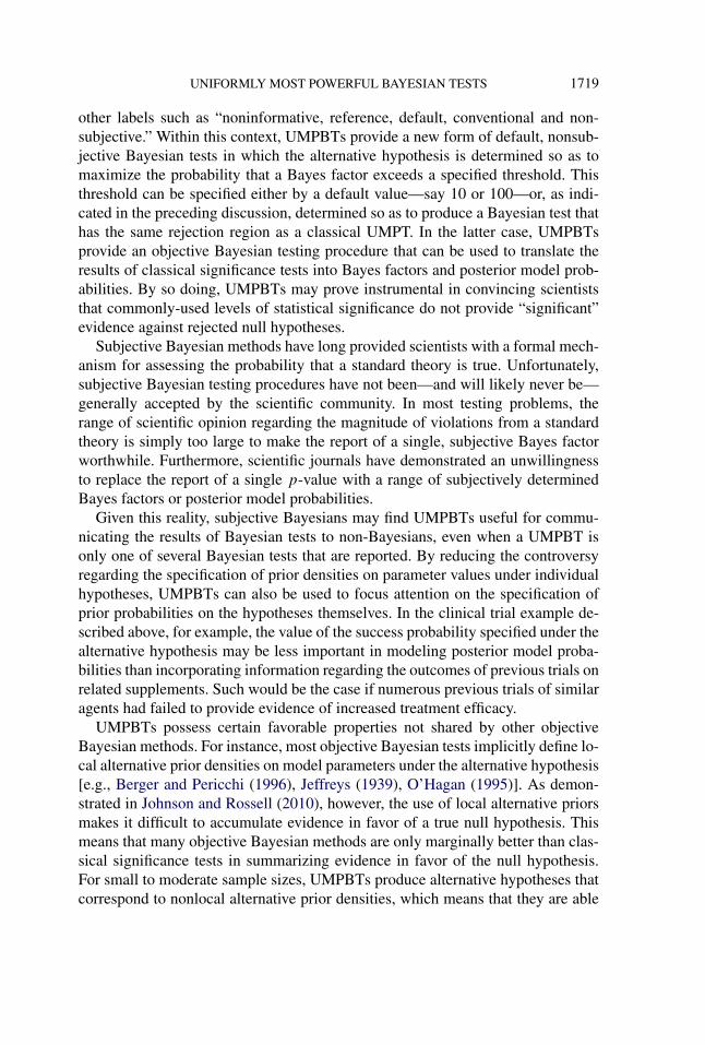
other labels such as “noninformative, reference, default, conventional and non-subjective.” Within this context, UMPBTs provide a new form of default, nonsub-jective Bayesian tests in which the alternative hypothesis is determined so as tomaximize the probability that a Bayes factor exceeds a specified threshold. Thisthreshold can be specified either by a default value—say 10 or 100—or, as indi-cated in the preceding discussion, determined so as to produce a Bayesian test thathas the same rejection region as a classical UMPT. In the latter case, UMPBTsprovide an objective Bayesian testing procedure that can be used to translate theresults of classical significance tests into Bayes factors and posterior model prob-abilities. By so doing, UMPBTs may prove instrumental in convincing scientiststhat commonly-used levels of statistical significance do not provide “significant”evidence against rejected null hypotheses.

Subjective Bayesian methods have long provided scientists with a formal mech-anism for assessing the probability that a standard theory is true. Unfortunately,subjective Bayesian testing procedures have not been—and will likely never be—generally accepted by the scientific community. In most testing problems, therange of scientific opinion regarding the magnitude of violations from a standardtheory is simply too large to make the report of a single, subjective Bayes factorworthwhile. Furthermore, scientific journals have demonstrated an unwillingnessto replace the report of a single p-value with a range of subjectively determinedBayes factors or posterior model probabilities.

Given this reality, subjective Bayesians may find UMPBTs useful for commu-nicating the results of Bayesian tests to non-Bayesians, even when a UMPBT isonly one of several Bayesian tests that are reported. By reducing the controversyregarding the specification of prior densities on parameter values under individualhypotheses, UMPBTs can also be used to focus attention on the specification ofprior probabilities on the hypotheses themselves. In the clinical trial example de-scribed above, for example, the value of the success probability specified under thealternative hypothesis may be less important in modeling posterior model proba-bilities than incorporating information regarding the outcomes of previous trials onrelated supplements. Such would be the case if numerous previous trials of similaragents had failed to provide evidence of increased treatment efficacy.

UMPBTs possess certain favorable properties not shared by other objectiveBayesian methods. For instance, most objective Bayesian tests implicitly define lo-cal alternative prior densities on model parameters under the alternative hypothesis[e.g., Berger and Pericchi (1996), Jeffreys (1939), O’Hagan (1995)]. As demon-strated in Johnson and Rossell (2010), however, the use of local alternative priorsmakes it difficult to accumulate evidence in favor of a true null hypothesis. Thismeans that many objective Bayesian methods are only marginally better than clas-sical significance tests in summarizing evidence in favor of the null hypothesis.For small to moderate sample sizes, UMPBTs produce alternative hypotheses thatcorrespond to nonlocal alternative prior densities, which means that they are able

1720 V. E. JOHNSON

to provide more balanced summaries of evidence collected in favor of true null andtrue alternative hypotheses.

UMPBTs also possess certain unfavorable properties. Like many objectiveBayesian methods, UMPBTs can violate the likelihood principle, and their be-havior in large sample settings can lead to inconsistency if evidence thresholdsare held constant. And the alternative hypotheses generated by UMPBTs are nei-ther vague nor noninformative. Further comments and discussion regarding theseissues are provided below.

In order to define UMPBTs, it useful to first review basic properties of Bayesianhypothesis tests. In contrast to classical statistical hypothesis tests, Bayesian hy-pothesis tests are based on comparisons of the posterior probabilities assigned tocompeting hypotheses. In parametric tests, competing hypotheses are character-ized by the prior densities that they impose on the parameters that define a sam-pling density shared by both hypotheses. Such tests comprise the focus of thisarticle. Specifically, it is assumed throughout that the posterior odds between twohypotheses H1 and H0 can be expressed as

P(H1 | x)

P(H0 | x)= m1(x)

m0(x)× p(H1)

p(H0),(2)

where BF10(x) = m1(x)/m0(x) is the Bayes factor between hypotheses H1and H0,

mi(x) =∫�

f (x | θ)πi(θ | Hi)dθ(3)

is the marginal density of the data under hypothesis Hi , f (x | θ) is the samplingdensity of data x given θ , πi(θ | Hi) is the prior density on θ under Hi and p(Hi)

is the prior probability assigned to hypothesis Hi , for i = 0,1. The marginal priordensity for θ is thus

π(θ) = π0(θ | H0)P (H0) + π1(θ | H1)p(H1).

When there is no possibility of confusion, πi(θ | Hi) will be denoted more simplyby πi(θ). The parameter space is denoted by � and the sample space by X . Thelogarithm of the Bayes factor is called the weight of evidence. All densities areassumed to be defined with respect to an appropriate underlying measure (e.g.,Lebesgue or counting measure).

Finally, assume that one hypothesis—the null hypothesis H0—is fixed on thebasis of scientific considerations, and that the difficulty in constructing a Bayesianhypothesis test arises from the requirement to specify an alternative hypothesis.This assumption mirrors the situation encountered in classical hypothesis tests inwhich the null hypothesis is known, but no alternative hypothesis is defined. In theclinical trial example, for instance, the null hypothesis corresponds to the assump-tion that the success probability of the new treatment equals that of the standardtreatment, but there is no obvious value (or prior probability density) that should

UNIFORMLY MOST POWERFUL BAYESIAN TESTS 1721

be assigned to the treatment’s success probability under the alternative hypothesisthat it is better than the standard of care.

With these assumptions and definitions in place, it is worthwhile to review aproperty of Bayes factors that pertains when the prior density defining an alter-native hypothesis is misspecified. Let πt(θ | H1) = πt(θ) denote the “true” priordensity on θ under the assumption that the alternative hypothesis is true, and letmt(x) denote the resulting marginal density of the data. In general πt(θ) is notknown, but it is still possible to compare the properties of the weight of evidencethat would be obtained by using the true prior density under the alternative hy-pothesis to those that would be obtained using some other prior density. From afrequentist perspective, πt might represent a point mass concentrated on the true,but unknown, data generating parameter. From a Bayesian perspective, πt mightrepresent a summary of existing knowledge regarding θ before an experiment isconducted. Because πt is not available, suppose that π1(θ | H1) = π1(θ) is insteadused to represent the prior density, again under the assumption that the alternativehypothesis is true. Then it follows from Gibbs’s inequality that∫

Xmt(x) log

[mt(x)

m0(x)

]dx −

∫X

mt(x) log[m1(x)

m0(x)

]dx

=∫

Xmt(x) log

[mt(x)

m1(x)

]dx

≥ 0.

That is, ∫X

mt(x) log[mt(x)

m0(x)

]dx ≥

∫X

mt(x) log[m1(x)

m0(x)

]dx,(4)

which means that the expected weight of evidence in favor of the alternative hy-pothesis is always decreased when π1(θ) differs from πt(θ) (on a set with measuregreater than 0). In general, the UMPBTs described below will thus decrease theaverage weight of evidence obtained in favor of a true alternative hypothesis. Inother words, the weight of evidence reported from a UMPBT will tend to underes-timate the actual weight of evidence provided by an experiment in favor of a truealternative hypothesis.

Like classical statistical hypothesis tests, the tangible consequence of a Bayesianhypothesis test is often the rejection of one hypothesis, say H0, in favor of the sec-ond, say H1. In a Bayesian test, the null hypothesis is rejected if the posteriorprobability of H1 exceeds a certain threshold. Given the prior odds between thehypotheses, this is equivalent to determining a threshold, say γ , over which theBayes factor between H1 and H0 must fall in order to reject H0 in favor of H1.It is therefore of some practical interest to determine alternative hypotheses thatmaximize the probability that the Bayes factor from a test exceeds a specifiedthreshold.

1722 V. E. JOHNSON

With this motivation and notation in place, a UMPBT(γ ) may be formally de-fined as follows.

DEFINITION. A uniformly most powerful Bayesian test for evidence thresh-old γ > 0 in favor of the alternative hypothesis H1 against a fixed null hypothe-sis H0, denoted by UMPBT(γ ), is a Bayesian hypothesis test in which the Bayesfactor for the test satisfies the following inequality for any θ t ∈ � and for all alter-native hypotheses H2 : θ ∼ π2(θ):

Pθ t

[BF10(x) > γ

] ≥ Pθ t

[BF20(x) > γ

].(5)

In other words, the UMPBT(γ ) is a Bayesian test for which the alternativehypothesis is specified so as to maximize the probability that the Bayes factorBF10(x) exceeds the evidence threshold γ for all possible values of the data gen-erating parameter θ t .

The remainder of this article is organized as follows. In the next section,UMPBTs are described for one-parameter exponential family models. As in thecase of UMPTs, a general prescription for constructing UMPBTs is available onlywithin this class of densities. Specific techniques for defining UMPBTs or approx-imate UMPBTs outside of this class are described later in Sections 4 and 5. Inapplying UMPBTs to one parameter exponential family models, an approximateequivalence between type I errors for UMPTs and the Bayes factors obtained fromUMPBTs is exposed.

In Section 3, UMPBTs are applied in two canonical testing situations: the test ofa binomial proportion, and the test of a normal mean. These two tests are perhapsthe most common tests used by practitioners of statistics. The binomial test is illus-trated in the context of a clinical trial, while the normal mean test is applied to eval-uate evidence reported in support of the Higgs boson. Section 4 describes severalsettings outside of one parameter exponential family models for which UMPBTsexist. These include cases in which the nuisance parameters under the null andalternative hypothesis can be considered to be equal (though unknown), and sit-uations in which it is possible to marginalize over nuisance parameters to obtainexpressions for data densities that are similar to those obtained in one-parameterexponential family models. Section 5 describes approximations to UMPBTs ob-tained by specifying alternative hypotheses that depend on data through statisticsthat are ancillary to the parameter of interest. Concluding comments appear inSection 6.

2. One-parameter exponential family models. Assume that {x1, . . . , xn} ≡x are i.i.d. with a sampling density (or probability mass function in the case ofdiscrete data) of the form

f (x | θ) = h(x) exp[η(θ)T (x) − A(θ)

],(6)

UNIFORMLY MOST POWERFUL BAYESIAN TESTS 1723

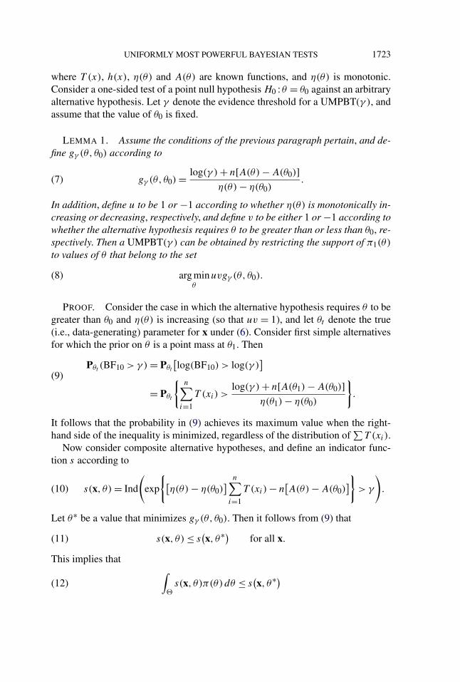
where T (x), h(x), η(θ) and A(θ) are known functions, and η(θ) is monotonic.Consider a one-sided test of a point null hypothesis H0 : θ = θ0 against an arbitraryalternative hypothesis. Let γ denote the evidence threshold for a UMPBT(γ ), andassume that the value of θ0 is fixed.

LEMMA 1. Assume the conditions of the previous paragraph pertain, and de-fine gγ (θ, θ0) according to

gγ (θ, θ0) = log(γ ) + n[A(θ) − A(θ0)]η(θ) − η(θ0)

.(7)

In addition, define u to be 1 or −1 according to whether η(θ) is monotonically in-creasing or decreasing, respectively, and define v to be either 1 or −1 according towhether the alternative hypothesis requires θ to be greater than or less than θ0, re-spectively. Then a UMPBT(γ ) can be obtained by restricting the support of π1(θ)

to values of θ that belong to the set

arg minθ

uvgγ (θ, θ0).(8)

PROOF. Consider the case in which the alternative hypothesis requires θ to begreater than θ0 and η(θ) is increasing (so that uv = 1), and let θt denote the true(i.e., data-generating) parameter for x under (6). Consider first simple alternativesfor which the prior on θ is a point mass at θ1. Then

Pθt (BF10 > γ ) = Pθt

[log(BF10) > log(γ )

](9)

= Pθt

{n∑

i=1

T (xi) >log(γ ) + n[A(θ1) − A(θ0)]

η(θ1) − η(θ0)

}.

It follows that the probability in (9) achieves its maximum value when the right-hand side of the inequality is minimized, regardless of the distribution of

∑T (xi).

Now consider composite alternative hypotheses, and define an indicator func-tion s according to

s(x, θ) = Ind

(exp

{[η(θ) − η(θ0)

] n∑i=1

T (xi) − n[A(θ) − A(θ0)

]}> γ

).(10)

Let θ∗ be a value that minimizes gγ (θ, θ0). Then it follows from (9) that

s(x, θ) ≤ s(x, θ∗)

for all x.(11)

This implies that ∫�

s(x, θ)π(θ) dθ ≤ s(x, θ∗)

(12)

1724 V. E. JOHNSON

for all probability densities π(θ). It follows that

Pθt (BF10 > γ ) =∫

Xs(x, θ)f (x | θt ) dx(13)

is maximized by a prior that concentrates its mass on the set for which gγ (θ, θ0) isminimized.

The proof for other values of (u, v) follows by noting that the direction of theinequality in (9) changes according to the sign of η(θ1) − η(θ0). �

It should be noted that in some cases the values of θ that maximize Pθt (BF10 >

γ ) are not unique. This might happen if, for instance, no value of the sufficientstatistic obtained from the experiment could produce a Bayes factor that exceededthe γ threshold. For example, it would not be possible to obtain a Bayes factor of10 against a null hypothesis that a binomial success probability was 0.5 based on asample of size n = 1. In that case, the probability of exceeding the threshold is 0 forall values of the success probability, and a unique UMPBT does not exist. Moregenerally, if T (x) is discrete, then many values of θ1 might produce equivalenttests. An illustration of this phenomenon is provided in the first example.

2.1. Large sample properties of UMPBTs. Asymptotic properties of UMPBTscan most easily be examined for tests of point null hypotheses for a canonicalparameter in one-parameter exponential families. Two properties of UMPBTs inthis setting are described in the following lemma.

LEMMA 2. Let X1, . . . ,Xn represent a random sample drawn from a den-sity expressible in the form (6) with η(θ) = θ , and consider a test of the precisenull hypothesis H0 : θ = θ0. Suppose that A(θ) has three bounded derivatives in aneighborhood of θ0, and let θ∗ denote a value of θ that defines a UMPBT(γ ) testand satisfies

dgγ (θ∗, θ0)

dθ= 0.(14)

Then the following statements apply:

(1) For some t ∈ (θ0, θ∗),

∣∣θ∗ − θ0∣∣ =

√2 log(γ )

nA′′(t).(15)

(2) Under the null hypothesis,

log(BF10) → N(− log(γ ),2 log(γ )

)as n → ∞.(16)

UNIFORMLY MOST POWERFUL BAYESIAN TESTS 1725

PROOF. The first statement follows immediately from (14) by expanding A(θ)

in a Taylor series around θ∗. The second statement follows by noting that theweight of evidence can be expressed as

log(BF10) = (θ∗ − θ0

) n∑i=1

T (xi) − n[A

(θ∗) − A(θ0)

].

Expanding in a Taylor series around θ0 leads to

log(BF10) =√

2 log(γ )

nA′′(t)

[n∑

i=1

T (xi) − nA′(θ0) − n

2A′′(θ0)

√2 log(γ )

nA′′(t)

]+ ε,(17)

where ε represents a term of order O(n−1/2). From properties of exponential fam-ily models, it is known that

Eθ0

[T (xi)

] = A′(θ0) and Varθ0

(T (xi)

) = A′′(θ0).

Because A(θ) has three bounded derivatives in a neighborhood of θ0, [A′(t) −A′(θ0)] and [A′′(t) − A′′(θ0)] are order O(n−1/2), and the statement follows byapplication of the central limit theorem. �

Equation (15) shows that the difference |θ∗ −θ0| is O(n−1/2) when the evidencethreshold γ is held constant as a function of n. In classical terms, this impliesthat alternative hypotheses defined by UMPBTs represent Pitman sequences oflocal alternatives [Pitman (1949)]. This fact, in conjunction with (16), exposesan interesting behavior of UMPBTs in large sample settings, particularly whenviewed from the context of the Jeffreys–Lindley paradox [Jeffreys (1939), Lindley(1957); see also Robert, Chopin and Rousseau (2009)].

The Jeffreys–Lindley paradox (JLP) arises as an incongruity between Bayesianand classical hypothesis tests of a point null hypothesis. To understand the para-dox, suppose that the prior distribution for a parameter of interest under the alter-native hypothesis is uniform on an interval I containing the null value θ0, and thatthe prior probability assigned to the null hypothesis is π1. If π1 is bounded awayfrom 0, then it is possible for the null hypothesis to be rejected in an α-level sig-nificance test even when the posterior probability assigned to the null hypothesisexceeds 1 − α. Thus, the anomalous behavior exhibited in the example of Table 1,in which the null hypothesis was rejected in a significance test while being sup-ported by the data, is characteristic of a more general phenomenon that may occureven in large sample settings. To see that the null hypothesis can be rejected evenwhen the posterior odds are in its favor, note that for sufficiently large n the widthof I will be large relative to the posterior standard deviation of θ under the alterna-tive hypothesis. Data that are not “too far” from fθ0 may therefore be much morelikely to have arisen from the null hypothesis than from a density fθ when θ isdrawn uniformly from I . At the same time, the value of the test statistic based onthe data may appear extreme given that fθ0 pertains.

1726 V. E. JOHNSON

For moderate values of γ , the second statement in Lemma 2 shows that theweight of evidence obtained from a UMPBT is unlikely to provide strong evi-dence in favor of either hypothesis when the null hypothesis is true. When γ = 4,for instance, an approximate 95% confidence interval for the weight of evidenceextends only between (−4.65,1.88), no matter how large n is. Thus, the posteriorprobability of the null hypothesis does not converge to 1 as the sample size grows.The null hypothesis is never fully accepted—nor the alternative rejected—whenthe evidence threshold is held constant as n increases.

This large sample behavior of UMPBTs with fixed evidence thresholds is, in acertain sense, similar to the JLP. When the null hypothesis is true and n is large, theprobability of rejecting the null hypothesis at a fixed level of significance remainsconstant at the specified level of significance. For instance, the null hypothesis isrejected 5% of the time in a standard 5% significance test when the null hypothesisis true, regardless of how large the sample size is. Similarly, when γ = 4, theprobability that the weight of evidence in favor of the alternative hypothesis willbe greater than 0 converges to 0.20 as n becomes large. Like the significance test,there remains a nonzero probability that the alternative hypothesis will be favoredby the UMPBT even when the null hypothesis is true, regardless of how large n is.

On a related note, Rousseau (2007) has demonstrated that a point null hypothe-sis may be used as a convenient mathematical approximation to interval hypothe-ses of the form (θ0 − ε, θ0 + ε) if ε is sufficiently small. Her results suggest thatsuch an approximation is valid only if ε < o(n). The fact that UMPBT alternativesdecrease at a rate of O(n−1/2) suggests that UMPBTs may be used to test smallinterval hypotheses around θ0, provided that the width of the interval satisfies theconstraints provided by Rousseau.

Further comments regarding the asymptotic properties of UMPBTs appear inthe discussion section.

3. Examples. Tests of simple hypotheses in one-parameter exponential fam-ily models continue to be the most common statistical hypothesis tests used bypractitioners. These tests play a central role in many science, technology and busi-ness applications. In addition, the distributions of many test statistics are asymp-totically distributed as standard normal deviates, which means that UMPBTs canbe applied to obtain Bayes factors based on test statistics [Johnson (2005)]. Thissection illustrates the use of UMPBT tests in two archetypical examples; the firstinvolves the test of a binomial success probability, and the second the test of thevalue of a parameter estimate that is assumed to be approximately normally dis-tributed.

3.1. Test of binomial success probability. Suppose x ∼ Bin(n,p), and con-sider the test of a null hypothesis H0 :p = p0 versus an alternative hypothesisH1 :p > p0. Assume that an evidence threshold of γ is desired for the test; that is,the alternative hypothesis is accepted if BF10 > γ .

UNIFORMLY MOST POWERFUL BAYESIAN TESTS 1727

From Lemma 1, the UMPBT(γ ) is defined by finding p1 that satisfies p1 > p0and

p1 = arg minp

log(γ ) − n[log(1 − p) − log(1 − p0)]log[p/(1 − p)] − log[p0/(1 − p0)] .(18)

Although this equation cannot be solved in closed form, its solution can be foundeasily using optimization functions available in most statistical programs.

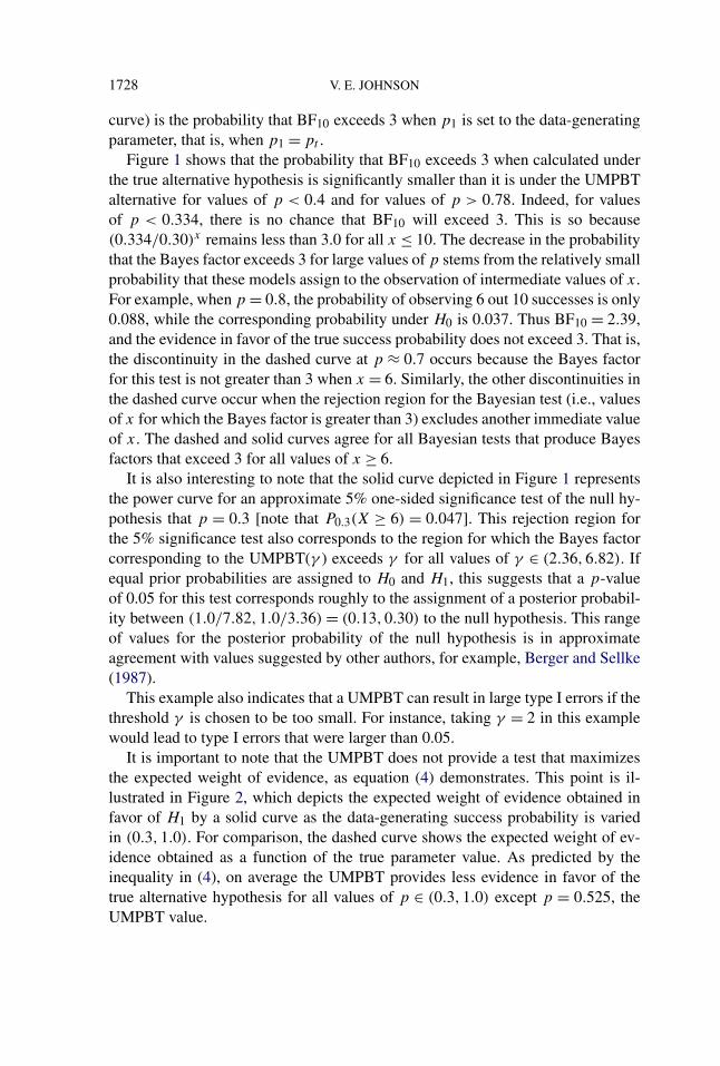
3.1.1. Phase II clinical trials with binary outcomes. To illustrate the resultingtest in a real-world application that involves small sample sizes, consider a one-arm Phase II trial of a new drug intended to improve the response rate to a diseasefrom the standard-of-care rate of p0 = 0.3. Suppose also that budget and timeconstraints limit the number of patients that can be accrued in the trial to n = 10,and suppose that the new drug will be pursued only if the odds that it offers animprovement over the standard of care are at least 3:1. Taking γ = 3, it followsfrom (18) that the UMPBT alternative is defined by taking H1 :p1 = 0.525. At thisvalue of p1, the Bayes factor BF10 in favor of H1 exceeds 3 whenever 6 or moreof the 10 patients enrolled in the trial respond to treatment.

A plot of the probability that BF10 exceeds 3 as function of the true responserate p appears in Figure 1. For comparison, also plotted in this figure (dashed

FIG. 1. Probability that the Bayes factor exceeds 3 plotted against the data-generating parameter.The solid curve shows the probability of exceeding 3 for the UMPBT. The dashed curve displays thisprobability when the Bayes factor is calculated using the data-generating parameter.

1728 V. E. JOHNSON

curve) is the probability that BF10 exceeds 3 when p1 is set to the data-generatingparameter, that is, when p1 = pt .

Figure 1 shows that the probability that BF10 exceeds 3 when calculated underthe true alternative hypothesis is significantly smaller than it is under the UMPBTalternative for values of p < 0.4 and for values of p > 0.78. Indeed, for valuesof p < 0.334, there is no chance that BF10 will exceed 3. This is so because(0.334/0.30)x remains less than 3.0 for all x ≤ 10. The decrease in the probabilitythat the Bayes factor exceeds 3 for large values of p stems from the relatively smallprobability that these models assign to the observation of intermediate values of x.For example, when p = 0.8, the probability of observing 6 out 10 successes is only0.088, while the corresponding probability under H0 is 0.037. Thus BF10 = 2.39,and the evidence in favor of the true success probability does not exceed 3. That is,the discontinuity in the dashed curve at p ≈ 0.7 occurs because the Bayes factorfor this test is not greater than 3 when x = 6. Similarly, the other discontinuities inthe dashed curve occur when the rejection region for the Bayesian test (i.e., valuesof x for which the Bayes factor is greater than 3) excludes another immediate valueof x. The dashed and solid curves agree for all Bayesian tests that produce Bayesfactors that exceed 3 for all values of x ≥ 6.

It is also interesting to note that the solid curve depicted in Figure 1 representsthe power curve for an approximate 5% one-sided significance test of the null hy-pothesis that p = 0.3 [note that P0.3(X ≥ 6) = 0.047]. This rejection region forthe 5% significance test also corresponds to the region for which the Bayes factorcorresponding to the UMPBT(γ ) exceeds γ for all values of γ ∈ (2.36,6.82). Ifequal prior probabilities are assigned to H0 and H1, this suggests that a p-valueof 0.05 for this test corresponds roughly to the assignment of a posterior probabil-ity between (1.0/7.82,1.0/3.36) = (0.13,0.30) to the null hypothesis. This rangeof values for the posterior probability of the null hypothesis is in approximateagreement with values suggested by other authors, for example, Berger and Sellke(1987).

This example also indicates that a UMPBT can result in large type I errors if thethreshold γ is chosen to be too small. For instance, taking γ = 2 in this examplewould lead to type I errors that were larger than 0.05.

It is important to note that the UMPBT does not provide a test that maximizesthe expected weight of evidence, as equation (4) demonstrates. This point is il-lustrated in Figure 2, which depicts the expected weight of evidence obtained infavor of H1 by a solid curve as the data-generating success probability is variedin (0.3,1.0). For comparison, the dashed curve shows the expected weight of ev-idence obtained as a function of the true parameter value. As predicted by theinequality in (4), on average the UMPBT provides less evidence in favor of thetrue alternative hypothesis for all values of p ∈ (0.3,1.0) except p = 0.525, theUMPBT value.

UNIFORMLY MOST POWERFUL BAYESIAN TESTS 1729

FIG. 2. Expected weight of evidence produced by a UMPBT(γ ) against a null hypothesis thatp0 = 0.3 when the sample size is n = 10 (solid curve), versus the expected weight of evidence ob-served using the data-generating success probability at the alternative hypothesis (dashed curve).The data-generating parameter value is displayed on the horizontal axis.

3.2. Test of normal mean, σ 2 known. Suppose xi , i = 1, . . . , n are i.i.d.N(μ,σ 2) with σ 2 known. The null hypothesis is H0 :μ = μ0, and the alterna-tive hypothesis is accepted if BF10 > γ . Assuming that the alternative hypothesistakes the form H1 :μ = μ1 in a one-sided test, it follows that

log(BF10) = n

σ 2

[x(μ1 − μ0) + 1

2

(μ2

0 − μ21)]

.(19)

If the data-generating parameter is μt , the probability that BF10 is greater than γ

can be written as

Pμt

[(μ1 − μ0)x >

σ 2 log(γ )

n− 1

2

(μ2

0 − μ21)]

.(20)

If μ1 > μ0, then the UMPBT(γ ) value of μ1 satisfies

arg minμ1

σ 2 log(γ )

n(μ1 − μ0)+ 1

2(μ0 + μ1).(21)

Conversely, if μ1 < μ0, then optimal value of μ1 satisfies

arg minμ1

σ 2 log(γ )

n(μ1 − μ0)+ 1

2(μ0 + μ1).(22)

1730 V. E. JOHNSON

FIG. 3. Probability that Bayes factor in favor of UMPBT alternative exceeds 10 when μ0 = 0 andn = 1 (solid curve). The dashed curve displays this probability when the Bayes factor is calculatedunder the alternative hypothesis that μ1 equals the data-generating parameter (displayed on thehorizontal axis).

It follows that the UMPBT(γ ) value for μ1 is given by

μ1 = μ0 ± σ

√2 logγ

n,(23)

depending on whether μ1 > μ0 or μ1 < μ0.Figure 3 depicts the probability that the Bayes factor exceeds γ = 10 when

testing a null hypothesis that μ = 0 based on a single, standard normal observation(i.e., n = 1, σ 2 = 1). In this case, the UMPBT(10) is obtained by taking μ1 =2.146. For comparison, the probability that the Bayes factor exceeds 10 when thealternative is defined to be the data-generating parameter is depicted by the dashedcurve in the plot.

UMPBTs can also be used to interpret the evidence obtained from classicalUMPTs. In a classical one-sided test of a normal mean with known variance, thenull hypothesis is rejected if

x > μ0 + zα

σ√n,

UNIFORMLY MOST POWERFUL BAYESIAN TESTS 1731

where α is the level of the test designed to detect μ1 > μ0. In the UMPBT, from(19)–(20) it follows that the null hypothesis is rejected if

x >σ 2 log(γ )

n(μ1 − μ0)+ 1

2(μ1 + μ0).

Setting μ1 = μ0 +σ√

2 log(γ )/n and equating the two rejection regions, it followsthat the rejection regions for the two tests are identical if

γ = exp(

z2α

2

).(24)

For the case of normally distributed data, it follows that

μ1 = μ0 + σ√nzα,(25)

which means that the alternative hypothesis places μ1 at the boundary of theUMPT rejection region.

The close connection between the UMPBT and UMPT for a normal meanmakes it relatively straightforward to examine the relationship between the p-values reported from a classical test and either the Bayes factors or posterior prob-abilities obtained from a Bayesian test. For example, significance tests for normalmeans are often conducted at the 5% level. Given this threshold of evidence for re-jection of the null hypothesis, the one-sided γ threshold corresponding to the 5%significance test is 3.87, and the UMPBT alternative is μ1 = μ0 + 1.645σ/

√n. If

we assume that equal prior probabilities are assigned to the null and alternative hy-potheses, then a correspondence between p-values and posterior probabilities as-signed to the null hypothesis is easy to establish. This correspondence is depictedin Figure 4. For instance, this figure shows that a p-value of 0.01 corresponds tothe assignment of posterior probability 0.08 to the null hypothesis.

3.2.1. Evaluating evidence for the Higgs boson. On July 4, 2012, scientists atCERN made the following announcement:

We observe in our data clear signs of a new particle, at the level of 5 sigma, inthe mass region around 126 gigaelectronvolts (GeV). (http://press.web.cern.ch/press/PressReleases/Releases2012/PR17.12E.html).

In very simplified terms, the 5 sigma claim can be explained by fitting a model fora Poisson mean that had the following approximate form:

μ(x) = exp(a0 + a1x + a2x

2) + sφ(x;m,w).

Here, x denotes mass in GeV, {ai} denote nuisance parameters that model back-ground events, s denotes signal above background, m denotes the mass of a newparticle, w denotes a convolution parameter and φ(x;m,w) denotes a Gaussiandensity centered on m with standard deviation w [Prosper (2012)]. Poisson events

1732 V. E. JOHNSON

FIG. 4. Correspondence between p-values and posterior model probabilities for a UMPBT testderived from a 5% test. This plot assumes equal prior probabilities were assigned to the null andalternative hypotheses. Note that both axes are displayed on the logarithmic scale.

collected from a series of high energy experiments conducted in the Large HadronCollider (LHC) at CERN provide the data to estimate the parameters in this styl-ized model. The background parameters {ai} are considered nuisance parameters.Interest, of course, focuses on testing whether s > 0 at a mass location m. The nullhypothesis is that s = 0 for all m.

The accepted criterion for declaring the discovery of a new particle in the fieldof particle physics is the 5 sigma rule, which in this case requires that the estimateof s be 5 standard errors from 0 (http://public.web.cern.ch/public/).

Calculation of a Bayes factor based on the original mass spectrum data is com-plicated by the fact that prior distributions for the nuisance parameters {ai}, m,and w are either not available or are not agreed upon. For this reason, it is morestraightforward to compute a Bayes factor for these data based on the test statisticz = s/ se(s) where s denotes the maximum likelihood estimate of s and se(s) itsstandard error [Johnson (2005, 2008)]. To perform this test, assume that under thenull hypothesis z has a standard normal distribution, and that under the alternativehypothesis z has a normal distribution with mean μ and variance 1.

In this context, the 5 sigma rule for declaring a new particle discovery meansthat a new discovery can only be declared if the test statistic z > 5. Using equation(24) to match the rejection region of the classical significance test to a UMPBT(γ )

UNIFORMLY MOST POWERFUL BAYESIAN TESTS 1733

implies that the corresponding evidence threshold is γ = exp(12.5) ≈ 27,000. Inother words, a Bayes factor of approximately γ = exp(12.5) ≈ 27,000 correspondsto the 5 sigma rule required to accept the alternative hypothesis that a new particlehas been found.

It follows from the discussion following equation (25) that the alternative hy-pothesis for the UMPBT alternative is μ1 = 5. This value is calculated under theassumption that the test statistic z has a standard normal distribution under thenull hypothesis [i.e., σ = 1 and n = 1 in (23)]. If the observed value of z wasexactly 5, then the Bayes factor in favor of a new particle would be approxi-mately 27,000. If the observed value was, say 5.1, then the Bayes factor wouldbe exp(−0.5[0.12 − 5.12]) = 44,000. These values suggest very strong evidencein favor of a new particle, but perhaps not as much evidence as might be inferredby nonstatisticians by the report of a p-value of 3 × 10−7.

There are, of course, a number of important caveats that should be consideredwhen interpreting the outcome of this analysis. This analysis assumes that an ex-periment with a fixed endpoint was conducted, and that the UMPBT value of thePoisson rate at 126 GeV was of physical significance. Referring to (23) and not-ing that the asymptotic standard error of z decreases at rate

√n, it follows that

the UMPBT alternative hypothesis favored by this analysis is O(n−1/2). For suf-ficiently large n, systematic errors in the estimation of the background rate couldeventually lead to the rejection of the null hypothesis in favor of the hypothesis ofa new particle. This is of particular concern if the high energy experiments werecontinued until a 5 sigma result was obtained. Further comments regarding thispoint appear in the discussion section.

3.3. Other one-parameter exponential family models. Table 2 provides thefunctions that must be minimized to obtain UMPBTs for a number of commonexponential family models. The objective functions listed in this table correspondto the function gγ (·, ·) specified in Lemma 1 with v = 1. The negative binomial isparameterized by the fixed number of failures r and random number of successes

TABLE 2Common one parameter exponential family models for which UMPBT(γ ) exist

Model Test Objective function

Binomial p1 > p0 {log(γ ) − n log[(1 − p)/(1 − p0)]}(log{[p(1 − p0)]/[(1 − p)p0]})−1

Exponential μ1 > μ0 {log(γ ) + n[log(μ1) − log(μ0)]}[1/μ0 − 1/μ1]−1

Neg. Bin. p1 > p0 {log(γ ) − r log[(1 − p1)/(1 − p0)]}[log(p1) − log(p0)]−1

Normal σ 21 > σ 2

0 {2σ 21 σ 2

0 (log(γ ) + n2 [log(σ 2

1 ) − log(σ 20 )])}[σ 2

1 − σ 20 ]−1

Normal μ1 > μ0 [σ 2 log(γ )](μ1 − μ0)−1 + 12 (μ0 + μ1)

Poisson μ1 > μ0 [log(γ ) + n(μ1 − μ0)][log(μ1) − log(μ0)]−1

1734 V. E. JOHNSON

x = 0,1, . . . observed before termination of sampling. The other models are pa-rameterized so that μ and p denote means and proportions, respectively, while σ 2

values refer to variances.

4. Extensions to other models. Like UMPTs, UMPBTs are most easily de-fined within one-parameter exponential family models. In unusual cases, UMPBTscan be defined for data modeled by vector-valued exponential family models, butin general such extensions appear to require stringent constraints on nuisance pa-rameters.

One special case in which UMPBTs can be defined for a d-dimensional param-eter θ occurs when the density of an observation can be expressed as

f (x | θ) = h(x) exp

[d∑

i=1

ηi(θ)Ti(x) − A(θ)

],(26)

and all but one of the ηi(θ) are constrained to have identical values under both hy-potheses. To understand how a UMPBT can be defined in this case, without loss ofgenerality suppose that ηi(θ), i = 2, . . . , d are constrained to have the same valueunder both the null and alternative hypotheses, and that the null and alternative hy-potheses are defined by H0 : θ1 = θ1,0 and H1 : θ1 > θ1,0. For simplicity, supposefurther that η1 is a monotonically increasing function.

As in Lemma 1, consider first simple alternative hypotheses expressible asH1 : θ1 = θ1,1. Let θ0 = (θ1,0, . . . , θd,0)

′ and θ1 = (θ1,1, . . . , θd,1)′. It follows that

the probability that the logarithm of the Bayes factor exceeds a threshold log(γ )

can be expressed as

P[log(BF10) > log(γ )

]= P

{[η1(θ1,1) − η1(θ1,0)

]T1(x) − [

A(θ1) − A(θ0)]> log(γ )

}(27)

= P[T1(x) >

log(γ ) + [A(θ1) − A(θ0)][η1(θ1,1) − η1(θ1,0)]

].

The probability in (27) is maximized by minimizing the right-hand side of theinequality. The extension to composite alternative hypotheses follows the logicdescribed in inequalities (11)–(13), which shows that UMPBT(γ ) tests can be ob-tained in this setting by choosing the prior distribution of θ1 under the alternativehypotheses so that it concentrates its mass on the set

arg minθ

log(γ ) + [A(θ1) − A(θ0)][η1(θ1,1) − η1(θ1,0)] ,(28)

while maintaining the constraint that the values of ηi(θ) are equal under both hy-potheses. Similar constructions apply if η1 is monotonically decreasing, or if thealternative hypothesis specifies that θ1,0 < θ0,0.

More practically useful extensions of UMPBTs can be obtained when it is pos-sible to integrate out nuisance parameters in order to obtain a marginal density

UNIFORMLY MOST POWERFUL BAYESIAN TESTS 1735

for the parameter of interest that falls within the class of exponential family ofmodels. An important example of this type occurs in testing whether a regressioncoefficient in a linear model is zero.

4.1. Test of linear regression coefficient, σ 2 known. Suppose that

y ∼ N(Xβ, σ 2In

),(29)

where σ 2 is known, y is an n × 1 observation vector, X an n × p design matrix offull column rank and β = (β1, . . . , βp)′ denotes a p × 1 regression parameter. Thenull hypothesis is defined as H0 :βp = 0. For concreteness, suppose that interestfocuses on testing whether βp > 0, and that under both the null and alternativehypotheses, the prior density on the first p − 1 components of β is a multivari-ate normal distribution with mean vector 0 and covariance matrix σ 2�. Then themarginal density of y under H0 is

m0(y) = (2πσ 2)−n/2|�|−1/2|F|−1/2 exp

(− R

2σ 2

),(30)

where

F = X′−pX−p + �−1, H = X−pF−1X′−p, R = y′(In − H)′y,(31)

and X−p is the matrix consisting of the first p − 1 columns of X.Let βp∗ denote the value of βp under the alternative hypothesis H1 that defines

the UMPBT(γ ), and let xp denote the pth column of X. Then the marginal densityof y under H1 is

m1(y) = m0(y) × exp{− 1

2σ 2

[βp∗2x′

p(In − H)xp − 2βp∗x′p(In − H)y

]}.(32)

It follows that the probability that the Bayes factor BF10 exceeds γ can be ex-pressed as

P[x′p(In − H)y >

σ 2 log(γ )

βp∗+ 1

2βp∗x′

p(In − H)xp

],(33)

which is maximized by minimizing the right-hand side of the inequality. TheUMPBT(γ ) is thus obtained by taking

βp∗ =√√√√ 2σ 2 log(γ )

x′p(In − H)xp

.(34)

The corresponding one-sided test of βp < 0 is obtained by reversing the sign ofβp∗ in (34).

Because this expression for the UMPBT assumes that σ 2 is known, it is not ofgreat practical significance by itself. However, this result may guide the specifica-tion of alternative models in, for example, model selection algorithms in which the

1736 V. E. JOHNSON

priors on regression coefficients are specified conditionally on the value of σ 2. Forexample, the mode of the nonlocal priors described in Johnson and Rossell (2012)might be set to the UMPBT values after determining an appropriate value of γ

based on both the sample size n and number of potential covariates p.

5. Approximations to UMPBTs using data-dependent alternatives. Insome situations—most notably in linear models with unknown variances—datadependent alternative hypotheses can be defined to obtain tests that are approxi-mately uniformly most powerful in maximizing the probability that a Bayes factorexceeds a threshold. This strategy is only attractive when the statistics used to de-fine the alternative hypothesis are ancillary to the parameter of interest.

5.1. Test of normal mean, σ 2 unknown. Suppose that xi , i = 1, . . . , n, are i.i.d.N(μ,σ 2), that σ 2 is unknown and that the null hypothesis is H0 :μ = μ0. For con-venience, assume further that the prior distribution on σ 2 is an inverse gamma dis-tribution with parameters α and λ under both the null and alternative hypotheses.

To obtain an approximate UMPBT(γ ), first marginalize over σ 2 in both mod-els. Noting that (1 + a/t)t → ea , it follows that the Bayes factor in favor of thealternative hypothesis satisfies

BF10(x) =[∑n

i=1(xi − μ0)2 + 2λ∑n

i=1(xi − μ1)2 + 2λ

]n/2+α

(35)

≈[

1 + (x − μ0)2/s2

1 + (x − μ1)2/s2

]n/2+α

(36)

≈ exp{− n

2s2

[(x − μ1)

2 − (x − μ0)2]}

,(37)

where

s2 =∑n

i=1(xi − x)2 + 2λ

n + 2α.(38)

The expression for the Bayes factor in (37) reduces to (19) if σ 2 is replaced by s2.This implies that an approximate, but data-dependent UMPBT alternative hypoth-esis can be specified by taking

μ1 = μ0 ± s

√2 logγ

n,(39)

depending on whether μ1 > μ0 or μ1 < μ0.Figure 5 depicts the probability that the Bayes factor exceeds γ = 10 when

testing a null hypothesis that μ = 0 based on an independent sample of size n = 30normal observations with unit variance (σ 2 = 1) and using (39) to set the valueof μ1 under the alternative hypothesis. For comparison, the probability that the

UNIFORMLY MOST POWERFUL BAYESIAN TESTS 1737

FIG. 5. Probability that Bayes factor based on data-dependent, approximate UMPBT alternativeexceeds 10 when μ0 = 0 and n = 30 (solid curve). The dashed curve displays this probability whenthe Bayes factor is calculated under the alternative hypothesis that μ1 equals data-generating pa-rameter (displayed on the horizontal axis) and σ 2 = 1 (the true value).

Bayes factor exceeds 10 when the alternative is defined by taking σ 2 = 1 andμ1 to be the data-generating parameter is depicted by the dashed curve in theplot. Interestingly, the data-dependent, approximate UMPBT(10) provides a higherprobability of producing a Bayes factor that exceeds 10 than do alternatives fixedat the data generating parameters.

5.2. Test of linear regression coefficient, σ 2 unknown. As final example, sup-pose that the sampling model of Section 4.1 holds, but assume now that the obser-vational variance σ 2 is unknown and assumed under both hypotheses to be drawnfrom an inverse gamma distribution with parameters α and λ. Also assume that theprior distribution for the first p − 1 components of β , given σ 2, is a multivariatenormal distribution with mean 0 and covariance matrix σ 2 . As before, assumethat H0 :βp = 0. Our goal is to determine a value βp∗ so that H1 :βp = βp∗ is theUMPBT(γ ) under the constraint that βp > 0.

Define y1 = y − xpβp∗ and let y0 = y. By integrating with respect to the priordensities on σ 2 and the first p − 1 components of β , the marginal density of the

1738 V. E. JOHNSON

data under hypothesis i, i = 0,1 can be expressed as

mi(y) = 2απ−n/2| |−1/2 λα

�(α)�(n/2 + α)|F|−1/2R

−n/2−αi ,(40)

where F is defined in (31), and

Ri = y′i (In − H)yi + 2λ.(41)

It follows that the Bayes factor in favor of H1 can be written as

BF10 =[1 + βp∗2x′

p(In − H)xp − 2βp∗x′p(In − H)y

R0

]−n/2−α

(42)

≈ exp{− 1

2s2p

[βp∗2x′

p(In − H)xp − 2βp∗x′p(In − H)y

]},(43)

where

s2p = R0

n + 2α.(44)

The UMPBT(γ ) is defined from (43) according to

P(BF10 > γ ) = P[x′p(In − H)y >

s2p log(γ )

βp∗+ 1

2βp∗x′

p(In − H)xp

].(45)

Minimizing the right-hand side of the last inequality with respect to βp∗ results in

βp∗ =√√√√ 2s2

p log(γ )

x′p(In − H)xp

.(46)

This expression is consistent with the result obtained in the known variancecase, but with s2

p substituted for σ 2.

6. Discussion. The major contributions of this paper are the definition ofUMPBTs and the explicit description of UMPBTs for regular one-parameter expo-nential family models. The existence of UMPBTs for exponential family modelsis important because these tests represent the most common hypothesis tests con-ducted by practitioners. The availability of UMPBTs for these models means thatthese tests can be used to interpret test results in terms of Bayes factors and poste-rior model probabilities in a wide range of scientific settings. The utility of thesetests is further enhanced by the connection between UMPBTs and UMPTs thathave the same rejection region. This connection makes it trivial to simultaneouslyreport both the p-value from a test and the corresponding Bayes factor.

The simultaneous report of default Bayes factors and p-values may play a piv-otal role in dispelling the perception held by many scientists that a p-value of 0.05corresponds to “significant” evidence against the null hypothesis. The preceding

UNIFORMLY MOST POWERFUL BAYESIAN TESTS 1739

sections contain examples in which this level of significance favors the alternativehypothesis by odds of only 3 or 4 to 1. Because few researchers would regard suchodds as strong evidence in favor of a new theory, the use of UMPBTs and the re-port of Bayes factors based upon them may lead to more realistic interpretationsof evidence obtained from scientific studies.

The large sample properties of UMPBTs described in Section 2.1 deserve fur-ther comment. From Lemma 2, it follows that the expected weight of evidence infavor of a true null hypothesis in an exponential family model converges to log(γ )

as the sample size n tends to infinity. In other words, the evidence threshold γ

represents an approximate bound on the evidence that can be collected in favor ofthe null hypothesis. This implies that γ must be increased with n in order to obtaina consistent sequence of tests.

Several criteria might be used for selecting a value for γ in large sample set-tings. One criterion can be inferred from the first statement of Lemma 2, where itis shown that the difference between the tested parameter’s value under the nulland alternative hypotheses is proportional to [log(γ )/n]1/2. For this difference tobe a constant—as it would be in a subjective Bayesian test—log(γ ) must be pro-portional to n, or γ = exp(cn) for some c > 0. This suggests that an appropriatevalue for c might be determined by calibrating the weight of evidence against anaccepted threshold/sample size combination. For example, if an evidence thresh-old of 4 were accepted as the standard threshold for tests conducted with a samplesize of 100, then c might be set to log(4)/100 = 0.0139. This value of c leads to anevidence threshold of γ = 16 for sample sizes of 200, a threshold of 64 for sam-ple sizes of 300, etc. From (24), the significance levels for corresponding z-testswould be 5%, 1% and 0.2%, respectively.

The requirement to increase γ to achieve consistent tests in large samplesalso provides insight into the performance of standard frequentist and subjectiveBayesian tests in large sample settings. The exponential growth rate of γ requiredto maintain a fixed alternative hypothesis suggests that the weight of evidenceshould be considered against the backdrop of sample size, even in Bayesian tests.This is particularly important in goodness-of-fit testing where small deviationsfrom a model may be tolerable. In such settings, even moderately large Bayes fac-tors against the null hypotheses may not be scientifically important when they arebased on very large sample sizes.

From a frequentist perspective, the use of UMPBTs in large sample settings canprovide insight into the deviations from null hypotheses when they are (inevitably)detected. For instance, suppose that a one-sided 1% test has been conducted todetermine if the mean of normal data is 0, and that the test is rejected with a p-value of 0.001 based on a sample size of 10,000. From (24), the implied evidencethreshold for the test is γ = 15, and the alternative hypothesis that has been im-plicitly tested with the UMPBT is that μ = 0.023σ . Based on the observation ofx = 0.031σ , the Bayes factor in favor of this alternative is 88.5. Although thereare strong odds against the null, the scientific importance of this outcome may be

1740 V. E. JOHNSON

tempered by the fact that the alternative hypothesis that was supported against thenull represents a standardized effect size of only 2.3%.

This article has focused on the specification of UMPBTs for one-sided alterna-tives. A simple extension of these tests to two-sided alternatives can be obtainedby assuming that the alternative hypothesis is represented by two equally-weightedpoint masses located at the UMPBT values determined for one-sided tests. TheBayes factors for such tests can be written as

P[

0.5ml(x) + 0.5mh(x)

m0(x)> γ

],(47)

where ml and mh denote marginal densities corresponding to one-sided UMPBTs.Letting m∗(x) = max(ml(x),mh(x)) for the data actually observed, and assumingthat the favored marginal density dominates the other, it follows that

P[

0.5ml(x) + 0.5mh(x)

m0(x)> γ

]≈ P

[m∗(x)

m0(x)> 2γ

].(48)

Thus, an approximate two-sided UMPBT(γ ) can be defined by specifying analternative hypothesis that equally concentrates its mass on the two one-sidedUMPBT(2γ ) tests.

Additional research is needed to identify classes of models and testing contextsfor which UMPBTs can be defined. The UMPBTs described in this article pri-marily involve tests of point null hypotheses, or tests that can be reduced to a testof a point null hypothesis after marginalizing over nuisance parameters. WhetherUMPBTs can be defined in more general settings remains an open question.

Acknowledgments. The author thanks an Associate Editor and two refereesfor numerous comments that improved this article. Article content is solely theresponsibility of the author and does not necessarily represent the official views ofthe National Cancer Institute or the National Institutes of Health.

REFERENCES

BERGER, J. (2006). The case for objective Bayesian analysis. Bayesian Anal. 1 385–402.MR2221271

BERGER, J. O. and PERICCHI, L. R. (1996). The intrinsic Bayes factor for model selection andprediction. J. Amer. Statist. Assoc. 91 109–122. MR1394065

BERGER, J. O. and SELLKE, T. (1987). Testing a point null hypothesis: Irreconcilability of P valuesand evidence. J. Amer. Statist. Assoc. 82 112–122.

BERGER, J. O. and WOLPERT, R. L. (1984). The Likelihood Principle. Institute of MathematicalStatistics Lecture Notes—Monograph Series 6. IMS, Hayward, CA. MR0773665

EDWARDS, W., LINDMAN, H. and SAVAGE, L. (1963). Bayesian statistical inference for psycho-logical research. Psychological Review 70 193–242.

HOWSON, C. and URBACH, P. (2005). Scientific Reasoning: The Bayesian Approach, 3rd ed. OpenCourt, Chicago, IL.

JEFFREYS, H. (1939). Theory of Probability. Cambridge Univ. Press, Cambridge.

UNIFORMLY MOST POWERFUL BAYESIAN TESTS 1741

JOHNSON, V. E. (2005). Bayes factors based on test statistics. J. R. Stat. Soc. Ser. B Stat. Methodol.67 689–701. MR2210687

JOHNSON, V. E. (2008). Properties of Bayes factors based on test statistics. Scand. J. Stat. 35 354–368. MR2418746

JOHNSON, V. E. and ROSSELL, D. (2010). On the use of non-local prior densities in Bayesianhypothesis tests. J. R. Stat. Soc. Ser. B Stat. Methodol. 72 143–170. MR2830762

JOHNSON, V. E. and ROSSELL, D. (2012). Bayesian model selection in high-dimensional settings.J. Amer. Statist. Assoc. 107 649–660. MR2980074

LEHMANN, E. L. and ROMANO, J. P. (2005). Testing Statistical Hypotheses, 3rd ed. Springer, NewYork. MR2135927

LINDLEY, D. (1957). A statistical paradox. Biometrika 44 187–192.MAYO, D. G. and SPANOS, A. (2006). Severe testing as a basic concept in a Neyman–Pearson

philosophy of induction. British J. Philos. Sci. 57 323–357. MR2249183NEYMAN, J. and PEARSON, E. (1928). On the use and interpretation of certain test criteria for

purposes of statistical inference. Biometrika 20A 175–240.NEYMAN, J. and PEARSON, E. (1933). On the problem of the most efficient tests of statistical

hypotheses. Philos. Trans. R. Soc. Lond. Ser. A Math. Phys. Eng. Sci. 231 289–337.O’HAGAN, A. (1995). Fractional Bayes factors for model comparison. J. R. Stat. Soc. Ser. B Stat.

Methodol. 57 99–118.PITMAN, E. (1949). Lecture Notes on Nonparametric Statistical Inference. Columbia Univ., New

York.POPPER, K. R. (1959). The Logic of Scientific Discovery. Hutchinson, London. MR0107593PROSPER (2012). Personal communication to news@bayesian.org.ROBERT, C. P., CHOPIN, N. and ROUSSEAU, J. (2009). Harold Jeffreys’s theory of probability

revisited. Statist. Sci. 24 141–172. MR2655841ROUSSEAU, J. (2007). Approximating interval hypothesis: p-values and Bayes factors. In Proceed-

ings of the 2006 Valencia Conference (J. Bernardo, M. Bayarri, J. Berger, A. Dawid, D. Hecker-man, A. Smith and M. West, eds.) 1–27. Oxford Univ. Press, Oxford.

DEPARTMENT OF STATISTICS

TEXAS A&M UNIVERSITY

3143 TAMUCOLLEGE STATION, TEXAS 77843-3143USAE-MAIL: vjohnson@stat.tamu.edu