Uniform hardness versus randomness tradeoffs for Arthur-Merlin

games ∗

Dan Gutfreund †

School of Computer Science and Engineering,The Hebrew University of Jerusalem, Israel, 91904

danig@cs.huji.ac.il.

Ronen Shaltiel‡

Dept. of Applied Mathematics and Computer Science,Weizmann Institute of Science, Rehovot, 76100, Israel.

ronens@wisdom.weizmann.ac.il

Amnon Ta-ShmaComputer Science Dept,

Tel-Aviv University, Israel, 69978amnon@post.tau.ac.il.

October 14, 2003

Abstract

Impagliazzo and Wigderson proved a uniform hardness vs. randomness ”gap theorem” for BPP. Weshow an analogous result for AM: Either Arthur-Merlin protocols are very strong and everything inE = DTIME(2O(n)) can be proved to a sub-exponential time verifier, or else Arthur-Merlin protocolsare weak and every language in AM has a polynomial time nondeterministic algorithm such that it isinfeasible to come up with inputs on which the algorithm fails. We also show that if Arthur-Merlinprotocols are not very strong (in the sense explained above) then AM ∩ coAM = NP ∩ coNP.

Our technique combines the nonuniform hardness versus randomness tradeoff of Miltersen and Vin-odchandran with “instance checking”. A key ingredient in our proof is identifying a novel “resiliency”property of hardness vs. randomness tradeoffs.

∗Preliminary version appeared in proceedings of the 18th Conference on Computational Complexity.†Research supported in part by the Leibniz Center, the Israel Foundation of Science, a US-Israel Binational research grant,

and an EU Information Technologies grant (IST-FP5).‡Research supported by the Koshland Scholarship.

1 Introduction

One of the most basic goals of computational complexity is understanding the relative power of probabilisticcomplexity classes such as BPP, MA and AM. In particular, a long line of research is aimed at showing thatrandomness does not add substantial computational power. Much research is aimed at achieving this byusing the mildest possible unproven assumptions.

1.1 Nonuniform hardness versus randomness tradeoffs

One very fruitful sequence of results uses the ”Hardness versus Randomness” paradigm, first suggested byBlum and Micali, and Yao [BM84, Yao82]. The approach is to show that one can take a function that iscomputable in exponential time and hard for small circuits and use it to construct a pseudo-random generatorthat ”stretches” a short string of truly random bits into a long string of ”pseudo-random bits” that cannot bedistinguished from uniform by small circuits. Such generators allow deterministic simulation of probabilisticclasses. Loosely speaking, these constructions differ in:

• The type of circuits ”fooled” by the generator. To derandomize BPP and MA one needs to ”fool”deterministic circuits, and to derandomize AM one needs to fool co-nondeterministic circuits.

• The ”stretch” of the generator. Generators with polynomial ”stretch” (t bits to tc bits) are called”low-end” generators and give subexponential time deterministic simulation (e.g., BPP ⊆ SUBEXP =

∩δ>0DTIME(2nδ

) or AM ⊆ NSUBEXP = ∩δ>0NTIME(2nδ

)). Generators with exponential stretch (tbits to 2Ω(t) bits) are called ”high-end” generators and give polynomial time deterministic simulation(e.g., BPP = P or AM = NP).

• The precise assumption on the hard function. Typically ”High-end” generators require lower bounds onlarger circuits (circuits of size 2Ω(n)) whereas ”Low-end” generators may require only super-polynomiallower bounds. Generators that fool co-nondeterministic circuits typically require hardness for co-nondeterministic circuits.

Today, after a long line of research [BM84, Yao82, NW94, BFNW93, IW97, STV99, KvM99, MV99,ISW99, ISW00, SU01, Uma02], we have powerful and elegant constructions of ”low-end” and ”high-end”generators that derandomize BPP, MA and AM using ”necessary assumptions” (i.e., assumptions that areimplied by the existence of pseudo-random generators). The reader is referred to a recent survey paper onderandomization for more details [Kab02].

All the above mentioned Hardness vs. Randomness tradeoffs give generators which fool some nonuniformclass of circuits and require a uniformly computable function that is hard against a non-uniform class ofcircuits. In fact, every generator against a non-uniform class of circuits implies such a function.

We would like to mention that the nonuniform assumptions used in the tradeoffs mentioned above canbe replaced by assumptions involving only uniform classes. It was shown by Karp and Lipton [KL79] (withimprovements in [BFL91]) that if EXP 6= PH then there is a function in exponential time that is hard forpolynomial size circuits (both deterministic and nondeterministic).

1.2 Uniform derandomization

It seems strange that when trying to derandomize uniform classes such as BPP, MA and AM one constructsgenerators which fool nonuniform circuits. It is natural to consider a weaker notion of pseudo-randomgenerators which fool only uniform machines (either deterministic or nondeterministic). (In fact, this wasthe notion defined in the seminal papers of [BM84, Yao82].) However, Such generators only suffice toderandomize BPP, MA and AM in a weak sense: It is infeasible to come up with inputs on which thesuggested derandomization fails.1

We now explain why generators against uniform machines do not suffice for “full derandomization”.Suppose that we use such a generator to derandomize say BPP. If the derandomization fails (almost every-where) then there exist a sequence of inputs xn on which the deterministic simulation is incorrect. There

1We remark that by [IKW01] even such weaker generators imply circuit lower bounds.

2

is no guarantee that these inputs can be feasibly computed by a uniform machine. Thus, we cannot arguethat there is a uniform machine which distinguishes the output of the generator from uniform. (Indeed,this is where nonuniformity usually comes in. These inputs are hardwired to the BPP-algorithm to createa distinguishing circuit.) Nevertheless, if we only require the derandomization to succeed on all “feasiblygenerated” inputs then it is guaranteed to work. Because if it fails then there is an efficient uniform machinethat can generate the “bad” inputs. These inputs can be served as distinguishers, resulting in a uniformdistinguisher for the generator. Following [Kab00] we refer to derandomization that is guaranteed only tosucceed on feasibly generated inputs as “pseudo-setting derandomization”. We now define this notion moreprecisely.

We say that two languages L1, L2 are C-different if there exists an algorithm REF ∈ C, called a refuter,that on almost all input lengths produces instances in the symmetric difference of L1 and L2. C maybe an arbitrary uniform class, and can be, e.g., a deterministic, probabilistic or a non-deterministic class.For two complexity classes C, C′ the complexity class [io-pseudo(C′)] C denotes all languages which are C′-similar (i.e., not C′-different) to some language in C 2. Notice that the stronger the refuter is, the smallerthe pseudo-class is. Precise definitions, as well as some other related notions are given in Section 3. Soin the context of derandomization, a deterministic simulation that places, for example, BPP in the class[io-pseudo(C′)] DTIME(t(n)), means that the simulation works in DTIME(t(n)), and it succeeds on allinputs that can be generated by algorithms in the class C′.

We remark that all the hardness versus randomness tradeoffs mentioned above require hardness fornonuniform circuits even when attempting to fool uniform machines. Namely, even if we only want de-randomization in the pseudo-setting, we still need to assume nonuniform hardness when working with thecurrent constructions. This is because their correctness proofs use nonuniform reductions. (More precisely,the proof of correctness of these tradeoffs follow by showing a reduction from a machine that distinguishes thegenerator from random into a circuit that computes the hard function. The reductions for all the tradeoffsabove use nonuniform advice.) In some sense (see [TV02] for precise details) every “black-box” constructionof generators must rely on nonuniform reductions, and hence on hardness for nonuniform circuits.

Impagliazzo and Wigderson [IW98] (see also [TV02]) construct a generator that only relies on a uni-form reduction. Thus it is guaranteed to fool uniform deterministic machines under a weaker (and uni-form) assumption: hardness for efficient uniform probabilistic machines (the previous nonuniform tradeoffof [BFNW93] required hardness for small circuits). This hardness versus randomness tradeoff has a niceinterpretation. It gives a ”gap theorem” for BPP: Loosely speaking, either BPP = EXP (i.e., BPP is asstrong as possible) or else every language in BPP has a subexponential time deterministic algorithm in the

pseudo-setting. More formally, if BPP 6= EXP then for every δ > 0, BPP ⊆ [io-pseudo(BPP)] TIME(2nδ

) 3.We mention that more ”gap theorems” for other classes (such as ZPP, MA, BPE, ZPE) were given in

[IKW01, Kab00], by using the easy-witness method of Kabanets [Kab00].

1.3 Our Results

In this paper we prove nondeterministic analogues of the results of Imapgliazzo and Wigderson [IW98]. Thatis, we replace the class BPP by the class AM.

1.3.1 Hitting-set generators against co-nondeterministic machines.

We construct a “hitting” generator that fools uniform co-nondeterministic machines using a uniform as-sumption: hardness for efficient uniform Arthur-Merlin games.4

Theorem 1 For every c > 0 there exists a generator G with exponential stretch that runs in polynomialtime in its output length, and:

2Here, as in [Kab00] the ”io” stands for infinitely often. One can also define ”almost everywhere” versions of ”pseudo”.3[IW98] use different notations and their statement is actually slightly stronger than the one we give here. The suggested

derandomization works for a random input with high probability. We elaborate on this later on.4A “hitting” generator is a one-sided version of a “pseudo-random” generator. We say that a generator G is ε-hitting for

a Boolean function h if there is an output of G which is accepted by h, or if h accepts less than an ε-fraction of the inputs.We say that G hits a complexity class, if it hits every language L in the class, where L is viewed as the membership functionL(x) = 1 iff x ∈ L.

3

1. If E 6⊆ AMTIME(2βn) for some β > 0 then G is [io] 12 -hitting against coNTIME(nc).

2. If E 6⊆ io–AMTIME (2βn) for some β > 0 then G is 12 -hitting against coNTIME 1

2(nc).

By exponential stretch we mean that the generator needs a seed of length O(log m) to produce an outputof length m. See Section 3 for the exact definition of the classes involved. For the time being the reader canthink of io–AMTIME (2βn) as an i.o. analogue of AM and of coNTIME 1

2as the class of co-nondeterministic

machines which answer “one” on at least half of the inputs. We later rephrase Theorem 1 in a more generaland formal way, see Theorem 30.

1.3.2 Uniform Gap Theorems for AM

We give an AM analogue of the [IW98] gap theorem for BPP. A technicality is that while [IW98] works onlyfor the low-end setting (see [TV02]), our result works only for the high-end setting.5 We prove:

Theorem 2 If E 6⊆ AMTIME(2βn) for some β > 0, then AM ⊆ [io-pseudo(NTIME(nc))] NP for all c > 0.

Precise definitions appear in Section 3. In words our result can be stated as a gap theorem for AMas follows: Either Arthur-Merlin protocols are very strong and everything in E can be proved to a sub-exponential time verifier, or else Arthur-Merlin protocols are very weak and Merlin can prove nothing thatcannot be proven in the pseudo-setting by standard NP proofs.

Our second gap theorem concerns the class AM ∩ coAM which we believe is of special interest as itcontains the well studied class SZK (Statistical Zero-Knowledge) [AH91], and therefore contains some verynatural problems that are not known to be in NP, e.g., Graph non-isomorphism [GMW91], approximationsof shortest and closest vectors in a lattice [GG98] and Statistical Difference [SV97]. For AM∩ coAM we cancompletely get rid of the [io-pseudo] quantifier and show:

Theorem 3

1. If E 6⊆ AMTIME(2βn) for some β > 0 then AM ∩ coAM ⊆ [io] NP ∩ [io] coNP.

2. If E 6⊆ io–AMTIME (2βn) for some β > 0 then AM ∩ coAM = NP ∩ coNP.

We chose to state the assumption as hardness for AMTIME(2βn) to make it similar to the assumptionof Theorem 2. However, our proof works even with hardness for AMTIME(2βn) ∩ coAMTIME(2βn).

We mention that the fact that we have both infinitely often and almost everywhere versions for the caseof AM ∩ coAM is not trivial and indeed some technical work is needed for showing that. The ImpagliazzoWigderson construction [IW98], as well as our Theorem 2 do not have both versions.

1.3.3 Comparison To Previous Work

We now compare our results to previous work on derandomizing AM.

• Nonuniform hardness vs. randomness tradeoffs for AM were given in [KvM99, MV99, SU01]. Miltersenand Vinodchandran [MV99] prove that if NE ∩ coNE 6⊆ NTIME(2βn)/2βn for some constant β thenAM = NP. This high-end result was extended in [SU01, Uma02] to the low-end setting.

• Using the easy witness method of Kabanets [Kab00], Lu [Lu01] showed a derandomization of AMunder a uniform assumption. Specifically, he showed that if NP 6⊆ [io-pseudo(NP )] DTIME(2nε

) forsome ε > 0 then AM = NP. Impagliazzo, Kabanets and Wigderson [IKW01] were able to remove the[io-pseudo] quantifier from [Lu01] and obtain the same conclusion using an assumption on exponentialclasses, namely, if NE ∩ coNE 6⊆ [io] DTIME(22εn

) for some ε > 0, then AM = NP.

5We remark that as observed in [TV02] the results of [IW98] can be adapted to the high-end setting if one assumes a hardfunction computable in polynomial space instead of exponential time.

4

Our result is a uniform version of the non-uniform result of Miltersen and Vinodchandran [MV99] anduses their construction. We soon explain our technique and the technical difficulty in this transition. Theresults of [Lu01] and [IKW01] are incomparable to ours and use different techniques. We would like tostress that our results give an analogue for AM of the derandomization result of Impagliazzo and Wigderson[IW98], while previous results do not. We also stress that our technique is very different from that of [IW98].We elaborate on our technique in Section 2.

1.4 Uniform generators and explicit construction of combinatorial objects

Our main motivation for constructing generators for uniform machines is obtaining a gap theorem for AM.However, such generators are useful in other contexts as well, as we now explain.

Some combinatorial objects can be easily constructed by probabilistic algorithms, yet no deterministicalgorithm which explicitly constructs them is known. Klivans and van-Melkebeek [KvM99] showed that thehardness versus randomness paradigm can sometimes be used to obtain conditional, deterministic explicitconstructions of such objects. The main observation is that if the property we are looking for can be checkedin coNP (i.e., checking whether a given object has the property can be done in coNP), then any generatorwhich “fools” co-nondeterministic circuits, must have an element with the desired property as one of itsoutputs (or else the coNP algorithm is a distinguisher for the generator). We observe that as we only wantto fool uniform machines we can use our construction to achieve the same conclusion under weaker uniformassumptions - namely under the assumption of Theorem 1.

In section 6 we identify a general setting in which our construction can be used to derandomize proba-bilistic combinatorial constructions. We demonstrate this with matrix rigidity. The rigidity of a matrix Mover a ring S, denoted RS

M (r), is the minimal number of entries that must be changed in order to reduce therank of M to r or below. Valiant [Val77] proved that almost all matrices have large rigidity. On the otherhand, known explicit constructions do not achieve this rigidity [Fri90, Raz, PV91]. [KvM99] proved thatunder the assumption that E requires exponential-size circuits with SAT -oracle gates, matrices with therequired rigidity can be explicitly constructed. [MV99] relaxed the hardness assumption to nondeterministiccircuits of exponential-size. We further relax the assumption to hardness against Arthur-Merlin protocols inwhich Arthur runs in exponential time 6.

Theorem 4 If there exists some constant β > 0 such that E 6⊆ io–AMTIME (2βn) then there exists anexplicit construction algorithm that for every large enough n constructs in time polynomial in n a matrix Mn

over Sn = Zp(n)[x], such that RSn

Mn= Ω((n− r)2/ log n), where p(n) = poly(n).

Another application of Theorem 1 was recently given in [BOV03] to achieve certain “bit-commitment”protocols.

1.5 Organization

In Section 2 we give an overview of the ideas used in the papers. In Section 3 we describe the tools and setup the definitions and notations that we use in the technical parts. In Section 4 we present the Miltersen-Vinodchandran generator, prove its correctness and its useful properties. In particular we show that it hasa resilient reconstruction algorithm. In Section 5 we prove Theorem 1 that under uniform assumptions givesus our generators against uniform co-non-deterministic machines. In Section 6 we apply Theorem 1 in thecontext of explicit constructions to achieve Theorem 4 about an explicit construction of rigid matrices. InSection 7 we prove our uniform gap theorems for AM (Theorems 2 and 3). We conclude in Section 8 withsome open problems and motivation for further research.

2 Overview of the technique

In this section we explain the main ideas in the paper on an “intuitive level”. In this presentation it is easierto be imprecise with respect to ”infinitely often”.

6Note that this is indeed a weaker assumption, because by standard inclusions of probabilistic classes in non-uniform classeswe have that AMTIME(t(n)) ⊆ NTIME(poly(t(n)))/poly(t(n)).

5

2.1 Previous work

We start with an overview of relevant previous work.

Reconstruction algorithms All current generators constructions under the hardness vs. randomnessparadigm exploit the ”reconstruction method” which we now explain. Let f be a hard function on whicha generator G = Gf is based. A circuit D is distinguishing if it distinguishes the ”pseudo-random bits” ofGf from uniformly distributed bits. A reconstruction algorithm R gets a distinguishing circuit D for Gf

and a short ”advice string” a (that may depend on f and D) and outputs a small circuit C = R(D, a) thatcomputes the function f . Reconstruction algorithms serve as “proofs of correctness” for hardness versusrandomness tradeoffs: If f is hard for small circuits and a reconstruction algorithm exists, then it must bethe case that the generator Gf is pseudo-random (or else if Gf is not pseudo-random, there exists a smalldistinguisher D, and C = R(D, a) is a small circuit for f , contradicting the hardness of f). As we previouslyexplained this argument is essentially nonuniform. There is not necessarily an efficient way to come up withthe distinguisher D or the advice string a.

[IW98]: Using the reconstruction method to find the advice string in a uniform way. Impagli-azzo and Wigderson made the simple observation that if the reconstruction algorithm R is efficient, then analgorithm which is trying to compute the hard function can “run” it. Furthermore, all known hardness vs.randomness tradeoffs for BPP use efficient reconstruction algorithms.

Let us use this observation to sketch a proof of the contra-positive of [IW98]. Recall that this means thatif BPP does not have a subexponential-time simulation in the pseudo-setting then BPP = EXP. Supposethat indeed BPP does not have a subexponential time deterministic algorithm. This means that BPP cannot be derandomized by any generator. In particular, if we take an EXP–complete function f and use anonuniform tradeoff to construct a generator Gf then Gf fails to derandomize BPP. Hence there exists adistinguisher D and an advice string a such that C = R(D, a) computes the EXP–complete function f . Theuniform pseudo-setting guarantees that D can be uniformly and efficiently generated. (This follows as in thissetting there is a uniform refuter which generates inputs on which the derandomization fails.) The problemwe are left with is how to uniformly find the advice string a. The key idea of [IW98] is to exploit specificlearning properties of a particular reconstruction algorithm of [NW94, BFNW93], as well as properties ofthe function f , to gradually and efficiently reconstruct the advice a uniformly. Once we can uniformly getthe correct advice a, C can be generated efficiently (in probabilistic polynomial-time) and therefore theEXP–complete function f and the class EXP itself are in BPP, i.e., EXP = BPP.

[BFL91]: A (possibly dishonest) prover supplies the non-uniformity. Babai, Fortnow and Lund[BFL91] show that EXP 6= MA implies EXP 6⊆ P/Poly. (Together with [BFNW93, GZ97, AK97] this givesa gap theorem for MA: If EXP 6= MA then by [BFL91] EXP 6⊆ P/Poly and such a hardness assumptionsuffices to conclude that MA ⊆ NSUBEXP.) Our technique for AM uses this approach. We now present the[BFL91] argument in more detail. We prove the contra-positive.

We use the terminology of instance checkers [BK95]. An instance checker for a function f , is a probabilisticpolynomial-time oracle machine that when given oracle access to f and input x outputs f(x), and whengiven oracle access to any f ′ 6= f either outputs f(x) or rejects with probability almost one. By [BFL91],every EXP–complete function f has an instance checker. Let f be an EXP–complete function and assumeEXP ⊆ P/Poly. To show that f ∈ MA consider the following proof system: On input x, Merlin sends

Arthur a polynomial size circuit for f ∩0, 1|x|. Arthur simulates the instance checker on the given input x,using the circuit as the oracle. It is easy to check that the protocol is sound and complete. The crucial factin the proof is so simple that it can be missed: by sending the circuit Merlin commits himself to a specificfunction.

2.2 Our technique

Our technique is an integration between the reconstruction method and the instance checking techniques.We now present it on an intuitive level. Again it is convenient to be imprecise with respect to infinitely

6

often. It is also easier to present the technique for the “low-end” setting, we will point out exactly where wehave to switch to the “high-end”. The presentation is sometimes oversimplified, and the reader can refer tothe technical parts for the exact details.

First attempt. Our aim is to construct a generator Gf that is based on an EXP–complete function f andfools co-nondeterministic machines, assuming that f does not have efficient Arthur-Merlin protocols. Suchgenerators suffice for derandomization of AM in the pseudo-setting (we give more details on this later). Ourstarting point is known constructions of generators that fools co-nondeterministic circuits under nonuniformhardness assumptions. Such generators are constructed in [MV99, SU01]. As usual, the correctness of theseconstructions is proved by presenting a reconstruction algorithm C = R(D, a). In contrast to generatorsagainst deterministic circuits where C, D are deterministic circuits, in the constructions of [MV99, SU01],the circuit D is a co-nondeterministic circuit and the circuit C is a nondeterministic single-valued circuit.Informally, a single valued circuit is a non-deterministic circuit in which each computation path can takeone value from 0, 1, quit such that all non-quitting paths take the same value (which we call the ”output”of the circuit).

Now Suppose that a co-nondeterministic distinguisher for Gf exists for every input length. Furtherassume that Arthur can somehow get hold of it (we later explain how this can be done). Arthur wants tocompute f with the help of Merlin (this would contradict the hardness assumption). Let us try to followthe arguments of [BFL91] together with the reconstruction algorithm R. Consider the following protocol forf : Merlin sends the advice string a. Then Arthur computes the circuit C = R(D, a). As we cannot trustMerlin and we don’t know if he sent the correct advice, we ask Arthur to run the instance checker for fusing C as the oracle. Since C is a nondeterministic circuit, Arthur cannot ”run” the circuit by himself.Therefore, each time Arthur wants to compute the function on some input, he asks Merlin to provide himwith a non-quitting computation path for that input.

This argument fails because not every nondeterministic circuit is necessarily single-valued. A dishonestprover may send an advice string a such that C = R(D, a) is not single valued. (We are only guaranteedthat for the “correct” a, C is single valued.) Consider a circuit that for every input has a non-quitting paththat evaluates to 1 and another that evaluates to 0. The prover can evaluate the circuit to any value hewishes, and is not committed to any specific function.

Resilient reconstruction algorithms. The new approach suggested in this paper is to study the be-havior of reconstruction algorithms when given an ”incorrect” advice string a. We cannot hope that thereconstruction algorithm R outputs a circuit C that computes f when given a wrong advice a. We canhowever hope that the circuit C is a nondeterministic single valued circuit for some function f ′. We saythat a reconstruction algorithm R is resilient, if it outputs a nondeterministic single-valued circuit given any(possibly wrong) advice a.

If R is a resilient reconstruction algorithm then even if Merlin is dishonest and sends an incorrect stringa, the constructed circuit C = R(D, a) is single-valued. Thus, even a dishonest Merlin has to commit himselfto some function f ′ (the one defined by the single-valued circuit C). With that we can continue with theargument of [BFL91], and Arthur can use the instance checker to validate his result.

While the reconstruction algorithm of [SU01] does not seem to be resilient, we show that the Miltersen-Vinodchandran “hitting-set” generator [MV99] has such a resilient probabilistic reconstruction algorithm.The Miltersen-Vinodchandran generator only works in the high-end setting, and this is why all our resultswork only in the high-end setting.

In order to complete the argument we have to show how Arthur gets hold of the distinguisher. Thisis done in different ways according to the statement we prove (namely Theorems 1,2, or 3), as we explainbelow.

A generator against co-nondeterministic machines. This is the easiest case. If the generator fails tohit uniform co-nondeterministic machines then there is a machine that is a distinguisher for the generatoron every input length. This machine is uniform and can be part of Arthur’s machine. This gives Theorem 1.

7

Gap theorems for AM. If the generator fails to derandomize a language L in AM, then for every inputlength n there is an instance xn on which the derandomization failed. It is standard that xn gives rise toa co-nondeterministic distinguisher for Gf . The problem we face now is how to find the ”refuting” inputxn ∈ 0, 1n. As we explained earlier this exact problem appears in most uniform derandomization works[IW98, Kab00, Lu01, TV02]. Previous works did not solve the problem, but rather weakened the result byrequiring the derandomization to succeed in the pseudo-setting. In our case this means that if Gf fails toderandomize L ∈ AM in the pseudo-setting, then there exists a uniform machine (the refuter) that on inputn presents xn that defines a co-nondeterministic machine Dn that distinguishes Gf . Arthur can use thisrefuter to obtain Dn. This gives Theorem 2.

Surprisingly, in the case of AM ∩ coAM (Theorem 3) we do not have to settle for pseudo-setting de-randomization. Instead of using the refuter, we now ask the prover to supply us with a correct refutinginput xn. Ofcourse, we should be wary of dishonest provers supplying incorrect inputs xn (namely, inputson which the derandomization hasn’t failed) that do not lead to distinguishing algorithms Dn. It turns outthat the Miltersen-Vinodchandran generator is even more resilient than what we required above. Namely, itis resilient not only in a, but also has the following resiliency property in D: Whenever D answers “zero”on few inputs (regardless of being a distinguisher or not), for every a, R(D, a) is single-valued. This addedresiliency is the basis for our improved result for AM∩ coAM. It means that we can trust Merlin to send xn

as long as he can prove that Dn answers “zero” on few inputs.In the case of AM ∩ coAM, Merlin can prove to Arthur that xn isn’t in the language. This means that

the AM protocol will accept xn with very low probability, which translates into a guarantee that Dn answers“zero” on few inputs.

2.3 A note on “infinitely often”

The appearance of “infinitely often” is an unavoidable technicality in hardness versus randomness tradeoffs.We have so far ignored this technicality and we strongly suggest the reader to ignore these issues at a firstreading. In fact, we encourage the reader to practice this strategy by ignoring the next paragraph in whichwe explain how we handle “infinitely often” in our argument.

Usually, hardness versus randomness tradeoffs come in two versions according to the positioning of the“infinitely often”. It is helpful to state the tradeoff in the contra-positive.

1. If the derandomization of the randomized class fails almost everywhere then the function is easy almosteverywhere.

2. If the derandomization of the randomized class fails infinitely often then the function is easy infinitelyoften.

Most proofs work in an “input length to input length basis”. That is, for every input length of f onwhich the generator based on f fails the proof uses a distinguisher to show that f is easy on that length.7

This usually suffices to achieve both versions above. However, in a uniform tradeoff there is a subtletyconcerning the second version. suppose that there are infinitely many lengths n on which a given functionD : 0, 1∗ → 0, 1 is a distinguisher for a generator. It is important to observe that using a hard functionwith input length `, the generator outputs m(`) >> ` bits. Thus, the same length ` is used against manydifferent input lengths of D - the input lengths between m(` − 1) and m(`). This poses a problem, whentrying to use the distinguisher D to show that f is easy on length ` we have to choose a length n in therange above and might miss the “interesting” lengths on which D is a distinguisher. Nonuniform tradeoffscan bypass this problem by hardwiring the “interesting n” to the circuit. We do not know how to overcomethis difficulty in Theorem 2. We overcome this difficulty in theorems 1,3 by having Merlin send the “good”length n. In these cases we use additional properties of the distinguisher D to argue that a dishonest provercannot cheat by sending “bad” lengths.

7We remark that the proof of [IW98] has a different structure and requires that the generator fails on all input lengths.

8

3 Preliminaries

The density of a set S ⊆ 0, 1n, denoted ρ(S), is ρ(S) = |S|2n . The density of a circuit D over Boolean

inputs of length m is ρ(D) = ρ(y ∈ 0, 1m | D(y) = 1). For a language L and an input x, L(x) is oneif the input is in the language and zero otherwise. For a language L and an input length n, we defineLn = L ∩ 0, 1n. The notation z ← Um denotes picking z uniformly at random from 0, 1m. In thisnotation ρ(Ln) = Prx←Un

[Ln(x) = 1]. For a class of languages C we define the class

[io] C = L : ∃M ∈ C s.t. for infinitely many n, Ln = Mn

3.1 Complexity Classes

We denote EXP = DTIME(2poly(n)), E = DTIME(2O(n)) and SUBEXP =⋂

ε>0 DTIME(2nε

). We letNEXP, NE and NSUBEXP be their nondeterministic analogs respectively. We define the non-standard classcoNTIMEγ(T (n)) to be the class of languages L solvable by a coNTIME(n) machine, and ρ(Ln) ≥ γ forevery n ∈ N .

Definition 5 (nondeterministic circuits) A nondeterministic Boolean circuit C(x, w) gets x as an inputand w as a witness. We say C(x) = 1 if there exists a witness w such that C(x, w) = 1, and C(x) = 0otherwise. A co-nondeterministic circuit is defined similarly with C(x) = 0 if there exits a witness w such thatC(x, w) = 0 and C(x) = 1 if C(x, w) = 1 for all witnesses w.

Next, we define classes of languages that have Arthur-Merlin games (or protocols).

Definition 6 (AM) A language L belongs to AMTIMEε(n)(TIME = t(n),COINS = m(n)) if there exists aconstant-round public-coin interactive protocol (P, V ) such that the verifier uses at most m(n) random coins,the protocol takes at most t(n) time, and,

• (Completeness) For every x ∈ L the verifier V always accepts when interacting with P , and,

• (Soundness) For every x 6∈ L and every possibly dishonest prover P ∗, the probability V accepts wheninteracting with P ∗ is at most ε(n).

If ε is omitted then its default value is 1/2. If we are not interested in the number of coins we omit it.The class AM denotes the class

⋃c>0 AMTIME 1

2(nc).

The original definition of [BM88] has two-sided error, but it was shown in [FGM+89] that this is equivalentto the one-sided version. Also, by the results of [BM88] and [GS89], a language has a constant-roundinteractive proof of complexity t(n), if and only if it has a two round protocol of complexity poly(t(n)),where Arthur sends his public random coins to Merlin and Merlin answers.

We will need a non-standard infinitely often version of the class AMTIME, in which the soundnesscondition holds for every input length but the completeness holds only for infinitely many input lengths. Wedenote this class by io–AMTIME .

Definition 7 (io–AMTIME ) A language L belongs to io–AMTIME ε(n)(TIME = t(n),COINS = m(n))if there exists a constant-round public-coin interactive protocol (P, V ) such that the verifier uses at most m(n)random coins, the protocol takes at most t(n) time, and the completeness condition in definition 6 holds forinfinitely many input lengths and the soundness condition of definition 6 holds for all input lengths.

Remark 8 It is instructive to compare [io] AM and io–AM. For a language L to be in [io] AM there shouldbe a language M ∈ AM such that infinitely often M agrees with L. In particular, for every input length,M should define some language such that there is a non-negligible gap between the acceptance probability ofinputs in the language and outside it. In contrast, the io–AM definition does not impose any restrictionon positive instances of lengths that are not in the good infinite sequence, however, false proofs cannot begiven even for these input lengths.

9

This strange “io” notion comes in when trying to reduce between different problems. Suppose there is alinear time (or polynomial time) Karp-reduction from problem A to problem B. This means that if B is inAM then A is in AM. However, suppose that B is only known to be in [io] AM. It does not follow that A isalso in [io] AM . Nevertheless, replacing [io] AM by io–AM (and requiring some additional properties ofB) the conclusion does follow. See Lemma 17.

3.2 Single valued proofs

The notion of proofs (e.g., NP proofs or interactive proofs) is asymmetric in nature, the prover can provemembership in a language but is unable to give false proofs of membership. The symmetric version of suchproofs is where the prover can prove membership or non-membership in a language and can not give falseproofs. It is not hard to see that if a language L has such a symmetric proof system, then both L and Lhave a one-sided proof system. Nevertheless, as we extensively use this notion we explicitly define it. Webegin with non-deterministic circuits:

Definition 9 (Nondeterministic SV circuits) A nondeterministic SV (single-valued) circuit C(x, w) hasthree possible outputs: 1,0 and quit such that all non-quit paths are consistent, i.e., for every input x ∈0, 1n, either ∀wC(x, w) ∈ 0, quit or ∀wC(x, w) ∈ 1, quit. We say that C(x) = b ∈ 0, 1 if there existsat least one w such that C(x, w) = b, and then we say that w is a proof that C(x) = b. When no such wexists we say that C(x) = quit.

We say that C is a nondeterministic TSV (total single-valued) circuit if for all x ∈ 0, 1n C(x) 6= quit,i.e., C defines a total function on 0, 1n. Otherwise, we say that it is a nondeterministic PSV (partialsingle-valued) circuit.

It is easy to see that a Boolean function f has a nondeterministic TSV circuit of size O(s(n)) if and onlyif f has both a nondeterministic and a co-nondeterministic circuits of size O(s(n)). We next define singlevalued AM protocols. We remind the reader that for a language L we let L(x) be one if x ∈ L and zerootherwise.

Definition 10 (SV–AM protocols) A language L has a SV–AMTIMEε(n)(TIME = t(n),COINS = m(n))protocol if there exists a constant-round public-coin interactive protocol (P, V ) such that on input (x, b) ∈0, 1n+1 the verifier uses at most m(n) random coins, the protocol takes at most t(n) time, and,

1. (Completeness) For every x, when interacting with the honest prover P , the verifier V accepts (x, L(x))with probability at least 1− ε(n).

2. (Soundness) For every x and every possibly dishonest prover P ∗, the probability V accepts (x, 1−L(x))is at most ε(n).

If soundness holds for every input length, but completeness holds only for infinitely many input lengthswe say that L has a SV–io–AMTIME ε(n)(t(n), m(n)) protocol.

Clearly, if L has a SV–AMTIMEε(n)(t(n), m(n)) protocol (resp. SV–io–AMTIME ε(n)(t(n), m(n))protocol) then L ∈ AMTIMEε(n)(t(n), m(n)) (resp. L ∈ io–AMTIME ε(n)(t(n), m(n))).

As usual if we are not interested in the number of coins we omit it. If the ε is omitted then its defaultvalue is 0.1.

3.3 Generators

A generator is a function G : 0, 1k → 0, 1m for m > k. We think of G as ”stretching” k bits into m bits.We say a generator G is:

• ε-hitting for a class A if for every function h : 0, 1m → 0, 1 in A such that Prz←Um[h(z) = 1] > ε

there exists a y ∈ 0, 1k such that h(G(y)) = 1.

10

• ε-pseudo-random for A, if for every function h : 0, 1m → 0, 1 in A, it holds that

| Pry←Uk

[h(G(y)) = 1]− Prz←Um

[h(z) = 1]| < ε

Note that every ε-pseudo-random generator is also ε-hitting.

We will be interested in A’s such as functions computed by deterministic circuits of some size t(m),nondeterministic circuits, co-nondeterministic circuits, etc. When G is not hitting (pseudo-random) for Awe call a function h ∈ A that violates the condition above an ε-distinguisher for G.

We often think of a generator G as a sequence Gk : 0, 1k → 0, 1m=m(k)defined for every k ∈ N .

Given an h : 0, 1m → 0, 1 we can try and fool it by choosing the smallest k such that m(k) ≥ m,and using Gk. When considering a sequence h = hm of functions. We can define two notions of hitting(pseudo-random) generators according to whether the generator succeeds almost everywhere or just infinitelyoften.

Definition 11 Let h = hm be a sequence of functions hm : 0, 1m → 0, 1.

• G : 0, 1k → 0, 1m(k)is ε-hitting (pseudo-random) for h if for every m ∈ N , taking k to be the

smallest number such that m(k) ≥ m, Gk : 0, 1k → 0, 1m(k)is ε-hitting (pseudo-random) for hm.

• G : 0, 1k → 0, 1m(k) is [io] ε-hitting (pseudo-random) for h if for infinitely many input lengths

m ∈ N , taking k to be the smallest number such that m(k) ≥ m, Gk : 0, 1k → 0, 1m(k)is ε-hitting

(pseudo-random) for hm.

Current PRG constructions, under the hardness vs. randomness paradigm, take a hard function f :

0, 1` → 0, 1 and use it to build a PRG Gf : 0, 1k(`) → 0, 1m(`). We say that a construction G is a

black-box generator if for every function f : 0, 1` → 0, 1 it defines a function Gf : 0, 1k(`) → 0, 1m(`),

and furthermore it is possible to compute Gf in time polynomial in its output length when given oracle accessto f . We remark that all existing constructions are black-box generators. If G is black-box then we sometimes

denote it by G` : 0, 1k(`) → 0, 1m(`), meaning that when Gf is given access to a Boolean function f on `

bits it constructs from it a function Gf : 0, 1k(`) → 0, 1m(`). We use the notation Gf when we want to

emphasize that we work with a specific function f : 0, 1` → 0, 1. When we want to emphasize both thespecific function f and the input length ` that we are currently working with, we use Gf,`. We sometimesadd m = m(`) as a subscript to emphasize the output length of the generator.

3.4 Pseudo Classes

In this section we define the notion of uniform indistinguishability which is sometimes called “the pseudosetting”. For the purposes of this paper, we define only indistinguishability with respect to nondeterministicobservers. Indistinguishability with respect to other observers (e.g. deterministic, probabilistic) can besimilarly defined. The following definitions and notations are adopted from [Kab00].

Definition 12 We say that two languages L, M ⊆ 0, 1∗ are NTIME(t(n))-distinguishable a.e. (almosteverywhere), if there exists a nondeterministic length-preserving procedure REF (which we call a refuter),that runs in time t(n), such that for all but finitely many n’s, R on input 1n has at least one acceptingcomputation path, and on every accepting path it outputs an instance x such that x ∈ L4M (where L4Mis the symmetric difference between L and M). If this holds only for infinitely many n’s, we say that L andM are NTIME(t(n))-distinguishable i.o. (infinitely often).

If L and M are not NTIME(t(n))-distinguishable a.e. (resp. i.o.), we say that they are NTIME(t(n))-indistinguishable i.o. (resp. a.e.).

Definition 13 Given a complexity class C of languages over 0, 1∗ we define the complexity classes:[pseudo(NTIME(t(n)))] C = L : ∃M ∈ C s.t. L and M are NTIME(t(n)) − indistinguishable a.e.[io-pseudo(NTIME(t(n)))] C = L : ∃M ∈ C s.t. L and M are NTIME(t(n))− indistinguishable i.o.

11

We remark that if the refuters have unlimited computational power, then the [io-pseudo(C)] definitioncoincides with the standard notion of [io] C.

Remark 14 We choose to use the notion of [Kab00] with nondeterministic refuters. This notion is incom-parable to that of [IW98]. The notion of refuter used in [IW98] concerns average case complexity. In [IW98]a refuter (relative to some samplable distribution µ) is a probabilistic algorithm which outputs a counterex-ample x with non-negligible probability. Thus, if two languages L and M are indistinguishable (relative tosome samplable distribution) then they agree with high probability on a random input.

Our results can work relative to such a probabilistic refuter. However we have to use refuters which outputa counterexample with high probability (significantly larger than a 1/2). It is important to observe that itdoesn’t immediately follow that one can amplify the success probability of a refuter (that is convert a refuterwhich outputs a counterexample with non-negligible probability into one which outputs a counterexample withhigh probability). The obvious strategy for performing this amplification requires sampling many candidates xand the ability to check whether a given input is a counterexample. This was done by [IW98] in the scenarioof BPP but seems harder for AM.8

3.5 Instance Checking

Blum and Kannan [BK95] introduced the notion of instance checkers. We give a slight variation on theirdefinition.

Definition 15 An instance checker for a language L, is a probabilistic polynomial-time oracle machineICO(y, r) whose output is 0, 1 or fail and such that,

• For every input y, Prr[ICL(y, r) = L(y)] = 1.

• For every input y ∈ 0, 1` and every oracle L′, Prr[ICL′

(y, r) 6∈ L(y), fail] ≤ 2−`.

It follows from [BFL91, AS98] that:

Theorem 16 For every complete problem in E, under linear-time reductions, there is a constant c and aninstance checker for the problem that makes queries of length exactly c` on inputs of length `.

The next Lemma allows us to use a fixed function f and a fixed instance checker in the constructions.We prove:

Lemma 17 There is a function f that is E-complete under linear-time reductions, and the following holds,

• There is a constant c and an instance checker for f that makes queries of length exactly c` on inputsof length `.

• If f ∈ ⋂β>0 AMTIME(2βn) then E ⊆ ⋂

β>0 AMTIME(2βn).

• If f has a SV–io–AMTIME 12(2O(βn)) protocol for every β > 0, then so does every language in E.

In particular, if f has such a protocol then E ⊆ ⋂β>0io–AMTIME 1

2(2O(βn)).

Proof: Let f be the characteristic function of the following language: (M, x, c) : M is a (padded)description of a deterministic machine that accepts x in time at most c. By “padded description” we meanthat M is a string with a (possibly empty) prefix of zeros, followed by a description of a machine that startswith the bit 1. It is easy to verify that this language is complete in E under linear-time reductions. Animportant property of this function is that there is a simple mapping reduction from instances of input length

8One of the reasons is that BPP algorithms can run a given deterministic circuit whereas AM protocols cannot run a givenco-nondeterministic circuit. Loosely speaking, to check that a given x is a counterexample one converts x into a “distinguishercircuit” to some generator and checks that the circuit is indeed a distinguisher. However, in the case of AM this circuit isco-nondeterministic and thus, it seems hard to perform this check by an Arthur-Merlin protocol. We remark that there are alsosome additional difficulties.

12

n to instances of input lengths larger than n, just by padding the description of the machine. We say thatthis reduction embeds instances of length n into instances of length m > n.

The first two items follow directly from the fact that f is E-complete (together with Theorem 16). weprove the third item. Let g ∈ E. Then there exists a linear-time reduction from g to f mapping inputsof length ` to inputs of length d`, for some constant d. Consider the following protocol for g: on inputy ∈ 0, 1` and b ∈ 0, 1, apply the reduction from g to f mapping y to y′ ∈ 0, 1d`

. Next, the proverspecifies an input length between d` and d(` + 1). Embed y′ into an instance y′′ of the specified length, andthen run the SV–io–AMTIME 1

2(2O(βn)) protocol for f on (y′′, b) and answer accordingly.

To see correctness observe that by the properties of SV–io–AMTIME protocols, for every y, no provercan convince the verifier to accept the wrong answer 1 − g(y) with probability larger than 0.1 (becausesoundness always holds, in particular for inputs of length |y′′|). Furthermore, there are infinitely many inputlengths ` for which the (honest) prover can find a good input length between d` and d(` + 1) where theSV–io–AMTIME 1

2(2O(βn)) protocol for f works well, and therefore on these input lengths the prover can

convince the verifier to accept g(y) with probability at least 0.9.

3.6 Deterministic Amplification

We will use explicit constructions of dispersers to reduce the error probability of algorithms and generators.

Definition 18 [Sip88] A function Dis : 0, 1m × 0, 1t → 0, 1m is an (u, η)-disperser if for every set

S ⊆ 0, 1m of size 2u, ρ(Dis(S, ·)) ≥ 1− η.

The following technique is taken from [Sip88] (see also the survey papers [Nis96, NTS99, Sha02] formore details). Say we have a one-sided probabilistic algorithm A using m random coins and having success

probability 12 . We design a new algorithm A using a few more random bits and having a much larger

success probability γ, as follows. We use a (m − log( 11−γ ), 1

2 )-disperser Dis : 0, 1m × 0, 1t → 0, 1m.

Algorithm A picks x ∈ 0, 1m and accepts the input iff for some r ∈ 0, 1t A accepts with the random

coins Dis(x, r) ∈ 0, 1m. It is not difficult to verify (and we do that soon) that A success probability is atleast γ.

We need this amplification in two settings. One, is where we want to amplify the success probability ofAM protocols. The other, is where we want to amplify the hitting properties of a generator. I.e., given agenerator that is hitting very-large sets, we want to design a new generator that is hitting even smaller sets.Details follow.

3.6.1 Amplifying AM

Following [MV99] we need AM protocols to have extremely small error probability, not only small withrespect to the input length but also small with respect to the number of random coins. Using dispersers wehave:

Lemma 19 (Implicit in [MV99]) There exists some constant ∆ > 1, such that for every 0 < δ < 1,AMTIME1/2(n

c) ⊆ AM2−m+mδ (TIME = m2∆,COINS = m = O(nc/δ)).

Similar amplifications of the success probability of single-valued Arthur-Merlin protocols are also true.

3.6.2 Amplifying Hitting-Set Generators

Given a generator that is hitting very large sets we want to design a new generator that is hitting even smallersets. The penalty is that the new generator uses a (slightly) larger seed and outputs a (slightly) shortersequence. The following lemma shows how to do that for the case of generators against co-nondeterministiccircuits, which is the relevant class for this paper. However, the same arguments apply for other classes aswell.

13

Lemma 20 Let G` : 0, 1k(`) → 0, 1m(`) be an efficient generator with k(`) ≥ log(m(`))). Then, there

exists another efficient generator G` : 0, 1k(`) → 0, 1m(`) with

• k(`) = k(`) + O(log(m(`))) = O(k(`)),

• m(`) = m− log( 11−γ ), and such that

• For every algorithm D running in co-nondeterministic time T ≥ m there exists an algorithm D runningin co-nondeterministic time poly(T ) such that

– If ρ(D) ≥ 12 then ρ(D) ≥ γ.

– If D 12 -distinguishes G` then D γ-distinguishes G`.

Proof: We use an explicit construction of a (m = m− log( 11−γ ), 1

2 )-disperser

Dis : 0, 1m × 0, 1t=O(log(m)) → 0, 1m

given by [SSZ98] (see also [TS98, TSUZ01]). We define

G(seed, r) = Dis(G(seed), r).

Define D : 0, 1m → 0, 1 by D(x) = 1 iff there exists some r ∈ 0, 1t such that D(x, r) = 1. Notethat D can be implemented in co-nondeterministic time poly(T, 2t) = poly(T ) . Now,

• Suppose ρ(D) ≥ 12 . I.e., if we let S ⊆ 0, 1m be the set of x ∈ 0, 1m such that D(x) = 0, then

ρ(S) ≤ 12 . Let X ⊆ 0, 1m be the set of x ∈ 0, 1m such that for every r ∈ 0, 1t, Dis(x, r) ∈ S. By

the definition of dispersers we have that |X | ≤ 2m = 2m−log( 11−γ

). Thus, 1−ρ(D) ≤ 2− log( 11−γ

) = 1−γand ρ(D) ≥ γ.

• Suppose that in addition D : 0, 1m → 0, 1 is a 12 -distinguisher for G. I.e., for every (seed, r) we

have D(G(seed, r)) = 0. It follows that D(G(seed)) = 0 for every seed, and D is a γ-distinguisher forG`.

4 The MV-generator and resilient reconstructions

4.1 The Miltersen-Vinodchandran Generator

Let f : 0, 1` → 0, 1. We look at f as a d-variate polynomial f : Hd → 0, 1 where |H | = h = 2`/d. For

a field F with q ≥ 2h elements and H ⊆ F , let f be the low degree extension of f [BFLS91]. That is, f is the

unique multi-variate polynomial f : F d → F that extends f and has degree at most h− 1 in each variable.We let ei = (0, . . . , 0, 1, 0, . . . , 0) be the i’th basis vector of F d, with one in the i’th coordinate and zeroseverywhere else. For w ∈ F d, the points w + aei | a ∈ F lie on an axis-parallel line that passes through w

with direction i. The restriction of the multi-variate polynomial f to that line is a univariate polynomial ofdegree at most h− 1, and we denote it by f |w+Fei

. The generator MV : 0, 1k → 0, 1m,

MV = MVf,`,m,d,h,q : [d]× F d → Fh−1

is defined by:

14

MVf,`,m,d,h,q(i, w) = f |w+Fei

where Fh−1 is the set of all degree h − 1 univariate polynomials over F . Note that MV is a black-boxgenerator. We often omit some (or all) of the subscripts. We now fix some of the parameters involved in theconstruction as a function of ` and some auxiliary parameter 0 < δ < 1. We choose: q = 2h and d = 1/δ.This makes h = 2δ`. We also require that ` ≥ Ω(1/δ). When we analyze parameters we often look at the

generator as a binary function MVf,`,δ : 0, 1k → 0, 1m and we see that

• k = log(d) + log(qd) ≤ 2`.

• m = h log(q) ≥ 2δ` (this is because 2m = qh). We truncate the output of MV to be of length exactly2δ`.

• if f ∈ DTIME(2O(`)) then for every 0 < δ < 1, MVf,`,δ ∈ DTIME(2O(`)).

The parameter δ > 0 will be a constant, and under this choice the generator has “exponential stretch”and stretches 2` bits into 2δ` bits.

Miltersen and Vinodchandran show that if f is sufficiently hard then this is a hitting-set generator forco-nondeterministic circuits, from which they derive a non-uniform hardness vs. randomness tradeoff forAM.

4.2 Resilient Reconstruction Algorithms

We define the notion of reconstruction algorithms for pseudo-random generator that are based on hardfunctions. The definition below is specialized to the case of generators which fool nondeterministic circuits.

Let G` : 0, 1k(`) → 0, 1m(`) be a black-box generator.

Definition 21 (Reconstruction algorithm) A deterministic machine R(·, ·, ·) is a γ-reconstruction al-gorithm for G` with success probability p and complexity T = T (`, t, γ), if

• For every ` ∈ N and every function f : 0, 1` → 0, 1, and,

• For every size t co-nondeterministic circuit D that is γ-distinguishing Gf : 0, 1k(`) → 0, 1m(`)

it holds that

Prs

[ ∃a s.t. C = R(D, a, s) is a nondeterministic TSV circuit that computes f ] ≥ p

and where the size of the circuit C is at most T = T (t, γ, `). A reconstruction algorithm R is calledefficient if it runs in time polynomial in its output length T .

We are interested in the behavior of the reconstruction algorithm R when given an ”incorrect” advice,i.e, when D isn’t a distinguisher or when a isn’t the correct string. Clearly, we can not expect R to outputthe correct circuit given an incorrect advice. We can, however, hope that R outputs a PSV circuit evenwhen given an incorrect (or malicious) advice. We call such a reconstruction algorithm resilient.

Definition 22 (Resilient reconstruction algorithm) A γ-reconstruction algorithm R(D, a; r) is resilientagainst a co-nondeterministic circuit D with probability p, if

Prs

[∀a R(D, a, s) is PSV] ≥ p.

A reconstruction algorithm is γ-resilient if it is a γ-reconstruction and it is resilient against any circuitD with ρ(D) > γ.

15

4.3 A Resilient Reconstruction Algorithm For The MV-generator

Our main observation is that the reconstruction algorithm for MVf that is given in [MV99] (with slightlydifferent parameters) is γ–resilient, for some (large) γ < 1.

Lemma 23 Let δ > 0 and ` ∈ N such that ` > 1δ2 . There exists an efficient γ = 1 − 2mδ−m-resilient

reconstruction algorithm R for MVf,`,δ, with success probability p = 1−2−mδ

and complexity T = O(212δ` ·t2).

Proof: We basically repeat the Miltersen-Vinodchandran proof that a reconstruction algorithm existsand we note that the reconstruction is resilient. Suppose D is a co-nondeterministic circuit that is γ–distinguishing MVf,`,δ. That is, if we denote

I = IMAGE(MVf ) = v ∈ Fh−1 | ∃i,w MVf (i, w) = vZ = ZEROS(D) = v ∈ Fh−1 | D(v) = 0

then I ⊆ Z because the generator does not hit any string v that D accepts, and |Z| < (1 − γ)2m =

2mδ−m · 2m = 2mδ

because ρ(D) ≥ γ. Denote, SIZE(D) = t(m).Every element z ∈ Z is an element of Fh−1 and is associated with some low-degree polynomial. For q ∈

Fh−1 and S = x1, . . . , xs ⊆ F , let q|S be the restriction of q to the set S, i.e., the vector (q(x1), . . . , q(xs)).We say that S ⊆ F ”splits” Z if for every q1 6= q2 ∈ Z it holds that q1|S 6= q2|S . The following claim saysthat a large enough randomly chosen S splits Z with high probability.

Claim 24 For a uniformly chosen S ⊆ F , Pr(S does not split Z) < |Z|22−|S|.

Proof: Let s = |S|. Fix q1 6= q2 ∈ Fh−1. As q1 and q2 are different univariate polynomials of degree at mosth−1, the probability that q1 and q2 agree on s randomly chosen elements in the field is at most (h−1

q )s ≤ 2−s

since we chose q to be 2h (this probability is even smaller when S is chosen without repetitions). Takingthe union bound over all pairs in Z, the probability that there exists such a bad pair q1, q2 is smaller than(|Z|2

)2−s < |Z|22−s.

We are now ready to describe the reconstruction algorithm R(·, ·, ·). The inputs to R are:

• A co-nondeterministic circuit D(Fh−1, ·) promised to be a γ-distinguisher for MVf .

• The random string s is a uniformly chosen S ⊆ F , where |S| = 3mδ ≥ 3 log |Z|.

• The “correct” advice string a is f(Sd), i.e., the value f(v) for every element v ∈ Sd.

R outputs a nondeterministic circuit C which we describe now. The input to C is y = (y1, . . . , yd) ∈ F d,

and its output is f(y1, . . . , yd). C successively learns the values f(Ai) for Ai = (y1, . . . , yi, si+1, . . . , sd) | sj ∈ S.A0 = Sd and so we have f(A0) as an input to R and we can hardwire it into C. Ad = (y1, . . . , yd), so

after d iterations C can output f(Ad) = f(y1, . . . , yd).

Say we already have the values f(Ai), we show how C computes f(Ai+1). For every si+2, . . . , sd ∈ S, Cdoes the following guesses:

• C guesses q ∈ Fh−1

• C guesses z

C then checks that

• D(q, z) = 0, and

• For every j ∈ S, q(j) = f(y1, . . . , yi, j, si+2, . . . , sd). This check is possible because for all j ∈ S we

already know f(y1, . . . , yi, j, si+2, . . . , sd) (since (y1, . . . , yi, j, si+2, . . . , sd) ∈ Ai).

16

We will soon show that at this point the only non-rejecting paths are those who guessed the polynomialq(j) = f(y1, . . . , yi, j, si+2, . . . , sd). In particular, f(y1, . . . , yi, yi+1, si+2, . . . , sd) = q(yi+1). After doing that

for every si+2, . . . , sd ∈ S we know all the values in f(Ai+1).

Claim 25 The above algorithm is a resilient reconstruction algorithm for MVf with parameters as stated inthe lemma.

Proof:

Correctness : To see that R is a reconstruction algorithm we have to show that when D is a distinguisher,with probability p (over the choice of r) there exists a such that our conclusions are correct in everyiteration. Since D is a γ–distinguisher, it must hold that ρ(D) > γ and hence |Z| = |ZEROS(D)| ≤(1 − γ)2m = 2mδ

. Therefore, by Claim 24, with probability at least p, S splits Z. Suppose that S isindeed splitting.

If C guessed a polynomial q for which D(q) = 1, then for all z, D(q; z) = 1 and C rejects. If, on theother hand, C guessed a polynomial q for which D(q) = 0, then for some z, D(q; z) = 0. Thus, thesurviving paths so far are exactly those who guessed q ∈ Z and a witness z for that. Next, C checks

that q and q′(j)def= f(y1, . . . , yi, j, si+2, . . . , sd) agree on S. Notice that q′ ∈ I ⊆ Z. However, as both

q and q′ are in Z, and both agree on S, it must be that q = q′ (because S splits Z). We thereforeconclude that the correct path guessing q = q′ survives, and furthermore, every surviving path guessedq′. It follows that every non-rejecting path computes the value f(Ai+1) correctly. Hence, the algorithmis TSV.

Complexity : The algorithm of the circuit C makes d iterations. In each iteration, for every si+2, . . . , sd

the circuit C guesses a polynomial, i.e. C guesses at most |S|d polynomials (strings of length m) onwhich it evaluates the circuit D, and each evaluation takes at most t(m) = SIZE(D) time. Thus, thetotal running time is: t(m) · O(d · |S|d) = t(m) · O(d(3mδ)d) ≤ t(m) · O(d3dmδd) ≤ t(m) · O(24dm).However, d = 1

δ ≤√

` ≤ δ`, and so 24d ≤ 24δ`. We also have, m ≤ h2 = 22`/d. Altogether, the runningtime is at most t(m) ·O(26δ`). The circuit size is at most the square of this.

Resiliency : Finally, we show that the reconstruction algorithm is γ-resilient with probability p. Firstnote that Claim 24 is correct even if D is not a distinguisher, as long as ρ(D) > γ. This is because

|Z| = |ZEROS(D)| ≤ (1 − γ)2m = 2mδ

and this is all that is needed in the proof of Claim 24. So Ssplits Z with probability at least p.

Now Suppose for contradiction that ρ(D) > γ, the random set S ⊆ F splits Z, and there is some(incorrect) advice a and some input y ∈ F d to C = R(D, a, r), such that C has two different ac-

cepting paths on y that result in different values for f(y). It must hold then that at some itera-tion C chooses q1 in the first path and q2 in the other, and q1 6= q2. Let us look at the first timethis happens, and suppose it is during the computation of val(Ai), and when the last values arefixed to some si+1, . . . , sd ∈ F . Since the two paths are accepting, it follows that for every j ∈ S,val(y1, . . . , yi−1, j, si+1, . . . , sd) = q1(j) = q2(j) (note that val(y1, . . . , yi−1, j, si+1, . . . , sd) does not

necessarily equal f(y1, . . . , yi−1, j, si+1, . . . , sd) because the advice val(A0) may be incorrect and is not

necessarily the restriction of f to Sd). However, as before, since S splits Z, and q1, q2 ∈ Z agree on S,it must hold that q1 = q2 contradicting our assumption. Thus, whenever S splits Z, R(D, a, r) is PSVfor every possible (correct or incorrect) advice a.

This completes the proof of Lemma 23.

5 A generator against uniform co-nondeterministic machines

In this section we construct a generator that hits uniform co-nondeterministic machines under a uniformassumption and prove Theorem 1.

Let

17

• f : 0, 1∗ → 0, 1 be the E–complete language from Lemma 17, and let IC(y, r) be the instance

checker for it. In particular, on inputs y ∈ 0, 1`, IC(y, r) makes queries of length exactly `′ = c`, forsome constant c.

• Let G = G`′ : 0, 1k(`′) → 0, 1m=m(`′)be a black box generator that has an efficient γ = γ(m)-

resilient reconstruction algorithm R(D, a, s) with probability p = p(m) > 0.99 and complexity T =T (t, `, γ).

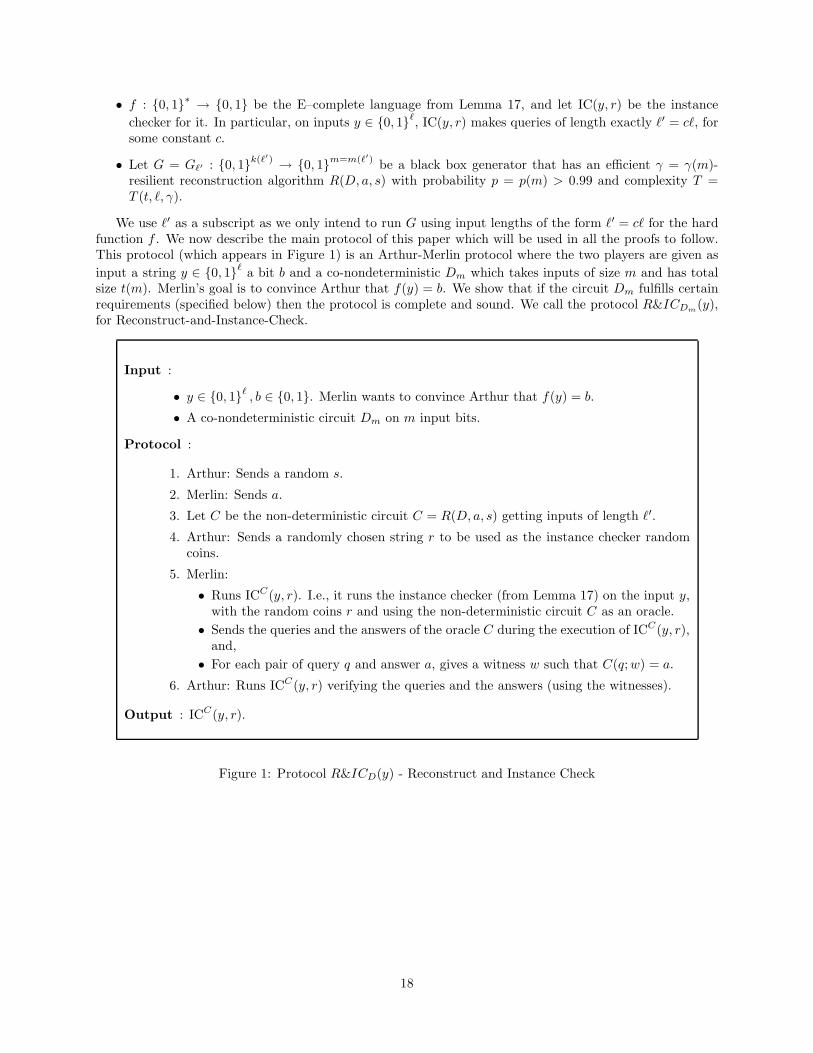
We use `′ as a subscript as we only intend to run G using input lengths of the form `′ = c` for the hardfunction f . We now describe the main protocol of this paper which will be used in all the proofs to follow.This protocol (which appears in Figure 1) is an Arthur-Merlin protocol where the two players are given as

input a string y ∈ 0, 1` a bit b and a co-nondeterministic Dm which takes inputs of size m and has totalsize t(m). Merlin’s goal is to convince Arthur that f(y) = b. We show that if the circuit Dm fulfills certainrequirements (specified below) then the protocol is complete and sound. We call the protocol R&ICDm

(y),for Reconstruct-and-Instance-Check.

Input :

• y ∈ 0, 1` , b ∈ 0, 1. Merlin wants to convince Arthur that f(y) = b.

• A co-nondeterministic circuit Dm on m input bits.

Protocol :

1. Arthur: Sends a random s.

2. Merlin: Sends a.

3. Let C be the non-deterministic circuit C = R(D, a, s) getting inputs of length `′.

4. Arthur: Sends a randomly chosen string r to be used as the instance checker randomcoins.

5. Merlin:

• Runs ICC(y, r). I.e., it runs the instance checker (from Lemma 17) on the input y,with the random coins r and using the non-deterministic circuit C as an oracle.

• Sends the queries and the answers of the oracle C during the execution of ICC(y, r),and,

• For each pair of query q and answer a, gives a witness w such that C(q; w) = a.

6. Arthur: Runs ICC(y, r) verifying the queries and the answers (using the witnesses).

Output : ICC(y, r).

Figure 1: Protocol R&ICD(y) - Reconstruct and Instance Check

18

We claim that if ρ(Dm) is large then for every (y, b) such that f(y) 6= b, no prover can convince theverifier to accept with probability larger than 0.1. Furthermore, if Dm is a distinguisher for Gf , then forevery (y, b) such that f(y) = b, there exists a prover who can convince the verifier to accept (y, b) withprobability at least 0.9.

Lemma 26 For every co-nondeterministic circuit Dm and every y ∈ 0, 1`,

• If ρ(Dm) ≥ γ(m), then for every prover P ∗ the verifier accepts (y, 1 − f(y)) with probability at most0.1.

• If Dm γ–distinguishes Gf , then there exists a prover for which the verifier accepts (y, f(y)) with prob-ability at least 0.9.

Proof: Assume ρ(Dm) ≥ γ(m) and let the prover be arbitrary. By Definition 22, for almost all s (exceptfor 1 − p fraction) for all possible values a, C = R(D, a, s) is PSV. Thus, C defines a partial function

g : 0, 1`′

→ 0, 1. We now run the instance checker for f over the input y with an oracle access to g (notethat the input lengths are right, since on input length `, the oracle calls are of length `′ = c`). By Lemma17 we get the correct answer f(y) or ”reject” with probability at least, say, 0.9.

Now, further assume that Dm γ–distinguishes Gf . By Definition 21, with probability at least p over s,there exists a witness a such that C = R(D, a, s) defines a TSV circuit computing f . When interacting withthe honest prover, Merlin sends this witness a and the right answers of the instance checker IC as specifiedby the protocol. Whenever C is indeed a TSV circuit for f , Lemma 17 guarantees that ICC computes fcorrectly on inputs of length ` with probability 1. Thus, the protocol accepts with probability at least p oninputs of length `.

We now check the running time of Protocol R&IC:

Claim 27 The interactive protocol of Figure 1 takes poly(`) · poly(T (t(m), `′, γ)) time.

Proof: The size of the advice string a and the circuit |C| are at most T ′ = T (t(m), `′, γ), the reconstructionalgorithm R is efficient, hence the complexity of steps 1, 2 and 3 is poly(T ′). Sending r takes poly(`′) = poly(`)bits. There are poly(`) steps of the instance checker IC, and each such step may involve a computation ofthe circuit C. Altogether, the running time of steps 4, 5 and 6 is poly(`) · T ′.

We get the following corollary:

Lemma 28

• If Gf is not [io] γ–hitting against coNTIME(t(m)) then f has an SV–AMTIME(poly(`)·poly(T (t(m), `′, γ)))protocol.

• If Gf is not γ–hitting against coNTIMEγ(t(m)) then f has an SV–io–AMTIME (poly(`)·poly(T (t(m), `′, γ)))protocol.

Proof: If Gf is not γ–hitting against coNTIMEγ(t(m)) then there exists a uniform machine D ∈coNTIMEγ(t(m)) that is a γ–distinguisher for Gf on infinitely many input lengths m = m(`′). If Gf isnot [io] γ–hitting then there exists such a machine M that is a γ–distinguisher for Gf for all input lengthsm = m(`′), except for possibly finitely many. In both cases, by Lemma 26, for every such input length

m = m(`′), and for every value y ∈ 0, 1`, there exists a proof for which the protocol accepts the correctresult with probability at least 0.9, and there is no proof that makes the verifier accept the wrong value withprobability more than 0.1. This gives completeness for both cases, and soundness for the first.

In addition we know that for every input length m = m(`′) ρ(Dm) ≥ γ (by the definition of the class

coNTIMEγ(t(m))). So by the first part of Lemma 26, for every input y ∈ 0, 1` and every prover, theprobability the prover convinces the verifier to accept the wrong answer is at most 0.1, which gives soundnessfor the second case.

19

5.1 Working With The MV Generator

We are now ready to prove Theorem 1. We do that by plugging the MV-generator and its resilient recon-struction algorithm into protocol R&IC.

Let δ > 0 be a constant. We will choose δ later, and for the time being we express other parametersin terms of δ. Let f be the E-complete language from Lemma 17 and IC be the instance checker for f ,having queries of length exactly `′ = c` on inputs of length `. We let Gf,`′,δ = MVf,`′,δ. (recall that

d = 1/δ and m = 2δ`′). We assume that ` is large enough so that ` > 1/δ2. Recall that Gf,`′,δ has an

efficient γ = 1 − 2mδ−m–resilient reconstruction algorithm with probability p = 1 − 2−mδ

and complexityT (t, `, γ) = 2O(δ`) · t2 (Lemma 23). Let Gf,`′,δ be the efficient generator defined in Lemma 20.

Lemma 29

• If Gf,`′,δ is not [io] 12–hitting against coNTIME 1

2(nO(1)) then f has a SV–AMTIME 1

2(2O(δ`)) protocol.

• If Gf,`′,δ is not 12–hitting against coNTIME 1

2(nO(1)) then f has a SV–io–AMTIME 1

2(2O(δ`)) protocol.

In both cases the constant in the O() notation is independent of δ.

Proof: We do the second statement, the first is essentially similar (and simpler). If Gf,δ is not 12–hitting

against coNTIME 12(nO(1)), then there exists some D ∈ coNTIME 1

2(nO(1)) that for infinitely many input

lengths n, 12–distinguishes Gf,δ. By Lemma 20 there exists D such that:

• For every input length n, ρ(Dn) ≥ γ, and,

• For every input length where D 12–distinguishes Gf,δ, D γ–distinguishes Gf,δ.

I.e., D ∈ coNTIMEγ(nO(1)) and Gf,`′,δ is not γ–hitting D. Recall that t(m) = SIZE(D) = mO(1) =2O(δ`). By Lemma 28, f ∈ SV–io–AMTIME 1

2(T (t(m), `′, γ)) = SV–io–AMTIME 1

2(2O(δ`)t2(m)) =

SV–io–AMTIME 12(2O(δ`)).

Combining Lemmas 29 and 17 we get Theorem 1 as we rephrase it more formally:

Theorem 30 Let c > 0.

• If for every δ > 0 Gf,`′,δ is not [io] 12–hitting against coNTIME(nc) then E ⊆ ⋂

β>0 AMTIME 12(2O(β`)).

• If for every δ > 0 Gf,`′,δ is not 12–hitting against coNTIME 1

2(nc) then E ⊆ ⋂

β>0io–AMTIME 12(2O(β`)).

6 Explicit Constructions Under Uniform Assumptions

Klivans and Van-Melkebeek [KvM99] suggested a general framework for derandomization under hardnessassumptions. They showed that non-uniform hardness vs. randomness tradeoffs can be used to conditionallyderandomize a broader class of randomized processes beyond decision problems. They give some examplesthat demonstrate the usefulness of their approach. Some of these applications concern “explicit constructionof combinatorial objects”. We observe that in some cases uniform hardness vs. randomness tradeoffs sufficeand we can use a weaker assumption than that of [KvM99, MV99]. We describe a general framework forderandomizing probabilistic constructions of combinatorial objects under uniform assumptions. Let us startby defining the notion of explicit and probabilistic constructions.

Definition 31 Let Q = Qnn≥1, Qn ⊆ 0, 1n, be a property of strings. We say that a procedure A is anexplicit construction for the property Q, if A runs in deterministic polynomial-time and on input 1n outputsx ∈ Qn′ , for some n′ ≥ n. We say that A is a probabilistic construction for Q, if A runs in deterministicpolynomial-time, and on input (1n, ρ), where |ρ| = poly(n), it holds that Prρ[A(1n, ρ) ∈ Qn′ ] > 1/2. Infinitelyoften (i.o.) construction algorithms are similarly defined, where the algorithms are required to succeed onlyon infinitely many input lengths.

20

Let Q be a property and A a probabilistic construction for Q. We need the following to hold in order toapply our approach.

1. Q ∈ coNP.

2. There exists a deterministic polynomial-time procedure B that given a list, x1, . . . , xk, of strings in0, 1n such that for at least one 1 ≤ i ≤ k, xi ∈ Qn, B outputs x ∈ Qn′ for some n′ ≥ n.

Lemma 32 Let Q be a property and A a probabilistic construction for Q such that conditions 1 and 2 hold,then Q has an explicit construction algorithm, unless E ⊆

⋂β>0io–AMTIME (2βn).

Proof: For input length n, let m = |ρ| be the length of the second part of A’s input. Let f be theE-complete language from Lemma 17. Let δ > 0, we define an explicit construction algorithm C for Q: oninput 1n, run the generator Gf,`′,δ (i.e the generator obtained from applying Lemma 20 on the generatorGf,`′,δ from Section 5.1) on all the possible seeds to obtain a list of strings ρ1, . . . , ρk ∈ 0, 1m, wherek = poly(n) (since the seed length is O(log m) = O(log n)). Then run A on (1n, ρi) for all 1 ≤ i ≤ k,

to obtain a list x1, . . . , xk ∈ 0, 1n′

(n′ = poly(n)). Finally, run the procedure B from condition 2, on

x1, . . . , xk, to obtain x ∈ 0, 1n′′

(n′′ = poly(n′) = poly(n)). Output x.Now suppose that for every δ > 0, for infinitely many input lengths the algorithm C fails to produce

elements in Q. We define a (deciding) co-nondeterministic algorithm A′, taking inputs ρ ∈ 0, 1m, asfollows: on input ρ, run A on (1n, ρ) to obtain an instance x, accept if x ∈ Q. By condition 1, this is aco-nondeterministic algorithm. By the fact that A is a probabilistic construction algorithm for Q, we knowthat ρ(A′m) ≥ 1

2 for every m (where A′m is the restriction of A′ to input length m). We conclude thatA′ ∈ coNTIME 1

2(nc) (for some constant c). Furthermore, for infinitely many input lengths, A′m does not

accept any of the elements generated by Gf,`′,δ. In other words, for every δ > 0 Gf,`′,δ is not 12–hitting

against coNTIME 12(nc). By Theorem 30 (second part) E ⊆ ⋂

β>0io–AMTIME 12(2βn).

Remark 33 By using the first part of Theorem 30, we can have a version of Lemma 32, in which theconstruction algorithm succeeds infinitely often, unless E ⊆

⋂β>0 AMTIME 1

2(2βn).

The matrix rigidity problem is a special case of Lemma 32. Valiant [Val77] showed that a random matrixis rigid, property 1 is clear, and Klivans and Van-Melkebeek [KvM99] showed property 2. Together, thisgives Theorem 4.

7 Gap Theorems

In this section we prove Theorems 2 and 3. We start by setting up some parameters and notations, commonto all the proofs in this section.

Let δ > 0 be a constant. We will choose δ later, and for the time being express other parameters in termsof δ. Let f be the E-complete language from Lemma 17. Set `′ = c` where c is the constant from Lemma 17.Let Gf,`′,δ = MVf,`′,δ as before we require that `′ > 1

δ2 . Recall that m = Ω(2δ`′). By Lemma 23, Gf,`′,δ has

an efficient γ = 1− 2mδ−m–resilient reconstruction algorithm with probability p = 1− 2−mδ

and complexityT (t, `, γ) = 2O(δ`) · t2.

For a language L ∈ AMTIMEε(TIME = poly(n), COINS = m = m(n)), let ML be the machine suchthat:

x ∈ Ln =⇒ Prz∈0,1m

[∃w ML(x; z, w) = 1 ] = 1 (1)

x 6∈ Ln =⇒ Prz∈0,1m

[∃w ML(x; z, w) = 1 ] ≤ ε (2)

The ”derandomized” language L′ is obtained by replacing the random coins of the AM protocol for L,with all the possible outputs of the generator. That is, let ` be the smallest integer such that 2δ`′ ≥ m. Wewill use the generator G based on the function f with input length `′.

21

L′(x) =

1 ∀z∈IMAGE(Gf,`′,δ)∃wML(x; z, w) = 1

0 Otherwise.

We show that L′ ∈ NP. Indeed, L′ calls the non-deterministic machine ML |IMAGE(Gf,`′,δ)| timeswhich is at most polynomial in m (and n). Also, since Gf,`′,δ is efficient, and f is in E, each element inthe set is generated in time polynomial in m (and n). Each execution of ML takes poly(m) = poly(n)non-deterministic time. Altogether, L′ ∈ NTIME(nO(1) and is in NP.

We now define a protocol that is used by all the proofs in this section. We assume that the prover is ableto present us with a circuit Dm such that:

• For every m = m(`), the prover can prove in poly(m) time that ρ(Dm) ≥ γ, and,

• For some (or all) input lengths, Dm is a distinguisher for Gf,`′,δ. The prover does not prove this part,though.

This assumption will be realized in different ways according to the different statements that we prove.We design the following protocol:

Input : y ∈ 0, 1` , b ∈ 0, 1. Merlin wants to prove that f(y) = b.

1. Merlin: Sends a co-nondeterministic circuit Dm.

2. Merlin proves to Arthur that ρ(Dm) ≥ γ (this is the place where the protocols forTheorems 2 and Theorem 3 differ, and we will later describe how this is done in eachproof).

3. Arthur and Merlin play Protocol R&ICDm(y, b).

Figure 2: Common Protocol for Theorems 2 and 3.

Claim 34 If for every ` the prover can choose a circuit Dm that is γ–distinguishing for Gf,`′,m,δ than E ⊆AMTIME1/2(2

O(δ`)). If the above only holds for infinitely many input lengths ` then E ⊆ io–AMTIME 1/2(2O(δ`)).

In both cases the constant in the O notation is independent of δ.

Proof:

Soundness : For every input length ` the prover proves that ρ(Dm) ≥ γ with sufficient soundness (this isour assumption). The rest follows from the soundness of protocol R&IC (Lemma 26).

Completeness: Whenever Dm is γ–distinguishing for Gf,`′,m,δ, the completeness follows again from Lemma26.

Running time: According to our assumption, the first part takes time poly(m) = 2O(δ`′) = 2O(δ`). ByClaim 27 and Lemma 23, Protocol R&IC runs in time 2O(δ`′) = 2O(δ`). Altogether, the total runningtime is 2O(δ`) with the constant in the O notation independent of δ.

It follows that in the first case, for every β > 0, f ∈ AMTIME(2β`), and in the second, for every β > 0,f ∈ io–AMTIME (2β`). Lemma 17 shows that the above also holds for the whole class E as desired.

We now prove Theorems 2 and 3, which by the discussion above amounts to realizing our assumptionsregarding Dm.

22

7.1 A gap theorem for AM

Proof: (of Theorem 2) Assume AM 6⊆ [io-pseudo(NTIME(nO(1)))] NP. Then there exists a lan-guage L ∈ AMTIME1/2(n

O(1)) such that L 6∈ [io-pseudo(NTIME(nO(1)))] NP. By Lemma 19, L ∈AMTIME2mδ

−m(TIME = mO(1), COINS = m = O(nO(1/δ))). In Lemma 36 (which appears in the ap-pendix) we prove that there exists a polynomial-time nondeterministic procedure A such that for all butfinitely many `′, on input 1n has at least one accepting computation path, and on every accepting path, Aoutputs a co-nondeterministic circuit Dm that is γ–distinguishing for Gf,`′,m,δ. The prover sends this Dm

and a proof that A(1n) = Dm, i.e., a computation path of A(1n) that outputs the circuit Dm. The restfollows now from Claim 34.

7.2 A gap theorem for AM ∩ coAM

Proof: (of Theorem 3 part 1) Assume AM∩coAM 6⊆ [io] NP∩[io] coNP. It follows that AM∩coAM 6⊆ [io] NPand therefore there is a language L ∈ AMTIME1/2(n

O(1))∩coAMTIME1/2(nO(1)) such that L 6∈ [io] NP. By

Lemma 19, L ∈ AMTIME2mδ−m(mO(1), m = nO(1/δ))∩coAM 1

10(nO(1), nO(1)).9 As before, the derandomized

language L′ is in NP and L 6∈ [io] NP, therefore it must be that for all input lengths, except finitely many,there exists an input xn ∈ L4L′ = L′ \ L. Merlin sends xn, and proves that xn 6∈ L using the AM protocolfor L. Let Dm be the co-nondeterministic circuit taking inputs from 0, 1m, defined to be Dm(z) = 1 iff∀w[ ML(xn; z, w) = 0 ]. That is, we hardwire xn into the circuit obtained from ML which now takes asinputs elements from 0, 1m (the random tape of ML becomes the input). We see that:

• ρ(Dm) ≥ γ (because xn 6∈ L), and,

• For every z ∈ IMAGE(Gf,`′,m,δ), Dm(z) = 0 (because xn ∈ L′).

Now the protocol continues as in Figure 2 with the circuit Dm.

Soundness : In the first step, the prover sends xn. If xn ∈ L, then the prover is caught cheating withprobability at least 0.9 during the proof that xn 6∈ L. Otherwise, xn 6∈ L, which implies that Dm

accepts almost all inputs, i.e., ρ(Dm) ≥ γ. The soundness now follows from Claim 34.

Completeness and running time follows directly from Claim 34.

7.3 An “almost everywhere” gap theorem for AM ∩ coAM

Proof: (of Theorem 3 part 2) The proof of Theorem 3 (2) is slightly more complicated than that ofTheorem 3 (1) because when the derandomization fails it only fails only on infinitely many input lengths.We will have to allow Merlin to also choose a “correct” input length when sending the distinguisher.

We start with the assumption that AM ∩ coAM 6⊆ NP, (whereas previously we had an [io] in thestatement) so there is a language L ∈ AMTIME1/2(n

O(1)) ∩ coAMTIME1/2(nO(1)) such that L 6∈ NP. By

Lemma 19, L ∈ AM2mδ

−m(mO(1), m = O(nO(1/δ))) ∩ coAM 110

(nO(1), nO(1)). As before, L′ ∈ NP, however,L 6∈ NP. It follows that there is an infinite set I of input lengths, such that for every n ∈ I there existsan input xn ∈ L4L′ = L′ \ L. We let Dm be the co-nondeterministic circuit taking inputs from 0, 1m,defined to be Dm(z) = 1 iff ∀w[ ML(xn; z, w) = 0 ].

We modify the protocol as follows: Previously n was fixed by Arthur to be n = mΘ(δ) = 2cδ2` for someconstant c. We now allow Merlin to choose an input length n between 2cδ2` and 2cδ2(`+1). This is needed toallow Merlin to send an input length on which he can send a counterexample xn. The rest of the protocolcontinues unchanged. Namely, Merlin sends xn, and proves that xn 6∈ L using the AM protocol for L, andthe protocol in Figure 2 continues with the circuit Dm.

9Note that we need the strong amplification of the success probability (i.e. Lemma 19) only for the protocol for L but notfor L. For the latter we can use the standard amplification technique of running many independent copies of the protocol inparallel and deciding by majority.

23

Completeness : There are infinitely many n’s such that there exist xn ∈ 0, 1n for which xn ∈ L′ \L. For

such n, let ` = b log(n)δ2c c. So, 2δ2c` ≤ n ≤ 2δ2c(`+1). For this choice of ` the honest Merlin can choose

a “good” n. As in the proof of part 1, the circuit Dm, obtained from xn, is a distinguisher for Gf,`′,δ

and the completeness follows from Claim 34. Thus, for infinitely many `’s, the protocol computes fcorrectly.

Soundness : For every input y, if xn ∈ L, then the prover is caught cheating with probability at least 0.9during the proof that xn 6∈ L. Otherwise, xn 6∈ L, hence ρ(Dm) ≥ γ, and the soundness follows fromClaim 34.

8 Discussion And Open Problems

In this section we discuss directions for further research and present open problems.

8.1 Towards Removing The [io-pseudo]

In Lemma 23 we show that the Miltersen-Vinodchandran generator has a reconstruction algorithm that isresilient against a large family of co-nondeterministic circuits. An interesting open problem is to construct agenerator that has a reconstruction algorithm which is resilient against all co-nondeterministic circuits. Wecall such a reconstruction algorithm completely resilient. Such a generator will immediately give a versionof Theorem 2 without the [io-pseudo] quantifier.

8.2 Towards A Low-End Gap Theorem

Our results are all in the ”high-end” setting. That is we assume a hard function for AMTIME(2Ω(n)) andconclude a ”full derandomization” placing AM in NP. We do not know how to extend these results to the”low-end” setting. That is, assume a hard function for AM and conclude a ”weak derandomization” (placingAM in NSUBEXP). This happens because the Miltersen-Vinodchandran generator [MV99] is only knownto work in the ”high-end” setting.

Recently, Shaltiel and Umans [SU01] gave a generator construction that improves that of Miltersenand Vinodchandran [MV99] and also works in the ”low-end” setting. However, the known reconstructionalgorithm for this construction does not seem to be resilient.

Another approach to try and get a ”low-end” result is to use the technique of the gap theorem of[IW98]. This paper uses a different property of reconstruction algorithms: They show that the reconstructionalgorithm of [NW94, BFNW93] is learning: The ”correct” advice string a can be efficiently computed withoracle access to the hard function.

Definition 35 (Learning reconstruction algorithm) A reconstruction algorithm R as in definition 21is p-learning if there exists a polynomial time oracle machine MA such that for every function f , anda co-nondeterministic circuit D that is a distinguisher for Gf , with probability p over the choice of r,R(D, Mf (r), r) outputs a nondeterministic TSV circuit C which computes f .

In [IW98] this property is used to efficiently find the ”correct” advice string a when the hard functionis ”downwards self reducible” (which they can assume in their setting) 10. We’d like to point out that thereconstruction algorithm for the Miltersen-Vinodchandran generator is learning. We also want to point outthat the reconstruction algorithm for [SU01, Uma02] isn’t learning 11.

10In [TV02] it was pointed out that this assumption is problematic when trying to extend their result to the ”high-end”setting.

11The construction of [SU01, Uma02] works for derandomizing both BPP and AM. The reconstruction algorithm given therefor BPP is ”learning”. However, the one given for AM isn’t and requires additional advice which we do not know how tocompute even with oracle access to f

24

8.3 Towards Placing AM In ΣP2

One of our motivations for studying this problem is the attempt to prove that AM ⊆ ΣP2 . We remark that

AM is known to be in ΠP2 (and therefore in ΣP

3 ), and that [San89] constructs an oracle relative to which

AM isn’t in ΣP2 .

Let us start with explaining why are “gap theorems” helpful to achieve this goal. Suppose that we couldprove a “dream version” of the “gap theorem”. That is, either EXP = AM or AM = NP. The goal follows

as if EXP = AM then AM is closed under complement, and thus AM = coAM ⊆ ΣP2 .

As we only have weaker versions of the “gap theorem” we obtain much weaker results which have an[io-pseudo] quantifier. We remark that even somewhat stronger results follow from the methods of [Kab00]12. It seems that unlike [Kab00], the use of [io-pseudo] in our results may not be inherent to our technique- indeed, we do not need [io-pseudo] when working with MA or AM ∩ coAM.

We now discuss the consequences of solving the open problems listed above on placing AM in “variants”

of ΣP2 .

• A ”high-end gap theorem” (without [io-pseudo] ) will give that for every β > 0, AM ⊆ [io]ΣTime(2βn)2 .

• A “low-end gap theorem” (without [io-pseudo] ) will give that for every β > 0, AM ⊆ [io]ΣTime(2nβ

)2 .

• It was pointed out to us by Chris Umans [Uma03] that if there exists a “high-end” generator which

has a completely resilient reconstruction that is learning for p > 1/2 then AM ⊆ ΣP2 . The argument is

a modification of the proof of [NW94, AK97] that MA ⊆ ZPPNP.

8.4 Towards replacing E by NE ∩ coNE

In nonuniform tradeoffs, when moving from BPP to AM one can allow the hard function to be in NE∩coNE.This only affects the complexity of the generator instead of in deterministic polynomial time is computable inNP ∩ coNP. However, as the application of the generator to derandomize AM already uses nondeterminism,this still gives the same result.

We cannot use a function in NE∩coNE because it is not known that such functions have instance checkers.This is another interesting open problem.

Acknowledgements

We thank Oded Goldreich, Russell Impagliazzo, Valentine Kabanets, Shien Jin Ong, Alon Rosen, ChrisUmans, Salil Vadhan and Avi Wigderson for helpful discussions. We thank Oded Goldreich and RahulSanthanam for very thorough and very helpful comments on the paper. The first author wishes to thank hissupervisor, Michael Ben-Or, for his encouragement and support.

References

[AH91] W. Aiello and J. Hastad. Statistical zero-knowledge languages can be recognized in two rounds.Journal of Computer and System Sciences, 42(3):327–345, 1991.

12In [Kab00] it was shown that for every β > 0, RP ⊆ [io-pseudo(ZP − SUBEXP )] ZPTIME(2nβ). The same technique

gives that for every β > 0,

AM ⊆ [io-pseudo(C)] ΣTime(2nβ

)2

where C allows refuters which run in ΣTime(2nβ )

2 . We remark that a slightly weaker result follows without delving into [Kab00],by just observing that the argument of [Kab00] relativizes, using the argument there with an NP oracle and observing that

AM ⊆ coRPNP.

25

[AK97] V. Arvind and Johannes Kobler. On resource-bounded measure and pseudorandomness. 17thInternational Conference on Foundations of Software Technology and Theoretival Computer Sci-ence, 1997.

[AS98] S. Arora and S. Safra. Probabilistic checking of proofs: A new characterization of NP. Journalof the ACM, 45(1):70–122, 1998.

[BFL91] L. Babai, L. Fortnow, and C. Lund. Nondeterministic exponential time has two-prover interactiveprotocols. Computational Complexity, 1(1):3–40, 1991.

[BFLS91] L. Babai, L. Fortnow, L. Levin, and M. Szegedy. Checking computations in polylogarithmictime. In In Proceedings of the 23rd Annual ACM Symposium on Theory of Computing, pages21–31, 1991.

[BFNW93] L. Babai, L. Fortnow, N. Nisan, and A. Wigderson. BPP has subexponential time simulationsunless EXPTIME has publishable proofs. Computational Complexity, 3(4):307–318, 1993.

[BK95] M. Blum and S. Kannan. Designing programs that check their work. Journal of the ACM,42(1):269–291, 1995.

[BM84] Manuel Blum and Silvio Micali. How to generate cryptographically strong sequences of pseudo-random bits. SIAM Journal on Computing, 13(4):850–864, November 1984.

[BM88] L. Babai and S. Moran. Arthur-merlin games: A randomized proof system and a hierarchy ofcomplexity classes. Journal of Computer and System Sciences, 36:254–276, 1988.

[BOV03] B. Barak, S.J. Ong, and S. Vadhan. Derandomization in cryptography. In 23rd internationalCryptography conference (Crypto 2003), 2003.

[FGM+89] M Furer, O. Goldriech, Y. Mansour, M. Sipser, and S. Zachos. On completeness and soundnessin interactive proof systems. S. Micali, editor, Advances in Computing Research 5: Randmnessand Computation, pages 429–442, 1989.

[Fri90] J. Friedman. A note on matrix rigidity. In Technical report TR-308-91, Department of ComputerScience, Princeton University, 1990.

[GG98] O. Goldreich and S. Goldwasser. On the limits of non-approximability of lattice problems. InProceedings of the 30th Annual ACM Symposium on Theory of Computing (STOC-98), pages1–9, New York, May 23–26 1998. ACM Press.

[GMW91] O. Goldreich, S. Micali, and A. Wigderson. Proofs that yield nothing but their validity or alllanguages in NP have zero-knowledge proof systems. Journal of the ACM, 38(1):691–729, 1991.

[GS89] S. Goldwasser and M. Sipser. Private coins versus public coins in interactive proof systems.volume 5 of Advances in Computing Research, pages 73–90, 1989.

[GZ97] O. Goldreich and D. Zuckerman. Another proof that BPP subseteq PH (and more). In ECCCTR:Electronic Colloquium on Computational Complexity, technical reports, 1997.

[IKW01] R. Impagliazzo, V. Kabanets, and A. Wigderson. In search of an easy witness: Exponential timevs. probabilistic polynomial time. In Proceedings of the 16th Annual Conference on Computa-tional Complexity (CCC-01), pages 2–12, 2001.

[ISW99] R. Impagliazzo, R. Shaltiel, and A. Wigderson. Near-optimal conversion of hardness into pseudo-randomness. In IEEE Symposium on Foundations of Computer Science (FOCS), 1999.

[ISW00] R. Impagliazzo, R. Shaltiel, and A. Wigderson. Extractors and pseudo-randomn generators withoptimal seed-length. In Proceedings of the Thirty-second Annual ACM Symposium on the Theoryof Computing, 21–23 May 2000.

26

[IW97] R. Impagliazzo and A. Wigderson. P = BPP if E requires exponential circuits: Derandomizing theXOR lemma. In Proceedings of the 29th Annual ACM Symposium on the Theory of Computing(STOC ’97), pages 220–229, 1997.

[IW98] R. Impagliazzo and A. Wigderson. Randomness vs. time: De-randomization under a uniformassumption. In 39th Annual Symposium on Foundations of Computer Science, pages 734–743,1998.

[Kab00] V. Kabanets. Easiness assumptions and hardness tests: Trading time for zero error. In Pro-ceedings of the 15th Annual IEEE Conference on Computational Colmplexity (COCO-00), pages150–157, 2000.

[Kab02] V. Kabanets. Derandomization: a brief overview. Bulletin of the European Association forTheoretical Computer Science, 76:88–103, February 2002. Columns: Computational Complexity.

[KL79] R. M. Karp and R. J. Lipton. Some connections between nonuniform and uniform complexityclasses. In Twelfth Annual ACM Symposium on Theory of Computing (STOC ’80), pages 302–309, New York, April 1979. ACM.

[KvM99] A. R. Klivans and D. van Melkebeek. Graph nonisomorphism has subexponential size proofsunless the polynomial-time hierarchy collapses. In Proceedings of the Thirty-First Annual ACMSymposium on Theory of Computing, pages 659–667, 1999.

[Lu01] C.J. Lu. Derandomizing arthur-merlin games under uniform assumptions. Computational Com-plexity, 10(3):247–259, 2001.

[MV99] P. B. Miltersen and N. V. Vinodchandran. Derandomizing Arthur-Merlin games using hittingsets. In 40th Annual Symposium on Foundations of Computer Science (FOCS ’99), pages 71–80,1999.

[Nis96] Noam Nisan. Extracting randomness: How and why: A survey. In Proceedings of the 11thAnnual IEEE Conference on Computational Complexity (CCC-96), pages 44–58, Los Alamitos,May 24–27 1996. IEEE Computer Society.

[NTS99] Nisan and Ta-Shma. Extracting randomness: A survey and new constructions. JCSS: Journalof Computer and System Sciences, 58, 1999.

[NW94] N. Nisan and A. Wigderson. Hardness vs randomness. Journal of Computer and System Sciences,49(2):149–167, October 1994.

[PV91] P. Pudlak and Z. Vavrin. Computation of rigidity of order n2/r for one simple matrix. Comment.Math. University of Carolina, 32:213–218, 1991.

[Raz] A. Razborov. On rigid matrices. Manuscript (in Russian).

[San89] M. Santha. Relativized arthur-merlin versus merlin-arthur games. Information and Computation,80(1):44-49, 1989.

[Sha02] R. Shaltiel. Recent developments in explicit constructions of extractors. Bulletin of the Eu-ropean Association for Theoretical Computer Science, 77:67–, June 2002. Also available onhttp://www.wisdom.weizmann.ac.il/ ronens.

[Sip88] M. Sipser. Expanders, randomness, or time versus space. Journal of Computer and SystemSciences, 36, 1988.

[SSZ98] M. Saks, A. Srinivasan, and S. Zhou. Explicit OR-dispersers with polylogarithmic degree. Journalof the ACM, 45(1):123–154, January 1998.

[STV99] M. Sudan, L. Trevisan, and S. Vadhan. Pseudorandom generators without the XOR lemma. InProceedings of the Thirty-First Annual ACM Symposium on Theory of Computing, 1999.

27

[SU01] R. Shaltiel and C. Umans. Simple extractors for all min-entropies and a new pseudo-randomgenerator. In 42nd IEEE Symposium on Foundations of Computer Science (FOCS-01), pages648–657, 2001.

[SV97] A. Sahai and S. Vadhan. A complete promise problem for statistical zero-knowledge. In Proceed-ings of the 38th Annual Symposium on the Foundations of Computer Science, pages 448–457.IEEE, 1997.

[TS98] A. Ta-Shma. Almost optimal dispersers. In Proceedings of the 30th Annual ACM Symposium onTheory of Computing (STOC-98), pages 196–202, New York, May 23–26 1998. ACM Press.

[TSUZ01] A. Ta-Shma, C. Umans, and D. Zuckerman. Loss-less condensers, unbalanced expanders, andextractors. In Proceedings of the 33rd Annual ACM Symposium on Theory of Computing, 2001.

[TV02] L. Trevisan and S. Vadhan. Pseudorandomness and average-case complexity via uniform reduc-tions. In Proceedings of the 17th Annual Conference on Computational Complexity, 2002.

[Uma02] C. Umans. Pseudo-random generators for all hardnesses. In Proceedings of the 34th AnnualACM Symposium on Theory of Computing (STOC-02), pages 627–634, 2002.

[Uma03] Chris Umans. Personal communication. 2003.

[Val77] L.G. Valiant. Graph-theoretic arguments in low-level complexity. In Proceedings of the 6thSymposium on Mathematical Foundations of Computer Science, vol. 53 of LNCS, Springer-Verlag, pages 162–176, 1977.

[Yao82] Andrew C. Yao. Theory and applications of trapdoor functions. In 23rd annual symposium onfoundations of computer science (Chicago, Ill., 1982), pages 80–91. IEEE, New York, 1982.

A Producing distinguishers

Lemma 36 Let c > 0 be an arbitrary constant. Let f : 0, 1` → 0, 1 be a language in E, and G` :

0, 1k(`) → 0, 1m(`)an efficient black-box generator with k(`) ≤ O(log(m)). If

AMTIMEε=ε(n)(TIME = poly(n), COINS(n) = poly(n)) 6⊆ [io-pseudo(NTIME(nc))] NP

then there exists a procedure A ∈ NP such that for all but finitely many `, on input 1n(`), A has atleast one accepting path, and on every accepting path A outputs a co-nondeterministic circuit Dm which isa γ = 1− ε–distinguisher for Gf,`,m, where n = n(`) is the first integer such that m(`) ≥ COINS(n).

Proof: Let L be a language in AMTIMEε(TIME = poly(n), COINS = m = m(n)), and yet L is not in[io-pseudo(NTIME(nc))] NP. Let ML the machine that defines L, and L′ the “derandomized” version of Lwith the generator Gf,`,m (as defined in section 7). Recall that L′ ∈ NP .

As L 6∈ [io-pseudo(NTIME(nc))] NP, there exists a refuter REF ∈ NTIME(nc) such that for all largeenough input lengths n, REF (1n) ∈ L4L′. Furthermore, L ⊆ L′ and so REF (1n) ∈ L′ \ L.

We can describe now the nondeterministic procedure A, that outputs distinguishers for the generator.On input 1n, A runs the refuter REF (1n), to obtain an instance xn (on accepting paths of REF ). Aoutputs the co-nondeterministic circuit Dm(z), with inputs from 0, 1m, defined to be Dm(z) = 1 iff∀w[ ML(xn; z, w) = 0 ]. We see that:

• ρ(Dm) ≥ γ (because REF (1n) 6∈ L), and,

• For every z ∈ IMAGE(Gf,`,m), Dm(z) = 0 (because REF (1n) ∈ L′).

• SIZE(Dm) ≤ poly(m), (because ML ∈ AMε(TIME = poly(n), COINS = m = poly(n)), and thetranslation to a circuit is at most quadratic in size).

Therefore, by definition, Dm is a γ–distinguisher for Gf,`,m.Clearly, A runs in poly(n) non-deterministic time, which completes the proof.

28